geometry with computers - tom davis
TRANSCRIPT
Geometrywith
Computers
Computer-Based Techniques toLearn and Teach
Euclidean Geometry
Tom DavisDraft Date: February 17, 2004

2
Chapter 0Preface
Mathematics must be written into the mind, not read into it. “No headfor mathematics” nearly always means “Will not use a pencil.”
Arthur Latham Baker
0.1 Why Another Geometry Book?
Euclidean Geometry is ancient, and thousands of books and articles have been writtenon the subject. Why write another?
Here are the differences between this book and the others:
• Most mathematics books are written to communicate results: theorems, calcula-tion methods and algorithms. This book concentrates on computer-based tech-niques for solving geometric problems.
i
ii PREFACE
• Although it may not be obvious, mathematics is highly geometrical—virtuallyevery formula has an associated picture. Often it is much easier to obtain under-standing by mentally manipulating the picture than by manipulating a formulaalgebraically. What better way to practice mental manipulation of pictures thanto study geometry?
Mental manipulation of geometry is difficult for many people, but today almostany personal computer has graphical capabilities that would have been unimagin-ably powerful 20 years ago. These machines can help visualize geometric resultsin a dynamic manner that is far more compelling than the fixed drawings appear-ing in standard mathematics books or that can be produced with pencil and paper.This book comes with a computer program called Geometer that allows you tomanipulate existing geometric diagrams and to create your own.
• Geometer can also be used as an experimental tool to run geometry “experi-ments” that can aid greatly in both understanding and proving results.
• Although Euclidean geometry is a huge field, it is not a big part of the generalmathematics curriculum in the United States. I have a Ph.D. in mathematics,and the only formal class I had in Euclidean geometry was in high school. Yourgeometry class may have been different, but in mine we somehow managed toavoid learning most of the truly beautiful results.
• High school geometry is often the first introduction students have to constructingmathematical proofs. It is obviously better to begin with simple examples whenteaching a student to write proofs, so the proof construction exercises in typicalhigh school texts can almost all be completed in three or four steps.
Unfortunately, if one is limited to proofs of only a few steps, a huge proportion ofgeometry is inaccessible. For people who can follow a ten or twenty step proof,it is amazing what results are accessible—some of the most beautiful theoremsin mathematics.
One’s technique of geometric proof can be honed with artificial drills, or one canwork on interesting problems. This is similar to the difference between runningon a treadmill or on mountain trails—the treadmill is completely predictablewhile the trails can be tricky but the trail runner will not be bored out of hismind. This book is aimed at those who did enough treadmill geometry in highschool and want to see some beauty while they learn advanced techniques.
The material here is accessible to brighter high school students, and can be usedas supplementary material by teachers or by the students themselves.
The Geometer program can also be used as a presentation device in geometryclasses. Although most of the material is beyond what is taught in high school,many of the more important introductory results are avaiable on the enclosed CDin Geometer format.
There is additional material on the CD to help—some more elementary theo-rems, and a tutorial on the construction of sophisticated Geometer diagrams, forexample. See the index file on the CD for up to date information.
0.2. AUDIENCE iii
• Finally, with computer graphics increasing in power every year, Euclidean ge-ometry (and projective geometry as well) may be destined for a comeback. Moreand more computer applications are being designed to help people visualizeproblems geometrically, but to make the computers do a good job of that, moregeometry is required.
0.2 Audience
This book is for teachers of Euclidean geometry but it contains topics of interest formotivated students or anyone who loves geometry. Students and coaches of studentswho compete in high level mathematics competitions should find the advanced materialin this text valuable as training aids.
0.3 Origins of Geometer
The I worked at Silicon Graphics for 16 years doing graphics programming and helpingdesign computer graphics hardware and so I have a fairly solid grounding in both thetheoretical and practical details of geometry.
Although I was paid money to be a computer engineer, I have never ceased to be amathematician as well. From time to time both in and out of work I ran into interestinggeometric theorems. A couple of them seemed so surprising and non-intuitive that Iwrote computer programs to help me visualize them. After going through that exercisea few times, I realized that it would not be hard to write a general-purpose programwhere arbitrary geometric diagrams could be entered with a graphical user interface(GUI) and dynamically altered. I hacked together the original version of Geometer onSilicon Graphics UNIX machines in my spare time. (I was wrong when I thought it“would not be hard.”)
The version of Geometer included with this book is vastly modified and improved(and it now runs on Windows, Macintosh OS X and Linux machines), but much of theunderlying philosophy is the same.
As I worked on this book, I tried to practice what I preach. I knew of many inter-esting results that I had never actually proved, and rather than just look up the standardproofs, I struggled to figure them out myself. Of course from time to time I had to lookin various books for “hints” and even when I did solve a problem completely withouthints, I later read the literature to see what the “standard” methods are.
In my struggles to find the proofs, I used Geometer extensively in exactly the sameways I expect you the reader to use it. It may not be bug-free, but I can assure youthat it is quite robust, and since it has been used to create thousands of real dynamicdiagrams, it is fairly well streamlined: when I got annoyed with something, I just fixedit.
iv PREFACE
0.4 AcknowledgementsA mathematician is a machine for turning coffee into theorems. 1
Alfred Renyi
Zvezdelina Stankova showed me many wonderful geometric ideas. In particular, Ilearned from her the power of the technique of inversion in a circle.
I would like to thank Joshua Zucker and his students in Palo Alto’s Gunn HighSchool Math Circle for all the stimulating discussions of mathematics problems andfor serving as unwitting guinea pigs for some of the presentation techniques used here.I also learned a lot in Zvezdelina’s UC Berkeley Math Circle, and in Tatiana Shubin’sMath Circle at San Jose State University.
Special thanks go to Gerald Alexanderson and Arthur Benjamin for their helpin converting what began as a disorganized collection of half-baked ideas into thecompletely-baked version you hold in your hands. Rudolf Fritsch provided many de-tailed corrections and suggestions.
I received many wonderful suggestions for improvements and enhancements to theGeometer program from Paul Haeberli and Henry Moreton.
This book was produced using LATEX, the Emacs editor, and the PostScript filesproduced by Geometer. After an infuriating attempt to use the most popular wordprocessor in the world for the text, Emacs and LATEX were a total pleasure to use, so Imust thank Donald Knuth for writing TEX and Leslie Lamport for writing LATEX.
My wife, Ellyn Bush, although not a mathematician, read and re-read many partsof the text, and provided many valuable insights on how to make things simpler andclearer. She put up with all of my complaints with only a few of her own.
Finally, as the quotation at the beginning of this section indicates, I would like tothank whoever it was who discovered that beans of the shrub Coffea arabica could beroasted, ground and steeped in boiling water to produce the nectar of life. I convertedthat nectar not only into theorems, but also into text and into the computer code thatproduced Geometer.
1This result was sharpened by Pal Turan who added that weak coffee produces only lemmas.
Contents
Preface i0.1 Why Another Geometry Book? . . . . . . . . . . . . . . . . . . . . . i
0.2 Audience . . . . . . . . . . . . . . . . . . . . . . . . . . . . . . . . iii
0.3 Origins of Geometer . . . . . . . . . . . . . . . . . . . . . . . . . . iii
0.4 Acknowledgements . . . . . . . . . . . . . . . . . . . . . . . . . . . iv
1 Introduction 11.1 Computer Geometry Programs . . . . . . . . . . . . . . . . . . . . . 2
1.2 The Contents of the CD . . . . . . . . . . . . . . . . . . . . . . . . . 3
1.3 Organization of the Book . . . . . . . . . . . . . . . . . . . . . . . . 4
1.4 Proofs in this Book . . . . . . . . . . . . . . . . . . . . . . . . . . . 7
1.5 Illustrations in this Book . . . . . . . . . . . . . . . . . . . . . . . . 7
1.6 How to Use this Book . . . . . . . . . . . . . . . . . . . . . . . . . . 9
1.7 Notation . . . . . . . . . . . . . . . . . . . . . . . . . . . . . . . . . 10
1.8 Where to Go from Here . . . . . . . . . . . . . . . . . . . . . . . . . 11
2 Computer-Assisted Geometry 152.1 Accurate Drawings . . . . . . . . . . . . . . . . . . . . . . . . . . . 16
2.2 Drawing Manipulation . . . . . . . . . . . . . . . . . . . . . . . . . 21
2.3 Finding and Testing Conjectures . . . . . . . . . . . . . . . . . . . . 22
2.4 Ease of Correction . . . . . . . . . . . . . . . . . . . . . . . . . . . 24
2.5 Stepping through Proofs . . . . . . . . . . . . . . . . . . . . . . . . 25
2.6 Making Measurements . . . . . . . . . . . . . . . . . . . . . . . . . 27
2.7 Searching for Patterns . . . . . . . . . . . . . . . . . . . . . . . . . . 30
v
vi CONTENTS
2.8 Searching for Extremes . . . . . . . . . . . . . . . . . . . . . . . . . 322.9 Locus of Points . . . . . . . . . . . . . . . . . . . . . . . . . . . . . 332.10 Computer-Generated Diagrams . . . . . . . . . . . . . . . . . . . . . 342.11 Animations . . . . . . . . . . . . . . . . . . . . . . . . . . . . . . . 382.12 Drawing for Publication . . . . . . . . . . . . . . . . . . . . . . . . 392.13 Computer Algebra Systems . . . . . . . . . . . . . . . . . . . . . . . 402.14 Non-Mathematical Uses of Geometer . . . . . . . . . . . . . . . . . 42
3 Mathematics Review 473.1 Types of Geometric Problems . . . . . . . . . . . . . . . . . . . . . . 483.2 Congruence . . . . . . . . . . . . . . . . . . . . . . . . . . . . . . . 483.3 Points . . . . . . . . . . . . . . . . . . . . . . . . . . . . . . . . . . 533.4 Lines . . . . . . . . . . . . . . . . . . . . . . . . . . . . . . . . . . 533.5 Angles . . . . . . . . . . . . . . . . . . . . . . . . . . . . . . . . . . 563.6 Triangles . . . . . . . . . . . . . . . . . . . . . . . . . . . . . . . . 583.7 Quadrilaterals . . . . . . . . . . . . . . . . . . . . . . . . . . . . . . 703.8 General Polygons . . . . . . . . . . . . . . . . . . . . . . . . . . . . 733.9 Circles . . . . . . . . . . . . . . . . . . . . . . . . . . . . . . . . . . 773.10 Trigonometric Definitions . . . . . . . . . . . . . . . . . . . . . . . . 813.11 Coordinate Geometry . . . . . . . . . . . . . . . . . . . . . . . . . . 893.12 Vectors . . . . . . . . . . . . . . . . . . . . . . . . . . . . . . . . . 953.13 Complex Numbers . . . . . . . . . . . . . . . . . . . . . . . . . . . 103
4 Geometric Construction 1074.1 The Circumcenter . . . . . . . . . . . . . . . . . . . . . . . . . . . . 1084.2 Available Tools . . . . . . . . . . . . . . . . . . . . . . . . . . . . . 1094.3 The Structure of a Geometer Diagram . . . . . . . . . . . . . . . . . 1094.4 Interpreting Geometer Files . . . . . . . . . . . . . . . . . . . . . . 1104.5 Simple Classical Examples . . . . . . . . . . . . . . . . . . . . . . . 1114.6 Intermediate Examples . . . . . . . . . . . . . . . . . . . . . . . . . 1214.7 Advanced Examples . . . . . . . . . . . . . . . . . . . . . . . . . . 1294.8 Poncelet’s Theorem Demonstration . . . . . . . . . . . . . . . . . . . 1294.9 Seven Tangent Circles . . . . . . . . . . . . . . . . . . . . . . . . . . 1314.10 A Tricky Construction . . . . . . . . . . . . . . . . . . . . . . . . . 1334.11 Classical Construction . . . . . . . . . . . . . . . . . . . . . . . . . 1354.12 Some Constructions Are Impossible . . . . . . . . . . . . . . . . . . 1364.13 139 More Problems . . . . . . . . . . . . . . . . . . . . . . . . . . . 1394.14 Construction Exercises . . . . . . . . . . . . . . . . . . . . . . . . . 139
CONTENTS vii
5 Computer-Aided Proof 1435.1 Finding the Steps in a Proof . . . . . . . . . . . . . . . . . . . . . . . 144
5.2 Testing a Diagram . . . . . . . . . . . . . . . . . . . . . . . . . . . . 144
5.3 Altitudes as Bisectors . . . . . . . . . . . . . . . . . . . . . . . . . . 145
5.4 Another Bisector . . . . . . . . . . . . . . . . . . . . . . . . . . . . 146
5.5 Perpendicular Diagonals . . . . . . . . . . . . . . . . . . . . . . . . 147
5.6 Constant Sum . . . . . . . . . . . . . . . . . . . . . . . . . . . . . . 148
5.7 Find a Radius . . . . . . . . . . . . . . . . . . . . . . . . . . . . . . 151
5.8 Sum of Lengths . . . . . . . . . . . . . . . . . . . . . . . . . . . . . 151
5.9 Bisector Bisector . . . . . . . . . . . . . . . . . . . . . . . . . . . . 153
5.10 The Simson Line . . . . . . . . . . . . . . . . . . . . . . . . . . . . 154
5.11 A Property of Two Cevians . . . . . . . . . . . . . . . . . . . . . . . 155
5.12 Tangent Line Problem . . . . . . . . . . . . . . . . . . . . . . . . . . 157
5.13 Cyclic Quadrilateral Problem . . . . . . . . . . . . . . . . . . . . . . 158
5.14 A Strange Relationship . . . . . . . . . . . . . . . . . . . . . . . . . 159
5.15 Sum of Powers . . . . . . . . . . . . . . . . . . . . . . . . . . . . . 161
6 More Useful Theorems 1676.1 Ceva’s Theorem . . . . . . . . . . . . . . . . . . . . . . . . . . . . . 167
6.2 Menelaus’ Theorem . . . . . . . . . . . . . . . . . . . . . . . . . . . 170
6.3 Alternate Proofs of Menelaus and Ceva . . . . . . . . . . . . . . . . 172
6.4 Using Menelaus’ and Ceva’s Theorem . . . . . . . . . . . . . . . . . 173
6.5 Ptolemy’s Theorem . . . . . . . . . . . . . . . . . . . . . . . . . . . 173
6.6 Heron’s Formula . . . . . . . . . . . . . . . . . . . . . . . . . . . . 175
6.7 The Radical Axis . . . . . . . . . . . . . . . . . . . . . . . . . . . . 178
7 Locus of Points 1837.1 Unknown Geometric Locus . . . . . . . . . . . . . . . . . . . . . . . 183
7.2 Euler’s Formula . . . . . . . . . . . . . . . . . . . . . . . . . . . . . 185
7.3 Triangle from Three Medians . . . . . . . . . . . . . . . . . . . . . . 186
7.4 The Ellipse . . . . . . . . . . . . . . . . . . . . . . . . . . . . . . . 188
7.5 Locus Construction Exercises . . . . . . . . . . . . . . . . . . . . . . 189
7.6 Higher-Order Curves . . . . . . . . . . . . . . . . . . . . . . . . . . 190
7.7 Plotting Curves of the Form: y = f(x) . . . . . . . . . . . . . . . . . 193
7.8 Plotting Curves in Polar Coordinates . . . . . . . . . . . . . . . . . . 194
7.9 Envelopes of Curves: the Epicycloid . . . . . . . . . . . . . . . . . . 195
viii CONTENTS
8 Triangle Centers 199
8.1 General Properties of Triangle Centers . . . . . . . . . . . . . . . . . 200
8.2 The Gergonne Point . . . . . . . . . . . . . . . . . . . . . . . . . . . 200
8.3 The Nine Point Center . . . . . . . . . . . . . . . . . . . . . . . . . 202
8.4 The Fermat Point . . . . . . . . . . . . . . . . . . . . . . . . . . . . 203
8.5 The Nagel Point . . . . . . . . . . . . . . . . . . . . . . . . . . . . . 205
8.6 The First Napoleon Point . . . . . . . . . . . . . . . . . . . . . . . . 206
8.7 The Brocard Points . . . . . . . . . . . . . . . . . . . . . . . . . . . 208
8.8 The Mittenpunkt . . . . . . . . . . . . . . . . . . . . . . . . . . . . 211
8.9 A New Center . . . . . . . . . . . . . . . . . . . . . . . . . . . . . . 213
8.10 Additional Triangle Centers . . . . . . . . . . . . . . . . . . . . . . . 214
8.11 Trilinear Coordinates . . . . . . . . . . . . . . . . . . . . . . . . . . 215
8.12 Triangle Center Finder . . . . . . . . . . . . . . . . . . . . . . . . . 216
8.13 Searching for the “True” Center of a Triangle . . . . . . . . . . . . . 219
9 Inversion in a Circle 223
9.1 Overview of Inversion . . . . . . . . . . . . . . . . . . . . . . . . . 224
9.2 Formal Definition of Inversion . . . . . . . . . . . . . . . . . . . . . 226
9.3 Simple Properties of Inversion . . . . . . . . . . . . . . . . . . . . . 227
9.4 Preservation of Angles Under Inversion . . . . . . . . . . . . . . . . 232
9.5 Summary of Inversion in a Circle . . . . . . . . . . . . . . . . . . . . 234
9.6 Circle through a Point Tangent to Two Circles . . . . . . . . . . . . . 235
9.7 Circle Tangent to Three Circles . . . . . . . . . . . . . . . . . . . . . 236
9.8 Ptolemy’s Theorem Revisited . . . . . . . . . . . . . . . . . . . . . . 237
9.9 Fermat’s Problem . . . . . . . . . . . . . . . . . . . . . . . . . . . . 238
9.10 Inversion to Concentric Circles . . . . . . . . . . . . . . . . . . . . . 240
9.11 The Steiner Porism . . . . . . . . . . . . . . . . . . . . . . . . . . . 241
9.12 Four Circle Problem . . . . . . . . . . . . . . . . . . . . . . . . . . 242
9.13 The Arbelos of Pappus . . . . . . . . . . . . . . . . . . . . . . . . . 244
9.14 Another Arbelos Result . . . . . . . . . . . . . . . . . . . . . . . . . 245
9.15 The Problems of Apollonius . . . . . . . . . . . . . . . . . . . . . . 247
9.16 Peaucellier’s Linkage . . . . . . . . . . . . . . . . . . . . . . . . . . 249
9.17 Feuerbach’s Theorem . . . . . . . . . . . . . . . . . . . . . . . . . . 250
CONTENTS ix
10 Projective Geometry 25510.1 Desargues’ Theorem . . . . . . . . . . . . . . . . . . . . . . . . . . 255
10.2 Projective Geometry . . . . . . . . . . . . . . . . . . . . . . . . . . 257
10.3 Monge’s Theorem . . . . . . . . . . . . . . . . . . . . . . . . . . . . 259
10.4 The Theorem of Pappus . . . . . . . . . . . . . . . . . . . . . . . . . 261
10.5 Another View of Projective Geometry . . . . . . . . . . . . . . . . . 263
10.6 Projective Duality . . . . . . . . . . . . . . . . . . . . . . . . . . . . 265
10.7 Pascal’s Theorem . . . . . . . . . . . . . . . . . . . . . . . . . . . . 266
10.8 Homogeneous (Projective) Coordinates . . . . . . . . . . . . . . . . 272
10.9 Higher Dimensional Projective Geometry . . . . . . . . . . . . . . . 274
10.10The Equation of a Conic . . . . . . . . . . . . . . . . . . . . . . . . 285
10.11Finite Projective Planes . . . . . . . . . . . . . . . . . . . . . . . . . 286
11 Harmonic Point Sets 28911.1 What is an Harmonic Set? . . . . . . . . . . . . . . . . . . . . . . . 289
11.2 Some Constructions of Harmonic Sets . . . . . . . . . . . . . . . . . 292
11.3 Harmonic Points and Music . . . . . . . . . . . . . . . . . . . . . . . 294
11.4 The Complete Quadrilateral . . . . . . . . . . . . . . . . . . . . . . 295
11.5 Poles and Polars . . . . . . . . . . . . . . . . . . . . . . . . . . . . . 298
11.6 The Problem of Apollonius (Again) . . . . . . . . . . . . . . . . . . 302
11.7 Poles and Polars Relative to Conics . . . . . . . . . . . . . . . . . . 303
12 Geometric Presentations 30512.1 General Considerations . . . . . . . . . . . . . . . . . . . . . . . . . 306
12.2 Improving the Appearance of a Diagram . . . . . . . . . . . . . . . . 307
12.3 Building Geometer Proofs and Constructions . . . . . . . . . . . . . 309
12.4 Some Final Touches . . . . . . . . . . . . . . . . . . . . . . . . . . . 314
12.5 Calculation in Geometer . . . . . . . . . . . . . . . . . . . . . . . . 316
12.6 Using Geometric Transformations . . . . . . . . . . . . . . . . . . . 321
12.7 Constructing Geometer Scripts . . . . . . . . . . . . . . . . . . . . . 323
12.8 Computer-Generated Diagrams . . . . . . . . . . . . . . . . . . . . . 330
13 Geometer Proofs 33713.1 Illustrated Theorems . . . . . . . . . . . . . . . . . . . . . . . . . . 338
13.2 Proof Exercises . . . . . . . . . . . . . . . . . . . . . . . . . . . . . 341
A Geometer Art 349
x CONTENTS
B Geometric Problem Solving Strategies 353B.1 Congruence . . . . . . . . . . . . . . . . . . . . . . . . . . . . . . . 355
B.2 Similarity . . . . . . . . . . . . . . . . . . . . . . . . . . . . . . . . 356
B.3 Special Figures . . . . . . . . . . . . . . . . . . . . . . . . . . . . . 356
B.4 Concurrence . . . . . . . . . . . . . . . . . . . . . . . . . . . . . . . 357
B.5 Measures . . . . . . . . . . . . . . . . . . . . . . . . . . . . . . . . 358
B.6 Equality and Inequality . . . . . . . . . . . . . . . . . . . . . . . . . 360
B.7 Ratios . . . . . . . . . . . . . . . . . . . . . . . . . . . . . . . . . . 360
B.8 Inversion in a Circle . . . . . . . . . . . . . . . . . . . . . . . . . . . 361
B.9 Algebraic Manipulation . . . . . . . . . . . . . . . . . . . . . . . . . 362
B.10 When to Draw the Line . . . . . . . . . . . . . . . . . . . . . . . . . 363
B.11 Construction Techniques . . . . . . . . . . . . . . . . . . . . . . . . 364
B.12 Relabeling . . . . . . . . . . . . . . . . . . . . . . . . . . . . . . . . 365
B.13 General Problem Solving Approaches . . . . . . . . . . . . . . . . . 365
Chapter 1Introduction
This book describes techniques and strategies that use computer software to enhancethe study of geometry. If you are itching to try the Geometer program on the enclosedCD, that is as good a way to start as any. Install the program and go directly to thetutorial which you will find under the Help pulldown menu.
The Geometer program upon which this book is based is freely available and inthe public domain. Anyone may obtain a copy at:
http://www.geometer.org/geometer
You may already be proficient in the use of one of the commercial computer ge-ometry programs such as Geometer’s Sketchpad, Cabri Geometry, Cinderella orothers, and if so, almost all the techniques described here can be applied using thosepackages. The main advantage of Geometer is that the included CD containscomputer-readable versions of all the examples and figures in this book in Geometerformat.
1
2 CHAPTER 1. INTRODUCTION
This book is for anyone who wants to learn about computer methods to enhance thestudy of geometry, be they students or teachers of the subject. The term “student” refersto anyone who is studying geometry—either as part of a formal course or simply forthe love of the subject. The text does assume a high school mathematics background,but Chapter 3 reviews all the important prerequisites.
The purpose of this book is to demonstrate techniques, not theorems. Althoughas far as possible interesting theorems have been chosen for the demonstrations, noattempt has been made to assure that the list of theorems presented is complete in anysense. While it is true that the text material combined with the additional exampleson the CD does cover a large number of theorems, please do not feel slighted if yourfavorite theorem does not appear.
1.1 Computer Geometry Programs
A computer geometry program is a computer program with a graphical user interfacethat allows you to draw geometric objects and to adjust them dynamically. Such sys-tems are constraint-based in that most of the objects in a figure are not placed abso-lutely, but are defined in terms of the positions of other objects on the screen. Forexample, your drawing may contain two freely movable points and a third point that istheir midpoint. In most computer geometry programs you can freely adjust the posi-tions of the first two points, but not the third. If you do adjust either of the first points,however, the position of third point will change so that it remains at their midpoint.
The constraints in such a system can be nested arbitrarily deeply. For example, aline passing through the midpoint described in the previous paragraph will also movewhen the midpoint moves, but the midpoint can only move if one of the two originalpoints is moved, and so on.
This book demonstrates many things that computer geometry programs can do, butit is equally important to be aware of what they cannot do.
Such programs do provide accurate drawings. They allow you to visualize not justone example of a drawing, but thousands of variations. They allow you to test geomet-ric conjectures, and can present dynamic illustrations of relationships or theorems.
What they cannot do (at least as of the publication date) is to generate proofs oftheorems. In order for a theorem to be accepted as true, a formal proof is required, andalthough computer geometry programs can help you to find that proof, it is you whowill have to provide the completed version.
The more geometry you know, the more helpful a computer can be. If you havedrawn a diagram and see in it a relationship that you would like to prove, it may be thatthe computer can discover other relationships in the diagram that you did not noticeand that may help you construct a formal proof. But it will be up to you to discoverhow to use that information to produce a formal proof.
For example, imagine that you are trying to show that three circles in a diagrammeet at a point. When you allow the computer to examine the diagram, suppose itnotices that a certain set of four seemingly unrelated points are concyclic (“concyclic”
1.2. THE CONTENTS OF THE CD 3
means that they all lie on the same circle). This unlikely occurrence is easy for acomputer to recognize, but usually difficult for a human, and it could easily be relatedto your three circle concurrence problem. But even if knowing that the points areconcyclic makes your result obvious, you still need to show that the four points are, infact, concyclic. It is clear that the more ways you know to prove that four points lie onthe same circle, the easier your task will be. (If you’re interested in what such a listmight look like, see item 14 in Section 1.3.)
Another obvious limitation of computers is due to round-off error in their calcu-lations. It should not surprise you if a computer indicates that a certain right trianglehas sides of lengths 3, 4, and 5.0000001, although any student of high school geom-etry knows that this cannot be true. Thus some common sense is required. If you areasked to find an unknown length, and the computer measures it as 7.000013, you willprobably have a lot more luck if you try to prove that it is 7, not 7.000013. If, however,the computer says the length is 7.071907, it is probably not equal to 7. If you are verygood, you may notice how close 7.071907 is to
√50—knowledge is power.
1.2 The Contents of the CD
The enclosed CD contains a copy of the public-domain computer geometry programcalled “Geometer” that runs on Windows and Linux machines as well as on Macintoshsystems running OS X. All the illustrations in this text were prepared with Geometer.See Section 1.5 for details about how to interpret the captions on the figures. TheGeometer CD includes:
• The Geometer program itself.
• A tutorial and user’s guide for the program.
• The source files for all the examples in the user’s guide and tutorial.
• The source files for all the illustrations in this book.
• Solutions to all the exercises in this book in the form of Geometer files.
• Many additional files of interesting geometric results not covered in this book.
The Geometer program can be used at many levels, depending on how much youwant to learn about it. See Chapter 2 for a much more detailed description of whatGeometer (and programs like it) can do.
• To view a diagram in this text simply double-click the corresponding Geometerfile on the CD.
• To manipulate the figure, click down on the mouse button when the cursor isover a point. Then until you release the button, the point will be dragged withthe cursor, and the figure will be modified appropriately.
4 CHAPTER 1. INTRODUCTION
• Some Geometer diagrams are “proofs”. The author of the proof organized thediagram so that you can step forward and back through the proof using the Start,Next and Prev (previous) buttons. During the proof, the figure can be manipu-lated as described above.
• Still other Geometer diagrams are scripts, in which case the Script button will besolidly drawn. If you click on this button with the mouse, the diagram will passthrough a prearranged script. Sometimes you can manipulate the figure beforepressing the Script button to observe the consequences of the script with differentinitial configurations.
• Using the mouse buttons and menus you can construct and save your own simpleGeometer diagrams to test conjectures and to search for patterns and geometricrelationships.
• In addition to manipulation with the mouse using a graphical user interface, Ge-ometer diagrams have a textual form that can be edited either within Geometeror using your favorite text editor. Using this technique, all the features are avail-able, including designing your own scripts or proofs.
1.3 Organization of the Book
Here is the basic organization of the rest of the book:
1. IntroductionWhat you are reading now.
2. Computer-Assisted GeometryThis chapter consists of a quick survey (with examples) of almost every possibleuse for a computer geometry program.
3. Mathematics ReviewHere we review parts of high school mathematics. Most of the topics are fromgeometry, but some trigonometry and analytic geometry are included. The im-portant results are listed, where “important” means that the result is useful forderiving other results. The results are standard, and most can be found in highschool mathematics texts.
4. Geometric ConstructionsTo be able to use a computer geometry program, you have to know how toconstruct diagrams that correspond to the problems you are investigating. Thischapter describes with many examples methods to construct computer diagrams.Classic straightedge and compass constructions are described and discussed, butmost of the emphasis is on how to use the more powerful techniques available incomputer geometry programs, Geometer in particular.
1.3. ORGANIZATION OF THE BOOK 5
At the end of the chapter is a list of construction exercises whose solutions appearin Geometer files on the CD.
5. Computer-Aided ProofThis chapter describes how to use your computer to help you search for a proofof a geometric theorem.
6. More Useful TheoremsHere are a few useful theorems and their proofs that are not typically covered ina high school course. When possible, Geometer will be used as an aid to findthose proofs. The results in this chapter plus those in the review chapter provideall the classical tools needed to solve the rest of the problems in the book.
7. Locus of PointsComputer geometry programs make the search for “locus of point” problemsalmost trivial. In this chapter we will examine some nice examples.
8. Triangle CentersThe centroid, circumcenter, incenter and orthocenter are four well-known clas-sical triangle centers, but there are hundreds of others. This chapter examinessome of them.
9. Inversion in a CircleThe technique of inversion in a circle is described, with and without computergeometry programs.
10. Projective GeometryGeometer and probably most other computer geometry programs do many oftheir calculations in projective geometry rather than Euclidean geometry. Inaddition, much of computer graphics is based upon projective geometry. Thischapter presents the fundamental concepts of projective geometry, but from a Eu-clidean point of view. Calculations in homogeneous coordinates are described.
11. Harmonic Point SetsThis is a continuation of the previous chapter on projective geometry, but again,from a Euclidean point of view. In many geometric configurations, sets of har-monic points appear, and if that is the case, many methods can be applied touse those methods to help solve problems. Geometer is very good at findingharmonic point sets.
12. Geometric PresentationsThis chapter is primarily for teachers of geometry or for anyone who would liketo present geometric results to others using Geometer. Various techniques arediscussed that will improve the quality of Geometer diagrams making them eas-ier to understand and more beautiful. Techniques for the presentation of proofs,constructions, and animated scripts are discussed with examples.
6 CHAPTER 1. INTRODUCTION
13. Geometer Proofs
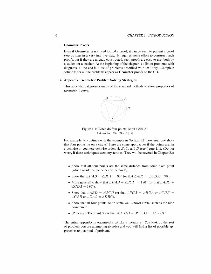
Even if Geometer is not used to find a proof, it can be used to present a proofstep by step in a very intuitive way. It requires some effort to construct suchproofs, but if they are already constructed, such proofs are easy to use, both bya student or a teacher. At the beginning of the chapter is a list of problems withdiagrams; at the end is a list of problems described with text only. Completesolutions for all the problems appear as Geometer proofs on the CD.
14. Appendix: Geometric Problem Solving Strategies
This appendix categorizes many of the standard methods to show properties ofgeometric figures.
AA
BB
CC
DD
Figure 1.1: When do four points lie on a circle?Intro/FourCircPts.D [D]
For example, to continue with the example in Section 1.1, how does one showthat four points lie on a circle? Here are some approaches if the points are, inclockwise or counterclockwise order, A, B, C, and D (see figure 1.1). (Do notworry if these techniques seem mysterious. They will be covered in Chapter 3.):
• Show that all four points are the same distance from some fixed point(which would be the center of the circle).
• Show that ∠DAB = ∠BCD = 90 (or that ∠ABC = ∠CDA = 90).
• More generally, show that ∠DAB + ∠BCD = 180 (or that ∠ABC +∠CDA = 180).
• Show that ∠ABD = ∠ACD (or that ∠BCA = ∠BDA or ∠CDB =∠CAB or ∠DAC = ∠DBC).
• Show that all four points lie on some well-known circle, such as the ninepoint circle.
• (Ptolemy’s Theorem) Show that AB · CD +BC ·DA = AC · BD.
The entire appendix is organized a bit like a thesaurus. You look up the sortof problem you are attempting to solve and you will find a list of possible ap-proaches to that kind of problem.
1.4. PROOFS IN THIS BOOK 7
1.4 Proofs in this BookWe have a habit in writing articles published in scientific journals to
make the work as finished as possible, to cover up all the tracks, to notworry about the blind alleys or describe how you had the wrong idea first,and so on. So there is not any place to publish, in a dignified manner, whatyou actually did in order to get to do the work.
Richard P. Feynman
I have had my results for a long time: but I do not yet know how I amto arrive at them.
Karl Friedrich Gauss
Most geometry texts present slick and polished proofs of each theorem—usuallythe best one that the author knows. In virtually every case, the first discovered proofof a new theorem is not “slick and polished”. The slick and polished proofs arise asmathematician after mathematician improves upon what has been done before.
There are different kinds of proofs. Some are seemingly miraculous, and it is almostimpossible to imagine how they were discovered. Some are beautiful in a different wayin that they make it completely obvious why a certain fact or theorem is true. Someare mechanical, and relatively easy to construct, although they may not be brilliant andmay not shed too much light on the problem.
One of this book’s goals is to show how to use computers to help you solve prob-lems. In geometry this often means you are trying to demonstrate some property thatyou have never proved before. Thus the proofs here will tend to be of a rougher form,more mechanical and less magical than what you will find in geometry textbooks. Theadvantage to this is that it is often much easier to see how to arrive at that proof.
Usually we will not concern ourselves with the process of polishing the proof tomake something beautiful, but from time to time there is such a wonderful and magicalproof available that it would be aesthetically criminal to omit it.
1.5 Illustrations in this Book
Uninvited advice is usually ignored; yet I wish to offer some in thehope that it will be helpful. No book on mathematics can have enoughillustrations or formulas. The thorough reader must always work withpencil and paper at hand.
Nicholas D. Kazarinoff in his preface to Geometric Inequalities
Although Kazarinoff’s claim from [Kazarinoff, 1961] is true, illustrations take alot of space so many books have fewer than they should. The author remembers howdepressed he was once when he opened a book whose title claimed that it presented thegeometric viewpoint of complex variables, and there were almost no illustrations.
8 CHAPTER 1. INTRODUCTION
But with a computer that has decent graphics and a suitable geometry program,it is possible to present not just one illustration of a geometric fact, but thousands oreven millions of variations of that illustration. The final sentence of Kazarinoff’s quoteshould be amended to “work with pencil, paper, and computer at hand.” (By the way,his book ([Kazarinoff, 1961]) is pretty good too.)
This book contains quite a few illustrations, and every one of them is also availableas a Geometer file that can be viewed and modified dynamically. In addition to beingsimply a displayer of these geometric diagrams, however, Geometer allows both themodification of existing diagrams and the creation of new ones.
Following each figure’s caption is a line that tells you where to find the Geometerdiagram used to produce the figure, including the directory and file names. This nameis relative to where you installed Geometer. All Geometer file names have a suffixof “.T” or “.D”. There is no difference between the two file types from Geometer’spoint of view, but if the figure cannot be reasonably manipulated and is only used as adrawing, then the .D suffix is used. Think of the “.D” as standing for “drawing” and of“.T” as standing for “theorem”.
Following the file name in brackets is a single letter that indicates what sort of adiagram it is. There are four possibilities:
D “Drawing”. These are the least interesting and usually have the .D suffix. A sim-ple drawing was needed for the text and although some parts may be movable, ifyou move them, the figure may no longer illustrate what it was supposed to. Buteven these figures can be interesting. If you are wondering how on earth some ofthe diagrams were drawn with Geometer, you can simply load the diagram anduse the Edit Geometry command to see. (Or examine the .D file in your favoritetext editor.)
M “Manipulation”. The drawing can be manipulated by moving various points.Usually it is obvious from the text what parts should be moved, but if not, thediagram itself will usually contain some clues in the form of text labels. In atiny percentage of these manipulation diagrams there are some extra labels thatare not tied to the geometry correctly but are placed where they are to make adiagram suitable for publication. The drawing changes correctly, but sometimesthe labels are left behind.
P “Proof”. When you see this sort of diagram, it is almost always a good idea toload it into Geometer. It is either a proof or construction where you are led,step by step, to the solution. To advance to the next stage, use the Next buttonin the control area of the screen, or simply type the letter “n” on your keyboard.To go back, use the Prev button or type “p” on your keyboard. To restart theproof or construction, use the Start button. In almost every proof, you can alsomanipulate the figure, both before or during the proof.
S “Script”. A script is a Geometer file that includes a scripted transformation ofthe drawing. These diagrams are also worth loading into Geometer. The built-in script can be accessed by pressing the Run Script button. To interrupt the
1.6. HOW TO USE THIS BOOK 9
script, simply click the mouse button with the cursor anywhere in the Geometerwindow. A few of the scripts do not do too much—they were simply used toguarantee evenly-spaced points for diagrams for publication, but the majorityare very useful to watch. In most cases, you can also manipulate the figurebefore running the script. For example, a script that draws a conic section giveninformation about certain lengths and foci can be run, then the lengths and/or focichanged, and when the script is run again you can see how your modificationsaffected the result.
If a picture is worth a thousand words, then are a thousand pictures worth a millionwords? Even if not, a thousand pictures is surely better than one. In addition, the factthat on a computer screen you can watch each of the thousand images blend into thenext one tends to provide an even better idea of what is going on.
Another less obvious advantage of using Geometer is that since every illustrationin this book is also a Geometer file on the CD, you can view and manipulate thatimage on your computer screen as you read about it and it is easy to continue viewingthe diagram when you turn the page.
In a few cases, there are two or more versions of the Geometer file on the CD,since a slightly different version was used to generate the figure in the text. A commonsituation is when the basic figure appears on the left and another version with someadditional constructions appears on the right. The file whose name appears with theillustration is usually neither—it is usually the basic figure plus the constructed lines.
Finally, on the first page of each chapter there appears an illustration that is moreartistic than the usual figure in a Euclidean geometry text. Appendix A provides a shortdescription of each, and the name of the Geometer file and (if appropriate) the nameof the “C” file that generated that Geometer file.
1.6 How to Use this Book
One of the reasons Americans on average do not do well in mathematics is that nowa-days we are conditioned by television and our society in general to expect instant grati-fication. Unfortunately, whether you like it or not, the best way to learn anything aboutmathematics is to think hard about it and to struggle with problems. If you simply reada problem and then immediately read its solution, you will not get too much out of it.The more you struggle with a problem, even if you do not solve it, the more you willlearn. If you do solve it by yourself, great! If you needed a hint or two, that is greattoo. But even if you get totally stumped, at least you will read the solution with muchmore interest.
Much of this book is organized as as follows: A problem is presented followed bya section that discusses how Geometer might be used to search for approaches to it.Finally, a complete solution to the problem is presented. You will learn the most, ofcourse, if you read the problem and try to use Geometer yourself to try to solve it. Seewhat you can learn. Only then should you look ahead at the solution.
10 CHAPTER 1. INTRODUCTION
Chapter 4 ends with a long set of construction problems. Each has a completesolution in a Geometer file on the CD, but of course there is no discussion of how thatconstruction was imagined. Similarly, Chapter 13 consists entirely of problems, eachof which has a corresponding proof in a Geometer file.
As you work on each problem, try not to get stuck in a rut. Draw pictures (evenbetter, draw pictures with Geometer). Load the associated Geometer file, if there isone. Look at the solution in the Geometer file only after you have worked on theproblem yourself, whether you solved it or not. Even if you did solve the problem,check the Geometer solution—it may be different from yours, and may shed additionallight on the problem.
1.7 Notation
A foolish consistency is the hobgoblin of little minds, adored by littlestatesmen and philosophers and divines. With consistency a great soul hassimply nothing to do.
Ralph Waldo Emerson
For fools rush in where angels fear to tread.Alexander Pope
For mathematicians rush in where fools fear to tread.Tom Davis
Some topics in this text are more difficult than others. Even within a topic, someparagraphs are difficult and can be skipped on the first reading. Others are very difficult,and only experts (or angels or fools) should wander into them on the first pass.
Difficult and very difficult paragraphs are indicated with black diamonds that looklike this: and this: . If you are a skier, you will recall that the most difficult slopesare often marked “double black diamond”. Sometimes entire sections are marked witha single or double black diamond in which case everything in the section has the indi-cated difficulty. You may even encounter a “triple black diamond”: . If an entiresection is marked with a warning and if some subsection or paragraph within it is alsomarked with a warning, it means that the subsection is relatively more difficult than thesection it lies within.
This book’s mathematical notation is fairly standard, but following Emerson, it isnot 100% consistent.
We use the symbol “∼=” to indicate congruence between two equal geometric fig-ures. The symbol “=” is for equality of lengths, angle measure, area, et cetera. Thesymbol “∼” indicates two similar figures.
Generally, points or vertices are indicated with upper-case letters, as: A,B, . . . Z.When they have a name, lines or line segments are indicated with lower-case letters:
1.8. WHERE TO GO FROM HERE 11
a, b, . . . , z. A segment or line can be indicated by two points on the line, as: “The lineAB”.
4ABC is the triangle whose vertices are the points A, B, and C. For more com-plex polygons, we will normally just list the vertices and include a word to say whatkind of polygon we mean, such as: “quadrilateralABCD” or “hexagonABCDEF ”.
The same notation is used for a segment as for the length of the segment, and thatshould not cause any confusion. If it appears in some equation, such as AB : CD =√
2 or AB +BC ≥ AC, we are obviously talking about the lengths of the segments.
Ratios of numbers, lengths or areas are often written as follows: a : b = c : d. Thisis almost equivalent to a/b = c/d, but remains true if b = d = 0, as long as a and c arenot zero.
If angles have a name, it will usually be a Greek letter, like “α, β, γ, . . .”. If thereis no name, the notation: “∠ABC” means the angle traced out by drawing a line frompoint A to point B and then on to point C. Sometimes the name of the vertex maybe used as the angle name if there is no possibility for confusion. For example, in4ABC, if there are no other lines passing through vertexA, then “∠A” is the same as“∠BAC”.
If two lines or segments AB and CD are parallel we write AB ‖ CD. If thosesame two segments were perpendicular, we would write AB ⊥ CD.
If two pointsA andB lie on a circle, the symbol
)
AB refers to the arc fromA to B.If there is any chance of confusion, the arc is the part of the circle beginning at A andgoing to B in a counterclockwise direction, so the arcs
)
AB and
)
BA together make upthe entire circle.
We will use the symbolA to indicate the area of a polygon. A(4ABC) stands forthe area of4ABC.
A few sets are important. N = 0, 1, 2, 3, . . . represents the set of natural numbers.Some people include zero in the set of natural numbers and some do not. In this text,we will include it. Z = . . . ,−4,−3,−2,−1, 0, 1, 2, 3, . . . is the set of integers. Qis the set of rational numbers, R is the set of real numbers, and C is the set of complexnumbers.
1.8 Where to Go from Here
The main reason to read this text is to learn some computer techniques that are usefulin Euclidean geometry, but in the process of learning those techniques you will beexposed to quite a few interesting and beautiful theorems that do not appear in highschool textbooks. If you want to learn more geometry or have more problems to try,there are plenty of other sources available.
One computer technique not mentioned up to now is simply the availability of agreat deal of information on the internet. Here is a short list of some sites that deal withvarious aspects of geometry. Unlike standard bibliographic references, it is impossibleto guarantee that the addresses below are still valid when you read this book.
12 CHAPTER 1. INTRODUCTION
• http://www.geometer.org/geometer/
The Geometer home page. Here you can obtain the latest version of the Ge-ometer program. There is additional material here of various sorts, includingadditional Geometer diagrams.
• http://freeabel.geom.umn.edu/docs/forum/
The Geometry Forum. This is an electronic community focused on geometryand math education based at Swarthmore college.
• http://www.ics.uci.edu/~eppstein/junkyard/
The Geometry Junkyard. A collection of usenet clippings, web pointers, lec-ture notes, research excerpts, papers, abstracts, programs, problems, and otherstuff related to discrete and computational geometry.
• http://www.geom.umn.edu/
The Geometry Center. Although the Geometry Center at the University ofMinnesota is now closed, its website is still available and filled with interestingitems.
• http://dmoz.org/Science/Math/Geometry/
Open Directory Project Science: Math: Geometry. An index to many moreinteresting web pages related to geometry.
• http://www.cut-the-knot.org/ctk/index.shtml
Cut The Knot! An internet column by Alex Bogomolny with many wonderfularticles mostly about geometry, and many with associated animations.
• http://www2.evansville.edu/ck6/encyclopedia/index.html
Encyclopedia of Triangle Centers. Clark Kimberling’s collection of over 1000triangle centers. See Chapter 8.
Finally, here is a list of some books that may be interesting. See the bibliographyfor complete citations.
• Geometry Revisited ([Coxeter and Greitzer, 1967]) is one of the best books ongeneral advanced Euclidean geometry. The information is quite dense, but it isamazing how much is packed into one small book.
• College Geometry ([Altshiller-Court, 1952]) is an old classic textbook that is alsoloaded with information. It contains an extensive set of problems and can oftenbe found in its paperback version in used bookstores.
• Advanced Euclidean Geometry ([Johnson, 1929]) is another classic. It is a bitmore difficult to find than the volume above, but it is worth the search. It wasalso more recently (1960) printed in a Dover Publications edition.
• A Survey of Geometry ([Eves, 1965]) is yet a third classic worth checking.
1.8. WHERE TO GO FROM HERE 13
• Geometry Turned On! ([King and Schattschneider, 1997]) contains a collectionof papers on the use of computer geometry programs both in and out of theclassroom.
• Geometric Inequalities ([Kazarinoff, 1961]) is a good place to learn about in-equalities. The topic of geometric inequalities is almost completely ignored inthe book you are holding.
• Geometric Transformations I, II, and III These three books by Irving Yaglom([Yaglom, 1962a], [Yaglom, 1962b], [Yaglom, 1962c]) approach geometry fromthe point of view of transformations. This is another topic barely touched uponin the current text.
• Dan Pedoe has written a couple of interesting books: Circles: A Mathemati-cal View ([Pedoe, 1995]), as advertised, tells a lot about circles. Another of hisbooks, Geometry, A Comprehensive Course ([Pedoe, 1988]) describes in greatdetail vector methods to solve geometric problems. This second text is a Doverrepublication of his A Course of Geometry for Colleges and Universities pub-lished in 1970 by Cambridge University Press.
• Berger’s texts: ([Berger, 1987a], [Berger, 1987b] and [Berger et al., 1984]), in-cluding the problem book have their good and bad points. On one hand, theyare wonderful to look through—you will get hundreds of ideas just by looking atthe illustrations. On the other hand, this author finds the proofs and explanationsvery difficult to follow—Berger seems to think about geometry in a differentway. If you have trouble following this book, perhaps you think like Berger, andhis books will make more sense to you.
• Two books called Proofs Without Words ([Nelson, 1993]) and Proofs WithoutWords II ([Nelson, 2000]) provide interesting geometric methods to visualizeproofs from many areas of mathematics, geometry included.
• Challenging Problems in Geometry ([Posamentier and Salkind, 1988]) containsa set of problems that are nice and not too difficult. A more challenging set canbe found in the Russian book Problems in Plane Geometry ([Sharygin, 1988]).Both contain a section of problems, another section of hints, and then a sectionof solutions.
• Two fun books include Excursions in Geometry ([Ogilvy, 1969]) and The Pen-guin Dictionary of Curious and Interesting Geometry ([Wells, 1991]). Both con-tain lots of topics, many of which are a bit off the beaten path.
• For bigger view of geometry—not just Euclidean, but the whole gamut—takea look at Coxeter’s Introduction to Geometry, Second Edition ([Coxeter, 1989])and Hilbert’s Geometry and the Imagination ([Hilbert and Cohn-Vossen, 1983]).
• A more rigorous approach to geometry can be found in Euclidean and Non-Euclidean Geometries, Third Edition ([Greenberg, 1993]), and in Companion toEuclid ([Hartshorne, 1997]), or Elementary Geometry from an Advanced Stand-point ([Moise, 1963]).
14 CHAPTER 1. INTRODUCTION
• The CRC Concise Encyclopedia of Mathematics ([Weisstein, 1999]) contains anamazing collection of mathematical information (including much geometry).
• Although there is probably no hope of finding these particular books, ancienthigh school and college geometry texts (leather-bound, even) can often be foundin used bookstores. They often present a very different view of the subject fromwhat is usually seen in modern texts. Two examples are New Plane and Solid Ge-ometry ([Beman and Smith, 1900]) and Geometrical Problems Deducible fromthe First Six Books of Euclid ([Bland, 1819]), but there are plenty of others. Notethat there is no error in this last citation; Bland’s book was really published in1819, not 1919.
Chapter 2Computer-Assisted Geometry
There are many computer programs that aid in the visualization of Euclidean geom-etry. Some available commercial ones at the time of this writing include Geometer’sSketchpad, Cabri Geometry, and Cinderella.
The CD accompanying this book contains yet another called simply “Geometer”that contains many of the features of the programs above, but is in the public domain.Geometer runs on PCs, Macintoshes running OS X and Linux machines. All the ex-amples in this book were created with Geometer, but most of them could have beendrawn equally well with any of the commercial programs. Similarly, every illustrationis a Geometer diagram, so if you read this with a computer at your side so you can ma-nipulate the Geometer diagram at the same time that you read about it. (The drawingsof geometric figures produced by Geometer are called “diagrams”.)
To understand this chapter you need to know how Geometer or some other com-puter geometry program works. If you use Geometer, the CD contains complete doc-umentation including a tutorial. If you have never used a computer geometry program
15
16 CHAPTER 2. COMPUTER-ASSISTED GEOMETRY
before, it is probably worthwhile to work your way through the Geometer tutorialbefore reading too much farther.
Finally, there is a chapter in the Geometer reference manual on the CD that con-tains another list of suggestions for effectively using the program to study geometryand to learn to prove theorems.
In each section of this chapter a different strategy or technique that uses a computergeometry program is discussed, together with one or two examples. Some uses areobvious, but in certain cases the example is followed by a more detailed technicaldescription. You will not miss much if you skip the technical details on first reading,but you may find it valuable to return to them when you try to apply that technique toyour own problem. Remember too that you can always load any Geometer file into atext editor and discover exactly how it was constructed.
Here is a list of the topics that will be covered in this chapter:
1. Accurate drawings2. Drawing manipulation3. Finding and testing conjectures4. Ease of correction5. Stepping through proofs6. Making measurements7. Searching for patterns8. Searching for extremes9. Locus of points
10. Computer-generated diagrams11. Animations12. Drawing for publication13. Computer algebra systems14. Non-mathematical uses of Geometer
2.1 Accurate Drawings
A computer geometry program can produce quite accurate pictures. If you have triedto make drawings with a straightedge and compass, you know how hard this is—thethree lines that are supposed to intersect at a point in fact form a little triangle that haseighth-inch sides, or perhaps the line that is supposed to be tangent to a circle clearlymisses or cuts off a sizeable chunk.
The more complicated the drawing, the more the errors compound themselves.Most people agree that it is almost impossible to draw, with a physical straightedge andcompass, a reasonable approximation of the construction of the regular heptadecagon
2.1. ACCURATE DRAWINGS 17
(17-sided figure). On a computer screen, the construction is easily accurate to thenearest pixel.
This section contains three examples. The first illustrates an interesting relationshipbetween a pair of constructions. It is simple enough that you can do it by hand witha pencil and paper and then compare your results with the illustration in the book (oron your computer screen). The second example shows a situation where a hastily-drawn figure may lead to an incorrect result which could not happen if a computergeometry program were used. Finally, the third example demonstrates the constructionof a regular heptadecagon which is so difficult that it is virtually impossible to dowithout a computer drawing program.
2.1.1 Harmonic Point Sets
For now, do not worry about what is meant by the term “harmonic point sets”; that willbe covered in Chapter 11.
You may find it interesting, however, to try to duplicate the drawing in figure 2.1using a straightedge and compass. The difficulties are best illustrated if you do not lookat the figure, but simply read and follow the directions in the following paragraph. Butyou will probably find the construction difficult even with the figure at hand.
BB
B’B’
AAA’A’
IIOO
CC
DD
EE
FF
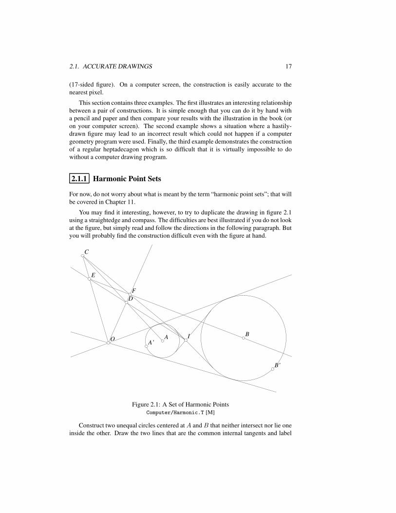
Figure 2.1: A Set of Harmonic PointsComputer/Harmonic.T [M]
Construct two unequal circles centered at A and B that neither intersect nor lie oneinside the other. Draw the two lines that are the common internal tangents and label
18 CHAPTER 2. COMPUTER-ASSISTED GEOMETRY
their intersection “I”, and similarly, draw the pair of common external tangents andlabel their intersection “O”. Now choose any point C not on the line IO and drawthe segments CO, CA, and CI . Select any point D on the segment CA and draw therays ID and OD that intersect the lines CO and CI at points E and F , respectively.Seemingly miraculously, the line EF passes through the point B, and this will be trueno matter where you choose to place the points C and D, and independent of the sizesand positions of the original circles.
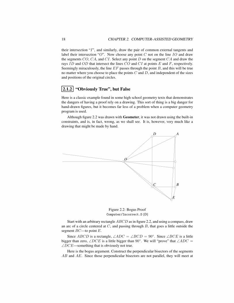
2.1.2 “Obviously True”, but False
Here is a classic example found in some high school geometry texts that demonstratesthe dangers of having a proof rely on a drawing. This sort of thing is a big danger forhand-drawn figures, but it becomes far less of a problem when a computer geometryprogram is used.
Although figure 2.2 was drawn with Geometer, it was not drawn using the built-inconstraints, and is, in fact, wrong, as we shall see. It is, however, very much like adrawing that might be made by hand.
AA
BB
DD
CC
EE
OO
Figure 2.2: Bogus ProofComputer/Incorrect.D [D]
Start with an arbitrary rectangleABCD as in figure 2.2, and using a compass, drawan arc of a circle centered at C, and passing through B, that goes a little outside thesegment BC—to point E.
Since ABCD is a rectangle, ∠ADC = ∠BCD = 90. Since ∠BCE is a littlebigger than zero, ∠DCE is a little bigger than 90. We will “prove” that ∠ADC =∠DCE—something that is obviously not true.
Here is the bogus argument. Construct the perpendicular bisectors of the segmentsAB and AE. Since those perpendicular bisectors are not parallel, they will meet at
2.1. ACCURATE DRAWINGS 19
some point O.Since ABCD is a rectangle, the perpendicular bisector of AB is also the perpen-
dicular bisector of DC, so all the points on it are equidistant from D and C. ThereforeDO = CO. By similar reasoning, O is equidistant from A and E, so AO = EO.
Points B and E are on the same circle centered at C, so BC = CE, and sinceABCD is a rectangle, AD = BC = CE.
To summarize, DO = CO, AD = CE, and AO = EO. Therefore the twotriangles4ADO and4ECO are congruent since they share three equal pairs of sides(using SSS congruence). Therefore ∠ECO = ∠ADO, and we can subtract the equalangles ∠CDO and ∠DCO to obtain the result we want—that ∠ADC = ∠ECD.
The result is clearly not true, but every step seems correct. What is wrong? Theanswer is that the diagram is not drawn accurately. (In fact, the author cheated and hadto misuse Geometer to get the desired misleading effect.)
AA
BB
DD
CC
EE
OO
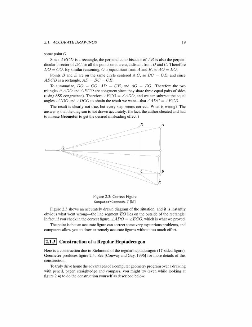
Figure 2.3: Correct FigureComputer/Correct.T [M]
Figure 2.3 shows an accurately drawn diagram of the situation, and it is instantlyobvious what went wrong—the line segment EO lies on the outside of the rectangle.In fact, if you check in the correct figure,∠ADO = ∠ECO, which is what we proved.
The point is that an accurate figure can correct some very mysterious problems, andcomputers allow you to draw extremely accurate figures without too much effort.
2.1.3 Construction of a Regular Heptadecagon
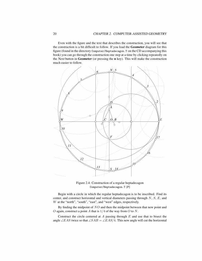
Here is a construction due to Richmond of the regular heptadecagon (17-sided figure).Geometer produces figure 2.4. See [Conway and Guy, 1996] for more details of thisconstruction.
To truly drive home the advantages of a computer geometry program over a drawingwith pencil, paper, straightedge and compass, you might try (even while looking atfigure 2.4) to do the construction yourself as described below.
20 CHAPTER 2. COMPUTER-ASSISTED GEOMETRY
Even with the figure and the text that describes the construction, you will see thatthe construction is a bit difficult to follow. If you load the Geometer diagram for thisfigure (found in the directory Computer/Heptadecagon.T on the CD accompanying thisbook) you can go through the construction one step at a time by clicking repeatedly onthe Next button in Geometer (or pressing the n key). This will make the constructionmuch easier to follow.
OO
NN
WW EE
SS
AA
BBCC
DD
FF
4466
13131515
11
55
33
77
1616
22
1717
1414
1212
1111
1010
99
88
Figure 2.4: Construction of a regular heptadecagonComputer/Heptadecagon.T [P]
Begin with a circle in which the regular heptadecagon is to be inscribed. Find itscenter, and construct horizontal and vertical diameters passing through N , S, E, andW at the “north”, “south”, “east”, and “west” edges, respectively.
By finding the midpoint of NO and then the midpoint between that new point andO again, construct a point A that is 1/4 of the way from O to N .
Construct the circle centered at A passing through E and use that to bisect theangle∠EAS twice so that ∠SAB = ∠EAS/4. This new angle will cut the horizontal
2.2. DRAWING MANIPULATION 21
diameter EW at B.
Now construct at A a 45 angle relative to AB intersecting EW at C. In otherwords, construct A such that ∠BAC = 45.
Find the intersections D nd F of the circle having EC as diameter with the lineNS.
Construct a circle with center B passing through D (or F ), and construct tangentsto it that are parallel to NS (this takes a few steps—first find the intersections of thecircle with EW , and then construct the tangents there).
If we call the point E “1”, and label the intersections of the vertical tangent linesfrom the last paragraph with the original circle “4”, “6”, “13”, and “14” as shown inthe figure, we have 5 points on the heptadecagon, and it is easy to construct the rest.For example, we could bisect the arc
)
46 to find point 5, and once we have the arc
)
45we can copy it all the way around the circle.
2.2 Drawing Manipulation
Once a figure is drawn in a computer geometry program, it can be manipulated. If youdraw one figure, it may be that some amazing relationship holds just by chance, butwhen you manipulate the diagram, it is extremely unlikely that the amazing relationshipwill continue to hold. This is particularly true for students in their first geometry course.When told to draw a triangle, they will almost invariably draw one that is very nearlyequilateral, and for equilateral triangles, all sorts of amazing relationships hold.
In this section we will examine a result that is not as well-known: Miquel’s theo-rem.
2.2.1 Miquel’s Theorem
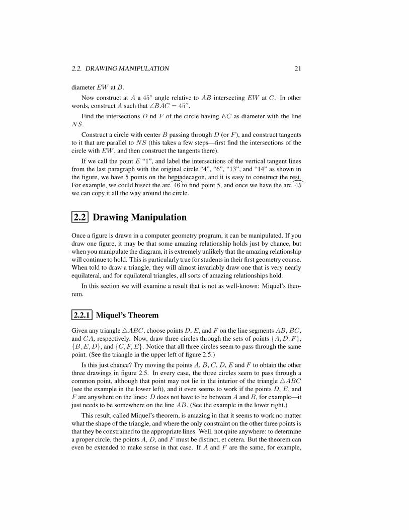
Given any triangle4ABC, choose pointsD, E, and F on the line segmentsAB, BC,and CA, respectively. Now, draw three circles through the sets of points A,D, F,B,E,D, and C,F,E. Notice that all three circles seem to pass through the samepoint. (See the triangle in the upper left of figure 2.5.)
Is this just chance? Try moving the points A, B, C, D, E and F to obtain the otherthree drawings in figure 2.5. In every case, the three circles seem to pass through acommon point, although that point may not lie in the interior of the triangle 4ABC(see the example in the lower left), and it even seems to work if the points D, E, andF are anywhere on the lines: D does not have to be betweenA andB, for example—itjust needs to be somewhere on the line AB. (See the example in the lower right.)
This result, called Miquel’s theorem, is amazing in that it seems to work no matterwhat the shape of the triangle, and where the only constraint on the other three points isthat they be constrained to the appropriate lines. Well, not quite anywhere: to determinea proper circle, the points A, D, and F must be distinct, et cetera. But the theorem caneven be extended to make sense in that case. If A and F are the same, for example,
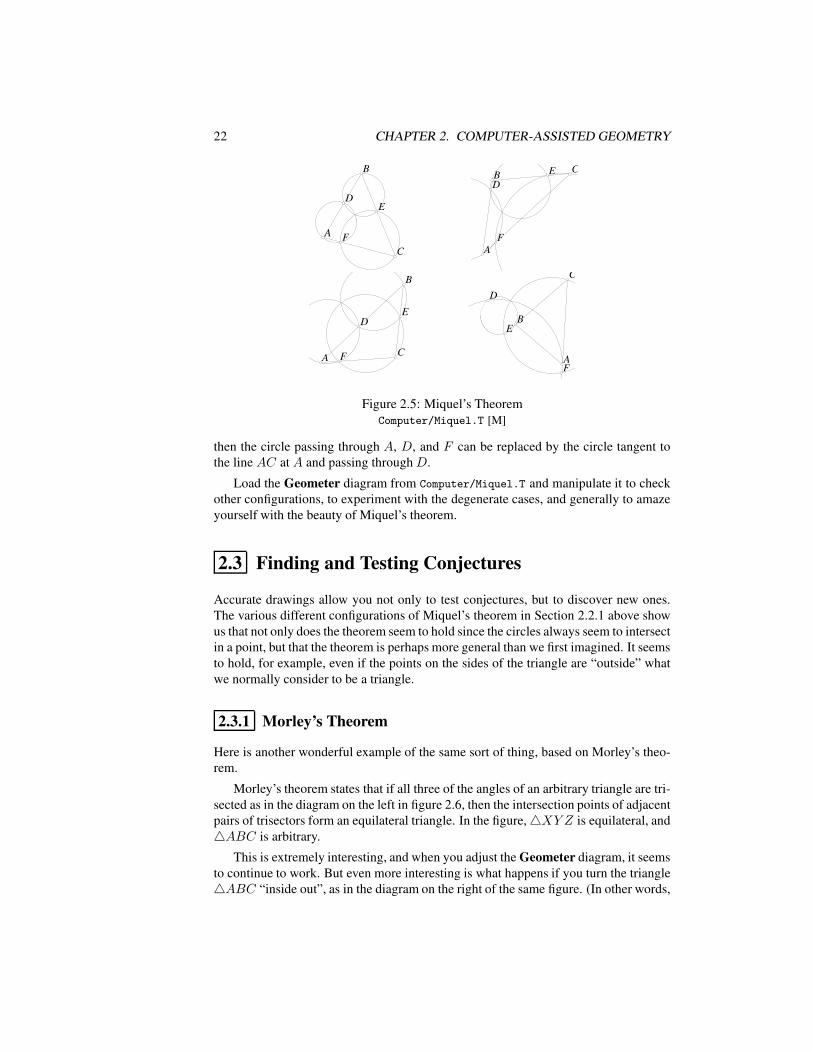
22 CHAPTER 2. COMPUTER-ASSISTED GEOMETRY
A
BB
CC
DDEE
FFAA
BB CCDD
EE
FF
AA
BB
CC
DDEE
FF AA
BB
CC
DD
EE
FF
Figure 2.5: Miquel’s TheoremComputer/Miquel.T [M]
then the circle passing through A, D, and F can be replaced by the circle tangent tothe line AC at A and passing throughD.
Load the Geometer diagram from Computer/Miquel.T and manipulate it to checkother configurations, to experiment with the degenerate cases, and generally to amazeyourself with the beauty of Miquel’s theorem.
2.3 Finding and Testing Conjectures
Accurate drawings allow you not only to test conjectures, but to discover new ones.The various different configurations of Miquel’s theorem in Section 2.2.1 above showus that not only does the theorem seem to hold since the circles always seem to intersectin a point, but that the theorem is perhaps more general than we first imagined. It seemsto hold, for example, even if the points on the sides of the triangle are “outside” whatwe normally consider to be a triangle.
2.3.1 Morley’s Theorem
Here is another wonderful example of the same sort of thing, based on Morley’s theo-rem.
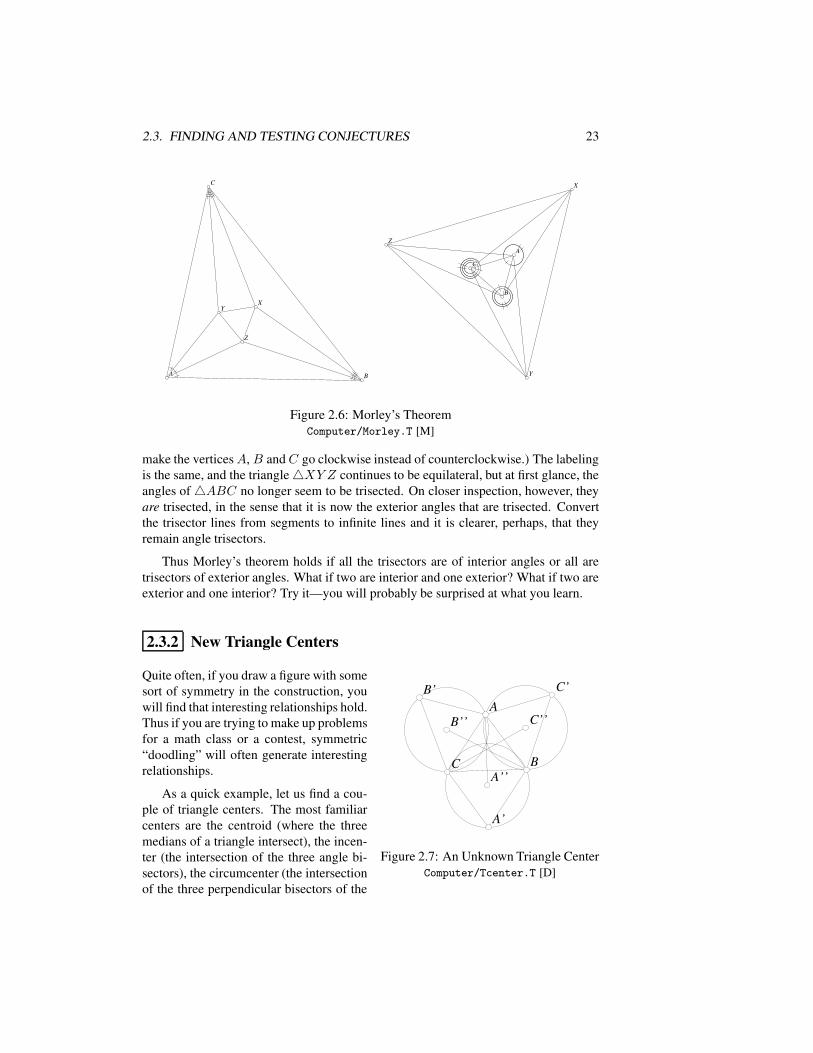
Morley’s theorem states that if all three of the angles of an arbitrary triangle are tri-sected as in the diagram on the left in figure 2.6, then the intersection points of adjacentpairs of trisectors form an equilateral triangle. In the figure,4XYZ is equilateral, and4ABC is arbitrary.
This is extremely interesting, and when you adjust the Geometer diagram, it seemsto continue to work. But even more interesting is what happens if you turn the triangle4ABC “inside out”, as in the diagram on the right of the same figure. (In other words,
2.3. FINDING AND TESTING CONJECTURES 23
AA
CC
BB
YY
ZZ
XX
AA
CC
BB
YY
ZZ
XX
Figure 2.6: Morley’s TheoremComputer/Morley.T [M]
make the verticesA, B andC go clockwise instead of counterclockwise.) The labelingis the same, and the triangle4XY Z continues to be equilateral, but at first glance, theangles of4ABC no longer seem to be trisected. On closer inspection, however, theyare trisected, in the sense that it is now the exterior angles that are trisected. Convertthe trisector lines from segments to infinite lines and it is clearer, perhaps, that theyremain angle trisectors.
Thus Morley’s theorem holds if all the trisectors are of interior angles or all aretrisectors of exterior angles. What if two are interior and one exterior? What if two areexterior and one interior? Try it—you will probably be surprised at what you learn.
2.3.2 New Triangle Centers
AA
BBCC
A’A’
B’B’ C’C’
B’’B’’ C’’C’’
A’’A’’
Figure 2.7: An Unknown Triangle CenterComputer/Tcenter.T [D]
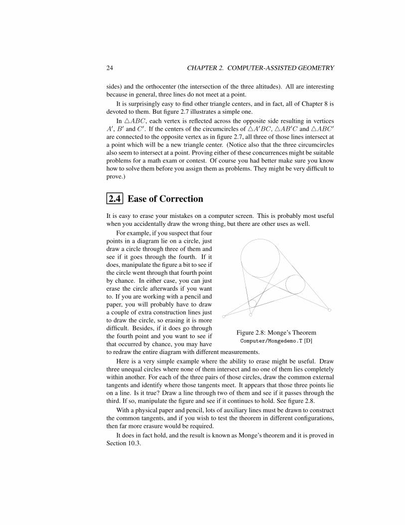
Quite often, if you draw a figure with somesort of symmetry in the construction, youwill find that interesting relationships hold.Thus if you are trying to make up problemsfor a math class or a contest, symmetric“doodling” will often generate interestingrelationships.
As a quick example, let us find a cou-ple of triangle centers. The most familiarcenters are the centroid (where the threemedians of a triangle intersect), the incen-ter (the intersection of the three angle bi-sectors), the circumcenter (the intersectionof the three perpendicular bisectors of the
24 CHAPTER 2. COMPUTER-ASSISTED GEOMETRY
sides) and the orthocenter (the intersection of the three altitudes). All are interestingbecause in general, three lines do not meet at a point.
It is surprisingly easy to find other triangle centers, and in fact, all of Chapter 8 isdevoted to them. But figure 2.7 illustrates a simple one.
In 4ABC, each vertex is reflected across the opposite side resulting in verticesA′, B′ and C ′. If the centers of the circumcircles of4A′BC, 4AB′C and4ABC ′are connected to the opposite vertex as in figure 2.7, all three of those lines intersect ata point which will be a new triangle center. (Notice also that the three circumcirclesalso seem to intersect at a point. Proving either of these concurrences might be suitableproblems for a math exam or contest. Of course you had better make sure you knowhow to solve them before you assign them as problems. They might be very difficult toprove.)
2.4 Ease of Correction
It is easy to erase your mistakes on a computer screen. This is probably most usefulwhen you accidentally draw the wrong thing, but there are other uses as well.
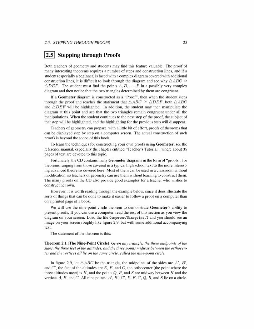
Figure 2.8: Monge’s TheoremComputer/Mongedemo.T [D]
For example, if you suspect that fourpoints in a diagram lie on a circle, justdraw a circle through three of them andsee if it goes through the fourth. If itdoes, manipulate the figure a bit to see ifthe circle went through that fourth pointby chance. In either case, you can justerase the circle afterwards if you wantto. If you are working with a pencil andpaper, you will probably have to drawa couple of extra construction lines justto draw the circle, so erasing it is moredifficult. Besides, if it does go throughthe fourth point and you want to see ifthat occurred by chance, you may haveto redraw the entire diagram with different measurements.
Here is a very simple example where the ability to erase might be useful. Drawthree unequal circles where none of them intersect and no one of them lies completelywithin another. For each of the three pairs of those circles, draw the common externaltangents and identify where those tangents meet. It appears that those three points lieon a line. Is it true? Draw a line through two of them and see if it passes through thethird. If so, manipulate the figure and see if it continues to hold. See figure 2.8.
With a physical paper and pencil, lots of auxiliary lines must be drawn to constructthe common tangents, and if you wish to test the theorem in different configurations,then far more erasure would be required.
It does in fact hold, and the result is known as Monge’s theorem and it is proved inSection 10.3.
2.5. STEPPING THROUGH PROOFS 25
2.5 Stepping through Proofs
Both teachers of geometry and students may find this feature valuable. The proof ofmany interesting theorems requires a number of steps and construction lines, and if astudent (especially a beginner) is faced with a complex diagram covered with additionalconstruction lines, it is difficult to look through the diagram and see why 4ABC ∼=4DEF . The student must find the points A,B, . . . , F in a possibly very complexdiagram and then notice that the two triangles determined by them are congruent.
If a Geometer diagram is constructed as a “Proof”, then when the student stepsthrough the proof and reaches the statement that 4ABC ∼= 4DEF , both 4ABCand 4DEF will be highlighted. In addition, the student may then manipulate thediagram at this point and see that the two triangles remain congruent under all themanipulations. When the student continues to the next step of the proof, the subject ofthat step will be highlighted, and the highlighting for the previous step will disappear.
Teachers of geometry can prepare, with a little bit of effort, proofs of theorems thatcan be displayed step by step on a computer screen. The actual construction of suchproofs is beyond the scope of this book.
To learn the techniques for constructing your own proofs using Geometer, see thereference manual, especially the chapter entitled “Teacher’s Tutorial”, where about 35pages of text are devoted to this topic.
Fortunately, the CD contains many Geometer diagrams in the form of “proofs”, fortheorems ranging from those covered in a typical high school text to the more interest-ing advanced theorems covered here. Most of them can be used in a classroom withoutmodification, so teachers of geometry can use them without learning to construct them.The many proofs on the CD also provide good examples for a teacher who wishes toconstruct her own.
However, it is worth reading through the example below, since it does illustrate thesorts of things that can be done to make it easier to follow a proof on a computer thanon a printed page of a book.
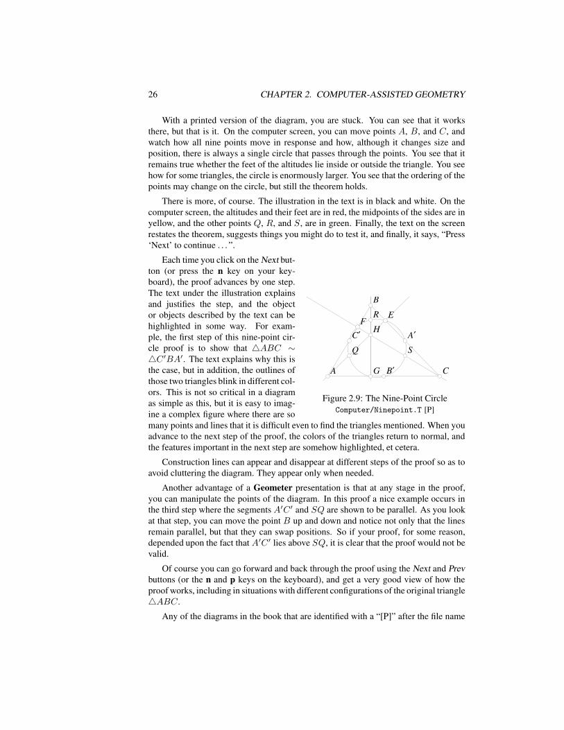
We will use the nine-point circle theorem to demonstrate Geometer’s ability topresent proofs. If you can use a computer, read the rest of this section as you view thediagram on your screen. Load the file Computer/Ninepoint.T and you should see animage on your screen roughly like figure 2.9, but with some additional accompanyingtext.
The statement of the theorem is this:
Theorem 2.1 (The Nine-Point Circle) Given any triangle, the three midpoints of thesides, the three feet of the altitudes, and the three points midway between the orthocen-ter and the vertices all lie on the same circle, called the nine-point circle.
In figure 2.9, let 4ABC be the triangle, the midpoints of the sides are A′, B′,and C ′, the feet of the altitudes are E, F , and G, the orthocenter (the point where thethree altitudes meet) is H , and the points Q, R, and S are midway between H and theverticesA, B, and C. All nine points: A′, B′, C ′, E, F , G, Q, R, and S lie on a circle.
26 CHAPTER 2. COMPUTER-ASSISTED GEOMETRY
With a printed version of the diagram, you are stuck. You can see that it worksthere, but that is it. On the computer screen, you can move points A, B, and C, andwatch how all nine points move in response and how, although it changes size andposition, there is always a single circle that passes through the points. You see that itremains true whether the feet of the altitudes lie inside or outside the triangle. You seehow for some triangles, the circle is enormously larger. You see that the ordering of thepoints may change on the circle, but still the theorem holds.
There is more, of course. The illustration in the text is in black and white. On thecomputer screen, the altitudes and their feet are in red, the midpoints of the sides are inyellow, and the other points Q, R, and S, are in green. Finally, the text on the screenrestates the theorem, suggests things you might do to test it, and finally, it says, “Press‘Next’ to continue . . . ”.
AA
BB
CC
FFEE
GG
HH
RR
SS
C′C′ A′A′
B′B′
Figure 2.9: The Nine-Point CircleComputer/Ninepoint.T [P]
Each time you click on the Next but-ton (or press the n key on your key-board), the proof advances by one step.The text under the illustration explainsand justifies the step, and the objector objects described by the text can behighlighted in some way. For exam-ple, the first step of this nine-point cir-cle proof is to show that 4ABC ∼4C ′BA′. The text explains why this isthe case, but in addition, the outlines ofthose two triangles blink in different col-ors. This is not so critical in a diagramas simple as this, but it is easy to imag-ine a complex figure where there are somany points and lines that it is difficult even to find the triangles mentioned. When youadvance to the next step of the proof, the colors of the triangles return to normal, andthe features important in the next step are somehow highlighted, et cetera.
Construction lines can appear and disappear at different steps of the proof so as toavoid cluttering the diagram. They appear only when needed.
Another advantage of a Geometer presentation is that at any stage in the proof,you can manipulate the points of the diagram. In this proof a nice example occurs inthe third step where the segments A′C ′ and SQ are shown to be parallel. As you lookat that step, you can move the point B up and down and notice not only that the linesremain parallel, but that they can swap positions. So if your proof, for some reason,depended upon the fact that A′C ′ lies above SQ, it is clear that the proof would not bevalid.
Of course you can go forward and back through the proof using the Next and Prevbuttons (or the n and p keys on the keyboard), and get a very good view of how theproof works, including in situations with different configurations of the original triangle4ABC.
Any of the diagrams in the book that are identified with a “[P]” after the file name
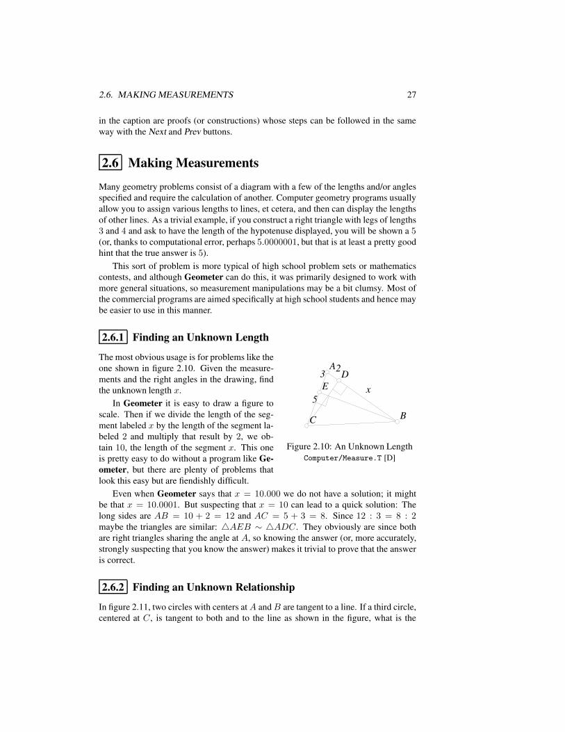
2.6. MAKING MEASUREMENTS 27
in the caption are proofs (or constructions) whose steps can be followed in the sameway with the Next and Prev buttons.
2.6 Making Measurements
Many geometry problems consist of a diagram with a few of the lengths and/or anglesspecified and require the calculation of another. Computer geometry programs usuallyallow you to assign various lengths to lines, et cetera, and then can display the lengthsof other lines. As a trivial example, if you construct a right triangle with legs of lengths3 and 4 and ask to have the length of the hypotenuse displayed, you will be shown a 5(or, thanks to computational error, perhaps 5.0000001, but that is at least a pretty goodhint that the true answer is 5).
This sort of problem is more typical of high school problem sets or mathematicscontests, and although Geometer can do this, it was primarily designed to work withmore general situations, so measurement manipulations may be a bit clumsy. Most ofthe commercial programs are aimed specifically at high school students and hence maybe easier to use in this manner.
2.6.1 Finding an Unknown Length
AADD
CC
EE
BB
2233
55xx
Figure 2.10: An Unknown LengthComputer/Measure.T [D]
The most obvious usage is for problems like theone shown in figure 2.10. Given the measure-ments and the right angles in the drawing, findthe unknown length x.
In Geometer it is easy to draw a figure toscale. Then if we divide the length of the seg-ment labeled x by the length of the segment la-beled 2 and multiply that result by 2, we ob-tain 10, the length of the segment x. This oneis pretty easy to do without a program like Ge-ometer, but there are plenty of problems thatlook this easy but are fiendishly difficult.
Even when Geometer says that x = 10.000 we do not have a solution; it mightbe that x = 10.0001. But suspecting that x = 10 can lead to a quick solution: Thelong sides are AB = 10 + 2 = 12 and AC = 5 + 3 = 8. Since 12 : 3 = 8 : 2maybe the triangles are similar: 4AEB ∼ 4ADC. They obviously are since bothare right triangles sharing the angle at A, so knowing the answer (or, more accurately,strongly suspecting that you know the answer) makes it trivial to prove that the answeris correct.
2.6.2 Finding an Unknown Relationship
In figure 2.11, two circles with centers atA andB are tangent to a line. If a third circle,centered at C, is tangent to both and to the line as shown in the figure, what is the
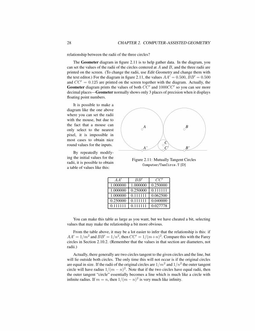
28 CHAPTER 2. COMPUTER-ASSISTED GEOMETRY
relationship between the radii of the three circles?
The Geometer diagram in figure 2.11 is to help gather data. In the diagram, youcan set the values of the radii of the circles centered at A and B, and the three radii areprinted on the screen. (To change the radii, use Edit Geometry and change them withthe text editor.) For the diagram in figure 2.11, the values AA′ = 0.500, BB′ = 0.500and CC ′ = 0.125 are printed on the screen together with the diagram. Actually, theGeometer diagram prints the values of both CC ′ and 1000CC ′ so you can see moredecimal places—Geometer normally shows only 3 places of precision when it displaysfloating point numbers.
A’A’
AA
B’B’
BB
CCC’C’
Figure 2.11: Mutually Tangent CirclesComputer/TanCircs.T [D]
It is possible to make adiagram like the one abovewhere you can set the radiiwith the mouse, but due tothe fact that a mouse canonly select to the nearestpixel, it is impossible inmost cases to obtain niceround values for the inputs.
By repeatedly modify-ing the initial values for theradii, it is possible to obtaina table of values like this:
AA′ BB′ CC ′
1.000000 1.000000 0.2500001.000000 0.250000 0.1111111.000000 0.111111 0.0625000.250000 0.111111 0.0400000.111111 0.111111 0.027778
You can make this table as large as you want, but we have cheated a bit, selectingvalues that may make the relationship a bit more obvious.
From the table above, it may be a lot easier to infer that the relationship is this: ifAA′ = 1/m2 andBB′ = 1/n2, thenCC ′ = 1/(m+n)2. Compare this with the Fareycircles in Section 2.10.2. (Remember that the values in that section are diameters, notradii.)
Actually, there generally are two circles tangent to the given circles and the line, butwill lie outside both circles. The only time this will not occur is if the original circlesare equal in size. If the radii of the original circles are 1/m2 and 1/n2 the outer tangentcircle will have radius 1/(m − n)2. Note that if the two circles have equal radii, thenthe outer tangent “circle” essentially becomes a line which is much like a circle withinfinite radius. If m = n, then 1/(m− n)2 is very much like infinity.
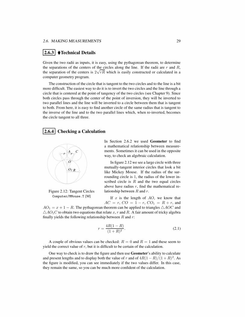
2.6. MAKING MEASUREMENTS 29
2.6.3 Technical Details
Given the two radii as inputs, it is easy, using the pythagorean theorem, to determinethe separations of the centers of the circles along the line. If the radii are r and R,the separation of the centers is 2
√rR which is easily constructed or calculated in a
computer geometry program.
The construction of the circle that is tangent to the two circles and to the line is a bitmore difficult. The easiest way to do it is to invert the two circles and the line through acircle that is centered at the point of tangency of the two circles (see Chapter 9). Sinceboth circles pass through the center of the point of inversion, they will be inverted totwo parallel lines and the line will be inverted to a circle between them that is tangentto both. From here, it is easy to find another circle of the same radius that is tangent tothe inverse of the line and to the two parallel lines which, when re-inverted, becomesthe circle tangent to all three.
2.6.4 Checking a Calculation
RR
rr rr
OO
O1O1
CCAA
Figure 2.12: Tangent CirclesComputer/MMouse.T [M]
In Section 2.6.2 we used Geometer to finda mathematical relationship between measure-ments. Sometimes it can be used in the oppositeway, to check an algebraic calculation.
In figure 2.12 we see a large circle with threemutually-tangent interior circles that look a bitlike Mickey Mouse. If the radius of the sur-rounding circle is 1, the radius of the lower in-scribed circle is R and the two equal circlesabove have radius r, find the mathematical re-lationship between R and r.
If x is the length of AO, we know thatAC = r, CO = 1 − r, CO1 = R + r, and
AO1 = x + 1− R. The pythagorean theorem can be applied to triangles4AOC and4AO1C to obtain two equations that relate x, r andR. A fair amount of tricky algebrafinally yields the following relationship between R and r:
r =4R(1−R)
(1 +R)2. (2.1)
A couple of obvious values can be checked: R = 0 and R = 1 and these seem toyield the correct value of r, but it is difficult to be certain of the calculation.
One way to check is to draw the figure and then use Geometer’s ability to calculateand present lengths and to display both the value of r and of 4R(1−R)/(1 +R)2. Asthe figure is modified, you can see immediately if the two values differ. In this case,they remain the same, so you can be much more confident of the calculation.
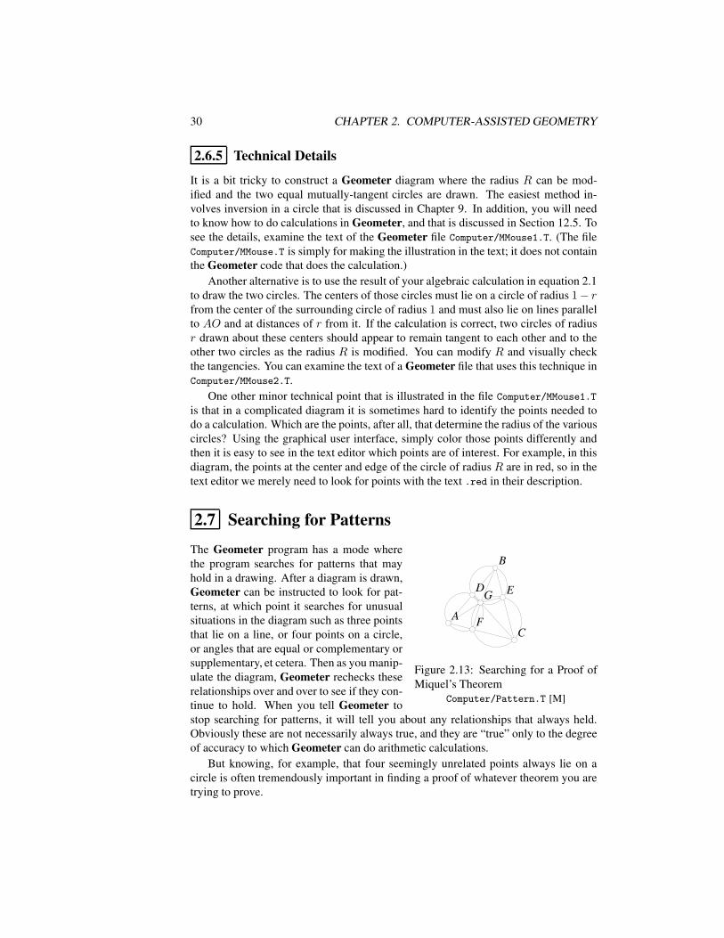
30 CHAPTER 2. COMPUTER-ASSISTED GEOMETRY
2.6.5 Technical Details
It is a bit tricky to construct a Geometer diagram where the radius R can be mod-ified and the two equal mutually-tangent circles are drawn. The easiest method in-volves inversion in a circle that is discussed in Chapter 9. In addition, you will needto know how to do calculations in Geometer, and that is discussed in Section 12.5. Tosee the details, examine the text of the Geometer file Computer/MMouse1.T. (The fileComputer/MMouse.T is simply for making the illustration in the text; it does not containthe Geometer code that does the calculation.)
Another alternative is to use the result of your algebraic calculation in equation 2.1to draw the two circles. The centers of those circles must lie on a circle of radius 1− rfrom the center of the surrounding circle of radius 1 and must also lie on lines parallelto AO and at distances of r from it. If the calculation is correct, two circles of radiusr drawn about these centers should appear to remain tangent to each other and to theother two circles as the radius R is modified. You can modify R and visually checkthe tangencies. You can examine the text of a Geometer file that uses this technique inComputer/MMouse2.T.
One other minor technical point that is illustrated in the file Computer/MMouse1.T
is that in a complicated diagram it is sometimes hard to identify the points needed todo a calculation. Which are the points, after all, that determine the radius of the variouscircles? Using the graphical user interface, simply color those points differently andthen it is easy to see in the text editor which points are of interest. For example, in thisdiagram, the points at the center and edge of the circle of radius R are in red, so in thetext editor we merely need to look for points with the text .red in their description.
2.7 Searching for Patterns
AA
BB
CC
DD EE
FF
GG
Figure 2.13: Searching for a Proof ofMiquel’s Theorem
Computer/Pattern.T [M]
The Geometer program has a mode wherethe program searches for patterns that mayhold in a drawing. After a diagram is drawn,Geometer can be instructed to look for pat-terns, at which point it searches for unusualsituations in the diagram such as three pointsthat lie on a line, or four points on a circle,or angles that are equal or complementary orsupplementary, et cetera. Then as you manip-ulate the diagram, Geometer rechecks theserelationships over and over to see if they con-tinue to hold. When you tell Geometer tostop searching for patterns, it will tell you about any relationships that always held.Obviously these are not necessarily always true, and they are “true” only to the degreeof accuracy to which Geometer can do arithmetic calculations.
But knowing, for example, that four seemingly unrelated points always lie on acircle is often tremendously important in finding a proof of whatever theorem you aretrying to prove.
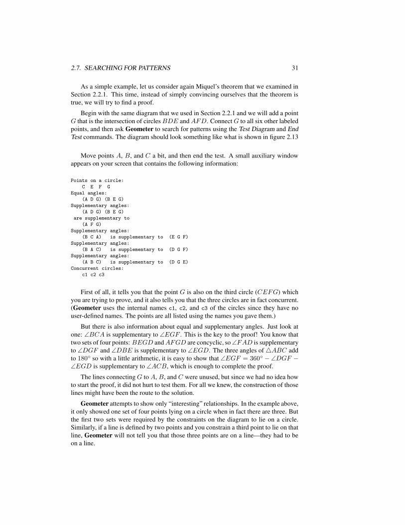
2.7. SEARCHING FOR PATTERNS 31
As a simple example, let us consider again Miquel’s theorem that we examined inSection 2.2.1. This time, instead of simply convincing ourselves that the theorem istrue, we will try to find a proof.
Begin with the same diagram that we used in Section 2.2.1 and we will add a pointG that is the intersection of circlesBDE andAFD. ConnectG to all six other labeledpoints, and then ask Geometer to search for patterns using the Test Diagram and EndTest commands. The diagram should look something like what is shown in figure 2.13
Move points A, B, and C a bit, and then end the test. A small auxiliary windowappears on your screen that contains the following information:
Points on a circle:
C E F G
Equal angles:
(A D G) (B E G)
Supplementary angles:
(A D G) (B E G)
are supplementary to
(A F G)
Supplementary angles:
(B C A) is supplementary to (E G F)
Supplementary angles:
(B A C) is supplementary to (D G F)
Supplementary angles:
(A B C) is supplementary to (D G E)
Concurrent circles:
c1 c2 c3
First of all, it tells you that the point G is also on the third circle (CEFG) whichyou are trying to prove, and it also tells you that the three circles are in fact concurrent.(Geometer uses the internal names c1, c2, and c3 of the circles since they have nouser-defined names. The points are all listed using the names you gave them.)
But there is also information about equal and supplementary angles. Just look atone: ∠BCA is supplementary to ∠EGF . This is the key to the proof! You know thattwo sets of four points: BEGD andAFGD are concyclic, so∠FAD is supplementaryto ∠DGF and ∠DBE is supplementary to ∠EGD. The three angles of4ABC addto 180 so with a little arithmetic, it is easy to show that ∠EGF = 360 − ∠DGF −∠EGD is supplementary to ∠ACB, which is enough to complete the proof.
The lines connectingG to A, B, and C were unused, but since we had no idea howto start the proof, it did not hurt to test them. For all we knew, the construction of thoselines might have been the route to the solution.
Geometer attempts to show only “interesting” relationships. In the example above,it only showed one set of four points lying on a circle when in fact there are three. Butthe first two sets were required by the constraints on the diagram to lie on a circle.Similarly, if a line is defined by two points and you constrain a third point to lie on thatline, Geometer will not tell you that those three points are on a line—they had to beon a line.
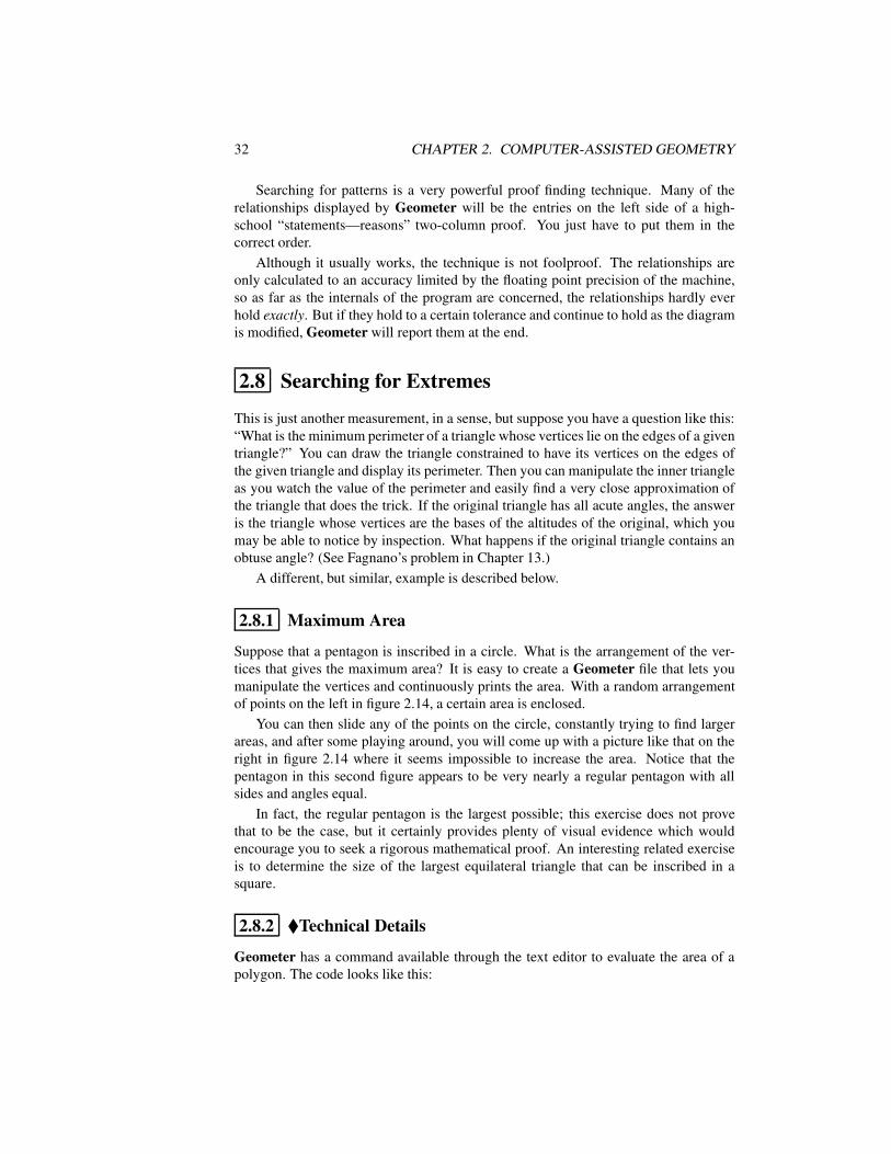
32 CHAPTER 2. COMPUTER-ASSISTED GEOMETRY
Searching for patterns is a very powerful proof finding technique. Many of therelationships displayed by Geometer will be the entries on the left side of a high-school “statements—reasons” two-column proof. You just have to put them in thecorrect order.
Although it usually works, the technique is not foolproof. The relationships areonly calculated to an accuracy limited by the floating point precision of the machine,so as far as the internals of the program are concerned, the relationships hardly everhold exactly. But if they hold to a certain tolerance and continue to hold as the diagramis modified, Geometer will report them at the end.
2.8 Searching for Extremes
This is just another measurement, in a sense, but suppose you have a question like this:“What is the minimum perimeter of a triangle whose vertices lie on the edges of a giventriangle?” You can draw the triangle constrained to have its vertices on the edges ofthe given triangle and display its perimeter. Then you can manipulate the inner triangleas you watch the value of the perimeter and easily find a very close approximation ofthe triangle that does the trick. If the original triangle has all acute angles, the answeris the triangle whose vertices are the bases of the altitudes of the original, which youmay be able to notice by inspection. What happens if the original triangle contains anobtuse angle? (See Fagnano’s problem in Chapter 13.)
A different, but similar, example is described below.
2.8.1 Maximum Area
Suppose that a pentagon is inscribed in a circle. What is the arrangement of the ver-tices that gives the maximum area? It is easy to create a Geometer file that lets youmanipulate the vertices and continuously prints the area. With a random arrangementof points on the left in figure 2.14, a certain area is enclosed.
You can then slide any of the points on the circle, constantly trying to find largerareas, and after some playing around, you will come up with a picture like that on theright in figure 2.14 where it seems impossible to increase the area. Notice that thepentagon in this second figure appears to be very nearly a regular pentagon with allsides and angles equal.
In fact, the regular pentagon is the largest possible; this exercise does not provethat to be the case, but it certainly provides plenty of visual evidence which wouldencourage you to seek a rigorous mathematical proof. An interesting related exerciseis to determine the size of the largest equilateral triangle that can be inscribed in asquare.
2.8.2 Technical Details
Geometer has a command available through the text editor to evaluate the area of apolygon. The code looks like this:
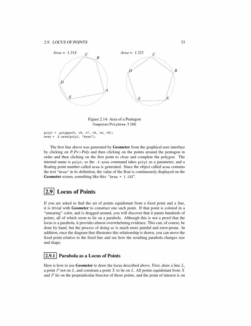
2.9. LOCUS OF POINTS 33
Area = 1.314Area = 1.314 CC
DD
EE
AA
BBArea = 1.521Area = 1.521 CC
DD
EE AA
BB
Figure 2.14: Area of a PentagonComputer/PolyArea.T [M]
poly1 = .polygon(5, v6, v7, v3, v4, v5);
area = .f.area(poly1, "Area");
The first line above was generated by Geometer from the graphical user interfaceby clicking on P..P=>Poly and then clicking on the points around the pentagon inorder and then clicking on the first point to close and complete the polygon. Theinternal name is poly1, so the .f.area command takes poly1 as a parameter, and afloating point number called area is generated. Since the object called area containsthe text "Area" in its definition, the value of the float is continuously displayed on theGeometer screen, something like this: “Area = 1.132”.
2.9 Locus of Points
If you are asked to find the set of points equidistant from a fixed point and a line,it is trivial with Geometer to construct one such point. If that point is colored in a“smearing” color, and is dragged around, you will discover that it paints hundreds ofpoints, all of which seem to lie on a parabola. Although this is not a proof that thelocus is a parabola, it provides almost overwhelming evidence. This can, of course, bedone by hand, but the process of doing so is much more painful and error-prone. Inaddition, once the diagram that illustrates this relationship is drawn, you can move thefixed point relative to the fixed line and see how the resulting parabola changes sizeand shape.
2.9.1 Parabola as a Locus of Points
Here is how to use Geometer to draw the locus described above. First, draw a line L,a point P not on L, and constrain a point X to lie on L. All points equidistant from Xand P lie on the perpendicular bisector of those points, and the point of interest is on
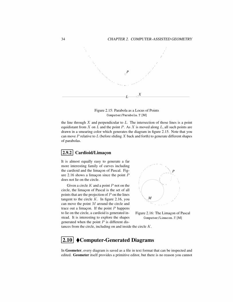
34 CHAPTER 2. COMPUTER-ASSISTED GEOMETRY
LL
PP
XX
Figure 2.15: Parabola as a Locus of PointsComputer/Parabola.T [M]
the line through X and perpendicular to L. The intersection of those lines is a pointequidistant from X on L and the point P . As X is moved along L, all such points aredrawn in a smearing color which generates the diagram in figure 2.15. Note that youcan move P relative to L (before slidingX back and forth) to generate different shapesof parabolas.
2.9.2 Cardioid/Limacon
PP
MM
Figure 2.16: The Limacon of PascalComputer/Limacon.T [M]
It is almost equally easy to generate a farmore interesting family of curves includingthe cardioid and the limacon of Pascal. Fig-ure 2.16 shows a limacon since the point Pdoes not lie on the circle.
Given a circleK and a point P not on thecircle, the limacon of Pascal is the set of allpoints that are the projection of P on the linestangent to the circle K. In figure 2.16, youcan move the point M around the circle andtrace out a limacon. If the point P happensto lie on the circle, a cardioid is generated in-stead. It is interesting to explore the shapesgenerated when the point P is different dis-tances from the circle, including on and inside the circle K.
2.10 Computer-Generated Diagrams
In Geometer, every diagram is saved as a file in text format that can be inspected andedited. Geometer itself provides a primitive editor, but there is no reason you cannot
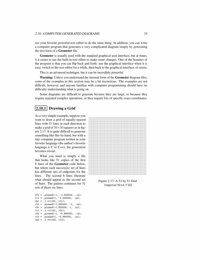
2.10. COMPUTER-GENERATED DIAGRAMS 35
use your favorite powerful text editor to do the same thing. In addition, you can writea computer program that generates a very complicated diagram simply by generatingthe text form of a Geometer file.
Geometer is usually used with the standard graphical user interface, but at times,it it easier to use the built-in text editor to make some changes. One of the beauties ofthe program is that you can flip back and forth: use the graphical interface when it iseasy, switch to the text editor for a while, then back to the graphical interface, et cetera.
This is an advanced technique, but it can be incredibly powerful.
Warning: Unless you understand the internal form of the Geometer diagram files,some of the examples in this section may be a bit mysterious. The examples are notdifficult, however, and anyone familiar with computer programming should have nodifficulty understanding what is going on.
Some diagrams are difficult to generate because they are large, or because theyrequire repeated complex operations, or they require lots of specific exact coordinates.
2.10.1 Drawing a Grid
Figure 2.17: A 51 by 51 GridComputer/Grid.T [D]
As a very simple example, suppose youwant to draw a grid of equally-spacedlines with 51 lines in each direction tomake a grid of 50×50 squares as in fig-ure 2.17. It is quite difficult to generatesomething like this by hand, but with atiny computer program written in yourfavorite language (the author’s favoritelanguage is C or C++), the generationbecomes trivial.
What you need is simply a filethat looks like 51 copies of the first6 lines of the Geometer code below,but where each successive set of lineshas different sets of endpoints for thelines. The second 6 lines illustratewhat should appear as the second setof lines. The pattern continues for 51sets of those six lines.
v01 = .pinned(-1, -1.000000, .in);
v11 = .pinned(1, -1.000000, .in);
lh1 = .l.vv(v01, v11);
v21 = .pinned(-1.000000, -1, .in);
v31 = .pinned(-1.000000, 1, .in);
lv1 = .l.vv(v21, v31);
v02 = .pinned(-1, -0.960000, .in);
v12 = .pinned(1, -0.960000, .in);
lh2 = .l.vv(v02, v12);
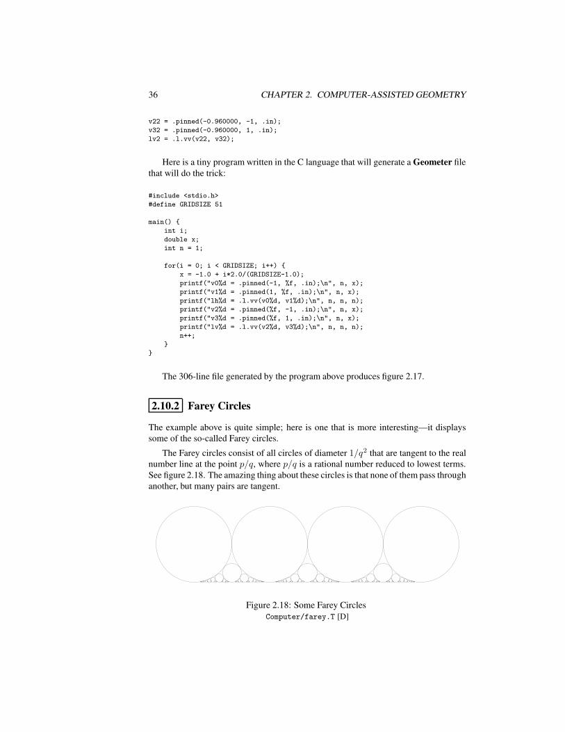
36 CHAPTER 2. COMPUTER-ASSISTED GEOMETRY
v22 = .pinned(-0.960000, -1, .in);
v32 = .pinned(-0.960000, 1, .in);
lv2 = .l.vv(v22, v32);
Here is a tiny program written in the C language that will generate a Geometer filethat will do the trick:
#include <stdio.h>
#define GRIDSIZE 51
main()
int i;
double x;
int n = 1;
for(i = 0; i < GRIDSIZE; i++)
x = -1.0 + i*2.0/(GRIDSIZE-1.0);
printf("v0%d = .pinned(-1, %f, .in);\n", n, x);
printf("v1%d = .pinned(1, %f, .in);\n", n, x);
printf("lh%d = .l.vv(v0%d, v1%d);\n", n, n, n);
printf("v2%d = .pinned(%f, -1, .in);\n", n, x);
printf("v3%d = .pinned(%f, 1, .in);\n", n, x);
printf("lv%d = .l.vv(v2%d, v3%d);\n", n, n, n);
n++;
The 306-line file generated by the program above produces figure 2.17.
2.10.2 Farey Circles
The example above is quite simple; here is one that is more interesting—it displayssome of the so-called Farey circles.
The Farey circles consist of all circles of diameter 1/q2 that are tangent to the realnumber line at the point p/q, where p/q is a rational number reduced to lowest terms.See figure 2.18. The amazing thing about these circles is that none of them pass throughanother, but many pairs are tangent.
Figure 2.18: Some Farey CirclesComputer/farey.T [D]
2.10. COMPUTER-GENERATED DIAGRAMS 37
To generate a list of circles for Geometer to draw, we would like to make a se-quence of entries in a Geometer file that look like this:
v6 = .pinned(2.500000, 0.125000, .in);
l6 = .l.vlperp(v6, l, .in);
vv6 = .v.ll(l, l6, .in);
c6 = .c.vv(v6, vv6);
In the example above, the circle above the point 2.5 on the real line corresponds tothe rational number 5/2, or p = 5 and q = 2. This circle must be centered at (2.5, .125)since its diameter is 1/q2 and hence must have radius 1/8 = .125. To construct thiscircle in the example code above, the point v6 is pinned with coordinates (2.5, 0.125).From that point, a perpendicular line l6 is dropped to the line l, which is defined oncein the file as the real axis. The point vv6 is the intersection of those lines, and finally,the circle that interests us is centered at v6 and passes through vv6.
Here is the C code that generates the complete Geometer file, including code togenerate the line l:
#include <stdio.h>
#define NMAX 12
int gcd(int i, int j)
if (i % j == 0) return j;
return gcd(j, i%j);
void outcircle(int q, int p)
static int n = 0;
printf("v%d = .pinned(%f, %f, .in);\n", n,
((float) p)/((float) q), 0.5/((float)q*q));
printf("l%d = .l.vlperp(v%d, l, .in);\n", n, n);
printf("vv%d = .v.ll(l, l%d, .in);\n", n, n);
printf("c%d = .c.vv(v%d, vv%d);\n", n, n, n);
n++;
main()
int p, q;
printf("v00 = .pinned(0, 0, .in);\n");
printf("v01 = .pinned(1, 0, .in);\n");
printf("l = .l.vv(v00, v01, .in);\n");
outcircle(1, 0);
for (q = 1; q <= NMAX; q++)
for (p = 1; p <= 3*q; p++)
if (gcd(q,p) == 1) outcircle(q,p);
The constant NMAX is 12, which is the largest denominator that the program willconsider. The routine gcd finds the greatest common divisor of two numbers whichis used to make certain that the fractions are reduced to lowest terms. The routineoutcircle prints all the data needed to draw a circle over the point p/q with radius
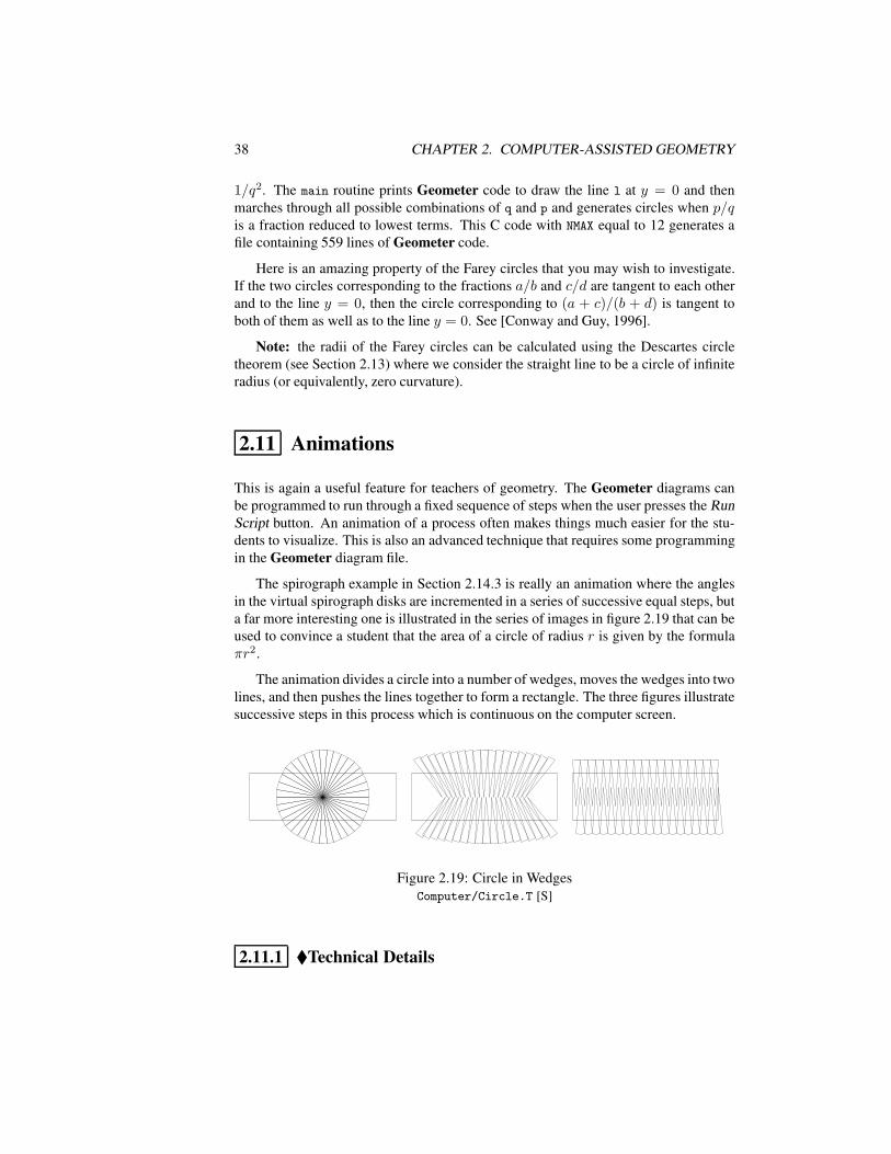
38 CHAPTER 2. COMPUTER-ASSISTED GEOMETRY
1/q2. The main routine prints Geometer code to draw the line l at y = 0 and thenmarches through all possible combinations of q and p and generates circles when p/qis a fraction reduced to lowest terms. This C code with NMAX equal to 12 generates afile containing 559 lines of Geometer code.
Here is an amazing property of the Farey circles that you may wish to investigate.If the two circles corresponding to the fractions a/b and c/d are tangent to each otherand to the line y = 0, then the circle corresponding to (a + c)/(b + d) is tangent toboth of them as well as to the line y = 0. See [Conway and Guy, 1996].
Note: the radii of the Farey circles can be calculated using the Descartes circletheorem (see Section 2.13) where we consider the straight line to be a circle of infiniteradius (or equivalently, zero curvature).
2.11 Animations
This is again a useful feature for teachers of geometry. The Geometer diagrams canbe programmed to run through a fixed sequence of steps when the user presses the RunScript button. An animation of a process often makes things much easier for the stu-dents to visualize. This is also an advanced technique that requires some programmingin the Geometer diagram file.
The spirograph example in Section 2.14.3 is really an animation where the anglesin the virtual spirograph disks are incremented in a series of successive equal steps, buta far more interesting one is illustrated in the series of images in figure 2.19 that can beused to convince a student that the area of a circle of radius r is given by the formulaπr2.
The animation divides a circle into a number of wedges, moves the wedges into twolines, and then pushes the lines together to form a rectangle. The three figures illustratesuccessive steps in this process which is continuous on the computer screen.
Figure 2.19: Circle in WedgesComputer/Circle.T [S]
2.11.1 Technical Details
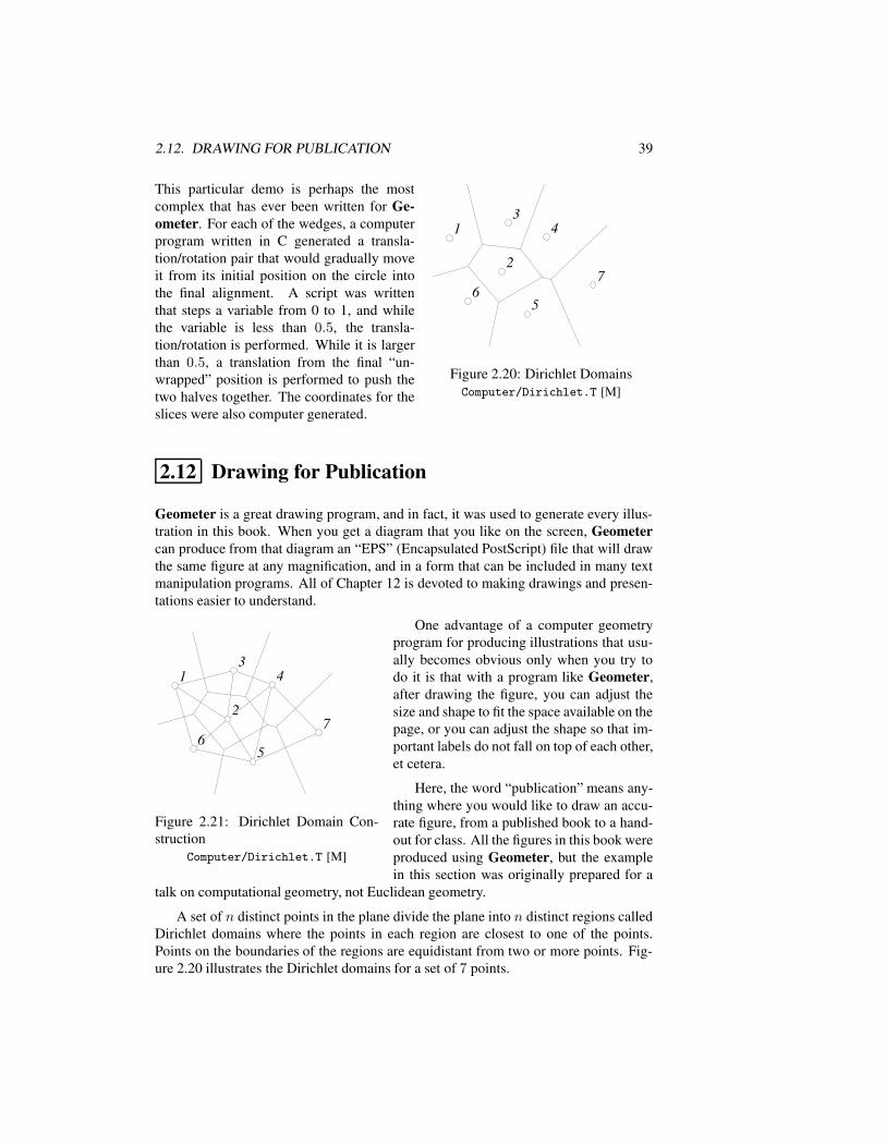
2.12. DRAWING FOR PUBLICATION 39
11
22
3344
5566
77
Figure 2.20: Dirichlet DomainsComputer/Dirichlet.T [M]
This particular demo is perhaps the mostcomplex that has ever been written for Ge-ometer. For each of the wedges, a computerprogram written in C generated a transla-tion/rotation pair that would gradually moveit from its initial position on the circle intothe final alignment. A script was writtenthat steps a variable from 0 to 1, and whilethe variable is less than 0.5, the transla-tion/rotation is performed. While it is largerthan 0.5, a translation from the final “un-wrapped” position is performed to push thetwo halves together. The coordinates for theslices were also computer generated.
2.12 Drawing for Publication
Geometer is a great drawing program, and in fact, it was used to generate every illus-tration in this book. When you get a diagram that you like on the screen, Geometercan produce from that diagram an “EPS” (Encapsulated PostScript) file that will drawthe same figure at any magnification, and in a form that can be included in many textmanipulation programs. All of Chapter 12 is devoted to making drawings and presen-tations easier to understand.
11
22
3344
5566
77
Figure 2.21: Dirichlet Domain Con-struction
Computer/Dirichlet.T [M]
One advantage of a computer geometryprogram for producing illustrations that usu-ally becomes obvious only when you try todo it is that with a program like Geometer,after drawing the figure, you can adjust thesize and shape to fit the space available on thepage, or you can adjust the shape so that im-portant labels do not fall on top of each other,et cetera.
Here, the word “publication” means any-thing where you would like to draw an accu-rate figure, from a published book to a hand-out for class. All the figures in this book wereproduced using Geometer, but the examplein this section was originally prepared for a
talk on computational geometry, not Euclidean geometry.
A set of n distinct points in the plane divide the plane into n distinct regions calledDirichlet domains where the points in each region are closest to one of the points.Points on the boundaries of the regions are equidistant from two or more points. Fig-ure 2.20 illustrates the Dirichlet domains for a set of 7 points.
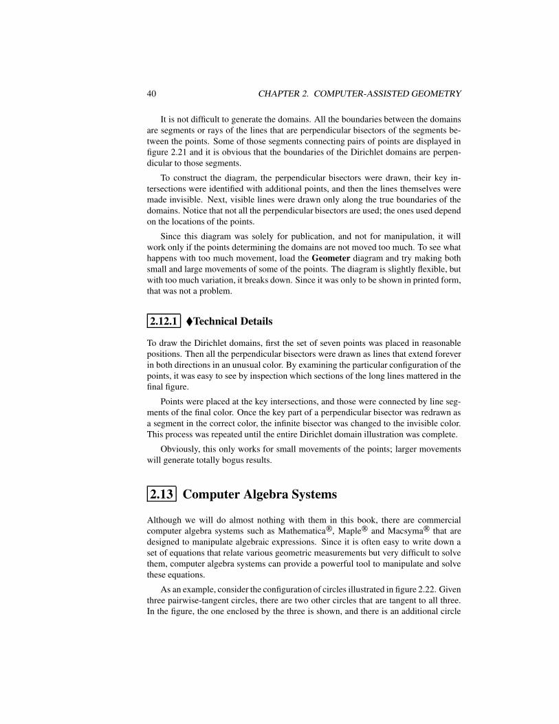
40 CHAPTER 2. COMPUTER-ASSISTED GEOMETRY
It is not difficult to generate the domains. All the boundaries between the domainsare segments or rays of the lines that are perpendicular bisectors of the segments be-tween the points. Some of those segments connecting pairs of points are displayed infigure 2.21 and it is obvious that the boundaries of the Dirichlet domains are perpen-dicular to those segments.
To construct the diagram, the perpendicular bisectors were drawn, their key in-tersections were identified with additional points, and then the lines themselves weremade invisible. Next, visible lines were drawn only along the true boundaries of thedomains. Notice that not all the perpendicular bisectors are used; the ones used dependon the locations of the points.
Since this diagram was solely for publication, and not for manipulation, it willwork only if the points determining the domains are not moved too much. To see whathappens with too much movement, load the Geometer diagram and try making bothsmall and large movements of some of the points. The diagram is slightly flexible, butwith too much variation, it breaks down. Since it was only to be shown in printed form,that was not a problem.
2.12.1 Technical Details
To draw the Dirichlet domains, first the set of seven points was placed in reasonablepositions. Then all the perpendicular bisectors were drawn as lines that extend foreverin both directions in an unusual color. By examining the particular configuration of thepoints, it was easy to see by inspection which sections of the long lines mattered in thefinal figure.
Points were placed at the key intersections, and those were connected by line seg-ments of the final color. Once the key part of a perpendicular bisector was redrawn asa segment in the correct color, the infinite bisector was changed to the invisible color.This process was repeated until the entire Dirichlet domain illustration was complete.
Obviously, this only works for small movements of the points; larger movementswill generate totally bogus results.
2.13 Computer Algebra Systems
Although we will do almost nothing with them in this book, there are commercialcomputer algebra systems such as Mathematica, Maple and Macsyma that aredesigned to manipulate algebraic expressions. Since it is often easy to write down aset of equations that relate various geometric measurements but very difficult to solvethem, computer algebra systems can provide a powerful tool to manipulate and solvethese equations.
As an example, consider the configuration of circles illustrated in figure 2.22. Giventhree pairwise-tangent circles, there are two other circles that are tangent to all three.In the figure, the one enclosed by the three is shown, and there is an additional circle
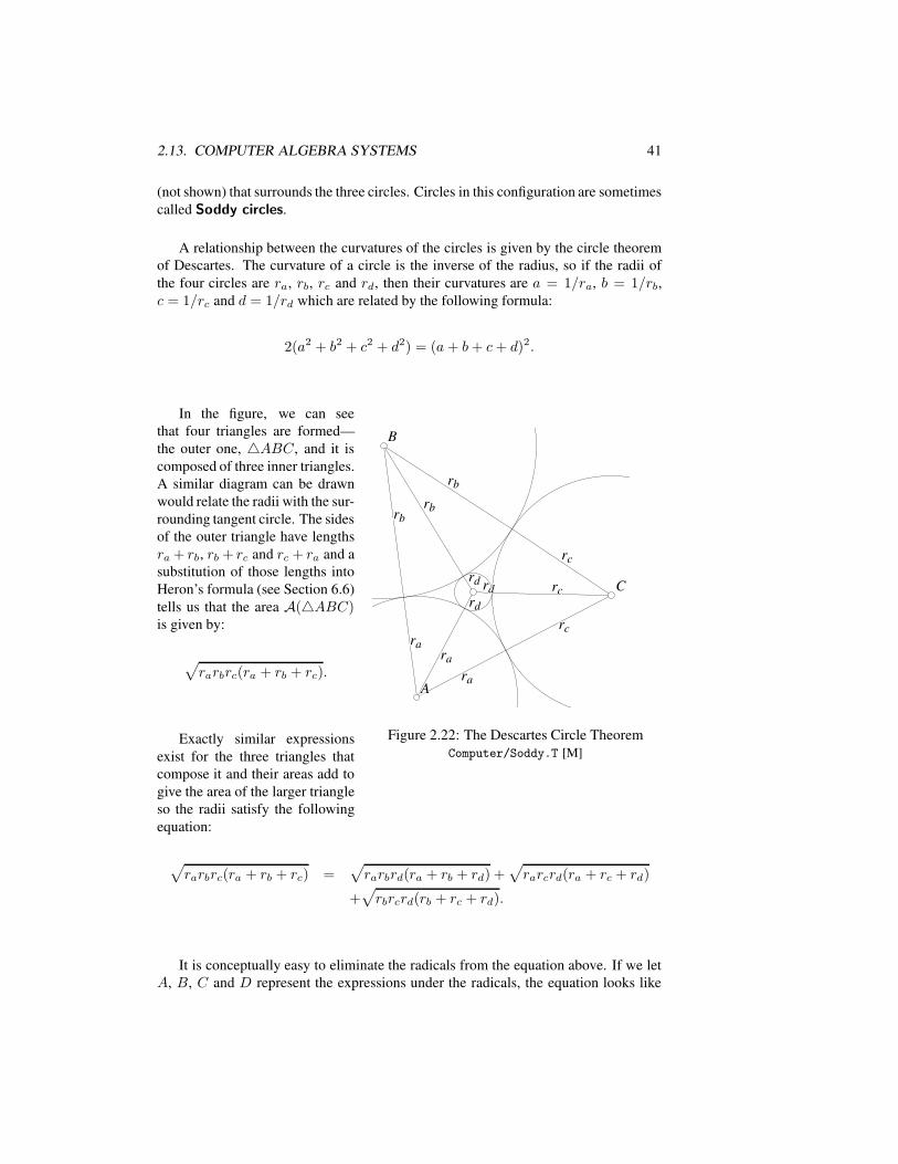
2.13. COMPUTER ALGEBRA SYSTEMS 41
(not shown) that surrounds the three circles. Circles in this configuration are sometimescalled Soddy circles.
A relationship between the curvatures of the circles is given by the circle theoremof Descartes. The curvature of a circle is the inverse of the radius, so if the radii ofthe four circles are ra, rb, rc and rd, then their curvatures are a = 1/ra, b = 1/rb,c = 1/rc and d = 1/rd which are related by the following formula:
2(a2 + b2 + c2 + d2) = (a+ b+ c+ d)2.
rbrb
rbrb
rara
rara
rcrc
rcrc
rdrdrdrd
rdrd
rcrc
rbrb
rara
AA
BB
CC
Figure 2.22: The Descartes Circle TheoremComputer/Soddy.T [M]
In the figure, we can seethat four triangles are formed—the outer one, 4ABC, and it iscomposed of three inner triangles.A similar diagram can be drawnwould relate the radii with the sur-rounding tangent circle. The sidesof the outer triangle have lengthsra + rb, rb + rc and rc + ra and asubstitution of those lengths intoHeron’s formula (see Section 6.6)tells us that the area A(4ABC)is given by:
√rarbrc(ra + rb + rc).
Exactly similar expressionsexist for the three triangles thatcompose it and their areas add togive the area of the larger triangleso the radii satisfy the followingequation:
√rarbrc(ra + rb + rc) =
√rarbrd(ra + rb + rd) +
√rarcrd(ra + rc + rd)
+√rbrcrd(rb + rc + rd).
It is conceptually easy to eliminate the radicals from the equation above. If we letA, B, C and D represent the expressions under the radicals, the equation looks like
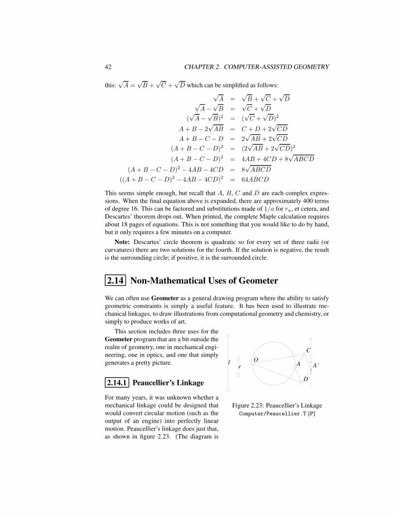
42 CHAPTER 2. COMPUTER-ASSISTED GEOMETRY
this:√A =
√B +
√C +
√D which can be simplified as follows:
√A =
√B +
√C +
√D√
A−√B =
√C +
√D
(√A−√B)2 = (
√C +
√D)2
A+B − 2√AB = C +D + 2
√CD
A+B − C −D = 2√AB + 2
√CD
(A+B − C −D)2 = (2√AB + 2
√CD)2
(A+B − C −D)2 = 4AB + 4CD + 8√ABCD
(A+B − C −D)2 − 4AB − 4CD = 8√ABCD
((A+B − C −D)2 − 4AB − 4CD)2 = 64ABCD
This seems simple enough, but recall that A, B, C and D are each complex expres-sions. When the final equation above is expanded, there are approximately 400 termsof degree 16. This can be factored and substitutions made of 1/a for ra, et cetera, andDescartes’ theorem drops out. When printed, the complete Maple calculation requiresabout 18 pages of equations. This is not something that you would like to do by hand,but it only requires a few minutes on a computer.
Note: Descartes’ circle theorem is quadratic so for every set of three radii (orcurvatures) there are two solutions for the fourth. If the solution is negative, the resultis the surrounding circle; if positive, it is the surrounded circle.
2.14 Non-Mathematical Uses of Geometer
We can often use Geometer as a general drawing program where the ability to satisfygeometric constraints is simply a useful feature. It has been used to illustrate me-chanical linkages, to draw illustrations from computational geometry and chemistry, orsimply to produce works of art.
rrll OO
AA
CC
DD
A’A’
Figure 2.23: Peaucellier’s LinkageComputer/Peaucellier.T [P]
This section includes three uses for theGeometer program that are a bit outside therealm of geometry, one in mechanical engi-neering, one in optics, and one that simplygenerates a pretty picture.
2.14.1 Peaucellier’s Linkage
For many years, it was unknown whether amechanical linkage could be designed thatwould convert circular motion (such as theoutput of an engine) into perfectly linearmotion. Peaucellier’s linkage does just that,as shown in figure 2.23. (The diagram is
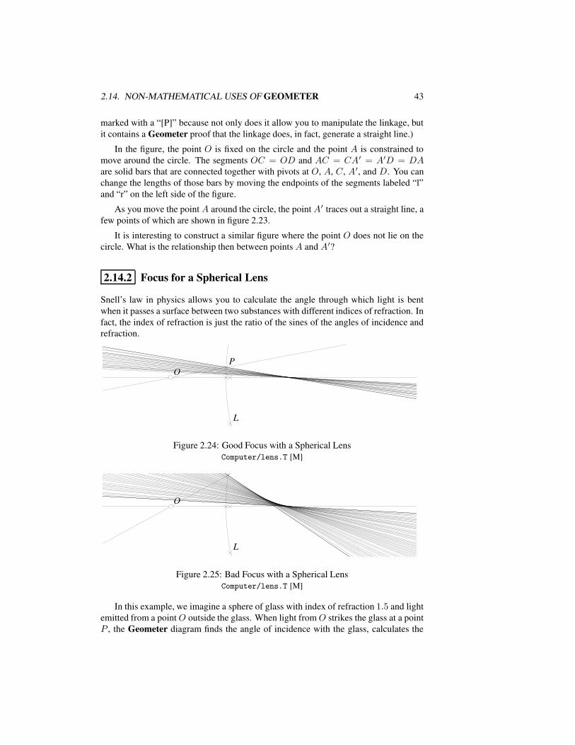
2.14. NON-MATHEMATICAL USES OF GEOMETER 43
marked with a “[P]” because not only does it allow you to manipulate the linkage, butit contains a Geometer proof that the linkage does, in fact, generate a straight line.)
In the figure, the point O is fixed on the circle and the point A is constrained tomove around the circle. The segments OC = OD and AC = CA′ = A′D = DAare solid bars that are connected together with pivots at O, A, C, A′, and D. You canchange the lengths of those bars by moving the endpoints of the segments labeled “l”and “r” on the left side of the figure.
As you move the point A around the circle, the point A′ traces out a straight line, afew points of which are shown in figure 2.23.
It is interesting to construct a similar figure where the point O does not lie on thecircle. What is the relationship then between points A and A′?
2.14.2 Focus for a Spherical Lens
Snell’s law in physics allows you to calculate the angle through which light is bentwhen it passes a surface between two substances with different indices of refraction. Infact, the index of refraction is just the ratio of the sines of the angles of incidence andrefraction.
LL
PPOO
Figure 2.24: Good Focus with a Spherical LensComputer/lens.T [M]
LL
PP
OO
Figure 2.25: Bad Focus with a Spherical LensComputer/lens.T [M]
In this example, we imagine a sphere of glass with index of refraction 1.5 and lightemitted from a pointO outside the glass. When light fromO strikes the glass at a pointP , the Geometer diagram finds the angle of incidence with the glass, calculates the
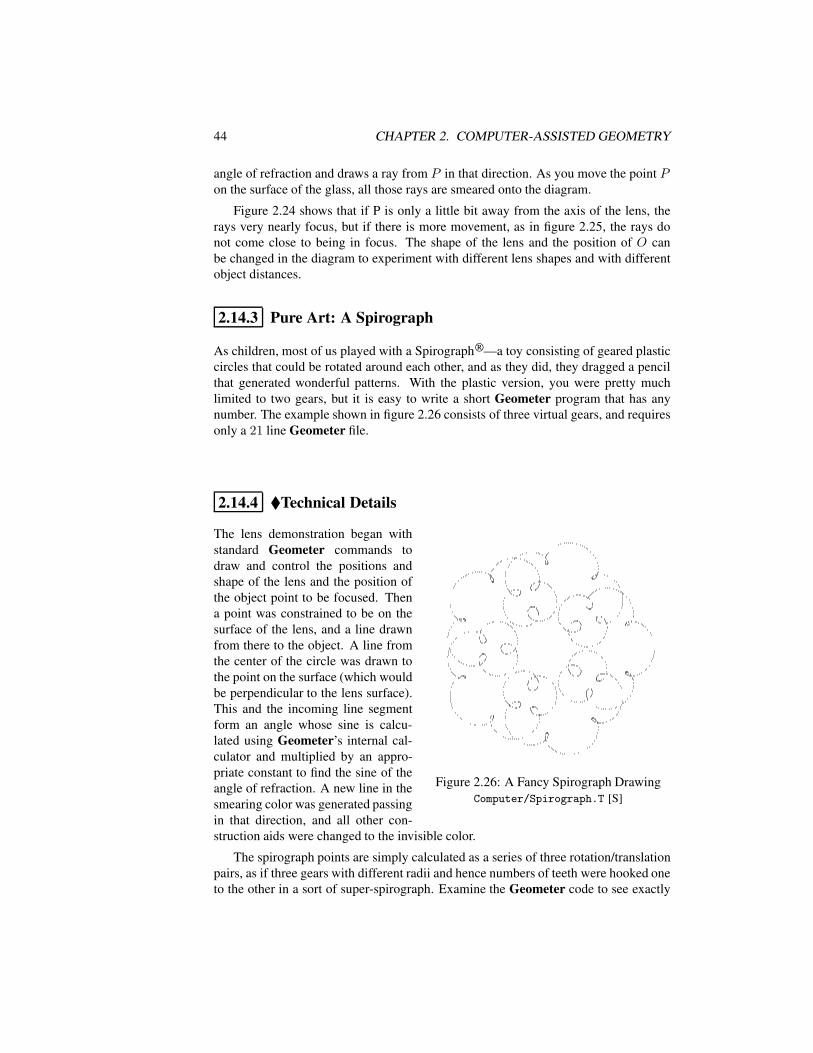
44 CHAPTER 2. COMPUTER-ASSISTED GEOMETRY
angle of refraction and draws a ray from P in that direction. As you move the point Pon the surface of the glass, all those rays are smeared onto the diagram.
Figure 2.24 shows that if P is only a little bit away from the axis of the lens, therays very nearly focus, but if there is more movement, as in figure 2.25, the rays donot come close to being in focus. The shape of the lens and the position of O canbe changed in the diagram to experiment with different lens shapes and with differentobject distances.
2.14.3 Pure Art: A Spirograph
As children, most of us played with a Spirograph—a toy consisting of geared plasticcircles that could be rotated around each other, and as they did, they dragged a pencilthat generated wonderful patterns. With the plastic version, you were pretty muchlimited to two gears, but it is easy to write a short Geometer program that has anynumber. The example shown in figure 2.26 consists of three virtual gears, and requiresonly a 21 line Geometer file.
2.14.4 Technical Details
Figure 2.26: A Fancy Spirograph DrawingComputer/Spirograph.T [S]
The lens demonstration began withstandard Geometer commands todraw and control the positions andshape of the lens and the position ofthe object point to be focused. Thena point was constrained to be on thesurface of the lens, and a line drawnfrom there to the object. A line fromthe center of the circle was drawn tothe point on the surface (which wouldbe perpendicular to the lens surface).This and the incoming line segmentform an angle whose sine is calcu-lated using Geometer’s internal cal-culator and multiplied by an appro-priate constant to find the sine of theangle of refraction. A new line in thesmearing color was generated passingin that direction, and all other con-struction aids were changed to the invisible color.
The spirograph points are simply calculated as a series of three rotation/translationpairs, as if three gears with different radii and hence numbers of teeth were hooked oneto the other in a sort of super-spirograph. Examine the Geometer code to see exactly

2.14. NON-MATHEMATICAL USES OF GEOMETER 45
how this is done. Using a script that takes all the gears through one complete cycle,a single point at the origin is put through the three translation/rotation transformationsand a point is drawn in the smearing color at the final resulting location.

46 CHAPTER 2. COMPUTER-ASSISTED GEOMETRY
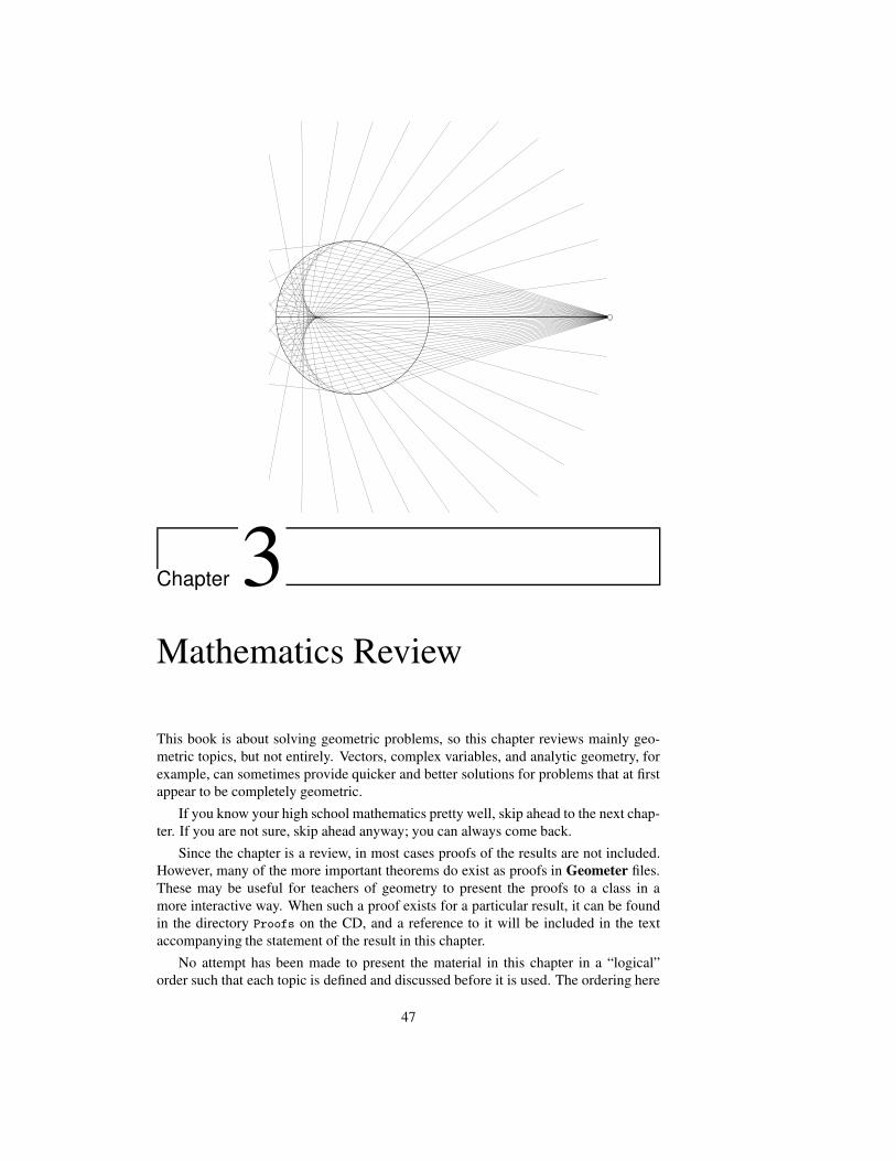
Chapter 3Mathematics Review
This book is about solving geometric problems, so this chapter reviews mainly geo-metric topics, but not entirely. Vectors, complex variables, and analytic geometry, forexample, can sometimes provide quicker and better solutions for problems that at firstappear to be completely geometric.
If you know your high school mathematics pretty well, skip ahead to the next chap-ter. If you are not sure, skip ahead anyway; you can always come back.
Since the chapter is a review, in most cases proofs of the results are not included.However, many of the more important theorems do exist as proofs in Geometer files.These may be useful for teachers of geometry to present the proofs to a class in amore interactive way. When such a proof exists for a particular result, it can be foundin the directory Proofs on the CD, and a reference to it will be included in the textaccompanying the statement of the result in this chapter.
No attempt has been made to present the material in this chapter in a “logical”order such that each topic is defined and discussed before it is used. The ordering here
47
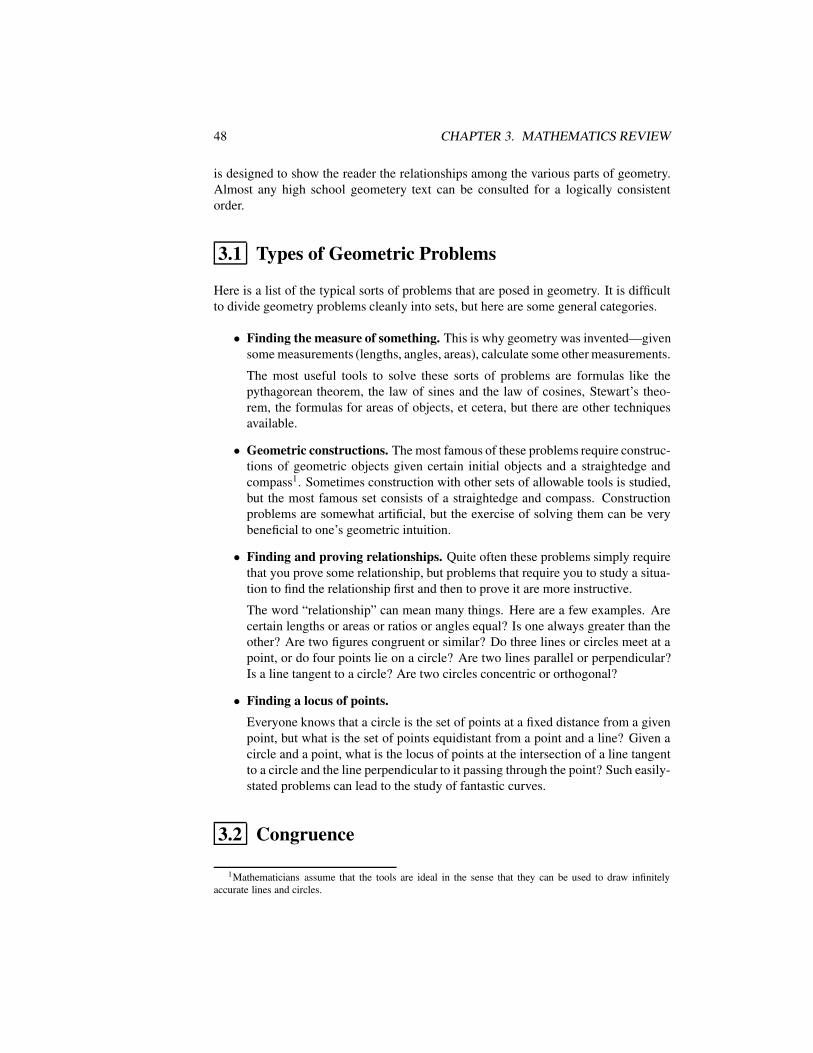
48 CHAPTER 3. MATHEMATICS REVIEW
is designed to show the reader the relationships among the various parts of geometry.Almost any high school geometery text can be consulted for a logically consistentorder.
3.1 Types of Geometric Problems
Here is a list of the typical sorts of problems that are posed in geometry. It is difficultto divide geometry problems cleanly into sets, but here are some general categories.
• Finding the measure of something. This is why geometry was invented—givensome measurements (lengths, angles, areas), calculate some other measurements.
The most useful tools to solve these sorts of problems are formulas like thepythagorean theorem, the law of sines and the law of cosines, Stewart’s theo-rem, the formulas for areas of objects, et cetera, but there are other techniquesavailable.
• Geometric constructions. The most famous of these problems require construc-tions of geometric objects given certain initial objects and a straightedge andcompass1. Sometimes construction with other sets of allowable tools is studied,but the most famous set consists of a straightedge and compass. Constructionproblems are somewhat artificial, but the exercise of solving them can be verybeneficial to one’s geometric intuition.
• Finding and proving relationships. Quite often these problems simply requirethat you prove some relationship, but problems that require you to study a situa-tion to find the relationship first and then to prove it are more instructive.
The word “relationship” can mean many things. Here are a few examples. Arecertain lengths or areas or ratios or angles equal? Is one always greater than theother? Are two figures congruent or similar? Do three lines or circles meet at apoint, or do four points lie on a circle? Are two lines parallel or perpendicular?Is a line tangent to a circle? Are two circles concentric or orthogonal?
• Finding a locus of points.Everyone knows that a circle is the set of points at a fixed distance from a givenpoint, but what is the set of points equidistant from a point and a line? Given acircle and a point, what is the locus of points at the intersection of a line tangentto a circle and the line perpendicular to it passing through the point? Such easily-stated problems can lead to the study of fantastic curves.
3.2 Congruence
1Mathematicians assume that the tools are ideal in the sense that they can be used to draw infinitelyaccurate lines and circles.
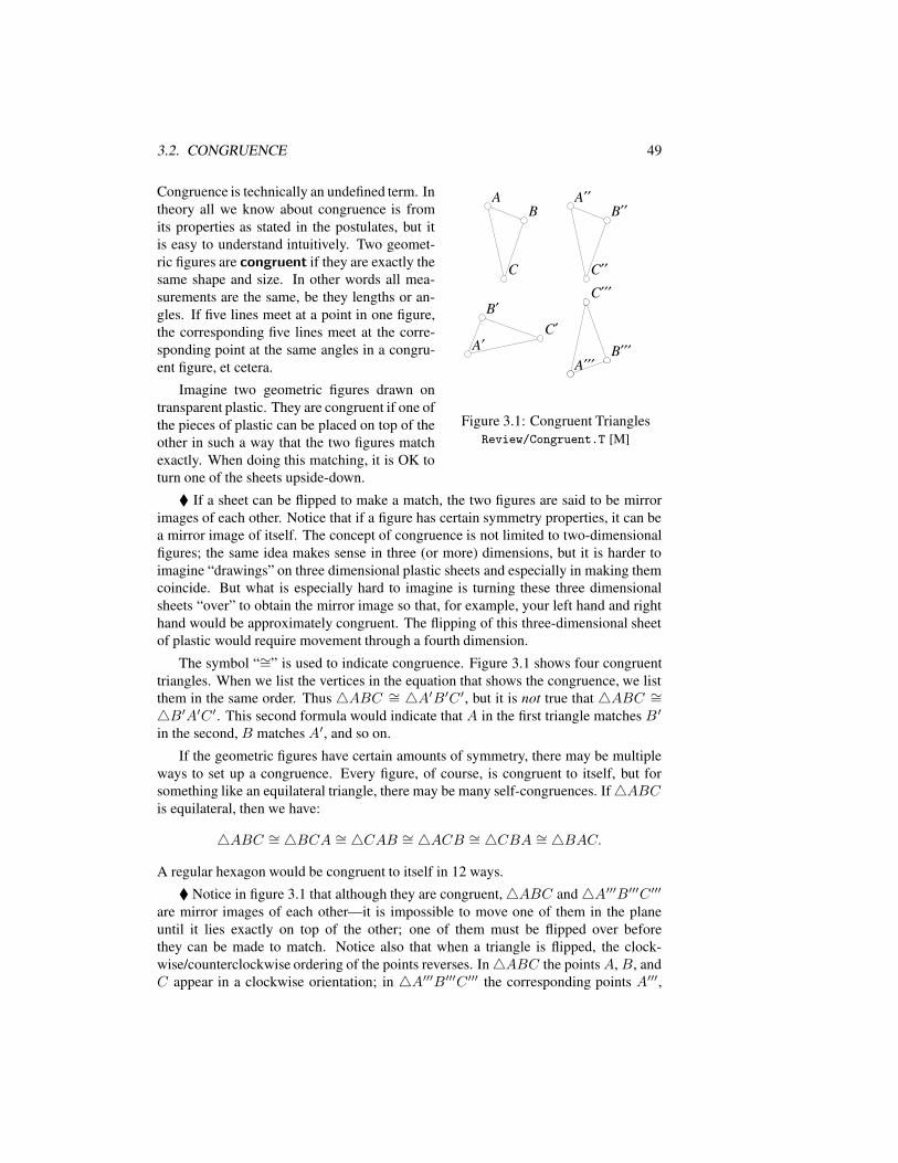
3.2. CONGRUENCE 49
AABB
CC
A′A′
B′B′C′C′
A′′A′′B′′B′′
C′′C′′
A′′′A′′′B′′′B′′′
C′′′C′′′
Figure 3.1: Congruent TrianglesReview/Congruent.T [M]
Congruence is technically an undefined term. Intheory all we know about congruence is fromits properties as stated in the postulates, but itis easy to understand intuitively. Two geomet-ric figures are congruent if they are exactly thesame shape and size. In other words all mea-surements are the same, be they lengths or an-gles. If five lines meet at a point in one figure,the corresponding five lines meet at the corre-sponding point at the same angles in a congru-ent figure, et cetera.
Imagine two geometric figures drawn ontransparent plastic. They are congruent if one ofthe pieces of plastic can be placed on top of theother in such a way that the two figures matchexactly. When doing this matching, it is OK toturn one of the sheets upside-down.
If a sheet can be flipped to make a match, the two figures are said to be mirrorimages of each other. Notice that if a figure has certain symmetry properties, it can bea mirror image of itself. The concept of congruence is not limited to two-dimensionalfigures; the same idea makes sense in three (or more) dimensions, but it is harder toimagine “drawings” on three dimensional plastic sheets and especially in making themcoincide. But what is especially hard to imagine is turning these three dimensionalsheets “over” to obtain the mirror image so that, for example, your left hand and righthand would be approximately congruent. The flipping of this three-dimensional sheetof plastic would require movement through a fourth dimension.
The symbol “∼=” is used to indicate congruence. Figure 3.1 shows four congruenttriangles. When we list the vertices in the equation that shows the congruence, we listthem in the same order. Thus 4ABC ∼= 4A′B′C ′, but it is not true that 4ABC ∼=4B′A′C ′. This second formula would indicate that A in the first triangle matches B ′
in the second, B matches A′, and so on.
If the geometric figures have certain amounts of symmetry, there may be multipleways to set up a congruence. Every figure, of course, is congruent to itself, but forsomething like an equilateral triangle, there may be many self-congruences. If4ABCis equilateral, then we have:
4ABC ∼=4BCA ∼= 4CAB ∼= 4ACB ∼= 4CBA ∼=4BAC.
A regular hexagon would be congruent to itself in 12 ways.
Notice in figure 3.1 that although they are congruent,4ABC and4A′′′B′′′C ′′′are mirror images of each other—it is impossible to move one of them in the planeuntil it lies exactly on top of the other; one of them must be flipped over beforethey can be made to match. Notice also that when a triangle is flipped, the clock-wise/counterclockwise ordering of the points reverses. In4ABC the pointsA, B, andC appear in a clockwise orientation; in 4A′′′B′′′C ′′′ the corresponding points A′′′,
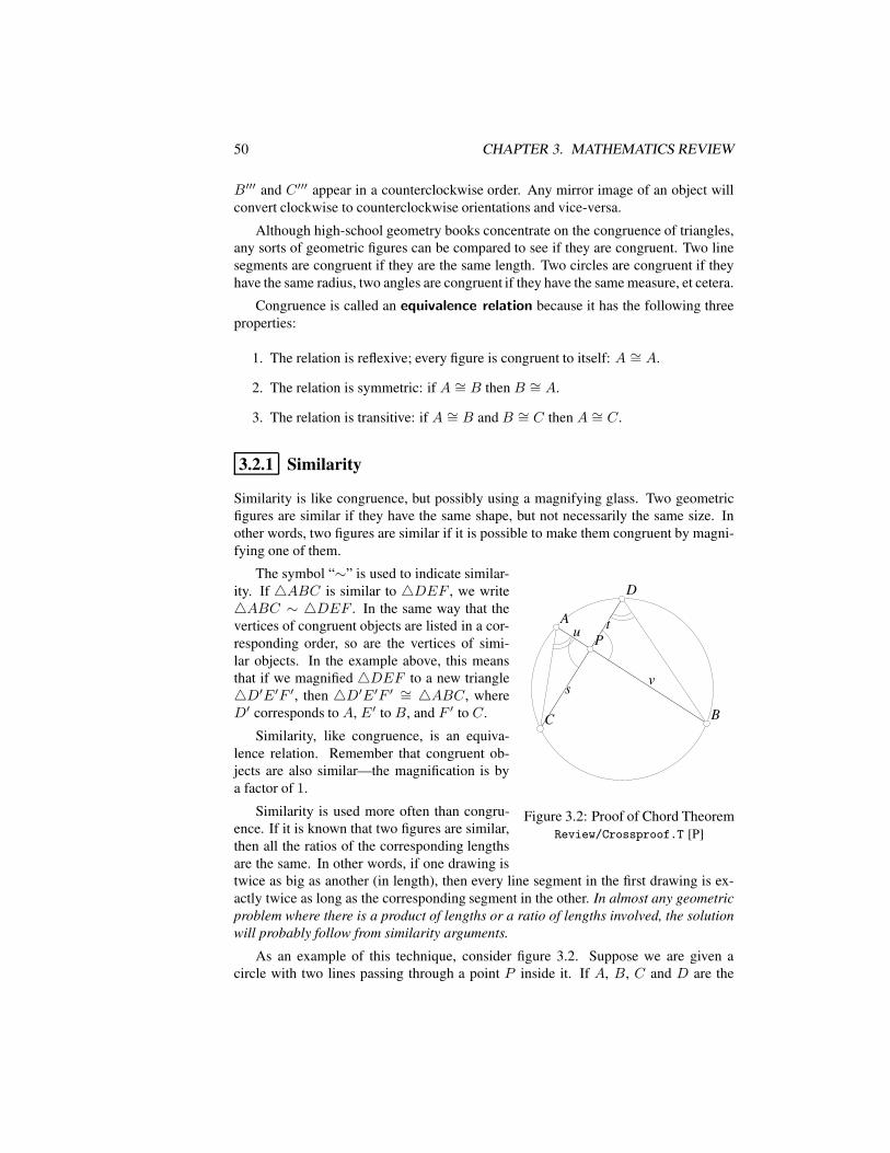
50 CHAPTER 3. MATHEMATICS REVIEW
B′′′ and C ′′′ appear in a counterclockwise order. Any mirror image of an object willconvert clockwise to counterclockwise orientations and vice-versa.
Although high-school geometry books concentrate on the congruence of triangles,any sorts of geometric figures can be compared to see if they are congruent. Two linesegments are congruent if they are the same length. Two circles are congruent if theyhave the same radius, two angles are congruent if they have the same measure, et cetera.
Congruence is called an equivalence relation because it has the following threeproperties:
1. The relation is reflexive; every figure is congruent to itself: A ∼= A.
2. The relation is symmetric: if A ∼= B then B ∼= A.
3. The relation is transitive: if A ∼= B and B ∼= C then A ∼= C.
3.2.1 Similarity
Similarity is like congruence, but possibly using a magnifying glass. Two geometricfigures are similar if they have the same shape, but not necessarily the same size. Inother words, two figures are similar if it is possible to make them congruent by magni-fying one of them.
ss
ttuu
vv
BB
AA
CC
DD
PP
Figure 3.2: Proof of Chord TheoremReview/Crossproof.T [P]
The symbol “∼” is used to indicate similar-ity. If 4ABC is similar to 4DEF , we write4ABC ∼ 4DEF . In the same way that thevertices of congruent objects are listed in a cor-responding order, so are the vertices of simi-lar objects. In the example above, this meansthat if we magnified 4DEF to a new triangle4D′E′F ′, then 4D′E′F ′ ∼= 4ABC, whereD′ corresponds to A, E ′ to B, and F ′ to C.
Similarity, like congruence, is an equiva-lence relation. Remember that congruent ob-jects are also similar—the magnification is bya factor of 1.
Similarity is used more often than congru-ence. If it is known that two figures are similar,then all the ratios of the corresponding lengthsare the same. In other words, if one drawing istwice as big as another (in length), then every line segment in the first drawing is ex-actly twice as long as the corresponding segment in the other. In almost any geometricproblem where there is a product of lengths or a ratio of lengths involved, the solutionwill probably follow from similarity arguments.
As an example of this technique, consider figure 3.2. Suppose we are given acircle with two lines passing through a point P inside it. If A, B, C and D are the
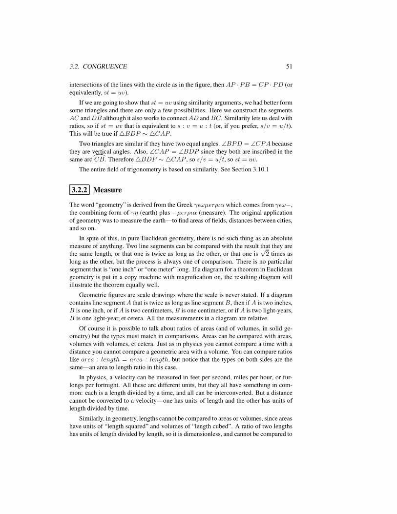
3.2. CONGRUENCE 51
intersections of the lines with the circle as in the figure, thenAP ·PB = CP ·PD (orequivalently, st = uv).
If we are going to show that st = uv using similarity arguments, we had better formsome triangles and there are only a few possibilities. Here we construct the segmentsAC andDB although it also works to connectAD andBC. Similarity lets us deal withratios, so if st = uv that is equivalent to s : v = u : t (or, if you prefer, s/v = u/t).This will be true if4BDP ∼ 4CAP .
Two triangles are similar if they have two equal angles. ∠BPD = ∠CPA becausethey are vertical angles. Also, ∠CAP = ∠BDP since they both are inscribed in thesame arc
)
CB. Therefore4BDP ∼ 4CAP , so s/v = u/t, so st = uv.
The entire field of trigonometry is based on similarity. See Section 3.10.1
3.2.2 Measure
The word “geometry” is derived from the Greek γεωµετρια which comes from γεω−,the combining form of γη (earth) plus −µετρια (measure). The original applicationof geometry was to measure the earth—to find areas of fields, distances between cities,and so on.
In spite of this, in pure Euclidean geometry, there is no such thing as an absolutemeasure of anything. Two line segments can be compared with the result that they arethe same length, or that one is twice as long as the other, or that one is
√2 times as
long as the other, but the process is always one of comparison. There is no particularsegment that is “one inch” or “one meter” long. If a diagram for a theorem in Euclideangeometry is put in a copy machine with magnification on, the resulting diagram willillustrate the theorem equally well.
Geometric figures are scale drawings where the scale is never stated. If a diagramcontains line segmentA that is twice as long as line segmentB, then ifA is two inches,B is one inch, or ifA is two centimeters,B is one centimeter, or ifA is two light-years,B is one light-year, et cetera. All the measurements in a diagram are relative.
Of course it is possible to talk about ratios of areas (and of volumes, in solid ge-ometry) but the types must match in comparisons. Areas can be compared with areas,volumes with volumes, et cetera. Just as in physics you cannot compare a time with adistance you cannot compare a geometric area with a volume. You can compare ratioslike area : length = area : length, but notice that the types on both sides are thesame—an area to length ratio in this case.
In physics, a velocity can be measured in feet per second, miles per hour, or fur-longs per fortnight. All these are different units, but they all have something in com-mon: each is a length divided by a time, and all can be interconverted. But a distancecannot be converted to a velocity—one has units of length and the other has units oflength divided by time.
Similarly, in geometry, lengths cannot be compared to areas or volumes, since areashave units of “length squared” and volumes of “length cubed”. A ratio of two lengthshas units of length divided by length, so it is dimensionless, and cannot be compared to
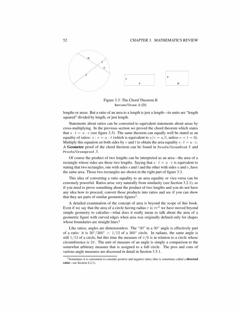
52 CHAPTER 3. MATHEMATICS REVIEW
ss
ttuu
vv
ttss
vv
uu
Figure 3.3: The Chord Theorem IIReview/Cross.D [D]
lengths or areas. But a ratio of an area to a length is just a length—its units are “lengthsquared” divided by length, or just length.
Statements about ratios can be converted to equivalent statements about areas bycross-multiplying. In the previous section we proved the chord theorem which statesthat s · t = u · v (see figure 3.3). The same theorem can equally well be stated as anequality of ratios: s : v = u : t (which is equivalent to s/v = u/t, unless v = t = 0).Multiply this equation on both sides by v and t to obtain the area equality s · t = u · v.A Geometer proof of the chord theorem can be found in Proofs/CrossProd.T andProofs/Crossproof.T.
Of course the product of two lengths can be interpreted as an area—the area of arectangle whose sides are those two lengths. Saying that s · t = u · v is equivalent tostating that two rectangles, one with sides s and t and the other with sides u and v, havethe same area. Those two rectangles are shown in the right part of figure 3.3.
This idea of converting a ratio equality to an area equality or vice-versa can beextremely powerful. Ratios arise very naturally from similarity (see Section 3.2.1), soif you need to prove something about the product of two lengths and you do not haveany idea how to proceed, convert those products into ratios and see if you can showthat they are parts of similar geometric figures2.
A detailed examination of the concept of area is beyond the scope of this book.Even if we say that the area of a circle having radius r is πr2 we have moved beyondsimple geometry to calculus—what does it really mean to talk about the area of ageometric figure with curved edges when area was originally defined only for shapeswhose boundaries are straight lines?
Like ratios, angles are dimensionless. The “30” in a 30 angle is effectively partof a ratio: it is 30/360 = 1/12 of a 360 circle. In radians, the same angle isstill 1/12 of a circle, but this time the measure of π/6 is in relation to a circle whosecircumference is 2π. The unit of measure of an angle is simply a comparison to thesomewhat arbitrary measure that is assigned to a full circle. The pros and cons ofvarious angle measures are discussed in detail in Section 3.5.1.
2Sometimes it is convenient to consider positive and negative ratios (this is sometimes called a directedratio—see Section 6.2.1).
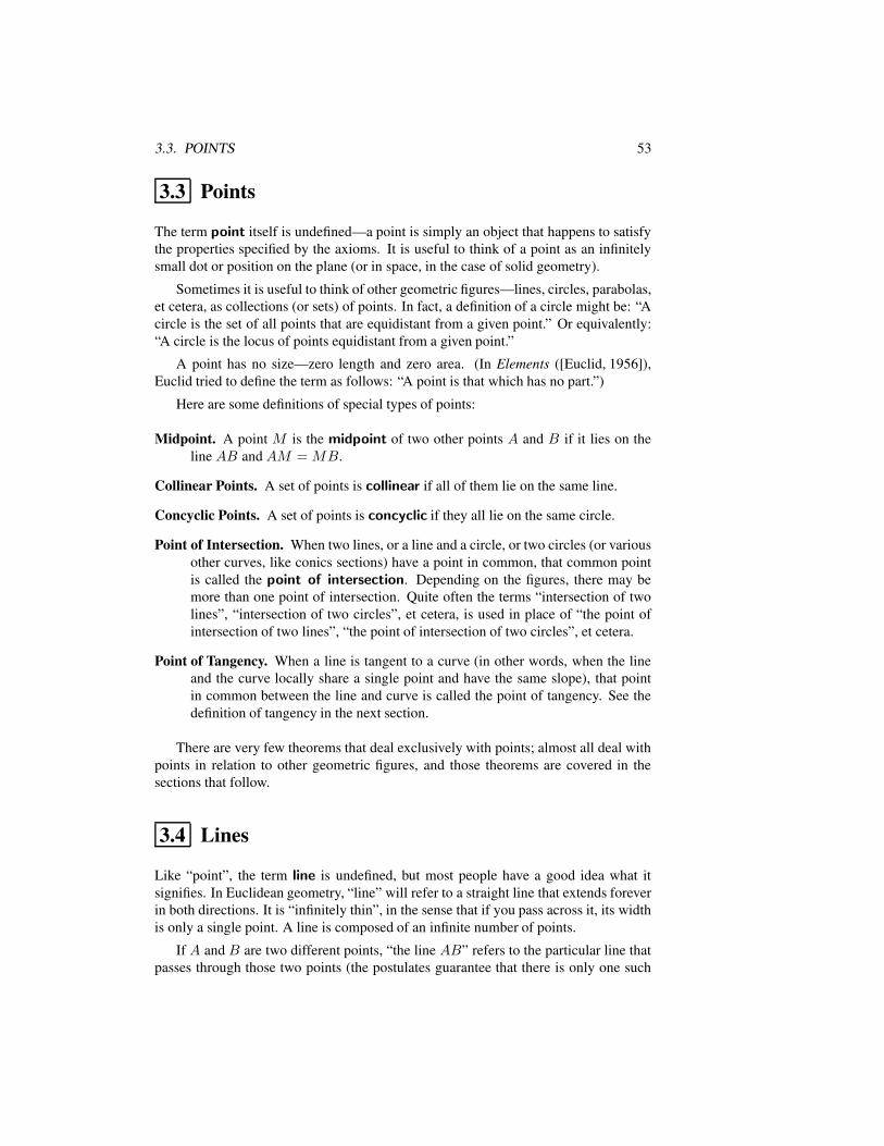
3.3. POINTS 53
3.3 Points
The term point itself is undefined—a point is simply an object that happens to satisfythe properties specified by the axioms. It is useful to think of a point as an infinitelysmall dot or position on the plane (or in space, in the case of solid geometry).
Sometimes it is useful to think of other geometric figures—lines, circles, parabolas,et cetera, as collections (or sets) of points. In fact, a definition of a circle might be: “Acircle is the set of all points that are equidistant from a given point.” Or equivalently:“A circle is the locus of points equidistant from a given point.”
A point has no size—zero length and zero area. (In Elements ([Euclid, 1956]),Euclid tried to define the term as follows: “A point is that which has no part.”)
Here are some definitions of special types of points:
Midpoint. A point M is the midpoint of two other points A and B if it lies on theline AB and AM = MB.
Collinear Points. A set of points is collinear if all of them lie on the same line.
Concyclic Points. A set of points is concyclic if they all lie on the same circle.
Point of Intersection. When two lines, or a line and a circle, or two circles (or variousother curves, like conics sections) have a point in common, that common pointis called the point of intersection. Depending on the figures, there may bemore than one point of intersection. Quite often the terms “intersection of twolines”, “intersection of two circles”, et cetera, is used in place of “the point ofintersection of two lines”, “the point of intersection of two circles”, et cetera.
Point of Tangency. When a line is tangent to a curve (in other words, when the lineand the curve locally share a single point and have the same slope), that pointin common between the line and curve is called the point of tangency. See thedefinition of tangency in the next section.
There are very few theorems that deal exclusively with points; almost all deal withpoints in relation to other geometric figures, and those theorems are covered in thesections that follow.
3.4 Lines
Like “point”, the term line is undefined, but most people have a good idea what itsignifies. In Euclidean geometry, “line” will refer to a straight line that extends foreverin both directions. It is “infinitely thin”, in the sense that if you pass across it, its widthis only a single point. A line is composed of an infinite number of points.
If A and B are two different points, “the line AB” refers to the particular line thatpasses through those two points (the postulates guarantee that there is only one such
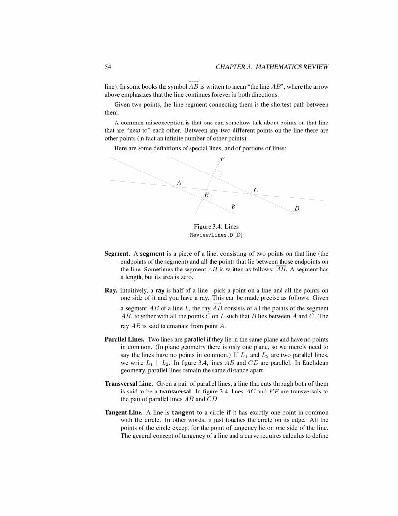
54 CHAPTER 3. MATHEMATICS REVIEW
line). In some books the symbol←→AB is written to mean “the lineAB”, where the arrow
above emphasizes that the line continues forever in both directions.
Given two points, the line segment connecting them is the shortest path betweenthem.
A common misconception is that one can somehow talk about points on that linethat are “next to” each other. Between any two different points on the line there areother points (in fact an infinite number of other points).
Here are some definitions of special lines, and of portions of lines:
AA
BB
CCEE
DD
FF
Figure 3.4: LinesReview/Lines.D [D]
Segment. A segment is a piece of a line, consisting of two points on that line (theendpoints of the segment) and all the points that lie between those endpoints onthe line. Sometimes the segment AB is written as follows: AB. A segment hasa length, but its area is zero.
Ray. Intuitively, a ray is half of a line—pick a point on a line and all the points onone side of it and you have a ray. This can be made precise as follows: Given
a segment AB of a line L, the ray−→AB consists of all the points of the segment
AB, together with all the points C on L such that B lies between A and C. The
ray−→AB is said to emanate from point A.
Parallel Lines. Two lines are parallel if they lie in the same plane and have no pointsin common. (In plane geometry there is only one plane, so we merely need tosay the lines have no points in common.) If L1 and L2 are two parallel lines,we write L1 ‖ L2. In figure 3.4, lines AB and CD are parallel. In Euclideangeometry, parallel lines remain the same distance apart.
Transversal Line. Given a pair of parallel lines, a line that cuts through both of themis said to be a transversal. In figure 3.4, lines AC and EF are transversals tothe pair of parallel lines AB and CD.
Tangent Line. A line is tangent to a circle if it has exactly one point in commonwith the circle. In other words, it just touches the circle on its edge. All thepoints of the circle except for the point of tangency lie on one side of the line.The general concept of tangency of a line and a curve requires calculus to define
3.4. LINES 55
TT
Figure 3.5: Tangent LineReview/Tangent.D [D]
what is meant by the slope of a curve at a point. A line is tangent to a curve if itpasses through a point on the curve and the slope of the line is the same as theslope of the curve at that point. Note that a line can be tangent at one point andthen pass through the curve at another or that the tangent line can pass throughthe curve at the point of tangency. Figure 3.5 illustrates a line tangent to a curveat the point T that passes through the curve at another point.
Two curves (including circles, of course) are tangent at a point if they both aretangent to the same line at that point.
Perpendicular Lines. Two lines are perpendicular if they form a right angle (a 90
angle). If L1 and L2 are perpendicular, we write L1 ⊥ L2. In figure 3.4, EF ⊥AB. (Of course EF ⊥ CD as well.)
Perpendicular Bisector. A line that is perpendicular to a segment and divides the seg-ment into two congruent segments is called the perpendicular bisector of thesegment. In figure 3.4, pointE is the midpoint of AB, so AE = EB. Since lineEF is perpendicular to line AB, then EF is the perpendicular bisector of thesegment AB.
Here are some key theorems about lines in plane Euclidean geometry. All can beproved from the postulates but many of them are simply assumed in a standard highschool geometry course.
• Two distinct lines can intersect in at most one point.
• Every line contains an infinite number of points.
• Given any four distinct points on a line, it is possible to label them A, B, C, andD such that B lies betweenA and C and also betweenA and D, and also that Clies between A and D and between B and D.
• Every line divides the plane into two regions such that if two points not on theline are in the same region, then the segment connecting them does not inter-sect the line, and if the two points are not in the same region, then the segmentconnecting them does have a point in common with the line.
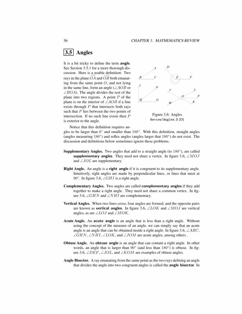
56 CHAPTER 3. MATHEMATICS REVIEW
3.5 Angles
AA
BB CC
DD
EE FF
HH GG
JJ
KK
LL
MM
II
OO
NN
PP
Figure 3.6: AnglesReview/Angles.D [D]
It is a bit tricky to define the term angle.See Section 3.5.1 for a more thorough dis-cussion. Here is a usable definition: Tworays in the plane
−→OA and
−→OB both emanat-
ing from the same point O, and not lyingin the same line, form an angle (∠AOB or∠BOA). The angle divides the rest of theplane into two regions. A point P of theplane is on the interior of ∠AOB if a lineexists through P that intersects both rayssuch that P lies between the two points ofintersection. If no such line exists then Pis exterior to the angle.
Notice that this definition requires an-gles to be larger than 0 and smaller than 180. With this definition, straight angles(angles measuring 180) and reflex angles (angles larger that 180) do not exist. Thediscussion and definitions below sometimes ignore these problems.
Supplementary Angles. Two angles that add to a straight angle (to 180), are calledsupplementary angles. They need not share a vertex. In figure 3.6, ∠MOJand ∠JOL are supplementary.
Right Angle. An angle is a right angle if it is congruent to its supplementary angle.Intuitively, right angles are made by perpendicular lines, or lines that meet at90. In figure 3.6, ∠GHI is a right angle.
Complementary Angles. Two angles are called complementary angles if they addtogether to make a right angle. They need not share a common vertex. In fig-ure 3.6, ∠GHN and ∠NHI are complementary.
Vertical Angles. When two lines cross, four angles are formed, and the opposite pairsare known as vertical angles. In figure 3.6, ∠LOK and ∠MOJ are verticalangles, as are ∠LOJ and ∠MOK.
Acute Angle. An acute angle is an angle that is less than a right angle. Withoutusing the concept of the measure of an angle, we can simply say that an acuteangle is an angle that can be obtained inside a right angle. In figure 3.6, ∠ABC,∠GHN , ∠NHI , ∠LOK, and ∠JOM are acute angles, among others .
Obtuse Angle. An obtuse angle is an angle that can contain a right angle. In otherwords, an angle that is larger than 90 (and less than 180) is obtuse. In fig-ure 3.6, ∠DEF , ∠JOL, and ∠KOM are examples of obtuse angles.
Angle Bisector. A ray emanating from the same point as the two rays defining an anglethat divides the angle into two congruent angles is called the angle bisector. In
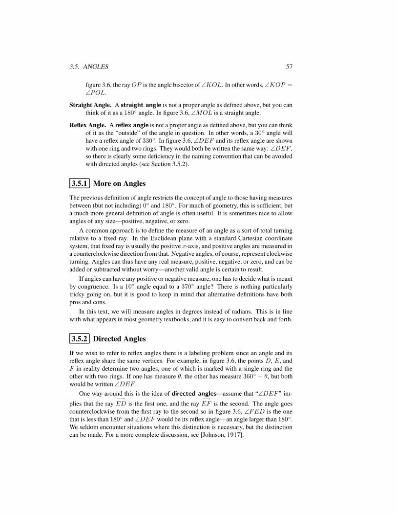
3.5. ANGLES 57
figure 3.6, the rayOP is the angle bisector of∠KOL. In other words,∠KOP =∠POL.
Straight Angle. A straight angle is not a proper angle as defined above, but you canthink of it as a 180 angle. In figure 3.6, ∠MOL is a straight angle.
Reflex Angle. A reflex angle is not a proper angle as defined above, but you can thinkof it as the “outside” of the angle in question. In other words, a 30 angle willhave a reflex angle of 330. In figure 3.6, ∠DEF and its reflex angle are shownwith one ring and two rings. They would both be written the same way: ∠DEF ,so there is clearly some deficiency in the naming convention that can be avoidedwith directed angles (see Section 3.5.2).
3.5.1 More on Angles
The previous definition of angle restricts the concept of angle to those having measuresbetween (but not including) 0 and 180. For much of geometry, this is sufficient, buta much more general definition of angle is often useful. It is sometimes nice to allowangles of any size—positive, negative, or zero.
A common approach is to define the measure of an angle as a sort of total turningrelative to a fixed ray. In the Euclidean plane with a standard Cartesian coordinatesystem, that fixed ray is usually the positive x-axis, and positive angles are measured ina counterclockwise direction from that. Negative angles, of course, represent clockwiseturning. Angles can thus have any real measure, positive, negative, or zero, and can beadded or subtracted without worry—another valid angle is certain to result.
If angles can have any positive or negative measure, one has to decide what is meantby congruence. Is a 10 angle equal to a 370 angle? There is nothing particularlytricky going on, but it is good to keep in mind that alternative definitions have bothpros and cons.
In this text, we will measure angles in degrees instead of radians. This is in linewith what appears in most geometry textbooks, and it is easy to convert back and forth.
3.5.2 Directed Angles
If we wish to refer to reflex angles there is a labeling problem since an angle and itsreflex angle share the same vertices. For example, in figure 3.6, the points D, E, andF in reality determine two angles, one of which is marked with a single ring and theother with two rings. If one has measure θ, the other has measure 360 − θ, but bothwould be written ∠DEF .
One way around this is the idea of directed angles—assume that “∠DEF ” im-
plies that the ray−→ED is the first one, and the ray
−→EF is the second. The angle goes
counterclockwise from the first ray to the second so in figure 3.6, ∠FED is the onethat is less than 180 and ∠DEF would be its reflex angle—an angle larger than 180.We seldom encounter situations where this distinction is necessary, but the distinctioncan be made. For a more complete discussion, see [Johnson, 1917].
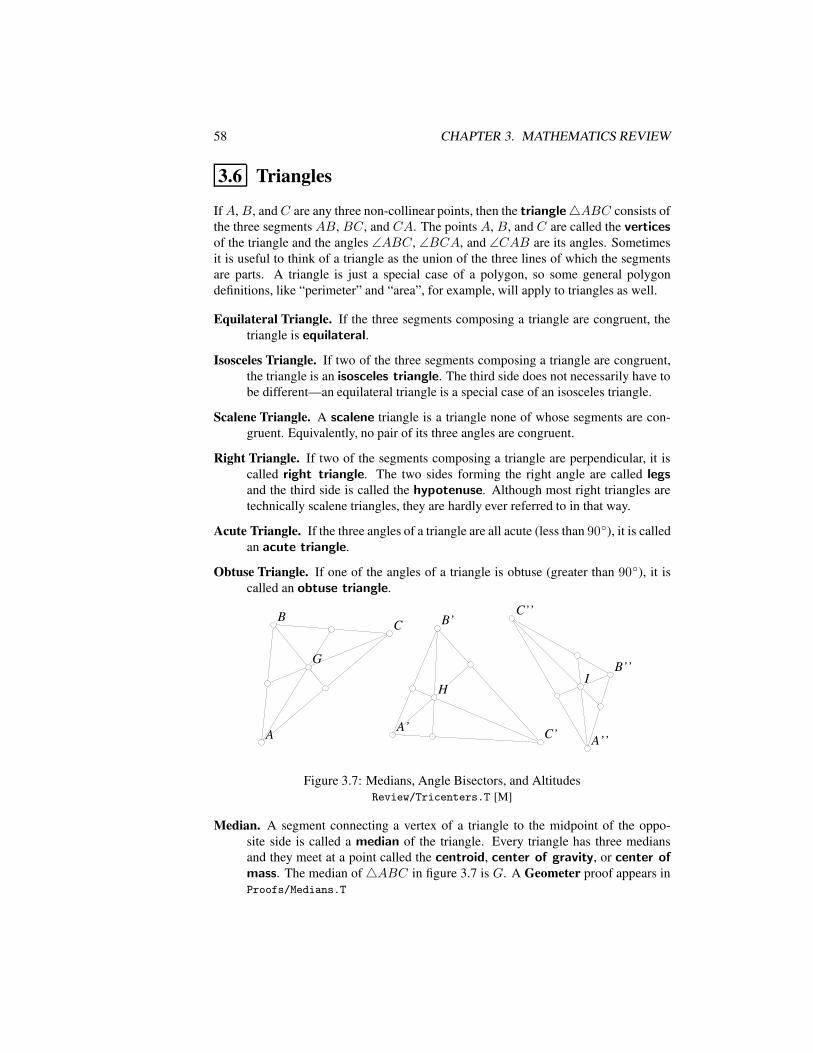
58 CHAPTER 3. MATHEMATICS REVIEW
3.6 Triangles
IfA, B, andC are any three non-collinear points, then the triangle4ABC consists ofthe three segments AB, BC, and CA. The points A, B, and C are called the verticesof the triangle and the angles ∠ABC, ∠BCA, and ∠CAB are its angles. Sometimesit is useful to think of a triangle as the union of the three lines of which the segmentsare parts. A triangle is just a special case of a polygon, so some general polygondefinitions, like “perimeter” and “area”, for example, will apply to triangles as well.
Equilateral Triangle. If the three segments composing a triangle are congruent, thetriangle is equilateral.
Isosceles Triangle. If two of the three segments composing a triangle are congruent,the triangle is an isosceles triangle. The third side does not necessarily have tobe different—an equilateral triangle is a special case of an isosceles triangle.
Scalene Triangle. A scalene triangle is a triangle none of whose segments are con-gruent. Equivalently, no pair of its three angles are congruent.
Right Triangle. If two of the segments composing a triangle are perpendicular, it iscalled right triangle. The two sides forming the right angle are called legsand the third side is called the hypotenuse. Although most right triangles aretechnically scalene triangles, they are hardly ever referred to in that way.
Acute Triangle. If the three angles of a triangle are all acute (less than 90), it is calledan acute triangle.
Obtuse Triangle. If one of the angles of a triangle is obtuse (greater than 90), it iscalled an obtuse triangle.
AA
BBCC
A’’A’’
C’’C’’
B’’B’’
A’A’
B’B’
C’C’
GGII
HH
Figure 3.7: Medians, Angle Bisectors, and AltitudesReview/Tricenters.T [M]
Median. A segment connecting a vertex of a triangle to the midpoint of the oppo-site side is called a median of the triangle. Every triangle has three mediansand they meet at a point called the centroid, center of gravity, or center ofmass. The median of4ABC in figure 3.7 is G. A Geometer proof appears inProofs/Medians.T
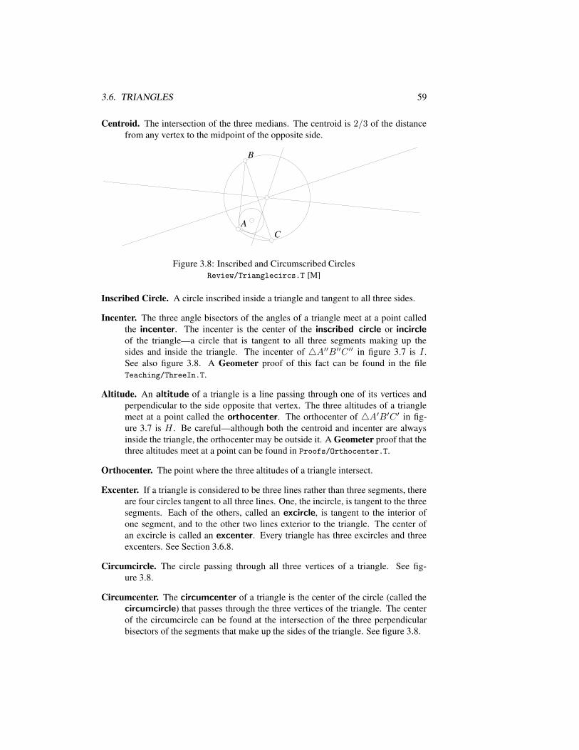
3.6. TRIANGLES 59
Centroid. The intersection of the three medians. The centroid is 2/3 of the distancefrom any vertex to the midpoint of the opposite side.
AA
BB
CC
Figure 3.8: Inscribed and Circumscribed CirclesReview/Trianglecircs.T [M]
Inscribed Circle. A circle inscribed inside a triangle and tangent to all three sides.
Incenter. The three angle bisectors of the angles of a triangle meet at a point calledthe incenter. The incenter is the center of the inscribed circle or incircleof the triangle—a circle that is tangent to all three segments making up thesides and inside the triangle. The incenter of 4A′′B′′C ′′ in figure 3.7 is I .See also figure 3.8. A Geometer proof of this fact can be found in the fileTeaching/ThreeIn.T.
Altitude. An altitude of a triangle is a line passing through one of its vertices andperpendicular to the side opposite that vertex. The three altitudes of a trianglemeet at a point called the orthocenter. The orthocenter of 4A′B′C ′ in fig-ure 3.7 is H . Be careful—although both the centroid and incenter are alwaysinside the triangle, the orthocenter may be outside it. A Geometer proof that thethree altitudes meet at a point can be found in Proofs/Orthocenter.T.
Orthocenter. The point where the three altitudes of a triangle intersect.
Excenter. If a triangle is considered to be three lines rather than three segments, thereare four circles tangent to all three lines. One, the incircle, is tangent to the threesegments. Each of the others, called an excircle, is tangent to the interior ofone segment, and to the other two lines exterior to the triangle. The center ofan excircle is called an excenter. Every triangle has three excircles and threeexcenters. See Section 3.6.8.
Circumcircle. The circle passing through all three vertices of a triangle. See fig-ure 3.8.
Circumcenter. The circumcenter of a triangle is the center of the circle (called thecircumcircle) that passes through the three vertices of the triangle. The centerof the circumcircle can be found at the intersection of the three perpendicularbisectors of the segments that make up the sides of the triangle. See figure 3.8.
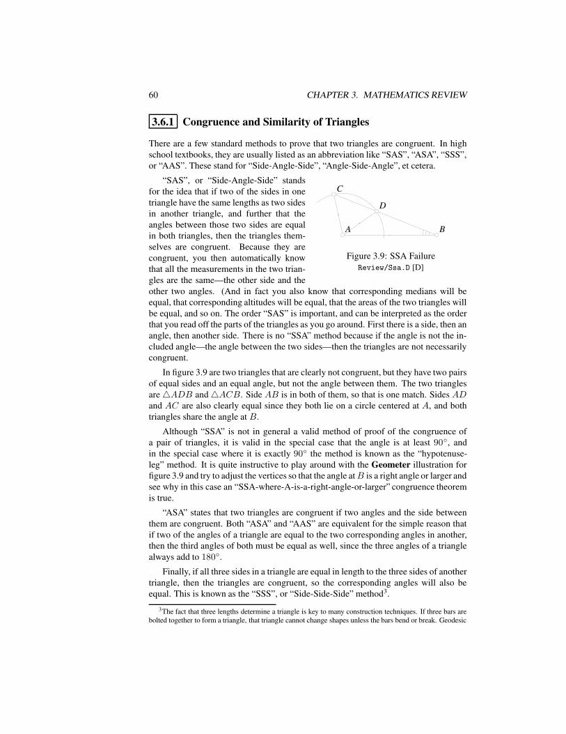
60 CHAPTER 3. MATHEMATICS REVIEW
3.6.1 Congruence and Similarity of Triangles
There are a few standard methods to prove that two triangles are congruent. In highschool textbooks, they are usually listed as an abbreviation like “SAS”, “ASA”, “SSS”,or “AAS”. These stand for “Side-Angle-Side”, “Angle-Side-Angle”, et cetera.
AA BB
CC
DD
Figure 3.9: SSA FailureReview/Ssa.D [D]
“SAS”, or “Side-Angle-Side” standsfor the idea that if two of the sides in onetriangle have the same lengths as two sidesin another triangle, and further that theangles between those two sides are equalin both triangles, then the triangles them-selves are congruent. Because they arecongruent, you then automatically knowthat all the measurements in the two trian-gles are the same—the other side and theother two angles. (And in fact you also know that corresponding medians will beequal, that corresponding altitudes will be equal, that the areas of the two triangles willbe equal, and so on. The order “SAS” is important, and can be interpreted as the orderthat you read off the parts of the triangles as you go around. First there is a side, then anangle, then another side. There is no “SSA” method because if the angle is not the in-cluded angle—the angle between the two sides—then the triangles are not necessarilycongruent.
In figure 3.9 are two triangles that are clearly not congruent, but they have two pairsof equal sides and an equal angle, but not the angle between them. The two trianglesare4ADB and4ACB. Side AB is in both of them, so that is one match. Sides ADand AC are also clearly equal since they both lie on a circle centered at A, and bothtriangles share the angle at B.
Although “SSA” is not in general a valid method of proof of the congruence ofa pair of triangles, it is valid in the special case that the angle is at least 90, andin the special case where it is exactly 90 the method is known as the “hypotenuse-leg” method. It is quite instructive to play around with the Geometer illustration forfigure 3.9 and try to adjust the vertices so that the angle atB is a right angle or larger andsee why in this case an “SSA-where-A-is-a-right-angle-or-larger” congruence theoremis true.
“ASA” states that two triangles are congruent if two angles and the side betweenthem are congruent. Both “ASA” and “AAS” are equivalent for the simple reason thatif two of the angles of a triangle are equal to the two corresponding angles in another,then the third angles of both must be equal as well, since the three angles of a trianglealways add to 180.
Finally, if all three sides in a triangle are equal in length to the three sides of anothertriangle, then the triangles are congruent, so the corresponding angles will also beequal. This is known as the “SSS”, or “Side-Side-Side” method3.
3The fact that three lengths determine a triangle is key to many construction techniques. If three bars arebolted together to form a triangle, that triangle cannot change shapes unless the bars bend or break. Geodesic
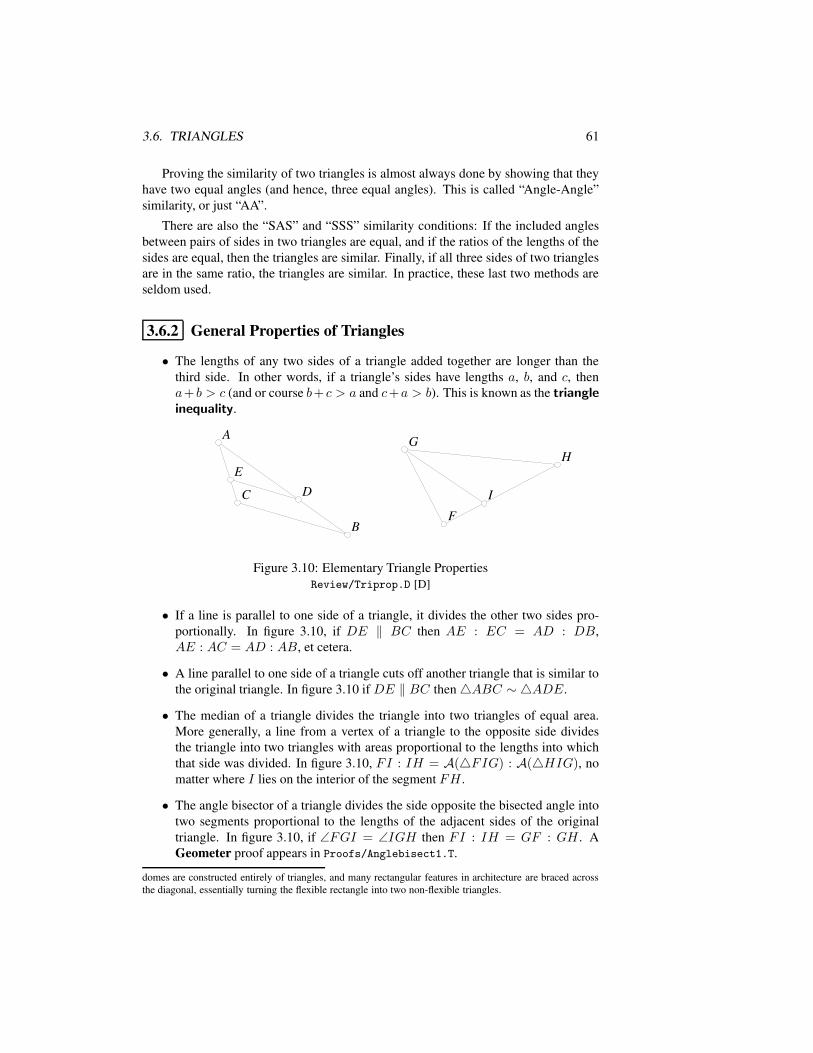
3.6. TRIANGLES 61
Proving the similarity of two triangles is almost always done by showing that theyhave two equal angles (and hence, three equal angles). This is called “Angle-Angle”similarity, or just “AA”.
There are also the “SAS” and “SSS” similarity conditions: If the included anglesbetween pairs of sides in two triangles are equal, and if the ratios of the lengths of thesides are equal, then the triangles are similar. Finally, if all three sides of two trianglesare in the same ratio, the triangles are similar. In practice, these last two methods areseldom used.
3.6.2 General Properties of Triangles
• The lengths of any two sides of a triangle added together are longer than thethird side. In other words, if a triangle’s sides have lengths a, b, and c, thena+ b > c (and or course b+ c > a and c+a > b). This is known as the triangleinequality.
AA
BB
CC DDEE
FF
GGHH
II
Figure 3.10: Elementary Triangle PropertiesReview/Triprop.D [D]
• If a line is parallel to one side of a triangle, it divides the other two sides pro-portionally. In figure 3.10, if DE ‖ BC then AE : EC = AD : DB,AE : AC = AD : AB, et cetera.
• A line parallel to one side of a triangle cuts off another triangle that is similar tothe original triangle. In figure 3.10 if DE ‖ BC then4ABC ∼ 4ADE.
• The median of a triangle divides the triangle into two triangles of equal area.More generally, a line from a vertex of a triangle to the opposite side dividesthe triangle into two triangles with areas proportional to the lengths into whichthat side was divided. In figure 3.10, FI : IH = A(4FIG) : A(4HIG), nomatter where I lies on the interior of the segment FH .
• The angle bisector of a triangle divides the side opposite the bisected angle intotwo segments proportional to the lengths of the adjacent sides of the originaltriangle. In figure 3.10, if ∠FGI = ∠IGH then FI : IH = GF : GH . AGeometer proof appears in Proofs/Anglebisect1.T.
domes are constructed entirely of triangles, and many rectangular features in architecture are braced acrossthe diagonal, essentially turning the flexible rectangle into two non-flexible triangles.
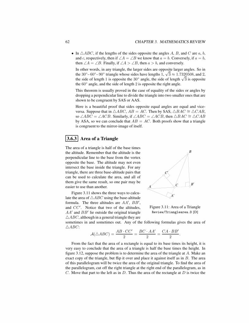
62 CHAPTER 3. MATHEMATICS REVIEW
• In 4ABC, if the lengths of the sides opposite the angles A, B, and C are a, b,and c, respectively, then if ∠A = ∠B we know that a = b. Conversely, if a = b,then ∠A = ∠B. Finally, if ∠A > ∠B, then a > b, and conversely.
In other words, in any triangle, the larger sides are opposite larger angles. So inthe 30– 60– 90 triangle whose sides have lengths 1,
√3 ≈ 1.7320508, and 2,
the side of length 1 is opposite the 30 angle, the side of length√
3 is oppositethe 60 angle, and the side of length 2 is opposite the right angle.
This theorem is usually proved in the case of equality of the sides or angles bydropping a perpendicular line to divide the triangle into two smaller ones that areshown to be congruent by SAS or AAS.
Here is a beautiful proof that sides opposite equal angles are equal and vice-versa. Suppose that in4ABC, AB = AC. Then by SAS,4BAC ∼= 4CAB,so ∠ABC = ∠ACB. Similarly, if ∠ABC = ∠ACB, then4BAC ∼= 4CABby ASA, so we can conclude that AB = AC. Both proofs show that a triangleis congruent to the mirror-image of itself.
3.6.3 Area of a Triangle
AA
BB
CC
C′C′
A′A′
B′B′
Figure 3.11: Area of a TriangleReview/Trianglearea.D [D]
The area of a triangle is half of the base timesthe altitude. Remember that the altitude is theperpendicular line to the base from the vertexopposite the base. The altitude may not evenintersect the base inside the triangle. For anytriangle, there are three base-altitude pairs thatcan be used to calculate the area, and all ofthem give the same result, so one pair may beeasier to use than another.
Figure 3.11 shows the three ways to calcu-late the area of4ABC using the base-altitudeformula. The three altitudes are AA′, BB′,and CC ′. Notice that two of the altitudes,AA′ and BB′ lie outside the original triangle4ABC, although in a general triangle they aresometimes in and sometimes out. Any of the following formulas gives the area of4ABC:
A(4ABC) =AB · CC ′
2=BC · AA′
2=CA · BB′
2.
From the fact that the area of a rectangle is equal to its base times its height, it isvery easy to conclude that the area of a triangle is half the base times the height. Infigure 3.12, suppose the problem is to determine the area of the triangle at A. Make anexact copy of the triangle, but flip it over and place it against itself as in B. The areaof this parallelogram will be twice the area of the original triangle. To find the area ofthe parallelogram, cut off the right triangle at the right end of the parallelogram, as inC. Move that part to the left as in D. Thus the area of the rectangle at D is twice the
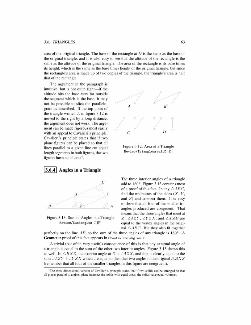
3.6. TRIANGLES 63
area of the original triangle. The base of the rectangle at D is the same as the base ofthe original triangle, and it is also easy to see that the altitude of the rectangle is thesame as the altitude of the original triangle. The area of the rectangle is its base timesits height, which is the same as the base times height of the original triangle, but sincethe rectangle’s area is made up of two copies of the triangle, the triangle’s area is halfthat of the rectangle.
AA BB
CC DD
Figure 3.12: Area of a TriangleReview/Trianglearea1.D [D]
The argument in the paragraph isintuitive, but is not quite right—if thealtitude hits the base very far outsidethe segment which is the base, it maynot be possible to slice the parallelo-gram as described. If the top point ofthe triangle written A in figure 3.12 ismoved to the right by a long distance,the argument does not work. The argu-ment can be made rigorous most easilywith an appeal to Cavalieri’s principle.Cavalieri’s principle states that if twoplane figures can be placed so that alllines parallel to a given line cut equallength segments in both figures, the twofigures have equal area4.
3.6.4 Angles in a Triangle
AABB
CC
XX
ZZ
YY
Figure 3.13: Sum of Angles in a TriangleReview/Sum3angles.T [P]
The three interior angles of a triangleadd to 180. Figure 3.13 contains mostof a proof of this fact. In any 4ABC,find the midpoints of the sides (X , Y ,and Z) and connect them. It is easyto show that all four of the smaller tri-angles produced are congruent. Thatmeans that the three angles that meet atZ: ∠AZY , ∠Y ZX , and ∠XZB areequal to the vertex angles in the origi-nal 4ABC. But they also fit together
perfectly on the line AB, so the sum of the three angles of any triangle is 180. AGeometer proof of this fact appears in Proofs/Sum3angles.T.
A trivial (but often very useful) consequence of this is that any external angle ofa triangle is equal to the sum of the other two interior angles. Figure 3.13 shows thisas well. In4BXZ, the exterior angle at Z is ∠AZX , and that is clearly equal to thesum ∠AZY +∠Y ZX which are equal to the other two angles in the original4BXZ(remember that all four of the smaller triangles in this figure are congruent).
4The three-dimensional version of Cavalieri’s principle states that if two solids can be arranged so thatall planes parallel to a given plane intersect the solids with equal areas, the solids have equal volumes.
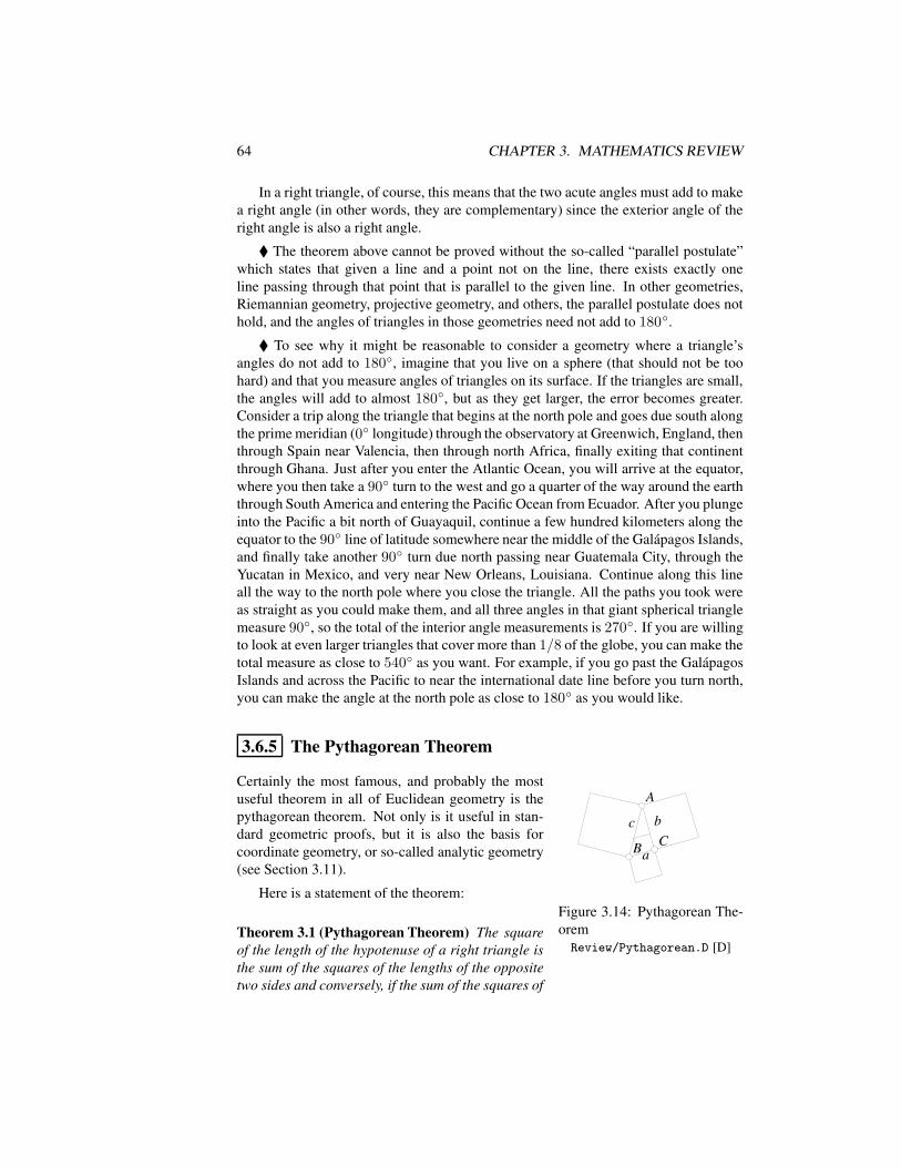
64 CHAPTER 3. MATHEMATICS REVIEW
In a right triangle, of course, this means that the two acute angles must add to makea right angle (in other words, they are complementary) since the exterior angle of theright angle is also a right angle.
The theorem above cannot be proved without the so-called “parallel postulate”which states that given a line and a point not on the line, there exists exactly oneline passing through that point that is parallel to the given line. In other geometries,Riemannian geometry, projective geometry, and others, the parallel postulate does nothold, and the angles of triangles in those geometries need not add to 180.
To see why it might be reasonable to consider a geometry where a triangle’sangles do not add to 180, imagine that you live on a sphere (that should not be toohard) and that you measure angles of triangles on its surface. If the triangles are small,the angles will add to almost 180, but as they get larger, the error becomes greater.Consider a trip along the triangle that begins at the north pole and goes due south alongthe prime meridian (0 longitude) through the observatory at Greenwich, England, thenthrough Spain near Valencia, then through north Africa, finally exiting that continentthrough Ghana. Just after you enter the Atlantic Ocean, you will arrive at the equator,where you then take a 90 turn to the west and go a quarter of the way around the earththrough South America and entering the Pacific Ocean from Ecuador. After you plungeinto the Pacific a bit north of Guayaquil, continue a few hundred kilometers along theequator to the 90 line of latitude somewhere near the middle of the Galapagos Islands,and finally take another 90 turn due north passing near Guatemala City, through theYucatan in Mexico, and very near New Orleans, Louisiana. Continue along this lineall the way to the north pole where you close the triangle. All the paths you took wereas straight as you could make them, and all three angles in that giant spherical trianglemeasure 90, so the total of the interior angle measurements is 270. If you are willingto look at even larger triangles that cover more than 1/8 of the globe, you can make thetotal measure as close to 540 as you want. For example, if you go past the GalapagosIslands and across the Pacific to near the international date line before you turn north,you can make the angle at the north pole as close to 180 as you would like.
3.6.5 The Pythagorean Theorem
aa
bbcc
AA
CCBB
Figure 3.14: Pythagorean The-oremReview/Pythagorean.D [D]
Certainly the most famous, and probably the mostuseful theorem in all of Euclidean geometry is thepythagorean theorem. Not only is it useful in stan-dard geometric proofs, but it is also the basis forcoordinate geometry, or so-called analytic geometry(see Section 3.11).
Here is a statement of the theorem:
Theorem 3.1 (Pythagorean Theorem) The squareof the length of the hypotenuse of a right triangle isthe sum of the squares of the lengths of the oppositetwo sides and conversely, if the sum of the squares of
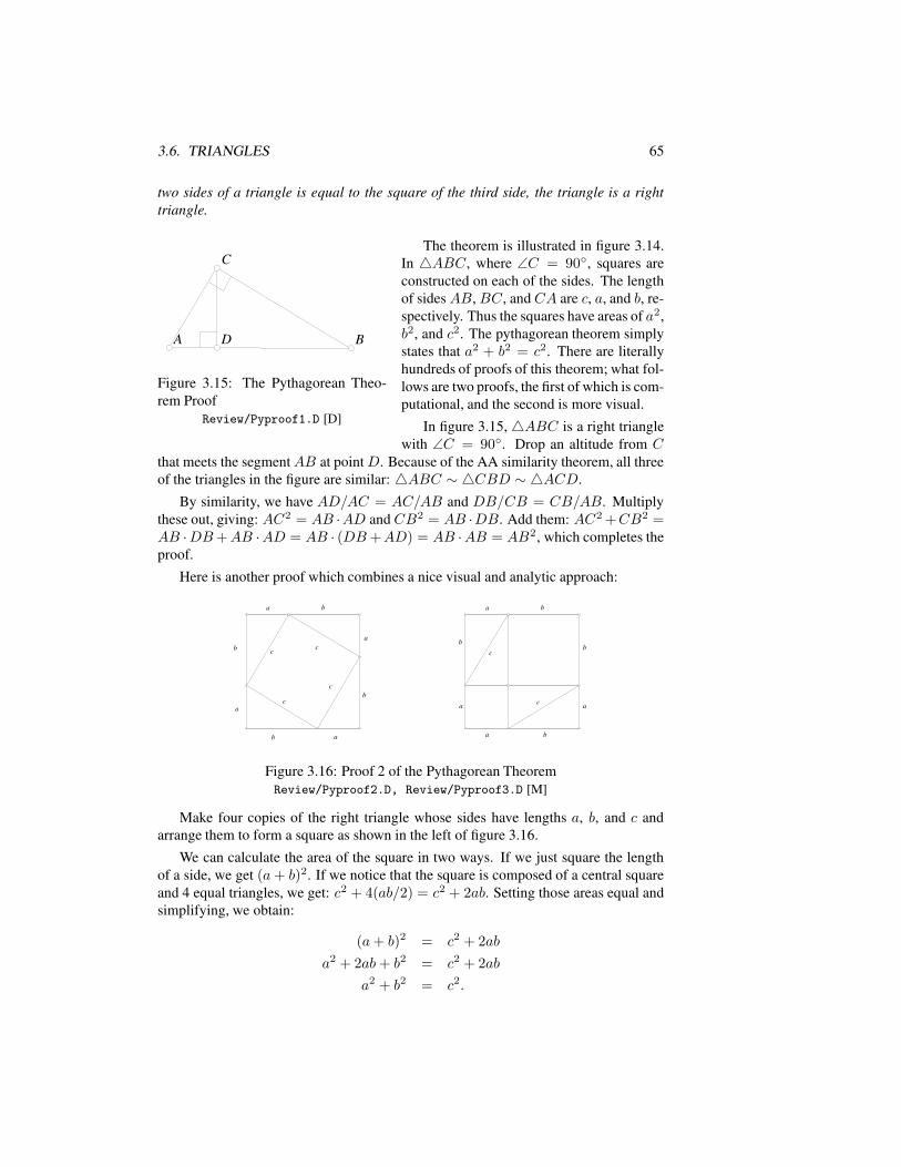
3.6. TRIANGLES 65
two sides of a triangle is equal to the square of the third side, the triangle is a righttriangle.
CC
AA BBDD
Figure 3.15: The Pythagorean Theo-rem Proof
Review/Pyproof1.D [D]
The theorem is illustrated in figure 3.14.In 4ABC, where ∠C = 90, squares areconstructed on each of the sides. The lengthof sides AB, BC, and CA are c, a, and b, re-spectively. Thus the squares have areas of a2,b2, and c2. The pythagorean theorem simplystates that a2 + b2 = c2. There are literallyhundreds of proofs of this theorem; what fol-lows are two proofs, the first of which is com-putational, and the second is more visual.
In figure 3.15,4ABC is a right trianglewith ∠C = 90. Drop an altitude from C
that meets the segmentAB at pointD. Because of the AA similarity theorem, all threeof the triangles in the figure are similar: 4ABC ∼ 4CBD ∼ 4ACD.
By similarity, we have AD/AC = AC/AB and DB/CB = CB/AB. Multiplythese out, giving: AC2 = AB ·AD and CB2 = AB ·DB. Add them: AC2 +CB2 =AB ·DB+AB ·AD = AB · (DB+AD) = AB ·AB = AB2, which completes theproof.
Here is another proof which combines a nice visual and analytic approach:
aa bb
aa
bb
aabb
aa
bb cc cc
cc
cc
aa bb
aa bb
aa
bb
aa
bb
cc
cc
Figure 3.16: Proof 2 of the Pythagorean TheoremReview/Pyproof2.D, Review/Pyproof3.D [M]
Make four copies of the right triangle whose sides have lengths a, b, and c andarrange them to form a square as shown in the left of figure 3.16.
We can calculate the area of the square in two ways. If we just square the lengthof a side, we get (a+ b)2. If we notice that the square is composed of a central squareand 4 equal triangles, we get: c2 + 4(ab/2) = c2 + 2ab. Setting those areas equal andsimplifying, we obtain:
(a+ b)2 = c2 + 2ab
a2 + 2ab+ b2 = c2 + 2ab
a2 + b2 = c2.
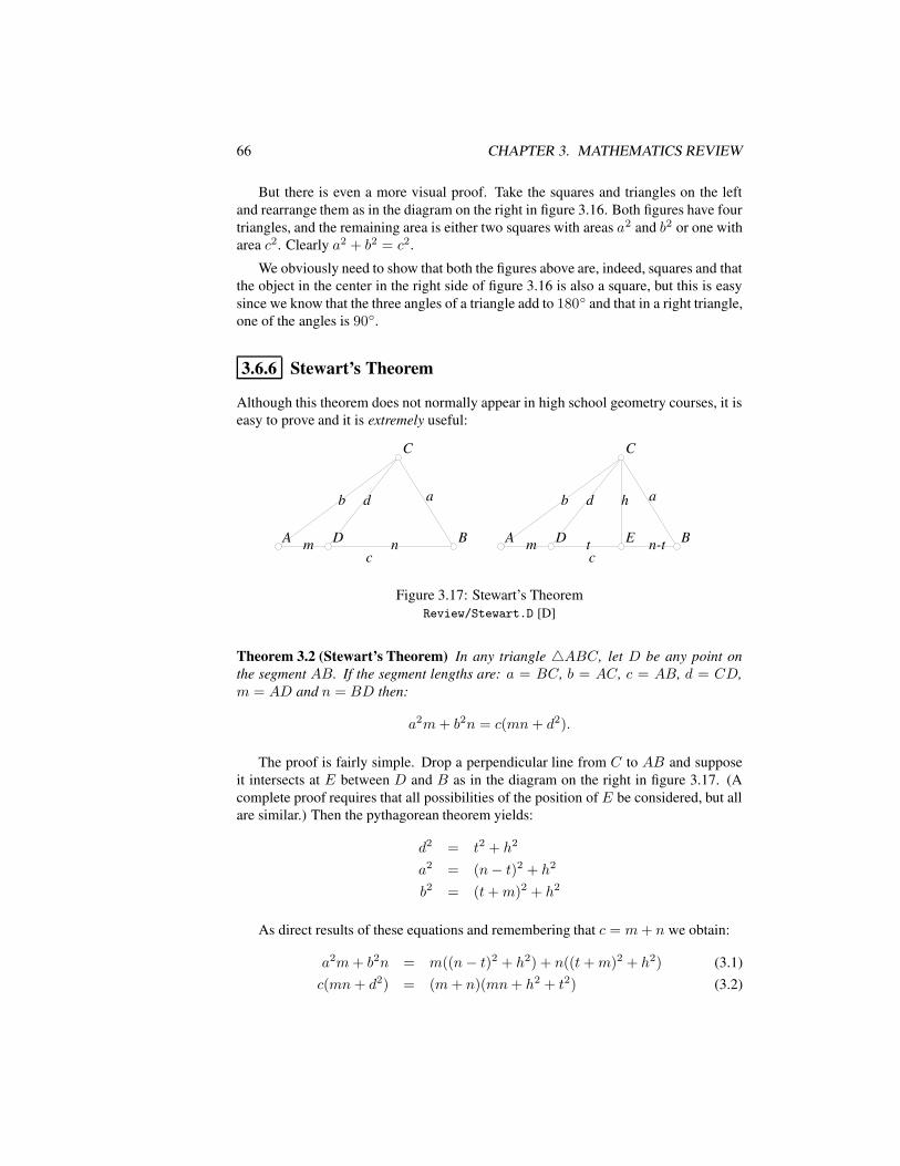
66 CHAPTER 3. MATHEMATICS REVIEW
But there is even a more visual proof. Take the squares and triangles on the leftand rearrange them as in the diagram on the right in figure 3.16. Both figures have fourtriangles, and the remaining area is either two squares with areas a2 and b2 or one witharea c2. Clearly a2 + b2 = c2.
We obviously need to show that both the figures above are, indeed, squares and thatthe object in the center in the right side of figure 3.16 is also a square, but this is easysince we know that the three angles of a triangle add to 180 and that in a right triangle,one of the angles is 90.
3.6.6 Stewart’s Theorem
Although this theorem does not normally appear in high school geometry courses, it iseasy to prove and it is extremely useful:
aabb dd
mm nn
bb aa
mm
hhdd
tt n-tn-tAA BB
CC
DDcc
AA BB
CC
DD EEcc
Figure 3.17: Stewart’s TheoremReview/Stewart.D [D]
Theorem 3.2 (Stewart’s Theorem) In any triangle 4ABC, let D be any point onthe segment AB. If the segment lengths are: a = BC, b = AC, c = AB, d = CD,m = AD and n = BD then:
a2m+ b2n = c(mn+ d2).
The proof is fairly simple. Drop a perpendicular line from C to AB and supposeit intersects at E between D and B as in the diagram on the right in figure 3.17. (Acomplete proof requires that all possibilities of the position of E be considered, but allare similar.) Then the pythagorean theorem yields:
d2 = t2 + h2
a2 = (n− t)2 + h2
b2 = (t+m)2 + h2
As direct results of these equations and remembering that c = m+ n we obtain:
a2m+ b2n = m((n− t)2 + h2) + n((t+m)2 + h2) (3.1)c(mn+ d2) = (m+ n)(mn+ h2 + t2) (3.2)
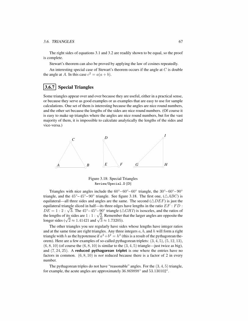
3.6. TRIANGLES 67
The right sides of equations 3.1 and 3.2 are readily shown to be equal, so the proofis complete.
Stewart’s theorem can also be proved by applying the law of cosines repeatedly.An interesting special case of Stewart’s theorem occurs if the angle at C is double
the angle at A. In this case c2 = a(a+ b).
3.6.7 Special Triangles
Some triangles appear over and over because they are useful, either in a practical sense,or because they serve as good examples or as examples that are easy to use for samplecalculations. One set of them is interesting because the angles are nice round numbers,and the other set because the lengths of the sides are nice round numbers. (Of course itis easy to make up triangles where the angles are nice round numbers, but for the vastmajority of them, it is impossible to calculate analytically the lengths of the sides andvice-versa.)
CC
BBAA
DD
FFEE GG HH
II
Figure 3.18: Special TrianglesReview/Special.D [D]
Triangles with nice angles include the 60– 60– 60 triangle, the 30– 60– 90
triangle, and the 45– 45– 90 triangle. See figure 3.18. The first one, (4ABC) isequilateral—all three sides and angles are the same. The second (4DEF ) is just theequilateral triangle sliced in half—its three edges have lengths in the ratio EF : FD :DE = 1 : 2 :
√3. The 45– 45– 90 triangle (4GHI) is isosceles, and the ratios of
the lengths of its sides are 1 : 1 :√
2. Remember that the larger angles are opposite thelonger sides (
√2 ≈ 1.41421 and
√3 ≈ 1.73205).
The other triangles you see regularly have sides whose lengths have integer ratiosand at the same time are right triangles. Any three integers a, b, and h will form a righttriangle with h as the hypotenuse if a2+b2 = h2 (this is a result of the pythagorean the-orem). Here are a few examples of so-called pythagorean triplets: (3, 4, 5), (5, 12, 13),(6, 8, 10) (of course the (6, 8, 10) is similar to the (3, 4, 5) triangle—just twice as big),and (7, 24, 25). A reduced pythagorean triplet is one where the entries have nofactors in common. (6, 8, 10) is not reduced because there is a factor of 2 in everynumber.
The pythagorean triples do not have “reasonable” angles. For the (3, 4, 5) triangle,for example, the acute angles are approximately 36.869898 and 53.130102.
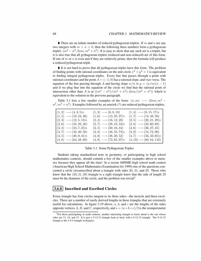
68 CHAPTER 3. MATHEMATICS REVIEW
There are an infinte number of reduced pythagorean triplets. If m and n are anytwo integers with m > n > 0, then the following three numbers form a pythagoreantriplet: (m2 − n2, 2mn,m2 + n2). It is easy to show that any such set is a triplet, butit is also true that all pythagorean triplets (reduced and non-reduced) are of this form.If one of m or n is even and if they are relatively prime, then the formula will producea reduced pythagorean triple.
It is not hard to prove that all pythagorean triples have this form. The problemof finding points with rational coordinates on the unit circle x2 + y2 = 1 is equivalentto finding integral pythagorean triples. Every line that passes through a point withrational coordinates and the pointA = (−1, 0) has a rational slope, and vice-versa. Theequation of the line passing through A and having slope n/m is y = (n/m)(x − 1)and if we plug that into the equation of the circle we find that the rational point ofintersection other than A is at ((m2 − n2)/(m2 + n2), 2mn/(m2 + n2)) which isequivalent to the solution in the previous paragraph.
Table 3.1 lists a few smaller examples of the form: (n,m) −→ (2mn,m2 −n2,m2 + n2). Examples followed by an asterisk (*) are reduced pythagorean triplets.
(1, 2) −→ (4, 3, 5)∗ (1, 3) −→ (6, 8, 10) (1, 4) −→ (8, 15, 17)∗(1, 5) −→ (10, 24, 26) (1, 6) −→ (12, 35, 37)∗ (1, 7) −→ (14, 48, 50)(2, 3) −→ (12, 5, 13)∗ (2, 4) −→ (16, 12, 20) (2, 5) −→ (20, 21, 29)∗(2, 6) −→ (24, 32, 40) (2, 7) −→ (28, 45, 53)∗ (2, 8) −→ (32, 60, 68)(3, 4) −→ (24, 7, 25)∗ (3, 5) −→ (30, 16, 34) (3, 6) −→ (36, 27, 45)(3, 7) −→ (42, 40, 58) (3, 8) −→ (48, 55, 73)∗ (3, 9) −→ (54, 72, 90)(4, 5) −→ (40, 9, 41)∗ (4, 6) −→ (48, 20, 52) (4, 7) −→ (56, 33, 65)∗(4, 8) −→ (64, 48, 80) (4, 9) −→ (72, 65, 97)∗ (4, 10)−→ (80, 84, 116)
Table 3.1: Some Pythagorean Triples
Students taking standardized tests in geometry, or participating in high schoolmathematics contests, should commit a few of the smaller examples above to mem-ory because they appear all the time! In a recent AHSME high school math contest(American High School Mathematics Examination for 1999) one of the questions con-cerned a circle circumscribed about a triangle with sides 20, 21, and 29. Those whoknew that the (20, 21, 29) triangle is a right triangle knew that the side of length 29must be the diameter of the circle, and the problem was trivial5.
3.6.8 Inscribed and Escribed Circles
Every triangle has four circles tangent to its three sides—the incircle and three excir-cles. There are a number of easily derived lengths in these triangles that are extremelyuseful for calculations. In figure 3.19 above, a, b, and c are the lengths of the sidesopposite verticesA, B, andC, respectively, and s = (a+b+c)/2 is the semiperimeter
5For those participating in math contests, another interesting triangle to know about is the one whosesides are 13, 14, and 15. It is just a 5-12-13 triangle back to back with a 9-12-15 triangle. The 9-12-15triangle is the 3-4-5 triangle in disguise.
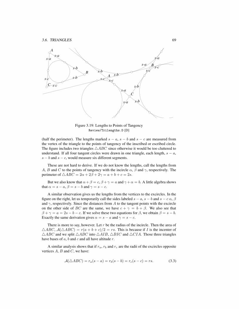
3.6. TRIANGLES 69
AA
BB
CC
AA
BB
CC
s-as-as-as-a s-as-a
s-as-a
s-as-a
s-as-a
s-bs-b
s-bs-b
s-bs-b
s-bs-b
s-bs-bs-bs-b
s-cs-c
s-cs-c
s-cs-cs-cs-c
s-cs-c s-cs-c
Figure 3.19: Lengths to Points of TangencyReview/Trilengths.D [D]
(half the perimeter). The lengths marked s − a, s − b and s − c are measured fromthe vertex of the triangle to the points of tangency of the inscribed or escribed circle.The figure includes two triangles4ABC since otherwise it would be too cluttered tounderstand. If all four tangent circles were drawn in one triangle, each length, s − a,s− b and s− c, would measure six different segments.
These are not hard to derive. If we do not know the lengths, call the lengths fromA, B and C to the points of tangency with the incircle α, β and γ, respectively. Theperimeter of4ABC = 2α+ 2β + 2γ = a+ b+ c = 2s.
But we also know that α+β = c, β+ γ = a and γ+α = b. A little algebra showsthat α = s− a, β = s− b and γ = s− c.
A similar observation gives us the lengths from the vertices to the excircles. In thefigure on the right, let us temporarily call the sides labeled s− a, s− b and s− c α, βand γ, respectively. Since the distances from A to the tangent points with the excircleon the other side of BC are the same, we have c + γ = b + β. We also see thatβ + γ = a = 2s− b− c. If we solve these two equations for β, we obtain β = s− b.Exactly the same derivation gives α = s− a and γ = s− c.
There is more to say, however. Let r be the radius of the incircle. Then the area of4ABC, A(4ABC) = r(a + b + c)/2 = rs. This is because if I is the incenter of4ABC and we split 4ABC into4AIB, 4BIC and4CIA. Those three triangleshave bases of a, b and c and all have altitude r.
A similar analysis shows that if ra, rb and rc are the radii of the excircles oppositevertices A, B and C, we have:
A(4ABC) = ra(s− a) = rb(s− b) = rc(s− c) = rs. (3.3)
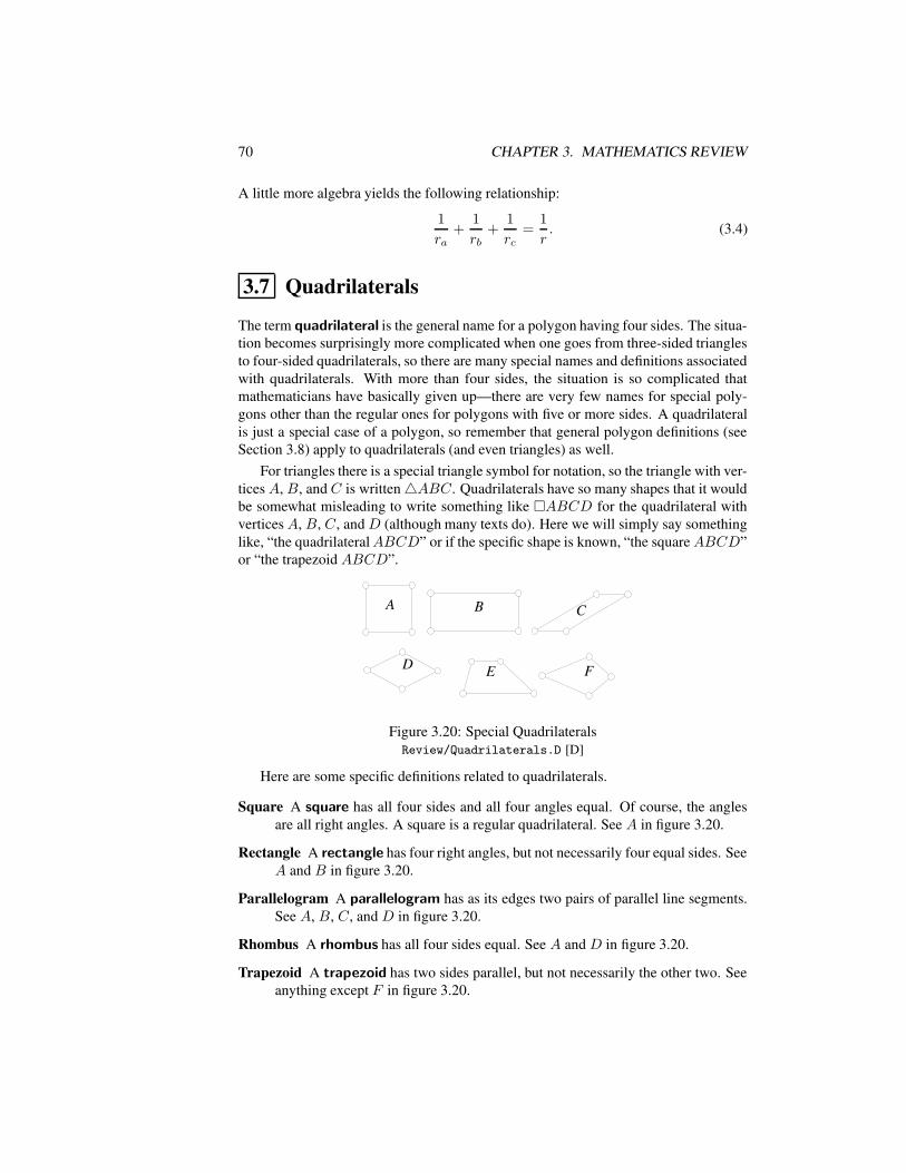
70 CHAPTER 3. MATHEMATICS REVIEW
A little more algebra yields the following relationship:
1
ra+
1
rb+
1
rc=
1
r. (3.4)
3.7 Quadrilaterals
The term quadrilateral is the general name for a polygon having four sides. The situa-tion becomes surprisingly more complicated when one goes from three-sided trianglesto four-sided quadrilaterals, so there are many special names and definitions associatedwith quadrilaterals. With more than four sides, the situation is so complicated thatmathematicians have basically given up—there are very few names for special poly-gons other than the regular ones for polygons with five or more sides. A quadrilateralis just a special case of a polygon, so remember that general polygon definitions (seeSection 3.8) apply to quadrilaterals (and even triangles) as well.
For triangles there is a special triangle symbol for notation, so the triangle with ver-tices A, B, and C is written4ABC. Quadrilaterals have so many shapes that it wouldbe somewhat misleading to write something like ABCD for the quadrilateral withverticesA, B, C, and D (although many texts do). Here we will simply say somethinglike, “the quadrilateralABCD” or if the specific shape is known, “the squareABCD”or “the trapezoid ABCD”.
AA BB CC
DD EE FF
Figure 3.20: Special QuadrilateralsReview/Quadrilaterals.D [D]
Here are some specific definitions related to quadrilaterals.
Square A square has all four sides and all four angles equal. Of course, the anglesare all right angles. A square is a regular quadrilateral. See A in figure 3.20.
Rectangle A rectangle has four right angles, but not necessarily four equal sides. SeeA and B in figure 3.20.
Parallelogram A parallelogram has as its edges two pairs of parallel line segments.See A, B, C, and D in figure 3.20.
Rhombus A rhombus has all four sides equal. See A and D in figure 3.20.
Trapezoid A trapezoid has two sides parallel, but not necessarily the other two. Seeanything except F in figure 3.20.
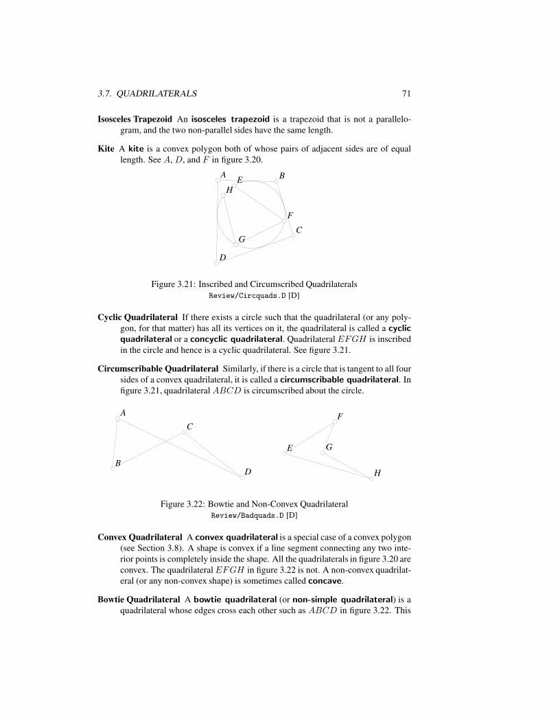
3.7. QUADRILATERALS 71
Isosceles Trapezoid An isosceles trapezoid is a trapezoid that is not a parallelo-gram, and the two non-parallel sides have the same length.
Kite A kite is a convex polygon both of whose pairs of adjacent sides are of equallength. See A, D, and F in figure 3.20.
BB
CC
DD
AA EE
FF
GG
HH
Figure 3.21: Inscribed and Circumscribed QuadrilateralsReview/Circquads.D [D]
Cyclic Quadrilateral If there exists a circle such that the quadrilateral (or any poly-gon, for that matter) has all its vertices on it, the quadrilateral is called a cyclicquadrilateral or a concyclic quadrilateral. QuadrilateralEFGH is inscribedin the circle and hence is a cyclic quadrilateral. See figure 3.21.
Circumscribable Quadrilateral Similarly, if there is a circle that is tangent to all foursides of a convex quadrilateral, it is called a circumscribable quadrilateral. Infigure 3.21, quadrilateral ABCD is circumscribed about the circle.
AA
BB
CC
DD
EE
FF
GG
HH
Figure 3.22: Bowtie and Non-Convex QuadrilateralReview/Badquads.D [D]
Convex Quadrilateral A convex quadrilateral is a special case of a convex polygon(see Section 3.8). A shape is convex if a line segment connecting any two inte-rior points is completely inside the shape. All the quadrilaterals in figure 3.20 areconvex. The quadrilateralEFGH in figure 3.22 is not. A non-convex quadrilat-eral (or any non-convex shape) is sometimes called concave.
Bowtie Quadrilateral A bowtie quadrilateral (or non-simple quadrilateral) is aquadrilateral whose edges cross each other such as ABCD in figure 3.22. This
72 CHAPTER 3. MATHEMATICS REVIEW
cannot happen with triangles, but once a polygon has more than three sides,this is possible, and it is the bane of computer graphics programmers. Whenthe edges of a polygon cross themselves, it no longer makes sense to talk about“inside” and “outside”.
3.7.1 Quadrilateral Theorems
Many properties of quadrilaterals are simple consequences of the fact that two oppositevertices can be connected by a segment dividing the quadrilateral into two triangleswhose properties are easy to calculate. For anything other than special quadrilateralslike rectangles or concyclic quadrilaterals, usually the easiest way to find the area, forexample, is to divide it into two triangles and find the sum of the areas of those twotriangles.
However, here are a few important facts about quadrilaterals, in no particular order.The vast majority are easy to prove:
• The four internal angles of a non-bowtie quadrilateral add to 360. For bowtiequadrilaterals, there is no such thing as an internal angle.
• The diagonals of a rectangle are congruent.
• The diagonals of a rhombus are perpendicular and conversely— if the diago-nals of a parallelogram are perpendicular, the parallelogram is a rhombus. SeeProofs/Rhombus.T for a Geometer proof.
• The diagonals of a rhombus bisect the angles at the vertices of the rhombus.
• The opposite sides of a parallelogram are of equal length and the opposite angleshave equal measures. See Proofs/EquParSides.T for a Geometer proof.
• Any pair of adjacent angles in a parallelogram are supplementary.
• Either diagonal of a parallelogram divides it into two congruent triangles. SeeProofs/EquParSides.T for a Geometer proof.
• The diagonals of a parallelogram bisect each other. See Proofs/ParBisect.T fora Geometer proof.
• If a parallelogram has sides of lengths a and b and diagonals of lengths x and y,then 2a2 + 2b2 = x2 + y2.
• The area of a parallelogram is the base times the height. Warning: the heightis the perpendicular distance from the base to the side parallel to it—it is not thedistance along the other edge.
• If the midpoints of the edges of any quadrilateral are connected in order, the re-sulting figure is a parallelogram. This remains true even for bowtie quadrilater-als. As long as it is not a bowtie quadrilateral, then the area of the parallelogramis half the area of the quadrilateral. This is known as Varignon’s theorem.
3.8. GENERAL POLYGONS 73
• An isosceles trapezoid can be inscribed in a circle. See Proofs/Isotrap.T for aGeometer proof.
• Isosceles trapezoids have congruent base angles. See Proofs/IsoTrapAng.T fora Geometer proof.
• The area of a trapezoid is the average of the lengths of the parallel sides timesthe distance between the sides.
• If a quadrilateralABCD can be circumscribed about a circle, thenAB+CD =AD +BC and conversely. See Proofs/QuadEdges.T for a Geometer proof.
• If a convex quadrilateral ABCD can be inscribed in a circle, then ∠A+ ∠C =∠B + ∠D = 180 and conversely.
3.8 General Polygons
Given n different points in the plane,A1, A2, . . . , An, a polygon is the set of segmentsA1A2, A2A3, A3A4, . . . , An−1An, and AnA1. A polygon has three or more sides—itis usually not very useful to think of one-sided or two-sided polygons since then yourtheorems usually would have the form, “For all polygons except those with one or twosides . . . ”. There is no upper limit, of course, to the number of sides a polygon mayhave. The points A1, . . . , An are called the vertices of the polygon, and the segmentsA1A2, . . . , AnA1 are called the edges. Sometimes it is important to talk about theangles of the polygon which are ∠A1A2A3, ∠A2A3A4, . . . , ∠AnA1A2. Notice thatthis is a quite general definition of a polygon and allows the edges to cross each other,et cetera6. Special names exist for more restricted classes of polygons. There are acouple of different schemes for naming polygons (including the names for 1- and 2-sided polygons), and the more common ones are listed in Table 3.2. The names usedin this book are listed first, and one alternative is listed in parentheses.
Here are some definitions relating to general polygons. Remember that trianglesand quadrilaterals are special cases of polygons, so we can talk about the perimeter ofa triangle or square, for example.
Perimeter The perimeter of a polygon is the sum of the lengths of the edges of thepolygon. It is the distance around the polygon.
Simple Polygon A simple polygon is one whose non-adjacent edges do not meet,even at the endpoints. In other words, there are no crossing lines, or placeswhere the polygon comes back and touches itself.
Although it is “obvious” what is meant by the inside and outside of a simplepolygon, in practice (for example, when you are trying to write a computer pro-gram that deals with general polygons) it can be difficult to determine whether a
6There are, however, still more general definitions of polygons that allow holes or which allow polygonsto have more than one component. Although such definitions are sometimes useful in computer graphics,they will not be considered here.
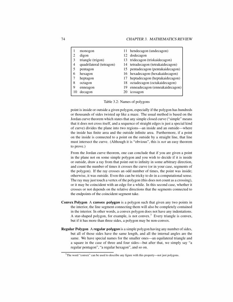
74 CHAPTER 3. MATHEMATICS REVIEW
1 monogon 11 hendecagon (undecagon)2 digon 12 dodecagon3 triangle (trigon) 13 tridecagon (triskaidecagon)4 quadrilateral (tetragon) 14 tetradecagon (tetrakaidecagon)5 pentagon 15 pentadecagon (pentakaidecagon)6 hexagon 16 hexadecagon (hexakaidecagon)7 heptagon 17 heptadecagon (heptakaidecagon)8 octagon 18 octadecagon (octakaidecagon)9 enneagon 19 enneadecagon (enneakaidecagon)10 decagon 20 icosagon
Table 3.2: Names of polygons
point is inside or outside a given polygon, especially if the polygon has hundredsor thousands of sides twisted up like a maze. The usual method is based on theJordan curve theorem which states that any simple closed curve (“simple” meansthat it does not cross itself, and a sequence of straight edges is just a special kindof curve) divides the plane into two regions—an inside and an outside—wherethe inside has finite area and the outside infinite area. Furthermore, if a pointon the inside is connected to a point on the outside by a straight line, that linemust intersect the curve. (Although it is “obvious”, this is not an easy theoremto prove.)
From the Jordan curve theorem, one can conclude that if you are given a pointin the plane not on some simple polygon and you wish to decide if it is insideor outside, draw a ray from that point out to infinity in some arbitrary direction,and count the number of times it crosses the curve (or in your case, segments ofthe polygon). If the ray crosses an odd number of times, the point was inside;otherwise, it was outside. Even this can be tricky to do in a computational sense.The ray may just touch a vertex of the polygon (this does not count as a crossing),or it may be coincident with an edge for a while. In this second case, whether itcrosses or not depends on the relative directions that the segments connected tothe endpoints of the coincident segment take.
Convex Polygon A convex polygon is a polygon such that given any two points inthe interior, the line segment connecting them will also be completely containedin the interior. In other words, a convex polygon does not have any indentations.A star-shaped polygon, for example, is not convex.7 Every triangle is convex,but if it has more than three sides, a polygon may be non-convex.
Regular Polygon A regular polygon is a simple polygon having any number of sides,but all of those sides have the same length, and all the internal angles are thesame. We have special names for the smaller ones—an equilateral triangle anda square in the case of three and four sides—but after that, we simply say “aregular pentagon”, “a regular hexagon”, and so on.
7The word “convex” can be used to describe any figure with this property—not just polygons.
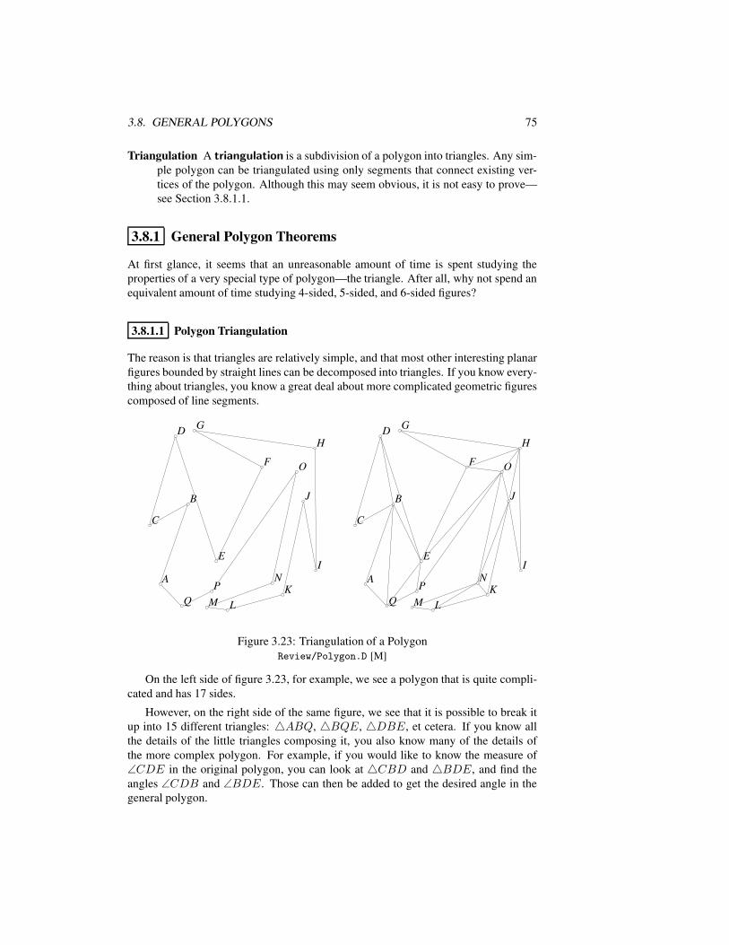
3.8. GENERAL POLYGONS 75
Triangulation A triangulation is a subdivision of a polygon into triangles. Any sim-ple polygon can be triangulated using only segments that connect existing ver-tices of the polygon. Although this may seem obvious, it is not easy to prove—see Section 3.8.1.1.
3.8.1 General Polygon Theorems
At first glance, it seems that an unreasonable amount of time is spent studying theproperties of a very special type of polygon—the triangle. After all, why not spend anequivalent amount of time studying 4-sided, 5-sided, and 6-sided figures?
3.8.1.1 Polygon Triangulation
The reason is that triangles are relatively simple, and that most other interesting planarfigures bounded by straight lines can be decomposed into triangles. If you know every-thing about triangles, you know a great deal about more complicated geometric figurescomposed of line segments.
AA
BB
CC
DD
EE
FF
GG
HH
II
JJ
KKLLMM
NN
OO
PPQQ
AA
BB
CC
DD
EE
FF
GG
HH
II
JJ
KKLLMM
NN
OO
PPQQ
Figure 3.23: Triangulation of a PolygonReview/Polygon.D [M]
On the left side of figure 3.23, for example, we see a polygon that is quite compli-cated and has 17 sides.
However, on the right side of the same figure, we see that it is possible to break itup into 15 different triangles: 4ABQ, 4BQE, 4DBE, et cetera. If you know allthe details of the little triangles composing it, you also know many of the details ofthe more complex polygon. For example, if you would like to know the measure of∠CDE in the original polygon, you can look at 4CBD and 4BDE, and find theangles ∠CDB and ∠BDE. Those can then be added to get the desired angle in thegeneral polygon.
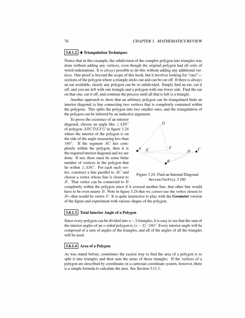
76 CHAPTER 3. MATHEMATICS REVIEW
3.8.1.2 Triangulation Techniques
Notice that in this example, the subdivision of the complex polygon into triangles wasdone without adding any vertices, even though the original polygon had all sorts ofweird indentations. It is always possible to do this without adding any additional ver-tices. One proof is beyond the scope of this book, but it involves looking for “ears”—sections of the polygon where a triangle sticks out and can be cut off. If there is alwaysan ear available, clearly any polygon can be so subdivided. Simply find an ear, cut itoff, and you are left with one triangle and a polygon with one fewer side. Find the earon that one, cut it off, and continue the process until all that is left is a triangle.
Another approach to show that an arbitrary polygon can be triangulated finds aninterior diagonal (a line connecting two vertices that is completely contained withinthe polygon). This splits the polygon into two smaller ones, and the triangulation ofthe polygon can be inferred by an inductive argument.
AA
BB
CCDDEE FF
GG
Figure 3.24: Find an Internal DiagonalReview/CutPoly.T [M]
To prove the existence of an interiordiagonal, choose an angle like ∠ABCof polygon ABCDEFG in figure 3.24where the interior of the polygon is onthe side of the angle measuring less than180. If the segment AC lies com-pletely within the polygon, then it isthe required interior diagonal and we aredone. If not, there must be some finitenumber of vertices in the polygon thatlie within 4ABC. For each such ver-tex, construct a line parallel to AC andchoose a vertex whose line is closest toB. That vertex can be connected to Bcompletely within the polygon since if it crossed another line, that other line wouldhave to be even nearer B. Note in figure 3.24 that we cannot use the vertex closest toB—that would be vertex F . It is quite instructive to play with the Geometer versionof the figure and experiment with various shapes of the polygon.
3.8.1.3 Total Interior Angle of a Polygon
Since every polygon can be divided into n−2 triangles, it is easy to see that the sum ofthe interior angles of an n-sided polygon is (n− 2) · 180. Every interior angle will becomposed of a sum of angles of the triangles, and all of the angles of all the triangleswill be used.
3.8.1.4 Area of a Polygon
As was stated before, sometimes the easiest way to find the area of a polygon is tosplit it into triangles and then sum the areas of those triangles. If the vertices of apolygon are described by coordinates in a cartesian coordinate system, however, thereis a simple formula to calculate the area. See Section 3.11.1.
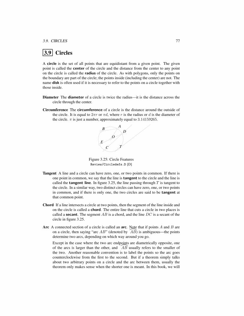
3.9. CIRCLES 77
3.9 Circles
A circle is the set of all points that are equidistant from a given point. The givenpoint is called the center of the circle and the distance from the center to any pointon the circle is called the radius of the circle. As with polygons, only the points onthe boundary are part of the circle; the points inside (including the center) are not. Thename disk is often used if it is necessary to refer to the points on a circle together withthose inside.
Diameter The diameter of a circle is twice the radius—it is the distance across thecircle through the center.
Circumference The circumference of a circle is the distance around the outside ofthe circle. It is equal to 2πr or πd, where r is the radius or d is the diameter ofthe circle. π is just a number, approximately equal to 3.14159265.
OO
CC
DD
TT
BBAA
EE
Figure 3.25: Circle FeaturesReview/Circledefs.D [D]
Tangent A line and a circle can have zero, one, or two points in common. If there isone point in common, we say that the line is tangent to the circle and the line iscalled the tangent line. In figure 3.25, the line passing through T is tangent tothe circle. In a similar way, two distinct circles can have zero, one, or two pointsin common, and if there is only one, the two circles are said to be tangent atthat common point.
Chord If a line intersects a circle at two points, then the segment of the line inside andon the circle is called a chord. The entire line that cuts a circle in two places iscalled a secant. The segment AB is a chord, and the line DC is a secant of thecircle in figure 3.25.
Arc A connected section of a circle is called an arc. Note that if points A and B areon a circle, then saying “arc AB” (denoted by
)
AB) is ambiguous—the pointsdetermine two arcs, depending on which way around you go.
Except in the case where the two arc endpoints are diametrically opposite, oneof the arcs is larger than the other, and
)
AB usually refers to the smaller ofthe two. Another reasonable convention is to label the points so the arc goescounterclockwise from the first to the second. But if a theorem simply talksabout two arbitrary points on a circle and the arc between them, usually thetheorem only makes sense when the shorter one is meant. In this book, we will
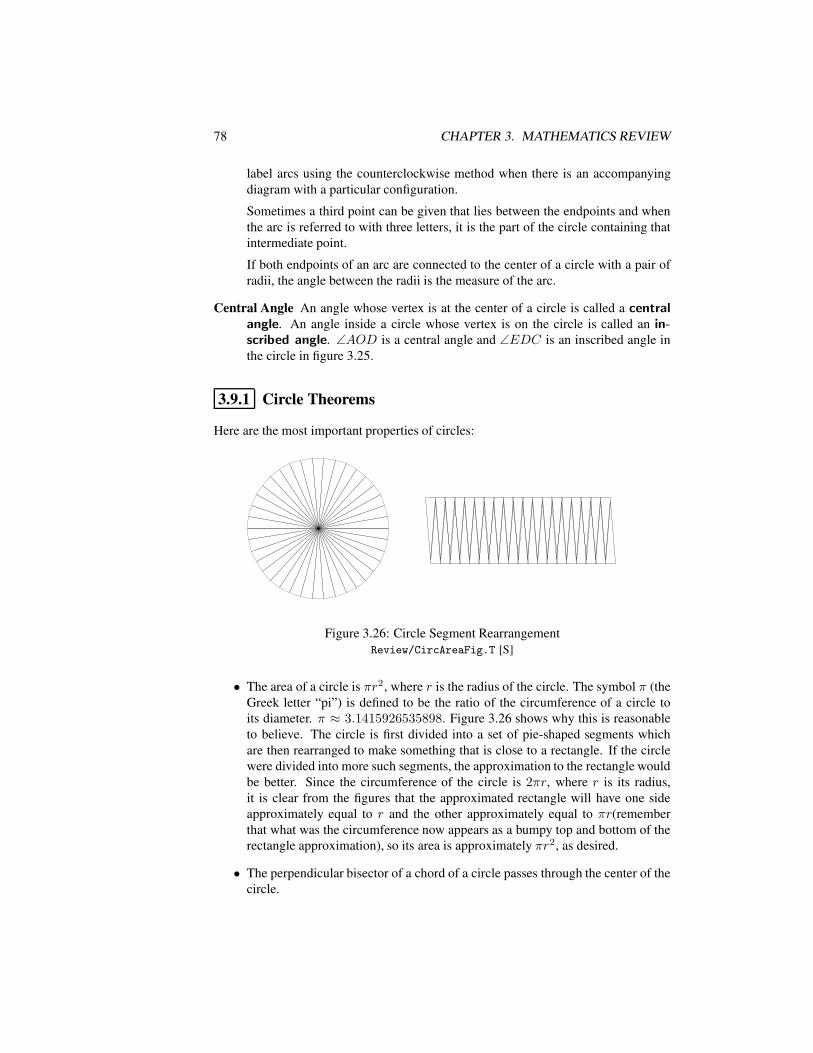
78 CHAPTER 3. MATHEMATICS REVIEW
label arcs using the counterclockwise method when there is an accompanyingdiagram with a particular configuration.
Sometimes a third point can be given that lies between the endpoints and whenthe arc is referred to with three letters, it is the part of the circle containing thatintermediate point.
If both endpoints of an arc are connected to the center of a circle with a pair ofradii, the angle between the radii is the measure of the arc.
Central Angle An angle whose vertex is at the center of a circle is called a centralangle. An angle inside a circle whose vertex is on the circle is called an in-scribed angle. ∠AOD is a central angle and ∠EDC is an inscribed angle inthe circle in figure 3.25.
3.9.1 Circle Theorems
Here are the most important properties of circles:
Figure 3.26: Circle Segment RearrangementReview/CircAreaFig.T [S]
• The area of a circle is πr2, where r is the radius of the circle. The symbol π (theGreek letter “pi”) is defined to be the ratio of the circumference of a circle toits diameter. π ≈ 3.1415926535898. Figure 3.26 shows why this is reasonableto believe. The circle is first divided into a set of pie-shaped segments whichare then rearranged to make something that is close to a rectangle. If the circlewere divided into more such segments, the approximation to the rectangle wouldbe better. Since the circumference of the circle is 2πr, where r is its radius,it is clear from the figures that the approximated rectangle will have one sideapproximately equal to r and the other approximately equal to πr(rememberthat what was the circumference now appears as a bumpy top and bottom of therectangle approximation), so its area is approximately πr2, as desired.
• The perpendicular bisector of a chord of a circle passes through the center of thecircle.
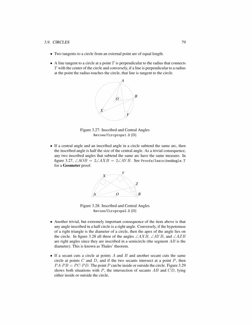
3.9. CIRCLES 79
• Two tangents to a circle from an external point are of equal length.
• A line tangent to a circle at a point T is perpendicular to the radius that connectsT with the center of the circle and conversely, if a line is perpendicular to a radiusat the point the radius touches the circle, that line is tangent to the circle.
OO
AA
BB
XXYY
Figure 3.27: Inscribed and Central AnglesReview/Circprops1.D [D]
• If a central angle and an inscribed angle in a circle subtend the same arc, thenthe inscribed angle is half the size of the central angle. As a trivial consequence,any two inscribed angles that subtend the same arc have the same measure. Infigure 3.27, ∠AOB = 2∠AXB = 2∠AY B. See Proofs/InscribedAngle.T
for a Geometer proof.
OO BBAA
XXYY
ZZ
Figure 3.28: Inscribed and Central AnglesReview/Circprops2.D [D]
• Another trivial, but extremely important consequence of the item above is thatany angle inscribed in a half circle is a right angle. Conversely, if the hypotenuseof a right triangle is the diameter of a circle, then the apex of the angle lies onthe circle. In figure 3.28 all three of the angles ∠AXB, ∠AY B, and ∠AZBare right angles since they are inscribed in a semicircle (the segment AB is thediameter). This is known as Thales’ theorem.
• If a secant cuts a circle at points A and B and another secant cuts the samecircle at points C and D, and if the two secants intersect at a point P , thenPA·PB = PC ·PD. The pointP can be inside or outside the circle. Figure 3.29shows both situations with P , the intersection of secants AB and CD, lyingeither inside or outside the circle.
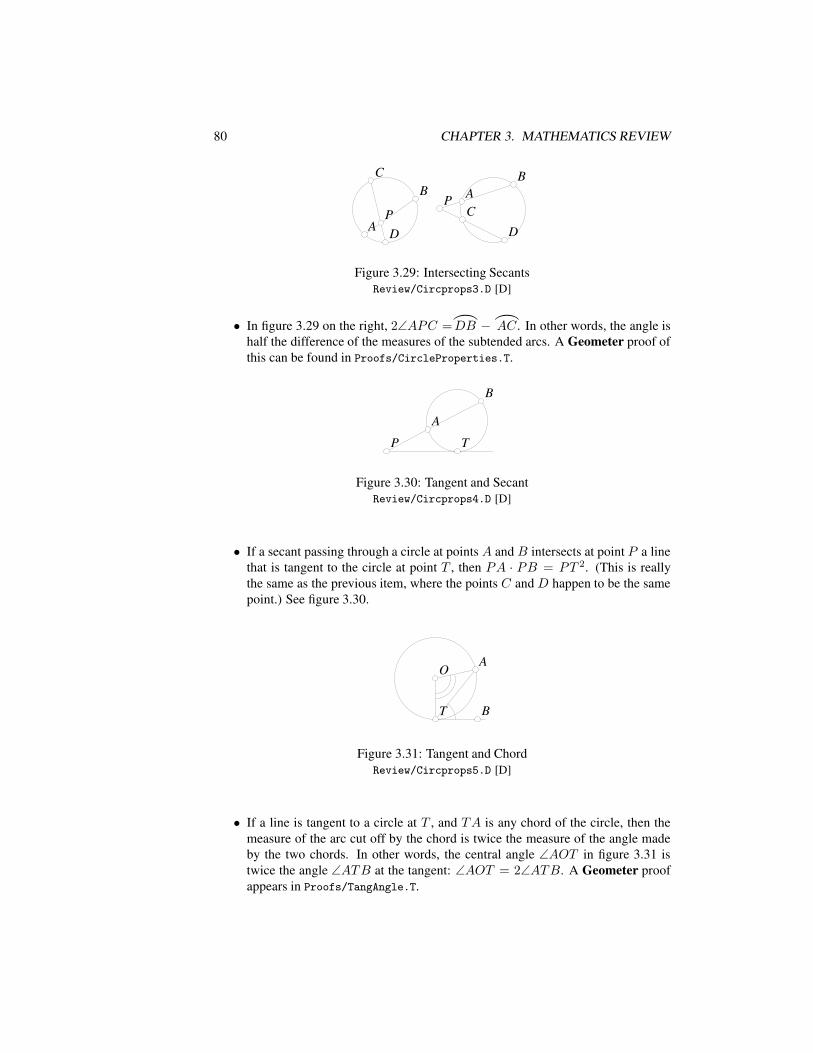
80 CHAPTER 3. MATHEMATICS REVIEW
AA
CC
DD
BB AABB
CC
DDPP
PP
Figure 3.29: Intersecting SecantsReview/Circprops3.D [D]
• In figure 3.29 on the right, 2∠APC =
)
DB − )AC . In other words, the angle ishalf the difference of the measures of the subtended arcs. A Geometer proof ofthis can be found in Proofs/CircleProperties.T.
AA
TT
BB
PP
Figure 3.30: Tangent and SecantReview/Circprops4.D [D]
• If a secant passing through a circle at points A and B intersects at point P a linethat is tangent to the circle at point T , then PA · PB = PT 2. (This is reallythe same as the previous item, where the points C and D happen to be the samepoint.) See figure 3.30.
AA
TT BB
OO
Figure 3.31: Tangent and ChordReview/Circprops5.D [D]
• If a line is tangent to a circle at T , and TA is any chord of the circle, then themeasure of the arc cut off by the chord is twice the measure of the angle madeby the two chords. In other words, the central angle ∠AOT in figure 3.31 istwice the angle ∠ATB at the tangent: ∠AOT = 2∠ATB. A Geometer proofappears in Proofs/TangAngle.T.
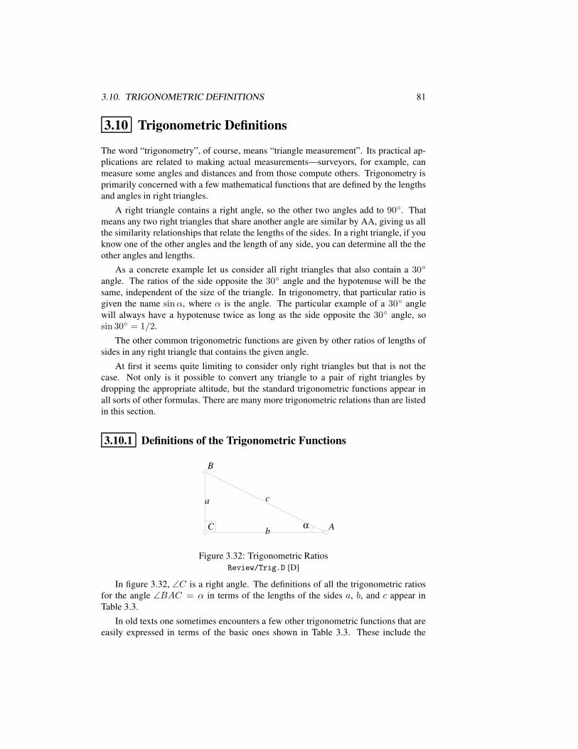
3.10. TRIGONOMETRIC DEFINITIONS 81
3.10 Trigonometric Definitions
The word “trigonometry”, of course, means “triangle measurement”. Its practical ap-plications are related to making actual measurements—surveyors, for example, canmeasure some angles and distances and from those compute others. Trigonometry isprimarily concerned with a few mathematical functions that are defined by the lengthsand angles in right triangles.
A right triangle contains a right angle, so the other two angles add to 90. Thatmeans any two right triangles that share another angle are similar by AA, giving us allthe similarity relationships that relate the lengths of the sides. In a right triangle, if youknow one of the other angles and the length of any side, you can determine all the theother angles and lengths.
As a concrete example let us consider all right triangles that also contain a 30
angle. The ratios of the side opposite the 30 angle and the hypotenuse will be thesame, independent of the size of the triangle. In trigonometry, that particular ratio isgiven the name sinα, where α is the angle. The particular example of a 30 anglewill always have a hypotenuse twice as long as the side opposite the 30 angle, sosin 30 = 1/2.
The other common trigonometric functions are given by other ratios of lengths ofsides in any right triangle that contains the given angle.
At first it seems quite limiting to consider only right triangles but that is not thecase. Not only is it possible to convert any triangle to a pair of right triangles bydropping the appropriate altitude, but the standard trigonometric functions appear inall sorts of other formulas. There are many more trigonometric relations than are listedin this section.
3.10.1 Definitions of the Trigonometric Functions
bb
aa cc
CC AA
BB
αα
Figure 3.32: Trigonometric RatiosReview/Trig.D [D]
In figure 3.32, ∠C is a right angle. The definitions of all the trigonometric ratiosfor the angle ∠BAC = α in terms of the lengths of the sides a, b, and c appear inTable 3.3.
In old texts one sometimes encounters a few other trigonometric functions that areeasily expressed in terms of the basic ones shown in Table 3.3. These include the
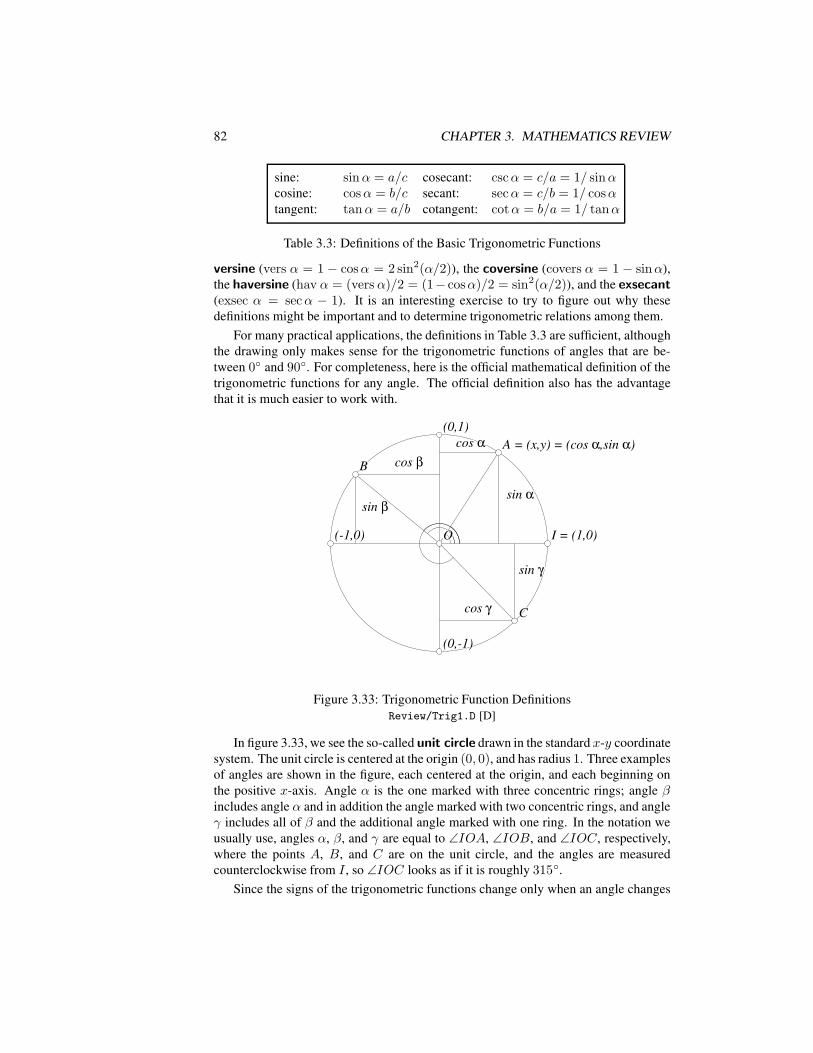
82 CHAPTER 3. MATHEMATICS REVIEW
sine: sinα = a/c cosecant: cscα = c/a = 1/ sinαcosine: cosα = b/c secant: secα = c/b = 1/ cosαtangent: tanα = a/b cotangent: cotα = b/a = 1/ tanα
Table 3.3: Definitions of the Basic Trigonometric Functions
versine (vers α = 1 − cosα = 2 sin2(α/2)), the coversine (covers α = 1 − sinα),the haversine (hav α = (vers α)/2 = (1− cosα)/2 = sin2(α/2)), and the exsecant(exsec α = secα − 1). It is an interesting exercise to try to figure out why thesedefinitions might be important and to determine trigonometric relations among them.
For many practical applications, the definitions in Table 3.3 are sufficient, althoughthe drawing only makes sense for the trigonometric functions of angles that are be-tween 0 and 90. For completeness, here is the official mathematical definition of thetrigonometric functions for any angle. The official definition also has the advantagethat it is much easier to work with.
OO I = (1,0)I = (1,0)(-1,0)(-1,0)
(0,1)(0,1)
(0,-1)(0,-1)
A = (x,y) = (cos α,sin α)A = (x,y) = (cos α,sin α)
BB
CC
cos αcos αcos βcos β
sin βsin βsin αsin α
sin γsin γ
cos γcos γ
Figure 3.33: Trigonometric Function DefinitionsReview/Trig1.D [D]
In figure 3.33, we see the so-called unit circle drawn in the standard x-y coordinatesystem. The unit circle is centered at the origin (0, 0), and has radius 1. Three examplesof angles are shown in the figure, each centered at the origin, and each beginning onthe positive x-axis. Angle α is the one marked with three concentric rings; angle βincludes angle α and in addition the angle marked with two concentric rings, and angleγ includes all of β and the additional angle marked with one ring. In the notation weusually use, angles α, β, and γ are equal to ∠IOA, ∠IOB, and ∠IOC, respectively,where the points A, B, and C are on the unit circle, and the angles are measuredcounterclockwise from I , so ∠IOC looks as if it is roughly 315.
Since the signs of the trigonometric functions change only when an angle changes
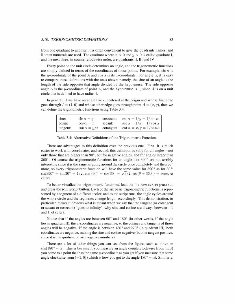
3.10. TRIGONOMETRIC DEFINITIONS 83
from one quadrant to another, it is often convenient to give the quadrants names, andRoman numerals are used. The quadrant where x > 0 and y > 0 is called quadrant I,and the next three, in counter-clockwise order, are quadrants II, III and IV.
Every point on the unit circle determines an angle, and the trigonometric functionsare simply defined in terms of the coordinates of those points. For example, sinα isthe y-coordinate of the point A and cosα is its x-coordinate. For angle α, it is easyto compare these definitions with the ones above; namely, the sine of an angle is thelength of the side opposite that angle divided by the hypotenuse. The side oppositeangle α is the y-coordinate of point A, and the hypotenuse is 1, since A is on a unitcircle that is defined to have radius 1.
In general, if we have an angle like α centered at the origin and whose first edgegoes through I = (1, 0) and whose other edge goes through point A = (x, y), then wecan define the trigonometric functions using Table 3.4.
sine: sinα = y cosecant: cscα = 1/y = 1/ sinαcosine: cosα = x secant: secα = 1/x = 1/ cosαtangent: tanα = y/x cotangent: cotα = x/y = 1/ tanα
Table 3.4: Alternative Definitions of the Trigonometric Functions
There are advantages to this definition over the previous one. First, it is mucheasier to work with coordinates, and second, this definition is valid for all angles—notonly those that are bigger than 90, but for negative angles, and for angles larger than360. Of course the trigonometric functions for an angle like 390 are not terriblyinteresting since it is the same as going around the circle once completely and then 30
more, so every trigonometric function will have the same value for 390 as for 30:sin 390 = sin 30 = 1/2; cos 390 = cos 30 =
√3/2, sec(θ + 360) = sec θ, et
cetera.
To better visualize the trigonometric functions, load the file Review/TrigFuncs.T
and press the Run Script button. Each of the six basic trigonometric functions is repre-sented by a segment of a different color, and as the script runs, the angle cycles aroundthe whole circle and the segments change length accordingly. This demonstration, inparticular, makes it obvious what is meant when we say that the tangent (or cotangentor secant or cosecant) “goes to infinity”, why sine and cosine are always between −1and 1, et cetera.
Notice that if the angles are between 90 and 180 (in other words, if the anglelies in quadrant II), the x-coordinates are negative, so the cosines and tangents of thoseangles will be negative. If the angle is between 180 and 270 (in quadrant III), bothcoordinates are negative, making the sine and cosine negative (but the tangent positive,since it is the quotient of two negative numbers).
There are a lot of other things you can see from the figure, such as sinα =sin(180 − α). This is because if you measure an angle counterclockwise from (1, 0)you come to a point that has the same y-coordinate as you get if you measure that sameangle clockwise from (−1, 0) (which is how you get to the angle 180−α). Similarly,
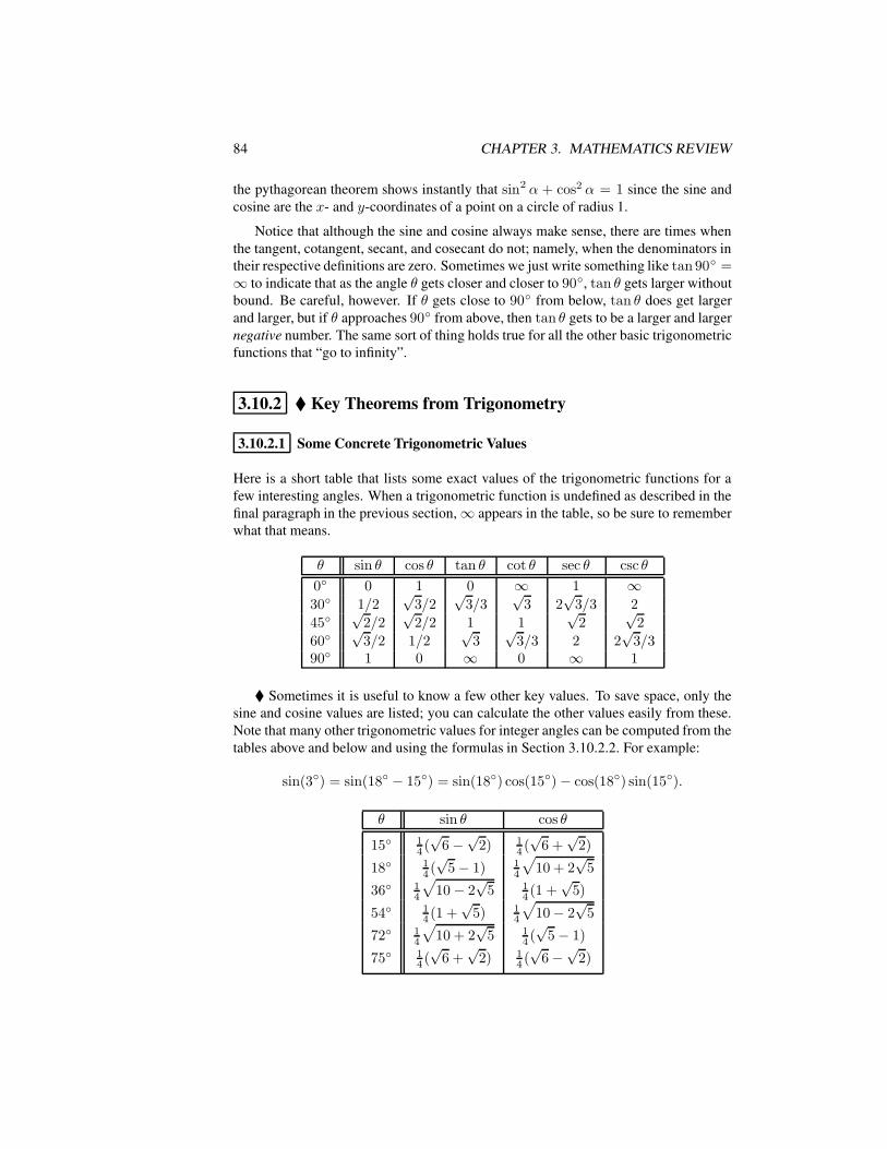
84 CHAPTER 3. MATHEMATICS REVIEW
the pythagorean theorem shows instantly that sin2 α + cos2 α = 1 since the sine andcosine are the x- and y-coordinates of a point on a circle of radius 1.
Notice that although the sine and cosine always make sense, there are times whenthe tangent, cotangent, secant, and cosecant do not; namely, when the denominators intheir respective definitions are zero. Sometimes we just write something like tan 90 =∞ to indicate that as the angle θ gets closer and closer to 90, tan θ gets larger withoutbound. Be careful, however. If θ gets close to 90 from below, tan θ does get largerand larger, but if θ approaches 90 from above, then tan θ gets to be a larger and largernegative number. The same sort of thing holds true for all the other basic trigonometricfunctions that “go to infinity”.
3.10.2 Key Theorems from Trigonometry
3.10.2.1 Some Concrete Trigonometric Values
Here is a short table that lists some exact values of the trigonometric functions for afew interesting angles. When a trigonometric function is undefined as described in thefinal paragraph in the previous section,∞ appears in the table, so be sure to rememberwhat that means.
θ sin θ cos θ tan θ cot θ sec θ csc θ
0 0 1 0 ∞ 1 ∞30 1/2
√3/2
√3/3
√3 2
√3/3 2
45√
2/2√
2/2 1 1√
2√
2
60√
3/2 1/2√
3√
3/3 2 2√
3/390 1 0 ∞ 0 ∞ 1
Sometimes it is useful to know a few other key values. To save space, only thesine and cosine values are listed; you can calculate the other values easily from these.Note that many other trigonometric values for integer angles can be computed from thetables above and below and using the formulas in Section 3.10.2.2. For example:
sin(3) = sin(18 − 15) = sin(18) cos(15)− cos(18) sin(15).
θ sin θ cos θ
15 14 (√
6−√
2) 14 (√
6 +√
2)
18 14 (√
5− 1) 14
√10 + 2
√5
36 14
√10− 2
√5 1
4 (1 +√
5)
54 14 (1 +
√5) 1
4
√10− 2
√5
72 14
√10 + 2
√5 1
4 (√
5− 1)
75 14 (√
6 +√
2) 14 (√
6−√
2)

3.10. TRIGONOMETRIC DEFINITIONS 85
3.10.2.2 Basic Trigonometric Identities
Without proof (and it is a great exercise to do the proofs), here is a list of equationssatisfied by various of the trigonometric functions:
If α+ β = 90 (if α and β are complementary8):
sinα = cosβ tanα = cotβ secα = cscβ.
For supplementary angles we have:
sinα = sin(180 − α) cscα = csc(180 − α)
cosα = − cos(180 − α) secα = − sec(180 − α)
tanα = − tan(180 − α) cotα = − cot(180 − α)
These are direct consequences of the fact that the trigonometric functions are de-fined in terms of coordinates of points on the unit circle:
sin2 α+ cos2 α = 1 sec2 α = tan2 α+ 1 csc2 α = cot2 α+ 1
Here are the angle addition formulas9:
sin(α± β) = sinα cosβ ± cosα sinβ (3.5)cos(α± β) = cosα cosβ ∓ sinα sinβ (3.6)
tan(α± β) =tanα± tanβ
1∓ tanα tanβ(3.7)
See the diagram Proofs/CosineSummation.T for a Geometer proof of the sum ofangles formula for the cosine.
From these, it is easy to derive the multiple angle formulas since sin(2α) = sin(α+α), sin(3α) = sin(2α+ α), et cetera10:
sin(2α) = 2 sinα cosα (3.8)cos(2α) = cos2 α− sin2 α = 2 cos2 α− 1 (3.9)
tan(2α) =2 tanα
1− tan2 α(3.10)
sin(3α) = 3 sinα− 4 sin3 α (3.11)cos(3α) = 4 cos3 α− 3 cosα (3.12)
tan(3α) =3 tanα− tan3 α
1− 3 tan2 α(3.13)
8Note the letters “co” in the words: sine–cosine, tangent–cotangent, secant–cosecant, andcomplementary. Coincidence? Not likely.
9The symbol ∓ is the opposite of ±. It means that if you choose the + option of ±, you must use the −option in ∓ and vice-versa. The use of ± and ∓ in equation 3.6 is equivalent to:
cos(α+ β) = cosα cos β − sinα sinβ
cos(α− β) = cosα cos β + sinα sinβ
10The formulas for cosnα are closely related to the Chebychev polynomials: If x = cosα, Tn(x) =cosnα. T0(x) = 1, T1(x) = x, T2(x) = 2x2 − 1, T3(x) = 4x3 − 3x, et cetera. It is an interestingexercise for a student to investigate these polynomials.
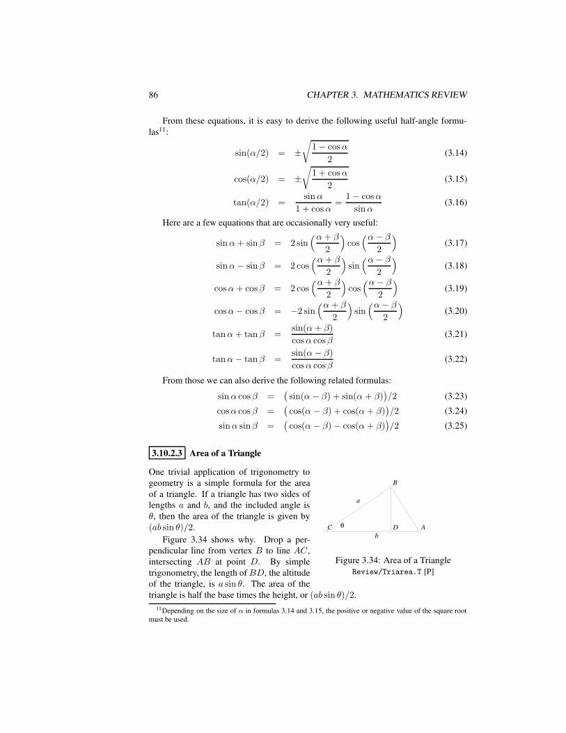
86 CHAPTER 3. MATHEMATICS REVIEW
From these equations, it is easy to derive the following useful half-angle formu-las11:
sin(α/2) = ±√
1− cosα
2(3.14)
cos(α/2) = ±√
1 + cosα
2(3.15)
tan(α/2) =sinα
1 + cosα=
1− cosα
sinα(3.16)
Here are a few equations that are occasionally very useful:
sinα+ sinβ = 2 sin(α+ β
2
)cos(α− β
2
)(3.17)
sinα− sinβ = 2 cos(α+ β
2
)sin(α− β
2
)(3.18)
cosα+ cosβ = 2 cos(α+ β
2
)cos(α− β
2
)(3.19)
cosα− cosβ = −2 sin(α+ β
2
)sin(α− β
2
)(3.20)
tanα+ tanβ =sin(α+ β)
cosα cosβ(3.21)
tanα− tanβ =sin(α− β)
cosα cosβ(3.22)
From those we can also derive the following related formulas:
sinα cosβ =(
sin(α− β) + sin(α + β))/2 (3.23)
cosα cosβ =(
cos(α − β) + cos(α+ β))/2 (3.24)
sinα sinβ =(
cos(α − β)− cos(α+ β))/2 (3.25)
3.10.2.3 Area of a Triangle
BB
CC AADDbb
aa
θθ
Figure 3.34: Area of a TriangleReview/Triarea.T [P]
One trivial application of trigonometry togeometry is a simple formula for the areaof a triangle. If a triangle has two sides oflengths a and b, and the included angle isθ, then the area of the triangle is given by(ab sin θ)/2.
Figure 3.34 shows why. Drop a per-pendicular line from vertex B to line AC,intersecting AB at point D. By simpletrigonometry, the length ofBD, the altitudeof the triangle, is a sin θ. The area of thetriangle is half the base times the height, or (ab sin θ)/2.
11Depending on the size of α in formulas 3.14 and 3.15, the positive or negative value of the square rootmust be used.
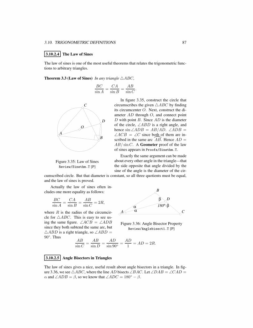
3.10. TRIGONOMETRIC DEFINITIONS 87
3.10.2.4 The Law of Sines
The law of sines is one of the most useful theorems that relates the trigonometric func-tions to arbitrary triangles.
Theorem 3.3 (Law of Sines) In any triangle4ABC,
BC
sinA=
CA
sinB=
AB
sinC.
AABB
CC
OODD
Figure 3.35: Law of SinesReview/Sinethm.T [P]
In figure 3.35, construct the circle thatcircumscribes the given 4ABC by findingits circumcenter O. Next, construct the di-ameter AD through O, and connect pointD with point B. Since AD is the diameterof the circle, ∠ABD is a right angle, andhence sin∠ADB = AB/AD. ∠ADB =∠ACB = ∠C since both of them are in-scribed in the same arc
)
AB. Hence AD =AB/ sinC. A Geometer proof of the lawof sines appears in Proofs/Sinethm.T.
Exactly the same argument can be madeabout every other angle in the triangle—thatthe side opposite that angle divided by thesine of the angle is the diameter of the cir-
cumscribed circle. But that diameter is constant, so all three quotients must be equal,and the law of sines is proved.
AA
BB
CC
DD
αααα
ββ180°-β180°-β
Figure 3.36: Angle Bisector PropertyReview/Anglebisect1.T [P]
Actually the law of sines often in-cludes one more equality as follows:
BC
sinA=
CA
sinB=
AB
sinC= 2R,
where R is the radius of the circumcir-cle for 4ABC. This is easy to see us-ing the same figure. ∠ACB = ∠ADBsince they both subtend the same arc, but4ABD is a right triangle, so ∠ABD =90. Thus
AB
sinC=
AB
sinD=
AD
sin 90=AD
1= AD = 2R.
3.10.2.5 Angle Bisectors in Triangles
The law of sines gives a nice, useful result about angle bisectors in a triangle. In fig-ure 3.36, we see4ABC, where the lineAD bisects∠BAC. Let∠DAB = ∠CAD =α and ∠ADB = β, so we know that ∠ADC = 180 − β.
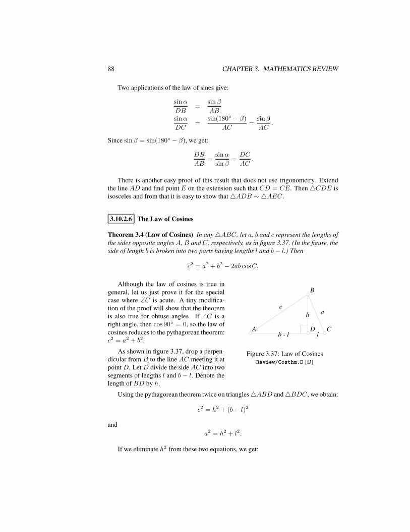
88 CHAPTER 3. MATHEMATICS REVIEW
Two applications of the law of sines give:
sinα
DB=
sinβ
ABsinα
DC=
sin(180 − β)
AC=
sinβ
AC.
Since sinβ = sin(180 − β), we get:
DB
AB=
sinα
sinβ=DC
AC.
There is another easy proof of this result that does not use trigonometry. Extendthe line AD and find point E on the extension such that CD = CE. Then4CDE isisosceles and from that it is easy to show that4ADB ∼ 4AEC.
3.10.2.6 The Law of Cosines
Theorem 3.4 (Law of Cosines) In any4ABC, let a, b and c represent the lengths ofthe sides opposite angles A, B and C, respectively, as in figure 3.37. (In the figure, theside of length b is broken into two parts having lengths l and b− l.) Then
c2 = a2 + b2 − 2ab cosC.
AA
BB
CC
aacc
DD
hh
b - lb - l ll
Figure 3.37: Law of CosinesReview/Costhm.D [D]
Although the law of cosines is true ingeneral, let us just prove it for the specialcase where ∠C is acute. A tiny modifica-tion of the proof will show that the theoremis also true for obtuse angles. If ∠C is aright angle, then cos 90 = 0, so the law ofcosines reduces to the pythagorean theorem:c2 = a2 + b2.
As shown in figure 3.37, drop a perpen-dicular from B to the line AC meeting it atpoint D. Let D divide the side AC into twosegments of lengths l and b − l. Denote thelength of BD by h.
Using the pythagorean theorem twice on triangles4ABD and4BDC, we obtain:
c2 = h2 + (b− l)2
anda2 = h2 + l2.
If we eliminate h2 from these two equations, we get:
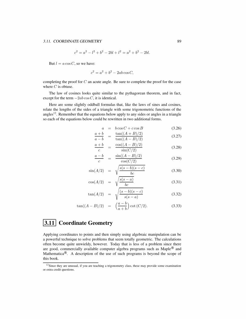
3.11. COORDINATE GEOMETRY 89
c2 = a2 − l2 + b2 − 2bl+ l2 = a2 + b2 − 2bl.
But l = a cosC, so we have:
c2 = a2 + b2 − 2ab cosC,
completing the proof for C an acute angle. Be sure to complete the proof for the casewhere C is obtuse.
The law of cosines looks quite similar to the pythagorean theorem, and in fact,except for the term−2ab cosC, it is identical.
Here are some slightly oddball formulas that, like the laws of sines and cosines,relate the lengths of the sides of a triangle with some trigonometric functions of theangles12. Remember that the equations below apply to any sides or angles in a triangleso each of the equations below could be rewritten in two additional forms.
a = b cosC + c cosB (3.26)a+ b
a− b =tan((A +B)/2)
tan((A −B)/2)(3.27)
a+ b
c=
cos((A−B)/2)
sin(C/2)(3.28)
a− bc
=sin((A −B)/2)
cos(C/2)(3.29)
sin(A/2) =
√s(s− b)(s− c)
bc(3.30)
cos(A/2) =
√s(s− a)
bc(3.31)
tan(A/2) =
√(s− b)(s− c)s(s− a)
(3.32)
tan((A−B)/2) =(a− ba+ b
)cot (C/2). (3.33)
3.11 Coordinate Geometry
Applying coordinates to points and then simply using algebraic manipulation can bea powerful technique to solve problems that seem totally geometric. The calculationsoften become quite unwieldy, however. Today that is less of a problem since thereare good, commercially available computer algebra programs such as Maple andMathematica. A description of the use of such programs is beyond the scope ofthis book.
12Since they are unusual, if you are teaching a trigonometry class, these may provide some examinationor extra credit questions.
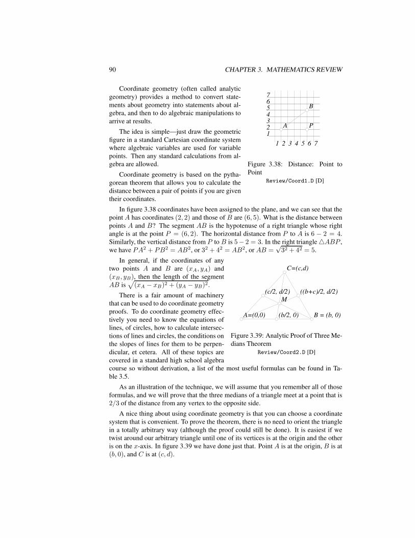
90 CHAPTER 3. MATHEMATICS REVIEW
11223344556677
11 22 33 44 55 66 77
AA
BB
PP
Figure 3.38: Distance: Point toPoint
Review/Coord1.D [D]
Coordinate geometry (often called analyticgeometry) provides a method to convert state-ments about geometry into statements about al-gebra, and then to do algebraic manipulations toarrive at results.
The idea is simple—just draw the geometricfigure in a standard Cartesian coordinate systemwhere algebraic variables are used for variablepoints. Then any standard calculations from al-gebra are allowed.
Coordinate geometry is based on the pytha-gorean theorem that allows you to calculate thedistance between a pair of points if you are giventheir coordinates.
In figure 3.38 coordinates have been assigned to the plane, and we can see that thepoint A has coordinates (2, 2) and those of B are (6, 5). What is the distance betweenpoints A and B? The segment AB is the hypotenuse of a right triangle whose rightangle is at the point P = (6, 2). The horizontal distance from P to A is 6 − 2 = 4.Similarly, the vertical distance from P to B is 5− 2 = 3. In the right triangle4ABP ,we have PA2 + PB2 = AB2, or 32 + 42 = AB2, or AB =
√32 + 42 = 5.
A=(0,0)A=(0,0) B = (b, 0)B = (b, 0)
C=(c,d)C=(c,d)
(c/2, d/2)(c/2, d/2) ((b+c)/2, d/2)((b+c)/2, d/2)
(b/2, 0)(b/2, 0)
MM
Figure 3.39: Analytic Proof of Three Me-dians Theorem
Review/Coord2.D [D]
In general, if the coordinates of anytwo points A and B are (xA, yA) and(xB , yB), then the length of the segmentAB is
√(xA − xB)2 + (yA − yB)2.
There is a fair amount of machinerythat can be used to do coordinate geometryproofs. To do coordinate geometry effec-tively you need to know the equations oflines, of circles, how to calculate intersec-tions of lines and circles, the conditions onthe slopes of lines for them to be perpen-dicular, et cetera. All of these topics arecovered in a standard high school algebracourse so without derivation, a list of the most useful formulas can be found in Ta-ble 3.5.
As an illustration of the technique, we will assume that you remember all of thoseformulas, and we will prove that the three medians of a triangle meet at a point that is2/3 of the distance from any vertex to the opposite side.
A nice thing about using coordinate geometry is that you can choose a coordinatesystem that is convenient. To prove the theorem, there is no need to orient the trianglein a totally arbitrary way (although the proof could still be done). It is easiest if wetwist around our arbitrary triangle until one of its vertices is at the origin and the otheris on the x-axis. In figure 3.39 we have done just that. Point A is at the origin, B is at(b, 0), and C is at (c, d).
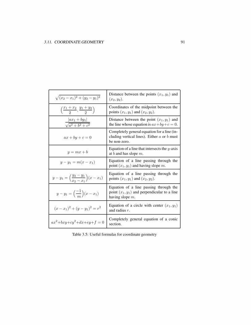
3.11. COORDINATE GEOMETRY 91
√(x2 − x1)2 + (y2 − y1)2
Distance between the points (x1, y1) and(x2, y2).
(x1 + x2
2,y1 + y2
2
) Coordinates of the midpoint between thepoints (x1, y1) and (x2, y2).
|ax1 + by1|√a2 + b2 + c2
Distance between the point (x1, y1) andthe line whose equation is ax+by+c = 0.
ax+ by + c = 0
Completely general equation for a line (in-cluding vertical lines). Either a or b mustbe non-zero.
y = mx+ bEquation of a line that intersects the y-axisat b and has slope m.
y − y1 = m(x− x1) Equation of a line passing through thepoint (x1, y1) and having slope m.
y − y1 =( y2 − y1
x2 − x1
)(x− x1)
Equation of a line passing through thepoints (x1, y1) and (x2, y2).
y − y1 =(−1
m
)(x − x1)
Equation of a line passing through thepoint (x1, y1) and perpendicular to a linehaving slope m.
(x− x1)2 + (y − y1)2 = r2 Equation of a circle with center (x1, y1)and radius r.
ax2+bxy+cy2+dx+ey+f = 0Completely general equation of a conicsection.
Table 3.5: Useful formulas for coordinate geometry
92 CHAPTER 3. MATHEMATICS REVIEW
The midpoints of the sides are easy to calculate—their coordinates are the averagesof the coordinates of the two endpoints of the segments, so they are as shown in thefigure: (b/2, 0), ((b+ c)/2, d/2), and (c/2, d/2).
The equations of the median lines originating at A, B, and C, respectively are:
y =d
b+ cx (3.34)
y =d
c− 2b(x − b) (3.35)
y =2d
2c− b(x − b/2) (3.36)
Solving equations 3.34 and 3.35 simultaneously:
d
b+ cx =
d
c− 2b(x− b)
1
b+ cx =
1
c− 2b(x− b)
(c− 2b)x = (b+ c)(x− b)(c− 2b− b− c)x = −b(b+ c)
−3bx = −b(b+ c)
x =b+ c
3
plug this result into equation 3.34:
y =( d
b+ c
)(b+ c
3
)=d
3.
If we solve another pair of equations, say equations 3.35 and 3.36, we find that weget exactly the same result, so the coordinates of the intersections of any pair of linesis the same, and we can give a single name M to that point. M = ((b+ c)/3, d/3).
Finally, to show that M is 2/3 of the distance between any vertex of the triangleand its opposite side, use the pythagorean theorem to write down the distances, andthen use algebra to show that the distances are equal. MA =
√((b+ c)/3)2 + (d/3)2
and the length of the median fromA is√
((b+ c)/2)2 + (d/2)2. We need to show thatMA is 2/3 the length of the median, or that
√((b+ c)/3)2 + (d/3)2 = (2/3)
√((b+ c)/2)2 + (d/2)2.
Square both sides and expand:
(b2 + 2bc+ c2 + d2)/9 = (4/9)(b2 + 2bc+ c2 + d2)/4,
which is clearly true.
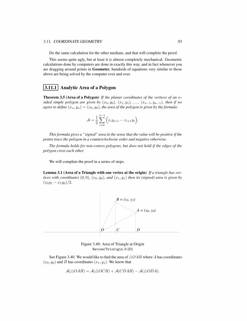
3.11. COORDINATE GEOMETRY 93
Do the same calculation for the other medians, and that will complete the proof.
This seems quite ugly, but at least it is almost completely mechanical. Geometriccalculations done by computers are done in exactly this way, and in fact whenever youare dragging around points in Geometer, hundreds of equations very similar to thoseabove are being solved by the computer over and over.
3.11.1 Analytic Area of a Polygon
Theorem 3.5 (Area of a Polygon) If the planar coordinates of the vertices of an n-sided simple polygon are given by (x0, y0), (x1, y1), . . . , (xn−1, yn−1), then if weagree to define (xn, yn) = (x0, y0), the area of the polygon is given by the formula:
A =1
2
n−1∑
i=0
(xiyi+1 − xi+1yi
).
This formula gives a “signed” area in the sense that the value will be positive if thepoints trace the polygon in a counterclockwise order and negative otherwise.
The formula holds for non-convex polygons, but does not hold if the edges of thepolygon cross each other.
We will complete the proof in a series of steps.
Lemma 3.1 (Area of a Triangle with one vertex at the origin) If a triangle has ver-tices with coordinates (0, 0), (x0, y0), and (x1, y1) then its (signed) area is given by(x0y1 − x1y0)/2.
OO
B = (x1, y1)B = (x1, y1)
A = (x0, y0)A = (x0, y0)
CC DD
Figure 3.40: Area of Triangle at OriginReview/Triorigin.D [D]
See Figure 3.40. We would like to find the area of4OAB whereA has coordinates(x0, y0) and B has coordinates (x1, y1). We know that
A(4OAB) = A(4OCB) +A(CDAB) −A(4ODA).
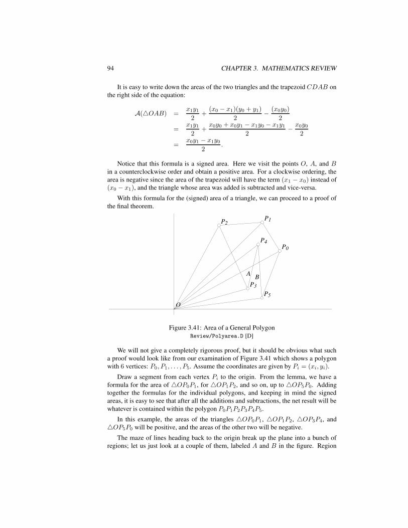
94 CHAPTER 3. MATHEMATICS REVIEW
It is easy to write down the areas of the two triangles and the trapezoid CDAB onthe right side of the equation:
A(4OAB) =x1y1
2+
(x0 − x1)(y0 + y1)
2− (x0y0)
2
=x1y1
2+x0y0 + x0y1 − x1y0 − x1y1
2− x0y0
2
=x0y1 − x1y0
2.
Notice that this formula is a signed area. Here we visit the points O, A, and Bin a counterclockwise order and obtain a positive area. For a clockwise ordering, thearea is negative since the area of the trapezoid will have the term (x1 − x0) instead of(x0 − x1), and the triangle whose area was added is subtracted and vice-versa.
With this formula for the (signed) area of a triangle, we can proceed to a proof ofthe final theorem.
OO
P1P1
P0P0
P2P2
P3P3
P4P4
P5P5
AA BB
Figure 3.41: Area of a General PolygonReview/Polyarea.D [D]
We will not give a completely rigorous proof, but it should be obvious what sucha proof would look like from our examination of Figure 3.41 which shows a polygonwith 6 vertices: P0, P1, . . . , P5. Assume the coordinates are given by Pi = (xi, yi).
Draw a segment from each vertex Pi to the origin. From the lemma, we have aformula for the area of 4OP0P1, for 4OP1P2, and so on, up to 4OP5P0. Addingtogether the formulas for the individual polygons, and keeping in mind the signedareas, it is easy to see that after all the additions and subtractions, the net result will bewhatever is contained within the polygon P0P1P2P3P4P5.
In this example, the areas of the triangles 4OP0P1, 4OP1P2, 4OP3P4, and4OP5P0 will be positive, and the areas of the other two will be negative.
The maze of lines heading back to the origin break up the plane into a bunch ofregions; let us just look at a couple of them, labeled A and B in the figure. Region
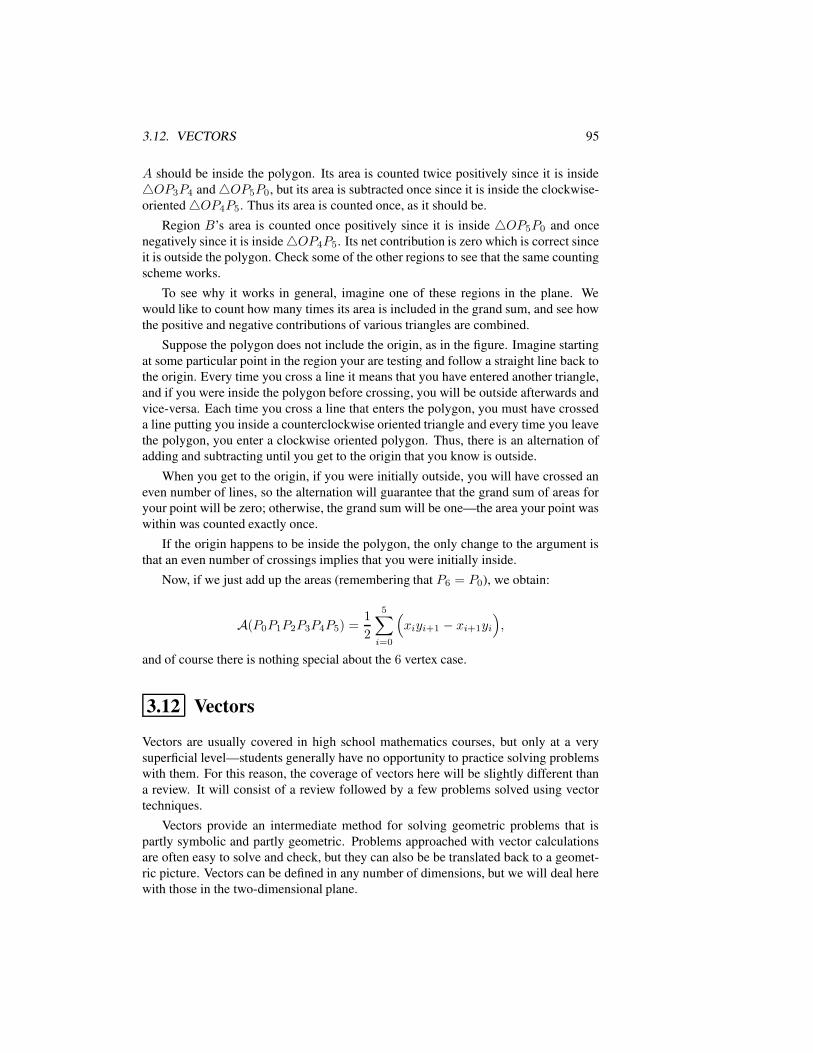
3.12. VECTORS 95
A should be inside the polygon. Its area is counted twice positively since it is inside4OP3P4 and4OP5P0, but its area is subtracted once since it is inside the clockwise-oriented4OP4P5. Thus its area is counted once, as it should be.
Region B’s area is counted once positively since it is inside 4OP5P0 and oncenegatively since it is inside4OP4P5. Its net contribution is zero which is correct sinceit is outside the polygon. Check some of the other regions to see that the same countingscheme works.
To see why it works in general, imagine one of these regions in the plane. Wewould like to count how many times its area is included in the grand sum, and see howthe positive and negative contributions of various triangles are combined.
Suppose the polygon does not include the origin, as in the figure. Imagine startingat some particular point in the region your are testing and follow a straight line back tothe origin. Every time you cross a line it means that you have entered another triangle,and if you were inside the polygon before crossing, you will be outside afterwards andvice-versa. Each time you cross a line that enters the polygon, you must have crosseda line putting you inside a counterclockwise oriented triangle and every time you leavethe polygon, you enter a clockwise oriented polygon. Thus, there is an alternation ofadding and subtracting until you get to the origin that you know is outside.
When you get to the origin, if you were initially outside, you will have crossed aneven number of lines, so the alternation will guarantee that the grand sum of areas foryour point will be zero; otherwise, the grand sum will be one—the area your point waswithin was counted exactly once.
If the origin happens to be inside the polygon, the only change to the argument isthat an even number of crossings implies that you were initially inside.
Now, if we just add up the areas (remembering that P6 = P0), we obtain:
A(P0P1P2P3P4P5) =1
2
5∑
i=0
(xiyi+1 − xi+1yi
),
and of course there is nothing special about the 6 vertex case.
3.12 Vectors
Vectors are usually covered in high school mathematics courses, but only at a verysuperficial level—students generally have no opportunity to practice solving problemswith them. For this reason, the coverage of vectors here will be slightly different thana review. It will consist of a review followed by a few problems solved using vectortechniques.
Vectors provide an intermediate method for solving geometric problems that ispartly symbolic and partly geometric. Problems approached with vector calculationsare often easy to solve and check, but they can also be be translated back to a geomet-ric picture. Vectors can be defined in any number of dimensions, but we will deal herewith those in the two-dimensional plane.
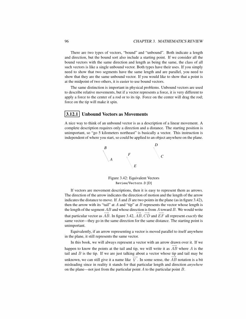
96 CHAPTER 3. MATHEMATICS REVIEW
There are two types of vectors, “bound” and “unbound”. Both indicate a lengthand direction, but the bound sort also include a starting point. If we consider all thebound vectors with the same direction and length as being the same, the class of allsuch vectors is like a single unbound vector. Both types have their uses. If you simplyneed to show that two segments have the same length and are parallel, you need toshow that they are the same unbound vector. If you would like to show that a point isat the midpoint of two others, it is easier to use bound vectors.
The same distinction is important in physical problems. Unbound vectors are usedto describe relative movements, but if a vector represents a force, it is very different toapply a force to the center of a rod or to its tip. Force on the center will drag the rod;force on the tip will make it spin.
3.12.1 Unbound Vectors as Movements
A nice way to think of an unbound vector is as a description of a linear movement. Acomplete description requires only a direction and a distance. The starting position isunimportant, so “go 5 kilometers northeast” is basically a vector. This instruction isindependent of where you start, so could be applied to an object anywhere on the plane.
AA
BB
CC
EE
DD
FF
Figure 3.42: Equivalent VectorsReview/Vectors.D [D]
If vectors are movement descriptions, then it is easy to represent them as arrows.The direction of the arrow indicates the direction of motion and the length of the arrowindicates the distance to move. IfA andB are two points in the plane (as in figure 3.42),then the arrow with its “tail” at A and “tip” at B represents the vector whose length isthe length of the segmentAB and whose direction is fromA towardB. We would write
that particular vector as−→AB. In figure 3.42,
−→AB,
−→CD and
−→EF all represent exactly the
same vector—they go in the same direction for the same distance. The starting point isunimportant.
Equivalently, if an arrow representing a vector is moved parallel to itself anywherein the plane, it still represents the same vector.
In this book, we will always represent a vector with an arrow drawn over it. If we
happen to know the points at the tail and tip, we will write it as−→AB where A is the
tail and B is the tip. If we are just talking about a vector whose tip and tail may be
unknown, we can still give it a name like−→V . In some sense, the
−→AB notation is a bit
misleading since in reality it stands for that particular length and direction anywhereon the plane—not just from the particular point A to the particular point B.
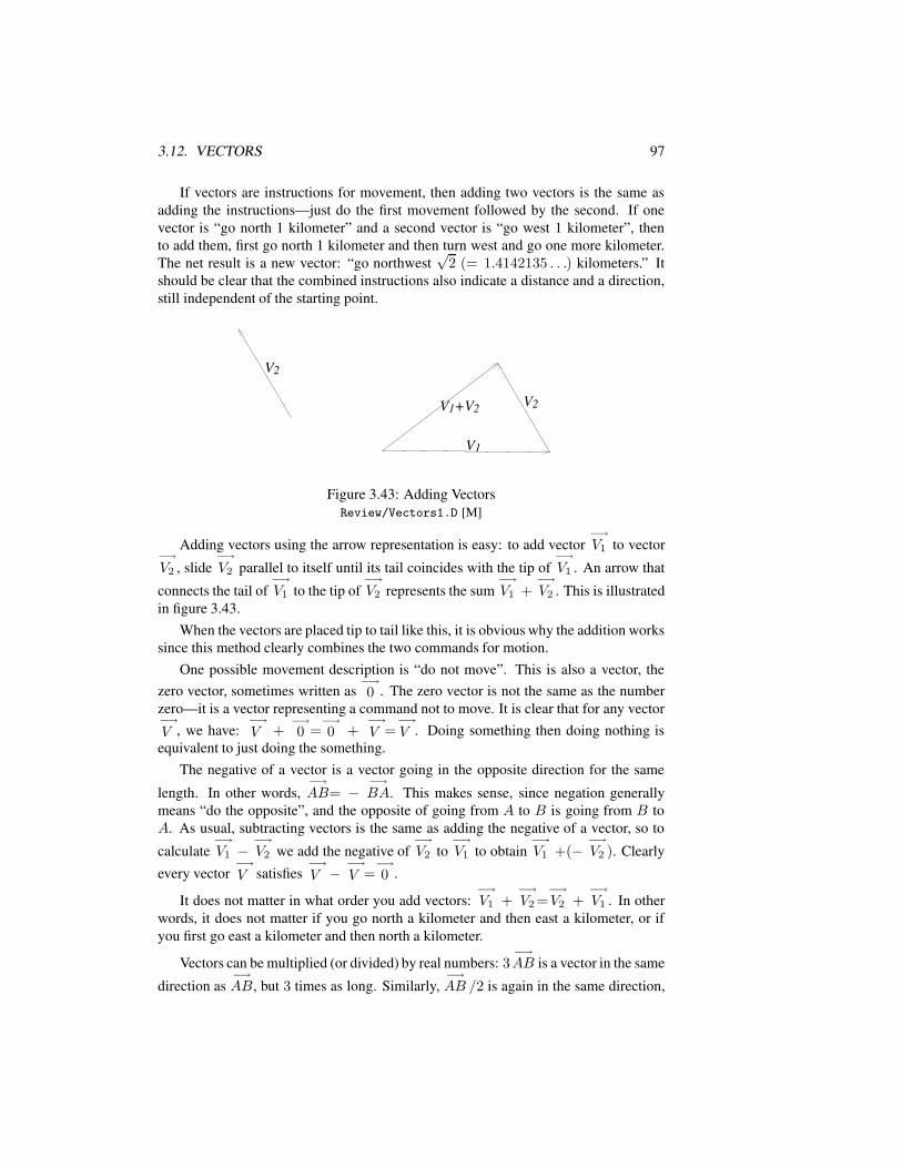
3.12. VECTORS 97
If vectors are instructions for movement, then adding two vectors is the same asadding the instructions—just do the first movement followed by the second. If onevector is “go north 1 kilometer” and a second vector is “go west 1 kilometer”, thento add them, first go north 1 kilometer and then turn west and go one more kilometer.The net result is a new vector: “go northwest
√2 (= 1.4142135 . . .) kilometers.” It
should be clear that the combined instructions also indicate a distance and a direction,still independent of the starting point.
V1V1
V2V2V1+V2V1+V2
V2V2
Figure 3.43: Adding VectorsReview/Vectors1.D [M]
Adding vectors using the arrow representation is easy: to add vector−→V1 to vector
−→V2 , slide
−→V2 parallel to itself until its tail coincides with the tip of
−→V1 . An arrow that
connects the tail of−→V1 to the tip of
−→V2 represents the sum
−→V1 +
−→V2 . This is illustrated
in figure 3.43.When the vectors are placed tip to tail like this, it is obvious why the addition works
since this method clearly combines the two commands for motion.One possible movement description is “do not move”. This is also a vector, the
zero vector, sometimes written as−→0 . The zero vector is not the same as the number
zero—it is a vector representing a command not to move. It is clear that for any vector−→V , we have:
−→V +
−→0 =
−→0 +
−→V =
−→V . Doing something then doing nothing is
equivalent to just doing the something.The negative of a vector is a vector going in the opposite direction for the same
length. In other words,−→AB= −
−→BA. This makes sense, since negation generally
means “do the opposite”, and the opposite of going from A to B is going from B toA. As usual, subtracting vectors is the same as adding the negative of a vector, so to
calculate−→V1 −
−→V2 we add the negative of
−→V2 to
−→V1 to obtain
−→V1 +(−
−→V2 ). Clearly
every vector−→V satisfies
−→V −
−→V =
−→0 .
It does not matter in what order you add vectors:−→V1 +
−→V2 =
−→V2 +
−→V1 . In other
words, it does not matter if you go north a kilometer and then east a kilometer, or ifyou first go east a kilometer and then north a kilometer.
Vectors can be multiplied (or divided) by real numbers: 3−→AB is a vector in the same
direction as−→AB, but 3 times as long. Similarly,
−→AB /2 is again in the same direction,
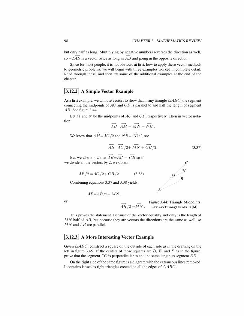
98 CHAPTER 3. MATHEMATICS REVIEW
but only half as long. Multiplying by negative numbers reverses the direction as well,
so −2−→AB is a vector twice as long as
−→AB and going in the opposite direction.
Since for most people, it is not obvious, at first, how to apply these vector methodsto geometric problems, we will begin with three examples worked in complete detail.Read through these, and then try some of the additional examples at the end of thechapter.
3.12.2 A Simple Vector Example
As a first example, we will use vectors to show that in any triangle4ABC, the segmentconnecting the midpoints of AC and CB is parallel to and half the length of segmentAB. See figure 3.44.
Let M and N be the midpoints of AC and CB, respectively. Then in vector nota-tion: −→
AB=−→AM +
−→MN +
−→NB .
We know that−→AM=
−→AC/2 and
−→NB=
−→CB/2, so:
−→AB=
−→AC/2+
−→MN +
−→CB/2. (3.37)
AA
BB
CC
MMNN
Figure 3.44: Triangle MidpointsReview/Trianglemids.D [M]
But we also know that−→AB=
−→AC +
−→CB so if
we divide all the vectors by 2, we obtain:
−→AB/2 =
−→AC /2+
−→CB/2. (3.38)
Combining equations 3.37 and 3.38 yields:
−→AB=
−→AB/2+
−→MN,
or −→AB/2 =
−→MN .
This proves the statement. Because of the vector equality, not only is the length ofMN half of AB, but because they are vectors the directions are the same as well, soMN and AB are parallel.
3.12.3 A More Interesting Vector Example
Given4ABC, construct a square on the outside of each side as in the drawing on theleft in figure 3.45. If the centers of those squares are D, E, and F as in the figure,prove that the segment FC is perpendicular to and the same length as segment ED.
On the right side of the same figure is a diagram with the extraneous lines removed.It contains isosceles right triangles erected on all the edges of4ABC.
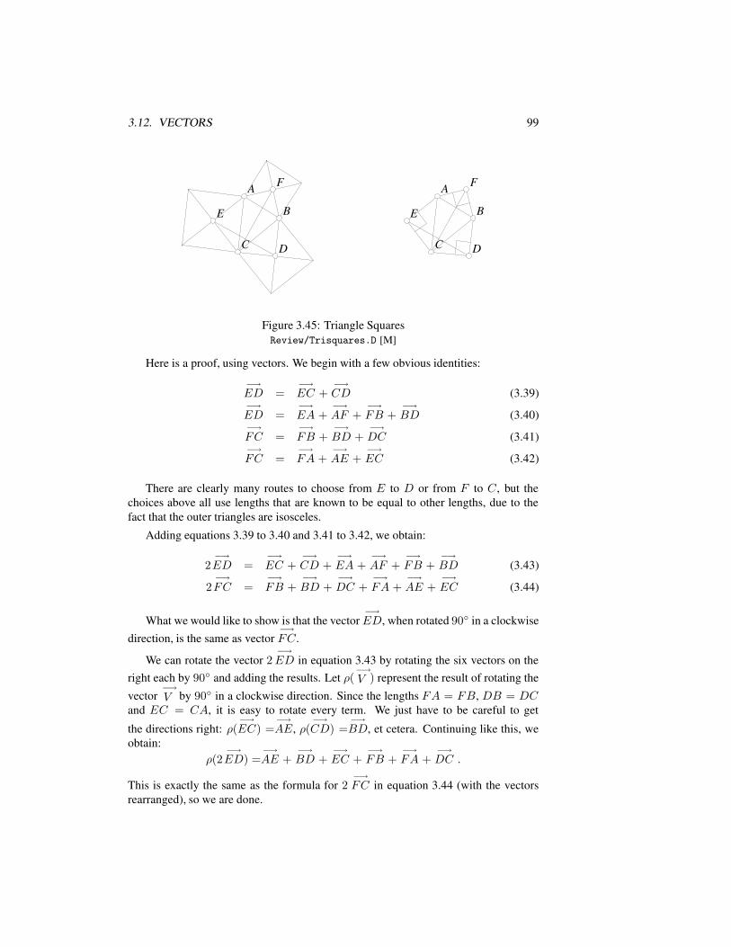
3.12. VECTORS 99
AA
BB
CC DD
EE
FF AA
BB
CC DD
EE
FF
Figure 3.45: Triangle SquaresReview/Trisquares.D [M]
Here is a proof, using vectors. We begin with a few obvious identities:
−→ED =
−→EC +
−→CD (3.39)
−→ED =
−→EA +
−→AF +
−→FB +
−→BD (3.40)
−→FC =
−→FB +
−→BD +
−→DC (3.41)
−→FC =
−→FA +
−→AE +
−→EC (3.42)
There are clearly many routes to choose from E to D or from F to C, but thechoices above all use lengths that are known to be equal to other lengths, due to thefact that the outer triangles are isosceles.
Adding equations 3.39 to 3.40 and 3.41 to 3.42, we obtain:
2−→ED =
−→EC +
−→CD +
−→EA +
−→AF +
−→FB +
−→BD (3.43)
2−→FC =
−→FB +
−→BD +
−→DC +
−→FA +
−→AE +
−→EC (3.44)
What we would like to show is that the vector−→ED, when rotated 90 in a clockwise
direction, is the same as vector−→FC.
We can rotate the vector 2−→ED in equation 3.43 by rotating the six vectors on the
right each by 90 and adding the results. Let ρ(−→V ) represent the result of rotating the
vector−→V by 90 in a clockwise direction. Since the lengths FA = FB, DB = DC
and EC = CA, it is easy to rotate every term. We just have to be careful to get
the directions right: ρ(−→EC) =
−→AE, ρ(
−→CD) =
−→BD, et cetera. Continuing like this, we
obtain:ρ(2
−→ED) =
−→AE +
−→BD +
−→EC +
−→FB +
−→FA +
−→DC .
This is exactly the same as the formula for 2−→FC in equation 3.44 (with the vectors
rearranged), so we are done.
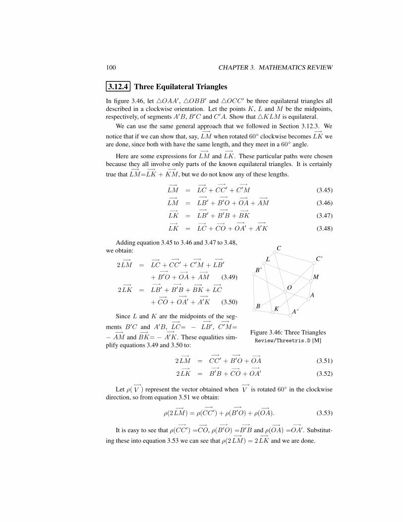
100 CHAPTER 3. MATHEMATICS REVIEW
3.12.4 Three Equilateral Triangles
In figure 3.46, let 4OAA′, 4OBB′ and 4OCC ′ be three equilateral triangles alldescribed in a clockwise orientation. Let the points K, L and M be the midpoints,respectively, of segments A′B, B′C and C ′A. Show that4KLM is equilateral.
We can use the same general approach that we followed in Section 3.12.3. We
notice that if we can show that, say,−→LM when rotated 60 clockwise becomes
−→LK we
are done, since both with have the same length, and they meet in a 60 angle.
Here are some expressions for−→LM and
−→LK. These particular paths were chosen
because they all involve only parts of the known equilateral triangles. It is certainly
true that−→LM=
−→LK +
−→KM , but we do not know any of these lengths.
−→LM =
−→LC +
−→CC ′ +
−→C ′M (3.45)
−→LM =
−→LB′ +
−→B′O +
−→OA +
−→AM (3.46)
−→LK =
−→LB′ +
−→B′B +
−→BK (3.47)
−→LK =
−→LC +
−→CO +
−→OA′ +
−→A′K (3.48)
OOAA
BB
CC
C’C’
A’A’
B’B’
KK
LL
MM
Figure 3.46: Three TrianglesReview/Threetris.D [M]
Adding equation 3.45 to 3.46 and 3.47 to 3.48,we obtain:
2−→LM =
−→LC +
−→CC ′ +
−→C ′M +
−→LB′
+−→B′O +
−→OA +
−→AM (3.49)
2−→LK =
−→LB′ +
−→B′B +
−→BK +
−→LC
+−→CO +
−→OA′ +
−→A′K (3.50)
Since L and K are the midpoints of the seg-
ments B′C and A′B,−→LC= −
−→LB′,
−→C ′M=
−−→AM and
−→BK= −
−→A′K. These equalities sim-
plify equations 3.49 and 3.50 to:
2−→LM =
−→CC ′ +
−→B′O +
−→OA (3.51)
2−→LK =
−→B′B +
−→CO +
−→OA′ (3.52)
Let ρ(−→V ) represent the vector obtained when
−→V is rotated 60 in the clockwise
direction, so from equation 3.51 we obtain:
ρ(2−→LM) = ρ(
−→CC ′) + ρ(
−→B′O) + ρ(
−→OA). (3.53)
It is easy to see that ρ(−→CC ′) =
−→CO, ρ(
−→B′O) =
−→B′B and ρ(
−→OA) =
−→OA′. Substitut-
ing these into equation 3.53 we can see that ρ(2−→LM) = 2
−→LK and we are done.
3.12. VECTORS 101
3.12.5 Bound Vectors and Coordinate Geometry
In this book we will consider all of our bound vectors to have their tail at the sameplace. If we want to use coordinate geometry, that same place will be the origin of ourcoordinate system: (0, 0).
If we wish to describe our bound vectors with coordinates and all of them havetheir tail at the origin, then each vector is completely determined by the coordinates ofthe tip. The point (x, y) thus stands for the bound vector whose tail is at the origin andwhose tip is at the point (x, y).
If the vectors−→V1 and
−→V2 are represented by the points (x1, y1) and (x2, y2), respec-
tively, the sum or difference:−→V1 ±
−→V2 is represented by the point (x1 ± x2, y1 ± y2).
Similarly, if α is a real number, then the vector α−→V1 is represented by (αx1, αy1).
In particular, −−→V1 is represented by (−x1,−y1). Finally, (0, 0) represents the zero
vector.
Following is a list of some properties of bound vectors. Some are important andwill be used later; some are not particularly important in the future, but shed somelight on how vectors work. Sometimes the arrow notation is used and sometimes thecoordinate notation, depending on which makes the property clearest.
• The average of two vectors (−→A +
−→B )/2 is a vector that goes from the origin
to a point exactly half way between the tips of the other two vectors. Thus if aparallelogram has a vertex at the origin and two others at
−→A and
−→B , then the
vector−→A +
−→B represents the fourth vertex, and (
−→A +
−→B )/2 is the the center
of the parallelogram.
• If α is a real number and−→A and
−→B are two vectors, then vectors of the form
(1−α)−→A +α
−→B represent all the vectors whose tips lie on the line connecting
the tips of−→A and
−→B . If 0 ≤ α ≤ 1 then the points lie between the tips of
−→A and
−→B ; otherwise, they lie outside. In fact, α represents the fraction of the
distance the tip of the new vector is between−→A and
−→B . If α = 1/3, then
(1 − α)−→A + α
−→B = (2/3)
−→A +(1/3)
−→B is (1/3) of the way from
−→A
to−→B 13. In the previous item, the average of the two vectors corresponds to
α = 1/2—half way between the two vectors.
• In 4ABC, if vectors−→A ,
−→B and
−→C represent the three vertices of the tri-
angle, then (−→A +
−→B +
−→C )/3 represents the centroid of the triangle. See
Section 3.12.6.
13Do not get confused by the fact that the numbers seem to be reversed. (2/3)−→A + (1/3)
−→B is 2/3
like−→A and 1/3 like
−→B . It is more like
−→A than
−→B , so it is closer to
−→A than to
−→B . If you get confused,
think of the extreme conditions where α = 0 or α = 1.
102 CHAPTER 3. MATHEMATICS REVIEW
• The length of the vector−→A = (x, y) is given by
√x2 + y2. (This is just the
pythagorean theorem applied to the triangle that includes the origin (0, 0), thepoint (x, 0), and the point (x, y). This right triangle has legs of lengths x andy, and the hypotenuse is the length of the vector.) An unbound vector describedwith tail (x1, y1) and head (x2, y2) has length
√(x2 − x1)2 + (y2 − y1)2.
• If (x, y) is a vector, then (−y, x) is another vector of the same length and perpen-dicular to (x, y). In fact, (−y, x) is the vector (x, y) rotated counterclockwiseby 90.
• If you rotate the vector (x, y) counterclockwise by an angle θ, the resulting vec-tor is (x cos θ − y sin θ, x sin θ + y cos θ). The previous item is a special case ofthis, where θ = 90.
• Vectors can be defined in any number of dimensions. In one dimension, theysimply represent directions to the left and to the right; a negative vector goes leftand a positive vector goes right. Only a single number is needed to representa one-dimensional vector. In three dimensions, three numbers are needed, andthese represent the motion in the x, y, and z directions, where the z-axis isperpendicular to both the x-axis and to the y-axis.
• If−→A′ is the same as
−→A rotated clockwise by an angle θ and
−→B′ is the same as
−→B rotated clockwise by the same angle θ, then
−→A′ +
−→B′ is the same as
−→A +
−→B
rotated clockwise by θ.
3.12.6 Example: Vector form of the Centroid
Suppose we have a triangle4ABC, where−→A ,−→B and
−→C are vectors from our origin
to the vertices of the triangle. What are the coordinates of the centroid? Notice thatin the proof that follows, we never need to make use of the actual coordinates of thevectors. In fact, although we think of our vectors here as being two-dimensional, thisproof works in any number of dimensions.
The centroid is at the intersection of any two medians, so let us use the mediansoriginating at
−→C and
−→A .
The median from−→C connects it with the midpoint of the vector (
−→A +
−→B )/2. We
know that all vectors along that line are described by:
α−→C +(1− α)
(−→A +
−→B
2
), (3.54)
for some value of α. Similarly, the values of the vectors along the other median aregiven by:
β−→A +(1− β)
(−→B +
−→C
2
), (3.55)
3.13. COMPLEX NUMBERS 103
for some value of β.The intersection will occur when those two vectors are equal, or when:
α−→C +(1− α)
(−→A +
−→B
2
)= β
−→A +(1− β)
(−→B +
−→C
2
).
If we multiply everything out and move all the terms to the left side, and gather liketerms, we obtain:
−→A
(1− α− 2β
2
)+−→B
(β − α
2
)+−→C
(1− β − 2α
2
)=−→0 .
For this to be identically zero, we need all three coefficients to be zero, and if yousolve the equations (at first is looks like there are three equations and two unknowns,but the equations are not independent), we find that the only solution is α = 1/3 andβ = 1/3. Putting these values back into either equation 3.54 or 3.55, we find that thevector describing the centroid is (
−→A +
−→B +
−→C )/3.
3.13 Complex Numbers
This section provides only a tiny introduction to the huge topic of complex numbers.You can learn much more in virtually any book on complex analysis, but Needham’sbook (see [Needham, 1997]) is a particularly geometrically oriented book as you cantell from its title, “Visual Complex Analysis”.
The reason complex numbers are so useful for geometers is that they provide yetanother method to describe the locations of points on a plane.
A complex number has the form a + bi, where i is the imaginary√−1 (in other
words i2 = −1), and a and b are arbitrary real numbers. Complex numbers are a lotlike two-dimensional vectors but instead of having an x- and a y-coordinate, you canthink of them having a real coordinate and an imaginary coordinate.
Thus they are commonly plotted on a plane with a real and an imaginary axis,where the real axis is drawn in place of the x-axis and the imaginary axis in place ofthe y-axis. The origin represents the point 0 + 0i, and the point a+ bi would be plotteda units to the right and b units above the origin (with the obvious reversals if a and/or bis negative). We usually use letters like z or w (or the Greek letter ζ “zeta”) to indicatearbitrary complex variables that include both a real and an imaginary part.
All the usual operations exist for complex numbers—addition, subtraction, multi-plication, division (except by zero). Here are formulas for the basic operations:
(a+ bi)± (c+ di) = (a± c) + (b± d)i
(a+ bi)(c+ di) = (ac− bd) + (ad+ bc)i
(a+ bi)
(c+ di)=
(ac+ bd
c2 + d2
)+(bc− adc2 + d2
)i
104 CHAPTER 3. MATHEMATICS REVIEW
To derive the equation for division of complex numbers above, simply multiply numer-ator and denominator of the expression on the left by c− di.
In addition to these, many of our favorite functions also make sense, such as: sin z,cos z, ez,
√z, log z, et cetera—although some care must be taken to define these prop-
erly, especially functions like√z and log z which are “multiple-valued” functions.
Except for the function ez (see Section 3.13.1) we will not need any of these here.If we think of points on the Euclidean plane as single complex numbers, many
important geometric operations have simple representations in terms of mathematicaloperations on the complex numbers.
For example, if we simply add the number c + di to every point on the complexplane, this has the effect of a translation of c units to the right and d units up (where cand d are positive—negative values, of course, translate left and/or down). If we multi-ply our numbers by cos θ+ i sin θ this has the effect of rotating them counterclockwiseabout the origin by an angle θ. There are many similar operations.
Similarly, the midpoint of z and z′ is given by (z + z′)/2. If z1, z2, and z3 are thevertices of a triangle, the centroid is given by (z1 + z2 + z3)/3. Multiplication by apure positive real number scales the points toward or away from the origin uniformly.For example, multiplication by 2 makes everything twice as big, and multiplicationby 1/3 makes everything one third as big. Multiplication by −1 reflects everythingthrough the origin (or equivalently, rotates it by 180), and multiplication by i rotatescounterclockwise by 90.
If z = a + bi is an arbitrary complex number, then we say that z = a − bi is thecomplex conjugate of z. Geometrically, it amounts to the reflection of z across the realline (the line containing all the complex numbers whose imaginary parts are zero.) Thecomplex conjugate has the following properties that are not hard to show:
(z ± w) = z ± wzw = zw
z/w = z/w.
The complex conjugate allows us to express the distance between a point and theorigin (0 + 0i), and this distance is written |z|, is defined by:
|z| =√zz,
and is called the absolute value of z.The formula above works because for any complex z, zz is always real and non-
negative. To see this, let z = a+ bi where a and b are real numbers. Then
zz = (a+ bi)(a− bi) = a2 + b2,
which is certainly always non-negative. In fact, if you think of a and b as coordinateson the complex plane, then we have
|z| = |a+ bi| =√a2 + b2,
which is exactly the same distance that the pythagorean theorem would give us for thedistance from a point z to the origin.
The distance between two complex numbers z and w is given by |z − w|.
3.13. COMPLEX NUMBERS 105
3.13.1 Euler’s Formula
If you are not afraid to work with complex numbers, there are some formulas whichcan simplify many of the trigonometric calculations substantially.
If θ is any real number, then Euler’s formula states that:
eiθ = cos θ + i sin θ.
We saw the expression cos θ + i sin θ in the previous section—multiplication by thisnumber is equivalent to a rotation by an angle θ.
If that is true, then we also have:
e−iθ = cos(−θ) + i sin(−θ) = cos θ − i sin θ.
The two equations above can be added or subtracted and manipulated in variousother ways to yield:
cos θ =eiθ + e−iθ
2sin θ =
eiθ − e−iθ
2itan θ =
eiθ − e−iθ
i(eiθ + e−iθ)
We will not spend much time on it, but here is an example of how Euler’s for-mula can be used to show one of the trigonometric equalities above. Let us deriveequation 3.6—the formula for cos(α+ β):
cos(α+ β) =ei(α+β) + e−i(α+β)
2
=eiαeiβ + e−iαe−iβ
2
=(cosα+ i sinα)(cosβ + i sinβ) + (cosα− i sinα)(cosβ − i sinβ)
2
=(cosα cosβ − sinα sinβ) + i(cosα sinβ + sinα cosβ)
2
+(cosα cosβ − sinα sinβ)− i(cosα sinβ + sinα cosβ)
2= cosα cosβ − sinα sinβ.
But if you are a little more lazy, you can get the formulas for both sin(α + β) andcos(α+ β) with less work:
ei(α+β) = eiαeiβ = cos(α+ β) + i sin(α+ β)
= (cosα+ i sinα)(cosβ + i sinβ)
= (cosα cosβ − sinα sinβ) + i(cosα sinβ + sinα cosβ).
Setting the real part of the right side of the first line equal to the real part of the finalline and similarly for the imaginary parts, we get both formulas:
cos(α+ β) = cosα cosβ − sinα sinβ
sin(α+ β) = cosα sinβ + sinα cosβ.

106 CHAPTER 3. MATHEMATICS REVIEW
Chapter 4Geometric Construction
To use Geometer or any computer geometry program to investigate new problems youwill need to be able to draw diagrams that correspond to those problems. In principle,a vast collection of drawings can be made with only two tools—a straightedge and acompass—but to draw complex diagrams quickly, the ability to use a larger set of toolsis extremely valuable.
The classical Greek construction problems that allow only the straightedge andcompass as tools are certainly interesting in their own right, and there is a large litera-ture associated with them. In this chapter when we wish to refer to that sort of problem,we will call it a classical construction problem.
We will examine the classical construction problems later in Section 4.11, but ifyou are planning to use a computer geometry program, you are going to be forced toface your own construction problems right away.
If you would like to illustrate a theorem with a computer drawing that can be manip-ulated, you need to draw it so that it has the same degrees of freedom that the theorem
107
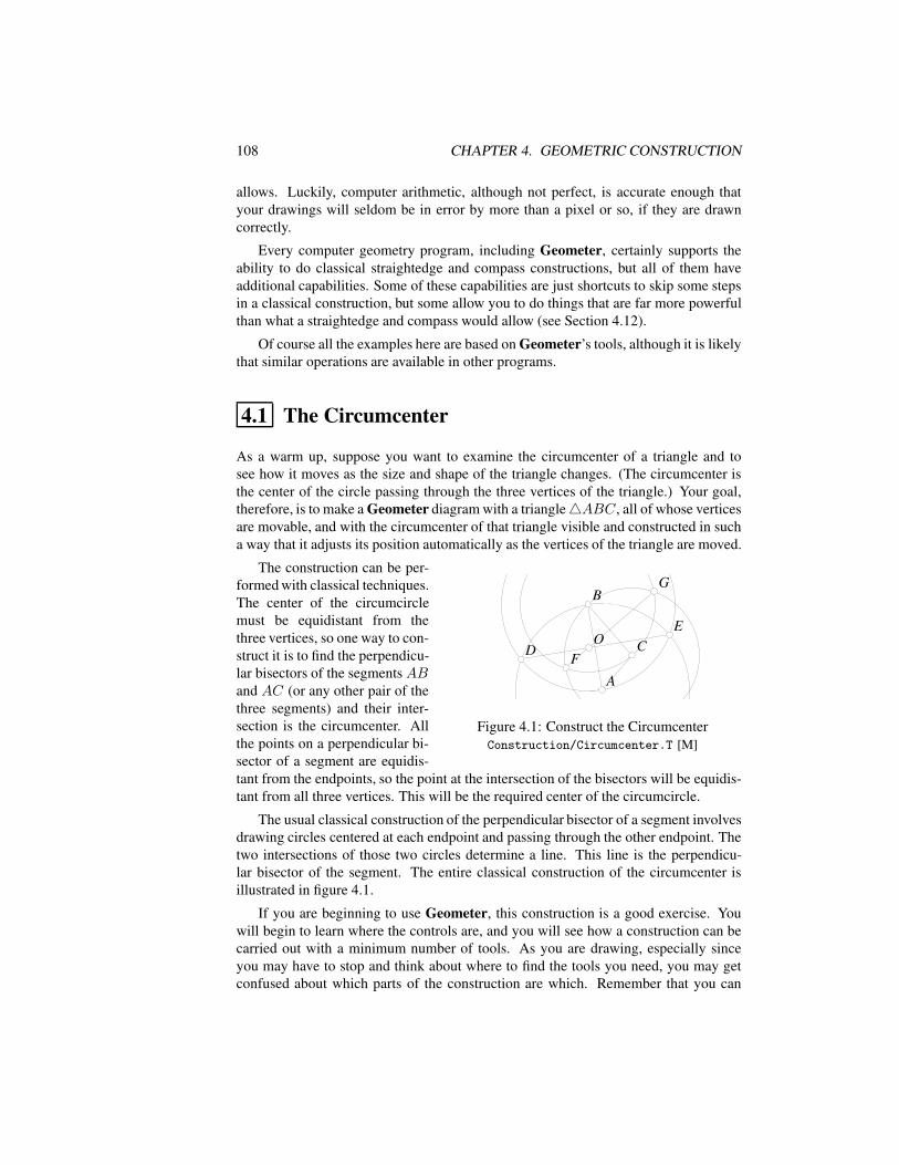
108 CHAPTER 4. GEOMETRIC CONSTRUCTION
allows. Luckily, computer arithmetic, although not perfect, is accurate enough thatyour drawings will seldom be in error by more than a pixel or so, if they are drawncorrectly.
Every computer geometry program, including Geometer, certainly supports theability to do classical straightedge and compass constructions, but all of them haveadditional capabilities. Some of these capabilities are just shortcuts to skip some stepsin a classical construction, but some allow you to do things that are far more powerfulthan what a straightedge and compass would allow (see Section 4.12).
Of course all the examples here are based on Geometer’s tools, although it is likelythat similar operations are available in other programs.
4.1 The Circumcenter
As a warm up, suppose you want to examine the circumcenter of a triangle and tosee how it moves as the size and shape of the triangle changes. (The circumcenter isthe center of the circle passing through the three vertices of the triangle.) Your goal,therefore, is to make a Geometer diagram with a triangle4ABC, all of whose verticesare movable, and with the circumcenter of that triangle visible and constructed in sucha way that it adjusts its position automatically as the vertices of the triangle are moved.
AA
BB
CCDD
EE
FF
GG
OO
Figure 4.1: Construct the CircumcenterConstruction/Circumcenter.T [M]
The construction can be per-formed with classical techniques.The center of the circumcirclemust be equidistant from thethree vertices, so one way to con-struct it is to find the perpendicu-lar bisectors of the segments ABand AC (or any other pair of thethree segments) and their inter-section is the circumcenter. Allthe points on a perpendicular bi-sector of a segment are equidis-tant from the endpoints, so the point at the intersection of the bisectors will be equidis-tant from all three vertices. This will be the required center of the circumcircle.
The usual classical construction of the perpendicular bisector of a segment involvesdrawing circles centered at each endpoint and passing through the other endpoint. Thetwo intersections of those two circles determine a line. This line is the perpendicu-lar bisector of the segment. The entire classical construction of the circumcenter isillustrated in figure 4.1.
If you are beginning to use Geometer, this construction is a good exercise. Youwill begin to learn where the controls are, and you will see how a construction can becarried out with a minimum number of tools. As you are drawing, especially sinceyou may have to stop and think about where to find the tools you need, you may getconfused about which parts of the construction are which. Remember that you can
4.2. AVAILABLE TOOLS 109
change the colors of lines, points and circles, and you can use that sort of marking tohelp remind you where you are in the construction. For example, color the lines ofthe original triangle differently, and use red construction lines to get the perpendicularbisector of the red side and green ones when you are working on the green side.
The classical approach requires eleven steps after the triangle is available. Fourcircles are drawn, four intersections of the circles are determined, two lines are drawnthrough these intersection points, and finally the intersection of those lines is the re-quired circumcenter.
This is a perfectly good construction, but as you can see, there are a lot of auxiliarylines, and altogether it required eleven steps to find the circumcenter.
Geometer has shortcuts. For example, there is a built-in command to construct theperpendicular bisector, after which only their intersection would need to be found for atotal of three steps. But there is an even faster way: Geometer has a command (calledPPP=>C in the command area under the Circles label) to construct a circle passingthrough three points (this would be the circumcircle) and another to find a point atthe center of a circle, so the lazy Geometer user can construct the circumcenter of atriangle in two steps. The command to find the point at the center of a circle is in thePrimitives pulldown menu under the Point submenu and is called C=>P Ctr.
4.2 Available Tools
Even if you do not know how to use all of them, it is good to have at least a vagueidea of what tools are available in your computer geometry program. Then if you arehaving trouble with a construction, you may decide that it would be a good idea to learnexactly how a couple of likely commands might be used.
In Geometer, the more common construction tools are listed in the menu to theright of the drawing area, organized by the type of primitive they create—at the top,the point and line creation commands, and so on. This list is not complete, however.In the Primitives pull-down menu are a lot of others, all of which are available via thegraphical user interface.
If you are willing to write Geometer textual descriptions directly, there are stillmore commands available, but most people will not need to use these. The textualdescriptions include quite powerful calculation tools that will allow you to draw almostanything.
4.3 The Structure of a Geometer Diagram
Think of a Geometer diagram as a list of commands, each of which is executed exactlyonce beginning with the first and continuing to the end of the list. There is no looping
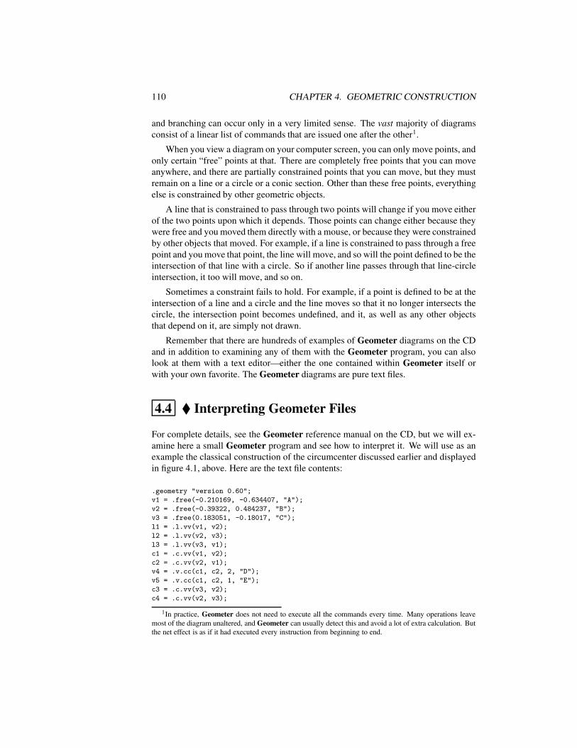
110 CHAPTER 4. GEOMETRIC CONSTRUCTION
and branching can occur only in a very limited sense. The vast majority of diagramsconsist of a linear list of commands that are issued one after the other1.
When you view a diagram on your computer screen, you can only move points, andonly certain “free” points at that. There are completely free points that you can moveanywhere, and there are partially constrained points that you can move, but they mustremain on a line or a circle or a conic section. Other than these free points, everythingelse is constrained by other geometric objects.
A line that is constrained to pass through two points will change if you move eitherof the two points upon which it depends. Those points can change either because theywere free and you moved them directly with a mouse, or because they were constrainedby other objects that moved. For example, if a line is constrained to pass through a freepoint and you move that point, the line will move, and so will the point defined to be theintersection of that line with a circle. So if another line passes through that line-circleintersection, it too will move, and so on.
Sometimes a constraint fails to hold. For example, if a point is defined to be at theintersection of a line and a circle and the line moves so that it no longer intersects thecircle, the intersection point becomes undefined, and it, as well as any other objectsthat depend on it, are simply not drawn.
Remember that there are hundreds of examples of Geometer diagrams on the CDand in addition to examining any of them with the Geometer program, you can alsolook at them with a text editor—either the one contained within Geometer itself orwith your own favorite. The Geometer diagrams are pure text files.
4.4 Interpreting Geometer Files
For complete details, see the Geometer reference manual on the CD, but we will ex-amine here a small Geometer program and see how to interpret it. We will use as anexample the classical construction of the circumcenter discussed earlier and displayedin figure 4.1, above. Here are the text file contents:
.geometry "version 0.60";
v1 = .free(-0.210169, -0.634407, "A");
v2 = .free(-0.39322, 0.484237, "B");
v3 = .free(0.183051, -0.18017, "C");
l1 = .l.vv(v1, v2);
l2 = .l.vv(v2, v3);
l3 = .l.vv(v3, v1);
c1 = .c.vv(v1, v2);
c2 = .c.vv(v2, v1);
v4 = .v.cc(c1, c2, 2, "D");
v5 = .v.cc(c1, c2, 1, "E");
c3 = .c.vv(v3, v2);
c4 = .c.vv(v2, v3);
1In practice, Geometer does not need to execute all the commands every time. Many operations leavemost of the diagram unaltered, and Geometer can usually detect this and avoid a lot of extra calculation. Butthe net effect is as if it had executed every instruction from beginning to end.
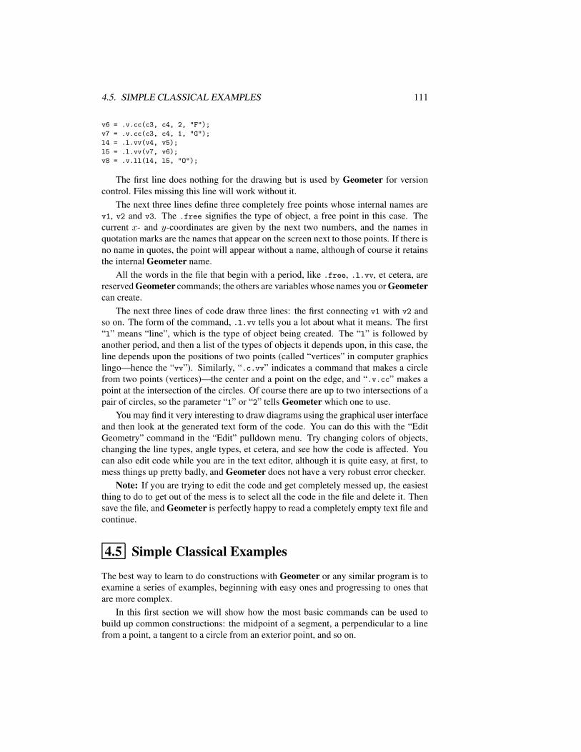
4.5. SIMPLE CLASSICAL EXAMPLES 111
v6 = .v.cc(c3, c4, 2, "F");
v7 = .v.cc(c3, c4, 1, "G");
l4 = .l.vv(v4, v5);
l5 = .l.vv(v7, v6);
v8 = .v.ll(l4, l5, "O");
The first line does nothing for the drawing but is used by Geometer for versioncontrol. Files missing this line will work without it.
The next three lines define three completely free points whose internal names arev1, v2 and v3. The .free signifies the type of object, a free point in this case. Thecurrent x- and y-coordinates are given by the next two numbers, and the names inquotation marks are the names that appear on the screen next to those points. If there isno name in quotes, the point will appear without a name, although of course it retainsthe internal Geometer name.
All the words in the file that begin with a period, like .free, .l.vv, et cetera, arereserved Geometer commands; the others are variables whose names you or Geometercan create.
The next three lines of code draw three lines: the first connecting v1 with v2 andso on. The form of the command, .l.vv tells you a lot about what it means. The first“l” means “line”, which is the type of object being created. The “l” is followed byanother period, and then a list of the types of objects it depends upon, in this case, theline depends upon the positions of two points (called “vertices” in computer graphicslingo—hence the “vv”). Similarly, “.c.vv” indicates a command that makes a circlefrom two points (vertices)—the center and a point on the edge, and “.v.cc” makes apoint at the intersection of the circles. Of course there are up to two intersections of apair of circles, so the parameter “1” or “2” tells Geometer which one to use.
You may find it very interesting to draw diagrams using the graphical user interfaceand then look at the generated text form of the code. You can do this with the “EditGeometry” command in the “Edit” pulldown menu. Try changing colors of objects,changing the line types, angle types, et cetera, and see how the code is affected. Youcan also edit code while you are in the text editor, although it is quite easy, at first, tomess things up pretty badly, and Geometer does not have a very robust error checker.
Note: If you are trying to edit the code and get completely messed up, the easiestthing to do to get out of the mess is to select all the code in the file and delete it. Thensave the file, and Geometer is perfectly happy to read a completely empty text file andcontinue.
4.5 Simple Classical Examples
The best way to learn to do constructions with Geometer or any similar program is toexamine a series of examples, beginning with easy ones and progressing to ones thatare more complex.
In this first section we will show how the most basic commands can be used tobuild up common constructions: the midpoint of a segment, a perpendicular to a linefrom a point, a tangent to a circle from an exterior point, and so on.
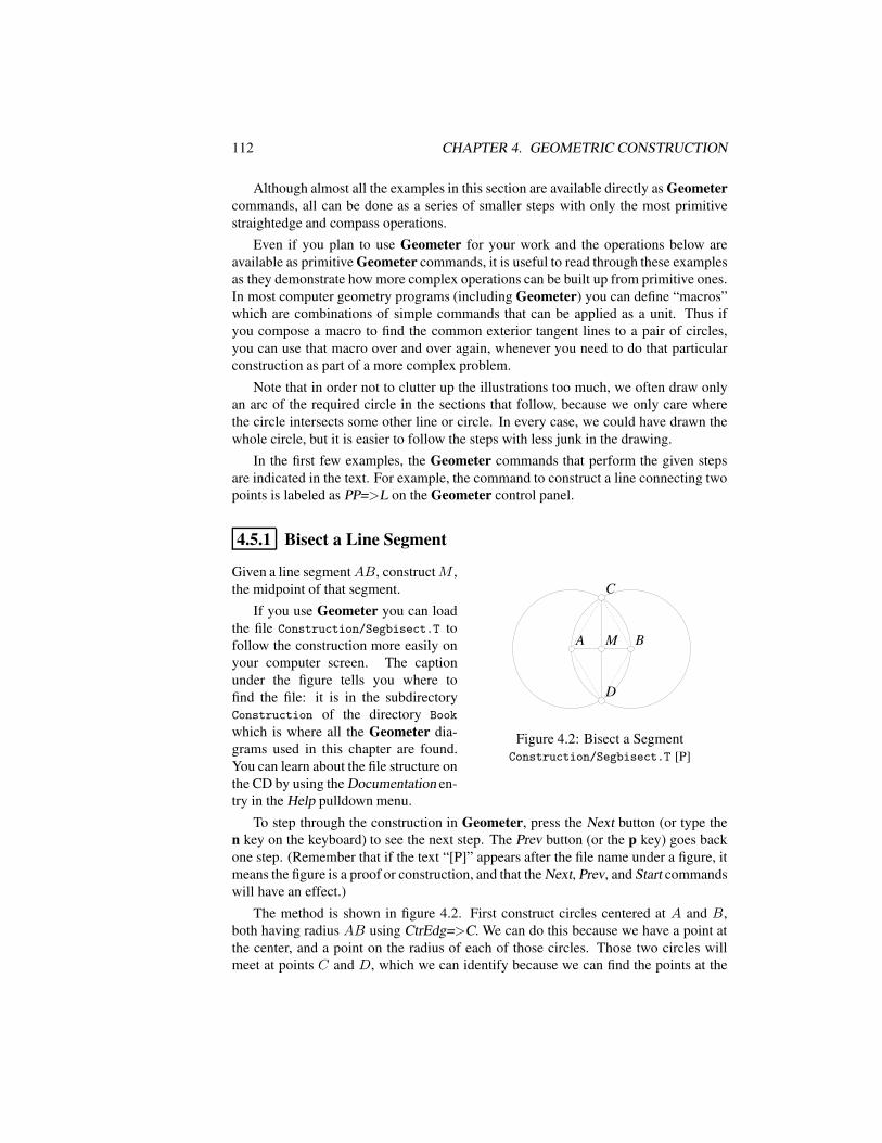
112 CHAPTER 4. GEOMETRIC CONSTRUCTION
Although almost all the examples in this section are available directly as Geometercommands, all can be done as a series of smaller steps with only the most primitivestraightedge and compass operations.
Even if you plan to use Geometer for your work and the operations below areavailable as primitive Geometer commands, it is useful to read through these examplesas they demonstrate how more complex operations can be built up from primitive ones.In most computer geometry programs (including Geometer) you can define “macros”which are combinations of simple commands that can be applied as a unit. Thus ifyou compose a macro to find the common exterior tangent lines to a pair of circles,you can use that macro over and over again, whenever you need to do that particularconstruction as part of a more complex problem.
Note that in order not to clutter up the illustrations too much, we often draw onlyan arc of the required circle in the sections that follow, because we only care wherethe circle intersects some other line or circle. In every case, we could have drawn thewhole circle, but it is easier to follow the steps with less junk in the drawing.
In the first few examples, the Geometer commands that perform the given stepsare indicated in the text. For example, the command to construct a line connecting twopoints is labeled as PP=>L on the Geometer control panel.
4.5.1 Bisect a Line Segment
AA BB
CC
DD
MM
Figure 4.2: Bisect a SegmentConstruction/Segbisect.T [P]
Given a line segmentAB, constructM ,the midpoint of that segment.
If you use Geometer you can loadthe file Construction/Segbisect.T tofollow the construction more easily onyour computer screen. The captionunder the figure tells you where tofind the file: it is in the subdirectoryConstruction of the directory Book
which is where all the Geometer dia-grams used in this chapter are found.You can learn about the file structure onthe CD by using the Documentation en-try in the Help pulldown menu.
To step through the construction in Geometer, press the Next button (or type then key on the keyboard) to see the next step. The Prev button (or the p key) goes backone step. (Remember that if the text “[P]” appears after the file name under a figure, itmeans the figure is a proof or construction, and that the Next, Prev, and Start commandswill have an effect.)
The method is shown in figure 4.2. First construct circles centered at A and B,both having radius AB using CtrEdg=>C. We can do this because we have a point atthe center, and a point on the radius of each of those circles. Those two circles willmeet at points C and D, which we can identify because we can find the points at the
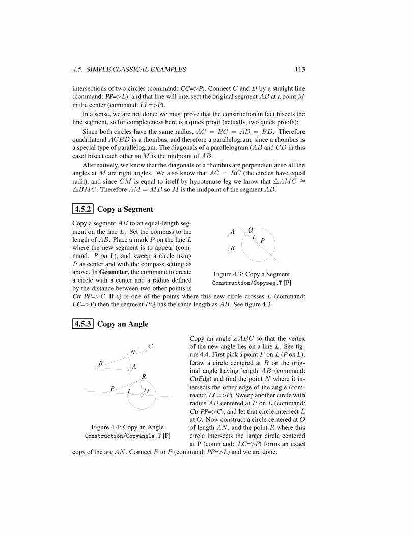
4.5. SIMPLE CLASSICAL EXAMPLES 113
intersections of two circles (command: CC=>P). Connect C and D by a straight line(command: PP=>L), and that line will intersect the original segmentAB at a pointMin the center (command: LL=>P).
In a sense, we are not done; we must prove that the construction in fact bisects theline segment, so for completeness here is a quick proof (actually, two quick proofs):
Since both circles have the same radius, AC = BC = AD = BD. Thereforequadrilateral ACBD is a rhombus, and therefore a parallelogram, since a rhombus isa special type of parallelogram. The diagonals of a parallelogram (AB and CD in thiscase) bisect each other so M is the midpoint of AB.
Alternatively, we know that the diagonals of a rhombus are perpendicular so all theangles at M are right angles. We also know that AC = BC (the circles have equalradii), and since CM is equal to itself by hypotenuse-leg we know that 4AMC ∼=4BMC. ThereforeAM = MB so M is the midpoint of the segment AB.
4.5.2 Copy a Segment
LLAA
BBPP
Figure 4.3: Copy a SegmentConstruction/Copyseg.T [P]
Copy a segment AB to an equal-length seg-ment on the line L. Set the compass to thelength of AB. Place a mark P on the line Lwhere the new segment is to appear (com-mand: P on L), and sweep a circle usingP as center and with the compass setting asabove. In Geometer, the command to createa circle with a center and a radius definedby the distance between two other points isCtr PP=>C. If Q is one of the points where this new circle crosses L (command:LC=>P) then the segment PQ has the same length as AB. See figure 4.3
4.5.3 Copy an Angle
LL
AABB
CC
PP
NN
OO
RR
Figure 4.4: Copy an AngleConstruction/Copyangle.T [P]
Copy an angle ∠ABC so that the vertexof the new angle lies on a line L. See fig-ure 4.4. First pick a point P on L (P on L).Draw a circle centered at B on the orig-inal angle having length AB (command:CtrEdg) and find the point N where it in-tersects the other edge of the angle (com-mand: LC=>P). Sweep another circle withradius AB centered at P on L (command:Ctr PP=>C), and let that circle intersect Lat O. Now construct a circle centered at Oof length AN , and the point R where thiscircle intersects the larger circle centeredat P (command: LC=>P) forms an exact
copy of the arc AN . Connect R to P (command: PP=>L) and we are done.
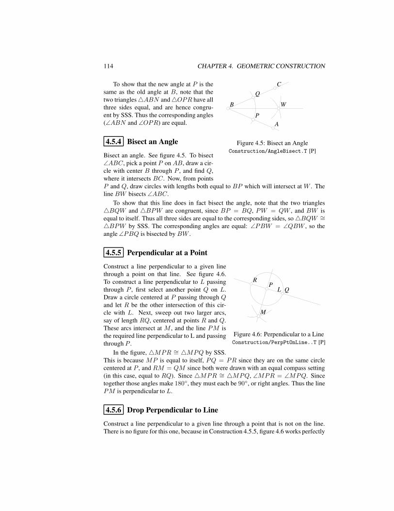
114 CHAPTER 4. GEOMETRIC CONSTRUCTION
AA
BB
CC
PP
WW
Figure 4.5: Bisect an AngleConstruction/AngleBisect.T [P]
To show that the new angle at P is thesame as the old angle at B, note that thetwo triangles4ABN and4OPR have allthree sides equal, and are hence congru-ent by SSS. Thus the corresponding angles(∠ABN and ∠OPR) are equal.
4.5.4 Bisect an Angle
Bisect an angle. See figure 4.5. To bisect∠ABC, pick a point P on AB, draw a cir-cle with center B through P , and find Q,where it intersects BC. Now, from pointsP and Q, draw circles with lengths both equal to BP which will intersect at W . Theline BW bisects ∠ABC.
To show that this line does in fact bisect the angle, note that the two triangles4BQW and 4BPW are congruent, since BP = BQ, PW = QW , and BW isequal to itself. Thus all three sides are equal to the corresponding sides, so4BQW ∼=4BPW by SSS. The corresponding angles are equal: ∠PBW = ∠QBW , so theangle ∠PBQ is bisected by BW .
4.5.5 Perpendicular at a Point
LLPP
QQRR
MM
Figure 4.6: Perpendicular to a LineConstruction/PerpPtOnLine..T [P]
Construct a line perpendicular to a given linethrough a point on that line. See figure 4.6.To construct a line perpendicular to L passingthrough P , first select another point Q on L.Draw a circle centered at P passing through Qand let R be the other intersection of this cir-cle with L. Next, sweep out two larger arcs,say of length RQ, centered at points R and Q.These arcs intersect at M , and the line PM isthe required line perpendicular to L and passingthrough P .
In the figure, 4MPR ∼= 4MPQ by SSS.This is because MP is equal to itself, PQ = PR since they are on the same circlecentered at P , and RM = QM since both were drawn with an equal compass setting(in this case, equal to RQ). Since 4MPR ∼= 4MPQ, ∠MPR = ∠MPQ. Sincetogether those angles make 180, they must each be 90, or right angles. Thus the linePM is perpendicular to L.
4.5.6 Drop Perpendicular to Line
Construct a line perpendicular to a given line through a point that is not on the line.There is no figure for this one, because in Construction 4.5.5, figure 4.6 works perfectly
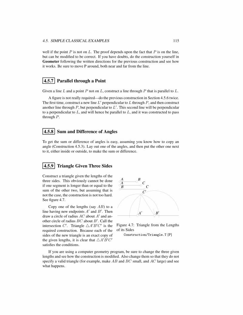
4.5. SIMPLE CLASSICAL EXAMPLES 115
well if the point P is not on L. The proof depends upon the fact that P is on the line,but can be modified to be correct. If you have doubts, do the construction yourself inGeometer following the written directions for the previous construction and see howit works. Be sure to move P around, both near and far from the line.
4.5.7 Parallel through a Point
Given a line L and a point P not on L, construct a line through P that is parallel to L.
A figure is not really required—do the previous construction in Section 4.5.6 twice.The first time, construct a new lineL′ perpendicular toL throughP , and then constructanother line through P , but perpendicular to L′. This second line will be perpendicularto a perpendicular to L, and will hence be parallel to L, and it was constructed to passthrough P .
4.5.8 Sum and Difference of Angles
To get the sum or difference of angles is easy, assuming you know how to copy anangle (Construction 4.5.3). Lay out one of the angles, and then put the other one nextto it, either inside or outside, to make the sum or difference.
4.5.9 Triangle Given Three Sides
AA BBAA CCBB CC
A′A′ B′B′
C′C′
Figure 4.7: Triangle from the Lengthsof its Sides
Construction/Triangle.T [P]
Construct a triangle given the lengths of thethree sides. This obviously cannot be doneif one segment is longer than or equal to thesum of the other two, but assuming that isnot the case, the construction is not too hard.See figure 4.7.
Copy one of the lengths (say AB) to aline having new endpoints A′ and B′. Thendraw a circle of radius AC about A′ and an-other circle of radius BC about B′. Call theintersection C ′. Triangle 4A′B′C ′ is therequired construction. Because each of thesides of the new triangle is an exact copy ofthe given lengths, it is clear that 4A′B′C ′satisfies the conditions.
If you are using a computer geometry program, be sure to change the three givenlengths and see how the construction is modified. Also change them so that they do notspecify a valid triangle (for example, make AB and BC small, and AC large) and seewhat happens.
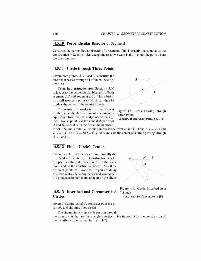
116 CHAPTER 4. GEOMETRIC CONSTRUCTION
4.5.10 Perpendicular Bisector of Segment
Construct the perpendicular bisector of a segment. This is exactly the same as as theconstruction in Section 4.5.1, except the result we want is the line, not the point wherethe lines intersect.
4.5.11 Circle through Three Points
AA BB
CCOO
Figure 4.8: Circle Passing throughThree PointsConstruction/CircFrom3Pts.T [P]
Given three points, A, B, and C, construct thecircle that passes through all of them. (See fig-ure 4.8.)
Using the construction from Section 4.5.10twice, draw the perpendicular bisectors of bothsegment AB and segment BC. Those bisec-tors will meet at a point O which can then beused as the center of the required circle.
The reason this works is that every pointon the perpendicular bisector of a segment isequidistant from the two endpoints of the seg-ment. So the pointO is the same distance fromA andB, since it is on the perpendicular bisec-tor of AB, and similarly, it is the same distance from B and C. Thus AO = BO andBO = CO, so AO = BO = CO, so O must be the center of a circle passing throughA, B, and C.
4.5.12 Find a Circle’s Center
AA BB
CC
OO
NN
Figure 4.9: Circle Inscribed in aTriangleConstruction/Incenter.T [P]
Given a circle, find its center. We basically didthis (and a little more) in Construction 4.5.11.Simply pick three different points on the givencircle and do the construction above. Any threedifferent points will work, but if you are doingthis with a physical straightedge and compass, itis a good idea to pick them far apart on the circle.
4.5.13 Inscribed and CircumscribedCircles
Given a triangle 4ABC, construct both the in-scribed and circumscribed circles.
The circumcircle is the circle passing throughthe three points that are the triangle’s vertices. See figure 4.9 for the construction ofthe inscribed circle (called the “incircle”).
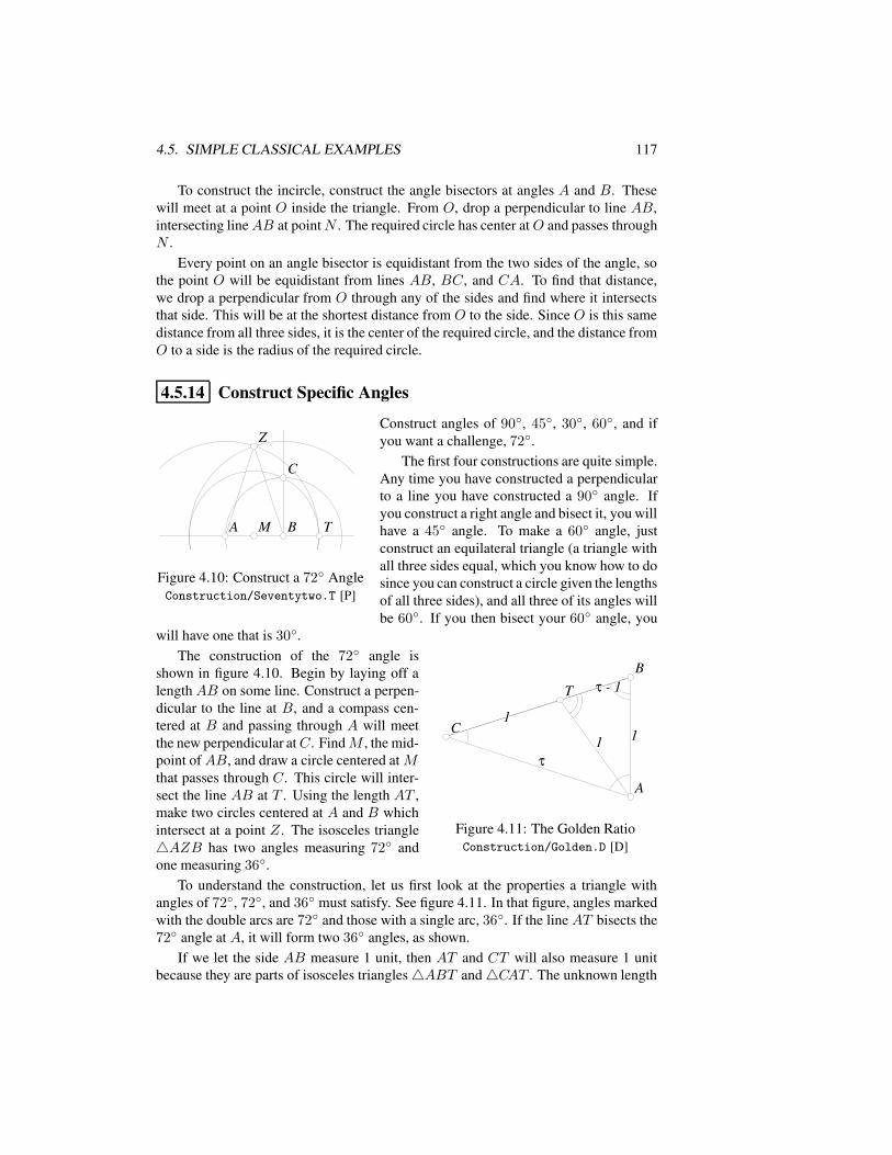
4.5. SIMPLE CLASSICAL EXAMPLES 117
To construct the incircle, construct the angle bisectors at angles A and B. Thesewill meet at a point O inside the triangle. From O, drop a perpendicular to line AB,intersecting lineAB at pointN . The required circle has center atO and passes throughN .
Every point on an angle bisector is equidistant from the two sides of the angle, sothe point O will be equidistant from lines AB, BC, and CA. To find that distance,we drop a perpendicular from O through any of the sides and find where it intersectsthat side. This will be at the shortest distance from O to the side. Since O is this samedistance from all three sides, it is the center of the required circle, and the distance fromO to a side is the radius of the required circle.
4.5.14 Construct Specific Angles
BBAA
CC
MM TT
ZZ
Figure 4.10: Construct a 72 AngleConstruction/Seventytwo.T [P]
Construct angles of 90, 45, 30, 60, and ifyou want a challenge, 72.
The first four constructions are quite simple.Any time you have constructed a perpendicularto a line you have constructed a 90 angle. Ifyou construct a right angle and bisect it, you willhave a 45 angle. To make a 60 angle, justconstruct an equilateral triangle (a triangle withall three sides equal, which you know how to dosince you can construct a circle given the lengthsof all three sides), and all three of its angles willbe 60. If you then bisect your 60 angle, you
will have one that is 30.
ττ
1111
11
τ - 1τ - 1BB
AA
CC
TT
Figure 4.11: The Golden RatioConstruction/Golden.D [D]
The construction of the 72 angle isshown in figure 4.10. Begin by laying off alength AB on some line. Construct a perpen-dicular to the line at B, and a compass cen-tered at B and passing through A will meetthe new perpendicular atC. FindM , the mid-point of AB, and draw a circle centered at Mthat passes through C. This circle will inter-sect the line AB at T . Using the length AT ,make two circles centered at A and B whichintersect at a point Z. The isosceles triangle4AZB has two angles measuring 72 andone measuring 36.
To understand the construction, let us first look at the properties a triangle withangles of 72, 72, and 36 must satisfy. See figure 4.11. In that figure, angles markedwith the double arcs are 72 and those with a single arc, 36. If the line AT bisects the72 angle at A, it will form two 36 angles, as shown.
If we let the side AB measure 1 unit, then AT and CT will also measure 1 unitbecause they are parts of isosceles triangles4ABT and4CAT . The unknown length
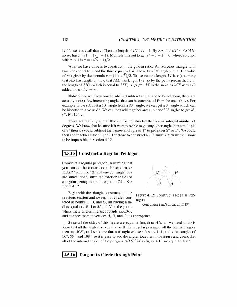
118 CHAPTER 4. GEOMETRIC CONSTRUCTION
isAC, so let us call that τ . Then the length ofBT is τ−1. By AA,4ABT ∼ 4CAB,so we have: τ/1 = 1/(τ − 1). Multiply this out to get τ 2 − τ − 1 = 0, whose solutionwith τ > 1 is τ = (
√5 + 1)/2.
What we have done is to construct τ , the golden ratio. An isosceles triangle withtwo sides equal to τ and the third equal to 1 will have two 72 angles in it. The valueof τ is given by the formula τ = (1 +
√5)/2. To see that the lengthAT is τ (assuming
that AB has length 1), note that MB has length 1/2, so by the pythagorean theorem,the length of MC (which is equal to MT ) is
√5/2. AT is the same as MT with 1/2
added on, so AT = τ .
Note: Since we know how to add and subtract angles and to bisect them, there areactually quite a few interesting angles that can be constructed from the ones above. Forexample, if we subtract a 30 angle from a 36 angle, we can get a 6 angle which canbe bisected to give us 3. We can then add together any number of 3 angles to get 3,6, 9, 12, . . ..
These are the only angles that can be constructed that are an integral number ofdegrees. We know that because if it were possible to get any other angle than a multipleof 3 then we could subtract the nearest multiple of 3 to get either 2 or 1. We couldthen add together either 10 or 20 of those to construct a 20 angle which we will showto be impossible in Section 4.12.
4.5.15 Construct a Regular Pentagon
AABB
CC
MMNN
Figure 4.12: Construct a Regular Pen-tagon
Construction/Pentagon.T [P]
Construct a regular pentagon. Assuming thatyou can do the construction above to make4ABC with two 72 and one 36 angle, youare almost done, since the exterior angles ofa regular pentagon are all equal to 72. Seefigure 4.12.
Begin with the triangle constructed in theprevious section and sweep out circles cen-tered at points A, B, and C, all having a ra-dius equal toAB. LetM andN be the pointswhere these circles intersect outside4ABC,and connect them to vertices A, B, and C, as appropriate.
Since all the sides of this figure are equal in length to AB, all we need to do isshow that all the angles are equal as well. In a regular pentagon, all the internal anglesmeasure 108, and we know that a triangle whose sides are 1, 1, and τ has angles of36, 36, and 108, so it is easy to add the angles together in the figure and check thatall of the internal angles of the polygonABNCM in figure 4.12 are equal to 108.
4.5.16 Tangent to Circle through Point
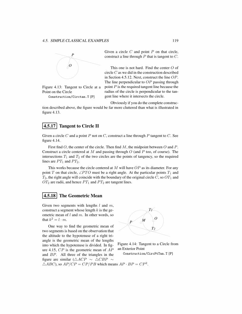
4.5. SIMPLE CLASSICAL EXAMPLES 119
PP
OO
Figure 4.13: Tangent to Circle at aPoint on the Circle
Construction/Circtan.T [P]
Given a circle C and point P on that circle,construct a line through P that is tangent to C.
This one is not hard. Find the center O ofcircleC as we did in the construction describedin Section 4.5.12. Next, construct the line OP .The line perpendicular to OP passing throughpoint P is the required tangent line because theradius of the circle is perpendicular to the tan-gent line where it intersects the circle.
Obviously if you do the complete construc-tion described above, the figure would be far more cluttered than what is illustrated infigure 4.13.
4.5.17 Tangent to Circle II
Given a circle C and a point P not on C, construct a line through P tangent to C. Seefigure 4.14.
First find O, the center of the circle. Then find M , the midpoint between O and P .Construct a circle centered at M and passing through O (and P too, of course). Theintersections T1 and T2 of the two circles are the points of tangency, so the requiredlines are PT1 and PT2.
This works because the circle centered at M will have OP as its diameter. For anypoint T on that circle, ∠PTO must be a right angle. At the particular points T1 andT2, the right angle will coincide with the boundary of the original circle C, so OT1 andOT2 are radii, and hence PT1 and PT2 are tangent lines.
4.5.18 The Geometric Mean
PPOOMM
T1T1
T2T2
Figure 4.14: Tangent to a Circle froman Exterior Point
Construction/CircPtTan.T [P]
Given two segments with lengths l and m,construct a segment whose length k is the ge-ometric mean of l and m. In other words, sothat k2 = l ·m.
One way to find the geometric mean oftwo segments is based on the observation thatthe altitude to the hypotenuse of a right tri-angle is the geometric mean of the lengthsinto which the hypotenuse is divided. In fig-ure 4.15, CP is the geometric mean of APand BP . All three of the triangles in thefigure are similar (4ACP ∼ 4CBP ∼4ABC), so AP/CP = CP/PB which means AP · BP = CP 2.
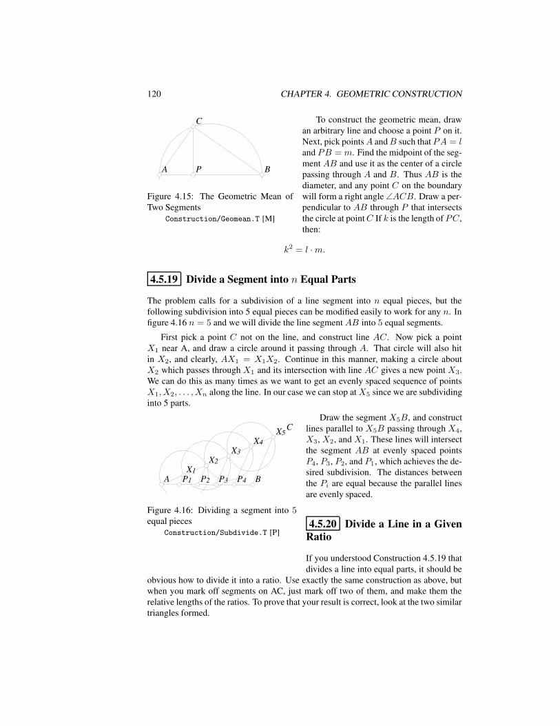
120 CHAPTER 4. GEOMETRIC CONSTRUCTION
AA BBPP
CC
Figure 4.15: The Geometric Mean ofTwo Segments
Construction/Geomean.T [M]
To construct the geometric mean, drawan arbitrary line and choose a point P on it.Next, pick pointsA andB such that PA = land PB = m. Find the midpoint of the seg-ment AB and use it as the center of a circlepassing through A and B. Thus AB is thediameter, and any point C on the boundarywill form a right angle ∠ACB. Draw a per-pendicular to AB through P that intersectsthe circle at pointC If k is the length of PC,then:
k2 = l ·m.
4.5.19 Divide a Segment into n Equal Parts
The problem calls for a subdivision of a line segment into n equal pieces, but thefollowing subdivision into 5 equal pieces can be modified easily to work for any n. Infigure 4.16 n = 5 and we will divide the line segment AB into 5 equal segments.
First pick a point C not on the line, and construct line AC. Now pick a pointX1 near A, and draw a circle around it passing through A. That circle will also hitin X2, and clearly, AX1 = X1X2. Continue in this manner, making a circle aboutX2 which passes through X1 and its intersection with line AC gives a new point X3.We can do this as many times as we want to get an evenly spaced sequence of pointsX1, X2, . . . , Xn along the line. In our case we can stop atX5 since we are subdividinginto 5 parts.
AA BB
CC
X1X1X2X2
X3X3X4X4
X5X5
P4P4P3P3P2P2P1P1
Figure 4.16: Dividing a segment into 5equal pieces
Construction/Subdivide.T [P]
Draw the segment X5B, and constructlines parallel to X5B passing through X4,X3, X2, and X1. These lines will intersectthe segment AB at evenly spaced pointsP4, P3, P2, and P1, which achieves the de-sired subdivision. The distances betweenthe Pi are equal because the parallel linesare evenly spaced.
4.5.20 Divide a Line in a GivenRatio
If you understood Construction 4.5.19 thatdivides a line into equal parts, it should be
obvious how to divide it into a ratio. Use exactly the same construction as above, butwhen you mark off segments on AC, just mark off two of them, and make them therelative lengths of the ratios. To prove that your result is correct, look at the two similartriangles formed.
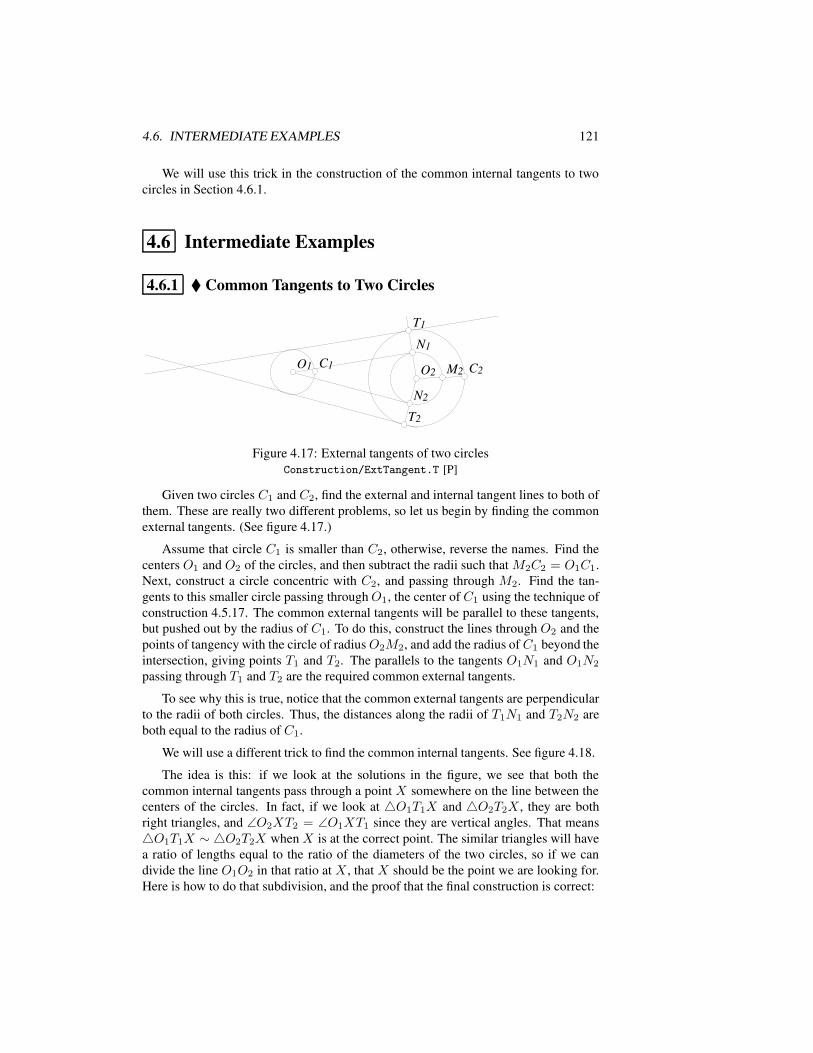
4.6. INTERMEDIATE EXAMPLES 121
We will use this trick in the construction of the common internal tangents to twocircles in Section 4.6.1.
4.6 Intermediate Examples
4.6.1 Common Tangents to Two Circles
C1C1 C2C2O1O1 O2O2 M2M2
N1N1
N2N2
T1T1
T2T2
Figure 4.17: External tangents of two circlesConstruction/ExtTangent.T [P]
Given two circles C1 and C2, find the external and internal tangent lines to both ofthem. These are really two different problems, so let us begin by finding the commonexternal tangents. (See figure 4.17.)
Assume that circle C1 is smaller than C2, otherwise, reverse the names. Find thecenters O1 and O2 of the circles, and then subtract the radii such that M2C2 = O1C1.Next, construct a circle concentric with C2, and passing through M2. Find the tan-gents to this smaller circle passing throughO1, the center of C1 using the technique ofconstruction 4.5.17. The common external tangents will be parallel to these tangents,but pushed out by the radius of C1. To do this, construct the lines through O2 and thepoints of tangency with the circle of radiusO2M2, and add the radius of C1 beyond theintersection, giving points T1 and T2. The parallels to the tangents O1N1 and O1N2
passing through T1 and T2 are the required common external tangents.
To see why this is true, notice that the common external tangents are perpendicularto the radii of both circles. Thus, the distances along the radii of T1N1 and T2N2 areboth equal to the radius of C1.
We will use a different trick to find the common internal tangents. See figure 4.18.
The idea is this: if we look at the solutions in the figure, we see that both thecommon internal tangents pass through a point X somewhere on the line between thecenters of the circles. In fact, if we look at 4O1T1X and 4O2T2X , they are bothright triangles, and ∠O2XT2 = ∠O1XT1 since they are vertical angles. That means4O1T1X ∼ 4O2T2X when X is at the correct point. The similar triangles will havea ratio of lengths equal to the ratio of the diameters of the two circles, so if we candivide the line O1O2 in that ratio at X , that X should be the point we are looking for.Here is how to do that subdivision, and the proof that the final construction is correct:
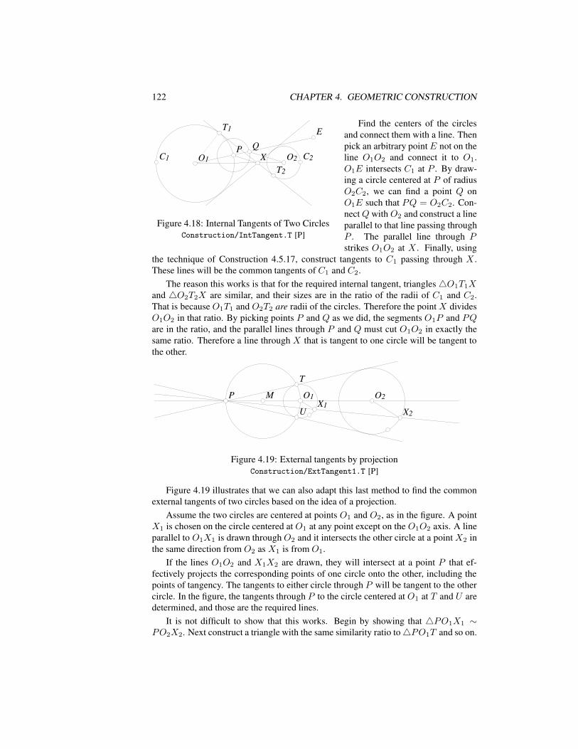
122 CHAPTER 4. GEOMETRIC CONSTRUCTION
C1C1 C2C2O1O1 O2O2
EE
PP QQXX
T1T1
T2T2
Figure 4.18: Internal Tangents of Two CirclesConstruction/IntTangent.T [P]
Find the centers of the circlesand connect them with a line. Thenpick an arbitrary pointE not on theline O1O2 and connect it to O1.O1E intersects C1 at P . By draw-ing a circle centered at P of radiusO2C2, we can find a point Q onO1E such that PQ = O2C2. Con-nectQ with O2 and construct a lineparallel to that line passing throughP . The parallel line through Pstrikes O1O2 at X . Finally, using
the technique of Construction 4.5.17, construct tangents to C1 passing through X .These lines will be the common tangents of C1 and C2.
The reason this works is that for the required internal tangent, triangles4O1T1Xand 4O2T2X are similar, and their sizes are in the ratio of the radii of C1 and C2.That is because O1T1 and O2T2 are radii of the circles. Therefore the point X dividesO1O2 in that ratio. By picking points P and Q as we did, the segments O1P and PQare in the ratio, and the parallel lines through P and Q must cut O1O2 in exactly thesame ratio. Therefore a line through X that is tangent to one circle will be tangent tothe other.
O2O2O1O1X1X1
X2X2
PP MM
TT
UU
Figure 4.19: External tangents by projectionConstruction/ExtTangent1.T [P]
Figure 4.19 illustrates that we can also adapt this last method to find the commonexternal tangents of two circles based on the idea of a projection.
Assume the two circles are centered at points O1 and O2, as in the figure. A pointX1 is chosen on the circle centered at O1 at any point except on the O1O2 axis. A lineparallel to O1X1 is drawn throughO2 and it intersects the other circle at a point X2 inthe same direction from O2 as X1 is from O1.
If the lines O1O2 and X1X2 are drawn, they will intersect at a point P that ef-fectively projects the corresponding points of one circle onto the other, including thepoints of tangency. The tangents to either circle through P will be tangent to the othercircle. In the figure, the tangents through P to the circle centered at O1 at T and U aredetermined, and those are the required lines.
It is not difficult to show that this works. Begin by showing that 4PO1X1 ∼PO2X2. Next construct a triangle with the same similarity ratio to4PO1T and so on.
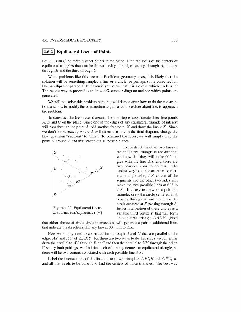
4.6. INTERMEDIATE EXAMPLES 123
4.6.2 Equilateral Locus of Points
Let A, B an C be three distinct points in the plane. Find the locus of the centers ofequilateral triangles that can be drawn having one edge passing through A, anotherthroughB and the third through C.
When problems like this occur in Euclidean geometry texts, it is likely that thesolution will be something simple: a line or a circle, or perhaps some conic sectionlike an ellipse or parabola. But even if you know that it is a circle, which circle is it?The easiest way to proceed is to draw a Geometer diagram and see which points aregenerated.
We will not solve this problem here, but will demonstrate how to do the construc-tion, and how to modify the construction to gain a lot more clues about how to approachthe problem.
To construct the Geometer diagram, the first step is easy: create three free pointsA, B and C on the plane. Since one of the edges of any equilateral triangle of interestwill pass through the point A, add another free point X and draw the line AX . Sincewe don’t know exactly where A will sit on that line in the final diagram, change theline type from “segment” to “line”. To construct the locus, we will simply drag thepoint X aroundA and thus sweep out all possible lines.
BB
AACC XXPP
RR
P’P’
Q’Q’R’R’
Figure 4.20: Equilateral LocusConstruction/EquLocus.T [M]
To construct the other two lines ofthe equilateral triangle is not difficult:we know that they will make 60 an-gles with the line AX and there aretwo possible ways to do this. Theeasiest way is to construct an equilat-eral triangle using AX as one of thesegments and the other two sides willmake the two possible lines at 60 toAX . It’s easy to draw an equilateraltriangle; draw the circle centered at Apassing through X and then draw thecircle centered atX passing throughA.Either intersection of these circles is asuitable third vertex Y that will forman equilateral triangle 4AXY . (Note
that either choice of circle-circle intersections will generate a pair of additional linesthat indicate the directions that any line at 60 will to AX .)
Now we simply need to construct lines through B and C that are parallel to theedges AY and XY of 4AXY , but there are two ways to do this since we can eitherdraw the parallel to AY throughB or C and then the parallel to XY through the other.If we try both pairings, we find that each of them generates an equilateral triangle, sothere will be two centers associated with each possible line AX .
Label the intersections of the lines to form two triangles: 4PQR and 4P ′Q′R′and all that needs to be done is to find the centers of those triangles. The best way
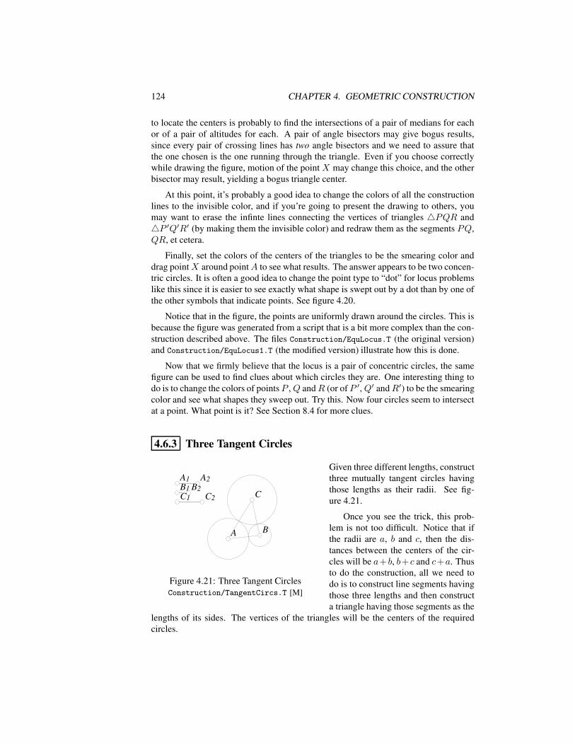
124 CHAPTER 4. GEOMETRIC CONSTRUCTION
to locate the centers is probably to find the intersections of a pair of medians for eachor of a pair of altitudes for each. A pair of angle bisectors may give bogus results,since every pair of crossing lines has two angle bisectors and we need to assure thatthe one chosen is the one running through the triangle. Even if you choose correctlywhile drawing the figure, motion of the point X may change this choice, and the otherbisector may result, yielding a bogus triangle center.
At this point, it’s probably a good idea to change the colors of all the constructionlines to the invisible color, and if you’re going to present the drawing to others, youmay want to erase the infinte lines connecting the vertices of triangles 4PQR and4P ′Q′R′ (by making them the invisible color) and redraw them as the segments PQ,QR, et cetera.
Finally, set the colors of the centers of the triangles to be the smearing color anddrag pointX around pointA to see what results. The answer appears to be two concen-tric circles. It is often a good idea to change the point type to “dot” for locus problemslike this since it is easier to see exactly what shape is swept out by a dot than by one ofthe other symbols that indicate points. See figure 4.20.
Notice that in the figure, the points are uniformly drawn around the circles. This isbecause the figure was generated from a script that is a bit more complex than the con-struction described above. The files Construction/EquLocus.T (the original version)and Construction/EquLocus1.T (the modified version) illustrate how this is done.
Now that we firmly believe that the locus is a pair of concentric circles, the samefigure can be used to find clues about which circles they are. One interesting thing todo is to change the colors of points P ,Q andR (or of P ′,Q′ andR′) to be the smearingcolor and see what shapes they sweep out. Try this. Now four circles seem to intersectat a point. What point is it? See Section 8.4 for more clues.
4.6.3 Three Tangent Circles
A1A1B1B1C1C1
A2A2B2B2
C2C2
AA BB
CC
Figure 4.21: Three Tangent CirclesConstruction/TangentCircs.T [M]
Given three different lengths, constructthree mutually tangent circles havingthose lengths as their radii. See fig-ure 4.21.
Once you see the trick, this prob-lem is not too difficult. Notice that ifthe radii are a, b and c, then the dis-tances between the centers of the cir-cles will be a+b, b+c and c+a. Thusto do the construction, all we need todo is to construct line segments havingthose three lengths and then constructa triangle having those segments as the
lengths of its sides. The vertices of the triangles will be the centers of the requiredcircles.
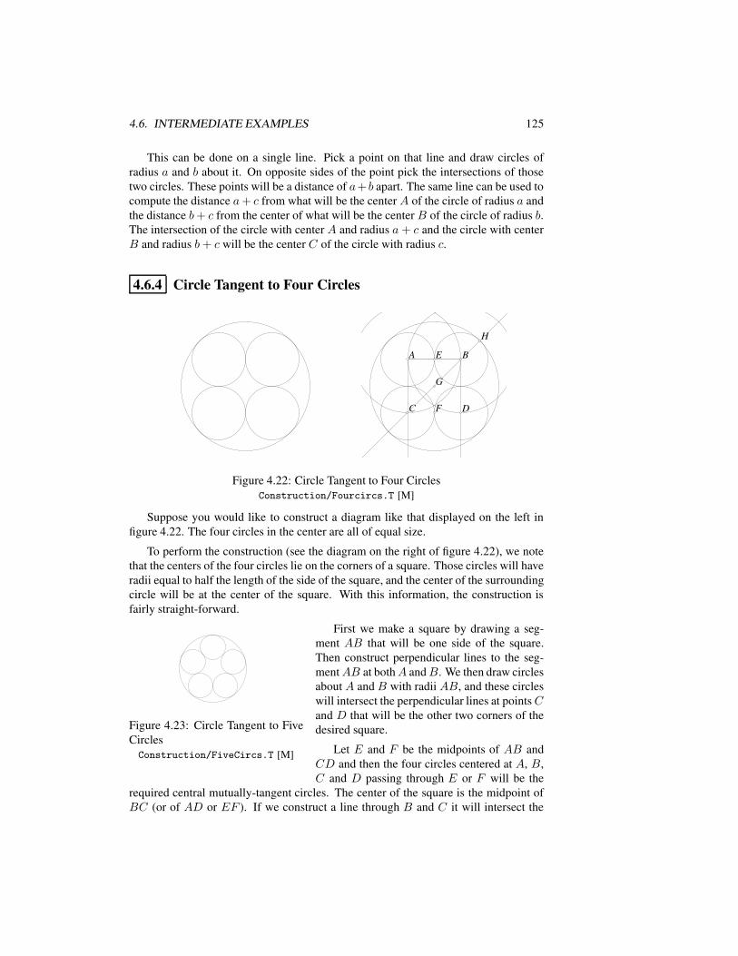
4.6. INTERMEDIATE EXAMPLES 125
This can be done on a single line. Pick a point on that line and draw circles ofradius a and b about it. On opposite sides of the point pick the intersections of thosetwo circles. These points will be a distance of a+ b apart. The same line can be used tocompute the distance a+ c from what will be the center A of the circle of radius a andthe distance b+ c from the center of what will be the center B of the circle of radius b.The intersection of the circle with center A and radius a+ c and the circle with centerB and radius b+ c will be the center C of the circle with radius c.
4.6.4 Circle Tangent to Four Circles
AA BB
CC DD
EE
FF
GG
HH
Figure 4.22: Circle Tangent to Four CirclesConstruction/Fourcircs.T [M]
Suppose you would like to construct a diagram like that displayed on the left infigure 4.22. The four circles in the center are all of equal size.
To perform the construction (see the diagram on the right of figure 4.22), we notethat the centers of the four circles lie on the corners of a square. Those circles will haveradii equal to half the length of the side of the square, and the center of the surroundingcircle will be at the center of the square. With this information, the construction isfairly straight-forward.
Figure 4.23: Circle Tangent to FiveCirclesConstruction/FiveCircs.T [M]
First we make a square by drawing a seg-ment AB that will be one side of the square.Then construct perpendicular lines to the seg-mentAB at bothA andB. We then draw circlesabout A and B with radii AB, and these circleswill intersect the perpendicular lines at pointsCand D that will be the other two corners of thedesired square.
Let E and F be the midpoints of AB andCD and then the four circles centered at A, B,C and D passing through E or F will be the
required central mutually-tangent circles. The center of the square is the midpoint ofBC (or of AD or EF ). If we construct a line through B and C it will intersect the
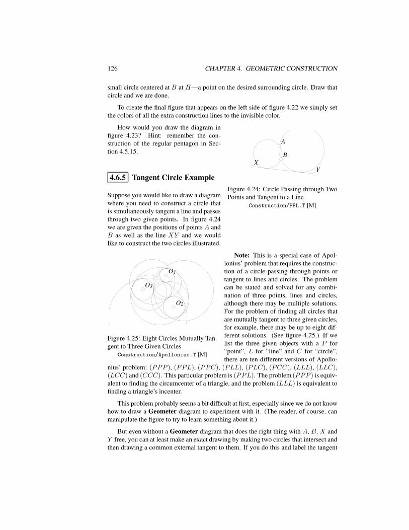
126 CHAPTER 4. GEOMETRIC CONSTRUCTION
small circle centered at B at H—a point on the desired surrounding circle. Draw thatcircle and we are done.
To create the final figure that appears on the left side of figure 4.22 we simply setthe colors of all the extra construction lines to the invisible color.
AA
BBXX
YY
Figure 4.24: Circle Passing through TwoPoints and Tangent to a Line
Construction/PPL.T [M]
How would you draw the diagram infigure 4.23? Hint: remember the con-struction of the regular pentagon in Sec-tion 4.5.15.
4.6.5 Tangent Circle Example
Suppose you would like to draw a diagramwhere you need to construct a circle thatis simultaneously tangent a line and passesthrough two given points. In figure 4.24we are given the positions of points A andB as well as the line XY and we wouldlike to construct the two circles illustrated.
O1O1
O2O2
O3O3
Figure 4.25: Eight Circles Mutually Tan-gent to Three Given Circles
Construction/Apollonius.T [M]
Note: This is a special case of Apol-lonius’ problem that requires the construc-tion of a circle passing through points ortangent to lines and circles. The problemcan be stated and solved for any combi-nation of three points, lines and circles,although there may be multiple solutions.For the problem of finding all circles thatare mutually tangent to three given circles,for example, there may be up to eight dif-ferent solutions. (See figure 4.25.) If welist the three given objects with a P for“point”, L for “line” and C for “circle”,there are ten different versions of Apollo-
nius’ problem: (PPP ), (PPL), (PPC), (PLL), (PLC), (PCC), (LLL), (LLC),(LCC) and (CCC). This particular problem is (PPL). The problem (PPP ) is equiv-alent to finding the circumcenter of a triangle, and the problem (LLL) is equivalent tofinding a triangle’s incenter.
This problem probably seems a bit difficult at first, especially since we do not knowhow to draw a Geometer diagram to experiment with it. (The reader, of course, canmanipulate the figure to try to learn something about it.)
But even without a Geometer diagram that does the right thing with A, B, X andY free, you can at least make an exact drawing by making two circles that intersect andthen drawing a common external tangent to them. If you do this and label the tangent
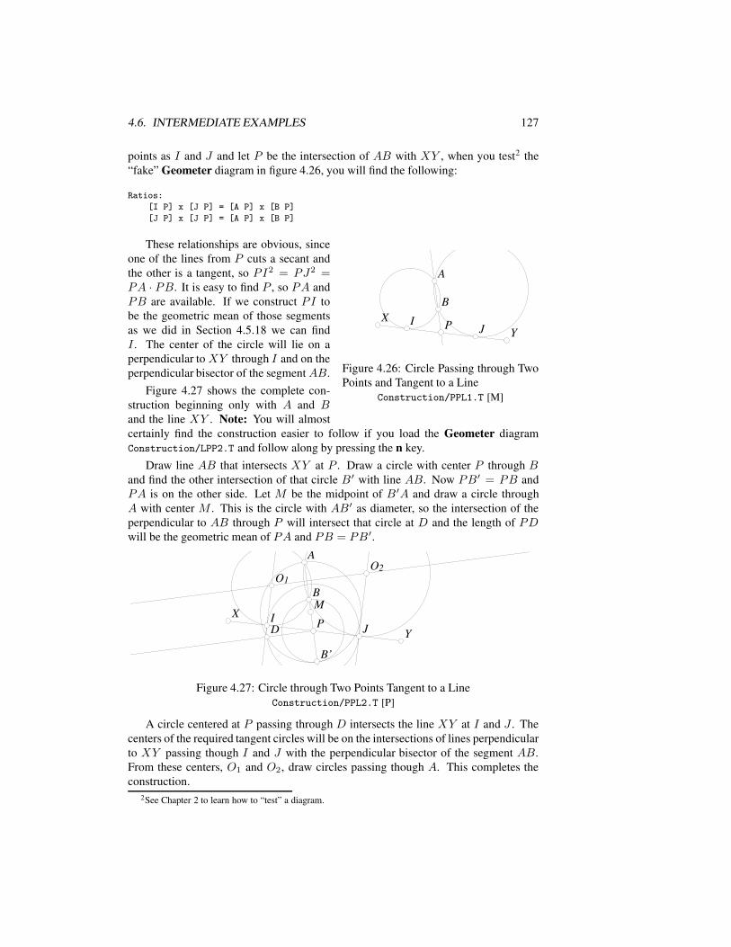
4.6. INTERMEDIATE EXAMPLES 127
points as I and J and let P be the intersection of AB with XY , when you test2 the“fake” Geometer diagram in figure 4.26, you will find the following:
Ratios:
[I P] x [J P] = [A P] x [B P]
[J P] x [J P] = [A P] x [B P]
AA
BBXX
YYII
JJPP
Figure 4.26: Circle Passing through TwoPoints and Tangent to a Line
Construction/PPL1.T [M]
These relationships are obvious, sinceone of the lines from P cuts a secant andthe other is a tangent, so PI2 = PJ2 =PA · PB. It is easy to find P , so PA andPB are available. If we construct PI tobe the geometric mean of those segmentsas we did in Section 4.5.18 we can findI . The center of the circle will lie on aperpendicular to XY through I and on theperpendicular bisector of the segmentAB.
Figure 4.27 shows the complete con-struction beginning only with A and Band the line XY . Note: You will almostcertainly find the construction easier to follow if you load the Geometer diagramConstruction/LPP2.T and follow along by pressing the n key.
Draw line AB that intersects XY at P . Draw a circle with center P through Band find the other intersection of that circle B′ with line AB. Now PB′ = PB andPA is on the other side. Let M be the midpoint of B ′A and draw a circle throughA with center M . This is the circle with AB′ as diameter, so the intersection of theperpendicular to AB through P will intersect that circle at D and the length of PDwill be the geometric mean of PA and PB = PB ′.
AA
BB
XX
YYPP
B’B’
MM
DDII
JJ
O1O1O2O2
Figure 4.27: Circle through Two Points Tangent to a LineConstruction/PPL2.T [P]
A circle centered at P passing through D intersects the line XY at I and J . Thecenters of the required tangent circles will be on the intersections of lines perpendicularto XY passing though I and J with the perpendicular bisector of the segment AB.From these centers, O1 and O2, draw circles passing though A. This completes theconstruction.
2See Chapter 2 to learn how to “test” a diagram.
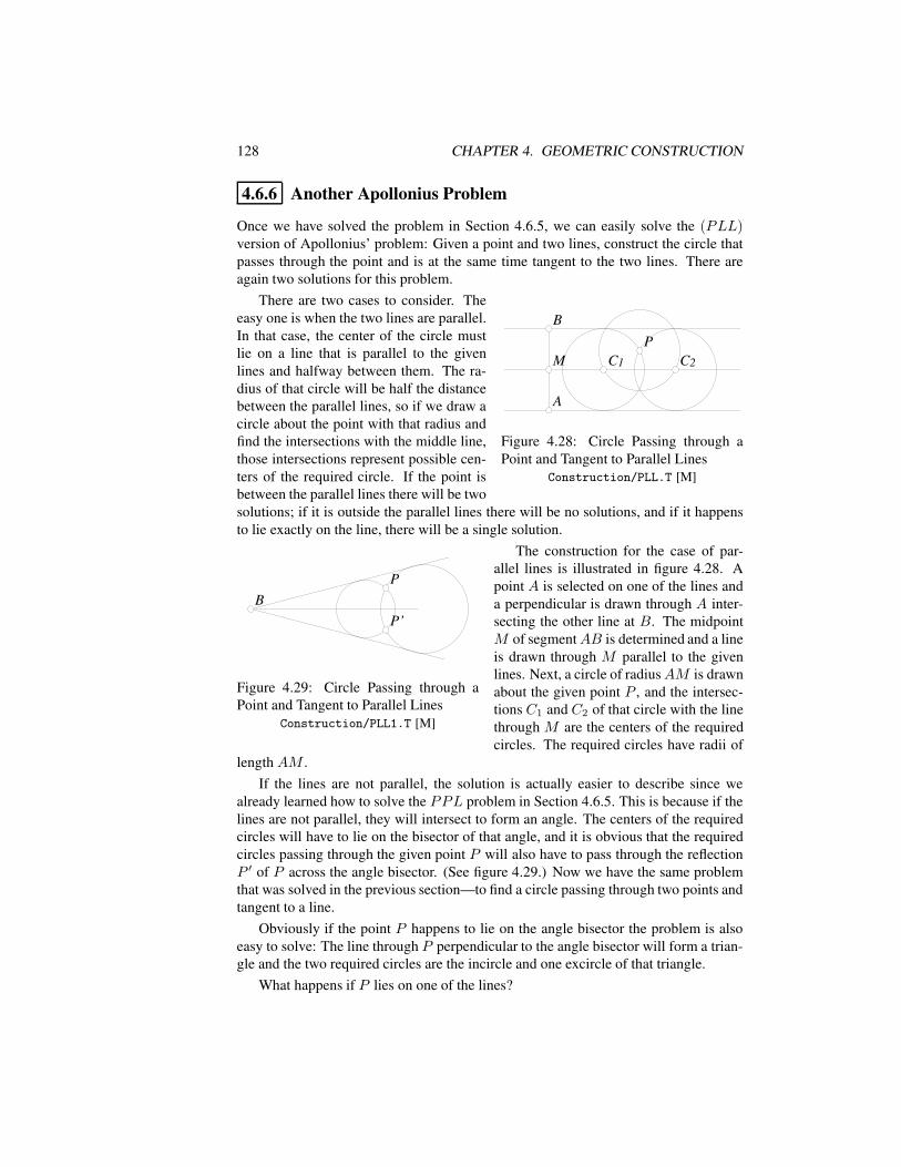
128 CHAPTER 4. GEOMETRIC CONSTRUCTION
4.6.6 Another Apollonius Problem
Once we have solved the problem in Section 4.6.5, we can easily solve the (PLL)version of Apollonius’ problem: Given a point and two lines, construct the circle thatpasses through the point and is at the same time tangent to the two lines. There areagain two solutions for this problem.
PP
AA
BB
MM C1C1 C2C2
Figure 4.28: Circle Passing through aPoint and Tangent to Parallel Lines
Construction/PLL.T [M]
There are two cases to consider. Theeasy one is when the two lines are parallel.In that case, the center of the circle mustlie on a line that is parallel to the givenlines and halfway between them. The ra-dius of that circle will be half the distancebetween the parallel lines, so if we draw acircle about the point with that radius andfind the intersections with the middle line,those intersections represent possible cen-ters of the required circle. If the point isbetween the parallel lines there will be twosolutions; if it is outside the parallel lines there will be no solutions, and if it happensto lie exactly on the line, there will be a single solution.
BBPP
P’P’
Figure 4.29: Circle Passing through aPoint and Tangent to Parallel Lines
Construction/PLL1.T [M]
The construction for the case of par-allel lines is illustrated in figure 4.28. Apoint A is selected on one of the lines anda perpendicular is drawn through A inter-secting the other line at B. The midpointM of segmentAB is determined and a lineis drawn through M parallel to the givenlines. Next, a circle of radiusAM is drawnabout the given point P , and the intersec-tions C1 and C2 of that circle with the linethrough M are the centers of the requiredcircles. The required circles have radii of
length AM .If the lines are not parallel, the solution is actually easier to describe since we
already learned how to solve the PPL problem in Section 4.6.5. This is because if thelines are not parallel, they will intersect to form an angle. The centers of the requiredcircles will have to lie on the bisector of that angle, and it is obvious that the requiredcircles passing through the given point P will also have to pass through the reflectionP ′ of P across the angle bisector. (See figure 4.29.) Now we have the same problemthat was solved in the previous section—to find a circle passing through two points andtangent to a line.
Obviously if the point P happens to lie on the angle bisector the problem is alsoeasy to solve: The line through P perpendicular to the angle bisector will form a trian-gle and the two required circles are the incircle and one excircle of that triangle.
What happens if P lies on one of the lines?
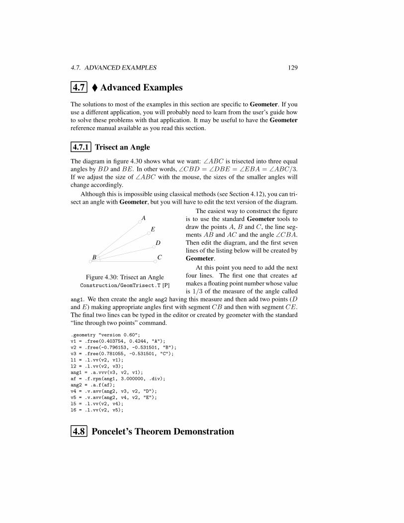
4.7. ADVANCED EXAMPLES 129
4.7 Advanced Examples
The solutions to most of the examples in this section are specific to Geometer. If youuse a different application, you will probably need to learn from the user’s guide howto solve these problems with that application. It may be useful to have the Geometerreference manual available as you read this section.
4.7.1 Trisect an Angle
The diagram in figure 4.30 shows what we want: ∠ABC is trisected into three equalangles by BD and BE. In other words, ∠CBD = ∠DBE = ∠EBA = ∠ABC/3.If we adjust the size of ∠ABC with the mouse, the sizes of the smaller angles willchange accordingly.
Although this is impossible using classical methods (see Section 4.12), you can tri-sect an angle with Geometer, but you will have to edit the text version of the diagram.
AA
BB CC
DD
EE
Figure 4.30: Trisect an AngleConstruction/GeomTrisect.T [P]
The easiest way to construct the figureis to use the standard Geometer tools todraw the points A, B and C, the line seg-ments AB and AC and the angle ∠CBA.Then edit the diagram, and the first sevenlines of the listing below will be created byGeometer.
At this point you need to add the nextfour lines. The first one that creates af
makes a floating point number whose valueis 1/3 of the measure of the angle called
ang1. We then create the angle ang2 having this measure and then add two points (Dand E) making appropriate angles first with segment CB and then with segment CE.The final two lines can be typed in the editor or created by geometer with the standard“line through two points” command.
.geometry "version 0.60";
v1 = .free(0.403754, 0.4244, "A");
v2 = .free(-0.796153, -0.531501, "B");
v3 = .free(0.781055, -0.531501, "C");
l1 = .l.vv(v2, v1);
l2 = .l.vv(v2, v3);
ang1 = .a.vvv(v3, v2, v1);
af = .f.rpn(ang1, 3.000000, .div);
ang2 = .a.f(af);
v4 = .v.avv(ang2, v3, v2, "D");
v5 = .v.avv(ang2, v4, v2, "E");
l5 = .l.vv(v2, v4);
l6 = .l.vv(v2, v5);
4.8 Poncelet’s Theorem Demonstration
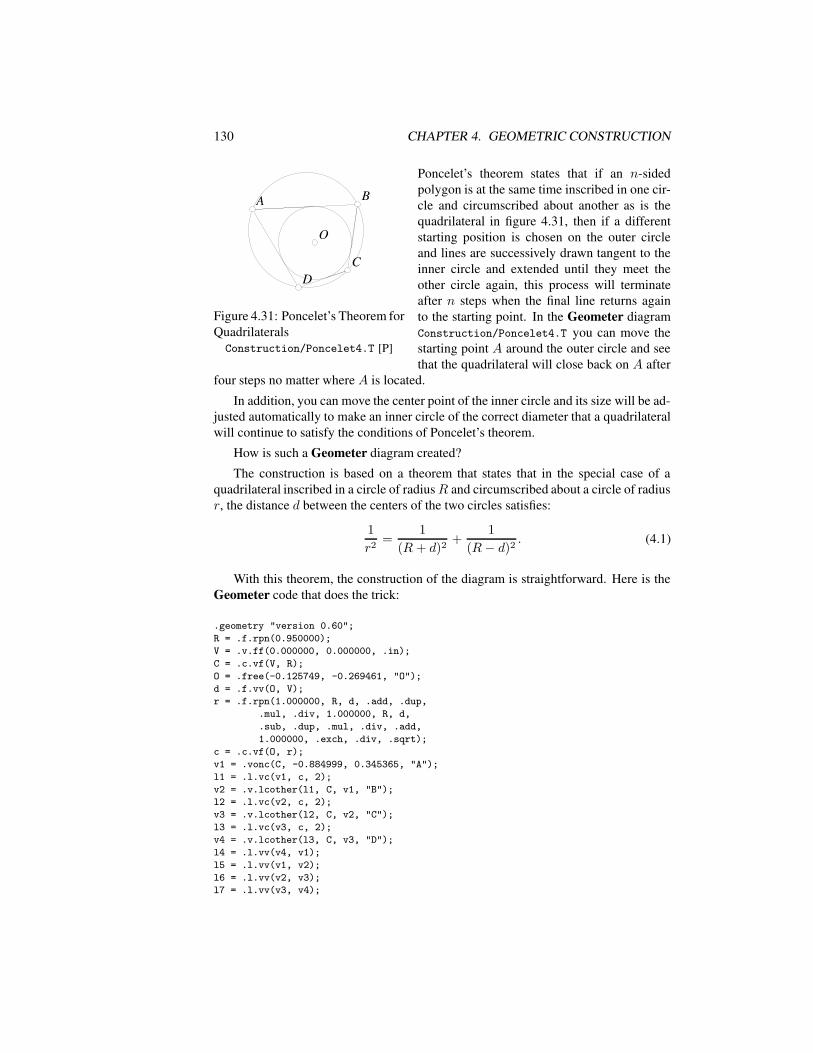
130 CHAPTER 4. GEOMETRIC CONSTRUCTION
OO
AA BB
CCDD
Figure 4.31: Poncelet’s Theorem forQuadrilateralsConstruction/Poncelet4.T [P]
Poncelet’s theorem states that if an n-sidedpolygon is at the same time inscribed in one cir-cle and circumscribed about another as is thequadrilateral in figure 4.31, then if a differentstarting position is chosen on the outer circleand lines are successively drawn tangent to theinner circle and extended until they meet theother circle again, this process will terminateafter n steps when the final line returns againto the starting point. In the Geometer diagramConstruction/Poncelet4.T you can move thestarting point A around the outer circle and seethat the quadrilateral will close back on A after
four steps no matter where A is located.
In addition, you can move the center point of the inner circle and its size will be ad-justed automatically to make an inner circle of the correct diameter that a quadrilateralwill continue to satisfy the conditions of Poncelet’s theorem.
How is such a Geometer diagram created?
The construction is based on a theorem that states that in the special case of aquadrilateral inscribed in a circle of radiusR and circumscribed about a circle of radiusr, the distance d between the centers of the two circles satisfies:
1
r2=
1
(R + d)2+
1
(R− d)2. (4.1)
With this theorem, the construction of the diagram is straightforward. Here is theGeometer code that does the trick:
.geometry "version 0.60";
R = .f.rpn(0.950000);
V = .v.ff(0.000000, 0.000000, .in);
C = .c.vf(V, R);
O = .free(-0.125749, -0.269461, "O");
d = .f.vv(O, V);
r = .f.rpn(1.000000, R, d, .add, .dup,
.mul, .div, 1.000000, R, d,
.sub, .dup, .mul, .div, .add,
1.000000, .exch, .div, .sqrt);
c = .c.vf(O, r);
v1 = .vonc(C, -0.884999, 0.345365, "A");
l1 = .l.vc(v1, c, 2);
v2 = .v.lcother(l1, C, v1, "B");
l2 = .l.vc(v2, c, 2);
v3 = .v.lcother(l2, C, v2, "C");
l3 = .l.vc(v3, c, 2);
v4 = .v.lcother(l3, C, v3, "D");
l4 = .l.vv(v4, v1);
l5 = .l.vv(v1, v2);
l6 = .l.vv(v2, v3);
l7 = .l.vv(v3, v4);
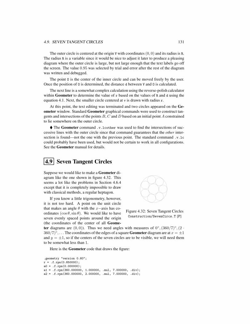
4.9. SEVEN TANGENT CIRCLES 131
The outer circle is centered at the origin V with coordinates (0, 0) and its radius is R.The radius R is a variable since it would be nice to adjust it later to produce a pleasingdiagram where the outer circle is large, but not large enough that the text labels go offthe screen. The value 0.95 was selected by trial and error after the rest of the diagramwas written and debugged.
The point O is the center of the inner circle and can be moved freely by the user.Once the position of O is determined, the distance d between V and O is calculated.
The next line is a somewhat complex calculation using the reverse-polish calculatorwithin Geometer to determine the value of r based on the values of R and d using theequation 4.1. Next, the smaller circle centered at v is drawn with radius r.
At this point, the text editing was terminated and two circles appeared on the Ge-ometer window. Standard Geometer graphical commands were used to construct tan-gents and intersections of the pointsB,C andD based on an initial pointA constrainedto lie somewhere on the outer circle.
The Geometer command .v.lcother was used to find the intersections of suc-cessive lines with the outer circle since that command guarantees that the other inter-section is found—not the one with the previous point. The standard command .v.lc
could probably have been used, but would not be certain to work in all configurations.See the Geometer manual for details.
4.9 Seven Tangent Circles
Figure 4.32: Seven Tangent CirclesConstruction/SevenCircs.T [P]
Suppose we would like to make a Geometer di-agram like the one shown in figure 4.32. Thisseems a lot like the problems in Section 4.6.4except that it is completely impossible to drawwith classical methods, a regular heptagon.
If you know a little trigonometry, however,it is not too hard. A point on the unit circlethat makes an angle θ with the x−axis has co-ordinates (cos θ, sin θ). We would like to haveseven evenly spaced points around the origin(the coordinates of the center of all Geome-ter diagrams are (0, 0)). Thus we need angles with measures of 0, (360/7), (2 ·360/7), . . . The coordinates of the edges of a square Geometer diagram are at x = ±1and y = ±1, so if the centers of the seven circles are to be visible, we will need themto be somewhat less than 1.
Here is the Geometer code that draws the figure:
.geometry "version 0.60";
r = .f.rpn(0.650000);
a0 = .f.rpn(0.000000);
a1 = .f.rpn(360.000000, 1.000000, .mul, 7.000000, .div);
a2 = .f.rpn(360.000000, 2.000000, .mul, 7.000000, .div);
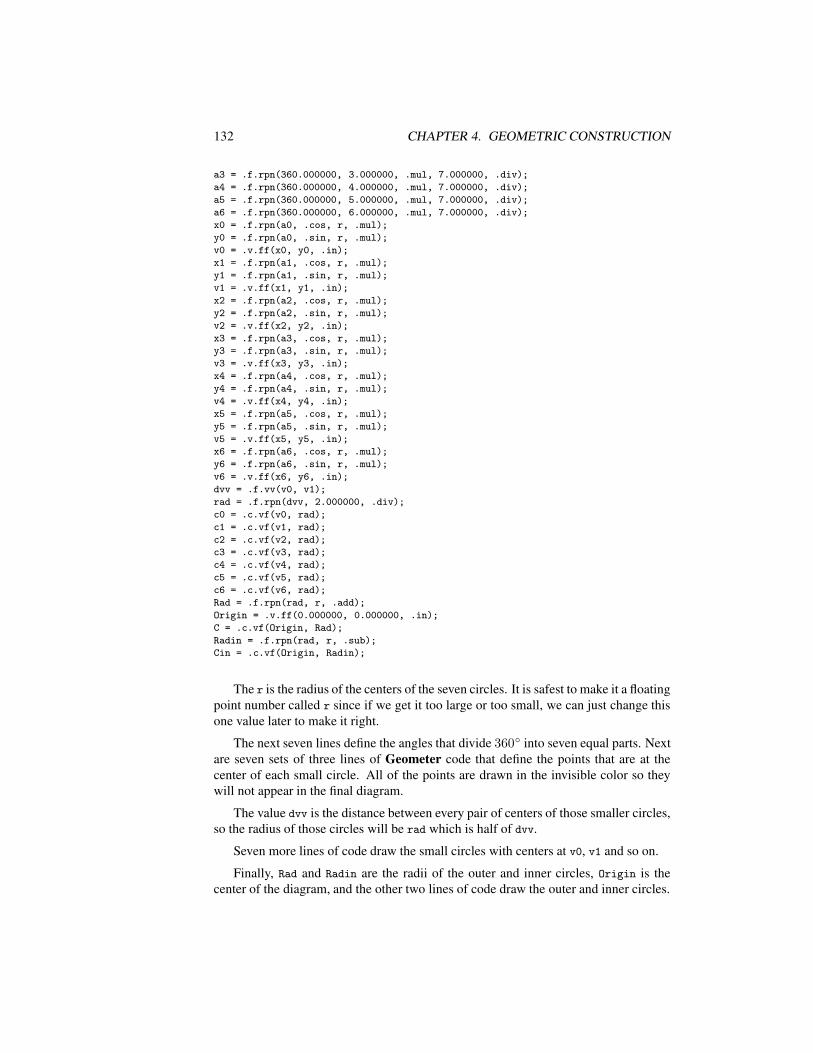
132 CHAPTER 4. GEOMETRIC CONSTRUCTION
a3 = .f.rpn(360.000000, 3.000000, .mul, 7.000000, .div);
a4 = .f.rpn(360.000000, 4.000000, .mul, 7.000000, .div);
a5 = .f.rpn(360.000000, 5.000000, .mul, 7.000000, .div);
a6 = .f.rpn(360.000000, 6.000000, .mul, 7.000000, .div);
x0 = .f.rpn(a0, .cos, r, .mul);
y0 = .f.rpn(a0, .sin, r, .mul);
v0 = .v.ff(x0, y0, .in);
x1 = .f.rpn(a1, .cos, r, .mul);
y1 = .f.rpn(a1, .sin, r, .mul);
v1 = .v.ff(x1, y1, .in);
x2 = .f.rpn(a2, .cos, r, .mul);
y2 = .f.rpn(a2, .sin, r, .mul);
v2 = .v.ff(x2, y2, .in);
x3 = .f.rpn(a3, .cos, r, .mul);
y3 = .f.rpn(a3, .sin, r, .mul);
v3 = .v.ff(x3, y3, .in);
x4 = .f.rpn(a4, .cos, r, .mul);
y4 = .f.rpn(a4, .sin, r, .mul);
v4 = .v.ff(x4, y4, .in);
x5 = .f.rpn(a5, .cos, r, .mul);
y5 = .f.rpn(a5, .sin, r, .mul);
v5 = .v.ff(x5, y5, .in);
x6 = .f.rpn(a6, .cos, r, .mul);
y6 = .f.rpn(a6, .sin, r, .mul);
v6 = .v.ff(x6, y6, .in);
dvv = .f.vv(v0, v1);
rad = .f.rpn(dvv, 2.000000, .div);
c0 = .c.vf(v0, rad);
c1 = .c.vf(v1, rad);
c2 = .c.vf(v2, rad);
c3 = .c.vf(v3, rad);
c4 = .c.vf(v4, rad);
c5 = .c.vf(v5, rad);
c6 = .c.vf(v6, rad);
Rad = .f.rpn(rad, r, .add);
Origin = .v.ff(0.000000, 0.000000, .in);
C = .c.vf(Origin, Rad);
Radin = .f.rpn(rad, r, .sub);
Cin = .c.vf(Origin, Radin);
The r is the radius of the centers of the seven circles. It is safest to make it a floatingpoint number called r since if we get it too large or too small, we can just change thisone value later to make it right.
The next seven lines define the angles that divide 360 into seven equal parts. Nextare seven sets of three lines of Geometer code that define the points that are at thecenter of each small circle. All of the points are drawn in the invisible color so theywill not appear in the final diagram.
The value dvv is the distance between every pair of centers of those smaller circles,so the radius of those circles will be rad which is half of dvv.
Seven more lines of code draw the small circles with centers at v0, v1 and so on.
Finally, Rad and Radin are the radii of the outer and inner circles, Origin is thecenter of the diagram, and the other two lines of code draw the outer and inner circles.
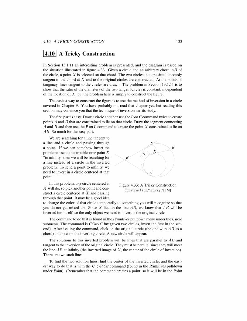
4.10. A TRICKY CONSTRUCTION 133
4.10 A Tricky Construction
In Section 13.1.11 an interesting problem is presented, and the diagram is based onthe situation illustrated in figure 4.33. Given a circle and an arbitrary chord AB ofthe circle, a point X is selected on that chord. The two circles that are simultaneouslytangent to the chord at X and to the original circles are constructed. At the points oftangency, lines tangent to the circles are drawn. The problem in Section 13.1.11 is toshow that the ratio of the diameters of the two tangent circles is constant, independentof the location of X , but the problem here is simply to construct the figure.
The easiest way to construct the figure is to use the method of inversion in a circlecovered in Chapter 9. You have probably not read that chapter yet, but reading thissection may convince you that the technique of inversion merits study.
The first part is easy. Draw a circle and then use the P on C command twice to createpoints A and B that are constrained to lie on that circle. Draw the segment connectingA and B and then use the P on L command to create the point X constrained to lie onAB. So much for the easy part.
AA
BBXX
CC
DD
EE
Figure 4.33: A Tricky ConstructionConstruction/Tricky.T [M]
We are searching for a line tangent toa line and a circle and passing througha point. If we can somehow invert theproblem to send that troublesome pointX“to infinity” then we will be searching fora line instead of a circle in the invertedproblem. To send a point to infinity, weneed to invert in a circle centered at thatpoint.
In this problem, any circle centered atX will do, so pick another point and con-struct a circle centered at X and passingthrough that point. It may be a good ideato change the color of that circle temporarily to something you will recognize so thatyou do not get mixed up. Since X lies on the line AB, we know that AB will beinverted into itself, so the only object we need to invert is the original circle.
The command to do that is found in the Primitives pulldown menu under the Circlesubmenu. The command is CC=>C Inv (given two circles, invert the first in the sec-ond). After issuing the command, click on the original circle (the one with AB as achord) and next on the inverting circle. A new circle will appear.
The solutions to this inverted problem will be lines that are parallel to AB andtangent to the inversion of the original circle. They must be parallel since they will meetthe line AB at infinity (the inverted image of X , the center of the circle of inversion).There are two such lines.
To find the two solution lines, find the center of the inverted circle, and the easi-est way to do that is with the C=>P Ctr command (found in the Primitives pulldownunder Point). (Remember that the command creates a point, so it will be in the Point
134 CHAPTER 4. GEOMETRIC CONSTRUCTION
submenu.) From the point that lies at the center, draw a line perpendicular toAB usingthe PL=>L Perp command in the control area. Then find the intersections of this linewith the inverted circle. There will be two solutions. Through both of those points,construct lines parallel to AB using the PL=>L Par command in the control area andwe will have the two solution lines in the inverted problem.
Finally, to obtain the circles that are mutually tangent to the chord AB at X andto the original circle, invert each of those lines in the circle of inversion to obtain thedesired tangent circles. Move X , A, and B to test your construction.
At this point, change the color of all the construction lines, points and circles tothe invisible color so that all you can see are the points A, B, X , the segment AB, theoriginal circle and the two tangent circles. (The names of the points in your diagrammay be different, of course.)
Next, we would like to construct lines that are mutually tangent to the original circleand to the two tangent circles that you just constructed. The first impulse is to identifypoints that are at the intersection of those two circles using the CC=>P command inthe control area, but there are some problems with this. Go ahead and try it and seewhat happens as you move points A, B and X .
The problem is that the circles are only constructed to the accuracy of the computer,not infinitely accurately. Thus the circles that appear tangent may actually pass throughthe outer circle twice (very close together), or they may miss it entirely due to numericalround-off error. As you move A, B and X the intersection points will tend to blink onand off which would cause the tangent lines also to blink on and off as the diagram ismodified.
The best solution to get a solid diagram is this. The point D in the diagram mustlie on the radius of both circles passing through that point. Thus the centers of bothcircles lie on a line passing throughD. Find the centers of both circles. Depending onhow you constructed the original circle, its center may be there, but simply colored theinvisible color. If that is the case, click on the Show Invis button to see it, select it, andchange its color temporarily.
When you have both circle centers, connect them with a line and find the intersec-tion of that line with the outer circle. Do the same thing to find the point C. Be carefulto find the intersection with the outer circle. We will see why shortly.
Finally, construct tangent lines to the outer circle using the PC=>L command inthe control area, selecting the point and the outer circle. Find the intersection of thetwo lines at E and you are done.
If you were not careful and selected D to be the intersection with the inner circle,it might be slightly inside the outer circle from the point of view of the computer sincethe computer’s mathematics is not perfect. If it is inside by a millionth of a centimeter,there will still be no tangent line. You could, of course, have selected C andD to be onthe inner circles, and then construct tangents through those points to the inner circles.Either way works fine; the only way to have problems is to select the points on onecircle and then draw tangents to the other. It may be worth experimenting with theincorrect constructions to see the sorts of problems you have: lines that blink on andoff again.
4.11. CLASSICAL CONSTRUCTION 135
4.11 Classical Construction
The classical constructions use only a straightedge and compass and a precise collec-tion of rules about how they may be used. In almost every case, you are given certainlengths, angles, points, lines, or circles, and are asked to construct others using only astraightedge and compass. See [Martin, 1991] for a book completely devoted to geo-metric construction.
Geometer and other computer geometry programs make this much easier than it iswith a physical compass and straightedge—the lines are more precise, any part of thedrawing can be adjusted as the construction progresses, and it is easy to undo errors.Besides, using Geometer’s “proof” technique, any of the sample constructions in thischapter may be viewed step by step much more easily with Geometer than by lookingat the diagrams in the text.
The problem statement in the first paragraph of this section is sloppy: what doesit mean when we say, “using only a straightedge and compass”? Are you allowed toput marks on the straightedge? Can you make a tangent to a circle by placing thestraightedge against it so that it just touches? Even if you are not allowed to mark thestraightedge, could you pin the compass to it with your fingers so that you can at leasteffectively have two marks?
Here is a precise definition of the meaning of construction with a straightedge andcompass.
At any stage in the construction, you may do any of the following things to obtainadditional points, lines or circles:
1. You may draw a straight line of any length through two existing points.
2. You may find a new point at the intersection of two lines, two circles, or of a lineand a circle. When you are given a segment, of course, you are given the twopoints at its ends, so you can certainly use those.
3. You may construct a circle centered at any existing point having a radius equalto the distance between any two existing points. In other words, you can set thesize of the compass from any two points A and B, and then you can move thepoint of the compass to another point C without changing the setting and draw acircle of radiusAB about the point C.3 (Of course this includes drawing a circlegiven its center and a point on the edge—you use the center and the edge to setthe compass size, and then you re-use the center point as the center of the circle.)
4. You may choose an arbitrary point on a line, circle, or on the plane. (And ofcourse you can also choose a point not on a line or circle as in “pick any pointnot on segment AB.”)
3This is a “modern compass”. Originally, most construction problems were stated in terms of a “Eu-clidean compass” which collapses after each circle is drawn. In other words, a Euclidean compass cannot beused to copy a length. But it is possible to do any construction with a Euclidean compass that can be donewith a modern compass. In fact, all constructions that can be done with a straightedge and compass can bedone with a compass alone—this is called the Mohr-Mascheroni theorem. See [Martin, 1991].
136 CHAPTER 4. GEOMETRIC CONSTRUCTION
In the real world of pencils and paper (or computer calculations) none of theseconstructions can be carried out exactly for arbitrary points. But a mathematical con-struction assumes perfect tools—that you can find exactly where two lines cross, andyou can set a compass width to exactly the distance between two points.
On the other side of the coin, given these perfect tools, you must find the requiredpoint or length exactly. Getting the answer accurate to one part in a trillion is not goodenough. If all that is required is an answer that is only accurate to, say, one part in atrillion, there is usually a totally mechanical way to proceed, which will be discussedlater.
4.12 Some Constructions Are Impossible
Many, many constructions using only a straightedge and compass are possible. In fact,it seemed to the ancient Greeks that almost any length could be constructed, but fromantiquity, there were three famous problems that seemed to defy solution:
Trisection of an angle: Given an arbitrary angle α, construct a new angle having one-third the size: α/3.
Doubling a cube: Given the length of the edge of a perfect cube, find the length of anedge of a cube having exactly twice the volume of the original cube.
Squaring the circle: Given a circle, construct a square having exactly the same area asthe circle.
One by one (but thousands of years later) all three of these constructions wereproved to be impossible. But the problem statements are so easy and the proofs ofimpossibility so difficult to understand, especially in the case of squaring the circle,that every day letters arrive at mathematics departments throughout the world fromcrackpots claiming to have solved one of these three classic problems (usually angletrisection)4.
The constructions that are claimed to solve one of the problems above invariablycontain an error. Quite often, however, the construction is correct in a sense—the“error” is that the solver did not understand the valid construction operations stated atthe beginning of this chapter. If you can put two marks on your straightedge, it is easyto trisect any angle, for example. Figure 4.34 shows how.
4.12.1 Angle Trisection
See figure 4.34. Construct an arbitrary circle with the angle α that you wish to trisectas a central angle. Then put two marks on your straightedge the same distance apartas the radius of the circle. Position the straightedge so that one of the marks is on the
4See [Dudley, 1994] for a huge collection of incorrect methods for angle trisections submitted by thesecrackpots.
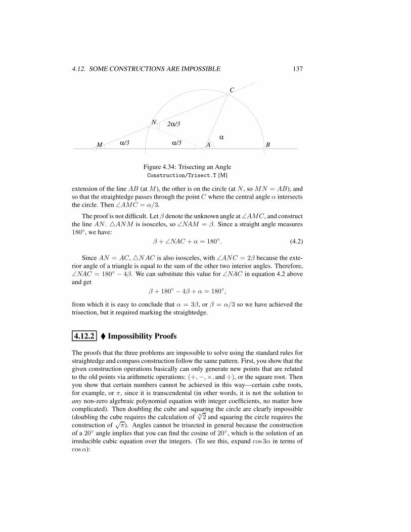
4.12. SOME CONSTRUCTIONS ARE IMPOSSIBLE 137
AA BB
CC
MM
NN
ααα/3α/3 α/3α/3
2α/32α/3
Figure 4.34: Trisecting an AngleConstruction/Trisect.T [M]
extension of the line AB (at M ), the other is on the circle (at N , so MN = AB), andso that the straightedge passes through the point C where the central angle α intersectsthe circle. Then ∠AMC = α/3.
The proof is not difficult. Let β denote the unknown angle at∠AMC, and constructthe line AN . 4ANM is isosceles, so ∠NAM = β. Since a straight angle measures180, we have:
β + ∠NAC + α = 180. (4.2)
Since AN = AC,4NAC is also isosceles, with ∠ANC = 2β because the exte-rior angle of a triangle is equal to the sum of the other two interior angles. Therefore,∠NAC = 180 − 4β. We can substitute this value for ∠NAC in equation 4.2 aboveand get
β + 180 − 4β + α = 180,
from which it is easy to conclude that α = 3β, or β = α/3 so we have achieved thetrisection, but it required marking the straightedge.
4.12.2 Impossibility Proofs
The proofs that the three problems are impossible to solve using the standard rules forstraightedge and compass construction follow the same pattern. First, you show that thegiven construction operations basically can only generate new points that are relatedto the old points via arithmetic operations: (+,−,×, and÷), or the square root. Thenyou show that certain numbers cannot be achieved in this way—certain cube roots,for example, or π, since it is transcendental (in other words, it is not the solution toany non-zero algebraic polynomial equation with integer coefficients, no matter howcomplicated). Then doubling the cube and squaring the circle are clearly impossible(doubling the cube requires the calculation of 3
√2 and squaring the circle requires the
construction of√π). Angles cannot be trisected in general because the construction
of a 20 angle implies that you can find the cosine of 20, which is the solution of anirreducible cubic equation over the integers. (To see this, expand cos 3α in terms ofcosα):
138 CHAPTER 4. GEOMETRIC CONSTRUCTION
cos 3α = cos(2α+ α) = cos 2α cosα− sin 2α sinα
= cos(α+ α) cosα− sin(α+ α) sinα
= (cos2 α− sin2 α) cosα− 2 sinα cosα sinα
= cos3 α− 3 sin2 α cosα
= cos3 α− 3(1− cos2 α) cosα
= 4 cos3 α− 3 cosα.
If 3α = 60, cos 3α = 1/2, so the equation for cosα is 1/2 = 4 cos3 α − 3 cosα,which is a cubic equation whose solution requires taking a cube root. In other words,if x = cos 20, then x is a solution to the equation
8x3 − 6x− 1 = 0.
Therefore, one cannot construct the cosine of 20, and hence one cannot constructa 20 angle. Since there is one particular angle that cannot be trisected, the problemhas no general solution. (Remember that some angles can be trisected—for example, itis pretty easy to trisect a 90 angle. In fact, it is often the case that the crackpot angletrisection solutions really trisect a single special angle.)
4.12.3 Constructible Regular Polygons
There are some “oddball” regular polygons that can be constructed. Without proof,here is the general formula.
If p1, p2, . . . , pn are distinct Fermat primes and k is any non-negative integer, thena regular polygon withm = 2kp1p2 · · · pn sides can be constructed with a straightedgeand compass. A Fermat prime is a prime number of the form 22i + 1, where i is aninteger. At the current time, only five different Fermat primes are known: 3, 5, 17, 257,and 65537, corresponding to i values of 0, 1, 2, 3, and 4. Thus it is possible to constructthe regular 17-gon (called a regular heptadecagon), and such a construction (but not aproof that the construction is correct) is shown in Section 2.1.3. But (in theory, at least),it is also possible to construct a regular 257-gon and a regular 65537-gon.
If you believe that it is possible to construct a regular equilateral triangle, a regularpentagon, et cetera, it is not hard to convince yourself that the other constructions of theform above can also be done. It is not so easy to show that these are the only possibleones.
For example, to construct a regular 60-gon (60 = 22 · 3 · 5), construct a regular3-gon (an equilateral triangle) and a regular 5-gon (a regular pentagon), and subtractthe central angles. One is a third of a circle and the other is a fifth of a circle, so thedifference is an angle that is 1/3−1/5 = 2/15 of a circle. Bisect that angle three timesto get an angle that is 1/60 of a circle.
4.13. 139 MORE PROBLEMS 139
4.13 139 More Problems
In [Wernick, 1982], William Wernick provided a list of 139 triangle construction prob-lems and gave the solutions for many of them. A more recent update on the state of theproblems appears in [Meyers, 1996].
Basically, all require the construction of a triangle given three located points chosenfrom among the following:
A, B, C, O the three points, and circumcenterMa, Mb, Mc, G feet of the three medians, and centroidHa, Hb, Hc, H feet of the three altitudes, and orthocenterTa, Tb, Tc, I feet of the internal angle bisectors, and incenter
In other words, a problem like “(A,Ma, G)” means “Construct the triangle4ABCgiven the points that identify the point A, the foot of the median beginning at A, andthe location of the centroid.”
At the time of publication of [Meyers, 1996], there were still 20 open problems,among them, the following: (O,Ha, Tb), (O,Ha, I), (O, Ta, Tb), (Ma,Mb, I).
Some of the constructions are impossible (for example (G,Ha, Hb), since it isequivalent to finding the root of an irreducible cubic equation) and some are trivial (forexample (A,B,C)).
4.14 Construction Exercises
The following exercises do not have solutions printed in the text. Unless they aremarked with a warning symbol, they are not too difficult. You can find the solutionsin Geometer files having the same name as the exercise. For example, to find thesolution to problem C15, view the file C15.T in the Construction directory.
1. [C1] Given an isosceles right triangle4ABC where ∠BAC = 90, find pointsH , I , J , and K such that H and I lie on BC, J lies on AB, and K lies on ACsuch that the quadrilateralHIJK is a square.
2. [C2] Given a semicircle centered at a point C with diameter AB, find points Iand J on AB, and points H and G on the semicircle such that the quadrilateralGHIJ is a square.
3. [C3] Given a quadrant of a circle (two radii that make an angle of 90 and theincluded arc), construct a new circle that is inscribed in the quadrant (in otherwords, the new circle is tangent to both rays and to the quarter arc of the quad-rant).
4. [C4] Given a pointA, a line L that does not pass throughA, and a point B on L,construct a circle passing throughA that is tangent to L at the point B.
5. [C5] Given a point A, a line L, and a length x, construct a circle passingthroughA of radius x that is tangent to the line L.
140 CHAPTER 4. GEOMETRIC CONSTRUCTION
6. [C6] Given a circle K, a line L, and a point A on L, construct a circle that istangent to K and tangent to L at the point A. (Hint: There may be more thanone solution.)
7. [C7] Given a point A and two straight lines L1 and L2, construct a line L thatpasses through A, and so that the angle L makes with L1 is the same angle thatit makes with L2.
8. [C8] Given two points A and B and a line L, find a point C on L such thatAC = BC.
9. [C9] Given two points A and B that both lie on the same side of a line L, find apoint C on L such that AC and BC make the same angle with L.
10. [C10] Given two points A and B that both lie on the same side of line L, find apoint C on L such that AC +BC is as small as possible. (Hint: This problem isrelated to the construction problem 9. Also remember that the shortest distancebetween two points is a line.)
11. [C11] Given a point A on a line L. If B is any point on L, divide the segmentAB into a given ratio by another point C (in other words, find C so that AC :BC = r for some fixed ratio r). What is the locus of all possible positions of thepoint C?
12. [C12] Trisect a right angle.13. [C13] If A and B lie on a line L, the two points C and D on L are said to
harmonically divide the segmentAB ifAC/CB = AD/DB. Given pointsA,B, and C on a line L, find the point D such that C and D harmonically divideAB.
14. [C14] Given three points, A, B, and C on the plane, but not collinear, findanother point X such that if L is any line through X , and if perpendiculars aredropped to L fromA, B, and C that meet L at A′, B′, and C ′, respectively, thenAA′ +BB′ = CC ′. (Hint: Can you find any particular lines that work?)
15. [C15] Given two non-parallel lines L1 and L2 and a radius r, construct a circleof radius r that is tangent to both L1 and L2.
16. [C16] Given a line L and two points A and B on the same side of L and not onL, and given an angle α, construct a point C on L such that ∠ACB = α. Forcertain configurations there may be no solutions.
17. [C17] Given a circle K, a point P , and a segment AB whose length is less thanthe diameter ofK, construct a line L through P which intersectsK at P1 and P2
such that AB = P1P2.18. [C18] Given two circles K1 andK2 that do not intersect, and such that neither
lies inside the other, together with a line segmentAB such that the length ofABis smaller than the diameter of the smaller circle, construct a line passing throughboth circles such that both of the chords cut by the circles have length equal toAB.
19. [C19] Given a circle K and two perpendicular radii of K, construct a line thatcuts the K twice and each chord so that the three segments of the line betweenthese intersections have equal length.
20. [C20] Given a triangle and a point on one of the sides of the triangle, constructa line through that point that divides the area of the triangle in half.
4.14. CONSTRUCTION EXERCISES 141
21. [C21] Given three lines in the plane, find all the circles that are simultaneouslytangent to all three lines.
22. [C22] Given any triangle4ABC, construct the point P inside4ABC such thatA(4APB) = A(4BPC) = A(4CPA).
23. [C23] Given a parallelogram and a point on one of its edges. Construct a linethrough that point that bisects the area of the parallelogram.
24. [C24] Given a convex quadrilateral ABCD, construct a line through A thatbisects the area of the quadrilateral.
25. [C25] Given a convex quadrilateral ABCD and a point P on segment AB,construct a line through P that bisects the area of ABCD.
26. [C26] Given a line L and two points P and Q on the same side of L, constructthe point R on L such that the angle ∠PRQ is as large as possible.
27. [C27] Given a circle K and two points P and Q on the outside of K, constructthe point R on K such that the angle ∠PRQ is as large as possible.
28. [C28] Given an isosceles triangle, construct an equilateral triangle of equalarea.
29. [C29] Given the two radii R and r, and a straight line L, construct two circleshaving those radii that are externally tangent to each other and are externallytangent to L.
30. [C30] Construct a circle that passes through two given points and is tangent to agiven circle.
31. [C31] Given a pointA, a circleK, and a point P onK, construct a circle passingthroughA that is tangent to K at P .
32. [C32] Given a circle K, a line L, and an angle α, construct a line tangent to Kwhich makes an angle α with L.
33. [C33] Suppose you are given two non-parallel lines that meet so far away thatyou cannot access the point of intersection. Construct the bisector of the angleformed by those two lines.
34. [C34] Given a circle K and two points P and Q. Construct a circle K1 passingthrough P and Q such that K1 intersects K at two diametrically opposite pointsof K.
35. [C35] Given the hypotenuse and area of a right triangle, construct the triangle.36. [C36] Given two points, construct two equal circles centered at those points such
that their common external tangent passes through a third given point.37. [C37] Given two points, construct two equal circles centered at those points such
that their common internal tangent passes through a third given point.38. [C38] Given two points and a circle, construct two circles of equal radius with
centers at the two points such that the common external tangent of the circles istangent to the given circle.
39. [C39] Given two concentric circles and a point P between them, construct thecircles tangent to both concentric circles and to P . What happens if P is outsidethe outer circle? Inside the inner circle?
40. [C40] Given three mutually tangent circles, construct the two Soddy circlesthat are tangent to all three of them. If the triangle whose vertices are the centersof the three circles, the centers of the Soddy circles are called the Soddy circles,centers.
142 CHAPTER 4. GEOMETRIC CONSTRUCTION
41. [C41] Given a right triangle and one of its legs, construct a point on that leg thatis equidistant from the hypotenuse and the vertex opposite the hypotenuse.
42. [C42] Given three points, construct a parallelogram such that the three points arethe midpoints of three of its sides.
43. [C43] Given a circle, a line, and two points, construct a circle passing throughthe two points whose common chord with the given circle is parallel to the givenline.
44. [C44] Construct4ABC given the length of side BC, the length of the bisectorof ∠ABC, and the size of ∠ABC.
45. [C45] Given segments of length x, y, and a, construct a segment of length bsuch that x : y = a2 : b2.
46. [C46] Construct 4ABC given BC, AC, and the length of the median from Ato the midpoint of BC.
47. [C47] Construct a quadrilateralABCD given ∠A, ∠B, ∠C, AB, and AD.48. [C48] Given two equal intersecting circles and an angle, construct two equal
chords of the two circles that meet at a point of intersection of the circles andform an angle equal to the given angle.
49. [C49] Given 4ABC construct its two Brocard points. A Brocard point is apoint Ω that makes equal angles with the sides of the triangle at the vertices. Inother words, find a point Ω such that ∠CAΩ = ∠ABΩ = ∠BCΩ. The otherBrocard point Ω′ makes the other angles equal: ∠BAΩ′ = ∠ACΩ′ = ∠CBΩ′.
50. [C50] Construct the midpoint M of segment AB using a compass alone.
Chapter 5Computer-Aided Proof
At the time this book is published, commercially available computer geometry pro-grams are not capable of constructing the proof of a geometric theorem, but they canbe used to aid in that process. In this chapter we will examine situations where testsand experiments can be done using Geometer to help construct a proof of geometrictheorems.
Perhaps the most common use of computer geometry programs is to search fortheorems and to provide evidence that a theorem or relationship is true. If you are toldthat the three altitudes of a triangle are concurrent at a point and you do not believe it,you can draw a triangle and its altitudes, and by moving the vertices of the triangle youcan see that (at least to the accuracy of the computer screen and your vision) that theyalways seem meet at a point in thousands of cases. This is not a proof, of course, butwhen one is convinced that a result is true, the proof is psychologically easier to find1.
1A great example of this is “the firing squad synchronization problem” described in [Minsky, 1967].
143
144 CHAPTER 5. COMPUTER-AIDED PROOF
Warning: All of the examples in this chapter rely on Geometer. Other computergeometry programs may have similar commands, but if you use one of those programs,you may need to have the Geometer reference manual available to fully understand allof the examples.
5.1 Finding the Steps in a Proof
At this point it might be good to review the example presented in Section 2.7.
A formal proof in geometry (and in mathematics in general) consists of a series ofstatements beginning with the given information, and where each statement after thatis a logical conclusion made from some combination of the previous statements. Everystatement in the proof will be a consequence of the initial information, and the finalstatement is the theorem which was to be proved.
Proofs that appear in mathematical texts and journals may differ from this some-what to make them easier to understand, but it should be clear how to convert them intoformal proofs. For example, quite often you will see something like this: “If we canshow that X is true, then our theorem is true because . . . ”. Later, there is a line likethis: “So since we now know that X is true, we are finished.” The formal proof wouldcontain those statements in the opposite order, but the rearrangement above probablymakes it easier for the reader to see where the argument is going.
The idea of a formal proof is driven home by the “T” proofs required in most highschool geometry classes. Students draw a giant “T” on their paper, and every statementon the left has a corresponding reason on the right why it is true. The final statementon the left is the theorem to be proved.
For any interesting theorem, the proof does not come out of a mathematician’s headthat way. A bunch of things seem to be true, some depending on others, and the jobof constructing a proof sometimes simply amounts to sorting these into a logical order.More often, however, it is difficult to discover many of those “true things”.
One of the most powerful features of Geometer is that it can often provide a longlist of possible entries for the left column of a “T” proof. Of course you then need tosort them into a logical order and provide reasons why each is true.
5.2 Testing a Diagram
Geometer contains a pair of commands, Test Diagram and End Test that provide a listof relationships that seem to be true.
The problem remained an unsolved research problem for years, but as soon as the first solution was found,it became a standard, not too difficult exercise in computer science texts. Another good example is thefollowing problem: “Prove that the number between any pair of twin primes except the pair (3, 5) is divisibleby 6.” Most mathematicians panic at this point, having no idea how to proceed since so little is known abouttwin primes. But as soon as you add, “You have 10 seconds to solve it”, almost all can prove it instantly.
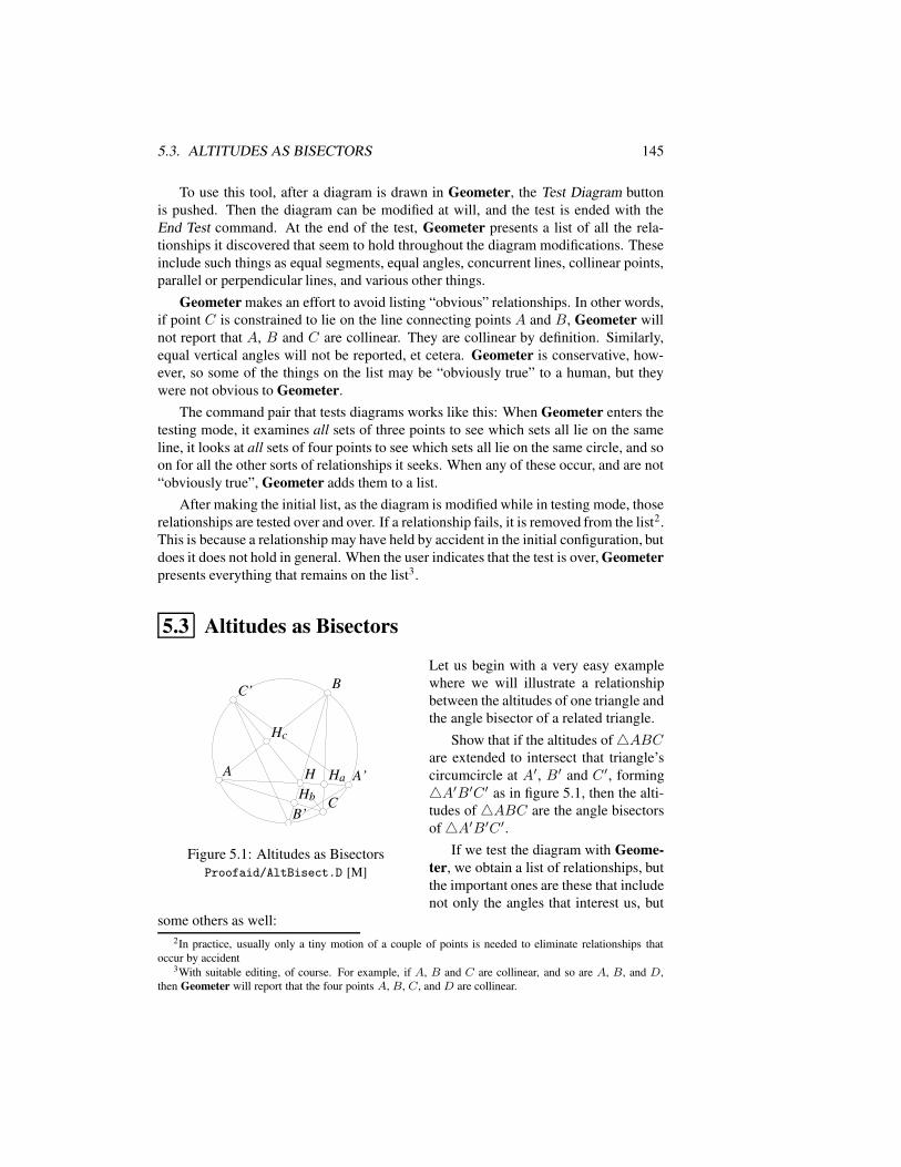
5.3. ALTITUDES AS BISECTORS 145
To use this tool, after a diagram is drawn in Geometer, the Test Diagram buttonis pushed. Then the diagram can be modified at will, and the test is ended with theEnd Test command. At the end of the test, Geometer presents a list of all the rela-tionships it discovered that seem to hold throughout the diagram modifications. Theseinclude such things as equal segments, equal angles, concurrent lines, collinear points,parallel or perpendicular lines, and various other things.
Geometer makes an effort to avoid listing “obvious” relationships. In other words,if point C is constrained to lie on the line connecting points A and B, Geometer willnot report that A, B and C are collinear. They are collinear by definition. Similarly,equal vertical angles will not be reported, et cetera. Geometer is conservative, how-ever, so some of the things on the list may be “obviously true” to a human, but theywere not obvious to Geometer.
The command pair that tests diagrams works like this: When Geometer enters thetesting mode, it examines all sets of three points to see which sets all lie on the sameline, it looks at all sets of four points to see which sets all lie on the same circle, and soon for all the other sorts of relationships it seeks. When any of these occur, and are not“obviously true”, Geometer adds them to a list.
After making the initial list, as the diagram is modified while in testing mode, thoserelationships are tested over and over. If a relationship fails, it is removed from the list2.This is because a relationship may have held by accident in the initial configuration, butdoes it does not hold in general. When the user indicates that the test is over, Geometerpresents everything that remains on the list3.
5.3 Altitudes as Bisectors
AA
BB
CCB’B’
A’A’
C’C’
HH HaHaHbHb
HcHc
Figure 5.1: Altitudes as BisectorsProofaid/AltBisect.D [M]
Let us begin with a very easy examplewhere we will illustrate a relationshipbetween the altitudes of one triangle andthe angle bisector of a related triangle.
Show that if the altitudes of4ABCare extended to intersect that triangle’scircumcircle at A′, B′ and C ′, forming4A′B′C ′ as in figure 5.1, then the alti-tudes of4ABC are the angle bisectorsof4A′B′C ′.
If we test the diagram with Geome-ter, we obtain a list of relationships, butthe important ones are these that includenot only the angles that interest us, but
some others as well:2In practice, usually only a tiny motion of a couple of points is needed to eliminate relationships that
occur by accident3With suitable editing, of course. For example, if A, B and C are collinear, and so are A, B, and D,
then Geometer will report that the four points A, B, C, and D are collinear.
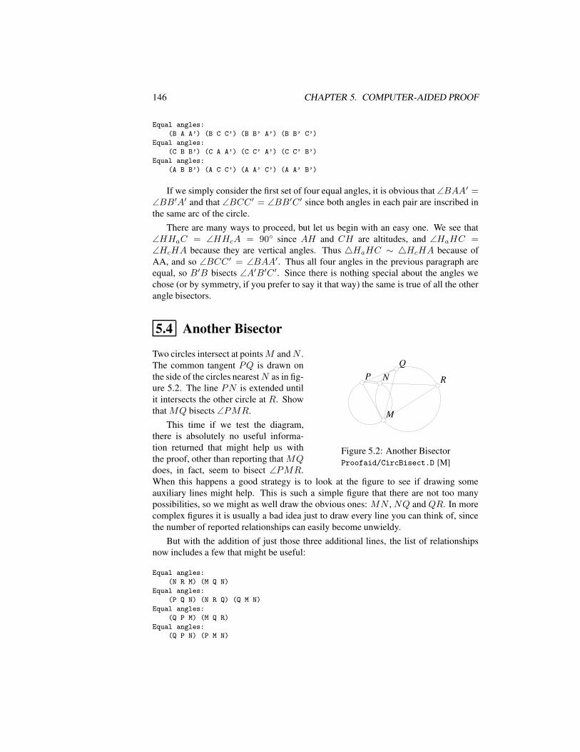
146 CHAPTER 5. COMPUTER-AIDED PROOF
Equal angles:
(B A A’) (B C C’) (B B’ A’) (B B’ C’)
Equal angles:
(C B B’) (C A A’) (C C’ A’) (C C’ B’)
Equal angles:
(A B B’) (A C C’) (A A’ C’) (A A’ B’)
If we simply consider the first set of four equal angles, it is obvious that ∠BAA′ =∠BB′A′ and that ∠BCC ′ = ∠BB′C ′ since both angles in each pair are inscribed inthe same arc of the circle.
There are many ways to proceed, but let us begin with an easy one. We see that∠HHaC = ∠HHcA = 90 since AH and CH are altitudes, and ∠HaHC =∠HcHA because they are vertical angles. Thus 4HaHC ∼ 4HcHA because ofAA, and so ∠BCC ′ = ∠BAA′. Thus all four angles in the previous paragraph areequal, so B′B bisects ∠A′B′C ′. Since there is nothing special about the angles wechose (or by symmetry, if you prefer to say it that way) the same is true of all the otherangle bisectors.
5.4 Another Bisector
NN
MM
PPQQ
RR
Figure 5.2: Another BisectorProofaid/CircBisect.D [M]
Two circles intersect at pointsM andN .The common tangent PQ is drawn onthe side of the circles nearestN as in fig-ure 5.2. The line PN is extended untilit intersects the other circle at R. Showthat MQ bisects ∠PMR.
This time if we test the diagram,there is absolutely no useful informa-tion returned that might help us withthe proof, other than reporting that MQdoes, in fact, seem to bisect ∠PMR.When this happens a good strategy is to look at the figure to see if drawing someauxiliary lines might help. This is such a simple figure that there are not too manypossibilities, so we might as well draw the obvious ones: MN , NQ and QR. In morecomplex figures it is usually a bad idea just to draw every line you can think of, sincethe number of reported relationships can easily become unwieldy.
But with the addition of just those three additional lines, the list of relationshipsnow includes a few that might be useful:
Equal angles:
(N R M) (M Q N)
Equal angles:
(P Q N) (N R Q) (Q M N)
Equal angles:
(Q P M) (M Q R)
Equal angles:
(Q P N) (P M N)
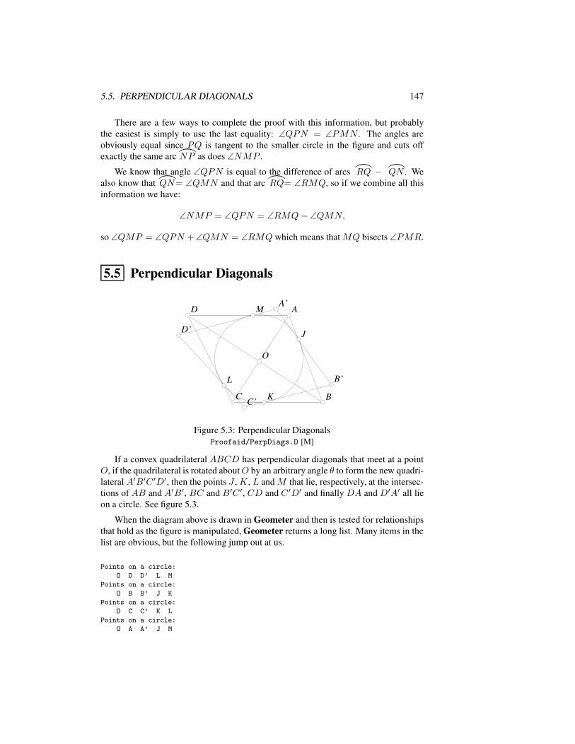
5.5. PERPENDICULAR DIAGONALS 147
There are a few ways to complete the proof with this information, but probablythe easiest is simply to use the last equality: ∠QPN = ∠PMN . The angles areobviously equal since PQ is tangent to the smaller circle in the figure and cuts offexactly the same arc
)
NP as does ∠NMP .
We know that angle ∠QPN is equal to the difference of arcs
)
RQ − )
QN . Wealso know that
)
QN= ∠QMN and that arc
)
RQ= ∠RMQ, so if we combine all thisinformation we have:
∠NMP = ∠QPN = ∠RMQ− ∠QMN,
so ∠QMP = ∠QPN +∠QMN = ∠RMQ which means that MQ bisects ∠PMR.
5.5 Perpendicular Diagonals
OO
AA
CC BB
DDA’A’
B’B’
C’C’
D’D’ JJ
KK
LL
MM
Figure 5.3: Perpendicular DiagonalsProofaid/PerpDiags.D [M]
If a convex quadrilateral ABCD has perpendicular diagonals that meet at a pointO, if the quadrilateral is rotated aboutO by an arbitrary angle θ to form the new quadri-lateral A′B′C ′D′, then the points J , K, L and M that lie, respectively, at the intersec-tions of AB and A′B′, BC and B′C ′, CD and C ′D′ and finally DA and D′A′ all lieon a circle. See figure 5.3.
When the diagram above is drawn in Geometer and then is tested for relationshipsthat hold as the figure is manipulated, Geometer returns a long list. Many items in thelist are obvious, but the following jump out at us.
Points on a circle:
O D D’ L M
Points on a circle:
O B B’ J K
Points on a circle:
O C C’ K L
Points on a circle:
O A A’ J M
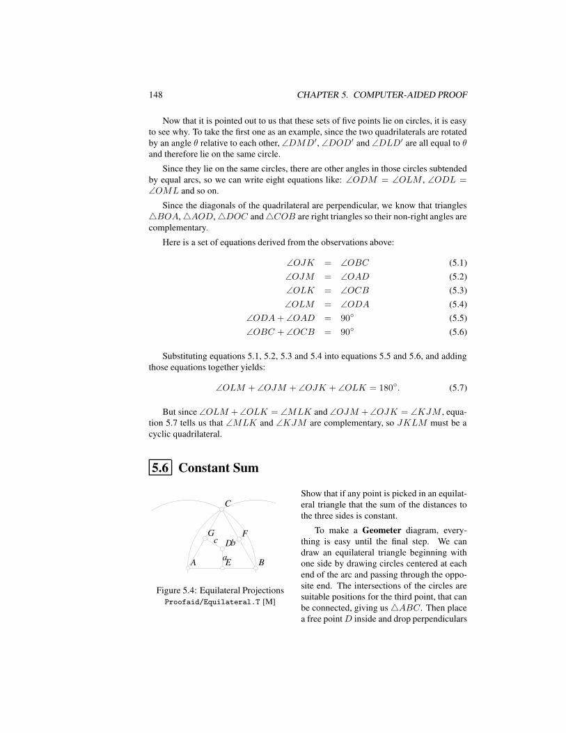
148 CHAPTER 5. COMPUTER-AIDED PROOF
Now that it is pointed out to us that these sets of five points lie on circles, it is easyto see why. To take the first one as an example, since the two quadrilaterals are rotatedby an angle θ relative to each other, ∠DMD′, ∠DOD′ and ∠DLD′ are all equal to θand therefore lie on the same circle.
Since they lie on the same circles, there are other angles in those circles subtendedby equal arcs, so we can write eight equations like: ∠ODM = ∠OLM , ∠ODL =∠OML and so on.
Since the diagonals of the quadrilateral are perpendicular, we know that triangles4BOA,4AOD,4DOC and4COB are right triangles so their non-right angles arecomplementary.
Here is a set of equations derived from the observations above:
∠OJK = ∠OBC (5.1)∠OJM = ∠OAD (5.2)∠OLK = ∠OCB (5.3)∠OLM = ∠ODA (5.4)
∠ODA+ ∠OAD = 90 (5.5)∠OBC + ∠OCB = 90 (5.6)
Substituting equations 5.1, 5.2, 5.3 and 5.4 into equations 5.5 and 5.6, and addingthose equations together yields:
∠OLM + ∠OJM + ∠OJK + ∠OLK = 180. (5.7)
But since ∠OLM +∠OLK = ∠MLK and ∠OJM +∠OJK = ∠KJM , equa-tion 5.7 tells us that ∠MLK and ∠KJM are complementary, so JKLM must be acyclic quadrilateral.
5.6 Constant Sum
aa
bbcc
AA BB
CC
DD
EE
FFGG
Figure 5.4: Equilateral ProjectionsProofaid/Equilateral.T [M]
Show that if any point is picked in an equilat-eral triangle that the sum of the distances tothe three sides is constant.
To make a Geometer diagram, every-thing is easy until the final step. We candraw an equilateral triangle beginning withone side by drawing circles centered at eachend of the arc and passing through the oppo-site end. The intersections of the circles aresuitable positions for the third point, that canbe connected, giving us4ABC. Then placea free pointD inside and drop perpendiculars
5.6. CONSTANT SUM 149
to each side. Geometer can only calculate the distances between points, so find the in-tersections, and you should have a diagram like that in figure 5.4. It would probably bebetter to give the circles the invisible color to simplify the final diagram.
Now we would like to display the lengths of the three segments DE, DF andDG. This is also not hard. Select one of the lines and then choose the Display Valuecommand from the Edit pulldown menu, you will get something like “l4 = 0.425”displayed in the upper left of the Geometer window. So far you have not given thatline a name (points receive names by default but other geometric figures do not). Youcan do so by selecting it (it should still be selected if you just issued the Display Valuecommand) and issue the Edit Name command in the Edit pulldown. This brings up adialog box into which you can type the name of the line. In figure 5.4, the lines havebeen named a, b and c and the display for each has been toggled on. (The keyboardshortcut for those commands is ctrl-T to toggle the display and ctrl-n to change thename.)
When the lengths are displayed, they appear in the upper left of the diagram likethis: “a = 0.514”.
As you move point D around, the values of the lengths are continuously updated,but it is still a bit of work to add the three each time to assure yourself that the sum isconstant. Why not have Geometer do that for you? To do this you will need to edit thetext version of the file. The entire modified file is listed below since you need to knowthe internal names that Geometer gave to the various points before you can type in thefinal code.
.geometry "version 0.60";
v1 = .free(-0.92, -0.871156, "A");
v2 = .free(0.893333, -0.871156, "B");
c1 = .c.vv(v1, v2);
c2 = .c.vv(v2, v1);
v3 = .v.cc(c1, c2, 2, "C");
l1 = .l.vv(v1, v2);
l2 = .l.vv(v2, v3);
l3 = .l.vv(v3, v1);
v4 = .free(0.026616, -0.372624, "D");
l4 = .l.vlperp(v4, l1, .display, "a");
l5 = .l.vlperp(v4, l2, .display, "b");
l6 = .l.vlperp(v4, l3, .display, "c");
v5 = .v.ll(l1, l4, "E");
v6 = .v.ll(l2, l5, "F");
v7 = .v.ll(l3, l6, "G");
DE = .f.vv(v4, v5);
DF = .f.vv(v4, v6);
DG = .f.vv(v4, v7);
S = .f.rpn(DE, DF, DG, .add, .add, "Sum");
The three lines beginning with DE, DF and DG set those names to be the distancebetween the points in parentheses. The function .f.vv makes a floating point number(.f) from the distance between two points (.vv). The final line performs a floating pointcalculation with Geometer’s built-in rpn4 calculator. The three lengths are pushed on
4Reverse Polish Notation.
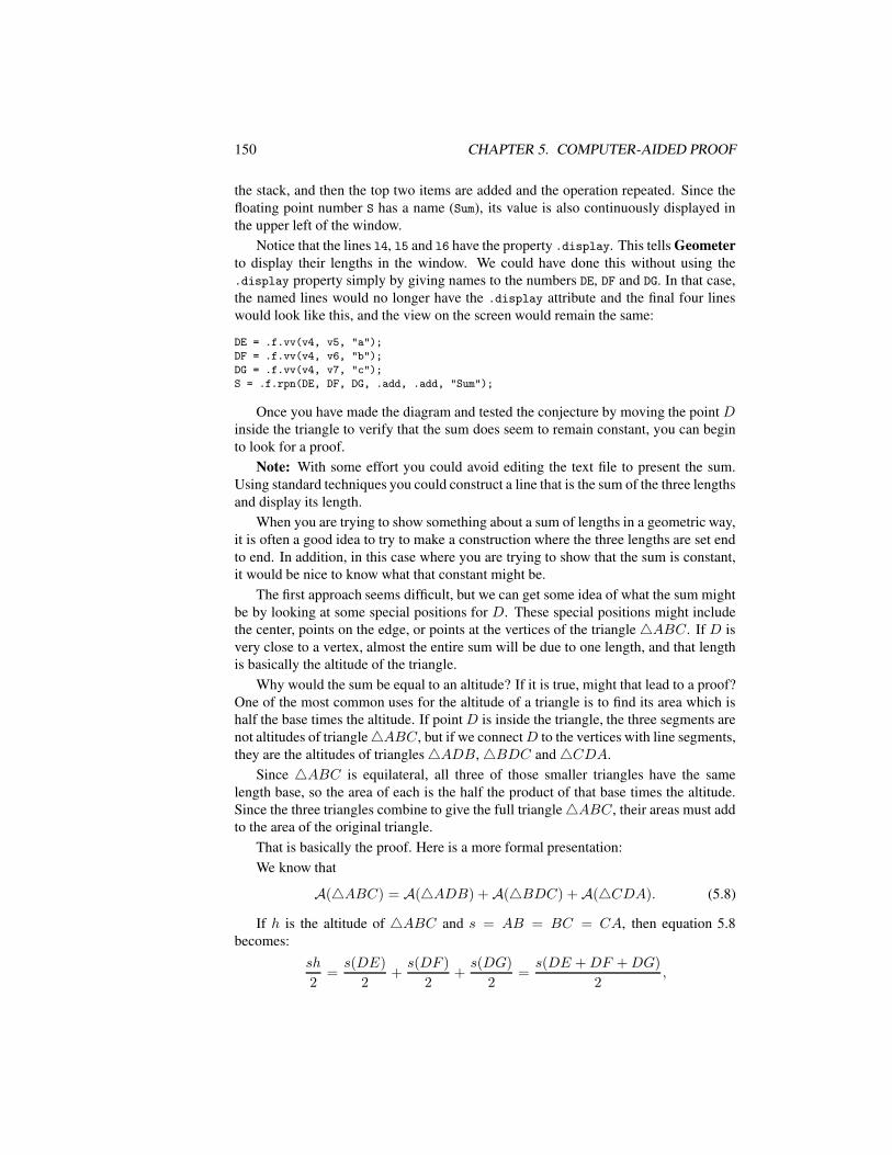
150 CHAPTER 5. COMPUTER-AIDED PROOF
the stack, and then the top two items are added and the operation repeated. Since thefloating point number S has a name (Sum), its value is also continuously displayed inthe upper left of the window.
Notice that the lines l4, l5 and l6 have the property .display. This tells Geometerto display their lengths in the window. We could have done this without using the.display property simply by giving names to the numbers DE, DF and DG. In that case,the named lines would no longer have the .display attribute and the final four lineswould look like this, and the view on the screen would remain the same:
DE = .f.vv(v4, v5, "a");
DF = .f.vv(v4, v6, "b");
DG = .f.vv(v4, v7, "c");
S = .f.rpn(DE, DF, DG, .add, .add, "Sum");
Once you have made the diagram and tested the conjecture by moving the point Dinside the triangle to verify that the sum does seem to remain constant, you can beginto look for a proof.
Note: With some effort you could avoid editing the text file to present the sum.Using standard techniques you could construct a line that is the sum of the three lengthsand display its length.
When you are trying to show something about a sum of lengths in a geometric way,it is often a good idea to try to make a construction where the three lengths are set endto end. In addition, in this case where you are trying to show that the sum is constant,it would be nice to know what that constant might be.
The first approach seems difficult, but we can get some idea of what the sum mightbe by looking at some special positions for D. These special positions might includethe center, points on the edge, or points at the vertices of the triangle4ABC. If D isvery close to a vertex, almost the entire sum will be due to one length, and that lengthis basically the altitude of the triangle.
Why would the sum be equal to an altitude? If it is true, might that lead to a proof?One of the most common uses for the altitude of a triangle is to find its area which ishalf the base times the altitude. If point D is inside the triangle, the three segments arenot altitudes of triangle4ABC, but if we connectD to the vertices with line segments,they are the altitudes of triangles4ADB,4BDC and4CDA.
Since 4ABC is equilateral, all three of those smaller triangles have the samelength base, so the area of each is the half the product of that base times the altitude.Since the three triangles combine to give the full triangle4ABC, their areas must addto the area of the original triangle.
That is basically the proof. Here is a more formal presentation:We know that
A(4ABC) = A(4ADB) +A(4BDC) +A(4CDA). (5.8)
If h is the altitude of 4ABC and s = AB = BC = CA, then equation 5.8becomes:
sh
2=s(DE)
2+s(DF )
2+s(DG)
2=s(DE +DF +DG)
2,
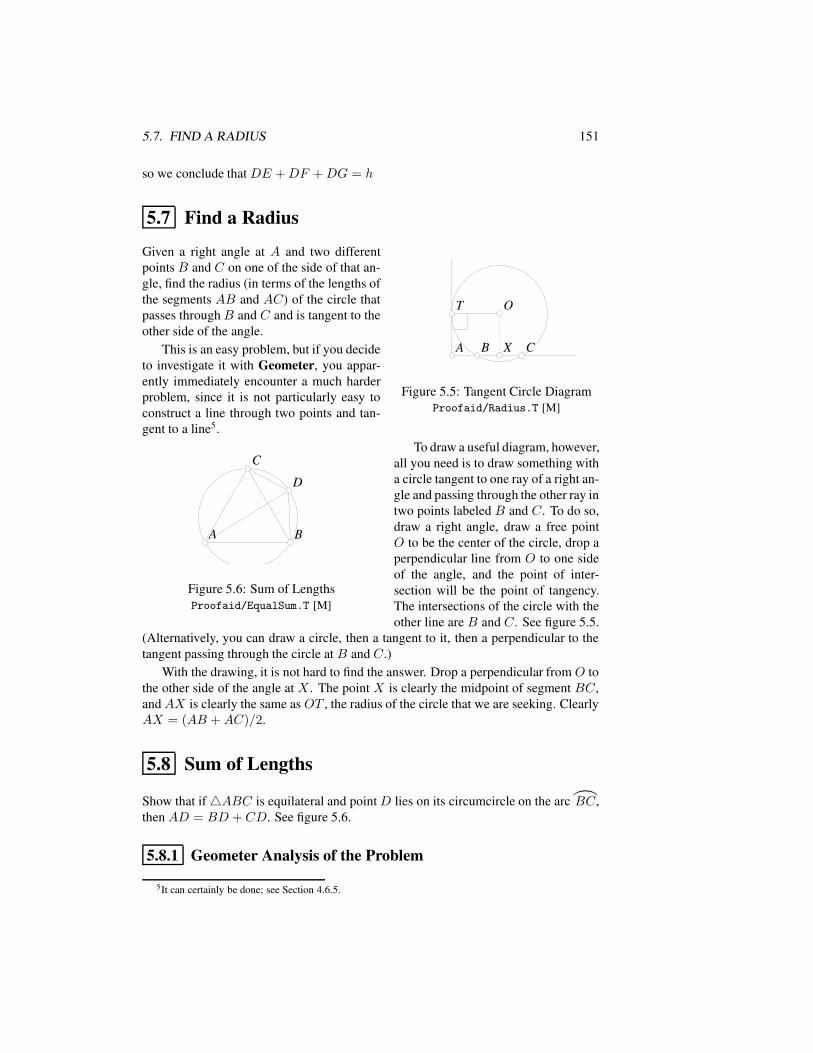
5.7. FIND A RADIUS 151
so we conclude that DE +DF +DG = h
5.7 Find a Radius
AA
OOTT
BB CCXX
Figure 5.5: Tangent Circle DiagramProofaid/Radius.T [M]
Given a right angle at A and two differentpoints B and C on one of the side of that an-gle, find the radius (in terms of the lengths ofthe segments AB and AC) of the circle thatpasses throughB and C and is tangent to theother side of the angle.
This is an easy problem, but if you decideto investigate it with Geometer, you appar-ently immediately encounter a much harderproblem, since it is not particularly easy toconstruct a line through two points and tan-gent to a line5.
AA BB
CC
DD
Figure 5.6: Sum of LengthsProofaid/EqualSum.T [M]
To draw a useful diagram, however,all you need is to draw something witha circle tangent to one ray of a right an-gle and passing through the other ray intwo points labeled B and C. To do so,draw a right angle, draw a free pointO to be the center of the circle, drop aperpendicular line from O to one sideof the angle, and the point of inter-section will be the point of tangency.The intersections of the circle with theother line are B and C. See figure 5.5.
(Alternatively, you can draw a circle, then a tangent to it, then a perpendicular to thetangent passing through the circle at B and C.)
With the drawing, it is not hard to find the answer. Drop a perpendicular from O tothe other side of the angle at X . The point X is clearly the midpoint of segment BC,andAX is clearly the same as OT , the radius of the circle that we are seeking. ClearlyAX = (AB +AC)/2.
5.8 Sum of Lengths
Show that if4ABC is equilateral and point D lies on its circumcircle on the arc
)
BC,then AD = BD + CD. See figure 5.6.
5.8.1 Geometer Analysis of the Problem
5It can certainly be done; see Section 4.6.5.
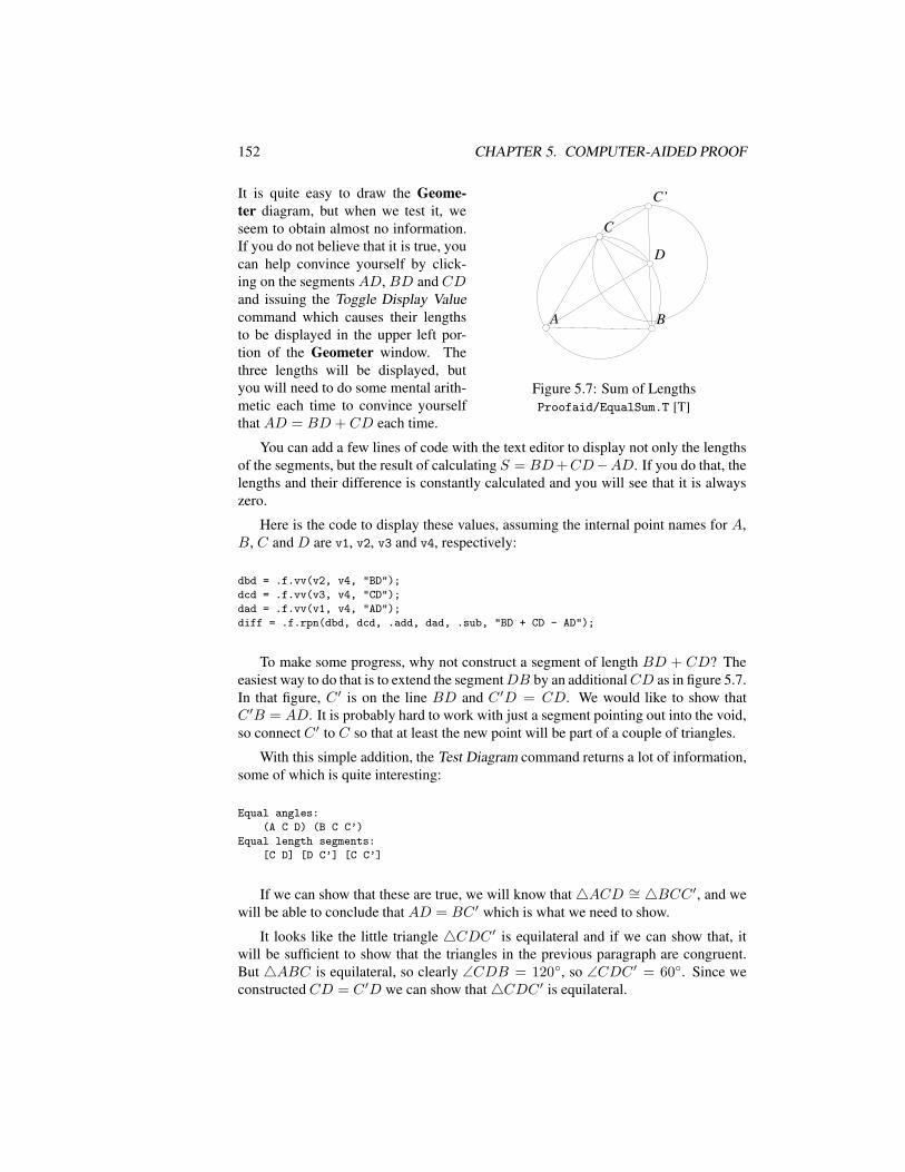
152 CHAPTER 5. COMPUTER-AIDED PROOF
AA BB
CC
DD
C’C’
Figure 5.7: Sum of LengthsProofaid/EqualSum.T [T]
It is quite easy to draw the Geome-ter diagram, but when we test it, weseem to obtain almost no information.If you do not believe that it is true, youcan help convince yourself by click-ing on the segments AD, BD and CDand issuing the Toggle Display Valuecommand which causes their lengthsto be displayed in the upper left por-tion of the Geometer window. Thethree lengths will be displayed, butyou will need to do some mental arith-metic each time to convince yourselfthat AD = BD + CD each time.
You can add a few lines of code with the text editor to display not only the lengthsof the segments, but the result of calculating S = BD+CD−AD. If you do that, thelengths and their difference is constantly calculated and you will see that it is alwayszero.
Here is the code to display these values, assuming the internal point names for A,B, C and D are v1, v2, v3 and v4, respectively:
dbd = .f.vv(v2, v4, "BD");
dcd = .f.vv(v3, v4, "CD");
dad = .f.vv(v1, v4, "AD");
diff = .f.rpn(dbd, dcd, .add, dad, .sub, "BD + CD - AD");
To make some progress, why not construct a segment of length BD + CD? Theeasiest way to do that is to extend the segmentDB by an additionalCD as in figure 5.7.In that figure, C ′ is on the line BD and C ′D = CD. We would like to show thatC ′B = AD. It is probably hard to work with just a segment pointing out into the void,so connect C ′ to C so that at least the new point will be part of a couple of triangles.
With this simple addition, the Test Diagram command returns a lot of information,some of which is quite interesting:
Equal angles:
(A C D) (B C C’)
Equal length segments:
[C D] [D C’] [C C’]
If we can show that these are true, we will know that4ACD ∼= 4BCC ′, and wewill be able to conclude that AD = BC ′ which is what we need to show.
It looks like the little triangle 4CDC ′ is equilateral and if we can show that, itwill be sufficient to show that the triangles in the previous paragraph are congruent.But 4ABC is equilateral, so clearly ∠CDB = 120, so ∠CDC ′ = 60. Since weconstructed CD = C ′D we can show that4CDC ′ is equilateral.
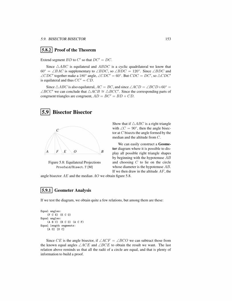
5.9. BISECTOR BISECTOR 153
5.8.2 Proof of the Theorem
Extend segment BD to C ′ so that DC ′ = DC.
Since 4ABC is equilateral and ABDC is a cyclic quadrilateral we know that60 = ∠BAC is supplementary to ∠BDC, so ∠BDC = 120. Since ∠BDC and∠CDC ′ together make a 180 angle, ∠CDC ′ = 60. But CDC = DC ′, so4CDC ′is equilateral and thus CC ′ = CD.
Since4ABC is also equilateral,AC = BC, and since∠ACD = ∠BCD+60 =∠BCC ′ we can conclude that 4ACB ∼= 4BCC ′. Since the corresponding parts ofcongruent triangles are congruent,AD = BC ′ = BD + CD.
5.9 Bisector Bisector
AA BBOO
CC
EEFF
Figure 5.8: Equilateral ProjectionsProofaid/Bisect.T [M]
Show that if4ABC is a right trianglewith ∠C = 90, then the angle bisec-tor at C bisects the angle formed by themedian and the altitude from C.
We can easily construct a Geome-ter diagram where it is possible to dis-play all possible right triangle shapesby beginning with the hypotenuse ABand choosing C to lie on the circlewhose diameter is the hypotenuseAB.If we then draw in the altitude AF , the
angle bisector AE and the median AO we obtain figure 5.8.
5.9.1 Geometer Analysis
If we test the diagram, we obtain quite a few relations, but among them are these:
Equal angles:
(F C E) (E C O)
Equal angles:
(A B C) (B C O) (A C F)
Equal length segments:
[A O] [O C]
Since CE is the angle bisector, if ∠ACF = ∠BCO we can subtract those fromthe known equal angles ∠ACE and ∠BCE to obtain the result we want. The lastrelation above reminds us that all the radii of a circle are equal, and that is plenty ofinformation to build a proof.
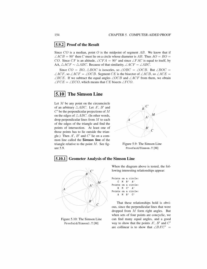
154 CHAPTER 5. COMPUTER-AIDED PROOF
5.9.2 Proof of the Result
Since CO is a median, point O is the midpoint of segment AB. We know that if∠ACB = 90 then C must lie on a circle whose diameter is AB. Thus AO = BO =CO. Since CF is an altitude, ∠CFA = 90 and since ∠FAC is equal to itself, byAA,4ACF ∼ 4ABC. Because of that similarity, ∠ACF = ∠ABC.
Since CO = BO, 4BOC is isosceles, so ∠OBC = ∠OCB. But ∠BOC =∠ACF , so ∠ACF = ∠OCB. Segment CE is the bisector of ∠ACB, so ∠ACE =∠BCE. If we subtract the equal angles ∠OCB and ∠ACF from them, we obtain∠FCE = ∠ECO, which means that CE bisects ∠FCO.
5.10 The Simson Line
AA
BB
CC
MM
B’B’
C’C’
A’A’
Figure 5.9: The Simson LineProofaid/Simson.T [M]
Let M be any point on the circumcircleof an arbitrary 4ABC. Let A′, B′ andC ′ be the perpendicular projections of Mon the edges of4ABC. (In other words,drop perpendicular lines from M to eachof the edges of the triangle and find thepoints of intersection. At least one ofthose points has to lie outside the trian-gle.) Then A′, B′ and C ′ lie on a com-mon line called the Simson line of thetriangle relative to the point M . See fig-ure 5.9.
5.10.1 Geometer Analysis of the Simson Line
AA
BB
CC
MM
B’B’
C’C’
A’A’
Figure 5.10: The Simson LineProofaid/Simson1.T [M]
When the diagram above is tested, the fol-lowing interesting relationships appear:
Points on a circle:
C M B’ A’
Points on a circle:
B M C’ A’
Points on a circle:
A M B’ C’
That these relationships hold is obvi-ous, since the perpendicular lines that weredropped from M form right angles. Butwhen sets of four points are concyclic, wecan find many equal angles, and a goodway to show that the points A′, B′ and C ′
are collinear is to show that ∠BA′C ′ =
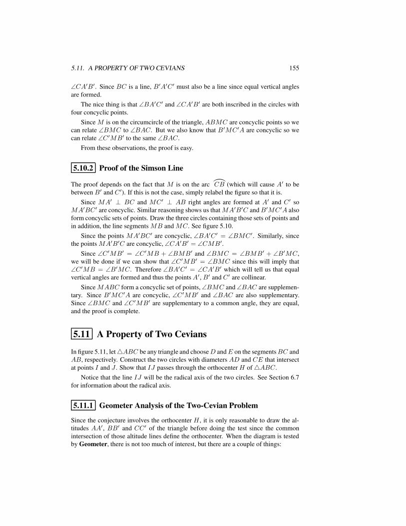
5.11. A PROPERTY OF TWO CEVIANS 155
∠CA′B′. Since BC is a line, B′A′C ′ must also be a line since equal vertical anglesare formed.
The nice thing is that ∠BA′C ′ and ∠CA′B′ are both inscribed in the circles withfour concyclic points.
Since M is on the circumcircle of the triangle, ABMC are concyclic points so wecan relate ∠BMC to ∠BAC. But we also know that B ′MC ′A are concyclic so wecan relate ∠C ′MB′ to the same ∠BAC.
From these observations, the proof is easy.
5.10.2 Proof of the Simson Line
The proof depends on the fact that M is on the arc
)
CB (which will cause A′ to bebetween B′ and C ′). If this is not the case, simply relabel the figure so that it is.
Since MA′ ⊥ BC and MC ′ ⊥ AB right angles are formed at A′ and C ′ soMA′BC ′ are concyclic. Similar reasoning shows us thatMA′B′C andB′MC ′A alsoform concyclic sets of points. Draw the three circles containing those sets of points andin addition, the line segments MB and MC. See figure 5.10.
Since the points MA′BC ′ are concyclic, ∠BA′C ′ = ∠BMC ′. Similarly, sincethe points MA′B′C are concyclic, ∠CA′B′ = ∠CMB′.
Since ∠C ′MB′ = ∠C ′MB + ∠BMB′ and ∠BMC = ∠BMB′ + ∠B′MC,we will be done if we can show that ∠C ′MB′ = ∠BMC since this will imply that∠C ′MB = ∠B′MC. Therefore ∠BA′C ′ = ∠CA′B′ which will tell us that equalvertical angles are formed and thus the points A′, B′ and C ′ are collinear.
SinceMABC form a concyclic set of points, ∠BMC and ∠BAC are supplemen-tary. Since B′MC ′A are concyclic, ∠C ′MB′ and ∠BAC are also supplementary.Since ∠BMC and ∠C ′MB′ are supplementary to a common angle, they are equal,and the proof is complete.
5.11 A Property of Two Cevians
In figure 5.11, let4ABC be any triangle and chooseD andE on the segmentsBC andAB, respectively. Construct the two circles with diameters AD and CE that intersectat points I and J . Show that IJ passes through the orthocenterH of4ABC.
Notice that the line IJ will be the radical axis of the two circles. See Section 6.7for information about the radical axis.
5.11.1 Geometer Analysis of the Two-Cevian Problem
Since the conjecture involves the orthocenter H , it is only reasonable to draw the al-titudes AA′, BB′ and CC ′ of the triangle before doing the test since the commonintersection of those altitude lines define the orthocenter. When the diagram is testedby Geometer, there is not too much of interest, but there are a couple of things:
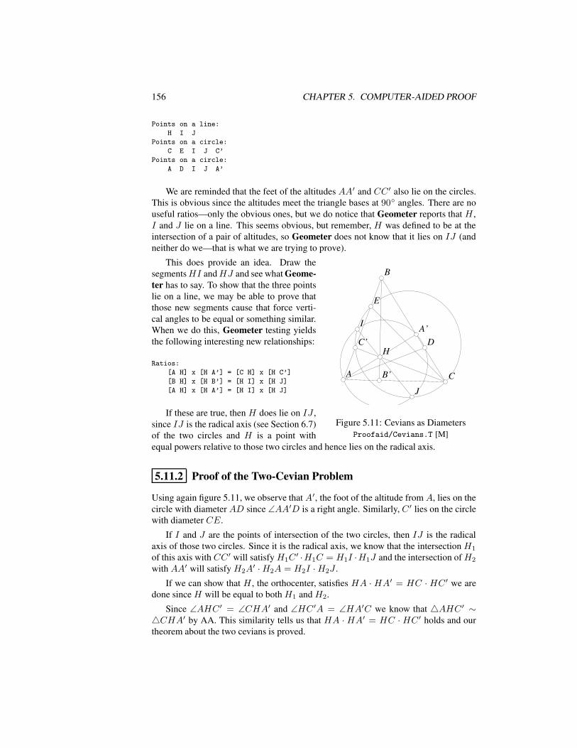
156 CHAPTER 5. COMPUTER-AIDED PROOF
Points on a line:
H I J
Points on a circle:
C E I J C’
Points on a circle:
A D I J A’
We are reminded that the feet of the altitudes AA′ and CC ′ also lie on the circles.This is obvious since the altitudes meet the triangle bases at 90 angles. There are nouseful ratios—only the obvious ones, but we do notice that Geometer reports that H ,I and J lie on a line. This seems obvious, but remember, H was defined to be at theintersection of a pair of altitudes, so Geometer does not know that it lies on IJ (andneither do we—that is what we are trying to prove).
AA
BB
CC
HHDD
EE
II
JJ
A’A’
B’B’
C’C’
Figure 5.11: Cevians as DiametersProofaid/Cevians.T [M]
This does provide an idea. Draw thesegmentsHI andHJ and see what Geome-ter has to say. To show that the three pointslie on a line, we may be able to prove thatthose new segments cause that force verti-cal angles to be equal or something similar.When we do this, Geometer testing yieldsthe following interesting new relationships:
Ratios:
[A H] x [H A’] = [C H] x [H C’]
[B H] x [H B’] = [H I] x [H J]
[A H] x [H A’] = [H I] x [H J]
If these are true, then H does lie on IJ ,since IJ is the radical axis (see Section 6.7)of the two circles and H is a point withequal powers relative to those two circles and hence lies on the radical axis.
5.11.2 Proof of the Two-Cevian Problem
Using again figure 5.11, we observe that A′, the foot of the altitude from A, lies on thecircle with diameter AD since ∠AA′D is a right angle. Similarly, C ′ lies on the circlewith diameter CE.
If I and J are the points of intersection of the two circles, then IJ is the radicalaxis of those two circles. Since it is the radical axis, we know that the intersection H1
of this axis with CC ′ will satisfy H1C′ ·H1C = H1I ·H1J and the intersection ofH2
with AA′ will satisfy H2A′ ·H2A = H2I ·H2J .
If we can show that H , the orthocenter, satisfies HA · HA′ = HC · HC ′ we aredone since H will be equal to both H1 and H2.
Since ∠AHC ′ = ∠CHA′ and ∠HC ′A = ∠HA′C we know that 4AHC ′ ∼4CHA′ by AA. This similarity tells us that HA · HA′ = HC · HC ′ holds and ourtheorem about the two cevians is proved.
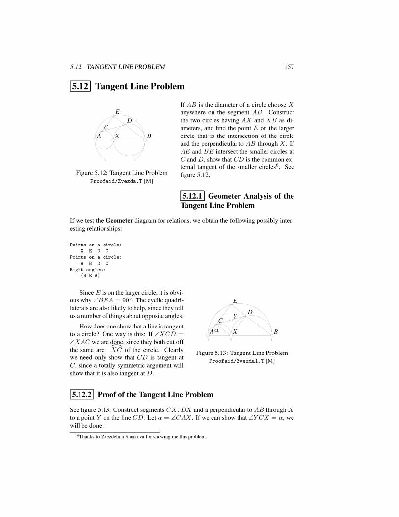
5.12. TANGENT LINE PROBLEM 157
5.12 Tangent Line Problem
AA BBXX
EEDD
CC
Figure 5.12: Tangent Line ProblemProofaid/Zvezda.T [M]
If AB is the diameter of a circle choose Xanywhere on the segment AB. Constructthe two circles having AX and XB as di-ameters, and find the point E on the largercircle that is the intersection of the circleand the perpendicular to AB through X . IfAE and BE intersect the smaller circles atC and D, show that CD is the common ex-ternal tangent of the smaller circles6. Seefigure 5.12.
5.12.1 Geometer Analysis of theTangent Line Problem
If we test the Geometer diagram for relations, we obtain the following possibly inter-esting relationships:
Points on a circle:
X E D C
Points on a circle:
A B D C
Right angles:
(B E A)
AA BBXX
EE
DDCC
YY
αα
Figure 5.13: Tangent Line ProblemProofaid/Zvezda1.T [M]
SinceE is on the larger circle, it is obvi-ous why ∠BEA = 90. The cyclic quadri-laterals are also likely to help, since they tellus a number of things about opposite angles.
How does one show that a line is tangentto a circle? One way is this: If ∠XCD =∠XAC we are done, since they both cut offthe same arc
)
XC of the circle. Clearlywe need only show that CD is tangent atC, since a totally symmetric argument willshow that it is also tangent at D.
5.12.2 Proof of the Tangent Line Problem
See figure 5.13. Construct segments CX , DX and a perpendicular to AB through Xto a point Y on the line CD. Let α = ∠CAX . If we can show that ∠Y CX = α, wewill be done.
6Thanks to Zvezdelina Stankova for showing me this problem..
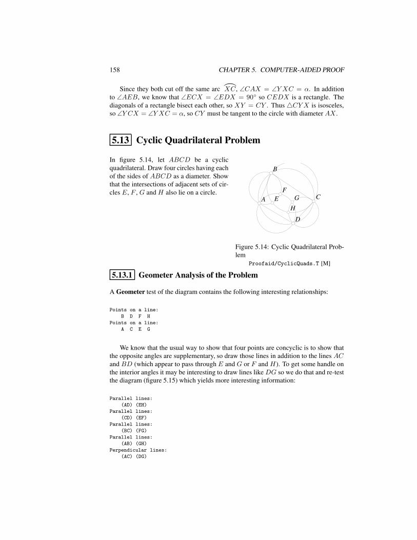
158 CHAPTER 5. COMPUTER-AIDED PROOF
Since they both cut off the same arc
)
XC, ∠CAX = ∠Y XC = α. In additionto ∠AEB, we know that ∠ECX = ∠EDX = 90 so CEDX is a rectangle. Thediagonals of a rectangle bisect each other, so XY = CY . Thus 4CYX is isosceles,so ∠Y CX = ∠Y XC = α, so CY must be tangent to the circle with diameter AX .
5.13 Cyclic Quadrilateral Problem
AA
BB
CC
DD
EEFF
GG
HH
Figure 5.14: Cyclic Quadrilateral Prob-lem
Proofaid/CyclicQuads.T [M]
In figure 5.14, let ABCD be a cyclicquadrilateral. Draw four circles having eachof the sides of ABCD as a diameter. Showthat the intersections of adjacent sets of cir-cles E, F , G and H also lie on a circle.
5.13.1 Geometer Analysis of the Problem
A Geometer test of the diagram contains the following interesting relationships:
Points on a line:
B D F H
Points on a line:
A C E G
We know that the usual way to show that four points are concyclic is to show thatthe opposite angles are supplementary, so draw those lines in addition to the lines ACand BD (which appear to pass through E and G or F and H). To get some handle onthe interior angles it may be interesting to draw lines like DG so we do that and re-testthe diagram (figure 5.15) which yields more interesting information:
Parallel lines:
(AD) (EH)
Parallel lines:
(CD) (EF)
Parallel lines:
(BC) (FG)
Parallel lines:
(AB) (GH)
Perpendicular lines:
(AC) (DG)
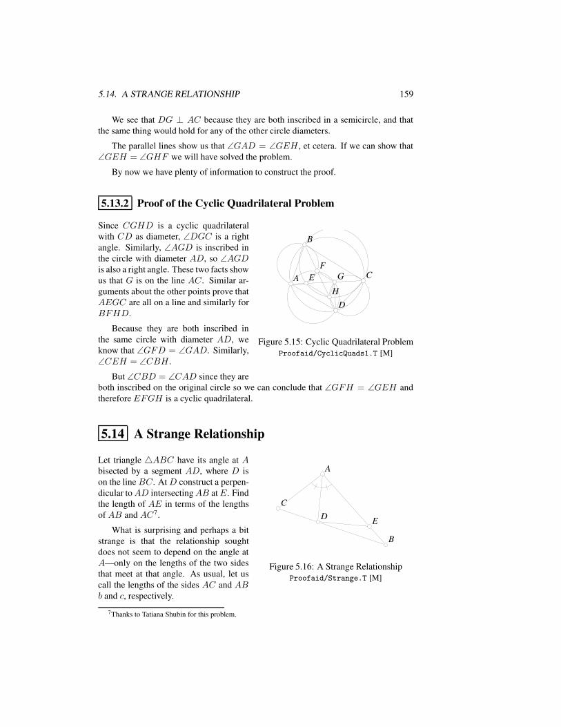
5.14. A STRANGE RELATIONSHIP 159
We see that DG ⊥ AC because they are both inscribed in a semicircle, and thatthe same thing would hold for any of the other circle diameters.
The parallel lines show us that ∠GAD = ∠GEH , et cetera. If we can show that∠GEH = ∠GHF we will have solved the problem.
By now we have plenty of information to construct the proof.
5.13.2 Proof of the Cyclic Quadrilateral Problem
AA
BB
CC
DD
EEFF
GG
HH
Figure 5.15: Cyclic Quadrilateral ProblemProofaid/CyclicQuads1.T [M]
Since CGHD is a cyclic quadrilateralwith CD as diameter, ∠DGC is a rightangle. Similarly, ∠AGD is inscribed inthe circle with diameter AD, so ∠AGDis also a right angle. These two facts showus that G is on the line AC. Similar ar-guments about the other points prove thatAEGC are all on a line and similarly forBFHD.
Because they are both inscribed inthe same circle with diameter AD, weknow that ∠GFD = ∠GAD. Similarly,∠CEH = ∠CBH .
But ∠CBD = ∠CAD since they areboth inscribed on the original circle so we can conclude that ∠GFH = ∠GEH andthereforeEFGH is a cyclic quadrilateral.
5.14 A Strange Relationship
AA
BB
CCDD EE
Figure 5.16: A Strange RelationshipProofaid/Strange.T [M]
Let triangle 4ABC have its angle at Abisected by a segment AD, where D ison the line BC. At D construct a perpen-dicular toAD intersectingAB atE. Findthe length of AE in terms of the lengthsof AB and AC7.
What is surprising and perhaps a bitstrange is that the relationship soughtdoes not seem to depend on the angle atA—only on the lengths of the two sidesthat meet at that angle. As usual, let uscall the lengths of the sides AC and ABb and c, respectively.
7Thanks to Tatiana Shubin for this problem.
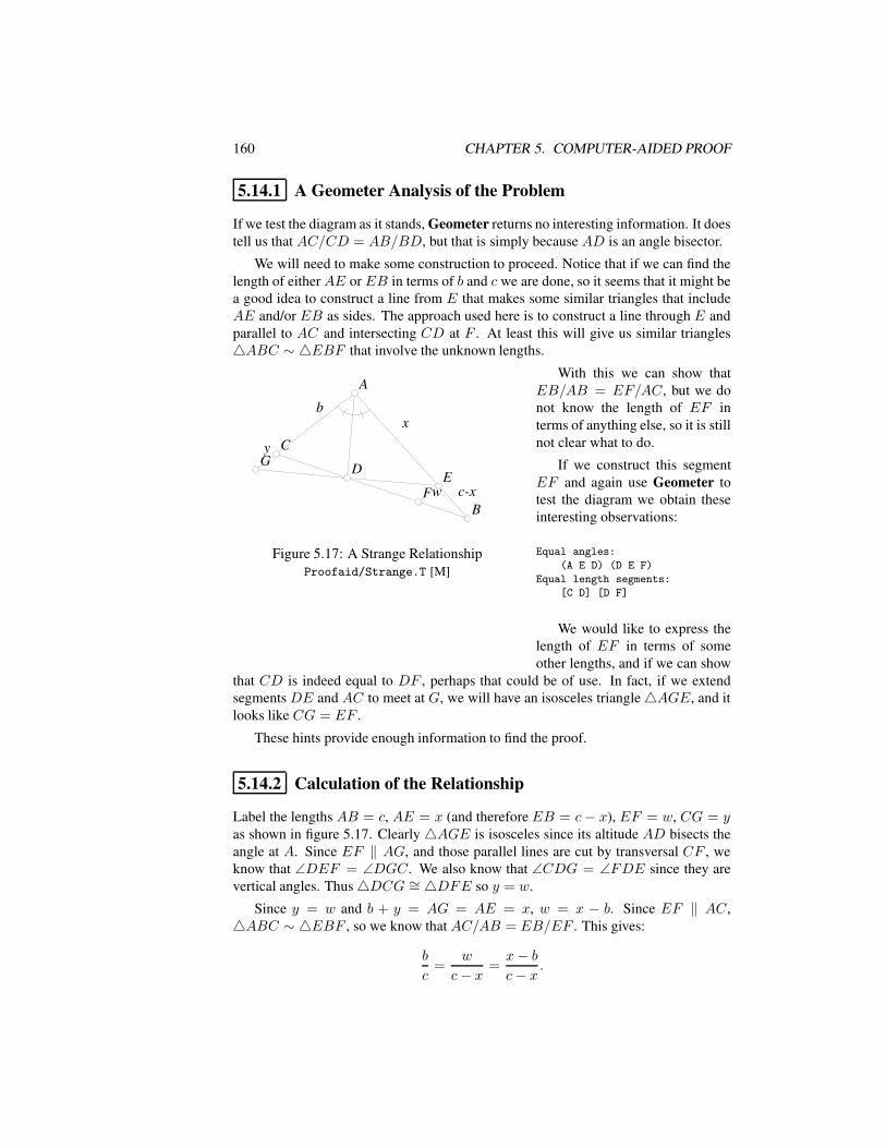
160 CHAPTER 5. COMPUTER-AIDED PROOF
5.14.1 A Geometer Analysis of the Problem
If we test the diagram as it stands, Geometer returns no interesting information. It doestell us that AC/CD = AB/BD, but that is simply because AD is an angle bisector.
We will need to make some construction to proceed. Notice that if we can find thelength of eitherAE or EB in terms of b and c we are done, so it seems that it might bea good idea to construct a line from E that makes some similar triangles that includeAE and/or EB as sides. The approach used here is to construct a line through E andparallel to AC and intersecting CD at F . At least this will give us similar triangles4ABC ∼ 4EBF that involve the unknown lengths.
AA
BB
CC
DD EEFF
GG
bb
yy
xx
c-xc-xww
Figure 5.17: A Strange RelationshipProofaid/Strange.T [M]
With this we can show thatEB/AB = EF/AC, but we donot know the length of EF interms of anything else, so it is stillnot clear what to do.
If we construct this segmentEF and again use Geometer totest the diagram we obtain theseinteresting observations:
Equal angles:
(A E D) (D E F)
Equal length segments:
[C D] [D F]
We would like to express thelength of EF in terms of someother lengths, and if we can show
that CD is indeed equal to DF , perhaps that could be of use. In fact, if we extendsegments DE and AC to meet at G, we will have an isosceles triangle4AGE, and itlooks like CG = EF .
These hints provide enough information to find the proof.
5.14.2 Calculation of the Relationship
Label the lengths AB = c, AE = x (and therefore EB = c− x), EF = w, CG = yas shown in figure 5.17. Clearly 4AGE is isosceles since its altitude AD bisects theangle at A. Since EF ‖ AG, and those parallel lines are cut by transversal CF , weknow that ∠DEF = ∠DGC. We also know that ∠CDG = ∠FDE since they arevertical angles. Thus4DCG ∼= 4DFE so y = w.
Since y = w and b + y = AG = AE = x, w = x − b. Since EF ‖ AC,4ABC ∼ 4EBF , so we know that AC/AB = EB/EF . This gives:
b
c=
w
c− x =x− bc− x .
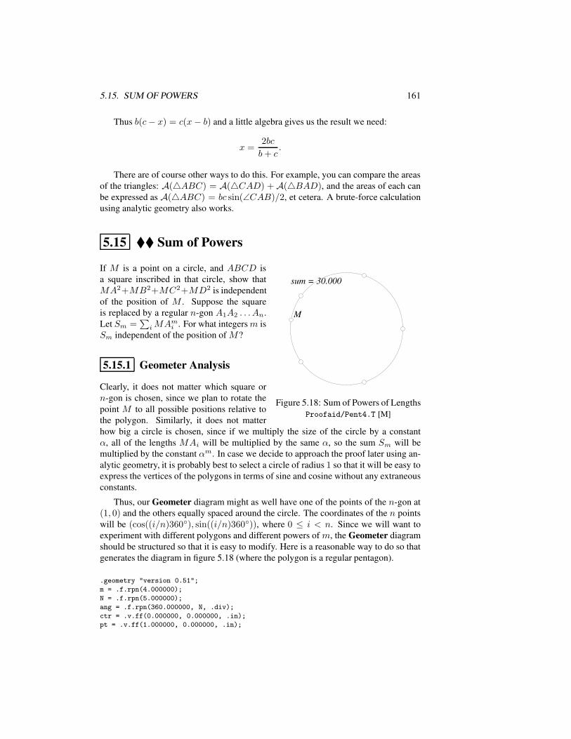
5.15. SUM OF POWERS 161
Thus b(c− x) = c(x− b) and a little algebra gives us the result we need:
x =2bc
b+ c.
There are of course other ways to do this. For example, you can compare the areasof the triangles: A(4ABC) = A(4CAD) +A(4BAD), and the areas of each canbe expressed as A(4ABC) = bc sin(∠CAB)/2, et cetera. A brute-force calculationusing analytic geometry also works.
5.15 Sum of Powers
sum = 30.000sum = 30.000
MM
Figure 5.18: Sum of Powers of LengthsProofaid/Pent4.T [M]
If M is a point on a circle, and ABCD isa square inscribed in that circle, show thatMA2+MB2+MC2+MD2 is independentof the position of M . Suppose the squareis replaced by a regular n-gon A1A2 . . . An.Let Sm =
∑iMAmi . For what integersm is
Sm independent of the position of M?
5.15.1 Geometer Analysis
Clearly, it does not matter which square orn-gon is chosen, since we plan to rotate thepoint M to all possible positions relative tothe polygon. Similarly, it does not matterhow big a circle is chosen, since if we multiply the size of the circle by a constantα, all of the lengths MAi will be multiplied by the same α, so the sum Sm will bemultiplied by the constant αm. In case we decide to approach the proof later using an-alytic geometry, it is probably best to select a circle of radius 1 so that it will be easy toexpress the vertices of the polygons in terms of sine and cosine without any extraneousconstants.
Thus, our Geometer diagram might as well have one of the points of the n-gon at(1, 0) and the others equally spaced around the circle. The coordinates of the n pointswill be (cos((i/n)360), sin((i/n)360)), where 0 ≤ i < n. Since we will want toexperiment with different polygons and different powers of m, the Geometer diagramshould be structured so that it is easy to modify. Here is a reasonable way to do so thatgenerates the diagram in figure 5.18 (where the polygon is a regular pentagon).
.geometry "version 0.51";
m = .f.rpn(4.000000);
N = .f.rpn(5.000000);
ang = .f.rpn(360.000000, N, .div);
ctr = .v.ff(0.000000, 0.000000, .in);
pt = .v.ff(1.000000, 0.000000, .in);
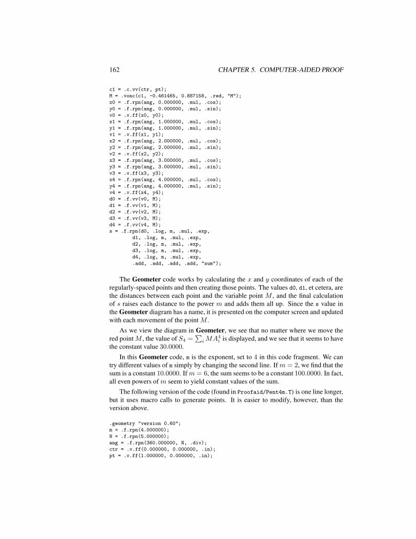
162 CHAPTER 5. COMPUTER-AIDED PROOF
c1 = .c.vv(ctr, pt);
M = .vonc(c1, -0.461465, 0.887158, .red, "M");
x0 = .f.rpn(ang, 0.000000, .mul, .cos);
y0 = .f.rpn(ang, 0.000000, .mul, .sin);
v0 = .v.ff(x0, y0);
x1 = .f.rpn(ang, 1.000000, .mul, .cos);
y1 = .f.rpn(ang, 1.000000, .mul, .sin);
v1 = .v.ff(x1, y1);
x2 = .f.rpn(ang, 2.000000, .mul, .cos);
y2 = .f.rpn(ang, 2.000000, .mul, .sin);
v2 = .v.ff(x2, y2);
x3 = .f.rpn(ang, 3.000000, .mul, .cos);
y3 = .f.rpn(ang, 3.000000, .mul, .sin);
v3 = .v.ff(x3, y3);
x4 = .f.rpn(ang, 4.000000, .mul, .cos);
y4 = .f.rpn(ang, 4.000000, .mul, .sin);
v4 = .v.ff(x4, y4);
d0 = .f.vv(v0, M);
d1 = .f.vv(v1, M);
d2 = .f.vv(v2, M);
d3 = .f.vv(v3, M);
d4 = .f.vv(v4, M);
s = .f.rpn(d0, .log, m, .mul, .exp,
d1, .log, m, .mul, .exp,
d2, .log, m, .mul, .exp,
d3, .log, m, .mul, .exp,
d4, .log, m, .mul, .exp,
.add, .add, .add, .add, "sum");
The Geometer code works by calculating the x and y coordinates of each of theregularly-spaced points and then creating those points. The values d0, d1, et cetera, arethe distances between each point and the variable point M , and the final calculationof s raises each distance to the power m and adds them all up. Since the s value inthe Geometer diagram has a name, it is presented on the computer screen and updatedwith each movement of the point M .
As we view the diagram in Geometer, we see that no matter where we move thered pointM , the value of S4 =
∑iMA4
i is displayed, and we see that it seems to havethe constant value 30.0000.
In this Geometer code, m is the exponent, set to 4 in this code fragment. We cantry different values of m simply by changing the second line. If m = 2, we find that thesum is a constant 10.0000. Ifm = 6, the sum seems to be a constant 100.0000. In fact,all even powers of m seem to yield constant values of the sum.
The following version of the code (found in Proofaid/Pent4m.T) is one line longer,but it uses macro calls to generate points. It is easier to modify, however, than theversion above.
.geometry "version 0.60";
m = .f.rpn(4.000000);
N = .f.rpn(5.000000);
ang = .f.rpn(360.000000, N, .div);
ctr = .v.ff(0.000000, 0.000000, .in);
pt = .v.ff(1.000000, 0.000000, .in);
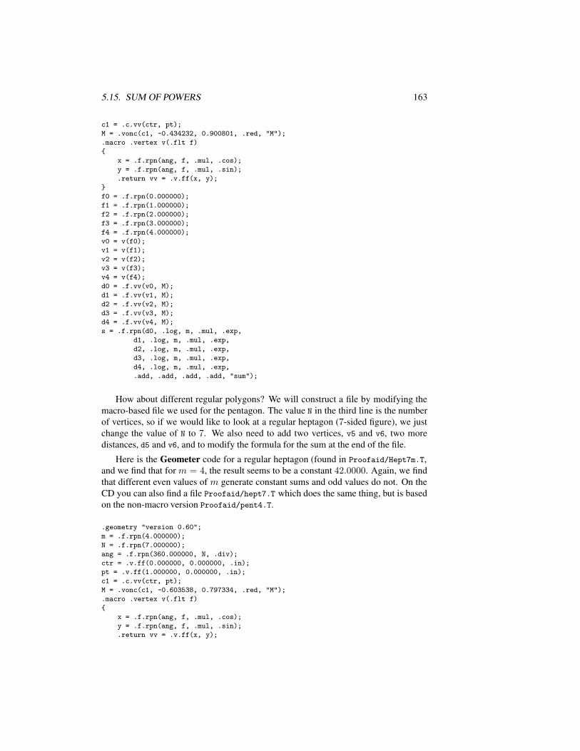
5.15. SUM OF POWERS 163
c1 = .c.vv(ctr, pt);
M = .vonc(c1, -0.434232, 0.900801, .red, "M");
.macro .vertex v(.flt f)
x = .f.rpn(ang, f, .mul, .cos);
y = .f.rpn(ang, f, .mul, .sin);
.return vv = .v.ff(x, y);
f0 = .f.rpn(0.000000);
f1 = .f.rpn(1.000000);
f2 = .f.rpn(2.000000);
f3 = .f.rpn(3.000000);
f4 = .f.rpn(4.000000);
v0 = v(f0);
v1 = v(f1);
v2 = v(f2);
v3 = v(f3);
v4 = v(f4);
d0 = .f.vv(v0, M);
d1 = .f.vv(v1, M);
d2 = .f.vv(v2, M);
d3 = .f.vv(v3, M);
d4 = .f.vv(v4, M);
s = .f.rpn(d0, .log, m, .mul, .exp,
d1, .log, m, .mul, .exp,
d2, .log, m, .mul, .exp,
d3, .log, m, .mul, .exp,
d4, .log, m, .mul, .exp,
.add, .add, .add, .add, "sum");
How about different regular polygons? We will construct a file by modifying themacro-based file we used for the pentagon. The value N in the third line is the numberof vertices, so if we would like to look at a regular heptagon (7-sided figure), we justchange the value of N to 7. We also need to add two vertices, v5 and v6, two moredistances, d5 and v6, and to modify the formula for the sum at the end of the file.
Here is the Geometer code for a regular heptagon (found in Proofaid/Hept7m.T,and we find that for m = 4, the result seems to be a constant 42.0000. Again, we findthat different even values of m generate constant sums and odd values do not. On theCD you can also find a file Proofaid/hept7.T which does the same thing, but is basedon the non-macro version Proofaid/pent4.T.
.geometry "version 0.60";
m = .f.rpn(4.000000);
N = .f.rpn(7.000000);
ang = .f.rpn(360.000000, N, .div);
ctr = .v.ff(0.000000, 0.000000, .in);
pt = .v.ff(1.000000, 0.000000, .in);
c1 = .c.vv(ctr, pt);
M = .vonc(c1, -0.603538, 0.797334, .red, "M");
.macro .vertex v(.flt f)
x = .f.rpn(ang, f, .mul, .cos);
y = .f.rpn(ang, f, .mul, .sin);
.return vv = .v.ff(x, y);
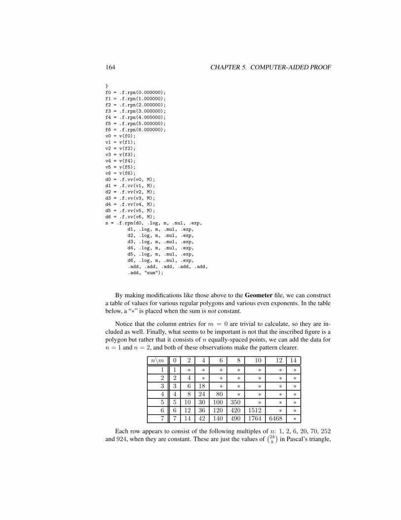
164 CHAPTER 5. COMPUTER-AIDED PROOF
f0 = .f.rpn(0.000000);
f1 = .f.rpn(1.000000);
f2 = .f.rpn(2.000000);
f3 = .f.rpn(3.000000);
f4 = .f.rpn(4.000000);
f5 = .f.rpn(5.000000);
f6 = .f.rpn(6.000000);
v0 = v(f0);
v1 = v(f1);
v2 = v(f2);
v3 = v(f3);
v4 = v(f4);
v5 = v(f5);
v6 = v(f6);
d0 = .f.vv(v0, M);
d1 = .f.vv(v1, M);
d2 = .f.vv(v2, M);
d3 = .f.vv(v3, M);
d4 = .f.vv(v4, M);
d5 = .f.vv(v5, M);
d6 = .f.vv(v6, M);
s = .f.rpn(d0, .log, m, .mul, .exp,
d1, .log, m, .mul, .exp,
d2, .log, m, .mul, .exp,
d3, .log, m, .mul, .exp,
d4, .log, m, .mul, .exp,
d5, .log, m, .mul, .exp,
d6, .log, m, .mul, .exp,
.add, .add, .add, .add, .add,
.add, "sum");
By making modifications like those above to the Geometer file, we can constructa table of values for various regular polygons and various even exponents. In the tablebelow, a “∗” is placed when the sum is not constant.
Notice that the column entries for m = 0 are trivial to calculate, so they are in-cluded as well. Finally, what seems to be important is not that the inscribed figure is apolygon but rather that it consists of n equally-spaced points, we can add the data forn = 1 and n = 2, and both of these observations make the pattern clearer.
n\m 0 2 4 6 8 10 12 14
1 1 ∗ ∗ ∗ ∗ ∗ ∗ ∗2 2 4 ∗ ∗ ∗ ∗ ∗ ∗3 3 6 18 ∗ ∗ ∗ ∗ ∗4 4 8 24 80 ∗ ∗ ∗ ∗5 5 10 30 100 350 ∗ ∗ ∗6 6 12 36 120 420 1512 ∗ ∗7 7 14 42 140 490 1764 6468 ∗
Each row appears to consist of the following multiples of n: 1, 2, 6, 20, 70, 252and 924, when they are constant. These are just the values of
(2kk
)in Pascal’s triangle,
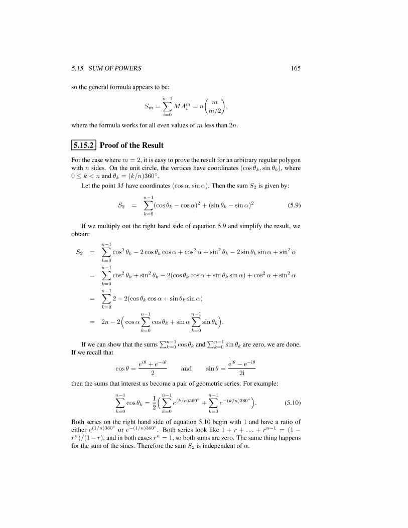
5.15. SUM OF POWERS 165
so the general formula appears to be:
Sm =n−1∑
i=0
MAmi = n
(m
m/2
),
where the formula works for all even values of m less than 2n.
5.15.2 Proof of the Result
For the case wherem = 2, it is easy to prove the result for an arbitrary regular polygonwith n sides. On the unit circle, the vertices have coordinates (cos θk, sin θk), where0 ≤ k < n and θk = (k/n)360.
Let the point M have coordinates (cosα, sinα). Then the sum S2 is given by:
S2 =
n−1∑
k=0
(cos θk − cosα)2 + (sin θk − sinα)2 (5.9)
If we multiply out the right hand side of equation 5.9 and simplify the result, weobtain:
S2 =
n−1∑
k=0
cos2 θk − 2 cos θk cosα+ cos2 α+ sin2 θk − 2 sin θk sinα+ sin2 α
=
n−1∑
k=0
cos2 θk + sin2 θk − 2(cos θk cosα+ sin θk sinα) + cos2 α+ sin2 α
=
n−1∑
k=0
2− 2(cos θk cosα+ sin θk sinα)
= 2n− 2(
cosα
n−1∑
k=0
cos θk + sinα
n−1∑
k=0
sin θk
).
If we can show that the sums∑n−1
k=0 cos θk and∑n−1
k=0 sin θk are zero, we are done.If we recall that
cos θ =eiθ + e−iθ
2and sin θ =
eiθ − e−iθ
2i
then the sums that interest us become a pair of geometric series. For example:
n−1∑
k=0
cos θk =1
2
( n−1∑
k=0
e(k/n)360 +
n−1∑
k=0
e−(k/n)360). (5.10)
Both series on the right hand side of equation 5.10 begin with 1 and have a ratio ofeither e(1/n)360 or e−(1/n)360 . Both series look like 1 + r + . . . + rn−1 = (1 −rn)/(1− r), and in both cases rn = 1, so both sums are zero. The same thing happensfor the sum of the sines. Therefore the sum S2 is independent of α.
166 CHAPTER 5. COMPUTER-AIDED PROOF
5.15.3 Alternative Proof with Vectors
The same result can be obtained with vectors. Let Ak for 0 ≤ k < n be the verticesof a regular n-gon inscribed in a circle with center O. If M is any point on the circle,
then−→MAk=
−→MO +
−→OAk . Then:
S2 =
n−1∑
k=0
(−→MAi)
2 =
n−1∑
k=0
(−→MO +
−→OAi)
2.
Expanding the expression on the right, we obtain:
S2 =
n−1∑
k=0
(−→MO
2
+2−→MO ·
−→OAi +
−→OAi
2
)
=
n−1∑
k=0
−→MO
2
+
n−1∑
k=0
2−→MO ·
−→OAi +
n−1∑
k=0
−→OAi
2
= n−→MO
2
+2−→MO ·
n−1∑
k=0
−→OAi +
n−1∑
k=0
−→OAi
2
Since−→MO
2
and−→Ak
2
are both constant and equal to r2, where r is the radius of thecircle, this is equivalent to:
S2 = nr2 + nr2 + 2−→MO ·
n−1∑
k=0
−→OAi
Clearly,∑n−1
k=0
−→OAi=
−→0 , since if it did point in any direction, by symmetry, it would
have to point the same amount in every one of n equally-spaced directions. Thus thesum S2 = 2nr2 which is what we obtained in the previous section with r = 1.
Chapter 6More Useful Theorems
The results in this chapter are generally not covered in high school geometry courses,but they are all very useful tools for solving other geometric problems. In this chapterwe will continue to use computer techniques to solve problems, so if you have notalready done so, it may be useful to read Chapter 5 before continuing.
6.1 Ceva’s Theorem
Ceva’s (pronounced “cheva’s”) theorem is perhaps the most useful geometric theoremthat is not taught in a standard high school course.
Theorem 6.1 (Ceva’s Theorem) Given any triangle 4ABC with a point P a insideit1 (see figure 6.1), if the lines from A, B and C through P intersect the opposite sides
1In fact, it is not difficult to show that P can be outside the triangle as well, as long as it does not lie onany of the (infinite) lines that make up the edges of the triangle.
167
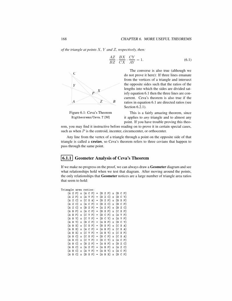
168 CHAPTER 6. MORE USEFUL THEOREMS
of the triangle at points X , Y and Z, respectively, then:
AZ
BZ· BXCX
· CYAY
= 1. (6.1)
AA BB
CC
PPXX
YY
ZZ
Figure 6.1: Ceva’s TheoremBigtheorems/Ceva.T [M]
The converse is also true (although wedo not prove it here): If three lines emanatefrom the vertices of a triangle and intersectthe opposite sides such that the ratios of thelengths into which the sides are divided sat-isfy equation 6.1 then the three lines are con-current. Ceva’s theorem is also true if theratios in equation 6.1 are directed ratios (seeSection 6.2.1).
This is a fairly amazing theorem, sinceit applies to any triangle and to almost anypoint. If you have trouble proving this theo-
rem, you may find it instructive before reading on to prove it in certain special cases,such as when P is the centroid, incenter, circumcenter, or orthocenter.
Any line from the vertex of a triangle through a point on the opposite side of thattriangle is called a cevian, so Ceva’s theorem refers to three cevians that happen topass through the same point.
6.1.1 Geometer Analysis of Ceva’s Theorem
If we make no progress on the proof, we can always draw a Geometer diagram and seewhat relationships hold when we test that diagram. After moving around the points,the only relationships that Geometer notices are a large number of triangle area ratiosthat seem to hold:
Triangle area ratios:
[A Z P] x [A C P] = [B Z P] x [B C P]
[A Z P] x [A Y P] = [B Z C] x [B C Y]
[A Z C] x [C X A] = [B Z P] x [B X P]
[A Z C] x [A C P] = [B Z C] x [B C P]
[A Z C] x [B Z P] = [A Z P] x [B Z C]
[A B P] x [A C P] = [B X P] x [C X P]
[A B P] x [C Y P] = [B C P] x [A Y P]
[A B Y] x [C Y P] = [B C Y] x [A Y P]
[A B Y] x [B C P] = [A B P] x [B C Y]
[A B X] x [C X P] = [B X P] x [C X A]
[A B X] x [A C P] = [A B P] x [C X A]
[A B X] x [C Y P] = [A B Y] x [C X P]
[A B C] x [C X P] = [B C P] x [C X A]
[A B C] x [C Y P] = [B C Y] x [A C P]
[A B C] x [B Z P] = [A B P] x [B Z C]
[A B C] x [A Z P] = [A B P] x [A Z C]
[A B C] x [A Y P] = [A B Y] x [A C P]
[A B C] x [B X P] = [A B X] x [B C P]
6.1. CEVA’S THEOREM 169
After examining a few, we notice that they all are based on the same idea. Rela-tionships like that shown in the fifth line are the easiest to see:
[A Z C] x [B Z P] = [A Z P] x [B Z C]
This basically says that 4AZC and 4BZC have the same ratio as 4AZP and4BZP . This is obvious because the ratios of the areas are the same as the ratio intowhich Z divides the base AB. Once we see this, it is obvious why the first ratio in thelist is true: 4AZC is composed of the two triangles4ACP and4AZP and4BZCcan be similarly decomposed.
Thus the ratios of the subdivisons of the sides are the same as the ratio of the areasof the triangles 4ACP , 4BCP and 4ABP . Since Ceva’s theorem concerns theseratios, we are probably on the right track. Using this information the proof is simple toconstruct.
6.1.2 Proof of Ceva’s Theorem
Here is a proof, derived from the observations above:Relative to the base AB, the triangles4AZP and4BZP have the same altitude,
their areas are proportional to AZ : BZ. The areas of triangles 4AZC and 4AZCare similarly related so we obtain:
AZ
BZ=
A(4AZP )
A(4BZP )=
A(4AZC)
A(4BZC)(6.2)
Triangle 4AZC is composed of triangles 4AZP and 4ACP and 4BZC canbe similarly decomposed, so their areas satisfy:
A(4AZC) = A(4AZP ) +A(4ACP ) (6.3)A(4BZC) = A(4BZP ) +A(4BCP ). (6.4)
Rearranging equations 6.3 and 6.4, we obtain:
A(4ACP ) = A(4AZC) −A(4AZP ) (6.5)A(4BCP ) = A(4BZC)−A(4BZP ). (6.6)
Combining equations 6.2, 6.5 and 6.6 by using the fact that if a/b = c/d = ewhereb and d are different then (a− c)/(b− d) = e, we obtain:
AZ
BZ=
(4ACP )
(4BCP ). (6.7)
There is nothing special about the selection of AB as a base of the triangle, andsimilar calculations give us:
BX
CX=
(4ABP )
(4ACP )(6.8)
CY
AY=
(4BCP )
(4ABP ). (6.9)
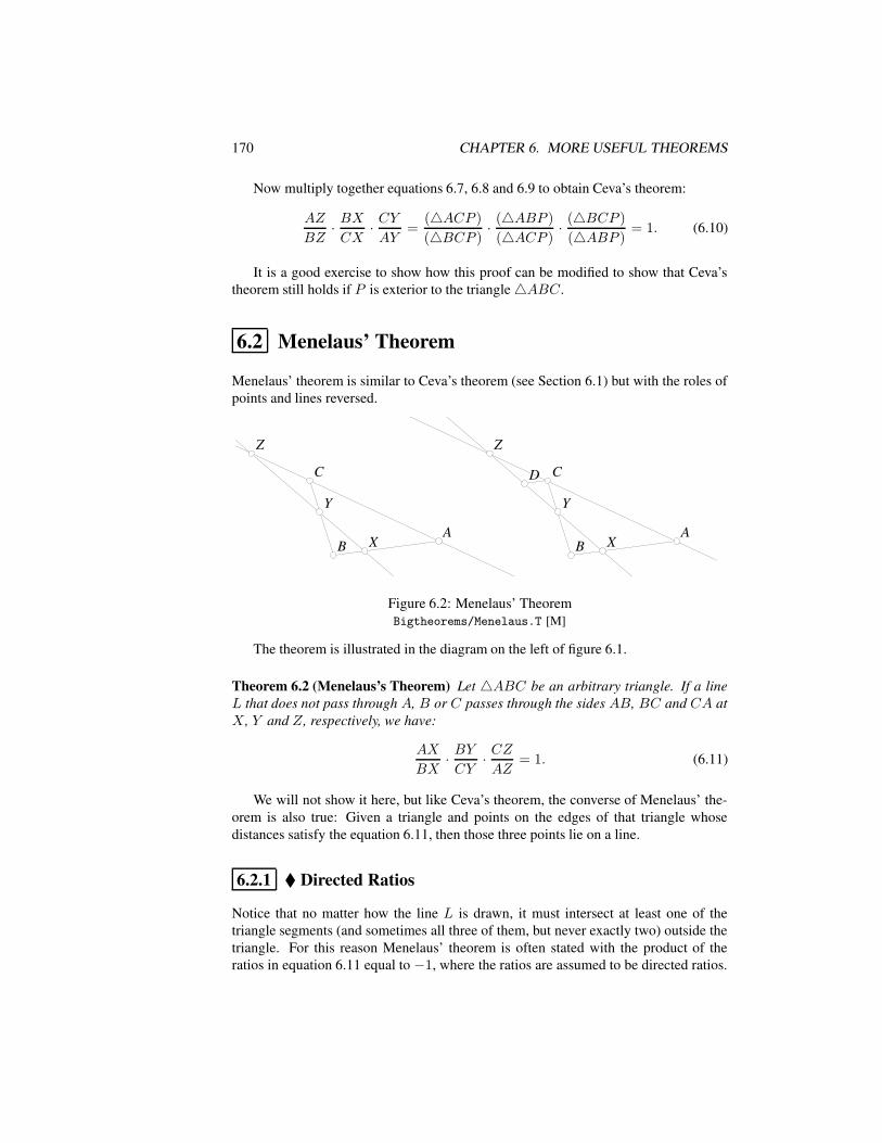
170 CHAPTER 6. MORE USEFUL THEOREMS
Now multiply together equations 6.7, 6.8 and 6.9 to obtain Ceva’s theorem:
AZ
BZ· BXCX
· CYAY
=(4ACP )
(4BCP )· (4ABP )
(4ACP )· (4BCP )
(4ABP )= 1. (6.10)
It is a good exercise to show how this proof can be modified to show that Ceva’stheorem still holds if P is exterior to the triangle4ABC.
6.2 Menelaus’ Theorem
Menelaus’ theorem is similar to Ceva’s theorem (see Section 6.1) but with the roles ofpoints and lines reversed.
AABB
CC
XX
YY
ZZ
AABB
CC
XX
YY
ZZ
DD
Figure 6.2: Menelaus’ TheoremBigtheorems/Menelaus.T [M]
The theorem is illustrated in the diagram on the left of figure 6.1.
Theorem 6.2 (Menelaus’s Theorem) Let 4ABC be an arbitrary triangle. If a lineL that does not pass through A, B or C passes through the sides AB, BC and CA atX , Y and Z, respectively, we have:
AX
BX· BYCY· CZAZ
= 1. (6.11)
We will not show it here, but like Ceva’s theorem, the converse of Menelaus’ the-orem is also true: Given a triangle and points on the edges of that triangle whosedistances satisfy the equation 6.11, then those three points lie on a line.
6.2.1 Directed Ratios
Notice that no matter how the line L is drawn, it must intersect at least one of thetriangle segments (and sometimes all three of them, but never exactly two) outside thetriangle. For this reason Menelaus’ theorem is often stated with the product of theratios in equation 6.11 equal to −1, where the ratios are assumed to be directed ratios.
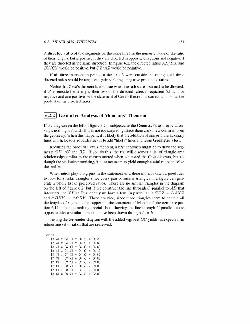
6.2. MENELAUS’ THEOREM 171
A directed ratio of two segments on the same line has the numeric value of the ratioof their lengths, but is positive if they are directed in opposite directions and negative ifthey are directed in the same direction. In figure 6.2, the directed ratios AX/BX andBY/CY would be positive, but CZ/AZ would be negative.
If all three intersection points of the line L were outside the triangle, all threedirected ratios would be negative, again yielding a negative product of ratios.
Notice that Ceva’s theorem is also true when the ratios are assumed to be directed:if P is outside the triangle, then two of the directed ratios in equation 6.1 will benegative and one positive, so the statement of Ceva’s theorem is correct with +1 as theproduct of the directed ratios.
6.2.2 Geometer Analysis of Menelaus’ Theorem
If the diagram on the left of figure 6.2 is subjected to the Geometer’s test for relation-ships, nothing is found. This is not too surprising, since there are so few constraints onthe geometry. When this happens, it is likely that the addition of one or more auxiliarylines will help, so a good strategy is to add “likely” lines and rerun Geometer’s test.
Recalling the proof of Ceva’s theorem, a first approach might be to draw the seg-ments CX , AY and BZ. If you do this, the test will discover a list of triangle arearelationships similar to those encountered when we tested the Ceva diagram, but al-though the set looks promising, it does not seem to yield enough useful ratios to solvethe problem.
When ratios play a big part in the statement of a theorem, it is often a good ideato look for similar triangles since every pair of similar triangles in a figure can gen-erate a whole list of preserved ratios. There are no similar triangles in the diagramon the left of figure 6.2, but if we construct the line through C parallel to AB thatintersects line XY at D, suddenly we have a few. In particular, 4CDZ ∼ 4AXZand 4BXY ∼ 4CDY . These are nice, since those triangles seem to contain allthe lengths of segments that appear in the statement of Menelaus’ theorem in equa-tion 6.11. There is nothing special about drawing the line through C parallel to theopposite side; a similar line could have been drawn throughA or B.
Testing the Geometer diagram with the added segmentDC yields, as expected, aninteresting set of ratios that are preserved:
Ratios:
[A Z] x [Z D] = [C Z] x [X Z]
[A C] x [Z D] = [C Z] x [X D]
[A C] x [X Z] = [A Z] x [X D]
[B Y] x [Y D] = [C Y] x [X Y]
[B C] x [Y D] = [C Y] x [X D]
[B C] x [X Y] = [B Y] x [X D]
[B X] x [Y D] = [X Y] x [C D]
[B X] x [C Y] = [B Y] x [C D]
[A X] x [Z D] = [X Z] x [C D]
[A X] x [C Z] = [A Z] x [C D]
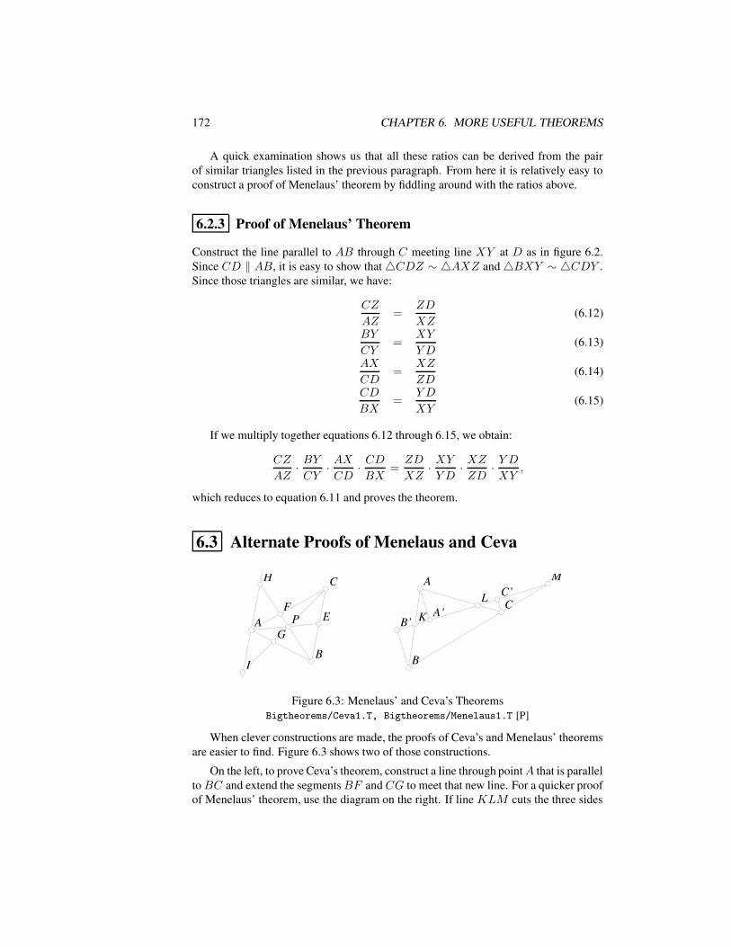
172 CHAPTER 6. MORE USEFUL THEOREMS
A quick examination shows us that all these ratios can be derived from the pairof similar triangles listed in the previous paragraph. From here it is relatively easy toconstruct a proof of Menelaus’ theorem by fiddling around with the ratios above.
6.2.3 Proof of Menelaus’ Theorem
Construct the line parallel to AB through C meeting line XY at D as in figure 6.2.Since CD ‖ AB, it is easy to show that4CDZ ∼ 4AXZ and4BXY ∼ 4CDY .Since those triangles are similar, we have:
CZ
AZ=
ZD
XZ(6.12)
BY
CY=
XY
YD(6.13)
AX
CD=
XZ
ZD(6.14)
CD
BX=
Y D
XY(6.15)
If we multiply together equations 6.12 through 6.15, we obtain:
CZ
AZ· BYCY· AXCD· CDBX
=ZD
XZ· XYYD
· XZZD· Y DXY
,
which reduces to equation 6.11 and proves the theorem.
6.3 Alternate Proofs of Menelaus and Ceva
AA
BB
CC
PP EEFF
GG
HH
II
AA
BB
CCKK
LL
MM
B’B’A’A’
C’C’
Figure 6.3: Menelaus’ and Ceva’s TheoremsBigtheorems/Ceva1.T, Bigtheorems/Menelaus1.T [P]
When clever constructions are made, the proofs of Ceva’s and Menelaus’ theoremsare easier to find. Figure 6.3 shows two of those constructions.
On the left, to prove Ceva’s theorem, construct a line through pointA that is paralleltoBC and extend the segmentsBF and CG to meet that new line. For a quicker proofof Menelaus’ theorem, use the diagram on the right. If line KLM cuts the three sides
6.4. USING MENELAUS’ AND CEVA’S THEOREM 173
of the triangle, construct perpendiculars from A, B and C to line KLM meeting itatA′, B′ and C ′, respectively.
Try to find alternate proofs of Menelaus’ and Ceva’s theorems based on these newconstructions. Those proofs are not difficult, but the solutions can be found in the filesCeva1.T and Menelaus1.T
6.4 Using Menelaus’ and Ceva’s Theorem
If you would like to practice using Ceva’s theorem, Chapter 8 on triangle centers con-tains a surprising number of examples where Ceva’s theorem leads to a proof of theexistence of some center.
If you would like to practice with Menelaus’ theorem, look in Chapter 10 on pro-jective geometry where Menelaus’ theorem is used to prove the Euclidean version of anumber of projective geometry theorems.
6.5 Ptolemy’s Theorem
Ptolemy’s theorem provides a powerful method for calculating lengths in a quadrilat-eral whose vertices happen to be concyclic. Conversely, if you know the lengths of thesides and diagonals, it can be used to determine if the quadrilateral is concyclic.
AABB
CC
DD
AABB
CC
DDHH
Figure 6.4: Ptolemy’s TheoremBigtheorems/Ptolemy.T [M]
The theorem is illustrated in the diagram on the left of figure 6.4.
Theorem 6.3 (Ptolemy’s Theorem) If A, B, C and D are four concyclic points inclockwise or counterclockwise order on the circle, then the following relationship holdsand conversely:
AB · CD +BC ·AD = AC · BD. (6.16)
Notice that Ptolemy’s theorem is a generalization of the pythagorean theorem; if thequadrilateralABCD is a rectangle, Ptolemy’s theorem is equivalent to the pythagoreantheorem.
174 CHAPTER 6. MORE USEFUL THEOREMS
6.5.1 Geometer Analysis of Ptolemy’s Theorem
Ptolemy’s theorem is not easy to prove, and if we simply draw the basic figure seenon the left of figure 6.4 and test it with Geometer’s relationship finding commands, itonly tells us about a few obvious angles that are equal (since they are inscribed in thesame circle) or supplementary (since they are opposite angles in a cyclic quadrilateral).It seems clear that we will have to use ratios and therefore similar triangles to makeany progress, so we need to convert equation 6.16 into ratios, but what are we going todo about that annoying “+” sign?
You probably cannot avoid looking at the answer, since it is drawn on the right ofthe figure, but here is why it (or any of the 7 other equivalent constructions) is a goodidea. To convert the product form of equation 6.4 into a ratio form, we need terms like,for example, AB/AC. Thus we would like to get AC and AD to be correspondingparts of similar triangles. If we imagine rotating4ABD until its angle at A matchesa new triangle, it is clear that a rotation by ∠CAB will align AB and AC. Of coursethis will rotateAD out of the circle by the same angle∠CAB. Therefore, a reasonableway to begin is to construct a line from A making angle ∠CAB with the line AD, asshown in the right side of figure 6.4. The new line must intersect the line CD at somepoint H outside the circle.
Now when Geometer tests the diagram, we obtain a far more interesting set ofrelations, including:
Equal angles:
(B C A) (C H A) (A D B)
Ratios:
[C H] x [A D] = [B D] x [A H]
[B C] x [A H] = [D H] x [A C]
[A B] x [A H] = [A D] x [A C]
[A B] x [C H] = [A C] x [B D]
[A B] x [D H] = [B C] x [A D]
The equal angle information is encouraging, since it shows clearly that4ABD ∼4ACH , and the ratios, if we can show that they hold due to similarities of triangles,include almost all of the lengths that appear in equation 6.4. We can also see fromthe ratios that 4ABC must be similar to 4ADH . At first it is a bit annoying to seelengths like CH and DH in the list, until we realize that CH = CD + DH! Thispulls in the missing CD, and gets a “+” sign into the equations.
Using these observations, the theorem is easy to prove.
6.5.2 Proof of Ptolemy’s Theorem
This is just a proof of one direction of the theorem, namely, that if the points areconcyclic, the relationship in equation 6.16 holds.
Construct a line from A making angle ∠CAB with line AD that intersects the lineCD at H .
6.6. HERON’S FORMULA 175
We know that ∠ABD = ∠ACD since they are inscribed in the same circle, and∠DAB = ∠HAC since they are both equal to ∠DAC + ∠CAB. Therefore by AAsimilarity,4DAB ∼ 4HAC.
We know that ∠ABC and ∠ADC are supplementary since they are opposite an-gles in an inscribed quadrilateral, and it is obvious that ∠ADC and ∠AHD are alsosupplementary, so ∠ADH = ∠ABC. This, and the fact that ∠BAC = ∠DAHallows us to conclude by AA similarity that4ADH ∼ 4ABC.
We know that:CD + DH = CH (6.17)
and the two sets of similar triangles show us that:
BD
CH=
AB
AC=
AD
AH(6.18)
AD
AB=
DH
BC=
AH
AC(6.19)
To get rid of the DH and CH in equation 6.17, we can substitute their valuesobtained from equations 6.18 and 6.19:
CD +BC · ADAB
=AC ·BDAB
(6.20)
If we multiply equation 6.20 by AB, we obtain:
AB · CD +BC ·AD = AC · BD,
which proves the theorem.
6.5.3 Additional Notes on Ptolemy’s Theorem
It is possible to prove the theorem using brute force by listing the lengths of all six sidesand relating them with the law of sines. Using the fact that various sets of angles addto 180 (because they form a triangle or are opposite angles in the cyclic quadrilateral),we can expand the equations using the formulas for the sine and cosine of a sum ofangles. After about ten lines of calculation, Ptolemy’s formula drops out.
There is also a beautiful derivation of Ptolemy’s theorem based on inversion in acircle. See Section 9.8.
6.6 Heron’s Formula
Heron’s formula provides an easy way to calculate the area of an arbitrary trianglegiven the lengths of its sides:
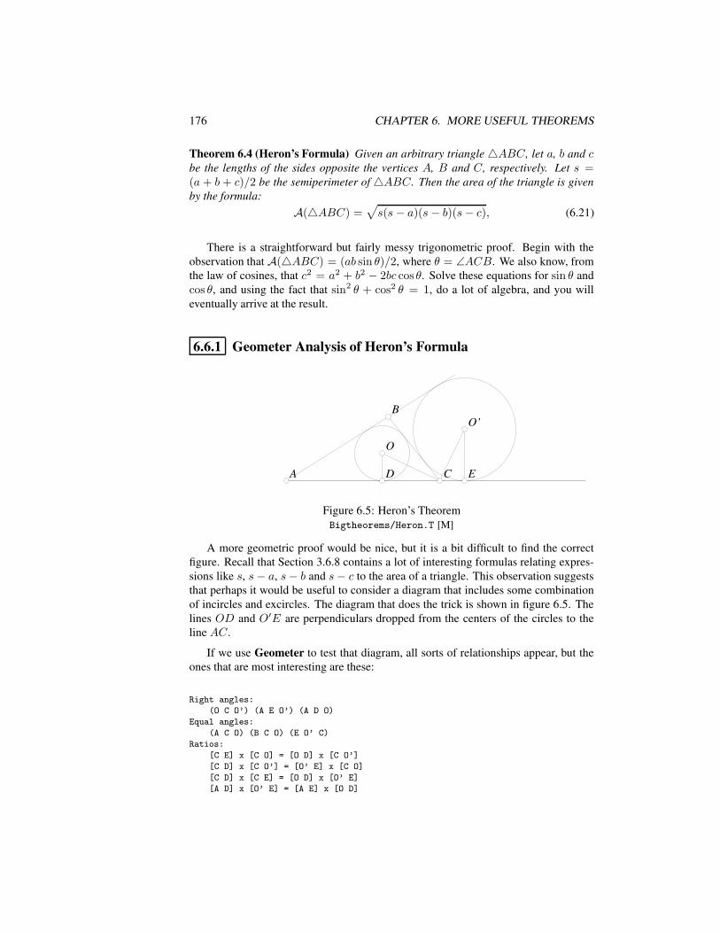
176 CHAPTER 6. MORE USEFUL THEOREMS
Theorem 6.4 (Heron’s Formula) Given an arbitrary triangle4ABC, let a, b and cbe the lengths of the sides opposite the vertices A, B and C, respectively. Let s =(a + b + c)/2 be the semiperimeter of4ABC. Then the area of the triangle is givenby the formula:
A(4ABC) =√s(s− a)(s− b)(s− c), (6.21)
There is a straightforward but fairly messy trigonometric proof. Begin with theobservation that A(4ABC) = (ab sin θ)/2, where θ = ∠ACB. We also know, fromthe law of cosines, that c2 = a2 + b2 − 2bc cos θ. Solve these equations for sin θ andcos θ, and using the fact that sin2 θ + cos2 θ = 1, do a lot of algebra, and you willeventually arrive at the result.
6.6.1 Geometer Analysis of Heron’s Formula
AA
BB
CC
OO
O’O’
DD EE
Figure 6.5: Heron’s TheoremBigtheorems/Heron.T [M]
A more geometric proof would be nice, but it is a bit difficult to find the correctfigure. Recall that Section 3.6.8 contains a lot of interesting formulas relating expres-sions like s, s− a, s− b and s− c to the area of a triangle. This observation suggeststhat perhaps it would be useful to consider a diagram that includes some combinationof incircles and excircles. The diagram that does the trick is shown in figure 6.5. Thelines OD and O′E are perpendiculars dropped from the centers of the circles to theline AC.
If we use Geometer to test that diagram, all sorts of relationships appear, but theones that are most interesting are these:
Right angles:
(O C O’) (A E O’) (A D O)
Equal angles:
(A C O) (B C O) (E O’ C)
Ratios:
[C E] x [C O] = [O D] x [C O’]
[C D] x [C O’] = [O’ E] x [C O]
[C D] x [C E] = [O D] x [O’ E]
[A D] x [O’ E] = [A E] x [O D]
6.6. HERON’S FORMULA 177
Since∠ACO = ∠EO′C andOD andO′E form right angles withAC,4COD ∼4O′CE. Using the notation from Section 3.6.8, we have DC = s − c, CE = s− b,OD = r and O′E = ra. This, plus a little algebra with the ratios is enough to yieldthe result.
6.6.2 Proof of Heron’s Formula
If we can show that ∠OCO′ = 90 then we will know that ∠ACO = ∠EO′C sinceboth ∠ACO and ∠EO′C are complementary to ∠O′CE. But ∠DCB + ∠BCE =180 and those angles are bisected by CO and CO′ so ∠OCO′ = 90.
Thus we know by AA that4COD ∼ 4O′CE. From this similarity, we have:
OD
DC=
CE
O′Eor
r
s− c=
s− b
ra. (6.22)
We also know from Section 3.6.8 that:
A(4ABC) = ra(s− a) = rs. (6.23)
From equation 6.23 we see that r = A(4ABC)/s and ra = A(4ABC)/(s− a).If we substitute these values into equation 6.22, we obtain:
A(4ABC)
s(s− c) =(s− b)(s− a)
A(4ABC)
Cross-multiply to obtain:
(A(4ABC))2 = s(s− a)(s− b)(s− c),
which is equivalent to Heron’s formula.
Note: In a sense, the pythagorean theorem is a special case of heron’s formula.If c is the hypotenuse of a right triangle, then the area of that triangle is ab/2. If wesubstitute s = (a+ b+ c)/2 into Heron’s formula, expand, and set it equal to ab/2, weobtain:
ab/2 = (1/4)√
(2ab)2 − (a2 + b2 − c2)2
a2b2
4=
a2b2
4− (a2 + b2 − c2)2
16
0 = a2 + b2 − c2.
6.6.3 Brahmagupta’s Formula
Heron’s formula looks a lot like another interesting formula called Brahmagupta’s for-mula that applies to cyclic quadrilaterals. If a quadrilateral is inscribed in a circle and
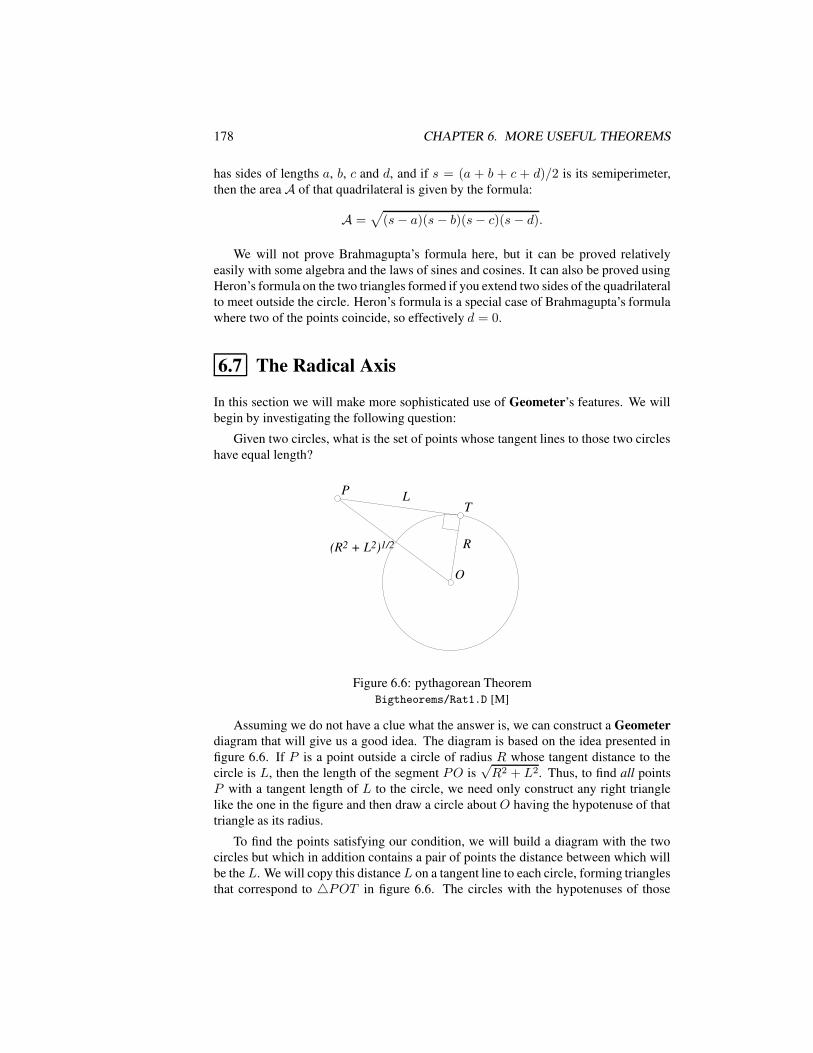
178 CHAPTER 6. MORE USEFUL THEOREMS
has sides of lengths a, b, c and d, and if s = (a + b + c + d)/2 is its semiperimeter,then the area A of that quadrilateral is given by the formula:
A =√
(s− a)(s− b)(s− c)(s− d).
We will not prove Brahmagupta’s formula here, but it can be proved relativelyeasily with some algebra and the laws of sines and cosines. It can also be proved usingHeron’s formula on the two triangles formed if you extend two sides of the quadrilateralto meet outside the circle. Heron’s formula is a special case of Brahmagupta’s formulawhere two of the points coincide, so effectively d = 0.
6.7 The Radical Axis
In this section we will make more sophisticated use of Geometer’s features. We willbegin by investigating the following question:
Given two circles, what is the set of points whose tangent lines to those two circleshave equal length?
OO
PPTT
RR
LL
(R2 + L2)1/2(R2 + L2)1/2
Figure 6.6: pythagorean TheoremBigtheorems/Rat1.D [M]
Assuming we do not have a clue what the answer is, we can construct a Geometerdiagram that will give us a good idea. The diagram is based on the idea presented infigure 6.6. If P is a point outside a circle of radius R whose tangent distance to thecircle is L, then the length of the segment PO is
√R2 + L2. Thus, to find all points
P with a tangent length of L to the circle, we need only construct any right trianglelike the one in the figure and then draw a circle about O having the hypotenuse of thattriangle as its radius.
To find the points satisfying our condition, we will build a diagram with the twocircles but which in addition contains a pair of points the distance between which willbe theL. We will copy this distanceL on a tangent line to each circle, forming trianglesthat correspond to 4POT in figure 6.6. The circles with the hypotenuses of those
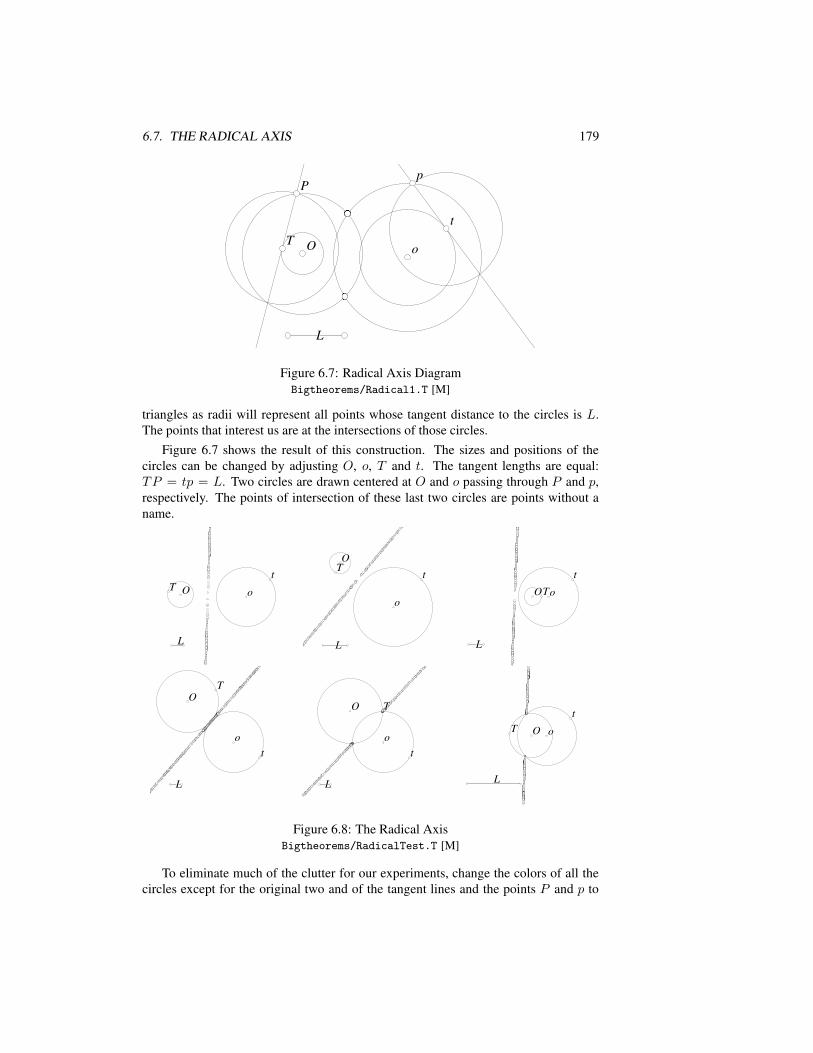
6.7. THE RADICAL AXIS 179
LL
OOTToo
tt
ppPP
Figure 6.7: Radical Axis DiagramBigtheorems/Radical1.T [M]
triangles as radii will represent all points whose tangent distance to the circles is L.The points that interest us are at the intersections of those circles.
Figure 6.7 shows the result of this construction. The sizes and positions of thecircles can be changed by adjusting O, o, T and t. The tangent lengths are equal:TP = tp = L. Two circles are drawn centered at O and o passing through P and p,respectively. The points of intersection of these last two circles are points without aname.
LL
OOTT oo
tt
LL
OOTT
oo
tt
LL
OOTToo
tt
LL
OOTT
oott
LL
OO TT
oott
LL
OOTT oo
tt
Figure 6.8: The Radical AxisBigtheorems/RadicalTest.T [M]
To eliminate much of the clutter for our experiments, change the colors of all thecircles except for the original two and of the tangent lines and the points P and p to
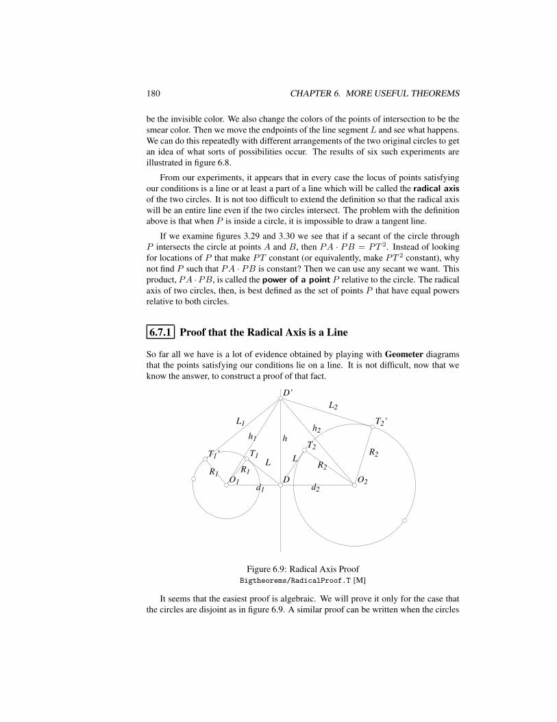
180 CHAPTER 6. MORE USEFUL THEOREMS
be the invisible color. We also change the colors of the points of intersection to be thesmear color. Then we move the endpoints of the line segment L and see what happens.We can do this repeatedly with different arrangements of the two original circles to getan idea of what sorts of possibilities occur. The results of six such experiments areillustrated in figure 6.8.
From our experiments, it appears that in every case the locus of points satisfyingour conditions is a line or at least a part of a line which will be called the radical axisof the two circles. It is not too difficult to extend the definition so that the radical axiswill be an entire line even if the two circles intersect. The problem with the definitionabove is that when P is inside a circle, it is impossible to draw a tangent line.
If we examine figures 3.29 and 3.30 we see that if a secant of the circle throughP intersects the circle at points A and B, then PA · PB = PT 2. Instead of lookingfor locations of P that make PT constant (or equivalently, make PT 2 constant), whynot find P such that PA · PB is constant? Then we can use any secant we want. Thisproduct, PA ·PB, is called the power of a point P relative to the circle. The radicalaxis of two circles, then, is best defined as the set of points P that have equal powersrelative to both circles.
6.7.1 Proof that the Radical Axis is a Line
So far all we have is a lot of evidence obtained by playing with Geometer diagramsthat the points satisfying our conditions lie on a line. It is not difficult, now that weknow the answer, to construct a proof of that fact.
O1O1 O2O2DD
T1T1T2T2
D’D’
T1’T1’
T2’T2’
d1d1 d2d2
LL LLR2R2
R2R2
R1R1R1R1
L1L1
L2L2
h1h1h2h2
hh
Figure 6.9: Radical Axis ProofBigtheorems/RadicalProof.T [M]
It seems that the easiest proof is algebraic. We will prove it only for the case thatthe circles are disjoint as in figure 6.9. A similar proof can be written when the circles
6.7. THE RADICAL AXIS 181
intersect. We will show that the radical axis is perpendicular to the line connecting thecenters of the circles. Pick D on that line of centers such thatDT1 = DT2. We need toshow that for any pointD′ on the line perpendicular to O1O2 throughD that L1 = L2,with the labeling as in the figure. To complete the proof, simply apply the pythagoreantheorem a few times and combine the results:
d21 = R2
1 + L2 (6.24)d2
2 = R22 + L2 (6.25)
h21 = d2
1 + h2 (6.26)h2
2 = d22 + h2 (6.27)
h21 = R2
1 + L21 (6.28)
h22 = R2
2 + L22 (6.29)
Combining equations 6.24, 6.26 and 6.28 and similarly equations 6.25, 6.27 and6.29we obtain:
L21 = h2 + L2
L22 = h2 + L2
which shows us that L1 = L2, so the proof is complete.
6.7.2 The Radical Center
Notice that if we have a set of three circles whose centers are not collinear, then eachpair will have a radical axis. The point P of intersection of any two of the radical axeswill have the same power relative to all three circles, so it must lie on the third radicalaxis. In other words, the three radical axes meet at a point called the radical center ofthe three circles.

182 CHAPTER 6. MORE USEFUL THEOREMS
Chapter 7Locus of Points
Computer geometry programs are particularly useful when studying locus problemswhose goal is to find all the points that satisfy certain conditions. The term “satisfycertain conditions” can be very general, and with Geometer or a similar program, it isoften easy to generate hundreds of such points automatically. This visual display of alarge set of solution points often makes it quite easy to guess the answer, even if youhave no idea how to prove it.
Here we will examine a number of applications of computer geometry programs tolocus problems.
7.1 Unknown Geometric Locus
Many geometric problems are stated directly as locus problems: “Given a circle withpoints B and C fixed upon it, if the point A is allowed to move on the arc
)
BC, what isthe locus of points of the incenter of4ABC?
183
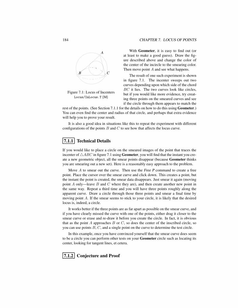
184 CHAPTER 7. LOCUS OF POINTS
AA
BB CC
Figure 7.1: Locus of IncentersLocus/InLocus.T [M]
With Geometer, it is easy to find out (orat least to make a good guess). Draw the fig-ure described above and change the color ofthe center of the incircle to the smearing color.Then move point A and see what happens.
The result of one such experiment is shownin figure 7.1. The incenter sweeps out twocurves depending upon which side of the chordBC it lies. The two curves look like circles,but if you would like more evidence, try creat-ing three points on the smeared curves and seeif the circle through them appears to match the
rest of the points. (See Section 7.1.1 for the details on how to do this using Geometer.)You can even find the center and radius of that circle, and perhaps that extra evidencewill help you to prove your result.
It is also a good idea in situations like this to repeat the experiment with differentconfigurations of the points B and C to see how that affects the locus curve.
7.1.1 Technical Details
If you would like to place a circle on the smeared images of the point that traces theincenter of4ABC in figure 7.1 using Geometer, you will find that the instant you cre-ate a new geometric object, all the smear points disappear (because Geometer thinksyou are smearing out a new set). Here is a reasonably easy approach to the problem.
Move A to smear out the curve. Then use the Free P command to create a freepoint. Place the cursor over the smear curve and click down. This creates a point, butthe instant the point is created, the smear data disappears. Just smear it again (movingpoint A only—leave B and C where they are), and then create another new point inthe same way. Repeat a third time and you will have three points roughly along theapparent curve. Draw a circle through those three points and smear a final time bymoving point A. If the smear seems to stick to your circle, it is likely that the desiredlocus is, indeed, a circle.
It works better if the three points are as far apart as possible on the smear curve, andif you have clearly missed the curve with one of the points, either drag it closer to thesmear curve or erase and re-draw it before you create the circle. In fact, it is obviousthat as the point A approaches B or C, so does the center of the inscribed circle, soyou can use points B, C, and a single point on the curve to determine the test circle.
In this example, once you have convinced yourself that the smear curve does seemto be a circle you can perform other tests on your Geometer circle such as locating itscenter, looking for tangent lines, et cetera.
7.1.2 Conjecture and Proof
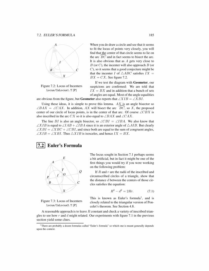
7.2. EULER’S FORMULA 185
XX
CCBB
AA
II
Figure 7.2: Locus of IncentersLocus/InLocus1.T [P]
When you do draw a circle and see that it seemsto fit the locus of points very closely, you willfind that the center of that circle seems to lie onthe arc
)
BC and in fact seems to bisect the arc.It is also obvious that as A gets very close toB (or C), the incenter will also approachB (orC), so it seems that a good conjecture might bethat the incenter I of 4ABC satisfies IX =BX = CX . See figure 7.2.
If we test the diagram with Geometer, oursuspicions are confirmed: We are told thatIX = BX and in addition that a bunch of setsof angles are equal. Most of the angle equalities
are obvious from the figure, but Geometer also reports that ∠XIB = ∠XBI .Using these ideas, it is simple to prove this lemma. AX is an angle bisector so
∠BAX = ∠CAX . In addition, AX will bisect the arc
)
BC, so X , the proposedcenter of our circle of locus points, is in the center of that arc. Of course ∠CBX isalso inscribed in the arc CX so it is also equal to ∠BAX and ∠CAX .
The line BI is also an angle bisector, so ∠CBI = ∠IBA. We also know that∠XIB is equal to ∠IAB +∠IBA since it is an exterior angle of4AIB. But clearly∠XBI = ∠XBC + ∠CBI , and since both are equal to the sum of congruent angles,∠XIB = ∠XBI . Thus4XIB is isosceles, and hence IX = BX .
7.2 Euler’s Formula
AA
BB CC
II OO
XX
PP
EE
TT
Figure 7.3: Locus of IncentersLocus/InLocus2.T [P]
The locus sought in Section 7.1 perhaps seemsa bit artificial, but in fact it might be one of thefirst things you would try if you were workingon the following problem:
If R and r are the radii of the inscribed andcircumscribed circles of a triangle, show thatthe distance d between the centers of those cir-cles satisfies the equation:
R2 − d2 = 2Rr. (7.1)
This is known as Euler’s formula1, and isclosely related to the triangular version of Pon-celet’s theorem. See Section 4.8.
A reasonable approach is to leaveR constant and check a variety of inscribed trian-gles to see how r and d might related. Our experiments with figure 7.1 in the previoussection yield some clues.
1There are probably a dozen formulas called “Euler’s formula” so which one is meant generally dependsupon the context.
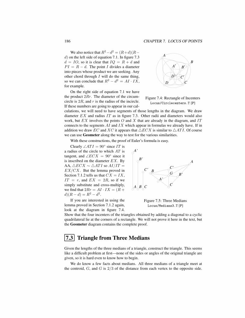
186 CHAPTER 7. LOCUS OF POINTS
BB
CCDD
AA
A′A′ B′B′
C′C′D′D′
Figure 7.4: Rectangle of IncentersLocus/Circlecenters.T [P]
We also notice thatR2−d2 = (R+d)(R−d) on the left side of equation 7.1. In figure 7.3d = IO, so it is clear that IQ = R + d andPI = R − d. The point I divides a diameterinto pieces whose product we are seeking. Anyother chord through I will do the same thing,so we can conclude that R2 − d2 = AI · IX ,for example.
On the right side of equation 7.1 we havethe product 2Rr. The diameter of the circum-circle is 2R, and r is the radius of the incircle.If these numbers are going to appear in our cal-culations, we will need to have segments of those lengths in the diagram. We drawdiameter EX and radius IT as in figure 7.3. Other radii and diameters would alsowork, but EX involves the points O and X that are already in the diagram, and ITconnects to the segments AI and IX which appear in formulas we already have. If inaddition we draw EC and XC it appears that4ECX is similar to4ATI . Of coursewe can use Geometer along the way to test for the various similarities.
With these constructions, the proof of Euler’s formula is easy.
AA BB CC
A’A’
B’B’
C’C’GG
AA
BB
CCA’A’
B’B’
C’C’
Figure 7.5: Three MediansLocus/Medians3.T [P]
Clearly ∠ATI = 90 since IT isa radius of the circle to which AT istangent, and ∠ECX = 90 since itis inscribed on the diameter EX . ByAA,4ECX ∼ 4ATI so AI/IT =EX/CX . But the lemma proved inSection 7.1.2 tells us that CX = IX ,IT = r, and EX = 2R, so if wesimply substitute and cross-multiply,we find that 2Rr = AI · IX = (R +d)(R − d) = R2 − d2.
If you are interested in using thelemma proved in Section 7.1.2 again,look at the diagram in figure 7.4.Show that the four incenters of the triangles obtained by adding a diagonal to a cyclicquadrilateral lie at the corners of a rectangle. We will not prove it here in the text, butthe Geometer diagram contains the complete proof.
7.3 Triangle from Three Medians
Given the lengths of the three medians of a triangle, construct the triangle. This seemslike a difficult problem at first—none of the sides or angles of the original triangle aregiven, so it is hard even to know how to begin.
We do know a few facts about medians. All three medians of a triangle meet atthe centroid, G, and G is 2/3 of the distance from each vertex to the opposite side.
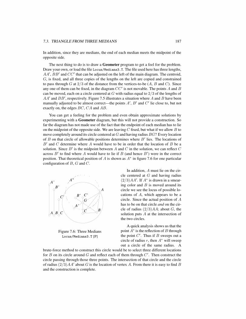
7.3. TRIANGLE FROM THREE MEDIANS 187
In addition, since they are medians, the end of each median meets the midpoint of theopposite side.
The next thing to do is to draw a Geometer program to get a feel for the problem.Draw your own, or load the file Locus/Medians3.T. The file used here has three lengths,AA′, BB′ and CC ′ that can be adjusted on the left of the main diagram. The centroid,G, is fixed, and all three copies of the lengths on the left are copied and constrainedto pass through G at 2/3 of the distance from the vertices-to-be (A, B and C). Sinceany one of them can be fixed, in the diagram CC ′ is not movable. The points A and Bcan be moved, each on a circle centered at G with radius equal to 2/3 of the lengths ofAA′ andBB′, respectively. Figure 7.5 illustrates a situation whereA and B have beenmanually adjusted to be almost correct—the points A′, B′ and C ′ lie close to, but notexactly on, the edges BC, CA and AB.
You can get a feeling for the problem and even obtain approximate solutions byexperimenting with a Geometer diagram, but this will not provide a construction. Sofar the diagram has not made use of the fact that the endpoint of each median has to lieon the midpoint of the opposite side. We are leavingC fixed, but what if we allowB tomove completely around its circle centered atG and having radiusBG? Every locationof B on that circle of allowable positions determines where B ′ lies. The locations ofB′ and C determine where A would have to be in order that the location of B be asolution. Since B′ is the midpoint between A and C in the solution, we can reflect Cacross B′ to find where A would have to lie if B (and hence B ′) were in the correctposition. That theoretical position of A is shown as A∗ in figure 7.6 for one particularconfiguration of B, G and C.
AA BB CC
A’A’B’B’
C’C’GG
AA
BBCCA’A’
B’B’ C’C’
A*A*
Figure 7.6: Three MediansLocus/Medians3.T [P]
In addition, A must lie on the cir-cle centered at G and having radius(2/3)AA′. If A∗ is drawn in a smear-ing color and B is moved around itscircle we see the locus of possible lo-cations of A, which appears to be acircle. Since the actual position of Ahas to be on that circle and on the cir-cle of radius (2/3)AA; about G, thesolution puts A at the intersection ofthe two circles.
A quick analysis shows us that thepointA∗ is the reflection ofB throughthe point C ′. Thus if B sweeps out acircle of radius r, then A∗ will sweepout a circle of the same radius. A
brute-force method to construct this circle would be to select three different locationsfor B on its circle around G and reflect each of them through C ′. Then construct thecircle passing through those three points. The intersection of that circle and the circleof radius (2/3)AA′ about G is the location of vertexA. From there it is easy to find Band the construction is complete.
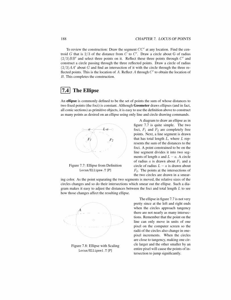
188 CHAPTER 7. LOCUS OF POINTS
To review the construction: Draw the segment CC ′ at any location. Find the cen-troid G that is 2/3 of the distance from C to C ′. Draw a circle about G of radius(2/3)BB′ and select three points on it. Reflect these three points through C ′ andconstruct a circle passing through the three reflected points. Draw a circle of radius(2/3)AA′ about G and find an intersection of it with the circle through the three re-flected points. This is the location of A. Reflect A through C ′ to obtain the location ofB. This completes the construction.
7.4 The Ellipse
An ellipse is commonly defined to be the set of points the sum of whose distances totwo fixed points (the foci) is constant. Although Geometer draws ellipses (and in fact,all conic sections) as primitive objects, it is easy to use the definition above to constructas many points as desired on an ellipse using only line and circle drawing commands.
aa L-aL-a
F1F1 F2F2
Figure 7.7: Ellipse from DefinitionLocus/Ellipse.T [P]
A diagram to draw an ellipse as infigure 7.7 is quite simple. The twofoci, F1 and F2 are completely freepoints. Next, a line segment is drawnthat has total length L, where L rep-resents the sum of the distances to thefoci. A point constrained to be on theline segment divides it into two seg-ments of length a and L− a. A circleof radius a is drawn about F1 and acircle of radius L − a is drawn aboutF2. The points at the intersections ofthe two circles are drawn in a smear-
ing color. As the point separating the two segments is moved, the relative sizes of thecircles changes and so do their intersections which smear out the ellipse. Such a dia-gram makes it easy to adjust the distances between the foci and total length L to seehow those changes affect the resulting ellipse.
AA
Figure 7.8: Ellipse with ScalingLocus/Ellipse1.T [P]
The ellipse in figure 7.7 is not verypretty since at the left and right endswhen the circles approach tangencythere are not nearly as many intersec-tions. Remember that the point on theline can only move in units of onepixel on the computer screen so theradii of the circles also change in one-pixel increments. When the circlesare close to tangency, making one cir-cle larger and the other smaller by anentire pixel will cause the points of in-tersection to jump significantly.
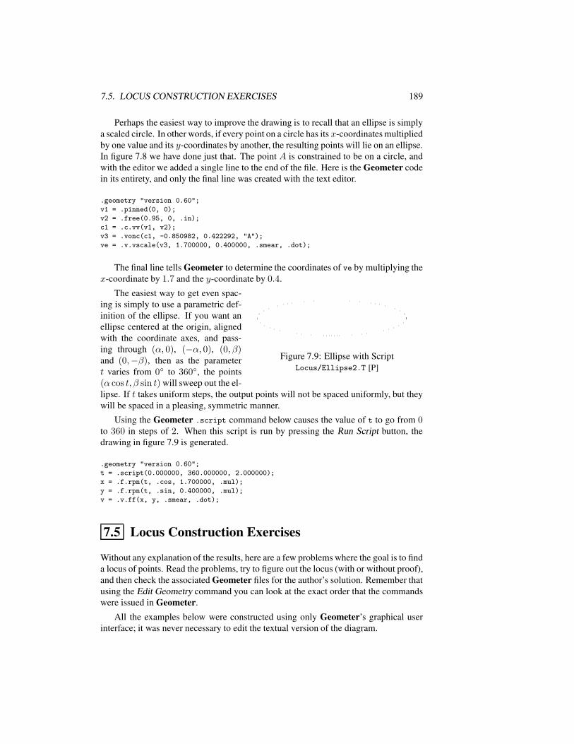
7.5. LOCUS CONSTRUCTION EXERCISES 189
Perhaps the easiest way to improve the drawing is to recall that an ellipse is simplya scaled circle. In other words, if every point on a circle has its x-coordinates multipliedby one value and its y-coordinates by another, the resulting points will lie on an ellipse.In figure 7.8 we have done just that. The point A is constrained to be on a circle, andwith the editor we added a single line to the end of the file. Here is the Geometer codein its entirety, and only the final line was created with the text editor.
.geometry "version 0.60";
v1 = .pinned(0, 0);
v2 = .free(0.95, 0, .in);
c1 = .c.vv(v1, v2);
v3 = .vonc(c1, -0.850982, 0.422292, "A");
ve = .v.vscale(v3, 1.700000, 0.400000, .smear, .dot);
The final line tells Geometer to determine the coordinates of ve by multiplying thex-coordinate by 1.7 and the y-coordinate by 0.4.
Figure 7.9: Ellipse with ScriptLocus/Ellipse2.T [P]
The easiest way to get even spac-ing is simply to use a parametric def-inition of the ellipse. If you want anellipse centered at the origin, alignedwith the coordinate axes, and pass-ing through (α, 0), (−α, 0), (0, β)and (0,−β), then as the parametert varies from 0 to 360, the points(α cos t, β sin t) will sweep out the el-lipse. If t takes uniform steps, the output points will not be spaced uniformly, but theywill be spaced in a pleasing, symmetric manner.
Using the Geometer .script command below causes the value of t to go from 0to 360 in steps of 2. When this script is run by pressing the Run Script button, thedrawing in figure 7.9 is generated.
.geometry "version 0.60";
t = .script(0.000000, 360.000000, 2.000000);
x = .f.rpn(t, .cos, 1.700000, .mul);
y = .f.rpn(t, .sin, 0.400000, .mul);
v = .v.ff(x, y, .smear, .dot);
7.5 Locus Construction Exercises
Without any explanation of the results, here are a few problems where the goal is to finda locus of points. Read the problems, try to figure out the locus (with or without proof),and then check the associated Geometer files for the author’s solution. Remember thatusing the Edit Geometry command you can look at the exact order that the commandswere issued in Geometer.
All the examples below were constructed using only Geometer’s graphical userinterface; it was never necessary to edit the textual version of the diagram.
190 CHAPTER 7. LOCUS OF POINTS
1. Let A, B, C and D be any four points on a circle. Let P be any point (inside,outside, or on the circle), and draw the lines PC and PD. Let Q and R be theintersections of PC and PD with the circle other than C and D. Find the locusof the intersections of the circles PRA and PQB. (Solution: Locus/Locus1.T)
2. Let B and C be two fixed points on a circle, and let A move freely on the cir-cle. Find the locus of the projections of the orthocenter H onto the bisector of∠CAB. Depending on what you mean by the angle bisector (there is an interiorand exterior bisector) this could mean different things. The included Geometerdiagram changes the interpretation from interior to exterior when the point Achanges sides of the segment. You may wish to draw both the interior and exte-rior bisectors to see what happens in both cases. (Solution: Locus/Locus2.T)
3. Given a fixed circleK, find the locus of the endpoints of the diameters parallel toa given line of a fixed-radius circle orthogonal toK. (Solution: Locus/Locus3.T)
4. Given a fixed circle K and a fixed point P , allow Q to move around K, andconstruct the circle through P that is tangent to K at Q. What is the locus of theintersection of the lines tangent to that new circle that pass through P and Q?(Solution: Locus/Locus4.T)
5. Given two pointsA andB, find the locus of pointsP such that PB : PA = r : 1,where r is a fixed ratio. (Solution: Locus/Locus5.T)
7.6 Higher-Order Curves
In Euclidean geometry, we normally deal with straight lines and circles, and sometimesconic sections: ellipses, hyperbolas and parabolas. All of these are first degree (lines)or second degree (all the rest). By “first degree” we mean that they can be describedby equations whose highest power is 1. Second degree curves have equations whosehighest power is 2, et cetera. The general equation for any straight line is given by:
ax+ by + c = 0,
for suitably-selected constants a, b and c. The general second degree equation is:
ax2 + bxy + cy2 + dx+ ey + f = 0,
where a, b, . . . , f are constants. Second degree equations describe all the conic sec-tions, where we consider a circle to be a special form of an ellipse.
We have already encountered two examples of curves of higher degree than 2 (thecardioid and the limacon) in Section 2.9.2.
7.6.1 Example: Strophoids and Freeth’s Nephroid
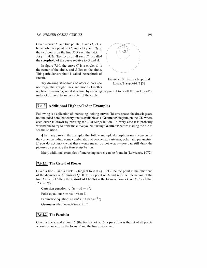
7.6. HIGHER-ORDER CURVES 191
OO
AA
Figure 7.10: Freeth’s NephroidLocus/Strophoid.T [S]
Given a curve C and two points, A and O, let Xbe an arbitrary point on C, and let P1 and P2 bethe two points on the line XO such that AX =AP1 = AP2. The locus of all such Pi is calledthe strophoid of the curve relative to O and A.
In figure 7.10, the curve C is a circle, O isthe center of the circle, and A lies on the circle.This particular strophoid is called the nephroid ofFreeth.
Try drawing strophoids of other curves (donot forget the straight line), and modify Freeth’snephroid to a more general strophoid by allowing the pointA to be off the circle, and/ormake O different from the center of the circle.
7.6.2 Additional Higher-Order Examples
Following is a collection of interesting looking curves. To save space, the drawings arenot included here, but every one is available as a Geometer diagram on the CD whereeach curve is drawn by pressing the Run Script button. In every case it is probablyworthwhile to try to draw the curve yourself using Geometer before loading the file tosee the solution.
In many cases in the examples that follow, multiple descriptions may be given forthe curve, including some combination of geometric, cartesian, polar, and parametric.If you do not know what these terms mean, do not worry—you can still draw thepictures by pressing the Run Script button.
Many additional examples of interesting curves can be found in [Lawrence, 1972].
7.6.2.1 The Cissoid of Diocles
Given a line L and a circle C tangent to it at Q. Let S be the point at the other endof the diameter of C through Q. If X is a point on L and R is the intersecion of theline XS with C, then the cissoid of Diocles is the locus of points P on XS such thatPX = RS.
Cartesian equation: y2(a− x) = x3.
Polar equation: r = a sin θ tan θ.
Parametric equation: (a sin2 t, a tan t sin2 t).
Geometer file: Locus/Cissoid1.T
7.6.2.2 The Parabola
Given a line L and a point F (the focus) not on L, a parabola is the set of all pointswhose distance from the focus F and the line L are equal.
192 CHAPTER 7. LOCUS OF POINTS
Cartesian equation: y2 = 4ax.
Polar equation: r sin2 θ = 4a cos θ.Parametric equation: (at2, 2at).
Geometer file: Locus/Parabola.T
7.6.2.3 The Conchoid of Nicomedes
Given a line L and a point O, let the point Q move along L. The conchoid ofNicomedes is the locus of points P1 and P2 on the line OQ such that P1Q = P2Q.
Cartesian equation: (x2 + y2)(x− b)2 = a2x2.
Polar equation: r = a+ b sec t.Parametric equation: (b+ a cos t, tan t(b+ a cos t)).
Geometer file: Locus/Conchoid.T
7.6.2.4 The Hypotrochoid and Rhodonea
If a small circle rolls around the inside of a larger circle and the ratio of their radii is aninteger (so that the small circle completes an integral number of turns when it returns toits starting point), then if P is a point connected to the smaller circle, a hypotrochoidis the path traversed by P . Note that P may be outside the smaller circle, but if that isthe case, it rotates as if it were connected to the smaller circle by a rigid rod.
A rhodonea is a special case of the hypotrochoid where if h is the distance ofP from the center of the smaller circle, the radii of the smaller and larger circles areh(n− 1)/(n+ 1) and 2nh/(n+ 1), respectively.
Polar equation: r = a cos(nθ).Geometer file: Locus/Rhodonea.T (for n = 7)
7.6.2.5 Lissijous Figures
If two wheels of the same size turn at different rates such that they eventually return tothe starting position after a certain number of turns, and if a point is selected on each,then a lissijous figure is the locus of points that are the intersection of a vertical linedrawn from one of the points and a horizontal line from the other.
Parametric equation: (cosnt, sinmt), (cosnt, cosmt) or (sinnt, sinmt).Geometer diagram: Locus/Lissijous.T
7.6.2.6 Dumbbell Curve
This is simply a curve that looks like a dumbbell.
Parametric equation: y2 = x4 − x6.Geometer file: Locus/Dumbbell.T
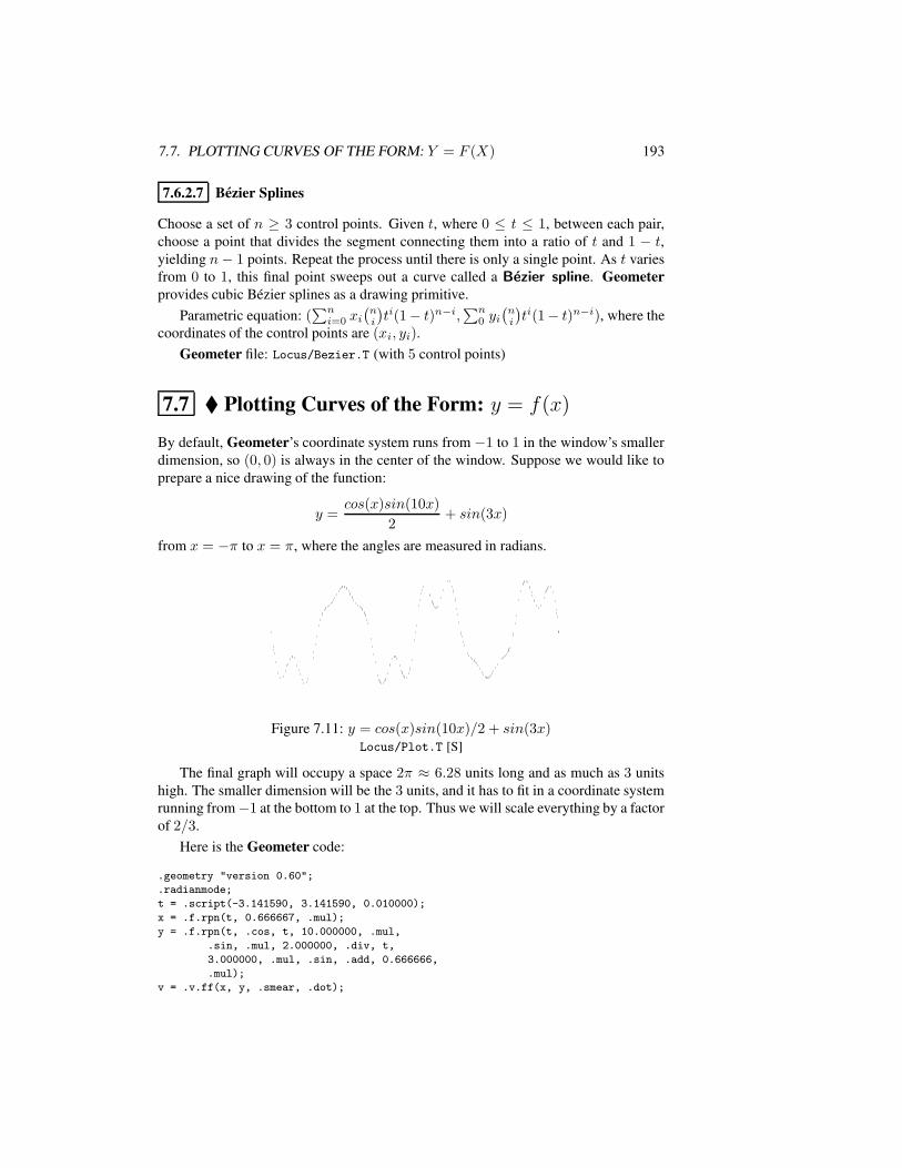
7.7. PLOTTING CURVES OF THE FORM: Y = F (X) 193
7.6.2.7 Bezier Splines
Choose a set of n ≥ 3 control points. Given t, where 0 ≤ t ≤ 1, between each pair,choose a point that divides the segment connecting them into a ratio of t and 1 − t,yielding n− 1 points. Repeat the process until there is only a single point. As t variesfrom 0 to 1, this final point sweeps out a curve called a Bezier spline. Geometerprovides cubic Bezier splines as a drawing primitive.
Parametric equation: (∑n
i=0 xi(ni
)ti(1− t)n−i,∑n
0 yi(ni
)ti(1− t)n−i), where the
coordinates of the control points are (xi, yi).Geometer file: Locus/Bezier.T (with 5 control points)
7.7 Plotting Curves of the Form: y = f(x)
By default, Geometer’s coordinate system runs from −1 to 1 in the window’s smallerdimension, so (0, 0) is always in the center of the window. Suppose we would like toprepare a nice drawing of the function:
y =cos(x)sin(10x)
2+ sin(3x)
from x = −π to x = π, where the angles are measured in radians.
Figure 7.11: y = cos(x)sin(10x)/2 + sin(3x)Locus/Plot.T [S]
The final graph will occupy a space 2π ≈ 6.28 units long and as much as 3 unitshigh. The smaller dimension will be the 3 units, and it has to fit in a coordinate systemrunning from−1 at the bottom to 1 at the top. Thus we will scale everything by a factorof 2/3.
Here is the Geometer code:
.geometry "version 0.60";
.radianmode;
t = .script(-3.141590, 3.141590, 0.010000);
x = .f.rpn(t, 0.666667, .mul);
y = .f.rpn(t, .cos, t, 10.000000, .mul,
.sin, .mul, 2.000000, .div, t,
3.000000, .mul, .sin, .add, 0.666666,
.mul);
v = .v.ff(x, y, .smear, .dot);
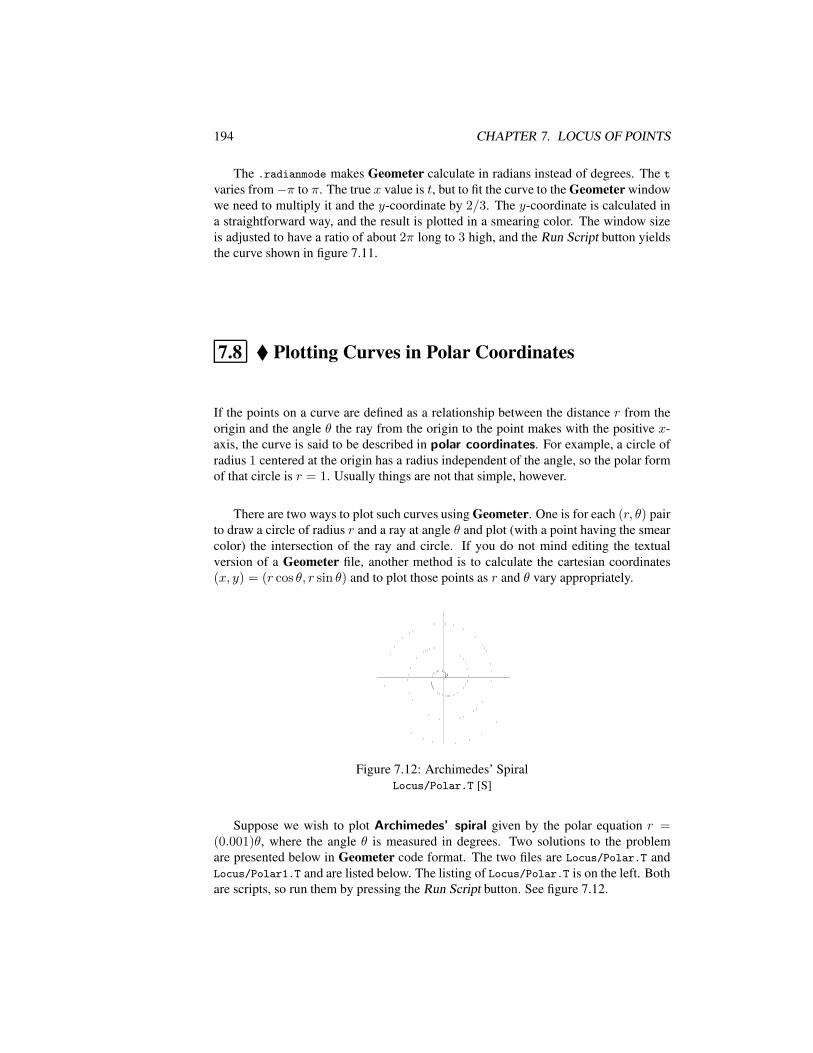
194 CHAPTER 7. LOCUS OF POINTS
The .radianmode makes Geometer calculate in radians instead of degrees. The t
varies from−π to π. The true x value is t, but to fit the curve to the Geometer windowwe need to multiply it and the y-coordinate by 2/3. The y-coordinate is calculated ina straightforward way, and the result is plotted in a smearing color. The window sizeis adjusted to have a ratio of about 2π long to 3 high, and the Run Script button yieldsthe curve shown in figure 7.11.
7.8 Plotting Curves in Polar Coordinates
If the points on a curve are defined as a relationship between the distance r from theorigin and the angle θ the ray from the origin to the point makes with the positive x-axis, the curve is said to be described in polar coordinates. For example, a circle ofradius 1 centered at the origin has a radius independent of the angle, so the polar formof that circle is r = 1. Usually things are not that simple, however.
There are two ways to plot such curves using Geometer. One is for each (r, θ) pairto draw a circle of radius r and a ray at angle θ and plot (with a point having the smearcolor) the intersection of the ray and circle. If you do not mind editing the textualversion of a Geometer file, another method is to calculate the cartesian coordinates(x, y) = (r cos θ, r sin θ) and to plot those points as r and θ vary appropriately.
OO
Figure 7.12: Archimedes’ SpiralLocus/Polar.T [S]
Suppose we wish to plot Archimedes’ spiral given by the polar equation r =(0.001)θ, where the angle θ is measured in degrees. Two solutions to the problemare presented below in Geometer code format. The two files are Locus/Polar.T andLocus/Polar1.T and are listed below. The listing of Locus/Polar.T is on the left. Bothare scripts, so run them by pressing the Run Script button. See figure 7.12.
7.9. ENVELOPES OF CURVES: THE EPICYCLOID 195
.geometry "version 0.60";
o = .pinned(0, 0, "O");
one = .pinned(1, 0, .in);
l1 = .l.vv(o, one, .longline);
l2 = .l.vlperp(o, l1, .longline);
theta = .script(0.0, 1080.0, 4.0);
r = .f.rpn(theta, 0.001, .mul);
x = .f.rpn(r, theta, .cos, .mul);
y = .f.rpn(r, theta, .sin, .mul);
p = .v.ff(x, y, .smear, .dot);
.geometry "version 0.60";
o = .pinned(0, 0, "O");
one = .pinned(1, 0, .in);
l1 = .l.vv(o, one, .longline);
l2 = .l.vlperp(o, l1, .longline);
theta = .script(0.0, 1080.0, 4.0);
r = .f.rpn(theta, 0.001, .mul);
c = .c.vf(o, r);
ang = .a.f(theta);
v1 = .v.avv(ang, one, o);
l3 = .l.vv(o, v1);
p = .v.lc(l3, c, 2, .smear, .dot);
7.9 Envelopes of Curves: the Epicycloid
Sometimes the shape of a curve is made obvious if you draw a large set of lines that aretangent to the curve. The various types of epicycloids provide some good examples.See figure 7.13.
An epicycloid is path traced by a point on the edge of a circle as it rolls aroundanother circle. If the ratio of the diameters of the circles is rational, the path closes.
To draw the envelope of an N -epicycloid begin by selecting a reference point ona circle. Next, for an evenly-spaced set of points around the circle, connect each ofthose points by a straight line to the point that is N times as far around the circle asthe original point, wrapping around the circle if necessary. Figure 7.13 illustrates theresults for N = 2, N = 3, N = 5 and N = 8.
The three examples were generated by the following Geometer code:
.geometry "version 0.61";
m = .script(0.000000, 360.000000, 2.000000);
rad = .f.rpn(0.800000);
vn2 = .pinned(-0.9, 0.92, .dot, "2");
vn3 = .pinned(-0.72, 0.92, .dot, "3");
vn4 = .pinned(-0.54, 0.92, .dot, "4");
vn5 = .pinned(-0.36, 0.92, .dot, "5");
vn6 = .pinned(-0.18, 0.92, .dot, "6");
vn7 = .pinned(0, 0.92, .dot, "7");
vn8 = .pinned(0.18, 0.92, .dot, "8");
vn9 = .pinned(0.36, 0.92, .dot, "9");
vn10 = .pinned(0.54, 0.92, .dot, "10");
vn11 = .pinned(0.72, 0.92, .dot, "11");
vn12 = .pinned(0.9, 0.92, .dot, "12");
l1 = .l.vv(vn2, vn12);
vmid = .vonl(l1, -0.365269, 0.92, .red, "N");
v2x = .f.vxcoord(vn2);
v12x = .f.vxcoord(vn12);
vmidx = .f.vxcoord(vmid);
n = .f.rpn(vmidx, v2x, .sub, v12x, v2x,
.sub, .div, 10.000000, .mul, 0.500000,
.add, .truncate, 2.000000, .add);
p0 = .pinned(0, 0, .in);
p1 = .v.ff(rad, 0.000000, .in);
c = .c.vv(p0, p1);
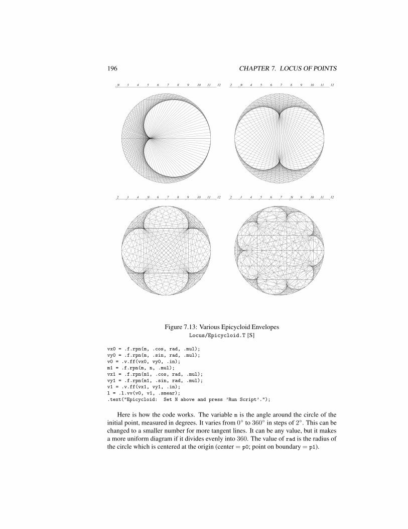
196 CHAPTER 7. LOCUS OF POINTS
22 121233 44 55 66 77 88 99 1010 1111NN 22 121233 44 55 66 77 88 99 1010 1111NN
22 121233 44 55 66 77 88 99 1010 1111NN 22 33 44 55 66 77 88 99 1010 1111 1212NN
Figure 7.13: Various Epicycloid EnvelopesLocus/Epicycloid.T [S]
vx0 = .f.rpn(m, .cos, rad, .mul);
vy0 = .f.rpn(m, .sin, rad, .mul);
v0 = .v.ff(vx0, vy0, .in);
m1 = .f.rpn(m, n, .mul);
vx1 = .f.rpn(m1, .cos, rad, .mul);
vy1 = .f.rpn(m1, .sin, rad, .mul);
v1 = .v.ff(vx1, vy1, .in);
l = .l.vv(v0, v1, .smear);
.text("Epicycloid: Set N above and press ’Run Script’.");
Here is how the code works. The variable m is the angle around the circle of theinitial point, measured in degrees. It varies from 0 to 360 in steps of 2. This can bechanged to a smaller number for more tangent lines. It can be any value, but it makesa more uniform diagram if it divides evenly into 360. The value of rad is the radius ofthe circle which is centered at the origin (center = p0; point on boundary = p1).
7.9. ENVELOPES OF CURVES: THE EPICYCLOID 197
The next few lines of code allow the user to choose the value of N for which theN -epicycloid will be generated. The point vmid (labeled N in the Geometer diagram)can be moved between vn2 and vn12 and its position is used to calculate n.
To calculate n we find the x-coordinates of vn2, vmid and vn12. The expression(vmidx - v2x)/(v12x - v2x) is the proportion of the distance along the line from vn2 tovn12 at which vmid lies. It will be between 0.0 and 10.0. When we multiply by ten,add 0.5 (for rounding) and truncate, we obtain an integer between 0 and 10. Adding 2to that gives us an integer n between 2 and 12, inclusive.
The points labeled vn3, . . . , vn11 are simply to label the line so the user can tellwhat value of n will be calculated.
Next the circle is drawn and the coordinates of the starting point (determined byangle m) and the endpoint (determined by angle mn) of the line segment are calculated.That line is then drawn in a smearing color.

198 CHAPTER 7. LOCUS OF POINTS
Chapter 8Triangle Centers
Perhaps the most amazing theorems from high school geometry concern the concur-rence of the medians, altitudes, angle bisectors and even the perpendicular bisectorsof the sides of a triangle. This occurs not just for particular triangles, but for everytriangle. These high school examples all have special names that may at first sightseem unrelated to how they are defined. The intersection of the three medians is calledthe centroid, the intersection of the three angle bisectors is called the incenter, theintersection of the three altitudes is the orthocenter, and the intersection of the threeperpendicular bisectors of the sides is the circumcenter.
As we shall see, the points of concurrence above just scratch the surface. These, andall the similar points that will be defined later in this chapter will go by the general nametriangle center. We will learn about more of these centers, about other properties thatthe centers satisfy, interrelationships among the centers, and how the various centershave applications not only to other areas of geometry, but very practical applications aswell.
199
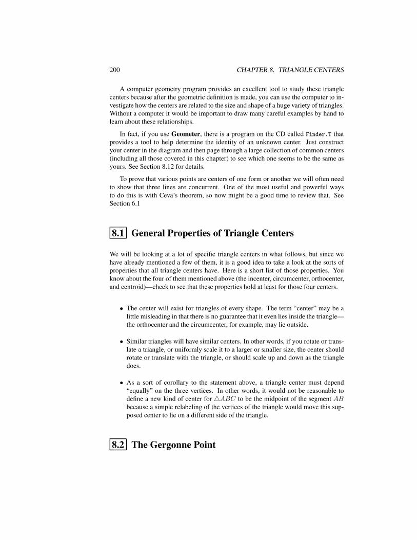
200 CHAPTER 8. TRIANGLE CENTERS
A computer geometry program provides an excellent tool to study these trianglecenters because after the geometric definition is made, you can use the computer to in-vestigate how the centers are related to the size and shape of a huge variety of triangles.Without a computer it would be important to draw many careful examples by hand tolearn about these relationships.
In fact, if you use Geometer, there is a program on the CD called Finder.T thatprovides a tool to help determine the identity of an unknown center. Just constructyour center in the diagram and then page through a large collection of common centers(including all those covered in this chapter) to see which one seems to be the same asyours. See Section 8.12 for details.
To prove that various points are centers of one form or another we will often needto show that three lines are concurrent. One of the most useful and powerful waysto do this is with Ceva’s theorem, so now might be a good time to review that. SeeSection 6.1
8.1 General Properties of Triangle Centers
We will be looking at a lot of specific triangle centers in what follows, but since wehave already mentioned a few of them, it is a good idea to take a look at the sorts ofproperties that all triangle centers have. Here is a short list of those properties. Youknow about the four of them mentioned above (the incenter, circumcenter, orthocenter,and centroid)—check to see that these properties hold at least for those four centers.
• The center will exist for triangles of every shape. The term “center” may be alittle misleading in that there is no guarantee that it even lies inside the triangle—the orthocenter and the circumcenter, for example, may lie outside.
• Similar triangles will have similar centers. In other words, if you rotate or trans-late a triangle, or uniformly scale it to a larger or smaller size, the center shouldrotate or translate with the triangle, or should scale up and down as the triangledoes.
• As a sort of corollary to the statement above, a triangle center must depend“equally” on the three vertices. In other words, it would not be reasonable todefine a new kind of center for 4ABC to be the midpoint of the segment ABbecause a simple relabeling of the vertices of the triangle would move this sup-posed center to lie on a different side of the triangle.
8.2 The Gergonne Point
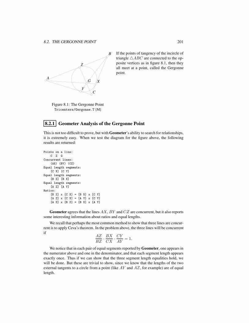
8.2. THE GERGONNE POINT 201
AA
BB
CC
XX
YY
ZZ
GG
Figure 8.1: The Gergonne PointTricenters/Gergonne.T [M]
If the points of tangency of the incircle oftriangle4ABC are connected to the op-posite vertices as in figure 8.1, then theyall meet at a point, called the Gergonnepoint.
8.2.1 Geometer Analysis of the Gergonne Point
This is not too difficult to prove, but with Geometer’s ability to search for relationships,it is extremely easy. When we test the diagram for the figure above, the followingresults are returned:
Points on a line:
C Z G
Concurrent lines:
(AX) (BY) (CZ)
Equal length segments:
[C X] [C Y]
Equal length segments:
[B Z] [B X]
Equal length segments:
[A Z] [A Y]
Ratios:
[B Z] x [C X] = [B X] x [C Y]
[A Z] x [C X] = [A Y] x [C Y]
[A Z] x [B Z] = [B X] x [A Y]
Geometer agrees that the lines AX ,BY andCZ are concurrent, but it also reportssome interesting information about ratios and equal lengths.
We recall that perhaps the most common method to show that three lines are concur-rent is to apply Ceva’s theorem. In the problem above, the three lines will be concurrentif
AZ
BZ· BXCX
· CYAY
= 1.
We notice that in each pair of equal segments reported by Geometer, one appears inthe numerator above and one in the denominator, and that each segment length appearsexactly once. Thus if we can show that the three segment length equalities hold, wewill be done. But these are trivial to show, since we know that the lengths of the twoexternal tangents to a circle from a point (like AY and AZ, for example) are of equallength.
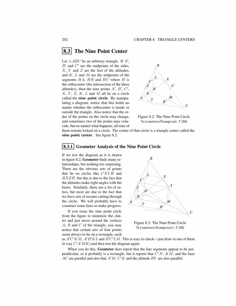
202 CHAPTER 8. TRIANGLE CENTERS
8.3 The Nine Point Center
AA
BB
CC
A’A’
B’B’
C’C’XX
YY
ZZHH
KK
LL
MM
Figure 8.2: The Nine Point CircleTricenters/Ninepoint.T [M]
Let 4ABC be an arbitrary triangle. If A′,B′ and C ′ are the midpoints of the sides,X , Y and Z are the feet of the altitudes,and K, L and M are the midpoints of thesegments HA, HB and HC where H isthe orthocenter (the intersection of the threealtitudes), then the nine points A′, B′, C ′,X , Y , Z, K, L and M all lie on a circlecalled the nine point circle. By manipu-lating a diagram, notice that this holds nomatter whether the orthocenter is inside oroutside the triangle. Also notice that the or-der of the points on the circle may change,and sometimes two of the points may coin-cide, but no matter what happens, all nine ofthem remain locked on a circle. The center of that circle is a triangle center called thenine point center. See figure 8.2.
8.3.1 Geometer Analysis of the Nine Point Circle
AA
BB
CC
A’A’
B’B’
C’C’XX
YY
ZZHH
KK
LL
MM
Figure 8.3: The Nine Point CircleTricenters/Ninepoint1.T [M]
If we test the diagram as it is drawnin figure 8.2, Geometer finds many re-lationships, but nothing too surprising.There are the obvious sets of pointsthat lie on circles like CXYH andBXZH , but this is due to the fact thatthe altitudes make right angles with thebases. Similarly, there are a lot of ra-tios, but most are due to the fact thatwe have sets of secants cutting throughthe circle. We will probably have toconstruct some lines to make progress.
If you erase the nine point circlefrom the figure to minimize the clut-ter and just move around the verticesA, B and C of the triangle, you maynotice that certain sets of four pointsseem always to lie on a rectangle, suchasA′C ′KM ,A′B′KL andB′C ′LM . This is easy to check—just draw in one of themin (say C ′A′MK) and then test the diagram again.
When you do this, Geometer does report that the line segments appear to be per-pendicular, so it probably is a rectangle, but it reports that C ′A′, KM , and the baseAC are parallel and also that A′M , C ′K and the altitude BY are also parallel.
8.4. THE FERMAT POINT 203
A look at the diagram shows us why: all those segments connect midpoints oftriangle edges, so they must be parallel to the bases of those triangles and equal to halftheir length. In this case, the triangles in question are4ABC, 4AHC, 4BHC and4BHA. What is more, the altitude BY is perpendicular to the base AC, so instead ofmerely being a parallelogram,A′C ′KM is a rectangle.
Obviously the same method can be used to show that other sets of four points alsolie on rectangles.
We can find the center of the rectangle if we wish by finding the intersection of thediagonals A′K and C ′M , and in fact it should be clear that both of those segmentsare diameters of the circle we are looking for. But then we notice that if A′K is thediameter of a circle and ∠A′XK = 90 then X must lie on the circle with diameterA′K. From here, the proof is obvious.
8.3.2 Proof of the Nine Point Circle
See figure 8.3. ConnectA′C ′ andMK. We know thatA′C ′ ‖ AC sinceA′C ′ connectsthe midpoints of AB and BC in4ABC. By exactly the same reasoning, KM ‖ ACusing 4AHC, C ′K ‖ BY using 4BAH and A′M ‖ BY using 4BCH . ThusA′M ‖ C ′K and A′C ′ ‖ KM .
We knowBY ⊥ AC since BY is an altitude, and since C ′K andA′M are parallelto BY and A′C ′ and CM are parallel to AC, C ′K ′ and A′M must be perpendicularto A′C ′ and KM . Thus A′C ′KM is a rectangle.
Using the other bases and altitudes of4ABC we can conclude in exactly the sameway that A′B′KL and B′C ′LM are also rectangles.
Consider rectangle A′C ′KM . Its center is at the intersection of A′K and C ′Mand the circle passing through its four vertices has A′K and C ′M as diameters. But∠KXA′ = 90 sinceAX is an altitude, soX must lie on the circle having the diameterC ′M . Similarly Z must lie on the circle having diameterA′K. Thus the pointsA′,M ,K, C ′, Z and X all lie on a single circle.
By similar reasoning with the other two rectangles we obtain two other sets of sixpoints lying on circles: A′B′KLXY and B′C ′LMYZ. Since each of these sets ofpoints shares three points with each of the others, all the points must lie on a singlecircle—the nine point circle.
8.4 The Fermat Point
Erect equilateral triangles on the outside of each segment of 4ABC. The line seg-ments connecting the vertices A, B and C to the tips of the opposite equilateral trian-gles are concurrent at a pointO called the Fermat point of the triangle. See figure 8.4.
8.4.1 Geometer Analysis of the Fermat Point
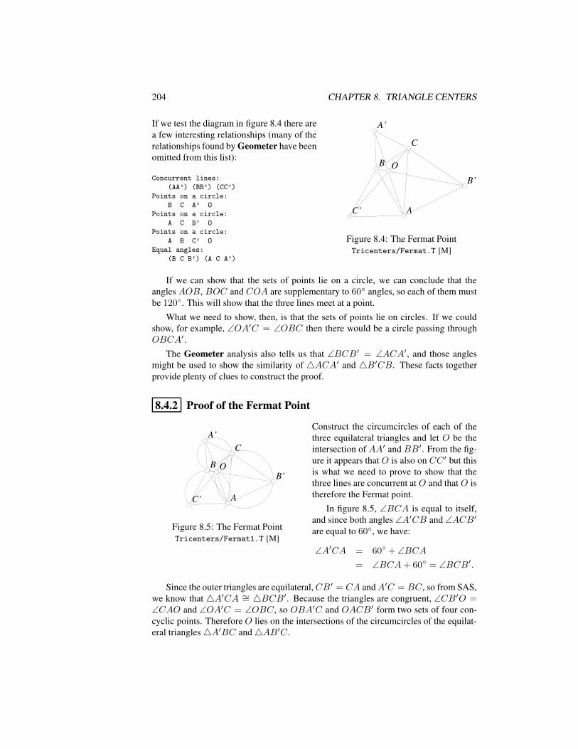
204 CHAPTER 8. TRIANGLE CENTERS
AA
BB
CC
A’A’
B’B’
C’C’
OO
Figure 8.4: The Fermat PointTricenters/Fermat.T [M]
If we test the diagram in figure 8.4 there area few interesting relationships (many of therelationships found by Geometer have beenomitted from this list):
Concurrent lines:
(AA’) (BB’) (CC’)
Points on a circle:
B C A’ O
Points on a circle:
A C B’ O
Points on a circle:
A B C’ O
Equal angles:
(B C B’) (A C A’)
If we can show that the sets of points lie on a circle, we can conclude that theangles AOB, BOC and COA are supplementary to 60 angles, so each of them mustbe 120. This will show that the three lines meet at a point.
What we need to show, then, is that the sets of points lie on circles. If we couldshow, for example, ∠OA′C = ∠OBC then there would be a circle passing throughOBCA′.
The Geometer analysis also tells us that ∠BCB′ = ∠ACA′, and those anglesmight be used to show the similarity of 4ACA′ and 4B′CB. These facts togetherprovide plenty of clues to construct the proof.
8.4.2 Proof of the Fermat Point
AA
BB
CCA’A’
B’B’
C’C’
OO
Figure 8.5: The Fermat PointTricenters/Fermat1.T [M]
Construct the circumcircles of each of thethree equilateral triangles and let O be theintersection of AA′ and BB′. From the fig-ure it appears that O is also on CC ′ but thisis what we need to prove to show that thethree lines are concurrent at O and that O istherefore the Fermat point.
In figure 8.5, ∠BCA is equal to itself,and since both angles ∠A′CB and ∠ACB′are equal to 60, we have:
∠A′CA = 60 + ∠BCA= ∠BCA+ 60 = ∠BCB′.
Since the outer triangles are equilateral,CB′ = CA andA′C = BC, so from SAS,we know that 4A′CA ∼= 4BCB′. Because the triangles are congruent, ∠CB ′O =∠CAO and ∠OA′C = ∠OBC, so OBA′C and OACB′ form two sets of four con-cyclic points. Therefore O lies on the intersections of the circumcircles of the equilat-eral triangles4A′BC and4AB′C.
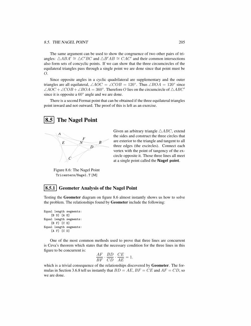
8.5. THE NAGEL POINT 205
The same argument can be used to show the congruence of two other pairs of tri-angles: 4ABA′ ∼= 4C ′BC and 4B′AB ∼= CAC ′ and their common intersectionsalso form sets of concyclic points. If we can show that the three circumcircles of theequilateral triangles pass through a single point we are done since that point must beO.
Since opposite angles in a cyclic quadrilateral are supplementary and the outertriangles are all equilateral, ∠AOC = ∠COB = 120. Thus ∠BOA = 120 since∠AOC+∠COB+∠BOA = 360. ThereforeO lies on the circumcircle of4ABC ′since it is opposite a 60 angle and we are done.
There is a second Fermat point that can be obtained if the three equilateral trianglespoint inward and not outward. The proof of this is left as an exercise.
8.5 The Nagel Point
AA
BB
CC
DDEE
FFNN
Figure 8.6: The Nagel PointTricenters/Nagel.T [M]
Given an arbitrary triangle 4ABC, extendthe sides and construct the three circles thatare exterior to the triangle and tangent to allthree edges (the excircles). Connect eachvertex with the point of tangency of the ex-circle opposite it. Those three lines all meetat a single point called the Nagel point.
8.5.1 Geometer Analysis of the Nagel Point
Testing the Geometer diagram on figure 8.6 almost instantly shows us how to solvethe problem. The relationships found by Geometer include the following:
Equal length segments:
[B D] [A E]
Equal length segments:
[B F] [C E]
Equal length segments:
[A F] [C D]
One of the most common methods used to prove that three lines are concurrentis Ceva’s theorem which states that the necessary condition for the three lines in thisfigure to be concurrent is:
AF
BF· BDCD· CEAE
= 1.
which is a trivial consequence of the relationships discovered by Geometer. The for-mulas in Section 3.6.8 tell us instantly that BD = AE, BF = CE andAF = CD, sowe are done.
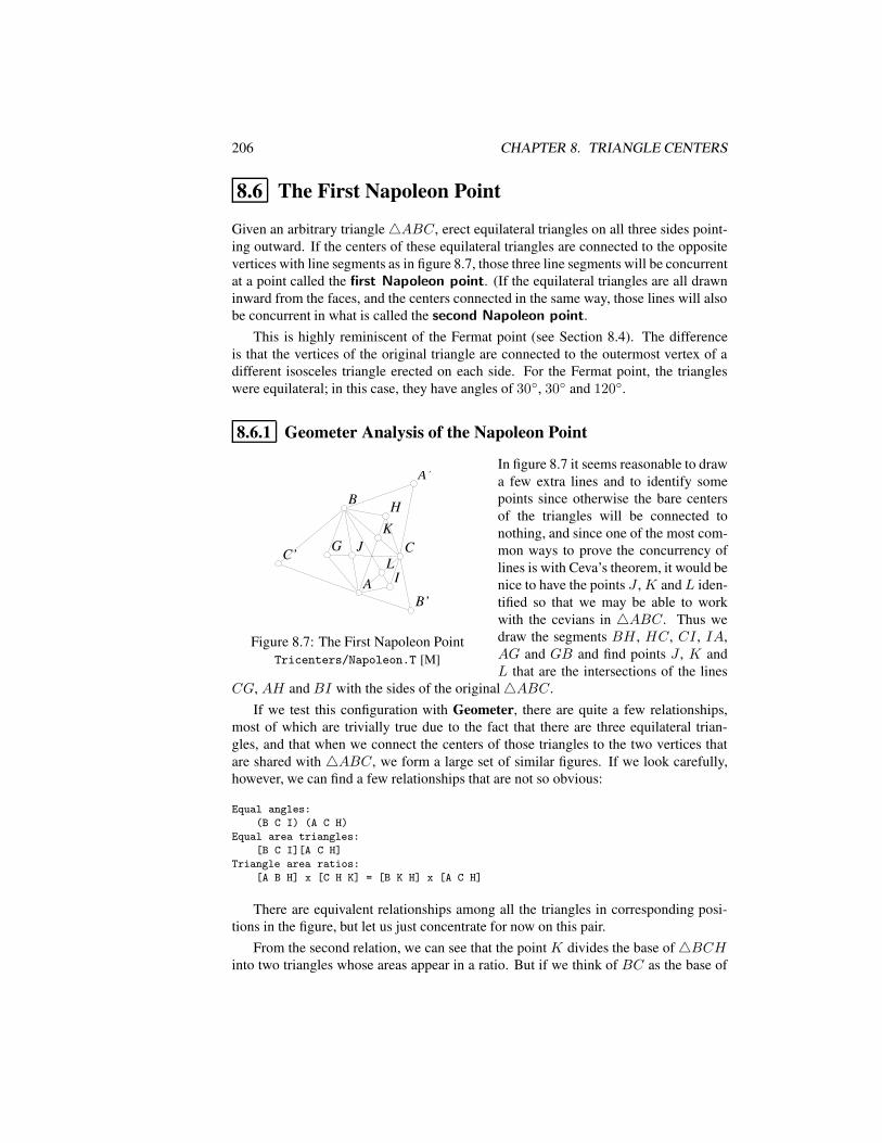
206 CHAPTER 8. TRIANGLE CENTERS
8.6 The First Napoleon Point
Given an arbitrary triangle4ABC, erect equilateral triangles on all three sides point-ing outward. If the centers of these equilateral triangles are connected to the oppositevertices with line segments as in figure 8.7, those three line segments will be concurrentat a point called the first Napoleon point. (If the equilateral triangles are all drawninward from the faces, and the centers connected in the same way, those lines will alsobe concurrent in what is called the second Napoleon point.
This is highly reminiscent of the Fermat point (see Section 8.4). The differenceis that the vertices of the original triangle are connected to the outermost vertex of adifferent isosceles triangle erected on each side. For the Fermat point, the triangleswere equilateral; in this case, they have angles of 30, 30 and 120.
8.6.1 Geometer Analysis of the Napoleon Point
AA
BB
CC
B’B’
C’C’
A’A’
GG
HH
II
JJKK
LL
Figure 8.7: The First Napoleon PointTricenters/Napoleon.T [M]
In figure 8.7 it seems reasonable to drawa few extra lines and to identify somepoints since otherwise the bare centersof the triangles will be connected tonothing, and since one of the most com-mon ways to prove the concurrency oflines is with Ceva’s theorem, it would benice to have the points J , K andL iden-tified so that we may be able to workwith the cevians in 4ABC. Thus wedraw the segments BH , HC, CI , IA,AG and GB and find points J , K andL that are the intersections of the lines
CG, AH and BI with the sides of the original4ABC.If we test this configuration with Geometer, there are quite a few relationships,
most of which are trivially true due to the fact that there are three equilateral trian-gles, and that when we connect the centers of those triangles to the two vertices thatare shared with 4ABC, we form a large set of similar figures. If we look carefully,however, we can find a few relationships that are not so obvious:
Equal angles:
(B C I) (A C H)
Equal area triangles:
[B C I][A C H]
Triangle area ratios:
[A B H] x [C H K] = [B K H] x [A C H]
There are equivalent relationships among all the triangles in corresponding posi-tions in the figure, but let us just concentrate for now on this pair.
From the second relation, we can see that the point K divides the base of4BCHinto two triangles whose areas appear in a ratio. But if we think of BC as the base of
8.6. THE FIRST NAPOLEON POINT 207
4BCH , the ratio BK : CK is equal to the ratio of the areas of the smaller triangles4BKH and 4CKH . If we are going to use Ceva’s theorem, we will need to useratios involving BK and CK, so perhaps we can convert them to ratios of triangleareas.
Using the equal angles found by Geometer and the ratios of sides due to the simi-larity of the equilateral triangles and the included 30 − 30 − 120 triangles we canshow prove the equality of the triangle areas found by Geometer.
8.6.2 Proof of the Existence of the First Napoleon Point
Let us begin by showing that A(4BCI) = A(4ACH). Since we have equilateraltriangles erected on the sides of the triangle as well as the 30 − 30 − 120 triangles,it is clear that both ∠BCI and ∠ACH are the sum of ∠ACB and a 30 angle, so theyare equal.
We know that the area of a triangle is equal to half the product of two sides multi-plied by the sine of the included angle, so
A(4BCI) =BC · CI sin(∠BCI)
2and A(4ACH) =
AC · CH sin(∠ACH)
2.
Since the two angles above are equal, the ratio of the two areas is therefore:
A(4BCI)
A(4ACH)=
BC · CIAC · CH . (8.1)
But since they are both 30 − 30 − 120 triangles, we know that 4ACI ∼4BCH , and thus CI/AC = CH/BC, and this, combined with equation 8.1 tellsus that the ratio of the areas is 1, or in other words,A(4BCI) = A(4ACH).
Exactly the same technique can be applied to show that A(4ABI) = A(4ACG)andA(4ABH) = A(4BCG).
If we consider BC to be the base of triangles4BCH and4BCA, it is clear thatKA and KH divide their areas into equal ratios and the ratio of the areas of 4ACHand4ABH will also be the same thing.
From this observation we obtain the following three ratios:
A(4ACH)
A(4ABH)=CK
BK,
A(4ABI)
A(4BCI)=AL
CL,
A(4BCG)
A(4ACG)=BJ
AJ
If we multiply the three ratios above together and take into account the equality ofthe pairs of triangle areas, we obtain:
CK
BK· ALCL· BJAJ
= 1,
and this, together with Ceva’s theorem, is sufficient to prove that the three lines areconcurrent.
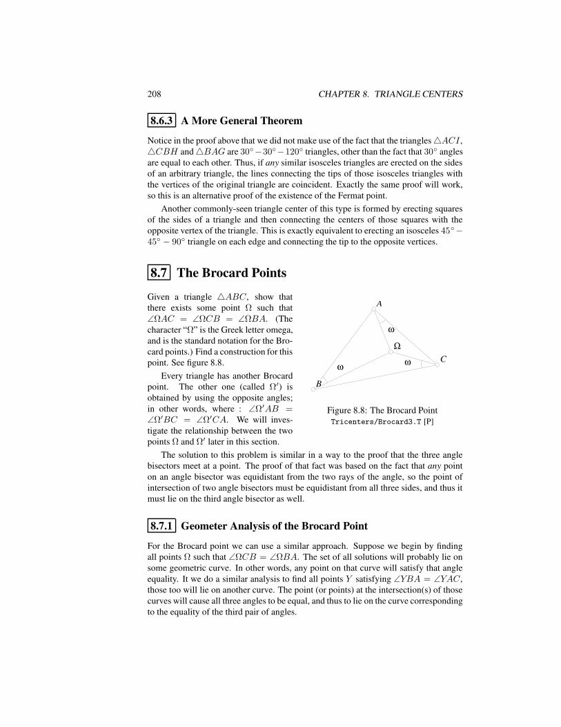
208 CHAPTER 8. TRIANGLE CENTERS
8.6.3 A More General Theorem
Notice in the proof above that we did not make use of the fact that the triangles4ACI ,4CBH and4BAG are 30−30−120 triangles, other than the fact that 30 anglesare equal to each other. Thus, if any similar isosceles triangles are erected on the sidesof an arbitrary triangle, the lines connecting the tips of those isosceles triangles withthe vertices of the original triangle are coincident. Exactly the same proof will work,so this is an alternative proof of the existence of the Fermat point.
Another commonly-seen triangle center of this type is formed by erecting squaresof the sides of a triangle and then connecting the centers of those squares with theopposite vertex of the triangle. This is exactly equivalent to erecting an isosceles 45−45 − 90 triangle on each edge and connecting the tip to the opposite vertices.
8.7 The Brocard Points
AA
BB
CCΩΩ
ωωωω
ωω
Figure 8.8: The Brocard PointTricenters/Brocard3.T [P]
Given a triangle 4ABC, show thatthere exists some point Ω such that∠ΩAC = ∠ΩCB = ∠ΩBA. (Thecharacter “Ω” is the Greek letter omega,and is the standard notation for the Bro-card points.) Find a construction for thispoint. See figure 8.8.
Every triangle has another Brocardpoint. The other one (called Ω′) isobtained by using the opposite angles;in other words, where : ∠Ω′AB =∠Ω′BC = ∠Ω′CA. We will inves-tigate the relationship between the twopoints Ω and Ω′ later in this section.
The solution to this problem is similar in a way to the proof that the three anglebisectors meet at a point. The proof of that fact was based on the fact that any pointon an angle bisector was equidistant from the two rays of the angle, so the point ofintersection of two angle bisectors must be equidistant from all three sides, and thus itmust lie on the third angle bisector as well.
8.7.1 Geometer Analysis of the Brocard Point
For the Brocard point we can use a similar approach. Suppose we begin by findingall points Ω such that ∠ΩCB = ∠ΩBA. The set of all solutions will probably lie onsome geometric curve. In other words, any point on that curve will satisfy that angleequality. It we do a similar analysis to find all points Y satisfying ∠YBA = ∠YAC,those too will lie on another curve. The point (or points) at the intersection(s) of thosecurves will cause all three angles to be equal, and thus to lie on the curve correspondingto the equality of the third pair of angles.
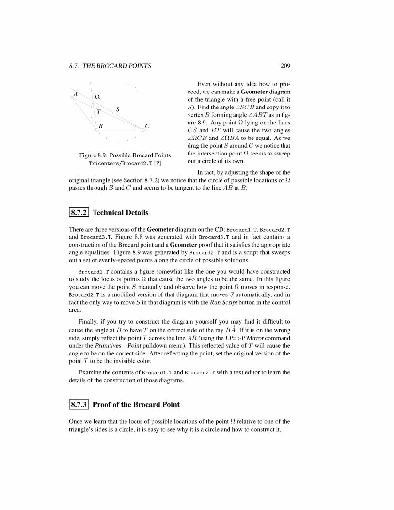
8.7. THE BROCARD POINTS 209
AA
BB CC
ΩΩ
SSTT
Figure 8.9: Possible Brocard PointsTricenters/Brocard2.T [P]
Even without any idea how to pro-ceed, we can make a Geometer diagramof the triangle with a free point (call itS). Find the angle∠SCB and copy it tovertexB forming angle∠ABT as in fig-ure 8.9. Any point Ω lying on the linesCS and BT will cause the two angles∠ΩCB and ∠ΩBA to be equal. As wedrag the pointS aroundC we notice thatthe intersection point Ω seems to sweepout a circle of its own.
In fact, by adjusting the shape of theoriginal triangle (see Section 8.7.2) we notice that the circle of possible locations of Ωpasses throughB and C and seems to be tangent to the line AB at B.
8.7.2 Technical Details
There are three versions of the Geometer diagram on the CD: Brocard1.T, Brocard2.Tand Brocard3.T. Figure 8.8 was generated with Brocard3.T and in fact contains aconstruction of the Brocard point and a Geometer proof that it satisfies the appropriateangle equalities. Figure 8.9 was generated by Brocard2.T and is a script that sweepsout a set of evenly-spaced points along the circle of possible solutions.
Brocard1.T contains a figure somewhat like the one you would have constructedto study the locus of points Ω that cause the two angles to be the same. In this figureyou can move the point S manually and observe how the point Ω moves in response.Brocard2.T is a modified version of that diagram that moves S automatically, and infact the only way to move S in that diagram is with the Run Script button in the controlarea.
Finally, if you try to construct the diagram yourself you may find it difficult tocause the angle at B to have T on the correct side of the ray
−−→BA. If it is on the wrong
side, simply reflect the point T across the lineAB (using the LP=>P Mirror commandunder the Primitives→Point pulldown menu). This reflected value of T will cause theangle to be on the correct side. After reflecting the point, set the original version of thepoint T to be the invisible color.
Examine the contents of Brocard1.T and Brocard2.T with a text editor to learn thedetails of the construction of those diagrams.
8.7.3 Proof of the Brocard Point
Once we learn that the locus of possible locations of the point Ω relative to one of thetriangle’s sides is a circle, it is easy to see why it is a circle and how to construct it.
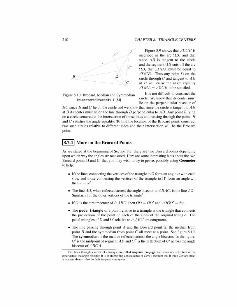
210 CHAPTER 8. TRIANGLE CENTERS
AA
BB
CC
ΩΩ
C’C’B’B’
C’’C’’
Figure 8.10: Brocard, Median and SymmedianTricenters/Brocard4.T [M]
Figure 8.9 shows that ∠ΩCB isinscribed in the arc ΩB, and thatsince AB is tangent to the circleand the segment ΩB cuts off the arcΩB, that ∠ΩBA must be equal to∠ΩCB. Thus any point Ω on thecircle through C and tangent to ABat B will cause the angle equality∠ΩBA = ∠ΩCB to be satisfied.
It is not difficult to construct thecircle. We know that its center mustlie on the perpendicular bisector of
BC since B and C lie on the circle and we know that since the circle is tangent to ABat B its center must lie on the line throughB perpendicular to AB. Any point Ω lyingon a circle centered at the intersection of those lines and passing through the points Band C satisfies the angle equality. To find the location of the Brocard point, constructtwo such circles relative to different sides and their intersection will be the Brocardpoint.
8.7.4 More on the Brocard Points
As we stated at the beginning of Section 8.7, there are two Brocard points dependingupon which way the angles are measured. Here are some interesting facts about the twoBrocard points Ω and Ω′ that you may wish to try to prove, possibly using Geometerto help:
• If the lines connecting the vertices of the triangle to Ω form an angle ω with eachside, and those connecting the vertices of the triangle to Ω′ form an angle ω′,then ω = ω′.
• The lineAΩ, when reflected across the angle bisector at ∠BAC, is the lineAΩ′.Similarly for the other vertices of the triangle1.
• If O is the circumcenter of4ABC, then OΩ = OΩ′ and ∠ΩOΩ′ = 2ω.
• The pedal triangle of a point relative to a triangle is the triangle that connectsthe projections of the point on each of the sides of the original triangle. Thepedal triangles of Ω and Ω′ relative to4ABC are congruent.
• The line passing through point A and the Brocard point Ω, the median frompoint B and the symmedian from point C all meet at a point. See figure 8.10.The symmedian is the median reflected across the angle bisector. In the figure,C ′ is the midpoint of segmentAB andC ′′ is the reflection of C ′ across the anglebisector of ∠BCA.
1Two lines through a vertex of a triangle are called isogonal conjugates if each is a reflection of theother across the angle bisector. It is an interesting consequence of Ceva’s theorem that if three Cevians meetat a point, then so also do their isogonal conjugates.
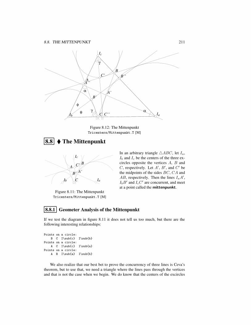
8.8. THE MITTENPUNKT 211
AA
BB
CC
IcIc
IaIaIbIb
C’C’
A’A’B’B’
A’’A’’
B’’B’’
C’’C’’ααθθ
φφ
γγ
γγ
αα
Figure 8.12: The MittenpunktTricenters/Mittenpunkt.T [M]
8.8 The Mittenpunkt
AABB
CC
IcIc
IaIaIbIb
C’C’
A’A’B’B’
Figure 8.11: The MittenpunktTricenters/Mittenpunkt.T [M]
In an arbitrary triangle 4ABC, let Ia,Ib and Ic be the centers of the three ex-circles opposite the vertices A, B andC, respectively. Let A′, B′, and C ′ bethe midpoints of the sides BC, CA andAB, respectively. Then the lines IaA′,IbB
′ and IcC ′ are concurrent, and meetat a point called the mittenpunkt.
8.8.1 Geometer Analysis of the Mittenpunkt
If we test the diagram in figure 8.11 it does not tell us too much, but there are thefollowing interesting relationships:
Points on a circle:
B C I\subc I\subb
Points on a circle:
A C I\subc I\suba
Points on a circle:
A B I\suba I\subb
We also realize that our best bet to prove the concurrency of three lines is Ceva’stheorem, but to use that, we need a triangle where the lines pass through the verticesand that is not the case when we begin. We do know that the centers of the excircles
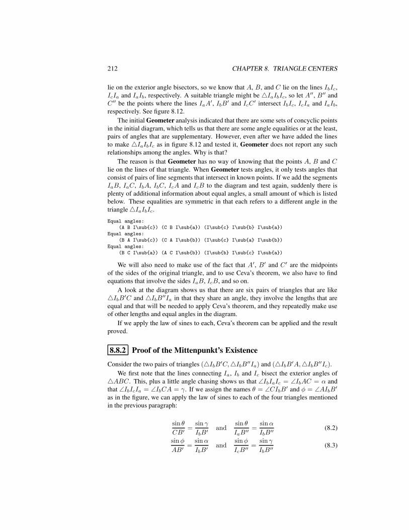
212 CHAPTER 8. TRIANGLE CENTERS
lie on the exterior angle bisectors, so we know that A, B, and C lie on the lines IbIc,IcIa and IaIb, respectively. A suitable triangle might be 4IaIbIc, so let A′′, B′′ andC ′′ be the points where the lines IaA′, IbB′ and IcC ′ intersect IbIc, IcIa and IaIb,respectively. See figure 8.12.
The initial Geometer analysis indicated that there are some sets of concyclic pointsin the initial diagram, which tells us that there are some angle equalities or at the least,pairs of angles that are supplementary. However, even after we have added the linesto make 4IaIbIc as in figure 8.12 and tested it, Geometer does not report any suchrelationships among the angles. Why is that?
The reason is that Geometer has no way of knowing that the points A, B and Clie on the lines of that triangle. When Geometer tests angles, it only tests angles thatconsist of pairs of line segments that intersect in known points. If we add the segmentsIaB, IaC, IbA, IbC, IcA and IcB to the diagram and test again, suddenly there isplenty of additional information about equal angles, a small amount of which is listedbelow. These equalities are symmetric in that each refers to a different angle in thetriangle4IaIbIc.Equal angles:
(A B I\subc) (C B I\suba) (I\subc I\subb I\suba)
Equal angles:
(B A I\subc) (C A I\subb) (I\subc I\suba I\subb)
Equal angles:
(B C I\suba) (A C I\subb) (I\subb I\subc I\suba)
We will also need to make use of the fact that A′, B′ and C ′ are the midpointsof the sides of the original triangle, and to use Ceva’s theorem, we also have to findequations that involve the sides IaB, IcB, and so on.
A look at the diagram shows us that there are six pairs of triangles that are like4IbB′C and 4IbB′′Ia in that they share an angle, they involve the lengths that areequal and that will be needed to apply Ceva’s theorem, and they repeatedly make useof other lengths and equal angles in the diagram.
If we apply the law of sines to each, Ceva’s theorem can be applied and the resultproved.
8.8.2 Proof of the Mittenpunkt’s Existence
Consider the two pairs of triangles (4IbB′C,4IbB′′Ia) and (4IbB′A,4IbB′′Ic).We first note that the lines connecting Ia, Ib and Ic bisect the exterior angles of
4ABC. This, plus a little angle chasing shows us that ∠IbIaIc = ∠IbAC = α andthat ∠IbIcIa = ∠IbCA = γ. If we assign the names θ = ∠CIbB′ and φ = ∠AIbB′as in the figure, we can apply the law of sines to each of the four triangles mentionedin the previous paragraph:
sin θ
CB′=
sin γ
IbB′and
sin θ
IaB′′=
sinα
IbB′′(8.2)
sinφ
AB′=
sinα
IbB′and
sinφ
IcB′′=
sin γ
IbB′′(8.3)
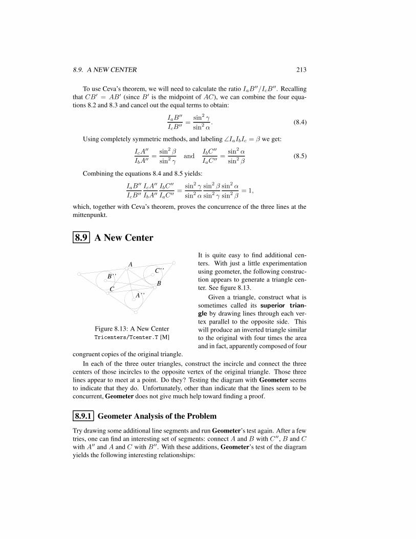
8.9. A NEW CENTER 213
To use Ceva’s theorem, we will need to calculate the ratio IaB′′/IcB′′. Recallingthat CB′ = AB′ (since B′ is the midpoint of AC), we can combine the four equa-tions 8.2 and 8.3 and cancel out the equal terms to obtain:
IaB′′
IcB′′=
sin2 γ
sin2 α. (8.4)
Using completely symmetric methods, and labeling ∠IaIbIc = β we get:
IcA′′
IbA′′=
sin2 β
sin2 γand
IbC′′
IaC ′′=
sin2 α
sin2 β(8.5)
Combining the equations 8.4 and 8.5 yields:
IaB′′
IcB′′IcA
′′
IbA′′IbC
′′
IaC ′′=
sin2 γ
sin2 α
sin2 β
sin2 γ
sin2 α
sin2 β= 1,
which, together with Ceva’s theorem, proves the concurrence of the three lines at themittenpunkt.
8.9 A New Center
AA
BBCC
B’’B’’C’’C’’
A’’A’’
Figure 8.13: A New CenterTricenters/Tcenter.T [M]
It is quite easy to find additional cen-ters. With just a little experimentationusing geometer, the following construc-tion appears to generate a triangle cen-ter. See figure 8.13.
Given a triangle, construct what issometimes called its superior trian-gle by drawing lines through each ver-tex parallel to the opposite side. Thiswill produce an inverted triangle similarto the original with four times the areaand in fact, apparently composed of four
congruent copies of the original triangle.In each of the three outer triangles, construct the incircle and connect the three
centers of those incircles to the opposite vertex of the original triangle. Those threelines appear to meet at a point. Do they? Testing the diagram with Geometer seemsto indicate that they do. Unfortunately, other than indicate that the lines seem to beconcurrent, Geometer does not give much help toward finding a proof.
8.9.1 Geometer Analysis of the Problem
Try drawing some additional line segments and run Geometer’s test again. After a fewtries, one can find an interesting set of segments: connect A and B with C ′′, B and Cwith A′′ and A and C with B′′. With these additions, Geometer’s test of the diagramyields the following interesting relationships:
214 CHAPTER 8. TRIANGLE CENTERS
Parallel lines:
(BA’’) (AB’’)
Parallel lines:
(BC’’) (CB’’)
Parallel lines:
(AC’’) (CA’’)
Equal length segments:
[B A’’] [A B’’]
Equal length segments:
[B C’’] [C B’’]
Equal length segments:
[A C’’] [C A’’]
If these are true, it is clear that AC ′′A′′C, BC ′′B′′C and AB′′A′′B are all paral-lelograms whose diagonals bisect each other. Since every diagonal bisects the other,all three must meet at a point.
Since all three exterior triangles are congruent, it is clear that the lengths in the listabove are equal. That they are parallel is also clear since, for example,BC ′′ and CB′′
are angle bisectors of corresponding angles in congruent triangles that have parallelsides.
This is a very rough sketch of the proof, but it is not difficult to fill in the details.
8.10 Additional Triangle Centers
There are, in fact, an infinite number of triangle centers, many of which, together withtheir properties, are listed in [Kimberling, 1994]. Without proof, here is a list of a fewmore of them, described in geometric terms.
• The Lemoine Point. If each of the medians of a triangle is reflected across thecorresponding angle bisector, then those three reflections are coincident at theLemoine point.
• The Spieker Center. The existence of the Spieker center is obvious—it is justthe incircle of the triangle whose vertices are the midpoints of the sides of theoriginal triangle (called the medial triangle). Physically, it is the center of massof the perimeter of the triangle. In other words, if a uniform wire were bent intothe shape of the triangle, it would balance at the Spieker center.
• The Feuerbach Point. This is the point of tangency of the incircle of a trianglewith its nine-point circle. The existence of this point is proved by Feuerbach’stheorem. See Section 9.17. The Feuerbach point is not precisely a triangle center,since it fails to exist for an equilateral triangle. When the triangle is equilateral,the nine-point circle and the incircle are the same so there are an infinite numberof points of tangency.
It is quite easy, especially with a computer geometry program, to experiment withvarious symmetric combinations of lines and to find other possible triangle centers.Often these centers turn out to be one of the many known centers and if that is the case,it is usually easy to prove that the new center makes sense.
8.11. TRILINEAR COORDINATES 215
8.11 Trilinear Coordinates
Trilinear coordinates provide a method to locate points on the plane relative to somegiven fixed triangle 4ABC (having sides a, b and c opposite the corresponding an-gles). The trilinear coordinates of a point are just a ratio of the (directed) distancesfrom the point to the sides of the triangle. If only points inside the triangle are consid-ered there is no need for the “directed” in the definition, but in fact trilinear coordinatescan be used to identify any point of the plane, be it inside, outside, or on the triangle.The “directed” in “directed distance” means that the distance is positive if the point ison the same side of the edge as the triangle and negative otherwise2.
The trilinear coordinates of a point are written “α : β : γ” where α, β and γ arethree real numbers, at least one of which is non-zero. The three numbers are propor-tional to the directed distances of the point from the sides a, b and c, respectively.
The trilinear coordinates of the incenter are 1 : 1 : 1 since the incenter is equallyfar from each of the sides, and it is inside the triangle. The trilinear coordinates of thethree excenters are similar: −1 : 1 : 1, 1 : −1 : 1 and 1 : 1 : −1 since those points arealso equidistant from the three edges, but they are outside the triangle in one of threedirections.
The trilinear coordinates of a point are not unique. If α : β : γ correspond toa point, then so do κα : κβ : κγ, where κ is any non-zero real number. Thus thecoordinates of the incenter could equally well have been written: 2 : 2 : 2, −1 : −1 :−1, 2/3 : 2/3 : 2/3, or even −π : −π : −π. This is not such a bizarre concept; wealready do something similar with fractions. Although 3/5 is usually not expressedthat way, we all agree that it is equal to 6/10 or even (−3π)/(−5π). Coordinates thatare unique only up to a real multiple are said to be homogeneous coordinates, sotrilinear coordinates are sometimes referred to as “homogeneous trilinear coordinates”.
At least one of the coordinates must be non-zero, but up to two of them may bezero. The point A has trilinear coordinates 1 : 0 : 0 (or α : 0 : 0), and any point on theline b has trilinear coordinates α : 0 : γ since it is a distance 0 from the line b but canbe anywhere relative to the other two lines.
As one non-trivial example, consider the centroid of a triangle (the intersection ofthe three medians). The trilinear coordinates of the centroid are 1/a : 1/b : 1/c. Thisis not too hard to see: Remember that the medians divide the triangle into six smallertriangles of equal area, so any two of them will amount to 1/3 the total triangle area.If we drop perpendiculars to each of the sides of the triangle, these can be thought ofas altitudes of triangles4ABG, 4BCG and4CAG, where G is the centroid. If thealtitudes to sides a, b and c have lengths ha, hb and hc then from the equality of theareas we obtain: aha = bhb = chc. Thus the values of ha, hb and hc (which are thedistances to the sides) are proportional to 1/a : 1/b : 1/c, which is what we wished toshow.
2This is not exactly correct, since we will allow multiplication of all the coordinates by an arbitraryvalue, positive or negative. A point inside the triangle will have all its directed distances positive, but if allare multiplied by −1 they will all be negative and no such point exists on the plane. If a set of trilinearcoordinates is nonsensical, flip the signs on all of them to obtain a set that makes geometric sense.
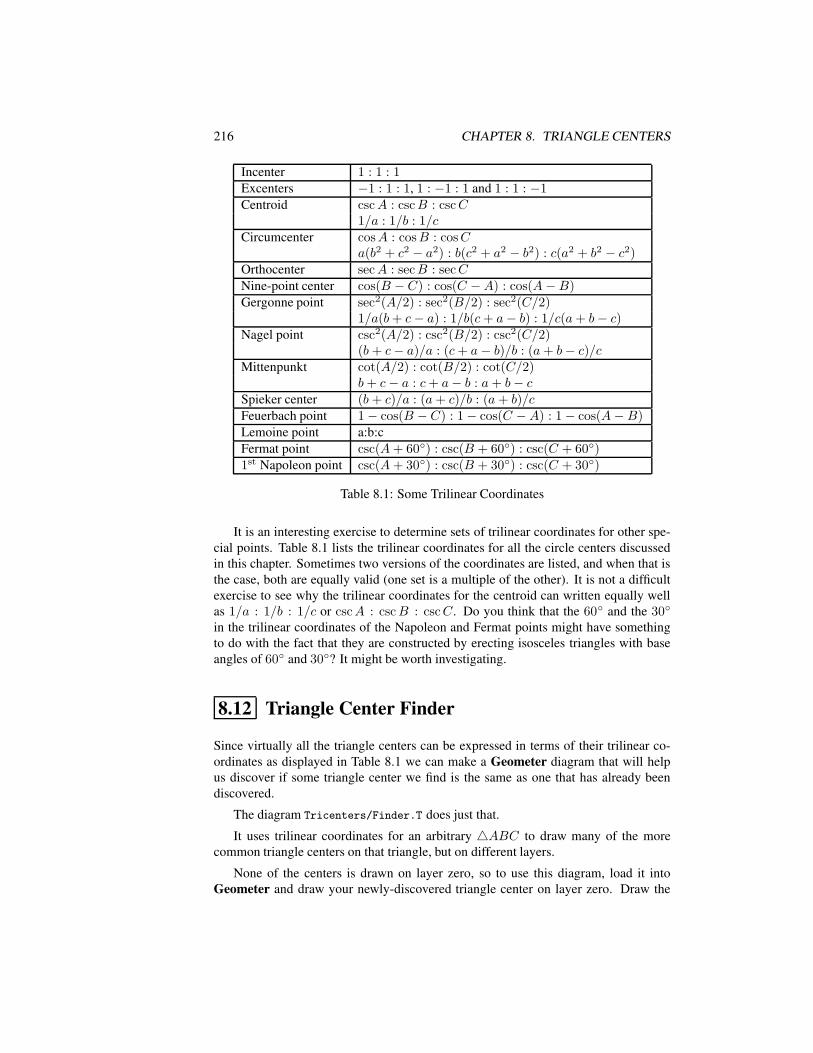
216 CHAPTER 8. TRIANGLE CENTERS
Incenter 1 : 1 : 1Excenters −1 : 1 : 1, 1 : −1 : 1 and 1 : 1 : −1Centroid cscA : cscB : cscC
1/a : 1/b : 1/cCircumcenter cosA : cosB : cosC
a(b2 + c2 − a2) : b(c2 + a2 − b2) : c(a2 + b2 − c2)Orthocenter secA : secB : secCNine-point center cos(B − C) : cos(C −A) : cos(A−B)Gergonne point sec2(A/2) : sec2(B/2) : sec2(C/2)
1/a(b+ c− a) : 1/b(c+ a− b) : 1/c(a+ b− c)Nagel point csc2(A/2) : csc2(B/2) : csc2(C/2)
(b+ c− a)/a : (c+ a− b)/b : (a+ b− c)/cMittenpunkt cot(A/2) : cot(B/2) : cot(C/2)
b+ c− a : c+ a− b : a+ b− cSpieker center (b+ c)/a : (a+ c)/b : (a+ b)/cFeuerbach point 1− cos(B − C) : 1− cos(C −A) : 1− cos(A−B)Lemoine point a:b:cFermat point csc(A+ 60) : csc(B + 60) : csc(C + 60)1st Napoleon point csc(A+ 30) : csc(B + 30) : csc(C + 30)
Table 8.1: Some Trilinear Coordinates
It is an interesting exercise to determine sets of trilinear coordinates for other spe-cial points. Table 8.1 lists the trilinear coordinates for all the circle centers discussedin this chapter. Sometimes two versions of the coordinates are listed, and when that isthe case, both are equally valid (one set is a multiple of the other). It is not a difficultexercise to see why the trilinear coordinates for the centroid can written equally wellas 1/a : 1/b : 1/c or cscA : cscB : cscC. Do you think that the 60 and the 30
in the trilinear coordinates of the Napoleon and Fermat points might have somethingto do with the fact that they are constructed by erecting isosceles triangles with baseangles of 60 and 30? It might be worth investigating.
8.12 Triangle Center Finder
Since virtually all the triangle centers can be expressed in terms of their trilinear co-ordinates as displayed in Table 8.1 we can make a Geometer diagram that will helpus discover if some triangle center we find is the same as one that has already beendiscovered.
The diagram Tricenters/Finder.T does just that.
It uses trilinear coordinates for an arbitrary 4ABC to draw many of the morecommon triangle centers on that triangle, but on different layers.
None of the centers is drawn on layer zero, so to use this diagram, load it intoGeometer and draw your newly-discovered triangle center on layer zero. Draw the
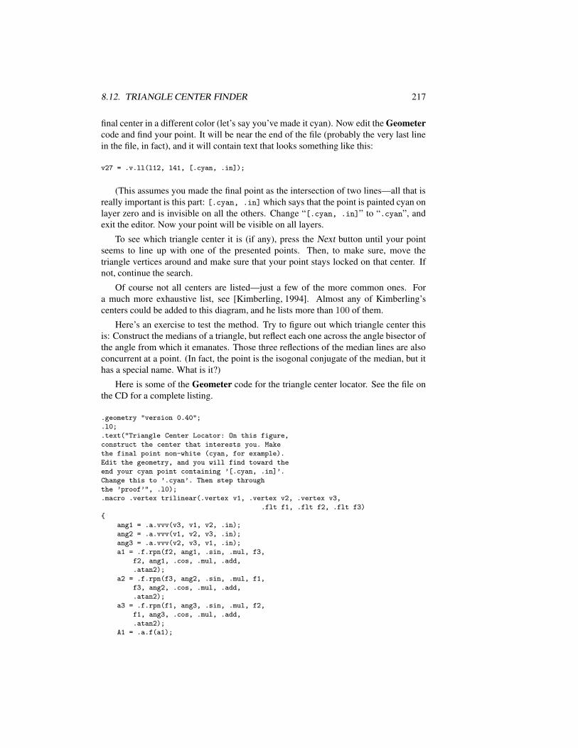
8.12. TRIANGLE CENTER FINDER 217
final center in a different color (let’s say you’ve made it cyan). Now edit the Geometercode and find your point. It will be near the end of the file (probably the very last linein the file, in fact), and it will contain text that looks something like this:
v27 = .v.ll(l12, l41, [.cyan, .in]);
(This assumes you made the final point as the intersection of two lines—all that isreally important is this part: [.cyan, .in] which says that the point is painted cyan onlayer zero and is invisible on all the others. Change “[.cyan, .in]” to “.cyan”, andexit the editor. Now your point will be visible on all layers.
To see which triangle center it is (if any), press the Next button until your pointseems to line up with one of the presented points. Then, to make sure, move thetriangle vertices around and make sure that your point stays locked on that center. Ifnot, continue the search.
Of course not all centers are listed—just a few of the more common ones. Fora much more exhaustive list, see [Kimberling, 1994]. Almost any of Kimberling’scenters could be added to this diagram, and he lists more than 100 of them.
Here’s an exercise to test the method. Try to figure out which triangle center thisis: Construct the medians of a triangle, but reflect each one across the angle bisector ofthe angle from which it emanates. Those three reflections of the median lines are alsoconcurrent at a point. (In fact, the point is the isogonal conjugate of the median, but ithas a special name. What is it?)
Here is some of the Geometer code for the triangle center locator. See the file onthe CD for a complete listing.
.geometry "version 0.40";
.l0;
.text("Triangle Center Locator: On this figure,
construct the center that interests you. Make
the final point non-white (cyan, for example).
Edit the geometry, and you will find toward the
end your cyan point containing ’[.cyan, .in]’.
Change this to ’.cyan’. Then step through
the ’proof’", .l0);
.macro .vertex trilinear(.vertex v1, .vertex v2, .vertex v3,
.flt f1, .flt f2, .flt f3)
ang1 = .a.vvv(v3, v1, v2, .in);
ang2 = .a.vvv(v1, v2, v3, .in);
ang3 = .a.vvv(v2, v3, v1, .in);
a1 = .f.rpn(f2, ang1, .sin, .mul, f3,
f2, ang1, .cos, .mul, .add,
.atan2);
a2 = .f.rpn(f3, ang2, .sin, .mul, f1,
f3, ang2, .cos, .mul, .add,
.atan2);
a3 = .f.rpn(f1, ang3, .sin, .mul, f2,
f1, ang3, .cos, .mul, .add,
.atan2);
A1 = .a.f(a1);
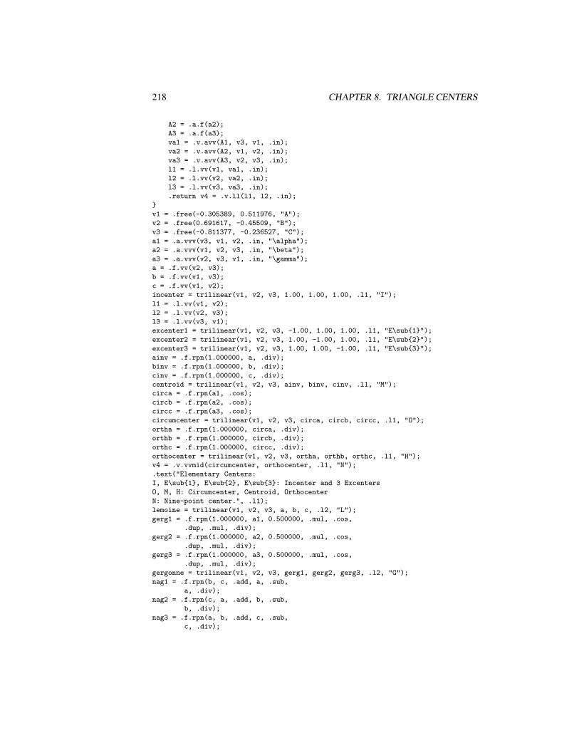
218 CHAPTER 8. TRIANGLE CENTERS
A2 = .a.f(a2);
A3 = .a.f(a3);
va1 = .v.avv(A1, v3, v1, .in);
va2 = .v.avv(A2, v1, v2, .in);
va3 = .v.avv(A3, v2, v3, .in);
l1 = .l.vv(v1, va1, .in);
l2 = .l.vv(v2, va2, .in);
l3 = .l.vv(v3, va3, .in);
.return v4 = .v.ll(l1, l2, .in);
v1 = .free(-0.305389, 0.511976, "A");
v2 = .free(0.691617, -0.45509, "B");
v3 = .free(-0.811377, -0.236527, "C");
a1 = .a.vvv(v3, v1, v2, .in, "\alpha");
a2 = .a.vvv(v1, v2, v3, .in, "\beta");
a3 = .a.vvv(v2, v3, v1, .in, "\gamma");
a = .f.vv(v2, v3);
b = .f.vv(v1, v3);
c = .f.vv(v1, v2);
incenter = trilinear(v1, v2, v3, 1.00, 1.00, 1.00, .l1, "I");
l1 = .l.vv(v1, v2);
l2 = .l.vv(v2, v3);
l3 = .l.vv(v3, v1);
excenter1 = trilinear(v1, v2, v3, -1.00, 1.00, 1.00, .l1, "E\sub1");
excenter2 = trilinear(v1, v2, v3, 1.00, -1.00, 1.00, .l1, "E\sub2");
excenter3 = trilinear(v1, v2, v3, 1.00, 1.00, -1.00, .l1, "E\sub3");
ainv = .f.rpn(1.000000, a, .div);
binv = .f.rpn(1.000000, b, .div);
cinv = .f.rpn(1.000000, c, .div);
centroid = trilinear(v1, v2, v3, ainv, binv, cinv, .l1, "M");
circa = .f.rpn(a1, .cos);
circb = .f.rpn(a2, .cos);
circc = .f.rpn(a3, .cos);
circumcenter = trilinear(v1, v2, v3, circa, circb, circc, .l1, "O");
ortha = .f.rpn(1.000000, circa, .div);
orthb = .f.rpn(1.000000, circb, .div);
orthc = .f.rpn(1.000000, circc, .div);
orthocenter = trilinear(v1, v2, v3, ortha, orthb, orthc, .l1, "H");
v4 = .v.vvmid(circumcenter, orthocenter, .l1, "N");
.text("Elementary Centers:
I, E\sub1, E\sub2, E\sub3: Incenter and 3 Excenters
O, M, H: Circumcenter, Centroid, Orthocenter
N: Nine-point center.", .l1);
lemoine = trilinear(v1, v2, v3, a, b, c, .l2, "L");
gerg1 = .f.rpn(1.000000, a1, 0.500000, .mul, .cos,
.dup, .mul, .div);
gerg2 = .f.rpn(1.000000, a2, 0.500000, .mul, .cos,
.dup, .mul, .div);
gerg3 = .f.rpn(1.000000, a3, 0.500000, .mul, .cos,
.dup, .mul, .div);
gergonne = trilinear(v1, v2, v3, gerg1, gerg2, gerg3, .l2, "G");
nag1 = .f.rpn(b, c, .add, a, .sub,
a, .div);
nag2 = .f.rpn(c, a, .add, b, .sub,
b, .div);
nag3 = .f.rpn(a, b, .add, c, .sub,
c, .div);
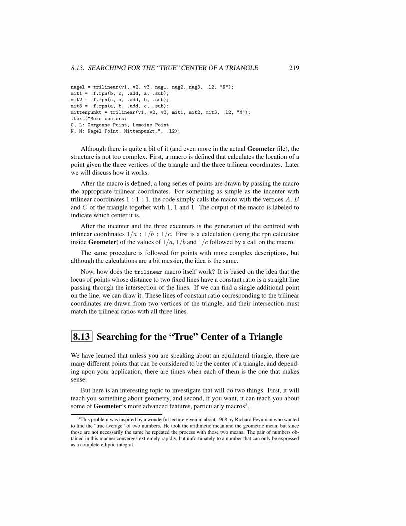
8.13. SEARCHING FOR THE “TRUE” CENTER OF A TRIANGLE 219
nagel = trilinear(v1, v2, v3, nag1, nag2, nag3, .l2, "N");
mit1 = .f.rpn(b, c, .add, a, .sub);
mit2 = .f.rpn(c, a, .add, b, .sub);
mit3 = .f.rpn(a, b, .add, c, .sub);
mittenpunkt = trilinear(v1, v2, v3, mit1, mit2, mit3, .l2, "M");
.text("More centers:
G, L: Gergonne Point, Lemoine Point
N, M: Nagel Point, Mittenpunkt.", .l2);
Although there is quite a bit of it (and even more in the actual Geometer file), thestructure is not too complex. First, a macro is defined that calculates the location of apoint given the three vertices of the triangle and the three trilinear coordinates. Laterwe will discuss how it works.
After the macro is defined, a long series of points are drawn by passing the macrothe appropriate trilinear coordinates. For something as simple as the incenter withtrilinear coordinates 1 : 1 : 1, the code simply calls the macro with the vertices A, Band C of the triangle together with 1, 1 and 1. The output of the macro is labeled toindicate which center it is.
After the incenter and the three excenters is the generation of the centroid withtrilinear coordinates 1/a : 1/b : 1/c. First is a calculation (using the rpn calculatorinside Geometer) of the values of 1/a, 1/b and 1/c followed by a call on the macro.
The same procedure is followed for points with more complex descriptions, butalthough the calculations are a bit messier, the idea is the same.
Now, how does the trilinear macro itself work? It is based on the idea that thelocus of points whose distance to two fixed lines have a constant ratio is a straight linepassing through the intersection of the lines. If we can find a single additional pointon the line, we can draw it. These lines of constant ratio corresponding to the trilinearcoordinates are drawn from two vertices of the triangle, and their intersection mustmatch the trilinear ratios with all three lines.
8.13 Searching for the “True” Center of a Triangle
We have learned that unless you are speaking about an equilateral triangle, there aremany different points that can be considered to be the center of a triangle, and depend-ing upon your application, there are times when each of them is the one that makessense.
But here is an interesting topic to investigate that will do two things. First, it willteach you something about geometry, and second, if you want, it can teach you aboutsome of Geometer’s more advanced features, particularly macros3.
3This problem was inspired by a wonderful lecture given in about 1968 by Richard Feynman who wantedto find the “true average” of two numbers. He took the arithmetic mean and the geometric mean, but sincethose are not necessarily the same he repeated the process with those two means. The pair of numbers ob-tained in this manner converges extremely rapidly, but unfortunately to a number that can only be expressedas a complete elliptic integral.
220 CHAPTER 8. TRIANGLE CENTERS
Here is the problem: We know that in general, the centroid, nine point center,and incenter of a triangle are different points. But if there is a “true” center of thetriangle, perhaps they are close to it. So form the triangle from these three pointsand find its “true” center. Since we do not know where the true center is, we canperhaps approximate it by finding the centroid, nine point center, and incenter of thisnew triangle. Repeat the process. Do the sets of three points tend to a limit insidethe triangle? Where is it? What if we had used different centers, like the centroid,orthocenter, and Fermat point?
We can investigate the convergence of these sets of points by using Geometer torepeatedly calculate the three centers, then the three centers of the triangle formed bythose three centers, and so on. Unfortunately, if the centers do get close together, it willbecome harder and harder to do the construction.
The solution is to write Geometer macros and then to call those repeatedly to seeif the points converge. The file Tricenters/TrueCenter.T does just this. Here is alisting:
.geometry "version 0.60";
v1 = .free(-0.320359, -0.227545, "A");
v2 = .free(0.185629, 0.314371, "B");
v3 = .free(0.0479042, -0.505988, "C");
.macro .vertex centroid(.vertex v1, .vertex v2, .vertex v3)
v4 = .v.vvmid(v1, v2, .in);
v6 = .v.vvmid(v3, v1, .in);
l1 = .l.vv(v2, v6, .in);
l2 = .l.vv(v3, v4, .in);
.return v7 = .v.ll(l1, l2);
.macro .vertex ninepointcenter(.vertex v1, .vertex v2, .vertex v3)
v12 = .v.vvmid(v1, v2, .in);
v23 = .v.vvmid(v2, v3, .in);
v31 = .v.vvmid(v3, v1, .in);
c1 = .c.vvv(v12, v23, v31, .in);
.return v4 = .v.ccenter(c1);
.macro .vertex incenter(.vertex v1, .vertex v2, .vertex v3)
l1 = .l.vv(v1, v2, .in);
l2 = .l.vv(v2, v3, .in);
l3 = .l.vv(v3, v1, .in);
c1 = .c.lll(l1, l2, l3, 1, .in);
.return v4 = .v.ccenter(c1);
vg0 = centroid(v1, v2, v3, .magenta);
vo0 = ninepointcenter(v1, v2, v3, .magenta);
vi0 = incenter(v1, v2, v3, .magenta);
vg1 = centroid(vg0, vo0, vi0, .red);
vo1 = ninepointcenter(vg0, vo0, vi0, .red);
vi1 = incenter(vg0, vo0, vi0, .red);
vg2 = centroid(vg1, vo1, vi1, .yellow);
vo2 = ninepointcenter(vg1, vo1, vi1, .yellow);
vi2 = incenter(vg1, vo1, vi1, .yellow);
8.13. SEARCHING FOR THE “TRUE” CENTER OF A TRIANGLE 221
The diagram begins with the three points of the original triangle drawn in white.Next are three macros to construct the three centers that interest us. The vertices vg0,vo0 and vi0 are the centroid, nine point center and incenter of that triangle. Replacethe 0s with 1s and we obtain the second level of centers, et cetera. Each set is drawn ina different color to see if the points converge or not. Experiment with the diagram andsee what you can learn. See what happens if you go another step or two deeper.
Sometimes bad things happen. Which ones are due to round-off error in the com-puter, and which are due to features of the original triangle?
If you wish to experiment with different triangle centers, the easiest way to build amacro is this: In the original triangle using the graphical user interface, construct thecenter in the normal way. For example, if you are just beginning and want to build themacro to draw the incenter, begin with a diagram having three free points and constructthe incenter. Your Geometer diagram will look something like this:
.geometry "version 0.60";
v1 = .free(-0.320359, -0.227545, "A");
v2 = .free(0.185629, 0.314371, "B");
v3 = .free(0.0479042, -0.505988, "C");
v4 = .v.vvmid(v1, v2, .in);
v6 = .v.vvmid(v3, v1, .in);
l1 = .l.vv(v2, v6, .in);
l2 = .l.vv(v3, v4, .in);
v7 = .v.ll(l1, l2);
In the text editor it is an easy exercise to convert this code to the macro form inthe original listing. The portion of the code above that will go into the macro includesthe line beginning with v4 = .v.vvmid and continues to the end of the listing. To testit before going on, add a single line of code (that you may wish to erase later) so thatyour entire program looks like this:
.geometry "version 0.60";
v1 = .free(-0.320359, -0.227545, "A");
v2 = .free(0.185629, 0.314371, "B");
v3 = .free(0.0479042, -0.505988, "C");
.macro .vertex centroid(.vertex v1, .vertex v2, .vertex v3)
v4 = .v.vvmid(v1, v2, .in);
v6 = .v.vvmid(v3, v1, .in);
l1 = .l.vv(v2, v6, .in);
l2 = .l.vv(v3, v4, .in);
.return v7 = .v.ll(l1, l2);
testvertex = centroid(v1, v2, v3, .magenta);
If it does the right thing, save your file and start working on the definition of themacro for the second triangle center.

222 CHAPTER 8. TRIANGLE CENTERS
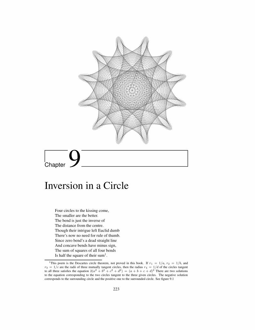
Chapter 9Inversion in a Circle
Four circles to the kissing come,The smaller are the better.The bend is just the inverse ofThe distance from the centre.Though their intrigue left Euclid dumbThere’s now no need for rule of thumb.Since zero bend’s a dead straight lineAnd concave bends have minus sign,The sum of squares of all four bendsIs half the square of their sum1.
1This poem is the Descartes circle theorem, not proved in this book. If r1 = 1/a, r2 = 1/b, andr3 = 1/c are the radii of three mutually tangent circles, then the radius r4 = 1/d of the circles tangentto all three satisfies the equation 2(a2 + b2 + c2 + d2) = (a + b + c + d)2 There are two solutionsto the equation corresponding to the two circles tangent to the three given circles. The negative solutioncorresponds to the surrounding circle and the positive one to the surrounded circle. See figure 9.1
223
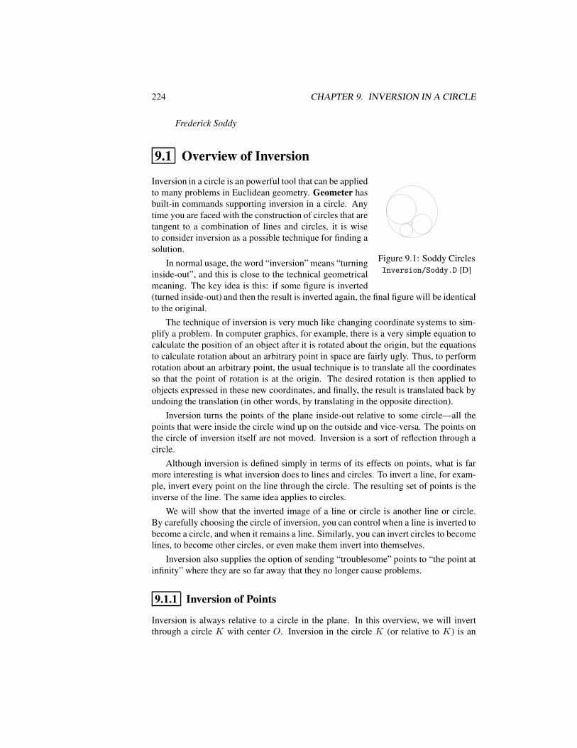
224 CHAPTER 9. INVERSION IN A CIRCLE
Frederick Soddy
9.1 Overview of Inversion
Figure 9.1: Soddy CirclesInversion/Soddy.D [D]
Inversion in a circle is an powerful tool that can be appliedto many problems in Euclidean geometry. Geometer hasbuilt-in commands supporting inversion in a circle. Anytime you are faced with the construction of circles that aretangent to a combination of lines and circles, it is wiseto consider inversion as a possible technique for finding asolution.
In normal usage, the word “inversion” means “turninginside-out”, and this is close to the technical geometricalmeaning. The key idea is this: if some figure is inverted(turned inside-out) and then the result is inverted again, the final figure will be identicalto the original.
The technique of inversion is very much like changing coordinate systems to sim-plify a problem. In computer graphics, for example, there is a very simple equation tocalculate the position of an object after it is rotated about the origin, but the equationsto calculate rotation about an arbitrary point in space are fairly ugly. Thus, to performrotation about an arbitrary point, the usual technique is to translate all the coordinatesso that the point of rotation is at the origin. The desired rotation is then applied toobjects expressed in these new coordinates, and finally, the result is translated back byundoing the translation (in other words, by translating in the opposite direction).
Inversion turns the points of the plane inside-out relative to some circle—all thepoints that were inside the circle wind up on the outside and vice-versa. The points onthe circle of inversion itself are not moved. Inversion is a sort of reflection through acircle.
Although inversion is defined simply in terms of its effects on points, what is farmore interesting is what inversion does to lines and circles. To invert a line, for exam-ple, invert every point on the line through the circle. The resulting set of points is theinverse of the line. The same idea applies to circles.
We will show that the inverted image of a line or circle is another line or circle.By carefully choosing the circle of inversion, you can control when a line is inverted tobecome a circle, and when it remains a line. Similarly, you can invert circles to becomelines, to become other circles, or even make them invert into themselves.
Inversion also supplies the option of sending “troublesome” points to “the point atinfinity” where they are so far away that they no longer cause problems.
9.1.1 Inversion of Points
Inversion is always relative to a circle in the plane. In this overview, we will invertthrough a circle K with center O. Inversion in the circle K (or relative to K) is an
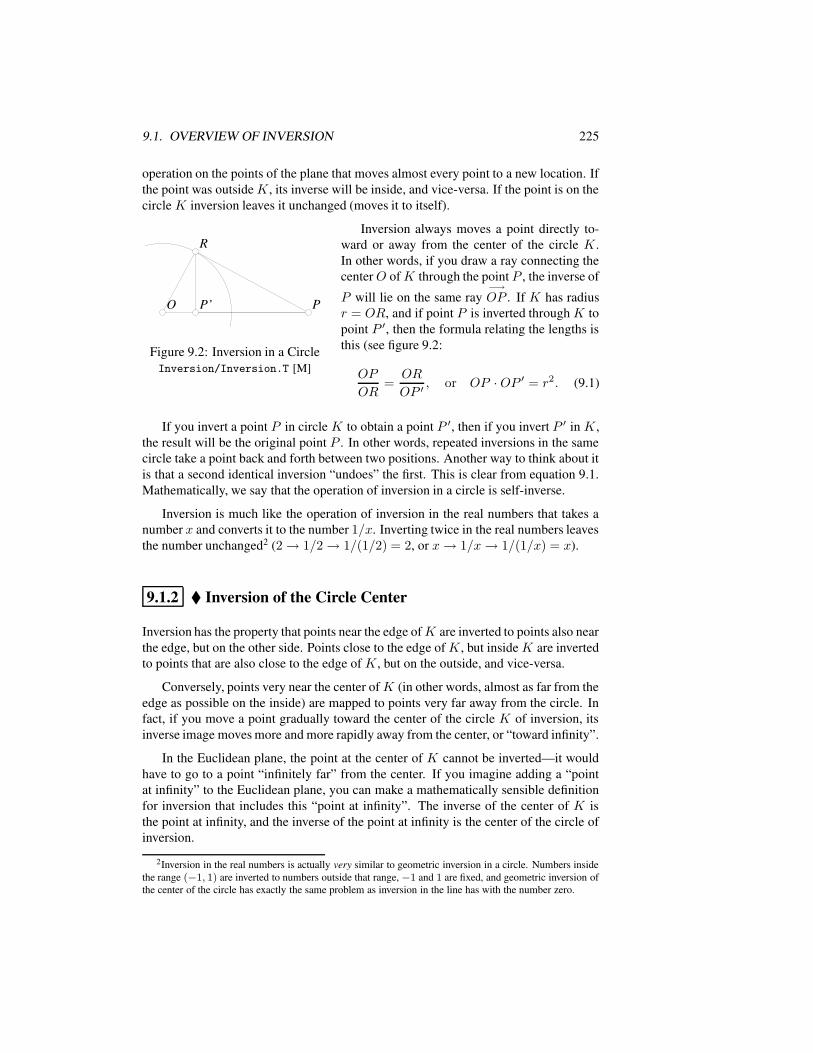
9.1. OVERVIEW OF INVERSION 225
operation on the points of the plane that moves almost every point to a new location. Ifthe point was outsideK, its inverse will be inside, and vice-versa. If the point is on thecircle K inversion leaves it unchanged (moves it to itself).
OO PP
RR
P’P’
Figure 9.2: Inversion in a CircleInversion/Inversion.T [M]
Inversion always moves a point directly to-ward or away from the center of the circle K.In other words, if you draw a ray connecting thecenterO ofK through the point P , the inverse of
P will lie on the same ray−→OP . If K has radius
r = OR, and if point P is inverted through K topoint P ′, then the formula relating the lengths isthis (see figure 9.2:
OP
OR=
OR
OP ′, or OP · OP ′ = r2. (9.1)
If you invert a point P in circle K to obtain a point P ′, then if you invert P ′ in K,the result will be the original point P . In other words, repeated inversions in the samecircle take a point back and forth between two positions. Another way to think about itis that a second identical inversion “undoes” the first. This is clear from equation 9.1.Mathematically, we say that the operation of inversion in a circle is self-inverse.
Inversion is much like the operation of inversion in the real numbers that takes anumber x and converts it to the number 1/x. Inverting twice in the real numbers leavesthe number unchanged2 (2→ 1/2→ 1/(1/2) = 2, or x→ 1/x→ 1/(1/x) = x).
9.1.2 Inversion of the Circle Center
Inversion has the property that points near the edge ofK are inverted to points also nearthe edge, but on the other side. Points close to the edge ofK, but inside K are invertedto points that are also close to the edge of K, but on the outside, and vice-versa.
Conversely, points very near the center ofK (in other words, almost as far from theedge as possible on the inside) are mapped to points very far away from the circle. Infact, if you move a point gradually toward the center of the circle K of inversion, itsinverse image moves more and more rapidly away from the center, or “toward infinity”.
In the Euclidean plane, the point at the center of K cannot be inverted—it wouldhave to go to a point “infinitely far” from the center. If you imagine adding a “pointat infinity” to the Euclidean plane, you can make a mathematically sensible definitionfor inversion that includes this “point at infinity”. The inverse of the center of K isthe point at infinity, and the inverse of the point at infinity is the center of the circle ofinversion.
2Inversion in the real numbers is actually very similar to geometric inversion in a circle. Numbers insidethe range (−1, 1) are inverted to numbers outside that range,−1 and 1 are fixed, and geometric inversion ofthe center of the circle has exactly the same problem as inversion in the line has with the number zero.
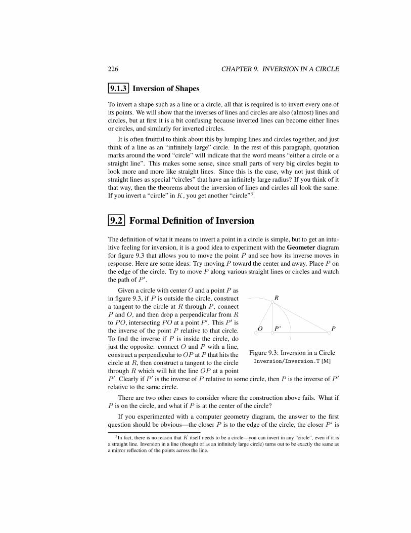
226 CHAPTER 9. INVERSION IN A CIRCLE
9.1.3 Inversion of Shapes
To invert a shape such as a line or a circle, all that is required is to invert every one ofits points. We will show that the inverses of lines and circles are also (almost) lines andcircles, but at first it is a bit confusing because inverted lines can become either linesor circles, and similarly for inverted circles.
It is often fruitful to think about this by lumping lines and circles together, and justthink of a line as an “infinitely large” circle. In the rest of this paragraph, quotationmarks around the word “circle” will indicate that the word means “either a circle or astraight line”. This makes some sense, since small parts of very big circles begin tolook more and more like straight lines. Since this is the case, why not just think ofstraight lines as special “circles” that have an infinitely large radius? If you think of itthat way, then the theorems about the inversion of lines and circles all look the same.If you invert a “circle” in K, you get another “circle”3.
9.2 Formal Definition of Inversion
The definition of what it means to invert a point in a circle is simple, but to get an intu-itive feeling for inversion, it is a good idea to experiment with the Geometer diagramfor figure 9.3 that allows you to move the point P and see how its inverse moves inresponse. Here are some ideas: Try moving P toward the center and away. Place P onthe edge of the circle. Try to move P along various straight lines or circles and watchthe path of P ′.
OO PP
RR
P’P’
Figure 9.3: Inversion in a CircleInversion/Inversion.T [M]
Given a circle with center O and a point P asin figure 9.3, if P is outside the circle, constructa tangent to the circle at R through P , connectP and O, and then drop a perpendicular from Rto PO, intersecting PO at a point P ′. This P ′ isthe inverse of the point P relative to that circle.To find the inverse if P is inside the circle, dojust the opposite: connect O and P with a line,construct a perpendicular toOP at P that hits thecircle at R, then construct a tangent to the circlethrough R which will hit the line OP at a pointP ′. Clearly if P ′ is the inverse of P relative to some circle, then P is the inverse of P ′
relative to the same circle.
There are two other cases to consider where the construction above fails. What ifP is on the circle, and what if P is at the center of the circle?
If you experimented with a computer geometry diagram, the answer to the firstquestion should be obvious—the closer P is to the edge of the circle, the closer P ′ is
3In fact, there is no reason that K itself needs to be a circle—you can invert in any “circle”, even if it isa straight line. Inversion in a line (thought of as an infinitely large circle) turns out to be exactly the same asa mirror reflection of the points across the line.
9.3. SIMPLE PROPERTIES OF INVERSION 227
to P . It only makes sense to define the inverse of a point on the circle to be the pointitself, so that is how it is defined.
If P is at O, the center of the circle, it is another story. The closer you move Pto O, the further away P ′ moves. If you look at what happens in our geometricalconstruction described above, you will see that the closer P is to O, the closer RP isto being parallel to OP . When P is at O, the construction will yield a pair of parallellines. For this reason, we will simply say that the inverse of the center of the circle isundefined.
“Undefined” is used in the same sense as in arithmetic when we say that 1 dividedby 0 is undefined—there is simply no sensible way to define “1/0” so that it makesmathematical sense. In the same way that even though it is undefined, you can thinkof 1/0 as being∞ (after all, 1/ε is very large if ε is very small), you can think of theinverse of the center of the circle as being a “point at infinity”. You cannot use thisidea in a formal proof, but nobody can prevent you from thinking about it like that, andthinking about it like that can sometimes be very useful.
We only have to make the point undefined in pure Euclidean geometry where weare only allowed to talk about points in the Euclidean plane. If we are willing to makea new kind of “inversive geometry” where we add a point at infinity to the Euclideanplane, we can formally define inversion of the center of the circle. For now, let us notchange geometries in mid-chapter.
9.3 Simple Properties of Inversion
In this section, assume that all inversions will be relative to a circle called K withcenter O and radius r.
9.3.1 Inversion Expressed as a Ratio
We can express inversion as a ratio. Since the radius of the circle is r, what is themathematical relationship between the lengths OP ′ and OP in figure 9.3? There arethree similar triangles: 4ORP ∼ 4OP ′R ∼ 4PP ′R. Using the similarity of thefirst and last triangles, we obtain:
OP
OR=
OR
OP ′
or, as it is more commonly written:
OP ·OP ′ = OR · OR = r2. (9.2)
In many books equation 9.2 is used as the definition of inversion. The construction weused to define it is derived as a result. Both definitions are equivalent.
This equation shows that the concept of the inverse of the center as a “point atinfinity” is exactly equivalent to the concept that 1/0 =∞—as OP gets close to zero,OP ′ gets “close to” r2/0 =∞.
228 CHAPTER 9. INVERSION IN A CIRCLE
9.3.2 Inversion in the Complex Plane
There is a nice analytic definition of inversion if you know something about complexnumbers (see Section 3.13).
If o is an imaginary number somewhere on the complex plane, and r is a real radius,then the transformation that inverts all the complex numbers z to their complementarypoints z′ through a circle of radius r centered at o in the complex plane is given by:
z′ =r2
z − o + o.
This clearly has the right properties—if z is very close to o (the center of inversion),then z will be very close to o, so the denominator is very small and the result will bevery large. Similarly, if we move the o to the other side and multiply both sides by(z − o) to get rid of the fraction, we obtain:
(z′ − o)(z − o) = r2
which looks a lot like the geometric definition, since the absolute value of z ′ − o rep-resents the distance between z′ and o.
If inversion in the complex plane is relative to the origin (in other words, if o = 0),and if the radius of the circle of inversion is 1 (in other words, if inversion is relative tothe unit circle), then the inverse of a (complex) point z is 1/z—very similar to inversionin the real line, since if z happens to be real, z = z.
9.3.3 The Inverse of a Line
Inverting single points relative to a circle is not too interesting, but what if all the pointson a line are inverted? What will be the resulting shape? Using Geometer, it is veryeasy to run experiments like this—take a point that is constrained to be on a line, andinvert it through a circle. Then move the point along the line and see which points areswept out by its inverse.
A bit of experimentation should convince you that in almost every case, the inverseof a line seems to be a circle. Can you find the case where it is not? Let us prove thefollowing theorem:
Theorem 9.1 (Inverse of a Line) If K is a circle and L is a line that does not passthrough the center of K, then the locus of the inverses of the points on L is a circlethat passes through the center of K. If L lies completely outside of K, its inverse willbe completely inside K. If L is tangent to K, its inverse will be a circle inside K, buttangent toK at the point where L is tangent. If L intersects K at two points, its inversewill be a circle intersecting K in those same two points. The inverse of L is not quitethe entire circle—it is the circle missing the point that is the center of K. If L passesthrough the center of K, the points on the inverse of L lie on L itself (although thepoints of L that were inside K map to points outside, and vice-versa). Of course if Lpasses through the center of K, that center point can not be inverted, and the inverseof L will be L itself with the exception of the point at the center of the circle.
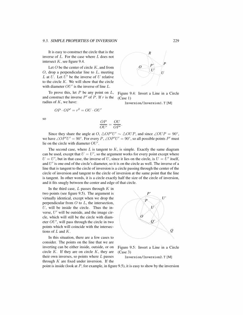
9.3. SIMPLE PROPERTIES OF INVERSION 229
OOPPP’P’
UUU’U’
RR
Figure 9.4: Invert a Line in a Circle(Case 1)
Inversion/Inversion1.T [M]
It is easy to construct the circle that is theinverse of L. For the case where L does notintersect K, see figure 9.4.
Let O be the center of circle K, and fromO, drop a perpendicular line to L, meetingL at U . Let U ′ be the inverse of U relativeto the circle K. We will show that the circlewith diameter OU ′ is the inverse of line L.
To prove this, let P be any point on L,and construct the inverse P ′ of P . If r is theradius of K, we have:
OP · OP ′ = r2 = OU ·OU ′
soOP
OU ′=
OU
OP ′.
Since they share the angle at O, 4OP ′U ′ ∼ 4OUP , and since ∠OUP = 90,we have ∠OP ′U ′ = 90. For every P , ∠OP ′U ′ = 90, so all possible points P ′ mustlie on the circle with diameter OU ′.
The second case, where L is tangent to K, is simple. Exactly the same diagramcan be used, except that U = U ′, so the argument works for every point except whereU = U ′, but in that case, the inverse of U , since it lies on the circle, is U = U ′ itself,and U ′ is one end of the circle’s diameter, so it is on the circle as well. The inverse of aline that is tangent to the circle of inversion is a circle passing through the center of thecircle of inversion and tangent to the circle of inversion at the same point that the lineis tangent. In other words, it is a circle exactly half the size of the circle of inversion,and it fits snugly between the center and edge of that circle.
OO
PP
P’P’
UU
U’U’
Q’Q’
Figure 9.5: Invert a Line in a Circle(Case 3)
Inversion/Inversion2.T [M]
In the third case, L passes through K intwo points (see figure 9.5). The argument isvirtually identical, except when we drop theperpendicular from O to L, the intersection,U , will be inside the circle. Thus the in-verse, U ′ will be outside, and the image cir-cle, which will still be the circle with diam-eter OU ′, will pass through the circle in twopoints which will coincide with the intersec-tions of L and K.
In this situation, there are a few cases toconsider. The points on the line that we areinverting can be either inside, outside, or oncircle K. If they are on circle K, they aretheir own inverses, so points where L passesthrough K are fixed under inversion. If thepoint is inside (look at P , for example, in figure 9.5), it is easy to show by the inversion
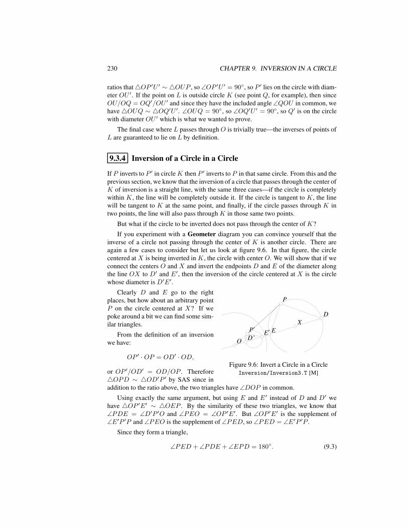
230 CHAPTER 9. INVERSION IN A CIRCLE
ratios that4OP ′U ′ ∼ 4OUP , so ∠OP ′U ′ = 90, so P ′ lies on the circle with diam-eter OU ′. If the point on L is outside circle K (see point Q, for example), then sinceOU/OQ = OQ′/OU ′ and since they have the included angle ∠QOU in common, wehave4OUQ ∼ 4OQ′U ′. ∠OUQ = 90, so ∠OQ′U ′ = 90, so Q′ is on the circlewith diameter OU ′ which is what we wanted to prove.
The final case where L passes throughO is trivially true—the inverses of points ofL are guaranteed to lie on L by definition.
9.3.4 Inversion of a Circle in a Circle
If P inverts to P ′ in circleK then P ′ inverts to P in that same circle. From this and theprevious section, we know that the inversion of a circle that passes through the center ofK of inversion is a straight line, with the same three cases—if the circle is completelywithin K, the line will be completely outside it. If the circle is tangent to K, the linewill be tangent to K at the same point, and finally, if the circle passes through K intwo points, the line will also pass through K in those same two points.
But what if the circle to be inverted does not pass through the center of K?
If you experiment with a Geometer diagram you can convince yourself that theinverse of a circle not passing through the center of K is another circle. There areagain a few cases to consider but let us look at figure 9.6. In that figure, the circlecentered at X is being inverted in K, the circle with center O. We will show that if weconnect the centers O and X and invert the endpoints D and E of the diameter alongthe line OX to D′ and E′, then the inversion of the circle centered at X is the circlewhose diameter is D′E′.
OO
XXEE
DD
E′E′D’D’
PP
P′P′
Figure 9.6: Invert a Circle in a CircleInversion/Inversion3.T [M]
Clearly D and E go to the rightplaces, but how about an arbitrary pointP on the circle centered at X? If wepoke around a bit we can find some sim-ilar triangles.
From the definition of an inversionwe have:
OP ′ · OP = OD′ · OD,
or OP ′/OD′ = OD/OP . Therefore4OPD ∼ 4OD′P ′ by SAS since inaddition to the ratio above, the two triangles have ∠DOP in common.
Using exactly the same argument, but using E and E ′ instead of D and D′ wehave 4OP ′E′ ∼ 4OEP . By the similarity of these two triangles, we know that∠PDE = ∠D′P ′O and ∠PEO = ∠OP ′E′. But ∠OP ′E′ is the supplement of∠E′P ′P and ∠PEO is the supplement of ∠PED, so ∠PED = ∠E ′P ′P .
Since they form a triangle,
∠PED + ∠PDE + ∠EPD = 180. (9.3)
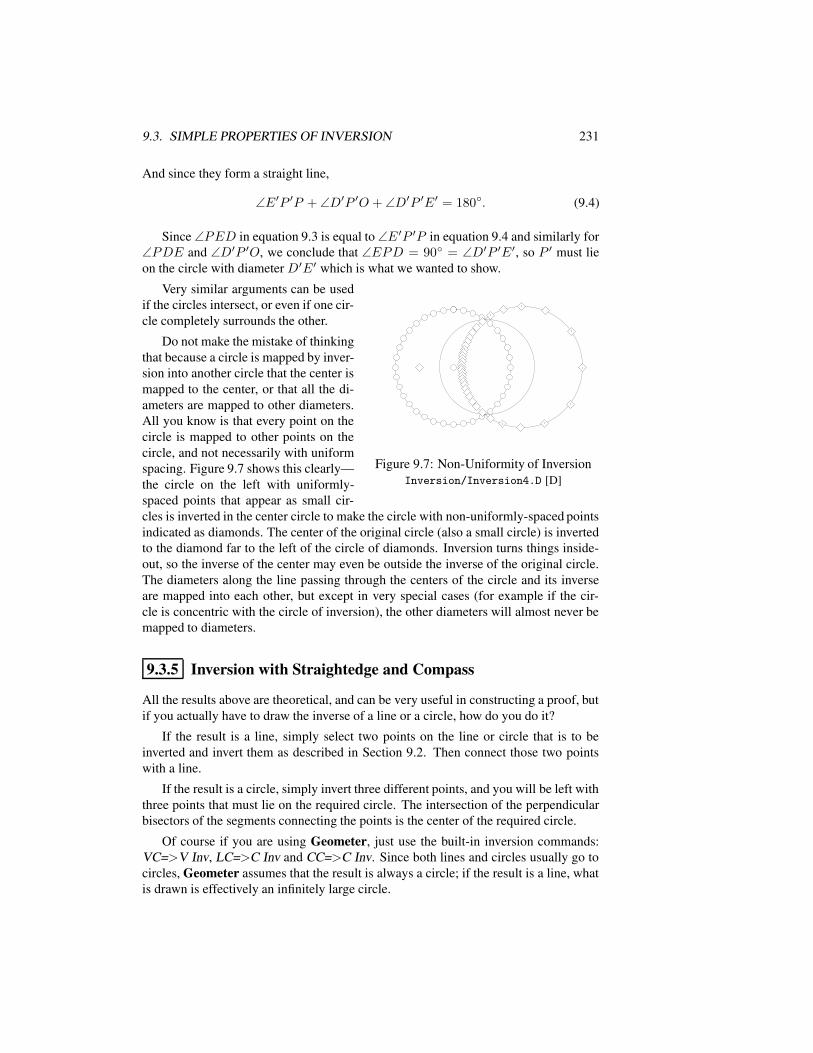
9.3. SIMPLE PROPERTIES OF INVERSION 231
And since they form a straight line,
∠E′P ′P + ∠D′P ′O + ∠D′P ′E′ = 180. (9.4)
Since ∠PED in equation 9.3 is equal to ∠E ′P ′P in equation 9.4 and similarly for∠PDE and ∠D′P ′O, we conclude that ∠EPD = 90 = ∠D′P ′E′, so P ′ must lieon the circle with diameter D′E′ which is what we wanted to show.
Figure 9.7: Non-Uniformity of InversionInversion/Inversion4.D [D]
Very similar arguments can be usedif the circles intersect, or even if one cir-cle completely surrounds the other.
Do not make the mistake of thinkingthat because a circle is mapped by inver-sion into another circle that the center ismapped to the center, or that all the di-ameters are mapped to other diameters.All you know is that every point on thecircle is mapped to other points on thecircle, and not necessarily with uniformspacing. Figure 9.7 shows this clearly—the circle on the left with uniformly-spaced points that appear as small cir-cles is inverted in the center circle to make the circle with non-uniformly-spaced pointsindicated as diamonds. The center of the original circle (also a small circle) is invertedto the diamond far to the left of the circle of diamonds. Inversion turns things inside-out, so the inverse of the center may even be outside the inverse of the original circle.The diameters along the line passing through the centers of the circle and its inverseare mapped into each other, but except in very special cases (for example if the cir-cle is concentric with the circle of inversion), the other diameters will almost never bemapped to diameters.
9.3.5 Inversion with Straightedge and Compass
All the results above are theoretical, and can be very useful in constructing a proof, butif you actually have to draw the inverse of a line or a circle, how do you do it?
If the result is a line, simply select two points on the line or circle that is to beinverted and invert them as described in Section 9.2. Then connect those two pointswith a line.
If the result is a circle, simply invert three different points, and you will be left withthree points that must lie on the required circle. The intersection of the perpendicularbisectors of the segments connecting the points is the center of the required circle.
Of course if you are using Geometer, just use the built-in inversion commands:VC=>V Inv, LC=>C Inv and CC=>C Inv. Since both lines and circles usually go tocircles, Geometer assumes that the result is always a circle; if the result is a line, whatis drawn is effectively an infinitely large circle.
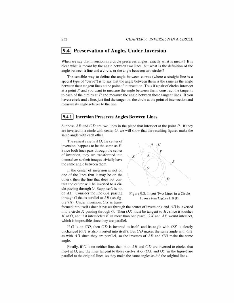
232 CHAPTER 9. INVERSION IN A CIRCLE
9.4 Preservation of Angles Under Inversion
When we say that inversion in a circle preserves angles, exactly what is meant? It isclear what is meant by the angle between two lines, but what is the definition of theangle between a line and a circle, or the angle between two circles?
The sensible way to define the angle between curves (where a straight line is aspecial type of “curve”) is to say that the angle between them is the same as the anglebetween their tangent lines at the point of intersection. Thus if a pair of circles intersectat a point P and you want to measure the angle between them, construct the tangentsto each of the circles at P and measure the angle between those tangent lines. If youhave a circle and a line, just find the tangent to the circle at the point of intersection andmeasure its angle relative to the line.
9.4.1 Inversion Preserves Angles Between Lines
Suppose AB and CD are two lines in the plane that intersect at the point P . If theyare inverted in a circle with center O, we will show that the resulting figures make thesame angle with each other.
AA
BB
CC
DD
OO
PPXX
YYKK
Figure 9.8: Invert Two Lines in a CircleInversion/Angles1.D [D]
The easiest case is ifO, the center ofinversion, happens to be the same as P .Since both lines pass through the centerof inversion, they are transformed intothemselves so their images trivially havethe same angle between them.
If the center of inversion is not onone of the lines (but it may be on theother), then the line that does not con-tain the center will be inverted to a cir-cle passing throughO. SupposeO is noton AB. Consider the line OX passingthroughO that is parallel toAB (see fig-ure 9.8). Under inversion, OX is trans-formed into itself (since it passes through the center of inversion), and AB is invertedinto a circle K passing through O. Then OX must be tangent to K, since it touchesK at O, and if it intersected K in more than one place, OX and AB would intersect,which is impossible since they are parallel.
If O is on CD, then CD is inverted to itself, and its angle with OX is clearlyunchanged (OX is also inverted into itself). But CD makes the same angle with OXas with AB since they are parallel, so the inverses of AB and CD make the sameangle.
Finally, if O is on neither line, then both AB and CD are inverted to circles thatmeet at O, and the lines tangent to those circles at O (OX and OY in the figure) areparallel to the original lines, so they make the same angles as did the original lines.
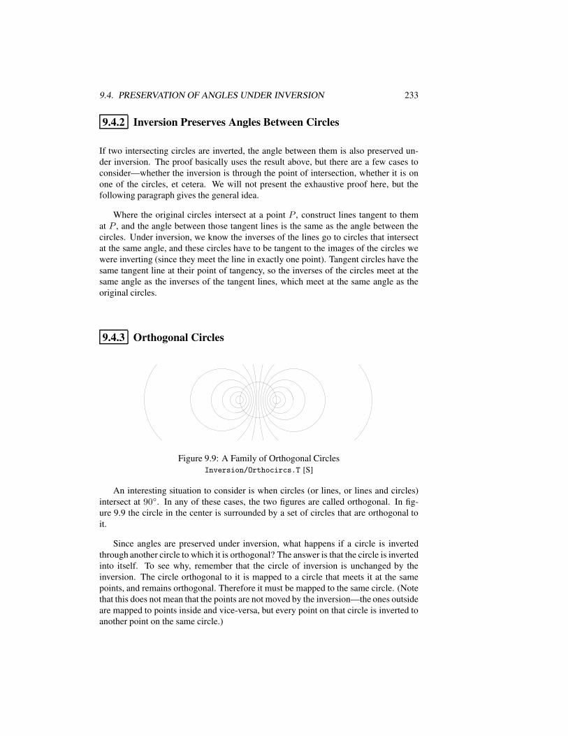
9.4. PRESERVATION OF ANGLES UNDER INVERSION 233
9.4.2 Inversion Preserves Angles Between Circles
If two intersecting circles are inverted, the angle between them is also preserved un-der inversion. The proof basically uses the result above, but there are a few cases toconsider—whether the inversion is through the point of intersection, whether it is onone of the circles, et cetera. We will not present the exhaustive proof here, but thefollowing paragraph gives the general idea.
Where the original circles intersect at a point P , construct lines tangent to themat P , and the angle between those tangent lines is the same as the angle between thecircles. Under inversion, we know the inverses of the lines go to circles that intersectat the same angle, and these circles have to be tangent to the images of the circles wewere inverting (since they meet the line in exactly one point). Tangent circles have thesame tangent line at their point of tangency, so the inverses of the circles meet at thesame angle as the inverses of the tangent lines, which meet at the same angle as theoriginal circles.
9.4.3 Orthogonal Circles
Figure 9.9: A Family of Orthogonal CirclesInversion/Orthocircs.T [S]
An interesting situation to consider is when circles (or lines, or lines and circles)intersect at 90. In any of these cases, the two figures are called orthogonal. In fig-ure 9.9 the circle in the center is surrounded by a set of circles that are orthogonal toit.
Since angles are preserved under inversion, what happens if a circle is invertedthrough another circle to which it is orthogonal? The answer is that the circle is invertedinto itself. To see why, remember that the circle of inversion is unchanged by theinversion. The circle orthogonal to it is mapped to a circle that meets it at the samepoints, and remains orthogonal. Therefore it must be mapped to the same circle. (Notethat this does not mean that the points are not moved by the inversion—the ones outsideare mapped to points inside and vice-versa, but every point on that circle is inverted toanother point on the same circle.)
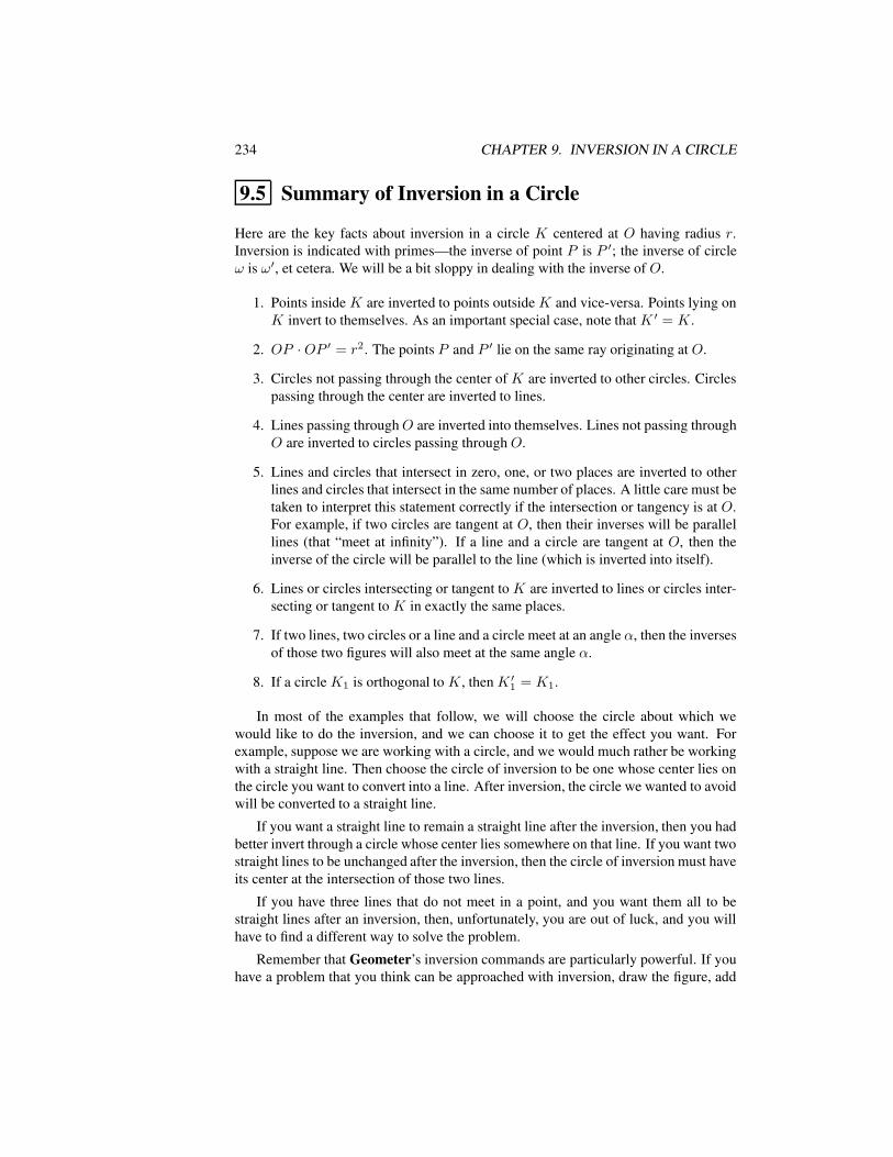
234 CHAPTER 9. INVERSION IN A CIRCLE
9.5 Summary of Inversion in a Circle
Here are the key facts about inversion in a circle K centered at O having radius r.Inversion is indicated with primes—the inverse of point P is P ′; the inverse of circleω is ω′, et cetera. We will be a bit sloppy in dealing with the inverse of O.
1. Points inside K are inverted to points outside K and vice-versa. Points lying onK invert to themselves. As an important special case, note that K ′ = K.
2. OP · OP ′ = r2. The points P and P ′ lie on the same ray originating at O.
3. Circles not passing through the center of K are inverted to other circles. Circlespassing through the center are inverted to lines.
4. Lines passing throughO are inverted into themselves. Lines not passing throughO are inverted to circles passing throughO.
5. Lines and circles that intersect in zero, one, or two places are inverted to otherlines and circles that intersect in the same number of places. A little care must betaken to interpret this statement correctly if the intersection or tangency is at O.For example, if two circles are tangent at O, then their inverses will be parallellines (that “meet at infinity”). If a line and a circle are tangent at O, then theinverse of the circle will be parallel to the line (which is inverted into itself).
6. Lines or circles intersecting or tangent to K are inverted to lines or circles inter-secting or tangent to K in exactly the same places.
7. If two lines, two circles or a line and a circle meet at an angle α, then the inversesof those two figures will also meet at the same angle α.
8. If a circle K1 is orthogonal to K, then K ′1 = K1.
In most of the examples that follow, we will choose the circle about which wewould like to do the inversion, and we can choose it to get the effect you want. Forexample, suppose we are working with a circle, and we would much rather be workingwith a straight line. Then choose the circle of inversion to be one whose center lies onthe circle you want to convert into a line. After inversion, the circle we wanted to avoidwill be converted to a straight line.
If you want a straight line to remain a straight line after the inversion, then you hadbetter invert through a circle whose center lies somewhere on that line. If you want twostraight lines to be unchanged after the inversion, then the circle of inversion must haveits center at the intersection of those two lines.
If you have three lines that do not meet in a point, and you want them all to bestraight lines after an inversion, then, unfortunately, you are out of luck, and you willhave to find a different way to solve the problem.
Remember that Geometer’s inversion commands are particularly powerful. If youhave a problem that you think can be approached with inversion, draw the figure, add
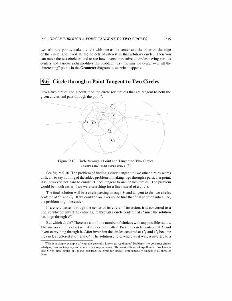
9.6. CIRCLE THROUGH A POINT TANGENT TO TWO CIRCLES 235
two arbitrary points, make a circle with one as the center and the other on the edgeof the circle, and invert all the objects of interest in that arbitrary circle. Then youcan move the test circle around to see how inversion relative to circles having variouscenters and various radii modifies the problem. Try moving the center over all the“interesting” points in the Geometer diagram to see what happens.
9.6 Circle through a Point Tangent to Two Circles
Given two circles and a point, find the circle (or circles) that are tangent to both thegiven circles and pass through the point4.
C1C1R1R1
C2C2
R2R2
PP
C1′C1′ C2′C2′
Figure 9.10: Circle through a Point and Tangent to Two CirclesInversion/Pointcirccirc.T [P]
See figure 9.10. The problem of finding a circle tangent to two other circles seemsdifficult, to say nothing of the added problem of making it go through a particular point.It is, however, not hard to construct lines tangent to one or two circles. The problemwould be much easier if we were searching for a line instead of a circle.
The final solution will be a circle passing through P and tangent to the two circlescentered at C1 and C2. If we could do an inversion to turn that final solution into a line,the problem might be easier.
If a circle passes through the center of its circle of inversion, it is converted to aline, so why not invert the entire figure through a circle centered at P since the solutionhas to go through P ?
But which circle? There are an infinite number of choices with any possible radius.The answer (in this case) is that it does not matter! Pick any circle centered at P andinvert everything through it. After inversion the circles centered at C1 and C2 becomethe circles centered at C ′1 and C ′2. The solution circle, wherever it was, is inverted to a
4This is a simple example of what are generally known as Apollonius’ Problems—to construct circlessatisfying various tangency and concurrency requirements. The most difficult of Apollonius’ Problems isthis: Given three circles in a plane, construct the circle (or circles) simultaneously tangent to all three ofthem.
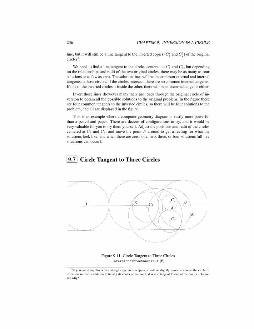
236 CHAPTER 9. INVERSION IN A CIRCLE
line, but it will still be a line tangent to the inverted copies (C ′1 and C ′2) of the originalcircles5.
We need to find a line tangent to the circles centered at C ′1 and C ′2, but dependingon the relationships and radii of the two original circles, there may be as many as foursolutions or as few as zero. The solution lines will be the common external and internaltangents to those circles. If the circles intersect, there are no common internal tangents.If one of the inverted circles is inside the other, there will be no external tangents either.
Invert those lines (however many there are) back through the original circle of in-version to obtain all the possible solutions to the original problem. In the figure thereare four common tangents to the inverted circles, so there will be four solutions to theproblem, and all are displayed in the figure.
This is an example where a computer geometry diagram is vastly more powerfulthan a pencil and paper. There are dozens of configurations to try, and it would bevery valuable for you to try them yourself. Adjust the positions and radii of the circlescentered at C1 and C2, and move the point P around to get a feeling for what thesolutions look like, and when there are zero, one, two, three, or four solutions (all fivesituations can occur).
9.7 Circle Tangent to Three Circles
C3C3
C2C2C1C1 XX
KK
SSTT UU
Figure 9.11: Circle Tangent to Three CirclesInversion/Threetancirc.T [P]
5If you are doing this with a straightedge and compass, it will be slightly easier to choose the circle ofinversion so that in addition to having its center at the point, it is also tangent to one of the circles. Do yousee why?
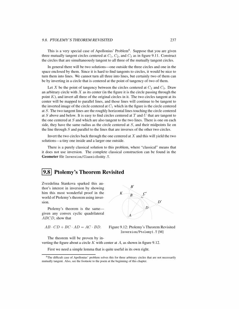
9.8. PTOLEMY’S THEOREM REVISITED 237
This is a very special case of Apollonius’ Problem6. Suppose that you are giventhree mutually tangent circles centered at C1, C2, and C3 as in figure 9.11. Constructthe circles that are simultaneously tangent to all three of the mutually tangent circles.
In general there will be two solutions—one outside the three circles and one in thespace enclosed by them. Since it is hard to find tangents to circles, it would be nice toturn them into lines. We cannot turn all three into lines, but certainly two of them canbe by inverting in a circle that is centered at the point of tangency of two of them.
Let X be the point of tangency between the circles centered at C2 and C3. Drawan arbitrary circle with X as its center (in the figure it is the circle passing through thepoint K), and invert all three of the original circles in it. The two circles tangent at itscenter will be mapped to parallel lines, and those lines will continue to be tangent tothe inverted image of the circle centered at C1 which in the figure is the circle centeredat S. The two tangent lines are the roughly horizontal lines touching the circle centeredat S above and below. It is easy to find circles centered at T and U that are tangent tothe one centered at S and which are also tangent to the two lines. There is one on eachside, they have the same radius as the circle centered at S, and their midpoints lie onthe line through S and parallel to the lines that are inverses of the other two circles.
Invert the two circles back through the one centered atX and this will yield the twosolutions—a tiny one inside and a larger one outside.
There is a purely classical solution to this problem, where “classical” means thatit does not use inversion. The complete classical construction can be found in theGeometer file Inversion/ClassicSoddy.T.
9.8 Ptolemy’s Theorem Revisited
CC
DD
AA
BB
B′B′
C′C′
D′D′
KK
Figure 9.12: Ptolemy’s Theorem RevisitedInversion/Ptolemy1.T [M]
Zvezdelina Stankova sparked this au-thor’s interest in inversion by showinghim this most wonderful proof in theworld of Ptolemy’s theorem using inver-sion.
Ptolemy’s theorem is the same—given any convex cyclic quadrilateralABCD, show that
AB · CD +BC ·AD = AC · BD.
The theorem will be proven by in-verting the figure about a circle K with center at A, as shown in figure 9.12.
First we need a simple lemma that is quite useful in its own right.
6The difficult case of Apollonius’ problem solves this for three arbitrary circles that are not necessarilymutually tangent. Also, see the footnote to the poem at the beginning of this chapter.
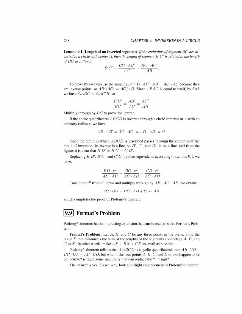
238 CHAPTER 9. INVERSION IN A CIRCLE
Lemma 9.1 (Length of an inverted segment) If the endpoints of segmentBC are in-verted in a circle with centerA, then the length of segmentB ′C ′ is related to the lengthof BC as follows:
B′C ′ =BC ·AB′
AC=BC · AC ′AB
.
To prove this we can use the same figure 9.12. AB ′ ·AB = AC ′ ·AC because theyare inverse points, so AB′/AC ′ = AC/AB. Since ∠BAC is equal to itself, by SASwe have4ABC ∼ 4AC ′B′ so
B′C ′
BC=AB′
AC=AC ′
AB.
Multiply through by BC to prove the lemma.If the entire quadrilateralABCD is inverted through a circle centered at A with an
arbitrary radius r, we have:
AB ·AB′ = AC ·AC ′ = AD · AD′ = r2.
Since the circle in which ABCD is inscribed passes through the center A of thecircle of inversion, its inverse is a line, so B′, C ′, and D′ lie on a line, and from thefigure, it is clear that B′D′ = B′C ′ + C ′D′.
ReplacingB′D′,B′C ′, andC ′D′ by their equivalents according to Lemma 9.1, wehave:
BD · r2
AD · AB =BC · r2
AC ·AB +CD · r2
AC ·AD.
Cancel the r2 from all terms and multiply through by AB · AC ·AD and obtain:
AC ·BD = BC · AD + CD · AB,
which completes the proof of Ptolemy’s theorem.
9.9 Fermat’s Problem
Ptolemy’s theorem has an interesting extension that can be used to solve Fermat’s Prob-lem:
Fermat’s Problem: Let A, B, and C be any three points in the plane. Find thepoint X that minimizes the sum of the lengths of the segments connecting A, B, andC to X . In other words, make AX +BX + CX as small as possible.
Ptolemy’s theorem tells us that ifABCD is a cyclic quadrilateral, thenAB ·CD+BC ·DA = AC ·BD, but what if the four points A, B, C, and D do not happen to lieon a circle? is there some inequality that can replace the “=” sign?
The answer is yes. To see why, look at a slight enhancement of Ptolemy’s theorem:
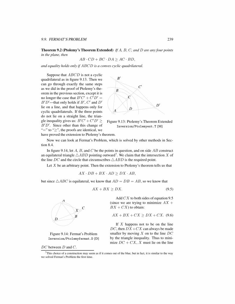
9.9. FERMAT’S PROBLEM 239
Theorem 9.2 (Ptolemy’s Theorem Extended) If A, B, C, andD are any four pointsin the plane, then
AB · CD +BC ·DA ≥ AC · BD,and equality holds only if ABCD is a convex cyclic quadrilateral.
CC
DDAA
BB
B′B′
C′C′
D′D′
Figure 9.13: Ptolemy’s Theorem ExtendedInversion/Ptolemyext.T [M]
Suppose that ABCD is not a cyclicquadrilateral as in figure 9.13. Then wecan go through exactly the same stepsas we did in the proof of Ptolemy’s the-orem in the previous section, except it isno longer the case that B′C ′ + C ′D′ =B′D′—that only holds if B′, C ′ and D′
lie on a line, and that happens only forcyclic quadrilaterals. If the three pointsdo not lie on a straight line, the trian-gle inequality gives us: B′C ′+C ′D′ ≥B′D′. Since other than this change of“=” to “≥”, the proofs are identical, wehave proved the extension to Ptolemy’s theorem.
Now we can look at Fermat’s Problem, which is solved by other methods in Sec-tion 8.4.
In figure 9.14, let A, B, and C be the points in question, and on side AB constructan equilateral triangle4ABD pointing outward7. We claim that the intersection X ofthe line DC and the circle that circumscribes4ABD is the required point.
Let X be an arbitrary point. Then the extension to Ptolemy’s theorem tells us that
AX ·DB +BX ·AD ≥ DX ·AB,
but since4ABC is equilateral, we know that AD = DB = AB, so we know that
AX +BX ≥ DX. (9.5)
AA
BBDD
CCXX
Figure 9.14: Fermat’s ProblemInversion/Ptolemyfermat.D [D]
AddCX to both sides of equation 9.5(since we are trying to minimize AX +BX + CX) to obtain:
AX +BX +CX ≥ DX +CX. (9.6)
If X happens not to be on the lineDC, thenDX+CX can always be madesmaller by moving X on to the line DCby the triangle inequality. Thus to mini-mize DC + CX , X must lie on the line
DC between D and C.7This choice of a construction may seem as if it comes out of the blue, but in fact, it is similar to the way
we solved Fermat’s Problem the first time.
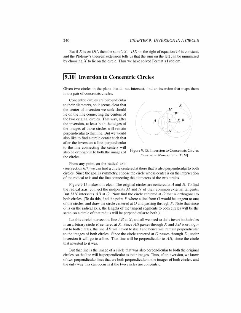
240 CHAPTER 9. INVERSION IN A CIRCLE
But ifX is onDC, then the sumCX+DX on the right of equation 9.6 is constant,and the Ptolemy’s theorem extension tells us that the sum on the left can be minimizedby choosingX to lie on the circle. Thus we have solved Fermat’s Problem.
9.10 Inversion to Concentric Circles
Given two circles in the plane that do not intersect, find an inversion that maps theminto a pair of concentric circles.
AA BB
MM
NN
OO
PP
XX
KK
Figure 9.15: Inversion to Concentric CirclesInversion/Concentric.T [M]
Concentric circles are perpendicularto their diameters, so it seems clear thatthe center of inversion we seek shouldlie on the line connecting the centers ofthe two original circles. That way, afterthe inversion, at least both the edges ofthe images of those circles will remainperpendicular to that line. But we wouldalso like to find a circle center such thatafter the inversion a line perpendicularto the line connecting the centers willalso be orthogonal to both the images ofthe circles.
From any point on the radical axis(see Section 6.7) we can find a circle centered at there that is also perpendicular to bothcircles. Since the goal is symmetry, choose the circle whose center is on the intersectionof the radical axis and the line connecting the diameters of the two circles.
Figure 9.15 makes this clear. The original circles are centered at A and B. To findthe radical axis, connect the midpoints M and N of their common external tangents.But MN intersects AB at O. Now find the circle centered at O that is orthogonal toboth circles. (To do this, find the point P where a line from O would be tangent to oneof the circles, and draw the circle centered at O and passing through P . Note that sinceO is on the radical axis, the lengths of the tangent segments to both circles will be thesame, so a circle of that radius will be perpendicular to both.)
Let this circle intersect the lineAB atX , and all we need to do is invert both circlesin an arbitrary circleK centered atX . SinceAB passes throughX andAB is orthogo-nal to both circles, the lineAB will invert to itself and hence will remain perpendicularto the images of both circles. Since the circle centered at O passes through X , underinversion it will go to a line. That line will be perpendicular to AB, since the circlethat inverted to it was.
But that line is the image of a circle that was also perpendicular to both the originalcircles, so the line will be perpendicular to their images. Thus, after inversion, we knowof two perpendicular lines that are both perpendicular to the images of both circles, andthe only way this can occur is if the two circles are concentric.
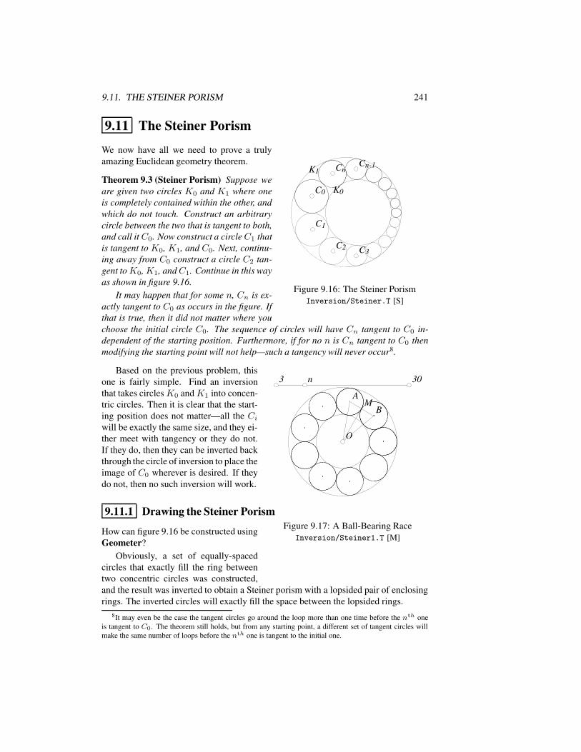
9.11. THE STEINER PORISM 241
9.11 The Steiner Porism
C0C0
C1C1
C2C2 C3C3
K1K1
K0K0
CnCnCn-1Cn-1
Figure 9.16: The Steiner PorismInversion/Steiner.T [S]
We now have all we need to prove a trulyamazing Euclidean geometry theorem.
Theorem 9.3 (Steiner Porism) Suppose weare given two circles K0 and K1 where oneis completely contained within the other, andwhich do not touch. Construct an arbitrarycircle between the two that is tangent to both,and call it C0. Now construct a circleC1 thatis tangent to K0, K1, and C0. Next, continu-ing away from C0 construct a circle C2 tan-gent toK0,K1, andC1. Continue in this wayas shown in figure 9.16.
It may happen that for some n, Cn is ex-actly tangent to C0 as occurs in the figure. Ifthat is true, then it did not matter where youchoose the initial circle C0. The sequence of circles will have Cn tangent to C0 in-dependent of the starting position. Furthermore, if for no n is Cn tangent to C0 thenmodifying the starting point will not help—such a tangency will never occur8.
33 3030nn
OO
AA
BBMM
Figure 9.17: A Ball-Bearing RaceInversion/Steiner1.T [M]
Based on the previous problem, thisone is fairly simple. Find an inversionthat takes circles K0 andK1 into concen-tric circles. Then it is clear that the start-ing position does not matter—all the Ciwill be exactly the same size, and they ei-ther meet with tangency or they do not.If they do, then they can be inverted backthrough the circle of inversion to place theimage of C0 wherever is desired. If theydo not, then no such inversion will work.
9.11.1 Drawing the Steiner Porism
How can figure 9.16 be constructed usingGeometer?
Obviously, a set of equally-spacedcircles that exactly fill the ring betweentwo concentric circles was constructed,and the result was inverted to obtain a Steiner porism with a lopsided pair of enclosingrings. The inverted circles will exactly fill the space between the lopsided rings.
8It may even be the case the tangent circles go around the loop more than one time before the nth oneis tangent to C0. The theorem still holds, but from any starting point, a different set of tangent circles willmake the same number of loops before the nth one is tangent to the initial one.
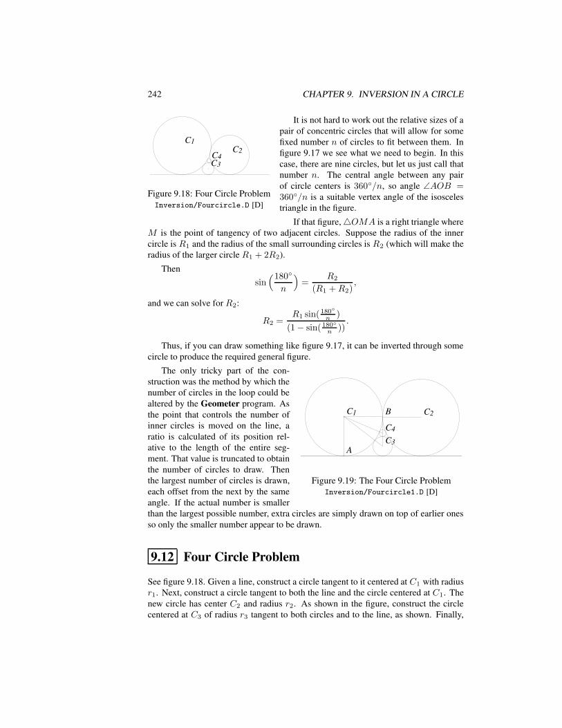
242 CHAPTER 9. INVERSION IN A CIRCLE
C1C1C2C2
C3C3C4C4
Figure 9.18: Four Circle ProblemInversion/Fourcircle.D [D]
It is not hard to work out the relative sizes of apair of concentric circles that will allow for somefixed number n of circles to fit between them. Infigure 9.17 we see what we need to begin. In thiscase, there are nine circles, but let us just call thatnumber n. The central angle between any pairof circle centers is 360/n, so angle ∠AOB =360/n is a suitable vertex angle of the isoscelestriangle in the figure.
If that figure,4OMA is a right triangle whereM is the point of tangency of two adjacent circles. Suppose the radius of the innercircle is R1 and the radius of the small surrounding circles is R2 (which will make theradius of the larger circle R1 + 2R2).
Thensin(180
n
)=
R2
(R1 +R2),
and we can solve for R2:
R2 =R1 sin( 180
n )
(1− sin( 180n ))
.
Thus, if you can draw something like figure 9.17, it can be inverted through somecircle to produce the required general figure.
C1C1 C2C2
C3C3
C4C4
BB
AA
Figure 9.19: The Four Circle ProblemInversion/Fourcircle1.D [D]
The only tricky part of the con-struction was the method by which thenumber of circles in the loop could bealtered by the Geometer program. Asthe point that controls the number ofinner circles is moved on the line, aratio is calculated of its position rel-ative to the length of the entire seg-ment. That value is truncated to obtainthe number of circles to draw. Thenthe largest number of circles is drawn,each offset from the next by the sameangle. If the actual number is smallerthan the largest possible number, extra circles are simply drawn on top of earlier onesso only the smaller number appear to be drawn.
9.12 Four Circle Problem
See figure 9.18. Given a line, construct a circle tangent to it centered at C1 with radiusr1. Next, construct a circle tangent to both the line and the circle centered at C1. Thenew circle has center C2 and radius r2. As shown in the figure, construct the circlecentered at C3 of radius r3 tangent to both circles and to the line, as shown. Finally,
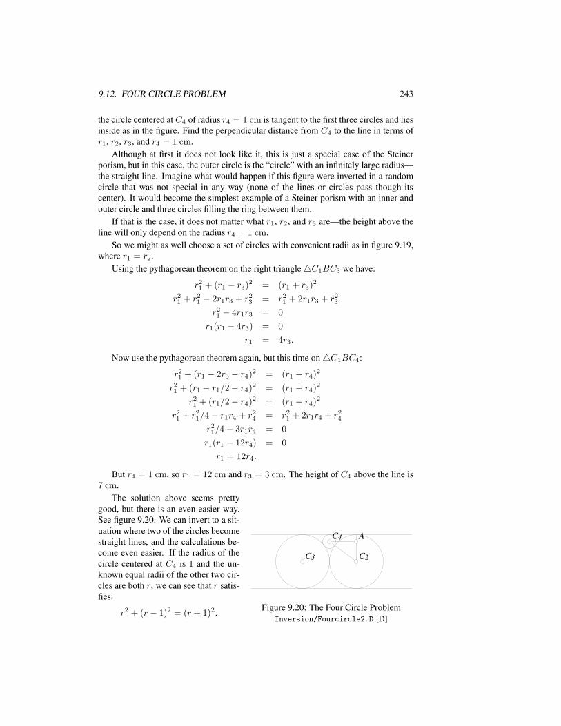
9.12. FOUR CIRCLE PROBLEM 243
the circle centered at C4 of radius r4 = 1 cm is tangent to the first three circles and liesinside as in the figure. Find the perpendicular distance from C4 to the line in terms ofr1, r2, r3, and r4 = 1 cm.
Although at first it does not look like it, this is just a special case of the Steinerporism, but in this case, the outer circle is the “circle” with an infinitely large radius—the straight line. Imagine what would happen if this figure were inverted in a randomcircle that was not special in any way (none of the lines or circles pass though itscenter). It would become the simplest example of a Steiner porism with an inner andouter circle and three circles filling the ring between them.
If that is the case, it does not matter what r1, r2, and r3 are—the height above theline will only depend on the radius r4 = 1 cm.
So we might as well choose a set of circles with convenient radii as in figure 9.19,where r1 = r2.
Using the pythagorean theorem on the right triangle4C1BC3 we have:
r21 + (r1 − r3)2 = (r1 + r3)2
r21 + r2
1 − 2r1r3 + r23 = r2
1 + 2r1r3 + r23
r21 − 4r1r3 = 0
r1(r1 − 4r3) = 0
r1 = 4r3.
Now use the pythagorean theorem again, but this time on4C1BC4:
r21 + (r1 − 2r3 − r4)2 = (r1 + r4)2
r21 + (r1 − r1/2− r4)2 = (r1 + r4)2
r21 + (r1/2− r4)2 = (r1 + r4)2
r21 + r2
1/4− r1r4 + r24 = r2
1 + 2r1r4 + r24
r21/4− 3r1r4 = 0
r1(r1 − 12r4) = 0
r1 = 12r4.
But r4 = 1 cm, so r1 = 12 cm and r3 = 3 cm. The height of C4 above the line is7 cm.
C4C4
C2C2C3C3
AA
Figure 9.20: The Four Circle ProblemInversion/Fourcircle2.D [D]
The solution above seems prettygood, but there is an even easier way.See figure 9.20. We can invert to a sit-uation where two of the circles becomestraight lines, and the calculations be-come even easier. If the radius of thecircle centered at C4 is 1 and the un-known equal radii of the other two cir-cles are both r, we can see that r satis-fies:
r2 + (r − 1)2 = (r + 1)2.
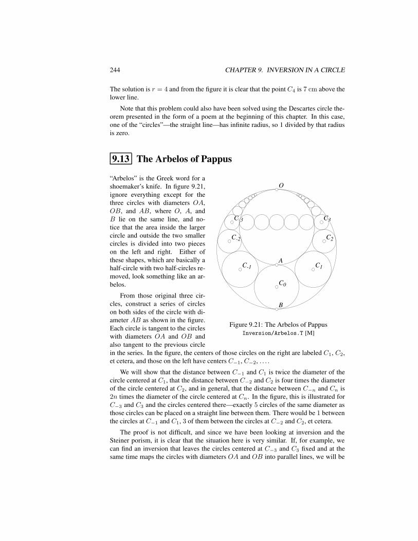
244 CHAPTER 9. INVERSION IN A CIRCLE
The solution is r = 4 and from the figure it is clear that the point C4 is 7 cm above thelower line.
Note that this problem could also have been solved using the Descartes circle the-orem presented in the form of a poem at the beginning of this chapter. In this case,one of the “circles”—the straight line—has infinite radius, so 1 divided by that radiusis zero.
9.13 The Arbelos of Pappus
AA
OO
BB
C0C0
C1C1
C2C2
C3C3
C-1C-1
C-2C-2
C-3C-3
Figure 9.21: The Arbelos of PappusInversion/Arbelos.T [M]
“Arbelos” is the Greek word for ashoemaker’s knife. In figure 9.21,ignore everything except for thethree circles with diameters OA,OB, and AB, where O, A, andB lie on the same line, and no-tice that the area inside the largercircle and outside the two smallercircles is divided into two pieceson the left and right. Either ofthese shapes, which are basically ahalf-circle with two half-circles re-moved, look something like an ar-belos.
From those original three cir-cles, construct a series of circleson both sides of the circle with di-ameter AB as shown in the figure.Each circle is tangent to the circleswith diameters OA and OB andalso tangent to the previous circlein the series. In the figure, the centers of those circles on the right are labeled C1, C2,et cetera, and those on the left have centers C−1, C−2, . . . .
We will show that the distance between C−1 and C1 is twice the diameter of thecircle centered at C1, that the distance between C−2 and C2 is four times the diameterof the circle centered at C2, and in general, that the distance between C−n and Cn is2n times the diameter of the circle centered at Cn. In the figure, this is illustrated forC−3 and C3 and the circles centered there—exactly 5 circles of the same diameter asthose circles can be placed on a straight line between them. There would be 1 betweenthe circles at C−1 and C1, 3 of them between the circles at C−2 and C2, et cetera.
The proof is not difficult, and since we have been looking at inversion and theSteiner porism, it is clear that the situation here is very similar. If, for example, wecan find an inversion that leaves the circles centered at C−3 and C3 fixed and at thesame time maps the circles with diameters OA and OB into parallel lines, we will be
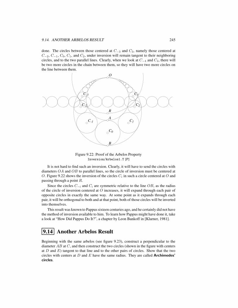
9.14. ANOTHER ARBELOS RESULT 245
done. The circles between those centered at C−3 and C3, namely those centered atC−2, C−1, C0, C1, and C2, under inversion will remain tangent to their neighboringcircles, and to the two parallel lines. Clearly, when we look at C−4 and C4, there willbe two more circles in the chain between them, so they will have two more circles onthe line between them.
AA
RR
OO
BB
C0C0
C1C1
C2C2
C3C3
C-1C-1
C-2C-2
C-3C-3
Figure 9.22: Proof of the Arbelos PropertyInversion/Arbelos1.T [P]
It is not hard to find such an inversion. Clearly, it will have to send the circles withdiameters OA and OB to parallel lines, so the circle of inversion must be centered atO. Figure 9.22 shows the inversion of the circles Ci in such a circle centered at O andpassing through a point R.
Since the circles C−i and Ci are symmetric relative to the line OB, as the radiusof the circle of inversion centered at O increases, it will expand through each pair ofopposite circles in exactly the same way. At some point as it expands through eachpair, it will be orthogonal to both and at that point, both of those circles will be invertedinto themselves.
This result was known to Pappus sixteen centuries ago, and he certainly did not havethe method of inversion available to him. To learn how Pappus might have done it, takea look at “How Did Pappus Do It?”, a chapter by Leon Bankoff in [Klarner, 1981].
9.14 Another Arbelos Result
Beginning with the same arbelos (see figure 9.23), construct a perpendicular to thediameterAB at C, and then construct the two circles (shown in the figure with centersat D and E) tangent to that line and to the other pairs of circles. Show that the twocircles with centers at D and E have the same radius. They are called Archimedes’circles.
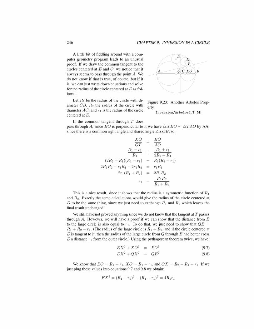
246 CHAPTER 9. INVERSION IN A CIRCLE
AA BBCC
DDEE
OOXX
TT
Figure 9.23: Another Arbelos Prop-erty
Inversion/Arbelos2.T [M]
A little bit of fiddling around with a com-puter geometry program leads to an unusualproof. If we draw the common tangent to thecircles centered at E and O, we notice that italways seems to pass through the point A. Wedo not know if that is true, of course, but if itis, we can just write down equations and solvefor the radius of the circle centered atE as fol-lows:
Let R1 be the radius of the circle with di-ameter CB, R2 the radius of the circle withdiameter AC, and r1 is the radius of the circlecentered at E.
If the common tangent through T doespass through A, since EO is perpendicular to it we have 4XEO ∼ 4TAO by AA,since there is a common right angle and shared angle ∠XOE, so:
XO
OT=
EO
AOR1 − r1
R1=
R1 + r1
2R2 +R1
(2R2 +R1)(R1 − r1) = R1(R1 + r1)
2R1R2 − r1R1 − 2r1R2 = r1R1
2r1(R1 +R2) = 2R1R2
r1 =R1R2
R1 +R2
This is a nice result, since it shows that the radius is a symmetric function of R1
and R2. Exactly the same calculations would give the radius of the circle centered atD to be the same thing, since we just need to exchange R1 and R2 which leaves thefinal result unchanged.
We still have not proved anything since we do not know that the tangent at T passesthrough A. However, we will have a proof if we can show that the distance from Eto the large circle is also equal to r1. To do that, we just need to show that QE =R1 + R2 − r1. (The radius of the large circle is R1 + R2, and if the circle centered atE is tangent to it, then the radius of the large circle from Q throughE had better crossE a distance r1 from the outer circle.) Using the pythagorean theorem twice, we have:
EX2 +XO2 = EO2 (9.7)EX2 +QX2 = QE2 (9.8)
We know that EO = R1 + r1, XO = R1 − r1, and QX = R2 − R1 + r1. If wejust plug these values into equations 9.7 and 9.8 we obtain:
EX2 = (R1 + r1)2 − (R1 − r1)2 = 4R1r1
9.15. THE PROBLEMS OF APOLLONIUS 247
soQE2 = 4R1r1 + (R2 −R1 + r1)2
We are done if QE = (R1 +R2 − r1) which is true if:
(R1 +R2 − r1)2 = 4R1r1 + (R2 −R1 + r1)2,
which we can check:
(R2 + (R1 − r1))2 − (R2 − (R1 − r1))2 = 4R1r1
4R2(R1 − r1) = 4R1r1
r1 =R1R2
R1 +R2,
which is true.
9.15 The Problems of Apollonius
Given any combination of three figures chosen from among points, lines, and circles,find all the circles that pass through the selected points and are tangent to the selectedlines and circles. There are ten possibilities which we discussed in Section 4.6.5, la-beled here as follows: (PPP ), (PPL), (PPC), (PLL), (PLC), (PCC), (LLL),(LLC), (LCC) and (CCC). The (PLL) problem, for example requires the construc-tion of all circles passing through a given point and tangent to two given lines.
The (PPP ) and (LLL) problems are solved in every high school geometry course.In Sections 4.6.5 and 4.6.6, we solved (PPL) and (PLL), and in Section 9.6 we solved(PCC). In Section 9.7 we even solved a special case (CCC).
Although all ten problems can be solved with classical techniques, the technique ofinversion simplifies many of the problems. In this section we will solve (and in somecases, re-solve) various Apollonius’ problems using that technique.
In many cases, we can consider lines and circles to be basically the same, fromthe point of view of inversion, so if you can solve, say, the (PCC) problem, you canprobably also solve the (PLL) and (PLC) problems, although you must be careful.
Here is a short discussion of all the cases. The one that is commonly known byitself as “Apollonius’ Problem” is the hardest one: (CCC). It has approximately thesame difficulty as (LLC), or (LCC). In fact, if you have a rock-solid solution to thethree circles problem, you could solve the other two as follows:
First, do an inversion around an arbitrary point not on any of the lines or circles,and convert your problem to (CCC). Solve that problem with your rock-solid method,and then that solution can be re-inverted through the circle around the arbitrary pointthat you initially selected. Notice that since your “rock-solid” method may itself in-volve inversion and re-inversion, you may have to do four total inversions to solve theproblem.
In what follows, we may ignore the degenerate cases, such as when the points lieon the lines or circles, when the points are coincident, or when the three lines or circlesmeet at a point. These cases are not hard, and you should be able to figure them outwithout much difficulty.
248 CHAPTER 9. INVERSION IN A CIRCLE
9.15.1 Apollonius: (PPP ) and (LLL)
The (PPP ) and (LLL) problems are equivalent to finding the circumcircle and incen-ter, respectively, of a triangle.
The (PPP ) problem can be solved using inversion—invert in a circle centered atone of the points, sending that point to infinity. If the line connecting the inversions ofthe other two points is re-inverted in that circle, it will be the required circle. Do yousee why?
9.15.2 Apollonius: (PPL)
Do an inversion centered at one of the points. This will send that point to infinity, andwill convert the line into a circle. The inverted solutions must pass through the pointat infinity, and hence must be lines. They must pass through the inversion of the otherpoint and be tangent to the circle, so if we can find the tangents from the inverted pointto the circle, and re-invert that, we will have the solutions. There may be none if theinverted point lies inside the inverted line (which is a circle).
It is not hard to consider the degenerate case where one of the points falls on a line.Invert through the other point, and now there will be only a single solution, since theinverted point will lie on the circle that is the inversion of the line, and there is henceonly a single tangent line.
9.15.3 Apollonius: (PPC)
This is exactly the same as the previous problem, except that the circle will be invertedto become a circle instead of the line becoming a circle.
9.15.4 Apollonius: (PLL), (PLC) and (PCC)
The (PLL) problem was solved in Section 9.6, but it, and the other two, can be solvedvia inversion. Send the point to infinity, and the lines and/or circles will become cir-cles. Find the common exterior tangents, re-invert them, and obtain the solutions. Thespecial cases where a line or circle passes though the point are also easily solved.
9.15.5 Apollonius: (LLC), (LCC) and (CCC)
All three of these problems are equivalent in the sense that a single inversion can con-vert all of them to (CCC). If the problem initially has any lines, do an inversionrelative to a circle K whose center does not lie on any of the lines or circles. All thelines and circles will be inverted to circles. We will demonstrate below how to solvethe three circles problem, and once you have done that for the inverted figures, re-invertthem in the circle K to obtain your final solution.
There are up to eight possible solutions, and figure 9.24 illustrates a situation whereall eight circles tangent to the three given circles exist.
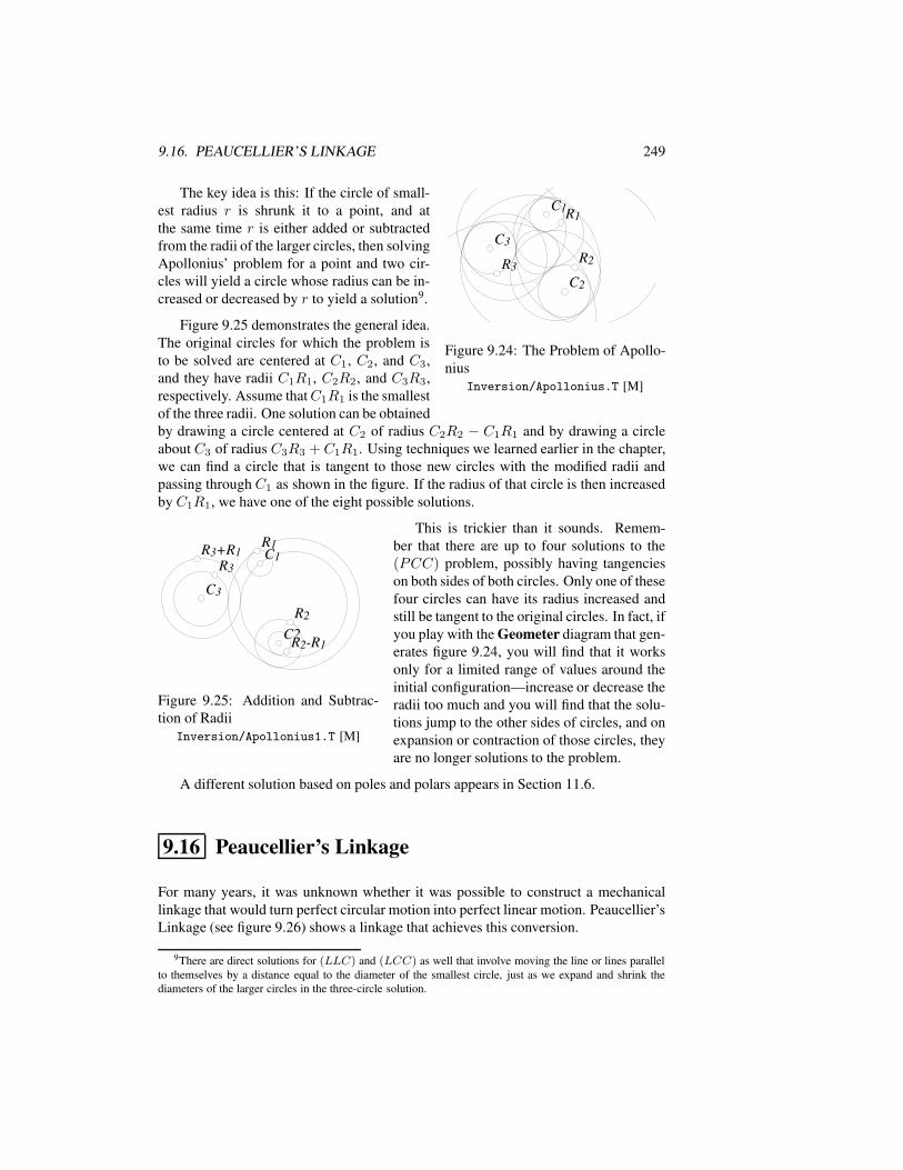
9.16. PEAUCELLIER’S LINKAGE 249
C1C1R1R1
C2C2
R2R2
C3C3
R3R3
Figure 9.24: The Problem of Apollo-nius
Inversion/Apollonius.T [M]
The key idea is this: If the circle of small-est radius r is shrunk it to a point, and atthe same time r is either added or subtractedfrom the radii of the larger circles, then solvingApollonius’ problem for a point and two cir-cles will yield a circle whose radius can be in-creased or decreased by r to yield a solution9.
Figure 9.25 demonstrates the general idea.The original circles for which the problem isto be solved are centered at C1, C2, and C3,and they have radii C1R1, C2R2, and C3R3,respectively. Assume thatC1R1 is the smallestof the three radii. One solution can be obtainedby drawing a circle centered at C2 of radius C2R2 − C1R1 and by drawing a circleabout C3 of radius C3R3 + C1R1. Using techniques we learned earlier in the chapter,we can find a circle that is tangent to those new circles with the modified radii andpassing through C1 as shown in the figure. If the radius of that circle is then increasedby C1R1, we have one of the eight possible solutions.
C1C1
C2C2
C3C3
R3+R1R3+R1R1R1
R3R3
R2-R1R2-R1
R2R2
Figure 9.25: Addition and Subtrac-tion of Radii
Inversion/Apollonius1.T [M]
This is trickier than it sounds. Remem-ber that there are up to four solutions to the(PCC) problem, possibly having tangencieson both sides of both circles. Only one of thesefour circles can have its radius increased andstill be tangent to the original circles. In fact, ifyou play with the Geometer diagram that gen-erates figure 9.24, you will find that it worksonly for a limited range of values around theinitial configuration—increase or decrease theradii too much and you will find that the solu-tions jump to the other sides of circles, and onexpansion or contraction of those circles, theyare no longer solutions to the problem.
A different solution based on poles and polars appears in Section 11.6.
9.16 Peaucellier’s Linkage
For many years, it was unknown whether it was possible to construct a mechanicallinkage that would turn perfect circular motion into perfect linear motion. Peaucellier’sLinkage (see figure 9.26) shows a linkage that achieves this conversion.
9There are direct solutions for (LLC) and (LCC) as well that involve moving the line or lines parallelto themselves by a distance equal to the diameter of the smallest circle, just as we expand and shrink thediameters of the larger circles in the three-circle solution.
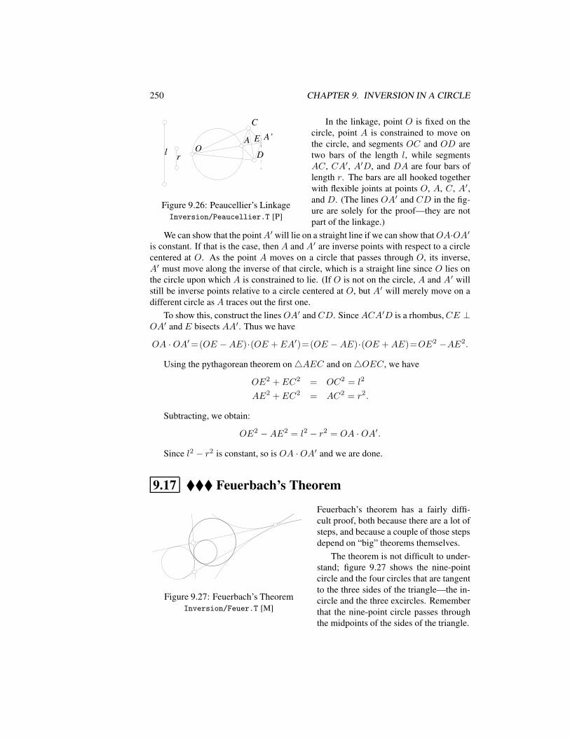
250 CHAPTER 9. INVERSION IN A CIRCLE
rrll OOAA
CC
DD
A’A’EE
Figure 9.26: Peaucellier’s LinkageInversion/Peaucellier.T [P]
In the linkage, point O is fixed on thecircle, point A is constrained to move onthe circle, and segments OC and OD aretwo bars of the length l, while segmentsAC, CA′, A′D, and DA are four bars oflength r. The bars are all hooked togetherwith flexible joints at points O, A, C, A′,and D. (The lines OA′ and CD in the fig-ure are solely for the proof—they are notpart of the linkage.)
We can show that the pointA′ will lie on a straight line if we can show thatOA·OA′is constant. If that is the case, then A and A′ are inverse points with respect to a circlecentered at O. As the point A moves on a circle that passes through O, its inverse,A′ must move along the inverse of that circle, which is a straight line since O lies onthe circle upon which A is constrained to lie. (If O is not on the circle, A and A′ willstill be inverse points relative to a circle centered at O, but A′ will merely move on adifferent circle as A traces out the first one.
To show this, construct the linesOA′ andCD. SinceACA′D is a rhombus,CE ⊥OA′ and E bisects AA′. Thus we have
OA ·OA′=(OE −AE)·(OE +EA′)=(OE −AE)·(OE +AE)=OE2 −AE2.
Using the pythagorean theorem on4AEC and on4OEC, we have
OE2 +EC2 = OC2 = l2
AE2 +EC2 = AC2 = r2.
Subtracting, we obtain:
OE2 −AE2 = l2 − r2 = OA · OA′.
Since l2 − r2 is constant, so is OA ·OA′ and we are done.
9.17 Feuerbach’s Theorem
Figure 9.27: Feuerbach’s TheoremInversion/Feuer.T [M]
Feuerbach’s theorem has a fairly diffi-cult proof, both because there are a lot ofsteps, and because a couple of those stepsdepend on “big” theorems themselves.
The theorem is not difficult to under-stand; figure 9.27 shows the nine-pointcircle and the four circles that are tangentto the three sides of the triangle—the in-circle and the three excircles. Rememberthat the nine-point circle passes throughthe midpoints of the sides of the triangle.
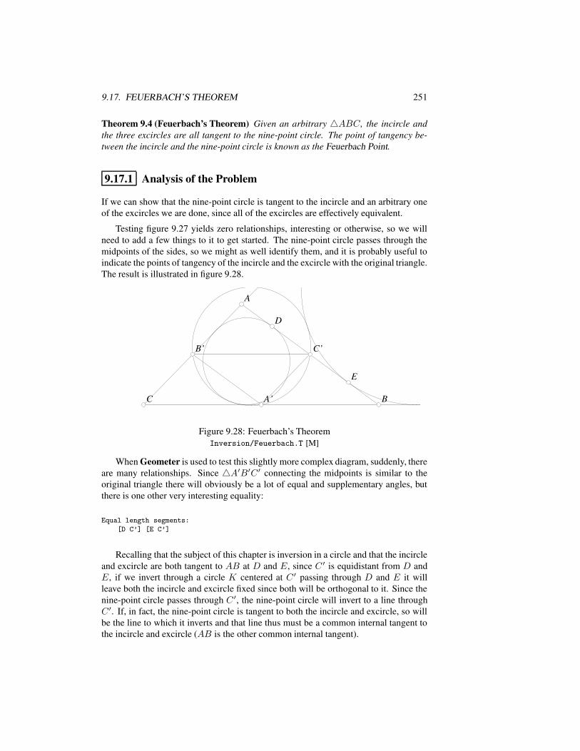
9.17. FEUERBACH’S THEOREM 251
Theorem 9.4 (Feuerbach’s Theorem) Given an arbitrary 4ABC, the incircle andthe three excircles are all tangent to the nine-point circle. The point of tangency be-tween the incircle and the nine-point circle is known as the Feuerbach Point.
9.17.1 Analysis of the Problem
If we can show that the nine-point circle is tangent to the incircle and an arbitrary oneof the excircles we are done, since all of the excircles are effectively equivalent.
Testing figure 9.27 yields zero relationships, interesting or otherwise, so we willneed to add a few things to it to get started. The nine-point circle passes through themidpoints of the sides, so we might as well identify them, and it is probably useful toindicate the points of tangency of the incircle and the excircle with the original triangle.The result is illustrated in figure 9.28.
CC
AA
BB
DD
EE
C’C’
A’A’
B’B’
Figure 9.28: Feuerbach’s TheoremInversion/Feuerbach.T [M]
When Geometer is used to test this slightly more complex diagram, suddenly, thereare many relationships. Since 4A′B′C ′ connecting the midpoints is similar to theoriginal triangle there will obviously be a lot of equal and supplementary angles, butthere is one other very interesting equality:
Equal length segments:
[D C’] [E C’]
Recalling that the subject of this chapter is inversion in a circle and that the incircleand excircle are both tangent to AB at D and E, since C ′ is equidistant from D andE, if we invert through a circle K centered at C ′ passing through D and E it willleave both the incircle and excircle fixed since both will be orthogonal to it. Since thenine-point circle passes through C ′, the nine-point circle will invert to a line throughC ′. If, in fact, the nine-point circle is tangent to both the incircle and excircle, so willbe the line to which it inverts and that line thus must be a common internal tangent tothe incircle and excircle (AB is the other common internal tangent).
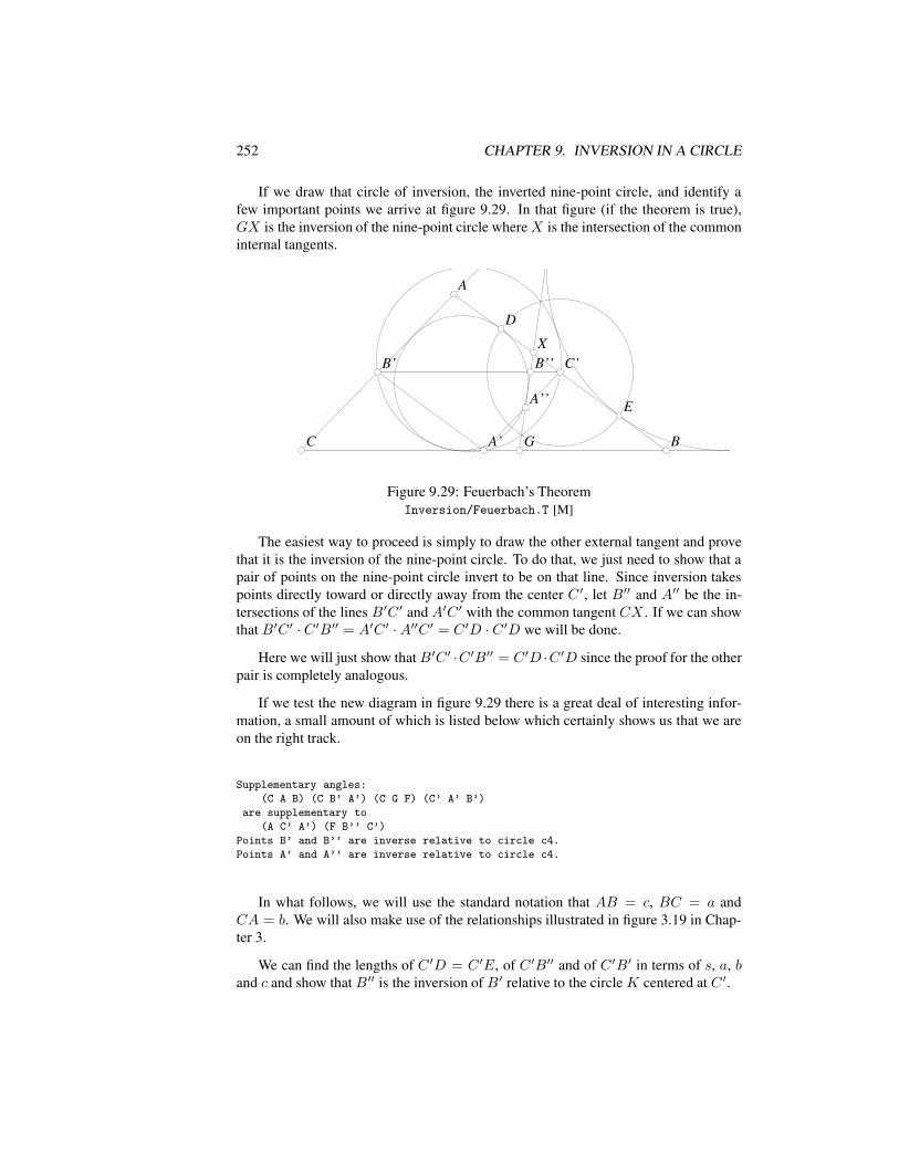
252 CHAPTER 9. INVERSION IN A CIRCLE
If we draw that circle of inversion, the inverted nine-point circle, and identify afew important points we arrive at figure 9.29. In that figure (if the theorem is true),GX is the inversion of the nine-point circle whereX is the intersection of the commoninternal tangents.
CC
AA
BB
DD
EE
C’C’
A’A’
B’B’
FF
GG
XXB’’B’’
A’’A’’
Figure 9.29: Feuerbach’s TheoremInversion/Feuerbach.T [M]
The easiest way to proceed is simply to draw the other external tangent and provethat it is the inversion of the nine-point circle. To do that, we just need to show that apair of points on the nine-point circle invert to be on that line. Since inversion takespoints directly toward or directly away from the center C ′, let B′′ and A′′ be the in-tersections of the lines B′C ′ and A′C ′ with the common tangent CX . If we can showthat B′C ′ · C ′B′′ = A′C ′ ·A′′C ′ = C ′D · C ′D we will be done.
Here we will just show thatB′C ′ ·C ′B′′ = C ′D ·C ′D since the proof for the otherpair is completely analogous.
If we test the new diagram in figure 9.29 there is a great deal of interesting infor-mation, a small amount of which is listed below which certainly shows us that we areon the right track.
Supplementary angles:
(C A B) (C B’ A’) (C G F) (C’ A’ B’)
are supplementary to
(A C’ A’) (F B’’ C’)
Points B’ and B’’ are inverse relative to circle c4.
Points A’ and A’’ are inverse relative to circle c4.
In what follows, we will use the standard notation that AB = c, BC = a andCA = b. We will also make use of the relationships illustrated in figure 3.19 in Chap-ter 3.
We can find the lengths of C ′D = C ′E, of C ′B′′ and of C ′B′ in terms of s, a, band c and show that B′′ is the inversion of B′ relative to the circle K centered at C ′.
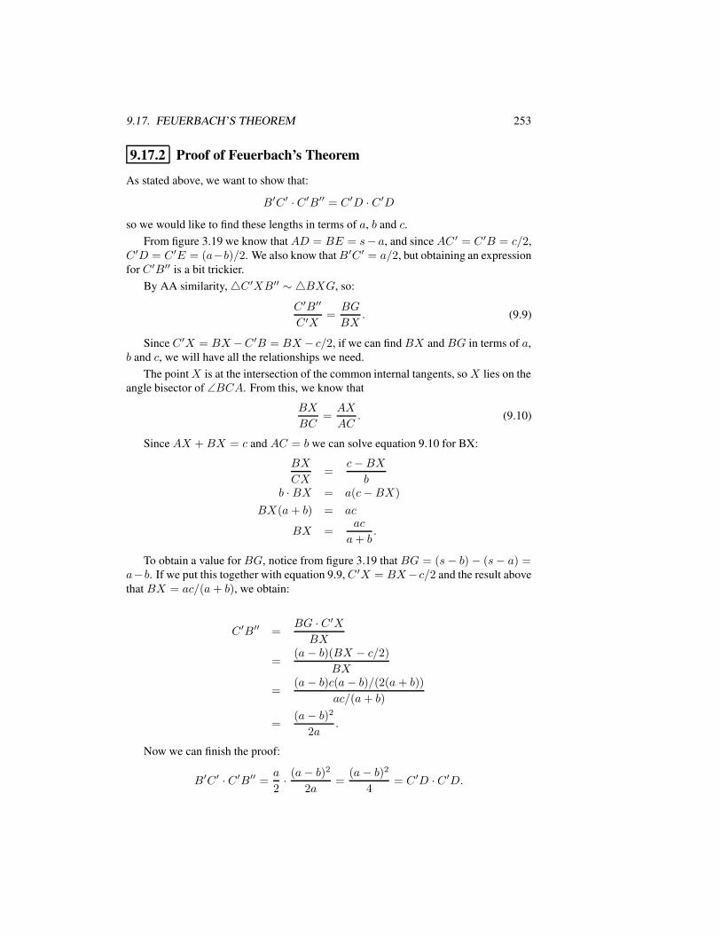
9.17. FEUERBACH’S THEOREM 253
9.17.2 Proof of Feuerbach’s Theorem
As stated above, we want to show that:
B′C ′ · C ′B′′ = C ′D · C ′Dso we would like to find these lengths in terms of a, b and c.
From figure 3.19 we know that AD = BE = s− a, and since AC ′ = C ′B = c/2,C ′D = C ′E = (a−b)/2. We also know thatB′C ′ = a/2, but obtaining an expressionfor C ′B′′ is a bit trickier.
By AA similarity,4C ′XB′′ ∼ 4BXG, so:
C ′B′′
C ′X=BG
BX. (9.9)
Since C ′X = BX −C ′B = BX − c/2, if we can find BX andBG in terms of a,b and c, we will have all the relationships we need.
The pointX is at the intersection of the common internal tangents, so X lies on theangle bisector of ∠BCA. From this, we know that
BX
BC=AX
AC. (9.10)
Since AX +BX = c and AC = b we can solve equation 9.10 for BX:
BX
CX=
c−BXb
b · BX = a(c−BX)
BX(a+ b) = ac
BX =ac
a+ b.
To obtain a value for BG, notice from figure 3.19 that BG = (s− b)− (s− a) =a−b. If we put this together with equation 9.9,C ′X = BX−c/2 and the result abovethat BX = ac/(a+ b), we obtain:
C ′B′′ =BG · C ′XBX
=(a− b)(BX − c/2)
BX
=(a− b)c(a− b)/(2(a+ b))
ac/(a+ b)
=(a− b)2
2a.
Now we can finish the proof:
B′C ′ · C ′B′′ =a
2· (a− b)2
2a=
(a− b)2
4= C ′D · C ′D.
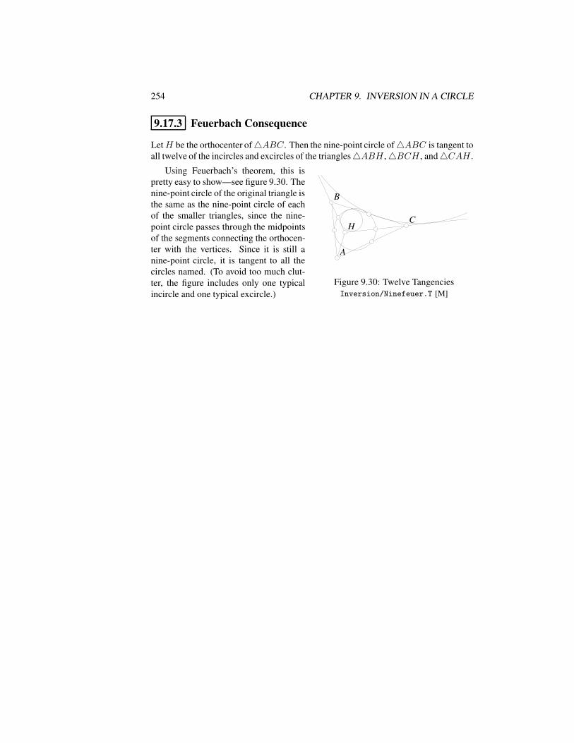
254 CHAPTER 9. INVERSION IN A CIRCLE
9.17.3 Feuerbach Consequence
LetH be the orthocenter of4ABC. Then the nine-point circle of4ABC is tangent toall twelve of the incircles and excircles of the triangles4ABH ,4BCH , and4CAH .
AA
BB
CCHH
Figure 9.30: Twelve TangenciesInversion/Ninefeuer.T [M]
Using Feuerbach’s theorem, this ispretty easy to show—see figure 9.30. Thenine-point circle of the original triangle isthe same as the nine-point circle of eachof the smaller triangles, since the nine-point circle passes through the midpointsof the segments connecting the orthocen-ter with the vertices. Since it is still anine-point circle, it is tangent to all thecircles named. (To avoid too much clut-ter, the figure includes only one typicalincircle and one typical excircle.)
Chapter 10 Projective Geometry
This chapter will not supply many new techniques for using Geometer (although itwill provide a few). It does, however, provide some insight about how Geometer (andprobably most other computer geometry programs) do many of their internal calcula-tions in terms of projective geometry as opposed to Euclidean geometry.
We will begin by proving the Euclidean version of a purely projective theorem. Acareful analysis of the theorem will then show why it is often useful to view a situationas if it were in projective space rather than Euclidean space.
10.1 Desargues’ Theorem
Desargues’ theorem, like most of the others in this chapter, is actually a theorem fromprojective geometry. We will begin by proving the Euclidean form of that theorem.
255
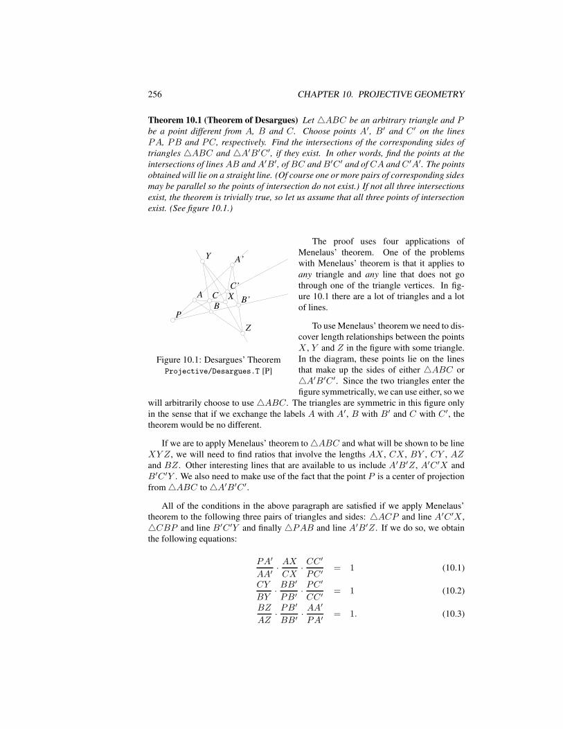
256 CHAPTER 10. PROJECTIVE GEOMETRY
Theorem 10.1 (Theorem of Desargues) Let 4ABC be an arbitrary triangle and Pbe a point different from A, B and C. Choose points A′, B′ and C ′ on the linesPA, PB and PC, respectively. Find the intersections of the corresponding sides oftriangles 4ABC and 4A′B′C ′, if they exist. In other words, find the points at theintersections of lines AB andA′B′, ofBC andB′C ′ and of CA andC ′A′. The pointsobtained will lie on a straight line. (Of course one or more pairs of corresponding sidesmay be parallel so the points of intersection do not exist.) If not all three intersectionsexist, the theorem is trivially true, so let us assume that all three points of intersectionexist. (See figure 10.1.)
AABBCC
PP
A’A’
C’C’
B’B’XX
YY
ZZ
Figure 10.1: Desargues’ TheoremProjective/Desargues.T [P]
The proof uses four applications ofMenelaus’ theorem. One of the problemswith Menelaus’ theorem is that it applies toany triangle and any line that does not gothrough one of the triangle vertices. In fig-ure 10.1 there are a lot of triangles and a lotof lines.
To use Menelaus’ theorem we need to dis-cover length relationships between the pointsX , Y and Z in the figure with some triangle.In the diagram, these points lie on the linesthat make up the sides of either 4ABC or4A′B′C ′. Since the two triangles enter thefigure symmetrically, we can use either, so we
will arbitrarily choose to use 4ABC. The triangles are symmetric in this figure onlyin the sense that if we exchange the labels A with A′, B with B′ and C with C ′, thetheorem would be no different.
If we are to apply Menelaus’ theorem to4ABC and what will be shown to be lineXY Z, we will need to find ratios that involve the lengths AX , CX , BY , CY , AZand BZ. Other interesting lines that are available to us include A′B′Z, A′C ′X andB′C ′Y . We also need to make use of the fact that the point P is a center of projectionfrom4ABC to4A′B′C ′.
All of the conditions in the above paragraph are satisfied if we apply Menelaus’theorem to the following three pairs of triangles and sides: 4ACP and line A′C ′X ,4CBP and line B′C ′Y and finally 4PAB and line A′B′Z. If we do so, we obtainthe following equations:
PA′
AA′· AXCX
· CC′
PC ′= 1 (10.1)
CY
BY· BB
′
PB′· PC
′
CC ′= 1 (10.2)
BZ
AZ· PB
′
BB′· AA
′
PA′= 1. (10.3)
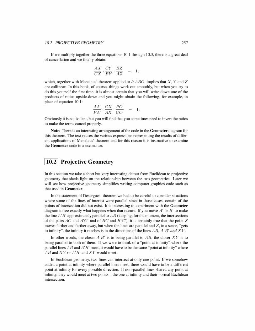
10.2. PROJECTIVE GEOMETRY 257
If we multiply together the three equations 10.1 through 10.3, there is a great dealof cancellation and we finally obtain:
AX
CX· CYBY· BZAZ
= 1,
which, together with Menelaus’ theorem applied to4ABC, implies that X , Y and Zare collinear. In this book, of course, things work out smoothly, but when you try todo this yourself the first time, it is almost certain that you will write down one of theproducts of ratios upside-down and you might obtain the following, for example, inplace of equation 10.1:
AA′
PA′· CXAX
· PC′
CC ′= 1.
Obviously it is equivalent, but you will find that you sometimes need to invert the ratiosto make the terms cancel properly.
Note: There is an interesting arrangement of the code in the Geometer diagram forthis theorem. The text reuses the various expressions representing the results of differ-ent applications of Menelaus’ theorem and for this reason it is instructive to examinethe Geometer code in a text editor.
10.2 Projective Geometry
In this section we take a short but very interesting detour from Euclidean to projectivegeometry that sheds light on the relationship between the two geometries. Later wewill see how projective geometry simplifies writing computer graphics code such asthat used in Geometer.
In the statement of Desargues’ theorem we had to be careful to consider situationswhere some of the lines of interest were parallel since in those cases, certain of thepoints of intersection did not exist. It is interesting to experiment with the Geometerdiagram to see exactly what happens when that occurs. If you move A′ or B′ to makethe lineA′B′ approximately parallel toAB (keeping, for the moment, the intersectionsof the pairs AC and A′C ′ and of BC and B′C ′), it is certainly true that the point Zmoves farther and farther away, but when the lines are parallel and Z, in a sense, “getsto infinity”, the infinity it reaches is in the directions of the lines AB, A′B′ and XY .
In other words, the closer A′B′ is to being parallel to AB, the closer XY is tobeing parallel to both of them. If we were to think of a “point at infinity” where theparallel linesAB andA′B′ meet, it would have to be the same “point at infinity” whereAB and XY or A′B′ and XY would meet.
In Euclidean geometry, two lines can intersect at only one point. If we somehowadded a point at infinity where parallel lines meet, there would have to be a differentpoint at infinity for every possible direction. If non-parallel lines shared any point atinfinity, they would meet at two points—the one at infinity and their normal Euclideanintersection.
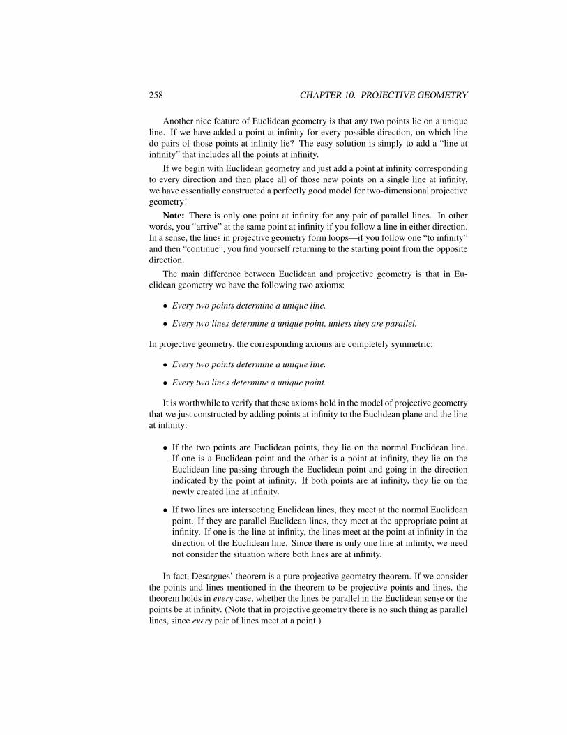
258 CHAPTER 10. PROJECTIVE GEOMETRY
Another nice feature of Euclidean geometry is that any two points lie on a uniqueline. If we have added a point at infinity for every possible direction, on which linedo pairs of those points at infinity lie? The easy solution is simply to add a “line atinfinity” that includes all the points at infinity.
If we begin with Euclidean geometry and just add a point at infinity correspondingto every direction and then place all of those new points on a single line at infinity,we have essentially constructed a perfectly good model for two-dimensional projectivegeometry!
Note: There is only one point at infinity for any pair of parallel lines. In otherwords, you “arrive” at the same point at infinity if you follow a line in either direction.In a sense, the lines in projective geometry form loops—if you follow one “to infinity”and then “continue”, you find yourself returning to the starting point from the oppositedirection.
The main difference between Euclidean and projective geometry is that in Eu-clidean geometry we have the following two axioms:
• Every two points determine a unique line.
• Every two lines determine a unique point, unless they are parallel.
In projective geometry, the corresponding axioms are completely symmetric:
• Every two points determine a unique line.
• Every two lines determine a unique point.
It is worthwhile to verify that these axioms hold in the model of projective geometrythat we just constructed by adding points at infinity to the Euclidean plane and the lineat infinity:
• If the two points are Euclidean points, they lie on the normal Euclidean line.If one is a Euclidean point and the other is a point at infinity, they lie on theEuclidean line passing through the Euclidean point and going in the directionindicated by the point at infinity. If both points are at infinity, they lie on thenewly created line at infinity.
• If two lines are intersecting Euclidean lines, they meet at the normal Euclideanpoint. If they are parallel Euclidean lines, they meet at the appropriate point atinfinity. If one is the line at infinity, the lines meet at the point at infinity in thedirection of the Euclidean line. Since there is only one line at infinity, we neednot consider the situation where both lines are at infinity.
In fact, Desargues’ theorem is a pure projective geometry theorem. If we considerthe points and lines mentioned in the theorem to be projective points and lines, thetheorem holds in every case, whether the lines be parallel in the Euclidean sense or thepoints be at infinity. (Note that in projective geometry there is no such thing as parallellines, since every pair of lines meet at a point.)
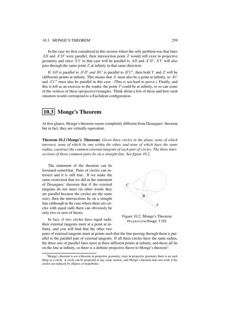
10.3. MONGE’S THEOREM 259
In the case we first considered in this section where the only problem was that linesAB and A′B′ were parallel, their intersection point Z would still exist in projectivegeometry and since XY in that case will be parallel to AB and A′B′, XY will alsopass through the same point Z at infinity in that same direction.
If AB is parallel to A′B′ and BC is parallel to B′C ′, then both Y and Z will be(different) points at infinity. This means that X must also be a point at infinity, so ACand A′C ′ must also be parallel in this case. (This is not hard to prove.) Finally, andthis is left as an exercise to the reader, the point P could be at infinity, or so can someof the vertices of these (projective) triangles. Think about a few of these and how eachsituation would correspond to a Euclidean configuration.
10.3 Monge’s Theorem
At first glance, Monge’s theorem seems completely different from Desargues’ theorembut in fact, they are virtually equivalent.
Theorem 10.2 (Monge’s Theorem) Given three circles in the plane, none of whichintersect, none of which lie one within the other, and none of which have the sameradius, construct the common external tangents of each pair of circles. The three inter-sections of those common pairs lie on a straight line. See figure 10.2.
AA
BB
CC
Figure 10.2: Monge’s TheoremProjective/Monge.T [D]
The statement of the theorem can beloosened somewhat. Pairs of circles can in-tersect and it is still true. If we make thesame restriction that we did in the statementof Desargues’ theorem that if the externaltangents do not meet (in other words theyare parallel because the circles are the samesize), then the intersections lie on a straightline (although in the case where there are cir-cles with equal radii there can obviously beonly two or zero of them).
In fact, if two circles have equal radii,their external tangents meet at a point at in-finity, and you will find that the other twopairs of external tangents meet at points such that the line passing through them is par-allel to the parallel pair of external tangents. If all three circles have the same radius,the three sets of parallel lines meet at three different points at infinity, and those all lieon the line at infinity, so there is a definite projective flavor to Monge’s theorem1.
1Monge’s theorem is not a theorem in projective geometry, since in projective geometry there is no suchthing as a circle. A circle can be projected to any conic section, and Monge’s theorem does not work if thecircles are replaced by ellipses or hyperbolas.
260 CHAPTER 10. PROJECTIVE GEOMETRY
AA
BB
CC
Figure 10.3: Monge’s TheoremProjective/MongeDes.T [M]
In figure 10.3 we see Monge’stheorem again, but with some ad-ditional constructions. It is clearthat the line connecting the centersof a pair of circles passes throughthe intersection of their commonexternal tangents, and in fact, ifwe think of that point of intersec-tion as a point of projection, weare really just projecting one cir-cle onto another. If that is the case,then any corresponding points onthe two circles will lie on a line
passing through that center of projection.
In the figure, a point drawn as a solid diamond is drawn in the corresponding posi-tion (at the same angle from the center) of each circle, and the lines connecting thosediamond points also pass through the common intersection of the external tangents andthe line of centers of the circles.
Now look at what is basically the same figure with some lines and circles erased(see figure 10.4). In this figure it is obvious that the two triangles whose vertices areall diamonds or all squares are projected from the same point at infinity (the linesconnecting the centers and corresponding points on the circles are parallel). Thus theprojective version of Desargues’ theorem (or a suitably extended Euclidean version)shows that Monge’s theorem and Desargues’ theorem are equivalent.
AA
BB
CC
Figure 10.4: Monge’s TheoremProjective/MongeDes1.T [M]
One final interesting feature ofMonge’s theorem is that there isa wonderful, obvious proof if wefirst make the situation a bit morecomplicated. Begin with the threecircles in a plane, but now con-sider them not to be circles, butrather spheres that extend aboveand below the plane. The ex-ternal tangents become cones thattouch each pair of spheres all theway around, and it is clear that thethree-dimensional model of conesand spheres, when cut by the planethrough the common centers of the spheres, gives the two-dimensional model withwhich we began.
In three dimensions, consider two additional planes that touch all three spheresabove and below. Clearly each of these planes will be tangent to the cones and willthus pass through all three tips. But two planes in three-dimensional space intersect ina line, so the three tips of the cones must lie on that line.
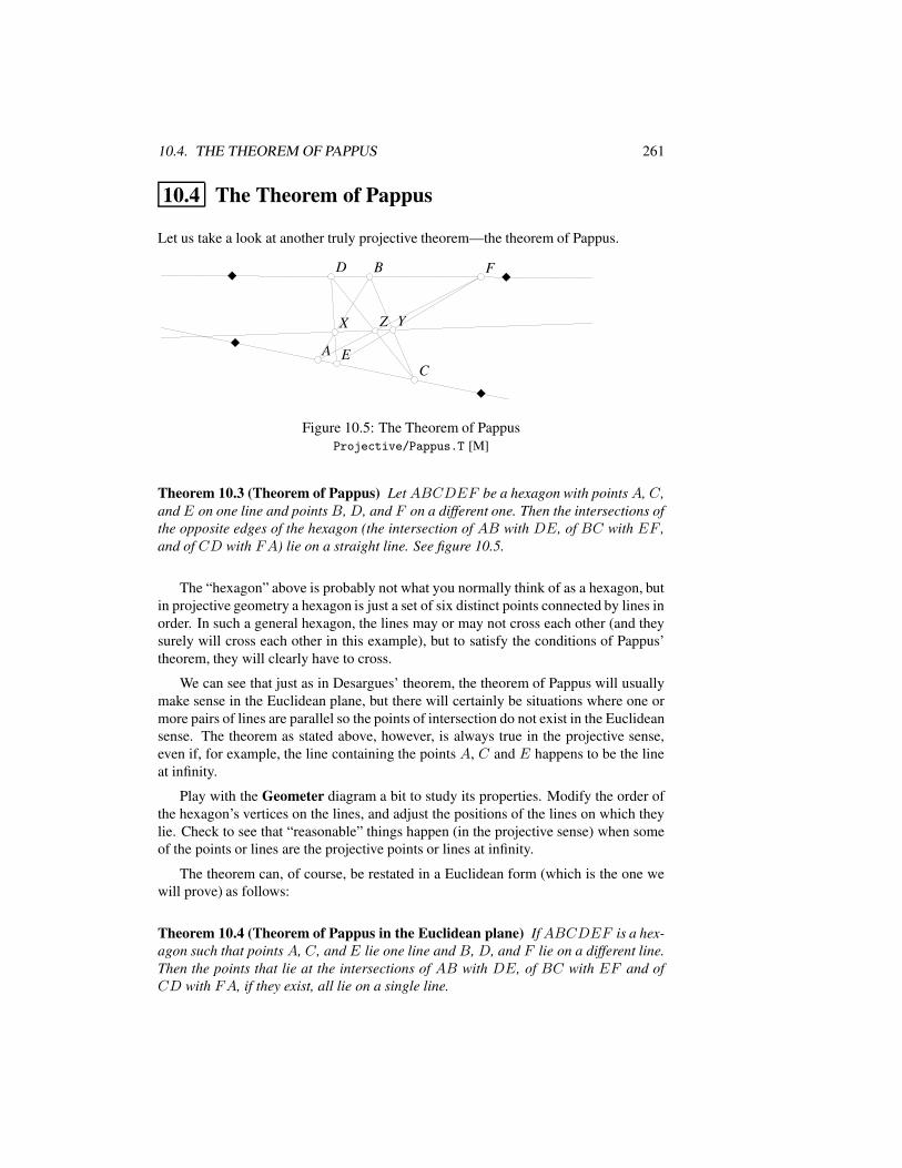
10.4. THE THEOREM OF PAPPUS 261
10.4 The Theorem of Pappus
Let us take a look at another truly projective theorem—the theorem of Pappus.
BB
CC
DD
EE
FF
AA
XX YYZZ
Figure 10.5: The Theorem of PappusProjective/Pappus.T [M]
Theorem 10.3 (Theorem of Pappus) LetABCDEF be a hexagon with pointsA, C,andE on one line and pointsB, D, and F on a different one. Then the intersections ofthe opposite edges of the hexagon (the intersection of AB with DE, of BC with EF ,and of CD with FA) lie on a straight line. See figure 10.5.
The “hexagon” above is probably not what you normally think of as a hexagon, butin projective geometry a hexagon is just a set of six distinct points connected by lines inorder. In such a general hexagon, the lines may or may not cross each other (and theysurely will cross each other in this example), but to satisfy the conditions of Pappus’theorem, they will clearly have to cross.
We can see that just as in Desargues’ theorem, the theorem of Pappus will usuallymake sense in the Euclidean plane, but there will certainly be situations where one ormore pairs of lines are parallel so the points of intersection do not exist in the Euclideansense. The theorem as stated above, however, is always true in the projective sense,even if, for example, the line containing the points A, C and E happens to be the lineat infinity.
Play with the Geometer diagram a bit to study its properties. Modify the order ofthe hexagon’s vertices on the lines, and adjust the positions of the lines on which theylie. Check to see that “reasonable” things happen (in the projective sense) when someof the points or lines are the projective points or lines at infinity.
The theorem can, of course, be restated in a Euclidean form (which is the one wewill prove) as follows:
Theorem 10.4 (Theorem of Pappus in the Euclidean plane) IfABCDEF is a hex-agon such that points A, C, andE lie one line and B, D, and F lie on a different line.Then the points that lie at the intersections of AB with DE, of BC with EF and ofCD with FA, if they exist, all lie on a single line.
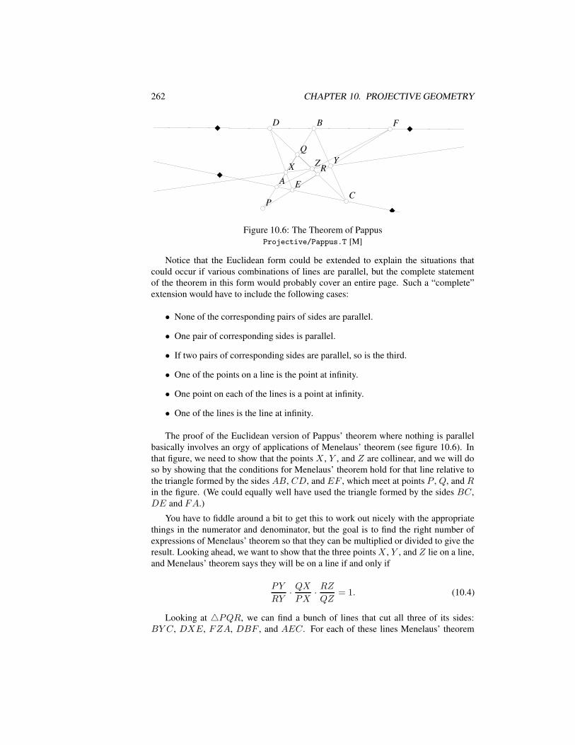
262 CHAPTER 10. PROJECTIVE GEOMETRY
BB
CC
DD
EE
FF
AA
XXYYZZ
RR
PP
Figure 10.6: The Theorem of PappusProjective/Pappus.T [M]
Notice that the Euclidean form could be extended to explain the situations thatcould occur if various combinations of lines are parallel, but the complete statementof the theorem in this form would probably cover an entire page. Such a “complete”extension would have to include the following cases:
• None of the corresponding pairs of sides are parallel.
• One pair of corresponding sides is parallel.
• If two pairs of corresponding sides are parallel, so is the third.
• One of the points on a line is the point at infinity.
• One point on each of the lines is a point at infinity.
• One of the lines is the line at infinity.
The proof of the Euclidean version of Pappus’ theorem where nothing is parallelbasically involves an orgy of applications of Menelaus’ theorem (see figure 10.6). Inthat figure, we need to show that the points X , Y , and Z are collinear, and we will doso by showing that the conditions for Menelaus’ theorem hold for that line relative tothe triangle formed by the sides AB, CD, and EF , which meet at points P , Q, and Rin the figure. (We could equally well have used the triangle formed by the sides BC,DE and FA.)
You have to fiddle around a bit to get this to work out nicely with the appropriatethings in the numerator and denominator, but the goal is to find the right number ofexpressions of Menelaus’ theorem so that they can be multiplied or divided to give theresult. Looking ahead, we want to show that the three pointsX , Y , and Z lie on a line,and Menelaus’ theorem says they will be on a line if and only if
PY
RY· QXPX
· RZQZ
= 1. (10.4)
Looking at 4PQR, we can find a bunch of lines that cut all three of its sides:BY C, DXE, FZA, DBF , and AEC. For each of these lines Menelaus’ theorem
10.5. ANOTHER VIEW OF PROJECTIVE GEOMETRY 263
will give a product of ratios that is equal to one. In the order above, those products ofratios are:
QB
PB· RCQC· PYRY
= 1
QX
PX· RDQD· PERE
= 1
QA
PA· RZQZ· PFRF
= 1
PB
QB· QDRD· RFPF
= 1
PA
QA· QCRC· REPE
= 1.
If we multiply all five equations above, everything cancels except for the desiredresult: equation 10.4. Remember that when you are looking for a proof of your own,you probably will not come up with exactly these five equations—some of yours maybe inverted and you will find you have to multiply and divide your equations, but thenet result will be the same.
Of course this is only a proof of the Euclidean version of the theorem, but thetheorem does hold in the general projective sense.
10.5 Another View of Projective Geometry
Imagine that you are looking out a glass window at the three-dimensional world out-side, and then, without moving your head at all, you take a paintbrush and at everypoint on the window, you paint on the glass exactly the color your eye sees there. Ifyour paint colors were accurate enough, if you were a good enough technician, and ifyou were unable to move your head, you would be unable to tell if you were lookingat the scene outside the window or at the painting you had just made on the windowglass.
The image on the glass is a projection of the objects in the three-dimensional worldon the plane of the window, and if you wish to study this sort of operation, projectivegeometry is just the thing. Three dimensional computer graphics software would notexist without it.
Although projective geometry exists in any number of dimensions (in the exampleabove we were projecting the three-dimensional world to a two-dimensional painting),in this chapter, unless we state otherwise, the words “projective geometry” will referto the two-dimensional version (two-dimensions projected onto two dimensions). Wecan learn quite a bit by looking at one-dimensional projective geometry, and much ofthat can be applied to higher-dimensional projective spaces as well. In fact, there areeven finite projective geometries where the entire geometry consists of a finite numberof lines and planes and theorems like those of Desargues and Pappus continue to betrue in those finite geometries as well. See Section 10.11.
264 CHAPTER 10. PROJECTIVE GEOMETRY
Go back to the painting example, but imagine that you are not looking at the worldthrough the window, but at a geometric diagram drawn on a flat plane. You can dothe same trick with the paintbrush and draw the image of the two-dimensional diagramon the two-dimensional window, and this is a perfectly good projection too. As youmove your eye around behind the window, or as you move or tilt the glass window, thepainting you would obtain on the window will clearly change.
10.5.1 Geometric Invariants
One way to think about Euclidean geometry is that it is the study of properties of figuresthat do not change if you move them around or rotate them (or even if you reflect themin a mirror). For example, if two triangles are congruent, they will continue to becongruent if you move them around without distorting them. In the same way, theangles between the lines in a figure remain unchanged if you move the figure rigidly.The areas of geometric objects are similarly unchanged if you move them elsewhere.
Other properties are also preserved, and in a sense they are almost too obvious tomention. For example, if you rigidly move a line or a circle, it remains a line or a circle.If you rigidly move two intersecting lines as a unit, they continue to intersect. Thereare lots of other properties that are preserved under rigid motions.
Of course there are properties that are not preserved under rigid motion—the dis-tance to a fixed point, for example, or which of two objects is to the right or left of theother (since you can rotate the figure to reverse this).
What if the operations allowed include projections in addition to mirrorings, trans-lations, and rotations? Now what properties are preserved?
Certainly not things like lengths, areas or angles. Projections of circles are veryrarely circles. Projections of parallel lines are not parallel.2 Even things like between-ness drop by the wayside—if point B is between points A and C on a line, the projec-tion of B may not be between the projections of A and C. They will, however, remainon the same projected line.
But plenty of things are preserved (although we do need to make some very slightchanges to what we mean by “points” and “lines”):
• If two lines intersect at a point, the projections of those lines intersect at theprojection of the point.
• If two points lie on a line, the projections of those points lie on the projection ofthe line.
• Although circles are not preserved, conic sections are. In other words, if youproject any conic section (a circle, ellipse, parabola, or hyperbola), its projectionwill also be a conic section, although any one of the types might be converted toany of the other types.
2In fact, in true projective geometry, there really is no such thing as a pair of parallel lines.
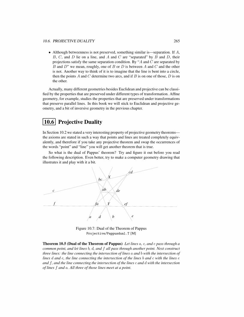
10.6. PROJECTIVE DUALITY 265
• Although betweenness is not preserved, something similar is—separation. If A,B, C, and D lie on a line, and A and C are “separated” by B and D, theirprojections satisfy the same separation condition. By “A and C are separated byB and D” we mean, roughly, one of B or D is between A and C and the otheris not. Another way to think of it is to imagine that the line is bent into a circle,then the points A and C determine two arcs, and if B is on one of those, D is onthe other.
Actually, many different geometries besides Euclidean and projective can be classi-fied by the properties that are preserved under different types of transformation. Affinegeometry, for example, studies the properties that are preserved under transformationsthat preserve parallel lines. In this book we will stick to Euclidean and projective ge-ometry, and a bit of inversive geometry in the previous chapter.
10.6 Projective Duality
In Section 10.2 we stated a very interesting property of projective geometry theorems—the axioms are stated in such a way that points and lines are treated completely equiv-alently, and therefore if you take any projective theorem and swap the occurrences ofthe words “point” and “line” you will get another theorem that is true.
So what is the dual of Pappus’ theorem? Try and figure it out before you readthe following description. Even better, try to make a computer geometry drawing thatillustrates it and play with it a bit.
XX
YY
cc
aa ee
ff
bbdd
abab
bcbc
cdcd
dede
efeffafa
Figure 10.7: Dual of the Theorem of PappusProjective/Pappusdual.T [M]
Theorem 10.5 (Dual of the Theorem of Pappus) Let lines a, c, and e pass through acommon point, and let lines b, d, and f all pass through another point. Next constructthree lines: the line connecting the intersection of lines a and b with the intersection oflines d and e, the line connecting the intersection of the lines b and c with the lines eand f , and the line connecting the intersection of the lines c and d with the intersectionof lines f and a. All three of those lines meet at a point.
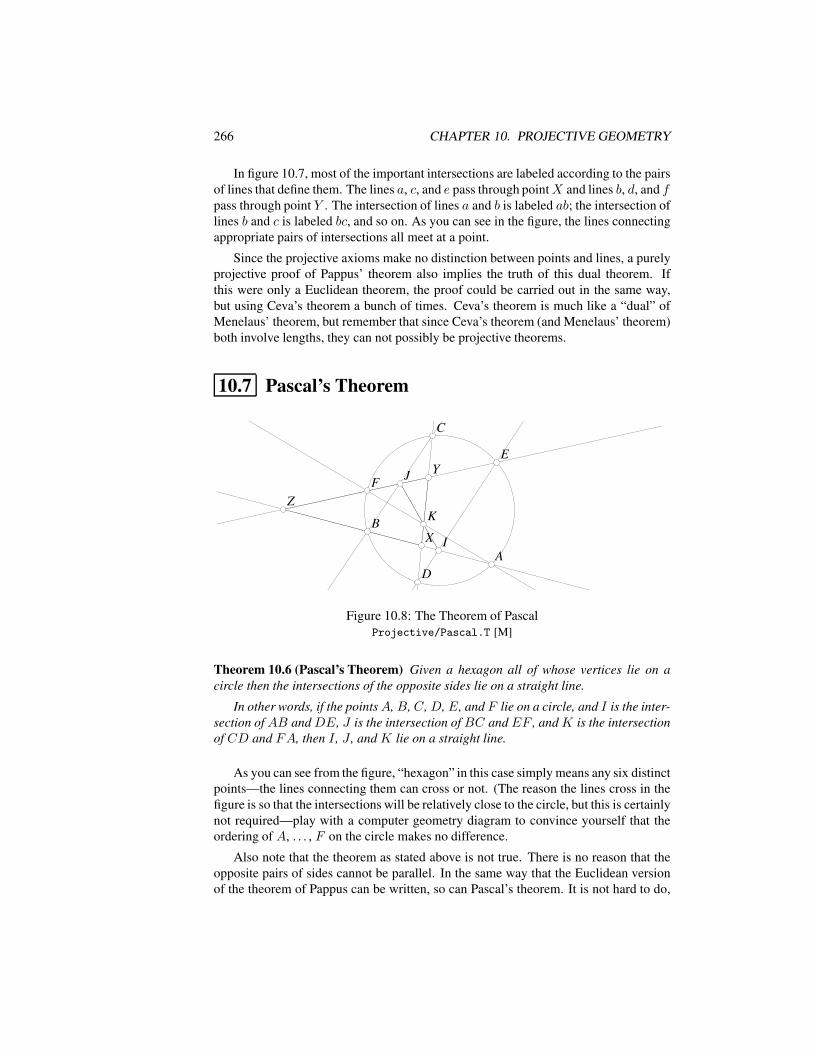
266 CHAPTER 10. PROJECTIVE GEOMETRY
In figure 10.7, most of the important intersections are labeled according to the pairsof lines that define them. The lines a, c, and e pass through pointX and lines b, d, and fpass through point Y . The intersection of lines a and b is labeled ab; the intersection oflines b and c is labeled bc, and so on. As you can see in the figure, the lines connectingappropriate pairs of intersections all meet at a point.
Since the projective axioms make no distinction between points and lines, a purelyprojective proof of Pappus’ theorem also implies the truth of this dual theorem. Ifthis were only a Euclidean theorem, the proof could be carried out in the same way,but using Ceva’s theorem a bunch of times. Ceva’s theorem is much like a “dual” ofMenelaus’ theorem, but remember that since Ceva’s theorem (and Menelaus’ theorem)both involve lengths, they can not possibly be projective theorems.
10.7 Pascal’s Theorem
CC
DD
EE
FF
AA
BBII
JJ
KKZZ
XX
YY
Figure 10.8: The Theorem of PascalProjective/Pascal.T [M]
Theorem 10.6 (Pascal’s Theorem) Given a hexagon all of whose vertices lie on acircle then the intersections of the opposite sides lie on a straight line.
In other words, if the pointsA,B, C, D,E, and F lie on a circle, and I is the inter-section of AB andDE, J is the intersection of BC andEF , andK is the intersectionof CD and FA, then I , J , and K lie on a straight line.
As you can see from the figure, “hexagon” in this case simply means any six distinctpoints—the lines connecting them can cross or not. (The reason the lines cross in thefigure is so that the intersections will be relatively close to the circle, but this is certainlynot required—play with a computer geometry diagram to convince yourself that theordering of A, . . . , F on the circle makes no difference.
Also note that the theorem as stated above is not true. There is no reason that theopposite pairs of sides cannot be parallel. In the same way that the Euclidean versionof the theorem of Pappus can be written, so can Pascal’s theorem. It is not hard to do,
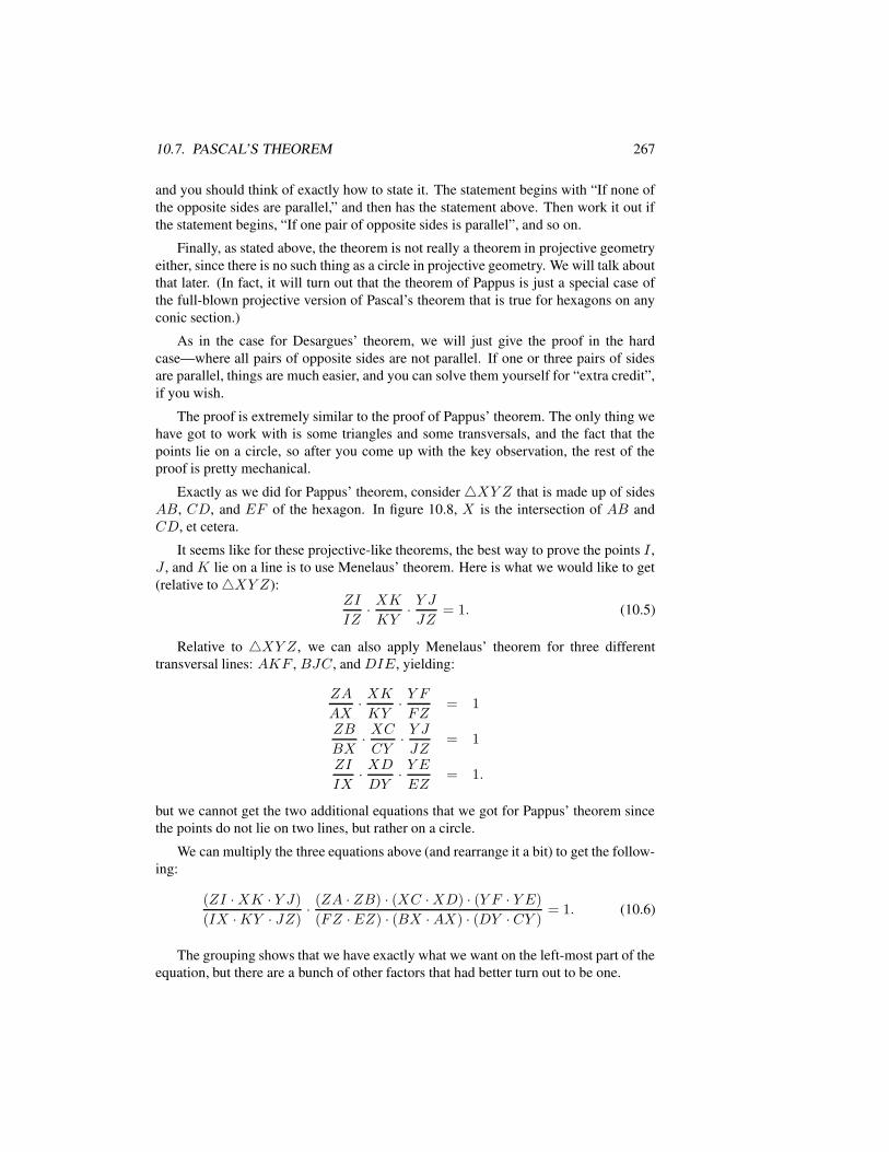
10.7. PASCAL’S THEOREM 267
and you should think of exactly how to state it. The statement begins with “If none ofthe opposite sides are parallel,” and then has the statement above. Then work it out ifthe statement begins, “If one pair of opposite sides is parallel”, and so on.
Finally, as stated above, the theorem is not really a theorem in projective geometryeither, since there is no such thing as a circle in projective geometry. We will talk aboutthat later. (In fact, it will turn out that the theorem of Pappus is just a special case ofthe full-blown projective version of Pascal’s theorem that is true for hexagons on anyconic section.)
As in the case for Desargues’ theorem, we will just give the proof in the hardcase—where all pairs of opposite sides are not parallel. If one or three pairs of sidesare parallel, things are much easier, and you can solve them yourself for “extra credit”,if you wish.
The proof is extremely similar to the proof of Pappus’ theorem. The only thing wehave got to work with is some triangles and some transversals, and the fact that thepoints lie on a circle, so after you come up with the key observation, the rest of theproof is pretty mechanical.
Exactly as we did for Pappus’ theorem, consider4XY Z that is made up of sidesAB, CD, and EF of the hexagon. In figure 10.8, X is the intersection of AB andCD, et cetera.
It seems like for these projective-like theorems, the best way to prove the points I ,J , and K lie on a line is to use Menelaus’ theorem. Here is what we would like to get(relative to4XY Z):
ZI
IZ· XKKY
· Y JJZ
= 1. (10.5)
Relative to 4XYZ, we can also apply Menelaus’ theorem for three differenttransversal lines: AKF , BJC, and DIE, yielding:
ZA
AX· XKKY
· Y FFZ
= 1
ZB
BX· XCCY· Y JJZ
= 1
ZI
IX· XDDY
· Y EEZ
= 1.
but we cannot get the two additional equations that we got for Pappus’ theorem sincethe points do not lie on two lines, but rather on a circle.
We can multiply the three equations above (and rearrange it a bit) to get the follow-ing:
(ZI ·XK · Y J)
(IX ·KY · JZ)· (ZA · ZB) · (XC ·XD) · (Y F · Y E)
(FZ ·EZ) · (BX · AX) · (DY · CY )= 1. (10.6)
The grouping shows that we have exactly what we want on the left-most part of theequation, but there are a bunch of other factors that had better turn out to be one.
268 CHAPTER 10. PROJECTIVE GEOMETRY
Luckily, the six points lie on a circle, so by looking at pairs of chords that intersectat X , Y , and Z we get the following ratios which are exactly what we need to canceloff all the unwanted pairs:
ZA · ZB = FZ ·EZXC ·XD = BX ·AXY F · Y E = DY · CY.
These, combined with equation 10.6, yield equation 10.5 and we are done.
10.7.1 Projective Version of Pascal’s Theorem
As we stated above, there is no such thing as a circle in projective geometry. Underprojections, circles are just one form of a conic section, and conic sections includeellipses, hyperbolas, parabolas, and even degenerate forms, such as a pair of crossinglines. But lines, under projection, remain lines.
Pascal’s theorem holds if the six points lie on any conic section. (If the conicsection happens to be a pair of crossing lines, Pascal’s theorem becomes the theoremof Pappus.)
AA
BB
CC
DD
EE
FF
XX
YY
ZZ
Figure 10.9: The Theorem of Pascal on an EllipseProjective/Pascalconic.T [M]
We will not prove the fully projective version here, but figure 10.9 shows an exam-ple where the conic section happens to be an ellipse and the vertices of the hexagon arein fairly general positions. (The unnamed points in the figure control the shape of theconic section.) The Geometer diagram can be modified to illustrate Pascal’s theoremon other conic sections.
Figure 10.10 illustrates a proof of a special case of Pascal’s theorem for a particularhyperbola (y = 1/x), a particular point (the point at infinity in the direction of they-axis) and a particular line (the x-axis). In the figure, the pointA is at infinity, and thehexagon is ABCDEF . Lines AB and DE intersect at point α, lines BC and EF atγ, and lines CD and FA at β, where α, β, and γ lie on the x-axis.

10.7. PASCAL’S THEOREM 269
CC
DD
EE
αα
BB
ββFF
γγ
AA
Figure 10.10: The Theorem of Pascal on y = 1/xProjective/Hyperbola.T [M]
As you can see, the positions of points D and E completely determine the locationof point B, and C and D determine the location of F , so since A is fixed at infinity inthe y-axis direction only points C, D and E can be moved in the Geometer diagram.
With this setup it is amazingly easy to show that lines BC and EF meet at a pointγ that is on the x-axis using just a little bit of analytic geometry.
For any two points P1 = (x1, 1/x1) and P2 = (x2, 1/x2) on the hyperbola, wewill find where the line P1P2 intersects the x-axis. The equation of the line through P1
and P2 is given by:
y − 1
x1=
(1x2− 1
x1
x2 − x1
)(x− x1).
Set y = 0 to find the intersection of the line with the x-axis, and we obtain:
− 1
x1= −
( 1
x1x2
)(x− x1),
orx = x1 + x2.
In other words, if P1 has x-coordinate x1 and P2 has x-coordinate x2, then the lineP1P2 intersects the x-axis at the point having the sum of those coordinates.
Looking back at figure 10.10, let the x coordinates of the pointsB, C, D, E, and Fbe b, c, d, e, and f , respectively. We know that e+ d = b and d+ c = f . To show thatγ lies on the x-axis, we need to show that the lines BC and EF intersect the x-axis atthe same x-coordinate. For BC, that point is at b+ c, and for EF , it is at e + f . Butsince e+ d = b and d+ c = f it is clear that b+ c = e+ f and we are done.
10.7.2 Brianchon’s Theorem—Pascal’s Dual
Since Pascal’s theorem is a pure projective theorem, it must have a dual. But what isthe dual of a conic section?
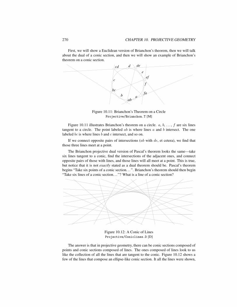
270 CHAPTER 10. PROJECTIVE GEOMETRY
First, we will show a Euclidean version of Brianchon’s theorem, then we will talkabout the dual of a conic section, and then we will show an example of Brianchon’stheorem on a conic section.
cc
dd
ee
ff
aabbabab
bcbc
cdcd dede
efef
fafa
Figure 10.11: Brianchon’s Theorem on a CircleProjective/Brianchon.T [M]
Figure 10.11 illustrates Brianchon’s theorem on a circle. a, b, . . . , f are six linestangent to a circle. The point labeled ab is where lines a and b intersect. The onelabeled bc is where lines b and c intersect, and so on.
If we connect opposite pairs of intersections (ab with de, et cetera), we find thatthose three lines meet at a point.
The Brianchon projective dual version of Pascal’s theorem looks the same—takesix lines tangent to a conic, find the intersections of the adjacent ones, and connectopposite pairs of those with lines, and those lines will all meet at a point. This is true,but notice that it is not exactly stated as a dual theorem should be. Pascal’s theorembegins “Take six points of a conic section. . . ”. Brianchon’s theorem should then begin“Take six lines of a conic section. . . ”? What is a line of a conic section?
Figure 10.12: A Conic of LinesProjective/Coniclines.D [D]
The answer is that in projective geometry, there can be conic sections composed ofpoints and conic sections composed of lines. The ones composed of lines look to uslike the collection of all the lines that are tangent to the conic. Figure 10.12 shows afew of the lines that compose an ellipse-like conic section. It all the lines were shown,
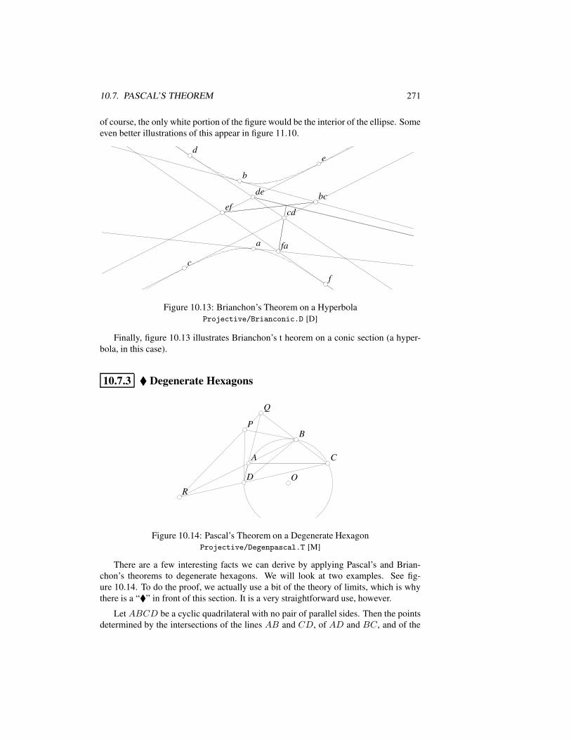
10.7. PASCAL’S THEOREM 271
of course, the only white portion of the figure would be the interior of the ellipse. Someeven better illustrations of this appear in figure 11.10.
cc
ddee
ff
aa
bb
abab
bcbc
cdcd
dede
efef
fafa
Figure 10.13: Brianchon’s Theorem on a HyperbolaProjective/Brianconic.D [D]
Finally, figure 10.13 illustrates Brianchon’s t heorem on a conic section (a hyper-bola, in this case).
10.7.3 Degenerate Hexagons
OO
AA
BB
CC
DD
RR
PP
Figure 10.14: Pascal’s Theorem on a Degenerate HexagonProjective/Degenpascal.T [M]
There are a few interesting facts we can derive by applying Pascal’s and Brian-chon’s theorems to degenerate hexagons. We will look at two examples. See fig-ure 10.14. To do the proof, we actually use a bit of the theory of limits, which is whythere is a “” in front of this section. It is a very straightforward use, however.
Let ABCD be a cyclic quadrilateral with no pair of parallel sides. Then the pointsdetermined by the intersections of the lines AB and CD, of AD and BC, and of the
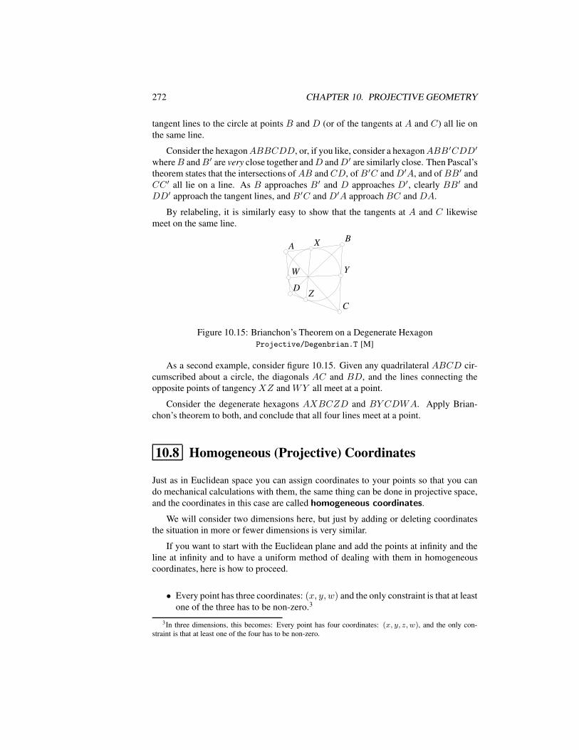
272 CHAPTER 10. PROJECTIVE GEOMETRY
tangent lines to the circle at points B and D (or of the tangents at A and C) all lie onthe same line.
Consider the hexagonABBCDD, or, if you like, consider a hexagonABB ′CDD′
whereB andB′ are very close together andD andD′ are similarly close. Then Pascal’stheorem states that the intersections ofAB andCD, ofB ′C andD′A, and ofBB′ andCC ′ all lie on a line. As B approaches B′ and D approaches D′, clearly BB′ andDD′ approach the tangent lines, and B′C and D′A approachBC and DA.
By relabeling, it is similarly easy to show that the tangents at A and C likewisemeet on the same line.
WW
XX
YY
ZZ
AABB
CC
DD
Figure 10.15: Brianchon’s Theorem on a Degenerate HexagonProjective/Degenbrian.T [M]
As a second example, consider figure 10.15. Given any quadrilateral ABCD cir-cumscribed about a circle, the diagonals AC and BD, and the lines connecting theopposite points of tangencyXZ and WY all meet at a point.
Consider the degenerate hexagons AXBCZD and BY CDWA. Apply Brian-chon’s theorem to both, and conclude that all four lines meet at a point.
10.8 Homogeneous (Projective) Coordinates
Just as in Euclidean space you can assign coordinates to your points so that you cando mechanical calculations with them, the same thing can be done in projective space,and the coordinates in this case are called homogeneous coordinates.
We will consider two dimensions here, but just by adding or deleting coordinatesthe situation in more or fewer dimensions is very similar.
If you want to start with the Euclidean plane and add the points at infinity and theline at infinity and to have a uniform method of dealing with them in homogeneouscoordinates, here is how to proceed.
• Every point has three coordinates: (x, y, w) and the only constraint is that at leastone of the three has to be non-zero.3
3In three dimensions, this becomes: Every point has four coordinates: (x, y, z,w), and the only con-straint is that at least one of the four has to be non-zero.
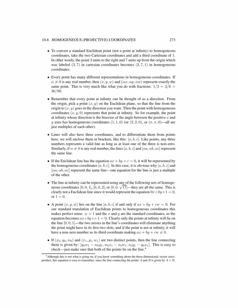
10.8. HOMOGENEOUS (PROJECTIVE) COORDINATES 273
• To convert a standard Euclidean point (not a point at infinity) to homogeneouscoordinates, take the two Cartesian coordinates and add a third coordinate of 1.In other words, the point 3 units to the right and 7 units up from the origin whichwas labeled (3, 7) in cartesian coordinates becomes (3, 7, 1) in homogeneouscoordinates.
• Every point has many different representations in homogeneous coordinates. Ifα 6= 0 is any real number, then (x, y, w) and (αx, αy, αw) represent exactly thesame point. This is very much like what you do with fractions: 1/3 = 2/6 =30/90.
• Remember that every point at infinity can be thought of as a direction. Fromthe origin, pick a point (x, y) on the Euclidean plane, so that the line from theorigin to (x, y) goes in the direction you want. Then the point with homogeneouscoordinates (x, y, 0) represents that point at infinity. So for example, the pointat infinity whose direction is the bisector of the angle between the positive x andy axes has homogeneous coordinates (1, 1, 0) (or (2, 2, 0), or (π, π, 0)—all arejust multiples of each other).
• Lines will also have three coordinates, and to differentiate them from pointshere, we will enclose them in brackets, like this: [a, b, c]. Like points, any threenumbers represents a valid line as long as at least one of the three is non-zero.Similarly, if α 6= 0 is any real number, the lines [a, b, c] and [αa, αb, αc] representthe same line.
• If the Euclidean line has the equation ax+ by + c = 0, it will be represented bythe homogeneous coordinates [a, b, c]. In this case, it is obvious why [a, b, c] and[αa, αb, αc] represent the same line—one equation for the line is just a multipleof the other.
• The line at infinity can be represented using any of the following sets of homoge-neous coordinates [0, 0, 1], [0, 0, 2], or [0, 0,
√17]—they are all the same. This is
clearly not a Euclidean line since it would represent the equation 0x+0y+1 = 0,or 1 = 0.
• A point (x, y, w) lies on the line [a, b, c] if and only if ax + by + cw = 0. Forour standard translation of Euclidean points to homogeneous coordinates thismakes perfect sense. w = 1 and the x and y are the standard coordinates, so theequation becomes ax+by+c·1 = 0. Clearly only the points at infinity will lie onthe line [0, 0, 1]—the two zeroes in the line’s coordinates will eliminate anythingthe point might have in its first two slots, and if the point is not at infinity, it willhave a non-zero number as its third coordinate making ax+ by + cw 6= 0.
• If (x0, y0, w0) and (x1, y1, w1) are two distinct points, then the line connectingthem is given by: [y0w1 − w0y1, w0x1 − x0w1, x0y1 − y0x1]. This is easy tocheck—just make sure that both of the points lie on the line.4
4Although this is not what is going on, if you know something about the three-dimensional vector cross-product, this equation is easy to remember, since the line connecting the points A and B is given by A×B,
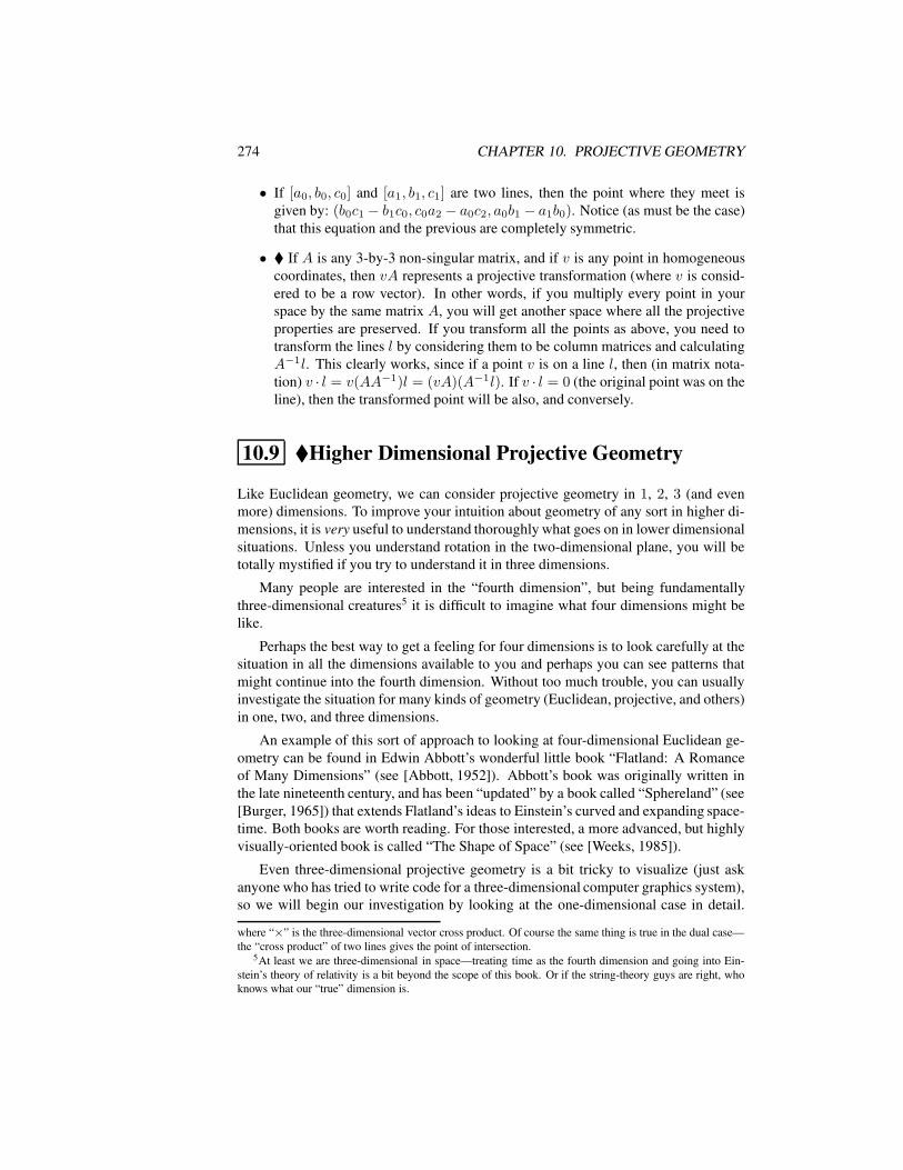
274 CHAPTER 10. PROJECTIVE GEOMETRY
• If [a0, b0, c0] and [a1, b1, c1] are two lines, then the point where they meet isgiven by: (b0c1 − b1c0, c0a2 − a0c2, a0b1 − a1b0). Notice (as must be the case)that this equation and the previous are completely symmetric.
• If A is any 3-by-3 non-singular matrix, and if v is any point in homogeneouscoordinates, then vA represents a projective transformation (where v is consid-ered to be a row vector). In other words, if you multiply every point in yourspace by the same matrix A, you will get another space where all the projectiveproperties are preserved. If you transform all the points as above, you need totransform the lines l by considering them to be column matrices and calculatingA−1l. This clearly works, since if a point v is on a line l, then (in matrix nota-tion) v · l = v(AA−1)l = (vA)(A−1l). If v · l = 0 (the original point was on theline), then the transformed point will be also, and conversely.
10.9 Higher Dimensional Projective Geometry
Like Euclidean geometry, we can consider projective geometry in 1, 2, 3 (and evenmore) dimensions. To improve your intuition about geometry of any sort in higher di-mensions, it is very useful to understand thoroughly what goes on in lower dimensionalsituations. Unless you understand rotation in the two-dimensional plane, you will betotally mystified if you try to understand it in three dimensions.
Many people are interested in the “fourth dimension”, but being fundamentallythree-dimensional creatures5 it is difficult to imagine what four dimensions might belike.
Perhaps the best way to get a feeling for four dimensions is to look carefully at thesituation in all the dimensions available to you and perhaps you can see patterns thatmight continue into the fourth dimension. Without too much trouble, you can usuallyinvestigate the situation for many kinds of geometry (Euclidean, projective, and others)in one, two, and three dimensions.
An example of this sort of approach to looking at four-dimensional Euclidean ge-ometry can be found in Edwin Abbott’s wonderful little book “Flatland: A Romanceof Many Dimensions” (see [Abbott, 1952]). Abbott’s book was originally written inthe late nineteenth century, and has been “updated” by a book called “Sphereland” (see[Burger, 1965]) that extends Flatland’s ideas to Einstein’s curved and expanding space-time. Both books are worth reading. For those interested, a more advanced, but highlyvisually-oriented book is called “The Shape of Space” (see [Weeks, 1985]).
Even three-dimensional projective geometry is a bit tricky to visualize (just askanyone who has tried to write code for a three-dimensional computer graphics system),so we will begin our investigation by looking at the one-dimensional case in detail.
where “×” is the three-dimensional vector cross product. Of course the same thing is true in the dual case—the “cross product” of two lines gives the point of intersection.
5At least we are three-dimensional in space—treating time as the fourth dimension and going into Ein-stein’s theory of relativity is a bit beyond the scope of this book. Or if the string-theory guys are right, whoknows what our “true” dimension is.
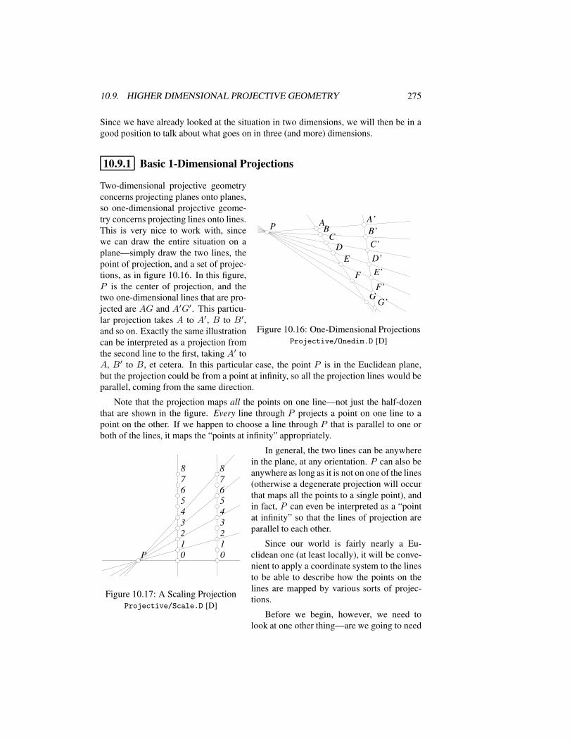
10.9. HIGHER DIMENSIONAL PROJECTIVE GEOMETRY 275
Since we have already looked at the situation in two dimensions, we will then be in agood position to talk about what goes on in three (and more) dimensions.
10.9.1 Basic 1-Dimensional Projections
PP AABB
CCDD
EE
FF
GG
A’A’B’B’C’C’
D’D’E’E’
F’F’
G’G’
Figure 10.16: One-Dimensional ProjectionsProjective/Onedim.D [D]
Two-dimensional projective geometryconcerns projecting planes onto planes,so one-dimensional projective geome-try concerns projecting lines onto lines.This is very nice to work with, sincewe can draw the entire situation on aplane—simply draw the two lines, thepoint of projection, and a set of projec-tions, as in figure 10.16. In this figure,P is the center of projection, and thetwo one-dimensional lines that are pro-jected are AG and A′G′. This particu-lar projection takes A to A′, B to B′,and so on. Exactly the same illustrationcan be interpreted as a projection fromthe second line to the first, taking A′ toA, B′ to B, et cetera. In this particular case, the point P is in the Euclidean plane,but the projection could be from a point at infinity, so all the projection lines would beparallel, coming from the same direction.
Note that the projection maps all the points on one line—not just the half-dozenthat are shown in the figure. Every line through P projects a point on one line to apoint on the other. If we happen to choose a line through P that is parallel to one orboth of the lines, it maps the “points at infinity” appropriately.
00
88
44
2211
33
6677
55
00
88
44
2211
33
6677
55
PP
Figure 10.17: A Scaling ProjectionProjective/Scale.D [D]
In general, the two lines can be anywherein the plane, at any orientation. P can also beanywhere as long as it is not on one of the lines(otherwise a degenerate projection will occurthat maps all the points to a single point), andin fact, P can even be interpreted as a “pointat infinity” so that the lines of projection areparallel to each other.
Since our world is fairly nearly a Eu-clidean one (at least locally), it will be conve-nient to apply a coordinate system to the linesto be able to describe how the points on thelines are mapped by various sorts of projec-tions.
Before we begin, however, we need tolook at one other thing—are we going to need
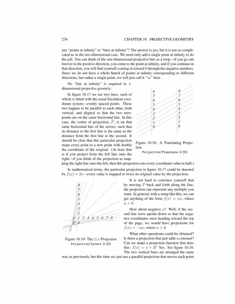
276 CHAPTER 10. PROJECTIVE GEOMETRY
any “points at infinity” or “lines at infinity”? The answer is yes, but it is not so compli-cated as in the two-dimensional case. We need only add a single point at infinity to dothe job. You can think of the one-dimensional projective line as a loop—if you go outforever in the positive direction, you come to the point at infinity, and if you continue inthat direction, you will find yourself coming in toward 0 through the negative numbers.Since we do not have a whole bunch of points at infinity corresponding to differentdirections, but rather a single point, we will just call it “∞” here.
00
88
44
2211
33
6677
55
00
88
44
2211
33
6677
55
Figure 10.18: A Translating Projec-tion
Projective/Translate.D [D]
No “line at infinity” is required in 1-dimensional projective geomety.
In figure 10.17 we see two lines, each ofwhich is fitted with the usual Euclidean coor-dinate system—evenly spaced points. Thesetwo happen to be parallel to each other, bothvertical, and aligned so that the two zero-points are on the same horizontal line. In thiscase, the center of projection, P , is on thatsame horizontal line of the zeroes, such thatits distance to the first line is the same as thedistance from the first line to the second. Itshould be clear that this particular projectionmaps every point to a new point with doublethe coordinate of the original. (At least thatis if you project from the left line onto theright—if you think of the projection as map-ping the right line onto the left, then this projection cuts every coordinate value in half.)
In mathematical terms, the particular projection in figure 10.17 could be denotedby f(x) = 2x—every value is mapped to twice its original value by the projection.
00
88
44
2211
33
6677
55
00 88442211 33 66 7755PP
Figure 10.19: The 1/x ProjectionProjective/Invert.D [D]
It is not hard to convince yourself thatby moving P back and forth along the line,the projection can represent any multiple youwant. In general, with a setup like this, we canget anything of the form f(x) = αx, whereα > 0.
How about negative α? Well, if the sec-ond line were upside-down so that the nega-tive coordinates were heading toward the topof the page, we would have projections forf(x) = −αx, where α > 0.
What other operations could be obtained?Is there a projection that just adds a constant?Can we make a projection function that doesthis: f(x) = x + 3? Yes. See figure 10.18.The two vertical lines are arranged the same
way as previously, but this time we just use a parallel projection that moves each point
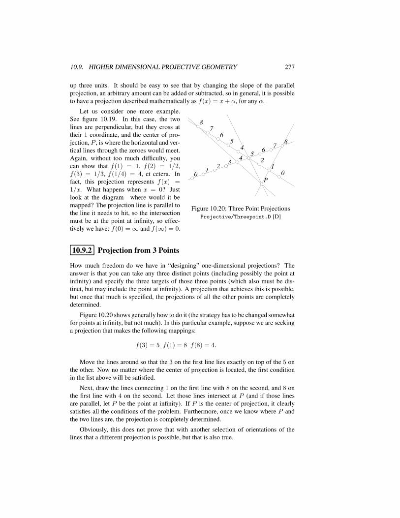
10.9. HIGHER DIMENSIONAL PROJECTIVE GEOMETRY 277
up three units. It should be easy to see that by changing the slope of the parallelprojection, an arbitrary amount can be added or subtracted, so in general, it is possibleto have a projection described mathematically as f(x) = x+ α, for any α.
00
88
44
2211
33
6677
55
00
88
4422
1133
6677
55
PP
Figure 10.20: Three Point ProjectionsProjective/Threepoint.D [D]
Let us consider one more example.See figure 10.19. In this case, the twolines are perpendicular, but they cross attheir 1 coordinate, and the center of pro-jection, P , is where the horizontal and ver-tical lines through the zeroes would meet.Again, without too much difficulty, youcan show that f(1) = 1, f(2) = 1/2,f(3) = 1/3, f(1/4) = 4, et cetera. Infact, this projection represents f(x) =1/x. What happens when x = 0? Justlook at the diagram—where would it bemapped? The projection line is parallel tothe line it needs to hit, so the intersectionmust be at the point at infinity, so effec-tively we have: f(0) =∞ and f(∞) = 0.
10.9.2 Projection from 3 Points
How much freedom do we have in “designing” one-dimensional projections? Theanswer is that you can take any three distinct points (including possibly the point atinfinity) and specify the three targets of those three points (which also must be dis-tinct, but may include the point at infinity). A projection that achieves this is possible,but once that much is specified, the projections of all the other points are completelydetermined.
Figure 10.20 shows generally how to do it (the strategy has to be changed somewhatfor points at infinity, but not much). In this particular example, suppose we are seekinga projection that makes the following mappings:
f(3) = 5 f(1) = 8 f(8) = 4.
Move the lines around so that the 3 on the first line lies exactly on top of the 5 onthe other. Now no matter where the center of projection is located, the first conditionin the list above will be satisfied.
Next, draw the lines connecting 1 on the first line with 8 on the second, and 8 onthe first line with 4 on the second. Let those lines intersect at P (and if those linesare parallel, let P be the point at infinity). If P is the center of projection, it clearlysatisfies all the conditions of the problem. Furthermore, once we know where P andthe two lines are, the projection is completely determined.
Obviously, this does not prove that with another selection of orientations of thelines that a different projection is possible, but that is also true.
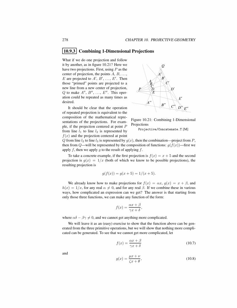
278 CHAPTER 10. PROJECTIVE GEOMETRY
10.9.3 Combining 1-Dimensional Projections
PP
A′A′B′B′
C′C′D′D′
E′E′
AABBCCDDEE
A′′A′′ B′′B′′ C′′C′′ D′′D′′ E′′E′′
Figure 10.21: Combining 1-DimensionalProjections
Projective/Concatenate.T [M]
What if we do one projection and followit by another, as in figure 10.21? Here wehave two projections. First, using P as thecenter of projection, the points A, B, . . . ,E are projected to A′, B′, . . . , E′. Thenthose “primed” points are projected to anew line from a new center of projection,Q to make A′′, B′′, . . . , E′′. This oper-ation could be repeated as many times asdesired.
It should be clear that the operationof repeated projection is equivalent to thecomposition of the mathematical repre-sentations of the projections. For exam-ple, if the projection centered at point Pfrom line l1 to line l2 is represented byf(x) and the projection centered at pointQ from line l2 to line l3 is represented by g(x), then the combination—project from P ,then from Q—will be represented by the composition of functions: g(f(x))—first weapply f , then we apply g to the result of applying f .
To take a concrete example, if the first projection is f(x) = x + 5 and the secondprojection is g(x) = 1/x (both of which we know to be possible projections), theresulting projection is
g(f(x)) = g(x+ 5) = 1/(x+ 5).
We already know how to make projections for f(x) = αx, g(x) = x + β, andh(x) = 1/x, for any real α 6= 0, and for any real β. If we combine these in variousways, how complicated an expression can we get? The answer is that starting fromonly those three functions, we can make any function of the form:
f(x) =αx+ β
γx+ δ,
where αδ − βγ 6= 0, and we cannot get anything more complicated.
We will leave it as an (easy) exercise to show that the function above can be gen-erated from the three primitive operations, but we will show that nothing more compli-cated can be generated. To see that we cannot get more complicated, let
f(x) =αx + β
γx+ δ(10.7)
andg(x) =
µx+ ν
ζx+ θ, (10.8)
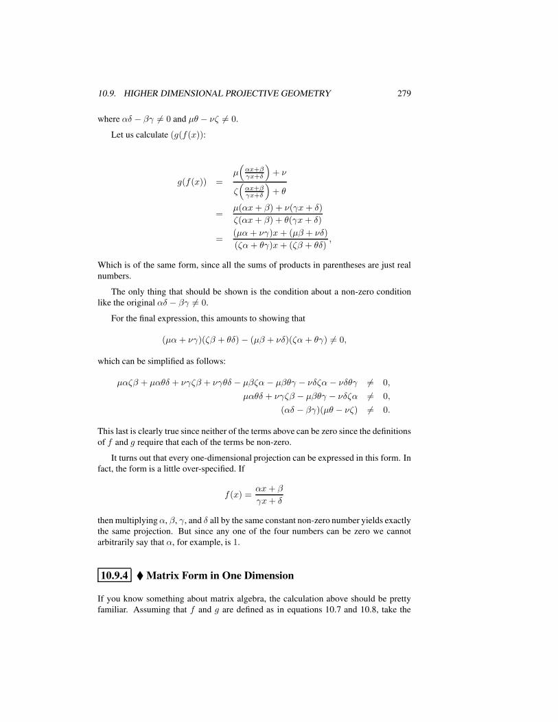
10.9. HIGHER DIMENSIONAL PROJECTIVE GEOMETRY 279
where αδ − βγ 6= 0 and µθ − νζ 6= 0.
Let us calculate (g(f(x)):
g(f(x)) =µ(αx+βγx+δ
)+ ν
ζ(αx+βγx+δ
)+ θ
=µ(αx+ β) + ν(γx+ δ)
ζ(αx + β) + θ(γx+ δ)
=(µα+ νγ)x+ (µβ + νδ)
(ζα+ θγ)x+ (ζβ + θδ),
Which is of the same form, since all the sums of products in parentheses are just realnumbers.
The only thing that should be shown is the condition about a non-zero conditionlike the original αδ − βγ 6= 0.
For the final expression, this amounts to showing that
(µα+ νγ)(ζβ + θδ)− (µβ + νδ)(ζα + θγ) 6= 0,
which can be simplified as follows:
µαζβ + µαθδ + νγζβ + νγθδ − µβζα − µβθγ − νδζα − νδθγ 6= 0,
µαθδ + νγζβ − µβθγ − νδζα 6= 0,
(αδ − βγ)(µθ − νζ) 6= 0.
This last is clearly true since neither of the terms above can be zero since the definitionsof f and g require that each of the terms be non-zero.
It turns out that every one-dimensional projection can be expressed in this form. Infact, the form is a little over-specified. If
f(x) =αx+ β
γx+ δ
then multiplyingα, β, γ, and δ all by the same constant non-zero number yields exactlythe same projection. But since any one of the four numbers can be zero we cannotarbitrarily say that α, for example, is 1.
10.9.4 Matrix Form in One Dimension
If you know something about matrix algebra, the calculation above should be prettyfamiliar. Assuming that f and g are defined as in equations 10.7 and 10.8, take the
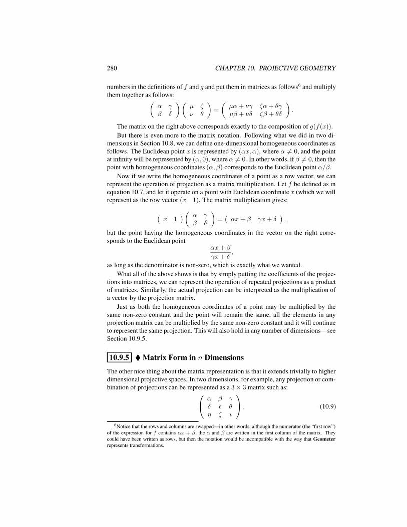
280 CHAPTER 10. PROJECTIVE GEOMETRY
numbers in the definitions of f and g and put them in matrices as follows6 and multiplythem together as follows:
(α γβ δ
)(µ ζν θ
)=
(µα+ νγ ζα+ θγµβ + νδ ζβ + θδ
).
The matrix on the right above corresponds exactly to the composition of g(f(x)).But there is even more to the matrix notation. Following what we did in two di-
mensions in Section 10.8, we can define one-dimensional homogeneous coordinates asfollows. The Euclidean point x is represented by (αx, α), where α 6= 0, and the pointat infinity will be represented by (α, 0), where α 6= 0. In other words, if β 6= 0, then thepoint with homogeneous coordinates (α, β) corresponds to the Euclidean point α/β.
Now if we write the homogeneous coordinates of a point as a row vector, we canrepresent the operation of projection as a matrix multiplication. Let f be defined as inequation 10.7, and let it operate on a point with Euclidean coordinate x (which we willrepresent as the row vector (x 1). The matrix multiplication gives:
(x 1
)( α γβ δ
)=(αx + β γx+ δ
),
but the point having the homogeneous coordinates in the vector on the right corre-sponds to the Euclidean point
αx+ β
γx+ δ,
as long as the denominator is non-zero, which is exactly what we wanted.What all of the above shows is that by simply putting the coefficients of the projec-
tions into matrices, we can represent the operation of repeated projections as a productof matrices. Similarly, the actual projection can be interpreted as the multiplication ofa vector by the projection matrix.
Just as both the homogeneous coordinates of a point may be multiplied by thesame non-zero constant and the point will remain the same, all the elements in anyprojection matrix can be multiplied by the same non-zero constant and it will continueto represent the same projection. This will also hold in any number of dimensions—seeSection 10.9.5.
10.9.5 Matrix Form in n Dimensions
The other nice thing about the matrix representation is that it extends trivially to higherdimensional projective spaces. In two dimensions, for example, any projection or com-bination of projections can be represented as a 3× 3 matrix such as:
α β γδ ε θη ζ ι
, (10.9)
6Notice that the rows and columns are swapped—in other words, although the numerator (the “first row”)of the expression for f contains αx + β, the α and β are written in the first column of the matrix. Theycould have been written as rows, but then the notation would be incompatible with the way that Geometerrepresents transformations.
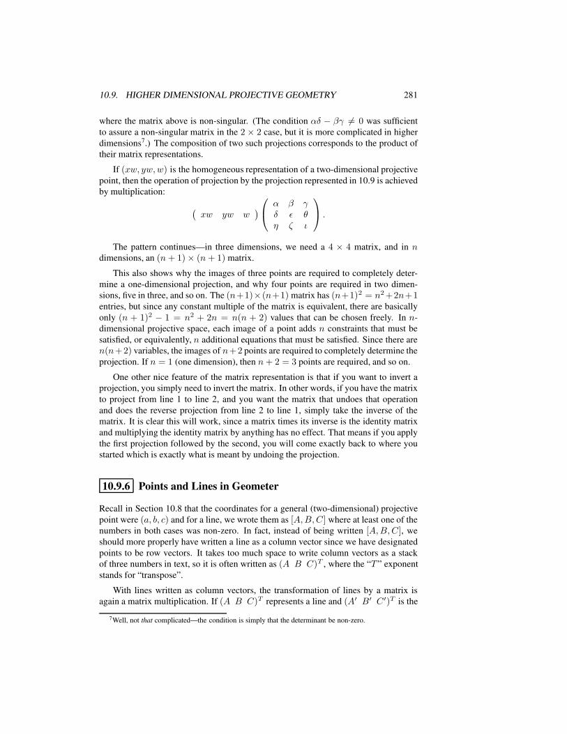
10.9. HIGHER DIMENSIONAL PROJECTIVE GEOMETRY 281
where the matrix above is non-singular. (The condition αδ − βγ 6= 0 was sufficientto assure a non-singular matrix in the 2× 2 case, but it is more complicated in higherdimensions7.) The composition of two such projections corresponds to the product oftheir matrix representations.
If (xw, yw,w) is the homogeneous representation of a two-dimensional projectivepoint, then the operation of projection by the projection represented in 10.9 is achievedby multiplication:
(xw yw w
)
α β γδ ε θη ζ ι
.
The pattern continues—in three dimensions, we need a 4 × 4 matrix, and in ndimensions, an (n+ 1)× (n+ 1) matrix.
This also shows why the images of three points are required to completely deter-mine a one-dimensional projection, and why four points are required in two dimen-sions, five in three, and so on. The (n+1)×(n+1) matrix has (n+1)2 = n2 +2n+1entries, but since any constant multiple of the matrix is equivalent, there are basicallyonly (n + 1)2 − 1 = n2 + 2n = n(n + 2) values that can be chosen freely. In n-dimensional projective space, each image of a point adds n constraints that must besatisfied, or equivalently, n additional equations that must be satisfied. Since there aren(n+2) variables, the images of n+2 points are required to completely determine theprojection. If n = 1 (one dimension), then n+ 2 = 3 points are required, and so on.
One other nice feature of the matrix representation is that if you want to invert aprojection, you simply need to invert the matrix. In other words, if you have the matrixto project from line 1 to line 2, and you want the matrix that undoes that operationand does the reverse projection from line 2 to line 1, simply take the inverse of thematrix. It is clear this will work, since a matrix times its inverse is the identity matrixand multiplying the identity matrix by anything has no effect. That means if you applythe first projection followed by the second, you will come exactly back to where youstarted which is exactly what is meant by undoing the projection.
10.9.6 Points and Lines in Geometer
Recall in Section 10.8 that the coordinates for a general (two-dimensional) projectivepoint were (a, b, c) and for a line, we wrote them as [A,B,C] where at least one of thenumbers in both cases was non-zero. In fact, instead of being written [A,B,C], weshould more properly have written a line as a column vector since we have designatedpoints to be row vectors. It takes too much space to write column vectors as a stackof three numbers in text, so it is often written as (A B C)T , where the “T ” exponentstands for “transpose”.
With lines written as column vectors, the transformation of lines by a matrix isagain a matrix multiplication. If (A B C)T represents a line and (A′ B′ C ′)T is the
7Well, not that complicated—the condition is simply that the determinant be non-zero.
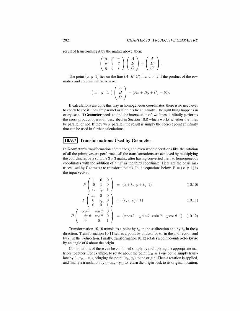
282 CHAPTER 10. PROJECTIVE GEOMETRY
result of transforming it by the matrix above, then:
α β γδ ε θη ζ ι
ABC
=
A′
B′
C ′
.
The point (x y 1) lies on the line (A B C) if and only if the product of the rowmatrix and column matrix is zero:
(x y 1
)
ABC
= (Ax +By + C) = (0).
If calculations are done this way in homogeneous coordinates, there is no need everto check to see if lines are parallel or if points lie at infinity. The right thing happens inevery case. If Geometer needs to find the intersection of two lines, it blindly performsthe cross product operation described in Section 10.8 which works whether the linesbe parallel or not. If they were parallel, the result is simply the correct point at infinitythat can be used in further calculations.
10.9.7 Transformations Used by Geometer
In Geometer’s transformation commands, and even when operations like the rotationof all the primitives are performed, all the transformations are achieved by multiplyingthe coordinates by a suitable 3×3 matrix after having converted them to homogeneouscoordinates with the addition of a “1” as the third coordinate. Here are the basic ma-trices used by Geometer to transform points. In the equations below, P = (x y 1) isthe input vector:
P
1 0 00 1 0tx ty 1
= (x+ tx y + ty 1) (10.10)
P
sx 0 00 sy 00 0 1
= (sxx syy 1) (10.11)
P
cos θ sin θ 0− sin θ cos θ 0
0 0 1
= (x cos θ − y sin θ x sin θ + y cos θ 1) (10.12)
Transformation 10.10 translates a point by tx in the x-direction and by ty in the ydirection. Transformation 10.11 scales a point by a factor of sx in the x-direction andby sy in the y-direction. Finally, transformation 10.12 rotates a point counter-clockwiseby an angle of θ about the origin.
Combinations of these can be combined simply by multiplying the appropriate ma-trices together. For example, to rotate about the point (x0, y0) one could simply trans-late by (−x0,−y0), bringing the point (x0, y0) to the origin. Then a rotation is applied,and finally a translation by (+x0,+y0) to return the origin back to its original location.
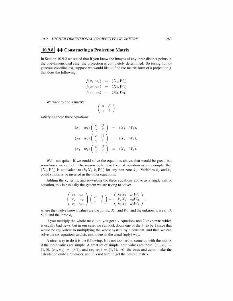
10.9. HIGHER DIMENSIONAL PROJECTIVE GEOMETRY 283
10.9.8 Constructing a Projection Matrix
In Section 10.9.2 we stated that if you know the images of any three distinct points inthe one-dimensional case, the projection is completely determined. So (using homo-geneous coordinates), suppose we would like to find the matrix form of a projection fthat does the following:
f(x1, w1) = (X1,W1)
f(x2, w2) = (X2,W2)
f(x3, w3) = (X3,W3)
We want to find a matrix (α βγ δ
)
satisfying these three equations:
(x1 w1)
(α βγ δ
)= (X1 W1),
(x2 w2)
(α βγ δ
)= (X2 W2),
(x3 w3)
(α βγ δ
)= (X3 W3).
Well, not quite. If we could solve the equations above, that would be great, butsometimes we cannot. The reason is, to take the first equation as an example, that(X1,W1) is equivalent to (k1X1, k1W1) for any non-zero k1. Variables k2 and k3
could similarly be inserted in the other equations.
Adding the ki terms, and re-writing the three equations above as a single matrixequation, this is basically the system we are trying to solve:
x1 w1
x2 w2
x3 w3
(α βγ δ
)=
k1X1 k1W1
k2X2 k2W2
k3X3 k3W3
,
where the twelve known values are the xi, wi, Xi, andWi, and the unknowns are α, β,γ, δ, and the three ki.
If you multiply the whole mess out, you get six equations and 7 unknowns whichis usually bad news, but in our case, we can lock down one of the ki to be 1 since thatwould be equivalent to multiplying the whole system by a constant, and then we cansolve the six equations and six unknowns in the usual (ugly) way.
A nicer way to do it is the following. It is not too hard to come up with the matrixif the input values are simple. A great set of simple input values are these: (x1, w1) =(1, 0), (x2, w2) = (0, 1), and (x3, w3) = (1, 1). All the ones and zeros make thecalculation quite a bit easier, and it is not hard to get the desired matrix.
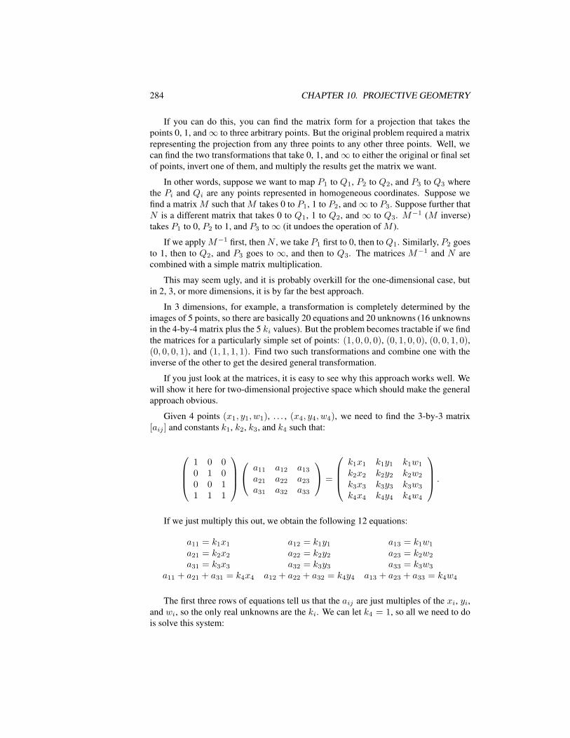
284 CHAPTER 10. PROJECTIVE GEOMETRY
If you can do this, you can find the matrix form for a projection that takes thepoints 0, 1, and∞ to three arbitrary points. But the original problem required a matrixrepresenting the projection from any three points to any other three points. Well, wecan find the two transformations that take 0, 1, and∞ to either the original or final setof points, invert one of them, and multiply the results get the matrix we want.
In other words, suppose we want to map P1 to Q1, P2 to Q2, and P3 to Q3 wherethe Pi and Qi are any points represented in homogeneous coordinates. Suppose wefind a matrix M such that M takes 0 to P1, 1 to P2, and∞ to P3. Suppose further thatN is a different matrix that takes 0 to Q1, 1 to Q2, and∞ to Q3. M−1 (M inverse)takes P1 to 0, P2 to 1, and P3 to∞ (it undoes the operation of M ).
If we applyM−1 first, thenN , we take P1 first to 0, then to Q1. Similarly, P2 goesto 1, then to Q2, and P3 goes to ∞, and then to Q3. The matrices M−1 and N arecombined with a simple matrix multiplication.
This may seem ugly, and it is probably overkill for the one-dimensional case, butin 2, 3, or more dimensions, it is by far the best approach.
In 3 dimensions, for example, a transformation is completely determined by theimages of 5 points, so there are basically 20 equations and 20 unknowns (16 unknownsin the 4-by-4 matrix plus the 5 ki values). But the problem becomes tractable if we findthe matrices for a particularly simple set of points: (1, 0, 0, 0), (0, 1, 0, 0), (0, 0, 1, 0),(0, 0, 0, 1), and (1, 1, 1, 1). Find two such transformations and combine one with theinverse of the other to get the desired general transformation.
If you just look at the matrices, it is easy to see why this approach works well. Wewill show it here for two-dimensional projective space which should make the generalapproach obvious.
Given 4 points (x1, y1, w1), . . . , (x4, y4, w4), we need to find the 3-by-3 matrix[aij ] and constants k1, k2, k3, and k4 such that:
1 0 00 1 00 0 11 1 1
a11 a12 a13
a21 a22 a23
a31 a32 a33
=
k1x1 k1y1 k1w1
k2x2 k2y2 k2w2
k3x3 k3y3 k3w3
k4x4 k4y4 k4w4
.
If we just multiply this out, we obtain the following 12 equations:
a11 = k1x1 a12 = k1y1 a13 = k1w1
a21 = k2x2 a22 = k2y2 a23 = k2w2
a31 = k3x3 a32 = k3y3 a33 = k3w3
a11 + a21 + a31 = k4x4 a12 + a22 + a32 = k4y4 a13 + a23 + a33 = k4w4
The first three rows of equations tell us that the aij are just multiples of the xi, yi,and wi, so the only real unknowns are the ki. We can let k4 = 1, so all we need to dois solve this system:
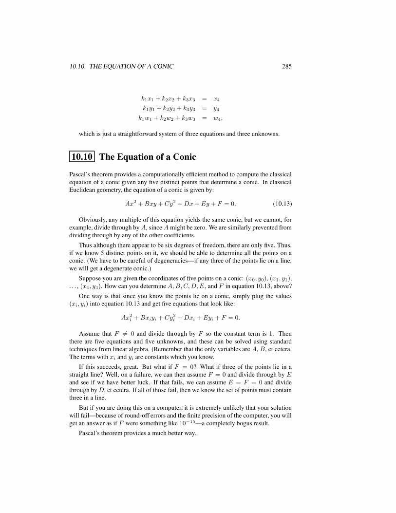
10.10. THE EQUATION OF A CONIC 285
k1x1 + k2x2 + k3x3 = x4
k1y1 + k2y2 + k3y3 = y4
k1w1 + k2w2 + k3w3 = w4,
which is just a straightforward system of three equations and three unknowns.
10.10 The Equation of a Conic
Pascal’s theorem provides a computationally efficient method to compute the classicalequation of a conic given any five distinct points that determine a conic. In classicalEuclidean geometry, the equation of a conic is given by:
Ax2 +Bxy + Cy2 +Dx+Ey + F = 0. (10.13)
Obviously, any multiple of this equation yields the same conic, but we cannot, forexample, divide through byA, since A might be zero. We are similarly prevented fromdividing through by any of the other coefficients.
Thus although there appear to be six degrees of freedom, there are only five. Thus,if we know 5 distinct points on it, we should be able to determine all the points on aconic. (We have to be careful of degeneracies—if any three of the points lie on a line,we will get a degenerate conic.)
Suppose you are given the coordinates of five points on a conic: (x0, y0), (x1, y1),. . . , (x4, y4). How can you determineA,B,C,D,E, and F in equation 10.13, above?
One way is that since you know the points lie on a conic, simply plug the values(xi, yi) into equation 10.13 and get five equations that look like:
Ax2i +Bxiyi + Cy2
i +Dxi +Eyi + F = 0.
Assume that F 6= 0 and divide through by F so the constant term is 1. Thenthere are five equations and five unknowns, and these can be solved using standardtechniques from linear algebra. (Remember that the only variables are A, B, et cetera.The terms with xi and yi are constants which you know.
If this succeeds, great. But what if F = 0? What if three of the points lie in astraight line? Well, on a failure, we can then assume F = 0 and divide through by Eand see if we have better luck. If that fails, we can assume E = F = 0 and dividethrough byD, et cetera. If all of those fail, then we know the set of points must containthree in a line.
But if you are doing this on a computer, it is extremely unlikely that your solutionwill fail—because of round-off errors and the finite precision of the computer, you willget an answer as if F were something like 10−15—a completely bogus result.
Pascal’s theorem provides a much better way.
286 CHAPTER 10. PROJECTIVE GEOMETRY
Given five points (xi, yi), convert them to homogeneous coordinates: (xi, yi, 1).Add a sixth unknown point that lies on the conic with coordinates (x, y, 1). Now writedown the equations that the six points must satisfy according to Pascal’s theorem. Thisis easy to do—we know exactly how to find the equations of the lines that pass throughpairs of points, the equations of the points that lie on the intersections of those lines,et cetera. For all the points but one, we have actual numbers. After you grind out theconditions that must be satisfied by the coordinates of your sixth point, it will be in theform of equation 10.13, and you can just read off A through F . If the solution fails forsome reason, it is not because of an equation with a zero coefficient; it is because threeor more of your given points lie on a straight line.
10.11 Finite Projective Planes
Although the typical computer geometry program will not help much with this subject,it is interesting to note that the axioms of projective geometry nowhere say that theremust be an infinite number of points (or an infinite number of lines). There exist, infact, some finite geometries, one of which has as few as seven points and seven lines.
The smallest finite projective plane contains seven points and is called the FanoPlane..
The seven points are A,B,C,D,E, F , and G, and the seven lines each containthree points. Here are the lines: ADB, BEC, CFA, AGE, BGF , CGD, and DEF .You can easily check that every two points determine a line, and every two lines inter-sect in exactly one point.
Clearly this is nothing like Euclidean geometry—you cannot draw it with straightlines on a Euclidean plane.
For certain n ≥ 2 there exists a finite projective plane of with n2 +n+1 points andthe same number of lines. Each line contains n + 1 points, and there are n + 1 linespassing through each point. You may find it interesting to try to construct examples forn = 3 (containing 13 points and lines) or even for n = 4 (with 21 points and lines).
There are still open questions about exactly which values of n ≥ 2 admit the exis-tence of a finite projective plane. It is known that if n is a power of a prime number,then a finite projective plane with n2 + n+ 1 points and lines exists, but for other val-ues of n nobody knows. No finite projective planes for such n have ever been found,and for certain values of n the existence of such a projective plane has been provedimpossible.
Most small n are powers of primes: 2 = 21, 3 = 31, 4 = 22, 5 = 51, 7 = 71,8 = 23, 9 = 32, and 11 = 111. So among the first ten possibilities, only 6 and 10are not powers of prime numbers. It has been proved that a projective plane of order62 + 6 + 1 = 43 is impossible, but nobody knows whether or not a projective planecorresponding to n = 10 (having 102 + 10 + 1 = 111 points and lines with 11 pointson each line and 11 lines going through each point) can exist. For more information,see [Ryser, 1963].
10.11. FINITE PROJECTIVE PLANES 287
10.11.1 The Finite Projective Plane of Order 13
Here is a list of lines for such a plane, where the points are simply A, B, C, . . . , M ,and the lines are denoted by l1, l2, l3, . . . , l13:
l1 = ABCD l2 = EFGA l3 = EHKBl4 = ELJC l5 = EIMD l6 = AHIJl7 = BFIL l8 = CFHM l9 = DFJKl10 = AKLM l11 = BGJM l12 = CGIK
l13 = DGHL
You can check a few examples to see that every two points have one line in commonand every two lines have one point in common.

288 CHAPTER 10. PROJECTIVE GEOMETRY
Chapter 11 Harmonic Point Sets
Harmonic point sets arise in a surprisingly large number of situations. The conditionof harmonicity is fundamentally a concept from projective geometry (see Chapter 10).However, it is often easy to use in Euclidean situations, and it is also related to inversionin a circle (see Chapter 9) and even to musical harmony!
11.1 What is an Harmonic Set?
Let us begin with a simple example. Consider the diagram in figure 11.1. Givencollinear points A, B and C, construct a circle with AB as its diameter. Choose apoint X arbitrarily on the circle and copy the angle ∠AXC to the other side of the rayXA. (This is most easily done in Geometer by reflecting the point C across the lineXA.) Let the line XC thus reflected across XA intersect the line AB at a point D.This works whether C is betweenA andB or not, and only fails if C happens to be themidpoint of the segment AB.
289
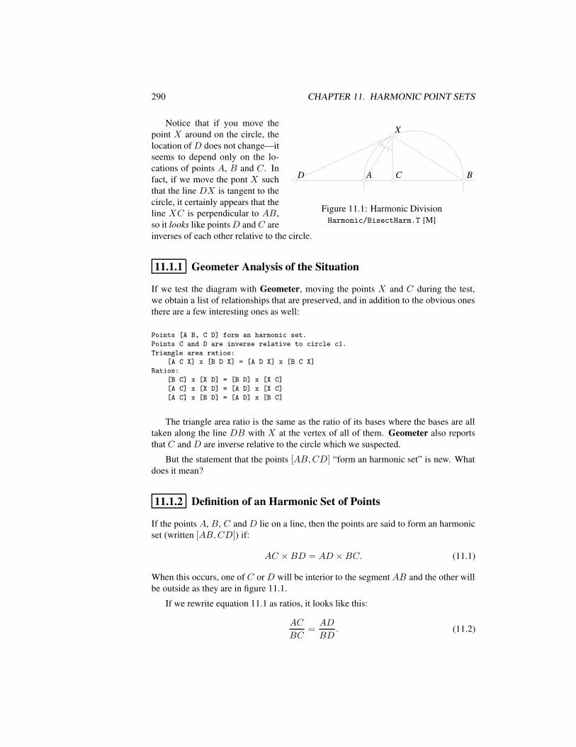
290 CHAPTER 11. HARMONIC POINT SETS
AA BB
XX
CCDD
Figure 11.1: Harmonic DivisionHarmonic/BisectHarm.T [M]
Notice that if you move thepoint X around on the circle, thelocation of D does not change—itseems to depend only on the lo-cations of points A, B and C. Infact, if we move the pont X suchthat the line DX is tangent to thecircle, it certainly appears that theline XC is perpendicular to AB,so it looks like pointsD and C areinverses of each other relative to the circle.
11.1.1 Geometer Analysis of the Situation
If we test the diagram with Geometer, moving the points X and C during the test,we obtain a list of relationships that are preserved, and in addition to the obvious onesthere are a few interesting ones as well:
Points [A B, C D] form an harmonic set.
Points C and D are inverse relative to circle c1.
Triangle area ratios:
[A C X] x [B D X] = [A D X] x [B C X]
Ratios:
[B C] x [X D] = [B D] x [X C]
[A C] x [X D] = [A D] x [X C]
[A C] x [B D] = [A D] x [B C]
The triangle area ratio is the same as the ratio of its bases where the bases are alltaken along the line DB with X at the vertex of all of them. Geometer also reportsthat C and D are inverse relative to the circle which we suspected.
But the statement that the points [AB,CD] “form an harmonic set” is new. Whatdoes it mean?
11.1.2 Definition of an Harmonic Set of Points
If the points A, B, C and D lie on a line, then the points are said to form an harmonicset (written [AB,CD]) if:
AC ×BD = AD ×BC. (11.1)
When this occurs, one of C or D will be interior to the segment AB and the other willbe outside as they are in figure 11.1.
If we rewrite equation 11.1 as ratios, it looks like this:
AC
BC=AD
BD. (11.2)
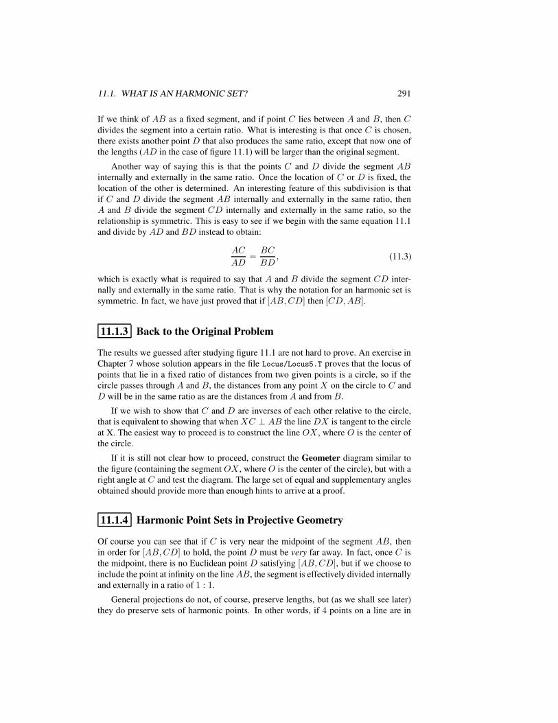
11.1. WHAT IS AN HARMONIC SET? 291
If we think of AB as a fixed segment, and if point C lies between A and B, then Cdivides the segment into a certain ratio. What is interesting is that once C is chosen,there exists another point D that also produces the same ratio, except that now one ofthe lengths (AD in the case of figure 11.1) will be larger than the original segment.
Another way of saying this is that the points C and D divide the segment ABinternally and externally in the same ratio. Once the location of C or D is fixed, thelocation of the other is determined. An interesting feature of this subdivision is thatif C and D divide the segment AB internally and externally in the same ratio, thenA and B divide the segment CD internally and externally in the same ratio, so therelationship is symmetric. This is easy to see if we begin with the same equation 11.1and divide by AD and BD instead to obtain:
AC
AD=BC
BD, (11.3)
which is exactly what is required to say that A and B divide the segment CD inter-nally and externally in the same ratio. That is why the notation for an harmonic set issymmetric. In fact, we have just proved that if [AB,CD] then [CD,AB].
11.1.3 Back to the Original Problem
The results we guessed after studying figure 11.1 are not hard to prove. An exercise inChapter 7 whose solution appears in the file Locus/Locus5.T proves that the locus ofpoints that lie in a fixed ratio of distances from two given points is a circle, so if thecircle passes through A and B, the distances from any point X on the circle to C andD will be in the same ratio as are the distances from A and from B.
If we wish to show that C and D are inverses of each other relative to the circle,that is equivalent to showing that whenXC ⊥ AB the line DX is tangent to the circleat X. The easiest way to proceed is to construct the line OX , where O is the center ofthe circle.
If it is still not clear how to proceed, construct the Geometer diagram similar tothe figure (containing the segment OX , where O is the center of the circle), but with aright angle at C and test the diagram. The large set of equal and supplementary anglesobtained should provide more than enough hints to arrive at a proof.
11.1.4 Harmonic Point Sets in Projective Geometry
Of course you can see that if C is very near the midpoint of the segment AB, thenin order for [AB,CD] to hold, the point D must be very far away. In fact, once C isthe midpoint, there is no Euclidean point D satisfying [AB,CD], but if we choose toinclude the point at infinity on the lineAB, the segment is effectively divided internallyand externally in a ratio of 1 : 1.
General projections do not, of course, preserve lengths, but (as we shall see later)they do preserve sets of harmonic points. In other words, if 4 points on a line are in
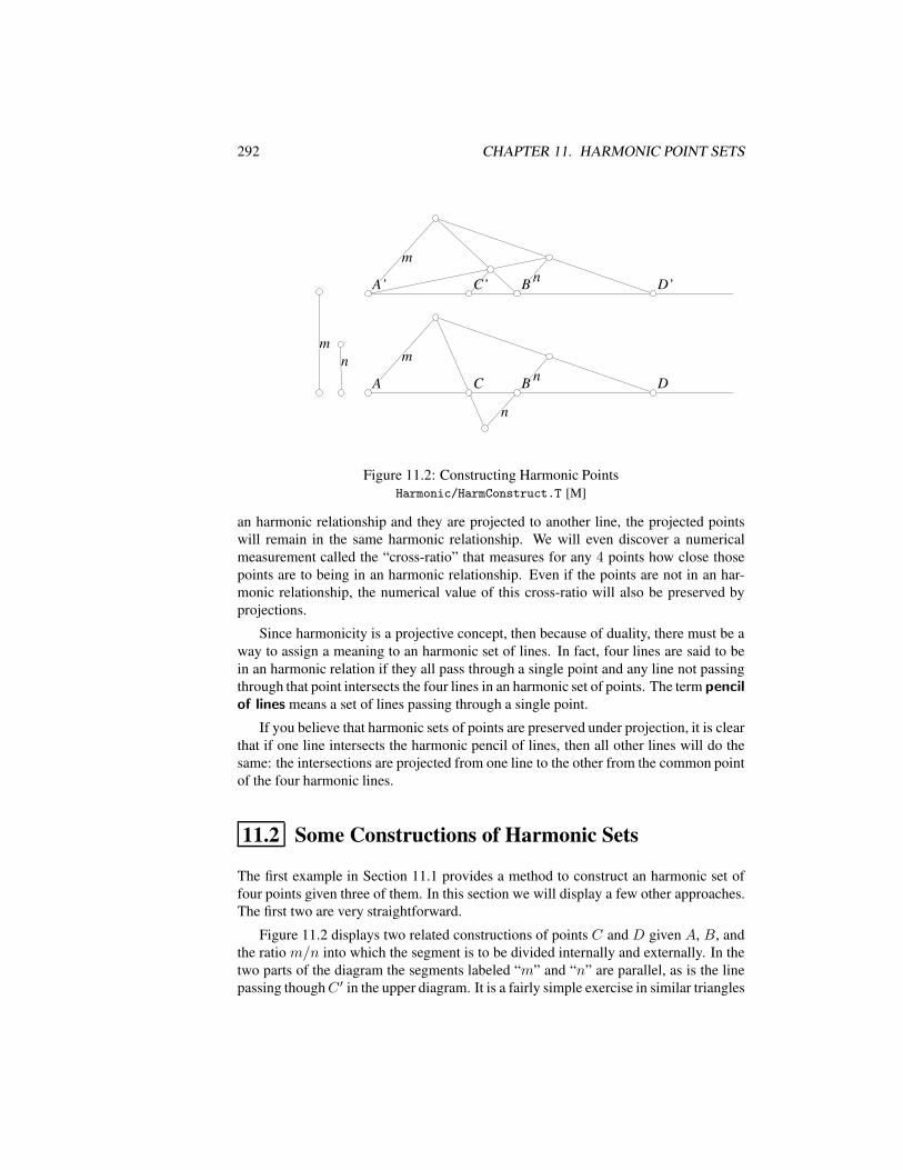
292 CHAPTER 11. HARMONIC POINT SETS
mmnn mm
nn
nn
mmnn
AA BBCC DD
A’A’ B’B’ D’D’C’C’
Figure 11.2: Constructing Harmonic PointsHarmonic/HarmConstruct.T [M]
an harmonic relationship and they are projected to another line, the projected pointswill remain in the same harmonic relationship. We will even discover a numericalmeasurement called the “cross-ratio” that measures for any 4 points how close thosepoints are to being in an harmonic relationship. Even if the points are not in an har-monic relationship, the numerical value of this cross-ratio will also be preserved byprojections.
Since harmonicity is a projective concept, then because of duality, there must be away to assign a meaning to an harmonic set of lines. In fact, four lines are said to bein an harmonic relation if they all pass through a single point and any line not passingthrough that point intersects the four lines in an harmonic set of points. The term pencilof lines means a set of lines passing through a single point.
If you believe that harmonic sets of points are preserved under projection, it is clearthat if one line intersects the harmonic pencil of lines, then all other lines will do thesame: the intersections are projected from one line to the other from the common pointof the four harmonic lines.
11.2 Some Constructions of Harmonic Sets
The first example in Section 11.1 provides a method to construct an harmonic set offour points given three of them. In this section we will display a few other approaches.The first two are very straightforward.
Figure 11.2 displays two related constructions of points C and D given A, B, andthe ratio m/n into which the segment is to be divided internally and externally. In thetwo parts of the diagram the segments labeled “m” and “n” are parallel, as is the linepassing thoughC ′ in the upper diagram. It is a fairly simple exercise in similar triangles
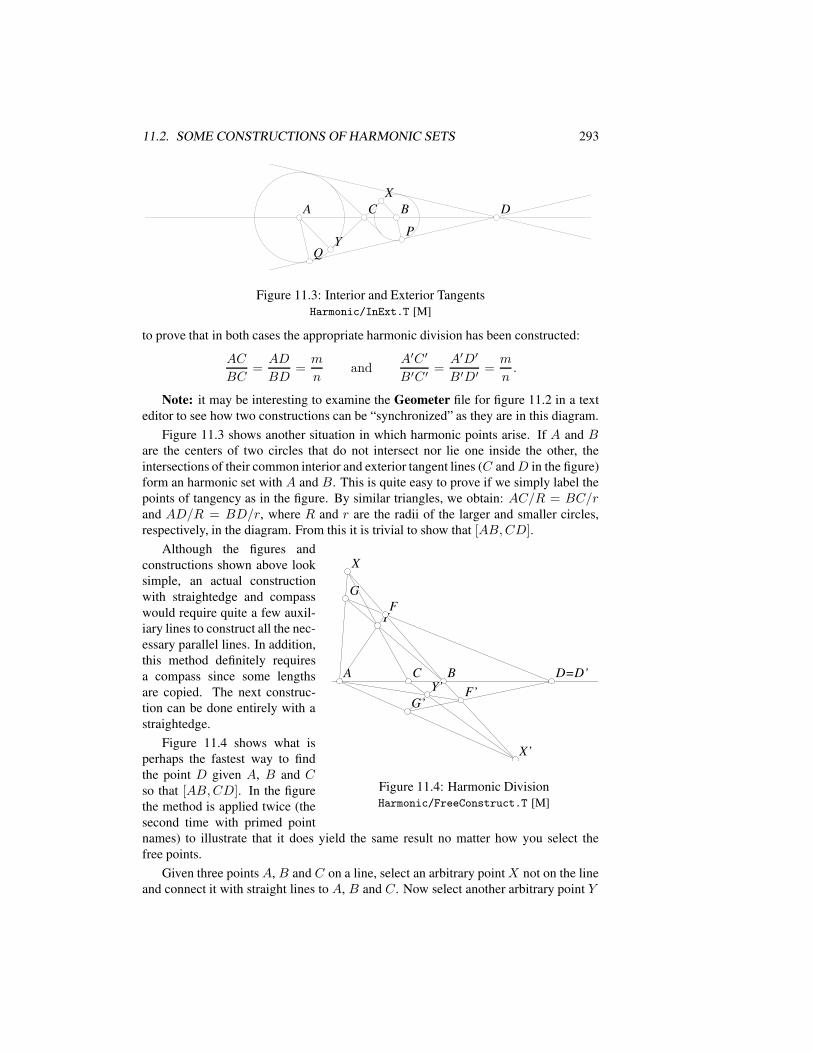
11.2. SOME CONSTRUCTIONS OF HARMONIC SETS 293
AA BBXX
YYPP
DDCC
Figure 11.3: Interior and Exterior TangentsHarmonic/InExt.T [M]
to prove that in both cases the appropriate harmonic division has been constructed:
AC
BC=AD
BD=m
nand
A′C ′
B′C ′=A′D′
B′D′=m
n.
Note: it may be interesting to examine the Geometer file for figure 11.2 in a texteditor to see how two constructions can be “synchronized” as they are in this diagram.
Figure 11.3 shows another situation in which harmonic points arise. If A and Bare the centers of two circles that do not intersect nor lie one inside the other, theintersections of their common interior and exterior tangent lines (C andD in the figure)form an harmonic set with A and B. This is quite easy to prove if we simply label thepoints of tangency as in the figure. By similar triangles, we obtain: AC/R = BC/rand AD/R = BD/r, where R and r are the radii of the larger and smaller circles,respectively, in the diagram. From this it is trivial to show that [AB,CD].
AA BBCC
XX
X’X’
YY
Y’Y’
FFGG
F’F’G’G’
D=D’D=D’
Figure 11.4: Harmonic DivisionHarmonic/FreeConstruct.T [M]
Although the figures andconstructions shown above looksimple, an actual constructionwith straightedge and compasswould require quite a few auxil-iary lines to construct all the nec-essary parallel lines. In addition,this method definitely requiresa compass since some lengthsare copied. The next construc-tion can be done entirely with astraightedge.
Figure 11.4 shows what isperhaps the fastest way to findthe point D given A, B and Cso that [AB,CD]. In the figurethe method is applied twice (thesecond time with primed pointnames) to illustrate that it does yield the same result no matter how you select thefree points.
Given three points A, B and C on a line, select an arbitrary pointX not on the lineand connect it with straight lines to A, B and C. Now select another arbitrary point Y
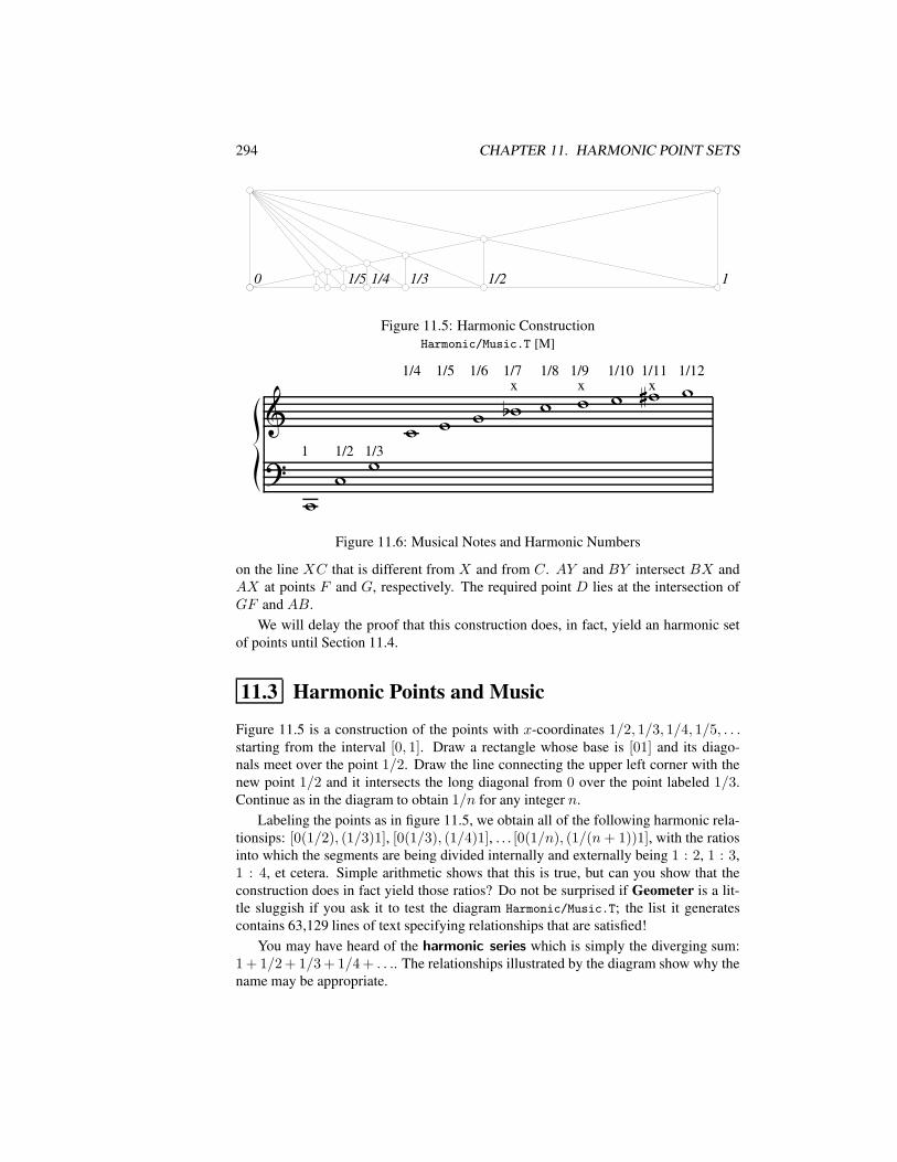
294 CHAPTER 11. HARMONIC POINT SETS
00 111/21/21/31/31/41/41/51/5
Figure 11.5: Harmonic ConstructionHarmonic/Music.T [M]ăIG 1
¯1/2¯ 1/3¯
1/4
¯1/5
¯1/6¯ 1/7
x2¯ 1/8¯ 1/9x¯ 1/10¯ 1/11
x4¯ 1/12¯
Figure 11.6: Musical Notes and Harmonic Numbers
on the line XC that is different from X and from C. AY and BY intersect BX andAX at points F and G, respectively. The required point D lies at the intersection ofGF and AB.
We will delay the proof that this construction does, in fact, yield an harmonic setof points until Section 11.4.
11.3 Harmonic Points and Music
Figure 11.5 is a construction of the points with x-coordinates 1/2, 1/3, 1/4, 1/5, . . .starting from the interval [0, 1]. Draw a rectangle whose base is [01] and its diago-nals meet over the point 1/2. Draw the line connecting the upper left corner with thenew point 1/2 and it intersects the long diagonal from 0 over the point labeled 1/3.Continue as in the diagram to obtain 1/n for any integer n.
Labeling the points as in figure 11.5, we obtain all of the following harmonic rela-tionsips: [0(1/2), (1/3)1], [0(1/3), (1/4)1], . . . [0(1/n), (1/(n+ 1))1], with the ratiosinto which the segments are being divided internally and externally being 1 : 2, 1 : 3,1 : 4, et cetera. Simple arithmetic shows that this is true, but can you show that theconstruction does in fact yield those ratios? Do not be surprised if Geometer is a lit-tle sluggish if you ask it to test the diagram Harmonic/Music.T; the list it generatescontains 63,129 lines of text specifying relationships that are satisfied!
You may have heard of the harmonic series which is simply the diverging sum:1 + 1/2 + 1/3 + 1/4 + . . .. The relationships illustrated by the diagram show why thename may be appropriate.
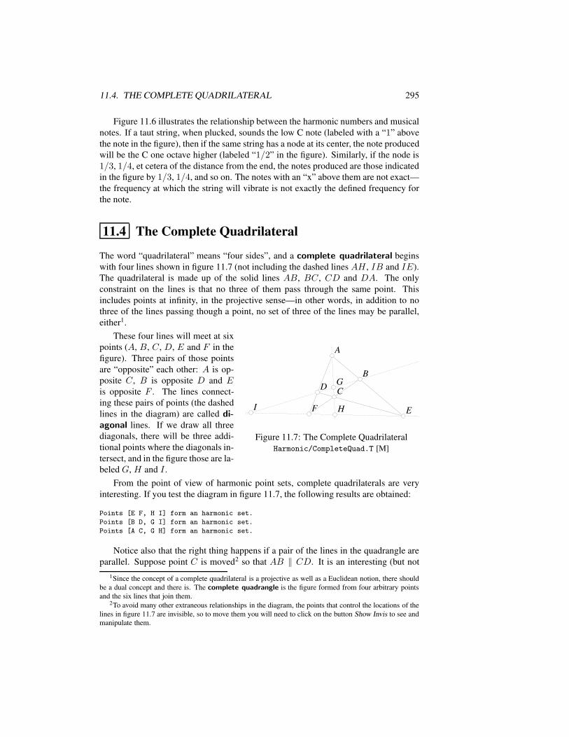
11.4. THE COMPLETE QUADRILATERAL 295
Figure 11.6 illustrates the relationship between the harmonic numbers and musicalnotes. If a taut string, when plucked, sounds the low C note (labeled with a “1” abovethe note in the figure), then if the same string has a node at its center, the note producedwill be the C one octave higher (labeled “1/2” in the figure). Similarly, if the node is1/3, 1/4, et cetera of the distance from the end, the notes produced are those indicatedin the figure by 1/3, 1/4, and so on. The notes with an “x” above them are not exact—the frequency at which the string will vibrate is not exactly the defined frequency forthe note.
11.4 The Complete Quadrilateral
The word “quadrilateral” means “four sides”, and a complete quadrilateral beginswith four lines shown in figure 11.7 (not including the dashed lines AH , IB and IE).The quadrilateral is made up of the solid lines AB, BC, CD and DA. The onlyconstraint on the lines is that no three of them pass through the same point. Thisincludes points at infinity, in the projective sense—in other words, in addition to nothree of the lines passing though a point, no set of three of the lines may be parallel,either1.
AA
BB
CCDD
EEFF
GG
HHII
Figure 11.7: The Complete QuadrilateralHarmonic/CompleteQuad.T [M]
These four lines will meet at sixpoints (A, B, C, D, E and F in thefigure). Three pairs of those pointsare “opposite” each other: A is op-posite C, B is opposite D and Eis opposite F . The lines connect-ing these pairs of points (the dashedlines in the diagram) are called di-agonal lines. If we draw all threediagonals, there will be three addi-tional points where the diagonals in-tersect, and in the figure those are la-beled G, H and I .
From the point of view of harmonic point sets, complete quadrilaterals are veryinteresting. If you test the diagram in figure 11.7, the following results are obtained:
Points [E F, H I] form an harmonic set.
Points [B D, G I] form an harmonic set.
Points [A C, G H] form an harmonic set.
Notice also that the right thing happens if a pair of the lines in the quadrangle areparallel. Suppose point C is moved2 so that AB ‖ CD. It is an interesting (but not
1Since the concept of a complete quadrilateral is a projective as well as a Euclidean notion, there shouldbe a dual concept and there is. The complete quadrangle is the figure formed from four arbitrary pointsand the six lines that join them.
2To avoid many other extraneous relationships in the diagram, the points that control the locations of thelines in figure 11.7 are invisible, so to move them you will need to click on the button Show Invis to see andmanipulate them.
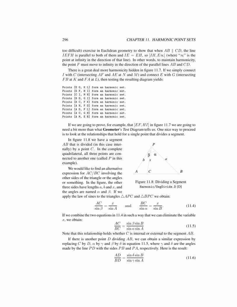
296 CHAPTER 11. HARMONIC POINT SETS
too difficult) exercise in Euclidean geometry to show that when AB ‖ CD, the lineIEFH is parallel to both of them and IE = EH , so [IH,E∞] (where “∞” is thepoint at infinity in the direction of that line). In other words, to maintain harmonicity,the point F must move to infinity in the direction of the parallel lines AB and CD.
There is a great deal more harmonicity hidden in figure 11.7. If we simply connectI with C (intersecting AF and AE at N and M ) and connect E with G (intersectingFB at K and FA at L), then testing the resulting diagram yields:
Points [E G, K L] form an harmonic set.
Points [E F, H I] form an harmonic set.
Points [C I, M N] form an harmonic set.
Points [B D, G I] form an harmonic set.
Points [B C, F K] form an harmonic set.
Points [A N, F D] form an harmonic set.
Points [A D, F L] form an harmonic set.
Points [A C, G H] form an harmonic set.
Points [A M, E B] form an harmonic set.
If we are going to prove, for example, that [EF,HI ] in figure 11.7 we are going toneed a bit more than what Geometer’s Test Diagram tells us. One nice way to proceedis to look at the relationships that hold for a single point that divides a segment.
bb aaxx
AA
PP
BBCC
ααββ
Figure 11.8: Dividing a SegmentHarmonic/SegDivide.D [D]
In figure 11.8 we have a segmentAB that is divided (in this case inter-nally) by a point C. In the completequadrilateral, all three points are con-nected to another one (called P in thisexample).
We would like to find an alternativeexpression for AC/BC involving theother sides of the triangle or the anglesor something. In the figure, the otherthree sides have lengths a, b and x, andthe angles are named α and β. If weapply the law of sines to the triangles4APC and4BPC we obtain:
AC
sinβ=
x
sinAand
BC
sinα=
x
sinB. (11.4)
If we combine the two equations in 11.4 in such a way that we can eliminate the variablex, we obtain:
AC
BC=
sinβ sinB
sinα sinA(11.5)
Note that this relationship holds whether C is internal or external to the segment AB.If there is another point D dividing AB, we can obtain a similar expression by
replacing C by D, α by γ and β by δ in equation 11.5, where γ and δ are the anglesmade by the line PD with the sides PB and PA, respectively. Here is the result:
AD
BD=
sin δ sinB
sin γ sinA(11.6)
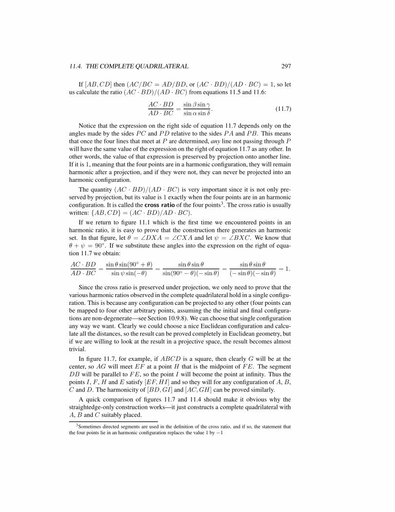
11.4. THE COMPLETE QUADRILATERAL 297
If [AB,CD] then (AC/BC = AD/BD, or (AC · BD)/(AD · BC) = 1, so letus calculate the ratio (AC · BD)/(AD ·BC) from equations 11.5 and 11.6:
AC ·BDAD ·BC =
sinβ sin γ
sinα sin δ. (11.7)
Notice that the expression on the right side of equation 11.7 depends only on theangles made by the sides PC and PD relative to the sides PA and PB. This meansthat once the four lines that meet at P are determined, any line not passing through Pwill have the same value of the expression on the right of equation 11.7 as any other. Inother words, the value of that expression is preserved by projection onto another line.If it is 1, meaning that the four points are in a harmonic configuration, they will remainharmonic after a projection, and if they were not, they can never be projected into anharmonic configuration.
The quantity (AC · BD)/(AD · BC) is very important since it is not only pre-served by projection, but its value is 1 exactly when the four points are in an harmonicconfiguration. It is called the cross ratio of the four points3. The cross ratio is usuallywritten: AB,CD = (AC · BD)/AD ·BC).
If we return to figure 11.1 which is the first time we encountered points in anharmonic ratio, it is easy to prove that the construction there generates an harmonicset. In that figure, let θ = ∠DXA = ∠CXA and let ψ = ∠BXC. We know thatθ + ψ = 90. If we substitute these angles into the expression on the right of equa-tion 11.7 we obtain:
AC · BDAD · BC =
sin θ sin(90 + θ)
sinψ sin(−θ) =sin θ sin θ
sin(90 − θ)(− sin θ)=
sin θ sin θ
(− sin θ)(− sin θ)= 1.
Since the cross ratio is preserved under projection, we only need to prove that thevarious harmonic ratios observed in the complete quadrilateral hold in a single configu-ration. This is because any configuration can be projected to any other (four points canbe mapped to four other arbitrary points, assuming the the initial and final configura-tions are non-degenerate—see Section 10.9.8). We can choose that single configurationany way we want. Clearly we could choose a nice Euclidean configuration and calcu-late all the distances, so the result can be proved completely in Euclidean geometry, butif we are willing to look at the result in a projective space, the result becomes almosttrivial.
In figure 11.7, for example, if ABCD is a square, then clearly G will be at thecenter, so AG will meet EF at a point H that is the midpoint of FE. The segmentDB will be parallel to FE, so the point I will become the point at infinity. Thus thepoints I , F , H and E satisfy [EF,HI ] and so they will for any configuration of A, B,C and D. The harmonicity of [BD,GI ] and [AC,GH ] can be proved similarly.
A quick comparison of figures 11.7 and 11.4 should make it obvious why thestraightedge-only construction works—it just constructs a complete quadrilateral withA, B and C suitably placed.
3Sometimes directed segments are used in the definition of the cross ratio, and if so, the statement thatthe four points lie in an harmonic configuration replaces the value 1 by −1
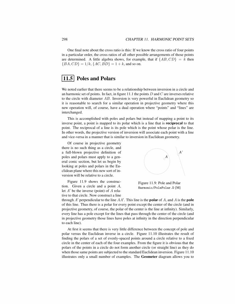
298 CHAPTER 11. HARMONIC POINT SETS
One final note about the cross ratio is this: If we know the cross ratio of four pointsin a particular order, the cross ratios of all other possible arrangements of those pointsare determined. A little algebra shows, for example, that if AB,CD = k thenBA,CD = 1/k, AC,BD = 1 + k, and so on.
11.5 Poles and Polars
We noted earlier that there seems to be a relationship between inversion in a circle andan harmonic set of points. In fact, in figure 11.1 the pointsD andC are inverses relativeto the circle with diameter AB. Inversion is very powerful in Euclidean geometry soit is reasonable to search for a similar operation in projective geometry where thisnew operation will, of course, have a dual operation where “points” and “lines” areinterchanged.
This is accomplished with poles and polars but instead of mapping a point to itsinverse point, a point is mapped to its polar which is a line that is reciprocal to thatpoint. The reciprocal of a line is its pole which is the point whose polar is the line.In other words, the projective version of inversion will associate each point with a lineand vice-versa in a manner that is similar to inversion in Euclidean geometry.
AAA’A’
Figure 11.9: Pole and PolarHarmonic/PolePolar.D [M]
Of course in projective geometrythere is no such thing as a circle, anda full-blown projective definition ofpoles and polars must apply to a gen-eral conic section, but let us begin bylooking at poles and polars in the Eu-clidean plane where this new sort of in-version will be relative to a circle.
Figure 11.9 shows the construc-tion. Given a circle and a point A,let A′ be the inverse (point) of A rela-tive to that circle. Now construct a linethroughA′ perpendicular to the lineAA′. This line is the polar ofA, andA is the poleof this line. Thus there is a polar for every point except the center of the circle (and inprojective geometry, of course, the polar of the center is the line at infinity). Similarly,every line has a pole except for the lines that pass through the center of the circle (andin projective geometry those lines have poles at infinity in the direction perpendicularto each line).
At first it seems that there is very little difference between the concept of pole andpolar versus the Euclidean inverse in a circle. Figure 11.10 illustrates the result offinding the polars of a set of evenly-spaced points around a circle relative to a fixedcircle in the center of each of the four examples. From the figure it is obvious that thepolars of the points in a circle do not form another circle (or straight line) as they dowhen those same points are subjected to the standard Euclidean inversion. Figure 11.10illustrates only a small number of examples. The Geometer diagram allows you to
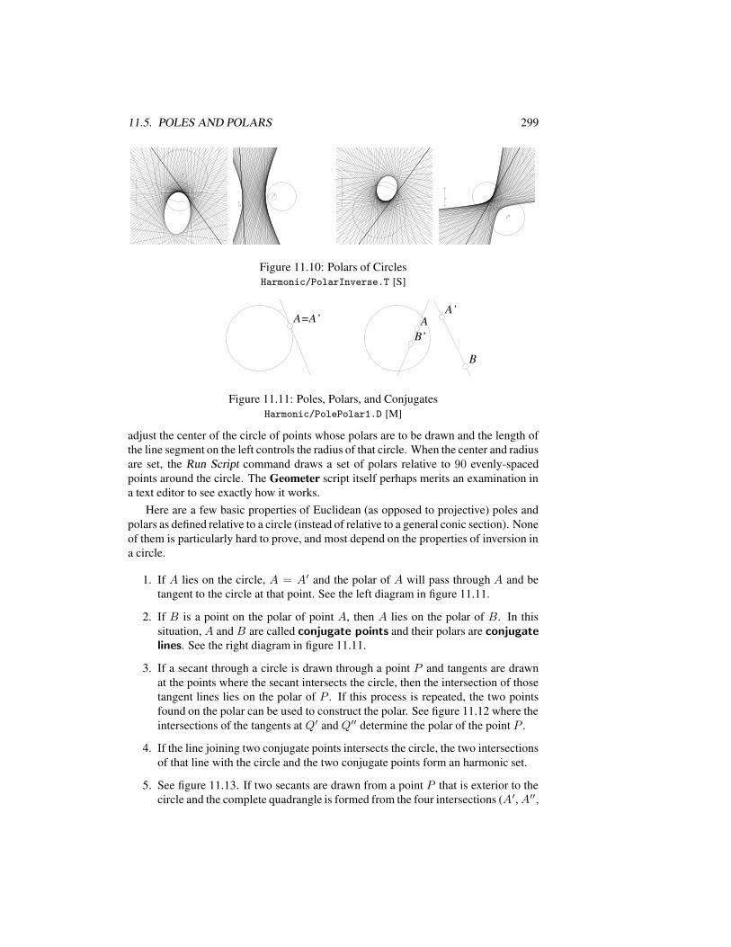
11.5. POLES AND POLARS 299
r r
AA
r r
AA r r
AA
r r
AA
Figure 11.10: Polars of CirclesHarmonic/PolarInverse.T [S]
A=A’A=A’ AAA’A’
BB
B’B’
Figure 11.11: Poles, Polars, and ConjugatesHarmonic/PolePolar1.D [M]
adjust the center of the circle of points whose polars are to be drawn and the length ofthe line segment on the left controls the radius of that circle. When the center and radiusare set, the Run Script command draws a set of polars relative to 90 evenly-spacedpoints around the circle. The Geometer script itself perhaps merits an examination ina text editor to see exactly how it works.
Here are a few basic properties of Euclidean (as opposed to projective) poles andpolars as defined relative to a circle (instead of relative to a general conic section). Noneof them is particularly hard to prove, and most depend on the properties of inversion ina circle.
1. If A lies on the circle, A = A′ and the polar of A will pass through A and betangent to the circle at that point. See the left diagram in figure 11.11.
2. If B is a point on the polar of point A, then A lies on the polar of B. In thissituation, A and B are called conjugate points and their polars are conjugatelines. See the right diagram in figure 11.11.
3. If a secant through a circle is drawn through a point P and tangents are drawnat the points where the secant intersects the circle, then the intersection of thosetangent lines lies on the polar of P . If this process is repeated, the two pointsfound on the polar can be used to construct the polar. See figure 11.12 where theintersections of the tangents at Q′ and Q′′ determine the polar of the point P .
4. If the line joining two conjugate points intersects the circle, the two intersectionsof that line with the circle and the two conjugate points form an harmonic set.
5. See figure 11.13. If two secants are drawn from a point P that is exterior to thecircle and the complete quadrangle is formed from the four intersections (A′,A′′,
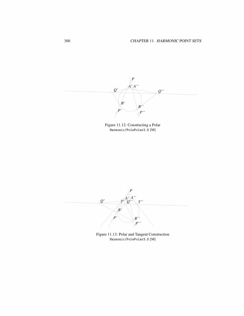
300 CHAPTER 11. HARMONIC POINT SETS
PP
P’P’ P’’P’’
B’B’
A’A’ A’’A’’
B’’B’’
Q’Q’ Q’’Q’’
Figure 11.12: Constructing a PolarHarmonic/PolePolar2.D [M]
PP
P’P’P’’P’’
B’B’
A’A’ A’’A’’
B’’B’’
Q’Q’ Q’’Q’’T’T’ T’’T’’
Figure 11.13: Polar and Tangent ConstructionHarmonic/PolePolar3.D [M]
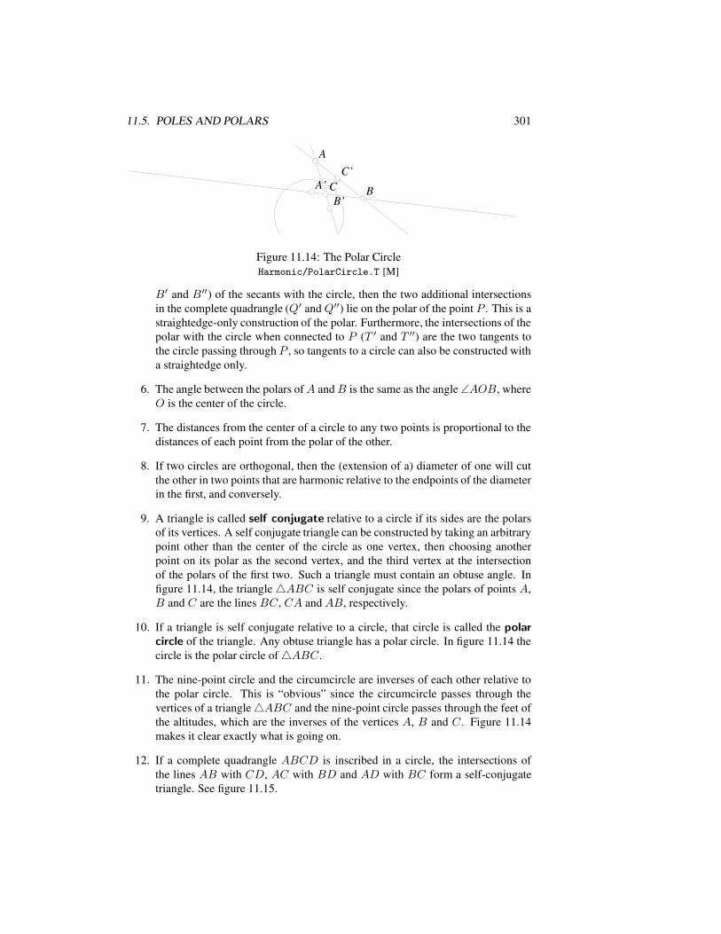
11.5. POLES AND POLARS 301
CC
AA
BBA’A’C’C’
B’B’
Figure 11.14: The Polar CircleHarmonic/PolarCircle.T [M]
B′ and B′′) of the secants with the circle, then the two additional intersectionsin the complete quadrangle (Q′ and Q′′) lie on the polar of the point P . This is astraightedge-only construction of the polar. Furthermore, the intersections of thepolar with the circle when connected to P (T ′ and T ′′) are the two tangents tothe circle passing through P , so tangents to a circle can also be constructed witha straightedge only.
6. The angle between the polars ofA andB is the same as the angle∠AOB, whereO is the center of the circle.
7. The distances from the center of a circle to any two points is proportional to thedistances of each point from the polar of the other.
8. If two circles are orthogonal, then the (extension of a) diameter of one will cutthe other in two points that are harmonic relative to the endpoints of the diameterin the first, and conversely.
9. A triangle is called self conjugate relative to a circle if its sides are the polarsof its vertices. A self conjugate triangle can be constructed by taking an arbitrarypoint other than the center of the circle as one vertex, then choosing anotherpoint on its polar as the second vertex, and the third vertex at the intersectionof the polars of the first two. Such a triangle must contain an obtuse angle. Infigure 11.14, the triangle4ABC is self conjugate since the polars of points A,B and C are the lines BC, CA and AB, respectively.
10. If a triangle is self conjugate relative to a circle, that circle is called the polarcircle of the triangle. Any obtuse triangle has a polar circle. In figure 11.14 thecircle is the polar circle of4ABC.
11. The nine-point circle and the circumcircle are inverses of each other relative tothe polar circle. This is “obvious” since the circumcircle passes through thevertices of a triangle4ABC and the nine-point circle passes through the feet ofthe altitudes, which are the inverses of the vertices A, B and C. Figure 11.14makes it clear exactly what is going on.
12. If a complete quadrangle ABCD is inscribed in a circle, the intersections ofthe lines AB with CD, AC with BD and AD with BC form a self-conjugatetriangle. See figure 11.15.
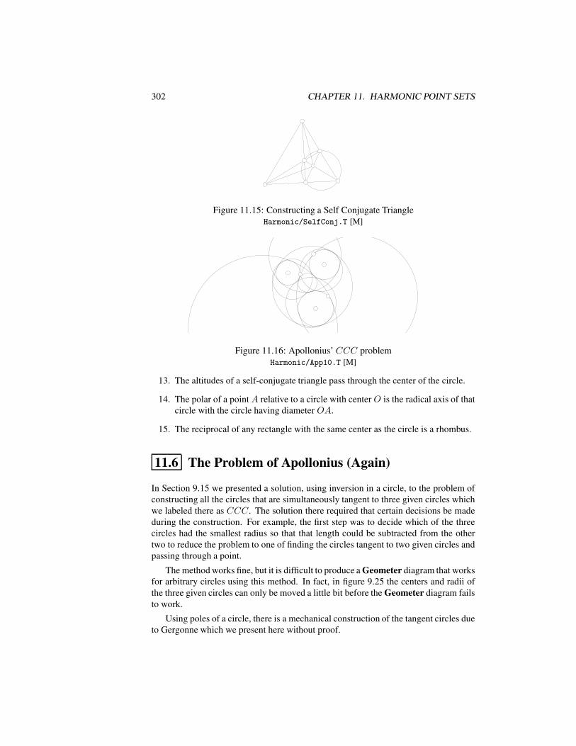
302 CHAPTER 11. HARMONIC POINT SETS
Figure 11.15: Constructing a Self Conjugate TriangleHarmonic/SelfConj.T [M]
Figure 11.16: Apollonius’ CCC problemHarmonic/App10.T [M]
13. The altitudes of a self-conjugate triangle pass through the center of the circle.
14. The polar of a point A relative to a circle with center O is the radical axis of thatcircle with the circle having diameter OA.
15. The reciprocal of any rectangle with the same center as the circle is a rhombus.
11.6 The Problem of Apollonius (Again)
In Section 9.15 we presented a solution, using inversion in a circle, to the problem ofconstructing all the circles that are simultaneously tangent to three given circles whichwe labeled there as CCC. The solution there required that certain decisions be madeduring the construction. For example, the first step was to decide which of the threecircles had the smallest radius so that that length could be subtracted from the othertwo to reduce the problem to one of finding the circles tangent to two given circles andpassing through a point.
The method works fine, but it is difficult to produce a Geometer diagram that worksfor arbitrary circles using this method. In fact, in figure 9.25 the centers and radii ofthe three given circles can only be moved a little bit before the Geometer diagram failsto work.
Using poles of a circle, there is a mechanical construction of the tangent circles dueto Gergonne which we present here without proof.
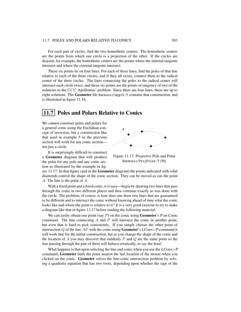
11.7. POLES AND POLARS RELATIVE TO CONICS 303
For each pair of circles, find the two homothetic centers. The homothetic centersare the points from which one circle is a projection of the other. If the circles aredisjoint, for example, the homothetic centers are the points where the internal tangentsintersect and where the external tangents intersect.
These six points lie on four lines. For each of those lines, find the poles of that linerelative to each of the three circles, and if they all exists, connect them to the radicalcenter of the three circles. The lines connecting the poles to the radical center willintersect each circle twice, and those six points are the points of tangency of two of thesolutions to the CCC Apollonius’ problem. Since there are four lines, there are up toeight solutions. The Geometer file Harmonic/App10.T contains that construction, andis illustrated in figure 11.16.
11.7 Poles and Polars Relative to Conics
AA
Figure 11.17: Projective Pole and PolarHarmonic/ProjPolar.T [M]
We cannot construct poles and polars fora general conic using the Euclidean con-cept of inversion, but a construction likethat used in example 5 in the previoussection will work for any conic section—not just a circle.
It is surprisingly difficult to constructa Geometer diagram that will producethe polar for any pole and any conic sec-tion as illustrated by the example in fig-ure 11.17. In that figure (and in the Geometer diagram) the points indicated with soliddiamonds control the shape of the conic section. They can be moved as can the pointA. The line is the polar of A.
With a fixed point and a fixed conic, it is easy—begin by drawing two lines that passthrough the conic in two different places and then continue exactly as was done withthe circle. The problem, of course, is how does one draw two lines that are guaranteedto be different and to intersect the conic without knowing ahead of time what the coniclooks like and where the point is relative to it? It is a very good exercise to try to makea diagram like that in figure 11.17 before reading the following material.
We can easily obtain one point (say P ) on the conic using Geometer’s P on Coniccommand. The line connecting A and P will intersect the conic in another point,but even that is hard to pick consistently. If you simply choose the other point ofintersectionQ of the line AP with the conic using Geometer’s LCon=>P command itwill work fine for the initial construction, but as you change the shape of the conic andthe location of A you may discover that suddenly P and Q are the same point so theline passing through the pair of them will behave erratically, to say the least!
What happens is that upon selecting the line and conic when you use the LCon=>Pcommand, Geometer finds the point nearest the last location of the mouse when youclicked on the conic. Geometer solves the line-conic intersection problem by solv-ing a quadratic equation that has two roots, depending upon whether the sign of the
304 CHAPTER 11. HARMONIC POINT SETS
discriminant is positive or negative. If it is positive for for the point of intersection,Geometer always uses the positive value of the discriminant for that solution and vice-versa. The new location of the point P on the conic, however, is constantly reprojectedto the conic as A moves or as the shape of the conic changes. The location of P maysuddenly become the same as Q because of that.
The best solution is that once you have the lineAP that intersects the conic twice tochange P to the invisible color, and then create two new points at the two intersectionsof the line with the conic. Geometer will find that it uses a positive discriminant forone and a negative discriminant for the other, so even if P swaps to a different solution,the two intersections will remain different.
Thus it is easy to obtain one line and its two different intersections with the conic.How do you obtain another line and pair of points?
If you simply choose another point P ′ constrained to lie on the conic, as you movethings around and P and P ′ are constantly reprojected, it is overwhelmingly likely thatthey will eventually converge to the same point. Try making a conic section through 5points, constrain two points to lie on that conic and then change the shape of the conicby moving the control points. You will find that almost always the two points willconverge to the same location on the conic. They may not be identical due to computerround-off error, but the distance between them will be so tiny that the line that joinsthem is very unstable.
But a perpendicular through P is guaranteed to intersect the conic in a new point,and that new point is generally not near either of the two intersections of the line AP .Of course this point has the same problem with respect to its definition and if we arenot careful, it may collapse to be the same as P . If you try the same trick, however,that may not work, since P and this new point may swap, and your line through P andA will, essentially, not pass through P .
Here is the solution: Pick P on the conic and draw the line AP . Through P ,construct a perpendicular to AP . Make P invisible and find the two intersections ofthe perpendicular line with the conic. When these different points are connected to A,they are guaranteed to be different lines4.
Draw the two lines from the intersections of the line perpendicular to AP at P .Next, color the intersection points invisible, and make two new points on each line thatintersect the conic in different places. These four points can then be used to constructthe polar in the same manner that it was constructed for a circle.
4Well, almost guaranteed: with incredibly bad luck, P may lie at a point where AP is tangent to theconic and hence only intersects it in one place, but this is very, very unlikely.
Chapter 12Geometric Presentations
If you are trying to solve a problem for yourself then as long as you understand whatyou are doing, the beauty and neatness of the solution is not too important. But as soonas you try to present your results to someone else it is important that the presentationbe neat and clear. If you are a geometry teacher using Geometer in front of a class, thepresentation will be easier for your students to understand if you make some effort topolish each diagram before you present it.
In this chapter we will investigate methods to make diagrams easier to understand.Teachers of geometry need to do this every day, but many mathematicians need to dothe same thing from time to time. In addition to dynamic presentations, Geometer canalso be quite useful for helping generate illustrations for publication, either electroni-cally or printed on paper. Every illustration in this book (and every one in the referencemanual except for the screen shots) was prepared using Geometer.
The chapter is much more about techniques for using Geometer (or other computergeometry programs) than it is about specific geometric facts, although the examples
305
306 CHAPTER 12. GEOMETRIC PRESENTATIONS
have been chosen to include some interesting results. Since many of the features andmethods described here are specific to Geometer you may wish to have the referenceguide available as you read this. Other computer geometry programs have most ofthese features, but probably not all, and Geometer is missing some features found inthose programs.
The reference guide that comes with the Geometer release contains a tutorial forteachers that is a useful addendum to the material in this chapter.
12.1 General Considerations
There are some obvious things to keep in mind, no matter whether your presentationis electronic, on an overhead projector, written in chalk on a blackboard or printed in abook or handout. Here are a few:
• Use standard notation if possible. If that is impossible, at least use consistentnotation. In other words, use “I” for the incenter of a triangle, “O” for thecircumcenter and “H” for the orthocenter. If your triangle is4ABC, let a, b andc represent the lengths of the sides opposite the verticesA,B andC, respectively.If you need to name angles, use Greek letters, and use α, β and γ for the anglesat vertices A, B and C, respectively. Use “s” for the semiperimeter, et cetera.
• Make certain it is easy to read labels, especially the important ones. The nicething about Geometer diagrams is that you can usually adjust the diagram insuch a way that the labels do not fall on top of each other and so that they are notobscured by other lines or circles in the diagram.
• Use appropriate fonts and point sizes for the illustration. In a classroom the texthas to be big enough to be read from the back of the class. In a book, smallerfonts may help remove the clutter from a diagram.
• Show a general configuration if possible. In other words, if the theorem youwish to demonstrate applies to all triangles, do not display it with a triangle thatis close to being equilateral or isosceles.
• Eliminate extraneous information. Hide your construction lines by making theminvisible. Eliminate names from points that are not important to the presentation.Do not color things differently unless you have a good reason to do so.
• Do use colors, line stippling, angle markings, point shapes, et cetera when thereis a good reason. For example, if you have a diagram where you construct asimilar object based on each side of a triangle and it might be confusing whatcorresponds to which side, draw the three sides in different colors, and drawthe objects associated with each side in the same color as the side. Similarly,if you are using inversion in a circle, you might draw objects in the originalconfiguration in one color and in the inverted configuration in another.
• In locus-of-points illustrations, try to make the representative points regularlyspaced.
12.2. IMPROVING THE APPEARANCE OF A DIAGRAM 307
12.2 Improving the Appearance of a Diagram
Many of Geometer’s primitives can be drawn in different styles. All can be drawn indifferent colors, but the other styles are primitive-dependent.
12.2.1 Colors
In addition to the standard colors that are available in the color selection box in Ge-ometer’s control area there are 24 additional available colors that you can customizeand use from Geometer’s text editor. The additional colors have names .c8, .c9, . . . ,.c31. (Colors .c0 through .c7 are the reserved colors: black, red, green, yellow, etcetera.)
In a Geometer file, the definition of the colors .c8 through .c31 can be set to aparticular combination of red, green and blue components that vary from 0.0 to 1.0.To set the color .c8 to be pink and then to use it as the color of point p1, insert a linedefining the color components for .c8 and edit the line for p1 so that it looks somethinglike this:
.c8 = (1.000000, 0.400000, 0.400000);
p1 = .free(0, 0, .c8, "A");
The definition of color .c8 above will remain in effect only as long as that particularGeometer file is loaded.
12.2.2 Names
Every primitive can have a user-assigned name, but by default, names are only assignedto points as they are created, and this feature can be turned on and off in the Edit Pref-erences dialog. The name can be as simple as a single character or it can be a wholestring. To create or change the name of a primitive, select it and then use the Edit Namecommand.
The names of points, lines and angles are drawn on the screen slightly above and tothe right of a point, or at the center of a line segment, either slightly above or slightlybelow the segment depending upon whether the segment slopes up or down. The nameof an angle is drawn inside the angle. It is a bit difficult to draw angle names in exactlythe right place, so for high-quality drawings you will sometimes need to resort to othermethods to place angle names properly.
Another primitive whose name is used by Geometer is the floating-point number(the .flt) that you can only have entered with the text editor. If a .flt has a name, thevalue of that number is drawn in the upper left of the display window, together with thename. For example, if the .flt named pi has the value 3.14159, it will be presentedas the string: “pi = 3.142” in the upper left of the screen. All values are presented onlyto three decimal places, since Geometer cannot guarantee accuracy much better thanthat. If there is more than one named .flt, all the values are listed in a column.
308 CHAPTER 12. GEOMETRIC PRESENTATIONS
If you wish to display the length of a line segment, the area of a polygon, or themeasure of an angle, you can select that item and use the Display Value command. Inthat case the primitive’s length, area, or measure is drawn in the same way in the upperleft portion of the display window. If the line segment named b has length 1.234 it willbe presented as “b = 1.234”. In the current version of Geometer, the coordinate systemruns from −1.0 to 1.0 in the shorter dimension of the viewing window so all lengthsand areas will be presented based on these dimensions.
The Display Value command is easy to use—you simply need to select a primitiveand toggle it on or off—but it is somewhat restricted by Geometer’s coordinate system.For high-quality presentations you may need to resort to working directly with the.flts. See Section 12.5.
Finally, the text you use for a primitive name can have certain special characters,superscripts, subscripts, and so on. See Section 12.2.4.
12.2.3 Primitive-Specific Styles
In addition to colors and names, points, lines, polygons and angles can be displayedin various modes. Points can be drawn as dots, small circles, diamonds, or as nothingat all. Lines can be drawn with various stippling options, hash marks (to indicatecongruence to other segments), or as a segment, ray or full line. Different sorts ofangle markings are available, different polygon fill types are available, and the linewidth of any line, circle, conic section or Bezier curve can be set from 0.5 to 6 pixels inwidth. On the computer screen a width of 0.5 pixels cannot be shown (so it is displayedas one pixel wide), but when printed it will produce a lighter line.
One of the main uses of a point with nothing displayed is for use as a label in a high-quality illustration. Although no mark is made for the point, its name is displayed, soit is basically a piece of text that can be moved to any position on the screen. If youwould like to have it locked at a certain location, use a .pinned point instead of a .free
point.
All these display styles for primitives are available in the Style pulldown menu or inthe selection boxes in the control area. Rather than give a complete description of eachhere, it is easier just to draw some primitives with geometer, select them, and changethe styles of each to look at the various options.
In classroom presentations, sometimes the thin width of the lines in Geometermakes them difficult to see across a classroom, especially if the image is projected ona television screen instead of a computer screen projector. You can make the lines inyour diagram wider, of course, but then they will be inappropriate for close-up viewing.The command Wide Lines (available in the Styles pulldown) doubles the width of allthe lines. The keyboard shortcut is Ctrl-L or Ctrl-l (lower-case “L”) which toggles thewide lines on and off.
The only reason to use the polygon primitive in Geometer is to obtain its areaautomatically or to have an easy way to stipple or fill regions for display purposes.
12.3. BUILDING GEOMETER PROOFS AND CONSTRUCTIONS 309
12.2.4 Descriptive Text
The text that appears at the bottom of the display window is the same as the text thatnames primitives with the one exception that a primitive name must consist of a singleline of text—no newline characters.
In addition to the standard characters, Geometer is capable of drawing a numberof special characters, subscripts, superscripts, and even lines or arcs over text. Thespecial characters are all introduced by a “\” character. If you would like to talk about4ABC, enter the following text: “\triangleABC”. The leading “\” tells Geometer totry to find a command name after it (and it finds “triangle” in this case). If it does finda match, the matching text is replaced by the corresponding symbol. See the referencemanual for a complete set of special characters supported in this way.
Two other commonly-used text commands produce superscripts and subscripts.The idea is similar: To produce “A1”, type: “A\sub1”; to produce “B3”, type:“B\sup3”. There are a few other special text commands that are rarely used, butare documented in the reference manual.
Finally, Geometer has a somewhat unusual method for indicating newlines withina piece of text in the textual description. If you type in your text and edit it using thedialog box available under the Descriptive Text command in the Primitives pulldownthis is all handled automatically. If you are typing in text by hand using the editor, hereis what it looks like.
Suppose you would like your textual description to read like this with two lines oftext:
Congruent Triangles:4ABC,4DEF ,4GHI
This is exactly what you would type into the Geometer text file to obtain that result:
.text("Congruent Triangles:
\triangleABC, \triangleDEF, \triangleGHI");
Note that the opening and closing quotation marks are on different lines which isvery non-standard in computer languages. It is easier to type, however.
12.3 Building Geometer Proofs and Constructions
It takes a fair amount of work to build a beautiful proof or construction that is ideallysuited for presentation in a classroom. Once it is done, however, it can be used overand over again. In this section we will build a few examples in a step by step manner.
In this section we assume that you know how to prove a result. You are simplytrying to present that proof in the clearest possible way.
Perhaps the best way to use this section is to read the description of how a particulardemonstration is built and then try to build it yourself using Geometer. If you haveproblems, read the section again, presumably with much more interest.
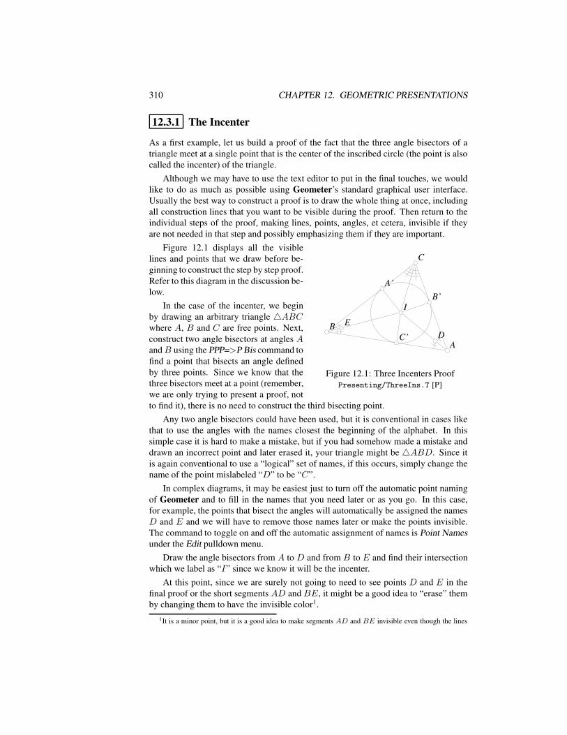
310 CHAPTER 12. GEOMETRIC PRESENTATIONS
12.3.1 The Incenter
As a first example, let us build a proof of the fact that the three angle bisectors of atriangle meet at a single point that is the center of the inscribed circle (the point is alsocalled the incenter) of the triangle.
Although we may have to use the text editor to put in the final touches, we wouldlike to do as much as possible using Geometer’s standard graphical user interface.Usually the best way to construct a proof is to draw the whole thing at once, includingall construction lines that you want to be visible during the proof. Then return to theindividual steps of the proof, making lines, points, angles, et cetera, invisible if theyare not needed in that step and possibly emphasizing them if they are important.
AA
BB
CC
DDEE
II
C’C’
B’B’A’A’
Figure 12.1: Three Incenters ProofPresenting/ThreeIns.T [P]
Figure 12.1 displays all the visiblelines and points that we draw before be-ginning to construct the step by step proof.Refer to this diagram in the discussion be-low.
In the case of the incenter, we beginby drawing an arbitrary triangle 4ABCwhere A, B and C are free points. Next,construct two angle bisectors at angles AandB using the PPP=>P Bis command tofind a point that bisects an angle definedby three points. Since we know that thethree bisectors meet at a point (remember,we are only trying to present a proof, notto find it), there is no need to construct the third bisecting point.
Any two angle bisectors could have been used, but it is conventional in cases likethat to use the angles with the names closest the beginning of the alphabet. In thissimple case it is hard to make a mistake, but if you had somehow made a mistake anddrawn an incorrect point and later erased it, your triangle might be 4ABD. Since itis again conventional to use a “logical” set of names, if this occurs, simply change thename of the point mislabeled “D” to be “C”.
In complex diagrams, it may be easiest just to turn off the automatic point namingof Geometer and to fill in the names that you need later or as you go. In this case,for example, the points that bisect the angles will automatically be assigned the namesD and E and we will have to remove those names later or make the points invisible.The command to toggle on and off the automatic assignment of names is Point Namesunder the Edit pulldown menu.
Draw the angle bisectors from A to D and from B to E and find their intersectionwhich we label as “I” since we know it will be the incenter.
At this point, since we are surely not going to need to see points D and E in thefinal proof or the short segments AD and BE, it might be a good idea to “erase” themby changing them to have the invisible color1.
1It is a minor point, but it is a good idea to make segments AD and BE invisible even though the lines
12.3. BUILDING GEOMETER PROOFS AND CONSTRUCTIONS 311
WE complete the drawing of the bisectors by drawing the segments AI , BI andCI .
Since we are going to want to indicate to the viewers that the lines AI , BI andCI are angle bisectors, we should also draw in the six angles ∠CAI , ∠IAB, ∠ABI ,∠IBC, ∠BCI and ∠ICA using the PPP=>A command. To indicate that there arethree pairs of equal angles, use the different angle styles to make them different. Thebest way to do this is probably to use the angle styles with the slashes, since otherwiseit will not be obvious whether you are talking about the single angle ∠CAB or the twoangles ∠CAI and ∠IAB. See the figure.
To complete the drawing we will need to drop perpendicular line segments to thesides of4ABC. Use the command PL=>L Perp to draw the three perpendiculars andthen use the LL=>P three times to create points at the feet of these perpendiculars. Weneed points here since we will need to name those points in the textual presentation ofthe proof. It might be nice to give those points logical names, so we use the Edit Namecommand in the Edit pulldown menu to change the names to A′, B′ and C ′ as in thefigure. The final touch is to draw the incircle centered at I and passing through A′ (orB′ or C ′), or just draw the circle passing through the three points A′, B′ and C ′.
Now that everything is drawn, let us convert our diagram to a proof. At this point,every primitive is either visible on all the layers or invisible on all the layers. The onesthat are invisible at this point were made that way because they will never be shown,so we do not need to worry about them. We will, however, need to make the visibleprimitives change color and/or become invisible as we move from layer to layer in thepresentation of the proof.
A Geometer proof works as follows. When you press the Start button, only itemson layer zero are visible. Each time you press the Next button the visible layer advancesby one so after one press you will view items on layer one, et cetera. If you wantgeometer to begin with only layer zero visible, you can add the line .l0; to the file.This is commonly done on prepared proofs or constructions.
By default, the layer information is hidden from users, so if it is not visible youprobably want to turn it on with the Layer Display command in the Edit pulldownmenu. If you are going to produce a lot of proof or geometric construction demonstra-tions you can use the Edit Preferences entry in the Edit pulldown to have the layersdisplayed every time you start the Geometer program.
An easy way to build the proof at this point is to press the Start button (so thatonly layer zero can be viewed and edited) and then to make the diagram on that layerlook exactly as you want it to look. When that step of the proof is complete, press theNext button to advance to the next step of the proof, and continue that way to the end.Geometer has 32 layers, which should be sufficient for almost any demonstration.
In this section we will describe in detail the production of the first two steps of theproof, but to complete it, you will have to perform the same general process on each
AI and BI will be drawn on top of them. This is because due to the fact that the lines are drawn as discretepixels, the part of the line AI that is supposed to be identical to AD will almost certainly differ in a fewpixels, so if AD is not made invisible, the line from A to I will be marginally wider during the part from Ato D. Also, if the triangle is made small enough, points D or E could be pushed outside of it.
312 CHAPTER 12. GEOMETRIC PRESENTATIONS
step. To view the final result, load the file Presenting/ThreeIns.T and press the Nextbutton to step through the entire proof.
In a computer geometry program it is probably best in the first step of the proofto display the final result and explain it so that users can manipulate the figure to seeexactly what is happening. A clear statement of the theorem should also be presentedin that first step (on layer zero).
Save your diagram so far (as a sort of backup in case you make a terrible error) andthen click on the Start button. Under Layer Control only box zero should be checkedafter doing this.
While viewing layer zero, select the points A′, B′ and C ′ and set them to theinvisible color. Similarly, set the line segments connecting I to those three points alsoto be invisible. All the rest of the diagram should be visible since it demonstrates thetheorem we are going to prove.
Next, enter the description that is to appear on layer zero. It should probably saysomething like this:
In \triangleABC the three internal angle bisectors
meet at a point I which is the center of the inscribed
circle--the circle inside the triangle that is
simultaneously tangent to all three sides. Move
points A, B and C.
You can enter this description by selecting the Descriptive Text entry under theText entry in the Primitives pulldown menu. If you prefer, you can enter it using theEdit Geometery command also in the Edit pulldown menu, but in this case you willhave to include with it the “wrappings” that make it a text file command:
.text("In \triangleABC the three internal angle bisectors
meet at a point I which is the center of the inscribed
circle--the circle inside the triangle that is
simultaneously tangent to all three sides. Move
points A, B and C.", .l0);
It is nice to include in the description an indication to the user of what parts of thediagram can be manipulated. In this case, for example, the user cannot move pointI—only points A, B and C are free.
When this first step is completed, press Next to view and edit layer 1. On thatlayer, many of the constructions are invisible, so select each one that is supposed tobe invisible and then select the invisible color. The keyboard shortcut that sets theselected primitive to be invisible is Ctrl-i. Since the first step of the proof concernstwo angle bisectors, select those and set them to the blinking color, and since they areangle bisectors, it might also be a good idea to select the angles themselves and makethem blink as well.
To complete this step, add text to describe this first step of the proof.
Continue in this way until all the steps are finished. In this presentation, it required9 steps, ending with a view of layer 8. (Remember that the first step is on layer 0.)
12.3. BUILDING GEOMETER PROOFS AND CONSTRUCTIONS 313
It is now a good idea to go to the beginning (using the Start button) and step forwardand backward through the demonstration, checking to see that all the primitives thatwere supposed to be invisible are, in fact, invisible. Correct any errors.
Next, edit the Geometer file with the Edit Geometery command in the Edit pull-down menu and add the line:
.l0;
at the beginning of the file so that when the diagram is loaded the viewer will see onlythe contents of layer 0 (as if the Start button were pressed automatically upon openingthe file).
Finally, it is nice to add a line at the end of the file like this:
.text("Press ’Next’ to continue ...", [8 .red, .in]);
This line appears after everything, but appears in red on the first 8 layers. Thus itwill be displayed underneath the text you entered earlier on every step except the finalone. It helps the user to know when the end of the proof is reached.
Now, load the diagram Presenting/ThreeIns.T and step through it, going forwardand backward with the Next and Prev keys to see what a reasonably good proof lookslike. You might also find it educational to view the code with the Edit Geometry com-mand. Finally, it would be very useful to try to reproduce this file, or something similar,starting from scratch. You can then refer to Presenting/ThreeIns.T if you get stuck.
12.3.2 Squaring a Rectangle
We will finish this section with one more example, the presentation of a geometricconstruction: Given an arbitrary rectangle, construct a square that has the same area.
The same techniques and cautions that were mentioned in Section 12.3.1 applyhere.
We first draw a Geometer diagram that does what we want and test it. Then wewill begin with the entire diagram, complete with all the construction lines, and convertit to a step by step construction.
In this case, the solution is not too hard. If the dimensions of the rectangle are aand b, then the side of the desired square is
√ab. If a circle has diameter a + b, then
the distance to the circle along a line perpendicular to the diameter that splits it intolengths a and b is
√ab.
The complete construction is illustrated in figure 12.2. The user can change theshape of rectangle OPRQ by moving points Q or P . Those points are constrained tobe on vertical and horizontal lines emanating from O. Since OP extends to the right,we can make a segment of lengthOP +OQ by copyingOQ down to the line OP witha circle centered at O passing throughQ and S. Clearly SP = OP +OQ.
In the figure, T is the midpoint of SP , so a circle centered at T will have SP asdiameter. A perpendicular to SP at O will intersect the circle with diameter SP at U .
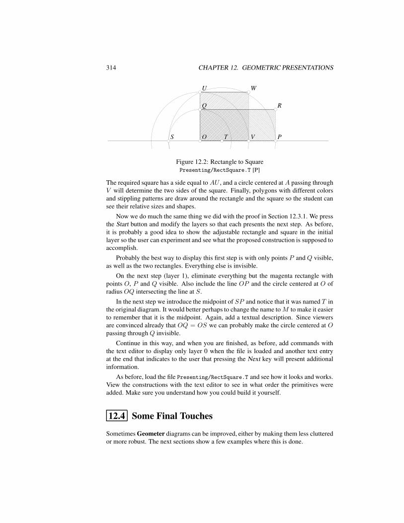
314 CHAPTER 12. GEOMETRIC PRESENTATIONS
OO PP
QQ RR
SS TT
UU
VV
WW
Figure 12.2: Rectangle to SquarePresenting/RectSquare.T [P]
The required square has a side equal to AU , and a circle centered at A passing throughV will determine the two sides of the square. Finally, polygons with different colorsand stippling patterns are draw around the rectangle and the square so the student cansee their relative sizes and shapes.
Now we do much the same thing we did with the proof in Section 12.3.1. We pressthe Start button and modify the layers so that each presents the next step. As before,it is probably a good idea to show the adjustable rectangle and square in the initiallayer so the user can experiment and see what the proposed construction is supposed toaccomplish.
Probably the best way to display this first step is with only points P and Q visible,as well as the two rectangles. Everything else is invisible.
On the next step (layer 1), eliminate everything but the magenta rectangle withpoints O, P and Q visible. Also include the line OP and the circle centered at O ofradius OQ intersecting the line at S.
In the next step we introduce the midpoint of SP and notice that it was named T inthe original diagram. It would better perhaps to change the name toM to make it easierto remember that it is the midpoint. Again, add a textual description. Since viewersare convinced already that OQ = OS we can probably make the circle centered at Opassing throughQ invisible.
Continue in this way, and when you are finished, as before, add commands withthe text editor to display only layer 0 when the file is loaded and another text entryat the end that indicates to the user that pressing the Next key will present additionalinformation.
As before, load the file Presenting/RectSquare.T and see how it looks and works.View the constructions with the text editor to see in what order the primitives wereadded. Make sure you understand how you could build it yourself.
12.4 Some Final Touches
Sometimes Geometer diagrams can be improved, either by making them less clutteredor more robust. The next sections show a few examples where this is done.
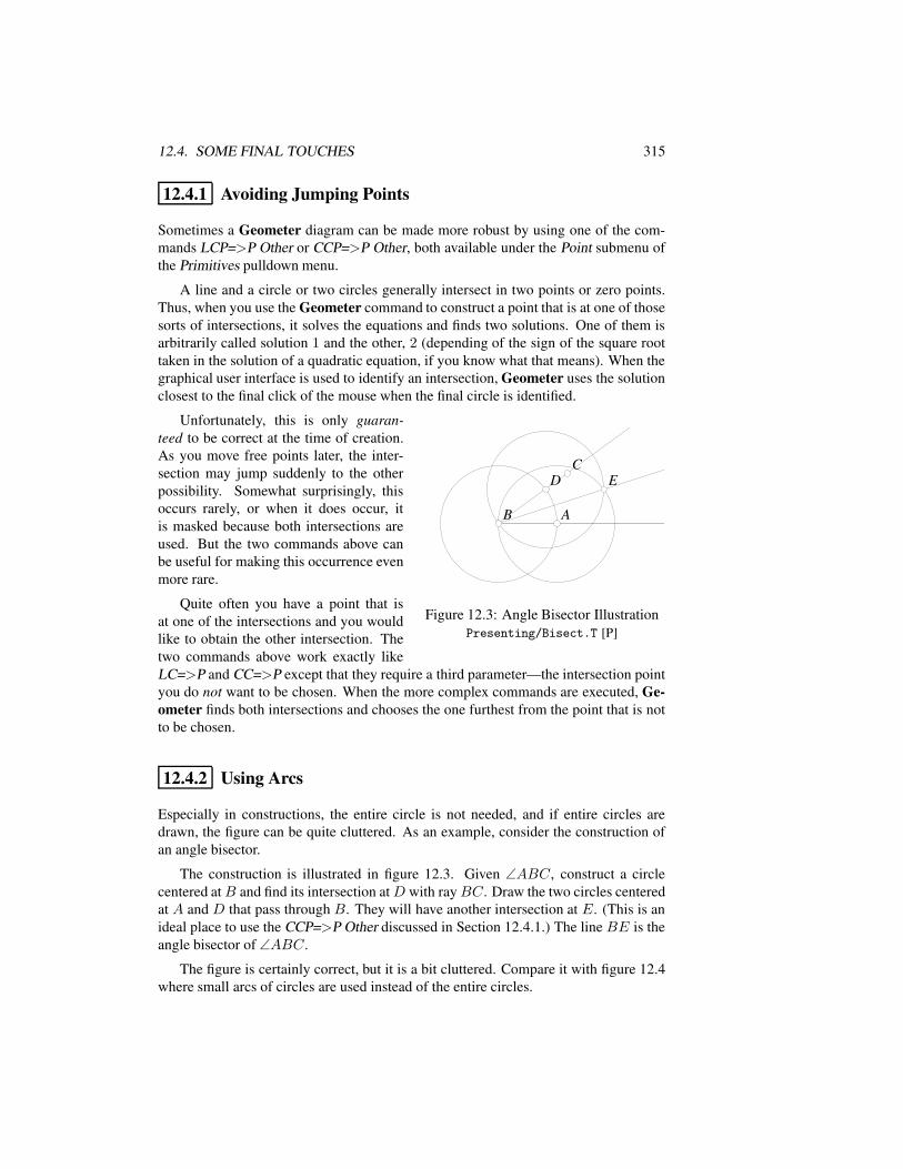
12.4. SOME FINAL TOUCHES 315
12.4.1 Avoiding Jumping Points
Sometimes a Geometer diagram can be made more robust by using one of the com-mands LCP=>P Other or CCP=>P Other, both available under the Point submenu ofthe Primitives pulldown menu.
A line and a circle or two circles generally intersect in two points or zero points.Thus, when you use the Geometer command to construct a point that is at one of thosesorts of intersections, it solves the equations and finds two solutions. One of them isarbitrarily called solution 1 and the other, 2 (depending of the sign of the square roottaken in the solution of a quadratic equation, if you know what that means). When thegraphical user interface is used to identify an intersection, Geometer uses the solutionclosest to the final click of the mouse when the final circle is identified.
AABB
CCDD EE
Figure 12.3: Angle Bisector IllustrationPresenting/Bisect.T [P]
Unfortunately, this is only guaran-teed to be correct at the time of creation.As you move free points later, the inter-section may jump suddenly to the otherpossibility. Somewhat surprisingly, thisoccurs rarely, or when it does occur, itis masked because both intersections areused. But the two commands above canbe useful for making this occurrence evenmore rare.
Quite often you have a point that isat one of the intersections and you wouldlike to obtain the other intersection. Thetwo commands above work exactly likeLC=>P and CC=>P except that they require a third parameter—the intersection pointyou do not want to be chosen. When the more complex commands are executed, Ge-ometer finds both intersections and chooses the one furthest from the point that is notto be chosen.
12.4.2 Using Arcs
Especially in constructions, the entire circle is not needed, and if entire circles aredrawn, the figure can be quite cluttered. As an example, consider the construction ofan angle bisector.
The construction is illustrated in figure 12.3. Given ∠ABC, construct a circlecentered atB and find its intersection atD with rayBC. Draw the two circles centeredat A and D that pass through B. They will have another intersection at E. (This is anideal place to use the CCP=>P Other discussed in Section 12.4.1.) The line BE is theangle bisector of ∠ABC.
The figure is certainly correct, but it is a bit cluttered. Compare it with figure 12.4where small arcs of circles are used instead of the entire circles.
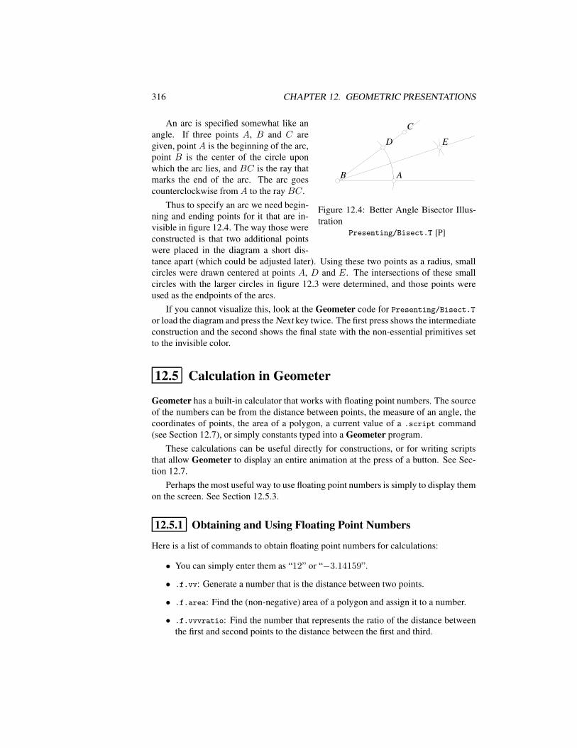
316 CHAPTER 12. GEOMETRIC PRESENTATIONS
AABB
CC
DD EE
Figure 12.4: Better Angle Bisector Illus-tration
Presenting/Bisect.T [P]
An arc is specified somewhat like anangle. If three points A, B and C aregiven, point A is the beginning of the arc,point B is the center of the circle uponwhich the arc lies, and BC is the ray thatmarks the end of the arc. The arc goescounterclockwise from A to the ray BC.
Thus to specify an arc we need begin-ning and ending points for it that are in-visible in figure 12.4. The way those wereconstructed is that two additional pointswere placed in the diagram a short dis-tance apart (which could be adjusted later). Using these two points as a radius, smallcircles were drawn centered at points A, D and E. The intersections of these smallcircles with the larger circles in figure 12.3 were determined, and those points wereused as the endpoints of the arcs.
If you cannot visualize this, look at the Geometer code for Presenting/Bisect.Tor load the diagram and press the Next key twice. The first press shows the intermediateconstruction and the second shows the final state with the non-essential primitives setto the invisible color.
12.5 Calculation in Geometer
Geometer has a built-in calculator that works with floating point numbers. The sourceof the numbers can be from the distance between points, the measure of an angle, thecoordinates of points, the area of a polygon, a current value of a .script command(see Section 12.7), or simply constants typed into a Geometer program.
These calculations can be useful directly for constructions, or for writing scriptsthat allow Geometer to display an entire animation at the press of a button. See Sec-tion 12.7.
Perhaps the most useful way to use floating point numbers is simply to display themon the screen. See Section 12.5.3.
12.5.1 Obtaining and Using Floating Point Numbers
Here is a list of commands to obtain floating point numbers for calculations:
• You can simply enter them as “12” or “−3.14159”.
• .f.vv: Generate a number that is the distance between two points.
• .f.area: Find the (non-negative) area of a polygon and assign it to a number.
• .f.vvvratio: Find the number that represents the ratio of the distance betweenthe first and second points to the distance between the first and third.
12.5. CALCULATION IN GEOMETER 317
• .f.vxcoord: Assign the x-coordinate of a point to a number.
• .f.vycoord: Assign the y-coordinate of a point to a number.
• You can also use angles directly as floating point numbers. The angles are mea-sured in degrees or radians, depending on the mode of Geometer. By default,Geometer is in degree mode.
Once you have some numbers to work with, you can do arbitrary calculations withthe command .f.rpn (discussed below).
After you have done your calculations, you can use the results of your calculationsas follows:
• .v.ff: Create a point whose coordinates are given by two floating point numbers.
• .c.vf: Create a circle with a point as center and number as radius.
• .a.f: Create an angle whose value is the floating point number. The angle’s sizeis set depending on whether Geometer is in degree or radian mode.
• Floating point numbers can be used in almost all of the transformation com-mands. See Section 12.6.
12.5.2 Calculating with Floating Point Numbers
Finally, you need to know how to calculate. All calculations are done with a singlefunction, .f.rpn. The “rpn” stands for “reverse Polish notation” which is a stack-basedsystem of calculation that eliminates the need for parentheses and complex parsing.
In the case of Geometer, the stack is simply an initially empty pile of numbers,and each new number is conceptually piled on top of the others. You can only accessthe stack from the top—sort of like a pile of trays in a cafeteria. You can put trays ontop or take them off the top, but it is difficult to access the trays below without firstremoving the ones on top.
The .f.rpn command is a list of numbers and operations that are evaluated fromleft to right. If it is a number or a variable that contains a number, the value of thatnumber is simply put on the top of the stack. If it is an operation, that operation isapplied to the top few elements of the stack and the result is usually put back on top ofthe stack. At the end of the evaluation, whatever number is left on top of the stack isthe result of the calculation.
For example, the operation .add adds the top two stack elements, removing themfrom the stack, and the sum is put back on the stack. The following command assignsthe value of 5 to r:
r = .f.rpn(2, 3, .add);
318 CHAPTER 12. GEOMETRIC PRESENTATIONS
The first two items are numbers, so each is put on top of the stack. When it istime to evaluate the .add, the stack consists of a 3 on top of a 2. The .add commandremoves the top two numbers (all of them in this case), adds them to obtain 5, and thenplaces the 5 on top of the stack. Since the .add is the final operation in this example,the value of 5 is assigned to r.
An application can be as simple as this:
p = .f.rpn(0.95);
which simply assigns the value 0.95 to the variable r.
It takes a bit of practice, but it is possible to evaluate extremely complex functionsusing this simple notation. For example, suppose we would like to evaluate:
r = sin(x2 − 3x) cos(1/x).
Here is the statement that will accomplish it:
r = .f.rpn(x, x, .mul, 3, x, .mul,
.sub, .sin, 1, x, .div, .cos, .mul);
The function puts on two copies of x, multiplies them, and returns the value of x2
to the stack. Then a 3 and an x are added on top of the x2. Those top two numbers aremultiplied and replaced on the stack leaving an x2 under a 3x. Those two values aresubtracted and the result is returned to the stack, leaving x2−3x on the stack. Next, thesine function is applied to the top stack element and the result is returned to the stackleaving a sin(x2 − 3x). The process continues in this way until the entire expressionis evaluated. Geometer understands about 30 operations and all are documented in thereference manual.
In the sections that follow, a few additional examples appear, but as one final exam-ple, here is some code to calculate the area of a triangle given the lengths of the sidesusing Heron’s formula. If a, b, and c are the lengths of the sides of a triangle, then ifs = (a + b + c)/2 is the semiperimeter, Heron’s formula tells us that the area of thetriangle is given by:
A =√s(s− a)(s− b)(s− c).
Here is Geometer code to do the calculation, supposing that the points are internallynamed v1, v2 and v3:
a = .f.vv(v1, v2);
b = .f.vv(v2, v3);
c = .f.vv(v3, v1);
s = .f.rpn(a, b, c, .add, .add, 2, .div);
A = .f.rpn(s, s, a, .sub, .mul, s, b, .sub,
.mul, s, c, .sub, .mul, .sqrt);
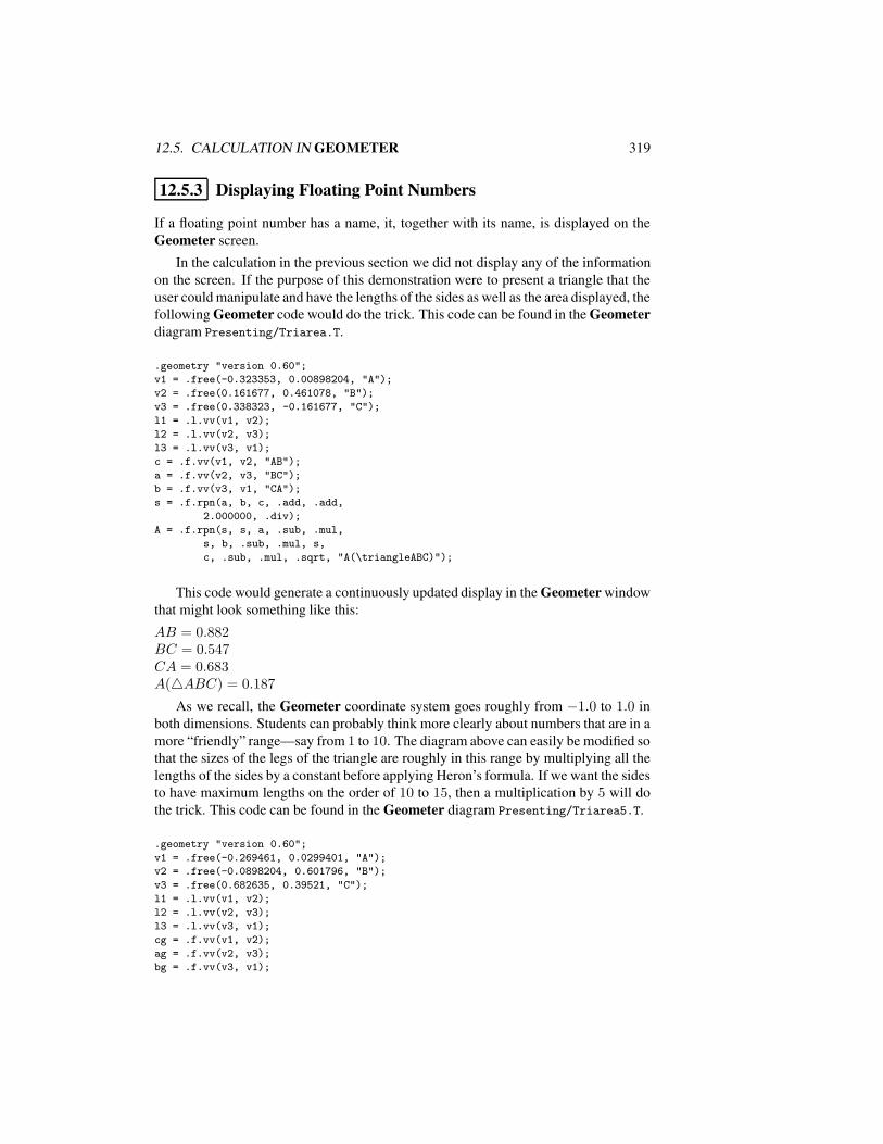
12.5. CALCULATION IN GEOMETER 319
12.5.3 Displaying Floating Point Numbers
If a floating point number has a name, it, together with its name, is displayed on theGeometer screen.
In the calculation in the previous section we did not display any of the informationon the screen. If the purpose of this demonstration were to present a triangle that theuser could manipulate and have the lengths of the sides as well as the area displayed, thefollowing Geometer code would do the trick. This code can be found in the Geometerdiagram Presenting/Triarea.T.
.geometry "version 0.60";
v1 = .free(-0.323353, 0.00898204, "A");
v2 = .free(0.161677, 0.461078, "B");
v3 = .free(0.338323, -0.161677, "C");
l1 = .l.vv(v1, v2);
l2 = .l.vv(v2, v3);
l3 = .l.vv(v3, v1);
c = .f.vv(v1, v2, "AB");
a = .f.vv(v2, v3, "BC");
b = .f.vv(v3, v1, "CA");
s = .f.rpn(a, b, c, .add, .add,
2.000000, .div);
A = .f.rpn(s, s, a, .sub, .mul,
s, b, .sub, .mul, s,
c, .sub, .mul, .sqrt, "A(\triangleABC)");
This code would generate a continuously updated display in the Geometer windowthat might look something like this:
AB = 0.882BC = 0.547CA = 0.683A(4ABC) = 0.187
As we recall, the Geometer coordinate system goes roughly from −1.0 to 1.0 inboth dimensions. Students can probably think more clearly about numbers that are in amore “friendly” range—say from 1 to 10. The diagram above can easily be modified sothat the sizes of the legs of the triangle are roughly in this range by multiplying all thelengths of the sides by a constant before applying Heron’s formula. If we want the sidesto have maximum lengths on the order of 10 to 15, then a multiplication by 5 will dothe trick. This code can be found in the Geometer diagram Presenting/Triarea5.T.
.geometry "version 0.60";
v1 = .free(-0.269461, 0.0299401, "A");
v2 = .free(-0.0898204, 0.601796, "B");
v3 = .free(0.682635, 0.39521, "C");
l1 = .l.vv(v1, v2);
l2 = .l.vv(v2, v3);
l3 = .l.vv(v3, v1);
cg = .f.vv(v1, v2);
ag = .f.vv(v2, v3);
bg = .f.vv(v3, v1);
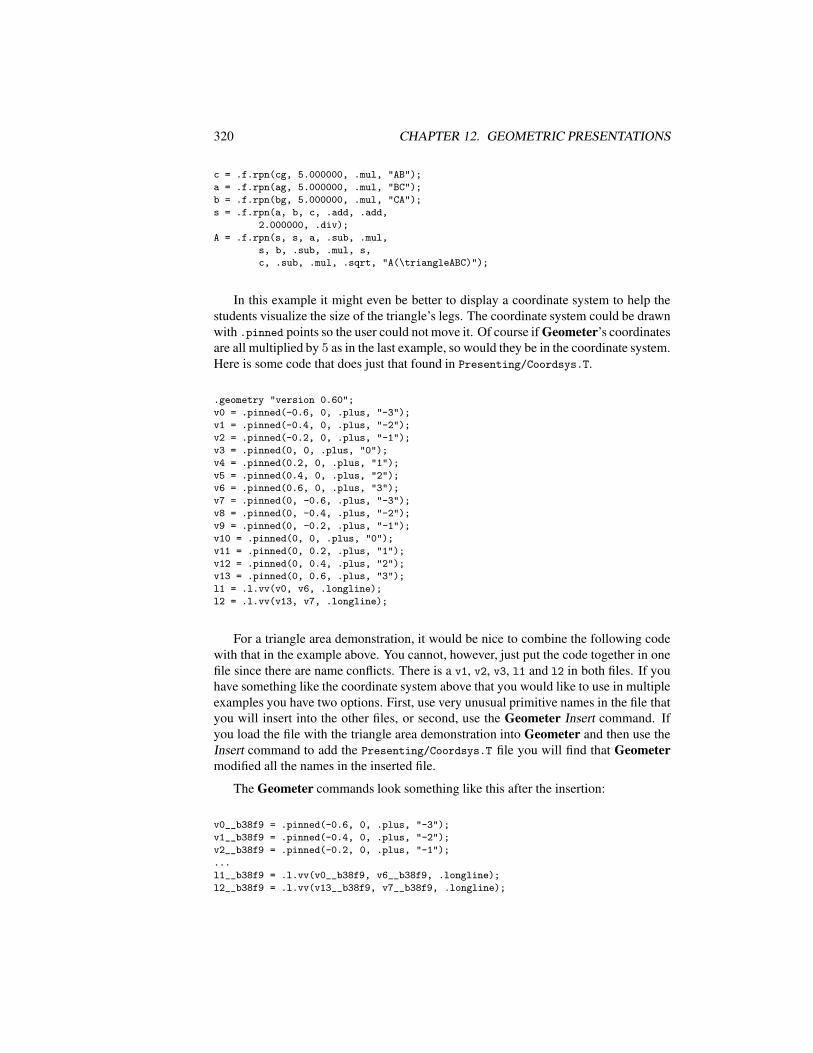
320 CHAPTER 12. GEOMETRIC PRESENTATIONS
c = .f.rpn(cg, 5.000000, .mul, "AB");
a = .f.rpn(ag, 5.000000, .mul, "BC");
b = .f.rpn(bg, 5.000000, .mul, "CA");
s = .f.rpn(a, b, c, .add, .add,
2.000000, .div);
A = .f.rpn(s, s, a, .sub, .mul,
s, b, .sub, .mul, s,
c, .sub, .mul, .sqrt, "A(\triangleABC)");
In this example it might even be better to display a coordinate system to help thestudents visualize the size of the triangle’s legs. The coordinate system could be drawnwith .pinned points so the user could not move it. Of course if Geometer’s coordinatesare all multiplied by 5 as in the last example, so would they be in the coordinate system.Here is some code that does just that found in Presenting/Coordsys.T.
.geometry "version 0.60";
v0 = .pinned(-0.6, 0, .plus, "-3");
v1 = .pinned(-0.4, 0, .plus, "-2");
v2 = .pinned(-0.2, 0, .plus, "-1");
v3 = .pinned(0, 0, .plus, "0");
v4 = .pinned(0.2, 0, .plus, "1");
v5 = .pinned(0.4, 0, .plus, "2");
v6 = .pinned(0.6, 0, .plus, "3");
v7 = .pinned(0, -0.6, .plus, "-3");
v8 = .pinned(0, -0.4, .plus, "-2");
v9 = .pinned(0, -0.2, .plus, "-1");
v10 = .pinned(0, 0, .plus, "0");
v11 = .pinned(0, 0.2, .plus, "1");
v12 = .pinned(0, 0.4, .plus, "2");
v13 = .pinned(0, 0.6, .plus, "3");
l1 = .l.vv(v0, v6, .longline);
l2 = .l.vv(v13, v7, .longline);
For a triangle area demonstration, it would be nice to combine the following codewith that in the example above. You cannot, however, just put the code together in onefile since there are name conflicts. There is a v1, v2, v3, l1 and l2 in both files. If youhave something like the coordinate system above that you would like to use in multipleexamples you have two options. First, use very unusual primitive names in the file thatyou will insert into the other files, or second, use the Geometer Insert command. Ifyou load the file with the triangle area demonstration into Geometer and then use theInsert command to add the Presenting/Coordsys.T file you will find that Geometermodified all the names in the inserted file.
The Geometer commands look something like this after the insertion:
v0__b38f9 = .pinned(-0.6, 0, .plus, "-3");
v1__b38f9 = .pinned(-0.4, 0, .plus, "-2");
v2__b38f9 = .pinned(-0.2, 0, .plus, "-1");
...
l1__b38f9 = .l.vv(v0__b38f9, v6__b38f9, .longline);
l2__b38f9 = .l.vv(v13__b38f9, v7__b38f9, .longline);
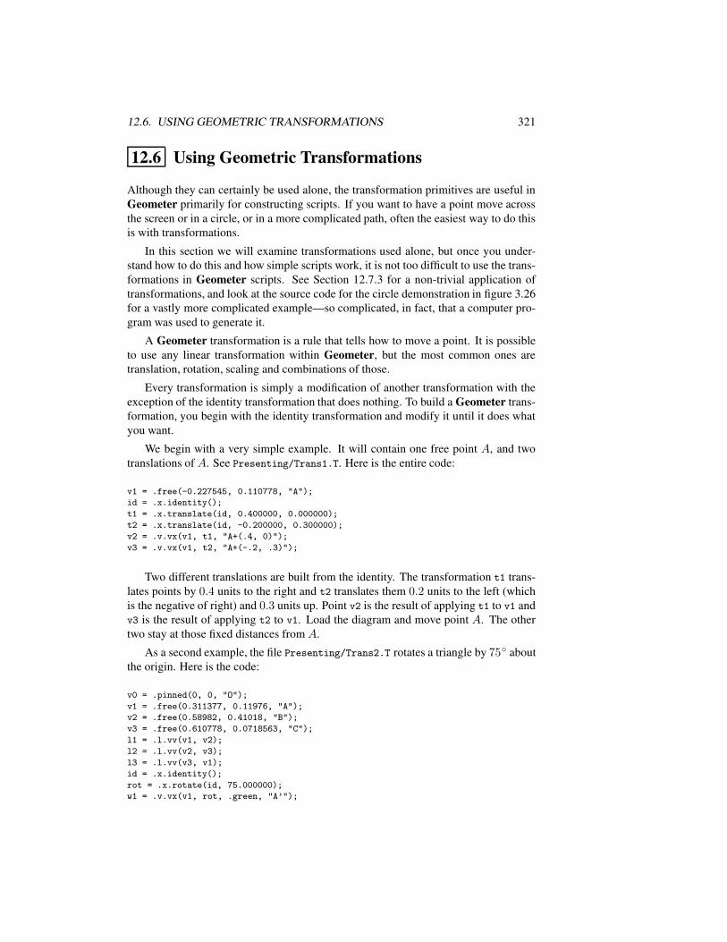
12.6. USING GEOMETRIC TRANSFORMATIONS 321
12.6 Using Geometric Transformations
Although they can certainly be used alone, the transformation primitives are useful inGeometer primarily for constructing scripts. If you want to have a point move acrossthe screen or in a circle, or in a more complicated path, often the easiest way to do thisis with transformations.
In this section we will examine transformations used alone, but once you under-stand how to do this and how simple scripts work, it is not too difficult to use the trans-formations in Geometer scripts. See Section 12.7.3 for a non-trivial application oftransformations, and look at the source code for the circle demonstration in figure 3.26for a vastly more complicated example—so complicated, in fact, that a computer pro-gram was used to generate it.
A Geometer transformation is a rule that tells how to move a point. It is possibleto use any linear transformation within Geometer, but the most common ones aretranslation, rotation, scaling and combinations of those.
Every transformation is simply a modification of another transformation with theexception of the identity transformation that does nothing. To build a Geometer trans-formation, you begin with the identity transformation and modify it until it does whatyou want.
We begin with a very simple example. It will contain one free point A, and twotranslations of A. See Presenting/Trans1.T. Here is the entire code:
v1 = .free(-0.227545, 0.110778, "A");
id = .x.identity();
t1 = .x.translate(id, 0.400000, 0.000000);
t2 = .x.translate(id, -0.200000, 0.300000);
v2 = .v.vx(v1, t1, "A+(.4, 0)");
v3 = .v.vx(v1, t2, "A+(-.2, .3)");
Two different translations are built from the identity. The transformation t1 trans-lates points by 0.4 units to the right and t2 translates them 0.2 units to the left (whichis the negative of right) and 0.3 units up. Point v2 is the result of applying t1 to v1 andv3 is the result of applying t2 to v1. Load the diagram and move point A. The othertwo stay at those fixed distances from A.
As a second example, the file Presenting/Trans2.T rotates a triangle by 75 aboutthe origin. Here is the code:
v0 = .pinned(0, 0, "O");
v1 = .free(0.311377, 0.11976, "A");
v2 = .free(0.58982, 0.41018, "B");
v3 = .free(0.610778, 0.0718563, "C");
l1 = .l.vv(v1, v2);
l2 = .l.vv(v2, v3);
l3 = .l.vv(v3, v1);
id = .x.identity();
rot = .x.rotate(id, 75.000000);
w1 = .v.vx(v1, rot, .green, "A’");
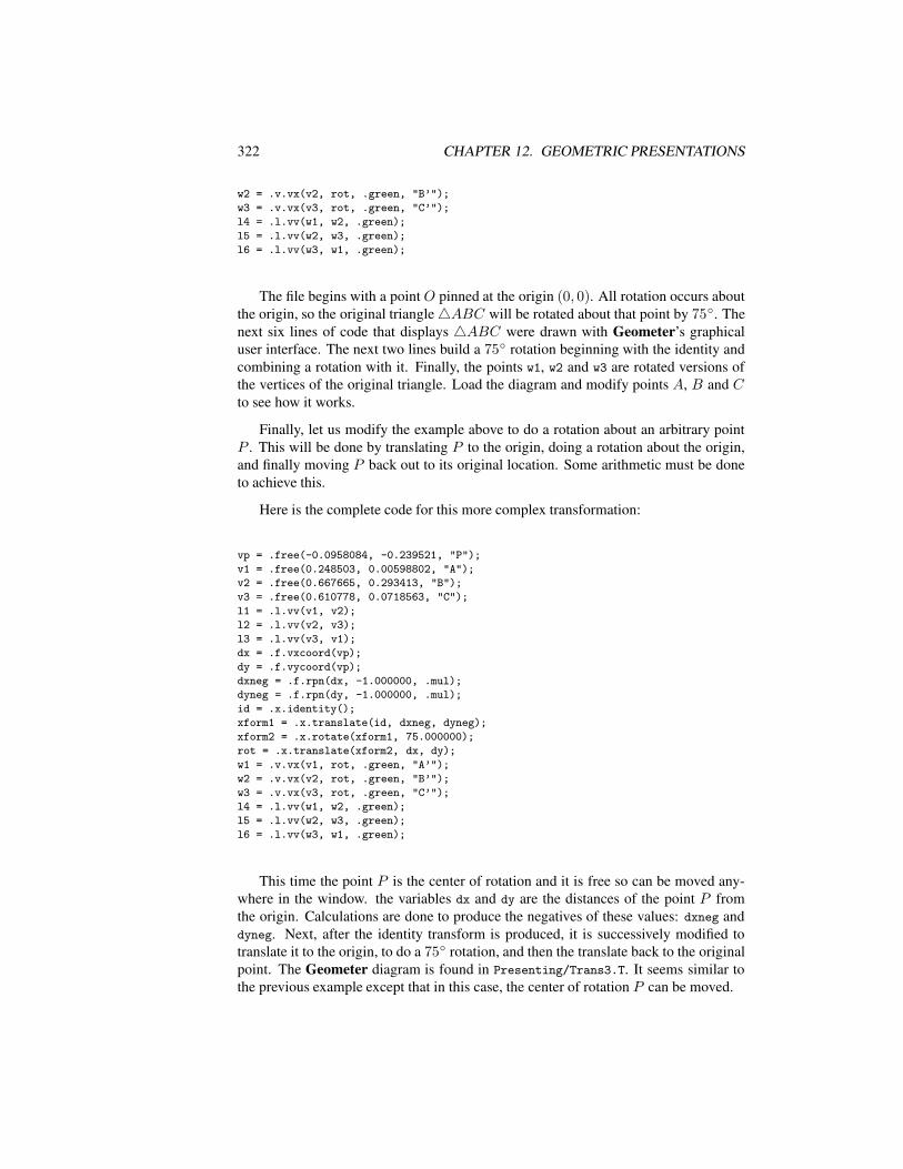
322 CHAPTER 12. GEOMETRIC PRESENTATIONS
w2 = .v.vx(v2, rot, .green, "B’");
w3 = .v.vx(v3, rot, .green, "C’");
l4 = .l.vv(w1, w2, .green);
l5 = .l.vv(w2, w3, .green);
l6 = .l.vv(w3, w1, .green);
The file begins with a point O pinned at the origin (0, 0). All rotation occurs aboutthe origin, so the original triangle4ABC will be rotated about that point by 75. Thenext six lines of code that displays 4ABC were drawn with Geometer’s graphicaluser interface. The next two lines build a 75 rotation beginning with the identity andcombining a rotation with it. Finally, the points w1, w2 and w3 are rotated versions ofthe vertices of the original triangle. Load the diagram and modify points A, B and Cto see how it works.
Finally, let us modify the example above to do a rotation about an arbitrary pointP . This will be done by translating P to the origin, doing a rotation about the origin,and finally moving P back out to its original location. Some arithmetic must be doneto achieve this.
Here is the complete code for this more complex transformation:
vp = .free(-0.0958084, -0.239521, "P");
v1 = .free(0.248503, 0.00598802, "A");
v2 = .free(0.667665, 0.293413, "B");
v3 = .free(0.610778, 0.0718563, "C");
l1 = .l.vv(v1, v2);
l2 = .l.vv(v2, v3);
l3 = .l.vv(v3, v1);
dx = .f.vxcoord(vp);
dy = .f.vycoord(vp);
dxneg = .f.rpn(dx, -1.000000, .mul);
dyneg = .f.rpn(dy, -1.000000, .mul);
id = .x.identity();
xform1 = .x.translate(id, dxneg, dyneg);
xform2 = .x.rotate(xform1, 75.000000);
rot = .x.translate(xform2, dx, dy);
w1 = .v.vx(v1, rot, .green, "A’");
w2 = .v.vx(v2, rot, .green, "B’");
w3 = .v.vx(v3, rot, .green, "C’");
l4 = .l.vv(w1, w2, .green);
l5 = .l.vv(w2, w3, .green);
l6 = .l.vv(w3, w1, .green);
This time the point P is the center of rotation and it is free so can be moved any-where in the window. the variables dx and dy are the distances of the point P fromthe origin. Calculations are done to produce the negatives of these values: dxneg anddyneg. Next, after the identity transform is produced, it is successively modified totranslate it to the origin, to do a 75 rotation, and then the translate back to the originalpoint. The Geometer diagram is found in Presenting/Trans3.T. It seems similar tothe previous example except that in this case, the center of rotation P can be moved.
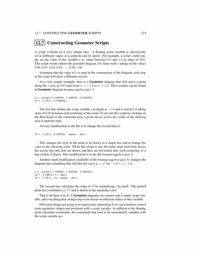
12.7. CONSTRUCTING GEOMETER SCRIPTS 323
12.7 Constructing Geometer Scripts
A script is based on a very simple idea. A floating point variable is successivelyset to different values at a uniform rate of speed. For example, a script could sim-ply set the value of the variable t to values between 0.0 and 1.0 in steps of 0.01.This script would redraw the geometer diagram 101 times with t taking on the values0.00, 0.01, 0.02, 0.03, . . . , 0.99, 1.00.
Assuming that the value of t is used in the construction of the diagram, each stepin the script will draw a different version.
As a very simple example, here is a Geometer diagram that will move a pointalong the x-axis in 101 steps from x = −1.0 to x = 1.0. This example can be foundin Geometer diagram Presenting/Script1.T.
t = .script(-1.000000, 1.000000, 0.020000);
v0 = .v.ff(t, 0.000000);
The first line defines the script variable t to begin at −1.0 and to end at 1.0 takingsteps of 0.02 between each rendering of the scene. If you run this script by clicking onthe Run Script in the command area, a point moves across the center of the drawingarea in uniform steps.
An easy modification to the file is to change the second line to:
v0 = .v.ff(t, 0.000000, .smear, .dot);
This changes the style of the point to be drawn as a single dot, and to change thecolor to the smearing color. When this script is run, the point steps uniformly acrossthe screen, but only dots are drawn, and they are not erased after each rendering, so aline of dots is drawn. This modification is in the file Presenting/Script2.T.
Another small modification (available in file Presenting/Script3.T) changes thediagram into something that will plot the curve y = x2 for −1.0 ≤ x ≤ 1.0:
t = .script(-1.000000, 1.000000, 0.020000);
t2 = .f.rpn(t, t, .mul);
v0 = .v.ff(t, t2, .smear, .dot);
The second line calculates the value of t2 by multiplying t by itself. The plottedpoint has coordinates (t, t2) and is drawn in the smearing color.
That is all there is to it! A Geometer diagram can contain only a single script vari-able, and everything that changes has to be based on different values of that variable.
Obviously things are going to be much more interesting if we can somehow controlsome geometric shapes and positions with a script variable. In addition to the floatingpoint calculator commands, the commands that tend to be immediately valuable withthe script variable are:
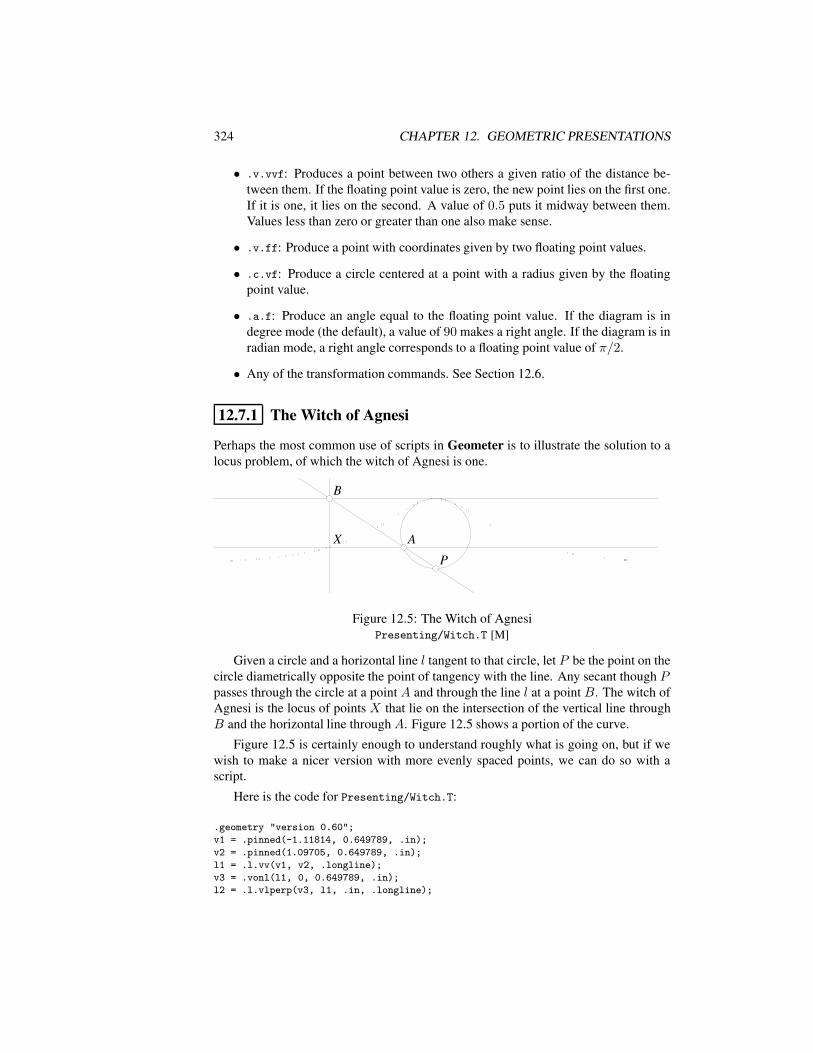
324 CHAPTER 12. GEOMETRIC PRESENTATIONS
• .v.vvf: Produces a point between two others a given ratio of the distance be-tween them. If the floating point value is zero, the new point lies on the first one.If it is one, it lies on the second. A value of 0.5 puts it midway between them.Values less than zero or greater than one also make sense.
• .v.ff: Produce a point with coordinates given by two floating point values.
• .c.vf: Produce a circle centered at a point with a radius given by the floatingpoint value.
• .a.f: Produce an angle equal to the floating point value. If the diagram is indegree mode (the default), a value of 90 makes a right angle. If the diagram is inradian mode, a right angle corresponds to a floating point value of π/2.
• Any of the transformation commands. See Section 12.6.
12.7.1 The Witch of Agnesi
Perhaps the most common use of scripts in Geometer is to illustrate the solution to alocus problem, of which the witch of Agnesi is one.
PP
BB
AAXX
Figure 12.5: The Witch of AgnesiPresenting/Witch.T [M]
Given a circle and a horizontal line l tangent to that circle, let P be the point on thecircle diametrically opposite the point of tangency with the line. Any secant though Ppasses through the circle at a point A and through the line l at a point B. The witch ofAgnesi is the locus of points X that lie on the intersection of the vertical line throughB and the horizontal line throughA. Figure 12.5 shows a portion of the curve.
Figure 12.5 is certainly enough to understand roughly what is going on, but if wewish to make a nicer version with more evenly spaced points, we can do so with ascript.
Here is the code for Presenting/Witch.T:
.geometry "version 0.60";
v1 = .pinned(-1.11814, 0.649789, .in);
v2 = .pinned(1.09705, 0.649789, .in);
l1 = .l.vv(v1, v2, .longline);
v3 = .vonl(l1, 0, 0.649789, .in);
l2 = .l.vlperp(v3, l1, .in, .longline);
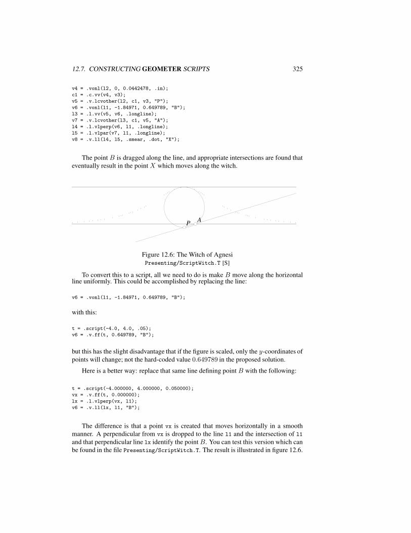
12.7. CONSTRUCTING GEOMETER SCRIPTS 325
v4 = .vonl(l2, 0, 0.0442478, .in);
c1 = .c.vv(v4, v3);
v5 = .v.lcvother(l2, c1, v3, "P");
v6 = .vonl(l1, -1.84971, 0.649789, "B");
l3 = .l.vv(v5, v6, .longline);
v7 = .v.lcvother(l3, c1, v5, "A");
l4 = .l.vlperp(v6, l1, .longline);
l5 = .l.vlpar(v7, l1, .longline);
v8 = .v.ll(l4, l5, .smear, .dot, "X");
The point B is dragged along the line, and appropriate intersections are found thateventually result in the point X which moves along the witch.
PP
BB
AA XX
Figure 12.6: The Witch of AgnesiPresenting/ScriptWitch.T [S]
To convert this to a script, all we need to do is make B move along the horizontalline uniformly. This could be accomplished by replacing the line:
v6 = .vonl(l1, -1.84971, 0.649789, "B");
with this:
t = .script(-4.0, 4.0, .05);
v6 = .v.ff(t, 0.649789, "B");
but this has the slight disadvantage that if the figure is scaled, only the y-coordinates ofpoints will change; not the hard-coded value 0.649789 in the proposed solution.
Here is a better way: replace that same line defining point B with the following:
t = .script(-4.000000, 4.000000, 0.050000);
vx = .v.ff(t, 0.000000);
lx = .l.vlperp(vx, l1);
v6 = .v.ll(lx, l1, "B");
The difference is that a point vx is created that moves horizontally in a smoothmanner. A perpendicular from vx is dropped to the line l1 and the intersection of l1and that perpendicular line lx identify the pointB. You can test this version which canbe found in the file Presenting/ScriptWitch.T. The result is illustrated in figure 12.6.
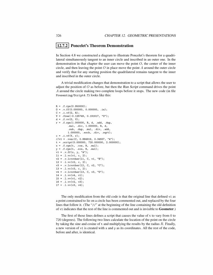
326 CHAPTER 12. GEOMETRIC PRESENTATIONS
12.7.2 Poncelet’s Theorem Demonstration
In Section 4.8 we constructed a diagram to illustrate Poncelet’s theorem for a quadri-lateral simultaneously tangent to an inner circle and inscribed in an outer one. In thedemonstration in that chapter the user can move the point O, the center of the innercircle, and then leaving the point O in place move the point A around the outer circleand verify that for any starting position the quadrilateral remains tangent to the innerand inscribed in the outer circle.
A trivial modification changes that demonstration to a script that allows the user toadjust the position of O as before, but then the Run Script command drives the pointA around the circle making two complete loops before it stops. The new code (in filePresenting/Script4.T) looks like this:
R = .f.rpn(0.950000);
O = .v.ff(0.000000, 0.000000, .in);
C = .c.vf(O, R);
V = .free(-0.125749, 0.191617, "O");
d = .f.vv(O, V);
r = .f.rpn(1.000000, R, d, .add, .dup,
.mul, .div, 1.000000, R, d,
.sub, .dup, .mul, .div, .add,
1.000000, .exch, .div, .sqrt);
c = .c.vf(V, r);
//v1 = .vonc(C, 0.884919, 0.34557, "A");
t = .script(0.000000, 720.000000, 2.000000);
x = .f.rpn(t, .cos, R, .mul);
y = .f.rpn(t, .sin, R, .mul);
v1 = .v.ff(x, y, "A");
l1 = .l.vc(v1, c, 2);
v2 = .v.lcvother(l1, C, v1, "B");
l2 = .l.vc(v2, c, 2);
v3 = .v.lcvother(l2, C, v2, "C");
l3 = .l.vc(v3, c, 2);
v4 = .v.lcvother(l3, C, v3, "D");
l4 = .l.vv(v4, v1);
l5 = .l.vv(v1, v2);
l6 = .l.vv(v2, v3);
l7 = .l.vv(v3, v4);
The only modification from the old code is that the original line that defined v1 asa point constrained to lie on a circle has been commented out, and replaced by the fourlines that follow it. (The “//” at the beginning of the line containing the old definitionof v1 indicates that the rest of the line is commented out and is invisible to Geometer.)
The first of those lines defines a script that causes the value of t to vary from 0 to720 (degrees). The following two lines calculate the location of the point on the circleby taking the sine and cosine of t and multiplying the results by the radius R. Finally,a new version of v1 is created with x and y as its coordinates. All the rest of the code,before and after, is identical.
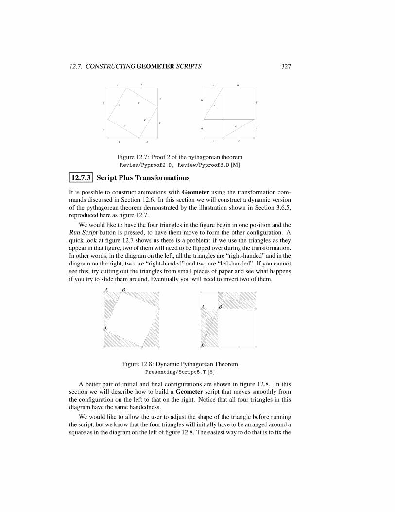
12.7. CONSTRUCTING GEOMETER SCRIPTS 327
aa bb
aa
bb
aabb
aa
bb cc cc
cc
cc
aa bb
aa bb
aa
bb
aa
bb
cc
cc
Figure 12.7: Proof 2 of the pythagorean theoremReview/Pyproof2.D, Review/Pyproof3.D [M]
12.7.3 Script Plus Transformations
It is possible to construct animations with Geometer using the transformation com-mands discussed in Section 12.6. In this section we will construct a dynamic versionof the pythagorean theorem demonstrated by the illustration shown in Section 3.6.5,reproduced here as figure 12.7.
We would like to have the four triangles in the figure begin in one position and theRun Script button is pressed, to have them move to form the other configuration. Aquick look at figure 12.7 shows us there is a problem: if we use the triangles as theyappear in that figure, two of them will need to be flipped over during the transformation.In other words, in the diagram on the left, all the triangles are “right-handed” and in thediagram on the right, two are “right-handed” and two are “left-handed”. If you cannotsee this, try cutting out the triangles from small pieces of paper and see what happensif you try to slide them around. Eventually you will need to invert two of them.
AA BB
CC
AA BB
CC
Figure 12.8: Dynamic Pythagorean TheoremPresenting/Script5.T [S]
A better pair of initial and final configurations are shown in figure 12.8. In thissection we will describe how to build a Geometer script that moves smoothly fromthe configuration on the left to that on the right. Notice that all four triangles in thisdiagram have the same handedness.
We would like to allow the user to adjust the shape of the triangle before runningthe script, but we know that the four triangles will initially have to be arranged around asquare as in the diagram on the left of figure 12.8. The easiest way to do that is to fix the
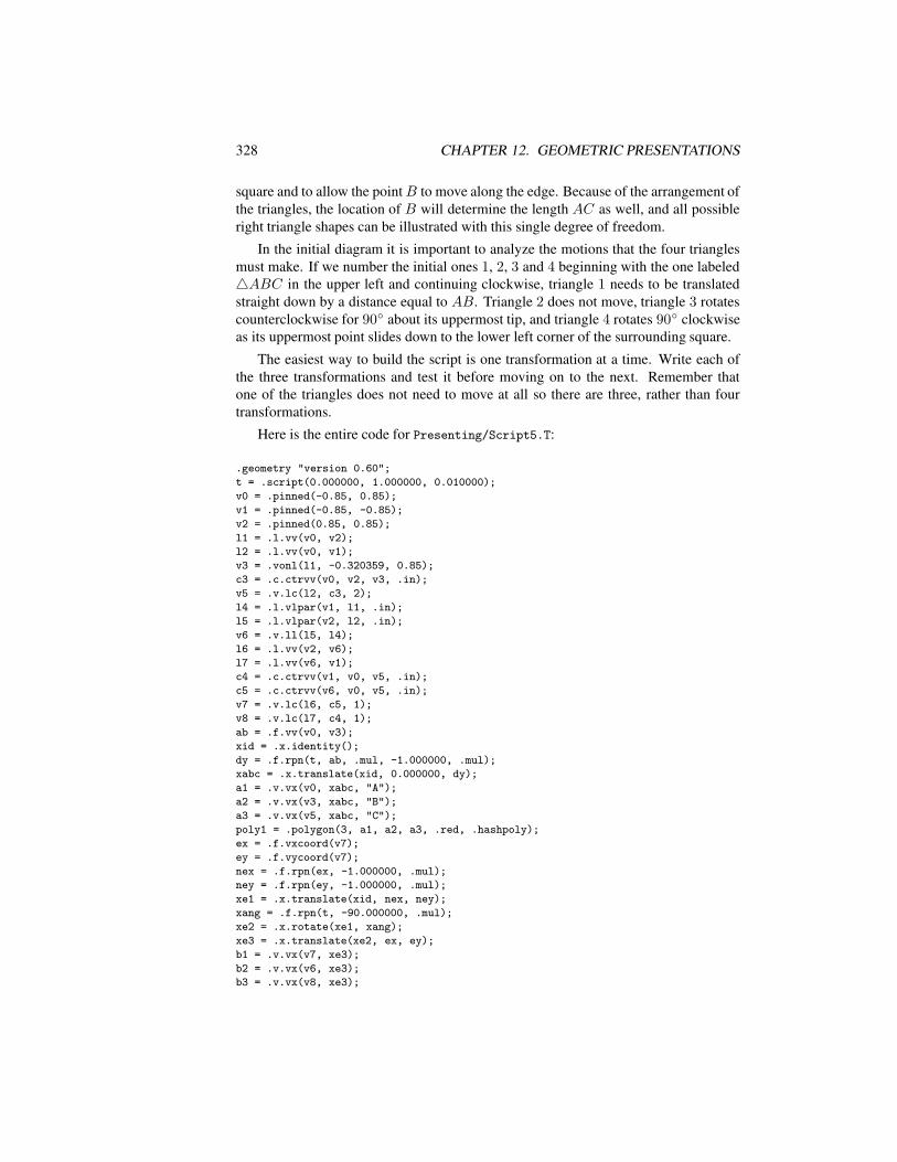
328 CHAPTER 12. GEOMETRIC PRESENTATIONS
square and to allow the pointB to move along the edge. Because of the arrangement ofthe triangles, the location of B will determine the length AC as well, and all possibleright triangle shapes can be illustrated with this single degree of freedom.
In the initial diagram it is important to analyze the motions that the four trianglesmust make. If we number the initial ones 1, 2, 3 and 4 beginning with the one labeled4ABC in the upper left and continuing clockwise, triangle 1 needs to be translatedstraight down by a distance equal to AB. Triangle 2 does not move, triangle 3 rotatescounterclockwise for 90 about its uppermost tip, and triangle 4 rotates 90 clockwiseas its uppermost point slides down to the lower left corner of the surrounding square.
The easiest way to build the script is one transformation at a time. Write each ofthe three transformations and test it before moving on to the next. Remember thatone of the triangles does not need to move at all so there are three, rather than fourtransformations.
Here is the entire code for Presenting/Script5.T:
.geometry "version 0.60";
t = .script(0.000000, 1.000000, 0.010000);
v0 = .pinned(-0.85, 0.85);
v1 = .pinned(-0.85, -0.85);
v2 = .pinned(0.85, 0.85);
l1 = .l.vv(v0, v2);
l2 = .l.vv(v0, v1);
v3 = .vonl(l1, -0.320359, 0.85);
c3 = .c.ctrvv(v0, v2, v3, .in);
v5 = .v.lc(l2, c3, 2);
l4 = .l.vlpar(v1, l1, .in);
l5 = .l.vlpar(v2, l2, .in);
v6 = .v.ll(l5, l4);
l6 = .l.vv(v2, v6);
l7 = .l.vv(v6, v1);
c4 = .c.ctrvv(v1, v0, v5, .in);
c5 = .c.ctrvv(v6, v0, v5, .in);
v7 = .v.lc(l6, c5, 1);
v8 = .v.lc(l7, c4, 1);
ab = .f.vv(v0, v3);
xid = .x.identity();
dy = .f.rpn(t, ab, .mul, -1.000000, .mul);
xabc = .x.translate(xid, 0.000000, dy);
a1 = .v.vx(v0, xabc, "A");
a2 = .v.vx(v3, xabc, "B");
a3 = .v.vx(v5, xabc, "C");
poly1 = .polygon(3, a1, a2, a3, .red, .hashpoly);
ex = .f.vxcoord(v7);
ey = .f.vycoord(v7);
nex = .f.rpn(ex, -1.000000, .mul);
ney = .f.rpn(ey, -1.000000, .mul);
xe1 = .x.translate(xid, nex, ney);
xang = .f.rpn(t, -90.000000, .mul);
xe2 = .x.rotate(xe1, xang);
xe3 = .x.translate(xe2, ex, ey);
b1 = .v.vx(v7, xe3);
b2 = .v.vx(v6, xe3);
b3 = .v.vx(v8, xe3);
12.7. CONSTRUCTING GEOMETER SCRIPTS 329
poly2 = .polygon(3, b1, b2, b3, .green, .hashpoly);
poly3 = .polygon(3, v2, v3, v7, .yellow, .hashpoly);
cx = .f.vxcoord(v5);
cy = .f.vycoord(v5);
ncx = .f.rpn(cx, -1.000000, .mul);
ncy = .f.rpn(cy, -1.000000, .mul);
xc1 = .x.translate(xid, ncx, ncy);
yang = .f.rpn(t, 90.000000, .mul);
xc2 = .x.rotate(xc1, yang);
xc3 = .x.translate(xc2, 0.000000, dy);
xc4 = .x.translate(xc3, cx, cy);
d1 = .v.vx(v1, xc4);
d2 = .v.vx(v5, xc4);
d3 = .v.vx(v8, xc4);
poly4 = .polygon(3, d1, d2, d3, .cyan, .hashpoly);
The first line defines a script variable t that varies from 0.0 to 1.0 in steps of 0.01.The 0.01 is not too important—we can adjust it later if the script seems to run too slowor too fast. The range 0.0 to 1.0 is arbitrary—we will have to transform it to moveangles from 0 to 90 and to translation amounts that depend on the lengths of thesides of4ABC.
The next few lines draw the surrounding square and define a point B that is con-strained to move on the upper line of the square. Notice that the point constrained tobe on the line does not have the name “B”. This is because the real point B will be atransformation of that point. Initially the transformation will be zero, but although thepoint v3 remains on the top edge of the enclosing square, its transformed image calledB will move down as the script proceeds.
In fact, in the construction of the diagram, all the vertices defining the four triangleswere visible and had readable names to make it easier to find the appropriate pointsto transform. When everything was working, the names were eliminated and certainconstructions were made invisible.
The next lines are standard Geometer constructions of the rest of the vertices on thesquare whose positions vary based on the location of the controlling point v3 (whichlooks like it is named B, but is not).
The script work begins with the line:
ab = .f.vv(v0, v3);
This line assigns the length of the segment AB to a variable called ab. Next webegin building a transformation that will slowly slide the triangle in the upper leftdownward. As all transformations must begin with an identity transform, that is whatis done in the next line. The amount of movement dy is calculated in the next line,and it depends on the script variable t. As t varies from 0.0 to 1.0 dy varies from0.0 to −AB. Next, xabc is produced by a translate command that moves objects by adistance dy in the y-direction and does not move them at all in the x-direction. Finally,transformation xabc is applied to the three initial vertices of the triangle in the upperleft corner to produce the version with vertices labeled A, B and C that slides downthe window.
330 CHAPTER 12. GEOMETRIC PRESENTATIONS
A polygon is drawn connecting these three vertices so that the solid effect will beobvious.
Next, a similar procedure is written to rotate the triangle in the lower right for 90
about its upper point. We cannot simply use a rotation command, since the rotationtransformation rotates about the origin. What we must do is translate the point to theorigin, rotate it there, and then translate back to the original position. That is whythe transformation xe3 is built in a series of steps: start with the identity, translateto the origin, do the rotation, and finally, translate back. When it is ready, the xe3
transformation is applied to the three vertices of the triangle in the lower right, andthose transformed points b1, b2 and b3 are connected to form a polygon.
The final transformation is almost the same, but it is a combination of a rotationand a translation. Thus the point about which the rotation is to occur is translated to theorigin, it is rotated and translated, and finally translated back to its original position,and the grand transformation that accomplishes all of this is called xc4. The originalvertices are transformed by xc4 and are also connected to form a polygon.
12.8 Computer-Generated Diagrams
Sometimes complex diagrams are required with hundreds or even thousands of lines.When that occurs, it is inefficient to enter thousands of primitives using the Geometerprogram. Geometer diagrams, however, are simply text files that can be generated byany means, including computer programs.
12.8.1 The Koch Snowflake Curve
The first example generates the first few approximations of the Koch snowflake curve—one of the simplest examples of a fractal. The “curve” is illustrated in figure 12.9.The first iteration is simply a triangle. The succeeding steps can be considered to besuccessive modifications of the previous version.
To traverse the triangle, imagine following three straight-line paths. In each suc-cessive iteration, replace the movement along a path by a four-step path that followsthe original path for 1/3 of its length, then turns to the right by 60 and continues forthe same distance. Next, turn 120 to the left, move another 1/3, and finally turn 60
to the right and follow the original curve to its end.After each such modification, the curve is composed of straight-line segments; just
four times as many of them. The first six stages are illustrated in figure 12.9. Whenthe Geometer diagram is loaded, the triangle appears, but each time the Next button ispressed, the next stage of the curve is presented.
The Geometer diagram simply consists of computer-generated sets of short linesegments that compose each stage, and those on each stage are presented on a newlayer.
The computer code (written in the C language) appears below and on the CD askoch.c:
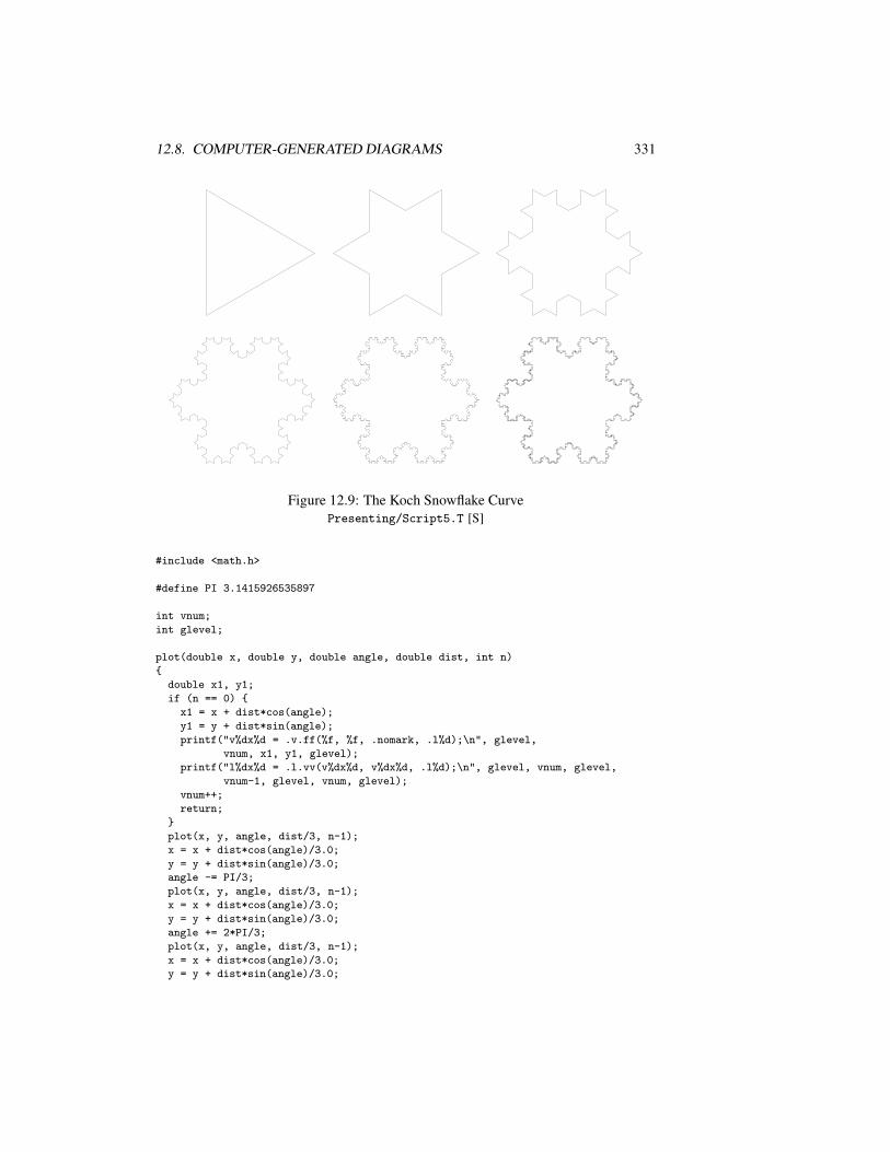
12.8. COMPUTER-GENERATED DIAGRAMS 331
Figure 12.9: The Koch Snowflake CurvePresenting/Script5.T [S]
#include <math.h>
#define PI 3.1415926535897
int vnum;
int glevel;
plot(double x, double y, double angle, double dist, int n)
double x1, y1;
if (n == 0)
x1 = x + dist*cos(angle);
y1 = y + dist*sin(angle);
printf("v%dx%d = .v.ff(%f, %f, .nomark, .l%d);\n", glevel,
vnum, x1, y1, glevel);
printf("l%dx%d = .l.vv(v%dx%d, v%dx%d, .l%d);\n", glevel, vnum, glevel,
vnum-1, glevel, vnum, glevel);
vnum++;
return;
plot(x, y, angle, dist/3, n-1);
x = x + dist*cos(angle)/3.0;
y = y + dist*sin(angle)/3.0;
angle -= PI/3;
plot(x, y, angle, dist/3, n-1);
x = x + dist*cos(angle)/3.0;
y = y + dist*sin(angle)/3.0;
angle += 2*PI/3;
plot(x, y, angle, dist/3, n-1);
x = x + dist*cos(angle)/3.0;
y = y + dist*sin(angle)/3.0;
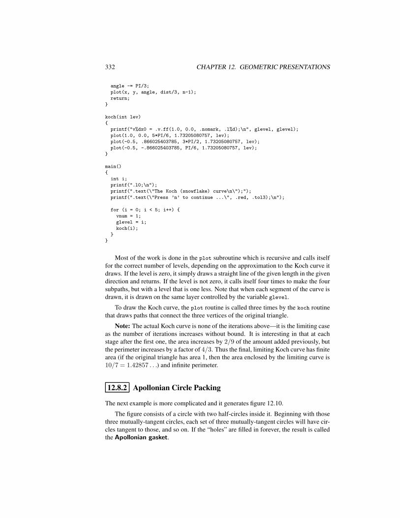
332 CHAPTER 12. GEOMETRIC PRESENTATIONS
angle -= PI/3;
plot(x, y, angle, dist/3, n-1);
return;
koch(int lev)
printf("v%dx0 = .v.ff(1.0, 0.0, .nomark, .l%d);\n", glevel, glevel);
plot(1.0, 0.0, 5*PI/6, 1.73205080757, lev);
plot(-0.5, .866025403785, 3*PI/2, 1.73205080757, lev);
plot(-0.5, -.866025403785, PI/6, 1.73205080757, lev);
main()
int i;
printf(".l0;\n");
printf(".text(\"The Koch (snowflake) curve\n\");");
printf(".text(\"Press ’n’ to continue ...\", .red, .tol3);\n");
for (i = 0; i < 5; i++)
vnum = 1;
glevel = i;
koch(i);
Most of the work is done in the plot subroutine which is recursive and calls itselffor the correct number of levels, depending on the approximation to the Koch curve itdraws. If the level is zero, it simply draws a straight line of the given length in the givendirection and returns. If the level is not zero, it calls itself four times to make the foursubpaths, but with a level that is one less. Note that when each segment of the curve isdrawn, it is drawn on the same layer controlled by the variable glevel.
To draw the Koch curve, the plot routine is called three times by the koch routinethat draws paths that connect the three vertices of the original triangle.
Note: The actual Koch curve is none of the iterations above—it is the limiting caseas the number of iterations increases without bound. It is interesting in that at eachstage after the first one, the area increases by 2/9 of the amount added previously, butthe perimeter increases by a factor of 4/3. Thus the final, limiting Koch curve has finitearea (if the original triangle has area 1, then the area enclosed by the limiting curve is10/7 = 1.42857 . . .) and infinite perimeter.
12.8.2 Apollonian Circle Packing
The next example is more complicated and it generates figure 12.10.
The figure consists of a circle with two half-circles inside it. Beginning with thosethree mutually-tangent circles, each set of three mutually-tangent circles will have cir-cles tangent to those, and so on. If the “holes” are filled in forever, the result is calledthe Apollonian gasket.
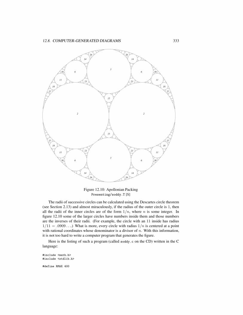
12.8. COMPUTER-GENERATED DIAGRAMS 333
2222
33
33
1515
1515
2727
1818
3030
1111
2626
1414
2323
66
2727
1818
3030
1111
2626
1414
2323
66
2727
1818
3030
1111
2626
1414
2323
66
2727
1818
3030
1111
2626
1414
2323
66
Figure 12.10: Apollonian PackingPresenting/soddy.T [S]
The radii of successive circles can be calculated using the Descartes circle theorem(see Section 2.13) and almost miraculously, if the radius of the outer circle is 1, thenall the radii of the inner circles are of the form 1/n, where n is some integer. Infigure 12.10 some of the larger circles have numbers inside them and those numbersare the inverses of their radii. (For example, the circle with an 11 inside has radius1/11 = .0909 . . ..) What is more, every circle with radius 1/n is centered at a pointwith rational coordinates whose denominator is a divisor of n. With this information,it is not too hard to write a computer program that generates the figure.
Here is the listing of such a program (called soddy.c on the CD) written in the Clanguage:
#include <math.h>
#include <stdlib.h>
#define RMAX 400
334 CHAPTER 12. GEOMETRIC PRESENTATIONS
#define RPRINTMAX 30
// for point: center = (x1/x2, y1/y2); radius = 1/R
int vertnum = 5;
struct point
int x1, x2, y1, y2, R;
;
int rightdist(struct point *p, int i, int j, int Rn)
int x1 = p->x1, x2 = p->x2, y1 = p->y1, y2 = p->y2, R = p->R;
if (R!=1 && (y2*y2*R*R*(x1*Rn-i*x2)*(x1*Rn-i*x2) +
x2*x2*R*R*(y1*Rn-j*y2)*(y1*Rn-j*y2) ==
x2*x2*y2*y2*(Rn+R)*(Rn+R))) return 1;
if (R==1 && (i*i+j*j == (Rn-1)*(Rn-1))) return 1;
return 0;
newcirc(struct point *p1, struct point *p2, struct point *p3, int depth)
int R1, R2, R3, Rnew;
int B, C, D, R;
int i, j;
struct point *p;
double Rad, Cx, Cy;
int imin, imax, jmin, jmax;
if (depth == 0) return;
R1 = p1->R;
R2 = p2->R;
R3 = p3->R;
if (R1 > R2) R = R1; R1 = R2; R2 = R; p = p1; p1 = p2; p2 = p;
if (R2 > R3) R = R2; R2 = R3; R3 = R; p = p2; p2 = p3; p3 = p;
if (R1 > R2) R = R1; R1 = R2; R2 = R; p = p1; p1 = p2; p2 = p;
if (R1 == 1) R1 = -1;
B = -2*(R1 + R2 + R3);
C = R1*R1 + R2*R2 + R3*R3 - 2*(R1*R2 + R2*R3 + R3*R1);
// now solve x^2 + Bx + C = 0;
D = B*B - 4*C;
R = (int)sqrt(D + .01);
Rnew = (R - B)/2;
if (Rnew < 0) Rnew = (-R- B)/2;
//printf("%d\n", Rnew);
Rad = 1.0/Rnew + 1.0/R3;
Cx = (double)(p3->x1)/p3->x2;
Cy = (double)(p3->y1)/p3->y2;
imin = (int)(Rnew*(Cx-Rad)-1);
imax = (int)(Rnew*(Cx+Rad)+1);
jmin = (int)(Rnew*(Cy-Rad)-1);
jmax = (int)(Rnew*(Cy+Rad)+1);
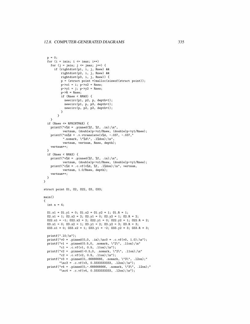
12.8. COMPUTER-GENERATED DIAGRAMS 335
p = 0;
for (i = imin; i <= imax; i++)
for (j = jmin; j <= jmax; j++)
if (rightdist(p1, i, j, Rnew) &&
rightdist(p2, i, j, Rnew) &&
rightdist(p3, i, j, Rnew))
p = (struct point *)malloc(sizeof(struct point));
p->x1 = i; p->x2 = Rnew;
p->y1 = j; p->y2 = Rnew;
p->R = Rnew;
if (Rnew < RMAX)
newcirc(p1, p2, p, depth+1);
newcirc(p1, p, p3, depth+1);
newcirc(p, p2, p3, depth+1);
if (Rnew <= RPRINTMAX)
printf("v%d = .pinned(%f, %f, .in);\n",
vertnum, (double)p->x1/Rnew, (double)p->y1/Rnew);
printf("vn%d = .v.vtranslate(v%d, -.037, -.037,"
".nomark, \"%d\", .l%don);\n",
vertnum, vertnum, Rnew, depth);
vertnum++;
if (Rnew < RMAX)
printf("v%d = .pinned(%f, %f, .in);\n",
vertnum, (double)p->x1/Rnew, (double)p->y1/Rnew);
printf("c%d = .c.vf(v%d, %f, .l%don);\n", vertnum,
vertnum, 1.0/Rnew, depth);
vertnum++;
struct point O1, O2, O22, O3, O33;
main()
int n = 4;
O1.x1 = O1.y1 = 0; O1.x2 = O1.y2 = 1; O1.R = 1;
O2.x1 = 1; O2.x2 = 2; O2.y1 = 0; O2.y2 = 1; O2.R = 2;
O22.x1 = -1; O22.x2 = 2; O22.y1 = 0; O22.y2 = 1; O22.R = 2;
O3.x1 = 0; O3.x2 = 1; O3.y1 = 2; O3.y2 = 3; O3.R = 3;
O33.x1 = 0; O33.x2 = 1; O33.y1 = -2; O33.y2 = 3; O33.R = 3;
printf(".l0;\n");
printf("v0 = .pinned(0,0, .in);\nc0 = .c.vf(v0, 1.0);\n");
printf("v1 = .pinned(0.5,0, .nomark, \"2\", .l1on);\n"
"c1 = .c.vf(v1, 0.5, .l1on);\n");
printf("v2 = .pinned(-0.5,0, .nomark, \"2\", .l1on);\n"
"c2 = .c.vf(v2, 0.5, .l1on);\n");
printf("v3 = .pinned(0,.66666666, .nomark, \"3\", .l2on);"
"\nc3 = .c.vf(v3, 0.3333333333, .l2on);\n");
printf("v4 = .pinned(0,-.666666666, .nomark, \"3\", .l2on);"
"\nc4 = .c.vf(v4, 0.3333333333, .l2on);\n");
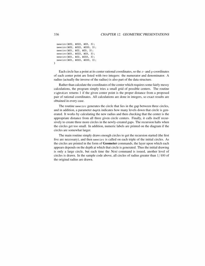
336 CHAPTER 12. GEOMETRIC PRESENTATIONS
newcirc(&O2, &O22, &O3, 3);
newcirc(&O2, &O22, &O33, 3);
newcirc(&O1, &O2, &O3, 3);
newcirc(&O1, &O22, &O3, 3);
newcirc(&O1, &O2, &O33, 3);
newcirc(&O1, &O22, &O33, 3);
Each circle has a point at its center rational coordinates, so the x- and y-coordinatesof each center point are listed with two integers: the numerator and denominator. Aradius (actually the inverse of the radius) is also part of the data structure.
Rather than calculate the coordinates of the center which requires some fairly messycalculations, the program simply tries a small grid of possible centers. The routinerightdist returns 1 if the given center point is the proper distance from a proposedpair of rational coordinates. All calculations are done in integers, so exact results areobtained in every case.
The routine newcirc generates the circle that lies in the gap between three circles,and in addition, a parameter depth indicates how many levels down that circle is gen-erated. It works by calculating the new radius and then checking that the center is theappropriate distance from all three given circle centers. Finally, it calls itself recur-sively to create three more circles in the newly-created gaps. The recursion halts whenthe circles get too small. In addition, numeric labels are printed on the diagram if thecircles are somewhat larger.
The main routine simply draws enough circles to get the recursion started (the firstfive are necessary), and then newcirc is called on each triple of the initial circles. Asthe circles are printed in the form of Geometer commands, the layer upon which eachappears depends on the depth at which that circle is generated. Thus the initial drawingis only a large circle, but each time the Next command is issued, another level ofcircles is drawn. In the sample code above, all circles of radius greater than 1/400 ofthe original radius are drawn.
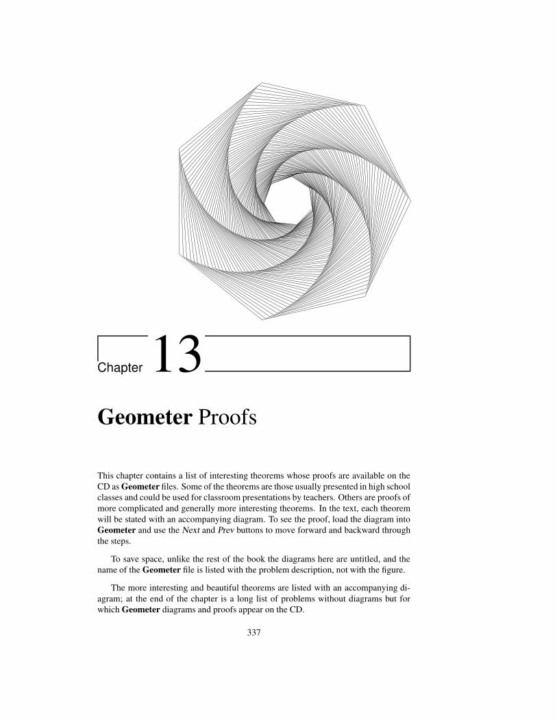
Chapter 13Geometer Proofs
This chapter contains a list of interesting theorems whose proofs are available on theCD as Geometer files. Some of the theorems are those usually presented in high schoolclasses and could be used for classroom presentations by teachers. Others are proofs ofmore complicated and generally more interesting theorems. In the text, each theoremwill be stated with an accompanying diagram. To see the proof, load the diagram intoGeometer and use the Next and Prev buttons to move forward and backward throughthe steps.
To save space, unlike the rest of the book the diagrams here are untitled, and thename of the Geometer file is listed with the problem description, not with the figure.
The more interesting and beautiful theorems are listed with an accompanying di-agram; at the end of the chapter is a long list of problems without diagrams but forwhich Geometer diagrams and proofs appear on the CD.
337
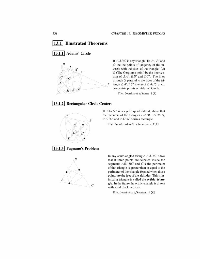
338 CHAPTER 13. GEOMETER PROOFS
13.1 Illustrated Theorems
13.1.1 Adams’ Circle
AA
BB
CC
C′C′
A′A′
B′B′
GG
HH
II
JJ
KKLL
MM
If4ABC is any triangle, let A′, B′ andC ′ be the points of tangency of the in-circle with the sides of the triangle. LetG (The Gergonne point) be the intersec-tion of AA′, BB′ and CC ′. The linesthroughG parallel to the sides of the tri-angle4A′B′C ′ intersect4ABC at sixconcentric points on Adams’ Circle.
File: GeomProofs/Adams.T[P]
13.1.2 Rectangular Circle Centers
BB
CCDD
AA
A′A′ B′B′
C′C′D′D′
If ABCD is a cyclic quadrilateral, show thatthe incenters of the triangles4ABC, 4BCD,4CDA and4DAB form a rectangle.
File: GeomProofs/Circlecenters.T[P]
13.1.3 Fagnano’s Problem
AA
BB
CC
In any acute-angled triangle 4ABC, showthat if three points are selected inside thesegments AB, BC and CA the perimeterof that triangle is greater than or equal to theperimeter of the triangle formed when thosepoints are the feet of the altitudes. This min-imizing triangle is called the orthic trian-gle. In the figure the orthic triangle is drawnwith solid black vertices.
File: GeomProofs/Fagnano.T[P]
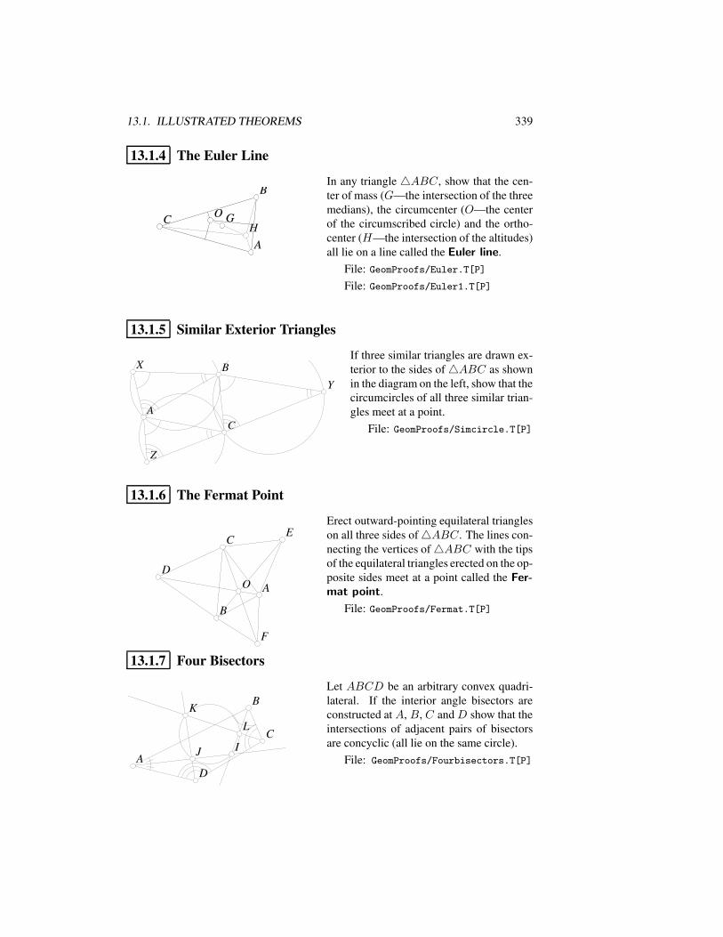
13.1. ILLUSTRATED THEOREMS 339
13.1.4 The Euler Line
AA
BB
CCHH
OO GG
AA
BB
CC OO GG
In any triangle 4ABC, show that the cen-ter of mass (G—the intersection of the threemedians), the circumcenter (O—the centerof the circumscribed circle) and the ortho-center (H—the intersection of the altitudes)all lie on a line called the Euler line.
File: GeomProofs/Euler.T[P]File: GeomProofs/Euler1.T[P]
13.1.5 Similar Exterior Triangles
AA
BB
CC
XX
YY
ZZ
If three similar triangles are drawn ex-terior to the sides of4ABC as shownin the diagram on the left, show that thecircumcircles of all three similar trian-gles meet at a point.
File: GeomProofs/Simcircle.T[P]
13.1.6 The Fermat Point
AA
BB
CC
FF
EE
DDOO
Erect outward-pointing equilateral triangleson all three sides of4ABC. The lines con-necting the vertices of4ABC with the tipsof the equilateral triangles erected on the op-posite sides meet at a point called the Fer-mat point.
File: GeomProofs/Fermat.T[P]
13.1.7 Four Bisectors
AA
BB
CC
DD
IIJJ
KK
LL
Let ABCD be an arbitrary convex quadri-lateral. If the interior angle bisectors areconstructed at A, B, C and D show that theintersections of adjacent pairs of bisectorsare concyclic (all lie on the same circle).
File: GeomProofs/Fourbisectors.T[P]
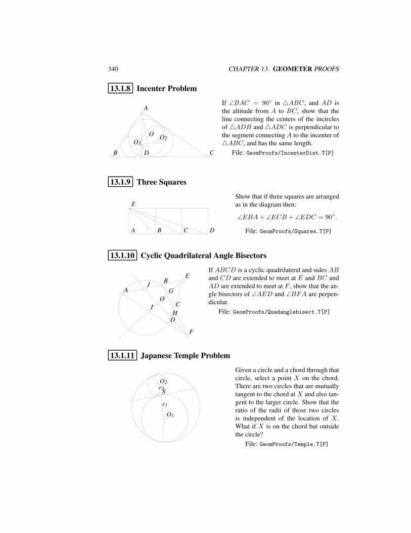
340 CHAPTER 13. GEOMETER PROOFS
13.1.8 Incenter Problem
AA
BB CCDD
O1O1
OO O2O2
If ∠BAC = 90 in 4ABC, and AD isthe altitude from A to BC, show that theline connecting the centers of the incirclesof 4ADB and4ADC is perpendicular tothe segment connectingA to the incenter of4ABC, and has the same length.
File: GeomProofs/IncenterDist.T[P]
13.1.9 Three Squares
BB CC DDAA
EEShow that if three squares are arrangedas in the diagram then:
∠EBA+ ∠ECB + ∠EDC = 90.
File: GeomProofs/Squares.T[P]
13.1.10 Cyclic Quadrilateral Angle Bisectors
BB
CC
DD
AA
FF
EE
GGJJ
OO
HHII
If ABCD is a cyclic quadrilateral and sides ABand CD are extended to meet at E and BC andAD are extended to meet at F , show that the an-gle bisectors of ∠AED and ∠BFA are perpen-dicular.
File: GeomProofs/Quadanglebisect.T[P]
13.1.11 Japanese Temple Problem
r2r2
r1r1
XX
O2O2
O1O1
Given a circle and a chord through thatcircle, select a point X on the chord.There are two circles that are mutuallytangent to the chord at X and also tan-gent to the larger circle. Show that theratio of the radii of those two circlesis independent of the location of X .What if X is on the chord but outsidethe circle?
File: GeomProofs/Temple.T[P]
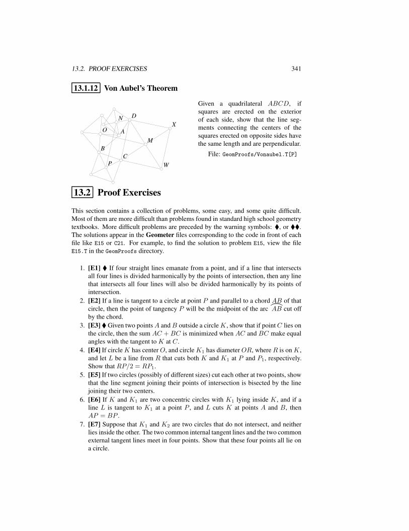
13.2. PROOF EXERCISES 341
13.1.12 Von Aubel’s Theorem
AA
BBCC
DD
WW
XX
MM
NN
OO
PP
Given a quadrilateral ABCD, ifsquares are erected on the exteriorof each side, show that the line seg-ments connecting the centers of thesquares erected on opposite sides havethe same length and are perpendicular.
File: GeomProofs/Vonaubel.T[P]
13.2 Proof Exercises
This section contains a collection of problems, some easy, and some quite difficult.Most of them are more difficult than problems found in standard high school geometrytextbooks. More difficult problems are preceded by the warning symbols: , or .The solutions appear in the Geometer files corresponding to the code in front of eachfile like E15 or C21. For example, to find the solution to problem E15, view the fileE15.T in the GeomProofs directory.
1. [E1] If four straight lines emanate from a point, and if a line that intersectsall four lines is divided harmonically by the points of intersection, then any linethat intersects all four lines will also be divided harmonically by its points ofintersection.
2. [E2] If a line is tangent to a circle at point P and parallel to a chord AB of thatcircle, then the point of tangency P will be the midpoint of the arc
)
AB cut offby the chord.
3. [E3] Given two pointsA andB outside a circleK, show that if pointC lies onthe circle, then the sum AC + BC is minimized when AC and BC make equalangles with the tangent to K at C.
4. [E4] If circleK has centerO, and circle K1 has diameterOR, whereR is onK,and let L be a line from R that cuts both K and K1 at P and P1, respectively.Show that RP/2 = RP1.
5. [E5] If two circles (possibly of different sizes) cut each other at two points, showthat the line segment joining their points of intersection is bisected by the linejoining their two centers.
6. [E6] If K and K1 are two concentric circles with K1 lying inside K, and if aline L is tangent to K1 at a point P , and L cuts K at points A and B, thenAP = BP .
7. [E7] Suppose that K1 and K2 are two circles that do not intersect, and neitherlies inside the other. The two common internal tangent lines and the two commonexternal tangent lines meet in four points. Show that these four points all lie ona circle.
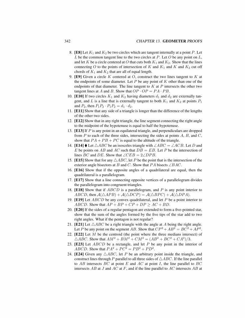
342 CHAPTER 13. GEOMETER PROOFS
8. [E8] LetK1 andK2 be two circles which are tangent internally at a point P . LetL be the common tangent line to the two circles at P . Let O be any point on L,and letK be a circle centered atO that cuts bothK1 andK2. Show that the linesconnecting O to the points of intersection of K and K1 and K and K2 cut offchords of K1 and K2 that are all of equal length.
9. [E9] Given a circle K centered at O, construct the two lines tangent to K atthe endpoints of some diameter. Let P be any point of K other than one of theendpoints of that diameter. The line tangent to K at P intersects the other twotangent lines at A and B. Show that OP · OP = PA · PB.
10. [E10] If two circles K1 and K2 having diameters d1 and d2 are externally tan-gent, and L is a line that is externally tangent to both K1 and K2 at points P1
and P2, then P1P2 · P1P2 = d1 · d2.11. [E11] Show that any side of a triangle is longer than the difference of the lengths
of the other two sides.12. [E12] Show that in any right triangle, the line segment connecting the right angle
to the midpoint of the hypotenuse is equal to half the hypotenuse.13. [E13] If P is any point in an equilateral triangle, and perpendiculars are dropped
from P to each of the three sides, intersecting the sides at points A, B, and C,show that PA+ PB + PC is equal to the altitude of the triangle.
14. [E14] Let4ABC be an isosceles triangle with ∠ABC = ∠ACB. LetD andE be points on AB and AC such that DB = EB. Let P be the intersection oflines BC and DE. Show that ∠CEB = 2∠DPB.
15. [E15] Show that for any4ABC, let P be the point that is the intersection of theexterior angle bisectors at B and C. Show that PA bisects ∠BAC.
16. [E16] Show that if the opposite angles of a quadrilateral are equal, then thequadrilateral is a parallelogram.
17. [E17] Show that a line connecting opposite vertices of a parallelogram dividesthe parallelogram into congruent triangles.
18. [E18] Show that if ABCD is a parallelogram, and P is any point interior toABCD, thenA(4APB) +A(4DCP ) = A(4BPC) +A(4DPA).
19. [E19] Let ABCD be any convex quadrilateral, and let P be a point interior toABCD. Show that AP +BP + CP +DP ≥ AC +BD.
20. [E20] If the sides of a regular pentagon are extended to form a five-pointed star,show that the sum of the angles formed by the five tips of the star add to tworight angles. What if the pentagon is not regular?
21. [E21] Let 4ABC be a right triangle with the angle at A being the right angle.Let P be any point on the segmentAB. Show that CP 2 +AB2 = BC2 +AP 2.
22. [E22] Let M be the centroid (the point where the three medians intersect) of4ABC. Show that AM2 +BM2 + CM2 = (AB2 +BC2 + CA2)/3.
23. [E23] Let ABCD be a rectangle, and let P be any point in the interior ofABCD. Show that PA2 + PC2 = PB2 + PD2.
24. [E24] Given any 4ABC, let P be an arbitrary point inside the triangle, andconstruct lines throughP parallel to all three sides of4ABC. If the line parallelto AB intersects BC at point E and AC at point I , the line parallel to BCintersects AB at J and AC at F , and if the line parallel to AC intersects AB at
13.2. PROOF EXERCISES 343
G and BC at H , show that PE · PF · PG = PH · PI · PJ . Is it necessary forP to be inside4ABC for this to hold?
25. [E25] If4ABC is a right triangle with right angle at A, and d is the diameterof the inscribed circle of4ABC, show that d = AB +AC −BC.
26. [E26] Let K be a circle and P be a point outside K. The two tangent lines fromP are tangent to K at points A and B. Let C be any point on the arc from A toB, and construct a tangent to K at C. The three tangent lines form a triangle.Show that the perimeter of the triangle is PA+ PB.
27. [E27] Let K be the inscribed circle of any4ABC, and let I be the center ofK. From B, drop a perpendicular to line AI , intersecting it at E. Show that Elies on the line connecting the points of tangency of K with BC and AC.
28. [E28] Let line L1 intersect a circle K at A and B, and let line L2 intersect K atC and D. If L1 ⊥ L2, then show that AC2 +BD2 = AD2 +BC2.
29. [E29] Let ABCD be a cyclic quadrilateral. Let G be the intersection of itsdiagonals. Let GH ⊥ AD with H on AD, and GI ⊥ BC with I on BC. Showthat GH : GI = AD : BC.
30. [E30] Let K be a circle, and let A and A′ be inverse points with respect to K,and similarly, B and B′ are another pair of inverse points with respect to K.Show that A, A′, B, and B′ either all lie on a straight line, or ABB′A′ is acyclic quadrilateral.
31. [E31] If O is the incenter of an arbitrary4ABC, and X and Y are the points oftangency of the incircle with edges AB andAC of4ABC, show that O, X , Y ,and A all lie on a circle.
32. [E32] Given an equilateral triangle, divide one side arbitrarily into two piecesof length x and y. Construct two more equilateral triangles using the pieces oflengths x and y as one side of each new triangle, and construct the new trianglesso that both are on the outside of the original triangle. Show that the triangleconnecting the centers of the three equilateral triangles is itself an equilateraltriangle.
33. [E33] If A and B are points at opposite ends of the diameter of a circle, and Cis any point on the circle, show that AC2 +BC2 is a constant.
34. [E34] Let AB be the diameter of a semicircle, and let C be a point on AB.The perpendicular to AB through C intersects the semicircle at D and let E bethe midpoint of the semicircle. If r is the radius of the semicircle, show thatCD2 + CE2 = 2r2.
35. [E35] Let AB be the diameter of a circle, and let CD be a chord of the circleparallel to AB, where C is closest to A. Let X be any point between A and B.Show that XC2 +XD2 = XA2 +XB2.
36. [E36] Suppose that the diameter of a circle is divided into a large number ofpieces, and that circles are constructed with each of those pieces as its diameter.Show that the sum of the circumferences of the smaller circles is equal to thecircumference of the original circle.
37. [E37] If three congruent circles are mutually tangent, what is the ratio of the areaof the triangle connecting their centers with the area of the triangle that connectstheir points of tangency?
344 CHAPTER 13. GEOMETER PROOFS
38. [E38] Let K be a circle and let P be a point outside K. From P draw the twotangents to K having points of tangency A and B. Let CD be any diameter ofK. If AC and BD intersect at a point Q, show that PQ ⊥ CD.
39. [E39] If K1 and K2 are two circles that are externally tangent to each other, andAB and CD are parallel diameters of K1 and K2, show that AD and BC passthrough the point of tangency of K1 and K2.
40. [E40] Let D be the midpoint of AC in 4ABC, and let E be any point onBC. The line DE intersects AB at G, and intersects the line through B that isparallel to AC at point F . Show that H(GE,DF ). In other words, show thatthe four points G and E divide D and F harmonically.
41. [E41] Given an angle, construct its bisector and a line perpendicular to the bisec-tor passing through the vertex of the angle. Let L be any line intersecting all fourof the lines in the figure. Show that this L intersects the four lines in a harmonicset.
42. [E42] Given two circles of radius 1 tangent to each other, and each tangent toa line that does not intersect the circles at their point of tangency. What is theradius of a circle that is tangent to both circles and to the line?
43. [E43] Given two circles that do not intersect and such that one does not lie in-side the other. Show that the four points where the common external tangentstouch the circles lie in a circle K1. Also show that the four points where thecommon internal tangents touch the circles lie in another circle K2. Show thatthe four points of intersection of the common external tangents and the commoninternal tangents also lie on a circle K3. Finally, show that K1, K2, and K3 areconcentric.
44. [E44] Given two circles that do not intersect and do not lie one inside theother, if the common internal and external tangents are constructed, show thatthe length of an internal tangent is equal to the distance between the points onthe external tangent where it is intersected by the two internal tangents.
45. [E45] Given an arbitrary 4ABC. Let D lie on BC such that AD bisects∠BAC. Show that AD2 = AB ·BC −BD · CD.
46. [E46] If4ABC is a right triangle with the right angle at A, and a perpendicularto BC is dropped from A that meets BC at D, show that AB2 : AC2 = BD :BC.
47. [E47] Given a circle K and a point A outside of K, let AX and AY be the twotangents from A to K, where X and Y lie on K. Let P be any point on K, andextend line AP to Q on K. Show that XP/XQ = Y P/Y Q.
48. [E48] Given any 4ABC, show that it is possible to construct a rectangle withone vertex at A, and the other three vertices on the circles whose diameters areAB, AC, and BC.
49. [E49] Suppose hexagonABCDEF is inscribed in a circle, and the diagonalsAD, BE, and CF meet at a point. Show that AB ·CD ·EF = BC ·DE ·FA.
50. [E50] Suppose a circle intersects all three sides of4ABC twice. It intersectsAB at C ′ and C ′′, it intersects BC at A′ and A′′, and it intersects CA at B′ andat B′′. Suppose further that the lines AA′, BB′, and CC ′ meet at a point. Thenthe lines AA′′, BB′′, and CC ′′ also meet at a (different) point.
13.2. PROOF EXERCISES 345
51. [E51] Given 4ABC and line L, let L intersect the sides of AB, BC, andCA at C ′, A′, and B′, respectively (some or all of the intersections may beoutside the triangle’s edges). Show that the midpoints of the segments AA′,BB′, and CC ′ all lie on a straight line. (This line is called the Gauss line.)
52. [E52] Given a right triangle 4ABC, where ∠B = 90, construct a circleinternally tangent to the legs AB and BC, and to the arc
)
AC. Show that thediameter of this circle is twice the diameter of the inscribed circle of4ABC.
53. [E53] Given 4ABC, let A′, B′, and C ′ be the feet of the altitudes oppositeA, B, and C, respectively. If perpendiculars are dropped from A′ to AB, AC,BB′, and CC ′ meeting them at K, N , L, and M , then K, L, M , and N lie in astraight line.
54. [E54] Given two squaresABCD andAEFG with centers P andQ that sharea common point A, let J and K be the midpoints of the segments DG and BE,respectively. Show that PJQK is a square. This is called the “Finsler-Hadwigertheorem”.
55. [E55] Pick four points A, B, C, and D in clockwise order on a circle. Let W ,X , Y , and Z be the midpoints of the arcs
)
AB,)
BC,
)CD, and
)
DA, respectively.Show that WY ⊥ XZ.
56. [E56] Let M be the midpoint of the longer arc
)
CD of a circle K. Pick a pointX at random on K. Construct XC, XD, and drop a perpendicular from M toXD, meeting it at Y . Show thatXC+XY = Y D. This is called “Archimedes’midpoint theorem”.
57. [E57] In any4ABC, let M be the midpoint ofAC and let MN be parallel tothe angle bisector of ∠ABC, where N is the other intersection with the triangle(on either AB or BC, depending on the shape of 4ABC). Show that MNdivides the perimeter into two equal areas. (Hint: See problem 56.)
58. [E58] If an altitude of a triangle is extended to intersect the circumcircle, thenthe length of the segment from the orthocenter to the base of the triangle is equalto the length of the segment from the base to the circumcircle.
59. [E59] In 4ABC if the excircle opposite ∠A touches the side BC at D, thenAD bisects the perimeter of4ABC.
60. [E60] Given two circles and a line that are all tangent at a common point Xwith both circles on the same side of the line, pick any other point on that lineand draw the other tangent to the inner circle. That line intersects the outercircle twice, at A and B, and is tangent to the inner circle at P . Show that∠AXP = ∠PXB.
61. [E61] Show that if ∠BAC = 30 in4ABC, then BC is equal to the length ofthe radius of the circumscribed circle of4ABC.
62. [E62] If circle K has its center on another circle, then the common chord ofthe two circles is equal to the length of the chord of K passing through theintersection of the two circles and tangent to the circle on which its center lies.
63. [E63] Let A, B, and C be three non-collinear centers of circles, none of whichintersect, and none of which lie inside another. Let A′, B′, and C ′ be the inter-sections of the common internal tangents to the circles centered at B and C, atC and A, and at A and B, respectively. Show that AA′, BB′, and CC ′ meet ata point.
346 CHAPTER 13. GEOMETER PROOFS
64. [E64] Given 4ABC, construct two right triangles 4BAD and 4BCE onthe outside of 4ABC such that ∠ABD = ∠CBE. Let F be the foot of thealtitude from B to AC. Show that the lines AE, CD, and BF are concurrent.
65. [E65] Draw a pentagram (a five-pointed star) by choosing five points A, C, E,G, I and forming the segments AE, EI , IC, CG, and GA. Let AE and ICintersect at B, CG and AE at D, EI and CG at F , GA and EI at H , and ICand GA at J . Show that
AB
BC· CDDE· EFFG· GHHI· IJJA
= 1.
66. [E66] Construct a square on the hypotenuse of a right triangle and draw a linefrom the vertex opposite the hypotenuse to the center of the square. Show thatthis line splits the right angle into two 45 angles. Does it matter on which sideof the hypotenuse the square is constructed?
67. [E67] Let 4ABC be a right triangle with ∠ABC = 90. Let AB = 3 · BC.If M is the midpoint of AC, and D and E trisect AB, show that4DME is anisosceles right triangle.
68. [E68] A circle with diameterPP ′ is tangent to a lineL at P ′. LetXY be a chordof the circle parallel to PP ′. If Q is the midpoint of the arc
)
XY , and if linesPX , PQ and PY are extended to intersect L at X ′, Q′, and Y ′, respectively,show that H(P ′Q′, X ′Y ′).
69. [E69] If a quadrilateral is circumscribed around a circle and if the lines con-necting the opposite points of tangency are perpendicular, then the quadrilateralcan be inscribed in a larger circle.
70. [E70] If the altitudes of 4ABC are ha, hb, and hc, and the radius of the in-scribed circle is r, show that 1/ha + 1/hb + 1/hc = 1/r.
71. [E71] If ABCD is a trapezoid with AB ‖ CD and squares are erected on theexterior of sides AB and CD, the line connecting the midpoints of the squarespasses through the intersection of lines AC and BD.
72. [E72] Let I be the incenter of 4ABC. If O is the circumcenter of 4BIC,show that A, I , and O lie in a straight line.
73. [E73] In a semicircle with center O inscribe a circle K tangent at O. Inscribe asecond circle K1 in the semicircle tangent to the semicircle, its diameter, and toK. What is the ratio of the radius of K1 to the radius of the semicircle?
74. [E74] Three circles of radius 1 are tangent to each other and their diameters areall part of the same line. A line is drawn from the left end of the diameter of theleftmost circle which is tangent to the rightmost circle. This tangent line cuts achord from the middle circle. Find the length of that chord.
75. [E75] Given two circles of radiusR and r tangent to each other, and both tangentto a line that does not pass through their point of common tangency, constructa circle tangent to both circles and the line. Find the radius of the new circle.Suppose that you begin with two circles of radius 1, inscribe the circle betweenthem and their tangent line, then inscribe circles between both pairs of the threecircles, then between all pairs of the set of 5 circles, and so on. What are theradii of the circles so generated? In fact, if two adjacent circles have radii 1/m2
and 1/n2, where m and n are integers, what’s the radius of the new circle? (SeeExercise 42.)
13.2. PROOF EXERCISES 347
76. [E76] Given two triangles4ABC and4DEF inscribed in a circle such thatthe vertices alternate: A,D,B,E,C, F , show that an ellipse can be inscribed inthe interior hexagon. What if the two triangles are inscribed in an ellipse insteadof in a circle?
77. [E77] In4ABC, let A′, B′, and C ′ lie on lines BC, CA, and AB, respectivelysuch that AA′, BB′, and CC ′ meet at a point. Show that
(sin∠BAA′sin∠CAA′
)·(
sin∠CBB′sin∠ABB′
)·(
sin∠ACC ′sin∠BCC ′
)= 1
.78. [E78] In4ABC, let A′, B′, and C ′ lie on lines BC, CA, and AB, respectively
such thatAA′,BB′, andCC ′ meet at a point P . If the linesAA′,BB′, andCC ′
are reflected across the corresponding interior angle bisectors, those reflectedlines will also meet at another point Q. Points P and Q are called isogonalconjugates. (See Exercise 77.)
79. [E79] Show that in any4ABC, the orthocenter and the circumcenter are isogo-nal conjugates. See Exercise 78 for the definition of isogonal conjugate.
80. [E80] Show that the diameter of the nine-point circle of a triangle is half thediameter of the circumcircle of that triangle.
81. [E81] Show that if a ray is drawn from the orthocenter H of a triangle thatintersects the nine-point circle at P and the circumcircle at Q, that HP = PQ.
82. [E82] Let AA′, BB′, and CC ′ be the altitudes of4ABC, where A′, B′, andC ′ lie on BC, CA, and AB, respectively. Show that AA′, BB′, and CC ′ arethe angle bisectors of4A′B′C ′.
83. [E83] Let P , A, B, and C lie on a circle. Construct the three circles with diam-eters PA, PB, and PC. In pairs, those three circles meet in three points otherthan point P where they all meet. Show that those three intersection points lieon a straight line.
84. [E84] If three circles of equal radius centered at A, B, and C all pass throughthe same point O, and no pair are tangent, let A′, B′, and C ′ be the pairwiseintersections of the circles centered at B and C, at C and A, and at A and B,respectively, show that AA′, BB′, and CC ′ meet at a point.
85. [E85] Let A, B, C, D and E be 5 concyclic points let A′, B′, C ′, D′ and E′ bethe midpoints of CD, DE, EA, AB and BC, respectively, and let V , W , X ,Y and Z be the midpoints of B′E′, A′C ′, B′D′, C ′E′ and E′A′, respectively.Show that V , W , X , Y and Z are concyclic.
86. [E86] Let A, B and C lie on a line with C between A and B such that AC =3CB. Two circles are drawn with diametersAC and CB. The common exteriortangents of those two circles meet at D. Show that 2BD = BC.
87. [E87] Let4ABC contain only acute angles. Construct circles having diametersAB, BC and CA. From each vertex of the triangle, draw the two tangent linesto the circle whose diameter is the opposite side. Show that the six points oftangency all lie on a circle.
88. [E88] Show that if the angle bisectors of a triangle are equal, then the triangleis isosceles. This is the Steiner-Lehmus theorem.
348 CHAPTER 13. GEOMETER PROOFS
89. [E89] If two circles intersect at points A and B and a line that passes throughthe segmentAB intersects the circles at the points W , X , Y and Z in that order,show that ∠ZAY = ∠WBX .
90. [E90] If the quadrilateral ABCD has perpendicular diagonals and if W , X , YandZ are the midpoints of the sides, then if perpendiculars are dropped fromW ,X , Y and Z to the points W ′, X ′, Y ′ and Z ′ on the opposite side, then all eightpoints W , X , Y , Z, W ′, X ′, Y ′ and Z ′ lie on the same circle. This is called theeight-point circle theorem.
91. [E91] If a circle is drawn whose diameter is the segment connecting the incenterwith one of the excenters, then that circle passes through two vertices of thetriangle. This is called the incenter-excenter theorem.
92. [E92] Let A be a point outside circle O and choose a point P such that thetangent PT to the circle has the same length as PA. If C is any point on O, letB and D be the intersections of PC and CA with O, respectively. Let E be theintersection of AB with O. Show that DE ‖ AP .
93. [E93] Show that if the ceviansAD, BE andCF of4ABC are concurrent, thenthe other intersections of the triangle with the circle passing through D, E andF are the endpoints of another set of concurrent cevians.
94. [E94] Show that if two chords of a circle are perpendicular, then the sum of thesquares of the chord segments is equal to the square of the diameter of the circle.
95. [E95] If three circles of equal radius R meet at a point, then the pairwise inter-sections of those circles lie on a circle that also has radius R. This is known asJohnson’s theorem.
96. [E96] Given two lines AB and AC, choose D and E to lie on lines AB andAC, respectively. Let F be the intersection of CD and BE. Show that the fourcircumcircles of4ABE, 4ADC, 4BDF and4CEF are concurrent. (Hint:consider the Simson line.)
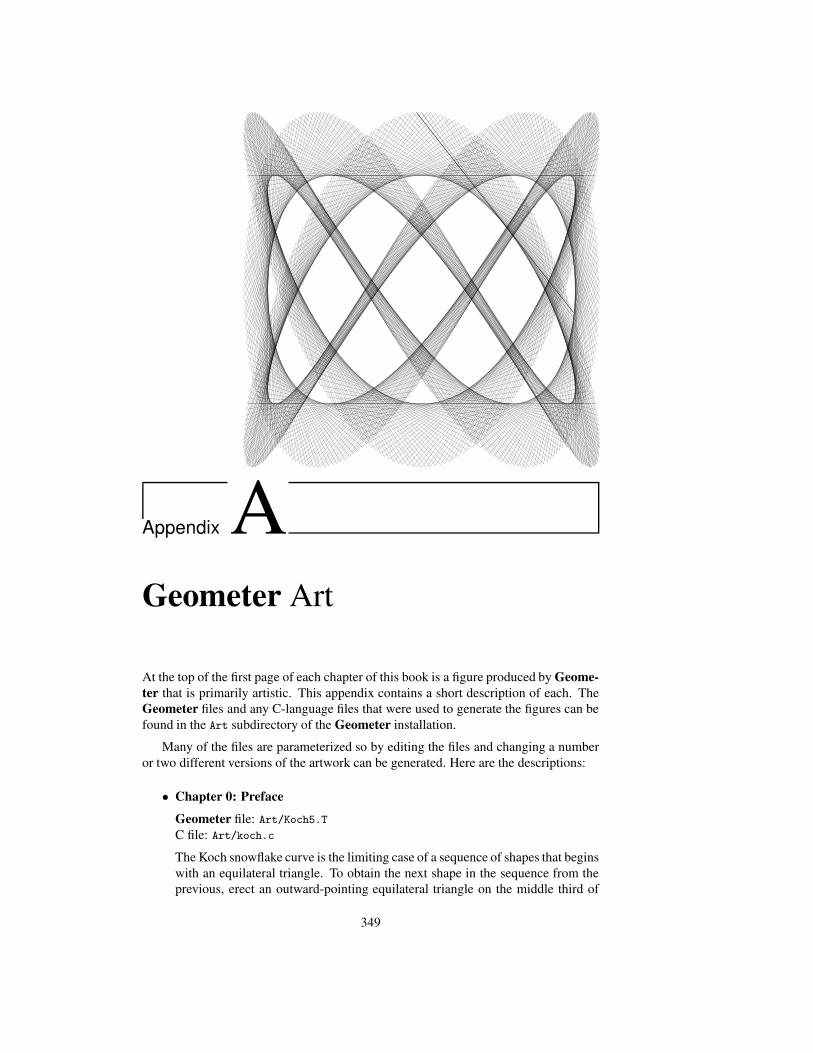
Appendix AGeometer Art
At the top of the first page of each chapter of this book is a figure produced by Geome-ter that is primarily artistic. This appendix contains a short description of each. TheGeometer files and any C-language files that were used to generate the figures can befound in the Art subdirectory of the Geometer installation.
Many of the files are parameterized so by editing the files and changing a numberor two different versions of the artwork can be generated. Here are the descriptions:
• Chapter 0: Preface
Geometer file: Art/Koch5.TC file: Art/koch.c
The Koch snowflake curve is the limiting case of a sequence of shapes that beginswith an equilateral triangle. To obtain the next shape in the sequence from theprevious, erect an outward-pointing equilateral triangle on the middle third of
349
350 APPENDIX A. GEOMETER ART
each segment of the boundary. Thus the second shape is like a star of David, etcetera. The illustration here is the fifth step in this sequence.
The curve is interesting because in its limiting form, it encloses a finite area, buthas a boundary whose length is infinite.
• Chapter 1: Introduction
Geometer file: Art/Pretty1.T
This pattern is the result of a Geometer programming bug. A cosine functionwas applied instead of a sine function in an attempt to generate the Maurer rosethat appears as the art at the beginning of Chapter 9.
• Chapter 2: Computer-Assisted GeometryGeometer file: Art/dragon.TC file: Art/dragon.c
This is the “dragon curve”. As you click on the Next button, successive approx-imations to the curve appear. The end result is a space-filling curve in the sensethat in the limit, every point of the region is approached arbitrarily closely by thecurve. The limiting length of the curve is, of course, infinite.
• Chapter 3: Mathematics Review
Geometer file: Art/Caustic.T
This illustration shows how caustic curves are generated in optics. Light raysfrom a point source are internally reflected within a sphere, and the resultingpattern of sparse and dense concentrations appears. Light through a wine glassgenerates similar patterns on a tablecloth. Press the Run Script button to generatethe caustic.
• Chapter 4: Geometric Construction
Geometer file: Art/epicycloid.T
One definition of an epicycloid is as the envelope of the straight lines connect-ing points on the circumference of a circle with points n times as far along thesurface. Press the Run Script button to view an example. If you edit the Geome-ter code, you can change the value of n to generate different epicycloids. Themultiple n need not be an integer, but the results are a bit less interesting.
• Chapter 5: Computer-Aided Proof This image is generated by beginning withan array of 9 circles arranged in three rows and columns, and inverting each ofthe circles in the other 8. Then those circles are again inverted in the original 9circles and the process is repeated for a few steps. Different initial arrangementsof circles and different depths can be achieved by modifying the “C” file andrerunning it.
• Chapter 6: More Useful TheoremsGeometer file: Art/fourier.T
351
Press Run Script to show a sequence of trogonometric Fourier series that approx-imate a square wave. Eight steps of the approximation are superimposed.
• Chapter 7: Locus of Points
Geometer file: Art/golden.T
A geometric illustration of one property of the golden section is illustrated here.Each time the Next command is pressed, a square is chopped off the end of arectangle whose sides are in the golden ratio: τ = (1 +
√5)/2 : 1. Each time a
square is chopped off, the resulting rectangle has exactly the same shape as theprevious.
• Chapter 8: Triangle Centers
Geometer file: Art/hilbert.TC file: Art/hilbert.c
Each press of the Next button displays another in a sequence of curves whoselimit is the Hilbert space-filling curve.
• Chapter 9: Inversion in a Circle
Geometer file: Art/Maurer.T
This figure is called the Maurer rose and is generated with the Run Script button.It is generated by connecting two points that move around an n-leaved rose witha fixed angular offset between them. The Geometer diagram can be modified tochange both n and the angular displacement.
• Chapter 10: Projective Geometry
Geometer file: Art/peano.TC file: Art/peano.c
The Peano curve is another space-filling curve. The Geometer file is generatedby a “C” computer program. Press Next to view successive approximations tothe true Peano curve.
• Chapter 11: Harmonic Point Sets
Geometer file: Art/Poly/Poly.TC file: Art/Poly/poly.c
This is the projection of the 3, 3, 5 4-dimensional polytope onto a two dimen-sional surface. The Geometer diagram is generated by a “C” program that canbe modified to change the direction of the projection.
• Chapter 12: Geometric Presentations
Geometer file: Art/square.TC file: Art/square.c
This is another space-filling curve whose approximations are quite interesting.
352 APPENDIX A. GEOMETER ART
• Chapter 13: Geometer ProofsGeometer file: Art/Whirl/Whirl.TC file: Art/Whirl/Whirl.c
This is a simple illustration created by drawing a regular polygon (in this case aregular heptagon) repeatedly drawn with a slight increment in the rotation angleand a slight decrement in size.
• Appendix A: Geometer ArtGeometer file: Art/Liss.T
In this pattern a pair of points follow each other with a fixed angular difference asthey trace out a lissijous curve. Those points are connected with a line segment.Both the frequencies of the curve and the angular difference can be changed byediting the Geometer file.
• Appendix B: Geometric Problem Solving StrategiesGeometer file: Art/Spirograph.T
This is similar to the Spirograph example in the text (see Section 2.14.3) ex-cept with different radii and numbers of teeth, and in addition, it is drawn withconnected line segments instead of as a series of dots.
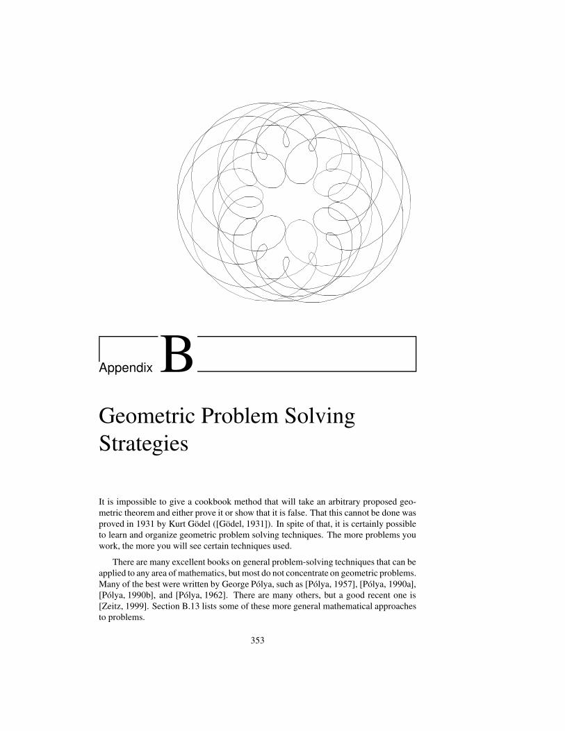
Appendix BGeometric Problem SolvingStrategies
It is impossible to give a cookbook method that will take an arbitrary proposed geo-metric theorem and either prove it or show that it is false. That this cannot be done wasproved in 1931 by Kurt Godel ([Godel, 1931]). In spite of that, it is certainly possibleto learn and organize geometric problem solving techniques. The more problems youwork, the more you will see certain techniques used.
There are many excellent books on general problem-solving techniques that can beapplied to any area of mathematics, but most do not concentrate on geometric problems.Many of the best were written by George Polya, such as [Polya, 1957], [Polya, 1990a],[Polya, 1990b], and [Polya, 1962]. There are many others, but a good recent one is[Zeitz, 1999]. Section B.13 lists some of these more general mathematical approachesto problems.
353
354 APPENDIX B. GEOMETRIC PROBLEM SOLVING STRATEGIES
This appendix is organized a bit like a thesaurus—look up a problem category toobtain a list of possible approaches to problems in that category. Obviously no suchlisting (either of categories or strategies) could ever be complete, so it may not containexactly what you need.
To use this appendix, first have a clear idea of what you are trying to do, like:“Show that points A, B and C all lie on a line.” or “Find the length of segment AB.”or “Construct a circle tangent to two circles and a line.” Then look through the list ofgeneral categories below to see which ones might apply. Go to the referenced sectionsand continue from there.
• Congruence: Methods to prove that geometric figures are congruent. Sec-tion B.1.
• Similarity: Methods to prove that geometric figures are similar. Section B.2.
• Special Figures: Showing that figures are special in some way. Is the figurea square? A rectangle? An equilateral triangle? An isosceles triangle? Sec-tion B.3.
• Concurrence: Methods to prove facts about concurrence—are two points in factthe same point? Do three points lie on a line? Do four points lie on a circle? Dothree lines go through the same point? Are two circles tangent? Section B.4.
• Measures: Methods to measure things. How long is a line segment? What is themeasure of an angle? What is the area of a triangle? Section B.5.
• Equality and Inequality: Methods to show line segments, angles, areas, etcetera, are of equal or different lengths. If they are different, which one is larger?How to show triangles are equilateral or isosceles, how to show that a quadrilat-eral is a parallelogram, rhombus, or trapezoid. Section B.6.
• Ratios: Methods to work with ratios: how to find them, how to calculate withthem, what to use them for. Section B.7.
• Inversion: Methods to use inversion to simplify a proof or construction.
• When to Draw the Line: When and how to construct auxiliary lines or circlesin a geometric figure to complete a proof.
• Construction Techniques: Making straightedge and compass constructions.
• Relabeling How to work out the details once, and then be able to say, “et cetera”.
Each section contains short descriptions of techniques, possibly followed by refer-ences to sections where that particular technique was used or described. Techniquesthat are advanced or somehow difficult to use are preceded by .
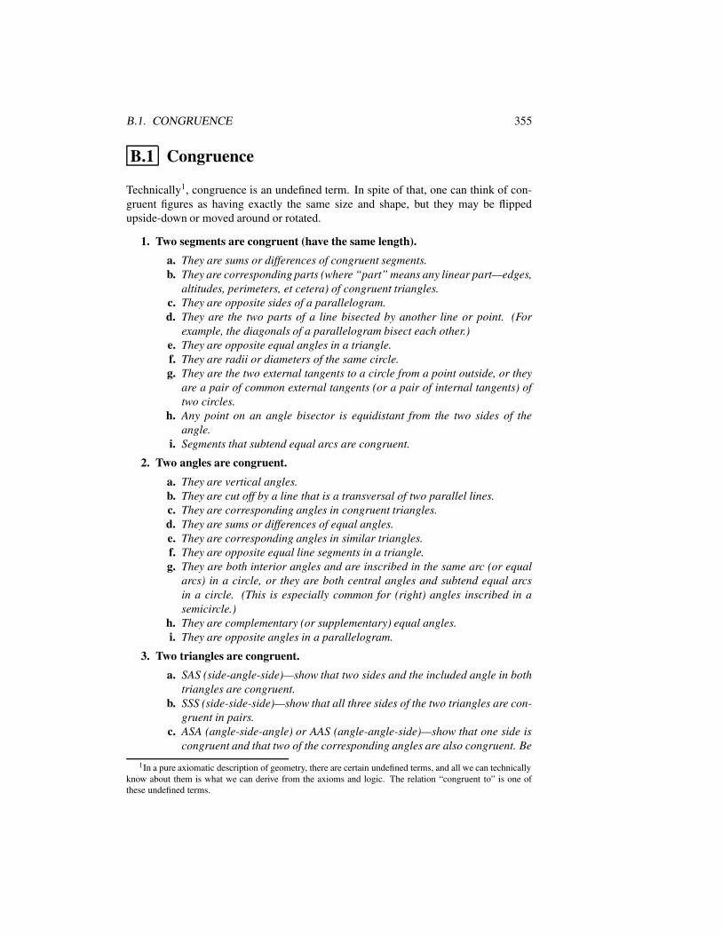
B.1. CONGRUENCE 355
B.1 Congruence
Technically1, congruence is an undefined term. In spite of that, one can think of con-gruent figures as having exactly the same size and shape, but they may be flippedupside-down or moved around or rotated.
1. Two segments are congruent (have the same length).a. They are sums or differences of congruent segments.b. They are corresponding parts (where “part” means any linear part—edges,
altitudes, perimeters, et cetera) of congruent triangles.c. They are opposite sides of a parallelogram.d. They are the two parts of a line bisected by another line or point. (For
example, the diagonals of a parallelogram bisect each other.)e. They are opposite equal angles in a triangle.f. They are radii or diameters of the same circle.g. They are the two external tangents to a circle from a point outside, or they
are a pair of common external tangents (or a pair of internal tangents) oftwo circles.
h. Any point on an angle bisector is equidistant from the two sides of theangle.
i. Segments that subtend equal arcs are congruent.
2. Two angles are congruent.a. They are vertical angles.b. They are cut off by a line that is a transversal of two parallel lines.c. They are corresponding angles in congruent triangles.d. They are sums or differences of equal angles.e. They are corresponding angles in similar triangles.f. They are opposite equal line segments in a triangle.g. They are both interior angles and are inscribed in the same arc (or equal
arcs) in a circle, or they are both central angles and subtend equal arcsin a circle. (This is especially common for (right) angles inscribed in asemicircle.)
h. They are complementary (or supplementary) equal angles.i. They are opposite angles in a parallelogram.
3. Two triangles are congruent.a. SAS (side-angle-side)—show that two sides and the included angle in both
triangles are congruent.b. SSS (side-side-side)—show that all three sides of the two triangles are con-
gruent in pairs.c. ASA (angle-side-angle) or AAS (angle-angle-side)—show that one side is
congruent and that two of the corresponding angles are also congruent. Be
1In a pure axiomatic description of geometry, there are certain undefined terms, and all we can technicallyknow about them is what we can derive from the axioms and logic. The relation “congruent to” is one ofthese undefined terms.
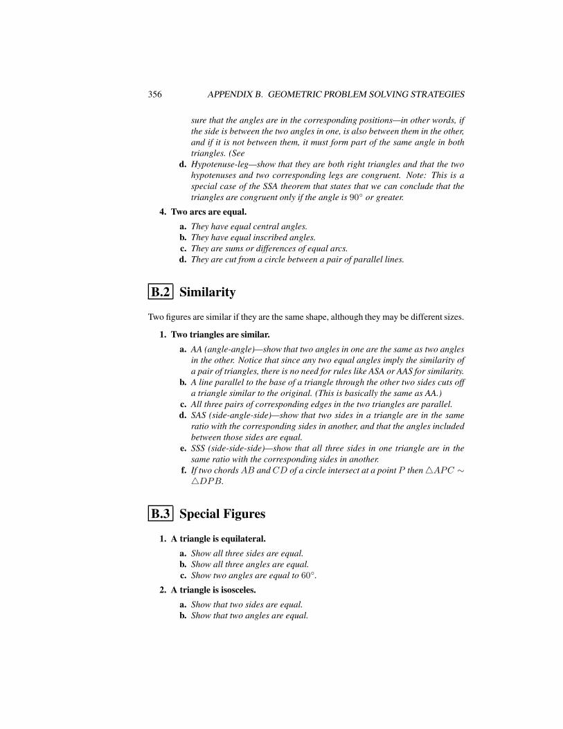
356 APPENDIX B. GEOMETRIC PROBLEM SOLVING STRATEGIES
sure that the angles are in the corresponding positions—in other words, ifthe side is between the two angles in one, is also between them in the other,and if it is not between them, it must form part of the same angle in bothtriangles. (See
d. Hypotenuse-leg—show that they are both right triangles and that the twohypotenuses and two corresponding legs are congruent. Note: This is aspecial case of the SSA theorem that states that we can conclude that thetriangles are congruent only if the angle is 90 or greater.
4. Two arcs are equal.a. They have equal central angles.b. They have equal inscribed angles.c. They are sums or differences of equal arcs.d. They are cut from a circle between a pair of parallel lines.
B.2 Similarity
Two figures are similar if they are the same shape, although they may be different sizes.
1. Two triangles are similar.a. AA (angle-angle)—show that two angles in one are the same as two angles
in the other. Notice that since any two equal angles imply the similarity ofa pair of triangles, there is no need for rules like ASA or AAS for similarity.
b. A line parallel to the base of a triangle through the other two sides cuts offa triangle similar to the original. (This is basically the same as AA.)
c. All three pairs of corresponding edges in the two triangles are parallel.d. SAS (side-angle-side)—show that two sides in a triangle are in the same
ratio with the corresponding sides in another, and that the angles includedbetween those sides are equal.
e. SSS (side-side-side)—show that all three sides in one triangle are in thesame ratio with the corresponding sides in another.
f. If two chordsAB andCD of a circle intersect at a point P then4APC ∼4DPB.
B.3 Special Figures
1. A triangle is equilateral.a. Show all three sides are equal.b. Show all three angles are equal.c. Show two angles are equal to 60.
2. A triangle is isosceles.a. Show that two sides are equal.b. Show that two angles are equal.
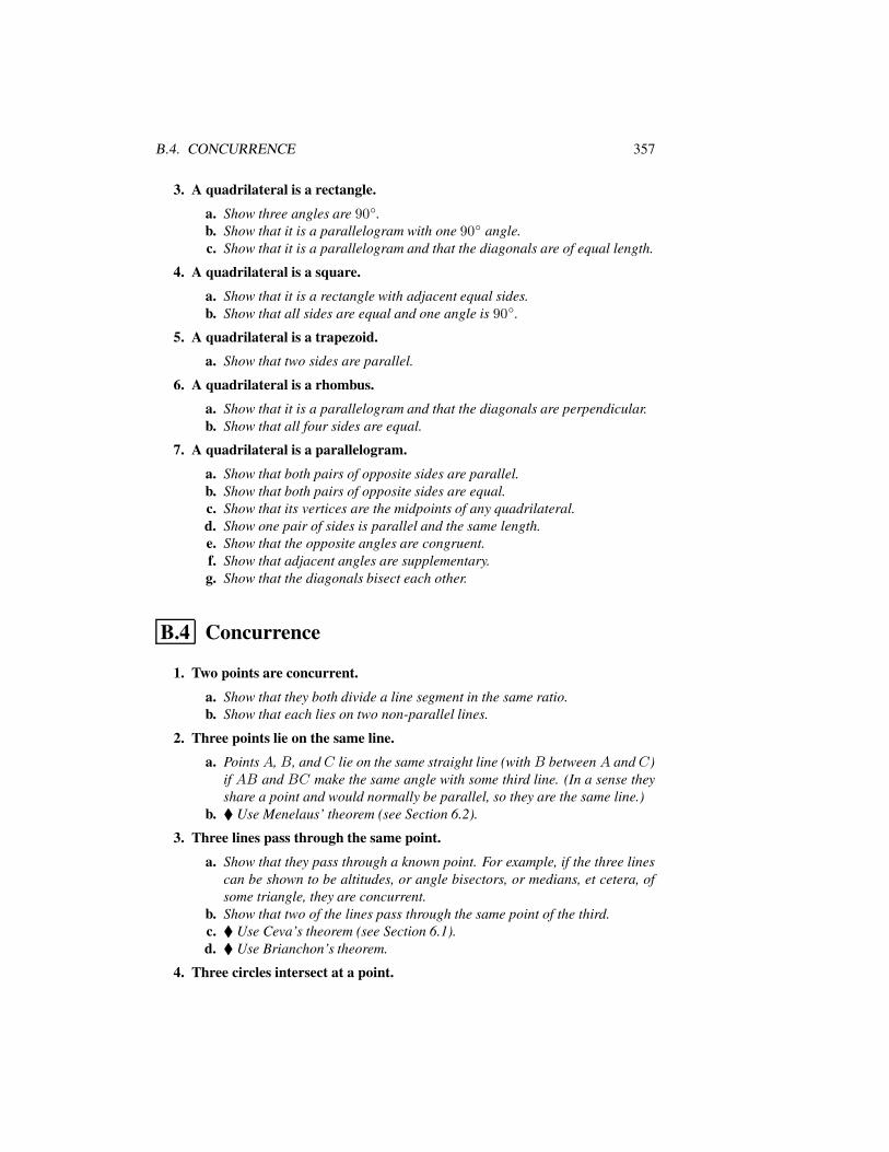
B.4. CONCURRENCE 357
3. A quadrilateral is a rectangle.
a. Show three angles are 90.b. Show that it is a parallelogram with one 90 angle.c. Show that it is a parallelogram and that the diagonals are of equal length.
4. A quadrilateral is a square.
a. Show that it is a rectangle with adjacent equal sides.b. Show that all sides are equal and one angle is 90.
5. A quadrilateral is a trapezoid.
a. Show that two sides are parallel.
6. A quadrilateral is a rhombus.
a. Show that it is a parallelogram and that the diagonals are perpendicular.b. Show that all four sides are equal.
7. A quadrilateral is a parallelogram.
a. Show that both pairs of opposite sides are parallel.b. Show that both pairs of opposite sides are equal.c. Show that its vertices are the midpoints of any quadrilateral.d. Show one pair of sides is parallel and the same length.e. Show that the opposite angles are congruent.f. Show that adjacent angles are supplementary.g. Show that the diagonals bisect each other.
B.4 Concurrence
1. Two points are concurrent.
a. Show that they both divide a line segment in the same ratio.b. Show that each lies on two non-parallel lines.
2. Three points lie on the same line.
a. PointsA, B, andC lie on the same straight line (with B betweenA andC)if AB and BC make the same angle with some third line. (In a sense theyshare a point and would normally be parallel, so they are the same line.)
b. Use Menelaus’ theorem (see Section 6.2).
3. Three lines pass through the same point.
a. Show that they pass through a known point. For example, if the three linescan be shown to be altitudes, or angle bisectors, or medians, et cetera, ofsome triangle, they are concurrent.
b. Show that two of the lines pass through the same point of the third.c. Use Ceva’s theorem (see Section 6.1).d. Use Brianchon’s theorem.
4. Three circles intersect at a point.
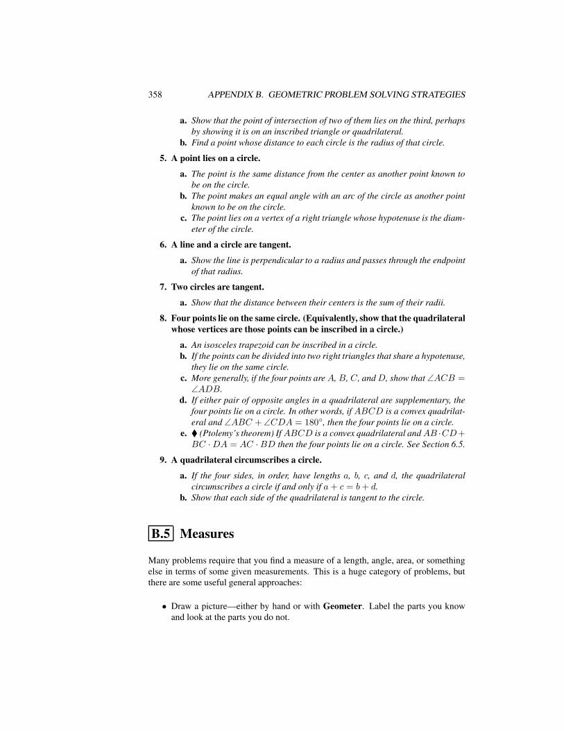
358 APPENDIX B. GEOMETRIC PROBLEM SOLVING STRATEGIES
a. Show that the point of intersection of two of them lies on the third, perhapsby showing it is on an inscribed triangle or quadrilateral.
b. Find a point whose distance to each circle is the radius of that circle.
5. A point lies on a circle.
a. The point is the same distance from the center as another point known tobe on the circle.
b. The point makes an equal angle with an arc of the circle as another pointknown to be on the circle.
c. The point lies on a vertex of a right triangle whose hypotenuse is the diam-eter of the circle.
6. A line and a circle are tangent.
a. Show the line is perpendicular to a radius and passes through the endpointof that radius.
7. Two circles are tangent.
a. Show that the distance between their centers is the sum of their radii.
8. Four points lie on the same circle. (Equivalently, show that the quadrilateralwhose vertices are those points can be inscribed in a circle.)
a. An isosceles trapezoid can be inscribed in a circle.b. If the points can be divided into two right triangles that share a hypotenuse,
they lie on the same circle.c. More generally, if the four points areA, B, C, andD, show that ∠ACB =∠ADB.
d. If either pair of opposite angles in a quadrilateral are supplementary, thefour points lie on a circle. In other words, if ABCD is a convex quadrilat-eral and ∠ABC + ∠CDA = 180, then the four points lie on a circle.
e. (Ptolemy’s theorem) IfABCD is a convex quadrilateral andAB ·CD+BC ·DA = AC ·BD then the four points lie on a circle. See Section 6.5.
9. A quadrilateral circumscribes a circle.
a. If the four sides, in order, have lengths a, b, c, and d, the quadrilateralcircumscribes a circle if and only if a+ c = b+ d.
b. Show that each side of the quadrilateral is tangent to the circle.
B.5 Measures
Many problems require that you find a measure of a length, angle, area, or somethingelse in terms of some given measurements. This is a huge category of problems, butthere are some useful general approaches:
• Draw a picture—either by hand or with Geometer. Label the parts you knowand look at the parts you do not.
B.5. MEASURES 359
• What relationships do you see in the figure. Look for things like right angles,parallel lines, centers of circles, equal included angles, angles that sum to a tri-angle or to a straight line, et cetera.
1. To find the length of a segment.
a. Use the pythagorean theorem (stated and proved in Section 3.6.5) on aright triangle.
b. Use the fact that the segment is the sum or difference of other segments thatyou can measure.
c. Use the law of cosines (see Section 3.10.2.6).d. Use the law of sines (see Section 3.10.2.4).
2. An angle is a right angle. (Equivalently, show that the two lines making upthe angle are perpendicular.)
a. Show that the angle is inscribed in a semicircle.b. Use the pythagorean theorem: If the angle is opposite a side of length c in
a triangle whose other sides are a and b, show a2 + b2 = c2.c. A radius (or diameter) that bisects a chord of a circle is perpendicular to
it. Similarly, a tangent to a circle is perpendicular to the radius at the pointof tangency.
d. The diagonals of a rhombus or kite are perpendicular.e. The line connecting the centers of two intersecting circles is perpendicular
to the line connecting the points of intersection.f. The two angle bisectors of two intersecting lines are perpendicular.g. Two lines that make the same angle with perpendicular lines are themselves
perpendicular.
3. Lines are perpendicular. (This is equivalent to showing they form a rightangle. See above.)
4. Lines are parallel.
a. Show that they have no points in common.b. Show that a transversal line makes equal angles with both the given lines.
(The most common special case of this is to show that they are both per-pendicular to the same line.)
c. Show that the lines are opposite sides in a parallelogram.d. Show that both are perpendicular to the same line.e. Show both are parallel to the same line.f. A line connecting the midpoints of two sides of a triangle is parallel to the
third side.g. Two lines that make the same angle with parallel lines are themselves par-
allel.
5. To find the measure of an angle.
a. The three angles in a triangle add to 180.b. The n internal angles in an n-sided polygon add to (n− 2) · 180 degrees.c. Complementary angles add to 90.
360 APPENDIX B. GEOMETRIC PROBLEM SOLVING STRATEGIES
d. Supplementary angles add to 180.e. Angles that go completely around a point add to 360.f. Angles that meet to form a straight angle add to 180.g. The central angle of an arc is twice an angle inscribed angle inscribed on
that arc.h. A tangent to a circle with a secant at its point of tangency form an angle of
half the measure of the arc it cuts.i. The exterior angle of a triangle is equal to the sum of the two interior
angles at the other vertices.j. Opposite angles in a cyclic quadrilateral add to 180.
6. To find the area of a polygon.
a. The area of a triangle is half the base times the height. Remember thatthere are three different base-height combinations and any of them works.
b. Use Heron’s Formula to find the area of a triangle given the lengths of thesides (see Section 6.6).
c. The area of a parallelogram (or rectangle, in particular) is the base timesthe height.
d. If a complex figure can be divided into smaller figures, its area is the sumof the areas of the smaller figures.
e. The area of a triangle that has sides of lengths a and b and included angleθ is (ab sin θ)/2.
f. Use Brahmagupta’s Formula (see Section 6.6.3) to find the area of a cyclicquadrilateral.
B.6 Equality and Inequality
1. One segment is larger than another.
a. Show that the segments are opposite unequal angles in a triangle. Thelarger segment is opposite the larger angle.
b. The hypotenuse of a right triangle is longer than either of the legs.c. The sum of any two legs of a triangle is longer than the third. The sum is
equal only for degenerate triangles. (This is called the triangle inequality.)
2. A line is an angle bisector.
a. Show that both the angles formed are equal.b. In4ABC, if the line through A hits the segment BC at a point D, and
if AD : BD = AC : CD then the line AD bisects ∠BAC.
B.7 Ratios
1. Equality of products or ratios of lengths.
B.8. INVERSION IN A CIRCLE 361
a. Usually when products of lengths are to be proved equal, or ratios are to beproved equal, it is done by finding one or a series of similar triangles whoseratios are then multiplied or divided together to get the desired product orratio.
b. Three parallel lines cut equal ratios of any transversal line.c. If two chordsAB andCD of a circle intersect at a point P thenPA·PB =PC · PD.
d. In a triangle, the angle bisector divides the opposite side in the same ratioas the lengths of the adjacent sides.
2. Finding Ratios – where to get ratios of lengths.
a. Similar triangles (or any similar polygons) have equal ratios of all thecorresponding linear parts. The “parts” may be sides, medians, altitudes,perimeters, et cetera.
b. Fixed ratios. For example, the diameter of a circle is always twice theradius, or the altitude of an equilateral triangle is always
√3/2 times the
length of the side.c. ChordsAB andCD of a circle that cross at P yieldAP ·PB = CP ·PD.
Note that P need not lie inside the circle for this to be true.d. Menelaus’ theorem yields products of ratios that are equal to 1 (see Sec-
tion 6.2).e. Ceva’s theorem yields products of ratios equal to 1 (see Section 6.1).f. Points that are inverted in the same circle yield ratios of lengths (ee Sec-
tion 9.8).
B.8 Inversion in a Circle
Inversion is so important that an entire chapter (Chapter 9)is devoted to it. The exam-ples in this section will not make much sense unless you are familiar with the contentsof that chapter.
This powerful technique converts circles and lines to other circles and lines, butwhich are converted to which depends on the location of the center of inversion, andon the radius of the circle of inversion. The technique is almost always the same—choose a center of inversion and a radius (sometimes the radius is unimportant), invertthe lines, circles, and points in the problem, solve the problem on the inverted figures,and then re-invert that solution to get a solution of the original problem.
For reference, here is a short list of the more important properties of inversionthrough a circle K centered at O:
1. Points are inverted to points.2. Circles and lines are inverted to circles and lines, but a circle may become a
line and a line may become a circle.3. Only lines or circles passing through O are inverted to lines.4. Angles between lines and/or circles are preserved by inversion.5. Inversion sends O to the point at infinity and the point at infinity to pointO.
362 APPENDIX B. GEOMETRIC PROBLEM SOLVING STRATEGIES
6. Points on K are inverted to themselves.
B.9 Algebraic Manipulation
If you are good at algebra, it is often not too hard to assign a coordinate system of somekind to your figure and then to state the various relationships algebraically and usingthose, to prove the desired result using solely algebraic manipulations.
There are many coordinate systems, and almost all are amenable to algebraic ma-nipulation. But there are coordinate-free representations (vectors) that can also be ma-nipulated algebraically.
Often, one can prove properties with a combination of geometric and algebraictechniques—purely geometric theorems are used to obtain various ratios and then thoseratios are manipulated algebraically to obtain the desired results.
B.9.1 Calculating with Angles
One of the most common uses of algebra in geometric proofs is for manipulation offormulas involving angles. It is easy to write down many angle equalities in mostfigures—the angles in a triangle add to 180 or in a quadrilateral to 360, oppositeangles in a cyclic quadrilateral add to 180, et cetera.
B.9.2 Calculating with Ratios
It is also easy to find ratios and quite often a bit of algebra is needed to combine thevarious formulas in a manner that gives the desired result.
B.9.3 Working with Areas
Often the area of a figure can be calculated in different ways, and those values can beset equal. For example, figures can be divided into triangles in many ways, and everysum of those triangle areas must be the same. Here are some places where areas areused in algebraic manipulations:
B.9.4 Primarily Algebraic Theorems
The following theorems are geometric, but their results are typically applied alge-braically:
1. The pythagorean theorem relates the lengths of the three sides in a righttriangle. See Section 3.6.5.
2. Stewart’s theorem relates the length of a cevian (a line connecting a vertexto the opposite side) of a triangle to the other lengths. See Section 3.6.6
B.10. WHEN TO DRAW THE LINE 363
3. Heron’s formula gives the area of any triangle in terms of the lengths of itssides. See Section 6.6.
4. Brahmagupta’s formula allows you to calculate the area of a cyclic quadri-lateral given the lengths of its sides. See Section 6.6.3.
5. Ptolemy’s theorem relates the lengths of the sides and diagonals of a cyclicquadrilateral. See Section 6.5.
6. The law of sines relates the sines of the angles of a triangle with the lengthsof the sides opposite them and to the diameter of the circumcircle. See Sec-tion 3.10.2.4.
7. The law of cosines is a generalization of the pythagorean theorem to arbi-trary triangles. See Section 3.10.2.6.
8. Various trigonometric formulas. See Section 3.10
B.9.5 Using Trigonometry
See Section 3.11 for a discussion of the technique and an example where we show thatthe three medians of a triangle meet at a point.
B.9.6 Vector Techniques
Section 3.12 is a nice introduction to this technique, together with a demonstration thatthe centroid of a triangle is the average of the three vectors to its vertices. Here are acouple of situations where vector techniques might be used:
1. If there is rotational symmetry in the problem or solution. For example, ifyou wish to prove that a triangle is equilateral, show that any edge can berotated 60 to become another edge.
2. If an entire figure is rotated or translated and relationships are sought be-tween the figure and the rotated or translated version.
B.10 When to Draw the Line
One of the hardest techniques for beginners to learn is when it might be useful to drawan auxiliary line or circle to complete a proof. Here are some rules of thumb:
1. If you want to apply some theorem about triangles, but your figure containsno triangles, it may be useful to draw a line that makes a triangle. Obviously,the word “triangle” in the previous sentence can be replaced by any othergeometric figure. A very common case is the construction of a line thatproduces a pair of similar triangles.
2. If you need to calculate lengths or relative lengths, it is often useful to usetheorems like the pythagorean theorem. To do so requires a right triangle,so to create one, you often need to drop a perpendicular or do somethingelse to make one or more right triangles in your figure.
364 APPENDIX B. GEOMETRIC PROBLEM SOLVING STRATEGIES
3. If you need to know something about a sum of lengths or angles, try to find aconstruction that puts the lines end-to-end, or the angles next to each otherso that addition simply amounts to looking at a combined length or angle.
4. If there is some apparent concurrency that is not obvious from the state-ment of the problem, it is often useful to make a construction that somehowhelps you prove that the concurrency is in fact true. For example, if in yourdrawings (with Geometer or drawn by hand) it seems like three points lieon a line, or that four points lie on a circle, try drawing that line throughtwo of the points or the circle through three of the points and see if you canprove that the other point lies on the line or circle.You can sometimes discover concurrencies using Geometer by drawing asuspicious point in a smearing color and then manipulating the rest of thefigure to see if that point moves in a regular way—along a line or around acircle, for example.
5. Remember that there is a whole class of problems that can be solved byinverting your figures through a circle. A discussion of when to use inversioncan be found in this chapter in Section B.8.
6. The list above does not cover all cases. Here is a list of other “miscella-neous” constructions that have been used in this book, together with a shortdescription of how and why each was used.
a. In Section 3.10.2.3, a perpendicular line is dropped to convert an arbitrarytriangle into one where we can use the definition of sin θ on a right triangle.
b. In Section 3.10.2.4, we construct a circle and a right triangle inscribed init to be able to use our definition of sin θ on a right triangle.
c. In Section 13.1.3, a series of reflections of a pair of triangles is constructed.The legs of one series of reflections lie in a line which is clearly the shortestdistance between two points.
d. In Section 9.17 in addition to all the inversion-related constructions, pointson a line are projected to use the fact that harmonic sets of points are pre-served under projection. Also, a triangle connecting the midpoints of theoriginal is constructed since those points are known to lie on the nine-pointcircle, and their positions are well-known relative to the original triangle.
e. In Section 13.1.12, a triangle is constructed so that an earlier theoremcould be applied to a small part of the figure. In addition, a few other linesrequired by the previous theorem were constructed.
B.11 Construction Techniques
To do general geometric constructions using a straightedge and compass, you shouldhave a solid idea of how to do the basic constructions presented in Section 4.5.
Most construction problems are solved by figuring out some properties that the so-lution has to satisfy, and then to apply some combination of the primitive constructionsreferred to above.
B.12. RELABELING 365
It is a bit difficult to divide construction problems into nice categories, but here atleast are a few general approaches that might be useful:
1. Draw a picture of a completed construction and work with it to see whatrelations hold. It is often quite easy to draw a solution and work back to theproblem. For example, if you are required to draw a circle tangent to threelines, draw a circle and then draw three lines tangent to it. From that youwill see that the three lines form a triangle, and then you will have somethingto analyze.
2. Sometimes you can use brute force. If you need to construct a 36, recallthat cos(36) = (1 +
√5)/4. Draw an arbitrary segment and call its length
1. Based on that, construct another segment of length (1+√
5)/4. The righttriangle having legs lengths 1 and (1 +
√5)/4 will contain a 36 angle.
3. If the problem requires the construction of a line or circle tangent to com-binations of lines and circles, consider inverting the problem through theproper circle. See Section B.8.
B.12 Relabeling
Quite often if you wish to prove something for a figure that is completely non-specific,you can work out the properties for one side or angle, and then just change the labelsin a consistent way to get the result for the others.
As an example, the law of sines states that
a
sinA=
b
sinB=
c
sinC= 2R
for any triangle 4ABC, where R is the radius of the circumscribed circle (See Sec-tion 3.10.2.4). If you can show that a/(sinA) = 2R you are done, since the triangleis completely arbitrary, so the labeling does not matter at all. In other words, if youhad taken the same triangle, but had originally exchanged the vertices where you wrotedown “A” and “B”, there would be no change in your proof, but your proof wouldhave shown that the ratio b/sinB is also equal to 2R.
An additional example can be found in Section 5.10 were the existence of the Sim-son line is shown. The theorem concerns an arbitrary triangle4ABC and a point Mon the circumcircle. The proof in Section 5.10 depends on the fact that M lies on thearc
)
CB, but had it been on a different arc, the same argument would hold after weproperly relabeled the vertices of the triangle.
B.13 General Problem Solving Approaches
Here is a list of strategies that can be applied to any mathematical problem, includinggeometric ones. The list here is by no means complete, but it may be helpful to reviewit if you are stuck on a particular problem.
366 APPENDIX B. GEOMETRIC PROBLEM SOLVING STRATEGIES
• Do you understand the problem? Make certain you know what you’re lookingfor. Name the unknowns. List the known facts.
• Did you draw a picture? This is almost always absolutely critical in geometry.In fact, more than one picture is even better. Try to draw pictures where the resultfails. Often your failed attempts to draw a counter-example make it clear whythe result must be true.
• Have you seen or solved a similar problem? If so, what techniques workedthere? Will they work again? If not, why not?
• Can you invent a simpler version of the problem that you can solve? If theproblem is for a general polygon, can you do it for a triangle? For a quadrilateral?If it is about a general triangle, can you solve it for an equilateral triangle? Foran isosceles or right triangle?
• Can you decompose the problem? Can you break the problem into parts sothat if you solve all the parts, you have solved the whole problem?
• Can you use contradiction? In other words, if you assume that the result youare trying to prove is false, does that lead to a nonsensical result? If so, you aredone.
• Did you use all the information? Sometimes there is extra data in a mathemat-ics problem, but it is rare. If you solve a problem without using some of the data,it is likely you have made a mistake.
• Can you guess, or at least estimate, what the correct answer might be? Thisgives a check of your final answer, and may help you to solve the problem.
• Can you work backwards? If you assume your final result and work towardthe problem statement, often those steps can be reversed to obtain a solution.
• Have you discussed the problem with others? If you can work with others, doso. Two heads are better than one. Surprisingly, even trying to explain what isgoing on to someone totally ignorant of mathematics often helps.
• Can you think of different approaches? Maybe vectors will work. Maybe asymmetry argument. Maybe you can assign coordinates and just grind out thesolution algebraically. Maybe you can use trigonometry.
• When you get a solution, can you find another approach? If so, you may havea way to check your first solution.
• Get some sleep. This can be surprisingly effective. You struggle late into thenight on a problem and make no progress, but with a clear head in the morning,the solution is obvious.
Bibliography
[Abbott, 1952] Abbott, E. A. (1952). Flatland: A Romance of Many Dimensions.Dover Publications, Inc., New York, seventh edition.
[Altshiller-Court, 1952] Altshiller-Court, N. (1952). College Geometry. Barnes &Noble, Inc., New York.
[Beman and Smith, 1900] Beman, W. W. and Smith, D. E. (1900). New Plane andSolid Geomtery. Ginn & Company, Boston.
[Berger, 1987a] Berger, M. (1987a). Geometry I. Springer-Verlag, Berlin, Heidelberg,New York.
[Berger, 1987b] Berger, M. (1987b). Geometry II. Springer-Verlag, Berlin, Heidel-berg, New York.
[Berger et al., 1984] Berger, M., Pansu, P., Berry, J.-P., and Saint-Raymond, X. (1984).Problems in Geometry. Springer-Verlag, New York, Berlin, Heidelberg, Tokyo.
[Bland, 1819] Bland, M. (1819). Geometrical Problems Deducible from the First SixBooks of Euclid. J. Smith, Cambridge, England.
[Burger, 1965] Burger, D. (1965). Sphereland: A Fantasy About Curved Spaces andan Expanding Universe. Apollo Editions, New York.
[Conway and Guy, 1996] Conway, J. and Guy, R. (1996). The Book of Numbers.Copernicus—An Imprint of Springer-Verlag, New York.
[Coxeter, 1989] Coxeter, H. S. M. (1989). Introduction to Geometry. John Wiley &Sons, Inc., New York, second edition.
[Coxeter and Greitzer, 1967] Coxeter, H. S. M. and Greitzer, S. L. (1967). GeometryRevisited. The Mathematical Association of America, New York.
[Dudley, 1994] Dudley, U. (1994). The Trisectors. The Mathematical Association ofAmerica, Washington D.C.
367
368 BIBLIOGRAPHY
[Euclid, 1956] Euclid (1956). The Thirteen Books of The Elements. Dover Publica-tions, Inc., New York.
[Eves, 1965] Eves, H. (1965). A Survey of Geometry. Allyn and Bacon, London.
[Godel, 1931] Godel, K. (1931). Uber formal unentscheidbare satze der principiamathematica und verwandter systeme, i. Monatsh. Math. u. Phys., 38:173–198.
[Greenberg, 1993] Greenberg, M. J. (1993). Euclidean and Non-Euclidean Geome-tries. W. H. Freeman and Company, New York, third edition.
[Hartshorne, 1997] Hartshorne, R. (1997). Companion to Euclid. Number 9 in Berke-ley Mathematics Lecture Notes. American Mathematical Society, Providence.
[Hilbert and Cohn-Vossen, 1983] Hilbert, D. and Cohn-Vossen, S. (1983). Geometryand the Imagination. Chelsea Publishing Company, New York.
[Johnson, 1929] Johnson, R. A. (1929). Advanced Euclidean Geometry. The RiversidePress, Cambridge, Mass.
[Johnson, 1917] Johnson, R. A. (Mar. 1917). Directed angles in elementary geometry.The American Mathematical Monthly, 24:3:101–105.
[Kazarinoff, 1961] Kazarinoff, N. D. (1961). Geometric Inequalities. The Mathemat-ical Association of America, Washington D.C.
[Kimberling, 1994] Kimberling, C. (1994). Central points and central lines in theplane of a triangle. Math. Mag., 67:163–187.
[King and Schattschneider, 1997] King, J. and Schattschneider, D., editors (1997).Geometry Turned On! Dynamic Software in Learning, Teaching, and Research.MAA Notes. The Mathematical Association of America, Washington, D.C.
[Klarner, 1981] Klarner, D. A. (1981). Mathematical Recreations, A Collection inHonor of Martin Gardner. Dover Publications, Inc., New York.
[Lawrence, 1972] Lawrence, J. D. (1972). A Catalog of Special Plane Curves. DoverPublications, Inc., New York.
[Martin, 1991] Martin, G. E. (1991). Geometric Constructions. Springer, New York.
[Meyers, 1996] Meyers, L. F. (1996). Update on william wernick’s “triangle construc-tions with three located points”. Mathematics Magazine, 69:46–49.
[Minsky, 1967] Minsky, M. L. (1967). Computation: Finite and Infinite Machines.Prentice-Hall, Inc., Englewood Cliffs, N.J.
[Moise, 1963] Moise, E. (1963). Elementary Geometry From An Advanced Stand-point. Addison-Wesley, Reading, Mass.
[Needham, 1997] Needham, T. (1997). Visual Complex Analysis. Oxford UniversityPress, Oxford.
BIBLIOGRAPHY 369
[Nelson, 1993] Nelson, R. B. (1993). Proofs Without Words: Exercises in VisualThinking. The Mathematical Association of America, Washington, D.C.
[Nelson, 2000] Nelson, R. B. (2000). Proofs Without Words II: More Exercises inVisual Thinking. The Mathematical Association of America, Washington, D.C.
[Ogilvy, 1969] Ogilvy, C. S. (1969). Excursions in Geometry. Dover Publications,Inc., New York.
[Pedoe, 1988] Pedoe, D. (1988). Geometry, A Comprehensive Course. Dover Publi-cations, Inc., New York.
[Pedoe, 1995] Pedoe, D. (1995). Circles: A Mathematical View. The MathematicalAssociation of America, Washington, D.C.
[Polya, 1957] Polya, G. (1957). How to Solve It. Doubleday, second edition.
[Polya, 1962] Polya, G. (1962). Mathematical Discovery: On Understanding, Learn-ing and Teaching Problem Solving. John Wiley & Sons.
[Polya, 1990a] Polya, G. (1990a). Mathematics and Plausible Reasoning. PrincetonUniversity Press, reprint edition.
[Polya, 1990b] Polya, G. (1990b). Mathematics and Plausible Reasoning: Volume IIPatterns of Plausible Inference. Princeton University Press, reprint edition.
[Posamentier and Salkind, 1988] Posamentier, A. S. and Salkind, C. T. (1988). Chal-lenging Problems in Geometry. Dover Publications, Inc., New York.
[Ryser, 1963] Ryser, J. H. (1963). Combinatorial Mathematics. The MathematicalAssociation of America, Rahway, N.J.
[Sharygin, 1988] Sharygin, I. F. (1988). Problems in Plane Geometry. Mir Publishers,Moscow.
[Weeks, 1985] Weeks, J. R. (1985). The Shape of Space: How to Visualize Surfacesand Three-Dimensional Manifolds. Marcel Dekker, Inc., New York.
[Weisstein, 1999] Weisstein, E. W. (1999). CRC Concise Encyclopedia of Mathemat-ics. CRC Press, Boca Raton.
[Wells, 1991] Wells, D. (1991). The Penguin Dictionary of Curious and InterestingGeometry. Penguin Books, London.
[Wernick, 1982] Wernick, W. (1982). Triangle constructions with three located points.Mathematics Magazine, 55:227–230.
[Yaglom, 1962a] Yaglom, I. M. (1962a). Geometric Transformations I. The Mathe-matical Association of America, New York.
[Yaglom, 1962b] Yaglom, I. M. (1962b). Geometric Transformations II. The Mathe-matical Association of America, New York.

370 BIBLIOGRAPHY
[Yaglom, 1962c] Yaglom, I. M. (1962c). Geometric Transformations III. The Mathe-matical Association of America, New York.
[Zeitz, 1999] Zeitz, P. (1999). The Art and Craft of Problem Solving. John Wiley &Sons, Inc., New York.
Index
AA similarity, 61, 356AAS congruence, 60absolute value, 104accurate drawings, 16acute angle, 56acute triangle, 58Adams’ circle, 338adding vectors, 97Alexanderson, Gerald, ivaltitude, 59analytic geometry, 89angle, 56
acute, 56central, 78complementary, 56directed, 57inscribed, 78obtuse, 56right, 56supplementary, 56triangle sum, 63trisection, 136under inversion, 232vertical, 51, 56, 355
angle bisector, 56, 87, 360angles between circles, 232animations, 38Apollonian circles, 332Apollonian gasket, 332Apollonius’ problem, 126, 235, 237,
248, 302arbelos, 245
of Pappus, 244
arc, 77, 356Archimedes’ circles, 245Archimedes’ midpoint theorem, 345Archimedes’ spiral, 194area, 52, 360
circle, 38, 78parallelogram, 72polygon, 33, 93trapezoid, 73triangle, 62, 86
ASA congruence, 60
Bezier spline, 193Baker, Arthur Latham, iBenjamin, Arthur, ivbetweenness, 264bisector
angle, 87, 114bound vector, 96, 101bowtie quadrilateral, 71Brahmagupta’s Formula, 177Brianchon’s theorem, 269
dual of, 266Brocard point, 142Brocard points, 208Bush, Ellyn, iv
Cabri Geometry, 1, 15calculations, 316cardioid, 34Cartesian coordinates, 57caustic curve, 350Cavalieri’s principle, 63center, 77
371
372 INDEX
center of gravity, 58center of mass, 58central angle, 78centroid, 24, 58, 199centroid, vector form, 102Ceva’s theorem, 167cevian, 168Chebychev polynomials, 85chord, 77Cinderella, 1, 15circle, 77
area, 38, 78inversion, 230nine point, 6, 202orthogonal, 233squaring, 136
circlesmutually tangent, 27
circumcenter, 24, 59, 199circumcircle, 59circumference, 77circumscribable quadrilateral, 71circumscribed circle, 117cissoid of Diocles, 191classical construction, 107collinear, 53color definition, 307combining files, 320compass construction, 16, 19, 48, 107,
135compass constructions, 112compass only construction, 135complementary angles, 56complete quadrangle, 295complete quadrilateral, 295complex conjugate, 104complex numbers, 105, 228computer geometry programs, 1, 15concave, 71concentric circles, 240conchoid of Nicomedes, 192concurrent lines, 357concurrent points, 357concyclic, 53concyclic points, 6concyclic quadrilateral, 71
congruenceangles, 355segments, 355triangles, 60, 355
congruent, 49conic section, 190conic sections, 264conic, equation for, 285conjugate lines, 299conjugate points, 299construction, 107, 135
approximate, 136bisect angle, 114center of circle, 116circle from three points, 116circumscribed circle, 117classical, 48copy angle, 113copy segment, 113difference of angles, 115division to ratio, 120external circle tangent, 121harmonic point sets, 17heptadecagon, regular, 19impossible, 136inscribed circle, 117internal circle tangent, 121midpoint, 112parallel to line, 115pentagon, regular, 118perpendicular bisector, 116perpendicular to line, 114regular polygons, 138specific angles, 117subdivide line, 120sum of angles, 115tangent to circle, 119triangle from sides, 115
construction exercises, 139convex polygon, 74convex quadrilateral, 71coordinate geometry, 89coordinate system, 320coordinates
Cartesian, 57change of, 224
INDEX 373
homogeneous, 272in Geometer, 308polar, 194projective, 272
copy angle, 113copy segment, 113cos, see cosinecosecant, 81cosine, 81cot, see cotangentcotangent, 81coversine, 82crackpots, 136cross product, 273, 282cross ratio, 297csc, see cosecantcube doubling, 136curve envelope, 195custom colors, 307cyclic quadrilateral, 71
Davis, Tom, 10decagon, 73degenerate conic, 285degenerate conics, 268degenerate hexagons, 271Desargues’ theorem, 255Descartes circle theorem, 41, 223diagonal, 295diagram, 15diagram appearance, 307diagrams
computer generated, 35diameter, 77digon, 73directed angles, 57directed ratio, 52, 171Dirichlet domains, 39disk, 77distance formula, 90dodecagon, 73doubling a cube, 136Dragon curve, 350drawing
for publication, 39drawing manipulation, 21
dualityprojective, 265
dumbbell curve, 192
ears, polygon, 76Edit Name, 307eight point circle theorem, 348ellipse, 188, 189, 190, 264Emerson, Ralph Waldo, 10encapsulated PostScript, 39enneadecagon, 73enneagon, 73enneakaidecagon, 73envelope of curve, 195epicycloid, 195, 350equilateral, 58equilateral triangle, 356equivalence relation, 50escribed circle, 68Euler line, 339Euler’s formula, 105, 185excenter, 59excircle, 59, 68exercises
construction, 139proof, 341
exsecant, 82external tangents, 121
Fagnano’s problem, 32, 338Fano Plane, 286Farey circles, 36Fermat point, 203, 208, 339Fermat’s problem, 238Feuerbach point, 214Feuerbach’s theorem, 250Feynman, Richard, 7, 219figures
file name, 8misleading, 18
finite projective plane, 286Finsler-Hadwiger theorem, 345first Napoleon point, 206floating point, 316focus of lens, 43Fourier series, 351
374 INDEX
fractal, 330, 350, 351Fritsch, Rudolf, iv
Gauss line, 345Gauss, Karl F., 7geodesic domes, 60Geometer
area of polygon, 33how to use, 15making measurements, 27proofs, 25Test Diagram command, 31
Geometer script, 4, 5, 9, 38, 39, 45,189, 191, 194, 316, 323
Geometer’s Sketchpad, 1, 15Gergonne, 302Gergonne point, 200Godel, Kurt, 353golden ratio, 117, 351grid drawing, 35
Haeberli, Paul, ivharmonic numbers, 294harmonic point sets, 17, 289harmonic series, 294harmonically divide, 140harmony in music, 295haversine, 82hendecagon, 73heptadecagon, 17, 19, 73, 138heptagon, 73, 352heptakaidecagon, 73Heron’s formula, 318hexadecagon, 73hexagon, 73hexakaidecagon, 73Hilbert curve, 351homogeneous coordinates, 215, 272homothetic center, 303hyperbola, 190, 264hypotenuse, 58hypotenuse-leg congruence, 60hypotrochoid, 192
icosagon, 73identities, trigonometric, 85
illustrations, 7imaginary numbers, 105impossible constructions, 136incenter, 24, 59, 199incenter-excenter theorem, 348incircle, 59, 68index of refraction, 43inequalities
angles, 360segments, 360
infinityhomogeneous coordinates, 273line at, 258, 273point at, 133, 224, 227, 234, 257,
259, 269, 291, 361inscribed angle, 78inscribed circle, 59, 68, 117insert file, 320internal tangent, 121intersecting secants, 79intersection, 53invariants
geometric, 264projective, 264
inverseof circle, 230of line, 228
inversion, 361complex plane, 228definition, 226of points, 224overview, 224properties, 227with Geometer, 231
inversion summary, 234isogonal conjugates, 210, 347isosceles trapezoid, 71, 73isosceles triangle, 58, 356
Japanese temple problem, 340Johnson’s theorem, 348Jordan curve theorem, 74
Kazarinoff, Nicholas, 7kite, 71Knuth, Donald, iv
INDEX 375
Koch curve, 330, 350
Lamport, Leslie, ivlaw of cosines, 88law of sines, 87legs, 58Lemoine point, 214length, 52
finding unknown, 27segment, 359
lens focus, 43limacon, 34line, 53
inverse, 228parallel, 359perpendicular, 359subdivision, 120
line at infinity, 258line width, 308linkage
Peaucellier, 43lissijous curve, 352lissijous figure, 192locus of points, 34locus problems, 183
manipulationof drawing, 21
Maurer rose, 351maximizing measurements, 32measure, 51
angle, 359segment, 359
measurements, 27mechanical linkage, 43medial triangle, 214median, 58Menelaus’ theorem, 170, 357midpoint, 53midpoint theorem
Archimedes, 345midpoint, construction of, 112Miquel’s theorem, 21, 31mittenpunkt, 211Mohr-Mascheroni theorem, 135Monge’s theorem, 24
monogon, 73Moreton, Henry, ivMorley’s theorem, 22
Nagel point, 205names of primitives, 307Napoleon points, 206nephroid, Freeth’s, 190nine point center, 202nine point circle, 6, 202, 202nine point circle theorem, 25non-simple quadrilateral, 71notation, 10, 306
obtuse angle, 56obtuse triangle, 58octadecagon, 73octagon, 73octakaidecagon, 73orthic triangle, 338orthocenter, 24, 59, 199orthogonal circles, 233
Pappusarbelos, 244
Pappus’ theorem, 261dual of, 265
parabola, 34, 190, 191, 264parallel, 54parallel line construction, 115parallel lines, 359parallel postulate, 64parallelogram, 70, 72, 357parametric curve, 189Pascal’s theorem, 266
dual, 269projective version, 268
patternsfinding, 30
Peano curve, 351Peaucellier’s linkage, 43, 249pedal triangle, 210pencil of lines, 292pentadecagon, 73pentagon, 73pentagon, regular, 118
376 INDEX
pentakaidecagon, 73perimeter, 73perimeter bisection, 345perpendicular, 55perpendicular bisector, 55perpendicular lines, 359point, 53
inversion, 224on circle, 358on line, 357
point at infinity, 257point of intersection, 53points, concyclic, 6polar, 298polar circle, 301polar coordinates, 194pole, 298poles and polars, 298Polya, George, 353polygon, 73
area, 93convex, 74ears, 76interior angles, 76names, 73regular, 74, 138simple, 73triangulation, 75
polygon area, 33polygon primitives, 308Poncelet’s theorem, 129, 185Pope, Alexander, 10porism, 241PostScript, 39postulate, parallel, 64power of a point, 180primitive names, 307primitive styles, 308problem solving strategies, 365projective coordinates, 272projective duality, 265projective geometry, 255proof exercises, 341proofs
Geometer, 25Ptolemy’s theorem, 6, 173, 237
extension, 238pythagorean theorem, 64pythagorean triples, 67
quadrangle, 295quadrant names, 83quadrilateral, 70, 70, 73
bowtie, 71circumscribable, 71concyclic, 71cyclic, 71, 173, 358properties, 72
Renyi, Alfred, ivradian, 52, 57radical axis, 180radical center, 181, 303radius, 77ratio, 52, 360ratio, directed, 171ratio, golden, 117ray, 54re-labeling, 365reciprocal, 298rectangle, 70, 357reduced pythagorean triplet, 67reflex angle, 57refraction, index of, 43regular polygon, 74relationships, 27rhodonea, 192rhombus, 70, 357right angle, 56, 359right triangle, 58rotation, 99, 100, 102, 321, 322, 330rpn calculations, 316
SAS congruence, 60SAS similarity, 61, 356scalene, 58scaling, 321script (Geometer), 4, 5, 9, 38, 39, 45,
189, 191, 194, 316, 323sec, see secantsecant, 77, 79, 81second Napoleon point, 206
INDEX 377
segment, 54segment length, 359self conjugate, 301semiperimeter, 68separation, 264Shubin, Tatiana, iv, 159similarity, 50
triangles, 356simple polygon, 73Simson line, 154, 154sin, see sinesine, 81Snell’s law, 43snowflake curve, 330Soddy circles, 41Soddy circles, centers, 141Soddy, Frederick, 224space-filling curve, 350, 351Spieker center, 214Spirograph, 44, 352spline, Bezier, 193square, 70, 357squaring a circle, 136SSS congruence, 60SSS similarity, 61, 356Stankova, Zvezdelina, iv, 157, 237Steiner porism, 241Steiner-Lehmus theorem, 347Stewart’s theorem, 66straight angle, 57straightedge and compass, 16, 19, 48,
107, 112, 135rules for use, 135
straightedge only construction, 293string theory, 274strophoid, 191style commands, 308subdivision of lines, 120superior triangle, 213supplementary angles, 56symmedian, 210symmetry, 365
tan, see tangenttangency, 358tangency, point of, 53
tangent, 53, 54, 77, 81external, 121internal, 121to circle, 79
tangent line, 77tangents, external, 121Test Diagram command, 31tetradecagon, 73tetragon, 73tetrakaidecagon, 73Thales’ theorem, 79transcendental number, 137translation, 321transversal, 54trapezoid, 70, 357
area, 73isosceles, 71, 73
triangle, 58, 73angles, 63area, 62, 86center, 200congruence, 60equilateral, 356inequality, 239isosceles, 356special, 67spherical, 64
triangle area, 68triangle center, 23, 199, 216triangle inequality, 61triangulation, 75tridecagon, 73trigon, 73trigonometric identities, 85trigonometry, 81Trilinear coordinates, 215trisection, angle, 136triskaidecagon, 73
unbound vector, 96undecagon, 73unit circle, 82unknown length, 27
Varignon’s theorem, 72vector centroid, 102
378 INDEX
vector notation, 96vector, bound, 96, 101vector, unbound, 96vectors, 95vectors, adding, 97versine, 82vertical angles, 56vertices, 58volume, 52Von Aubel’s theorem, 341
wide lines, 308witch of Agnesi, 324
zero vector, 97Zucker, Joshua, iv