geometry of complex domains - albert
TRANSCRIPT
GEOMETRY OF COMPLEX DOMAINS
a seinlnar condticted by
PROFESSORS OSWALD VEBLEN and JOHN VON NEUMANN
193^-36
First fbenti lectures by Professor'Veblen Sepond term lectures by Mri J. -W, Givens
I
Notes by Dr. A. H. Taub and Mt*. J. ¥. Givens
The Institute for Advanced Study Princeton, New Jers^
. Reissued with corrections,1955.
ccai TENTSChapter
1.2.3.k.
I. SPINORS AND FROJECTIVE GECfflEIRYThe Miikowski space Represented by Herlnitian MatricesThe Complex Projective Line----------------------------------The Lorentz Group Isomorphic to the Quadric GroupThe Projective Group in P^ Isomorphic to the Proper Lorentz
Group5. The Antiprojective Group in P
6.7.8.9.
10. 11. 4. 12.
“ 13.1 lU.
Isomorphic to the Lorentz Groun------ 1---- ---------------- i______________________ __
Coordinate -Transformations and Tensor Calculus-----------The Alternating Numerical Tensors------------------------- -------Dual Coordinates in R^ -—-—— ------ ---——_____ ___The Spinor Calculus in P, -------------------- ----------------------Transformations of Coordinates in P^ ---------------------------Involutions in P]^----------------------- i___________________Antiinvolutions in P^ ------------------------------------------------Point-Place Reflections in R- -------------------------------------Line Reflections in R_------ --------- ---------- --------Factorization of the Fundan^ntal Quadratic Form---------- -
Chapter II.1. Underlying and Tangent Spaces —2. Spin and Gauge Spaces ---------------3. Definition of Spinors ---------------
^ it. Gauge Transformations---------------^ 5. Spinors of Weight ------ --------=: 6. Spinors of Qtiier Weights-------- —^ 7. Spinors of Indices l/O and J=0 —^ 8. Differentiation of Spinors ---------
'9. Invariant Differential Equations10. Dirac Equations ---------------- -------11. " ” (Coiitihued)--------12. ” (Continued)--------
t
13. Current Vector
Chapter III.1. Covariant Differentiation —-------------------------------------2. The Transformation Law of p |_____________ _____________3. Examples of Covariant Differentiation-------------------------it. Covariant Differentiation of Spinors with Tensor Indices^ i'; delations between P ^ and i 1
" 6. " " ■ »'7. Extension to the General Theory of Relativity 8k Geodesic Spin Coordinates9. Definition of the Covariant Derivative of a Spinor _____
10. Relations between the Curvature Tensor and the CurvatureSpinor______ ____ ________ ________________________
11, Dirac Equations___ ______ __________ _______ ____ ___ _
Page1-11-71-101-13
1-181-211-231-251-311-331-37'1-itll-it5I4t6I4t8
2-12-it2-72-112-132-162-182-192-222-262-272-292-31
3-13-it3-63-103-123-133-153-173-21
3-233-25
Chapter IV. PROJECTIVE GEOMETRY OF (k=l)-DIMENSICHIS Pagfe1. Definition of Projective Spaces —---------------------------- -------- U-12. Hyperplanes —--------- ------ ---------------------- ----------------------- h-33. Coordinates of Linear Subspaces -------------------------------------- k-$ii, Antiprojective Group --------- —------------ ----------- -—------ —---- k“9
Matrix Notation -—-----------------------------------------------6. iCornmuting Transformations--------- —----- ---------------------------- U-197. Involutions------ ----------------------————------------------— ii-238. Anti-Involutions-------------- ------------------------------------- -------- U-289. Polarities-----------------------—------- ------------------- —-------------- U-31
10. Antipolarities ------ —---- ------ -—---------—--------------- -—------- i;-33
Chapter1.2.3.U.9*6.7.
8. 9.10.11.12.13.
V. LINEAR FAMILIES OF REFLECTIONSStatement of the Problem ——------------- ----------------------The Centered Euclidean Space E - --------------------------------■Transformations of Linear Famines of Involutions--- -——Existence of Linear Families of Involutions ------ -----------Equivalence of T^sets ------------------ —---------—----- —Algebraic Properties of -/-sets —-----------------------------—Representation of Rotation Group .in by Collineations
The Case 'k»2 ——------ ----- ------- ------- --------- ------ -----------Commutative and Anticommutative Involutions ------------------Equivalence of Pairs of Anticommuting Involutions ------ r—The Reguli Determined by Two Anticommuting Involutions —Algebraic Discussion of the Involutions ------------------------Brbof of Theorems (5.1) to (5.U) ----------------------------------
5-15-25-55-85-Ï25-13
5-165-195-235-255-285-305r33
Chapter VI. THE EXTENSION TO CORRELATIONS1. The Dual Mapping of Egy , onto Itself ------------------------------ 6-12. Representation of Improper Orthogonal Transformations -------- 6-23. The Invariant Polarity —------------------ -----——------- — 6-5i;. Geometrical Fi’operties' of the Invariant-Polarity------- ^------ 6-75. The (1-2) Matrix Representation of ------------- --------- -- 6-96. Linear Families of Correlations ———------ 6-107. The Representation of Collineations in ------ -
Chapter VII. TENSOR COORDINATES OF LINEAR SPACES1. Introduction -----— -----—------------ -—-— ----------------- 7-12. Definition of the Coordinate Tensors------------------- -------—— 7-23. The Quadratic Identities------ ---- ---------------------------------— 7-i^ij.. Joins and Intersections —------ —------ -—-————------ -—- 7-75. The Quadratic Form ———------------ 7-116, Linear Spaces on a Quadric--------------------- ———7-I6
Page8-18-3
Chapter VIII. REPRESENTATION OF LINEAR SPACES OH A QUADRIC IN P«^ ,1, The Projective Space P2y„i ----------------------------------------- -Zi-j 2, The Correspopdence between Tensor Sets and Matrices --------- —
3. The Collineations Corresponding to Linear Spaces on theQuadric —-------------- ----------------—------------- ----------------
ii. Spaces in P2>^„i Determined by Spaces on the Quadric in P» .5. Piroperties of R« and Na —---------------------------------------- -—6. Geometry of a Generalization of the Pluecker-Klein Cor
respondence —~—----------------- ------ ----------------------- -7. Collineation Representatipn of for >'> 2 ---------------------8. Matrix Representation of H^v/ fdr^^ a/ > 2 ------ ---------------9. Representations of and ------------ -------- ------------------------
8-^8-78-9
8-lii8-1$8-208-2^
Chapter IX. THE LORENTZ GROUPS1. Definition of the Lorentz Groups------------ ------ ---------------2. Definition and Spinor Representation of the Antiorthogonal
Group A.--------------------------------------------------------- --3. The Invariant Antiinvolution and 'Antipblarity —-—----------li. Reality of the Spinor Representation of Lpy ——-----—5>. -Sets in which' Eabh Matrix is Real or P№e’imaginary —6. Spatial and Tei^oral Signatures of Lorentz Matrices ——7. The Invariant Spinors Associated with L〇 , -------------------¿vjs
9-1
9-39-69-109^129-139-17
Chapter I
SPINCES MB PROJECTIVE GEOMETRY
1-1
THE MIHKOi^KI SPACE REPRESffl'pD BY HEEMITIAH MATRICES
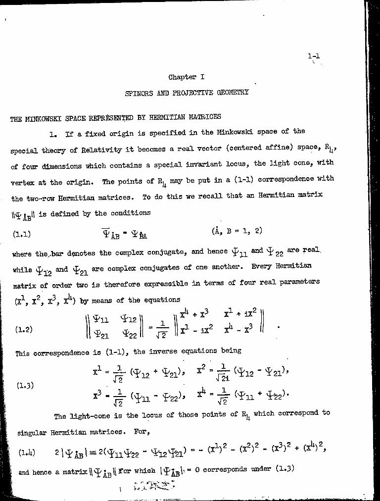
1. If a fixed origin is specified in the Minkowski space of the
special theory of Relativity it becomes a real vector (centered affine) space, R]^,
of foxir dimensions which contains a special invariant locus, the light cone, with
vertex at the origin. The points of R|^ may be put in a (1-1) correspondence with
the two-row Hermitian matrices. To do this we recall that an Hermitian matrix
is defined ty the conditions
where thenar d^otes the complex conjugate, and hence and are real
while 'i'21 congjlex conjugates of one another. Every Hermitian
matrix of order two is therefore expressible in terms of four real parameters
The light-cone is the locus of those points of Rj^ which correspond to
singular Hermitian matrices. For,
(1.1) (A, B = 1, 2)
(X^, X^, X^, X^) 137 means of the equations
(1.2)^12
'i'22
This correspondence is (1-1), the inverse equations being
and hence a matrix\(icar which ^ corresponds under (1.3)
I
1
1-2
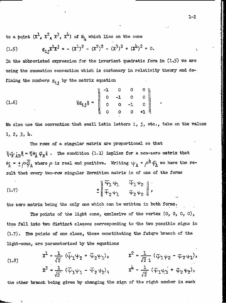
to a t>qint of Rj^ which lies on the cone
(1.^) g-..xV = - (X^)^ - (X^)^ - (X^)^ + (X^)^ = 0. ;J-J
In the abhreryiated expression for the invariant quadratic form in (1^5) we are
using the summation convention which is customary in relativity theory and de
fining tbe numberp g.. by the matrix equation
<1^6)
-1 0 0 00 -1 0 00 a -1 00 0 0 +1
We also use the convention that small Latin letters i, etc., take on the values
1, 2, 3, h.The rofws of a singular matrix are proportional so that
condition (l.l) implies for a non-zero matrix that
~ real and positive. I'^iting ^ we have the re
sult that every two-row singular Hermitian matrix is of one of the forms
(1.7) +Hi Ml ^1^2 ^2^1 ^2^2 9
•v>the zero matrix being the only one which can be written in both foi*ras.
The points of the light cone, exclusive of the vertex (O, 0, 0, O),
thus fall into two distinct elapses corresponding to -the two possible signs in
(1.7). The points of one class, those constituting the futtpe branch of the
light-cone, are parameterized by the equations
(^1^2 ~
the other branch being given by changing the sign of the right member in each
1-3
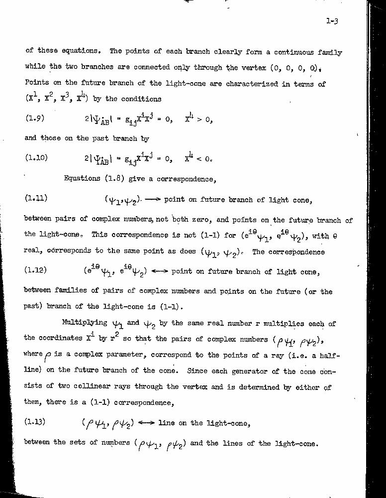
of these equations. The points of each branch clearly form a continuous fainily
while the two branches are connected only through the vertex (O, 0, 0, Q)^
Points on the futxire branch of the light-cone are characterized in terms of (X^, X^, X^) by the conditions
(1-9) > 0,
and those on the past branch by
(1.10) < Oc
Equations (1.8) give a correspondence^
(l.U) ^ point on future branch of light cone^
i© i@(e e ^ point on future branch of light cone.
between pairs of cor^lex numbers, not both zero, and points on the future branch of the light-cone 9 This correspondence is not (1-1) for (e^®v^^, ®
real, cdrresponds to the same point as does correspondence
(1.12)
between families of pairs of complex numbers and points on the future (or the
past) branch of the light-cone is (1-1).
Multiplying and by the same real number r multiplies each of 1 2the coordinates X ly r so that the pairs of complex numbers (^y^j ^
where ^ is a con5)lex parameter, correspond to the points of a ray (i.e. a half
line) on the futiire branch of the cone. Since each generator of the cone con
sists of two collinear rays through the vertex and is determined by either 〇f
them, there is a (l-l) correspondence.
(1-13) ^ line on the light-cone,
between the sets of numbers (lines of the Ught-cone.
1-U
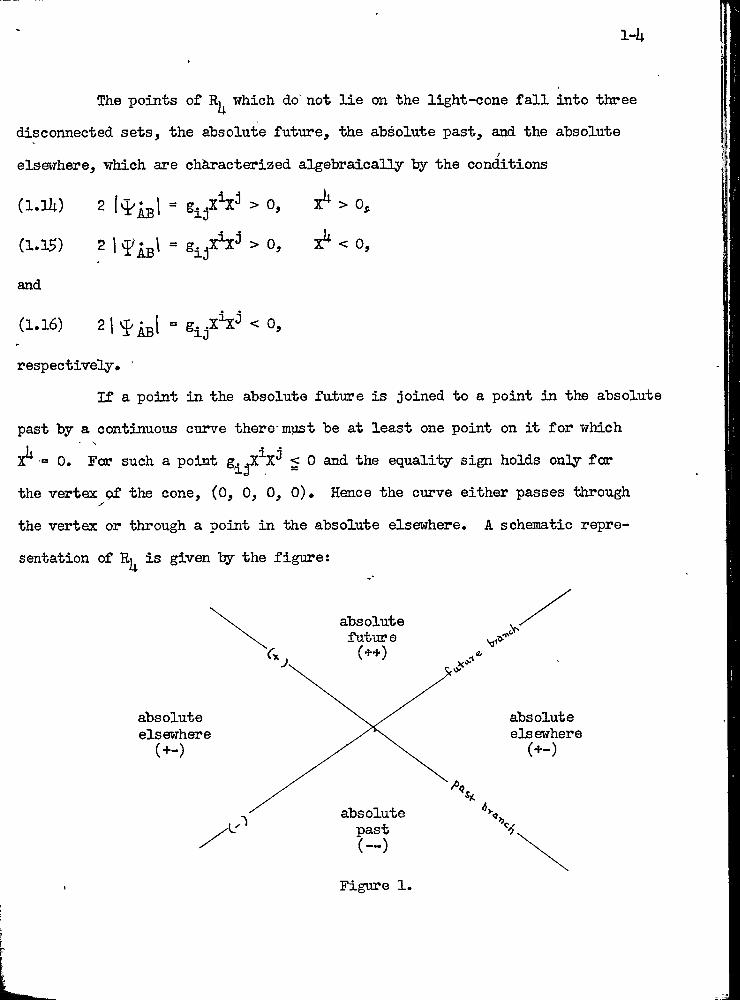
The points of Rj^ which do' not lie on the light-cone fall into three
disconnected sets, the absolute future, the absolute past, and the absolute
elsewhere, which are characterized algebraically by the conditions
(l.lU) 2 >0, X^ > 0,
(1.15) 2 1 = g^jXV >0, X^ < 0,
and
(1.16) = g^.xV < 0,
respectively# '
If a point in the absolute future is joined to a point in the absolute
past by a continuous curve there'must be at least one point on it for which X^ = 0. For such a point g^^X^X^ < 0 and the equality sign holds only for
the vertex pf the cone, (O, 0, 0, O). Hence the cturve either passes throughy'
the vertex or through a point in the absolute elsewhere. A schematic repre
sentation of Rj^ is given by the figure:
Figure 1.
t
1-5
The division qf into regions is easily described in terms of the
Hemitian matrices isrhich correspond to the points of Rj^. The condition (1®!)♦ \implies that the Hermitian form
(1.17) ^¿3
1 2is real for all values of the complex-variables Z , Z 9 In particular, iiie
point (0, 0,■〇, 1) of R|^ lies in the absolute future and corresponds under (1.2) to the Hermitian form (2^^ + Z^Z^) which is always > 0〇 if we agree to
vi2 12'exclude (0, o) as a possible pair of values for (Z , Z ). Similarly, the point
(0, 0, 1, 1) lies on the future branch of the light-cone and corresponds to the form yf2 Z^^ which is always > Oj the point (0, 0, 1, O) lies in the absolute
-2 2Z Z ) which assumes all realelsewhere and corresponds to the form —i-^ -1,1
valuesj the point (0, 0, -1, -1) corresponds to the form - /2 which isX -1 1 —P Palways < Oj ^d the point (0, 0, 0, -1) corresponds to---- (-Z Z - Z Z ) which
is always <0.
If an Hermitian form assumes one positive value it assumes all positive 1 2values since multiplying Z and Z by a real number r multiplies the form ly the
2positive number r . A similar result holds for negative values and hence the
range of values of an arbitrary Hermitian form is identical with the range of
values of one and only one of the typical foanns
(ipi8) zV^ -z^^, zh^ + Z^Z^з -Z^^ - Z^Z^, Z^^ - Z^Z^.
Hence an Hermitian form in two variables falls into one of five distinct classes
according as its range of values is > 0, < 0, >0,<0, or = 0.
The range of values assumed ly an Hermitian form is unchanged if we
make the linear substitution
AZ"^ = B(1.19)
1-6
with ^ 0. On making this substitution in (1.17) we find that
where
(1.20)
'i'ÀB ■ ?ÂB
icD'
To determine a substitution (1.19) which will reduce (1.17) to one of
the typical forms (1,18), we proceed as follows. Choose such that
*^1 ^1 ^/^1 ^ which is possible since we are assuming ^ 〇» Then
let O) be a solution of the single equation = 0 (and hence
not a multiple of ) and write Qg Qg ^ P 2’ transformation (1?19) with ^ and P^^ = will reduce to
wV or -W^V'e If ^2 ^ transformation (1.19) with P^'^ =
p2^ = P2^^2 reduce Z^Z® to + (iîV + W^) or + (wV* - wV).
¥e do not need to include both of the forms and -w\?^ + in our
list of canonical forms since interchanging thé variables carries one into the other.
It follows that an arbitrary Hermltian matrix || || 0) can be
transformed under (1.20) into one and only one of the matrices
1 0 -1 0 1 〇i -1 0 1 0(1,21) 3 9 > 90 0 0 0 0 11 0 -1 0 -1
and the matrix is then said to be of signature (+), (-), (++), (—), or (+-)g re
spectively. From (1.20)
1?Ав1 " I^A I I^B I I'^CdI ’
and hence a matrix of signature (+-) is characterized hy the condition | < 〇•
Referring to (I.I6) we see that the'absolute elsewhere is the locus of points
corresponding to matrices of signature (+-)« Since (1.7) with the plus sign is
1-7
of signature (+), the future branch of the light-cone ia the Ibcus of matrices pf
this signature and similarly the past branch of the cone is the locus of matrices
of signature (-). Since the absolute future is bounded by the future branch of
the cone, its points correspond to matrices of signature (++) and not of signature
(—). The regions of R|^ are therefore characterized in a manner iridicated in Figure
THE COMPLEX PROJECTIVE LINE
2. An ordered pair of con5>le3c numbers '^2'^ “^3^ interpreted <
as homogeneous coordinates of a point in a complex projective space of one
dimension, i.e* a complex projective line P^. Each point of P^ is represented
by one, and but one, family of pairs (^ where ^ takes on nil complex
values except zero. The pair of numbers (0, 0) does not correspond to any point
but any other pair does determine a unique point. Equations (1.8) define a (l-l)
correspondence (1.13) between points of P, and generators of the light-cone.In a similar way the ordered sets of real numbers (X^, X^, X^, X^) may
be Interpreted as homogeneous coordinates in a real projective space R^. This
amounts to recognizing that the lines through the origin of R|^ constitute a
projective three-space. The equation (1.5) represents a real non-ruled quadric in
R^. Thus the lines of the light-cone in R|^ are points of the quadric in R^. The
equations (1.8) give a (1-1) correspondence between the points of this quadric
and the points of the complex line P^.
If we set
(2.1) = Z,
we see the quadric (1.5) as the sphere
(2.2) + У^ + = 1
1-8
in a Euclidean three-space 'E^. This Euclidean space may be defined by specifying
the plane 0 of as plane at infinity and (1.^) as unit sphere. The points
of the sphere (2.2) represent the lines of the- light-cone in R|^.
Let us also set
(2.3)^1----= = Z = X + ny^2
where x and y are real. These equations establish a (1-1) correspondence between
the points of the compleS; line and the totality of- complex numbers z, including
00. The numbafs x and y can be interpreted as rectangular cartesian coordinates
in a Euclidean plane and we thus have a (1-1) correspondence between the points
of this plane, including one point at infinity, and the points of the coti5)lex
line P^.GoBibining (1.3) "With (2.1) and (2.3) 'we have the formulas
„ H^l'+'2 '+'2 ^ i + z _ 2xX = ------------ —---------------- 3 2 2^
vfiVfi + V2^2 1 + x+y
, X „1 ^1^2 ■ ^2"^1 _ 1 5 - z _ -2y(2.1i) Y = ^ -:::--------------------- - - 1------ ::------ -- 2 ? ’
^1^1 ^2^2 1 + 3Z 1 + x+y
„ ” ^2^2 _ z z - 1 _ x^- +--y^-- 1Z = -------- -----= 2 2^
+ \^2^2 ^ + 2Z 1+x+y
which define a (1-1) correspondence between the sphere and the z-plane (or xy-
plane). This coirespondence is discussed in function theory by means of stereo
graphic projection and indeed (2.U) nre the formulas for the stereographic pro
jection of the sphere upon an equatorial plane.
The points of R^ not on the sphere may also be represented in the xy-plane. Fdr, a point (A^, A^, A^, A^) uniquely determines its polar pldhe
(2.5) -A^^ - A^X^ - A^X^ + aV^ = 0,
■a
1-9
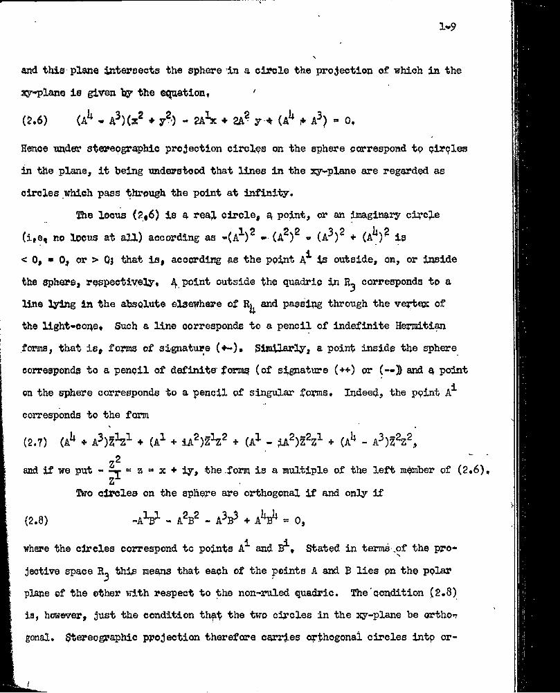
and this plane intepsects the sphere in a circle the projection of which in the
ay-plane is given hy the e<^ation, '
(2,6) (A^ - A^)(?^ ♦ y^-) - 2A^ + 2A^ y-fr (A^ A^) = 0,
Hence nn,der sterepgraphic projection circles on the sphere correspond tp pirples
in the plane, it being nnderstood that lines in the xy-plane are regarded as
circles which pass through the point at infinity.
13ie locus (2#6) is a real circle, a point, or an imaginary circle (i,e, no locus at all) according as -(A^)^ (A^)® - (A^)^ + (A^)^ is
<0,•0, or > 〇3 that is, according as the point A is oiitside, on, or li^ide
the sphere, respectively, 4. outside the quadrip in corresponds to a
line lying in the absolute elsewhere of and passing through the veptex of
the light-o〇ne. Such a line corresponds to a pencil of indefinite Herwitian
forms, that is, forms of signature (+-). Similarly, a point inside the sphere
corresponds to a pencil of definite'forms (〇f signature (++) 〇r (—)) and a point on the sphere corresponds to a pencil of singular forms. Indeed, the point A^
corresponds to the form
(2.7) (A^ + + (A^ + iA^)Z^^ + (A^ - + (A^ - A^)2^Z^,
and if we put - z » x + iy, the foriti, is a multiple of the left m^ber of (2,6), Z*^
iRro circles on the sphere are orthogonal if and only if
(2.8) -aV - A^B^ - A^B^ + A^^ = 0,
whace the circles correspond to points A^ and B^, Stated in terms ^.of the pro*
jective space R^ this means that each of the points A and B lies pn the pplar
plane of the other iJlth respect to the non-ruled quadric. The'condition (2.8)
is, however, just the condition th^t the two circles in the xy-plane be orthon
gonal. $tOTeographic projection therefore carries orthogonal circles intp or
I
1-10
thogonal circles.
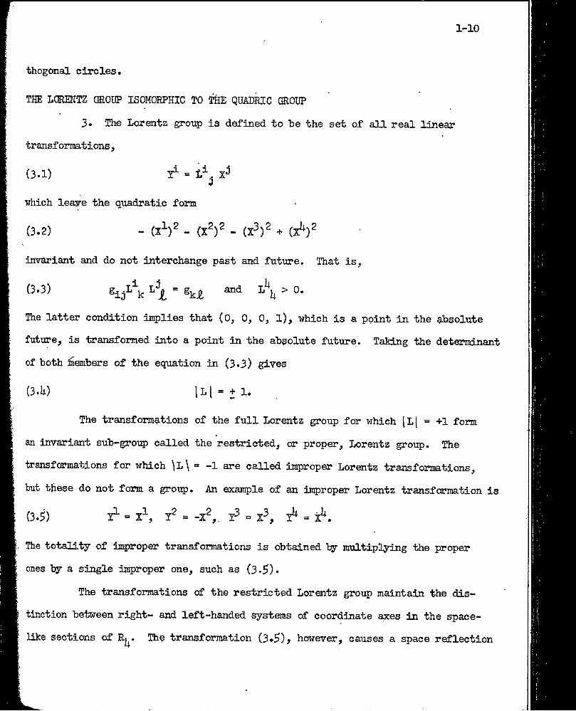
THE LCilEEiTZ GRODP ISOMORPHIC TO THE QUADRIC GROUP
3. The Lorentz group is defined to be the set of all real linear
transformations,
(3.1) = 1^. X^*w
which leasre the quadratic form
(3.2) - (X^)^ - (X^)^ - (X^)^ + (X^)^
invariant and do not interchange past and future. That is,
(3*3) “ ^kJi ^
The latter condition in^lies that (O, 0, 0, 1), which is a ppint in the absolute
future, is transfonned into a point in the absolute future. Taking the determinant
of both inembers of the equation in (3.3) gives
(3.1i) 1L[ = + 1.
The transformations of the full Lorentz group for which [Lj = +1 form
an invariant sub-group called the restricted, or proper, Lorentz group. The
transformations for xihich \L\ = -1 are called improper Lorentz transformations,
but these do not form a group. An example of an improper Lorentz transformation is
(3.5) = X^, T^ = -X^,. = X^, = X^.
The totality of improper transformations is obtained by multiplying the proper
ones by a single improper one, such as (3-5).
The transformations of the restricted Lorentz group maintain the dis
tinction between right- and left-handed systems of coordinate axes in the space
like sections of Rj^. The transformation (3*5)j however, causes a space reflection
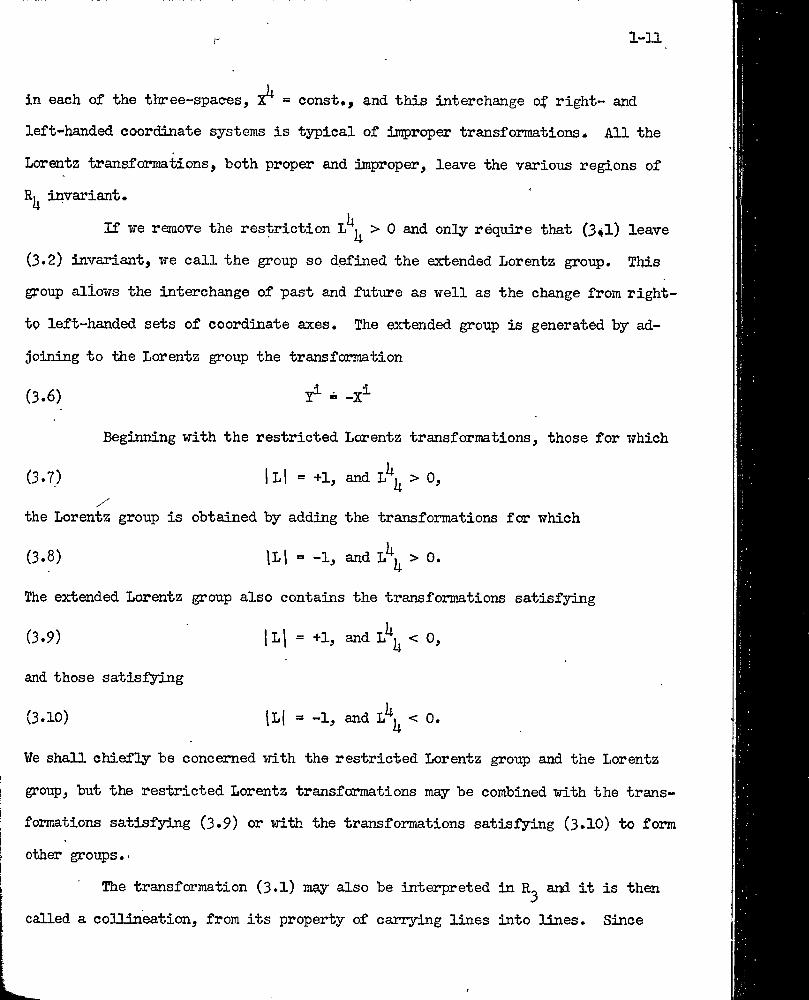
r 1-n
in each of the three-spaces, = const», and this interchange of right- apd
left-handed coordinate systems is typical of iirproper transformations. All the
Lorentz transformations, both proper and improper, leave the various regions of
R|^ invariant.
If Tie remove the restriction > 0 and only require that (3^1) leave
(3*2) invariant, Tre call the group so defined the extended Lorentz group. This
group alloTfs the interchange of past and future as well as the change from right-
tp left-handed sets of coordinate axes. The extended group is generated by ad
joining to the Lorentz group the transformation
(3.6)
Beginning with the restricted Lorentz transformations, those for which
(3.7) |l1 = +1, and L^j^ > 0,
the Lorentz group is obtained by adding the transformations for which
(3.8) iLl = -1, and L^j^ > 0.
The extended Lorentz group also contains the transformations satisfying
(3.9) 1l| = +1, and L^^ < 0,
and those satisfying
(3.10) lL| = -1, and L^i^ < 0.
We shall chiefly be concerned trith the restricted Lorentz group and the Lorentz
group, but the restricted Lorentz transformations may be combined with the trans
formations satisfying (3.9) or with the transformations satisfying (3.IO) to form
other groups.'
The transformation (3*1) inay also be interpreted in and it is then
called a coUineation, from its property of carrying lines into lines. Since
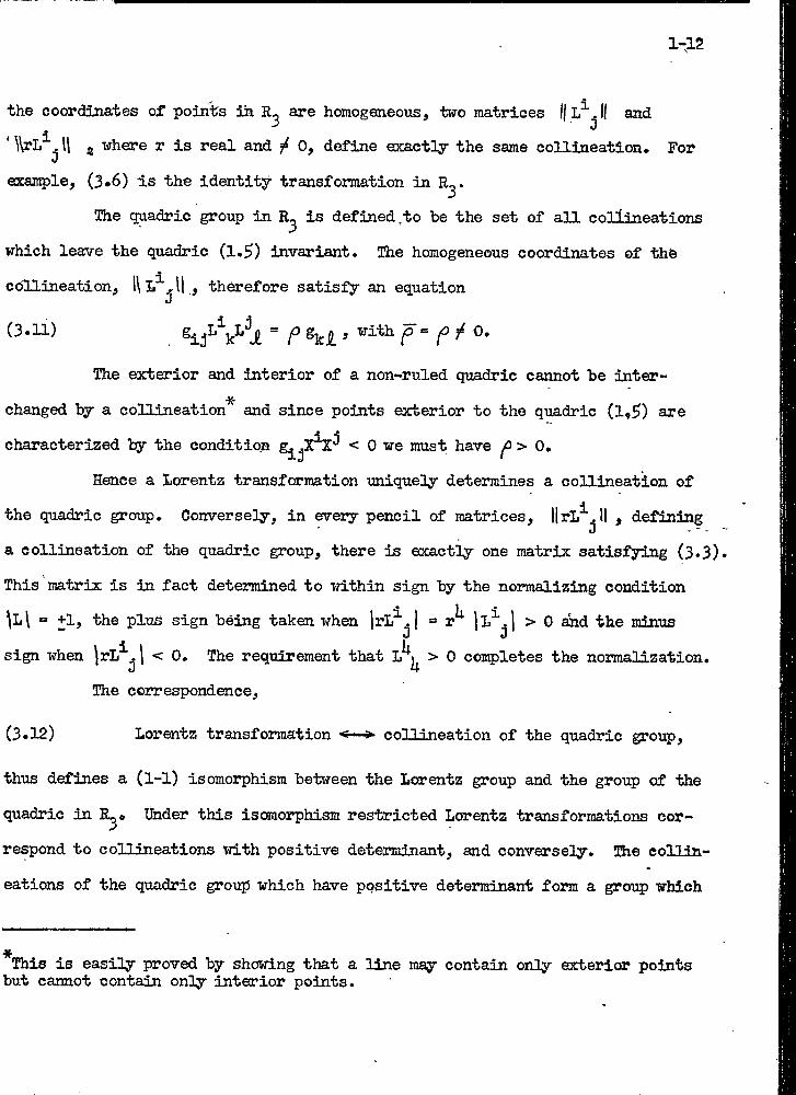
1-12
the coordinates of points in R_ are homogeneous, tero matrices and( d.' \\tL . H g where r is real and f 0, define exactly the same collineation. For
exaitqjle, (3*6) is the identity transformation in
Ihe quadric group in is defined,to be the set of all collineations
which leave the quadric (1.5) invariant. The homogeneous coordinates of -fee
collineation, , therefore satisfy an equation
(3.11) , with O,
The exterior and Interior of a non-ruled quadric cannot be inter-
changed ly a collineation and since points exterior to the quadric (1,5) are characterized by the condition g^^X^^ < 0 we must have p> 0,
Hence a lorentz transformation uniquely determines a collineation of the quadric group. Conversely, in every pencil of matrices, llrL^^H , defining
a collineation of the quadric group, there is exactly one matrix satisfying (3*3).
This matrix is in fact determined to T^rithin sign by the normalizing condition ^L\ = +1, the plus sign being taken when IrL^.j = r^ jl^.j > 0 abd the minus
sign when jrL^^I < 0. The requirement that > 0 completes the normalization.
The correspondence,
(3.12) Lorentz transformation <—■» collineation of the quadric group,
thus defines a (l-l) isomorphism between the Lorentz group and the group of -üie
quadric in E^« Under this isomorphism restricted Lorentz transformations cor
respond to collineations with positive deteiminant, and conversely. Bie collin
eations of the quadric group which hâve positive determinant form a group which
This is easily proved by showing that a line m^ contain only exterior pointsbut cannot contain only interior points.
1-13
we can the restricted quadric group.
The one-to-one character of the isomorphism (3*12) is evident from the
fact that a Lorentz transformation is completeOy deterinined hy the way in which
it permutes the lines through the origin of Rj^.
THE RROJECTIW)- ®〇IP IN ISCMORPHIC TO THE PROPER LORENTZ (210UP
li,. The projective group on the complex projective line is the set
of all linear transformations --
^1"
= e + d
with 1c ^ 1 Oj where two transfbrmations are identical if and only if their
coefficients are proportional. Thus if (H.l) is abhreviated to
B.
Oi.i)
(h.2)
the equations (p^ ® ^ coiEplex and ^ 0, effect exactly the sane
permutation of the pencils of number pairs (hence define the
same transformation* In terms of the non-homogeneous coordinate z ® V^i/
(It.l) is the general linear fractional transformation
n az + b(U.3) ’Si = 72-+-a Í
where w =Two configurations in P^ (for exanple, two ordered sets of points) are
said to be projectively equivalent if there exists a projactivity (li*2) which
carries one configuration into the other* The fundamental theorem of one^
dimensional projective geometry then States that there is a uniquely determined
projectivity which carries three distinct points into any other three distittct
points. To prove this theorem it is stifficient to shew that the points (1, O),
(0, 1), (1, 1) can be carried Into the distinct points- (〇(0(2^» /^2^*
and ilf-^3 ^2^^ respectively, in just one way. In order that (1, 0) shall go
into (〇( (X 2) have in (U.l) a = ° " /^^2
to go into (y^2.A /^2^^ ^ ^ ^/^1* ^ ~ "Hlth ^ and 0. Then jO and <r
are determined by the equations
“ f«l * ’^f‘v
which have a unique solution with y〇 7^ 〇 and cr 0 if the points 〇( 3 jS, and ^ are
distinct. Hitroducing a factor of proportionality into the coordinates of theBpoints alters the four components by a common factor. Similarly, in
n-dimensional complex projective geometry two sets of n+2 points are equivalent
under a uniquely determined projectivity if no n+1 points of either set lie in
the same^Jiyper”plane.
The transformation (lj..2) brings about a linear homogeneous transformation,
(H.l;)
of the degenerate Herraitian matrices ^ agree that (U.U)
is also induced by (U»2) on all Hermitian matrices, we have the transformation
(1.20) studied in §1.
Let us write (1.3) in the abbreviated form
x-* iABy,S ^AB •
iABThe coefficients g have the values given by the four matrix equations
llg3ABll . _i_4i
0 11 01 0
0 -1
1y〇
01
J
1-1$
The equations (1,2),which are inverse to ih»$) may then be written
(h.7)
and we have
(4.8)
where
^Ab " %Ab ^
.iAB 2 • ® ^ ®jAB 3 ’
S^jll -1 ,
and also
(4.9)
where
=iAB giCD C, rD^ A ^ B *
^ ° II = IlS^giiI IS ¿J ; - n 0 X
The transformation (4.4) induces a transformation X
ables which is represented by
(4.10)
This is of the form (3.1) with
T of the vari-
iAB p C p D .
(k.U) ,
and is real since (4.4) carries Hermitian matrices into Hermitian matrices.
As a transformation of the four variables ^2# 'f'21» 'P22
has a matrix
(4.12)f
ab bbaa ba a b 0 0 a 0 b 0ca da cb db
B c d 0 0 0 a 0 bac be ad bd 0 0 a b c 0 d 0cc dc cd dd 0 0 c d 0 c 0 d
Hence (4.11) is equivalent to
(4.13) 1 |L^ J I “ k -19
1-16
where k denotes the foitr-row matrix of (li.5) regarded as a linear transformation
of vj^21» ^22^ Taking the determinant of
both members of (li*13) gives
(i.U) li.'-jl = wl=■lp/l^\p/l^
and therefore [L^.[ is positive* Since (li.lt) changes singular matrices into J
singular matrices the colliiieation (3*1) with L^. given by (li.ll) is an elementJ
of the quadric group. Hence every projectivity of corresponds under (It. 11)
to a uniquely determined collineation of the restricted quadric group in R^.
This correspondence is a (l-l) isomorphism between the projective
group in and the restricted quadric group in R^. We shall prove this by
a simple geometric argument which makes use of the fact that a collineation of
the restricted quadric group is completely determined by the fate of three
points on,the quadric.
The points on the quadric correspond to the points of the complex line
P^. We have already constructed the uniquely determined projectivity of P^
which carries three distinct points into aj:y other three distinct points. This,
combined ■with equations (It.10), gives a collineation of the restricted quadric
group which carries any three points of the quadric into any other three points.
Moreover, there is just one collineation of the restricted quadric group which
does this. For, if T^ and T2 are transformations of the restricted quadric
group which have the same effect on three points, ^ is an element of
the group which leaves three points on the quadric invariant. We shall show
that in this case T is the identity.
The plane of the three points is invariant, and hence the conic in
: which this plane intersects the quadric is invariant. The intersection of the
tangents to the conic at two of the points is a fourth point, not collinear with
1-17
any two of the other three, which is also invariant-. The collineation T there
fore induces in this invariant plane a collineation which leaves four points in
variant, no three of the points being coUlnear. JEgr the fundamental theorem of
two-dimensional projective geometry, this collineation in the plane is the
identity and hence T leaves each point of the plane invariant.
The polar point of the plane with respect to the quadric is an invariant
point not in the plane. ' If we draw a line through this point which intersects the
quadric in two real^points, and P^, the line intersects the plane in an in
variant point and is therefore itself invariant. Hence T either leaves P^ and
separately invariant, or it interchanges them. In either case the fundamental
theorem for three-dimensional projective geometry assures us that there is. just
one collineation having the givqn effect. ¥e have therefore found that there
are just two cpllineations of the quadric group which leave three points A, B,
C on the quadric invariant. One of these two transfonnations must have negative
determinant. For, consider an arbitrary collineation with negative determinant,*
it carries the points A, B, G into three points which may be called A*, B’, G*5
and a collineation with positive determinant can be found which carries A’, B‘, G’
back into A, B, G. The product of these two collineations has negative determinant
and leaves the points A, B, G invariant. Hence, of the two collineations which
leave three points invariant, one is the identity and the other is a collineation
whose determinant is negative.
¥e have now completed our proof that there is a (l-l) isomorphism be
tween the restricted quadric group in and the projective group in P^. In
the last section we established the existence of a (l-l) isomorphism betiieen the
restricted Lorentz group and the restricted quadric group. Hence, combining
these two isomoiphisms, we get the (1-1) correspondence
1-18
(li,l5) projectivity of > restricted Lorentz •toansfomation. ’
To escpress tfiis isoraorphisia as a correspondence between matrices, we
normalize tbe matrix of a projectivity to within sign by the condition
(1^*16) jp^®| = +1.
The matrix 'defined by (U.ll) is consequently nomalized so that
(lt.l7) ' = +1,%)
as follows from (l].«ll})* Moreover, we saw in §1 that or the equivalent
transformation (I4..IO), does not interchange the absolute future and the absolute
past. Hence is a proper Lorentz matrix and not the negative of one.
This result means that if we are given a restricted Lorentz matrix,
, there are just two^unimodular matrices, and - , which
satisfy (lj.,11). Conversely each of the two uniraodular matrices IjP.®i/ix
and - Hp^ (I determine the same restricted Lorentz matrix by means of (it. 11).
Since the product of two Lorentz matrices corresponds to the products of the
corresponding unimodular matrices, we have the (2-1) isomorphism,
(lt.l8) unimodular matrix llP^^K —restricted Lorentz matrix /|L^.|j ,
betvieen the group of unimodular matrices of order two (with complex elements)
and the group of restricted Lorentz matrices (with real elements).
THE ANTIPROJECTIVE GROUP ITT P^ ISCMORPHIG TO THE LORENTZ OlODP
equations
5'* An antiprojectivity in P^ is a transformation of P^ defined by
of the form
(5.1), ?A = ’’a®
fi'th I ^ 0, and two sets of equations of this form define the same anti-
1-19
projectivity if and only if their coefficients are proportional. In terms of
the non-honrageh'eous coordinate z = —= , (5.1) is^2
(5.2) w - 4-—c5 + d
where 11II = || jj ? Clearly, the set of all antiprojectivities results
fpom comhihing all the projectivities with the special antiprojectivity
(5.3) ‘f'A‘^A
^ HThe antiprojectivfe group is the set of all projectivities and anti-
pro jectivities. It contains as an invariant sub-group the projective group.
The aiTbiprojactivities alone do not foimi a group since the product of two anti-
pro jectivities is a projectivity. Thus the product of (5.1) and the antipro-
jectivity^ is the projectivity antiprojective
group ia-Obtained by adjoining any one antiprojactivity, say (5.3), to the
projective group.
The transformation <5.3) carries the singular .Hermitian matrix
that is.
H^l M-i
^2^into
+l'h.
'^2^1
(5.W $21=i'l2^ ^22"'^22>
and we assume that (S»h) is induced on all Hermitian matrices by (5.3), Referring
to (1.2), we see that (5.it) is represented in the coordinates of by the trans
formation (3.5). Multiplying all the projectivities. of by (5.3) gives the
set of all antiprojactivities and multiplying the restricted Lorentz trans
formations by the corresponding transformation (3.5) gives the set of all
1-20
iuqjroper Lorentz transformations, as we saw in §3.
In the last section we established a (1-1) isomorphism between the
projective ^oup in and the restricted Lorentz group in R|^., This has how
been extended to include toe (1-1) correspondence.
(5.^) antiprojectivity of improper Lorentz transformation.
and hence there is a ,(1-1) isomorphism between the antiprojective group in P^
and the Lorentz gropp in
The equations defining (5.5) are got by following (5.1j) with the
transformation (i;.*ii). Thqy are
(5.6) = p C p D-AB "A *^¿0^/
and hence in the coordinates of R^ th〇y are of the form (3.1) with
(5.7) L^ = P ^ P ^ e • j ^ ^A ^B ®jDC*
Since the determinant of (3.5) is -1,
(5.8) = . 1P^B| 2
Horraalizing the coefficients of the antiprojectivities to Tiithin sign by the
condition
(5.9) ip/i = .1.
equations (5*7) determine a (2-1) correspondence,
B(5.10) unimodular matrix Hp.^H in^roper Lorentz matrix (¡L^.l/ ,0
ihe correspondences (U.18) and (5.10) may be combined to give the theorem:
For every proper Lorentz matrix 11 . |( there are exactly two unimodular
matrices, RP^ |( and - ||p^ (I ^ which satxsfjr (U#U), and for every improper Lorentz
matrix there are exactly two unimodular matrices, and -(/P ,are
1-21
/
which à&tlsfy (5.7). Conversel7, if ||P^®I| is a tmlaiodular matrix it determines
a proper lorentz transformation by means of (U.U) and if I|P^^®(1 is a nnimodular
matrix it determines an improper Lorentz transformation by means of (5.7). More
over, the ptpodnct of two Lorentz transformations corresponds to the product of
the corresponding normalized transformations in P^.
COCEDIÏÏATE mnSFCEMTIONS ATO TENSOR CALCULUS
6. to this point we hâve employed only a single coordinate system
in each of the spaces considered. The linear transformation (3.1) 〇f was
regarded as a permutation of the points of The coordinate transformation
(6.1) - A^J,
with |Aj 1 0, is of the same form as (3.1) but is to be regarded as a renaming
of the points of R|^, rather than as a pernratation of the points. Defining a coordinater^system' in as a (1-1) correspondence between the points of R^
For a gener^^scussion of coordinate systems see the Cambridge Tract «Foundations of differential geometry", ty Veblen and Whitehead.
and sets of four real numbers, the cartesian coordinate systems are those de
rived from the special one we have been using in the sections above, by the
group of transfonnations (6.1) with H A^ || real and constant.
Ifeder (6.1) the quadratic form g. becomes g. .*X^*X^* where g *ij °i;5
is related to
(6.2)
«13 by the usual tensor law
» “ *i ^3 ^kl
with aj defined byf
(6.3) .3
I
1-22
In what^ follows is a general quadratic form which can be reduced to (3»2)
hy uiqans of a real transformation (6.1) but which is not necessarily identical
with (3.2).
Coordinate systems in which the quadratic form is given by (3*2) are
called Galilean coordinate systems. Since a transformation of coordinates be
tween two Galilean coordinate systems satisfies (6.2) with g. .•» = g. ,, the ex-
tended LdTentz 'group could have been defined as the set of all those transformations
which carry one Galilean coordinate system into another one of the same kind.
(6.ii)
The covariant tensor g . and the contravariant tensor g^^ defined by
enable us to raise and lower tensor indices. Thus if is a contravariant
vector transforming by the law (6.1) and we put
(6.5) ’-
then
(6.6) X.1a9 X. 1 J
and this is the law of transformation of a cpvariant vector. Moreover^
(6.7) X^ =
If we take the determinant of both members of (6.2), we find that
(6.8) * 2 g = a g
where g ~ ^ ~ This is the law of transformation of a relative
4scalar of wei^t two. In general we consider relative tensors having the trans-
* Some writers use the term'density". ¥e prefer to reserve density for the case to which this tepa has been applied in physics. Thus a relative scalar of weight one is a density.
1-23
formation law
(6.9) 0™ “ Aj ... af a^ ,.. xP^**'* .Jim... P q X m st...
and the weight of such a tensor is said to be w. îhe right member of (6,9) is
a linear and homogeneous pol^omial in the components of the tensor and is ahomogeneous expression in the elements of the matrix Ha^H .
THE ALTERNATING NUMERICAL TENSCRS
7* The rule (6.^) is the familiar way of associating with a contra-
variant tensor a covariant one. A less familiar way of doing this employs a
covariant tensor 6 weight -1. In any one coordinate system wedefine to be +1 if (i, k, Jt) is an even permutation of
(1, 2, 3, U)^ -1 if it is an odd permutation, and zero otherwise. Then the formula, for the expansion of |a^j , which IS
,P .q «r ^s(7.1) “ Sqrs ^i ^
insures that the tensor shall have exactly the same components in any other
coordinate system. The weight of the tensor &jLjk£ exponent of a
when (7.1) is written in the form
.. -1 ^ ears^ij'kfl. “ ^ ^pqrs h \ ’
A contravariant vector determines a covariant tensor
(7.2) ^ijk “ ^ijki^'^*
This amounts merely to a renumbering of the components X^, X^, ..., X^as
indicated in the formulas
(7.3) X^23 “ "^213 U U U 'Î~ “ ^231 ” ^ > ^^2li ~ )[ ** ... “ -X , etc.
u ^While the components of ^lak are equal to plus or minus the components of X^,^
f
l-2lt
it is nevertheless true that a is a contravariant tensor and is a covariant -ione. If A is of weight w^ is of weight w-1.
For the ccsrresponding operation of raising indices we -use the relative
tensor 6^^
(7.W
kJlof weight +1 defined "by the relations
,ijki= +1 if (i,j,k^) is an even permutation of
= -1 if (i#j,k^) is an odd permutation’of
= 0 if two of the indices are equel.The expansion of )A^1 can be written in the form
.ii-i
>^2 ■ ae aJ a3 AÏ a! , p q r s '
since )a^) = la^j = a and this identity proves that if is a
contravariant tensor of weight +1 then its components have the same values in
all coordinate systems.
''A covariant index is converted into three contravariant ones by the rule
(7.5) ÿjkl = y g ijkû i
*^ik-Hand if is of weight w, is of weight 1+w. We may also sum off two of
ijkil against two covariant indices as in the equations
- i I.. ê2 ij
ijkl
the indices of 6.
(7.6)
which are an abbreviated form for ''
(7.7) = I (Yjl, - Yjjj), = i (X|,, - Y„,), etc.2 ■‘21»'
Since the right members of these equations involve only the combinations
(Y^^ - the equations will not have a unique inverse unless the
components Y^^ are restricted in some way. The simplest restriction is
Y. . = - Y..,(7.8)
and such a tensor is said to be skew-symmetric. We shall apply (7.6) only to
skew-symmetcic tensors and for them the equations inverse to (7.6) are
(7.9) ij 2 xjkl
since
(7.10)
where
1 e2 ‘"ijkJL ^ =
IThe equations inverse to (7.2) may be written in a form similar to
(7.5) since
(7.12)
and hence
1 ^ijkp 31 ^ ^ijkJl
(7.13) xP = 1 ^IT ^ijk gijkp^
For a more extended treatment of the tensor calculus, the reader is
referred to: "Applications of the absolute differential calculus", hy A, J.
McConnellj "Riemannian geometry", 1:^ L. P. Eisenharti "The differential in
variants of generalized spaces", by T, I, Thomas; the Cambridge Tract, "Invari
ants of quadratic differential forms", by 0• Veblen; or to any of the numerous
books on the subject. The first chapter of the Cambridge Tract, "Invariants
of quadratic differential forms", contains general fomulas of which (7.10)
and (7.11) are special cases.
DUAL COORDINATES IN R^
8* The linear transformation (6.1) may be interpreted as a coordin
ate transformation in R^ instead of in R|^. In doing this we must remember
1-26
that (6.1) and
(8.1)
effect exactly the same permutation of the sets of homogeneous coordinates (rX^, rX^, rX^, rX^) and therefore define the same coordinate transformation in
R^. The formalism in R〇 is identical with that in R, but many of the relations3 J5 4
have a simpler geometric interpretation in R^ than in Rj^.
Thus in general coordinates the plane polar to with respect to the
quadric is
(8.2) g^^ X^ = 0, or A^X"" = 0,
and so lowering an index by the rule (6.5) corresponds to the geometric opera
tion of taking the polar plane with respect to the fundamental quadric. Thei *1inverse of this operation, raising an index by means of g corresponds to
taking the polar point of a plane with respect to the quadric.
The homogeneous coordinates of a point P of R^ are uniquely determined
as solutions of the set of equations
(8.3) P. .. X"" = 0,ijk
where P.is defined in temis of P^ by means of (7*2)» This is evident if I3K
we use (7.3) to write out (8.3) in the form
- P^X^ = 0, pV^ - P^^ = 〇r etc.(8.1;)
Hence a point has covariant coordinates well as contravariant ones
P^. These covariant coordinates, like the contravariant ones, are homogeneous.
The existence of covariant coordinates corresponds to the possibility
of defining a point as the intersection of the planes containing it. Thus if
p. arid' . are three independent planes which contain P^, then the tensor
1-27
(8.5)
TT = JL c ni /.V
- 1“T"
is not zero and satisfies the equation
(8.6) = 0.
In a coordinate system in which P has the coordinates (1, 0, 0, 〇) this equation,
together ifith the skew-synmetry of ijïç)lies that the only non-vanishing
components of are TÎ23^ obtained by a permutation of these
indices. The same result holds for hence
(8.7) "^ijk "^ijk ,
In equation (8.7) we must remember that if P^, CX ^ and are
of weight zero, then is of weight -1 and is weight zero so that ^
musttrans:Ç〇rm as a relative scalar of weight +1. ¥e could, for example, putX^ rr <r (-g)** where <r is a scalar of weight zero.
Two points, P and Q, of determine the line joining them, and this
line has the contravariant Pltlcker coordinates
* A discussion of thesè coordinates is given in Veblen and ïoung*s "Projective geometry", Vol. I, p. 327.
(8.8) = pV - Q^P^
Replacing P^ by P^ + XQ^ in this equation does not change the value of p ^
and since a similar result holds for the homogeneous coordinates p ^ do not
depend upon which points on the line are chosen to define it. In particular,
we may take P to be the point in which the line intersects the plane ^ and
then p^^ 'ۥ " -)P^* Hence p^^^. is the point in which the linen i) ^
1-28
intersects the plane ? . and the condition that the plane contain the line is^ 3
(8.9) .^3
Similar]^, if ^ and are planes tihich contain the line PQ, co
variant Plflcker coordinates of the line are ''
(8.10) " °^i /5j “ /^i^o
Then is proportional to the tensor p^^ defined by
(8.11) u 1 ^ ki ^ij “ 2 ^ijk£ P
as we readily prove by taking the coordinates of P and Q to be (1, 0, 0, O) and
(0, 1, 0, O) and of 〇( and yd to be (O, 0, 1, O) and (0, 0, 0, 1). The tensor p. . is said to be the dual of p^^ and (cf. (7*6)) is the dual of q... The
term "dual" is appropriate since the principle of duality in a projective (or
vector) space implies the existence of the two sorts of coordinates. If we applyu ii <j iithe rule (7«6) to p. . we recover p and hence the dual of p. . is p
The coordinates of a line, p^^* satisfy the equations
(8.12) = 0,Pjk
since the left member is just
*2 ^jkilm
and for fixed i and k = 1, 2, 3, this is the expression for the minors of the matrix -P^Q^ + -P^Q^ + -P^Q^ + -P^Q^ +
ij ilm
Q" 〇5
•We shall now prove the converse proposition, namely, that if an arbitrary skew-
symmetric tensor not equal to zero satisfies (8.12), its components are the
1-29
coordinates of a line.
From (8.12) it follows that the stim of the nullities of Ij p^^|( and
llP^k^ is equal to or greater than the range of the index J and hence ranlc llp^^ii +rank <k. If rank = 1, the equations p^^ = 0
have three independent solutions, and after a suitable transformation of
coordinates we may take these solutions to be the unit vectors and^Then p^^ « p^^ a p^^ = 0, and since p^^ = 0 on account of the skew-
symmetry, we have p^^ = 0, contrary to assumption. Hence rank llp^^lj > 2.
A similar result holds for p^^ and consequently rank llp^^H = rank Up. ./( =2.The equations p^^ = 〇 therefore have just two independent sdlutions and if
we choose the coordinate system so that they are andP^^ “ and hence represents a line. In the same coordinate
system P^^ = 〇“( j “ ^i corresponds to the same line as does
In this argument we have not made use of the relationship (8,11) between p^^ and p^^ and we have therefore proved that if p^^ and q^. are skew-
symmetric tensors different from zero and
(8.13) ii ¡k • °>
then and are coordinates of the same line. Indeed, by an entlreOy
similar argument it is possible to prove that if p ^ ^ ^ and ^are non-vanishing skew-symmetric tensors which satisfy the equation ^ ^
(8.U,) p 1 2 ^ °
then p and q are coordinates of the same linear space of (a-1)-dimensions in a
projective space of (k-l)-dimensions.
1-30
Equations (8♦13) are equivalent to
(8.15)
as follows readily from the identity
(8.16)
which holds for arbitrary skew-symmetric tensors (« -1^^) and (* -T^^).
To reviSy this identity we use (8.11) and its inverse, which is of the form (7*6),
to get
(6.17X
C Sgs
^ XWJjyWg Og^ Wj. Opg O l£/*pq
Putting in (8.16) gives
(8.18)
and hence (8.12) is equivalent to(8^W) P% si e^^^jjp«p'=^-l, (pV . pV= . pV^) - 0.
Hiis equation is therefore the necessary and sufficient condition that be
the coordinates of a line. The condition for the lines with coordinates
and to Intersect can be shown to be
(8.20) ii»JP - 0.
To interpret the covariant tensor p^^^ geometrically, we observe that
Kultiplying (8.8) by gj^ gj^^ and summing gives
i 1-31
(8.21) Pkfi, “
and hence are the covariant coordinates of the line polar to p^^ with
respect to the q-uadric. The line p^^ intersects its polar if
(8.22) p^^p.^ = 0
and so this is the condition for p^^ to be tangent to the quadric. The line
win lie on the quadric if it coincides with its polar and the condition for
this is (cf. (8.13))
(8.23)
This condition is not satisfied by the coordinates of any real line.
THE SPINOR CALCULUS IN
9. In the coit5)lex projective line the hyperplanes are themselves
points and^therefore a point is equally well represented by its contravariant 1 2coordinates (vjy 9 (jj ) and by the coefficients of its equation
(9.1)
Indeed, we have anticipated this result by tTriting the coordinates of a point
with the indices in covariant position. In order that (9*1) shall be the1 2equation of the point (\|^ , ) it is necessary and sufficient that
(9.2) _^2S^l
This relationship can be expressed in terras of a i*ule, analogous to (7*2) andAB(7.13) j foi* lowering and raising indices by means of matrices 1| H and ||6 il
defined by the equations'^
^ The left and right indices will always refer to the rows and columns, respectively.
•X1-32
(9.3) ne^gll =|j_° J|| . Iie^ll .
The covariant components of a point are related to the contravariant
ones by the formxila
In vre had two methods of converting contravariant indices into covariant
ones. In P^, however, we have no fundamental quadratic form and so the rule
(9.1;) is our only way of lowering indices. For this reason we write for
the left member of (9<>a) instead of as we should do by strict analogy with
(7.2).
The equations inverse to (9.1;) are
(9.?) y^
BAin which^it is important to notice that we sum on the first index of 6 .
The proof that (9*5) is inverse to (p.h) is contained in the equations.
(9.6) ^
It follows at once that
(9.7) hence =
Moreover,
(9.8)
where
(9.9)
s B
HSbH - 1
0
TRANSFOR^aTIŒÎS OF COORDINATES IN
10. A tr'ansformation of coordinates in is given by equations of
the form
(10.1)
*pwhere lt?| / 0. The equations
xT = lB
vrith yo a complex number 0, determine exact]y the same permutation of the homo
geneous coordinates (crX^, cr'^2^ therefore define the same transformation
of coordinates.lBIn every pencil of non-singular matrices there are just two
•animodular ones which are
3 _ +B . ■^ ®A " ^A ^(10.2)
wh^e t = 11® I and the two values of [1 S® || arise from the ambiguous sign of
“ At . For the purposes of projective geometry we could therefore restrict our
selves to the transfonnations of coordinates
(X0.3)
With unimodular matrices. ¥e however find it advisable to make use of the
general transformation (10.1) which is a composite of the coordinate transformation
(10.3) and the transformation
(10.1.)
which multiplies the coordinates of each point by a factor but does not change
the coordinate system.
¥e may achieve the effect of restricting ourselves to the unimodular
transformations (10.3) ty assigning a suitable weight to Thus ±C Kjj^
is of weight - ~ its transformation law is±
(10.5)
Similarly, a geometric being of weight will have the transformation law
(10.6)
where
(10.7) “ S〇
to (7.1),
(10.8)
and
(10.9)
The formula for the expansion of a two-rowed determinant is analogousABand therefore the transformation laws of 6 and 6^^ are
t\®Vb 6__t CD-1
’ABC D== Vb CD
^C^D6®t = .AB = sis? CD
C“Dfrom which it follows that 6'^® is of weight +1 and is of weight -1.
Hence the weights +J[, for and -1 for are consistent with the rules
(9.h) and (9.5).
The geometric being which has the components closely
analogous to a covariant vector in the sense that we have used this term, but
the coefficients of the transformation (10.l), or (10.3), are complex instead
of real. This allows the more general transformation law
(10.10)
for a geometric being with components (10.10) we call w and d the
weight and antiweight, respectively. "When w = d the transformation may be
1-3$
written as lt(^ where Itl =■ (t t)* is the absolute value of the
determinant, t* In this case is s.aid to be of absolute weight 2W.
A geometric being with the transfcrmation law (10.10) is a particular
instance of what we shall in the next chapter define' to be a spinor. Whatever
the values of w and d in (10.10), still represents a point, but we shall
usually take w = -i-,d=0.
A less trivial instance of a spinor is the geometric beir^ defining
an antiprojactivity. Thus if an antiprojectivity of has the equations
(10.11)
in one coordinate system, then in a coordinate system related to the first by
(10.l), it will have the equations
(10.12)
where
(10.13) 7*0 .«■. D mB■A
,c-w ^•'^-4
and V and c are the weights of and w and d of v//^. We. shall usually take
V = w = -1 and c = d = 0, so that (10.13) may be written
(10. Hi) _ _ -C D „B ,
Bwith these weights the normalization |P^ I - 1 is invariant. The placing of
the dot over the index C in (10.13) or (lO.lii) serves as a reminder that a bar
is to be placed over the corresponding t^ or s^ in the law of transformation.
Equations (10.13) are of a more general type than is encountered in
the ordinary tensor calculus in that they involve not only the components ofl\tt 11 but also the complex conjugates of these, components. This possibility
B
does not arise in tensor calculus, which refers to real coordinates and real
transformations. ¥e shall consider spinors having a transformation laii of the
type
(IO9I5) x^B“*CD***HP••p GH• •«
^ ^ ^Q.. .RS. ► . . mi rpBTU...W,..-^P ^Q*
mC sD T . U rV r¥ .Wrd ^F***^G ^ •
It is always possible to choose the weights w and d so that the transformation
can be written in terms of the unimodular matrices || s^ 11 and 1)3^11 and we
shall usually do this.
The raising and lowering of dotted indices is accomplished Tidth the• •
aid of spinors and 6^^ by the rules
(10.16) and - ^AB
where(10.17) •' =|_° "II . .
These rules are consistent vrith the antiweights + £ for contravariant dotted• •
indices and -1 for covariant dotted ones since € and e :A have the trans-AB
formation laws
tTjf; 6mB cCD ^ ^AB ^ ^CD gA gB(10.18)
and
(10.19)
and hence have the antiweights +1 and -1, respectively.
r“^ rC rD ^ . -C -DA B CD AB Cb A B"
¥e also need to consider spinors having some indices which refer to a
coordinate system in Ri and some which refer to a coordinate system in P_^ 1
For example, the coefficients of the fundamental equations (li.7) transform
under (6.1) by the rule
1-37
(10.20) ^iAB “ 4.
and under (10«1) by the rule
^iAB(10.21)
_ . rC .D .-X %CD ^B ^
-C D ^i6d ®A %
INVOLUTIONS IN
11. Using our rule for raising and lowering indices, the equations
of a projectivity in may be written in the four equivalent forms
(11.1) / . and' - P«(^g,
where if 1| P^gll ^ Jj i "then
№ab" “ll-a -bll> "®A®« = lit " lt:d Jll'respectively. It is to be observed that the’ order of the indices distinguishes P^g from Under the transformation of coordinates (10.1) the equations
of the projectivity become where
(11.3) pA _ rpA pC .D iq~p
.A ^Aif p and q gre the weights of and ^ ^ respectively, and their anti-/ A Bweights are zero. Taking q = p = ^, Pg and P^ are of weight zero, P^
is of weight -1, and P^^ is of weight +1. ’ The normalization iP'^gl = +1 is
invariant if the weight of P^_ is zero.a
The matrix llP^B» will define an involution if P^g P®^ ^ “
^and II P^gll is not a multiple of j| ^ ^|j . That is,
(ll.A)2a + be b(a+d) K 0
c(a+d) be + d^ 1 0
1-38
•or a + d = О, !Ehis is expressed in convenient forms try the equivalent equations
(11.5)
only if
The point
<?A =
у will be invariant under the projectivity (11,1) if and This is equivalent to v^Va = 0, or
(11.6) = + (P^2 +
All the coefficients of this quadratic equation vapish only when P.„ is a multipleaJj
of and in this case the projectivity is the identity. Otherwise a projectivity
has just two invariant points which are distinct when the symmetric matrix
^AB non-singular and coincident when it is singular.
¥e can always express the coefficients of a projectivity in the form
(11.7) ^AB *^AB ^ C ^AB
Sdnce Рдв “ = P C e^, we have
(11.8) *^AB ~ ^^лта Ртзл) Q'■AB BA" ’‘BA
and so with a projactivity P there is associated the uniquely determined involu
tion Q. The double points of P are the same as those of Q.
The invariant points of an involution completely determine it. For,
the roots of (11.6) determine its coefficients to within a common factor and the
additional condition = P21 gives *'^Ab'^ within a factor. Indeed, the
projectivity defined by
(11.9) ^AB "
is the involution which leaves 0^ and jS invariant. Since
(U.IO) /вА“<В - 〇^А/«в“ '^AB
the involution is also given by
1-39
(11.11)
or by
(11.12) = 2y5^(Vg - «g) e^^g.
A singular projectivity (/〇) is of the form this is
to be an involution (that is to say, symmetric) we must have cTg = Putting
- (-^)^ the general singular involution is
(11.13) ^AB "" ^A^B^
and this is just what we get by putting y(S^ = in (11.9). This singular in-
volution carries every point, except of j into (X .Two points, and I^, determine the homogeneous scalar the
vanishing of which inplies the coincidence of the points. If the scalar does not vanisli, its value is changed when the coordinates X^ are multiplied by a
factor’. Four points, however, determine the absolute scalar
(li.lil)
which is called the cross-ratio of the four points, ( (p i^jiJ^). The valtte of A
is invariant under transformations of coordinates. Moreover, since the right
member of (11.lit) is homogeneous of degree zero in the coordinates of the
points, the value of X*depends only on the points and not on the coordinates
chosen to represent the points. Under a projactivity a set of four points goes
into a new set which has the same cross-ratio as the old, but under an anti-
projectivity the cross-ratio is changed into its coit^ilex conjugate.
“ ?A " «Ab/ Q^g is given by (11.9), we have
(11.15)
When this relation holds, the points (j) and (pare said to be harmonic conjugateswith respect to and ^ . Since (11.1^) determines (Ji^ as a. function of to
within a factor, the involution with invariant points 〇( and ^ may be defined
as the transformation which carries any point into its harmonic conjugate with
respect to the pair of points, 〇( and .
A projactivity which interchanges two points is an involution. For,
by a suitable choice of coordinate system we may take the covariant coordinatesBof the points to be (l, 0) and (D, 1) and then 11 \( will interchange them only
12 Aif “ ^2 ” implies the invariant condition P^ = 0, which characterizes
an involution. Indeed, the projactivity
(ll〇l6) ^
with X and pi arbitrary complex numbers is an involution which interchanges
and^ . The most general proj activity with this property is of this form.
For a projectivity is determined by the fate of three points and if X and JJ
are solutions of the equations
(11.17) ’Va>
Q will carry a t 3 ^ ^ 3 (X 3 1) 3 respectively, where and 7)
are arbitrary points distinct from both 〇( and y3 .
It is an important theorem that every projectivity in P^ is the product
of two involutions. ¥e prove this theorem by considering several cases. The
identity is the square of an involution and we have seen that ary other projectivity
has just two double points, which may coincide. Hence it is sufficient to consider
projectivities with two distinct double points, non-singular projectivities with
1-ia
one double point, and singular projectirities.If the distinct invariant points of the projectivity P are a and b, we
let C( and^ be a pair of points harmonic conjugate with respect to them and
define to be the involution with double points 〇( and ^ . Then, denoting
the projectivity which results from following P by hy we have that
Q^P interchanges a and b and hence is an involution, Since - 1,
P = Q^^P = Q^Q2 and P is the product of two involutions.
If P is non-singular with the single invariant point a, we take 〇< to
be a point distinct from a and call ^ = P(X the transform of iX under P. Let b
be the harmonic conjugate of a with respect to a' and^ , the involution with
double points a and b, and Qg the involution with double points a and /3. Then
Q Q a = a, Q„Q, 〇( = Q^& - /S . Moreover QgQ^ cannot leave invariant any point 2 1 2 1-jf ^ a for Q2<2;j_ 'JT = ^ would imply Q^'Zi = ^nd and would both inter
change and $ = . This and the invariance of a under both and Q2
would imply = Q2J which is false. Hence, P and each have the single
invariant point a and each carry(X into^ 〇 Reference to a canonical coordinate
system novr easily gives P = ^2*^1”A singular projectivity is given by a matrix H and if (V and ^
are distinct points this is the product of the singular involutions II Wj^oCgll
and 11/S^jnll • 'When the projectivity is a singular involution, , it is
the product of II «¿«bH and Wc(\ + , where y is distinct from 〇i 〇
AHTIINVaLUTIONS IN P^
12. An antiprojectivity vjx—^ (f may be written in the four equivalent
forms
(12.1) 9a = p* ^ABB ^A^A = “ ^A ^ “ P^Bv//,
B’
the coniponents of the four matrices "being related as in (11.2). If we take both Cf and vjy^ to be of weight i and antiweight zero, we must take P^_ to be of
weight - ^ and antiweight + -i, to be of weight + | and antiweight -
to be of absolute weight -1, and P^ to be of absolute weight +1, With these
weights the determinant of each of the four matrices is'invariant and a
normalization such as = 1 is preserved under coordinate transformations.
Ihe invariant points of the antiprojactivity (12.1) are given by
(12.2)
If we put
(12.3) HAB"2 ^ ^AB “ I ^^AB " ^BA^ ^
then and l|K*gll are Hermitian matrices and
(12.h) P. 25 H* + i K* AB AB AB”
Equating the real and imaginary parts of the left member of (12.2) to zero gives
(12.^) = 0 and = 0.
Representing the points of P^ by points of the sqjr-plane as in §2 by the equation
(cf. (2.3))
(12.6) X + iy
(12.^) are the equations of two circles (i*eal, degenerate, or imaginary) in the
sy-plane. (In the special cases in which = 0 or = 〇, one of the equations
is satisfied identically and there is only one circle.)
If the two circles do not coincide, they may intersect in two points,
be tangent, or fail to intersect, and the antlprojectivlty will then have two,
one or no invariant points, respectively. Si-om (12.li) we see that
(12.7) ( X* l>l)PiE = (XH^ - + 1 (XK^j +
and hence the homogeneous components, H^P^gH j of an antlprojectivity do not
determine a unique pair of circles (12.5) but only the pencil of which they
are members.
If equations (12.5) define one or a pair of coincident circles (real
or imaginary), and only in this case, the antiprojectivity will be an antiinvolution. For, if llP^gll “ I|q antiinvolutions are characterized
ly the matrix equation
a b a b 1 0
c d c d
1
0 1(12.8)
and multiplying both members by ^c -a
•n= transpose 1] || gives
a b -d b (-(ad - be)
c d 1 c -a 1using the fact that (P^^)(P^^) = - |P^p, | transpose. Thus
—D — p D(P q) = ------— (P^ ). Lowering the index D we find that a non-singularbet (P®p)
antiinvolution therefore satisfies the equation
(12.9) P*^AB
where 〇-= - ^ and it follows from (12.3) that the two circles (12.5)
coincide. Taking the determinant of both members of (12.9) we see that
cry = 1, so that
(j- ^ p. = p.AB ^ ^BA
and hence \\ <r^ W Hermitian. The matrix defining an antiinvolution is therefore proportional to an Hermitian matrix and conversely every Hermitian
matrix defines an antiinvolution.
A non-singular antiinvolution is of one of two kinds according as theV.
Hermitian matrices defining it are indefinite or definite. The discussion of
§1 proves that a suitable choice of coordinate system will allow us to take—1 1 —2 2the equation of the invariant circle to be ^ vp = 0 or
_2^ '^2 2 = 0 according as the antiinvolution is of the first or second
kind, respectively. In terms of the non-homogeneous coordinate z, these
circles are zz = 1 and zz = -1, and the corresponding antiprojectivities are
w = ~ and w ------ •3 z
A singular antiinvolution (/〇) is of the form and (12.8) now
q) = 0, or
singular antiiiprolution are proportional to and the antiinvolution
carries every point, except (X , into 〇( .
^e antiinvolutions which leave two points, say 〇< and yS , invariant,
correspond to the circles through 〇( and . These circles are linearly de
pendent upon any two among them so that
(12.10) = X((V^y6g + ^
is, for a suitable choice of the real numbers X and , any antiinvolution
leaving 〇( and ^ invariant.
The involution with invariant points 〇( and ^ is the product of the
antiinvolutions i6( ^^^a/b " Aa^b'^’
(12.11) aA〇 ^ A^
Moreover, the singular involution 〇(^0(-q product of Aa^B
and Hence every involution is the product of two antiinvolutions.
Me saw in the preceding section that every projectivity was the product of texo
/«B V“b- Hence the matrices defining theimplies c< jS-o
involutions and so every projectivity is the product of four antiinyolutions.
Remembering that all the antiprojectivities are obtained by multiplying the pro-
jectivities by a single antiinvolution, we have the result that the antiinvolu
tions generate the entire antiprojective group.'
POINT-PLANE EEFLECTIQNS IN
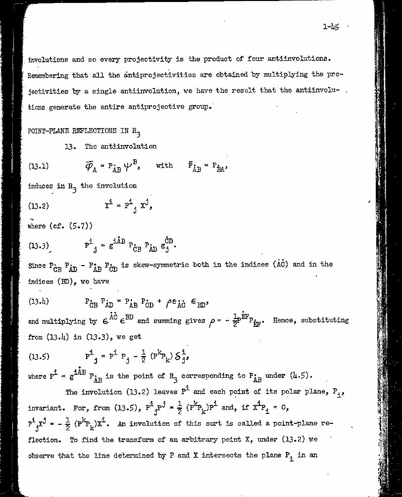
13. The antiinvolution
induces in the involution
(13.2) 2^ = P^.%)
where (cf. (5»7))
(13.3)
'’6b '’¿b
indices (ED),
- P* Pi_ is skew-symmetric both in the indices (AC) and in the AB CD
we have
(13.h) P^3 P^jj = P^ Pqjj + €gjj,
and multiplying by 6® and summing gives - ip^P|jp. Hence, substituting
from (I3.il) in (13.3)j we get
(13.^) = P^ P^ - i CP\)Sy
where P^ = g^® P^ is the point of R^ corresponding to P^^ under (i|.5).
The involution (13.2) leaves P^ and each point of its polar plane, P^,invariant. For, from (13.5), ^^^P^ “ ^ (P^jj)P^ and, if X^P^ = 0,
P^.X^ ® - -K (P^i )X^. An involution of this sort is called a point-plane re- 0 2 k
flection. To find the transform of an arbitrary point X, under (13.2) we
observe that the line determined by P and X intersects the plane P^j^ in an
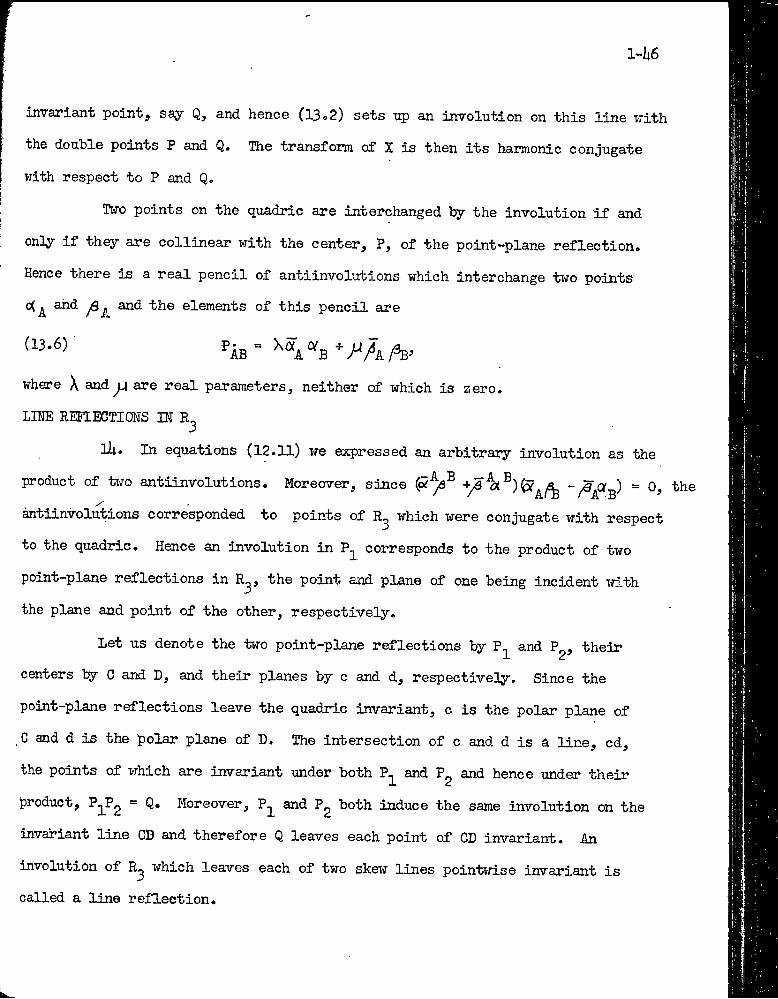
l-li6
invariant point, say Q, and hence (13〇2) sets up an involution on this line with
the double points P and Q. The transform of X is then its harmonic conjugate
with respect to P and Q.
Two points on the quadric are interchanged by the involution if and
only if -they are collinear with the center, P, of the point-plane reflection.
Hence there is a real pencil of antiinvolutions which interchange two points
〇(^ and jSj. and the elements of this pencil are
where \ and^ are real parameters, neither of which is zero.
LINE REFLECTIONS IN
lU. In equations (12.11) we expressed an arbitrary involution as the
product of ttro antiinvolutions. Morecrver, since ~
antiinvolutions corresponded to points of R^ which were conjugate with respect
to the quadric. Hence an involution in P^ corresponds to the product of two
point—plane reflections in R^, the point and plane of one being incident with
the plane and point of the other, respectively.
Let us denote the two point-plane reflections by P^ and P^, their
centers by C and D, and their planes by c and d, respectively. Since the
point-plane reflections leave the quadric invariant, c is the polar plane of
C and d is the polar plane of D. The intersection of c and d is a line, cd,
the points of which are invariant under both P^ and P^ and hence under their
product, 1*2^2 “ Moreover, P^ and P^ both induce the same involution cn the
invariant line CD and therefore Q leaves each point of CD invariant. An
involution of R^ which leaves each of two skew lines pointwise invariant is
called a line reflection.
l-U-7
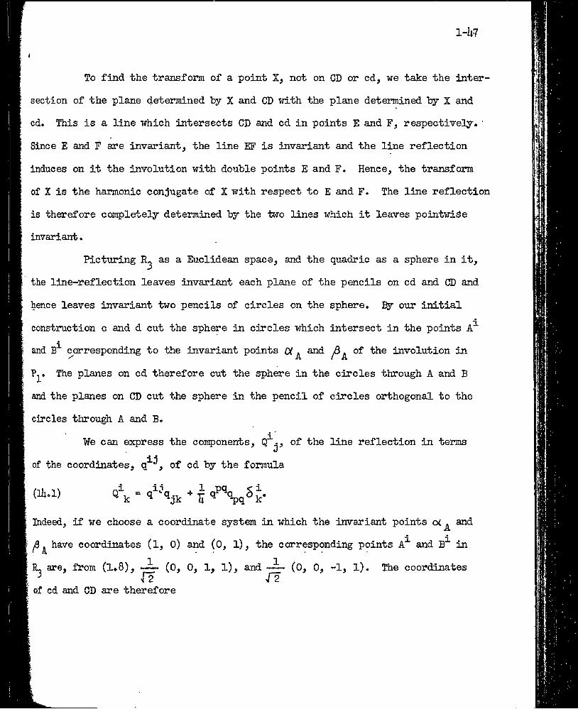
To find the transform of a point X, not on CD or cd, we take the inter-
section of the plane determined hy X and CD with the plane determined by X and
cd. This is a line which intersects CD and cd in points E and F, respectively. '
Since E and I? are Invariant, the line EF is invariant and the line reflection
induces on it the involution with double points E and F. Hence, the transform
of X is the harmonic conjugate of X with respect to E and F. The line reflection
is therefore carnpletely determined by the two lines which it leaves pointwiSe
invariant.
the line-reflection leaves invariant each plane of the pencils on cd and CD and
hence leaves invariant two pencils of circles on the sphere. By our initial
P^. The planes on cd therefore cut the sphere in the circles through A and B
and the planes on CD cut the sphere in the pencil of circles orthogonal to the
circles through A and B.
Indeed, if we choose a coordinate system in which the invariant points oi . and
construction c and d cut the sphere in circles which intersect in the points A' and B^ corresponding to the invariant points C( ^ and of the involution in
i
We can express the components, Q^., of the line reflection in termsJ
iiof the coordinates, q of cd by the formula
AjS ^ have coordinates (1, O) and (O, 1), the corresponding points A^ and B^ in
3 ' ¡2 T2\ of cd and CD are therefore
R. are, from (1.8), —i- (O, 0, 1, 1), and —i- (O, 0, -1, 1). The coordinates
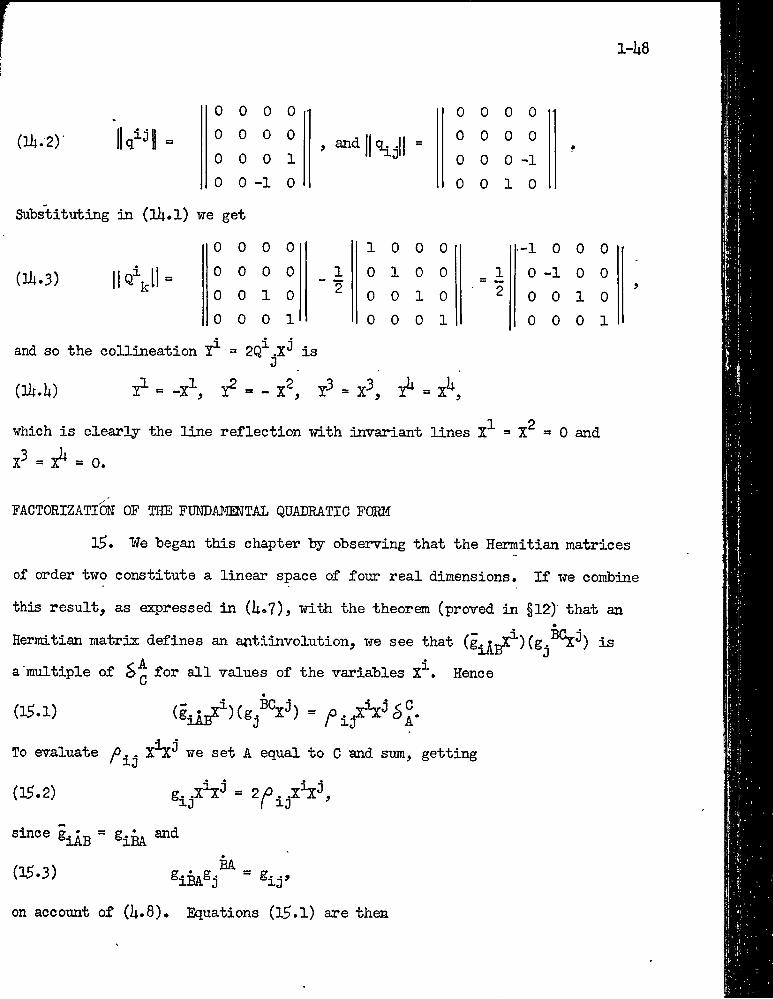
(lil.2)'
1-U8
=
0 00 00 0 00 0-1
0 0
0 0 1
and KJI ■
0 0 0
0 0 0 0 0 0
001
00
-10
Substituting in (iH.l) we get
(Hl.3) ||Q^[i =0 0 0 0 1 0 0 0 -1 0 0 00 0 0 0 1
" 20 1 0 0 _ 1 0 1 H 0 0
0 0 1 0 0 0 1 0 2 0 0 1 00 0 0 1 0 0 0 1 0 0 0 1
and so the coUineation = 2Q^.X^ isd
(3i{4) - X^ , = x^, = x^.
which is clearly the line reflection with invariant lines X”^ = X^X^ = X^ = 0.
0 and
FACTORIZATIQEJ OF THE FUEDAMENTAL QUADRATIC FORM
l5. ¥e began this chapter by observing that the Hermitian matrices
of order two constitute a linear space of four real dimensions. If we combine
this result, as expressed in (U®7), with the theorem (proved in §12) that an Hermitian matrix defines an antiinvolution, we see that (g^gX^) (g is
^ A *ia multiple of ^ for all values of the variables X . Hence
(15.1) (i^gX^)(g^®V) =
To evaluate X^^ we set A equal to C and sum, getting
(15.2)
since = e.i. and ^iAB ^iBA
(15.3) BA®iBA®j “ ^ij’
on account of (I4..8). Equations (l5*l) are then
1-U9
cA*
Equating coefficients in (l5.it) gives the important equations
(15,5) BC ^ - BC ®iAB®3 ®jAB®icC ^i j ^A*
Equations (15«U) may he interpreted as a factorization of the quadratic form into the product of two linear forms, >[2 j.and <[2 gjgQ ^> with
matrix coefficients. We shall be able to write as the square of a
single linear form if we combine 11 g^^ 11 and \\ \\ into the four-rowed matrices
(15.6) ti=>T2 0 00 0 0 0
and observe that (l5«5) and its conjugate iniplies
(15.7)
Then (15.U) may be written
(15.8) Oi ¿X^)^ = 1
2-1
GMapter II
1. The space underlying the theory of relativity is the Mnkowski
UNDERLIING AM) TANGENT SPACES
space which we will call It is a four-dimensional space in which the dis-' tance between two space-time points (events) and y^ is given ly
a.i) s^ = - y^)(x^ - y^).
The preferred coordinate S3^tems of are those in which the distanceformula (1.1) becomes
(1.2) 5^ = - (X^ - y^)^ - (x^ y^)^ - (x^ - 7^)^■ + (x^ - y^)^.
Cartesian coordinates are obtained from preferred ones by transformations of the
form
= A^xj + a^(1.3) Xwhere A^ and a^ are constants and A = 1A^ | ^ 0.
0 JIf the quantities A^ are the coefficients of an extended Lorentz trans-
Jformation, the transformation (1.3) carries one preferred coordinate system’into
another.
Fixing an arbitrary point y in Xi changes it into the space Ri con
sidered in Chapter I for if we make the transformation to the Cartesian coordinates
(l.ii) - x^ - y^ yi « / _ yi = 0
equation (1.2)
(1.5)
Scomes
s2 = - (x^)^ - (X^)^ - (X^)^ + (X^)^
L6
The transformations which leave the right member of (1.5) invariant in form and
the point = € invariant are just the transformations of the extended Lorentz
group. Thus the four-space characterized by the quadratic form (1.5) and its
2-2
preferred coordinate systems is Rj^.
Allowable coordinate systems in are obtained from preferred
coordinate systems transformations of the type
(1.6) = f^(x)
where f^(x) are analytic functions of x^x^x^ and x^ such that
(1.7) ji 0.
Since (1.2) defines the distance between two arbitrary points of we may
mploy this formula in the usual way to define the length of a curve.
Thus the length of a segment of. a curve is the integral of ds taken
along the segment, where
(1.8) ds^ = - (dx^)2 - (dx^)2 - (dx^)2 + (dx^)2.
In allowable coordinates this equation becomes
(1.9) ds^ = g^^ (x)dx^dx^.
The quantities dx^ dx^ dx^ and dx^ may be considered as coordinates in
a space Tj^(x), the tangent space. Thus at every point of Xj^ we have an associated
tangent space T^^(x). The transformation (1.6) of X|^ induces in T^^(x) the linear
homogeneous transformation with constant coefficients
(1.10) dx^^ = dx^
5x^^since the quantities ----r- are independent of dx*^.
9x^The point whose coordinates have the value (O, 0, 0, 0) in one coordi
nate system in Tj^(x) has these coordinates in all coordinate systems of T^(x).¥e identity this point with the point x^ ... x^ of the underlying space and call
it the point of contact of T|^(x) and X^^. Because of the special role of the
2-3
point (O, 0, 〇5 〇)> T^(x) is a centered affine (or vector) space in which the length of the vector is given ty equation (1.9). The points -of T|^(x) which
satisfy the equationds^ = dx^ dx^ = 0
are said to be on the light cone. In a preferred coordinate system in this
equatiori becomes(1,11) - (dx^)^ - (dx^)^ - (dx^)^ + (dx^) = 0.
Thus each T|^(x) is a replica of the space Rj^ studied in Chapter I.
The geometry* of any space may be characterized by the class of pre-
# Veblen and ^Jhitehead, Foundations of differential geometry.
ferred coordinate systems in it and the pseudo group of transformations which
transforms one into another. In the case of the tangent space T^(x), the pre
ferred coordinate systems are the Galilean ones and the group is the extended
Lorentz "group.From the relations between the transformations in and Tj^(x) we see
that a general transformation in Xj^ induces the satellite Cartesian transforma
tion (1.10) in The only coordinate systems we will use in T^(x) are the
Cartesian ones.It is possible to consider the dx^ as the homogeneous coordinates of
the lines through the origin in T^(x). As remarked in §2, Chapter I, these
lines constitute a three-space, which will be denoted by T^(x). Since dx and
pdx^ correspond to the same point in T^(x) and since th^ also represent the
same direction in it is evident that T^Cx) is the space of directions of
vectors in T|^(x). Thus at every point x of there is associated a. real pro
jective three-dimensional space with a real non-ruled quadric, the space of
directions T^Cx).
SPIN AND GAUGE SPACES
2* Rrom the correspondence, discussed in Chapter I, between and
the complex projective line P^, we see that to every Tj^(x) there is associated
a P^(x). That is, with every point x in the underlying space there is associated
a con5)lex projective line P^(x).The points of each Pj^(x) are denoted by the homogeneous coordinates
'^2^* ^ transformation of coordinates
(2.1) ,where the t^ are arbitrary coH5)lex numbers such that(2.2) T^t® = Sq and t = (t^l 0
changes a given homogeneous coordinate system in another such system.
Two pairs of equations like (2.1) represent the same transformation in P^(x) if
their coefficients are proportional. All transformations of the type (2.1)
with proportional coefficients determine the same unimodular transformation:
(2.3)
where
_(2.U) Sg = tgt and hence s = |sg| = 1.
These homogeneous coordinate systems ire the preferred coordinate systems
in P,(x). Ai^ two of them are connected by the transformations (2.1) or (2.3).
2-5
ihe transformations (2.1) >JilI be called general spin ti-ansformations.
The space P^(x) differs from the tangent space in that there is no
singular point in it which may be regarded as the- point of contact with the
underlying space. Also the transformations in P〇_(x) are completely independent
of the transformations in and of the satellite transformations in T^(x).
Transformations of the type (2.1) are generated by a unimodular trans
formation of the type (2.3) followed by the transformation
(£.U) . y// = .
If we write
(2.5) ^
where r and 0 are real, we see that the transformation (2.1i) may be written as
the product'lie the following two,
(2.6) Y'a* '
and
(2.7) ■
The transformations (2.6) and (2.7) will be shown to be closely related
to transformations which we will call gauge transformations of the first and
second kind respectively. Since P^(x) is a projective space (-^^, and
represent the same point in P^(x)^ hence the transformations
(2.U), (2.6) and (2.7) cannot be pictured in P^(x).
However, the totality of transformations (2.6) is a group simply iso
morphic with the group of rotations about the origin in a real Euclidean plane
and is multiply isomorphic with the group of translations of a real Euclidean
line into itself. Hence, if we associate with each P^(x) a real Euclidean line.
we can picture the transformations (2.6) as translations along this line. We
shall call this associated space the gauge space of the first kind Gj^(x) and
describe it by the variable x®. The transformations in G^(x) are of the form
(2.8) = X® +0,
Similarly the transformations (2.7) nay be picttired as translations
along another real Euclidean line which we will call the gauge space of the
second kind GgCx), We shall d:escribe it by the variable The transforma
tions in Gg(x) are of the form
(2.9) = y“ + log r.
Hence we see that the general spin transformation of the type (2.1)
may be picttired as a transformation in P-j^(x) followed by translations in G^(x)
and G2^) • if;Just as in tensor analysis wHere the geometry of all the tangent spaces
is studied simultaneously by considering vectors which are functions of the
coordinates of the underlying space, we propose to study the geometry of all
the spin spaces simultaneously by considering the as analytic Complexscalar Inunctions of x^ x^ x^ x^ and the transformation coefficients (2.1)
and (2.3) as arbitrary analytic complex functions of x^ ... x^ subject to the
conditions (2.2) and (2.U). Similarly all the gauge spaces G^(x) and Gg(x)
are studied simultaneously by considering r and 0 in equations (2.8) to (2*9)as arbitrary real functions of x^ ... x^.
In the following we shall restrict ourselves to spinors of the form
(2.10) Vi “ **•
where I is a pure imaginary number and J is real. Also x® and y® are arbitrary
2-7
real ntmibersi they are the coordinates in the spaces G^^(x) and GgC^c) respectively.
If we fix a point x in the ‘ underlying space, and homogeneous
coordinates of a definite point in the'associated spin space P^^(x). That is,
equations (2.10) are another means of writing the infinite set
(J> arbitrary) of homogeneous coordinates of a point in P]_(x), which is
specified as soon as a point in P^(x) is- specified. If x° is* given a -definite
value, that is, if a point in the first gauge' space G^^(x) is specified, then the
argument of ^ is fixed. Similarly, if y° is given a definite value, that is, a
point in 〇2(х) is specified, the moduliis of is fixed. Hence assigning ddfinite
values t〇'X° and y® selects a particular pair of hompgeneous coordinates of a
point in Рд^(х).
DEFINITION OP SPINORS
3. A frame of reference is specified when we give an arbitrary coordinate system in and a preferred one in each of the spaces T|^(x), Рд_(^)>
Од^(х) and GgCx). There is a change of frame of reference whenever the coordi
nate system in or any of the associated spaces is changed.
■ A geometric or physical being win fcxr our present I»u3iposes'be an
entity which has a unique set of* components in each frame of reference. 'The
components in two frames of reference are related by a transformation law,
namely a formula which gives the components in one frame in terms of the
components of the other.
Tensors are a special class of geometric beings. Their transformation
law is such that only the change in reference frame produced by the transformation
(3.1) = x^*(x)
of X|^, produces a change in the components of the tensor. Under the 1;ransforraa-
2-8
tion (3*l)j the components of the tensor in- the new frame of reference are linear
homogeneous functions of the components in the old frame, and the coefficientsi-^9xare homogeneous functions in The degree of homogeneity of these func
tions is determined by the number of covariant and contravariant indices and the
weight of the tensor.
For example, the transformation law of a contravariant vector is
(3.2) = V^(x)
where the right member is a homogeneous polynomial of the first degree in - ,9x^
For a mixed tensor of second order and weight w we have
(3.3) ji^t ^ ^ 9x^ 9x 0
i*
^ <yx‘^ <yx. li:
homogeneous functions of
9 -«mXw
9x^The right member is a linear homogeneous functions of and the coefficients are
〇:-
9x^ . ax^ .-- !— Since ■ - - -j-j and9x^
9x.mif-
in--- of degree minus one and I4.W respectively.9x^
o n (9xw are homogeneous functions
A spinor is a geometric being which has a transformation law of the
following t3^)e. It is a tensor under coordinate transformations, a scalar under
gauge transformations of either kind, but under spin transformations of the type
(2.1), the new components are linear homogeneous functions of the old components and the coefficients are homogeneous functions in the t? and t? . For example
A A(31)
is the transformation law of a simple covariant spinor of weight w. The trans
formation law of a contravariant spinor of weight w under the same transformation is
(3.5)
where
2-9
ABThe quantities £ and 6j^g which-we have used to raise and lower sjiin
indices are spinors of weight +1 and -1 respectively. Their transformation laws are
(3.6)
(3.7)
A spin 'density may be defined as a spinor which transforms as a scalar
or weight 1 under spin transformations. If we require that this densityyo have
the value 1 in a particular Spin coordinate system, than in any'other spin
Coordinate system it will have the value
= ¿AB ^ gCD qA
«AB -
(3.8) p = t
where t is the determinant of the spin transformation which carrier the first
coordinate ss^stem into the second. From equations (3-6), (3*7) and (3*8) we1 ABsee that ^ (5 will then have the transformation laws
(3.9) ''
(3.10)
P ^AB "/^CD^aS
1 c AB«- ^ 2_ c CD rpA „B ^ p ^ C D'/
■ ABThat is, £ and are weightless contravariant and- covariant
spinors of second order respectively. They have been \ised by Van der WaerdenABand Inf eld to raise and lower indices in plage of £ and
* Infeld and Van der ¥aerden,'”Die Wellengleichung des Electrons in der allge- meinen Relativitatstheorie”, Sitzungsberichte der Preussische Akaderaie der Wissenschaften, £ (1933)^ 33〇.
From equations (3»U) and (3*^) we see that the transformation law for
spinors of the type ik ’ -^k
2-10 .
(3.11) e.
¥e have calleii the member a the anti-height of the spinor cp
Since the geometric transformation determined by the spinor P:_ isAJd
invariant, the equations
(3.12) =■
in a new coordinate system are
(3.13)
That is, the spinor has the transformation law
(3.lii) p.* = p. rC xD xW ra
where the numbers w and a are the weight and anti-weight of the spinor P:t3*AnThese are po chosen so that the weight of both sides of equation (3*12) are equal*
The above are examples of spinors which transform as scalars under
coordinate transformations. An example of a spinor which transforms as a vector-
under a coordinate transformation is one which .may be denoted ly . Under
spin transformations it has the transformation Taw
(3.1^) i
and under coordinate transformations it has the transformation law
%(3.16) V'kl " ^Aj p^i*
iABAnother exanple of this type of spinor is g . Under a spin trans
formation it has the transformation law
(3.17) giA©^ _ _iCD ^ jB ^a ^w= g C D
and under a coordinate transformation it has the transformation law
2-11
(3A8) g,iAB» _ jAB 9x‘
"* S - - 1 -9x^i*
iABThe weights w and a of g will be chosen so that the quantities
(3.19) = g^®
will be con5)〇nents of contravariant vectors and thus be independent of spin transformations. That is, if the weight of is w and a then the weight of g^® must be -w and -a.
GAUGE TRANSFCEMATIONS
I4. The components of spinors are arbitrary complex functions of x^, x^. They may also be functions- of the gauge variables x^ and y® •
However, these variables will only be allowed to enter as factors in the form e^ and . Thus, for simple spinors we have
(11.1) Yi -
where I is a ptire imaginary number (usually + /-l' or O) and J is a real number1 i}-
(usually 1 or 0), and f^(x) is an arbitraiy complex fTinction of (x , ...5 x ). The nttmbers I and J will be referred to as the indices of the first and second
kind respectively.
If we now make the gauge transformation of the first kind
(11.2) X®* « x*’ - e(x)
since spinors are scalars with respect to gatige transformations of either kind,
we have
〇4.3) - Vi(x°) = f^(x) = eIx^ ^ /„N - ^I(x'’*+9(x)) ^
A.Ix‘ (x)
where
f
2-12
ih.h) f/(x) =
Similarly under the gauge transformation of the second kind
(U.5) = 7° - log J3(x)
we see that
(k.6) - - Yity») = f*(^)
where
(1>.7) iA*W =P(x)
Hence under spin transformations of the first kind we see that the
geometric being xihose components are f^(x), which wp will call the basis of the
spinor undergoes then transformation of the type (2.6). Under gauge
transfomptions of the second kind the basis undergoes the transformation of
tABthe type (2.7)•
The spinors and will be defined to be of indices
I = J = 0• Hence they will be unaffected by gauge transformations.TTins implies that the spinors g"*^ and g^g will have the same indices
(i.e. depend in the same manner on the gauge variables). Hence the quantities
(1.8) ij ^ „iAB Jg g■AB
which are the ocmponents of the metric tensor of (see Chapter I, section 1$) will have indices 21 and 2J, where I and J are the indices of If the
are to be unaffected by gauge transformations, then we must have I = J = 0.
Since the length of a vector in Xj^ must have an absolute meaning, we Impose the
condition that the tenser g. . is independent of gauge transformationsj that is,
the spinor g^^ has indices I = J = 0.
- - V
〇〇
SPINORS OF WEIGHT - i
5* If is a spinor of weight w and anti-weight a and indices1 t1=0 and J = 0 so that the components are functions of x^ alone, then
in' each coordinate system in each P,(x) the c〇n5>onents assume only one set of values "^) and this gives only one of the infinite set of homogeneous
coordinates (^ point in each P^(x). In case w i and a 0,
when the multiplication spin transformation
(5.1) y-/ -
is applied, the coordinate system in each remains unchanged but the com
ponents are multiplied by CT . Thus the transformation (^.l) conver.ts them into
another* pair of numbers ^ constitute another selection of a
particular pair out of the set of pairs (J^y^i
In case w = - and a = 0, the spinors have the transformation law
(5.2) ■»IX BVOl ■ \ •
That is, the siii^le spinors of weight - are the substratum of the unimodnlar
group in P., (x). Since the only multiplicative spin transformations in thisV
group are +1, the general transformation (5-1) cannot be applied to spinors of
weight - Thus in this case the components of are not, strictly speaking,
homogeneous coordinates in P^(x), but give a particular choice of one pair of
numbers ^2^ from the infinite set Thus, specifying a
point in e^ch specifies the spinor completely.However, sing)le spinors of weight - ^ and indices I «= i and J = 1 are
homogeneous coordinates in each P^(x). This may be seen from the fact that in
each frame of reference the components are of the form
2-lh
(^.3) yy, = ... x^)A “ ^ ^A'
where x° and y° are arbitrary real numbers. If we apply the two gauge transformations (i|.2) and (5-3) is changed into
(S.W y/ =
'Where
.19.A -(5.5) f
The basis of y/^ is a multiple of the basis of However
since spinors are scalars under gauge transformations, hence in each P^(x),
i homogeneous coordinates of the same point asin the same coordinate system.
In case of a spinor of this type, specifying a point in each P^(x)ydetermines the components in the form (U.IO) with x® and y® variable. If in
addition a point is specified in each gauge space, the numerical value of the
components is fully determined.
The spinors of weight - and indices I = 0, J = 1 evaluated at a
point X of X^, determine a singly infinite subset out of the doubly infinite set of homogeneoTis coordinates of a point in P^ix), since the components
are of the form
(5.6) 7^^ = f^(x)
where y° is arbitrary and real. This subset is the set with k
real. If we apply the gauge transformation (1|..5), (5.6) is changed into
(5.7)
where
(5.8)
2-lB
The basis of is a real multiple of the basis of Again-,, since
^ each P^(x), same homogeneous coordinates,
selected from the subset of all homogeneous coordinates, of the same point as
^ same coordinate system."1The spinors of weight - and indices I = i, J = 0 evaluated at a point
X of X|^ form another singly infinite subset of the doubly infinite set of homo
geneous coordinates of a point in P^(x), since the components -5^/^ are of the form(5-9) = e^° f^(x)
where x® is an arbitrary real number. This subset is the set where
e is real. If we apply the gauge transformation (i;.2), (j^.9) is changed into
(5.10) iX°'S^e (x)
where
(5.11) ■ f^^(x) = e^®f^(x).
Thus, the basis of is the basis of multiplied by a factor of absolute
value one. Since in each P^^(x), » '^2'^ same homogeneous
coordinates, selected from the subset of all homogeneous coordinates, of the same
point as ~tp2} coordinate system.
The space underlying the Pauli quantum theory of the electron is the
infinitely many dimensional space P^ formed by taking the direct егдт of all the
associated spin spaces Рд^(х). The physical states of any quantum mechanical
system are represented/b^ points in this space. The coordinates of the points
in this space are normalized so that an infinite^ dimensional hermitian form is
always equal to one. Two points are to be identified if the functions which
2-16
represent them in a given coordinate system have a ratio of absolute value one.
This is, the space is a pro;jective space where only a §ingljr infinite subset
of the doubly infinite set of homogeneous coordinates is tised. It is the same
subset which in the case of P^(x) we have described ly means of spinors of
weight - “ and Indices I = i and J = 0, In the following we shall restrict our
selves to spinors of this type.
SPINORS OF OTHER VJEIGHTS
6. Kie same subset of the infinite set of homogeneous coordinates may
be described by the spinors of weight -l/k anti-weight -l/U? and indices I = J = 0.
This may be seen from the transformation lai'7' for these spinoys. It isI j,
wherei.
(6.2) ^
and the bars denote the absolute value. That is, spinors of weight -l/h and
anti-weight ~l/h are the substratum of the linear homogeneous group in P^(x)
with determinant of absolute value one, since
(6«3) s = t/t =
where ^ is arbitrary.
The only multiplicative spin transformations of this group are of the form (5*1) where cr= e^® that is
(6.1.) y// =
Hence the numbers another selection of homogeneous coordinatesof a point in each P^(x) out of the subset (e^^y^, of "the infinite set
2-T.?
of homogeneous coordinates.
Ihe spinors of weight -lA, anti-weight -l/k) and indices I = X), J = 1,
are homogeneous coordinates from the latter-set since in each frame of reference
they are of the form (5.6). Th-us if we hatre the homogeneous coordinate "^2^
and wish to obtain a new pair need only make the multiplicative
spin transformation (6.i;) where 6 = Jp/p and choose a new y*® so that
y** - y^ = log/jO , This implies specifying a new point in G2(x) and is not a
gauge transformation.
Similarly the subsets (k"^^, , k real, of the set of homogeneous
coordinates may be described by the spinors of weight -l/l;, anti-weight +l/h, and indices I = J = 0. Their transformation law is
' ■?{■
(6.5)
where nqii
(6.6)¥e note that
(6,7)
B
J. _J- ^s = t^t‘*'« It/ >0 and real.
That is, these spinors are the substratum of the linear homogeneous group in
P^(x) with real and positive determinants. The only multiplicative spin trans
formations are of the form (I^.S) where CT= r and r is real, that is
(6.8)Hence the numbers (Tpy^y ~zf/^) are another selection of homogeneous coordinates
of a point in each P^(x) out of the subset ("^y^y k^g) ^ i*eal, of the infinite
set of homogeneous coordinates (j^'p-^y •
t
2-18
The spinors of weight -l/kj anti-weight +l/h, and indices I * i and
J = 1 are homogeneous coordinates froni the latter set since in each frame of
reference th^ are of the form (5.1〇). Thus if we have the homogeneous coor
dinates- wish to obtain a new pair need only
make the multiplicative spin transformation (6*8) where r and choose-I i(x°’-x®) / 7^
a nei/ X so that e '• = V P/j° • This implies specifying a new pointin (^(x) and i^ not a gauge transformation.
SPINCRS OF lUDICES I 0 and J = 0
7* The equations derived in Chapter I to express the correspondence
between points in P^(x) and-vectors on the light cone at the point x of are
(7.1)
If is a spinor of indices I 0 and J *» 0, that is if it is of the form
(7.2)
aad if x) is a solution of equation (7.1)^ then "^^(x® + k, x), where
k is an arbitrary real number, is also a solution of equations (7.1)*
Thus the correspondence is (1-1) between null vectors in Xj^ and spinors
of the type (7*2)* These spinors characterize the single infinite subset of the
doubly infinite set of homogeneous coordinates of a point in P^(x), namely the
set (e ® 5^) where x is an arbitrary real nttmber* For, if in a
definite frame of reference, we specify a point x in X|^ and a point xP iii-C^(35,),
then a
the numerical value of is altered but it is still in the same subset of
homogeneous coordinates of a point in P^(x)*
nm^ic^ value of is obtained* If we change the value of x° than
2-19
DIFFERENTIAÏIOÎT OF SPINORS
8* 'What we propose to do next is analogous to the treatment of
differentiation in the special relativity theory by limiting the discussion
ponents of any tensor with respect to these coordinates behave like the
components of a tensor with .one additional covariant index, under a Cartesian
transformtion of coordinates.
are the components of a tensor of the sort indicated by the arrai^ement of in
dices on the left-hand side of the equation. The equation (8.1) holds in all
member satisfies the tensor law of transformation under transformations from
one Cartesian coordinate- system to another, since the coefficients of such a
transformation are constants. But the tensor whose components are given in the
preferred coordinate system ."by equation (8.1) is given in an arbitray coordi
nate system by a formula involving the Christoff el symbols of the g. ,'s.
Toe right-hand member will obviously transform as a covariant vector under
formations. Thus a spinor which is defined by equations (8,2) in a particular
coordinate system and spin frame is given in any other coordinate system and
any spin frame obtainable from the first "bj a constant spin transformation "by
to Cartesian coordinate systems in X^. The partial derivatives of the com
For example
(8.1) ■ 73?
Cartesian coordinate systems in X^ but not in general ones. The right-hand
In a like manner we may write
(8.2)
arbitrary allowable coordinate transformations since is a scalar function
of to . It will also transform as a spinor under constant spin trans
2-20
the transfccmation laws (3.1^) and (3.I6).In order to obtain the spinor defined by equations (8.2) in more general
spin coordinate systems, it will be necessary to discuss the covariant differen
tiation of spinors. This will be done in Chapter III.
If has indices I = J = 0, then it is unaffected by gauge trans
formations. Hence under a gauge transformation we have
(8.3)
In case has
the first kind
0 i ~ 'T^r ^ y^A,± " ^,i*
indices 1^0 and J = 0, then under the gauge transformation of
(8.1i) c 0*X = X® + 6〇s)
the equation
(8.5) / = e^‘’f^(x)
becomes
(8.6)where
(8.7)
(8.8)
'Va = ® ^A
= e"^®^^^f^(x).
From equation (8.5) we haveIx^ ^ ^A
9x^From equation (8.6) we have
= e o?x^
2-21
9^9f.(2C)
Ix‘= e (. 3x^
9x‘
^ 9?
In virtue of equations (8*8) and (8.6) this becomes'm(8.9) _ ^ 99
or
(8.10) 9=f^Since the vector potential of the electromagnetic theory. A., may be
«)changed by the addition of the gradient of a scalar without affecting the electro
magnetic field corresponding to it, we see that it has in addition to the usual
vector transformation law the transformation law
(8.11) A * = A. - ^
Hence if <jp^. is the vector A^, and if X in equation (8.11) is identified with ©(x)
in the gauge transformation (8.h), it is ervident that
(8.12)Hence, if is a spinor of indices I / 0 and J = 0, the geometric being
9x^transfprms as a vector under arbitrary coordinate transformation as a spinor
under constant spin transformations, and as a scalar under gauge transforma
tions of the first kind. It is unaffected ty gauge transformations of the
second kind.
(8.13) J -
2-22
We shall denote the differential operator —^ ~ 1 CD.) where h27Ti
is Planck's constant, by p^. Thus the quantity
^ 27Ti '■9x‘
is a geometric being with the Same transformation laws as those of the geometric
being defined by the expression (8.13).
INVARIANT DIFFSiESTIAL EQUATIONS
9» The differential equations
(9.1) ^ _ h /‘^V'k _ ny'^) = 0
where I and ^ ars different from zero, have np solutions Other than = 0 tinless is the gradient of a scalar (that is, unless the electromagnetic
fieid is absent).
However, the equations
(9.2) dxds
dxds
= 0
have solutions for arbitrary values of (p^. Equations (9.2) may be consideredas the equating for a displacement of spinors along a curve in Xi whose tangent
dx^vector is --- . Then equations (9.1) are the equations for the displacement
dswhich is independent of the curve in X. .
4Althou^ the equations (9.1) have no solutions other than = 0
for arbitrary the sinç>lest linear combinations of these equations, namely,
(9.3) ^ . 0
do have other solutionsk ly taking the conçlex conjugate of equation (9.3), we have
\
2-23
(9.E) g h = 0
since and since I is a pure imaginary rnmiber. Multiplying equation
(9.3) ty and equation (9.U) ty .and adding, we obtain
(9.5) -Vig^PjVt ^ Pj = 7^ -h - °JAB TF, JAB.2tT±
or
(9.6)
where
(9.7)
0
= V'.g^“y'R'
Item the fundamental correspondence between T^(x) and P^(x) discussed
in Chap-feer 1, we know that the vector defined by equations (9.7) ie the ^vector
on the light cone in T|^(x) corresponding to the point whose coordinates are
in P^(x). Since satisfies the equation (9.6) which is a continuity
equation, it may be interpreted as the current vector of a particle whose Xirave
function satisfies equation (9.3). That is i *7-ix) is the probability at time t
that the particle will be found in the volume element bounded by the points1 2 ‘ 3X, y, z and X + dx, y + dy, z + dz^ and J , J , and y are the probabilities that
L
the particle will cross the yz, xz, and xy planes at (x, y, z, t) in unit time
respectively.
However, since is on the light cone, this particle travels with the
velocity of light. The only particles treated in the physical theories with
this property are the photons and neutrinos. Since photons, or the light fields
which th^ represent, are described fully by the vector and tensor representations
of the Lorentz group (that is, have integer angular momenta), we see that the
spinor satisfying equation (9.3) probably does not correspond to a photon. It
2-2ii
may correspond to a neutrino. If in equation (9.3) we set I => 0, it becomes the equation for the neutrino used by Fermi.*
* E. Fermi, Versuch einer Theories der >0-strahlen, Zeitschr. f. PhVB. 88 (I93lt), 161. r V —
iABSince the spinor g transforms as a contravariant vector under
coordinate transformations, it is evident that equations (9.3) and also (9.]+) are
invariant under arbitrary coordinate and gauge transfcxrmations, and constant
spin transformations. Equations (9.3) are also invariant in form under Lorentz
transfonnations, as we shall now show.^ iABThe spinors g*^ have the numerical values given in Chapt^ I in a
frame of reference consisting of a particular galilean coordinate system in
aM a particular coordinate system in each spin space P^(x). Th^ have the weight + ^ and anti-wei^t + ■^. The values of the g^'^® in any other frame of
reference are obtained from these by means of the transformation law embodied
in equations (3*17) snd (3.I8), In particular a constant unimodalar spin«transformation changes the numerical values of the g^® as follows
(9.8) ■
From the fundamental isomorphism between and Pj^(x) we know that to each con
stant unimodular spin transformation there corresponds a unique proper Lorentz
transformation with constant coefficients, namely
i i 83®-
This transformation carries one galilean coordinate system in into another one. If we define j2 ^ by the equations
2-25
(9.10)then
(9.11)where
(9.12)
0 i iAB -G D ^6 В ^jCD
4 4 ■ «〇•
Hence, if we simultaneously perform the transfcsrmation (9.11) in 3:2^
and the transformation
(9.13) ’y/'' =
in P^(x), we have from eqxiations (3.17) and (3.18)
(9 111'» ^ q® P ^ ^ H „(9.141 g - g Sp ii - g SJ Sjj g Sg sp gjGH
.iAB
sinceg
gCCD ^® ^〇GH ®G^H*
ДПThat is, the spinors g are numerically invariant if we make a constant spin
transformation and then perform the proper Lorentz transformation corresponding
to "the inverse of this transformation.
In virtue of-equations (9.14), equations (9*3) may be written:
(9.15)
or
(9.16)
where
2-26
(9,17) x" = i y\ (/>/ = 1 •
This is, eqaations (9.3) are invariant in form if we perform a proper Lorentz
transformation, given liy the first of equations (9*17) and simultaneously per
form the spin transformation corresponding to the inverse of this transformation.
DIRAC EQIIATIONS10* In this section we shall consider a set of differential equations
which are slightly more complicated than (9«l) and involve two spinorsi
and
In these eqaations a is a constant, is a spinor of weight - indesc of
first I, and indeK of second kind zero, and is a spinor of weight -
index of first kind -I and index of second kind zero.From the previous sections it is evident that equations (10.l) and
(10.2) are invariant under arbitrary coordinate and gauge transformations and
constant spin transformations. They are also invariant in form under proper lorentz transformations. This will be proved by the argument used in section 9.
frm equations (9.lU) we see that equation (10.l) may be written as
where
2-27
(10*5) <p; - J> ^ <f,. < - a® f,, and
Similarly equations (10.2) become*
(10.6) _kCDg% *
d±t= a
Ey a similar argment it can be shown that the equations (10.1) and
(10.2) are invariant in form under improper Lorentz transformations provided that
where 4 is the anti-projectivity corresponding to the inverse of the in5)roper Lorentz transformation.
Equations (10.1) and (10.2) are equivalent to the Dirac equations for
an electron provided (p^ is the electromagnetic potential vector and
(10.8) I - and a .
where h is Planck’s constant, c is the velocity of light, and e and m are the
charge and mass of the electron respectively. This we shall prove in section 12.
DIRAC EQUATIONS (Continued)
11. Dirac’s derivation of the differential equation for the wave funo-
tion of a £ree electron employed four-rowed matrices and hence the wave functions
were really four-component spinors. His argument is essentially the following
one. The equation for the wave function of the free electron must be linear,
invariant under Lorentz and gauge transformations, and contain only first-order
time dgfivatives. Because of the Lorentz invariance the equati,on may only con-
tain first order spatial derivatives. In addition, the solutions of this
equation must be solutions of the relntivistic analogue to the Schr0dinger
equation, namely the equation
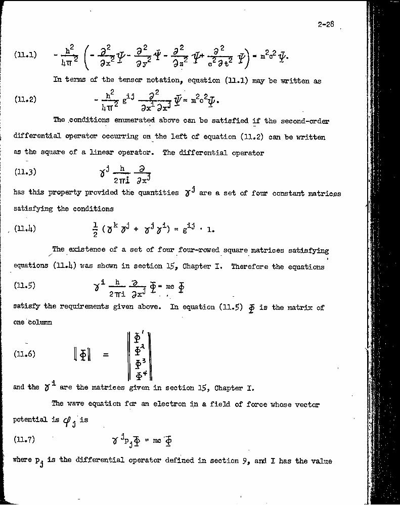
2-28
(11*1)h2 ^ J'^ = m2c2f.
(11.2)In tenns cxf the tensor notation, equation (11.1) may he witten as
Bie .conditions entiraerated above can be satisfied if the second-order
differential operator occ\nTing on the left of equation (11.2) can be writtan
as the square of a linear operator. The differential operator
(11.3) 4 h2Tri
has this property provided the quantities are a set of four constant matric.es
satisfying the conditions
(ll.li) •J = g1 .1.
The existence of a set of four four-rotired square matrices satisfying
equations (ll.it) was shown in section 15, Chapter I. Therefore the equations
(11.5)27Ti 9x^
satisfy the requirements given above. In equation (11.5) ^ is the matrix of
one Column
(11.6) II fl =f' '
and the ^ are the matrices given in section 15, Chapter I.
The wave equation for an electron Зи a field of force whose vector
potential is is
(11*7) 7Г “ me
where p^ is the differential operator defined in section 9, ani I has the value
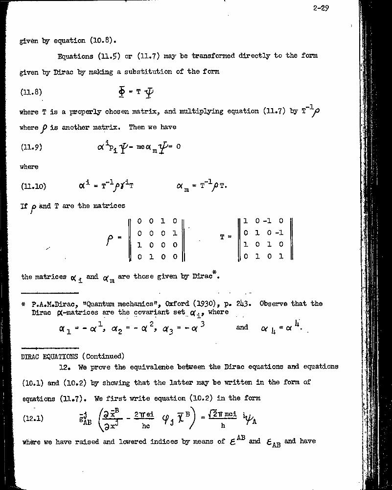
2-29
given lijr equation (10.8).
Equations (11.^) or (11.7) may te transformed directly to the form
given by Dirac by making a stibstitution of the form
(11.8) $ = T
—1where T is a properly chosen matrix, and multiplying equation (11.7) by T p
where p is another matrix. Then we have
(11.9) where
(11.10)If p and T are the matrices
〇(i = T"^j〇2r^T a m’f^p T.
0 0 10 0 0 0 1 10 0 0 0 10 0
10-10 0 10-1 10 10
0 10 1the matrices 〇( . and are those given by Dirac
^ P.A.M.Dirac, «Quantum mechanics”, Oxford (193〇)j P* 2h3» Observe that the Dirac p(-matrices are the covariant set where
Of2 = -C(^, (X^ = -〇(^ and £Y = 〇<
DIMC EQUATIONS (Continued)12* We prove the equivalence between the Dirac equations and equations
(10.1) and (10.2) by showing that the latter may be written in the form of
equations (11*7) • We first write equation (10.2) in the form
(12.1)■35® ,3^
2TTeihe
9 itvB 1 _ ^TTmcl Vi
ABwhere we have raised and lowered indices ly means of £ and and have
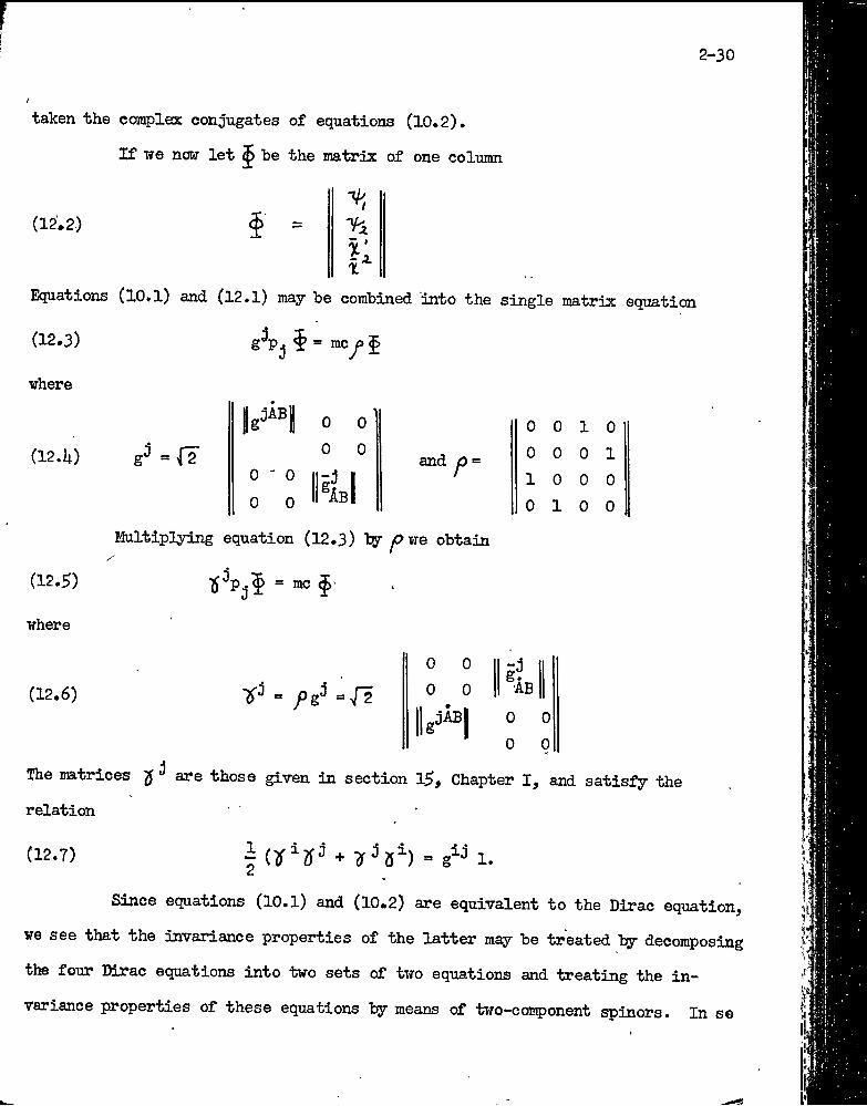
2-30
taken the coH5)lea: conjugates of equations (10,2).If we now let ^ he the matrix of one column
(12.2) J =
Equations (10.1) and (12,1) may he comhined into the single matrix equation
{12.3) gJp. f = mcyj ^
where|g^“| 0 0 ’
0 0 10 1(12.it) = Î2 0 0
0 0 11 AbIand y〇 = 0 0 0 1
10 0 00 10 0
Multiplying equation (12.3) ty /Owe obtain
(12,^)
where
(12.6)
The matrices ^ ^ are those given in section l5, Chapter I, and satisfy the
relation
(12-7) + Ï^S^) = 1.
Since equations (10,1) and (10.2) are equivalent to the Dirac equation,
we see that the invariance properties of the latter may he treated hy decomposing
the four Dirac equations into two sets of two equations and treating the in
variance properties of these equations hy means of two-coirponent spinors. In so
______________ ' . -
0 0 0 0 •AB
00
Xi •
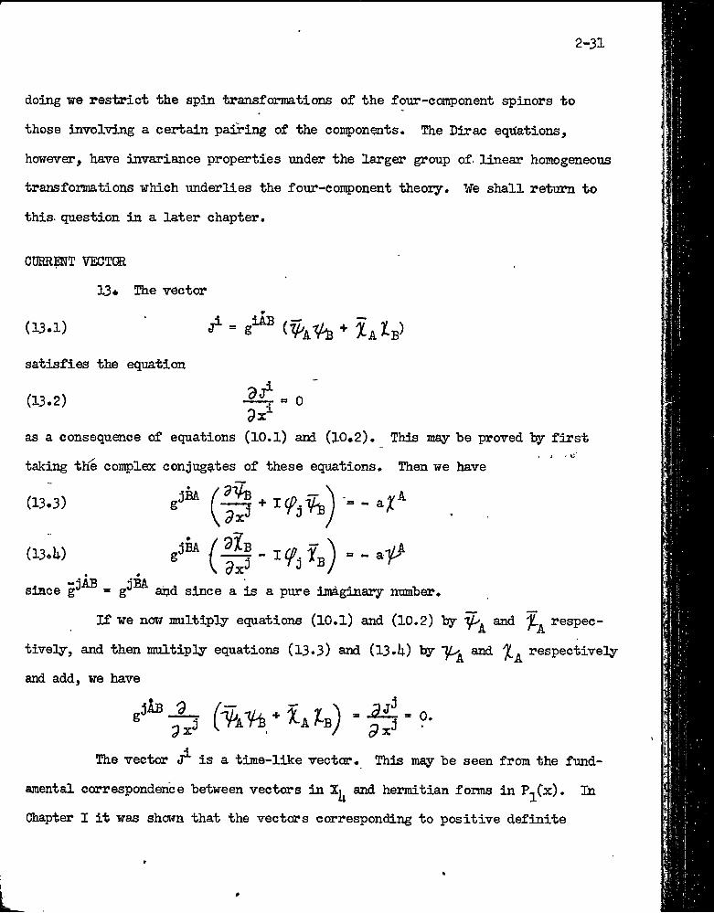
2-31
doing иге restrict the spin transformtions of the fonr-coraponent spinors to
those involving a certain pairing of the components. The Dirac eqtiations,
however, have invariance properties •under the larger group of. linear homogeneous
transformations -which underlies the four-component theory. ¥e shall return to
this, question in a later chapter.
CDRRMT VECTGB
as a consequence of equations (10.1) and (l〇*2). This may be proved by first
tively, and then multiply equations (13.3) and (13.U) "by and respectively
and add, we have
Chapter I it was shown that the vectors corresponding to positive definite
13* The vector
(33.1)
satisfis the equation
(13.2)э/T ° 0.1
taking the comples: conjugates of these equations. Then we have
= g^ and since a is a pure imaginary number.
If we now multiply equations (10.1) and (10.2) by and respec-
The vector is a time-like vector. This may be seen from the fund'
amental correspondence between vectors in and heimiitian forms in P^C^c). In
2-32
hermitian matrices are timelike. Since
^AB “ VaVb * Wb
is a positive definite hermitian matrix, the vector is tiraelike. This fact may algo be seen computing the length of the vector J^, we have
* tcf>
"2 (iA^HfcV-®) =2|tA'V'^l
since g^^g?® = 6“^^ 6^, and since = T/J^ = 0. The right-hand member
of equation (13*6) is always positive if is not proportional to and
hence is a timelike vector.
Since and are both spinors with indices of first kind different
from zero &ad indices of second kind equal to zero, is independent of the
gauge variables.
Since is a timelike vector, whose divergence vanishes, it may be
interpreted as the current vector for the electron which is described by the
two spinors and which satisfy equations (10.l) and (10.2) respectively.
3-1'
Chapter III
COVARIAKT DIFFERENTIATION
1. A galilean frame of reference is given by specifying the gauge
coordinate systems, a galilean coordinate system in X|^, and a spin codrdinate
system in such that the spinors take on the numerical values given in
Chapter I, section h. We have shown, in section 9, Chapter II, that the spinors
^ AB numerically invariant if^we make a spin transformation with constant
coefficients and then perform the proper Lorentz transformation corresponding to
the inverse of this transformation. Since the latter transformation carries
galilean coordinate systems in into galilean coordinate systems, we see that
the group of transformations which carries galilean frames of reference into
galilean frames is the restricted Lorentz group,
A cartesian frame of reference is obtained from a galilean one by making
a cartesiaij transformation of coordinates in or a transformation with con
stant coefficients in P^, or both. That is, in a cartesian frame of reference the spinors g^^g may have any constant values subject to the quadratic identity
between them (i.e. independent of thq coordinates of X^).
The covariant derivative of a spinor is a spinor with one additional •
covariant tensor index, which reduces to the ordinary derivative of the spinor
in a cartesian frame of reference. In the case of the simple spinor in
a cartesian frame of reference we have
(1.1) -f, . = ^ax" '
In section 8, Chapter II we have shown that AjJ^ ^ transforms as a vector under
arbitrary coordinate transformations and as a spinor under constant spin trans
formations .
We shall now use the definition of the covariant derivative of a
3-2
spinor to compute •'j^. . after a gênerai spin transformation. If this trans-
formatipn is
(1.2)B 1 ii
where J>^ are arbitrary complex functions of x , x such that , the determinant of is different from zero, then since ^ is a spinor, we have
where
®A ^B,i
B = Pa rS
and w and a are the weight and anti-weight of a|/^ respectively.
(1.5)
Sincea^A* 3% Ba?"
'l Bd S.
'Y® 8x^3Yb b -c ^ it ^®a
ax' 3x^
where Sg s® = ^
we have
(1.6)3Yb b 5Ya
3x^ - s'
Hence if we define
(1.7) 〇G•= ^B ■9s'
we have
(1.8)_d%
c ^“a «^X'
Yc
G i!- »'-Aj YcEquation (1.8) is the formula for the covariant derivative of a spinor of weight
w and antiMweight a in any frame of reference. If are the components of a
spinor in a general coordinate system, equation (1.8) may be written without the
asterisks, thus
(1.9) — - A° .-t'3 ''A j Y cAC ^
Where yV^j is defined by equations (1.7) and (l.U).
A„. may be coirqauted from
3-3
equation (1.9). Under a general transformation of spin coordinates equation (1,9)
becomes ^
(1.10) . 'fA,! “ ^B,i®A •^ ^ BSince s^, equation (l.lO) may be written
A“* ®^ ax'" Ai ®C
Hence[Ar4-(=?A^^^)]Y〇-
Since this is to hold for arbitrary we must have..G
(1.11) A B » ^ B / A C „D-'Laí + TT:/ *
0 XSince Sg are scalar functions of x^, ..., x^, it is evident that
transforms as a covariant vector with respect to coordinate transformations.
/If we set B = A and sum, equations (l.ll) become
(1.12) A B _ A B t? log s-/V. EL “ ^ Bi _ iPx
where s is the determinant of the transformation st,B
From equations (l.ii) we see that equations (1.7) may be written as
B ^ G
(1.13)Aj
where
(l.lii) r ^and hence
(1.1Í) pC ' Gj
.c■B
pO aff
,BP° ii® ax^
p'^ ~' G _ d log 9ax‘
by the definition of the derivative of a determinant. The geometric being j3 is
3-ii
a scalar under coordinate transformations and a scalar density under spin trans
formations .The geometric being with the components P ^ will be called a spin
connection. It transforms as a covariant vector under a coordinate transforma
tion, Its transformation law under spin transformations will be obtained below.
Instead of equation (l.lO) we may write
(1.16) a-TAA,3
as an alternative expression for the covariant derivative of a spinor of weight
w and anti-weight a.
THE lEANSFORMATION LAW OF pA
2, The transformation law for the spin connection may be obtained
from equations (l.ll) and (1.13). If we set w = a = 0 in equations (1.13), we
have
(2.1) and
(2.2)
-A- ^ pCA^
s® = t^®A hlB .where t^ is a general spin transformation. Hence in virtue of equations (1.13)
we have
(2.3)
and
(2.1;)
pB * nB(r C
piB-it-f—,0 ^ 9log tIf we now compare equations (2.3) and (l.lb) we see that they are the
uC nCsame if in equation (2.3) we set = 0 and t^ = That is in the cartesian
coordinate system the components of the spin connection are zero and their law of
transformation under spin coordinate’transformations then determines them in any
3-5
spin coordinate system (P ^ is "the transformation from the cartesian coordinate
system to the general one). Ihus the determined in a general spin
coordinate system as soon as we know the transformation which carries a cartesisn
frame of reference into a general one»
From equation (l.l^) we see that just giving the value of the.deter-
•minant of the transformation from a cartesian to a general spin coordinate
system determines the trace of the spin connection. That is the spin scalar of
weight one, J , determines the trace of the spin connection. Equation (l.l5) may
be written as
/Ta-o •
But this is just the statement that the covariant derivative of y is zero. By
specifying the absolute value of j> or the argument of we specify the real
or imaginary part of the trace of the spin connection. This may be seen as
followsr From equation (l.l5) we have
(2.6)hence
(2.7) 1 a logpp 3 log/pTipx**But the left member of this equation is just the real part of the trace of the
spin connection and the right member involves only the absolute value of p .Hence giving the absolute value of j> determines the real part of the trace of the
spin connection. Equation (2.7) may be written as
(2.8)
That is, the covariant derivative of the real scalar density is zero,
3-6
Similarly, we have
(2.9) (r〇j. ” r Q ^ •
Hence we see that giving the argument of j determines the imaginary part of the trace of the spin connection. Equation (2.9) may be written as
(2.10) (/>/?)- ?lj =ax"
That is, the covariant derivative of the pure imaginary scalar is zero.
EXAMPLES OF COVARIANT DIFFERENTIATION
3. The formula for the covariant derivative of a contravariant spinor
may be obtained in the same manner as that of a covariant spinor. In the
cartesian frame of reference we have(3.1) ^
If we make the transformation (1.2) in the spin space, then
(3.2) f -a
where -w and -a are the weight and anti-weight of respectively and where
(3.3)
Since
^ 3A £::t^ . 3A ^ ^ ^0. 2$x
we have
(3〇h)
But
dx'^
B^ 9x^ ^ “O ’!9x"
A,A _B ^®B /w G*4 ~ 4 “ 4 I •gx^ 9x^ dx^
_B _ .A _ A As„ ^ - s„ —, = - . .T(3.5)
3-7
Therefore we have in any coordinate system
A - 2'^(3.6)
An alternative expression for equation (3.6) is
(3.7) -*^^*-^* A .. C . nC A . . C Aax
for the covariant derivative of a contravariant spinor of weight -w and anti
weight -a.
The formula for the covariant derivative of a spinor with a “dotted
index may be obtained by considering the simple spinor
(3.8) •
In a cartesian frame of reference we have
(3.9)
Therefore, in general frame of reference we have
(3.10) A,i ^^i 7 ^6 r’Ai ■* ^^A ^Gi “ ^CiFiC
for the covariant derivativ-e of a spinor of weight w and anti-weight a with a
single dotted index.
Equations (3.9) express the fact that the process of taking the com
plex conjugate of a spinor is commutative with the process of taking its co
variant derivative. Equation (3.10) can also be derived from the definition
of the covariant derivative in the same manner as equation (l.l6) was. It
holds for any spinor with a dotted index.
The formula for the covariant derivative of a product of sin^jle
spinors is the same as the formula for the ordinary derivative of a product.
For in the galilean frame of reference we have
3-8
(3-11) (-I'aXbv’ gx),. «'^A-T*
gx■B . ail
Hence in any frame pf reference we have
By the same argument it can be shown that the covariant derivative of the product
of any t3rpes of spinors obey the same law as the ordinary derivative of the product.From equation (3 «12) we see that the formula for the covariant derivative
of the spinor,
(3.13) . = Ya t
is3$AB
B
AB,j-'5ACr^j-§〇Br“, -wr°, I
GB » Aj ■ ” I Cj AB - aAB
(3.11;) Jgx‘ - “where w and a are the weights and anti—weights of $,p respectively. Equation
Ad(3.11;) is obtained from equation (3.12) where the values of X and ■'ti^ are
a,i ' A,igiven by equations of the type (1.16), Equation (3.H;) is also valid for any spinor with two covariant spin indices, as can be proved by a consideration of thp
transformation law of
In particular we have for the spinor defined in Chapter I, the
relation
■ (3.1^)
(3.16)
where
(3.17) •
"AB,i - 6:.1 ^GB I Ai ^AC I Bi ^AB ' Ci^x
<^AB,i " "^CCB ^Ai ^AC BC
.C^Ai
Ci
'AG ^BL
jrA pA _ 1 r~> C r A^Bi I Bi ?l Ci c •
That is, is the traceless part Since the trace of is zero we have
'AC ^Bi = ^ABi “ ^BAi •(3.18)
Hence
(3.19)
This means that the process of lowering spin indices is commutative with
the process of covariant differentiation. We shall now verify that
^AB,i “ °
3-9
^A,i “ \i ‘ \
'A ^AG ^
(3.20)
Since the relation
(3.21)t
holds in all coordinate systems if the weight of is one greater t-|iqn the
weight of we need only verify equation (3.20) in the cartesian frame of
reference. Since the ordinary derivative of ¿q is zero, equation (3.20) holds
in this frame and therefore in any frame of reference.
Equation (3.12) together with equations (3.7) and. (I.l6) enables us to
show that the covariant derivative of the spinor(3.22) ' -Va ®
isB
^A,i ' Aj XA • Cj ^ lA > Cj i A I Cjwhere w and a are the weight and anti-weight of the spinor ^ ^ respectively.
Equation-^3.23) is also valid for any spinor with one covariant and one contra-
variant spin index as may be proved by a consideration of the transformation law
In particular it holds for the spinor c5 the Kronecker delta.D
Thus
(3.2ii) r A nC P C „A
• c ^ ^Since o g is a constant spinor with both weights zero.
From the relation -(3.25) ' £ab^“-S =
and the rule for differentiating a product we see that
(3.26)
since
(3.27)
. = 0 and AB,〇
"ABS"
. = 0id
B,0 = °*
= 0 . 9 J
Hence we have
3-10
That is, the process of raising indices is comrautative with the process
of covariant differentiation. It is readily verified that
(3.28)
The formula for the covariant derivative of a spinor with any number of
spin indices may be obtained in a similar manner from the definition of the co-
variant derivative and its transformation law.
Then we have
A... B...
B... B... ,1
(3.29)
A... B. • • G... B...+ (f . rIt
1
fct
• • • •* • D... ill...3x^
A C _ A... 6...•D... E...
^ C... fi... r_ A... B... — n A... B... r-i
D... G... D... E...A... B...
-afD... £... r °' Ci ■a
AGi
CDi
CCi
COVARIANT DIFFERENTIATION OF SPINORS WITH TENSOR INDICES
ii. Before taking up the discussion of covariant differentiation of
spinors with tensor indices, we shall briefly outline the theory"of covariant
differentiation of tensors. The covariant derivative of a tensor with respect
to the g^j is another tensor with one additional covariant index which reduces
to the ordinary derivative in the cartesian coordinate systems in X^. Thus in
a cartesian coordinate system we have for the vector V.9V. ^
ih,l) , H = --T •If we now make the transformation to the general coordinate x^ where
(il.2) X = X (x)
3-11
the vector 7^ undergoes the transformation
ih,3) rr*'7. = 17.t9
3 1where
tJ = 1
3x^T~r*dx
, *^ an argument analogous to that given in section 2 we see that
» See 0. Veblen, "Invariants of quadratic differential forms," Cambridge Tract No. 2h, (1927).
ih.S)
where
(h,6)and
(h.7)
We note that
. (ii.8)
7. .ax
« V * r-jk *i* k I ij
1ax
yk t*^ » ¿k . \ ®i •
ri/- rVij > ji
as a consequence of equation (U.U).
ih.S)
Hence in a general coordinate system we have9v,
axThe transformation law for the geometric being with con^jopents may be ob-
tained in the same manner as that for A nA was.GlThe relation between the quantities and the Christoffel symbols
space may be obtained from the definition of cartesian coordinate systems
1^ In such a coordinate system the metric tensor g. . is a constant. Hence we
have in the cartesian coordinate systems
Since is 3- tensor and since it vanishes in one coordinate system, it must
3-12
vanish in all coordinate systems*. Therefore we have- «te ri ■
Equations (1;,8) may be considered as the equations relating the quantities n/ and the derivatives of the tensor g... Since the
only solutions of these equations are
ragmkJ m^ 3x“ Bx'' dxThus the p^j^'s are the Christoff el symbols formed from the g^^
xA6Consider the spinor g In a cartesian frame of reference it is a
constantj hence we have
(li.lO) (9giAB
If we now change the frame of reference b;^ going over to a general
coordinar
Ot.ll)system in Xi equation (ii.lO) becomes
^ ikB 4;r, rng ¿>X
ijkjIf we gO/Over to another fr^e of reference by changing to a general spin
coordinate system, we have
(I4.I2) iAH • ✓ <-v • • • •Bg . pjAB Ci 7 iCB j=íA iAC pB __ 1 UBpC 1 ÍABrCyjr + g U^] \ Gk* ^ I Ck 2^ r〇k - 2g Pck
since g^^® is a spinor with weight + ^ and anti-weight +
A AnSince g ,k is a spinor which is zero in the cartesian frame of
reference it is zero in any frame of reference. We will use this fact in the
next section to obtain relations between the
REUTIONS BETWEEN P and .
5. Equation (U.12) may be written asi
(9.1) dggAB,k Bx
AB j ir-^ ^AB
Ib j^kjj " ^CB ^Ak “ ®lc °
where
3-13
(5;2) zA ^ pA 1 r A P C' Bj ? ^ B « C jThe equations (5 «1) may be solved for the in terms of the ^^ | vice
AEversa. If we multiply equations (5«1) by and sura, we have .
(i-3) ^4 ■ 4 m ^ ^
• , A. S -Asince 4 = 5aiD and since » 0. Equations (2,6) express the traceless
part of the spin connection in terras of the Christoffel symbols formed from the
g. . of the underlying space X, .h ABIf we multiply equations (^.1) by g^ and sum, we have
(5.It) f i 1 ÁB / i „C ^ i 1?C ^ %Bj mj j “ (^AC ®CB ^Aj "
since g^^ g|g “ ^ m Christoffel symbols of are thus- expressed in terms
of the traceless part of the spin connection. The former must be real since X|^
is a real" space. This condition is satisfied since the right-hand side of
equation i$,k) is real as a consequence of the fact that g^g is hermitian.
Since equation (5.1) only involves the traceless part of Hcj
may be completely arbitrary and equations (5.1) are unaffected,
6. In the preceding we have determined the in a general spin
coordinate system in terms of the unimodular transformation from a cartesian spin
coordinate system to the general one. In this section we shall consider the
problem of reversing this procediirej that is, we shall assume that we are given
the quantities in a general spin coordinate system and find the transforma
tion which carries it into a cartesian one.
¥e first note that our previous definition of a cartesian frame ofíÁBreference, namely, one in which the tensor g^^ and the spinor g have constant
values , is equivalent' to the following: A cartesian frame of reference is one *
* = constants implies g^^ = constants of course.
3-lU
in which both S>'i and vanish. It is well known that ^ necessary and sufficient condition for the tensor to be constant in a given coordinate
systea is that the Christoffel syhbols vanish in that coordinate ^sten. ~A^oa equation ($.3) it follows that if | ^ ^ ^ constants, then
- 0. Conversely if | ■ 0 and ■ 0, then.the g^^ are constant. This
proves the equivalence of the two definitions of cartesian fraaes of referenoe*Jn terms of this definition of a cartesian spin coordinate qrstea and
the transformation law of the (equation (1,11) where are coefficients of unlaodttlar transformations) the problem may be stated as followsi T6 find the transformation qoefficients at such that _(6.1)
subject to the condition that |sq| • l/]Sg| ^ 0. In virtue of this condition equations (6.1) may be written as
^ ir®
(6.2) e?
(6.3)
where
(6Ji)
-^--*63 "A •
the integrabllity conditions for these equations are9^1 ^«5 C E
" ITTJ " " % jk ®A " ®axV ax* 9x
The geometric being with c<wiponents is a spinn* as may readily be seen from the anal<^e of the Ricci identity
A Twhere th〇 'Y is an arbitrary spinor of weight * ^ .Hence the necessary and sufficient conditions idiioh must be satisfied In
order to solve equations (¿.1) are that the spinor must be aero. Since this
3-15
spinor is zero in a cartesian frame of reference, it is zero in every frame ofreference-. Hence we can solve equations (6.1) for the s^.
67. EXTENSION TO THE GENERAL THEORY OF RELATIVITY
The general theory of relativity differs from the special theory in that
the underlying space is a certain general four-dimensional Riemannian manifold
instead of a flat space. That is, there exists no coordinate system in which the
tensor g^j is constant throughout the space. If we replace the underlying flat
space of Chapter II by a more general Riemannian space, everything but the theory
of covariant differentiation of spinors is unaffected. We must find a new defini
tion for the covariant derivative of a spinor for the old one is based on the
notion of a cartesian frame of reference and in general relativity we cannot
introduce such frames.
However, at any point of the underlying space we can introduce a co-
ordinate system in a neighborhood of the point in which the first derivatives of
the tensor g, vanish at this point, i.e. the Christoffel symbols vanish there.
Such coordinates are called the geodesic coordinates. We shall briefly review
* Eisenhart, Riemannian Geometry, Princeton University Press, 1926, p. 53.
some of the facts about geodesic coordinates.
If the coordinates of an arbitrary point P^ are x^ in a coordinate system
in which the Christoff el symbols have the values at the point x^, then the
series
(7.1) x"" = x^ + x«^ + ^cjj^x«^x'^ + ^ cjj^x'jx'^x'*^ + ...
where the c*s are arbitrary constants symmetric in the subscripts so chosen so thaï the series converges in a neighborhood of x^, defines a transformation of coordi?"
3-16
nates. The constants may be chosen so that the Christoff el sjTnbols vanish in
the primed coordinate system.
From equations (7.1) we have that in the primed coordinate system thepoint P has,coordinates x’^ = 0. Hence at the point P we have
0 ^ 〇
(7.2) ax = <5^ i 3x«Vo J i3x»%x»^> m
ri-^m i (( gx”^ )
’〇 O -- *•‘ o \ax'From the transformation law of the Christoffel symbols we have
bx»^Px'fc}〇 " fe)〇 feAm virtue of equations (7.2) this may be written as
jjkjo " •
Hence a necessary and sufficient condition that = 〇 is that c^j^ =
Therefore/the equations
(7.U) ^ . ...
where the c's are arbitrary constants symmetric in the subscripts define a trans-:formation to a coordinate system in which .the first derivatives of the e at P
ij 〇vanish.
From equations (7.it) we see that to every point in the underlying space there corresponds a family of geodesic coordinates. If we perform a linear transformation on the x>^, such as
(7.5) x»iJ = a9x>^ 1
we again get a geodesic coordinate system. In particular we may choose the a^
SO that the tensor has the values
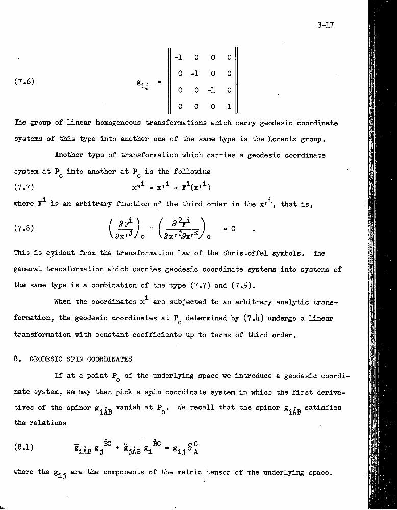
3-17
(7.6)
-10 0 00-100 0 0-10 0 0 0 1
The group of linear homogeneous transformations which carry geodesic coordinate
systems of this type into another one of the same type is the Lorentz group.
Another type of transformation which carries a geodesic coordinate
system at into another at is the following (7.7) x"^ = x»^ + F^(x«^)
where is an arbitrary function of the third order in the x'^, that is,
(7.8) f lit)\ ax*^/ 0 = 0
This is evident from the transformation law of the Christoffel symbols. The
general transformation which carries geodesic coordinate systems into systems of
the same type is a combination of the type (7.7) and (7.5).When the coordinates x^ are subjected to an arbitrary analytic trans
formation, the geodesic coordinates at P^ determined by C7.i;) undergo a linear
transformation with constant coefficients up to terms of third order.
8. GEODESIC SPIN COORDINATES
If at a point P^ of the underlying space we introduce a geodesic coordi
nate system, we may then pick a spin coordinate system in which the first deriva
tives of the spinor vanish at P^. We recall that the spinor g^^g satisfies
the relations
(8.1) ®iAB ® jBC CA
where the g.. are the components of the metric tensor of the underlying space.
3-18
From these equations it is evident that if the derivatives of the spinor
vanished throughout the space, then the derivatives of the g.. would vanish, which
is in^jossible. Hence we must expect that the spin coordinate system can at most be
so chosen that the first derivatives of the spinor vanish at a point.xAB
The differential equations which determine the unimodular spin trans
formation coefficients are
(8.2) That is,
(8.3) -c D
I -c D X( HcsVb ) - 0 •
ax'-^A^B * ®iCD
D9x
_ n3 «IGD =A 0
Equations (8.3) may be written as
■SSipE(8,ii)
85?
ex'-* ^iCE “3 ^ Si
aX„BiFD —J
3x0
where Sg is such that
(8.5) 4iFN
3x*
Multiplying by g and summing, we have
(8.6) g
Since
(8.7)
iFN rN -il ^
^ A ^ ^ log Is I9x^
0
in virtue of the fact that Js] =1, equations (8.6) may be written asN
(8.8)^®B _ 1 iFN ^%Fe1 _E
^ \ dx^9^ B
If we set
3-19
(8.9) 1 iFN5-g 9x‘ = 4these equations (8.8) become
/ asg(8.10) E
;〇The integrability conditions for these equations have been considered
in the previous section. In section 10 we shall show that they are satisfied if /
and only if the underlying space is a flat space. Hence in the general case there
exists no spin coordinate system in which the derivatives of the spinor g; vanish.Nevertheless equations (8.10) may be used to define a spin coordinate system in which the first derivatives of the spinor g| vanish at the .origin of
the geodesic coordinate system. If we start with an arbitrary spin coordinate
system and define the by (8.9), then a set of transformation coefficients
Sg are given by the power series
(8.11) A
A
A Ji.Ej„AEik s,, = s „ - x'^ X + ...oB Sj oB,A E ■'Ejk^oB
where are constants and the coefficients of the second and higher order terms
^e arbitrary. Spin coordinate systems in which the derivatives of the spinor g|g
vanish at the origin of geodesic coordinates will be called geodesic spin co
ordinate systems.
Just as in the case of the geodesic coordinate systems of the underlying%
space, at every point there exists a family of geodesic spin coordinate systems.
The members of a family of geodesic spin coordinate systems are permuted among
themselves by transformations of the type
(8.12)4 -
where is a constant spin transformation and is of second or' higher order in
the x*s, that is
3-20
(8.13) i I - 0
/〇The transformation (8〇12) induces the linear homogeneous transformation of the components of a spinor (e„g.) at the point P
JJir O
(8.1ii)
iAB
has the values given\
in §ii. Chapter I , at the point P^ j namely
lAB 1 0 1 ^2AB 1(8.15)
g "/T 1 0 g ■/r
II
0 -i1 0
Ubg 1
¥e can find a geodesic spin coordinate system in which the spinor g
0 -i1 0
1 0 0 1
A frame of reference defined by a geodesic coordinate system of the under
lying space and a geodesic spin coordinate system will be called a geodesic frame
of reference, A geodesic frame of reference in which the g.. have the form (7.6)〇
and the g^'^^ the form (8〇l5) will be called a normal geodesic frame of referenceA transformation of the type of the combination of (7.5) and (7.7) in the
underlying space and one of the type (8,12) in spin space induces the following transformation on the components of the spinor g^^ at the point P s
(8〇l6) ^^Ab^o “ '^B ^®^CD^o °
If we now require that
(8.17) ''^AB^o = (gin)AB'o
equation (8,l6) defines an isomorphism between a linear group in the tangent space
at P^ and a group in the spin space.
3-21
9. DEFINITION OF THE COVARIANT DERIVATIVE OF A SPINOR
Th^ covariant derivative of a spinor is a spinor with one additional
tensor index which reduces to the ordinary derivative at the origin of a geodesic
frame of reference when evaluated in that frame. Thus
(9.1)
By the argument of §8, Chapter II, it is evident that . transforms as a vectorXunder arbitrary coordinate transformations and as a spinor under arbitrary spin,
transformations.
If undergoes the unimodular spin transformation
(9.2) B
then by definitiony''
(9.3) ^^A,i^o “ ^®A ^B,i^o
Since
i9.h)
then
(9.5)
_/^^B B
\®3xV〇 \8x^ ^ ® °
^®A^o ^"^B,i^o
A
:3). ,3x‘*1
9x*
C / o
A ^ B ‘^^B
If Sg are the transformation coefficients from a geodesic spin coordinate system to an arbitrary one in which the K^. defined by equations (8.9) have
the values (K^.) at P., then s2 are the transformation coefficients of the oj 0 o B
inverse transformation and equation (8.10) applies to them. Thus
3-22
'as'B(9.6)
Equations (9.^) then becomeo
wC qE^jo ®Bo
-'aj Vc*X ■ (<j)〇 •
Since was an arbitrary point, we have that at any point of the under-
l3dng space in an arbitrary spin-coordinate system
(9.8)A,j C .- 4^ <
dryThe covariant derivative of the spinor g^_ is zeroj for its value at any point P
■ABin the underlying space in a geodesic frame of reference is
^®ABV o
and by the definition of a geodesic frame of reference the right member vanishes.
By the argument of section k of this chapter, we have that in a general frame of
reference and at any point x
(9.10)' ®AB,j fkj - i -C i c ^5b ^Aj ” ^Ac ^Bj “ ®
. These equations may be solved for the in terms of the and the
derivatives of the g^g and we again obtain equation (5,3). Equations (5.1i) may
also be obtained from (9.10). It is readily seen that equations (^.3) reduce to
equations (8.10) at P^ in a frame of reference in which the coordinate system of
the underlying space is a geodesic one at P .o
With the definition of the covariant derivative of a spinor given in
this section all the results of the preceding sections of this chapter and df; Chapter II may be taken over to general relativity.
3-23
10.. RELATIONS BETWEEN THE CURVATURE TENSOR AND THE CURVATURE SPIN(®
In Riemannian geometry it is well known that the vanishing of the Rieraann iChristoffel tensor where
■it- In the notation of Eisenhart, op. cit.
ClO.l)
is the necessary and sufficient condition that there exist a coordinate system in
which the tensor g^^ has constant values. From the results of the section 6 we
see that the necessary and sufficient condition that there exist a coordinate
system in which the vanish is that the spinor ^ vanish. If both R., p andBi;5 Ljki-B^ . vanish, then from equations (^.3) it follows that there exists a cartesian
frame of reference.iABHowever, from relations between the g.. and the g it is to be expected
that these two conditions are not independent. In fact, we will show that the vanishing of ingslies the vanishing of B^^ and conversely. We will then
have the result: The necessary and sufficient condition for the existence of acartesian frame of reference in that = 0 (or B^^ = 0).
The relations between the tensor R_. 〇 and the spinor B“. « may beijki.obtained from the following generalization of the Ricci identity:
nn «iAB „mAB 〇i „iAE „B iEB(10.2) g,k£-e,ek“-S W-g %ki-S ^kl
iABSince the covariant derivative of the spinor g vanishes, we have
(10.3) niAB „i iAE „B iEB -=A
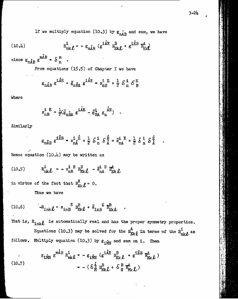
:»3-2k
(10.1;)
If we multiply equation (10.3) by and sum, we have
^nkl ■ " ^nAB ®Ekji ®
SnAB SmAB mn
From equations (l5.5) of Chapter I we have
_iAE .iAE _ _i E . 1 ^i ^E®nAB ® “ ^nBA ^ “®nB ■^7°n°B
where
Similarly
i E 1,- . iAE -i AEx =nB = ?®nk 8 - Sm Sn ) •
iEB i E . 1___ IE 1 rl rESnAB^ = ®nA ^?^n ^A = s-iE^l r>i 〇E ®nA 7 * n A
Hence equation (lO.U) may be written as
(10.5) = - s.i E „B "nB ®Ek£ “
in virtue of the fact that 4/=°-
Thus we have
(10,6) "^inki“ ®inB ■*■ ®inB^ ^ki.
That is, is automatically real and has the proper symmetry properties.
Equations (10.3) may be solved for the in terms of the as
follows. Multiply equation (10.3) by and sum on i. Then
^raAB „i / iAE _B iEB «A x®iMN ® ®mk£ “ “ ®iMN ®Ek^ * ^ ^
(10.7)
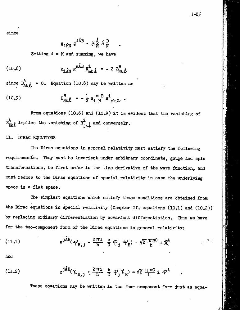
3-25
sinceiAB
M NSetting A = M and summing, we have
(10.8)since
(10.9)
inAB _i 〇 _B®iAN ® ^rtkl " “ ^ \s.t
0, Equation (10,8) may be written as
„B _ 1 m B _i■ “ ? ®i N ^ mki/
From .equations (10.6) and (10.9) it is evident that the vanishing of B^£^ in5)lies the vanishing of and conversely.
11. DIRAC EQUATIONS
The Dirac equations in general relativity must satisfy the following
requirements. They must be invariant under arbitrary coordinate, gauge and spin
transformations, be first order in the time derivative of the wave function, and
must reduce to the Dirac equations of special relativity in case the underlying
space is a flat space.
The sin^jlest equations which satisfy these conditions are obtained from
the Mrac equations in special relativity (Chapter II, equations (10,1) and (10,2))
by replacing ordinary differentiation by covariant differentiation. Thus we have
for the two-con^jonent form of the Dirac equations in general relativity:
(11,1) 27Ti e
and
(11.2) jAB,^ ¿ 111 e ^ Y \ - ./^irmc ^ jr?
^ ^^B,〇 ^ -ET ? Tj V » V2 1 -K
2TTi e TTinC . jr?A
These equations may be written in the foinr-component form just as equa-
3-26
tions (10,1) and (10,2) of Chapter II. The equations thus obtained are included
in the class of Dirac equations discussed in the paper "The Dirac Equation in ■i^ojeOtive Relativity”,^
* The Dirac equation in projective relativity, A. H. Taub, 0. Veblen, and J. vonNeumann, Ppoc. Nat. Acad,. Sci,, vol. 20 (193lt), pp. 383-388.
References to other papers oh the Dirac equation in general relativity and covariant differentiation of spinors are:H. ¥eyl. Gravitation and the electron, Proc.Nat.Acad,Sci. vol. 1^ (1929), 323
Electron and gravitation, Zeit. Phys. vol, 56 (1929), 330B. L. Van der Waerden, Spinoranalyse, Gdttinger Nachrichten, vol. 100 (1929)W. Infeld and B. L. Van der Waerden, Die Wellungleichung des Electrons in
der allgemeinen RelativitAtstheorie, Berlin Berich., vol. 9 (1933), 38〇V. Fock, Geometrisierung der Diracschen Théorie des Electrons, Zeitsch. Phys. vol. 57 (1929), 261
J. A. Schouten, Dirac equations in^eneral relativity, 1. Four dimensional
theory, 2. Five dimensional theory. Jour. Math, and Phys. vol. l〇 (1931), 239E. Schrôdinger, Diracsches Electron ira Schwerefeld 1, Sitzungsberidhte der
Preussischen Akademie der Wissenschaften, Phys.-Math. Klasse, 11 (1932), 105-128
W. Pâuli and J. Solomon, La théorie unitaire d’Einstein et Mayer et les équations de Dirac' I and II, Journ. de Pl^s. et la Radium, vol. 3, series 7, (1932), U52, 582
W. Paul.i, Dié Diracschen Gleichungen für die Materiewellen, Ann. der’Pln^s,, vol. 18 (1933), 337
0. Veblen aûd A. H. Taüb, Projective differentiation of spinors., FSroc. Nat. Acad. Sci., vol. 20 (I93k), 85-92
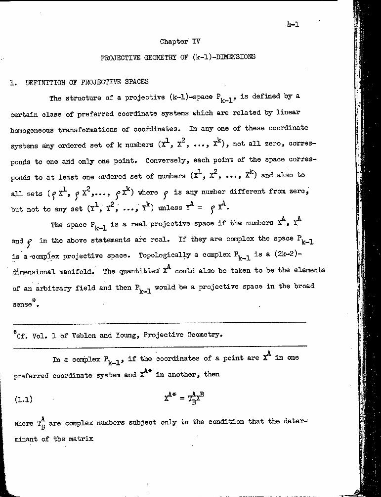
Chapter' TTPR0JEGTI7E GEOMETRT OF (k-l)-DIMENSIONS
1. DEFINITION OF PROJECTIVE SPACESThe structure of a projective (Jc-l)-space is defined by a
certain class of preferred coordinate systems which are related by linear
homogeneous transformations of coordinates. In any one of these coordinate systems any ordered set of k numbers (X^, X^), not all zero, corres
ponds to one and only one point. Conversely, each point of the space corresponds to at least one ordered set of numbers (X^, X^, X^) and also to
all sets (^X^, ^X^,..., ^X^) where ^ is any number different from zero,
but not to any set ^» •••5^) unless ^ X^.The space P^__^ is a real projective space if the numbers X^,
and ^ in the above statements are real. If they are complex the space Pj^_^
is a’■complex projective space. Topologically a complex is ^ (2k-2)—dimensional manifold. The quantities X^ could also be taken to be the elements
of an arbitrary field and then Pj^ -j^ would be a projective space in the broad
sense •
*Cf. Yol. 1 of Veblen and Toung, Projective Geometry.
U-1
In a complex if coordinates of a point are X^ in one
preferred coordinate system and X^ in another, then
(1.1) x^* = itx®B
where T^ are complex numbers subject only to the condition that the deter- B
minant of the matrix
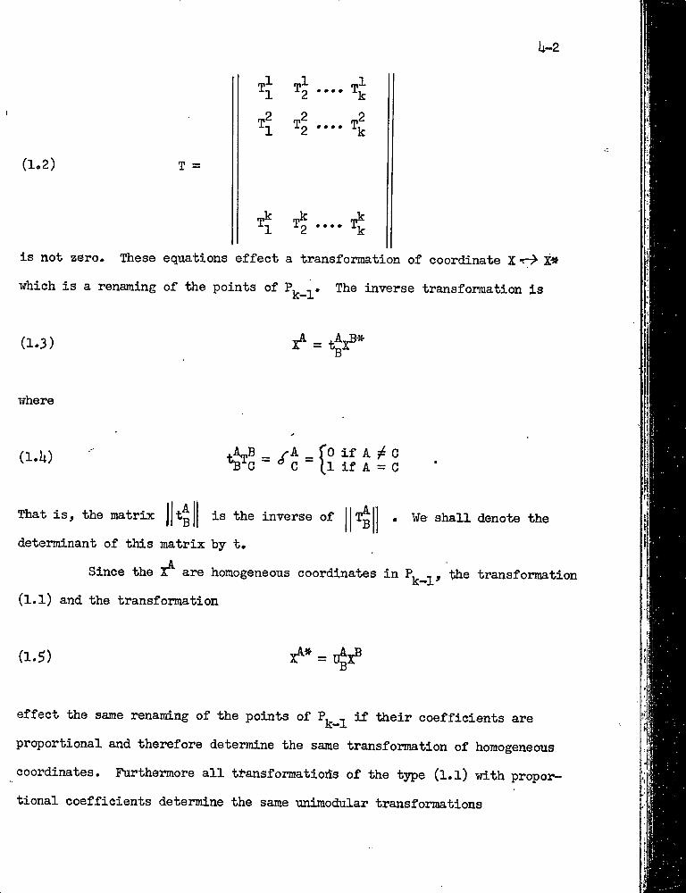
h-2
(1.2) T =
„2 T:
2,22 '
>000
T;
mk „k „k1 -^2 '**• ■‘•k
is not zero. These equations effect a transformation of coordinate X t-> X»
which is a renaming of the points of The inverse transformation is
(1.3)
where
(I.U) *^0 = '^0=i? if A 5^ C if A = C
is the inverse of T^B ¥e shall denote the
That is, the matrix jjt
determinant of this matrix by t.Since the X^ are homogeneous coordinates in the transformation
(l.l) and the transformation
(1.5)
effect the same renaming of the points of if their coefficients are
proportional and therefore determine the same transformation of homogeneoTis
coordinates. Furthermore all transformatioiis of the type (l.l) with propor
tional coefficients determine the same unimodular transformations
(1.6)
k-3
where
(1.7)
l/kThere are k of these transformations corresponding to the k values of t ' .
Thus the group of all coordinate transformations is (l-> k) isomorphic with
the uniraodular matrix group.
The inverse of the transformation (1,6) is
(1.8) x'^ = s^X®^ij
where
(1.9) Sg = t^t”^'^^ and hence s = 3AB = 1,
In this chapter the 'discussion of coordinate transformations will
be made in’ terms of unimodular matrices,
2, HTPERPLANES
The points on the hyperplane whose homogeneous coordinates are
satisfy the equation
(2.1) Va^= 0
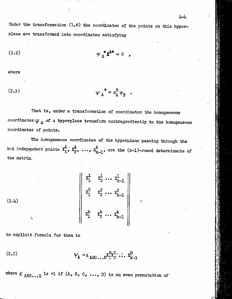
Under the transformation (1.6) the coordinates of the points on this hyper^
plane are transformed into coordinates satisf^ng
(2.2)
where
(2.3) * B.
That is^ under a transformation of coordinates the homogeneous
coordinates ^ of a hypeiplane transform contragrediently to the homogeneous
coordinates of points.
The homogeneous coordinates of the hyperplane passing through the
k-1 independent points are the (k-l)-rowed determinants of
the matrix.
(2.U)
^ xj ...
y2 y2 „2^ ^2 ...
yk yk —k^ -^-1
An explicit formula for them is
(2.3) ,,. -D
where f abc,,,p (A# B, G, ..., D) is an even permutation of
it-?(1, 2, 3, k), -1 if it is an odd permutation, and zero otherwise. From
the formula for the expansion of a determinant we have
(2,6) ®^ABC...D ^EFG, 〇e„f G.h®aVc' sÏÏD *
Hence the formula (2,?) is unaffected by coordinate transformations.
From the symmetry properties of it is evident that
(2-7) '("¿4 = ° 1 = 1, 2, k-1 .
Thus the points on the hyperplane are those linearly■dependent on X^, .
Similarly the homogeneous coordinates of the point determined by
the k-1 independent planes ^ VzV k-lA
(2.8) IB ^2G V-k-lD
where £ ■^BC...D according as (A, B, C, D) is an even or an
odd permutation of (1, 2, k) and zero otherwise. Again from the formula
for the expansion of a determinant, we have in a new coordinate system
(2,9) ^ AB AB ,.D _ EF,— S £ ,G„A〇B c,D
Therefore equation (2.8) is unaffected by coordinate transformations.
3. COORDINATES OF LINEAR SUBSPACES
The homogeneous coordinates of a point in P ^ satisfy the set
of equations
U-6(3.1) ^ABC...D^ “ °
where jj has k-1 indices and is defined by the equations
(3.2) ASC•»•D = £ABC*••
That is, the quantities ^AB.. are just a renumbering of the coordinatesT® with appropriate plus and minus signs. If we write „ as a matrix
AB*•*Dwith the different combinations of the first k-.-2 indices labeling the rows,
and the last index labeling the columns, the matrix will be of rank k-1.
Thus the homogeneous coordinates are determined uniquely by equations (3.1).
The quantities ^AB.. are called the covariant coordinates of the
point .
^Similarly the quantities
(3.2) D _^ABG...DE^ ^
where (p ■^®***^ indices. These are the contravariant coordinates of
the hyperplane g* Also the homogeneous coordinates of the hyperplane are
uniquely determined as solutions of the equations
(3.3) AB»*. = 0 .
The existence of the covariant coordinates of points enables us
to ejqjress some aspects of the principle of duality analytically. Thus the
covariant coordinates of a point may be 63q)ressed in terms of the coordinates
of k-1 hyperplanes on the point as follows:
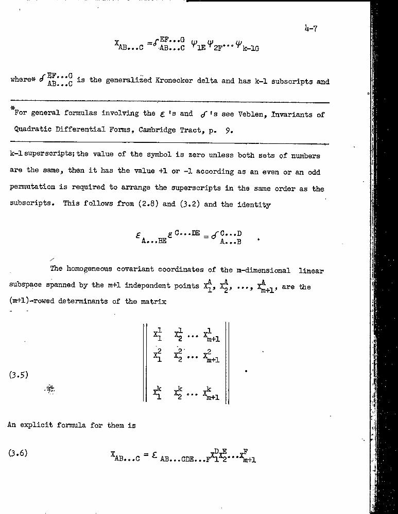
U-7
whereii- 6 is 'the generalized Kronecker delta and has k-1 subscripts and
For general formulas involving the £ >s and cT’s see Veblen, Invariants of
Quadratic Differential Forms, Cambridge Tract, p. 9,
k—1 superscripts; the value of the symbol is zero unless both sets Qf numbers
are the same, then it has the value +1 or —1 according as an even or an odd
permutation is required to arrange the superscripts in the same order as the
subscripts. This follows from (2.8) and (3.2) and the identity
^ C » • • Œ! __ ^ G « • • !D
The homogeneous covariant coordinates of the m-dimensional linear
subspace spanned by the m+1 independent points
(m+l)-r〇wed determinants of the matrix
(3.5)
An explicit formula for them is
(3.6)
U-8where ^AB.. Q has k-m-1 indices and is antisymmetric in all of them. From
the antisymmetry properties of the £ ^ p it is evident that
(3.7) = 0
is satisfied by (i = 1, ...; m+l). Hence also the points linearly dependent on the X^ satisfy the equations (3.7). The m-diraensional subspace
is deterftiined by-the equations (3.7).
The contravariant coordinates of the m-dimensional subspace are
(3.8)- AB« • «F.(k-m-l)i . f .F
They have m+l indices and are antisymmetric in all of idiera.
The necessary and sufficient condition that an arbitrary quantity
with m+l antisymmetric indices be the coordinates of a linear sub-
space is
(3.9) ^ *GD...E ^
where is obtained from ... C by means of the equations
(3.10) ^CD. _ 1 ^ yFG...HE CD...EFG...H^
and is the covariant coordinate of the subspace.
This theorem is a generalization of the theorem proved in f Q, Chapter I, and is proved in the same manner.
k-9
A line is" a simple example of a linear subspace. It is a one-
■' ^i®®nsional space determined by two points» The homogeneous contra variant
coordinates 〇f the line determined by the two points 2^ and are
(3.11) = (X^X^ - :^X^) .
From (3.11) it is evident that if we replace by X^ + remainsunaltered. Since a similar result holds for X25 we see that any two points on the line determine ttie same homogeneous coordinates of that line. The
covariant coordinates of a line are obtained from the quantities X^® by means
The linear subspace determined by the intersection of the two
hyperplanes and IjJ has the covariant coordinates
The contravariant coordinates of this subspace are obtained by means of the ^ AB.»»F
In the intersection of two planes is again a line. If the two
ho ANTIPROJECTIVE GROUP
A geometric transformation is a permutation of the elements (points^
hypeiplanes, lines, etc.) of It should be sharply distinguished from a
(3.12)
planes lA and 9 contain the line covariant coordinates of X^. That is
■the (jJ ^ are proportional to the
(3.13)
•coordinate transformation which singjly renames them. Geometric transfomjations A AX —^ y , of the types
U-10
(U.l)and
(U.2)
y^ =
-A =
where the bar denotes the complex conjugate, are called collineations and
anticollineations respectively. Both transfomnations parry points into
points, and linear subspaces into linear subspaces of the same kind, but in
the latter transformation the coitplex conjugates of the coordinates appear
and the transformation is said to be anti-linear.
Under the collineation (U.l) the points on a hyperplane
(U.3) I = 0
go into the points on the hyperplane
(U.ti)
where
ih.S)and
^ ^A i В
(U.6) p = pA ^ В В ^В ^ A
Here we must assume that the determinant of the matrix Цр^^Ц is not zero,В
That is, the collineation (U.l) is non-singular.
Equation (U.^) represents the transformation induced on the hyper
planes by the transfoiraation (b.l).
U-ixSimilarly the transformation induced on the hyperplanes hy the
anticollineation (U.2) is
(U.7)
where
(U.8)
7} = p*® I‘a u ^b
A ^ C G q ^A^c '
Again we assume that the determinant of the matrix f| 1| is not zero.B
The product of the collineation (U.l) and the collineation
(U.9) = Q^^y®
is the collineation(ii.io) = q\p®
Hence the set of all non-singular collineations form a group, the pollin-
eation group in Pj^
The product of the anticollineation (U.2) and the anticollineation
(It.ii) ^
is the transformation(U.12) = Q^gP^^x'^
■ which is a collineation. Similarly the product, of the collineation (U.9)
and the anticollineation (U.2) is the transformation
(U.13)
which is an anticollineation. The product of (J4.2) and (U.9) is also an
H-12anticollinea.'bion» Hsncs "the sst of all non-singular collineations and anii—
collineations form a group. This is called the anticollineation group’ in
The anticollineations alone^ howeverj do not form a group.
The transformations
№.11.) I ^
and№.15) 5 ^
are called correlations and anticorrelations respectively. Both trans-
foimations carry points into hyperplanes, but the latter^ transformation ip
anti-linear. The transformations are non-singular if the deteiminants of
the matrices and are different from zero.
The transformations induced on the hyperp3,anes by the non—singular
correlation (U.lU) and the non-singular anticorrelation .(U.l^) are
(U.l6) =B
and
(U.17)
respectively, where(U.18) pABp^^ = = i B
and
№.15) •
Correlations and anticorrelations may be described as transform
ations which carry hyperplanes into points as well as transformations which
carry points into hypevplanes.
in a the hyperplanes are again points. Hence in this case
correlations and anlicorrelations carry points into points and are indis-»
tingnishahle from collineations and anticollineatipns respectively.
ih the points on a line are carried into planes on a line by
transfoiroations of these types. Hence in a three—dimensional space they
are transformations which pernrate the lines of this space.
The produpt of the two correlations, given by (li.li^) and-
given by
(it.2〇)
is the transformation(it. 21) yA ^
h-13
which ^ries points into points and hence is a colllneatipn. AIsp the
product of the correlation (ii''.2〇) and the collineation (U.l) is the trans
formation N
(U.22) \ 3 „CX *AB" C\ -which carries points into hyperplanes and I ence is a correlation. We see,
then, that although the correlations alone do not form a group, the non—
singular collineations together with the non—singular correlations do form
a group. This group is called the projective group.
The product of the correlation (U.2〇) and the anticorrelation (4,l5)
is the transformation
(4.23)
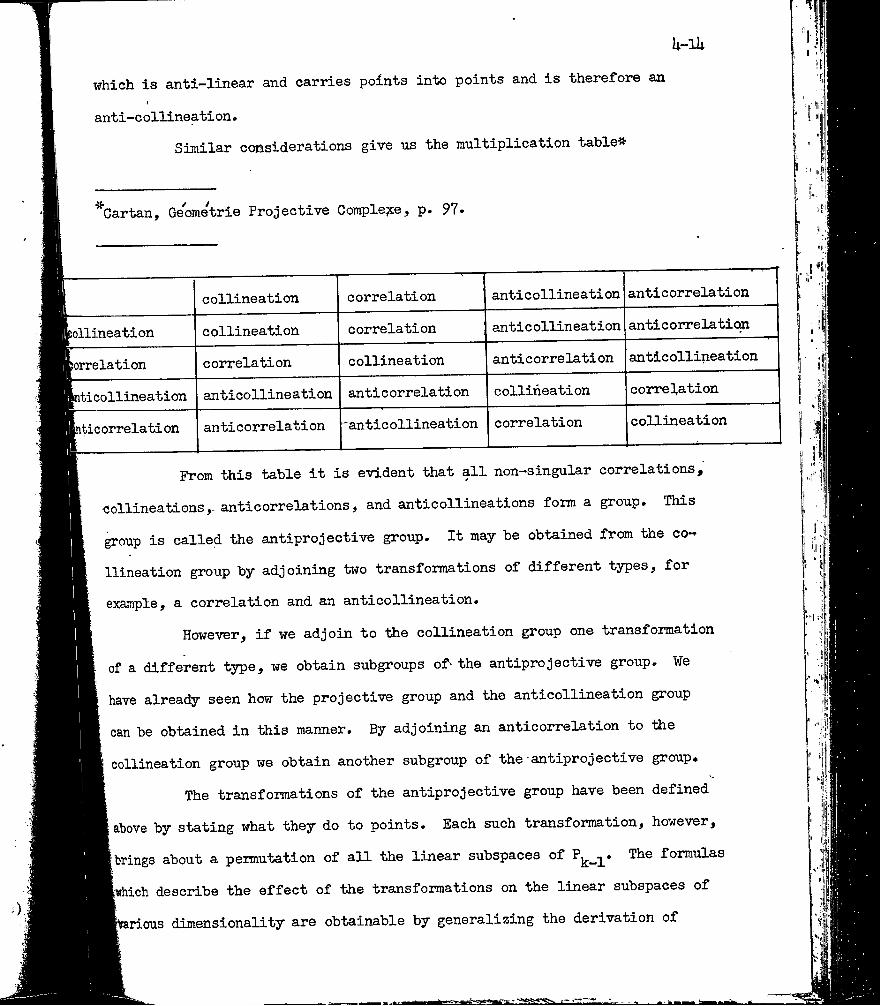
which is anti-linear and carries points into points and is therefore an
anti-collineation.Similar considerations give us the multiplication table-»
^Cartan, Geometrie Projective Comple?;e, p. 97.
ollineation
orrelation
ticollineation
ticorrelation
collineation
collineation
correlation
anticollineation
anticorrelation
correlation
correlation
collineation
anticorrelati on
antic ollineati on
anticollineation
antic ollineation
anticorrelation
collineation
correlation
anticorrelation
anticorrelation
anticollineation
correlation
collineation
From this table it is evident that all non-singular correlations,
collineations,. anticorrelations, and anticollineations fom a group. This
group is called the antiprojective group. It may be obtained from the co
llineation group by adjoining two transformations of different types, for
example, a correlation and an anticollineation.
However, if we adjoin to the collineation group one transfomiation
of a different type, we obtain subgroups of^ the antiprojective group. ¥e
have already seen how the projective group and the anticollineation group
can be obtained in this manner. By adjoining an anticorrelation to the
collineation group we obtain another subgroup of the•antiprojective group.
The transformations of the antiprojective group have been defined
above by stating what they do to points. Each such transformation, however,
brings about a permutation of aU the linear subspaces of formulas
3!hich describe the effect of the transformations on the linear subspaces of ^rious dimensionality are obtainable by generalizing the derivation of
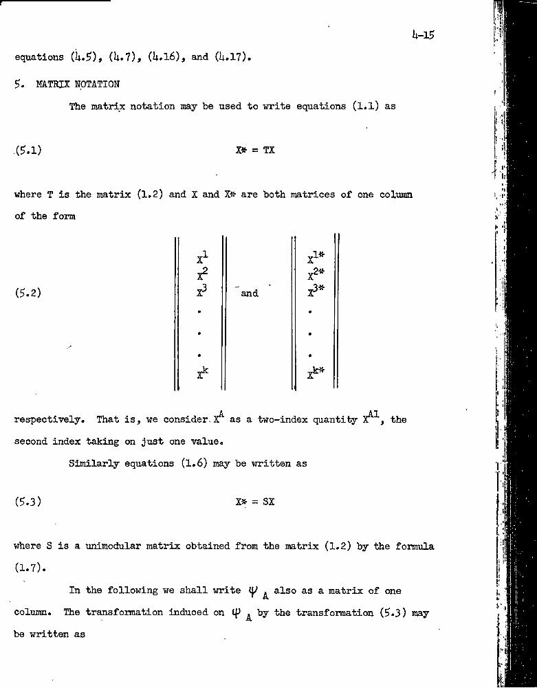
k-iB
equations (U.^), (U.7), (U#l6), and (U.17).
MATRIX NOTATION
The matrix notation my be used to write equations (l.l) as
,(?.!) X* = TX
where T is the matrix (1.2) and X and are both mtrices of one column
of the form
(5.2)
X
X^ and x3*
respectively. That is, we consider. as a two-index quantity X^-^, the
second index taking on just one value.
Similarly equations (1.6) my be written as
(5.3) X* = SX
where S is a unimodular matrix obtained from the mtrix (1.2) by Uie formula
(1.7).
In the following we shall write ^ also as a matrix of one
column. The transformation induced on If* ^ by the transformation (5.3) my
be written as
U-16
(5.U)
'where s is the inverse matrix to that used in (5.3) and the prime denotes
the transposed matrix.The transpose of the matrix X is denoted by X* and is a matrix
of one row. Thus we may write for X^(^^ the matrix X'<// which has only one
row and one column and is therefore ^qual to its transpose ly *X.The matrices S and s of a coordinate transformation have indices
which refer to different coordinate systems. ¥e take account of this fact
by writing the contravariant index of the transformation matrix directly
above the covariant one, thus Sg and Sg. For a matrix of this type the
contravariant index is assumed to come first (i.e., be leftmost). The in
verse of a matrix is indicated by the exponent -1 so that s = S With
these coventions equation (5.U) may be rewritten as
-1it = S' (^ = S cp
where S = S’The equations of geometric transformations may be written in
matrix notation. Thus equation (U.l) may be written as
(5.5) ,
where X and J are matrices of - one column and || P^g || is the matrix representing
the collineation. In the index notation for a geometric transformation, and
indeed for any geometric being, we never place one index directly above another.
Thus it SLlw3.ys hsLS cL niGSruTig to Sciy thclt on© ind.G3C pr©c8dBs 3,noth©r 6V6n if
one is a covariant and the other is a contravariant index. ¥e shall use the
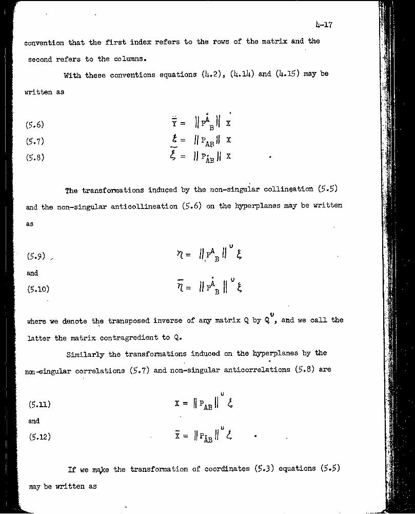
convention that the first index refers to the taws of the matrix and the
second refers to the colu3ims»With these conventions equations (U.2), (U.lU) and (U.l5) may be
U-17
written as
(5.6)
(5.7)
(5.8)
r= X
4 = DpabII ^
The transformations induced by the non-singular collineation (5*5)
and the non-singular anticollineation (5»6) on the hyperplanes may be written
as
(5.?) , >?= ll/gfi
and
(5.10) n= IMg ir 4
Vwhere we denote the transposed inverse of any matrix Q by Q , and we call the
latter the matrix contragredient to Q.
Similarly the transfomations induced on the hyperplanes by the
ncn-singular correlations (5.7) and non-singular anticorrelations (5.8) are
(5.11) X= I|p4bII 4
and
(5.12) x=
If we ms^e the transformation of coordinates (5.3) equations (5»5)
may be written as
U-18 .
(5.13)= 11 p^gll s'^^:
orT* = II P^gll* X*
(5.1U)
where(5.15)
Thus in a new coordinate system, the ccmponents of the matrix || which
determine the collineation, are linear homogeneous functions of the components
in the old coordinate system. The coefficients are homogeneous functions of
the elements of the transformation matrix. Geometric beings* with this type
«geometric being” is an entity described by components in every coordinate system. The components in two coordinate systems are related by a transformation law, namely a formula which gives the components in one coordinate system in terms of the pomponents in the other.
of transformation law are special types of spinors. Equation (5.l5) is a
special case of a transformation law which satisfies the two homogeneity
requirements given above, and hence g are the components of a spinor.
Similarly, we see that in a new coordinate system, equations (5.6)I
may be written as
(5.16)’Y* = ||p^gl|*X*
where1 1
(5.17) ||/gll* =s||p^3ll s'
Also equations (5.7) and (5.8) may be written as
(5.18) = llp^glkx*
and
(5.19) 4 * = il
h-l9
where1 II II .,—1(5.20) II ^abI 1 * = s II Pjsjll S
and
(5.21) II '’abIl» = s”||p^lls"’- .
Equations (5.17), (5.20) and (5.21) are all special cases of
transformation laws for spinors. Prom these equations, together with equations
(5.15), we see that if in one coordinate system a single matrix, for example
the unit matrix, represents a collineation, a correlation, an anticollineation
and an anticorrelation, in another coordinate system, these different trans
formations will not in general be represented by the same matrix. We have
used the convention that placing a dot over one of the indices of a spinor
implies that the complex conjugates of the elements of the transformation
matrix enter into the law of transformation of the spinor.
6. COMMUTING TRANSFORMATIONS
In this section we will discuss the transforms of geometric trans
formations when a different geometric transformation is made. This differs
from the work of the previous section where we obtained the transformation
laws of the components of a geometric transformation under a transformation
of coordinates.Let point Y be the transform of the point X under the non-singular
collineation P, that is,
(6.1) T = PX
If we now perform the non-singular collineation Q, the points X and X are
transformed into the points Z and W where
Z = QX and ¥ = . QI(6.2)Equations (6.1) then become
(6.3)
or
(6.U)where(6.5)
Q"^ = PQ~^Z
W = RZ
R = QPQ“^
lt-20
_1That is, the collineation P goes into the collineation R = QPQ
under the collineation Q.
Two geometric transformations are said to be geometrically
commutative if each transforms the other into itself. It is geometrically
obvious that if a geometric transformation A transforms a transformation B
into itself', then B will transform A into itself. Thus if R = ^ P where ^
is an arbitrary number, the two collineations P and Q are geometrically
commutative. In this case equations (6.5) may be written as
(6.6) P = QPQ”^
or(6.7) QP = f PQ ^
From equation (6.7) we see that geometrical commutativity of two
collineations does not distinguish between commutativity and anticommutativity
of the matrices representing the collineations. A geometric distinction be
tween these two cases will be given in the next chapter.
If instead of performing a collin^ation, we perfqrm the anti-
U-21
collineation Q:
(6.8) Z = QX and
Equations (6.1) then become
(6.9) Q“^ = PQ"^Z
or(6.10) W = RZ
where
(6.11) R = QPQ“^
Thus the collineation P and the anticollineation Q are geometrically
coinmutative if
(6.12) QP = fP^ .
If the transformation Q is T go into the hsrperplanes 4 ^.nd
a correlation, then the points X and
. That is,
(6.1U) ^ = QX and = QY
Equation (6.1) then becomes
(6.15) Q"^ ->2 = PQ“^ 4
or(6.16) ■>) = R 4
whereR = QPQ"^ .(6.17) ■
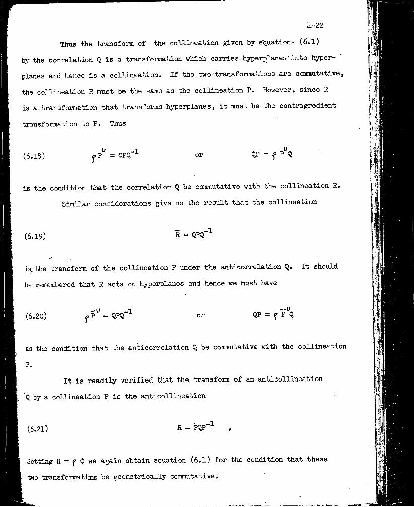
k-22
Thus the transform of the collineation given by equations (6.1)
by the correlation Q is a transformation which carries hyperplanes'into hyper
planes and. hence is a collineation. If the two transformations are commutative^
the collineation R must be the same as the collineation P. However, since R
is a transformation that transforms hyperplanes, it must be the contragredient
transformation to P. Thus
(6.18) oi* QP = f P*^Q
is the condition that the correlation Q be commutative with the collineation R.
Similar considerations give us the result that the collineation
(6.19) R = QPQ'"^
is. the transform of the collineation P under the antieorrelation Q. It should
be remembered that R acts on hyperplanes and hence we must have
(6.20) ^P = QPQ or QP = f P q
as the condition that the anticorrelation q be commutative with the collineation
P.It is readily verified that the, transform of an anticollineation
Q by a collineation P is the anticollineation
(6.21) R = PQP"^ .
Setting R = f Q we again obtain equation (6.1) for the condition that these
two transforma tins be geometrically commutative.
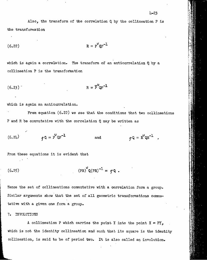
U-23Also, the transform of the correlation Q by the collineation P is
the transformation
(6.22) H = p‘^QP"^
which is again a correlation. The transform of an anticorrelation Q by a
collineation P is the transfoimation
(6.23) ' R = P^QP”^
which is again an anticorrelation.
Prom equation (6.22) we see that the conditions that two collineations
P and E be commutative with the correlation Q may be written as
(6.2l|) ^Q = P^QP“^ and j>Q = r'^QR"^ ,
From these equations it is evident that
(6.25) , (PR)'^Q(PR)“^ = f Q .
Hence the set of collineations commutative with a correlation form a group.
Similar arguments show that the set of all geometric transformations commu
tative with a given one form a group.
7. INVOLUTIOIS
A collineation P which carries the point X into the point X = PT,
whi6h is not the identity collineation and such that its square is the identity
collineation, is said to be of period two. It is also called an involution.
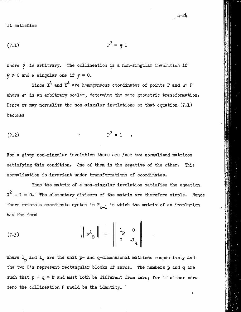
It satisfies
(7.1)
where y is arbitrary. The collineation is a non-singular involution if
f ^ 0 and a singular one if ^ = 0.
Since and are homogeneous coordinates of points P and <r P
where tr is an arbitrary scalar, determine the same geometric transformation. Hence we may normalize the non-singular involutions so that equation (7«l)
becomes
(7.2) P^ = 1 ,
For a giv^ non-singular involution there are just two normalized matrices
satisfying this condition. One of them is the negative of the other. This
normalization is invariant under transformations of coordinates.
Thus the matrix of a non-singular involution satisfies the equation2X -1 = 0.' The elementary divisors of the matrix are therefore simple. Hence
there exists a coordinate system in Pj^ ^ in which iiie matrix of an involution
has the fond
(7.3)0 -1
q
where 1 and 1 are the unit p- and q-dimensional matrices respectively and P ^the two 0*s represent rectangular blocks of zeros. The numbers p and q are
such that p + q = k and must both be different from zero; for if either were
zero the collineation P would be the identity.
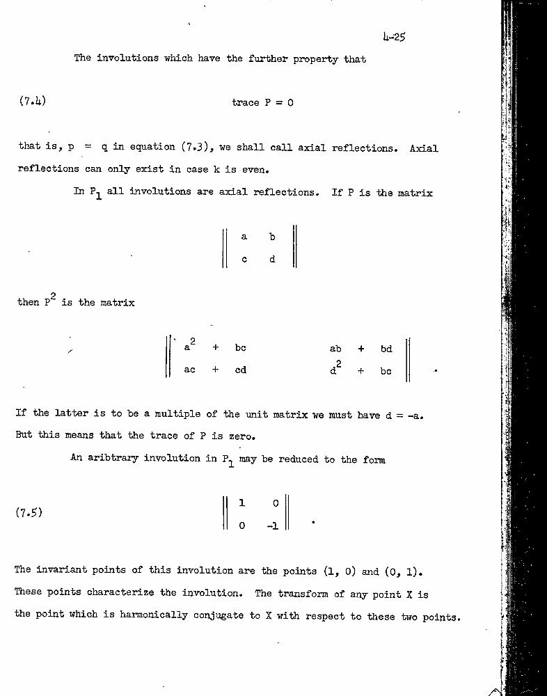
The involutions which have the further property that
U-2^
(7.W trace P = 0
that is, p = q in equation (7-3), we shall call axial reflections. Axial
reflections can only exist in case k is even.
In all involutions are axial reflections. If P is the matrix
a b
c d
then P2 is the matrix
y<1a be ab + bd
ac + cd + be .m
If the latter is to be a multiple of the unit matrix we must have d =But this means that the trace of P is zero.
An aribtrary involution in P^ may be reduced to the form
(7.5) 1 0 0 -1
The invariant points of this involution are the points (l, O) and (O, l).
These points characterize the involution. The transform of any point X is
the point which is harmonically conjugate to X with respect to these two points
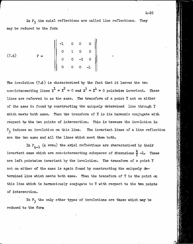
h-Z6
nil the axial reflections are called line reflections. Thej
may be reduced to the form
(7.6) P =
+10
0
0
0
1
0
0
0 00 0-1 00 -1
The involution {1*6) is characterized by the fact that it leaves the two non-intersecting lines = 0 and X^ = X^ 0 pointwise invariant. These
lines are referred to as the axes. The transform of a point Y not on either
of the axes is found by constructing the uniquely determined line through Y
which meets both axes. Then the transform of Y is its harmonic conjugate with
respect tp' the two points of intersection. This is because the involution in
P^ induces an involution on this line. The invariant lines of a line reflection
are the two axes and all the lines which meet them both.
In Pj^ ^ (k even) the axial reflections are characterized by theirIcinvariant axes which are non-intersecting subspaces of dimensions ^ -1. These
are left pointwise invariant by the involution. The transform of a point Y
not on either of the axes is again found by constructing the uniquely de
termined line which meets both axes. Then the transform of Y is the point on
this line which is harmoniously conjugate to Y with respect to the two points
of intersection.
In P^ the only other types of involutions are those which may be
reduced to the form
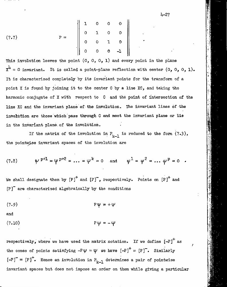
(7.7)
h-27
10 0 0 0 10 0
P =0 0 100 0 0 -1
This involution leaves the point (0, 0, 0, l) and every point in the plane
= 0 invariant. It is called a point-plane reflection with center (0, 0, 0, l).
It is characterized completely by its invariant points for the transform of a
point X is found-by joining it to the center C by a line XC, and taking the
harmonic conjugate of X with respect to C and thé point of intersection of the
line XC and the invariant plane of the involution. The invariant lines of the
involution are those which pass throTigh G and meet the invariant plane or lie
in the invariant plané.of the involution.
If the matrix of the involution in P is reduced to the form (7*3),
the point^se invariant spaces of the involution are
(7.8) Ip = ... = = 0 and = 1//^ = ... tpP = 0 .
*4“ "• * 4"We shall designate them by [P] and [P] , respectively. Points on [P] and
[P]" are characterized algebraically by the conditions
(7.9) pij; = +(p
and
(7.10) Pl^ = _l|j
respectively, where we have used the matrix notation. If we define [-P]**" as/the cones of points satisfying -Pi^ = ip we have [-P]"*" = [P]"*. Similarly
[-P] = [P]"*". Hence an involution in Pj^ ^ determines a pair of pointwise
invariant spaces but does not impose an order on them while giving a particular
matrix P in the form (7.3) determines a positive and negative space.
The pointwise invariant spaces of an involution detemine it completely. To prove this we let S'*" and S” be the two non-intersecting
pointwise invariant subspaces of dimensions r-1 and k-r-1 respectively, and
construct the unique involution in with these spaces as pointwise invariant spaces. If is any point not on S’*” or S there is a unique line
through it and intersecting S'*’.’ s^nd S”. The involution then leaves points on
s’*” and S~ invariant and transforms any other point into its harmonic con
jugate with respect to the two points in which the line through ijJ meets S
and S .The invariant lines of an involution are all the lines which meet
both s’*' and S” or lie entirely in either one of them. Indeed if is any
space of r-1 dimensions which is invariant under the involution, then it is
either pojntwise invariant and lies in S’*" or S”, or it intersects them in
spaces of dimensions Tg-l with ^2 ~ proof of this de
pends on the fact that if a space is invariant, the involution induces in
it either the identity or an involution which necessarily has two pointwise
■invariant subspaces.
• 8. ANTI-INVOLUTIONS
An anticollineation
U-28
(8.1) X = PT
will be of period two and will be called an anti-involution if and only if
(8.2) PP = ^ 1
where f Is a number different from zero. • Tf we take the trace of both sides
of equation (8.2) we see that = trace (PP) = trace (PP) = kj" . Hence ^
must be real.
'From the transformation law of P (cf. equation (5.17)) we see that
the normalization condition, ) P} = 1, where |P/ is the determinant of P, is
invariant under coordinate transformations. Under this normalization we haveIc 1f =1. Hence for odd k, ^ = +1, and for even k we have = -1. Thus for
even k we have the two cases
(8.3) PP = 1
and
(8.U) PP = -1
Anti-involutions which satisf^r (8.3) are said to be of the first kind and
those which satisfy (8.1i) are of the second kind.
Any two anti-involutions of the same kind are equivalent under a
trapisformation of coordinates. The proof of this statement is contained in
an ruipublished theolrem of Dr. H. Jacobson which states that two non-singular
anticollineations are protectively equivalent if -Uae matrices of their squares
are equal.'» *
U“29
*The proof follows!Let the two non-singular anticollineations be P and Q. Then the
hypothesis isPP = QQ .
Let us now sub;5ect Q to the transformation of coordinates with matrix T whereT = e^^l+e'^^P^^q
and Q is real and such that | T|;<i 0. This gives0» = TQT"^ = P
since^-1 ^ ^
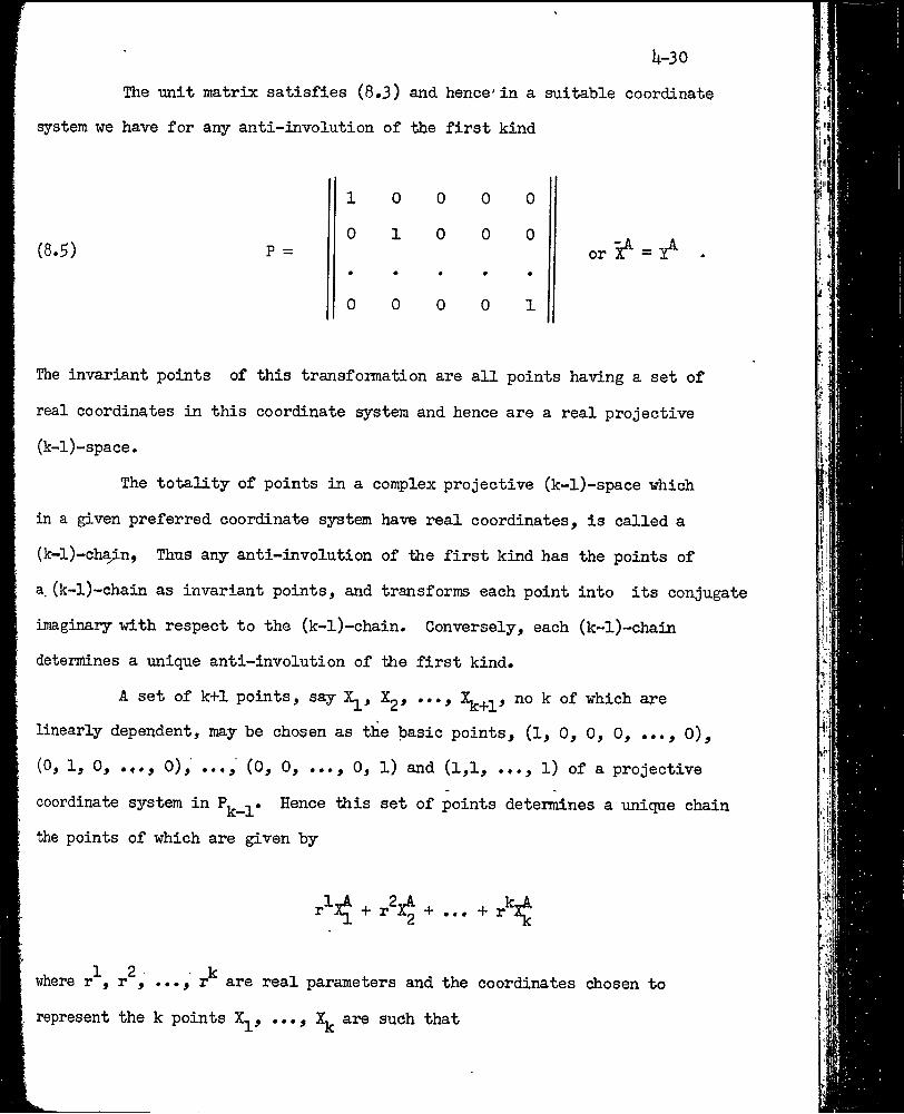
The unit
system we have for
matrix satisfies (8.3) and hence*in a suitable coordinate
any anti-involution of the first kind
(8.5) P =
1 0 0 0 0 0 10 0 0
or .
0 0 0 0 1
The invariant points of this transfomation are all points having a set of
real coordinates in this coordinate system and hence are a real projective
(k-l)-space.
The totality of points in a con^jlex projective (k-l)-space which
in a given preferred coordinate system have real coordinates, is called a
(k-l)-ch^n. Thus any anti-involution of the first kind has the points of
a. (k-l)-chain as invariant points, and transforms each point into its conjugate
imaginary id.th respect to the (k-l)-chain. Conversely, each (k-l)-chain
determines a unique anti-involution of the first kind.
A set of k+1 points, say Xj_, Xg, ..., no k of which ape
linearly dependent, may be chosen as the basic points, (1, 0, 0, 0, ..., O),
(O, 1, 0, O), (0, 0, ..., 0, l) and (1,1, ..., l) of a projective
coordinate system in Hence this set of points determines a unique chain
the points of which are given by
r^X^ + r^X^ + ... + r^X¿
12 • kwhere r ,r , ..., r are real parameters and the coordinates chosen to
, ..., X. are such thatrepresent the k points X,
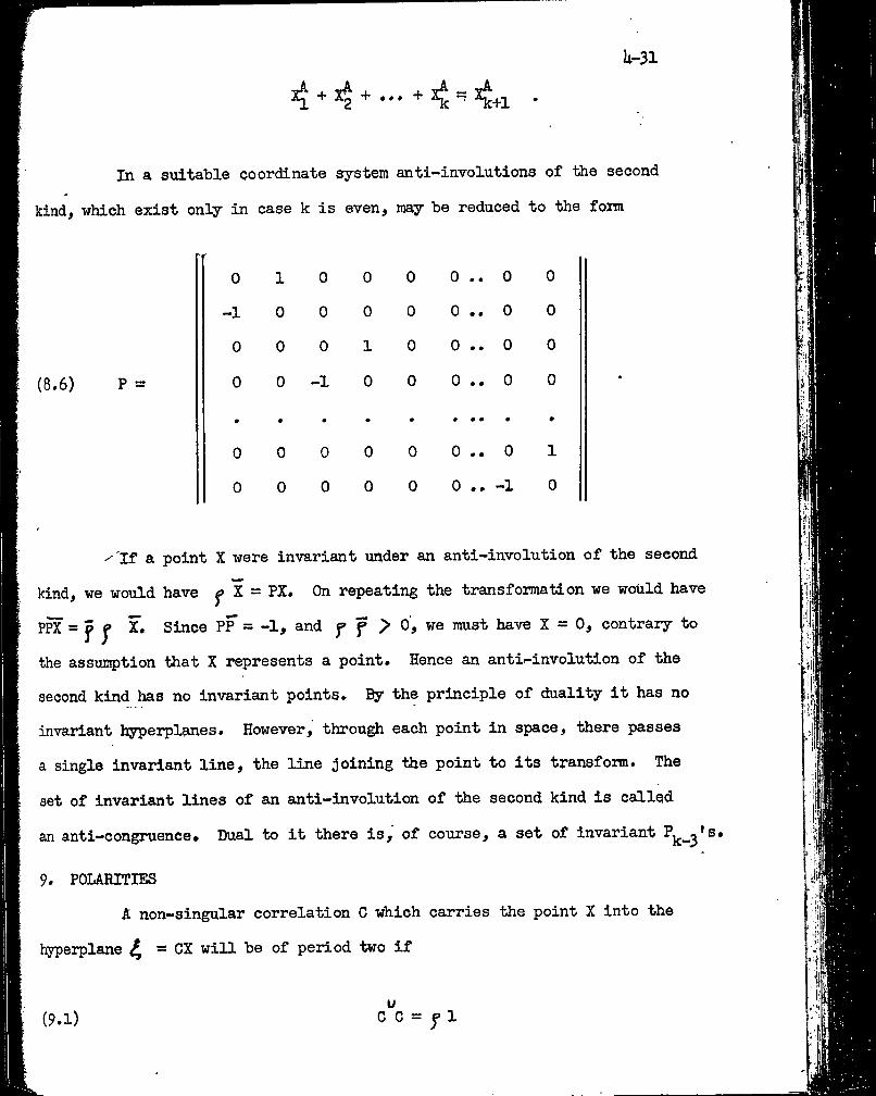
U-31
+ •» • + :+l
In a suitable qoordinate system anti-involutions of the second
kind, which exist only in case k is even, may be reduced to the foim
-^'If a point X were invariant under an anti-involution of the second
kind, we would have ^ X = PX. On repeating the transfoimation we would have
the assui!?)tlon that X represents a point. Hence an anti-involution of the
second kind has no invariant points. By the principle of duality it has no
invariant hyperplanes. However, through each point in space, there passes
a single invariant line, the line joining the point to its transfoiro. The
set of invariant lines of an anti-involution of the second kind is called
an anti-congruence* Dual to it there is, of course, a set of invariant
9. POLARITIES
A non-singular correlation C which carries the point X into the
hyperplane will be of period two if
0 1 0 0 0 0 0 0-1 0 0 0 0 0 0 00 0 0 1 0 0 0 0
(8.6) P = 0 0 -1 0 0 0..0 0
0 0 0 0 0 0 0 1
0 0 0 0 0 0.. -1 0
PPX = ^ j» X. Since PP = -1, and j? ^ > 0, we must have X = 0, contrary to
uC C = el(9.1)
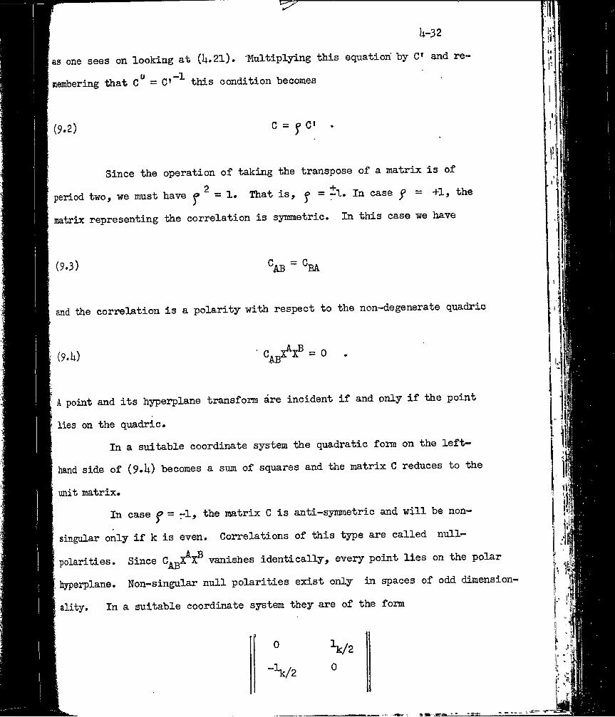
U-32[as one sees on looking at (U.21). -Multiplying this equation by 0» and re-
Kembering that = C'“^ this condition becomes
(9.2) C = ^ C»
Since the operation of taking the transpose of a matrix is of
period two, we must have ^ ^ = 1. That is, ^ = ~1. In case f - +1, the
matrix representing the correlation is symmetric. In this case we have
(9.3)
and the correlation is a polarity with respect to the non-degenerate quadric
(9.U)
A point and its hyperplane transform áre incident if and pnly if the point
lies on the quadric.In a sui-bable coordinate system the quadratic forra on the left-
hand side of (9.U) becomes a sum of squares and the matrix C reduces to the
unit matrix.In case ^ = 7-1» matrix C is anti-symmetric and will be non
singular only if k is even. Correlations of -this type are called null-
' polarities. Since vanishes identically, every point lies on the polar
[ hyperplane. Non-singular null polarities exist only in spaces of odd dimension
ality. In a suitable coordinate system they are of the form
0 \/2
0
U-33idiere lonit matrix in k/2 dimensions and we have normalized the
+correlation to have determinant -1.
10. ANTIPOLARITIES
A non-singulap anticorrelation G which carries the point X into tiie hyperplane where 4 = CX will be of period two and will be called
an antipolarity if )
f ^
u-C C = j 1
that is if (cf. ^ 3)
(10.1) iMultiplying by C’ this condition becomes
(10.2) C = ^C» or
From the second of equations (10.2) we see that
‘^AB BA
°AB ~ ? '^BA ff °AB
hence ^ ^ =1. Replacing the homogeneous coefficients
= ? i°ABAB of the aptipolarity
(10.3) H = H? .
A matrix satisfying this condition is said to be hermitian. Hence
the necessary and sufficient condition for an anticorrelation to be of period
two is that the matrix of its coefficients be proportional to an heztnitian
one. The normalization made to obtain equation (10.3) is Invariant under
coordinate transformations as may be verified from equation (^.2l).
■The locus of points which lie on their antipolar planes is the
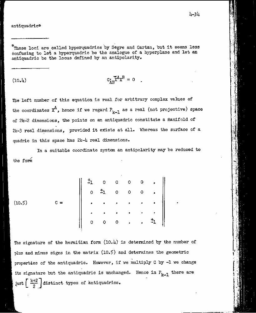
antiquadric*
h-3h
These loci are called hyperquadrics by Segre and Cartan, but it seems lessconfusing to lei a hyperquadric be the analogue of a hyperplane and let an antiquadric be ihe locus defined by an antipolarity»
T^e left number of this equation is real for arbitrary complex values of
of 2k-2 dimensions, the points on an antiquadric constitute a manifold of
2k-3 real dimensions, provided it exists at all. Whereas the surface of a
quadric in this space has 2k-U real dimensions.
In a suitable coordinate system an antipolarity may be reduced to
the form
The signature of the hemitian form (10. U) is determined by the number of
plus and minus signs in "(¿le matrix (10.5) and determines the geometric
properties of the anti quadric. However, if we multiply C by -1 we change
its signature but the antiquadric is unchanged. Hence in
(10. U)
the coordinates Z^, hence if we regard as a real (not projective) space
il 0 0 0 00 il 0 0 0
(10.5) c =
0 0 0
J distinct types of antiquadrics.there are
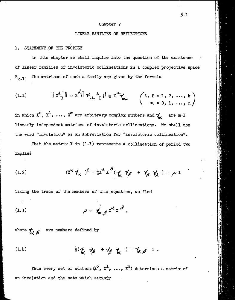
i-1Chapter V
LIHEAR FAMILIES OF REFLECTIOHS
1. . STATEMENT ,0F THE PROBLEM
In this chapter we shall inquire into the question of the existence
of linear families of involutoric collineations in a complex projective space
The matrices of such a family are given by the formгlla
(1.1) 11 /g II = x‘^11 \ II = A, B = 1, 2, k
\ =< = 〇i li •••i m
in which X° are arbitrary complex numbers and are m+1
linearly independent matrices of involutoric collineations. ¥e shall use
the word "involution” as an abbreviation for "involutoric collineation".
That the matrix X in (l.l) represents a collineation of period two
implies
(1-2)
Taking the trace of the members of this equation, we find
(1.3) ,
where are numbers defined by
(i.ii)
Thus every set of numbers (X°, X^, ..., 2?”) determines a matrix of
an involution and the sets which satisfy
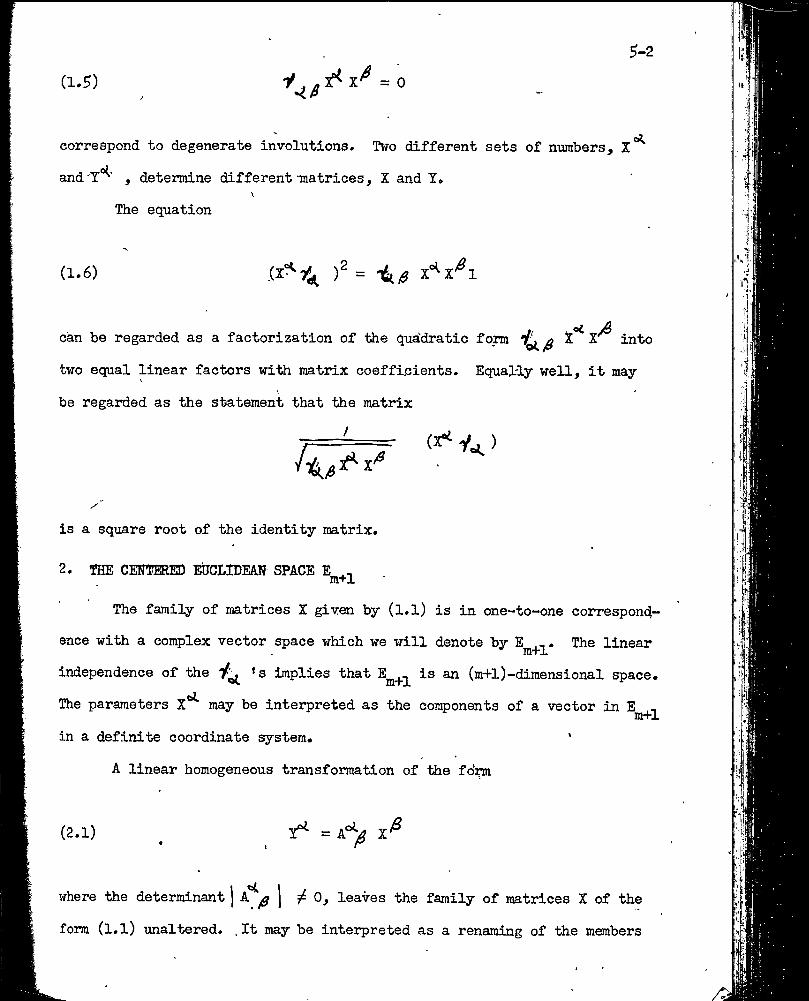
5-2(1.5) = o
correspond to degenerate involutions. Two different sets of numbers,and T*^' , determine different Tjiatrices, X and T.
\The equation
(1.6) ,(Z^7^ f = 'ii
, 〇l jQcan be regarded as a factorization of the quadratic fom X X into
two equal linear factors with matrix coefficients. Equally well, it may
be regarded as the statement that the matrix
is a square root of the identity matrix.
2. THE CENTEEIED EUCLIDEAN SPACE E m+1
The family of matrices X given by (1.1) is in one-to-one correspon4-
ence with a complex vector space which we will denote by E -. The linearra+1
independence of the *s implies that is an (m-fl)-dimensional space.
The parameters X^ may be interpreted as the conponents of a vector in Em+1
in a defini-be coordinate system.
A linear homogeneous transformation of the form
(2.1) = A°^
where the determinant | | 5^ 0, lea-ires the family of matrices X of theform (1.1) unaltered. .It may be interpreted as a renaming of the members
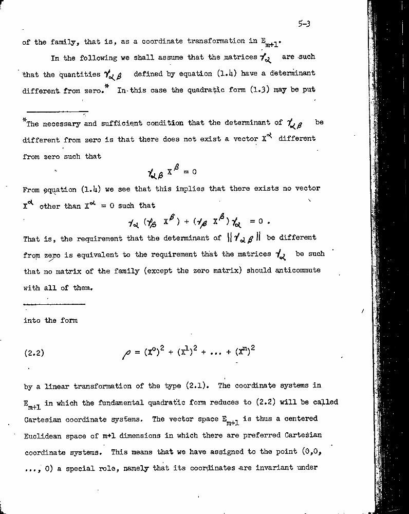
^-3of the family, that is, as a coordinate transformation in ®m+l*
In the following we shall assume that the matrices are such
that the quantities defined by equation (l.U) haire a determinantdifferent, from zero.* In-this case the quadratic form (1.3) may be put
*The necessary and sufficient condition that the determinant of be
different from zero is that there does not exist a vector different
from zero such that
From equation (l.U) we see that this implies that there exists no vector
other than X'^ = 0 such that
That is, the requirement that the determinant of be different
from z^o is equivalent to the requirement that the matrices be such
that no matrix of the family (except the zero matrix) should anticommute
with all of them.
into the form
(2.2) ^ = (X°)^ + (Г^)^ + ... + (X?")^
Iby a linear transformation of the type (2.1). The coordinate systems in
E , in which the fundamental quadratic form reduces to (2.2) will be called iri+1Cartesian coordinate systems. The vector space is thus a centered
Euclidean space of m+1 dimensions in which there are preferred Cartesian
coordinate systems. This means that we have assigned to the point (0,0,
...,〇) a special role, namely that its coordinates a.re invariant under
transformations of coordinates. This point corresponds to 'the matrix all
of whose elements are zero.When Cartesian coordinates are used in "the relations (l.U)
reduce to /
5-U
(2.3)1 if ^
0 If oi, ^
Hence the , if existent, are a set of m+1 anticoramuting k-row matrices
each- ‘of which is a square root bf thé identity matrix.
In the space we shall use the familiar notations of tensor
analysis. In particular we shall raise and lower indices by means of the
fundamental tensor and the^ tensor defined by
(2.ur V y/3tj where II II = 1
This gives, a definite meaning to •/' and (l.U) may be written in the
0 *form
(2.5)
Of course in Cartesian coordinates is the same matrix as 7^ •
It is clear that" constant matrices which satisfy (1.6) must
also satisfy the differential relation
a x'’(2.6) t
5-5
which on putting in indices becomes
J< ^ -2ihlI]
^ V ^ ) ax'
Thus we have what may be regarded as a factorization of the quadratic
differential operator# ^ which is expressed as the square of adir dV
linear differential operator ««i __d<?X*^
This observation, made by P. A. M. Dirac, was the starting point
in his theory of the spinning electron which has given the theory of spinors
its vogue.
3. JRANSFORMATIONS OF LlilEAR FAMILIES OF INVOLUTIONS
A non-singular collineation iy ^ <p
A rA ,,, B(3.1) (p
in P brings about a transformation X-» T of the collineations given by k-1
(1.1) according to the formula
(3.2)-1 «AY = PXP = X
where
(3.3)>1< = P Va p"’-
5-6
In case the family as a whole is transformed into itself we have
also
(3.W
Coit^jaring (3*U) and (3.?) we have
(3.5) = (pV^ p"^)x
To solve this equation for Y we make use of the relation
(3.6) Trace (V*^ ) = k J ,
which is obtained from (2.5) by taking the trace of both members.
Multiplying (3.5) by and taking the trace, gives
(3.7) X
where
(3.8) - Trace (V'^PT^ P"^) . k
Hence in case (3*1) transforms the family (l;l) into itself, it
m+1 •induces the non-singular transformation (3.7) in the Euclidean space E
1;
5-7
Since the degenerate transformations of the family (l.l) are carried into
themselves, the points on the cone (1.5) in are permuted among them
selves. Indeed we may prove that the quadratic form (1.3) is left in
variant by (3.7). To do this we first substitute from (3.7) for in
(3.5) and equate coefficients of the arbitrary variables to get
(3.9)
But,'
(3.10)
is a consequence of (3.3) and (l.U) and substitution from (3.9) in this
equation now gives
(3.11) ^ •
Multiplying through by and summing, we obtain
(3.12) X'^X'^..
Equation (3.12) is equivalent to the statement that (3.7) is a
rotation of the Euclidean space about the origin. Hence the group
of collineations in which leave the linear family (l.l) invariant is
5-8
isomorphic (perhaps multiply) with a sub-group H of' the group of rotations
about the center of
¥e shall find that the group H'thus defined coincides with the
whole orthogonal group when m + 1 = 2 y and k = 2 . It is the proper
y.orthogonal group when m + l = 2y +1 and k = 2 . ¥e shall also prove
that the isomorphism (3»8) between the collineatibns which leave the
family invariant and the group H is (l-l) in these cases. This
inplies that the equation (3.8) is satisfied by a iinique collineation
II ^ P II when II I' defines an arbitrary transformation of H.
U.- EXISTENCE OF LINEAR FAMILIES OF INV〇i,UTIONS
/In 2 we saw that the existence of a linear family satis
fying (1.2) Implied the existence of a set of matrices (〇^ = 0, 1, ..., m)
satisfying (2.3). The converse ,is also true,for a set of matrices satisfy
ing
(U.l) (^ )^ = 1» and -'/^'>¿(^7^/^)
serve to define a linear family which'satisfies (1.2). The ex
istence of linear families of involutions in Pjj._2 then reduced to thp
problem of discovering sets of matrices of order k satisfying (if.l). ¥®
call an ordered set of linearly independent matrices satisfying (U.l) a

Y’ —set and say. that it is even (or odd) if the number of matrices is even
(or odd). Two y'-sets and are said to be similar if (3.3) is
satisfied for a non-singular mâtrix P.
The existence of a i -set in the case k = 2 has been known since
quaternions were represented by two-row matrices. Such a set is
^-9
0 i 0 1(U.2), . IIH> 0•H1
. 5 1^2 ^1 0
» y〇 -i ”^1^2 ~
A y-set containing more than one matrix can exist only if the dimension
ality, k—1, of the space is odd (see^10) so that in an even—dimensional
space a Y -set consists of a single non-singular involution. Fop. an odd-
dimensional space the problem reduces essentially to the case k = 2^ ás
we shall see later. When K = 1 we have the V-set exhibited in (U.2) and
when y = 2 (k = U) ay -set is
(Í4.3)
1 0 ' f
•Ho it
1
o1 \ H 1
o y (2) _ -i 0 ( 0 Y (2) - > ' 20 1 H o 〇 0 1 H*
o M H* o
f 1• i 0 11 0
•H !1
〇1
〇l11 and
Ó *^0 1•-----f-------
-i 0 1 0 1 0 f 0
•H1o
0 1 Í11 '
00 ' 0
Iri(
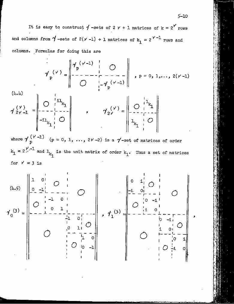
5-XO
It is easy to construct 'f -sets of 2 y + 1 matrices of k = 2' rows
and columns from 'j -sets of 2(y -l) +1 matrices of = 2'^"^ rows and
columns. Formulas for doing this are
y (v^) ^P
yP o
(U.U)
-iiV-. - o-il.k.
il.
o
O !-y
o'• 2V
, p = 0, 1,..., 2(y-l)
00
where y^ ^ (p - 0, 1, 2V-2) is a y-set of matrices of order
_ y -1k^ - 2/-' and Ij^ is the unit matrix of order k^. Thus a set of matrices
for >^ = 3 is
(k.^)
y (3) _’ 0
,1 0 0 -1
o
o
-1 00 1
o
o
1 0 0 1
o
o
1 0 0 -1
y (»" '1
0 i
-i. 0
o
o—0 -i
1 0
o
o
b -i r
i 〇i o,0 i
O -i
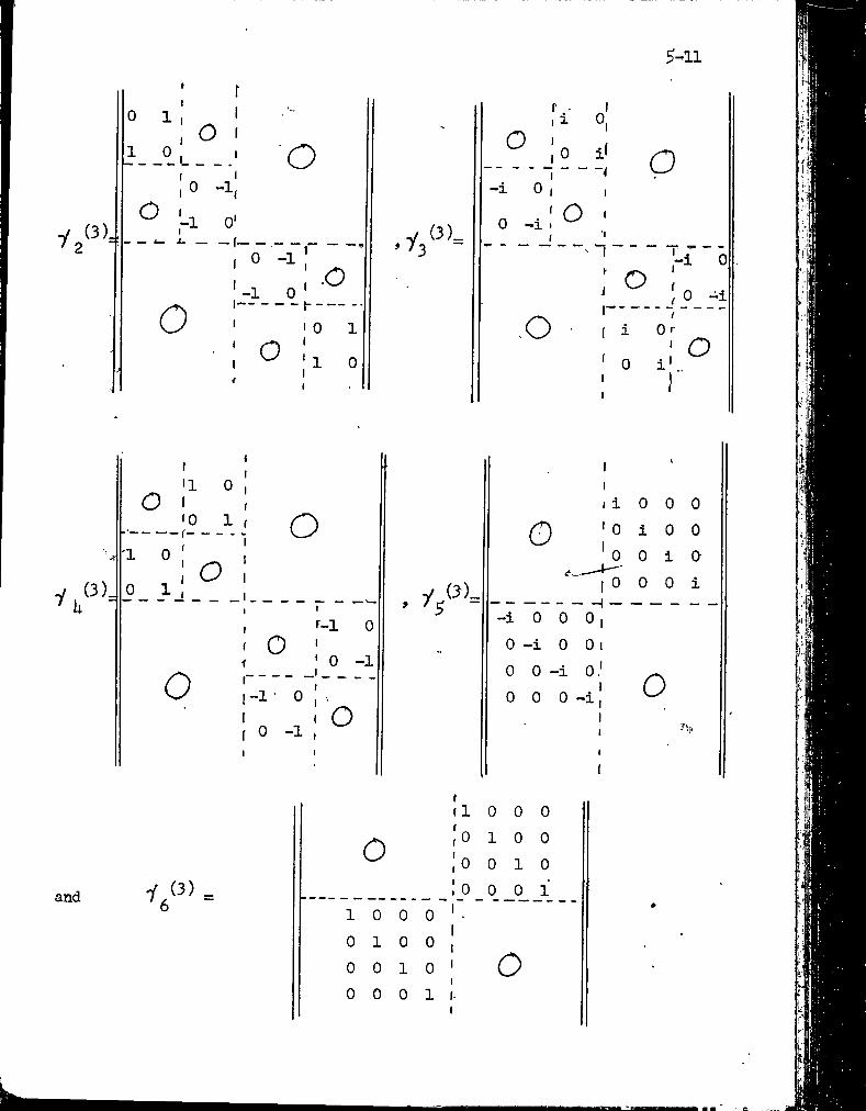
y,
0 1f1
1 00 1
1 00
0 -1;
-1 0'
0
0 -1 1.0
-1_ _0
1 0 1
>
114
0 011
y (3). ^ h
5-11
»У-(3)_
0 1 0
0 1 0'1 0
_ 0 1 0
0
T-1 00 :o-i
-î"o 5
Л ' 00 -11
O
-1
y (3)., /5 -
0
0 -i
i 0
0
I
O
1'-4
IIЧ
O
: O'-1
,0J1—I iÍ
, 0 -i
0〇r
O
O
III i ' 0I 0
0i0
I 0 0
00i0
000i
H-i 0 0 0 0 -i 0 00 0 -i 0 0 0 0 -i O
and i (3) _ ’в
tl 0
0;〇:〇
10
:〇 01 0 0 0 1
0 1 0 0 11
0 0 1 0 10 0 0 1 1-
(
01
0001
O
5-12
Using (I4..U) we readily show by induction on y that the equations
(I4.6) V0(>^)y y (>^)
2y-l 7 2y
and(U.7) Trace ii *** ~ Trace 1= (+i) 2^
hold for the •/ -sets defined in this explicit manner.
5. EQUi?ALENGE OP Y -SETS
The remainder of this chapter will be devoted to a discussion of the
geometric properties of the linear family of involutions determined by a
y -set, and to the equivalence of -sets under collineation. The main«
results are contained in the following theorems.
Theorem (5.1). If k = 2 >2 (X odd), the maximum number of matrices
of order k in a i -set is 2 1^+ Land this maximum is attained.Theorem (5«2). Two even Y-sets are similar if and only if their
matrices are of the same order and equal in number.
Theorem (5.3)» Two odd 'j -sets, and (〇4 = 9» ***»
of matrices of order k are similar if and only if
(5.1) Trace (T| q 2p^ ~ Trace ( tfq J •* *
5-13Theorem (5.U). If k = 2^ , an arbitrary / -set 7^ 71 q (i =
1, 2 V ) is ei-Uaer similar to , 'f or is similar to f ,
- according as Trace ()| q, >1 , 7l g / ) 2^or-(+i) 2 7^.
The proof of these theorems is quite simple when one assumes sufficient
knowledge of (k-l)-dimensional projective geometry. Not wishing to pre
suppose this knowledge, we shall first (§6) derive some algebraic properties
* of •/ -sets, then (§7) deduce a few consequences of Theorems (5*l) to (5.U),
and in 9 to 12 derive some general theorems on axial reflections, and
finally (fl3) give the proofs of Theorems (5.l) to (5.U).
6. ALGEBRAIC PROPERTIES OF '/ -SETS
Some important properties of Y-sets may be established without
using the theorems of 45 or the numerically given matrices of i U. In this
y'section we take to be any Y -set of 2 V + l matrices of order 2 , where
The
ii. f
product of
zero trace
trace of each of the matrices is zero because
, where ^ and jS is not summed. Indeed, the
p< 2 X + 1 different 'll -matrices, has a1 ^2 ^p
because
(6.1) ) K -1
if we take ^ different from all the indices ^
odd, and equal to some one of them when p is even. Hence the product
V , of 2 y + 1 factors, some of which may coincide,2 y0
has zero trace unless all the indices are different, so that in any case
(6.2) Trace ... Vei ./=¡2
where ^ is 'ttie alternating quantity defined in Chapter IV.'^O'^l •• • '=>^2 y
Using (U.7) we get for the canonical matrices u (y)
(6.3) Trace ... 22>^
The matrices
(6.U)
are aset of 1 t (2 y tl) t t ... t = *(1+1)2*'+!
2 yl (y+l)i
= 22.y
matrices which are linearly independent. For, if we had
(6.5) A =; al + a^y^ + +...+ a ^ 2 y V -/ ... y, = 0
where , ... etc., were alternating in their indices, taking the
trace of aY, y ...Y would give =0 . Hence there can exist/V (1 (7"
no non-trivial linear relation between the matrices of (6.U). Since thereO ^are 2 of them, they form a basis for all matrices of qrder 2 , that is
to say, any 2 -rowed matrix B is expressible in the form
(6.6) B = bl + b ^ j3 ® • • + b ' ^
2An exactly similar argument proves that the 2 matrices
(6.7) 1, -/i,fi-Zj (±¿3), (1-^3^ k),
(^5 •♦♦5 2 ) i2^***^
which are obtained by taking products of the matrices V2 /yalso form a basis for all matrices of order 2 . Any matrix which commutes
with all the y ^(i = 1, ..., 2v') will therefore commute with all matrices
and must therefore be a multiple of the identity matrix. In particular, if
(f is a matrix which anticommutes with the the matrix '1q<^ will
commute with 'i ^ and hence
(6.8) i Q<r - /^1 or 〇'= ^Vq .
y'It follows that a 7 -set of 2 V matrices of order 2 can be extended to
a i -set of 2^+1 matrices in just two ways, by adding to the set the matrix y Q = (-i)'^ y ]_y2"» "/2^ negative. The linear independ
ence of the resulting set of 2 y' +1 matrices is obvious since the matrices
^-16are proportional to 2 + 1 elements of the basis (6.7)»
7. REPR^ENTATION of rotation group, in by Cpm^TIONS IN
Using the theorems of f 5 on y-sets which we have stated (but not
yet proved), it is now possible to establish the theorems;
Theorem (7.1). The group ^2V+1 Proper rotations about the
origin in ^2 y is (1-i) isomorphic with the group G of collineationS' in
f^y ^ which transfonn the linear family of involutions defined by the matrices
x° + ... + i 2\>
into itself.Theorem (7.2).' The group Hg ^ of all rotations, proper and dnproper,
abou-i the origin in Egy/ is (l-l) isomorphic with the group Gq of collinea-
tions in Pgv* which transform the linear family of involutions defined by
the matrices
X^y^ + X^yg + ... + 2V
into itself•
We take the points of Eg y to be the matrices, of the linear Yamily X = («!,= 0, 1, ..., 2v^) of order 2*^and use Cartesian co
ordinates so that the matrices form a 'i' -set. In ^ 3 we showed that
a collineation in P^v* -• which left the linear family X invariant in—^ ,duced in Eg ^ an orthogonal transf oimation Y = L ^ X . This was
shown by means of the equations (3.3) and (3.9) which combine into
We shall use these equations to establish the isomorphism of Theorem (7.1).
If P is a matrix defining a collineation of the group G, we already
know (cf. (3.8)) that equation (7.1) uniquely determines an orthogonal matrfx ji )1 . But from (7.1)
(7.2) P('/ Q'i^... y2 y/ )^ “ 7^ * •' )^ 0^ 1* * 2 V *
and taking the trace gives
(7.3) Trace (y Ygy/) ~ ^/3 ...A^O^l**^
or(7.^)
1= / I'l / .
Consequently a collineation of G always induces in ^29 +1 ^ proper rotation. Conversely, if /1 L , || is a proper orthogonal matrix, the matrices
again form a -set which, by the computation of the last
paragraph, satisfy the relation
(7.5) Trace (>| 〇 - • 712 ^ “1 I (“/〇 yi* • • Ya ^
Theorem (5.3) can now be applied to give us the existence of a matrix P such that P1^ P ^ and this matrix will then, correspond to (/h V
under the isomorphism of (7.1).K
The proof of. Theorem (7.1) will be conqjlete if we can show that the
transformation Y = X cannot be’induced in by two different
5-18collineations of P That is, we mst prove that (7.1) and Q Q ^ -
lC““irj^ in^ly P = ^ Q for some number ^ . But these equations give
P-ti P'-1 -1 or (Q"^)7^ = Id. •
Since Q"V commutes with it commutes with all the matrices of (6.U).
This can be the case only if Q ^P = ^ 1^ or P = ^ Q.
Theorem (7.2) follows as a corollary of TJieorem (7.1) by observing
that the full rotation group Hg ^ in '^2^ essentially the 5ub-group ofT which leaves the hyperplane X° = 〇 invariant. Bideed, if =
,X^ is a proper rotation in Eg y
(7.6) = L^^X^ , Y° = X°
is a proper rotation in Eg^ and if is an improper rotation in
"2^
(7.7) , Y° = -X° ,3
is a proper rotation in Eg y Conversely, any proper rotation in Eg ywhich leaves the hyperplane X° = 〇 invariant, is either of the form (7*6) or
(7.7)5 where in (7.6) j = +1 and in (7.7) / = -1.
The collineations of G which , induce in Eg y ^ rotations of the
special forms (7.6) and (7.7) are those which satisfy
(7.8)
respectively. The collineations of G which satisfy either one or the other
of these conditions constitute a group isonorphic to H2y • This is, however, the group Gq of all collin6ations which leave the linear family
(i = 1, 2,..., 2'/ ) invariant. To prove this we suppose that P transforms
E2y into itself, so that P'f ~ ^ Then both '/q and Panticommute wijbh all the yj ^ a^d hence (cf. (6,8)) P^qP””^ - t Y q*
5-19
8. THE CASE k = 2'
The geometry of 'Z -sets as interpreted in P^__^ makes considerable use
of ttie geometry of involutions in the complex projective line P^, As a pre
liminary to the geometry in ihe general case, we therefore discuss the case
k = 2.
A matrix X of order two will define an involution if and only if its\
trace is zero (cf. /11. Chapter I), and so liie matrices of involutions in
Pj^ constitute the linear family
(8.1)
I
iX'+X^
-X°(〇4 = 0, 1, 2) ,
where the are given by (U.2). The numbers ^ (61^ = 0, 1, 2) are then
coordinates of points in the centered complex Euclidean space E^ and the plane to E^ given by X° = 0 is our space Eg.
Using the notation described inf 7^ Chapter IV, the invariant points of 4 ^ And 4 ^ are
V
(8.2) ii^t = (1, -i), li^r = (1, i), [-/gf = (1. 1). and [/gF = (1, -1)
(yIn terms of a non-homogeneous coordinate (z =-L- ) they are^2.
5-20
(8.3) ttif = i. iVll" = -i > liz^* = [•/2^ = •
These are two pairs of points which are hamohic conjugates with respect to
one another. Moreover, this is a stifficient as well as a necessary condition
in order that two involutions shall antlcommute.
A harmonic set of points is determined by one pair of points and\
one point of the other pair* Hence in order to find a collineation carrying
the y~set into another '/ -set necessary to
find a collineation can^dng t ¡iiT ^^1^^ *
and * rsspsc't'i'^^y* Th® existence and uniqueness of spch a coUin»
eation is the fundamental theorem of projective geometry for the line. InUiterms of the non-homogeneous cooirdinate z =-—!—• the collineations of
' jrare just the linear fractional transformations (cf. tU, Chapter I)
, X az + b(8*li) w = ------cz + d
where a, b, e, and d are complex numbers and 0. It is evident that
the ratios of a, b, c and d may be chosen so as to transform any three dis
tinct points into any other three distinct points.
The invariant points of an involution ahticorarautative at once with
and "i 2 are harmonic conjugates with respect to both the pairs i, -i
and 1, -1. The points are therefore uniquely determined to be 0 and 0〇 •
Corresponding to the two,possible orders in which these points may be given.
we have the matrices 1 0 0 -1 and -1 0
0 +1 for i f^0 Choosing the first of
these, we have y q = -i yi"/2' For V “ 1 we have now proved the theorems
of i 5.
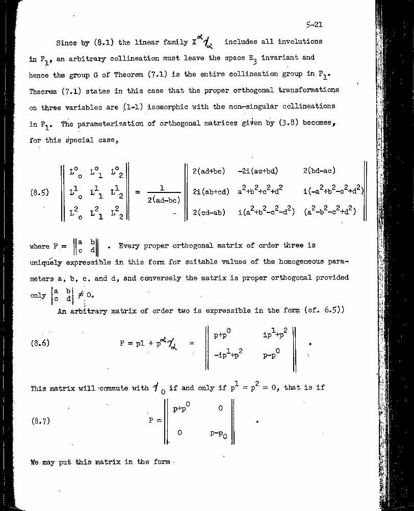
Since by (8.1) the linear family includes all involutions
in P^, an arbitraiy collineation must leave the space invariant and
hence the group G of Theorem (7.1) is the entire collineation group in P^.
Theorem (7.1) states in this case that the proper orthogonal transformations
on three variables are ,(l-l) isomorphic with the nonr-singular collineations
in P^. The parameterization of orthogonal matrices giten by (3.8) becomes,
for this Special case.
5-21
(8.5)
^0 ^0 _0L 0 L ^ L 2 2(ad-t-bc) -2i(ac-f-bd) 2(bd-ac)1 2i(ab-fcd) a^+b^-^c^-t•d^ i(-a^+b^-c^+d^)
2(cd-ab) i(a^-^b^-c^-d^) (a^-b^-c^+d^)
^0 ^1 ^22 2 2L 0 ^1 L 2
2(ad-bc)
where P = a b c d . Every proper orthogonal matrix of order three is
uniquely expressible in this form for suitable values of the homogeneous para-r
meters a, b, c, and d, and conversely the matrix is proper orthogonal provided
only a b c d ^ 0.An arbitrary matrix of order two is ejjpressible in the fortp (cf. 6.5))
(8.6) P = pi + p'^y,, 0 • 1^2p+p ip +p
j 1 2 0-ip +p p-p
J 12This matrix will -commute with 7 ^ if and only if p — p 0, that is if
(8.7) P =
0〇• 0
0 P-P〇
¥e may put this matrix in the form •
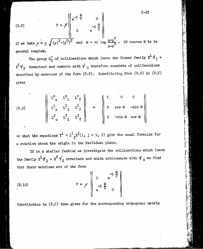
5-22
(8.8). 0e“^ ? 0
P = ^0
+ie
Q2
if we take ^ = + i(p)^-(p°)^ and © = +i log 2^ . 〇f course © is in/ - y p-p
general complex.The group Gq of collineations which leave the linear family Y-j_ +
X^V2 invariant and commute with Q therefore consists of collineations described by matrices of the form (8.8). Substituting from (8.8) in (8.5)
gives
oo Ho T ^^ 2 1 0 0
!?■o ro = 0 cos © -sin ©
l20
CMCM
0 +sin 0 cos ©
so that the. equations = L^.X^(i, 〇 = 1, 2) give the usual foiroulas for%)
a rotation about the origin in the Euclidean plane.If in a similar fashion we investigate the collineations which leave
the family ^'ll i + ^ '^2 invariant and which anticoramute with Y q we find
that their matrices are of the form
(8.10) P =0
+ie
©
0
Substitution in (8.5) then gives for the corresponding orthogonal matrix
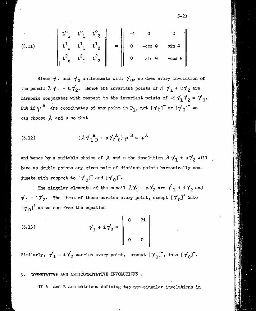
5-23
_ 0 ,0 ,0Jj ^ -1 00 1 2 -10 O'
(8.11) = 0 -cos Q sin 0
0 sin 0 +COS 0
Since y ^ and -j 2 anticoramute with "/q, so does every involution of
the pencil /VVi + M./2* Hence the invariant points of^ +
harmonic conjugates with respect to the invariant points of -i = ^0-
But if are coordinates of any point in not [yQ]"*" or ['/'〇]'" we can choose yl and p so that
(8.12) =
and ^ence by a suitable choice of A and p the involution A + ^-7^2 will have as double points any given pair of distinct points harmonically conjugate with respect to ['/'q]'*' and [7^0]".
The singular elements of the pencil are •/ ^ + i "/2y^ - iT*2* first of these carries every point, except [yQ]"*" into
[yQ]"*" as we see from the equation
(8.13) -/l + i /2 =0 2i
0 0
Similarly, Vi - carries every point, except [yQ]”, into [yQ]”.
9. COMMUTATIVE AND ANTIC'OMMUTATIVE INVOLUTIONS .
If A and B are matrices defining two non-singular involutions in
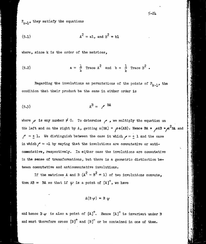
they satisfy the equations
(9.1) = al, and = bl
5-2li
where, since k is the order of the matrices,
(9.2) a = — Trace and b = i Trace .k k
Regarding ttie involutions as permutations of the points of the
condition that their product be the same in either order is
(9.3) aB^ ^ BA
where ^ is any number ^ 0. To determine ^ , we multiply the equation on
the left and on the right by A, getting a (BA) = ^a(AB). Hence BA ? ^AB BA and
^ = + 1. We distinguish between the case in which ^ = + 1 and the case
in which ^ = -1 by sa3Ting that the involutions are commutative or anti-V
commutative, respectively. In ei,ther case the involutions are commutative
in the sense of transformations, but there is a geometric distinction be-i'
tween commutative and anticommutative involutions.2 2If the matrices A and B (A = B = l) of two involutions commute,
then AB = BA so that if ^ is a point of [A]'*', we have
A(B If ) = B
and hence B tp is also a point of [A]"*". Hence [A]^ is invariant under B
and must therefore cross [B]'*’ and [B]~ or be contained in one of them.
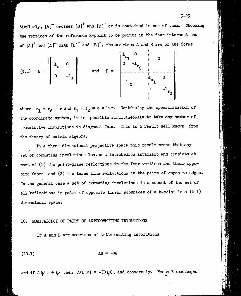
5-25Similarly, [A]“ crosses [B]"^ and [B]“ or is contained in one of them. Choosing
the vertices of the reference k—point to he points in the four intersections
of [A]"^ and [A]“ with [B]"^ and [B]“, the matrices A and B are of the forms
(9.U) A =0
-1.and B =
1 0 1^1 1 00 --1 1^2 1
Sl 0
0° -^s1 ®2t
idiere r^ + Tg = r and s^ + Sg = s = k-r. Continuing the specialization of
the coordinate system, it is possible simultaneously to take any number of
commutative involutions in diagonal form. This is a result well known from
the theory of matrix algebra.In a three-dimensional projective space this result means that any
y'set of commuting involutions leaves a tetrahedron invariant and consists at
most of (1) the point-plane reflections in the four vertices and their oppo
site faces, and (2) the three line reflections in the pairs of opposite edges.
In the general case a set of commuting involutions is a subset of the set of
all reflections in pairs of opposite linear subspaces of a k-point in a (k-l)-
diraensional space.
10. EQUIVALENCE OF PAIRS OF ANTICOMMUTING INVOLUTIONS
If A and B are matrices of anticoramuting involutions
(10.1) AB = -BA
and if A(p = + (^ then A(Bt^) = -(Bi^), and conversely. Hence B exchanges
the two pointwise invariant subspaces [A]’*’ and [A]"”. Similarly, A ex
changes [B]"'’ and [B]“. This is possible only if the dimensions of [A]"^
and [A]” as well as of [B]"^ and [B]“ are equal. Of course no two of these
four axes can intersect. From (9.U) we see that the difference between ttie dimensions of [A]"^ and [A]", (r-l)-(k-r-l), is equal to trace PAP"*^ = trace
A, so that if A and B satisfy (lO.l) we must have-sf-
(5.26)
These equations also follow by taking the trace of both members of the equations BAB“^ = -A and ABA~^ = -B. It was this method that we used to prove Trace -Q = 0 in ^ 6, but we now see the geometric interpretation of this result.
(10.2) Trace A = Trace B = 0.
If the matrices A and B are of order k, they define involutions in
a complex projective space of (k-l)-dimensions, Pj^ The pointwise in
variant spaces of A and B must be of equal dimensionality and .so are ( ^ -l)-spaces. This is possible only if k is even and consequently pairs
of anticommuting involutions exist only in projective spaces of an odd number of dimensions. ¥e shall speak of [A]”^ and [A]” as the axes of the
involution determined by A and as a natural extension of this usage weshall call any linear ( ^ -l)-dimensional sub-space of P,, ^ an axis. The
2 k—1 —"axes" of a space are then the self-dual linear sub-spaces of the space.
The two ordered pairs of axes [A]’*', [A]", and [B]’*', [B]“ con^jletely
determine (in a given coordinate system) the two matrices A and B in view2 2of the normalization A = B =1. However, because A and B anticommute it
is only necessary to give three of these spaces, the fourth, say [B]“, being determined as the transform of [B]'*' by the involution with axes [A]"**
and [A]“.
S-21
Putting k — 2kj^, [B] is a (k^-l)-space and so is determined as the
join of any k^ of its points which do not lie in the same (k^-2)-space.
Through each of the points of such a set of k^ points there goes a unique line intersecting both [A]"^ and [A]". These k^ lines intersect [A]"^ and
[A] in two sets of k^ points which are 2kj^ = k linearly independent points»
¥e are now in a position to observe that any pair of anticommuting matrices,
say A and B, are equivalent under collineation to any other pair, say A^ and
B^. For, since ary k linearly independent points may be carried into any other similar set, we may transform [A]'*' and [A]“ into the axes [A^]"*" and
[A^]“ and indeed may carry any set of k^ independent lines intersecting[A] '*’, [A]" and №]■*■ into any similar set Intersecting [A^]“ and
[B^]"^. Then a suitable collineation on each of these k^ lines will carry
[B] into [B] and yet leave [A] = [A^]*^ and [A] = [A^] invariant.
Thus we have the theorems
Theorem (lO.l). If A, B, A^ and B^ are matrices of order k = 2k^
satisfying the conditions
= B^ = 1, AB = -BA,
and
=1, A^B^ = -B^A^
then there exists a non-singular collineation represented by the matrix P
PAP“^ = A^ and PBP“^ = B^
such that
5-28
11. THE REGTJLl DETEEtHlNED BY TWO ANTI.GOMMOTING INVOLUTIONS
A line which intersects ary three of the four axes of A and B will also intersect the fourth. For example, if the line intersects [A]"^, [A]”,
and it is invariant under A and the transform under A of its inter
section with [B]"^ is a point of [B]“ which also lies on the line. By
analogy with the usual definition of a regulus in 3-space, we shall call
the system of lines which intersect three non-interseciting axes a regulus
of lines or, briefly, a line-regulus.
The lines of a line regulus may also be defined as the lines in
variant under each of two anticommuting involutions. This suggests the
desirability of considering the set of all linear sub-spaces of which
are invariant under A and B. This set contains no points since we have
already seen that the axes of A cannot intersect the axes of B. Hence no
two lines of the line-regulus can intersect.
No space of an even number of dimensions can be invariant under
both A and B for if there were such a space, A and B would induce in it
two anticommuting involutions which we know cannot exist. Furthermore,
any space pointwlse invariant under one of the involutions A or B, is not
invariant \mder the other.
Any linear space S, of p-1 dimensions, which is invariant under A2and B is also invariant under the product K = -iAB. Moreover K =1 and
K anticommutes with A and with B. Consequently S intersects [K]”^ and [K]
in the axes of an involution in S. Hence the intersection of S and [K]’*' is
a space, S*'', of ^ - 1 dimensions. Since is transformed into S , the
intersection of S and [K]~, by the matrix A (or B), S is determined by S’**.
Moreover if is an arbitrary subspace of [K]’*' then its join with its
transform vuider A (or B) Is invariant under both A and B.
5-29
The join of two invariant spaces S and T will again be an invariant space and will intersect [K]"*" in the join of and T^. A similar remark
holds for the intersection of two invariant spaces and therefore the linear
spaces invariant -under both A and B are in (l-l) correspondence with the
linear subspaces of This correspondence is such that a point of [K]'*’
corresponds to the line of the line-regulus which intersects itj a line of [K]”^ corresponds to a three-space con-baining the lines of the line regulus
which intersect itj and so on.
In 3-dimensional projective space the regulus conjugate to a line-
regulus is again a line-regulus, but in (k > U) this is not the case.
Indeed, in -fche conjugate regulus by definition consists of the set of
axes each of which intersects all the lines of the line-regulus. ‘ We may
call this conjugate regulus an axis-regulus.
The lines of a line regulus could have been defined as the system
of lines invariant under both A and B. The axes of the conjugate regulus
may be defined as the axes of the pencil of involutions.
'(11.1) 1= ;^A-+ pB (A 3nd n not both zero)^
The axes of I belong to the axis-regulus, for if is a point on any line
of the line regulus, -then I<p = AAtf+pBi/^ is a point of the same line,
which is therefore invariant under I. To show that every axis of the
regulus is an axis of I for suitable values of A and p may be accomplished by observing -that the problem reduces to the consideration of any one
(necessarily typical) line of -the line regulus and referring to the dis-r-
cussion of / 8.
The singular elements of the pencil, namely.
(11.2) = A + iB, and Kg = A - iB
5-30
transform every point not on [K]**" or [K]~, respectively, into a point of an
axis of K. Thus if 51^ 0 we have
= (KA + iKB)t|^ = (iB + A)
and consequently yj ^ ±s a. point of [K]"*", and it is indeed any such point.
Similarly Kg carries an arbitrary point, not on [K]“, into a point of [K]'*.¥e may regard [K]'*’ and [K]“ as the coincident axes of K^ and Kg, respectively.
12. The geometric discussion of the two preceding paragraphs may easily
be paralleled by an algebraic one. Thus the matrix K = -iAB may be taken
in the form
(12.1)
by performing a collineation which carries [K]^ and [K] into the axes
k,+l k,+2 = ij}^ = 0 and
respectively, where k^ = k/2.
Since B anticoramutes with K and has its square equal to one, a
simple calculation shows it to be of the form
(12.2) B =
' 0 B-,
0
5-31The collineation with matrix P =
-1% 0
0 1will therefore transform B into
(12.3) PBP“^0
1
0
and leave K invariant. After this collineation is performed the matrix A =
iKB will be
(12.U)0
We therefore have
Theorem (12.1). If A and B are matrices of anticommuting involutions
2 2and A = B =1, then there exists- a non-singular matrix P such that
(12.5) PAP~^ =
•Ho
and PBP-^ =0
0•H1 0
Hence the normalized matrices of two anticommuting involutions may simul
taneously be taken in the given canonical forms.
If we determine idiat conditions the equations
PAP"^ = A and PBP“^ = B
in?)〇se on P idien A and B are in their canonical forms (12.5), we find that
5^32
(12.6) p =
0 P.1
where P^ is an arbitrary non-singular matrix of order = k/2. A c〇- llineation which leaves both A and B Invariant therefore determines an
axis of the axis-regulus containing them and effects the same collineation
in each of these axes. The collineation in Pj^ ^ therefore determines and
is determined by the collineation which it induces in the Pij/2-l consisting
of the linear sub-spaces invariant under both A and B.
A matrix H will anticomraute with A and B if and only if the pro
duct r K commutes with both A and B. For,
arbitraiy collineation on [K] and the same collineation on [K] . Sines it leaves [A]^, [A]”, [B]"*" and [B]” invariant, it leaves invariant every
(12.7) (r K)A = A( r K) implies T A = -A T , ,
and conversely. A similar statement of course holds for B. Hence Z’ must
be of the form
(12.8) r = (/^K)K =0
1.
Performing a collineation of the form (12.6) gives
0
0
(12.9)
5-33and so has the effect of an arbitrary collineation, with matrix on the
matrix /^2®
The matrices anticomimiting with A and B are of the form (12.8) andr* 2 2r = 1 is equivalent to (f*^) = 1, Two matrices, H and A. of the form* (12.8) with r ^ = 1 will be similar under collineations of the form
(12.6) if and only if (cf. ^7, Chapter IV)
(12.10) Trace ^ — Trace ,
that is to say, if the corresponding axes of H and A intersect [K]”*" in
spaces of the same number of dimensions. This condition is equivalent to
(12.11) Trace KA = Trace K A
on account of the fact that r and A anticommute with both A, and B and are therefore of the form (12.8).
13. PROOF OF THEOREMS (5.1) to (5.1i)
With the geometrical discussion of the preceding sections in mind,
we are in a position to prove the theorems of ^ 5»
Theorem (5.1) has been proved for k = 2^(J^ odd) when X = 0, for
we have seen that two anticommuting involutions cannot exist when P, ^ is of even dimensionality. . Of course a single matrix of order k satisfying ^ ^ = 1
can always be found? it is 1, -1 or thè matrix of an involution. We may
therefore prove the theorem by induction on V , taking JZ. fixed. But any
y-set of W (> 2) matrices of order k gives rise to a y -set of N-2 matrices
of order k^ = k/2 by taking two matrices of the first set in the canonical
^-3k-
forms (12.$) so that the remaining matrices are of the form (12.8). Then the maximum number of matrices of order k = 2^Ji in a //-set is two greater than the maximum number in a set of matrices of order k^ = 2^^ But
for every odd , this latter maximum is 2(t^-1) + 1 by the induction
hypothesis. Hence there are 2(-x^-l) + 1 + 2 = 2'i) +1 matrices in a maximal ^-set of order k = 2 , which proves the theorem.
Theorem (5«2) states the similarity of any two even -/ -sets con
taining the same number of matrices and this was proved in the lowest case
(for two matrices) in Theorem (12.1). We may therefore use induction on
the number of matrices, the induction going by steps of two matrices and
the assumption being that the theorem is true for 2p matrices of any order.
But if7)j|^ (i = l, 2,..,, 2p+2) is a ^-set of 2p+2 matrices it is similar,
by^e results off 12, to the set
(13.1)
H C_l. O
(j ~ 2,...,2p),
•Ho
s
o H
° - \i
By the hypothesis of the induction, the set 7]^^ is similar to any other
set of the same number of matrices. Since any ^ -set of 2p+2 matrices is
similar to the set given by equations (13.l), any two y-sets of 2p+2 matrices
are similar.
Theorem (5»3) was proved inf?. Chapter (IV) for a y —set consisting
of one matrix. We again use induction on the number of matrices in the set, supposing the theorem true for y-sets of 2p-l matrices of any order
and proving it for 2p+l matrices. As before, we take two matrices, say
Tl2p^l ^2p the^-pet {ck= 0, 1, ,.., 2p) to be in the canonical foiTO of (12,5), and then the remaining ones will be of. the form
5-35
(13.2)-^1/3 °
V(~ 〇., I,,»,, 2p“2),
Similarly, we may reduce the matrices of another Y-set, say , to be of
the same foim. Using the matrices (12.5) for >1 « - and 7) „ it is clear¿p—J. ‘ 2p
that the equation
(13.3) Trace (^2*** ^2p^ - 2i Trace (^l(2p-2)^
holds for the set and a similar equation for T» • By the hypothesis
of Theorem (5.3),
(13.U) Trace (Yjg>/j^...7l2p) =< io fl"•i’ap'
This, however, implies the hypothesis of the theorem for the '/-sets 7? 1/^^ ~ ^»***> 2p-2) which are therefore similar by the hypothesis
of the induction.
To prove Theorem (5,U) we make use of Theorem (5,2) to establish the existence of a matrix P such that
(13.5) P7?^P"^ (i = 1, 2,..,2V)
Then PT^qP”*^ and both anticoramute with all the matrices ,
Hence
^V^ = iV〇(13.6)9
^-36
where the sign agree? with that in the equation
(13.7) Trace (7? pT^r •• >?jy ) ' : p^''V ... Ygy
6-1
Chapter VI
THE EXTENSION TO CORRELATIONS
1. THE DUAL MAPPING OF E2^^^ ONTO ITSELFIn the last chapter we regarded the matrices X = X°y^ + X + ...+X /
of the linear family x“y^ as defining point ^ point transformations of a complex
projective space means of the equation(1.1) I if'^11 =X|K®II , or .
If the matrix X is non-singular, the collineation (l.l) may be described equally
well as a hyperplane —> hyperplane transformation by the equations
(1.2) llfill -iXll^gll,
where
"^The operation of taking the transposed inverse is one which maps the set
of all non-singular matrices upon itself〇 It is well known that this mapping does
not extend in a (1-1) and continuous way to the singular matrices» However, by a
suitable choice of the factor , the mapping
(l〇3) px
of the non-singular matrices of the (2V+1)-parameter set X may be extended to
include the singular matrices of the set. Indeed, since X =2 (Trace X )1,
(l„ii) X = 2"^ (Trace X^)"V ,
and consequently the mapping (1.3) may be written in the form X—>|?2 (Trace X )X 〇
Choosing p to be a 2”^ Trace X^, where u is independent of X, the mapping becomes
linear and is extended to the singular matrices of the family in the obvious way.We shall find it conveirlent to take = (-lt^''^^2 Trace X and we
accordingly associate with a point x“ of E2^^3_ the hyperplane —> hyperplane trans
formation
6-2
(1.5)
as well as the point
i<p^M = (-1)'^'"^ x'iih^bII
> point transformation (1,1). When X is a singular matrix
of the linear family * (^*^) transforms the points of a hyperplane intopoints of a linear space of at most 2^“^-l dimensions and so the point —^ point
transformation does not induce a hyperplane----> hyperplane transformation in the
same way that a non-singular transformation does. However, both (l.l) and (1,5)
determine a permutation of the axes (i.e,, the subspaces of 2 -1 dimensions) of
^ and by choosing a coordinate system in which (cf. (11,2) and (12.5) of
Chapter V)
(1.6) X = 2il〇J^-l
it is easily shown that these two permutations are identical. It is in this sense
that we shall speak of (l.l) and (1,5) as defining the same (singular) involution.
REPRESENTATION OF IMmOPER ORTHOGONAL TRANSFORMATIONSB ^A correlation ^ defined by the equations
(2.1) = «ab4^"
transforms the point—appoint collineation (1,1) into the hyperplane—> hyperplane
or9l\ \ = (QXQ"bl|H;^ll
collineation
where Q = ] |Q^g| | and | |Q^^| ] = .
If the correlation is to transform every involution of the linear family into an involution belonging to the family, the matrix Q(xf^ )Q ^ must define a
collineation of the set (1,5) with matrix (-1)^'^^('X^ ) so that
(2.3)
6-3
for all values of , Hence the correlation (2.1) induces in the linear
transformation(2.UX ^
by means of the equations, „-1 / , y+1 ’ T®
(2.5) %'i P •
Solving these last equatiaas for l“^ we obtain
(2.6)( =1 '^ Trace ( ^ °^ Q“^)
Instead of using the point----^ hyperplane equations (2.1) of a cor
relation, we might have employed hyperplane —> point equations
(2,7)where ]1e^^|1 = 1
.A*
The family of transformations (1.5) woqld then be
carried into the family (l.l) by the equations^[(-1)*'*’-x'1r' -Y
or
consequently, y“ - and (-1)'^*'^ k' = . When Q - R these equations
are equivalent to (2〇l4,) and (2.5)»
Combining the correlations (2.1) and (2,?) we get the collineation
j j^A.| I p1 1, where P = RQ. The corresponding transformation in ^2\>+l
(2.9) t“ - (m“^ )X
where
(2.10) ^ ^Comparing these equations with equations (7.1) 〇f Chapter V, we see that Hi* ■
is the proper orthogonal matrix corresponding to the collineation jj^ U = P|1H^ I
under the isomorphism of Theorem (7〇l)i Chapter V,
The improper orthogonal matrices of order 2 v* + 1 are all obtained if we
multiply the proper orthogonal matrices by a single Improper one. Similarly, all
txi *<
,
6-i;
correlations which transform into itself are obtained by multiplying the
collineations leaving E2v>+1 ^ single correlation with this property.
We shall therefore extend the isomorphism of Theorem (7〇l)s Chapter V, to a
representation of improper orthogonal matrices by means of correlations in the
spin space if we show that a single correlation corresponds under (2.5) to an
■imprnpp.r orthogonal matrix. In a coordinate system in which the matrices ^
take the forms given in (Ji.ii), Chapter V, we have(2.11) Ya = summed».) ,
and consequently in this coordinate system the correlation described by the unit
matrix corresponds under (2.5) to the linear transformation
(2.12) T° . .... (-ij
The right members of these equations contain (V+1) minus signs if iJ is even and
minus signs if v' is odd. Hence the orthogonal transformation induced in
®2V+1 "unit" correlation is always improper. This result of course depends
upon our having chosen the numerical factor in (2,5) in the way that we did.
Our results on the spinor representation of the orthogonal group ard
summarized in the theoremTheorem (2,1), The group rotations about the origin in
is (l-l) isomorphic with the group ^ of all the collineations and correlations of
the spin space P2y transform the linear family of Involutions defined by the
matrices into itself. In this isomorphism the collineation with matrix0 a
P = 11^3! I “ corresponds to the proper orthogonal matrix determined by
the equations
B .aB"/5 C D Kt D^ /3
|I<M = -I.(2.13) or
6-5
and the correlation with matrix E = || = i1 corresponds to the
improper orthogonal matrix determined by the equations
™ n B „DC _ / , vi/+l D
|l.“p I = -1 .
¥e shall refer to the isomorphism of this theorem as the isomorphism
(or representation) If only the correspondence between proper rotations
and collineations in the spin space is in question, we shall speak of the isomor
phism 2!^ 2141*
3. THE INVARIANT POLARITT
"The improper rotation
(3.1) y“ = -x“
is of period two and is commutative with all rotations〇 Hence its image in the
spin space under is a correlation
(3.2) llfjl = or =
which is of period two and commutes with all the collineations and correlations of the group 5 . ,
In order for (3.2) to be of period two we must have G = eC, where
e « ±1. To determine e we observe that (3.1) is the product of (2〇12) and a
proper rotation. In the coordinate system of (U.U), Chapter V, this proper rota
tion is the image under ^2^^^ collineation with matrix V2v' 1‘
Hence in this coordinate system
(3.3) ^ ^AB “f^AcYl 0/3 E y2V-1'® •
Using (2.11) we find
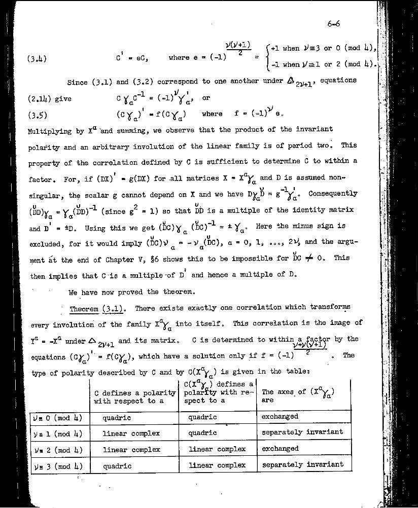
6-6
(3.U) c eG, 2where e = (-1)+1 when or 0 (mod 1a),
•=1 when)y = l or 2 (mod U).i,
Since (3,1) and (3,2) correspond to one another under equations
(2,11;) give °(3.5) f = (=l)^e,
Multipljring by x“ 'and summing, we observe that the product of the invariant
polarity and an arbitrary involution of the linear family is of period two. This
property of the correlation defined by C is sufficient to determine C to within a
factor. For, if (DX)’ = g(DX) for all matrices X = x“^^ and D is assumed non-
singular, the scalar g cannot depend on X and we have - g y^. Consequently
(DD)y = ^^(00)“^ (since g^ = 1) so that DD is a multiple of the identity matrix
and d' = tD. Using this we get (D〇Y^ (Sw)“^ = tHere the minus sign is
excluded, for it would imply (DC)V = “V (DC), a = 0, 1, ,〇〇, 2v>^, and the argu-oc cc U Jment at the end of Chapter V, §6 shows this to be impossible for DC 〇, This
then implies that C is a multiple-of d’ and hence a multiple of D.
We have now proved the theorem.
Theorem (3,1). There exists exactly one correlation which transforms
every involution of the family x“y^ into itself. This correlation is the image of
T® = -x“ under A and its matrix, C is determined to within^a^^^cti^r by the
equations (〇^)' = which have a solution only if f = (-1) .The
type of polarity described by C and by C(x“y^) is given in the tables
G defines a polarity with respect to a
C(x“y ) defines a polarity with respect to a
The axes of (^^y^) are
il* 0 (mod i;) quadric quadric exchanged
1 (mod U) linear coitplex quadric separately invariant
y® 2 (mod li) linear complex linear complex exchanged
V*5 3 (mod li) quadric linear complex separately invariant
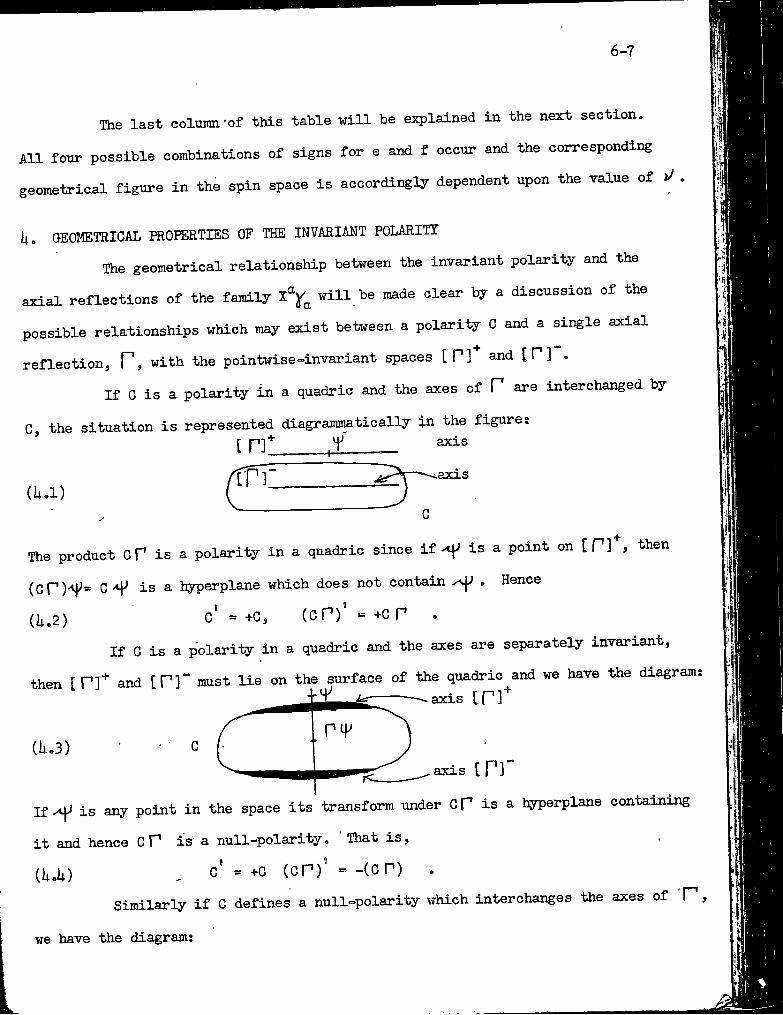
6-7
The last column-of this table will be explained in the next section.
All four possible combinations of signs for e and f occur and the corresponding
geomatriaal figure in the spin space is accordingly dependent upon the value of >>
ii. GEOMETRICAL PROPERTIES OF THE INVARIANT POLARITY
The geometrical relationship between the invariant polarity and the
axial reflections of the family will be made clear by a discussion of the
possible relationships which may exist between a polarity C and a single axial
reflection, P, with the pointwise-invariant spaces and {T] .
If C is a polarity in a quadric and the axes of P are interchanged by
C. the situation is represented diagramsmtically in the figures* .1. .. I •cn''
(U.i)fT]l_
axis
.axis
The product CT is a polarity in a quadric since if ^ is a point on [P] , then
(cP)''f'= Cis a hyperplane which does not contain ^ . Hence
(1;.2) o' = +C, (CP)’=+GP .
If G is a polarity in a quadric and the axes are separately invariant,
then [P]'*' and IP]“ must lie on the surface of the quadric and we have the diagram;+ 4^ ----------^axis in'"
ih.3). axis [ P]
is any point in the space its transform under Cp is a hyperplane containing
it and hence C P is' a null-polarity, That is,, g' = +G (CP)’ = -(CP) .
Similarly if G defines a null-polarity which interchanges the axes of P ,
we have the diagrams
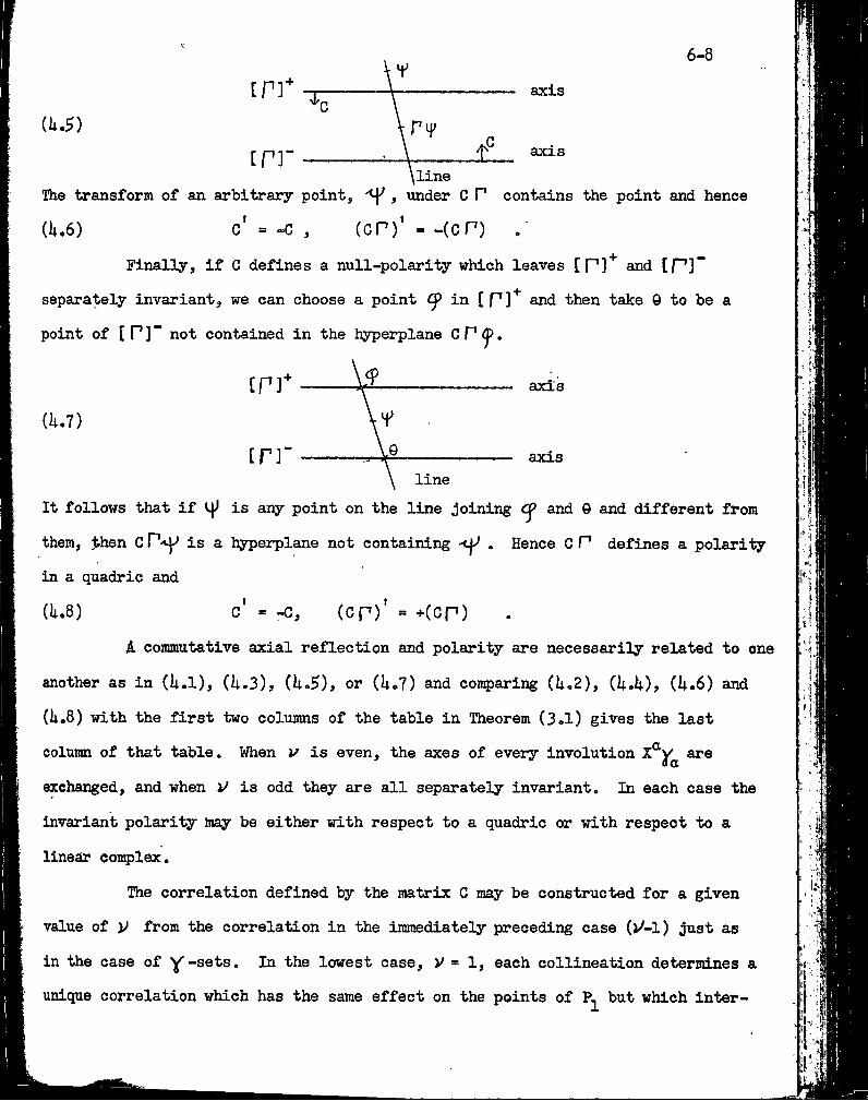
y6-8
iP]* ----------- 1-------------------- axis(h.$) ° \rц>
[pr_________\line
The transform of an arbitrary point, <Y , under C P contains the point and hence
(U.6) o' =-c , (cr)’*=-(cn)Finally, if C defines a null-polarity which leaves [P]^ and [P]~
separately invariant, we can choose a point Cp in [P]^ and then take 0 to be a
point of [r]~ not contained in the hyperplane C P p.
(h.7)
It follows that if
them, Jthen C is a
in a quadric and
is any point on the line joining Cj> and 9 and different from
hyperplane not containing . Hence C P defines a polarity
(1;.8) o' - -c, (cp)' = +(cp)
A commutative axial reflection and polarity are necessarily related to one
another as in (U.l), (h,3), (U.5), or (i;〇7) and con?)aring (ii.2), (U.!;), (Ji.6) and
(li,8) with the first two columns of the table in Theorem (3.1) gives the last
coltimn of that table. When is even, the axes of every involution are
exchanged, and when y is odd they are all separately invariant. In each case the
invariant polarity may be either with respect to a quadric or with respect to a
linear coi^lex.
The correlation defined by the matrix C may be constructed for a given
value of from the correlation in the immediately preceding case (v'-l) just as
in the case of lowest case, V = 1, each collineation determines a
unique correlation which has the same effect on the points of but which inter-
changes the empty set and the whole line» The matrix j l^gl I serves as C in this
case and transforms the coordinates of a point into coordinates ^ of the
same point regarded as a hyperplane.
The polarity induces on the axis regulus containing the axes of ^ 2)^—1
and ^2v> ^ collineation which either leaves four axes separately invariant or
exchanges them by pairs. In either event V^2W^ " ^ ^are separately invariant. To construct we first define ^ on the lines of
the line regulus,. The transform of a line of the regulus is then a '^2'^which
intersects every axis of the axis regulus in a P2V—1 „2'
When V is odd, leaves every axis of the axis regulus invariant, and
when v» is even it induces on the axis regulus an involution with double elements
and S”. If <p is any point on a line, , of the line regulus, it is determined
as the intersection of this line with an axis, A. W® therefore define the hyperplane
C^^^^'to be the join*of and This extends the definition of to
all the lines which contain two points lying on lines of the line regulus, Every
point of Ppv» , is either the intersection of two such lines or lies on a line of
the line regulus, and in either event its transform under C has been defined,
^5. THE (1-2) MATRIX REffiESENTATION OF
Since the iitqjroper rotation commutes with all rotations in ^2^+1^
the correlation commutes with all the collineations and correlations of
the group, «^, isomorphic to the rotation group ^2'i}+\.° ^ matrix of
a collineation belonging to , GP = or PGP = J>G, and the matrix of the collinea
tion may be normalized to within sign by the equation
(5.1) ' P GP = G ,
Similarly the matrix of a correlation may be normalized to within sign by
the equation
6-10
4
(5.2) = C.
It may be observed that the normalization (5^.1) is unchanged if the matrix C is
multiplied by a scalar factor while the normalization (5.2) is relative to a
particular choice of the matrix G. One may readily verify that the normalized
pairs of matrices form a group provided we multiply correlations by collineations
in the appropriate w- Hence we have the first part of the theorem..Theorem (5,1). If the collineations and correlations of S are described
by matrices normalized by (5.1) &i)d (5.2) respectively, then the collineation iso
morphism A becomes a (1-2) matrix representation of the rotation group on
2^+1 variables by means of matrices of order 2^. This representation cannot be
sharpen to a (1-1) represexifiation.
If it were possible to select one out of eveiy pair of matrices
satisfj^ng (5.1) in such a way that the resulting matrices formed a group, then it
would be necessary to include matrices corresponding to the proper rotations
x°, -p- » -x\ = -:J^, ..., = -X^^0 a .a -2
and
+X-", ■x*-, ..., ^ « -X^^(5.3) r(5.1i) = »X°, ^
In the coordinate system of (k.li), Chapter V, these rotations correspond to matrices
which are multiples of and and these matrices anticomraute while (5.3) and
(5J;) commute. Hence the assumed selection of matrices would fail to determine a
single matrix corresponding to the product of (5.3) and (5.U). follows that the
matrix representation of sssentially double valued and cannot be sharpened
to a (1-i) representation.
6. LINEAR FAMILIES OF CORRELATIONS
If the matrices form a y-set, then the matrices
(6.1)|CoARl , ...ll^AcVo
and 11C
"2)/AB* I JS.c^v B‘
’2)/+l AB‘ - il G’AB‘
define 2V+2 correlations which form a linear family. That is to say, if we define
<6.2) (cr = D, 1, ..., 2^'+l)
6-11
then
(6〇3)
and consequently the equations(6.1.) “<* f ^
define the same correlation»
In general, we shall say that two sets of p+1 matrices of order k,
and Bjj.Co’ = Oj 1> 〇〇〇) p)> define a linear family of correlations if Цсрд1| = (X^C^) j I and |1<^^|| = I I'^gl I define the same correlation,
that is, if(6.5) (X'^G^XX'^D^) = |)1
Taking the trace of this equation, we have p =y^^X°X*^ where
Y = ^ Trace (C d' + Cj'), ¥e shall consider only those linear families of
correlations for which I IY 〇• x I^ non-singular.
The problem of determining all linear families of correlations is on
account of (6,5) identical with the problem of factoring a quadratic form into two
linear factors which may not be identical. If we choose a coordinate system in which p = Z(X^)^ equating coefficients in (6.5) gives and consequently the
matrices satisfy the equation
(6.6) (X^C )(X'^G^“^) = 2 (X^)^ 1 .cr=o
Conversely, any such set of matrices defines a linear family of correlations. We
shall say that an ordered set of matrices G^, G^, -">'>> satisfying (6.6) is
a C-set. Ay-set is also a G=set but we regard the matrices of a G=set as having
two covariant indices while the matrices of a y-set have one contravariant and one
covariant index.Multipl3ring equations (6.6) on the left by iG”^ and on the right by -iG ,
P P
6-12
the resulting equatiohs are equivalent to2 „/„0x2
(6.7)
where
(6.8)
Hence we have the theorem
(X“S f = 2(X“) 1 a
a — 0^ Ij oo.j P^lj
S - iC C p a
Theorem (6.1). If S^(a = 0, 1, P-D is a ^-set of p matrices and
C- is an arbitrary non-singular matrix, then P'
G = -iC S’ , G a pap(6.9)
is a C-set of p+1 matrices. Conversely, if is a C-set of p+1 matrices, then
S = ic“^C is a y-set of p matrices, a p a ®
This theorem enables us to use the properties of y-sets to prove a
number of theorems on C-sets. We omit the proofs where they can easily be supplied.
Theorem (6.2). The maximum number of matrices in a C-set of matrices ofX- —— ———
order 2^i(i odd) is 29+2 and this maximum is attained.
Theorem (6.3). If C^ is a C-set, so is AG^B, where A and B are any non-
singular matrices.f u =1Theorem (6.U). If C^ is a C-set, so are C^, C^, and C^ .
VTheorem (6.^). If C^ is a C-set of 29+2 matrices of order 2 and
VA' ^2°A>
(6.1〇) A2 “ J* A^ and 1-2 -fB„ = ■?■ B^.
Theorem (6.6). If C and D are C-sets of 29+2 matrices of order 2 ,. I, ■ . cr O’
there exist "two non-singular matrices A and B such that either
(6.11)or
AC B = D^, o o*
(6.12) AC B a
and AC2^^iB - D2^^^,—(flt — 0, 1, ..., 29),
according as the trace of (CqCi^G2 °°° ^29^29+1^0 o o
6-13
(D d”^ negative, respectively. If (6〇ll) holds, there does not
exist a pair of matrices satisfying (6〇12) and if (6.12) holds there does not exist
a pair of matrices satisfying (6〇11)〇
This theorem implies that every G-set in ?2*^~1 obtained from (6.1) by
a transformation of the type (6.11) or by such a transformation combined with a
change in the sign of one matrix. When 0 (mod it) all the matrices (6.1) are
symmetric, and when h 2 (mod Ii) they are all skew—symmetric. Hence when is
even there exists a maximal linear family of correlations all of which aré of period
two. Such a set of transformations will be called a linear family of polarities.
Using the fact that the equations (Cy'jj) = determine C to within a factor,' it
is not difficult to prove the theorem
Theorem (6.7). A (2i^+2)-parameter linear family of polarities ex;ists in
if and only if V' is even.
7. THE REPRESENTATION OF ^2')>+2 CObLINEATIONS IN Pgi^^^
Theorem (7.1), If is a G-set and | 1L°t:1 1 is orthogonal matrix,
then G if is also a C-set and if ¡L^Lj = +1, there exists a pair of matrices A a ~c ^
and B such that(7.1) ag^ = g^l\ ,
These equations may be regarded as establishing a correspondence .a Ir . / . 1(7.2) ||l\||^ C^A, i B) .
between proper orthogonal matrices and pairs of matrices A and B which, by Theorem1(6.3) are determined to within the scalar factors p and , respectively. It is
evident that if | [ corresponds to (p A^, y bben corresponds
to (pAA^, i B^B) and hence the correspondence
(7.3) • j|L\il-^pA
is a representation of the orthogonal group ^2i/+2 collineations in P2^=l“
6-iU
Except for the order of multiplication the correspondence 1 | ^ B is a
representation of equations (7.1) also determine a represen
tation(7.ii) IlLxll
where P = BTheorem (7.2). If C is a C-set of 21/+2 > h matrices of order 2 and
(7.5) G B = CL °-〇 a X' ' 〇 C,tor some matrix | iL ^| |, then B ■ bl and = b£j . Simllarty, If AC^ = fl^I.
then A = al and LA C-set of 2>^+2 = U matrices of order 2 is a basis for all matrices of
order 2 and hence if B is any matrijc there will exist coefficients satisfying
(7.5). The theorem may be proved by multiplying (7.5) on the left by ±〇2i^+l
using the linear independence of the matrices Is = ^^2y+l°a*S S (a < 6 and a,fi = 〇, 1, 2V), This linear independence was proved in §6,
a p ' 'Chapter V, and of course depends upon the hypothesis that 2>/+2 > U, 〇r V > 1.
Theorem (7.3). When >^> 1, the correspondences (7.3) and (7〇k) esta
blished by equations (7.1) are (2-1) representations of the proper orthogonal
group in P2v^„3_. When )^ = 1 the representations are (l - 〇〇 )
We have already observed that la proper orthogonal matrix determines A
and P = B“^ to within a common factor. To prove the converse we assume that
AC^B = and-AC^B^ = a. Then C^(BB^^) = where and
by Theorem (7.2), BB^^ = bl and = b <S so that L% = and b may equal +1
or -1 since the order is even (i.e.,,-12^+2 orthogonal). When >/» 1, agiven matrix A will occur in (7.1) associated with oo^ matrices B, thus with oo
collineations.If V» is even, the matrices (6.1) are either all symmetric or all skew-
symmetric. Hence, if C is this set of matrices, taking the transpose of (7.1)
6-15
gives(7.6) AO^B - b'o^a'
aM by Theorem (6.5), A - b’ . (- ^ P) By making a suitable relative normalization
of A and B so that A = b’, we obtain the theorem
Theorem If v* is even, there exists a C=set of 2l42 matrices of
Vorder 2 such that
(7.7) CcT “
For such a set the ecjuations(7.8) rc/"’- -
establish a (2-1) matrix isomorphism
(7.9) “P <r-> I I
between normalized matrices of collineations in which leave the linear
family X*^C invariant and the proper orthogonal matrices of order 2i/+2 ) „
For = 2 the matrices G of this theorem are a set of six skew-
symmetric matrices which form a basis for all four-rowed skew-symmetric matrices.
Such a set of matrices has been used as a starting point for a discussion of the
HLuecker-Klein correspondence* and the geometry underlying the representation
» "Geometry of Four-Component Spinors", by 0. Veblen, Rroc. Nat. Acad. Sci.,19 (1933), PP〇 5〇3“5l7.
(7.9) may be regarded as a generalization of the Pluecker-Klein correspondence.
Theorem (7.5). isomorphism of Theorem (7.^) niay be extended to
include the representation of improper orthogonal matrices by means of correlations
by'the equations
(7.10) « 〇.« - a
or by the equivalent equationsI 〇 -cQ C^Q = C^L ^(7.11) (i.e,^ %A%B “ *VAB^ °
Chapter VII
TENSOR COORDINATES OF LINEAR SPACES
7-1
INTRODUCTION1. Homogeneous coordinates of linear subspaces of a projective space
1 2were defined by Grassman and have been studied by Severi, Antonelli, and others.
^ Annali di Matemática, 2h (3)> 191^i PP* 89-120.
^ Annali della R. Scuola nórmale Sup. di Pisa, Bd. Ill, 1883, pp. 71-77*
These studies have not, however, employed the notation and methods of the tensor
calculus. In this chapter we define contravariant and covariant tensor coordinates
of the linear subspaces of a projective space and derive ab initio the quadratic
relations "Which they satisfy.These coordinates enable us to give elegant algebraic expression to the
geometric operation of perspection and section, where the center of perspectibn is
a linear space of any number of dimensions. Two expressions are found for the
coordinate tensor of the join and intersection of two spaces and in verifying the
equivalence of these two expressions we are led to a useful Identity.
In §5 we introduce a non-singular quadratic form into the geometry and
employ the matrix of this form to lower and raise tensor indices in the familiar
fashion. ¥e then derive some of the properties of the linear spaces which lie on
a quadric. In particular, we find the algebraic characterization of the two fam
ilies of rulings on a quadric in a complex projective space of 2i> -1 dimensions
and obtain the intersection properties of these rulings. Certain exceptional
, features of .the quadric in 3-space are noted which imply special properties of
the orthogonal group on four variables.
7-2
In §8, Chapter I, we gave a detailed discussidn of the linear subspaces
of a 3-dimensional space. That section may be read as an introduction to the
present chapter, but we do not need to make use of the special results there ob
tained.
2i DEFINITION OF THE GOOEIDINATE TENSORSAn (r-1)-dimensional linear subspace, V, of the real or complex projec
tive space determined by any r linearly independent points which it con-
X j fid .i .i A^ ii = 1, 2, ..., n) are coordinates of r suchtains. If A^, ky \ X, <1, ..«j y
points, then the tensor1 //...a:
i.]
r •ri
. ■' [dl ^2 ‘r= A^^A2^...a/
.here 13 the generalised Rroneeker delta,^ is said to he. a contra-®1®2* * *®r
3 TTnr the definition and properties of these symbols see I of theShSdge Saot no. i\i, "Invariants of Quadratic Differential Ferns", by
0. Veblen.
variant coordinate tensor of V. Thus the coordinate tensor of the line deter
mined by points A^ and is =i(A^B^ - B^A^), and the components of the
coordinate tensor of an (r-1)-dimensional space are proportional to the minors
of the matrix of r rows and n coltonns formed by the coordinates of r points of
In computations involving many indices we replace a set of indices such
asii ... i by a single underlined index i. The number of indices in a set iis din!ted by Ul, or liU in words, the length of i. Thus (2.1) becomes in this
7-3
notation
such as to denote sets of
ordinary indices, the underline not being extended under the subscript for
typographical reasons.If we define I iI = n, to be +1 if i is an even permutation of
(1, 2, ... n), “1 if it is an odd permutation, and 2sero otherwise, and define
to be a covariant tensor of weight -1, then the components of 6^ have the
same values in all coordinate systems. This numerically invariant tensor is
always present in our geometry and we employ it to define a covariant tensor
(2.2) 111, "2 -",sl
where \sl = \il “ r. ¥e shall also use symbols
e . . 1-
associated with V-. In this definition p is assumed to be a scalar (which may
depend on \il) of weight +1 so that and vi have the same weight, which we shall
take to be zero. For many purposes in projective geometry it would be sufficient
to take p = 1 in an arbitrarily chosen coordinate system. When we introduce the
matrix of a quadratic form we will determine the value of ^ (| il) so as to give
a convenient calculus.Observing that equations (2.3) amount to no more than a renumbering of
the components of vi, we may invert the equations to get
^(lil) Ijl’-Vj eii,
Where 6 - is numerically invariant contravariant tensor of weight +1 defined
by the equations 6^ » 6^. In (2.3) and (2.U) we have^given rules for lowering
and raising sets of skew-symmetric indices, the hook (u) being added or removed
7-U
by the operation. We also use (2.1i) to define in tei*ms of W^ and then (2〇-3)
gives W. in terms' of wi. So far we have no way of defining a tensor V. associated 2 0 ±
with vi.
The operations of raising and lowering sets of skew-s3nnmetric indices
give algebraic expression to the law of duality as applied to linear spaces.
Thus if we choose coordinates so that =* ^ ^ (a * 1, 2, ..., r) in (2.2),
will vanish unless j is a permutation of ((r+1), (r+2), n) and conse
quently is a multiple of S • • • S• Hence a set of r independent— ^ ^2 ^n-r^
points in ? determines vi to within a factor and a set of n-r linearly independentu '' . iplanes containing V determine V. to within a factor. Also, the coordinates X ofJ
a point in V satisfy the linear equations
y(2.5) X® = 0 ,
and the coordinates of a hyperplane containing V satisfy the equations
(2.6) V- ® Xg « 0 .
^1 ^2 ^r sMoreover, writing (2.5) in the form ^ s "^l ^^2 * * * ■^ ^ = 0, we see that
“ ~ i i ievery solution of (2.5) is linearly dependent on A^, A^, and A^. and so de
termines a point of V. A similar statement holds for (2.6). This completes the
proof of the theorem.
Theorem (2.1). A linear space determines its coordinate tensors to
within a factor and is uniquely determined by them.
3. THE QUADRATIC IDENTITIES
The coordinate tensors of a linear space are necessarily skew-symmetric
and non-vanishing. Not all such tensors, however, are expressible in the form
7-5
(2.1) and consequently a tensor » X^i^ 7^ 0 must satisfy additional conditions
in order to be a coordinate tensor. One form of these conditions is given in
the theorem.Theorem (3.1). A necessary and sufficient condition that vi = / 0
shall be the coordinate tensor of a linear space is that
rank II V— ^ II = I k s I ,
where the set of indices k numbers the rows of the matrix and the single index s numbers the columns. (Thus 11° H is rectangular with n'^' rows and n columns.)
We first prove the Lemma:
Lemma 1. If 1- = ^ 〇, then
rank 11V— ^ ll > I k s I .
If rank \\V- ®11 were less than, Ik s( “ r, equations (2.6) would have
more than n-r independent solutions. By a suitable choice of coordinate system
a linearly independent set of these solutions could be taken to beil> Sl> where t > n-r. Then ^ = V- ^ ^ ^ = 0
and since r indices i cannot be chosen different from one another and from all
the numbers (1, 2, 3, •••> t), we would conclude from the skew-symmetry of V-
that vi = 0, contrary to hypothesis.
The necessity of Theorem (3.1) now follows from Lemma 1 and the obser
vation that equations (2.6) have at least n-r independent solutions so that rank
ftV- < r. To prove the sufficiency of the condition we need only choose
coordinates so that a set of n-r linearly independent solutions of (2.6) arer ^^1 ^2 c
^r+1^ ^r+2^ and S then 1- will be a multiple of hi 6 2 *•* 〇 r *Theorem (3.2). If xi ® ^ = 0, where xi = X^S^ ^ \ ^
7-6
and the indices range from one to n, then
(1) \x\ + lyl < n, and
(2) if lx I + I yl ” n, then Y “ ^ ^ Y are coordinate tensors of the£ Z £
same linear space.
For each choice of the indices j the vector Y. _ belongs to the right
null-space of the matrix 11X- ®l| and consequently
(3.1) rank IIY. II < n- rank IIX— 3 ° ~
1 S|
But by Lemma 1,
(3.2) \xl < rank 11 xi ®I1 and |yl < rank IIY^
Combining these inequalities we have the first part of the theorem. Moreover, ifIxl + lyT = n, the equality signs must hold in (3*2) so that by Theorem (3*1) ^
[x^ X^is a coordinate tensor. Choosing coordinates so that = 〇2 ••• 〇
the hypothesis of the theorem implies that Y. 2 ~ ***
"ixi^ |xl ’
txl+1 ^lxl+2• • • 0 V
|X|uconsequently Y„ = U 6 r,,Z f^l ’^2 ■'(yl - ^ r^]
Theorem (3.3). A necessary and sufficient condition that V— = V — f 0
y. j is a multiple of X^.
shall be a coordinate tensor is that
(3.3) ^k s = 0 D s
The sufficdency of the condition follows from Theorem (3*2) by putting
■ vi and Y. * vV. The necessity follows from the observation that when V-jJ_ J
is expressible in the form (2.2), then for each set of values of the indices k
and 3) Y- ^ is a determinant in which two rows are equal.— s
Equations (3.3) obviously imply the vanishing of V- - ^ if £ contains more than one index. In Theorem (3.U) we shall prove that ^ ^ ® V
j r s
7-7
implies the apparently stronger condition (3〇3)» This will prove the theorem.Theorem (3.U)» A necesssiry and sufficient condition that V*- = V^—^ / 0
shall be a coordinate tensor is that
(3.U) ® = 0 . 0 r s
The quadratic relations satisfied by the components of a coordinate
tensor are usually given in the non-tensorial form
^ Bertini, «Einftlhrung in die Projektive Geometrie Mehrdimensionaler Rftume", page U3, formula (lii)*
(3.5) ^a^tv2cd^^ac^db^^ad^bc^Q^
where the set of indices m occurs twice but without being summed. These equations
are obtained by multiplying (3-3) by € i 2 ^ summing, and putting m a for k.
We shall here employ only the tensor form of the quadratic relations, (3*3) 〇r
(3.U).
U. JOINS AND INTERSECTIONSWe call the linear space of smallest dimensionality which contains two
linear spaces, X and T, the join of X and I and denote it by X + Y. Similarly,
we call the space of greatest dimensionality contained in both X and Y the inter
section (meet) of X and Y and denote it by XY. We write 0 and 1 for the null-
set and the entire space, respectively.
Theorem (U»D- If X, Y and J = X + Y are linear spaces with the
respective coordinate tensors S?, and jl, and XY =■ 0, then is proportional
to T>-' and to X,% y£. If XY / 0, - X;^y 5^ = 〇.X X ^ O' mmrn **
7-8
If X is the join of; the [x\ points A^, A^, •••, A.^. and Y is the join
"■'‘ui * ®1 * ®2 * ••• + B,of the \j\ points Bgj •••, ^jyj> "then J = A^ + A^ +
and XY = 0 implies that these \x\ + \y\ points are linearly independent. Consequently
X,... y, y„ yX, x«y = 6. A- A« i 1 jc y 1 2
‘Ixt ^1V V B 171171
is different from zero and is by definition a covariant coordinate tensor of J. Using the definition of xi and ^ ^ xi Y^ = (-1) ^ ^ Y^
so that is proportional to and to Y—. If XY 0, the points
\x(^ "V "2^i z
, B^y.j are linearly dependent so that = 〇
A similar proof gives the dual theorem.Theorem (ii.2). If X + Y = 1 and XY = I, then li is proportional to
- Y^ and to Y^ - X^. If X + Y / 1, then X^ - Y^ - X*^ = 0.r s ' r s
• * Theorem (i4.«3)« If X and Y are linear spaces with coordinate tensors
xi and Y—, respectively, then the ’’projection operator" pi. = Y^ — X."^ defines^ j. s,
a transformation
(U.i) cpi=pi^^l
with the following properties;
1. If is the coordinate tensor of a linear space vp such that X 1^ = 0 and
Y + X + If* = 1, then (p i (/ O) is a coordinate tensor of the linear space
Y(X + <f).
2. If either or both of the conditions X 4^ = 0 and Y + X + (^ = 1 fail to hold,then C|)i = 0. I
The theorem follows immediately by applying Theorem (It.l) to the spaces
X and Vj^and then Theorem (U»2) to the spaces Y and (X + y). Dualizing Theorem
(U.3) gives
1-9
Theorem (Ij.l;). is a coordinate tensor of \pJ + X unless
v|y+ Y / 1 or VpYX / 0, and then it is zero.
Theorem (U.^). If X? and Y^ are coordinate tensors of linear spaces
and we form the sequence of tensors
■< i| ? i-S_ s.(ll.2) Y± X“ ^ , T ^ ^ X>Y,1 ¿1^1 ¿2-2
Y^ X^ or Y^ X>- ,¿a ¿a^
where \s \ = r and a is the minimum of the two numbers n - 1 x I and [ yl , then the r
last non-vanishing tensor factors into the form
i(li.3)
Jir
and 1”^ and J. are coordinate tensors of I = XY and J = X + Y, respectively, ¿r
The spaces X and Y intersect in a space of dimensionality < |xl - 1
and < \yl - 1. Hence if 1- is a coordinate tensor of I = XY, we may put
\±\ = lyl - r where r > 0. ' Now applying Theorem (U.3)j the expression
ih.h)(J,ir . jii¿r w
¿r-r
is either zero or is the coordinate tensor of (^ = Y(X + ). In the latter case
(f includes XY and its dimension, li\-l=lyl-r-l, equals the dimensioni L
of XY. Hence (P =' XY and <p ~ *
It is now convenient to regard (ii.li) as a vector equation (p= Ei„s^
where M is the rectangular matrix 1|Y x)^ (I . Choosing as a basis for
the set of all vectors i|;- the vectors where \kl = and p is any
set of \kl numbers between one and n, the matrix M transforms every vector of
the basis either into the zero vector or into a multiple of I . Hence M is of
rank one and therefore factors into the product of two vectors. That is.
7-10
isy" xX = X j.
where is a coordinate tensor of XY. Applying Theorem (U.U) to this projection
operator proves that J. is a coordinate tensor of X + Y.
Summing off r + 1 indices of y2 against r + 1 indices of xV gives zero
since each component of this tensor is a sum of terms of the form where P
is a point of I = XY and Q is a hyperplane containing J = X + Y and a fortiori
containing P. It is obvious that if any one of the terms of (U.2) vanish, then
all following terms als.o vanish.
If we exchange X and Y in (U.2) we get the sequence
_i il®l ^ ¿2-2 Yy ¿2^2
(li.6)¿riX"^ or X^ Y^ g ,
whepe \s^l = r and a is the minimum of n - \ yl and lx\. It is to be observed that
the number of terms in the sequences (U.2) and (U«6) are, respectively, n - \xl + 1
and n - lyl + 1 if n < Ixl + I yl, and 1 yl + 1 and ixl + 1 if n > lx| + 1 y(.
Hence the sequences are in general of unequal length. For coordinate tensors
^ and Theorem implies a special case of the theorem-
Theorem (U.6). If X? and Y^ are any two skew-symmetric tensors, then
the last non-vanishing terms in (U.2) and (14.6) are proportional.
To prove this theorem without,restricting xi and Y^ to be coordinate
tensors we use the definition (2.3) and its. inverse (2.1i) to express Y^ and xi
in terms of ^ and X^, respectively. This gives
7-11
m
^ XV + x^ S ' ^[It ^“1 j.'V.
1 £ [j- ^2*‘*^lj(^-l
+ (additional terms in which more than Isl + 1 indices are summed),
with \s,l = \s\ + 1 where the integer Isl and scalars X, aM X2 (possibly
zero) depend on the lengths of the various indices. Consequently, if 1= -
A meaningless summand in (li-7) implies that its coefficient A is zero.
is the last non-vanishing term in (U.2), then X---- r last non-vanishing
terra in (U*6), and
(U.8) 1£
5. THE QUAimtIC FCfiM¥e now introduce into our geometry a fundamental quadratic form YX^X^
and use the symmetric matrix H to lower single tensor indices by the familiarrule, X. = T. .X^. Covariant indices are raised by the rule X^T “ X^, where
1fki r =
kj r . .If we lower each of the indices of a skew-symketric tensor X- by Y^.
.the resulting tensor is skew-symmetric and is denoted by X^. Applying the rule
(2.it) to raise the indices _j by means ofA 4 _X0 ii — gives the tensor X—.
Alternatively, we could first lower the indices of X~ by the rule (2.3) to get X^
and then raise them with The result of these two processes id the same to
within a factor. Indeed, computation with (2.3) and (2.U) shows that
7-12
(5,1) Y - -
where y—— = ~T ^ ^ y ^ Y ^ and Yis the determinant 1 Y^.
The scalar factor in the right member of (5»1) will be +1 if we put
(5.2)± liil(n-lil)
r^(-i)
This choice has the disadvantage that ^〇i\) is sometimes imaginary. This
cannot always be avoided without introducing additional complications into the
calculus for in the special case in which n =■ 2v^ and li\ =? V, (5.1) reduces
to
(5.3)Y- - = /〇2(v) Y’^ (-i)'^ xi
so that =< Y^^^ (-1)^^^. However, if is a real matrix of signature
(+-+-...+-), then y〇(V) is real (cf. Theorem (6.1)).
¥e now restate our rules for lowering and raising sets of skew-syinmetric
indices. They are:y. {Úl]!l e. . xi
\ill 1 iand
(5.1i)
where
(5.5)
¿ = M:Íͱ1X.
{^i} = (-1)¿1 il(n-\il)
In (5.U) if a hook (u) is added to the X in the right member it is erased from
the left member. We observe that k} = (k) if (il + Ul = n. The operations of
7-13
calculus are summarized in the theorem^
^ If Yj. 4 “ - 5 a factor (-1)^^* must be added to the right member of (5*1) •• ij Mi ' . I \
in¿\il(n-|il+l)
Theorem (^.1) will continue to hold if we put J.i} = (-1)
In order that I1 0, n must be even and hence [i| is always
real. Equations (5»7) of course require modification when Y^^^ “ -
Theorem (5*1)» If single tensor indices are lowered and raised by
i.. and while sets of skew-symmetric indices are lowered and raised by the-LJ
rules (5.U)j the resulting calculus is consistent and giv^es the relations in
dicated in the diagram
4 /= X.xi ^
(5.6)
X. <- 1->• x^
The rules regulating the manner in which sets of summed indices may be
raised and lowered are computed to be
(5-7) liy, -X, xil“=x“xii n
and
(5.8) _L_ ^ Y. = xyliU i Ikll -
The numerical coefficients in equations (U.7) may be evaluated by com
putation with (5.i;). The result of this computation is contained in the theorem
Theorem (5.2). If ^ and Y- are skew-symmetric tensors, lil is < |x|
and < ^yl, and Ij | is < n - [x\ and < n - f y| , then
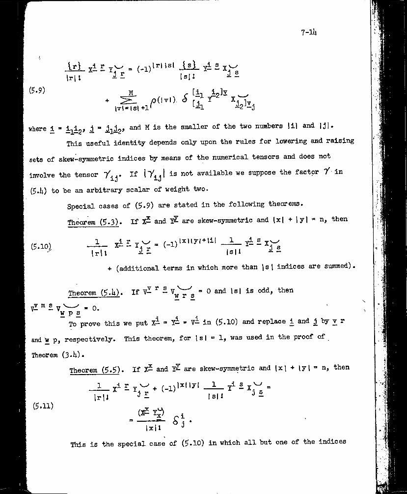
7-lb
xi I j'y = (-1)^’^' - X.'-<I-.. 0 ls|l i-Irll j s
(^.9) M
\v\ = ls\ +1
r [in ip3z ^^(,.0. <i r
where i » iii2> ^ “ ¿1^2’ ^ smaller of the two numbers |il and |jl.
This useful identity depends only upon the rules for lowering and raising
sets of skew-symmetric indices by means of the numerical tensors and does not
iirrolve the tensor If lY^^I is not available we suppose the factor Y-in
(5,b) to be an arbitrary scalar of weight two.
Special cases of (5.9) are stated in the following theorems.
Theorem (5.3). If 2? and are skew-symmetric and Ixl + lyl =• n, then
(9.10)Irll
^i r „ WX- - J. (-1) ixuyl + lil __1 Y- - X>|s|I 3 s
+ (additional terms in which more than )sl indices are summed)
,v r sTheorem (5.b). If V- " - “ 〇 and Isl is odd, then
vl " ® V ^ “ 0.w p sTo"prove this we put xi = li - vi in (5.1〇) and replace i and j by v r
and w p, respectively. This theorem, for 1s1 = 1, was used in the proof of
Theorem (3.b)«Theorem (5.5). If 2^ and are skew-symmetric and \x\ + \yl = n, then
(5.11)
_i_ xi E _i_ ji £ X,\Irll UI1
“ -------;— b i *Ixll ^
This is the special case of (5«l〇) in which all but one of the indices
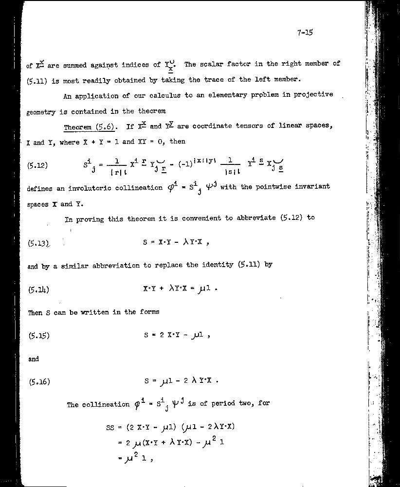
7-15
of 3^ are STimmed against indices of The scalar factor in the right member of
(5.11) is most readily obtained by taking the trace of the left member.
An application of our calculus to an elementary problem in projective
geometry is contained in the theoremTheorem (5.6). If X? and are coordinate tensors of linear spaces,
X and Y, where X + Y “ 1 and XY - 0, then
(5.12) S^. = 3
1 „XT / ,,,lxlly> 1 yi s— X - Xj r - -:7r7 31(r| I - ls|l
defines an involutoric collineation Cp^ = S^. with the pointwise invariantJ
spaces T and Y.In proving this theorem it is convenient to abbreviate (5.12) to
(5.13), S = X-Y - Ay-x ,
and by a similar abbreviation to replace the identity (5.11) by
(5.lU) r«Y + AY»X = jM .
Then S can be written in the forms
(5.15) S = 2 X-Y - JJI ,
and
(5.16) - 2 A Y*X .
The collineation = S^. is of period two, for
SS = (2 X-Y - ^1) (^1 - 2AY-X)
= 2 ju(X*Y + A Y»X) -
= >1^1,1
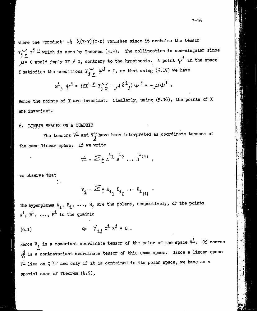
7-16
where the "product" rh X(X*Y)(Y*X) vanishes since it contains the tensor
y-5 i which is zero by Theorem (3.3)* The collineation is non-singular sincej £ i
JJ= 0 would imply XY 0, contrary to the hypothesis. A point in the space
I satisfies the conditions that using (5.l5) we have
tpJ = (2X^ - Y^'^ - .
Hence the points of Y are invariant. Similarly, using (5.l6), the points of X
are invarisint.
6. LINEAR SPACES ON A QUADRICThe tensors vi and V^have been interpreted as coordinate tensors of
the same linear space. If we write
9
we observe that
• « •
The hyperplanes A^, ..., are the polars, respectively, of the points
A^, B^, ..., in the quadric
(6.1) Q: X^ X^ = 0 .
Hence is a covariant coordinate tensor of the polar of the space V—. Of course
V-^ is a contravariant coordinate tensor of this same space. Since a linear space n
V- lies on Q if and only if it is contained in its polar space, we have as a
special case of Theorem
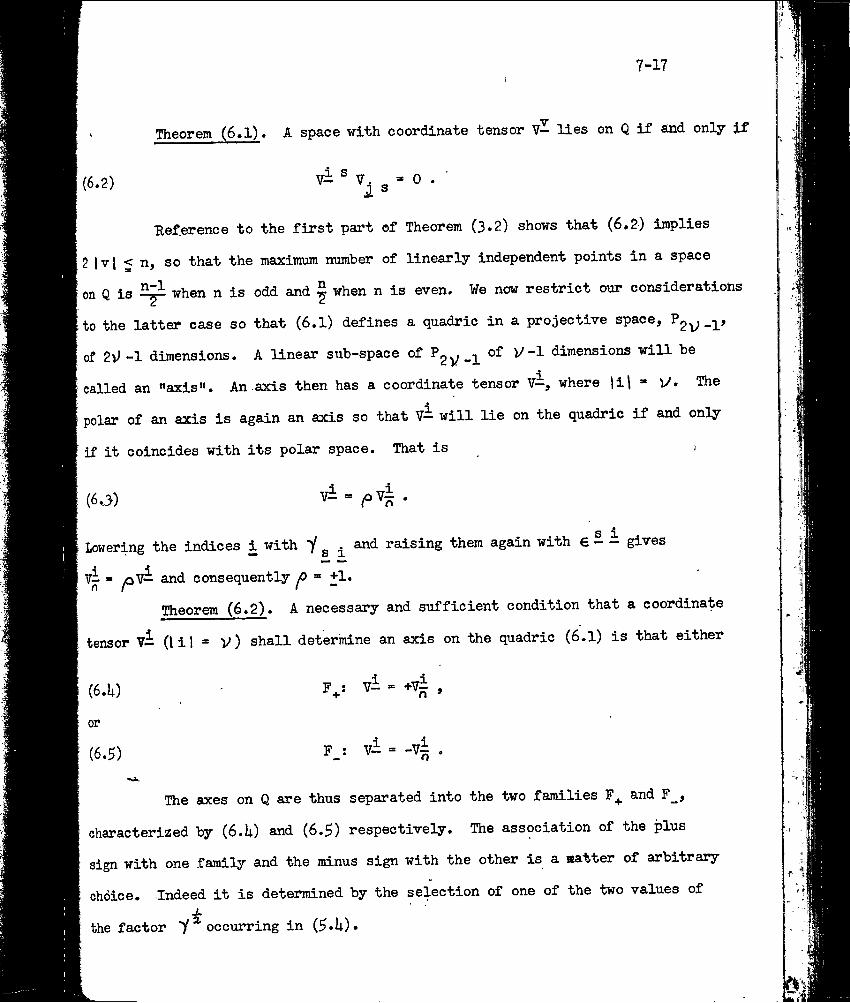
7-17
Theorem (6.1). A space with coordinate tensor V— lies on Q if and only if
(6.2) V- ® V. „ = 0 .
Ref.erence to the first part of Theorem (3*2) shows that (6.2) implies
2 |vl < n, so that the maxiimxra number of linearly independent points in a space
on Q is when n is odd and ^ when n is even. ¥e now restrict our considerations
to the latter case so that (6.1) defines a quadric in a projective space, P2V»-1'
of 2v) -1 dimensions. A linear sub-space of P2V-I dimensions will be
called an "axis". An axis then has a coordinate tensor 4—, where lil “ The
polar of an axis is again an axis so that V— will lie on the quadric if and only
if it coincides with its polar space. That is >
Theorem (6.2). A necessary and sufficient condition that a coordinate
tensor V- Oil = V) shall deterinine an axis on the quadric (6.1) is that either
The axes on Q are thus separated into the two families F_^ and F_,
characterized by (6.I4) and (6.5) respectively. The association of the plus
sign with one family and the minus sign with the other is a matter of arbitrary
choice. -Indeed it is determined by the selection of one of the two values of
(6.3)
Lowering the indices i with Y g 3^ and raising them again with € B i gives
fi « y〇V— and consequently ^0 = +1.
(6.U)
or
(6.5)
the factor occvicvlng in (5.U).
■ 7-18
■ Theorem (6,3). If V and W are two axes on Q, then
(5.6) dimension of (W) S V - 1 (mod 2)
if V and W belong to the same family, and
(5.7) dimension of (W) = (mod 2)
if V and W belong to different families*^
^ A proof of this theorem based upon stereographic projection is given by Bertini, "Einftlhrung in die Projektive Geometrie", p. 1U3.
Since V and W are axes on Q,
(6.8) vi=A^vi, wi=A^wi, \il = ,
and the spaces will belong to the same family if Ay “ +1 and to different
families if Ay = -1* let us put D(VW) = 1 + dimension of (W). Assuming
that D(W) =>J+1, using (6.8), and applying Theorem (U.5), we have °
for Ihl > V-JU • Hence if we put X- = and I^= in equations (5.1〇) they
reduce to
(6.9) vi - ^ = -(-l)'^ 1 •
On accotint of (6.8) these equations imply
(6.10) ^ = -(-1)^"^ Xy A^ wi Vj ^ .
By Theorem (U.^) ^ ^ = I- where li and are coordinate tensors of V¥
and V + ¥, respectively. Since V + W is the polar of W, J. = g
7-19
consequently ^ is symmetric in the sets i and Hence
= vi-W^. Substituting in (6.10) now givesV V
(6.11) (1 + (-!)''->') ii^W,'V ¥ ' r
and therefore if X.^. X^ = +1 V— — ¥^ ^ ^ 0 implies - jA—1- (mod 2), or if
X^ X^ = -1, implies V-^= 0 (mod 2).
Theorem (6.U). If S2V-I c〇™Pl®x 〇r if it is real and the signature
of Q is zero, then Q contains axes. If 82^ is real, Q contains axes only if
its signature is zero.
¥e omit the proof.
Theorem (6.5). If Q contains axes, then axes V and ¥ on Q exist for
which D(V¥) = CK , where C< is any integer > 0 and < il .
Under the hypothesis of the theorem we may choose coordinates in the
real or complex S2y_]_ so that the equation of Q is
(6.12) * ... -0.
Let us call the vertices of the coordina'^e 2 V>-point E^, £2» •••>
E|, E^, ..., and E^ , where ,the coordinates of E^ (a = 1, 2, ..., ) are S
and of E* are . Then the spacesa di+u
(6.13)
? = E^ + E2 + ... + + ... + E^ and
¥ = E^ + E2 + ... + Eq^ + EJ^^^ + ... + E[^
lie on Q and D(V¥) = 0( .
Theorem (6.6). If the quadric Q in 82^ contains the distinct axes V
and ¥, V > 2, and ^ is any integer > 0 and < \) » then there exists an axis A on
Q such that D(A?) = ^ D(A¥).
7-20
The theorem would he untrue for ™ 2, ^ = Ij and D(V¥) = 0 for then
V and ¥ would be non-intersecting lines on a quadric in and any line on Q
which intersects one of two such lines in a point also intersects the other in
a point. In the other cases which occur when 1 or 2 the theorem is
trivially satisfied.Let us put D(VW) = <X . Then it can be shown that by a suitable choice
of coordinate system we may take the equation of Q to be (6.12) while V and W are
the faces of the coordinate 2V-point given by (6.13). We now distinguish several
cases:Case 1. <« . Take A = + E2 + ... + ^ +1 * ***
Then D(AY) = ^, and D(A¥) =/3 + v' - •
Case 2. yfl > 〇{ and / V. +oi . Take A as in Case 1. Then
D(AV)'"“ y3 , and D(A¥) = 〇i * ^ ^ •
Case 3. 2y8 = V> + 〇i . Take A = E| + E^ + ... + EJ_^ + E^_^ +
+ ... + E^ . Then. D(AV) = ^ , andif〇^+y5> 1/, E(A¥) = Oi + ^- ^ iif Qk*p i J3(A¥) = V - Of - , which is different from^ unless
2y9av;-〇f, In this event Of = 〇, and 2jB = V •
Case h. 2y8 = V > 2, or = 0. The 3-space E^_j^ + ®y-l
intersects Q in a non-degenerate quadric which contains the non-intersecting
lines E^ 1 + and + E^ . Let F + G another line of the regulns con
taining these two lines, and take F on E^_^_ + E^ and G on E'^ + E^ . If
we put A=Ej^ + E2 + ... +E^ ■^^^+1'*'***'*' -2 ^ ^ ^
D(AV) =■ yS ® 1^/2 and D(A¥) ~2 "f /^ •
Theorem (6.7). If two collineations of S2^_3^ (V >2) leave Q invariant
and effect the same permutation of the axes of F^, then they are identical.
7-21
By the preceding theorem an axis of F is unambiguously determined by
the axes of which intersect it in a space of - 1 dimensions, where ^ is
any number congruent to V - 1 (mod 2) and between 0 and j/ - 1, Hence the two
collineations must effect the same permutation on the axes of F^. Since every
point on Q is the complete intersection of two suitably chosen axes on Q (of the
same or different families), the two collineations transform the points of Q in
the same way and are therefore identical throughout the space.
8-1
Chapter VIII
REPRESENTATION OF LINEAR SPACES ON A QUADRIC IN
1. THE PROJECTIVE SPACE P2V-I
In this chapter we shall apply the correspondence of Chapters V and VI
between points in E^^ and matrices of order 2'^ to study the linear spaces on
a quadric in a projective spqce of (2V -1) dimensions. To do this we first
introduce a coordinate system in Egy in which the cone ^ ^
(pi “0, 1, •••, 2v> ) has the equation
(1.1) (X°)^ + “ 0 . (i, j = 1, 2, 2V/) .
The form of this equation will be preserved under transformations of coordinates
in E^y if we allow only transformations with equations
(1.2) ^ X°^^ - X°, = T^^, (i, j = 1, 2, 21^)
where )T^| / 0.
The group of transformations (1.2) leaves the hyperplane X° * 0 invari
ant and induces in it the linear transformation X^* = T^^, where HT^I] is anJ J
arbitrary non-singular matrix. Hence the hyperplane X° =» 0 is a 2)/>-dimensional
12 2v^complex affine space E^y in which the coordinates of a point are(X , X , ..., X ).Thus the coordinate vector (X°, X^, X^, X^*^ of a point in ^2y +1
of a scalar X®, and the coordinate vector (X^, X^, X^^) of a point in ^2])*
Under (1.2) a covariant vector has the law of transformation
(1.3) >
where ‘t^T^ = 6^. Consequently the coordinate vector (Z^, Z^, ‘*•» ^2)?
a h3q5erplane in E2y is composed of the scalar Z^ and the vector (X〇^j ^2» •••> ^2if
8-2
Indeed, sinceij 0 ... 0
0 1
11 0 ... 0〇;
(i.U) ; i 11 y^jii • 10 1
and::
1• 10 .1
where covariant components x'^ of a vector
are related to the contravariant ones by the equations
X
(1.5) = 3E°. h - •
The rules for raising and lowering Greek indices (of,yfl j etc.) with the range
(0, 1, 2, •••> 2V) rasiy therefore be replaced by the corresponding rules for
raising and lowering Latin indices (i, j, etc.) with the range (1, 2> 2]^)
by means of andIf we regard the numbers X^ as being homogeneous rather than non-homogeneous
coordinates of a point, we shall be dealing with a complex projective space P2y_l
of 2V-I dimensions. In effect, this amounts to taking the lines through the
origin in E^y to be the points of ^2^-1° points of P2y'-1 coordihates
^X^ therefore correspond to a pencil yollx^^ll , of matrices of order 2 by
means of the equations
(1.6) X = x^ .
Since Y X°^X^ = (X°)^ + y., X^ X^ we have from (1.6), Chapter ?, oiyS
(1.7) X® = 1 .
The fundamental quadric
8-3'
(1.8) 0
in thus appears as
involutions with matrices
the locus of singular
X"
elements of the linear family of
In the following sections we shall pass freely from the affine space
with non-homogeneous coordinates X to the projective space ^2y —1 ^Ith
homogeneous coordinates ^X^» Equations (1»6) will then be regarded as estab
lishing the correspondence X^ ^ llx^gll between points of ^2y matrices
in ^ or, equally well, the correspondence ^X^ <—> ^llx^gll between points
of and involutions in
/2. THE CORRESPONDENCE BETWEEN TENSOR SETS AND MATRICES
In §6 of Chapter V we proved that if the form a '/-set, then the
matrices
(2.1) 1, 7j(l < 5)> ^2^3 *'* '^2V
are linearly independent. Since there are 2^^ of them every matrix of order 2^
can be expressed as a linear sum of these matrices. That is, an arbitrary matrix
X = llx^gH
(2.2)
of order 2^ is expressible in the form
2)1X =
|il=〇 I illX— s. ,,
where
(2.3)
It is understood that when li| = 0, s^ = 1. When X is a matrix of the linear
family X^ the coefficients X- in (2.2) vanish unless li] = 1 so that equations
8-h
(2.2) include (1.6) as a special case.
When the elements of a Tf-set, the quantit7 s^ = is
skew-symmetric in the indices i. With the definition (2.3) this property is not
preserved under transformations of coordinates in ^2^ • We therefore define s^
by the formula
which reduces to (2.3) in a cartesian coordinate system, that is, when
solve for them in terms of the matrix X. To do this we employ cartesian
may be verified in a cartesian coordinate system and evidently remains valid
If we take the coefficients X- in (2.2) to be skew-symmetric, we can
coordinates to prove that Trace = 0 if lil / Ij/ snd otherwise it is a
multiple of ‘ o i. The exact relation
(2.5) Trace (s^.) = (-1)cl
under coordinate transformations. Multiplying (2.2) by si and taking the trace
therefore gives
(2.6)xi = 101(131-1)2“'*^ Trace X s^
and we have the theoremTheorem (2.1). Equations (2.2) and (2,6) establish a (1-1) corres
pondence
8-5
ietweeri matrices of order and sets of skew-syinmetric tensors.
3. THE COLLINEATIONS CORRESPONDING TO LINEAR SPACES ON THE QUADRIC
The correspondence of this theorem allows us to represent a linear
subspace of P^y collineation in the spin space P^V To do this it
is only necessary to take the tensor set to be |_〇s 〇s ...j 〇j A—j Oj ...j 0^
where A— is a coordinate tensor of the linear subspace.
A lemma, which we shall need in the proof of the next theorem is2 2Lemma. If A and B are square matrices, A == B =0, and AB = + BA, then
(3.1) rank AB < •£ rank A
This-is obtained from the general relation-if-
* C.C.MacDuffee, "The-Theory of Matrices," Berlin 1933, Theorem 8.3.
' rank AB + rank BC < rank B + rank ABC
by putting C = A.Theorem (3.1). If L^ is a coordinate tensor of a linear space L on the
quadric (1.5) and A'= s., then = 0 and rank A= .)il I “
Let us take L^, L^, ..., L,., to be lil linearly independent points on'lilL. Then L = L^ + L^ + ... + L • 1'^ is possible to find additional points
Ijil such that A = L^ + ... + L^ is an axis on the quadric. Then
y. = 0 for a, b = 1, 2, v' , where L^ is a coordinate vector of the3i"^Td
pointEquating coefficients of the arbitrary variables in (1.7) gives
(3.2)
8-6
Multiplying both raembers of and summing gives
(3.3) A|^ - - A^Ag^ (a, b = 1, .ooj V)
where Aa = Lg (= L^s^)In particular^ ^ Ag)^ “ 〇? s〇 'that rank Ag < ^ (order 〇f A g) = 2^^
Jhe product of any number of the matrices Ag also has square zero for ^ ^(AgA^ ... Ap)^ = t (Aa)^(A^)^ ...(Ap)^ = 0. Since 1^^= \ L,||‘ ,
X= A^Ag ... Aj^^ and there A^ = 〇.
Repeated application of the lemma now gives the chain of inequalities
,V^-2< 2
(3.U)
rankrank (A^A2) < -{rank A^ <2'
rank (A ^A2*" Aj.) < ¿rank (X^X2...Aj._3^) ^
rank (AiA2--. X^) < ¿rank (A;lA2--°'^v'-1^ <2'^"^=1
However, if A- is a coordinate tensor of A = + L2 + ... + s, Jl- a- s. = A, X5, ... A . ^ 0 and consequently rank (A 2^X2°‘'A^ ) = 1» Hencelill •— .\ \ V ^the inequality.sign cannot hold at any step and rank (A2^A2®*® ^[i| ' " ^ *
Theorem (3.2). If A^ (li\ = V) is the coordinate tensor of an axis on
the quadric and <X =
(3.^)
Ai s., then\i| I “
By Theorem (3.1) the rank of 〇( is one and hence all the columns of the1 2matrix are proportional to any non-vanishing column with elements (j/ , • i
If the factors of proportionality are called <p^, we have (3.^). Interpreting
as the coordinates of a point in the spin space, we have a representation
8-7
(3.6) A —^ V//
of the axes on the quadric in V -1 ^ points in i) In the follow
ing sections we shall study the figures ’in the spin space determined ty linear
spaces on the quadric and-apply these results to the representation (3.6).
k, SPACES IN P2W DETERMINED BY SPACES ON THE QUADRIC IN ?2v; -1
The matrix /3 = —— ^s. corresponding to a linear space B with. ^ \±\l icoordinate tensor ^ is, by Theorem (3.1), singular if B lies on the quadric.
Hence the collineation determined by ^ transforms all the points of P2^’-l
the points of a subspace , the »rank« space of ^ . A point l^with coordinates
KjA will therefore be contained in R^ if and only if there exists a coordinate
vector 9^ such that ~ A ^ B0®.
The singular points of the collineation form a linear space N^ , the
«null»» space of Thus a point belongs to N^ if and only if = 〇. ¥e
recall the notation of Chapter VII:
/number of points necessary to determine the (l;.l) D(S) = 1 + dimension of (S) = (^linear space S.
It is then evident that D(R^ ) = rank^ and D(N^ ) = nullity of ^ , so that
(li,2) D(R^ ) + D(N^ ) a 2^^ .
In the following theorems of this and the next section, we shall
suppose that B is a linear space on the quadric and that ^ is the matrix corres
ponding to B under (2.7).
Theorem (U.l). is ® subspace of N^ .If Vi/belongs to R^, /9 0. But = 0, so that /SV/=/^0 = 0 and
8-8
hence \^also "belongs to . The space will be a proper snbspace of ^
if the rank of^ is less than the nullity of ^ and the spaces will coincide
if the rank and nullity are equal. By Theorem (3*1) the latter case will arise
only when B is a point and then R^ and ^ are the coincident axe's of the
degenerate involution V ^ (cf. the last paragraph of §11, Chapter V).
Theorem The invariant polarity interchanges- and ,
The invariant polarity in was discussed in detail in Chapter VI.
For our present purposes it is sufficient to recall that it was determined by a
matrix C = llC.r.!! which satisfied the equations (cf. and (3»5)j Chapter VI).
(U.3) C« = eC , e = (-1)^ ,
and
(it.li) (cy^)' = f(cy^) , f = (-l)^e .
1 X iLet us put D(B) = r and take B^, B^, ..., B^ to be coordinate vectors
of r linearly independent points in B. Multiplying (U.h) through by B^(p = 1,.2, r) and putting = bJ we get y^^C* = or, using
(ii.3),
ft-5) Vp •
Since 11 C^^ll is non-singular, D (polar ofR^) = 2'^ - D(R^ ) and
combining this equation with (4.2) gives D (polar of R^ ) = D(N^ ). Hence to
show that the invariant polarity transforms R^ into it will be sufficient
to prove that the .polar of contains . This will be the case if the -polar
hyperplane of an arbitrary point of contains every point of ^ .• Wq shallA Btherefore have the theorem if we -can provq that ^ C^ * 0 whenever
r\
8-9
vp® =» and * 0.
Calling II |l<J>^il and ||0^|| matrices of one colnmn, the conditioh
is that ¿p'Gif'* 0 whenever jS 9 and j8f= 0. But since yd = /^1/^2 ***
can -employ (it»5) to get
- ^*Cy6 e = "* /r® " i i/^2 *•* *»
The points B are conjugate by pairs in the quadric and consequently the matrices
anticoiffinute by pairs. Hence
” '/r ••• ■ - '/^1/^2 ••• Ai**’' ■ - ■ °
and substituting in the last equations gives the required condition, (p'C^J » 0.
PROPERTIES OF ^ AND
Under the restricted group (1.3) 〇f“ transformations in the matrix
11 "Y ^ 11 behaves as a scalar. Indeed we saw in Chapter V that the equations o B
(5.1) ( = 1 and "/〇 A “ “ '^o
determine 'Z to within sign and it is evident that these conditions are not ' o
changed if we replace Y by t^ 1 ^ where |t^| / 〇. The invariant nature of the
matrix i is also put into evidence if we define0 i!
(5.2)• n
- z
(2 V)i■e~ ~^i^^i2 ^^21^
which we may do since the right ^ember reduces in a cartesian coordinate system to + (-l)^'^^ •** ^2V matrix satisfies (5.1). The advantage of.
(9.2) is that it determines a particular one of the two matrices satisfying (5.1)
— at least to within a choice of one of the square roots of the determinant .
/
8-10
If this root is the same as that- used in the definition of in terms
of ((^»U) Chapter VII), 'i satisfies the equations
(5.3)
and
(5.U)
'i S'' O 1 (-1)KV+lil)
us.-
1 i i(v'-lil) T .(_L_ xi s^) « (-1) x| s ) .UU - |jli ■' ^
These equations are most easily -T-erified in a cartesian coordinate system and
their tensor form then insures their validity in all centered affine coordinate
systems in . The corresponding formulas for multiplication on the right
^ '^o are obtained from these by using the invariant relations
(5.5)
invariant.
i s,' O 1(-1)'^' s, .
Theorem (5»1). The involution defined by leaves and each
Since A = —i— fiis., where is a coordinate tensor of the space B^ liU ~
onthe quadric, we can use (5.5) to get = ("1)'If I// is a point
of so that
involution transforms [jy into a point which again belongs to ^ . The invariance
of follows from Theorem (U.2) by using the commutativity of the invariant
polarity and the involution
If A is an axis on the quadric in P^y its corresponding matrix is,
by Theorem (3-2), of the form 〇< = where ^ is the point with coordinates
and is the hyperplane with coordinates By Theorem (U.2) the vector
is determined as a multiple of and therefore the point <// determines
the ma-trixof' -to within a factor. But the matrixes determines a coordinate tensor
8-11
of A by the equations (2.6) and hence If i// corresponds to any axis under (3.6)
it uniquely determines the axis. This proves the first part of the theorem
Theorem ($.2). The equations
(5.6) - '1'^ ’
and their inverses
(5.7) Ai =» (-1)*^ >
establish a (1-1) correspondence
(5.8)
between the axes on the quadric in points in Under the corres
pondence'' axes belonging to F_^ correspond to points of the axis ['T'q] and axes
belonging to F correspond to points belonging to the axis [ 'Z q] «
To prove the last part of the theorem we apply (5-U) to the matrix
^ ~ A-s. to get -y 〇< = +〇( where the plus sign is used if A- = +A^Uli °
and the minus sign if A— = -A^ . Hence g if A belongs to F_^,
^ A^j^B _ _ j^A if A .belongs to F . Theorem (5*1) could have been used to
prove that ij; lies in either [ i〇r i i〇]~» l^ut the argument just given proves
in addition that points corresponding to axes of the same family lie in the same
axis of and points corresponding to axes of different families lie in differ
ent axes ofThe invariance of under 'i^ implies that intersects [ '/^1
and [ '/p]“ in spaces Hsuch that
(5.9) d(r^ [fj*) * d(r^ [yj-) = KE^).
.A .. and
8-12
If B is not an axis, the statement that [ 'j and spaces of
the same dimensionality is contained in the theorem
Theorem (5»3)« If D(R^ ) >1, then
(5.10) D(R^[y^]^) =D(R^[y^]“) =tD(R^) .
If B is not an axis, its polar space does not lie entirely on the.
quadric and hence we may choose a point in it in such a way that its corres
ponding collineation Pis non-singular. Of course P commutes (or anticommutes)-
with the collineation ^ corresponding to B. If is any point of R^ ,
PjbQ =■ + ^iPQ) and hence P leaves invariant. Since T is an
involution of the family 'j it anticommutes with 7^ and interchanges
liand [Yq]~* Hence P interchanges R^ [Íand R^ spaces
are óí" the same dimension.
An (r+1)-dimensional linear space B^, on the quadric is determined as
the join of an r-dimensional subspace B and a point in B^ but not in B. The
spaces corresponding to B and determine the spaces corresponding to B^^ in the
way stated in the theorem
Theorem (5»U). If B^ = B + is a linear space on the quadric,
is a point, BL^ = 0, and B^, B and correspond to matrices jSjS and
respectively, then
(5.11) . and \ •
The second of these equations is obtained from the first by taking
polars with respect to the invariant polarity. Moreover, since ® i A
it is evident that R^ is included in both R^ and R^ and therefore in
R^ . Hence it is sufficient to prove that H(R^R^ ) = D(R^^).
8-13
Let us choose to be a point on the intersection of the quadric Q with
the polar of B. This can always be done in such a way that is not conjugate
to and then = B + will lie on Q and the line L^_ + will not lie on Q.
¥e now take and to be two distinct points on which are conjugate
with respect to Q and call their corresponding matrices andjj^. Then
>4i = aXi + b and >»2 = 〇 + d X^. Since both and X ^ commute with ^
so do jJ^ and jUgi and hence the non-singular involutions with matrices and
transform into itself. The same is therefore true of their product.
Chapter V, we discussed the axis regulus determined by a pencil
of involutions and there proved that the axes of a product,commutative involutions are the rank spaces of the singular elements, X]_ and X g,
of the pencil. Hence D(R^ R^ ) + D(R^ R;^^) = D(R^ ). But interchanges R;,^
and R;^ and leaves R^ invariant so that D(R^ R;^) = D(R^ R;^^) . Therefore
D(R^R^ ) = iB(R^ ), which is equal to B(^^) by Theorem (3.1)*
^ Theorem (5»^). If \ and L2 are points on Q and A^ and X2 are thexr
corresponding matrices, then either
(5.12)
and the line + L2 lias Q> c^
(5.13) " °
and the line + L2 does not lie on Q.If + L2 lies on Q we may put B = L2 in Theorem (5«ij') and use the
fact that D(R^ ) = = 2'^'^ to get (5.12). The only other possibility
is that \ + \ does not lie on Q, and in this case R;^^ and are distinct
8-lb
axes of the axis regulus determined by the pencil of involutions aA^ + bX^. Dis
tinct axes of a non-degenerate axis regains do not intersect and we therefore
have (5.13)»
6. GEOMETRY OF A GENERALIZATION OF THE PLUECKER-KLEIN CORRESPONDENCE
The properties of the geometrical correspondence
(6.1) B
between linear spaces on Q and the spaces into which the corresponding matrices
transform the whole of F2^-l clearer if we discuss some special
cases. Tfilhen V = 1 the quadric in P^ consists of two distinct points and these
points correspond, respectively, to two distinct points in the spin space, which
is again a P^.When v' = 2 the spaces P21/-I s®*"® 〇f
dimensions but the axes on the quadric are now represented by points of two non
intersecting lines and '*^^® space P^. Two lines of the same
regultis correspond to points of the same line in the spin space. Two lines on
the quadric which intersect in a point P^ correspond to two points and Lg
lying on the lines and respectively, and the point P^ corresponds to the
line + Lj) crossing and ^2*
When \)= 3 the quadric is in P^ and the spin space is 7-dimensional.
The axes ['fQ]''' and [ 'i〇]~ are non-intersecting 3-spaces. A point on Q corres
ponds to a P^ in P^ which intersects each of the 3-spaces [Y〇3"'' ^
line. Two points and B^ on Q therefore determine a pair of lines in [ i
and a pair in ['iThese two pairs of lines may intersect in points and
8-15
Lg and if they do the line lies on Q and corresponds to the line + Lg
crossing [i and If the plane A = B^ + B^ + determined by the
three points B^, B^ and B^ lies on Q and belongs to F^, then the points determine
edges of a non-degenerate triangle while in [ 'llthey determine
three lines through the point corresponding to A under (6.1).For = 1, 2, or 3 it can be shown that all the points of [yQ]"*" and
[ '/q]~ occur as images of axes on Q. When p* > 3 this is no longer the case, as
could be proved by comparing the dimensions 2^ ^-1 of CT^q] with the dimension
* Bertini, "Einffihrung in die Projektive Geometrie Mehrdimensionaler Raume", Vienna 1924, P* IU2.
7 >/ (V ’■1) of "th® families of axes on Q.
Referring to the table of Theorem (3.1), Chapter VI, we observe that
the invariant polarity determined by G = interchanges and [
if V is even, and leaves them separately invariant if is odd. Hence when
if even a point i^of transformed into a hyperplane C which contains[y 1“ and intersects ['i in a space of 2'^”^-2 dimensions. That is, when v'
is even, C induces a polarity within the space ['i and, similarly, within
When v' is odd, however, a point [¡J of [i is transformed into a hjrperplane G which contains and intersects in a space of ^ ^-2
dimensions. The invariant polarity therefore defines a mapping of the subspaces
of [Yq]'*' in'to subspaces of ['/〇]” in which points correspond to hyperplanes (with
respect to ['j lines correspond to spaces of 2^ ^-3 dimensions, and so on.
8-16
If is an axis in corresponding to a point on Q, and
Theorem (li*2) states that the polarity G leaves R^ invariant. However,£ = R ['7' + B.. ['f ]” and hence the mapping of [7^-] into [ /^] trans-
forms R rV l"^ into R^[y ]'. The space R^ is therefore determined ty its' 0 (A 0 ^
intersection with [ i . Similarly, a point of [/〇]“ is determined hy the
(2'^“^-2)-dimensional space in which its polar hyperplane intersects
These results can be combined with the theorems of §5 to give the theorem
Theorem (6.1) . The points of a quadric Q in ^2^-1
coi^respond to axes in ^ ^ n i^ such a way that the points of an (r-l)—dimensional¿ ”i f V—l~r \
space, r < vJ , on Q correspond to axes all of which contain the same (2 -^l)-
dimensional space. Under the correspondence the points of an axis on Q either
correspond to axes all of which contain the same point or to axes all of which
lie in the same hyperplane.For ^ = 3 this theorem gives the Pluecker-Klein correspondence between
points on a quadric in and lines in P^. In this case all the lines in P^ enter
into the correspondence. Lines on the quadric correspond to pencils of lines
in P^ and the points of a plane on the quadric correspond to all the lines
through a point or to all the lines in a plane.
7. COLLINEATION REPRESENTATION OF FOR > 2
The geometrical correspondences established in this chapter give rise
to representations of the proper orthogonal group on 2^ variables, In
this and the next two sections we shall discuss these representations.In Chapter V we used the equations P*^ P ^ to establish a
(1-1) collineation isomorphism between the proper orthogonal group y 〇n 2 y +1 variables and the group of collineations leaving the linear family i
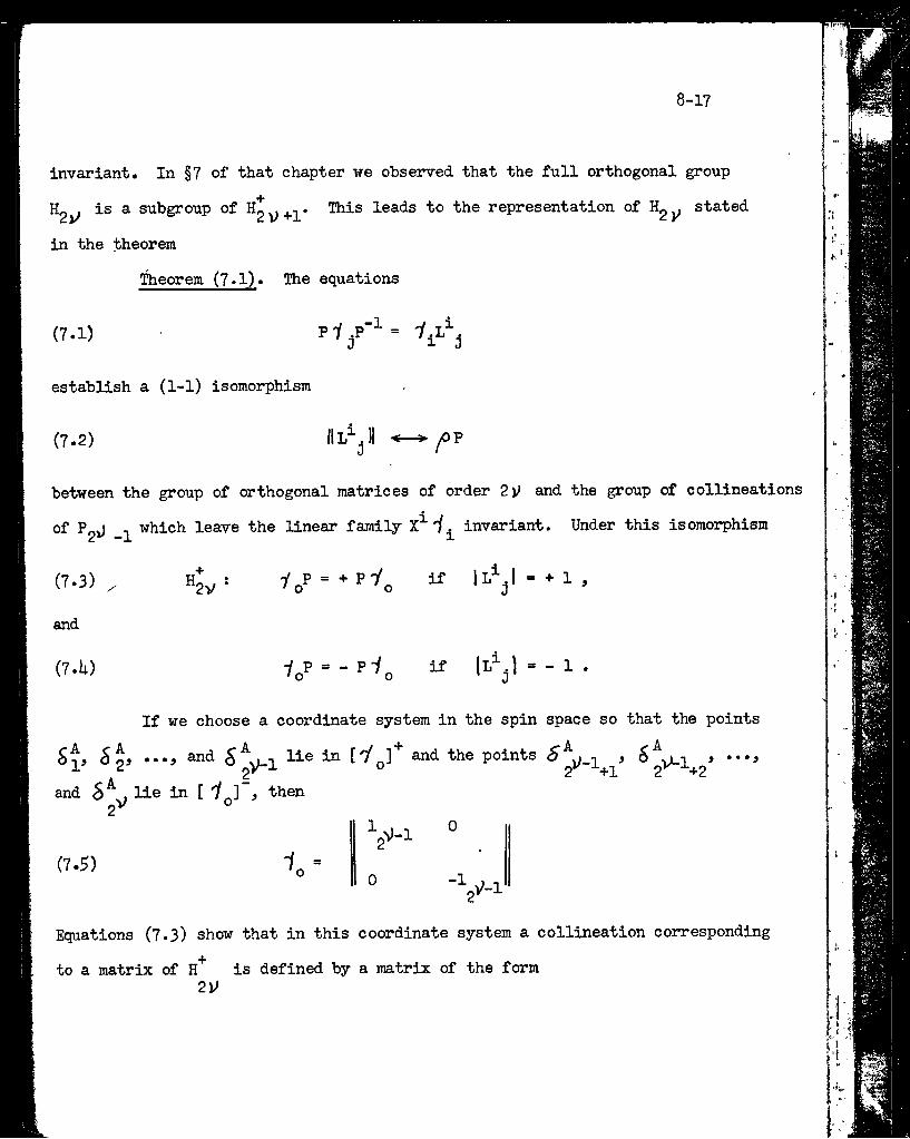
8-17
invariant. In §7 of that chapter we observed that the full orthogonal group
is a subgroup of leads to the representation of stated
in the theorem
^eorem (7»1)« The equations
(7.1) '^i^S
establish a (1-1) isomorphism
(7.2) f>V
between the group of orthogonal matrices of order 2V and the group of collineations
of ^ which leave the linear family invariant. Under this isomorphism
(7.3) = ^
and
(7.U) Y〇P = “P-^〇 ^ iL^^l = - 1 .
If we choose a coordinate system in the spin space so that the points
S0> •••» and ^ points i f •••#1 d 2^"^ ° 2*^ ■‘■+1 2*^"^+2
and lie in [ '/^] , then
(7.5)
>1 0
0 -V-1
Equations (7.3) show that in this coordinate
to a matrix of h'*’2)J
system a collineation corresponding
is defined by a matrix of the form
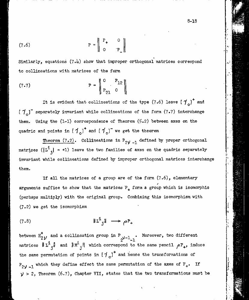
8-18
orthogonal matrices correspond
the type (7.6) leave [7^^]^ and
[ 7^3]" separately invariant while collineations of the form (7»7) interchange
them. Using the (1-1) correspondence of Theorem (5*2) between axes on the
quadric and points in [ '/q]'*' and [ we get the theorem
Theorem (7»2). Collineations in P^y defined by proper orthogonal
matrices (iL^-l = +1) leave the two families of axes on the quadric separately
invariant while collineations defined by improper orthogonal matrices interchange
them.
If all the matrices of a group are of the form (7.6), elementary/
arguments suffice to show that the matrices P_^ form a group which is isomorphic
(perhaps multiply) with the original group. Combining this isomorphism with
(7.2) we get the isomorphism
(7.6) P =p^ 0+0 •p_
Similarly, equations (7.h) show that improper
to collineations with matrices of the form
0 P,(7.7) P = 12
P21 0
It is evident that collineations of
(7.8) 111% II
between and a collineation group in P . Moreover, two differentmatrices Hl^.H and which correspond to the same pencil induce
the same permutation of points in i'l 〇] and hence the transformations of
?2y ^ which they define effect the same permutation of the axes of F^. If
y > 2, Theorem (6.7), Chapter VII, states that the two transformations must be
s
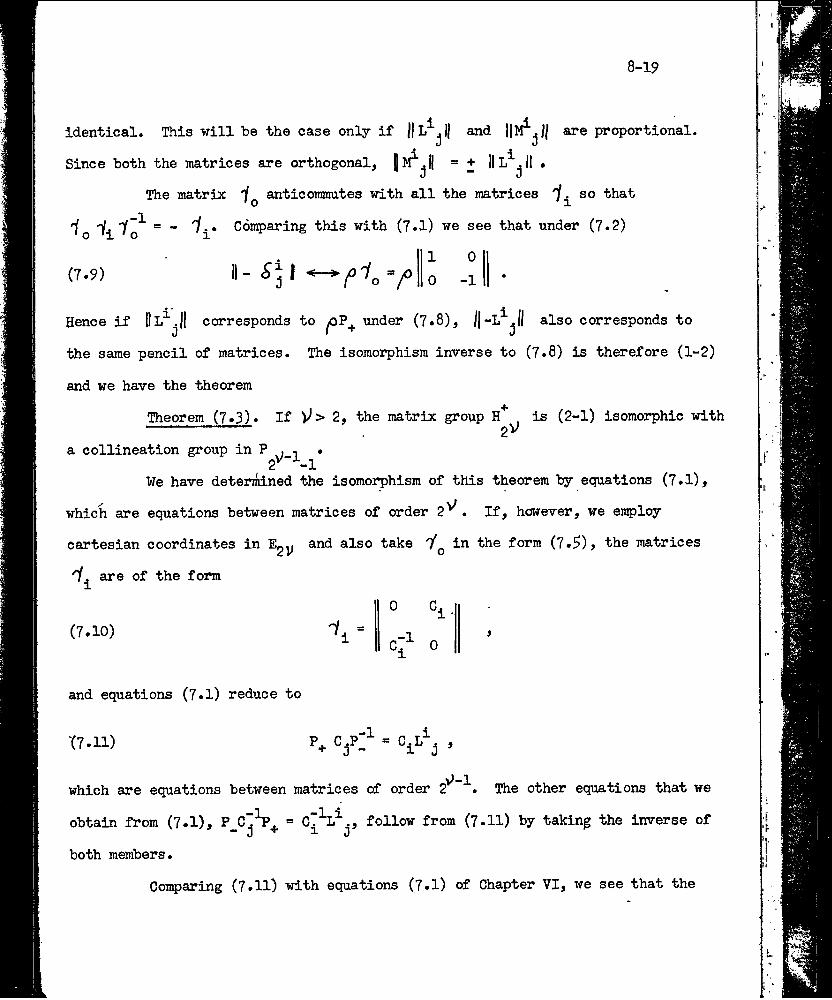
8-19
Identical. This will be the case on]y if and are proportional.
Since both the matrices are orthogonal, *
The matrix if anticoramutes with all the matrices '1. so that ' 0 * 1
^ = “ '1^» Comparing this with (7.1) we see that under (7.2)
1 0 0 -1(7.9)
Hence if corresponds to under (7.8), also corresponds to
the same pencil of matrices. The isomorphism inverse to (7.8) is therefore (1-2)
and we have the theorem
Theorem (7.3). If V^>2, the matrix gronp is (2-1) isomorphic with-------------------- 2^
a collineation group in P . , .2'^” -1
¥e have determined the isomorphism of this theorem by equations (7.1),
whicli are equations between matrices of order 2^ . If, however, we engsloy
cartesian coordinates in ^2^ a.nd also take in the form (7.5), the matrices
are of the fonu
(7.10) 0
and equations (7.1) reduce to
'(7.11) P, CjP;^ . ,
.v>-lwhich are equations between matrices of order 2 . The other equations that we
obtain from (7.1), follow from (7.H) by taking the inverse of
both members.
Comparing (7.11) with equations (7.1) of Chapter VI, we see that the
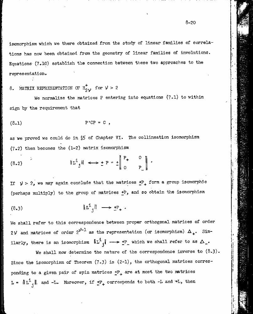
8-20
isomorphism which we there obtained from the study of linear families of correla
tions has now been obtained from the geometry of linear families of involutions.
Equations (7.10) establish the connection between these two approaches to the
representation.
8. MATRIX REPRESENTATION OF for V > 2
¥e normalize the matrices P entering into equations (7.1) to within
sign by the requirement that
(8.1) P'CP = c ,
as we proved we could do in §5 of Chapter VI. The collineation isomorphism
(7.2) then becomes the (1-2) matrix isomorphism
> • II ° II(8.2) IlL^ Jl -s—^ + P = +
J " 11 0 P^ 11
jf \) > we may again conclude that the matrices +P_^_ form a group isomorphfc
(perhaps multiply) to the group of matrices +P, and so obtain the isoraoi^hism
(8.3) iP+ »
¥e shall refer to this correspondence between proper orthogonal matrices of order 2V and matrices of order 2'^"^ as the representation (or isomorphism) A_^. Sim
ilarly, there is an isomorphism 11l^.| —+P_ which we shall refer to as A_.
¥e shall now determine the nature of the correspondence inverse to (8.3).
Since the isomorphism of Theorera (7.3) is (2-1), the orthogonal matrices corres
ponding to a given pair of spin matrices +P^ are at most the two matrices
L = IIl^.11. and -L. Moreover, if +P_j_ corresponds to both -L and ‘+L, then
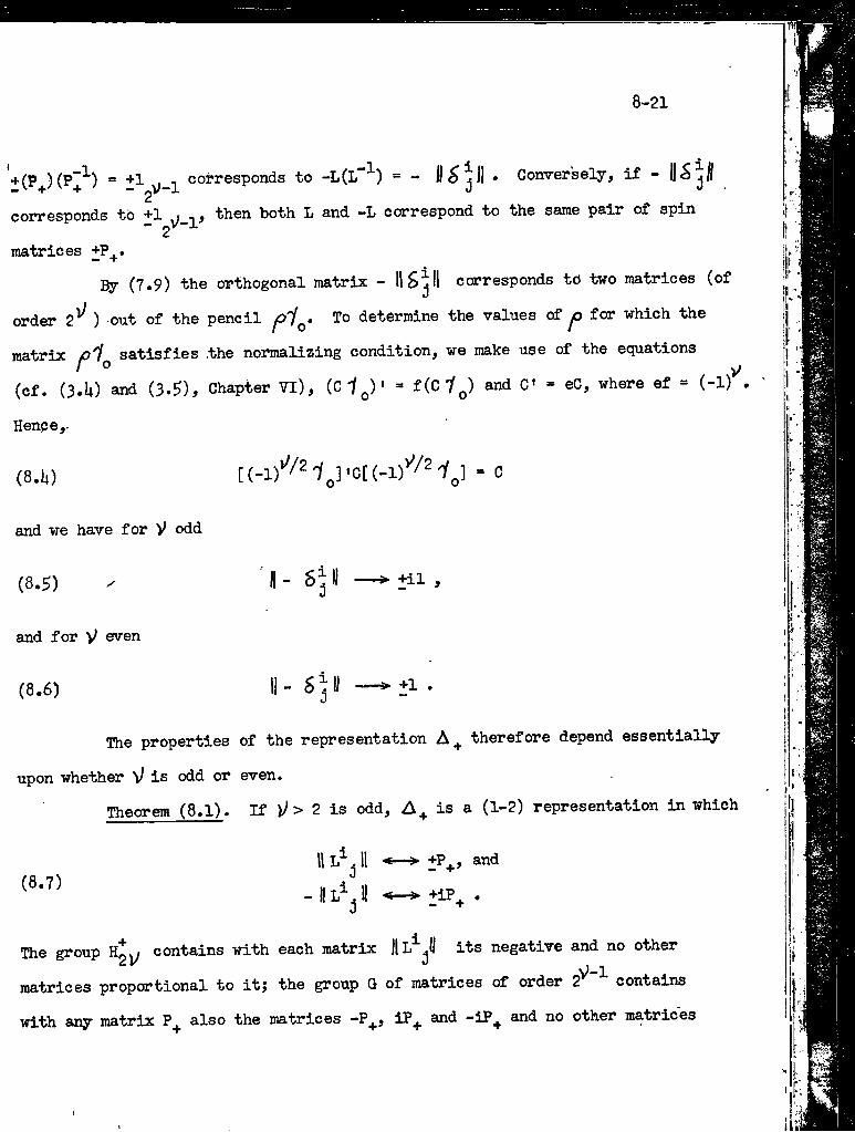
8-21
+ (p^)(p“^) “+1^2. coi’^ssponds to -L(L ^) = - 11^ jll • Conversely, if - 11^
corresponds to +1 . then both L and -L correspond to the same pair of spin - 2''-!
matrices +P^.By (7.9) the orthogonal matrix - IIS^H corresponds to two matrices (of
order 2^ ) -out of the pencil To determine the values of yO for which the
matrix satisfies the normalizing condition, we make use of the equations(cf. (3.U) and (3.5), Chapter VI), (C 1 ' = f(ci^) and C» » eC, where ef = (-l)'^.
Hence,.
(8.1.) - C
and we have for V odd
(8.5) ^ ^ ^ j ** —^ "
and for V even
(8.6) +1 .
The properties of the representation therefore depend essentially
upon whether V is odd or even.
Theorem (8.1). If 1/> 2 is odd, is a (1-2) representation in which
(8.7)11 II ► +P+, and
- II 11 +iP^. .
The group Hgj/ contains with each matrix || its negative and no othermatrices proportional to itj the group G of matrices of order 2^ contains
with any matrix P^ also the matrices -P_^., iP^ and -iP^ and no other matrices
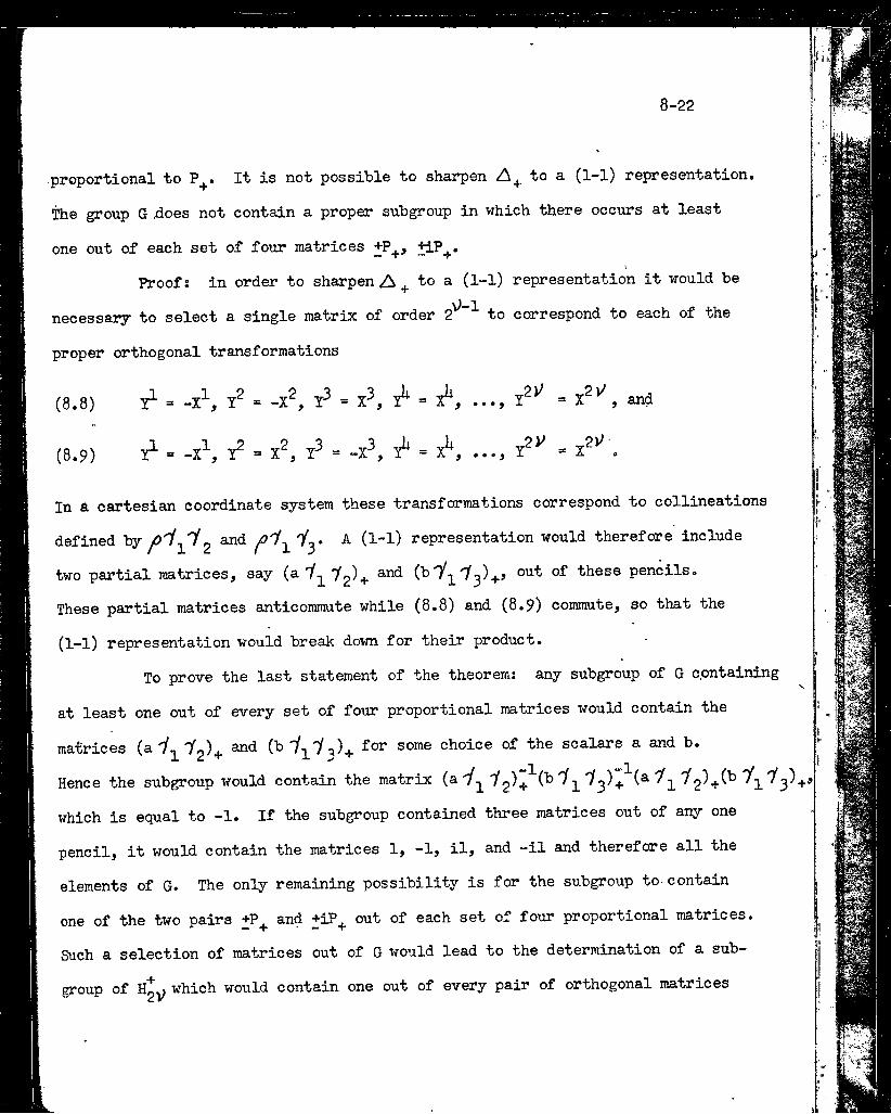
8-22
proportional to P_j_. It is not possible to sharpen to a (1-1) representation.
The group G xioes not contain a proper subgroup in which there occurs at least
one out of each set of four matrices +P_j_, JiP^.
Proofs in order to sharpen A + to a (1-1) representation it would be
necessary to select a single matrix of order to correspond to each of the
proper orthogonal transformations
(8.8)
(8.9)
= -X^, - X^,
= X^, Y^ “ -X^, = X^,
and
In a cartesian coordinate system these transformations correspond to collineations
defined by 2 /’^l '^y ^ representation would therefore include
two partial matrices, say (a"/2^+ '7^)+» 〇at of these pencils.
These partial matrices anticommute while (8.8) and (8.9) commute, so that the
(1-1) representation would break down for their product.
To prove the last statement of the theorem: any subgroup of G containing
at least one out of every set of four proportional matrices would contain the
matrices and (b'/^'/3)+ some choice of the scalars a and b.
Hence the subgroup would contain the matrix {s.'i^^
which is equal to -1. If the subgroup contained three matrices out of any one
pencil, it would contain the matrices 1, -1, il, and -il and therefore all the
elements of G. The only remaining possibility is for the subgroup to-contain
one of the two pairs +P^ and +iP^ out of each set of four proportional matrices.
Such a selection of matrices out of G would lead to the determination of a sub
group of which would contain one out of every pair of orthogonal matrices
i
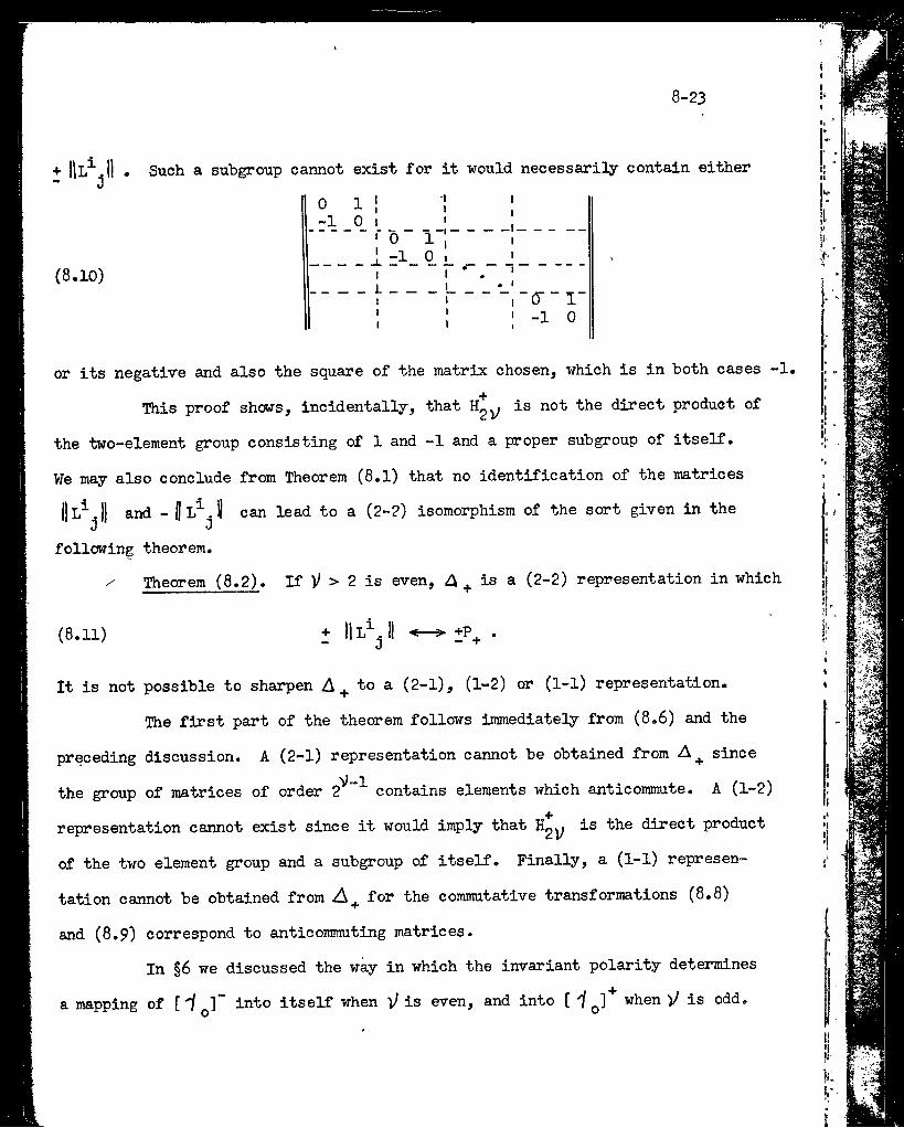
8-23
(8.10)
Such a subgroup cannot exist for it would necessarily contain either
0 1 j 11
1
-1 0 1 1I' 0 111
______ 1 =1_ 0 1_ 1
1 1 •L 1 • i1 1 1
(T ■■ I1 1
111
-1 0
or its negative and also the square of the matrix chosen, which is in both cases -1.
This proof shows, incidentally, that is not the direct product of
the two-element group consisting of 1 and -1 and a proper subgroup of itself.
We may also conclude from Theorem (8.1) that no Identification of the matrices
〇L^Jl and - can lead to a (2-2) isomorphism of the sort given in theJ 0
following theorem.^ Theorem (8.2). If V > 2 is even, a ^ is a (2-2) representation in which
(8.11) t II •
It is not possible to sharpen A ^ to a (2-1), (1-2) or (l-l) representation.
The first part of the theorem follows immediately from (8.6) and the
preceding discussion. A (2-1) representation cannot be obtained from sincethe group of matrices of order 2^~^ contains elements which anticommute. A (1-2)
representation cannot exist since it would imply that ^2)) direct product
of the two element group and a subgroup of itself. Finally, a (1-1) represen
tation cannot be obtained from for the commutative transformations (8.8)
and (8.9) correspond to anticomrauting matrices.
In §6 we discussed the way in which the invariant polarity determines
a mapping of [ if ]" into itself when is even, and into [ i when )/ is odd.
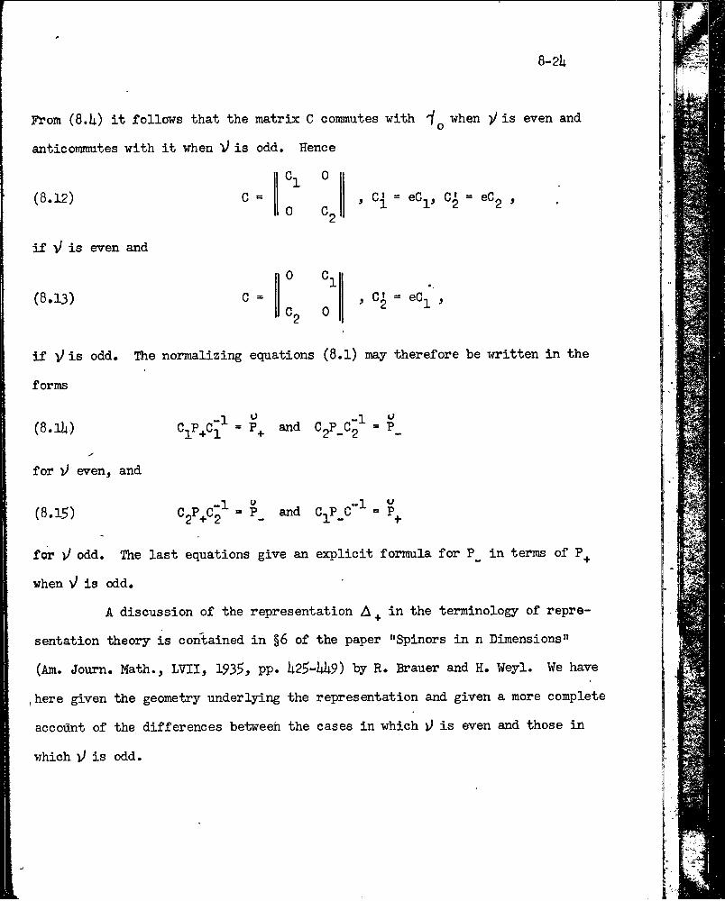
8-21;
From (8.1;) it follows that the matrix C commutes with when y is even and
anticommutes with it when V is odd. Hence
(8.12) , C> = eC1,c« eC,
if y is even and
(8.13)0 9
if y is odd. The normalizing equations (8,1) may therefore be written in the
forms
(8.11;) ^l^+^l^ ' K
for y even, and
(8.15) ^2^2^ = C^P_C“^ =
for y odd. The last equations give an explicit formula for P_ in terras of P^
when y is odd.
A discussion of the representation A ^ in the terminology of repre
sentation theory is contained in §6 of the paper “Spinors in n Dimensions”
(Am. Journ. Math., LVII, 1935, PP,i;25-U;9) by R. Brauer and H. Weyl. We have
I here given the geometry underlying the representation and given a more complete
account of the differences between the cases in which y is even and those in
which y is odd.
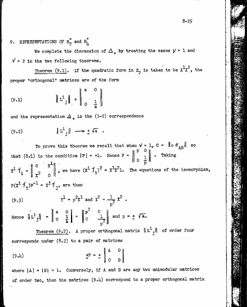
8-25
9. REPRESENTATIONS OF H2 and
We complete the discussion of A^ by treating the cases ^ = 1 and
= 2 in the two following theorems.
Theorem (9.1). If the quadratic form in E^ is taken to be the
proper "orthogonal” matrices are of the form
a 0
(9.1) l\0 I
and the representation ^ is the (1-2) correspondence
(9.2) ----> + >ir .
To prove this theorem we recall that when = 1, C = lie s〇P 0
that (8.1.) is the condition 1?! = +1. Hence P =
00
° 5Taking
, we have (X^ 1= X^^l. The equations of the isomorphism,
P(X^ y
(9.3)
Hence llb^jll =
= p^X^ and = X^P
a 0 11 2.P 0
—5 „ 1 1 = 1° al 0p
and p = + ^~a.
Theorem (9.2). A proper orthogonal matrix order four
corresponds under (8.2) to a pair of matrices
A 0 II(9.U) iP = i
0 B II
where I A) = iBj = 1. Conversely, if A and B are arjy two unimodular matrices
of order two, then the matrices (9.U) correspond to a proper orthogonal matrix
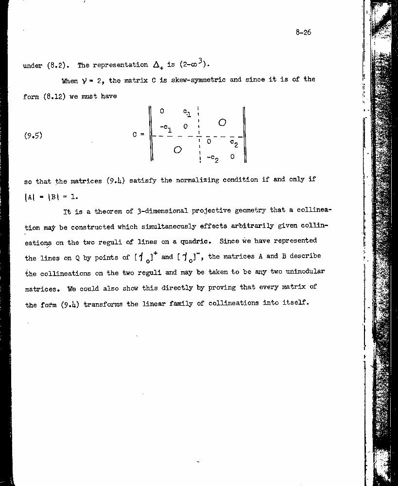
8-26
under (8.2). The representation is (2-oo*^).
When V = 2, the matrix C is skew-symmetric and since it is of the
form (8.12) we must have
(9.5) C =
so that the matrices (9.U) satisfy the normalizing condition if and only if
(Al = IBI = 1.
It is a theorem of 3-diraensional projective geometry that a collinea'
tion mat be constructed which simultaneously effects arbitrarily given collin-
eations on the two reguli of lines on a quadric. Since we have represented
the lines on Q by points of [j and [ ^1“, the matrices A and B describe
the collineations on the two reguli and may be taken to be any two unimodular
matrices. ¥e could also show this directly by proving that every matrix of
the fofm (9»U) transforms the linear family of collineations into itself.
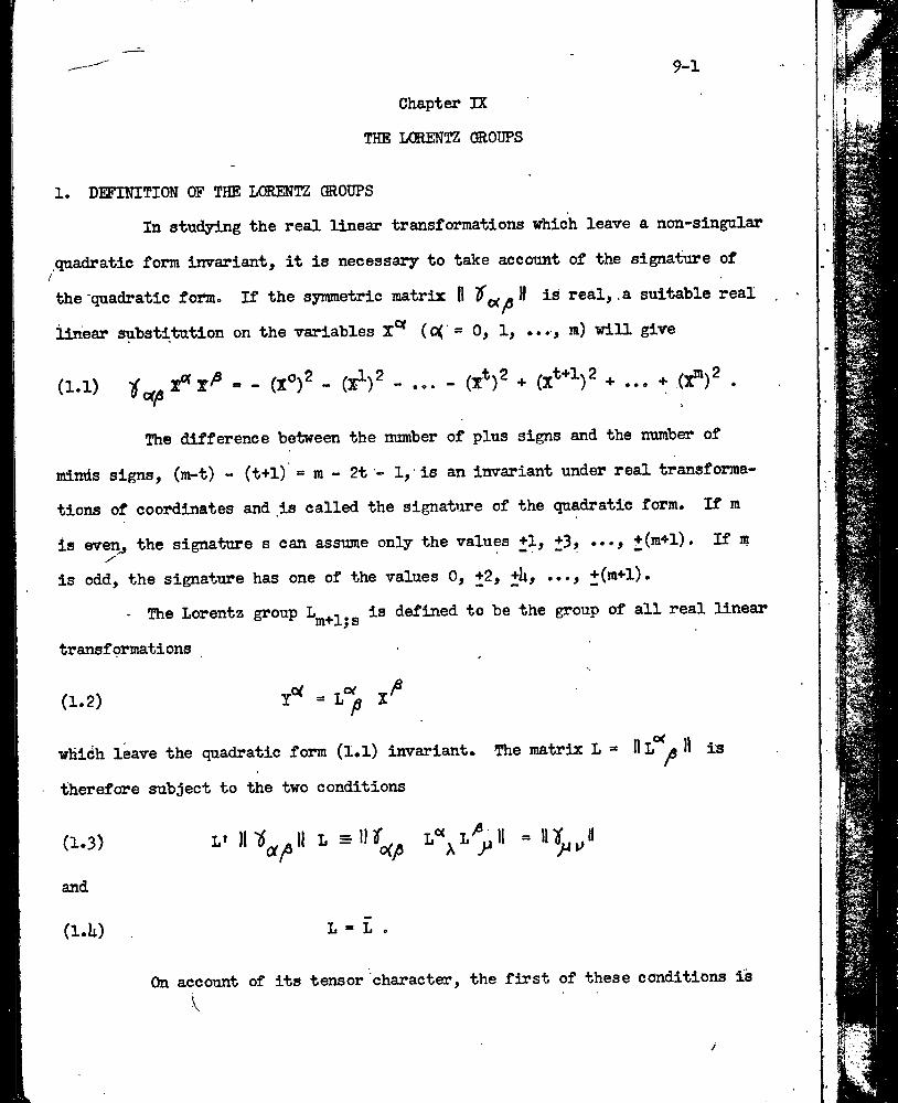
Chapter IX
THE LCEENTZ GROUPS
9-1
1. DEFINITION OF THE LORENTZ GROUPSIn studying the real linear transformations which leave a non-singular
quadratic form invariant, it is necessary to take account of the signature of
the quadratic form» If the symmetric matrix H is real, .a suitable real
linear substitution on the variables (〇( “ 〇> ly •••y will giwe
(1.1) - ... - + ... + (x“)^ .
The difference between the number of plus signs and the number of
тr^^тм4g signs, (mr-t) - (t+1) = ra - 2t - 1, is an invariant under real transforma
tions of coordinates and is called the signature of the quadratic form. If m
is even^ the signature s can assume only the values +1, +3, •••y t(m+l). If m
is odd, the signature has one of the values 0, +2, +ky ..., +(m+l).
- The Lorentz group defined to be the group of all real linear
transformations ■ '
(1.2) 1°^ =
which leave the quadratic form (1.1) invariant. The matrix L =* IIL ^ H is
therefore subject to the two conditions
C1.3)
and
(l.U) . L = L .
On account of its tensor character, the first of these conditions is^ ■ ■
j
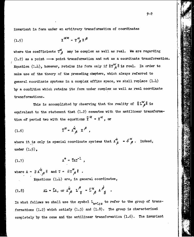
9-2
invariant in form under an arbitrary transformation of coordinates
(1.5) x/3
where the coefficients may be complex as well as real. ¥e are regarding
(1.2) as a point —> point transformation and not as a coordinate transformation*
Equation (I.I4.), however, retains its form only if is real. In order to
make use of the theory of the preceding chapters, which always referred to
general coordinate systems in a complex affine space, we shall replace (l.li)
by a condition which retains its form under conqjlex as well as real coordinate
transformations.This is accomplished by observing that the reality of I|L*^H is
equivalent to the statement that (1.2) commutes with the antilinear transforma.*- 〇( 〇(tion -of period two with the equations Y = X , or
(1.6) *
〇<where it is only in special coordinate systems that “ 〇 yS • Indeed,
under (1.5)p
(1.7) A* = TAT"^ ,
where A = || A*^^ II and T = llT ^ II .
Equations (l.ii) are, in general coordinates,
(1.8) AL “ LA, or a'^ .
In what follows we shall use the symbol to refer to the group of trans
formations (1.2) which satisfy (1.3) and (1.8). The group is characterized
completely by the cone and the antilinear transformation (1.6). The invariant
9-3
points of (1.6) constitute a real which intersects the cone in a real
cone with the signature s.
2. DEFINITION AND SPINOR REPRESENTATION OF THE ANTIORTHOGONAL GROUP A^^^
We have regarded the orthogonal group as the group of all the linear
transformations which leave invariant. ¥e may extend the orthogonaloip
group to a group which we shall call the antibrthogonal group by adding to
it all the antilinear transformations
which leave Hf = X°^X invariant in the sense that , or
and this partial normalization ofH and L ^ will be preserved if we restrictr
the transformations (1.5) to be unimodular.
Theorem (2.1). The antiorthogonal group Ag^ on 2+1 variables is
(1-1) isomorphic with the subgroup of the antiprojective group in P^v which
(2.2)
Taking the determinant of both members of this equation, we get
(2.3)ci I t= ^ ^
SO that
(2.U)
leaves the linear family X°'ip+X^7T3^+...+ X^^У2'^’ involutions invariant.
The equations establishing this isomorphism are:
9-li
(2.5) P => 11 P% 11 , n
I—1
1pH
(2.6) Q=
O’
II
f—t10
(2.7) n = llR^gll , . R-1. (-1)'' 7, , IL*)! - *1 !
and
(2.8) S = llS^gll , S 3^ S“^ - - , 1 l'^I = -1 .
Under this isomorphism collineations and anticollineations correspond to linear
and antilinear transformations, respectively, of determinant +1 and correlations
and anticorrelations correspond to linear and antilinear transformations, re
spectively, of determinant -1.
Equations (2.5) and (2.6) have already been used to establish a
collineation-correlation representation of the orthogonal group. To show that
equations (2.7) and (2.8) extend this to a representation of the antiorthogonal
group we should first show that when we multiply two transformations in
the corresponding transfonnations in +i proper way. This
is an elementary computation which we omit.
The antiorthogonal group is obtained from the orthogonal group by
adjunction of any one antilinear transformation which leaves the quadratic
form invariant. Similarly, the group of all antiprojectivities which leave
the family invariant is obtained from the group of all projactivities
with' this property by adjunction of a single anticollineation or anticor
relation which leaves the family invariant. Hence the isomorphism stated in
the theorem will be established if we show that a single anticorrelation in
^ has as its image in £2^ an antiorthogonal transformation. We do
this by using special coordinates.
1
9-5
Choosing a cartesian coordinate system in and making a suitable
choice of coordinate system in we may suppose that the matrices are
given by the formulas (ii.2) and (h.Ii) of Chapter V. ¥e shall call this combination
of coordinate systems a Canonical frame of reference. In such a frame the
matrices anticoramute by pairs and satisfy the equations
(2.9) (<X not summed) .
If we now put S = 1 in (2.8) we get so that the antipolarity
(2.10)
in the antiquadric
transformationA=1
= 0 corresponds under (2.8) to the antiorthogonal
(2.11)
Theorem (2.2). The matrices P = II P^gll j Q = HQ^'p II > R = ^
and S = 11 S^pll , defining antiprojectivities which leave invariant, may
be normalized to within sign by the equations
(2.12) P’CP = C, Q'CQ = C, R«CR = C, and S'CS = C ,
respectively. With these normalizations the equations of Theorem (2»1) determine
a (^2) matrix representation of the antiorthogonal group.
The possibility of normalizing the matrices of the anticollineations
and anticorrelations follows from the fact that their corresponding antiorthog
onal transfoi*mations coTumute with in a canonical frame, which is the
image of CP . = The proof of the theorem is similar to the proof
9-6
preceding Theorem (5〇l)j Chapter VI.
3. THE INVAEIANT ANTIIN70LTJTI0N AHD ANTIPOLARITT
By regarding as a subgroup of A^^ we obtain from Theorems
(2.1) and (2.2) representations of I-2V+1JS* describe these represen
tations only for the group 1*2^ +l*s Lorentz transformations
with determinant plus one. The extension to the representation of Lorentz
transformations with determinant minus one by means of correlations in P2^
can easily be made.
Theorem (3.1). The Lorentz group *1}S isomorphic with
the group of collineations of which leave invariant the linear family
"i and an antiinvolution 〇(
(3.1) / =
The antiihvolution of the theorem is the image under (2.7) of the
antilinear transformation (1.6) in ^21^+\ period two. Thus the transforma
tion of coordinates
(3.2) = iX®, = iX^ ... Xt* ,t+l*...
carries the quadratic form (1.1) into
2t>(3.3) ■»s2(X«")
〇C =0
~〇( 0(and carries the antilinear transformation Y =p X into
(3.ii)^(t+1)* ^ j(t+l)*^
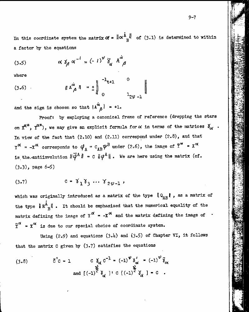
9-7
In this coordinate system the matrix i3f « of (3*1) is detemilhed to within
a factor ly the equations
(3.5) o(2(^〇i~'=C-
where
(3.6) II II =1
and the sign is chosen so that lA'*^) = +1.
Proof: ty employing a canonical frame of reference (dropping the stars
on i“*) , we may give an explicit formula for 〇< in terms of the matrices
In view of the fact that (2.10) and (2.11) correspond under (2.8), and that
s corresponds to under (2.6), the image of » X°‘
is, the^tiinvolution IKf^ll = G . We are here using the matrix (cf.
(3.3), page 6-5)
〇( P
1 ~\+l 0
' 0 I—1
1
(3.7) C “ "^1^3 *'* ^2'y-l *
which was originally introduced as a matrix of the type 11 | , as a matrix of
the type BR^gll . It should be emphasized that the numerical equality of the
matrix defining the image of and the matrix clefining the image of -
y°^ = is due to our special choice of coordinate system.
Using (2.9) and equations (3.U) and (3.5) 〇f Chapter ¥1, it follows
that the matrix C given by (3.7) satisfies the equations
(3.8) c'c = 1 C
and [(-1)^ 1' C [(-1)^ 1 ° •
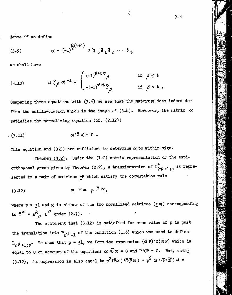
/
9-8
Hence if we define
(3.9) 〇( (-1) C ^ 〇^l"^2 *** t
we shall have
(3.10) C3( Tiyfl of =if ^ < t
if yd > t .
Comparing these equations with (3*5) we see that the matrix « does indeed de
fine the antiinvolution which is the image of (3»h)* Moreover, the matrix oc
satisfies the normalizing equation (cf. (2*12))
(3.11) 〇('0 〇( - C .
This equation and (3.5) are sufficient to determine 〇( to within sign.
Theorem (3.2). Under the (1-2) matrix representation of the anti-4orthogonal group given by Theorem (2.2), a transformation of ^2t^+ljs repre
sented by a pair of matrices +P which satisfy the commutation rule
(3.12) <x P =
where p = +1 and 〇( is either of-the two normalized matrices (+〇<) corresponding
to under (2.7).r
The statement that (3.12) is satisfied for some value of p is just
the translation into of the condition (1.8) which was used to define
1, , . To show that p » +1, we form the expression (〇( P)*C(〇cP) which is2"^ +lj s '
equal to C on account of the equations oi'CiX “ C and P’CP = C. But, using(3.12) , the expression is also equal to p^(?OC )'C(P〇f) = p cs( ’(P’CP)〇< =*
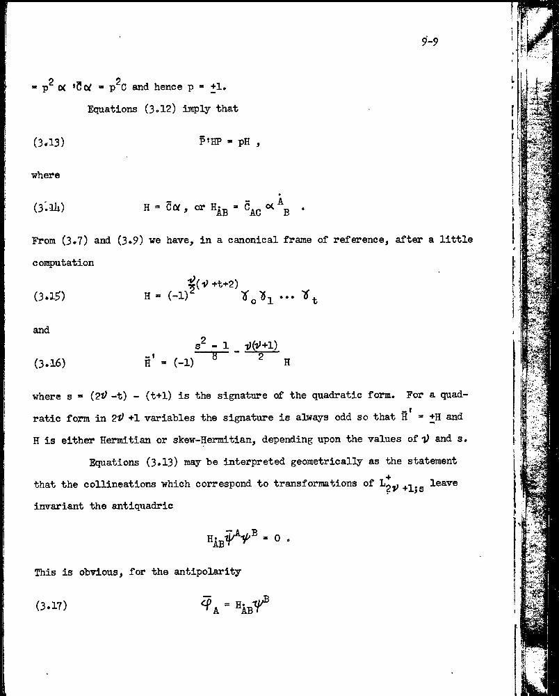
9-9
л Л= р (X *0(Х = р с and hence р = +1.
Equations (3〇12) imply that
(ЗЛЗ) Р’НР » pH ,
where
O'.ali) н - 〇〇(, or 〇< \ .
From (3.7) and (3.9) we have, in a canonical frame of reference, after a little
coi^utation¿( V +t+2)
(3.15) H = (-1)^ ■Ji'o'ii ...
ands^ - 1 _
(3.16) h’ * (-1) ^ ^ H
where s * (2t^ -t) - (t+1) is the signature of the quadratic form. For a quad
ratic form in 2lf +1 variables the signature is always odd so that H = +H and
H is either Hermitian or skew-Hermitian, depending upon the values of •]) and s.
Equations (3«13) may be interpreted geometrically as the statement
that the collineations which correspond to transformations of leave
invariant the antiquadric
= 0 .
This is obvious, for the antipolarity
= Чъ-Ч^(3.17)
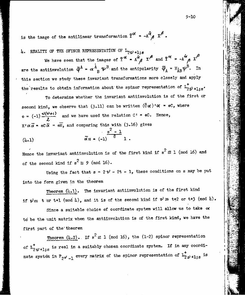
— 0( 0(is the image of the antillnear transformation Y = .
li. REALITY CF THE SPINOR REPRESENTATION OF I-2t;+l-s
We have seen that the images of Y “ A ^ and Y = -A ^ X
are the antiimrolution and the antipolarity
this section we study these invariant transformations more closely and apply
the results to obtain information about'the spinor representation of ^2t>+ljs*
To determine whether the invariant antiinvolution is of the first or
second kind, we observe that (3.H) can be written (〇〇()’0< = eC, where
e = (-1) —and we have used the relation C’ = eC. Hence,Z _
H'«〇r = eCo? = eH, and comparing this with (3»l6) givess^ - 1
(U.l) ^« = (-1) 1 •
Hence the invariant antiinvolution is of the first kind if s — 1 (mod 16) and
of the second kind if s^ = 9 (mod 16).
Using the fact that s = 2V - 2t - 1, these conditions on s may be put
into the form given in the theoremTheorem (ij.l). The invariant antiinvolution is of the first kind
if i9= t or t+1 (mod U), and it is of the second kind if = t+2 or t+3 (mod U).
Since a suitable choice of coordinate system will allow us to take 〇(
to be the unit matrix when the antiinvolution is of the first kind, we have the
first part of the'theorem
Theorem (U»2).. If = 1 (mod l6), the (1-2) spinor representation
of , is real in a suitably chosen coordinate system. If in any coordi-2t^ +l|s +nate system in P^v every matrix of the spinor representation of ■‘〇 l) +1 ! S is
9-11
2either real or pure imaginarj, then s 1 (mod l6)〇
Without affecting the real (or pure imaginary) character of the
matrices P = llP^gH we can choose cartesian coordinates in *1
the antilinear transformation (1.6) determining ^21}+I°s form (3«U).
Then the matrix (-l)"*^ 7f is properly normalized and corresponds to theA+ Xtransformation of L*, .,. which changes the sign of X and X and leaves
all the other variables unaltered. Hence X is either real or pure1l ^
imaginary and so is li ^ ~ (-1)^ (1(3^ ^2^ *** 2i>-l'^
this we can conclude that every matrix IT^ = )Tp(2rQ)rp^ ) is either real or
pure imaginary.
The antiinvolution therefore leaves the linear family
X invariant and its image in is a transformation
(h.2) Y° = e^X°, = e^x\ ... = e^^ X^^ , with e^ = ll •
Since commutes (or anticomrautes) with every collineation
of the group in (h.2) commutes (or anticommutes) with
every transformation of +l"s‘’ product of (h*2) and (3»h) is there
fore an orthogonal transformation with this property. Such an orthogonal
transformation is either the identity or Y*^ = -X and so ^ is the invariant antiinvolution corresponding toY =A*^X^. By Theorem (U.l) this
is possible if and only if s^ = 1 (mod I6)〇
Theorem (U.3). The invariant antipolarity is'a polarity in an
antiquadric of signature (+ - + - + -) unless s = +(2i>+l) and then
the signature is (++...+), or (---- ...-). The spinor representation
of the real orthogonal group is then unitary in a suitably chosen coordinate
9-12
system.
Choosing the index Of equal to zero if t + 1 is even, and equal to
t + 2 if t + 1 is odd, we have, from (3«l5) and (2.9), in a canonical frame
of reference
(lt.3) ij H = -H
and hence the signature of H is equal to the signature of -H and is therefore
(+- + _ +-), Our choice of fails only ift + l“0or2il + l and
then s=+(2l^ +1) and H is a multiple of the unit matrix. Equations (3*13)
cannot be satisfied if p * -1 for the signature of H is invariant under trans
formations of the form P»HP. For p » +1 and H = hi, (3.13) is the condition
that P be unitary.
K-SETS IN WHICH EACH MATRIX IS REAL CE PURE IMAGINARY
The existence of ¡f -sets of 2V +1 matrices of ohder 2'^ in which each
matrix is either real or pure imaginary may be settled in the following way.
If t) » t + lip or i) “ t + Up + 1, theorem (U.l) states that the
invariant antiinvolution associated with L〇-i .i, (s * 2tJ-2t-l) is' of the
first kind. In a suitably chosen coordinate system its matrix of will be
the unit matrix. For li = t + Up, equations (3.1〇) imply that 2t>-t = t«^+Up
of the matrices are pure imaginary and t + l = t^-Up + l are real. In the
other case, -t) =» t + Up + 1, the number of pure imaginary ones is t + 1 = - Up.
Hence in either event the number of pure imaginaiy ones is congruent to modulus
U. Since p may have any value which does not make either t + lor2V-t
negative, we have the sufficiency of the condition stated in the theorem
9-13
Theorem (^.1). There exists a ^ -set of 2V + 1 matrices of order
2"^ in which I of the matrices are pure imaginary and R are real (I+R=2l^+1) if
and only if
(^.1) I mod U) .
This condition is equivalent to the congruence
(^.2) R - I S 1 (mod 8)*
1
* In a paper by M.H.A.Newman entitled "Note on an Algebraic Theorem of Eddington" (Journ. Lend. Math. Soc., 7^ 1932, pp. 93-99) it is incorrectly stated that R-I = 1 or -7.
The necessity of the condition follows from the observation that a
^ -set of I pure imaginary and R real matrices could be used to obtain a
representation of a Lorentz group for which the invariant antiinvolution is
of the first kind.
Theorem (^.2). A real maximal if-set exists if and only if
.i)~〇 (mod k) • A pure imaginary maximal "jf-set exists if and only if
l)= 3 (mod U).
This theorem is obtained by putting 1*0 and I * 2i>+l in (5«l)»
6. SPATIAL AND TEMPORAL SIGNATURES OF LCEENTZ MATRICES
¥e return for the moment to a coordinate system in which
is given by (1,1) and determine the conditions which the elements
matrix L must satisfy in order that it define a transformation of
group. Siting
of a real
the Lorentz
9-lii
(6.1)A B
C D
where A is a square matrix of t + 1 rows and columns, these conditions are
found to be
(6.2)
A'A - C'C = 1^^^ ,
BtB _ d*D = -1 . , andm-t ’A»B - CD = 0 .
A« -C«If we form the product of the matrices |j q ^
may use the first and third of equations (6.2) to get
and
(6.3)A« -C 0 1
A B C D
1 0 C D
A B C D we
Taking determinants gives
(6.ii) U1 ILI - IDI .
The determinant |Al is not equal to zero, for then there would exist a vector (X°, ..., X^, 0, ..., 〇) such that is zero for ck < t and
this is impossible since X^ X^ = and X*^X^ < 0 while Y^ Y^ > 0.
We shall call X°, X^, ..., and the «spatial»» coordinates of
as a natural extension of the terminology of the Special Theory of Relativity. The variables ..., X^^ will be called the "temporal" variables. We shall
also speak of the spatial and temporal signatures CT_(L) and 0*^(L) of the
Lorentz matrix L. Thqy are defined by the relations
(6.5) 〇•+1 if lAl > 0 -1 if IA| < 0
and
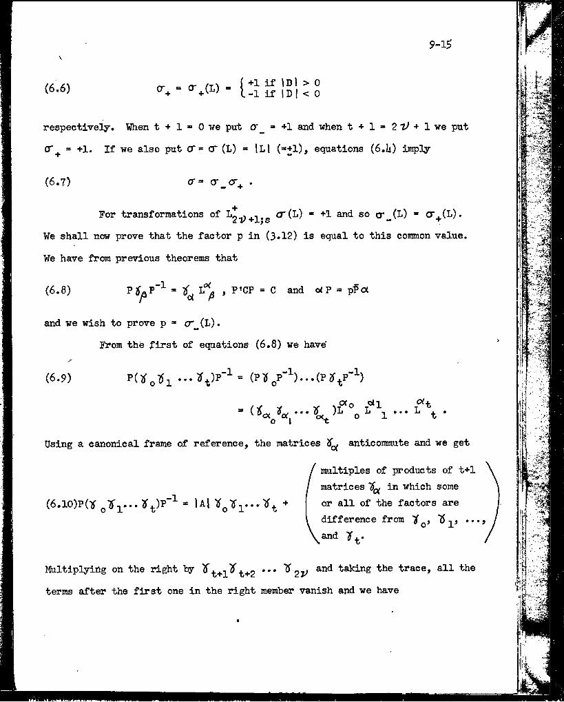
9-1^V
(6.6) +1 if \Dl > 0 -1 if 1 D I < 0
respectively. When t + 1 * 0 we put 〇r =• +1 and when t + l*2Z^+lwe put
(T^ “ +1. If we also put CT = CT (L) “ iLl (=+l), equations (6.1i) imply
(6.7) •
For transformations of 〇'(L) “ +1 and so cr_(L) = 〇r^(L).
We shall now prove that the factor p in (3»12) is equal to this common value.
We have from previous theorems that
(6.8) ^ ^
and we wish to prove p = cr_(L).
From thte first of equations (6.8) we have'
(6.9) P()(〇7ii (PigP''^)...(Pi^P'’^)
" i ®cx «oi, • * * o ^ 1 »• • L ^ .O I T
Using a canonical frame of reference, the matrices ^ anticommute and we get
(6.1〇)P(7T QlTi.-.y^.)P"^ = lAl +
multiples of products of t+1 matrices 7^ in which some or all of the factors are difference from •••and 7T^.
Multiplying on the right ly ^^+]L^'t+2 *** ^ 2V taking the trace, all the
terms after the first one in the right member vanish and we have
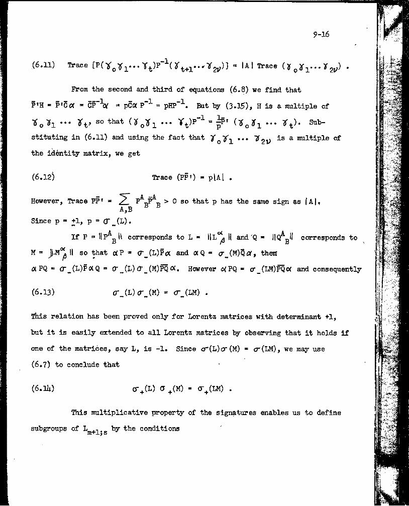
9-16
,(6.11) Trace [P(V〇yi‘-* “ lAl Trace (H y. li .
From the second and third of equations (6.8) we find that P’H = P'Cof = CP“V = pca P"^ = pHP"^. But by (3.15), H is a imiltiple of
^^0^1 *•* ^^0^1 *•* '^0-
stituting in (6.11) and using the fact that ... Tfis a multiple of
the identity matrix, we get
(6.12) Trace (PP〇 = pUl .
However, Trace PP’ * > 0 so that p has the same sign as (A|,A,B ^ "
Since p = +1, p = CT_(L).If P « llP^gll corresponds to L = II and 'Q » corresponds to
M = 'I so "that 〇(P “ (T_(L)P(X and 〇( Q = (7_(M)5cir, theh
(X PQ = CT_(L)P〇(Q = <T_(L) ¿T_(M)PQ〇<. However o(PQ » £T_(LH)^0( and consequently
(6.13) £T_(L)(r_(M) = cr_(LM) .
ltds relation has been proved only for Lorentz matrices with determinant +1,
but it is easily extended to all Lorentz matrices ty observing that it holds if
one of the matrices, say L, is -1. Since 〇r(L)a'(M) = cr(LM), we may use
(6.7) to conclude that
(6.1i;) CT^.(L) a ^(M) = (T^(LM) .
This multiplicative property of the signatures enables us to define
subgroups of ^7 "the conditions
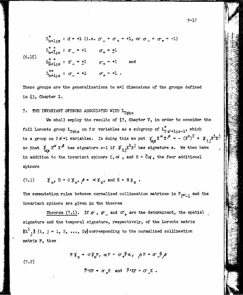
9-17
(6.1^)
T .■^m+lis • 〇■ “ +1 (i.e. n+bH
1
b +1, or cr _ = cr^ "= -1)
+ +^m+Ijs 〇r_ “ +1
1—1 + 1
II+b
T+ +L— im+ljs 〇r_ = +1 cr+ = +1 and
++\l+lj s 〇*_
iH+n
cr^ = +1 .
These groups are the generalizations to m+1 dimensions of the groups defined
in §3j Chapter I.
7. THE INVARIANT SPINORS ASSOCIATED WITH
We shall en^jloy the results of §7, Chapter V, in order to consider the
full Lorentz group variables as a subgroup of whichis a group on 2t^+l variables. In doing this we put / = - (X°)^ + .X^^
«/〇 ijso ,that If, X^ X^ has signature s-1 if 2T. .X^X^ has signature s. We then have ^
XJin addition to the invariant spinors C, oi , and H = CcV , the four additional
spinors
(7.1) D = C7i〇, ^ and K = Hii^ .
The commutation rules between normalized collineation matrices in ^2'^-X
invariant spinors are given in the theorem
Theorem (7.1). If cr , 〇r and are the determinant, the spatial
signature and the temporal signature, respectively, of the Lorentz matrix
(i, j = 1, 2, ..., 2v)corresponding to the normalized collineation
matrix P, then
(7.2)= cry^P, 〇(P =■ <r^p«, ^p = y^
P'HP « cr^H and P»KP = <yy .
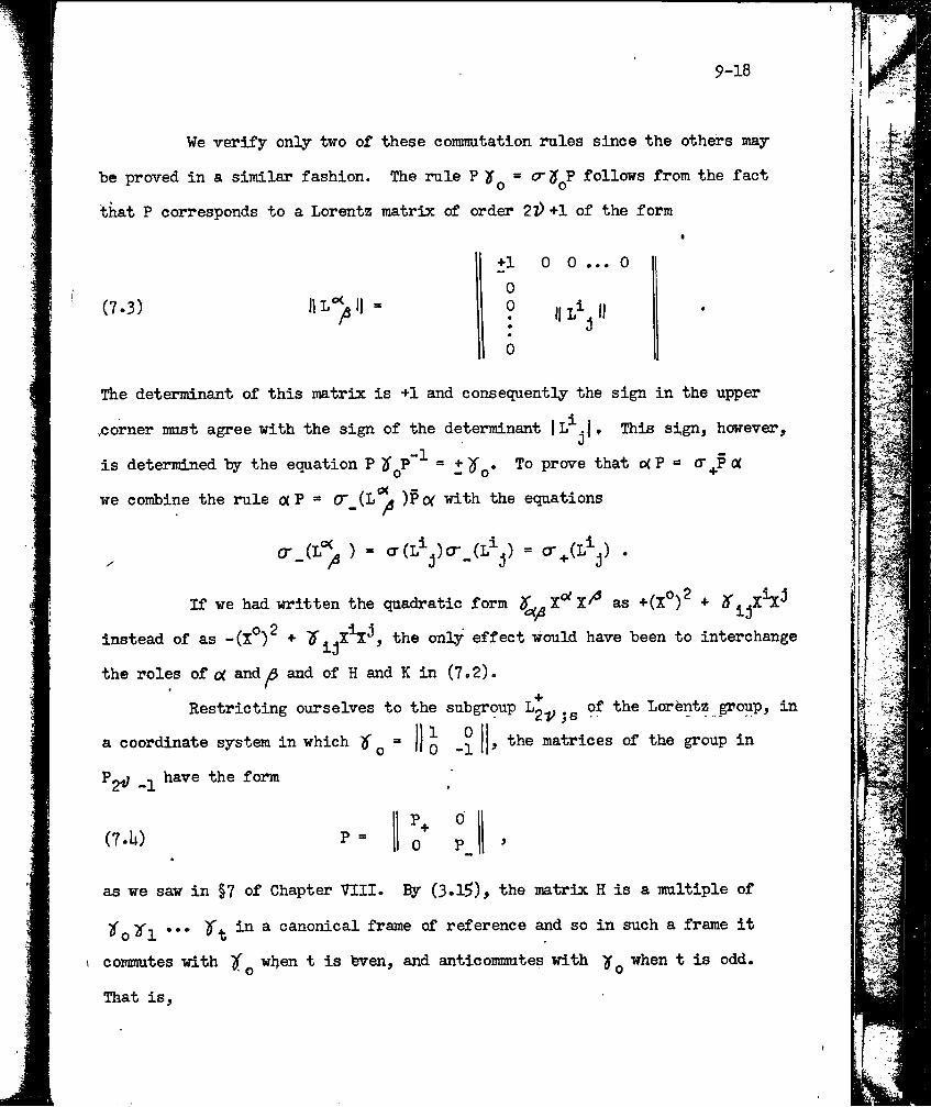
9-18
We verify only two of these comimatation rules since the others may
be proved in a similar fashion. The rule P follows from the fact
ihat P corresponds to a Lorentz matrix of order 2l) +1 of the form
(7.3)
+1 0 0 ... 0
II00
50
The determinant of this matrix is +1 and consequently the sign in the upper
.corner must agree with the sign of the determinant iL^.j. This sign, however,
is determined by the equation P 2T^P ^ To prove that 〇( P “ o’^ oi
we combine the rule o(P ® )P〇^ with the equations
CT_(l‘^ ) = <T(L^j)cr_(L^j) * .
If we had written the quadratic form as +(X°)^ +
instead of as -(X°)^ + the only effect would have been to interchange
the roles of 〇( and^ and of H and K in (7.2).
Restricting ourselves to the subgroup .g "the Lorentz group, in a coordinate system in which iT ^ = ]) 〇 matrices of the group in
Pj^ -1 form
(7.U) P =0p
as we saw in §7 of Chapter VIII. By 〇.l5), the matrix H is a multiple of
^0^1 *** ^t ^ canonical frame of reference and so in such a frame it
commutes with when t is feven, and smticommutes with when t is odd.
That is.
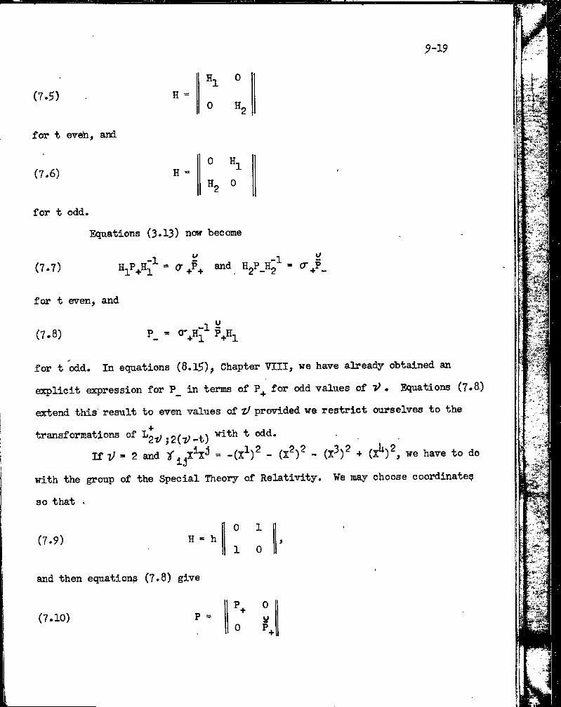
.9-19
(7.9)
for t eveh, and
(7.6)
for t odd.
H
Equations (3.13) notr become
(7.7)-1 ~ -1 \j
for t even, and
(7.8) P_ =
for t "odd. In equations (8.19), Chapter VIII, we have already obtained an
explicit expression for P_ in terms of for odd values of V . Equations (7.8.)
extend this result to even values of Z/ provided we restrict ourselves to the
transformations of .2(-z; r-t) ^If “ 2 and = -(X^)^ - (X^)^ - (X^)^ + (X^)^, we have to do
with the group of the Special Theory of Relativity. We may choose coordinate?
so that '
(7.9) H = h0
1 0
and then equation? (7.8) give
0
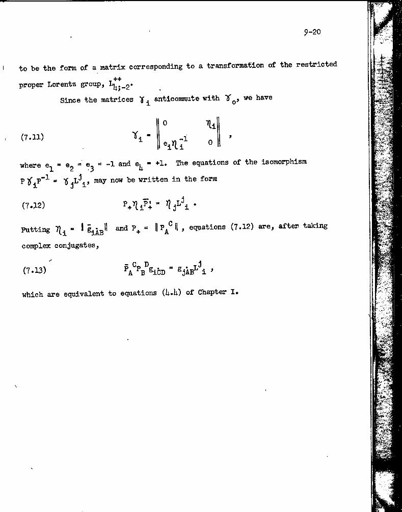
?-20
to be the form of a matrix corresponding to a transformation of the restricted
++proper Lorentz group,
Since the matrices Y ^ anticomniate with we have
(7.11)
0 ’ll
0
where e^ = e^ = « -1 and ej^ * +1. The equations of the isomorphism
p , may now be written in the form
(7.12)
Putting 7}^ - I and P^ - li/H , equations (7.12) are, after taking
complex conjugates.
(7.13) B ^iCD ®jAB^ i
\
which are equivalent to equations (U.U) of Chapter I