Genetic diversification in the Tropical Western Atlantic Ocean

Phylogeography of the gastropod Bulla occidentalis

Thesis for the degree of Master of Science in Biology

Biodiversity, evolution and ecology

by Jørgen Aarø

Department of Biology

University of Bergen

June 2011

2

TABLE OF CONTENTS

1. ABSTRACT . . . . . . . . . . 1

2. INTRODUCTION . . . . . . . . 3

2.1. Biogeography of the Tropical Western Atlantic . . . . 3

2.2. Genetic discontinuities in the Tropical Western Atlantic . . . 4

2.3. Physical and geological description of the Tropical Western Atlantic Ocean 6

2.3.1. The outer-Atlantic region . . . . . . 6

2.3.2. The Caribbean sea and the Gulf of Mexico . . . . 8

2.3.3. Bathtmetry and sea level variation . . . . . 9

2.4. Model species: Bulla occidentalis . . . . . . 10

2.4.1. Phylogeny, ecology and palaeontological history . . . 10

2.4.2. Genetic differentiation . . . . . . 12

2.5. Choice of genetic markers . . . . . . . 13

2.6. Project aims . . . . . . . . . 13

3. MATERIAL AND METHODS . . . . . . 15

3.1. Sampling . . . . . . . . . 15

3.2. DNA extraction, PCR and sequencing . . . . . 16

3.3. DNA analyses . . . . . . . . 19

3.3.1. Assembly and alignment . . . . . 19

3.3.2. Molecular clocks . . . . . . 19

3.3.3. Population genetics . . . . . 19

3.3.4. Phylogenetic analysis and estimating divergence times . 21

3.3.5. Demographic history of Bulla occidentalis . . 22

3.3.6. Isolation by distance . . . . . 23

4. RESULTS . . . . . . . . . 25

4.1. Sequence analysis . . . . . . . . 25

4.2. Molecular clocks . . . . . . . . 26

4.3. Population genetic structure . . . . . . 27

4.4. Haplotype networks . . . . . . . 32

4.5. Phylogenetic analysis and estimating divergence times . . . 32

4.6. Demographic history . . . . . . . 34

4.7. Isolation by distance . . . . . . . 34

5. DISCUSSION . . . . . . . . . 37

5.1. Species genealogy and genetic diversity . . . . . 37

5.2. Patterns and forces of marine diversification in the TWA . . . 38

5.2.1. Are present isolating mechanisms detectable for Bulla occidentalis? 38

5.2.2. Historical patterns and processes . . . . . 40

5.3. Demographic history . . . . . . . 42

6. CONCLUSIONS . . . . . . . . . 45

7. ACKNOWLEDGEMENTS . . . . . . . . 47

8. REFERENCES . . . . . . . . . 49

APPENDIX I . . . . . . . . . . 57

APPENDIX II . . . . . . . . . . 60

APPENDIX III . . . . . . . . . . 61

APPENDIX IV . . . . . . . . . . 62

1. ABSTRACT

The region under study is the Tropical Western Atlantic (TWA) which includes the Caribbean Sea

with adjacent coastlines, the Gulf of Mexico, Bermuda and the coast of South America down to the

tropical/temperate transitional zone near Uruguay. There are several examples of genetic breaks

within the Caribbean that have been attributed to oceanographic factors, transient allopatry, as well

as ecological factors, but no common biogeographical pattern has been found and mechanisms

behind diversification within the region are not fully understood. The aim of this project was to

shed light on diversification patterns of shallow-water soft-bottom invertebrates in the TWA by

using the gastropod Bulla occidentalis as a model species. The following questions were adressed:

(1) Is B. occidentalis a homogenous genetic entity or is it made-up of more than one genetic

partition (ESUs) as hypothesized by Malaquias and Reid (2009)? (2) What caused the pattern of

genetic discontinuities (ESUs)? (3) Are the genetic breaks shared with other species? and (4) Are

there periods of major expansion or contraction in population size and what may have caused these

events? Material was obtained from museum collections and through fieldwork, and sequences

fragments of the cytochrome c oxidase subunit I (COI) and 16S rRNA mitochondrial genes were

amplified and sequenced using standard methods. Population genetic indices such as number of

haplotypes, haplotype diversity, nucleotide diversity, and fixation indices were estimated, and

statistical parsimony haplotype networks for the individual genes were constructed to assess the

population structure. The B. occidentalis species genealogy with divergence times between main

lineages was estimated based on calibration with the oldest known fossil attributed to the B.

occidentalis lineage (Early Miocene, 20,43 – 15,97 Mya) under the assumption of a strict molecular

clock. Isolation-by-distance methods were employed to test correlation between genetic

differentiation and geographic distance. The demographic history was reconstructed using a

Bayesian Skyline method. The B. occidentalis population showed a structured genealogy with three

ESUs (A: all coastline samples from Brazil to Eastern Florida, including Yucatan and the islands of

Guadeloupe and Bermuda; B: all samples from the Florida Keys; C: predominantly Cuban

samples). The three lineages had an average genetic distance of 4,6% – 5,9% (uncorrected p-

distance). Divergence between the three lineages was dated to the Late Miocene (11,06 – 6,11

Mya), and may have been caused by vicariance related to the Panamanian Isthmus up-lift. The

mechanisms maintaining divergence of these lineages are difficult to pinpoint because no direct link

was established between the geographical subdivision and present oceanographic patterns,

ecological factors or Isolation-by-distance. Genetic divergence of the Florida Keys-lineage mirrors

1

patterns found in other groups. The genealogy and demographic history reconstruction showed an

increase in genetic diversification and effective population size during the Pleistocene. This

coincides with an increase in the magnitude of glaciation cycles that may have caused periods of

transient allopatry likely reducing population connectivity leading to genetic diversification, as well

as potentially creating new niche-opportunities during low sea-level stands allowing the population

to expand.

2

2. INTRODUCTION

2.1. Biogeography of the Tropical Western Atlantic

The aim of phylogeography is to understand intra-specific and species-complex patterns of

divergence and how they coincide with present-day and historical geologic and geographic features

and processes (Chan et al. 2011). The geographical area under study in this research project is the

Tropical Western Atlantic (TWA) as defined by Spalding et al. (2007): the Caribbean Sea with

adjacent coastlines, Bermuda and the coast of South America down to the tropical/temperate

transitional zone near Uruguay, but in addition including the Gulf of Mexico.

The TWA is a region that has been through large changes in recent geological history. The rise of

the Panamanian Isthmus, a process taking place over 12 million years, and reaching completion

approximately 2.8 Ma ago, had large consequences for ocean circulation patterns, global climate,

and evolution of both marine and terrestrial organisms (Coates and Obando 1996; Lessios 2008).

The changes in the Tropical Western Atlantic environment included new current patterns as well as

raised temperature and salinity, which in turn marked the onset of glaciaction cycles and increasing

eustatic changes during the Pliocene (5,332-2,588 Mya) and Pleistocene periods (2,588 Mya – 12

Kya) (Lessios 2008).

The TWA is traditionally divided into distinct biogeographic provinces identified and characterized

by unique assemblages of species and clades, but the exact names, numbers and boundaries of these

provinces vary somewhat between authors (summarized by Reid (2009)). At least two provinces are

commonly recognized within the TWA, the Caribbean and the Brazilian (Reid 2009), but a separate

West Indian province (including Bermuda, the Bahamas, the Leeward and Windward Antilles

Islands) has also been suggested (Briggs 1974). The northern bound of the Caribbean province is

placed somewhere along the east coast of the United States in a transition zone between Warm-

Temperate and Tropical climates and another such transitional zone was placed on the gulf-side of

the Florida peninsula, based on many examples of faunal breaks between Tropical Florida and the

temperate Gulf of Mexico (Briggs 1974). North of the Caribbean province lies the Carolinian, and

the division between these two have a long history dating back to the Early Miocene, represented by

the Caloosahatchian province (North Carolina to Florida and the Yucatán peninsula) and the

Gatunian province (includes the Caribbean) (Vermeij 2005). A major feature along the north-eastern

3

coast of South America, separating the Caribbean and Brazilian provinces is the Amazon Barrier,

which is created by freshwater run-off from the Orinoco and Amazon rivers that was established in

its present form during the Pliocene (Briggs 1974; Campbell Jr. et al. 2006)). This over 2300

kilometre stretch of coastline is influenced by sediment-rich freshwater forming a plume of lower

salinity that represents a biogeographic barrier for many species (Rocha 2003). The Brazilian

province stretches to the southern transitional zone between tropical and warm-temperate climates

near Uruguay.

Taxonomically based biogeographic subdivisions have traditionally been defined by unique

assemblies of groups at low taxonomic levels. These are, however, seldom exhaustive. For instance

the system proposed by Briggs (1974) was mostly based on fish, and for the Caribbean, subdivision

has largely been based on taxonomic levels in the range from Class to Family (Miloslavich et al.

2010). Recently an attempt was made at making a global classification of the marine environment

based on the presence of homogenous composition of species, and the predominance of a small

number of ecosystems, oceanographic and topographic features (Spalding et al. 2007), but this was

not consistently supported by a later regionalization (Miloslavich et al. 2010). Focus on certain

taxonomic groups or focusing on higher taxonomic levels will result in species distributions

sometimes failing to be consistent with established subdivisions (Miloslavich et al. 2010). For

bivalves and gastropods in the Caribbean no general pattern of species distributions exists (with

exceptions in Yucatán and Belize), suggesting that distribution of species in the Caribbean is

controlled by availability of different habitat types (Miloslavich et al. 2010). There are, however,

certain examples of groups at low taxonomic levels (genus and family) that show specific patterns

in their distribution due to vicariant events during the evolution of the Caribbean Sea, and this

variation can be masked if focus lies on higher taxonomic levels (Miloslavich et al. 2010).

Miloslavich et al. (2010) suggest that the Caribbean as a whole is a distinctive sub-region of the

Northern Tropical Western Atlantic Province, but that the region is not biogeographically uniform

due to its complex geological history, and present-day geographic variation in hydrologic and

habitat regimes.

2.2. Genetic discontinuities in the Tropical Western Atlantic

A large part of the TWA is the Caribbean Sea, which is known to be a marine biodiversity hotspot

(Roberts et al. 2002; Miloslavich et al. 2010) despite being a fairly compact area with few obvious

4

physical barriers and large degree of faunal homogeneity (Taylor and Hellberg 2006; Reid 2009).

Despite this perceived uniformity there are several examples of established genetic breaks within

species, suggesting that some drivers of genetic differentiation do exist (Brachidontes exustus, Lee

and Ó Foighil 2005; Elacatinus sp., Taylor and Hellberg 2006; Bulla occidentalis, Malaquias and

Reid 2009; Cittarium pica, Diaz-Ferguson et al. 2010). Both ecological and vicariant explanations

have been offered, but the processes seem to differ between different animal groups, and patterns of

genetic discontinuities do not seem consistent between animal groups (Taylor and Hellberg 2006;

Rocha et al. 2008; Diaz-Ferguson et al. 2010).

Strong evidence was found for the presence of a phylogenetic break in the Mona Passage between

the islands of Hispaniola and Puerto Rico islands for different ecologies of the coral reef fish genus

Elacatinus (Taylor and Hellberg 2006). The strong northbound current through the passage was

thought to inhibit dispersal between the two islands, thereby causing a genetic discontinuity. Weak

support for a genetic barrier was also found in the Exuma Sound of the Bahamas, but if present, this

is likely established later than the Mona barrier (Taylor and Hellberg 2006).

Another approach for identifying genetic discontinuities and recognizing regions of high

connectivity, thereby also biogeographic break points, is by the use of hydrodynamic models of

larval dispersal (fish, Cowen et al. 2006). Cowen et al. (2006) detected the presence of four such

connectivity-regions, corresponding to the Eastern Caribbean, Western Caribbean, the Bahamas-

region and the coastlines influenced by the Colombia-Panama gyre. The central Caribbean was

suggested to be a zone of admixture, mediating a low level of connectivity between regions. These

four connectivity regions were only partly supported by the genetic structure of the trochid

gastropod Cittarium pica (Diaz-Ferguson et al. 2010). A low level of differentiation was uncovered

between the Eastern Caribbean and the Bahamas, a Venezuelan population that was expected to

group with the Eastern Caribbean proved to be differentiated from all other groups and a

Panamanian population was strongly differentiated from geographically close populations in

Panama and Costa Rica. The authors viewed their results as supporting the Carribean as a uniform

biogeographical province, with high genetic diversity due to meso-scale oceanographic features

(Diaz-Ferguson et al. 2010). For instance, the Colombia-Panama gyre is likely causing some

isolation in the area encompassed by the coastlines of Colombia, Panama, Costa Rica and

Nicaragua, as is evident from the mentioned modelling experiment (Cowen et al. 2006) and from

the trochid gastropod Cittarium pica (Diaz-Ferguson et al. 2010). The Antilles Current (Figure 1) is

5

weak compared to the other mentioned currents which potentially creates a difference in dispersal

capacity in a East-North direction compared to a East-West direction along the Caribbean current.

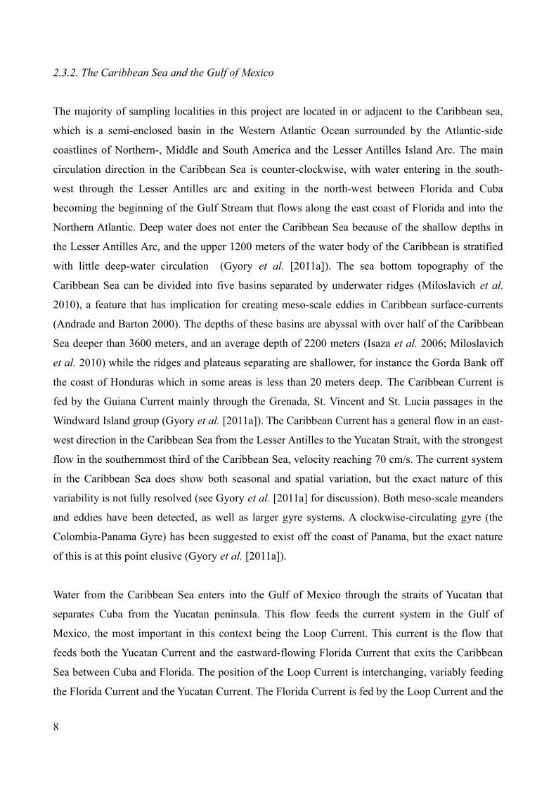
Figure 2 depicts variation in coastline range with variable sea levels, which likely made an impact

of connectivity within the adjacent areas of the Caribbean sea. This possibility is especially relevant

when discussing Pleistocene glacial cycles that have been taking place in the last 2,5 million years

(Lessios 2008; Miller et al. 2005). There is evidence for periods (or pulses) with a high rate of

mollusc extinctions and species origination in the Pleistocene, and these glaciation events could be

directly related to the diversification of Western Atlantic shallow water organisms (Lessios 2008).

Transient allopatry has been suggested as a potential mechanism producing species pairs along

single coastlines in the TWA and in the Tropical East Pacific Ocean for example in calyptraid

gastropods (Collin 2003).

2.3. Physical and geological description of the Tropical Western Atlantic Ocean

The flow of surface currents can have implications for potential genetic connectivity in marine

populations (White et al. 2010), and an understanding of the ocean surface current system in the

TWA is therefore a vital piece of the puzzle in uncovering underlying causes for genetic

discontinuities. The online service Ocean Surface Currents summarizes data from a vast amount of

literature on ocean surface currents. For convenience we divide the review into two parts; the

Caribbean Sea (including Tropical Florida) with the Gulf of Mexico, and the outer-Atlantic region

(Bermuda, Brazil, and the Atlantic ocean east of the Antilles). The most relevant and general

information is included here to produce a broad picture of the Tropical Western Atlantic surface

current-system, but for detailed information on the current system, see the Ocean Surface Currents

website (http://oceancurrents.rsmas.miami.edu/index.html).

2.3.1. The outer-Atlantic region

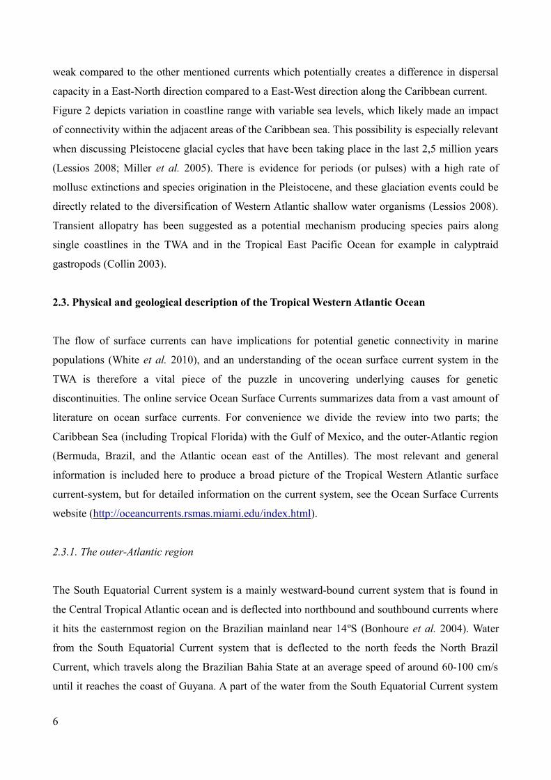
The South Equatorial Current system is a mainly westward-bound current system that is found in

the Central Tropical Atlantic ocean and is deflected into northbound and southbound currents where

it hits the easternmost region on the Brazilian mainland near 14ºS (Bonhoure et al. 2004). Water

from the South Equatorial Current system that is deflected to the north feeds the North Brazil

Current, which travels along the Brazilian Bahia State at an average speed of around 60-100 cm/s

until it reaches the coast of Guyana. A part of the water from the South Equatorial Current system

6

travels in a north-eastward direction, feeding the North Equatorial Counter-Current or feeding the

Caribbean Current depending on the season (Bischof et al. 2003). The North Brazil Current feeds

the Guiana Current which has a mean velocity that is measured to be 41.6 cm/s. The Guiana Current

enters the Caribbean Sea mostly through the Windward Islands and constitutes the majority of the

water that enters the Caribbean Sea (about 70%). The Guiana Current varies in flow velocity during

the year, and with the peak speeds observed in April-May and a minimum speed in September. The

Antilles Current flows from the northern Lesser Antilles north-west into the Florida Current, but is

of a variable nature and its existence has been discussed (Rowe et al. 2011).

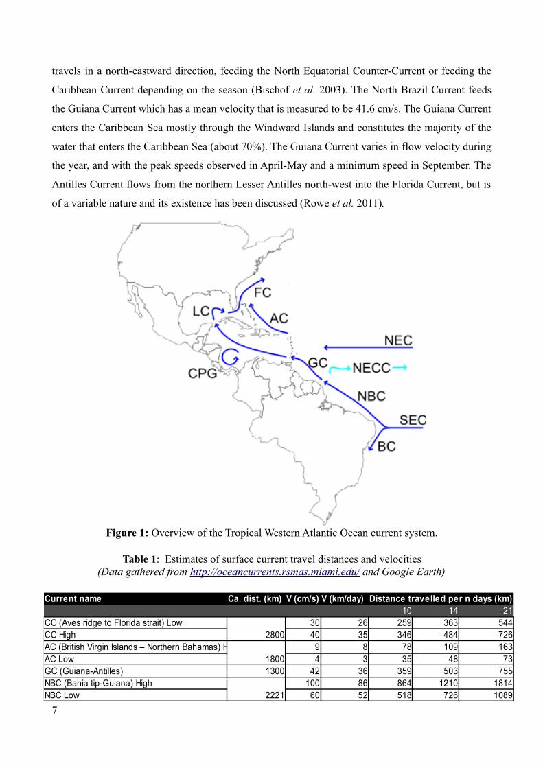
Table 1: Estimates of surface current travel distances and velocities(Data gathered from http://oceancurrents.rsmas.miami.edu/ and Google Earth)

7

FC= Florida CurrentLC = Loop CurrentAC = Antilles CurrentGC = Guiana CurrentNEC = North Equatorial CurrentNECC = North Equatorial Counter-CurrentNBC = North Brazil CurrentSEC = South Equatorial CurrentBC = Brazil CurrentCPG = Colombia-Panama Gyre

Figure 1: Overview of the Tropical Western Atlantic Ocean current system.

Current name Ca. dist. (km) V (cm/s) V (km/day) Distance travelled per n days (km)86400 10 14 21

CC (Aves ridge to Florida strait) Low2800

30 26 259 363 544CC High 40 35 346 484 726AC (British Virgin Islands – Northern Bahamas) High

18009 8 78 109 163

AC Low 4 3 35 48 73GC (Guiana-Antilles) 1300 42 36 359 503 755NBC (Bahia tip-Guiana) High

2221100 86 864 1210 1814

NBC Low 60 52 518 726 1089

2.3.2. The Caribbean Sea and the Gulf of Mexico

The majority of sampling localities in this project are located in or adjacent to the Caribbean sea,

which is a semi-enclosed basin in the Western Atlantic Ocean surrounded by the Atlantic-side

coastlines of Northern-, Middle and South America and the Lesser Antilles Island Arc. The main

circulation direction in the Caribbean Sea is counter-clockwise, with water entering in the south-

west through the Lesser Antilles arc and exiting in the north-west between Florida and Cuba

becoming the beginning of the Gulf Stream that flows along the east coast of Florida and into the

Northern Atlantic. Deep water does not enter the Caribbean Sea because of the shallow depths in

the Lesser Antilles Arc, and the upper 1200 meters of the water body of the Caribbean is stratified

with little deep-water circulation (Gyory et al. [2011a]). The sea bottom topography of the

Caribbean Sea can be divided into five basins separated by underwater ridges (Miloslavich et al.

2010), a feature that has implication for creating meso-scale eddies in Caribbean surface-currents

(Andrade and Barton 2000). The depths of these basins are abyssal with over half of the Caribbean

Sea deeper than 3600 meters, and an average depth of 2200 meters (Isaza et al. 2006; Miloslavich

et al. 2010) while the ridges and plateaus separating are shallower, for instance the Gorda Bank off

the coast of Honduras which in some areas is less than 20 meters deep. The Caribbean Current is

fed by the Guiana Current mainly through the Grenada, St. Vincent and St. Lucia passages in the

Windward Island group (Gyory et al. [2011a]). The Caribbean Current has a general flow in an east-

west direction in the Caribbean Sea from the Lesser Antilles to the Yucatan Strait, with the strongest

flow in the southernmost third of the Caribbean Sea, velocity reaching 70 cm/s. The current system

in the Caribbean Sea does show both seasonal and spatial variation, but the exact nature of this

variability is not fully resolved (see Gyory et al. [2011a] for discussion). Both meso-scale meanders

and eddies have been detected, as well as larger gyre systems. A clockwise-circulating gyre (the

Colombia-Panama Gyre) has been suggested to exist off the coast of Panama, but the exact nature

of this is at this point elusive (Gyory et al. [2011a]).

Water from the Caribbean Sea enters into the Gulf of Mexico through the straits of Yucatan that

separates Cuba from the Yucatan peninsula. This flow feeds the current system in the Gulf of

Mexico, the most important in this context being the Loop Current. This current is the flow that

feeds both the Yucatan Current and the eastward-flowing Florida Current that exits the Caribbean

Sea between Cuba and Florida. The position of the Loop Current is interchanging, variably feeding

the Florida Current and the Yucatan Current. The Florida Current is fed by the Loop Current and the

8

Antilles Current with the main portion coming from the Loop Current, which is considered to be the

beginning of the Gulf Stream (Gyory et al. [2011b]).

2.3.3. Bathtmetry and sea level variation

Global sea level changes (eustasy) related to the formation and melting of continental ice-sheets can

happen very rapidly, up to 200 meters pr. thousand years for the formation of ice-sheets and

9

Figure 2: Illustration showing Caribbean coastlines at A) present sea level B) Sea-level 150 meters below todays level (as during Pleistocene glacial maxima). Dark grey areas show depths of 0-50 m. Adapted from Bellwood and Wainwright (2002).

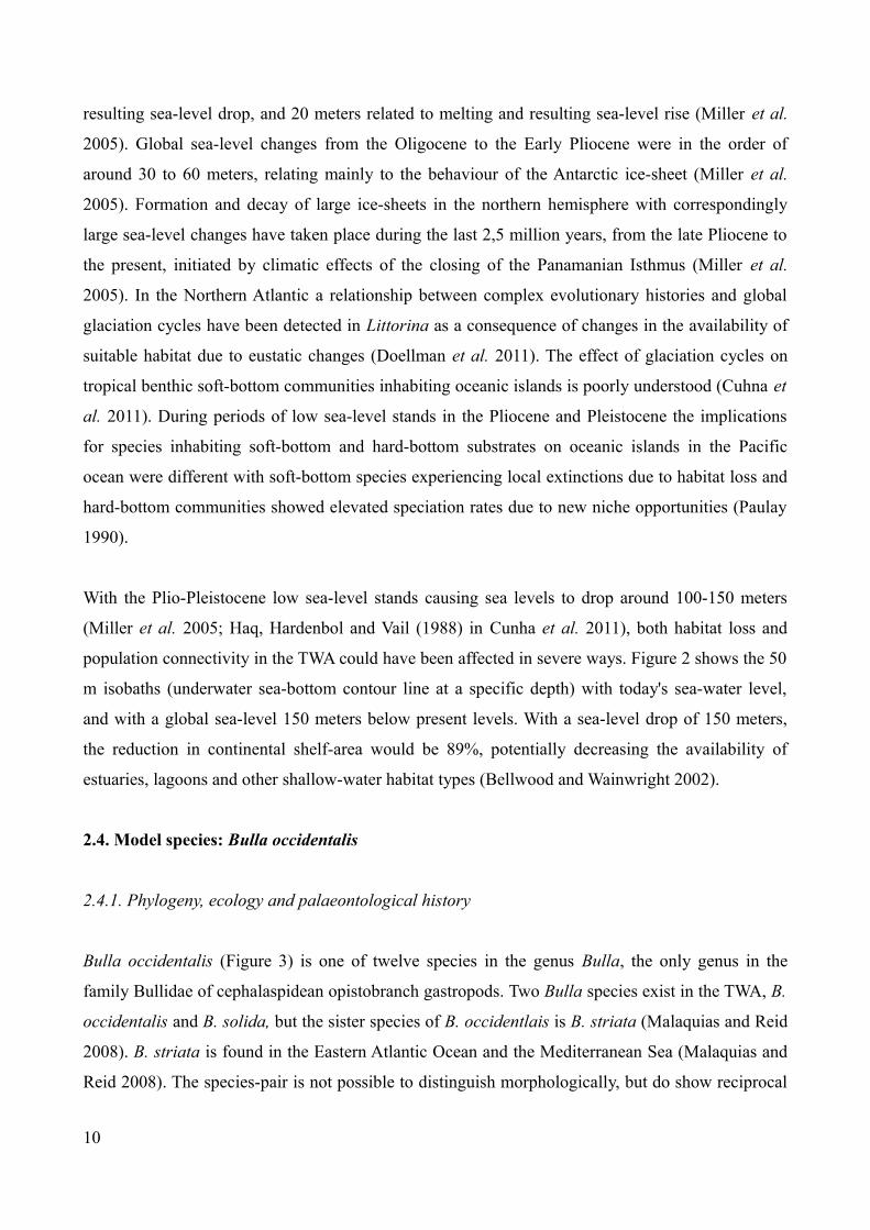
resulting sea-level drop, and 20 meters related to melting and resulting sea-level rise (Miller et al.

2005). Global sea-level changes from the Oligocene to the Early Pliocene were in the order of

around 30 to 60 meters, relating mainly to the behaviour of the Antarctic ice-sheet (Miller et al.

2005). Formation and decay of large ice-sheets in the northern hemisphere with correspondingly

large sea-level changes have taken place during the last 2,5 million years, from the late Pliocene to

the present, initiated by climatic effects of the closing of the Panamanian Isthmus (Miller et al.

2005). In the Northern Atlantic a relationship between complex evolutionary histories and global

glaciation cycles have been detected in Littorina as a consequence of changes in the availability of

suitable habitat due to eustatic changes (Doellman et al. 2011). The effect of glaciation cycles on

tropical benthic soft-bottom communities inhabiting oceanic islands is poorly understood (Cuhna et

al. 2011). During periods of low sea-level stands in the Pliocene and Pleistocene the implications

for species inhabiting soft-bottom and hard-bottom substrates on oceanic islands in the Pacific

ocean were different with soft-bottom species experiencing local extinctions due to habitat loss and

hard-bottom communities showed elevated speciation rates due to new niche opportunities (Paulay

1990).

With the Plio-Pleistocene low sea-level stands causing sea levels to drop around 100-150 meters

(Miller et al. 2005; Haq, Hardenbol and Vail (1988) in Cunha et al. 2011), both habitat loss and

population connectivity in the TWA could have been affected in severe ways. Figure 2 shows the 50

m isobaths (underwater sea-bottom contour line at a specific depth) with today's sea-water level,

and with a global sea-level 150 meters below present levels. With a sea-level drop of 150 meters,

the reduction in continental shelf-area would be 89%, potentially decreasing the availability of

estuaries, lagoons and other shallow-water habitat types (Bellwood and Wainwright 2002).

2.4. Model species: Bulla occidentalis

2.4.1. Phylogeny, ecology and palaeontological history

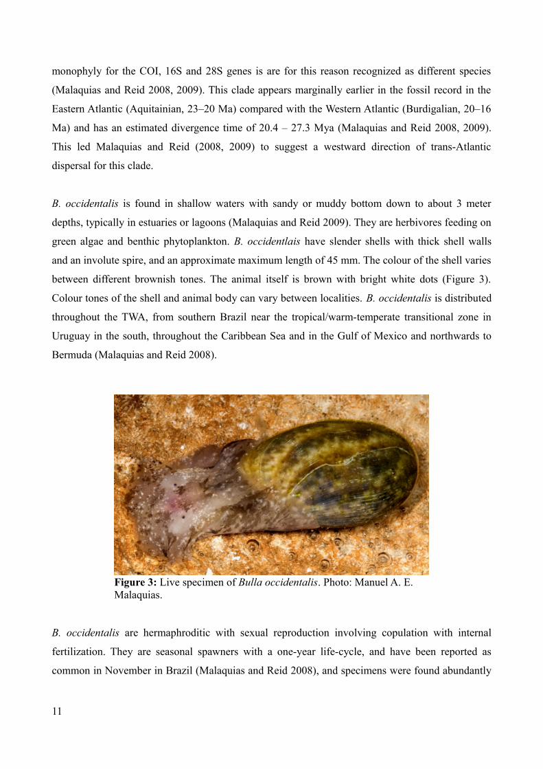
Bulla occidentalis (Figure 3) is one of twelve species in the genus Bulla, the only genus in the

family Bullidae of cephalaspidean opistobranch gastropods. Two Bulla species exist in the TWA, B.

occidentalis and B. solida, but the sister species of B. occidentlais is B. striata (Malaquias and Reid

2008). B. striata is found in the Eastern Atlantic Ocean and the Mediterranean Sea (Malaquias and

Reid 2008). The species-pair is not possible to distinguish morphologically, but do show reciprocal

10

monophyly for the COI, 16S and 28S genes is are for this reason recognized as different species

(Malaquias and Reid 2008, 2009). This clade appears marginally earlier in the fossil record in the

Eastern Atlantic (Aquitainian, 23–20 Ma) compared with the Western Atlantic (Burdigalian, 20–16

Ma) and has an estimated divergence time of 20.4 – 27.3 Mya (Malaquias and Reid 2008, 2009).

This led Malaquias and Reid (2008, 2009) to suggest a westward direction of trans-Atlantic

dispersal for this clade.

B. occidentalis is found in shallow waters with sandy or muddy bottom down to about 3 meter

depths, typically in estuaries or lagoons (Malaquias and Reid 2009). They are herbivores feeding on

green algae and benthic phytoplankton. B. occidentlais have slender shells with thick shell walls

and an involute spire, and an approximate maximum length of 45 mm. The colour of the shell varies

between different brownish tones. The animal itself is brown with bright white dots (Figure 3).

Colour tones of the shell and animal body can vary between localities. B. occidentalis is distributed

throughout the TWA, from southern Brazil near the tropical/warm-temperate transitional zone in

Uruguay in the south, throughout the Caribbean Sea and in the Gulf of Mexico and northwards to

Bermuda (Malaquias and Reid 2008).

B. occidentalis are hermaphroditic with sexual reproduction involving copulation with internal

fertilization. They are seasonal spawners with a one-year life-cycle, and have been reported as

common in November in Brazil (Malaquias and Reid 2008), and specimens were found abundantly

11

Figure 3: Live specimen of Bulla occidentalis. Photo: Manuel A. E. Malaquias.

in Venezuela during March 2010 (M. A. E. Malaquias), Panama during June 2010 (M. Kambestad),

and Guadeloupe in July 2010 (by the author). In the latter three cases the specimens were not yet

full adults. They produce an egg-mass that is deposited on benthic vegetation, often sea-grass

(Malaquias and Reid 2008). Little is known about the dispersal capabilities of B. occidentalis, as

these have never been specifically studied. The precence of a planktotrophic veliger larva has been

detected in B. gouldiana, B. solida and B. striata, but the exact longevity is not known. Larval

development of B. striata has been observed under experimental conditions, and shown to last at

least ten days (Murillo and Templado 1998). However, in this study the development was

prematurely terminated so this can only serve as a minimum estimate of larval longevity. The

detected presence of a planktotrophic veliger larva in three different Bulla species and similarities

between the protoconch of all Bulla could be an indication for similar development throughout the

genus (Malaquias and Reid 2009). Typically, shelled cephalspids with indirect development last in

average two to four weeks in the plankton (Schaeffer 1996).

2.4.2. Genetic differentiation

B. occidentalis is considered to be a single species, but harbours a large degree of genetic

differentiation within its distributional range. Malaquias and Reid (2009) identified four

Evolutionary Significant Units (ESUs) with genetic distance between 5,5% - 8% (uncorrected p-

distance for the COI mitochondrial gene). The explanation for this large genetic differentiation was

suggested to be related to ecological selection across continental and oceanic lineages (Malaquias

and Reid 2009). The differences in habitats are thought to be due to larger nutrient influx to the

continental shelf by freshwater run-off from the continents as well as upwelling, while oceanic

environments like in the Caribbean islands are thought to be poorer in nutrients. This explanation

has been suggested for different organisms (Brachidontes exustus, Lee and Ó Foighil 2005; Bulla

occidentalis, Malaquias and Reid 2008; Echinolittorina, Reid 2009). Because of a small sample size

(n=20), the result could only be seen as provisional, and the need for further examination was

suggested by the authors. An increase in samples size and sampling localities will give the analysis

better resolution to discover patterns at a more detailed level, as well as lowering the influence of

sampling stochasitcity in the observed pattern.

12

2.5. Choice of genetic markers

The mitochondrial COI-gene was selected as an appropriate marker for this study because of its

potential to reveal intra-specific genetic variability. Because mitochondrial DNA has a smaller

effective population size (Ne) than nuclear DNA, variation in the mitochondrial genome becomes

detectable at a more rapid pace (Sunnucks 2000). The less variable mitochondrial 16S rRNA gene

was also selected for use as a marker. COI is a protein-coding gene while 16S is a structural rRNA

subunit in the mitochondrial ribosome and both are part of the same locus, but are under different

selective pressures due to functional constraints (Mueller 2006). Previous work on B. occidentalis

used both COI and 16S as genetic markers (Malaquias and Reid 2008, 2009), making it practical to

continue using these two as this data could be easily included in this study. In addition, COI and

16S are commonly used markers in phylogeographic studies of marine invertebrates (Siphonaria

pectinata, gastropod, Kawauchi and Giribet 2001; Patelloida profunda, gastropod, Kirkendale and

Meyer 2004; Doris kerguelenensis, nudibranch, Wilson et al. 2009; Brachidontes puniceus, mussel,

Cuhna et al. 2011).

2.6. Project aims

This phylogeographic study aims to contribute to the increased understanding of diversification of

shallow-water benthic organisms inhabiting soft-bottom habitats in the Western Tropical Atlantic

Ocean. This will be accomplished by further investigating the observed genetic diversity and

phylogeographic discontinuities detected in Bulla occidentalis by Malaquias and Reid (2009),

which in this context serves as a model organism. The data-set used by the latter authors will be

expanded both in number of specimens and localities, and Bayesian phylogenetic inference

calibrated with fossil data will be use to establish the genealogy and the time of diversification

events. The demographic history of the species will be inferred by Bayesian Skyline reconstruction,

and standard population genetic methods will be applied to uncover patterns of population structure.

The outcomes from these analyses will be related to past and present ecological, geological, and

oceanographic conditions in the TWA in an effort to uncover patterns and potential causes of marine

diversification in B. occidentalis. This will hopefully contribute to increasing the general

understanding of marine biogeography and diversification patterns in the Western Tropical Atlantic

Ocean.

13

We aim to answer the following questions:

1) Is Bulla occidentalis a homogenous genetic entity or is it made-up of more than one genetic

partition (ESUs) as hypothesized by Malaquias and Reid (2009)?

2) What caused the pattern of genetic discontinuities (ESUs)?

◦ Isolation due to geographical distance between localities?

◦ Isolation due to ecological selection: segregation across oceanic versus insular

habitats?

◦ Current Ocean circulation patterns and surface current-mediated genetic

connectivity?

◦ Pliocene-Pleistocene eustatic changes?

◦ Vicariant events in the geological evolution of the Tropical Western Atlantic Ocean?

3) Are the genetic breaks shared with other species?

4) Are there periods of major expansion or contraction in population size and what may have

caused these events?

14

3. MATERIAL AND METHODS

3.1. Sampling

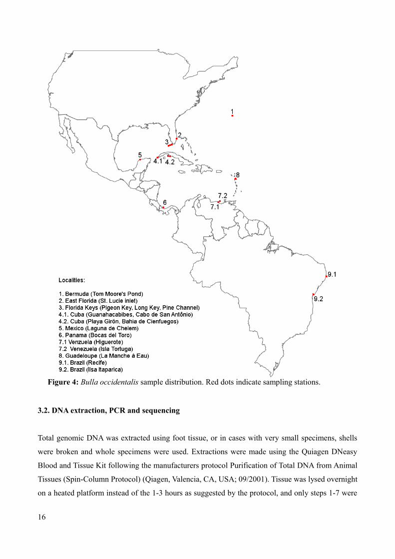
Specimens were acquired from museum collections as well as through field work performed by the

candidate, main supervisor, student colleagues and other acquaintances. A total number of 84 new

specimens have been used for DNA-extraction to produce a total dataset of 98 sequences including

sequences downloaded from GenBank (see Figure 4 for sampling sites, Table 2 for sample list and

Appendix I for detailed information). Field-work was performed by snorkelling and the collection

itself was done by hand picking or by use of simple tools like kitchen sieves. Collected specimens

were immediately preserved in 96% ethanol with ethanol volume approximately 3 times larger than

the volume of specimens in jars.

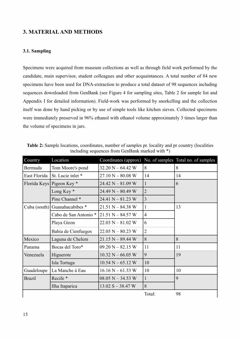
Table 2: Sample locations, coordinates, number of samples pr. locality and pr country (localities including sequences from GenBank marked with *)

Country Location Coordinates (approx) No. of samples Total no. of samplesBermuda Tom Moore's pond 32.20 N – 64.42 W 8 8East Florida St. Lucie inlet * 27.10 N – 80.08 W 14 14Florida Keys Pigeon Key * 24.42 N – 81.09 W 1 6

Long Key * 24.49 N – 80.49 W 2Pine Channel * 24.41 N – 81.23 W 3

Cuba (south) Guanahacabibes * 21.51 N – 84.38 W 1 13Cabo de San Antonio * 21.51 N – 84.57 W 4Playa Giron 22.03 N – 81.02 W 6

Bahia de Cienfuegos 22.05 N – 80.23 W 2Mexico Laguna de Chelem 21.15 N – 89.44 W 8 8Panama Bocas del Toro* 09.20 N – 82.15 W 11 11Venezuela Higuerote 10.32 N – 66.05 W 9 19

Isla Tortuga 10.54 N – 65.12 W 10Guadeloupe La Manche à Eau 16.16 N – 61.33 W 10 10Brazil Recife * 08.05 N – 34.53 W 1 9

Ilha Itaparica 13.02 S – 38.47 W 8Total: 98

15

3.2. DNA extraction, PCR and sequencing

Total genomic DNA was extracted using foot tissue, or in cases with very small specimens, shells

were broken and whole specimens were used. Extractions were made using the Quiagen DNeasy

Blood and Tissue Kit following the manufacturers protocol Purification of Total DNA from Animal

Tissues (Spin-Column Protocol) (Qiagen, Valencia, CA, USA; 09/2001). Tissue was lysed overnight

on a heated platform instead of the 1-3 hours as suggested by the protocol, and only steps 1-7 were

16

Figure 4: Bulla occidentalis sample distribution. Red dots indicate sampling stations.

performed to produce 200 µL of total genomic DNA extract. The steps are as follows: 1 - 2) lysis of

approximately 25 mg of tissue in 180 μL Qiagen ATL-buffer and 20 μL Qiagen proteinase-K, 3) 15

second vortexing and adding of 200 μL of each of Qiagen AL-buffer and 96% ethanol, 4) pipet

mixture into a Qiagen Dneasy spin-column placed in a 2 mL collection tube and centrifuge at 8000

rpm for 1 minute, 5) discard flow-through and collection tube and place spin column in new

collection tube before adding 500 μL Qiagen AW1-buffer and centrifuging for 1 minute at 8000

rpm, 6) discard flow-through and collection tube and place spin column in new collection tube

before adding 500 μL Qiagen AW2-buffer and centrifuging for 3 minutes at 14000 rpm, 7) place

spin-column in 1,5 mL microcentrifuge tube before pipetting 200 μL Qiagen AE-buffer, incubate

the sample at room temperature for 1 min before centrifuging for 1 minute at 8000 rpm, 8) repeat

step 7.

Approximately 700 bp COI DNA was amplified in 50 µL reactions containing 17,5 µL Sigma

Water, 5 µL Qiagen 10X PCR Buffer, 5 µL 2 µM dNTPS's, 10 µL Qiagen Q-solution, 7 µL 25 mM

MgCl2, 2 µL 10 µM of each of the primers HCO2198 and LCO1490 (Folmer et al. 1994), 0,5 µL

Qiagen Taq DNA Polymerase and 1 µL DNA-extract pr. sample. Sequences were amplified with an

initial denaturation phase of 95°C for 3 minutes, followed by 40 cycles with a 45 second 94°C

denaturation phase, a 45 second 45°C annealing phase and a 2 minute 72°C extension phase. The

program was finalized with 10 minutes at 72°C. Some of the COI-PCRs were performed using the

Qiagen HotStart+ TAQ polymerase, for which the initial denaturation phase was prolonged from 3

to 5 minutes.

Approximately 500 bp of the mitochondrial 16S-rRNA gene was amplified using the same amounts

of reagents as for COI, the only differences being the primers. The primers used for 16S PCRs were

16Sar-L and 16Sbr-H (Palumbi 2002). Qiagen HotStart+ TAQ polymerase was used for all 16S-

PCRs. Sequences were amplified with an initial denaturation phase of 95°C for 5 minutes, followed

by 39 cycles with a 45 second 94°C denaturation phase, a 45 second 51,5°C annealing phase and a

2 minute 72°C extension phase. The program was finalized with 10 minutes at 72°C. See Table 3

for primer details.

17

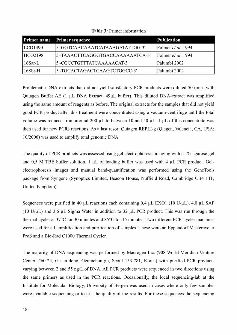
Table 3: Primer information

Primer name Primer sequence PublicationLCO1490 5'-GGTCAACAAATCATAAAGATATTGG-3' Folmer et al. 1994HCO2198 5'-TAAACTTCAGGGTGACCAAAAAATCA-3' Folmer et al. 199416Sar-L 5'-CGCCTGTTTATCAAAAACAT-3' Palumbi 200216Sbr-H 5'-TGCACTAGACTCAAGTCTGGCC-3' Palumbi 2002

Problematic DNA-extracts that did not yield satisfactory PCR products were diluted 50 times with

Quiagen Buffer AE (1 µL DNA Extract, 49µL buffer). This diluted DNA-extract was amplified

using the same amount of reagents as before. The original extracts for the samples that did not yield

good PCR product after this treatment were concentrated using a vacuum-centrifuge until the total

volume was reduced from around 200 µL to between 10 and 50 µL. 1 µL of this concentrate was

then used for new PCRs reactions. As a last resort Quiagen REPLI-g (Qiagen, Valencia, CA, USA;

10/2006) was used to amplify total genomic DNA.

The quality of PCR products was assessed using gel electrophoresis imaging with a 1% agarose gel

and 0,5 M TBE buffer solution. 1 µL of loading buffer was used with 4 µL PCR product. Gel-

electrophoresis images and manual band-quantification was performed using the GeneTools

package from Syngene (Synoptics Limited, Beacon House, Nuffield Road, Cambridge CB4 1TF,

United Kingdom).

Sequences were purified in 40 µL reactions each containing 0,4 µL EXO1 (10 U/µL), 4,0 µL SAP

(10 U/µL) and 3,6 µL Sigma Water in addition to 32 µL PCR product. This was run through the

thermal cycler at 37°C for 30 minutes and 85°C for 15 minutes. Two different PCR-cycler machines

were used for all amplification and purification of samples. These were an Eppendorf Mastercycler

ProS and a Bio-Rad C1000 Thermal Cycler.

The majority of DNA sequencing was performed by Macrogen Inc. (908 World Meridian Venture

Center, #60-24, Gasan-dong, Geumchun-gu, Seoul 153-781, Korea) with purified PCR products

varying between 2 and 55 ng/L of DNA. All PCR products were sequenced in two directions using

the same primers as used in the PCR reactions. Occasionally, the local sequencing-lab at the

Institute for Molecular Biology, University of Bergen was used in cases where only few samples

were available sequencing or to test the quality of the results. For these sequences the sequencing

18

reactions were prepared using a Big-Dye v3.1. The protocol included using 10 ng template DNA, 1

µL Big-Dye, 1 µL Sequencing buffer, 3,2 pmol Primer and water up to a total volume of 10 µL. The

sequencing-reaction was run in a PCR-cycler with the following conditions: An initial step of 96º C

for 5 min followed by 25 cycles of 96ºC for 10 sec, 50 º C for 5 sec and 60ºC for 4 min. 10 µL of

water was added to the reactions before delivery to the sequencing facility.

3.3. DNA analyses

3.3.1. Assembly and alignment

Sequences were assembled from forward and reverse primers using Sequencher v4.10.1 (Gene

Codes Corporation) and were aligned together with the sequences downloaded from GenBank

(Appendix I) using ClustalX v2.0 (Larkin et al. 2007) before being manually inspected and adjusted

in BioEdit v7.0.5.3 (Hall 1999). BioEdit v7.0.5.3 (Hall 1999) was used for trimming sequences

prior to analysis.

3.3.2. Molecular clocks

The assumption that the COI and 16S mitochondrial genes evolved under a strict molecular clock

was assessed using model parameters from two Bayesian tree searches, set up as in section 3.3.4.,

and inspected in Tracer v1.5 (Drummond and Rambaut 2007). The first run used the combined

dataset with outgroup and a Yule prior for speciation, and the second run excluded the outgroup and

used a Bayesian Skyline coalescent prior. The parameter ucld.stdev can be used to assess the

behaviour of substitution rates in the dataset. If this value is zero there is no variation in rates

among branches, but if this value becomes larger than 1, the standard deviation in branch rates is

greater than mean rates, and rate heterogeneity can be expected. In addition, if the distribution of

estimated substitution rates abbute against zero there is no among-branch rate heterogeneity. This

also applies to the coefficient of variation-parameter (Drummond et al. 2007).

3.3.3. Population genetics

In all analyses falling under the population genetics heading the sequence Cuba074 was excluded

due to one nucleotide ambiguity (IUPAC ambiguity code R). When describing population genetics

19

analyses the term population will be used to describe all sequences falling into one sampling

country (Table 2), meaning that specimens from for instance Venezuela will fall into one

Venezuelan population even though there are two sampling stations in this country.

Standard genetic diversity-calculations were performed in Arlequin v3.5.1.2 (Excoffier and Lischer

2010). The statistics include number of haplotypes (Nh), haplotype diversity (h), number of

polymorphic sites (Np), nucleotide diversity (πn) and mean number of pairwise differences between

sequences (k) in each of the populations. This was done for each of the individual genes and for the

combined dataset. This software was also used for calculating pairwise population FST and

population ФST values to assess the degree of subdivision within the TWA. Pairwise FST values

represent comparisons between pairs of populations and provide information on the degree of

differentiation between populations. Significance tests are performed with 5000 permutations under

the null hypothesis that there are no differences between populations. The obtained p-value is the

proportion of permutations that provide an FST-value that is larger than the observed value

(Excoffier and Lischer 2010). ФST is a fixation index measured through Analysis of Molecular

Variance (AMOVA) and this was used to assess hierarchical population structure by computing the

degree of explained variability within and between groups of populations based on a priori

assumptions of groups. These analyses were set up to: 1) test the hypothesis of one panmictic TWA-

population 2) test the hypothesis of four connectivity regions corresponding to: Eastern Caribbean,

Western Caribbean, the Bahamas-region and the coastlines influenced by the Colombia-Panama

gyre (Cowen et al. 2006). The significance of the test was assessed by performing 20000

permutations of the underlying data and recomputing statistics to create a null distribution. The

assumption of normal distribution and equality of variance in the populations is not necessary in

AMOVA as implemented in Arlequin v3.5.1.2 because of null-distributions from permutations

(Excoffier and Lischer 2010).

Haplotype networks for COI and 16S were created using TCS v1.21 (Posada and Crandall 2000)

with default settings and treating insertions and deletions as a fifth state. We also tested for

neutrality using standard tests, Tajima's D and Fu's Fs in Arlequin v3.5.1.2 (Excoffier and Lischer

2010). p-values for Tajima's D and Fu's Fs were calculated with 10000 permutations to asses

statistical significance. This process generates random samples under the hypothesis of neutrality

and a population in equilibrium with the use of a coalescent simulation algorithm (Excoffier and

Lischer 2010). Both Tajima's test and Fu's Fs are based on an infinite-site model without

20

recombination, and significance is tested by generating random samples (permutations) of the

samples under the hypothesis of selective neutrality and a population in equilibrium, with the use of

a coalescent simulation algorithm.

3.3.4. Phylogenetic analysis and estimating divergence times

Appropriate nucleotide substitution models were selected with the software MEGA 5.0 (Tamura et

al. 2011) according to the Akaike Information Criterion. The selected model for COI was the

HKY+G+I and for 16S the GTR+G model was selected (see Appendix II for details). Using the

same software, the substitution saturation of first second and third codon positions in the COI gene

was visually inspected both including and excluding an outgroup in the dataset. This was done by

plotting total number of sequence differences (transitions + transversions) against pairwise p-

uncorrected distances for each of the codon positions. The intraspecfic phylogeny of B. occidentalis

was inferred using a Bayesian Markov-Chain Monte Carlo (MCMC) analysis in Beast v1.6.1

(Drummond and Rambaut 2007). This was done separately for each gene to assess the congruence

of gene tree topologies. Searches ran for ten million generations with sampling every 1000

generations. The first 100 trees in each run were discarded as burn-in after visual inspection of

convergence in Tracer v1.5 (Drummond and Rambaut 2007). The tree searches were set up in

Beauti v1.6.1 (Drummond and Rambaut 2007) using the same settings as for the combined dataset,

which will be described next.

Based on the combined dataset the genealogy and divergence times were estimated in Beast v1.6.1

(Drummond and Rambaut 2007) using two B. striata sequences as an outgroup (16S: DQ986625,

DQ986631, COI: DQ986564, DQ986566). The run was set up in Beauti v1.6.1 (Drummond and

Rambaut 2007) with data partitioned into two genes with the nucleotide substitution-models as

found in MEGA 5.0 (HKY+I+G for COI, GTR+G for 16S), but the tree priors were linked to reflect

the fact that the non-recombining mitochondrial genome in reality is one locus and therefore the

genes are expected not to have significantly different genealogies. Substitution models and clock

rates were unlinked, and a Yule-prior for speciation was used because we included an outgroup

from another species. The tree root height prior was set up with a lognormal distribution. The

lognormal distribution is considered to be appropriate for fossil calibrated phylogenies because it

incorporate the uncertainty related to fossil age estimates and the fact that fossils can only provide

minimum age estimates (Forest 2009). The lognormal distribution was set up with a mean of 18.2

21

Mya, a ln standard deviation of 0.066 and an offset of 0, yielding a 2.5% quantile of 15.96 Mya and

a 97.5% quantile 20.67 Mya. These priors were based on fossils of B. chipolana which is to our best

knowledge the earliest fossil sharing synapomorphic traits with B. occidentalis. These fossils are

known from the Chipola formation in Florida, USA, and date to the Burdigalian in the Early

Miocene (20.43 – 15.97 Ma) (Huddlestun 1984; Weisbord 1971). We let the two genes evolve under

the assumption of a strict molecular clock as suggested by test parameters from Beast under

different models (see Results). The substitution rate was allowed to be estimated for both genes

with uniform priors in the range 0-10 for both with a 0.1 initial value for COI and a 0.01 initial

value for 16S. This was based on prior knowledge about substitution rates in Bulla spp. (COI: 0.5%

My-1 and 16S: 0.05% My-1) (Malaquias and Reid 2009). The Bayesian MCMC analysis was run for

twenty million generations with sampling every thousand generations. The computations were

performed in Beast v1.6.1 (Drummond and Rambaut 2007). The parameter log file was visually

inspected in Tracer v1.5 (Drummond and Rambaut 2007). TreeAnnotator v1.6.1 (Drummond and

Rambaut 2007) was used to produce a consensus maximum clade credibility tree with mean node

heights from the stored trees from the MCMC run with a 10% burn-in fraction.

3.3.5. Demographic history of B. occidentalis

The demographic history of B. occidentalis in the period after the three main lineages split at 11,06

– 6,11 Mya as inferred from the species genealogy (see Results) was estimated using Beast v1.6.1

(Drummond and Rambaut 2007). The reconstruction of demographic history based on a genealogy

is subjected to a large degree of uncertainty (Ho and Shapiro 2011), and this problem is adressed in

the Bayesian Skyline method where the genealogy, the demographic history and parameters in the

substitution models are co-estimated in one single analysis together with credibility intervals that

represent phylogenetic and coalescent uncertainty. This should therefore minimize the errors as far

as possible (Ho and Shapiro 2011).

The run was set up in Beauti v1.6.1 (Drummond and Rambaut 2007) with data partitioned into two

genes with the nucleotide substitution-models as found in MEGA 5.0 (HKY+I+G for COI, GTR+G

for 16S), but the tree priors were linked. As tree prior, we used the Coalescent Bayesian Skyline,

and default priors were used for the rest of the parameters except for the tree root height, molecular

clocks and skyline population size. The coalescent framework implies assumptions about the

dataset: ideally the sequences should be gathered randomly from a panmictic population, the

22

markers should be orthologous, non-recombining and should evolve neutrally (Drummond et al.

2005). The piecewise-constant model embedded in the analysis assumes that population size is

constant in any one time interval and changes instantaneously at the transition between two

intervals (Ho and Shapiro 2011). Selecting the correct number of groups (i.e. intervals) is at this

point not a simple task because of the lack of thorough guidelines (Ho and Shapiro 2011). The

default number of ten groups was selected based on what is used in a similar study with a dataset of

comparable size (Cunha et al. 2011) and based on advice from the developers of the methodology

(Simon Ho, personal communication).

The tree root height prior was set up based on the divergence times estimated from the analysis in

section 3.3.4. The lognormal distribution was set up with a mean of 8,5 Mya, a ln standard deviation

of 0,155 and an offset of 0,5, yielding a 2.5% quantile of 6,197 Mya and a 97.5% quantile 11,38

Mya. We let the two genes evolve under the assumption of a strict molecular clock as suggested by

test parameters from Beast under different models (see Results) and because we are dealing with an

intra-specific genealogy, it is unlikely that there is considerable variation between lineages. The

substitution rate was allowed to be estimated with uniform priors in the range 0-10 for both with a

0.1 initial value for COI and a 0.01 initial value for 16S. The population size prior was set to a

uniform distribution with a lower bound of 1 and an upper bound of 109 and a starting value of 1.

Little is known about the size of the B. occidentalis population in the TWA, and we therefore chose

to use a generous upper bound to avoid restriction of the effective population size estimate. The

Bayesian MCMC analysis was run for 10 million generations with sampling every thousand

generations. The computations were performed in Beast v1.6.1 (Drummond and Rambaut 2007).

The demographic history was inferred from a Bayesian Skyline Plot (BSP) produced using Tracer

v1.5 (Drummond and Rambaut 2007) with a 10% burn-in fraction.

3.3.6. Isolation-by-distance

Correlation between genetic differentiation and geographic distance was assessed using the

Isolation-by-distance web-service (Jensen et al. 2005). All distinct sample localities were treated as

populations, so that for instance Cuba had two populations (Cabo de San Antonio and Playa Giron).

All sample sites with only one individual were excluded from the analysis because limitations in the

software allow only one such population. This included Bahia de Cienfuegos, Recife,

Guanahacabibes and Pigeon Key. The Isolation by Distance-analysis was set up with the following

23

settings: 10000 randomizations for testing statistical significance, genetic distances measured as FST

and gaps ignored. Statistical significance was tested by a Mantel test, to assess if the pairwise

genetic distance-matrix was correlated with the pairwise geographical distance-matrix, as well as

linear regression (Bohonak 2002). All distances were measured using Google Earth

(http://www.google.com/earth/index.html).

Two different analyses were performed; one with straight-line distances between sites and one with

approximate distances along the trajectories of ocean surface currents connecting the sites.

Measuring distances in straight lines between sites is, of course, unrealistic as the effective distance

between two localities in the ocean cannot be measured across land, but this method was chosen

because it does not require subjective opinions about travel routes.

Some assumptions were made for the analysis using distances along hypothetical dispersal routes.

Based on general current patters (Figure 1) it was assumed that Brazil, East Florida, Guadeloupe

and Bermuda were most plausibly connected without implying dispersal through the entire

Caribbean Sea and instead measure distance on the outside of the Antilles Arc. The extremely large

distances resulting from Carribbean Sea dispersal-routes and the possibility of the Antilles current

acting as a connective force suggests that this is a plausible connective pattern. As the approximated

oceanographic distances are approximations and may be unrealistic, this test was performed to

investigate whether correlation is improved by scaling geographic distances. See Appendix II for

distance matrices.

24

4. RESULTS

4.1. Sequence analysis

Including the sequences from GenBank, our dataset numbered a total of 98 sequences with 571 bp

for COI and 98 sequences with 387 bp for 16S. Both COI and 16S were successfully sequenced for

all samples, yielding a 958 basepair long concatenated alignment of 98 sequences. One of the

sequences (Cuba074) had one ambiguous position (IUPAC ambiguity code R) and was included in

the phylogenetic analysis and the reconstruction of demographic history, but excluded from all

population genetic analyses. See Table 2 for overview of sampling localities and Appendix I for full

specimen list.

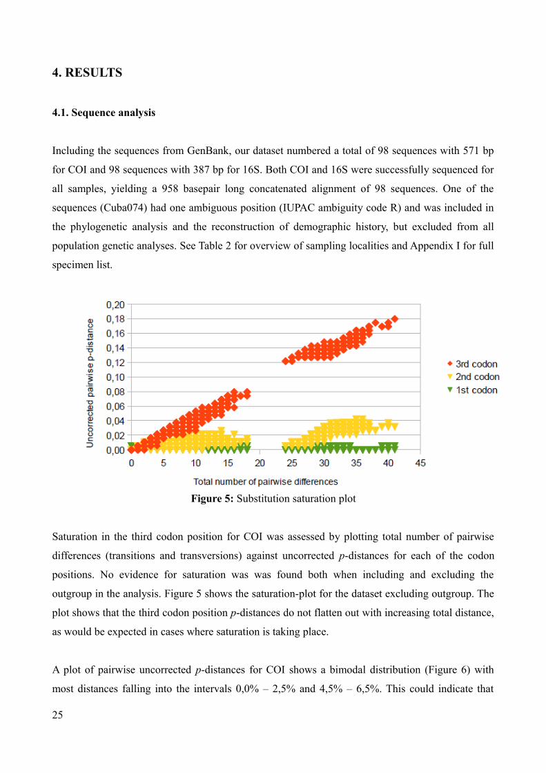
Saturation in the third codon position for COI was assessed by plotting total number of pairwise

differences (transitions and transversions) against uncorrected p-distances for each of the codon

positions. No evidence for saturation was was found both when including and excluding the

outgroup in the analysis. Figure 5 shows the saturation-plot for the dataset excluding outgroup. The

plot shows that the third codon position p-distances do not flatten out with increasing total distance,

as would be expected in cases where saturation is taking place.

A plot of pairwise uncorrected p-distances for COI shows a bimodal distribution (Figure 6) with

most distances falling into the intervals 0,0% – 2,5% and 4,5% – 6,5%. This could indicate that

25

Figure 5: Substitution saturation plot

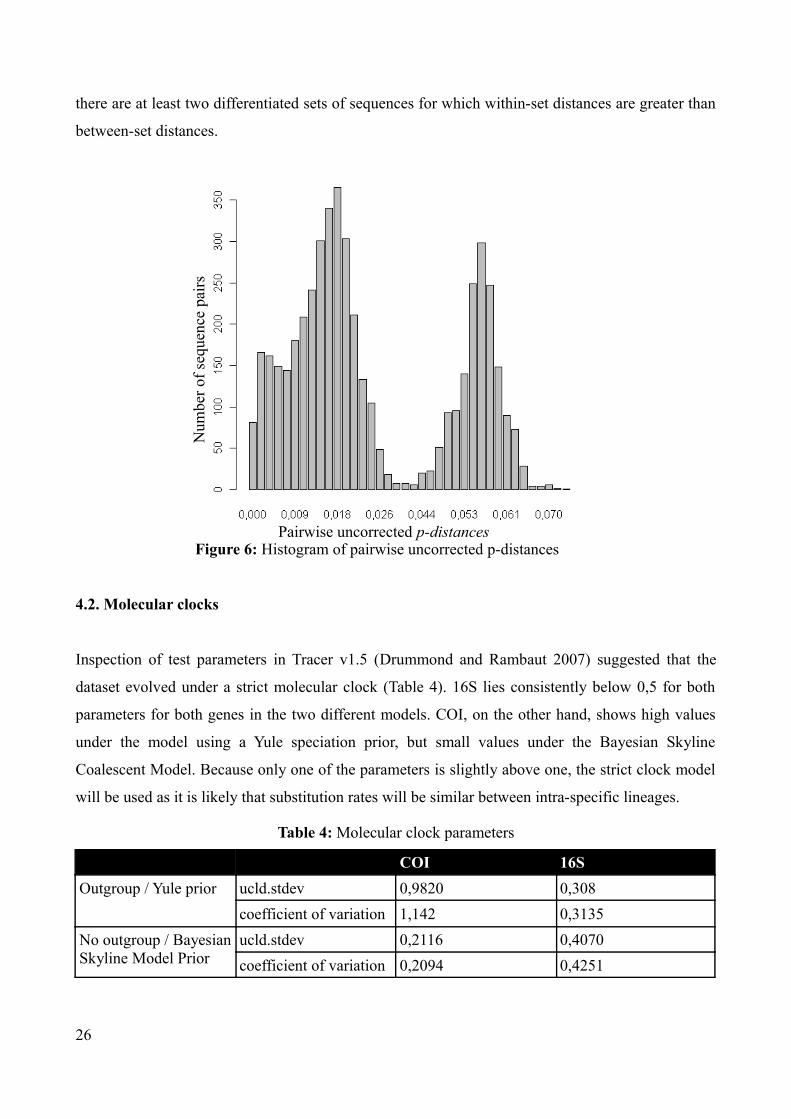
there are at least two differentiated sets of sequences for which within-set distances are greater than

between-set distances.

4.2. Molecular clocks

Inspection of test parameters in Tracer v1.5 (Drummond and Rambaut 2007) suggested that the

dataset evolved under a strict molecular clock (Table 4). 16S lies consistently below 0,5 for both

parameters for both genes in the two different models. COI, on the other hand, shows high values

under the model using a Yule speciation prior, but small values under the Bayesian Skyline

Coalescent Model. Because only one of the parameters is slightly above one, the strict clock model

will be used as it is likely that substitution rates will be similar between intra-specific lineages.

Table 4: Molecular clock parameters

COI 16SOutgroup / Yule prior ucld.stdev 0,9820 0,308

coefficient of variation 1,142 0,3135No outgroup / Bayesian Skyline Model Prior

ucld.stdev 0,2116 0,4070coefficient of variation 0,2094 0,4251

26

Figure 6: Histogram of pairwise uncorrected p-distances

Num

ber o

f seq

uenc

e pa

irs

Pairwise uncorrected p-distances

4.3. Population genetic structure

For all population genetics-related analyses the sequence Cuba074 was left out because of an

ambiguous position and the fact that ambiguities are not supported for some software packages.

This left us with a dataset of 97 sequences of 958 bps for population genetic analyses. When

discussing population genetic analyses, the term population will be used for describing all sampling

localities from one country as evident from Table 2.

Table 5 sums up standard diversity indices for the two genes and combined dataset for each of the

populations. COI is generally more variable than 16S, with a higher haplotype-diversity for all

populations, often several times higher. COI has a haplotype-diversity that varies from 0,6667 – 1,0

within populations while 16S haplotype-diversity varies between 0,0 – 0,7912. A haplotype-

diversity of 1,0 essentially means that all specimens from that locality are different while a

haplotype diversity of 0,0 means that all sequences from a single locality share the same haplotype.

The COI nucleotide-diversity varies between 0,002484 to 0,010819 while it varies between 0,0 and

0,006719 for 16S. This means that most of the variety in this dataset comes from COI. This is also

evident from the fact that the COI gene has 60 and 16S only has 22 unique haplotypes out of a total

of 97 sequences.

27

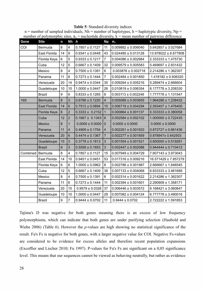
Table 5: Standard diversity indices n = number of sampled individuals, Nh = number of haplotypes, h = haplotypic diversity, Np = number of polymorphic sites, πn = nucleotide diversity, k = mean number of pairwise difference

Gene Site n Nh h Np πn kCOI Bermuda 8 4 0.7857 ± 0.1127 11 0.009882 ± 0.006040 5.642857 ± 3.027684

East Florida 14 9 0.9341 ± 0.0448 43 0.024480 ± 0.013128 13.978022 ± 6.677808

Florida Keys 6 5 0.9333 ± 0.1217 7 0.004086 ± 0.002984 2.333333 ± 1.475730

Cuba 12 5 0.6667 ± 0.1409 32 0.009579 ± 0.005583 5.469697 ± 2.831432

Mexico 8 4 0.7500 ± 0.1391 6 0.003878 ± 0.002718 2.214286 ± 1.362307

Panama 11 6 0.7273 ± 0.1444 7 0.002484 ± 0.001850 1.418182 ± 0.936320

Venezuela 20 14 0.9474 ± 0.0344 35 0.009264 ± 0.005216 5.289474 ± 2.666604

Guadeloupe 10 10 1.0000 ± 0.0447 26 0.010819 ± 0.006354 6.177778 ± 3.208330

Brazil 9 6 0.8333 ± 0.1265 8 0.003113 ± 0.002248 1.777778 ± 1.131547

16S Bermuda 8 3 0.6786 ± 0.1220 4 0.005089 ± 0.003655 1.964286 ± 1.238432

East Florida 14 6 0.7912 ± 0.0894 10 0.006719 ± 0.004294 2.593407 ± 1.476400

Florida Keys 6 2 0.3333 ± 0.2152 1 0.000864 ± 0.001137 0.333333 ± 0.380058

Cuba 12 2 0.1667 ± 0.1343 6 0.002584 ± 0.002102 1.000000 ± 0.722435

Mexico 8 1 0.0000 ± 0.0000 0 0.0000 ± 0.0000 0.0000 ± 0.0000

Panama 11 4 0.4909 ± 0.1754 4 0.002261 ± 0.001933 0.872727 ± 0.661436

Venezuela 20 6 0.4474 ± 0.1367 7 0.002277 ± 0.001859 0.878947± 0.642503

Guadeloupe 10 3 0.3778 ± 0.1813 3 0.001554 ± 0.001521 0.600000 ± 0.519281

Brazil 9 3 0.5556 ± 0.1653 3 0.002447 ± 0.002088 0.944444 ± 0.710412

Combined Bermuda 8 4 0.7857 ± 0.1127 15 0.007949 ± 0.004729 7.607143 ± 3.973043

East Florida 14 10 0.9451 ± 0.0451 53 0.017316 ± 0.009216 16.571429 ± 7.857279

Florida Keys 6 6 1.0000 ± 0.0962 8 0.002786 ± 0.001987 2.666667 ± 1.646545

Cuba 12 5 0.6667 ± 0.1409 38 0.007133 ± 0.004068 6.833333 ± 3.461689

Mexico 8 4 0.7500 ± 0.1391 6 0.002314 ± 0.001622 2.214286 ± 1.362307

Panama 11 6 0.7273 ± 0.1444 11 0.002394 ± 0.001601 2.290909 ± 1.358171

Venezuela 20 15 0.9579 ± 0.0328 37 0.006446 ± 0.003572 6.168421 ± 3.060647

Guadeloupe 10 10 1.0000 ± 0.0447 29 0.007082 ± 0.004124 6.777778 ± 3.490018

Brazil 9 7 0.9444 ± 0.0702 11 0.9444 ± 0.0702 2.722222 ± 1.591853

Tajima's D was negative for both genes meaning there is an excess of low frequency

polymorphisms, which can indicate that both genes are under purifying selection (Haubold and

Wiehe 2006) (Table 6). However the p-values are high showing no statistical significance of the

result. Fu's Fs is negative for both genes, with a larger negative value for COI. Negative Fs-values

are considered to be evidence for excess alleles and therefore recent population expansions

(Excoffier and Lischer 2010; Fu 1997). P-values for Fu's Fs are significant on a 0,05 significance

level. This means that our sequences cannot be viewed as behaving neutrally, but rather as evidence

28

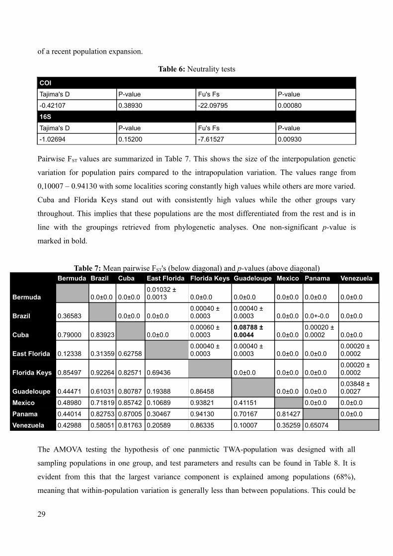
of a recent population expansion.

Table 6: Neutrality tests

COITajima's D P-value Fu's Fs P-value

-0.42107 0.38930 -22.09795 0.00080

16STajima's D P-value Fu's Fs P-value

-1.02694 0.15200 -7.61527 0.00930

Pairwise FST values are summarized in Table 7. This shows the size of the interpopulation genetic

variation for population pairs compared to the intrapopulation variation. The values range from

0,10007 – 0.94130 with some localities scoring constantly high values while others are more varied.

Cuba and Florida Keys stand out with consistently high values while the other groups vary

throughout. This implies that these populations are the most differentiated from the rest and is in

line with the groupings retrieved from phylogenetic analyses. One non-significant p-value is

marked in bold.

Table 7: Mean pairwise FST's (below diagonal) and p-values (above diagonal)Bermuda Brazil Cuba East Florida Florida Keys Guadeloupe Mexico Panama Venezuela

Bermuda 0.0±0.0 0.0±0.00.01032 ± 0.0013 0.0±0.0 0.0±0.0 0.0±0.0 0.0±0.0 0.0±0.0

Brazil 0.36583 0.0±0.0 0.0±0.00.00040 ± 0.0003

0.00040 ± 0.0003 0.0±0.0 0.0+-0.0 0.0±0.0

Cuba 0.79000 0.83923 0.0±0.00.00060 ± 0.0003

0.08788 ± 0.0044 0.0±0.0

0.00020 ± 0.0002 0.0±0.0

East Florida 0.12338 0.31359 0.627580.00040 ± 0.0003

0.00040 ± 0.0003 0.0±0.0 0.0±0.0

0.00020 ± 0.0002

Florida Keys 0.85497 0.92264 0.82571 0.69436 0.0±0.0 0.0±0.0 0.0±0.00.00020 ± 0.0002

Guadeloupe 0.44471 0.61031 0.80787 0.19388 0.86458 0.0±0.0 0.0±0.00.03848 ± 0.0027

Mexico 0.48980 0.71819 0.85742 0.10689 0.93821 0.41151 0.0±0.0 0.0±0.0

Panama 0.44014 0.82753 0.87005 0.30467 0.94130 0.70167 0.81427 0.0±0.0

Venezuela 0.42988 0.58051 0.81763 0.20589 0.86335 0.10007 0.35259 0.65074

The AMOVA testing the hypothesis of one panmictic TWA-population was designed with all

sampling populations in one group, and test parameters and results can be found in Table 8. It is

evident from this that the largest variance component is explained among populations (68%),

meaning that within-population variation is generally less than between populations. This could be

29

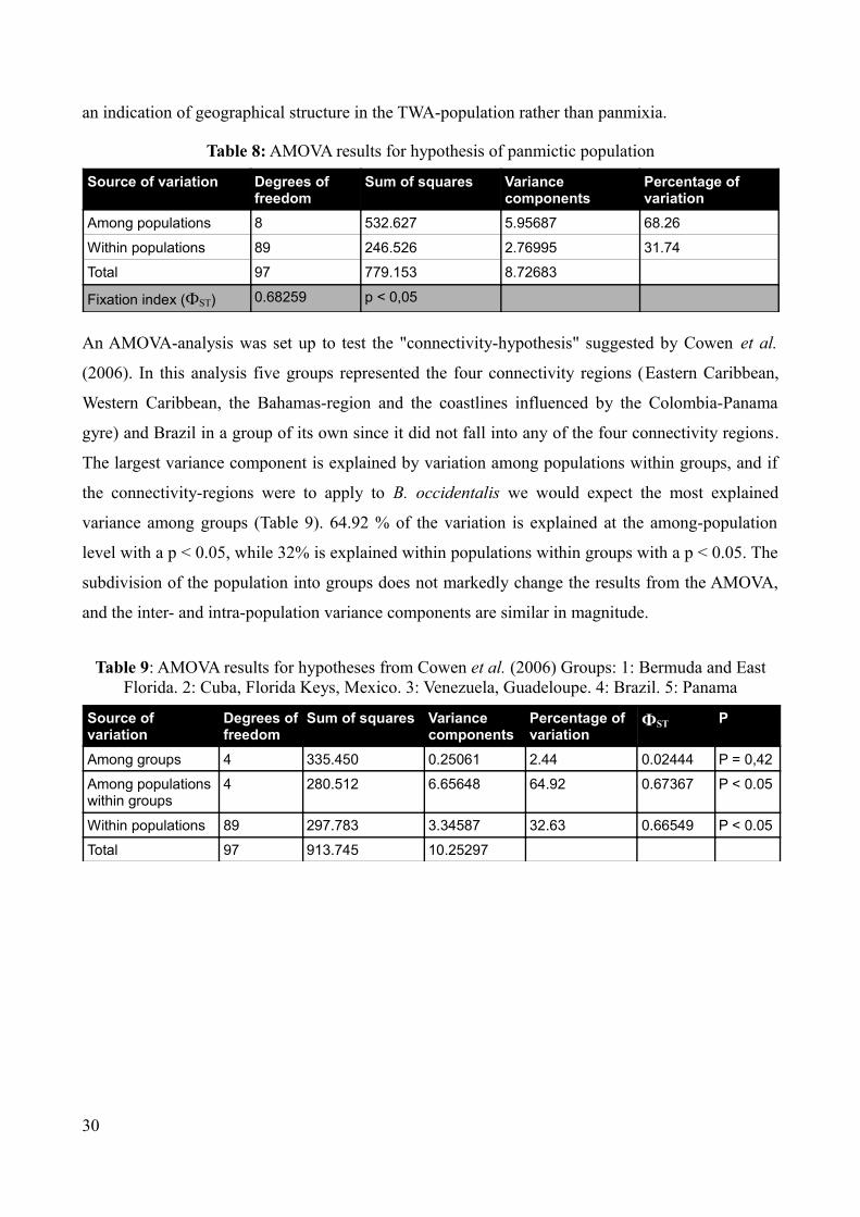
an indication of geographical structure in the TWA-population rather than panmixia.

Table 8: AMOVA results for hypothesis of panmictic population

Source of variation Degrees of freedom

Sum of squares Variance components

Percentage of variation

Among populations 8 532.627 5.95687 68.26

Within populations 89 246.526 2.76995 31.74

Total 97 779.153 8.72683

Fixation index (ФST) 0.68259 p < 0,05

An AMOVA-analysis was set up to test the "connectivity-hypothesis" suggested by Cowen et al.

(2006). In this analysis five groups represented the four connectivity regions (Eastern Caribbean,

Western Caribbean, the Bahamas-region and the coastlines influenced by the Colombia-Panama

gyre) and Brazil in a group of its own since it did not fall into any of the four connectivity regions.

The largest variance component is explained by variation among populations within groups, and if

the connectivity-regions were to apply to B. occidentalis we would expect the most explained

variance among groups (Table 9). 64.92 % of the variation is explained at the among-population

level with a p < 0.05, while 32% is explained within populations within groups with a p < 0.05. The

subdivision of the population into groups does not markedly change the results from the AMOVA,

and the inter- and intra-population variance components are similar in magnitude.

Table 9: AMOVA results for hypotheses from Cowen et al. (2006) Groups: 1: Bermuda and East Florida. 2: Cuba, Florida Keys, Mexico. 3: Venezuela, Guadeloupe. 4: Brazil. 5: Panama

Source of variation

Degrees of freedom

Sum of squares Variance components

Percentage of variation

ФST P

Among groups 4 335.450 0.25061 2.44 0.02444 P = 0,42

Among populations within groups

4 280.512 6.65648 64.92 0.67367 P < 0.05

Within populations 89 297.783 3.34587 32.63 0.66549 P < 0.05

Total 97 913.745 10.25297

30

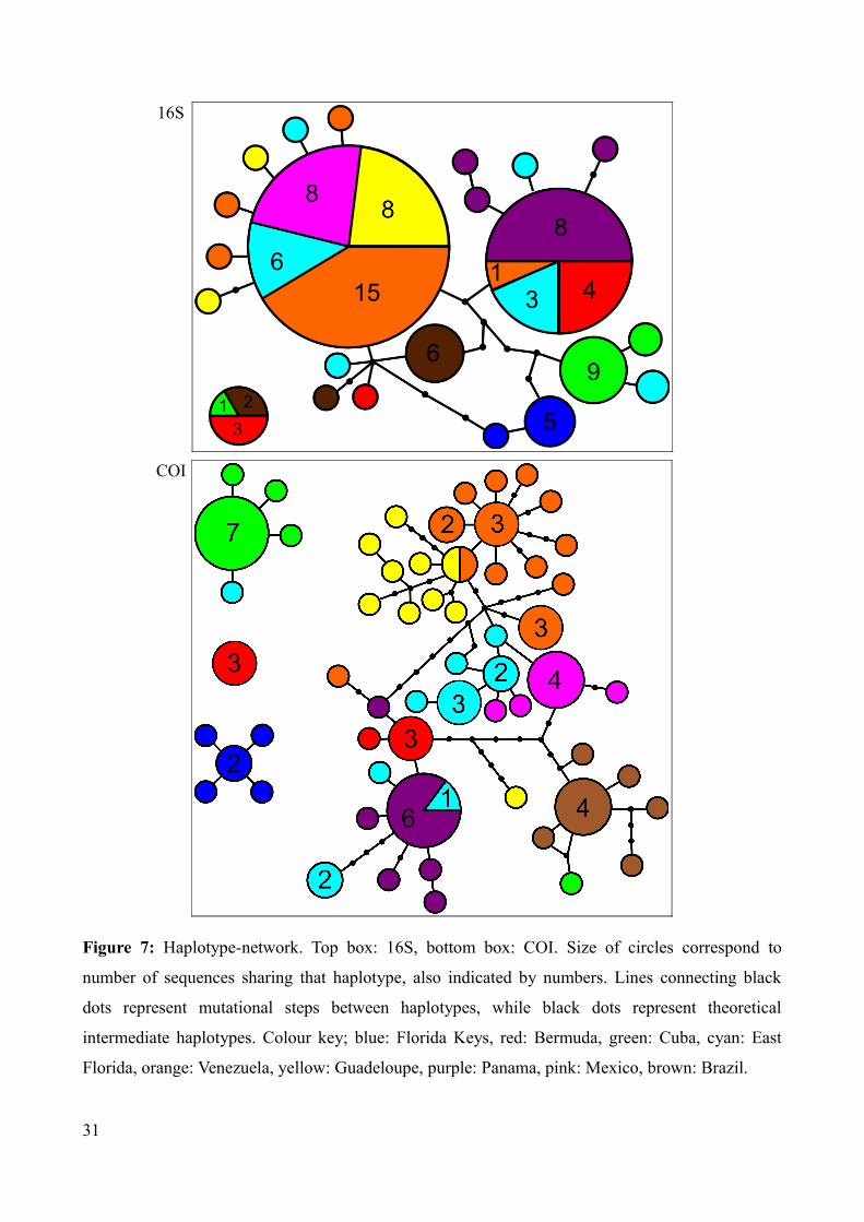
Figure 7: Haplotype-network. Top box: 16S, bottom box: COI. Size of circles correspond to

number of sequences sharing that haplotype, also indicated by numbers. Lines connecting black

dots represent mutational steps between haplotypes, while black dots represent theoretical

intermediate haplotypes. Colour key; blue: Florida Keys, red: Bermuda, green: Cuba, cyan: East

Florida, orange: Venezuela, yellow: Guadeloupe, purple: Panama, pink: Mexico, brown: Brazil.

31

16S

COI

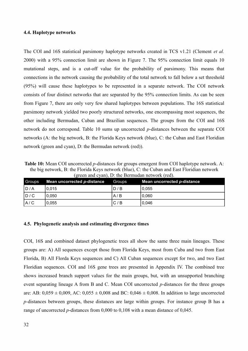
4.4. Haplotype networks

The COI and 16S statistical parsimony haplotype networks created in TCS v1.21 (Clement et al.

2000) with a 95% connection limit are shown in Figure 7. The 95% connection limit equals 10

mutational steps, and is a cut-off value for the probability of parsimony. This means that

connections in the network causing the probability of the total network to fall below a set threshold

(95%) will cause these haplotypes to be represented in a separate network. The COI network

consists of four distinct networks that are separated by the 95% connection limits. As can be seen

from Figure 7, there are only very few shared haplotypes between populations. The 16S statistical

parsimony network yielded two poorly structured networks, one encompassing most sequences, the

other including Bermudan, Cuban and Brazilian sequences. The groups from the COI and 16S

network do not correspond. Table 10 sums up uncorrected p-distances between the separate COI

networks (A: the big network, B: the Florida Keys network (blue), C: the Cuban and East Floridian

network (green and cyan), D: the Bermudan network (red)).

Table 10: Mean COI uncorrected p-distances for groups emergent from COI haplotype network. A: the big network, B: the Florida Keys network (blue), C: the Cuban and East Floridian network

(green and cyan), D: the Bermudan network (red).Groups Mean uncorrected p-distance Groups Mean uncorrected p-distanceD / A 0,015 D / B 0,055

D / C 0,050 A / B 0,060

A / C 0,055 C / B 0,046

4.5. Phylogenetic analysis and estimating divergence times

COI, 16S and combined dataset phylogenetic trees all show the same three main lineages. These

groups are: A) All sequences except those from Florida Keys, most from Cuba and two from East

Florida, B) All Florda Keys sequences and C) All Cuban sequences except for two, and two East

Floridian sequences. COI and 16S gene trees are presented in Appendix IV. The combined tree

shows increased branch support values for the main groups, but, with an unsupported branching

event separating lineage A from B and C. Mean COI uncorrected p-distances for the three groups

are: AB: 0,059 ± 0,009, AC: 0,055 ± 0,008 and BC: 0,046 ± 0,008. In addition to large uncorrected

p-distances between groups, these distances are large within groups. For instance group B has a

range of uncorrected p-distances from 0,000 to 0,108 with a mean distance of 0,045.

32

33

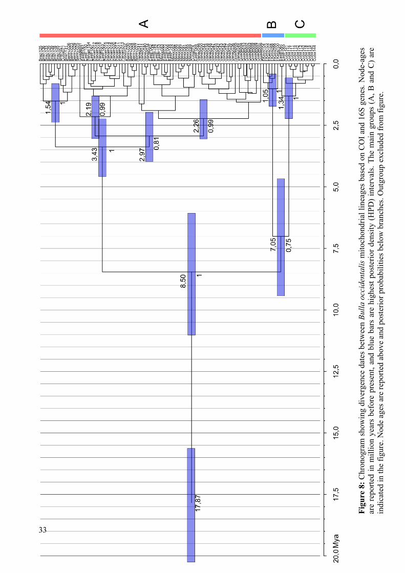
Figu

re 8

: Chr

onog

ram

sho

win

g di

verg

ence

dat

es b

etw

een

Bulla

occ

iden

talis

mito

chon

dria

l lin

eage

s ba

sed

on C

OI a

nd 1

6S g

enes

. Nod

e-ag

es

are

repo

rted

in m

illio

n ye

ars

befo

re p

rese

nt, a

nd b

lue

bars

are

hig

hest

pos

terio

r den

sity

(HPD

) in

terv

als.

The

mai

n gr

oups

(A, B

and

C) a

re

indi

cate

d in

the

figur

e. N

ode

ages

are

repo

rted

abov

e an

d po

ster

ior p

roba

bilit

ies b

elow

bra

nche

s. O

utgr

oup

excl

uded

from

figu

re.

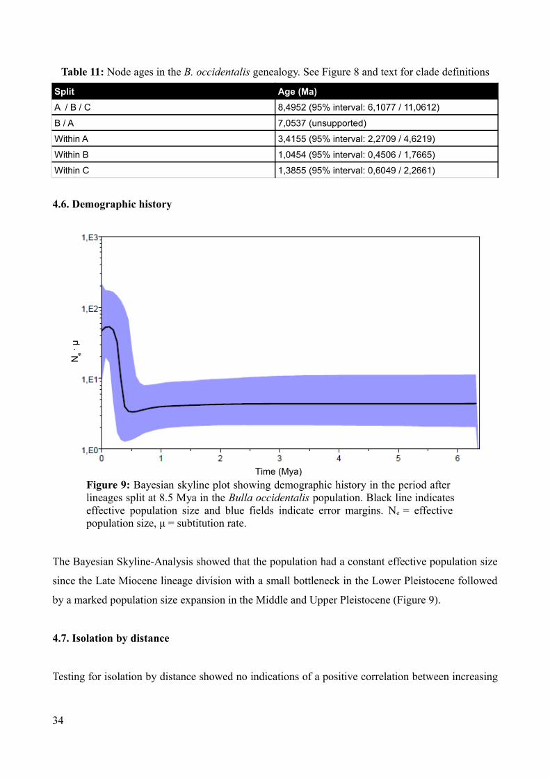
Table 11: Node ages in the B. occidentalis genealogy. See Figure 8 and text for clade definitions

Split Age (Ma)A / B / C 8,4952 (95% interval: 6,1077 / 11,0612)

B / A 7,0537 (unsupported)

Within A 3,4155 (95% interval: 2,2709 / 4,6219)

Within B 1,0454 (95% interval: 0,4506 / 1,7665)

Within C 1,3855 (95% interval: 0,6049 / 2,2661)

4.6. Demographic history

The Bayesian Skyline-Analysis showed that the population had a constant effective population size

since the Late Miocene lineage division with a small bottleneck in the Lower Pleistocene followed

by a marked population size expansion in the Middle and Upper Pleistocene (Figure 9).

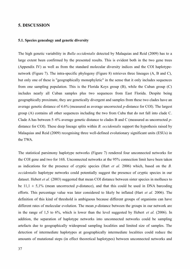
4.7. Isolation by distance

Testing for isolation by distance showed no indications of a positive correlation between increasing

34

Figure 9: Bayesian skyline plot showing demographic history in the period after lineages split at 8.5 Mya in the Bulla occidentalis population. Black line indicates effective population size and blue fields indicate error margins. Ne = effective population size, μ = subtitution rate.

Time (Mya)

Ne · μ

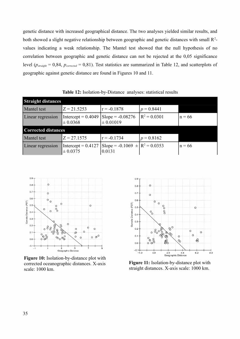
genetic distance with increased geographical distance. The two analyses yielded similar results, and

both showed a slight negative relationship between geographic and genetic distances with small R2-

values indicating a weak relationship. The Mantel test showed that the null hypothesis of no

correlation between geographic and genetic distance can not be rejected at the 0,05 significance

level (pstraight = 0,84, pcorrected = 0,81). Test statistics are summarized in Table 12, and scatterplots of

geographic against genetic distance are found in Figures 10 and 11.

Table 12: Isolation-by-Distance analyses: statistical results

Straight distancesMantel test Z = 21.5253 r = -0.1878 p = 0.8441 Linear regression Intercept = 0.4049

± 0.0368Slope = -0.08276 ± 0.01019

R2 = 0.0301 n = 66

Corrected distancesMantel test Z = 27.1575 r = -0.1734 p = 0.8162Linear regression Intercept = 0.4127

± 0.0375 Slope = -0.1069 ± 0.0131

R2 = 0.0353 n = 66

35

Figure 11: Isolation-by-distance plot with straight distances. X-axis scale: 1000 km.

Figure 10: Isolation-by-distance plot with corrected oceanographic distances. X-axis scale: 1000 km.

36

5. DISCUSSION

5.1. Species genealogy and genetic diversity

The high genetic variability in Bulla occidentalis detected by Malaquias and Reid (2009) has to a

large extent been confirmed by the presented results. This is evident both in the two gene trees

(Appendix IV) as well as from the standard molecular diversity indices and the COI haplotype-

network (Figure 7). The intra-specific phylogeny (Figure 8) retrieves three lineages (A, B and C),

but only one of these is "geographically monophyletic" in the sense that it only includes sequences

from one sampling population. This is the Florida Keys group (B), while the Cuban group (C)

includes nearly all Cuban samples plus two sequences from East Florida. Despite being

geographically proximate, they are genetically divergent and samples from these two clades have an

average genetic distance of 4.6% (measured as average uncorrected p-distance for COI). The largest

group (A) contains all other sequences including the two from Cuba that do not fall into clade C.

Clade A has between 5–6% average genetic distance to clades B and C (measured as uncorrected p-

distance for COI). These deep lineage splits within B. occidentalis support the hypothesis raised by

Malaquias and Reid (2009) recognising three well-defined evolutionary significant units (ESUs) in

the TWA.

The statistical parsimony haplotype networks (Figure 7) rendered four unconnected networks for

the COI gene and two for 16S. Unconnected networks at the 95% connection limit have been taken

as indications for the presence of cryptic species (Hart et al. 2006) which, based on the B.

occidentalis haplotype networks could potentially suggest the presence of cryptic species in our

dataset. Hebert et al. (2003) suggested that mean COI distance between sister species in molluscs to

be 11,1 ± 5,1% (mean uncorrected p-distance), and that this could be used in DNA barcoding

efforts. This percentage value was later considered to likely be inflated (Hart et al. 2006). The

definition of this kind of threshold is ambiguous because different groups of organisms can have

different rates of molecular evolution. The mean p-distance between the groups in our network are

in the range of 1,5 to 6%, which is lower than the level suggested by Hebert et al. (2006). In

addition, the separation of haplotype networks into unconnected networks could be sampling

artefacts due to geographically widespread sampling localities and limited size of samples. The

detection of intermediate haplotypes at geographically intermediate localities could reduce the

amounts of mutational steps (in effect theoretical haplotypes) between unconnected networks and

37

thereby establishing connection between these. Moreover, Malaquias and Reid (2009) established a

cut-off value between species in the genus Bulla at 10% uncorrected p-distance for COI gene and

did not find the genetic breaks of the COI and 16S phylogenies to be mirrored by a phylogeny of

the slower evolving nuclear gene 28S rRNA. With all of this taken into account, the suggestion by

Malaquias and Reid (2008, 2009) to consider B. occidentalis as one single taxonomic entity seems

to be valid.

A striking result was the high haplotype diversity in the COI gene (0.6667 ± 0,1409 – 1.0000 ±

0,0447), something that is both uncommon and difficult to explain. Wilson et al. (2009) reported

similar high genetic diversity (0,6429 ± 0,184 – 0,1000 ± 0,096) for the opisthobranch Doris

kerguelenensis from the South Atlantic/Antarctic region. Despite its direct mode of development

and therefore theoretically limited dispersal capacity D. kerguelenes showed no shared haplotypes

between major geographical regions, though within regions shared haplotypes could be found up to

450 kilometres apart (Wilson et al. 2009). Faster evolutionary rate in COI compared to 16S

presumably has greater potential for capturing glaciation events (Wilson et al. 2009) and the large

differentiation in the COI statistical parsimony network (Figure 7) may have been caused by this.

Wilson et al. (2009) attributed the genetic diversity in D. kerguelenensis to glaciations events,

where in Antarctica the ice-sheets grew over the continental shelf severely reducing the amount of

available habitat and restricting survival to small pockets (Thatje 2005). Likely, with receding ice-

sheets re-colonization took place followed by rapid differentiation caused by increased allele

fixation due to small population sizes in refugia. Regarding B. occidentalis it is possible that

fragmentation of populations and reduced gene-flow during Plio-Pleistocene eustasy coupled with

species biological intrinsic factors could have lead to the high diversity of unique haplotypes found

in this snail.

5.2. Patterns and forces of marine diversification in the TWA

5.2.1. Are present isolating mechanisms detectable for Bulla occidentalis?

The degree of genetic connectivity and longevity of larval stages in marine organisms (and thereby

dispersal potential) are not always correlated, and larval longevity is therefore not necessarily a

good predictor for dispersal potential (Weersing and Toonen 2009). Our results do indicate that B.

occidentalis has a high level of connectivity throughout most of the Tropical Western Atlantic.

38

Clade (A) consists of a diverse assembly of sequences from vastly different localities, including the

extremes of the geographical range in this study (Bermuda, Brazil and Mexico). These are separated

by geographic distances of approximately 6700 km (Brazil-Mexico), 5700 km (Brazil-Bermuda)

and 2700 km (Bermuda-Mexico), while the Florida Keys clade and Cuban clade lie closer to each

other and deviate more genetically. There was no evidence for a clear-cut isolation-by-distance

pattern in our dataset, a conclusion that is strengthened by the fact that pairwise FST values vary

greatly an in a non-systematic way. Localities in the opposite range of the species distribution (e.g.

Bermuda-Brazil,) have lower FST (0.36583) than localities that are geographically closer (e.g.

Brazil-Guadeloupe, FST = 0.61031). Another interesting result is the fact that samples from the

southern-most sampling locality at Isla Itaparica, Brazil, were not divergent compared to the rest of

the sampling set. It was our expectation that this locality could be divergent due to the bifurcating

nature of the South Equatorial Current System and mainly uni-directional transport of water along

the Brazilian coastline as well as its large geographical distance from the remaining sampling

stations. However, all Brazilian sequences fall into one well-supported sub-clade (PP = 1) with one

Cuban and four Bermudan sequences, as well as being differentiated by 5–8 mutational steps in the

COI haplotype network. This could indicate an ongoing diversification process, and would make an

interesting hypothesis for further study at a later time.

There are several examples of studies that aim to uncover mechanisms inhibiting genetic

connectivity in the TWA and it seems that different barriers apply to different animal groups

(marine bivalves, Mikkelsen and Bieler 2000; Brachidontes exustus, Lee and Ó Foighil 2004, 2005;

trochid gastropods, Diáz-Ferguson et al. 2010). One such hypothesis was tested, namely whether

the "connectivity-hypothesis" proposed by Cowen et al. (2006) that recognized four regions of high

connectivity (Eastern Caribbean, Western Caribbean, the Bahamas-region and the coastlines

influenced by the Colombia-Panama gyre) could explain the genetic breaks observed in B.

occidentalis. Like for trochid gastropods (Díaz-Ferguson et al. 2010) this hypothesis is not

supported for B. occidentalis. Sixty-five percent of the observed variation was explained between

populations within these pre-defined groups (p < 0,05), indicating that these regions do not

realistically reflect a common pattern of surface-current mediated pattern of gene-flow.

The hypothesis of a general pattern of segregation between continental and oceanic populations due

to ecological specialization (e.g. Brachidontes exustus, Lee and Ó Foighil 2005; Bulla occidentalis,

Malaquias and Reid 2009) was not supported by the presented results. The phylogeny and

39

haplotype networks grouped oceanic and continental populations together, providing no evidence

that such a mechanism is causing diversification within B. occidentalis. In addition, there does not

seem to be a consistent pattern of higher FST-values between oceanic and continental populations

pairs compared to values between continental-continental and oceanic-oceanic pairs.

5.2.2. Historical patterns and processes

The deep lineage splits within B. occidentalis are dated to the Late Miocene at between 11,06 – 6,11

Mya. The slightly younger node splitting groups B and C is unsupported, so we consider splits

between the three main lineages (A, B and C) to be dated to the same period, several million years

earlier than the final closure of the Panamanian Isthmus. However, the shoaling process that lead to

the closing of the Isthmus took place over 12 million years, and it is likely that these splits are in

some way related to oceanographic and geophysical changes in the region that may have caused

vicariance between groups A, B and C prior to the closing of the Isthmus. There exist examples of

divergences in a wide range of Trans-Isthmian geminate clades from diverse animal groups (fish,

Molluscs, Crustacea and Echinodea) that do pre-date the closing of the Panamanian Isthmus

(Lessios 2008).

The Strait of Florida has been described in early literature as an important barrier for dispersal of

marine organisms based on large differences in fish faunas on either side of the strait (Briggs 1974).

Certain properties of the Florida current, like fast flow and little mixing were put forth to explain

genetic breaks in the area such as a potential barrier between Florida and the Bahamas (Briggs

1974). The Florida Keys are located in the intersection between temperate and tropical Gulf of

Mexico, sub-tropical north-western Atlantic and the tropical Caribbean, and the environments on

the two sides of the Florida Keys provide substantially different habitats. This has resulted in

examples of genetic disjunction in species distributed on both the Atlantic and Gulf-sides of the

Florida Peninsula (Crassostrea virginica, Reeb and Avise 1989, Brachidontes exustus, Lee and Ó

Foighil 2004). For American oysters (C. virginica) this discrepancy was explained by divergence

under allopatry during Pleistocene low sea-level stands that to a large degree isolated the Gulf of

Mexico (see Figure 2 for illustration) from the Atlantic side of Florida (Reeb and Avise 1989). For

the scorched mussel Brachidontes, the maintenance of genetic discontinuities was suggested to be

caused by post-recruitment ecological filters, and that the origin of this genetic disjunction was

slightly too old to be caused by Pleistocene transient allopatry (2.91–2.18 Ma) (Lee and Ó Foighil

40

2004; Lee and Ó Foighil 2005). A survey of the Florida Keys bivalve-fauna showed that the species

composition of the high-salinity environment of the Florida Bay (north of the Florida Keys) has its

own identity compared to other parts of the Keys (Mikkelsen and Bieler 2000), but our sampling

localities are all close to the oceanic side of the Keys, so it is not clear whether the observed

divergence of Florida Keys compared to the rest of the TWA can be attributed to this ecological

difference. The fact that the Florida Keys form the only "geographically monophyletic" group could

serve as an indication that there is a stronger driving force maintaining genetic differentiation in this

lineage compared to the rest of the Caribbean.

The Yucatán current, flowing between Cuba and the Yucatán peninsula connecting the Caribbean

Current and the Loop Current has a strong flow on the western side of the Yucatán strait, but a weak

southern flow off the eastern tip of Cuba (Gyory [2011c]). Excess water from the Loop Current that

does not enter the Florida Current constitutes this southern-bound flow, and if this flow has been

sufficiently persistent through time, and strong enough to inhibit larvae from the Cuban population

entering the Loop Current, then this could also have been a mechanism promoting genetic

differentiation between the Cuban population and the rest of the Caribbean. The fact that the

predominantly Cuban group includes specimens found in East Florida can be explained by the fact

that the current pattern places East Florida downstream from Cuba increasing the probability of

finding specimens from East Florida specimens in the Cuban clade. However, this picture is

somewhat obscured by the fact that Cuban sequences are found in the larger group encompassing

sequences from the entire region.

The origin of the biggest clade (A) that contains sequences from throughout the TWA also has its

origin in the Late Miocene, but this group contains two large and well supported sub-clades that

originate in Late Pliocene or Lower Pleistocene, 4,6 – 2,3 Mya. The main part of this interval pre-

dates the final closure of the Panamanian Isthmus (2,8 Mya), but places it in the final stages of the

Isthmus up-lift, and possibly links the lineage split to this event.

The majority of lineage splits for all the three main clades are dated to the Pleistocene, during the

last 2 Ma, with the main diversification happening during the Lower to Upper Pleistocene in the last

1 Ma. This could be related to transient allopatry caused by sea level changes. Figure 2 shows that

under low sea-level stands the Caribbean Sea can roughly be divided into three semi-enclosed

basins, possibly with strong effects on ocean circulation patterns. If ocean circulation in the

41

Caribbean was reduced in strength or hindered, this could potentially reduce gene-flow throughout

the Caribbean, which could lead to temporary isolation of populations – transient allopatry –

allowing for genetic differentiation of isolated populations. For D. kergelenuensis genetic

diversification was attributed to transient allopatry causing reduction in habitat size with increased

selection and allele fixation, the so-called Antarctic diversity-pump (Wilson et al. 2009). The timing

of the diversification of B. occidentalis lineages coincides with an increase in the magnitude of

glaciations outside polar regions from approximately 1 Mya to 800 Kya as opposed to large

glaciation events throughout the Quaternary as has been the common view (Ehlers and Gibbard

2007).

5.3. Demographic history

The Bayesian Skyline analysis (Figure 9) suggests a stable effective population size for B.

occidentalis since the three main lineages split 11,06 – 6,11 Mya, suffering a small bottleneck

between 1 Mya and 500 Kya followed by a large population expansion event during the last 500 Ka.

This population expansion is also suggested by the negative values of Fu's Fs. The increase in

Pleistocene sea level fluctuations due to glaciation would have caused an increase in periodic shifts

of habitat availability.

Despite constantly changing coastal habitats during the Pleistocene it seems the causes of molluscan

turnover since the closing of the Panamanian Isthmus have mainly been related to the drop in

primary productivity and resulting change in the structure of food-webs (Todd et al. 2002; O'Dea et

al. 2007). For bivalves, extinctions caused by the reduction in habitat availability due to receding

sea-level has been suggested to be unlikely (Stanley 1986). The effect of marine regression on

species extinction has been questioned by Stanley and Campbell (1981), as declining sea-level can

lead to an increase in sublittoral areas, and thereby making it unlikely that marine organisms would

suffer from crowding or habitat loss. However, this stands in contrast to results from Tropical

Pacific islands where soft-bottom bivalves experienced local extinctions due to habitat loss during

Pleistocene glaciation cycles, and were more severely affected than hard-bottom species (Paulay

1996). Climatic cooling has been suggested as a more plausible mechanism causing mass-

extinctions in marine habitats than marine regression (Stanley and Campbell 1981). B. occidentalis

is found in the tropical/temperate transitional-zone and its sister species B. striata inhabits

temperate waters in the Eastern Atlantic (Malaquias and Reid 2008, 2009), which might suggest that

42

B. occidentalis has the ability to tolerate shifts in temperature regimes. The results could serve as an

indication that sea-level oscillations during the Pleistocene likely presented new niche opportunities

for B. occidentalis and that this species did not suffer from the effects of habitat loss or crowding,

since receding sea-level might have created new soft-bottom habitats available for colonization.

Nevertheless, recent findings suggest that mitochondrial DNA alone has poor ability to estimate

demographic parameters due to the small effective population size of the mitochondrial genome

which combined with high mutation rates may obscure demographic history reconstruction (Eytan

and Hellberg 2010). It seems that mitochondrial DNA is more suitable to reconstruct demographic

history on short time scales. In addition, single locus-reconstructions cannot recover population

history further back than to the most recent population bottleneck, meaning that a significant

amount of information may have been lost in the Bayesian skyline analysis (Heled and Drummond

2008). This explains the long period of apparent stability in the effective population size observed

in our analysis, and unfortunately limits our reconstruction to the last 1 Ma. A possibility for future

work is to include another locus in the analysis to provide resolution for the reconstruction of the B.

occidentalis demographic history. In addition, the assumption of neutrally evolving markers was not

strictly held, something that may be a source of error in analyses of demographic and population

genetic parameters.

43

44

6. CONCLUSIONS

B. occidentalis harbours intra-specific genetic diversity that is not easily explained by current

factors mediating gene-flow between local populations. The results did not support the notion of

oceanic/continental subdivision, correlation between geographical and genetic distance, and the

integrity of regions of high connectivity. Three main lineages showing deep mitochondrial

divergence were discovered, and possibly stem from vicariance during the formation of the

Panamanian Isthmus in the Late Miocene. The most plausible explanation for the large present

genetic variation in B. occidentalis seems to be transient allopatry caused by Pleistocene eustatic

changes related to glaciation cycles, but the mechanisms responsible for maintaining genetic

structure in three distinct groups through history are not known.

To further explore the population genetic structure in B. occidentalis a good strategy would be to

perform comparisons at a smaller scale. Genetic break-points such as the Mona Passage and the

Exuma sound will not be revealed unless the sampling design accounts for testing these hypotheses.

The seasonality of spawning is also an aspect that needs to be addressed, as it is only the

oceanographic conditions during larval release that will have potential to influence population

connectivity, so knowledge about spawning in populations throughout the TWA is necessary for

further understanding the genetic diversity of populations of B. occidentalis.

45

46

7. ACKNOWLEDGEMENTS

This project would not have been possible without the help of many collaborators. First of all I

would like to thank my supervisors, Manuel A. E. Malaquias and Endre Willassen for being

generous with their time and support. I am quite sure the allotted hours for supervision were used up

after the first few months of work. Another big thank you goes to Professor Olivier Gros at the

University of the French Antilles and Guyana for hospitality and assistance in the field. He made it

quite enjoyable and relaxed to be an inexperienced field biologist far away from home. Thanks to

Marius Kambestad for taking time during his own field work for collecting Bulla specimens at the

Smithsonian Tropical Research Institute at Bocas del Toro in Panama.

I also want to thank my parents for both moral and financial support making it possible for me to

travel to London and Guadeloupe without using all my savings and leaving room for some

adventures as well as thesis work. At last I want to thank my partner Emilie who has assisted me

both at home and in the field. Without you I would still be swimming in the Guadeloupean

mangrove lagoons looking for Bulla occidentalis!

47

48

8. REFERENCES

Andrade, C.A. and Barton E.D. (2000) Eddy development and motion in the Caribbean Sea.

Journal of Geophysical Research-Oceans, 105, 26191-26201.

Bellwood, D.R. and Wainwright P.C. (2002) The history and biogeography of fishes on coral reefs.

Coral reef fishes (ed. by P. F. Sale), pp. 5-32. Elsevier Science, Burlington.

Bischof, B., Mariano, A.J. and Ryan, E.H. (2003) The North Brazil Current. Ocean Surface

Currents (http://oceancurrents.rsmas.miami.edu/atlantic/north-brazil.html).

Last accessed: 22.05.2011.

Bohonak, A. J. (2002) IBD (Isolation By Distance): a program for analyses of isolation by distance.

Journal of Heredity, 93: 153-154.

Briggs, J.C. (1974) Marine Zoogeography. McGraw-Hill, New York.

Budd, A.F., Johnson, K.G. and Stemann T.A. (1996) Plio-Pleistocene turnover and extinctions in

the Caribbean reef coral fauna. Evolution and environment in Tropical America (ed. by J. B.

C Jackson, A. F. Budd and A. G. Coates), University of Chicago Press, Chicago.

Campbell Jr., K.E., Frailey, C.D. and Romero-Pittman, L. (2006) The Pan-Amazonian Ucayali

Peneplain, late Neogene sedimentation in Amazonia, and the birth of the modern Amazon

River system. Palaeogeography Palaeoclimatology, Palaeoecology, 239: 166-219.

Chan, L.M., Brown, J.L. and Yodera, A.D. (2011) Integrating statistical genetic and geospatial

methods brings new power to phylogeography. Molecular Phylogenetics and Evolution, 59:

523-537.

Clement, M., Posada, D. and Crandall K. (2000) TCS: a computer program to estimate gene

genealogies. Molecular Ecology, 9: 1657-1660.

49

Coates, A.G. and Obando, J.A. (1996) The Geologic Evolution of the Central American Isthmus.

Evolution and Environment in Tropical America, (ed. by J. B. C. Jackson, A. F. Budd and A.

G. Coates). University of Chicago Press, Chicago.

Collin, R. (2003) Phylogenetic Relationships Among Calyptraeid Gastropods and Their

Implications for the Biogeography of Marine Speciation. Systematic Biology, 52 (5): 618-

640.

Cowen, R.K., Paris, B. and Srinivasan, A. (2006) Scaling of Connectivity in Marine Populations.

Science, 311: 522-527.

Cunha, R.L., Lopes, E.P., Reis, D.M. and Castilho, R. (2011) Genetic structure of Brachidontes

puniceus populations in Cape Verde archipelago shows signature of expansion during the

last glacial maximum. Journal of Molluscan Studies. 77(2): 175-181.

Díaz-Ferguson, E., Haney, R., WARES J. and Silliman, B. (2010) Population Genetics of a Trochid

Gastropod Broadens Picture of Caribbean Sea Connectivity. Public Library of Science: One,

5(9): e12675. doi:10.1371/journal.pone.0012675.

Doellman, M.M., Trussel, G.C., Grahame, J.W. and Vollmer, S.V. (2011) Phylogeographic

analysis reveals a deep lineage split within North Atlantic Littorina saxatilis. Proceedings of

the Royal Society. doi: 10.1098/rspb.2011.0346

Drummond, A.J., Rambaut, A., Shapiro, B., and Pybus, O. G. (2005) Bayesian Coalescent

Inference of Past Population Dynamics from Molecular Sequences. Molecular Biology and

Evolution, 22: 1185-1192.

Drummond, A.J. and Rambaut, A. (2007) BEAST: Bayesian evolutionary analysis by sampling

trees. BioMed Central: Evolutionary Biology 7: 214.

Drummond, A.J., Ho S.Y.W., Rawlence, N. And Rambaut, R. (2007) A rough guide to BEAST 1.4.

Department of Computer Science, Auckland.

50

Ehlers, J. and Gibbard, P.L. (2007) The extent and chronology of Cenozoic Global Glaciation.

Quaternary International, 164–165, 6–20.

Excoffier, L. and Lischer, H.E.L. (2010) Arlequin suite ver 3.5: A new series of programs to

perform population genetics analyses under Linux and Windows. Molecular Ecology

Resources, 10: 564-567.

Eytan, R.I., and Hellberg, M.E. (2010) Nuclear and mitochondrial sequence data reveal and

conceal different demographic histories and population genetic processes in Caribbean reef

fishes. Evolution, 64: 3380-3397.

Folmer, O., Black, M., Hoeth W., Lutz, R. and Vrijenhoek, R. (1994) DNA primers for

amplification of mitochondrial cytochrome c oxidase subunit I from diverse metazoan

invertebrates. Molecular Marine Biology and Biotechnology, 3: 294-299.

Forest, F. (2009) Calibrating the Tree of Life: fossils, molecules and evolutionary timescales.

Annals of Botany, 104: 789-794.

Fu, Y. (1997) Statistical Tests of Neutrality of Mutations Against Population Growth, Hitchhiking

and Background Selection. Genetics, 147: 915-925.

Gyory, J., Mariano, A.J. and Ryan, E.H. [2011a] The Caribbean Current, Ocean Surface Currents

(http://oceancurrents.rsmas.miami.edu/caribbean/caribbean.html).

Last accessed: 22.05.2011.

Gyory, J., Mariano, A.J. and Ryan, E.H. [2011b] The Guiana Current, Ocean Surface Currents

(http://oceancurrents.rsmas.miami.edu/atlantic/guiana.html). Last accessed: 22.05.2011.

Gyory, J., Mariano, A.J. and Ryan, E.H. [2011c] The Yucatan Current. Ocean Surface Currents.

(http://oceancurrents.rsmas.miami.edu/caribbean/yucatan.html). Last accessed: 22.05.2011.

Hall, T.A. (1999) BioEdit: a user-friendly biological sequence alignment editor and analysis

program for Windows 95/98/NT. Nucleic Acids Symposium Series, 41: 95-98.

51

Hart, M.W., Keever, C.C., Dartnall, A.J. and Byrne, M. (2006) Morphological and genetic

variation indicate cryptic species within Lamarck’s Little Sea Star, Parvulastra (Patiriella)

exigua. The Biological Bulletin, 210: 158-167.

Hebert, P.D.N., Ratnasingham, S. and Waard, J.R.D. (2003) Barcoding animal life: cytochrome c

oxidase subunit 1 divergences among closely related species. Proceedings of the Royal

Society, 270: S96–S99.

Heled, J. and Drummond, A.J. (2008) Bayesian inference of population size history from multiple

loci. BioMed Central: Evolutionary Biology 88(289): doi:10.1186/1471-2148-8-289.

Ho, S., and Shapiro, B. (2011) Skyline-plot methods for estimating demographic history from

nucleotide sequences. Molecular Ecology Resources. 11(3): 423–434.

Huddlestun, P.F. (1984) The Neogene stratigraphy of the Central Florida Panhandle. Florida State

University, Tallahasseee.

Isaza, C.F.A., Sierra-Correa, P.C., Bernal-Velasquez, M., Londoño, L.M. and W. Troncoso. (2006)

Global International Waters Assessment Caribbean Sea/Colombia and Venezuela, Central

America and Mexico, GIWA Regional assessment 3b, 3c. United Nations Environment

Programme. University of Kalmar for United Nations Environment Programme, Kalmar.

Jensen, J.L., Bohonak, A.J. and Kelley, S.T. (2005) Isolation by distance, web service v. 3.16.

BioMed Central: Genetics, 6:13.

Kawauchi, G.Y. and Giribet, G. (2011) On the amphi-Atlantic Siphonaria pectinata (Linnaeus,

1758) (Gastropoda: Heterobranchia: Siphonariidae): invader from the east or endemic?

Journal of Molluscan Studies, 77:196-201.

Kirkendale, L.A. and Meyer, C.P. (2004) Phylogeography of the Patelloida profunda group

(Gastropoda: Lottidae): diversification in a dispersal-driven marine system. Molecular

ecology, 13(9): 2749-2762

52

Larkin, M.A., Blackshields, G., Brown, N.P., Chenna, R., McGettigan, P.A., McWilliam, H.,

Valentin, F., Wallace, I.M., Wilm, A., Lopez, R., Thompson, J.D., Gibson, T.J. and

Higgins, D.G. (2007) Clustal W and Clustal X version 2.0. Bioinformatics, 23: 2947-2948.

Lessios, H.A. (2008) The Great American Schism: Divergence of marine organisms after the rise

of the Central American Isthmus. The Annual Review of Ecology, Evolution, and Systematic,

39: 63-91.

Lee, T. and Ó Foighil, D. (2004) Hidden Floridian biodiversity: mitochondrial and nuclear gene

trees reveal four cryptic species within the scorched mussel, Brachidontes exustus, species

complex. Molecular Ecology, 13: 3527–3542.

Lee, T. and Ó Foighil, D. (2005). Placing the Gloridian marine genetic disjunction into a regional

evolutionary context using the scorched mussel, Brachidontes exustus, species complex.

Evolution, 59(10): 2139-2158.

Malaquias, M.A.E. and Reid, D.G. (2008) Systematic revision of the living species of Bullidae

(Mollusca: Gastropoda: Cephalaspidea), with a molecular phylogenetic analysis. Zoological

Journal of the Linnean Society, 153: 453–543.

Malaquias, M.A.E. and Reid, D.G. (2009) Tethyan vicariance, relictualism and speciation:

evidence from a global molecular phylogeny of the opistobranch genus Bulla. Journal of

Biogrography, 36: 1760-1777.

Mikkelsen, P.M. and Bieler, R. (2000) Marine bivalves of the Florida Keys: discovered

biodiversity. The Evolutionary Biology of the Bivalvia, Special publications (ed. by E. M.

Harper, J. D. Taylor and J. A. Crame) pp. 367-387. The Geological Society of London.

Miller, K.G., Kominz, M.A., Browning, J.V., Wright, J.D, Mountain, G.S., Katzl, M.E., Sugarman,

P. J., Cramer B. S., Christie-Blick, N. And Pekar, S. F. (2005) The phanerozoic record of

global sea-level change. Science, 310: 1293-1298.

53

Miloslavich, P., Díaz, J.M., Klein, E., Alvarado, J.J., Díaz, C., Gobin, J., Escobar-Briones, E.,

Cruz-Motta, J.J., Weil, E., Cortés, J., Bastidas, A.C., Robertson, R., Zapata, F., Martín, A.,

Castillo, J., Kazandjian, A. and Ortiz, M. (2010) Marine Biodiversity in the Caribbean:

Regional Estimates and Distribution Patterns. Public Library of Science: ONE, 5 (8):

e11916.

Mueller, R.L. (2006) Evolutionary rates, divergence dates, and the performance of mitochondrial

genes in Bayesian phylogenetic analysis. Systematic Biology, 55(2): 289-300.

Murillo, L. and Templado, J. (1998) Spawn and development of Bulla striata (Opisthobranchia,

Cephalaspidea) from the western Mediterranean. Iberus, 16: 11-19.

O’Dea, A., Jackson, J.B.C., Fortunato, H., Smith, J.T., D’Croz, L., Johnson, K.G.and Todd, J.A.

(2007) Environmental change preceded Caribbean extinction by 2 million years.

Proceedings of the National Academy of Science of the United States of America, 104(13):

5501-5506.

Palumbi, S., Martin, A., Roman, S., McMillan, W.O., Stice, L. and Grabowski, G. (2002) The

Simple Fool's Guide to PCR. Department of Zoology and Kewalo Marine Laboratory,

University of Hawaii, Honolulu.

Paulay, G. (1990) Effects of late Cenozoic sea-level fluctuations on the bivalve faunas of tropical

oceanic islands. Palaeobiology, 16: 415-434.

Reid, D.G. (2009) The genus Echinolittorina Habe, 1956 (Gastropoda: Littorinidae) in the western

Atlantic Ocean. Zootaxa, 2184: 1-103.

Roberts, C.M., Mcclean, C.J., Veron, J.E.N., Hawkins, J.P., Allen, G.R., Mcallister, D.E.,

Mittermeier, C.G., Schueler, F.W., Spalding, M., Wells, F., Vynne, C. And Werner, T.B.

(2002) Marine biodiversity hotspots and conservation priorities for tropical reefs. Science,

295, 1280-1284.

54

Rocha, L.A. (2003) Patterns of distribution and processes of speciation in Brazilian reef fishes.

Journal of Biogeography, 30: 1161-1171.

Rocha, L.A., Lindemann, K.C., Rocha, C.R. and Lessios, H.A. (2008) Historical

biogeography and speciation in the reef fish genus Haemulon (Teleostei: Haemulidae).

Molecular Phylogenetics and Evolution, 48: 918-928.

Ronquist, F. and Huelsenbeck, J.P. (2003) MrBayes 3: Bayesian phylogenetic inference under

mixed models. Bioinformatics, 19: 1572–1574.

Rowe, E., Mariano, A.J. and Ryan E.H. [2011] The Antilles Current. Ocean Surface Currents,

(http://oceancurrents.rsmas.miami.edu/atlantic/antilles.html). Last accessed 22.05.2011.

Saunders, J.B., Jung, P. and Biju-Duval, B. (1986) Neogene paleontology in the northern

Dominican Republic. 1. Field surveys, lithology, environment, and age. Bulletins of

American Paleontology, 89.

Schaeffer, K. (1996) Review of data on cephalaspid reproduction, with special reference to the

genus Haminaea (Gastropoda, Opisthobranchia). Ophelia, 45: 17-37.

Spalding, M.D., Fox, H.E., Allen, G.R., Davidson, N., Ferdaña, Z.A., Finlayson, M., Halpern, B.S.,

Jorge, M.A., Lombana, A., Lourie, S.A., Martin, K.D., Mcmanus, E., Molnar, J., Recchia,

C.A. and Robertson, J. (2007) Marine ecoregions of the world: A bioregionalization of

coastal and shelf areas. BioScience, 57, 573-583

Stanley, S.M. (1986) Anatomy of a Regional Mass Extinction: Plio-Pleistocene Decimation of the

Western Atlantic Bivalve Fauna. Palaios, 1(1): 17-36.

Stanley, S.M. and Campbell, L.D. (1981) Neogene mass extintion of Western Atlantic molluscs.

Nature, 293(8): 457-459.

Sunnucks, P. (2000) Efficient genetic markers for population biology. Trends in Ecology and

Evolution, 15: 199-203.

55

Tamura, K., Peterson, D., Peterson, N., Stecher, G., Nei, M., and Kumar, S. (2011) MEGA5:

Molecular evolutionary genetics analysis using maximum likelihood, evolutionary

distance, and maximum parsimony methods. Molecular Biology and Evolution (In Press).

Taylor, M.S. and Hellberg, M.E. (2006) Comparative phylogeography in a genus of coral reef

fishes: biogeographic and genetic concordance in the Caribbean. Molecular Ecology, 15:

695–707.

Thatje, S., Hillenbrand, C-D. and Larter, R. (2005) On the origin of Antarctic marine benthic

community structure. Trends in Ecology and Evolution, 20(10): 534-540.

Todd, J.A., Jackson, J.B.C., Johnson, K.G., Fortunato, H.M., Heitz, A., Alvarez, M. and Jung, P.

(2002) The ecology of extinction: molluscan feeding and faunal turnover in the Caribbean

Neogene. Proceedings of the Royal Society, 269(1492): 571-577.

Vermeij, G.J. (2005) One-way traffic in the western Atlantic: causes and consequences of Miocene

to early Pleistocene molluscan invasions in Florida and the Caribbean. Paleobiology, 31(4):

624-642.

Weersing, K. and Toonen, R.J. (2009) Population genetics, larval dispersal, and connectivity in

marine systems. Marine Ecology Progress Series, 393: 1-12.

Weisbord, N.E. (1971) Corals from the Chipola and Jackson Bluff formations of Florida.

Geological Bulletin, 53: 100.

White, C., Selkoe, K.A., Watson, J., Siegel, D.A., Zacherl, D.C. and Toonen, R.J. (2010) Ocean

currents help explain population genetic structure. Proceedings of the Royal Society, 277:

1685-1689.

Wilson, N.G., Schrödl, M. and Halanych, K.M. (2009) Ocean barriers and glaciation: evidence for

the explosive radiation of mitochondrial lineages in the Atlantic sea slug Doris

Kergulenensis (Mollusca, Nudibranchia). Molecular Ecology, 18: 965-984.

56

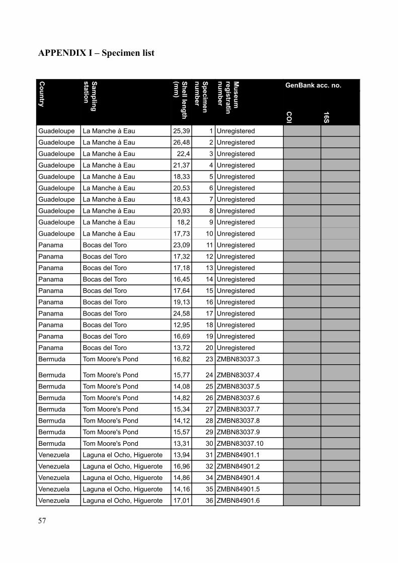
APPENDIX I – Specimen list

Country

Sampling

station

Shell length (m

m)

Specimen

number

Museum

registratin num

ber

GenBank acc. no.

CO

I

16S

Guadeloupe La Manche à Eau 25,39 1 Unregistered

Guadeloupe La Manche à Eau 26,48 2 Unregistered

Guadeloupe La Manche à Eau 22,4 3 Unregistered

Guadeloupe La Manche à Eau 21,37 4 Unregistered

Guadeloupe La Manche à Eau 18,33 5 Unregistered

Guadeloupe La Manche à Eau 20,53 6 Unregistered

Guadeloupe La Manche à Eau 18,43 7 Unregistered

Guadeloupe La Manche à Eau 20,93 8 Unregistered

Guadeloupe La Manche à Eau 18,2 9 Unregistered

Guadeloupe La Manche à Eau 17,73 10 Unregistered

Panama Bocas del Toro 23,09 11 Unregistered

Panama Bocas del Toro 17,32 12 Unregistered

Panama Bocas del Toro 17,18 13 Unregistered

Panama Bocas del Toro 16,45 14 Unregistered

Panama Bocas del Toro 17,64 15 Unregistered

Panama Bocas del Toro 19,13 16 Unregistered

Panama Bocas del Toro 24,58 17 Unregistered

Panama Bocas del Toro 12,95 18 Unregistered

Panama Bocas del Toro 16,69 19 Unregistered

Panama Bocas del Toro 13,72 20 Unregistered

Bermuda Tom Moore's Pond 16,82 23 ZMBN83037.3

Bermuda Tom Moore's Pond 15,77 24 ZMBN83037.4

Bermuda Tom Moore's Pond 14,08 25 ZMBN83037.5

Bermuda Tom Moore's Pond 14,82 26 ZMBN83037.6

Bermuda Tom Moore's Pond 15,34 27 ZMBN83037.7

Bermuda Tom Moore's Pond 14,12 28 ZMBN83037.8

Bermuda Tom Moore's Pond 15,57 29 ZMBN83037.9

Bermuda Tom Moore's Pond 13,31 30 ZMBN83037.10

Venezuela Laguna el Ocho, Higuerote 13,94 31 ZMBN84901.1

Venezuela Laguna el Ocho, Higuerote 16,96 32 ZMBN84901.2

Venezuela Laguna el Ocho, Higuerote 14,86 34 ZMBN84901.4

Venezuela Laguna el Ocho, Higuerote 14,16 35 ZMBN84901.5

Venezuela Laguna el Ocho, Higuerote 17,01 36 ZMBN84901.6

57

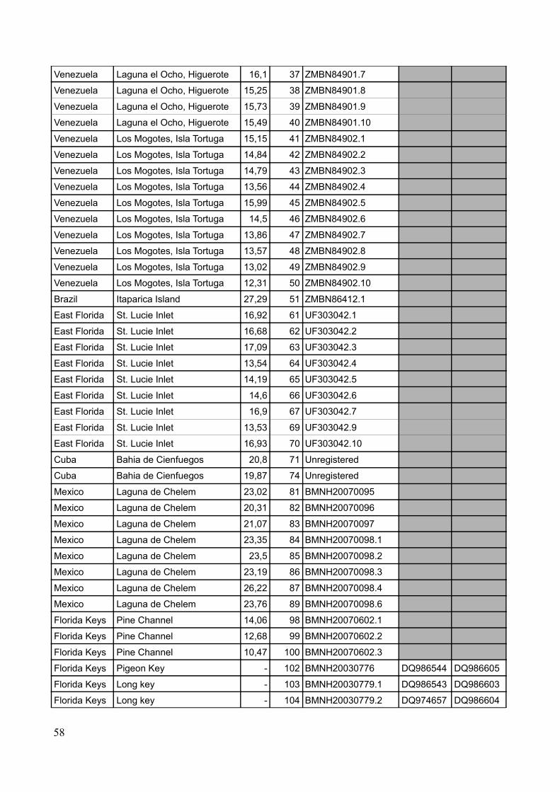
Venezuela Laguna el Ocho, Higuerote 16,1 37 ZMBN84901.7

Venezuela Laguna el Ocho, Higuerote 15,25 38 ZMBN84901.8

Venezuela Laguna el Ocho, Higuerote 15,73 39 ZMBN84901.9

Venezuela Laguna el Ocho, Higuerote 15,49 40 ZMBN84901.10

Venezuela Los Mogotes, Isla Tortuga 15,15 41 ZMBN84902.1

Venezuela Los Mogotes, Isla Tortuga 14,84 42 ZMBN84902.2

Venezuela Los Mogotes, Isla Tortuga 14,79 43 ZMBN84902.3

Venezuela Los Mogotes, Isla Tortuga 13,56 44 ZMBN84902.4

Venezuela Los Mogotes, Isla Tortuga 15,99 45 ZMBN84902.5

Venezuela Los Mogotes, Isla Tortuga 14,5 46 ZMBN84902.6

Venezuela Los Mogotes, Isla Tortuga 13,86 47 ZMBN84902.7

Venezuela Los Mogotes, Isla Tortuga 13,57 48 ZMBN84902.8

Venezuela Los Mogotes, Isla Tortuga 13,02 49 ZMBN84902.9

Venezuela Los Mogotes, Isla Tortuga 12,31 50 ZMBN84902.10

Brazil Itaparica Island 27,29 51 ZMBN86412.1

East Florida St. Lucie Inlet 16,92 61 UF303042.1

East Florida St. Lucie Inlet 16,68 62 UF303042.2

East Florida St. Lucie Inlet 17,09 63 UF303042.3

East Florida St. Lucie Inlet 13,54 64 UF303042.4

East Florida St. Lucie Inlet 14,19 65 UF303042.5

East Florida St. Lucie Inlet 14,6 66 UF303042.6

East Florida St. Lucie Inlet 16,9 67 UF303042.7

East Florida St. Lucie Inlet 13,53 69 UF303042.9

East Florida St. Lucie Inlet 16,93 70 UF303042.10

Cuba Bahia de Cienfuegos 20,8 71 Unregistered

Cuba Bahia de Cienfuegos 19,87 74 Unregistered

Mexico Laguna de Chelem 23,02 81 BMNH20070095

Mexico Laguna de Chelem 20,31 82 BMNH20070096

Mexico Laguna de Chelem 21,07 83 BMNH20070097

Mexico Laguna de Chelem 23,35 84 BMNH20070098.1

Mexico Laguna de Chelem 23,5 85 BMNH20070098.2

Mexico Laguna de Chelem 23,19 86 BMNH20070098.3

Mexico Laguna de Chelem 26,22 87 BMNH20070098.4

Mexico Laguna de Chelem 23,76 89 BMNH20070098.6

Florida Keys Pine Channel 14,06 98 BMNH20070602.1

Florida Keys Pine Channel 12,68 99 BMNH20070602.2

Florida Keys Pine Channel 10,47 100 BMNH20070602.3

Florida Keys Pigeon Key - 102 BMNH20030776 DQ986544 DQ986605

Florida Keys Long key - 103 BMNH20030779.1 DQ986543 DQ986603

Florida Keys Long key - 104 BMNH20030779.2 DQ974657 DQ986604

58

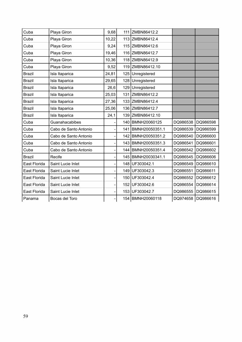
Cuba Playa Giron 9,68 111 ZMBN86412.2

Cuba Playa Giron 10,22 113 ZMBN86412.4

Cuba Playa Giron 9,24 115 ZMBN86412.6

Cuba Playa Giron 19,46 116 ZMBN86412.7

Cuba Playa Giron 10,36 118 ZMBN86412.9

Cuba Playa Giron 9,52 119 ZMBN86412.10

Brazil Isla Itaparica 24,81 125 Unregistered

Brazil Isla Itaparica 29,65 128 Unregistered

Brazil Isla Itaparica 26,6 129 Unregistered

Brazil Isla Itaparica 25,03 131 ZMBN86412.2

Brazil Isla Itaparica 27,36 133 ZMBN86412.4

Brazil Isla Itaparica 25,06 136 ZMBN86412.7

Brazil Isla Itaparica 24,1 139 ZMBN86412.10

Cuba Guanahacabibes - 140 BMNH20060125 DQ986538 DQ986598

Cuba Cabo de Santo Antonio - 141 BMNH20050351.1 DQ986539 DQ986599

Cuba Cabo de Santo Antonio - 142 BMNH20050351.2 DQ986540 DQ986600

Cuba Cabo de Santo Antonio - 143 BMNH20050351.3 DQ986541 DQ986601

Cuba Cabo de Santo Antonio - 144 BMNH20050351.4 DQ986542 DQ986602

Brazil Recife - 145 BMNH20030341.1 DQ986545 DQ986606

East Florida Saint Lucie Inlet - 148 UF303042.1 DQ986549 DQ986610

East Florida Saint Lucie Inlet - 149 UF303042.3 DQ986551 DQ986611

East Florida Saint Lucie Inlet - 150 UF303042.4 DQ986552 DQ986612

East Florida Saint Lucie Inlet - 152 UF303042.6 DQ986554 DQ986614

East Florida Saint Lucie Inlet - 153 UF303042.7 DQ986555 DQ986615

Panama Bocas del Toro - 154 BMNH20060118 DQ974658 DQ986616

59

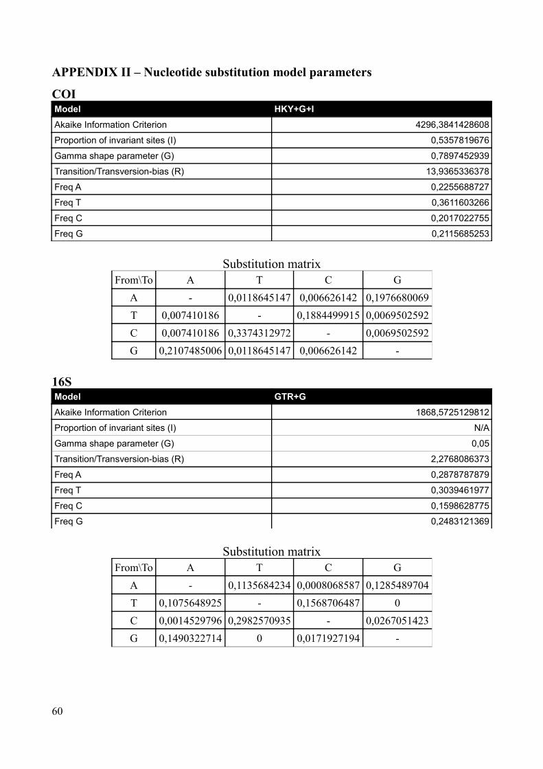
APPENDIX II – Nucleotide substitution model parameters

COIModel HKY+G+IAkaike Information Criterion 4296,3841428608

Proportion of invariant sites (I) 0,5357819676

Gamma shape parameter (G) 0,7897452939

Transition/Transversion-bias (R) 13,9365336378

Freq A 0,2255688727

Freq T 0,3611603266

Freq C 0,2017022755

Freq G 0,2115685253

Substitution matrixFrom\To A T C G

A - 0,0118645147 0,006626142 0,1976680069T 0,007410186 - 0,1884499915 0,0069502592C 0,007410186 0,3374312972 - 0,0069502592G 0,2107485006 0,0118645147 0,006626142 -

16SModel GTR+GAkaike Information Criterion 1868,5725129812

Proportion of invariant sites (I) N/A

Gamma shape parameter (G) 0,05

Transition/Transversion-bias (R) 2,2768086373

Freq A 0,2878787879

Freq T 0,3039461977

Freq C 0,1598628775

Freq G 0,2483121369

Substitution matrixFrom\To A T C G

A - 0,1135684234 0,0008068587 0,1285489704T 0,1075648925 - 0,1568706487 0C 0,0014529796 0,2982570935 - 0,0267051423G 0,1490322714 0 0,0171927194 -

60

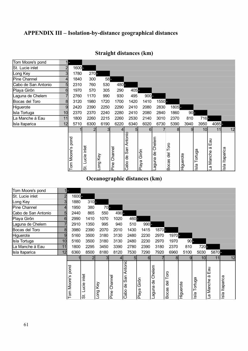
APPENDIX III – Isolation-by-distance geographical distances

Straight distances (km)

Oceanographic distances (km)

61

Tom Moore's pond 1 -St. Lucie inlet 2 1600 -Long Key 3 1880 310 -Pine Channel 4 1950 380 70 -Cabo de San Antonio 5 2440 865 550 490 -Playa Girôn 6 2990 1410 1070 1020 460 -Laguna de Chelem 7 2910 1350 995 940 510 990 -Bocas del Toro 8 3980 2390 2070 2010 1430 1415 1870 -Higuerote 9 5160 3500 3180 3130 2480 2230 2970 1970 -Isla Tortuga 10 5160 3500 3180 3130 2480 2230 2970 1970 90 -La Manche á Eau 11 1800 2295 3450 3390 2780 2390 3180 2370 810 720 -Isla Itaparica 12 6360 8500 8180 8120 7530 7290 7920 6960 5100 5030 5870 -

1 2 3 4 5 6 7 8 9 10 11 12

Tom

Moo

re's

pon

d

St.

Luci

e in

let

Long

Key

Pin

e C

hann

el

Cab

o de

San

Ant

onio

Pla

ya G

irôn

Lagu

na d

e C

hele

m

Boc

as d

el T

oro

Hig

uero

te

Isla

Tor

tuga

La M

anch

e á

Eau

Isla

Itap

aric

a

Tom Moore's pond 1 -St. Lucie inlet 2 1600 -Long Key 3 1780 270 -Pine Channel 4 1840 300 58 -Cabo de San Antonio 5 2310 760 530 480 -Playa Girôn 6 1970 570 305 290 405 -Laguna de Chelem 7 2760 1170 990 930 495 900 -Bocas del Toro 8 3120 1980 1720 1700 1420 1410 1550 -Higuerote 9 2420 2390 2250 2290 2410 2080 2830 1805 -Isla Tortuga 10 2370 2370 2240 2280 2410 2080 2840 1860 90 -La Manche á Eau 11 1800 2260 2215 2260 2530 2140 3010 2370 810 716 -Isla Itaparica 12 5710 6300 6190 6220 6340 6020 6730 5390 3940 3950 4085 -

1 2 3 4 5 6 7 8 9 10 11 12

Tom

Moo

re's

pon

d

St.

Luci

e in

let

Long

Key

Pin

e C

hann

el

Cab

o de

San

Ant

onio

Pla

ya G

irôn

Lagu

na d

e C

hele

m

Boc

as d

el T

oro

Hig

uero

te

Isla

Tor

tuga

La M

anch

e á

Eau

Isla

Itap

aric

a

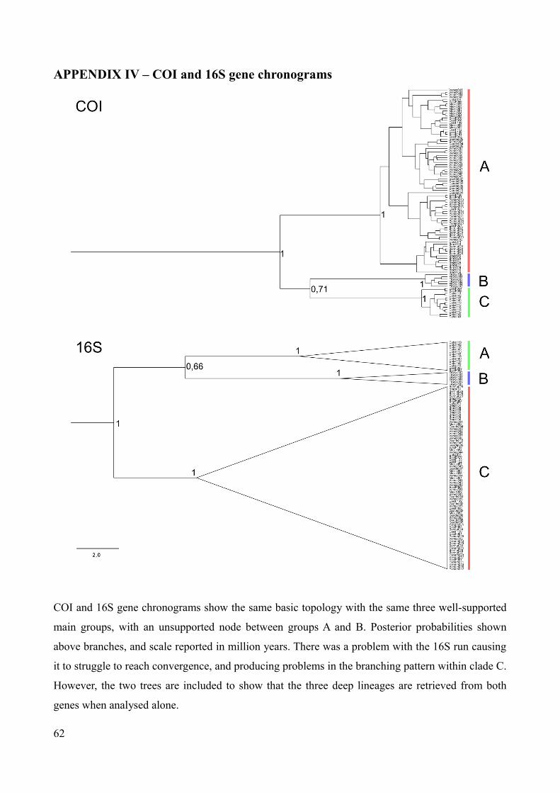
APPENDIX IV – COI and 16S gene chronograms

COI and 16S gene chronograms show the same basic topology with the same three well-supported

main groups, with an unsupported node between groups A and B. Posterior probabilities shown

above branches, and scale reported in million years. There was a problem with the 16S run causing

it to struggle to reach convergence, and producing problems in the branching pattern within clade C.

However, the two trees are included to show that the three deep lineages are retrieved from both

genes when analysed alone.

62