arX

iv:1

507.

0850

8v1

[m

ath-

ph]

30

Jul 2

015

General solutions of the supersymmetric CP 2 sigma

model and its generalisation to CPN−1

L. Delisle1,5, V. Hussin2,3,6 and W. J. Zakrzewski4,7

August 3, 2015

Abstract

A new approach for the construction of finite action solutions of the supersymmetric

CPN−1 sigma model is presented. We show that this approach produces more non-

holomorphic solutions than those obtained in previous approaches. We study the CP2

model in detail and present its solutions in an explicit form. We also show how to

generalise this construction to N > 3.

1 Introduction

Study of exact solutions of integrable models is a subject of great interest to the mathematicsand physics communities. In addition, the 2-dimensional integrable bosonic CPN−1 sigmamodel has found applications in physics, biology, and mathematics [1, 2, 3, 4, 5, 6]. Thesolutions of this model are known [7] and were used to construct solutions of more generalgrassmannian sigma models [7] and to generate surfaces immersed in the Lie algebra su(N)[8, 9, 10, 11, 12, 13, 14, 15, 16, 17, 18, 19] . Indeed, the present authors have discussed thesolutions of general grassmannian models which correspond to surfaces of constant gaussiancurvatures [8, 9, 10]. Other papers discussed also different geometric quantities of thesesurfaces such as their fundamental forms, their mean curvatures and the Willmore functional[10, 11, 12].

In a recent paper [20], we studied the surfaces obtained from the solutions of the super-symmetric CPN−1 sigma models. We classified the surfaces of constant gaussian curvatureassociated to holomorphic solutions and showed their deep connection with the bosonicVeronese curve. This curve was shown to be useful to obtain a classification of all constantcurvature surfaces in the bosonic CPN−1 model when one generates the complete set ofsolutions of this model via the repeated application of an orthogonalisation operator [14].

In this same paper [20], we obtained some non-holomorphic solutions using two differentstrategies: the first one relied on imposing supersymmetric invariance and, the other, onforcing the conformality of the constructed surfaces. Although we managed to present somenon-holomorphic solutions, a general method of constructing all of them still has not beenfound and the present paper addresses this problem. Our main idea here is to generalizethe so-called holomorphic method [7], used in constructing the complete set of solutions ofthe bosonic model, and to apply it to the supersymmetric CPN−1 sigma model. So, let

1Institut de mathematiques de Jussieu-Paris Rive Gauche, UP7D-Campus des Grands Moulins, BatimentSophie Germain, Cases 7012, 75205 Paris Cedex 13.

2Departement de Mathematiques et de Statistique, Universite de Montreal, C.P. 6128, Succ. Centre-ville,Montreal (Quebec) H3C 3J7, Canada.

3Centre de Recherches Mathematiques, Universite de Montreal, C.P. 6128, Succ. Centre-ville, Montreal(Quebec) H3C 3J7, Canada.

4Department of Mathematical Sciences, University of Durham, Durham DH1 3LE, United Kingdom.5email:laurent.delisle@imj-prg.fr6email:hussin@dms.umontreal.ca7email:w.j.zakrzewski@durham.ac.uk

1

us remind the reader of the bosonic holomorphic method. In this method we consider aholomorphic N -component vector ψ0 = ψ0(x+) such that the sequence

ψ0, ψ1 = ∂+ψ0, ψ2 = ∂+ψ1, · · · , ψN−1 = ∂+ψN−2 (1)

forms a linearly independent set of vectors. Using Gram-Schmidt, we orthogonalize thevectors of the above set and, then, obtain a new set consisting of N vectors

z0 = ψ0, zj = ψj −

j−1∑

k=0

z†kψj

|zk|2zk, j = 1, 2, · · · , N − 1. (2)

Then, as is well known [7], the vectors

Zj =zj

|zj |, j = 0, 1, · · · , N − 1, (3)

are solutions of the Euler-Lagrange equations of the model. Furthermore, it is also knownthat the set {Z0, Z1, · · · , ZN−1} is complete and thus all solutions are of this type. In ourrecent paper [20], we have asked the question whether a similar classification of solutionsexisted in the supersymmetric case. In that paper, we were not able to present a definitiveanswer to this question. There exists other papers which have also looked for solutions ofthis model. In [21], the authors solved the linear Dirac equation associated to the model.This reduced model only considered quadratic fermionic terms in the Lagrangian eliminat-ing higher order odd terms. In another paper [22], the authors considered the fermioniccontributions as commuting quantities. This method has given formal solutions but somepractical uncertainties as to the validity of this procedure had been raised. In the presentpaper, we go a step further and present a systematic method for constructing solutions ofthe general model without any of the above assumptions. In fact, our approach is based ona generalisation of the holomorphic method for constructing solutions in the bosonic model[7].

In order to make the paper self-contained, we present, in the next section, a brief de-scription of the supersymmetric CPN−1 sigma model and of its formulation in terms oforthogonal projectors. We then discuss, in detail, the CP 2 model, the simplest one pos-sessing non-holomorphic solutions, and we construct its solutions using our new approach.This approach is a generalization to the supersymmetric context of the general constructionin the bosonic case [7]. We show that our method enlarges a class of solutions and eventhough we feel that it generates all of them we have no proof that this is the case. We finishthis section by presenting some explicit examples of the obtained solutions. In section 4,we generalize our procedure to the more general supersymmetric CPN−1 sigma models andmake some remarks on constraints that have to be imposed in the construction of solutionsof these models. We conclude the paper with some remarks and our future outlook.

2 The supersymmetric CPN−1 sigma model

In this section, for completeness, we recall the definition of the two-dimensional CPN−1

supersymmetric sigma model and its orthogonal projector formulation [7]. We will use thisformulation in the subsequent sections.

The two-dimensional supersymmetric CPN−1 sigma model involves the collection ofbosonic superfields Φ defined on the complex superspace of local coordinates (x+, x−; θ+, θ−)with values in the Grassmannian manifold CPN−1. In this formulation, (x+, x−) are local

coordinates of the complex plane C (x†+ = x−) and (θ+, θ−) are complex odd Grassmannvariables satisfying

θ+θ− + θ−θ+ = 0, θ2+ = θ2− = 0, θ†+ = θ−. (4)

2

The superfields Φ are N -components vectors and satisfy the nonlinear condition

Φ†Φ = 1. (5)

The classical solutions of the model, which we want to discuss, are actually critical pointsof finite energy of the action functional defined in terms of the Lagrangian density

L = 2(|D+Φ|2 − |D−Φ|

2), (6)

where D±Λ = ∂±Λ − Λ(Φ†∂±Φ) are the covariant derivatives constructed from the gauge-invariance of the Lagrangian density under the transformation

Φ −→ V ΦU, (7)

where U ∈ U(1) and V ∈ U(N) are respectively local and global gauge transformations ofthe unitary group. The operators ∂± are odd derivatives defined by

∂± = −i∂θ± + θ±∂±, (8)

that satisfy∂2± = −i∂± = −i∂x± . (9)

We use the following convention: |Λ|2 = Λ†Λ for Λ a bosonic or a fermionic field [23]. Thisconvention is used to eliminate the ambiguity for fermionic constants. As is well known theEuler-Lagrange equations corresponding to (6) are given by:

D+D−Φ+ |D−Φ|2Φ = 0, Φ†Φ = 1. (10)

As we are interested only in finite energy solutions of (10), we have to impose theboundary conditions. We actually want the fields Φ (or strictly speaking their bosonic part)to converge to a constant at infinity, and sufficiently fast. We thus impose the boundaryconditions

D±Φ −→ 0, as |x+| −→ ∞. (11)

These boundary conditions have the effect of compactifying the bosonic part of the super-space (x+, x−; θ+, θ−) into the 2-sphere S2 via the stereographic projection.

A convenient reformulation of the two-dimensional CPN−1 supersymmetric sigma modelinvolves considering it in a gauge-invariant way in terms of orthogonal projectors [7, 20, 24].Indeed, let Φ be a solution of the model and define P as

P = ΦΦ†. (12)

Then using (7), we see that P −→ V PV † which corresponds to a global gauge transformation,since V is independent of local coordinates. Using the nonlinear constraint (5), we deducethat P is a rank-one orthogonal projector, i.e. it possesses the following properties

P2 = P

† = P, TrP = 1. (13)

In this setting, the Lagrangian density (6) takes the form

L = 2Tr(

∂−P∂+P)

(14)

and the Euler-Lagrange equations (10) can be equivalently rewritten as

[∂+∂−P,P] = 0, P2 = P, (15)

where [A,B] = AB − BA is the usual matrix commutator. Furthermore, a fact that willbecome useful in the subsequent sections is that the Euler-Lagrange equations (15) may bewritten as a super-conservation law:

∂+Ξ + ∂−Ξ† = 0, Ξ = [P, ∂−P]. (16)

This equation differs from the one obtained in the bosonic case [7]. Here, the equationinvolves the odd derivatives ∂± and the fermionic quantities Ξ and Ξ†.

3

3 The CP 2 model

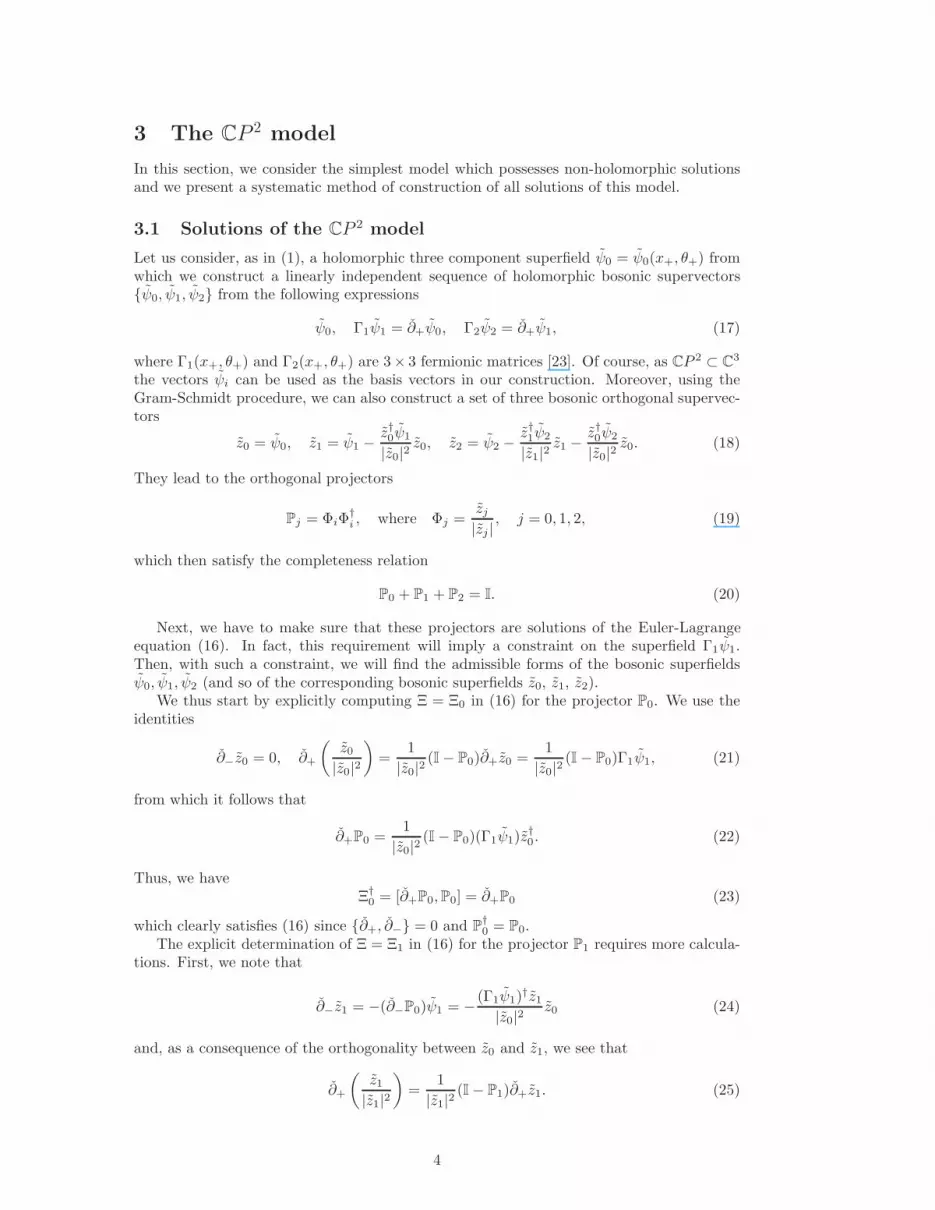
In this section, we consider the simplest model which possesses non-holomorphic solutionsand we present a systematic method of construction of all solutions of this model.

3.1 Solutions of the CP 2 model

Let us consider, as in (1), a holomorphic three component superfield ψ0 = ψ0(x+, θ+) fromwhich we construct a linearly independent sequence of holomorphic bosonic supervectors{ψ0, ψ1, ψ2} from the following expressions

ψ0, Γ1ψ1 = ∂+ψ0, Γ2ψ2 = ∂+ψ1, (17)

where Γ1(x+, θ+) and Γ2(x+, θ+) are 3× 3 fermionic matrices [23]. Of course, as CP 2 ⊂ C3

the vectors ψi can be used as the basis vectors in our construction. Moreover, using theGram-Schmidt procedure, we can also construct a set of three bosonic orthogonal supervec-tors

z0 = ψ0, z1 = ψ1 −z†0ψ1

|z0|2z0, z2 = ψ2 −

z†1ψ2

|z1|2z1 −

z†0ψ2

|z0|2z0. (18)

They lead to the orthogonal projectors

Pj = ΦiΦ†i , where Φj =

zj

|zj |, j = 0, 1, 2, (19)

which then satisfy the completeness relation

P0 + P1 + P2 = I. (20)

Next, we have to make sure that these projectors are solutions of the Euler-Lagrangeequation (16). In fact, this requirement will imply a constraint on the superfield Γ1ψ1.Then, with such a constraint, we will find the admissible forms of the bosonic superfieldsψ0, ψ1, ψ2 (and so of the corresponding bosonic superfields z0, z1, z2).

We thus start by explicitly computing Ξ = Ξ0 in (16) for the projector P0. We use theidentities

∂−z0 = 0, ∂+

(

z0

|z0|2

)

=1

|z0|2(I− P0)∂+z0 =

1

|z0|2(I− P0)Γ1ψ1, (21)

from which it follows that

∂+P0 =1

|z0|2(I− P0)(Γ1ψ1)z

†0. (22)

Thus, we haveΞ†0 = [∂+P0,P0] = ∂+P0 (23)

which clearly satisfies (16) since {∂+, ∂−} = 0 and P†0 = P0.

The explicit determination of Ξ = Ξ1 in (16) for the projector P1 requires more calcula-tions. First, we note that

∂−z1 = −(∂−P0)ψ1 = −(Γ1ψ1)

†z1

|z0|2z0 (24)

and, as a consequence of the orthogonality between z0 and z1, we see that

∂+

(

z1

|z1|2

)

=1

|z1|2(I− P1)∂+z1. (25)

4

But, we have that

∂+z1 = −(∂+P0)ψ1 + (I− P0)∂+ψ1 = (I− P0)

(

Γ2ψ2 −z†0ψ1

|z0|2Γ1ψ1

)

, (26)

from which we deduce the expression

∂+

(

z1

|z1|2

)

=1

|z1|2(I− P0 − P1)

(

Γ2ψ2 −z†0ψ1

|z0|2Γ1ψ1

)

. (27)

From these preliminary calculations, we derive an expression for the superderivative ofthe projector P1:

∂+P1 =1

|z1|2(I− P0 − P1)

(

Γ2ψ2 −z†0ψ1

|z0|2Γ1ψ1

)

z†1 −

z†1(Γ1ψ1)

|z0|2|z1|2z1z

†0. (28)

From this, we now have an explicit expression for Ξ†1 to be put into (16):

Ξ†1 =

1

|z1|2(I− P0 − P1)

(

Γ2ψ2 −z†0ψ1

|z0|2Γ1ψ1

)

z†1 +

z†1(Γ1ψ1)

|z0|2|z1|2z1z

†0 (29)

and we note that

P1∂+P0 =z†1(Γ1ψ1)

|z0|2|z1|2z1z

†0. (30)

As a consequence we may rewrite Ξ†1 as

Ξ†1 = ∂+P1 + 2P1∂+P0. (31)

From this, we see that the Euler-Lagrange equations (16) reduce to having to satisfy:

∂+Ξ1 + ∂−Ξ†1 = ∂+((∂−P0)P1) + ∂−(P1∂+P0) = 0. (32)

We will show in Proposition 1 that this condition is equivalent to the constraint Γ1ψ1 ∈ker(I− P0 − P1), i.e. (I− P0 − P1)(Γ1ψ1) = 0.

Before we do this let us note that for the projector P2, we can use a result proved in [20],that demonstrates that P0+P1 is a holomorphic solution of the supersymmetricG(2, 3) modeland so, using the completeness relation (20), P2 also solves the Euler-Lagrange equations.Furthermore, the projector P2 corresponds to an anti-holomorphic solution in the sense thatit satisfies (∂+P2)P2 = 0. Again, using the completeness relation (20), we get

(∂+P2)P2 = −∂+(P0 + P1)(I− (P0 + P1)) = −∂+(P0 + P1) + ∂+(P0 + P1)(P0 + P1) (33)

and the result follows from the fact that P0 + P1, being holomorphic, satisfies the identity∂+(P0 + P1)(P0 + P1) = ∂+(P0 + P1).

Proposition 1: The projector P1 solves the Euler-Lagrange equations (15) if and only if

Γ1ψ1 ∈ ker(I − P0 − P1). (34)

Proof: By direct computation, we can show that (32) is equivalent to the following equation

(

a1 + α1(Γ1ψ1)

†z0

|z0|2

)

z1z†0

|z0|2−

(

a†1 +

z†0(Γ1ψ1)

|z0|2α†1

)

z0z†1

|z0|2− α1

z1(Γ1ψ1)†

|z0|2− α

†1

(Γ1ψ1)z†1

|z0|2= 0,

(35)

5

where a1 and α1 are, respectively, bosonic and fermionic functions defined by

a†1 = (Γ1ψ1)

†∂+

(

z1

|z1|2

)

, α1 =z†1(Γ1ψ1)

|z1|2. (36)

We easily see from these expressions that a1 = ∂−α1.We can now act on (35) from the left with z†0. It leads to (recall that z†1z0 = 0 and, that

Γ1ψ1 and α†1 are fermionic and so anticommute)

a1z1 = 0 =⇒ a1 = 0, (37)

which is equivalent to

(

Γ2ψ2 −z†0ψ1

|z0|2Γ1ψ1

)†

(I− P0 − P1)(Γ1ψ1) = 0. (38)

So, putting a1 = 0, (35) becomes

α1z1(Γ1ψ1)†(P0 − I) + α

†1(P0 − I)(Γ1ψ1)z

†1 = 0. (39)

Acting on this expression from the right with z1 and using the fact that P1(Γ1ψ1) = α1z1we get

α†1(I− P0 − P1)(Γ1ψ1) = 0. (40)

The equation is clearly satisfied if α1 = 0. However, this choice has to be rejected. Indeed,α1 = 0 is equivalent to

z†1(Γ1ψ1) = 0 (41)

and, from (24), we would have then got that ∂−z1 = 0. However, this would have meantthat the supervector z1 = z1(x+, θ+) is holomorphic but we want z1 to be non-holomorphic.Thus we require α1 6= 0. This leads immediately to the constraint (34). Moreover, in thiscase the equation (38) is automatically satisfied. Thus we have shown that in order for P1 tobe a solution of the Euler-Lagrange equation, we require the constraint (34) to be satisfied.

Finally, we have to show that if the constraint (34) is satisfied P1 is a solution of theEuler-Lagrange equation. Indeed, the constraint (34) can be rewritten as

P1(Γ1ψ1) = (I− P0)(Γ1ψ1) (42)

from which we deduce, from the expression (30), that

P1∂+P0 = P1(Γ1ψ1)z†0

|z0|2= (I− P0)(Γ1ψ1)

z†0

|z0|2= ∂+P0. (43)

From this last result, we see that Ξ†1 = ∂+(P1+2P0) and so, using the fact that {∂+, ∂−} = 0,

we conclude that P1 is indeed a solution of the Euler-Lagrange equation.This concludes the proof.

3.2 The study of the constraint

Here we look at the constraint (34).The constraint (34) can be equivalently written as

(P0 + P1)(Γ1ψ1) = Γ1ψ1, (44)

which implies that Γ1ψ1 is an eigenvector of the matrix P0 + P1 of eigenvalue 1. The nextstep is to show that the matrix P0 + P1 is diagonalisable. We note that

(P0 + P1)ψj = ψj , (P0 + P1)z2 = 0 (45)

6

for j = 0, 1 and, by construction, the vectors ψ0, ψ1 and z2 are linearly independent implyingthat the matrix is diagonalisable. From the constraint (34), we deduce that Γ1ψ1 lies in theeigenspace of (P0 + P1) and its eigenvalue is 1. So we can write

Γ1ψ1 = α0ψ0 + α1ψ1, (46)

where α0 and α1 are fermionic functions of (x+, θ+).For Γ2ψ2 we can use the completeness relation, i.e. that vectors ψi, i = 1, 2, 3 can be

taken as basis vectors of C3, to expand

Γ2ψ2 = β0ψ0 + β1ψ1 + β2ψ2, (47)

where β0, β1 and β2 are fermionic functions of (x+, θ+). So, finding the solutions of thesystem (17) together with the constraint (34) is equivalent to finding the solutions of thesystem

α0ψ0 + α1ψ1 = ∂+ψ0, β0ψ0 + β1ψ1 + β2ψ2 = ∂+ψ1. (48)

This we do in the next section.

3.3 General construction of ψ0, ψ1 and ψ2

Here we determine the general expressions for the superfields ψ0, ψ1 and ψ2 of the system(48). To do so, we put

αj = αfj + iθ+α

bj , βk = β

fk + iθ+β

bk, ψk = ψb

k + iθ+ψfk (49)

for j = 0, 1 and k = 0, 1, 2. The superscripts f and b refers to, respectively, to fermionic andbosonic quantities. From these expressions, we may rewrite system (48) in component formas a set of four equations:

αf0 ψ

b0 + α

f1 ψ

b1 = ψ

f0 , (50)

αb0ψ

b0 + αb

1ψb1 − α

f0 ψ

f0 − α

f1 ψ

f1 = −i∂+ψ

b0, (51)

βf0 ψ

b0 + β

f1 ψ

b1 + β

f2 ψ

b2 = ψ

f1 , (52)

βb0ψ

b0 + βb

1ψb1 + βb

2ψb2 − β

f0 ψ

f0 − β

f1 ψ

f1 − β

f2 ψ

f2 = −i∂+ψ

b1. (53)

The details of the above resolution are given in Appendix A and, as it is shown there, thegeneral solution of this system may be expressed in terms of the field ψb

0 and its consecutive

ordinary derivatives. Indeed, the expressions for ψf0 and ψb

1 are given by

ψf0 =

(

αf0 −

αf1α

b0

αb1

)

ψb0 − i

αf1

αb1

∂+ψb0, (54)

ψb1 = A0ψ

b0 +A1∂+ψ

b0 − i

αf1β

f2

αb1β

b2

(

(∂+A0)ψb0 + (A0 + ∂+A1)∂+ψ

b0 +A1∂

2+ψ

b0

)

, (55)

where the quantities A0 and A1, in their explicit form, are given by

A0 = −αb0

αb1

(

1 +αf0α

f1

αb1

)

+αf1

αb1

(

βf0 −

βf2β

b0

βb2

+βf2 β

f1β

f0

βb2

)

−αb0α

f1

(αb1)

2

(

βf1 −

βf2β

b1

βb2

)

+αf1β

f2β

f0

αb1β

b2

(

αf0 −

αf1α

b0

αb1

)

, (56)

A1 = −i

αb1

(

1 +αf0α

f1

αb1

+αf1

αb1

(

βf1 −

βf2β

b1

βb2

))

. (57)

7

Moreover, the explicit expression of the field ψf1 can be given in terms of the fields ψb

0, ψf0

and ψb1 and it takes the form

ψf1 =

(

βf0 −

βf2β

b0

βb2

+βf2 β

f1β

f0

βb2

)

ψb0 +

(

βf1 −

βf2β

b1

βb2

)

ψb1 +

βf2β

f0

βb2

ψf0 − i

βf2

βb2

∂+ψb1. (58)

The above expressions can then be used to determine the field ψb2 and ψf

2 although we donot really need them as, in fact, we are interested in the form of Φ2 which provides the last(i.e. antiholomorphic) solution of the model. Φ2 is, however, orthogonal to Φ1 and so can becalculated by taking, as an example, ψ2 = ψ1× ψ0 where × denotes the vector product. Welike to point out that this particular choice is restrictive in the sense that ψf

2 is completely

determined in opposition with the general case where ψf2 is a free field. Note that we stated

just before (just before our proposition 1) that Φ2 is an antiholomorphic solution.The details of all these calculations are presented in Appendix A. In the next section,

we explore some special cases of the obtained solutions.

3.4 Special solutions and connection with the operator Px+

In this section, we discuss, in more detail, a special case of the solution obtained in theprevious section, in which we have made the particular choice α0 = β0 = β1 = 0, i.e.

Γ1ψ1 = α1ψ1, Γ2ψ2 = β2ψ2. (59)

In this case, the quantities A0 and A1 take the simple forms

A0 = 0, A1 = −i

αb1

(60)

and, in consequence, the fields ψf0 , ψ

b1, ψ

f1 and ψb

2 are given by

ψf0 = −i

αf1

αb1

∂+ψb0, ψ

f1 = −i

βf2

βb2

∂+ψb1, ψb

2 =βf2

βb2

ψf2 −

i

βb2

∂+ψb1, (61)

together with

ψb1 =

(

−i

αb1

+αf1β

f2 ∂+α

b1

(αb1)

3βb2

)

∂+ψb0 −

αf1β

f2

(αb1)

2βb2

∂2+ψb0. (62)

Remark: One important thing to stress here is that the obtained solutions in this paperare more general then the one discussed in the [20]. One way of seeing this involves lookingat the expression for z1, for the system (59), in which we set θ+ = θ− = 0. For z0 = ψ0, letus use the following notation

z0|θ+=θ−=0 = ψb0 = u(x+). (63)

In this case we find that the bosonic part of z1 is given by

z1|θ+=θ−=0 =

(

−i

αb1

+αf1β

f2

(αb1)

3βb2

∂+αb1

)

Px+u−

αf1β

f2

(αb1)

2βb2

(

I−uu†

|u|2

)

∂2+u. (64)

This expression is different then the one we have obtained in [20]. Indeed, in [20] we had

z1|θ+=θ−=0 = − iαb

1

Px+u, where Px+

u = ∂+u− u†∂+u

|u|2 u.

As a final comment, it might be worthwhile to give the explicit expressions of ψ0, ψ1 andψ2 in terms of the free components ψb

0 and ψf2 . We have

ψ0 = ψb0 + θ+

αf1

αb1

∂+ψb0, (65)

8

ψ1 = −i

αb1

∂+ψb0 +

βf2

βb2

(

αf1

αb1

+ iθ+

(

1− iαf1∂+β

f2

αb1β

b2

))

∂+

(

1

αb1

∂+ψb0

)

, (66)

ψ2 = −i

βb2

∂+

(

−i

αb1

∂+ψb0 −

αf1β

f2

αb1β

b2

∂+

(

1

αb1

∂+ψb0

)

)

+βf2 + iθ+β

b2

βb2

ψf2 . (67)

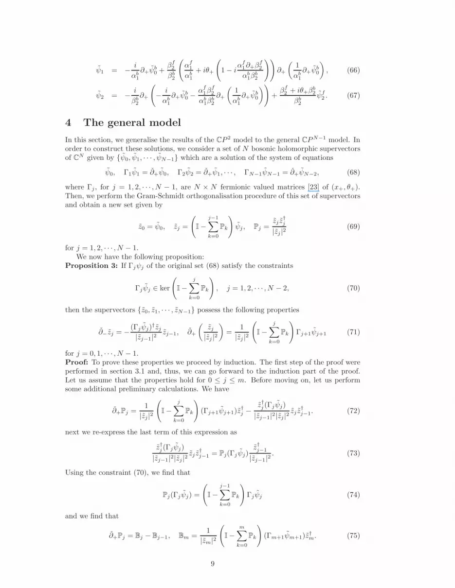
4 The general model

In this section, we generalise the results of the CP 2 model to the general CPN−1 model. Inorder to construct these solutions, we consider a set of N bosonic holomorphic supervectorsof CN given by {ψ0, ψ1, · · · , ψN−1} which are a solution of the system of equations

ψ0, Γ1ψ1 = ∂+ψ0, Γ2ψ2 = ∂+ψ1, · · · , ΓN−1ψN−1 = ∂+ψN−2, (68)

where Γj , for j = 1, 2, · · · , N − 1, are N × N fermionic valued matrices [23] of (x+, θ+).Then, we perform the Gram-Schmidt orthogonalisation procedure of this set of supervectorsand obtain a new set given by

z0 = ψ0, zj =

(

I−

j−1∑

k=0

Pk

)

ψj , Pj =zj z

†j

|zj |2(69)

for j = 1, 2, · · · , N − 1.We now have the following proposition:

Proposition 3: If Γjψj of the original set (68) satisfy the constraints

Γjψj ∈ ker

(

I−

j∑

k=0

Pk

)

, j = 1, 2, · · · , N − 2, (70)

then the supervectors {z0, z1, · · · , zN−1} possess the following properties

∂−zj = −(Γjψj)

†zj

|zj−1|2zj−1, ∂+

(

zj

|zj |2

)

=1

|zj |2

(

I−

j∑

k=0

Pk

)

Γj+1ψj+1 (71)

for j = 0, 1, · · · , N − 1.Proof: To prove these properties we proceed by induction. The first step of the proof wereperformed in section 3.1 and, thus, we can go forward to the induction part of the proof.Let us assume that the properties hold for 0 ≤ j ≤ m. Before moving on, let us performsome additional preliminary calculations. We have

∂+Pj =1

|zj|2

(

I−

j∑

k=0

Pk

)

(Γj+1ψj+1)z†j −

z†j (Γjψj)

|zj−1|2|zj|2zj z

†j−1. (72)

next we re-express the last term of this expression as

z†j (Γjψj)

|zj−1|2|zj |2zj z

†j−1 = Pj(Γj ψj)

z†j−1

|zj−1|2. (73)

Using the constraint (70), we find that

Pj(Γjψj) =

(

I−

j−1∑

k=0

Pk

)

Γjψj (74)

and we find that

∂+Pj = Bj − Bj−1, Bm =1

|zm|2

(

I−m∑

k=0

Pk

)

(Γm+1ψm+1)z†m. (75)

9

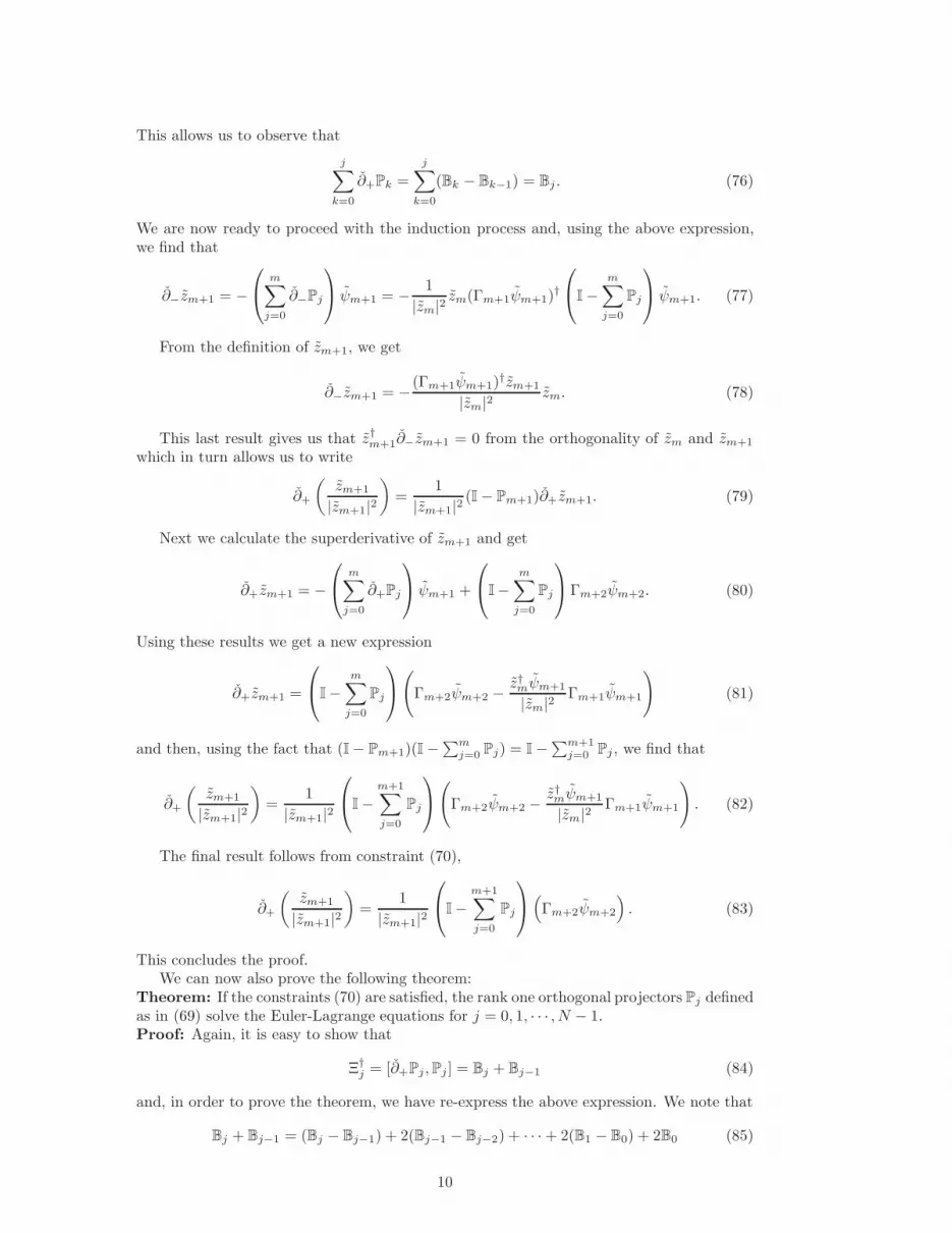
This allows us to observe that

j∑

k=0

∂+Pk =

j∑

k=0

(Bk − Bk−1) = Bj . (76)

We are now ready to proceed with the induction process and, using the above expression,we find that

∂−zm+1 = −

m∑

j=0

∂−Pj

ψm+1 = −1

|zm|2zm(Γm+1ψm+1)

†

I−

m∑

j=0

Pj

ψm+1. (77)

From the definition of zm+1, we get

∂−zm+1 = −(Γm+1ψm+1)

†zm+1

|zm|2zm. (78)

This last result gives us that z†m+1∂−zm+1 = 0 from the orthogonality of zm and zm+1

which in turn allows us to write

∂+

(

zm+1

|zm+1|2

)

=1

|zm+1|2(I− Pm+1)∂+zm+1. (79)

Next we calculate the superderivative of zm+1 and get

∂+zm+1 = −

m∑

j=0

∂+Pj

ψm+1 +

I−m∑

j=0

Pj

Γm+2ψm+2. (80)

Using these results we get a new expression

∂+zm+1 =

I−

m∑

j=0

Pj

(

Γm+2ψm+2 −z†mψm+1

|zm|2Γm+1ψm+1

)

(81)

and then, using the fact that (I− Pm+1)(I −∑m

j=0 Pj) = I−∑m+1

j=0 Pj , we find that

∂+

(

zm+1

|zm+1|2

)

=1

|zm+1|2

I−

m+1∑

j=0

Pj

(

Γm+2ψm+2 −z†mψm+1

|zm|2Γm+1ψm+1

)

. (82)

The final result follows from constraint (70),

∂+

(

zm+1

|zm+1|2

)

=1

|zm+1|2

I−

m+1∑

j=0

Pj

(

Γm+2ψm+2

)

. (83)

This concludes the proof.We can now also prove the following theorem:

Theorem: If the constraints (70) are satisfied, the rank one orthogonal projectors Pj definedas in (69) solve the Euler-Lagrange equations for j = 0, 1, · · · , N − 1.Proof: Again, it is easy to show that

Ξ†j = [∂+Pj,Pj ] = Bj + Bj−1 (84)

and, in order to prove the theorem, we have re-express the above expression. We note that

Bj + Bj−1 = (Bj − Bj−1) + 2(Bj−1 − Bj−2) + · · ·+ 2(B1 − B0) + 2B0 (85)

10

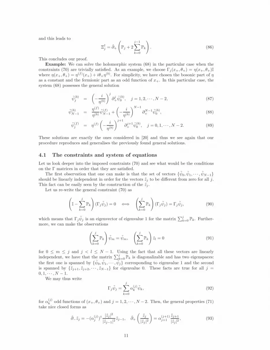
and this leads to

Ξ†j = ∂+

(

Pj + 2

j−1∑

k=0

Pk

)

. (86)

This concludes our proof.Example: We can solve the holomorphic system (68) in the particular case when the

constraints (70) are trivially satisfied. As an example, we choose Γj(x+, θ+) = η(x+, θ+)Iwhere η(x+, θ+) = η(f)(x+) + iθ+η

(b). For simplicity, we have chosen the bosonic part of ηas a constant and the fermionic part as an odd function of x+. In this particular case, thesystem (68) possesses the general solution

ψ(b)j =

(

−i

η(b)

)j

∂j+ψ

(b)0 , j = 1, 2, · · · , N − 2, (87)

ψ(b)N−1 =

η(f)

η(b)ψ(f)N−1 +

(

−i

η(b)

)N−1

∂N−1+ ψ

(b)0 , (88)

ψ(f)j = η(f)

(

−i

η(b)

)j+1

∂j+1+ ψ

(b)0 , j = 0, 1, · · · , N − 2. (89)

These solutions are exactly the ones considered in [20] and thus we see again that ourprocedure reproduces and generalises the previously found general solutions.

4.1 The constraints and system of equations

Let us look deeper into the imposed constraints (70) and see what would be the conditionson the Γ matrices in order that they are satisfied.

The first observation that one can make is that the set of vectors {ψ0, ψ1, · · · , ψN−1}should be linearly independent in order for the vectors zj to be different from zero for all j.This fact can be easily seen by the construction of the zj .

Let us re-write the general constraint (70) as

(

I−

j∑

k=0

Pk

)

(Γjψj) = 0 ⇐⇒

(

j∑

k=0

Pk

)

(Γjψj) = Γjψj , (90)

which means that Γjψj is an eigenvector of eigenvalue 1 for the matrix∑j

k=0 Pk. Further-more, we can make the observations

(

j∑

k=0

Pk

)

ψm = ψm,

(

j∑

k=0

Pk

)

zl = 0 (91)

for 0 ≤ m ≤ j and j < l ≤ N − 1. Using the fact that all these vectors are linearlyindependent, we have that the matrix

∑j

k=0 Pk is diagonalizable and has two eigenspaces:

the first one is spanned by {ψ0, ψ1, · · · , ψj} corresponding to eigenvalue 1 and the secondis spanned by {zj+1, zj+2, · · · , zN−1} for eigenvalue 0. These facts are true for all j =0, 1, · · · , N − 1.

We may thus write

Γjψj =

j∑

k=0

α(j)k ψk, (92)

for α(j)k odd functions of (x+, θ+) and j = 1, 2, · · · , N − 2. Then, the general properties (71)

take nice closed forms as

∂−zj = −(α(j)j )†

|zj |2

|zj−1|2zj−1, ∂+

(

zj

|zj |2

)

= α(j+1)j+1

zj+1

|zj |2, (93)

11

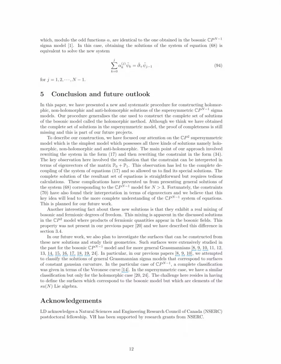
which, modulo the odd functions α, are identical to the one obtained in the bosonic CPN−1

sigma model [1]. In this case, obtaining the solutions of the system of equation (68) isequivalent to solve the new system

j∑

k=0

α(j)k ψk = ∂+ψj−1 (94)

for j = 1, 2, · · · , N − 1.

5 Conclusion and future outlook

In this paper, we have presented a new and systematic procedure for constructing holomor-phic, non-holomorphic and anti-holomorphic solutions of the supersymmetric CPN−1 sigmamodels. Our procedure generalises the one used to construct the complete set of solutionsof the bosonic model called the holomorphic method. Although we think we have obtainedthe complete set of solutions in the supersymmetric model, the proof of completeness is stillmissing and this is part of our future projects.

To describe our construction, we have focused our attention on the CP 2 supersymmetricmodel which is the simplest model which possesses all three kinds of solutions namely holo-morphic, non-holomorphic and anti-holomorphic. The main point of our approach involvedrewriting the system in the form (17) and then rewriting the constraint in the form (34).The key observation here involved the realisation that the constraint can be interpreted interms of eigenvectors of the matrix P0 + P1. This observation has led to the complete de-coupling of the system of equations (17) and so allowed us to find its special solutions. Thecomplete solution of the resultant set of equations is straightforward but requires tediouscalculations. These complications have prevented us from presenting general solutions ofthe system (68) corresponding to the CPN−1 model for N > 3. Fortunately, the constraints(70) have also found their interpretation in terms of eigenvectors and we believe that thiskey idea will lead to the more complete understanding of the CPN−1 system of equations.This is planned for our future work.

Another interesting fact about these new solutions is that they exhibit a real mixing ofbosonic and fermionic degrees of freedom. This mixing is apparent in the discussed solutionsin the CP 2 model where products of fermionic quantities appear in the bosonic fields. Thisproperty was not present in our previous paper [20] and we have described this difference insection 3.4.

In our future work, we also plan to investigate the surfaces that can be constructed fromthese new solutions and study their geometries. Such surfaces were extensively studied inthe past for the bosonic CPN−1 model and for more general Grassmannians [8, 9, 10, 11, 12,13, 14, 15, 16, 17, 18, 19, 24]. In particular, in our previous papers [8, 9, 10], we attemptedto classify the solutions of general Grassmannian sigma models that correspond to surfacesof constant gaussian curvature. In the particular case of CPN−1, a complete classificationwas given in terms of the Veronese curve [14]. In the supersymmetric case, we have a similarclassification but only for the holomorphic case [20, 24]. The challenge here resides in havingto define the surfaces which correspond to the bosonic model but which are elements of thesu(N) Lie algebra.

Acknowledgements

LD acknowledges a Natural Sciences and Engineering Research Council of Canada (NSERC)postdoctoral fellowship. VH has been supported by research grants from NSERC.

12

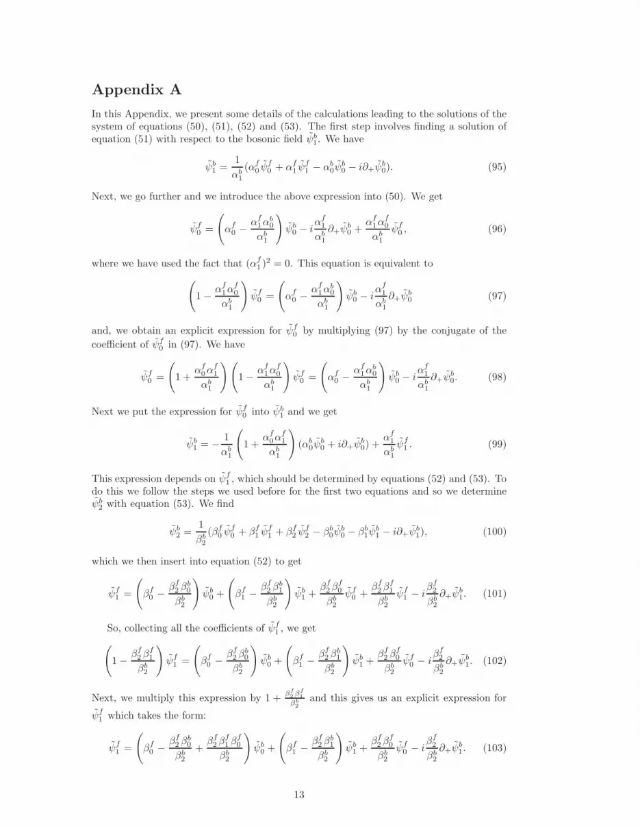
Appendix A

In this Appendix, we present some details of the calculations leading to the solutions of thesystem of equations (50), (51), (52) and (53). The first step involves finding a solution ofequation (51) with respect to the bosonic field ψb

1. We have

ψb1 =

1

αb1

(αf0 ψ

f0 + α

f1 ψ

f1 − αb

0ψb0 − i∂+ψ

b0). (95)

Next, we go further and we introduce the above expression into (50). We get

ψf0 =

(

αf0 −

αf1α

b0

αb1

)

ψb0 − i

αf1

αb1

∂+ψb0 +

αf1α

f0

αb1

ψf0 , (96)

where we have used the fact that (αf1 )

2 = 0. This equation is equivalent to

(

1−αf1α

f0

αb1

)

ψf0 =

(

αf0 −

αf1α

b0

αb1

)

ψb0 − i

αf1

αb1

∂+ψb0 (97)

and, we obtain an explicit expression for ψf0 by multiplying (97) by the conjugate of the

coefficient of ψf0 in (97). We have

ψf0 =

(

1 +αf0α

f1

αb1

)(

1−αf1α

f0

αb1

)

ψf0 =

(

αf0 −

αf1α

b0

αb1

)

ψb0 − i

αf1

αb1

∂+ψb0. (98)

Next we put the expression for ψf0 into ψb

1 and we get

ψb1 = −

1

αb1

(

1 +αf0α

f1

αb1

)

(αb0ψ

b0 + i∂+ψ

b0) +

αf1

αb1

ψf1 . (99)

This expression depends on ψf1 , which should be determined by equations (52) and (53). To

do this we follow the steps we used before for the first two equations and so we determineψb2 with equation (53). We find

ψb2 =

1

βb2

(βf0 ψ

f0 + β

f1 ψ

f1 + β

f2 ψ

f2 − βb

0ψb0 − βb

1ψb1 − i∂+ψ

b1), (100)

which we then insert into equation (52) to get

ψf1 =

(

βf0 −

βf2 β

b0

βb2

)

ψb0 +

(

βf1 −

βf2 β

b1

βb2

)

ψb1 +

βf2β

f0

βb2

ψf0 +

βf2β

f1

βb2

ψf1 − i

βf2

βb2

∂+ψb1. (101)

So, collecting all the coefficients of ψf1 , we get

(

1−βf2 β

f1

βb2

)

ψf1 =

(

βf0 −

βf2β

b0

βb2

)

ψb0 +

(

βf1 −

βf2β

b1

βb2

)

ψb1 +

βf2 β

f0

βb2

ψf0 − i

βf2

βb2

∂+ψb1. (102)

Next, we multiply this expression by 1 +βf2βf1

βb2

and this gives us an explicit expression for

ψf1 which takes the form:

ψf1 =

(

βf0 −

βf2 β

b0

βb2

+βf2β

f1 β

f0

βb2

)

ψb0 +

(

βf1 −

βf2β

b1

βb2

)

ψb1 +

βf2β

f0

βb2

ψf0 − i

βf2

βb2

∂+ψb1. (103)

13

To go further we insert this expression into the equation (99) for ψb1. This leads to a

complicated expression which we rewrite by collecting all the terms involving ψb1. We get

{

1−αf1

αb1

(

βf1 −

βf2β

b1

βb2

)}

ψb1 + i

αf1β

f2

αb1β

b2

∂+ψb1 =

αf1β

f2β

f0

αb1β

b2

ψf0 −

i

αb1

(

1 +αf0α

f1

αb1

)

∂+ψb0

+ψb0

{

−αb0

αb1

(

1 +αf0α

f1

αb1

)

+αf1

αb1

(

βf0 −

βf2β

b0

βb2

+βf2 β

f1β

f0

βb2

)}

. (104)

To solve for ψb1, we proceed in two steps. The first one involves multiplying the equation

above by the conjugate of the coefficient of ψb1:

1 +αf1

αb1

(

βf1 −

βf2β

b1

βb2

)

. (105)

This gives us:

(

1 + iαf1β

f2

αb1β

b2

∂+

)

ψb1 =

αf1β

f2β

f0

αb1β

b2

ψf0 −

i

αb1

(

1 +αf0α

f1

αb1

+αf1

αb1

(

βf1 −

βf2β

b1

βb2

))

∂+ψb0

+

{

−αb0

αb1

(

1 +αf0α

f1

αb1

)

+αf1

αb1

(

βf0 −

βf2β

b0

βb2

+βf2β

f1 β

f0

βb2

)

−αb0α

f1

(αb1)

2

(

βf1 −

βf2β

b1

βb2

)}

ψb0. (106)

Next we use the explicit expression for ψf0 given above to get

(

1 + iαf1β

f2

αb1β

b2

∂+

)

ψb1 = A0ψ

b0 +A1∂+ψ

b0, (107)

where the bosonic functions A0 and A1 are given by expressions (56) and (57). The secondand final step involves the application of the inverse of the operator acting on ψb

1 which isgiven by

(

1 + iαf1β

f2

αb1β

b2

∂+

)−1

= 1− iαf1β

f2

αb1β

b2

∂+. (108)

This result follows directly from the fact that (αf1 )

2 = (βf2 )

2 = 0. This leads to the expressionfor ψb

1 given in (55).

References

[1] D. G. Gross, T. Piran and S. Weinberg, Two Dimensional Quantum Gravity and Ran-

dom Surfaces (World Scientific, Singapore, 1992).

[2] S. Safram, Statistical Thermodynamics of Surfaces Interface and Membranes (Addison-Wesley, Massachusetts, 1994).

[3] A. Davydov, Solitons in Molecular Systems (Kluwer, New York, 1999).

[4] R. Rajaraman, ”CPn solitons in quantum Hall systems,” Eur. Phys. B 28, 157–162(2002).

[5] N. Manton and P. Sutcliffe, Topological Solitons (Cambridge University Press, NewYork, 2004)

[6] G. Landolfi, ”On the Canham-Helfrich membrane model,” J. Phys. A: Math. Theor.36, 4699 (2003).

14

[7] W. J. Zakrzewski, Low Dimensional Sigma Models. (Hilger, Bristol, 1989).

[8] L. Delisle, V. Hussin and W. J. Zakrzewski, ”Constant curvature solutions of Grass-mannian sigma models: (1) Holomorphic solutions,” J. Geom. Phys. 66, 24–36 (2013).

[9] L. Delisle, V. Hussin and W. J. Zakrzewski, ”Constant curvature solutions of Grassman-nian sigma models: (2) Non-holomorphic solutions,” J. Geom. Phys. 71, 1–10 (2013).

[10] L. Delisle, V. Hussin and W. J. Zakrzewski, ”Geometry of surfaces associated to grass-mannian sigma models,” accepted for publication in J. Phys.: Conference Proceedings(2015).

[11] A. M. Grundland and I. Yurdusen, ”On analytic descriptions of two-dimensional sur-faces with the CPN−1 models,” J. Phys. A: Math. Theor. 42, 172001 (2009).

[12] A. M. Grundland, A. Strasburger and W. J. Zakrzewski, ”Surfaces immersed in su(N+1) Lie algebras obtained from the CPN sigma models,” J. Phys. A: Math. Gen. 39,9187-9214 (2006).

[13] V. Hussin, I. Yurdusen and W. J. Zakrzewski, ”Canonical surfaces associated withprojectors in Grassmannian sigma models,” J. Math. Phys. 51, 103509 (2010).

[14] J. Bolton, G. R. Jensen, M. Rigoli and L. M. Woodward, ”On conformal minimalimmersions of S2 into CPn,” Math. Ann. 279, 599-620 (1988).

[15] X. X. Jiao and J. G. Peng, ”Pseudo-holomorphic curves in complex Grassmann mani-folds,” Trans. Am. Math. Soc. 355, 3715–3726 (2003).

[16] X. X. Jiao and J. G. Peng, ” Classification of holomorphic two-spheres with constantcurvature in the complex Grassmannians G2,5,” Differ. Geo. Its Appl. 20, 267–277(2004).

[17] F. Jie, J. Xiaoxiang and X. Xiaowei, ” Construction of homogeneous minimal 2-spheresin complex Grassmannians,” Acta Math. Sci. 31, 1889-1898 (2011).

[18] C. Peng and X. Xu, ”Minimal two-spheres with constant curvature in the complexGrassmannians,” Israel J. Math. 202, 1–20 (2014).

[19] C. Peng and X. Xu, ”Classification of minimal homogeneous two-spheres in the complexGrassmann manifold G(2, n),” J. de Mathematiques Pures et Appliquees 103, 374–399(2015).

[20] L. Delisle, V. Hussin, I. Yurdusen and W. J. Zakrzewski, ”Constant curvature surfacesof the supersymmetric CPN−1 sigma model,” J. Math. Phys. 56, 023506 (2015).

[21] K. Fujii, T. Koikawa and R. Sasaki, ”Classical solutions for supersymmetric Grassman-nian sigma models in two dimensions. I,” Prog. Theor. Phys. 71, 388-394 (1984).

[22] A. M. Din, J. Lukierski, and W. J. Zakrzewski, ”General classical solutions of a super-symmetric non-linear coupled boson-fermion model in two-dimension,” Nucl. Phys. B194, 157-171 (1982).

[23] J. F. Cornwell, Group theory in Physics: Supersymmetries and Infinite-Dimensional

Algebras, Techniques of Physics Vol. 3 (Academic, New York, 1989)

[24] V. Hussin and W. J. Zakrzewski, ”Susy CPN−1 model and surfaces in RN2−1,” J. Phys.A: Math. Gen. 39, 14231 (2006).

15