arX

iv:h

ep-t

h/92

1108

8v1

19

Nov

199

2

hep-th/9211088DIAS–92/27IHEP 92-155

LPTENS–92/40NI92008

November 1992

GAUGE CONDITIONS FOR THECONSTRAINED-WZNW–TODA REDUCTIONS

Jean-Loup GERVAISLaboratoire de Physique Theorique de l’Ecole Normale Superieure1,

24 rue Lhomond, 75231 Paris CEDEX 05, France.

Lochlainn O’RAIFEARTAIGHSchool of Theoretical Physics, Dublin Institute for Advanced Studies,

10 Burlington Road, Dublin 4, Ireland.

Alexander V. RAZUMOVInstitute for High Energy Physics,

142284, Protvino, Moscow region, Russia.and

Mikhail V. SAVELIEV 2

Isaac Newton Institute for Mathematical Sciences, University of Cambridge,

20 Clarkson Road, Cambridge CB3 0EH, U.K.

Abstract

There is a constrained-WZNW–Toda theory for any simple Lie algebra equippedwith an integral gradation. It is explained how the different approaches to these dy-namical systems are related by gauge transformations. Combining Gauss decomposi-tions in relevent gauges, we unify formulae already derived, and explictly determinethe holomorphic expansion of the conformally reduced WZNW solutions — whoserestriction gives the solutions of the Toda equations. The same takes place also forsemi-integral gradation. Most of our conclusions are also applicable to the affine Todatheories.

1Unite Propre du Centre National de la Recherche Scientifique, associee a l’Ecole NormaleSuperieure et a l’Universite de Paris-Sud.

2 On leave of absence from the Institute for High Energy Physics, 142284, Protvino, Moscowregion, Russia.

1 Introduction

Two-dimensional conformal Toda systems have been invented and explicitly inte-grated on the basis of the group-algebraic approach more than ten years ago inpapers3 [1] and [2]. They are in general associated with any integral gradation ofa simple Lie algebra. We shall deal with the general case, that is, not only withthe principal gradation that leads to the so-called finite non-periodic Toda systems,but also with their non-abelian versions4 introduced in refs.[2]. In what follows,and for the sake of brevity, we call them all Toda-type systems. Some time afterrefs.[1][2], a number of investigations appeared where these systems arose in the con-text of two dimensional gravity, of various aspects of W-algebras and W-geometries,of constrained WZNW-models, of “topological and anti-topological fusion”, and soon, – see [4]-[12] and references therein. At present, however, the link between thesepapers is not easy to make, although they basically deal with the same objects andnotions. Different notations have often been used, and, more importantly, equiva-lent formulae may be connected only when one sees that for the various problems itwas convenient to use different gauges.

This disaccordance is quite unsuitable to make further progress. This is true,not only for concrete applications, but also for the possibility (and desirability) ofextending the ideas to multi-dimensional systems following a path opened, e.g. inrefs.[10], [12]. Accordingly, the present paper is partly a unifying review of the vari-ous gauge conditions that have been used and of the relationship between them. Ourcontribution is, to some extent, a methodological one proposed for a wide audienceof people interested in varous aspects of integrable systems and related subjects.Systematically combining Gauss decompositions in these different gauges will nev-ertheless lead us to novel results, such as the explicit formula for the holomorphicdecomposition of the WZNW solution.

2 The basic framework

We consider two–dimensional space with coordinates z+, z−. In this discussion, theunifying feature is the zero-curvature condition – also called Maurer-Cartan, Lax,and so on:

[∂+ + A+, ∂− + A−]− ≡ ∂+A− − ∂−A+ + [A+, A−]− = 0. (2.1)

As usual, ∂± stands for ∂/∂z±. A± takes values in a simple finite-dimensional Liealgebra G. One considers a Z-gradation

G = ⊕m∈ZGm ≡ G− ⊕ G0 ⊕ G+,3In what follows, and when we use the results obtained by the authors of refs.[1], [2], in the

framework of the algebraic approach, we give reference to their review book[3] (of course, if theresult is described there) rather that to the original papers[1], [2].

4Here we deal with systems that are different from those proposed by A. M. Polyakov at theend of the seventies, and also called by him “nonabelian Toda theories”.

1

and, associated with this choice, we have the modified Gauss decompositions, suchthat any regular element U of the corresponding Lie group G may be written underthe form5

U = U(+)U(0)U(−), U(±) ∈ G±, U(0) ∈ G0. (2.2)

G± are the nilpotent algebras generated by G±, and G0 is the subgroup generated byG0. Note that G0 may be a non-abelian algebra – just then the Toda theory is callednon-abelian. In Eq.2.2 we introduced a notation which we will use throughout thearticle: group elements that belong to G± or Gm are given the same subscripts inparenthesis. We shall also use a similar notational rule for elements of G± or Gm

Of course the zero-curvature condition Eq.2.1 is invariant under the general gaugetransformation

A± → Ah± = h−1A± h+ h−1∂±h, (2.3)

where h is any element of G. A basic requirement of the Toda dynamics is that theabove vector potentials satisfy the condition A± ∈ G0 ⊕ G± in some gauges. Thesegauges will be called triangular. This triangular gauge condition is left invariant bythe gauge transformations

A± → Ah(0)

± = h−1(0)A± h(0) + h−1

(0)∂± h(0), with h(0) ∈ G0. (2.4)

We shall call them G0-gauge transformations, in the present paper. The abelianand non-abelian Toda theories have abelian and non-abelian G0-gauge groups re-spectively. Obviously the solution of the zero-curvature condition is

A± = g−1∂±g, (2.5)

with g ∈ G. Thus under the gauge transformation Eq.2.3,

g → gh. (2.6)

Following ref.[2], let us recall that the Toda equation may be written as6

∂+(g−1(0)∂−g(0)) = [X(−1), g

−1(0)X(1)g(0)]. (2.7)

where X(±1) are fixed elements of G±1 such that the whole G±1 may be recovered byadjoint action of G0, and where the dynamical fields are lumped into g(0)(z+, z−) ∈G0. We shall see how this is connected with Eq.2.1 in different gauges. Let usmention some well known examples. The elements X(±1) could be the generatorsof a sl(2,C)-subalgebra of G, and the corresponding Z-gradation be performed by

5Of course there are equivalent decompositions such as U = U ′

(−)U′

(0)U′

(+) where the elements

of G± and G0 are in different orders.6 Note also that the equation ∂+i(g

−1(0)∂−j g(0)) = [X−j , g

−1(0)Xig(0)], 1 ≤ i, j ≤ n, recently pro-

posed in [13] as a natural generalization of the so-called special geometry, represents, at leastformally, a multi-dimensional analogue of Eq.2.7. This generalized equation may probably be con-sidered as an appropriate reduction of the 2n-dimensional WZNW-model[10], just with the samereasonings as in [5] for the usual 2D case.

2

the Cartan element H = [X(1), X(−1)] of this sl(2,C), i.e., [H,Gm] = mGm. Inparticular, for the principal (canonical) gradation of a simple Lie algebra G (withthe abelian subalgebra G0 and X(±1) decomposable over the Chevalley generators ofthe positive and negative simple roots, respectively), equation (2.7) reduces to theabelian Toda system

∂+∂−xi = exp ρi, 1 ≤ i ≤ r ≡ rank G; ρi =r∑

j=1

kijxj , (2.8)

where xi(z+, z−) are the Toda fields, k is the Cartan matrix of G. Recall here thedefining relations for the Cartan (hi) and Chevalley (X±i) generators of G:

[hi, hj] = 0, [hi, X±j] = ±kjiX±j , [Xi, X−j] = δijhi; 1 ≤ i, j ≤ r. (2.9)

Of course, the simple Lie algebras G, in general, could be also supplied with non-principal gradations, in particular those associated with non-principal sl(2,C) sub-algebras of G. For such gradations the subalgebra G0 is not abelian.

The Toda field equations Eq.2.7 follow from the zero-curvature condition if onerequires that there exist triangular gauges where

A± ∈ G0 ⊕ G±1. (2.10)

We shall characterize these gauges as being restricted-triangular. Of course, sincethese conditions are not invariant under the general transformations Eq.2.3, we mayonly require that there exist gauges such that the vector potentials take certainrestricted forms. It is clearly not true that any vector potential may be gauge-transformed to become restricted-triangular. Thus the restricted-triangularity con-dition is not a matter of gauge choice. In fact, it determines the dynamics.Other hypothesis may be contradictory, that is, only give trivial dynamics (suchas A± ∈ G∓m ⊕ G0 ⊕ G±1); or lead to higher Toda flows (such as A± ∈ G0 ⊕ G±m,with m > 1). The equations associated with the last possibility also are integrable[3]. The holomorphic expansions in different gauges could be studied, following themethod described here, but we shall not do so, at present.

3 Relevent gauges

In this section we discuss three different gauges which are relevent for this or thatproblems under consideration, namely “general triangular”, “Toda”, and “WZNW”gauges.

3.1 General triangular gauges

To begin with, we discuss properties that hold in any triangular gauge, withoutassuming that the restriction condition Eq.2.10 holds. We distinguish these gauges

3

by a superscript (t). This is essentially a review of some results from [3]. Two usefulforms for the Gauss decomposition of the corresponding g(t) of Eq.2.5 are as follows

g(t) = M(−)N(+)g(0)− = M(+)N(−)g(0)+, (3.1)

Under the G0-gauge transformation Eq.2.4, M(±), N(±) are clearly invariant. On the

other hand, g(t)(0)± → g

(t)(0)±h(0), and we introduce the G0-gauge-invariant.

g(0) ≡ g(0)+g−1(0)− (3.2)

Next, it is easily seen that the triangular gradation properties are satisfied iff M(±)

are holomorphic functions, that is

∂∓M(±) = 0, (3.3)

and one deduces from Eq.2.5 that7

A(t)+ = g−1

(0)−N−1(+)∂+N(+)g(0)− + g−1

(0)+∂+g(0)−,

A(t)− = g−1

(0)+N−1(−)∂−N(−)g(0)+ + g−1

(0)+∂−g(0)+. (3.4)

According to Eq.3.3, one may define two holomorphic functions L(±)(z±) ∈ G± suchthat

dM(±)/dz± = L(±)M(±). (3.5)

On the other hand, it follows from Eqs.3.1, and 3.2 that

K ≡M−1(+)M(−) = N(−)g(0)N

−1(+). (3.6)

The differential equations 3.5 give

K−1 ∂−K = L(−), ∂+KK−1 = −L(+). (3.7)

Substituting in these equations the element K expressed via the second part of theformula (3.6), we arrive at

N−1(−)∂−N(−) = g(0)L(−)g

−1(0) , N−1

(+)∂+N(+) = g−1(0)L(+)g(0). (3.8)

It finally follows from Eqs.3.2, 3.4, and 3.8 that, in any triangular gauge,

A(t)+ = g−1

(0)+L(+)g(0)+ + g−1(0)−∂+g(0)−,

A(t)− = g−1

(0)−L(−)g(0)− + g−1(0)+∂−g(0)+. (3.9)

7For simplicity of notation, ∂± only act on the first following function, unless parenthesis indicateotherwize.

4

3.2 Toda gauges

For the Toda dynamics, there exist restricted-triangular gauges where the more re-strictive condition Eq.2.10 holds. These gauges will be characterized by a superscript(rt). If one is in such a gauge, and using the formulae just written, it is easy to seethat, N(±) ∈ G±1, M(±) ∈ G±1, and L(±) ∈ G±1. In accordance with our generalconvention, we may write them as N(±1), M(±1), L(±1). According to ref.[3], L(±1)

may be obtained from fixed elements X(±1) ∈ G±1 by adjoint action of G0. Thus wemay write

L(±1) = y(0)±X(±1)y−1(0)±, (3.10)

where, according to Eqs.3.3, 3.5, y(0)± are holomorphic: ∂±y(0)∓ = 0. Therefore

A(rt)+ =

(y−1

(0)+ g(0)+

)−1X(1)

(y−1

(0)+ g(0)+

)+ g−1

(0)−∂+g(0)−,

A(rt)− =

(y−1

(0)− g(0)−

)−1X(−1)

(y−1

(0)− g(0)−

)+ g−1

(0)+∂−g(0)+. (3.11)

The precise form Eq.2.7 of the Toda equation comes out directly from the zero-curvature condition with specific conditions introduced in ref.[3]. There are twoassociated gauge choices which we call Toda gauges, and distinguish with a super-script (T ). They may be characterized by the fact that the gradation-zero part in

one of the connections, say A(T )+ is set equal to zero, while the gradation-one compo-

nent of the other A(T )− is chosen to be constant. Next we verify that, starting from

any restricted-triangular gauge, there exists a G0-gauge transformation

A(T )± ≡ h−1

(0)(A(rt)± + ∂±)h(0), i.e., g(T ) ≡ g(rt)h(0), (3.12)

such that

A(T )(0)+ =

(g(0)− h(0)

)−1∂+

(g(0)− h(0)

)= 0,

A(T )(1)− =

(y−1

(0)− g(0)− h(0)

)−1X(−1)

(y−1

(0)− g(0)− h(0)

)= constant. (3.13)

In the last equations we made use of Eqs.3.11. Indeed, it is enough to choose

h(0) = g−1(0)− y(0)−. (3.14)

Next, it is easily seen that the Toda equations 2.7 come out from the flatness con-dition Eq.2.1 in this gauge, if we identify

g(0) = y−1(0)+ g(0)+ h(0), (3.15)

and one gets

A(T )+ = g−1

(0)X(1)g(0), A(T )− = g−1

(0)∂−g(0) +X(−1). (3.16)

5

Finally, one may rewrite h(0), g(T ), and g0 in terms of the original quantities intro-

duced above for an arbitrary restricted triangular gauge, obtaining,

h(0) = (y(0)− g(0)−)−1 = g−1(0)+ y(0)+g(0); (3.17)

g(T ) = g(rt) g−1(0)− y

−1(0)−; (3.18)

g(0) = y−1(0)+ g(0)+ g

−1(0)− y(0)− ≡ y−1

(0)+ g(0) y(0)−. (3.19)

Note that the functions (3.16) for the case of the abelian Toda system (2.8) arereduced to the form

A(T )+ =

∑

j

eρj Xj, A(T )− = −

∑

j

∂−xj hj +∑

j

X−j. (3.20)

where the sum runs over the step operators associated with simple roots.The role of the components A+ and A− in the Toda gauge may be, of course,

reversed by letting

A(T )± = g(0)A

(T )± g−1

(0) + g(0)∂±g−1(0) , (3.21)

so thatA

(T )+ = g(0)∂+g

−1(0) +X(1), A

(T )− = g(0)X(−1)g

−1(0) . (3.22)

3.3 W-gauges

In accordance with [5]-[8], the WZNW dynamics is best seen by going to othergauges which we characterize with a superscript (W±). They are gauges of the

axial type where one component, that is, A(W±)∓ vanishes. In this subsection, we

rederive results of refs.[5]-[8], for completeness. The change of gauge is most easilyachieved starting from the T-gauge. Let us write, for the (W+) gauge,

A(W+)± = ω(+)A

(T )± ω−1

(+) + ω(+)∂±ω−1(+), that is, g(W+) = g(T )ω−1

(+). (3.23)

It follows from Eq.3.16 that, if

ω−1(+)∂+ω(+) = g−1

(0)X(1)g(0), (3.24)

then

A(W+)+ = 0, A

(W+)− ≡ −J = ω(+)(X(−1) + g−1

(0)∂−g(0) + ∂−)ω−1(+). (3.25)

It is clear from Eq.3.24 that ω(+) ∈ G+ as the notation anticipated. Thus theW-gauges are not triangular. On the other hand, it is easy to see that J satisfies

∂+J = 0, J(−) = −X(−1). (3.26)

The first equation follows from the zero-curvature condition Eq.2.1, since A(W+)+ = 0.

The second may be verified from the explicit expression just given (following thegeneral convention, J(−) is the negative-gradation component of J).

6

The other W gauge is treated similarly, starting from the other Toda gauge

potentials A(T )± :

A(W−)± = ω−1

(−)A(T )± ω(−) + ω−1

(−)∂±ω(−), that is, g(W−) = gTω(−); (3.27)

ω(−)∂+ω−1(−) = g(0)X(−1)g

−1(0); (3.28)

A(W−)− = 0, A

(W−)+ ≡ −J = ω−1

(−)(X(1) + g(0)∂−g−1(0) + ∂+)ω−1

(+); (3.29)

J(+) = X(1), ∂−J = 0. (3.30)

In accordance with [5]-[11], the group element ω which parametrises the solution ofthe constrained WZNW equation is defined as follows:

ω ≡ ω = ω+ ω0 ω−; where ω0 = g−1(0) . (3.31)

Indeed, by explicit computation one verifies that the currents J and J introducedabove are the corresponding WZNW currents, that is,

J ≡ ∂−ω ω−1, J ≡ −ω−1∂+ω. (3.32)

Therefore, Eqs.3.26, and 3.30 show that ω is a solution of the corresponding confor-mally reduced WZNW model.

4 Explict solution of the WZNW model

As noted in refs. [5] - [8], the Toda field g(0) is recovered from ω by using the fact thatEq.3.31 is a Gauss decomposition, so that, when we compute matrix elements be-tween states |λj > which are annihilated by G+, we get < λj |ω|λj >=< λj|g

−1(0) |λj >.

Of course ω contains more informations. It is the purpose of the present section toestablish its full connection with the group-elements which appeared in the triangu-lar gauges of subsections 3.1 and 3.2. It follows from Eqs.3.24, and 3.28 that

ω−1(+)∂+ω(+) = (g(0) y(0)−)−1 L(1) g(0) y(0)− = y−1

(0)−N−1(1) ∂+N(1) y(0)−;

ω(−)∂−ω−1(−) =

(g−1(0) y(0)+

)−1L(−1) g

−1(0)y(0)+ = y−1

(0)+ N−1(−1) ∂−N(−1) y(0)+.

Since ω(±) ∈ G±, a more convenient form of these formulae is

ω−1(+)∂+ω(+) =

[y(0)−N(1) y

−1(0)−

]−1∂+

[y(0)−N(1) y

−1(0)−

];

andω(−)∂−ω

−1(−) =

[y−1

(0)+ N−1(−1) y(0)+

]∂−

[y−1

(0)+N−1(−1) y(0)+

]−1.

where we used the fact that ∂∓y(0)± = 0. Thereof,

ω(+) = q(+)(z−) y(0)−N(1) y−1(0)−, ω(−) = y−1

(0)+ N−1(1) y(0)+ q(−)(z+), (4.1)

7

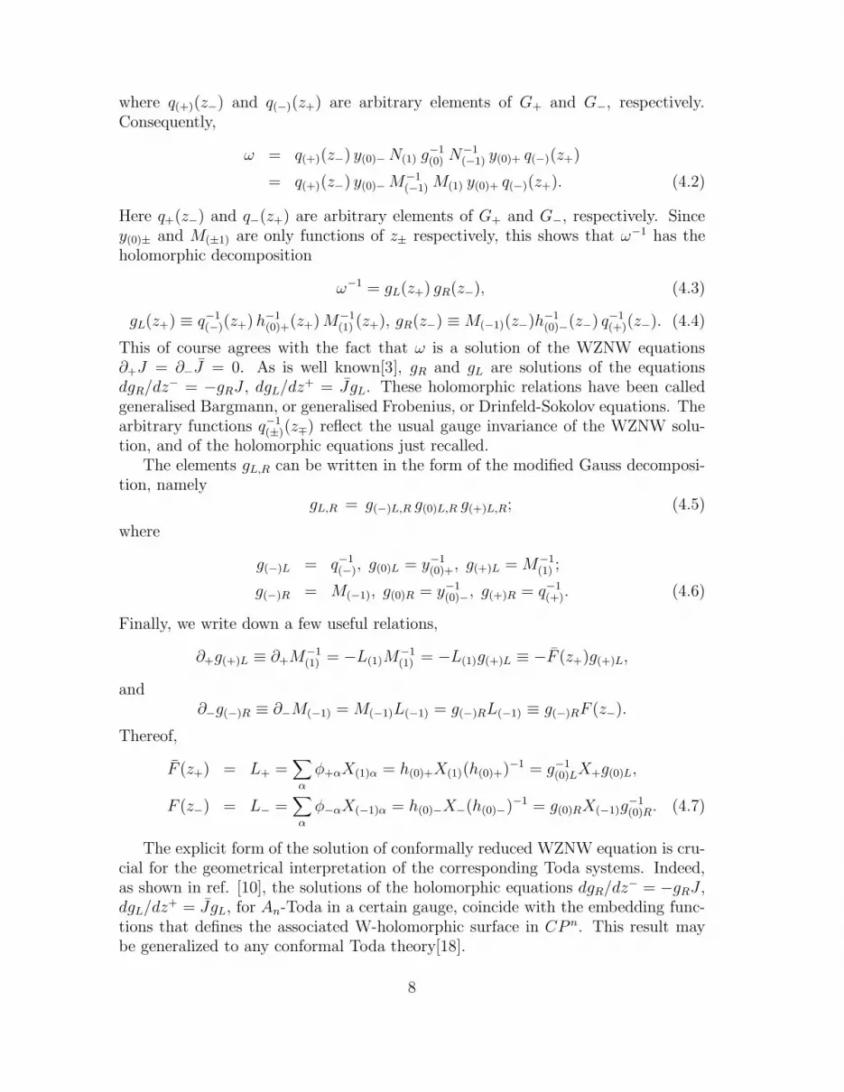
where q(+)(z−) and q(−)(z+) are arbitrary elements of G+ and G−, respectively.Consequently,

ω = q(+)(z−) y(0)−N(1) g−1(0) N

−1(−1) y(0)+ q(−)(z+)

= q(+)(z−) y(0)−M−1(−1) M(1) y(0)+ q(−)(z+). (4.2)

Here q+(z−) and q−(z+) are arbitrary elements of G+ and G−, respectively. Sincey(0)± and M(±1) are only functions of z± respectively, this shows that ω−1 has theholomorphic decomposition

ω−1 = gL(z+) gR(z−), (4.3)

gL(z+) ≡ q−1(−)(z+) h−1

(0)+(z+)M−1(1) (z+), gR(z−) ≡M(−1)(z−)h−1

(0)−(z−) q−1(+)(z−). (4.4)

This of course agrees with the fact that ω is a solution of the WZNW equations∂+J = ∂−J = 0. As is well known[3], gR and gL are solutions of the equationsdgR/dz

− = −gRJ , dgL/dz+ = JgL. These holomorphic relations have been called

generalised Bargmann, or generalised Frobenius, or Drinfeld-Sokolov equations. Thearbitrary functions q−1

(±)(z∓) reflect the usual gauge invariance of the WZNW solu-tion, and of the holomorphic equations just recalled.

The elements gL,R can be written in the form of the modified Gauss decomposi-tion, namely

gL,R = g(−)L,R g(0)L,R g(+)L,R; (4.5)

where

g(−)L = q−1(−), g(0)L = y−1

(0)+, g(+)L = M−1(1) ;

g(−)R = M(−1), g(0)R = y−1(0)−, g(+)R = q−1

(+). (4.6)

Finally, we write down a few useful relations,

∂+g(+)L ≡ ∂+M−1(1) = −L(1)M

−1(1) = −L(1)g(+)L ≡ −F (z+)g(+)L,

and∂−g(−)R ≡ ∂−M(−1) = M(−1)L(−1) = g(−)RL(−1) ≡ g(−)RF (z−).

Thereof,

F (z+) = L+ =∑

α

φ+αX(1)α = h(0)+X(1)(h(0)+)−1 = g−1(0)LX+g(0)L,

F (z−) = L− =∑

α

φ−αX(−1)α = h(0)−X−(h(0)−)−1 = g(0)RX(−1)g−1(0)R. (4.7)

The explicit form of the solution of conformally reduced WZNW equation is cru-cial for the geometrical interpretation of the corresponding Toda systems. Indeed,as shown in ref. [10], the solutions of the holomorphic equations dgR/dz

− = −gRJ ,dgL/dz

+ = JgL, for An-Toda in a certain gauge, coincide with the embedding func-tions that defines the associated W-holomorphic surface in CP n. This result maybe generalized to any conformal Toda theory[18].

8

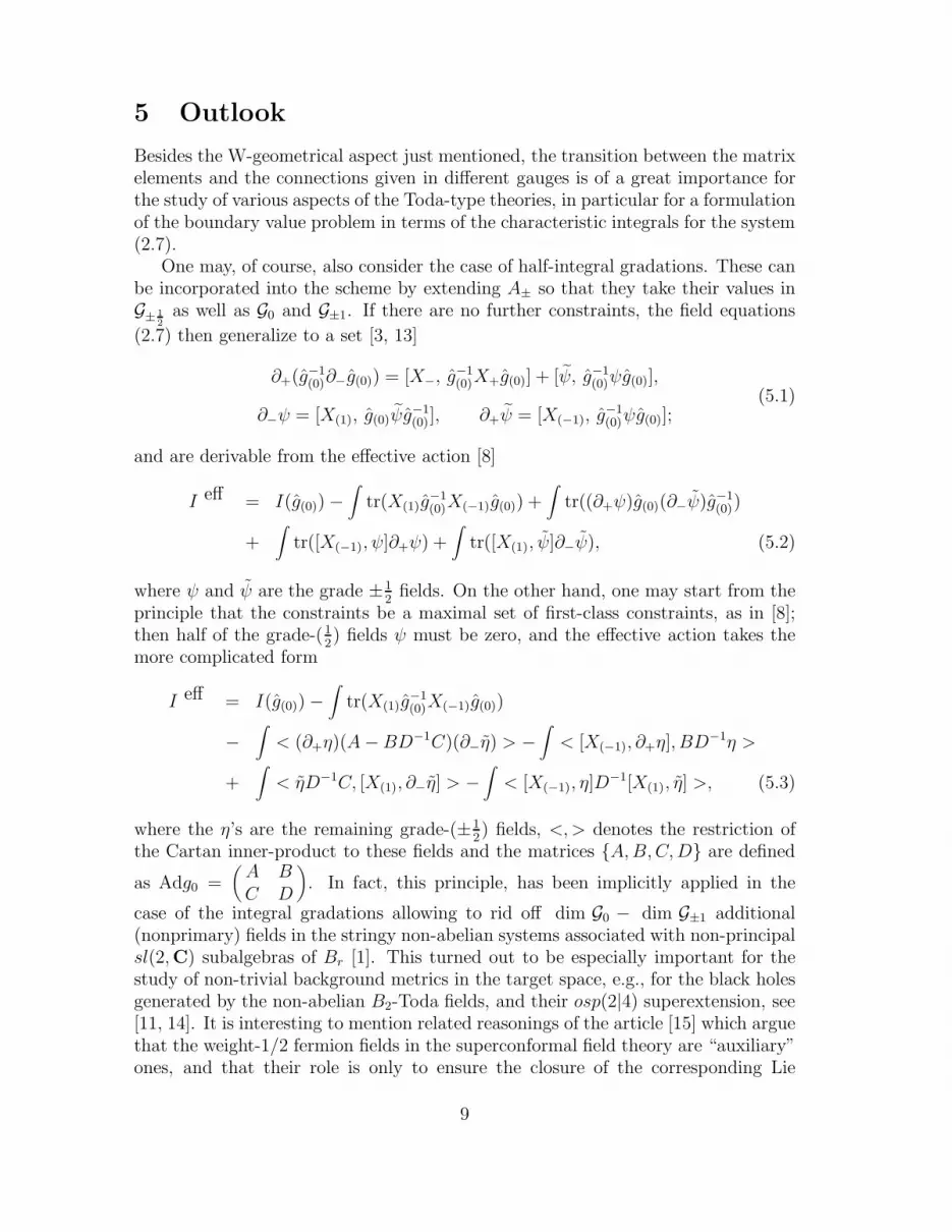
5 Outlook

Besides the W-geometrical aspect just mentioned, the transition between the matrixelements and the connections given in different gauges is of a great importance forthe study of various aspects of the Toda-type theories, in particular for a formulationof the boundary value problem in terms of the characteristic integrals for the system(2.7).

One may, of course, also consider the case of half-integral gradations. These canbe incorporated into the scheme by extending A± so that they take their values inG± 1

2as well as G0 and G±1. If there are no further constraints, the field equations

(2.7) then generalize to a set [3, 13]

∂+(g−1(0)∂−g(0)) = [X−, g

−1(0)X+g(0)] + [ψ, g−1

(0)ψg(0)],(5.1)

∂−ψ = [X(1), g(0)ψg−1(0)], ∂+ψ = [X(−1), g

−1(0)ψg(0)];

and are derivable from the effective action [8]

I eff = I(g(0)) −∫

tr(X(1)g−1(0)X(−1)g(0)) +

∫tr((∂+ψ)g(0)(∂−ψ)g−1

(0))

+∫

tr([X(−1), ψ]∂+ψ) +∫

tr([X(1), ψ]∂−ψ), (5.2)

where ψ and ψ are the grade ±12

fields. On the other hand, one may start from theprinciple that the constraints be a maximal set of first-class constraints, as in [8];then half of the grade-(1

2) fields ψ must be zero, and the effective action takes the

more complicated form

I eff = I(g(0)) −∫

tr(X(1)g−1(0)X(−1)g(0))

−∫< (∂+η)(A−BD−1C)(∂−η) > −

∫< [X(−1), ∂+η], BD

−1η >

+∫< ηD−1C, [X(1), ∂−η] > −

∫< [X(−1), η]D

−1[X(1), η] >, (5.3)

where the η’s are the remaining grade-(±12) fields, <,> denotes the restriction of

the Cartan inner-product to these fields and the matrices {A,B,C,D} are defined

as Adg0 =(A BC D

). In fact, this principle, has been implicitly applied in the

case of the integral gradations allowing to rid off dim G0 − dim G±1 additional(nonprimary) fields in the stringy non-abelian systems associated with non-principalsl(2,C) subalgebras of Br [1]. This turned out to be especially important for thestudy of non-trivial background metrics in the target space, e.g., for the black holesgenerated by the non-abelian B2-Toda fields, and their osp(2|4) superextension, see[11, 14]. It is interesting to mention related reasonings of the article [15] which arguethat the weight-1/2 fermion fields in the superconformal field theory are “auxiliary”ones, and that their role is only to ensure the closure of the corresponding Lie

9

superalgebra. A similar conclusion takes place for the aforementioned non-abelianB2 (and osp(2|4)) – Toda systems, as well as for their generalizations to the Lie(super)algebras of higher ranks.

Consider the supersymmetrical extensions[16] of the equation (2.7),

D+

(g−1(0)D−g(0)

)=

[Y(−1), g

−1(0)Y(1)g(0)

]

+, (5.4)

associated with a classical Lie algebras and superalgebra Gs supplied with a Z-gradation. Here D± are the supercovariant derivatives in 2|2-superspace; g(0) is aregular element of the Grassmann span of the Lie group G0 = Lie G0; Y(±1) arefixed (odd) elements of G±1. Most of the results given above can be derived for thesystem (5.4) as well, with the corresponding modifications. (For the relation witha supersymmetric extension of the constrained-WZNW-model see also [17].) It isinteresting to emphasize that, under the relevant conditions, the component-form ofEqs.5.4 coincides with Eqs.5.1. This is, of course, only formal, since the fermioniccomponents entering in Eq.5.4 are Majorana spinors with anticommuting values,contrary to the functions ψ and ψ in Eq.5.1.

Finishing up this paper, we would like to mention that most of the relations andconclusions given here are applicable to the periodic Toda-type system associatedwith the affine Lie Kac-Moody algebras G, of course, with the appropriate mod-ifications. For many interesting cases, these equations, in particular those calledlast time also as affine and conformal affine Toda theories, — which are given inquite general a form in ref.[3] following the results of ref.[19], together with theirgroup-algebraic integration scheme — can be rewritten in the form Eq.2.7. Herethe meaning of the elements X(±1) is different, however, and the relevent gradingoperator H, [H,Gm] = mGm, of course does not belong to the corresponding finite-dimensional Lie algebra G. It can be constructed in a degenerate representation ofG with the spectral parameter λ as H = H + c λd/dλ. Then, following the samereasonings as in ref.[11] for the construction of a nontrivial background metric inthe target space, one can describe the black holes associated with the non-canonical

gradation of the affine algebra B(1)2 , and the soliton solutions of the model, for ex-

ample. Here, at a formal level, the difference between the corresponding finite andaffine cases arises from the insertion, in the expression for X(±1), of the additionalterm like λ±1X∓M , where M is the maximal root of B2. (In the general case amodification of X(±1) is the relevant element of the Heisenberg subalgebra of thecorresponding affine Lie algebra.) The final equations, of course, do not depend onλ, and provide the simplest example of a nontrivial background metric, while thecanonical gradation of the affine Lie algebras leads, as in the finite-dimensional case,to constant metrics in the target space of the corresponding σ-model. It seems quitebelievable that a quantization procedure for such systems, completely integrable atthe classical level, could follow along the line of the corresponding construction givenin [3], and in [20] for finite-dimensional systems, with the necessary modification ofsuch objects as the Casimir operator of the second order, the Whittaker vectors,etc.

10

Acknowledgements. One of the authors (M.S.) would like to thank LPTENSin Paris, ENSLAPP in Lyon, IAS in Dublin, and the Isaac Newton Institute inCambridge for kind hospitality. His research was supported in part by SERC Vis-iting fellowship, grant GB.929.612/RG.14173-MTA-R3. This work was partiallysupported by the European Twinning Program, contract # 540022.

References

[1] A. N. Leznov, M. V. Saveliev: Phys. Lett. B, v. 79 (1978) 294; Lett. Math.Phys. v. 3 (1979) 207; Comm. Math. Phys. v. 74 (1980) 111.

[2] A. N. Leznov, M. V. Saveliev: Lett. Math. Phys. v. 6 (1982) 505; Comm. Math.Phys. v. 89 (1983) 59.

[3] A. N. Leznov, M. V. Saveliev: Group-Theoretical Methods for Integration of

Nonlinear Dynamical Systems. Progress in Physics v. 15, Birkhauser-Verlag,1992.

[4] J.-L. Gervais, Comm. Math. Phys. 130 (1990) 257; 138 (1991) 301.

[5] J. Balog, L. Feher, L. O’Raifeartaigh, P. Forgacs, A. Wipf: Ann. Phys. (N.Y.),v. 203 (1990) 76.

[6] L. O’Raifeartaigh, P. Ruelle, I. Tsutsui, A. Wipf: Comm. Math. Phys. v. 143(1992) 333.

[7] L. Feher, L. O’Raifeartaigh, P. Ruelle, I. Tsutsui, A. Wipf: Ann, Phys. (N.Y.),v. 213 (1992) 1.

[8] L. Feher, L. O’Raifeartaigh, P. Ruelle, I. Tsutsui, A. Wipf: to appear in Phys.Reports.

[9] J.-L. Gervais, Y. Matsuo: Phys. Lett. B, v. 274 (1992) 309;

[10] J.-L. Gervais, Y. Matsuo: W -Geometries. Preprint LPTENS-91/29, 1992; toappear in Comm. Math. Phys.

[11] J.-L. Gervais, M. V. Saveliev: Phys. Lett. B, v. 286 (1992) 271.

[12] S. Cecotti, C. Vafa: Nucl. Phys. B, v. 367 (1991) 359.

[13] A. N. Leznov: Exactly Integrable Systems with Fermionic Fields. Preprint IHEP83-7, Serpukhov, 1983.

[14] F. Delduc, J.-L. Gervais, M. V. Saveliev: Phys. Lett. B, v. 292 (1992) 295.

[15] P. Goddard, A. Schwimmer: Phys. Lett. B, v. 214 (1988) 209.

11

[16] M. V. Saveliev: Comm. Math. Phys. v. 95 (1984) 199;A. N. Leznov, M. V. Saveliev: Sov. J. Theor. Math. Phys., v. 61 (1984) 150;D. A. Leites, M. V. Saveliev, V. V. Serganova: – in Group Theoretical Methods

in Physics. V. I. Manko, M. A. Markov, eds., VNU Sci. Press, v. 1 (1986) 255.

[17] F. Delduc, E. Ragoucy, P. Sorba: Comm. Math. Phys. v. 146 (1992) 403.

[18] J.-L. Gervais, M. V. Saveliev, in preparation.

[19] A. N. Leznov, M. V. Saveliev, V. G. Smirnov: Sov. J. Theor. Math. Phys., v.48 (1981) 3.

[20] A.Bilal, J.-L.Gervais: Phys. Lett. 206B (1988), 412; Nucl. Phys. 314B (1989)646; 318B (1989) 579.

12