1

From the Sup-Decomposition

to a Sequential Decomposition

Ronaldo Fumio Hashimoto

Junior Barrera

Edward R. Dougherty

Computer Science Department

University of São Paulo - Brazil

2

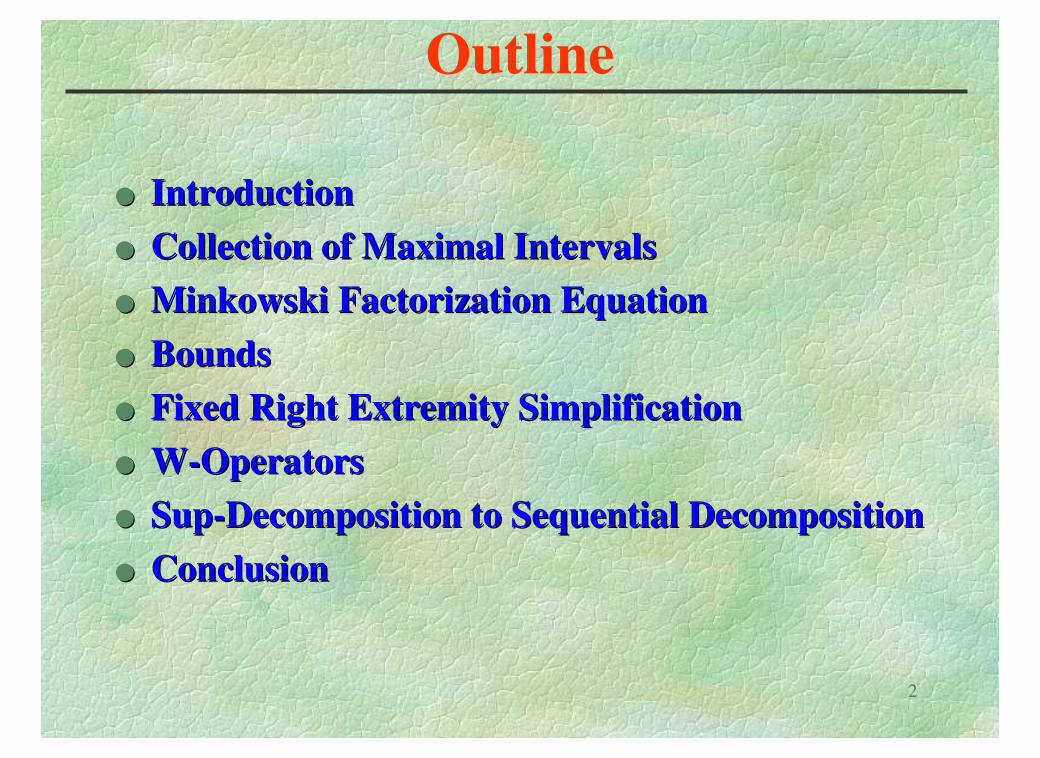
Outline

ÊÊ IntroductionIntroduction

ÊÊ Collection of Maximal IntervalsCollection of Maximal Intervals

ÊÊ Minkowski Factorization EquationMinkowski Factorization Equation

ÊÊ BoundsBounds

ÊÊ Fixed Right Extremity SimplificationFixed Right Extremity Simplification

ÊÊ WW--OperatorsOperators

ÊÊ SupSup--Decomposition to Sequential DecompositionDecomposition to Sequential Decomposition

ÊÊ ConclusionConclusion

3

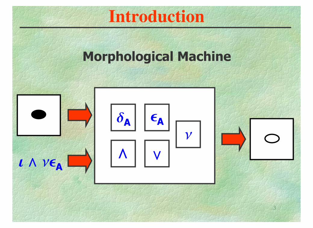
Introduction

dA eA

⁄n

i neA

Morphological Machine

4

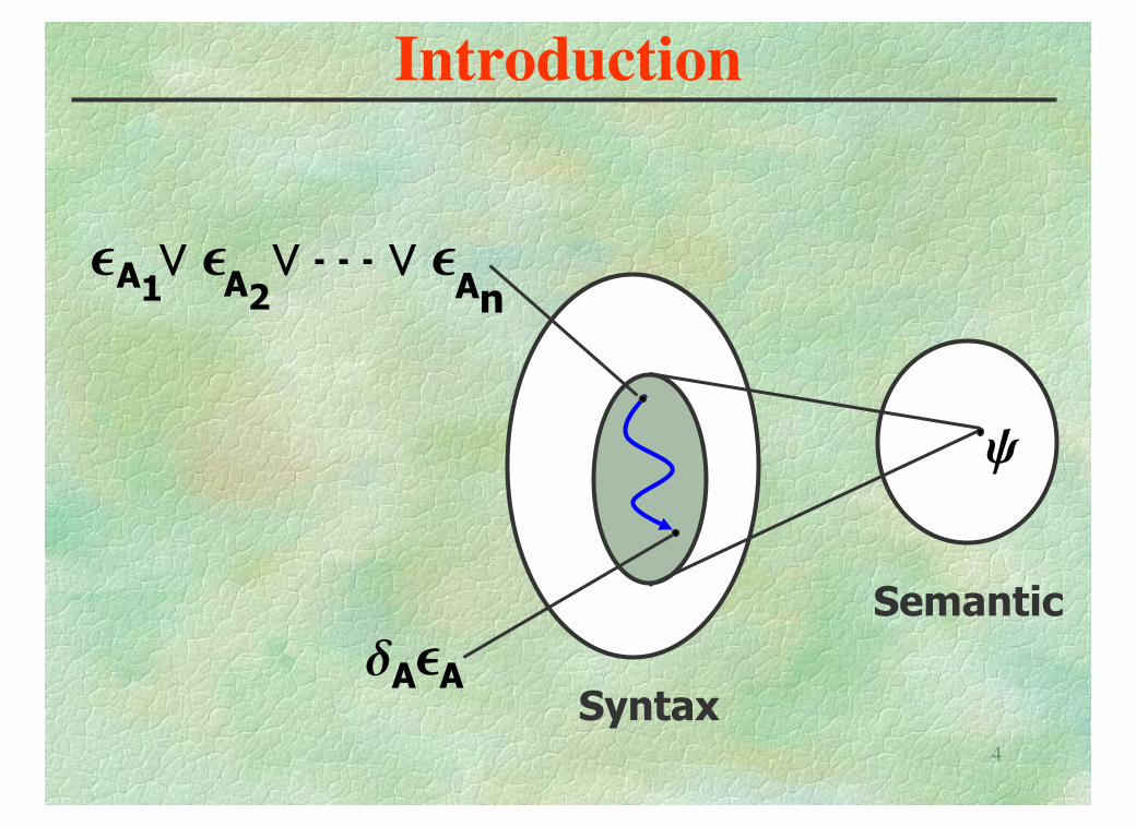
Introduction

dAeA

e ⁄ e ⁄ Ä Ä Ä ⁄ eA1 A2 An

y

Syntax

Semantic

5

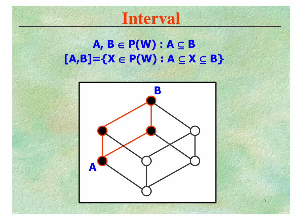
Interval

A, B Œ P(W) : A Õ B

[A,B]={X Œ P(W) : A Õ X Õ B}

A

B

6

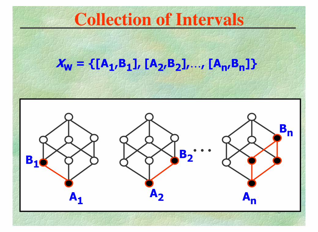
Collection of Intervals

XW = {[A1,B1], [A2,B2],…………, [An,Bn]}

…………

A1A2 An

B1B2

Bn

7

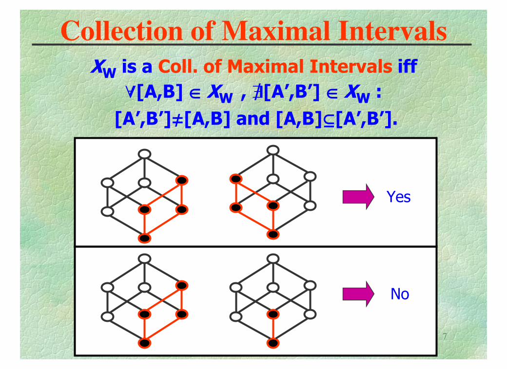
Collection of Maximal Intervals

XW is a Coll. of Maximal Intervals iff

"[A,B] Œ XW , ±[A’,B’] Œ XW :

[A’,B’]π[A,B] and [A,B]Õ[A’,B’].

Yes

No

8

Collection of Maximal Intervals

Let ΠΠΠΠW denote the set of all collections of maximal intervals contained in

P(P(W)).

9

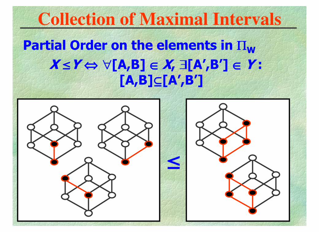
Collection of Maximal Intervals

Partial Order on the elements in ΠΠΠΠW

X £Y ¤ ∀∀∀∀[A,B] Œ X, $[A’,B’] Œ Y : [A,B]Õ[A’,B’]

£

10

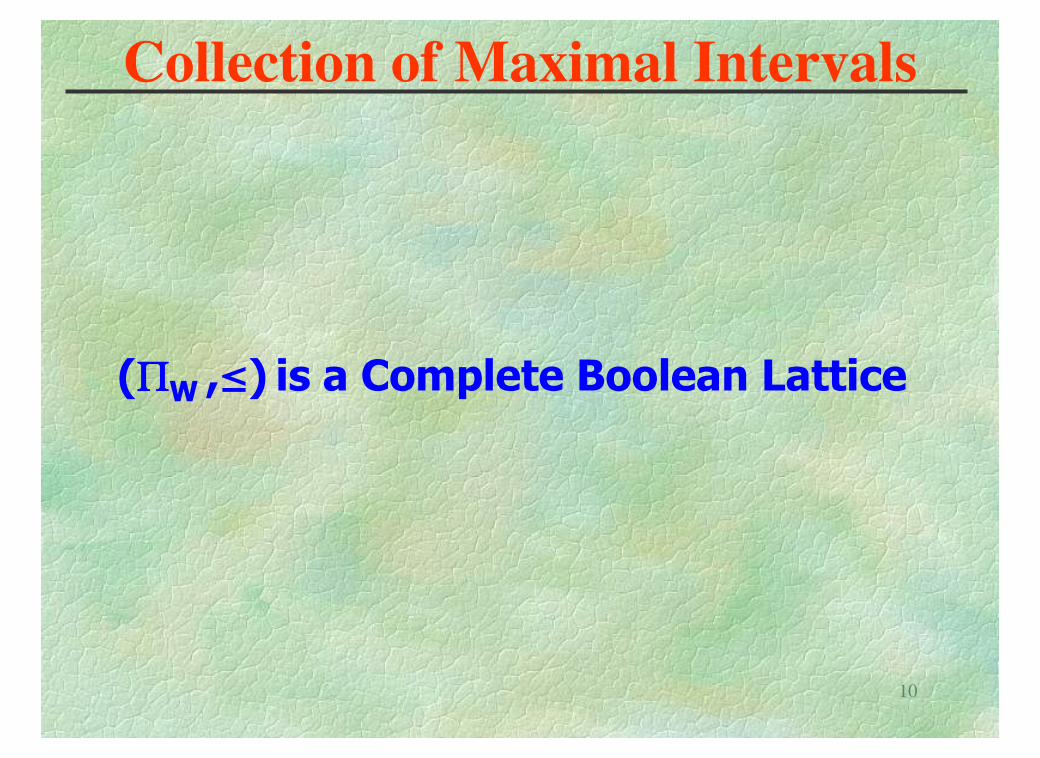
Collection of Maximal Intervals

(ΠΠΠΠW ,£) is a Complete Boolean Lattice

11

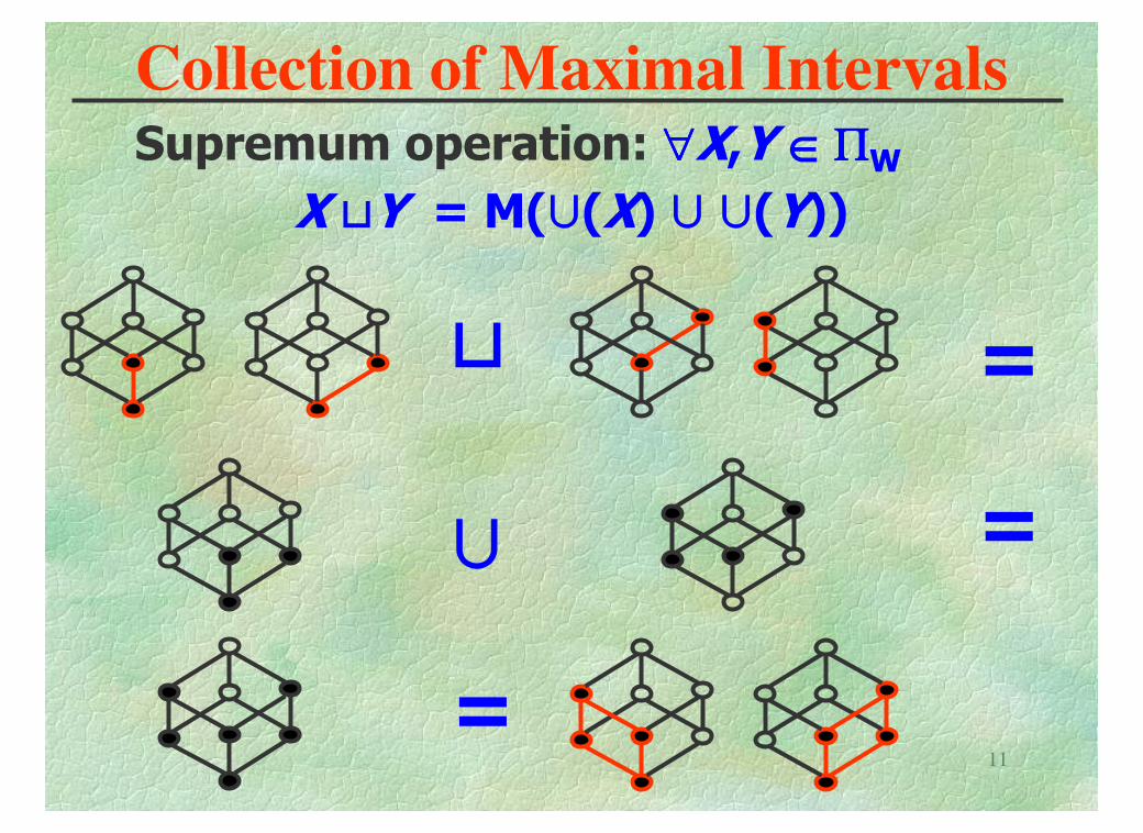
Collection of Maximal IntervalsSupremum operation: ∀∀∀∀X,Y Œ ΠΠΠΠW

X +Y = M(«(X) « «(Y))

+

« =

=

=

12

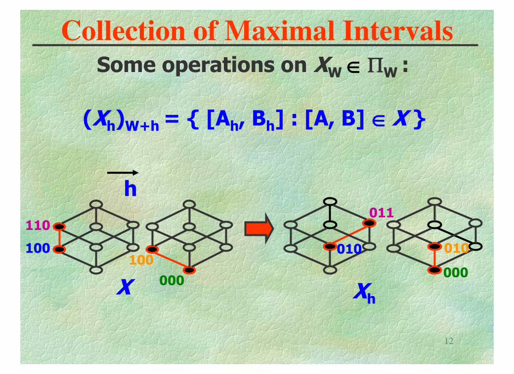
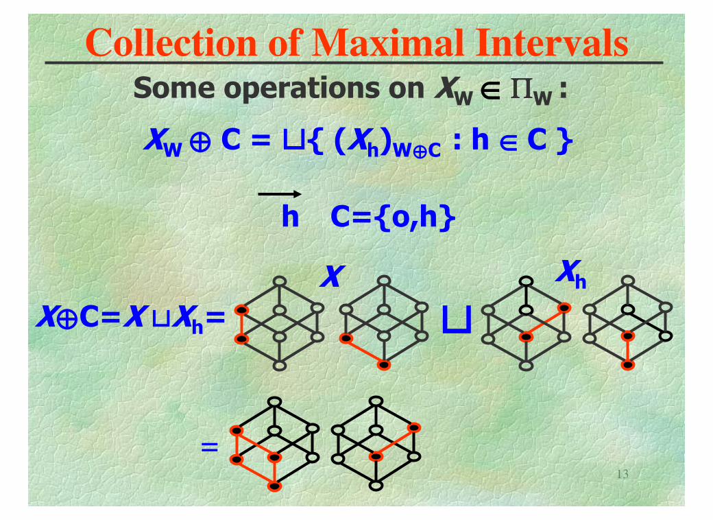
Collection of Maximal IntervalsSome operations on XW Œ ΠΠΠΠW :

(Xh)W+h = { [Ah, Bh] : [A, B] ΠX }

X Xh

h

110

100

000

100000

011

010 010

13

Collection of Maximal IntervalsSome operations on XW Œ ΠΠΠΠW :

XW ≈ C = +{ (Xh)W≈C : h Œ C }

h C={o,h}

X≈C=X +Xh=

X Xh

+

=

14

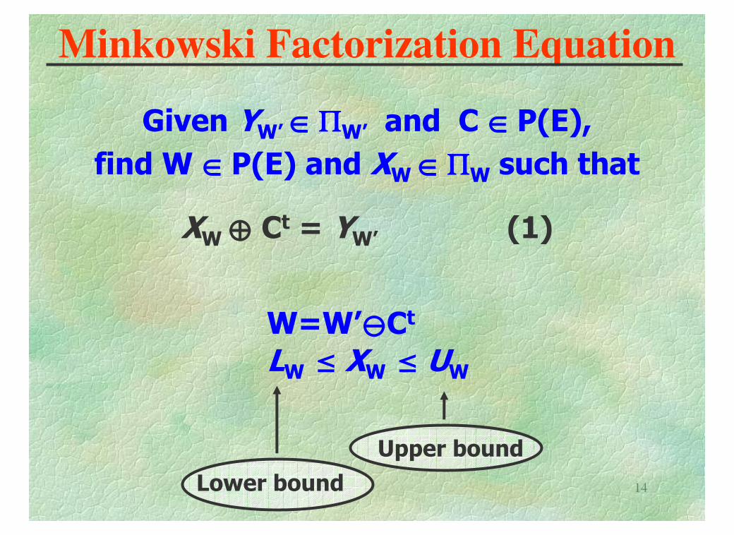
Minkowski Factorization Equation

Given YW’Œ ΠΠΠΠW’ and C Œ P(E),

find W Œ P(E) and XW Œ ΠΠΠΠW such that

XW ≈ Ct = YW’ (1)

Lower bound

Upper bound

W=W’ûCt

LW £ XW £ UW

15

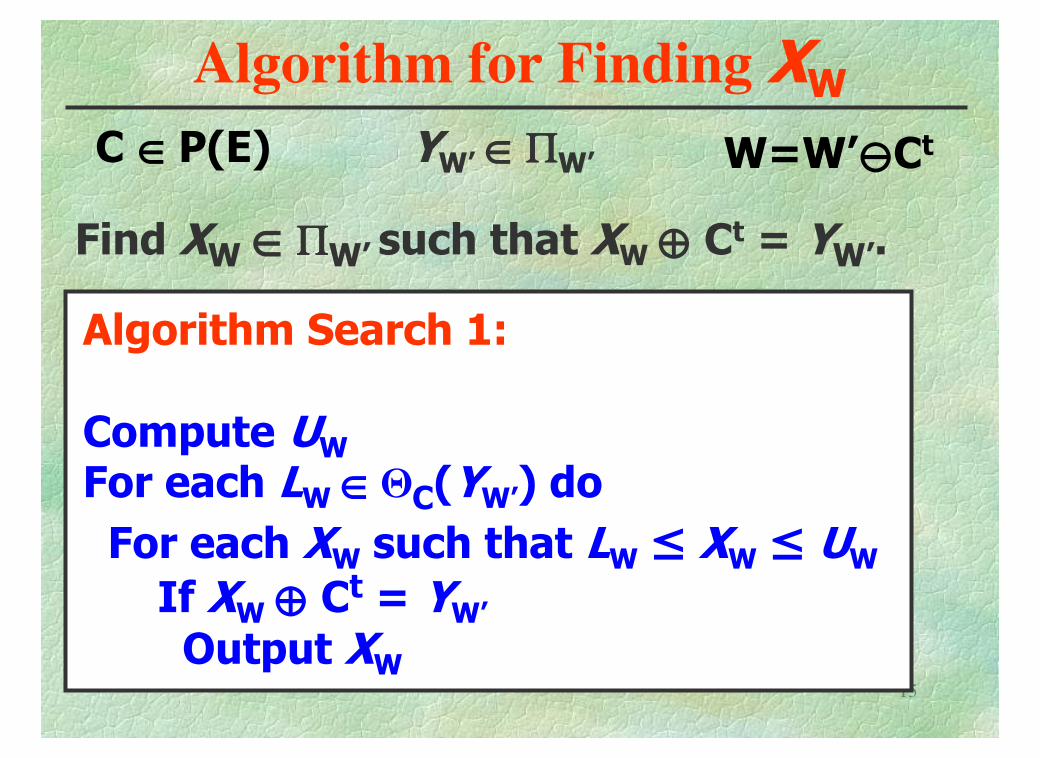
Algorithm for Finding XW

Find XW Œ ΠΠΠΠW’ such that XW ≈ Ct = YW’.

C Œ P(E) YW’Œ ΠΠΠΠW’ W=W’ûCt

Algorithm Search 1:

Compute UW

For each LW Œ QC(YW’) do

For each XW such that LW £ XW £ UW

If XW ≈ Ct = YW’

Output XW

16

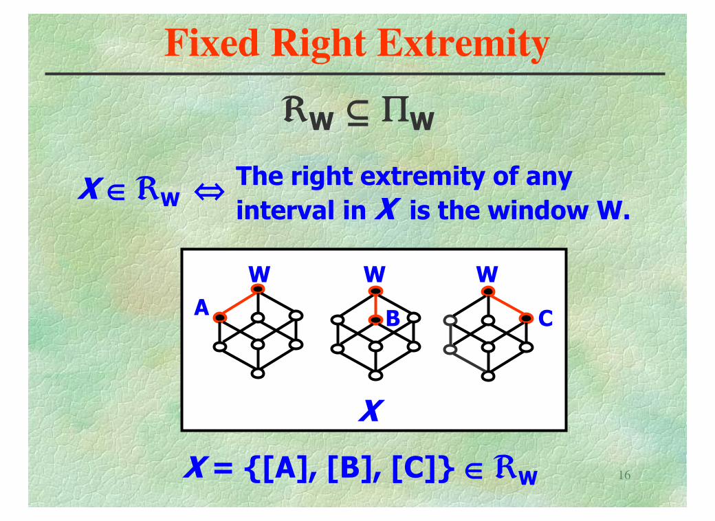
Fixed Right Extremity

ëW Õ ΠΠΠΠW

X

WWW

AB C

X = {[A], [B], [C]} Œ ëW

X Œ ëWThe right extremity of any

interval in X is the window W.¤

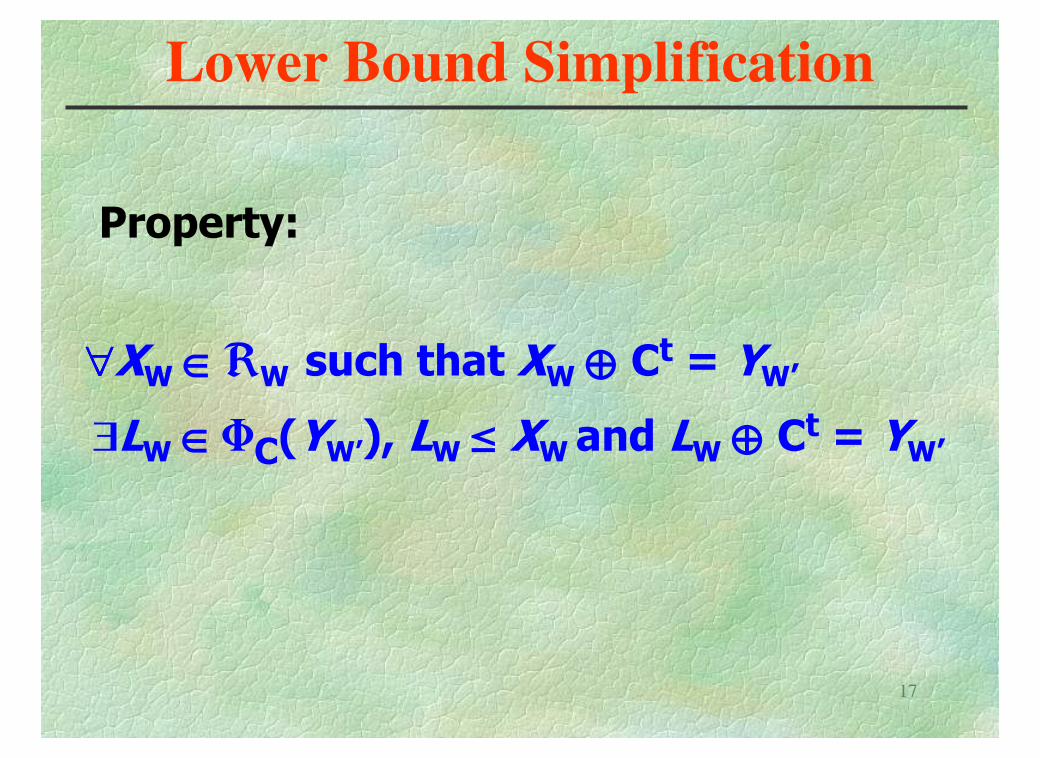
17

Lower Bound Simplification

Property:

∀∀∀∀XW Œ ëW such that XW ≈ Ct = YW’

$LW Œ FC(YW’), LW £ XW and LW ≈ Ct = YW’

18

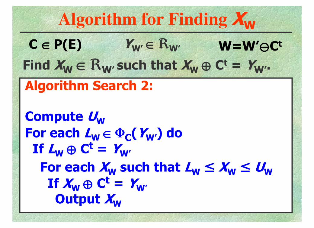
Algorithm for Finding XW

Find XW Œ ëW’ such that XW ≈ Ct = YW’.

C Œ P(E) YW’Œ ëW’ W=W’ûCt

Algorithm Search 2:

Compute UW

For each LW Œ FC(YW’) do

If LW ≈ Ct = YW’

For each XW such that LW £ XW £ UW

If XW ≈ Ct = YW’

Output XW

19

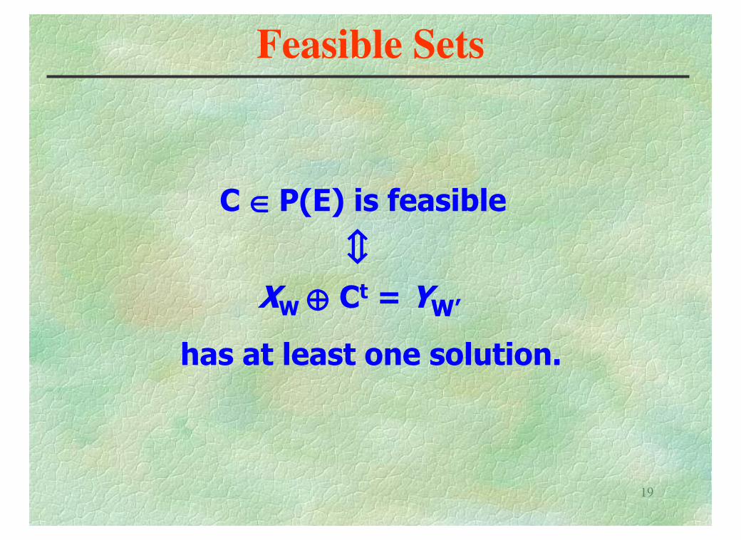
Feasible Sets

C ΠP(E) is feasible

êXW ≈ Ct = YW’

has at least one solution.

20

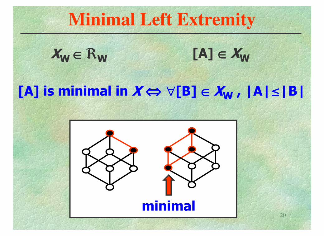
Minimal Left Extremity

XWŒ ëW [A] Œ XW

[A] is minimal in X¤ ∀∀∀∀[B] Œ XW , |A|£|B|

minimal

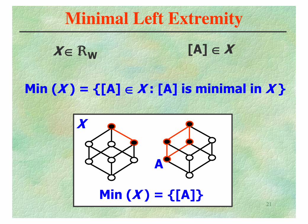
21

Minimal Left Extremity

XŒ ëW[A] Œ X

Min (X ) = {[A] ΠX : [A] is minimal in X }

A

Min (X ) = {[A]}

X

22

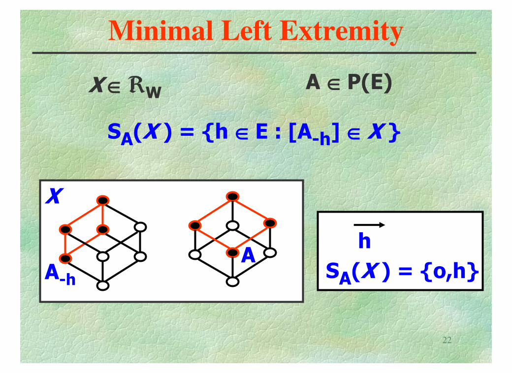
Minimal Left Extremity

SA(X ) = {h ΠE : [A-h] ΠX }

XŒ ëWA Œ P(E)

A

X

h

SA(X ) = {o,h}A-h

23

Invariant

A, B ΠP(E)

B is an invariant of A iffB = (AûB)≈B

24

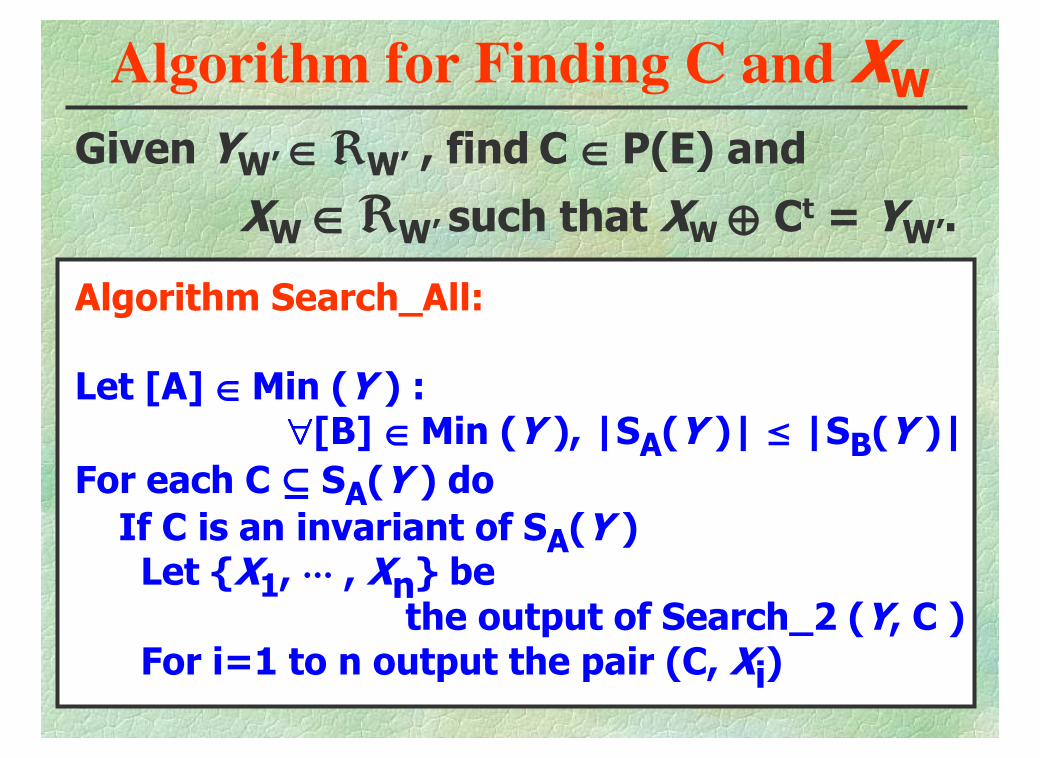
Algorithm for Finding C and XW

Given YW’Œ ëW’ , find C Œ P(E) and

XW Œ ëW’ such that XW ≈ Ct = YW’.

Algorithm Search_All:

Let [A] Œ Min (Y ) : ∀∀∀∀[B] Œ Min (Y ), |SA(Y )| £ |SB(Y )|

For each C Õ SA(Y ) doIf C is an invariant of SA(Y )Let {X1, ◊◊◊ , Xn} be

the output of Search_2 (Y, C )For i=1 to n output the pair (C, Xi)

25

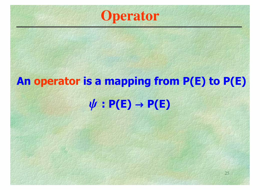
Operator

An operator is a mapping from P(E) to P(E)

y : P(E) Æ P(E)

26

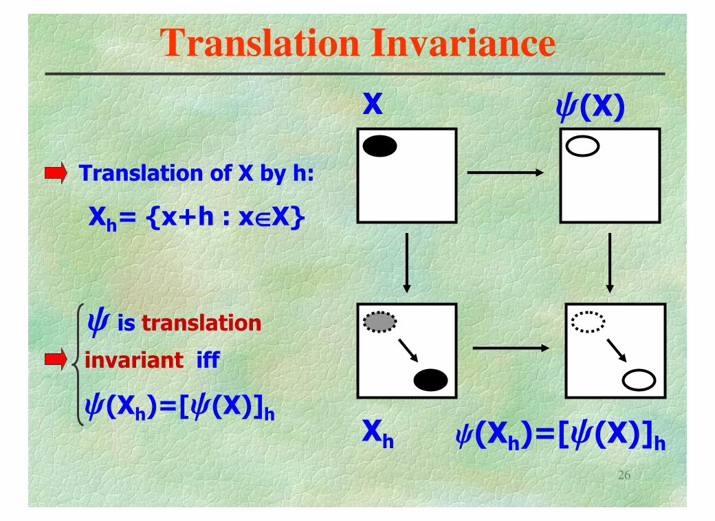
Translation Invariance

invariant iff

Translation of X by h:

y is translation

X y(X)

y(Xh)=[y(X)]hXh

Xh= {x+h : xŒX}

y(Xh)=[y(X)]h

27

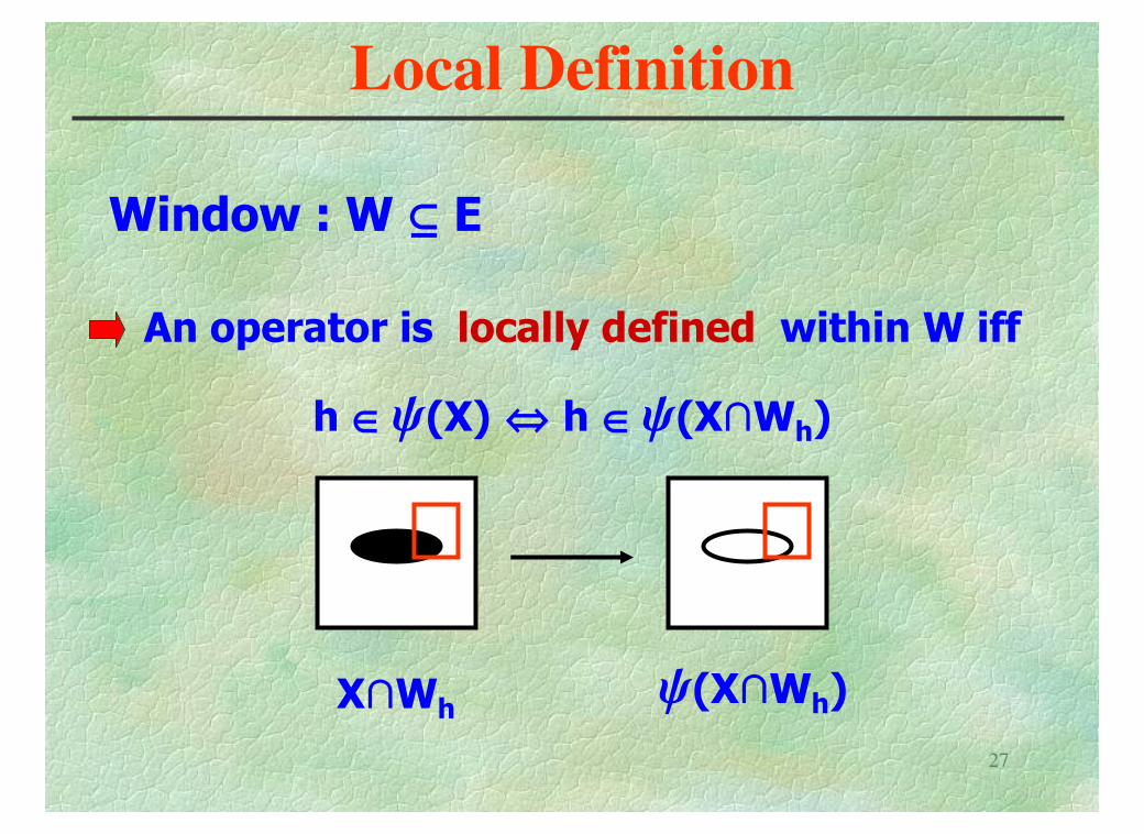
Local Definition

An operator is locally defined within W iff

Window : W Õ E

h Œ y(X) ¤ h Œ y(X»Wh)

X»Why(X»Wh)

28

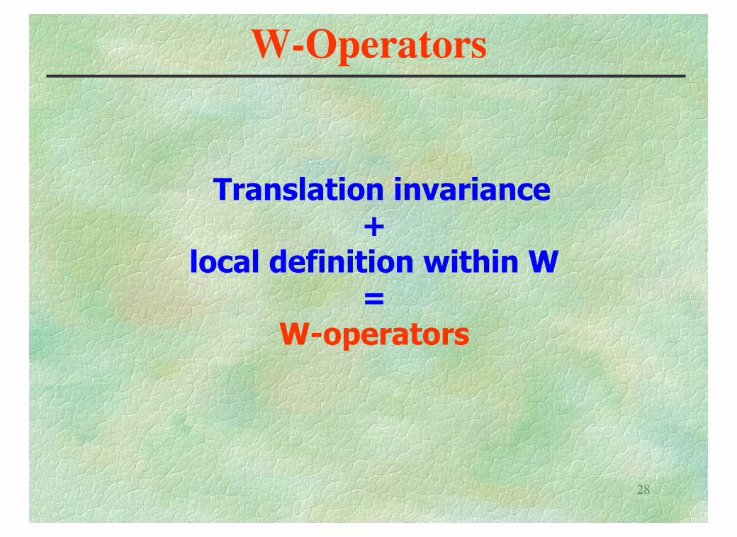
W-Operators

Translation invariance +

local definition within W =

W-operators

29

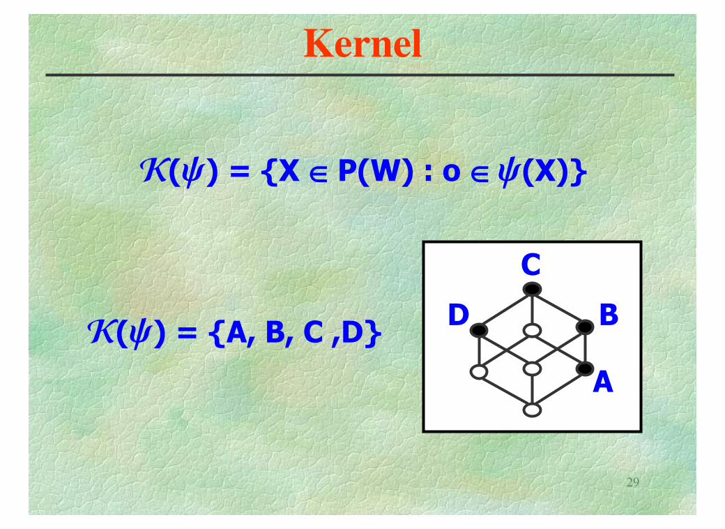
Kernel

K(y) = {X ΠP(W) : o Πy(X)}

B

A

C

DK(y) = {A, B, C ,D}

30

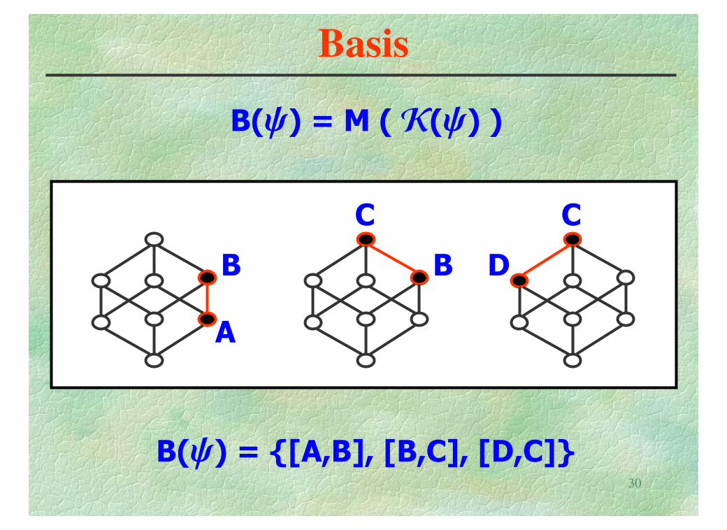
Basis

B(y) = M ( K(y) )

B(y) = {[A,B], [B,C], [D,C]}

B

A

B

C C

D

31

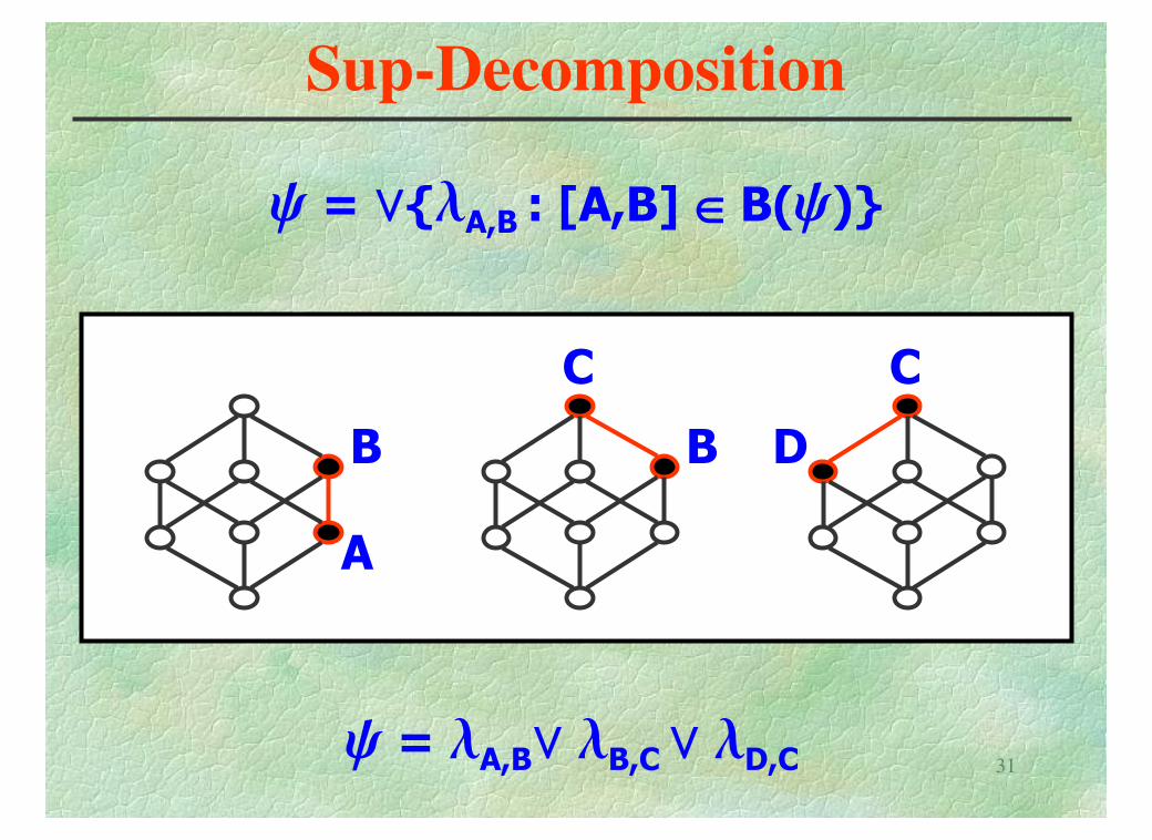
Sup-Decomposition

y = lA,B⁄ lB,C ⁄ lD,C

B

A

B

C C

D

y = ⁄{lA,B : [A,B] Œ B(y)}

32

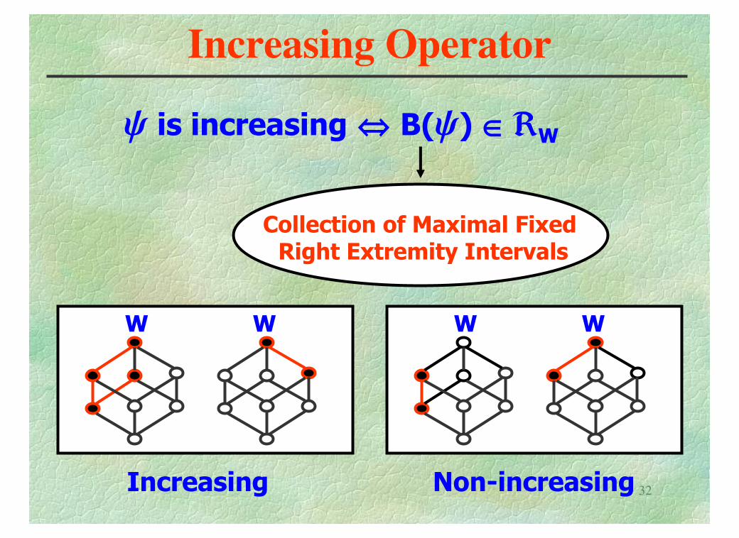
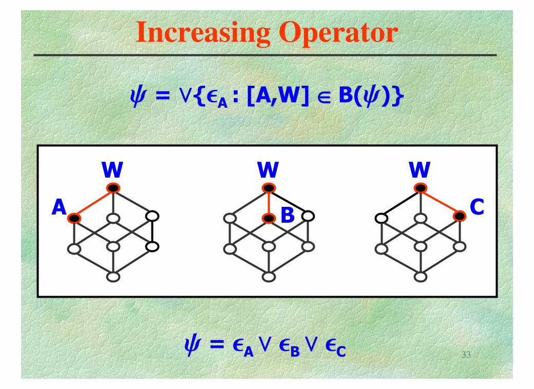
Increasing Operator

y is increasing ¤ B(y) Œ ëW

Collection of Maximal Fixed Right Extremity Intervals

W W W W

Increasing Non-increasing

33

Increasing Operator

y = eA ⁄ eB ⁄ eC

W

A B

W

C

W

y = ⁄{eA : [A,W] Œ B(y)}

34

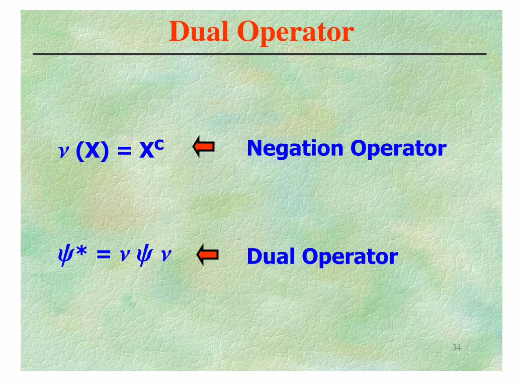
Dual Operator

n (X) = Xc Negation Operator

y* = n y n Dual Operator

35

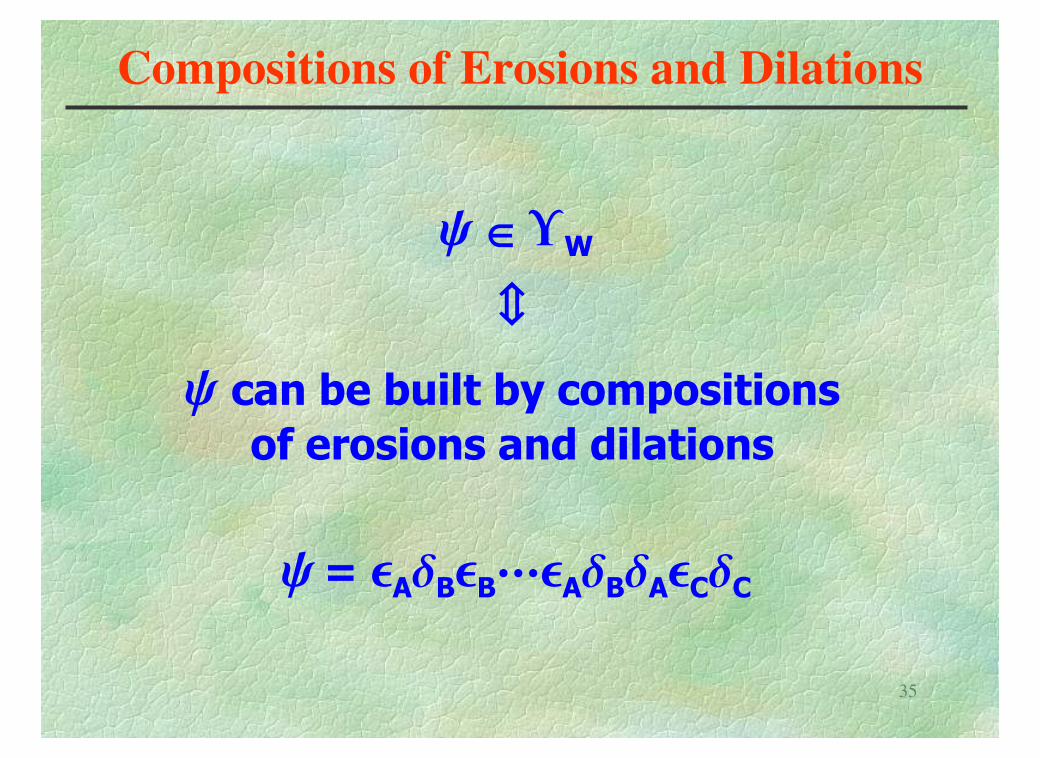
Compositions of Erosions and Dilations

y can be built by compositions

of erosions and dilations

y ΠUW

ê

y= eAdBeB◊◊◊eAdBdAeCdC

36

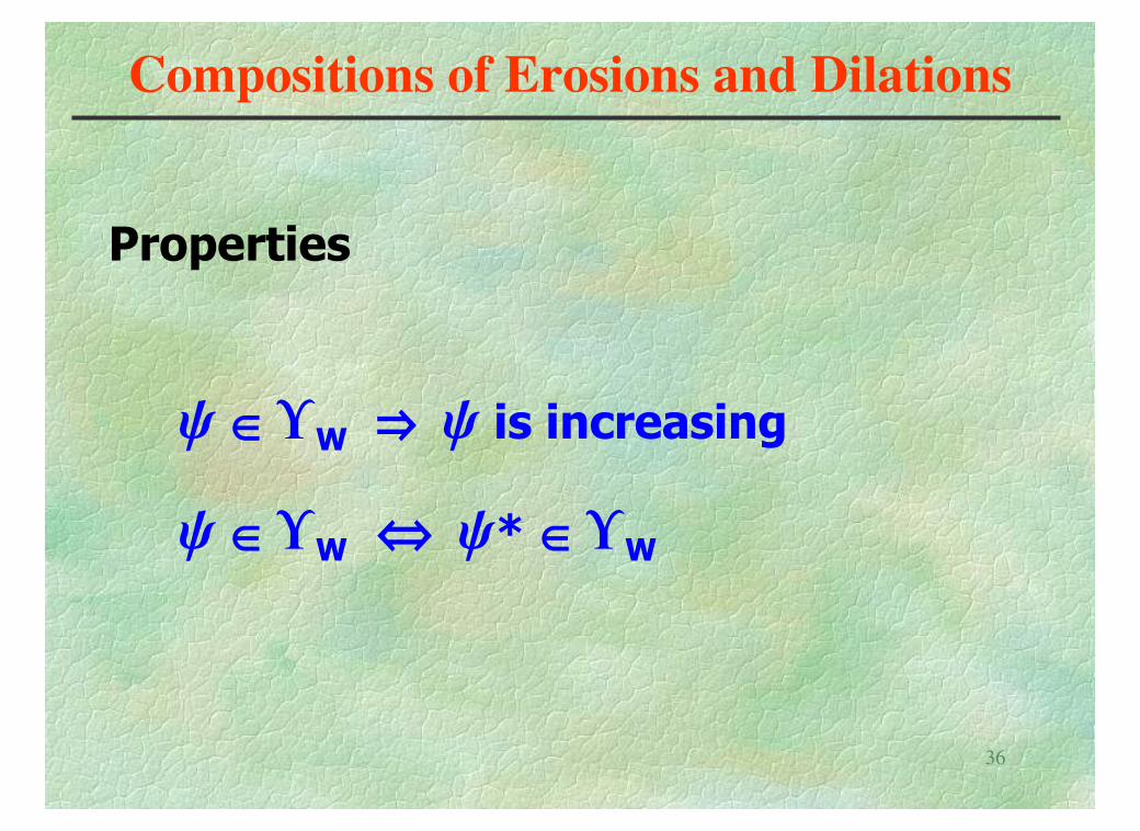
Compositions of Erosions and Dilations

y ΠUW fi y is increasing

y Œ UW ¤ y* Œ UW

Properties

37

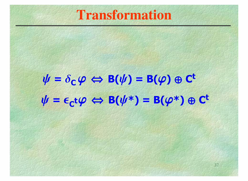
Transformation

y = dCj ¤ B(y) = B(j) ≈ Ct

y = e j ¤ B(y*) = B(j*) ≈ CtCt

38

Transformation

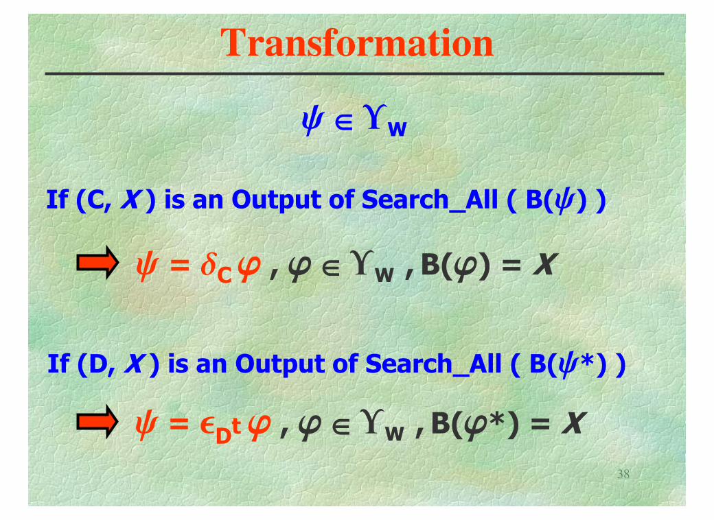
y ΠUW

If (C, X ) is an Output of Search_All ( B(y) )

If (D, X ) is an Output of Search_All ( B(y*) )

y = dCj , j ΠUW , B(j) = X

y = e j , j ΠUW , B(j*) = XDt

39

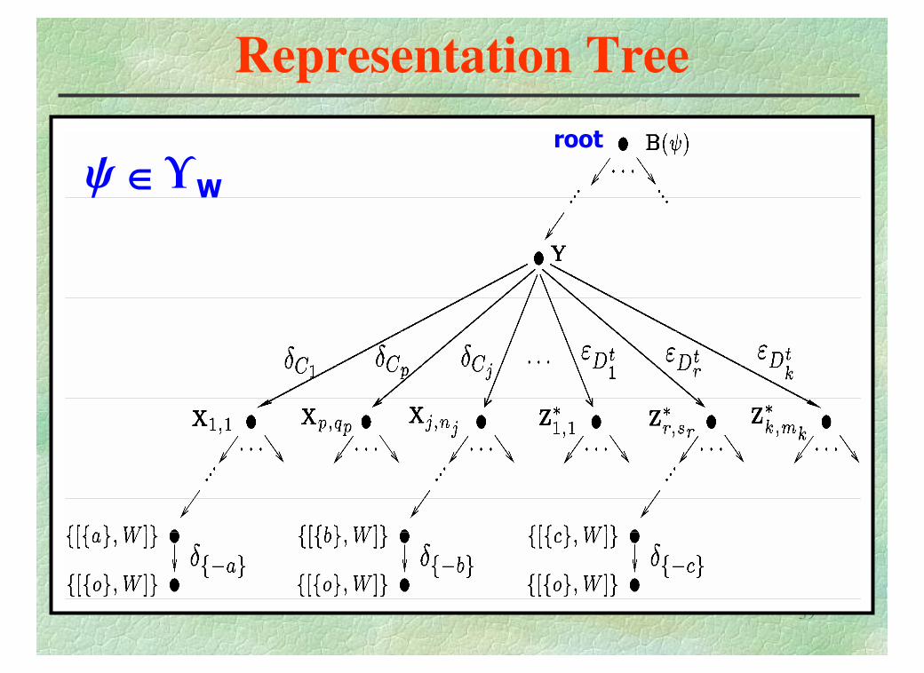
Representation Tree

y ΠUW

root

40

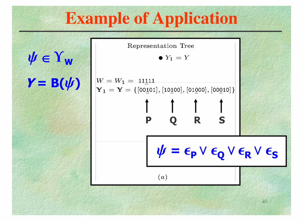
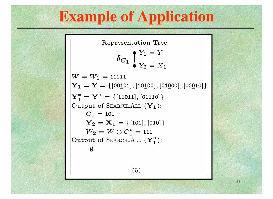
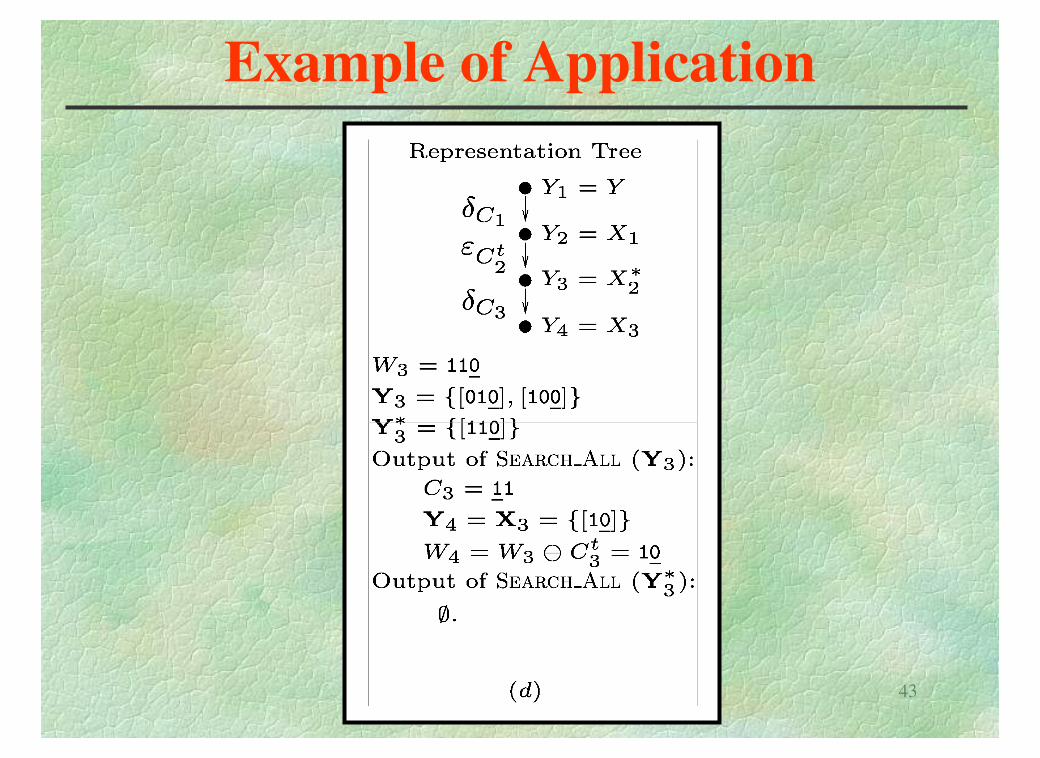
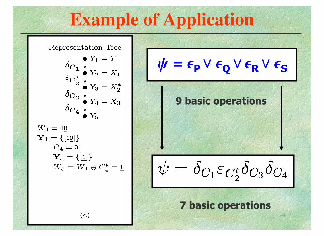
Example of Application

y ΠUW

Y = B(y)

P Q R S

y = eP⁄ eQ ⁄ eR⁄ eS

41

Example of Application

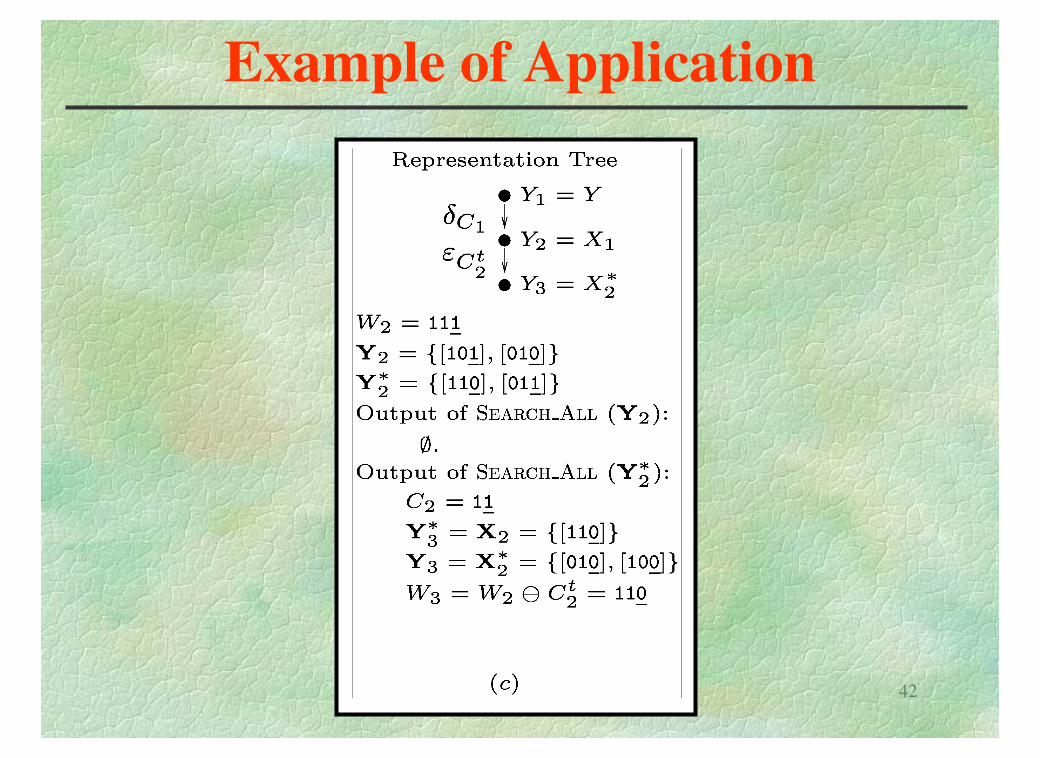
42

Example of Application

43

Example of Application

44

Example of Application

7 basic operations

y = eP⁄ eQ ⁄ eR⁄ eS

9 basic operations

45

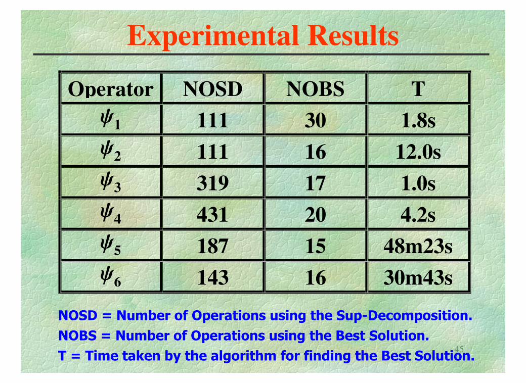
Experimental Results

Operator NOSD NOBS T

y1 111 30 1.8s

y2 111 16 12.0s

y3 319 17 1.0s

y4 431 20 4.2s

y5 187 15 48m23s

y6 143 16 30m43s

NOSD = Number of Operations using the Sup-Decomposition.

NOBS = Number of Operations using the Best Solution.

T = Time taken by the algorithm for finding the Best Solution.

46

Conclusions

• Problem of transforming the sup-decomposition to sequential decompositions (when they exist).

• Applied to compute sequential decompositions of operators built by compositions of dilations and erosions.

• Minkowski Factorization Equation:• General case;• Fixed Right Extremities.

• Future step: Find parallel algorithms for these results.