fracking, farmers, and rural electrification in india* - american
TRANSCRIPT
Fracking, farmers, and rural electrification in India*
Faraz Usmani T. Robert Fetter
December 3, 2018
Job Market Paper
Latest version available at: http://www.farazusmani.com/jmp
Abstract
Is large-scale electrification necessary for the structural transformation of rural economies?We combine two natural experiments in India within a regression discontinuity design to shedlight on this question. Most of the world’s guar, a crop that yields a potent thickening agent usedduring hydraulic fracturing (“fracking”), is grown in northwestern India. In response to theUnited States’ fracking boom, Indian guar prices increased by nearly 1,000 percent. Leveragingpopulation-based discontinuities in the contemporaneous roll-out of India’s massive ruralelectrification scheme, we show that access to electricity significantly increased non-agriculturalemployment in villages located in India’s booming guar belt. In contrast, electrification had nodiscernible impact on labor-market outcomes in villages in the rest of the country. The growthof non-farm work is partly driven by the rise of electricity-intensive firms that complementagricultural production. Electrification alone is typically not sufficient to deliver economicbenefits but it may be necessary to enable households and firms to respond to rapidly changingeconomic contexts in welfare-enhancing ways.
JEL codes: O13, O18, Q40
*Usmani: Duke University. Nicholas School of the Environment, and Sanford School of Public Pol-icy. [email protected]. Fetter: Duke University. Nicholas Institute for Environmental Policy [email protected]. We thank Fiona Burlig, Esther Heesemann, Marc Jeuland, David Kaczan, Robyn Meeks, BrianMurray, Jennifer Orgill-Meyer, Subhrendu Pattanayak, Louis Preonas, Seth Sanders, Steven Sexton, Smriti Sharma,Saurabh Singhal, Eswaran Somanathan, and seminar participants at Camp Resources XXIV, Duke University, NorthCarolina State University, UNU-WIDER, SETI 2018 and WCERE 2018 for valuable comments and suggestions. We alsothank Lauren Masatsugu for her help acquiring data that made this project possible. Usmani is grateful for support fromthe Duke Global Health Institute, Duke University Energy Initiative, Duke University Department of Economics, andthe United Nations University World Institute for Development Economics Research (UNU-WIDER). Any remainingerrors are our own.
1
1 Introduction
Over a billion people worldwide lack access to electricity, and many more are served by unreliable
systems capable of supporting little more than a light bulb. The belief that access to reliable
electricity catalyzes job creation and economic growth—reflected in the inclusion of energy access
targets as part of the United Nations’ Sustainable Development Goals—has thrust energy to
the fore of development policy (United Nations, 2018). Indeed, governments and international
organizations alike are mobilizing considerable resources to ensure access for all. According to the
International Energy Agency (2011), over $9 billion was spent in 2009 to extend modern energy
services to underserved populations, a figure that it estimates must rise to over $48 billion per year
by 2030 in order to achieve universal access. Yet the evidence on the impacts of such efforts remains
mixed. Dinkelman (2011) and Lipscomb et al. (2013), for instance, identify large positive effects
on employment as a result of rural electrification in South Africa and Brazil, respectively. Burlig
and Preonas (2016), on the other hand, find that the effects of rural electrification on labor-market
outcomes in India are far more muted. Others have uncovered similarly lackluster impacts in the
African context (Bernard and Torero, 2015; Lenz et al., 2017).1
This lack of consensus surrounding the benefits of grid expansion highlights both a significant
knowledge gap and a critical policy challenge. Indeed, the world’s poor are constrained by far
more than a lack of access to modern energy services (Banerjee and Duflo, 2007), and there may
be profound opportunity costs associated with large-scale investments in energy infrastructure in
low- and middle-income settings. India alone is home to nearly 250 million people living without
electricity (International Energy Agency, 2015). If electrification by way of resource-intensive grid
expansion is foundational in promoting livelihoods among unconnected populations, it represents
a necessary first step for development policy. If, on the other hand, expected benefits are highly
uncertain—or, worse, illusory—scarce public resources are better targeted elsewhere, and cost-
effective approaches that enhance access to only rudimentary energy services (such as basic lighting)
may be more appropriate (Grimm et al., 2017).
1In a recent review of the empirical literature, Bonan et al. (2017) note that the current evidence on the impacts ofelectrification on adults’ time allocation and labor activities suggests “mild increases in employment and labor supply,particularly for women, non-agricultural activities and more formal activities” but that the magnitude of such effects“varies significantly across studies and geographical areas.”
2
Is large-scale electrification necessary for the structural transformation of rural economies? We
exploit the interaction of two natural experiments in India to shed light on this question. As the
hydraulic fracturing (“fracking”) boom began in the United States, it induced a parallel commodity
boom in India in the production of an otherwise obscure crop called guar in India. Guar provides a
key input into the fracking process and is primarily grown in the semi-arid northwestern tracts of
the country by small and marginal farmers (Rai, 2015). Between 2006 and 2011, its price increased by
over 1,000 percent, resulting in a large exogeneous shock to rural economies in the region. Almost
simultaneously, India began rolling out its massive rural electrification scheme, which aimed to
electrify approximately 400,000 villages across 27 states. It prioritized villages for electrification on
the basis of a strict population-based threshold, giving rise to discontinuous changes in a village’s
probability of being electrified. We combine these two natural experiments within a regression
discontinuity design to evaluate how the causal effect of electrification on labor-market outcomes
varies with exogenous changes in economic contexts.
First, we show that electrification increased non-agricultural employment in villages located
in India’s guar belt by approximately six percentage points (seventy percent). In these same vil-
lages, electrification reduced agricultural employment by a corresponding amount, representing
a reduction of approximately twenty percent. This is particularly notable given the fact that this
region—spread across three states in northwestern India—was in the grip of an unprecedented
agricultural boom. We next highlight potential mechanisms by providing suggestive evidence that
these labor-market dynamics are driven by the rise of complementary non-agricultural opportu-
nities. An increase in guar production necessitates a shift in the labor force towards processing,
which is made possible by new electricity connections. Simultaneously, increased wages and agri-
cultural profits from both the production boom and new processing opportunities can be reinvested
in household enterprises, which may also benefit from electricity connections. Consistent with
this, we uncover a large increase in (i) the number of workers at firms related to the industrial
(electricity-intensive) parts of the guar production chain (such as guar processing); and (ii) home
production of income-generating products in electrified guar-growing regions. Finally, we find no
discernible evidence of any effect of electrification on these labor-market outcomes in villages or
regions located in the rest of India, suggesting that complementary economic conditions play a
crucial role in driving the impacts of large-scale electrification infrastructure.
3
In so doing, we revisit work by Burlig and Preonas (2016), who conduct the first large-scale
impact evaluation of India’s rural electrification scheme. They show that the program increased
electrification rates, but also demonstrate that its impacts on a wide range of socioeconomic
outcomes (including those related to the rural labor market) are precisely estimated null results.2
Our results from non-guar regions of India—using an empirical strategy that follows their own—are
consistent with these earlier findings. Using the exogenous shock to economic activity generated
by the guar boom, however, also allows us to respond to some of the questions that emerge from
this prior body of work and shed light on important drivers of heterogeneity.
Our study, thus, makes three key contributions. First, our results highlight how grid-scale elec-
trification can support potentially welfare-enhancing structural change in the rural economy. Access
to electricity alone cannot deliver economic and social welfare, as has been demonstrated a number
of times in the literature. That electrification significantly enhances non-agricultural employment in
boom areas suggests, however, that it may be necessary to fully exploit the opportunities presented
by rapidly changing economic contexts.
Second, our findings highlight that the impacts of large-scale investments in grid electrification
are crucially tied to local economic contexts, opportunity and potential. For instance, electricity
from the grid may enable local industrial production of certain goods, yet this may make little
difference in the short run if complementary factors—such as demand for these locally produced
goods, a trained labor force to meet that demand, and rural roads that enable access to markets—are
not also in place. If they are, however, grid-scale electricity may considerably expand how firms
and households take advantage of economic opportunities to generate income and enhance welfare.
Prior research—which typically estimates the “average treatment effect” of such investments as
part of national rural electrification programs—implicitly neglects these context-specific factors.3
While the particular agricultural boom we study is clearly unique to our setting, it—in combination
with the roll-out of rural electrification—gives us an opportunity to investigate how electrified
villages in boom and non-boom areas perform relative to unelectrified villages in the same regions.
2Results from a randomized controlled trial in Kenya by Lee et al. (2018) echo these findings.3This, we contend, is one reason we observe mixed evidence from settings as diverse as Bhutan, Brazil and Vietnam
(Khandker et al., 2013; Lipscomb et al., 2013; Litzow et al., 2017). In addition, many national rural electrification schemesare grounded in an obligation—either perceived or real—to ensure universal access to electricity (Tully, 2006). Whilecertainly aligned with broader equity goals, it is not immediately clear that such rights-based approaches are necessarilydesigned to maximize economic outcomes. That short- or medium-term impact evaluations of such efforts over largespatial scales may yield null results is unsurprising.
4
Insofar as the economic promise or potential of certain areas can be accurately assessed, the insights
we generate can be used to inform spatial targeting of resource-intensive infrastructure by allowing
policymakers to better gauge cost-benefit trade-offs, and choose appropriate grid-based and off-grid
energy solutions for different contexts.4
Finally, from a methodological perspective, our study is part of a growing body of work that
adopts a rigorous approach to understanding treatment-effect heterogeneity in the real world.5
That the same intervention can have different impacts in superficially similar settings points to
the importance of context-dependence; learning about what these contextual factors are is crucial
to learning from these impact evaluations (Vivalt, 2015). Where a sufficiently large number of
studies have been conducted, rigorous meta-analyses can shed light on underlying drivers of
effectiveness. In most other cases, however, such efforts are typically restricted to relatively crude
subgroup analyses, involving interactions of endogenous binary variables representing various
subgroups of interest with the main treatment-effect parameter. Our quasi-experimental setting—
the combination of an exogenous shock to economic activity with quasi-experimental variation
in access to electricity within a regression discontinuity design—provides the first opportunity
to study the heterogeneous effects of access to electricity over large spatial scales in a real-world
setting.
This rest of this paper is organized as follows. In Section 2, we provide background on our
two natural experiments. Section 3 highlights our conceptual framework, and discusses our
identification strategies. Section 4 describes our data. Section 5 reports impacts on the first set
of outcomes, the size and composition of the rural labor force. Section 6 reports impacts from
additional analyses to uncover mechanisms related to the growth of firms. Section 7 summarizes
results, and discusses policy implications and avenues for future research.
4We emphasize that there may be other channels driving heterogeneity in the benefits generated by large-scaleinfrastructure projects, such as institutions or access to markets. We believe this is a promising avenue for future research.
5In its use of multiple sources of exogenous variation in real-world settings, our study is related to Duque et al.(2018), who examine how early-life exposure to adverse weather shocks (that reduce children’s initial skills) in Colombiainteracts with the introduction of conditional cash transfers (that promote investments in children’s health and education)to influence long-term outcomes. It is also similar to Wysokinska (2017), who studies the determinants of long-rundevelopment by similarly examining the interplay between plausibly exogenous variation in institutional and culturalfactors in Poland.
5
2 Background
In this section, we first describe India’s rural electrification scheme. We then provide a basic
overview of hydraulic fracturing (“fracking”). Finally, we discuss guar production in India and, in
particular, how it responded to the fracking boom in the United States.
2.1 Rural electrification
Rural electrification in India has a checkered past. In 1947, newly independent India had only
1,500 electrified villages, and progress on rural electrification remained slow well into the late
1960s (Banerjee et al., 2014, p. 35). The country’s initial electrification efforts focused primarily on
urban and peri-urban areas. Severe droughts and food shortages in the early 1960s brought rural
electrification into the spotlight, yet subsequent policies prioritized productive uses over household
access, and primarily aimed to increase access to electricity for irrigation. Rural household access
finally emerged as a key priority area in the late 1970s, and has since featured prominently in
India’s successive Five-Year Plans. The growing recognition of the role of electrification in rural
development—coupled with the existence of multiple national- and state-level electrification
agencies with overlapping responsibilities—gave rise to a number of schemes over the decades.6
The Rajiv Gandhi Grameen Vidyutikaran Yojana (RGGVY), launched in 2005, subsumed all existing
grid-related rural electrification initiatives.
RGGVY was charged with enhancing access to electricity in over 100,000 unelectrified and
300,000 “partially electrified” villages across 27 Indian states. It aimed to do so primarily by
installing and upgrading electricity infrastructure (namely, transmission and distribution lines, and
transformers) to support commercial and productive activities in growing rural economies. These
included electric irrigation pumps, education and health-care facilities, and small and medium
enterprises. In addition to its focus on electricity infrastructure, RGGVY also extended free grid
connections to rural households below the poverty line; households above the poverty line could
6For instance, the Kutir Jyoti Yojana was launched in the late 1980s to increase access to electric lighting for householdsbelow the poverty line; the Pradhan Mantri Gramodaya Yojana, launched in 2001, extended financing to states to enhanceaccess to public services, including electrification, in rural areas; the Remote Village Electrification program, launched in2002, aimed to provide lighting to remote villages using solar photovoltaics and other off-grid energy technologies; andthe country’s Minimum Needs Program was updated in 2002 to extend financing for rural electrification to states thatwere seen to be performing especially poorly (Banerjee et al., 2014, p. 37-38).
6
purchase connections.7 Both groups remained responsible for their own power use as RGGVY did
not subsidize electricity consumption.
Although a national program that was largely funded by India’s federal government, RGGVY
was implemented in practice through decentralized district-level projects overseen by local imple-
menting agencies (such as the State Electricity Board).8 Electrification under RGGVY proceeded in
two steps. First, to qualify for RGGVY funds, the local implementing agency prepared a Detailed
Project Report (DPR) for the district in question. The DPR outlined in detail the electrification-
related infrastructure needs of the district, the number of households expected to be connected to
the grid, and expected project costs. It also identified the set of villages eligible for electrification
under RGGVY. These DPRs were reviewed and approved by India’s Rural Electrification Corpora-
tion as well as its Ministry of Power before disbursement of funds. Once approved, district-level
implementation commenced in line with the village-by-village plan outlined in the DPR.
[Figure 1 about here.]
Districts were allocated to India’s Tenth (2002-2007) and Eleventh (2007-2012) Five-Year Plans
for funding based on the order in which DPRs were submitted and approved. We refer to these
as “RGGVY Phase I” and “RGGVY Phase II” districts, respectively, and identify these districts
using state-level five-year-plan progress reports for RGGVY.9 To keep program costs low, during
Phase I, villages containing at least one habitation (a geographically distinct sub-village cluster
of households) with a population of 300 or more were eligible to be electrified. Approximately
178,000 villages across 234 Phase I districts in 25 states (as per 2011 administrative boundaries)
fit this criterion. Nearly all funds associated with Phase I districts had been disbursed between
2005 and 2008, while funding for Phase II districts—for which the RGGVY eligibility threshold
7According to the Ministry of Power (2006), RGGVY’s primary mandate included the (i) provision of electric-ity sub-stations and transmission lines of adequate capacity to establish a “rural electricity distribution backbone;”(ii) electrification of unelectrified villages, including provision of distribution transformers of appropriate capacity;(iii) establishment decentralized distributed generation and supply in a subset of villages where grid connectivity isinfeasible or not cost effective; and (iv) provision of household-level connections for households below the poverty line.
8An Indian district is administratively analogous to a county in the United States.9For each state, these reports—entitled “Report C-Physical & Financial Progress of RGGVY Projects Under Imple-
mentation (Plan-wise)”—list the district name and DPR code, the name of the district-level local implementing agency,details about the financial scope and progress of the project (such as project approval date, total sanctioned amount, andthe amount released so far), as well as the scope and progress of electrification (in terms of village- and household-levelelectrification targets).These reports are available via the website of the Deendayal Updhayaya Gram Jyoti Yojana(DDUGJY)—into which RGGVY was ultimately subsumed—at http://www.ddugjy.gov.in/.
7
was reduced to 100—was disbursed between 2008 and 2011. In this paper, we specifically focus
on Phase I districts (shown in Figure 1) as village-level electrification in these districts had been
completed well in advance of the release of the 2011 round of the Indian Census, one of our main
data sources.10
2.2 Fracking
Hydraulic fracturing (“fracking”) is the process by which fracking fluid (a mixture of mostly
water, granular “proppants” such as sand, and chemicals) is injected into crude oil and natural
gas wellbores at high pressures to create small cracks (fractures) in the underlying rock formation.
While not an entirely new approach, recent technological refinements—and, in particular, fracking
in combination with horizontal drilling—have considerably increased the effectiveness of the
process and transformed the energy landscape in the United States.11
[Figure 2 about here.]
Figure 2 provides an overview of natural gas (panel a) and oil (panel b) production from fracked
and “conventional” wells in the United States between 2000 and 2015. In 2000, fracked wells
produced 3.6 billion cubic feet per day of marketed gas, less than seven percent of the United
States’ total. Starting in approximately 2005, the industry grew rapidly. By 2015, fracked wells
produced around 67 percent of the country’s total natural gas. Oil production underwent a similarly
momentous shift, albeit slightly later. In 2000, fracked wells yielded less than two percent of the
national total. Following a period of growth that began around 2009, approximately half of the
United States’ total oil output could be traced back to a fracked well in 2015.
A typical “frac job” is preceded by a vertical drill to a depth of around 1,000–5,000 meters,
depending on the geophysical characteristics of the shale formation being explored. Upon reaching
the desired depth, the well is then drilled horizontally, allowing for greater access to the shale
10Indeed, because enumeration for the 2011 Census began in April 2010, villages electrified as part of RGGVY PhaseII would have been only captured inconsistently during Census survey activities. In addition, they would have beenelectrified for a considerably shorter period of time.
11Compared to conventional (vertical) wells, horizontal wells can typically access greater reserves, and are two to fivetimes more productive (Joshi, 2003). This can lead to considerable cost savings in the long run, despite higher initialdrilling costs. Orr (2016) notes that “[a]lthough hydraulic fracturing and horizontal drilling had been used separatelyto stimulate production at conventional wells since 1947 and 1929, respectively, the combination of these methods hasenabled scientists to extract oil and gas trapped in impermeable source rocks such as shale, well-cemented sandstone,and coal bed methane deposits once considered too costly to develop.”
8
formation. Once drilling is complete, fracking fluid is injected at high pressures into the drill site
to induce fractures in the formation. Reductions in pressure following the initial injections cause
fluids in the well to return to the surface as “flowback.” As production continues, the amount of
flowback returning to the surface gradually decreases and the amount of oil or gas increases.
Fracking fluid consists almost entirely of water and proppants; the remaining elements usually
include various chemicals that serve, among other things, as gelling agents, corrosion inhibitors,
friction reducers, clay controls, and biocides (Tollefson, 2013). Of these chemicals, the gelling
agent—which increases the viscosity (thickness) of fracking fluid—comprises the largest share. Its
use confers two important advantages. First, viscous fluids enable better control of leak-off into
the surrounding rock formation, reducing the amount of fracking fluid needed for a given frac job
(Barati and Liang, 2014). Second, viscous fluids are more effective at suspending sand and other
granular proppants and carrying them deep into the wellbore (Bellarby, 2009). These proppants
prevent fractures induced in the rock by high-pressure pumping from closing down completely
once the pressure has fallen. These partially open fractures are the passageways through which oil
and gas flow out of rocks and into the well.
No particular combination of ingredients is perfect, and operators often face trade-offs.12 For
this reason, experimentation with the specific mix of chemicals used is rife (Fetter, 2018; Fetter
et al., 2018). Yet despite operators’ readiness to modify the make-up of fracking fluid, guar gum—a
powdery substance derived from the bean of the guar plant—is the industry’s most widely used
gelling agent. Indeed, between 25-50 percent of all fracking operations rely on guar gum, making
it “at least two to three times preferred over synthetic [alternatives]” (Elsner and Hoelzer, 2016).
This is unsurprising; guar gum is uniquely effective at its job. It can alter the viscosity of fracking
fluid by more than two orders of magnitude under certain conditions (Tapscott, 2015). In addition,
whereas other natural gums require prolonged cooking, guar gum attains its full viscosity potential
in cold water, and is effective even at relatively dilute concentrations (Thombare et al., 2016). Its
viscosity potential also remains relatively stable over changes in temperature, and in the acidity or
basicity of the solution in which it is mixed (Chudzikowski, 1971). Despite considerable efforts by
major chemical companies in recent years, a synthetic alternative that is as effective as guar gum
12For instance, although more viscous fluids are better able to suspend proppants, they are less “pumpable” andrequire more energy to be pumped at sufficiently high rates.
9
for high-viscosity fracking is yet to be developed (Beckwith, 2012).
2.3 Guar and guar gum
Guar (Cyamopsis tetragonoloba) is a drought-resistant legume that is primarily cultivated in the
semi-arid northwestern tracts of the Indian subcontinent (Kuravadi et al., 2013). It can tolerate
relatively high temperatures and requires only sparse but regular rainfall, which makes the rain
patterns associated with the monsoon in this region ideal for cultivation (Mudgil et al., 2011).
Guar—whose name is derived from the Sanskrit term for “cow food”—has traditionally been
cultivated as both fodder and a vegetable crop. It grows well in many different types of soil, and
its nitrogen-fixing potential combined with its relatively short planting season also make it an
excellent soil-improving crop that fits conveniently within farmers’ crop-rotation cycles.13
Guar gum (sometimes also called guar flour) is obtained from the endosperm of guar seeds in
two distinct energy-intensive steps (Chudzikowski, 1971). Guar seeds are first exposed to a rapid
flame treatment, which loosens the hard seed hull (outer shell), which is removed in a scouring or
“pearling” operation. The glassy endosperm that this process exposes is then separated from the
germ in a milling operation. The resulting guar “splits” can be ground to various levels of fineness
to obtain guar gum in powder form. This powder is sometimes further processed and combined
with additional chemicals to obtain industry-specific derivatives.
India accounts for approximately eighty percent of global production, making it by far the
world’s largest producer of guar (National Rainfed Area Authority, 2014).14 The country occupies
a similarly dominant role in the global trade of guar derivatives. Within India, guar is almost
exclusively produced in the northwestern part of the country. The state of Rajasthan—which,
in 2013-14, was home to nearly ninety percent of India’s total area under guar cultivation, and
eighty percent of its production—is the epicenter of this industry. Other important producers
include Haryana and Gujarat, which—together with Rajasthan—comprise nearly all of the total
area under guar cultivation in India. At the level of the farmer, however, guar cultivation in India
is relatively decentralized, and the crop is grown by thousands of small and marginal farmers.
While precise data on agricultural practices are unavailable, industry experts also believe most
13Like other legumes, the roots of the guar plant contain nodules inhabited by nitrogen-fixing bacteria, and cropresidues—when plowed under—can improve soil fertility and the yield of subsequent crops (Undersander et al., 1991).
14Pakistan, the next largest producer, is responsible for approximately fifteen percent of global production.
10
guar cultivation is rainfed, and farmers have typically planted it as a secondary or tertiary crop on
small subsistence-level plots of land (Beckwith, 2012).
Nearly all of India’s guar is processed domestically, and the country’s guar-processing industry
dates back to the late 1950s. Indeed, the widespread use of guar gum in the petroleum industry is a
relatively recent phenomenon.15 In addition to its oil and gas applications, guar gum has long been
used in a variety of industries, including as a food additive, thickener of cosmetics/toiletries such
as toothpaste, and waterproofing agent for explosives (Thombare et al., 2016).
[Figure 3 about here.]
Nevertheless, the unprecedented growth of fracking in the United States in recent years has
resulted in an equally unprecedented expansion in guar production in India.16 Figure 3 shows
trends in India’s global guar gum exports—by total weight and as a share of global trade value—
between 2001 and 2015. At the beginning of this period, the value of India’s guar gum exports
comprised approximately 35 percent of the global trade in guar gum. This share began to rise
starting in 2004-05 as shale-gas exploration became increasingly feasible in the United States. It
spiked sharply starting in 2009-10 corresponding to the rise in the use of fracking in oil production.
At the height of the boom, nearly ninety percent of the global trade in guar gum (by value)
originated in India. The total weight of India’s guar gum exports follows a similar pattern, except
for a drop in 2009-10 on account of drought conditions in northwestern India (Rai, 2015). Because
we rely on data from the 2001 and 2011 rounds of the Indian Census, our main analyses focus on
the pre-2011 part of this boom.
3 Conceptual framework and empirical strategy
In this section, we collect three main hypotheses that connect access to electricity with household-
level labor supply. We use these to develop a simple model of household time allocation. We15The Department of Agriculture first introduced guar to the United States in 1903 to investigate its potential as a
soil-improving legume and as emergency cattle feed. These initial experiments appear to have been disappointing,and the crop fell into relative obscurity until World War II. Spurred on by the sudden unavailability of a thickeningagent derived from the locust bean (Ceratonia siliqua)—which, until then, had been imported from the Mediterraneanregion—a search for domestically available alternatives for the paper industry ultimately unveiled the potential of guar(Hymowitz, 1972).
16Indeed, as we show in Appendix A using an application of the synthetic control approach to two decades ofvillage-level nighttime luminosity data from India, the start of the fracking boom in the United States led to largeincreases in economic activity across the guar-growing regions of northwestern India.
11
then describe our regression discontinuity and difference-in-differences empirical strategies, and
comment on the identifying assumptions implicit in each.
3.1 Electrification and labor supply
There are a number of pathways through which electrification can modify households’ labor-supply
decisions. One popular argument relates to the time burden imposed by home production activities,
such as collecting and preparing traditional fuels for cooking and heating. If electricity can be
used for these purposes instead, it frees up household members’ time for engaging in market
activities.17 In practice, exclusive reliance on electricity for cooking is relatively uncommon in
low- and middle-income countries, and use of traditional fuels such as firewood is widespread,
including among electrified households (Barron and Torero, 2017; Pattanayak et al., 2016; Thom,
2000). In India, for instance, 66 percent of all households use biomass-based fuels for cooking
(Adair-Rohani et al., 2016). In such settings, access to electricity is unlikely to significantly influence
households’ time allocation in this way.
Another prominent argument relates to the provision of lighting and its effect on total working
hours. If electric lighting can enable households to allocate domestic activities that require good
lighting to evening hours, daylight time can be allocated to activities that generate income. Yet
this hypothesis also faces a number of limitations. Households in many rural areas have already
transitioned away from low-quality kerosene lighting to relatively high-quality electric lamps
powered by small-scale batteries (Bensch et al., 2017). The additional benefits of electric lighting
delivered by the grid in such settings are unlikely to be large. More fundamentally, an increase in
the total number of well-lit hours may simply lead to an increase in the time households dedicate
to leisure activities (Pereira et al., 2011).18
A third channel—and one that is the focus of our paper—relates to the productive potential of
domestic and income-generating activities that the household can conduct. Specifically, electrifica-
tion may considerably increase the productivity of domestic or income-generating activities that
17The burden of such household activities in the developing world falls almost entirely on women and girls. Forthis reason, access to modern energy services (including electricity) is also often promoted as contributing to women’sempowerment (O’Dell et al., 2014).
18All else constant, an increase in the total number of hours available to households can unambiguously increase timededicated to leisure. This is because additional hours need not lead to more time allocated to market-based activities(i.e., a “substitution effect”) unless also accompanied by a change in the opportunity cost of leisure (e.g., the marketwage rate).
12
do not necessarily require electricity, such as water collection or sewing. It may also enable new
opportunities to engage in activities that were previously not possible, such as soldering/metal-
working or industrial production. Together, these can (i) yield time savings, which can be allocated
to income-generating activities; and (ii) influence the market wage rate that the household faces,
which changes the opportunity cost of not participating in income-generating activities. Depending
on the magnitude of these effects, households may reduce the amount of time allocated to leisure,
and increase that allocated to home- or market-based activities.19 Conditional on already being
engaged in income generation, households may also reallocate hours to new types of work.
More formally, such changes in individuals’ productive potential can be captured in an applica-
tion of the basic home-production and household time-allocation model (Gronau, 1977). In this
framework, the representative individual in household i obtains utility from consumption (ci) and
leisure(tli). Consumption is generated through a home-production function:
ci = c(
thi , xi, vi; ψi
)(1)
where thi is the time allocated to home-based work; xi is a numeraire input to home production that
is purchased in the market; and vi is non-labor income. In addition, ψi represents a production
productivity parameter. It is, in turn, determined by a productivity production function given by
ψi = f (ηi, εi, γ) (2)
where ηi represents the household’s electrification status on a continuous scale, thus capturing both
basic access and quality. Productivity is also determined by household- and community-level unob-
served factors, represented by εi and γ, respectively. For instance, households’ stock of education
and health can drive the labor productivity of its members. Community-level characteristics—such
as weather, institutions, and, in particular, differences in local or regional economic conditions—can
play a similar role.
19We use “leisure” here to mean time not spent engaged in consumption- or income-generating activities at home orin the market.
13
The problem of the household’s representative individual is then given by
maxci ,tl
i
ui = u(
ci, tli ; ψi
)(3)
subject to time and budget constraints, given by
tmi + th
i + tli 6 T (4)
and
xi 6 witmi + vi, (5)
where tmi is the time allocated to market-based work; T is the total time endowment; and wi is the
market wage. Equations (4) and (5) together yield the household’s full-income constraint:
wiT + vi = xi + wi
(thi + tl
i
). (6)
The Lagrangian associated with the household’s problem is as follows:
maxci ,li
L = u(
c(
thi , xi, vi; ψi
), li)+ λ
(wiT + vi − xi − wi
(thi + tl
i
)). (7)
As shown in Appendix B, the first-order conditions associated with the household’s problem in
Equation (7) equate the marginal rate of substitution between leisure and consumption with (i) the
shadow value of home production; and (ii) the shadow value of market-based activities. Solving
this system of equations yields a set of expressions for the household’s optimum time allocation:
tj∗i = f j (wi, vi; ψ) (8)
for j = h, l, m.
We look to investigate how changes in the household’s access to electricity (ηi) interact with
community-level factors (γ) to influence the household’s productive potential (ψi) and ultimately
determine the time it allocates to home production, leisure, and market-based activities. Specifically,
by exploiting exogenous variation in levels of economic activity across guar- and non-guar-growing
14
regions of India, we aim to shed light on how and why differences in the impacts of access to
electricity can emerge.
There are at least two reasons why our model does not offer a clear answer to this question.
First, even if we assume that an improvement in the household’s access to electricity increases
its productivity potential (i.e., ψ′i,η > 0 and ψ′′
i,η < 0), additional assumptions are necessary about
the exact shape of the home-production function in Equation (1) to predict how changes in ψ as a
result of simultaneous changes in electrification and community-level characteristics influence time
allocation. Second, even with such assumptions in place, variation in household-level preferences
over labor and leisure—the shape of the household utility function—may give rise to counteracting
income and substitution effects. Indeed, an increase in its productive potential may ultimately
induce a household to allocate less time to income-generating activities.
This ambiguity is further compounded by the role household-level characteristics (εi) can play.
The household’s opportunity cost of leisure is determined by a variety of factors, such as its stock
of education and health, the liquidity or credit constraints it faces, or its “entrepreneurial spirit.”
Thus, how the impacts of electrification on labor-market outcomes vary with economic conditions
is ultimately a question that can be best answered with data. Our study setting allows us a unique
opportunity to address this question.
3.2 Regression discontinuity design
A comparison of labor-market outcomes in electrified villages located in guar-growing districts
before and after electrification is unlikely to yield a causal estimate of the impact of electrification
in the presence of high levels of economic opportunity for three reasons.20 First, this approach
lacks a suitable “non-boom” control. Second, it neglects heterogeneity within the set of electrified
villages. Among other things, the largest electrified villages are also likely to have better access to
schools and health facilities, both of which can directly influence labor-force productivity. Finally,
this approach fails to account for changes in other factors over the course of the decade—such as
the launch of India’s massive rural workfare program in 2006—that can act as confounders. A
cross-sectional comparison of guar-growing electrified villages with electrified villages in non-guar-
growing regions would yield similarly unreliable estimates. Indeed, most guar-growing districts
20We describe how we identify India’s guar-growing districts in Section 4.1.
15
are located in Rajasthan, which, despite the recent boom, remains one of India’s poorest states. A
simple ex post comparison of guar-growing electrified villages with those in relatively wealthier
regions is likely to provide an underestimate of our parameter of interest.
In contrast, we exploit a population-based threshold that guided the roll-out of India’s rural elec-
trification scheme as part of a village-level regression discontinuity (RD) design. Villages in districts
approved under Phase I of RGGVY were eligible for electrification if they contained a habitation
with at least 300 people. Indian villages, however, can contain multiple habitations—typically
between one and three—which complicates identification. For instance, a village with a relatively
large population may have been ineligible under RGGVY if its population was spread out over
multiple habitations; a less populous (but more concentrated) village may have been electrified.
A village’s overall population can, thus, be a poor measure of its RGGVY eligibility; comparing
villages with overall populations above the RGGVY threshold to villages with populations just
below it is unlikely to yield an accurate estimate of the impact of electrification without additional
information on sub-village habitation characteristics. To address this concern, we restrict our nation-
wide sample of villages to single-habitation villages, following the empirical approach developed
by Burlig and Preonas (2016). This allows us to similarly estimate the local average treatment
effect (LATE) of electrification on labor-market outcomes for villages with overall populations close
to RGGVY’s eligibility threshold. To highlight the importance of local economic conditions, we
pay close attention to differences in the magnitude of the estimated LATE for villages located in
guar-growing districts versus those in the rest of India.
We focus on all single-habitation villages in RGGVY Phase I districts with a population within a
suitable bandwidth, b, of 300, the RGGVY Phase I threshold for electrification. Within this sample,
we look at two overlapping subsets of villages: (i) those that are located in guar-growing districts;
and (ii) those with a population greater than or equal to 300 (i.e., those that were electrified as
part of RGGVY Phase I). The intersection of these criteria represents our sample of interest: guar-
growing villages that were electrified as part of RGGVY Phase I. We compare the impacts of rural
electrification in this sample to those in villages that were electrified in non-guar regions of the
country.
16
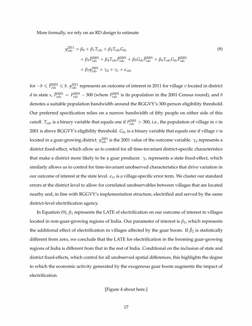
More formally, we rely on an RD design to estimate
y2011vds = β0 + β1Tvds + β2TvdsGds (9)
+ β3P̃2001vds + β4TvdsP̃2001
vds + β5GdsP̃2001vds + β6TvdsGdsP̃2001
vds
+ β7y2001vds + γd + γs + εvds
for −b 6 P̃2001vds 6 b. y2011
vds represents an outcome of interest in 2011 for village v located in district
d in state s, P̃2001vds = P2001
vds − 300 (where P2001vds is its population in the 2001 Census round), and b
denotes a suitable population bandwidth around the RGGVY’s 300-person eligibility threshold.
Our preferred specification relies on a narrow bandwidth of fifty people on either side of this
cutoff. Tvds is a binary variable that equals one if P2001vds > 300, i.e., the population of village in v in
2001 is above RGGVY’s eligibility threshold. Gds is a binary variable that equals one if village v is
located in a guar-growing district. y2001vds is the 2001 value of the outcome variable. γd represents a
district fixed-effect, which allow us to control for all time-invariant district-specific characteristics
that make a district more likely to be a guar producer. γs represents a state fixed-effect, which
similarly allows us to control for time-invariant unobserved characteristics that drive variation in
our outcome of interest at the state level. εvs is a village-specific error term. We cluster our standard
errors at the district level to allow for correlated unobservables between villages that are located
nearby and, in line with RGGVY’s implementation structure, electrified and served by the same
district-level electrification agency.
In Equation (9), β1 represents the LATE of electrification on our outcome of interest in villages
located in non-guar-growing regions of India. Our parameter of interest is β2, which represents
the additional effect of electrification in villages affected by the guar boom. If β̂2 is statistically
different from zero, we conclude that the LATE for electrification in the booming guar-growing
regions of India is different from that in the rest of India. Conditional on the inclusion of state and
district fixed-effects, which control for all unobserved spatial differences, this highlights the degree
to which the economic activity generated by the exogenous guar boom augments the impact of
electrification.
[Figure 4 about here.]
17
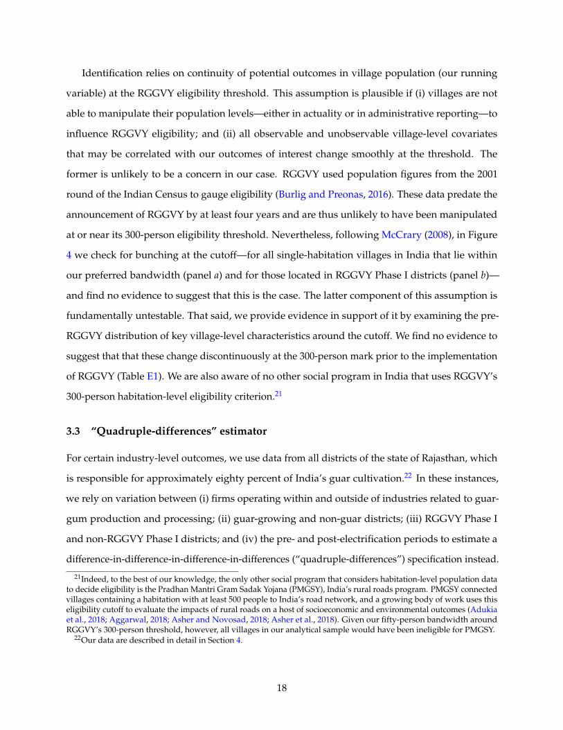
Identification relies on continuity of potential outcomes in village population (our running
variable) at the RGGVY eligibility threshold. This assumption is plausible if (i) villages are not
able to manipulate their population levels—either in actuality or in administrative reporting—to
influence RGGVY eligibility; and (ii) all observable and unobservable village-level covariates
that may be correlated with our outcomes of interest change smoothly at the threshold. The
former is unlikely to be a concern in our case. RGGVY used population figures from the 2001
round of the Indian Census to gauge eligibility (Burlig and Preonas, 2016). These data predate the
announcement of RGGVY by at least four years and are thus unlikely to have been manipulated
at or near its 300-person eligibility threshold. Nevertheless, following McCrary (2008), in Figure
4 we check for bunching at the cutoff—for all single-habitation villages in India that lie within
our preferred bandwidth (panel a) and for those located in RGGVY Phase I districts (panel b)—
and find no evidence to suggest that this is the case. The latter component of this assumption is
fundamentally untestable. That said, we provide evidence in support of it by examining the pre-
RGGVY distribution of key village-level characteristics around the cutoff. We find no evidence to
suggest that that these change discontinuously at the 300-person mark prior to the implementation
of RGGVY (Table E1). We are also aware of no other social program in India that uses RGGVY’s
300-person habitation-level eligibility criterion.21
3.3 “Quadruple-differences” estimator
For certain industry-level outcomes, we use data from all districts of the state of Rajasthan, which
is responsible for approximately eighty percent of India’s guar cultivation.22 In these instances,
we rely on variation between (i) firms operating within and outside of industries related to guar-
gum production and processing; (ii) guar-growing and non-guar districts; (iii) RGGVY Phase I
and non-RGGVY Phase I districts; and (iv) the pre- and post-electrification periods to estimate a
difference-in-difference-in-difference-in-differences (“quadruple-differences”) specification instead.
21Indeed, to the best of our knowledge, the only other social program that considers habitation-level population datato decide eligibility is the Pradhan Mantri Gram Sadak Yojana (PMGSY), India’s rural roads program. PMGSY connectedvillages containing a habitation with at least 500 people to India’s road network, and a growing body of work uses thiseligibility cutoff to evaluate the impacts of rural roads on a host of socioeconomic and environmental outcomes (Adukiaet al., 2018; Aggarwal, 2018; Asher and Novosad, 2018; Asher et al., 2018). Given our fifty-person bandwidth aroundRGGVY’s 300-person threshold, however, all villages in our analytical sample would have been ineligible for PMGSY.
22Our data are described in detail in Section 4.
18
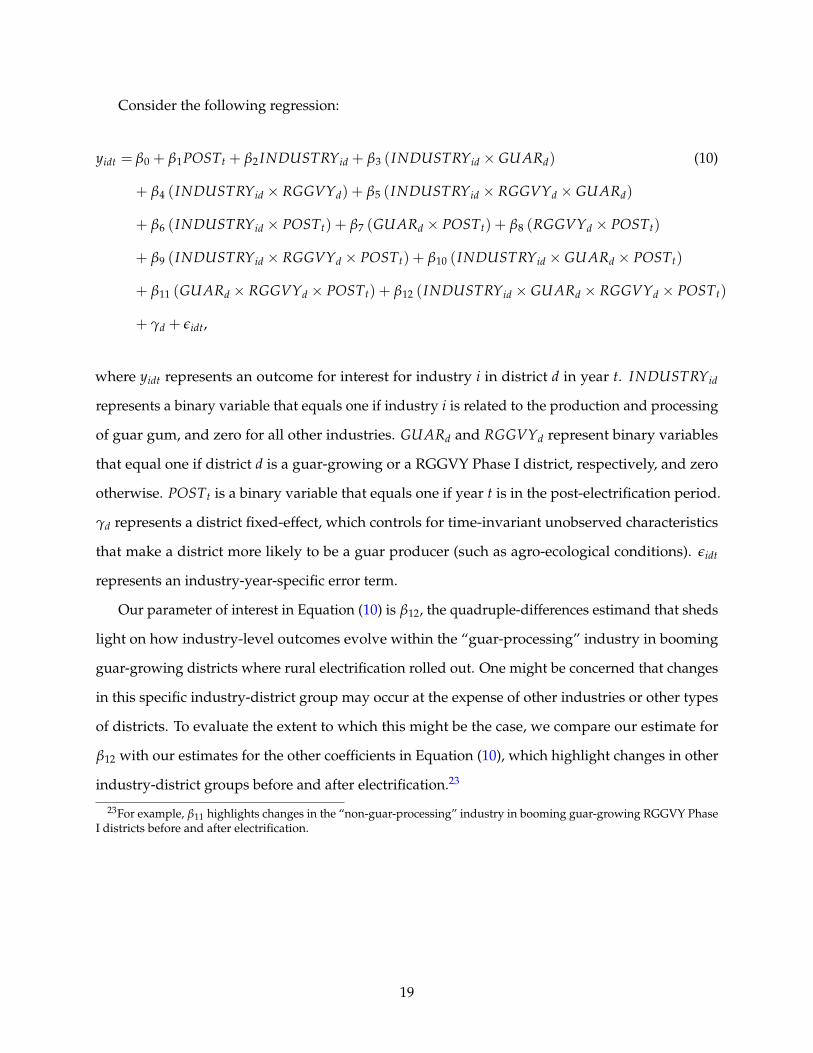
Consider the following regression:
yidt = β0 + β1POSTt + β2 INDUSTRYid + β3 (INDUSTRYid × GUARd) (10)
+ β4 (INDUSTRYid × RGGVYd) + β5 (INDUSTRYid × RGGVYd × GUARd)
+ β6 (INDUSTRYid × POSTt) + β7 (GUARd × POSTt) + β8 (RGGVYd × POSTt)
+ β9 (INDUSTRYid × RGGVYd × POSTt) + β10 (INDUSTRYid × GUARd × POSTt)
+ β11 (GUARd × RGGVYd × POSTt) + β12 (INDUSTRYid × GUARd × RGGVYd × POSTt)
+ γd + εidt,
where yidt represents an outcome for interest for industry i in district d in year t. INDUSTRYid
represents a binary variable that equals one if industry i is related to the production and processing
of guar gum, and zero for all other industries. GUARd and RGGVYd represent binary variables
that equal one if district d is a guar-growing or a RGGVY Phase I district, respectively, and zero
otherwise. POSTt is a binary variable that equals one if year t is in the post-electrification period.
γd represents a district fixed-effect, which controls for time-invariant unobserved characteristics
that make a district more likely to be a guar producer (such as agro-ecological conditions). εidt
represents an industry-year-specific error term.
Our parameter of interest in Equation (10) is β12, the quadruple-differences estimand that sheds
light on how industry-level outcomes evolve within the “guar-processing” industry in booming
guar-growing districts where rural electrification rolled out. One might be concerned that changes
in this specific industry-district group may occur at the expense of other industries or other types
of districts. To evaluate the extent to which this might be the case, we compare our estimate for
β12 with our estimates for the other coefficients in Equation (10), which highlight changes in other
industry-district groups before and after electrification.23
23For example, β11 highlights changes in the “non-guar-processing” industry in booming guar-growing RGGVY PhaseI districts before and after electrification.
19
4 Data
We rely on four main sources of data. First, we refer to technical reports published by the gov-
ernments of both India and the United States to identify India’s main guar-growing districts. We
complement these data on guar production with information on the roll-out of rural electrification
in India to identify those districts that were approved for electrification under RGGVY Phase I.
Next, we obtain data on the composition of the village-level labor force from multiple rounds of
the Census of India. We complement these with data on individual-level labor-market outcomes
and domestic time allocation from multiple rounds of India’s National Sample Survey. Finally, we
rely on multiple rounds of the Economic Census of India to obtain data on the size and sectoral
composition of firms in Rajasthan.
4.1 Guar production
We review three separate technical reports on guar production in India to identify our sample
of guar-producing Indian districts. Two of these—prepared by the Agricultural and Processed
Food Products Export Development Authority (2011) and the National Rainfed Area Authority
(2014)—represent efforts by the Indian government to systematically quantify and summarize the
nationwide production and trade of guar.24 The third—prepared by the United States Department
of Agriculture—signals the growing interest the agency took in guar production as the crop grew
to become India’s main agricultural export to the United States (Singh, 2014).
For each of these three reports, we systematically create lists of states and districts that they
characterize as key producers of guar in India. In particular, we examine changes in state- and
district-level rankings along three related metrics: overall production, total cultivated area, and
productivity. We then combine each of our generated lists together, and identify the subset of
districts that consistently appear on all three. Based on district boundaries at the time of the 2011
Indian Census, we ultimately identify a total of 23 districts: thirteen in the state of Rajasthan, six in
Gujarat, and four in Haryana (Figure 1). In 2011, these 23 districts were home to nearly 60 million
24The Agricultural and Processed Food Products Export Development Authority (APEDA) is housed within India’sMinistry of Commerce & Industry. It is broadly tasked with supporting the development of industries related to productswith export potential. The National Rainfed Area Authority (NRAA) is housed within the Ministry of Agriculture &Farmers welfare, where it provides technical advice and monitoring for government schemes operating in rural areaswith significant levels of rainfed agriculture.
20
people living over an estimated area of 300,000 km2—roughly equal in terms of both population
and size to all of Italy.25
To partially validate our selection of these districts, we also estimate their share in total reported
production and area under cultivation for guar using national data from the Ministry of Agriculture
on annual district-wise production of the crop between approximately 1999 and 2015.26 We note
that the quality of these data is poor. For instance, districts in the state of Haryana—consistently
referred to in the technical reports we use as one of the most important guar-producing states in
India after Rajasthan—have non-missing data on guar production only for 2012. At the same time,
other districts in regions of India not known for guar production consistently report trivial amounts
of production for multiple years in the sample. Nevertheless, we find that the guar-growing
districts we identify account for nearly 94 percent of overall guar production in 2012 (the year that
contains these statistics for the largest number of districts).
4.2 Rural electrification
As mentioned previously, we identify Phase I districts for which DPRs were successfully submitted
and approved using state-level five-year-plan progress reports for RGGVY. Identifying villages
that were eligible to be electrified within these districts poses additional challenges. RGGVY
implementing agencies were directed to determine a village’s eligibility for electrification based
on the populations of its constituent habitations (geographically distinct sub-village clusters of
households). A village was eligible for electrification under RGGVY Phase I if it contained at least
one constituent habitation with a population greater than 300. Although a growing number of
public-sector interventions are now tracked at the habitation level, to the best of our knowledge,
there are only two comprehensive datasets that shed light on habitation-level populations: (i) the
census of habitations conducted by the National Rural Drinking Water Program (NRDWP) in 2009;
and (ii) the directory of habitation-level populations made available by the Pradhan Mantri Gram
Sadak Yojana (PMGSY), India’s national rural roads program. In line with the directives for RGGVY
implementing agencies, we rely on the former, which contains habitation-level population (by
25In this paper, we interchangeably refer to these districts as India’s “guar-growing districts” or “guar-growingregions.”
26These data are available via the Ministry of Agriculture’s Crop Production Statistics Information System at https://aps.dac.gov.in/APY/Index.htm.
21
caste) for each village. Because the NRDWP data indicates only the name—and not the unique
Census code—for each habitation’s corresponding village, we adopt a fuzzy matching algorithm
originally developed by Asher and Novosad (2018) to match it with a list of Census-designated
villages.27 India’s nearly 600,000 villages consist of just over 1.6 million habitations. We are able
to successfully match approximately 531,000 (89 percent) of these villages to their constituent
habitations. To further validate the quality of these matches, we calculate the discrepancy between
the given Census 2011 population for each village and the NRDWP 2009 population estimate that
we obtain from summing over the population of all habitations in a village. We drop all villages
with a Census-NRDWP population discrepancy of greater than twenty percent; these, we assume,
are incorrect fuzzy matches. This leaves us with approximately 370,000 villages.28
Our fuzzy-matched dataset consists of village-level identifiers (i.e., state, district, subdistrict
and village names, and their corresponding Census codes), village-level count of habitations,
village population (obtained by summing over all habitations in a village), population of the largest
habitation, and a variable indicating the quality of the match (i.e., distinct groupings based on the
extent to which matches across the NRDWP and Census lists of names are exact or fuzzy). The
average village in this fuzzy-matched sample contains three habitations; approximately 47 percent
of villages contain exactly one habitation.
To obtain the analytical sample with which to estimate Equation (9), we restrict our sample
of villages in three ways: (i) those located in RGGVY Phase I districts; (ii) those with exactly one
habitation; and (iii) those with a Census 2001 population within a narrow fifty-person bandwidth
of the 300-person RGGVY Phase I threshold. This yields 7,655 villages located across 22 Indian
states; 148 are located in guar-growing districts.
4.3 Rural labor-market outcomes
Our data on the make-up of the rural labor force come from the 2001 and 2011 rounds of the
Indian Census. Specifically, in addition to data on population for each of India’s approximately
600,000 villages, the Primary Census Abstract (PCA) data tables in the Census report information
by gender on three distinct village-level subgroups: (i) “main workers,” who engage in any
27The NRDWP census of habitation was first conducted in 2003, and again in 2009. The 2003 data are no longerpublicly available, which is why we rely on the 2009 data, which are available at https://indiawater.gov.in.
28We describe our fuzzy habitation-village matching procedure in detail in Appendix C.
22
economically productive activity for at least six months a year; (ii) “marginal workers,” who do so
for less than six months a year; and (iii) “non-workers,” who do not engage in any economically
productive activity. Within the first two subgroups, workers are further categorized as cultivators,
agricultural laborers, household-industry workers, or “other.” A person is classified as a cultivator
if they are engaged in cultivation of land that they own or lease, implying that they bear the risks
associated with cultivation. In contrast, a person is classified an agricultural laborer if they work on
another person’s land for payment. In rural areas, a household industry is defined as “production,
processing, servicing, repairing, or making and selling (but not merely selling) of goods” that is
done by one or more members of a household within the confines of the village. Finally, “other”
workers include all professions not captured by the other three categories, such as government
employees, teachers and traders.29
For each village-year in our Census panel, we combine cultivators and agricultural laborers
(both main and marginal) to calculate the population of agricultural workers, overall and by gender.
We similarly combine household-industry and other workers to obtain corresponding figures for
the village-level population of non-agricultural workers. These data—together with information
on village population as well as the breakdown of that population into workers and non-workers—
allow us to evaluate impacts along two dimensions: (i) the extensive margin, i.e., the net change in
the overall labor force as a percentage of the village population; and (ii) the sectoral composition of
the labor force, namely, the relative shares of agricultural versus non-agricultural workers.
We complement our village-level data on the composition of the labor force with individual-level
data on labor-force outcomes and domestic time allocation from the Employment-Unemployment
surveys conducted as part of the 2004 (60th) and 2011-12 (68th) rounds of India’s National Sample
Survey (NSS).30 These quinquennial surveys are representative at the level of the NSS region, a
non-administrative sampling unit below the state but above the district. NSS regions typically
consist of two or more contiguous districts and do not cross state boundaries. We combine our data
on district-level guar production and roll-out of rural electrification with these NSS regions to create
a region-level repeated cross-section covering over 400,000 people across rural India. In particular,
29Additional information about these definitions is available in the 2011 Census’ meta data documentation at http://www.censusindia.gov.in/2011census/HLO/Metadata_Census_2011.pdf.
30Information on how NSS data can be purchased from the Ministry of Statistics and Program Implementation isavailable at http://mospi.gov.in/sample-surveys.
23
we focus on (i) respondents’ “usual principal activity” (the activity an individual contributed the
bulk of their time to over the past year); (ii) for those in the labor force, the industry to which they
belong; and (iii) for those not in the labor force, the extent to which they engage in home production
in addition to domestic duties.
4.4 Firm-level data
Our data on the universe of firms and establishments employing more than ten people in the state
of Rajasthan come from the Economic Census (EC) of India. Specifically, we rely on the “Directory
of Establishments” associated with the 2005 (Fifth) and 2013-14 (Sixth) rounds of the EC.31 This
directory reports information on basic firm characteristics, including name, address, number of
employees, and the sector/industry to which the firm belongs, as indicated by a National Industrial
Classification (NIC) code.
In 2005, this directory listed a total of 20,715 firms in Rajasthan. By 2013, this number had
increased to 27,803. We combine these two rounds of the EC in a district-level panel dataset with
which to study changes in the nature and composition of firms in response to guar boom and the
roll-out of rural electrification in Rajasthan. We focus, in particular, on firms in industries related to
the guar production chain (such as industrial guar-processing units).
5 Size and sectoral composition of the rural labor force
In this section, we estimate how rural electrification affects the size and composition of the labor
force across guar- and non-guar-growing regions of India. We measure this using data on pop-
ulation and employment at the village- and region levels from the Indian Census and National
Sample Survey (NSS), respectively. We find no evidence to suggest that electrification has a net
effect on the overall size of the labor force in electrified villages located in guar-growing regions
of India. We show next, however, that access to electricity substantially reduces (increases) the
share of agricultural (non-agricultural) workers in these villages. In electrified villages located in
non-guar-growing districts across the rest of India, in contrast, we find no evidence that access to
electricity has any discernible effect on the labor-market outcomes that we study.
31The Directories of Establishments for the Fifth as well as the Sixth round of the EC are available from the Ministry ofStatistics and Program Implementation at http://www.mospi.gov.in/economic-census-3.
24
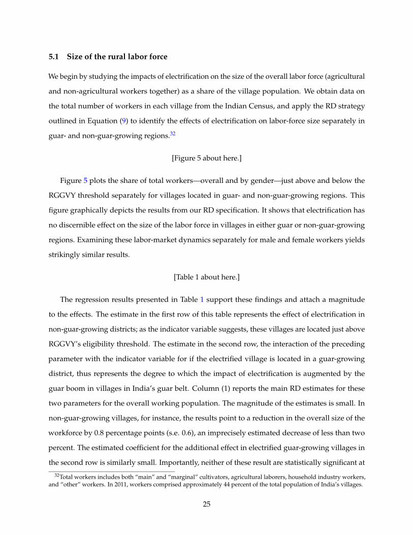
5.1 Size of the rural labor force
We begin by studying the impacts of electrification on the size of the overall labor force (agricultural
and non-agricultural workers together) as a share of the village population. We obtain data on
the total number of workers in each village from the Indian Census, and apply the RD strategy
outlined in Equation (9) to identify the effects of electrification on labor-force size separately in
guar- and non-guar-growing regions.32
[Figure 5 about here.]
Figure 5 plots the share of total workers—overall and by gender—just above and below the
RGGVY threshold separately for villages located in guar- and non-guar-growing regions. This
figure graphically depicts the results from our RD specification. It shows that electrification has
no discernible effect on the size of the labor force in villages in either guar or non-guar-growing
regions. Examining these labor-market dynamics separately for male and female workers yields
strikingly similar results.
[Table 1 about here.]
The regression results presented in Table 1 support these findings and attach a magnitude
to the effects. The estimate in the first row of this table represents the effect of electrification in
non-guar-growing districts; as the indicator variable suggests, these villages are located just above
RGGVY’s eligibility threshold. The estimate in the second row, the interaction of the preceding
parameter with the indicator variable for if the electrified village is located in a guar-growing
district, thus represents the degree to which the impact of electrification is augmented by the
guar boom in villages in India’s guar belt. Column (1) reports the main RD estimates for these
two parameters for the overall working population. The magnitude of the estimates is small. In
non-guar-growing villages, for instance, the results point to a reduction in the overall size of the
workforce by 0.8 percentage points (s.e. 0.6), an imprecisely estimated decrease of less than two
percent. The estimated coefficient for the additional effect in electrified guar-growing villages in
the second row is similarly small. Importantly, neither of these result are statistically significant at
32Total workers includes both “main” and “marginal” cultivators, agricultural laborers, household industry workers,and “other” workers. In 2011, workers comprised approximately 44 percent of the total population of India’s villages.
25
conventional levels. We are, thus, unable to reject the hypothesis that access to electricity had no
effect on the overall size of the labor force in these two settings.
Columns (2) and (3) report the same specification estimated separately for the share of male
and female workers, respectively. The estimates are similar: electrification has no discernible effect
on the share of male or female workers in both guar- and non-guar villages.
Taken together, these results suggest that, on net, households do not respond to electrification
by adjusting their labor choices along the extensive margin.33 Although we cannot rule out that
large-scale entry and exit of workers in response to electrification may be taking place, these
findings stand in contrast to those from earlier work (e.g., Dinkelman, 2011) that finds that access
to electricity can increase labor-force participation (especially for women).
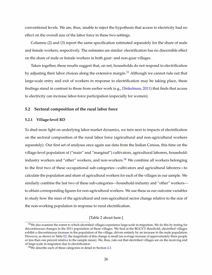
5.2 Sectoral composition of the rural labor force
5.2.1 Village-level RD
To shed more light on underlying labor-market dynamics, we turn next to impacts of electrification
on the sectoral composition of the rural labor force (agricultural and non-agricultural workers
separately). Our first set of analyses once again use data from the Indian Census, this time on the
village-level population of (“main” and “marginal”) cultivators, agricultural laborers, household-
industry workers and “other” workers, and non-workers.34 We combine all workers belonging
to the first two of these occupational sub-categories—cultivators and agricultural laborers—to
calculate the population and share of agricultural workers for each of the villages in our sample. We
similarly combine the last two of these sub-categories—household-industry and “other” workers—
to obtain corresponding figures for non-agricultural workers. We use these as our outcome variables
to study how the sizes of the agricultural and non-agricultural sector change relative to the size of
the non-working population in response to rural electrification.
[Table 2 about here.]
33We also examine the extent to which electrified villages experience large-scale in-migration. We do this by testing fordiscontinuous changes in the 2011 population of these villages. We find at the RGGVY threshold, electrified villagesexhibit a discontinuous increase in the population of the village, driven entirely by an increase in the male population.However, as shown in Table E2, the magnitude of this change is small (an average increase of approximately three peopleor less than one percent relative to the sample mean). We, thus, rule out that electrified villages are on the receiving endof large-scale in-migration due to electrification.
34We describe each of these categories in detail in Section 4.3.
26
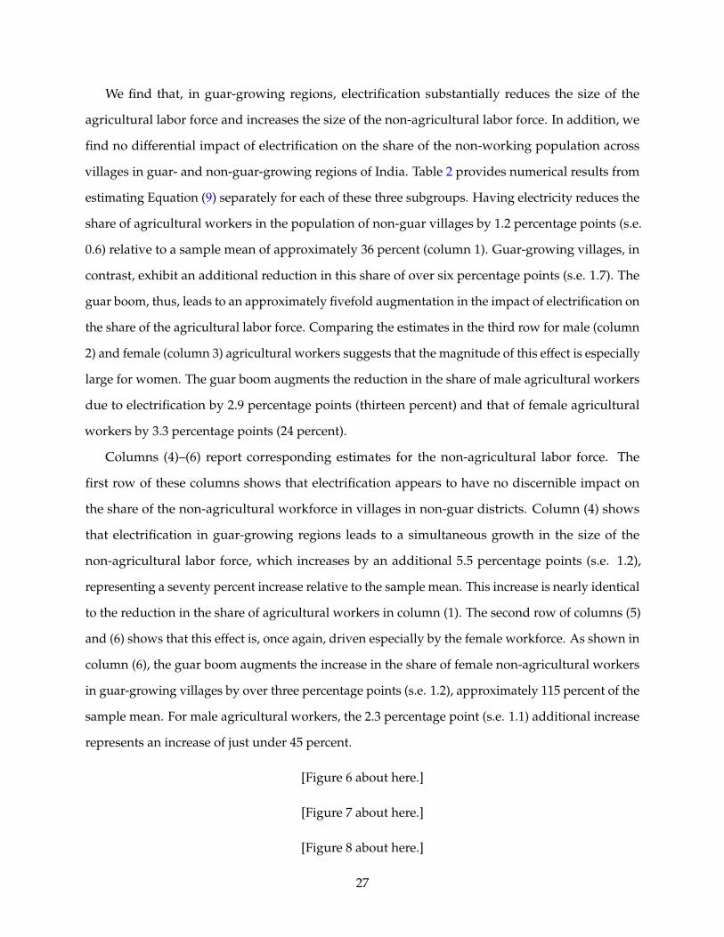
We find that, in guar-growing regions, electrification substantially reduces the size of the
agricultural labor force and increases the size of the non-agricultural labor force. In addition, we
find no differential impact of electrification on the share of the non-working population across
villages in guar- and non-guar-growing regions of India. Table 2 provides numerical results from
estimating Equation (9) separately for each of these three subgroups. Having electricity reduces the
share of agricultural workers in the population of non-guar villages by 1.2 percentage points (s.e.
0.6) relative to a sample mean of approximately 36 percent (column 1). Guar-growing villages, in
contrast, exhibit an additional reduction in this share of over six percentage points (s.e. 1.7). The
guar boom, thus, leads to an approximately fivefold augmentation in the impact of electrification on
the share of the agricultural labor force. Comparing the estimates in the third row for male (column
2) and female (column 3) agricultural workers suggests that the magnitude of this effect is especially
large for women. The guar boom augments the reduction in the share of male agricultural workers
due to electrification by 2.9 percentage points (thirteen percent) and that of female agricultural
workers by 3.3 percentage points (24 percent).
Columns (4)–(6) report corresponding estimates for the non-agricultural labor force. The
first row of these columns shows that electrification appears to have no discernible impact on
the share of the non-agricultural workforce in villages in non-guar districts. Column (4) shows
that electrification in guar-growing regions leads to a simultaneous growth in the size of the
non-agricultural labor force, which increases by an additional 5.5 percentage points (s.e. 1.2),
representing a seventy percent increase relative to the sample mean. This increase is nearly identical
to the reduction in the share of agricultural workers in column (1). The second row of columns (5)
and (6) shows that this effect is, once again, driven especially by the female workforce. As shown in
column (6), the guar boom augments the increase in the share of female non-agricultural workers
in guar-growing villages by over three percentage points (s.e. 1.2), approximately 115 percent of the
sample mean. For male agricultural workers, the 2.3 percentage point (s.e. 1.1) additional increase
represents an increase of just under 45 percent.
[Figure 6 about here.]
[Figure 7 about here.]
[Figure 8 about here.]
27
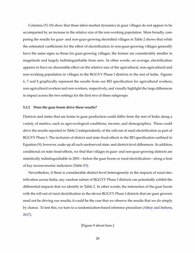
Columns (7)–(9) show that these labor-market dynamics in guar villages do not appear to be
accompanied by an increase in the relative size of the non-working population. More broadly, com-
paring the results for guar- and non-guar-growing electrified villages in Table 2 shows that while
the estimated coefficients for the effect of electrification in non-guar-growing villages generally
have the same signs as those for guar-growing villages, the former are considerably smaller in
magnitude and largely indistinguishable from zero. In other words, on average, electrification
appears to have no discernible effect on the relative size of the agricultural, non-agricultural and
non-working population in villages in the RGGVY Phase I districts in the rest of India. Figures
6, 7 and 8 graphically represent the results from our RD specification for agricultural workers,
non-agricultural workers and non-workers, respectively, and visually highlight the large differences
in impact across the two settings for the first two of these subgroups.
5.2.2 Does the guar boom drive these results?
Districts and states that are home to guar production could differ from the rest of India along a
variety of metrics, such as agro-ecological conditions, income, and demographics. These could
drive the results reported in Table 2 independently of the roll-out of rural electrification as part of
RGGVY Phase I. The inclusion of district and state fixed-effects in the RD specification outlined in
Equation (9), however, soaks up all such unobserved state- and district-level differences. In addition,
conditional on state fixed-effects, we find that villages in guar- and non-guar-growing districts are
statistically indistinguishable in 2001—before the guar boom or rural electrification—along a host
of key socioeconomic indicators (Table E3).
Nevertheless, if there is considerable district-level heterogeneity in the impacts of rural elec-
trification across India, any random subset of RGGVY Phase I districts can potentially exhibit the
differential impacts that we identify in Table 2. In other words, the interaction of the guar boom
with the roll-out of rural electrification in the eleven RGGVY Phase I districts that are guar growers
need not be driving our results; it could be the case that we observe the results that we do simply
by chance. To test this, we turn to a randomization-based inference procedure (Athey and Imbens,
2017).
[Figure 9 about here.]
28
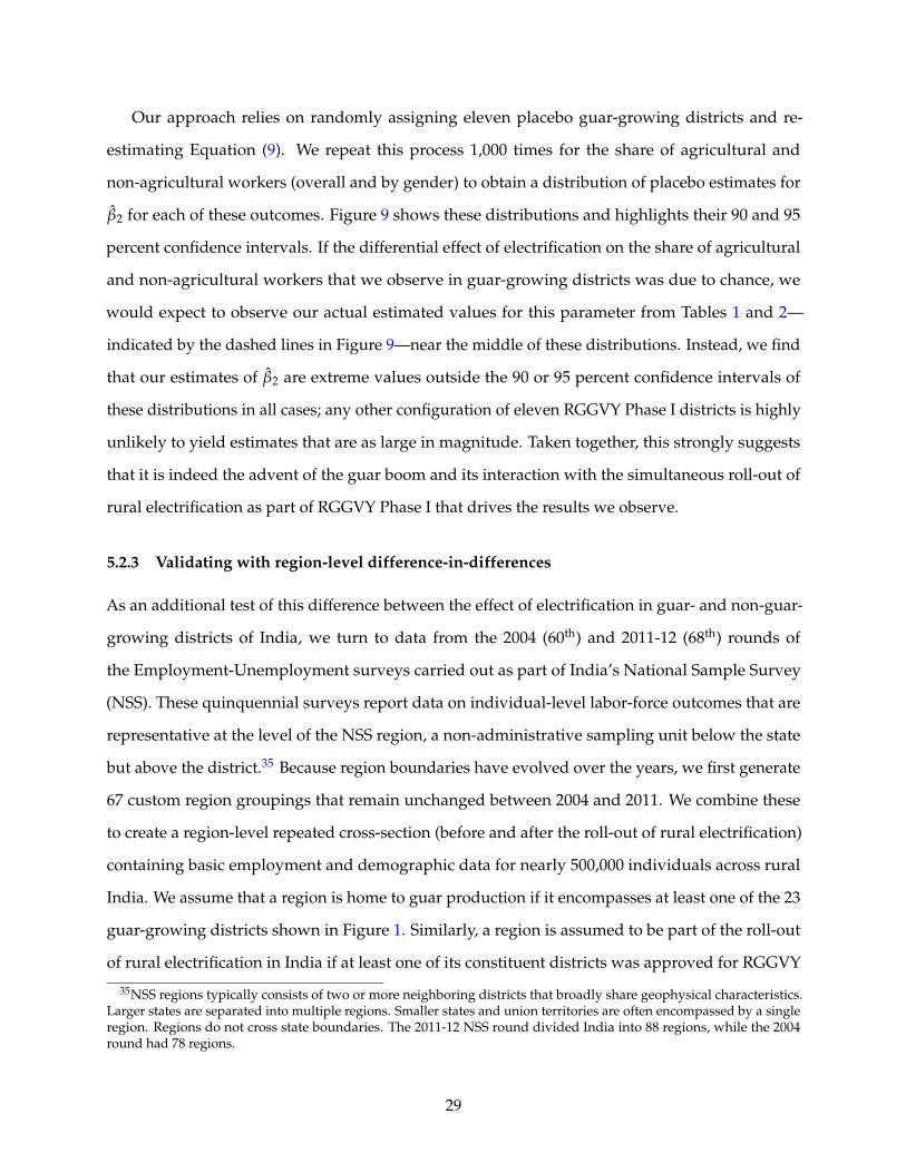
Our approach relies on randomly assigning eleven placebo guar-growing districts and re-
estimating Equation (9). We repeat this process 1,000 times for the share of agricultural and
non-agricultural workers (overall and by gender) to obtain a distribution of placebo estimates for
β̂2 for each of these outcomes. Figure 9 shows these distributions and highlights their 90 and 95
percent confidence intervals. If the differential effect of electrification on the share of agricultural
and non-agricultural workers that we observe in guar-growing districts was due to chance, we
would expect to observe our actual estimated values for this parameter from Tables 1 and 2—
indicated by the dashed lines in Figure 9—near the middle of these distributions. Instead, we find
that our estimates of β̂2 are extreme values outside the 90 or 95 percent confidence intervals of
these distributions in all cases; any other configuration of eleven RGGVY Phase I districts is highly
unlikely to yield estimates that are as large in magnitude. Taken together, this strongly suggests
that it is indeed the advent of the guar boom and its interaction with the simultaneous roll-out of
rural electrification as part of RGGVY Phase I that drives the results we observe.
5.2.3 Validating with region-level difference-in-differences
As an additional test of this difference between the effect of electrification in guar- and non-guar-
growing districts of India, we turn to data from the 2004 (60th) and 2011-12 (68th) rounds of
the Employment-Unemployment surveys carried out as part of India’s National Sample Survey
(NSS). These quinquennial surveys report data on individual-level labor-force outcomes that are
representative at the level of the NSS region, a non-administrative sampling unit below the state
but above the district.35 Because region boundaries have evolved over the years, we first generate
67 custom region groupings that remain unchanged between 2004 and 2011. We combine these
to create a region-level repeated cross-section (before and after the roll-out of rural electrification)
containing basic employment and demographic data for nearly 500,000 individuals across rural
India. We assume that a region is home to guar production if it encompasses at least one of the 23
guar-growing districts shown in Figure 1. Similarly, a region is assumed to be part of the roll-out
of rural electrification in India if at least one of its constituent districts was approved for RGGVY
35NSS regions typically consists of two or more neighboring districts that broadly share geophysical characteristics.Larger states are separated into multiple regions. Smaller states and union territories are often encompassed by a singleregion. Regions do not cross state boundaries. The 2011-12 NSS round divided India into 88 regions, while the 2004round had 78 regions.
29
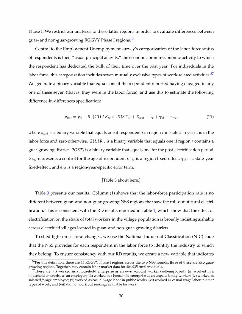
Phase I. We restrict our analyses to these latter regions in order to evaluate differences between
guar- and non-guar-growing RGGVY Phase I regions.36
Central to the Employment-Unemployment survey’s categorization of the labor-force status
of respondents is their “usual principal activity,” the economic or non-economic activity to which
the respondent has dedicated the bulk of their time over the past year. For individuals in the
labor force, this categorization includes seven mutually exclusive types of work-related activities.37
We generate a binary variable that equals one if the respondent reported having engaged in any
one of these seven (that is, they were in the labor force), and use this to estimate the following
difference-in-differences specification:
yirst = β0 + β1 (GUARrs × POSTt) + Xirst + γr + γst + εirst, (11)
where yirst is a binary variable that equals one if respondent i in region r in state s in year t is in the
labor force and zero otherwise. GUARrs is a binary variable that equals one if region r contains a
guar-growing district. POSTt is a binary variable that equals one for the post-electrification period.
Xirst represents a control for the age of respondent i. γr is a region fixed-effect, γst is a state-year
fixed-effect, and εrst is a region-year-specific error term.
[Table 3 about here.]
Table 3 presents our results. Column (1) shows that the labor-force participation rate is no
different between guar- and non-guar-growing NSS regions that saw the roll-out of rural electri-
fication. This is consistent with the RD results reported in Table 1, which show that the effect of
electrification on the share of total workers in the village population is broadly indistinguishable
across electrified villages located in guar- and non-guar-growing districts.
To shed light on sectoral changes, we use the National Industrial Classification (NIC) code
that the NSS provides for each respondent in the labor force to identify the industry to which
they belong. To ensure consistency with our RD results, we create a new variable that indicates
36Per this definition, there are 45 RGGVY Phase I regions across the two NSS rounds; three of these are also guar-growing regions. Together, they contain labor-market data for 406,935 rural inviduals.
37These are: (i) worked in a household enterprise as an own account worker (self-employed); (ii) worked in ahousehold enterprise as an employer; (iii) worked in a household enterprise as an unpaid family worker; (iv) worked assalaried/wage employee; (v) worked as casual wage labor in public works; (vi) worked as casual wage labor in othertypes of work; and (vii) did not work but seeking/available for work.
30
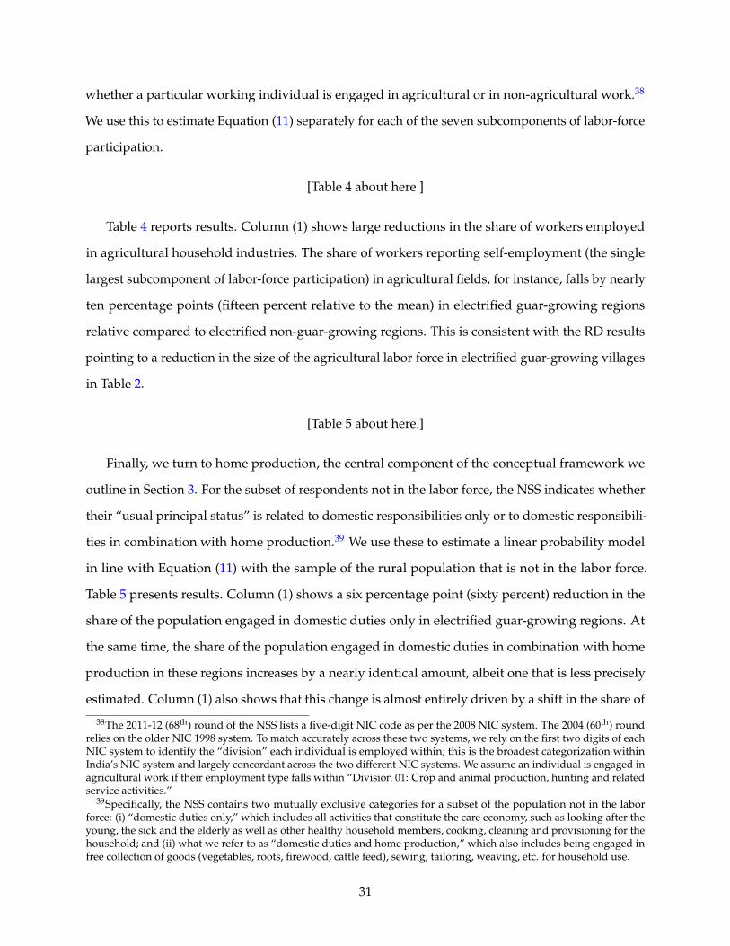
whether a particular working individual is engaged in agricultural or in non-agricultural work.38
We use this to estimate Equation (11) separately for each of the seven subcomponents of labor-force
participation.
[Table 4 about here.]
Table 4 reports results. Column (1) shows large reductions in the share of workers employed
in agricultural household industries. The share of workers reporting self-employment (the single
largest subcomponent of labor-force participation) in agricultural fields, for instance, falls by nearly
ten percentage points (fifteen percent relative to the mean) in electrified guar-growing regions
relative compared to electrified non-guar-growing regions. This is consistent with the RD results
pointing to a reduction in the size of the agricultural labor force in electrified guar-growing villages
in Table 2.
[Table 5 about here.]
Finally, we turn to home production, the central component of the conceptual framework we
outline in Section 3. For the subset of respondents not in the labor force, the NSS indicates whether
their “usual principal status” is related to domestic responsibilities only or to domestic responsibili-
ties in combination with home production.39 We use these to estimate a linear probability model
in line with Equation (11) with the sample of the rural population that is not in the labor force.
Table 5 presents results. Column (1) shows a six percentage point (sixty percent) reduction in the
share of the population engaged in domestic duties only in electrified guar-growing regions. At
the same time, the share of the population engaged in domestic duties in combination with home
production in these regions increases by a nearly identical amount, albeit one that is less precisely
estimated. Column (1) also shows that this change is almost entirely driven by a shift in the share of
38The 2011-12 (68th) round of the NSS lists a five-digit NIC code as per the 2008 NIC system. The 2004 (60th) roundrelies on the older NIC 1998 system. To match accurately across these two systems, we rely on the first two digits of eachNIC system to identify the “division” each individual is employed within; this is the broadest categorization withinIndia’s NIC system and largely concordant across the two different NIC systems. We assume an individual is engaged inagricultural work if their employment type falls within “Division 01: Crop and animal production, hunting and relatedservice activities.”
39Specifically, the NSS contains two mutually exclusive categories for a subset of the population not in the laborforce: (i) “domestic duties only,” which includes all activities that constitute the care economy, such as looking after theyoung, the sick and the elderly as well as other healthy household members, cooking, cleaning and provisioning for thehousehold; and (ii) what we refer to as “domestic duties and home production,” which also includes being engaged infree collection of goods (vegetables, roots, firewood, cattle feed), sewing, tailoring, weaving, etc. for household use.
31
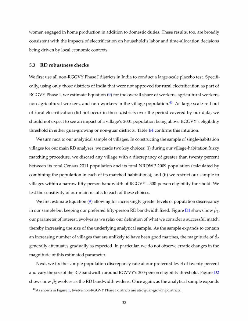
women engaged in home production in addition to domestic duties. These results, too, are broadly
consistent with the impacts of electrification on household’s labor and time-allocation decisions
being driven by local economic contexts.
5.3 RD robustness checks
We first use all non-RGGVY Phase I districts in India to conduct a large-scale placebo test. Specifi-
cally, using only those districts of India that were not approved for rural electrification as part of
RGGVY Phase I, we estimate Equation (9) for the overall share of workers, agricultural workers,
non-agricultural workers, and non-workers in the village population.40 As large-scale roll out
of rural electrification did not occur in these districts over the period covered by our data, we
should not expect to see an impact of a village’s 2001 population being above RGGVY’s eligibility
threshold in either guar-growing or non-guar districts. Table E4 confirms this intuition.
We turn next to our analytical sample of villages. In constructing the sample of single-habitation
villages for our main RD analyses, we made two key choices: (i) during our village-habitation fuzzy
matching procedure, we discard any village with a discrepancy of greater than twenty percent
between its total Census 2011 population and its total NRDWP 2009 population (calculated by
combining the population in each of its matched habitations); and (ii) we restrict our sample to
villages within a narrow fifty-person bandwidth of RGGVY’s 300-person eligibility threshold. We
test the sensitivity of our main results to each of these choices.
We first estimate Equation (9) allowing for increasingly greater levels of population discrepancy
in our sample but keeping our preferred fifty-person RD bandwidth fixed. Figure D1 shows how β̂2,
our parameter of interest, evolves as we relax our definition of what we consider a successful match,
thereby increasing the size of the underlying analytical sample. As the sample expands to contain
an increasing number of villages that are unlikely to have been good matches, the magnitude of β̂2
generally attenuates gradually as expected. In particular, we do not observe erratic changes in the
magnitude of this estimated parameter.
Next, we fix the sample population discrepancy rate at our preferred level of twenty percent
and vary the size of the RD bandwidth around RGVVY’s 300-person eligibility threshold. Figure D2
shows how β̂2 evolves as the RD bandwidth widens. Once again, as the analytical sample expands
40As shown in Figure 1, twelve non-RGGVY Phase I districts are also guar-growing districts.
32
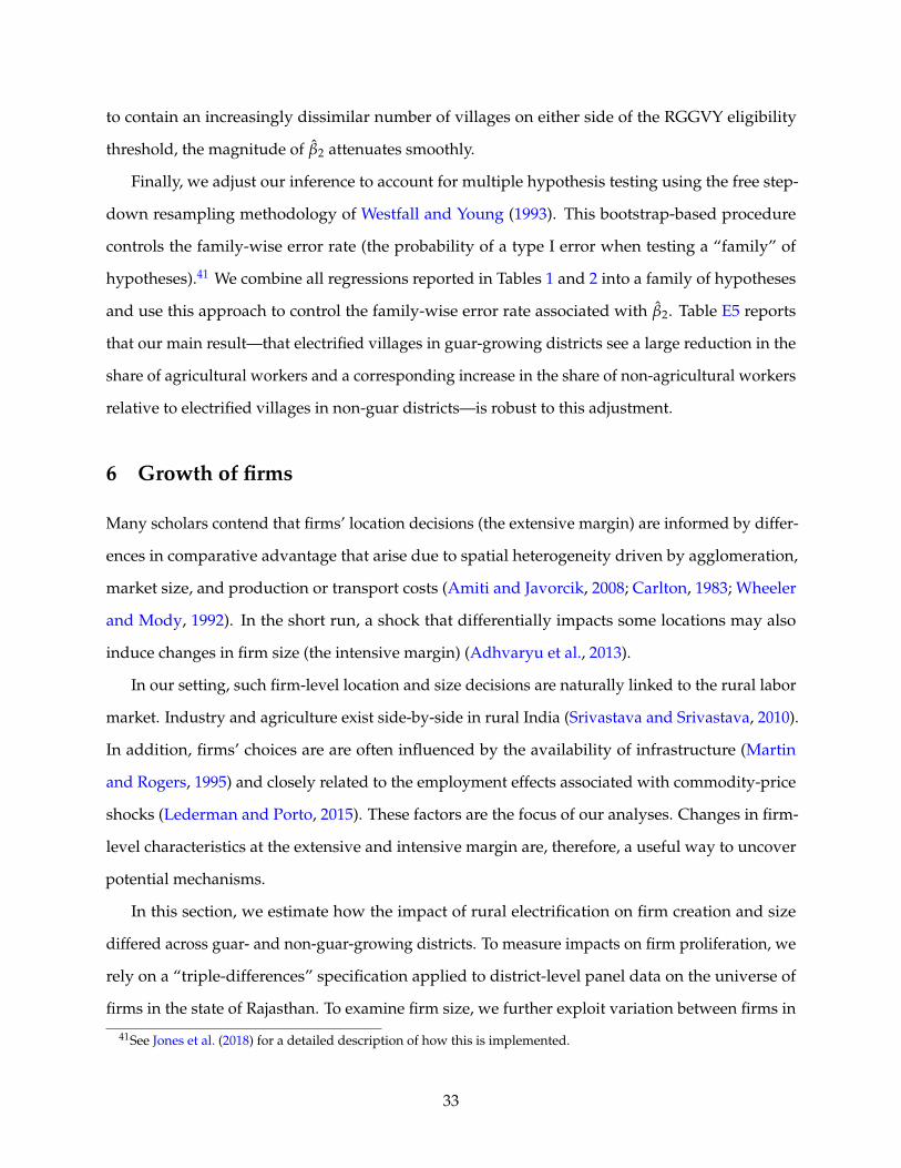
to contain an increasingly dissimilar number of villages on either side of the RGGVY eligibility
threshold, the magnitude of β̂2 attenuates smoothly.
Finally, we adjust our inference to account for multiple hypothesis testing using the free step-
down resampling methodology of Westfall and Young (1993). This bootstrap-based procedure
controls the family-wise error rate (the probability of a type I error when testing a “family” of
hypotheses).41 We combine all regressions reported in Tables 1 and 2 into a family of hypotheses
and use this approach to control the family-wise error rate associated with β̂2. Table E5 reports
that our main result—that electrified villages in guar-growing districts see a large reduction in the
share of agricultural workers and a corresponding increase in the share of non-agricultural workers
relative to electrified villages in non-guar districts—is robust to this adjustment.
6 Growth of firms
Many scholars contend that firms’ location decisions (the extensive margin) are informed by differ-
ences in comparative advantage that arise due to spatial heterogeneity driven by agglomeration,
market size, and production or transport costs (Amiti and Javorcik, 2008; Carlton, 1983; Wheeler
and Mody, 1992). In the short run, a shock that differentially impacts some locations may also
induce changes in firm size (the intensive margin) (Adhvaryu et al., 2013).
In our setting, such firm-level location and size decisions are naturally linked to the rural labor
market. Industry and agriculture exist side-by-side in rural India (Srivastava and Srivastava, 2010).
In addition, firms’ choices are are often influenced by the availability of infrastructure (Martin
and Rogers, 1995) and closely related to the employment effects associated with commodity-price
shocks (Lederman and Porto, 2015). These factors are the focus of our analyses. Changes in firm-
level characteristics at the extensive and intensive margin are, therefore, a useful way to uncover
potential mechanisms.
In this section, we estimate how the impact of rural electrification on firm creation and size
differed across guar- and non-guar-growing districts. To measure impacts on firm proliferation, we
rely on a “triple-differences” specification applied to district-level panel data on the universe of
firms in the state of Rajasthan. To examine firm size, we further exploit variation between firms in
41See Jones et al. (2018) for a detailed description of how this is implemented.
33
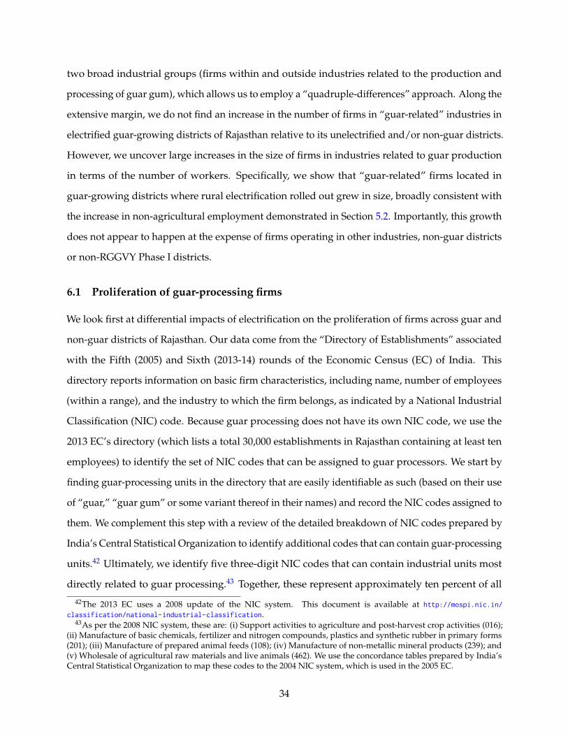
two broad industrial groups (firms within and outside industries related to the production and
processing of guar gum), which allows us to employ a “quadruple-differences” approach. Along the
extensive margin, we do not find an increase in the number of firms in “guar-related” industries in
electrified guar-growing districts of Rajasthan relative to its unelectrified and/or non-guar districts.
However, we uncover large increases in the size of firms in industries related to guar production
in terms of the number of workers. Specifically, we show that “guar-related” firms located in
guar-growing districts where rural electrification rolled out grew in size, broadly consistent with
the increase in non-agricultural employment demonstrated in Section 5.2. Importantly, this growth
does not appear to happen at the expense of firms operating in other industries, non-guar districts
or non-RGGVY Phase I districts.
6.1 Proliferation of guar-processing firms
We look first at differential impacts of electrification on the proliferation of firms across guar and
non-guar districts of Rajasthan. Our data come from the “Directory of Establishments” associated
with the Fifth (2005) and Sixth (2013-14) rounds of the Economic Census (EC) of India. This
directory reports information on basic firm characteristics, including name, number of employees
(within a range), and the industry to which the firm belongs, as indicated by a National Industrial
Classification (NIC) code. Because guar processing does not have its own NIC code, we use the
2013 EC’s directory (which lists a total 30,000 establishments in Rajasthan containing at least ten
employees) to identify the set of NIC codes that can be assigned to guar processors. We start by
finding guar-processing units in the directory that are easily identifiable as such (based on their use
of “guar,” “guar gum” or some variant thereof in their names) and record the NIC codes assigned to
them. We complement this step with a review of the detailed breakdown of NIC codes prepared by
India’s Central Statistical Organization to identify additional codes that can contain guar-processing
units.42 Ultimately, we identify five three-digit NIC codes that can contain industrial units most
directly related to guar processing.43 Together, these represent approximately ten percent of all
42The 2013 EC uses a 2008 update of the NIC system. This document is available at http://mospi.nic.in/
classification/national-industrial-classification.43As per the 2008 NIC system, these are: (i) Support activities to agriculture and post-harvest crop activities (016);
(ii) Manufacture of basic chemicals, fertilizer and nitrogen compounds, plastics and synthetic rubber in primary forms(201); (iii) Manufacture of prepared animal feeds (108); (iv) Manufacture of non-metallic mineral products (239); and(v) Wholesale of agricultural raw materials and live animals (462). We use the concordance tables prepared by India’sCentral Statistical Organization to map these codes to the 2004 NIC system, which is used in the 2005 EC.
34
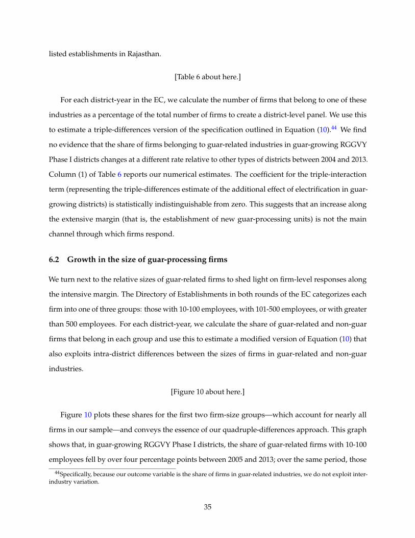
listed establishments in Rajasthan.
[Table 6 about here.]
For each district-year in the EC, we calculate the number of firms that belong to one of these
industries as a percentage of the total number of firms to create a district-level panel. We use this
to estimate a triple-differences version of the specification outlined in Equation (10).44 We find
no evidence that the share of firms belonging to guar-related industries in guar-growing RGGVY
Phase I districts changes at a different rate relative to other types of districts between 2004 and 2013.
Column (1) of Table 6 reports our numerical estimates. The coefficient for the triple-interaction
term (representing the triple-differences estimate of the additional effect of electrification in guar-
growing districts) is statistically indistinguishable from zero. This suggests that an increase along
the extensive margin (that is, the establishment of new guar-processing units) is not the main
channel through which firms respond.
6.2 Growth in the size of guar-processing firms
We turn next to the relative sizes of guar-related firms to shed light on firm-level responses along
the intensive margin. The Directory of Establishments in both rounds of the EC categorizes each
firm into one of three groups: those with 10-100 employees, with 101-500 employees, or with greater
than 500 employees. For each district-year, we calculate the share of guar-related and non-guar
firms that belong in each group and use this to estimate a modified version of Equation (10) that
also exploits intra-district differences between the sizes of firms in guar-related and non-guar
industries.
[Figure 10 about here.]
Figure 10 plots these shares for the first two firm-size groups—which account for nearly all
firms in our sample—and conveys the essence of our quadruple-differences approach. This graph
shows that, in guar-growing RGGVY Phase I districts, the share of guar-related firms with 10-100
employees fell by over four percentage points between 2005 and 2013; over the same period, those
44Specifically, because our outcome variable is the share of firms in guar-related industries, we do not exploit inter-industry variation.
35
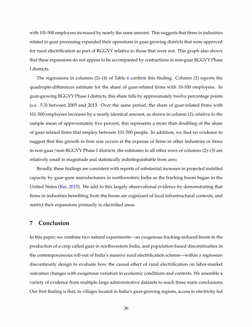
with 101-500 employees increased by nearly the same amount. This suggests that firms in industries
related to guar processing expanded their operations in guar-growing districts that were approved
for rural electrification as part of RGGVY relative to those that were not. This graph also shows
that these expansions do not appear to be accompanied by contractions in non-guar RGGVY Phase
I districts.
The regressions in columns (2)–(4) of Table 6 confirm this finding. Column (2) reports the
quadruple-differences estimate for the share of guar-related firms with 10-100 employees. In
guar-growing RGGVY Phase I districts, this share falls by approximately twelve percentage points
(s.e. 5.3) between 2005 and 2013. Over the same period, the share of guar-related firms with
101-500 employees increases by a nearly identical amount, as shown in column (2); relative to the
sample mean of approximately five percent, this represents a more than doubling of the share
of guar-related firms that employ between 101-500 people. In addition, we find no evidence to
suggest that this growth in firm size occurs at the expense of firms in other industries or firms
in non-guar/non-RGGVY Phase I districts; the estimates in all other rows of columns (2)–(3) are
relatively small in magnitude and statistically indistinguishable from zero.
Broadly, these findings are consistent with reports of substantial increases in projected installed
capacity by guar-gum manufacturers in northwestern India as the fracking boom began in the
United States (Rai, 2015). We add to this largely observational evidence by demonstrating that
firms in industries benefiting from the boom are cognizant of local infrastructural contexts, and
restrict their expansions primarily to electrified areas.
7 Conclusion
In this paper, we combine two natural experiments—an exogenous fracking-induced boom in the
production of a crop called guar in northwestern India, and population-based discontinuities in
the contemporaneous roll-out of India’s massive rural electrification scheme—within a regression
discontinuity design to evaluate how the causal effect of rural electrification on labor-market
outcomes changes with exogenous variation in economic conditions and contexts. We assemble a
variety of evidence from multiple large administrative datasets to reach three main conclusions.
Our first finding is that, in villages located in India’s guar-growing regions, access to electricity led
36
to a large increase in non-agricultural employment relative to agricultural employment, especially
among women. Our second finding is that these labor-market dynamics appear to be driven by an
increase in employment by electricity-intensive industrial firms that complement guar production
(such as guar-processing units) near these communities. It is also related to a proliferation of
household-level enterprises and home production in these areas. Finally, our third finding is
that, on average, access to electricity appears to have no discernible impact on these labor-market
outcomes in villages located in the rest of India.
The main implication of these findings is related to the necessity of grid electrification. Pro-
ponents have long claimed that reliable electricity delivered by the grid is foundational for the
structural transformation of rural economies. Its potential to drive job creation and employment
growth is often central to this argument.45 Yet the evidence base on this point remains thin. In
particular, impact evaluations are typically unable to rigorously shed light on drivers of spatial
and temporal heterogeneity. We show that access to electricity from the grid led to large-scale
structural transformation of the rural economy in large swathes of northwestern India, which saw
the rise of complementary economic opportunities. In the rest of India, where these complementary
conditions were lacking on average, the impacts of grid-scale electrification on rural labor-market
outcomes were largely negligible.
These results highlight the role electrification—and large-scale infrastructure, more broadly—
can play in low- and middle-income countries. Alone, such investments may be insufficient, yet
built in anticipation of (and to support) other policies and changes, large-scale infrastructure can
provide a foundation for sustained economic growth and development. In our setting, access to
grid-scale electricity allowed individuals, households, and firms to respond to rapidly changing
economic contexts in ways that potentially deliver economic benefits and improve welfare. We
believe that rigorously identifying other potential drivers of the success of large-scale infrastructure
is a promising avenue for future research.
45In an evaluation of one of its grid expansion projects in Namibia, for instance, the Swedish International DevelopmentCorporation Agency notes that “the most important effect of electricity expansion on the poor is . . . through the effectit can have on the general economic development by providing power to new investments in industry and smallbusinesses” (Goppers, 2006). Other international donors echo these sentiments (Independent Evaluation Group, 2008;United Nations, 2018).
37
References
ABADIE, A., A. DIAMOND, AND J. HAINMUELLER (2010): “Synthetic Control Methods for Com-parative Case Studies: Estimating the Effect of California’s Tobacco Control Program,” Journal ofthe American Statistical Association, 105, 493–505.
ABADIE, A. AND J. GARDEAZABAL (2003): “The Economic Costs of Conflict: A Case Study of theBasque Country,” American Economic Review, 93, 113–132.
ACEMOGLU, D., S. JOHNSON, A. KERMANI, J. KWAK, AND T. MITTON (2016): “The value ofconnections in turbulent times: Evidence from the United States,” Journal of Financial Economics,121, 368–391.
ADAIR-ROHANI, H., J. LEWIS, J. MINGLE, AND S. GUMY (2016): “Burning Opportunity: CleanHousehold Energy for Health, Sustainable Development, and Wellbeing of Women and Children,”Tech. rep., World Health Organization.
ADHVARYU, A., A. V. CHARI, AND S. SHARMA (2013): “Firing Costs and Flexibility: Evidencefrom Firms' Employment Responses to Shocks in India,” Review of Economics and Statistics, 95,725–740.
ADUKIA, A., S. ASHER, AND P. NOVOSAD (2018): “Educational Investment Responses to EconomicOpportunity: Evidence from Indian Road Construction,” Working paper.
AGGARWAL, S. (2018): “Do rural roads create pathways out of poverty? Evidence from India,”Journal of Development Economics, 133, 375–395.
AGRICULTURAL AND PROCESSED FOOD PRODUCTS EXPORT DEVELOPMENT AUTHORITY (2011):“APEDA Agri Exchange Ready Reckoner Series: Guargum,” Tech. rep., Ministry of Commerce& Industry, retrieved from http://apeda.gov.in/apedawebsite/six_head_product/Guargum_final_
Profile.pdf on April 16, 2017.
AMITI, M. AND B. S. JAVORCIK (2008): “Trade costs and location of foreign firms in China,” Journalof Development Economics, 85, 129–149.
ASHER, S., T. GARG, AND P. NOVOSAD (2018): “The Ecological Impact of Transportation Infras-tructure,” World Bank Policy Research Working Paper № 8507.
ASHER, S. AND P. NOVOSAD (2018): “Rural Roads and Local Economic Development,” Workingpaper.
ATHEY, S. AND G. IMBENS (2017): “The Econometrics of Randomized Experiments a,” in Handbookof Field Experiments, Elsevier, 73–140.
BANERJEE, A. V. AND E. DUFLO (2007): “The Economic Lives of the Poor,” Journal of EconomicPerspectives, 21, 141–167.
BANERJEE, S. G., D. BARNES, K. SINGH, BIPULAND MAYER, AND H. SAMAD (2014): Power for All:Electricity Access Challenge in India, World Bank.
BARATI, R. AND J.-T. LIANG (2014): “A review of fracturing fluid systems used for hydraulicfracturing of oil and gas wells,” Journal of Applied Polymer Science, 131.
38
BARRON, M. AND M. TORERO (2017): “Household electrification and indoor air pollution,” Journalof Environmental Economics and Management, 86, 81–92.
BECKWITH, R. (2012): “Depending On Guar For Shale Oil And Gas Development,” Journal ofPetroleum Technology, 64, 44–55.
BELLARBY, J. (2009): Well Completion Design, Volume 56 (Developments in Petroleum Science), ElsevierScience.
BENSCH, G., J. PETERS, AND M. SIEVERT (2017): “The lighting transition in rural Africa — Fromkerosene to battery-powered LED and the emerging disposal problem,” Energy for SustainableDevelopment, 39, 13–20.
BERNARD, T. AND M. TORERO (2015): “Social Interaction Effects and Connection to Electricity:Experimental Evidence from Rural Ethiopia,” Economic Development and Cultural Change, 63,459–484.
BONAN, J., S. PAREGLIO, AND M. TAVONI (2017): “Access to modern energy: a review of barriers,drivers and impacts,” Environment and Development Economics, 22, 491–516.
BURLIG, F. AND L. PREONAS (2016): “Out of the Darkness and Into the Light? Development Effectsof Rural Electrification in India,” Energy Institute at Haas Working Paper № WP-268R.
CARLTON, D. W. (1983): “The Location and Employment Choices of New Firms: An EconometricModel with Discrete and Continuous Endogenous Variables,” The Review of Economics andStatistics, 65, 440.
CAVALLO, E., S. GALIANI, I. NOY, AND J. PANTANO (2013): “Catastrophic Natural Disasters andEconomic Growth,” Review of Economics and Statistics, 95, 1549–1561.
CHEN, X. AND W. D. NORDHAUS (2011): “Using luminosity data as a proxy for economic statistics,”Proceedings of the National Academy of Sciences, 108, 8589–8594.
CHUDZIKOWSKI, R. J. (1971): “Guar gum and its applications,” Journal of the Society of CosmeticChemists, 22, 43–60.
COFFMAN, M. AND I. NOY (2011): “Hurricane Iniki: measuring the long-term economic impact ofa natural disaster using synthetic control,” Environment and Development Economics, 17, 187–205.
CORREIA, S. (2015): “Singletons, cluster-robust standard errors and fixed effects: A bad mix,”Technical note.
DINKELMAN, T. (2011): “The Effects of Rural Electrification on Employment: New Evidence fromSouth Africa,” American Economic Review, 101, 3078–3108.
DOLL, C. N., J.-P. MULLER, AND J. G. MORLEY (2006): “Mapping regional economic activity fromnight-time light satellite imagery,” Ecological Economics, 57, 75–92.
DUQUE, V., M. ROSALES-RUEDA, AND F. SANCHEZ (2018): “How do early-life shocks interact withsubsequent human-capital investments? Evidence from administrative data,” Working paper.
ELSNER, M. AND K. HOELZER (2016): “Quantitative Survey and Structural Classification ofHydraulic Fracturing Chemicals Reported in Unconventional Gas Production,” EnvironmentalScience & Technology, 50, 3290–3314.
39
FETTER, T. R. (2018): “Fracking, Toxics, and Disclosure,” http://sites.duke.edu/trfetter/
research.
FETTER, T. R., A. L. STECK, C. TIMMINS, AND D. H. WRENN (2018): “Learning by Viewing? SocialLearning, Regulatory Disclosure and Firm Productivity in Shale Gas,” http://sites.duke.edu/
trfetter/research.
GABA, K. M., B. MIN, A. THAKKER, AND C. ELVIDGE (2016): “nightlights.io: Twenty Years ofIndia Lights,” Accessed on September 9, 2016.
GOPPERS, K. (2006): “The Auas High-voltage Transmission Line in Namibia Supported by aSwedish Concessionary Credit,” Tech. rep., Swedish International Development CooperationAgency, Sida, sida Evaluation 06/53.
GRIMM, M., A. MUNYEHIRWE, J. PETERS, AND M. SIEVERT (2017): “A First Step up the EnergyLadder? Low Cost Solar Kits and Household’s Welfare in Rural Rwanda,” The World BankEconomic Review, 31, 631649.
GRONAU, R. (1977): “Leisure, Home Production, and Work–the Theory of the Allocation of TimeRevisited,” Journal of Political Economy, 85, 1099–1123.
HENDERSON, J. V., A. STOREYGARD, AND D. N. WEIL (2012): “Measuring Economic Growth fromOuter Space,” American Economic Review, 102, 994–1028.
HYMOWITZ, T. (1972): “The trans-domestication concept as applied to Guar,” Economic Botany, 26,49–60.
INDEPENDENT EVALUATION GROUP (2008): “The welfare impact of rural electrification: A reassess-ment of the costs and benefits,” Tech. rep., World Bank.
INTERNATIONAL ENERGY AGENCY (2011): “World Energy Outlook 2011: Energy for All,” Tech.rep., OECD/IEA.
——— (2015): “WEO-2015 Special Report: India Energy Outlook,” Tech. rep., OECD/IEA.
JONES, D., D. MOLITOR, AND J. REIF (2018): “What Do Workplace Wellness Programs Do?Evidence from the Illinois Workplace Wellness Study,” National Bureau of Economic Research(NBER) Working Paper № 24229.
JOSHI, S. (2003): “Cost/Benefits of Horizontal Wells,” in SPE Western Regional/AAPG Pacific SectionJoint Meeting, Society of Petroleum Engineers.
KHANDKER, S. R., D. F. BARNES, AND H. A. SAMAD (2013): “Welfare Impacts of Rural Electri-fication: A Panel Data Analysis from Vietnam,” Economic Development and Cultural Change, 61,659–692.
KURAVADI, N. A., S. VERMA, S. PAREEK, P. GAHLOT, S. KUMARI, U. K. TANWAR, P. BHATELE,M. CHOUDHARY, K. S. GILL, V. PRUTHI, S. K. TRIPATHI, K. S. DHUGGA, AND G. S. RANDHAWA
(2013): “Guar,” in Agricultural Sustainability: Progress and Prospects in Crop Research, Elsevier, 47–60.
LEDERMAN, D. AND G. PORTO (2015): “The Price Is Not Always Right: On the Impacts ofCommodity Prices on Households (and Countries),” The World Bank Research Observer, lkv013.
40
LEE, K., E. MIGUEL, AND C. WOLFRAM (2018): “Experimental Evidence on the Economics of RuralElectrification,” Working paper.
LENZ, L., A. MUNYEHIRWE, J. PETERS, AND M. SIEVERT (2017): “Does Large-Scale InfrastructureInvestment Alleviate Poverty? Impacts of Rwanda’s Electricity Access Roll-Out Program,” WorldDevelopment, 89, 88–110.
LIPSCOMB, M., A. M. MOBARAK, AND T. BARHAM (2013): “Development Effects of Electrification:Evidence from the Topographic Placement of Hydropower Plants in Brazil,” American EconomicJournal: Applied Economics, 5, 200–231.
LITZOW, E., S. K. PATTANAYAK, AND T. THINLEY (2017): “Evaluating Rural Electrification: Illus-trating Research Gaps with the Case of Bhutan,” Environment for Development (EfD) DiscussionPaper № 17-19.
MARTIN, P. AND C. A. ROGERS (1995): “Industrial location and public infrastructure,” Journal ofInternational Economics, 39, 335–351.
MCCRARY, J. (2008): “Manipulation of the running variable in the regression discontinuity design:A density test,” Journal of Econometrics, 142, 698–714.
MIN, B., Z. O’KEEFFE, AND F. ZHANG (2017): “Whose Power Gets Cut? Using High-FrequencySatellite Images to Measure Power Supply Irregularity,” World Bank Policy Research WorkingPaper № 8131.
MINISTRY OF POWER (2006): “The Rural Electrification Policy,” Extraordinary Gazette of India,2006, No. 197.
——— (2012): “Rajiv Gandhi Grameen Vidyutikaran Yojana,” http://pib.nic.in/newsite/PrintRe-lease.aspx?relid=83765.
MUDGIL, D., S. BARAK, AND B. S. KHATKAR (2011): “Guar gum: processing, properties and foodapplications—A Review,” Journal of Food Science and Technology, 51, 409–418.
NATIONAL RAINFED AREA AUTHORITY (2014): “Potential of Rainfed Guar (Cluster beans) Culti-vation, Processing and Export in India,” Tech. rep., Ministry of Agriculture & Farmers Welfare,retrieved from http://nraa.gov.in/pdf/Rainfed-guar-final-pdf.pdf on April 16, 2017.
O’DELL, K., S. PETERS, AND K. WHARTON (2014): “Women, Energy and Economic Empowerment:Applying a gender lens to amplify the impact of energy access,” Tech. rep., Deloitte ConsultingLLP.
ORR, I. (2016): “Hydraulic Fracturing: A Game-Changer for Energy and Economies,” in AlternativeEnergy and Shale Gas Encyclopedia, John Wiley & Sons, Inc., 700–719.
PATTANAYAK, S. K., M. JEULAND, J. J. LEWIS, V. BHOJVAID, N. BROOKS, A. KAR, L. LIPINSKI,L. MORRISON, O. PATANGE, N. RAMANATHAN, I. H. REHMAN, R. THADANI, F. USMANI,M. VORA, AND V. RAMANATHAN (2016): “Cooking Up Change in the Himalayas: ExperimentalEvidence on Cookstove Promotion,” Duke Environmental and Energy Economics Working Paper№ EE 16-03.
PEREIRA, M. G., J. A. SENA, M. A. V. FREITAS, AND N. F. DA SILVA (2011): “Evaluation of theimpact of access to electricity: A comparative analysis of South Africa, China, India and Brazil,”Renewable and Sustainable Energy Reviews, 15, 1427–1441.
41
PINKOVSKIY, M. AND X. SALA-I-MARTIN (2016): “Lights, Camera . . . Income! Illuminating theNational Accounts-Household Surveys Debate,” The Quarterly Journal of Economics, 131, 579–631.
RAI, D. K. (2015): “Trends and Economic Dynamics of Guar in India,” Indian Council for Researchon International Economic Relations Working Paper No. 311.
SINGH, S. K. (2014): “An Analysis of Guar Crop in India,” Tech. rep., United States Department ofAgriculture.
SINGHAL, S. AND R. NILAKANTAN (2016): “The economic effects of a counterinsurgency policy inIndia: A synthetic control analysis,” European Journal of Political Economy, 45, 1–17.
SRIVASTAVA, N. AND R. SRIVASTAVA (2010): “Women, Work, and Employment Outcomes in RuralIndia,” Economic and Political Weekly, 45, 49–63.
TAPSCOTT, C. E. (2015): “An evaluation of flow and transport properties for hydraulic fracturingfluids in porous medium systems,” Master’s thesis, The University of North Carolina at ChapelHill.
THOM, C. (2000): “Use of grid electricity by rural households in South Africa,” Energy for SustainableDevelopment, 4, 36–43.
THOMBARE, N., U. JHA, S. MISHRA, AND M. SIDDIQUI (2016): “Guar gum as a promising startingmaterial for diverse applications: A review,” International Journal of Biological Macromolecules, 88,361–372.
TOLLEFSON, J. (2013): “Secrets of fracking fluids pave way for cleaner recipe,” Nature, 501, 146–147.
TULLY, S. (2006): “The Human Right to Access Electricity,” The Electricity Journal, 19, 30–39.
UNDERSANDER, D., D. H. PUTNAM, A. R. KAMINSKI, K. A. KELLING, J. D. DOLL, E. S. OPLINGER,AND J. L. GUNSOLUS (1991): “Guar,” in Alternative Field Crops Manual, University of Wisconsin-Exension, Cooperative Extension; University of Minnesota Center for Alternative Plant & AnimalProducts and the Minnesota Extension Service.
UNITED NATIONS (2018): “Accelerating SDG 7 achievement: Policy briefs in support of the firstSDG 7 review at the UN High-Level Political Forum 2018,” Tech. rep., United Nations Departmentof Economic and Social Affairs, retrieved from https://sustainabledevelopment.un.org/content/
documents/18041SDG7_Policy_Brief.pdf on October 18, 2018.
VIVALT, E. (2015): “Heterogeneous Treatment Effects in Impact Evaluation,” American EconomicReview, 105, 467–470.
WESTFALL, P. H. AND S. S. YOUNG (1993): Resampling-Based Multiple Testing: Examples and Methodsfor p-Value Adjustment, Wiley-Interscience.
WHEELER, D. AND A. MODY (1992): “International investment location decisions,” Journal ofInternational Economics, 33, 57–76.
WYSOKINSKA, A. (2017): “Institutions or Culture? Lessons for development from two naturalexperiments of history,” LSE Institute of Global Affairs Research Paper № 03/2017.
42
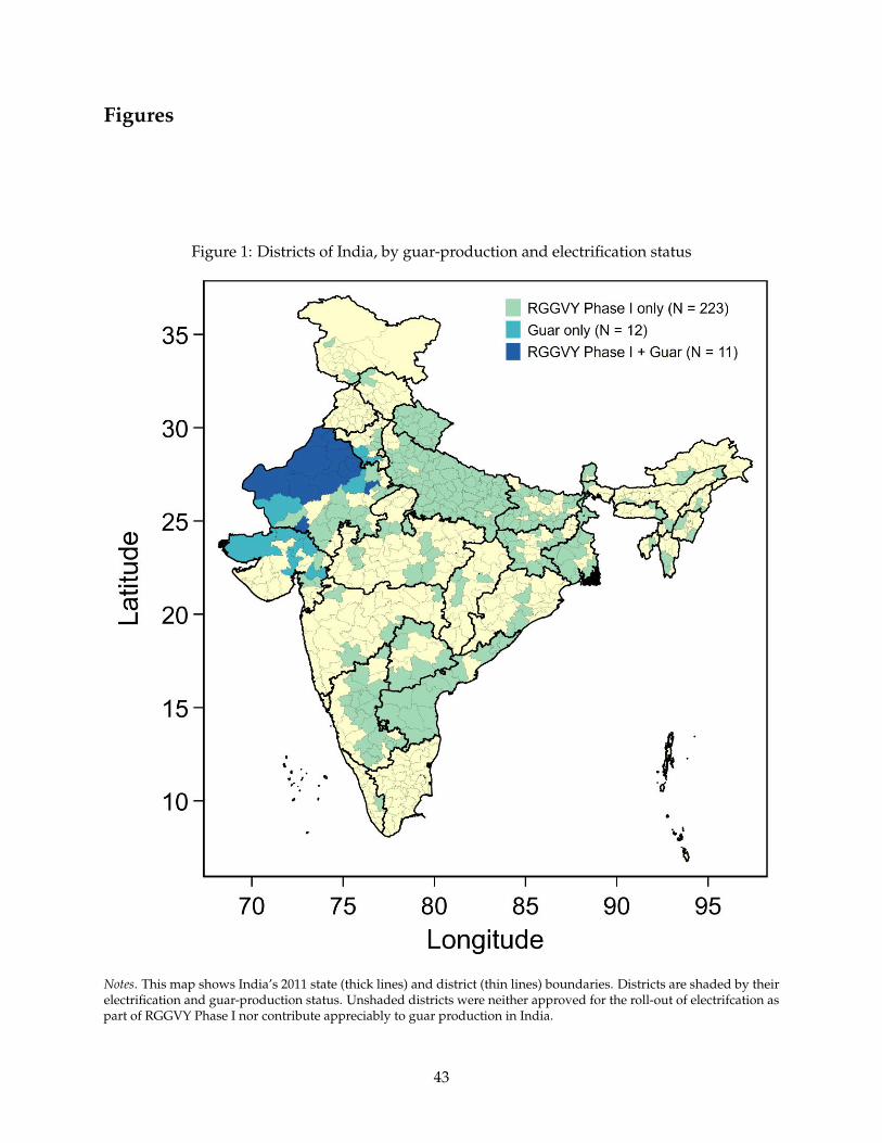
Figures
Figure 1: Districts of India, by guar-production and electrification status
Notes. This map shows India’s 2011 state (thick lines) and district (thin lines) boundaries. Districts are shaded by theirelectrification and guar-production status. Unshaded districts were neither approved for the roll-out of electrifcation aspart of RGGVY Phase I nor contribute appreciably to guar production in India.
43
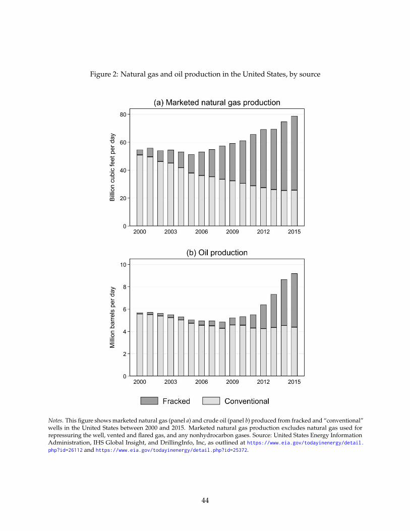
Figure 2: Natural gas and oil production in the United States, by source
Notes. This figure shows marketed natural gas (panel a) and crude oil (panel b) produced from fracked and “conventional”wells in the United States between 2000 and 2015. Marketed natural gas production excludes natural gas used forrepressuring the well, vented and flared gas, and any nonhydrocarbon gases. Source: United States Energy InformationAdministration, IHS Global Insight, and DrillingInfo, Inc, as outlined at https://www.eia.gov/todayinenergy/detail.php?id=26112 and https://www.eia.gov/todayinenergy/detail.php?id=25372.
44
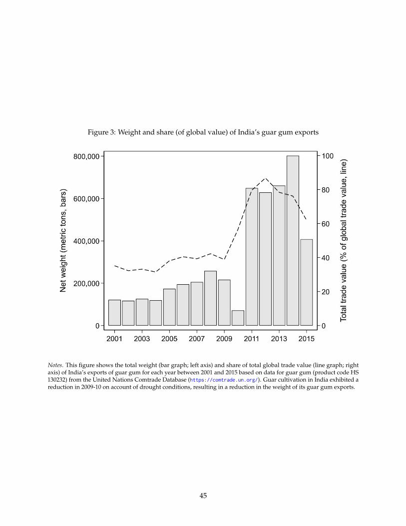
Figure 3: Weight and share (of global value) of India’s guar gum exports
Notes. This figure shows the total weight (bar graph; left axis) and share of total global trade value (line graph; rightaxis) of India’s exports of guar gum for each year between 2001 and 2015 based on data for guar gum (product code HS130232) from the United Nations Comtrade Database (https://comtrade.un.org/). Guar cultivation in India exhibited areduction in 2009-10 on account of drought conditions, resulting in a reduction in the weight of its guar gum exports.
45
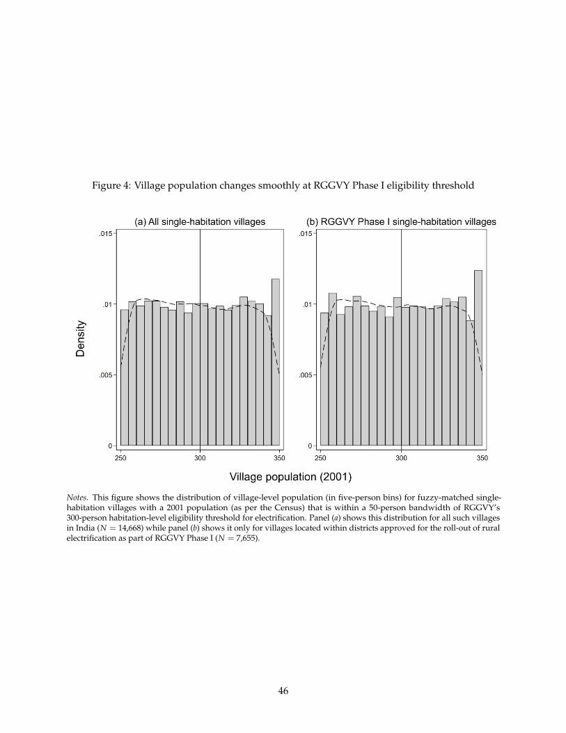
Figure 4: Village population changes smoothly at RGGVY Phase I eligibility threshold
Notes. This figure shows the distribution of village-level population (in five-person bins) for fuzzy-matched single-habitation villages with a 2001 population (as per the Census) that is within a 50-person bandwidth of RGGVY’s300-person habitation-level eligibility threshold for electrification. Panel (a) shows this distribution for all such villagesin India (N = 14,668) while panel (b) shows it only for villages located within districts approved for the roll-out of ruralelectrification as part of RGGVY Phase I (N = 7,655).
46
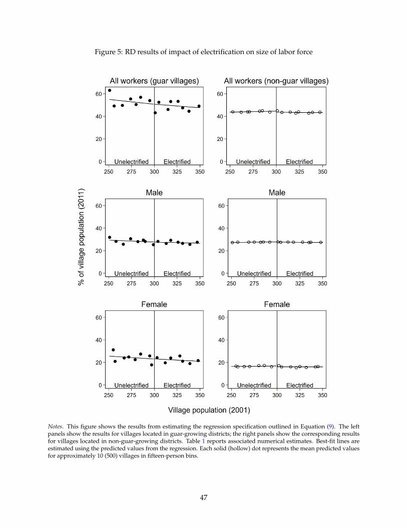
Figure 5: RD results of impact of electrification on size of labor force
Notes. This figure shows the results from estimating the regression specification outlined in Equation (9). The leftpanels show the results for villages located in guar-growing districts; the right panels show the corresponding resultsfor villages located in non-guar-growing districts. Table 1 reports associated numerical estimates. Best-fit lines areestimated using the predicted values from the regression. Each solid (hollow) dot represents the mean predicted valuesfor approximately 10 (500) villages in fifteen-person bins.
47
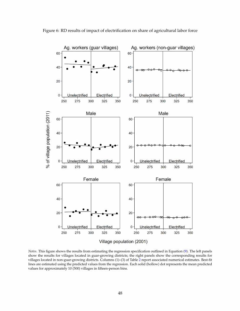
Figure 6: RD results of impact of electrification on share of agricultural labor force
Notes. This figure shows the results from estimating the regression specification outlined in Equation (9). The left panelsshow the results for villages located in guar-growing districts; the right panels show the corresponding results forvillages located in non-guar-growing districts. Columns (1)–(3) of Table 2 report associated numerical estimates. Best-fitlines are estimated using the predicted values from the regression. Each solid (hollow) dot represents the mean predictedvalues for approximately 10 (500) villages in fifteen-person bins.
48
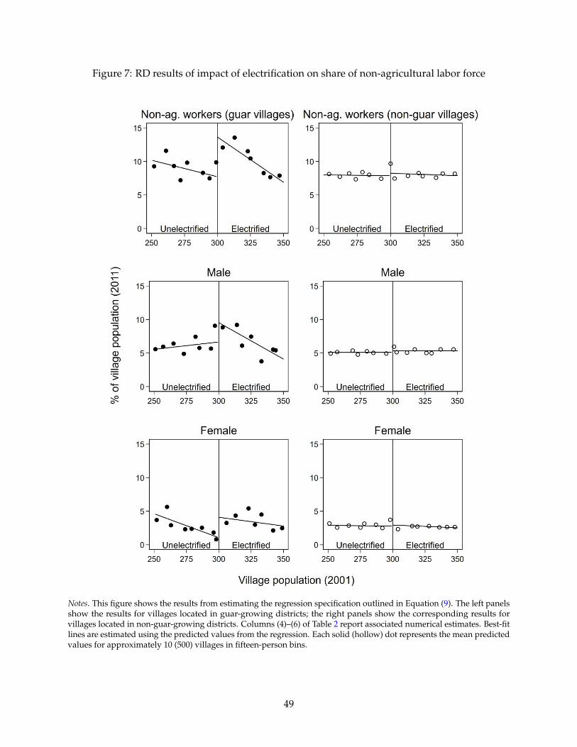
Figure 7: RD results of impact of electrification on share of non-agricultural labor force
Notes. This figure shows the results from estimating the regression specification outlined in Equation (9). The left panelsshow the results for villages located in guar-growing districts; the right panels show the corresponding results forvillages located in non-guar-growing districts. Columns (4)–(6) of Table 2 report associated numerical estimates. Best-fitlines are estimated using the predicted values from the regression. Each solid (hollow) dot represents the mean predictedvalues for approximately 10 (500) villages in fifteen-person bins.
49
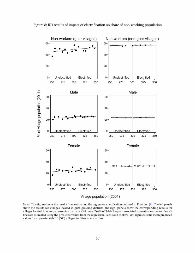
Figure 8: RD results of impact of electrification on share of non-working population
Notes. This figure shows the results from estimating the regression specification outlined in Equation (9). The left panelsshow the results for villages located in guar-growing districts; the right panels show the corresponding results forvillages located in non-guar-growing districts. Columns (7)–(9) of Table 2 report associated numerical estimates. Best-fitlines are estimated using the predicted values from the regression. Each solid (hollow) dot represents the mean predictedvalues for approximately 10 (500) villages in fifteen-person bins.
50
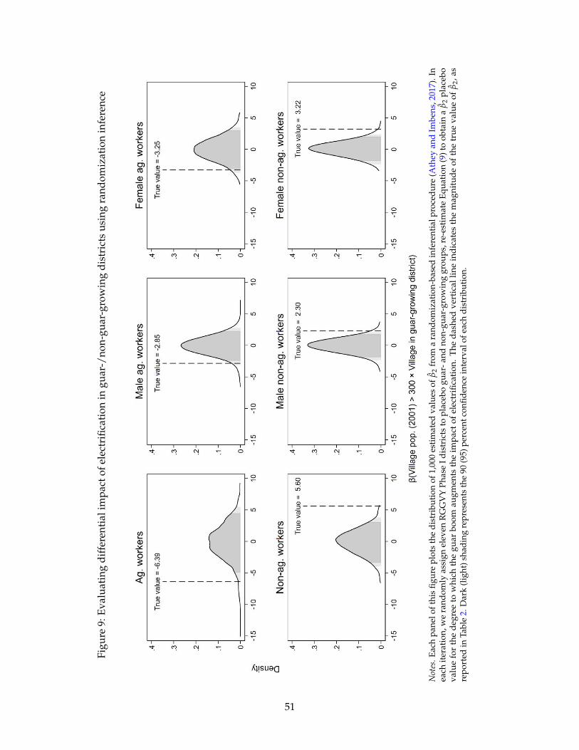
Figu
re9:
Eval
uati
ngdi
ffer
enti
alim
pact
ofel
ectr
ifica
tion
ingu
ar-/
non-
guar
-gro
win
gdi
stri
cts
usin
gra
ndom
izat
ion
infe
renc
e
Not
es.E
ach
pane
loft
his
figur
epl
ots
the
dist
ribu
tion
of1,
000
esti
mat
edva
lues
ofβ̂
2fr
oma
rand
omiz
atio
n-ba
sed
infe
rent
ialp
roce
dure
(Ath
eyan
dIm
bens
,201
7).I
nea
chit
erat
ion,
we
rand
omly
assi
gnel
even
RG
GV
YPh
ase
Idis
tric
tsto
plac
ebo
guar
-and
non-
guar
-gro
win
ggr
oups
,re-
esti
mat
eE
quat
ion
(9)t
oob
tain
aβ̂
2pl
aceb
ova
lue
for
the
deg
ree
tow
hich
the
guar
boom
augm
ents
the
imp
act
ofel
ectr
ifica
tion
.T
hed
ashe
dve
rtic
allin
ein
dic
ates
the
mag
nitu
de
ofth
etr
ue
valu
eof
β̂2,
asre
port
edin
Tabl
e2.
Dar
k(l
ight
)sha
ding
repr
esen
tsth
e90
(95)
perc
entc
onfid
ence
inte
rval
ofea
chdi
stri
buti
on.
51
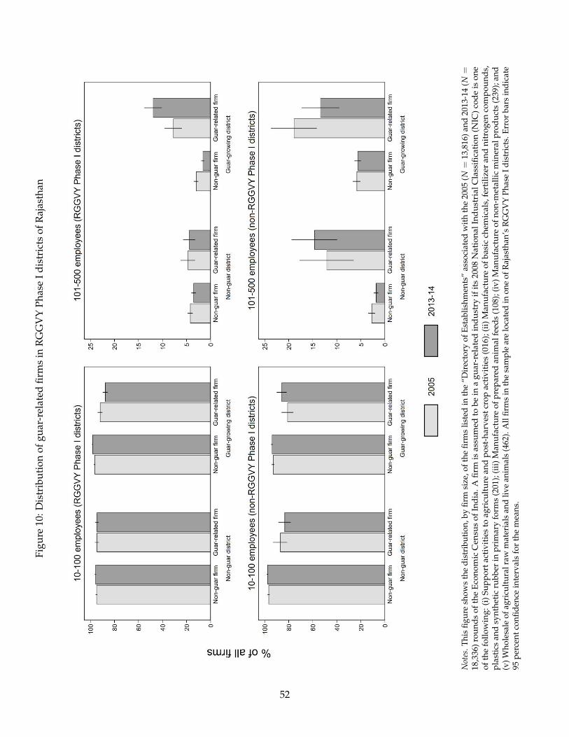
Figu
re10
:Dis
trib
utio
nof
guar
-rel
ated
firm
sin
RG
GV
YPh
ase
Idis
tric
tsof
Raj
asth
an
Not
es.T
his
figur
esh
ows
the
dist
ribu
tion,
byfir
msi
ze,o
fthe
firm
slis
ted
inth
e“D
irec
tory
ofEs
tabl
ishm
ents
”as
soci
ated
with
the
2005
(N=
13,8
16)a
nd20
13-1
4(N
=18
,336
)rou
nds
ofth
eE
cono
mic
Cen
sus
ofIn
dia
.Afi
rmis
assu
med
tobe
ina
guar
-rel
ated
ind
ust
ryif
its
2008
Nat
iona
lInd
ust
rial
Cla
ssifi
cati
on(N
IC)c
ode
ison
eof
the
follo
win
g:(i
)Su
ppor
tact
ivit
ies
toag
ricu
ltu
rean
dpo
st-h
arve
stcr
opac
tivi
ties
(016
);(i
i)M
anu
fact
ure
ofba
sic
chem
ical
s,fe
rtili
zer
and
nitr
ogen
com
pou
nds,
plas
tics
and
synt
heti
cru
bber
inpr
imar
yfo
rms
(201
);(i
ii)M
anuf
actu
reof
prep
ared
anim
alfe
eds
(108
);(i
v)M
anuf
actu
reof
non-
met
allic
min
eral
prod
ucts
(239
);an
d(v
)Who
lesa
leof
agri
cultu
ralr
awm
ater
ials
and
live
anim
als
(462
).A
llfir
ms
inth
esa
mpl
ear
elo
cate
din
one
ofR
ajas
than
’sR
GG
VY
Phas
eId
istr
icts
.Err
orba
rsin
dica
te95
perc
entc
onfid
ence
inte
rval
sfo
rth
em
eans
.
52
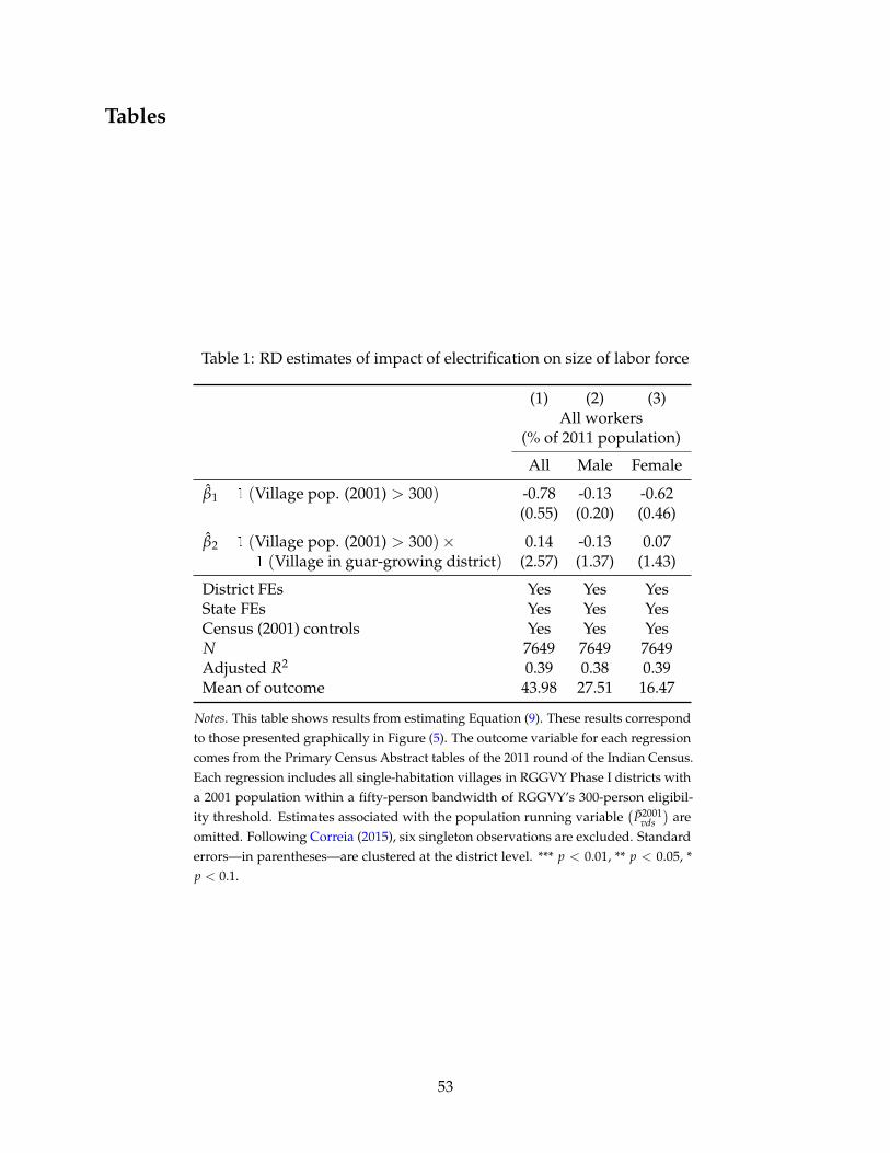
Tables
Table 1: RD estimates of impact of electrification on size of labor force
(1) (2) (3)All workers
(% of 2011 population)
All Male Female
β̂1 1 (Village pop. (2001) > 300) -0.78 -0.13 -0.62(0.55) (0.20) (0.46)
β̂2 1 (Village pop. (2001) > 300)× 0.14 -0.13 0.071 (Village in guar-growing district) (2.57) (1.37) (1.43)
District FEs Yes Yes YesState FEs Yes Yes YesCensus (2001) controls Yes Yes YesN 7649 7649 7649Adjusted R2 0.39 0.38 0.39Mean of outcome 43.98 27.51 16.47
Notes. This table shows results from estimating Equation (9). These results correspondto those presented graphically in Figure (5). The outcome variable for each regressioncomes from the Primary Census Abstract tables of the 2011 round of the Indian Census.Each regression includes all single-habitation villages in RGGVY Phase I districts witha 2001 population within a fifty-person bandwidth of RGGVY’s 300-person eligibil-ity threshold. Estimates associated with the population running variable
(P̃2001
vds)
areomitted. Following Correia (2015), six singleton observations are excluded. Standarderrors—in parentheses—are clustered at the district level. *** p < 0.01, ** p < 0.05, *p < 0.1.
53
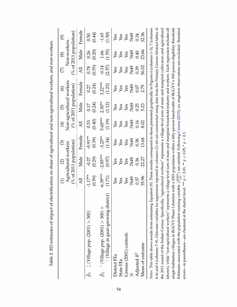
Tabl
e2:
RD
esti
mat
esof
impa
ctof
elec
trifi
cati
onon
shar
eof
agri
cult
ural
and
non-
agri
cult
ural
wor
kers
,and
non-
wor
kers
(1)
(2)
(3)
(4)
(5)
(6)
(7)
(8)
(9)
Agr
icul
tura
lwor
kers
Non
-agr
icul
tura
lwor
kers
Non
-wor
kers
(%of
2011
popu
lati
on)
(%of
2011
popu
lati
on)
(%of
2011
popu
lati
on)
All
Mal
eFe
mal
eA
llM
ale
Fem
ale
All
Mal
eFe
mal
e
β̂1
1(V
illag
epo
p.(2
001)
>30
0 )-1
.17*
*-0
.27
-0.9
1**
0.53
0.17
0.27
0.78
0.26
0.50
(0.5
9)(0
.29)
(0.3
9)(0
.40)
(0.2
4)(0
.24)
(0.5
5)(0
.20)
(0.4
4)
β̂2
1(V
illag
epo
p.(2
001)
>30
0 )×
-6.3
9***
-2.8
5***
-3.2
5**
5.60
***
2.30
**3.
22**
*-0
.14
1.66
-1.6
51(V
illag
ein
guar
-gro
win
gdi
stri
ct)
(1.7
1)(0
.97)
(1.3
4)(1
.19)
(1.1
2)(1
.23)
(2.5
7)(1
.55)
(1.5
0)
Dis
tric
tFEs
Yes
Yes
Yes
Yes
Yes
Yes
Yes
Yes
Yes
Stat
eFE
sYe
sYe
sYe
sYe
sYe
sYe
sYe
sYe
sYe
sC
ensu
s(2
001)
cont
rols
Yes
Yes
Yes
Yes
Yes
Yes
Yes
Yes
Yes
N76
4976
4976
4976
4976
4976
4976
4976
4976
49A
djus
ted
R2
0.37
0.36
0.38
0.16
0.25
0.07
0.39
0.40
0.34
Mea
nof
outc
ome
35.9
622
.27
13.6
88.
025.
232.
7956
.02
23.6
632
.36
Not
es.T
his
tabl
esh
ows
resu
lts
from
esti
mat
ing
Equa
tion
(9).
The
sere
sult
sco
rres
pond
toth
ose
pres
ente
dgr
aphi
cally
inFi
gure
s6
(col
umns
1–3)
,7(c
olum
ns4–
6)an
d8
(col
umns
7–9)
.Out
com
eva
riab
les
for
regr
essi
ons
repo
rted
inco
lum
ns(1
)–(6
)are
cons
truc
ted
usin
gda
tafr
omth
ePr
imar
yC
ensu
sA
bstr
actt
able
sof
the
2011
rou
ndof
the
Ind
ian
Cen
sus.
Spec
ifica
lly,“
agri
cult
ura
lwor
kers
”re
pre
sent
sa
villa
ge-l
evel
sum
ofm
ain
and
mar
gina
lcu
ltiv
ator
san
dag
ricu
ltu
ral
labo
rers
,whi
le“n
on-a
gric
ultu
ralw
orke
rs”
repr
esen
tsa
villa
ge-l
evel
sum
ofm
ain
and
mar
gina
lhou
seho
ld-i
ndus
try
and
wor
kers
.Eac
hre
gres
sion
incl
udes
all
sing
le-h
abit
atio
nvi
llage
sin
RG
GV
YP
hase
Idis
tric
tsw
ith
a20
01po
pula
tion
wit
hin
afi
fty-
pers
onba
ndw
idth
ofR
GG
VY
’s30
0-pe
rson
elig
ibili
tyth
resh
old
.E
stim
ates
asso
ciat
edw
ith
the
popu
lati
onru
nnin
gva
riab
le( P̃
2001
vds) ar
eom
itte
d.F
ollo
win
gC
orre
ia(2
015)
,six
sing
leto
nob
serv
atio
nsar
eex
clud
ed.S
tand
ard
erro
rs—
inpa
rent
hese
s—ar
ecl
uste
red
atth
edi
stri
ctle
vel.
***
p<
0.01
,**
p<
0.05
,*p<
0.1.
54
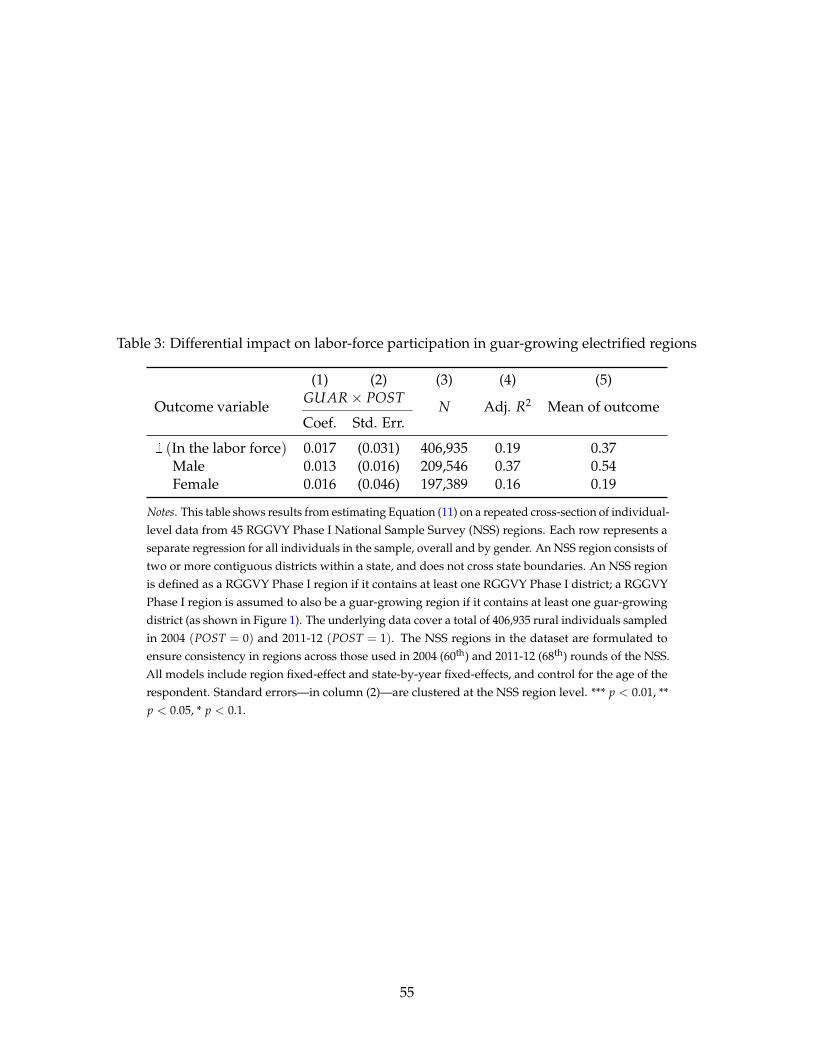
Table 3: Differential impact on labor-force participation in guar-growing electrified regions
(1) (2) (3) (4) (5)
Outcome variableGUAR × POST N Adj. R2 Mean of outcomeCoef. Std. Err.
1 (In the labor force) 0.017 (0.031) 406,935 0.19 0.37Male 0.013 (0.016) 209,546 0.37 0.54Female 0.016 (0.046) 197,389 0.16 0.19
Notes. This table shows results from estimating Equation (11) on a repeated cross-section of individual-level data from 45 RGGVY Phase I National Sample Survey (NSS) regions. Each row represents aseparate regression for all individuals in the sample, overall and by gender. An NSS region consists oftwo or more contiguous districts within a state, and does not cross state boundaries. An NSS regionis defined as a RGGVY Phase I region if it contains at least one RGGVY Phase I district; a RGGVYPhase I region is assumed to also be a guar-growing region if it contains at least one guar-growingdistrict (as shown in Figure 1). The underlying data cover a total of 406,935 rural individuals sampledin 2004 (POST = 0) and 2011-12 (POST = 1). The NSS regions in the dataset are formulated toensure consistency in regions across those used in 2004 (60th) and 2011-12 (68th) rounds of the NSS.All models include region fixed-effect and state-by-year fixed-effects, and control for the age of therespondent. Standard errors—in column (2)—are clustered at the NSS region level. *** p < 0.01, **p < 0.05, * p < 0.1.
55
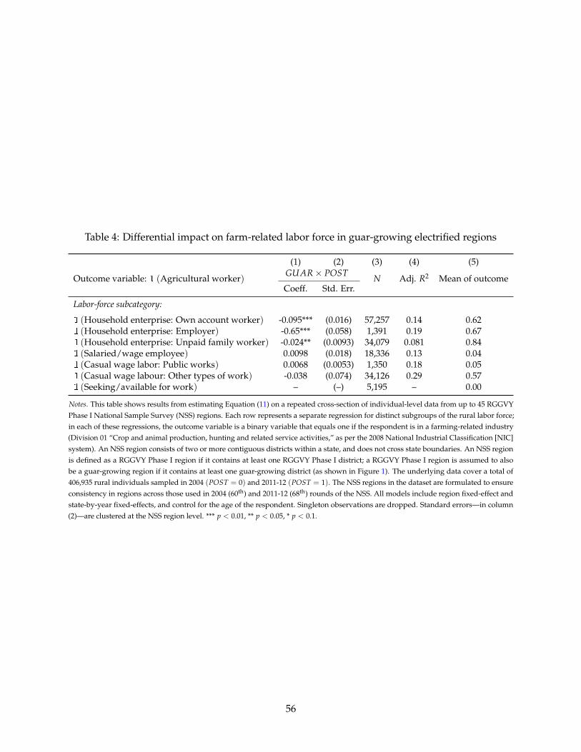
Table 4: Differential impact on farm-related labor force in guar-growing electrified regions
(1) (2) (3) (4) (5)
Outcome variable: 1 (Agricultural worker)GUAR × POST N Adj. R2 Mean of outcomeCoeff. Std. Err.
Labor-force subcategory:
1 (Household enterprise: Own account worker) -0.095*** (0.016) 57,257 0.14 0.621 (Household enterprise: Employer) -0.65*** (0.058) 1,391 0.19 0.671 (Household enterprise: Unpaid family worker) -0.024** (0.0093) 34,079 0.081 0.841 (Salaried/wage employee) 0.0098 (0.018) 18,336 0.13 0.041 (Casual wage labor: Public works) 0.0068 (0.0053) 1,350 0.18 0.051 (Casual wage labour: Other types of work) -0.038 (0.074) 34,126 0.29 0.571 (Seeking/available for work) – (–) 5,195 – 0.00
Notes. This table shows results from estimating Equation (11) on a repeated cross-section of individual-level data from up to 45 RGGVYPhase I National Sample Survey (NSS) regions. Each row represents a separate regression for distinct subgroups of the rural labor force;in each of these regressions, the outcome variable is a binary variable that equals one if the respondent is in a farming-related industry(Division 01 “Crop and animal production, hunting and related service activities,” as per the 2008 National Industrial Classification [NIC]system). An NSS region consists of two or more contiguous districts within a state, and does not cross state boundaries. An NSS regionis defined as a RGGVY Phase I region if it contains at least one RGGVY Phase I district; a RGGVY Phase I region is assumed to alsobe a guar-growing region if it contains at least one guar-growing district (as shown in Figure 1). The underlying data cover a total of406,935 rural individuals sampled in 2004 (POST = 0) and 2011-12 (POST = 1). The NSS regions in the dataset are formulated to ensureconsistency in regions across those used in 2004 (60th) and 2011-12 (68th) rounds of the NSS. All models include region fixed-effect andstate-by-year fixed-effects, and control for the age of the respondent. Singleton observations are dropped. Standard errors—in column(2)—are clustered at the NSS region level. *** p < 0.01, ** p < 0.05, * p < 0.1.
56
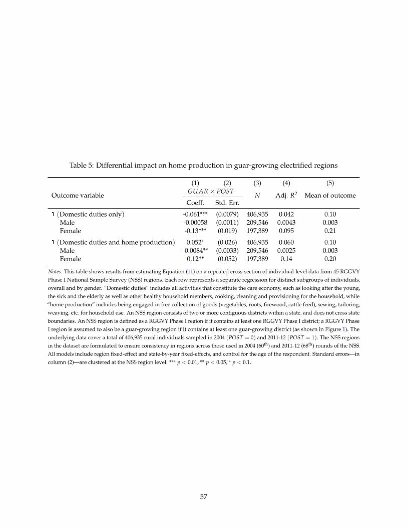
Table 5: Differential impact on home production in guar-growing electrified regions
(1) (2) (3) (4) (5)
Outcome variableGUAR × POST N Adj. R2 Mean of outcomeCoeff. Std. Err.
1 (Domestic duties only) -0.061*** (0.0079) 406,935 0.042 0.10Male -0.00058 (0.0011) 209,546 0.0043 0.003Female -0.13*** (0.019) 197,389 0.095 0.21
1 (Domestic duties and home production) 0.052* (0.026) 406,935 0.060 0.10Male -0.0084** (0.0033) 209,546 0.0025 0.003Female 0.12** (0.052) 197,389 0.14 0.20
Notes. This table shows results from estimating Equation (11) on a repeated cross-section of individual-level data from 45 RGGVYPhase I National Sample Survey (NSS) regions. Each row represents a separate regression for distinct subgroups of individuals,overall and by gender. “Domestic duties” includes all activities that constitute the care economy, such as looking after the young,the sick and the elderly as well as other healthy household members, cooking, cleaning and provisioning for the household, while“home production” includes being engaged in free collection of goods (vegetables, roots, firewood, cattle feed), sewing, tailoring,weaving, etc. for household use. An NSS region consists of two or more contiguous districts within a state, and does not cross stateboundaries. An NSS region is defined as a RGGVY Phase I region if it contains at least one RGGVY Phase I district; a RGGVY PhaseI region is assumed to also be a guar-growing region if it contains at least one guar-growing district (as shown in Figure 1). Theunderlying data cover a total of 406,935 rural individuals sampled in 2004 (POST = 0) and 2011-12 (POST = 1). The NSS regionsin the dataset are formulated to ensure consistency in regions across those used in 2004 (60th) and 2011-12 (68th) rounds of the NSS.All models include region fixed-effect and state-by-year fixed-effects, and control for the age of the respondent. Standard errors—incolumn (2)—are clustered at the NSS region level. *** p < 0.01, ** p < 0.05, * p < 0.1.
57
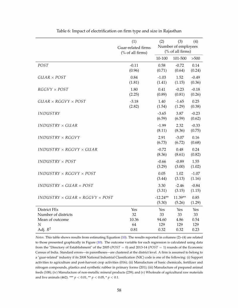
Table 6: Impact of electrification on firm type and size in Rajasthan
(1) (2) (3) (4)
Guar-related firms Number of employees
(% of all firms) (% of all firms)
10-100 101-500 >500
POST -0.11 0.58 -0.72 0.14(0.96) (0.71) (0.64) (0.24)
GUAR × POST 0.84 -1.03 1.52 -0.49(1.81) (1.41) (1.15) (0.36)
RGGVY × POST 1.80 0.41 -0.23 -0.18(2.25) (0.89) (0.81) (0.26)
GUAR × RGGVY × POST -3.18 1.40 -1.65 0.25(2.82) (1.54) (1.29) (0.38)
INDUSTRY -3.65 3.87 -0.23(6.59) (6.59) (0.62)
INDUSTRY × GUAR -1.99 2.32 -0.33(8.11) (8.36) (0.75)
INDUSTRY × RGGVY 2.91 -3.07 0.16(6.73) (6.72) (0.68)
INDUSTRY × RGGVY × GUAR -0.72 0.48 0.24(8.36) (8.61) (0.82)
INDUSTRY × POST -0.66 -0.89 1.55(3.29) (3.00) (1.02)
INDUSTRY × RGGVY × POST 0.05 1.02 -1.07(3.44) (3.13) (1.16)
INDUSTRY × GUAR × POST 3.30 -2.46 -0.84(3.31) (3.15) (1.15)
INDUSTRY × GUAR × RGGVY × POST -12.24** 11.39** 0.85(5.30) (5.26) (1.29)
District FEs Yes Yes Yes YesNumber of districts 32 33 33 33Mean of outcome 10.36 94.60 4.86 0.54N 64 129 129 129Adj. R2 0.81 0.32 0.32 0.23
Notes. This table shows results from estimating Equation (10). The results reported in columns (2)–(4) are relatedto those presented graphically in Figure (10). The outcome variable for each regression is calculated using datafrom the "Directory of Establishment" of the 2005 (POST = 0) and 2013-14 (POST = 1) rounds of the EconomicCensus of India. Standard errors—in parentheses—are clustered at the district level. A firm is assumed to belong toa "guar-related" industry if its 2008 National Industrial Classification (NIC) code is one of the following: (i) Supportactivities to agriculture and post-harvest crop activities (016); (ii) Manufacture of basic chemicals, fertilizer andnitrogen compounds, plastics and synthetic rubber in primary forms (201); (iii) Manufacture of prepared animalfeeds (108); (iv) Manufacture of non-metallic mineral products (239); and (v) Wholesale of agricultural raw materialsand live animals (462). *** p < 0.01, ** p < 0.05, * p < 0.1.
58
Appendix A Using nighttime luminosity to evaluate the impact of thefracking-induced guar boom on economic activity
Did the fracking-induced guar boom in northwestern India have a meaningful impact on economicactivity? To answer this question, we rely on the synthetic control methodology (SCM) appliedto two decades of nighttime luminosity data covering nearly all of India’s approximately 600,000villages. We find that guar-growing districts shine brighter at night as a result of the start of theguar boom than a synthetic “counterfactual.” As nighttime luminosity is a widely accepted proxyfor regional economic activity, these results point to a large increase in economic activity in India’sguar-growing regions due to the start of the United States’ fracking boom.
A.1 Synthetic control methodology
Like the conventional difference-in-differences estimator, the SCM relies on differences between“treated” and “untreated” units before and after an event of interest (Abadie and Gardeazabal, 2003;Abadie et al., 2010). However, SCM does not give equal weight to all untreated units. Instead, ithinges on using a linear combination of untreated units to generate a weighted average whose pre-treatment outcome trends closely match those of the treated unit. This synthetic “counterfactual”unit is then projected into the post-treatment period and compared with the treated unit to gaugethe direction and magnitude of impacts.
This feature makes it particularly attractive for estimating treatment effects in small-samplesettings such as our own, in which only 23 mostly contiguous districts in nothwestern India areassumed to be “treated” by the fracking boom. Indeed, many applications have featured only onetreated unit that is compared with multiple untreated units over time (e.g., Coffman and Noy, 2011;Singhal and Nilakantan, 2016).
Formally, let T0 represent the number of pre-treatment periods (out of T total periods) and Jrepresent the number of untreated units. Let W = (w1, . . . , wJ) be a (J × 1) vector of non-negativeweights such that ∑J
j=1 wj = 1. Each wj ∈ W represents the weight of the jth untreated unit. LetY1 be a (T0 × 1) vector of outcome measures in the treated unit for each pre-treatment period t.Similarly, let Y0 be a (T0 × J) matrix that contains the same outcome measures for each untreatedunit j in pre-treatment period t. Broadly, the aim of the SCM is to pick W∗ such that:
Y1 = Y0W∗. (A.1)
Applications of the SCM typically specify a set of k pre-treatment characteristics X as predictors,where X includes observed covariates Z that are unaffected by the treatment as well as linearcombinations of the pre-treatment outcomes Y. Given Y and X, W is picked so as to minimize theroot-mean-squared prediction error (RMSPE) of the predictors:
W∗ = arg minW
{√(X1 − X0W)′ V (X1 − X0W)
}, (A.2)
where the subscripts denote treated and untreated units as in Equation (A.1), and V represents a(k × k) matrix that specifies the relative importance of the predictors.46 Placebo tests determine thestatistical significance of the effects observed in the post-treatment period. Specifically, the treatedunit is excluded from the sample, and the analysis is repeated for each untreated unit, which is
46Abadie and Gardeazabal (2003) choose V so as to minimize the RMSPE of the outcome variable in the pre-treatmentperiod.
59
now assumed to have been treated instead. The presence of many large effects in the resultingdistribution of post-treatment placebo effects suggests that the original estimated effect may havebeen the result of chance.47
A.2 Nighttime luminosity
Nighttime luminosity measures are increasingly used by economists to investigate changes inregional economic activity over time (Doll et al., 2006; Henderson et al., 2012). Recent applicationsalso demonstrate that they serve as useful proxies for information on socioeconomic outcomes inlow-income settings, where high-quality statistical data are often missing (Chen and Nordhaus,2011; Pinkovskiy and Sala-i-Martin, 2016). This work typically uses data generated as part of theDefense Meteorological Satellite Program (DMSP) led by the National Oceanic and AtmosphericAdministration (NOAA). DMSP satellites take pictures of the Earth every night. NOAA processesand cleans these nightly images to remove irregularities (such as cloud cover or solar glare),averages them across years, and makes the annual composite images publicly available.48 Eachpixel of these annual images—representing 30 arc seconds or approximately 1 km2 at the equator—is assigned a number on a relative brightness scale ranging from 0 to 63.
Most prior research has relied on these annual composites. While annual averages certainlyprovide useful information, they smooth away substantial variation in brightness over the calendaryear and are, therefore, less precise (Min et al., 2017). We use a considerably richer dataset ofmonthly village-level nighttime luminosity measures developed by Gaba et al. (2016), who revisitthe complete archive of raw visible band (VIS) imagery captured during every night in Indiabetween 1993 and 2013 to generate each observation. Because the DMSP includes multiple satellites,this archive consists of approximately 30,000 high-resolution image strips. Brightness valuesare extracted from these images for each date from each pixel corresponding to the latitude andlongitude of each of India’s approximately 600,000 villages. These values are processed in line withNOAA recommendations to remove irregularities, and the resulting 4.4 billion observations areaggregated to the village-month level by taking the median measurement for each village overthe course of a month. In addition, because the 0–63 relative brightness levels in the raw data arenot directly comparable over time, additional image processing and background noise reductionprocedures are applied to generate statistically recalibrated visible band (SR-VIS) measures, whichenable more reliable comparisons both cross-sectionally and across time.49
We use these data to evaluate differential impacts of the fracking-induced guar boom onnighttime luminosity—and, by proxy, economic activity—across guar- and non-guar-growingregions of India. Because we identify guar-growing regions of India at the district level, in ouranalysis we rely on district-month measures of nighttime brightness.50
60
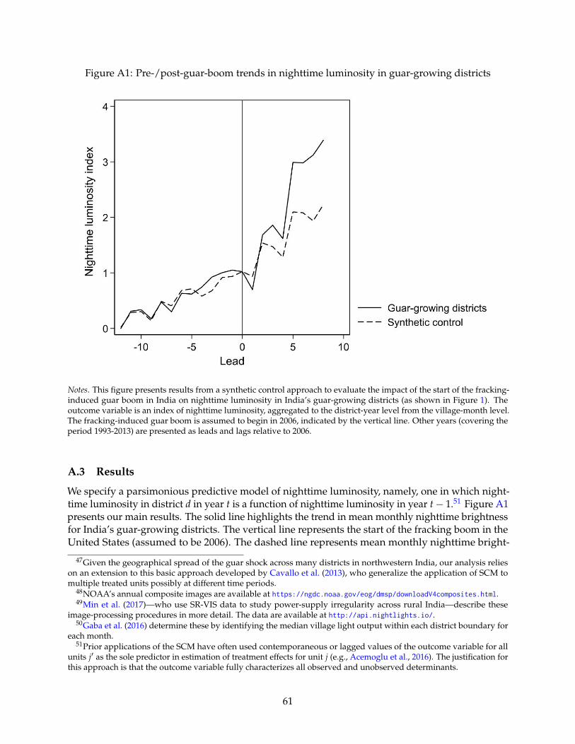
Figure A1: Pre-/post-guar-boom trends in nighttime luminosity in guar-growing districts
Notes. This figure presents results from a synthetic control approach to evaluate the impact of the start of the fracking-induced guar boom in India on nighttime luminosity in India’s guar-growing districts (as shown in Figure 1). Theoutcome variable is an index of nighttime luminosity, aggregated to the district-year level from the village-month level.The fracking-induced guar boom is assumed to begin in 2006, indicated by the vertical line. Other years (covering theperiod 1993-2013) are presented as leads and lags relative to 2006.
A.3 Results
We specify a parsimonious predictive model of nighttime luminosity, namely, one in which night-time luminosity in district d in year t is a function of nighttime luminosity in year t − 1.51 Figure A1presents our main results. The solid line highlights the trend in mean monthly nighttime brightnessfor India’s guar-growing districts. The vertical line represents the start of the fracking boom in theUnited States (assumed to be 2006). The dashed line represents mean monthly nighttime bright-
47Given the geographical spread of the guar shock across many districts in northwestern India, our analysis relieson an extension to this basic approach developed by Cavallo et al. (2013), who generalize the application of SCM tomultiple treated units possibly at different time periods.
48NOAA’s annual composite images are available at https://ngdc.noaa.gov/eog/dmsp/downloadV4composites.html.49Min et al. (2017)—who use SR-VIS data to study power-supply irregularity across rural India—describe these
image-processing procedures in more detail. The data are available at http://api.nightlights.io/.50Gaba et al. (2016) determine these by identifying the median village light output within each district boundary for
each month.51Prior applications of the SCM have often used contemporaneous or lagged values of the outcome variable for all
units j′ as the sole predictor in estimation of treatment effects for unit j (e.g., Acemoglu et al., 2016). The justification forthis approach is that the outcome variable fully characterizes all observed and unobserved determinants.
61
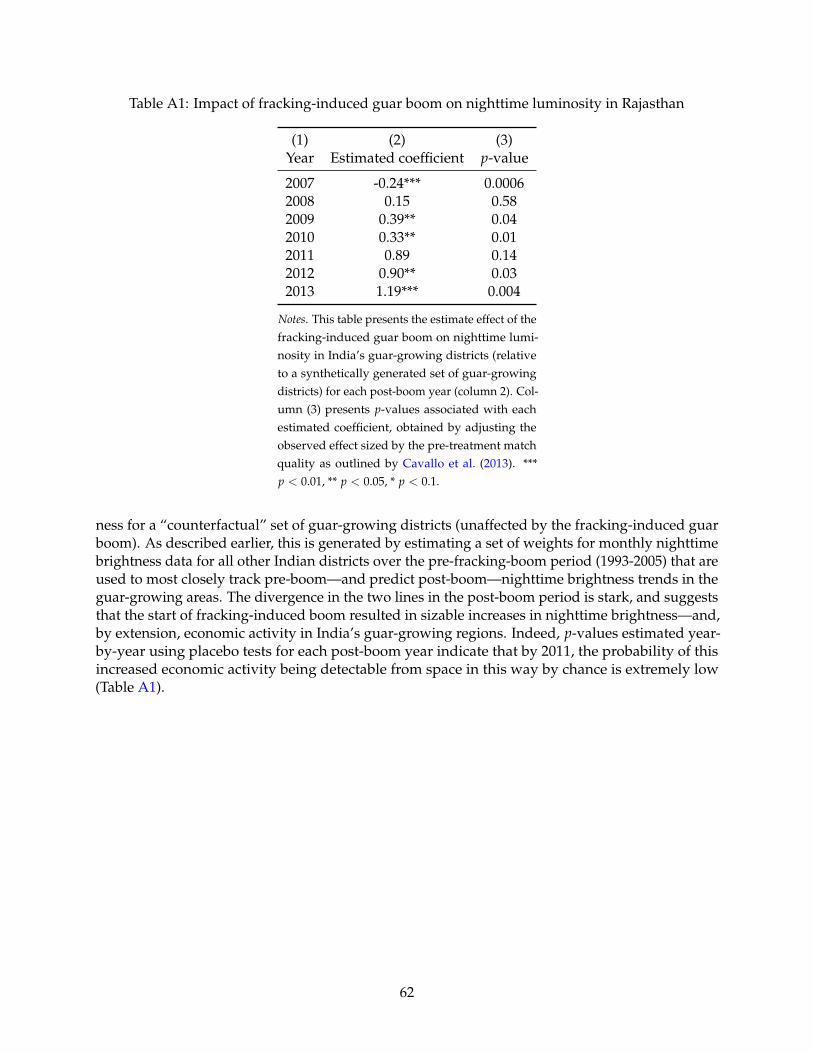
Table A1: Impact of fracking-induced guar boom on nighttime luminosity in Rajasthan
(1) (2) (3)Year Estimated coefficient p-value
2007 -0.24*** 0.00062008 0.15 0.582009 0.39** 0.042010 0.33** 0.012011 0.89 0.142012 0.90** 0.032013 1.19*** 0.004
Notes. This table presents the estimate effect of thefracking-induced guar boom on nighttime lumi-nosity in India’s guar-growing districts (relativeto a synthetically generated set of guar-growingdistricts) for each post-boom year (column 2). Col-umn (3) presents p-values associated with eachestimated coefficient, obtained by adjusting theobserved effect sized by the pre-treatment matchquality as outlined by Cavallo et al. (2013). ***p < 0.01, ** p < 0.05, * p < 0.1.
ness for a “counterfactual” set of guar-growing districts (unaffected by the fracking-induced guarboom). As described earlier, this is generated by estimating a set of weights for monthly nighttimebrightness data for all other Indian districts over the pre-fracking-boom period (1993-2005) that areused to most closely track pre-boom—and predict post-boom—nighttime brightness trends in theguar-growing areas. The divergence in the two lines in the post-boom period is stark, and suggeststhat the start of fracking-induced boom resulted in sizable increases in nighttime brightness—and,by extension, economic activity in India’s guar-growing regions. Indeed, p-values estimated year-by-year using placebo tests for each post-boom year indicate that by 2011, the probability of thisincreased economic activity being detectable from space in this way by chance is extremely low(Table A1).
62
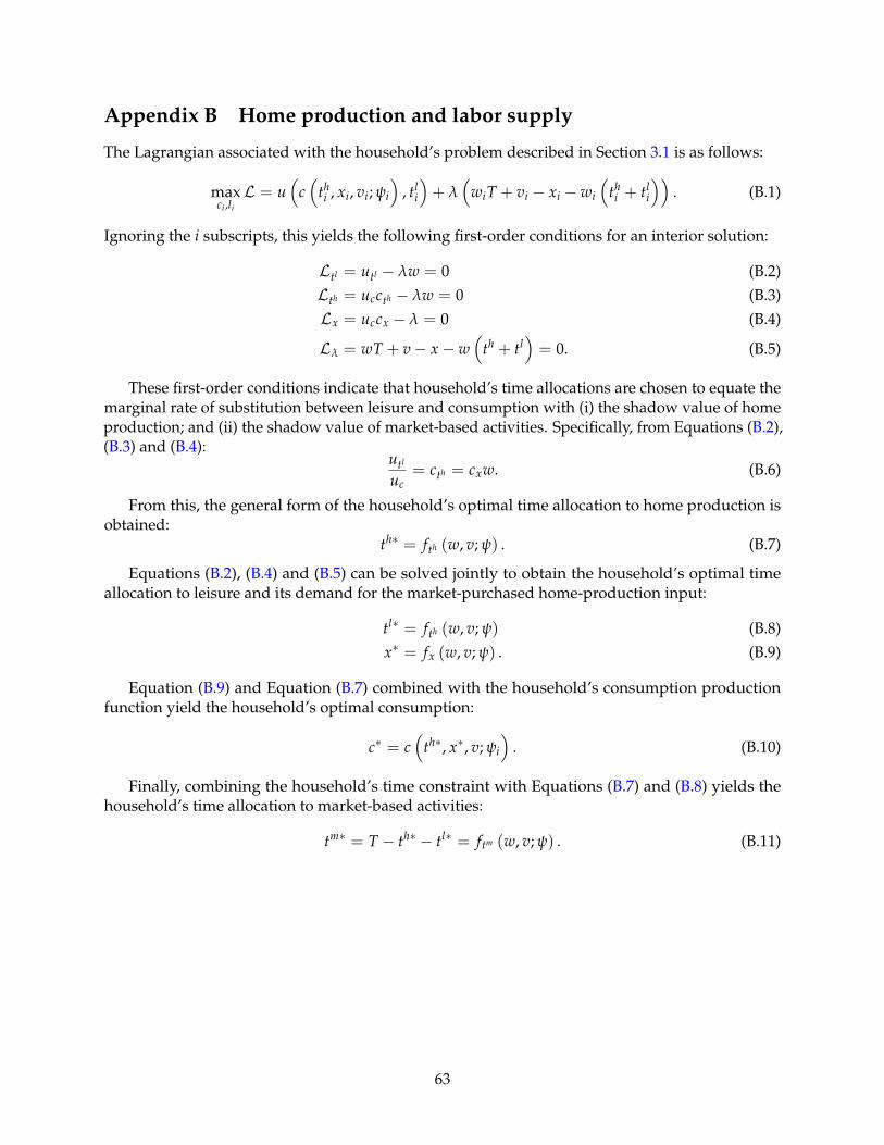
Appendix B Home production and labor supply
The Lagrangian associated with the household’s problem described in Section 3.1 is as follows:
maxci ,li
L = u(
c(
thi , xi, vi; ψi
), tl
i
)+ λ
(wiT + vi − xi − wi
(thi + tl
i
)). (B.1)
Ignoring the i subscripts, this yields the following first-order conditions for an interior solution:
Ltl = utl − λw = 0 (B.2)Lth = uccth − λw = 0 (B.3)Lx = uccx − λ = 0 (B.4)
Lλ = wT + v − x − w(
th + tl)= 0. (B.5)
These first-order conditions indicate that household’s time allocations are chosen to equate themarginal rate of substitution between leisure and consumption with (i) the shadow value of homeproduction; and (ii) the shadow value of market-based activities. Specifically, from Equations (B.2),(B.3) and (B.4):
utl
uc= cth = cxw. (B.6)
From this, the general form of the household’s optimal time allocation to home production isobtained:
th∗ = fth (w, v; ψ) . (B.7)
Equations (B.2), (B.4) and (B.5) can be solved jointly to obtain the household’s optimal timeallocation to leisure and its demand for the market-purchased home-production input:
tl∗ = fth (w, v; ψ) (B.8)x∗ = fx (w, v; ψ) . (B.9)
Equation (B.9) and Equation (B.7) combined with the household’s consumption productionfunction yield the household’s optimal consumption:
c∗ = c(
th∗, x∗, v; ψi
). (B.10)
Finally, combining the household’s time constraint with Equations (B.7) and (B.8) yields thehousehold’s time allocation to market-based activities:
tm∗ = T − th∗ − tl∗ = ftm (w, v; ψ) . (B.11)
63
Appendix C Habitation-Village matching procedure
We use a multi-step matching procedure to identify villages eligible for electrification under RGGVYPhase I based on the populations of their constituent habitations, and identify corresponding villagenames from the 2001 and 2011 Census to those in the 2009 census of habitations conducted by theNational Rural Drinking Water Program (NRDWP). The NRDWP habitation census covers 1.65million habitations in 574,259 villages.52 Because the NRDWP survey indicates only the name ofeach village (and not its unique Census code), matching on names is necessary; however, not allvillage names match exactly between the names used in NRDWP and those used in the Census,even conditional on an exact match for state and district. Accordingly, our matching processincorporates a combination of exact and fuzzy name matches, prioritizing exact matches wherepossible.
We treat the 2001 Primary Census Abstract (PCA) villages as the master dataset. As a first stepfor matching village names with the 2009 NRDWP habitations data, we standardize state, district,block, and village names to correct minor differences in spelling between the names in use by theNRDWP and the Census. We also account for districts that were renamed between 2001 and 2009.Our procedure for standardizing state and district names is sufficiently comprehensive to achieve a100 percent match among state and district names between the NRDWP and Census, except for ahandful of cases where districts are split or combined (not just renamed) between 2001 and 2009.53
We use information from the state, district, block, and village level, and prioritize exact matches.Where exact name matches are not possible, we employ a fuzzy match, using the “masalafiedLevenshtein” distance and “Masala merge” code in Stata and Python (Asher and Novosad, 2018).This is a modification of the standard Levenshtein string distance metric, one that lowers the costof certain substitutions that are common in Indian languages.54 We thus create a five-tier matchinghierarchy:
1. Exact match on state, district, block, and village name;
2. Exact match on state, district, and village name, with a fuzzy match on block name;
3. Exact match on state and district name, with a fuzzy match on block and village name;
4. Exact match on state, district, and village name (without regard to block name); and
5. Exact match on state and district name, with a fuzzy match on village name (without regardto block name).
52This includes five of the seven Union Territories—Chandigarh, Dadra and Nagar Haveli, Daman and Diu, Lakshad-weep, and Puducherry—and Goa. However, we exclude these from the merge process because Goa and all seven UnionTerritories were fully electrified prior to 2005, so were excluded in RGGVY (Ministry of Power, 2012). Excluding theseven Union Territories and Goa, the 2009 survey covers 1.65 million habitations in 573,702 villages.
53One approach to match villages in split or combined districts would be to geolocate all villages from the old district(s)into the new district(s). We take a somewhat less intensive approach and look for name-based village matches in aproper subset of the old or new district area—specifically, an area of known overlap between old and new. For instance,Tiruppur district in Tamil Nadu was formed in 2009 from parts of Coimbatore and Erode. Among villages in theNRDWP belonging to Tiruppur district, we look for matching Census village names within Erode district, but not withinCoimbatore district. We also flag any matches associated with split or combined districts. We have run our matchingalgorithm excluding these flagged matches and, after completing all five steps of the multi-step procedure, achievedvirtually identical results.
54Additional information about Masala merge (including its underlying code) is available at http://www.dartmouth.edu/~novosad/code.html.
64
Of the 563,338 villages in the 2001 Census, we match 531,325 to villages in the NRDWP habi-tation census (94.3 percent). This includes 400,457 exact matches (71 percent), of which 271,774(48 percent) are exact matches on state, district, block, and village name.55 Further, our algorithmachieves a 90 percent or greater match rate across every state with the exception of Tripura (36percent), Tamil Nadu (76 percent), Jammu and Kashmir (78 percent), Nagaland (82 percent), andAssam (83 percent). We also match at least 96 percent of villages in each of the three northwesternstates where guar is produced (98 percent in Rajasthan and Gujarat, and 96 percent in Haryana).
As a further verification step, we compare the village population recorded by the NRDWP in2009 to the village population recorded by the 2011 PCA. For any village name match in whichthese figures diverge by more than 20 percent, we exclude the village from the matched set.56 Usingthis matched sample, we identify single-habitation villages, and use the population of each of thesein the 2001 round of the Census to gauge its eligibility for electrification under RGGVY Phase I.
55Our match rate is comparable to others in the literature. For instance, Burlig and Preonas (2016) report matching86 percent of villages from the 2003 and 2009 NRDWP habitation surveys to corresponding Census villages. WhileAsher and Novosad (2018) do not report a village-level match rate, they do indicate they matched over 85 percent ofhabitations listed in the PMGSY to corresponding Census villages. Aggarwal (2018), who also evaluates the impact ofIndia’s rural roads program, reports a match rate of 80 percent.
56We have also run our analysis using thresholds other than 20 percent and find substantially similar results (FigureD1).
65
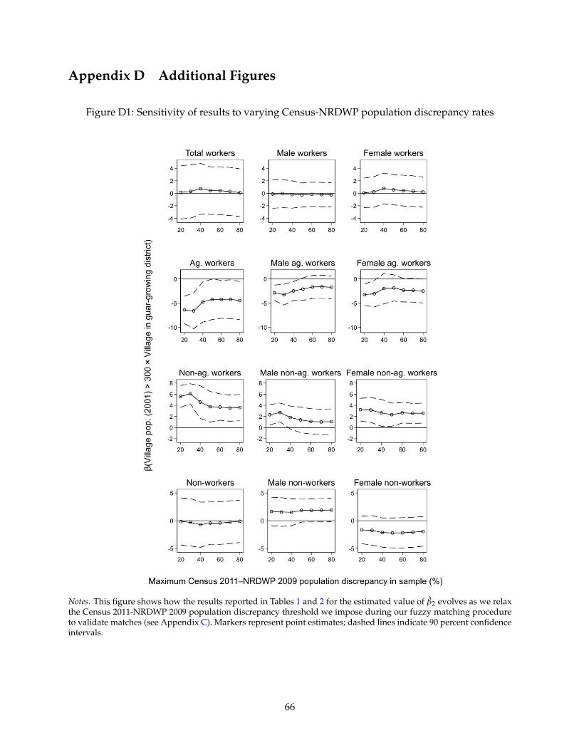
Appendix D Additional Figures
Figure D1: Sensitivity of results to varying Census-NRDWP population discrepancy rates
Notes. This figure shows how the results reported in Tables 1 and 2 for the estimated value of β̂2 evolves as we relaxthe Census 2011-NRDWP 2009 population discrepancy threshold we impose during our fuzzy matching procedureto validate matches (see Appendix C). Markers represent point estimates; dashed lines indicate 90 percent confidenceintervals.
66
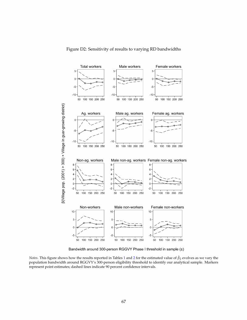
Figure D2: Sensitivity of results to varying RD bandwidths
Notes. This figure shows how the results reported in Tables 1 and 2 for the estimated value of β̂2 evolves as we vary thepopulation bandwidth around RGGVY’s 300-person eligibility threshold to identify our analytical sample. Markersrepresent point estimates; dashed lines indicate 90 percent confidence intervals.
67
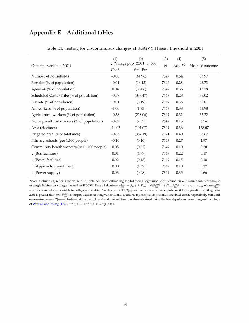
Appendix E Additional tables
Table E1: Testing for discontinuous changes at RGGVY Phase I threshold in 2001
(1) (2) (3) (4) (5)
Outcome variable (2001)1 (Village pop. (2001) > 300) N Adj. R2 Mean of outcomeCoef. Std. Err.
Number of households -0.08 (61.96) 7649 0.64 53.97
Females (% of population) -0.01 (16.43) 7649 0.28 48.73
Ages 0–6 (% of population) 0.04 (35.86) 7649 0.36 17.78
Scheduled Caste/Tribe (% of population) -0.57 (338.47) 7649 0.28 36.02
Literate (% of population) -0.01 (6.49) 7649 0.36 45.01
All workers (% of population) -1.00 (1.93) 7649 0.38 43.98
Agricultural workers (% of population) -0.38 (228.06) 7649 0.32 37.22
Non-agricultural workers (% of population) -0.62 (2.87) 7649 0.15 6.76
Area (Hectares) -14.02 (101.07) 7649 0.36 158.07
Irrigated area (% of total area) -0.65 (387.19) 7324 0.40 35.67
Primary schools (per 1,000 people) -0.10 (0.40) 7649 0.27 1.97
Community health workers (per 1,000 people) 0.05 (0.22) 7649 0.10 0.20
1 (Bus facilities) 0.01 (4.77) 7649 0.22 0.17
1 (Postal facilities) 0.02 (0.13) 7649 0.15 0.18
1 (Approach: Paved road) 0.00 (4.37) 7649 0.10 0.37
1 (Power supply) 0.03 (0.08) 7649 0.35 0.66
Notes. Column (1) reports the value of β̂1 obtained from estimating the following regression specification on our main analytical sampleof single-habitation villages located in RGGVY Phase I districts: y2001
vds = β0 + β1Tvds + β2P̃2001vds + β3Tvds P̃2001
vds + γd + γs + εvds, where y2001vds
represents an outcome variable for village v in district d in state s in 2001, Tvds is a binary variable that equals one if the population of village v in2001 is greater than 300, P̃2001
vds is the population running variable, and γd and γs represent a district and state fixed-effect, respectively. Standarderrors—in column (2)—are clustered at the district level and inferred from p-values obtained using the free step-down resampling methodologyof Westfall and Young (1993). *** p < 0.01, ** p < 0.05, * p < 0.1.
68
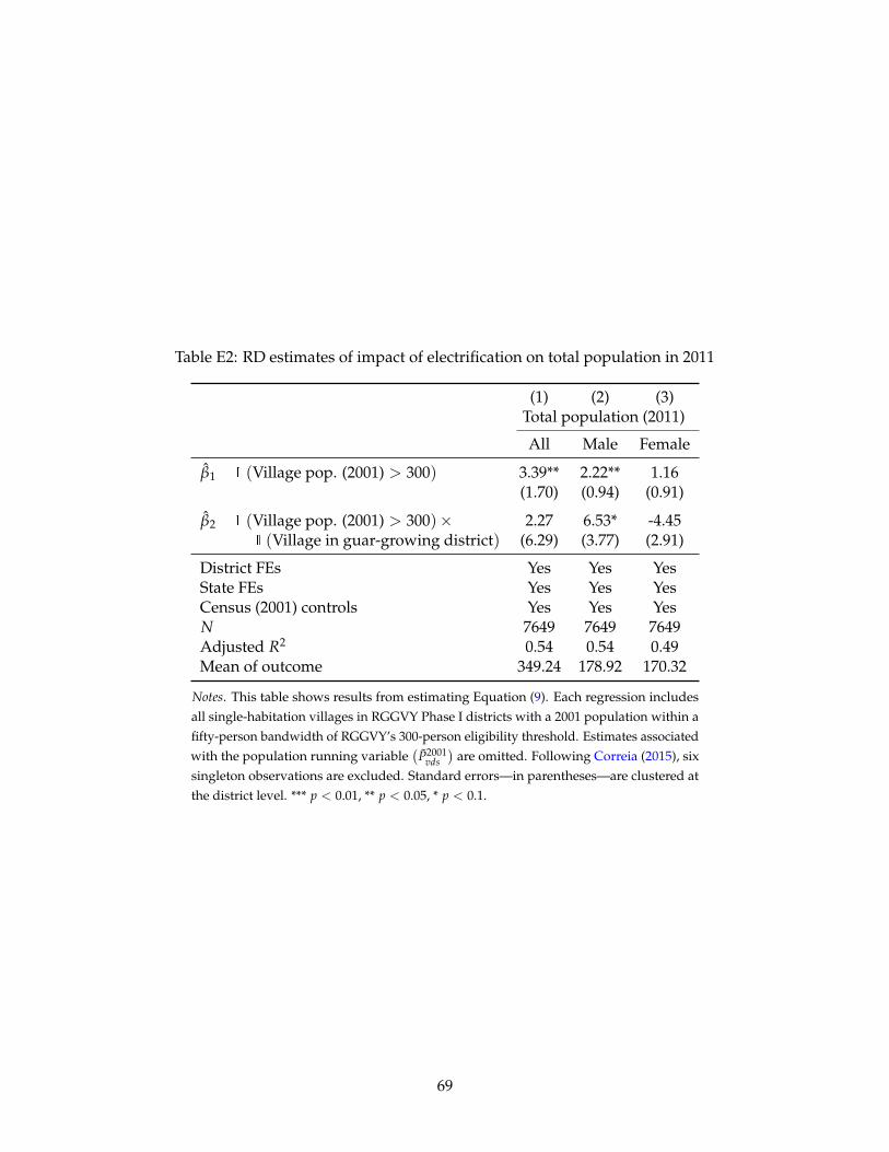
Table E2: RD estimates of impact of electrification on total population in 2011
(1) (2) (3)Total population (2011)
All Male Female
β̂1 1 (Village pop. (2001) > 300) 3.39** 2.22** 1.16(1.70) (0.94) (0.91)
β̂2 1 (Village pop. (2001) > 300)× 2.27 6.53* -4.451 (Village in guar-growing district) (6.29) (3.77) (2.91)
District FEs Yes Yes YesState FEs Yes Yes YesCensus (2001) controls Yes Yes YesN 7649 7649 7649Adjusted R2 0.54 0.54 0.49Mean of outcome 349.24 178.92 170.32
Notes. This table shows results from estimating Equation (9). Each regression includesall single-habitation villages in RGGVY Phase I districts with a 2001 population within afifty-person bandwidth of RGGVY’s 300-person eligibility threshold. Estimates associatedwith the population running variable
(P̃2001
vds)
are omitted. Following Correia (2015), sixsingleton observations are excluded. Standard errors—in parentheses—are clustered atthe district level. *** p < 0.01, ** p < 0.05, * p < 0.1.
69
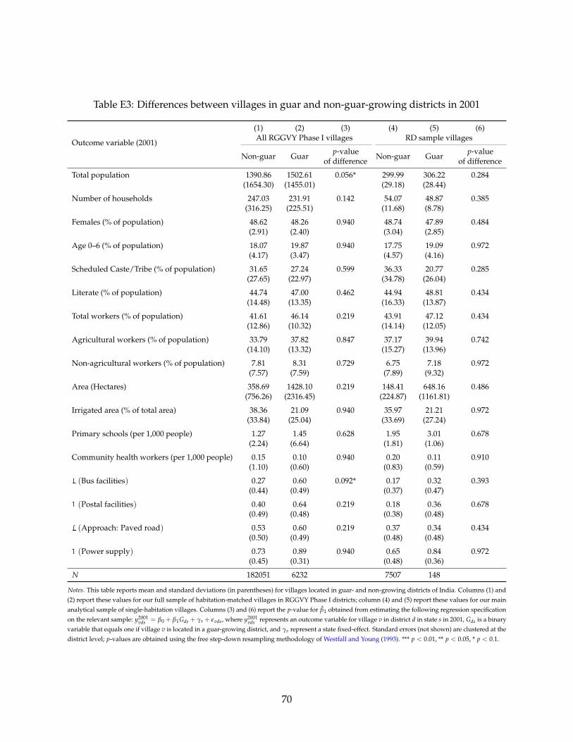
Table E3: Differences between villages in guar and non-guar-growing districts in 2001
Outcome variable (2001)
(1) (2) (3) (4) (5) (6)All RGGVY Phase I villages RD sample villages
Non-guar Guarp-value
Non-guar Guarp-value
of difference of difference
Total population 1390.86 1502.61 0.056* 299.99 306.22 0.284(1654.30) (1455.01) (29.18) (28.44)
Number of households 247.03 231.91 0.142 54.07 48.87 0.385(316.25) (225.51) (11.68) (8.78)
Females (% of population) 48.62 48.26 0.940 48.74 47.89 0.484(2.91) (2.40) (3.04) (2.85)
Age 0–6 (% of population) 18.07 19.87 0.940 17.75 19.09 0.972(4.17) (3.47) (4.57) (4.16)
Scheduled Caste/Tribe (% of population) 31.65 27.24 0.599 36.33 20.77 0.285(27.65) (22.97) (34.78) (26.04)
Literate (% of population) 44.74 47.00 0.462 44.94 48.81 0.434(14.48) (13.35) (16.33) (13.87)
Total workers (% of population) 41.61 46.14 0.219 43.91 47.12 0.434(12.86) (10.32) (14.14) (12.05)
Agricultural workers (% of population) 33.79 37.82 0.847 37.17 39.94 0.742(14.10) (13.32) (15.27) (13.96)
Non-agricultural workers (% of population) 7.81 8.31 0.729 6.75 7.18 0.972(7.57) (7.59) (7.89) (9.32)
Area (Hectares) 358.69 1428.10 0.219 148.41 648.16 0.486(756.26) (2316.45) (224.87) (1161.81)
Irrigated area (% of total area) 38.36 21.09 0.940 35.97 21.21 0.972(33.84) (25.04) (33.69) (27.24)
Primary schools (per 1,000 people) 1.27 1.45 0.628 1.95 3.01 0.678(2.24) (6.64) (1.81) (1.06)
Community health workers (per 1,000 people) 0.15 0.10 0.940 0.20 0.11 0.910(1.10) (0.60) (0.83) (0.59)
1 (Bus facilities) 0.27 0.60 0.092* 0.17 0.32 0.393(0.44) (0.49) (0.37) (0.47)
1 (Postal facilities) 0.40 0.64 0.219 0.18 0.36 0.678(0.49) (0.48) (0.38) (0.48)
1 (Approach: Paved road) 0.53 0.60 0.219 0.37 0.34 0.434(0.50) (0.49) (0.48) (0.48)
1 (Power supply) 0.73 0.89 0.940 0.65 0.84 0.972(0.45) (0.31) (0.48) (0.36)
N 182051 6232 7507 148
Notes. This table reports mean and standard deviations (in parentheses) for villages located in guar- and non-growing districts of India. Columns (1) and(2) report these values for our full sample of habitation-matched villages in RGGVY Phase I districts; column (4) and (5) report these values for our mainanalytical sample of single-habitation villages. Columns (3) and (6) report the p-value for β̂1 obtained from estimating the following regression specificationon the relevant sample: y2001
vds = β0 + β1Gds + γs + εvds, where y2001vds represents an outcome variable for village v in district d in state s in 2001, Gds is a binary
variable that equals one if village v is located in a guar-growing district, and γs represent a state fixed-effect. Standard errors (not shown) are clustered at thedistrict level; p-values are obtained using the free step-down resampling methodology of Westfall and Young (1993). *** p < 0.01, ** p < 0.05, * p < 0.1.
70
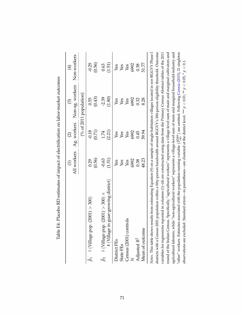
Tabl
eE4
:Pla
cebo
RD
esti
mat
esof
impa
ctof
elec
trifi
cati
onon
labo
r-m
arke
tout
com
es
(1)
(2)
(3)
(4)
All
wor
kers
Ag.
wor
kers
Non
-ag.
wor
kers
Non
-wor
kers
(%of
2011
popu
lati
on)
β̂1
1(V
illag
epo
p.(2
001)
>30
0 )0.
29-0
.18
0.55
-0.2
9(0
.56)
(0.7
1)(0
.43)
(0.5
6)
β̂2
1(V
illag
epo
p.(2
001)
>30
0 )×
-0.6
31.
74-2
.39
0.63
1(V
illag
ein
guar
-gro
win
gdi
stri
ct)
(1.5
1)(2
.21)
(1.8
0)(1
.51)
Dis
tric
tFEs
Yes
Yes
Yes
Yes
Stat
eFE
sYe
sYe
sYe
sYe
sC
ensu
s(2
001)
cont
rols
Yes
Yes
Yes
Yes
N69
9269
9269
9269
92A
djus
ted
R2
0.38
0.45
0.32
0.38
Mea
nof
outc
ome
48.2
339
.94
8.28
51.7
7
Not
es.T
his
tabl
esh
ows
resu
lts
from
esti
mat
ing
Equ
atio
n(9
)on
asa
mpl
eof
sing
le-h
abit
atio
nvi
llage
slo
cate
din
non-
RG
GV
YP
hase
Id
istr
icts
wit
ha
Cen
sus
2001
popu
lati
onw
ithi
na
fifty
-per
son
band
wid
thar
ound
RG
GV
Y’s
300-
pers
onel
igib
ility
thre
shol
d.O
utco
me
vari
able
sfo
rre
gres
sion
sre
por
ted
inco
lum
ns(1
)–(4
)are
cons
tru
cted
usi
ngd
ata
from
the
Pri
mar
yC
ensu
sA
bstr
actt
able
sof
the
2011
rou
ndof
the
Ind
ian
Cen
sus.
Spec
ifica
lly,“
agri
cult
ura
lwor
kers
”re
pres
ents
avi
llage
-lev
elsu
mof
mai
nan
dm
argi
nalc
ult
ivat
ors
and
agri
cult
ural
labo
rers
,whi
le“n
on-a
gric
ultu
ralw
orke
rs”
repr
esen
tsa
villa
ge-l
evel
sum
ofm
ain
and
mar
gina
lhou
seho
ld-i
ndus
try
and
“oth
er”
wor
kers
.Est
imat
esas
soci
ated
with
the
popu
latio
nru
nnin
gva
riab
le( P̃
2001
vds) ar
eom
itted
.Fol
low
ing
Cor
reia
(201
5),2
1si
ngle
ton
obse
rvat
ions
are
excl
uded
.Sta
ndar
der
rors
—in
pare
nthe
ses—
are
clus
tere
dat
the
dist
rict
leve
l.**
*p<
0.01
,**
p<
0.05
,*p<
0.1.
71
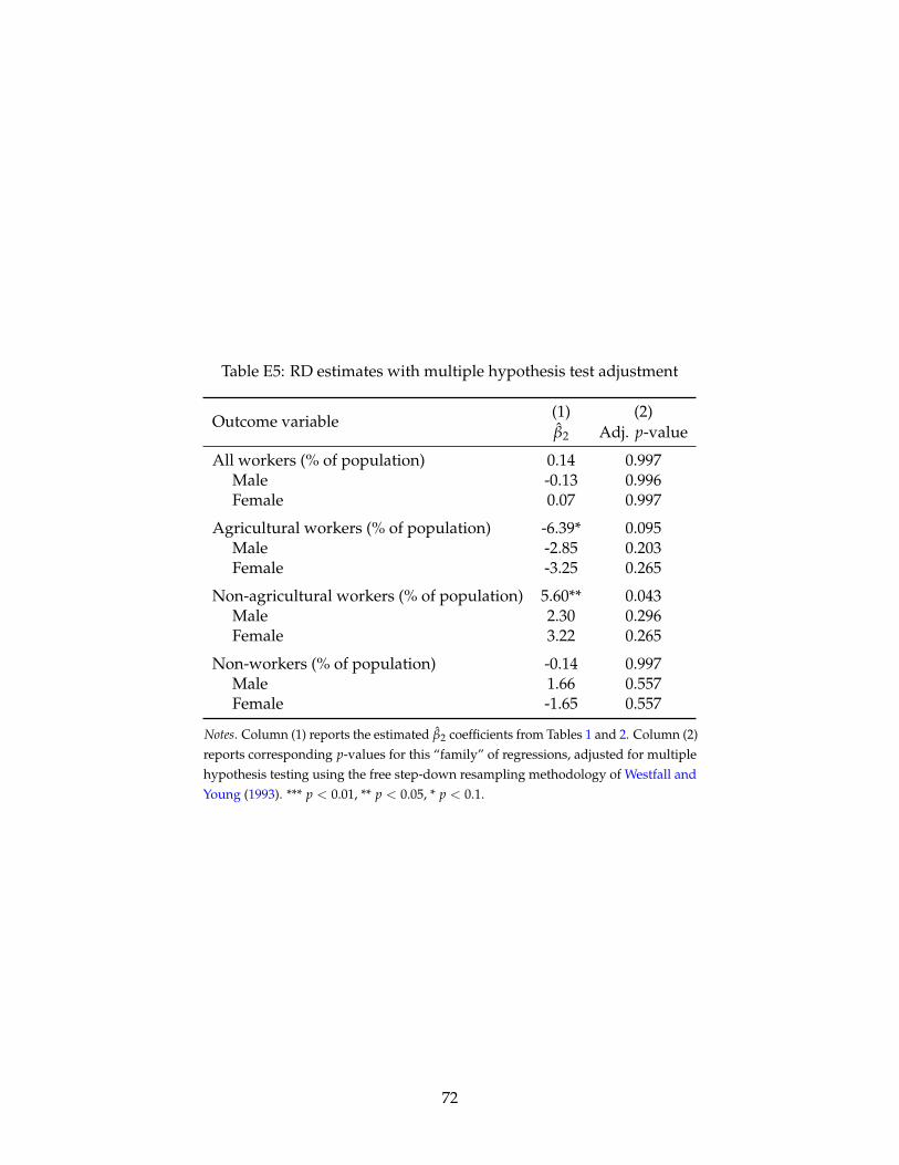
Table E5: RD estimates with multiple hypothesis test adjustment
Outcome variable(1) (2)β̂2 Adj. p-value
All workers (% of population) 0.14 0.997Male -0.13 0.996Female 0.07 0.997
Agricultural workers (% of population) -6.39* 0.095Male -2.85 0.203Female -3.25 0.265
Non-agricultural workers (% of population) 5.60** 0.043Male 2.30 0.296Female 3.22 0.265
Non-workers (% of population) -0.14 0.997Male 1.66 0.557Female -1.65 0.557
Notes. Column (1) reports the estimated β̂2 coefficients from Tables 1 and 2. Column (2)reports corresponding p-values for this “family” of regressions, adjusted for multiplehypothesis testing using the free step-down resampling methodology of Westfall andYoung (1993). *** p < 0.01, ** p < 0.05, * p < 0.1.
72