foundation engineering prof. kousik deb department of civil
TRANSCRIPT

Foundation EngineeringProf. Kousik Deb
Department of Civil EngineeringIndian Institute of Technology, Kharagpur
Lecture - 15Shallow Foundation - Bearing Capacity V
So, in the last lecture I have discussed about the Meyerhof bearing capacity theory and
the Hansen bearing capacity theory. Now, this lecture I will discuss 2 more bearing
capacity theories, which is proposed by the basic and the is code or Indian standard code.
So, in the basic also proposed the similar type of bearing capacity theory.
(Refer Slide Time: 00:42)
So, that is this is similar to the Hansen’s equation. So, the N c N q is same as Meyerhof
recommendation, which is also similar to the Hansen’s equation, but N gamma
expression is different as compared to the Meyerhof theory and the Hansen’s theory.
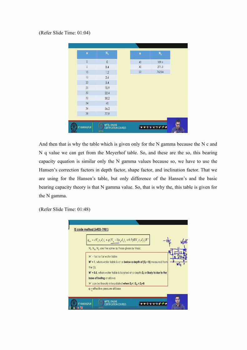
(Refer Slide Time: 01:04)
And then that is why the table which is given only for the N gamma because the N c and
N q value we can get from the Meyerhof table. So, and these are the so, this bearing
capacity equation is similar only the N gamma values because so, we have to use the
Hansen’s correction factors in depth factor, shape factor, and inclination factor. That we
are using for the Hansen’s table, but only difference of the Hansen’s and the basic
bearing capacity theory is that N gamma value. So, that is why the, this table is given for
the N gamma.
(Refer Slide Time: 01:48)

And then the next one is the, is code method. So, is code Indian standard code also
recommend the net ultimate bearing capacity. So, all the previous theories are given the
ultimate bearing capacity, but is code is given directly the net ultimate bearing capacity,
that is why this in N q minus 1, because this minus 1 value means basically the minus
gamma into D f. So, in that form so, that is why this minus 1 term is introduced so, these
are N c N q N gamma are the same those are given by the basic. So, that when the N c N
q r in the Meyerhof’s N c N q and N gamma is the basic N gamma.
So, and then there is a water table effect is also incorporated. So, W dash is the factor for
the water table here the s c d c i c s shape depth factor, inclination factor, along that the
water table factor is also incorporated.
So, here the W dash value is 1, when the water is below the D f by B so; that means,
here. So, which is the similar to the other cases so; that means, if we if we this is the
ground surface and this is the depth of foundation and this is the B width of width of
foundation and if the depth of water table is here. So; that means, the total depth is D f by
B, then definitely there will be no effect. So, and then that value is 1.
Now, if this value is 0.5 when your W value is here so; that means, here W value is as
the 1 when water table is at D f or above that so; that means, from the below. So; that
means, if your D f value within if your water table is within the D f, above the base of
the footing then the W dash value is 0.5.
So, here the W dash value is 1 and here within this zone total zone. So, W dash value is
W dash value is 0.5. So, this is the recommendation is given and if so; that means, here
also 0.5. So, this point also 0.5 and here also 1.
So, now if water table is in between the base of the foundation and within the B from the
base then we have to calculate the W dash in by linear interpolation; that means, here is 1
here is 0.5. So, if it is at by 2 from the base, then it will be 0.7 5 like this. So, linearly we
have 2. So, this will be 0.7 5 it is at the base of the foundation.
So, like this we have 2 linearly interpolate the values of the W dash and here and as it is
mentioned that q in the effective pressure, which is acting on the base. So, and which is 2
for all the theories.
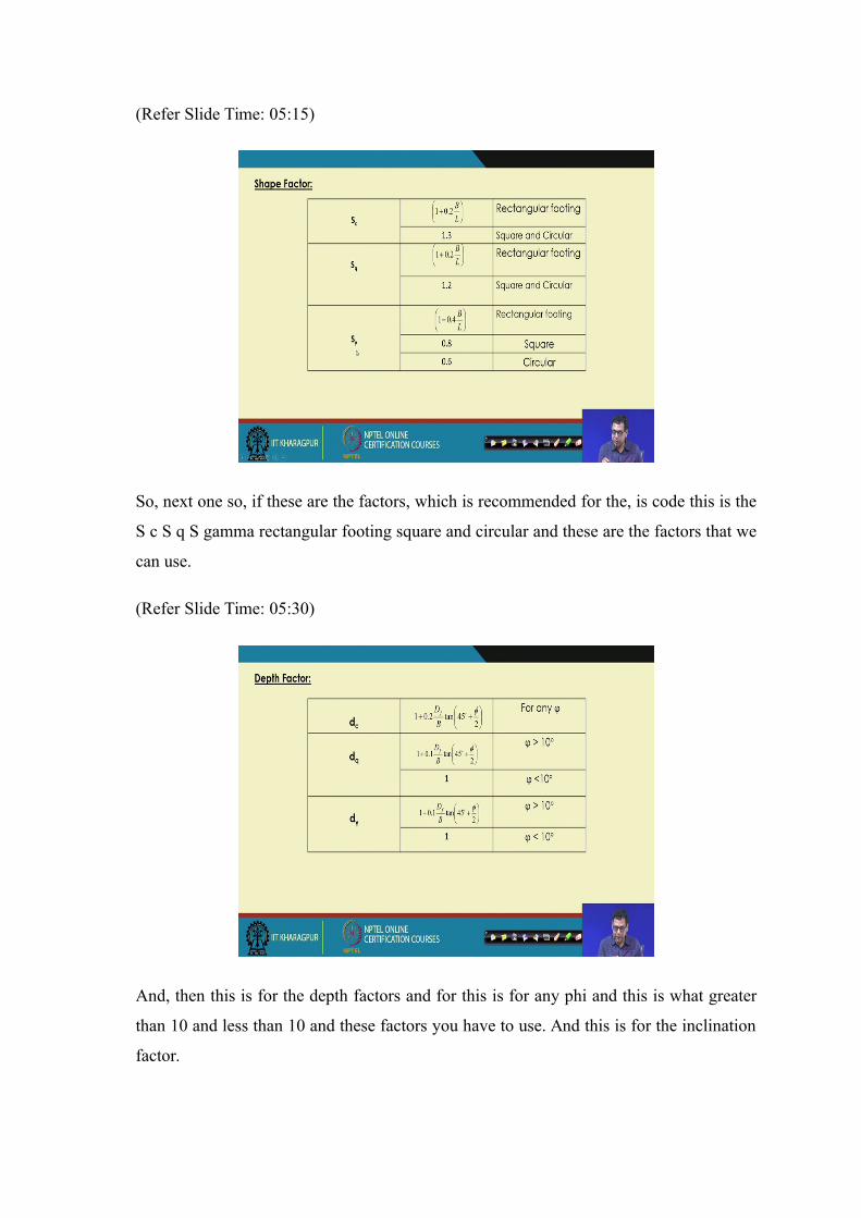
(Refer Slide Time: 05:15)
So, next one so, if these are the factors, which is recommended for the, is code this is the
S c S q S gamma rectangular footing square and circular and these are the factors that we
can use.
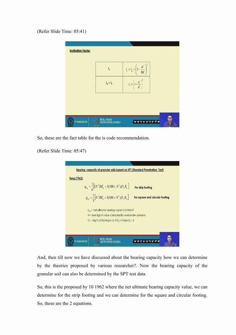
(Refer Slide Time: 05:30)
And, then this is for the depth factors and for this is for any phi and this is what greater
than 10 and less than 10 and these factors you have to use. And this is for the inclination
factor.
(Refer Slide Time: 05:41)
So, these are the fact table for the is code recommendation.
(Refer Slide Time: 05:47)
And, then till now we have discussed about the bearing capacity how we can determine
by the theories proposed by various researcher?. Now the bearing capacity of the
granular soil can also be determined by the SPT test data.
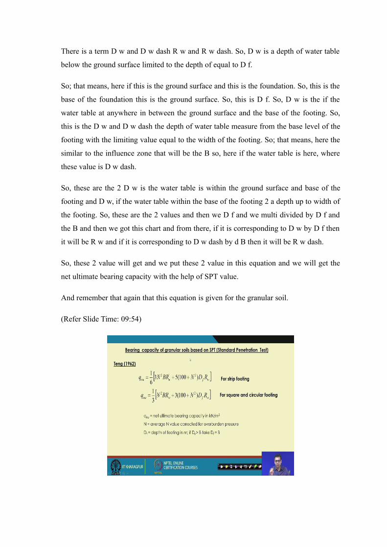
So, this is the proposed by 10 1962 where the net ultimate bearing capacity value, we can
determine for the strip footing and we can determine for the square and circular footing.
So, these are the 2 equations.
So, these equations or these recommendations are based on the observation. So, these are
called empirical relationship. So, this is some empirical relationship such are given. So,
these are coming from the observation, where this is the q nu is the net ultimate bearing
capacity, which is in kilo newton per meter square N is the average N value corrected for
overburden pressure.
So, this is corrected only for the overburden pressure not any other corrections is applied
along the measure m value. So, that corrected N value corrected by overburden is this N
and D f with the depth of the footing and if D f is greater than B, then take D f is equal to
B. So, this is the recommendation.
And so; that means, here what we have to do that we have to know the R w dash and R
w. So, these are the factors, which is for the water table in factors. So; that means, how I
can calculate R w dash and R w, because other things N value we can get we will get the
D f value if D f is greater than B we will get the D f is equal to B and then we will get the
B is the width of the foundation.
. So, now and in case of circular instead of B it will be the radius R so, that is obvious for
all the equations. And, then but these 2 corrections for the water table so, these are the
chart we can use for this is so; that means, what is D w.
(Refer Slide Time: 08:00)
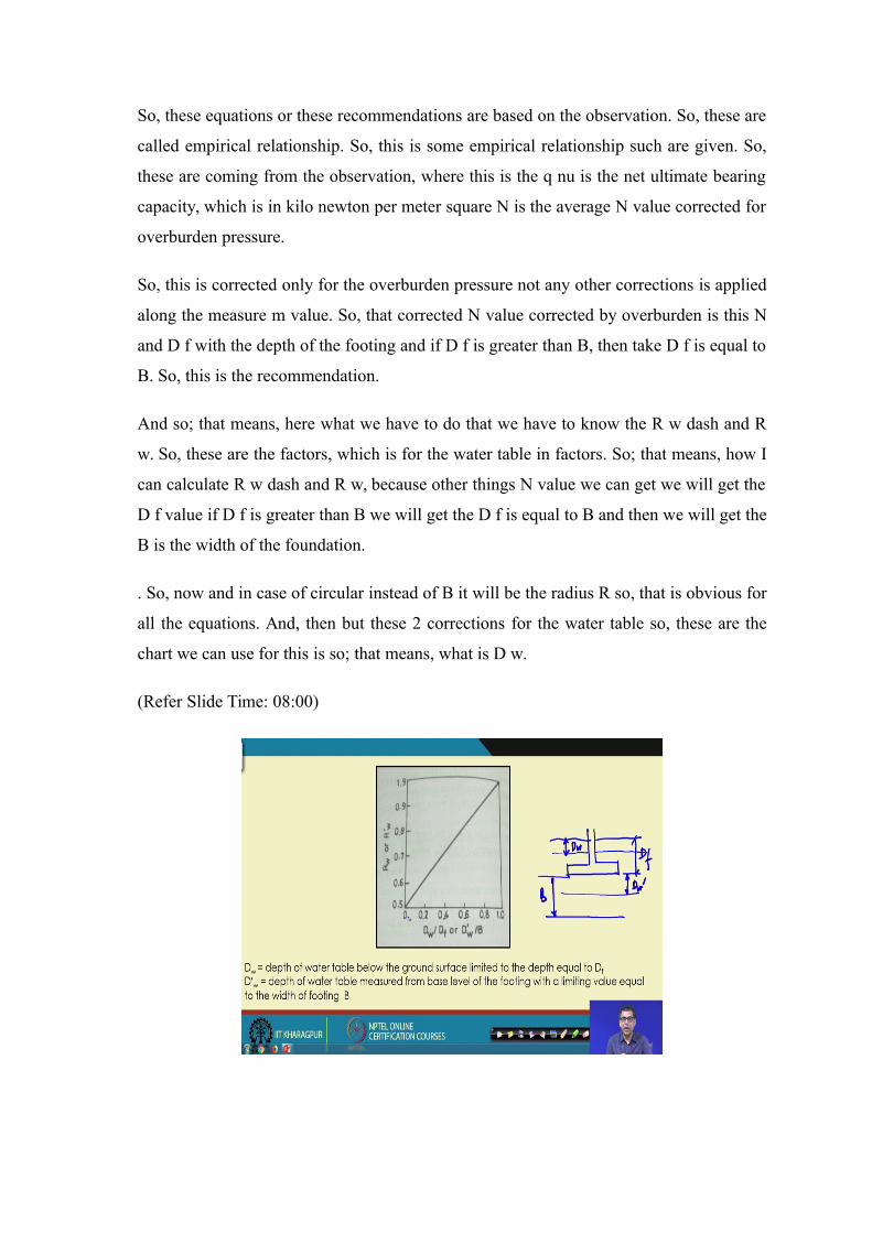
There is a term D w and D w dash R w and R w dash. So, D w is a depth of water table
below the ground surface limited to the depth of equal to D f.
So; that means, here if this is the ground surface and this is the foundation. So, this is the
base of the foundation this is the ground surface. So, this is D f. So, D w is the if the
water table at anywhere in between the ground surface and the base of the footing. So,
this is the D w and D w dash the depth of water table measure from the base level of the
footing with the limiting value equal to the width of the footing. So; that means, here the
similar to the influence zone that will be the B so, here if the water table is here, where
these value is D w dash.
So, these are the 2 D w is the water table is within the ground surface and base of the
footing and D w, if the water table within the base of the footing 2 a depth up to width of
the footing. So, these are the 2 values and then we D f and we multi divided by D f and
the B and then we got this chart and from there, if it is corresponding to D w by D f then
it will be R w and if it is corresponding to D w dash by d B then it will be R w dash.
So, these 2 value will get and we put these 2 value in this equation and we will get the
net ultimate bearing capacity with the help of SPT value.
And remember that again that this equation is given for the granular soil.
(Refer Slide Time: 09:54)
Because in all, the field test as I mentioned is most suitable for the granular soil and
before the cohesive soil because we can collect the undisturbed soil sample. So, we can
collect undisturbed sample take it to the lab then tasted get the proper shear strength of
bearing capacity equation parameters, and then we can get those parameter easily. So;
that means, here these test it is suitable for this expressions with the help of SPT suitable
for the granular soil.
(Refer Slide Time: 10:33)
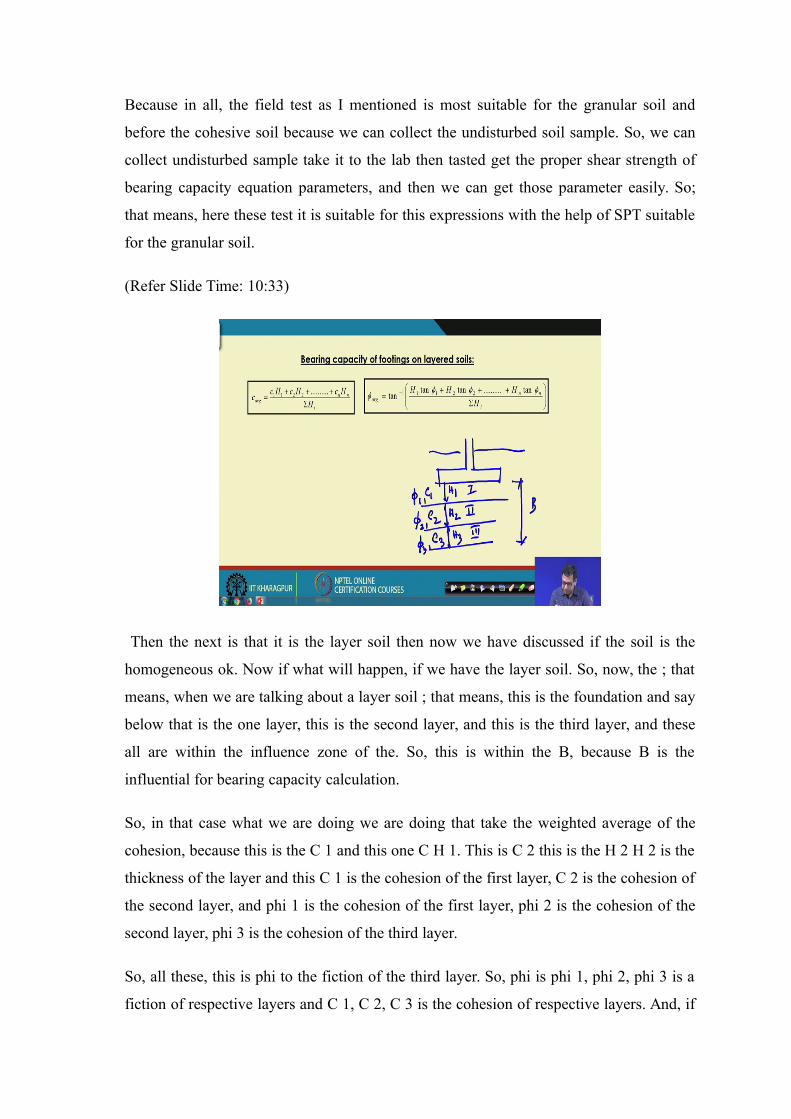
Then the next is that it is the layer soil then now we have discussed if the soil is the
homogeneous ok. Now if what will happen, if we have the layer soil. So, now, the ; that
means, when we are talking about a layer soil ; that means, this is the foundation and say
below that is the one layer, this is the second layer, and this is the third layer, and these
all are within the influence zone of the. So, this is within the B, because B is the
influential for bearing capacity calculation.
So, in that case what we are doing we are doing that take the weighted average of the
cohesion, because this is the C 1 and this one C H 1. This is C 2 this is the H 2 H 2 is the
thickness of the layer and this C 1 is the cohesion of the first layer, C 2 is the cohesion of
the second layer, and phi 1 is the cohesion of the first layer, phi 2 is the cohesion of the
second layer, phi 3 is the cohesion of the third layer.
So, all these, this is phi to the fiction of the third layer. So, phi is phi 1, phi 2, phi 3 is a
fiction of respective layers and C 1, C 2, C 3 is the cohesion of respective layers. And, if
all these things is within the influence zone then we have to take the weighted average of
the C and then the again the weighted average of the phi by using these expressions ok.
So, that is the one way we take care if the soil is layered soil. So, that way we can take
care this thing.
Another one these theories also develop for the layered soil, but for the design purpose in
this course I will use this technique, when this is the layered soil and we will use in this
way we will determine the friction and cohesion value by taking the weighted average.
(Refer Slide Time: 12:45)
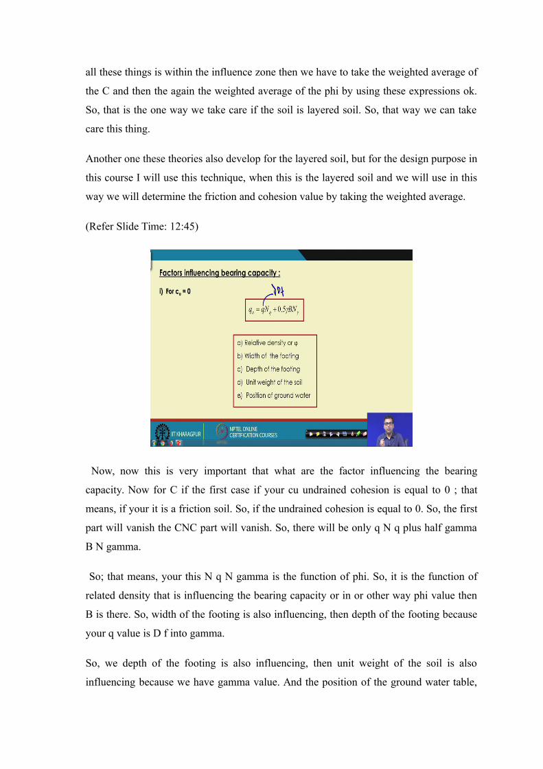
Now, now this is very important that what are the factor influencing the bearing
capacity. Now for C if the first case if your cu undrained cohesion is equal to 0 ; that
means, if your it is a friction soil. So, if the undrained cohesion is equal to 0. So, the first
part will vanish the CNC part will vanish. So, there will be only q N q plus half gamma
B N gamma.
So; that means, your this N q N gamma is the function of phi. So, it is the function of
related density that is influencing the bearing capacity or in or other way phi value then
B is there. So, width of the footing is also influencing, then depth of the footing because
your q value is D f into gamma.
So, we depth of the footing is also influencing, then unit weight of the soil is also
influencing because we have gamma value. And the position of the ground water table,
because as the position of the groundwater table changes then you have to your bearing
capacity value will change.
So, if it is the phi soil or the C equal to 0 case or if it is the granular soil, then these 5 are
the influencing factor for the bearing capacity.
(Refer Slide Time: 14:12)
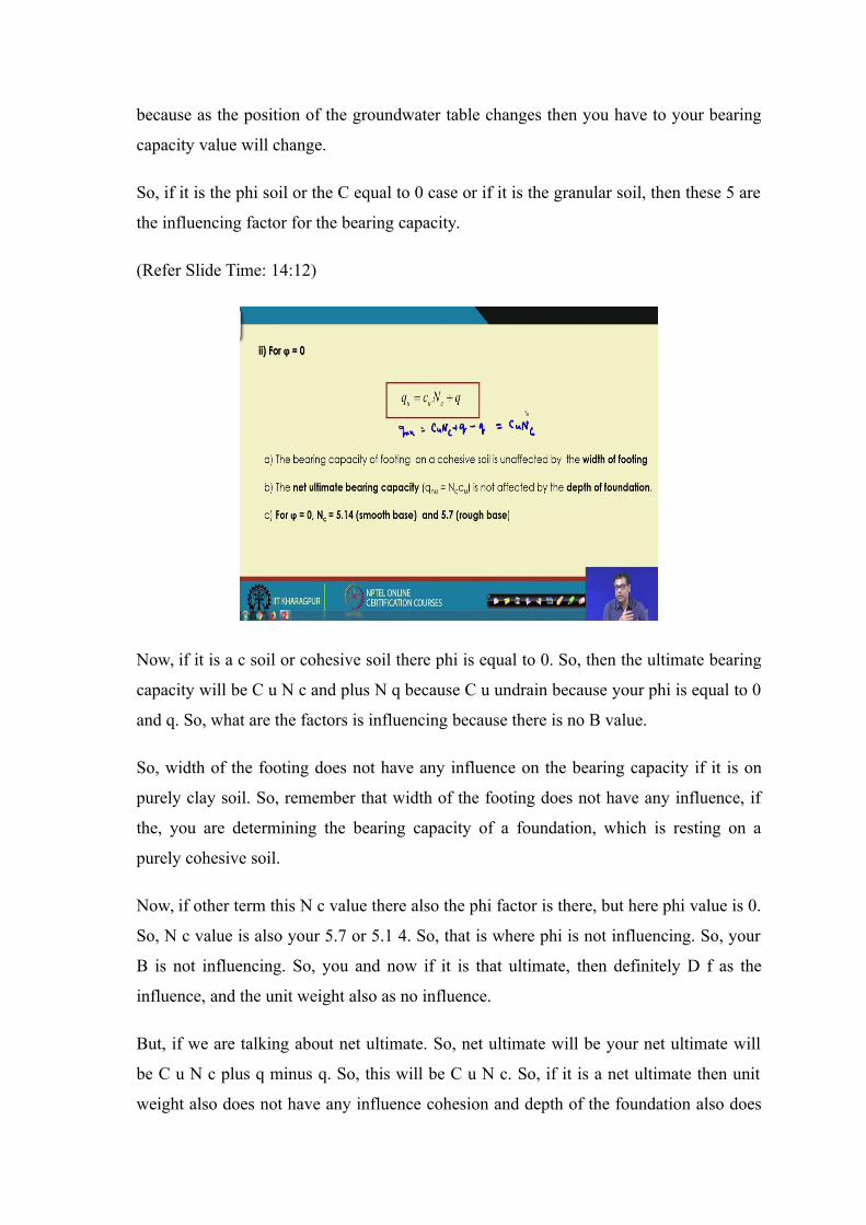
Now, if it is a c soil or cohesive soil there phi is equal to 0. So, then the ultimate bearing
capacity will be C u N c and plus N q because C u undrain because your phi is equal to 0
and q. So, what are the factors is influencing because there is no B value.
So, width of the footing does not have any influence on the bearing capacity if it is on
purely clay soil. So, remember that width of the footing does not have any influence, if
the, you are determining the bearing capacity of a foundation, which is resting on a
purely cohesive soil.
Now, if other term this N c value there also the phi factor is there, but here phi value is 0.
So, N c value is also your 5.7 or 5.1 4. So, that is where phi is not influencing. So, your
B is not influencing. So, you and now if it is that ultimate, then definitely D f as the
influence, and the unit weight also as no influence.
But, if we are talking about net ultimate. So, net ultimate will be your net ultimate will
be C u N c plus q minus q. So, this will be C u N c. So, if it is a net ultimate then unit
weight also does not have any influence cohesion and depth of the foundation also does

not have any influence in the bearing capacity. It is only cohesion and then 5.7 or 5.14
depending upon your roughness of the footing so; that means, it is only the cohesion
dependent value for if it is the net ultimate.
And so, and when we are talking about there is water table also when I discuss about the
water table correction, then we have not applied any correction in first term that is c N c
term. So, water table also does not have any influence, but water table indirectly as the
influence, but in that case this C u value will be influenced by the water. So, as I
mentioned if there is a water the in case of cohesive soil you have to determine the C
value under saturated condition.
(Refer Slide Time: 16:41)
Till now we have discussed so, many theories now this is the first example that we are
we are solving, that we are taking a common example and then we will determine the
bearing capacity value by using all the available theories ok.
So, the example that you are taking the rectangular footing of size 3 meter cross 6 meter
is founded at a depth of one meter in a homogeneous sandy soil. So, the water table is at
a great depth the unit weight of soil is 18th kilo newton meter per meter. So, this will be
the meter cube. So, this will be the meter cube 18 kilo Newton per meter cube, determine
the net ultimate bearing capacity if C is equal to 0 and phi is equal to 40 degree.
So, because if the sandy soil C cohesion value is 0 and the friction value is 40 degree and
this is a 3 cross 6 meter foundation and it is a homogeneous and so, and ion case of layer
will do the weighted average so, so, but it is a homogeneous.
And what our table is great; that means, water table is far below the depth from the base
of the footing; that means, you know the if water table from the base of the footing is
greater than the width of the footing and then we do not consider the water table effect.
So; that means, water does not have any effect. So, that is why the unit weight of the soil
and the unit weight we are taking the uniform because it is a homogeneous soil.
So, the first theory if I use the terzaghis bearing capacity theory so, the net ultimately
will be ultimate minus gamma D f. And D f is also 1 meter depth of foundation is 1
meter. And this is the equation and we are taking N q minus 1, because the gamma D f it
is common for q term. So, we are taking this equation.
So, now, from the terzaghis table N q value is 81.3 and N gamma value is 100.4 4
corresponding to phi equal to 40 degree, and B is equal to 3 meter l equal to 6 meter. So,
net ultimate bearing capacity will be 388 5.12 kilo Newton per Newton square. Now, if I
want to get the q net safe then we have to apply the q net ultimate by factor of safety. So,
this factor of safety value we are taking 2.5 to 3 and if I want to calculate the q safe
ultimate safe or safe ultimate then q ultimate divided by the factor of safety.
So, here a factor of safety is not used because we want the ultimate bear in net ultimate
bearing capacity. If it is safe net ultimate bearing capacity then you have to apply a factor
of safety of 2.5 by 3 with this value ; that means, 3 8 8 5. 12 divided by the 2.5 or 3,
which one you are using.
(Refer Slide Time: 20:00)
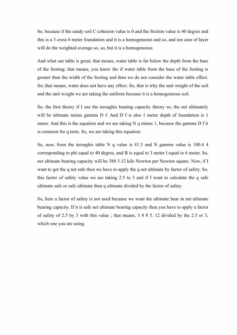
So, next theory is the meyerhofs theory and this is the expression q ultimate is this one
here we are using in the terzaghis theory you are using only the only the shape factor,
and here we are using shape factor and there factor, but inclination factor, we are not
using because the loading is acting vertically and at the center. So, it is not inclined it is
not even eccentric. So, it is vertically and the center, if it is not vertically, then you have
to incorporate the inclination factor also, but here it is not included
So, these are the factors from the table we are getting and from there from the
Meyerhof’s theory also in q 64.1 N gamma 90 3.7 and phi value is equal to 4
corresponding to the phi value 40 degree. And so, that is why we are using this value 4 8
3 0.11 by using the Meyerhof’s theory and remember that another thing I want to
mention that here your phi value is greater than 36 degree. So, this will be the local shear
failure so; that means, you have to we can use these phi directly as the phi value is
greater than 36 degree, if it is less than 29 degree then you have to or equal to 29 degree,
then you have to go for the. So, this it is phis greater than 36 degree. So, we have to go
for that general shear failure.
So, that is why we are using this equation. So, if because phi is great less than equal to
29 degree, then you have to go for the local shear failure so, but as the phi value is
greater than 36 degree. So, remember that so, when you using this equation. So, check
that what is the phi value? So, if the phi value is greater than equal to 36 degree, then you
have to go for the general shear failure. And all these expressions or theories are
developed for general shear failure so, directly we can use the, these theories or if
because here phi is 40 degrees. So, that is why you are using that.
Later I will solve the problem where the phi is less than 29 degree, then you can see how
we can solve those problems. So, but for general shear failure so, we have a so, this is the
value for the Meyerhof’s theory and then similar to the Hansen’s theory, if I use and we
use the N q and the N gamma of by Meyerhof’s chart N q and N c same.
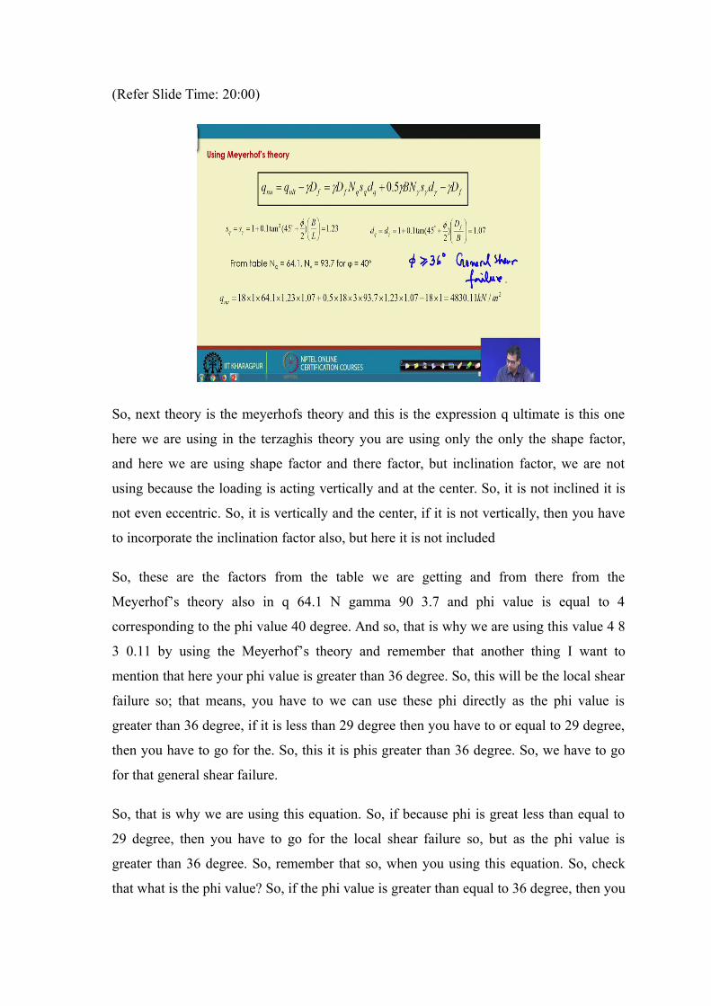
(Refer Slide Time: 22:34)
So, here using N q because N c value here this term we are not considering, because that
N c value c value is 0. So, first term is vanish.
So, N n q is same as the Meyerhof’s value, but the N gamma is different. So, that is why
we are getting we are taking N gamma from the chart corresponding to 40 degree. And if
I put all these correction factors and the bearing capacity factors, then we will get the net
ultimate bearing capacity is 3 3 to 8.8 kilo Newton per meter square for Hansen’s theory.
Now, similarly for the vesics theory thus N q is same as Meyerhof’s and Hansen, but N
gamma is different. So, and we have this factor, which is similar to the instance factor
this S c is gamma d q d gamma and we are getting if you put this value we will get this
value is here 4085.77.
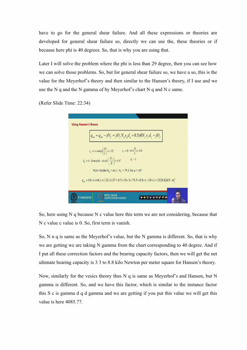
Now, as per the is code is code is given in this form this net bearing capacity ultimate
bearing capacity.
(Refer Slide Time: 23:49)
And these are the factors for is code and these N q and N gamma they are all same as the
vesic. So, and if I put value if I put these things into this equation will get this value.
Ah. Remember that in many of the textbook you may find that, they are using the net
ultimate value in this form. So, that you can use, but I would recommend that you
calculate the net ultimate in this way, that first the ultimate minus gamma W.
Because this is true for the this there will be no problem if it is terzaghis bearing
capacity, because there is no factor like s c d c i c is there, but in other cases if you write
in this form then you are also multiplying these factors i c i q d q and s q with the gamma
D f.
So, that that I will recommend that you use in this form ok. Because, if you multiply that
there will be a very slight difference, but in because there will be only say 1 or 2 or say 5
10 kpa difference ah, but I will recommend that you use in this way, but is code has
already recommended to use in this form. So, that is why you will use this way or in case
of is only, but other case we will use in this form. So, in the is code also if I put this value
this will give you this value.
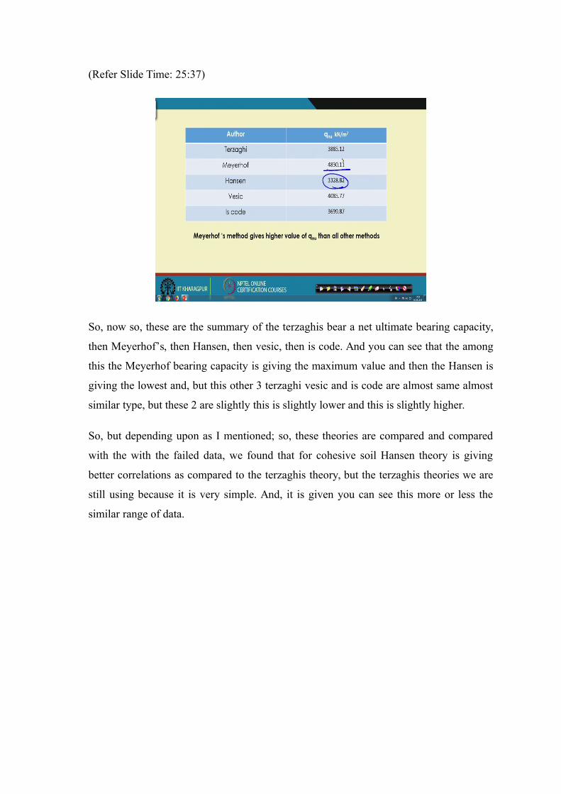
(Refer Slide Time: 25:37)
So, now so, these are the summary of the terzaghis bear a net ultimate bearing capacity,
then Meyerhof’s, then Hansen, then vesic, then is code. And you can see that the among
this the Meyerhof bearing capacity is giving the maximum value and then the Hansen is
giving the lowest and, but this other 3 terzaghi vesic and is code are almost same almost
similar type, but these 2 are slightly this is slightly lower and this is slightly higher.
So, but depending upon as I mentioned; so, these theories are compared and compared
with the with the failed data, we found that for cohesive soil Hansen theory is giving
better correlations as compared to the terzaghis theory, but the terzaghis theories we are
still using because it is very simple. And, it is given you can see this more or less the
similar range of data.
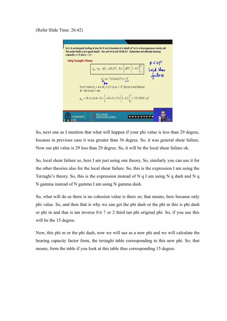
(Refer Slide Time: 26:42)
So, next one as I mention that what will happen if your phi value is less than 29 degree,
because in previous case it was greater than 36 degree. So, it was general shear failure.
Now our phi value is 29 less than 29 degree. So, it will be the local shear failure ok.
So, local shear failure so, here I am just using one theory. So, similarly you can use it for
the other theories also for the local shear failure. So, this is the expression I am using the
Terzaghi’s theory. So, this is the expression instead of N q I am using N q dash and N q
N gamma instead of N gamma I am using N gamma dash.
So, what will do as there is no cohesion value is there so; that means, here because only
phi value. So, and then that is why we can get the phi dash or the phi m this is phi dash
or phi m and that is tan inverse 0.6 7 or 2 third tan phi original phi. So, if you use this
will be the 15 degree.
Now, this phi m or the phi dash, now we will use as a new phi and we will calculate the
bearing capacity factor form, the terzaghi table corresponding to this new phi. So; that
means, form the table if you look at this table thus corresponding 15 degree.
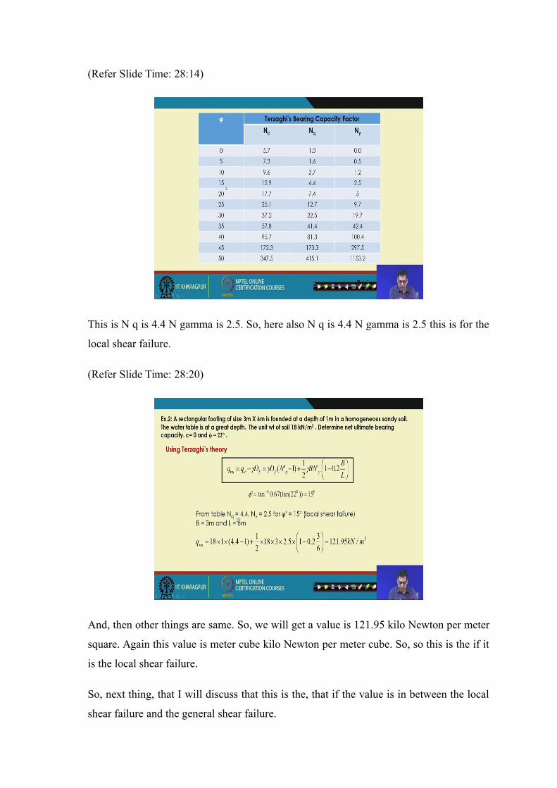
(Refer Slide Time: 28:14)
This is N q is 4.4 N gamma is 2.5. So, here also N q is 4.4 N gamma is 2.5 this is for the
local shear failure.
(Refer Slide Time: 28:20)
And, then other things are same. So, we will get a value is 121.95 kilo Newton per meter
square. Again this value is meter cube kilo Newton per meter cube. So, so this is the if it
is the local shear failure.
So, next thing, that I will discuss that this is the, that if the value is in between the local
shear failure and the general shear failure.

(Refer Slide Time: 28:52)
So, what will happen if the value is in between local shear failure and the general shear
failure.
So, if because here you can see the phi value is taken 35 degree, which is less than 36.
So, in between local shear failure and the general shear failure. So, in these case what
will do first we will calculate the N q and N gamma corresponding to actual phi, that is
35 degree. Then we can get the phi N for the local shear failure as I discuss in just
previous problem and that phi m we are getting just this phi m.
So, this phi m is equal to tan inverse two-third of tan phi. So, this is now it is giving 25
degree. So, you get the corresponding N q and N gamma value from the terzaghis table
and that is give 12.7 and 9.7.
So, now it is in between that so, now, what we so, what we will do suppose we have this
is the N q dash, that is local shear failure and this is the value for N q. So, general shear
failure and this deference of angle is 36 minus 29. And then you are linearly interpolating
that and it is in so, this is for 36 and this is for 29 and here we are here that is say 35.
So, this is the difference of 29 and then what will. So, that will be basically the 12 bar
means the N q dash plus the N q minus N q dash, then into that your phi value minus 29
degree divided by 36 degree minus 29 degree.
So, this is the expression because we are doing the linear interpolation. So, that way
similarly for the N gamma also so, your N q bar will be this value. Similarly, we can get
for N gamma bar also. So, that is the, that way we can determine the N gamma N q bar
and then that value we are using here and we will get a value here 1569.99 that is kilo
Newton per meter square so, this is q. So, this is the value if it is in between local shear
failure and the general shear failure.
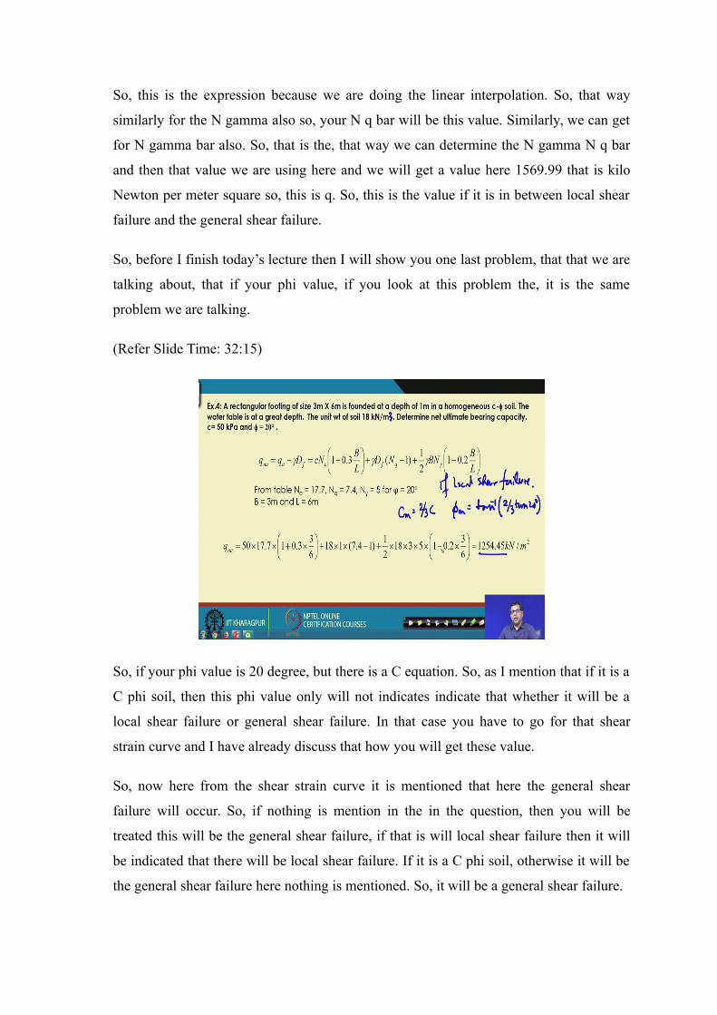
So, before I finish today’s lecture then I will show you one last problem, that that we are
talking about, that if your phi value, if you look at this problem the, it is the same
problem we are talking.
(Refer Slide Time: 32:15)
So, if your phi value is 20 degree, but there is a C equation. So, as I mention that if it is a
C phi soil, then this phi value only will not indicates indicate that whether it will be a
local shear failure or general shear failure. In that case you have to go for that shear
strain curve and I have already discuss that how you will get these value.
So, now here from the shear strain curve it is mentioned that here the general shear
failure will occur. So, if nothing is mention in the in the question, then you will be
treated this will be the general shear failure, if that is will local shear failure then it will
be indicated that there will be local shear failure. If it is a C phi soil, otherwise it will be
the general shear failure here nothing is mentioned. So, it will be a general shear failure.

So, in the general shear failure that is why we will we will not reduce anything we will
use same phi value same C value and you will get the N c and N gamma for the same phi
and so; that means, here we are using 20 degree phi using terzaghis table so, N c and N
gamma. So, this value we are putting we will get the bearing capacity, that is kilo
1254.45 kilo Newton meter square.
and remember that if it is mentioned that there will be a local shear failure, then you
have to use the cm mu cm by two-third of C, if local shear failure and your phi N will be
tan inverse two-third of tan 20 here because your phi value is 20.
So, that nu phi calculate and get the N c N gamma corresponding to that nu phi and then
put the instead of C you put here we are getting 50’s it will be two-third of 50 and the
corresponding N c N gamma and N n N q value, and then we will get the bearing
capacity.
So, in this I am finishing this today’s lecture and so, in the there will be one more
problem, that will solve I will solve in the next class, that how I can incorporate the
water table effect in the bearing capacity equation.
So, next class I will first solve that problem, then I will go for the settlement calculation
part which is also very important because we have 2 criterias one is bearing capacity. So,
till now I am discussing about the bearing capacity. So, next class first I will solve the
water table problem effect I am I will solve the how to incorporate the water table in to
the bearing capacity and then I will solve discuss over the settlement criteria of the
foundation design.
Thank you.