formal verification of simulations between i»o automata by
TRANSCRIPT
Formal veri�cation of simulations between I/O automata
by
Andrej Bogdanov
B.S., Massachusetts Institute of Technology (2000)
Submitted to the Department of Electrical Engineering and Computer Sciencein partial ful�llment of the requirements for the degree of
Master of Engineering in Electrical Engineering and Computer Science
at the
MASSACHUSETTS INSTITUTE OF TECHNOLOGY
September 2001
c 2001 Massachusetts Institute of Technology. All rights reserved.
The author hereby grants to MIT permission to reproduce and distribute publiclypaper and electronic copies of this thesis and to grant others the right to do so.
Author . . . . . . . . . . . . . . . . . . . . . . . . . . . . . . . . . . . . . . . . . . . . . . . . . . . . . . . . . . . . . . . . . . . . . . . . . . . .Department of Electrical Engineering and Computer Science
July 31, 2001
Certi�ed by. . . . . . . . . . . . . . . . . . . . . . . . . . . . . . . . . . . . . . . . . . . . . . . . . . . . . . . . . . . . . . . . . . . . . . . .Stephen J. Garland
Principal Research ScientistThesis Supervisor
Certi�ed by. . . . . . . . . . . . . . . . . . . . . . . . . . . . . . . . . . . . . . . . . . . . . . . . . . . . . . . . . . . . . . . . . . . . . . . .Nancy A. Lynch
NEC Professor of Software Science and EngineeringThesis Supervisor
Accepted by . . . . . . . . . . . . . . . . . . . . . . . . . . . . . . . . . . . . . . . . . . . . . . . . . . . . . . . . . . . . . . . . . . . . . . .Arthur C. Smith
Chairman, Department Committee on Graduate Students

2
Formal veri�cation of simulations between I/O automata
by
Andrej Bogdanov
Submitted to the Department of Electrical Engineering and Computer Scienceon July 31, 2001, in partial ful�llment of the
requirements for the degree ofMaster of Engineering in Electrical Engineering and Computer Science
Abstract
This thesis presents a tool for validating descriptions of distributed algorithms inthe IOA language using an interactive theorem prover. The tool translates IOAprograms into Larch Shared Language speci�cations in a style which is suitable forformal reasoning. The framework supports two common strategies for establishingthe correctness of distributed algorithms: Invariants and simulation relations. Thesestrategies are used to verify three distributed data management algorithms: A strongcaching algorithm, a majority voting algorithm and Lamport's replicated state ma-chine algorithm.
Thesis Supervisor: Stephen J. GarlandTitle: Principal Research Scientist
Thesis Supervisor: Nancy A. LynchTitle: NEC Professor of Software Science and Engineering
3

4
Na mama i tato,
za dosegaxnite dvaeset i tri godini.

6
Acknowledgments
My advisors, Dr. Stephen Garland and Prof. Nancy Lynch provided me with excellent
guidance throughout this project. Their critical insights and suggestions helped me
shape my ideas in a useful and presentable form. Above all, it is their genuine interest
and con�dence in my work that encouraged me to pursue diÆcult and exciting yet
attainable goals.
This work would not have been possible without the contributions of all the stu-
dents who have participated in the development of the IOA language and toolkit.
Rui Fan provided some interesting suggestions at the initial stages of design. Michael
Tsai was my main source of help on questions about the IOA front end. Chris Luhrs
was the �rst user of the translation tool developed in this work. His struggles with
the tool led to several improvements in design. His overall positive experience was a
reason for much satisfaction.
Discussions with Josh Tauber, Dimitris Vyzovitis and Shien Jin Ong revealed
many insights about the replicated state machine algorithm.
The ultimate \thanks" is reserved for my parents. They have been my unfailing
source of support in moments of weakness and in moments of happiness.
7

8
Contents
1 Introduction 15
1.1 The input/output automaton model . . . . . . . . . . . . . . . . . . . 16
1.2 The IOA language and toolkit . . . . . . . . . . . . . . . . . . . . . . 16
1.3 Techniques for verifying automaton properties . . . . . . . . . . . . . 18
1.4 IOA and theorem proving . . . . . . . . . . . . . . . . . . . . . . . . 20
1.4.1 Choosing a logic . . . . . . . . . . . . . . . . . . . . . . . . . 20
1.4.2 Interpreting IOA speci�cations . . . . . . . . . . . . . . . . . 21
1.5 Thesis overview . . . . . . . . . . . . . . . . . . . . . . . . . . . . . . 22
2 Reasoning about I/O automata 25
2.1 The mathematical framework . . . . . . . . . . . . . . . . . . . . . . 26
2.1.1 The I/O automaton model . . . . . . . . . . . . . . . . . . . . 26
2.1.2 Describing behaviors of automata . . . . . . . . . . . . . . . . 27
2.1.3 Invariants and simulation relations . . . . . . . . . . . . . . . 28
2.1.4 Describing the step correspondence . . . . . . . . . . . . . . . 29
2.2 The Larch theory of I/O automata . . . . . . . . . . . . . . . . . . . 31
2.2.1 Automaton basics . . . . . . . . . . . . . . . . . . . . . . . . . 31
2.2.2 Executions and traces . . . . . . . . . . . . . . . . . . . . . . 32
2.2.3 Safety properties . . . . . . . . . . . . . . . . . . . . . . . . . 33
3 The translation process 35
3.1 An illustrative example . . . . . . . . . . . . . . . . . . . . . . . . . . 37
3.2 Referenced traits, datatypes and formals . . . . . . . . . . . . . . . . 39
9
3.3 Automaton states . . . . . . . . . . . . . . . . . . . . . . . . . . . . . 39
3.4 Action declarations . . . . . . . . . . . . . . . . . . . . . . . . . . . . 40
3.5 Transition de�nitions . . . . . . . . . . . . . . . . . . . . . . . . . . . 42
3.5.1 The enabled clause . . . . . . . . . . . . . . . . . . . . . . . . 43
3.5.2 Variable maps . . . . . . . . . . . . . . . . . . . . . . . . . . . 43
3.5.3 Assignments . . . . . . . . . . . . . . . . . . . . . . . . . . . . 46
3.5.4 Conditionals . . . . . . . . . . . . . . . . . . . . . . . . . . . . 47
3.5.5 Loops . . . . . . . . . . . . . . . . . . . . . . . . . . . . . . . 48
3.6 Invariants . . . . . . . . . . . . . . . . . . . . . . . . . . . . . . . . . 51
3.7 Forward simulation relations . . . . . . . . . . . . . . . . . . . . . . . 51
4 Nondeterminism 55
4.1 Choose parameters of transitions . . . . . . . . . . . . . . . . . . . . 56
4.2 Assignments of the form choose..where . . . . . . . . . . . . . . . . . 57
4.3 Assignments of the form choose..so that . . . . . . . . . . . . . . . . . 58
4.4 Nondeterminism within conditionals . . . . . . . . . . . . . . . . . . . 59
5 A caching algorithm 61
5.1 Shared data types of the memory models . . . . . . . . . . . . . . . . 62
5.2 The central memory model . . . . . . . . . . . . . . . . . . . . . . . . 64
5.3 The strong caching algorithm . . . . . . . . . . . . . . . . . . . . . . 66
5.4 The equivalence of cache and mem . . . . . . . . . . . . . . . . . . . . 66
5.4.1 Key invariant of cache . . . . . . . . . . . . . . . . . . . . . . 68
5.4.2 The simulation from cache to mem . . . . . . . . . . . . . . . . 68
5.4.3 The simulation from mem to cache . . . . . . . . . . . . . . . . 70
6 Majority voting 73
6.1 The majority voting algorithm . . . . . . . . . . . . . . . . . . . . . . 73
6.2 Analyzing the e�ect of write . . . . . . . . . . . . . . . . . . . . . . 76
6.3 The equivalence of voting and mem . . . . . . . . . . . . . . . . . . . 77
6.3.1 Key invariant of voting . . . . . . . . . . . . . . . . . . . . . 77
10
6.3.2 The simulation from voting to mem . . . . . . . . . . . . . . . 79
6.3.3 The simulation from mem to voting . . . . . . . . . . . . . . . 81
7 The replicated state machine 83
7.1 Data type speci�cations . . . . . . . . . . . . . . . . . . . . . . . . . 84
7.2 Automaton speci�cations . . . . . . . . . . . . . . . . . . . . . . . . . 86
7.2.1 The replicated state machine automaton . . . . . . . . . . . . 86
7.2.2 The synchronized replicated memory . . . . . . . . . . . . . . 88
7.3 The simulation from synch to mem . . . . . . . . . . . . . . . . . . . . 88
7.3.1 De�nitions . . . . . . . . . . . . . . . . . . . . . . . . . . . . . 90
7.3.2 Invariants of synch . . . . . . . . . . . . . . . . . . . . . . . . 91
7.3.3 The simulation relation . . . . . . . . . . . . . . . . . . . . . . 95
7.3.4 Notes on the formal proof . . . . . . . . . . . . . . . . . . . . 98
7.4 The simulation from rsm to synch . . . . . . . . . . . . . . . . . . . . 99
7.4.1 Invariants of rsm . . . . . . . . . . . . . . . . . . . . . . . . . 101
7.4.2 The simulation relation . . . . . . . . . . . . . . . . . . . . . . 107
8 Discussion and future work 111
8.1 Semantic checks . . . . . . . . . . . . . . . . . . . . . . . . . . . . . . 112
8.2 Improving the translation of loops . . . . . . . . . . . . . . . . . . . . 113
8.2.1 Nondeterminism within loops . . . . . . . . . . . . . . . . . . 114
8.2.2 Semantic analysis of loops . . . . . . . . . . . . . . . . . . . . 115
8.3 Organizing proofs . . . . . . . . . . . . . . . . . . . . . . . . . . . . . 115
8.4 The step correspondence language . . . . . . . . . . . . . . . . . . . . 116
A Formal proofs 119
11

12
List of Figures
3-1 IOA speci�cation of automaton channel . . . . . . . . . . . . . . . . 37
3-2 LSL speci�cation of channel . . . . . . . . . . . . . . . . . . . . . . . 38
3-3 Translation of action declarations . . . . . . . . . . . . . . . . . . . . 41
3-4 IOA speci�cation of automaton loop . . . . . . . . . . . . . . . . . . 50
3-5 LSL speci�cation of transition add . . . . . . . . . . . . . . . . . . . . 51
3-6 Template for the invariants of automaton A . . . . . . . . . . . . . . 52
4-1 Translation of a choose transition parameter . . . . . . . . . . . . . 57
4-2 Translation of a choose..where clause . . . . . . . . . . . . . . . . . 58
4-3 Translation of a choose..so that clause . . . . . . . . . . . . . . . . 59
4-4 Translation of nondeterminism within a conditional . . . . . . . . . . 60
5-1 IOA speci�cation of the atomic variable model . . . . . . . . . . . . . 65
5-2 IOA speci�cation of the strong caching algorithm . . . . . . . . . . . 67
5-3 Larch proof of the invariant of cache . . . . . . . . . . . . . . . . . . 68
5-4 Larch proof of the simulation from cache to mem . . . . . . . . . . . . 70
5-5 Larch proof of the simulation from mem to cache . . . . . . . . . . . . 72
6-1 IOA speci�cation of the majority voting algorithm . . . . . . . . . . . 74
6-2 Simplifying the e�ect of a loop in Larch . . . . . . . . . . . . . . . . . 76
7-1 IOA speci�cation of the replicated state machine algorithm . . . . . . 87
7-2 IOA speci�cation of the synchronized replicated memory . . . . . . . 89
13

14
Chapter 1
Introduction
Typical distributed systems can be surprisingly diÆcult to reason about. Our intu-
itive notion of program correctness can be shattered at the blink of an eye even years
after a system has been written and used in practice, sometimes with disastrous con-
sequences. Even elementary distributed algorithms may contain concurrency issues
subtle enough to fool the most experienced of designers.
System failures often stem from our inadequate notions of correctness. At an
informal level, sloppy correctness arguments serve to \justify" imprecise system spec-
i�cations. However, experience has demonstrated that many of the problems arising
in concurrent systems are direct consequences of this sloppiness in design. As a result,
researchers spend considerable e�ort in developing formal yet practical environments
for specifying concurrent systems.
In the framework of a formal system description together with a precise semantics,
it often happens that our intuitive understanding of correctness is highly ambiguous.
Most of us perceive the task of translating a high-level statement into a speci�c
formalism as daunting, unenlightening and perhaps even unnecessary. Yet, in the
context of concurrent systems, this approach of formalizing the systems as well as
the properties we are interested in verifying pays o� for several reasons. In addition
to the obvious bene�t of resolving ambiguities in our understanding of correctness,
a good formalism imposes structural restrictions which force the designer to produce
well-written, modular speci�cations.
15
Perhaps the greatest bene�t of formal speci�cation is its connection to a variety of
manual and automatic validation techniques, such as simulation, invariant generation,
automated theorem proving and model checking. These techniques can be used both
to improve our understanding of the system and its properties and to verify that the
system satis�es the desired properties.
1.1 The input/output automaton model
The input/output automaton (I/O automaton) model is a state machine-based for-
malism for describing distributed systems. In addition to the states and transitions
of ordinary state machines, I/O automata introduce the notion of external behavior
which captures the observable portion of a state machine execution.
Owing to its relatively simple mathematical structure, the theory of I/O automata
can be used to describe a wide variety of asynchronous distributed systems. The
inherent nondeterminism of I/O automata allows such systems to be described in
their most general forms.
Despite its simplicity, the theory is expressive enough to capture important classes
of properties which are commonly used in the development and veri�cation of dis-
tributed systems. In particular, the theory supports the formulation of automaton
invariants and simulations between automata.
Finally, the I/O automaton model is based on set-theoretic mathematics rather
than a particular logic or programming language. This provides enough exibility for
this model to interact with a wide range of analysis tools.
1.2 The IOA language and toolkit
IOA is a formal language for specifying, validating and implementing distributed
systems based on the I/O automaton formalism. It derives its form from guarded
command-style syntax similar to pseudocode descriptions of distributed algorithms,
such as the pseudocode segments from [14]. Since the I/O automaton model is re-
16
active rather than sequential, IOA is distinguished from most typical functional pro-
gramming languages by its constructs for explicit and implicit nondeterminism and
concurrency.
The language is designed to support expressing designs at di�erent levels of ab-
straction, starting with a high-level, global speci�cation of the system behavior and
ending with a low-level version which is translatable into real code. IOA also supports
descriptions of systems composed from several interacting components, building upon
the notion of composition in the theory of I/O automata.
IOA is meant to interface with a variety of tools, including code generators pro-
ducing output in executable languages such as C++ or Java, a simulator which can
be used to study sample behaviors of distributed systems, automatic invariant dis-
covery packages, model checkers and interactive theorem provers. Each of these tools
imposes a stringent set of constraints on the nature of the language. Code generators
interface best with deterministic programs written in imperative style. On the other
hand, nondeterminism is a useful abstraction in formal veri�cation, and most veri�-
cation tools support only declarative style speci�cations. As an intermediary between
these tools, IOA must provide enough exibility to allow natural interaction with all
of them.
IOA is based on pseudocode used in previous work on I/O automata. Automaton
components such as states, actions and transitions are explicitly represented in IOA.
States are represented by collections of strongly typed variables. Transitions are
speci�ed through transition de�nitions which can be parameterized. Each transition
de�nition contains a precondition and an e�ect. The precondition is a predicate
specifying whether the transition is enabled in the current (initial) state. The e�ect
speci�es the �nal state in terms of the initial state, the transition parameters and
possibly additional nondeterministically chosen parameters. The code may be written
either as an imperative style sequence of instructions or as a predicate relating the
state variables, transition parameters and nondeterministic parameters.
17
1.3 Techniques for verifying automaton properties
As a practical tool for distributed system analysis, IOA provides a mechanism for
computer-based formal veri�cation of I/O automaton properties. In particular, it al-
lows the use of mathematical techniques for proving assertions about abstract I/O au-
tomata such as invariants and simulations to ensure correctness of real world systems
implemented in the IOA language. Owing to the abstract nature of the underlying
mathematical model, IOA has the potential to interface with a variety of veri�cation
tools.
Most of the interesting results in computer-based formal veri�cation have been
obtained with the help of model checkers and interactive theorem provers. The veri-
�cation features provided by these two types of tools are, in many respects, comple-
mentary. An interesting area of research is the discovery of techniques that would
allow the combination of their respective strengths.
Model checkers have the advantage of requiring considerably less attention from
the user and are suitable for verifying properties of relatively complex automata
as long as the state space is not prohibitively large. If veri�cation of the desired
property fails, these tools provide the user with a counterexample which can be useful
for remedying the perceived defect. Model checkers have been used for checking
a variety of temporal properties, including safety properties (invariants, simulation
relations) and liveness properties (livelock, deadlock). Unfortunately, despite frequent
improvements and optimizations in the architecture of model checkers, the size of the
models to which these techniques can be applied is too small to be useful for many
common software systems.
Model checkers have been used to study a number of challenge problems and
practical algorithms. The basic ideas are illustrated in a variety of typical exam-
ples including two-process mutual exclusion [6] and the alternating bit protocol [13].
Clarke et al. [5] demonstrate the application of model checking techniques to a cache
coherence protocol for high-performance computers.
Theorem provers provide environments for conducting formal proofs of statements
18
in a prespeci�ed logical system. They support a combination of automatic and manual
procedures which mirror the common proof techniques from mathematics, such as
deductive and inductive reasoning, proofs by cases and proofs by contradiction. The
computational complexity of the theorem prover procedures is closely related to the
length and intricacy of the informal proof of the conjectured property.
To verify properties of automata, the automaton speci�cation and the properties
of interest are translated to the logical language supported by the theorem prover.
The properties are then veri�ed through an interactive session, in which the user
feeds the theorem prover with hints on how to establish the desired conclusion. Since
mathematical proofs usually rely on reasoning about abstract models rather than
detailed low level descriptions of systems, theorem proving techniques are highly
scalable. In particular, they do not su�er from the state explosion problem exhibited
by model checkers and may be even used to verify system speci�cations with in�nite
state spaces.
Unlike model checkers, theorem provers require an extensive amount of user un-
derstanding and interaction. Before venturing into a formal proof, one needs to have
a good idea of the underlying mathematical argument. Even with the mathematics
in mind, it takes a considerable amount of skill and patience to transform this into a
fully formalized proof which can be handled by the tool. Yet, this formalization pro-
cess is not merely a waste of time, as problems with the model tend to surface in the
intricate details of the formal proof. A simple (though somewhat tedious) method of
translating informal arguments into formal proofs which can be useful in this context
is explained in [12].
Theorem provers have been used to verify a variety of distributed algorithms. A
toy example which illustrates theorem proving techniques for distributed algorithms
is the lossy queue [20]. M�uller [17] provides formal correctness proofs for a distributed
alarm example and the alternating bit protocol in Isabelle/HOL. Garland and Lynch
used the Larch Prover to analyze a complicated distributed banking example [9].
19
1.4 IOA and theorem proving
IOA descriptions of automata have precise and relatively simple interpretations in
the I/O automaton model. The theory of I/O automata is elementary enough that
automatic reasoning tools, such as theorem provers, can provide considerable help
in the reasoning process. To establish this connection between IOA and a theorem
proving environment, we must address two important issues: (1) the choice of an
appropriate logic and a theorem prover and (2) the interpretation of IOA speci�cations
in the context of this logic.
1.4.1 Choosing a logic
The choice of an appropriate logic presents a tradeo� between expressiveness and
complexity. If the logic is too constrained, we cannot express interesting properties.
If it is too rich, formal reasoning in it may become cumbersome and computationally
expensive. It is instructive to consider the types of properties which we may want to
verify and choose the logic accordingly.
Interesting properties of distributed systems are divided in two classes: liveness
properties, which specify that some \good" event eventually happens in an execution,
and safety properties, which specify that a particular \bad" event never happens.
Precise de�nitions of these classes of properties can be found in [1].
Liveness properties are somewhat awkward to express in �rst-order logic. Most
formal frameworks for reasoning about these properties are based in more elaborate
temporal logics [18]. Some specialized theorem provers such as STeP [2] provide built-
in support for reasoning in temporal logic. General purpose theorem provers do not
support temporal logic, so temporal operators are usually de�ned using constructs
from higher order logic. This approach has been used to obtain frameworks for
veri�cation of I/O automaton properties in PVS [7] and Isabelle/HOL [17]. The
resulting frameworks are very general, but the reasoning is complicated because the
rules of temporal logic are less intuitive than the rules of �rst-order logic.
Safety properties can be expressed naturally in multisorted �rst-order logic. The
20
Larch proof assistant [8] is specialized for reasoning in this type of logic. It provides
a rich syntax for expressing properties in familiar notation, admits intuitive speci-
�cations of theories in the Larch Shared Language (LSL) and supports a variety of
proof techniques similar to the ones used in less formal mathematical arguments.
Distributed algorithms of varying levels of complexity have been sucessfully veri�ed
in Larch [20, 9]. These experiences suggest that Larch is a useful tool for checking
safety properties of automata.
The framework described in this thesis allows the veri�cation of safety properties
stated in Larch-style multisorted �rst-order logic. By restricting our attention to this
speci�c class of properties, we hope to increase the automation level of our tool and
reduce (or at least facilitate) the human interaction with the theorem prover. This,
in turn, will allow us to formally verify highly complex distributed algorithms.
1.4.2 Interpreting IOA speci�cations
The choice of Larch as a veri�cation environment for I/O automata provides an extra
bene�t. As the IOA type system is speci�ed in LSL, the declarations and properties
of datatypes are readily available for theorem proving. In addition, IOA and LSL
formulas (terms) are syntactically equivalent.
The �rst task in interpreting IOA speci�cations is to �nd a suitable formalization
of I/O automata theory in multisorted �rst-order logic. Garland et al. [9] devised
a Larch theory based on the primitive notions of states and actions. The theory is
powerful enough to make claims of invariants, forward simulations and backward sim-
ulations. It provides the starting point for the framework presented here. We adopt a
number of modi�cations to this theory in the hope of automating part of the theorem
proving process by extracting additional information from the IOA speci�cation.
With the theory of I/O automata formalized, we can tackle the issue of interpreting
a particular IOA speci�cation in the context of this theory. The interpretation must
be concise and readable to the user of the theorem proving tool. On the other hand,
it should interact well with the automation features provided by the theorem prover.
Since the interpretation is speci�ed in �rst-order logic, all this must be performed
21
with relatively simple mathematical machinery.
1.5 Thesis overview
The principal contribution of this thesis is the design and implementation of a transla-
tion process which converts automaton declarations in the IOA language to equivalent
speci�cations in the Larch Shared Language. This tool allows the application of inter-
active theorem proving techniques to verify a wide range of practical safety properties
of I/O automata.
A number of distributed data management algorithms serve to illustrate the prac-
tical bene�ts of this tool. These algorithms were developed as challenge problems
for software synthesis and analysis in the IOA language and toolkit. Ranging from
simple to highly complex, they capture many of the diÆculties encountered in formal
modeling and veri�cation. In many cases, the frustrations and successes experienced
in the formal veri�cation of these examples were the driving force behind important
design decisions about the tool.
Chapter 2 sets up the formal framework in which the translation process is con-
ducted. It de�nes the elements of the I/O automaton model relevant to the properties
of interest and describes their formalization in Larch style multisorted �rst-order logic.
A number of new de�nitions relevant to our formalization of explicit nondeterminism
are provided in this chapter.
The ideas and architecture of the translation process are discussed in Chapter 3.
The bulk of the chapter is dedicated to translating imperative-style IOA code into
the declarative syntax supported by Larch.
The representation of explicit nondeterminism in Larch is the topic of Chapter
4. IOA allows nondeterminism to appear at various parts of the speci�cation. Some
forms of nondeterminism may be constrained by a predicate. We look closely at the
interpretation of these various kinds of nondeterminism and provide a faithful scheme
for its resolution.
The next three chapters illustrate the application of the theorem proving method-
22
ology discussed so far to a series of distributed data management models. Chapter 5
discusses a strong caching system. The correctness proofs are transparent, but provide
a good illustration of the basic technique. In Chapter 6 we verify the more compli-
cated majority voting model. Some of the issues in this model are subtle enough to
require more re ection.
In Chapter 7 we present a simulation proof of Lamport's replicated state ma-
chine model [11], a highly complex data management algorithm for asynchronous
distributed systems. To our knowledge, this is the �rst proof of the algorithm written
in successive re�nement style. Parts of this proof were carried out using Larch. The
rest of the proof requires a suitable extension of the Larch theory of I/O automata,
which is left as an open problem.
Chapter 8 is the conclusion of our exposition. It suggests a number of possible
improvements to the translation process and underlying machinery as part of future
work.
23

24
Chapter 2
Reasoning about I/O automata
When we attempt to gain an intuitive understanding of an automaton, we use in-
formal arguments to single out essential ideas and interesting properties. Intuitive
reasoning is helpful because it allows us to gain better understanding of our system,
but is often awed because it may depend on unstated or incorrect assumptions. In
practice, these mistakes in reasoning may be extraordinarily subtle yet critical to the
proper functioning of the system. To establish correctness beyond reasonable doubt,
reasoning strategies about automata need to be conducted at a level more formal than
typical arguments used in ordinary mathematics. Unfortunately, formal arguments
tend to be long, tedious, dull, and time consuming.
A useful reasoning methodology combines the exibility of intuitive reasoning with
the persuasive power of formal arguments. Our attempt at resolving this tradeo� de-
rives from two ingredients: the theory of I/O automata and computer assisted formal
proofs. The former provides a precise model and introduces formal proof techniques
which approximate popular intuitive arguments. The latter facilitates the tedious
task of conducting the formal proof by automating the cumbersome computational
details in the proofs.
I/O automata are based on set-theoretic mathematics; theorem provers work with
speci�cations in a particular logic. In this chapter we set up the framework that
establishes the connection between the two. First, we introduce the I/O automaton
model and its relevant properties. We then describe a multisorted �rst order theory,
25
generated by a simple set of axioms, which will be used to study the model.
2.1 The mathematical framework
In this section, we provide formal de�nitions of the elements of I/O automata theory
and their properties. These notions were introduced by Lynch and Tuttle in [15].
They are used as the foundation for the formalism in Distributed Algorithms [14].
Some of the de�nitions are stated in modi�ed forms which are more suitable for the
discussion presented in this thesis. A number of new abstractions are introduced in
order to facilitate the discussion in the following chapters.
We omit the components of the model pertaining to liveness properties, for they
do not play a role in the methodology and tools described in this thesis.
2.1.1 The I/O automaton model
We assume a universal set of actions, used to describe the transitions between states.
De�nition A signature S is a collection of three disjoint sets of actions: The input
actions in(S), the output actions out(S) and the internal actions int(S).
The actions in in(S) [ out(S) are called external actions. This set is denoted by
ext(S). The set int(S) [ ext(S) is denoted by acts(S).
De�nition A relabeling from signature S to signature S 0 is a map � from the set
ext(S) to the set ext(S 0) for which �(in(S)) � in(S 0) and �(out(S)) � out(S 0).
De�nition An I/O automaton A consists of
1. A set of states (denoted by states(A)),
2. A signature (denoted by sig(A)),
3. A relation steps(A) � states(A)� acts(sig(A))� states(A) called a labeling.
The entry (s; �; s0) 2 steps(A), also written as s��! s0, is called a transition of A.
26
We say that action � is enabled in state s of automaton A if there exists a state s0
such that s��! s0 is a transition of A. Automaton A is input-enabled if every input
action of A is enabled in every state of A.
The original de�nition of I/O automata [15] requires input-enabledness by default.
This property is important for theorems on liveness and composition. For safety prop-
erties, input-enabledness bears no particular relevance. Relaxing this requirement will
simplify our reasoning.
Finally, we want to single out a particular form of automaton in which the action
labels are unique at each state. This de�nition, which is not included in standard I/O
automaton theory, will be useful for formal descriptions of automata in multisorted
�rst-order logic.
De�nition The I/O automaton A is pseudodeterministic if for every state s and
every action label � of A, there exists at most one s0 so that s��! s0 is a transition
of A.
2.1.2 Describing behaviors of automata
In this section we introduce the ideas of execution and external behavior of an I/O
automaton. In addition to the standard notions from Distributed Algorithms, we
de�ne explicit operators which will be useful for comparing the executions of two
automata.
De�nition An execution fragment of an I/O automaton A is a (�nite or in�nite)
sequence s0; �1; s1; : : : ; �k; sk; : : : ; (sf) of alternating states and actions of A such that
sk�k+1�! sk+1 is a transition of A. If s0 is a start state of A, then the execution fragment
is an execution.
Note that if A is pseudodeterministic, then the states sk for k � 1 in the execution
fragment are implicitly determined by s0 and the �ks.
De�nition A state of A is reachable if it is the �nal state of some execution of A.
De�nition The trace of an execution fragment �, denoted by trace(�), is the sub-
sequence of � consisting of all external actions of �.
27
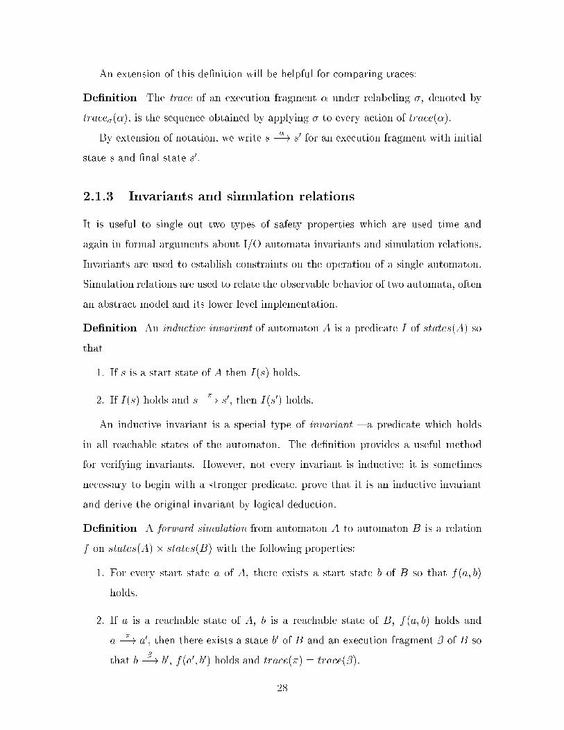
An extension of this de�nition will be helpful for comparing traces:
De�nition The trace of an execution fragment � under relabeling �, denoted by
trace�(�), is the sequence obtained by applying � to every action of trace(�).
By extension of notation, we write s��! s0 for an execution fragment with initial
state s and �nal state s0.
2.1.3 Invariants and simulation relations
It is useful to single out two types of safety properties which are used time and
again in formal arguments about I/O automata invariants and simulation relations.
Invariants are used to establish constraints on the operation of a single automaton.
Simulation relations are used to relate the observable behavior of two automata, often
an abstract model and its lower level implementation.
De�nition An inductive invariant of automaton A is a predicate I of states(A) so
that
1. If s is a start state of A then I(s) holds.
2. If I(s) holds and s��! s0, then I(s0) holds.
An inductive invariant is a special type of invariant { a predicate which holds
in all reachable states of the automaton. The de�nition provides a useful method
for verifying invariants. However, not every invariant is inductive; it is sometimes
necessary to begin with a stronger predicate, prove that it is an inductive invariant
and derive the original invariant by logical deduction.
De�nition A forward simulation from automaton A to automaton B is a relation
f on states(A)� states(B) with the following properties:
1. For every start state a of A, there exists a start state b of B so that f(a; b)
holds.
2. If a is a reachable state of A, b is a reachable state of B, f(a; b) holds and
a��! a0, then there exists a state b0 of B and an execution fragment � of B so
that b��! b0, f(a0; b0) holds and trace(�) = trace(�).
28
The importance of forward simulations is captured in the next theorem, which
provides a practical method for establishing properties of global behaviors by rea-
soning about individual actions. Its correctness is easily established by reasoning
inductively on the length of executions.
Theorem 2.1 If there is a forward simulation relation from A to B, then every trace
of A is a trace of B.
The converse to this theorem does not hold. Lynch and Vandraager [16] and
others show examples of automata which are related by trace inclusion even though
no relation between their states is a forward simulation. Despite their incompleteness
with respect to trace inclusion, a wide range of distributed systems used in practice
can be related by forward simulation relations. In all case studies presented here,
trace inclusion is established by exhibiting a forward simulation.
Several additional kinds of mappings and relations which can be used to establish
trace inclusion are studied in [16]. Apart from forward simulations, notions used to
describe correspondences between automata include backward simulations, history
variables and prophecy variables. It is likely that the tool for formal reasoning about
I/O automata presented here can be extended to handle these notions.
2.1.4 Describing the step correspondence
Theorem 2.1 provides a method for verifying that automaton A implements automa-
ton B, in the sense that every external behavior of A is allowed by B. To use the
theorem, we �rst look for a candidate simulation relation; once a candidate has been
found, we must verify that f satis�es properties 1 and 2 of the de�nition.
Properties 1 and 2 are typically veri�ed using constructive arguments. To ver-
ify property 2, for each transition a��! a0 of A we must produce a corresponding
execution fragment b��! b0 of B. The execution fragment itself is described as an
alternating sequence of states and actions. All this introduces a plethora of interme-
diate variables which need to be explicitly instantiated.
29
If the automata A and B are pseudodeterministic, the notation is greatly sim-
pli�ed. The states a0, b0 and the intermediate states of � become implicit in the
description. This is especially helpful if the veri�cation is to be performed by an
interactive theorem prover. We now show how to transform a generic automaton to
a pseudodeterministic one.
Theorem 2.2 For every automaton A, there exists an automaton A0 and a relabeling
� : sig(A0)! sig(A) so that:
1. states(A0) = states(A).
2. A0 is a pseudodeterministic automaton.
3. traces�(A0) = traces(A).
The translation process from IOA to LSL automatically converts every automaton
into a pseudodeterministic automaton. The proof does not describe the exact pro-
cedure used in the translation process, but it reveals the basic idea of parametrizing
the action labels to make them locally unique.
Proof Given the automaton A, we construct A0 and �.
1. Let states(A0) = states(A).
2. Let acts(sig(A0)) = acts(sig(A))�states(A). Action (�; s0) is an input (output,
internal) action of S 0 if and only if � is an input (output, internal) action of S.
3. s(�;s0)�! s0 is a transition of A0 if and only if s
��! s0 is a transition of A.
Properties 1, 2 and 3 of the theorem are easy to verify.
It is possible that automaton A0 fails to be input-enabled even if A were input-
enabled. This is why it was necessary to adopt a relaxed de�nition of I/O automaton.
30
2.2 The Larch theory of I/O automata
We are now in a position to investigate possible axiomatizations of the theory of
I/O automata. The theory must be powerful enough to express the safety properties
introduced in the previous sections|invariants and simulation relations.
The theory is formulated in the Larch Shared Language, a formal language for
describing �nitely axiomatizable theories in multisorted �rst order logic. The theory
is based on a prototype developed by Garland [20].
Theorem 2.2 shows that every automaton can be transformed to a pseudodeter-
ministic automaton, if we introduce an appropriate relabeling. Consequently it is
suÆcient to limit the theory to pseudodeterministic automata. The transformation
that converts IOA speci�cations to pseudodeterministic automata is very natural.
This is demonstrated in the case studies from Chapters 5 and 6. We modify some
notions from [20] and introduce two additional ones (signatures and relabelings) as
part of the formal machinery for this transformation.
2.2.1 Automaton basics
We build the theory of automata from a number of primitives. For each automaton
A, we assume:
� A sort States[A] representing the states of A.
� A sort Actions[A] representing the actions of A.
In addition, we assume a universal sort Actions, which will be used to compare
the actions of two automata. We begin by de�ning signatures:
Signature(S): trait
introduces
ext: S ! Bool
internal: S ! Bool
input: S ! Bool
output: S ! Bool
asserts with �: S
internal(�) , : ext(�);
31
ext(�) , input(�) _ output(�);
: (input(�) ^ output(�));
Automata are de�ned as follows:
Automaton(A): trait
includes Signature(Actions[A])
introduces
start: States[A] ! Bool
enabled: States[A], Actions[A] ! Bool
effect: States[A], Actions[A] ! States[A]
isStep: States[A], Actions[A], States[A] ! Bool
asserts with s, s': States[A], �: Actions[A]
isStep(s, �, s') , enabled(s, �) ^ effect(s, �) = s';
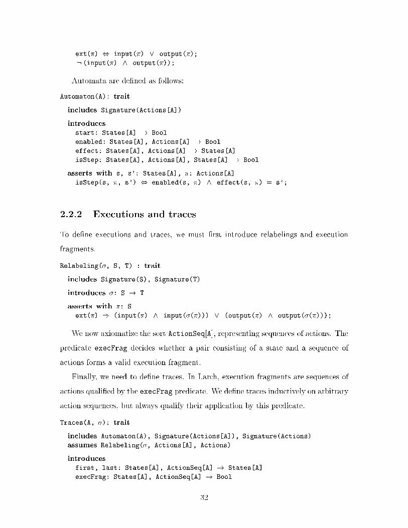
2.2.2 Executions and traces
To de�ne executions and traces, we must �rst introduce relabelings and execution
fragments.
Relabeling(�, S, T) : trait
includes Signature(S), Signature(T)
introduces �: S ! T
asserts with �: S
ext(�) ) (input(�) ^ input(�(�))) _ (output(�) ^ output(�(�)));
We now axiomatize the sort ActionSeq[A], representing sequences of actions. The
predicate execFrag decides whether a pair consisting of a state and a sequence of
actions forms a valid execution fragment.
Finally, we need to de�ne traces. In Larch, execution fragments are sequences of
actions quali�ed by the execFrag predicate. We de�ne traces inductively on arbitrary
action sequences, but always qualify their application by this predicate.
Traces(A, �): trait
includes Automaton(A), Signature(Actions[A]), Signature(Actions)
assumes Relabeling(�, Actions[A], Actions)
introduces
first, last: States[A], ActionSeq[A] ! States[A]
execFrag: States[A], ActionSeq[A] ! Bool
32
?: ! ActionSeq[A]
?: ! Traces
__ � __: Actions[A], ActionSeq[A] ! ActionSeq[A]
__ � __: Actions, Traces ! Traces
trace: ActionSeq[A] ! Traces
trace: Actions[A] ! Traces
asserts with s: States[A], �: Actions[A], �: ActionSeq[A]
sort ActionSeq[A] generated by ?, �;
execFrag(s, ?);
execFrag(s, � � �) , enabled(s, �) ^ execFrag(effect(s, �), �);
first(s, �) = s;
last(s, ?) = s;
last(s, � � �) = last(effect(s, �), �);
trace(?) = ?;
trace(� � �) = (if ext(�) then �(�) � trace(�) else trace(�));
trace(�) = trace(� � ?);
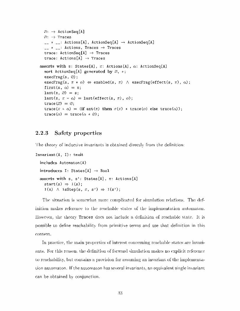
2.2.3 Safety properties
The theory of inductive invariants is obtained directly from the de�nition:
Invariant(A, I): trait
includes Automaton(A)
introduces I: States[A] ! Bool
asserts with s, s': States[A], �: Actions[A]
start(s) ) I(s);
I(s) ^ isStep(s, �, s') ) I(s');
The situation is somewhat more complicated for simulation relations. The def-
inition makes reference to the reachable states of the implementation automaton.
However, the theory Traces does not include a de�nition of reachable state. It is
possible to de�ne reachability from primitive terms and use that de�nition in this
context.
In practice, the main properties of interest concerning reachable states are invari-
ants. For this reason, the de�nition of forward simulation makes no explicit reference
to reachability, but contains a provision for assuming an invariant of the implementa-
tion automaton. If the automaton has several invariants, an equivalent single invariant
can be obtained by conjunction.
33
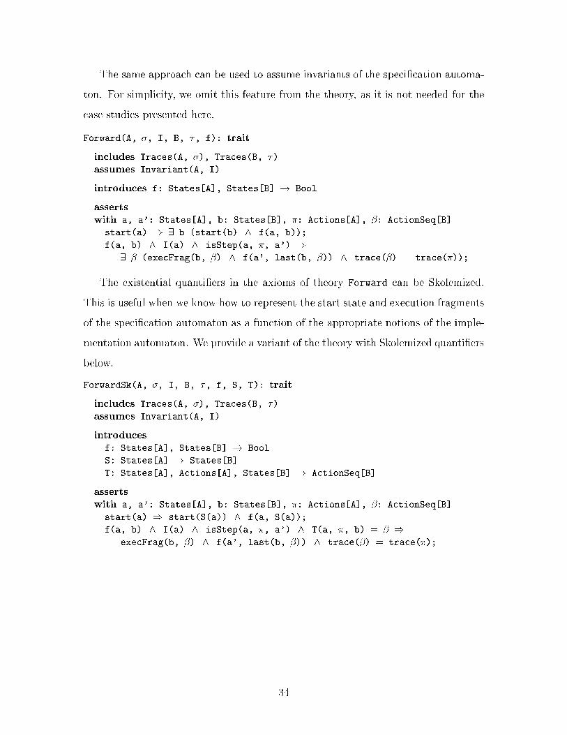
The same approach can be used to assume invariants of the speci�cation automa-
ton. For simplicity, we omit this feature from the theory, as it is not needed for the
case studies presented here.
Forward(A, �, I, B, �, f): trait
includes Traces(A, �), Traces(B, �)
assumes Invariant(A, I)
introduces f: States[A], States[B] ! Bool
asserts
with a, a': States[A], b: States[B], �: Actions[A], �: ActionSeq[B]
start(a) ) 9 b (start(b) ^ f(a, b));
f(a, b) ^ I(a) ^ isStep(a, �, a') )
9 � (execFrag(b, �) ^ f(a', last(b, �)) ^ trace(�) = trace(�));
The existential quanti�ers in the axioms of theory Forward can be Skolemized.
This is useful when we know how to represent the start state and execution fragments
of the speci�cation automaton as a function of the appropriate notions of the imple-
mentation automaton. We provide a variant of the theory with Skolemized quanti�ers
below.
ForwardSk(A, �, I, B, �, f, S, T): trait
includes Traces(A, �), Traces(B, �)
assumes Invariant(A, I)
introduces
f: States[A], States[B] ! Bool
S: States[A] ! States[B]
T: States[A], Actions[A], States[B] ! ActionSeq[B]
asserts
with a, a': States[A], b: States[B], �: Actions[A], �: ActionSeq[B]
start(a) ) start(S(a)) ^ f(a, S(a));
f(a, b) ^ I(a) ^ isStep(a, �, a') ^ T(a, �, b) = � )
execFrag(b, �) ^ f(a', last(b, �)) ^ trace(�) = trace(�);
34
Chapter 3
The translation process
The Larch theory of I/O automata provides a framework for carrying out formal
reasoning about automaton properties. We are interested in applying this theory to
particular speci�cations written in the IOA language. The �rst step is to translate
the IOA speci�cation to the language of I/O automata from Chapter 2.
IOA programs describe I/O automata in a precise and direct manner. The IOA
Reference Manual [10] explains the intended interpretations of IOA syntactic con-
structs in the I/O automaton model. This close relationship between IOA and the
underlying model is a good starting point for the translation process. Many IOA
constructs|states, signatures, invariants, simulation relations|have simple inter-
pretations in the I/O automaton model; these can be readily translated to the Larch
theory of I/O automata. Others, such as imperative-style programs and choose
clauses, have more complicated semantics. For example, an imperative-style program
may be interpreted either as a sequence of successive state changes, one for each
statement, or as a single transition from an initial to a �nal state, without explicit
notation for the intermediate states. The challenge is to select the interpretation
which is most convenient for interactive theorem proving.
Theorem provers serve to verify the correctness of arguments carried out in infor-
mal mathematics. The reasoning strategies they support closely re ect the rules of
deductive calculus. Theorem provers are useful because they allow us to mirror our
informal arguments at a formal level. The starting point of the argument|the prim-
35
itive notions and assumptions of the theory|must be intuitive to our understanding.
If the speci�cations are cumbersome and unreadable, the interaction with the tool
can become extremely diÆcult.
In many cases, our intuition about programs does not correspond well with the
complexity of the underlying semantics. Facts like \transition � does not change
the value of x" or \the value of y does not depend on the value of x" are often so
obvious to us that we do not even bother to state them explicitly in informal proofs.
Establishing these facts may require nontrivial reasoning at a formal level. A good
translation scheme must keep this reasoning out of sight and preserve the illusion
that what appears obvious to the user is also obvious to the theorem proving tool.
It is important to keep in mind that many of the design decisions presented in this
chapter are driven by the need to preserve this transparency between informal and
formal reasoning.
To achieve this transparency between the original program and its translated ver-
sion, translated speci�cations should interact well with the automatic features of the
theorem proving tool. These automatic features are most productive on speci�cations
with widely applicable rewrite rules (statements of equality or boolean equivalence)
and lack of existential quanti�ers. To obtain such speci�cations, we adopt the follow-
ing two general guidelines:
1. Representations by functions are preferred to representations by relations (i.e.,
predicates). Functional speci�cations usually give rise to more useful rewrite
rules in theorem proving.
2. Nondeterministic choices are represented by global parameters rather than by
existentially quanti�ed variables.
The �rst guideline principally concerns the translation of e�ects clauses of tran-
sition de�nitions. Transitions are speci�ed by Larch functions that \compute" the
post-state from the pre-state. The second guideline is exhibited in our treatment of
nondeterminism. We postpone this issue until Chapter 4. In this chapter we restrict
36
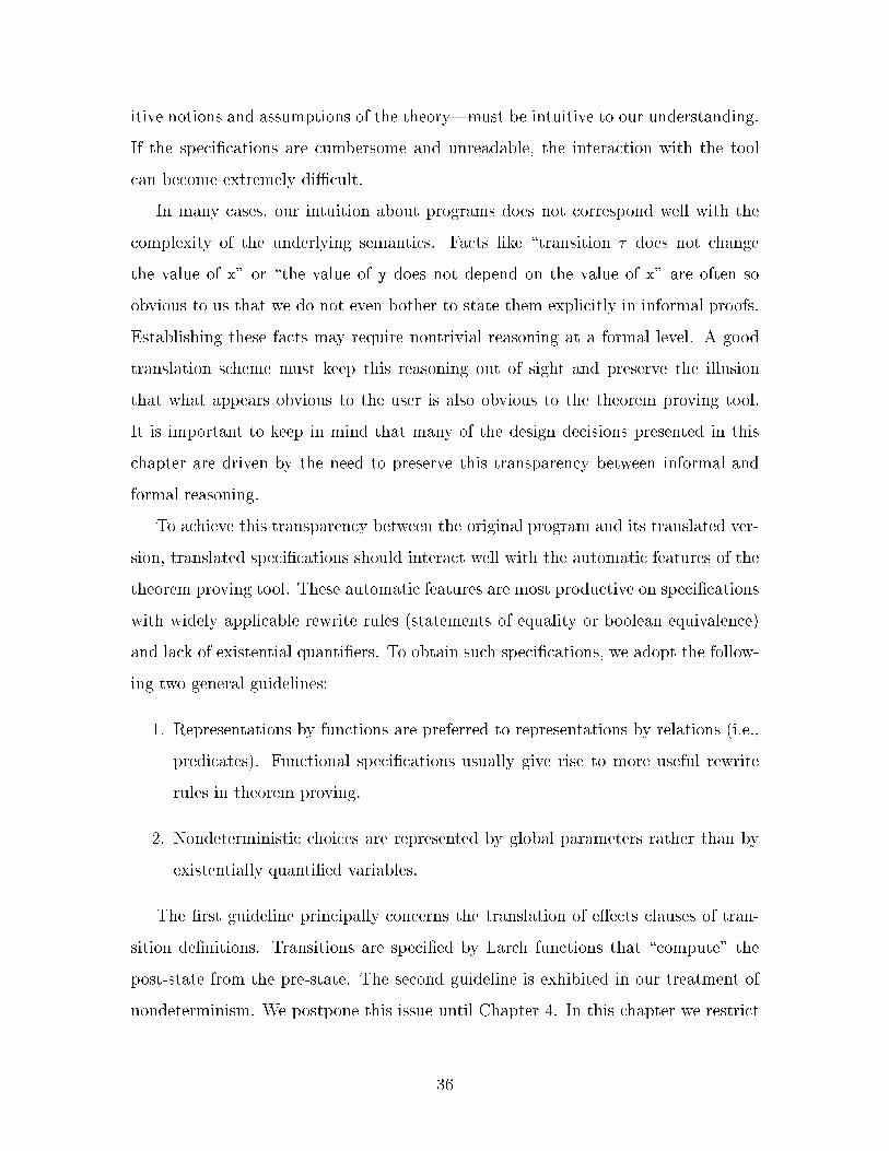
uses Sequence(T)
automaton channel
signature
input send(t: T)
output receive(t: T)
states
queue: Seq[T] := ?
transitions
input send(t)
e� queue := t a queue
output receive(t)
pre queue 6= ? ^ last(queue) = t
e� queue := init(queue)
Figure 3-1: IOA speci�cation of automaton channel
our attention to the class of IOA programs which do not exhibit explicit nondeter-
minism (i.e., that do not contain the keyword choose).
3.1 An illustrative example
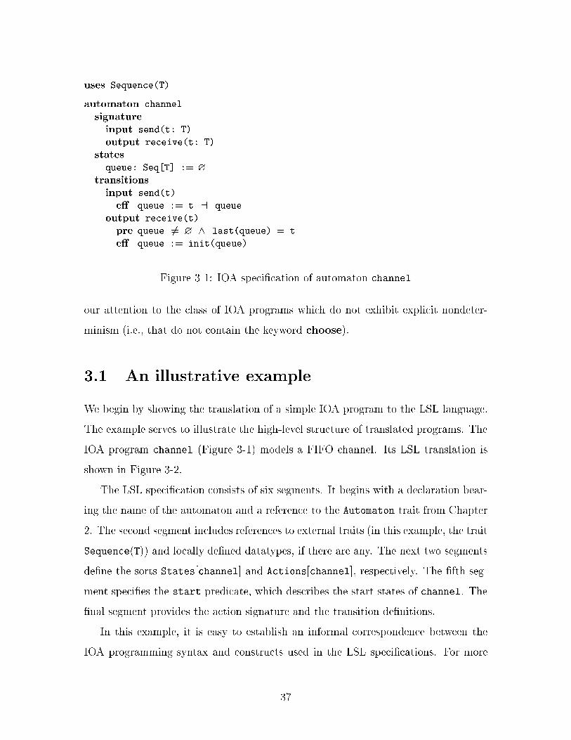
We begin by showing the translation of a simple IOA program to the LSL language.
The example serves to illustrate the high-level structure of translated programs. The
IOA program channel (Figure 3-1) models a FIFO channel. Its LSL translation is
shown in Figure 3-2.
The LSL speci�cation consists of six segments. It begins with a declaration bear-
ing the name of the automaton and a reference to the Automaton trait from Chapter
2. The second segment includes references to external traits (in this example, the trait
Sequence(T)) and locally de�ned datatypes, if there are any. The next two segments
de�ne the sorts States[channel] and Actions[channel], respectively. The �fth seg-
ment speci�es the start predicate, which describes the start states of channel. The
�nal segment provides the action signature and the transition de�nitions.
In this example, it is easy to establish an informal correspondence between the
IOA programming syntax and constructs used in the LSL speci�cations. For more
37
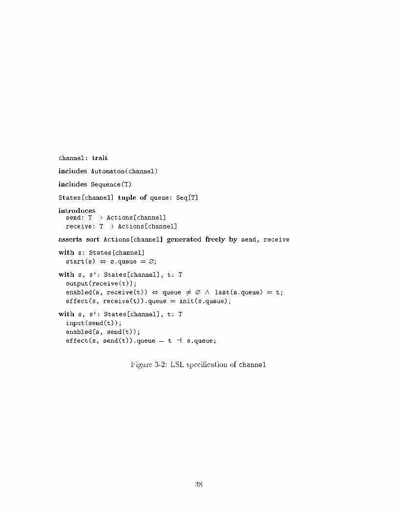
channel: trait
includes Automaton(channel)
includes Sequence(T)
States[channel] tuple of queue: Seq[T]
introducessend: T ! Actions[channel]
receive: T ! Actions[channel]
asserts sort Actions[channel] generated freely by send, receive
with s: States[channel]
start(s) , s.queue = ?;
with s, s': States[channel], t: T
output(receive(t));
enabled(s, receive(t)) , queue 6= ? ^ last(s.queue) = t;
effect(s, receive(t)).queue = init(s.queue);
with s, s': States[channel], t: T
input(send(t));
enabled(s, send(t));
effect(s, send(t)).queue = t a s.queue;
Figure 3-2: LSL speci�cation of channel
38
complicated programs, this correspondence may become less transparent as the trans-
lation process involves nontrivial transformations of the IOA code.
3.2 Referenced traits, datatypes and formals
The LSL speci�cation for automaton A includes the following external traits:
� The trait Automaton(A).
� All traits referenced in uses and assumes clauses in the IOA speci�ation which
contains the declaration of A.
All datatypes de�ned locally as tuples, enumerations and unions are repre-
sented by the equivalent form in LSL.
The formal parameters of the automaton are declared as LSL constants of the
appropriate type. A constraint on a formal parameter speci�ed by an assumes clause
is translated into a constraint on the constant corresponding to this parameter.
3.3 Automaton states
The states of automaton A are represented by LSL variables of the sort States[A].
This sort is de�ned as a tuple of state variables. For readability, a single LSL variable
references the \current" state of A throughout the speci�cation; we call this variable
the state name.1 Post-states of transitions are represented by a primed instance of
the state name.
Variables in the IOA program are always interpreted with respect to a particu-
lar state. This implicit dependence in the IOA code must be made explicit in the
translation. In most cases (start state declarations, where clauses and transition
preconditions) the implicit state corresponds to the state name. In imperative style
1In the implementation, the state name consists of a single letter like s or u. Long state names areunwieldy because they make the speci�cation less readable. Distinct automata within a speci�cationare assigned distinct state names to avoid confusion.
39
transition de�nitions, the state undergoes changes after each instruction, while the
state name refers to the state before the transition. The representation of these
intermediate states is described in Section 3.5.
IOA provides the option of specifying an initial value for each of the state variables.
If an initial value is speci�ed, the assignment appears as a conjunct in the start
predicate, with the assignment symbol replaced by equality. If the start state is
constrained by a so that predicate, the constraint is conjoined to the start predicate.
The following example shows a simple IOA speci�cation for the start states of an
automaton (with state name s):
statesx: Int := 4
y: Int
z: Int
so that (x * x) + (y * y) + (z * z) = 17
The resulting LSL predicate for the start states is:
start(s) , s.x = 4 ^ (s.x * s.x) + (s.y * s.y) + (s.z * s.z) = 17
3.4 Action declarations
In IOA, a single action declaration may correspond to multiple transition de�ni-
tions. Di�erent transition de�nitions with the same action label may yield di�erent
post-states, thereby violating the pseudodeterminism condition. In such a case it is
necessary to relabel the actions so that each transition de�nition corresponds to a
unique action label. Technically, we distinguish multiple transition de�nitions corre-
sponding to the same action by appending a unique integer label to the transition
name.
The actions of automaton A are declared as functions of their parameters into the
sort Actions[A]. This sort is introduced as a free sort generated by all actions in the
signature. We can formally verify properties that hold for all actions by reasoning
inductively over the sort Actions[A].
40
IOA speci�cation of automaton move:
uses Integer
automaton move
signature
output jump
output back
states x: Int := 0
transitions
output jump
e� x := x + 2
output jump
e� x := x + 3
output back
e� x := x - 5
LSL translation of the action declarations:
move: trait
introduces
jump_1: ! Actions[move]
jump_2: ! Actions[move]
back: ! Actions[move]
asserts sort Actions[move] generated freely by jump_1, jump_2, back
: : :
asserts with s: States[move]
effect(s, jump_1).x = s.x + 2;
: : :
effect(s, jump_2).x = s.x + 3;
: : :
effect(s, back).x = s.x - 5;
Figure 3-3: Translation of action declarations
41
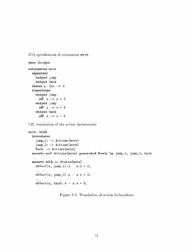
Figure 3-3 shows the translation for the action declarations of automaton move.
In the IOA speci�cation of move, the action jump corresponds to two transition de�ni-
tions. In the translation, these are represented by constants of the sort Actions[move]
named jump 1 and jump 2. Action back corresponds to a single transition de�nition.
It is represented by the constant back in Actions[move].
For each family of parameterized actions, an axiom specifying their type (input,
output or internal) is included in the LSL speci�cation.
The original signature is important for checking properties like simulation rela-
tions. For this purpose we introduce a relabeling which maps the modi�ed action
signature to the original one. Whenever a property which depends on the signature
is to be veri�ed, it needs to be checked with respect to this relabeling.
Notation. We use the notation �? for the name of the Larch function representing
the transition de�nition �. For example, if � is the second transition de�nition in
automaton move, then �? = jump 2.
3.5 Transition de�nitions
For each transition de�nition � in the IOA speci�cation of automaton A, we need to
specify two LSL forms: the predicate enabled(s; �) and the function effect(s; �).
In the absence of explicit nondeterminism, the e� clause of a transition de�nition
is a well-de�ned function on states(A). Therefore, it is possible to decouple the
translation process in a natural manner so that
� Predicate enabled(s; �) depends only on the pre clause of �, the where clause
of � and the where clause of the action declaration for �.
� Function effect(s; �) depends only on the e� clause of �.
Notation. In what follows, we use the notation t[s=x] for the term obtained by
substituting all instances of variable x in term t by term s (assuming that x and s
have the same sort). If s = (s1; : : : ; sn) is a collection of terms and x = (x1; : : : ; xn)
42
is a collection of distinct variables so that xi and si are of the same sort, we write
t[s=x] for the term t[s1=x1] � � � [sn=xn].
3.5.1 The enabled clause
A transition de�nition with action signature
�(y1,: : : ,yn) where s1
transition declaration
�(x1,: : : ,xn) where s2
and precondition t is represented with the following enabled predicate:
enabled(s, �?(x1,: : : ,xn)) , s1? ^ s2 ^ t
where
s1? = s1[x1; : : : ; xn=y1; : : : ; yn]:
Here s denotes the implicit state of the automaton (before the transition). As
explained in Section 3.3, the state variables in all expressions are implicitly evaluated
at state s.
3.5.2 Variable maps
The semantics of the effect clause for transition � is more complicated. In the IOA
program, the e�ect of � is represented by a sequence of statements. Each statement
represents a transformation on the state of the automaton. This transformation can
be described by a function which maps the state before the transition to the state
after the transition. The function may also depend on the actual parameters of the
transition. By composing the functions corresponding to each statement in order of
their appearance in the program, we obtain a function which describes the post-state
of � in terms of the pre-state and the transition actuals.
For this translation scheme to work, two important issues need to be addressed:
1. Each type of IOA statement must be expressed as a Larch function describing
the post-state of the statement as a function of the pre-state and the transition
parameters.
43
2. The functions corresponding to each statement must be composed.
There are two possible approaches to the problem. The �rst approach is to index
the functions corresponding to program statements, and to de�ne composition induc-
tively over the index. This approach has the bene�t of providing shorthand notation
for the intermediate states (the states between instructions) within a program. For
example, to reference the state after the third instruction we simply evaluate the
function representing the loop at index 3. Unfortunately, this scheme is not particu-
larly suitable for theorem proving because even the simplest property of the program
would require a proof by induction. The veri�cation of inductive properties needs
to be initiated by the user. This violates the requirement that intuitively obvious
properties of programs should also be obvious to the theorem prover.
Our approach attacks these problems by using implicit representations to describe
the e�ects of a particular statement. Composition is then interpreted as an operation
which combines two consecutive e�ects into a single one. This eliminates the need
for explicit iterators to represent the sequencing of instructions. The post-state is
represented directly as a function of a pre-state. In a theorem prover, this representa-
tion is turned into a rewrite rule which can be used to automatically deduce intuitive
properties of programs.
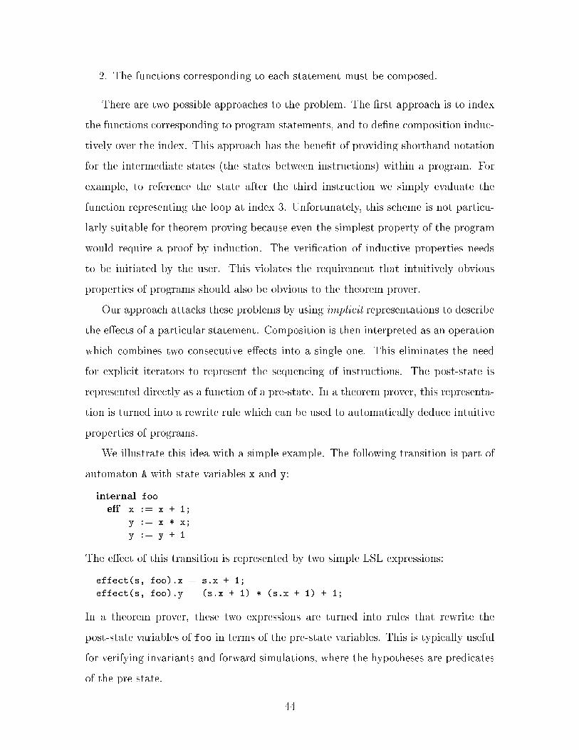
We illustrate this idea with a simple example. The following transition is part of
automaton A with state variables x and y:
internal foo
e� x := x + 1;
y := x * x;
y := y + 1
The e�ect of this transition is represented by two simple LSL expressions:
effect(s, foo).x = s.x + 1;
effect(s, foo).y = (s.x + 1) * (s.x + 1) + 1;
In a theorem prover, these two expressions are turned into rules that rewrite the
post-state variables of foo in terms of the pre-state variables. This is typically useful
for verifying invariants and forward simulations, where the hypotheses are predicates
of the pre-state.
44
The main drawback of this approach is the lack of shorthand notation for inter-
mediate states. For instance, to refer to the value of y after the second assignment
in the above example we must type the whole expression (s.x + 1) * (s.x + 1).
Such references need to be evaluated when translating conditionals, loops and non-
deterministic assignments. When the transition de�nitions are long and complicated,
these expressions may become cumbersome for the user of the theorem proving tool.
In our case studies, the transition de�nitions are short and simple, so we did not
encounter this problem.
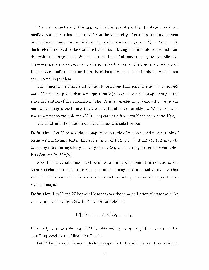
The principal structure that we use to represent functions on states is a variable
map. Variable map V assigns a unique term V (x) to each variable x appearing in the
state declaration of the automaton. The identity variable map (denoted by id) is the
map which assigns the term x to variable x, for all state variables x. We call variable
v a parameter to variable map V if v appears as a free variable in some term V (x).
The most useful operation on variable maps is substitution:
De�nition Let V be a variable map, y an n-tuple of variables and t an n-tuple of
terms with matching sorts. The substitution of t for y in V is the variable map ob-
tained by substituting t for y in every term V (x), where x ranges over state variables.
It is denoted by V [t=y].
Note that a variable map itself denotes a family of potential substitutions; the
term associated to each state variable can be thought of as a substitute for that
variable. This observation leads to a very natural interpretation of composition of
variable maps:
De�nition Let V andW be variable maps over the same collection of state variables
x1; : : : ; xn. The composition V ;W is the variable map
W [V (x1); : : : ; V (xn)=x1; : : : ; xn]:
Informally, the variable map V ;W is obtained by computing W , with its \initial
state" replaced by the \�nal state" of V .
Let V be the variable map which corresponds to the e� clause of transition �.
45
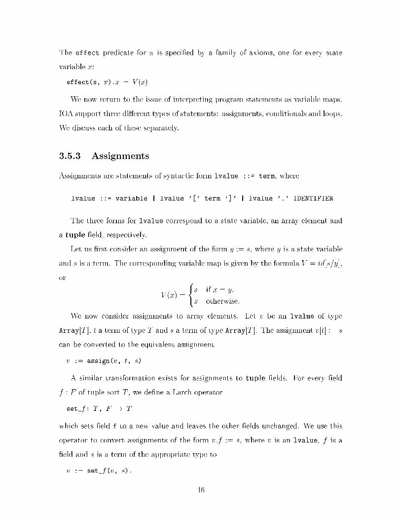
The effect predicate for � is speci�ed by a family of axioms, one for every state
variable x:
effect(s, �).x = V (x)
We now return to the issue of interpreting program statements as variable maps.
IOA support three di�erent types of statements: assignments, conditionals and loops.
We discuss each of these separately.
3.5.3 Assignments
Assignments are statements of syntactic form lvalue ::= term, where
lvalue ::= variable | lvalue '[' term ']' | lvalue '.' IDENTIFIER
The three forms for lvalue correspond to a state variable, an array element and
a tuple �eld, respectively.
Let us �rst consider an assignment of the form y := s, where y is a state variable
and s is a term. The corresponding variable map is given by the formula V = id[s=y],
or
V (x) =
(s if x = y;
x otherwise:
We now consider assignments to array elements. Let v be an lvalue of type
Array[T ], t a term of type T and s a term of type Array[T ]. The assignment v[t] := s
can be converted to the equivalent assignment
v := assign(v, t, s)
A similar transformation exists for assignments to tuple �elds. For every �eld
f : F of tuple sort T , we de�ne a Larch operator
set_f: T, F ! T
which sets �eld f to a new value and leaves the other �elds unchanged. We use this
operator to convert assignments of the form v:f := s, where v is an lvalue, f is a
�eld and s is a term of the appropriate type to
v := set_f(v, s).
46
After performing a �nite number of substitutions, the original assignment will be
reduced to an assignment of the form y := s, where y is a state variable.
We can optimize the computation of variable maps using the following observation:
Assignments leave all but one state variable unchanged. Say we are interested in
composing the variable map V with the map corresponding to the assignment y := s.
For this purpose, it is unnecessary to generate the latter map; the result is equal to
the substitution V [s=y].
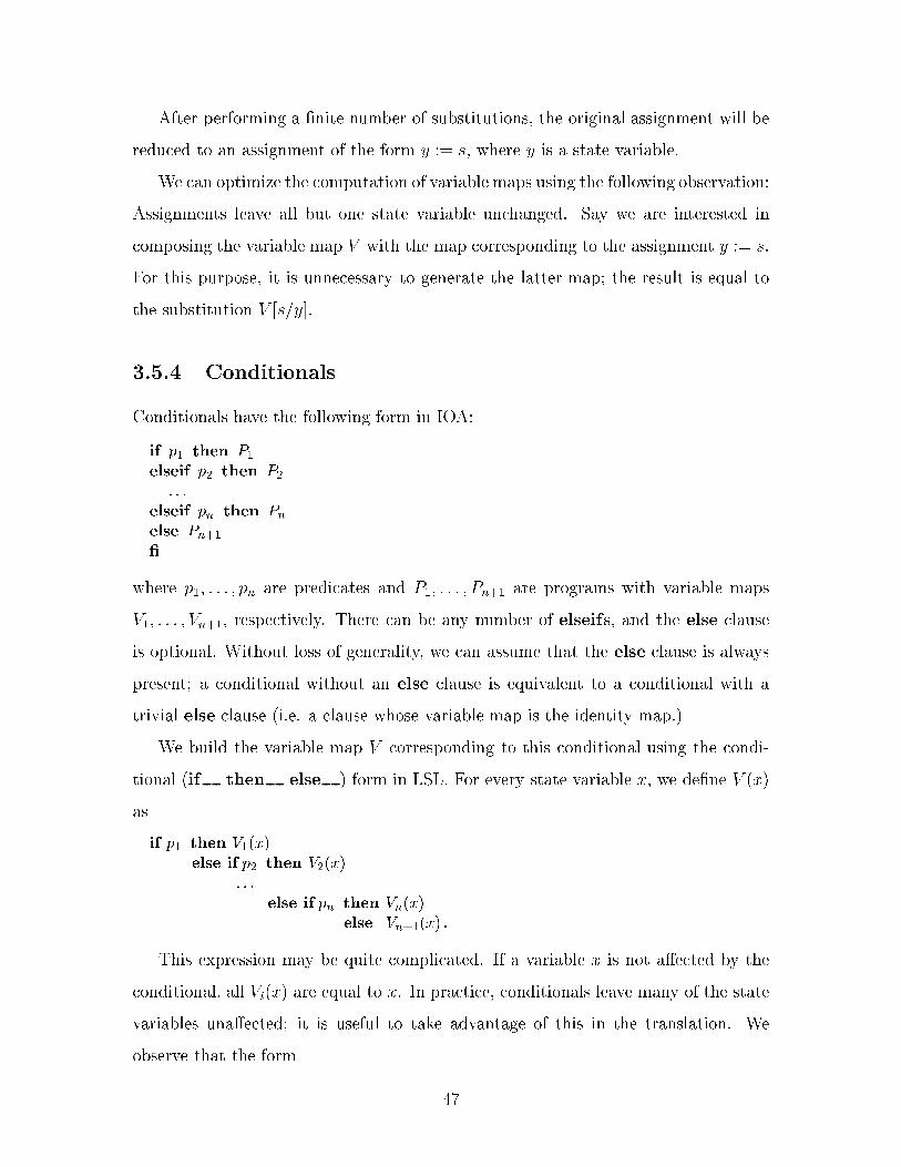
3.5.4 Conditionals
Conditionals have the following form in IOA:
if p1 then P1
elseif p2 then P2
: : :
elseif pn then Pnelse Pn+1
�
where p1; : : : ; pn are predicates and P1; : : : ; Pn+1 are programs with variable maps
V1; : : : ; Vn+1, respectively. There can be any number of elseifs, and the else clause
is optional. Without loss of generality, we can assume that the else clause is always
present; a conditional without an else clause is equivalent to a conditional with a
trivial else clause (i.e. a clause whose variable map is the identity map.)
We build the variable map V corresponding to this conditional using the condi-
tional (if then else ) form in LSL. For every state variable x, we de�ne V (x)
as
if p1 then V1(x)
else if p2 then V2(x)
: : :
else if pn then Vn(x)
else Vn+1(x).
This expression may be quite complicated. If a variable x is not a�ected by the
conditional, all Vi(x) are equal to x. In practice, conditionals leave many of the state
variables una�ected; it is useful to take advantage of this in the translation. We
observe that the form
47
if p then s else s
is equivalent to s. We apply this reduction to the formula for V (x). As a result, the
formula simpli�es to V (x) = x if state variable x is not a�ected by the conditional.
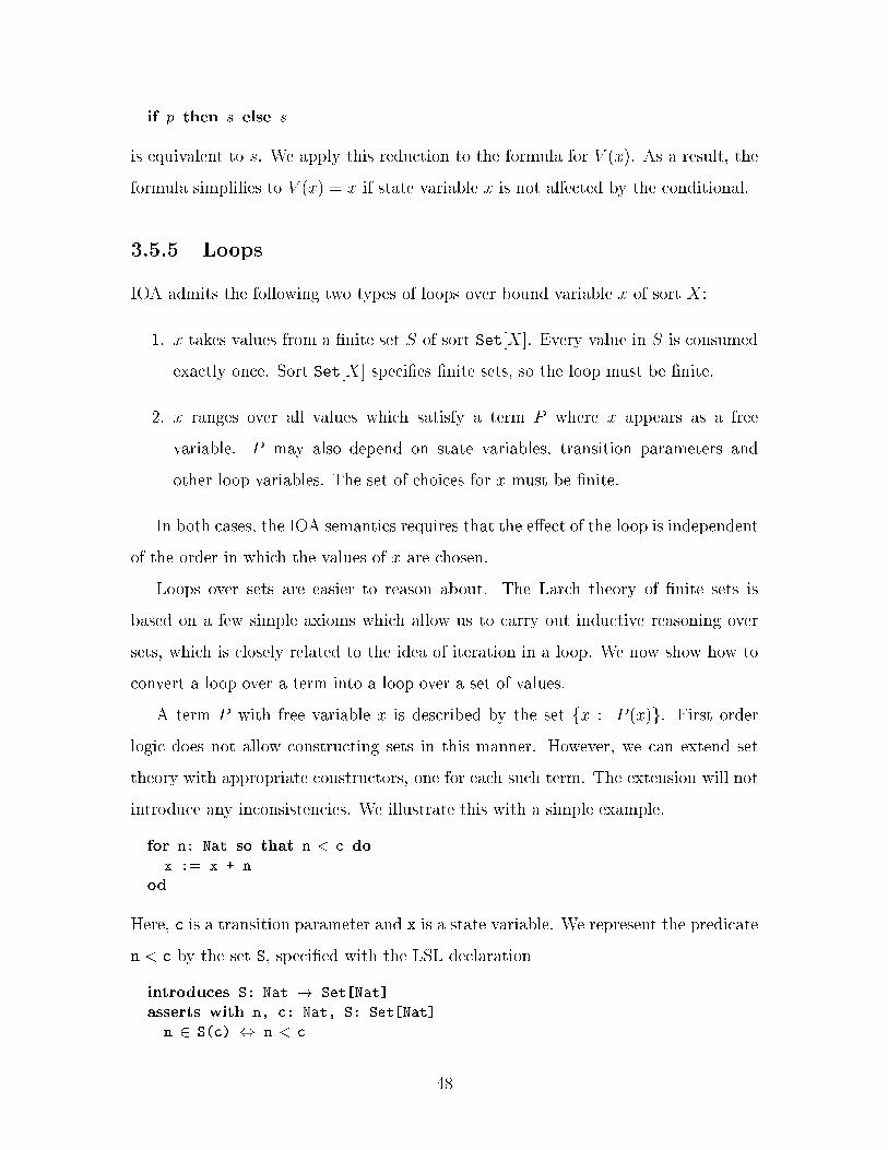
3.5.5 Loops
IOA admits the following two types of loops over bound variable x of sort X:
1. x takes values from a �nite set S of sort Set[X]. Every value in S is consumed
exactly once. Sort Set[X] speci�es �nite sets, so the loop must be �nite.
2. x ranges over all values which satisfy a term P where x appears as a free
variable. P may also depend on state variables, transition parameters and
other loop variables. The set of choices for x must be �nite.
In both cases, the IOA semantics requires that the e�ect of the loop is independent
of the order in which the values of x are chosen.
Loops over sets are easier to reason about. The Larch theory of �nite sets is
based on a few simple axioms which allow us to carry out inductive reasoning over
sets, which is closely related to the idea of iteration in a loop. We now show how to
convert a loop over a term into a loop over a set of values.
A term P with free variable x is described by the set fx : P (x)g. First order
logic does not allow constructing sets in this manner. However, we can extend set
theory with appropriate constructors, one for each such term. The extension will not
introduce any inconsistencies. We illustrate this with a simple example.
for n: Nat so that n < c do
x := x + n
od
Here, c is a transition parameter and x is a state variable. We represent the predicate
n < c by the set S, speci�ed with the LSL declaration
introduces S: Nat ! Set[Nat]
asserts with n, c: Nat, S: Set[Nat]
n 2 S(c) , n < c
48
To ensure consistency, we must verify that such a set exists in the theory Set[Nat].
In this case, the set exists because there are only �nitely many n so that n < c. In
general, the semantics of IOA requires that the so that clause ranges over a �nite
set, so the extension will be consistent.
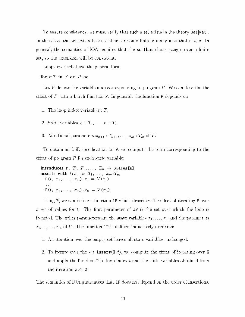
Loops over sets have the general form
for t:T in S do P od
Let V denote the variable map corresponding to program P . We can describe the
e�ect of P with a Larch function P. In general, the function P depends on
1. The loop index variable t : T ,
2. State variables x1 : T1; : : : ; xn : Tn,
3. Additional parameters xn+1 : Tn+1; : : : ; xm : Tm of V .
To obtain an LSL speci�cation for P, we compute the term corresponding to the
e�ect of program P for each state variable:
introduces P: T, T1, : : : , Tm ! States[A]
asserts with t:T, x1:T1, : : : , xm:TmP(t, x1, : : : , xm).x1 = V (x1)
: : :
P(t, x1, : : : , xm).xn = V (xn)
Using P, we can de�ne a function lP which describes the e�ect of iterating P over
a set of values for t. The �rst parameter of lP is the set over which the loop is
iterated. The other parameters are the state variables x1; : : : ; xn and the parameters
xn+1; : : : ; xm of V . The function lP is de�ned inductively over sets:
1. An iteration over the empty set leaves all state variables unchanged.
2. To iterate over the set insert(X; t), we compute the e�ect of iterating over X
and apply the function P to loop index t and the state variables obtained from
the iteration over X.
The semantics of IOA guarantees that lP does not depend on the order of insertions.
49
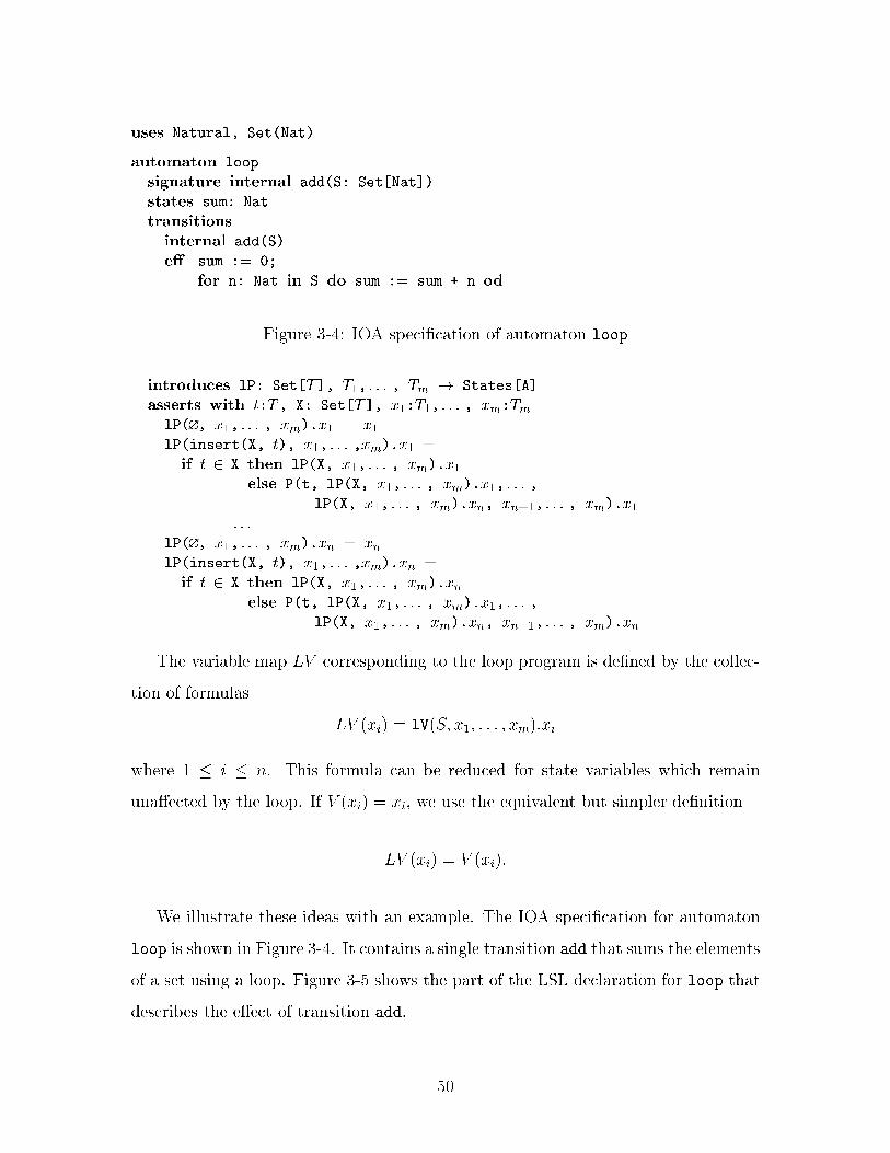
uses Natural, Set(Nat)
automaton loop
signature internal add(S: Set[Nat])
states sum: Nat
transitions
internal add(S)
e� sum := 0;
for n: Nat in S do sum := sum + n od
Figure 3-4: IOA speci�cation of automaton loop
introduces lP: Set[T], T1, : : : , Tm ! States[A]
asserts with t:T, X: Set[T], x1:T1, : : : , xm:TmlP(?, x1, : : : , xm).x1 = x1lP(insert(X, t), x1, : : : ,xm).x1 =
if t 2 X then lP(X, x1, : : : , xm).x1else P(t, lP(X, x1, : : : , xm).x1, : : : ,
lP(X, x1, : : : , xm).xn, xn+1, : : : , xm).x1: : :
lP(?, x1, : : : , xm).xn = xnlP(insert(X, t), x1, : : : ,xm).xn =
if t 2 X then lP(X, x1, : : : , xm).xnelse P(t, lP(X, x1, : : : , xm).x1, : : : ,
lP(X, x1, : : : , xm).xn, xn+1, : : : , xm).xn
The variable map LV corresponding to the loop program is de�ned by the collec-
tion of formulas
LV (xi) = lV(S; x1; : : : ; xm):xi
where 1 � i � n. This formula can be reduced for state variables which remain
una�ected by the loop. If V (xi) = xi, we use the equivalent but simpler de�nition
LV (xi) = V (xi):
We illustrate these ideas with an example. The IOA speci�cation for automaton
loop is shown in Figure 3-4. It contains a single transition add that sums the elements
of a set using a loop. Figure 3-5 shows the part of the LSL declaration for loop that
describes the e�ect of transition add.
50
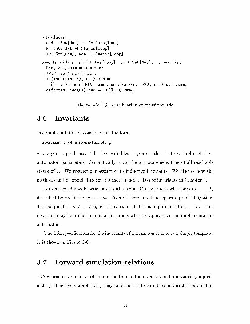
introduces
add : Set[Nat] ! Actions[loop]
P: Nat, Nat ! States[loop]
lP: Set[Nat], Nat ! States[loop]
asserts with s, s': States[loop], S, X:Set[Nat], n, sum: Nat
P(n, sum).sum = sum + n;
lP(?, sum).sum = sum;
lP(insert(n, X), sum).sum =
if n 2 X then lP(X, sum).sum else P(n, lP(X, sum).sum).sum;
effect(s, add(S)).sum = lP(S, 0).sum;
Figure 3-5: LSL speci�cation of transition add
3.6 Invariants
Invariants in IOA are constructs of the form
invariant I of automaton A: p
where p is a predicate. The free variables in p are either state variables of A or
automaton parameters. Semantically, p can be any statement true of all reachable
states of A. We restrict our attention to inductive invariants. We discuss how the
method can be extended to cover a more general class of invariants in Chapter 8.
Automaton Amay be associated with several IOA invariants with names I1; : : : ; In
described by predicates p1; : : : ; pn. Each of these entails a separate proof obligation.
The conjunction p1 ^ : : : ^ pn is an invariant of A that implies all of p1; : : : ; pn. This
invariant may be useful in simulation proofs where A appears as the implementation
automaton.
The LSL speci�cation for the invariants of automaton A follows a simple template.
It is shown in Figure 3-6.
3.7 Forward simulation relations
IOA characterizes a forward simulation from automaton A to automaton B by a pred-
icate f . The free variables of f may be either state variables or variable parameters
51
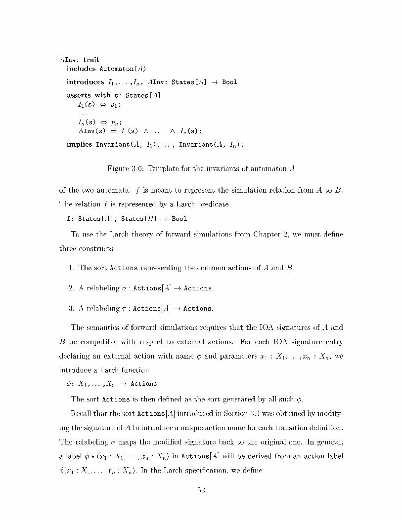
AInv: trait
includes Automaton(A)
introduces I1, : : : ,In, AInv: States[A] ! Bool
asserts with s: States[A]
I1(s) , p1;
: : :
In(s) , pn;
AInv(s) , I1(s) ^ : : : ^ In(s);
implies Invariant(A, I1), : : : , Invariant(A, In);
Figure 3-6: Template for the invariants of automaton A
of the two automata. f is meant to represent the simulation relation from A to B.
The relation f is represented by a Larch predicate
f: States[A], States[B] ! Bool
To use the Larch theory of forward simulations from Chapter 2, we must de�ne
three constructs:
1. The sort Actions representing the common actions of A and B.
2. A relabeling � : Actions[A]! Actions.
3. A relabeling � : Actions[A]! Actions.
The semantics of forward simulations requires that the IOA signatures of A and
B be compatible with respect to external actions. For each IOA signature entry
declaring an external action with name � and parameters x1 : X1; : : : ; xn : Xn, we
introduce a Larch function
�: X1, : : : ,Xn ! Actions
The sort Actions is then de�ned as the sort generated by all such �.
Recall that the sort Actions[A] introduced in Section 3.4 was obtained by modify-
ing the signature of A to introduce a unique action name for each transition de�nition.
The relabeling � maps the modi�ed signature back to the original one. In general,
a label � ? (x1 : X1; : : : ; xn : Xn) in Actions[A] will be derived from an action label
�(x1 : X1; : : : ; xn : Xn). In the Larch speci�cation, we de�ne
52
asserts with x1: X1, : : : , xn: Xn
�(�?(x1,: : : ,xn)) = �(x1,: : : ,xn)
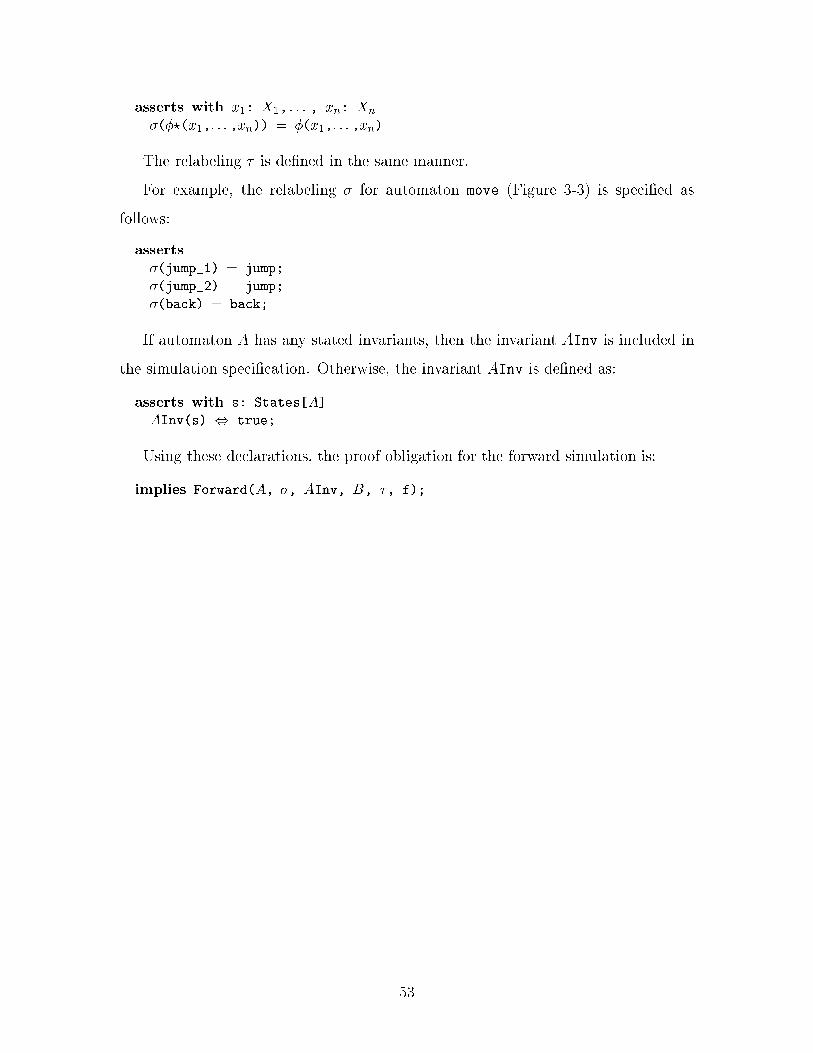
The relabeling � is de�ned in the same manner.
For example, the relabeling � for automaton move (Figure 3-3) is speci�ed as
follows:
asserts
�(jump_1) = jump;
�(jump_2) = jump;
�(back) = back;
If automaton A has any stated invariants, then the invariant AInv is included in
the simulation speci�cation. Otherwise, the invariant AInv is de�ned as:
asserts with s: States[A]
AInv(s) , true;
Using these declarations, the proof obligation for the forward simulation is:
implies Forward(A, �, AInv, B, �, f);
53

54
Chapter 4
Nondeterminism
In Chapter 3 we devised a scheme for translating IOA programs into equivalent Larch
speci�cations. The translation process was limited to the class of programs that do
not exhibit explicit nondeterminism. In this chapter we extend the basic translation
process from Chapter 3 to a much more general class of programs.
Not every IOA program describes a pseudodeterministic automaton. One ap-
proach towards obtaining a pseudodeterministic description is to follow the construc-
tion from the proof of Theorem 2.2. From a practical point of view, such an approach
would be diÆcult to justify because it will introduce unnecessary transformations
to transitions which are locally unambiguous. Moreover, it parameterizes transition
labels by all components of the post-state, while the dependence is more naturally
described by a small number of choose parameters. Fortunately, these problems can
be avoided if we take a closer look at the relation between IOA and the underlying
model.
It is worthwhile to consider which parts of the IOA description may be responsible
for a lack of pseudodeterminism. We refer to these as points of ambiguity:
1. Two transition de�nitions may bear the same action label, be enabled at the
same pre-state, but produce di�erent post-states.
2. A transition de�nition may include explicit choices in the form of choose
clauses.
55
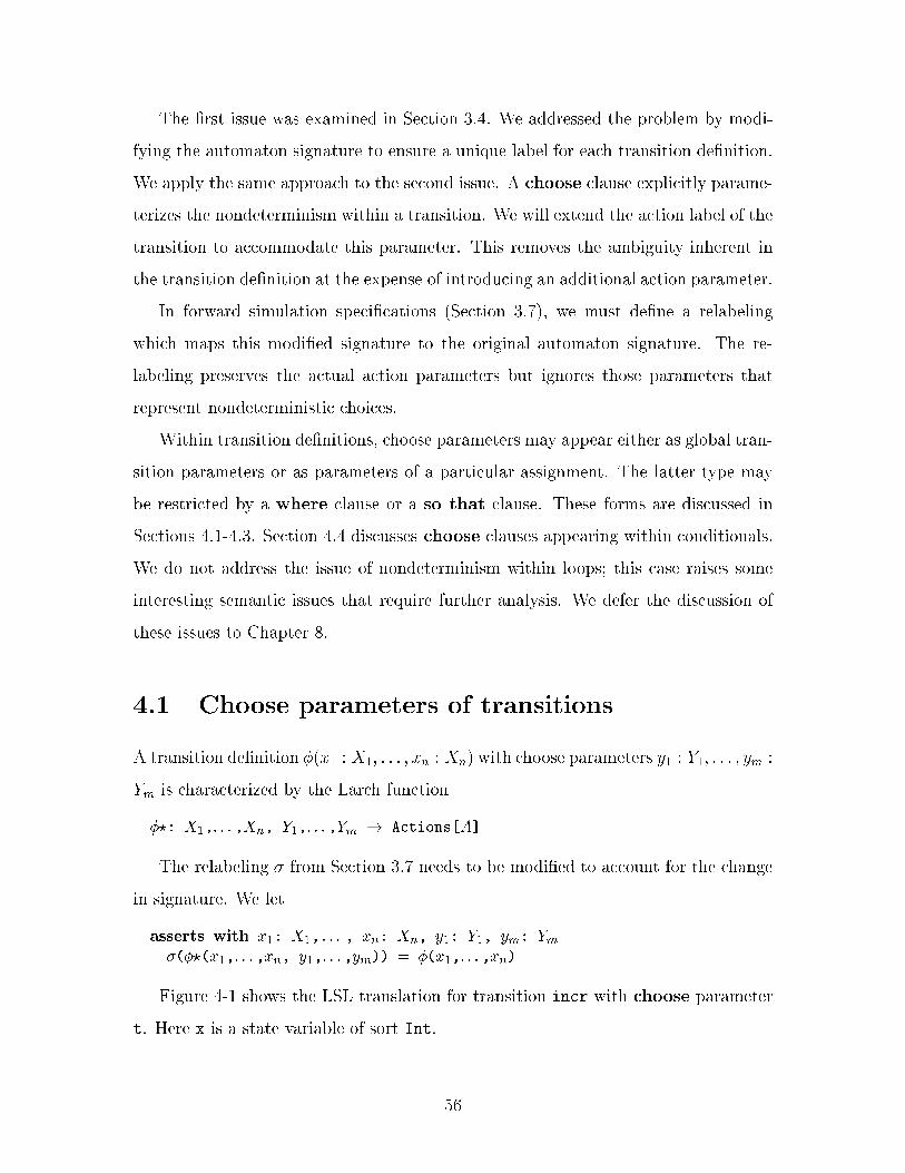
The �rst issue was examined in Section 3.4. We addressed the problem by modi-
fying the automaton signature to ensure a unique label for each transition de�nition.
We apply the same approach to the second issue. A choose clause explicitly parame-
terizes the nondeterminism within a transition. We will extend the action label of the
transition to accommodate this parameter. This removes the ambiguity inherent in
the transition de�nition at the expense of introducing an additional action parameter.
In forward simulation speci�cations (Section 3.7), we must de�ne a relabeling
which maps this modi�ed signature to the original automaton signature. The re-
labeling preserves the actual action parameters but ignores those parameters that
represent nondeterministic choices.
Within transition de�nitions, choose parameters may appear either as global tran-
sition parameters or as parameters of a particular assignment. The latter type may
be restricted by a where clause or a so that clause. These forms are discussed in
Sections 4.1-4.3. Section 4.4 discusses choose clauses appearing within conditionals.
We do not address the issue of nondeterminism within loops; this case raises some
interesting semantic issues that require further analysis. We defer the discussion of
these issues to Chapter 8.
4.1 Choose parameters of transitions
A transition de�nition �(x1 : X1; : : : ; xn : Xn) with choose parameters y1 : Y1; : : : ; ym :
Ym is characterized by the Larch function
�?: X1,: : : ,Xn, Y1,: : : ,Ym ! Actions[A]
The relabeling � from Section 3.7 needs to be modi�ed to account for the change
in signature. We let
asserts with x1: X1, : : : , xn: Xn, y1: Y1, ym: Ym�(�?(x1,: : : ,xn, y1,: : : ,ym)) = �(x1,: : : ,xn)
Figure 4-1 shows the LSL translation for transition incr with choose parameter
t. Here x is a state variable of sort Int.
56
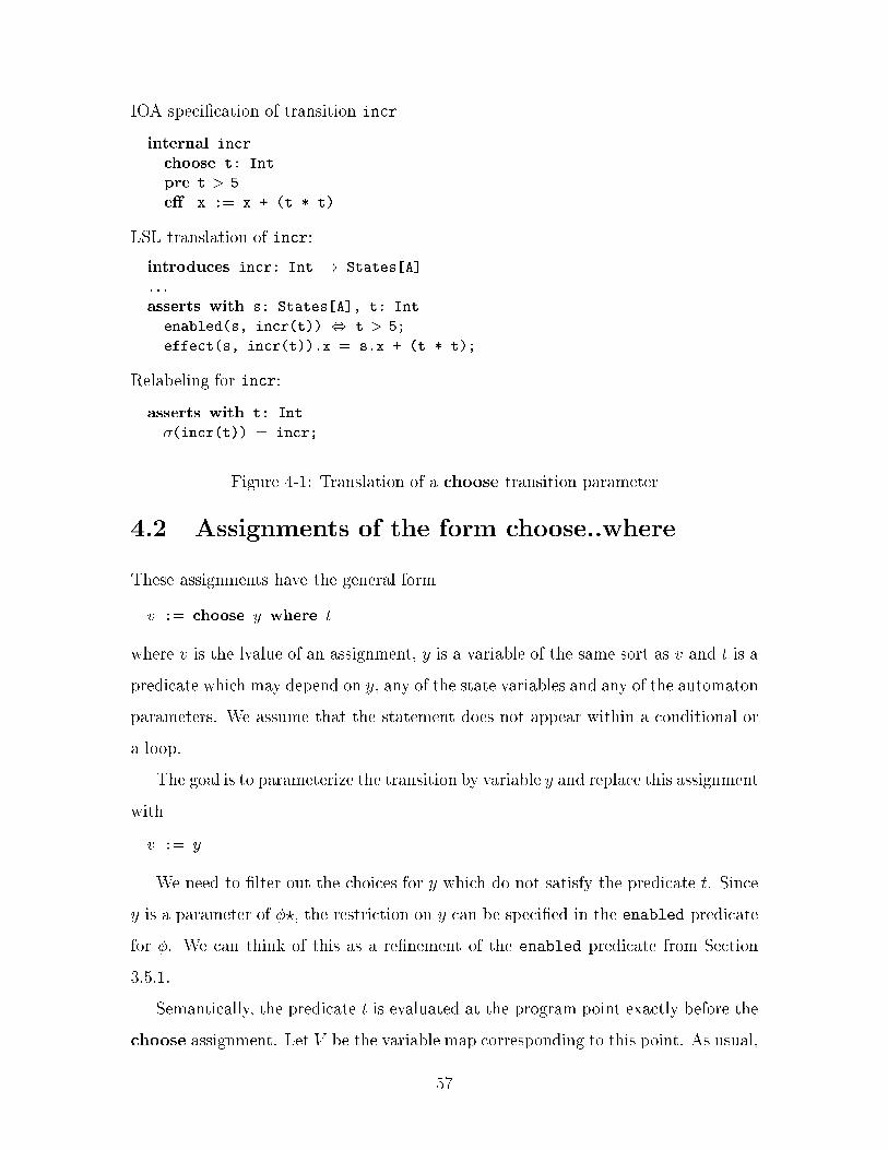
IOA speci�cation of transition incr
internal incr
choose t: Int
pre t > 5
e� x := x + (t * t)
LSL translation of incr:
introduces incr: Int ! States[A]
: : :
asserts with s: States[A], t: Int
enabled(s, incr(t)) , t > 5;
effect(s, incr(t)).x = s.x + (t * t);
Relabeling for incr:
asserts with t: Int
�(incr(t)) = incr;
Figure 4-1: Translation of a choose transition parameter
4.2 Assignments of the form choose..where
These assignments have the general form
v := choose y where t
where v is the lvalue of an assignment, y is a variable of the same sort as v and t is a
predicate which may depend on y, any of the state variables and any of the automaton
parameters. We assume that the statement does not appear within a conditional or
a loop.
The goal is to parameterize the transition by variable y and replace this assignment
with
v := y
We need to �lter out the choices for y which do not satisfy the predicate t. Since
y is a parameter of �?, the restriction on y can be speci�ed in the enabled predicate
for �. We can think of this as a re�nement of the enabled predicate from Section
3.5.1.
Semantically, the predicate t is evaluated at the program point exactly before the
choose assignment. Let V be the variable map corresponding to this point. As usual,
57
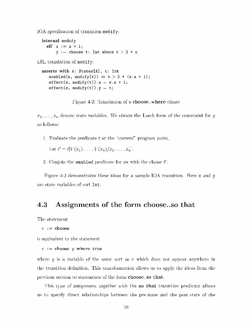
IOA speci�cation of transition modify:
internal modify
e� x := x + 1;
y := choose t: Int where t > 2 * x
LSL translation of modify:
asserts with s: States[A], t: Int
enabled(s, modify(t)) , t > 2 * (s.x + 1);
effect(s, modify(t)).x = s.x + 1;
effect(s, modify(t)).y = t;
Figure 4-2: Translation of a choose..where clause
x1; : : : ; xn denote state variables. We obtain the Larch form of the constraint for y
as follows:
1. Evaluate the predicate t at the \current" program point.
Let t0 = t[V (x1); : : : ; V (xn)=x1; : : : ; xn].
2. Conjoin the enabled predicate for �? with the clause t0.
Figure 4-2 demonstrates these ideas for a sample IOA transition. Here x and y
are state variables of sort Int.
4.3 Assignments of the form choose..so that
The statement
v := choose
is equivalent to the statement
v := choose y where true
where y is a variable of the same sort as v which does not appear anywhere in
the transition de�nition. This transformation allows us to apply the ideas from the
previous section to statements of the form choose..so that.
This type of assignment together with the so that transition predicate allows
us to specify direct relationships between the pre-state and the post-state of the
58
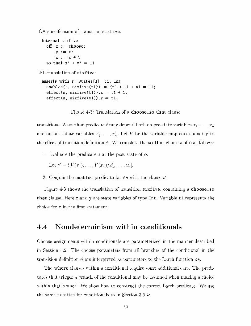
IOA speci�cation of transition sixfive:
internal sixfive
e� x := choose;
y := x;
x := x + 1
so that x' + y' = 11
LSL translation of sixfive:
asserts with s: States[A], t1: Int
enabled(s, sixfive(t1)) , (t1 + 1) + t1 = 11;
effect(s, sixfive(t1)).x = t1 + 1;
effect(s, sixfive(t1)).y = t1;
Figure 4-3: Translation of a choose..so that clause
transitions. A so that predicate t may depend both on pre-state variables x1; : : : ; xn
and on post-state variables x0
1; : : : ; x0
n. Let V be the variable map corresponding to
the e�ect of transition de�nition �. We translate the so that clause s of � as follows:
1. Evaluate the predicate s at the post-state of �.
Let s0 = t[V (x1); : : : ; V (xn)=x0
1; : : : ; x0
n].
2. Conjoin the enabled predicate for �? with the clause s0.
Figure 4-3 shows the translation of transition sixfive, containing a choose..so
that clause. Here x and y are state variables of type Int. Variable t1 represents the
choice for x in the �rst statement.
4.4 Nondeterminism within conditionals
Choose assignments within conditionals are parameterized in the manner described
in Section 4.2. The choose parameters from all branches of the conditional in the
transition de�nition � are interpreted as parameters to the Larch function �?.
The where clauses within a conditional require some additional care. The predi-
cates that trigger a branch of the conditional may be assumed when making a choice
within that branch. We show how to construct the correct Larch predicate. We use
the same notation for conditionals as in Section 3.5.4:
59
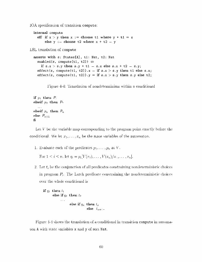
IOA speci�cation of transition compute:
internal compute
e� if x > y then x := choose t1 where y + t1 = x
else y := choose t2 where x + t2 = y
LSL translation of compute
asserts with s: States[A], t1: Nat, t2: Nat
enabled(s, compute(t1, t2)) ,
if s.x > s.y then s.y + t1 = s.x else s.x + t2 = s.y;
effect(s, compute(t1, t2)).x = if s.x > s.y then t1 else s.x;
effect(s, compute(t1, t2)).y = if s.x > s.y then s.y else t2;
Figure 4-4: Translation of nondeterminism within a conditional
if p1 then P1
elseif p2 then P2
: : :
elseif pn then Pnelse Pn+1
�
Let V be the variable map corresponding to the program point exactly before the
conditional. We let x1; : : : ; xn be the state variables of the automaton.
1. Evaluate each of the predicates p1; : : : ; pn at V .
For 1 � i � n, let qi = pi[V (x1); : : : ; V (xn)=x1; : : : ; xn].
2. Let ti be the conjunction of all predicates constraining nondeterministic choices
in program Pi. The Larch predicate constraining the nondeterministic choices
over the whole conditional is
if q1 then t1else if q2 then t2
: : :
else if qn then tnelse tn+1.
Figure 4-4 shows the translation of a conditional in transition compute in automa-
ton A with state variables x and y of sort Nat.
60
Chapter 5
A caching algorithm
This chapter and the following two demonstrate the application of theorem proving
techniques to a collection of IOA programs describing distributed data management
algorithms. These examples were developed as test studies for tools that interface
with IOA (simulators, code generators, invariant discovery packages, model checkers
and theorem provers).
The examples describe three commonly used data management algorithms: A
strong caching algorithm, a majority voting algorithm and Lamport's replicated state
machine algorithm [11]. We are interested in verifying that each of these algorithms
implements an atomic variable. In other words, we want to show that every trace
allowed by these algorithms corresponds to a trace of an atomic variable model. The
natural tools for studying such relationships between traces are simulation relations.
The proofs in Chapters 5 and 6, as well as parts of the proof in Chapter 7, were
veri�ed formally using the Larch prover. Our exposition of these proofs attempts to
emphasize interesting aspects from the perspective of interacting with the theorem
prover. The mathematical insights of the proof are not of primary concern (especially
in this chapter); they merely serve to bring up ideas that are important in the formal
proofs. As a result, the proofs may seem duller and more technical than usual. It
is important to keep in mind that this level of detail is often necessary in formal
theorem proving.
We begin this chapter with a collection of datatype declarations and global conven-
61
tions used by all the examples. We then introduce the atomic variable model, which
will serve as a reference for establishing the correctness of the algorithms. The bulk
of the chapter is dedicated to the strong caching algorithm and its properties. Using
invariants and forward simulations, we show that this algorithm exhibits the same
external behavior as the atomic variable. The exposition includes some interesting
examples of theorem proving code.
Parts of Chapters 5, 6 and 7 were published in [3] and [4]. The complete scripts
for the proofs carried out in Larch are provided in Appendix A.
5.1 Shared data types of the memory models
We describe the data types used in the speci�cation of the memory models and the
external transitions shared between the models. Data type speci�cations are provided
at an abstract level, through a set of axioms that each type satis�es. The formal
description of the data type speci�cations is written in the Larch Shared Language
(LSL).
The following sorts are used to describe the data components of the memory
models:
Node. Nodes represent the distributed entities of the system. Nodes receive requests
from the environment in the form of actions and send noti�cations of completed
requests in the form of responses. The set of nodes allnodes is �nite. The
integer constant numnodes denotes size(allnodes).
Value. A value is the type of entity stored by the variable. The constant value v0 is
the default value to which the variable is initialized.
Action and Response. Actions model requests that the environment submits at a
given node. They may be either read actions or write actions. Responses
are reports that nodes submit to the environment as a result of processing
invocations. We de�ne the following operators on these types:
62
isRead; isWrite : Action ! Bool: Predicates specifying whether an action is
a read action or a write action.
perform : Action; Value! Value: The e�ect of performing an action on the
variable's value. If the action is a read action, the value remains the same.
result : Action; Value ! Response: The response computed as a result of
performing an action on the variable's value.
Null[T]. This sort contains all elements of the sort T and the special constant nil.
The operator embed embeds elements of T into Null[T]. The operator :val is
the partial inverse of embed.
Array[S; T] and Matrix[S; T]. The sort Array[S; T] represents an array of elements of
sort T indexed by elements of sort S. This sort has two constructors: constant,
which sets the array to a constant value and assign, which modi�es the value
of a single array element. The operator [ ] looks up an array element. Sort
Matrix[S; T] represents two-dimensional arrays.
The models interact with the environment through the following two external
actions:
invoke(a:Action, n:Node). The invoke transition is used to specify an action re-
quest at a node.
respond(r:Response, n:Node). The respond transition produces a response as a
result of an action invoked at a node.
To simplify bookkeeping of current actions and responses at each node, we make
the following environment assumption: Concurrent requests cannot be submitted at
a single node. In other words, the environment must wait for a response to its current
request at any given node before it can submit a new one.
Such environment assumptions are usually formalized by composing the automa-
ton of interest with a suitable environment automaton, which describes the desired
automaton behavior. Unfortunately, our translation tool does not support reasoning
63
about compositions of automata yet. We get around this constraint by manually
composing the memory models with an environment which guarantees that action
invoke cannot be triggered at node n when n has an active request. Action invoke
is an output action of the composition automaton. Its precondition speci�es the
environment assumption.
Notation. We denote a state of an automaton by the �rst letter of the automaton
name. Thus, m denotes a state of mem. In proofs and statements about an automaton
with state name s, we use s0 for a start state of the automaton. When discussing
automaton transitions, we use s and s0 to denote the state before and after the
transition, respectively. If there is no ambiguity about the automaton and state in
consideration, we may omit explicit references to the state. For example, we may write
rsp[n] instead of s:rsp[n]. In simulation proofs, f denotes the simulation relation and
T denotes the step correspondence.
Variables and parameters that appear in IOA speci�cations and LSL declarations
of datatypes are typeset in courier. Mathematical variables introduced in statements
about automata or in the course of a proof are typeset in italics.
For long formulas, we use the notation introduced in [12].
5.2 The central memory model
The mem automaton models an atomic variable. Its speci�cation in the IOA language
is shown in Figure 5-1. The trait t mem de�nes references to all the datatypes used
by the speci�cation.
The internal update transitions perform the read/write computation which is
requested by an invocation at a node. The act and rsp variables are used to keep
track of the current action requested and response computed at each node respectively.
These variables take the value nil when the current action or response have not been
instantiated yet.
64
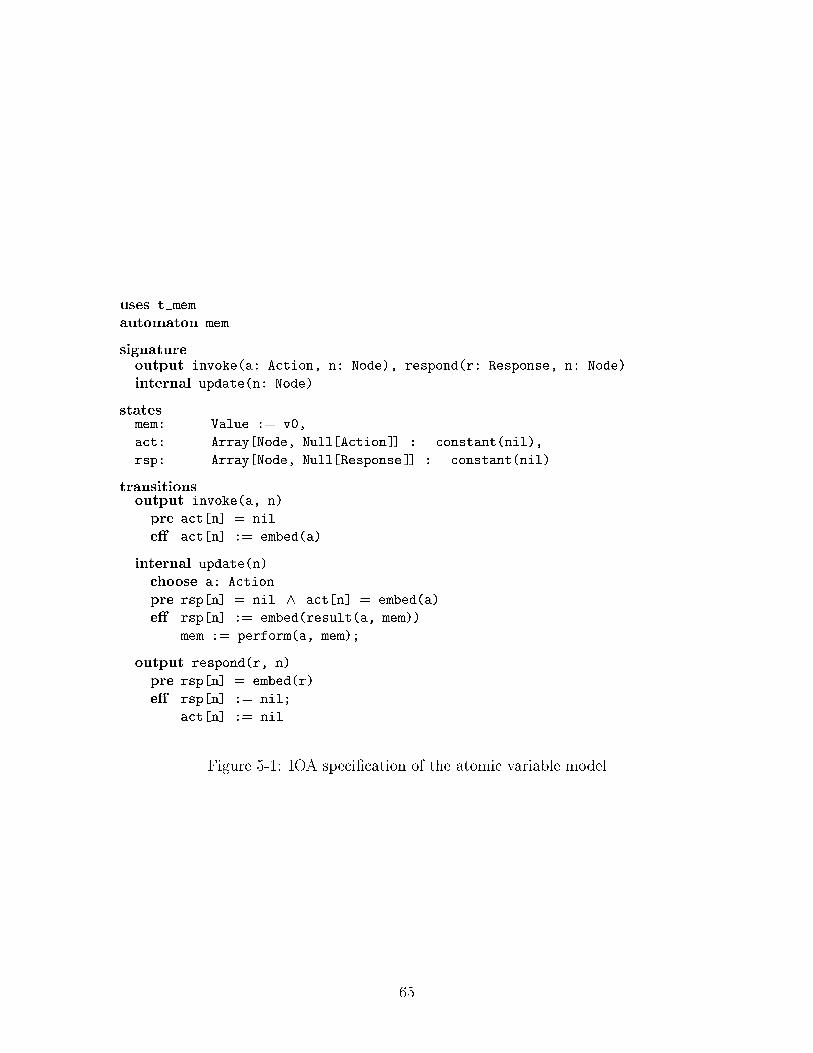
uses t_mem
automaton mem
signatureoutput invoke(a: Action, n: Node), respond(r: Response, n: Node)
internal update(n: Node)
statesmem: Value := v0,
act: Array[Node, Null[Action]] := constant(nil),
rsp: Array[Node, Null[Response]] := constant(nil)
transitionsoutput invoke(a, n)
pre act[n] = nil
e� act[n] := embed(a)
internal update(n)
choose a: Action
pre rsp[n] = nil ^ act[n] = embed(a)
e� rsp[n] := embed(result(a, mem))
mem := perform(a, mem);
output respond(r, n)
pre rsp[n] = embed(r)
e� rsp[n] := nil;
act[n] := nil
Figure 5-1: IOA speci�cation of the atomic variable model
65
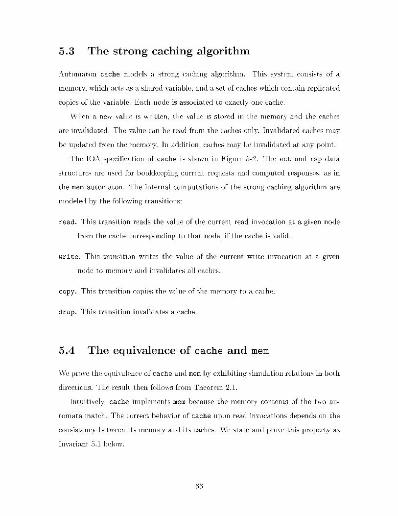
5.3 The strong caching algorithm
Automaton cache models a strong caching algorithm. This system consists of a
memory, which acts as a shared variable, and a set of caches which contain replicated
copies of the variable. Each node is associated to exactly one cache.
When a new value is written, the value is stored in the memory and the caches
are invalidated. The value can be read from the caches only. Invalidated caches may
be updated from the memory. In addition, caches may be invalidated at any point.
The IOA speci�cation of cache is shown in Figure 5-2. The act and rsp data
structures are used for bookkeeping current requests and computed responses, as in
the mem automaton. The internal computations of the strong caching algorithm are
modeled by the following transitions:
read. This transition reads the value of the current read invocation at a given node
from the cache corresponding to that node, if the cache is valid.
write. This transition writes the value of the current write invocation at a given
node to memory and invalidates all caches.
copy. This transition copies the value of the memory to a cache.
drop. This transition invalidates a cache.
5.4 The equivalence of cache and mem
We prove the equivalence of cache and mem by exhibiting simulation relations in both
directions. The result then follows from Theorem 2.1.
Intuitively, cache implements mem because the memory contents of the two au-
tomata match. The correct behavior of cache upon read invocations depends on the
consistency between its memory and its caches. We state and prove this property as
Invariant 5.1 below.
66
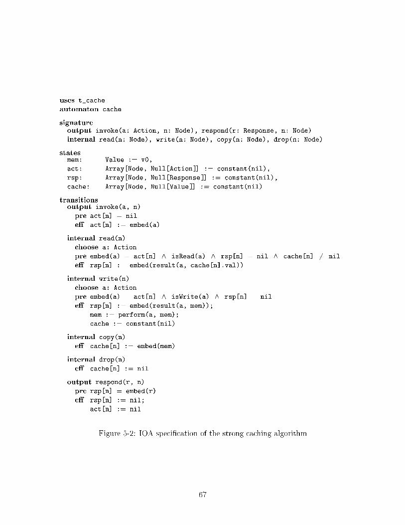
uses t_cache
automaton cache
signatureoutput invoke(a: Action, n: Node), respond(r: Response, n: Node)
internal read(n: Node), write(n: Node), copy(n: Node), drop(n: Node)
statesmem: Value := v0,
act: Array[Node, Null[Action]] := constant(nil),
rsp: Array[Node, Null[Response]] := constant(nil),
cache: Array[Node, Null[Value]] := constant(nil)
transitionsoutput invoke(a, n)
pre act[n] = nil
e� act[n] := embed(a)
internal read(n)
choose a: Action
pre embed(a) = act[n] ^ isRead(a) ^ rsp[n] = nil ^ cache[n] 6= nil
e� rsp[n] := embed(result(a, cache[n].val))
internal write(n)
choose a: Action
pre embed(a) = act[n] ^ isWrite(a) ^ rsp[n] = nil
e� rsp[n] := embed(result(a, mem));
mem := perform(a, mem);
cache := constant(nil)
internal copy(n)
e� cache[n] := embed(mem)
internal drop(n)
e� cache[n] := nil
output respond(r, n)
pre rsp[n] = embed(r)
e� rsp[n] := nil;
act[n] := nil
Figure 5-2: IOA speci�cation of the strong caching algorithm
67
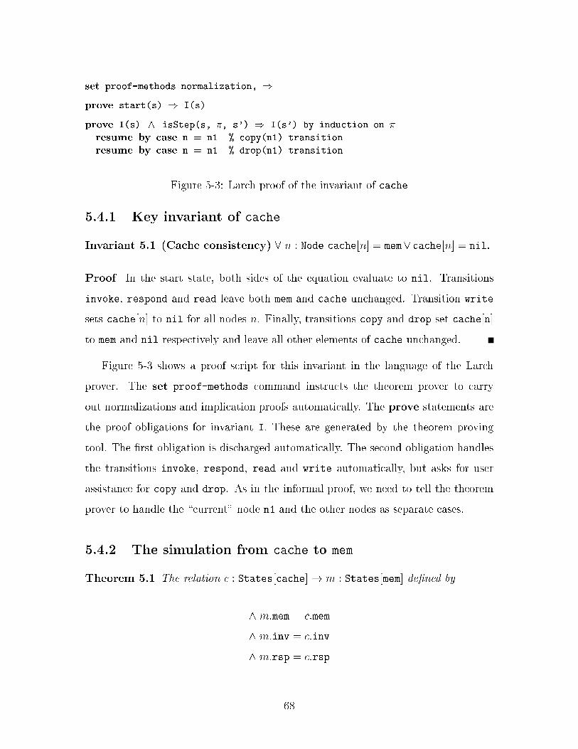
set proof-methods normalization, )
prove start(s) ) I(s)
prove I(s) ^ isStep(s, �, s') ) I(s') by induction on �
resume by case n = n1 % copy(n1) transition
resume by case n = n1 % drop(n1) transition
Figure 5-3: Larch proof of the invariant of cache
5.4.1 Key invariant of cache
Invariant 5.1 (Cache consistency) 8 n : Node cache[n] = mem_cache[n] = nil:
Proof In the start state, both sides of the equation evaluate to nil. Transitions
invoke, respond and read leave both mem and cache unchanged. Transition write
sets cache[n] to nil for all nodes n. Finally, transitions copy and drop set cache[n]
to mem and nil respectively and leave all other elements of cache unchanged.
Figure 5-3 shows a proof script for this invariant in the language of the Larch
prover. The set proof-methods command instructs the theorem prover to carry
out normalizations and implication proofs automatically. The prove statements are
the proof obligations for invariant I. These are generated by the theorem proving
tool. The �rst obligation is discharged automatically. The second obligation handles
the transitions invoke, respond, read and write automatically, but asks for user
assistance for copy and drop. As in the informal proof, we need to tell the theorem
prover to handle the \current" node n1 and the other nodes as separate cases.
5.4.2 The simulation from cache to mem
Theorem 5.1 The relation c : States[cache]! m : States[mem] de�ned by
^ m:mem = c:mem
^ m:inv = c:inv
^ m:rsp = c:rsp
68
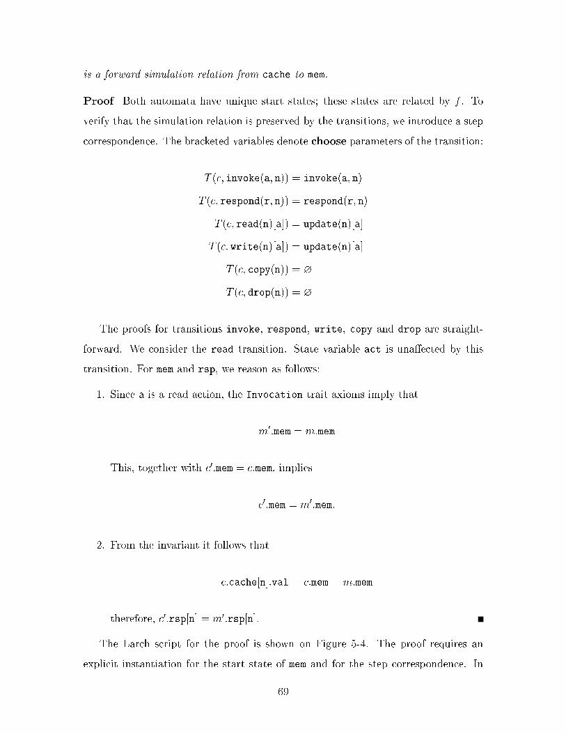
is a forward simulation relation from cache to mem.
Proof Both automata have unique start states; these states are related by f . To
verify that the simulation relation is preserved by the transitions, we introduce a step
correspondence. The bracketed variables denote choose parameters of the transition:
T (c; invoke(a; n)) = invoke(a; n)
T (c; respond(r; n)) = respond(r; n)
T (c; read(n)[a]) = update(n)[a]
T (c; write(n)[a]) = update(n)[a]
T (c; copy(n)) = ?
T (c; drop(n)) = ?
The proofs for transitions invoke, respond, write, copy and drop are straight-
forward. We consider the read transition. State variable act is una�ected by this
transition. For mem and rsp, we reason as follows:
1. Since a is a read action, the Invocation trait axioms imply that
m0:mem = m:mem
This, together with c0:mem = c:mem, implies
c0:mem = m0:mem:
2. From the invariant it follows that
c:cache[n]:val = c:mem = m:mem
therefore, c0:rsp[n] = m0:rsp[n].
The Larch script for the proof is shown on Figure 5-4. The proof requires an
explicit instantiation for the start state of mem and for the step correspondence. In
69
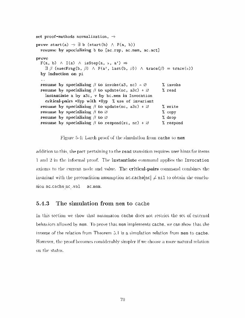
set proof-methods normalization, )
prove start(a) ) 9 b (start(b) ^ F(a, b))
resume by specializing b to [ac.rsp, ac.mem, ac.act]
proveF(a, b) ^ I(a) ^ isStep(a, �, a') )
9 � (execFrag(b, �) ^ F(a', last(b, �)) ^ trace(�) = trace(�))
by induction on pi
..
resume by specializing � to invoke(a3, nc) � ? % invoke
resume by specializing � to update(nc, a3c) � ? % read
instantiate a by a3c, v by bc.mem in Invocation
critical-pairs *Hyp with *Hyp % use of invariant
resume by specializing � to update(nc, a3c) � ? % write
resume by specializing � to ? % copy
resume by specializing � to ? % drop
resume by specializing � to respond(rc, nc) � ? % respond
Figure 5-4: Larch proof of the simulation from cache to mem
addition to this, the part pertaining to the read transition requires user hints for items
1 and 2 in the informal proof. The instantiate command applies the Invocation
axioms to the current node and value. The critical-pairs command combines the
invariant with the precondition assumption ac:cache[nc] 6= nil to obtain the conclu-
sion ac:cache[nc]:val = ac:mem.
5.4.3 The simulation from mem to cache
In this section we show that automaton cache does not restrict the set of external
behaviors allowed by mem. To prove that mem implements cache, we can show that the
inverse of the relation from Theorem 5.1 is a simulation relation from mem to cache.
However, the proof becomes considerably simpler if we choose a more natural relation
on the states.
70
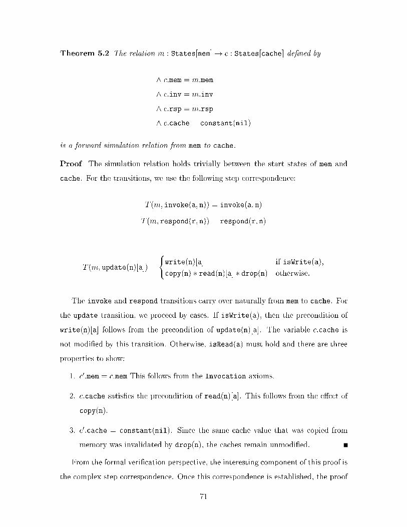
Theorem 5.2 The relation m : States[mem]! c : States[cache] de�ned by
^ c:mem = m:mem
^ c:inv = m:inv
^ c:rsp = m:rsp
^ c:cache = constant(nil)
is a forward simulation relation from mem to cache.
Proof The simulation relation holds trivially between the start states of mem and
cache. For the transitions, we use the following step correspondence:
T (m; invoke(a; n)) = invoke(a; n)
T (m; respond(r; n)) = respond(r; n)
T (m; update(n)[a]) =
(write(n)[a] if isWrite(a);
copy(n) � read(n)[a] � drop(n) otherwise:
The invoke and respond transitions carry over naturally from mem to cache. For
the update transition, we proceed by cases. If isWrite(a), then the precondition of
write(n)[a] follows from the precondition of update(n)[a]. The variable c:cache is
not modi�ed by this transition. Otherwise, isRead(a) must hold and there are three
properties to show:
1. c0:mem = c:mem This follows from the Invocation axioms.
2. c:cache satis�es the precondition of read(n)[a]. This follows from the e�ect of
copy(n).
3. c0:cache = constant(nil). Since the same cache value that was copied from
memory was invalidated by drop(n), the caches remain unmodi�ed.
From the formal veri�cation perspective, the interesting component of this proof is
the complex step correspondence. Once this correspondence is established, the proof
71
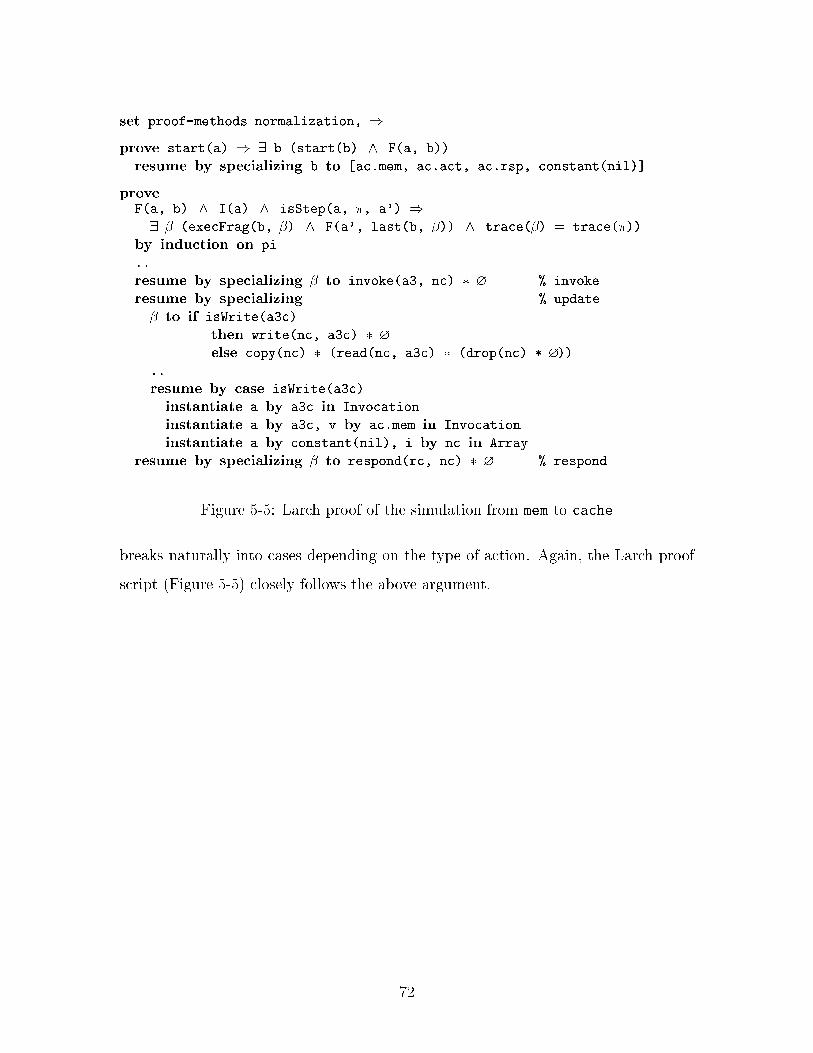
set proof-methods normalization, )
prove start(a) ) 9 b (start(b) ^ F(a, b))
resume by specializing b to [ac.mem, ac.act, ac.rsp, constant(nil)]
proveF(a, b) ^ I(a) ^ isStep(a, �, a') )
9 � (execFrag(b, �) ^ F(a', last(b, �)) ^ trace(�) = trace(�))
by induction on pi
..
resume by specializing � to invoke(a3, nc) � ? % invoke
resume by specializing % update
� to if isWrite(a3c)
then write(nc, a3c) � ?
else copy(nc) � (read(nc, a3c) � (drop(nc) * ?))
..
resume by case isWrite(a3c)
instantiate a by a3c in Invocation
instantiate a by a3c, v by ac.mem in Invocation
instantiate a by constant(nil), i by nc in Array
resume by specializing � to respond(rc, nc) � ? % respond
Figure 5-5: Larch proof of the simulation from mem to cache
breaks naturally into cases depending on the type of action. Again, the Larch proof
script (Figure 5-5) closely follows the above argument.
72
Chapter 6
Majority voting
In this chapter we verify the correctness of the majority voting algorithm for dis-
tributed data management [14]. We begin by presenting a model of this algorithm
written in the IOA language. The IOA speci�cation takes advantage of some inter-
esting features of the language, such as explicit nondeterminism and loops. We take
this opportunity to discuss reasoning strategies about e�ects of loops in the Larch
prover.
Finally, we demonstrate the equivalence of the majority voting algorithm with the
atomic variable model from Chapter 5. The equivalence is established by exhibiting
simulation relations in both directions. The proof was veri�ed formally using the
Larch Prover. The complete proof script is provided in Appendix A.
6.1 The majority voting algorithm
The voting automaton (Figure 6-1) models the majority voting algorithm described
on page 573 in [14]. The data in this system is kept in a collection of storage locations,
one per node, with no centralized memory. Each node also contains a nonnegative
integer variable tag. Initially, all storage is instantiated to the default value v0 and
all tags are set to the value 0.
To perform a read request at a given node, the algorithm reads the stored value
at a majority of the nodes. It chooses the node in the majority with the largest tag
73
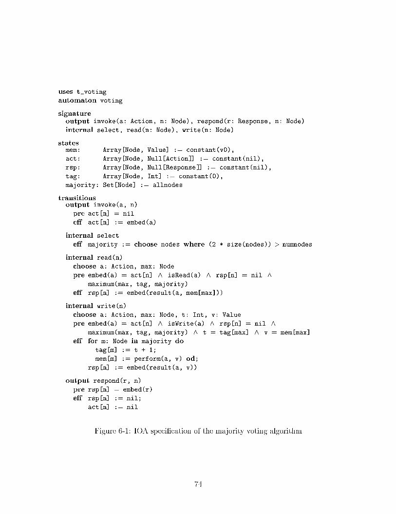
uses t_voting
automaton voting
signatureoutput invoke(a: Action, n: Node), respond(r: Response, n: Node)
internal select, read(n: Node), write(n: Node)
statesmem: Array[Node, Value] := constant(v0),
act: Array[Node, Null[Action]] := constant(nil),
rsp: Array[Node, Null[Response]] := constant(nil),
tag: Array[Node, Int] := constant(0),
majority: Set[Node] := allnodes
transitionsoutput invoke(a, n)
pre act[n] = nil
e� act[n] := embed(a)
internal select
e� majority := choose nodes where (2 * size(nodes)) > numnodes
internal read(n)
choose a: Action, max: Node
pre embed(a) = act[n] ^ isRead(a) ^ rsp[n] = nil ^
maximum(max, tag, majority)
e� rsp[n] := embed(result(a, mem[max]))
internal write(n)
choose a: Action, max: Node, t: Int, v: Value
pre embed(a) = act[n] ^ isWrite(a) ^ rsp[n] = nil ^
maximum(max, tag, majority) ^ t = tag[max] ^ v = mem[max]
e� for m: Node in majority do
tag[m] := t + 1;
mem[m] := perform(a, v) od;
rsp[n] := embed(result(a, v))
output respond(r, n)
pre rsp[n] = embed(r)
e� rsp[n] := nil;
act[n] := nil
Figure 6-1: IOA speci�cation of the majority voting algorithm
74
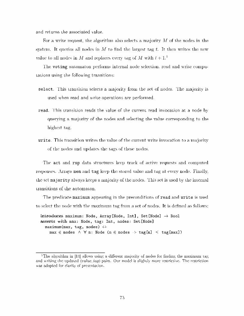
and returns the associated value.
For a write request, the algorithm also selects a majority M of the nodes in the
system. It queries all nodes in M to �nd the largest tag t. It then writes the new
value to all nodes in M and replaces every tag of M with t+ 1.1
The voting automaton performs internal node selection, read and write compu-
tations using the following transitions:
select. This transition selects a majority from the set of nodes. The majority is
used when read and write operations are performed.
read. This transition reads the value of the current read invocation at a node by
querying a majority of the nodes and selecting the value corresponding to the
highest tag.
write. This transition writes the value of the current write invocation to a majority
of the nodes and updates the tags of these nodes.
The act and rsp data structures keep track of active requests and computed
responses. Arrays mem and tag keep the stored value and tag at every node. Finally,
the set majority always keeps a majority of the nodes. This set is used by the internal
transitions of the automaton.
The predicate maximum appearing in the preconditions of read and write is used
to select the node with the maximum tag from a set of nodes. It is de�ned as follows:
introduces maximum: Node, Array[Node, Int], Set[Node] ! Bool
asserts with max: Node, tag: Int, nodes: Set[Node]
maximum(max, tag, nodes) ,
max 2 nodes ^ 8 n: Node (n 2 nodes ) tag[n] � tag[max])
1The algorithm in [14] allows using a di�erent majority of nodes for �nding the maximum tagand writing the updated (value; tag) pairs. Our model is slightly more restrictive. The restrictionwas adopted for clarity of presentation.
75
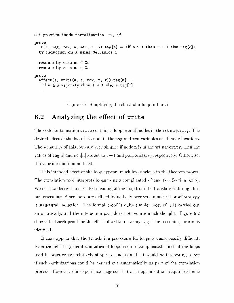
set proof-methods normalization, ), if
provelP(X, tag, mem, a, max, t, v).tag[m] = (if m 2 X then t + 1 else tag[m])
by induction on X using SetBasics.1
..
resume by case nc 2 Xc
resume by case nc 2 Xc
proveeffect(s, write(n, a, max, t, v)).tag[m] =
if m 2 s.majority then t + 1 else s.tag[m]
..
Figure 6-2: Simplifying the e�ect of a loop in Larch
6.2 Analyzing the e�ect of write
The code for transition write contains a loop over all nodes in the set majority. The
desired e�ect of the loop is to update the tag and mem variables at all node locations.
The semantics of this loop are very simple: if node n is in the set majority, then the
values of tag[n] and mem[n] are set to t+1 and perform(a; v) respectively. Otherwise,
the values remain unmodi�ed.
This intended e�ect of the loop appears much less obvious to the theorem prover.
The translation tool interprets loops using a complicated scheme (see Section 3.5.5).
We need to derive the intended meaning of the loop from the translation through for-
mal reasoning. Since loops are de�ned inductively over sets, a natural proof strategy
is structural induction. The formal proof is quite simple; most of it is carried out
automatically, and the interaction part does not require much thought. Figure 6-2
shows the Larch proof for the e�ect of write on array tag. The reasoning for mem is
identical.
It may appear that the translation procedure for loops is unnecessarily diÆcult.
Even though the general semantics of loops is quite complicated, most of the loops
used in practice are relatively simple to understand. It would be interesting to see
if such optimizations could be carried out automatically as part of the translation
process. However, our experience suggests that such optimizations require extreme
76
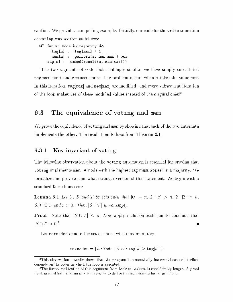
caution. We provide a compelling example. Initially, our code for the write transition
of voting was written as follows:
e� for m: Node in majority do
tag[m] := tag[max] + 1;
mem[m] := perform(a, mem[max]) od;
rsp[n] := embed(result(a, mem[max]))
The two segments of code look strikingly similar; we have simply substituted
tag[max] for t and mem[max] for v. The problem occurs when m takes the value max.
In this iteration, tag[max] and mem[max] are modi�ed. and every subsequent iteration
of the loop makes use of these modi�ed values instead of the original ones!2
6.3 The equivalence of voting and mem
We prove the equivalence of voting and mem by showing that each of the two automata
implements the other. The result then follows from Theorem 2.1.
6.3.1 Key invariant of voting
The following observation about the voting automaton is essential for proving that
voting implements mem: A node with the highest tag must appear in a majority. We
formalize and prove a somewhat stronger version of this statement. We begin with a
standard fact about sets:
Lemma 6.1 Let U , S and T be sets such that jU j = n, 2 � jSj > n, 2 � jT j > n,
S; T � U and n > 0. Then jS \ T j is nonempty.
Proof Note that jS [ T j � n; Now apply inclusion-exclusion to conclude that
jS \ T j > 0.3
Let maxnodes denote the set of nodes with maximum tag:
maxnodes = fn : Node j 8 n0 : tag[n] � tag[n0]g:
2This observation actually shows that the program is semantically incorrect because its e�ectdepends on the order in which the loop is executed.
3The formal veri�cation of this argument from basic set axioms is considerably longer. A proofby structural induction on sets is necessary to derive the inclusion-exclusion principle.
77
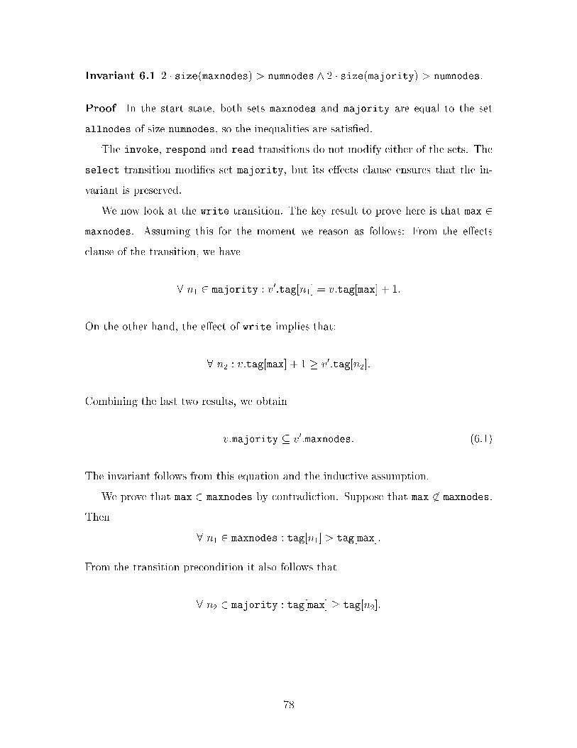
Invariant 6.1 2 � size(maxnodes) > numnodes ^ 2 � size(majority) > numnodes:
Proof In the start state, both sets maxnodes and majority are equal to the set
allnodes of size numnodes, so the inequalities are satis�ed.
The invoke, respond and read transitions do not modify either of the sets. The
select transition modi�es set majority, but its e�ects clause ensures that the in-
variant is preserved.
We now look at the write transition. The key result to prove here is that max 2
maxnodes. Assuming this for the moment we reason as follows: From the e�ects
clause of the transition, we have
8 n1 2 majority : v0:tag[n1] = v:tag[max] + 1:
On the other hand, the e�ect of write implies that:
8 n2 : v:tag[max] + 1 � v0:tag[n2]:
Combining the last two results, we obtain
v:majority � v0:maxnodes: (6.1)
The invariant follows from this equation and the inductive assumption.
We prove that max 2 maxnodes by contradiction. Suppose that max 62 maxnodes.
Then
8 n1 2 maxnodes : tag[n1] > tag[max]:
From the transition precondition it also follows that
8 n2 2 majority : tag[max] � tag[n2]:
78
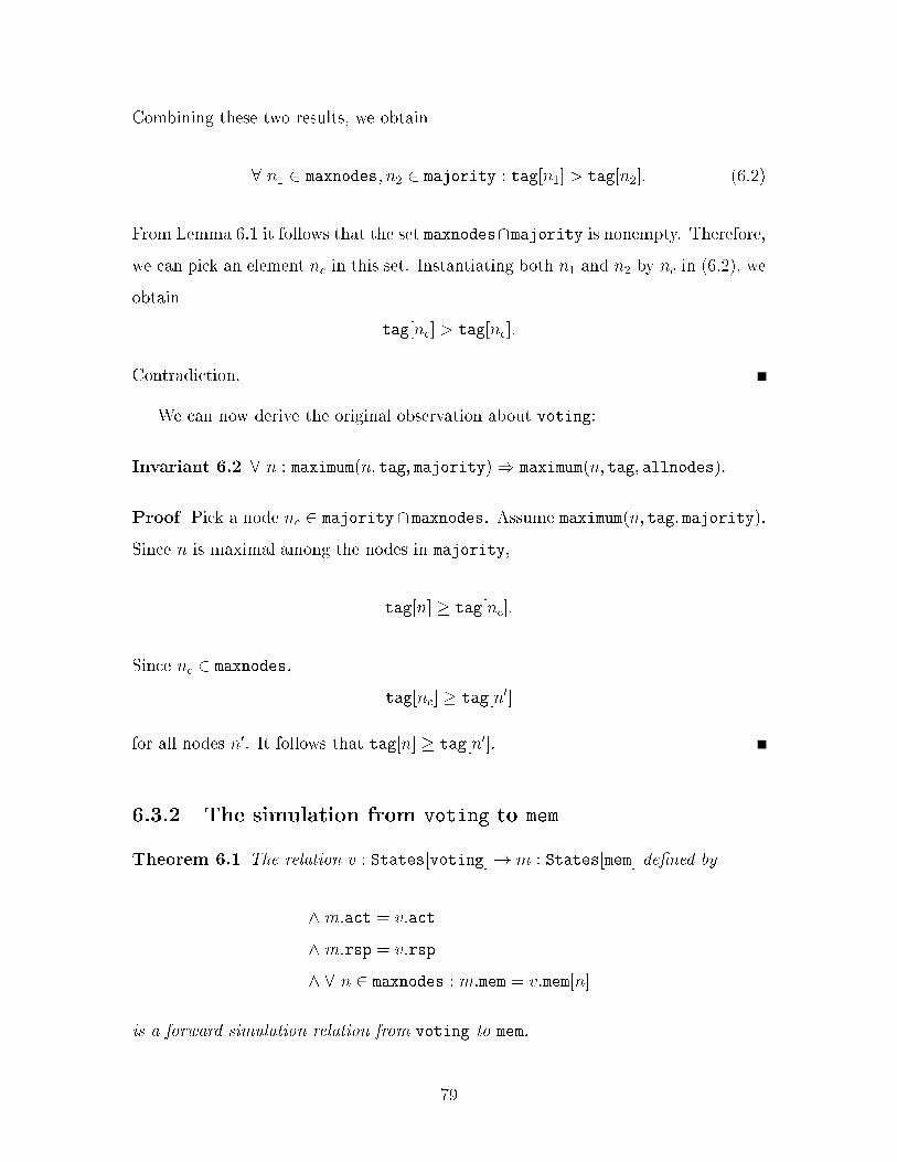
Combining these two results, we obtain
8 n1 2 maxnodes; n2 2 majority : tag[n1] > tag[n2]: (6.2)
From Lemma 6.1 it follows that the set maxnodes\majority is nonempty. Therefore,
we can pick an element nc in this set. Instantiating both n1 and n2 by nc in (6.2), we
obtain
tag[nc] > tag[nc]:
Contradiction.
We can now derive the original observation about voting:
Invariant 6.2 8 n : maximum(n; tag; majority)) maximum(n; tag; allnodes):
Proof Pick a node nc 2 majority\ maxnodes. Assume maximum(n; tag; majority).
Since n is maximal among the nodes in majority,
tag[n] � tag[nc]:
Since nc 2 maxnodes,
tag[nc] � tag[n0]
for all nodes n0. It follows that tag[n] � tag[n0]:
6.3.2 The simulation from voting to mem
Theorem 6.1 The relation v : States[voting]! m : States[mem] de�ned by
^ m:act = v:act
^ m:rsp = v:rsp
^ 8 n 2 maxnodes : m:mem = v:mem[n]
is a forward simulation relation from voting to mem.
79
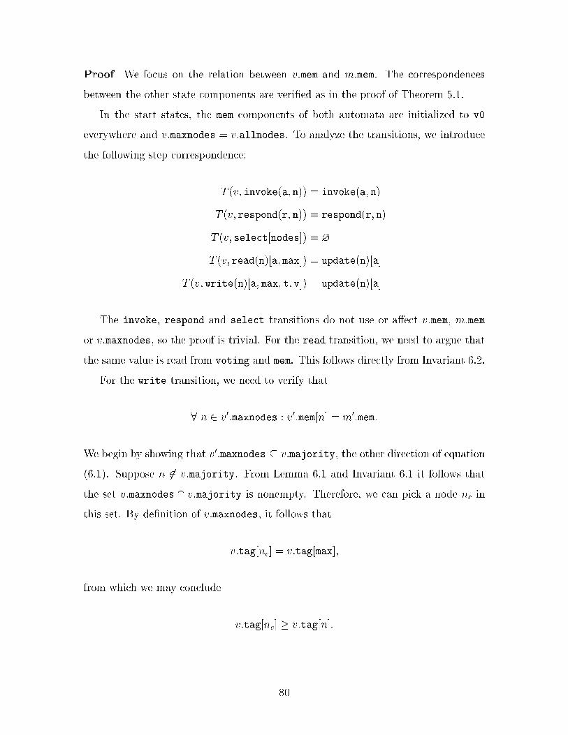
Proof We focus on the relation between v:mem and m:mem. The correspondences
between the other state components are veri�ed as in the proof of Theorem 5.1.
In the start states, the mem components of both automata are initialized to v0
everywhere and v:maxnodes = v:allnodes. To analyze the transitions, we introduce
the following step correspondence:
T (v; invoke(a; n)) = invoke(a; n)
T (v; respond(r; n)) = respond(r; n)
T (v; select[nodes]) = ?
T (v; read(n)[a; max]) = update(n)[a]
T (v; write(n)[a; max; t; v]) = update(n)[a]
The invoke, respond and select transitions do not use or a�ect v:mem, m:mem
or v:maxnodes, so the proof is trivial. For the read transition, we need to argue that
the same value is read from voting and mem. This follows directly from Invariant 6.2.
For the write transition, we need to verify that
8 n 2 v0:maxnodes : v0:mem[n] = m0:mem:
We begin by showing that v0:maxnodes � v:majority, the other direction of equation
(6.1). Suppose n 62 v:majority. From Lemma 6.1 and Invariant 6.1 it follows that
the set v:maxnodes \ v:majority is nonempty. Therefore, we can pick a node nc in
this set. By de�nition of v:maxnodes, it follows that
v:tag[nc] = v:tag[max];
from which we may conclude
v:tag[nc] � v:tag[n]:
80
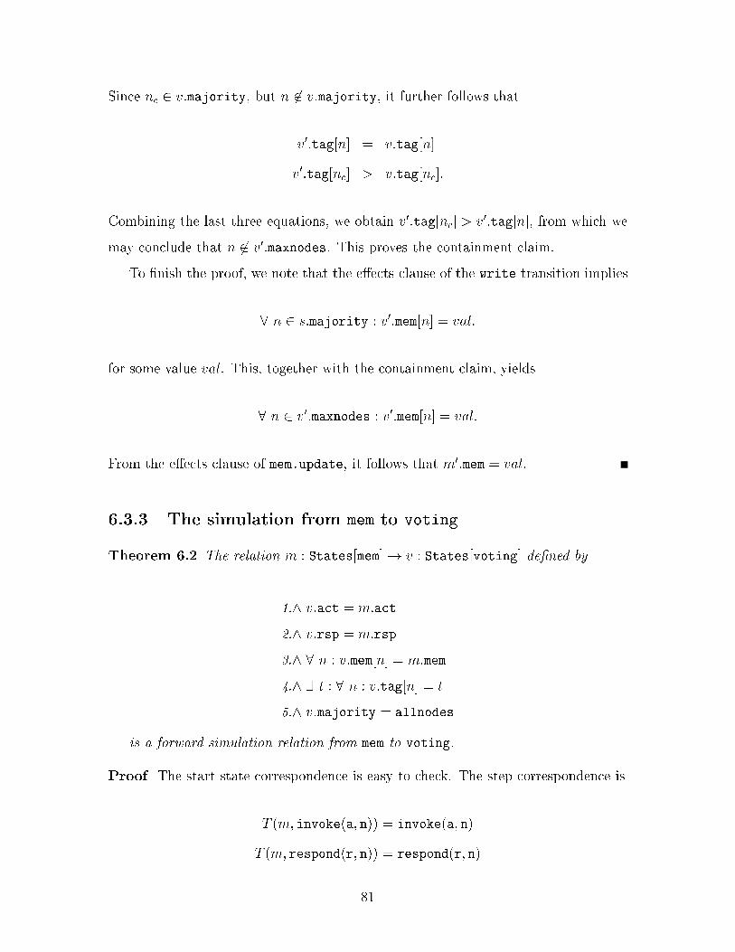
Since nc 2 v:majority, but n 62 v:majority, it further follows that
v0:tag[n] = v:tag[n]
v0:tag[nc] > v:tag[nc]:
Combining the last three equations, we obtain v0:tag[nc] > v0:tag[n], from which we
may conclude that n 62 v0:maxnodes. This proves the containment claim.
To �nish the proof, we note that the e�ects clause of the write transition implies
8 n 2 s:majority : v0:mem[n] = val:
for some value val. This, together with the containment claim, yields
8 n 2 v0:maxnodes : v0:mem[n] = val:
From the e�ects clause of mem.update, it follows that m0:mem = val.
6.3.3 The simulation from mem to voting
Theorem 6.2 The relation m : States[mem]! v : States[voting] de�ned by
1.^ v:act = m:act
2.^ v:rsp = m:rsp
3.^ 8 n : v:mem[n] = m:mem
4.^ 9 t : 8 n : v:tag[n] = t
5.^ v:majority = allnodes
is a forward simulation relation from mem to voting.
Proof The start state correspondence is easy to check. The step correspondence is
T (m; invoke(a; n)) = invoke(a; n)
T (m; respond(r; n)) = respond(r; n)
81
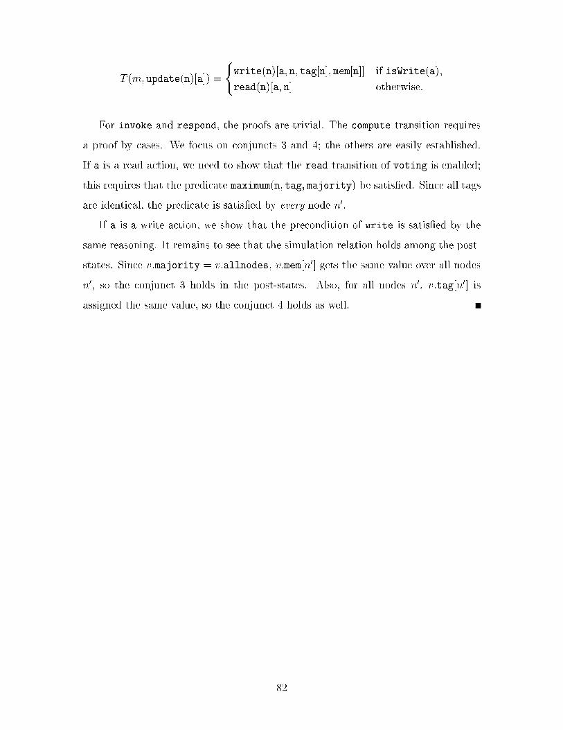
T (m; update(n)[a]) =
(write(n)[a; n; tag[n]; mem[n]] if isWrite(a);
read(n)[a; n] otherwise:
For invoke and respond, the proofs are trivial. The compute transition requires
a proof by cases. We focus on conjuncts 3 and 4; the others are easily established.
If a is a read action, we need to show that the read transition of voting is enabled;
this requires that the predicate maximum(n; tag; majority) be satis�ed. Since all tags
are identical, the predicate is satis�ed by every node n0.
If a is a write action, we show that the precondition of write is satis�ed by the
same reasoning. It remains to see that the simulation relation holds among the post-
states. Since v:majority = v:allnodes, v:mem[n0] gets the same value over all nodes
n0, so the conjunct 3 holds in the post-states. Also, for all nodes n0, v:tag[n0] is
assigned the same value, so the conjunct 4 holds as well.
82
Chapter 7
The replicated state machine
The previous two chapters discussed the application of formal reasoning strategies for
I/O automata to two distributed data management algorithms. The strong caching
algorithm from Chapter 5 had a very simple and intuitive correctness proof. In
Chapter 6, the correctness of the majority voting algorithm was not immediately
obvious; still, the proof contained only a handful of interesting ideas and was mostly
an exercise in formalism.
This chapter discusses yet another distributed data management algorithm|
Lamport's replicated state machine [11]. This is a complex algorithm used for man-
aging data in asynchronous distributed systems. Unlike strong caching and majority
voting, the correctness of this algorithm is far from obvious. The proof of this algo-
rithm presented in [14] relies on reasoning about whole executions rather than about
individual states and actions. Unfortunately, our formal reasoning machinery from
Chapter 2 does not support this type of reasoning.
We construct a new correctness proof for the replicated state machine (RSM)
using only the notions introduces in Chapter 2|invariants and forward simulation
relations. Our goal is to show that there exists a forward simulation relation from the
RSM algorithm to the central memory model. This simulation relation is diÆcult to
establish directly; instead, we take advantage of the principle of successive re�nement.
We introduce an intermediate automaton which models the data management issues
of RSM but abstracts away the timing issues. The proof then breaks into two parts:
83
1. Show that the intermediate model implements the central memory model.
2. Show that the RSM algorithm implements the intermediate model.
We prove both of these statement by exhibiting forward simulation relations. Even
in this simpli�ed setting, the proofs are intricate; they make use of subtle properties of
the implementation automata. These properties are singled out as formal invariants.
The �rst part of the proof was veri�ed formally using the Larch prover. Formal
veri�cation for the second part has not been carried out yet. Part of the challenge
is to �nd good axiomatizations of the datatypes which will make the properties of
interest transparent to the theorem prover. There is also a technical problem related
to the expressiveness of the Larch theory of automata from Chapter 2; we postpone
the discussion of this issue until Chapter 8.
Section 7.1 introduces the data types used by the automaton speci�cations. In
Section 7.2 we provide the formal speci�cation of the RSM model (automaton rsm)
and the intermediate model (automaton synch). Section 7.3 describes the properties
of synch and the simulation relation from synch to mem. In Section 7.4, we state the
important invariants of rsm and verify the simulation relation from rsm to synch.
7.1 Data type speci�cations
In this section we describe the datatypes used in the IOA speci�cations of automata
rsm and synch. Some of these are extensions to the data types from Section 5.1.
Others model structures that are particular to the RSM algorithm (time, clocks,
queues and channels).
Node. We impose a total ordering < on the set of nodes and de�ne n0 to be the
smallest node.
Time. A time is a pair [t : T; node : Node] where T is a totally ordered sort with respect
to < bounded below by 0. We de�ne a total order < on times by
[t, node] < [t', node'] , t < t' _ (t = t' ^ node < node').
84
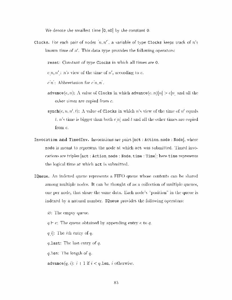
We denote the smallest time [0; n0] by the constant 0.
Clocks. For each pair of nodes [n; n0], a variable of type Clocks keeps track of n's
known time of n0. This data type provides the following operators:
reset: Constant of type Clocks in which all times are 0.
c[n; n0]: n's view of the time of n0, according to c.
c[n]: Abbreviation for c[n; n].
advance(c; n): A value of Clocks in which advance(c; n)[n] > c[n] and all the
other times are copied from c.
synch(c; n; n0; t): A value of Clocks in which n's view of the time of n0 equals
t, n's time is bigger than both c[n] and t and all the other times are copied
from c.
Invocation and TimedInv. Invocations are pairs [act : Action; node : Node], where
node is meant to represent the node at which act was submitted. Timed invo-
cations are triples [act : Action; node : Node; time : Time]; here time represents
the logical time at which act is submitted.
IQueue. An indexed queue represents a FIFO queue whose contents can be shared
among multiple nodes. It can be thought of as a collection of multiple queues,
one per node, that share the same data. Each node's \position" in the queue is
indexed by a natural number. IQueue provides the following operators:
?: The empty queue.
q ` e: The queue obtained by appending entry e to q.
q[i]: The ith entry of q.
q:last: The last entry of q.
q:len: The length of q.
advance(q; i): i+ 1 if i < q:len, i otherwise.
85
7.2 Automaton speci�cations
7.2.1 The replicated state machine automaton
Automaton rsm (Figure 7-1) speci�es Lamport's replicated state machine algorithm.
It consists of a collection of nodes, described by the state variables mem, act, rsp,
clks and ticked and a collection of FIFO channels modeled by state variable chan.
The variables front and rcv describe the interaction of the nodes with the channels.
As usual, mem, act and rsp represent the storage locations, the active invocation
and the computed response at each node. Variable clks captures the logical times in
the system. The indicator variable ticked ensures that every computation at node
n is followed by a clock tick. After each event at node n, ticked[n] is set to false.
This forces the automaton to take a tick(n) transition that advances the clock of n
and resets ticked[n] to true.
The variable chan[n] is an indexed queue of all the messages that were ever sent
by node n. The receiving end of the channel from node n0 to node n is indexed by
rcv[n; n0]. The index front[n; n0] points to the earliest invocation in the channel from
n0 to n that has not yet been performed by node n.
Transition invoke accepts an action request from the environment and informs all
nodes in the system of this request, together with the location and time of its occur-
rence. As usual, transition respond reports the response to the active request. The
receive transition models the reception of a message from a channel. It synchronizes
the clock of the receiving node with the time stamp of the message.
Transition perform is the heart of the algorithm; it performs invocation inv at
node n if (1) the time of inv is no larger than the smallest of n's known times and
(2) inv is the earliest invocation pending at n with this property. If this invocation
was initiated at node n, a response to it is computed as well.
Finally, transition tick models the passage of logical time.
86
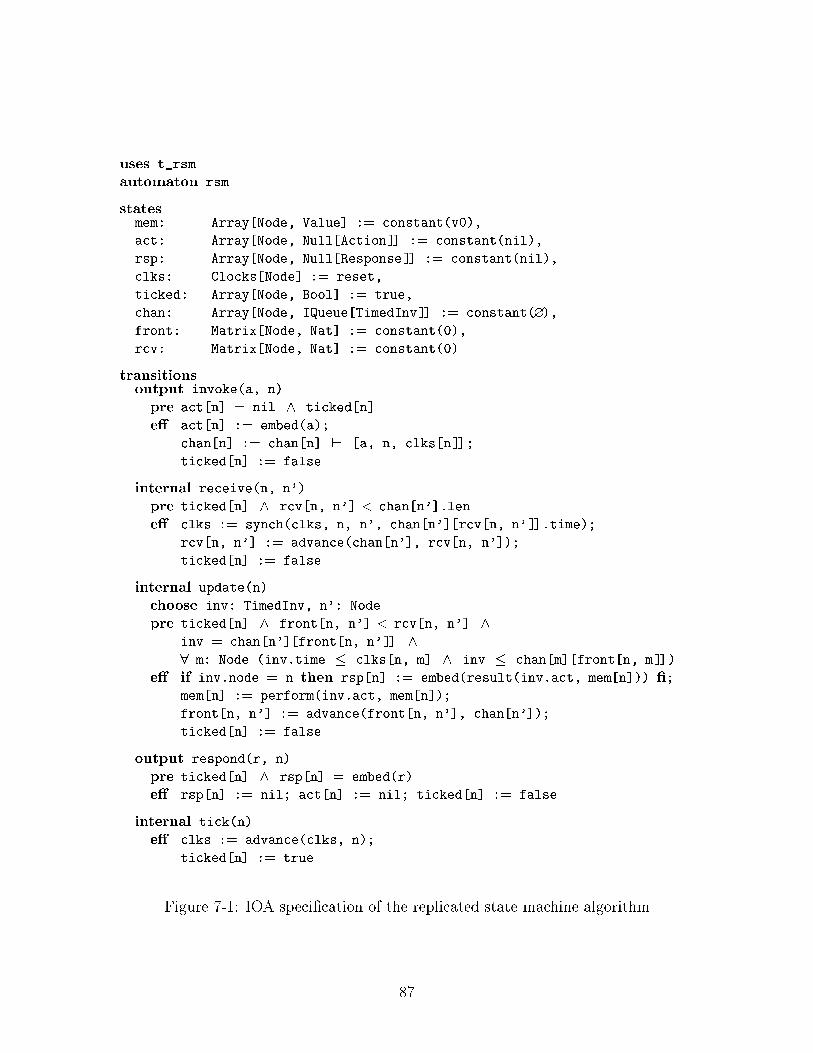
uses t_rsm
automaton rsm
statesmem: Array[Node, Value] := constant(v0),
act: Array[Node, Null[Action]] := constant(nil),
rsp: Array[Node, Null[Response]] := constant(nil),
clks: Clocks[Node] := reset,
ticked: Array[Node, Bool] := true,
chan: Array[Node, IQueue[TimedInv]] := constant(?),
front: Matrix[Node, Nat] := constant(0),
rcv: Matrix[Node, Nat] := constant(0)
transitionsoutput invoke(a, n)
pre act[n] = nil ^ ticked[n]
e� act[n] := embed(a);
chan[n] := chan[n] ` [a, n, clks[n]];
ticked[n] := false
internal receive(n, n')
pre ticked[n] ^ rcv[n, n'] < chan[n'].len
e� clks := synch(clks, n, n', chan[n'][rcv[n, n']].time);
rcv[n, n'] := advance(chan[n'], rcv[n, n']);
ticked[n] := false
internal update(n)
choose inv: TimedInv, n': Node
pre ticked[n] ^ front[n, n'] < rcv[n, n'] ^
inv = chan[n'][front[n, n']] ^
8 m: Node (inv.time � clks[n, m] ^ inv � chan[m][front[n, m]])
e� if inv.node = n then rsp[n] := embed(result(inv.act, mem[n])) �;
mem[n] := perform(inv.act, mem[n]);
front[n, n'] := advance(front[n, n'], chan[n']);
ticked[n] := false
output respond(r, n)
pre ticked[n] ^ rsp[n] = embed(r)
e� rsp[n] := nil; act[n] := nil; ticked[n] := false
internal tick(n)
e� clks := advance(clks, n);
ticked[n] := true
Figure 7-1: IOA speci�cation of the replicated state machine algorithm
87
7.2.2 The synchronized replicated memory
Automaton synch (Figure 7-2) models a simpli�ed version of the replicated state
machine algorithm where the channels are instantaneous. In the absence of channel
delays, all components have an identical view of the system as a whole. Consequently,
this model eliminates the need for logical time as a tool for synchronization. Yet, in
terms of distributing the data between nodes, this system captures most of the com-
plexities present in the rsm algorithm. For this purpose, the synch model represents
a good abstraction for analyzing the features of the distributed data management
scheme without having to worry about the timing features of rsm.
Since communications in the system are synchronous, the invocation history (the
sequence of all invocations that happened so far) can be represented by a shared queue
pend. Actions arriving from the environment are not immediately appended to the
queue. Instead, a node may delay informing the other nodes that it owns an active
action. The inf ag indicates that there is an active execution at a node which has
not made its way to pend yet. When the inform transition is triggered, the current
action is added to pend and the inf ag is reset.
Each node may be at a di�erent processing stage with respect to the shared invo-
cation list. The index variable points to the �rst invocation waiting to be processed
at a given node. When a node has processed all invocations on the list, index takes
the value pend.len. The update transition performs the computation required by
the indexed invocation and generates a response if the invocation belongs to the host
node.
7.3 The simulation from synch to mem
The relation between synch and mem is diÆcult to analyze without some preparatory
work. In particular, it will be helpful to gain some understanding (both intuitive and
formal) of the properties of synch before we construct and prove a forward simulation
relation from synch to mem.
88
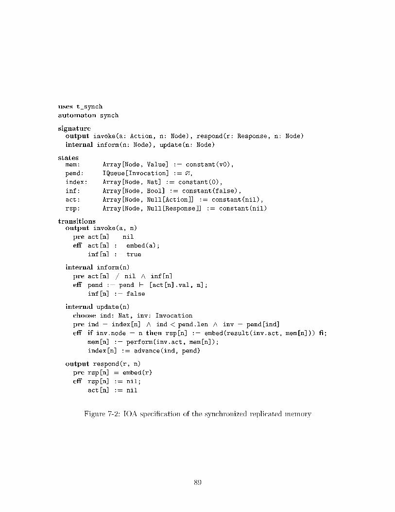
uses t_synch
automaton synch
signatureoutput invoke(a: Action, n: Node), respond(r: Response, n: Node)
internal inform(n: Node), update(n: Node)
statesmem: Array[Node, Value] := constant(v0),
pend: IQueue[Invocation] := ?,
index: Array[Node, Nat] := constant(0),
inf: Array[Node, Bool] := constant(false),
act: Array[Node, Null[Action]] := constant(nil),
rsp: Array[Node, Null[Response]] := constant(nil)
transitionsoutput invoke(a, n)
pre act[n] = nil
e� act[n] := embed(a);
inf[n] := true
internal inform(n)
pre act[n] 6= nil ^ inf[n]
e� pend := pend ` [act[n].val, n];
inf[n] := false
internal update(n)
choose ind: Nat, inv: Invocation
pre ind = index[n] ^ ind < pend.len ^ inv = pend[ind]
e� if inv.node = n then rsp[n] := embed(result(inv.act, mem[n])) �;
mem[n] := perform(inv.act, mem[n]);
index[n] := advance(ind, pend)
output respond(r, n)
pre rsp[n] = embed(r)
e� rsp[n] := nil;
act[n] := nil
Figure 7-2: IOA speci�cation of the synchronized replicated memory
89
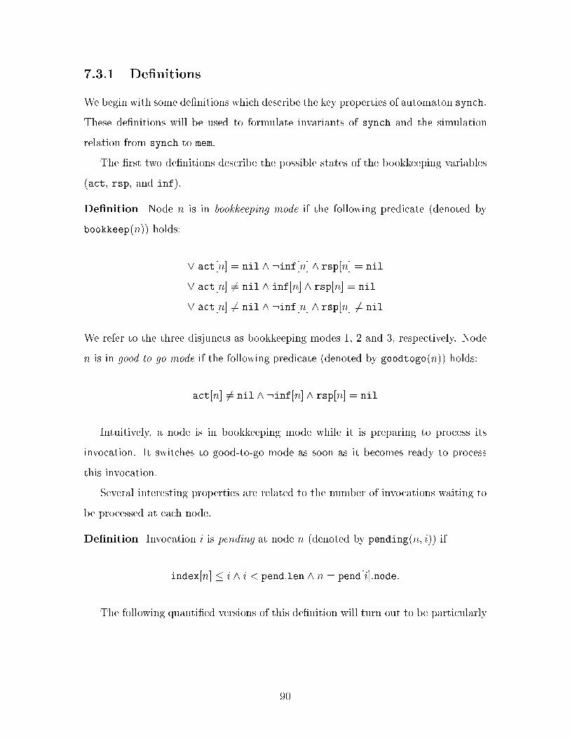
7.3.1 De�nitions
We begin with some de�nitions which describe the key properties of automaton synch.
These de�nitions will be used to formulate invariants of synch and the simulation
relation from synch to mem.
The �rst two de�nitions describe the possible states of the bookkeeping variables
(act, rsp, and inf).
De�nition Node n is in bookkeeping mode if the following predicate (denoted by
bookkeep(n)) holds:
_ act[n] = nil ^ :inf[n] ^ rsp[n] = nil
_ act[n] 6= nil ^ inf[n] ^ rsp[n] = nil
_ act[n] 6= nil ^ :inf[n] ^ rsp[n] 6= nil
We refer to the three disjuncts as bookkeeping modes 1, 2 and 3, respectively. Node
n is in good-to-go mode if the following predicate (denoted by goodtogo(n)) holds:
act[n] 6= nil ^ :inf[n] ^ rsp[n] = nil
Intuitively, a node is in bookkeeping mode while it is preparing to process its
invocation. It switches to good-to-go mode as soon as it becomes ready to process
this invocation.
Several interesting properties are related to the number of invocations waiting to
be processed at each node.
De�nition Invocation i is pending at node n (denoted by pending(n; i)) if
index[n] � i ^ i < pend:len ^ n = pend[i]:node:
The following quanti�ed versions of this de�nition will turn out to be particularly
90
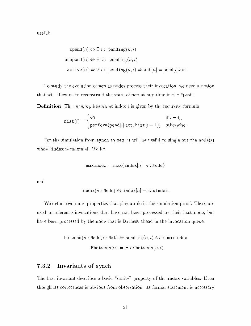
useful:
Epend(n), 9 i : pending(n; i)
onepend(n), 9! i : pending(n; i)
active(n), 8 i : pending(n; i)) act[n] = pend[i]:act
To study the evolution of mem as nodes process their invocation, we need a notion
that will allow us to reconstruct the state of mem at any time in the \past".
De�nition The memory history at index i is given by the recursive formula
hist(i) =
(v0 if i = 0;
perform(pend[i]:act; hist(i� 1)) otherwise:
For the simulation from synch to mem, it will be useful to single out the node(s)
whose index is maximal. We let
maxindex = maxfindex[n]j n : Nodeg
and
ismax(n : Node), index[n] = maxindex:
We de�ne two more properties that play a role in the simulation proof. These are
used to reference invocations that have not been processed by their host node, but
have been processed by the node that is farthest ahead in the invocation queue:
between(n : Node; i : Nat), pending(n; i) ^ i < maxindex
Ebetween(n), 9 i : between(n; i):
7.3.2 Invariants of synch
The �rst invariant describes a basic \sanity" property of the index variables. Even
though its correctness is obvious from observation, its formal statement is necessary
91
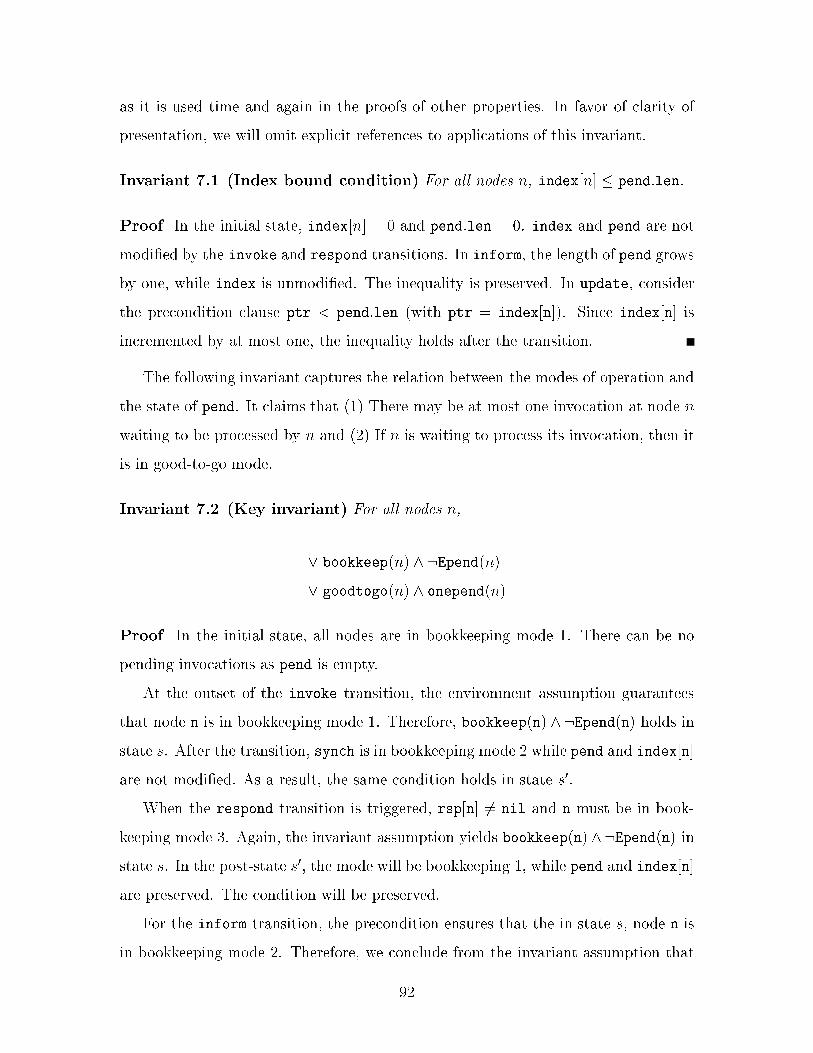
as it is used time and again in the proofs of other properties. In favor of clarity of
presentation, we will omit explicit references to applications of this invariant.
Invariant 7.1 (Index bound condition) For all nodes n, index[n] � pend:len.
Proof In the initial state, index[n] = 0 and pend:len = 0. index and pend are not
modi�ed by the invoke and respond transitions. In inform, the length of pend grows
by one, while index is unmodi�ed. The inequality is preserved. In update, consider
the precondition clause ptr < pend:len (with ptr = index[n]). Since index[n] is
incremented by at most one, the inequality holds after the transition.
The following invariant captures the relation between the modes of operation and
the state of pend. It claims that (1) There may be at most one invocation at node n
waiting to be processed by n and (2) If n is waiting to process its invocation, then it
is in good-to-go mode.
Invariant 7.2 (Key invariant) For all nodes n,
_ bookkeep(n) ^ :Epend(n)
_ goodtogo(n) ^ onepend(n)
Proof In the initial state, all nodes are in bookkeeping mode 1. There can be no
pending invocations as pend is empty.
At the outset of the invoke transition, the environment assumption guarantees
that node n is in bookkeeping mode 1. Therefore, bookkeep(n) ^:Epend(n) holds in
state s. After the transition, synch is in bookkeeping mode 2 while pend and index[n]
are not modi�ed. As a result, the same condition holds in state s0.
When the respond transition is triggered, rsp[n] 6= nil and n must be in book-
keeping mode 3. Again, the invariant assumption yields bookkeep(n) ^:Epend(n) in
state s. In the post-state s0, the mode will be bookkeeping 1, while pend and index[n]
are preserved. The condition will be preserved.
For the inform transition, the precondition ensures that the in state s, node n is
in bookkeeping mode 2. Therefore, we conclude from the invariant assumption that
92
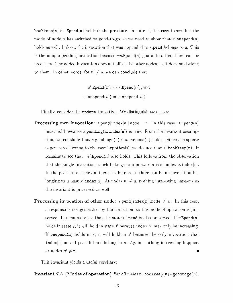
bookkeep(n) ^:Epend(n) holds in the pre-state. In state s0, it is easy to see that the
mode of node n has switched to good-to-go, so we need to show that s0:onepend(n)
holds as well. Indeed, the invocation that was appended to s:pend belongs to n. This
is the unique pending invocation because :s:Epend(n) guarantees that there can be
no others. The added invocation does not a�ect the other nodes, as it does not belong
to them. In other words, for n0 6= n, we can conclude that
s0:Epend(n0), s:Epend(n0); and
s0:onepend(n0), s:onepend(n0):
Finally, consider the update transition. We distinguish two cases:
Processing own invocation: s:pend[index[n]]:node = n. In this case, s:Epend(n)
must hold because s:pending(n; index[n]) is true. From the invariant assump-
tion, we conclude that s:goodtogo(n) ^ s:onepend(n) holds. Since a response
is generated (owing to the case hypothesis), we deduce that s0:bookkeep(n). It
remains to see that :s0:Epend(n) also holds. This follows from the observation
that the single invocation which belongs to n in state s is at index s:index[n].
In the post-state, index[n] increases by one, so there can be no invocation be-
longing to n past s0:index[n]. At nodes n0 6= n, nothing interesting happens so
the invariant is preserved as well.
Processing invocation of other node: s:pend[index[n]]:node 6= n. In this case,
a response is not generated by the transition, so the mode of operation is pre-
served. It remains to see that the state of pend is also preserved. If :Epend(n)
holds in state s, it will hold in state s0 because index[n] may only be increasing.
If onepend(n) holds in s, it will hold in s0 because the only invocation that
index[n] moved past did not belong to n. Again, nothing interesting happens
at nodes n0 6= n.
This invariant yields a useful corollary:
Invariant 7.3 (Modes of operation) For all nodes n, bookkeep(n)_goodtogo(n).
93
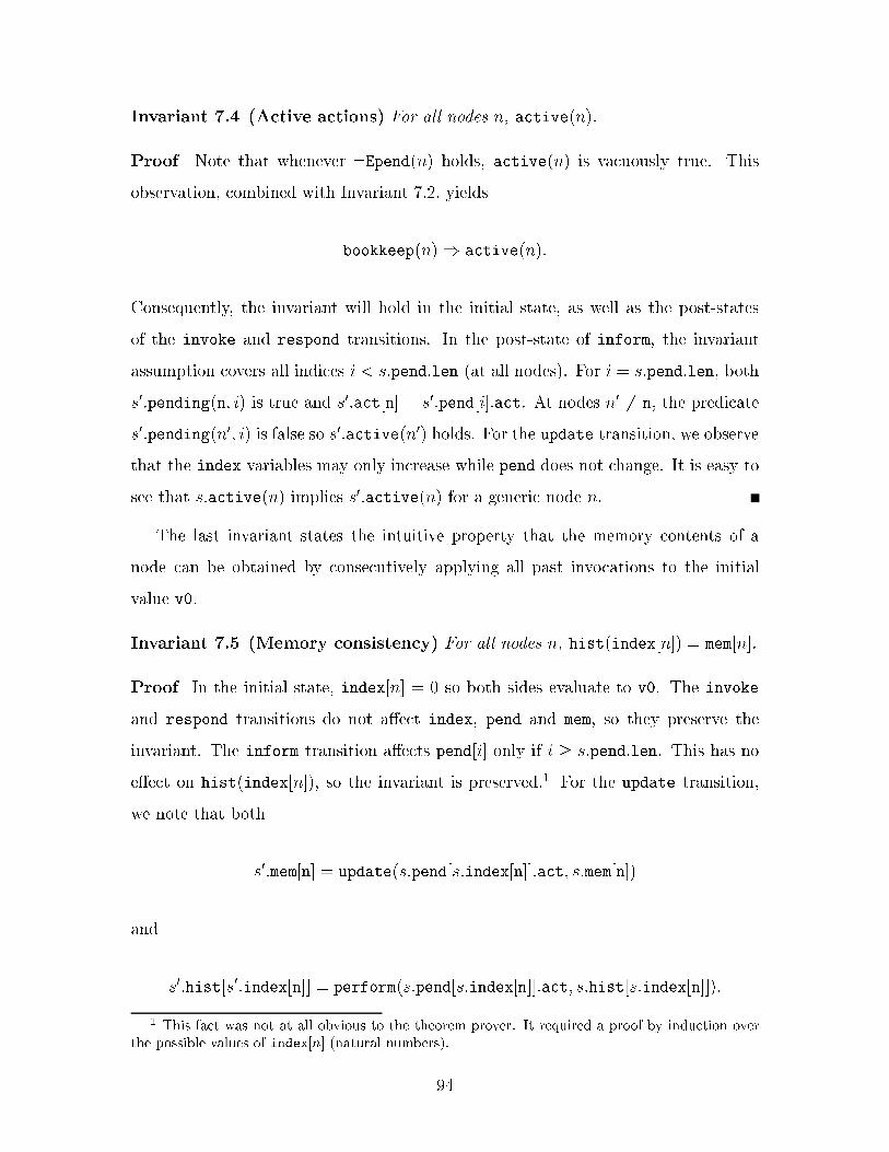
Invariant 7.4 (Active actions) For all nodes n, active(n).
Proof Note that whenever :Epend(n) holds, active(n) is vacuously true. This
observation, combined with Invariant 7.2, yields
bookkeep(n)) active(n):
Consequently, the invariant will hold in the initial state, as well as the post-states
of the invoke and respond transitions. In the post-state of inform, the invariant
assumption covers all indices i < s:pend:len (at all nodes). For i = s:pend:len, both
s0:pending(n; i) is true and s0:act[n] = s0:pend[i]:act. At nodes n0 6= n, the predicate
s0:pending(n0; i) is false so s0:active(n0) holds. For the update transition, we observe
that the index variables may only increase while pend does not change. It is easy to
see that s:active(n) implies s0:active(n) for a generic node n.
The last invariant states the intuitive property that the memory contents of a
node can be obtained by consecutively applying all past invocations to the initial
value v0.
Invariant 7.5 (Memory consistency) For all nodes n, hist(index[n]) = mem[n].
Proof In the initial state, index[n] = 0 so both sides evaluate to v0. The invoke
and respond transitions do not a�ect index, pend and mem, so they preserve the
invariant. The inform transition a�ects pend[i] only if i � s:pend:len. This has no
e�ect on hist(index[n]), so the invariant is preserved.1 For the update transition,
we note that both
s0:mem[n] = update(s:pend[s:index[n]]:act; s:mem[n])
and
s0:hist[s0:index[n]] = perform(s:pend[s:index[n]]:act; s:hist[s:index[n]]):
1 This fact was not at all obvious to the theorem prover. It required a proof by induction overthe possible values of index[n] (natural numbers).
94
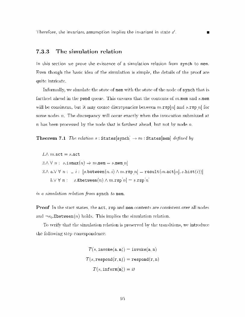
Therefore, the invariant assumption implies the invariant in state s0.
7.3.3 The simulation relation
In this section we prove the existence of a simulation relation from synch to mem.
Even though the basic idea of the simulation is simple, the details of the proof are
quite intricate.
Informally, we simulate the state of mem with the state of the node of synch that is
farthest ahead in the pend queue. This ensures that the contents of m:mem and s:mem
will be consistent, but it may create discrepancies between m:rsp[n] and s:rsp[n] for
some nodes n. The discrepancy will occur exactly when the invocation submitted at
n has been processed by the node that is farthest ahead, but not by node n.
Theorem 7.1 The relation s : States[synch]! m : States[mem] de�ned by
1.^ m:act = s:act
2.^ 8 n : s:ismax(n)) m:mem = s:mem[n]
3.^ a._ 8 n : 9 i : [s:between(n; i) ^m:rsp[n] = result(m:act[n]; s:hist(i))]
b._ 8 n : :s:Ebetween(n) ^m:rsp[n] = s:rsp[n]
is a simulation relation from synch to mem.
Proof In the start states, the act, rsp and mem contents are consistent over all nodes
and :s0:Ebetween(n) holds. This implies the simulation relation.
To verify that the simulation relation is preserved by the transitions, we introduce
the following step correspondence:
T (s; invoke(a; n)) = invoke(a; n)
T (s; respond(r; n)) = respond(r; n)
T (s; inform(n)) = ?
95
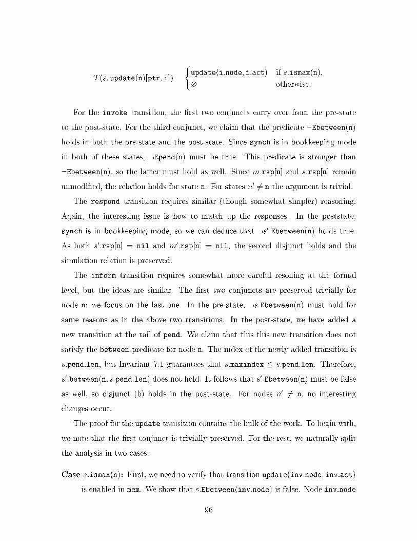
T (s; update(n)[ptr; i]) =
(update(i:node; i:act) if s:ismax(n);
? otherwise:
For the invoke transition, the �rst two conjuncts carry over from the pre-state
to the post-state. For the third conjunct, we claim that the predicate :Ebetween(n)
holds in both the pre-state and the post-state. Since synch is in bookkeeping mode
in both of these states, :Epend(n) must be true. This predicate is stronger than
:Ebetween(n), so the latter must hold as well. Since m:rsp[n] and s:rsp[n] remain
unmodi�ed, the relation holds for state n. For states n0 6= n the argument is trivial.
The respond transition requires similar (though somewhat simpler) reasoning.
Again, the interesting issue is how to match up the responses. In the poststate,
synch is in bookkeeping mode, so we can deduce that :s0:Ebetween(n) holds true.
As both s0:rsp[n] = nil and m0:rsp[n] = nil, the second disjunct holds and the
simulation relation is preserved.
The inform transition requires somewhat more careful resoning at the formal
level, but the ideas are similar. The �rst two conjuncts are preserved trivially for
node n; we focus on the last one. In the pre-state, :s:Ebetween(n) must hold for
same reasons as in the above two transitions. In the post-state, we have added a
new transition at the tail of pend. We claim that this this new transition does not
satisfy the between predicate for node n. The index of the newly added transition is
s:pend:len, but Invariant 7.1 guarantees that s:maxindex � s:pend:len. Therefore,
s0:between(n; s:pend:len) does not hold. It follows that s0:Ebetween(n) must be false
as well, so disjunct (b) holds in the post-state. For nodes n0 6= n, no interesting
changes occur.
The proof for the update transition contains the bulk of the work. To begin with,
we note that the �rst conjunct is trivially preserved. For the rest, we naturally split
the analysis in two cases:
Case s:ismax(n): First, we need to verify that transition update(inv:node; inv:act)
is enabled in mem. We show that s:Ebetween(inv:node) is false. Node inv:node
96
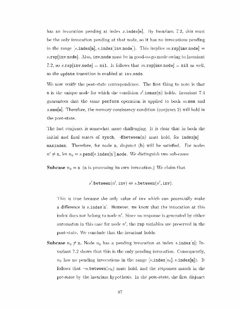
has an invocation pending at index s:index[n]. By Invariant 7.2, this must
be the only invocation pending at that node, so it has no invocations pending
in the range [s:index[n]; s:index[inv:node]). This implies m:rsp[inv:node] =
s:rsp[inv:node]. Also, inv:node must be in good-to-go mode owing to Invariant
7.2, so s:rsp[inv:node] = nil. It follows that m:rsp[inv:node] = nil as well,
so the update transition is enabled at inv:node.
We now verify the post-state correspondence. The �rst thing to note is that
n is the unique node for which the condition s0:ismax(n) holds. Invariant 7.4
guarantees that the same perform operation is applied to both m:mem and
s:mem[n]. Therefore, the memory consistency condition (conjunct 2) will hold in
the post-state.
The last conjunct is somewhat more challenging. It is clear that in both the
initial and �nal states of synch, :Ebetween(n) must hold, for index[n] =
maxindex. Therefore, for node n, disjunct (b) will be satis�ed. For nodes
n0 6= n, let n0 = s:pend[s:index[n]]:node. We distinguish two sub-cases:
Subcase n0 = n (n is processing its own invocation.) We claim that
s0:between(n0; inv), s:between(n0; inv):
This is true because the only value of inv which can potentially make
a di�erence is s:index[n]. However, we know that the invocation at this
index does not belong to node n0. Since no response is generated by either
automaton in this case for node n0, the rsp variables are preserved in the
post-state. We conclude that the invariant holds.
Subcase n0 6= n. Node n0 has a pending invocation at index s:index[n]; In-
variant 7.2 shows that this is the only pending invocation. Consequently,
n0 has no pending invocations in the range [s:index[n0]; s:index[n]). It
follows that :s:between(n0) must hold, and the responses match in the
pre-state by the invariant hypothesis. In the post-state, the �rst disjunct
97
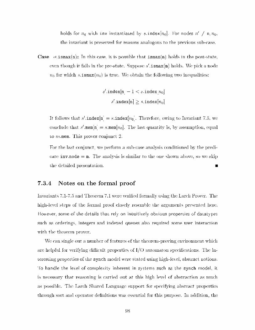
holds for n0 with inv instantiated by s:index[n0]. For nodes n0 6= n; n0,
the invariant is preserved for reasons analogous to the previous sub-case.
Case :s:ismax(n): In this case, it is possible that ismax(n) holds in the post-state,
even though it fails in the pre-state. Suppose s0:ismax(n) holds. We pick a node
n0 for which s:ismax(n0) is true. We obtain the following two inequalities:
s0:index[n] � 1 < s:index[n0]
s0:index[n] � s:index[n0]
It follows that s0:index[n] = s:index[n0]. Therefore, owing to Invariant 7.5, we
conclude that s0:mem[n] = s:mem[n0]. The last quantity is, by assumption, equal
to m:mem. This proves conjunct 2.
For the last conjunct, we perform a sub-case analysis conditioned by the predi-
cate inv:node = n. The analysis is similar to the one shown above, so we skip
the detailed presentation.
7.3.4 Notes on the formal proof
Invariants 7.1-7.5 and Theorem 7.1 were veri�ed formally using the Larch Prover. The
high-level steps of the formal proof closely resemble the arguments presented here.
However, some of the details that rely on intuitively obvious properties of datatypes
such as orderings, integers and indexed queues also required some user interaction
with the theorem prover.
We can single out a number of features of the theorem-proving environment which
are helpful for verifying diÆcult properties of I/O automaton speci�cations. The in-
teresting properties of the synch model were stated using high-level, abstract notions.
To handle the level of complexity inherent in systems such as the synch model, it
is necessary that reasoning is carried out at this high level of abstraction as much
as possible. The Larch Shared Language support for specifying abstract properties
through sort and operator de�nitions was essential for this purpose. In addition, the
98
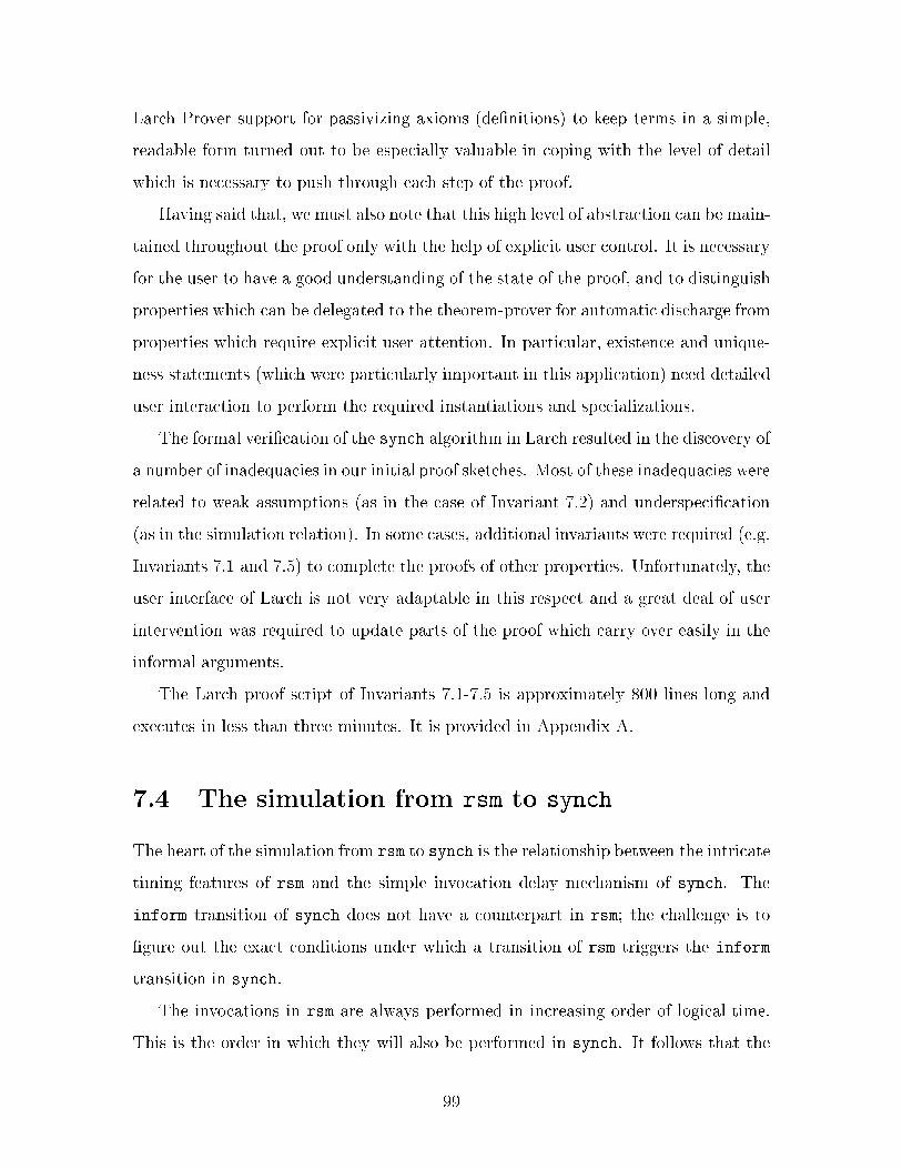
Larch Prover support for passivizing axioms (de�nitions) to keep terms in a simple,
readable form turned out to be especially valuable in coping with the level of detail
which is necessary to push through each step of the proof.
Having said that, we must also note that this high level of abstraction can be main-
tained throughout the proof only with the help of explicit user control. It is necessary
for the user to have a good understanding of the state of the proof, and to distinguish
properties which can be delegated to the theorem-prover for automatic discharge from
properties which require explicit user attention. In particular, existence and unique-
ness statements (which were particularly important in this application) need detailed
user interaction to perform the required instantiations and specializations.
The formal veri�cation of the synch algorithm in Larch resulted in the discovery of
a number of inadequacies in our initial proof sketches. Most of these inadequacies were
related to weak assumptions (as in the case of Invariant 7.2) and underspeci�cation
(as in the simulation relation). In some cases, additional invariants were required (e.g.
Invariants 7.1 and 7.5) to complete the proofs of other properties. Unfortunately, the
user interface of Larch is not very adaptable in this respect and a great deal of user
intervention was required to update parts of the proof which carry over easily in the
informal arguments.
The Larch proof script of Invariants 7.1-7.5 is approximately 800 lines long and
executes in less than three minutes. It is provided in Appendix A.
7.4 The simulation from rsm to synch
The heart of the simulation from rsm to synch is the relationship between the intricate
timing features of rsm and the simple invocation delay mechanism of synch. The
inform transition of synch does not have a counterpart in rsm; the challenge is to
�gure out the exact conditions under which a transition of rsm triggers the inform
transition in synch.
The invocations in rsm are always performed in increasing order of logical time.
This is the order in which they will also be performed in synch. It follows that the
99
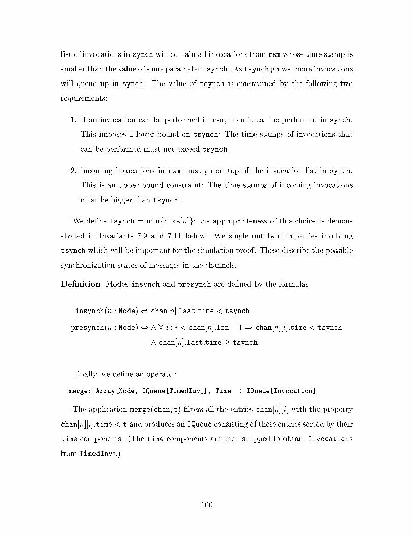
list of invocations in synch will contain all invocations from rsm whose time stamp is
smaller than the value of some parameter tsynch. As tsynch grows, more invocations
will queue up in synch. The value of tsynch is constrained by the following two
requirements:
1. If an invocation can be performed in rsm, then it can be performed in synch.
This imposes a lower bound on tsynch: The time stamps of invocations that
can be performed must not exceed tsynch.
2. Incoming invocations in rsm must go on top of the invocation list in synch.
This is an upper bound constraint: The time stamps of incoming invocations
must be bigger than tsynch.
We de�ne tsynch = minfclks[n]g; the appropriateness of this choice is demon-
strated in Invariants 7.9 and 7.11 below. We single out two properties involving
tsynch which will be important for the simulation proof. These describe the possible
synchronization states of messages in the channels.
De�nition Modes insynch and presynch are de�ned by the formulas
insynch(n : Node), chan[n]:last:time < tsynch
presynch(n : Node), ^ 8 i : i < chan[n]:len� 1) chan[n][i]:time < tsynch
^ chan[n]:last:time � tsynch
Finally, we de�ne an operator
merge: Array[Node, IQueue[TimedInv]], Time ! IQueue[Invocation]
The application merge(chan; t) �lters all the entries chan[n][i] with the property
chan[n][i]:time < t and produces an IQueue consisting of these entries sorted by their
time components. (The time components are then stripped to obtain Invocations
from TimedInvs.)
100
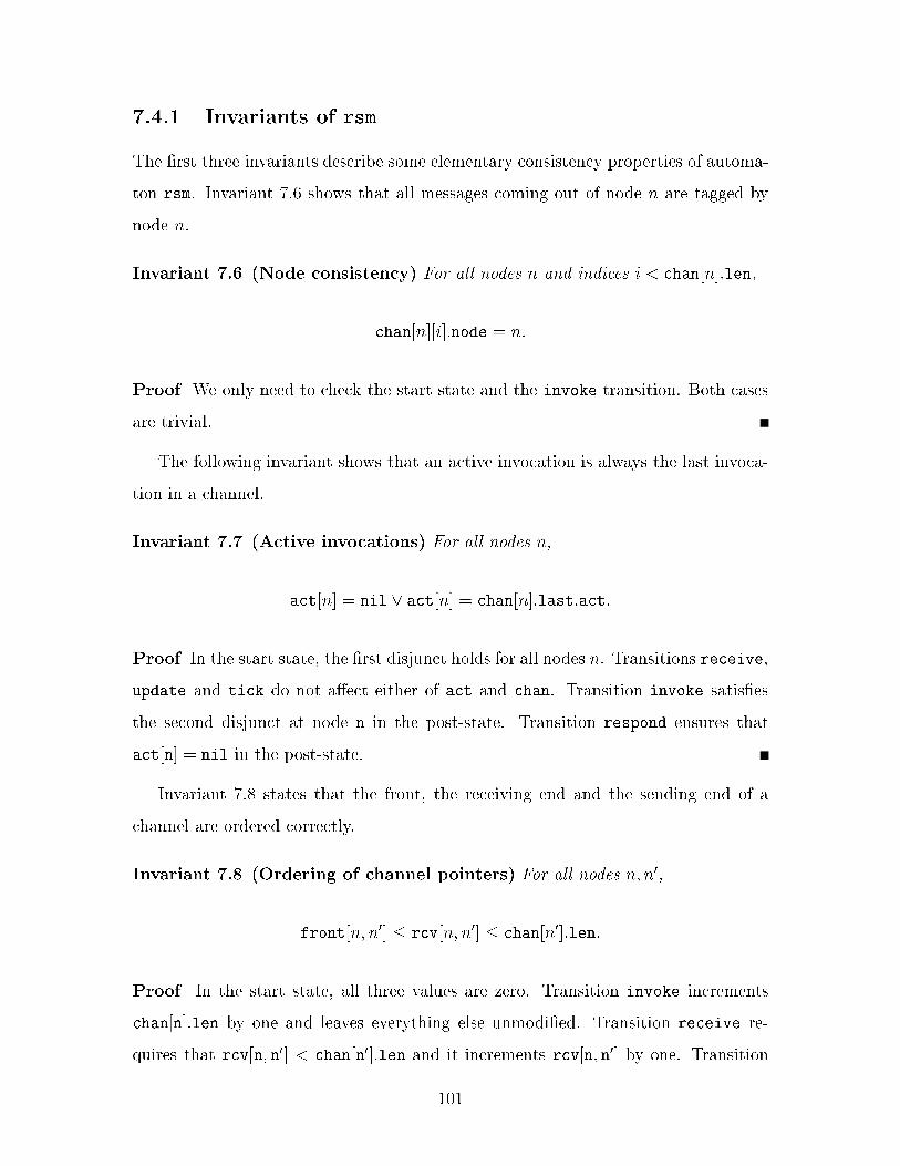
7.4.1 Invariants of rsm
The �rst three invariants describe some elementary consistency properties of automa-
ton rsm. Invariant 7.6 shows that all messages coming out of node n are tagged by
node n.
Invariant 7.6 (Node consistency) For all nodes n and indices i < chan[n]:len,
chan[n][i]:node = n:
Proof We only need to check the start state and the invoke transition. Both cases
are trivial.
The following invariant shows that an active invocation is always the last invoca-
tion in a channel.
Invariant 7.7 (Active invocations) For all nodes n,
act[n] = nil _ act[n] = chan[n]:last:act:
Proof In the start state, the �rst disjunct holds for all nodes n. Transitions receive,
update and tick do not a�ect either of act and chan. Transition invoke satis�es
the second disjunct at node n in the post-state. Transition respond ensures that
act[n] = nil in the post-state.
Invariant 7.8 states that the front, the receiving end and the sending end of a
channel are ordered correctly.
Invariant 7.8 (Ordering of channel pointers) For all nodes n; n0,
front[n; n0] � rcv[n; n0] � chan[n0]:len:
Proof In the start state, all three values are zero. Transition invoke increments
chan[n]:len by one and leaves everything else unmodi�ed. Transition receive re-
quires that rcv[n; n0] < chan[n0]:len and it increments rcv[n; n0] by one. Transition
101
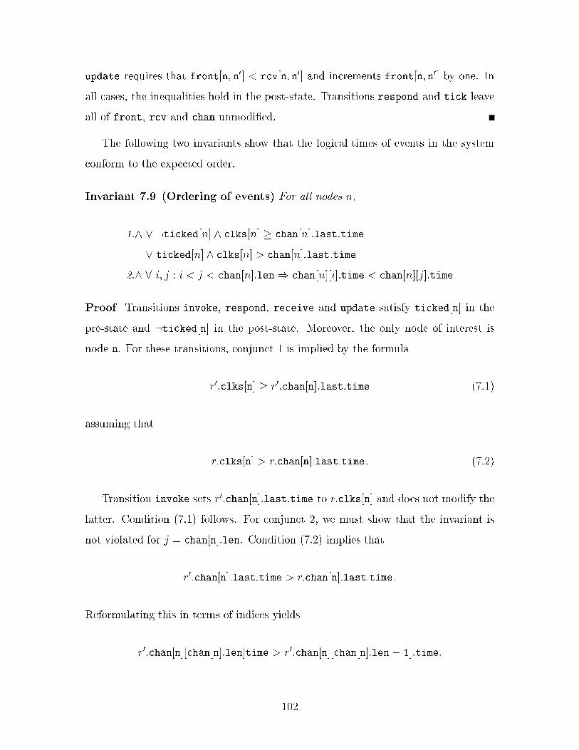
update requires that front[n; n0] < rcv[n; n0] and increments front[n; n0] by one. In
all cases, the inequalities hold in the post-state. Transitions respond and tick leave
all of front, rcv and chan unmodi�ed.
The following two invariants show that the logical times of events in the system
conform to the expected order.
Invariant 7.9 (Ordering of events) For all nodes n,
1.^ _ :ticked[n] ^ clks[n] � chan[n]:last:time
_ ticked[n] ^ clks[n] > chan[n]:last:time
2.^ 8 i; j : i < j < chan[n]:len) chan[n][i]:time < chan[n][j]:time
Proof Transitions invoke, respond, receive and update satisfy ticked[n] in the
pre-state and :ticked[n] in the post-state. Moreover, the only node of interest is
node n. For these transitions, conjunct 1 is implied by the formula
r0:clks[n] � r0:chan[n]:last:time (7.1)
assuming that
r:clks[n] > r:chan[n]:last:time: (7.2)
Transition invoke sets r0:chan[n]:last:time to r:clks[n] and does not modify the
latter. Condition (7.1) follows. For conjunct 2, we must show that the invariant is
not violated for j = chan[n]:len. Condition (7.2) implies that
r0:chan[n]:last:time > r:chan[n]:last:time:
Reformulating this in terms of indices yields
r0:chan[n][chan[n]:len]time > r0:chan[n][chan[n]:len � 1]:time:
102
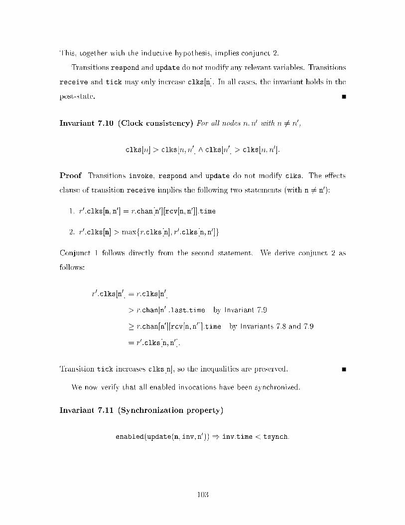
This, together with the inductive hypothesis, implies conjunct 2.
Transitions respond and update do not modify any relevant variables. Transitions
receive and tick may only increase clks[n]. In all cases, the invariant holds in the
post-state.
Invariant 7.10 (Clock consistency) For all nodes n; n0 with n 6= n0,
clks[n] > clks[n; n0] ^ clks[n0] > clks[n; n0]:
Proof Transitions invoke, respond and update do not modify clks. The e�ects
clause of transition receive implies the following two statements (with n 6= n0):
1. r0:clks[n; n0] = r:chan[n0][rcv[n; n0]]:time
2. r0:clks[n] > maxfr:clks[n]; r0:clks[n; n0]g
Conjunct 1 follows directly from the second statement. We derive conjunct 2 as
follows:
r0:clks[n0] = r:clks[n0]
> r:chan[n0]:last:time by Invariant 7.9
� r:chan[n0][rcv[n; n0]]:time by Invariants 7.8 and 7.9
= r0:clks[n; n0]:
Transition tick increases clks[n], so the inequalities are preserved.
We now verify that all enabled invocations have been synchronized.
Invariant 7.11 (Synchronization property)
enabled(update(n; inv; n0))) inv:time < tsynch:
103
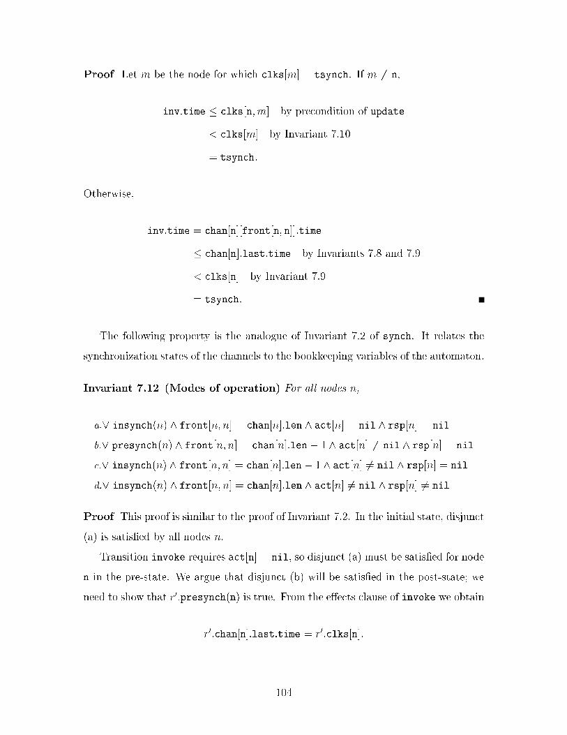
Proof Let m be the node for which clks[m] = tsynch. If m 6= n,
inv:time � clks[n; m] by precondition of update
< clks[m] by Invariant 7.10
= tsynch:
Otherwise,
inv:time = chan[n][front[n; n]]:time
� chan[n]:last:time by Invariants 7.8 and 7.9
< clks[n] by Invariant 7.9
= tsynch:
The following property is the analogue of Invariant 7.2 of synch. It relates the
synchronization states of the channels to the bookkeeping variables of the automaton.
Invariant 7.12 (Modes of operation) For all nodes n,
a._ insynch(n) ^ front[n; n] = chan[n]:len ^ act[n] = nil ^ rsp[n] = nil
b._ presynch(n) ^ front[n; n] = chan[n]:len� 1 ^ act[n] 6= nil ^ rsp[n] = nil
c._ insynch(n) ^ front[n; n] = chan[n]:len� 1 ^ act[n] 6= nil ^ rsp[n] = nil
d._ insynch(n) ^ front[n; n] = chan[n]:len ^ act[n] 6= nil ^ rsp[n] 6= nil
Proof This proof is similar to the proof of Invariant 7.2. In the initial state, disjunct
(a) is satis�ed by all nodes n.
Transition invoke requires act[n] = nil, so disjunct (a) must be satis�ed for node
n in the pre-state. We argue that disjunct (b) will be satis�ed in the post-state; we
need to show that r0:presynch(n) is true. From the e�ects clause of invoke we obtain
r0:chan[n]:last:time = r0:clks[n]:
104
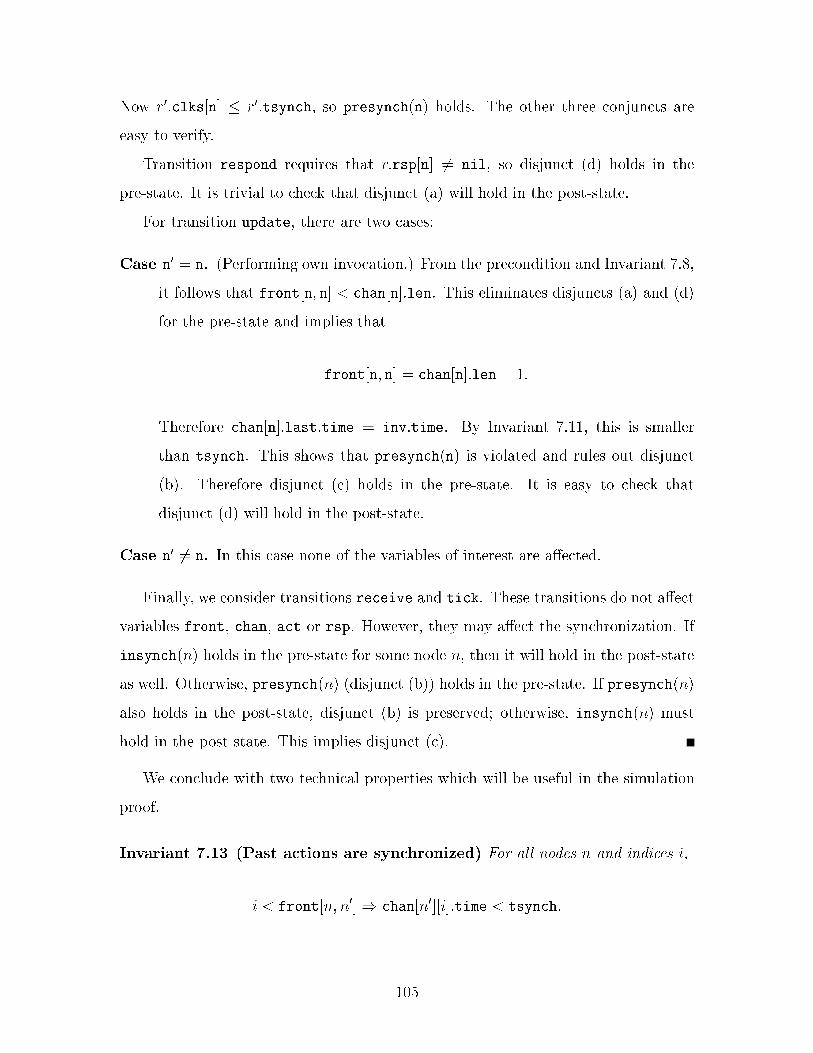
Now r0:clks[n] � r0:tsynch, so presynch(n) holds. The other three conjuncts are
easy to verify.
Transition respond requires that r:rsp[n] 6= nil, so disjunct (d) holds in the
pre-state. It is trivial to check that disjunct (a) will hold in the post-state.
For transition update, there are two cases:
Case n0 = n. (Performing own invocation.) From the precondition and Invariant 7.8,
it follows that front[n; n] < chan[n]:len. This eliminates disjuncts (a) and (d)
for the pre-state and implies that
front[n; n] = chan[n]:len � 1:
Therefore chan[n]:last:time = inv:time. By Invariant 7.11, this is smaller
than tsynch. This shows that presynch(n) is violated and rules out disjunct
(b). Therefore disjunct (c) holds in the pre-state. It is easy to check that
disjunct (d) will hold in the post-state.
Case n0 6= n. In this case none of the variables of interest are a�ected.
Finally, we consider transitions receive and tick. These transitions do not a�ect
variables front, chan, act or rsp. However, they may a�ect the synchronization. If
insynch(n) holds in the pre-state for some node n, then it will hold in the post-state
as well. Otherwise, presynch(n) (disjunct (b)) holds in the pre-state. If presynch(n)
also holds in the post-state, disjunct (b) is preserved; otherwise, insynch(n) must
hold in the post-state. This implies disjunct (c).
We conclude with two technical properties which will be useful in the simulation
proof.
Invariant 7.13 (Past actions are synchronized) For all nodes n and indices i,
i < front[n; n0]) chan[n0][i]:time < tsynch:
105
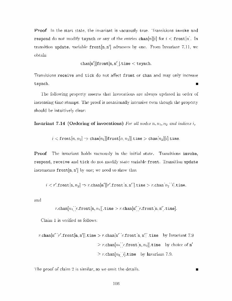
Proof In the start state, the invariant is vacuously true. Transitions invoke and
respond do not modify tsynch or any of the entries chan[n][i] for i < front[n]. In
transition update, variable front[n; n0] advances by one. From Invariant 7.11, we
obtain
chan[n0][front[n; n0]]:time < tsynch:
Transitions receive and tick do not a�ect front or chan and may only increase
tsynch.
The following property asserts that invocations are always updated in order of
increasing time stamps. The proof is notationally intensive even though the property
should be intuitively clear:
Invariant 7.14 (Ordering of invocations) For all nodes n; n1; n2 and indices i,
i < front[n; n2]) chan[n1][front[n; n1]]:time > chan[n2][i]:time:
Proof The invariant holds vacuously in the initial state. Transitions invoke,
respond, receive and tick do not modify state variable front. Transition update
increments front[n; n0] by one; we need to show that
i < r0:front[n; n2]) r:chan[n0][r0:front[n; n0]]:time > r:chan[n2][i]:time:
and
r:chan[n1][r:front[n; n1]]:time > r:chan[n0][r:front[n; n0]:time]:
Claim 1 is veri�ed as follows:
r:chan[n0][r0:front[n; n0]]:time > r:chan[n0][r:front[n; n0]]:time by Invariant 7.9
� r:chan[n2][r:front[n; n2]]:time by choice of n0
� r:chan[n2][i]:time by Invariant 7.9:
The proof of claim 2 is similar, so we omit the details.
106
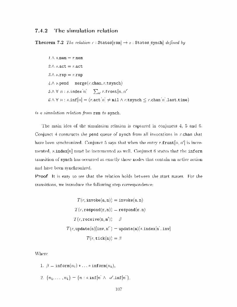
7.4.2 The simulation relation
Theorem 7.2 The relation r : States[rsm]! s : States[synch] de�ned by
1.^ s:mem = r:mem
2.^ s:act = r:act
3.^ s:rsp = r:rsp
4.^ s:pend = merge(r:chan; r:tsynch)
5.^ 8 n : s:index[n] =P
n0 r:front[n; n0]
6.^ 8 n : s:inf[n] = (r:act[n] 6= nil ^ r:tsynch � r:chan[n]:last:time)
is a simulation relation from rsm to synch.
The main idea of the simulation relation is captured in conjuncts 4, 5 and 6.
Conjunct 4 constructs the pend queue of synch from all invocations in r:chan that
have been synchronized. Conjunct 5 says that when the entry r:front[n; n0] is incre-
mented, s:index[n] must be incremented as well. Conjunct 6 states that the inform
transition of synch has occurred at exactly those nodes that contain an active action
and have been synchronized.
Proof It is easy to see that the relation holds between the start states. For the
transitions, we introduce the following step correspondence:
T (r; invoke(a; n)) = invoke(a; n)
T (r; respond(r; n)) = respond(r; n)
T (r; receive(n; n0)) = �
T (r; update(n)[inv; n0]) = update(n)[s:index[n]; inv]
T (r; tick(n)) = �
Where
1. � = inform(n1) � : : : � inform(nk),
2. fn1; : : : ; nkg = fn : s:inf[n] ^ :s0:inf[n]g,
107
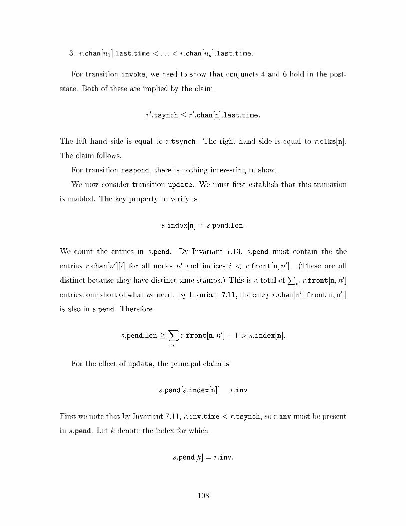
3. r:chan[n1]:last:time < : : : < r:chan[nk]:last:time.
For transition invoke, we need to show that conjuncts 4 and 6 hold in the post-
state. Both of these are implied by the claim
r0:tsynch � r0:chan[n]:last:time:
The left hand side is equal to r:tsynch. The right hand side is equal to r:clks[n].
The claim follows.
For transition respond, there is nothing interesting to show.
We now consider transition update. We must �rst establish that this transition
is enabled. The key property to verify is
s:index[n] < s:pend:len:
We count the entries in s:pend. By Invariant 7.13, s:pend must contain the the
entries r:chan[n0][i] for all nodes n0 and indices i < r:front[n; n0]. (These are all
distinct because they have distinct time stamps.) This is a total ofP
n0 r:front[n; n0]
entries, one short of what we need. By Invariant 7.11, the entry r:chan[n0][front[n; n0]]
is also in s:pend. Therefore
s:pend:len �Xn0
r:front[n; n0] + 1 > s:index[n]:
For the e�ect of update, the principal claim is
s:pend[s:index[n]] = r:inv
First we note that by Invariant 7.11, r:inv:time < r:tsynch, so r:inv must be present
in s:pend. Let k denote the index for which
s:pend[k] = r:inv:
108
We show that k = s:index[n] as follows:
1. k � s:index[n]. From Invariant 7.14,
r:inv:time > r:chan[n2][i]:time
for all nodes n2 and indices i < r:front[n; n2]. All these entries must be in
s:pend because their time stamps are smaller than r:tsynch. Moreover, their
indices in s:pend are all smaller than k. There are exactlyP
n2s:front[n; n2] =
s:index[n] such entries. The claim follows.
2. k � s:index[n]. We proceed by contradiction. If this property is violated, there
must exist an index i < k and node n2 with i � r:front[n; n2] and
s:pend[i] = r:chan[n2][front[n; n2]]:
(All pairs (n2; i) which violate this condition were accounted for in the previous
part.) Then
r:inv:time = chan[n0][front[n; n0]]:time
� r:chan[n2][front[n; n2]]:time by choice of n0
� r:chan[n2][i]:time by Invariant 7.9
This implies that k � i. Contradiction. This veri�es the principal claim.
The post-state correspondence is now easy to verify. For conjunct 5, we note
that both sides of the equation are incremented by one. The other conjuncts follow
directly.
Finally we consider transitions receive and tick. Of all the variables of rsm that
appear in the simulation relation, only tsynch may be modi�ed by the transitions.
First, we show that each of the inform transitions from the step correspondence is
enabled. Property 2 of � ensures that s:inf[ni] is satis�ed for all ni (1 � i � k), and
this implies s:act[ni] 6= nil as well.
109
For the step correspondence, we need to verify two properties:
1. s0:pend = merge(r:chan; r0:tsynch). By Invariant 7.12, the additions to s:pend
are entries for which r:presynch(n) and r0:insynch(n). These are the entries
of the form r:chan[n]:last which satisfy
r:act[n] 6= nil ^ r:tsynch � r:chan[n]:last:time < r0:tsynch:
The set of nodes that satisfy this condition is exactly fn1; : : : ; nkg. It remains
to show that the entries added to s:pend are the \correct" ones, i.e.
r:chan[ni]:last:act = s:act[ni]:val
for all the ni. This is guaranteed by Invariant 7.7. Condition 3 for � ensures
that the entries are added in the correct order.
2. 8 n : s0:inf[n] = (r0:act[n] 6= nil ^ r0:tsynch � r0:chan[n]:last:time). This
follows by choice of the nodes ni (condition 2 for �).
110
Chapter 8
Discussion and future work
The translation process from IOA to Larch developed in this thesis is meant to serve
as a practical tool for verifying the correctness of distributed algorithms speci�ed in
the IOA language. The design of the tool was driven by the need to make the output
suitable for interactive theorem proving. The relationship between the translated
speci�cation and the original IOA program is transparent; had this not been the case,
the user of the theorem proving tool would not be able to �nd his or her way through
the interactive proof. On the other hand, the translation is structured in a manner
which takes advantage of the automatic features of the theorem prover. Generally,
these features are most helpful in speci�cations with widely applicable rewrite rules
(statements of equality or boolean equivalence), well thought out inductive de�nitions
and a lack of existentially quanti�ed statements.
The Larch theory of I/O automata, as formalized in Chapter 2, is a simple but
powerful apparatus for formal reasoning about automata. It provides two basic con-
structs for specifying correctness properties: Invariants and forward simulation rela-
tions. The logic of these notions is simple and their proof strategies are schematic;
as formal reasoning tools, they are both intuitive and convenient for automatic veri-
�cation strategies.
Usability and automation are at the heart of the translation tool described in
Chapter 3. The top level anatomy of a translated speci�cation closely re ects the
original IOA program. Formal arguments about automata are centered on careful
111
reasoning about transitions. The translation process facilitates this reasoning by
computing the transition post-state as an explicit function of the pre-state. In theo-
rem proving, these relationships are turned into rewrite rules; a great many obvious
and technical proof obligations are discharged automatically in this manner, keeping
the user focused on the important parts of the proof.
IOA allows explicit nondeterminism by providing choose parameters. The trans-
lation tool handles this nondeterminism explicitly by extending transition signatures
with choose parameters. This technique eliminates the need for existential quanti�-
cation of choose assignments suggested in the IOA Reference Manual [10].
The correctness proofs for the strong caching algorithm (Chapter 5) and the ma-
jority voting algorithm (Chapter 6) illustrate a practical application of the formal
reasoning techniques for IOA programs. Chapter 7 demonstrates the full power of
the elementary notions in the theory of I/O automata: The correctness of a complex
distributed data management algorithm|the replicated state machine|is demon-
strated using only invariants and forward simulations.
Despite these initial successes, the translation process from IOA to LSL is by no
means perfect. In Sections 8.1-8.4, we single out four directions in which the current
tool may be extended to better serve its purpose. We believe that the ideas in this
thesis provide a solid foundation upon which these (and possibly other) extensions
may be built.
8.1 Semantic checks
The current version of the translation tool assumes that the IOA programs it operates
on are semantically correct. If this is not the case, the Larch speci�cation generated
by the tool may be inconsistent. Not all semantic properties of IOA programs can be
veri�ed by a typical static checker. Some properties are intricate enough to require
the full power of a theorem prover; some may even be undecidable.
The translation scheme developed in this thesis can be leveraged to formulate
proof obligations for those semantic properties that cannot be discharged statically.
112
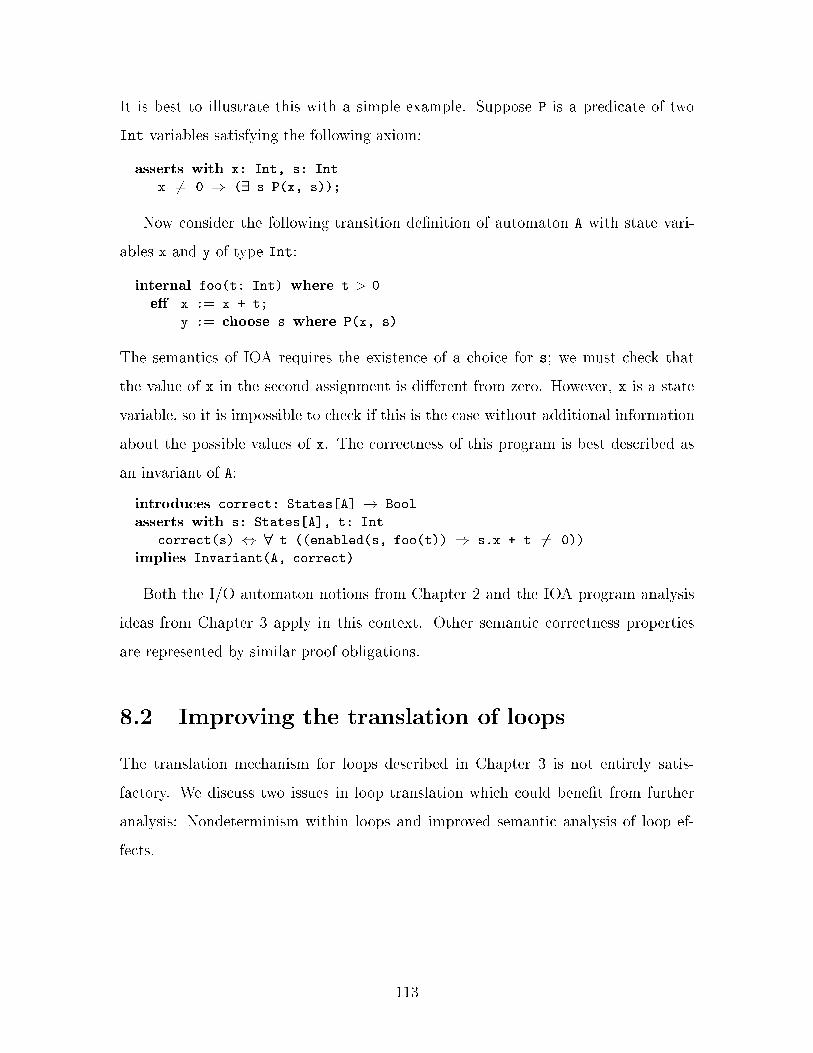
It is best to illustrate this with a simple example. Suppose P is a predicate of two
Int variables satisfying the following axiom:
asserts with x: Int, s: Int
x 6= 0 ) (9 s P(x, s));
Now consider the following transition de�nition of automaton A with state vari-
ables x and y of type Int:
internal foo(t: Int) where t > 0
e� x := x + t;
y := choose s where P(x, s)
The semantics of IOA requires the existence of a choice for s; we must check that
the value of x in the second assignment is di�erent from zero. However, x is a state
variable, so it is impossible to check if this is the case without additional information
about the possible values of x. The correctness of this program is best described as
an invariant of A:
introduces correct: States[A] ! Bool
asserts with s: States[A], t: Int
correct(s) , 8 t ((enabled(s, foo(t)) ) s.x + t 6= 0))
implies Invariant(A, correct)
Both the I/O automaton notions from Chapter 2 and the IOA program analysis
ideas from Chapter 3 apply in this context. Other semantic correctness properties
are represented by similar proof obligations.
8.2 Improving the translation of loops
The translation mechanism for loops described in Chapter 3 is not entirely satis-
factory. We discuss two issues in loop translation which could bene�t from further
analysis: Nondeterminism within loops and improved semantic analysis of loop ef-
fects.
113
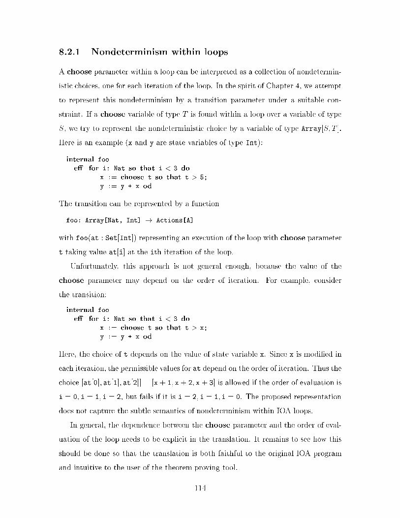
8.2.1 Nondeterminism within loops
A choose parameter within a loop can be interpreted as a collection of nondetermin-
istic choices, one for each iteration of the loop. In the spirit of Chapter 4, we attempt
to represent this nondeterminism by a transition parameter under a suitable con-
straint. If a choose variable of type T is found within a loop over a variable of type
S, we try to represent the nondeterministic choice by a variable of type Array[S; T ].
Here is an example (x and y are state variables of type Int):
internal foo
e� for i: Nat so that i < 3 do
x := choose t so that t > 5;
y := y + x od
The transition can be represented by a function
foo: Array[Nat, Int] ! Actions[A]
with foo(at : Set[Int]) representing an execution of the loop with choose parameter
t taking value at[i] at the ith iteration of the loop.
Unfortunately, this approach is not general enough, because the value of the
choose parameter may depend on the order of iteration. For example, consider
the transition:
internal foo
e� for i: Nat so that i < 3 do
x := choose t so that t > x;
y := y + x od
Here, the choice of t depends on the value of state variable x. Since x is modi�ed in
each iteration, the permissible values for at depend on the order of iteration. Thus the
choice [at[0]; at[1]; at[2]] = [x + 1; x+ 2; x + 3] is allowed if the order of evaluation is
i = 0; i = 1; i = 2, but fails if it is i = 2; i = 1; i = 0. The proposed representation
does not capture the subtle semantics of nondeterminism within IOA loops.
In general, the dependence between the choose parameter and the order of eval-
uation of the loop needs to be explicit in the translation. It remains to see how this
should be done so that the translation is both faithful to the original IOA program
and intuitive to the user of the theorem proving tool.
114
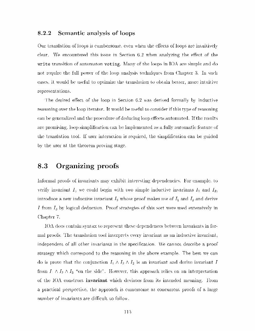
8.2.2 Semantic analysis of loops
Our translation of loops is cumbersome, even when the e�ects of loops are intuitively
clear. We encountered this issue in Section 6.2 when analyzing the e�ect of the
write transition of automaton voting. Many of the loops in IOA are simple and do
not require the full power of the loop analysis techniques from Chapter 3. In such
cases, it would be useful to optimize the translation to obtain better, more intuitive
representations.
The desired e�ect of the loop in Section 6.2 was derived formally by inductive
reasoning over the loop iterator. It would be useful to consider if this type of reasoning
can be generalized and the procedure of deducing loop e�ects automated. If the results
are promising, loop simpli�cation can be implemented as a fully automatic feature of
the translation tool. If user interaction is required, the simpli�cation can be guided
by the user at the theorem proving stage.
8.3 Organizing proofs
Informal proofs of invariants may exhibit interesting dependencies. For example, to
verify invariant I, we could begin with two simple inductive invariants I1 and I2,
introduce a new inductive invariant I3 whose proof makes use of I1 and I2 and derive
I from I3 by logical deduction. Proof strategies of this sort were used extensively in
Chapter 7.
IOA does contain syntax to represent these dependences between invariants in for-
mal proofs. The translation tool interprets every invariant as an inductive invariant,
independent of all other invariants in the speci�cation. We cannot describe a proof
strategy which correspond to the reasoning in the above example. The best we can
do is prove that the conjunction I1 ^ I2 ^ I3 is an invariant and derive invariant I
from I1 ^ I2 ^ I3 \on the side". However, this approach relies on an interpretation
of the IOA construct invariant which deviates from its intended meaning. From
a practical perspective, the approach is cumersome as concurrent proofs of a large
number of invariants are diÆcult to follow.
115
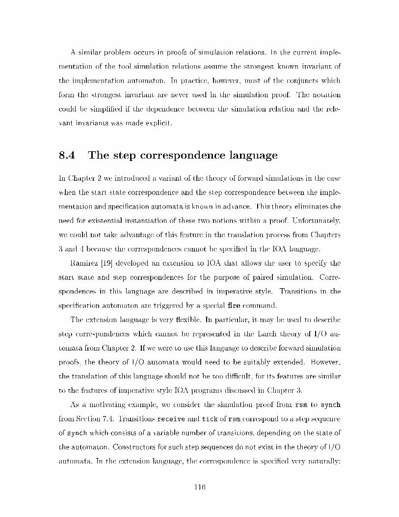
A similar problem occurs in proofs of simulation relations. In the current imple-
mentation of the tool simulation relations assume the strongest known invariant of
the implementation automaton. In practice, however, most of the conjuncts which
form the strongest invariant are never used in the simulation proof. The notation
could be simpli�ed if the dependence between the simulation relation and the rele-
vant invariants was made explicit.
8.4 The step correspondence language
In Chapter 2 we introduced a variant of the theory of forward simulations in the case
when the start state correspondence and the step correspondence between the imple-
mentation and speci�cation automata is known in advance. This theory eliminates the
need for existential instantiation of these two notions within a proof. Unfortunately,
we could not take advantage of this feature in the translation process from Chapters
3 and 4 because the correspondences cannot be speci�ed in the IOA language.
Ramirez [19] developed an extension to IOA that allows the user to specify the
start state and step correspondences for the purpose of paired simulation. Corre-
spondences in this language are described in imperative style. Transitions in the
speci�cation automaton are triggered by a special �re command.
The extension language is very exible. In particular, it may be used to describe
step correspondences which cannot be represented in the Larch theory of I/O au-
tomata from Chapter 2. If we were to use this language to describe forward simulation
proofs, the theory of I/O automata would need to be suitably extended. However,
the translation of this language should not be too diÆcult, for its features are similar
to the features of imperative style IOA programs discussed in Chapter 3.
As a motivating example, we consider the simulation proof from rsm to synch
from Section 7.4. Transitions receive and tick of rsm correspond to a step sequence
of synch which consists of a variable number of transitions, depending on the state of
the automaton. Constructors for such step sequences do not exist in the theory of I/O
automata. In the extension language, the correspondence is speci�ed very naturally:
116
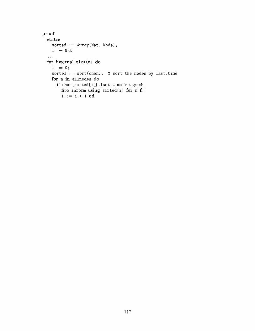
proof
states
sorted := Array[Nat, Node],
i := Nat
: : :
for internal tick(n) do
i := 0;
sorted := sort(chan); % sort the nodes by last.time
for n in allnodes do
if chan[sorted[i]].last.time > tsynch
�re inform using sorted[i] for n �;
i := i + 1 od
117

118
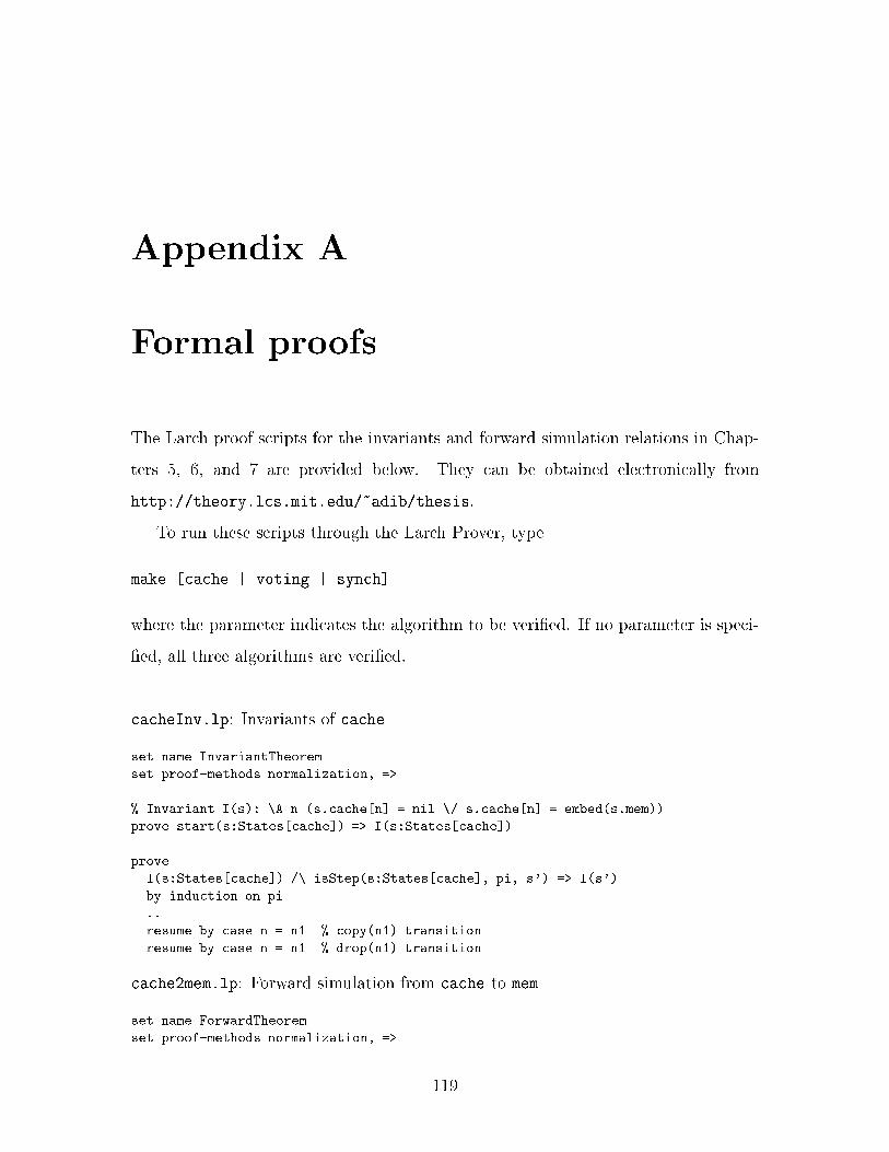
Appendix A
Formal proofs
The Larch proof scripts for the invariants and forward simulation relations in Chap-
ters 5, 6, and 7 are provided below. They can be obtained electronically from
http://theory.lcs.mit.edu/~adib/thesis.
To run these scripts through the Larch Prover, type
make [cache | voting | synch]
where the parameter indicates the algorithm to be veri�ed. If no parameter is speci-
�ed, all three algorithms are veri�ed.
cacheInv.lp: Invariants of cache
set name InvariantTheorem
set proof-methods normalization, =>
% Invariant I(s): \A n (s.cache[n] = nil \/ s.cache[n] = embed(s.mem))
prove start(s:States[cache]) => I(s:States[cache])
prove
I(s:States[cache]) /\ isStep(s:States[cache], pi, s') => I(s')
by induction on pi
..
resume by case n = n1 % copy(n1) transition
resume by case n = n1 % drop(n1) transition
cache2mem.lp: Forward simulation from cache to mem
set name ForwardTheorem
set proof-methods normalization, =>
119
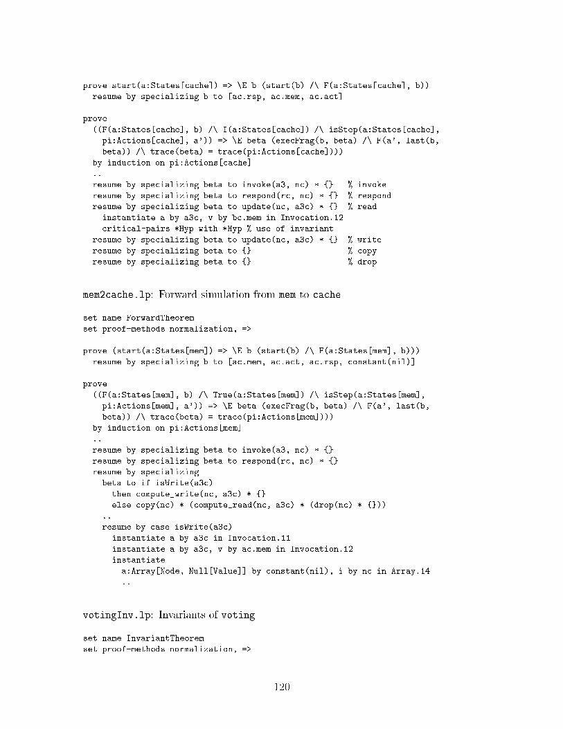
prove start(a:States[cache]) => \E b (start(b) /\ F(a:States[cache], b))
resume by specializing b to [ac.rsp, ac.mem, ac.act]
prove
((F(a:States[cache], b) /\ I(a:States[cache]) /\ isStep(a:States[cache],
pi:Actions[cache], a')) => \E beta (execFrag(b, beta) /\ F(a', last(b,
beta)) /\ trace(beta) = trace(pi:Actions[cache])))
by induction on pi:Actions[cache]
..
resume by specializing beta to invoke(a3, nc) * {} % invoke
resume by specializing beta to respond(rc, nc) * {} % respond
resume by specializing beta to update(nc, a3c) * {} % read
instantiate a by a3c, v by bc.mem in Invocation.12
critical-pairs *Hyp with *Hyp % use of invariant
resume by specializing beta to update(nc, a3c) * {} % write
resume by specializing beta to {} % copy
resume by specializing beta to {} % drop
mem2cache.lp: Forward simulation from mem to cache
set name ForwardTheorem
set proof-methods normalization, =>
prove (start(a:States[mem]) => \E b (start(b) /\ F(a:States[mem], b)))
resume by specializing b to [ac.mem, ac.act, ac.rsp, constant(nil)]
prove
((F(a:States[mem], b) /\ True(a:States[mem]) /\ isStep(a:States[mem],
pi:Actions[mem], a')) => \E beta (execFrag(b, beta) /\ F(a', last(b,
beta)) /\ trace(beta) = trace(pi:Actions[mem])))
by induction on pi:Actions[mem]
..
resume by specializing beta to invoke(a3, nc) * {}
resume by specializing beta to respond(rc, nc) * {}
resume by specializing
beta to if isWrite(a3c)
then compute_write(nc, a3c) * {}
else copy(nc) * (compute_read(nc, a3c) * (drop(nc) * {}))
..
resume by case isWrite(a3c)
instantiate a by a3c in Invocation.11
instantiate a by a3c, v by ac.mem in Invocation.12
instantiate
a:Array[Node, Null[Value]] by constant(nil), i by nc in Array.14
..
votingInv.lp: Invariants of voting
set name InvariantTheorem
set proof-methods normalization, =>
120
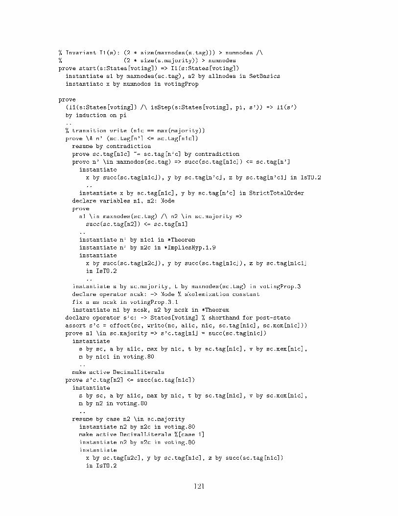
% Invariant I1(s): (2 * size(maxnodes(s.tag))) > numnodes /\
% (2 * size(s.majority)) > numnodes
prove start(s:States[voting]) => I1(s:States[voting])
instantiate s1 by maxnodes(sc.tag), s2 by allnodes in SetBasics
instantiate x by numnodes in votingProp
prove
(I1(s:States[voting]) /\ isStep(s:States[voting], pi, s')) => I1(s')
by induction on pi
..
% transition write (n1c == max(majority))
prove \A n' (sc.tag[n'] <= sc.tag[n1c])
resume by contradiction
prove sc.tag[n1c] ~= sc.tag[n'c] by contradiction
prove n' \in maxnodes(sc.tag) => succ(sc.tag[n1c]) <= sc.tag[n']
instantiate
x by succ(sc.tag[n1c]), y by sc.tag[n'c], z by sc.tag[n'c1] in IsTO.2
..
instantiate x by sc.tag[n1c], y by sc.tag[n'c] in StrictTotalOrder
declare variables n1, n2: Node
prove
n1 \in maxnodes(sc.tag) /\ n2 \in sc.majority =>
succ(sc.tag[n2]) <= sc.tag[n1]
..
instantiate n' by n1c1 in *Theorem
instantiate n' by n2c in *ImpliesHyp.1.9
instantiate
x by succ(sc.tag[n2c]), y by succ(sc.tag[n1c]), z by sc.tag[n1c1]
in IsTO.2
..
instantiate s by sc.majority, t by maxnodes(sc.tag) in votingProp.3
declare operator ncsk: -> Node % skolemization constant
fix n as ncsk in votingProp.3.1
instantiate n1 by ncsk, n2 by ncsk in *Theorem
declare operator s'c: -> States[voting] % shorthand for post-state
assert s'c = effect(sc, write(nc, a11c, n1c, sc.tag[n1c], sc.mem[n1c]))
prove n1 \in sc.majority => s'c.tag[n1] = succ(sc.tag[n1c])
instantiate
s by sc, a by a11c, max by n1c, t by sc.tag[n1c], v by sc.mem[n1c],
m by n1c1 in voting.80
..
make active DecimalLiterals
prove s'c.tag[n2] <= succ(sc.tag[n1c])
instantiate
s by sc, a by a11c, max by n1c, t by sc.tag[n1c], v by sc.mem[n1c],
m by n2 in voting.80
..
resume by case n2 \in sc.majority
instantiate n2 by n2c in voting.80
make active DecimalLiterals %[case 1]
instantiate n2 by n2c in voting.80
instantiate
x by sc.tag[n2c], y by sc.tag[n1c], z by succ(sc.tag[n1c])
in IsTO.2
121
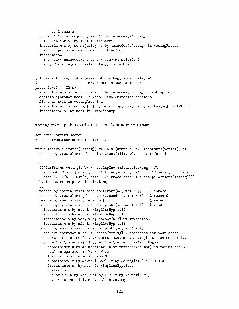
.. %[case 2]
prove n1 \in sc.majority => n1 \in maxnodes(s'c.tag)
instantiate n1 by n1c1 in *Theorem
instantiate s by sc.majority, t by maxnodes(s'c.tag) in votingProp.4
critical-pairs votingProp with votingProp
instantiate
x by succ(numnodes), y by 2 * size(sc.majority),
z by 2 * size(maxnodes(s'c.tag)) in IsTO.2
..
% Invariant I2(s): \A n (maximum(n, s.tag, s.majority) =>
% maximum(n, s.tag, allnodes))
prove I1(s) => I2(s)
instantiate s by sc.majority, t by maxnodes(sc.tag) in votingProp.3
declare operator ncsk: -> Node % skolemization constant
fix n as ncsk in votingProp.3.1
instantiate x by sc.tag[n'], y by sc.tag[ncsk], z by sc.tag[nc] in IsTO.2
instantiate n' by ncsk in *ImpliesHyp
voting2mem.lp: Forward simulation from voting to mem
set name ForwardTheorem
set proof-methods normalization, =>
prove (start(a:States[voting]) => \E b (start(b) /\ F(a:States[voting], b)))
resume by specializing b to [constant(nil), v0, constant(nil)]
prove
((F(a:States[voting], b) /\ votingInv(a:States[voting]) /\
isStep(a:States[voting], pi:Actions[voting], a')) => \E beta (execFrag(b,
beta) /\ F(a', last(b, beta)) /\ trace(beta) = trace(pi:Actions[voting])))
by induction on pi:Actions[voting]
..
resume by specializing beta to invoke(a3, nc) * {} % invoke
resume by specializing beta to respond(rc, nc) * {} % respond
resume by specializing beta to {} % select
resume by specializing beta to update(nc, a3c) * {} % read
instantiate n by n1c in *ImpliesHyp.1.12
instantiate n by n1c in *ImpliesHyp.1.13
instantiate a by a3c, v by ac.mem[n1c] in Invocation
instantiate n by n2c in *ImpliesHyp.1.13
resume by specializing beta to update(nc, a3c) * {}
declare operator a'c: -> States[voting] % shorthand for post-state
assert a'c = effect(ac, write(nc, a3c, n1c, ac.tag[n1c], ac.mem[n1c]))
prove ~(n \in ac.majority) => ~(n \in maxnodes(a'c.tag))
instantiate s by ac.majority, t by maxnodes(ac.tag) in votingProp.3
declare operator ncsk: -> Node
fix n as ncsk in votingProp.3.1
instantiate x by ac.tag[ncsk], y by ac.tag[n1c] in IsTO.3
instantiate n' by ncsk in *ImpliesHyp.1.11
instantiate
s by ac, a by a3c, max by n1c, t by ac.tag[n1c],
v by ac.mem[n1c], m by nc1 in voting.159
122
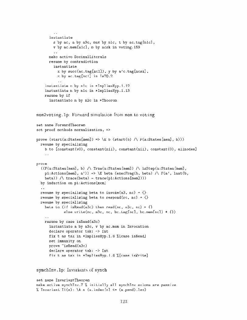
..
instantiate
s by ac, a by a3c, max by n1c, t by ac.tag[n1c],
v by ac.mem[n1c], m by ncsk in voting.159
..
make active DecimalLiterals
resume by contradiction
instantiate
x by succ(ac.tag[nc1]), y by a'c.tag[ncsk],
z by ac.tag[nc1] in IsTO.2
..
instantiate n by n1c in *ImpliesHyp.1.12
instantiate n by n1c in *ImpliesHyp.1.13
resume by if
instantiate n by n2c in *Theorem
mem2voting.lp: Forward simulation from mem to voting
set name ForwardTheorem
set proof-methods normalization, =>
prove (start(a:States[mem]) => \E b (start(b) /\ F(a:States[mem], b)))
resume by specializing
b to [constant(v0), constant(nil), constant(nil), constant(0), allnodes]
..
prove
((F(a:States[mem], b) /\ True(a:States[mem]) /\ isStep(a:States[mem],
pi:Actions[mem], a')) => \E beta (execFrag(b, beta) /\ F(a', last(b,
beta)) /\ trace(beta) = trace(pi:Actions[mem])))
by induction on pi:Actions[mem]
..
resume by specializing beta to invoke(a3, nc) * {}
resume by specializing beta to respond(rc, nc) * {}
resume by specializing
beta to (if isRead(a3c) then read(nc, a3c, nc) * {}
else write(nc, a3c, nc, bc.tag[nc], bc.mem[nc]) * {})
..
resume by case isRead(a3c)
instantiate a by a3c, v by ac.mem in Invocation
declare operator tsk: -> Int
fix t as tsk in *ImpliesHyp.1.6 %[case isRead]
set immunity on
prove ~isRead(a3c)
declare operator tsk: -> Int
fix t as tsk in *ImpliesHyp.1.6 %[case isWrite]
synchInv.lp: Invariants of synch
set name InvariantTheorem
make active synchInv.7 % initially all synchInv axioms are passive
% Invariant I1(s): \A n (s.index[n] <= (s.pend).len)
123
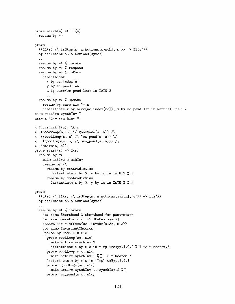
prove start(s) => I1(s)
resume by =>
prove
((I1(s) /\ isStep(s, a:Actions[synch], s')) => I1(s'))
by induction on a:Actions[synch]
..
resume by => % invoke
resume by => % respond
resume by => % inform
instantiate
x by sc.index[n],
y by sc.pend.len,
z by succ(sc.pend.len) in IsTO.2
..
resume by => % update
resume by case n1c ~= n
instantiate x by succ(sc.index[nc]), y by sc.pend.len in NaturalOrder.3
make passive synchInv.7
make active synchInv.8
% Invariant I(s): \A n
% (bookkeep(s, n) \/ goodtogo(s, n)) /\
% ((bookkeep(s, n) /\ ~ex_pend(s, n)) \/
% (goodtogo(s, n) /\ one_pend(s, n))) /\
% active(s, n));
prove start(s) => I(s)
resume by =>
make active synchInv
resume by /\
resume by contradiction
instantiate x by 0, y by ic in IsTO.3 %[]
resume by contradiction
instantiate x by 0, y by ic in IsTO.3 %[]
prove
((I(s) /\ I1(s) /\ isStep(s, a:Actions[synch], s')) => I(s'))
by induction on a:Actions[synch]
..
resume by => % invoke
set name Shorthand % shorthand for post-state
declare operator s'c: -> States[synch]
assert s'c = effect(sc, invoke(a13c, n1c))
set name InvariantTheorem
resume by case n = n1c
prove bookkeep(sc, n1c)
make active synchInv.2
instantiate n by n1c in *ImpliesHyp.1.9.2 %[] -> *Theorem.6
prove bookkeep(s'c, n1c)
make active synchInv.1 %[] -> *Theorem.7
instantiate n by n1c in *ImpliesHyp.1.9.1
prove ~goodtogo(sc, n1c)
make active synchInv.1, synchInv.2 %[]
prove ~ex_pend(s'c, n1c)
124
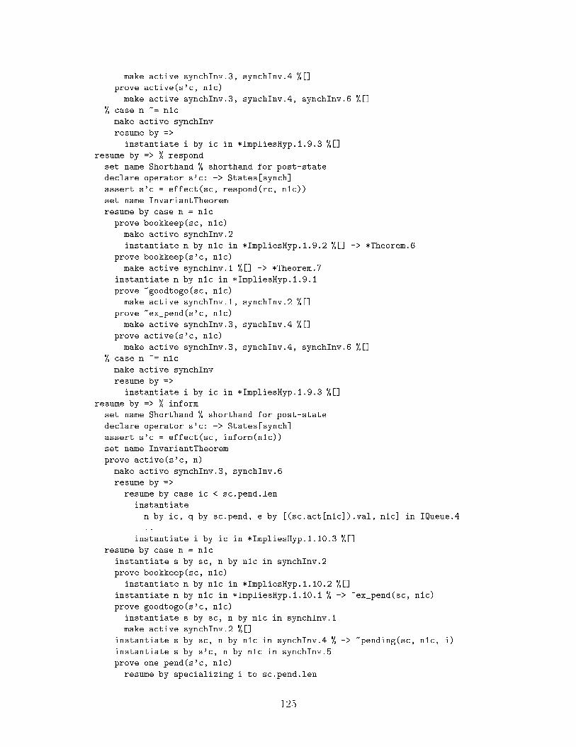
make active synchInv.3, synchInv.4 %[]
prove active(s'c, n1c)
make active synchInv.3, synchInv.4, synchInv.6 %[]
% case n ~= n1c
make active synchInv
resume by =>
instantiate i by ic in *ImpliesHyp.1.9.3 %[]
resume by => % respond
set name Shorthand % shorthand for post-state
declare operator s'c: -> States[synch]
assert s'c = effect(sc, respond(rc, n1c))
set name InvariantTheorem
resume by case n = n1c
prove bookkeep(sc, n1c)
make active synchInv.2
instantiate n by n1c in *ImpliesHyp.1.9.2 %[] -> *Theorem.6
prove bookkeep(s'c, n1c)
make active synchInv.1 %[] -> *Theorem.7
instantiate n by n1c in *ImpliesHyp.1.9.1
prove ~goodtogo(sc, n1c)
make active synchInv.1, synchInv.2 %[]
prove ~ex_pend(s'c, n1c)
make active synchInv.3, synchInv.4 %[]
prove active(s'c, n1c)
make active synchInv.3, synchInv.4, synchInv.6 %[]
% case n ~= n1c
make active synchInv
resume by =>
instantiate i by ic in *ImpliesHyp.1.9.3 %[]
resume by => % inform
set name Shorthand % shorthand for post-state
declare operator s'c: -> States[synch]
assert s'c = effect(sc, inform(n1c))
set name InvariantTheorem
prove active(s'c, n)
make active synchInv.3, synchInv.6
resume by =>
resume by case ic < sc.pend.len
instantiate
n by ic, q by sc.pend, e by [(sc.act[n1c]).val, n1c] in IQueue.4
..
instantiate i by ic in *ImpliesHyp.1.10.3 %[]
resume by case n = n1c
instantiate s by sc, n by n1c in synchInv.2
prove bookkeep(sc, n1c)
instantiate n by n1c in *ImpliesHyp.1.10.2 %[]
instantiate n by n1c in *ImpliesHyp.1.10.1 % -> ~ex_pend(sc, n1c)
prove goodtogo(s'c, n1c)
instantiate s by sc, n by n1c in synchInv.1
make active synchInv.2 %[]
instantiate s by sc, n by n1c in synchInv.4 % -> ~pending(sc, n1c, i)
instantiate s by s'c, n by n1c in synchInv.5
prove one_pend(s'c, n1c)
resume by specializing i to sc.pend.len
125
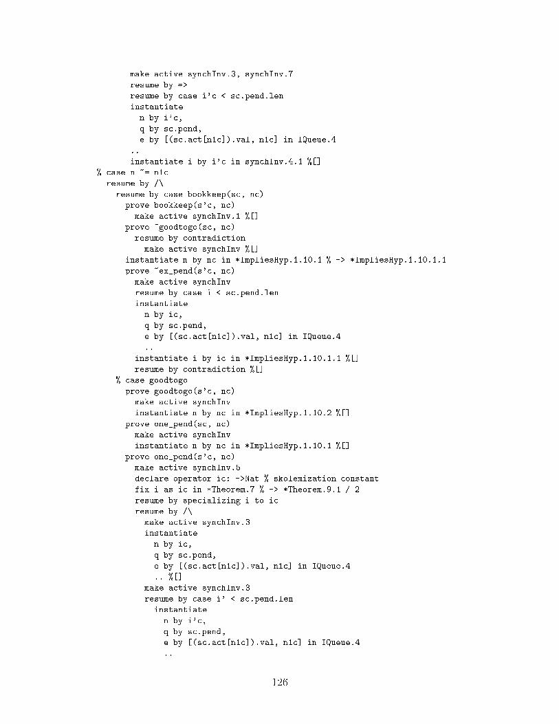
make active synchInv.3, synchInv.7
resume by =>
resume by case i'c < sc.pend.len
instantiate
n by i'c,
q by sc.pend,
e by [(sc.act[n1c]).val, n1c] in IQueue.4
..
instantiate i by i'c in synchInv.4.1 %[]
% case n ~= n1c
resume by /\
resume by case bookkeep(sc, nc)
prove bookkeep(s'c, nc)
make active synchInv.1 %[]
prove ~goodtogo(sc, nc)
resume by contradiction
make active synchInv %[]
instantiate n by nc in *ImpliesHyp.1.10.1 % -> *ImpliesHyp.1.10.1.1
prove ~ex_pend(s'c, nc)
make active synchInv
resume by case i < sc.pend.len
instantiate
n by ic,
q by sc.pend,
e by [(sc.act[n1c]).val, n1c] in IQueue.4
..
instantiate i by ic in *ImpliesHyp.1.10.1.1 %[]
resume by contradiction %[]
% case goodtogo
prove goodtogo(s'c, nc)
make active synchInv
instantiate n by nc in *ImpliesHyp.1.10.2 %[]
prove one_pend(sc, nc)
make active synchInv
instantiate n by nc in *ImpliesHyp.1.10.1 %[]
prove one_pend(s'c, nc)
make active synchInv.5
declare operator ic: ->Nat % skolemization constant
fix i as ic in *Theorem.7 % -> *Theorem.9.1 / 2
resume by specializing i to ic
resume by /\
make active synchInv.3
instantiate
n by ic,
q by sc.pend,
e by [(sc.act[n1c]).val, n1c] in IQueue.4
.. %[]
make active synchInv.3
resume by case i' < sc.pend.len
instantiate
n by i'c,
q by sc.pend,
e by [(sc.act[n1c]).val, n1c] in IQueue.4
..
126
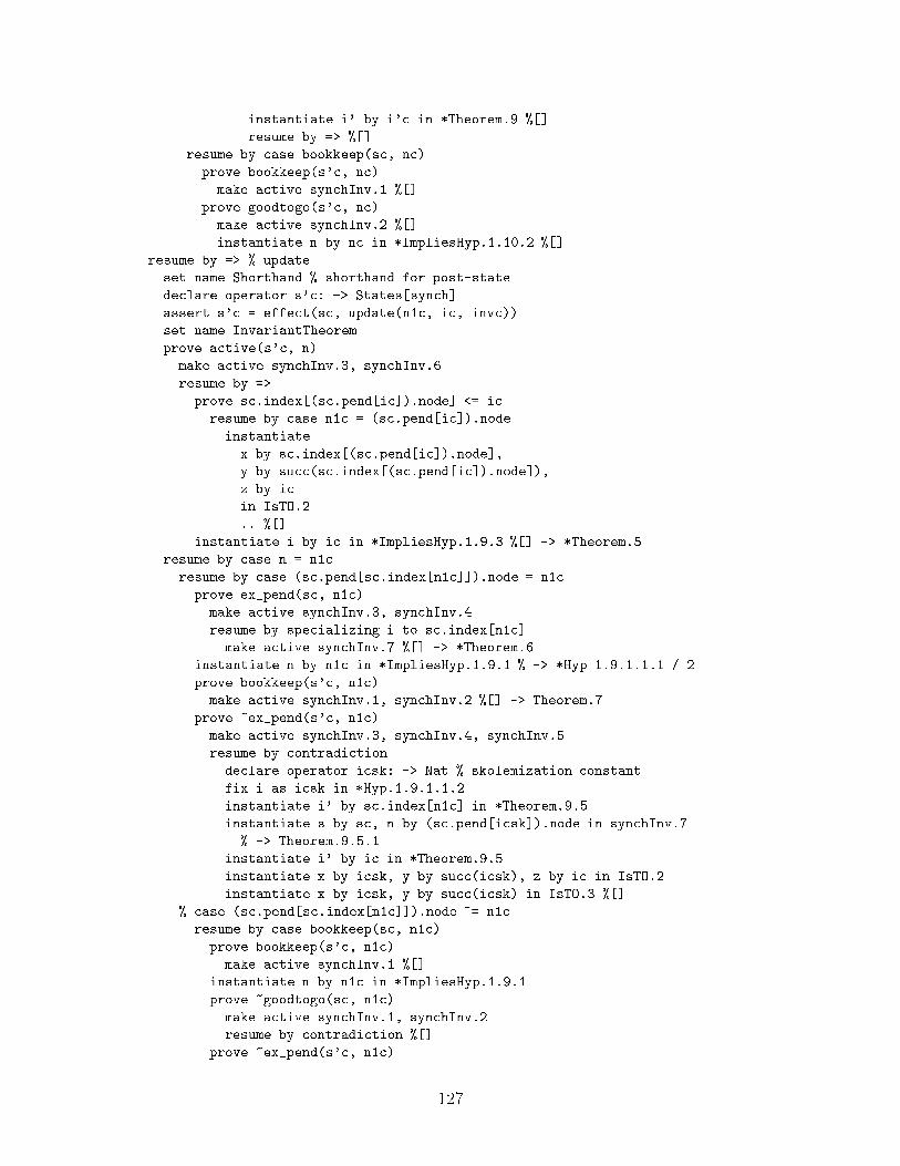
instantiate i' by i'c in *Theorem.9 %[]
resume by => %[]
resume by case bookkeep(sc, nc)
prove bookkeep(s'c, nc)
make active synchInv.1 %[]
prove goodtogo(s'c, nc)
make active synchInv.2 %[]
instantiate n by nc in *ImpliesHyp.1.10.2 %[]
resume by => % update
set name Shorthand % shorthand for post-state
declare operator s'c: -> States[synch]
assert s'c = effect(sc, update(n1c, ic, invc))
set name InvariantTheorem
prove active(s'c, n)
make active synchInv.3, synchInv.6
resume by =>
prove sc.index[(sc.pend[ic]).node] <= ic
resume by case n1c = (sc.pend[ic]).node
instantiate
x by sc.index[(sc.pend[ic]).node],
y by succ(sc.index[(sc.pend[ic]).node]),
z by ic
in IsTO.2
.. %[]
instantiate i by ic in *ImpliesHyp.1.9.3 %[] -> *Theorem.5
resume by case n = n1c
resume by case (sc.pend[sc.index[n1c]]).node = n1c
prove ex_pend(sc, n1c)
make active synchInv.3, synchInv.4
resume by specializing i to sc.index[n1c]
make active synchInv.7 %[] -> *Theorem.6
instantiate n by n1c in *ImpliesHyp.1.9.1 % -> *Hyp 1.9.1.1.1 / 2
prove bookkeep(s'c, n1c)
make active synchInv.1, synchInv.2 %[] -> Theorem.7
prove ~ex_pend(s'c, n1c)
make active synchInv.3, synchInv.4, synchInv.5
resume by contradiction
declare operator icsk: -> Nat % skolemization constant
fix i as icsk in *Hyp.1.9.1.1.2
instantiate i' by sc.index[n1c] in *Theorem.9.5
instantiate s by sc, n by (sc.pend[icsk]).node in synchInv.7
% -> Theorem.9.5.1
instantiate i' by ic in *Theorem.9.5
instantiate x by icsk, y by succ(icsk), z by ic in IsTO.2
instantiate x by icsk, y by succ(icsk) in IsTO.3 %[]
% case (sc.pend[sc.index[n1c]]).node ~= n1c
resume by case bookkeep(sc, n1c)
prove bookkeep(s'c, n1c)
make active synchInv.1 %[]
instantiate n by n1c in *ImpliesHyp.1.9.1
prove ~goodtogo(sc, n1c)
make active synchInv.1, synchInv.2
resume by contradiction %[]
prove ~ex_pend(s'c, n1c)
127
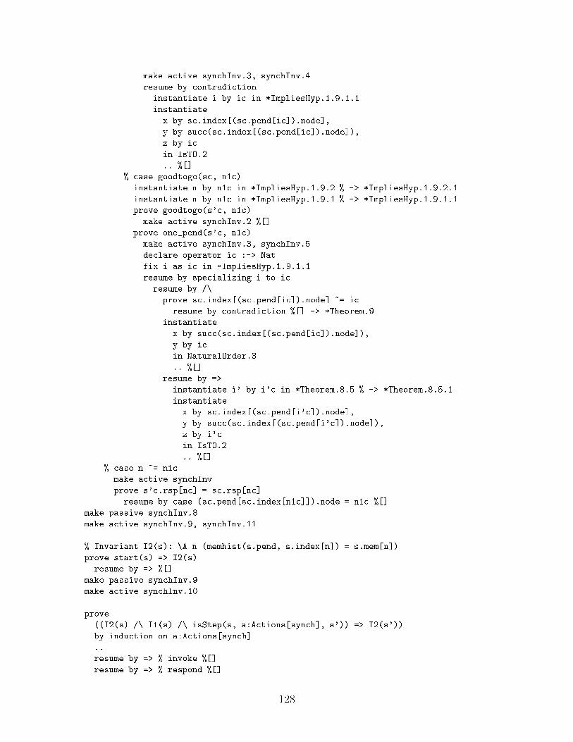
make active synchInv.3, synchInv.4
resume by contradiction
instantiate i by ic in *ImpliesHyp.1.9.1.1
instantiate
x by sc.index[(sc.pend[ic]).node],
y by succ(sc.index[(sc.pend[ic]).node]),
z by ic
in IsTO.2
.. %[]
% case goodtogo(sc, n1c)
instantiate n by n1c in *ImpliesHyp.1.9.2 % -> *ImpliesHyp.1.9.2.1
instantiate n by n1c in *ImpliesHyp.1.9.1 % -> *ImpliesHyp.1.9.1.1
prove goodtogo(s'c, n1c)
make active synchInv.2 %[]
prove one_pend(s'c, n1c)
make active synchInv.3, synchInv.5
declare operator ic :-> Nat
fix i as ic in *ImpliesHyp.1.9.1.1
resume by specializing i to ic
resume by /\
prove sc.index[(sc.pend[ic]).node] ~= ic
resume by contradiction %[] -> *Theorem.9
instantiate
x by succ(sc.index[(sc.pend[ic]).node]),
y by ic
in NaturalOrder.3
.. %[]
resume by =>
instantiate i' by i'c in *Theorem.8.5 % -> *Theorem.8.5.1
instantiate
x by sc.index[(sc.pend[i'c]).node],
y by succ(sc.index[(sc.pend[i'c]).node]),
z by i'c
in IsTO.2
.. %[]
% case n ~= n1c
make active synchInv
prove s'c.rsp[nc] = sc.rsp[nc]
resume by case (sc.pend[sc.index[n1c]]).node = n1c %[]
make passive synchInv.8
make active synchInv.9, synchInv.11
% Invariant I2(s): \A n (memhist(s.pend, s.index[n]) = s.mem[n])
prove start(s) => I2(s)
resume by => %[]
make passive synchInv.9
make active synchInv.10
prove
((I2(s) /\ I1(s) /\ isStep(s, a:Actions[synch], s')) => I2(s'))
by induction on a:Actions[synch]
..
resume by => % invoke %[]
resume by => % respond %[]
128
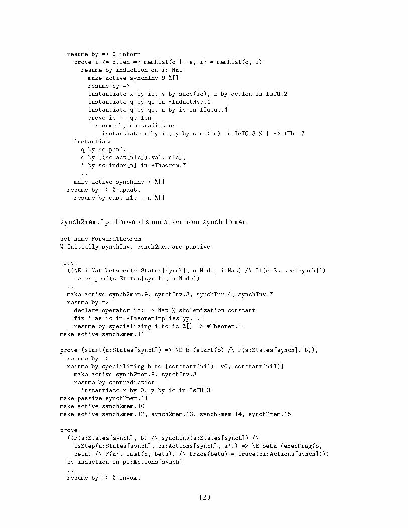
resume by => % inform
prove i <= q.len => memhist(q |- e, i) = memhist(q, i)
resume by induction on i: Nat
make active synchInv.9 %[]
resume by =>
instantiate x by ic, y by succ(ic), z by qc.len in IsTO.2
instantiate q by qc in *InductHyp.1
instantiate q by qc, n by ic in IQueue.4
prove ic ~= qc.len
resume by contradiction
instantiate x by ic, y by succ(ic) in IsTO.3 %[] -> *Thm.7
instantiate
q by sc.pend,
e by [(sc.act[n1c]).val, n1c],
i by sc.index[n] in *Theorem.7
..
make active synchInv.7 %[]
resume by => % update
resume by case n1c = n %[]
synch2mem.lp: Forward simulation from synch to mem
set name ForwardTheorem
% Initially synchInv, synch2mem are passive
prove
((\E i:Nat between(s:States[synch], n:Node, i:Nat) /\ I1(s:States[synch]))
=> ex_pend(s:States[synch], n:Node))
..
make active synch2mem.9, synchInv.3, synchInv.4, synchInv.7
resume by =>
declare operator ic: -> Nat % skolemization constant
fix i as ic in *TheoremImpliesHyp.1.1
resume by specializing i to ic %[] -> *Theorem.1
make active synch2mem.11
prove (start(a:States[synch]) => \E b (start(b) /\ F(a:States[synch], b)))
resume by =>
resume by specializing b to [constant(nil), v0, constant(nil)]
make active synch2mem.9, synchInv.3
resume by contradiction
instantiate x by 0, y by ic in IsTO.3
make passive synch2mem.11
make active synch2mem.10
make active synch2mem.12, synch2mem.13, synch2mem.14, synch2mem.15
prove
((F(a:States[synch], b) /\ synchInv(a:States[synch]) /\
isStep(a:States[synch], pi:Actions[synch], a')) => \E beta (execFrag(b,
beta) /\ F(a', last(b, beta)) /\ trace(beta) = trace(pi:Actions[synch])))
by induction on pi:Actions[synch]
..
resume by => % invoke
129
resume by specializing beta to invoke(a3c, n1c) * {}
set name Shorthand % shorthand for post-state
declare operator a'c: -> States[synch]
assert a'c = effect(ac, invoke(a13c, n1c))
set name ForwardTheorem
make active synch2mem.2, synch2mem.3
resume by /\
resume by =>
prove is_max(ac, nc)
make active synch2mem.6 %[]
instantiate n by nc in *ImpliesHyp.1.11.1 %[]
resume by case n1c = n
instantiate
s by ac, s' by a'c, a:Actions[synch] by invoke(a3c, n1c)
in synchInv.13, synchInv.15
..
make active synchInv.8
make active synchInv.2
instantiate n by n1c in synchInv.15.1.1, *ImpliesHyp.1.3.1
instantiate s by ac, n by n1c in *Theorem.1
instantiate s by a'c, n by n1c in *Theorem.1
instantiate n by nc in *ImpliesHyp.1.11.3 %[]
prove between(ac, nc, i) <=> between(a'c, nc, i)
make active synch2mem.9, synchInv.3, synch2mem.6, synch2mem.7
prove max_index(ac) = max_index(a'c)
declare operator ncsk : -> Node % skolemization constant
instantiate s by ac in synch2mem.8
fix n as ncsk in synch2mem.8.1
instantiate s by a'c, n by ncsk in synch2mem.7 %[]
instantiate n by nc in *ImpliesHyp.1.11.3 %[]
resume by => % respond
resume by specializing beta to respond(rc, n1c) * {}
set name Shorthand % shorthand for post-state
declare operator a'c: -> States[synch]
assert a'c = effect(ac, respond(rc, n1c))
set name ForwardTheorem
make active synch2mem.4, synch2mem.5
make active synchInv.8, synchInv.2
instantiate n by n1c in *ImpliesHyp.1.3.1
instantiate s by ac, n by n1c in *Theorem.1
instantiate n by n1c in *ImpliesHyp.1.11.3
resume by /\
resume by =>
prove is_max(ac, nc)
make active synch2mem.6 %[]
instantiate n by nc in *ImpliesHyp.1.11.1 %[]
resume by case n1c = n
instantiate
s by ac, s' by a'c, a:Actions[synch] by respond(rc, n1c)
in synchInv.13, synchInv.15
..
instantiate n by n1c in synchInv.15.1.1
instantiate s by a'c, n by n1c in *Theorem.1 %[]
prove between(ac, nc, i) <=> between(a'c, nc, i)
130
make active synch2mem.9, synchInv.3, synch2mem.6, synch2mem.7
prove max_index(ac) = max_index(a'c)
declare operator ncsk : -> Node % skolemization constant
instantiate s by ac in synch2mem.8
fix n as ncsk in synch2mem.8.1
instantiate s by a'c, n by ncsk in synch2mem.7 %[]
instantiate n by nc in *ImpliesHyp.1.11.3 %[]
resume by => % case inform
resume by specializing beta to update(n1c, ic, invc) * {}
set name Shorthand % shorthand for post-state
declare operator a'c: -> States[synch]
assert a'c = effect(ac, update(n1c, ic, invc))
set name ForwardTheorem
resume by /\
make active synch2mem.6 %[]
prove max_index(a'c) = max_index(ac)
declare operator ncsk :-> Node % skolemization constant
instantiate s by ac in synch2mem.8
fix n as ncsk in synch2mem.8.1
make active synch2mem.6, synch2mem.7
instantiate s by a'c, n by ncsk in synch2mem.6, synch2mem.7
resume by case \E i between(ac, n, i)
% case \E i between(ac, n, i)
instantiate n by nc in *ImpliesHyp.1.12.3 % -> *Hyp.1.12.3.1
declare operator ic: -> Nat % skolemization constant
fix i as ic in *ImpliesHyp.1.12.3.1 % -> *Theorem.6.*
resume by specializing i to ic
prove between(a'c, nc, ic)
make active synch2mem.9, synchInv.3
instantiate
q by ac.pend, n by ic, e by [(ac.act[n1c]).val, n1c]
in IQueue.4
.. %[] -> *Theorem.6
prove i <= q.len => memhist(q |- e, i) = memhist(q, i)
resume by induction on i: Nat
make active synchInv.9 %[]
resume by =>
instantiate x by ic1, y by succ(ic1), z by qc.len in IsTO.2
instantiate q by qc in *InductHyp.1
instantiate q by qc, n by ic1 in IQueue.4
prove ic1 ~= qc.len
resume by contradiction
instantiate x by ic1, y by succ(ic1) in IsTO.3 %[]
make active synchInv.10 %[] -> *Theorem.7
prove ic <= ac.pend.len
make active synch2mem.9, synchInv.3 %[]
instantiate
i by ic, q by ac.pend, e by [(ac.act[n1c]).val, n1c]
in *Theorem.7
.. %[]
% case ~(\E i between(ac, n, i))
instantiate n by nc in *ImpliesHyp.1.12.3
prove ~between(a'c, nc, i)
make active synch2mem.9, synchInv.3
131
resume by contradiction
instantiate i by ic in *CaseHyp.1.2 % -> *CaseHyp.1.2.1
prove ic ~= ac.pend.len
declare operator ncsk: -> Node % skolemization constant
instantiate s by ac in synch2mem.8
fix n as ncsk in synch2mem.8.1 % -> *Theorem.7
instantiate s by ac, n by ncsk in synch2mem.7
make active synchInv.7
instantiate
x by succ(ic), y by ac.index[ncsk], z by ac.pend.len in IsTO.2
..
instantiate x by succ(ic), y by ac.index[ncsk] in NaturalOrder.4
resume by contradiction
instantiate x by ac.pend.len, y by succ(ac.pend.len) in IsTO.3
%[]
instantiate
q by ac.pend, e by [(ac.act[n1c]).val, n1c], n by ic
in IQueue.4
.. %[]
resume by => % case update
set name Shorthand % shorthand for post-state
declare operator a'c: -> States[synch]
assert a'c = effect(ac, update(n1c, ic, invc))
set name ForwardTheorem
resume by case is_max(ac, n1c)
% case is_max(ac, n1c)
resume by specializing beta to update(invc.node, invc.act) * {}
% verify that mem.update is enabled
prove ex_pend(ac, (ac.pend[ac.index[n1c]]).node)
make active synchInv.4
resume by specializing i to ac.index[n1c]
make active synchInv.3
instantiate s by ac, n by n1c in synch2mem.6
instantiate x by ac.index[n1c], y by ac.pend.len in IsTO.4 %[]
prove ac.rsp[(ac.pend[ac.index[n1c]]).node] = nil
instantiate s by ac in synchInv.8
instantiate n by (ac.pend[ac.index[n1c]]).node in synchInv.8.1.1
make active synchInv.2 %[] -> *Theorem.5
prove ~between(ac, (ac.pend[ac.index[n1c]]).node, i)
instantiate s by ac in synchInv.8
instantiate n by (ac.pend[ac.index[n1c]]).node in synchInv.8.1.1
make active synchInv.5, synchInv.3, synchInv.7
declare operator ic:-> Nat % skolemization constant
fix i as ic in synchInv.8.1.1.1.2 % -> *Theorem.7.*
instantiate s by ac, n by n1c in synch2mem.6
instantiate i' by ac.index[n1c] in *Theorem.7.5 % *Theorem.7.5.1
make active synch2mem.9
resume by contradiction
instantiate i' by ic1 in *Theorem.7.5
instantiate s by ac, n by n1c in synch2mem.7 %[] -> *Theorem.6
resume by /\
prove
enabled(mc, update((ac.pend[ac.index[n1c]]).node,
(ac.pend[ac.index[n1c]]).act))
132
..
instantiate n by (ac.pend[ac.index[n1c]]).node in *ImpliesHyp.1.11.3
make active synchInv.3
instantiate
s by ac, n by (ac.pend[ac.index[n1c]]).node in
synchInv.6, synchInv.8
..
instantiate i by ac.index[n1c] in synchInv.6.1
instantiate s by ac, n by n1c in synch2mem.6
instantiate s by ac, n by n1c in synchInv.7
instantiate
n5 by (ac.act[(ac.pend[ac.index[n1c]]).node]),
n6 by embed((ac.pend[ac.index[n1c]]).act)
in Null.2
.. %[] -> *Theorem.7
resume by /\
prove is_max(a'c, n) => n = n1c
resume by =>
make active synch2mem.6
resume by contradiction
instantiate n' by n1c in *ImpliesHyp.2 % -> *ImpliesHyp.2.1
instantiate
x by succ(ac.index[nc]),
y by succ(ac.index[n1c]),
z by ac.index[nc]
in IsTO.2
..
instantiate x by succ(ac.index[nc]), y by ac.index[nc] in IsTO.3
critical-pairs IsTO with IsTO
critical-pairs *ImpliesHyp.2.1 with IsTO
critical-pairs *Theorem with NaturalOrder %[] -> *Theorem.7
resume by case n = n1c
instantiate n by n1c in *ImpliesHyp.1.11.1 %[]
instantiate n by nc in *Theorem.7 %[]
% rsp consistency
prove is_max(a'c, n1c)
make active synch2mem.6
resume by case n1c = n' %[]
instantiate
x by ac.index[n'c], y by ac.index[n1c],
z by succ(ac.index[n1c]) in IsTO.2
.. %[] -> Theorem.7
resume by case ac.pend[ac.index[n1c]].node = n1c
% case ac.pend[ac.index[n1c]].node = n1c
instantiate n by n1c in *ImpliesHyp.1.11.3 % -> *Hyp.1.11.3.1
resume by case n = n1c
% case n = n1c
prove ~ex_pend(a'c, n1c)
instantiate
s by ac, s' by a'c, a by perform(n1c, ac.index[n1c],
ac.pend[ac.index[n1c]]) in synchInv.15
.. % -> synchInv.15.1
instantiate s by a'c in synchInv.8
instantiate n by n1c in synchInv.8.1.1
133
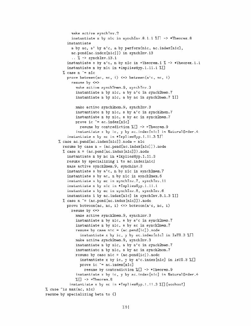
make active synchInv.2
instantiate n by n1c in synchInv.8.1.1 %[] -> *Theorem.8
instantiate
s by ac, s' by a'c, a by perform(n1c, ac.index[n1c],
ac.pend[ac.index[n1c]]) in synchInv.13
.. % -> synchInv.13.1
instantiate s by a'c, n by n1c in *Theorem.1 % -> *Theorem.1.1
instantiate n by n1c in *ImpliesHyp.1.11.1 %[]
% case n ~= n1c
prove between(ac, nc, i) <=> between(a'c, nc, i)
resume by <=>
make active synch2mem.9, synchInv.3
instantiate n by n1c, s by a'c in synch2mem.7
instantiate n by n1c, s by ac in synch2mem.7 %[]
make active synch2mem.9, synchInv.3
instantiate n by n1c, s by a'c in synch2mem.7
instantiate n by n1c, s by ac in synch2mem.7
prove ic ~= ac.index[n1c]
resume by contradiction %[] -> *Theorem.9
instantiate x by ic, y by ac.index[n1c] in NaturalOrder.4
instantiate n by nc in *ImpliesHyp.1.11.3 %[]
% case ac.pend[ac.index[n1c]].node = n1c
resume by case n = (ac.pend[ac.index[n1c]]).node
% case n = (ac.pend[ac.index[n1c]]).node
instantiate n by nc in *ImpliesHyp.1.11.3
resume by specializing i to ac.index[n1c]
make active synch2mem.9, synchInv.3
instantiate s by a'c, n by n1c in synch2mem.7
instantiate s by ac, n by n1c in synch2mem.6
instantiate s by ac in synchInv.7, synchInv.11
instantiate n by n1c in *ImpliesHyp.1.11.1
instantiate s by ac in synchInv.8, synchInv.6
instantiate i by ac.index[n1c] in synchInv.8.1.3 %[]
% case n ~= (ac.pend[ac.index[n1c]]).node
prove between(ac, nc, i) <=> between(a'c, nc, i)
resume by <=>
make active synch2mem.9, synchInv.3
instantiate n by n1c, s by a'c in synch2mem.7
instantiate n by n1c, s by ac in synch2mem.7
resume by case n1c = (ac.pend[ic]).node
instantiate x by ic, y by ac.index[n1c] in IsTO.3 %[]
make active synch2mem.9, synchInv.3
instantiate n by n1c, s by a'c in synch2mem.7
instantiate n by n1c, s by ac in synch2mem.7
resume by case n1c = (ac.pend[ic]).node
instantiate x by ic, y by a'c.index[n1c] in IsTO.3 %[]
prove ic ~= ac.index[n1c]
resume by contradiction %[] -> *Theorem.9
instantiate x by ic, y by ac.index[n1c] in NaturalOrder.4
%[] -> *Theorem.8
instantiate n by nc in *ImpliesHyp.1.11.3 %[][woohoo!]
% case ~is_max(ac, n1c)
resume by specializing beta to {}
134
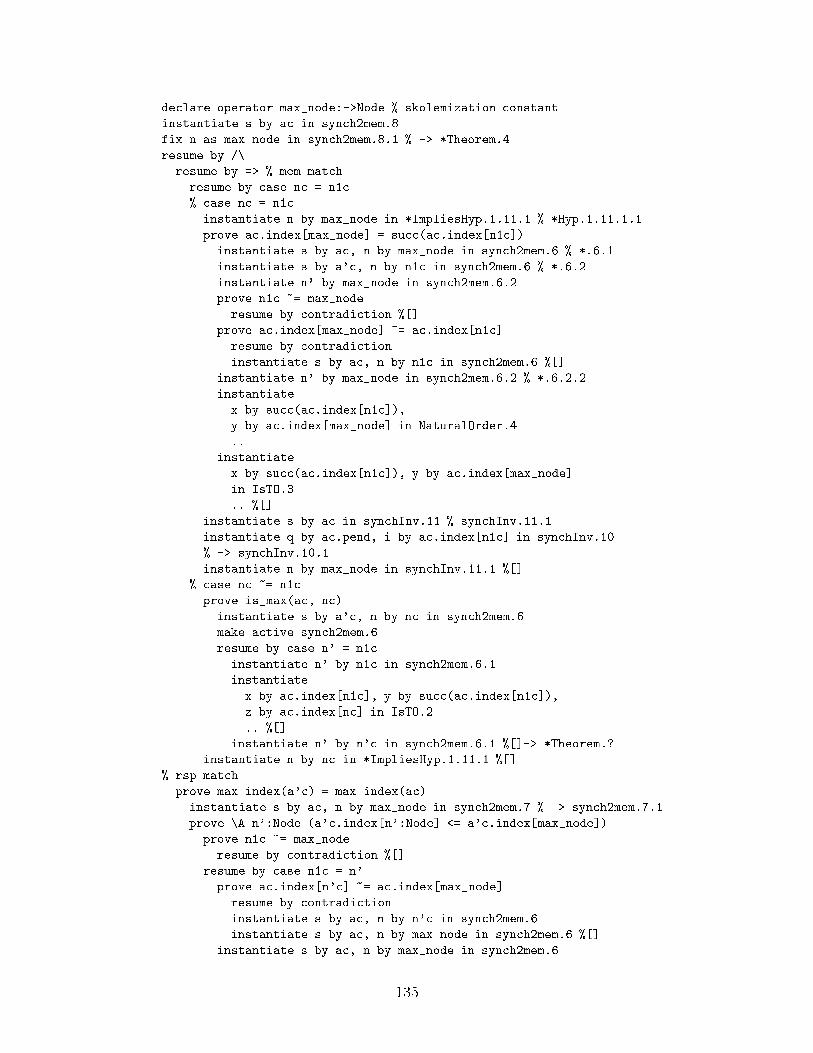
declare operator max_node:->Node % skolemization constant
instantiate s by ac in synch2mem.8
fix n as max_node in synch2mem.8.1 % -> *Theorem.4
resume by /\
resume by => % mem match
resume by case nc = n1c
% case nc = n1c
instantiate n by max_node in *ImpliesHyp.1.11.1 % *Hyp.1.11.1.1
prove ac.index[max_node] = succ(ac.index[n1c])
instantiate s by ac, n by max_node in synch2mem.6 % *.6.1
instantiate s by a'c, n by n1c in synch2mem.6 % *.6.2
instantiate n' by max_node in synch2mem.6.2
prove n1c ~= max_node
resume by contradiction %[]
prove ac.index[max_node] ~= ac.index[n1c]
resume by contradiction
instantiate s by ac, n by n1c in synch2mem.6 %[]
instantiate n' by max_node in synch2mem.6.2 % *.6.2.2
instantiate
x by succ(ac.index[n1c]),
y by ac.index[max_node] in NaturalOrder.4
..
instantiate
x by succ(ac.index[n1c]), y by ac.index[max_node]
in IsTO.3
.. %[]
instantiate s by ac in synchInv.11 % synchInv.11.1
instantiate q by ac.pend, i by ac.index[n1c] in synchInv.10
% -> synchInv.10.1
instantiate n by max_node in synchInv.11.1 %[]
% case nc ~= n1c
prove is_max(ac, nc)
instantiate s by a'c, n by nc in synch2mem.6
make active synch2mem.6
resume by case n' = n1c
instantiate n' by n1c in synch2mem.6.1
instantiate
x by ac.index[n1c], y by succ(ac.index[n1c]),
z by ac.index[nc] in IsTO.2
.. %[]
instantiate n' by n'c in synch2mem.6.1 %[]-> *Theorem.?
instantiate n by nc in *ImpliesHyp.1.11.1 %[]
% rsp match
prove max_index(a'c) = max_index(ac)
instantiate s by ac, n by max_node in synch2mem.7 % -> synch2mem.7.1
prove \A n':Node (a'c.index[n':Node] <= a'c.index[max_node])
prove n1c ~= max_node
resume by contradiction %[]
resume by case n1c = n'
prove ac.index[n'c] ~= ac.index[max_node]
resume by contradiction
instantiate s by ac, n by n'c in synch2mem.6
instantiate s by ac, n by max_node in synch2mem.6 %[]
instantiate s by ac, n by max_node in synch2mem.6
135
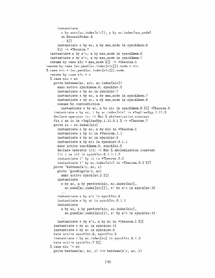
instantiate
x by succ(ac.index[n'c]), y by ac.index[max_node]
in NaturalOrder.4
.. %[]
instantiate s by ac, n by max_node in synch2mem.6
%[] -> *Theorem.?
instantiate s by a'c, n by max_node in synch2mem.6
instantiate s by a'c, n by max_node in synch2mem.7
resume by case n1c = max_node %[] -> *Theorem.5
resume by case (ac.pend[ac.index[n1c]]).node = n1c
% case n1c = (ac.pend[ac.index[n1c]]).node
resume by case n1c = n
% case n1c = nc
prove between(ac, n1c, ac.index[n1c])
make active synch2mem.9, synchInv.3
instantiate s by ac in synchInv.7
instantiate s by ac, n by max_node in synch2mem.7
instantiate s by ac, n by max_node in synch2mem.6
resume by contradiction
instantiate s by ac, n by n1c in synch2mem.6 %[] *Theorem.6
instantiate n by nc, i by ac.index[n1c] in *ImpliesHyp.1.11.3
declare operator ic: -> Nat % skolemization constant
fix i as ic in *ImpliesHyp.1.11.3.1 % -> *Theorem.7
prove ic = ac.index[n1c]
instantiate s by ac, n by n1c in *Theorem.1
instantiate i by ic in *Theorem.1.1
instantiate s by ac in synchInv.8
instantiate n by n1c in synchInv.8.1.1
make active synch2mem.9, synchInv.5
declare operator ic1: -> Nat % skolemization constant
fix i as ic1 in synchInv.8.1.1.1.2
instantiate i' by ic in *Theorem.9.2
instantiate i' by ac.index[n1c] in *Theorem.9.2 %[]
prove ~between(a'c, nc, i)
prove ~goodtogo(a'c, nc)
make active synchInv.2 %[]
instantiate
s by ac, a by perform(n1c, ac.index[n1c],
ac.pend[ac.index[n1c]]), s' by a'c in synchInv.15
..
instantiate s by a'c in synchInv.8
instantiate n by nc in synchInv.8.1.1
instantiate
s by ac, a by perform(n1c, ac.index[n1c],
ac.pend[ac.index[n1c]]), s' by a'c in synchInv.13
..
instantiate s by a'c, n by nc in *Theorem.1 %[]
instantiate s by ac in synchInv.11
instantiate s by ac in synchInv.8
make active synchInv.6, synchInv.3
instantiate i by ac.index[nc] in synchInv.8.1.3
make active synchInv.7 %[]
% case n1c ~= nc
prove between(ac, nc, i) <=> between(a'c, nc, i)
136
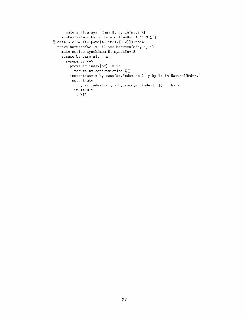
make active synch2mem.9, synchInv.3 %[]
instantiate n by nc in *ImpliesHyp.1.11.3 %[]
% case n1c ~= (ac.pend[ac.index[n1c]]).node
prove between(ac, n, i) <=> between(a'c, n, i)
make active synch2mem.9, synchInv.3
resume by case n1c = n
resume by <=>
prove ac.index[nc] ~= ic
resume by contradiction %[]
instantiate x by succ(ac.index[nc]), y by ic in NaturalOrder.4
instantiate
x by ac.index[nc], y by succ(ac.index[nc]), z by ic
in IsTO.2
.. %[]
137

138
Bibliography
[1] Bowen Alpern and Fred B. Schneider. De�ning liveness. Information Processing
Letters, 21(4):181{185, October 1985.
[2] Nikolaj Bj�rner, Anca Browne, Michael Colon, Bernd Finkbeiner, Zohar Manna,
Henny Sipma, and Tomas Uribe. Verifying temporal properties of reactive sys-
tems: A STeP tutorial. In Formal Methods in System Design. Kluwer Academic
Publishers, 1999.
[3] Andrej Bogdanov, Laura Dean, Christine Karlovich, and Ezra Rosen. Distributed
memory algorithms coded in IOA: Challenge problems for software analysis and
synthesis methods. Technical Note, January 2001.
[4] Andrej Bogdanov, Joshua Tauber, and Dimitris Vyzovitis. Formal veri�cation
of a replicated data management algorithm, May 2001. 6.897 Class Project.
[5] Edmund M. Clarke, Orna Grumberg, Hiromi Hirashi, Somesh Jha, David E.
Long, Kenneth L. McMillan, and Linda A. Ness. Veri�cation of the Futurebus+
cache coherence protocol. In L. Claesen, editor, Proceedings of the 11th Inter-
national Symposium on Computer Hardware Description Languages and their
Applications, North Holland, 1993.
[6] Edmund M. Clarke, Orna Grumberg, and Doron A. Peled. Model Checking. The
MIT Press, 1999.
[7] Marco Devillers. Mechanized support of I/O automata. Technical Report CSI-
N710, Computing Science Institute, University of Nijmengen, 1997.
139
[8] Stephen J. Garland and John V. Guttag. A guide to LP, the larch prover.
Technical report, DEC Systems Research Center, 1991. Updated version available
as http://nms.lcs.mit.edu/Larch/LP.
[9] Stephen J. Garland and Nancy A. Lynch. Using I/O automata for developing
distributed systems. In Gary T. Leavens and Murali Sitaraman, editors, Founda-
tions of Component-Based Systems, pages 285{312. Cambridge University Press,
2000.
[10] Stephen J. Garland, Nancy A. Lynch, and Mandana Vaziri. IOA: a language for
specifyng, programming, and validating distributed systems. MIT Laboratory for
Computer Science, 1997 (revised January, 2001).
[11] Leslie A. Lamport. Time, clocks and the ordering of events in a distributed
system. Communications of the ACM, 21(7):558{565, July 1978.
[12] Leslie A. Lamport. How to write a proof, 1993.
[13] Leslie A. Lamport. Specifying concurrent systems with TLA+. Preliminary
draft, December 2000.
[14] Nancy A. Lynch. Distributed Algorithms. Morgan Kaufman Pubishers Inc., 1996.
[15] Nancy A. Lynch and Mark Tuttle. Hierarchical correctness proofs for distributed
algorithms. Technical Report MIT/LCS/TR-387, MIT Laboratory for Computer
Science, 1987.
[16] Nancy A. Lynch and Frits Vaandrager. Forward and backward simulations { part
I: Untimed systems. Information and Computation, 121(2):214{233, September
1995.
[17] Olaf M�uller. A Veri�cation Environment for I/O Automata Based on Formalized
Meta-Theory. PhD thesis, Technische Universit�at M�unchen, 1998.
140
[18] Amir Pnueli. The temporal logic of programs. In Proceedings of the 18th annual
symposium on Foundations of Computer Science, pages 46{57. IEEE, October-
November 1977.
[19] J. Antonio Ramirez-Robredo. Paired simulation of I/O automata. Master of
engineering thesis, MIT, 2000.
[20] J�rgen F. S�gaard-Andersen, Stephen J. Garland, John V. Guttag, Nancy A.
Lynch, and Anna Pogosyants. Computer-assisted simulation proofs. In
Computer-Aided Veri�cation, volume 697 of Lecture Notes in Computer Science,
Elounda, Greece, June-July 1993. Fifth International Conference, CAV'93.
141