flight path control during hypersonic atmospheric entry
TRANSCRIPT
Flight Path Control During Hypersonic Atmospheric Entry Using Active Magnetic
Arrays
by
Matthew Tyler Austin
A thesis submitted to the College of Engineering and Science of
Florida Institute of Technology
in partial fulfillment of the requirements
for the degree of
Master of Science
in
Aerospace Engineering
Melbourne, Florida
May 2020
We the undersigned committee hereby approve the attached thesis, “Flight Path
Control During Hypersonic Atmospheric Entry Using Active Magnetic Arrays,” by
Matthew Tyler Austin.
_________________________________________________
Markus Wilde, Ph.D.
Assistant Professor
Aerospace, Physics and Space Sciences
_________________________________________________
Brian Kish, Ph.D.
Assistant Professor
Aerospace, Physics and Space Sciences
_________________________________________________
Andrew Aldrin, Ph.D.
Associate Professor, Director
Aldrin Space Institute
_________________________________________________
Daniel Batcheldor, Ph.D.
Professor and Department Head
Aerospace, Physics and Space Sciences
iii
Abstract
Title: Flight Path Control During Hypersonic Atmospheric Entry Using Active Magnetic
Arrays
Author: Matthew Tyler Austin
Advisor: Markus Wilde, Ph.D.
The purpose of this thesis is to study the reaction to the Lorentz force induced during the
hypersonic regime of flight by an active magnetic field. The effect that a magnetic array
has on the flight characteristics of a blunt body during Earth atmospheric entry is
characterized and isolated for independent analysis. This is done to show that mission-
specific benefits to utilizing this method of entry control exist and therefore warrant further
study. To conduct this analysis, a 1000 kg blunt body test case was used. This craft
contains three separate magnets located behind the nose with two of them offset by 45° to
provide the possibility of varying the magnetic flux density in each magnet. The craft’s
initial altitude, velocity, and flight path angle were 120 km, 6.5 km/s, and -0.5°
respectively. MATLAB was used to study the atmospheric entry and a Simulink model
was developed to simulate the lift and drag forces produced by the reaction to the Lorentz
force. The angle of attack was varied from 0 - 25° and the initial magnetic flux density was
varied from 0.1 – 1 T. The resulting flight characteristics were compared to those with no
applied magnetic field to quantify the effects of utilizing this type of entry control. Based
on the results of this study, a magnetic flux density of 1 T does impact the flight
characteristics of a blunt body craft by adding a lift force of 2857 N and a drag force of
240.8 N. The Lorentz lift and drag forces produced and their exact impact on flight
trajectory warrant future study using CFD analysis.
iv
Table of Contents
Table of Contents ................................................................................................ iv
List of Figures ..................................................................................................... vi
List of Tables ........................................................................................................ x
Nomenclature ...................................................................................................... xi
Acknowledgement ............................................................................................. xiii
Dedication.......................................................................................................... xiv
Chapter 1 Introduction ........................................................................................ 1 1.1 Scope of Thesis ...................................................................................................... 4
Chapter 2 Background ........................................................................................ 6 2.1 Atmosphere ........................................................................................................... 6 2.2 Real Gas Effects .................................................................................................... 9 2.3 Speed of Sound .................................................................................................... 11 2.4 Entry Dynamics................................................................................................... 12 2.5 Blunt Body Entry Vehicles.................................................................................. 19 2.6 Hypersonic Flow ................................................................................................. 21 2.7 Magnetohydrodynamics ..................................................................................... 23
Chapter 3 Model ................................................................................................ 29 3.1 Model Limitations ............................................................................................... 29 3.2 Assumptions ........................................................................................................ 30 3.3 Atmosphere ......................................................................................................... 30 3.4 Atmospheric Descent .......................................................................................... 35 3.5 Entry Vehicle....................................................................................................... 35 3.6 Electrodynamic Force ......................................................................................... 38
Chapter 4 Results and Discussion ..................................................................... 41 4.1 Model Validation ................................................................................................. 41 4.2 Summary of Model Validation ........................................................................... 45 4.3 Study Rationale ................................................................................................... 46 4.4 Lorentz Forces .................................................................................................... 47 4.5 Comparison: B = 0.1 – 1 T .................................................................................. 50 4.6 Comparison: Standard Entry & B = 1 T ............................................................ 56 4.7 Comparison: Min & Max Lorentz Lift & Drag ................................................. 60 4.8 Extended Analysis of Angle of Attack ................................................................ 61
Chapter 5 Conclusion ........................................................................................ 65 5.1 Suggestions for Future Work.............................................................................. 67
References .......................................................................................................... 68
v
Appendix A: Skin Friction ................................................................................. 74
Appendix B: Aerodynamic Heating .................................................................. 75
Appendix C: Simplified Navier-Stokes Equations ............................................ 77
Appendix D: Basic Hypersonic Shock Relations .............................................. 79
Appendix E: Simulink Model ............................................................................ 83
Appendix F: Atmosphere Characteristics ......................................................... 89
Appendix G: Atmosphere Table ........................................................................ 90
Appendix H: Lorentz Lift & Drag Forces ......................................................... 91
Appendix I: Varied Angle of Attack & B-Field Strength ................................. 92 B = 0.1 T .................................................................................................................... 92 B = 0.2 T .................................................................................................................... 94 B = 0.3 T .................................................................................................................... 97 B = 0.4 T .................................................................................................................... 99 B = 0.5 T .................................................................................................................. 102 B = 0.6 T .................................................................................................................. 104 B = 0.7 T .................................................................................................................. 107 B = 0.8 T .................................................................................................................. 109 B = 0.9 T .................................................................................................................. 112 B = 1.0 T .................................................................................................................. 114
Appendix J: Varied B-Field at 0 Angle of Attack ........................................... 117 B = 0.1 T .................................................................................................................. 117 B = 0.2 T .................................................................................................................. 119 B = 0.3 T .................................................................................................................. 121 B = 0.4 T .................................................................................................................. 123 B = 0.5 T .................................................................................................................. 125 B = 0.6 T .................................................................................................................. 127 B = 0.7 T .................................................................................................................. 129 B = 0.8 T .................................................................................................................. 131 B = 0.9 T .................................................................................................................. 133 B = 1.0 T .................................................................................................................. 135
Appendix K: Dynamic Pressure – Heat Rate .................................................. 138
Appendix L: Extended Angle of Attack Analysis ........................................... 139
vi
List of Figures
Figure 1 - Reaction Force of Lorentz Force [9]....................................................... 2
Figure 2 - Blunt Body with Parallel Magnet Configuration [9] ............................... 3 Figure 3 - Blunt Body with Inclined Magnet Configuration [9] .............................. 3
Figure 4 - Atmosphere Profile [26] ......................................................................... 7 Figure 5 - Real Gas Effects [30] ............................................................................. 9
Figure 6 - Planet - fixed and local horizon frames [34] ......................................... 14 Figure 7 - Scaling Factor [35] .............................................................................. 15 Figure 8 - Newtonian Flow Theory [36] ............................................................... 15
Figure 9 - Blunt Body Ballistic Coefficients [37] ................................................. 17 Figure 10 - Ballistic Entry [35]............................................................................. 18
Figure 11 - Lifting Entry [35] ............................................................................... 18 Figure 12 - Mars Entry Capsules [38] ................................................................... 19
Figure 13 - Typical Blunt Body Geometry ........................................................... 20 Figure 14 - Hypersonic Flow Around Blunt Nose Vehicle [41] ............................ 22
Figure 15 - Post shock scalar electrical conductivity - Earth altitude and vehicle
velocity [47] ................................................................................................. 27
Figure 16 - Knudsen Number Range [39] ............................................................. 34 Figure 17 - Blunt Body Entry Craft ...................................................................... 36
Figure 18 - Entry Vehicle Geometry [13] ............................................................. 37 Figure 19 - Entry Vehicle Coordinate System [13] ............................................... 38
Figure 20 - Altitude vs. Velocity Mars Entry Case [16] ........................................ 41 Figure 21 - Altitude vs. Velocity Earth Entry ....................................................... 42
Figure 22 - Mars shock density ratio as a function of altitude and freestream
velocity [16] ................................................................................................. 43
Figure 23 - Altitude vs. Velocity Previous Earth Entry Case [8] ........................... 43 Figure 24 - Altitude vs. Velocity Thesis Test Case ............................................... 44
Figure 25 - Drag During Mars Entry [53] ............................................................. 46 Figure 26 – Lorentz L/D Ratio vs Applied B-Field ............................................... 48
Figure 27 - Lift - Drag Reactions to Lorentz Force at 0 AoA ................................ 49 Figure 28 – Altitude vs Time Combined B-Field .................................................. 51
Figure 29 – Altitude vs Time B = 0.1 T & B = 1 T ............................................... 51 Figure 30 - Mach vs Time Combined B-Field ...................................................... 52
Figure 31 - Mach vs Time B = 0.1 T & B = 1 T.................................................... 53 Figure 32 - Velocity vs Time Combined B-Field .................................................. 54
Figure 33 - Velocity vs Time B = 0.1 T & B = 1 T ............................................... 54 Figure 34 - Acceleration vs Time Combined B-Field ........................................... 55
Figure 35 - Acceleration vs Time B = 0.1 T & B = 1 T ......................................... 56 Figure 36 - Altitude vs Time B = 0 T & B = 1 T................................................... 57
vii
Figure 37 - Mach vs Time B = 0 T & B = 1 T ...................................................... 58 Figure 38 - Velocity vs Time B = 0 T & B = 1 T .................................................. 58
Figure 39 - Acceleration vs Time B = 0 T & B = 1 T ........................................... 59 Figure 40 - Schematic of the Flow Region Behind a Blunt Body in Hypersonic
Flow [69] ..................................................................................................... 79 Figure 41 - Blunt Body Entry Flows [70] ............................................................. 80
Figure 42 - Full Simulink Schematic .................................................................... 83 Figure 43 - Simulink Schematic: Magnetic Field .................................................. 84
Figure 44 - Simulink Schematic: Current Density ................................................ 85 Figure 45 - Simulink Schematic: Cross Products .................................................. 86
Figure 46 - Simulink Schematic: Lorentz Drag..................................................... 87 Figure 47 - Simulink Schematic: Lorentz Lift ...................................................... 88
Figure 48 - Acceleration vs Time B = 0.1 T, Varied AoA..................................... 92 Figure 49 - Altitude vs Time B = 0.1 T, Varied AoA ............................................ 93
Figure 50 - Mach vs Time B = 0.1 T, Varied AoA ............................................... 93 Figure 51 - Velocity vs Time B = 0.1 T, Varied AoA ........................................... 94
Figure 52 - Acceleration vs Time B = 0.2 T, Varied AoA..................................... 95 Figure 53 - Altitude vs Time B = 0.2 T, Varied AoA ............................................ 95
Figure 54 - Mach vs Time B = 0.2 T, Varied AoA ............................................... 96 Figure 55 - Velocity vs Time B = 0.2 T, Varied AoA ........................................... 96
Figure 56 - Acceleration vs Time B = 0.3 T, Varied AoA..................................... 97 Figure 57 - Altitude vs Time B = 0.3 T, Varied AoA ............................................ 98
Figure 58 - Mach vs Time B = 0.3 T, Varied AoA ............................................... 98 Figure 59 - Velocity vs Time B = 0.3 T, Varied AoA ........................................... 99
Figure 60 - Acceleration vs Time B = 0.4 T, Varied AoA................................... 100 Figure 61 - Altitude vs Time B = 0.4 T, Varied AoA .......................................... 100
Figure 62 - Mach vs Time B = 0.4 T, Varied AoA ............................................. 101 Figure 63 - Velocity vs Time B = 0.4 T, Varied AoA ......................................... 101
Figure 64 - Acceleration vs Time B = 0.5 T, Varied AoA................................... 102 Figure 65 - Altitude vs Time B = 0.5 T, Varied AoA .......................................... 103
Figure 66 - Mach vs Time B = 0.5 T, Varied AoA ............................................. 103 Figure 67 - Velocity vs Time B = 0.5 T, Varied AoA ......................................... 104
Figure 68 - Acceleration vs Time B = 0.6 T, Varied AoA................................... 105 Figure 69 - Altitude vs Time B = 0.6 T, Varied AoA .......................................... 105
Figure 70 - Mach vs Time B = 0.6 T, Varied AoA ............................................. 106 Figure 71 - Velocity vs Time B = 0.6 T, Varied AoA ......................................... 106
Figure 72 - Acceleration vs Time B = 0.7 T, Varied AoA................................... 107 Figure 73 - Altitude vs Time B = 0.7 T, Varied AoA .......................................... 108
Figure 74 - Mach vs Time B = 0.7 T, Varied AoA ............................................. 108 Figure 75 - Velocity vs Time B = 0.7 T, Varied AoA ......................................... 109
Figure 76 - Acceleration vs Time B = 0.8 T, Varied AoA................................... 110 Figure 77 - Altitude vs Time B = 0.8 T, Varied AoA .......................................... 110
viii
Figure 78 - Mach vs Time B = 0.8 T, Varied AoA ............................................. 111 Figure 79 - Velocity vs Time B = 0.8 T, Varied AoA ......................................... 111
Figure 80 - Acceleration vs Time B = 0.9 T, Varied AoA................................... 112 Figure 81 - Altitude vs Time B = 0.9 T, Varied AoA .......................................... 113
Figure 82 - Mach vs Time B = 0.9 T, Varied AoA ............................................. 113 Figure 83 - Velocity vs Time B = 0.9 T, Varied AoA ......................................... 114
Figure 84 - Acceleration vs Time B = 1 T, Varied AoA ..................................... 115 Figure 85 - Altitude vs Time B = 1 T, Varied AoA............................................. 115
Figure 86 - Mach vs Time B = 1 T, Varied AoA ................................................ 116 Figure 87 - Velocity vs Time B = 1 T, Varied AoA ............................................ 116
Figure 88 - Altitude vs Time 0.1T T, 0 AoA ...................................................... 117 Figure 89 - Mach vs Time 0.1 T, 0 AoA ............................................................. 118
Figure 90 - Velocity vs Time 0.1 T, 0 AoA ........................................................ 118 Figure 91 - Acceleration vs Time 0.1 T, 0 AoA .................................................. 119
Figure 92 - Altitude vs Time 0.2 T, 0 AoA ......................................................... 119 Figure 93 - Mach vs Time 0.2 T, 0 AoA ............................................................. 120
Figure 94 - Velocity vs Time 0.2 T, 0 AoA ........................................................ 120 Figure 95 - Acceleration vs Time 0.2 T, 0 AoA .................................................. 121
Figure 96 - Altitude vs Time 0.3 T, 0 AoA ......................................................... 121 Figure 97 - Mach vs Time 0.3 T, 0 AoA ............................................................. 122
Figure 98 - Velocity vs Time 0.3 T, 0 AoA ........................................................ 122 Figure 99 - Acceleration vs Time 0.3 T, 0 AoA .................................................. 123
Figure 100 - Altitude vs Time 0.4 T, 0 AoA ....................................................... 123 Figure 101 - Mach vs Time 0.4 T, 0 AoA ........................................................... 124
Figure 102 - Velocity vs Time 0.4 T, 0 AoA ...................................................... 124 Figure 103 - Acceleration vs Time 0.4 T, 0 AoA ................................................ 125
Figure 104 - Altitude vs Time 0.5 T, 0 AoA ....................................................... 125 Figure 105 - Mach vs Time 0.5 T, 0 AoA ........................................................... 126
Figure 106 - Velocity vs Time 0.5 T, 0 AoA ...................................................... 126 Figure 107 - Acceleration vs Time 0.5 T, 0 AoA ................................................ 127
Figure 108 - Altitude vs Time 0.6 T, 0 AoA ....................................................... 127 Figure 109 - Mach vs Time 0.6 T, 0 AoA ........................................................... 128
Figure 110 - Velocity vs Time 0.6 T, 0 AoA ...................................................... 128 Figure 111 - Acceleration vs Time 0.6 T, 0 AoA ................................................ 129
Figure 112 - Altitude vs Time 0.7 T, 0 AoA ....................................................... 129 Figure 113 - Mach vs Time 0.7 T, 0 AoA ........................................................... 130
Figure 114 - Velocity vs Time 0.7 T, 0 AoA ...................................................... 130 Figure 115 - Acceleration vs Time 0.7 T, 0 AoA ................................................ 131
Figure 116 - Altitude vs Time 0.8 T, 0 AoA ....................................................... 131 Figure 117 - Mach vs Time 0.8 T, 0 AoA ........................................................... 132
Figure 118 - Velocity vs Time 0.8 T, 0 AoA ...................................................... 132 Figure 119 - Acceleration vs Time 0.8 T, 0 AoA ................................................ 133
ix
Figure 120 - Altitude vs Time 0.9 T, 0 AoA ....................................................... 133 Figure 121 - Mach vs Time 0.9 T, 0 AoA ........................................................... 134
Figure 122 - Velocity vs Time 0.9 T, 0 AoA ...................................................... 134 Figure 123 - Acceleration vs Time 0.9 T, 0 AoA ................................................ 135
Figure 124 - Altitude vs Time 1 T, 0 AoA .......................................................... 135 Figure 125 - Mach vs Time 1 T, 0 AoA .............................................................. 136
Figure 126 - Velocity vs Time 1 T, 0 AoA ......................................................... 136 Figure 127 - Acceleration vs Time 1 T, 0 AoA ................................................... 137
Figure 128 - Dynamic Pressure vs Time 0 AoA ................................................. 138 Figure 129 - Heat Rate vs Time 0 AoA .............................................................. 138
x
List of Tables
Table 1 - Earth Atmosphere [29] ............................................................................ 8
Table 2 - Chemical Reactions Due to Increasing Temperature .............................. 10 Table 3 - Hypersonic Flow Regimes .................................................................... 21
Table 4 - Hypersonic Flow Characteristics ........................................................... 23 Table 5 - Vehicle Properties ................................................................................. 36
Table 6 - Magnet Properties ................................................................................. 37 Table 7 - Lorentz L/D as B-Field and Angle of Attack Vary................................. 47 Table 8 - Lift and Drag Reactions to Lorentz Force: Zero Angle of Attack ........... 49
Table 9 - B-Field Strength Where Min / Max Lift & Drag Occur ......................... 60 Table 10 - Lift Forces as AoA Varies from 0 - 1° ................................................. 62
Table 11 - Drag Forces as AoA Varies from 0 - 1° ............................................... 63 Table 12 – Lorentz L/D Ratio .............................................................................. 64
Table 13 - B-Field MATLAB Code...................................................................... 84 Table 14 - Current Density MATLAB Code ......................................................... 85
Table 15 - Cross Product MATLAB Code ............................................................ 86 Table 16 - Lorentz Drag MATLAB Code ............................................................. 87
Table 17 - Lorentz Lift MATLAB Code ............................................................... 88 Table 18 - Atmosphere Characteristics and Constants .......................................... 89
Table 19 - Hybrid Standard Atmosphere Table [34] ............................................. 90 Table 20 - Lorentz Lift and Drag Forces from 0-25 AoA...................................... 91
Table 21 - 0.1 - 1° Angle of Attack Lift and Drag Results .................................. 139

xi
Nomenclature
𝐴 Cross-section area
𝑎 Speed of sound
𝛼 Angle of attack
𝐵 Magnetic flux density
𝐵0 Initial magnetic flux density
𝛽 Ballistic coefficient
𝛽𝐻𝑎𝑙𝑙 Hall parameter
𝐶𝐴 Axial force coefficient
𝐶𝐷 Drag coefficient
𝐶𝐿 Lift coefficient
𝐶𝑚 Moment coefficient
𝐶𝑛 Normal force coefficient 𝐶𝑝 Specific heat coefficient (pressure)
𝐶𝑣 Specific heat coefficient (volume) 𝑐𝜂 Molecules’ normal velocity component
𝑐𝑝𝑐 Constant pressure of specific heat
𝐷 Drag
𝛿𝑐 Cone half-angle
𝐸 Total energy
𝑓𝑡 Thrust force component
𝛾 Ratio of specific heats
𝑔 gravity
𝑔0 Force of gravity at Earth surface
ℎ Static enthalpy
𝐻 Total enthalpy
𝐻𝑠 Scale height
𝐽 Electric current density
𝑘𝑇 Thermal conductivity
𝐾𝑛 Knudsen number
𝐿 Lift 𝐿𝑝 Characteristic length - plasma structure
𝐿𝑟𝑒𝑓 Max diameter
𝜆 Mean free path of molecule
𝑀 Mach number
𝑚 Mass
𝑀0 Local Mach number
𝑀∞ Freestream Mach number
𝑚𝑒 Mass of electron

xii
𝑚0 Molecular weight at sea level
𝑛𝑒 Electron number density
𝑝 Pressure
𝑝0 Local pressure
𝑝𝑖 Normal momentum flux – incident Mol
𝑝𝑟 Normal momentum flux – reflected Mol
𝑝𝑤 Pressure acting on body surface
𝑝∞ Freestream pressure
𝑃𝑟 Prandtl number
𝜙 Cone half radius
𝑞0 Pressure forces scaling factor
𝑟 Radius
𝑅 Gas constant
𝜌 Density
𝑅𝑚 Magnetic Reynolds number
𝑅𝑒𝑎 Reynolds number
𝑅𝑏 Nose radius
𝜎 Scalar electrical conductivity 𝜎𝑝 Plasma electrical conductivity
𝜎𝑆 Modified electrical conductivity
𝑆 Sutherland’s temperature
𝑇 Temperature
𝜃𝑏 Local body slope
�̿� Viscous stress tensor
𝑈∞ Freestream velocity 𝑢𝑝 Plasma velocity
𝜇 Dynamic viscosity coefficient
𝜇0 Magnetic permeability of free space
𝑉 Volume
𝑣 Vehicle speed relative to the atmosphere 𝑣𝑒,𝑠
𝑚 Electron collision frequency
𝜔 Angular rate of rotation

xiii
Acknowledgement
The work in this thesis represents an extended effort inspired by Dr. Robert Moses at
NASA Langley Research Center. Through multiple NASA Innovative Advanced Concept
(NIAC) proposals this topic has continuously evolved, and the advice given by Dr. Moses
and our NIAC collaborators has been instrumental to the success of this work.
The resources, guidance, and support provided by Dr. Andrew Aldrin and Dr. Brian
Kaplinger at the Florida Tech Aldrin Space Institute were vital for this work.
I would like to thank my academic advisor Dr. Markus Wilde for his continued guidance
and encouragement to represent this work in the most comprehensive and complete way.
I also want to thank Dr. Hamid Rassoul. As the Dean of the College of Science at Florida
Tech, he continuously supported my undergraduate and graduate research endeavors.
The assistance of fellow graduate student Ryan Capozzi in utilizing the modified
MATLAB model was also greatly appreciated.
Finally, I need to acknowledge my parents. They pushed me to succeed and to never stop
learning.

xiv
Dedication
I would like to dedicate this thesis to my significant other, Sarah Thomas. Her support
during my time as a graduate student cannot be overstated. Through the all-night study
sessions, sleeping in my office for days at a time, and endless peer reviews, she was there
every step of the way to support me. I am forever grateful.
1
Chapter 1
Introduction
Interest in hypersonic aerodynamics has been steadily growing over the past few decades.
Example applications have been primarily military [1,2], however, the National
Aeronautics and Space Administration (NASA) has always maintained an interest in
hypersonic flight [3]. Although there have been documented cases of successful hypersonic
flight [4], many technological obstacles still need to be overcome [5]. The extreme
temperature environment encountered by hypersonic vehicles during a ballistic entry is one
of these. Body surface temperatures can be as high as 10,000 K during atmospheric entry
due to heat conduction and friction. At these temperatures, the flow can ionize, introducing
ions and electrons and subjecting both the flow (now considered a plasma) and the
entering body to electromagnetic forces and induced currents. The study of this
phenomenon is referred to as magnetohydrodynamics (MHD). The concept of MHD
presents opportunities for studies to be conducted in which magnetic fields are purposely
generated to observe effects on the MHD flow, entry body dynamics, and surface
temperature reduction.
To mitigate the effects of high temperatures, the shape of the entry body can be optimized.
Allen and Eggers [6] discovered that high drag blunt body shapes naturally provide an
effective heat protection system. Additionally, MHD flow control techniques were first
proposed in the 1950s [7]. Other examples of applications using MHD flow modulation
have also been proposed by Moses [8]. These suggested the possibility of reducing heat
transfer at the stagnation point on blunt bodies during hypersonic flight using an artificially
generated magnetic field.
2
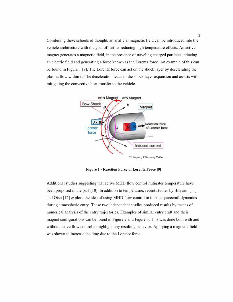
Combining these schools of thought, an artificial magnetic field can be introduced into the
vehicle architecture with the goal of further reducing high temperature effects. An active
magnet generates a magnetic field, in the presence of traveling charged particles inducing
an electric field and generating a force known as the Lorentz force. An example of this can
be found in Figure 1 [9]. The Lorentz force can act on the shock layer by decelerating the
plasma flow within it. The deceleration leads to the shock layer expansion and assists with
mitigating the convective heat transfer to the vehicle.
Figure 1 - Reaction Force of Lorentz Force [9]
Additional studies suggesting that active MHD flow control mitigates temperature have
been proposed in the past [10]. In addition to temperature, recent studies by Bityurin [11]
and Otsu [12] explore the idea of using MHD flow control to impact spacecraft dynamics
during atmospheric entry. These two independent studies produced results by means of
numerical analysis of the entry trajectories. Examples of similar entry craft and their
magnet configurations can be found in Figure 2 and Figure 3. This was done both with and
without active flow control to highlight any resulting behavior. Applying a magnetic field
was shown to increase the drag due to the Lorentz force.
3
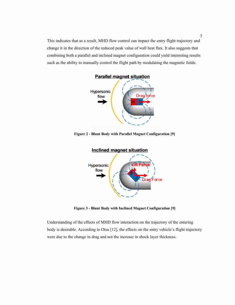
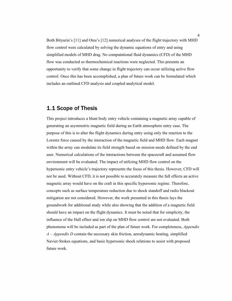
This indicates that as a result, MHD flow control can impact the entry flight trajectory and
change it in the direction of the reduced peak value of wall heat flux. It also suggests that
combining both a parallel and inclined magnet configuration could yield interesting results
such as the ability to manually control the flight path by modulating the magnetic fields.
Figure 2 - Blunt Body with Parallel Magnet Configuration [9]
Figure 3 - Blunt Body with Inclined Magnet Configuration [9]
Understanding of the effects of MHD flow interaction on the trajectory of the entering
body is desirable. According to Otsu [12], the effects on the entry vehicle’s flight trajectory
were due to the change in drag and not the increase in shock layer thickness.
4
Both Bityurin’s [11] and Otsu’s [12] numerical analyses of the flight trajectory with MHD
flow control were calculated by solving the dynamic equations of entry and using
simplified models of MHD drag. No computational fluid dynamics (CFD) of the MHD
flow was conducted so thermochemical reactions were neglected. This presents an
opportunity to verify that some change in flight trajectory can occur utilizing active flow
control. Once this has been accomplished, a plan of future work can be formulated which
includes an outlined CFD analysis and coupled analytical model.
1.1 Scope of Thesis
This project introduces a blunt body entry vehicle containing a magnetic array capable of
generating an asymmetric magnetic field during an Earth atmosphere entry case. The
purpose of this is to alter the flight dynamics during entry using only the reaction to the
Lorentz force caused by the interaction of the magnetic field and MHD flow. Each magnet
within the array can modulate its field strength based on mission needs defined by the end
user. Numerical calculations of the interactions between the spacecraft and assumed flow
environment will be evaluated. The impact of utilizing MHD flow control on the
hypersonic entry vehicle’s trajectory represents the focus of this thesis. However, CFD will
not be used. Without CFD, it is not possible to accurately measure the full effects an active
magnetic array would have on the craft in this specific hypersonic regime. Therefore,
concepts such as surface temperature reduction due to shock standoff and radio blackout
mitigation are not considered. However, the work presented in this thesis lays the
groundwork for additional study while also showing that the addition of a magnetic field
should have an impact on the flight dynamics. It must be noted that for simplicity, the
influence of the Hall effect and ion slip on MHD flow control are not evaluated. Both
phenomena will be included as part of the plan of future work. For completeness, Appendix
A – Appendix D contain the necessary skin friction, aerodynamic heating, simplified
Navier-Stokes equations, and basic hypersonic shock relations to assist with proposed
future work.
5
Other previous works by Masuda [13] and Fujino [14,15] introduced a single dipole
magnet into the nose of a blunt body entry vehicle. While this architecture is sufficient for
determining potential surface heat reduction and exploring interactions between the plasma
flow and entry body, it is not enough when considering the maximum potential of this
methodology. A controllable magnetic array that includes multiple magnets positioned in a
non-axisymmetric configuration can provide a more stable flight profile.
This is important to note because most current studies [16] assume that the flow is
impacting the blunt body entry vehicle at center and that the flow is evenly distributed
across the surface. Real flight conditions are more dynamic and minor instabilities will
most likely be encountered during flight. This thesis suggests that these can be easily
compensated for if enough controllability using MHD flow principles is obtained. The
introduction of a magnetic array as opposed to a single dipole can also present new
capabilities not previously considered or expected.
In summary, this work explores the feasibility of using an active magnetic array to
modulate ionized flow during hypersonic atmospheric entry. Building off previous work
[17,18,19], the following relevant questions will be addressed:
1. Using a simplified atmosphere and gas dynamics model, can an active magnetic
field change the flight profile of a blunt body entry vehicle?
2. Can variations in the magnetic flux density be used to control the entry trajectory?
3. Do the lift and drag forces produced by the reaction to the Lorentz force vary with
angle of attack?

6
Chapter 2
Background
Utilizing MHD flow control during hypersonic flight has the potential to provide a range of
advantages. Some of these include vehicle surface temperature reduction [20], shock layer
modulation [21], and drag reduction [22]. If it was found that substantial trajectory
modification can be achieved using MHD flow control schemes, then opportunities will
arise for this methodology to be used for additional hypersonic flight applications. These
include more precise guidance, navigation, and control (GN&C) methods for hypersonic
missiles as well as increased lift / drag ratio, onboard power generation during flight using
MHD power generation [24], and a reduction of communication blackout zones [23,25].
To better understand the logic behind analyzing the effects of active hypersonic MHD flow
modulation, it is important to outline the problem as a collection of flight principles and
characteristics. This chapter aims to do that by describing the vehicle operating
environment (Earth’s atmosphere), vehicle’s geometry (blunt body), entry flight dynamics,
hypersonic flow conditions, and MHD flow properties. Each section contains the
associated concepts and characteristic equations relevant to each component of the project.
2.1 Atmosphere
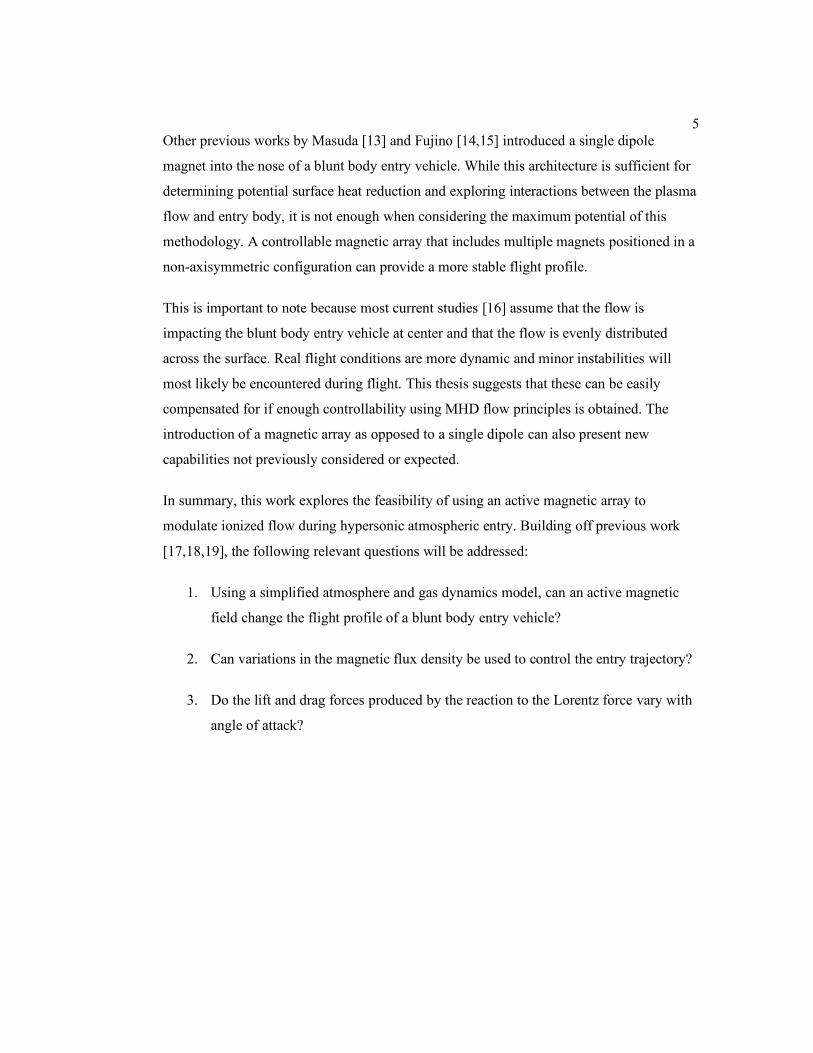
The standard atmosphere is modeled as a series of layers with temperature variation as a
function of altitude. Figure 4 defines each layer in the standard atmospheric model [26].
7
Figure 4 - Atmosphere Profile [26]
The troposphere extends from standard sea level up to 11 km and has a linearly decreasing
temperature based on altitude. Between 11 and 47 km lies the stratosphere. This region
consists of areas of isothermal and linearly increasing temperatures. Beyond the
stratosphere is the mesosphere which extends to a height of 86 km. This region has two
areas with linearly decreasing temperature and one isothermal layer. Above the mesosphere
is the thermosphere which extends to a height of 500 km. This region’s characteristics are
dominated by solar radiation and associated chemical reactions.
8
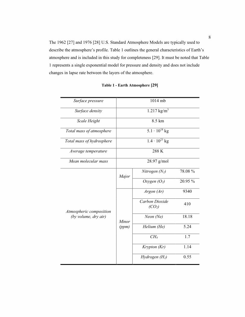
The 1962 [27] and 1976 [28] U.S. Standard Atmosphere Models are typically used to
describe the atmosphere’s profile. Table 1 outlines the general characteristics of Earth’s
atmosphere and is included in this study for completeness [29]. It must be noted that Table
1 represents a single exponential model for pressure and density and does not include
changes in lapse rate between the layers of the atmosphere.
Table 1 - Earth Atmosphere [29]
Surface pressure 1014 mb
Surface density 1.217 kg/m3
Scale Height 8.5 km
Total mass of atmosphere 5.1 ∙ 1018 kg
Total mass of hydrosphere 1.4 ∙ 1023 kg
Average temperature 288 K
Mean molecular mass 28.97 g/mol
Atmospheric composition
(by volume, dry air)
Major Nitrogen (N2) 78.08 %
Oxygen (O2) 20.95 %
Minor
(ppm)
Argon (Ar) 9340
Carbon Dioxide
(CO2) 410
Neon (Ne) 18.18
Helium (He) 5.24
CH4 1.7
Krypton (Kr) 1.14
Hydrogen (H2) 0.55
9
2.2 Real Gas Effects
Figure 5 - Real Gas Effects [30]
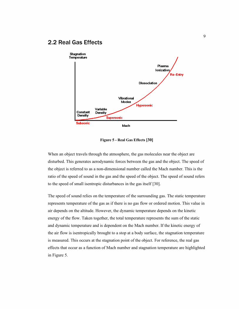
When an object travels through the atmosphere, the gas molecules near the object are
disturbed. This generates aerodynamic forces between the gas and the object. The speed of
the object is referred to as a non-dimensional number called the Mach number. This is the
ratio of the speed of sound in the gas and the speed of the object. The speed of sound refers
to the speed of small isentropic disturbances in the gas itself [30].
The speed of sound relies on the temperature of the surrounding gas. The static temperature
represents temperature of the gas as if there is no gas flow or ordered motion. This value in
air depends on the altitude. However, the dynamic temperature depends on the kinetic
energy of the flow. Taken together, the total temperature represents the sum of the static
and dynamic temperature and is dependent on the Mach number. If the kinetic energy of
the air flow is isentropically brought to a stop at a body surface, the stagnation temperature
is measured. This occurs at the stagnation point of the object. For reference, the real gas
effects that occur as a function of Mach number and stagnation temperature are highlighted
in Figure 5.
10
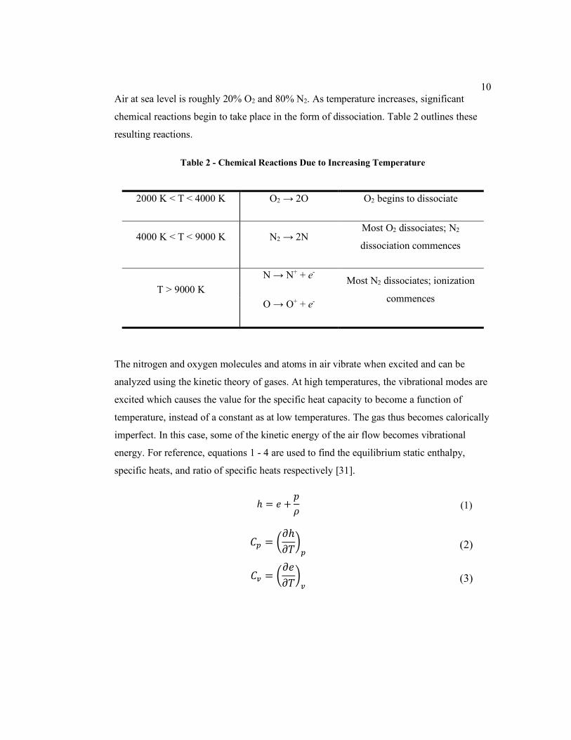
Air at sea level is roughly 20% O2 and 80% N2. As temperature increases, significant
chemical reactions begin to take place in the form of dissociation. Table 2 outlines these
resulting reactions.
Table 2 - Chemical Reactions Due to Increasing Temperature
2000 K < T < 4000 K O2 → 2O O2 begins to dissociate
4000 K < T < 9000 K N2 → 2N Most O2 dissociates; N2
dissociation commences
T > 9000 K
N → N+ + e-
Most N2 dissociates; ionization
commences O → O+ + e-
The nitrogen and oxygen molecules and atoms in air vibrate when excited and can be
analyzed using the kinetic theory of gases. At high temperatures, the vibrational modes are
excited which causes the value for the specific heat capacity to become a function of
temperature, instead of a constant as at low temperatures. The gas thus becomes calorically
imperfect. In this case, some of the kinetic energy of the air flow becomes vibrational
energy. For reference, equations 1 - 4 are used to find the equilibrium static enthalpy,
specific heats, and ratio of specific heats respectively [31].
ℎ = 𝑒 +𝑝
𝜌 (1)
𝐶𝑝 = (𝜕ℎ
𝜕𝑇)
𝑝 (2)
𝐶𝑣 = (𝜕𝑒
𝜕𝑇)
𝑣 (3)
11
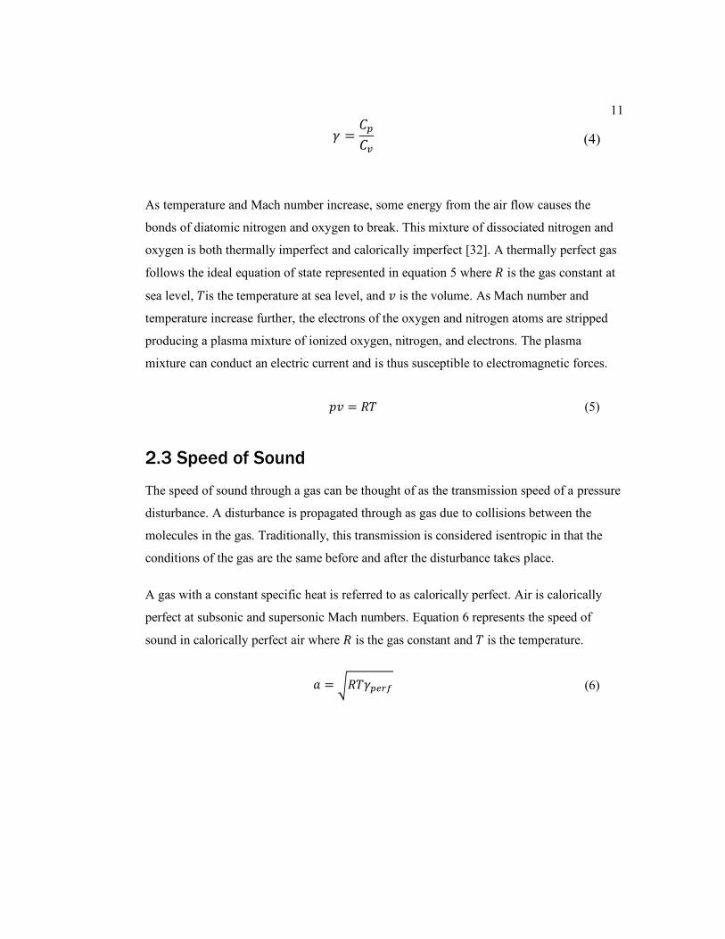
𝛾 =𝐶𝑝
𝐶𝑣 (4)
As temperature and Mach number increase, some energy from the air flow causes the
bonds of diatomic nitrogen and oxygen to break. This mixture of dissociated nitrogen and
oxygen is both thermally imperfect and calorically imperfect [32]. A thermally perfect gas
follows the ideal equation of state represented in equation 5 where 𝑅 is the gas constant at
sea level, 𝑇is the temperature at sea level, and 𝑣 is the volume. As Mach number and
temperature increase further, the electrons of the oxygen and nitrogen atoms are stripped
producing a plasma mixture of ionized oxygen, nitrogen, and electrons. The plasma
mixture can conduct an electric current and is thus susceptible to electromagnetic forces.
𝑝𝑣 = 𝑅𝑇 (5)
2.3 Speed of Sound
The speed of sound through a gas can be thought of as the transmission speed of a pressure
disturbance. A disturbance is propagated through as gas due to collisions between the
molecules in the gas. Traditionally, this transmission is considered isentropic in that the
conditions of the gas are the same before and after the disturbance takes place.
A gas with a constant specific heat is referred to as calorically perfect. Air is calorically
perfect at subsonic and supersonic Mach numbers. Equation 6 represents the speed of
sound in calorically perfect air where 𝑅 is the gas constant and 𝑇 is the temperature.
𝑎 = √𝑅𝑇𝛾𝑝𝑒𝑟𝑓 (6)
12
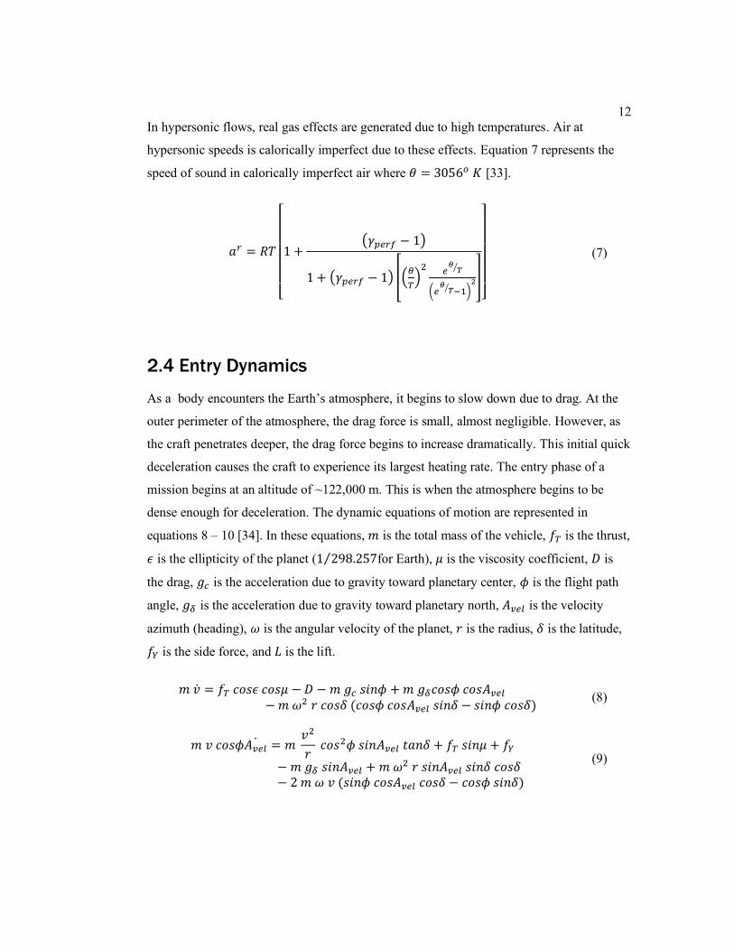
In hypersonic flows, real gas effects are generated due to high temperatures. Air at
hypersonic speeds is calorically imperfect due to these effects. Equation 7 represents the
speed of sound in calorically imperfect air where 𝜃 = 3056𝜊 𝐾 [33].
𝑎𝑟 = 𝑅𝑇
[
1 +(𝛾𝑝𝑒𝑟𝑓 − 1)
1 + (𝛾𝑝𝑒𝑟𝑓 − 1) [(𝜃
𝑇)2 𝑒
𝜃𝑇⁄
(𝑒𝜃
𝑇⁄ −1)2]
]
(7)
2.4 Entry Dynamics
As a body encounters the Earth’s atmosphere, it begins to slow down due to drag. At the
outer perimeter of the atmosphere, the drag force is small, almost negligible. However, as
the craft penetrates deeper, the drag force begins to increase dramatically. This initial quick
deceleration causes the craft to experience its largest heating rate. The entry phase of a
mission begins at an altitude of ~122,000 m. This is when the atmosphere begins to be
dense enough for deceleration. The dynamic equations of motion are represented in
equations 8 – 10 [34]. In these equations, 𝑚 is the total mass of the vehicle, 𝑓𝑇 is the thrust,
𝜖 is the ellipticity of the planet (1 298.257⁄ for Earth), 𝜇 is the viscosity coefficient, 𝐷 is
the drag, 𝑔𝑐 is the acceleration due to gravity toward planetary center, 𝜙 is the flight path
angle, 𝑔𝛿 is the acceleration due to gravity toward planetary north, 𝐴𝑣𝑒𝑙 is the velocity
azimuth (heading), 𝜔 is the angular velocity of the planet, 𝑟 is the radius, 𝛿 is the latitude,
𝑓𝑌 is the side force, and 𝐿 is the lift.
𝑚 �̇� = 𝑓𝑇 𝑐𝑜𝑠𝜖 𝑐𝑜𝑠𝜇 − 𝐷 − 𝑚 𝑔𝑐 𝑠𝑖𝑛𝜙 + 𝑚 𝑔𝛿𝑐𝑜𝑠𝜙 𝑐𝑜𝑠𝐴𝑣𝑒𝑙
− 𝑚 𝜔2 𝑟 𝑐𝑜𝑠𝛿 (𝑐𝑜𝑠𝜙 𝑐𝑜𝑠𝐴𝑣𝑒𝑙 𝑠𝑖𝑛𝛿 − 𝑠𝑖𝑛𝜙 𝑐𝑜𝑠𝛿) (8)
𝑚 𝑣 𝑐𝑜𝑠𝜙𝐴𝑣𝑒𝑙̇ = 𝑚
𝑣2
𝑟 𝑐𝑜𝑠2𝜙 𝑠𝑖𝑛𝐴𝑣𝑒𝑙 𝑡𝑎𝑛𝛿 + 𝑓𝑇 𝑠𝑖𝑛𝜇 + 𝑓𝑌
− 𝑚 𝑔𝛿 𝑠𝑖𝑛𝐴𝑣𝑒𝑙 + 𝑚 𝜔2 𝑟 𝑠𝑖𝑛𝐴𝑣𝑒𝑙 𝑠𝑖𝑛𝛿 𝑐𝑜𝑠𝛿− 2 𝑚 𝜔 𝑣 (𝑠𝑖𝑛𝜙 𝑐𝑜𝑠𝐴𝑣𝑒𝑙 𝑐𝑜𝑠𝛿 − 𝑐𝑜𝑠𝜙 𝑠𝑖𝑛𝛿)
(9)
13
𝑚 𝑣 �̇� = 𝑚 𝑣2
𝑟 𝑐𝑜𝑠𝜙 + 𝑓𝑇 𝑠𝑖𝑛𝜖 𝑐𝑜𝑠𝜇 + 𝐿 − 𝑚 𝑔𝑐 𝑐𝑜𝑠𝜙
− 𝑚 𝑔𝛿 𝑠𝑖𝑛𝜙 𝑐𝑜𝑠𝐴𝑣𝑒𝑙
+ 𝑚 𝜔2 𝑟 𝑐𝑜𝑠𝛿 (𝑠𝑖𝑛𝜙 𝑐𝑜𝑠𝐴𝑣𝑒𝑙 𝑠𝑖𝑛𝛿 + 𝑐𝑜𝑠𝜙 𝑐𝑜𝑠𝛿)+ 2 𝑚 𝜔 𝑣 𝑠𝑖𝑛𝐴𝑣𝑒𝑙 𝑐𝑜𝑠𝛿
(10)
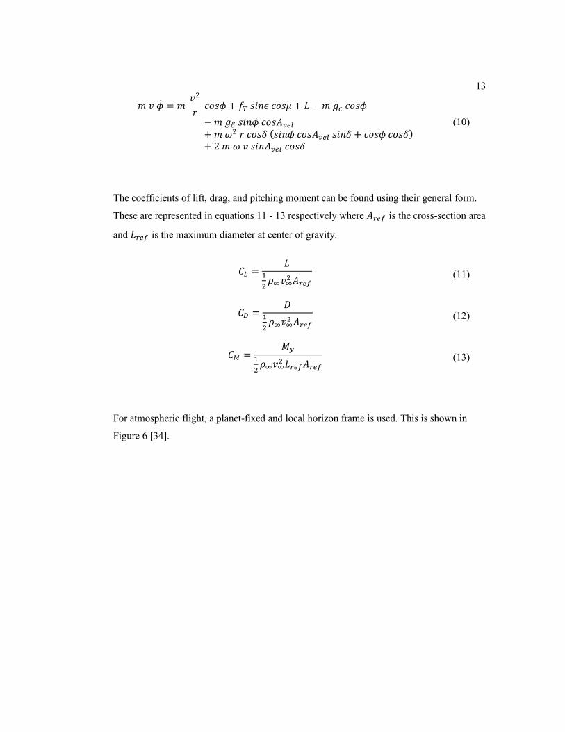
The coefficients of lift, drag, and pitching moment can be found using their general form.
These are represented in equations 11 - 13 respectively where 𝐴𝑟𝑒𝑓 is the cross-section area
and 𝐿𝑟𝑒𝑓 is the maximum diameter at center of gravity.
𝐶𝐿 =𝐿
1
2𝜌∞𝑣∞
2 𝐴𝑟𝑒𝑓
(11)
𝐶𝐷 =𝐷
1
2𝜌∞𝑣∞
2 𝐴𝑟𝑒𝑓
(12)
𝐶𝑀 =𝑀𝑦
1
2𝜌∞𝑣∞
2 𝐿𝑟𝑒𝑓𝐴𝑟𝑒𝑓
(13)
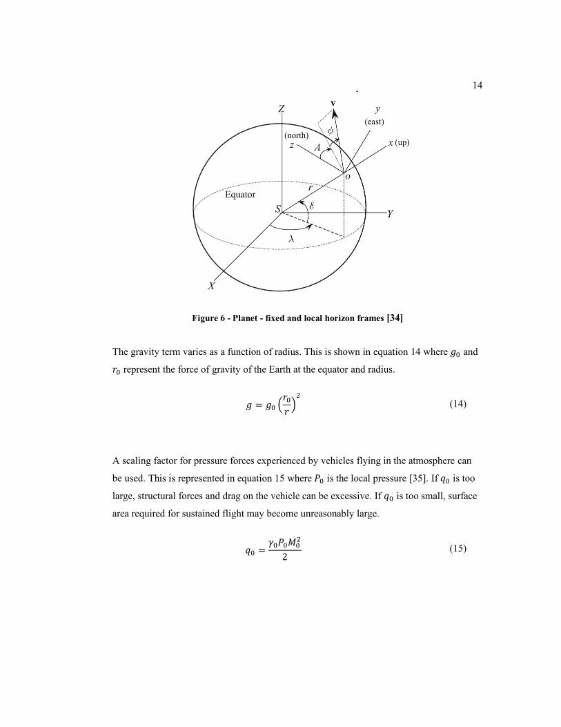
For atmospheric flight, a planet-fixed and local horizon frame is used. This is shown in
Figure 6 [34].
14
Figure 6 - Planet - fixed and local horizon frames [34]
The gravity term varies as a function of radius. This is shown in equation 14 where 𝑔0 and
𝑟0 represent the force of gravity of the Earth at the equator and radius.
𝑔 = 𝑔0 (𝑟0𝑟)2
(14)
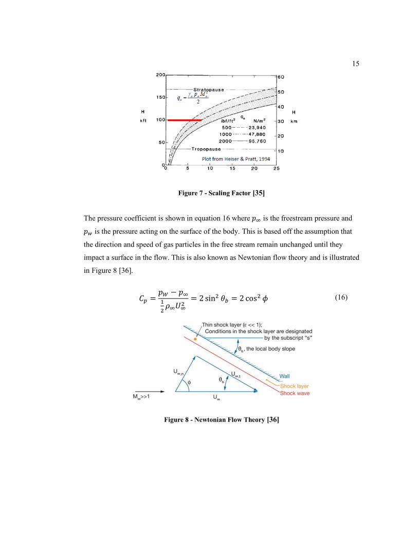
A scaling factor for pressure forces experienced by vehicles flying in the atmosphere can
be used. This is represented in equation 15 where 𝑃0 is the local pressure [35]. If 𝑞0 is too
large, structural forces and drag on the vehicle can be excessive. If 𝑞0 is too small, surface
area required for sustained flight may become unreasonably large.
𝑞0 =𝛾0𝑃0𝑀0
2
2 (15)
15
Figure 7 - Scaling Factor [35]
The pressure coefficient is shown in equation 16 where 𝑝∞ is the freestream pressure and
𝑝𝑤 is the pressure acting on the surface of the body. This is based off the assumption that
the direction and speed of gas particles in the free stream remain unchanged until they
impact a surface in the flow. This is also known as Newtonian flow theory and is illustrated
in Figure 8 [36].
𝐶𝑝 =𝑝𝑊 − 𝑝∞
1
2𝜌∞𝑈∞
2= 2 sin2 𝜃𝑏 = 2 cos2 𝜙 (16)
Figure 8 - Newtonian Flow Theory [36]
16
The pressure acting on the body surface is found using the sum of the normal momentum
fluxes of both reflected and incident molecules per unit time. This is shown in equation 17
where 𝑐𝜂 is the molecules’ normal velocity component and 𝑚 is the molecules’ mass.
𝑝𝑤 = 𝑝𝑖 + 𝑝𝑟 = ∑[𝑚𝑗𝑐𝜂𝑗2 ]
𝑖+
𝑁
𝑗=1
[𝑚𝑗𝑐𝜂𝑗2 ]
𝑟 (17)
For reference, a section outlining how to calculate the skin friction coefficient during entry
can be found in Appendix A.
The acceleration on an object reentering the atmosphere due to drag depends on:
• Object size (cross-sectional area exposed to the wind)
• Drag coefficient (how streamlined it is)
• Velocity
• Density of the air
The magnitude of deceleration an object experiences while traveling through the
atmosphere is inversely related to the object’s ballistic coefficient 𝛽. The vehicle ballistic
coefficient can be found using equation 18 where 𝑚 is the vehicle mass, 𝐴 is the vehicle
area, and 𝐶𝐷 is the vehicle drag coefficient.
𝛽 =𝑚
𝐶𝐷𝐴 (18)
17
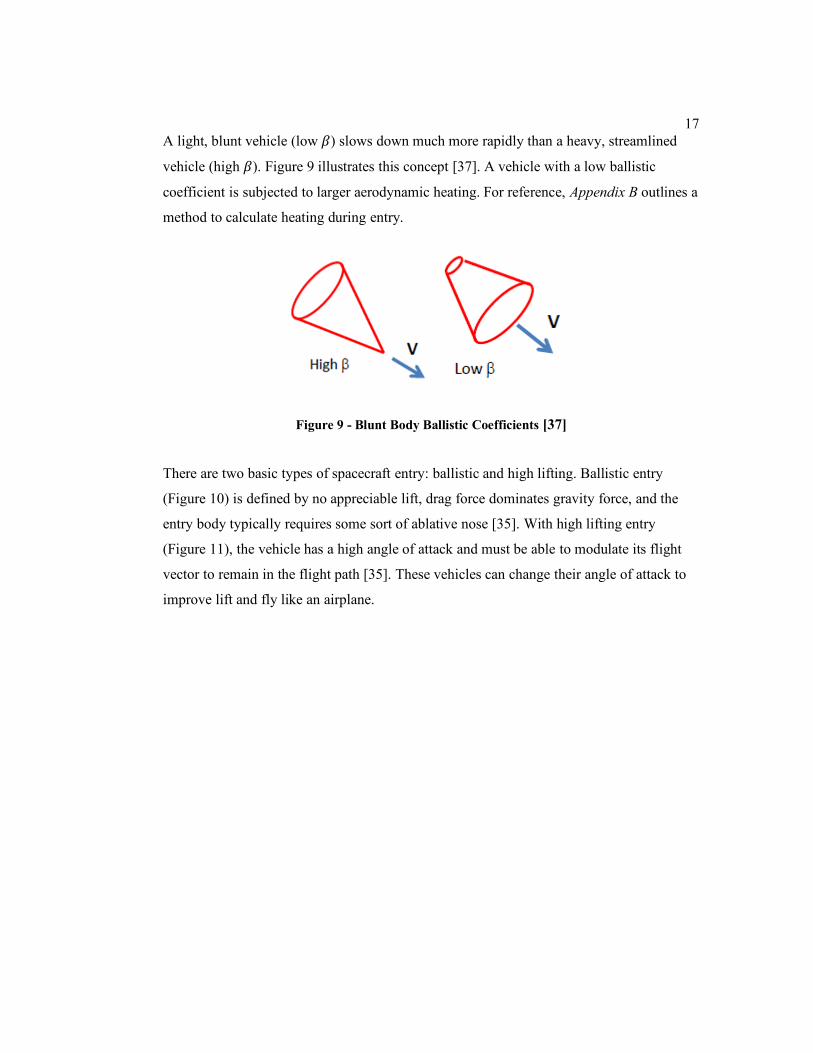
A light, blunt vehicle (low 𝛽) slows down much more rapidly than a heavy, streamlined
vehicle (high 𝛽). Figure 9 illustrates this concept [37]. A vehicle with a low ballistic
coefficient is subjected to larger aerodynamic heating. For reference, Appendix B outlines a
method to calculate heating during entry.
Figure 9 - Blunt Body Ballistic Coefficients [37]
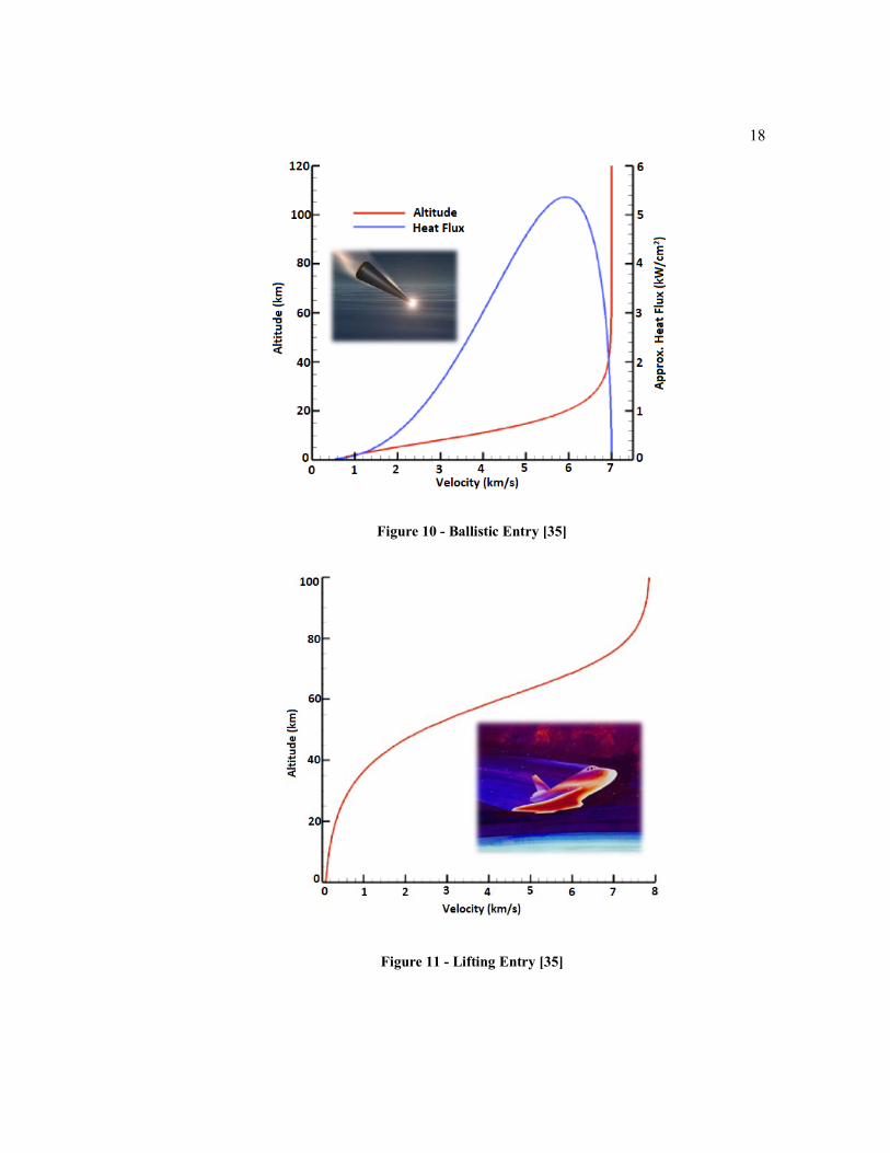
There are two basic types of spacecraft entry: ballistic and high lifting. Ballistic entry
(Figure 10) is defined by no appreciable lift, drag force dominates gravity force, and the
entry body typically requires some sort of ablative nose [35]. With high lifting entry
(Figure 11), the vehicle has a high angle of attack and must be able to modulate its flight
vector to remain in the flight path [35]. These vehicles can change their angle of attack to
improve lift and fly like an airplane.
18
Figure 10 - Ballistic Entry [35]
Figure 11 - Lifting Entry [35]
19
2.5 Blunt Body Entry Vehicles
The aerodynamic requirements for planetary entry capsules are different from those
designed for in-atmosphere flight. The objective is to safely decelerate a fragile payload
(scientific or manned) from an outer atmosphere trajectory to a landing altitude at low
supersonic velocity. In this scenario, deceleration must occur at the highest possible
altitude. This is done to mitigate mechanical and thermal stresses that the capsule
undergoes during entry. To achieve this, a small path angle (shallow trajectory) and a blunt
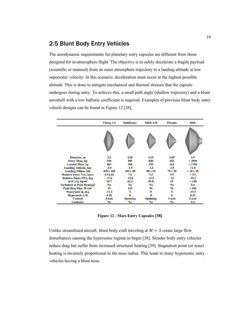
aeroshell with a low ballistic coefficient is required. Examples of previous blunt body entry
vehicle designs can be found in Figure 12 [38].
Figure 12 - Mars Entry Capsules [38]
Unlike streamlined aircraft, blunt body craft traveling at 𝑀 = 3 create large flow
disturbances causing the hypersonic regime to begin [38]. Slender body entry vehicles
reduce drag but suffer from increased structural heating [39]. Stagnation point (or nose)
heating is inversely proportional to the nose radius. This leads to many hypersonic entry
vehicles having a blunt nose.
20
During entry when the angle of attack is near zero, these types of shape have the following
characteristics: a small positive normal force coefficient 𝐶𝑁 above 𝑀 = 1.5 and a relatively
high axial force coefficient 𝐶𝐴 ≈ 1 − 1.7 [40]. The lift coefficients of this shape type are
negative up to a moderate angle of attack and are typically generated by the axial force.
Equation 19 shows the coefficient of lift for this entry shape.
𝐶𝐿 = 𝐶𝑁 𝑐𝑜𝑠 �̅� − 𝐶𝐴 𝑐𝑜𝑠 �̅� ≈ −𝐶𝐴 𝑠𝑖𝑛 �̅� (19)
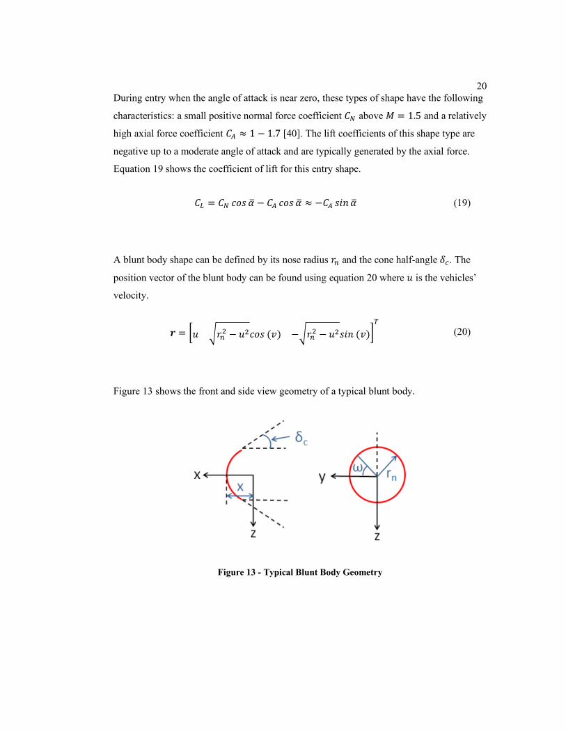
A blunt body shape can be defined by its nose radius 𝑟𝑛 and the cone half-angle 𝛿𝑐. The
position vector of the blunt body can be found using equation 20 where 𝑢 is the vehicles’
velocity.
𝒓 = [𝑢 √𝑟𝑛2 − 𝑢2𝑐𝑜𝑠 (𝑣) −√𝑟𝑛
2 − 𝑢2𝑠𝑖𝑛 (𝑣)]𝑇
(20)
Figure 13 shows the front and side view geometry of a typical blunt body.
Figure 13 - Typical Blunt Body Geometry
21
2.6 Hypersonic Flow
Hypersonic flow is defined by a high-speed flow regime where energy transfer between
fluid dynamic, thermodynamic, and chemical processes become dominating factors. Table
3 shows how hypersonic flow can be considered within its various regimes. This study is
focused on the ionized gas regime. When analyzing hypersonic flows, the simplified
Navier-Stokes equations are used. These are outlined in Appendix C.
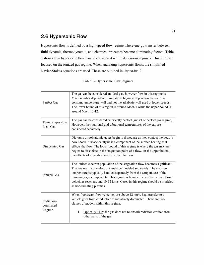
Table 3 - Hypersonic Flow Regimes
Perfect Gas
The gas can be considered an ideal gas, however flow in this regime is
Mach number dependent. Simulations begin to depend on the use of a
constant temperature wall and not the adiabatic wall used at lower speeds.
The lower bound of this region is around Mach 5 while the upper bound is
around Mach 10-12.
Two-Temperature
Ideal Gas
The gas can be considered calorically perfect (subset of perfect gas regime).
However, the rotational and vibrational temperatures of the gas are
considered separately.
Dissociated Gas
Diatomic or polyatomic gases begin to dissociate as they contact the body’s
bow shock. Surface catalysis is a component of the surface heating as it
effects the flow. The lower bound of this regime is where the gas mixture
begins to dissociate in the stagnation point of a flow. At the upper bound,
the effects of ionization start to affect the flow.
Ionized Gas
The ionized electron population of the stagnation flow becomes significant.
This means that the electrons must be modeled separately. The electron
temperature is typically handled separately from the temperature of the
remaining gas components. This regime is bounded where freestream flow
velocities reach around 10-12 km/s. Gases in this regime should be modeled
as non-radiating plasmas.
Radiation-
dominated
Regime
When freestream flow velocities are above 12 km/s, heat transfer to a
vehicle goes from conductive to radiatively dominated. There are two
classes of models within this regime:
1. Optically Thin: the gas does not re-absorb radiation emitted from
other parts of the gas
22
2. Optically Thick: the radiation must be considered a separate source
of energy. This is very difficult to model. The radiation must be
calculated at each point therefore the computational load increases
as the number of points increases.
Hypersonic speeds are those where the Mach number is greater than 5 and aerodynamic
heating is the main factor in the physics of flight. It should be noted that this number
represents streamlined aircraft. Some characteristics of hypersonic flow can be found in
Table 4. Supersonic linear theory fails at these speeds. Variations in Mach number are
caused by changing static temperature and speed of sound. In this flow regime, the specific
heat ratio (γ) can no longer be thought of as constant. The temperature effects on fluid
properties must be evaluated and total temperature exists as primarily kinetic energy.
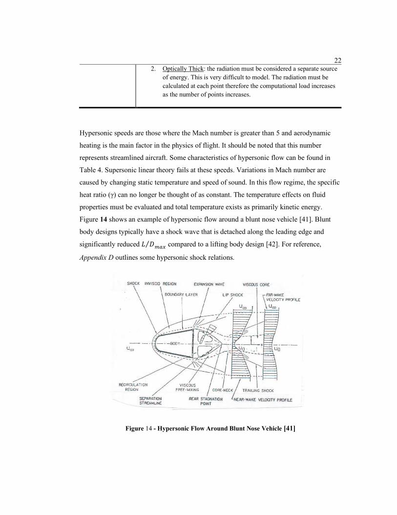
Figure 14 shows an example of hypersonic flow around a blunt nose vehicle [41]. Blunt
body designs typically have a shock wave that is detached along the leading edge and
significantly reduced 𝐿 𝐷⁄𝑚𝑎𝑥 compared to a lifting body design [42]. For reference,
Appendix D outlines some hypersonic shock relations.
Figure 14 - Hypersonic Flow Around Blunt Nose Vehicle [41]
23
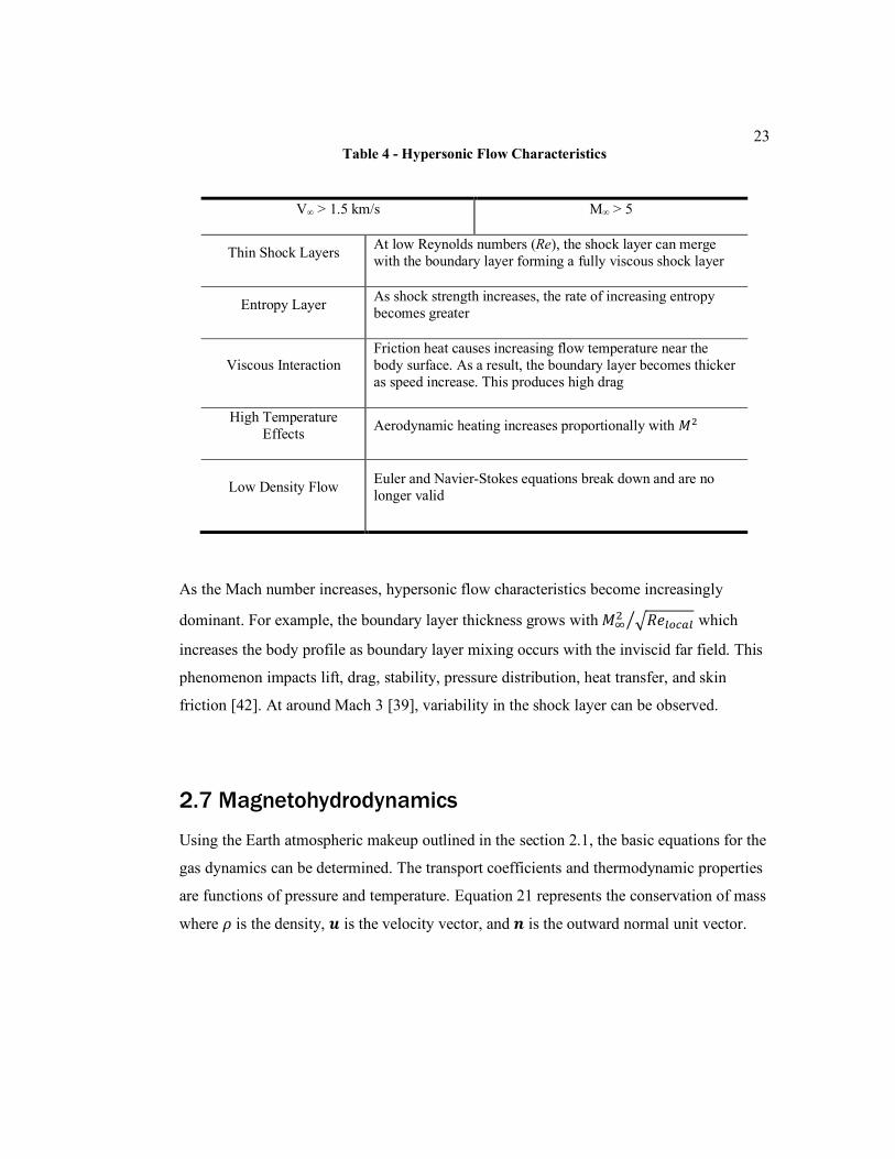
Table 4 - Hypersonic Flow Characteristics
V∞ > 1.5 km/s M∞ > 5
Thin Shock Layers At low Reynolds numbers (Re), the shock layer can merge
with the boundary layer forming a fully viscous shock layer
Entropy Layer As shock strength increases, the rate of increasing entropy
becomes greater
Viscous Interaction
Friction heat causes increasing flow temperature near the
body surface. As a result, the boundary layer becomes thicker
as speed increase. This produces high drag
High Temperature
Effects Aerodynamic heating increases proportionally with 𝑀2
Low Density Flow Euler and Navier-Stokes equations break down and are no
longer valid
As the Mach number increases, hypersonic flow characteristics become increasingly
dominant. For example, the boundary layer thickness grows with 𝑀∞2 √𝑅𝑒𝑙𝑜𝑐𝑎𝑙⁄ which
increases the body profile as boundary layer mixing occurs with the inviscid far field. This
phenomenon impacts lift, drag, stability, pressure distribution, heat transfer, and skin
friction [42]. At around Mach 3 [39], variability in the shock layer can be observed.
2.7 Magnetohydrodynamics
Using the Earth atmospheric makeup outlined in the section 2.1, the basic equations for the
gas dynamics can be determined. The transport coefficients and thermodynamic properties
are functions of pressure and temperature. Equation 21 represents the conservation of mass
where 𝜌 is the density, 𝒖 is the velocity vector, and 𝒏 is the outward normal unit vector.
24
𝜕
𝜕𝑡∭𝜌
𝑉
𝑑𝑉 + ∬𝜌𝒖
𝑆
∙ 𝒏 𝑑𝑆 = 0 (21)
Equation 22 represents the conservation of momentum where �̿� is the viscous stress tensor,
𝑱 is the electric current density vector, and 𝑩 is the magnetic field vector.
𝜕
𝜕𝑡∭𝜌𝒖
𝑉
𝑑𝑉 + ∬(𝜌𝒖(𝒖
𝑆
∙ 𝒏) + 𝜌𝒖) 𝑑𝑆
= ∬𝜏̿ ∙ 𝒏
𝑆
𝑑𝑆 + ∭𝑱 𝑥 𝑩 𝑑𝑉
𝑉
(22)
The total energy 𝐸 is found using equation 23 where 𝑒 is the internal energy and 𝒖 is the
velocity vector. The total enthalpy 𝐻 is shown in equation 24.
𝐸 = 𝑒 +𝒖2
2 (23)
𝐻 = 𝐸 +𝑝
𝜌 (24)
Therefore, equation 25 represents the conservation of the total energy where 𝜅 is the
thermal conductivity.
𝜕
𝜕𝑡∭𝜌𝐸
𝑉
𝑑𝑉 + ∬𝜌𝐻𝒖 ∙ 𝒏
𝑆
𝑑𝑆
= ∬𝜅(𝛻𝑇 ∙ 𝒏)
𝑆
𝑑𝑆 + ∬(𝜏̿ ∙ 𝒏) ∙ 𝒏
𝑆
𝑑𝑆
+ ∭ (𝑱𝟐
𝝈+ 𝒖 ∙ (𝑱 𝑥 𝑩)) 𝑑𝑉
𝑉
(25)
The quasi-one-dimensional MHD flow equations are represented in equation 26 – 29 [43].
25
𝑑𝑝
𝑑𝑥=
1
𝑀2 − 1[−((𝛾 − 1)𝑀2 + 1) 𝐹 +
(𝛾 − 1)𝑀
𝑎 �̇�] (26)
𝑑𝑀
𝑑𝑥=
1
𝑎𝑝
1
𝑀2 − 1[𝑢 (1 +
𝛾 − 1
2𝑀2) 𝐹 −
(𝛾 − 1)
2𝛾(𝛾 𝑀2 + 1) �̇�]
(27)
𝑑𝑢
𝑑𝑥=
𝑢
𝑝
1
𝑀2 − 1 (𝐹 −
𝛾 − 1
𝛾 𝑢 �̇�)
(28)
𝑑𝑇
𝑑𝑥=
𝑇
𝑝 𝛾 − 1
𝛾
1
𝑀2 − 1 (−𝛾 𝑀2 𝐹 +
𝛾 𝑀2 − 1
𝑢 �̇�)
(29)
where equation 30 and equation 31 are the Lorentz force and Joule heat per unit volume
respectively and 𝛼𝑒𝑓𝑓 is the effective Joule heating factor.
𝐹𝑙 = 𝑗𝑦𝐵𝑧 (30)
�̇�𝑗 = 𝛼𝑒𝑓𝑓 𝑗𝑦𝐸𝑦 (31)
The generalized Ohm’s law is used to find the current density and the Maxwell equations
make up the electrodynamic calculations. These can be found in equations 32 - 34.
𝛻 × 𝑬 = 0 (32)
𝛻 ∙ 𝑱 = 0 (33)
𝑱 = 𝜎(𝑬 + 𝒖 × 𝑩) −𝛽𝐻𝑎𝑙𝑙
|𝑩|(𝑱 × 𝑩)
(34)
26
In equation 34, the 𝛽𝐻𝑎𝑙𝑙 term is the Hall parameter. In a plasma, the Hall parameter is the
ratio between the electron gyrofrequency and the electron particle collision frequency. The
Hall effect takes place in a plasma when electrons drift with the magnetic field, but ions do
not. In fully ionized plasmas, this effect can be ignored since it only occurs at frequencies
between the ion and electron cyclotron frequencies. The Hall parameter is not considered
as part of this study, so this term becomes zero. Equation 35 represents the new form of the
electric current density vector.
𝑱 = 𝜎(𝑬 + 𝒖 × 𝑩) (35)
The rate that the flow velocity changes due to MHD interactions can be estimated by
analyzing the momentum transfer from the charged electrons and ions to the neutrals by
collision. The Lorentz force applied to the entire plasma is balanced by the collision drag
force [44].
This is shown in equation 36 where 𝑛𝑒and 𝑛𝑖 are electron and ion number densities, 𝜇𝑒 and
𝜇𝑖are their mobilities, 𝑚𝑒 and 𝑚𝑖 are their masses, 𝑣𝑒𝑛 and 𝑣𝑖𝑛 are electron-neutral and
ion-neutral collision frequencies, and 𝑢𝑝 − 𝑢 is the plasma velocity relative to the flow
[45]. This plasma velocity relationship is the ion-slip velocity.
The ion-slip effect is also not considered in this study since it does not have a substantial
influence on the electric current in the plasma region located behind the shock [46]. The
Coulomb forces on the charged particles produced by the Hall field cancel out.
𝑒 (𝑛𝑒 𝜇𝑒 + 𝑛𝑖 𝜇𝑖)𝑬𝒚 𝑩𝒛 = (𝑛𝑒 𝑚𝑒 𝑣𝑒𝑛 + 𝑛𝑖 𝑚𝑖 𝑣𝑖𝑛)(𝑢𝑝 − 𝑢) (36)
27
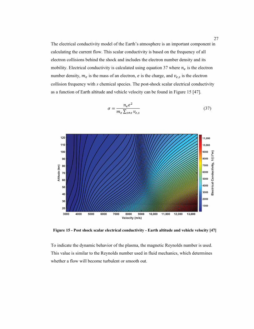
The electrical conductivity model of the Earth’s atmosphere is an important component in
calculating the current flow. This scalar conductivity is based on the frequency of all
electron collisions behind the shock and includes the electron number density and its
mobility. Electrical conductivity is calculated using equation 37 where 𝑛𝑒 is the electron
number density, 𝑚𝑒 is the mass of an electron, 𝑒 is the charge, and 𝑣𝑒,𝑠 is the electron
collision frequency with s chemical species. The post-shock scalar electrical conductivity
as a function of Earth altitude and vehicle velocity can be found in Figure 15 [47].
𝜎 =𝑛𝑒𝑒
2
𝑚𝑒 ∑ 𝑣𝑒,𝑠𝑠≠𝑒 (37)
Figure 15 - Post shock scalar electrical conductivity - Earth altitude and vehicle velocity [47]
To indicate the dynamic behavior of the plasma, the magnetic Reynolds number is used.
This value is similar to the Reynolds number used in fluid mechanics, which determines
whether a flow will become turbulent or smooth out.
28
The magnetic Reynolds number can be found using equation 38 where the magnetic
permeability of free space is 𝜇0, the plasma electrical conductivity is 𝜎𝑝, the plasma
velocity is 𝑢𝑝, and the characteristic length of the plasma structure is 𝐿𝑝 [48].
𝑅𝑚 = 𝜇0𝜎𝑝𝑢𝐿𝑝 (38)
The magnetic field can exhibit two general types of behavior depending on the value of the
magnetic Reynolds number. If 𝑅𝑚 is very large, the magnetic field lines are considered
frozen in the plasma and travel along with the plasma flow. If 𝑅𝑚 is smaller than 1, the
magnetic field will diffuse away. When this happens, the inhomogeneities in the field will
smooth out like the flow of fluid becoming smooth [49].
29
Chapter 3
Model
To conduct this study, three models were developed. These include Earth’s atmospheric
profile, dynamics of the entry phase of a spacecraft, and methodology for determining the
effects of the Lorentz force on the trajectory of the spacecraft. To execute each simulation,
the strength of the magnetic flux density will be varied from 𝐵 = 0.1 − 1 𝑇. The values of
lift and drag generated by the force acting on the Lorentz force are determined using a
Simulink model. These values are then inserted into MATLAB to determine the vehicle’s
entry trajectory. A description of the Simulink model can be found in Appendix E.
3.1 Model Limitations
1. Gas effects – MHD coupling was not applied. This would require a very thorough
analysis of the gas effects during entry [50,19].
2. No CFD analysis, so pressure forces produced due to the reaction to the Lorentz
force acting on the shock wave are not accurately obtained. Performing CFD
analysis of this entry scenario is part of the plan of future work. As the purpose of
this thesis was to only determine if a reaction to the Lorentz force could be
generated, proposing a future study based on CFD presents itself as a valid next
step.
3. Due to the lack of CFD, it is difficult to measure the exact impact of having a 3-
magnet configuration with two magnets angled at 45°. However, the overall effect
of the additional force can still be determined.
30
4. Simplified model for sigma results in an estimation of its impact on the current
density (J). A temperature of 2000 K is used as the temperature behind the shock.
The temperature in equation 68 is not held constant throughout the flight and
varies due to the heating effects of atmospheric entry. This leads to a current
density value that fluctuates throughout the entry profile. The 2000 K temperature
is estimated in the high range based on the maximum temperature (1750 K) that
the space shuttle experienced during atmospheric entry [37].
3.2 Assumptions
1. Vehicle geometry simplified to flat cylinder with characteristics shown in Table 5
2. Bow shock simplified using the Raizer model for temperature behind the shock
[51]
3. Local thermodynamic equilibrium (LTE) assumed
4. Magnetic field from 3 magnets is calculated as a sum and represented as a single
source
5. All thermal and ionization properties uniform behind the shock wave
6. Non-conductive vehicle forebody (heatshield is a dielectric)
7. Electrical conductivity is a scalar (valid for weak ionization, high neutral density,
minimal Hall effect interaction)
3.3 Atmosphere
Using the table of constants found in Appendix F, an atmosphere model was constructed
using MATLAB. For heights between 0 and 86 km, the 1976 U.S. Standard Atmosphere
model is used [34]. Above 86 km the 1962 U.S. Standard Atmosphere model is used [34].
31
This model uses a linearly varying temperature past 86 km and addresses the nonlinearity
found in the temperature variation above 86 km the 1976 model. These models are
combined into a hybrid table of values which can be found in the Appendix G [34]. This
was done in order to maintain consistency between the atmospheric and flight dynamics
sections since they are both formed using the method from Tewari as a guide [34]. The
following equations are used to calculate the atmospheric properties in the MATLAB
model.
The specific gas constant R can be found in equation 39 where 𝑀𝑚𝑜𝑙 is the molar mass and
�̅� is the ideal gas constant.
𝑅 =�̅�
𝑀𝑚𝑜𝑙 (39)
The molecular weight variation can be absorbed into the definition of a molecular
temperature as shown in equation 40. The 𝑚0 term represents the molecular weight at sea
level, 𝑚 is the molecular weight at a specific altitude, and 𝑇 is temperature at that altitude.
𝑇𝑚 =̇ 𝑇𝑚0
𝑚 (40)
The speed of sound can be found using equation 41 where 𝛾 is the ratio of specific heats, 𝑅
is the gas constant, and 𝑇 is the absolute temperature. The ratio of specific heats is 1.4 for
air.
𝑎∞ = √𝛾𝑅𝑇 (41)
32
Mach number can be found using equation 42 where the 𝑣 term indicates the vehicle speed
relative to the atmosphere and 𝑎∞ is the speed of sound.
𝑀 = 𝑣
𝑎∞ (42)
Sutherland’s law can be found in equation 43 where 𝑇𝑟𝑒𝑓 is a reference temperature, 𝑆 is
the Sutherland temperature (110.4 K), and 𝜇𝑟𝑒𝑓 is the viscosity at the reference
temperature. This is based on an idealized intermolecular force potential and the kinetic
theory of ideal gases.
𝜇 = 𝜇𝑟𝑒𝑓 (𝑇
𝑇𝑟𝑒𝑓)
32⁄ 𝑇𝑟𝑒𝑓 + 𝑆
𝑇 + 𝑆
(43)
Using Sutherland’s law, the dynamic air viscosity coefficient can be determined using
equation 44 where the value of 1.458 ∙ 10−6 is in units of 𝑘𝑔
𝑚∙𝑠∙𝐾1
2⁄.
𝜇∗ = 1.458 ∙ 10−6𝑇
32⁄
(𝑇 + 110.4)
(44)
The isobaric specific heat of a perfect gas can be found using equation 45.
𝑐𝑝𝑐=
𝑅 𝛾
𝛾 − 1
(45)
Thermal conductivity of a perfect gas can be found using equation 46 [34] where 𝑘𝑇 is in
units of 𝐽
𝑚∙𝑠∙𝐾.
33
𝑘𝑇 = 2.64638 ∙ 10−3𝑇
32⁄
𝑇 + 245.4(10−12𝑇⁄ )
(46)
The Prandtl number can be found using equation 47. This number represents the ratio
between thermal and viscous diffusion times.
𝑃𝑟 = 𝜇𝑐𝑝𝑐
𝑘𝑇 (47)
The mean free path of free stream molecules can be found using equation 48. The collision
diameter of the molecule is represented by 𝜎 and 𝑁𝑎 is Avogadro’s constant
(6.022 ∙ 1023 [1
𝑚𝑜𝑙]).
𝜆 = 𝑚
√2𝜋𝜎2𝜌𝑁𝑎
(48)
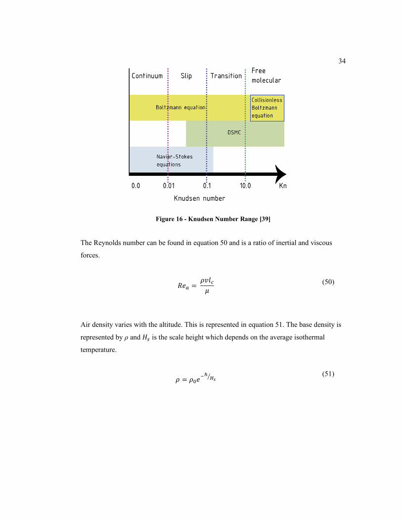
The Knudsen number can be found using equation 49 where 𝑙𝑐 is the characteristic length.
This number relates the mean free path length and flow scale. Four flow regime parameters
are considered and are dependent on the Knudsen number. These are free molecular flow,
continuum flow, slip flow, and the transition flow. Figure 16 shows the classification of
flow regimes and the Knudsen number range for each regime.
𝐾𝑛 = 𝜆
𝑙𝑐
(49)
34
Figure 16 - Knudsen Number Range [39]
The Reynolds number can be found in equation 50 and is a ratio of inertial and viscous
forces.
𝑅𝑒𝑎 = 𝜌𝑣𝑙𝑐𝜇
(50)
Air density varies with the altitude. This is represented in equation 51. The base density is
represented by ρ and 𝐻𝑠 is the scale height which depends on the average isothermal
temperature.
𝜌 = 𝜌0𝑒−ℎ
𝐻𝑠⁄
(51)
35
Scale height, 𝐻𝑠, can be found using equation 52 where 𝑘 is the Boltzmann constant
(1.3806 ∙ 10−23 [𝐽 𝐾⁄ ]), 𝑇 is the temperature at altitude, 𝜇𝑎𝑣𝑔 is the average mass of an
atmospheric particle in units of a hydrogen atom mass, 𝑚𝐻 is the mass of a hydrogen atom
(1.67 ∙ 10−27[𝑘𝑔]), and 𝑔 is the acceleration of gravity (9.81 [𝑚
𝑠2]).
𝐻𝑠 =𝑘 𝑇
𝜇𝑎𝑣𝑔 𝑚𝐻 𝑔 (52)
3.4 Atmospheric Descent
The propulsion terms in equations 8 - 10 are dropped during ballistic entry and the
resulting dynamic equations of motion are presented in equations 53 - 55.
𝑚 �̇� = 𝐷 − 𝑚 𝑔𝑐 𝑠𝑖𝑛𝜙 + 𝑚 𝑔𝛿 𝑐𝑜𝑠𝜙 𝑐𝑜𝑠𝐴𝑣𝑒𝑙
− 𝑚 𝜔2 𝑟 𝑐𝑜𝑠𝛿 (𝑐𝑜𝑠𝜙 𝑐𝑜𝑠𝐴𝑣𝑒𝑙 𝑠𝑖𝑛𝛿 − 𝑠𝑖𝑛𝜙 𝑐𝑜𝑠𝛿) (53)
𝑚 𝑣 𝑐𝑜𝑠𝜙 𝐴𝑣𝑒𝑙̇ = 𝑚
𝑣2
𝑟𝑐𝑜𝑠2𝜙 𝑠𝑖𝑛𝐴𝑣𝑒𝑙 𝑡𝑎𝑛𝛿 + 𝑓𝑌 − 𝑚 𝑔𝛿 𝑠𝑖𝑛𝐴𝑣𝑒𝑙
+ 𝑚 𝜔2 𝑟 𝑠𝑖𝑛𝐴𝑣𝑒𝑙 𝑠𝑖𝑛𝛿 𝑐𝑜𝑠𝛿− 2 𝑚 𝜔 𝑣 (𝑠𝑖𝑛𝜙 𝑐𝑜𝑠𝐴𝑣𝑒𝑙 𝑐𝑜𝑠𝛿 − 𝑐𝑜𝑠𝜙 𝑠𝑖𝑛𝛿)
(54)
𝑚 𝑣 �̇� = 𝑚𝑣2
𝑟 𝑐𝑜𝑠𝜙 + 𝐿 − 𝑚 𝑔𝑐 𝑐𝑜𝑠𝜙 − 𝑚 𝑔𝛿 𝑠𝑖𝑛𝜙 𝑐𝑜𝑠𝐴𝑣𝑒𝑙
+ 𝑚 𝜔2 𝑟 𝑐𝑜𝑠𝛿 (𝑠𝑖𝑛𝜙 𝑐𝑜𝑠𝐴𝑣𝑒𝑙 𝑠𝑖𝑛𝛿 + 𝑐𝑜𝑠𝜙 𝑐𝑜𝑠𝛿)+ 2 𝑚 𝜔 𝑣 𝑠𝑖𝑛𝐴𝑣𝑒𝑙 𝑐𝑜𝑠𝛿
(55)
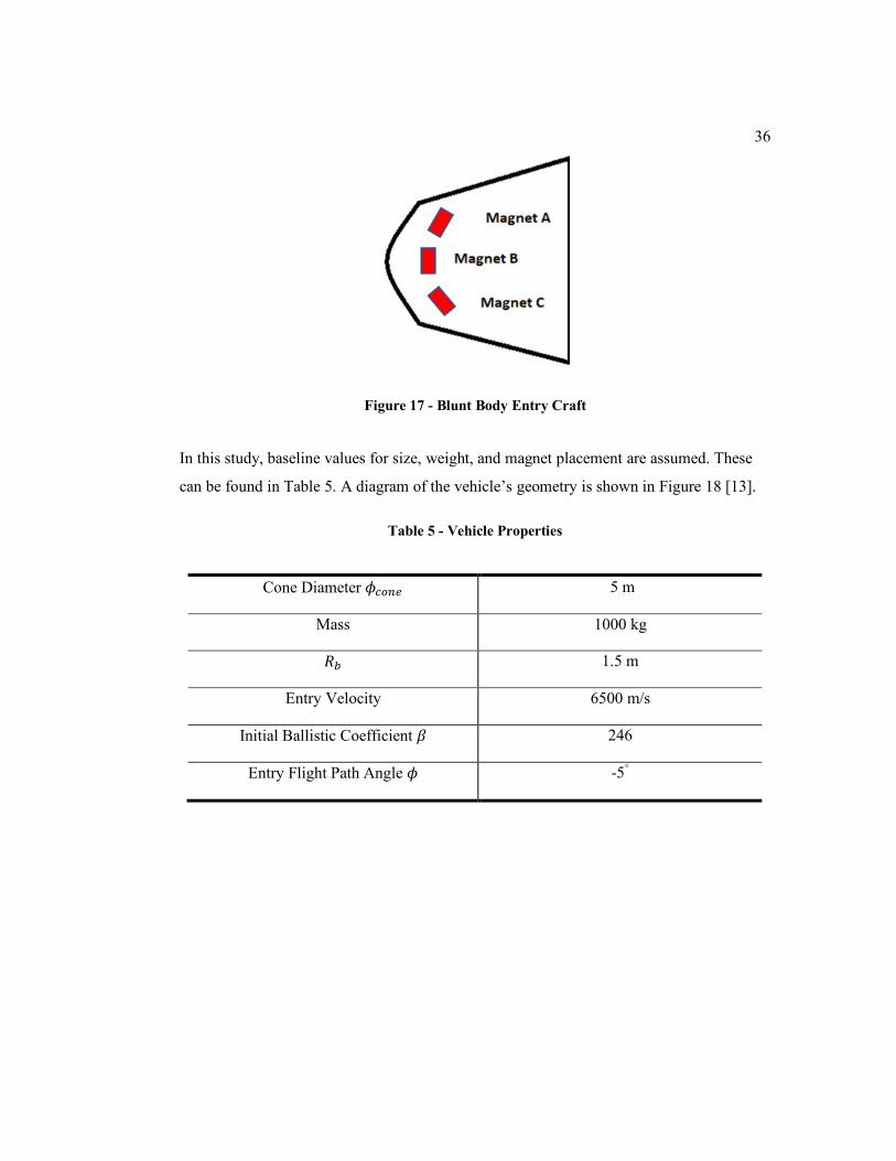
3.5 Entry Vehicle
The entry craft has three dipole magnets installed in the nose of the craft. One magnet is
placed parallel to the nose while two others are offset by 45⁰. Creo Parametric was used to
design the entry craft and a diagram of its layout can be found in Figure 17.
36
Figure 17 - Blunt Body Entry Craft
In this study, baseline values for size, weight, and magnet placement are assumed. These
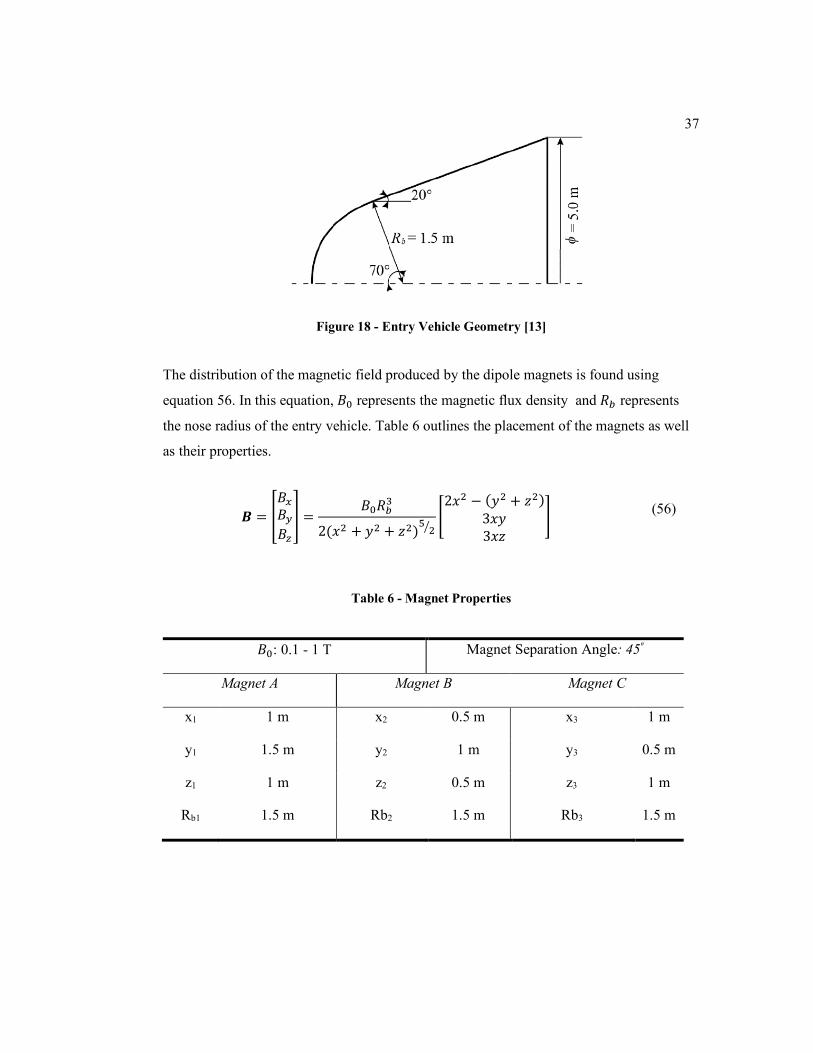
can be found in Table 5. A diagram of the vehicle’s geometry is shown in Figure 18 [13].
Table 5 - Vehicle Properties
Cone Diameter 𝜙𝑐𝑜𝑛𝑒 5 m
Mass 1000 kg
𝑅𝑏 1.5 m
Entry Velocity 6500 m/s
Initial Ballistic Coefficient 𝛽 246
Entry Flight Path Angle 𝜙 -5°
37
Figure 18 - Entry Vehicle Geometry [13]
The distribution of the magnetic field produced by the dipole magnets is found using
equation 56. In this equation, 𝐵0 represents the magnetic flux density and 𝑅𝑏 represents
the nose radius of the entry vehicle. Table 6 outlines the placement of the magnets as well
as their properties.
𝑩 = [
𝐵𝑥
𝐵𝑦
𝐵𝑧
] =𝐵0𝑅𝑏
3
2(𝑥2 + 𝑦2 + 𝑧2)5
2⁄[2𝑥2 − (𝑦2 + 𝑧2)
3𝑥𝑦3𝑥𝑧
] (56)
Table 6 - Magnet Properties
𝐵0: 0.1 - 1 T Magnet Separation Angle: 45⁰
Magnet A Magnet B Magnet C
x1 1 m x2 0.5 m x3 1 m
y1 1.5 m y2 1 m y3 0.5 m
z1 1 m z2 0.5 m z3 1 m
Rb1 1.5 m Rb2 1.5 m Rb3 1.5 m
38
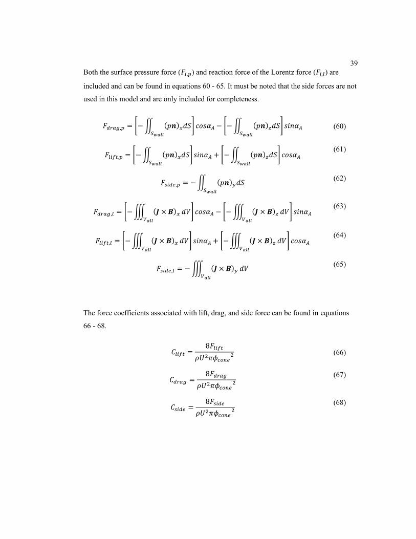
3.6 Electrodynamic Force
The forces of lift and drag exerted on the entry vehicle are a combination of the surface
pressure and the force attributed to the reaction to the Lorentz force. Equation 57
represents the drag force, equation 58 represents the lift force, and equation 59 represents
the side force.
𝐹𝑑𝑟𝑎𝑔 = 𝐹𝑑𝑟𝑎𝑔,𝑝 + 𝐹𝑑𝑟𝑎𝑔,𝑙 (57)
𝐹𝑙𝑖𝑓𝑡 = 𝐹𝑙𝑖𝑓𝑡,𝑝 + 𝐹𝑙𝑖𝑓𝑡,𝑙 (58)
𝐹𝑠𝑖𝑑𝑒 = 𝐹𝑠𝑖𝑑𝑒,𝑝 + 𝐹𝑠𝑖𝑑𝑒,𝑙 (59)
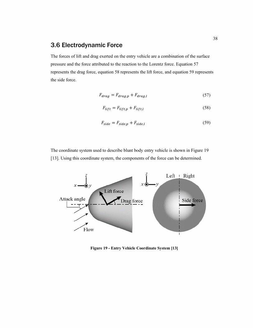
The coordinate system used to describe blunt body entry vehicle is shown in Figure 19
[13]. Using this coordinate system, the components of the force can be determined.
Figure 19 - Entry Vehicle Coordinate System [13]
39
Both the surface pressure force (𝐹𝑖,𝑝) and reaction force of the Lorentz force (𝐹𝑖,𝑙) are
included and can be found in equations 60 - 65. It must be noted that the side forces are not
used in this model and are only included for completeness.
𝐹𝑑𝑟𝑎𝑔,𝑝 = [−∬ (𝑝𝒏)𝑥𝑑𝑆
𝑆𝑤𝑎𝑙𝑙
] 𝑐𝑜𝑠𝛼𝐴 − [−∬ (𝑝𝒏)𝑧𝑑𝑆
𝑆𝑤𝑎𝑙𝑙
] 𝑠𝑖𝑛𝛼𝐴 (60)
𝐹𝑙𝑖𝑓𝑡,𝑝 = [−∬ (𝑝𝒏)𝑥𝑑𝑆
𝑆𝑤𝑎𝑙𝑙
] 𝑠𝑖𝑛𝛼𝐴 + [−∬ (𝑝𝒏)𝑧𝑑𝑆
𝑆𝑤𝑎𝑙𝑙
] 𝑐𝑜𝑠𝛼𝐴 (61)
𝐹𝑠𝑖𝑑𝑒,𝑝 = −∬ (𝑝𝒏)𝑦𝑑𝑆
𝑆𝑤𝑎𝑙𝑙
(62)
𝐹𝑑𝑟𝑎𝑔,𝑙 = [−∭ (𝑱 × 𝑩)𝑥
𝑉𝑎𝑙𝑙
𝑑𝑉] 𝑐𝑜𝑠𝛼𝐴 − [−∭ (𝑱 × 𝑩)𝑧
𝑉𝑎𝑙𝑙
𝑑𝑉] 𝑠𝑖𝑛𝛼𝐴 (63)
𝐹𝑙𝑖𝑓𝑡,𝑙 = [−∭ (𝑱 × 𝑩)𝑥
𝑉𝑎𝑙𝑙
𝑑𝑉] 𝑠𝑖𝑛𝛼𝐴 + [−∭ (𝑱 × 𝑩)𝑧
𝑉𝑎𝑙𝑙
𝑑𝑉] 𝑐𝑜𝑠𝛼𝐴 (64)
𝐹𝑠𝑖𝑑𝑒,𝑙 = −∭ (𝑱 × 𝑩)𝑦
𝑉𝑎𝑙𝑙
𝑑𝑉 (65)
The force coefficients associated with lift, drag, and side force can be found in equations
66 - 68.
𝐶𝑙𝑖𝑓𝑡 =8𝐹𝑙𝑖𝑓𝑡
𝜌𝑈2𝜋𝜙𝑐𝑜𝑛𝑒2 (66)
𝐶𝑑𝑟𝑎𝑔 =8𝐹𝑑𝑟𝑎𝑔
𝜌𝑈2𝜋𝜙𝑐𝑜𝑛𝑒2
(67)
𝐶𝑠𝑖𝑑𝑒 =8𝐹𝑠𝑖𝑑𝑒
𝜌𝑈2𝜋𝜙𝑐𝑜𝑛𝑒2
(68)
40
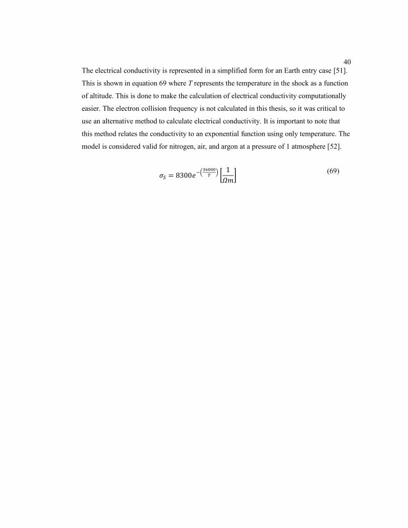
The electrical conductivity is represented in a simplified form for an Earth entry case [51].
This is shown in equation 69 where T represents the temperature in the shock as a function
of altitude. This is done to make the calculation of electrical conductivity computationally
easier. The electron collision frequency is not calculated in this thesis, so it was critical to
use an alternative method to calculate electrical conductivity. It is important to note that
this method relates the conductivity to an exponential function using only temperature. The
model is considered valid for nitrogen, air, and argon at a pressure of 1 atmosphere [52].
𝜎𝑆 = 8300𝑒−(
36000
𝑇) [
1
𝛺𝑚]
(69)
41
Chapter 4
Results and Discussion
4.1 Model Validation
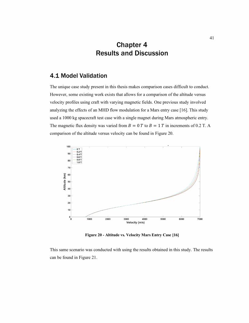
The unique case study present in this thesis makes comparison cases difficult to conduct.
However, some existing work exists that allows for a comparison of the altitude versus
velocity profiles using craft with varying magnetic fields. One previous study involved
analyzing the effects of an MHD flow modulation for a Mars entry case [16]. This study
used a 1000 kg spacecraft test case with a single magnet during Mars atmospheric entry.
The magnetic flux density was varied from 𝐵 = 0 𝑇 to 𝐵 = 1 𝑇 in increments of 0.2 T. A
comparison of the altitude versus velocity can be found in Figure 20.
Figure 20 - Altitude vs. Velocity Mars Entry Case [16]
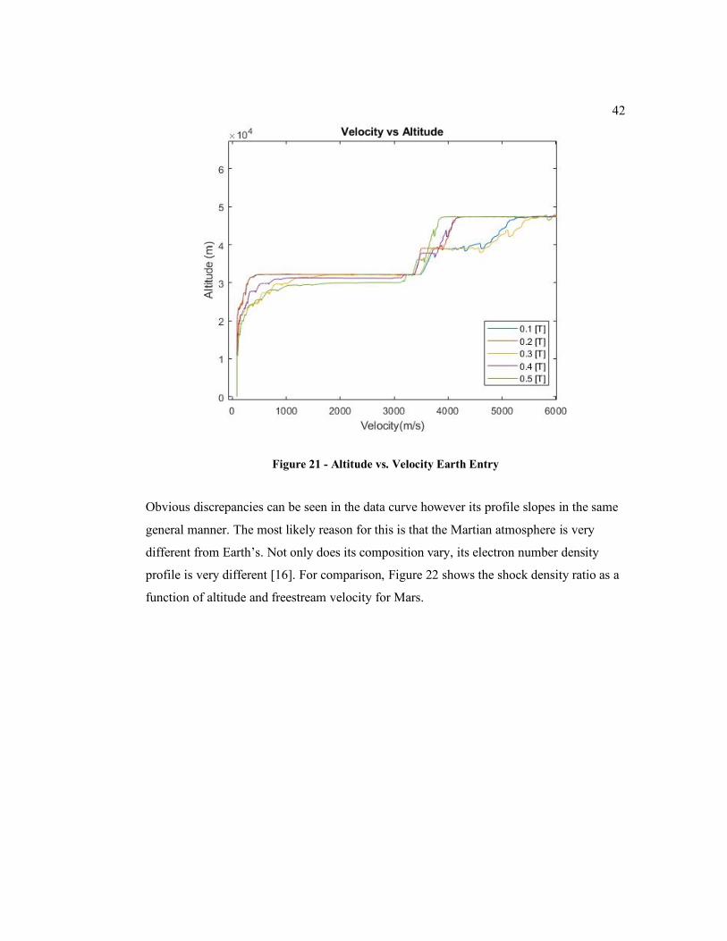
This same scenario was conducted with using the results obtained in this study. The results
can be found in Figure 21.
42
Figure 21 - Altitude vs. Velocity Earth Entry
Obvious discrepancies can be seen in the data curve however its profile slopes in the same
general manner. The most likely reason for this is that the Martian atmosphere is very
different from Earth’s. Not only does its composition vary, its electron number density
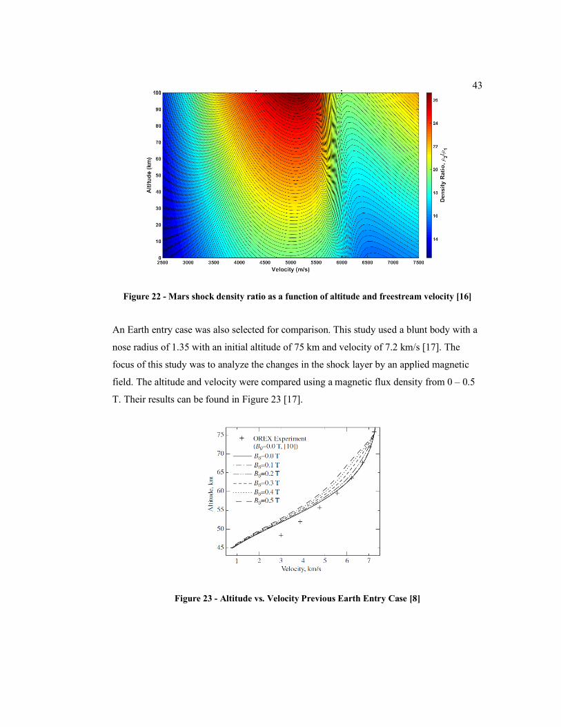
profile is very different [16]. For comparison, Figure 22 shows the shock density ratio as a
function of altitude and freestream velocity for Mars.
43
Figure 22 - Mars shock density ratio as a function of altitude and freestream velocity [16]
An Earth entry case was also selected for comparison. This study used a blunt body with a
nose radius of 1.35 with an initial altitude of 75 km and velocity of 7.2 km/s [17]. The
focus of this study was to analyze the changes in the shock layer by an applied magnetic
field. The altitude and velocity were compared using a magnetic flux density from 0 – 0.5
T. Their results can be found in Figure 23 [17].
Figure 23 - Altitude vs. Velocity Previous Earth Entry Case [8]
44
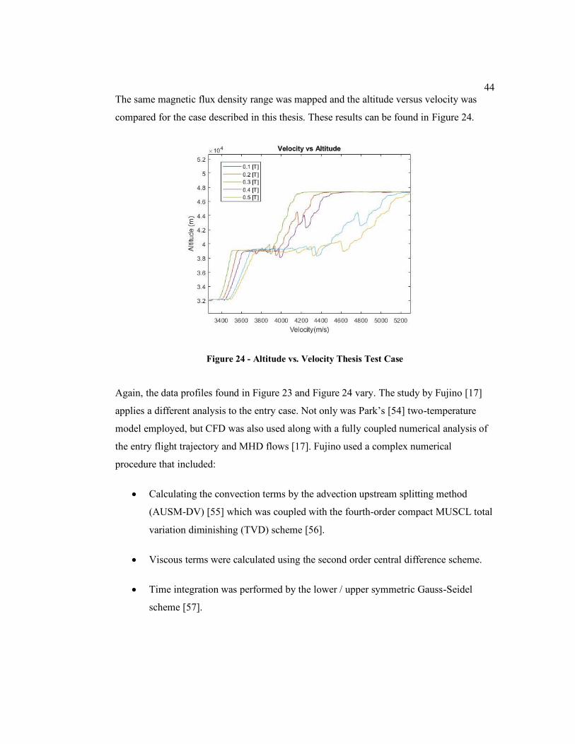
The same magnetic flux density range was mapped and the altitude versus velocity was
compared for the case described in this thesis. These results can be found in Figure 24.
Figure 24 - Altitude vs. Velocity Thesis Test Case
Again, the data profiles found in Figure 23 and Figure 24 vary. The study by Fujino [17]
applies a different analysis to the entry case. Not only was Park’s [54] two-temperature
model employed, but CFD was also used along with a fully coupled numerical analysis of
the entry flight trajectory and MHD flows [17]. Fujino used a complex numerical
procedure that included:
• Calculating the convection terms by the advection upstream splitting method
(AUSM-DV) [55] which was coupled with the fourth-order compact MUSCL total
variation diminishing (TVD) scheme [56].
• Viscous terms were calculated using the second order central difference scheme.
• Time integration was performed by the lower / upper symmetric Gauss-Seidel
scheme [57].
45
This drastic difference in methodology assists with explaining the discrepancy between this
study and Fujino’s [17].
It should be noted that the change in dynamic pressure and aerodynamic heat rate due to
the magnetic field were not part of this study. The results obtained for these values are
included in Figure 128 and Figure 129 which can be found in Appendix K. This was done
to show that there was little variation in their values depending on magnetic flux density.
Based on previous studies [17,58], the heat rate and pressure should fluctuate more
drastically. This furthers the case for conducting further analysis using alternative methods.
4.2 Summary of Model Validation
A Simulink model was designed using the analytical equations described by previous work
by Fujino [13]. These equations were used to find the 𝐿 𝐷⁄𝑙𝑜𝑟𝑒𝑛𝑡𝑧 forces based on the entry
craft characteristics and active magnetic field. The lift and drag forces produced by the
Simulink model were then applied to a modified MATLAB entry model originally
developed by Tewari [34] and the entry dynamics were analyzed.
Two previous studies were then analyzed to validate the results obtained in this work. The
first study involved analyzing the effects of an MHD flow modulation for a Mars entry
case [16]. Altitude versus velocity of a 1000 kg spacecraft were plotted as the magnetic
flux density is varied from 𝐵 = 0 𝑇 to 𝐵 = 1 𝑇. Figure 20 and Figure 21 compared these
results and the discrepancies were discussed with the most notable difference being that
this study was an Earth entry case and the comparison case was a Mars atmospheric entry.
The difference in shock density ratio as a function of altitude and velocity was highlighted
for Earth and Mars’ atmosphere in Figure 15 and Figure 22.
The second comparison case was an Earth atmospheric entry study [17]. The altitude
versus velocity plots were compared as the magnetic flux density was varied from 𝐵 =
0 .1 𝑇 to 𝐵 = 0.5 𝑇. Their results can be found in Figure 23 and Figure 24. These plots
showed similar profiles, however major discrepancies exist due to a different methodology
being employed. This was discussed in greater detail in the previous section.
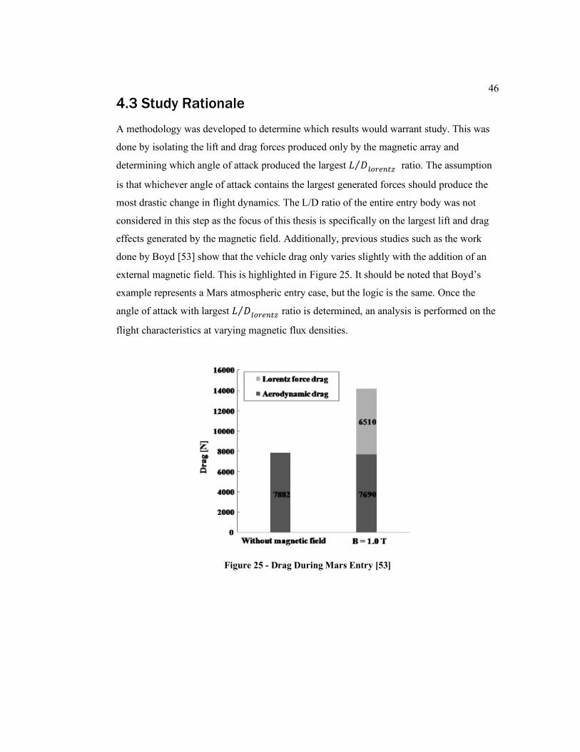
46
4.3 Study Rationale
A methodology was developed to determine which results would warrant study. This was
done by isolating the lift and drag forces produced only by the magnetic array and
determining which angle of attack produced the largest 𝐿 𝐷⁄𝑙𝑜𝑟𝑒𝑛𝑡𝑧 ratio. The assumption
is that whichever angle of attack contains the largest generated forces should produce the
most drastic change in flight dynamics. The L/D ratio of the entire entry body was not
considered in this step as the focus of this thesis is specifically on the largest lift and drag
effects generated by the magnetic field. Additionally, previous studies such as the work
done by Boyd [53] show that the vehicle drag only varies slightly with the addition of an
external magnetic field. This is highlighted in Figure 25. It should be noted that Boyd’s
example represents a Mars atmospheric entry case, but the logic is the same. Once the
angle of attack with largest 𝐿 𝐷⁄𝑙𝑜𝑟𝑒𝑛𝑡𝑧 ratio is determined, an analysis is performed on the
flight characteristics at varying magnetic flux densities.
Figure 25 - Drag During Mars Entry [53]
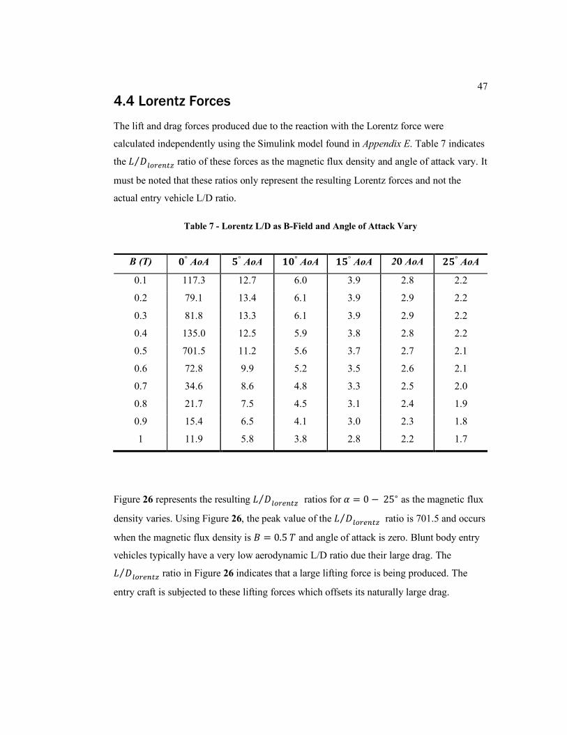
47
4.4 Lorentz Forces
The lift and drag forces produced due to the reaction with the Lorentz force were
calculated independently using the Simulink model found in Appendix E. Table 7 indicates
the 𝐿 𝐷⁄𝑙𝑜𝑟𝑒𝑛𝑡𝑧 ratio of these forces as the magnetic flux density and angle of attack vary. It
must be noted that these ratios only represent the resulting Lorentz forces and not the
actual entry vehicle L/D ratio.
Table 7 - Lorentz L/D as B-Field and Angle of Attack Vary
B (T) 𝟎° AoA 𝟓° AoA 𝟏𝟎° AoA 𝟏𝟓° AoA 2𝟎 AoA 𝟐𝟓° AoA
0.1 117.3 12.7 6.0 3.9 2.8 2.2
0.2 79.1 13.4 6.1 3.9 2.9 2.2
0.3 81.8 13.3 6.1 3.9 2.9 2.2
0.4 135.0 12.5 5.9 3.8 2.8 2.2
0.5 701.5 11.2 5.6 3.7 2.7 2.1
0.6 72.8 9.9 5.2 3.5 2.6 2.1
0.7 34.6 8.6 4.8 3.3 2.5 2.0
0.8 21.7 7.5 4.5 3.1 2.4 1.9
0.9 15.4 6.5 4.1 3.0 2.3 1.8
1 11.9 5.8 3.8 2.8 2.2 1.7
Figure 26 represents the resulting 𝐿 𝐷⁄𝑙𝑜𝑟𝑒𝑛𝑡𝑧 ratios for 𝛼 = 0 − 25∘ as the magnetic flux
density varies. Using Figure 26, the peak value of the 𝐿 𝐷⁄𝑙𝑜𝑟𝑒𝑛𝑡𝑧 ratio is 701.5 and occurs
when the magnetic flux density is 𝐵 = 0.5 𝑇 and angle of attack is zero. Blunt body entry
vehicles typically have a very low aerodynamic L/D ratio due their large drag. The
𝐿 𝐷⁄𝑙𝑜𝑟𝑒𝑛𝑡𝑧 ratio in Figure 26 indicates that a large lifting force is being produced. The
entry craft is subjected to these lifting forces which offsets its naturally large drag.
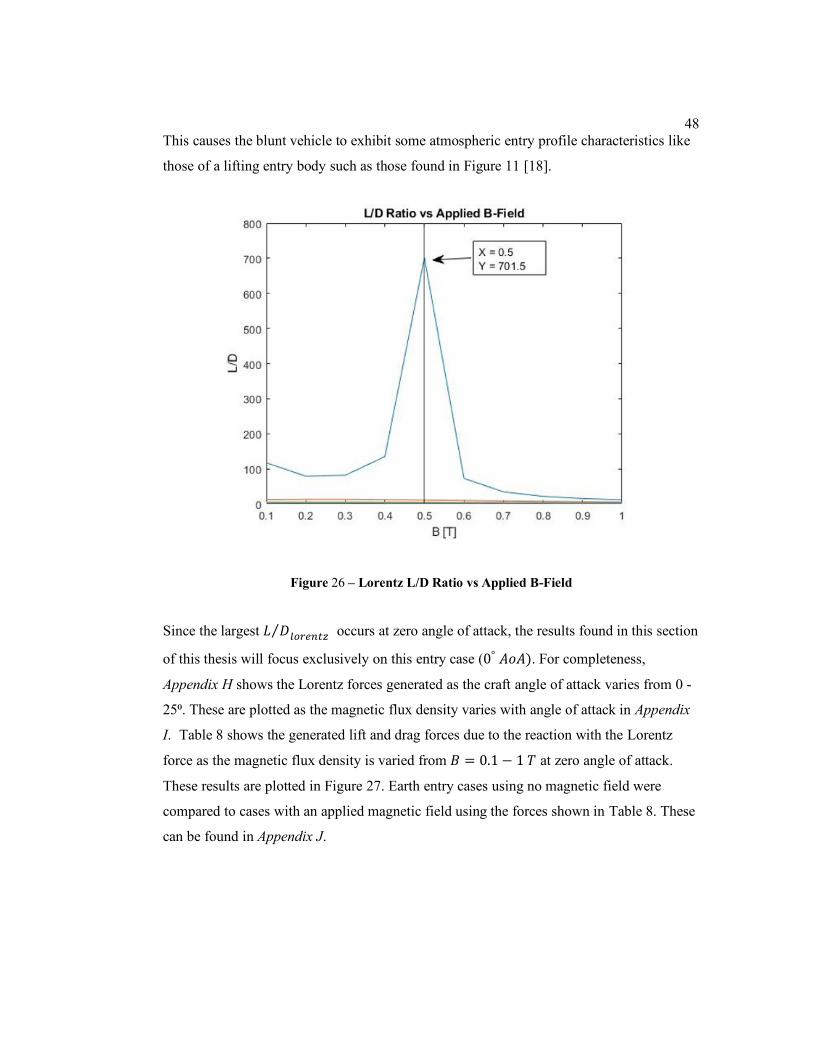
48
This causes the blunt vehicle to exhibit some atmospheric entry profile characteristics like
those of a lifting entry body such as those found in Figure 11 [18].
Figure 26 – Lorentz L/D Ratio vs Applied B-Field
Since the largest 𝐿 𝐷⁄𝑙𝑜𝑟𝑒𝑛𝑡𝑧 occurs at zero angle of attack, the results found in this section
of this thesis will focus exclusively on this entry case (0° 𝐴𝑜𝐴). For completeness,
Appendix H shows the Lorentz forces generated as the craft angle of attack varies from 0 -
25⁰. These are plotted as the magnetic flux density varies with angle of attack in Appendix
I. Table 8 shows the generated lift and drag forces due to the reaction with the Lorentz
force as the magnetic flux density is varied from 𝐵 = 0.1 − 1 𝑇 at zero angle of attack.
These results are plotted in Figure 27. Earth entry cases using no magnetic field were
compared to cases with an applied magnetic field using the forces shown in Table 8. These
can be found in Appendix J.
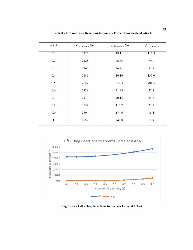
49
Table 8 - Lift and Drag Reactions to Lorentz Force: Zero Angle of Attack
B (T) 𝐹𝑙𝑖𝑓𝑡𝑙𝑜𝑟𝑒𝑛𝑡𝑧 (N) 𝐹𝑑𝑟𝑎𝑔𝑙𝑜𝑟𝑒𝑛𝑡𝑧
(N) 𝐿 𝐷⁄𝑙𝑜𝑟𝑒𝑛𝑡𝑧
0.1 2125 18.11 117.3
0.2 2125 26.85 79.1
0.3 2145 26.21 81.8
0.4 2186 16.19 135.0
0.5 2247 3.203 701.5
0.6 2328 31.98 72.8
0.7 2430 70.13 34.6
0.8 2552 117.7 21.7
0.9 2694 174.6 15.4
1 2857 240.8 11.9
Figure 27 - Lift - Drag Reactions to Lorentz Force at 0 AoA
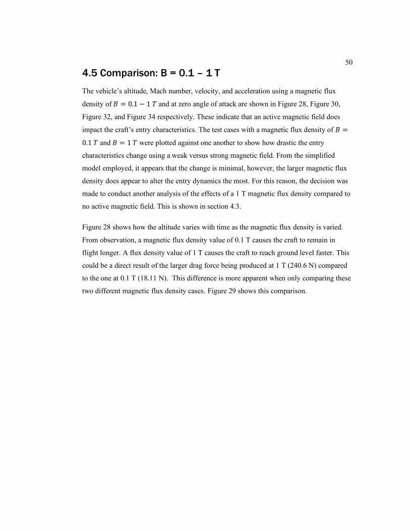
50
4.5 Comparison: B = 0.1 – 1 T
The vehicle’s altitude, Mach number, velocity, and acceleration using a magnetic flux
density of 𝐵 = 0.1 − 1 𝑇 and at zero angle of attack are shown in Figure 28, Figure 30,
Figure 32, and Figure 34 respectively. These indicate that an active magnetic field does
impact the craft’s entry characteristics. The test cases with a magnetic flux density of 𝐵 =
0.1 𝑇 and 𝐵 = 1 𝑇 were plotted against one another to show how drastic the entry
characteristics change using a weak versus strong magnetic field. From the simplified
model employed, it appears that the change is minimal, however, the larger magnetic flux
density does appear to alter the entry dynamics the most. For this reason, the decision was
made to conduct another analysis of the effects of a 1 T magnetic flux density compared to
no active magnetic field. This is shown in section 4.3.
Figure 28 shows how the altitude varies with time as the magnetic flux density is varied.
From observation, a magnetic flux density value of 0.1 T causes the craft to remain in
flight longer. A flux density value of 1 T causes the craft to reach ground level faster. This
could be a direct result of the larger drag force being produced at 1 T (240.6 N) compared
to the one at 0.1 T (18.11 N). This difference is more apparent when only comparing these
two different magnetic flux density cases. Figure 29 shows this comparison.
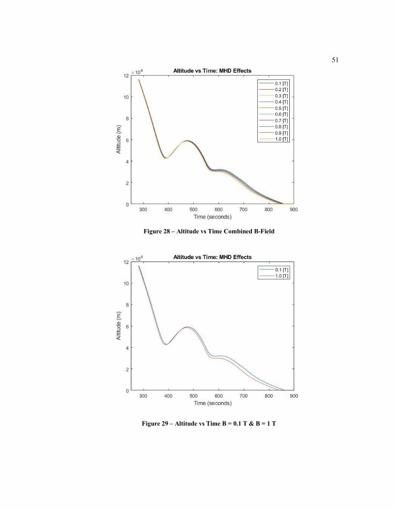
51
Figure 28 – Altitude vs Time Combined B-Field
Figure 29 – Altitude vs Time B = 0.1 T & B = 1 T
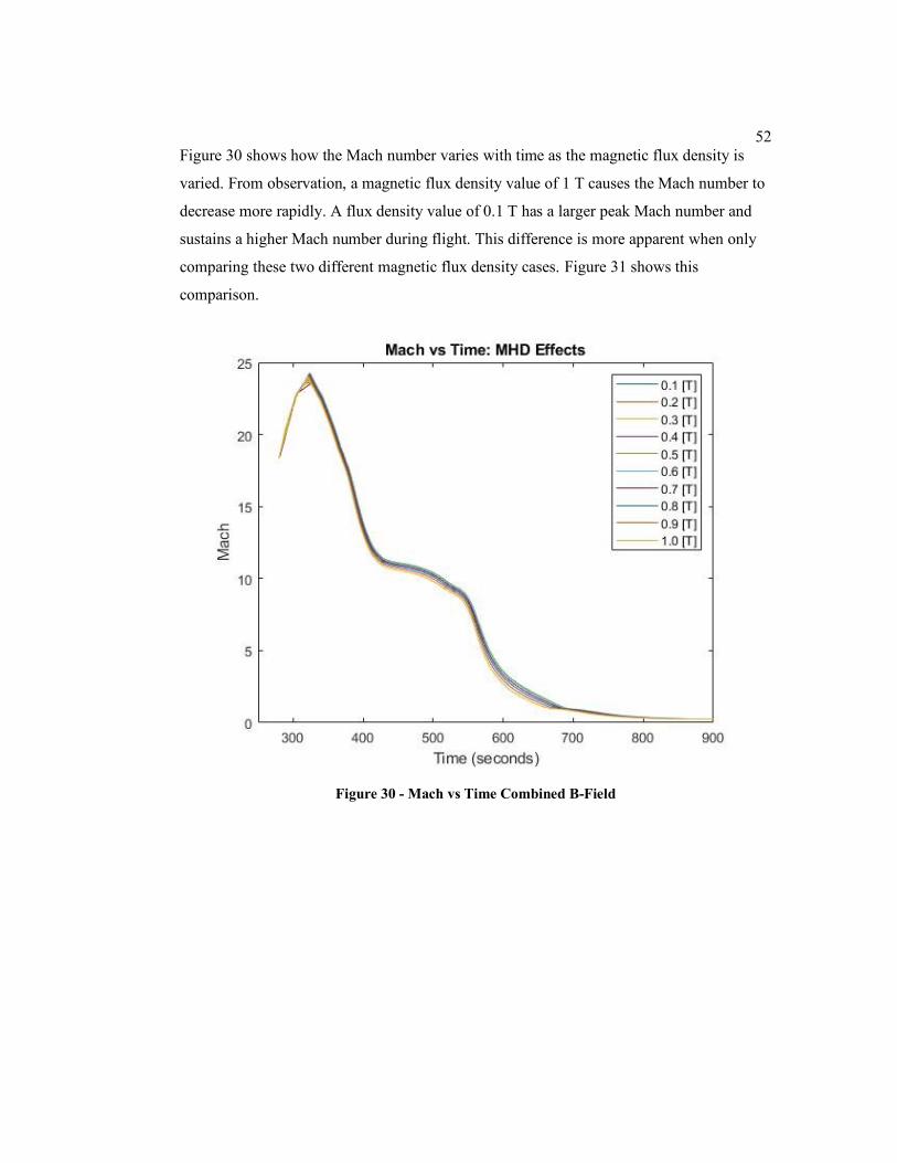
52
Figure 30 shows how the Mach number varies with time as the magnetic flux density is
varied. From observation, a magnetic flux density value of 1 T causes the Mach number to
decrease more rapidly. A flux density value of 0.1 T has a larger peak Mach number and
sustains a higher Mach number during flight. This difference is more apparent when only
comparing these two different magnetic flux density cases. Figure 31 shows this
comparison.
Figure 30 - Mach vs Time Combined B-Field
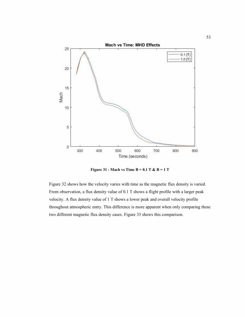
53
Figure 31 - Mach vs Time B = 0.1 T & B = 1 T
Figure 32 shows how the velocity varies with time as the magnetic flux density is varied.
From observation, a flux density value of 0.1 T shows a flight profile with a larger peak
velocity. A flux density value of 1 T shows a lower peak and overall velocity profile
throughout atmospheric entry. This difference is more apparent when only comparing these
two different magnetic flux density cases. Figure 33 shows this comparison.
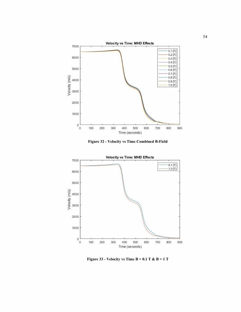
54
Figure 32 - Velocity vs Time Combined B-Field
Figure 33 - Velocity vs Time B = 0.1 T & B = 1 T
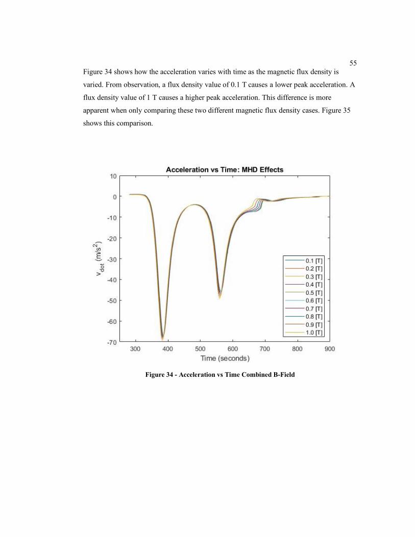
55
Figure 34 shows how the acceleration varies with time as the magnetic flux density is
varied. From observation, a flux density value of 0.1 T causes a lower peak acceleration. A
flux density value of 1 T causes a higher peak acceleration. This difference is more
apparent when only comparing these two different magnetic flux density cases. Figure 35
shows this comparison.
Figure 34 - Acceleration vs Time Combined B-Field
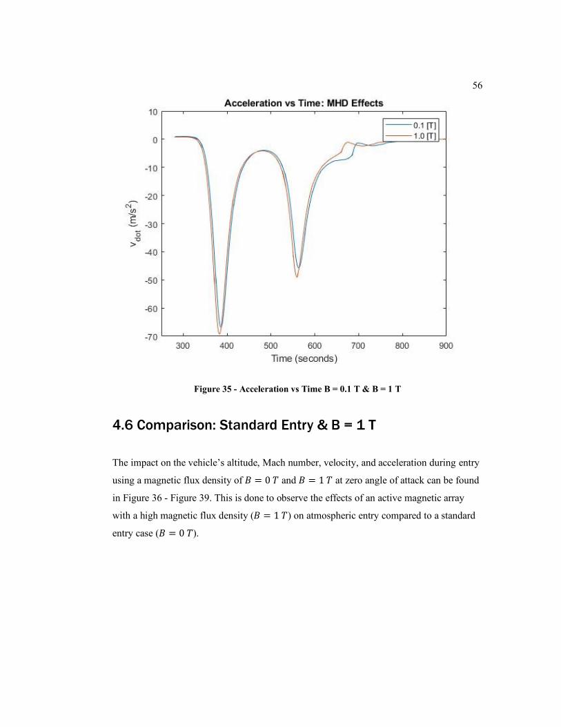
56
Figure 35 - Acceleration vs Time B = 0.1 T & B = 1 T
4.6 Comparison: Standard Entry & B = 1 T
The impact on the vehicle’s altitude, Mach number, velocity, and acceleration during entry
using a magnetic flux density of 𝐵 = 0 𝑇 and 𝐵 = 1 𝑇 at zero angle of attack can be found
in Figure 36 - Figure 39. This is done to observe the effects of an active magnetic array
with a high magnetic flux density (𝐵 = 1 𝑇) on atmospheric entry compared to a standard
entry case (𝐵 = 0 𝑇).
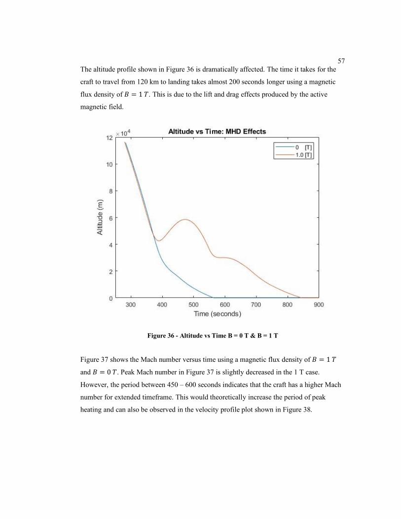
57
The altitude profile shown in Figure 36 is dramatically affected. The time it takes for the
craft to travel from 120 km to landing takes almost 200 seconds longer using a magnetic
flux density of 𝐵 = 1 𝑇. This is due to the lift and drag effects produced by the active
magnetic field.
Figure 36 - Altitude vs Time B = 0 T & B = 1 T
Figure 37 shows the Mach number versus time using a magnetic flux density of 𝐵 = 1 𝑇
and 𝐵 = 0 𝑇. Peak Mach number in Figure 37 is slightly decreased in the 1 T case.
However, the period between 450 – 600 seconds indicates that the craft has a higher Mach
number for extended timeframe. This would theoretically increase the period of peak
heating and can also be observed in the velocity profile plot shown in Figure 38.
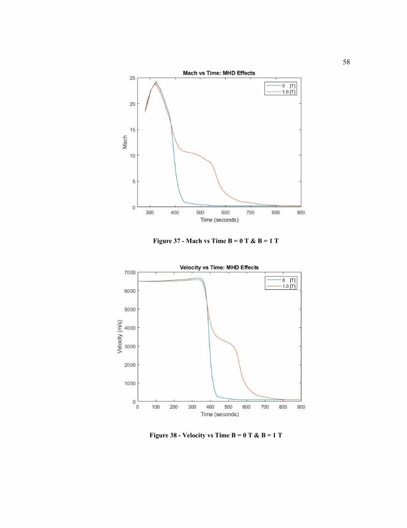
58
Figure 37 - Mach vs Time B = 0 T & B = 1 T
Figure 38 - Velocity vs Time B = 0 T & B = 1 T
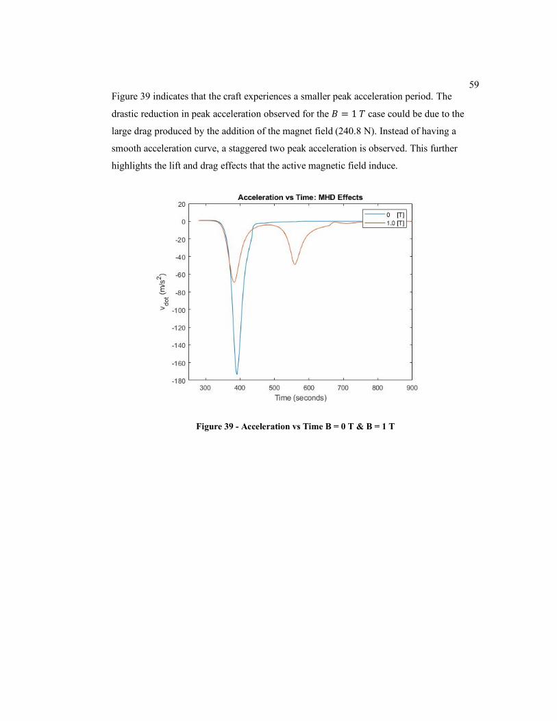
59
Figure 39 indicates that the craft experiences a smaller peak acceleration period. The
drastic reduction in peak acceleration observed for the 𝐵 = 1 𝑇 case could be due to the
large drag produced by the addition of the magnet field (240.8 N). Instead of having a
smooth acceleration curve, a staggered two peak acceleration is observed. This further
highlights the lift and drag effects that the active magnetic field induce.
Figure 39 - Acceleration vs Time B = 0 T & B = 1 T
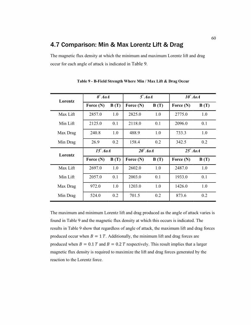
60
4.7 Comparison: Min & Max Lorentz Lift & Drag
The magnetic flux density at which the minimum and maximum Lorentz lift and drag
occur for each angle of attack is indicated in Table 9.
Table 9 - B-Field Strength Where Min / Max Lift & Drag Occur
Lorentz 0° AoA 5° AoA 10° AoA
Force (N) B (T) Force (N) B (T) Force (N) B (T)
Max Lift 2857.0 1.0 2825.0 1.0 2775.0 1.0
Min Lift 2125.0 0.1 2118.0 0.1 2096.0 0.1
Max Drag 240.8 1.0 488.9 1.0 733.3 1.0
Min Drag 26.9 0.2 158.4 0.2 342.5 0.2
Lorentz 15° AoA 20° AoA 25° AoA
Force (N) B (T) Force (N) B (T) Force (N) B (T)
Max Lift 2697.0 1.0 2602.0 1.0 2487.0 1.0
Min Lift 2057.0 0.1 2003.0 0.1 1933.0 0.1
Max Drag 972.0 1.0 1203.0 1.0 1426.0 1.0
Min Drag 524.0 0.2 701.5 0.2 873.6 0.2
The maximum and minimum Lorentz lift and drag produced as the angle of attack varies is
found in Table 9 and the magnetic flux density at which this occurs is indicated. The
results in Table 9 show that regardless of angle of attack, the maximum lift and drag forces
produced occur when 𝐵 = 1 𝑇. Additionally, the minimum lift and drag forces are
produced when 𝐵 = 0.1 𝑇 and 𝐵 = 0.2 𝑇 respectively. This result implies that a larger
magnetic flux density is required to maximize the lift and drag forces generated by the
reaction to the Lorentz force.

61
It is interesting to note that the lift force generated decreases as angle of attack is increased.
Since the magnetic field is projected out from a single point source, it is most effective
head on, or at zero angle of attack. As the angle of attack is increased, the effect of the
magnetic field becomes a component of the total field generated. This would explain the
decrease in lift force generated as the angle of attack increases.
4.8 Extended Analysis of Angle of Attack
The scope of this work included an analysis of how lift and drag forces generated due to
the reaction of the ionized flow and a magnetic field would vary with angle of attack. The
angle of attack was varied in increments of 5° from 0 - 25°. When the ratio of the lift and
drag forces was taken, it was determined that zero angle of attack would be the ideal
candidate based on the results shown in Figure 26. It was also an ideal angle of attack since
the interaction of the magnetic field and the flow would be when occurring head on.
However, the large ratio of 701.5 found at a magnetic flux density of 𝐵 = 0.5 𝑇 and zero
angle of attack appeared to be an outlier. For reference, at a magnetic flux density of 𝐵 =
0.4 𝑇, the 𝐿 𝐷⁄𝑙𝑜𝑟𝑒𝑛𝑡𝑧 ratio was 135 and at 𝐵 = 0.4 𝑇, the 𝐿 𝐷⁄
𝑙𝑜𝑟𝑒𝑛𝑡𝑧 ratio was 72.8.
An attempt was made to explore this large jump in 𝐿 𝐷⁄𝑙𝑜𝑟𝑒𝑛𝑡𝑧 ratio. To do this, the angle
of attack was varied from 0 - 1° in increments of 0.1°. A full table of these results can be
found in Appendix L. The lift forces generated as angle of attack and magnetic flux density
vary can be found in Table 10. These results indicate that the lift forces generated do not
vary significantly as the angle of attack is varied by such a small amount. It can also be
determined that lift forces generated increase as magnetic flux density increases.
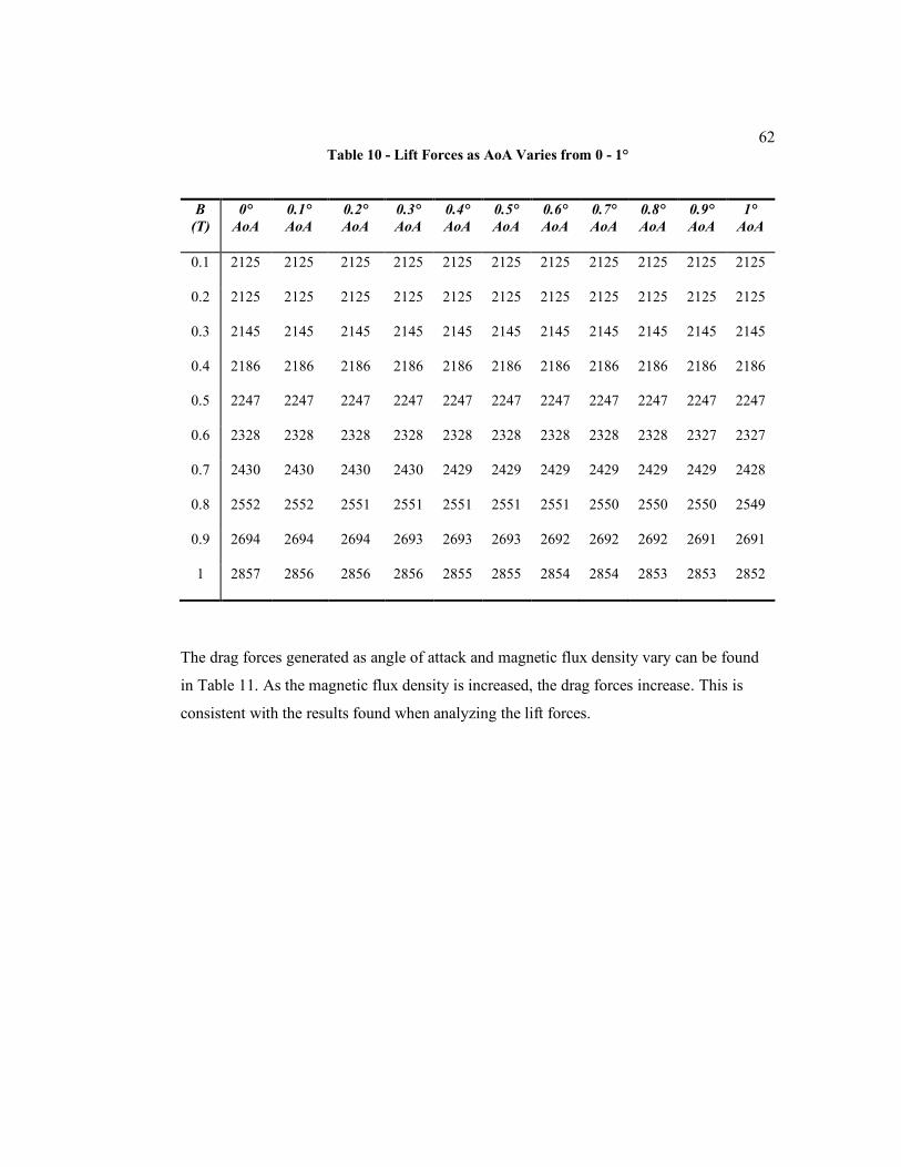
62
Table 10 - Lift Forces as AoA Varies from 0 - 1°
B
(T)
0°
AoA
0.1°
AoA
0.2°
AoA
0.3°
AoA
0.4°
AoA
0.5°
AoA
0.6°
AoA
0.7°
AoA
0.8°
AoA
0.9°
AoA
1°
AoA
0.1 2125 2125 2125 2125 2125 2125 2125 2125 2125 2125 2125
0.2 2125 2125 2125 2125 2125 2125 2125 2125 2125 2125 2125
0.3 2145 2145 2145 2145 2145 2145 2145 2145 2145 2145 2145
0.4 2186 2186 2186 2186 2186 2186 2186 2186 2186 2186 2186
0.5 2247 2247 2247 2247 2247 2247 2247 2247 2247 2247 2247
0.6 2328 2328 2328 2328 2328 2328 2328 2328 2328 2327 2327
0.7 2430 2430 2430 2430 2429 2429 2429 2429 2429 2429 2428
0.8 2552 2552 2551 2551 2551 2551 2551 2550 2550 2550 2549
0.9 2694 2694 2694 2693 2693 2693 2692 2692 2692 2691 2691
1 2857 2856 2856 2856 2855 2855 2854 2854 2853 2853 2852
The drag forces generated as angle of attack and magnetic flux density vary can be found
in Table 11. As the magnetic flux density is increased, the drag forces increase. This is
consistent with the results found when analyzing the lift forces.
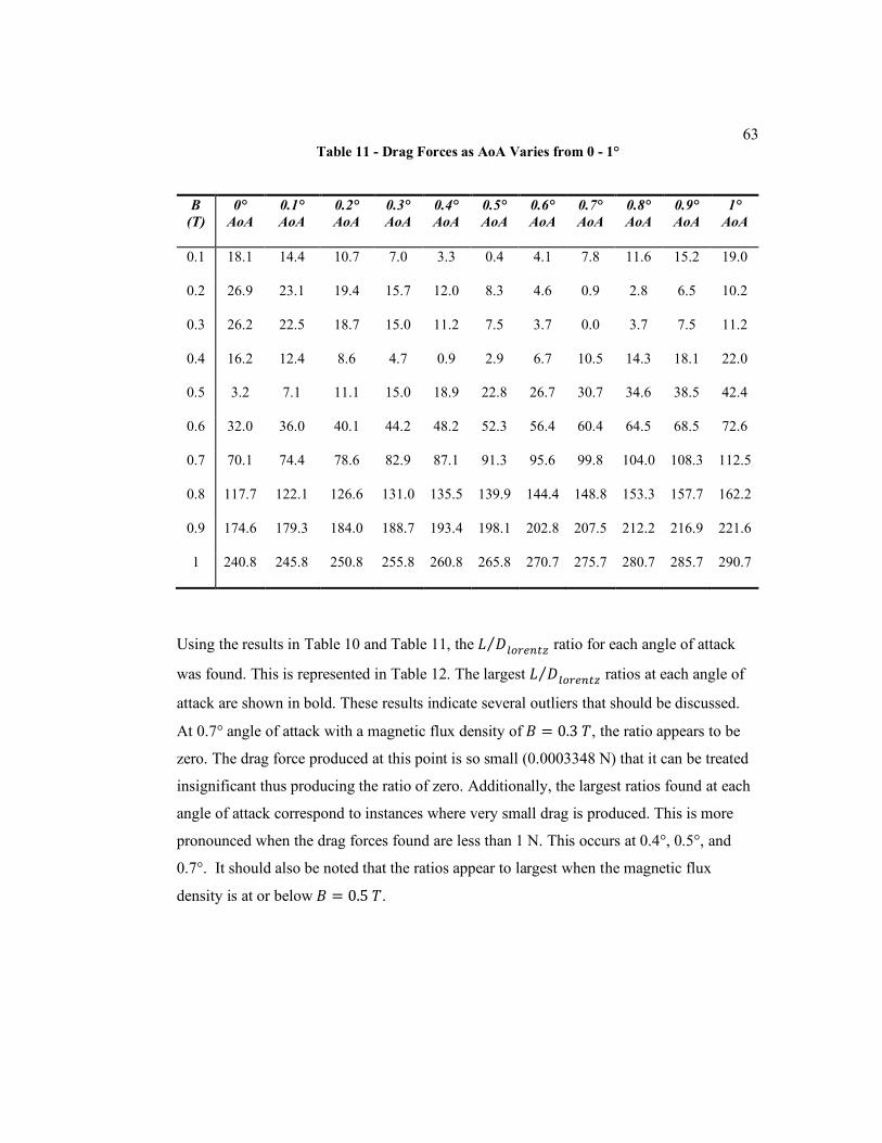
63
Table 11 - Drag Forces as AoA Varies from 0 - 1°
B
(T)
0°
AoA
0.1°
AoA
0.2°
AoA
0.3°
AoA
0.4°
AoA
0.5°
AoA
0.6°
AoA
0.7°
AoA
0.8°
AoA
0.9°
AoA
1°
AoA
0.1 18.1 14.4 10.7 7.0 3.3 0.4 4.1 7.8 11.6 15.2 19.0
0.2 26.9 23.1 19.4 15.7 12.0 8.3 4.6 0.9 2.8 6.5 10.2
0.3 26.2 22.5 18.7 15.0 11.2 7.5 3.7 0.0 3.7 7.5 11.2
0.4 16.2 12.4 8.6 4.7 0.9 2.9 6.7 10.5 14.3 18.1 22.0
0.5 3.2 7.1 11.1 15.0 18.9 22.8 26.7 30.7 34.6 38.5 42.4
0.6 32.0 36.0 40.1 44.2 48.2 52.3 56.4 60.4 64.5 68.5 72.6
0.7 70.1 74.4 78.6 82.9 87.1 91.3 95.6 99.8 104.0 108.3 112.5
0.8 117.7 122.1 126.6 131.0 135.5 139.9 144.4 148.8 153.3 157.7 162.2
0.9 174.6 179.3 184.0 188.7 193.4 198.1 202.8 207.5 212.2 216.9 221.6
1 240.8 245.8 250.8 255.8 260.8 265.8 270.7 275.7 280.7 285.7 290.7
Using the results in Table 10 and Table 11, the 𝐿 𝐷⁄𝑙𝑜𝑟𝑒𝑛𝑡𝑧 ratio for each angle of attack
was found. This is represented in Table 12. The largest 𝐿 𝐷⁄𝑙𝑜𝑟𝑒𝑛𝑡𝑧 ratios at each angle of
attack are shown in bold. These results indicate several outliers that should be discussed.
At 0.7° angle of attack with a magnetic flux density of 𝐵 = 0.3 𝑇, the ratio appears to be
zero. The drag force produced at this point is so small (0.0003348 N) that it can be treated
insignificant thus producing the ratio of zero. Additionally, the largest ratios found at each
angle of attack correspond to instances where very small drag is produced. This is more
pronounced when the drag forces found are less than 1 N. This occurs at 0.4°, 0.5°, and
0.7°. It should also be noted that the ratios appear to largest when the magnetic flux
density is at or below 𝐵 = 0.5 𝑇.
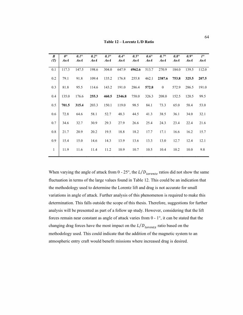
64
Table 12 – Lorentz L/D Ratio
B
(T)
0°
AoA
0.1°
AoA
0.2°
AoA
0.3°
AoA
0.4°
AoA
0.5°
AoA
0.6°
AoA
0.7°
AoA
0.8°
AoA
0.9°
AoA
1°
AoA
0.1 117.3 147.5 198.6 304.0 647.9 4962.6 513.7 270.9 184.0 139.5 112.0
0.2 79.1 91.8 109.4 135.2 176.8 255.8 462.1 2387.6 753.8 325.5 207.5
0.3 81.8 95.5 114.6 143.2 191.0 286.4 572.8 0 572.9 286.5 191.0
0.4 135.0 176.6 255.3 460.5 2346.8 758.0 326.3 208.0 152.5 120.5 99.5
0.5 701.5 315.4 203.3 150.1 119.0 98.5 84.1 73.3 65.0 58.4 53.0
0.6 72.8 64.6 58.1 52.7 48.3 44.5 41.3 38.5 36.1 34.0 32.1
0.7 34.6 32.7 30.9 29.3 27.9 26.6 25.4 24.3 23.4 22.4 21.6
0.8 21.7 20.9 20.2 19.5 18.8 18.2 17.7 17.1 16.6 16.2 15.7
0.9 15.4 15.0 14.6 14.3 13.9 13.6 13.3 13.0 12.7 12.4 12.1
1 11.9 11.6 11.4 11.2 10.9 10.7 10.5 10.4 10.2 10.0 9.8
When varying the angle of attack from 0 - 25°, the 𝐿 𝐷⁄𝑙𝑜𝑟𝑒𝑛𝑡𝑧 ratios did not show the same
fluctuation in terms of the large values found in Table 12. This could be an indication that
the methodology used to determine the Lorentz lift and drag is not accurate for small
variations in angle of attack. Further analysis of this phenomenon is required to make this
determination. This falls outside the scope of this thesis. Therefore, suggestions for further
analysis will be presented as part of a follow up study. However, considering that the lift
forces remain near constant as angle of attack varies from 0 - 1°, it can be stated that the
changing drag forces have the most impact on the 𝐿 𝐷⁄𝑙𝑜𝑟𝑒𝑛𝑡𝑧 ratio based on the
methodology used. This could indicate that the addition of the magnetic system to an
atmospheric entry craft would benefit missions where increased drag is desired.
65
Chapter 5
Conclusion
Although a spacecraft reentering the Earth’s atmosphere experiences multiple flight
regimes, the focus of this study was specifically on the ionization component of hypersonic
flight. Using a modified atmospheric entry MATLAB code based on the work of Tewari
[34] and a Simulink model developed using the principles in [13], a unique analysis was
conducted on a blunt body craft. This spacecraft design included three magnets housed
near the nose capable of producing an active magnetic field of varying strength.
The following questions were posed in the scope of thesis section:
1. Using a simplified atmosphere and gas dynamics model, can an active magnetic
field change the flight profile of a blunt body entry vehicle?
The results of this analysis indicate that the flight profile of a blunt body vehicle with an
active magnetic array during atmospheric entry does change. This is highlighted in Figure
36 - Figure 39 and in the results located in Appendix J. The point of this work was to
determine if the flight profile would change. Considering this, it should be clearly stated
that a higher fidelity model needs to be used to quantify the exact changes to the flight
profile. The methodology used in this thesis is meant only to show that changes to the
flight profile should occur. The magnitude of these changes is outside the scope of work
and will be a component of the suggested follow up study.
2. Can variations in the magnetic flux density be used to control the entry trajectory?
Since a change in the flight profile is observed, it is important to analyze the effects that
various magnetic flux densities have. As the magnetic flux density is varied from 𝐵 =
0.1 − 1 𝑇, the altitude, Mach number, velocity, and acceleration are all impacted. Figure
28, Figure 30, Figure 32, and Figure 34 show the magnitude of these changes with every
magnetic flux density compared against one another (respectively).
66
To visualize the difference of having a weak (0.1 T) and strong (1 T) magnetic flux
density, these two test cases were plotted against one another. This is shown in Figure 29,
Figure 31, Figure 33, and Figure 35. Although there is only a slight difference in
magnitude of these results, it can be confirmed that there is an impact that varies with
strength of magnetic field. For completeness, each flight characteristic was plotted against
a test case with no magnetic field and the results can be found in Appendix J. Again, it
should be stated that exact changes to the trajectory are not fully represented in this work.
The results shown only indicate that as the magnetic flux density is increased, a change
should occur. The suggested follow up study includes a more accurate analysis regarding
the impact of the increasing flux density on the flight trajectory.
3. Do the lift and drag forces produced by the reaction to the Lorentz force
(𝐿 𝐷⁄𝑙𝑜𝑟𝑒𝑛𝑡𝑧) vary with angle of attack?
The reaction to the Lorentz force (𝐿 𝐷⁄𝑙𝑜𝑟𝑒𝑛𝑡𝑧) was calculated using a magnetic flux
density that varied from 𝐵 = 0.1 − 1 𝑇 while the angle of attack was varied from 0 – 25° in
increments of 5°. The resulting 𝐿 𝐷⁄𝑙𝑜𝑟𝑒𝑛𝑡𝑧 forces can be found in Table 20 located in
Appendix H. These results were plotted in Appendix I against one another and include a test
case with no active magnetic field. A follow up analysis of the changing lift and drag
forces as angle of attack is varied from 0 – 1° in increments of 0.1° is included in section
4.8.
In summary, this thesis sought to analyze the effects between an active magnetic field and
the ionized flow regime present during hypersonic flight. Using a varying magnetic flux
density, this study showed that liftlorentz and draglorentz forces can be produced. An attempt
was also made to show how the addition of a magnetic field impacts atmospheric entry
dynamics. The benefits of such a system are based on mission need and can be applied to
achieve increased drag and lift and controllability. This study has laid the groundwork for
future analysis.
67
5.1 Suggestions for Future Work
This study was primarily conducted to justify a more in depth and detailed analysis. The
work done here represents a good baseline that further studies could build on. Therefore,
suggestions for future work are included. These highlight a natural progression in the
analysis of the concept presented in this thesis. One suggestion is to attempt to vary the
strength of each magnet. This was not done in this study due to time constraints. However,
the Simulink model shown in Appendix E can do this by establishing a new value of 𝐵0 for
each magnet. The separation angles for the magnets would have to be considered by taking
the sine and cosine of the magnets force to determine its effect on lift and drag. The effects
of varying the field strength of each magnet could also be further explored and validated
based on cases where a desired heat rate, drag, and flight profile are initially stated and
investigated. Once this is done, a proper control algorithm can be developed that attempts
to mitigate each of these entry characteristics
Another suggestion is to include a proper CFD analysis of the entry craft such as the one
conducted by Shafeeque [59]. This work could be further bolstered by coupling the
numerical analysis of atmospheric entry done by of Fujino [17] and Berton [60] with the
magnetohydrodynamic flow analysis conducted by Macheret [19]. Also, the work by
Guarendi and Chandy which studies hypersonic flow over a cylinder using axial and
transverse oriented magnetic dipoles using ANSYS CFX would be a good test case to use
for comparison [61]. Beyond using CFD for analysis, the addition of an ablating surface
would represent a more realistic example of an entry craft as modern spacecraft typically
use these. The recent work by Bityurin which focuses on MHD heat flux mitigation in
hypersonic flow around a blunt body with an ablating surface is a good candidate for
continued study into the effects of an ablating surface [62]. When combined with the
suggested variable field control of the three-magnet configuration presented in this thesis, a
fully realized methodology could be developed. This would allow for more accurate case
comparisons involving previous atmospheric entry craft and the one proposed in this thesis.
68
References
[1] J. R. Wilson, “The emerging world of hypersonic weapons technology,” Military &
Aerospace Electronics, 01-May-2019. [Online]. Available:
https://www.militaryaerospace.com/power/article/14033431/the-emerging-world-
of-hypersonic-weapons-technology. [Accessed: 17-Mar-2020].
[2] K. M. Sayler, “Hypersonic Weapons: Background and Issues for
Congress,” Congressional Research Service, 04-Mar-2020. [Online]. Available:
https://crsreports.congress.gov/product/pdf/R/R45811. [Accessed: 17-Mar-2020].
[3] L. Obringer, “Hypersonics and Space Technologies,” NASA, 26-Oct-2015. [Online].
Available: https://www.nasa.gov/feature/hypersonics-and-space-technologies.
[Accessed: 17-Mar-2020].
[4] “Air Force conducts successful hypersonic weapon flight test,” U.S. Air Force, 13-Jun-
2019. [Online]. Available: https://www.af.mil/News/Article-
Display/Article/1874470/air-force-conducts-successful-hypersonic-weapon-flight-
test/. [Accessed: 17-Mar-2020].
[5] “Hypersonic research spotlights future flight challenges,” ScienceDaily, 08-Oct-2019.
[Online]. Available:
https://www.sciencedaily.com/releases/2019/10/191008094247.htm. [Accessed:
17-Mar-2020].
[6] H. J. Allen and A. J. Eggars., “A study of the motion and aerodynamic heating of
ballistic missiles entering the earth’s atmosphere at high supersonic speeds,”
NACA Report 1381., 1958.
[7] R. C. Meyer, “On Reducing Aerodynamic Heat-Transfer Rates by
Magnetohydrodynamic Techniques,” Journal of the Aerospace Sciences, vol. 25,
no. 9, pp. 561–566, 1958.
[8] R. W. Moses, “Regenerative Aerobraking,” AIP Conference Proceedings, Jan. 2005.
[9] Y. Nagata, K. Yamada, T. Abe, and S. Yanase, “MHD Heat Shield in Argon Arcjet
Plasma Flow,” Japan-Russia Workshop on Supercomputer Modelling, Instability
and Turbulence in Fluid Dynamics (JR SMIT2015), Moscow, March 4–6, 2015.
[10] W. B. Bush, “Magnetohydrodynamic-Hypersonic Flow Past a Blunt Body,” Journal
of the Aerospace Sciences, vol. 25, no. 11, pp. 685–690, 1958.
69
[11] V. Bityurin, A. Bocharov, and J. Lineberry, “MHD Flow Control in Hypersonic
Flight,” AIAA/CIRA 13th International Space Planes and Hypersonics Systems and
Technologies Conference, 2005.
[12] H. Otsu, A. Matsuda, T. Abe, and D. Konigorski, “Feasibility Study on the Flight Demonstration for a reentry vehicle with the Magnetic Flow Control System,” 37th
AIAA Plasmadynamics and Lasers Conference, May 2006.
[13] K. Masuda, Y. Shimosawa, and T. Fujino, “Influence of Attack Angle on Magnetohydrodynamic Flow Control in Reentry Flight,” Transactions of The
Japan Society For Aeronautical And Space Sciences, Aerospace Technology
Japan, vol. 14, no. ists30, 2016.
[14] Y. Imamura and T. Fujino, “Numerical Simulation of Magnetohydrodynamic Flow
Control in Reentry Flight with Three-Temperature Model,” 2018 AIAA Aerospace
Sciences Meeting, Jul. 2018.
[15] T. Yoshino, T. Fujino, and M. Ishikawa, “Possibility of Thermal Protection in Earth Re-entry Flight by MHD Flow Control with Air-Core Circular Magnet,” IEEJ
Transactions on Electrical and Electronic Engineering, vol. 4, no. 4, pp. 510–517,
2009.
[16] H. K. Ali and R. D. Braun, “Effects of Magnetohydrodynamic Energy Generation on
Planetary Entry Vehicle Flight Dynamics,” 13th International Energy Conversion
Engineering Conference, 2015.
[17] T. Fujino, T. Yoshino, and M. Ishikawa, “Numerical Analysis of Reentry Trajectory
Coupled with Magnetohydrodynamics Flow Control,” Journal of Spacecraft and
Rockets, vol. 45, no. 5, pp. 911–920, 2008.
[18] J. Poggie and D. V. Gaitonde, “Magnetic control of flow past a blunt body: Numerical
validation and exploration,” Physics of Fluids, vol. 14, no. 5, pp. 1720–1731, 2002.
[19] S. O. Macheret, M. N. Shneider, and R. B. Miles, “Magnetohydrodynamic and
Electrohydrodynamic Control of Hypersonic Flows of Weakly Ionized
Plasmas,” AIAA Journal, vol. 42, no. 7, pp. 1378–1387, 2004.
[20] J. Poggie, “Plasma-Based Hypersonic Flow Control,” 37th AIAA Plasmadynamics and
Lasers Conference, May 2006.
[21] R. B. Miles, “Flow Control by Energy Addition into High-Speed Air”, AIAA Fluids
2000 Conference, June 19-22, 2000, Denver, CO, AIAA 2000-2324.
70
[22] J. S. Shang, “Validation of Plasma Injection for Hypersonic Blunt-Body Drag
Reduction”, RTO AVT Symposium, April 22-25, 2002, Paris, France, RTO-MO-
089.
[23] M. Kim, I. D. Boyd, M. Keider, “Modeling of Electromagnetic Manipulation of Plasmas for Communication During Reentry Flight”, Journal of Spacecraft and
Rockets, Vol. 47, No. 1, Jan-Feb, 2010.
[24] S. Macheret, M. Shneider, G. Candler, R. Moses, and J. Kline, “Magnetohydrodynamic Power Generation for Planetary Entry Vehicles,” 35th
AIAA Plasmadynamics and Lasers Conference, 2004.
[25] Y. Takahashi, R. Nakasato, and N. Oshima, “Analysis of Radio Frequency Blackout for a Blunt-Body Capsule in Atmospheric Reentry Missions,” Aerospace, vol. 3,
no. 1, p. 2, Jun. 2016.
[26] “The variation of temperature with altitude in the atmosphere,” Observing Weather.
[Online]. Available: https://www.sir-ray.com/Observing Weather.htm. [Accessed:
17-Mar-2020].
[27] N. Sissenwine, M. Dubin, and H. Wexler, “The U.S. Standard Atmosphere,
1962,” Journal of Geophysical Research, vol. 67, no. 9, pp. 3627–3630, 1962.
[28] R. Carmichael, “Properties of The U.S. Standard Atmosphere 1976,” The U.S.
Standard Atmosphere 1976. [Online]. Available: http://www.pdas.com/atmos.html.
[Accessed: 17-Mar-2020].
[29] “U.S Standard Atmosphere,” Appendix A - 1962 U.S. Standard Atmosphere. [Online].
Available: https://engineering.purdue.edu/~propulsi/propulsion/flow/stdatm.html.
[Accessed: 17-Mar-2020].
[30] “Real Gas Effects,” NASA. [Online]. Available:
https://www.grc.nasa.gov/WWW/BGH/realgas.html. [Accessed: 17-Mar-2020].
[31] E. H. Hirschel, Basics of Aerothermodynamics, Springer Verlag, Berlin, 2005
[32] “Equation of State,” NASA. [Online]. Available:
https://www.grc.nasa.gov/WWW/BGH/eqstat.html. [Accessed: 17-Mar-2020].
[33] “Speed of Sound,” NASA. [Online]. Available:
https://www.grc.nasa.gov/WWW/BGH/sound.html. [Accessed: 23-Mar-2020].
[34] A. Tewari, Atmospheric and Space Flight Dynamics Modeling and Simulation with
MATLAB® and Simulink®. Boston, MA: Birkhäuser Boston, 2007.
71
[35] W. H. Heiser and D. T. Pratt, Hypersonic airbreathing propulsion. Washington, D.C.:
American Institute of Aeronautics and Astronautics, 1994.
[36] J. J. Bertin and R. M. Cummings, “Critical Hypersonic Aerothermodynamic
Phenomena,” Annual Review of Fluid Mechanics, vol. 38, no. 1, pp. 129–157,
2006.
[37] “Returning from Space,” FAA seal, 11-Apr-2018. [Online] Available:
https://www.faa.gov/about/office_org/headquarters_offices/avs/offices/aam/cami/library/online_libraries/aerospace_medicine/tutorial/media/iii.4.1.7_returning_from
_space.pdf. [Accessed: 17-Mar-2020].
[38] K. T. Edquist, B. R. Hollis, A. A. Dyakonov, B. Laub, M. J. Wright, T. P. Rivellini, E. M. Slimko, and W. H. Willcockson, “Mars Science Laboratory Entry Capsule
Aerothermodynamics and Thermal Protection System,” 2007 IEEE Aerospace
Conference, 2007.
[39] J. Anderson, Hypersonic and High-Temperature Gas Dynamics. Second Edition.
AIAA, 2006.
[40] P. Gallais, Atmospheric Re-Entry Vehicle Mechanics. Berlin, Heidelberg: Springer
Berlin Heidelberg, 2007.
[41] D. G. Fletcher, “Fundamentals of Hypersonic Flow -Aerothermodynamics,” 2005.
[42] J. Khatri, “Modeling, Analysis, and Control of a Hypersonic Vehicle with Significant
Aero-Thermo-Elastic-Propulsion Interactions: Elastic, Thermal and Mass
Uncertainty,” 2011.
[43] G. W. Sutton and A. Sherman, Engineering Magnetohydrodynamics, McGraw-Hill,
New York, 1965.
[44] M. Nishihara, J. W. Rich, W. R. Lempert, I. V. Adamovich, and S. Gogineni, “Low-temperature M=3 flow deceleration by Lorentz force,” Physics of Fluids, vol. 18,
no. 8, 2006.
[45] R. J. Rosa, Magnetohydrodynamic Energy Conversion, McGraw-Hill, New York,
1968.
[46] T. Fujino, H. Sugita, M. Mizuno, I. Funaki, and M. Ishikawa, “Influences of Electrical
Conductivity of Wall on Magnetohydrodynamic Control of Aerodynamic
Heating,” Journal of Spacecraft and Rockets, vol. 43, no. 1, pp. 63–70, 2006.
72
[47] H. K. Ali and R. D. Braun, “Modeling Magnetohydrodynamic Energy Generation and
Storage in Planetary Entry System Conceptual Design,” Journal of Spacecraft and
Rockets, vol. 55, no. 2, pp. 356–364, 2018.
[48] P. A. Davidson, An Introduction to Magnetohydrodynamics, Cambridge University
Press, Cambridge, U.K., 2001.
[49] T. L. Benyo, “Analytical and computational investigations of a
magnetohydrodynamics (MHD) energy-bypass system for supersonic gas turbine
engines to enable hypersonic flight,” 2013.
[50] R. Balasubramanian and K. Anandhanarayanan, “Development of an Ideal
Magnetohydrodynamics Flow solver for High Speed Flow Control,” Journal of
The Institution of Engineers (India): Series C, vol. 99, no. 5, pp. 489–502, 2017.
[51] Y. P. Raizer, Gas discharge physics. Berlin: Springer, 1997.
[52] N. Bisek, I. Boyd, and J. Poggie, “Three Dimensional Simulations of Hypersonic
MHD Flow Control,” 40th AIAA Plasmadynamics and Lasers Conference, 2009.
[53] M. Kim and I. D. Boyd, “Effectiveness of a Magnetohydrodynamics System for Mars
Entry,” Journal of Spacecraft and Rockets, vol. 49, no. 6, pp. 1141–1149, 2012.
[54] C. Park, “Assessment of two-temperature kinetic model for ionizing air,” 22nd
Thermophysics Conference, Aug. 1987.
[55] Y. Wada and M. S. Liou, “A flux splitting scheme with high-resolution and robustness
for discontinuities,” 32nd Aerospace Sciences Meeting and Exhibit, Oct. 1994.
[56] S. Yamamoto, “Shock-vortex capturing method for strongly unsteady flow
problems,” Fifteenth International Conference on Numerical Methods in Fluid
Dynamics Lecture Notes in Physics, pp. 590–595.
[57] S. Yoon and A. Jameson, “Lower-upper Symmetric-Gauss-Seidel method for the Euler and Navier-Stokes equations,” AIAA Journal, vol. 26, no. 9, pp. 1025–1026,
1988.
[58] F. Dias, J. Páscoa, and C. Xisto, “Numerical Computations of MHD Flow on Hypersonic and Re-Entry Vehicles,” Volume 1: Advances in Aerospace
Technology, Nov. 2016.
[59] A. P. Shafeeque, “CFD Analysis on an Atmospheric Re-Entry Module,” International
Research Journal of Engineering Research and Technology, Vol. 4, No. 1, Jan.
2017.
73
[60] R. P. H. Berton, “Analytic model of a resistive magnetohydrodynamic shock without
Hall effect,” Journal of Fluid Mechanics, vol. 842, pp. 273–322, Jul. 2018.
[61] A. N. Guarendi and A. J. Chandy, “Magnetohydrodynamic Simulations of Hypersonic
Flow over a Cylinder Using Axial- and Transverse-Oriented Magnetic
Dipoles,” The Scientific World Journal, vol. 2013, pp. 1–15, 2013.
[62] V. A. Bityurin and A. N. Bocharov, “MHD heat flux mitigation in hypersonic flow
around a blunt body with ablating surface,” Journal of Physics D: Applied Physics,
vol. 51, no. 26, p. 264001, May 2018.
[63] G. A. Bird, Molecular gas dynamics and the direct simulation of gas flows. Oxford:
Clarendon Press, 2003.
[64] J. A. Fay and F. R. Riddell, “Theory of Stagnation Point Heat Transfer in Dissociated
Air,” Journal of the Aerospace Sciences, vol. 25, no. 2, pp. 73–85, 1958.
[65] K. Sutton and R. A. Graves, “A General Stagnation-Point Convective-Heating
Equation for Arbitrary Gas Mixtures,” NASA Technical Report, R-376, 1971.
[66] M. E. Tauber and K. Sutton, “Stagnation-point radiative heating relations for earth and
Mars entries,” Journal of Spacecraft and Rockets, vol. 28, no. 1, pp. 40–42, 1991.
[67] J. E. Carter, “Numerical solutions of the supersonic, laminar flow over a two-dimensional compression corner,” Proceedings of the Third International
Conference on Numerical Methods in Fluid Mechanics Lecture Notes in Physics,
pp. 69–78.
[68] C. J. Greenshields and J. M. Reese, “Rarefied hypersonic flow simulations using the
Navier–Stokes equations with non-equilibrium boundary conditions,” Progress in
Aerospace Sciences, vol. 52, pp. 80–87, 2012.
[69] T. Horvath and K. Hannemann, “Blunt body near-wake flow field at Mach 10,” 35th
Aerospace Sciences Meeting and Exhibit, Jun. 1997.
[70] J. M. A. Longo, K. Hannemann, and V. Hannemann “The challenge of Modeling High
Speed Flows,” Conference Proceedings Aerodynamics and Flow Technology,
2007.
[71] M. A. Bolender and D. B. Doman, “A Non-Linear Model for the Longitudinal
Dynamics of a Hypersonic Air-Breathing Vehicle,” in Proceedings of the 2005
Guidance, Navigation and Control Conf., Paper No. 2005-6255, 2005.
[72] J. D. Anderson, Modern Compressible Flow, 3rd Edition. McGraw-Hill, 2002.
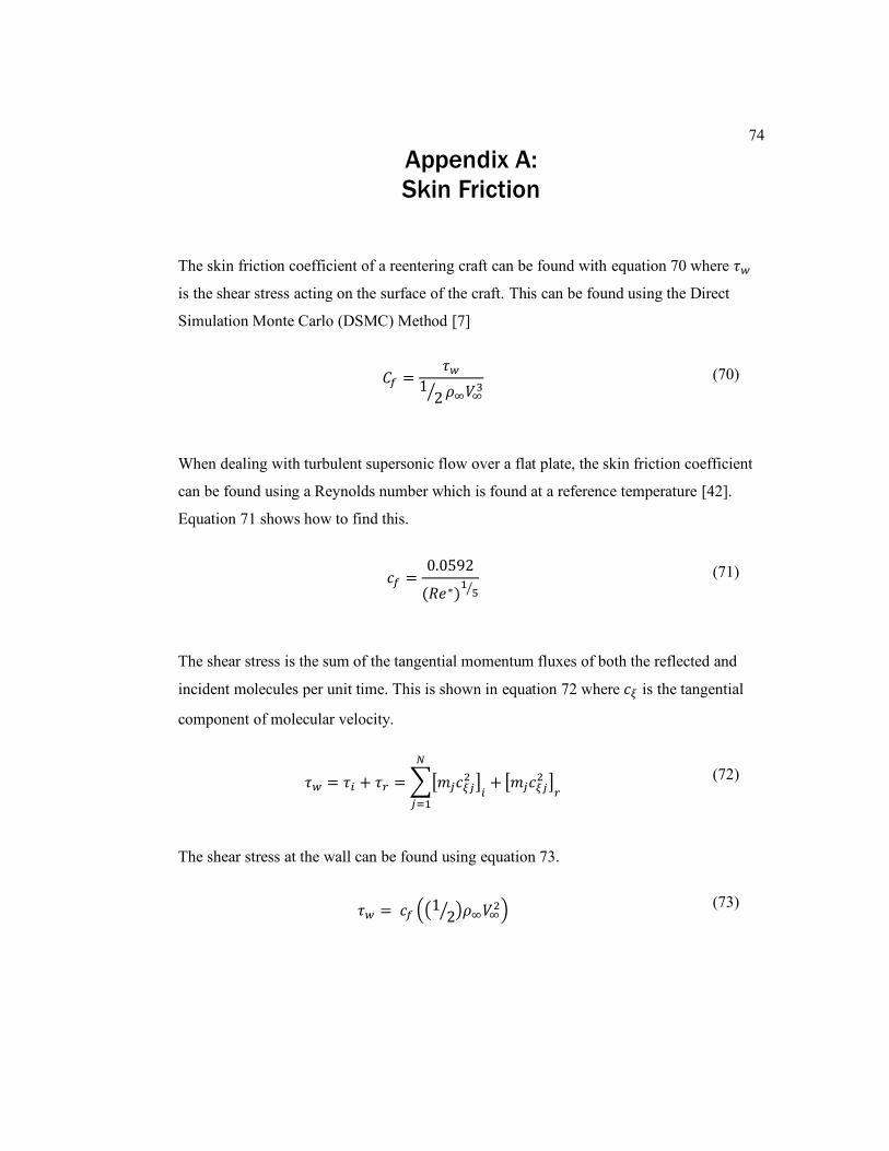
74
Appendix A:
Skin Friction
The skin friction coefficient of a reentering craft can be found with equation 70 where 𝜏𝑤
is the shear stress acting on the surface of the craft. This can be found using the Direct
Simulation Monte Carlo (DSMC) Method [7]
𝐶𝑓 =𝜏𝑤
12⁄ 𝜌∞𝑉∞
3 (70)
When dealing with turbulent supersonic flow over a flat plate, the skin friction coefficient
can be found using a Reynolds number which is found at a reference temperature [42].
Equation 71 shows how to find this.
𝑐𝑓 =0.0592
(𝑅𝑒∗)1
5⁄ (71)
The shear stress is the sum of the tangential momentum fluxes of both the reflected and
incident molecules per unit time. This is shown in equation 72 where 𝑐𝜉 is the tangential
component of molecular velocity.
𝜏𝑤 = 𝜏𝑖 + 𝜏𝑟 = ∑[𝑚𝑗𝑐𝜉𝑗2 ]
𝑖+
𝑁
𝑗=1
[𝑚𝑗𝑐𝜉𝑗2 ]
𝑟 (72)
The shear stress at the wall can be found using equation 73.
𝜏𝑤 = 𝑐𝑓 ((1 2⁄ )𝜌∞𝑉∞2) (73)
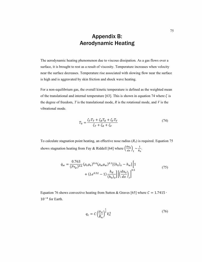
75
Appendix B:
Aerodynamic Heating
The aerodynamic heating phenomenon due to viscous dissipation. As a gas flows over a
surface, it is brought to rest as a result of viscosity. Temperature increases when velocity
near the surface decreases. Temperature rise associated with slowing flow near the surface
is high and is aggravated by skin friction and shock wave heating.
For a non-equilibrium gas, the overall kinetic temperature is defined as the weighted mean
of the translational and internal temperature [63]. This is shown in equation 74 where 𝜁 is
the degree of freedom, T is the translational mode, R is the rotational mode, and V is the
vibrational mode.
𝑇0 =𝜁𝑇𝑇𝑇 + 𝜁𝑅𝑇𝑅 + 𝜁𝑉𝑇𝑉
𝜁𝑇 + 𝜁𝑅 + 𝜁𝑉
(74)
To calculate stagnation point heating, an effective nose radius (Rn) is required. Equation 75
shows stagnation heating from Fay & Riddell [64] where (𝑑𝑢𝑒
𝑑𝑥)𝑡~
1
𝑅𝑛.
�̇�𝑤 =0.763
(𝑃𝑟𝑤)0.6(𝜌𝑒𝜇𝑒)
0.4(𝜌𝑤𝜇𝑤)0.1[(ℎ0)𝑒 − ℎ𝑤] [1
+ (𝐿𝑒0.52 − 1)ℎ𝑑
(ℎ0)𝑒] [(
𝑑𝑢𝑒
𝑑𝑥)𝑡]0.5
(75)
Equation 76 shows convective heating from Sutton & Graves [65] where 𝐶 = 1.7415 ∙
10−4 for Earth.
𝑞𝑐 = 𝐶 (𝜌∞
𝑅𝑛)
1
2𝑉∞
3 (76)
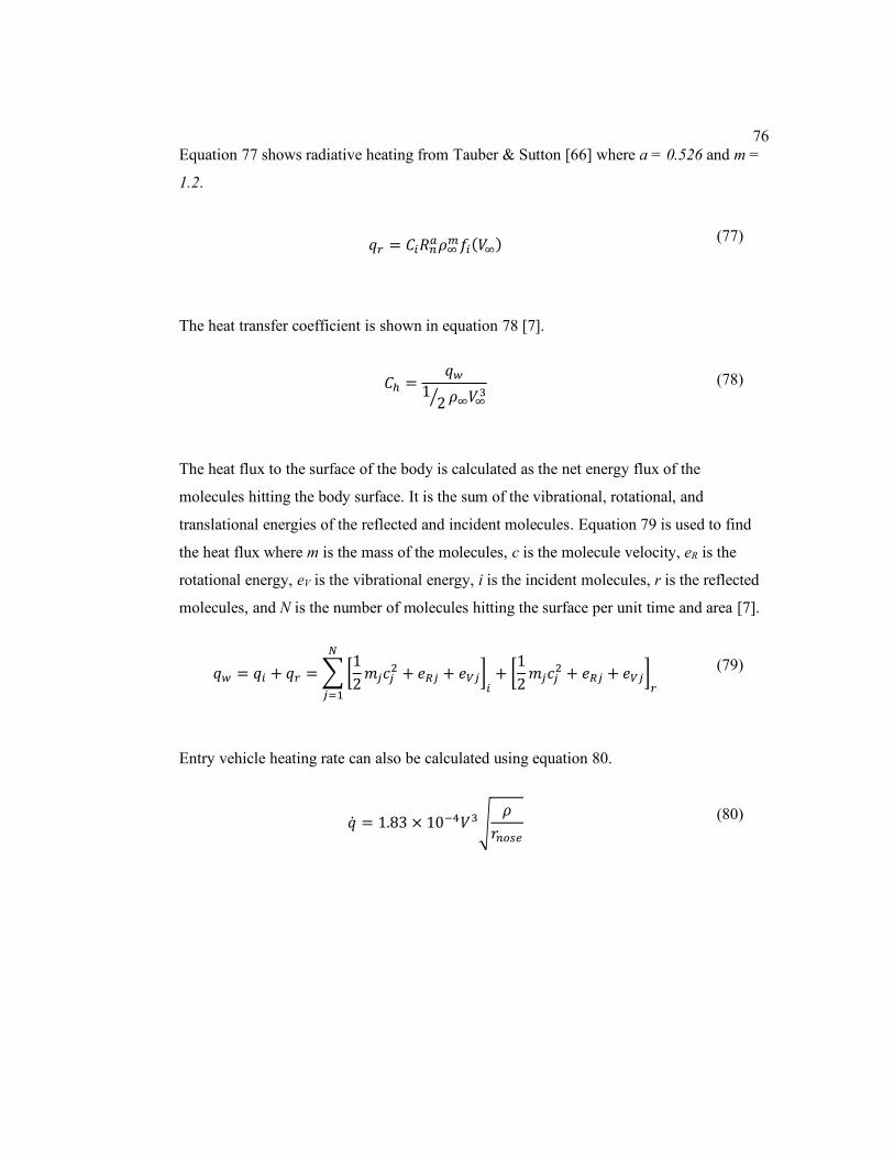
76
Equation 77 shows radiative heating from Tauber & Sutton [66] where a = 0.526 and m =
1.2.
𝑞𝑟 = 𝐶𝑖𝑅𝑛𝑎𝜌∞
𝑚𝑓𝑖(𝑉∞) (77)
The heat transfer coefficient is shown in equation 78 [7].
𝐶ℎ =𝑞𝑤
12⁄ 𝜌∞𝑉∞
3 (78)
The heat flux to the surface of the body is calculated as the net energy flux of the
molecules hitting the body surface. It is the sum of the vibrational, rotational, and
translational energies of the reflected and incident molecules. Equation 79 is used to find
the heat flux where m is the mass of the molecules, c is the molecule velocity, eR is the
rotational energy, eV is the vibrational energy, i is the incident molecules, r is the reflected
molecules, and N is the number of molecules hitting the surface per unit time and area [7].
𝑞𝑤 = 𝑞𝑖 + 𝑞𝑟 = ∑[1
2𝑚𝑗𝑐𝑗
2 + 𝑒𝑅𝑗 + 𝑒𝑉𝑗]𝑖
𝑁
𝑗=1
+ [1
2𝑚𝑗𝑐𝑗
2 + 𝑒𝑅𝑗 + 𝑒𝑉𝑗]𝑟
(79)
Entry vehicle heating rate can also be calculated using equation 80.
�̇� = 1.83 × 10⁻⁴𝑉3√𝜌
𝑟𝑛𝑜𝑠𝑒 (80)
77
Appendix C:
Simplified Navier-Stokes Equations
For supersonic and hypersonic flows, a simplified form of the steady Navier-Stokes
equations can be used [67]. This form contains governing equations with viscous
derivatives omitted in the streamwise direction [69].
Continuity Equation:
𝜕𝜌𝑢
𝜕𝑥+
𝜕𝜌𝑣
𝜕𝑦+
𝜕𝜌𝑤
𝜕𝑧= 0
(81)
X Momentum Equation:
𝜕𝜌𝑢𝑢
𝜕𝑥+
𝜕𝜌𝑢𝑣
𝜕𝑦+
𝜕𝜌𝑢𝑤
𝜕𝑧= −
𝜕𝑝
𝜕𝑥+
𝜕
𝜕𝑦(𝜇
𝜕𝑢
𝜕𝑦) +
𝜕
𝜕𝑧(𝜇
𝜕𝑢
𝜕𝑧)
(82)
Y Momentum Equation
𝜕𝜌𝑣𝑢
𝜕𝑥+
𝜕𝜌𝑣𝑣
𝜕𝑦+
𝜕𝜌𝑣𝑤
𝜕𝑧
= −𝜕𝑝
𝜕𝑦+
𝜕
𝜕𝑦((𝜆 + 2𝜇)
𝜕𝑣
𝜕𝑦+ 𝜇
𝜕𝑤
𝜕𝑧) +
𝜕
𝜕𝑧(𝜇 [
𝜕𝑤
𝜕𝑦+
𝜕𝑣
𝜕𝑦])
(83)
78
Z Momentum Equation:
𝜕𝜌𝑤𝑢
𝜕𝑥+
𝜕𝜌𝑤𝑣
𝜕𝑦+
𝜕𝜌𝑤𝑤
𝜕𝑧
= −𝜕𝑝
𝜕𝑧+ +
𝜕
𝜕𝑦(𝜇 [
𝜕𝑣
𝜕𝑧+
𝜕𝑤
𝜕𝑦])
+𝜕
𝜕𝑧((𝜆 + 2𝜇)
𝜕𝑤
𝜕𝑧+ 𝜇
𝜕𝑣
𝜕𝑦)
(84)
Energy Equation:
𝜕𝜌𝑢𝐸
𝜕𝑥+
𝜕𝜌𝑣𝐸
𝜕𝑦+
𝜕𝜌𝑤𝐸
𝜕𝑧
= 𝜌�̇� +𝜕
𝜕𝑦(𝑘
𝜕𝑇
𝜕𝑦) +
𝜕
𝜕𝑧(𝑘
𝜕𝑇
𝜕𝑧) − (
𝜕𝜌𝑢
𝜕𝑥+
𝜕𝜌𝑣
𝜕𝑦+
𝜕𝜌𝑤
𝜕𝑧)
+𝜕
𝜕𝑦(𝑢𝜇
𝜕𝑢
𝜕𝑦) +
𝜕
𝜕𝑧(𝑢𝜇
𝜕𝑢
𝜕𝑧) +
𝜕
𝜕𝑦(𝑣𝜆 [
𝜕𝑣
𝜕𝑦+
𝜕𝑤
𝜕𝑧] + 2𝑣𝜇
𝜕𝑣
𝜕𝑦)
+𝜕
𝜕𝑧(𝑣𝜇 [
𝜕𝑤
𝜕𝑦+
𝜕𝑣
𝜕𝑧]) +
𝜕
𝜕𝑦(𝑤𝜇 [
𝜕𝑤
𝜕𝑦+
𝜕𝑣
𝜕𝑧])
+𝜕
𝜕𝑧(𝑤𝜆 [
𝜕𝑣
𝜕𝑦+
𝜕𝑤
𝜕𝑧] + 2𝑤𝜇
𝜕𝑤
𝜕𝑧)
(85)
where µ is the dynamic viscosity and λ (second viscosity) is 2
3μ.
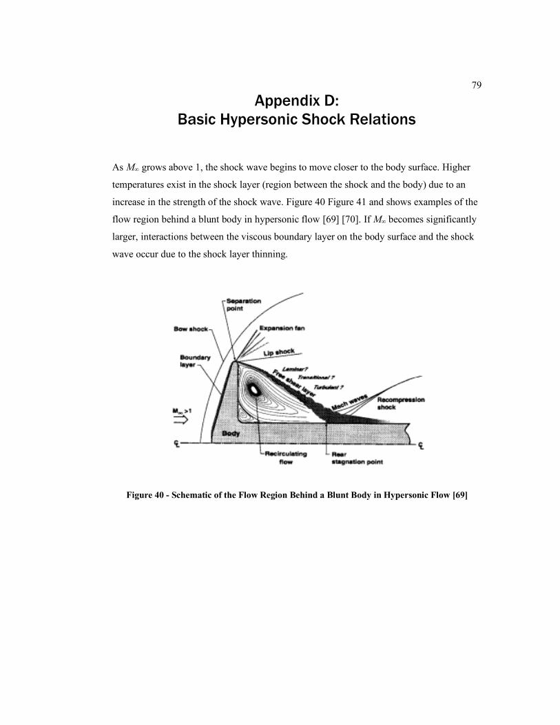
79
Appendix D:
Basic Hypersonic Shock Relations
As M∞ grows above 1, the shock wave begins to move closer to the body surface. Higher
temperatures exist in the shock layer (region between the shock and the body) due to an
increase in the strength of the shock wave. Figure 40 Figure 41 and shows examples of the
flow region behind a blunt body in hypersonic flow [69] [70]. If M∞ becomes significantly
larger, interactions between the viscous boundary layer on the body surface and the shock
wave occur due to the shock layer thinning.
Figure 40 - Schematic of the Flow Region Behind a Blunt Body in Hypersonic Flow [69]
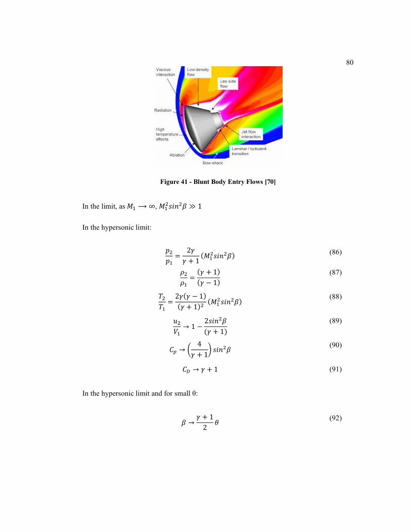
80
Figure 41 - Blunt Body Entry Flows [70]
In the limit, as 𝑀1 ⟶ ∞, 𝑀12𝑠𝑖𝑛2𝛽 ≫ 1
In the hypersonic limit:
𝑝2
𝑝1=
2𝛾
𝛾 + 1(𝑀1
2𝑠𝑖𝑛2𝛽) (86)
𝜌2
𝜌1=
(𝛾 + 1)
(𝛾 − 1)
(87)
𝑇2
𝑇1=
2𝛾(𝛾 − 1)
(𝛾 + 1)2(𝑀1
2𝑠𝑖𝑛2𝛽) (88)
𝑢2
𝑉1→ 1 −
2𝑠𝑖𝑛2𝛽
(𝛾 + 1)
(89)
𝐶𝑝 → (4
𝛾 + 1) 𝑠𝑖𝑛2𝛽
(90)
𝐶𝐷 → 𝛾 + 1 (91)
In the hypersonic limit and for small θ:
𝛽 →𝛾 + 1
2𝜃
(92)
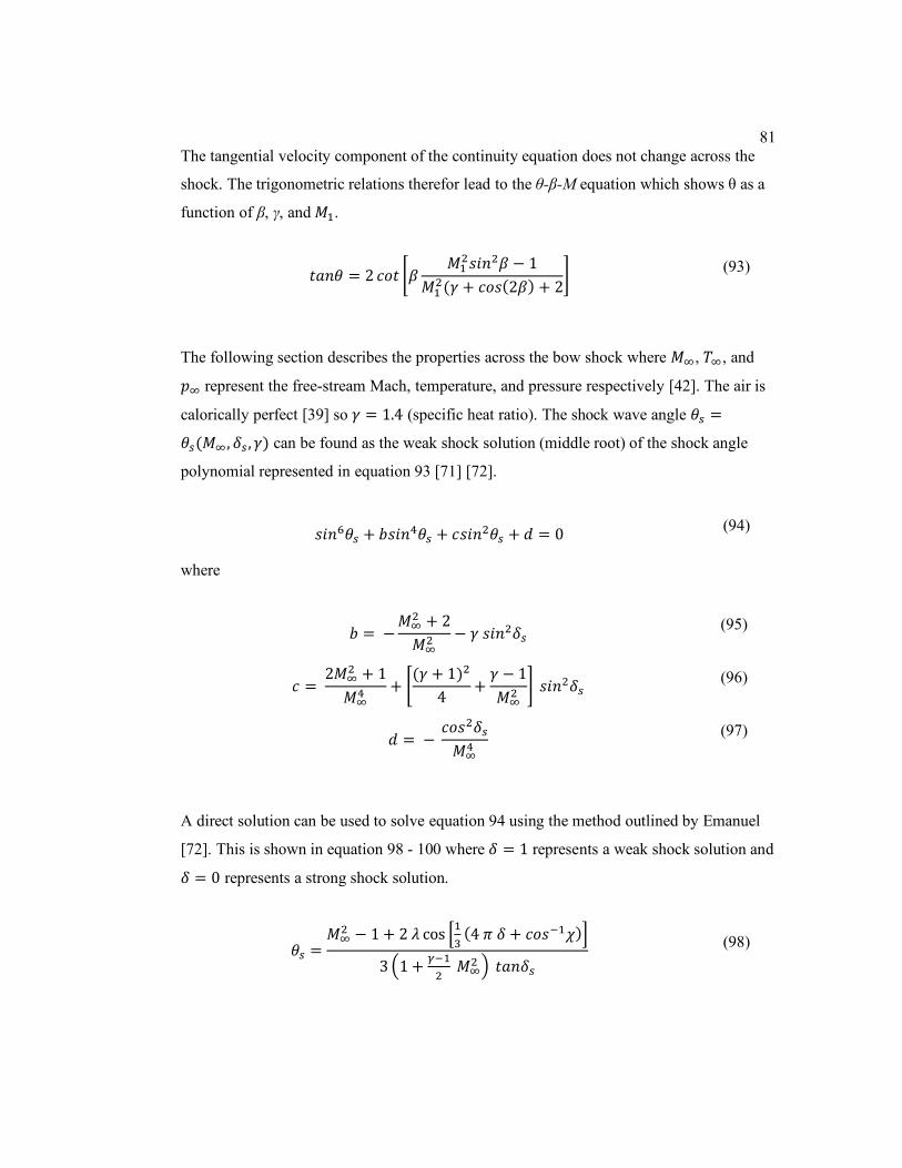
81
The tangential velocity component of the continuity equation does not change across the
shock. The trigonometric relations therefor lead to the θ-β-M equation which shows θ as a
function of β, γ, and 𝑀1.
𝑡𝑎𝑛𝜃 = 2 𝑐𝑜𝑡 [𝛽𝑀1
2𝑠𝑖𝑛2𝛽 − 1
𝑀12(𝛾 + 𝑐𝑜𝑠(2𝛽) + 2
] (93)
The following section describes the properties across the bow shock where 𝑀∞, 𝑇∞, and
𝑝∞ represent the free-stream Mach, temperature, and pressure respectively [42]. The air is
calorically perfect [39] so 𝛾 = 1.4 (specific heat ratio). The shock wave angle 𝜃𝑠 =
𝜃𝑠(𝑀∞, 𝛿𝑠 , 𝛾) can be found as the weak shock solution (middle root) of the shock angle
polynomial represented in equation 93 [71] [72].
𝑠𝑖𝑛6𝜃𝑠 + 𝑏𝑠𝑖𝑛4𝜃𝑠 + 𝑐𝑠𝑖𝑛2𝜃𝑠 + 𝑑 = 0 (94)
where
𝑏 = −𝑀∞
2 + 2
𝑀∞2 − 𝛾 𝑠𝑖𝑛2𝛿𝑠
(95)
𝑐 = 2𝑀∞
2 + 1
𝑀∞4 + [
(𝛾 + 1)2
4+
𝛾 − 1
𝑀∞2
] 𝑠𝑖𝑛2𝛿𝑠 (96)
𝑑 = − 𝑐𝑜𝑠2𝛿𝑠
𝑀∞4
(97)
A direct solution can be used to solve equation 94 using the method outlined by Emanuel
[72]. This is shown in equation 98 - 100 where 𝛿 = 1 represents a weak shock solution and
𝛿 = 0 represents a strong shock solution.
𝜃𝑠 =𝑀∞
2 − 1 + 2 𝜆 cos [1
3(4 𝜋 𝛿 + 𝑐𝑜𝑠−1𝜒)]
3 (1 +𝛾−1
2 𝑀∞
2 ) 𝑡𝑎𝑛𝛿𝑠
(98)
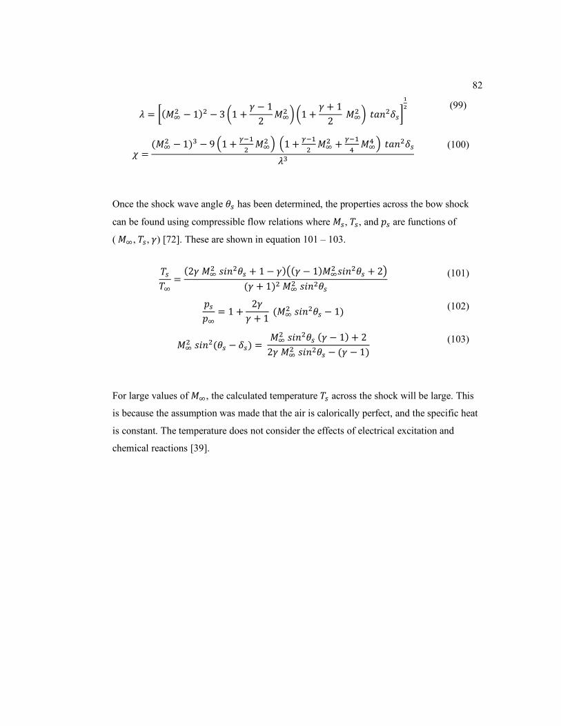
82
𝜆 = [(𝑀∞2 − 1)2 − 3(1 +
𝛾 − 1
2𝑀∞
2 ) (1 +𝛾 + 1
2 𝑀∞
2 ) 𝑡𝑎𝑛2𝛿𝑠]
1
2
(99)
𝜒 =(𝑀∞
2 − 1)3 − 9(1 +𝛾−1
2𝑀∞
2 ) (1 +𝛾−1
2𝑀∞
2 +𝛾−1
4𝑀∞
4 ) 𝑡𝑎𝑛2𝛿𝑠
𝜆3
(100)
Once the shock wave angle 𝜃𝑠 has been determined, the properties across the bow shock
can be found using compressible flow relations where 𝑀𝑠, 𝑇𝑠, and 𝑝𝑠 are functions of
( 𝑀∞, 𝑇𝑠, 𝛾) [72]. These are shown in equation 101 – 103.
𝑇𝑠
𝑇∞=
(2𝛾 𝑀∞2 𝑠𝑖𝑛2𝜃𝑠 + 1 − 𝛾)((𝛾 − 1)𝑀∞
2 𝑠𝑖𝑛2𝜃𝑠 + 2)
(𝛾 + 1)2 𝑀∞2 𝑠𝑖𝑛2𝜃𝑠
(101)
𝑝𝑠
𝑝∞= 1 +
2𝛾
𝛾 + 1 (𝑀∞
2 𝑠𝑖𝑛2𝜃𝑠 − 1) (102)
𝑀∞2 𝑠𝑖𝑛2(𝜃𝑠 − 𝛿𝑠) =
𝑀∞2 𝑠𝑖𝑛2𝜃𝑠 (𝛾 − 1) + 2
2𝛾 𝑀∞2 𝑠𝑖𝑛2𝜃𝑠 − (𝛾 − 1)
(103)
For large values of 𝑀∞, the calculated temperature 𝑇𝑠 across the shock will be large. This
is because the assumption was made that the air is calorically perfect, and the specific heat
is constant. The temperature does not consider the effects of electrical excitation and
chemical reactions [39].
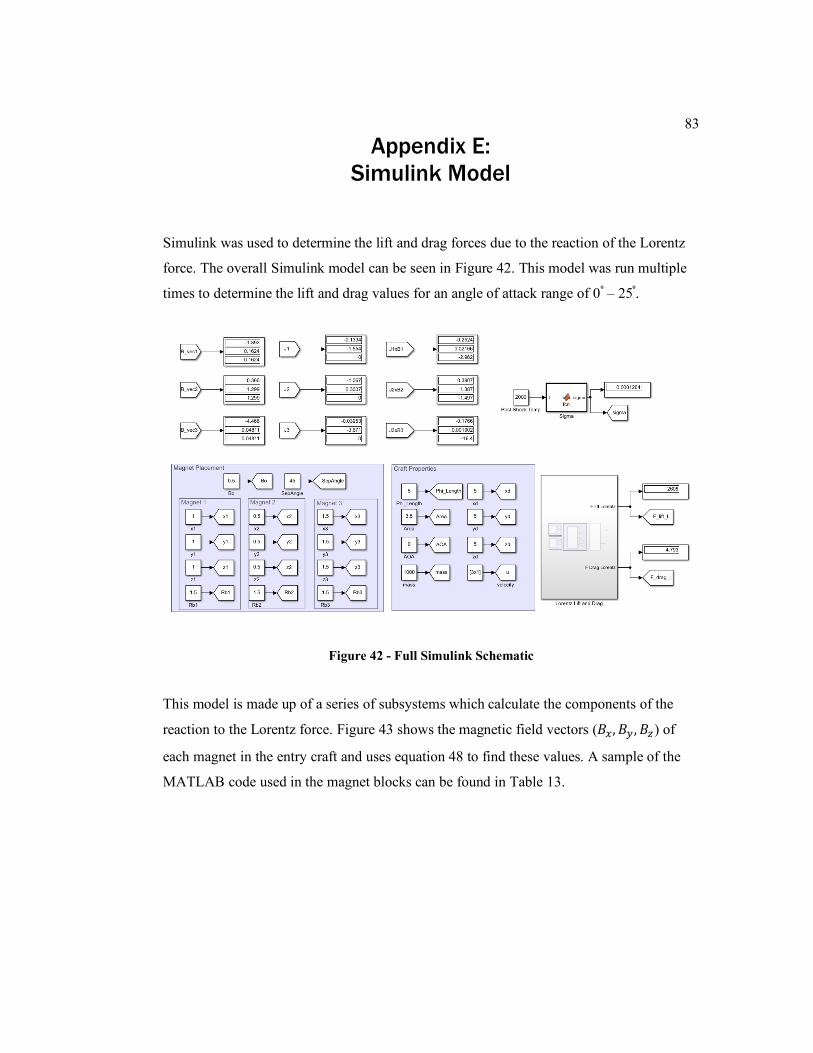
83
Appendix E:
Simulink Model
Simulink was used to determine the lift and drag forces due to the reaction of the Lorentz
force. The overall Simulink model can be seen in Figure 42. This model was run multiple
times to determine the lift and drag values for an angle of attack range of 0⁰ – 25⁰.
Figure 42 - Full Simulink Schematic
This model is made up of a series of subsystems which calculate the components of the
reaction to the Lorentz force. Figure 43 shows the magnetic field vectors (𝐵𝑥, 𝐵𝑦 , 𝐵𝑧) of
each magnet in the entry craft and uses equation 48 to find these values. A sample of the
MATLAB code used in the magnet blocks can be found in Table 13.
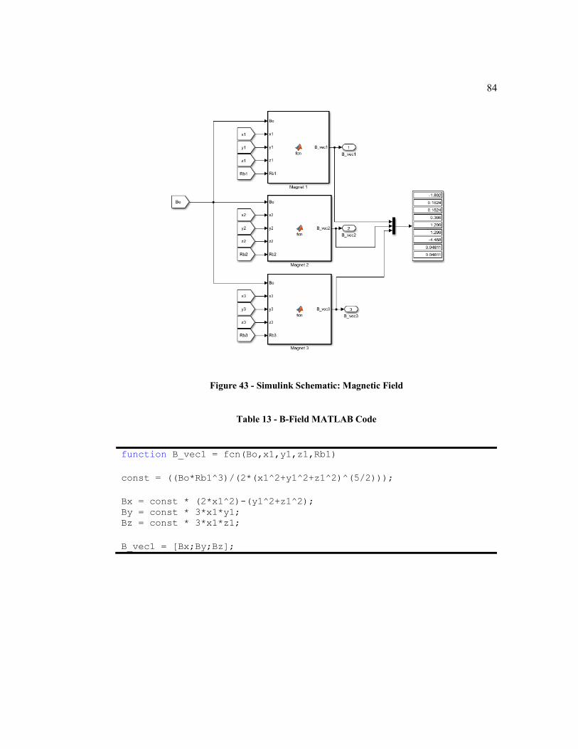
84
Figure 43 - Simulink Schematic: Magnetic Field
Table 13 - B-Field MATLAB Code
function B_vec1 = fcn(Bo,x1,y1,z1,Rb1)
const = ((Bo*Rb1^3)/(2*(x1^2+y1^2+z1^2)^(5/2)));
Bx = const * (2*x1^2)-(y1^2+z1^2); By = const * 3*x1*y1; Bz = const * 3*x1*z1;
B_vec1 = [Bx;By;Bz];
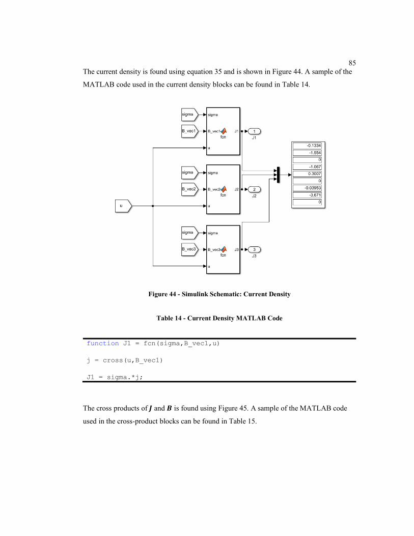
85
The current density is found using equation 35 and is shown in Figure 44. A sample of the
MATLAB code used in the current density blocks can be found in Table 14.
Figure 44 - Simulink Schematic: Current Density
Table 14 - Current Density MATLAB Code
function J1 = fcn(sigma,B_vec1,u)
j = cross(u,B_vec1)
J1 = sigma.*j;
The cross products of 𝑱 and 𝑩 is found using Figure 45. A sample of the MATLAB code
used in the cross-product blocks can be found in Table 15.
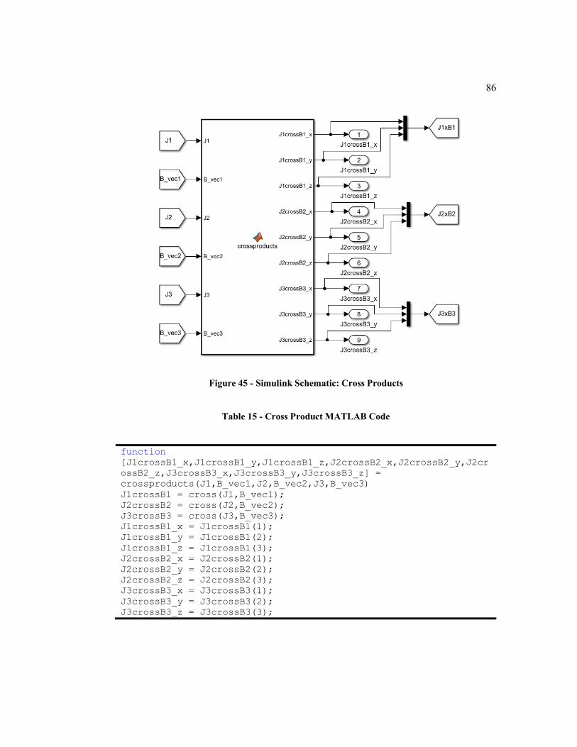
86
Figure 45 - Simulink Schematic: Cross Products
Table 15 - Cross Product MATLAB Code
function
[J1crossB1_x,J1crossB1_y,J1crossB1_z,J2crossB2_x,J2crossB2_y,J2cr
ossB2_z,J3crossB3_x,J3crossB3_y,J3crossB3_z] =
crossproducts(J1,B_vec1,J2,B_vec2,J3,B_vec3) J1crossB1 = cross(J1,B_vec1); J2crossB2 = cross(J2,B_vec2); J3crossB3 = cross(J3,B_vec3); J1crossB1_x = J1crossB1(1); J1crossB1_y = J1crossB1(2); J1crossB1_z = J1crossB1(3); J2crossB2_x = J2crossB2(1); J2crossB2_y = J2crossB2(2); J2crossB2_z = J2crossB2(3); J3crossB3_x = J3crossB3(1); J3crossB3_y = J3crossB3(2); J3crossB3_z = J3crossB3(3);
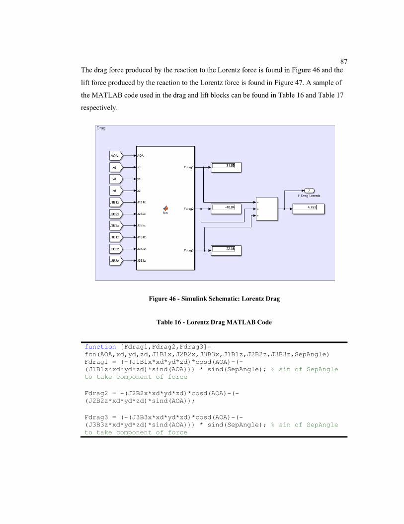
87
The drag force produced by the reaction to the Lorentz force is found in Figure 46 and the
lift force produced by the reaction to the Lorentz force is found in Figure 47. A sample of
the MATLAB code used in the drag and lift blocks can be found in Table 16 and Table 17
respectively.
Figure 46 - Simulink Schematic: Lorentz Drag
Table 16 - Lorentz Drag MATLAB Code
function [Fdrag1,Fdrag2,Fdrag3]=
fcn(AOA,xd,yd,zd,J1B1x,J2B2x,J3B3x,J1B1z,J2B2z,J3B3z,SepAngle) Fdrag1 = (-(J1B1x*xd*yd*zd)*cosd(AOA)-(-
(J1B1z*xd*yd*zd)*sind(AOA))) * sind(SepAngle); % sin of SepAngle
to take component of force
Fdrag2 = -(J2B2x*xd*yd*zd)*cosd(AOA)-(-
(J2B2z*xd*yd*zd)*sind(AOA));
Fdrag3 = (-(J3B3x*xd*yd*zd)*cosd(AOA)-(-
(J3B3z*xd*yd*zd)*sind(AOA))) * sind(SepAngle); % sin of SepAngle
to take component of force
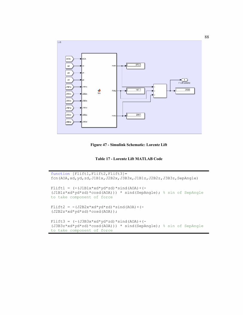
88
Figure 47 - Simulink Schematic: Lorentz Lift
Table 17 - Lorentz Lift MATLAB Code
function [Flift1,Flift2,Flift3]=
fcn(AOA,xd,yd,zd,J1B1x,J2B2x,J3B3x,J1B1z,J2B2z,J3B3z,SepAngle)
Flift1 = (-(J1B1x*xd*yd*zd)*sind(AOA)+(-
(J1B1z*xd*yd*zd)*cosd(AOA))) * sind(SepAngle); % sin of SepAngle
to take component of force
Flift2 = -(J2B2x*xd*yd*zd)*sind(AOA)+(-
(J2B2z*xd*yd*zd)*cosd(AOA));
Flift3 = (-(J3B3x*xd*yd*zd)*sind(AOA)+(-
(J3B3z*xd*yd*zd)*cosd(AOA))) * sind(SepAngle); % sin of SepAngle
to take component of force
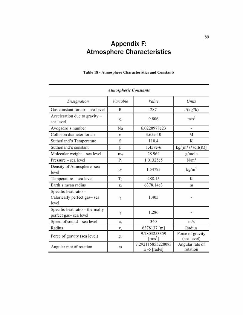
89
Appendix F:
Atmosphere Characteristics
Table 18 - Atmosphere Characteristics and Constants
Atmospheric Constants
Designation Variable Value Units
Gas constant for air – sea level R 287 J/(kg*k)
Acceleration due to gravity –
sea level g0 9.806 m/s2
Avogadro’s number Na 6.0220978e23 -
Collision diameter for air σ 3.65e-10 M
Sutherland’s Temperature S 110.4 K
Sutherland’s constant β 1.458e-6 kg/[m*s*sqrt(K)]
Molecular weight – sea level m0 28.964 g/mole
Pressure – sea level P0 1.01325e5 N/m2
Density of Atmosphere -sea
level ρ0 1.54793 kg/m3
Temperature – sea level T0 288.15 K
Earth’s mean radius re 6378.14e3 m
Specific heat ratio –
Calorically perfect gas– sea
level
γ 1.405 -
Specific heat ratio – thermally
perfect gas– sea level γ 1.286 -
Speed of sound – sea level as 340 m/s
Radius r0 6378137 [m] Radius
Force of gravity (sea level) g0 9.7803253359
[m/s2]
Force of gravity
(sea level)
Angular rate of rotation ω 7.292115855228083
E -5 [rad/s] Angular rate of
rotation
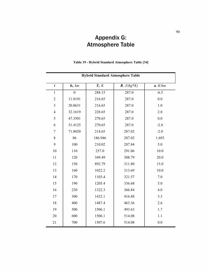
90
Appendix G:
Atmosphere Table
Table 19 - Hybrid Standard Atmosphere Table [34]
Hybrid Standard Atmosphere Table
i hi, km Ti, K R, J/(kg*K) a, K/km
1 0 288.15 287.0 -6.5
2 11.0191 216.65 287.0 0.0
3 20.0631 216.65 287.0 1.0
4 32.1619 228.65 287.0 2.8
5 47.3501 270.65 287.0 0.0
6 51.4125 270.65 287.0 -2.8
7 71.8020 214.65 287.02 -2.0
8 86 186.946 287.02 1.693
9 100 210.02 287.84 5.0
10 110 257.0 291.06 10.0
11 120 349.49 308.79 20.0
12 150 892.79 311.80 15.0
13 160 1022.2 313.69 10.0
14 170 1103.4 321.57 7.0
15 190 1205.4 336.68 5.0
16 230 1322.3 366.84 4.0
17 300 1432.1 416.88 3.3
18 400 1487.4 463.36 2.6
19 500 1506.1 493.63 1.7
20 600 1506.1 514.08 1.1
21 700 1507.6 514.08 0.0
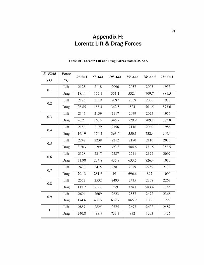
91
Appendix H:
Lorentz Lift & Drag Forces
Table 20 - Lorentz Lift and Drag Forces from 0-25 AoA
B- Field
(T)
Force
(N) 0⁰ AoA 5⁰ AoA 10⁰ AoA 15⁰ AoA 20⁰ AoA 25⁰ AoA
0.1 Lift 2125 2118 2096 2057 2003 1933
Drag 18.11 167.1 351.1 532.4 709.7 881.5
0.2 Lift 2125 2119 2097 2059 2006 1937
Drag 26.85 158.4 342.5 524 701.5 873.6
0.3 Lift 2145 2139 2117 2079 2025 1955
Drag 26.21 160.9 346.7 529.9 709.1 882.8
0.4 Lift 2186 2179 2156 2116 2060 1988
Drag 16.19 174.4 363.6 550.1 732.4 909.1
0.5 Lift 2247 2238 2212 2170 2110 2035
Drag 3.203 199 393.3 584.6 771.5 952.5
0.6 Lift 2328 2317 2287 2241 2177 2097
Drag 31.98 234.8 435.8 633.5 826.4 1013
0.7 Lift 2430 2415 2381 2329 2259 2173
Drag 70.13 281.6 491 696.6 897 1090
0.8 Lift 2552 2532 2493 2435 2358 2263
Drag 117.7 339.6 559 774.1 983.4 1185
0.9 Lift 2694 2669 2623 2557 2472 2368
Drag 174.6 408.7 639.7 865.9 1086 1297
1 Lift 2857 2825 2775 2697 2602 2487
Drag 240.8 488.9 733.3 972 1203 1426
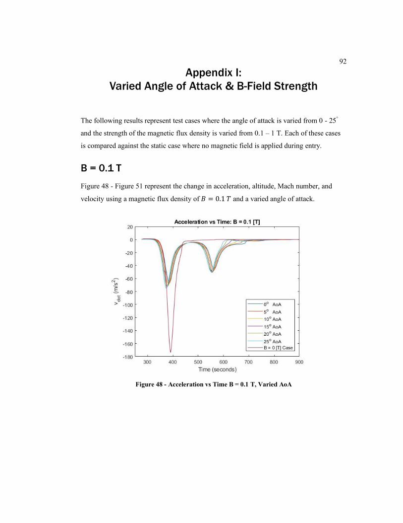
92
Appendix I:
Varied Angle of Attack & B-Field Strength
The following results represent test cases where the angle of attack is varied from 0 - 25°
and the strength of the magnetic flux density is varied from 0.1 – 1 T. Each of these cases
is compared against the static case where no magnetic field is applied during entry.
B = 0.1 T
Figure 48 - Figure 51 represent the change in acceleration, altitude, Mach number, and
velocity using a magnetic flux density of 𝐵 = 0.1 𝑇 and a varied angle of attack.
Figure 48 - Acceleration vs Time B = 0.1 T, Varied AoA
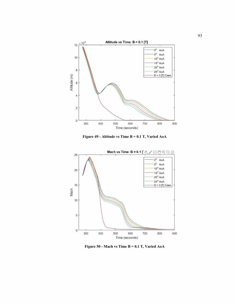
93
Figure 49 - Altitude vs Time B = 0.1 T, Varied AoA
Figure 50 - Mach vs Time B = 0.1 T, Varied AoA
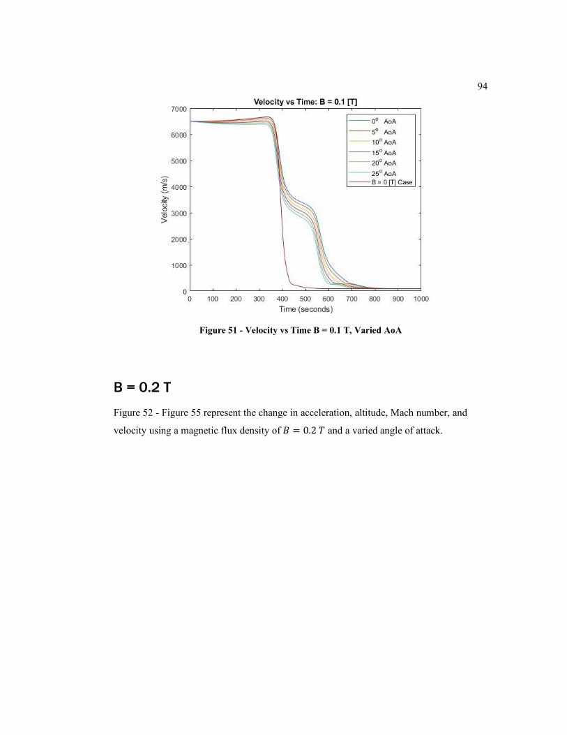
94
Figure 51 - Velocity vs Time B = 0.1 T, Varied AoA
B = 0.2 T
Figure 52 - Figure 55 represent the change in acceleration, altitude, Mach number, and
velocity using a magnetic flux density of 𝐵 = 0.2 𝑇 and a varied angle of attack.
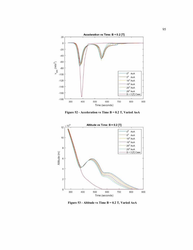
95
Figure 52 - Acceleration vs Time B = 0.2 T, Varied AoA
Figure 53 - Altitude vs Time B = 0.2 T, Varied AoA
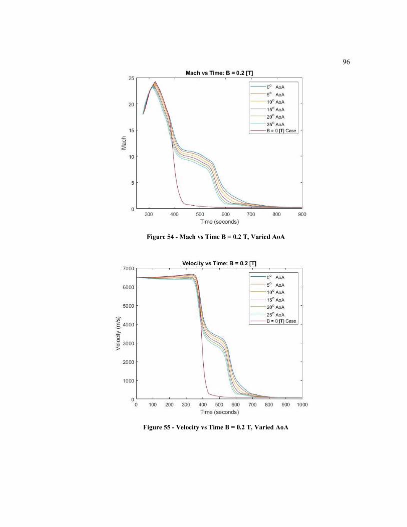
96
Figure 54 - Mach vs Time B = 0.2 T, Varied AoA
Figure 55 - Velocity vs Time B = 0.2 T, Varied AoA
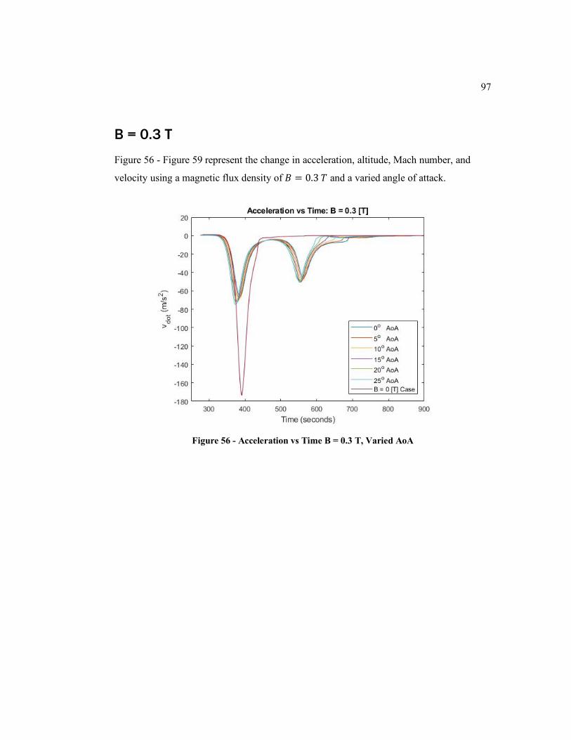
97
B = 0.3 T
Figure 56 - Figure 59 represent the change in acceleration, altitude, Mach number, and
velocity using a magnetic flux density of 𝐵 = 0.3 𝑇 and a varied angle of attack.
Figure 56 - Acceleration vs Time B = 0.3 T, Varied AoA
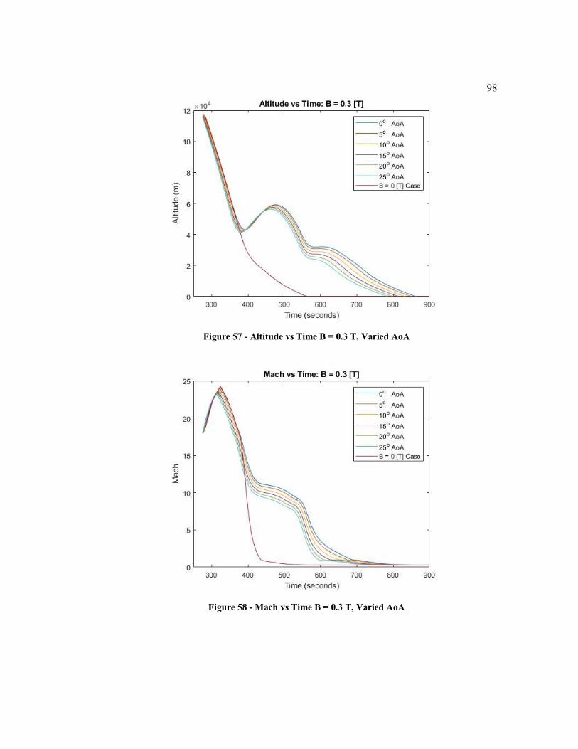
98
Figure 57 - Altitude vs Time B = 0.3 T, Varied AoA
Figure 58 - Mach vs Time B = 0.3 T, Varied AoA

99
Figure 59 - Velocity vs Time B = 0.3 T, Varied AoA
B = 0.4 T
Figure 60 - Figure 63 represent the change in acceleration, altitude, Mach number, and
velocity using a magnetic flux density of 𝐵 = 0.4 𝑇 and a varied angle of attack.
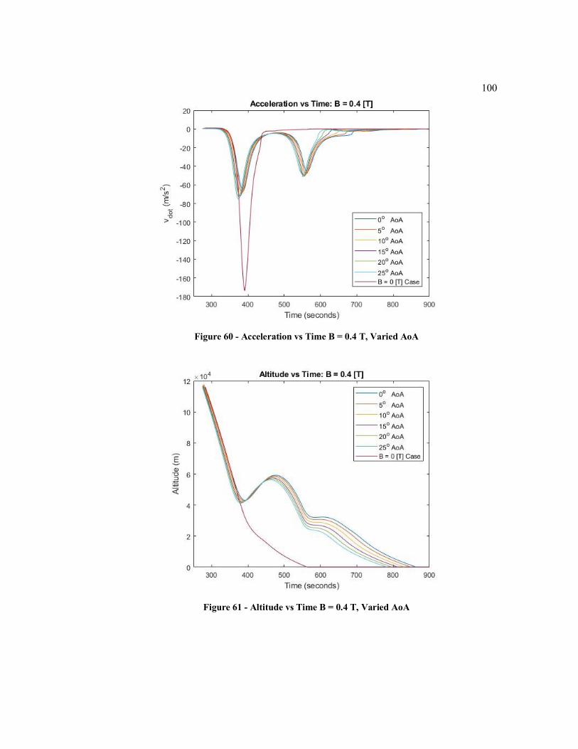
100
Figure 60 - Acceleration vs Time B = 0.4 T, Varied AoA
Figure 61 - Altitude vs Time B = 0.4 T, Varied AoA

101
Figure 62 - Mach vs Time B = 0.4 T, Varied AoA
Figure 63 - Velocity vs Time B = 0.4 T, Varied AoA
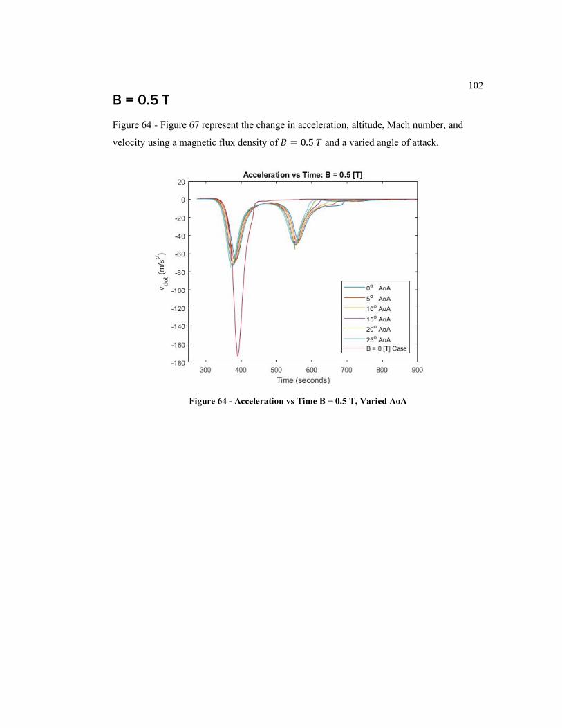
102
B = 0.5 T
Figure 64 - Figure 67 represent the change in acceleration, altitude, Mach number, and
velocity using a magnetic flux density of 𝐵 = 0.5 𝑇 and a varied angle of attack.
Figure 64 - Acceleration vs Time B = 0.5 T, Varied AoA
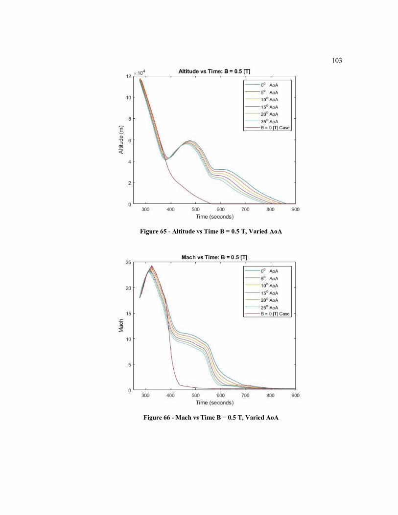
103
Figure 65 - Altitude vs Time B = 0.5 T, Varied AoA
Figure 66 - Mach vs Time B = 0.5 T, Varied AoA
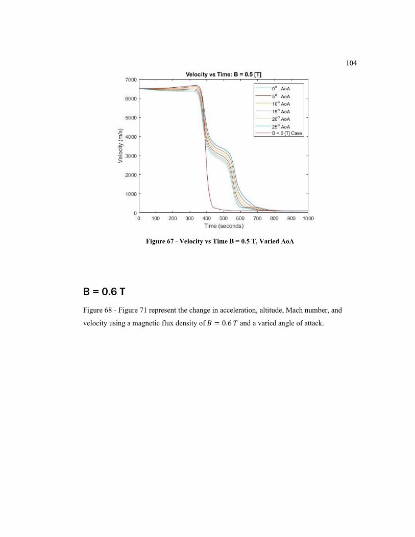
104
Figure 67 - Velocity vs Time B = 0.5 T, Varied AoA
B = 0.6 T
Figure 68 - Figure 71 represent the change in acceleration, altitude, Mach number, and
velocity using a magnetic flux density of 𝐵 = 0.6 𝑇 and a varied angle of attack.
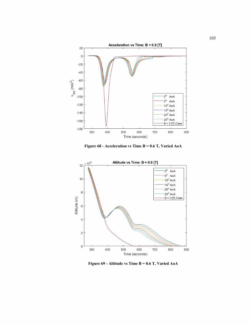
105
Figure 68 - Acceleration vs Time B = 0.6 T, Varied AoA
Figure 69 - Altitude vs Time B = 0.6 T, Varied AoA
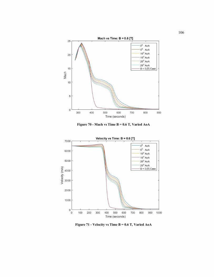
106
Figure 70 - Mach vs Time B = 0.6 T, Varied AoA
Figure 71 - Velocity vs Time B = 0.6 T, Varied AoA
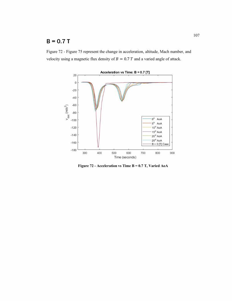
107
B = 0.7 T
Figure 72 - Figure 75 represent the change in acceleration, altitude, Mach number, and
velocity using a magnetic flux density of 𝐵 = 0.7 𝑇 and a varied angle of attack.
Figure 72 - Acceleration vs Time B = 0.7 T, Varied AoA
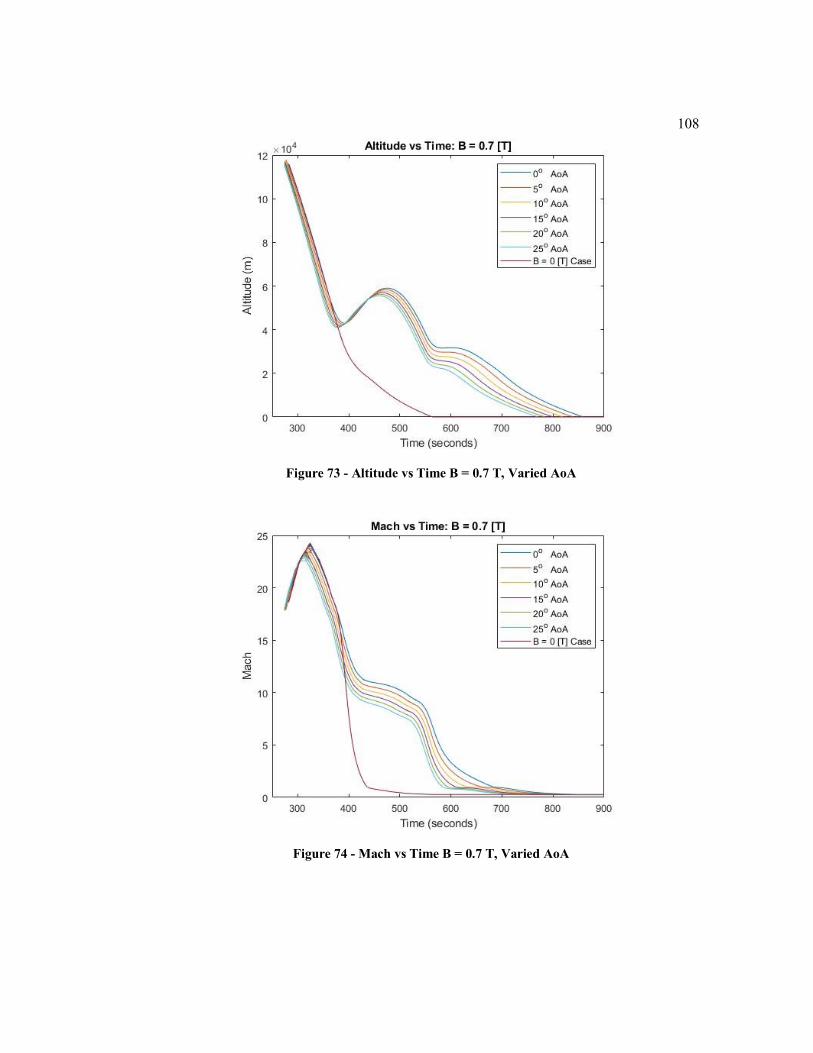
108
Figure 73 - Altitude vs Time B = 0.7 T, Varied AoA
Figure 74 - Mach vs Time B = 0.7 T, Varied AoA
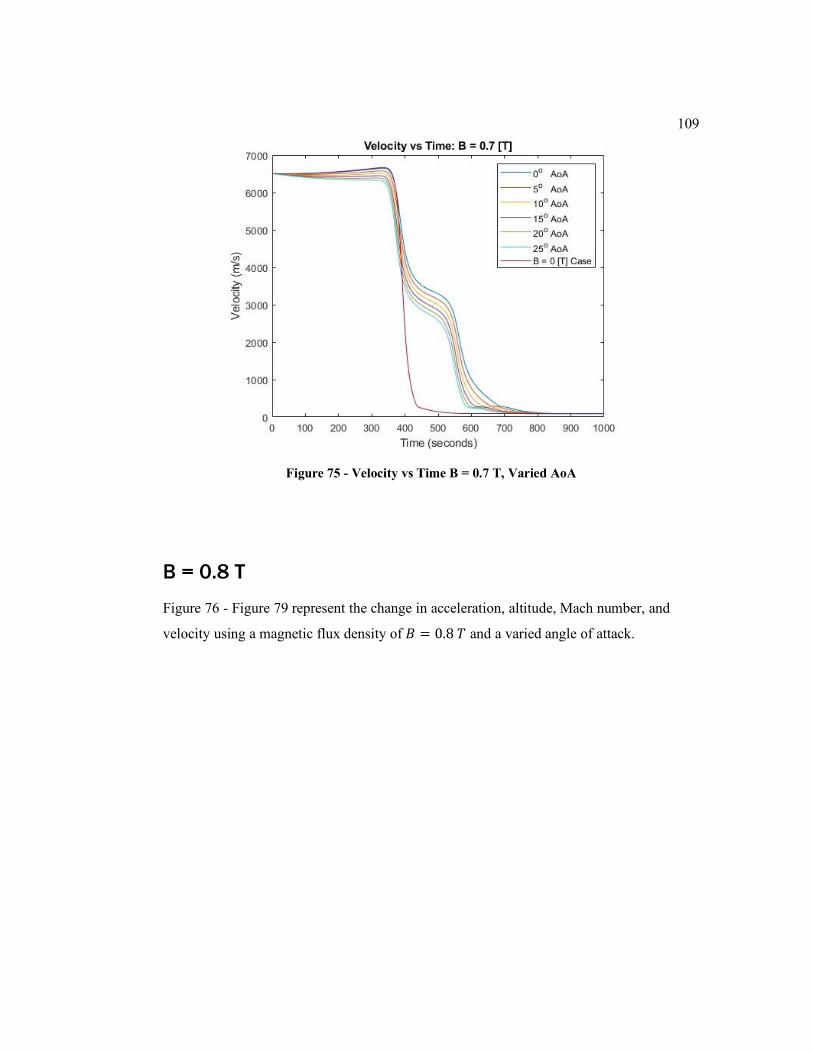
109
Figure 75 - Velocity vs Time B = 0.7 T, Varied AoA
B = 0.8 T
Figure 76 - Figure 79 represent the change in acceleration, altitude, Mach number, and
velocity using a magnetic flux density of 𝐵 = 0.8 𝑇 and a varied angle of attack.
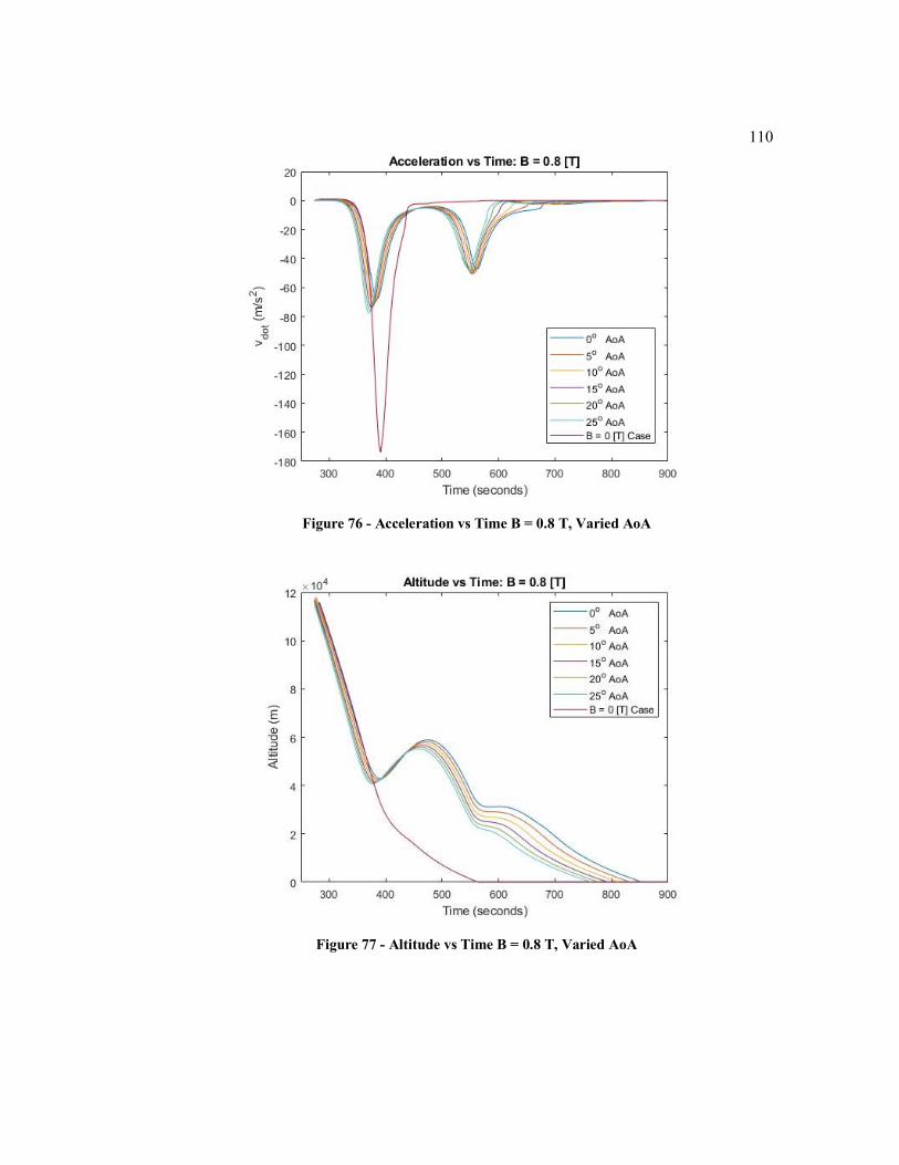
110
Figure 76 - Acceleration vs Time B = 0.8 T, Varied AoA
Figure 77 - Altitude vs Time B = 0.8 T, Varied AoA
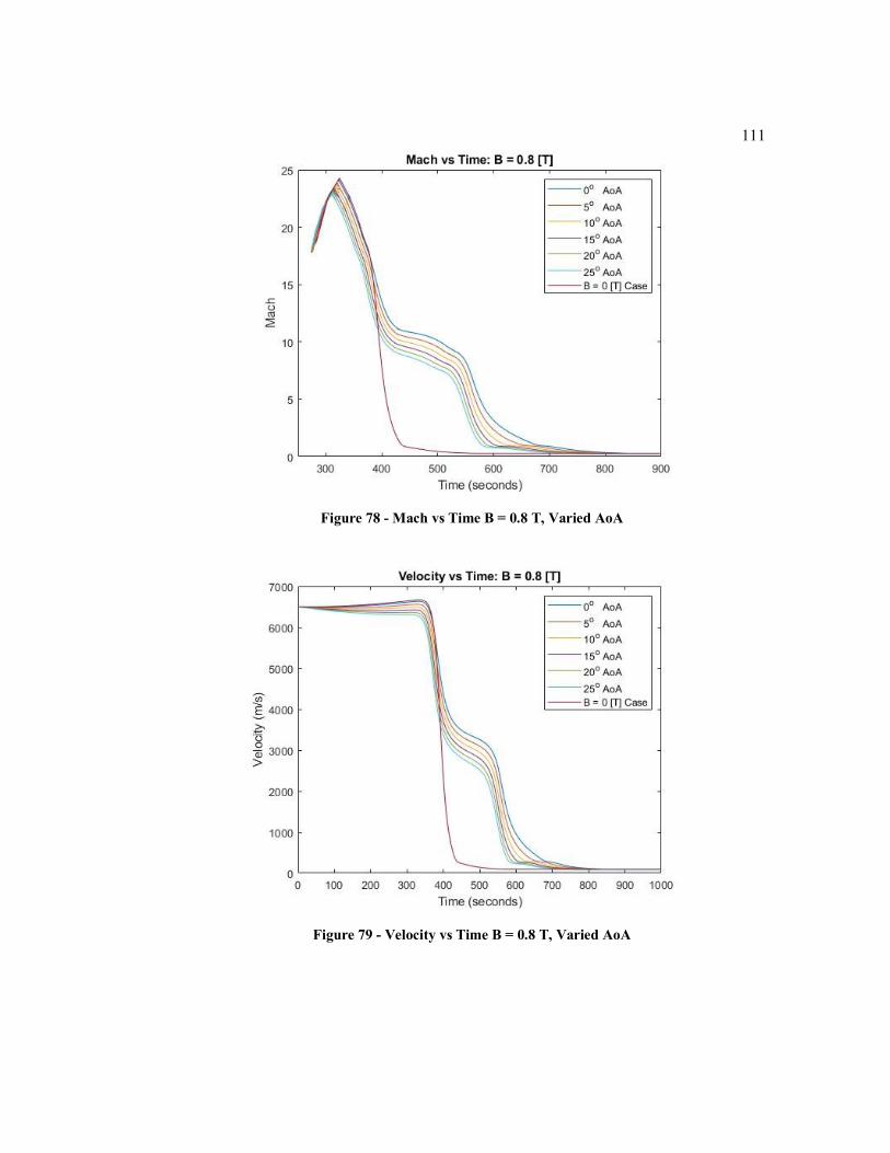
111
Figure 78 - Mach vs Time B = 0.8 T, Varied AoA
Figure 79 - Velocity vs Time B = 0.8 T, Varied AoA
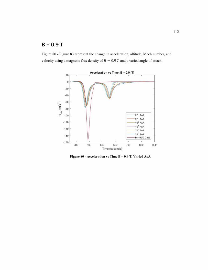
112
B = 0.9 T
Figure 80 - Figure 83 represent the change in acceleration, altitude, Mach number, and
velocity using a magnetic flux density of 𝐵 = 0.9 𝑇 and a varied angle of attack.
Figure 80 - Acceleration vs Time B = 0.9 T, Varied AoA
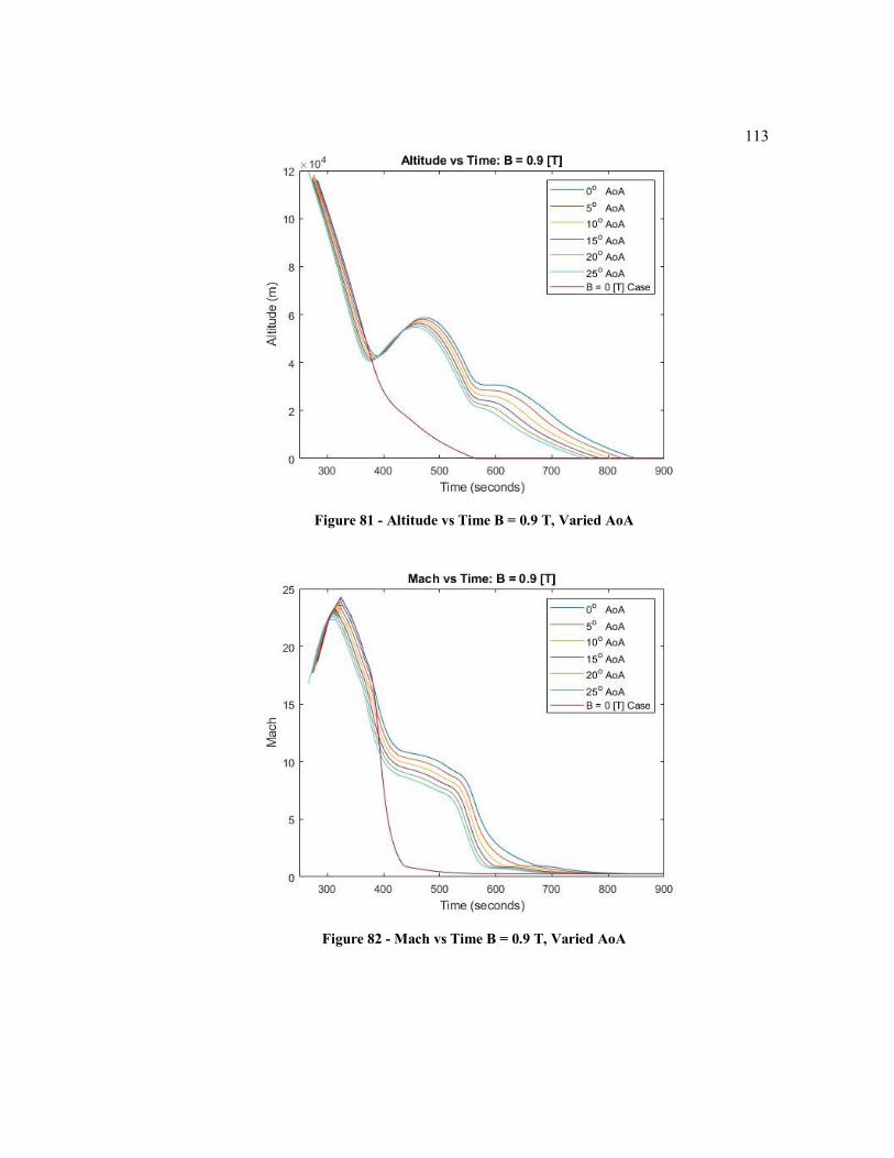
113
Figure 81 - Altitude vs Time B = 0.9 T, Varied AoA
Figure 82 - Mach vs Time B = 0.9 T, Varied AoA

114
Figure 83 - Velocity vs Time B = 0.9 T, Varied AoA
B = 1.0 T
Figure 84 - Figure 87 represent the change in acceleration, altitude, Mach number, and
velocity using a magnetic flux density of 𝐵 = 1 𝑇 and a varied angle of attack.
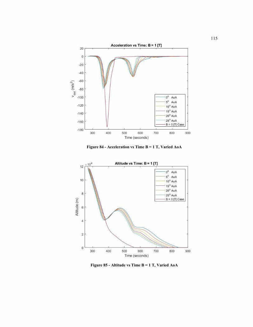
115
Figure 84 - Acceleration vs Time B = 1 T, Varied AoA
Figure 85 - Altitude vs Time B = 1 T, Varied AoA
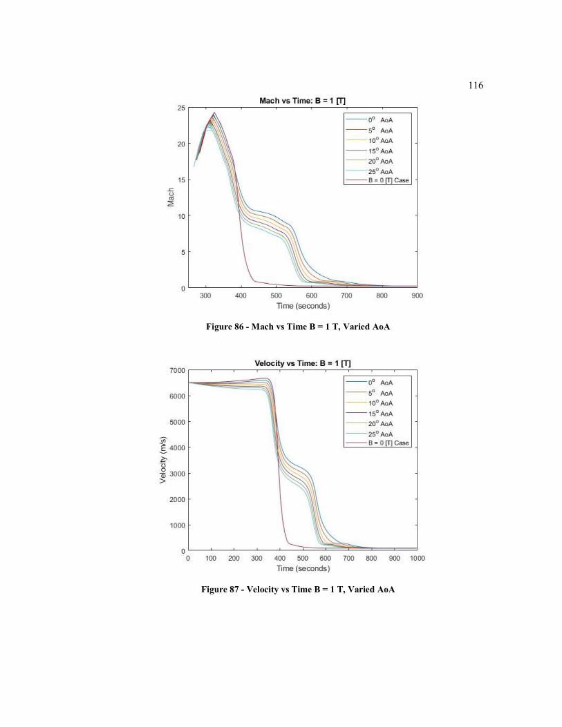
116
Figure 86 - Mach vs Time B = 1 T, Varied AoA
Figure 87 - Velocity vs Time B = 1 T, Varied AoA
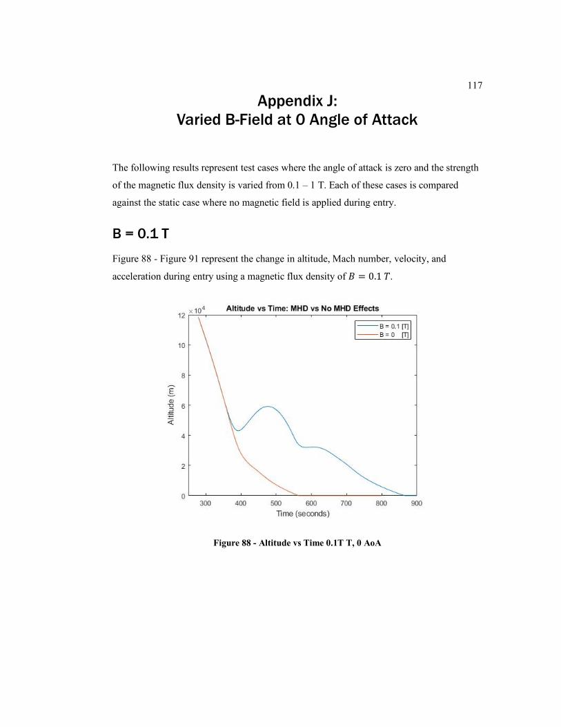
117
Appendix J:
Varied B-Field at 0 Angle of Attack
The following results represent test cases where the angle of attack is zero and the strength
of the magnetic flux density is varied from 0.1 – 1 T. Each of these cases is compared
against the static case where no magnetic field is applied during entry.
B = 0.1 T
Figure 88 - Figure 91 represent the change in altitude, Mach number, velocity, and
acceleration during entry using a magnetic flux density of 𝐵 = 0.1 𝑇.
Figure 88 - Altitude vs Time 0.1T T, 0 AoA
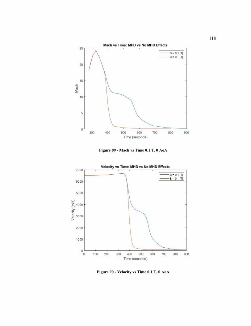
118
Figure 89 - Mach vs Time 0.1 T, 0 AoA
Figure 90 - Velocity vs Time 0.1 T, 0 AoA
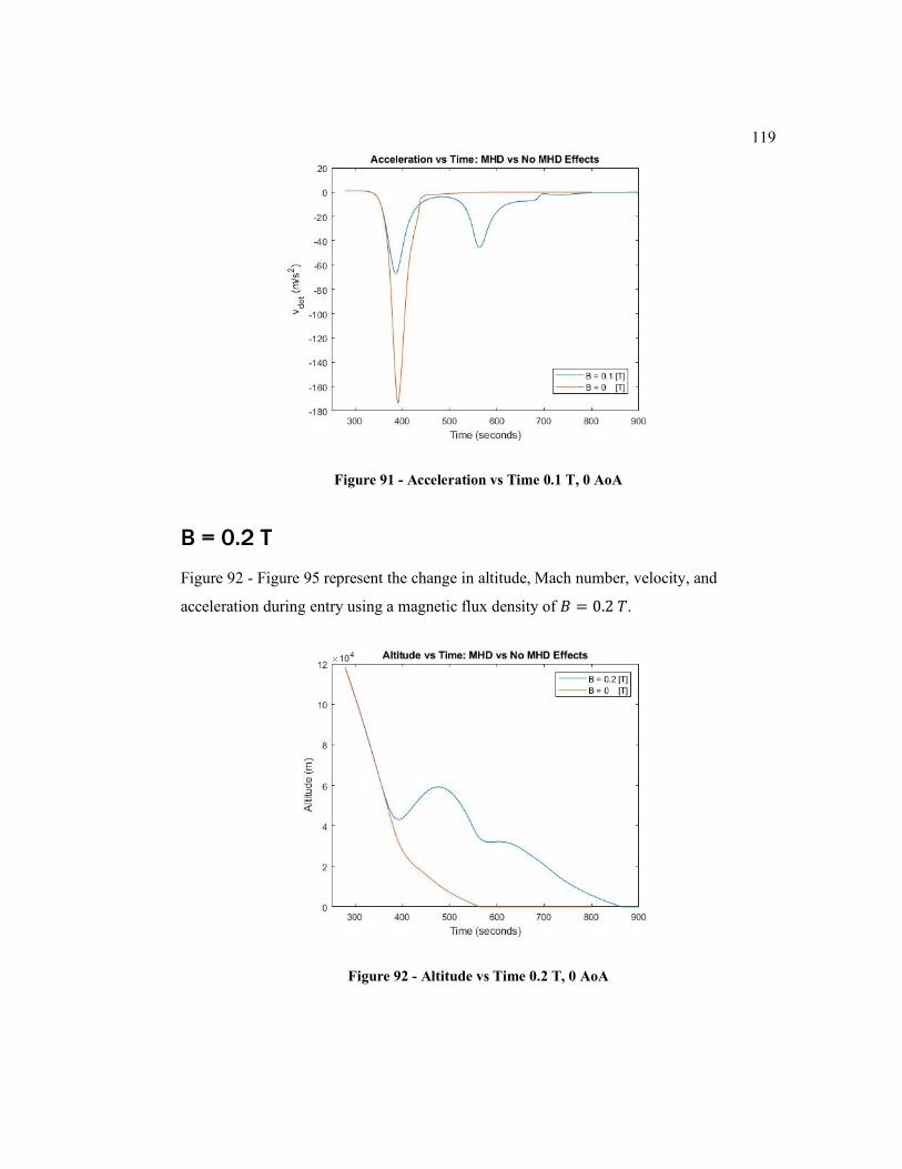
119
Figure 91 - Acceleration vs Time 0.1 T, 0 AoA
B = 0.2 T
Figure 92 - Figure 95 represent the change in altitude, Mach number, velocity, and
acceleration during entry using a magnetic flux density of 𝐵 = 0.2 𝑇.
Figure 92 - Altitude vs Time 0.2 T, 0 AoA
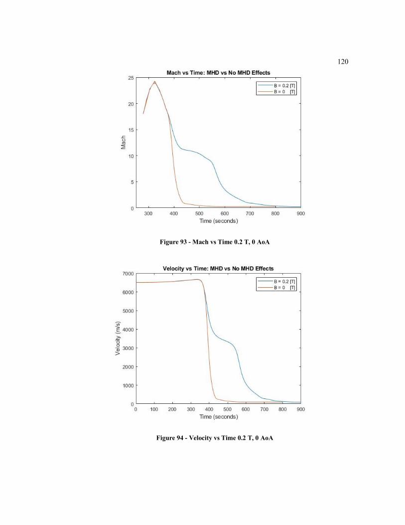
120
Figure 93 - Mach vs Time 0.2 T, 0 AoA
Figure 94 - Velocity vs Time 0.2 T, 0 AoA

121
Figure 95 - Acceleration vs Time 0.2 T, 0 AoA
B = 0.3 T
Figure 96 - Figure 99 represent the change in altitude, Mach number, velocity, and
acceleration during entry using a magnetic flux density of 𝐵 = 0.3 𝑇.
Figure 96 - Altitude vs Time 0.3 T, 0 AoA
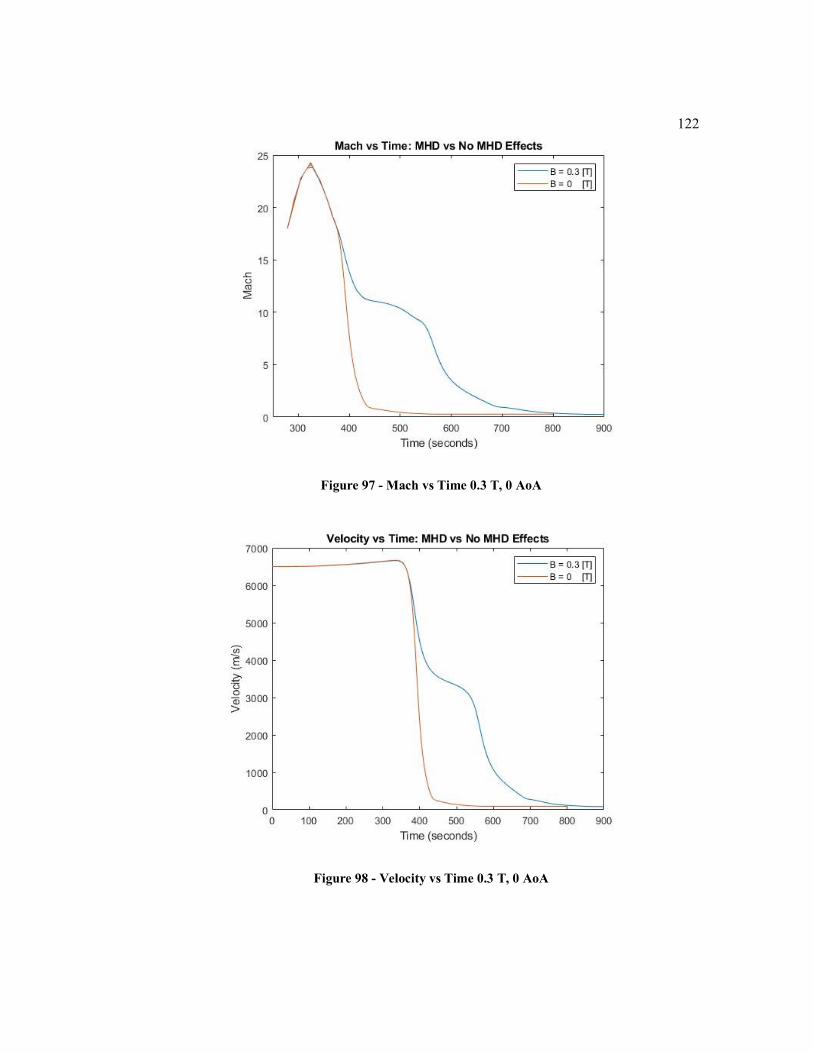
122
Figure 97 - Mach vs Time 0.3 T, 0 AoA
Figure 98 - Velocity vs Time 0.3 T, 0 AoA
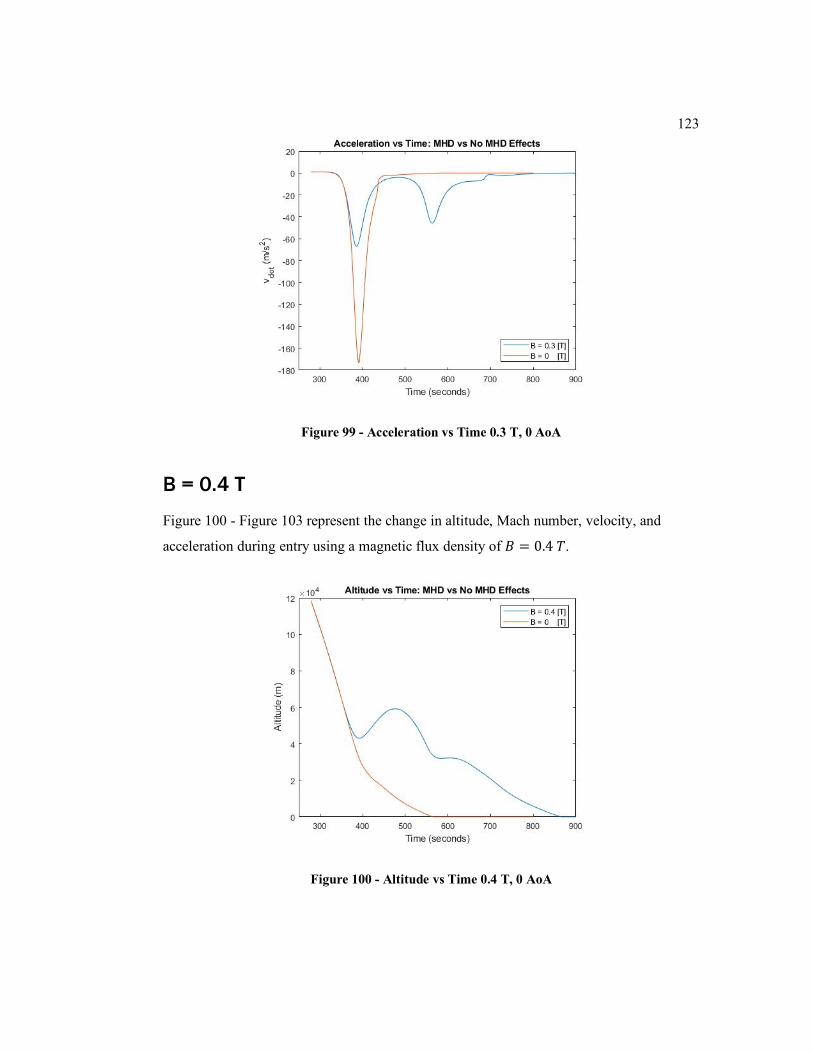
123
Figure 99 - Acceleration vs Time 0.3 T, 0 AoA
B = 0.4 T
Figure 100 - Figure 103 represent the change in altitude, Mach number, velocity, and
acceleration during entry using a magnetic flux density of 𝐵 = 0.4 𝑇.
Figure 100 - Altitude vs Time 0.4 T, 0 AoA
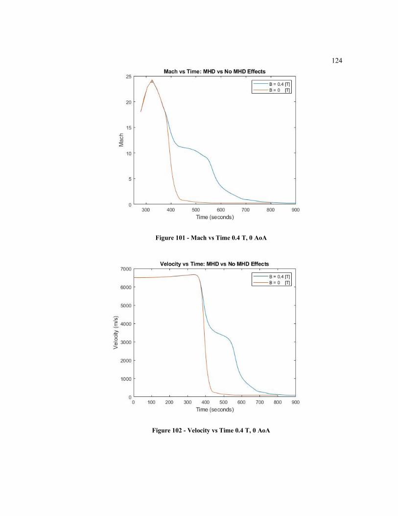
124
Figure 101 - Mach vs Time 0.4 T, 0 AoA
Figure 102 - Velocity vs Time 0.4 T, 0 AoA
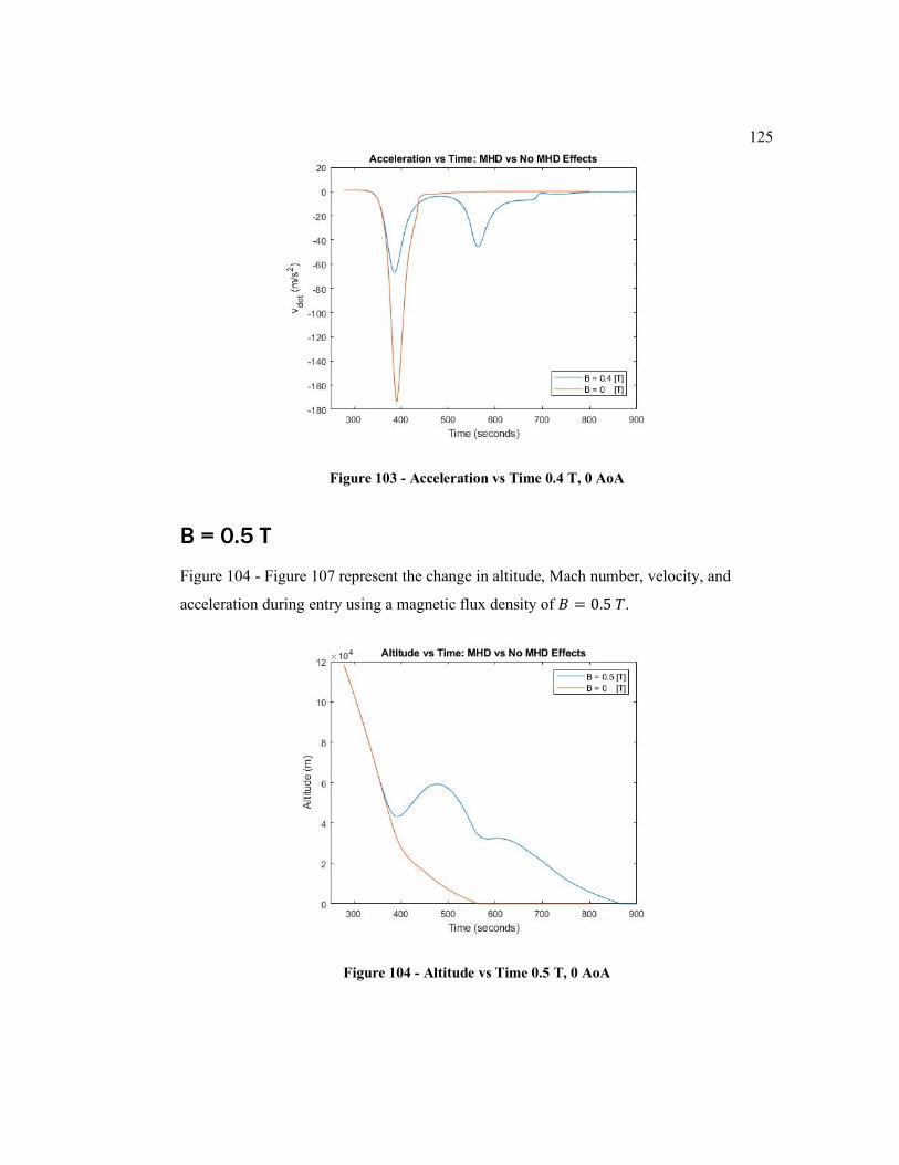
125
Figure 103 - Acceleration vs Time 0.4 T, 0 AoA
B = 0.5 T
Figure 104 - Figure 107 represent the change in altitude, Mach number, velocity, and
acceleration during entry using a magnetic flux density of 𝐵 = 0.5 𝑇.
Figure 104 - Altitude vs Time 0.5 T, 0 AoA
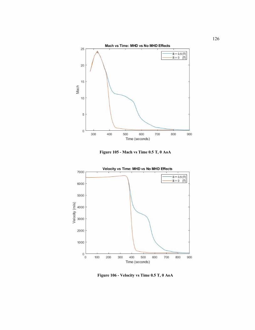
126
Figure 105 - Mach vs Time 0.5 T, 0 AoA
Figure 106 - Velocity vs Time 0.5 T, 0 AoA
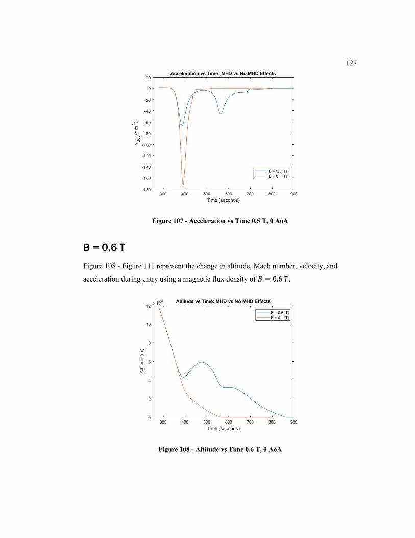
127
Figure 107 - Acceleration vs Time 0.5 T, 0 AoA
B = 0.6 T
Figure 108 - Figure 111 represent the change in altitude, Mach number, velocity, and
acceleration during entry using a magnetic flux density of 𝐵 = 0.6 𝑇.
Figure 108 - Altitude vs Time 0.6 T, 0 AoA
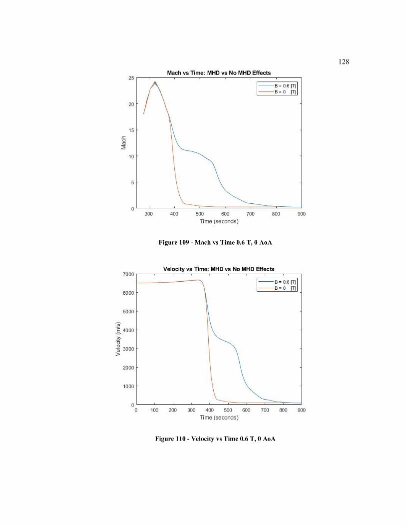
128
Figure 109 - Mach vs Time 0.6 T, 0 AoA
Figure 110 - Velocity vs Time 0.6 T, 0 AoA
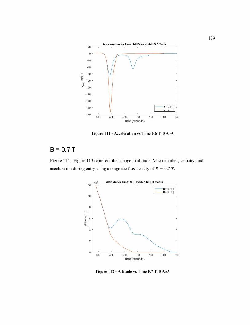
129
Figure 111 - Acceleration vs Time 0.6 T, 0 AoA
B = 0.7 T
Figure 112 - Figure 115 represent the change in altitude, Mach number, velocity, and
acceleration during entry using a magnetic flux density of 𝐵 = 0.7 𝑇.
Figure 112 - Altitude vs Time 0.7 T, 0 AoA
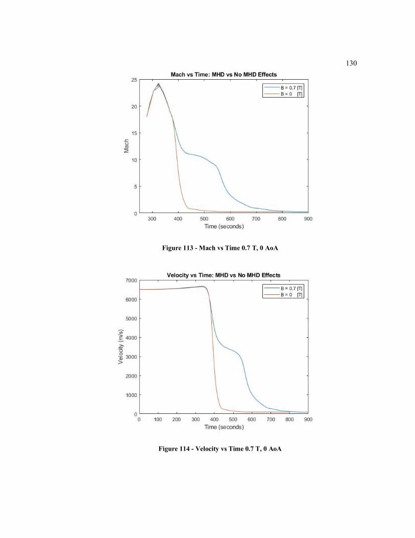
130
Figure 113 - Mach vs Time 0.7 T, 0 AoA
Figure 114 - Velocity vs Time 0.7 T, 0 AoA
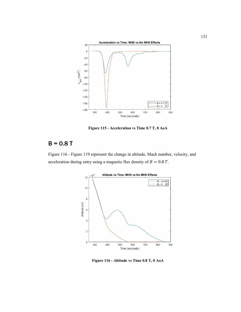
131
Figure 115 - Acceleration vs Time 0.7 T, 0 AoA
B = 0.8 T
Figure 116 - Figure 119 represent the change in altitude, Mach number, velocity, and
acceleration during entry using a magnetic flux density of 𝐵 = 0.8 𝑇.
Figure 116 - Altitude vs Time 0.8 T, 0 AoA
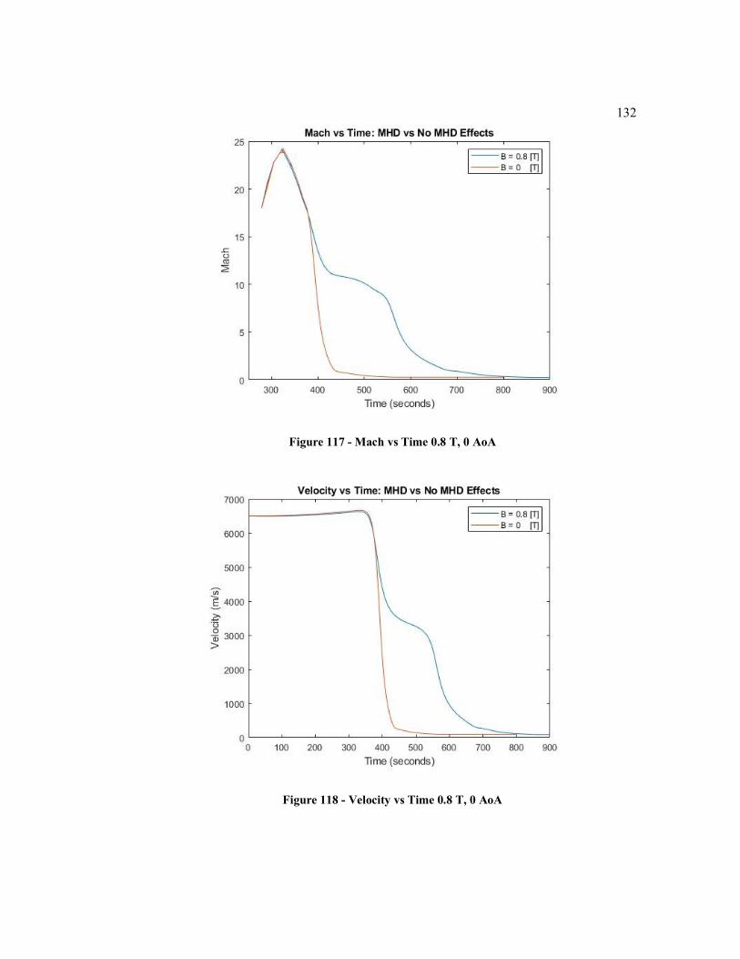
132
Figure 117 - Mach vs Time 0.8 T, 0 AoA
Figure 118 - Velocity vs Time 0.8 T, 0 AoA
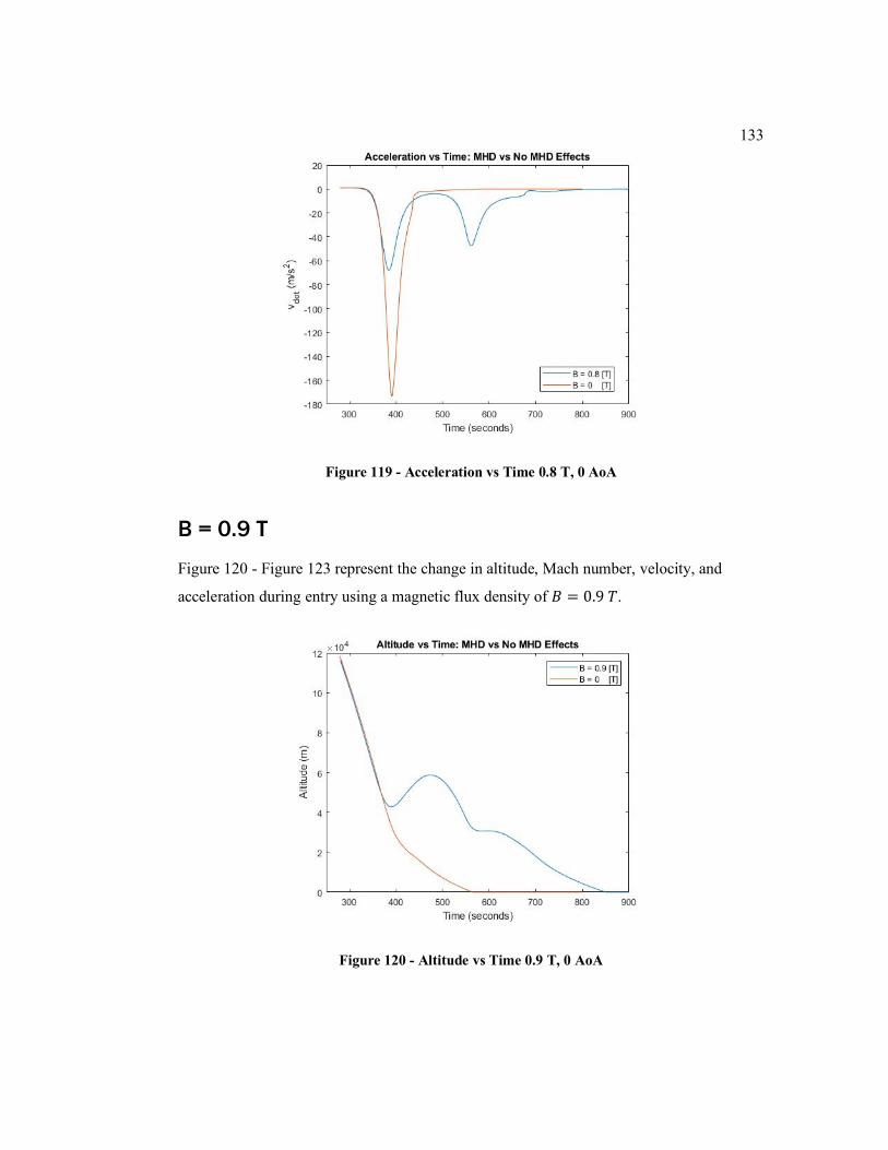
133
Figure 119 - Acceleration vs Time 0.8 T, 0 AoA
B = 0.9 T
Figure 120 - Figure 123 represent the change in altitude, Mach number, velocity, and
acceleration during entry using a magnetic flux density of 𝐵 = 0.9 𝑇.
Figure 120 - Altitude vs Time 0.9 T, 0 AoA
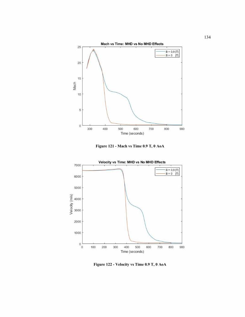
134
Figure 121 - Mach vs Time 0.9 T, 0 AoA
Figure 122 - Velocity vs Time 0.9 T, 0 AoA

135
Figure 123 - Acceleration vs Time 0.9 T, 0 AoA
B = 1.0 T
Figure 124 - Figure 127 represent the change in altitude, Mach number, velocity, and
acceleration during entry using a magnetic flux density of 𝐵 = 1 𝑇.
Figure 124 - Altitude vs Time 1 T, 0 AoA
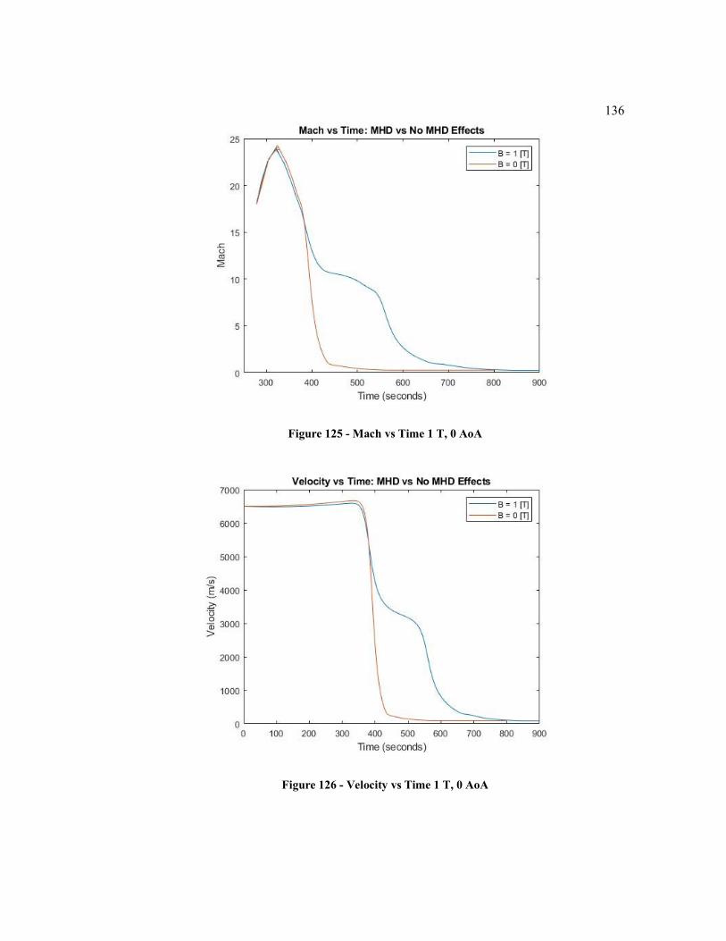
136
Figure 125 - Mach vs Time 1 T, 0 AoA
Figure 126 - Velocity vs Time 1 T, 0 AoA
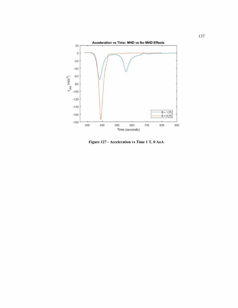
137
Figure 127 - Acceleration vs Time 1 T, 0 AoA
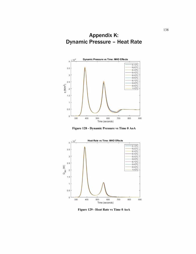
138
Appendix K:
Dynamic Pressure – Heat Rate
Figure 128 - Dynamic Pressure vs Time 0 AoA
Figure 129 - Heat Rate vs Time 0 AoA
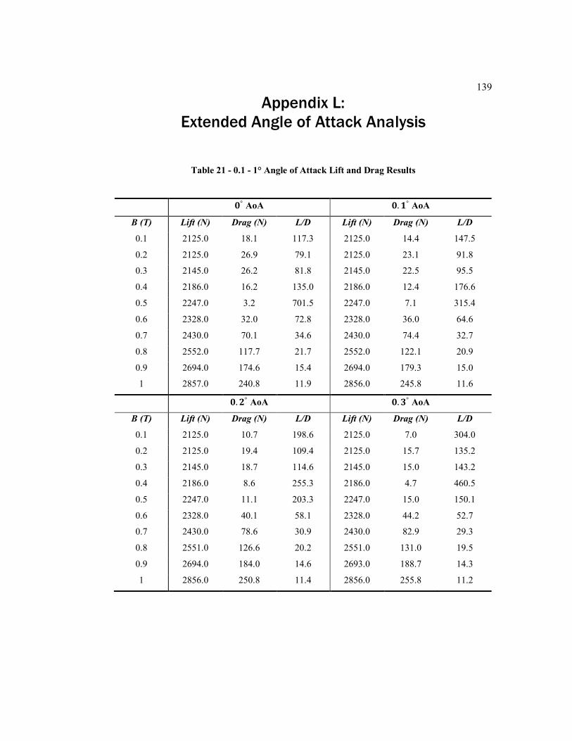
139
Appendix L:
Extended Angle of Attack Analysis
Table 21 - 0.1 - 1° Angle of Attack Lift and Drag Results
𝟎° AoA 𝟎. 𝟏° AoA
B (T) Lift (N) Drag (N) L/D Lift (N) Drag (N) L/D
0.1 2125.0 18.1 117.3 2125.0 14.4 147.5
0.2 2125.0 26.9 79.1 2125.0 23.1 91.8
0.3 2145.0 26.2 81.8 2145.0 22.5 95.5
0.4 2186.0 16.2 135.0 2186.0 12.4 176.6
0.5 2247.0 3.2 701.5 2247.0 7.1 315.4
0.6 2328.0 32.0 72.8 2328.0 36.0 64.6
0.7 2430.0 70.1 34.6 2430.0 74.4 32.7
0.8 2552.0 117.7 21.7 2552.0 122.1 20.9
0.9 2694.0 174.6 15.4 2694.0 179.3 15.0
1 2857.0 240.8 11.9 2856.0 245.8 11.6
𝟎. 𝟐° AoA 𝟎. 𝟑° AoA
B (T) Lift (N) Drag (N) L/D Lift (N) Drag (N) L/D
0.1 2125.0 10.7 198.6 2125.0 7.0 304.0
0.2 2125.0 19.4 109.4 2125.0 15.7 135.2
0.3 2145.0 18.7 114.6 2145.0 15.0 143.2
0.4 2186.0 8.6 255.3 2186.0 4.7 460.5
0.5 2247.0 11.1 203.3 2247.0 15.0 150.1
0.6 2328.0 40.1 58.1 2328.0 44.2 52.7
0.7 2430.0 78.6 30.9 2430.0 82.9 29.3
0.8 2551.0 126.6 20.2 2551.0 131.0 19.5
0.9 2694.0 184.0 14.6 2693.0 188.7 14.3
1 2856.0 250.8 11.4 2856.0 255.8 11.2
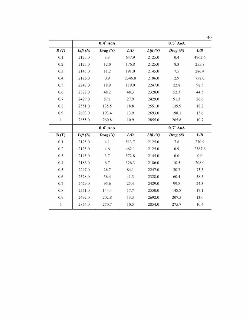
140
𝟎. 𝟒° AoA 𝟎. 𝟓° AoA
B (T) Lift (N) Drag (N) L/D Lift (N) Drag (N) L/D
0.1 2125.0 3.3 647.9 2125.0 0.4 4962.6
0.2 2125.0 12.0 176.8 2125.0 8.3 255.8
0.3 2145.0 11.2 191.0 2145.0 7.5 286.4
0.4 2186.0 0.9 2346.8 2186.0 2.9 758.0
0.5 2247.0 18.9 119.0 2247.0 22.8 98.5
0.6 2328.0 48.2 48.3 2328.0 52.3 44.5
0.7 2429.0 87.1 27.9 2429.0 91.3 26.6
0.8 2551.0 135.5 18.8 2551.0 139.9 18.2
0.9 2693.0 193.4 13.9 2693.0 198.1 13.6
1 2855.0 260.8 10.9 2855.0 265.8 10.7
𝟎. 𝟔° AoA 𝟎. 𝟕° AoA
B (T) Lift (N) Drag (N) L/D Lift (N) Drag (N) L/D
0.1 2125.0 4.1 513.7 2125.0 7.8 270.9
0.2 2125.0 4.6 462.1 2125.0 0.9 2387.6
0.3 2145.0 3.7 572.8 2145.0 0.0 0.0
0.4 2186.0 6.7 326.3 2186.0 10.5 208.0
0.5 2247.0 26.7 84.1 2247.0 30.7 73.3
0.6 2328.0 56.4 41.3 2328.0 60.4 38.5
0.7 2429.0 95.6 25.4 2429.0 99.8 24.3
0.8 2551.0 144.4 17.7 2550.0 148.8 17.1
0.9 2692.0 202.8 13.3 2692.0 207.5 13.0
1 2854.0 270.7 10.5 2854.0 275.7 10.4
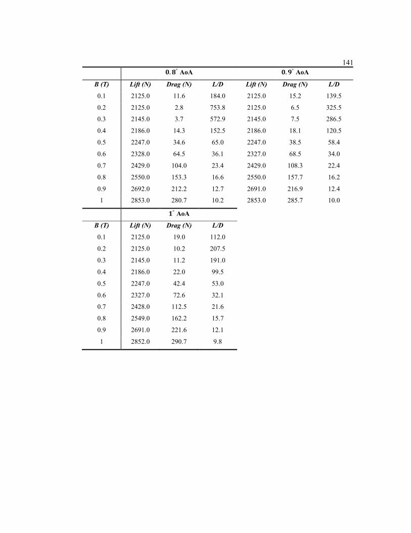
141
𝟎. 𝟖° AoA 𝟎. 𝟗° AoA
B (T) Lift (N) Drag (N) L/D Lift (N) Drag (N) L/D
0.1 2125.0 11.6 184.0 2125.0 15.2 139.5
0.2 2125.0 2.8 753.8 2125.0 6.5 325.5
0.3 2145.0 3.7 572.9 2145.0 7.5 286.5
0.4 2186.0 14.3 152.5 2186.0 18.1 120.5
0.5 2247.0 34.6 65.0 2247.0 38.5 58.4
0.6 2328.0 64.5 36.1 2327.0 68.5 34.0
0.7 2429.0 104.0 23.4 2429.0 108.3 22.4
0.8 2550.0 153.3 16.6 2550.0 157.7 16.2
0.9 2692.0 212.2 12.7 2691.0 216.9 12.4
1 2853.0 280.7 10.2 2853.0 285.7 10.0
𝟏° AoA
B (T) Lift (N) Drag (N) L/D
0.1 2125.0 19.0 112.0
0.2 2125.0 10.2 207.5
0.3 2145.0 11.2 191.0
0.4 2186.0 22.0 99.5
0.5 2247.0 42.4 53.0
0.6 2327.0 72.6 32.1
0.7 2428.0 112.5 21.6
0.8 2549.0 162.2 15.7
0.9 2691.0 221.6 12.1
1 2852.0 290.7 9.8