Flexible Causal Inference forInternational RelationsBear F. Braumoeller,* Giampiero Marra,† Rosalba Radice,‡, and Aisha Bradshaw.*

Abstract. Measuring the causal impact of state behavior on outcomes is one of the biggest methodological challenges in the fieldof international relations, for two reasons: behavior is generally endogenous, and the threat of unobserved variables that confoundthe relationship between behavior and outcomes is pervasive. Matching methods, widely considered to be the state of the art incausal inference in political science, are ill-suited to inference in the presence of unobserved confounders. Heckman-style modelsoffer a solution to this problem; however, they rely on functional form assumptions that can produce nontrivial bias in estimates ofaverage treatment effects. We describe a category of models, flexible simultaneous likelihood models, that account for both featuresof the data while avoiding reliance on rigid functional form assumptions. We then assess these models’ performance in a series ofneutral simulations, in which they produce substantial (55% to 90+%) reduction in bias relative to competing models. Finally, wedemonstrate their utility in a reanalysis of Simmons’ (2000) classic study of the impact of Article VIII commitment on compliancewith the IMF’s currency-restriction regime.

Version 3.2., July 10, 2016.

1 IntroductionThe study of international relations (IR) has under-gone a methodological renaissance in the past 20years. A subfield that was once content to baseits conclusions on garden-variety logit and probitresults has created or imported methods for mod-eling strategic interaction (Signorino 1999; Smith1999; Lewis 2003; c.f. Carrubba, Yuen and Zorn2007), selection bias (Sartori, 2003; von Stein, 2005;Boehmke, Morey and Shannon, 2006; Chiba, Mar-tin and Stevenson, 2014), split-population or partial-observability models (Xiang, 2010; Braumoeller andCarson, 2011), zero-inflated or rare events data (Kingand Zeng, 2001; Bagozzi, Hill, Moore and Mukher-jee, 2015), network analysis (Dorussen and Ward,2008; Hafner-Burton and Kahler, 2009; Maoz, 2009;Cranmer, Desmarais and Menninga, 2012), andmore.

Unfortunately, empirical studies of IR continueto be plagued by the problem of endogeneity. En-

dogeneity occurs when an omitted variable or vari-ables confounds the relationship between cause andeffect, thereby introducing bias into the estimate ofthe causal effect. Contrary to what most practition-ers seem to believe, endogeneity bias cannot reliably be elim-inated, or even reduced, by simply adding observed confound-ing variables to the right-hand side of the equation: doing sofails to account for the correlation between the con-founder(s) and the endogenous variable. While en-dogeneity is endemic to the social sciences, the en-dogeneity problem in IR is especially acute becausethe data are both imprecise and scarce: the time andexpense involved in obtaining data that precisely cap-ture a quantity of interest in IR across a meaningfulspan of time can be prohibitive. As a result, unmea-sured confounders are a threat to inference in eventhe most well-designed studies.

Fortunately, political methodologists have increas-ingly focused on the development of methods de-signed to account for it. While scholars during the

1

so-called “age of regression” (Morgan and Winship,2007, ch. 1) were often content to base their conclu-sions on simple correlational methods such as regres-sion, hazard models, logit, and the like, the 21st cen-tury has brought with it a renewed appreciation ofthe hazards of basing causal claims on observationaldata. Except in the case of randomized experiments,one can rarely assume that variables of interest aretruly exogenous—or, put differently, that assignmentto a “treatment condition” of interest, like commit-ment to an institution, is truly randomized. Greaterappreciation of this point has brought with it an in-creased interest in experiments as well as a renewedfocus on statistical techniques designed to accountfor the confounding variables that represent a majorthreat to causal inference in observational studies.

In this paper we elaborate one such methodology,flexible simultaneous likelihood models, that we be-lieve conveys a host of advantages to students of po-litical science in general and IR in particular. Byvirtue of their structure, these models can accountfor endogeneity. Unlike matching methods, the cur-rent state of the art for causal inference in political sci-ence, they can also account for the unmeasured con-founders that plague studies of IR. Finally, relative totraditional simultaneous likelihood models, they arefar less reliant on rigid distributional assumptions thatcan bias results.

To establish the validity of these models, we use aseries of simulations to explore their ability to reduceendogeneity bias. To illustrate their utility, we thentake up the debate among Simmons (2000), von Stein(2005), and Simmons and Hopkins (2005) on the im-pact of formal commitment to Article VIII of the In-ternational Monetary Fund’s Articles of Agreementon states’ willingness to refrain from currency restric-tions. By loosening the parametric assumptions of therecursive bivariate probit model we show both thatvon Stein was correct to argue that Article VIII pro-duces a screening effect and that Simmons was cor-

rect to argue that it produces a constraining effect—one that is both smaller and much longer-lived thanthe original study suggested. At the same time, weshow that von Stein was correct to argue that unmea-sured confounders cannot be ignored.

2 The Problem of EndogeneityEndogeneity occurs when one or more omitted vari-ables confounds the relationship between cause andeffect, rendering estimates of the causal effect prob-lematic (Kish, 1959). Because confounding is a po-tential threat to inference whenever the causal vari-able is itself caused by something else, and becausevirtually everything is endogenous in social science,endogeneity is ubiquitous. For instance, democracy issaid to cause peace (Maoz and Russett, 1993; Buenode Mesquita, Morrow, Siverson and Smith, 1999;Bausch, 2015), but democracy itself is thought tobe endogenous (Gates, Knutsen and Moses, 1996;Reuveny and Li, 2003). Similarly, military alliancesare widely accepted as a tool that can reduce the riskof conflict (Leeds, 2003; Johnson and Leeds, 2011;Benson, 2011; Fang, Johnson and Leeds, 2014), butboth alliance formation and conflicts are driven bythe (typically unobserved) interests and security envi-ronment of the states involved. Failing to account forthese interests leads to bias in the estimation of theimpact of alliances on conflict (Levy, 1981; Bearce,Flanagan and Floros, 2006). In the same vein, pooreconomic conditions are thought to increase the riskof terrorism (Blomberg, Hess and Weerapana, 2004;Freytag, Krüger, Meierrieks and Schneider, 2011;Meierrieks and Gries, 2012), but important variablesaffect both the state of the economy and the incidenceof terrorism. For example, low levels of political free-dom have been linked to both poor economic growth(Grier and Tullock, 1989) and terrorism (Krieger andMeierrieks, 2011). Even weather, often used as an in-strumental variable because of its independence from

2

human influence, has become endogenous to anthro-pogenic climate change in studies of civil conflict (see,e.g., Tir and Stinnett 2012 and Theisen 2012).

In statistical terms, the endogeneity of a given vari-able manifests itself as an association between thatvariable and the error term. For example, in the lin-ear regression y = Xβ + ϵ each of the variables indesign matrix X is assumed to be independent of ϵ.If some omitted variable, w, influences both y andone of the right-hand-side variables, x1, w is said toconfound the relationship between y and x1 becausex1 is no longer uncorrelated with ϵ. In this case theestimator for β will be biased and inconsistent, withβ1 (the impact of x1 on y) being the most affected(Wooldridge, 2010). The same logic applies to tech-niques like logit and probit that are designed to han-dle binary dependent variables.

Unfortunately, there is no perfect answer to theproblem of endogeneity in observational studies. Asa theoretical solution, Manski (1990) did derive anonparametric technique that calculates the boundswithin which the average treatment effect of an en-dogenous causal variable must lie, but those boundsare typically so broad as to be of little use to practi-tioners. It is worth noting, however, that any solu-tion that offers a more precise answer than Manski’smust leverage some assumptions in order to do so. Ingeneral, the technique that is best able to recover thecausal effect of a treatment with both accuracy andprecision should be the technique whose assumptionsare best-suited to the circumstances. In the follow-ing sections we argue that flexible simultaneous like-lihood methods are exceptionally well-suited to thechallenging circumstances that are typically found inthe study of international relations.

2.1 Existing SolutionsWhile the majority of IR scholars are aware of theproblem of endogeneity, at least in principle, most

seem to believe that it can be taken care of simply byadding observed confounding variables to the right-hand side of the equation (see, e.g., Simmons 2000,829, fn 25 and Doyle and Sambanis 2000). Unfortu-nately, doing so generally does not resolve the prob-lem. While it is technically not impossible to addressendogeneity bias in this manner, the technique as-sumes both that all possible confounders have beenmeasured and included in the equation and that thefunctional form of their relationship to y has beencorrectly specified—assumptions that will almost cer-tainly not be met.

The desire to account for confounding variables’effects on both left-hand-side and endogenous right-hand-side variables has also led researchers to ex-plore instrumental variables approaches (e.g., Sim-mons 2009). These typically take the linear form

y = β1x1 + {Xβ}[−β1x1] + ϵ,

x1 = Zγ + υ,

where {Xβ}[−β1x1] excludes the component β1x1from Xβ and Z is a design matrix. This approachis generally preferable to ordinary single-equationmodels in that it explicitly addresses the endogene-ity of x1 (Angrist and Krueger, 2001). It can createsome practical difficulties, however, in that it relieson the existence of an instrument—a variable in Z thatis independent of the unobserved confounders (i.e.,independent of the error terms), independent of yconditional on the unobserved and unobserved con-founders, and associated with x1. Instruments can bedifficult to identify in studies of IR. In the worst-casescenario, every cause of an outcome is also a cause ofthe anticipatory behavior that is designed to influencethat outcome. This issue is especially problematic inthe literature on peacekeeping, for example (see, e.g.,Fortna and Howard 2008, 290). Moreover, instru-ments may be invalid, in that they are correlated with

3

the error term, ϵ, in the outcome equation, or theymay be weak, or only weakly correlated with the en-dogenous variable x1 (Murray, 2006).

Another, less commonly noted problem with esti-mators of this sort is their ability to identify causaleffects typically hinges on their functional form, andfunctional form assumptions are often made arbitrar-ily:

Given the model, least squares and its variantscan be used to estimate parameters and todecide whether or not these are zero. How-ever, the model cannot in general be re-garded as given, because current social sci-ence theory does not provide the requisitelevel of technical detail for deriving speci-fications. (Freedman, Collier, Sekhon andStark, 2010, 46)

As we demonstrate in our simulations below, the biasintroduced by even minor differences in functionalform assumptions can be nontrivial.

It is perhaps not surprising, then, that practitionershave turned to matching methods to estimate causaleffects (Simmons and Hopkins, 2005; Gilligan andSergenti, 2008; Hill, 2010; Lupu, 2013). Matching isa simple and powerful methodology for dealing withconfounding. The basic idea behind it is to matcheach “treated” unit (x1 = 1) with one “control”unit (x1 = 0) (or vice versa) based on observed con-founders. In this way the matched data resemble, asmuch as possible, observations from a natural experi-ment in which one comparable set of units was givena treatment while the other constituted a control. Ac-cordingly, the impact of x1 on y can be measured viaa simple difference of means. Because the techniqueis nonparametric, concerns about functional form as-sumptions are eliminated—a feature that is often em-phasized by the method’s proponents.

2.2 The Threat of Unobserved Con-founders

Matching methods are a compelling way to cutthrough the thicket of problems surrounding instru-mental variable approaches. They are not withoutproblems of their own, however. Foremost amongthem is the assumption that all confounders havebeen measured and incorporated into the analysis—an assumption known as “selection on observables.”To the extent that this assumption has been recog-nized as being potentially problematic, the solutionis typically to measure unmeasured confounders andinclude them in the analysis (see, e.g., Simmons andHopkins 2005; Lupu 2013). As Keele (2015, 322)notes in a recent review, however,

I can’t emphasize enough that selection onobservables is a very strong assumption. Itis often difficult to imagine that selection onobservables is plausible in many contexts.

This assumption is especially problematic in the con-text of IR, for two reasons. First, gathering cross-sectional time series data across many decades andacross nearly 200 independent political entities is adaunting task. Measures are bound to be approxi-mate in many cases, missing data are common, andrelevant measures are either approximated using ex-isting but tenuously related data (“proxies”) or sim-ply omitted due to the cost of data collection. Ac-cordingly, the coarseness and sparsity of internationalrelations data make it nearly impossible to accountfor all unobserved confounders, even in principle.1Second, using matching alone, there is no way toknow whether all relevant confounders have beenmeasured and included in the analysis.

1One of the authors once asked a methodologist colleaguewhy he had chosen the variables he chose for an IR example andreceived the response, “Don’t IR people only have six variables?”

4

Indeed, doing so can prove difficult even in actualexperiments. Consider, for example, the role that un-observable confounders played in a significant con-troversy from the American politics literature on theefficacy of get-out-the-vote efforts prior to the 1998election. Gerber and Green (2000) carried out a fieldexperiment involving 30,000 registered voters in NewHaven, Connecticut and concluded that, while per-sonal canvassing increased voter turnout, telephonecalls did not. Imai (2005) argued that this findingwas an artifact of discrepancies between Gerber andGreen’s experimental design and the actual imple-mentation of the experiment. Using propensity scorematching, he concluded that telephone calls increasevoter turnout by five percentage points. Gerber andGreen (2005) correct the data issues that Imai bringsto light, re-estimate their model using two-stage leastsquares, and find results that are substantively identi-cal to those in the original study. In addition, Gerberand Green use Imai’s matching technique to estimatethe difference in turnout rates between individualswho were not assigned to the “treatment” group andwere therefore not called and individuals who wereplaced in the “treatment” group but were never con-tacted. Because neither group was contacted, the im-pact of simply being in the treatment group should bezero, but Gerber and Green find a treatment effect of-5.6%, with a standard error of 2.3—implying, as theauthors put it, that “placing phone numbers on a listand not calling them depresses turnout” (310).

Both the absurdity of this conclusion and the dis-parity between Gerber and Green’s findings andthose of Imai led Sekhon (2009, 502-503) to concludethat “it is clear that the selection-on-observables as-sumption is not valid in this case.” More generally,he concludes,

[s]election on observables and other iden-tifying assumptions not guaranteed by thedesign should be considered incorrect un-

less compelling evidence to the contrary isprovided. (503)

Consider the import of this conclusion for studentsof international relations. The overwhelming ma-jority of our research designs are observational, andsuch designs cannot make the selection on observ-ables assumption remotely plausible in and of them-selves. That leaves users of matching techniques withthe second-best strategy of measuring all conceivableconfounders, including them in the analysis, and hop-ing that they have all been accounted for. The oddsthat they have been, however, would seem to be ex-traordinarily low in any realistic application. If stu-dents of American politics, conducting an experimentin which the subjects are individuals, the treatment isa telephone call, and the outcome is voting cannotmeet the selection-on-observables assumption, howcan students of international politics ever hope to doso?

All of these considerations point toward a straight-forward conclusion: causal inference in IR requiresa methodology that accounts for unobserved con-founders.

2.3 Accounting for UnobservablesFortunately for students of international relations, itis possible to account for the impact of unobservedconfounders, which manifests itself as an associa-tion between the error terms of the treatment andoutcome equations. Multiple-equation instrumen-tal variable approaches accomplish this, though theyrely on generally arbitrary functional form assump-tions. Moreover, in the case of binary dependentand endogenous right-hand-side variables, which areubiquitous in IR, the two-stage estimation techniquetypical of such studies has been shown to be deeplyproblematic (Freedman and Sekhon, 2010). A morepromising approach is the use of simultaneous likeli-hood methods—in particular, multiple equation pro-

5

bit models with endogenous dummy regressors, alsoknown as recursive models. These models addressendogeneity directly by estimating the coefficients intwo (or more) equations simultaneously. They alsocapture the impact of unobserved confounders by al-lowing for correlation between the error terms of theequations.

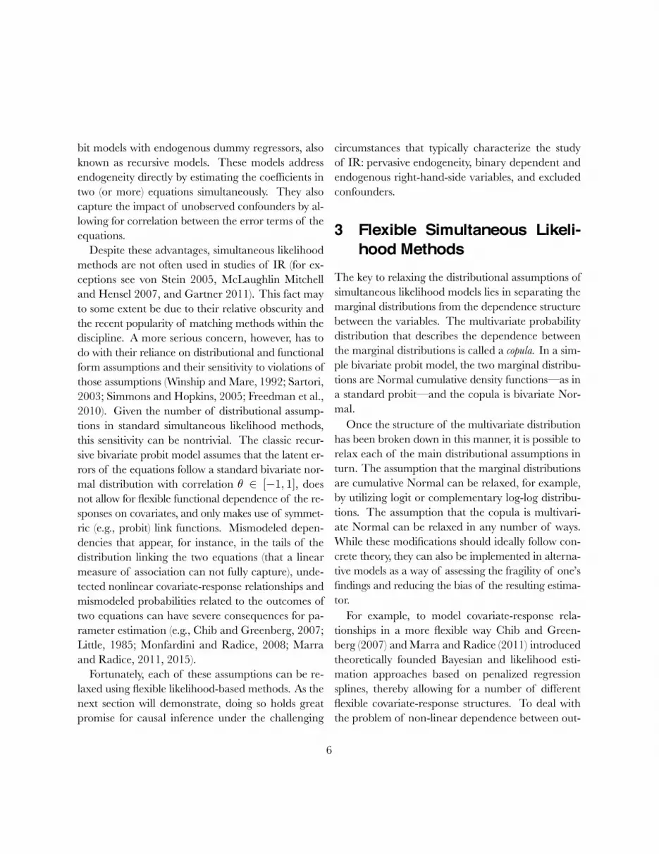
Despite these advantages, simultaneous likelihoodmethods are not often used in studies of IR (for ex-ceptions see von Stein 2005, McLaughlin Mitchelland Hensel 2007, and Gartner 2011). This fact mayto some extent be due to their relative obscurity andthe recent popularity of matching methods within thediscipline. A more serious concern, however, has todo with their reliance on distributional and functionalform assumptions and their sensitivity to violations ofthose assumptions (Winship and Mare, 1992; Sartori,2003; Simmons and Hopkins, 2005; Freedman et al.,2010). Given the number of distributional assump-tions in standard simultaneous likelihood methods,this sensitivity can be nontrivial. The classic recur-sive bivariate probit model assumes that the latent er-rors of the equations follow a standard bivariate nor-mal distribution with correlation θ ∈ [−1, 1], doesnot allow for flexible functional dependence of the re-sponses on covariates, and only makes use of symmet-ric (e.g., probit) link functions. Mismodeled depen-dencies that appear, for instance, in the tails of thedistribution linking the two equations (that a linearmeasure of association can not fully capture), unde-tected nonlinear covariate-response relationships andmismodeled probabilities related to the outcomes oftwo equations can have severe consequences for pa-rameter estimation (e.g., Chib and Greenberg, 2007;Little, 1985; Monfardini and Radice, 2008; Marraand Radice, 2011, 2015).

Fortunately, each of these assumptions can be re-laxed using flexible likelihood-based methods. As thenext section will demonstrate, doing so holds greatpromise for causal inference under the challenging

circumstances that typically characterize the studyof IR: pervasive endogeneity, binary dependent andendogenous right-hand-side variables, and excludedconfounders.

3 Flexible Simultaneous Likeli-hood Methods

The key to relaxing the distributional assumptions ofsimultaneous likelihood models lies in separating themarginal distributions from the dependence structurebetween the variables. The multivariate probabilitydistribution that describes the dependence betweenthe marginal distributions is called a copula. In a sim-ple bivariate probit model, the two marginal distribu-tions are Normal cumulative density functions—as ina standard probit—and the copula is bivariate Nor-mal.

Once the structure of the multivariate distributionhas been broken down in this manner, it is possible torelax each of the main distributional assumptions inturn. The assumption that the marginal distributionsare cumulative Normal can be relaxed, for example,by utilizing logit or complementary log-log distribu-tions. The assumption that the copula is multivari-ate Normal can be relaxed in any number of ways.While these modifications should ideally follow con-crete theory, they can also be implemented in alterna-tive models as a way of assessing the fragility of one’sfindings and reducing the bias of the resulting estima-tor.

For example, to model covariate-response rela-tionships in a more flexible way Chib and Green-berg (2007) and Marra and Radice (2011) introducedtheoretically founded Bayesian and likelihood esti-mation approaches based on penalized regressionsplines, thereby allowing for a number of differentflexible covariate-response structures. To deal withthe problem of non-linear dependence between out-

6

0.02

0.04

0.06

0.08 0.1

0.12

0.14

0.16

0.1

8

−3 −2 −1 0 1 2 3

−3

−2

−1

01

23

AMH

0.02

0.04

0.06

0.08

0.1

0.12 0.14

0.16

0.18

0.2

−3 −2 −1 0 1 2 3

−3

−2

−1

01

23

Clayton

0.02

0.04

0.06

0.08

0.1

0.12

0.14

0.16 0.1

8

0.2

−3 −2 −1 0 1 2 3

−3

−2

−1

01

23

Frank

0.02

0.04

0.06

0.08

0.1

0.12

0.14

0.16

0.1

8

−3 −2 −1 0 1 2 3

−3

−2

−1

01

23

Gaussian

0.02

0.04

0.06

0.08

0.1

0.12

0.14

0.16

0.18

0.2

−3 −2 −1 0 1 2 3

−3

−2

−1

01

23

Gumbel

0.02

0.04

0.06

0.08

0.1

0.12

0.14

0.16

0.18

0.2

0.22

−3 −2 −1 0 1 2 3

−3

−2

−1

01

23

Joe

Figure 1: Contour plots of some of the copulae implemented in SemiParBIVProbit with standard normal margins for data simulatedusing a Kendall’s τ of 0.5 for all copulae but AMH where a value of 1/3 (the maximum allowed for this copula) was used. The Gaussianand Frank copulae allow for equal degrees of positive and negative dependence with Frank exhibiting a slightly stronger dependence in themiddle of the distribution. AMH and Clayton are asymmetric with a strong lower tail dependence for Clayton but a weaker upper taildependence. Vice versa for the Gumbel and Joe copulae.

comes, Winkelmann (2012) discussed a modificationof the recursive bivariate probit which introducesnon-normal dependence between the marginal dis-tributions of the two equations using the Frank andClayton copulae. Radice, Marra and Wojtys (2015)took a more general approach and extended the pro-cedures discussed in Marra and Radice (2011) andWinkelmann (2012) to make it possible to deal simul-taneously with unobserved confounding, flexible co-variate effects and non-linear dependencies betweentwo binary responses. In particular, they general-ized the approach based on the assumption of bi-

variate normality presented in Marra and Radice(2011) by allowing for non-normal dependencies be-tween the two equations through Clayton, Frank,Gumbel, Joe, Ali-Mikhail-Haq and Farlie-Gumbel-Morgenstern copulae and the rotated versions ofClayton, Gumbel and Joe. Building on the generalmodeling framework introduced by Radice, Marraand Wojtys (2015), for this work we extended thescope of the modeling approach by also allowing forlogit and complementary log-log link functions—aninnovation in its own right. Radice, Marra and Wo-jtys (2015) provided a theoretical argumentation re-

7

lated to the asymptotic behavior of the proposed es-timator and the ensuing formula to calculate the av-erage treatment effect (ATE). Importantly, efficientand stable algorithms implementing the ideas abovehave been made available through the R packageSemiParBIVProbit (Marra and Radice, 2016). Themodel can be formulated as follows:

y∗ = β1x1 + f1({X}[−x1]

)+ ϵ,

x∗1 = f2 (Z) + υ,

where y∗ and x∗1 are allowed to follow one of the Nor-mal, logistic or Gumbel distributions with zero meanand variance equal to 1 (hence yielding probit, logitand cloglog link functions, respectively), the observedoutcome variables are determined by the classic rulesy = 1(y∗ > 0) and x1 = 1(x∗1 > 0), the proba-bility that y = 1 and x1 = 1 is defined as P(y =1, x1 = 1) = C(P(y = 1),P(x1 = 1); θ) where Cis a two-place copula function and θ an associationparameter (see Figure 1 for some copula shapes), andf1 and f2 represent flexible functions of the variablesin {X}[−x1] and Z. For instance, f1

({X}[−x1]

)could

be equal to β2x2 + s(x3) + s(x3)x2, where x2 is abinary predictor with impact β2, s(x3) is a smoothfunction of the continuous covariate x3, and s(x3)x2is an interaction term. Parameter θ can be modeledthrough a flexible linear predictor like those used formodeling y∗ and x∗1: since the strength of the associ-ation between the treatment and outcome equationsmay vary across groups of observations (specifically,across years), θ = m(f3(W)), where m is a one-to-one transformation which ensures that the depen-dence parameter lies in its range and W is a designmatrix (e.g., Radice, Marra and Wojtys, 2015).

Inference for the ATE is best achieved by utiliz-ing a useful connection between Bayesian and max-imum likelihood penalized regression spline estima-tors (Marra and Wood, 2012). This implies that

intervals with close-to-nominal frequentist coverageprobabilities for non-linear functions of the model co-efficients (e.g., ATE) can be conveniently obtainedby posterior simulation (Radice, Marra and Wojtys,2015). This has the obvious advantage of avoidingcomputationally expensive bootstrap methods, whichwould hinder the model building process that is piv-otal for practical modeling.

4 SimulationsThe aim of this section is to use simulations to as-sess the empirical effectiveness of the copula recur-sive bivariate model for binary outcomes. Becausesimulated results are of marginal interest when thedata-generating process conforms to the assumptionsof the authors’ preferred model and the parameterscan be set to degrade the performance of its com-petitors, we focus mostly on simulations in which noneof the models captures the correct distributional as-sumptions. The goal is to compare model perfor-mance under what we take to be the most likely sce-nario for IR scholars attempting causal inference: atleast one confounder is omitted, the marginal distri-butions and dependence structure are unknown, andthe goal is to recover the best (i.e., least biased andlowest RMSE) estimate of the ATE.

In the following simulations a binary instrument,two continuous observed confounders, one continu-ous unobserved confounder, a binary treatment anda binary outcome are denoted as z3, z1, z4, z2, x andy, respectively. We constructed the responses y andx using several distributions for the unobserved con-founding variable z2 (standard Normal, Student’s twith four degrees of freedom, χ2 with one degree offreedom and uniform[-3, 3]) and used logit link func-tions for the treatment and outcome variable, givingfour simulation scenarios in total. Variable z3 wassimulated with 2 categories (0 and 1) with Pr(z3 =1) = 0.5. Variables z1 and z4 were generated from

8

Link Logit-Logit Probit-Probit Cloglog-CloglogDistribution N (0, 1) t4 χ2

1 U(−3, 3) N (0, 1) t4 χ21 U(−3, 3) N (0, 1) t4 χ2

1 U(−3, 3)

% Bias

Mod

el

Univariate 33 53 42 119 32 53 41 119 33 43 40 121Matching 42 90 80 145 42 89 80 144 41 87 80 143Gaussian C 3 3 12 11 2 4 13 6 3 4 14 10Flexible C 3 0 5 4 2 1 6 1 6 0 7 4

% RMSE

Mod

el

Univariate 0.17 0.25 0.24 0.39 0.17 0.25 0.24 0.39 0.17 0.25 0.23 0.40Matching 0.23 0.44 0.46 0.49 0.22 0.44 0.46 0.48 0.22 0.43 0.46 0.48Gaussian C 0.05 0.06 0.08 0.07 0.06 0.06 0.08 0.08 0.07 0.06 0.08 0.07Flexible C 0.06 0.07 0.05 0.08 0.06 0.06 0.05 0.07 0.08 0.07 0.07 0.08

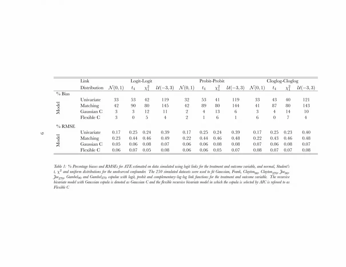
Table 1: % Percentage biases and RMSEs for ATE estimated on data simulated using logit links for the treatment and outcome variable, and normal, Student’st, χ2 and uniform distributions for the unobserved confounder. The 250 simulated datasets were used to fit Gaussian, Frank, Clayton90, Clayton270, Joe90,Joe270, Gumbel90 and Gumbel270 copulae with logit, probit and complementary-log-log link functions for the treatment and outcome variable. The recursivebivariate model with Gaussian copula is denoted as Gaussian C and the flexible recursive bivariate model in which the copula is selected by AIC is refereed to asFlexible C

9

uniform distributions over [0,1]. Non-linear covari-ate effects between y and z1 and z4, and between xand z1 and z4 were also introduced. The sample sizewas 1000. Each scenario was replicated 250 times.

Table 1 compares the bias and root mean squarederror (RMSE) for the ATE from a univariate model(i.e., a recursive model that assumes uncorrelated er-rors and therefore adjusts only on observed covari-ates), genetic matching (an approach that matches onindividual observed covariates using an automatedsearch algorithm to balance covariates), a recursivebivariate model with Gaussian copula (Gaussian Cin the table), and a flexible recursive bivariate modelin which the preferred model is selected by AIC (thisis refereed to as Flexible C). Note that the recursivebivariate model with Gaussian copula and probit linkfunctions corresponds to a bivariate probit.

Given the existence of an unobserved confounder,we should expect the first two models, both of whichassume selection on observables, to perform poorly,and they do: bias ranges from 32%–121% and 41%–145%, respectively, and RMSE from 0.17–0.40 and0.22–0.49.

Moving to a standard recursive bivariate modelwith a Gaussian copula, we can see that simply allow-ing for unobserved confounders dramatically reducesboth bias and RMSE relative to the models that as-sume selection on observables: decreases in averagebias of 90% or more are not uncommon. By contrast,allowing different marginal distributions across recur-sive bivariate models with a Gaussian copula does vir-tually nothing to decrease bias or improve RMSE.2

Use of the flexible copula model improves our esti-mates even further. On the whole, use of the flexiblecopula model results in a reduction by about 55% ofthe bias of the ATE relative to a standard recursive

2Experiments with more flexible marginal distributions thatrequired the estimation of additional parameters—skewed pro-bit, for example—resulted in little improvement but producednontrivial identification issues.

model with the same marginal distributions. This dif-ference is greatest in the case of non-Gaussian errors,where the performance of the traditional recursivebivariate model worsens nontrivially whereas that ofthe flexible copula model remains reasonably consis-tent. In these cases, reduction of the bias of the ATEaverages about 64%. Differences in ATE estimatesbetween Gaussian and flexible copula models weregenerally statistically significant at p = 0.05.3

Although these conclusions are valid for the sim-ulation settings considered here, it cannot be de-termined a priori whether relaxing the distributionalassumptions will lead to dramatically different esti-mated ATE as the true structure in the data is un-known. However, these results do suggest that thereare a variety of scenarios in which incorrect distribu-tional assumptions lead to biased results and in whicha flexible recursive bivariate model can substantiallymitigate this bias.

In order to illustrate the utility of the flexible re-cursive bivariate model in practice, we now turn toan example from the literature on international in-stitutions: the debate over the impact of ratificationof Article VIII of the International Monetary Fund’sArticles of Agreement on compliance.

5 The Impact of International In-stitutions

To highlight the capabilities of these models in thestudy of institutions, we have reexamined the debateover Article VIII ratification and compliance that wasfirst explored by Simmons (2000). This is an ideal in-stitutional example to examine for two reasons: itsstructure—endogenous ratification as a determinant

3The only exceptions are the logit-logit and probit-probitcases with N (0, 1) errors, where the assumptions of the conven-tional recursive bivariate model most closely reflected the data-generating process.

10

of compliance—is quite typical of studies of interna-tional institutions (as well as for regimes, internationalorganizations, and state behavior more generally),and in the course of the debate the original study’sconclusions have been reexamined using both simul-taneous likelihood methods (von Stein, 2005) andmatching methods (Simmons and Hopkins, 2005).

At issue is the impact of treaty commitment oncompliance, using the example of Article VIII ofthe International Monetary Fund’s Articles of Agree-ment. Article VIII stipulates that signatories mustkeep their current accounts free from restrictions. In-dividual governments may be tempted to restrict cur-rent accounts to realize short-term gains, such as de-velopmental objectives or the easing of balance-of-payment difficulties, but doing so is inimical to thelonger-term collective goal of open foreign exchange.Simmons chose to explore Article VIII because itseffects are uncontaminated by external considera-tions: commitment to Article VIII is voluntary, andthere are neither positive incentives to commit norsanctions for noncompliance (Simmons, 2000, 820).The interesting question for students of institutionsis whether, and to what extent, formal commitmentto Article VIII increases compliance by reducing theprobability that a state will impose current-accountsrestrictions.

Simmons (2000) recognizes the endogeneity of Ar-ticle VIII status but, citing the absence of a goodinstrument (fn. 25), utilizes a logit model on cross-sectional time-series data. In doing so, she leveragesthe insight of Beck, Katz and Tucker (1998), whopointed out that annual cross-series time-section dataare equivalent to grouped duration data. Followingtheir recommendations, she accounts for temporaldependency using two time splines of a measure ofthe time elapsed since the state’s last currency restric-tion. She finds that Article VIII commitments in-crease the probability of compliance by up to 27%in the first year after commitment, though the effect

subsequently diminishes and fades to insignificanceafter about five years.

In a followup study, von Stein (2005) argues thatscreening effects, rather than constraining effects,could easily account for Simmons’ results—that is,that states preferentially opt in to treaties with whichthey are already willing to comply. She also un-derscores the endogeneity of Article VIII status andargues that unmeasured confounders—that is, vari-ables that have an impact both on commitment andcompliance—are potentially problematic for Sim-mons’ results. von Stein points to Vreeland (2003,5-8), who lists two examples of unobservables thatcould confound the impact of IMF programs on out-comes: “political will,” or the resolve of countries thatare determined both to make a commitment in thefirst place and, subsequently, to uphold it; and trustin government, which provides the societal supportnecessary both to permit a government to make anIMF commitment and to weather its possible adverserepercussions.

To estimate the impact of Article VIII commit-ment net of these unobservables, von Stein derivesan original dual-selection model based on a standardbivariate probit in which the probability of restric-tion is modeled separately for signatories and non-signatories—that is, states are “selected” into eithersignatory or nonsignatory status. Like Simmons, vonStein uses time splines to account for temporal depen-dence (fn. 12). In addition, she utilizes two dummyvariables in the selection equation that are equal to1 if the state in question restricted current accountsin the present or the previous year, respectively, andequal to 0 otherwise, to ensure that the coefficient es-timates are “based on the variables’ effects before andwhen states sign, but not after” (618).

Based on her results, von Stein concludes that Sim-mons’ estimate of the impact of treaty commitmenton compliance is overly optimistic—roughly doublewhat it should be. Moreover, this reduced effect can

11

no longer be distinguished from zero at standard lev-els of statistical significance. von Stein also finds astatistically significant correlation between the errorterms of the selection and outcome equations for sig-natories, implying that the unmeasured confoundersthat produce commitment also produce compliance.Intriguingly, the correlation of the error terms of theequations for non-signatories is not statistically signif-icant, implying that the converse is not true.

Simmons and Hopkins (2005) reply by pointing tothe well-known frailty of “Heckman-style” models inthe face of violations of their distributional assump-tions (624-627). Moreover, they point out that thedummy variables used by von Stein to restrict the se-lection equation to the pre-commitment period areproblematic, both in that they induce quasi-perfectseparation and in that they account for almost all ofthe difference between von Stein’s estimate of the ef-fect of treaty commitment and Simmons’ original es-timate (626).

Simmons and Hopkins’ solution to the largerselection-on-unobservables issue involves theoriz-ing and measuring the unobserved confounders—specifically, using capital account openness andGATT/WTO membership as proxies for unobservedpolitical will—and then using matching to calculatethe ATE of commitment to Article VIII. While theirmatching-based estimate of the ATE correspondswell with the estimate from Simmons’ original paper,they admit in the final paragraph that,

[t]o be sure, von Stein’s critique is aboutnonrandom assignment to treatment ow-ing to both observable and unobservableselection factors, and matching assumesthat there is no selection on unobserved co-variates. Certainly, though, matching canplay a role in narrowing the range of possi-ble unobservables, just as we demonstratedearlier. (630)

While this statement is true, it does raise importantquestions. How can we be reasonably certain that allunmeasured confounders have been accounted for?If unobserved confounders remain, to what extentdoes their omission bias the matching-based estimateof the ATE? And how can we obtain separate es-timates of the screening and constraining effects ofArticle VIII commitment, rather than the impact ofcommitment net of both?

Rather than addressing these questions within thecontext of matching, which is fundamentally ill-suitedto the task, we instead address Simmons and Hop-kins’ concerns about the impact of rigid functional-form assumptions in simultaneous likelihood modelsby relaxing those assumptions.

5.1 Analysis and ResultsTo explore the screening and constraining impacts ofArticle VIII, we utilized a flexible recursive bivari-ate binary model on the commitment and compli-ance variables from Simmons and Hopkins’ reanaly-sis. We use a Gaussian copula because, as we will dis-cuss momentarily, our results indicate that there areboth positive and negative variations in the impactof unobservable confounders, and this flexible formallows us to capture both. We account for tempo-ral dependence with smoothing splines to capture thenonlinear relationships between both years of IMFmembership and commitment and years since last re-striction and compliance. The exclusion restriction isclearly satisfied: universality and regional norms, inparticular, are unlikely to produce currency restric-tion except via Article VIII commitment. Utilizingalternative marginal distributions produced no no-ticeable improvement in fit and empirical findings.

The results of the analysis, displayed in Table 2,comport very well with theoretical expectations andfindings from Simmons’ original study. Of more than20 coefficients, only one—Change in GDP, an eco-

12

Article VIII Commitment RestrictionVariable β s.e. γ s.e.

Article VIII Commitment −1.204 0.268∗∗∗

Terms of Trade Volatility 0.428 0.141∗∗∗

Balance of Payments/GDP −0.017 0.007∗∗

Use of Fund Credits −0.367 0.157∗∗ 1.022 0.179∗∗∗

Openness 0.024 0.003∗∗∗ −0.006 0.003∗∗

Change in GDP −0.027 0.012∗∗ −0.012 0.016Reserves/GDP −0.896 0.963 0.553 0.925Democracy 0.015 0.009 0.020 0.014GATT/WTO Member −0.698 0.164∗∗∗ −0.149 0.206Universality 0.027 0.054Regional Norm 0.065 0.004∗∗∗

Flexible Exchange Rate −0.227 0.179Surveillance −0.626 0.266∗∗

GNP/Capita 0.000 0.000∗∗∗

Reserve Volatility −1.154 0.147∗∗∗

Year −0.029 0.041s(Years of IMF Membership)† 3.02 13.5∗∗∗

Years Since Last Restriction ‡Intercept −6.565 1.743∗∗∗ 0.963 0.516∗

θ s.e.s(Years Since Commitment)† 1.631 7.011∗∗

Intercept 0.112 0.118

∗p < 0.1, ∗∗p < 0.05, ∗∗∗p < 0.01.† Reported spline values are effective degrees of freedom and Chi-square, respectively.‡ Ten coefficients (for dummy variables for one year, two years, …, 10 years) omitted to

save space. Coefficients ranged from -3.919 to -5.397; all were significant at p < 0.01.n = 2,288, average θ = 0.089 (-0.199, 0.339), total edf = 39.7.

Table 2: Determinants of Article VIII ratification and compliance.

13

nomic control in the Commitment equation—bothchanges sign and becomes statistically significant.Two variables in the Restriction equation, Change inGDP and Reserves/GDP, retain their predicted sign butbecome statistically insignificant, while two others—Reserve Volatility in the Commitment equation andOpenness in the Restriction equation—retain their pre-dicted sign but become statistically significant. Leav-ing aside the impact of Article VIII commitmenton restriction for the moment, then, the remainingtheoretical conclusions regarding the determinantsof commitment and restriction are largely similar tothose in the original study.

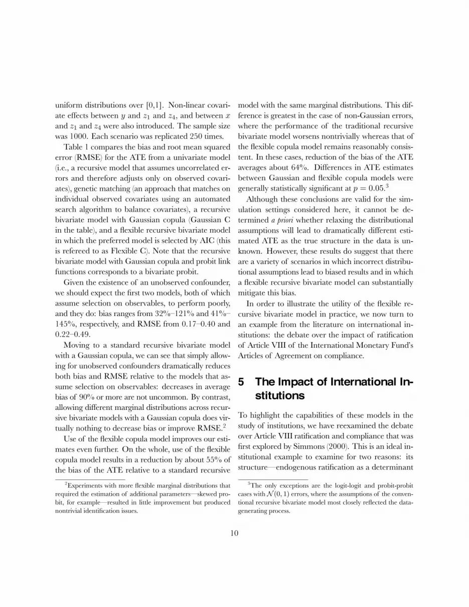
The third equation, at bottom, models θ, the cor-relation of the errors between the two equations, as afunction of years since (or, if negative, prior to) com-mitment to Article VIII. The goal is to capture ei-ther transient shocks around the time of signing—the temporary rise of an unusually sympathetic gov-ernment, say, or the presence of propitious short-term conditions—or longer-term internalization ofthe norms of the treaty. The results show a weaklypositive correlation, and a plot of the spline function(not shown) shows a linear relationship, which is con-sistent with a modest internalization of Article VIII’snorms over time.

As Figure 2 demonstrates, the impact of unob-served confounders also varies markedly betweennon-signatories and signatories. As we might ex-pect, unobserved “shocks” were negatively correlatedamong non-signatories, indicating that unobservedconfounders that decreased (increased) the propen-sity to commit also increased (decreased) the proba-bility of currency restriction. What is perhaps moresurprising is the fact that, among signatories, the op-posite is true: unobserved confounders that increasedthe propensity to commit also increased the probabil-ity of currency restriction. The fact that unobservedconfounders pull in opposite directions across the twogroups of states is one of the important conclusions

-1.0

-0.5

0.0

0.5

1.0

θ̂

Non-signatories

-1.0

-0.5

0.0

0.5

1.0

θ̂

Signatories

Figure 2: Estimated values of θ for non-signatories and signatories.

that would have been missed by a less flexible stan-dard recursive bivariate probit model. As we willsoon see, it turns out to be an important one.

When considering these results, it is important tokeep in mind that the substantive impact of an en-dogenous variable in a nonlinear bivariate modeldoes not automatically follow from the magnitudeand statistical significance of its coefficient (see, e.g.,Hanmer and Ozan Kalkan 2013). Accordingly, wecalculate the ATE of Article VIII commitment, givenby

1

n

n∑i=1

Φ(β̂1+ f̂1({X}[−x1],i

))−Φ(f̂1

({X}[−x1],i

)).

This formula captures the difference between theprobability of restriction given Article VIII commit-ment (the first term) and the probability of restrictiongiven no Article VIII commitment (the second term)for each observation i, summed across all n observa-tions. We generate a 95% confidence interval for theATE via posterior simulation.

The screening hypothesis, in which the states thatsign are states for which compliance involves very lit-

14

010

2030

40

Effects of Article VIII Commitment

0 2 4 6 8 10

Screening effect Constraining effect

Trea

tmen

t effe

ct

Years since signing

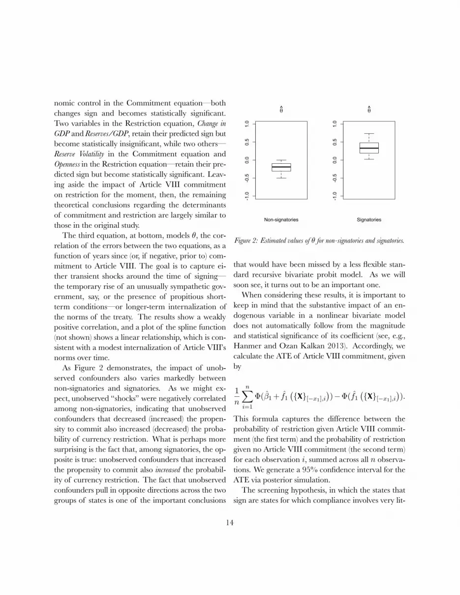
Figure 3: Average treatment effect of commitment to Article VIII, for signatories and non-signatories. The Y-axis represents the ATE measuredin terms of percentage change in the probability of compliance. For the screening effect, the shaded areas represent the distributions of treatmenteffects for signatories (bottom) and non-signatories (top), while for the constraining effect the shaded area represents 95% confidence intervals.

tle change in behavior, implies that there is a sys-tematic difference in the average treatment effect be-tween signatories and non-signatories. To the extentthat it holds, we should expect to see that the ATEamong non-signatories is systematically greater thanit is among signatories, indicating that they wouldhave to change their behavior more radically thanwould signatories in order to comply. The compli-ance hypothesis, by contrast, suggests that the aver-age treatment effect for signatories should be positiveand statistically significant.

Across all cases, the ATE for signatories is foundto be −0.066. That is, the average effect of signingArticle VIII is to reduce the risk of current accountrestriction (that is, increase the probability of compli-ance) by 6.6%. These results suggest that signing on

to Article VIII has a significant, if modest, impact onstate behavior.

For non-signatories, the model produces an ATEof −0.118—nearly twice that of signatories.4 Thisdifference, illustrated on the left of Figure 3, providesstrong evidence of a screening effect. The states thatsign are fundamentally different from the states thatdo not: in the counterfactual world in which thesenon-signatories were to sign, doing so would require amuch more substantial change in behavior. In short,von Stein is correct that Article VIII screens statesthat have a higher cost of compliance.

To explore the role of commitment on compliance

4The difference between the two distributions, as gauged bya Kolmogorov-Smirnov test, is highly statistically significant (D= 0.7438, p < 0.00).

15

over time, we disaggregate the ATE by year sincesigning (Figure 3, right-hand graph). As one mightexpect, the effect of the treaty is not constant overtime. When unobservables are properly accountedfor in the bivariate model, the effect of Article VIIIcommitment shrinks to about a 10% increase in theprobability of restriction immediately after signing.That effect fades slightly in the first few years but—contra Simmons—remains roughly constant, and sta-tistically significant, thereafter.

The results suggest, therefore, that both Simmonsand von Stein were correct. Simmons was correctabout the main finding: commitment to Article VIIIdoes increase compliance. von Stein was correctabout the magnitude of the average treatment effect(if not its statistical significance) and about the exis-tence both of significant screening effects and of un-observed confounders.

The flexibility of the model is both essential to en-suring the robustness of its conclusions and importantfor theoretical reasons. Substantively, one of the mostuseful aspects of our model is the ability to distinguishbetween constraining and screening effects. From astatistical perspective, the ability to model associa-tions between positive and negative “shocks” to bothcommitment and compliance is essential to our abil-ity to model screening and commitment and crucialto gauging the screening effect in particular. More-over, though in the end we needed neither alternativemarginal distributions nor non-Gaussian copulae tocapture the effects of Article VIII, our ability to com-pare the results of models that incorporated them tothose of our final model greatly enhances our faith inthe results.

6 ConclusionFor many years, IR scholars seeking to engage incausal inference have been forced to choose whichunpalatable assumptions they wished to embrace:

they could utilize a potentially weak or invalid in-strument, ignore the influence of unobserved con-founders, or embrace simultaneous likelihood meth-ods with restrictive functional form assumptions.Flexible simultaneous likelihood models represent aconsiderable improvement over this status quo. Thesemodels are capable of capturing the impact of un-measured confounders, and their flexible functionalform assumptions significantly reduce bias in the es-timate of average treatment effects. As our resultsdemonstrate, the increased flexibility of these mod-els can greatly enhance our understanding of inter-national relations.

16

ReferencesAngrist, Joshua and Alan B. Krueger. 2001. In-

strumental variables and the search for identifica-tion: From supply and demand to natural experi-ments. Technical report National Bureau of Eco-nomic Research.

Bagozzi, B. E., D. W. Hill, W. H. Moore and B.Mukherjee. 2015. “Modeling Two Types of Peace:The Zero-inflated Ordered Probit (ZiOP) Modelin Conflict Research.” Journal of Conflict Resolution59(4):728–752.

Bausch, Andrew W. 2015. “Democracy, War Ef-fort, and the Systemic Democratic Peace.” Journalof Peace Research 52(4):435–447.

Bearce, David H., Kristen M. Flanagan andKatharine M. Floros. 2006. “Alliances, In-ternal Information, and Military ConflictAmong Member-States.” International Organization60(3):595–625.

Beck, Nathaniel, Jonathan N. Katz and RichardTucker. 1998. “Taking Time Seriously: Time-Series-Cross-Section Analysis with a Binary De-pendent Variable.” American journal of Political Science42(4):1260–1288.

Benson, Brett V. 2011. “Unpacking Alliances: De-terrent and Compellent Alliances and Their Rela-tionship with Conflict, 1816–2000.” The Journal ofPolitics 73(04):1111–1127.

Blomberg, S. Brock, Gregory D. Hess and AkilaWeerapana. 2004. “Economic Conditions andTerrorism.” European Journal of Political Economy20(2):463–478.

Boehmke, Frederick J., Daniel S. Morey and MeganShannon. 2006. “Selection Bias and Continuous-

Time Duration Models: Consequences and a Pro-posed Solution.” American Journal of Political Science50(1):192–207.

Braumoeller, B. F. and A. Carson. 2011. “Polit-ical Irrelevance, Democracy, and the Limits ofMilitarized Conflict.” Journal of Conflict Resolution55(2):292–320.

Bueno de Mesquita, Bruce, James D. Morrow, Ran-dolph M. Siverson and Alastair Smith. 1999.“An Institutional Explanation of the DemocraticPeace.” American Political Science Review 93(4):791 –807.

Carrubba, C. J., A. Yuen and C. Zorn. 2007. “In De-fense of Comparative Statics: Specifying EmpiricalTests of Models of Strategic Interaction.” PoliticalAnalysis 15(4):465–482.

Chib, S. and E. Greenberg. 2007. “Semiparametricmodeling and estimation of instrumental variablemodels.” Journal of Computational and Graphical Statis-tics 16:86–114.

Chiba, Daina, Lanny Martin and Randy Stevenson.2014. “A Copula Approach to the Problem of Se-lection Bias in Models of Government Survival.”.

Cranmer, Skyler J., Bruce A. Desmarais and Eliza-beth J. Menninga. 2012. “Complex Dependenciesin the Alliance Network.” Conflict Management andPeace Science 29(3):279–313.

Dorussen, H. and H. Ward. 2008. “Intergovern-mental Organizations and the Kantian Peace: ANetwork Perspective.” Journal of Conflict Resolution52(2):189–212.

Doyle, Michael W. and Nicholas Sambanis. 2000.“International Peacebuilding: A Theoretical andQuantitative Analysis.” The American Political ScienceReview 94(4):779.

17

Fang, Songying, Jesse C. Johnson and Brett AshleyLeeds. 2014. “To Concede or to Resist? The Re-straining Effect of Military Alliances.” InternationalOrganization 68(4):775–809.

Fortna, Virginia Page and Lise Morjé Howard. 2008.“Pitfalls and Prospects in the Peacekeeping Liter-ature.” Annual Review of Political Science 11(1):283–301.

Freedman, D. A. and J. S. Sekhon. 2010. “Endo-geneity in Probit Response Models.” Political Anal-ysis 18(2):138–150.

Freedman, David, David Collier, Jasjeet SinghSekhon and Philip B. Stark. 2010. Statistical mod-els and causal inference: a dialogue with the social sci-ences. Cambridge ; New York: Cambridge Uni-versity Press.

Freytag, Andreas, Jens J. Krüger, Daniel Meierrieksand Friedrich Schneider. 2011. “The Originsof Terrorism: Cross-Country Estimates of Socio-Economic Determinants of Terrorism.” EuropeanJournal of Political Economy 27(Supplement 1):S5–S16.

Gartner, Scott Sigmund. 2011. “Signs of Trou-ble: Regional Organization Mediation and CivilWar Agreement Durability.” The Journal of Politics73(02):380–390.

Gates, Scott, Torbjørn Knutsen and Jonathon W.Moses. 1996. “Democracy and Peace: A MoreSkeptical View.” Journal of Peace Research 33(1):1–10.

Gerber, Alan S. and Donald P. Green. 2000. “TheEffects of Canvassing, Telephone Calls, and Di-rect Mail on Voter Turnout: A Field Experiment.”American Political Science Review 94(3):653–663.

Gerber, Alan S. and Donald P. Green. 2005. “Cor-rection to Gerber and Green (2000), replication of

disputed findings, and reply to Imai (2005).” Amer-ican Political Science Review 99(2):301–313.

Gilligan, Michael J. and Ernest J. Sergenti. 2008. “DoUN Interventions Cause Peace? Using Matchingto Improve Causal Inference.” Quarterly Journal ofPolitical Science 3(2):89–122.

Grier, Kevin B. and Gordon Tullock. 1989. “AnEmpirical Analysis of Cross-National EconomicGrowth, 1951-80.” Journal of Monetary Economics24(2):259–276.

Hafner-Burton, Emilie M. and Miles Kahler. 2009.“Network analysis for international relations.” In-ternational Organization 63:559–92.

Hanmer, Michael J. and Kerem Ozan Kalkan.2013. “Behind the Curve: Clarifying the Best Ap-proach to Calculating Predicted Probabilities andMarginal Effects from Limited Dependent Vari-able Models.” American Journal of Political Science57(1):263–277.

Hill, Daniel W. 2010. “Estimating the Effects of Hu-man Rights Treaties on State Behavior.” The Jour-nal of Politics 72(04):1161–1174.

Imai, Kosuke. 2005. “Do get-out-the-vote calls re-duce turnout? The importance of statistical meth-ods for field experiments.” American Political ScienceReview 99(2):283–300.

Johnson, Jesse C. and Brett Ashley Leeds. 2011. “De-fense Pacts: A Prescription for Peace?” Foreign Pol-icy Analysis 7(1):45–65.

Keele, Luke. 2015. “The Statistics of Causal Infer-ence: A View from Political Methodology.” Politi-cal Analysis 23(3):313–335.

King, Gary and Langche Zeng. 2001. “Logisticregression in rare events data.” Political analysis9(2):137–163.

18

Kish, Leslie. 1959. “Some Statistical Problemsin Research Design.” American Sociological Review24(3):328–338.

Krieger, Tim and Daniel Meierrieks. 2011. “WhatCauses Terrorism?” Public Choice 147(1):3–27.

Leeds, Brett Ashley. 2003. “Do Alliances Deter Ag-gression? The Influence of Military Alliances onthe Initiation of Militarized Interstate Disputes.”American Journal of Political Science 47(3):427–439.

Levy, Jack S. 1981. “Alliance Formation and WarBehavior: An Analysis of the Great Powers, 1495-1975.” Journal of Conflict Resolution 25(4):581–613.

Lewis, J. B. 2003. “Revealing Preferences: EmpiricalEstimation of a Crisis Bargaining Game with In-complete Information.” Political Analysis 11(4):345–367.

Little, R. J. A. 1985. “A note about models for selec-tivity bias.” Econometrica 53:1469–1474.

Lupu, Yonatan. 2013. “The Informative Power ofTreaty Commitment: Using the Spatial Model toAddress Selection Effects.” American Journal of Polit-ical Science pp. 912–925.

Manski, Charles F. 1990. “Nonparametric Boundson Treatment Effects.” The American Economic Re-view pp. 319–323.

Maoz, Zeev. 2009. “The effects of strategic and eco-nomic interdependence on international conflictacross levels of analysis.” American Journal of Politi-cal Science 53(1):223–240.

Maoz, Zeev and Bruce Russett. 1993. “Normativeand Structural Causes of Democratic Peace, 1946-1986.” American Political Science Review 87(3):624–638.

Marra, G. and R. Radice. 2011. “Estimation of asemiparametric recursive bivariate probit model inthe presence of endogeneity.” Canadian Journal ofStatistics 39:259–279.

Marra, G. and R. Radice. 2015. “Flexible Bivari-ate Binary Models for Estimating the Efficacy ofPhototherapy for Newborns with Jaundice.” Inter-national Journal of Statistics and Probability 4:46–58.

Marra, G. and S.N. Wood. 2012. “Coverage Prop-erties of Confidence Intervals for Generalized Ad-ditive Model Components.” Scandinavian Journal ofStatistics 39:53–74.

Marra, Giampiero and Rosalba Radice. 2016.SemiParBIVProbit: Semiparametric Copula BivariateRegression Models. R package version 3.7-1.URL: http://CRAN.R-project.org/package=SemiParBIVProbit

McLaughlin Mitchell, Sara and Paul R. Hensel.2007. “International Institutions and Compliancewith Agreements.” American Journal of Political Science51(4):721–737.

Meierrieks, Daniel and Thomas Gries. 2012.“Causality Between Terrorism and EconomicGrowth.” Journal of Peace Research 50(1):91–104.

Monfardini, C. and R. Radice. 2008. “Testing Ex-ogeneity in the Bivariate Probit Model: A MonteCarlo Study.” Oxford Bulletin of Economics and Statis-tics 70:271–282.

Morgan, Stephen L. and Christopher Winship. 2007.Counterfactuals and causal inference: methods and princi-ples for social research. Analytical methods for socialresearch New York: Cambridge University Press.

Murray, Michael P. 2006. “Avoiding Invalid Instru-ments and Coping with Weak Instruments.” Jour-nal of Economic Perspectives 20(4):111–132.

19

Radice, Rosalba, Giampiero Marra and MalgorzataWojtys. 2015. “Copula Regression Spline Modelsfor Binary Outcomes.” Statistics and Computing, DOI10.1007/s11222-015-9581-6.

Reuveny, Rafael and Quan Li. 2003. “The JointDemocracy-Dyadic Conflict Nexus: A Simultane-ous Equations Model.” International Studies Quarterly47(3):325–346.

Sartori, Anne E. 2003. “An Estimator for SomeBinary-Outcome Selection Models Without Ex-clusion Restrictions.” Political Analysis 11(2):111–138.

Sekhon, Jasjeet S. 2009. “Opiates for the Matches:Matching Methods for Causal Inference.” AnnualReview of Political Science 12(1):487–508.

Signorino, Curtis S. 1999. “Strategic Interaction andthe Statistical Analysis of International Conflict.”American Political Science Review 93(2):279–297.

Simmons, Beth A. 2000. “International Law andState Behavior: Commitment and Compliance inInternational Monetary Affairs.” The American Po-litical Science Review 94(4):819.

Simmons, Beth A. 2009. Mobilizing for Human Rights:International Law in Domestic Politics. Cambridge:Cambridge University Press.

Simmons, Beth A. and Daniel J. Hopkins. 2005.“The Constraining Power of InternationalTreaties: Theory and Methods.” American PoliticalScience Review 99(04).

Smith, Alastair. 1999. “Testing Theories of StrategicChoice: The Example of Crisis Escalation.” Amer-ican Journal of Political Science 43(4):1254–1283.

Theisen, Ole Magnus. 2012. “Climate clashes?Weather variability, land pressure, and organized

violence in Kenya, 1989–2004.” Journal of Peace Re-search 49(1):81–96.

Tir, Jaroslav and Douglas M. Stinnett. 2012. “Weath-ering Climate Change: Can Institutions MitigateInternational Water Conflict?” Journal of Peace Re-search 49(1):211–225.

von Stein, Jana. 2005. “Do Treaties Constrain OrScreen? Selection Bias And Treaty Compliance.”American Political Science Review 99(04):611–622.

Vreeland, James Raymond. 2003. The IMF and eco-nomic development. New York: Cambridge UniversityPress.

Winkelmann, R. 2012. “Copula bivariate probitmodels: with an application to medical expendi-tures.” Health Economics 21:1444–1455.

Winship, Christopher and Robert D. Mare. 1992.“Models for Sample Selection Bias.” Annual Reviewof Sociology 18:327–350.

Wooldridge, J. M. 2010. Econometric Analysis of CrossSection and Panel Data. Cambridge: MIT Press.

Xiang, Jun. 2010. “Relevance as a Latent Variable inDyadic Analysis of Conflict.” The Journal of Politics72(02):484.

20