fixed nitrogen dynamics and heterocyst
TRANSCRIPT

FIXED NITROGEN DYNAMICS AND HETEROCYST
PATTERNING IN FILAMENTOUS HETEROCYSTOUSCYANOBACTERIA
by
Aidan I Brown
Submitted in partial fulfillment of therequirements for the degree of
Master of Science
at
Dalhousie UniversityHalifax, Nova Scotia
August 2012
c© Copyright by Aidan I Brown, 2012

DALHOUSIE UNIVERSITY
DEPARTMENT OF PHYSICS AND ATMOSPHERIC SCIENCE
The undersigned hereby certify that they have read and recommend to the
Faculty of Graduate Studies for acceptance a thesis entitled “FIXED NITROGEN
DYNAMICS AND HETEROCYST PATTERNING IN FILAMENTOUS
HETEROCYSTOUS CYANOBACTERIA” by Aidan I Brown in partial fulfillment
of the requirements for the degree of Master of Science.
Dated: August 10, 2012
Supervisor:
Readers:
ii

DALHOUSIE UNIVERSITY
DATE: August 10, 2012
AUTHOR: Aidan I Brown
TITLE: FIXED NITROGEN DYNAMICS AND HETEROCYSTPATTERNING IN FILAMENTOUS HETEROCYSTOUSCYANOBACTERIA
DEPARTMENT OR SCHOOL: Department of Physics and Atmospheric Science
DEGREE: M.Sc. CONVOCATION: October YEAR: 2012
Permission is herewith granted to Dalhousie University to circulate and tohave copied for non-commercial purposes, at its discretion, the above title upon therequest of individuals or institutions. I understand that my thesis will be electronicallyavailable to the public.
The author reserves other publication rights, and neither the thesis norextensive extracts from it may be printed or otherwise reproduced without theauthor’s written permission.
The author attests that permission has been obtained for the use of anycopyrighted material appearing in the thesis (other than brief excerpts requiringonly proper acknowledgement in scholarly writing) and that all such use is clearlyacknowledged.
Signature of Author
iii

Table of Contents
List of Figures . . . . . . . . . . . . . . . . . . . . . . . . . . . . . . . . . . vii
Abstract . . . . . . . . . . . . . . . . . . . . . . . . . . . . . . . . . . . . . . x
List of Abbreviations and Symbols Used . . . . . . . . . . . . . . . . . . xi
Acknowledgements . . . . . . . . . . . . . . . . . . . . . . . . . . . . . . . xii
Chapter 1 Introduction . . . . . . . . . . . . . . . . . . . . . . . . . . 1
1.1 Motivation . . . . . . . . . . . . . . . . . . . . . . . . . . . . . . . . . 1
1.2 Hypothesis . . . . . . . . . . . . . . . . . . . . . . . . . . . . . . . . . 2
1.3 Outline . . . . . . . . . . . . . . . . . . . . . . . . . . . . . . . . . . . 3
Chapter 2 Background . . . . . . . . . . . . . . . . . . . . . . . . . . . 4
2.1 Cyanobacteria . . . . . . . . . . . . . . . . . . . . . . . . . . . . . . . 4
2.2 Heterocysts . . . . . . . . . . . . . . . . . . . . . . . . . . . . . . . . 7
2.3 Heterocyst patterns . . . . . . . . . . . . . . . . . . . . . . . . . . . . 9
2.4 Heterocyst differentiation, the canonical experiment, and the genetic
network . . . . . . . . . . . . . . . . . . . . . . . . . . . . . . . . . . 10
2.5 Nitrogen storage . . . . . . . . . . . . . . . . . . . . . . . . . . . . . 14
2.5.1 Cyanophycin . . . . . . . . . . . . . . . . . . . . . . . . . . . 14
2.5.2 Phycobiliprotein . . . . . . . . . . . . . . . . . . . . . . . . . . 15
2.6 Modeling biological pattern formation . . . . . . . . . . . . . . . . . . 16
2.7 Previous heterocyst pattern modeling efforts . . . . . . . . . . . . . . 17
Chapter 3 Nitrogen Distribution in the Cyanobacterial Filament 20
3.1 Motivation and background . . . . . . . . . . . . . . . . . . . . . . . 20
3.2 Model . . . . . . . . . . . . . . . . . . . . . . . . . . . . . . . . . . . 22
3.2.1 Fixed nitrogen transport . . . . . . . . . . . . . . . . . . . . . 22
3.2.2 Cell growth and division . . . . . . . . . . . . . . . . . . . . . 27
iv

3.2.3 Some numerical details . . . . . . . . . . . . . . . . . . . . . . 28
3.3 Cytoplasmic transport . . . . . . . . . . . . . . . . . . . . . . . . . . 29
3.3.1 Short time fixed nitrogen distributions . . . . . . . . . . . . . 29
3.3.2 Long time fixed nitrogen distributions . . . . . . . . . . . . . 32
3.3.3 Stochasticity of long time distributions . . . . . . . . . . . . . 34
3.4 Periplasmic transport . . . . . . . . . . . . . . . . . . . . . . . . . . . 36
3.4.1 Long time nitrogen distributions with cytoplasmic and periplas-
mic transport . . . . . . . . . . . . . . . . . . . . . . . . . . . 36
3.4.2 Long time nitrogen distributions with only periplasmic transport 38
3.4.3 Long time nitrogen distributions with graded growth . . . . . 40
3.5 Discussion . . . . . . . . . . . . . . . . . . . . . . . . . . . . . . . . . 42
Chapter 4 Growth Rates of and Heterocyst Placement in the Cyanobac-
terial Filament . . . . . . . . . . . . . . . . . . . . . . . . . 46
4.1 Motivation and background . . . . . . . . . . . . . . . . . . . . . . . 46
4.2 Model . . . . . . . . . . . . . . . . . . . . . . . . . . . . . . . . . . . 49
4.2.1 Fixed nitrogen transport . . . . . . . . . . . . . . . . . . . . . 49
4.2.2 Cell growth and division . . . . . . . . . . . . . . . . . . . . . 51
4.2.3 Heterocyst placement . . . . . . . . . . . . . . . . . . . . . . . 51
4.2.4 Some numerical details . . . . . . . . . . . . . . . . . . . . . . 52
4.3 Results with no heterocysts . . . . . . . . . . . . . . . . . . . . . . . 53
4.4 Results with heterocysts . . . . . . . . . . . . . . . . . . . . . . . . . 56
4.4.1 No leakage . . . . . . . . . . . . . . . . . . . . . . . . . . . . . 56
4.4.2 Leakage . . . . . . . . . . . . . . . . . . . . . . . . . . . . . . 60
4.4.3 Varying external fixed nitrogen concentration . . . . . . . . . 62
4.4.4 Heterocyst spacing . . . . . . . . . . . . . . . . . . . . . . . . 63
4.5 Discussion . . . . . . . . . . . . . . . . . . . . . . . . . . . . . . . . . 65
Chapter 5 De Novo Heterocyst Patterning . . . . . . . . . . . . . . 71
5.1 Motivation and background . . . . . . . . . . . . . . . . . . . . . . . 71
5.2 Model . . . . . . . . . . . . . . . . . . . . . . . . . . . . . . . . . . . 73
5.2.1 Fixed nitrogen storage . . . . . . . . . . . . . . . . . . . . . . 73
v

5.2.2 Cell growth and division . . . . . . . . . . . . . . . . . . . . . 74
5.2.3 Heterocysts . . . . . . . . . . . . . . . . . . . . . . . . . . . . 75
5.2.4 Some numerical details . . . . . . . . . . . . . . . . . . . . . . 78
5.3 Results for wild type . . . . . . . . . . . . . . . . . . . . . . . . . . . 79
5.4 Discussion of wild type results . . . . . . . . . . . . . . . . . . . . . . 84
5.5 Results for genetic knockouts . . . . . . . . . . . . . . . . . . . . . . 86
5.6 Discussion of gene knockout results . . . . . . . . . . . . . . . . . . . 90
5.7 Predictions . . . . . . . . . . . . . . . . . . . . . . . . . . . . . . . . 91
Chapter 6 Percolation of Starvation . . . . . . . . . . . . . . . . . . . 93
6.1 Motivation and background . . . . . . . . . . . . . . . . . . . . . . . 93
6.2 Percolation background . . . . . . . . . . . . . . . . . . . . . . . . . . 93
6.2.1 One Dimensional Lattice . . . . . . . . . . . . . . . . . . . . . 94
6.2.2 Two Dimensional Lattice . . . . . . . . . . . . . . . . . . . . . 95
6.3 Model . . . . . . . . . . . . . . . . . . . . . . . . . . . . . . . . . . . 95
6.4 Percolation . . . . . . . . . . . . . . . . . . . . . . . . . . . . . . . . 96
6.4.1 One dimensional percolation . . . . . . . . . . . . . . . . . . . 97
6.4.2 Two dimensions . . . . . . . . . . . . . . . . . . . . . . . . . . 98
6.4.3 Deviations from percolation in two dimensions . . . . . . . . . 101
6.4.4 Discussion . . . . . . . . . . . . . . . . . . . . . . . . . . . . . 106
Chapter 7 Conclusion and Future Outlook . . . . . . . . . . . . . . 109
7.1 Summary of results . . . . . . . . . . . . . . . . . . . . . . . . . . . . 109
7.2 Future outlook . . . . . . . . . . . . . . . . . . . . . . . . . . . . . . 111
Bibliography . . . . . . . . . . . . . . . . . . . . . . . . . . . . . . . . . . . 113
Appendix A Correlation Functions . . . . . . . . . . . . . . . . . . . . . 124
A.1 Calculation . . . . . . . . . . . . . . . . . . . . . . . . . . . . . . . . 124
A.1.1 Numerical . . . . . . . . . . . . . . . . . . . . . . . . . . . . . 128
A.2 Discussion . . . . . . . . . . . . . . . . . . . . . . . . . . . . . . . . . 129
Appendix B Permissions . . . . . . . . . . . . . . . . . . . . . . . . . . . 131
vi

List of Figures
1.1 Heterocyst pattern . . . . . . . . . . . . . . . . . . . . . . . . 1
2.1 Cyanobacteria cell types . . . . . . . . . . . . . . . . . . . . . 5
2.2 Heterocyst and vegetative cell . . . . . . . . . . . . . . . . . . 7
2.3 Metabolic interactions of heterocysts . . . . . . . . . . . . . . 8
2.4 Heterocyst spacing pattern . . . . . . . . . . . . . . . . . . . . 9
2.5 Genetic network model . . . . . . . . . . . . . . . . . . . . . . 11
2.6 Cyanophycin granules . . . . . . . . . . . . . . . . . . . . . . . 15
2.7 General biological pattern formation with inhibitors . . . . . . 17
3.1 Schematic of fixed nitrogen transport . . . . . . . . . . . . . . 23
3.2 Short time fixed nitrogen distributions . . . . . . . . . . . . . 30
3.3 Long time fixed nitrogen distributions . . . . . . . . . . . . . . 33
3.4 Distributions with cytoplasmic and periplasmic transport . . . 37
3.5 Distributions with only periplasmic transport . . . . . . . . . 39
3.6 Fixed nitrogen distribution with graded growth . . . . . . . . 41
4.1 Schematic of fixed nitrogen transport . . . . . . . . . . . . . . 50
4.2 Growth rate versus external fixed nitrogen concentration withno heterocysts . . . . . . . . . . . . . . . . . . . . . . . . . . . 53
4.3 Growth rate vs. heterocyst frequency with zero leakage andrandom heterocyst placement . . . . . . . . . . . . . . . . . . 57
4.4 Growth rate and heterocyst frequency with zero leakage andrandom heterocyst placement . . . . . . . . . . . . . . . . . . 58
4.5 Growth rate and heterocyst frequency with zero leakage andrandom heterocyst placement . . . . . . . . . . . . . . . . . . 60
4.6 Growth rates with variable leakage and heterocyst placementstrategy . . . . . . . . . . . . . . . . . . . . . . . . . . . . . . 61
vii

4.7 Growth rates and heterocyst frequency with variable externalfixed nitrogen concentration . . . . . . . . . . . . . . . . . . . 62
4.8 Heterocyst spacing distribution for variable placement strategy 64
4.9 Heterocyst spacing distribution for variable external fixed ni-trogen concentration . . . . . . . . . . . . . . . . . . . . . . . 65
5.1 Heterocyst commitment and differentiation model . . . . . . . 75
5.2 Length and commitment after nitrogen deprivation . . . . . . 80
5.3 Heterocyst spacing at 24 hours after nitrogen deprivation withdifferent inhibition ranges . . . . . . . . . . . . . . . . . . . . 81
5.4 Experimental heterocyst spacing distribution at 24 hours . . . 81
5.5 Heterocyst spacing distribution each day . . . . . . . . . . . . 82
5.6 Experimental heterocyst spacing distribution each day . . . . 82
5.7 Heterocyst frequency in time and cell cycle effect . . . . . . . 83
5.8 Heterocyst spacing distributions without PatS inhibition . . . 87
5.9 Experimental heterocyst spacing distribution for ∆patS at 24hours . . . . . . . . . . . . . . . . . . . . . . . . . . . . . . . . 88
5.10 Experimental heterocyst spacing distribution for ∆patS each day 89
5.11 Heterocyst spacing distribution without HetN inhibition . . . 90
6.1 Fraction of starving cells . . . . . . . . . . . . . . . . . . . . . 96
6.2 Cluster length distribution . . . . . . . . . . . . . . . . . . . . 98
6.3 Two-dimensional cluster size distribution . . . . . . . . . . . . 99
6.4 Spacetime visualizations . . . . . . . . . . . . . . . . . . . . . 100
6.5 Temporal starvation distribution . . . . . . . . . . . . . . . . . 101
6.6 Two-dimensional cluster size distribution with model reducedto percolation . . . . . . . . . . . . . . . . . . . . . . . . . . . 102
6.7 Two-dimensional cluster size distribution with model reducedto percolation with reinsertions . . . . . . . . . . . . . . . . . 103
6.8 Two-dimensional cluster size distribution with model reducedto percolation with cell growth reinserted and growth rate varied105
viii

6.9 Spacetime visualizations of correlation . . . . . . . . . . . . . 105
6.10 Two-dimensional cluster size distribution with fullest modelwith percolation . . . . . . . . . . . . . . . . . . . . . . . . . . 107
A.1 Correlation functions . . . . . . . . . . . . . . . . . . . . . . . 129
ix

Abstract
Cyanobacteria are prokaryotes that can grow photoautotrophically using oxygenic
photosynthesis. Some filamentous cyanobacteria in media with insufficient fixed ni-
trogen develop a regular pattern of heterocyst cells that fix nitrogen for the remaining
vegetative cells. We have built an integrated computational model of fixed nitrogen
transport and cell growth for filamentous cyanobacteria. With our model, two qual-
itatively different experimentally observed nitrogen distributions between a pair of
heterocysts are reconciled. By adding dynamic heterocyst placement into our model,
we can optimize heterocyst frequency with respect to growth. Further introduction
of modest leakage leads to distinct growth rates between different heterocyst place-
ment strategies. A local placement strategy yields maximal growth and steady state
heterocyst spacings similar to those observed experimentally. Adding more realistic
fixed nitrogen storage based heterocyst commitment together with lateral inhibition
to the model allows us to address initial heterocyst commitment and qualitatively re-
produces many aspects of heterocyst differentiation. We also investigate patterns of
starving cells and correlations of fixed nitrogen in filaments without heterocysts. We
find percolation transitions in both spatial one dimensional patterns and space-time
two dimensional patterns.
x

List of Abbreviations and Symbols Used
2-OG: 2-oxoglutarate
efN: External fixed nitrogen
fN: fixed nitrogen
FRAP: Fluorescence recovery after photobleaching
GFP: Green fluorescent protein
Mch: Multiple contiguous heterocysts
PCC: Pasteur Culture Collection
WT: Wild type
xi

Acknowledgements
I would like to thank all the people who have helped and inspired me during my
research and work on this thesis. I would also like to thank anyone who correctly
reminded me that maybe I should be doing work. I would like to thank airports with
free wifi and friends with cellphones that can send email for helping me to remember
things I otherwise would have likely forgotten.
I first and foremost want to thank my supervisor, Andrew Rutenberg, for his
encouragement, guidance, and support during my research, the results of which reside
inside and outside of this thesis. I would also like to thank him for putting up with me
when I did not listen to his advice, answered emails late or not at all, for explaining
things a third or fourth time when I was lost, and for telling me when it was time to
figure things out by myself, among other things. I would really like to thank him for
his relentless constructive criticism and for telling me to ‘own it’ and other ways of
saying to always try hard and put my best into everything.
I would like to thank my parents for completely supporting my decision to go move
to Halifax and loving and supporting me the entire time. I would like to also thank
my parents for politely asking about my work and then politely nodding through
what were probably poor explanations.
xii

Chapter 1
Introduction
1.1 Motivation
Since the work of Fogg in the 1940’s [1, 2], scientists have been trying to understand
heterocysts in filamentous cyanobacteria, how they produce and are affected by fixed
nitrogen, and how the filament controls its differentiation pattern. The initiation and
maintenance of a pattern of heterocysts within filaments is a simple and compelling
example of both cell differentiation and pattern formation.
Figure 1.1: Heterocyst pattern in the filamentous cyanobacterium Anabaena PCC7120. Heterocysts are denoted by arrows. N- indicates that the filament was grownin a medium without fixed nitrogen. Figure from Golden and Yoon [3].
Physical pattern formation has long been studied [4], and more recently so has
pattern formation in biological systems [5]. Cyanobacterial heterocyst patterns have
been studied quantitatively only recently [6], with recent quantitative measurements
also involving involving transport [7] and the nitrogen distribution [8], among other
measurements.
1

2
These quantitative measurements have made the theoretical and computational
study of heterocyst differentiation much more appealing because there are now results
to compare to and a more quantitatively literate community to speak to.
Of course, in addition to available quantitative measurements, there are other
reasons for a physical study of heterocyst differentiation. The primary one for me is
the apparent lack of a broken symmetry. In a very wide range of systems, symmetry is
broken by an outside influence. In the Ising model of magnetic systems, the symmetry
is broken by an external magnetic field [9], and in Drosophila embryos, maternal
determinants set up the anterior-posterior axis for the process that eventually localizes
and orients the mature segments of the fly [10]. In cyanobacteria there is no known
outside influence which chooses which cells will differentiate. I want to understand
how the filament determines which cells will become heterocysts.
1.2 Hypothesis
We hypothesize that much of the phenomena associated with heterocyst differentia-
tion, including the symmetry breaking behind the formation of the pattern, can be
explained with simple, physical rules. We want to discover, understand, and, as much
as possible, quantify these rules. Equally important, we want to understand how the
collective effect of these rules leads to a pattern of differentiated cells, and how the
aspects of the pattern quantitatively depend on the rules. Almost all of the literature
on the topic of heterocyst differentiation focuses on the genetic and biochemical de-
tails of heterocysts and cyanobacteria, and our understanding will necessarily be in
the context of this large body of work.
Our work will focus on the areas that have been quantitatively investigated exper-
imentally. We will investigate how the nitrogen distribution is affected by transport
and growth, in the context of relevant studies. We will go beyond the existing inves-
tigation of the wild type pattern, and focus on the pattern in growing systems. We
will also examine the initiation of the heterocyst pattern and the symmetry breaking
that must take place. Finally, we will understand a system of starving cells in the
context of traditional physical measurements.
Also, to develop a full model that includes detailed genetic effects (which we have
not done), you must first develop a physical model of growth and metabolite exchange.

3
As such, this thesis forms a strong foundation for further work.
1.3 Outline
The purpose of Chapter 2 is to provide a background to understand the work of
Chapters 3-5, and also to provide context for the work. It introduces cyanobacteria,
heterocysts, and the heterocyst pattern, and then goes through much of the infor-
mation in the literature relevant to our investigation of the pattern. Chapter 6 is
significantly different than the previous three and the relevant background for that
chapter is provided at its beginning.
Chapters 3-6 all use a similar model, but one that evolves between chapters as we
test it against experimental data. The chapters investigate different phenomena and
the models were chosen to be as simple as possible for those phenomena.
Chapter 3 focuses on the fixed nitrogen distribution in the filament. The disagree-
ment between the experimentally determined fixed nitrogen distributions of Wolk et
al [11] and Popa et al [8] is resolved and cytoplasmic and periplasmic transport are
discussed.
Chapter 4 looks at steady state growth of a filament with heterocysts that has
ongoing heterocyst placement. Comparisons between filaments with different hetero-
cyst placement strategies and external fixed nitrogen concentrations are made using
the filament growth rate and the heterocyst patterns in the filament.
Chapter 5 investigates initial pattern formation in filaments deprived of external
fixed nitrogen. Storage of fixed nitrogen and lateral inhibition of differentiation are
introduced to the model. Several quantities produced by simulation are compared to
experimental results from the literature.
Chapter 6 presents the cluster size distributions of starving cells in filaments with-
out heterocysts. These are compared to percolation in one and two dimensions.

Chapter 2
Background
2.1 Cyanobacteria
Cyanobacteria, often known as blue-green algae, are Gram-negative bacteria rang-
ing in diameter from less than one micrometre to greater than 100 micrometres [12].
Cyanobacteria were present in both unicellular and filamentous forms at least 3.5
billion years ago [13, 14]. Cyanobacteria are significant to the history of the earth
because they were the first organisms to evolve oxygenic photosynthesis [15] between
2.78 and 3.7 billion years ago [16]. As early photosynthesizers cyanobacteria oxy-
genated the atmosphere between 2.5 and 2.2 billion years ago [16]. This oxygenation
of the atmosphere is hypothesized to have caused a global glaciation (through re-
duced methane levels) [16], the retreat of many anaerobic life forms due to their
decreased viability in the presence of oxygen, and also encouraged the development
of the oxygen-requiring respiratory electron transport chain central to the metabolism
of much of eukaryotic life today [17].
Cyanobacteria can be found in both freshwater and marine environments as well
as on top of and in the soil where they can increase nitrogen content and are im-
portant to agriculture [18]. They form symbiotic relationships with other bacteria as
well as fungi, lower and higher plants, and invertebrate animals [18]. Cyanobacteria
are also thought to be the ancestors of chloroplasts in plants, which were originally
endosymbionts [18].
At the cellular level cyanobacteria exist as individual cells, unbranched filaments,
or branched filaments [18]. I will focus on unbranched filamentous cyanobacteria,
which have several cell types. The cell types allow the cyanobacterium to withstand
unfavourable conditions [19]. The first and most common are vegetative cells whose
primary function is to perform photosynthesis to provide fixed carbon to the organism
[15]. Akinetes are spores which are larger than vegetative cells and only differentiate
under adverse conditions [15, 19]. Hormogonia are short, motile filaments composed of
4

5
Figure 2.1: (a) Filaments of Anabaena PCC 7120 grown on N2 as the nitrogen source.An intercalary heterocyst is indicated by the black arrow, and a terminal heterocyst isindicated by the white arrow. (b) Branched filaments of Fischerella muscicola. (c) N2
grown filaments of Anabaena cylindrica. A heterocyst is indicated by the black arrowand akinetes indicated by ‘aki’. (d) N2 grown Nostoc PCC 9203 showing filaments aswell as one hormogonium, indicated by ‘hrm’. Figure from Flores and Herrero [15].
small cells that are derived from cell division without increase in biomass; hormogonia
also only differentiate under adverse conditions [15, 19]. I will focus on filamentous
heterocystous cyanobacteria that do not differentiate either akinetes or hormogonia.
These filaments consist of vegetative cells and occasional heterocyst cells.
Nitrogen in the atmosphere must be ‘fixed’ into ammonia and then changed into
other forms to be used by life because dinitrogen can otherwise not be metabolized.

6
The enzyme responsible for nitrogen fixation is nitrogenase, which is poisoned by oxy-
gen [20]. The oxygenation of the earth by cyanobacteria, mentioned above, was there-
fore problematic for nitrogen fixing organisms. Many species retreated to suitable
anoxic environments, but cyanobacteria did not have this option due to the oxygen
produced by its own photosynthesis [12]. To continue to fix nitrogen, cyanobacteria
evolved to either temporally or spatially separate out photosynthesis and nitrogen
fixation [20, 21, 22]. For temporal separation, some cyanobacteria fix nitrogen at
night and photosynthesize during the day while others, such as Trichodesmium spp.,
fix nitrogen in the morning and photosynthesize in the afternoon [23]. Some fila-
mentous cyanobacteria were able to spatially separate photosynthesis and nitrogen
fixation by specializing a fraction of the cells in the filament to fix nitrogen. These
cells are known as heterocysts. Heterocyst differentiation evolved more than three
billion years ago, relatively late in the evolutionary history of cyanobacteria [24].
Heterocysts are possibly the earliest example of mutualistic differentiation where a
differentiated cell provides nutrients to other cells, and receives other nutrients from
the other cells [25]. Heterocysts evolved in filamentous cyanobacteria and do not
occur in unicellular species or unicellular mutants of filamentous species.
The study of heterocysts has used many different cyanobacterial species. The
primary species used in experiments today is Anabaena sp. PCC 7120, which I will
often shorten to PCC 7120. It has been used to study a wide range of character-
istics of filamentous heterocystous cyanobacteria, from the heterocyst pattern [26]
to transport [7] to gene expression analysis [27] and is chosen because it only has
vegetative and heterocyst cells, and not other cell types, and because it has been
developed to become a convenient genetic system. Other species that have been used
are Anabaena variabilis [28], Anabaena oscillarioides [8], and Anabaena flos-aquae
[29], among others. Much of the older work has been done with these other species.
Because comparable studies have often not yet been redone with PCC 7120, we will
use the results of studies with these other species to both parameterize our models
and compare to our results. We do this under the assumption that the relevant data
does not drastically change between these species.

7
Figure 2.2: A transmission electron micrograph with a heterocyst on the left anda vegetative cell on the right from a filament of Anabaena PCC 7120. ‘CPG’ indi-cates the location of the heterocyst’s polar cyanophycin granule. ‘HEP’ indicates theheterocyst polysaccharide layer, and ‘HGL’ indicates the heterocyst glycolipid layer.Figure from Flores and Herrero [15].
2.2 Heterocysts
Once differentiated, heterocysts no longer divide, but remain metabolically active [12].
Heterocyst death leads to filament breakage at the heterocyst [19]. The development
and maintenance of heterocysts involves between 15% and 25% of the cyanobacterial
genome [30]. Heterocysts have many adaptations to maintain the microoxic environ-
ment necessary for nitrogen fixation, resulting in them being darker and larger than
vegetative cells. Heterocysts are surrounded by a thick envelope, composed of gly-
colipids and polysaccharides [19], which is impermeable to gases [15, 31]. Molecular
nitrogen, N2, is necessary for nitrogen fixation. If N2 is able to enter the heterocyst,
so is O2, because the van der Waal’s radii of nitrogen and oxygen are similar [32].
The heterocyst envelope decreases the ability of both gases to enter heterocysts to
reduce the amount of O2 that enters but still allows enough N2 to be available for
nitrogen fixation [32]. The 4 N2:1 O2 ratio in the atmosphere helps as well [32]. In
heterocysts, photosystem II has been dismantled [33, 34], likely to avoid the oxygen
produced by its water splitting activity [3, 15, 31]. Photosystem I remains, as its
phosphorylation activity is important to heterocyst bioenergetics [15]. Heterocysts
also have high oxidase activity to consume the O2 that does get into heterocysts.
Nitrogenase fixes nitrogen in the microoxic environment inside the heterocyst.

8
That nitrogen fixation is restricted to heterocysts [35] has been demonstrated by
a variety of means including 55Fe labelling of nitrogenase [36] and immunoelectron
microscopy [37, 38, 39, 40, 41]. Nitrogenase is encoded by three polypeptides in the
nif operon [42].
Figure 2.3: Some important metabolic interactions between heterocysts and vegeta-tive cells. The left cell is a vegetative cell, and the right is a heterocyst. Carbondioxide (CO2) is fixed in vegetative cells by photosynthesis (PS); some of this fixedcarbon becomes α-ketoglutarate (αKG), which is also known as 2-oxoglutarate (2-OG). α-ketoglutarate combines with glutamine (Gln) using the enzyme glutamatesynthase (GOGAT) to form glutamate (Glu). In the heterocyst, sugar from thevegetative cell is used to provide reductant for the nitrogenase (Nase) and produceammonia (NH3) which then becomes part of glutamine. The glutamine is then theform of fixed nitrogen which moves from heterocyst to the vegetative cell. Figurefrom Meeks and Elhai [31].
Ammonium is the initial product of nitrogen fixation, but it is quickly incorpo-
rated into other forms of fixed nitrogen [43]. For transport back to the vegetative
cells, glutamine synthetase catalyzes the formation of glutamine from ammonium
and glutamate [44]. Glutamate synthase catalyzes the formation of two glutamate
molecules from a molecule of glutamine and a molecule of 2-oxoglutarate (2-OG)
(also known as α-ketoglutarate (α-KG)) [44]. It is thought that glutamine synthase
converts ammonium into glutamine in the heterocyst while the conversion of glu-
tamine and 2-OG to glutamate occurs primarily in vegetative cells (heterocysts are
deficient in glutamate synthase) [45]. Lacking the enzyme Rubisco and photosystem
II, heterocysts cannot fix CO2 and rely on vegetative cells to supply fixed carbon to
support nitrogen fixation [12]. It is thought that vegetative cells send carbon to the
heterocysts in the form of sucrose [3, 15, 31]. Much of this sucrose is converted to

9
2-oxoglutarate (2-OG) and then has nitrogen atoms added to become glutamate and
glutamine [25]. The possible physical connections for intercellular movement of fixed
carbon and fixed nitrogen compounds are discussed in Section 3.1.
2.3 Heterocyst patterns
0 2 4 6 8 10 12 14 16 18 20 22 24
Number of Vegetative Cells Between Heterocysts0.00
0.02
0.04
0.06
0.08
0.10
0.12
Fraction
Number of Vegetative Cells Between Heterocysts
24 hrs
0 2 4 6 8 10 12 14 16 18 20 22 24
48 hrs
Figure 2.4: Heterocyst spacing pattern for wild type PCC 7120 24 and 48 hours afternitrogen deprivation. Data from Toyoshima et al [46].
As discussed in Section 1.1, we are most interested in the regularly spaced hetero-
cyst pattern. The spacing distribution of this pattern has been measured by several
groups for both wild type and knockout strains [26, 46, 47]. In wild type strains the
distribution spans from roughly 5 cells to roughly 20 cells between heterocysts, with
a peak at approximately 10 cells. It has been speculated that the pattern is to ensure
efficient production and distribution of fixed nitrogen [12].
This thesis moves towards understanding the pattern of differentiation. This pat-
tern is an excellent choice to study experimentally because the pattern only involves
two cell types (which are visually distinguishable from one another), cell differentia-
tion is induced by the lack of a single nutrient, and the system is one dimensional.
The heterocyst pattern is completely formed by approximately 24 hours after ni-
trogen deprivation. The pattern at later times (>48 hours) is quantitatively different
than the pattern at 24 hours, but overall quite similar [26], as illustrated in Figure
2.4. At later times the pattern is maintained by the differentiation of new, intercalary,

10
heterocysts between subsequent existing heterocysts as the number of vegetative cells
between them increases through division [12].
2.4 Heterocyst differentiation, the canonical experiment, and the genetic
network
Heterocyst development is metabolically expensive, and heterocysts do not grow or
divide, making it important that no more cells than necessary differentiate [12]. This
is achieved by having flexibility in the development process using prospective hete-
rocysts, or proheterocysts, which, before a point of no return in the differentiation
process known as commitment, can halt differentiation and revert to a vegetative
state [12]. Visually, proheterocysts are clearly different from vegetative cells, but lack
the fully thickened walls and polar bodies of mature heterocysts [12].
The canonical experiment to investigate the development and pattern of hetero-
cysts involves growing filaments in fixed nitrogen replete medium, and then trans-
ferring them to a medium lacking fixed nitrogen. Once in this depleted medium the
development of proheterocysts and mature heterocysts occurs within 24 hours. Genes
may also be knocked out and/or chemicals added to observe their effect on heterocyst
development, frequency, pattern, as well as other quantities and characteristics.
Visible development of proheterocysts begins at 6-8 hours after fixed nitrogen
deprivation (in a species with doubling time of 15-20 hours) [48] or 6-12 hours (in a
species with doubling time of 15-25 hours) [49]. Proheterocysts mature and gain the
thickened cell walls and polar bodies of mature heterocysts, with mature heterocysts
reaching a maximum in frequency at 25-30 hours [48]. Because there is no fixed
nitrogen being produced prior to maturity, the pattern formation, at least initially,
does not depend on nitrogen fixation [50].
Most of the understanding of the process of heterocyst selection and differentia-
tion cannot be determined by visual inspection in bright-field microscopy and uses
fluorescent reporters to observe biochemical and genetic events.
In conditions of limited fixed nitrogen, 2-oxoglutarate (2-OG) levels become el-
evated because glutamate and glutamine are limited. The main metabolic role of
2-OG is to provide a carbon skeleton for the incorporation of nitrogen and so it links
the carbon and nitrogen metabolisms [19]. The elevated 2-oxoglutarate levels which

11
Figure 2.5: Model of the gene network controlling heterocyst differentiation. Nitrogenstarvation induces ntcA expression, which then induces hetR expression. NtcA andHetR upregulate each other and themselves. HetR activates patS, which represseshetR. PatA represses patS and hetN. HetN is produced by heterocysts after a certainstage of differentiation and represses hetR. These genes are discussed in more detailin Section 2.4. Figure from Orozco et al [51].
signal nitrogen deprivation are sensed by the protein NtcA. ntcA playes a central role
in nitrogen control in cyanobacteria [19] and is activated rapidly after nitrogen de-
privation [49]. One aspect of ntcA’s response to nitrogen deprivation is the initiation
of the heterocyst differentiation program [19, 52] and ntcA has been shown to be
required for heterocyst differentiation [19]. Positive autoregulation of ntcA increases
the NtcA protein levels and if the cell is selected to complete differentiation, and ntcA
continues to be expressed, it will control the progression of heterocyst differentiation
[19].
Once some cells in the filament have run out of fixed nitrogen due to the lack
of external fixed nitrogen, growth will slow because of nitrogen limitation. Lineage
data [53] indicates that the number of cells does not increase or increases very little
in the first 15-20h after nitrogen deprivation. The growth rate of the filament length,
however, is about 1/4 of the nitrogen replete rate in the first 15-20h after nitrogen
deprivation, indicating that the cells do not divide or rarely divide in the initial fixed
nitrogen starvation, but continue to increase in length at a slower rate than when
there is sufficient fixed nitrogen.

12
The first gene important to heterocyst differentiation and not just the nitrogen
deprivation response is hetR. hetR is regarded as the master switch of heterocyst
differentiation [25] and knockout mutants show no sign of heterocyst differentiation
[54]. Induction of hetR begins 2 hours after nitrogen deprivation, and by 3 hours
its transcription rate is strongly enhanced [55]. Once it is expressed, hetR positively
autoregulates, and also positively regulates ntcA and vice versa [19]. It has been
speculated that hetR primarily determines whether or not a cell will complete differ-
entiation, but does not itself direct differentiation [19].
Because hetR is expressed after nitrogen deprivation, positively autoregulates, and
acts as the master switch controlling heterocyst differentiation, it must be turned off
in the majority of cells that will not complete differentiation. The gene patS encodes
a short peptide that acts as a diffusible negative signal of differentiation [6, 26] and
is thought to inhibit hetR expression [49]. Indeed, strains without a functional patS
gene have far more heterocysts after 24 hours and exhibit the multiple contiguous
heterocyst (Mch) phenotype [6, 26]. Interestingly, patS expression is positively regu-
lated by HetR [56]. PatS levels are observed using GFP fusions; 6 hours after nitrogen
deprivation individual cells and small groups of cells show increased fluorescence, and
after 8 hours many cells showed even higher fluorescence, and in a pattern similar to
mature heterocysts [26]. At 10 hours most clusters of fluorescence have resolved to
single cells [26].
Since PatS inhibits heterocyst differentiation, an interesting question is how patS
does not inhibit the differentiation of the cell which is expressing it. It has been
suggested that the product of patA expression attenuates the inhibition from PatS
[51]. Transcription of patA is increased between 3 and 6 hours after fixed nitrogen
deprivation [57]. PatA is not thought to be transferred to other cells, unlike the active
peptide fragments of PatS. In this way, proheterocysts can inhibit adjoining cells from
progressing to become heterocysts while not inhibiting themselves.
Cells which are undergoing differentiation into a heterocyst will at some point
commit to becoming a heterocyst and no longer be able to halt differentiation and
revert to a vegetative cell. To determine commitment times, either ammonia or PatS
peptides are added to the growth medium of the cyanobacteria at different times after
nitrogen deprivation, and then the number of heterocysts can be counted at 24 hours.

13
Yoon and Golden [26] found no heterocysts at 24 hours if the ammonia or PatS was
added before 8 hours, and little change from experiments with no additions if the
ammonia or PatS was added after 14 hours. The cells are therefore committing to
differentiation between 8 and 14 hours after nitrogen deprivation. Similar experiments
by Bradley and Carr [48] find commitment times between 5 and 10 hours with a faster
growing species. The 8 to 14 hour commitment time is very similar to the increased
fluorescence and patterning of fluorescence of GFP PatS fusions mentioned above.
Committed cells will complete differentiation into mature nitrogen-fixing hetero-
cysts. Bradley and Carr [48] see a growth effect indicating the beginning of nitrogen
fixation after 20 hours of nitrogen deprivation in Anabaena cylindrica. Maldener et
al [58] observe a slight increase in nitrogen fixation after 13 hours and a very rapid
increase after 22 hours in Anabaena variabilis. Golden et al [42] measured the expres-
sion of the nif genes (that encode the three proteins that compose nitrogenase) every
six hours in PCC 7120. At 18 hours there is no signal, at 24 hours there is a weak
signal, and at 30 hours there is a signal that is very strong in comparison to the signal
at 24 hours. The expression of the heterocyst ferrodoxin, which directs electron flow
to Anabaena nitrogenase from several sources, is also not transcribed in heterocysts
until 18-24 hours after nitrogen deprivation in PCC 7120 [59]. It seems that in PCC
7120 nitrogen fixation begins between 18 and 24 hours and increases to much higher
levels later, with faster growing strains such as Anabaena cylindrica fixing nitrogen
even earlier.
In strains with doubling times of 15-20 hours, the fraction of cells that are pro-
heterocysts reaches a maximum of 5-10% by 12-15 hours after nitrogen deprivation,
and mature heterocysts increase in frequency until a maximum at 25-30 hours after
nitrogen deprivation [48]. Strains that grow with N2 as a nitrogen source are referred
to as growing diazotrophically. The diazotrophic growth rate has been measured to
be approximately 3/4 of the growth rate in nitrogen replete media [60].
Another gene, hetN, is important to the pattern after 24 hours of nitrogen depri-
vation. While hetN mutants exhibit a wild type heterocyst pattern after 24 hours of
nitrogen deprivation, they exhibit an Mch phenotype after 48 hours [61]. HetN pre-
vents activation of hetR and suppresses differentiation [62]. HetN is not present until
sometime betwen 6 and 12 hours after nitrogen deprivation [63] and is thought to act

14
similarly to PatS but plays a role in maintaining the pattern, rather than initializing
it.
To summarize the developmental process as it is presented here, it begins with
nitrogen deprivation. This then leads to the elevation of 2-OG levels. These cause the
expression of ntcA and hetR, which reinforce the expression of themselves and each
other. HetR turns on patS expression, which can diffuse to other cells and inhibits
hetR expression; local patA expression weakens this inhibition. The combination of
HetR, PatS, and PatA determines which cells will commit to differentiation and which
will revert to vegetative states. NtcA guides development in cells that commit until
they are mature and express the genes to fix nitrogen. Mature heterocysts express
hetN to maintain the heterocyst pattern.
There are many genes involved in forming the pattern and controlling heterocyst
differentiation other than those we have mentioned [15, 19], but we have focused
on those that are strongly supported in the literature as being important for the
establishment of the pattern. Other genes are instead thought necessary for heterocyst
development rather than pattern determination.
We believe that much of the variability between experiments in the timing of
specific events can be attributed to the different growth rates with different growth
conditions, though some may be due to the use of different species of heterocys-
tous filamentous cyanobacteria. Quantitative data is not yet of sufficient quality or
quantity, so we will use results from various conditions and species to estimate quan-
titative parameters with the understanding that the resulting parameters will be only
approximate.
2.5 Nitrogen storage
2.5.1 Cyanophycin
Cyanophycin is a branched polypeptide of 1:1 arginine to aspartic acid that is a prod-
uct of non-ribosomal synthesis (cphA encodes a cyanophycin synthesis enzyme, and
cphB encodes a cyanophycin degradation enzyme [65]), and is a nitrogen-rich reserve
material found in most cyanobacteria [66, 67]. Cyanophycin serves as a cellular nitro-
gen reserve and is mostly found in granules [67]. In nitrogen deprivation experiments

15
Figure 2.6: Cross section of the cyanobacteria Cyanothece ATCC 51142. ‘CGP’indicates a cyanophycin granule. Black dots are 10nm gold labels conjugated toantibodies. Figure from Li et al [64].
cyanophycin is degraded before phycobiliprotein (introduced in the next subsection,
2.5.2) [67].
One experiment has found that when cyanobacteria are grown in a 12h light,
12h dark cycle, cyanophycin had accumulated to 20% of the total protein [64].
Cyanophycin has been reported as between zero and 8% of dry weight [68], as well as
568 µg of arginine per µg of chlorophyll more than cyanophycin-free species [65].
It has been suggested [69] that the uneven accumulation of cyanophycin would
cause the cells with the lowest supply to notice starvation first, but a reason for
uneven accumulation was not provided.
2.5.2 Phycobiliprotein
Phycobiliproteins are the most abundant proteins in the cyanobacterial cell, and
are typically found in phycobilisomes [67]. Phycobilisomes are composed of light
harvesting phycobiliprotein pigments that absorb energy to transfer to photosystem
II [67].

16
Nitrogen starvation results in the activation or new synthesis of proteases that
break down phycobiliproteins [69]. During the first hours after fixed nitrogen de-
privation, phycobiliprotein degradation appears to start in all vegetative cells but
only completes in the heterocysts, where the phycobiliprotein content goes to nearly
zero [70]. Mature heterocysts seem to regain phycobiliproteins later on [70]. The
phycobiliprotein in vegetative cells degrade only transiently and partially.
Cellular levels of phycobiliprotein markedly decrease when cells are deprived of
a source of combined nitrogen [67]. Cells depleted of phycobiliproteins can continue
to photosynthesize because sufficient chlorophyll a remains with photosystem II [67].
Phycobiliproteins therefore represent an additional potential pool of amino acids to
be utilized with no irretrievable damage for a cell starved of fixed nitrogen.
2.6 Modeling biological pattern formation
Chemical and biological pattern formation studies often refer to Turing [71], who
showed that under certain conditions two interacting chemicals can generate a stable
inhomogeneous pattern.
Theoretical models for biological pattern formation must give satisfactory an-
swers to two questions: 1) How can a system give rise to and maintain large-scale
inhomogeneities like gradients even when starting from more or less homogeneous
conditions?; and 2) How do cells measure the local concentration in order to interpret
their position in a gradient and choose the corresponding developmental pathway [5]?
Both of these questions apply to heterocyst differentiation in filamentous cyanobac-
teria. Although it is known which genes must have their levels rise to become a het-
erocyst, it is not known how the filament decides which cells are destined to become
heterocysts and increase the expression of these genes. It has been suggested that
the cell cycle [72, 73] or differences in nitrogen storage [69] could contribute to the
breaking of this symmetry. With regard to the second question, it is also unknown
how all the relevant proteins interact with one another, in particular, how PatS does
not inhibit the differentiation of the cell which produced it.
Generally, there are two features important to biological pattern formation: local
self-enhancement and long-range inhibition. Self enhancement is essential for local
inhomogeneities to be amplified. A substance is said to be self-enhancing if a small

17
Figure 2.7: The progression of inhomogeneities in a model where (a) the inhibitoris produced by the activator, and (b) the inhibiting substrate is consumed by theactivator. In both (a) and (b) the top sequence is the activator distribution andthe bottom is the inhibitor distribution, with initial, intermediate, and final patternsgoing from left to right. Figure from Koch and Meinhardt [5].
increase over the steady state concentration induces further increase. Self enhance-
ment must be accompanied by a fast diffusing inhibitor to avoid overall activation.
There are two options for an inhibitory substance: one which is produced by the
activator, the other is a substrate consumed by the activator. For the correct range
of parameters, inhibitors produced by the activator tend to produce sharp peaks of
activator while substrates which are consumed tend to have rounded, gradual activa-
tor maxima. Insertion of new maxima in systems where the activator produces the
inhibitor occur where the inhibitor is too low to suppress the activator production
[5].
Both of these paradigms fit heterocyst differentiation well. During initial differen-
tiation, fixed nitrogen, which inhibits heterocyst differentiation, is consumed, leaving
clusters of proheterocysts. This fits as a substrate (fixed nitrogen) consumed by the
activator (starving cells). For the other type, the fast diffusing inhibitor in the system
is PatS, and it is produced by the activator, HetR. In wild type filaments, there are
no Mch heterocysts, indicating the sharp peak consistent with the activator produced
inhibitor.
2.7 Previous heterocyst pattern modeling efforts
There have been several modeling studies of fixed nitrogen and heterocyst patterns
in cyanobacteria in the past.

18
In 1974 Wolk et al [11] developed a quantitative model of fixed nitrogen transport
and incorporation along the cyanobacterial filament, including diffusive transport and
fixed nitrogen consumption in vegetative cells. The model treated the filament as a
continuous medium, treated the filament as a single compartment, did not include
stochasticity or growth, and assumed that consumption was linearly related to the
fixed nitrogen concentration at all concentrations.
In 1975, Wolk and Quine [74] simulated random heterocyst placement in a fila-
ment with an inhibition zone and found that the resulting heterocyst pattern was
qualitatively consistent with the experimental heterocyst pattern. This identified lat-
eral inhibition as a plausible mechanism behind the observed heterocyst patterns.
The model did not include fixed nitrogen or growth.
In 2002, Meeks and Elhai [31] found that for random placement the heterocyst
spacing distribution is maximum for neighbouring heterocysts (spacing of zero) and
monotonically decreases for larger spacings. This demonstrated that random spacing
is in clear disagreement with the experimentally measured wild type distribution and
also does not correspond to the distributions of any observed mutants.
In 2007, Allard et al [56] developed a stochastic cellular computational model
of the cyanobacterial filament with growth, fixed nitrogen dynamics, and heterocyst
selection and differentiation. The work found the numerical range of parameters for
their model that most closely reproduced the experimental heterocyst spacing distri-
bution for a particular mutant cyanobacteria. The model only assumed periplasmic
transport (no cytoplasm to cytoplasm transport) and did not investigate the possi-
bility of local fixed nitrogen starvation.
Our approach is most similar to that of Allard et al [56]. Our cyanobacteria
model has growth, fixed nitrogen dynamics, heterocyst selection and differentiation.
In contrast to Allard et al, we consider both cytoplasmic and periplasmic transport
and we do not find our model parameters as an outcome of our work, but instead our
models use parameters that have been estimated from the literature. We investigate
transport and consumption, as Wolk et al did in 1974 [11], and spacings, as Wolk
and Quine did in 1975 [74], but in the context of our more fleshed out model. We
also add other elements to the model that have not been considered before, such
as storage. Our choice of model is guided by what we want to investigate. To

19
investigate the nitrogen distribution and transport, the model needed to have fixed
nitrogen transport and consumption, growth, and a model for existing heterocysts.
To explain the advantage of the heterocyst pattern we of course needed to add a
model for the dynamic placement of heterocysts. Finally, to consider the formation
of the heterocyst pattern upon fixed nitrogen starvation, we further developed the
heterocyst placement model with lateral inhibition and use fixed nitrogen storage to
break the symmetry.

Chapter 3
Nitrogen Distribution in the Cyanobacterial Filament
3.1 Motivation and background
This chapter is based on a paper we have published in Physical Biology, volume 9,
page 016007, 2012 [75]. IOP Publishing has given me permission to reproduce the
contents of the paper in this thesis (see Appendix B). For this paper my contributions
were to write the simulation, do the analytical and computational work, generate the
figures, and write the first draft. I was also an equal partner with my supervisor in
developing the model and revising the paper.
The first thing we wanted to understand was the dynamics of fixed nitrogen, the
limiting nutrient for heterocyst differentiation, in the filament. To help understand
this we looked in the literature for experimental nitrogen distributions in the filament
and found two: the distribution of Wolk et al [11], which I will refer to as the Wolk
data, and the distribution of Popa et al [8], which I will refer to as the Popa data.
An immediate challenge was that these two distributions are quite different.
The study of Wolk et al in 1974 [11] provided growing filaments of Anabaena
cylindrica with dinitrogen gas composed of 13N (half-life of less than 10 min) for 2
min before being fixed and imaged. Radioactive tracks from decaying 13N were used
to approximate the distribution of labelled fixed nitrogen in the filament. Wolk found
that the fixed nitrogen was peaked at the location of the heterocysts - consistent with
diffusive transport away from a heterocystous source.
The more recent study by Popa et al in 2007 [8] provided growing filaments of
Anabaena oscillarioides with dinitrogen gas composed of (stable) 15N. They used
NanoSIMS (nanometer-scale secondary-ion mass spectrometry) to obtain the distri-
bution of 15N in the filament. After 4 hours of growth, they found dips in the nitrogen
distribution at the locations of the heterocysts, and a noisy plateau between them.
There was no evidence of a concentration gradient consistent with diffusive transport.
The clear contrast between these two distributions is that Wolk found a peak
20

21
in the nitrogen distribution at the heterocysts, as is expected for the source, while
Popa found a dip. It is not clear how to reconcile these two distributions. A differ-
ence between the two experiments is that Wolk used cyanobacterial species Anabaena
cylindrica, while Popa used Anabaena oscillarioides. Neither of these two species is
the more commonly used model organism Anabaena sp. PCC 7120. It is tempt-
ing, but not necessary, to attribute the qualitative differences between the Wolk and
Popa distributions to distinct species-species physiology. We expect that fixed nitro-
gen transport is qualitatively similar in all heterocystous filamentous cyanobacterial
species and we investigated the quantitative fixed nitrogen patterns expected from
the two experimental approaches by using a single model.
To understand the distribution of fixed nitrogen in the cyanobacterial filament we
must model several processes, one of which is the transport of fixed nitrogen between
the cells in the filament. Transport can either be from cytoplasm to cytoplasm, or
periplasm to periplasm. There is evidence supporting either process in the literature.
Direct cytoplasmic connections between adjacent vegetative cells were first ob-
served in electron microscopy images of small (about 50A in diameter) holes in the
septal cell membrane called microsplasmodesmata, after the much larger plasmod-
esmata of plant cells [76, 77, 78]. Large pores have also been observed connecting
heterocysts to adjoining vegetative cells [79]. More recent measurements of direct
cytoplasmic transport have been made using the small exogenous fluorophore calcein
(molecular mass 623 Da) in Anabaena sp. PCC 7120 using the technique of fluores-
cence recovery after photobleaching (FRAP) [7]. The FRAP technique photobleaches
a specific region, whether smaller than a cell or encompassing many cells, and then
allows the fluorescence to recover. Any fluorescence recovery is due to the diffusion of
fluorophores that were not in the photobleached region at the time of photobleaching,
and can often allow the quantification of transport. Mullineaux et al [7] photobleached
individual cells whose fluorescence then recovered on the timescale of tens of seconds
and allowed the constant for a transport model between cells to be estimated. Since
calcein is not native to cyanobacteria, specific transport mechanisms are unlikely,
and any passive diffusive transport mechanism could also be used to transport fixed
nitrogen products. The protein SepJ (also known as FraG) appears to be important
for direct cytoplasmic transport. SepJ has a coiled-coil domain that prevents filament
22
fragmentation and a permease domain that is required for diazotrophic growth [80].
SepJ also appears to be needed for microplasmodesmata formation [81]. There is no
evidence that the operation of SepJ requires ATP or has any energy requirements for
action, meaning that the direct cytoplasm to cytoplasm transport of fixed nitrogen
and other small molecules is likely to be by passive diffusion.
Electron microscopy has also shown that the periplasmic space of cyanobacterial
filaments is continuous, that is, the outer cell membrane does not come between the
inner cell membranes of adjacent cells and the outer cell membrane is common to
all cells in the filament [82]. Supporting these observations, the transport of GFP
(molecular mass of about 27kDa) from one periplasm to the periplasm of an adjacent
cell has been observed in FRAP experiments [83], although it is controversial [76, 84,
85]. The outer membrane has been shown to provide a permeability barrier to fixed
nitrogen compounds [86]. Also, knocking out amino acid permeases (transporters)
between the periplasm and cytoplasm has led to reduced diazotrophic growth [87, 88,
60]. The continuous periplasm, GFP transport, and amino acid permease relation
to growth all suggest that some amount of fixed nitrogen is transported through the
periplasmic space.
There is evidence for both cytoplasmic and periplasmic fixed nitrogen transport
and no measurements of the relative fluxes. The evidence for cytoplasmic transport
shows rapid transport between cells and is consistent with diffusion. There is likely
some fixed nitrogen in the periplasm, and lateral gradients would lead to diffusion.
There is no evidence that the gradients in the periplasm are significant or that the
diffusion is rapid.
Previous modeling efforts relating to this work are reviewed in Section 2.7.
3.2 Model
3.2.1 Fixed nitrogen transport
Our fN transport and incorporation model is similar to that of Allard et al [56] and
tracks the total amount of cytoplasmic fixed nitrogen, NC(i, t), in each cell i versus
time t:d
dtNC(i, t) = ΦC(i) +DINP (i, t)−DENC(i, t) +Gi (3.1)
23
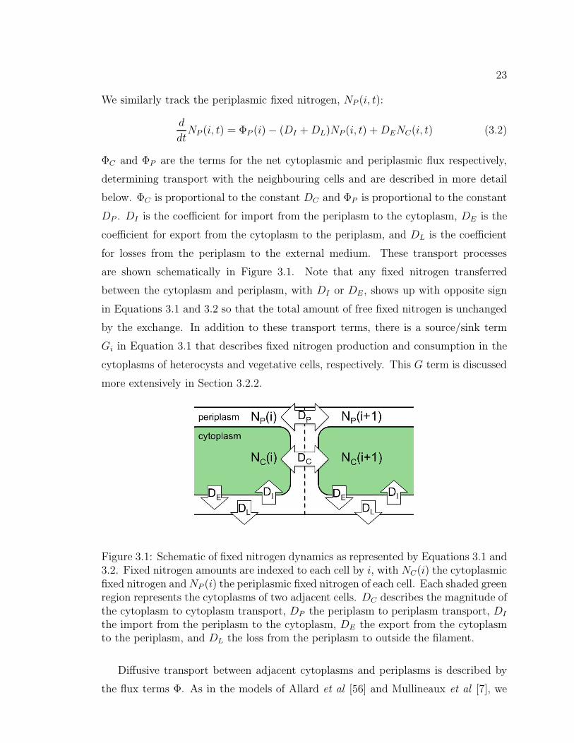
We similarly track the periplasmic fixed nitrogen, NP (i, t):
d
dtNP (i, t) = ΦP (i)− (DI +DL)NP (i, t) +DENC(i, t) (3.2)
ΦC and ΦP are the terms for the net cytoplasmic and periplasmic flux respectively,
determining transport with the neighbouring cells and are described in more detail
below. ΦC is proportional to the constant DC and ΦP is proportional to the constant
DP . DI is the coefficient for import from the periplasm to the cytoplasm, DE is the
coefficient for export from the cytoplasm to the periplasm, and DL is the coefficient
for losses from the periplasm to the external medium. These transport processes
are shown schematically in Figure 3.1. Note that any fixed nitrogen transferred
between the cytoplasm and periplasm, with DI or DE , shows up with opposite sign
in Equations 3.1 and 3.2 so that the total amount of free fixed nitrogen is unchanged
by the exchange. In addition to these transport terms, there is a source/sink term
Gi in Equation 3.1 that describes fixed nitrogen production and consumption in the
cytoplasms of heterocysts and vegetative cells, respectively. This G term is discussed
more extensively in Section 3.2.2.
Figure 3.1: Schematic of fixed nitrogen dynamics as represented by Equations 3.1 and3.2. Fixed nitrogen amounts are indexed to each cell by i, with NC(i) the cytoplasmicfixed nitrogen andNP (i) the periplasmic fixed nitrogen of each cell. Each shaded greenregion represents the cytoplasms of two adjacent cells. DC describes the magnitude ofthe cytoplasm to cytoplasm transport, DP the periplasm to periplasm transport, DI
the import from the periplasm to the cytoplasm, DE the export from the cytoplasmto the periplasm, and DL the loss from the periplasm to outside the filament.
Diffusive transport between adjacent cytoplasms and periplasms is described by
the flux terms Φ. As in the models of Allard et al [56] and Mullineaux et al [7], we

24
assume every compartment in our model is well mixed and that transport is limited
by the junctions between cells. Supporting this, there is no evidence in the images
of fixed nitrogen by Popa et al [8] or of calcein by Mullineaux et al [7] of subcellular
gradients. Fick’s law states that the net diffusive flux between two cells will be
proportional to the density difference between the cells. If a cell’s neighbours were
empty of fixed nitrogen, it would have two outgoing fluxes, one to the left neighbour,
ΦL,out, and one to the right neighbour, ΦR,out. If a cell were empty of fixed nitrogen,
it would have two incoming fluxes, one from the left neighbour, ΦL,in, and one from
the right neighbour, ΦR,in. The actual net flux into a cell is the sum of these four
fluxes:
Φ = ΦL,in − ΦL,out + ΦR,in − ΦR,out
The flux is proportional to the concentration of fixed nitrogen. With the cross sec-
tion of the cells in the filament remaining constant as they grow and divide, we use
the one dimensional concentration N(i, t)/l(i, t) (l is the cell length) and absorb the
cross section into the proportionality constant. The cytoplasmic flux in our model is
proportional to DC .
ΦC = DC
(
NC(i− 1, t)
l(i− 1, t)− NC(i, t)
l(i, t)+
NC(i+ 1, t)
l(i+ 1, t)− NC(i, t)
l(i, t)
)
= DC
(
NC(i− 1, t)
l(i− 1, t)+
NC(i+ 1, t)
l(i+ 1, t)− 2
NC(i, t)
l(i, t)
)
Similarly for the periplasmic flux.
ΦP = DP
(
NP (i− 1, t)
l(i− 1, t)+
NP (i+ 1, t)
l(i+ 1, t)− 2
NP (i, t)
l(i, t)
)
As long as the transport coefficients (DC and DP ) are constant along the filament,
these flux terms look like a discrete Laplacian ∇2d ≡ N(i − 1, t)/l(i − 1, t) + N(i +
1, t)l(i+ 1, t)− 2N(i, t)l(i, t) and lead to the diffusion equation when coarse grained
(see Equation 3.5 below).
The magnitudes of DC and DP will be proportional to the microscopic diffusivity
of fixed nitrogen but, given that we are assuming that transport is limited by the
junctions between cells, is also dependent on the nature of the junctions between cells.
Because of this we have simply taken experimentally measured transport constants
for other molecules and scaled them to glutamine, which is the molecule that carries

25
fixed nitrogen from heterocysts to vegetative cells. In doing this we have assumed
that glutamine and the other molecules are treated the same by the cell connections
and that the transport will only change as it would for regular diffusion. By this
we mean that we are assuming a Stokes-Einstein diffusivity for the diffusion, so the
diffusion is inversely proportional to radius, corresponding to the inverse cube root
of the molecular mass.
To estimate DC , we will use the cytoplasm to cytoplasm transport coefficients for
calcein in Anabaena sp. PCC 7120 filaments [7]. We choose to use the transport
constants in filaments that have been starved of fixed nitrogen for 96 h, because the
experiments of Wolk et al [11] and Popa et al [8] use starved filaments. Multiplying
the exchange coefficient E of units s−1 by a cell length of 3.38 µm gives the constant
in the required units of µm s−1. They are then scaled from calcein to glutamine by
a factor of the cube root of the ratio of the molecular masses. We obtain DC = 1.54
µm·s−1 between two vegetative cells and DC = 0.19 µm·s−1 between a vegetative cell
and a heterocyst. We do not change these values in this thesis.
To estimate DP , we do not have a measured value in the literature for periplasm
to periplasm transport of a small molecule in Anabaena sp. PCC 7120. Instead, we
will use the periplasm to periplasm transport of GFP in Anabaena sp. PCC 7120
[83] to obtain a floor on DP and the intraperiplasm transport of GFP in Anabaena
sp. PCC 7120 [85] to obtain a ceiling on the value of DP .
Mariscal et al observed a FRAP timescale of approximately 150s for GFP moving
between adjacent cells [83]. This corresponds to a DP for GFP of approximately
L/150s ≈ 0.02 µm·s−1 using a cell length L ≈ 3 µm. Scaling the transport of GFP
(27 kDa) to glutamine (146 kDa) by the cube root of the molecular masses [89], i.e.
by a factor of (27 kDa/146 Da)1/3 ≈ 5.7, and taking this as a lower bound, then gives
DP & 0.1 µm·s−1. FRAP experiments with GFP in Anabaena sp. PCC 7120 showed
recovery in part of a single cell’s periplasm after around 60 s [85] and after around 5 s
[83]. This faster time of 5 s is similar to the 4 s recovery time observed in the periplasm
of E. coli [90], which also measured an associated diffusivity of DP,Ecoli ≈ 2.6 µm2·s−1.
Scaling this diffusivity to glutamine, we obtain DP = DP,Ecoli × 5.7/3.8µm≈ 4.4µm
s−1. Given that glutamine has a much smaller mass than GFP, it is unlikely that it
will diffuse any slower from periplasm to periplasm than when scaled from GFP. The

26
broad range we consider for periplasmic transport is then 0.1 µm s−1 . DP . 10µm
s−1.
When we consider periplasmic transport, we must also consider exchange between
the cytoplasm and periplasm, as well as loss from the periplasm to the external
medium. We expect that uptake of fixed nitrogen from the periplasmic to the cyto-
plasmic compartment, controlled by DI in Equations 3.1 and 3.2, is an active process,
controlled by ABC transporters [60] or a similar system. Nevertheless, we expect that
the rate of import is proportional to the periplasmic fixed nitrogen density, NP/l, and
to the number of transporters, which will themselves be proportional to the cell length
l. Similarly, transport of fixed nitrogen from the cytoplasmic to the periplasmic com-
partment, controlled by DE , will be proportional to the cytoplasmic density NC/l but
also to the amount of membrane or (possibly leaky) ABC transporters [91], which
will be proportional to l. The result is that the transport terms with coefficients DI
and DE are independent of the cell length l and the coefficients have units of s−1.
To estimate the value of DI (from Equations 3.1 and 3.2), we begin with the
measurement of Pernil et al [60] that 1.65 nmol/(mg protein) is imported into a
PCC 7120 filament in 10 min from a medium containing 1 µM glutamine. From our
discussion in Section 3.2.2, the dry mass of a PCC 7120 cell is 4.89×10⁻¹²g and the
mass of protein, approximated at 55% of the dry mass of the cell [92], is 2.69×10⁻¹²g.
This implies that there is 4.44×10⁻⁹ nmol of glutamine, or NG = 2.67×10⁶ glutamine
molecules, imported in 10 min into each cell. The term in Equation 3.1 describing
import from the periplasm to the cytoplasm is ∂NC/∂t = DINP . If we assume that
the periplasmic concentration is equal to the glutamine concentration in the external
medium, then NP can be replaced by the product of the glutamine concentration in
the periplasm, ρP,G, the cross-sectional area of the periplasm A (for a 0.1 µm thick
periplasm surrounding a cytoplasm 1 µm in radius A = 0.21π µm2) and the cell length
l giving NG = DIρP,GlAτ , with τ = 10 min. Solving this for DI using l = lmin = 2.25
µm yields DI = 4.98 s−1. ABC transporters, known to transport amino acids [88], are
asymmetric, and we assume that export is ten times weaker than import, and that DE
= 0.498 s−1. It is also known that the outer cell membrane provides a permeability
barrier [86], implying that the periplasmic glutamine concentration may not be as
high as the external glutamine concentration, and so we also consider a DE and DI

27
pair that is ten times larger with DI = 49.8 s−1 and DE = 4.98 s−1.
There is evidence that fixed nitrogen is lost from the filament to the external
medium [93, 94] and we include a loss term for the periplasm with the coefficient
DL in Equation 3.2. We assume the loss rate is very small compared to the other
membrane fluxes, using 1% of the lower DI value, i.e. DL = 0.0498 s−1. This
qualitatively corresponds to the observation of a permeability barrier in the outer
membrane [86]. Our results are qualitatively unchanged in the range of 0 ≤ DL/DI
. 0.1.
3.2.2 Cell growth and division
The cells in Anabaena sp. PCC 7120 have a minimum size of lmin = 2.25 µm and a
maximum size of lmax = 2lmin = 4.5 µm [15, 84]. When the length of a cell reaches
lmax, it is divided into two cells. Each of these two daughter cells is assigned a
new random growth rate and is given half of the fixed nitrogen of the parent cell.
In our investigation we found that stochastic effects were not always necessary for
our conclusions and so we have both deterministic and stochastic results. For the
deterministic results all cells begin with the same length, l0 = 2.8 µm and have the
same doubling time of TD = 20 h [88, 95]. Doubling time determines the optimal
growth rate by having the optimal growth rate of an individual cell, Ropt = lmin/TD.
For stochastic results, shown in Figures 3.3 (b) and (c), all initial cells are assigned
a length between lmin and lmax according to an analytical steady state distribution
of cell lengths [96]. An optimal growth rate is chosen randomly and uniformly in the
range between the minimum optimal growth rate Roptmin = lmin/Tmax and the maximum
growth rate Roptmax = lmin/Tmin. The maximum cell period is defined as Tmax = TD+∆
and the minimum cell period is defined as Tmin = TD −∆. The standard deviation
of the growth rate is then σR =√
2/3∆lmin/[(TD + ∆)(TD − ∆)]. We expect that
the coefficient of variation of the growth rate σR/Ravg is of similar magnitude to that
seen in a study of mutant Anabaena [56], which was σR/Ravg ≈ 0.165.
In Equation 3.1 there is a source/sink term Gi. For vegetative cells Gi = Gveg is
a sink term that takes into account the fixed nitrogen consumption that contributes
to growth. The fixed nitrogen consumed by a cell depends on the growth rate of the

28
cell, and also on the amount of local cytoplasmic fixed nitrogen available for growth.
Gveg = −gR(Ropti , NC(i, t)), (3.3)
g is the amount of fixed nitrogen that a cell needs to grow one µm; here we will
estimate this quantity. Dunn and Wolk [97] measure a dry cell mass for one cell
of A. cylindrica of 1.65×10⁻¹¹ g. Cobb et al [98] measured the nitrogen content
of A. cylindrica to be 5-10% of dry mass (see also [99]). We will use the typical
value of 10% and scale it by volume from A. cylindrica to PCC 7120. A. cylindrica
is approximately 1.5 times as wide and 1.5 times as long as PCC 7120 [15], giving
≈2.07×10¹⁰ N atoms per average cell of PCC 7120. According to Powell’s steady
state length distribution of growing bacteria [96], the average cell size is 1.44 times
as long as the smallest cell, so that ≈1.4×10¹⁰ N atoms are needed for a newly born
cell to double in length. This implies that g = 1.4× 10¹⁰/lmin ≃ 6.2× 109 µm−1.
In our growth model we assume that individual cells grow at their optimal growth
rate Ropti as long as the cell has greater than zero cytoplasmic fixed nitrogen (this
assumption is discussed in Section 3.5). When at zero cytoplasmic fixed nitrogen, a
cell can only grow using the flux of fixed nitrogen into the cell from neighbouring cells
and the periplasm.
R =
Ropti if NC(i, t) > 0
min(
Φin/g, Ropti
)
if NC(i, t) = 0(3.4)
It is important to note that cells with NC = 0 can still grow, but this growth is
limited to what can be supported by the incoming fixed nitrogen flux: gR = Φin =
ΦL,in+ΦR,in+DINP . A cell transitioning fromNC = 0 toNC > 0 will have Φin > Ropti ;
in this instance the Ri = Ropti .
In Equation 3.1, for heterocyst cells Gi = Ghet. The heterocyst fixed nitrogen
production rate Ghet is chosen to supply the growth of approximately 20 vegetative
cells and is 3.15×10⁶ s−1 unless otherwise stated.
3.2.3 Some numerical details
Filaments were initiated with two heterocysts, separated on either side by vegetative
cells, on a periodic loop. Periodic boundary conditions were used to minimize end

29
effects. We have presented our data with a fixed number of vegetative cells between
heterocysts because of cell division. Most of our data has 20 vegetative cells between
the heterocyts. This is approximately twice the typical heterocyst separation [15,
84], which allows us to investigate fixed nitrogen depletion at the midpoint, which
corresponds to the location of an intercalating heterocyst.
We distinguish free from incorporated fixed nitrogen. Free fixed nitrogen is freely
diffusing in the cytoplasm and can be transported to other cells, and is simply given by
NC(i, t). We report this as a linear density ρF ≡ NC(i)/li. Incorporated fixed nitrogen
is the fixed nitrogen that has been incorporated by cellular growth through the growth
term Gveg. This nitrogen is locked to a specific cell and its daughters. We report the
incorporated concentration ρI ≡∫
Gvegdt/li, where the growth is integrated over
a fixed duration. During cell division, half of the parent cell’s incorporated fixed
nitrogen is assigned to each daughter cell. We are interested in isotopically labeled
fixed nitrogen [8, 11], and so we set allNC(i) = 0 at the start of our data gathering (t =
0), consistent with the introduction of isotopically labeled dinitrogen to the filament
that is then fixed by the heterocysts and subsequently supplied to the filament as free
fixed nitrogen via Ghet. The total fixed nitrogen, for e.g. Figures 3.4(a) and (c), in
a cell is ρT ≡ ρF + NP/L + ρI , where we include periplasmic contributions as well.
The two experiments this work is in the context of, from Wolk et al [11] and Popa et
al [8], could not distinguish between freely diffusing and incorporated nitrogen, and
recorded only their sum. Therefore the total fixed nitrogen is the quantity that is
important to compare to experimental results.
3.3 Cytoplasmic transport
3.3.1 Short time fixed nitrogen distributions
First we investigated systems with only cytoplasmic transport (i.e. DI = DE = DP =
0) over short periods of time to be consistent with the experiments of Wolk et al [11].
The rate of cytoplasmic transport was held constant, with the coefficient DC = 1.54
µm s−1 between vegetative cells, and DC = 0.19 µm s−1 between vegetative cells and
heterocysts, as described in Section 3.2.1. In Figure 3.2 we show the fixed nitrogen
distributions in the filament. A heterocyst is at the left end of the distribution,

30
Figure 3.2: Model fixed nitrogen concentration vs. cell index i (the number of cellsfrom a heterocyst at i = 0), for short intervals of labelled nitrogen fixation rangingfrom 10s to 180s as indicated by the legend in (b). The incorporated fixed nitrogenρI is shown in (a), the free fixed nitrogen ρF in (b), and the total fixed nitrogen ρTin (c). In (d) the red circles indicate the experimental data digitized from Wolk etal [11], and the blue squares are the t = 30s ρT data from (c) (using the right axis,scaled and shifted to best agree with experimental data). Our model data is from ourdeterministic model with no periplasmic transport, i.e. DC = 1.54 µm s−1 and DI =DE = DP = 0.

31
indicated by an “H”, and the vegetative cells are indexed by i, counting from the
heterocyst. We varied the amount of time between the start of fixation of labelled
nitrogen and the time the distribution was sampled (t = 10, 30, 60, 120, and 180
s, refer to the legend in the top right figure). (a) shows that the incorporated fixed
nitrogen, ρI , increases steadily in all cells reached by the free fixed nitrogen, ρF , except
the heterocyst. The heterocyst is not incorporating any fixed nitrogen because it is
not growing. (b) shows the free fixed nitrogen, ρF , as it slowly extends out from the
heterocyst and increases. ρF is non-zero seven cells away from the heterocyst, while
the eighth cell receives some fixed nitrogen it does not receive enough to exceed the
amount that could be used for growth. The fixed nitrogen in the heterocyst and cells
one through seven increases until it reaches a steady state: at this time the rate that
nitrogen is fixed by the heterocyst is equal to the rate it is used by the cells to grow.
In (c) we show the total fixed nitrogen, ρT = ρI + ρF . The form of ρT changes in
time. At the shortest times, there is a spike in ρT at the heterocyst and a gradient
moving away; this reflects ρF and ρT is dominated by ρF at the shortest times. At
time increases, the spike at the heterocyst flips to a dip, and the magnitude of the
gradient becomes small compared to the magnitude of the total fixed nitrogen; this
reflects ρI and ρT has more of the character of ρI as the time increases.
The radiographic technique used by Wolk et al [11] is unable to distinguish be-
tween free and incorporated fixed nitrogen, and can only measure the total. Therefore
it is appropriate to compare the ρT distribution of Figure 3.2(c) to the experimental
data. We have shown the average of two sets of experimental data in Figure 3.2 (d)
as filled red circles (left scale). We have also included a qualitatively similar ρT curve
from t = 30 s as the blue curve (right scale). We have adjusted the ρT scale so that
the two curves agree at the location of the heterocyst and with the experimental back-
ground far from the heterocyst. We have reproduced the main feature of the Wolk
data for short exposure to fixed nitrogen, the spike at the heterocyst, and the other
scales are also approximately correct. Wolk’s data was taken after 120 s of exposure
to labelled fixed nitrogen, but our curve that best matches this data is from after
30 s. This is because in our model, heterocysts immediately provide fixed nitrogen
to be transported, but this is not the case for real heterocysts. Glutamine levels in
Anabaena cylindrica linearly increase during the first minute of exposure to labelled

32
dinitrogen and other fixed nitrogen products appear after 2 min [43]. This 1-2 min
lag between exposure to dinitrogen and its transport and incorporation is consistent
with the 90 s difference between the curves in Figure 3.2(d).
3.3.2 Long time fixed nitrogen distributions
We again examined systems with only cytoplasmic transport, but at long times com-
parable to those of Popa et al [8].
In the last section we found that after approximately 120 s, the free fixed nitro-
gen distribution had reached a steady state. To find an analytic expression for this
free fixed nitrogen distribution we approximate the filament as a continuous diffu-
sive medium rather than discrete cells. The diffusion and consumption of free fixed
nitrogen in one dimension is
∂ρF/∂t = D∇2ρF − c (3.5)
where ρF is the one dimensional concentration of free fixed nitrogen, D is the dif-
fusivity (which is related to our cytoplasmic transport parameter DC) of free fixed
nitrogen and c is the consumption of free fixed nitrogen per unit length (related to
gR from our growth model). For the steady state (∂ρF /∂t = 0) the general solution
is quadratic against the distance x. We define x = 0 as the location of a heterocyst.
When in steady state, the flux out of the heterocyst in each direction is equal to half
the fixed nitrogen production of the heterocyst. Combining with Fick’s Law, we have
Ghet/2 = −D∂ρ/∂x. The flux out of the heterocyst must also equal the total fixed
nitrogen consumed by the vegetative cells on either side of it. If x0 is the distance
from the heterocyst that the fixed nitrogen reaches and where growth stops, then
cx0 = Ghet/2 and ρF (x0 = Ghet/(2c)) = 0. Applying these two boundary conditions
to the general quadratic solution we get
ρF (x) =1
2
c
Dx2 − Ghet
2Dx+
G2het
8cD, (3.6)
for x ≤ x0 and ρF (x) = 0 for x ≥ x0. This is in excellent agreement with the
steady state ρF from our numerical model with no stochasticity and only cytoplasmic
transport, as shown in Figure 3.3(a).
In our non-stochastic model all cells with free fixed nitrogen levels above zero grow
at the same rate and so incorporate fixed nitrogen at the same rate. This produces

33
Figure 3.3: (a) non-stochastic concentrations after t = 4h of labeled fixed nitrogenexposure vs. the cell index i. Heterocysts are indicated by (“H”). Shown are thetotal fixed nitrogen (ρT , blue solid line with circles using the left axis) and the freefixed nitrogen (ρF , red solid line with squares using the right axis). Note the dra-matic difference in scale. The steady state analytic result for the free fixed nitrogenfrom a continuum approximation, Equation 3.6, is shown as a green line; while thecorresponding plateau in ρT due to incorporated fixed nitrogen is shown by the blackdashed line. (b) averaged stochastic ρT using doubling-time variation ∆ = 4.5h, witherror bars too small to be seen outside data points. The average is over 1000 distri-butions. (c) the experimental fixed nitrogen concentrations of Popa et al [8] in redcircles (scale on left axis) and from a single stochastic result from our model using ∆= 4.5h and Ghet = 4.25×10⁶ s−1 with ρT in blue squares and 25ρF in green diamonds(scale on right axis, offset for clarity). Also shown as black lines are the vegetativecell averages. (d) the coefficient of variation in vegetative cell fixed nitrogen levels,σT/∆ρT , vs. the coefficient of variation in the growth rate of the vegetative cells,σR/Ravg . The error bars indicate statistical errors of the average variation measuredover 100 samples. The grey shaded region indicates the size of the standard devia-tion, which corresponds to the expected error for a single sample. The red dashedline indicates the variation in the experimental data of Popa et al [8], with a singlesample. For (a)-(d), we have used only cytoplasmic transport with DC = 1.54 µms−1 and DI = DE = DP = 0.

34
a constant plateau in ρI for vegetative cells between the heterocyst at x = 0 and the
cell where the free fixed nitrogen vanishes, i.e. for 0 < x < x0. We see this in the
discrete cellular model, which is shown with ρT in Figure 3.3(a). In this figure there
are heterocysts at both ends of the distribution, indicated by “H”, and vegetative
cells are indexed by i, counting from the left heterocyst. The cells i = 9 and i = 11
have significantly less fixed nitrogen than cells 1-8 and 12-19. This is because the free
fixed nitrogen ρF never goes above zero for cells 9 and 11 and they are only able to
grow using Φin as described in Section 3.2.2. All the other cells reach non-zero ρF
and grow at their optimum rate. The height of the plateau reflects how much time
has elapsed since the labelled fixed nitrogen was provided.
In Figure 3.3(a) we show non-stochastic results for t = 4h, to be able to directly
compare with the data of Popa [8]. The predicted plateau height (<Ropt>gt/<L>)
from our previous continuum model is shown with a black dashed line, and the agree-
ment is excellent. We also see that the free fixed nitrogen ρF (scale on right side)
is approximately two orders of magnitude smaller than the total fixed nitrogen ρT
(scale on left side), which is dominated by the incorporated fixed nitrogen ρI . We
see excellent qualitative agreement with the plateau-like distribution seen by Popa.
The gradient of free fixed nitrogen on top of the much larger amount of total fixed
nitrogen is too small to be easily resolved by the experimental technique.
3.3.3 Stochasticity of long time distributions
Figure 3.3(b) shows the total fixed nitrogen distribution using our stochastic model
that has been averaged over 1000 vegetative segments between two heterocysts. It
looks qualitatively very similar to the deterministic results of Figure 3.3(a). A direct
comparison of a single ρT distribution produced by our stochastic model (blue curve
with squares, right axis) and the experimental data of Popa (red curve with circles,
left axis) is in Figure 3.3(c) (the two curves are offset by an arbitrary amount). The
distributions are qualitatively quite similar and much rougher than those of Figures
3.3(a) and (b). However, the ρF from the stochastic model (green curve, diamonds) is
very smooth, maintaining the gradient despite the noisy ρT distribution and indicating
that the roughness can entirely be attributed to incorporated fixed nitrogen, ρI .
In our stochastic simulation, the variation of ρT shown in (c) is due both to the

35
varying growth rates of cells along the filament and to their varying lengths. This
leads to the observed differences in the density of incorporated fixed nitrogen after
a fixed time. This means that it is possible that the noise in the distribution seen
by Popa is due to the stochasticity of the individual cell’s growth rates, rather than
the experimental apparatus or method. In (d) we plot the coefficient of variation
of the total fixed nitrogen, σT/∆ρT against the coefficient of growth rate variation,
σR/Ravg . Here σR is the standard deviation of the growth rate distribution, and
Ravg is the average growth rate. Similarly σT is the standard deviation of ρT in
vegetative cells, while ∆ρT is the difference between the average ρT in vegetative cells
and the average ρT in the heterocysts. Because we have implemented the growth
rate range in our model, we are able to calculate σR/Ravg exactly for our simulated
filaments. For σT /∆ρT for our simulated filaments in Figure 3.3(d) we measured over
100 filaments to get an average (shown as black circles), standard deviation (shown
as the grey region), and standard deviation of the mean (black error bars on black
circles). The red dashed line represents the same quantity for the experimental Popa
data when determined by the same procedure as for our simulation data. Given that
the experimental data is for a single sample, the experimental value is best compared
to the single standard deviation region in grey. It shows that the fixed nitrogen
distribution variability for a broad range of growth rate variabilities is consistent
with the observed variability in the Popa nitrogen distribution. This range is near
the coefficient of variation σR/Ravg = 0.165 reported for a mutant of PCC 7120 [56].
We conclude that the variability in the Popa nitrogen distribution may be entirely
due to stochasticity of the individual cell growth rates.
After extended isotopic dinitrogen exposure, much longer than typical cell dou-
bling times, we expect a nearly constant distribution of ρT — corresponding to the
nearly uniform concentration of fixed nitrogen in a cyanobacterial filament. Notably,
the variation within the plateau, evident in the data of Popa et al [8] and modelled in
Figure 3.3(d), will also vanish at late times. After a long enough period of time, most
of the fixed nitrogen in the filament will be labelled and among vegetative cells it will
be evenly distributed. Old heterocysts will retain their dip for longer than vegetative
cells retain their variability, but nitrogen recycling will occur through basal processes
and eventually even the old heterocysts will have the same labelled nitrogen density

36
as the rest of the filament. On top of the large and nearly constant ρI in the cells
will be the small gradient of ρF that is described in Equation 3.6 and illustrated in
Figures 3.3(a)-(c). It is possible that determining the fixed nitrogen distribution in
filaments that have been grown for weeks would allow the small gradients of ρF to be
discerned with NanoSIMS techniques [8].
3.4 Periplasmic transport
3.4.1 Long time nitrogen distributions with cytoplasmic and periplasmic
transport
We have established that the qualitative characteristics of both the spiked distribution
of Wolk et al [11] and the flat distribution of Popa et al [8] can be reproduced using
a single quantitative model for the cyanobacterial filament using only cytoplasmic
transport. In this section, we explore how the addition of periplasmic transport
affects the Popa-like plateau formed in ρT .
In Figures 3.4(a) and (b) import and export between the cytoplasm and periplasm
has DI = 4.98 s−1 and DE = 0.498 s−1 (see Section 3.2.1). The only parameter that
varies is the value of the periplasmic diffusivity DP , as indicated by the legend in
(b). We vary DP up to the magnitude expected for unimpeded diffusive transport of
glutamine along the filament, as discussed in Section 3.2.1. The characteristic dip in
the centre of the total fixed nitrogen distribution, ρT , in (a) fills in at larger values of
DP , but is not sufficient to qualitatively change the form of the distribution. The mid-
segment dip fills in because periplasmic transport allows free fixed nitrogen to move
past the first starving vegetative cell with NC = 0. To evaluate how significant the
periplasmic transport is, we show in (b) the fraction of the flux along the periplasm
to the total flux along the cytoplasm and periplasm. This essentially shows how
much of the fixed nitrogen is transported through the periplasm. The flux is mostly
cytoplasmic next to the heterocysts, and mostly periplasmic next to starving cells. In
between, up to 50% of the flux can be periplasmic. For the larger DI and DE values of
Figures 3.4(c) and (d) the results are very similar. These results indicate that, within
our model, the periplasmic transport cannot be the dominant form of transport of
fixed nitrogen from heterocysts to vegetative cells. However, we have shown that a

37
Figure 3.4: Fixed nitrogen distributions for systems with additional periplasmic trans-port, as discussed in Section 3.4.1. In all four plots the periplasmic transport rateDP (in units of µm s−1) is varied according to the legend in (b). (a) the total fixednitrogen distribution, ρT , for transport between the cytoplasm and periplasm withDI = 4.98 s−1 and DE = 0.498 s−1. The data of (b) corresponds to the curves of thesame colour in (a) and shows the fraction of the total fixed nitrogen flux along thefilament that is periplasmic vs. the cell index i. (c) and (d) are similar to (a) and (b),respectively, except that import and export between the cytoplasm and periplasm aretenfold stronger, with DI = 49.8 s−1 and DE = 4.98 s−1. As before, DC=1.54 µms−1. We use DL = 0.0498s−1 and Ghet = 3.67×10⁶ s−1.

38
range from completely cytoplasmic transport, to roughly half cytoplasmic and half
periplasmic transport is consistent with the qualitative fixed nitrogen distribution
reported by Popa et al [8]. Nevertheless, cytoplasmic transport alone can be used to
determine the fixed nitrogen distribution and the growth it controls.
3.4.2 Long time nitrogen distributions with only periplasmic transport
We have also considered the model in absence of cytoplasmic transport, with only
periplasmic transport of fixed nitrogen.
In Figure 3.5(a), import and export between the cytoplasm and periplasm has DI
= 4.98 s−1 and DE = 0.498 s−1. Again, we have only varied DP , as indicated by
the legend in (b). With only periplasmic transport in the filament, there is a very
different fixed nitrogen distribution. For the slowest transport, DP = 0.1 µm s−1,
only the two cells nearest the heterocysts are growing at their maximum rate, with
the third receiving a much smaller amount of nitrogen. Cells further than three cells
from the heterocyst are receiving no nitrogen and are not growing. As the periplasmic
transport rate increases, fixed nitrogen reaches cells further from the heterocysts. For
DP = 10 µm s−1 some fixed nitrogen has reached all of the cells, although we still
do not observe a Popa-like dip. Instead there is a broad trough in the middle of the
distribution, indicating that fixed nitrogen in the periplasm is able to get past the
first starving cell (with NC = 0) and somewhat supply cells even further from the
heterocyst. Also note that the height of ρT does not change with how many cells are
being supplied with nitrogen. For slower transport, the nitrogen that is not being
used for growth is being lost through leakage to outside the filament before it can be
transported to starving cells.
In Figure 3.5(b), import and export between the cytoplasm and periplasm are
tenfold faster, at DI = 49.8 s−1 and DE = 4.98 s−1. The story here is similar to
(a), where for slower transport the middle cells are starved, and as the transport is
sped up, more cells are reached. In contrast, a broad trough is never achieved and
the boundary between non-starving cells and starving cells remains sharp. This is
the effect of increasing the import and export by a factor of ten: fixed nitrogen is
unable to sneak past the first starving cell it encounters. It also suggests that for some
value of the periplasmic transport rate coefficient, DP , the distribution would exhibit
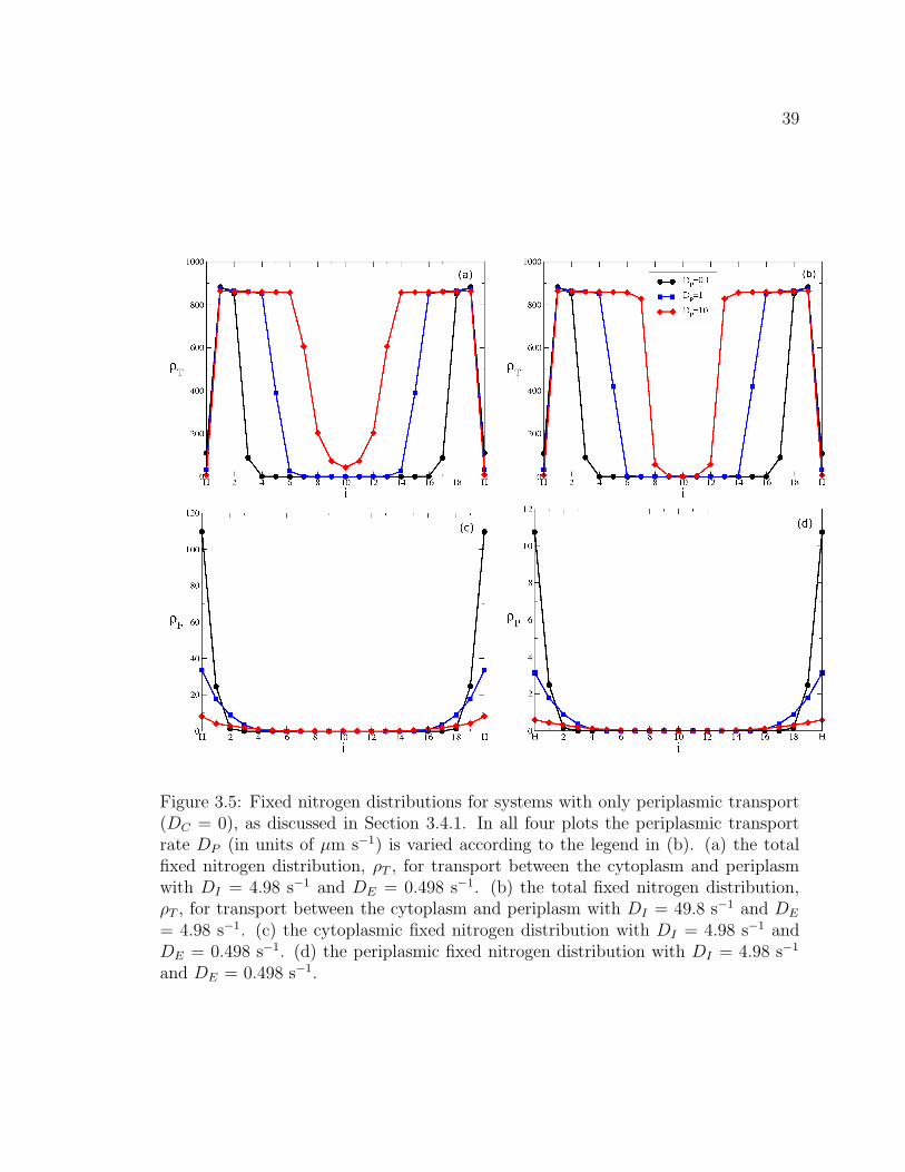
39
Figure 3.5: Fixed nitrogen distributions for systems with only periplasmic transport(DC = 0), as discussed in Section 3.4.1. In all four plots the periplasmic transportrate DP (in units of µm s−1) is varied according to the legend in (b). (a) the totalfixed nitrogen distribution, ρT , for transport between the cytoplasm and periplasmwith DI = 4.98 s−1 and DE = 0.498 s−1. (b) the total fixed nitrogen distribution,ρT , for transport between the cytoplasm and periplasm with DI = 49.8 s−1 and DE
= 4.98 s−1. (c) the cytoplasmic fixed nitrogen distribution with DI = 4.98 s−1 andDE = 0.498 s−1. (d) the periplasmic fixed nitrogen distribution with DI = 4.98 s−1
and DE = 0.498 s−1.

40
a Popa-like dip. We have shown that cytoplasmic transport, at the experimentally
measured rates, is able to do this. A similar measurement of the rates associated with
periplasmic transport would be necessary to assert this for periplasmic transport as
well.
In Figures 3.5(c) and (d) we show the free cytoplasmic (ρF ) and the periplasmic
(ρP ) fixed nitrogen distributions respectively, for the case of DI = 4.98 s−1 and DE =
0.498 s−1, which is shown in (a). Cells furthest from the heterocyts do not have free
fixed nitrogen in the cytoplasm for any rate of periplasmic transport, but the fastest
transport rate allows some fixed nitrogen to be in the periplasm for cells furthest from
the heterocysts. The loss from the filament is proportional to NP , and because ρP is
so high for slow transport, more fixed nitrogen is lost via leakage and it reaches fewer
cells.
3.4.3 Long time nitrogen distributions with graded growth
In Section 3.1 we mentioned the growth model of Wolk et al [11], which assumed
that growth was linearly related to fixed nitrogen concentrations. Our growth model,
laid out in Section 3.2.2, instead has the growth of a cell be constant unless there is
not enough free fixed nitrogen to support it. All the results in the above sections in
this chapter have used our constant growth model. Here we will address the linear or
graded growth model. Growth is expected to increase when nutrient concentration
increases, in contrast to our model. We want to show that a graded model cannot
explain the nitrogen distribution of Popa et al [8].
With the graded growth that is linearly proportional to ρF , the dynamics or ρF
are then
∂ρF/∂t = D∇2ρF − kρF , (3.7)
The first term on the right represents diffusion and the second is a local sink due
to vegetative growth. Comparing to Equation 3.5 we see that this second term has
changed from a constant term in Equation 3.5 to a linear term here. As above
with Equation 3.5 we ignore the discreteness of cells so that we can obtain an
analytic solution. Following Section 3.3.2, a heterocyst at x = 0 has a flux of
J = −D∂ρF /∂x = Ghet/2 to both sides. Demanding a steady state, ∂ρF /∂t = 0,

41
and applying the heterocyst flux boundary condition yields the solution
ρF =1
2√kD
e−√
k/Dx. (3.8)
The amount of free fixed nitrogen used to grow by the filament and therefore incor-
porated by the cell is proportional to the free fixed nitrogen concentration, ρF , and
therefore the total fixed nitrogen, ρT , will be proportional to ρF and decay away ex-
ponentially from the heterocyst with a length scale√
D/k. This is inconsistent with
the nitrogen distribution of Popa et al [8] for all√
D/k. A large√
D/k will lead
to a gradual decrease in the ρT at larger x while a small√
D/k will lead to a rapid
decrease in ρT at small x.
Figure 3.6: The numerical total fixed nitrogen distributions vs. cell index i usinggraded growth proportional to local ρF as Eq. 3.9. The growth rate proportionalityconstant k (in units of µm s−1) is varied, as indicated by the legend. This is adeterministic cellular model with cytoplasmic transport: DC = 1.54 µm s−1 and DI
= DE = DP = 0.
With our discrete deterministic model, we have modelled the graded growth
Rgraded(Nc) = kNc/Li. (3.9)
This equation can be used just as Equation 3.4 was used in Equation 3.3 to determine
the value of the sink term G in Equation 3.1. The results are shown in Figure 3.6.
We either recover a plateau with no dip in the middle region (for small k) or a quick
drop to a central trough with no plateau. The discrete nature of the model modifies
the observed pattern near bounding heterocysts compared to Equation 3.8.

42
3.5 Discussion
We have presented a quantitative model for fixed nitrogen transport and dynamics in
a cyanobacterial filament, including growth of vegetative cells and production of fixed
nitrogen by heterocysts. The goal of this model in this chapter was to understand
how the fixed nitrogen transport in the filament determines the fixed nitrogen dis-
tribution, and to use this understanding to address the disagreement of the nitrogen
distributions of Wolk et al [11] and Popa et al [8]. We also wanted to investigate how
the distribution changed when the model included cytoplasmic and/or periplasmic
connections that could transport fixed nitrogen.
Our model has reproduced the qualitative fixed nitrogen distribution near hete-
rocysts seen after short exposure to fixed nitrogen (Figure 3.2), similar to the spiked
distribution of Wolk et al [11], as well as the distribution seen after much longer
exposure to fixed nitrogen (Figure 3.3), similar to the plateau distribution of Popa et
al [8]. These two distributions, seemingly at odds, are really the product of the same
dynamics but at different time scales. The apparent lack of a fixed nitrogen gradient
away from the heterocysts in the Popa distribution is explained by the much larger
amount of incorporated fixed nitrogen, which also explains the noisy plateau between
heterocysts. When modelled, the free fixed nitrogen does show a smooth gradient
away from the heterocysts even when the total fixed nitrogen is quite rough (Figure
3.3(c)).
Qualitatively, our results indicate the importance of the large, noisy, plateau-
shaped concentration profile of incorporated fixed nitrogen. The level of the plateau
will increase linearly in time after the free fN gradient away from heterocysts reaches
a steady state, which takes minutes. The free fN, ρF , is soon much smaller than the
incorporated fN, ρI . The spike in the Wolk distribution, seen in the first few minutes
of exposure to isotopically labeled dinitrogen, was when the free fN still dominated
the total ρT . In contrast, the plateau seen in the Popa distribution was after hours of
exposure, when the total fN was dominated by the incorporated component and the
gradient in ρF was relatively small even with respect to variations of ρI within the
plateau (see Figure 3.3(c)). At times that are long after the steady state is reached
but still much shorter than division times the heterocysts present dips of labelled fixed
nitrogen, as observed by Popa et al [8]. Stochasticity, through initial cell lengths and

43
cellular growth rates, adds noise to the incorporated fN distribution, ρI . As we show
in Figure 3.3 (d), the modelled cell-to-cell variation is due to differences in growth
rate which manifest themselves as different amounts of labeled fN incorporated by
growth. We believe this explains the observed variation in the experimental nitrogen
distribution of Popa et al [8].
The possibility of periplasmic fixed nitrogen transport raised by a continuous
periplasm [82], transport of GFP [83], and an outer membrane permeability barrier
[86] led us to explore the possible impact of periplasmic transport in addition to
cytoplasmic cell-to-cell connections [7]. As illustrated in Figure 3.4, we found that
a significant proportion (up to 50%) of fN transport along the filament can occur
through the periplasm without qualitatively changing our fN distributions. We cannot
rule out a role for the periplasm in fN transport, and larger proportions may be
achievable with more extensive parameter searches. Indeed, the fact that knocking
out amino acid permeases leads to impaired diazotrophic growth [60, 87, 88] does
indicate that significant leakage from the cytoplasm does occur (i.e. DE > 0) — which
is a necessary part of periplasmic transport. Nevertheless, the fact that modelling
with only cytoplasmic transport was able to qualitatively match both experimental
distributions means that our results are also consistent with no significant periplasmic
transport. For simplicity, the models developed in future chapters will be without
periplasmic transport.
We have also explored the resulting distribution when there is only periplasmic
transport and there is no cytoplasmic transport (DC = 0). The results are in Figure
3.5. For relatively slow import and export between cytoplasm and periplasm, they
show either a large trough lacking fixed nitrogen between the heterocysts, or a wider
dip that does not reach zero. For relatively fast import and export between the cy-
toplasm and periplasm, they show a sharp transition from a constant fixed nitrogen
level to zero. It seems possible that with fine tuning to some intermediate rate of
import and export, the fixed nitrogen distribution could match the Popa plateau phe-
notype. With these results, it seems very unlikely that fixed nitrogen is transported
through the periplasm alone.
We have used a simple model, Equation 3.4, to limit growth in response to local
fixed nitrogen starvation: cells grow at a fixed rate Ropt if there is sufficient free fixed

44
nitrogen available locally (NC > 0), and at the maximal rate allowed by local input
fluxes of free fixed nitrogen if not. This model reflects the absolute limitation on
growth placed by available fixed nitrogen, but also recovers the characteristic plateau
of ρT seen in the Popa distribution. As we illustrate in Section 3.4.3, “graded” growth
rates, that smoothly depend on NC and vanish at NC = 0, respond to the graded
distribution of free fixed nitrogen away from heterocysts, Equation 3.8, and produce
graded growth patterns and graded distributions of ρI and ρT (see Figure 3.6), un-
like those observed by Popa [8]. Graded growth models, such as the Monod model
[100], are typically designed to describe response to external metabolite concentra-
tions rather than cytoplasmic concentrations. Like our growth model, Salmonella
typhimurium [101] and Escherichia coli [102, 103] both show non-graded growth in
response to cytoplasmic fixed nitrogen starvation. However, there is no direct evi-
dence of how growth of vegetative cells in cyanobacterial filaments depends on the
cytoplasmic freely available fixed nitrogen, ρF .
The experimental work was done on different species of filamentous cyanobacteria,
namely Anabaena cylindrica by Wolk et al [11] and Anabaena oscillarioides by Popa
et al [8]. In contrast, our models were parameterized by consideration of transport
studies done in Anabaena sp. strain PCC 7120 (see Section 3.2.1). While we expect
parameter values to differ between species, so that precise numerical agreement with
the Wolk and Popa results is not to be expected, our qualitative agreement indicates
that similar fixed nitrogen transport and dynamics could apply in these different
model organisms.
We expect the qualitative features of the Wolk and Popa fixed nitrogen distribu-
tions to apply to the early and late time fixed nitrogen distributions, respectively,
of all filamentous cyanobacteria with heterocysts that are growing in media lacking
fixed nitrogen and that have significant cytoplasmic connections. Nevertheless, quan-
titative details will depend, via the model parameterization, on the cyanobacterial
strain and the experimental conditions. For example, sufficiently large periplasmic
transport (via DP ) would broaden Popa’s dip in incorporated fixed nitrogen between
heterocysts due to transport and growth past the first starving cell. Conversely, a
larger cytoplasmic diffusivity (via DC) would alter the magnitude of Wolk’s free fixed
nitrogen (via Equation 3.6) but not the incorporated fixed nitrogen. The average

45
doubling time determines the characteristic time at which we expect the later time
distribution to emerge. Cell to cell variations in the doubling time, in turn, determine
the amount of variation expected within the Popa-like plateau of incorporated fixed
nitrogen near heterocysts for the first few generations of labelled growth.
Our results reconcile the metabolite patterns shown by the autoradiographic tech-
nique of Wolk et al [11] with the NanoSIMS technique of Popa et al [8]. It is not
obvious which would currently have the best resolution, and it would be useful to have
either or both applied to Anabaena PCC 7120 — the most popular current model for
filamentous cyanobacteria and for which recent transport studies exist [7, 83]. We can
make four qualitative but testable predictions from our work. First, as the duration
of labelled fN is increased the total fN distribution away from heterocysts will evolve
from a Wolk-like peak, dominated by free fN, to a Popa-like plateau, dominated by
incorporated fN. As indicated by Figure 3.2, the crossover takes place after only a few
minutes of labelled dinitrogen fixation. Second, on a similar timescale the free fN will
reach a steady state smooth parabolic shape even in a single sample. This free fN may
be directly measurable in vivo, for example, by fluorescence resonance energy transfer
(FRET)-based metabolite nanosensors [104]. The parabolic gradient of ρF could also
be uncovered by averaging the results of many experiments measuring ρT . Third, the
variations seen by Popa et al [8] will decrease in relative magnitude after at least one
doubling time of exposure to labeled fN. Fourth is more of an assumption, but we
expect that growth of vegetative cells will slow abruptly when the freely available fN
vanishes — according to Equation 3.4 rather than in a graded fashion according to
Equation 3.9. Finally, with more precise parameterization of our transport parame-
ters, sources, and sinks we can make quantitatively testable predictions. Prediction
of the variance of cell-to-cell fN, σI , requires only the observed growth rate variance
σR and the duration of exposure to labeled dinitrogen.
Chapter 4
Growth Rates of and Heterocyst Placement in the
Cyanobacterial Filament
4.1 Motivation and background
This chapter is based on a paper we have published in Physical Biology, volume 9,
page 046002, 2012 [105]. IOP Publishing has given me permission to reproduce the
contents of the paper in this thesis (see Appendix B). For this paper my contributions
were to write the simulation, do the analytical and computational work, generate the
figures, and write the first draft. I was also an equal partner with my supervisor in
developing the model and revising the paper.
Chapter 3 has allowed us to understand the dynamics of fixed nitrogen in the
cyanobacterial filament. It has established, by comparison with experimental nitro-
gen distributions, that our model is a reasonable approximation of the actual fixed
nitrogen dynamics of a living filament. It has demonstrated that a model includ-
ing cytoplasmic transport alone is sufficient to be consistent with the experimental
nitrogen distributions. It has also shown that our constant growth model, in con-
trast to a graded growth model, can explain the distribution of nitrogen between two
heterocysts.
With our fixed nitrogen model established, we wanted to investigate the growth of
filaments on time scales larger than division times, which also facilitates investigation
of the dynamic placement of heterocysts. In comparison to Chapter 3 we have made
several changes to the model. We now only consider the cytoplasmic compartment,
and no longer consider the periplasmic compartment. We add external fixed nitrogen
and its import. We now need to dynamically place heterocysts instead of only having
two heterocysts at the beginning of a simulation. Detailed explanations of these
changes are in Section 4.2.
As detailed in Section 2.4, significant progress has been made in characterizing the
46

47
genetic network underlying the observed heterocyst pattern [3, 15] that is developed
in response to the absence of external fixed nitrogen. The efforts to understand the
genetic network and other possible mechanisms controlling heterocyst differentiation
focus on understanding how the cells in the filament choose which particular cells
will be heterocysts. While we will address heterocyst selection from a physical point
of view, we will focus on understanding why the heterocyst pattern exists and what
advantages it provides. Importantly, we wanted to examine growth not just at very
high or nearly zero exogenous fixed nitrogen, but at intermediate levels.
As we shall show, a filament with too few (or inactive) heterocysts will starve of
fixed nitrogen and grow slowly without external fixed nitrogen [106], while too many
heterocysts, which do not grow and divide, will also inhibit growth [47]. Balancing
these effects in the filament qualitatively explains the heterocyst frequency of ap-
proximately 10% observed with no external fixed nitrogen, but does not explain the
distinctive pattern of heterocyst spacings that is seen in the model cyanobacterium
Anabaena sp. PCC 7120 [6, 26, 46, 47]. Indeed, the observation that mutant strains
exhibiting a distinct pattern of multiple contiguous heterocysts (Mch) show reduced
growth [62] indicates that heterocyst placement is important. In this chapter, we use
quantitative modelling to explore the hypotheses that simple heterocyst placement
strategies can affect filament growth, and that observed heterocyst patterns reflect
placement strategies that maximize growth.
Previous modeling efforts relating to this work are reviewed in Section 2.7.
We hypothesize that leakage of fixed nitrogen from the cyanobacterial filament
may distinguish between heterocyst patterns, in terms of growth rates. Evidence for
leakage was first reported by Fogg et al [2, 107], who found fixed nitrogen products
outside the filament. Supporting this, Paerl [93] observed bacteria clustering around
cyanobacterial filaments, particularly at junctions between heterocysts and vegeta-
tive cells, and indicated a possible symbiosis based on enhanced nitrogen fixation and
leaked fixation products. Thiel [94] found protein proteolysis byproducts in the extra-
cellular medium after fixed nitrogen starvation. Significant leakage is also consistent
with the observation of reduced diazotrophic growth in strains with impaired amino
acid uptake transporters [60, 88]. Nevertheless, we are not aware of any quantitative
measurements of the rate of leakage. Qualitatively, a regular pattern of heterocysts
48
would minimize the distance traveled by fixed nitrogen products so as to minimize
leakage from vegetative cells, leaving more fixed nitrogen available for growth.
In this chapter, we examine heterocyst frequencies that maximize filament growth
within the context of a quantitative transport model [75] that incorporates fixed ni-
trogen transport, vegetative cell growth, and fixed nitrogen production at heterocysts.
We explore the impact on growth of different heterocyst placement strategies, includ-
ing random placement, and find that they are almost indistinguishable in the absence
of leakage of fixed nitrogen from the filament, but clearly distinct with leakage. We
find that the heterocyst spacing patterns corresponding to maximal filament growth
are qualitatively similar to those seen experimentally.
The genera Anabaena, which includes heterocystous cyanobacteria, is widely dis-
tributed geographically in freshwater lakes [108, 109], where fixed nitrogen is one of
the major substances limiting growth [110, 111, 112]. Nitrification turns ammonia
into nitrite and then nitrate [109, 113]. Nitrate levels in lakes range from 0-10 mg/l
(0-10×1022 m−3) in unpolluted freshwater, but vary both seasonally and spatially
[109, 114]. Heterocystous cyanobacteria are also found in the oceans [115, 116] where
nitrate levels have been recorded to vary from approximately 0-50 µmol/kg [117] (0-
3×10²² m−3). It has long been known that sources of fixed nitrogen initially present
in the medium can increase the mean spacing between heterocysts [2, 118] and that
heterocysts will differentiate at non-zero levels of external fixed nitrogen (efN) [2].
Field studies of heterocystous cyanobacteria also show both a range of heterocyst
counts and a range of efN concentrations, with significant positive correlations be-
tween the two (see e.g. [119]). In addition, steady state chemostat experiments show
that Anabaena flos-aquae can adjust nitrogen fixation to achieve constant growth,
within approximately 10%, as efN concentrations are varied [29]. While growth inde-
pendence from efN seems desirable in the face of environmental variability, it raises
the question of how and how well it is achieved in terms of heterocyst fraction and
pattern.
The heterocyst pattern changes with time as it evolves towards a steady state
distribution after efN deprivation [26, 46, 47]. Earlier models [31, 74] have focused
on the early heterocyst pattern observed 24 h after efN deprivation. While the early
pattern and the later patterns are qualitatively similar, with broad distributions of

49
heterocyst spacings ranging from zero to more than twenty cells between heterocysts
with a peak at about a ten cell spacing, we focus on the steady state distribution
in this paper. We explore the hypothesis that cyanobacterial filaments use a unified
heterocyst placement strategy even at non-zero levels of efN. With all of our strategies,
we find that maximal growth is observed with heterocyst frequencies that decrease
continuously with increasing levels of efN.
4.2 Model
4.2.1 Fixed nitrogen transport
Our model of fixed nitrogen (fN) transport and incorporation is similar to the model
from Chapter 3. Since periplasmic transport was not required to explain the ex-
perimentally measured nitrogen distributions, we will not be including periplasmic
nitrogen in our model here. Accordingly, any leakage of fixed nitrogen from the fila-
ment will be modelled as being directly lost from the cytoplasm. We are considering
exogenous sources of fixed nitrogen and therefore also have import of fixed nitrogen
from the extracellular medium. This chapter also does not focus on accumulation of
nitrogen, so we track only the freely diffusing fixed nitrogen of Chapter 3 and call
it just nitrogen, with the understanding that this is the cytoplasmic freely diffusing
fixed nitrogen. Our model tracks the amount of fN, N(i, t), in each cell i vs. time t:
d
dtN(i, t) = Φ(i, t) +DOρefN l(i, t)−DMN(i, t) +Gi, (4.1)
Φ is the same as ΦC in Equation 3.1 that is described by Equation 3.2.1. We will still
use DC = 1.54 µm s−1 between two vegetative cells and DC = 0.19 µm s−1 between
a vegetative cell and a heterocyst and do not change these values in this chapter.
DO is the coefficient of the term describing import of fixed nitrogen from outside the
filament, and DM is the coefficient of the term describing loss of fixed nitrogen to the
medium outside the filament. These transport processes are shown schematically in
Figure 4.1.
To estimate DO, we use Fogg’s observations of heterocyst frequency in a medium
to which a fixed amount of efN in the form of ammonia was added [2]. Heterocyst
frequency decreased in time due to vegetative growth until the ammonia concentra-
tion dropped to 4 × 10⁻⁵M (see p. 245 of [2]). We assume that a slightly higher

50
Figure 4.1: Schematic of fixed nitrogen transport as represented by Equation 4.1.N(i) is the amount of freely diffusing fixed nitrogen for cell i. DC governs transportbetween cells, DO governs import from the medium outside the filament into the cell,and DM controls loss from the cell to the external medium.
concentration of efN, 5 × 10⁻⁵M (ρefN = 3×10²²m−3), is just sufficient for maximal
growth. From Equation 4.1 the amount of fixed nitrogen imported from the external
medium in a time T is DOρefN lT . For a cell to double in length over a period of
time T = 20 h it needs approximately 1.4×10¹⁰ N atoms to be imported [75]. Using
l = lmin = 2.25 µm, this yields DO = 2.9× 10⁻¹⁸m3/(µm·s).
We also include a loss term with coefficient DM in Equation 4.1, following [2,
60, 88, 93, 94, 107]. Loss is expected to be proportional to the cytoplasmic density,
N/(Al), where l is the length of the cell and A is the cross-sectional area, and also
to the number of transporters, which will themselves be proportional to the cell
length. This results in a loss term that is independent of length l, with a coefficient
DM with units of s−1. There are no direct measurements of leakage rates of fN
from cyanobacterial filaments that we are aware of. We take the loss rate as small
compared to the import rate, and so use eitherDM=0.01DO/A (referred to as 1% loss)
and DM=0.1DO/A (referred to as 10% loss). We use a fixed A = πµm2 corresponding
to a radius of 1µm.
As in the model in Chapter 3, in addition to transport terms, there is also a
source/sink term Gi in Equation 4.1 that describes fN production and consumption
in the heterocysts and vegetative cells, respectively. This G term is discussed in the
next section.

51
4.2.2 Cell growth and division
Our model of cell growth and division is very similar to the model in Chapter 3
described in Section 3.2.2, with some changes. Instead of selecting randomly and
uniformly between a minimum and a maximum growth rate, as in Chapter 3, we
select randomly and uniformly from between a minimum cell period Tmin = TD −∆
and a maximum cell period Tmax+∆. We anticipate this change will not significantly
affect the results. As in Chapter 3, TD = 20 h and ∆ = 4.5 h. The cell growth rate is
then Ropt = lmin/T . Also, the flux into the cell Φin in Equation 3.4 that determines
the amount of growth has changed to Rg = Φin = ΦL,in + ΦR,in +DOρefN li.
4.2.3 Heterocyst placement
While we know that experimentally observed heterocyst patterns are not due to ran-
dom placement [31], it is useful to evaluate the steady state growth rate achievable
with random heterocyst placement. We will use random placement as a point of
reference for other heterocyst placement strategies. We consider three simple strate-
gies: random placement, random placement with no contiguous heterocysts, and local
placement. For all of them, once a heterocyst is placed it immediately stops growing
(Ropti = 0) and fixes nitrogen (Gi = Ghet). Commitment to differentiation does not
occur until after approximately 8 h of efN deprivation and can take as long as 14
h [26, 27, 28]. Heterocysts mature and begin to fix nitrogen approximately 18-24 h
after efN deprivation [84, 26, 27] (though see [56]). For random strategies, heterocyst
placement corresponds to when heterocysts begin to produce fN. For local placement,
we have an explicit delay (see below).
Our first, reference, strategy is random placement (“random”). The heterocyst
fraction f is fixed, and during filament growth a random vegetative cell is replaced
with a heterocyst whenever possible but without exceeding f .
Our second strategy (“no-Mch”) reflects the observation that contiguous hetero-
cysts are not observed during normal development [15, 84]. It consists of our random
strategy, but with the additional restriction that vegetative cells adjacent to existing
heterocysts are never selected for development.
Our third strategy is local heterocyst placement (“local”). Any vegetative cell that
has been continuously starving for a defined interval τ is changed into a heterocyst.

52
Starvation is defined as N(i) = 0, so that these cells have reduced growth R < Ropt
for a significant period of time. We vary τ within the range 1 − 20 h. Starvation
occurs due to distance from heterocysts [75], but can also reflect local clusters of
fast growing cells. The waiting period τ combines the periods until commitment and
maturity/nitrogen fixation discussed in Section 2.4. In Chapter 5 we will introduce a
local heterocyst placement model that reflects more of the knowledge of the heterocyst
commitment and differentiation process. The more complicated model of Chapter 5
is not necessary in this chapter, as we only investigate heterocysts in a steady state
pattern, while the model of Chapter 5 is necessary to examine the de novo heterocyst
pattern within the first 24 hours.
4.2.4 Some numerical details
Periodic boundary conditions were used to minimize end effects. Filaments were
initiated with no heterocysts and the different strategies were followed until a steady
state was reached. For the local strategy, a “no-Mch” rule was followed for the first
24 hours of differentiation to reduce initial transients.
The growth rate constant µ was calculated every six simulated hours using the
total length of the filament L(t), where L(t) = L(t − 6h)eµ·6h. Heterocyst frequency
was sampled every six simulated hours by dividing the number of heterocysts by
the total number of cells in the filament. Heterocyst spacings were also recorded
every six simulated hours. Measurements were averaged daily, and the results of
ten independently seeded runs were used to determine an overall daily average and
standard deviation. All data shown is for the fifth day, which exhibits steady state
for the parameters explored (in comparison with data from the fourth day).
We begin each simulation with 100 cells. Most of the phenomena we investigate
occurs in filaments with a growth rate constant greater than µ =0.02 h−1, which
would allow the filament to grow to more than 1100 cells after five days. We use a
computational timestep ∆t =0.01s with a simpler Euler discretization of Equation 4.1;
smaller timesteps yield indistinguishable results.
For random heterocyst placement strategies, optimal heterocyst frequencies for
growth without leakage in Figures 4.5(a), and the corresponding growth rates in
Figures 4.5(d), were found by locally using the standard Marquardt-Levenberg fit

53
algorithm with a quadratic function to the left of the optimum frequency and a linear
function to the right, with the two functions meeting at the optimum frequency.
Optimum heterocyst frequencies with leakage in Figures 4.7(b) and (d), and the
corresponding growth rates in Figures 4.7(a) and (c), were found by a least squares
quadratic fit near the maximum growth rate.
4.3 Results with no heterocysts
Figure 4.2: (a) growth rate exponent µ vs. external fixed nitrogen concentration ρefNin filaments with no heterocyts. Red circles indicate filaments with zero exchangebetween cells (DC = 0), zero growth rate stochasticity (∆ = 0), and high leakage (highDM), while blue squares indicate filaments with the usual exchange (DC = 1.54),growth rate stochasticity (∆ = 4.5 h), and zero leakage (DM = 0). Black lines arethe corresponding analytical curves from Equation 4.8. “A”, “B”, and “C” indicatethe efN ranges corresponding to the different regimes of Equation 4.8. (b) fractionof cells starving in the filament (a starving cell is defined by N(i) = 0) vs. externalfixed nitrogen concentration ρefN for filaments with no heterocysts. Red circles andblue squares indicate the same type of filaments as in (a) and the black curves arefrom Equations 4.9 and 4.10.
We first examined systems with no heterocysts, no exchange between cells (DC =
0), zero growth rate stochasticity (∆ = 0), and high leakage (DM high). These
conditions provide a filament of isolated cells that cannot share excess fixed nitrogen
and cannot retain any unused fixed nitrogen they have imported from outside the
filament. We choose these conditions to be able to calculate the growth rate constant
µ for the filament, which we do here.

54
There are two possible cases for individual cells: fixed nitrogen starvation or excess
fixed nitrogen. When a cell is fixed nitrogen starved the amount imported in a small
time ∆t, DOρefN l∆t, is equal to the amount of nitrogen used for growth, g dldt∆t. This
yields
l(t) = loeDOρefN
gt (4.2)
A cell is starving when dldt
= R = DOρefN l/g, or equivalently when ρefN = Rg/(DOl).
When a cell is importing excess fixed nitrogen it simply grows at its optimum growth
rate Ropt
l(t) = lo +Roptt (4.3)
There are three cases for what fixed nitrogen conditions a cell can experience during a
cell cycle. The cell could always be starving; this occurs when ρefN < Roptg/(DO/lmax) =
1.48×10²² m−3 (assuming Ropt = TD/lmin = 20h/2.25µm). The cell length will always
follow Equation 4.2 and has doubling time
tD1 =g · log(2)DOρefN
(4.4)
The cell could be starving at the beginning of the cell cycle, when it is too short
to bring in enough fixed nitrogen to grow optimally, and have available excess fixed
nitrogen for the latter part of the cell cycle; this will occur when 1.48 × 10²² m−3 =Roptg
DOlmax< ρefN < Roptg
DOlmin= 2.97 · 1022 m−3 and the transition between starving and
excess fN occurs when l = lt = Roptg/DOρefN . The cell will first grow at the starving
rate until it reaches lt according to Equation 4.2 over a time
t1 =g
DOρefNlog
(
Roptg
DOρefN lmin
)
(4.5)
The cell reaches lt at t1 and then grows until it reaches 2lmin according to Equation
4.3 over a time
t2 =2lmin
Ropt− g
DOρefN(4.6)
The total doubling time is
tD2 = t1 + t2 =g
DOρefN
[
log
(
Roptg
DOρefN lmin
)
− 1
]
+2lmin
Ropt(4.7)
The growth of cells that always experience excess fixed nitrogen, occurring when
ρefN > RoptgDOlmin
= 2.97 × 10²² m−3, follows Equation 4.3 and have doubling time
tD3 = lmin/Ropt.

55
Growth rate constants are simply determined from the doubling time by µ =
log(2)/tD.
µ =
DOρefN/g if 0 < ρefN < Roptg/(DO/lmax) “A”
log(2)
gDOρefN
[
log
(
RoptgDOρefNlmin
)
−1
]
+2lminRopt
if Roptg/(DO/lmax) < ρefN < Roptg/(DO/lmin) “B”
Ropt · log(2)/lmin if ρefN > Roptg/(DO/lmin) “C”
(4.8)
This is plotted as the solid black line in Figure 4.2(a), which shows the three
regimes: “A”, “B”, and “C”. For the regime at the lowest ρefN , µ increases linearly
with ρefN , as all cells are starving and growth increases with available fixed nitrogen.
Once ρefN is large enough, some cells spend part of the cell cycle not starving, and
then µ increases nonlinearly. When ρefN is even larger still none of the cells are
starving at any point in the cell cycle. The growth levels out and does not increase
with further increases in ρefN . Simulation data for this case of no exchange and no
accumulation is plotted in Figure 4.2(a) as red circles.
For filaments with exchange and accumulation of fixed nitrogen, we do not fol-
low the second, intermediate regime, and only have the first, all cells are starving
regime, and the third no cells are starving regime. This is because with exchange and
accumulation the filament will starve or not starve as a whole and the first regime
of starvation will hold until all cells are provided for. This curve is plotted as the
dashed black line in Figure 4.2(a). Simulation data for this case with exchange and
accumulation of fixed nitrogen is plotted in Figure 4.2(a) as blue squares.
We determine the fraction of the cells starving by assuming that it is equal to the
fraction of time spent starving. Only cells in the range Roptg/(DO/lmax) < ρefN <
Roptg/(DO/lmin) will spend part of the cell cycle starving and the rest not starving.
Cells in lower ρefN will always starve, and those in higher ρefN will never starve. The
time in the cell cycle spent starving is t1, while the total time of the cell cycle is
t1 + t2, so the fraction of time spent starving is
F =t1
t1 + t2(4.9)
This curve is the black solid curve plotted in Figure 4.2(b). This prediction of fraction
starving is for filaments with no exchange between cells and no accumulation of fixed

56
nitrogen. Simulation results for cells in these conditions are plotted in Figure 4.2(b)
as red circles.
We now take exchange and accumulation of fixed nitrogen into consideration.
We assume that all non-starving cells have the same length, halfway between the
length at which they stop starving, lt, and the length at which they divide, 2lmin:
lNS = 0.5(lt + 2lmin). Extra fixed nitrogen will accumulate in these cells at a rate
∆NNS = 0.5DOρefN(lt+2lmin)−Roptg. Similarly, the fixed nitrogen necessary to lift
a starving cell out of starvation is ∆NS = Roptg− 0.5DOρefN (lt + lmin). The number
of starving cells that a single non-starving cell can lift from starvation is ∆NNS/∆NS.
Multiplying this by the fraction of cells that are not starving will tell us what fraction
of the total cells can be lifted from starvation by exchange of excess fixed nitrogen.
The fraction of the total cells lifted from starvation is then
∆F =t2
t1 + t2
∆NNS
∆NS
The fraction starving with exchange, Fex, is then F from Equation 4.9 subtract this
∆F
Fex =t1
t1 + t2− t2
t1 + t2
∆NNS
∆NS
(4.10)
This curve is the black dashed line plotted in Figure 4.2(b). Simulation results for
the with exchange and accumulation of fixed nitrogen are shown in Figure 4.2(b) as
blue squares.
Comparing the simulation data and curve for no exchange and no accumulation
with that of exchange and accumulation in Figure 4.2(b) illustrates that exchange
and accumulation allow fewer cells to starve, as is expected. It is also consistent
with the higher growth rate at intermediate fixed nitrogen levels in Figure 4.2(a); less
starvation results in higher growth.
4.4 Results with heterocysts
4.4.1 No leakage
With heterocysts, we first examined systems with heterocysts that were randomly
placed in filaments with zero leakage. Qualitatively there are two growth regimes:
starving or excess fixed nitrogen. At small heterocyst fractions and small levels of

57
Figure 4.3: Growth rate exponent µ vs. heterocyst frequency f for systems with zeroleakage (DM = 0) and random heterocyst placement. Red circles indicate ρefN = 0,blue squares indicate ρefN = 0.5 × 10²² m−3, and green diamonds indicate ρefN =1×10²² m−3. Black lines indicate asymptotic behavior from Equations 4.11 and 4.12.
efN, starved growth will be determined by the amount of fN produced by heterocysts
as well as fN imported from outside the filament. First we set the fN consumed
by growth equal to the fN produced by heterocysts and imported from outside the
filament.
NRg = GhetNf +DOρefNL
N is the total number of cells in the filament, f is the fraction of cells that are
heterocysts, and L is the length of the entire filament. We can say that NR = dL/dt
and N = L/lavg where lavg is the length of the average cell. This gives us
gdL
dt= Ghet
L
lavgf +DOρefNL =
(
Gget
lavg+DOρefN
)
L
This rearranges todL
dt=
(
Ghet
g · lavgf +
DO
gρefN
)
L
The growth constant µ is the expression in the brackets, so
µstarve =Ghet
g · lavgf +
DO
gρefN , (4.11)
At large heterocyst fractions or with large levels of efN, sufficient fN is present for
growth but only the vegetative cells, with fraction 1− f , will grow:
dL
dt= (1− f)NR = (1− f)
L
lavgR = (1− f)
R
lavgL

58
lmin = lavg · ln(2), and the coefficient of L is µ so
µexcess =R · ln(2)lmin
(1− f), (4.12)
Both of these limiting behaviors µstarve and µexcess are shown as straight black lines
in Figures 4.3.
The modelling results for filaments with different levels of efN and with zero
leakage (DM = 0), shown in Figure 4.3, agree well with the limiting behaviours for
small or large f . There is a clear optimal heterocyst frequency, f ∗, at which growth
is maximal. Increasing the amount of efN shifts µstarve up, while µexcess is unaffected.
As efN increases, the optimal frequency decreases and the corresponding maximal
growth rate µ∗ increases.
Figure 4.4: (a) highlights the data near the maximum µ in Figure 4.3. The red dashedcurve indicates the best fit near the indicated optimal heterocyst fraction f ∗. (b) datanear the maximum µ in Figure 4.3 except with infinite diffusivity.
The modelled growth rates are somewhat below the limiting regimes near f ∗, as
highlighted in Figure 4.4(a). This growth deficit appears to be due to finite diffusivity
of fN within the filament. With heterocysts placed randomly in the filament, near
f ∗ some sections of the filament have more heterocysts than necessary to fulfill the
fixed nitrogen needs of all vegetative cells and other sections have fewer heterocysts
than necessary to achieve this. With no leakage from the filament, one would expect
that the excess fixed nitrogen from the sections with extra heterocysts would diffuse
to the sections with too few heterocysts. This is not the case because the filament is
growing, and on large enough scales growth is able to outpace the diffusion.

59
We tested this hypothesis by implementing infinite diffusivity by taking DC →∞, expecting that this would then give agreement between the numerical data and
the analytical lines and yield a clear distinction and transition between filaments
that are starving and filaments that have excess fixed nitrogen. This is plotted in
Figure 4.4(b), showing two linear regions and sharp intersection, but not agreement
between analytical and numerical. The numerical data is consistently higher than the
analytical prediction in the starving regime. µ(f) for the starving regime is predicted
by Equation 4.11. The only part of this equation that could change is lavg, and the
higher µ implies that infinite diffusivity results in a smaller lavg.
Infinite diffusivity means that all cells have the same concentration of fixed ni-
trogen, implying that larger cells have more fixed nitrogen than smaller cells. In a
starving filament, this means that larger cells are able to grow more than smaller
cells, so that cells are small for a larger fraction of their time to division and are big
for a smaller fraction of their time to division. This explains a smaller lavg. A smaller
lavg also affects the number of heterocysts. In a filament with shorter cells, there are
more cells per length of filament, and therefore more heterocysts at a given hetero-
cyst frequency. In our model, heterocysts produce the same amount of fixed nitrogen
regardless of their length, and so more heterocysts in the filament results in more
fixed nitrogen provided to the filament. This increase in fixed nitrogen production is
the source of the increased growth rate.
The growth deficit seen in Figure 4.4(a) is smaller when heterocysts are placed
close to starving cells (see below). We do not have an analytical treatment of this
growth deficit, though it is intriguing. As a result of the growth deficit, the optimal
heterocyst frequency from our quantitative model, f ∗, is larger than given by the
intersection of µstarve and µexcess, as shown in Figure 4.5(a).
The maximum growth rates, µ∗, corresponding to the optimal heterocyst frequen-
cies f ∗, are plotted with a solid red line vs. ρefN in Figure 4.5(b). The dashed orange
line shows the growth rate with no heterocysts (f = 0), which exhibits sharply re-
duced growth at smaller ρefN . The dashed black line shows the growth rate exhibited
by the fixed heterocyst fraction f0 that is optimal for ρefN = 0, which exhibits a
constant but reduced growth when ρefN > 0. In general, filaments that maintain
an optimal heterocyst fraction by maintaining f = f ∗ as ρefN varies will outgrow

60
Figure 4.5: (a) optimum heterocyst frequency f ∗ vs. ρefN using random heterocystplacement with zero leakage. Numerical data is shown as red circles while the fre-quency described by the intersection of Equations 4.11 and 4.12 is shown as a solidblack line. Disagreement between the red circles and black line is due to the growthdeficit highlighted in Figure 4.4(a). (b) growth rate µ vs. ρefN . Red circles with asolid line indicate µ∗ from random heterocyst placement with zero leakage. Orangesquares with a dashed orange line indicate µ for a filament with no heterocysts, whilethe black diamonds and black dashed line indicate µ for a filament maintaining aconstant heterocyst frequency that is optimal at ρefN = 0.
filaments with any given fixed heterocyst fraction.
4.4.2 Leakage
As shown in Figure 4.6, with no leakage the random (solid red line) and no-Mch
(dashed red line) heterocyst placement strategies have almost indistinguishable growth
rates. Local heterocyst placement (red circles) leads to slightly faster growth with
short wait times τ = 1 h, but shows significantly slower growth at longer wait times
comparable to heterocyst maturation times. Note that f is not independently con-
trolled with local placement, so that only a narrow range of f is seen as τ is varied.
Faster local growth is seen with smaller τ as starving cells are provided with fN earlier,
and experience shorter periods of restricted growth.
With non-zero leakage, the three heterocyst placement strategies produce notice-
ably different growth curves. At 1% leakage (blue lines and squares), the growth rates
with no-Mch are slightly above the random placement strategy. More striking is the
dramatic improvement with local placement, which has significantly better growth at

61
Figure 4.6: Growth rate constant µ vs. heterocyst frequency f for different hetero-cyst placement strategies and leakage levels with zero external fixed nitrogen. Zeroleakage is shown in red, 1% leakage is shown in blue, and 10% leakage is shown ingreen. Solid lines are random heterocyst placement, dashed lines are no-Mch hetero-cyst placement. Red circles, blue squares, and green diamonds show data for localheterocyst placement for zero, 1%, and 10% leakage respectively. The local heterocystplacement data points show variation of the period of starvation until commitment τfrom 1-20 h, with shorter τ exhibiting larger µ.
any given heterocyst frequency, but also better maximal growth µ∗ for τ ∈ [1, 13]h.
The same trends continue when leakage is increased to 10% (green lines and green
diamonds): the growth rates of filaments with local heterocyst placement are higher
than the maximal growth rates of other strategies for τ ∈ [1, 17]h, and we also see
that the corresponding heterocyst frequencies f ∗ are much lower with local strategies
than with either random placement or no-Mch placement strategies.
Note that f ∗ and µ∗ correspond to the heterocyst frequency and growth rate
exhibited by the local placement strategy for a given delay time τ , or to the growth-
optimized heterocyst frequency and corresponding growth rate exhibited by the ran-
dom or no-Mch placement strategies.
In general, leakage of fN from the cyanobacterial filament will more strongly inhibit
growth if heterocysts are not placed close to starving vegetative cells. In any case,
leakage decreases the growth rate at a given heterocyst frequency, and so leads to
a larger heterocyst frequency f ∗ and correspondingly decreased growth rate µ∗ with
both the local strategy and the growth-optimized random strategies.

62
4.4.3 Varying external fixed nitrogen concentration
Figure 4.7: (a) growth rate constant µ vs. external fixed nitrogen concentration ρefNfor filaments with 1% leakage. Red circles with a solid line are random heterocystplacement at the optimum frequency, blue squares with a solid line are no-Mch hete-rocyst placement at the optimum frequency, green diamonds with a solid line are localheterocyst placement, and the orange dotted line is filaments with no heterocysts. (b)heterocyst frequency at which maximum growth occurs vs. external fixed nitrogenconcentration ρefN . Red circles with solid line are random heterocyst placement,blue squares with solid line are no-Mch heterocyst placement and green diamondswith solid line are local heterocyst placement. (c) and (d) are similar runs labelledin the same fashion as (a) and (b), respectively, with higher leakage of 10%.
When the external fixed nitrogen concentration, ρefN , is increased from zero the
differences between the heterocyst placement strategies diminish. Figure 4.7(a) shows
growth, µ∗, vs. ρefN for all three placement strategies with 1% leakage. Also shown
with the orange dashed line is the growth expected with no heterocysts (f = 0).

63
We see that local heterocyst placement has a significantly higher growth rate than
optimized random or no-Mch strategies. The differences are largest at ρefN = 0,
decrease as efN increases, and vanish when all growth is supported by efN alone.
Similar qualitative behavior is seen with 10% leakage, in Figure 4.7(c), though the
growth rates are somewhat lower.
Figures 4.7(b) and (d) show the heterocyst frequency, f ∗, for all three heterocyst
placement strategies for a range of efN, for 1% and 10% leakage respectively. For most
of the lower fixed nitrogen levels, local heterocyst placement has a significantly lower
heterocyst frequency than optimized random or no-Mch heterocyst placement. When
heterocysts are placed near starving cells fewer heterocysts are necessary to satisfy the
fixed nitrogen requirements for the growing vegetative cells. As f ∗ approaches zero,
the trend reverses. The local heterocyst placement has a higher f ∗ than either random
or no-Mch placement because local can continue to beneficially place heterocysts
near starving cells as f increases and fewer cells starve, while random strategies
cannot. The reversal of this trend is particularly apparent with larger leakage levels
(Figure 4.7(d)), where placement of heterocysts close to fast growing vegetative cells
is particularly important, and leads to a noticeable nonlinearity of the heterocyst
frequency f ∗ with local placement at larger ρefN .
4.4.4 Heterocyst spacing
Figures 4.8(a)-(c) show heterocyst spacing distributions for the different heterocyst
placement strategies with 1% leakage, all with approximately f = 0.1 for ease of
comparison. Both random placement and no-Mch favour small heterocyst spacings.
Random placement, in Figure 4.8(a), peaks at adjacent heterocysts (corresponding
to the Mch phenotype) and drops off for larger separations, while no-Mch placement,
in Figure 4.8(b), peaks at a spacing of 4 intercalating cells between heterocysts. Sig-
nificant bias towards even spacings, due to ongoing filament growth, is also seen. The
distribution for local placement is quite different, with a symmetric peak at approxi-
mately 12 intercalating cells and very few heterocysts separated by less than 6 cells.
Figure 4.8(d) is an experimental spacing distribution after 96h of fixed nitrogen de-
privation for WT Anabaena PCC 7120 [26]. The heterocyst spacing distribution with
the local placement strategy is qualitatively similar to the experimental distribution,

64
even though the strategy selection was done with respect to growth alone — without
consideration of the spacing distribution.
Figure 4.8: (a)-(c) are heterocyst spacing distributions from stochastic simulationswith 1% leakage and zero external fixed nitrogen with error bars representing thestandard deviation of the mean. (a) is random heterocyst placement with 10% het-erocysts, (b) is no-Mch heterocyst placement with 10% heterocysts, and (c) is localheterocyst placement with period of starvation until commitment of τ = 8h after 5days of growth. (d) is the experimental steady state WT distribution from [26] after96 hours.
With non-zero ρefN we consider only the heterocyst spacing distributions for the
local heterocyst placement strategy, as illustrated in Figures 4.9(a)-(c) with 1% leak-
age. The peak separation increases with ρefN , consistent with the decreasing f ∗ we
saw in Figure 4.7 (b). The distribution also becomes significantly wider. By scaling
the heterocyst separation by the average separation for each distribution we see in
Figure 4.9 (d) that the distributions at different ρefN approximately collapse to a sin-
gle scaled distribution independent of ρefN . The inset in Figure 4.9(d) is the average

65
heterocyst separation vs. ρefN .
Figure 4.9: Heterocyst spacing distributions for filaments with local heterocystplacement, 1% leakage for various ρefN and a period of starvation until committ-ment of τ = 8h. (a) ρefN = 0.5 × 10²²m−3, (b) ρefN = 1 × 10²²m−3, and (c)ρefN = 1.5 × 10²²m−3. (d) shows the probability density of the distributions withρefN = 0 (red), 0.5 (blue), 1 (green), and 1.5 (orange) ×1022m−3 vs. scaled heterocystseparation. Inset in (d) is the average heterocyst separation vs. efN concentration.
4.5 Discussion
We first explored the growth and starvation of filaments with no heterocysts with
a quantitative model for fixed nitrogen (fN) transport and dynamics that includes
growth of vegetative cells. Filaments in low fixed nitrogen increase their growth rate
linearly with the external fixed nitrogen level until their growth needs are satisfied,
when the growth rate levels off for all higher external fixed nitrogen levels. For lower
external fixed nitrogen, all cells starved. For intermediate levels, some cells starved

66
and once the external fixed nitrogen level was high enough, no cells starved. The
end of intermediate range coincided with the concentration at which the growth rate
plateaued.
We then explored three heterocyst placement strategies in a cyanobacterial fila-
ment using the same quantitative model with production of fN by heterocysts. The
three strategies were random placement, random placement with no-Mch, and local
placement. For random strategies, we found an optimal heterocyst frequency f ∗ at
which the growth rate of the filament is maximized, µ∗. With fewer heterocysts than
f ∗, filaments are fN limited. With more heterocysts than f ∗, the filament is hampered
by an excess of non-growing heterocysts. As the external fN, ρefN , is increased from
zero, the optimal heterocyst frequency decreases continuously until it reaches zero at
a concentration ρ∗efN where all fN needs are met by imported extracellular fN. The
local placement strategy led to a similar decreasing heterocyst fraction f ∗ with ρefN ,
though without explicit optimization of the heterocyst frequency.
Without leakage of cytoplasmic fN from the filament, via DM , the difference be-
tween these strategies is small (see Figure 4.6, red lines and circles). With leakage
there are significant growth differences between the strategies under limiting efN con-
ditions (with ρefN < ρ∗efN ). Filaments using local placement of heterocysts grow
faster than filaments with no-Mch, which in turn grow faster than filaments using
random heterocyst placement. The differences between the strategies are largest
when ρefN = 0, and decrease as ρefN increases, until it vanishes above ρ∗efN where
the heterocyst frequency f ∗ = 0 for all three strategies. We suggest that leakage of
fN from growing filaments may be important for understanding the adaptive nature
of heterocyst placement strategies. Moving forward we will use 1% leakage, because
Figure 4.7(b) indicates that at ρefN = 0 the heterocyst frequency is close to 10% for
the local strategy, which is about right for PCC 7120, while Figure 4.7(d) indicates
that at ρefN = 0 the heterocyst frequency is about 18%, which is too high for PCC
7120.
We believe that the observed growth differences are relevant. Selective sweeps
occur when a beneficial mutation ‘sweeps’ a population and becomes fixed [120]. Se-
lective sweeps have been observed in cultures of E. coli for mutations with a fitness
parameter as small as m = 0.006 [120], which in our system corresponds to a growth

67
rate constant difference of 0.0003h−1. Figure 4.7(a) shows that the growth rate differ-
ence between random heterocyst placement strategies and local heterocyst placement
is about 0.0025h−1 for 1% leakage for zero external fixed nitrogen, and is similar for
10% leakage — substantially larger than necessary for a selective sweep in E. coli.
Significantly, we did not pick our best strategy to match the heterocyst spacing
pattern nor did we tweak the heterocyst frequency f . Rather we implemented a simple
local strategy which itself chose f ∗. This best, local strategy resulted in faster growth
than optimized random strategies, and in heterocyst spacings remarkably similar to
those seen experimentally. The similarity of our model heterocyst spacing distribu-
tions with observed patterns suggests that local fN starvation may drive heterocyst
development. Indeed, during steady state development we believe that the exten-
sive genetic network of Anabaena heterocyst development [84] effectively implements
something similar to our local strategy. This is consistent with experimental work
[8] (see also [75]) showing a dip in the fixed nitrogen level approximately halfway
between two widely separated heterocysts.
We note that the heterocyst spacing patterns themselves are not adaptive. Rather
the patterns reflect an adaptive local strategy for placing heterocysts close to locally
starving cells. This starvation is a combination of distance from heterocysts and
fast growing cells. Local placement is particularly adaptive when fN leaks from the
cyanobacterial filament (see [2, 60, 88, 93, 94, 107], as discussed in Section 4.1).
Qualitatively our best strategy is easy to state: “quickly differentiate cells that
are locally starving of fixed nitrogen”. Effectively implementing the strategy is not
trivial. We note two complications. The first is that our local strategy works for
ongoing differentiation of heterocysts, during steady state growth. In that regime,
long after efN deprivation, a dedicated mechanism to avoid Mch is not needed be-
cause nearby cells begin to starve at different times. However, in the first burst of
differentiation we need to avoid Mch with a temporary mechanism to prevent dif-
ferentiation of the entire filament. Indeed, the initial heterocyst spacing is distinct
from the steady state pattern [26] and cyanobacterial filaments are thought to use
diffusible inhibitors derived from PatS to suppress Mch [6]. The second is that we
have simplified heterocyst commitment [26] and subsequent delay before de novo ni-
trogen fixation into a single delay τ . While we find that a smaller τ always leads to

68
faster filament growth, heterocysts do take significant time to both commit and to
begin to fix nitrogen [26, 27, 28, 84] (though see [56]). While we have explored a cor-
respondingly large range of τ ∈ {1−20}h, with similar results throughout, the details
may be expected to change with a more detailed model of heterocyst commitment.
As such, a more detailed model of heterocyst commitment is explored in Chapter 5.
We predict a plastic developmental response of heterocyst frequency to levels of
efN, where the heterocyst frequency f decreases rapidly with ρefN . This implicitly
assumes that there is no threshold extracellular fixed nitrogen concentration above
which heterocysts will not differentiate, and more broadly that there is not a fixed
developmental pattern of heterocysts. Supporting a plastic developmental response,
early work by Fogg [2] showed a time dependent heterocyst frequency that increased
with decreasing levels of efN, Ogawa and Carr [118] found heterocyst frequency and
nitrate concentration to be inversely related, and Horne et al [119] found the same
correlation in field studies. Fogg also observed significant heterocyst development
at 40 µM extracellular fixed nitrogen (Figure 2 of [2]), though not in steady state
conditions. Plastic developmental responses are observed in systems ranging from
plants [121] to the brain [122]. We feel that filamentous cyanobacteria are particularly
amenable to exploring and understanding the adaptiveness of this plastic response.
The time is now ripe to undertake constant external fixed nitrogen concentrations with
single filament studies in the chemostat-like environment of microfluidic systems, such
as filamentous cyanobacteria within the long channels used in studies of persister cells
of E. coli [123, 124].
Our heterocyst placement strategy is deliberately simple and designed to be suf-
ficient to investigate steady state heterocyst patterns. Chapter 5 discusses a more
detailed but still coarse grained model for heterocyst differentiation. The more de-
tailed model approximates commitment as the time at which fixed nitrogen storage
(also introduced in Chapter 5) runs out, and explicitly includes the effects of the gene
products of patS and hetN in forming an inhibition range around committed and
mature heterocyst cells. In contrast to this chapter, the next chapter also separates
the timing of commitment and fixed nitrogen production.
Our model and its results assume that, apart from fixed nitrogen, there are no
nutrient or metabolite requirements that limit growth differentially along the filament.

69
Doubtless, there are experimental conditions where this assumption is not warranted.
Certainly, there are interesting nutrients that we have not included in our model. For
example, the supply of carbohydrates from vegetative cells to heterocysts [125, 126]
was not considered. Nevertheless, while carbohydrate transport would be expected to
starve the interior cells of clusters of contiguous heterocysts and reduce their capacity
for nitrogen fixation, our primary focus was on the local heterocyst placement strategy
under conditions of nonzero external fixed nitrogen, where no clusters of heterocysts
are observed and heterocysts are broadly spaced. However, carbohydrate limitation
would affect random placement strategies, which might then have even more reduced
growth compared to our best, local strategy.
For cyanobacterial filaments implementing a local heterocyst placement strategy
we have several experimentally testable predictions that we expect to be observed
in steady state conditions, which are independent of the specific parameterization of
our quantitative model. To explore them in the lab, external concentrations of fixed
nitrogen (ρefN ) would need to be controlled by microfluidic devices [123, 124] or flow
cells. The first is that heterocyst frequency f ∗ will decrease rapidly and continuously
as ρefN is increased from zero. As shown in Figures 4.7 (b) and (d), the dependence
is markedly nonlinear with larger leakage rates of fN from the growing filament. The
second, related, prediction is that the peak of the heterocyst spacing distribution will
increase as ρefN increases. This is illustrated in Figures 4.9 (a)-(c). We also expect
that the width, or standard deviation, of the heterocyst spacing will increase as the
mean spacing increases. Indeed, for our model, the standard deviation and mean
spacing are approximately proportional.
Our results may also have implications for quantitative models of biogeochem-
ical cycling of fixed nitrogen in marine and lake environments, where filamentous
cyanobacteria can play a significant role. We note that a number of existing mod-
els [117, 127, 128] use growth rates and nitrogen fixation rates that are independent
of the biologically available fixed nitrogen. We find that, with a local heterocyst
placement strategy, the filament growth rate µ∗ is approximately (but not exactly)
independent of ρefN — see Figure 4.7 (a) and (c), consistent with the approximately
constant growth reported for chemostat studies by Elder and Parker [29]. However we
expect that de novo nitrogen-fixation to be proportional to f ∗, which in turn strongly

70
decreases with increasing ρefN .
Chapter 5
De Novo Heterocyst Patterning
5.1 Motivation and background
Chapter 3 looked at the nitrogen distribution in the filament, while Chapter 4 exam-
ined the growth and heterocyst patterns in the filament during steady state growth.
In this chapter we want to investigate the initial pattern formation of heterocyst dif-
ferentiation following nitrogen deprivation. This process was discussed in Section 2.4
but I will briefly summarize here.
Upon nitrogen deprivation, the gene ntcA is activated [49], which activates the
gene hetR [19], which is regarded as the master switch of heterocyst differentiation
[25]. Both individual cells and clusters of cells in the cyanobacterial filament begin
differentiation into heterocysts. HetR turns on the gene patS [56], which inhibits
differentiation [6, 26] and participates in the resolution of differentiating clusters into
single cells that complete differentiation, while the other cells of each cluster revert
to a vegetative state [26]. In filaments with mature heterocysts, hetN maintains the
heterocyst pattern [61, 62].
When deprived of fixed nitrogen, the filament growth slows [53]. In Anabaena
PCC 7120, cells commit to heterocyst differentiation between approximately 8 and
14 hours after nitrogen deprivation [26]. After about 18-24 hours the heterocysts
have matured and begin to fix nitrogen [42, 59], and occur in a regular pattern in the
filament.
It is not clear how committing cells are selected from the cells that have begun
differentiation, although it is thought to be related to hetR and patS expression. It
has been suggested [69] that the uneven accumulation of nitrogen storage would cause
the cells with the lowest storage to notice nitrogen starvation first.
The heterocyst differentiation model of Chapter 4 did a good job of reproducing
the experimental steady state heterocyst pattern. However, the model relies on a lack
of cytoplasmic fixed nitrogen and a long waiting time, and this is not sufficient to
71

72
model the initial heterocyst differentiation upon nitrogen deprivation. In steady state,
existing heterocysts provide most cells with fixed nitrogen, and only those furthest
from the heterocysts will starve. In contrast, upon initial nitrogen deprivation all the
cells will starve nearly simultaneously. A starvation based model in which all cells
begin differentiation upon starvation will lead to most or all of the cells completing
differentiation, because there are no existing heterocysts to provide fixed nitrogen to
prevent differentiation. A successful model requires a means to break the starvation
symmetry between the cells, and a way to prevent other cells from differentiating.
In this chapter, we have modelled the differentiation of heterocysts using the level
of fixed nitrogen storage to determine which cells will commit to differentiation and
break the starvation symmetry. Also in the model, when a cell commits, it inhibits
nearby cells from commitment with PatS. Strong evidence exists for both fixed ni-
trogen storage and lateral inhibition. Cyanobacteria have fixed nitrogen storage (dis-
cussed in Section 2.5), primarily composed of cyanophycin [67] and phycobiliprotein
[69, 67]. Upon nitrogen deprivation, proheterocysts produce PatS, which has been
shown to resolve clusters of proheterocysts into single cells that complete differentia-
tion [6, 26]. Using this commitment model, based on storage and lateral inhibition,
we generate the heterocyst pattern at 24 hours and later times, as well as filament
length, cell commitment, and heterocyst frequency in time. The pattern and other
characteristics qualitatively match existing experimental measurements.
It has been suggested that heterocyst differentiation is related to the cell cycle
[31, 72, 73, 129] and that only recently divided cells can become heterocysts. How-
ever, experiments have shown that cells that have not recently divided can become
heterocysts [46, 53]. Despite the lack of any cell cycle criteria in our commitment
model, we show that our model favours shorter cells for heterocyst differentiation.
The genes patS and hetN are involved in formation and maintenance of the het-
erocyst pattern, and ∆patS [26] and ∆hetN [61] mutants deviate significantly from
the wild type heterocyst spacing pattern. We are able to remove the elements of our
model corresponding to the action of PatS and HetN and qualitatively reproduce the
effect of the mutants.

73
5.2 Model
Our model is an improvement upon the model of Chapter 4, with 1% leakage. In
addition to the fixed nitrogen dynamics and the growth model built upon them, here
we include the dynamics of fixed nitrogen storage. We also outline a more complex
heterocyst commitment and differentiation model that depends on the amount of
remaining nitrogen storage and has inhibition of the commitment of nearby cells.
5.2.1 Fixed nitrogen storage
The first new element of the model is the storage of fixed nitrogen. Stored fixed
nitrogen, NS, will provide fixed nitrogen for the cell to grow when the cytoplasmic
fixed nitrogen has run out. A fraction of the fixed nitrogen incorporated by the cell,
fs, will be stored when growing on cytoplasmic fixed nitrogen and available for growth
when the growth rate falls below a fraction fg of the optimal growth rate Ropt.
NS =
fsgR if NC(i, t) > 0 or NC(i, t) = 0 and Φin/g > fgRopt
fsΦin − gfgRopt if NC(i, t) = 0 and Φin/g ≤ fgR
opt(5.1)
The fraction of the optimal growth rate supported by storage, fg, is 0.25 to be
consistent with the filament length growth rate after nitrogen deprivation [53], as
discussed in Section 2.4.
To determine the fraction of the fixed nitrogen that is storage, fs, we look at the
amounts of the fixed nitrogen reserves cyanophycin and phycobiliprotein in cyanobac-
teria.
PCC 7120 has 636 µg arginine/mg cholorophyll, while a cyanobacterial species
that does not synthesize cyanophycin has 68 µg arginine/mg chlorophyll, so we esti-
mate that 568 µg arginine/mg chlorophyll is from cyanophycin [65]. Cyanophycin is
1:1 arginine:aspartic acid, with arginine with four nitrogen atoms and aspartic acid
with one nitrogen atom, so there are approximately five nitrogen atoms in cyanophycin
for every arginine from cyanophycin. Anabaena cylindrica has 0.58 µg chlorophyll/106
cells, but A. cylindrica is 2.25 times as large as PCC 7120 [75], so we estimate that
PCC 7120 has 0.26 µg chlorophyll/106 cells. Together, the 568 arginine/mg chloro-
phyll × 5 N atoms per arginine× 0.26 µg chlorophyll/106 cells gives 2.55×10⁹ nitrogen

74
atoms in cyanophycin per cell. There are 2.07×10¹⁰ nitrogen atoms per cell in PCC
7120 (see Section 3.2.2) and so 12.3% of the nitrogen atoms are in cyanophycin. This
ballpark estimate for the amount of cyanophycin from A. cylindrica approximately
matches Li et al [64] who observed a maximum accumulation of cyanophycin as 20%
of protein, so we choose a value of 15% of the fixed nitrogen in the cell as cyanophycin.
Phycobiliprotein can comprise up to 60% of the soluble protein in a cell [130]
and upon nitrogen deprivation is observed to degrade incompletely and transiently
in cells that remain vegetative, and completely in cells that become heterocysts [70].
We choose another 15% of the total fixed nitrogen in the cell to be phycobiliprotein
available for growth upon nitrogen starvation. This gives a total of 30% of the fixed
nitrogen as storage available for growth, and we assign fs = 0.3. The dependence of
our results on this value is discussed in Section 5.4.
5.2.2 Cell growth and division
The growth of a cell proceeds as in Section 4.2.2 unless the growth rate would fall
below fgRopt. When the growth due to cytoplasmic fixed nitrogen would fall below
fgRopt then the storage supports growth at that rate unless storage runs out.
R =
Ropt if NC(i, t) > 0
min(
Φin/g, Ropti
)
if NC(i, t) = 0 and Φin/g > fgRopt
fgRopt if NC(i, t) = 0, Φin/g ≤ fgR
opt, and NS(i, t) > 0
Φin/g +NS/g if NC(i, t) = 0, Φin/g +NS/g < fgRopt
(5.2)
The first case is when there is sufficient cytoplasmic fixed nitrogen to fully support
the optimal growth of the cell. The second case describes when there is not sufficient
cytoplasmic fixed nitrogen to fully support the optimal growth of the cell, but the
growth rate has not dropped low enough for the storage to support any growth, and
so the cell grows less than optimally using the available cytoplasmic fixed nitrogen.
The third case is when the growth supported by the cytoplasmic fixed nitrogen has
dropped low enough for storage to provide the fixed nitrogen to maintain the growth
rate at a fraction of the optimal growth rate, fgRopt. The final case is when there is
not enough storage to support growth at fgRopt and so the cell grows using whatever
cytoplasmic and stored fixed nitrogen is available.

75
Cells divide as in Section 3.2.2, except that when NC = 0 then a cell is not allowed
to divide. This is consistent with the increase in filament length but not cell number
at early times after fixed nitrogen deprivation in Asai et al [53] (see inset in Figure
5.2(a)).
The change in the cytoplasmic fixed nitrogen is similar to that described in Section
4.2.2.
Gveg =
−gR if NC(i, t) > 0 or NC(i, t) = 0 and Φin/g > fgRopt
−Φin if NC(i, t) = 0 and Φin/g ≤ fgRopt
(5.3)
5.2.3 Heterocysts
Figure 5.1: Heterocyst commitment and differentiation model. Indicated times aretypical but can depend on timing parameters such as TN and TS. Times are not toscale. t = 0 when efN → 0. “cfN” represents cytoplasmic fixed nitrogen, “PatS”represents the time period that PatS type inhibition is in effect, “HetN” representsthe time period that HetN type inhibition is in effect, and “Het fN” represents thefixed nitrogen produced by heterocysts. We have designed this model around theexisting knowledge of storage [67], PatS inhibition [6, 26], HetN inhibition [63, 61, 62],differentiation timing [42, 59, 26], and filament growth [53].

76
The role of storage in commitment
Our model relies on fixed nitrogen storage to determine which cells will commit
to heterocyst differentiation. When cyanobacteria are deprived of fixed nitrogen,
cyanophycin degrades before phycobiliprotein [67]. When the cyanophycin is de-
pleted the cell will begin to use phycobiliprotein as a fixed nitrogen reserve. Given
that heterocysts completely deplete their phycobiliprotein and vegetative cells do
so incompletely and transiently, the beginning of phycobiliprotein degradation could
serve as a differentiation signal. Our model commits cells to heterocyst differentiation
when half or more (dependence of the results on this value are discussed in Section
5.4) of their potential storage is emptied unless they are inhibited from differenti-
ation by a committed or mature heterocyst. Committed heterocysts do not grow:
their Ropt = 0.
Lateral inhibition
Inhibition of heterocyst differentiation is performed by the products of the genes patS
and hetN. Accordingly, our model includes two types of lateral inhibition, each with
characteristics corresponding to what is known about the action of each gene.
PatS is involved in the resolution of differentiating cell clusters into a single cell
and so in our model this type of inhibition acts when a cell commits to become a
heterocyst. Mitchison et al found a fixed inhibition range around developing hete-
rocysts [72], so in our model committed heterocysts inhibit a range of cells on both
sides from committing. We vary this range (see Figure 5.3). The PatS type inhibition
ends when a cell completes differentiation and is mature.
The second type of inhibition is HetN type inhibition. HetN is described as being
associated with mature heterocysts but is actually activated 6-12 hours after nitrogen
deprivation [63]. In our model HetN type inhibition does not act until a period TN
after commitment. TN = 1 h unless otherwise stated. We think that one hour is a
reasonable minimum amount of time after commitment for the gene to begin to take
effect. TN is varied to larger values to investigate the possibility that a gap between
commitment and HetN inhibition could explain the ∆patS heterocyst pattern. In our
model HetN inhibition blocks the differentiation of the same range of cells as PatS
inhibition. HetN inhibition never ends once it has begun.

77
Heterocyst maturity
In our model, committed cells always take 10 hours to mature. This time is chosen to
be consistent with the range of 8-14 hours after nitrogen deprivation for commitment
[26] and 18-24 hours after nitrogen deprivation for maturity and expression of nitro-
genase [42]. Bradley and Carr [48] find the earliest commitment of heterocysts at 5
hours and the earliest mature heterocysts at 14 hours, which also supports a roughly
10 hour timeframe for a newly committed heterocyst to reach maturity. Mature het-
erocysts do not grow: their Ropt = 0. Mature heterocysts produce fixed nitrogen at a
rate Ghet = 3.15×10⁶ s−1 (see Section 3.2.2) after waiting a period TS after maturity.
TS = 1 s unless otherwise stated. TS is kept short in most of the situations, where we
assume that it is closely tied to heterocyst maturity. We vary TS to investigate the
possibility that a gap between PatS inhibition and nitrogen fixation could be respon-
sible for the deviation from the wild type heterocyst pattern in ∆hetN mutants, but
we find little sensitivity on TS.
Implementation
The model of Figure 5.1 is has many components and here we will explain how they are
implemented. The implementations of other elements of our cyanobacterial filament
model, such as the nitrogen dynamics or the cell growth, are not described here, but
are similarly implemented.
There are five types of cells: vegetative cells able to commit to heterocyst differ-
entiation, vegetative cells blocked from commitment by PatS, vegetative cells blocked
from commitment by HetN, committed heterocysts, and mature heterocysts. I will
describe how these cell types interact over the first 24 hours after nitrogen deprivation.
At first, all cells are vegetative cells able to commit, and these cells have nonzero
cytoplasmic fixed nitrogen concentrations and grow at Ropt. They rapidly exhaust
their cytoplasmic fixed nitrogen, but deplete their storage to continue to grow at
fgRopt.
When storage is depleted to half its maximum amount, 0.5fsgl, a cell becomes
a candidate for heterocyst commitment. During every timestep, once all the can-
didates have been identified, one of these candidates is randomly chosen to commit
to heterocyst differentiation. This committed heterocyst then inhibits its neighbours

78
with PatS type inhibition for a range to both sides, turning them into vegetative cells
blocked from commitment by PatS. The candidates to commit to heterocyst differ-
entiation may have changed from this inhibition, but if there are candidate cells left
another is chosen randomly and the process repeated until there are no candidates
left. The timestep then finishes with other tasks.
When a cell has been a committed heterocyst for a time TN , the heterocyst also
inhibits its neighbours within a range with HetN type inhibition. PatS type inhibition
takes precedence and is not changed to HetN type inhibition. At the beginning of
each timestep all the vegetative cells are turned into vegetative cells able to commit.
Then each committed heterocyst inhibits its neighbours within a range with PatS
type inhibition, turning them into vegetative cells blocked from commitment by PatS.
Then committed heterocysts older than TN inhibit their neighbours within a range,
turning any vegetative cells that are not blocked by PatS into vegetative cells that are
blocked from commitment by HetN. Removing and then renewing the PatS and HetN
inhibition within the range each timestep allows cell division to push cells outside the
inhibition range. After the PatS and HetN inhibition has been applied, the candidate
cells for heterocyst commitment can be identified.
When a cell has been committed for 10 hours, the heterocyst matures and the
PatS type inhibition stops, leaving only the HetN type inhibition. A time TS after
the heterocyst matures, the heterocyst begins to produce fixed nitrogen.
We explore the hypothesis that the patterning and other characteristics of het-
erocysts can be explained with stored fixed nitrogen, in combination with a crude
model of the inhibitory action of patterning proteins PatS and HetN. This model is
a significant improvement over the model of Chapter 4.
5.2.4 Some numerical details
Periodic boundary conditions were used to minimize end effects. Filaments were
initiated as a single cell with zero cytoplasmic fixed nitrogen and maximum storage
(i.e. NS = fsgl) in a high concentration of external fixed nitrogen. After seven days
of growth in high external fixed nitrogen the external fixed nitrogen concentration
was set to zero and the amount of cytoplasmic nitrogen set to 5% of the current fixed
nitrogen content incorporated into the cell: 0.05 · g · li. This amount is chosen so

79
that the depletion of this cytoplasmic fixed nitrogen approximately coincides with
the 0.5 hour time at which nitrate assimilation genes are activated [131], one of the
earliest signals of nitrogen deprivation. The time at which the external fixed nitrogen
concentration is set to zero is the time of nitrogen deprivation from which all other
times are measured.
Most of our measurements are straightforward. Filament length and hetero-
cyst frequency are simply recorded every hour. Heterocyst spacing distributions are
recorded at the indicated time. The fraction of the cell cycle is determined at com-
mitment using the cell length as the indicator of cell cycle progress. Commitment
is measured similar to the experimental technique of Yoon and Golden [26], where
ammonia was added to the medium at a certain time to quickly revert any uncom-
mitted proheterocysts to vegetative status and the heterocyst frequency recorded at
24 hours. In the simulation the external fixed nitrogen level was simply changed to
a high concentration at a certain time, and the filament allowed to grow until the
frequency was recorded at 24 hours.
5.3 Results for wild type
We first looked at the length of the filament in the first 48 hours after nitrogen
deprivation, shown in Figure 5.2(a). We recover the same qualitative growth as
Asai et al [53] (inset of Figure 5.2), with slow growth until 20-24 hours followed by
increased growth. The growth we find is slower than that of Asai, and this is discussed
in Section 5.4.
Heterocyst commitment is shown in Figure 5.2(b). The filament is deprived of
nitrogen at zero hours and then at some later time the external fixed nitrogen is
raised to a high concentration. This rise stops further commitment to differentiation
and at 24 hours the cells that had committed before the rise in the fixed nitrogen level
will be mature heterocysts. This is the experiment of Yoon and Golden [26] and we
recover the same qualitative commitment curve as they observe (Figure 5.2(b) inset).
Commitment occurs primarily from 8-14 hours after nitrogen deprivation.
The approximate commitment timing and the range of commitment is determined
by the fixed nitrogen storage. Commitment does not begin until after 8 hours; this is
when the first cells have run down half of their nitrogen storage. This earliest time is

80
Figure 5.2: (a) Relative length of the cyanobacterial filament. The inset plot is fromthe length data of PCC 7120 of Asai et al [53] from movie B of the supplementaldata. For both plot and inset the nitrogen deprivation begins at zero hours and therelative length of one is set to be the length at the onset of nitrogen deprivation. (b)The heterocyst fraction at 24 hours after initial nitrogen deprivation against time,with the time indicating when the external fixed nitrogen level was raised. The insetplot is from Yoon and Golden [26] for PCC 7120. For both plot and inset the nitrogendeprivation begins at zero hours. Model data for both (a) and (b) used a five cellinhibition range. Only qualitative agreement is expected between the experimentaland modelling curves, since most parameters have been approximated.
determined by a combination of the smallest cells and the fastest growth rate. After
this time, cells will continue to commit until all cells have either committed to differ-
entiation or been blocked by PatS type inhibition. There is a range in both storage
amount (due to its proportionality to cell size) and cell growth rate; these ranges
combine such that commitment does not stop until about 14 hours. The heterocyst
fraction increases beyond this point but that is not due to further commitment, but
instead due to cell division and filament growth following later ammonia application.
In the experiment, when the external fixed nitrogen level is increased, the cells that
have not committed will have sufficient fixed nitrogen for optimal growth. The later
the external fixed nitrogen level is increased, the fewer cells are able to divide be-
fore 24 hours to dilute the committed and mature heterocysts, and the higher the
heterocyst frequency at 24 hours.
The heterocyst spacing distribution at 24 hours from the model is shown in Figure
5.3 for inhibition ranges of three to seven cells. There are two trends as the inhibition

81
0 2 4 6 8 10 12 14 16 18 20 22 24
Number of Vegetative Cells Between Heterocysts0.00
0.02
0.04
0.06
0.08
0.10
0.12
0.14
0.16
Fraction
Number of Vegetative Cells Between Heterocysts
3 Cell Range
0 2 4 6 8 10 12 14 16 18 20 22 24
4 Cell Range
0 2 4 6 8 10 12 14 16 18 20 22 24
5 Cell Range
0 2 4 6 8 10 12 14 16 18 20 22 24
6 Cell Range
0 2 4 6 8 10 12 14 16 18 20 22 24
7 Cell Range
Figure 5.3: Heterocyst spacing distribution at 24 hours after nitrogen deprivationfrom the model, using different inhibition ranges. Inhibition ranges can overlap,leading to the nonzero counts for spacings equal in size to the inhibition range.
0 2 4 6 8 10 12 14 16 18 20 22 24Number of Vegetative Cells Between Heterocysts
0.00
0.02
0.04
0.06
0.08
0.10
0.12
Fraction
Figure 5.4: The heterocyst spacing distribution at 24 hours after nitrogen deprivationfor wild type PCC 7120 from Toyoshima et al [46].
range increases. As expected, the minimum spacing between heterocysts increases as
the inhibition range between heterocysts increases. Also, for low inhibition ranges
the spacing distribution decays with the distance from the heterocyst, while at the
higher inhibition ranges the distribution is more peaked near its mean. Due to the
inhibition in the model having a sharp cutoff, the lower end of distribution does not
increase gradually but instead does so suddenly.
The experimental heterocyst spacing distribution for PCC 7120 at 24 hours from
Toyoshima et al [46] is shown in Figure 5.4. This distribution shows a gradual increase
at the lower spacings, is fairly flat in the middle of the distribution and has a tail at
larger spacings. It is also similar to the distribution for PCC 7120 at 30 hours found
by Khudyakov et al [47].
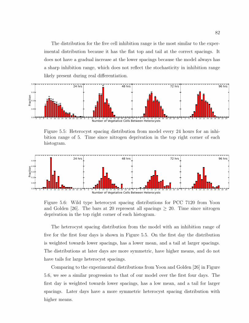
82
The distribution for the five cell inhibition range is the most similar to the exper-
imental distribution because it has the flat top and tail at the correct spacings. It
does not have a gradual increase at the lower spacings because the model always has
a sharp inhibition range, which does not reflect the stochasticity in inhibition range
likely present during real differentiation.
0 2 4 6 8 10 12 14 16 18 20 22 24
Number of Vegetative Cells Between Heterocysts0.00
0.05
0.10
0.15
0.20
Fraction
Number of Vegetative Cells Between Heterocysts
24 hrs
0 2 4 6 8 10 12 14 16 18 20 22 24
48 hrs
0 2 4 6 8 10 12 14 16 18 20 22 24
72 hrs
0 2 4 6 8 10 12 14 16 18 20 22 24
96 hrs
Figure 5.5: Heterocyst spacing distribution from model every 24 hours for an inhi-bition range of 5. Time since nitrogen deprivation in the top right corner of eachhistogram.
0 2 4 6 8 10 12 14 16 18 20 22 24
Number of Vegetative Cells Between Heterocysts0.00
0.05
0.10
0.15
0.20
0.25
Fraction
Number of Vegetative Cells Between Heterocysts
24 hrs
0 2 4 6 8 10 12 14 16 18 20 22 24
48 hrs
0 2 4 6 8 10 12 14 16 18 20 22 24
72 hrs
0 2 4 6 8 10 12 14 16 18 20 22 24
96 hrs
Figure 5.6: Wild type heterocyst spacing distributions for PCC 7120 from Yoonand Golden [26]. The bars at 20 represent all spacings ≥ 20. Time since nitrogendeprivation in the top right corner of each histogram.
The heterocyst spacing distribution from the model with an inhibition range of
five for the first four days is shown in Figure 5.5. On the first day the distribution
is weighted towards lower spacings, has a lower mean, and a tail at larger spacings.
The distributions at later days are more symmetric, have higher means, and do not
have tails for large heterocyst spacings.
Comparing to the experimental distributions from Yoon and Golden [26] in Figure
5.6, we see a similar progression to that of our model over the first four days. The
first day is weighted towards lower spacings, has a low mean, and a tail for larger
spacings. Later days have a more symmetric heterocyst spacing distribution with
higher means.

83
Figure 5.7: (a) is the heterocyst frequency against time since nitrogen deprivationfor an inhibition range of five. (b) is the distribution of cell size of heterocysts atcommitment for an inhibition range of five. The times since nitrogen deprivation arelabelled in the legend.
Figure 5.7(a) shows the heterocyst frequency vs. time after nitrogen depriva-
tion. The first heterocysts mature at 19 hours and the heterocyst frequency increases
rapidly for several hours afterwards until it reaches roughly the steady state level.
After about 24 hours the heterocyst frequency oscillates with approximately a 24
hour period, and frequencies dampen at later times. The frequency also drops from
a peak at about 42 hours at nearly 10% to about 8% at 96 hours. The decay of the
heterocyst frequency comes about because the frequency after the first generation
of differentiation is determined by the inhibition range, while later it is determined
by the number of heterocysts necessary to provide sufficient fixed nitrogen for the
remaining vegetative cells. Since the initial differentiation provides slightly too many
heterocysts, the frequency decreases at later times. The oscillation is also due to
the similarity in differentiation times for the first generation heterocysts. The sec-
ond generation differentiates when the gap between heterocysts is sufficiently wide;
this tends to occur at roughly the same time after differentiation for each heterocyst
pair. Before the second generation of differentiation, the number of cells increases,
diluting the heterocysts and decreasing the frequency. When the second generation
of heterocysts matures, they tend to do so at roughly the same time, pushing the
heterocyst frequency up. The dilution and differentiation/maturity together result in
the oscillation.

84
Figure 5.7(b) shows the distribution of the cell cycle at commitment for cells that
have become mature heterocysts. At 24 hours the shortest cells, from about the first
10% of the cell cycle, have not become heterocysts. For cells beyond this initial 10%,
there is a strong preference for shorter cells, as the likelihood of a cell committing to
heterocyst differentiation to be at a given stage of the cell cycle drops for later in the
cell cycle. At 96 hours this distribution has significantly changed. There is a large
peak in the distribution at about 10% of the cell cycle, dropping off sharply on both
sides. At 96 hours there is an even stronger preference for shorter cells to commit to
heterocyst differentiation.
5.4 Discussion of wild type results
We have developed a dynamic model for cell growth, nitrogen transport, nitrogen
storage, and heterocyst commitment in cyanobacterial filaments. The model is built
on experimental data and has been able to reproduce many experimental observations.
As shown in Figure 5.2(a), growth after nitrogen deprivation with the model is
qualitatively similar to the growth data from the experiments of Asai et al [53].
There is an initial, approximately one day period of slow growth when the filament
is growing on stored nitrogen and heterocysts are committing and maturing. After
24 hours many heterocysts have matured and the growth rate increases. The plots
indicate that the growth of the filament in the experiment of Asai et al [53] is greater
than the growth of our model filament. We have chosen the centre of our doubling
time distribution to be 20 hours, consistent with PCC 7120 [88, 95]. However, there
are many instances of PCC 7120 with shorter doubling times [132, 133], specifically
in the range of 6-18 hours [134]. Growth rates were affected by a change in the
fraction of fixed nitrogen as storage available for growth, fs, which we have estimated
to be 0.3. A lower value will result in a decrease in the growth of the filament between
heterocyst commitment and maturity, which is between roughly 10 and 20 hours after
nitrogen deprivation (results not shown).
In Figure 5.2(b), commitment is measured by increasing the external fixed nitro-
gen level, just as it is measured experimentally [26]. The resulting commitment curve
is qualitatively similar to the data of Yoon and Golden [26], with the first cells com-
mitting to heterocyst differentiation after 9 hours of nitrogen deprivation and most

85
of the cells committing by about 14 hours of nitrogen deprivation. The timing of
commitment for a given cell is determined by the amount of fixed nitrogen storage
it has. As described in Section 5.2.3, when a cell has used half of its storage, and if
it is not inhibited from differentiation by a nearby committed or mature heteocyst,
then it will commit to differentiation. This model predicts that strains that grow
faster will commit to differentiation sooner, because they will use up the stored fixed
nitrogen faster. Indeed Bradley and Carr [48] performed an experiment similar to the
commitment experiment of Yoon and Golden [26] using Anabaena cylindrica with
a generation time of 16.4 hours (shorter than the typical PCC 7120 20 hours) and
found commitment ranged from 5 hours to 10 hours, instead of the 8 to 14 hours for
PCC 7120 [26]. Our commitment results are affected by a change in either the stor-
age fraction, fs, or the fraction of storage that must be emptied before commitment,
which is 0.5. Lower or higher values of either lead to earlier or later commitment,
respectively.
In Figure 5.3, we compare the heterocyst spacing distributions found at 24 hours
for different heterocyst inhibition ranges. We found that a five cell inhibition range
was the closest match to the experimental heterocyst spacing distribution of Toyoshima
et al [46], shown in Figure 5.4. The model was able to recover the position and tail of
the distribution, but because our model used a sharp, coarse grained, inhibition range,
we were unable to recover the gradual increase in the distribution for the lower hete-
rocyst spacings. A detailed model of the genetic interactions that this coarse grained
inhibition range represents would likely be able to recover all aspects of the distribu-
tion more accurately. Nevertheless, the five cell inhibition range that we found agrees
with the inhibition range recorded by Mitchison et al [72] for Anabaena catenula.
Our model was also able to qualitatively recover the characteristics of the hetero-
cyst spacing distribution at 48, 72, and 96 hours. The distributions from the model
are in Figure 5.5 while the experimental distributions from Yoon and Golden [26] are
in Figure 5.6. The experimental distributions at later times have a slightly higher
mean, are much more symmetric, and do not have as much of a tail as the 24 hour
distribution. Experimental distributions at later times from Toyoshima et al [46] and
Khudyakov et al [47] also follow this trend. The modelled results recover this change.
The heterocyst spacing distribution changes from an asymmetric to a symmetric
86
distribution from 24 to 48 hours. This is because the 24 hour spacings are controlled
by the lateral inhibition range and this causes smaller spacings to be favoured. The
48 hours spacings are instead controlled by the fixed nitrogen production of the het-
erocysts. This production prevents cells near to the heterocysts from starving and
committing to heterocyst differentiation. The maximum in the heterocyst spacing
distribution is defined by the maximum number of cells away a cell can be before it
will differentiate into a heterocyst, and the minimum is half of the minimum number
of cells away a cell can be before it will differentiate into a heterocyst. This leads to
the spacings to be more evenly favoured and a more symmetric distribution.
Figure 5.7(a) shows the heterocyst frequency in time. The frequency is zero until
approximately 20 hours, when it rapidly increases as the first generation of heterocysts
matures, reaches a maximum, and then slowly decreases and oscillates. The mature
heterocyst frequency has been observed to reach a maximum after the first heterocyst
generation matures and then decrease [12]. In experiments the heterocyst frequency
has also been observed to oscillate [48].
The literature holds several suggestions that the cell cycle is important to the dif-
ferentiation of heterocysts [31, 73, 129], and at least one that points to a requirement
that cells be early in the cell cycle to be able to commit to heterocyst differentia-
tion [72]. The existence of these suggestions in the literature have been sufficient
to warrant the explicit demonstration of heterocyst differentiation without recent cell
division [46, 53]. Figure 5.7(b) shows a preference for the commitment of shorter cells,
demonstrating that the cell cycle affects heterocyst commitment. This is despite our
model including no cell cycle criteria in determining heterocyst commitment. The
cell cycle effect that we find is instead due to the role of storage in the heterocyst
commitment model. In our model the fixed nitrogen storage is proportional to the
size of the cell. A small cell growing at the same rate as a larger cell will run out of
storage before the larger cell. Smaller cells therefore commit to becoming heterocysts
more often than larger cells.
5.5 Results for genetic knockouts
Figure 5.8 shows the heterocyst spacing distributions for filaments with the PatS
type inhibition removed from the model. The amount of time after commitment that

87
∆patS and TN = 1h
0 2 4 6 8 10 12 14 16 18 20 22 24
Number of Vegetative Cells Between Heterocysts0.00
0.05
0.10
0.15
0.20
0.25
Fraction
Number of Vegetative Cells Between Heterocysts
24 hrs
0 2 4 6 8 10 12 14 16 18 20 22 24
48 hrs
0 2 4 6 8 10 12 14 16 18 20 22 24
72 hrs
0 2 4 6 8 10 12 14 16 18 20 22 24
96 hrs
∆patS and TN = 2h
0 2 4 6 8 10 12 14 16 18 20 22 24
Number of Vegetative Cells Between Heterocysts0.00
0.05
0.10
0.15
0.20
0.25
Fract
ion
Number of Vegetative Cells Between Heterocysts
24 hrs0.401
0 2 4 6 8 10 12 14 16 18 20 22 24
48 hrs0.425
0 2 4 6 8 10 12 14 16 18 20 22 24
72 hrs0.391
0 2 4 6 8 10 12 14 16 18 20 22 24
96 hrs0.345
∆patS and TN = 3h
0 2 4 6 8 10 12 14 16 18 20 22 24
Number of Vegetative Cells Between Heterocysts0.00
0.05
0.10
0.15
0.20
0.25
Fract
ion
Number of Vegetative Cells Between Heterocysts
24 hrs0.527
0 2 4 6 8 10 12 14 16 18 20 22 24
48 hrs0.570
0 2 4 6 8 10 12 14 16 18 20 22 24
72 hrs0.533
0 2 4 6 8 10 12 14 16 18 20 22 24
96 hrs0.482
∆patS and TN = 4h
0 2 4 6 8 10 12 14 16 18 20 22 24
Number of Vegetative Cells Between Heterocysts0.00
0.05
0.10
0.15
0.20
0.25
Fraction
Number of Vegetative Cells Between Heterocysts
24 hrs0.586
0 2 4 6 8 10 12 14 16 18 20 22 24
48 hrs0.684
0 2 4 6 8 10 12 14 16 18 20 22 24
72 hrs0.658
0 2 4 6 8 10 12 14 16 18 20 22 24
96 hrs0.601
Figure 5.8: The heterocyst spacing distribution from the model without PatS inhi-bition for proheterocysts but with HetN inhibition. TN is the amount of time aftercommitment that HetN type inhibition begins (see Figure 5.1). Each row shows thepatterns at 24, 48, 72, and 96 hours for a different TN , as indicated.
HetN type inhibition begins, TN , is varied from one to four hours. There are many
striking differences in common for all four TN , with PatS inhibition removed, when
compared with the wild type model of Figure 5.5. With PatS inhibition removed,
spacings of zero, known as multiple contiguous heterocysts (Mch), occur and are the

88
most common spacing for all four days and all four TN values. The number of Mch
is fewest for TN = 1 hour and increases as TN is increased. In contrast, the wild type
model does not have Mch. There are also nonzero but low heterocyst spacings present
without PatS inhibition that are not present for the wild type. For the TN = 1h the
24 hour spacing distribution shows some structure, while the longer waiting times all
decay from a spacing of zero. With all four TN values the distribution is furthest from
the wild type for 24 hours and recovers somewhat toward the wild type distribution in
subsequent days. This recovery is strongest for TN = 1h and weaker as TN increases,
likely due to an increasing proportion of heterocysts as Mch for longer TN . The
number of Mch follows a trend across all four TN of increasing from the first to
second day, and then decreasing in subsequent days.
0 2 4 6 8 10 12 14 16 18 20 22 24Number of Vegetative Cells Between Heterocysts
0.00
0.05
0.10
0.15
0.20
0.25
Fraction
24 hrs
Figure 5.9: The heterocyst spacing distribution at 24 hours after nitrogen deprivationfor a ∆patS strain from Yoon and Golden, 1998 [6]. The data is continued to latertimes in Figure 5.10, although without Mch data.
Our modelled distributions lacking PatS inhibition can be compared to experi-
mental ∆patS mutants lacking a functional patS gene. Figure 5.9 shows such data
from Yoon and Golden in 1998 [6] and Figure 5.10 from Yoon and Golden in 2001
[26]. The 1998 data is only for 24 hours. The 1998 data indicates a little more than
25% Mch spacing, similar to the almost 25% Mch spacing for TN = 1h with the model
when PatS inhibition is removed in Figure 5.8(a). The 1998 data also shows that the
distribution for nonzero but low spacings has structure, again supporting the one hour
HetN wait time after commitment. The 2001 data shows that although the 24 hour
data is far from the wild type, that the distribution somewhat recovers a wild type

89
distribution for later days, as do the distributions from the model. Unfortunately
there is no experimental data on the number of Mch spacings as time passes.
0 2 4 6 8 10 12 14 16 18 20 22 24
Number of Vegetative Cells Between Heterocysts0.00
0.05
0.10
0.15
0.20
0.25
Fraction
Number of Vegetative Cells Between Heterocysts
24 hrs
0 2 4 6 8 10 12 14 16 18 20 22 24
48 hrs
0 2 4 6 8 10 12 14 16 18 20 22 24
72 hrs
0 2 4 6 8 10 12 14 16 18 20 22 24
96 hrs
Figure 5.10: The heterocyst spacing distribution for a ∆patS strain from Yoon andGolden, 2001 [26]. Time since nitrogen deprivation in the top right corner of eachhistogram. The paper did not include quantitative data for Mch (number of vegetativecells between heterocysts of zero).
Figure 5.11 shows the heterocyst spacing distributions for filaments with the HetN
type inhibition removed from the model. TS is varied from one minute to four hours.
At 24 hours after nitrogen deprivation, there is little difference between the distribu-
tions lacking HetN inhibition and the wild type distributions of Figure 5.5, although
the biggest differences are with the longer TS. The main difference between wild type
and filaments lacking HetN inhibition is at later times. For 48 hours and afterwards
the filaments without HetN inhibition have Mch and short spacings between hetero-
cysts. The value of TS, in the range of one minute to four hours, has little effect on
these later time distributions.
Here we draw a distinction between two possible types of multiple contiguous
heterocysts. In the systems lacking PatS, the Mch occur when neighbouring cells
commit to heterocyst differentiation before either of them mature. They cannot
commit beside a mature heterocyst because HetN prevents commitment beside a
mature heterocyst. The Mch for systems lacking HetN occur by having a cell commit
to heterocyst differentiation beside a pre-existing heterocyst that has not yet started
to produce fixed nitrogen (see the ∆hetN gap in Figure 5.1), as PatS prevents the
commitment of two neighbouring cells.
Although there are no experimental heterocyst spacing distributions for ∆hetN
filaments there are experimental observations with such systems. hetN mutants ex-
hibit a wild type heterocyst pattern after 24 hours of nitrogen deprivation, but have
an Mch phenotype after 48 hours [61]. This is what we see in the results using the

90
∆hetN and de novo fN production waits 1min after PatS is off
0 2 4 6 8 10 12 14 16 18 20 22 24
Number of Vegetative Cells Between Heterocysts0.00
0.05
0.10
0.15
0.20
Fraction
Number of Vegetative Cells Between Heterocysts
24 hrs
0 2 4 6 8 10 12 14 16 18 20 22 24
48 hrs
0.252
0 2 4 6 8 10 12 14 16 18 20 22 24
72 hrs
0.246
0 2 4 6 8 10 12 14 16 18 20 22 24
96 hrs
∆hetN and de novo fN production waits 10min after PatS is off
0 2 4 6 8 10 12 14 16 18 20 22 24
Number of Vegetative Cells Between Heterocysts0.00
0.05
0.10
0.15
0.20
Fract
ion
Number of Vegetative Cells Between Heterocysts
24 hrs
0 2 4 6 8 10 12 14 16 18 20 22 24
48 hrs
0.235
0 2 4 6 8 10 12 14 16 18 20 22 24
72 hrs
0 2 4 6 8 10 12 14 16 18 20 22 24
96 hrs
∆hetN and de novo fN production waits 1h after PatS is off
0 2 4 6 8 10 12 14 16 18 20 22 24
Number of Vegetative Cells Between Heterocysts0.00
0.05
0.10
0.15
0.20
Fract
ion
Number of Vegetative Cells Between Heterocysts
24 hrs
0 2 4 6 8 10 12 14 16 18 20 22 24
48 hrs
0.243
0 2 4 6 8 10 12 14 16 18 20 22 24
72 hrs
0.238
0 2 4 6 8 10 12 14 16 18 20 22 24
96 hrs
∆hetN and de novo fN production waits 4h after PatS is off
0 2 4 6 8 10 12 14 16 18 20 22 24
Number of Vegetative Cells Between Heterocysts0.00
0.05
0.10
0.15
0.20
Fraction
Number of Vegetative Cells Between Heterocysts
24 hrs
0 2 4 6 8 10 12 14 16 18 20 22 24
48 hrs
0.242
0 2 4 6 8 10 12 14 16 18 20 22 24
72 hrs
0.248
0 2 4 6 8 10 12 14 16 18 20 22 24
96 hrs
Figure 5.11: The heterocyst spacing distribution from the model without HetN inhi-bition but with PatS inhibition.
model.
5.6 Discussion of gene knockout results
Yoon and Golden have found that knocking out PatS results in heterocyst spacing
distributions that are not wild type [6, 26], and this has been attributed to PatS

91
being a diffusible inhibitor of heterocyst differentiation. They also found [26] that the
pattern somewhat recovers at later times, even without functional PatS. By removing
the PatS type inhibition of heterocyst differentiation from our model, we were able
to produce qualitatively similar distributions, as shown in Figure 5.8. The time that
hetN is first expressed has only been determined to be in the range of 6-12 hours
after nitrogen deprivation [63]. Assuming that hetN is not expressed until after a
cell has committed to heterocyst differentiation, we varied the amount of time after
commitment that HetN type inhibition would begin to take effect, in systems with the
PatS inhibition removed, and found that a one hour waiting time was most consistent
with the experimental distributions.
Knocking out hetN results in wild type heterocyst spacings at 24 hours after
nitrogen fixation, but significantly different spacing distributions at later times [61]
with Mch and short vegetative cell intervals between heterocysts. We are able to
recover this phenotype using our model by removing the HetN type inhibition and
having a temporal gap between the end of PatS type inhibition and the beginning
of nitrogen fixation, as shown in Figure 5.11. We vary the amount of time between
the end of PatS inhibition and nitrogen fixation to as little as one minute and still
observe Mch and short heterocyst spacings. In the experiment of Wei et al using
PCC 7120 [135], the first mature heterocysts were observed between 15 and 16 hours
after nitrogen deprivation, but the nitrogenase genes nifHDK were not detected until
18 hours, supporting the idea of a gap between maturity and nitrogen fixation.
5.7 Predictions
We have shown that the timing of heterocyst commitment can be explained by the
depletion of stored fixed nitrogen. The depletion would occur earlier in instances
where the same amount of storage is initially present but the growth rate was higher.
We therefore predict that if the growth rate of PCC 7120 could be controlled (say,
by variation of light intensity or phosphate concentration), then the timing of com-
mitment to heterocyst differentiation could be changed, with faster growing strains
committing earlier. Also, if cyanophycin was genetically knocked out (such as in the
strain studied by Ziegler et al [66]), we expect that the commitment to heterocyst
differentiation would occur earlier and more uniformly. Specifically we expect that

92
hetR and patS expression, possibly reported by a GFP fusion, would occur earlier
(do not have to wait for storage to run out) and more uniformly (cells do not have
different amounts of stored fixed nitrogen) in strains lacking cyanophycin compared
to the wild type with cyanophycin.
The cell cycle effect we observed using our model depended upon shorter cells
having less stored fixed nitrogen, leading to these shorter cells being more likely
to deplete their storage first and commit to heterocyst differentiation. Genetically
knocking out cyanophycin would then lead to a weaker or nonexistent cell cycle effect
in comparison to wild type strains. We also predict, consistent with Figure 5.7(b),
that the cell cycle effect will be stronger in later generations of heterocysts than in
the first generation of heterocysts.
We were able to reproduce the Mch phenotype in ∆hetN mutants for 48 hours and
later by having a temporal gap between the end of PatS inhibition and the beginning
of nitrogen fixation. In the wild type, HetN inhibition would prevent heterocysts
from committing to heterocyst differentiation during this time, but without HetN
the starving cells are free to commit. We predict that the Mch in filaments lacking
functional hetN will occur by having cells commit to heterocyst differentiation beside
mature heterocysts, rather than two neighbouring cells committing and maturing
around the same time, as this second option would be prevented by PatS inhibition.

Chapter 6
Percolation of Starvation
6.1 Motivation and background
The previous three chapters have focused on the cyanobacterial filament in the con-
text of heterocysts. In this chapter I want to examine the patterns of starving cells
within the filament in the absence of heterocysts. Cyanobacterial filaments without
heterocysts are real systems. Many strains of filamentous cyanobacteria do not have
heterocysts [22], and heterocystous strains with ∆hetR cannot differentiate hetero-
cysts.
Starving cells in one dimension, or in two dimensions with time as the second
dimension, can be considered with percolation theory. Percolation theory can be
used to consider the pattern of occupation of squares in a grid, and if we assign
starving cells as occupied and non-starving cells as unoccupied, then we can explore
the patterns of starving cells using the tools of percolation theory.
We want to investigate the transition of the filament from starving to non-starving
as the external fixed nitrogen level increases. Such transitions in percolation theory
involve finding critical exponents that characterize the behaviour and patterns of the
occupied squares near the transition. Percolation usually involves the assumption
that the occupation of a square is uncorrelated with the occupation of other squares.
This assumption prevents an exact mapping from our model to percolation and we
will investigate to what extent percolation theory does apply and how the results
from the model deviate from percolation theory.
6.2 Percolation background
The information for this background is largely from Introduction to Percolation The-
ory by Stauffer and Aharony [136].
Percolation can be considered in any number of dimensions and with any lattice
93

94
geometry. However, in this background we will only consider square lattices in one
and two dimensions. Beginning with a two dimensional square lattice, each square in
the lattice is either filled in or not filled in. Squares that are filled in are referred to as
occupied and those that are not are referred to as not occupied. A cluster is defined as
a group of neighbouring occupied squares. To be considered neighbours the squares
need to be nearest neighbours, i.e. they must have one side in common. Squares that
touch only at a corner are not considered nearest neighbours. The squares within a
cluster are connected to one another by an unbroken chain of nearest-neighbour links.
In percolation theory the occupied sites are usually not considered to be correlated.
The occupation of each square is random, with p being the probability of a square
being occupied. A cluster is said to percolate in a system if the cluster extends from
the top to the bottom and the left to the right of the system. In the thermodynamic
limit such a cluster would be infinite and a percolating cluster can be referred to as
an infinite cluster. As the occupation probability p is increased from zero towards
one, at some point it will reach the critical concentration pc, which is the lowest p
value at which a percolating cluster is formed in an infinite system.
The measurement we are going to consider is the number of clusters of size s, ns.
It is found that the function vs(p) = ns(p)/ns(pc) depends only on the variables s and
(p−pc) and only in the combination |p−pc|sσ. Power law behaviour is also expected
at the critical point. We then assume that the distribution is
ns = s−τf [(p− pc)sσ]. (6.1)
The Fisher exponent τ describes the power law term and is a constant. f is a scaling
function that can act as a cutoff for the power law. σ is a free exponent, and if
|(p− pc)sσ| ≪ 1 then f [(p− pc)s
σ] approaches a constant value, leaving a power law.
Thus, close to pc we generally expect a power law distribution of cluster sizes.
6.2.1 One Dimensional Lattice
On a one dimensional lattice all sites must be occupied for a cluster to reach both
ends of the lattice. This means that the critical concentration pc = 1.
The probability of a cluster of s occupied sites beginning on a particular site is
equal to the product of ps, the probability of a single site being occupied to the power

95
of the number of sites, and (1− p)2, the probability of a single site being unoccupied
squared for the unoccupied sites on each end. This gives us
ns = ps(1− p)2 (6.2)
We want to find a power law in s for ns near pc and so we wish to find ns as a function
of s alone and independent of p for p → pc.
We can rewrite p = eln(p) = eln(p−1+1). ln(1 + x) ≈ x if x is small, so if p is near
to one then p ∼= ep−1. pc = 1 (making the condition of p near one into p → pc) and
so p = ep−pc. Close to p = pc, we can rewrite Equation 6.2 as
ns(p) = (pc − p)2e−(pc−p)s (6.3)
Considering Equation 6.1, we know the scaling function has as its argument (p−pc)sσ.
Defining z ≡ (p−pc)sσ, we can rewrite the right side of Equation 6.3 as s−2σz2ezs
1−σ
.
The scaling function f must be a function of z alone, so ezsσ−1
demands that σ = 1.
This gives us the scaling form equation
ns(z) = s−2z2ez, (6.4)
which satisfies Equation 6.1 with τ = 2. Knowing that f(z) = z2ez goes to a constant
if |(p − pc)sσ| ≪ 1, when p → pc, ns has a power law in s for one dimensional
percolation when near pc. Also, z = (p − pc)s is negative because p ≤ pc and is
causing a decay with the increasing s.
6.2.2 Two Dimensional Lattice
For a two dimensional square lattice pc = 0.5927, found by Monte Carlo simulation
[137]. For the power law in ns, it has been found exactly that τ = 187/91 ≈ 2.055
for two dimensions.
6.3 Model
This chapter has used the model from Chapter 4, described in Section 4.2, with 1%
leakage and no heterocysts.
Many of our measurements are made of starving cells. Starving cells are defined as
cells that have a cytoplasmic nitrogen level of zero, meaning the cell is growing slower

96
than its optimal growth rate. The measurement of the fraction of cells starving is
simply the number of starving cells divided by the total number of cells in the filament.
For one dimension, cluster length is measured. The length of a starving cluster is
defined to be the number of consecutive cells in the filament that are starving.
For two dimensions (space and time), cluster size is measured. Consecutive starv-
ing cells in the filament at a specific time are part of a cluster. A starving cell and
that same cell starving at the next time sampled are also part of a cluster. If a starv-
ing cell divides and one or both of the daughter cells are starving, then those two or
three cells are part of a cluster. Cells that can be connected to one another through
these spatial or temporal links are a single space-time cluster.
For two dimensions, the average cluster size is defined as the∑∞
s=1 s ·ns/∑∞
s=1 ns,
where ns is the number of clusters of size s.
6.4 Percolation
1.0 1.5 2.0 2.5 3.0
External Fixed Nitrogen Concentration (1022 m−3 )
0.0
0.2
0.4
0.6
0.8
1.0
Fraction of Cells Starving
Figure 6.1: Fraction of starving cells as the external fixed nitrogen concentrationvaries. Fraction first decreases below one at 1.22 × 10²² m−3 and reaches zero at2.66×1022 m−3. The system used the model described in Section 4.2, with DC = 1.54µm s−1, DO = 2.9× 10⁻¹⁸m3/(µm·s), DM = 0.01DO/(π µm2), TD = 20 h, ∆ = 4.5 h,lmin = 2.25 µm, and g = 6.2× 109 µm−1.
Only when the fraction of cells starving is between zero and one can the starving
cells form clusters in the system. Figure 6.1 shows the fraction of cells starving in the
filament as a function of the external fixed nitrogen concentration.

97
As discussed in Section 6.1, we are using a model with no heterocysts, and so the
only source of fixed nitrogen for growth is from the import of external fixed nitrogen.
The import of fixed nitrogen is linearly related to the length of the cell (see Section
4.2.1). For low concentrations of external fixed nitrogen, no cell is long enough to
import enough fixed nitrogen to fully supply growth and not starve. For high concen-
trations of external fixed nitrogen, all cells are long enough to import enough fixed
nitrogen to fully supply growth. For intermediate concentrations of external fixed
nitrogen, some of the cells are long enough to import enough fixed nitrogen to fully
supply growth. Whether or not a particular cell is able to obtain enough fixed nitro-
gen is dependent on how long the cell is and its growth rate, because faster growing
cells require more fixed nitrogen to avoid starvation. Also, if a neighbouring cell is
not starving and has extra fixed nitrogen, diffusion could lift a cell from starvation.
This is discussed quantitatively in Section 4.3.
6.4.1 One dimensional percolation
We consider one dimensional percolation of starving clusters at a given time.
Figure 6.2(a) shows the cluster length distribution at various external fixed nitro-
gen concentrations in log-log format, which will highlight any power law behaviour.
The range shown in Figure 6.2(a) covers most of the concentrations that lead to some
starving cells. The best power law is seen for the second highest curve in the figure,
which has τ = 2.048 and starvation of 94.8% of the cells. This τ value is very close to
the expected value of 2 for one-dimensional percolation, and a power law with τ = 2
agrees well in Figure 6.2(a) (dashed line). The highest curve in the figure has an even
higher percentage of starving cells, and we would expect that this larger percentage,
being closer to the critical concentration of 100%, would yield an improved power
law. This is not the case and could be caused by correlations of the starving cells or
could be an artefact of the finite system size.
Power law behaviour is seen for the highest curves in Figure 6.2, for which the fixed
nitrogen concentration causes nearly all cells to starve. As the external fixed nitrogen
concentration increases and the fraction of cells starving decreases, the curves (the
lower curves in Figure 6.2(a)) begin as power laws at low cluster size but trail down
for higher cluster sizes. This is expected as the exponential in Equation 6.4 becomes

98
100 101 102 103 104 105
Cluster Length
10-8
10-6
10-4
10-2
100
102
104
106
Shifted Counts
(a)
efN=1.35E22
efN=1.475E22
efN=1.6E22
efN=1.725E22
efN=1.85E22
efN=1.975E22
efN=2.1E22τ=2
0 20 40 60 80 100
Cluster Length
10-3
10-2
10-1
100
101
102
103
104
105
106
107
108
109
1010
1011
Shifted Counts
(b)
efN=1.725E22
efN=1.85E22
efN=1.975E22
efN=2.1E22
efN=2.225E22
efN=2.35E22
efN=2.475E22
efN=2.6E22
Figure 6.2: (a) Cluster length distribution in log-log format, using the same parame-ters as Figure 6.1. Each line is from a different external fixed nitrogen concentration,efN. The highest line is the lowest efN. The slope of the straight part of the greenline for 1.475× 10²² m−3 is -2.048, found by linear regression. This concentration has94.8% starving cells. The black dashed line is a power law s−τ with τ = 2. The high-est line has counts multiplied by 10, and each subsequent line has counts multipliedby a factor of 10 less to keep the lines from being on top of one another; this is whatis meant by ‘shifted’ counts. (b) Cluster size distribution in log-linear format. Thehighest line is the lowest efN. The highest line has counts multiplied by 10000, andeach subsequent line has counts multiplied by a factor of 10 less.
dominant at larger cluster sizes and starving cell densities are further from one.
Figure 6.2(b) shows the cluster length distribution at various external fixed ni-
trogen concentrations in log-linear format, which will highlight any exponential be-
haviour. The fixed nitrogen concentrations in Figure 6.2(b) are not close to p = pc = 1
and so exponential behaviour is expected and observed. The slope is increasing in
magnitude as the external fixed nitrogen concentration increases, as is expected be-
cause Equation 6.4 goes as e(p−pc)s and p will be further from pc = 1 for higher external
fixed nitrogen concentrations.
6.4.2 Two dimensions
We now consider two dimensional percolation of starving clusters. The first dimension
is filament length and the second is starvation time. A single cluster is any connected
spacetime area of starving cells.

99
100 101 102 103 104 105
Cluster Size
10-10
10-8
10-6
10-4
10-2
100
102
104
106
Shifted Counts
(a)
efN=1.475E22
efN=1.6E22
efN=1.725E22
efN=1.85E22
efN=1.975E22
efN=2.1E22
efN=2.225E22
efN=2.35E22
efN=2.475E22
efN=2.6E22
100 101 102 103 104 105
Cluster Size
10-4
10-3
10-2
10-1
100
101
102
103
104
105
Counts
(b)
Plateau
efN=1.85E22
1.2 1.4 1.6 1.8 2.0 2.2 2.4 2.6 2.8
External Fixed Nitrogen Concentration (1022 m−3 )
0
50
100
150
200
250
300
Average Cluster Size
(c)
Day 2
Day 4
Day 6
Day 8
Day 10
1.2 1.4 1.6 1.8 2.0 2.2 2.4 2.6 2.8
External Fixed Nitrogen Concentration (1022 m−3 )
0
50
100
150
200
250
300
Average Cluster Size
(d)
Figure 6.3: (a) Cluster size (two dimensions) distribution in log-log format, using thesame parameters as Figure 6.1. The highest line has counts multiplied by 1000, andeach subsequent line has counts multiplied by a factor of 10 less to keep the linesfrom being on top of one another; this is what is meant by ‘shifted’ counts. (b) Thedistribution with the largest cluster sizes from (a), ρefN = 1.85 × 10²² m−3. Theplateau in the distribution is indicated. (c) Average cluster size as the external fixednitrogen concentration varies. The average does not include the ‘infinite’ cluster thatspans the system in systems for which it exists. The day number indicates how longafter the beginning of the simulation the data was taken. (d) Same as (c) except onlythe final distribution.
Figure 6.3(a) shows cluster size distribution in log-log format for a range of ex-
ternal fixed nitrogen concentrations. The lower curves are for filaments that only
have a few starving cells. At those external fixed nitrogen concentrations there are
not enough starving cells to form one infinite cluster and instead there are smaller,
isolated clusters. These curves have flat power law regions for smaller cluster sizes
and then tail off at larger cluster sizes. As more cells starve, the tailing off behaviour

100
is pushed out to larger cluster sizes. A spacetime visualization of this type of system
is shown in Figure 6.4(a).
Figure 6.4: Spacetime visualizations of filament starvation, using the same parametersas Figure 6.1. Red represents starving cells and green represents non-starving cells.Each horizontal bar is the first 100 cells in the filament, and subsequent bars areseparated by 10 minutes. There tends to be streaming to the right due to growth ofthe filament. (a) is for ρefN = 1.6 × 10²² m−3, well below the transition of starvingcells to an infinite cluster, with only a few starving cells. (b) is for ρefN = 1.85×10²²
m−3, roughly at the transition of starving cells to an infinite cluster. (c) is for ρefN =2.1× 10²² m−3, well above the transition of starving cells to an infinite cluster, withmany starving cells.
As the external fixed nitrogen concentration is decreased (higher curves in the plot)
the number of starving cells increases and there are more clusters and the clusters
tend to be larger. When enough cells are starving a single infinite cluster will form
spanning the entire space-time system. A spacetime sample of this type of system
is shown in Figure 6.4(b). This transition can be seen in Figure 6.3(d) as the peak
in the average cluster size distribution (the peak is not divergent because of finite
size effects, shown by the sharpening of the curve in Figure 6.3(c) as time passes and
the system gets larger). Unlike the one dimensional case above, we do not observe
power law behaviour at all cluster sizes when approaching this transition. For the
ρefN concentration that yields the largest clusters, we instead see a plateau form in

101
the cluster size distribution, indicated in Figure 6.3(b). This will be discussed more
below.
When the infinite cluster forms all of the cells are not starving and inside the
infinite cluster there are pockets of cells that are not starving. Within these pockets
of non-starving cells there can be clusters of starving cells which are not connected
to the infinite cluster. A spacetime sample of this type of system is shown in Figure
6.4(c). These clusters compose the distribution for the highest curves in Figure 6.3(a).
6.4.3 Deviations from percolation in two dimensions
The lack of a power law and the plateau in two dimensions at the transition indicates
that the system has correlations, which must be either spatial or temporal. In Section
6.4.1 we examined the behaviour along the filament and there are no apparent spatial
correlations that could explain the plateau in Figures 6.3(a) and (b).
100 101 102 103
Period of Cell Starvation (min)
10-3
10-2
10-1
100
101
102
103
Counts
Figure 6.5: The distribution of the amount of time each cell starves for ρefN =1.85×10²² m−3, the concentration from the curve from Figure 6.3(b), using the sameparameters as Figure 6.1.
Figure 6.5 shows the distribution of the amount of time each cell starves. The
distribution is approximately a power law for the smaller cluster sizes, a bump below
103 minutes, and a cutoff above 103 minutes. The bump corresponds to the average
cell period of 20 hours or 1200 minutes and indicates that there are temporal corre-
lations in cell starvation associated with the cell period. From this, we expect that

102
the cause of the plateau in Figures 6.3(a) and (b) is due to temporal correlations in
starvation associated with the cell cycle.
100 101 102 103 104 105 106
Cluster Size
10-5
10-4
10-3
10-2
10-1
100
101
102
103
104
105
106
Shifted Counts
(a)100 101 102 103 104 105 106
Cluster Size
10-5
10-4
10-3
10-2
10-1
100
101
102
103
104
105
106
107
Shifted Counts
(b)
efN=1.85E22
efN=1.875E22
efN=1.9E22
Figure 6.6: Cluster size distribution in log-log format for a bare model reduced topercolation, using the same parameters as Figure 6.1. (a) The external fixed nitrogenconcentration is ρefN = 1.875 × 10²² m−3. The slope of the line is -2.064, found bylinear regression. (b) is the curve from (a) as well as two curves with nearby externalfixed nitrogen concentrations. The curve with lower efN decays at high cluster sizeand the curve with higher efN does not record cluster sizes much higher than 103.
To further investigate why there is not power law behaviour at the transition to
the infinite cluster we begin by stripping away several aspects of the model to leave
only a two dimensional percolating system. All growth rates are set to zero and there
is no cell division. All cell sizes are the same and the fixed nitrogen consumption rate
of each cell is chosen every 10 seconds. There are very high losses and no exchange
between cells. Together, these changes provide a bare model with a constant number
of cells, each of which is starving independently of the starvation of itself and other
cells in space and time. Each cell will be starving with some independent probability,
corresponding to two dimensional percolation. The result at ρefN = 1.875×10²² m−3
is shown in Figure 6.6(a), where we have a power law with a slope of -2.064, very close
to the expected power law from Section 6.2.2 of slope -2.055. Cluster size distributions
for higher and lower ρefN exhibit cutoff behaviour, as seen in Figure 6.6(b), indicating
that ρefN = 1.875 × 10²² m−3 is the critical value. ρefN = 1.875 × 10²² m−3 also
corresponds to p = 0.62±0.02 for a 1000x1000 system (1000 cells, 1000 time samples),
which is within two standard deviations of the expected result for criticality of pc =

103
0.5927.
Now we want to individually add back the aspects of the model that have been
removed and see the effect of each on the cluster size distribution. For each of the
distributions I have adjusted ρefN to get the cluster size distribution as close to a
power law as possible, judging by inspection.
100 101 102 103 104 105 106
Cluster Size
10-5
10-4
10-3
10-2
10-1
100
101
102
103
104
105
106
107
Shifted Counts
(a)
bare
+ exchange
100 101 102 103 104 105 106
Cluster Size
10-5
10-4
10-3
10-2
10-1
100
101
102
103
104
105
106
Shifted Counts
(b)
bare
+ low losses
100 101 102 103 104 105 106
Cluster Size
10-5
10-4
10-3
10-2
10-1
100
101
102
103
104
105
106
107
Shifted Counts
(c)
bare
+ division
100 101 102 103 104 105 106
Cluster Size
10-5
10-4
10-3
10-2
10-1
100
101
102
103
104
105
106
107
Shifted Counts
(d)
bare
+ cell growth
Figure 6.7: Cluster size distribution in log-log format, using the same parameters asFigure 6.1. All lower curves are for the bare model reduced to percolation with ρefN =1.875 × 10²² m−3. Upper curves have different aspects of the model reinserted. Allcurves have ρefN varied to get as close as possible to power law behaviour. (a)-(d) eachhave a single aspect reinserted into the bare model; reinsertion is not sequential. (a)Upper curve has cell to cell exchange reinserted in the model with ρefN = 1.8625×10²²
m−3. (b) Upper curve has high losses removed from the model with ρefN = 1.825×10²²
m−3. (c) Upper curve has division reinserted into the model with ρefN = 1.875×10²²
m−3. (d) Upper curve has cell growth reinserted into the model with ρefN = 2.075×10²² m−3.
In Figure 6.7(a) we show the cluster size distribution for both the bare percolation

104
model and the bare model with exchange between cells reinserted into the model. The
external fixed nitrogen concentration had to be slightly adjusted to find power law
behaviour with the exchange present, but the power law remains.
In Figure 6.7(b) we show the cluster size distribution for both the bare percolation
model and the bare model with the large losses removed from the model. The external
fixed nitrogen concentration had to be slightly adjusted to find power law behaviour
with the lower losses, but the power law remains.
In Figure 6.7(c) we show the cluster size distribution for both the bare percolation
model and the bare model with cell division reinserted into the model. This addition
does not change the power law and the external fixed nitrogen concentration was not
adjusted.
In Figure 6.7(d) we show the cluster size distribution for both the bare percolation
model and the bare model with cell growth reinserted. To get the largest clusters to
form, ρefN had to be significantly adjusted, from 1.875×10²² m−3 to 2.125×10²² m−3.
This adjustment is due to import of the external fixed nitrogen being proportional to
length (see Equation 4.1). The cluster size distribution for the bare model plus cell
growth has a significant difference from a power law with the cell growth, as it has a
dip and a rise between cluster sizes of 102 and 103. Given that it is the only difference
from the stripped down model, this feature is related to the changing cell size. The
feature is not removed by adjusting ρefN , the only free parameter, except when it is
able to bring the cutoff to a cluster size that is smaller than the location of the dip.
The feature is similar to the deviation of the full model cluster size distribution from
power law behaviour that is seen in Figure 6.3(a). The deviation from a power law
in the full model is likely a smeared out version of the feature.
Figure 6.8 demonstrates how this dip and bump feature can be moved by changing
the growth rate of the filament. A slower growth rate (longer cell period) increases
the cluster size at which the feature occurs. This increase appears to occur linearly.
This relationship between the plateau feature and the cell period was predicted by
the temporal starvation distribution in Figure 6.5.
To achieve percolation the consumption rate was changed from being chosen every
cell cycle, to being chosen every 10 seconds. Reinserting the choosing of growth rates
every cell cycle resulted in a distribution that was very different from a power law

105
100 101 102 103 104 105 106
Cluster Size
10-4
10-3
10-2
10-1
100
101
102
103
104
105
106
107
Shifted Counts
(a)
0 5 10 15 20 25 30 35 40 45
Cell Period (h)
0
100
200
300
400
500
Loca
tion of Dip
(b)
Figure 6.8: (a) Cluster size distribution in log-log format, using the same parametersas Figure 6.1. Systems have the bare model with cell growth reinserted. Uppercurve is the same data as the upper curve in Figure 6.7(d). The lower curve is from afilament with half the growth rate of the upper curve, and highlights how the locationof the dip moves. (b) is the location of the dip as the cell period is varied. Error barsrepresent the uncertainty in assigning the location of the dip.
(data not shown). This was because nothing about cells, including starvation status,
could change until a cell cycle had passed.
Figure 6.9: Spacetime visualizations of filament starvation, using the same parametersas Figure 6.1. Red represents starving cells and green represents non-starving cells.Each horizontal bar is the first 100 cells in the filament, and subsequent bars areseparated by 1 minute. The left is for the bare model critical percolation system withthe cluster distribution in Figure 6.6(a), as well as the bottom curve in Figures 6.7(a),(b), (c), and (d). The right is the top curve in Figure 6.7(d), with cell size dependentimport of fixed nitrogen. This figure is meant to highlight the contrast in temporalcorrelations between the two spacetime visualizations.
In Figure 6.10 we have taken the full model of the filament and removed each of
the elements of the model that cause deviations from power law behaviour separately

106
and together. Figure 6.10(a) shows the cluster size distribution for the full model
again. Figure 6.10(b) is the cluster size distributions with the full model except with
the cell size set to a constant for the calculation of fixed nitrogen import. At no
external fixed nitrogen concentration do we see power law behaviour; instead all of
the distributions decay with increasing cluster size. Figure 6.10(c) is the cluster size
distribution with the full model except with the cell growth rate chosen frequently
instead of every cell cycle. This does not yield power law behaviour. Figure 6.10(d)
shows the cluster size distribution for the full model except with both of these changes
(cell size set to a constant for import and frequent choice of growth rate). This system
does yield power law behaviour and appears similar to the percolating bare model.
These two elements of the model prevent percolation because they introduce corre-
lations in time. Figure 6.9 shows spacetime visualizations for both the bare model to
achieve correlation, and the bare model with cell growth reinserted. The lack of cor-
relations in the former and strong temporal correlations in the latter are immediately
evident upon inspection.
A fixed nitrogen consumption rate that is maintained for a cell cycle introduces
temporal correlations in whether or not that cell is starving. Cell size dependent
fixed nitrogen import also introduces temporal correlations because short cells are
more likely to be starving than large cells. Cell size does not jump within the range,
but instead linearly increases, and so temporal correlations in the starving status of
the cell are caused by cell size dependent fixed nitrogen import.
6.4.4 Discussion
The previous three subsections have shown that with the full cyanobacterial filament
model the starving cells are not strongly correlated in space but correlated in time.
The weak spatial correlations are shown in Section 6.4.1 by the power law for the
one dimensional percolation. The lack of strong spatial correlations is despite the
exchange of fixed nitrogen between cells.
Strong temporal correlations occur because cells maintain the same growth rate
until they divide and because the import of fixed nitrogen is related to cell size.
The evidence that the cyanobacterial cells maintain the same growth rate is the
variable nitrogen incorporation observed by Popa et al [8] that we discussed in detail

107
100 101 102 103 104 105
Cluster Size
10-10
10-8
10-6
10-4
10-2
100
102
104
106
Shifted Counts
(a)
Full Model
efN=1.475E22
efN=1.6E22
efN=1.725E22
efN=1.85E22
efN=1.975E22
efN=2.1E22
efN=2.225E22
efN=2.35E22
efN=2.475E22
efN=2.6E22
100 101 102 103 104 105
Cluster Size
10-7
10-6
10-5
10-4
10-3
10-2
10-1
100
101
102
103
104
105
106
107
Shifte
d C
ounts
(b)
Cell Growth Removed
efN=1.875E22
efN=1.925E22
efN=1.975E22
efN=2.025E22
efN=2.075E22
efN=2.125E22
efN=2.175E22
100 101 102 103 104 105
Cluster Size
10-7
10-6
10-5
10-4
10-3
10-2
10-1
100
101
102
103
104
105
106
107
Shifte
d C
ounts
(c)
Random growth rate added
efN=1.75E22
efN=1.875E22
efN=2.0E22
efN=2.125E22
efN=2.25E22
efN=2.375E22
100 101 102 103 104 105 106
Cluster Size
10-5
10-4
10-3
10-2
10-1
100
101
102
103
104
105
106
107
Shifted Counts
(d)
Full Model with both changes
Reduced Model
Figure 6.10: Cluster size distribution in log-log format, using the same parameters asFigure 6.1. (a) Full model. (b) Full model with fixed nitrogen import independentof cell size. (c) Full model with the growth rate of each cell chosen every 10 seconds.(d) Bare model reduced to percolation (the lower curve) and full model with frequentfixed nitrogen consumption rate changes and length independent import (the highercurve). ρefN = 1.875× 10²² m−3 for the bare model and ρefN = 1.85× 10²² m−3 forthe full model with both changes. Data for full model with both changes is shiftedto the right because of a factor of ten difference in the frequency of cluster sampling.
in Chapter 3. However, the variable nitrogen incorporation could be explained by
each cell having a growth rate that changes in time, and each cell just has a different
average growth rate (corresponding to the amount of fixed nitrogen incorporated)
over that time. This is in contrast to our model, in which cells maintain a growth
rate over a cell cycle, and choose a new one at division. The linear relationship
between fixed nitrogen import and cell size is based upon the assumption that import
is proportional to the surface area of the cell, and we do not have experimental data to

108
support it. It is therefore possible that both of the elements of the model that cause
correlations and deviations from percolation behaviour could be plausibly omitted.
The dip in the cluster size distribution in Figure 6.7(d) seems to indicate a spe-
cific type of correlation in a two-dimensional system. The starving cells in this system
have strong correlations in one direction, in which the starving cells connect for long
stretches, and weak correlations in the other, in which the starving connections are
relatively short and infrequent. The dip indicates the scale of these infrequent con-
nections in the direction with weak correlations. It is possible that similar dips could
suggest the presence of other scales in similar systems.
System growth is not usually considered in the percolation framework, but Figure
6.7(c) shows that cell division and growth of the system does not alter the percolating
critical behaviour. The universality of the critical exponent describing the power law,
despite cell division, is consistent with the expectation of the same percolating critical
behaviour on irregular lattices as on regular lattices, and the observation that the rules
of percolation can even be changed to some extent [137].
Correlation functions of fixed nitrogen concentration are calculated in Appendix
A.

Chapter 7
Conclusion and Future Outlook
In this thesis we have developed quantitative models to investigate how filamentous,
heterocystous cyanobacteria choose which cells will differentiate into heterocysts.
7.1 Summary of results
We have four main questions, each associated with an appropriate model.
The first question is how is the fixed nitrogen distributed and transported in the fil-
ament, and in Chapter 3 we examined the nitrogen distribution in the cyanobacterial
filament between two heterocysts. This was motivated by two experimental distri-
butions in the literature: that of Wolk et al [11] and that of Popa et al [8]. These
distributions are quite different, with Wolk’s nitrogen peaking at the heterocyst and
dropping off away from the heterocyst, and Popa’s nitrogen dipping significantly at
the heterocyst and mostly being flat between the heterocysts. Wolk’s distribution
with its peak at the heterocyst agreed with our intuition, but Popa’s was more recent
with a better technique and better data. We found that both of these distributions
are correct, and that the distribution of Wolk is for a much earlier time than the
distribution of Popa. The initially counterintuitive distribution that Popa found is
explained by the fact that vegetative cells grow and heterocysts do not. The vegeta-
tive cells accumulate the nitrogen when they grow, and this accumulation of nitrogen
quickly dwarfs the magnitude of the freely diffusing fixed nitrogen that peaks at the
heterocyst. We found that periplasmic transport of fixed nitrogen was not necessary
to explain the experimental nitrogen distributions, but also could not be ruled out.
Our model was successful when the cells had a maximum growth rate, instead of
having growth linearly related to fixed nitrogen concentration at all fixed nitrogen
levels, a situation which could not recover the Popa distribution.
This model formed the basis of the models that followed, though we removed
periplasmic transport for simplicity and added rules for heterocyst placement.
109

110
The second question is why are the heterocysts patterned in the filament? Chapter
4 looked at the growth of the filament in the context of fixed nitrogen leakage and
heterocyst placement strategies. We found that heterocyst frequency can optimize
growth by balancing the fixed nitrogen produced by the heterocysts with the lack
of growth that comes from heterocysts not dividing. By comparing the growth of
the filament using different strategies for heterocyst placement we found that only
with leakage present did the different strategies yield different growth rates. A local
placement strategy was found to produce filaments that grew faster than filaments
placing heterocysts randomly. For all three strategies, the heterocyst frequency was
found to decrease continuously as the external fixed nitrogen level was increased.
Heterocyst patterns for the random heterocyst placement strategies were significantly
different than the experimental wild type patterns, but the pattern for the local
placement strategy was qualitatively very similar.
This model, with small but nonzero leakage, and with an adaptive placement
strategy was then used as the basis for the next model. In that case, we added
fixed nitrogen storage and lateral inhibition. This produced a more refined model of
heterocyst commitment.
We wanted to know how a filament recently deprived of fixed nitrogen breaks the
starvation symmetry and decides which cells will become heterocysts. In Chapter
5 we recover many of the aspects of initial heterocyst differentiation upon nitrogen
deprivation using a storage based commitment model. The model has a cell commit to
heterocyst differentiation once the stored fixed nitrogen in the cell has decreased to a
certain level. Cells that have been committed for a period of time then become mature
heterocysts that produce fixed nitrogen. Committed cells and mature heterocysts
inhibit nearby cells from commitment. This model qualitatively reproduced filament
growth, heterocyst commitment, heterocyst pattern, and heterocyst frequency. It
also produced a cell cycle effect on commitment and, by removing certain elements
of the model, we qualitatively recovered mutant heterocyst patterns.
The final question is more curiosity driven: how are starving cells arranged in
space and time in the absence of heterocysts? In Chapter 6 we showed that without
heterocysts the quantitative model of the cyanobacterial filament was similar to the
one dimensional percolation of starving cells and a more limited model exhibited two

111
dimensional percolation of starving cells. The elements of the model that caused
deviations from percolation behaviour were identified.
7.2 Future outlook
There are some things that can be investigated within the fixed nitrogen model we
have built without adding other elements such as other metabolites or genetic re-
sponse.
In chapter 4 we investigated the steady state optimal heterocyst frequency for
a local heterocyst placement strategy while varying the external fixed nitrogen con-
centration. A similar investigation could be performed with the more sophisticated
heterocyst differentiation model of Chapter 5 to see what changes. In Chapter 5 the
external fixed nitrogen concentration was held at zero after dropping from a high
concentration. Instead of dropping to zero, the concentration could be dropped to
the low but finite concentrations investigated in Chapter 4. The heterocyst frequency
24 hours after the drop in the fixed nitrogen concentration could be determined as
the external fixed nitrogen concentration after the drop is varied. This would allow
a similar plot to Figure 4.7 to be determined in this new situation. The heterocyst
frequency after 24 hours of nitrogen deprivation in Chapter 5 is only after one gen-
eration of heterocyst differentiation and is largely controlled by the range of lateral
inhibition. The steady state heterocyst frequency in Chapter 4 is after many genera-
tions of heterocyst differentiation and is controlled by the fixed nitrogen produced by
the heterocysts. Because of this difference, the heterocyst frequency 24 hours after a
drop in the external fixed nitrogen concentration might qualitatively vary differently
with the external fixed nitrogen concentration after the drop compared to Figure 4.7,
which varies smoothly. In particular, I think it is possible that the frequency could
experience a shape similar to a step function as the external fixed nitrogen level af-
ter the drop is increased. This is because the storage has to run out for heterocyst
commitment to occur, and the more fixed nitrogen the cells are able to import, the
longer they can put this off, and eventually the earliest completion of differentiation
will fall after the 24 hour mark.
In chapter 5 the storage fraction was set at a value that was determined from the
literature. This value could be set to zero and the same type of measurements made

112
to see what the heterocyst pattern, commitment, etc. look like in this situation. One
could also vary the amount of fixed nitrogen per unit length, g, as well as the amount
of storage, and look at growth or whether the optimal inhibition range changes.
Cyanobacteria in the wild experience the day and night cycle, although those in
the lab often do not. The model could be used to investigate the growth of the filament
and the heterocyst pattern in a day and night cycle. Nitrogen fixation and growth
would have to be varied depending on the light, and a full treatment might need to
include carbohydrates. This type of investigation could help understand phenomena
that the current canonical experiment misses.
In terms of understanding why a particular cell becomes a heterocyst and another
does not, I think that our model (the most sophisticated version, from Chapter 5),
which does everything with only fixed nitrogen, is probably at or near its limit. Our
model is good at obtaining accurate overall distributions and other measurements for
the entire filament, but we have approximated the commitment process. To progress
further the model needs to include genes and proteins. Detailed modelling of the three
genes that seem to be important to commitment, hetR, patS, and patA, will probably
increase understanding. The goal of this type of work would not be to provide more
accurate heterocyst spacing distributions and other measurements, although it prob-
ably would. It instead would work towards being able to accurately predict which
individual cells were going to differentiate out of a cluster of starving cells. Certain
information will have be gathered first. Do larger cells produce some or all of these
proteins faster? Does the starvation state affect the rate of protein production? Also,
the different ways PatS is hypothesized to act will all have to be investigated.
We have built into our model the resistance of the proheterocyst to its own PatS
or HetN. In vivo this resistance is the result of genetic interactions, probably involving
PatA, which are not completely understood. Inspiration in understanding how PatS
acts and how it does not inhibit the cell that produced it may come from the Delta
Notch system [138]. This system allows for the patterning of cells by the mutual
inactivation of neighbouring cells and amplifies a small difference in signalling between
two cells. It has also been modelled [139].
Bibliography
[1] Fogg G E. Growth and heterocyst production in Anabaena cylindrica Lemm.New Phytol, 43:164–175, 1944.
[2] Fogg G E. Growth and heterocyst production in Anabaena cylindrica Lemm.II. In relation to carbon and nitrogen metabolism. Ann of Bot, 13:241–259,1949.
[3] Golden J W and Yoon H. Heterocyst development in Anabaena. Curr OpinMicrobiol, 6:557–563, 2003.
[4] Cross M C and Hohenberg P C. Pattern formation outside of equilibrium. RevMod Phys, 65:851, 1993.
[5] Koch A J and Meinhardt H. Biological pattern formation: from basic mecha-nisms to complex structures. Rev Mod Phys, 66:1481–1507, 1994.
[6] Yoon H and Golden J W. Heterocyst pattern formation controlled by a diffusiblepeptide. Science, 282:935–938, 1998.
[7] Mullineaux C W, Mariscal V, Nenninger A, Khanum H, Herrero A, Flores E,and Adams D G. Mechanism of intercellular molecular exchange in heterocyst-forming cyanobacteria. EMBO Journal, 27:1299–1308, 2008.
[8] Popa R, Weber P K, Pett-Ridge J, Finzi J A, Fallon S J, Hutcheon I D, Neal-son K H, and Capone D G. Carbon and nitrogen fixation and metaboliteexchange in and between individual cells of Anabaena oscillarioides. ISMEJournal, 1:354–360, 2007.
[9] Plischke M and Bergersen B. Equilibrium statistical physics. World ScientificPublishing Co, 2006.
[10] Ephrussi A and St Johnston D. Seeing is believing: the bicoid morphogengradient matures. Cell, 116:143–152, 2004.
[11] Wolk C P, Austin S M, Bortins J, and Galonsky A. Autoradiographic localiza-tion of 13N after fixation of 13N-labeled nitrogen gas by a heterocyst-formingblue-green alga. J Cell Biol, 61:440–453, 1974.
[12] Adams D G and Duggan P S. Heterocyst and akinete differentiation incyanobacteria. New Phytol, 144:3–33, 1999.
[13] Schopf J W. Disparate rates, differing fates: tempo and mode of evolutionchanged from the Precambrian to the Phanerozoic. Proc Natl Acad Sci, 91:6735–6742, 1994.
113
114
[14] Schopf J W. Are the oldest fossils cyanobacteria? In Roberts D M, Sharp P,Alderson G, and Collins M, editors, Evolution of Microbial Life, pages 23–61.Cambridge University Press, 1996.
[15] Flores E and Herrero A. Compartmentalized function through cell differentia-tion in filamentous cyanobacteria. Nat Rev Microbiol, 8:39–50, 2010.
[16] Kopp R E, Kirschvink J L, Hilburn I A, and Nash C Z. The paleoprotero-zoic snowball earth: a climate disaster triggered by the evolution of oxygenicphotosynthesis. Proc Nat Acad Sci, 102:11131–11136, 2005.
[17] Falkowski P G. Tracing oxygen’s imprint on earth’s metabolic evolution. Sci-ence, 311:1724–1725, 2006.
[18] Fay P. The Blue-Greens. Edward Arnold Publishers Ltd, 1983.
[19] Herrero A, Muro-Pastor A M, Valladares A, and Flores E. Cellular differenti-ation and the NtcA transcription factor in filamentous cyanobacteria. FEMSMicrobiol Rev, 28:469–487, 2004.
[20] Gallon J R. Reconciling the incompatible: N2 fixation and O2. New Phytol,122:571–609, 1992.
[21] Fay P. Oxygen relations of nitrogen fixation in cyanobacteria. Microbiol Rev,56:340–373, 1992.
[22] Bergman B, Gallon J R, Rai A N, and Stal L J. N2 fixation by non-heterocystouscyanobacteria. FEMS Microbiol Rev, 19:139–185, 1997.
[23] Kasting J F and Siefert J L. Life and the evolution of earth’s atmosphere.Science, 296:1066–1068, 2002.
[24] Giovannoni S J, Turner S, Olsen G F, Barns S, Lane D J, and Pace N R. Evolu-tionary relationships among cyanobacteria and green chloroplasts. J Bacteriol,170:3584–3592, 1988.
[25] Wolk C P, Ernst A, and Elhai J. Heterocyst metabolism and development.In Bryant D A, editor, The molecular biology of cyanobacteria, pages 770–823.Kluwer Academic Publishers, 1994.
[26] Yoon H and Golden J W. PatS and products of nitrogen fixation control hete-rocyst pattern. J Bacteriol, 183:2605–2613, 2001.
[27] Ehira S, Ohmori M, and Sato N. Genome-wide expression analysis of the re-sponses to nitrogen deprivation in the heterocyst-forming cyanobacterium An-abaena sp. strain PCC 7120. DNA Res, 10:97–113, 2003.

115
[28] Thiel T and Pratte B. Effect on heterocyst differentiation of nitrogen fixationin vegetative cells of the cyanobacterium Anabaena variabilis ATCC 29413. JBacteriol, 183:280–286, 2001.
[29] Elder R G and Parker M. Growth response of a nitrogen fixer (Anabaena flos-aquae, cyanophyceae) to low nitrate. J Phycol, 20:296–301, 1984.
[30] Lynn M E, Bantle J A, and Ownby J D. Estimation of gene expression in hete-rocysts of Anabaena variabilis by using DNA-RNA hybridisation. J Bacteriol,167:940–946, 1986.
[31] Meeks J C and Elhai J. Regulation of cellular differentiation in filamentouscyanobacteria in free-living and plant-associated symbiotic growth states. Mi-crobiol Mol Biol Rev, 66:94–121, 2002.
[32] Walsby A E. The permeability of heterocysts to the gases nitrogen and oxygen.Proc R Soc Lond B, 226:345–366, 1985.
[33] Tel-Or E and Stewart W D P. Photosynthetic components and activities ofnitrogen fixing, isolated heterocysts of Anabaena cylindrica. Proc R Soc LondB, 198:61–86, 1977.
[34] Almon H and Bohme H. Components and activity of the photosynthetic electrontransport system of intact heterocysts isolated from the blue-green alga Nostocmuscorum. Biochim Biophys Acta, 592:113–120, 1980.
[35] Fay P, Stewart W D P, Walsby A E, and Fogg G E. Is the heterocyst the siteof nitrogen fixation in the blue-green algae? Nature, 220:810–812, 1968.
[36] Peterson R B and Wolk C P. Localization of an uptake hydrogenase in An-abaena. Plant Physiol, 61:688–691, 1978.
[37] Murry M A, Horne A J, and Benemann J R. Immunochemical evidence thatnitrogenase is restricted to the heterocysts in Anabaena cylindrica. Arch Mi-crobiol, 137:194–199, 1984.
[38] Bergman B, Lindblad P, and Rai A N. Nitrogenase in free-living and symbi-otic cyanobacteria: immunoelectron microscopic localization. FEMS Microbiol,35:75–78, 1986.
[39] Braun-Howland E B, Lindblad P, Nierzwicki-Bauer S A, and Bergman B. Dini-trogenase reductase (Fe-protein) of nitrogenase in the cyanobacterial symbiontsof three Azolla species: localization and sequence of appearance during hetero-cyst differentiation. Planta, 176:319–332, 1988.
[40] Rai A N, Borthakur M, Singh S, and Bergman B. Anthoceros-Nostoc sym-biosis: immunoelectronmicroscopic localization of nitrogenase, glutamine syn-thetase, phycoerythrin and ribulose-l,5-bisphosphate carboxylase/oxygenase in

116
the cyanobiont and the cultured (free-living) isolate Nostoc 7801. J Gen Mi-crobiol, 135:385–395, 1989.
[41] Bergman B and Rai A. The Nostoc-Nephroma symbiosis: localization, dis-tribution pattern and levels of key proteins involved in nitrogen and carbonmetabolism of the cyanobiont. Physiol Plant, 77:216–224, 1989.
[42] Golden J W, Whorff L L, and Wiest D R. Independent regulation of nifHDKoperon transcription and DNA rearrangement during heterocyst differentiationin the cyanobacterium Anabaena sp. strain PCC 7120. J Bacteriol, 173:7098–7105, 1991.
[43] Wolk C P, Thomas J, and Shaffer P W. Pathway of nitrogen metabolismafter fixation of 13N-labeled nitrogen gas by the cyanobacterium, Anabaenacylindrica. J Biol Chem, 251:5027–5034, 1976.
[44] Wolk C P. Heterocysts. In Carr N G and Whitton B A, editors, The Biologyof Cyanobacteria, pages 359–386. Blackwell Scientific Publishers, 1982.
[45] Thomas J, Meeks J C, Wolk C P, Shaffer P W, Austin S M, and Chien W S.Formation of glutamine from 13N ammonia, 13N dinitrogen, and 14C glutamateby heterocysts isolated from Anabaena cylindrica. J Bacteriol, 129:1545–1555,1977.
[46] Toyoshima M, Sasaki N V, Fujiwara M, Ehira S, Ohmori M, and Sato N. Earlycandidacy for differentiation into heterocysts in the filamentous cyanobacteriumAnabaena sp. PCC 7120. Arch Microbiol, 192:23–31, 2010.
[47] Khudyakov I Y and Golden J W. Different functions of HetR, a master regulatorof heterocyst differentiation in Anabaena sp. PCC 7120, can be separated bymutation. Proc Natl Acad Sci, 101:16040–16045, 2004.
[48] Bradley S and Carr N G. Heterocyst and nitrogenase development in Anabaenacylindrica. J Gen Microbiol, 96:175–184, 1976.
[49] Adams D G. Heterocyst formation in cyanobacteria. Curr Opin Microbiol,3:618–624, 2000.
[50] Neilson A, Rippka R, and Kunisawa R. Heterocyst formation and nitrogenasesynthesis in Anabaena sp. Arch Microbiol, 76:139–150, 1971.
[51] Orozco C C, Risser D D, and Callahan S M. Epistasis analysis of four genesfrom Anabaena sp. strain PCC 7120 suggests a connection between PatA andPatS in heterocyst pattern formation. J Bacteriol, 188:1808–1816, 2006.
[52] Grossman A R, Schaefer M R, Chiang G G, and Collier J L. The responses ofcyanobacteria to environmental conditions: light and nutrients. In Bryant DA, editor, The molecular biology of cyanobacteria, pages 641–676. Kluwer Aca-demic Publishers, 1994.

117
[53] Asai H, Iwamori S, Kawai K, Ehira S, Ishihara J, Aihara K, Shoji S, and IwasakiH. Cyanobacterial cell lineage analysis of the spatiotemporal hetR expressionprofile during heterocyst pattern formation in Anabaena sp. PCC 7120. PLOSOne, 4:e7371, 2009.
[54] Buikema W J and Haselkorn R. Characterization of a gene controlling hetero-cyst differentiation in the cyanobacterium Anabaena 7120. Genes Dev, 5:321–330, 1991.
[55] Black T A, Cai Y, and Wolk C P. Spatial expression and autoregulation ofhetR, a gene involved in the control of heterocyst development in Anabaena.Mol Microbiol, 9:77–84, 1993.
[56] Allard J F, Hill A L, and Rutenberg A D. Heterocyst patterns without pat-terning proteins in cyanobacterial filaments. Dev Biol, 312:427–434, 2007.
[57] Liang J, Scappino L, and Haselkorn R. The patA gene product, which contains aregion similar to CheY of Escherichia coli, controls heterocyst pattern formationin the cyanobacterium Anabaena 7120. Proc Natl Acad Sci, 89:5655–5659, 1992.
[58] Maldener I, Lockau W, Cai Y, and Wolk C P. Calcium-dependent protease ofthe cyanobacterium Anabaena: molecular cloning and expression of the genein Escherichia coli, sequencing and site-directed mutagenesis. Mol Gen Genet,225:113–120, 1991.
[59] Bohme H and Haselkorn R. Molecular cloning and nucleotide sequence analysisof the gene coding for heterocyst ferredoxin from the cyanobacterium Anabaenasp. strain PCC 7120. Mol Gen Genet, 214:278–285, 1988.
[60] Pernil R, Picossi S, Mariscal V, Herrero A, and Flores E. ABC-type aminoacid uptake transporters Bgt and N-II of Anabaena sp strain PCC 7120 sharean ATPase subunit and are expressed in vegetative cells and heterocysts. MolMicro, 67:1067–1080, 2008.
[61] Borthakur P B, Orozco C C, Young-Robbins S S, Haselkorn R, and Callahan SM. Inactivation of patS and hetN causes lethal levels of heterocyst differentia-tion in the filamentou cyanobacterium Anabaena sp. PCC 7120. Mol Microbiol,57:111–123, 2005.
[62] Callahan S M and Buikema W J. The role of HetN in maintenance of theheterocyst pattern in Anabaena sp. PCC 7120. Mol Micro, 40:941–950, 2001.
[63] Bauer C C, Ramaswamy K S, Endley S, Scappino L A, Golden J W, andHaselkorn R. Suppression of heterocyst differentiation in Anabaena PCC 7120by a cosmid carrying wild-type genes encoding enzyme for fatty acid synthesis.FEMS Microbiol Lett, 151:23–30, 1997.

118
[64] Li H, Sherman D M, Bao S, and Sherman L A. Pattern of cyanophycin accumu-lation in nitrogen-fixing and non-nitrogen-fixing cyanobacteria. Arch Microbiol,176:9–18, 2001.
[65] Picossi S, Valladares A, Flores E, and Herrero A. Nitrogen-regulated genes forthe metabolism of cyanophycin, a bacterial nitrogen reserve polymer. J BiolChem, 279:11582–11592, 2004.
[66] Ziegler K, Stephan D P, Pistorius E K, Ruppel H G, and Lockau W. A mutantof the cyanobacterium Anabaena variabilis ATCC 29413 lacking cyanophycinsythetase: growth properties and ultrastructural aspects. FEMS Microbiol Lett,196:13–18, 2001.
[67] Allen M M. Cyanobacterial cell inclusions. Ann Rev Microbiol, 38:1–25, 1984.
[68] Simon R D. Measurement of the cyanophycin granule polypeptide contained inthe blue-green alga Anabaena cylindrica. J Bacteriol, 114:1213–1216, 1973.
[69] Buikema W J and Haselkorn R. Molecular genetics of cyanobacterial develop-ment. Annu Rev Plant Physiol Plant Mol Biol, 44:33–52, 1993.
[70] Baier K, Lehmann H, Stephan D P, and Lockau W. NblA is essential for phyco-bilisome degradation in Anabaena sp. strain PCC 7120 but not for developmentof functional heterocysts. Microbiology, 150:2739–2749, 2004.
[71] Turing A M. The chemical basis of morphogenesis. Philos Trans R Soc LondonSer B, 237:37–72, 1952.
[72] Mitchison G J, Wilcox M, and Smith R J. Measurement of an inhibitory zone.Science, 191:866–868, 1976.
[73] Adams D G and Carr N G. Control of heterocyst development in the cyanobac-terium Anabaena cylindrica. J Gen Microbiol, 135:839–849, 1989.
[74] Wolk C P and Quine M P. Formation of one-dimensional patterns by stochasticprocesses and by filamentous blue-green algae. Dev Biol, 46:370–382, 1975.
[75] Brown A I and Rutenberg A D. Reconciling cyanobacterial fixed-nitrogen dis-tributions and transport experiments with quantitative modelling. Phys Biol,9:016007, 2012.
[76] Haselkorn R. Cell-cell communication in filamentous cyanobacteria. MolecularMicrobiology, 70:783–785, 2008.
[77] Giddings T H and Staehelin L A. Plasma membrane architecture of Anabaenacylindrica: occurrence of microplasmodesmata and changes associated with het-erocyst development and the cell cycle. Cytobiologie, 16:235–249, 1978.

119
[78] Giddings T H and Staehelin L A. Observation of microplasmodesmata in bothheterocyst-forming and non-heterocyst forming filamentous cyanobacteria byfreeze-fracture electron microscopy. Arch Microbiol, 129:295–298, 1981.
[79] Lang N J and Fay P. The heterocysts of blue-green algae. I. Ultrastructuralintegrity after isolation. Proc R Soc Lond B, 178:193–203, 1971.
[80] Mariscal V, Herrero A, Nenninger A, Mullineaux C W, and Flores E. Functionaldissection of the three-domain SepJ protein joining the cells in cyanobacterialtrichomes. Mol Micro, 79:1077–1088, 2011.
[81] Flores E, Pernil R, Muro-Pastor A M, Mariscal V, Maldener I, Lechno-YossefS, Fan Q, Wolk C P, and Herrero A. Septum-localized protein required forfilament integrity and diazotrophy in the heterocyst-forming cyanobacteriumAnabaena sp. strain PCC 7120. J Bacteriol, 189:3884–3890, 2007.
[82] Flores E, Herrero A, Wolk C P, and Maldener I. Is the periplasm continuous infilamentous multicellular cyanobacteria? Trends Microbiol, 14:439–443, 2006.
[83] Mariscal V, Herrero A, and Flores E. Continuous periplasm in a filamentous,heterocyst-forming cyanobacterium. Mol Microbiol, 65:1139–1145, 2007.
[84] Kumar K, Mella-Herrera R A, and Golden J W. Cyanobacterial heterocysts.Cold Spring Harb Perspect Biol, 2:a000315, 2010.
[85] Zhang L-C, Chen Y-F, Chen W-L, and Zhang C-C. Existence of periplasmicbarriers preventing green fluorescent protein diffusion from cell to cell in thecyanobacterium Anabaena sp. strain PCC 7120. Mol Micro, 70:814–823, 2008.
[86] Nicolaisen K, Mariscal V, Bredemeier R, Pernil R, Moslavac S, Lopez-IgualR, Maldener I, Herrero A, Schlieff E, and Flores E. The outer membrane ofa heterocyst-forming cyanobacterium is a permeability barrier for uptake ofmetabolites that are exchanged between cells. Mol Micro, 74:58–70, 2009.
[87] Montesinos M L, Herrero A, and Flores E. Amino acid transport systemsrequired for diazotrophic growth in the cyanobacterium Anabaena sp. strainPCC 7120. J Bacteriol, 177:3150–3157, 1995.
[88] Picossi S, Montesinos M L, Pernil R, Lichtle C, Herrero A, and Flores E.ABC-type neutral amino acid permease N-I is required for optimal diazotrophicgrowth and is repressed in the heterocysts of Anabaena sp. strain PCC 7120.Mol Microbiol, 57:1582–1592, 2005.
[89] Nenninger A, Mastroianni G, and Mullineaux C W. Size dependence of proteindiffusion in the cytoplasm of Escherichia coli. J Bacteriol, 192:4535–4540, 2010.
[90] Mullineaux C W, Nenninger A, Ray N, and Robinson C. Diffusion of greenfluorescent protein in three cell environments in Escherichia Coli. J Bacteriol,188:3442–3448, 2006.

120
[91] Rees D C, Johnson E, and Lewinson O. ABC transporters: the power to change.Nat Rev Mol Cell Biol, 10:218–227, 2009.
[92] Philips R, Kondev J, and Theriot J. Physical Biology of the Cell. GarlandScience, New York, 2009.
[93] Paerl HW. Role of heterotrophic bacteria in promoting N2 fixation by Anabaenain aquatic habitats. Microb Ecol, 4:215–231, 1978.
[94] Thiel T. Protein turnover and heterocyst differentiation in the cyanobacteriumAnabaena variabilis. J Phycol, 26:50–54, 1990.
[95] Herrero A and Flores E. Transport of basic amino acids by the dinitrogen-fixingcyanobacterium Anabaena PCC 7120. J Biol Chem, 265:3931–3935, 1990.
[96] Powell E O. Growth rate and generation time of bacteria, with special referenceto continuous culture. J Gen Microbiol, 15:492–511, 1956.
[97] Dunn J H and C P Wolk. Composition of the cellular envelopes of Anabaenacylindrica. J Bacteriol, 103:153–158, 1970.
[98] Cobb H D and Myers J. Comparative studies of nitrogen fixation and photo-synthesis in Anabaena cylindrica. Amer Jour Bot, 51:753–762, 1964.
[99] Flores E and Herrero A. Assimilatory nitrogen metabolism and its regulation.In Bryant D A, editor, The molecular biology of cyanobacteria, pages 487–517.Kluwer Academic Publishers, 1994.
[100] Kovarova-Kovar D and Egli T. Growth kinetics of suspended microbial cell:from single substrate-controlled growth to mixed-substrate kinetics. MicrobiolMol Biol Rev, 62:646–666, 1998.
[101] Ikeda T P, Shauger A E, and Kustu S. Salmonella typhimurium apparentlyperceives external nitrogen limitation as internal glutamine limitation. J MolBiol, 259:589–607, 1996.
[102] Brauer M J, Yuan J, Bennett B D, Lu W, Kimball E, Botstein D, and Rabi-nowitz J D. Conservation of the metabolomic response to starvation across twodivergent microbes. P Natl Acad Sci (USA), 103:19302–19307, 2006.
[103] Hart Y, Madar D, Yuan J, Bren A, Mayo A E, Rabinowitz J D, and Alon U.Robust control of nitrogen assimilation by a bifunctional enzyme in E. coli. MolCell, 41:117–127, 2011.
[104] Fehr M, Ehrhardt D W, Lalonde S, and Frommer W B. Minimally invasivedynamic imaging of ions and metabolites in living cells. Curr Opin Plant Biol,7:345–351, 2004.

121
[105] Brown A I and Rutenberg A D. Heterocyst placement strategies to maximizethe growth of cyanobacterial filaments. Phys Biol, 9:046002, 2012.
[106] Jones K M, Buikema W J, and Haselkorn R. Heterocyst-specific expression ofpatB, a gene required for nitrogen fixation in Anabaena sp. strain PCC 7120. JBacteriol, 185:2306–2314, 2003.
[107] Walsby A E and Fogg G E. The extracellular products of Anabaena cylindricalemm. III. excretion and uptake of fixed nitrogen. Br Phycol J, 10:339–345,1975.
[108] Gibson C E and Smith R V. Freshwater plankton. In Carr N G and Whitton BA, editors, The biology of cyanobacteria, pages 492–513. University of CaliforniaPress, 1982.
[109] Wetzel R G. Limnology. W. B. Saunders Company, Toronto, 1975.
[110] Lund J W G. The ecology of the freshwater phytoplankton. Biol Rev, 40:231–293, 1965.
[111] Nielsen E S. Productivity of the oceans. Annu Rev Pl Physiol, 11:341–362,1960.
[112] Reynolds C S and Walsby A E. Water-blooms. Biol Rev, 50:437–481, 1975.
[113] Stumm W and Morgan J J. Aquatic chemistry. John Wiley and Sons, NewYork, 1996.
[114] Downing J A and McCauley E. The nitrogen:phosphorus relationship in lakes.Limnol Oceanogr, 37:936–945, 1992.
[115] Charpy L, Palinska K A, Casareto B, Langlade M J, Suzuki Y, Abed R MM, and Golubic S. Dinitrogen-fixing cyanobacteria in microbial mats of twoshallow coral reef ecosystems. Microb Ecol, 59:174–186, 2010.
[116] Stacey G, Baalen C V, and Tabita F R. Isolation and characterization of amarine Anabaena sp. capable of rapid growth on molecular nitrogen. ArchMicrobiol, 114:197–201, 1977.
[117] Tyrrell T. The relative influences of nitrogen and phosphorus on oceanic pri-mary production. Nature, 400:525–531, 1999.
[118] Ogawa R E and Carr J F. The influence of nitrogen on heterocyst productionin blue-green algae. Limnol Oceanogr, 14:342–351, 1969.
[119] Horne A J, Sandusky J C, and Carmiggelt C J W. Nitrogen fixation in ClearLake, California. 3. repetitive synoptic sampling of the spring Aphanizomenonblooms. Limnol Oceanogr, 24:316–328, 1979.

122
[120] Imhof M and Schlotterer C. Fitness effects of advantageous mutations in evolv-ing Escherichia coli populations. Proc Natl Acad Sci, 98:1113–1117, 2000.
[121] Sultan S E. Phenotypic plasticity for plant development, function and lifehistory. Trends Plant Sci, 5:537–542, 2000.
[122] Holtmaat A and Svoboda K. Experience-dependent structural synaptic plas-ticity in the mammalian brain. Nat Rev Neurosci, 10:647–658, 2009.
[123] Balaban N Q, Merrin J, Chait R, Kowalik L, and Leibler S. Bacterial persistenceas a phenotypic switch. Science, 305:1622–1625, 2004.
[124] Bennett M R and Hasty J. Microfluidic devices for measuring gene networkdynamics in single cells. Nat Rev Genet, 10:628–638, 2009.
[125] Turpin D H, Layzell D B, and Elrifi I R. Modeling the C economy of Anabaenaflos-aquae. Plant Physiol, 78:746–752, 1985.
[126] Cumino A C, Marcozzi C, Barreiro R, and Salerno G L. Carbon cycling inAnabaena sp. PCC 7120. sucrose synthesis in the heterocysts and possible rolein nitrogen fixation. Plant Physiol, 143:1385–1397, 2007.
[127] Bissett W P, Walsh J J, Dieterle D A, and Carder K L. Carbon cycling in theupper waters of the Sargasso sea: I. numerical simulation of differential carbonand nitrogen fluxes. Deep-Sea Res, 46:205–269, 1999.
[128] Neumann T. Towards a 3D-ecosystem model of the Baltic sea. J Marine Syst,25:405–419, 2000.
[129] Sakr S, Jeanjean R, Zhang C, and Arcondeguy T. Inhibition of cell division sup-presses heterocyst development in Anabaena sp. strain PCC 7120. J Bacteriol,188:1396–1404, 2006.
[130] Bogorad L. Phycobiliproteins and complementary chromatic adaptation. AnnRev Plant Physiol, 26:369–401, 1975.
[131] Wolk C P. Heterocyst formation. Annu Rev Genet, 30:59–78, 1996.
[132] Frias J E, Flores E, and Herrero A. Nitrate assimilation gene cluster from theheterocyst-forming cyanobacterium Anabaena sp. strain PCC 7120. J Bacteriol,179:477–486, 1997.
[133] Hebbar P B and Curtis S E. Characterization of devH, a gene encoding aputative DNA binding protein required for heterocyst function in Anabaena sp.strain PCC 7120. J Bacteriol, 182:3572–3581, 2000.
[134] Aldea M R, Mella-Herrera R A, and Golden J W. Sigma factor genes sigC,sigE, and sigG are upregulated in heterocysts of the cyanobacterium Anabaenasp. strain PCC 7120. J Bacteriol, 189:8392–8396, 2007.

123
[135] Wei T F, Ramasubramanian T S, and Golden J W. Anabaena sp. strain PCC7120 ntcA gene required for growth on nitrate and heterocyst development. JBacteriol, 176:4473–4482, 1994.
[136] Stauffer D and Aharony A. Introduction to percolation theory. Taylor andFrancis, 2004.
[137] Isichenko M B. Percolation, statistical topography, and transport in randommedia. Rev Mod Phys, 64:961–1043, 1992.
[138] Sprinzak D, Lakhanpal A, LeBon L, Santat L A, Fontes M E, Anderson G A,Garcia-Ojalvo J, and Elowitz M B. Cis-interactions between Notch and Deltagenerate mutually exclusive signalling states. Nature, 465:86–90, 2010.
[139] Sprinzak D, Lakhanpal A, LeBon L, Garcia-Ojalvo J, and Elowitz M B. Mutualinactivation of notch receptor and ligands facilitates developmental patterning.PLOS Comput Biol, 7:e1002069, 2011.

Appendix A
Correlation Functions
Spatial and temporal correlations are important to understanding the pattern of
starving cells, and we wanted to investigate the correlations of fixed nitrogen in a
filament with no heterocysts. The goal is to determine what sets the spatial and
temporal scales in the perturbative limit and then check the generality of these results.
We also seek the functional form of the correlations.
A.1 Calculation
We first model the change in fixed nitrogen density in time, ρ, in a continuum with sev-
eral terms. The first is a diffusion term, D∇2ρ. The second is a consumption/uptake
term G, which represents the balance of consumption of fixed nitrogen due to growth
and the uptake of fixed nitrogen from outside the filament. The third is a leakage
term proportional to the density, −ρ/τ . The fourth term is the noise term, η, which
will embody the stochasticity of consumption from stochastic growth:
ρ = D∇2ρ+G− ρ
τ+ η(x, t). (A.1)
We will use the following Fourier Transform Pair conventions:
ρ(x) =1
2π
∫ ∞
−∞ρ(k)eikxdk,
ρ(k) =
∫ ∞
−∞ρ(x)e−ikxdx,
ρ(t) =1
2π
∫ ∞
−∞ρ(ω)eiωtdω,
ρ(ω) =
∫ ∞
−∞ρ(t)e−iωtdt. (A.2)
We, conventionally, choose η to be white noise with no scales in time or space:
< η(x, t) > = 0,
< η(x, t)η(x′, t′) > = aδ(x− x′)δ(t− t′). (A.3)
124

125
Solving the differential equation A.1 yields
iωρ(k, ω) = −Dk2ρ(k, ω) +Gδ(k)δ(ω)− 1
τρ(k, ω) + η(k, ω)
Solving for ρ(k, ω)
ρ(k, ω) =η(k, ω) +Gδ(k)δ(ω)
iω +Dk2 + 1τ
The correlation function is then (terms with a single η do not survive because the
average is zero)
< ρ(k, ω)ρ(k′, ω′) > =
(
1
iω +Dk2 + 1τ
)(
1
iω′ +Dk′2 + 1τ
)
[< η(k, ω)η(k′, ω′) > +Gδ(k)δ(k′)δ(ω)δ(ω′)] (A.4)
To find < η(k, ω)η(k′, ω′) > we use the noise characteristics of Equation A.3
< η(k, ω)η(k′, ω′) >=
∫ ∞
−∞dx
∫ ∞
−∞dx′
∫ ∞
−∞dt
∫ ∞
−∞dt′ < η(x, t)η(x′, t′) > e−ikxe−ik′x′
e−iωte−iω′t′
=
∫ ∞
−∞dx
∫ ∞
−∞dx′
∫ ∞
−∞dt
∫ ∞
−∞dt′aδ(x− x′)δ(t− t′)e−ikxe−ik′x′
e−iωte−iω′t′
= a
∫ ∞
−∞dxe−i(k+k′)x
∫ ∞
−∞dte−i(ω+ω′)t
= a(2π)2δ(k + k′)δ(ω + ω′) (A.5)
Putting Equation A.5 back into Equation A.4 gives
< ρ(k, ω)ρ(k′, ω′) > =
(
1
iω +Dk2 + 1τ
)(
1
iω′ +Dk′2 + 1τ
)
[a(2π)2δ(k + k′)δ(ω + ω′)
+Gδ(k)δ(k′)δ(ω)δ(ω′)] (A.6)
This expression will now be taken back to real space. There are two terms.
< ρ(x, t)ρ(x′, t′) >=< ρ(x, t)ρ(x′, t′) >1 + < ρ(x, t)ρ(x′, t′) >2
The first term is
< ρ(x, t)ρ(x′, t′) >1=1
(2π)4
∫ ∞
−∞dω
∫ ∞
−∞dω′
∫ ∞
−∞dk
∫ ∞
−∞dk′ < ρ(k, ω)ρ(k′, ω′) >1 e
ikxeik′x′
eiωteiω′t′
=a
(2π)2
∫ ∞
−∞dω
∫ ∞
−∞dω′
∫ ∞
−∞dk
∫ ∞
−∞dk′
(
1
iω +Dk2 + 1τ
)(
1
iω′ +Dk′2 + 1τ
)
δ(k + k′)δ(ω + ω′)eikxeik′x′
eiωteiω′t′

126
=a
(2π)2
∫ ∞
−∞dω
∫ ∞
−∞dk
(
1
ω2 + (Dk2 + 1τ)2
)
eik(x−x′)eiω(t−t′) (A.7)
The second term is
< ρ(x, t)ρ(x′, t′) >2=1
(2π)4
∫ ∞
−∞dω
∫ ∞
−∞dω′
∫ ∞
−∞dk
∫ ∞
−∞dk′ < ρ(k, ω)ρ(k′, ω′) >2 e
ikxeik′x′
eiωteiω′t′
= G
∫ ∞
−∞dω
∫ ∞
−∞dω′
∫ ∞
−∞dk
∫ ∞
−∞dk′
(
1
iω +Dk2 + 1τ
)(
1
iω′ +Dk′2 + 1τ
)
δ(k)δ(k′)δ(ω)δ(ω′)eikxeik′x′
eiωteiω′t′
= Gτ 2 (A.8)
Returning to the first term, Equation A.7, the ω integral is performed first. Look-
ing at only the ω integral
∫ ∞
−∞dω
(
1
ω2 + (Dk2 + 1τ)2
)
eiω(t−t′)
We have two poles where ω2 + (Dk2 + 1τ)2 = 0. These occur at ω = ±i(Dk2 + 1
τ).
Using two semicircular contours, each with the flat part on the real axis, only the
positive pole is inside the upper contour. Using this upper pole to find the residue
R = limω→i(Dk2+ 1
τ )
(
ω − i
(
Dk2 +1
τ
))
(
1
ω2 +(
Dk2 + 1τ
)2
)
eiω(t−t′)
=e−(Dk2+ 1
τ)(t−t′)
2i(Dk2 + 1τ)
(A.9)
This means the integral
∫ ∞
−∞dω
(
1
ω2 + (Dk2 + 1τ)2
)
eiω(t−t′) = 2πiR =π
Dk2 + 1τ
e−(Dk2+ 1
τ)(t−t′) (A.10)
This gives
< ρ(x, t)ρ(x′, t′) >1=a
(2π)2
∫ ∞
−∞dkeik(x−x′) π
Dk2 + 1τ
e−(Dk2+ 1
τ)(t−t′)
Here we set x′ = 0 and t′ = 0, which simplifies the expression without loss of
generality.
< ρ(x, t)ρ(0, 0) >1=a
4πe−t/τ
∫ ∞
−∞
dk
Dk2 + 1τ
eikx−Dk2t (A.11)

127
First we want to try two special cases. The first special case is t = 0. This gives
us
< ρ(x, 0)ρ(0, 0) >1=a
4π
∫ ∞
−∞
dk
Dk2 + 1τ
eikx
Performing the contour integral yields
< ρ(x, 0)ρ(0, 0) >1=a
4π2πiR =
a
4π2πi
1
2i
√
τ
De−x/
√Dτ (A.12)
< ρ(x, 0)ρ(0, 0) >1=a
4
√
τ
De−x/
√Dτ (A.13)
With both terms the t = 0 case is
< ρ(x, 0)ρ(0, 0) >=a
4
√
τ
De−x/
√Dτ +Gτ 2 (A.14)
Now we want to try the second special case: x = 0. From Equation A.11 this
gives
< ρ(0, t)ρ(0, 0) >1=a
4πe−t/τ
∫ ∞
−∞
dk
Dk2 + 1τ
e−Dk2t
This can be rewritten as
< ρ(0, t)ρ(0, 0) >1=a
2πe−t/τ
∫ ∞
0
t · dkDk2t+ t
τ
e−Dk2t =at
2πe−t/τ
∫ ∞
0
dk′
(k′)2 + tτ
e−(k′)2
where k′ =√Dtk. This is now in the form for (solution from Mathematica)
∫ ∞
0
dk
k2 + ae−k2 =
eaπ · erfc(√a)
2√a
Therefore
< ρ(0, t)ρ(0, 0) >1=at
2πe−t/τ · e
t/τπ · erfc(t/τ)2t/τ
=aτ
4erfc(t/τ) (A.15)
With both terms the x = 0 case is
< ρ(0, t)ρ(0, 0) >=aτ
4erfc(t/τ) +Gτ 2 (A.16)
Now we want to go back to Equation A.11 and attempt generally. By completing
the square the argument of the exponential can be changed to
ikx−Dk2t = −Dt
[
k2 − ix
Dtk +
(
ix
2Dt
)2]
− x2
4Dt= −Dt
(
k − ix
2Dt
)2
− x2
4Dt
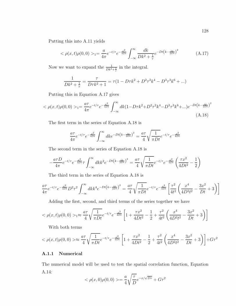
128
Putting this into A.11 yields
< ρ(x, t)ρ(0, 0) >1=a
4πe−t/τe−
x2
4Dt
∫ ∞
−∞
dk
Dk2 + 1τ
e−Dt(k− ix2Dt)
2
(A.17)
Now we want to expand the 1Dk2+ 1
τ
in the integral.
1
Dk2 + 1τ
=τ
Dτk2 + 1= τ(1−Dτk2 +D2τ 2k4 −D3τ 3k6 + ...)
Putting this in Equation A.17 gives
< ρ(x, t)ρ(0, 0) >1=aτ
4πe−t/τe−
x2
4Dt
∫ ∞
−∞dk(1−Dτk2+D2τ 2k4−D3τ 3k6+...)e−Dt(k− ix
2Dt)2
(A.18)
The first term in the series of Equation A.18 is
aτ
4πe−t/τe−
x2
4Dt
∫ ∞
−∞dke−Dt(k− ix
2Dt)2
=aτ
4
√
1
πDte−t/τe−
x2
4Dt
The second term in the series of Equation A.18 is
−aτD
4πe−t/τe−
x2
4Dt τ
∫ ∞
−∞dkk2e−Dt(k− ix
2Dt)2
=aτ
4
√
1
πDte−t/τe−
x2
4Dt
(
τx2
4Dt2− 1
2
)
The third term in the series of Equation A.18 is
aτ
4πe−t/τe−
x2
4DtD2τ 2∫ ∞
−∞dkk4e−Dt(k− ix
2Dt)2
=aτ
4
√
1
πDte−t/τe−
x2
4Dt
[
τ 2
4t2
(
x4
4D2t2− 3x2
Dt+ 3
)]
Adding the first, second, and third terms of the series together we have
< ρ(x, t)ρ(0, 0) >1≈aτ
4
√
1
πDte−t/τe−
x2
4Dt
[
1 +τx2
4Dt2− 1
2+
τ 2
4t2
(
x4
4D2t2− 3x2
Dt+ 3
)]
With both terms
< ρ(x, t)ρ(0, 0) >≈ aτ
4
√
1
πDte−t/τe−
x2
4Dt
[
1 +τx2
4Dt2− 1
2+
τ 2
4t2
(
x4
4D2t2− 3x2
Dt+ 3
)]
+Gτ 2
A.1.1 Numerical
The numerical model will be used to test the spatial correlation function, Equation
A.14:
< ρ(x, 0)ρ(0, 0) >=a
4
√
τ
De−x/
√Dτ +Gτ 2

129
0 20 40 60 80 100
Number of Cells
0.70
0.75
0.80
0.85
0.90
0.95
1.00
1.05
Norm
alized Spatial Correlation (a)
0 10 20 30 40 50
Number of Cells
0.5
0.6
0.7
0.8
0.9
1.0
1.1
Norm
aliz
ed Spatial Correlation (b)
Figure A.1: Normalized spatial correlation functions < ρ(0)ρ(x) > in blue, with xmeasured as the number of cells. Normalization forced < ρ(0)ρ(0) >= 1. Greenindicates fitted curve. (a) is for DM = 0.029/π s−1, and found a fit to a generalexponential a+ b · e−(x−c)/d with a = 0.751392, b = 0.285534, c = 0, and d = 12.6625.(b) is for DM = 0.29/π s−1, and found a fit to a general exponential a + b · e−(x−c)/d
with a = 0.615668, b = 0.422847, c = 0, and d = 3.70343. Parameters are the sameas those described in Section 3.2
In the numerical model (see Equation 4.1), two DM values will be used: DM =
0.029/π s−1 and DM = 0.29/π s−1. These are loss terms, and correspond to 1/τ in
the analytical model (see Equation A.1. DM = 0.029/π s−1 corresponds to a value of
τ = 12.5 cells and DM = 0.29/π s−1 to a value of τ = 3.94 cells.
The numerical correlation functions for both of these loss parameter values have
been plotted in Figure A.1. Also plotted in the figure are Marquardt-Levenberg fits
to a general exponential function: a + b · e−(x−c)/d. The parameter d corresponds to
the value of τ . For DM = 0.029/π s−1, the fitted value of d = 12.6625 cells was quite
close to the expected value of 12.5 cells. For DM = 0.29/π s−1, the fitted value of
d = 3.70343 cells was also close to the expected value of 3.94 cells.
A.2 Discussion
The three main results of the calculation are Equation A.14, for spatial correlations,
Equation A.16, for temporal correlations, and Equation A.1, for spacetime correla-
tions. The magnitude of all three of these of these functions is determined by the τ ,
which sets the magnitude of fixed nitrogen leakage.

130
The leakage sets the scale for the spatial correlations. In Equation A.14 the
correlations go as e−x/√Dτ . The numerical results shown in Figure A.1 show that
correlations of this form and this dependence on τ are a good approximation. This
accuracy tells us that the choice of white noise in Equation A.3, although artifi-
cial, is good enough for accurate spatial correlations. It also tells us that the ab-
sence of growth/advection in the model of Equation A.1 does little to affect spatial
correlations. If the spatial correlations could be measured experimentally then, if
the diffusivity was known, experiments could be used to measure the leakage in the
cyanobacterial filament.
Furthermore, the leakage sets the scale for temporal correlations. In Equation A.16
the correlations go as erfc(t/τ). We have not measured the numerical correlations
because they are not expected to be similar to the calculated correlations due to
strong temporal correlations set by the devision time (see Section 6.4.2) that are not
included in this preliminary calculation. This is for the same reasons that the there are
temporal correlations in the spacetime pattern of starving cells, discussed in Section
6.4.4. Cells maintain a growth rate over a cell cycle and import of fixed nitrogen
depends on the size of the cell. Both of these lead to temporal correlations lasting
about a cell cycle. This would be very different from the white noise of Equation A.3.
If these two parts of the model are removed, it is possible that Equation A.16 would
describe the temporal correlations.

Appendix B
Permissions
131
132