fish avoid visually noisy environments where prey targeting

vol . 1 98 , no . 3 the amer ican natural i st september 202 1

Fish Avoid Visually Noisy Environments

Where Prey Targeting Is Reduced

Joanna R. Attwell,1,2,* Christos C. Ioannou,1 Chris R. Reid,2 and James E. Herbert-Read3

1. Department of Life Sciences, University of Bristol, Bristol, United Kingdom; 2. Department of Biological Sciences, Macquarie University,Sydney, Australia; 3. Department of Zoology, University of Cambridge, Cambridge, United Kingdom; and Department of Aquatic Ecology,Lund University, Lund, Sweden

Submitted September 1, 2020; Accepted April 23, 2021; Electronically published July 12, 2021

Online enhancements: supplemental PDF. Dryad data: https://doi.org/10.5061/dryad.rfj6q577x.

abstract: The environment contains different forms of ecologicalnoise that can reduce the ability of animals to detect information. Here,we ask whether animals adapt their behavior to either exploit or avoidareas of their environment with increased dynamic visual noise. Three-spined sticklebacks (Gasterosteus aculeatus) were immersed in envi-ronmentswith a simulated form of naturally occurring visual noise—moving light bands that form on underwater substrates caused by therefraction of light through surface waves. We tested whether this formof visual noise affected fish’s habitat selection, movements, and prey-targeting behavior. Fish avoided areas of the environment with in-creased visual noise and achieved this by increasing their activity asa function of the locally perceived noise level. Fish were less likely torespond to virtual prey in environments with increased visual noise,highlighting a potential impact that visual noise has on their percep-tual abilities. Fish did not increase or decrease their refuge use in en-vironments with increased visual noise, providing no evidence that vi-sual noise increased either exploratory or risk-aversive behavior. Ourresults indicate that animals can use simple behavioral strategies toavoid visually noisy environments, therebymitigating the impacts thatthese environments appear to have on their perceptual abilities.

Keywords: perception, virtual prey, Gasterosteus aculeatus, caustics,environmental noise.

Introduction

Animals live in inherently noisy environments, where noisecan be defined as any environmental stimulus that inter-feres with the ability of animals to detect or respond to bi-ologically meaningful cues (Brumm 2013; Corcoran andMoss 2017; Cuthill et al. 2017). Noise can take acoustic,chemical, or visual formsandcanvarydynamically in the en-vironment. For example, windblown vegetation, turbidity

* Corresponding author; email: [email protected]: Attwell, https://orcid.org/0000-0003-4112-6315; Ioannou, https://

orcid.org/0000-0002-9739-889X; Reid, https://orcid.org/0000-0002-8671-4463;Herbert-Read, https://orcid.org/0000-0003-0243-4518.

American Naturalist, volume 198, number 3, September 2021. q 2021 The UniversiNonCommercial 4.0 International License (CC BY-NC 4.0), which permits [email protected]. Published by The University of Chicago Pre

(Chamberlain and Ioannou 2019), and the refraction andscattering of light through water (Matchette et al. 2018,2020) can create backgrounds with dynamically changingillumination, while weather, traffic, and other human ac-tivities can generate varying intensities of backgroundacoustic noise (Vasconcelos et al. 2007; Slabbekoorn andRipmeester 2008; Tasker et al. 2010; Lampe et al. 2012;Morris-Drake et al. 2016). These forms of noise can reducethe likelihood of animals detecting information in their en-vironment through two processes. First, by adding statisti-cal error to the sensory modality being utilized, noise canmake detection of a stimulus within that sensory channelmore difficult because of masking effects. Alternatively,by distracting an animal, noise may limit its ability to de-tect or respond to information across sensory modalities(Morris-Drake et al. 2016). Through these processes, noisecan reduce the ability of animals to communicate withconspecifics (Fleishman 1986; Ord et al. 2007; Peters et al.2007; Vasconcelos et al. 2007; Slabbekoorn and Ripmeester2008; Lampe et al. 2012; Herbert-Read et al. 2017), detectmoving targets (Matchette et al. 2018), forage efficiently(Purser and Radford 2011; Party et al. 2013; Wale et al.2013; Azeem et al. 2015; Evans et al. 2018; Matchette et al.2019), and respond to predatory attacks (Wale et al. 2013;Morris-Drake et al. 2016), all of which have significant sur-vival and fitness consequences for individuals.Because noise can reduce the ability of animals to detect

or respond to information in their environment, prey andpredators may use behavioral strategies to either exploit oravoid noisy environments, thereby increasing their likeli-hood of detecting information or avoiding being detectedthemselves.Forexample, if attempting toremainundetected,some speciesmay preferentially select noisier environmentsor increase their exploration of the environment duringtimes of increased environmental noise. Indeed, fathead

ty of Chicago. This work is licensed under a Creative Commons Attribution-ommercial reuse of the work with attribution. For commercial use, contactss for The American Society of Naturalists. https://doi.org/10.1086/715434

mailto:[email protected]

https://orcid.org/0000-0003-4112-6315

https://orcid.org/0000-0002-9739-889X

https://orcid.org/0000-0002-9739-889X

https://orcid.org/0000-0002-8671-4463

https://orcid.org/0000-0003-0243-4518

mailto:[email protected]

422 The American Naturalist

minnows (Pimephales promelas), three-spined sticklebacks(Gasterosteus aculeatus), and larval pike (Esox lucius) showdecreased antipredator behavior inmore turbidwater (Abra-hams and Kattenfeld 1997; Lehtiniemi et al. 2005; Soheland Lindstrom 2015), suggesting that they may exploittimes of high turbidity to avoid being detected by visualpredators (although see Chamberlain and Ioannou 2019).On the other hand, some speciesmay attempt to avoid nois-ier environments as gathering information in those environ-ments becomes more difficult. Indeed, some species ofbats avoid areas of their environment with higher levelsof acoustic noise (Bennett and Zurcher 2013), and othersspend more time foraging in areas with lower levels ofacoustic noise (Schaub et al. 2008; but see Bonsen et al.2015). When avoidance of noisy areas is impossible, how-ever, some species may adapt their behavior to compensatefor reduced information detection. Zebra finches (Taeniopy-gia guttata), for example, spend more time being vigilantin noisier acoustic environments, but this comes at the costof decreased foraging rates (Evans et al. 2018). While ani-mals’ behavioral responses to noise, in particular acousticnoise, have been relatively well documented (Kunc et al.2016; Shannon et al. 2016), whether animals adapt their be-havior in response to noise in other sensory channels, inparticular dynamic visual noise, has received far less atten-tion. Moreover, whether these changes to behavior repre-sent adaptive behavioral decisions to exploit or avoid noisyenvironments remains unclear.Shallow aquatic environments are particularly prone to

one form of naturally occurring dynamic visual noise—caustics. Caustics are formed from the diffraction and re-fraction of light from the disturbance of surface waves thatis projected through thewater columnonto the substrate be-low (Lock andAndrews 1992). This formof dynamic illumi-nation can reduce the likelihood of humans detecting a tar-get on a computer-animated display (Matchette et al. 2018)and can increase the latency of triggerfish (Rhinecanthusaculeatus) to attack a moving target (Matchette et al. 2020).Because caustics appear to reduce the ability of animals to de-tect or respond to information, animals could try to mitigatethe impacts of or exploit these visually noisy environments.For example, species might avoid areas with higher levels ofvisual noise to increase the likelihood of detecting informa-tion themselves, or alternatively, they could preferentially as-sociate with visually noisy environments to reduce their ownlikelihood of being detected.Here, we ask how visual noise affects themovements, ref-

uge use, and prey targeting of three-spined sticklebacks (G.aculeatus). Sticklebacks are a small (∼2–6 cm) fish found inboth shallow marine and freshwater environments wherecaustics are prevalent. They feed on small insects, fish fry,and crustaceans by actively searching for prey among thesubstrate and in the water column and are themselves

predominantly predated by birds and larger fishes, suchas pike (E. lucius). Tounderstandwhether sticklebacks exploitor avoid these visually noisy areas, we performed a seriesof three experiments. We first asked whether sticklebacksavoided or spentmore time in areas of the environmentwithincreased levels of visual noise. In this experiment, we alsodetermined whether fish were actively or passively avoidingareas of the environment with different levels of visual noise.We did this by quantifying their activity (speed and timespent stationary) in response to the locally perceived levelof noise and by asking whether there was directed move-ment toward or away from noisier areas. Second, we testedwhether the fish increased or decreased refuge use in differ-ent levels of visual noise. Last, we tested whether visuallynoisy environments affected the ability of sticklebacks to re-spond to prey in their environment by quantifying the like-lihood that individual sticklebacks targeted virtual prey inenvironments with different levels of visual noise.

Methods

Playbacks

For each of the three experiments, we projected videoplaybacks of simulated caustics into an experimental arena(fig. 1a). These refracted patterns of light naturally vary intheir spatial distribution, intensity, and velocity as a functionof the water depth and the properties of the surface waves(Lock and Andrews 1992). To produce the playbacks, wefirst generated a series of 600 images of caustic patternsusing the software Caustics Generator Pro (Dual Heights2018), cropped to an aspect ratio of 3,840# 2,159 pixels(see software settings in table S1; tables S1–S5 are availableonline).Wecreated animations of these images inMATLAB(2018), where the images were stitched together sequentially(see video S1; videos S1, S2 are available online). The ani-mations were designed so that they could be looped with-out the caustics appearing to spatially or temporally “jump.”To create six different levels of visual noise, we wanted toensure that we manipulated only one property of the causticpatterns. For example, if we had manipulated the spatialfractal nature of the caustic patterns, this would have alsochanged the total light intensity within our animations.Therefore, we chose to manipulate the speed that thecaustics moved while maintaining their spatial properties.To do this, we created videos where the images loopedthrough at different speeds, so that the slowest to fastestanimations took 80, 40, 20, 10, 5, and 2.5 s, respectively, tocomplete a full loop. We classified faster-moving playbacksas having higher levels of visual noise. We ensured that thespeed at which the caustics moved in the arena and the lightlevels in the arena were representative of those found in na-ture (see the supplemental PDF and fig. S1; figs. S1–S8 are

Fish Avoid Visually Noisy Environments 423

available online). Furthermore, we chose to not include atreatment of a static projected image of the caustic patterns,as we were specifically interested in how different levels ofvisual noise affect behavior and static caustics are ecologi-cally unrealistic in aquatic environments.

Study Subjects and Experimental Arena

Three-spined sticklebacks (n p 204) were caught fromRiver Cary in Somerton, Somerset, United Kingdom (lat.

51.069990, long.22.758014), and we observed that causticswere present where the fish were caught. Fish used in exper-iment 1were caught inNovember 2017, andfish used in ex-periments 2 and 3 were caught inMarch 2019. All fish werein nonbreeding condition when used in experiments. Allfish were housed for at least 2 weeks before experimenta-tion. The fish were housed in glass housing tanks (40 cm#70 cm#35 cm; height#length#width) on a flow-throughrecirculating freshwater system with plastic plants andtubes for environmental enrichment. The fish were held

Figure 1: Experimental arena and choice test in experiment 1. a, Schematic of the experimental setup. b, Still image from a video of a choicetrial depicting a section of the trajectory of a fish superimposed in blue. The red dashed line shows the virtual boundary between the twochoice areas. c, Proportion of time the fish spent on the side of the arena with more or less visual noise (ignoring absolute differences in noiselevel). Fish spent more time on the side of the arena with less visual noise. The central line of each box shows the median value, while theupper and lower lines of the box show the upper and lower quartiles of the data, with the whiskers extending to the most extreme data pointwithin 1.5 times the interquartile range. Jittered dots represent raw data points. d, Matrix showing the mean proportion of time across trials(the heat) that fish spent on the left-hand side (LHS) of the arena, where each cell represents the choice a fish was given between two levels ofvisual noise. One through six correspond to the lowest to highest levels of noise, respectively. Fish avoided areas with high levels of visualnoise. When the noise level was lower on the left side of the arena (upper-right corner of the plot), the fish spent more time on that side.When the noise level was higher on the left side of the arena (lower-left corner of the plot), the fish spent less time on that side. Note that oneminus this matrix would give the proportion of time spent on the right-hand side of the arena.


at 147C under a 11L∶13D cycle. Each tank housed approx-imately 40 individuals, and fish were fed bloodworms onceper day, 6 days per week.The experimental tank for all three experiments con-

sisted of a test arena (1.46 m# 0.84 m; length#width)and a holding area (0.84 m#0.34 m; length#width) sep-arated by white opaque plastic (fig. 1a). Both sections werefilled to a depth of 15 cm with water from the recirculatingfreshwater system.Water was filtered within the tank usingan Eheim classic 600 external filter and chilled to between14.27 and 15.27C using a D-D DC-300 chiller. The holdingarea contained plastic plants and tubes for environmentalenrichment. Water was changed in the experimental tankbetween each of the three experiments but not between in-dividual trials. Before each day of trials, all fish that wouldbe tested in the subsequent day were placed in the holdingarea together overnight, allowing them to acclimate to theconditions of the tank. Fish were not fed for 24 h beforeeach experiment.A camera (Panasonic HC-VX870) located 2.15 m above

the center of the test arena filmed the trials at 4K resolution(3,840#2,160 pixels) at 25 frames per second. The camerawas controlled remotely using the Panasonic image app op-erated by an experimenter outside the room. The experi-menter was not present in the room while the trials wererun.ABenQW1700/HT2550 digital projectorwith 4K reso-lution operating at a 60-Hz vertical scan rate located 2.19 mabove the arena (fig. 1a) projected the playbacks intothe arena. The projections were played using a Dell Ins-piron 15 notebook connected to the projector via a 4KHDMI cable located outside the experimental room. Thearena was surrounded by blackout curtains to minimizeany external light source entering.

Experiment 1: Do Fish Prefer to Associate with Moreor Less Visually Noisy Environments?

To determine whether fish avoided or preferred to asso-ciate with more or less visually noisy environments, in-dividual fish were presented with a binary choice, whereon one side of the arena we projected one level of visualnoise and on the other side we projected a different levelof visual noise. As there were six different levels of noise,this gave 15 possible combinations of noise pairings. Weconstructed six different playbacks, where each playbackcontained all 15 different noise pairings, played one afterthe other. Each choice (noise pairing) was presented for320 s, with the total length of each playback equaling 80min.Across the different playbacks (n p 6), each noise levelwas presented evenly on each side of the test arena to con-trol for any potential side biases (table S2). The ordering ofthe noise pairings within a playback was also assorted (see

table S2) between the six playbacks so that there was nosystematic bias in their ordering across the trials. For eachtrial, a single fish was exposed to one of these six playbacks.The order of the six playbacks was randomizedwithin eachday, with each playback being used amaximumof once perday.For each trial (n p 48), an individual fish (5:450:7 cm;

mean5SD) was moved from the holding area to the testarena and left to acclimate for 10 min. During this period,the first frame of the playback was projected into the testarena as a static image, but the videoplaybackwas not started.After 10min, we started the video playback remotely. Aftereach trial, the fish was removed, placed in a separate hous-ing tank, and fed. No fish were reused between trials.Fish were tracked using an adapted version of DIDSON

tracking software (Handegard and Williams 2008) inMATLAB (2018; fig. 1b). Because the fish were darkerthan the arena or moving projections, we took a grayscalethreshold of each frame to isolate the fish within the videoswithout requiring any background subtraction. TheX- andY-coordinates of the fish were smoothed using a rollingaverage of 12 frames (approximately half a second). Trackswere smoothed only if at least 50% of the track was presentwithin these 12 frames (using the function nanfastsmoothinMATLAB); otherwise, these segments of the tracks wereremoved (replaced with NaN). Smoothing is a standardprocedure used in trajectory analysis, allowing spuriouserrors in point estimates to be reduced (Calenge et al.2009; Chachet et al. 2011; Herbert-Read et al. 2011; Katzet al. 2011; Lacey et al. 2011; Gautrais et al. 2012; Spitzenet al. 2013; Tunstrøm et al. 2013; Pérez-Escudero et al.2014; MacGregor et al. 2020). In the supplementary mate-rial, we provide a visualization of this smoothing (fig. S2).In addition to plotting and manually inspecting the tracksfor accuracy, we calculated that fish were tracked for 88.2%of all frames (see below). The tracking accuracy was notsystematically affected by different levels of visual noise(see the supplemental PDF and fig. S3). There was alsonot a difference in the tracking accuracy between differentsides of the arena (figs. S3, S4).From the trajectories of each fish, we calculated the

amount of time the fish spent on each side of the test arenain each paired choice. To do this, we used the inpolygonfunction in MATLAB to determine when a fish’s trackwas on either the left or right side of the arena.We then cal-culated the proportion of time that the fish spent in thenoisier side of the arena for each noise pairing.We also cal-culated the amount of time the fish spent stationary and thespeed that they adoptedwhen theyweremoving in differentlevels of noise. To do this, the instantaneous speed of thefish was calculated as the displacement in their position be-tween two consecutive frames. We defined a fish as beingstationary when its speed was less than 2 mm s21, informed


by plotting a histogram of all the fish’s speeds across alltrials (see fig. S5). The mean speed of a fish was calculatedexcluding the times when they were stationary (i.e., whenspeeds were 12 mm s21) and was calculated when the fishwas on each side of the arena separately.

Experiment 2: Do Fish Use a Refuge More or Lessin Increased Levels of Visual Noise?

To determine whether the fish were more or less likely touse a refuge in different levels of visual noise, two plasticplants (each 5 cm#2 cm#15 cm; length#width#heightat the base) were placed as a refuge in the middle of the testarena (see fig. S6). For each trial (n p 48), an individualfish (450:5 cm; mean standard length5SD) was exposedto six different levels of visual noise, with each level of noisebeing projected throughout the entire arena (unlike in ex-periment 1) and each level of noise projected sequentiallyone after the other. To ensure that each noise level waspresented in a different order within trials, we again createdsix playbacks, where each playback contained each level ofnoise, but each noise level occurred in a different orderwithin each playback (referred to as “order within trial”)in a Latin square design (see table S3). Each trial, therefore,consisted of six levels of noise, each presented for 320 s,with the total running length of the playbacks equaling32 min. Every playback was presented once per day (be-tween 9:00 a.m. and 5:00 p.m.) and in a random order ondifferent days. As in the choice tests, individual fish weremoved from the holding area and placed in the test arenafor 10 min of acclimation time (while a static caustic imagewas projected into the arena) before the playback wasstarted remotely. Experimented fish were removed, placedin a separate housing tank, and later fed. Used fish werekept separately from unused fish, and fish were not reusedbetween trials. Fish that were used in this experiment hadnot been used in experiment 1.We scored the amount of time (in seconds) that the fish

spent under the refuge during each level of noise. To do this,videos were imported into the software BORIS (ver. 7.9.15;Friard et al. 2016), where we defined the fish to be underthe refuge when any part of its body was under any of thefronds of the plastic plant (see fig. S6). Each fish couldtherefore be under the refuge for a minimum of 0 s to amaximum of 320 s in each level of visual noise.

Experiment 3: Does Visual Noise Affect the LikelihoodThat Fish Respond to Virtual Prey?

To determine whether visual noise affected whether fish re-sponded to prey in their environment, we created playbacksof the six different levels of visual noise (as in experiment 2,played sequentially and throughout the entire arena) that

included virtual prey that appeared and disappeared inrandom locations. In particular, the prey appeared as mov-ing uniform red dots (similar to the virtual prey experi-ments in Duffield and Ioannou [2017] and Ioannou et al.[2012, 2019]) on top of the caustic patterns (see video S2).Because the sticklebacks were fed red bloodworms in theirhousing tanks, they were highly responsive to these reddots, often attempting to peck at them if in range, mimick-ing natural feeding behavior. Therefore, the fish did notneed to be trained to attack the virtual prey. Each virtualprey appeared at a random location within the arena as alooming stimulus, increasing in size from 0 to 12.5 mmin diameter within three-fourths of a second, maintaininga 12.5-mm diameter for ∼1 s, and then shrinking to 6 mmbefore disappearing. Each prey was visible in the arena fora total of 2 s, moving on a correlated random walk at 7 cms21. Playbacks of the caustics and prey were created inMATLAB (2018).The limited presentation time of each prey (2 s) was

designed to allow the fish to detect and start swimming to-ward the prey while reducing the likelihood of the fish sam-pling the prey and learning that the preywere not edible. Be-cause of the short presentation times, the large size of thearena, and the prey appearing in random locations, the preywould often appear far from the fish’s position. To increasethe potential for the fish to detect the prey, therefore, eachlevel of noise contained 50 individual prey presentations(300 presentations within a single trial), with 4 s betweenthe end of one prey presentation and the start of another.As in experiment 2, for each trial (n p 108), individual

fish (3.35 0.4 cm; mean standard length5 SD) were ex-posed to six different levels of visual noise but here in com-bination with virtual prey. To control for order effects, sixdifferent playbacks were created, where each playback con-tained each level of noise, with each noise level occurring atdifferent times (order within trial) in the playbacks in a Latinsquare design (table S3). Controlling for order effects wasparticularly important here, as there was the potential forthe fish to become habituated to the prey over time. In theseplaybacks, we also added transitions between the differentlevels of noise so that the change in speed of the movingcaustics between different noise levels was smooth. This in-volved creating animations that increased or decreased inspeed from one noise level to another, which were subse-quently placed between the respective animations of visualnoise with the prey.Within these transition periods, no preywere projected. As in the other experiments, each level ofnoise lasted 320 s, with each transition period lasting be-tween 70 and 90 s. Each playback in total, therefore, lasted∼50 min and 45 s. Each playback was presented once perday and at different times of the day (between 9:00 a.m.and 5:00 p.m.) on different days. As in the previous twoexperiments, individual fish were moved from the holding


area to the test arena and allowed 10 min of acclimationtime. During this time, the lowest level of noise was pro-jected into the test arena for 10 min before transitioningto the start of the playback. Experimented fish were re-moved, placed in a separate housing tank, and fed. No fishused in experiment 1 or 2 were used in this experiment,and fish were not reused between trials.Videos of the trials were manually inspected to deter-

mine whether the fish responded to the virtual prey. A re-sponse to the prey was defined as when there was a notice-able change in the speed or direction of the fish toward theprey (for examples, see video S2). Therefore, if the fish ac-celerated or decelerated while moving toward the prey, thiscounted as a response. We quantified how many prey (outof a maximum of 50) the fish responded to in each level ofnoise within each trial. These changes in speed or directioncould be misclassified as a response if by chance the fishchanged its speed or direction toward the prey withoutdetecting it (i.e., false positives). To quantify the likelihoodof false positives, for each experimental trial, we simulatedthe appearance of a single simulated prey within a randomlocation in the arena at a random time when there wereno prey presented within each level of noise in the trial(i.e., 648 simulated prey events, 108 events for each noiselevel). In these events, we asked whether our classificationmethod would have scored the fish as responding to theseprey (even though the prey were not there). This methodallowed us to estimate the baseline level of false positivesas a function of noise level.

Statistics

All statistics were performed inR (ver. 3.5.1; RDevelopmentCore Team 2018). The package lme4 (Bates et al. 2015) wasused for all mixed models. Assumptions for all linear mixedmodels (LMMs) were checked using standard diagnosticplots (quantile-quantile normal plots and residuals plottedagainst fitted values). Models were also checked for collin-earity. Assumptions for all generalized linear mixed mod-els (GLMMs) were checked using the DHARMa package(Hartig 2019), including checking the dispersion and thedistribution of the residuals. The full models were simplifiedby removal of nonsignificant terms. We used the anovafunction in R (ver. 3.5.1; R Development Core Team 2018)to compare pairs of models using the x2 statistic. The es-timates and effect sizes (Cohen’s D) are presented in ta-ble S4. All R graphs were created using ggplot2 (Wickham2016). All data used here have been deposited in the DryadDigital Repository (https://doi.org/10.5061/dryad.rfj6q577x;Attwell 2021).

Experiment 1. To test whether fish spent more or lesstime in areas with more or less visual noise (regardless

of absolute noise level), we subtracted 0.5 from the pro-portion of time they spent on the noisier side of the arenaseparately for each of the 15 noise pairings per trial. Wetested whether the intercept of an LMM predicting thoseproportions, with trial included as a random effect, dif-fered from zero (i.e., proportion of time on the noisierside 20.5 ∼ 1 1 (1FTrial) in lme4 nomenclature).We then asked whether the absolute difference in noiselevel within a choice affected the amount of time the fishspent on the noisier side of the arena. To do this, we cal-culated the difference between noise levels on each sideof the arena for each noise pairing. For example, the dif-ference between a choice of noise levels 1 and 5 was cal-culated as 4. We then used an LMM to ask whether thisdifference could predict the proportion of time the fishspent on the noisier side of the arena. In this model,the difference in noise was treated as a discrete numericvariable, trial (fish identity) was included as a random in-tercept, and difference in noise levels was included as arandom slope. We also checked that including times whenfish did not visit both sides of the arena during a singlechoice did not qualitatively affect the interpretation ofour results (see the supplemental PDF).We then askedwhether a fish changed itsmovements de-

pending on the level of noise on each side of the arena. Toinvestigate this, we used LMMs to predict whether a fish’smean speed and, in a separatemodel, its time spent station-ary on the side of the arena the fish was on could bepredicted on the basis of the level of noise on each side ofthe arena (modeled as separate fixed effects: noise levelon the side occupied by the fish and noise level on the un-occupied side). Mean speed and the proportion of time sta-tionary were square root transformed because of a positiveskew in these data. Order within trial (1–6) was also addedas a fixed effect, trial (fish identity) was included as a ran-dom intercept, and noise level on the side occupied bythe fish was included as a random slope.Because a fish’s speed and time spent stationary were de-

pendent on the noise level they were in (but not dependenton the noise level on the other side of the arena; see below),we asked whether these differences in speed and time spentstationary could explain the amount of time fish spent inthe corresponding levels of visual noise. To test this, themeanspeed that the fish adopted in different levels of noise and theproportion of time spent stationary were added as covariatesto themodel investigating the proportion of time spent on theside of the arena with more visual noise. We also testedwhether the fish showed any evidence of directed movementtoward or away from the sides of the arena with more or lessvisual noise (for full details, see the supplemental PDF).

Experiment 2. We tested whether the level of visual noisehad a significant influence on the time the fish spent

https://doi.org/10.5061/dryad.rfj6q577x


under refuge. We initially attempted to model the timespent in the refuge as a binomial response (time in vs. timeout of refuge); however, these models were overdispersed.Therefore, because of the relatively bimodal distributionof the response variable (fig. S7a), we transformed the timespent in refuge into a binary response variable, where fishthat spent more than 50% of their time in the refuge weregiven a value of 1 and fish that spent less than or equal to50% of their time in the refuge were given a value of 0. Thisbinary response variable was modeled using a GLMMwith a binomial error structure. Noise level was includedas a fixed effect (discrete numeric as before) along with or-der within trial, and trial (fish identity) was added as a ran-dom intercept. We did not include noise as a randomslope in this experiment because there was no effect ofnoise on the response variable.

Experiment 3. To test whether the level of visual noise af-fected the likelihood that fish responded to the virtualprey, we used a GLMM with a Poisson family error struc-ture. The response variable was the number of responsesto prey at each level of noise, and fixed effects were thelevel of visual noise and order within trial. Trial (fish iden-tity) was added as a random intercept, but noise was notadded as a random slope in this case because the modeldid not converge when this term was included.

Results

Experiment 1: Do Fish Prefer to Associate with Moreor Less Visually Noisy Environments?

Fish spent more time on the side of the arena with lessvisual noise (fig. 1c; LMM: t47 p 27:8, P ! :001). Fur-thermore, the relative difference between the noise levelson each side of the arena affected the time the fish spentin the noisier side of the arena. As the relative differencein noise between the two sides of the arena increased,fish spent less time on the side of arena with more visualnoise (fig. 1d; LMM: x2 p 9:77, df p 7, P p :002; for95% confidence intervals, see table S5).The fish’s movements were affected by the level of visual

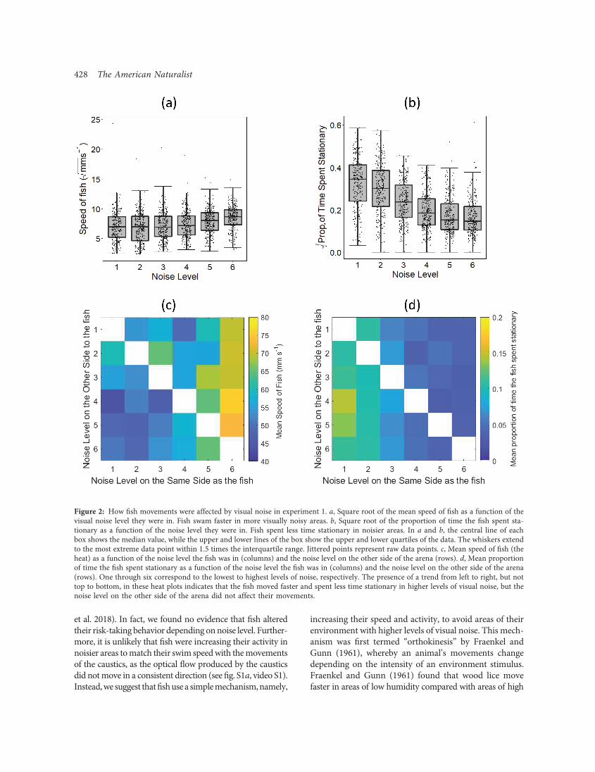
noise on the side of the arena they were in. Fishmoved faster(fig. 2a; LMM: x2 p 52:3, df p 8, P ! :001) and spent lesstime stationary when on the side of the arena with more vi-sual noise (fig. 2b; LMM: x2 p 90:8, df p 8, P ! :001).The noise level on the other side of the arena (across fromthe side the fish was on) did not affect the fish’s speed(fig. 2c; LMM: x2 p 0:35, df p 8, P p :55), and the noiselevel on the other side also did not affect the proportion oftime the fish spent stationary (fig. 2d; LMM: x2 p 0:34,df p 8, P p :56). When these movement variables wereadded as covariates to themodel, the difference in noise level

between the two sides of the arena was no longer a signifi-cant predictor of the time the fish spent on the noisier side(LMM: x2 p 1:61, df p 11, P p :20). Therefore, how afish adapted its movements to the locally perceived levelof noise determined the amount of time it spent in that re-gion. There was no evidence, however, that the fish weremore likely to show directed movement toward or awayfrom the side of the arena with more or less visual noise(see the supplemental PDF).

Experiment 2: Do Fish Use a Refuge Moreor Less in Increased Levels of Visual Noise?

There was no evidence that the level of visual noise affectedwhether the fish spent themajority of time under the refuge(fig. S7b; GLMM: x2 p 1:75, df p 4, P p :19). However,fish spent less time under the refuge as the trial progressed(GLMM: x2 p 7:07, df p 4, P p :0079).

Experiment 3: Does Visual Noise Affect the LikelihoodThat Fish Respond to Virtual Prey?

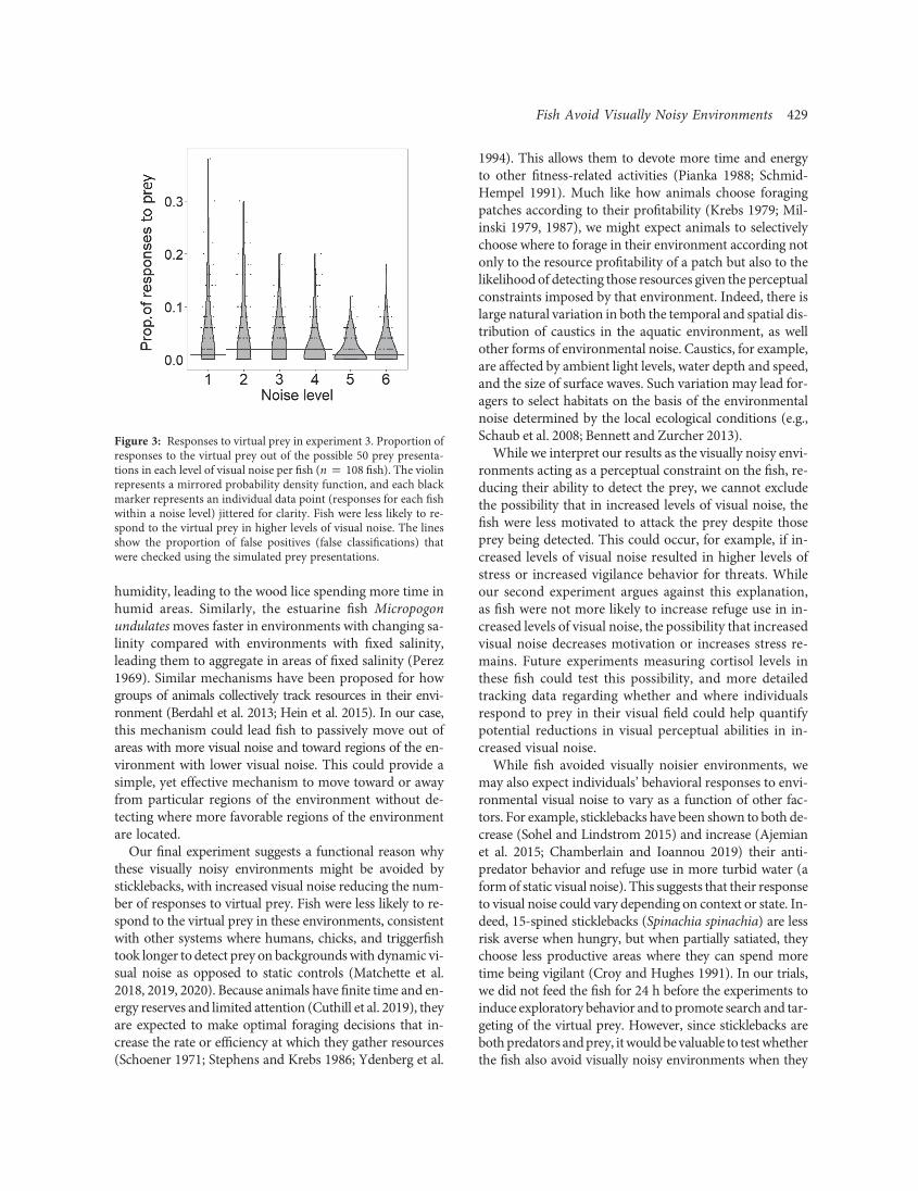
Fish were less likely to respond to the virtual prey inhigher levels of visual noise (fig. 3; GLMM: x2 p 155:3,df p 4, P ! :01). There was an effect of the order withintrial on the number of responses to prey by the fish(GLMM: x2 p 451:3, df p 4, P ! :01); fish became lesslikely to respond to the prey over the course of the trial.Our estimations of the number of false positives (classifi-cation of the fish responding to the prey even if the preyhad not been detected) were far below that observed in theresponses to the real virtual prey (fig. 3).

Discussion

Fish spent less time in areas with more visual noise, and thisreduction in time could be attributed to how thefish adaptedtheir movements in response to noise. In particular, fish in-creased their speed and spent less time stationary in areaswith more visual noise. There was no evidence, however,that the level of visual noise on the other side of the arenaaffected their movements or that fish directed their move-ment toward less noisy areas, suggesting that the fish wereresponding only to the level of noise in their local vicinity.While increases in speed and decreases in time spent sta-tionary could be interpreted as the fish exploiting theseenvironments to increase exploration during times ofincreased environmental noise, our second experimentprovided evidence against this explanation. If fish wereexploiting times of higher visual noise to avoid being de-tected themselves, we would have expected the fish to spendless time in the refuge in higher levels of visual noise (as ref-uge use is a keymeasure of risk taking in sticklebacks; Bevan


et al. 2018). In fact, we found no evidence that fish alteredtheir risk-taking behavior depending onnoise level. Further-more, it is unlikely that fish were increasing their activity innoisier areas tomatch their swim speedwith themovementsof the caustics, as the optical flow produced by the causticsdid notmove in a consistent direction (see fig. S1a, video S1).Instead,we suggest thatfishuse a simplemechanism,namely,

increasing their speed and activity, to avoid areas of theirenvironment with higher levels of visual noise. This mech-anism was first termed “orthokinesis” by Fraenkel andGunn (1961), whereby an animal’s movements changedepending on the intensity of an environment stimulus.Fraenkel and Gunn (1961) found that wood lice movefaster in areas of low humidity compared with areas of high

Figure 2: How fish movements were affected by visual noise in experiment 1. a, Square root of the mean speed of fish as a function of thevisual noise level they were in. Fish swam faster in more visually noisy areas. b, Square root of the proportion of time the fish spent sta-tionary as a function of the noise level they were in. Fish spent less time stationary in noisier areas. In a and b, the central line of eachbox shows the median value, while the upper and lower lines of the box show the upper and lower quartiles of the data. The whiskers extendto the most extreme data point within 1.5 times the interquartile range. Jittered points represent raw data points. c, Mean speed of fish (theheat) as a function of the noise level the fish was in (columns) and the noise level on the other side of the arena (rows). d, Mean proportionof time the fish spent stationary as a function of the noise level the fish was in (columns) and the noise level on the other side of the arena(rows). One through six correspond to the lowest to highest levels of noise, respectively. The presence of a trend from left to right, but nottop to bottom, in these heat plots indicates that the fish moved faster and spent less time stationary in higher levels of visual noise, but thenoise level on the other side of the arena did not affect their movements.


humidity, leading to the wood lice spending more time inhumid areas. Similarly, the estuarine fish Micropogonundulatesmoves faster in environments with changing sa-linity compared with environments with fixed salinity,leading them to aggregate in areas of fixed salinity (Perez1969). Similar mechanisms have been proposed for howgroups of animals collectively track resources in their envi-ronment (Berdahl et al. 2013; Hein et al. 2015). In our case,this mechanism could lead fish to passively move out ofareas with more visual noise and toward regions of the en-vironment with lower visual noise. This could provide asimple, yet effective mechanism to move toward or awayfrom particular regions of the environment without de-tecting where more favorable regions of the environmentare located.Our final experiment suggests a functional reason why

these visually noisy environments might be avoided bysticklebacks, with increased visual noise reducing the num-ber of responses to virtual prey. Fish were less likely to re-spond to the virtual prey in these environments, consistentwith other systems where humans, chicks, and triggerfishtook longer to detect prey on backgroundswith dynamic vi-sual noise as opposed to static controls (Matchette et al.2018, 2019, 2020). Because animals have finite time and en-ergy reserves and limited attention (Cuthill et al. 2019), theyare expected to make optimal foraging decisions that in-crease the rate or efficiency at which they gather resources(Schoener 1971; Stephens and Krebs 1986; Ydenberg et al.

1994). This allows them to devote more time and energyto other fitness-related activities (Pianka 1988; Schmid-Hempel 1991). Much like how animals choose foragingpatches according to their profitability (Krebs 1979; Mil-inski 1979, 1987), we might expect animals to selectivelychoose where to forage in their environment according notonly to the resource profitability of a patch but also to thelikelihood of detecting those resources given the perceptualconstraints imposed by that environment. Indeed, there islarge natural variation in both the temporal and spatial dis-tribution of caustics in the aquatic environment, as wellother forms of environmental noise. Caustics, for example,are affected by ambient light levels, water depth and speed,and the size of surface waves. Such variation may lead for-agers to select habitats on the basis of the environmentalnoise determined by the local ecological conditions (e.g.,Schaub et al. 2008; Bennett and Zurcher 2013).While we interpret our results as the visually noisy envi-

ronments acting as a perceptual constraint on the fish, re-ducing their ability to detect the prey, we cannot excludethe possibility that in increased levels of visual noise, thefish were less motivated to attack the prey despite thoseprey being detected. This could occur, for example, if in-creased levels of visual noise resulted in higher levels ofstress or increased vigilance behavior for threats. Whileour second experiment argues against this explanation,as fish were not more likely to increase refuge use in in-creased levels of visual noise, the possibility that increasedvisual noise decreases motivation or increases stress re-mains. Future experiments measuring cortisol levels inthese fish could test this possibility, and more detailedtracking data regarding whether and where individualsrespond to prey in their visual field could help quantifypotential reductions in visual perceptual abilities in in-creased visual noise.While fish avoided visually noisier environments, we

may also expect individuals’ behavioral responses to envi-ronmental visual noise to vary as a function of other fac-tors. For example, sticklebacks have been shown to both de-crease (Sohel and Lindstrom 2015) and increase (Ajemianet al. 2015; Chamberlain and Ioannou 2019) their anti-predator behavior and refuge use in more turbid water (aformof static visual noise). This suggests that their responseto visual noise could vary depending on context or state. In-deed, 15-spined sticklebacks (Spinachia spinachia) are lessrisk averse when hungry, but when partially satiated, theychoose less productive areas where they can spend moretime being vigilant (Croy and Hughes 1991). In our trials,we did not feed the fish for 24 h before the experiments toinduce exploratory behavior and to promote search and tar-geting of the virtual prey. However, since sticklebacks areboth predators andprey, itwould be valuable to testwhetherthe fish also avoid visually noisy environments when they

Figure 3: Responses to virtual prey in experiment 3. Proportion ofresponses to the virtual prey out of the possible 50 prey presenta-tions in each level of visual noise per fish (n p 108 fish). The violinrepresents a mirrored probability density function, and each blackmarker represents an individual data point (responses for each fishwithin a noise level) jittered for clarity. Fish were less likely to re-spond to the virtual prey in higher levels of visual noise. The linesshow the proportion of false positives (false classifications) thatwere checked using the simulated prey presentations.


are satiated or when the level of risk in the environment isgreater. Indeed, we might expect animals to choose noisierareas of the environment when satiated or when faced withgreater risk. While not measured here, animals might alsoswitch to relying on other sensory modalities in visuallynoisy environments when their vision is compromised (Par-tan 2017; Suriyampola et al. 2018). For example, femalethree-spined sticklebacks rely more on visual cues whenchoosing a mate in clear water, but in turbid water, wherevision is compromised, they rely more on olfactory cues(Heuschele et al. 2009). When habitats consistently differin their ecological noise, this could have sweeping effectson populations. For example, gray squirrels (Sciurus caro-linensis) from acoustically noisy urban habitats respondmore to visual alarm signals than squirrels from rural hab-itats, which instead rely more on acoustic alarm signals(Partan et al. 2010). Hence, animals from different popula-tions may show different behavioral responses, highlight-ing the need for cross-population comparisons. We mightalso expect animals to rely more heavily on social informa-tion in sensory-demanding environments. Indeed, animalsin groups often benefit from pooling imperfect estimatesof the world around them in order to make more accuratedecisions collectively (Dall et al. 2005; Ward et al. 2011;Ioannou 2017; Berdahl et al. 2018). Using playbacks ofcaustic visual noise, it would be possible to test how relianceon social information changes when individuals are ex-posed to an ecologically relevant form of environmentalnoise that reduces their visual perceptual abilities.

Conclusion

Our results demonstrate that natural forms of ecologicalnoise reduce the likelihood of animals responding to in-formation in their environment. To combat this, animalscan update their behavior to avoid noisy areas, whichcould lead to an increased likelihood of gathering infor-mation and thereby compensate for the potential nega-tive impacts of environmental noise on their perception.

Acknowledgments

J.R.A. was supported by a Natural Environment ResearchCouncil Great Western 4 (GW41) Centre for DoctoralTraining PhD studentship (NE/L002434/1) and an Interna-tional Macquarie University Research Excellence Scholar-ship. J.E.H.-R. was supported by the Whitten Lectureshipin Marine Biology and a Swedish Research Council grant(2018-04076). C.C.I. was supported by a Leverhulme Trustgrant (RPG-2017-041 V). C.R.R. was supported by an Aus-tralian Research Council Discovery Early Career ResearcherAward (DE190-10-15-13). We thank Andy Radford, InnesCuthill, Sam Matchette, and Nick Scott-Samuel for useful

discussions and advice. Thanks are also given to the staffat theAnimal Services Unit at Bristol University and in par-ticular Peter Gardiner for all his help and advice with caringfor the fish. Finally, thanks are given to two anonymousreviewers for their helpful comments on the manuscript.

Statement of Authorship

J.R.A. and J.E.H.-R. were involved in the conceptualization,all authors were involved in the experimental design, andJ.R.A. collected the data, performed the data analysis, andwrote the original draft of the manuscript. All authors wereinvolved in editing the manuscript.

Data and Code Availability

All data used in this article have been deposited in the DryadDigital Repository (https://doi.org/10.5061/dryad.rfj6q577x;Attwell et al. 2021).

Literature Cited

Abrahams, M. V., and M. G. Kattenfeld. 1997. The role of turbid-ity as a constraint on predator-prey interactions in aquatic en-vironments. Behavioral Ecology and Sociobiology 40:169–174.

Ajemian, M., S. Sohel, and J. Mattila. 2015. Effects of turbidity andhabitat complexity on antipredator behavior of three-spinedsticklebacks (Gasterosteus aculeatus). Environmental Biologyof Fishes 98:45–55.

Attwell, J. R., C. C. Ioannou, C. R. Reid, and J. E. Herbert-Read.2021. Data from: Fish avoid visually noisy environments whereprey targeting is reduced. American Naturalist, Dryad DigitalRepository, https://doi.org/10.5061/dryad.rfj6q577x.

Azeem, M., G. K. Rajarao, O. Terenius, G. Nordlander, H.Nordenhem, K. Nagahama, E. Norin, and A. K. Borg-Karlson.2015. A fungal metabolite masks the host plant odor for the pineweevil (Hylobius abietis). Fungal Ecology 13:103–111.

Bates, D., M. Machler, B. Bolker, and S. Walker. 2015. Fitting lin-ear mixed-effects models using lme4. Journal of Statistical Soft-ware 67:1–48. https://doi.org/10.18637/jss.v067.i01.

Bennett, V. J., and A. A. Zurcher. 2013. When corridors collide:road-related disturbance in commuting bats. Journal of WildlifeManagement 77:93–101.

Berdahl, A., C. J. Torney, C. C. Ioannou, J. J. Faria, and I. D.Couzin. 2013. Emergent sensing of complex environments bymobile animal groups. Science 339:574–576.

Berdahl, A. M., A. B. Kao, A. Flack, P. A. Westley, E. A. Codling, I. D.Couzin, A. I. Dell, and D. Biro. 2018. Collective animal naviga-tion and migratory culture: from theoretical models to empiricalevidence. Philosophical Transactions of the Royal Society B 373:20170009.

Bevan, P. A., I. Gosetto, E. R. Jenkins, I. Barnes, and C. C.Ioannou. 2018. Regulation between personality traits: individualsocial tendencies modulate whether boldness and leadership arecorrelated. Proceedings of the Royal Society B 285:20180829.

Bonsen, G., B. Law, and D. Ramp. 2015. Foraging strategies determinethe effect of traffic noise on bats. Acta Chiropterologica 17:347–357.



https://doi.org/10.18637/jss.v067.i01


Brumm, H. 2013. Animal communication and noise. Vol. 2. Ani-mal Signals and Communication. Springer, Berlin.

Calenge, C., S. Dray, and M. Royer-Carenzi. 2009. The concept ofanimals’ trajectories from a data analysis perspective. EcologicalInformatics 4:34–41.

Chachet, J., A. Stewart, E. Utterback, P. Hart, S. Gaikwad, K. Wong,E. Kyzar, N. Wu, and A. Kalueff. 2011. Three-dimensional neuro-phenotyping of adult zebrafish behavior. PLoS ONE 6:e17597.

Chamberlain, A. C., and C. C. Ioannou. 2019. Turbidity increasesrisk perception but constrains collective behaviour during for-aging by fish shoals. Animal Behaviour 156:129–138.

Corcoran, A. J., and C. F. Moss. 2017. Sensing in a noisy world:lessons from auditory specialists, echolocating bats. Journal ofExperimental Biology 220:4554–4566.

Croy, M., and R. Hughes. 1991. Effects of food supply, hunger,danger and competition on choice of foraging location by thefifteen-spined stickleback, Spinachia spinachia L. Animal Be-haviour 42:131–139.

Cuthill, I. C., W. L. Allen, K. Arbuckle, B. Caspers, G. Chaplin, M. E.Hauber, G. E.Hill, et al. 2017. The biology of color. Science 357:6350.

Cuthill, I. C., S. R. Matchette, and N. E. Scott-Samuel. 2019. Cam-ouflage in a dynamic world. Current Opinion in BehavioralSciences 30:109–115.

Dall, S. R., L. A. Giraldeau, O. Olsson, J. M. McNamara, and D. W.Stephens. 2005. Information and its use by animals in evolu-tionary ecology. Trends in Ecology and Evolution 20:187–193.

Dual Heights. 2018. Caustics generator pro. Dual Heights SoftwareAB, Linköping, Sweden.

Duffield, C., and C. C. Ioannou. 2017. Marginal predation: do en-counter or confusion effects explain the targeting of prey groupedges? Behavioural Ecology 28:1283–1292.

Evans, J. C., S. R. Dall, and C. R. Kight. 2018. Effects of ambient noiseon zebra finch vigilance and foraging efficiency. PLoS ONE 13:e0209471.

Fleishman, L. J. 1986. Motion detection in the presence and ab-sence of background motion in an Anolis lizard. Journal ofComparative Physiology A 159:711–720.

Fraenkel, G. S., and D. L. Gunn. 1961. The orientation of animals.2nd ed. Dover, New York.

Friard, O., and M. Gamba. 2016. BORIS: a free, versatile open-source event-logging software for video/audio coding and liveobservations. Methods in Ecology and Evolution 7:1325–1330.

Gautrais, J., F. Ginelli., R. Fournier, S. Blanco, M. Soria, H. Chaté,and G. Theraulaz. 2012. Deciphering interactions in moving an-imal groups. PLoS Computational Biology 8:e1002678.

Handegard, N. O., and K. Williams. 2008. Automated tracking offish in trawls using the DIDSON (Dual frequency IDentificationSONar). ICES Journal of Marine Science 65:636–644.

Hartig, F. 2019. DHARMa: residual diagnostics for hierarchical (multi-level/mixed) regression models. R package version 0.2.4. https://cran.r-project.org/web/packages/DHARMa/vignettes/DHARMa.html.

Hein, A. M., S. B. Rosenthal, G. I. Hagstrom, A. Berdahl, C. J. Torney,and I. D. Couzin. 2015. The evolution of distributed sensing andcollective computation in animal populations. eLife 4:e10955.

Herbert-Read, J. E., L. Kremer, R. Bruintjes, A. N. Radford, andC. C. Ioannou. 2017. Anthropogenic noise pollution from pile-driving disrupts the structure and dynamics of fish shoals. Pro-ceedings of the Royal Society B 284:20171627.

Herbert-Read, J. E., A. Perna, R. P. Mann, T. M. Schaerf, D. J. T.Sumpter, and A. J. W. Ward. 2011. Inferring the rules of inter-

action of shoaling fish. Proceedings of the National Academy ofSciences of the USA 108:18726–18731.

Heuschele, J., M. Mannerla, P. Gienapp, and U. Candolin. 2009.Environment-dependent use of mate choice cues in sticklebacks.Behavioral Ecology 20:1223–1227.

Ioannou, C. C. 2017. Swarm intelligence in fish? the difficulty in dem-onstrating distributed and self-organised collective intelligence in(some) animal groups. Behavioural Processes 141:141– 151.

Ioannou, C. C., V. Guttal, and I. D. Couzin. 2012. Predatory fishselect for coordinated collective motion in virtual prey. Science337:1212–1215.

Ioannou, C. C., F. Rocque, J. E. Herbert-Read, C. Duffield, andJ. A. Firth. 2019. Predators attacking virtual prey reveal the costsand benefits of leadership. Proceedings of the National Acad-emy of Sciences of the USA 116:8925–8930.

Katz, Y., K. Tunstrøm, C. C. Ioannou, C. Huepe, and I. D. Couzin.2011. Inferring the structure and dynamics of interactions inschooling fish. Proceedings of the National Academy of Sciencesof the USA 108:18720–18725.

Krebs, J. R. 1979. Foraging strategies and their social significance.Pages 225 – 270 in P. Marler, ed. Social behavior and commu-nication. Plenum, New York.

Kunc, H. P., K. E. McLaughlin, and R. Schmidt. 2016. Aquaticnoise pollution: implications for individuals, populations, andecosystems. Proceedings of the Royal Society B 283:20160839.

Lacey, E. S., and R. T. Cardé. 2011. Activation, orientation andlanding of female Culex quinquefasciatus in response to car-bon dioxide and odour from human feet: 3-D flight analysisin a wind tunnel. Medical and Veterinary Entomology 25:94–103.

Lampe, U., T. Schmoll, A. Franzke, and K. Reinhold. 2012. Stayingtuned: grasshoppers from noisy roadside habitats producecourtship signals with elevated frequency components. Func-tional Ecology 26:1348–1354.

Lehtiniemi, M., J. Engström-Öst, and M. Viitasalo. 2005. Turbiditydecreases anti-predator behaviour in pike larvae, Esox lucius.Environmental Biology of Fishes 73:1–8.

Lock, J. A., and J. H. Andrews. 1992. Optical caustics in naturalphenomena. American Journal of Physics 60:397–407.

MacGregor, H. E. A., J. E. Herbert-Read., and C. C. Ioannou. 2020.Information can explain the dynamics of group order in animalcollective behaviour. Nature Communications 11:2737.

Matchette, S. R., I. C. Cuthill, K. L. Cheney, N. J. Marshall, and N. E.Scott-Samuel. 2020.Underwater caustics disrupt prey detection by areef fish. Proceedings of the Royal Society B 287:20192453.

Matchette, S. R., I. C. Cuthill, and N. E. Scott-Samuel. 2018. Con-cealment in a dynamic world: dappled light and caustics maskmovement. Animal Behaviour 143:51–57.

———. 2019. Dappled light disrupts prey detection by maskingmovement. Animal Behaviour 155:89–95.

MATLAB. 2018. MATLAB version R2018a. MathWorks, Natick,Massachusetts.

Milinski, M. 1979. An evolutionarily stable feeding strategy insticklebacks. Zeitschrift für Tierpsychologie 51:36–40.

———. 1987. Competition for non-depleting resources: the idealfree distribution in sticklebacks. Pages 363–388 in A. C. Kamil,J. R. Krebs, and H. R. Pulliam eds. Foraging behavior. Plenum,New York.

Morris-Drake, A., J. M. Kern, and A. N. Radford. 2016. Cross-modal impacts of anthropogenic noise on information use. Cur-rent Biology 26:R911–R912.

https://cran.r-project.org/web/packages/DHARMa/vignettes/DHARMa.html

https://cran.r-project.org/web/packages/DHARMa/vignettes/DHARMa.html


Ord, T. J., R. A. Peters, B. Clucas, and J. A. Stamps. 2007. Lizardsspeed up visual displays in noisy motion habitats. Proceedingsof the Royal Society B 274:1057–1062.

Partan, S. R. 2017. Multimodal shifts in noise: switching channelsto communicate through rapid environmental change. AnimalBehaviour 124:325–337.

Partan, S. R., A. G. Fulmer, M. A. Gounard, and J. E. Redmond.2010. Multimodal alarm behavior in urban and rural graysquirrels studied by means of observation and a mechanical ro-bot. Current Zoology 56:313–326.

Party, V., C. Hanot, D. S. Busser, D. Rochat, and M. Renou. 2013.Changes in odor background affect the locomotory response topheromone in moths. PLoS ONE 8:e52897.

Perez, K. T. 1969. An orthokinetic response to rates of salinitychange in two estuarine fishes. Ecology 50:454–457.

Pérez-Escudero, A., J. Vicente-Page, R. C. Hinz, S. Arganda, andG. G. de Polavieja. 2014. idTracker: tracking individuals in agroup by automatic identification of unmarked animals. NatureMethods 11:743–748.

Peters, R. A., J. M. Hemmi, and J. Zeil. 2007. Signaling against thewind: modifying motion-signal structure in response to in-creased noise. Current Biology 17:1231–1234.

Pianka, E. 1988. Evolutionary ecology. Harper & Row, New York.Purser, J., and A. N. Radford. 2011. Acoustic noise induces atten-

tion shifts and reduces foraging performance in three-spinedsticklebacks (Gasterosteus aculeatus). PLoS ONE 6:e17478.

RDevelopmentCoreTeam. 2018.R: a language and environment for sta-tistical computing. R Foundation for Statistical Computing, Vienna.

Schaub, A., J. Ostwald, and B. M. Siemers. 2008. Foraging batsavoid noise. Journal of Experimental Biology 211:3174–3180.

Schmid-Hempel, P. 1991. Searchingbehaviour: thebehavioural ecologyof finding resources. Trends in Ecology and Evolution 6:370–371.

Schoener, T. W. 1971. Theory of feeding strategies. Annual Reviewof Ecology and Systematics 2:369–404.

Shannon, G., M. F. McKenna, L. M. Angeloni, K. R. Crooks, K. M.Fristrup, E. Brown, K. A. Warner, et al. 2016. A synthesis of twodecades of research documenting the effects of noise on wildlife.Biological Reviews 91:982–1005.

Slabbekoorn, H., and E. A. P. Ripmeester. 2008. Birdsong and an-thropogenic noise: implications and applications for conserva-tion. Molecular Ecology 17:72–83.

Sohel, S., and K. Lindstrom. 2015. Algal turbidity reduces risk assess-ment ability of the three-spined stickleback. Ethology 121:548–555.

Spitzen, J., C. W. Spoor, F. Grieco, C. ter Braak, J. Beeuwkes, S. P. vanBrugge, S. Kranenbarg, L. P. J. J. Noldus, J. L. van Leeuwen, andW.Takken. 2013. A 3D analysis of flight behavior of Anophelesgambiae sensu stricto malaria mosquitoes in response to humanodor and heat. PLoS ONE 8:e62995.

Sketch of a three-spined stickleback

Stephens, D. W., and J. R. Krebs. 1986. Foraging theory. Vol. 1.Princeton University Press, Princeton, NJ.

Suriyampola, P. S., J. Caceres, and E. P. Martins. 2018. Effects ofshort-term turbidity on sensory preference and behaviour ofadult fish. Animal Behaviour 146:105–111.

Tasker, M., M. Amundin, M. Andre, A. Hawkins, W. Lang, T. Merck,A. Scholik-Schlomer, et al. 2010. Marine strategy framework direc-tive, task group 11 report, underwater noise and other forms of en-ergy. Publications Office of the European Union, Luxembourg.

Tunstrøm, K., Y. Katz, C. C. Ioannou, C. Huepe, M. J. Lutz, and I. D.Couzin. 2013. Collective states, multistability and transitional be-haviour in schooling fish. PLoSComputational Biology 9:e1002915.

Vasconcelos, R. O., M. C. P. Amorim, and F. Ladich. 2007. Effectsof ship noise on the detectability of communication signals inthe lusitanian toadfish. Journal of Experimental Biology 210:2104–2112.

Wale, M. A., S. D. Simpson, and A. N. Radford. 2013. Noise neg-atively affects foraging and antipredator behaviour in shorecrabs. Animal Behaviour 86:111–118.

Ward, A. J. W., J. E. Herbert-Read, D. J. Sumpter, and J. Krause.2011. Fast and accurate decisions through collective vigilancein fish shoals. Proceedings of the National Academy of Sciencesof the USA 108:2312–2315.

Wickham, H. 2016. ggplot2: elegant graphics for data analysis.Springer, New York.

Ydenberg, R., C.Welham,R. Schmid-Hempel, P. Schmid-Hempel, andG. Beauchamp. 1994. Time and energy constraints and the relation-shipsbetweencurrenciesinforagingtheory.BehavioralEcology5:28–34.

References Cited Only in the Online Enhancements

Francis, J. 1951. The aerodynamic drag of a free water surface.Proceedings of the Royal Society A 206:387–406.

Goerg, G. M. 2014. The Lambert way to Gaussianize heavy-taileddata with the inverse of Tukey’s h transformation as a specialcase. Scientific World Journal 2015:909231.

———. 2020. LambertW: probabilistic models to analyze andGaussianize heavy-tailed, skewed data. R package version 0.6.5.https://cran.r-project.org/web/packages/LambertW/index.html.

Korner-Nievergelt, F., T. Roth, S. von Felten, J. Guelat, B. Almasi, andP. Korner-Nievergelt. 2015. Bayesian data analysis in ecology usinglinear models with R, BUGS and Stan: including comparisons tofrequentist statistics. Academic Press, Amsterdam.

Venables, W. N., and B. D. Ripley. 2002. Modern applied statisticswith S. 4th ed. Springer, New York.

Associate Editor: Peter NonacsEditor: Jennifer A. Lau

in caustics. Artist: David Clarke.

https://cran.r-project.org/web/packages/LambertW/index.html

fish avoid visually noisy environments where prey targeting

Documents