first-principles prediction and partial characterization of the vibrational states of water up to...

This article appeared in a journal published by Elsevier. The attachedcopy is furnished to the author for internal non-commercial researchand education use, including for instruction at the authors institution

and sharing with colleagues.

Other uses, including reproduction and distribution, or selling orlicensing copies, or posting to personal, institutional or third party

websites are prohibited.

In most cases authors are permitted to post their version of thearticle (e.g. in Word or Tex form) to their personal website orinstitutional repository. Authors requiring further information

regarding Elsevier’s archiving and manuscript policies areencouraged to visit:

http://www.elsevier.com/copyright

http://www.elsevier.com/copyright

Author's personal copy

First-principles prediction and partial characterization of thevibrational states of water up to dissociation

Attila G. Csaszar a, Edit Matyus a, Tamas Szidarovszky a, Lorenzo Lodi b, Nikolai F. Zobov c,Sergei V. Shirin c, Oleg L. Polyansky b,c, Jonathan Tennyson b,�

a Laboratory of Molecular Spectroscopy, Institute of Chemistry, Lorand Eotvos University, P.O. Box 32, H-1518 Budapest 112, Hungaryb Department of Physics and Astronomy, University College London, London WC1E 6BT, UKc Institute of Applied Physics, Russian Academy of Sciences, Uljanov Street 46, Nizhny Novgorod 603950, Russia

a r t i c l e i n f o

Article history:

Received 3 December 2009

Received in revised form

12 February 2010

Accepted 18 February 2010

Keywords:

Water vapor

Transition wavenumbers

Atmospheric physics

Energy levels

Assignation

a b s t r a c t

A new, accurate, global, mass-independent, first-principles potential energy surface

(PES) is presented for the ground electronic state of the water molecule. The PES is

based on 2200 energy points computed at the all-electron aug-cc-pCV6Z IC-MRCI(8,2)

level of electronic structure theory and includes the relativistic one-electron mass-

velocity and Darwin corrections. For H216O, the PES has a dissociation energy of D0 =

41 109 cm�1 and supports 1150 vibrational energy levels up to 41 083 cm�1. The

deviation between the computed and the experimentally measured energy levels is

below 15 cm�1 for all the states with energies less than 39 000 cm�1. Characterization

of approximate vibrational quantum numbers is performed using several techniques:

energy decomposition, wave function plots, normal mode distribution, expectation

values of the squares of internal coordinates, and perturbing the bending part of the PES.

Vibrational normal mode labels, though often not physically meaningful, have been

assigned to all the states below 26 500 cm�1 and to many more above it, including some

highly excited stretching states all the way to dissociation. Issues to do with calculating

vibrational band intensities for the higher-lying states are discussed.

& 2010 Elsevier Ltd. All rights reserved.

1. Introduction

The spectroscopy of the water molecule is fundamen-tal to a wide variety of scientific and engineeringapplications [1]. High-resolution spectra of the waterisotopologues have been extensively studied; indeed,several of us are part of an international task groupdevoted to developing a definitive information systemcontaining water transitions [2]. Computational techni-ques to study the rotation–vibration states of water up todissociation for a given potential energy surface (PES),although computationally demanding, have been avail-able for more than a decade [3–5]. However, as noted inRef. [3], the available potential energy surfaces used in

those early calculations were not designed for the highenergy region approaching dissociation. The resultsobtained using those preliminary PESs should thereforebe treated with caution. Indeed, as described below, thevibrational states predicted by the earlier studies are, incertain aspects, even qualitatively different from thosepresented here.

In the last decade or so several ab initio [6–8] andsemi-theoretical [6,9–12] potential energy surfaces havebeen produced for the water molecule, driven in large partby the needs of spectroscopic measurements at infraredand visible wavelengths. These potentials have generallyaimed at covering spectral regions up to the near-ultraviolet, which is as far as water spectra have so farbeen probed with one-photon spectroscopy [13,14].

Experimentally, higher regions of the water potentialhave started to be systematically probed by Rizzo et al.using two- [15,16] and three-photon [16–19] excitation

Contents lists available at ScienceDirect

journal homepage: www.elsevier.com/locate/jqsrt

Journal of Quantitative Spectroscopy &Radiative Transfer

ARTICLE IN PRESS

0022-4073/$ - see front matter & 2010 Elsevier Ltd. All rights reserved.

doi:10.1016/j.jqsrt.2010.02.009

� Corresponding author.

E-mail address: [email protected] (J. Tennyson).

Journal of Quantitative Spectroscopy & Radiative Transfer 111 (2010) 1043–1064


schemes. These studies give information on some of thevibrational states of H2

16O all the way to dissociation andbeyond, but are only sensitive to states which areaccessed by the excitation scheme chosen. In particular,these experiments probe the lowest local mode pair ofstretching states within each polyad plus, in many cases,some bending excitation on top of these. The ability toprobe the vibrational levels all the way to dissociationrepresents a major advance; however, so far only aminority of the states have yielded themselves toobservation.

The lack of direct observation of higher vibrationalstates of water does not necessarily mean that such statesare unimportant. For example, recent observations ofcometary emission spectra suggest that highly excitedvibrational states of water are naturally populated incomets [20], although the mechanism for this remains amatter of speculation.

In this paper we present a complete list of computedbound vibrational energy levels for water almost all theway to dissociation obtained using a new, accurate, global,mass-independent, ab initio potential energy surface andvariational-like nuclear motion treatments employingexact kinetic energy operators. We also include a discus-sion of issues related to calculating vibrational bandintensities at ultraviolet wavelengths. Finally, we give ourbest estimates for the (approximate) associated vibra-tional normal mode quantum numbers where possible.

2. Computational details

2.1. Electronic structure calculations

Our new electronic structure calculations were brieflyreported in a communication by Grechko et al. [17]. Thesecalculations used an atom-centered, sextuple-zeta,so-called aug-cc-pCV6Z Gaussian basis set from thecorrelation-consistent family of Dunning [21]. Unlike thequintuple-zeta and lower sets in this series, this extendedbasis set is not yet completely standardized. For H, weused the standard aug-cc-pV6Z basis. For O, the aug-cc-pV6Z part of the basis is also standard [22,23] and the ‘‘C’’(core-correlation) functions are available via EMSL as ‘‘cc-pCV6Z(old)’’ [24]. The basis set employed consists of s, p,d, f, g, h and i functions for oxygen and s, p, d, f, g and h

functions for hydrogen, yielding for H2O a total of 562/533uncontracted/contracted primitive gaussian functions.Note that in previous studies [7,8] on the PES of waterwe found full augmentation of the basis with diffusefunctions (aug) to be of particular importance. No basisset extrapolation to the complete basis set (CBS) limit[25,26] was attempted.

Electron correlation was treated at the internallycontracted multireference configuration interaction (IC-MRCI) level [27] with a renormalised Davidson correction(+Q) [28,29]. The calculations were performed using theMOLPRO electronic structure package [30]. Unlike duringgeneration of our earlier CVRQD surface [7,8], employing avalence-only treatment at the IC-MRCI level, here all

electrons were directly included in the correlation treat-ment.

A series of test calculations were performed to studythe effect of varying the MRCI reference (complete active)space, which included comparison with small basis (cc-pVDZ) full configuration interaction (FCI) calculations atseveral geometries, in particular those toward dissocia-tion, and comparisons with a series of single-referencecoupled cluster (CC) treatments, up to quadruple excita-tion (CCSDTQ), at and around equilibrium. The FCI and CCcalculations employed the code MRCC [31]. Our finalchoice for the reference space for the MRCI computationscan be designated as (8,2) in Cs point-group symmetry,which means 8 A0 and 2 A00 orbitals were chosen to befreely occupied by the 8 valence electrons. This choiceextends the (6,2) complete active space used in a numberof previous studies [6–8,32]. Calculations were performedat 2 200 geometries which were chosen to thoroughlysample the PES of the ground electronic state of water upto its first dissociation limit. The IC-MRCI(8,2)+Q/aug-cc-pCV6Z energies were augmented by relativistic correc-tions calculated as the sum of one-electron mass-velocityand Darwin (MVD1) terms [33,34]. These energies werefitted to a flexible functional form [35] suitable forgenerating a dissociative PES; an electronic version ofthe resulting surface has been given previously [17].

2.2. Nuclear motion computations

Nuclear motion calculations were performed on ournew potential energy surface using several codes devel-oped either in London or in Budapest, all based on exactkinetic energy operators. The masses (in u) adopted in allcomputations were mH = 1.007276 and mO = 15.990526.

An augmented version of the DVR3D program suite[36,37] employing orthogonal Radau coordinates and adiscrete variable representation [38,39] of the Hamilto-nian was used to obtain the energy values reported in thispaper. Calculations were performed using previouslyoptimized [16] spherical-oscillator [40] functions for theradial and Legendre functions for the angular motions(120 and 70 of them, respectively, during the final run).Increasing the size of the final, contracted Hamiltonianmatrix from 15 000 to 20 000 changed the VBOs by nomore than 0.1 cm�1. These calculations converged energylevels to better than 1 cm�1, with the exception of an evenstate at about 40 570 cm�1 which can tentatively beidentified as (0 26 0) and which shows considerablesensitivity to the number of angular grid points used.Convergence of the computed energy levels was checkedusing the latest variant of the code DOPI3 [41], D2FOPI[42]. DVR3D and D2FOPI agreed to better than 1 cm�1 forall the VBOs reported. Altogether 1 150 VBOs aresupported by our computations up to 41 083 cm�1. Thisenergy range includes the last observed pair of vibrationalstate below dissociation; above this the open nature of thePES (see below) should lead to an increasingly diffuse setof vibrational states which we have not attempted tosystematically characterize. The last bound state assignedby our present computations of even symmetry is at

ARTICLE IN PRESS

A.G. Csaszar et al. / Journal of Quantitative Spectroscopy & Radiative Transfer 111 (2010) 1043–10641044


41 082.75 cm�1, it is (19 0 0) in normal-mode notation(vide infra). The last assigned bound state of oddsymmetry, (18 0 1), is at 41 082.78 cm�1.

Approximate vibrational band intensities were calcu-lated using the Eckart frame [43] and an updated version ofthe code DIPJ0 [36]; as a check parallel transitionsintensities were also calculated taking three times theJ¼ 0-1 transition intensity calculated using the codeDIPOLE3 [37]. Our calculations initially used the recentlydeveloped CVR dipole moment surface (DMS) of water [32].For vibrational states lying at infrared and visible frequen-cies, our calculations gave satisfactory agreement withobserved band intensities [44]. However, these calculationsgave surprisingly strong band intensities above30 000 cm�1. Calculations with the dipole moment surfaceof Schwenke and Partridge (SP2000) [45] gave qualitativelythe same results but significantly different intensities forindividual states. Previous analyses [32,45] have shown thatsmall imperfections in the fits can lead to the calculation ofover-intense transitions for bending overtones at visiblewavelengths. We suspected that similar effects werecausing our calculations to overestimate the vibrationalband intensities to higher vibrational states. Tests per-formed with low-order polynomial fits to the dipolemoment surface supported this conjecture.

As a final test we tried the DMS of Gabriel et al. [46].This surface, which was demonstrated by the authors togive very good results for the vibrational band intensitiesof low-lying states, retains no terms higher than fourth-order in the fit. We note that the fit of Gabriel et al. is onlyvalid for a rather limited range of nuclear geometries;however, as here we only consider transitions from the

vibrational ground state this should not be a problem.This calculation gave significantly lower vibrational bandintensities than equivalent calculations using the CVR orSP2000 surfaces, see Fig. 1. Our conclusion from thesestudies is that it is not possible at present to make securepredictions of the vibrational band intensities, or indeedof the intensity of individual rotation–vibrationtransitions, going from the ground vibrational statedirectly to states lying in the ultraviolet.

Vibrational energy levels and wave functions were alsodetermined with the DEWE program system [47,48] tohelp the assignment of normal mode labels. DEWE isbased on the DVR of the Eckart–Watson Hamiltonian[49,50] and allows the exact inclusion of a PES repre-sented in arbitrarily chosen coordinates. The DEWEcomputations employed a direct-product Hermite-DVRgrid with 20 and 75 grid points for the bending andstretching vibrational degrees of freedom, respectively.

2.3. Wave function plots

Generation of the plots corresponding to real wavefunctions employed a locally developed code [51]. Theinput to the code is the file with the wave functionsobtained with DVR3D for J=0. All the 1 150 wave functionplots are given as PDF files in the Supplementary Material.The plots of real wave functions contain two-dimensional(2D) cuts of the functions presented in the three usualRadau coordinates, r1, r2, and y. We note that for waterRadau coordinates are very close to the more standardbondlength–bondangle coordinates.

ARTICLE IN PRESS

01×10-36

1×10-33

1×10-30

1×10-27

1×10-24

1×10-21

1×10-18

Inte

nsity

in c

m/m

olec

ule

CVRSP2000Gabriel et al

Upper state wavenumber in cm-1

10000 20000 30000 40000

Fig. 1. Vibrational band intensities for even-symmetry H2O states calculated using three different dipole moment surfaces (DMSs). The plot shows that

for transition energies above � 30 000 cm�1 recent DMSs based on high-order polynomial expansions such as CVR and SP2000 considerably overestimate

band intensities. See text for details and references.

A.G. Csaszar et al. / Journal of Quantitative Spectroscopy & Radiative Transfer 111 (2010) 1043–1064 1045


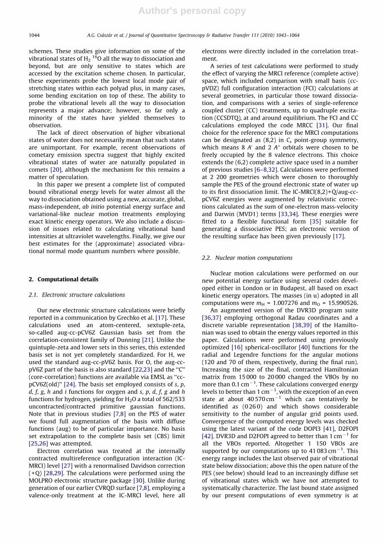
Wave function plots for selected states are presentedin Figs. 2–5. In Figs. 2–5 the positive and negative valuesare in red and blue, respectively. Change of colorstherefore indicates a node in the wavefunction. Eachplot also gives a contour corresponding to the classicalturning point of the potential at the eigenenergy of thestate under consideration. This contour is useful forassessing the chaotic nature of the state: classicallychaotic states are ergodic meaning that they sample allavailable phase space (see Fig. 5). Quantum mechanicallyan ergodic state would be expected to sample the wholeof the available PES [52]. We note that for states neardissociation the potential is in principle open todissociation, although the molecule has insufficientenergy to occupy the OH vibrational ground state andtherefore to dissociate. This is a feature of all polyatomicsystems and has been found to lead to interestingasymptotic structures in the vibrational states [53].

3. Results

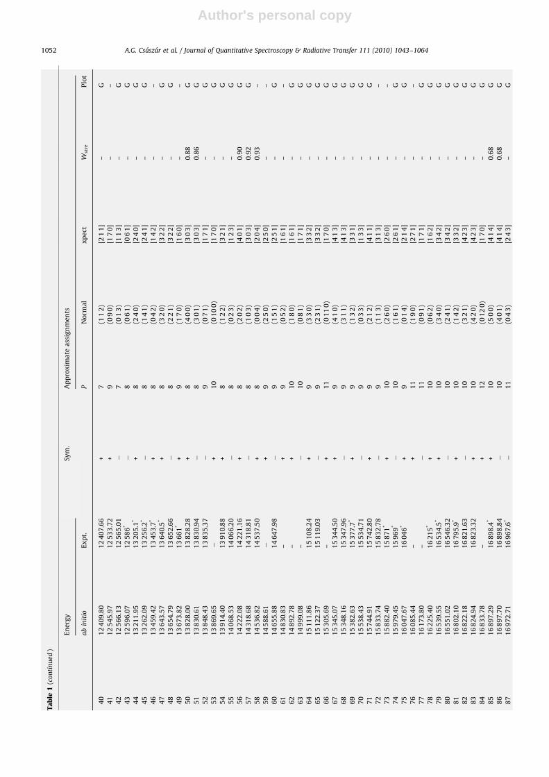
Table 1 presents our calculated vibrational bandorigins (VBOs) for H2

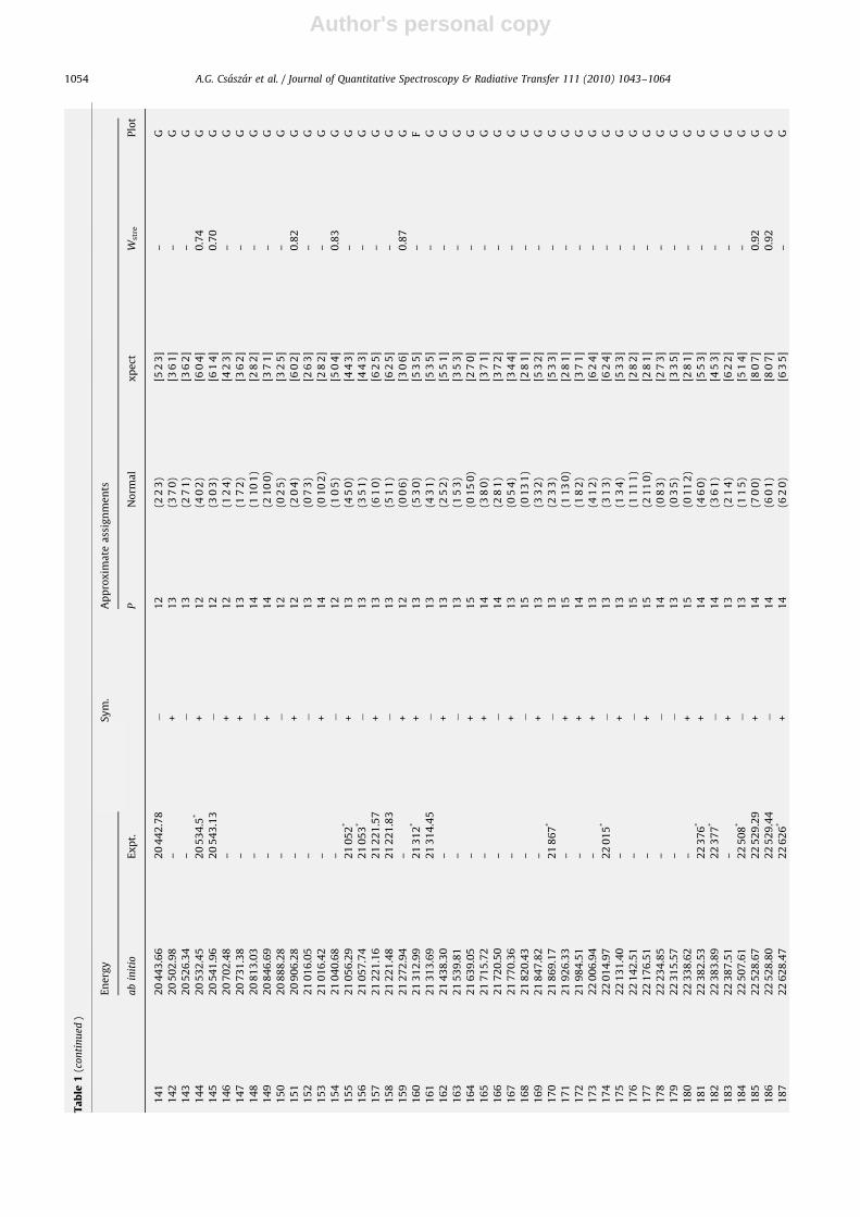
16O up to 25 200 cm�1; wherepossible, they are compared to available experimentaldata [16–18,54,55]. It should be noted that as yettransitions to only about 15% of all the VBOs haveactually been observed, so the majority of the reportedlevels represent our predictions for VBOs of water. Table 1also lists approximate vibrational quantum numbers andinformation related to several assignment schemes formany of the calculated VBOs. A complete set of VBOsdetermined in this study are given as Table S1 in theSupplementary Material. Those VBOs lying above25 200 cm�1 for which we could determine approximatenormal mode labels are given in Table 2; this table coversall those higher-lying VBOs which have experimentalcounterparts.

3.1. Quality of the PES

In the past we have advocated the use of the compositefocal-point analysis (FPA) approach [25,26,56,57] for thecomputation of the PESs and DMSs of smaller molecules[7,8,32,58]. There were three reasons for deviating slightlyfrom this approach during this study. First, previouselectronic structure studies on the ground-state PES ofwater [7,8] and on its barrier to linearity [59,60] provedthat one must use as large of a Gaussian basis set aspossible for treating appropriately the large-amplitudeexcited bending and stretching motions of water. Thislimits considerably the accessible choices for the level ofelectronic structure theory applicable to generate thelarge number of energy points needed for the surfaces.Second, it turned out that high quality treatment ofelectron correlation is less important than the choice ofthe Gaussian basis. Third, by far the most important so-called ‘‘small effects’’ [26] are the core and the MVD1relativistic energy corrections, covered by the presentstudy in a single computation per energy point. Thepresent PES, when used in a variational nuclear motion

computation with exact kinetic energy operators, canreproduce excellently the measured vibrational energylevels up to the dissociation limit. The differencesbetween the computed and the experimental levels canbe seen in Fig. 6.

There are a number of salient features of the presentPES which are worth discussing. The Born–Oppenheimerequilibrium structure, re

BO, has re(OH)=0.95782 A andyeðHOHÞ ¼ 104:463. These values are extremely close tothe best available re

BO estimates, corresponding to thecomposite CVRQD PES of H2

16O [61], namely re=0.95785A and ye ¼ 104:503. The independent quadratic forceconstants, in units of aJ An rad2�n, n=0�2, correspondingto the global PES are frr = 8.453, frr0 ¼ �0:105, fyy ¼ 0:704,and fry ¼ 0:257. These valence coordinate force constantsare also very close to those characterizing the CVRQD PES(frr=8.460, frr0 ¼ �0:103, fyy ¼ 0:703, and fry ¼ 0:258).These structural and force field parameters have beenused, along with the masses, to construct the normalcoordinates in DEWE and the normal mode decomposi-tion. Finally, we note that the D0 dissociation energy of H216O for the present ab initio PES differs from the well-established experimental value, 41 145.94(15) cm�1 [19],by only 37 cm�1. This difference comes about as follows.The aug-cc-pCV6Z IC-MRCI+Q(8,2) PES has De=43 951cm�1. The MVD1 correction to this is �50 cm�1. Thezero-point vibrational energy (ZPVE) correction for H2O,corresponding to the present PES, is �4 638.6 cm�1

(compare to �4 638.3 cm�1 corresponding to the CVRQDPES), while that of OH is +1 847 cm�1.

The results presented above and below and thebenchmark ab initio calculation of D0 by Ruscic et al.[62] together with the results of previous studies on waterbuilt upon the FPA philosophy can be used to providepointers on how one could improve the present globalpotential. There are at least four main ‘‘effects’’ notconsidered in our computational treatment. First, theaug-cc-pCV6Z basis set used, while very large, carries abasis set incompleteness error (BSIE) due to its finite sizeand especially to the use of fixed exponents and centers[63]. We estimate that the correction to D0 due to BSIEmay be as much as +80 cm�1. Second, estimation of thecorrelation energy is based on the IC-MRCI approachwhich, with respect to full-CI, introduces a noticeableerror. As several observations made during this studysuggest, this error could be as large as 40–50 cm�1. Forexample, using the cc-pVDZ basis which permits going tothe FCI limit, further away from equilibrium the error ofIC-MRCI+Q using the enlarged active space is of the orderof 40 cm�1. Third, though scalar relativistic effects,calculated as expectation values of the mass-velocityand one-electron Darwin operators, were included in thecalculation, these do not account for all relativistic effectseven for the molecule of water [64,65]. Of particularconcern when approaching the first dissociation limit, notconsidered in the present study, is the effect of spin–orbitinteraction on D0. It was reported by Ruscic et al. [62] tobe 38 cm�1. Fourth, the electronic structure treatmentemployed does not go beyond the Born–Oppenheimerseparation of nuclear and electronic degrees of freedom.An improvement in the accuracy of the ab initio calcula-

ARTICLE IN PRESS



tions could be made by inclusion of adiabatic and non-adiabatic corrections. For example, the adiabatic correc-tion contributes about +40 cm�1 to the dissociationenergy. The non-adiabatic contribution is hard to estimatebut we would expect it to partially cancel the adiabaticcorrection. In summary, even at the very high level ofelectronic structure theory employed in this study itseems that we are gaining accuracy from a fortuitouscancellation of some of the effects mentioned and nottaken into account. Further advance in the ab initio

computation of the complete set of VBOs for water wouldbenefit only from a joint consideration of all these factors

as individual inclusion of any one of them might evenmake some of our predictions appear worse.

3.2. Vibrational band origins

Some estimates of the accuracy of our first-principlespredictions can be made by comparison of the computedVBOs with the observed ones. Fig. 6 shows that not onlythe differences are small but also the trends aresystematic. For the lower-energy VBOs there are clearseries corresponding to bending overtones with no

ARTICLE IN PRESS

Fig. 2. Plots of real wave functions for selected pure symmetric and antisymmetric stretching states of even symmetry. For symmetric stretches the

nodes can be observed along the r1 and r2 internal coordinates. For antisymmetric stretches the nodes are along r1�r2. Each plot also gives a contour

corresponding to the classical turning point of the potential at the eigenenergy of the state under consideration. The plots and thus the states are labelled

as (v1 v2 v3), for details see the text. (a) (1 0 0), (b) (8 0 0), (c) (16 0 0), (d) (17 0 0), (e) (0 0 4), (f) (0 0 12).



stretching excitation, one quanta of stretch (two series),two quanta of stretch (two series) and three quanta ofstretch (two series). These series show that the errorsincrease quite rapidly with increasing bending excita-tions: it is actually well known that this motion is hard totreat correctly ab initio [66,67]. At higher frequenciesthere are very few observed states with significantbending excitation. In contrast the errors in the calculatedpure stretching VBOs remains small, 1 cm�1 or less, up toabout 25 000 cm�1; above this value the error becomespositive and then, in the last 2000 cm�1 below dissocia-tion, sharply negative. At dissociation the error in thehighest stretching states, (17 0 0)–(18 0 1), approaches40 cm�1, the amount our PES underestimates D0. Thesystematic nature of these errors suggest that there isscope to improve the calculated VBOs by fitting the PES tothe observed levels. Predicted transition frequenciesbased on the predicted VBOs can be improved either bymaking manual corrections [68] or by performing a fit tothe experimental data starting from our PES.

It can be expected that vibrational band intensitiesdecrease systematically with increasing energy of theVBOs since it is well known that overtone bands becomeincreasingly weaker. However, this decrease is notmonotonic with respect to the energy. Instead, somestretching VBOs decrease less rapidly than others as couldbe anticipated from the fact that direct excitation of stateswith eight quanta of stretch has already been achievedusing cavity ring-down spectroscopy [14].

The absorption of light by water vapor at ultravioletwavelengths could be of atmospheric importance, parti-cularly at wavelengths below the onset of the main ozoneabsorptions. The ability to estimate the magnitude of thisabsorption should be within the scope of our presentstudy but in practice we found that the presently availabledipole moment surfaces are not suitable for such calcula-tions. The harmonic model of molecular vibrationssuggests that the intensity of a fundamental transitiondepends principally on the first derivative of the dipolemoment at equilibrium taken along the vibrational modebeing excited. Within this model, the intensity of the n thovertone then depends on the (n+1)th derivative of thedipole surface. What we have found is that the best dipole

moment surfaces available for water [32,45] do not givereliable tenth or higher derivatives in the region ofequilibrium geometry. Resolving this problem will bethe subject of future work. Before leaving this topic weshould note that our concern about the use of theavailable dipole moment surfaces for studying highovertones does not invalidate the transition intensitycalculations presented by Grechko et al. [17]. In this workintensities were given for individual rotation–vibrationtransitions which reached states near the dissociationlimit. However, these transitions link states differing by 8or less quanta of stretch, for which no difficulties havebeen identified.

3.3. Vibrational state assignments

The variational-type nuclear motion proceduresemployed in this study are based on the use of rigorousquantum numbers. For the vibrational states of H2

16Othis means that the states are only distinguished by asingle quantum number: the permutational symmetry ofthe state, which can be viewed as ð�1Þv3 for states with anormal-mode assignment, where v3 is the vibrationalnormal-mode quantum number corresponding to theantisymmetric stretch. Other, approximate vibrationalquantum number labels have to be assigned by othermeans.

Previous calculations [3], which used a different PES,suggested that at energies approaching D0 the vibrationalstates of water become highly irregular with littlesystematic underlying structure. This situation is notpromising for assigning approximate vibrational labels.Indeed, there is no guarantee that such labels exist [52],although there are clear rules when they can beconsidered rigorous [69].

In some contrast to this picture, a previous jointexperimental–theoretical study of water spectra up todissociation [17] observed spectra which were stronglystructured with a relatively small number of fairly stronglines. This observation was mirrored by the associatedtransition intensity calculations. For these states, at least,it proved straightforward to assign vibrational labels [17]

ARTICLE IN PRESS

Fig. 3. Wave function plots for pure bending states. For a detailed description see the legend to Fig. 2. (a) (0 1 0), (b) (0 22 0).



using the PES described here. These results demonstratethat the VBOs given by our PES are at least partiallystructured. This motivated us to try and find a set of labelsfor as many vibrational states as possible, extending aprevious study of some of the authors [70] employing adifferent PES.

To make normal mode quantum number assignments,five strategies were investigated.

1. Energy decomposition. The simplest method is to usethe energy dependence based on the normal modequantum numbers. This can be expressed as

Eðv1;v2;v3Þ ¼ v1n1þv2n2þv3n3; ð1Þ

where v1, v2, v3 (v1 v2 v3) and n1, n2, n3 are thevibrational quantum numbers and the vibrationalfundamentals for the so-called symmetric stretch,bend, and antisymmetric stretch normal modes,respectively. This method works well up to about12 000 cm�1 and no additional information is requiredto label the VBOs. We note that at the higher end ofthis region the stretching motions of water are alreadymuch closer described by a local mode rather than anormal mode picture [71]. Above this energy, thedensity of states increases and there are often severalcandidates for a given set of vibrational normal modequantum numbers. Furthermore, as the normal modedecomposition (NMD) analysis presented below

ARTICLE IN PRESS

Fig. 4. Wave function plots for stretching states with small bending excitation. For a detailed description see the legend to Fig. 2. (a) (1 1 0), (b) (1 2 0), (c)

(15 1 0), (d) (16 1 0), (e) (14 2 0), (f) (15 2 0).



shows, even when normal mode labels can be allocatedbased on this scheme, their physical relevance canclearly be questioned.

2. Wave function plots. Inspection of 2D cuts of the realwave function plots along appropriately chosencoordinates sometimes gives valuable qualitative in-formation on the level and is particularly useful forstates of more or less pure stretching or bendingcharacter. However, plots cannot be used to getquantitative information on mixtures without signifi-cant manipulation [72], which was not attempted here.It would also be hard to identify multiply excitedlevels, e.g., (5 5 5), by visual inspection even if such astate was fairly harmonic.

3. Mean values of squares of the Jensen coordinates /s2i S

i=1,2,3 [73]. These expectation values were calculatedby the program XPECT3 [37]. Normal mode-likelabels can be created by rounding the expectationvalues to the nearest integers. For a harmonic oscillatorthis label should be proportional to the normalmode quantum number vi. Indeed, for the lowest-lying levels these labels reproduce the normal modelabels of the most dominant harmonic oscillatorfunctions contributing to the ‘‘exact’’ state. However,for a Morse-like real oscillator the well is wider and themean values grow quicker than vi. Thus, /s2

i S for thetwo stretching modes grows too fast. The largest‘xpect’ stretching quantum numbers are for states(n 0 0), decreasing for other members of the samepolyad. The v2 ‘xpect’ quantum number, on the otherhand, grows slower than the ‘‘harmonic’’ quantumnumber. By extrapolating the behavior of these ‘xpect’quantum numbers from states with known labels tounknown ones one can guess normal mode labels. Theresulting labels are given in Table 1 under the heading‘‘xpect’’.

4. Perturbing the bending part of the PES. Assignment ofvibrational quantum numbers to levels with large v2

values is particularly difficult. Therefore, we analyzed

the change in the energy of a level with the inclusion ofan artificial term in the PES depending only on theangle. For this we actually used a term designed tocorrect the height of the barrier to linearity of water[60,66,67]. Changes in a level’s energy were found tobe practically independent of the stretching quantumnumbers v1 and v3. For values of the bending quantumnumber v2 between 0 and 7, shifts in the levels werefound to be directly proportional to v2, greatlyfacilitating the assignment procedure. Consequently,comparing changes observed for unlabelled levels withthose of already labelled ones we could determine thevalues of v2 for these states. The maximum changeoccurred near v2=8. For higher v2 values the changeswere found to be apparently only indicators that v2 hasa high value.

5. Normal mode decomposition (NMD). Another assign-ment procedure used in this work was based on thenormal mode decomposition [74] of the variationalwave function. In the NMD the variationally computed,normalized vibrational wave functions, ci, are char-acterized by the square of their overlaps with thenormalized harmonic oscillator wave functions, fHO

v ,expressed in terms of normal coordinates correspond-ing to the actual PES,

wiv ¼ j/cijfHOv Sj2; ð2Þ

where v=(v1 v2 v3) is a composite index. For eachvibrational state the sum of the NMD entries equalsone,

Pj ¼ 0wij ¼ 1, as the wave function can be

expressed as a linear combination of harmonic oscil-lator wave functions. The wave functions obtainedwith the DEWE program [47,48] are given in terms ofnormal coordinates, so the computation of their over-lap with the actual harmonic oscillator wave functionsis straightforward. As the bending modes of water arevery anharmonic and higher bends cannot be treatedwith the DEWE protocol, the method provides mean-ingful results only for states with v2=0 values, as could

ARTICLE IN PRESS

Fig. 5. Wave function plot for an ergodic state. For a detailed description see the legend to Fig. 2.


Author's personal copyARTICLE IN PRESS

Ta

ble

1T

he

low

est

25

0v

ibra

tio

na

lb

an

do

rig

ins

(co

mp

ute

da

sp

art

of

this

stu

dy

an

de

xp

eri

me

nta

l(E

xp

t.))

,th

eir

sym

me

trie

s(S

ym

.),t

he

corr

esp

on

din

gp

oly

ad

nu

mb

er

P,d

efi

ne

da

sP

=2

v1

+v

2+

2v

3,a

nd

ap

pro

xim

ate

vib

rati

on

al

ass

ign

me

nts

corr

esp

on

din

gto

the

PE

Sd

ev

elo

pe

din

this

pa

pe

r.a

En

erg

yS

ym

.A

pp

rox

ima

tea

ssig

nm

en

ts

ab

init

ioE

xp

t.P

No

rma

lx

pe

ctW

stre

Plo

t

11

59

6.3

71

59

4.7

5+

1(0

10

)[0

10

]–

G

23

15

4.4

53

15

1.6

3+

2(0

20

)[0

20

]–

G

33

65

7.4

13

65

7.0

5+

2(1

00

)[1

00

]0

.98

G

43

75

5.9

33

75

5.9

3�

2(0

01

)[0

01

]0

.99

G

54

67

0.8

64

66

6.7

9+

3(0

30

)[0

30

]–

G

65

23

6.7

55

23

4.9

7+

3(1

10

)[1

10

]–

G

75

33

2.8

75

33

1.2

7�

3(0

11

)[0

11

]–

G

86

13

9.6

26

13

4.0

1+

4(0

40

)[0

40

]–

G

96

77

8.2

56

77

5.0

9+

4(1

20

)[1

20

]–

G

10

68

74

.32

68

71

.52

�4

(02

1)

[02

1]

–G

11

72

02

.45

72

01

.54

+4

(20

0)

[20

0]

0.9

6G

12

72

50

.44

72

49

.82

�4

(10

1)

[10

1]

0.9

7G

13

74

44

.91

74

45

.05

+4

(00

2)

[10

2]

0.9

8G

14

75

50

.09

75

42

.44

+5

(05

0)

[05

0]

–G

15

82

78

.89

82

73

.98

+5

(13

0)

[13

0]

–G

16

83

77

.92

83

73

.85

�5

(03

1)

[03

1]

–G

17

87

63

.71

87

61

.58

+5

(21

0)

[21

0]

–G

18

88

08

.85

88

07

.00

�5

(11

1)

[11

1]

–G

19

88

80

.85

88

69

.95

+6

(06

0)

[06

0]

–G

20

90

01

.59

90

00

.14

+5

(01

2)

[11

2]

–G

21

97

31

.26

97

24

.3*

+6

(14

0)

[14

0]

–G

22

98

39

.13

98

33

.59

�6

(04

1)

[04

1]

–G

23

10

10

0.3

61

00

86

.05

+7

(07

0)

[07

0]

–G

24

10

28

7.8

11

02

84

.37

+6

(22

0)

[22

1]

–G

25

10

33

1.6

51

03

28

.73

�6

(12

1)

[12

1]

–G

26

10

52

4.5

31

05

21

.76

+6

(02

2)

[12

2]

–G

27

10

60

0.3

81

05

99

.69

+6

(30

0)

[30

1]

0.9

3G

28

10

61

3.8

21

06

13

.35

�6

(20

1)

[20

2]

0.9

4G

29

10

86

9.6

21

08

68

.88

+6

(10

2)

[20

1]

0.9

4G

30

11

03

2.0

41

10

32

.40

�6

(00

3)

[10

3]

0.9

6G

31

11

10

9.0

0–

+7

(15

0)

[15

0]

–G

32

11

25

0.1

51

12

42

.78

�7

(05

1)

[05

1]

–G

33

11

26

7.4

41

12

54

.00

+8

(08

0)

[07

0]

–G

34

11

77

2.5

31

17

67

.39

+7

(23

0)

[23

1]

–G

35

11

81

7.5

11

18

13

.20

�7

(13

1)

[23

1]

–G

36

12

01

2.0

31

20

07

.78

+7

(03

2)

[13

2]

–G

37

12

14

0.9

11

21

39

.32

+7

(31

0)

[31

2]

–G

38

12

15

2.6

01

21

51

.25

�7

(21

1)

[21

2]

–G

39

12

39

2.9

6–

+8

(16

0)

[16

0]

––



Ta

ble

1(c

on

tin

ued

)

En

erg

yS

ym

.A

pp

rox

ima

tea

ssig

nm

en

ts

ab

init

ioE

xp

t.P

No

rma

lx

pe

ctW

stre

Plo

t

40

12

40

9.8

01

24

07

.66

+7

(11

2)

[21

1]

–G

41

12

54

5.9

71

25

33

.72

+9

(09

0)

[17

0]

––

42

12

56

6.1

31

25

65

.01

�7

(01

3)

[11

3]

–G

43

12

59

6.0

71

25

86

*�

8(0

61

)[0

61

]–

G

44

13

21

1.9

51

32

05

.1*

+8

(24

0)

[24

0]

–G

45

13

26

2.0

91

32

56

.2*

�8

(14

1)

[24

1]

–G

46

13

45

9.4

21

34

53

.7*

+8

(04

2)

[14

2]

––

47

13

64

3.5

71

36

40

.5*

+8

(32

0)

[32

2]

–G

48

13

65

4.7

91

36

52

.66

�8

(22

1)

[32

2]

–G

49

13

67

3.8

21

36

61

*+

9(1

70

)[1

60

]–

–

50

13

82

8.0

01

38

28

.28

+8

(40

0)

[30

3]

0.8

8G

51

13

83

0.6

11

38

30

.94

�8

(30

1)

[30

3]

0.8

6G

52

13

84

8.4

31

38

35

.37

�9

(07

1)

[17

1]

–G

53

13

86

9.6

5�

+1

0(0

10

0)

[17

0]

–G

54

13

91

4.4

01

39

10

.88

+8

(12

2)

[32

1]

–G

55

14

06

8.5

31

40

66

.20

�8

(02

3)

[12

3]

–G

56

14

22

2.0

81

42

21

.16

+8

(20

2)

[40

1]

0.9

0G

57

14

31

8.6

81

43

18

.81

�8

(10

3)

[30

3]

0.9

2G

58

14

53

6.8

21

45

37

.50

+8

(00

4)

[20

4]

0.9

3–

59

14

58

8.6

1�

+9

(25

0)

[25

0]

––

60

14

65

5.8

81

46

47

.98

�9

(15

1)

[25

1]

–G

61

14

83

0.8

3–

+9

(05

2)

[16

1]

––

62

14

89

2.7

8–

+1

0(1

80

)[1

61

]–

G

63

14

99

9.0

8–

�1

0(0

81

)[1

71

]–

G

64

15

11

1.8

61

51

08

.24

+9

(33

0)

[33

2]

–G

65

15

12

2.3

71

51

19

.03

�9

(23

1)

[33

2]

–G

66

15

30

5.6

9–

+1

1(0

11

0)

[17

0]

–G

67

15

34

5.0

71

53

44

.50

+9

(41

0)

[41

3]

–G

68

15

34

8.1

61

53

47

.96

�9

(31

1)

[41

3]

–G

69

15

38

2.6

31

53

77

.7*

+9

(13

2)

[33

1]

–G

70

15

53

8.4

31

55

34

.71

�9

(03

3)

[13

3]

–G

71

15

74

4.9

11

57

42

.80

+9

(21

2)

[41

1]

–G

72

15

83

3.7

41

58

32

.78

�9

(11

3)

[31

3]

––

73

15

88

2.4

01

58

71

*+

10

(26

0)

[26

0]

––

74

15

97

9.4

51

59

69

*�

10

(16

1)

[26

1]

–G

75

16

04

7.6

71

60

46

*+

9(0

14

)[2

14

]–

G

76

16

08

5.4

4–

+1

1(1

90

)[2

71

]–

–

77

16

17

3.8

0–

�1

1(0

91

)[1

71

]–

G

78

16

22

5.4

01

62

15

*+

10

(06

2)

[16

2]

–G

79

16

53

9.5

51

65

34

.5*

+1

0(3

40

)[3

42

]–

G

80

16

55

1.0

21

65

46

.32

�1

0(2

41

)[3

42

]–

G

81

16

80

2.1

01

67

95

.9*

+1

0(1

42

)[3

32

]–

G

82

16

82

2.1

81

68

21

.63

�1

0(3

21

)[4

23

]–

G

83

16

82

4.9

41

68

23

.32

+1

0(4

20

)[4

23

]–

G

84

16

83

3.7

8–

+1

2(0

12

0)

[17

0]

–G

85

16

89

7.2

91

68

98

.4*

+1

0(5

00

)[4

14

]0

.68

G

86

16

89

7.7

01

68

98

.84

�1

0(4

01

)[4

14

]0

.68

G

87

16

97

2.7

11

69

67

.6*

�1

1(0

43

)[2

43

]–

G



88

17

15

1.4

31

71

39

*+

11

(27

0)

[26

0]

–G

89

17

23

0.9

21

72

27

.38

+1

0(2

22

)[4

21

]–

G

90

17

24

2.0

4–

�1

1(1

71

)[2

61

]–

G

91

17

31

4.5

91

73

12

.55

�1

0(1

23

)[3

23

]–

G

92

17

39

6.0

9–

+1

2(1

10

0)

[17

1]

–G

93

17

45

6.9

7–

�1

2(0

10

1)

[17

1]

–G

94

17

45

8.3

61

74

58

.21

+1

0(3

02

)[5

02

]0

.86

G

95

17

49

4.7

91

74

95

.53

�1

0(2

03

)[4

03

]0

.86

G

96

17

50

4.0

5–

+1

1(0

72

)[1

72

]–

G

97

17

52

8.3

41

75

26

.3*

+1

0(0

24

)[2

24

]–

G

98

17

74

8.0

01

77

48

.11

+1

0(1

04

)[4

03

]0

.88

G

99

17

91

8.4

51

79

11

.6*

+1

1(3

50

)[3

41

]–

G

10

01

79

34

.32

17

92

8*

�1

1(2

51

)[3

42

]–

G

10

11

79

47

.30

–�

10

(00

5)

[20

5]

0.9

1G

10

21

81

70

.61

18

16

2*

+1

1(1

52

)[3

51

]–

–

10

31

82

67

.50

18

26

5.8

2�

11

(33

1)

[43

3]

–G

10

41

82

68

.81

18

26

7.1

*+

11

(43

0)

[43

3]

–G

10

51

83

46

.16

–+

12

(28

0)

[27

0]

–G

10

61

83

57

.81

18

35

0.3

*�

11

(05

3)

[25

3]

––

10

71

83

91

.95

18

39

2.7

8+

11

(51

0)

[52

4]

–G

10

81

83

92

.51

18

39

3.3

1�

11

(41

1)

[52

4]

–G

10

91

84

35

.01

–+

13

(01

30

)[1

80

]–

G

11

01

84

36

.95

–�

12

(18

1)

[27

2]

–G

11

11

86

57

.57

–+

12

(08

2)

[17

2]

–G

11

21

86

80

.15

–+

11

(23

2)

[43

1]

–G

11

31

87

61

.97

18

75

8.6

3�

11

(13

3)

[33

3]

–G

11

41

88

17

.64

–+

13

(11

10

)[2

80

]–

G

11

51

88

30

.31

–�

13

(01

11

)[1

81

]–

G

11

61

89

57

.16

18

95

5.7

*+

11

(31

2)

[51

2]

–G

11

71

89

80

.19

18

97

7.2

*+

11

(03

4)

[33

4]

–G

11

81

89

90

.12

18

98

9.9

6�

11

(21

3)

[41

3]

–G

11

91

92

32

.48

19

22

3.5

*+

12

(36

0)

[35

1]

–G

12

01

92

43

.31

–+

11

(11

4)

[41

3]

–G

12

11

92

58

.70

19

25

0*

�1

2(2

61

)[3

52

]–

G

12

21

94

32

.72

–�

11

(01

5)

[31

5]

–G

12

31

94

51

.40

–+

12

(16

2)

[36

2]

–G

12

41

95

64

.31

–�

13

(19

1)

[27

2]

–G

12

51

95

87

.41

–+

13

(29

0)

[37

1]

–G

12

61

96

80

.63

19

67

7.8

*+

12

(44

0)

[43

3]

–G

12

71

96

82

.08

19

67

9.1

9�

12

(34

1)

[43

3]

–G

12

81

97

29

.44

19

72

0.2

*�

12

(06

3)

[25

3]

–G

12

91

97

79

.54

19

78

1.3

2+

12

(60

0)

[60

5]

0.8

7G

13

01

97

79

.78

19

78

1.1

0�

12

(50

1)

[60

5]

0.8

8G

13

11

97

93

.51

–+

13

(09

2)

[18

2]

–G

13

21

98

64

.02

19

86

4.7

*+

12

(52

0)

[52

4]

–G

13

31

98

64

.47

19

86

5.2

8�

12

(42

1)

[52

4]

–G

13

42

00

39

.28

–+

14

(01

40

)[1

70

]–

G

13

52

00

85

.94

–+

12

(24

2)

[54

1]

–G

13

62

01

73

.47

–�

12

(14

3)

[34

3]

–G

13

72

02

88

.91

–�

14

(01

21

)[1

81

]–

G

13

82

03

21

.93

–+

14

(11

20

)[2

80

]–

G

13

92

03

90

.73

–+

12

(04

4)

[33

4]

–G

14

02

04

21

.53

–+

12

(32

2)

[52

2]

–G



Ta

ble

1(c

on

tin

ued

)

En

erg

yS

ym

.A

pp

rox

ima

tea

ssig

nm

en

ts

ab

init

ioE

xp

t.P

No

rma

lx

pe

ctW

stre

Plo

t

14

12

04

43

.66

20

44

2.7

8�

12

(22

3)

[52

3]

–G

14

22

05

02

.98

–+

13

(37

0)

[36

1]

–G

14

32

05

26

.34

–�

13

(27

1)

[36

2]

–G

14

42

05

32

.45

20

53

4.5

*+

12

(40

2)

[60

4]

0.7

4G

14

52

05

41

.96

20

54

3.1

3�

12

(30

3)

[61

4]

0.7

0G

14

62

07

02

.48

–+

12

(12

4)

[42

3]

–G

14

72

07

31

.38

–+

13

(17

2)

[36

2]

–G

14

82

08

13

.03

–�

14

(11

01

)[2

82

]–

G

14

92

08

46

.69

–+

14

(21

00

)[3

71

]–

G

15

02

08

88

.28

–�

12

(02

5)

[32

5]

–G

15

12

09

06

.28

–+

12

(20

4)

[60

2]

0.8

2G

15

22

10

16

.05

–�

13

(07

3)

[26

3]

–G

15

32

10

16

.42

–+

14

(01

02

)[2

82

]–

G

15

42

10

40

.68

–�

12

(10

5)

[50

4]

0.8

3G

15

52

10

56

.29

21

05

2*

+1

3(4

50

)[4

43

]–

G

15

62

10

57

.74

21

05

3*

�1

3(3

51

)[4

43

]–

G

15

72

12

21

.16

21

22

1.5

7+

13

(61

0)

[62

5]

–G

15

82

12

21

.48

21

22

1.8

3�

13

(51

1)

[62

5]

–G

15

92

12

72

.94

–+

12

(00

6)

[30

6]

0.8

7G

16

02

13

12

.99

21

31

2*

+1

3(5

30

)[5

35

]–

F

16

12

13

13

.69

21

31

4.4

5�

13

(43

1)

[53

5]

–G

16

22

14

38

.30

–+

13

(25

2)

[55

1]

–G

16

32

15

39

.81

–�

13

(15

3)

[35

3]

–G

16

42

16

39

.05

–+

15

(01

50

)[2

70

]–

G

16

52

17

15

.72

–+

14

(38

0)

[37

1]

–G

16

62

17

20

.50

–�

14

(28

1)

[37

2]

–G

16

72

17

70

.36

–+

13

(05

4)

[34

4]

–G

16

82

18

20

.43

–�

15

(01

31

)[2

81

]–

G

16

92

18

47

.82

–+

13

(33

2)

[53

2]

–G

17

02

18

69

.17

21

86

7*

�1

3(2

33

)[5

33

]–

G

17

12

19

26

.33

–+

15

(11

30

)[2

81

]–

G

17

22

19

84

.51

–+

14

(18

2)

[37

1]

–G

17

32

20

06

.94

–+

13

(41

2)

[62

4]

–G

17

42

20

14

.97

22

01

5*

�1

3(3

13

)[6

24

]–

G

17

52

21

31

.40

–+

13

(13

4)

[53

3]

–G

17

62

21

42

.51

–�

15

(11

11

)[2

82

]–

G

17

72

21

76

.51

–+

15

(21

10

)[2

81

]–

G

17

82

22

34

.85

–�

14

(08

3)

[27

3]

–G

17

92

23

15

.57

–�

13

(03

5)

[33

5]

–G

18

02

23

38

.62

–+

15

(01

12

)[2

81

]–

G

18

12

23

82

.53

22

37

6*

+1

4(4

60

)[5

53

]–

G

18

22

23

83

.89

22

37

7*

�1

4(3

61

)[4

53

]–

G

18

32

23

87

.51

–+

13

(21

4)

[62

2]

–G

18

42

25

07

.61

22

50

8*

�1

3(1

15

)[5

14

]–

G

18

52

25

28

.67

22

52

9.2

9+

14

(70

0)

[80

7]

0.9

2G

18

62

25

28

.80

22

52

9.4

4�

14

(60

1)

[80

7]

0.9

2G

18

72

26

28

.47

22

62

6*

+1

4(6

20

)[6

35

]–

G



18

82

26

30

.29

22

62

9*

�1

4(5

21

)[6

35

]–

G

18

92

27

08

.35

–+

14

(26

2)

[55

2]

–G

19

02

27

32

.30

–+

13

(01

6)

[41

6]

–G

19

12

27

38

.51

–�

14

(44

1)

[63

5]

–G

19

22

27

44

.61

–+

14

(54

0)

[54

5]

–G

19

32

28

10

.73

–�

15

(29

1)

[37

3]

–G

19

42

28

85

.31

–+

15

(39

0)

[47

1]

–G

19

52

29

25

.68

–�

14

(16

3)

[36

2]

––

19

62

30

67

.43

–+

15

(19

2)

[36

3]

––

19

72

31

57

.70

–+

14

(06

4)

[36

3]

––

19

82

32

36

.60

–+

14

(34

2)

[64

2]

–G

19

92

32

57

.08

–�

14

(24

3)

[54

3]

–G

20

02

32

63

.52

–+

16

(11

40

)[3

70

]–

G

20

12

33

22

.45

–�

15

(09

3)

[28

3]

––

20

22

33

66

.38

–�

16

(01

41

)[2

82

]–

G

20

32

34

00

.04

23

40

1*

+1

4(5

02

)[7

15

]0

.74

G

20

42

34

04

.07

23

40

5.4

*�

14

(40

3)

[71

5]

0.7

6G

20

52

34

66

.78

–+

14

(42

2)

[62

4]

–G

20

62

34

74

.45

–�

14

(32

3)

[62

5]

–G

20

72

35

24

.78

–+

14

(14

4)

[54

3]

–G

20

82

35

59

.74

–+

16

(21

20

)[3

81

]–

G

20

92

36

05

.07

–�

16

(11

21

)[3

82

]–

G

21

02

36

52

.29

–+

16

(01

60

)[3

72

]–

–

21

12

36

63

.89

–+

15

(47

0)

[37

2]

––

21

22

36

65

.77

–�

15

(37

1)

[46

3]

–G

21

32

37

13

.51

–�

14

(04

5)

[34

5]

–G

21

42

37

87

.05

–+

16

(01

22

)[2

81

]–

–

21

52

38

25

.74

–+

14

(22

4)

[72

2]

–G

21

62

39

35

.12

23

93

4*

�1

4(1

25

)[6

25

]–

G

21

72

39

44

.48

23

94

2*

+1

5(7

10

)[7

26

]–

G

21

82

39

47

.68

23

94

7*

�1

5(6

11

)[7

17

]–

G

21

92

39

60

.85

–+

15

(27

2)

[55

3]

––

22

02

39

77

.25

–+

14

(30

4)

[81

3]

0.7

3G

22

12

39

98

.57

–�

15

(45

1)

[55

4]

––

22

22

40

15

.44

–+

15

(55

0)

[64

5]

–G

22

32

40

33

.57

–�

16

(21

01

)[4

63

]–

–

22

42

40

38

.37

–�

14

(20

5)

[71

4]

0.6

9G

22

52

40

91

.22

–+

16

(31

00

)[4

82

]–

G

22

62

41

42

.76

–�

15

(53

1)

[64

6]

–G

22

72

41

43

.05

–+

15

(63

0)

[64

6]

–F

22

82

41

62

.05

–+

14

(02

6)

[42

6]

–G

22

92

41

77

.98

–�

15

(17

3)

[46

3]

––

23

02

42

90

.62

–+

14

(10

6)

[60

5]

0.7

8G

23

12

43

12

.65

–+

16

(11

02

)[3

72

]–

F

23

22

44

35

.42

–+

15

(07

4)

[36

3]

–F

23

32

44

66

.99

–�

16

(01

03

)[2

83

]–

F

23

42

45

08

.22

–�

14

(00

7)

[40

7]

0.8

3G

23

52

45

82

.36

–+

15

(35

2)

[64

2]

–F

23

62

46

09

.05

–�

15

(25

3)

[54

3]

–G

23

72

47

98

.22

–+

15

(51

2)

[73

4]

––

23

82

48

07

.86

–�

15

(41

3)

[72

5]

––

23

92

48

26

.40

–+

17

(21

30

)[4

61

]–

F

24

02

48

56

.94

–�

16

(38

1)

[46

3]

––

24

12

48

69

.48

–+

15

(15

4)

[54

3]

––



be seen when comparing the eigenvalues obtainedwith DVR3D and DEWE (the latter are not presentedhere).

The mean values of the squares of the Jensen coordi-nates provide meaningful labels for the lowest vibrationallevels. The labels obtained agree with the chosen normalmode labels up to (0 0 2) at 7441.91 cm�1. Above thisstate there are still a lot of meaningful labels but theyincreasingly start to break down. Of course, the mean-ingful labels are the same as those produced by the energydecomposition scheme.

According to the NMD analysis, the lowest-lyingvibrational energy levels are characterized by a single,dominant harmonic oscillator function, and thus theirassignment is absolutely unambiguous. For example, thevibrational state at 4670.86 cm�1 and described as (0 3 0)with a polyad number P = 3, where P = 2v1 + v2 + 2v3, isthe following mixture of the harmonic oscillator basisstates: 0.88(0 3 0) + 0.05(1 1 0) + 0.03(0 4 0). At the sametime, for higher-lying levels, with polyad numbers P =4�6, i.e., the second and third stretching overtone andcombination levels, the identification of a single, domi-nant harmonic oscillator wave function is not possible.Already for these states the attachment of a single (v1 v2

v3) normal mode label cannot be carried out withoutoverwhelming and steadily increasing ambiguities. Forexample, it seems completely natural to give the labels(4 0 0) and (2 0 2) to the states computed at 13 828 and14 222 cm�1. Nevertheless, the NMD analysis clearlyindicates that the harmonic oscillator basis functions(4 0 0) and (2 0 2) have basically zero weight in both exactwave functions. Both wave functions are extremely heavymixtures of the basis states, the largest NMD contribu-tions are 0.20(1 0 2), 0.12(3 0 2), and 0.11(3 0 0) for thestate at 13 828 cm�1, and 0.21(5 0 0), 0.18(3 0 0), and0.11(1 0 2) for the state at 14 222 cm�1. It is of particularinterest to note that Choi and Light [75], based on theirwave function analysis, reversed the order of the (4 0 0)and (2 0 2) states. The reverse order is supported by the‘xpect’ values of this study (Table 1). Nevertheless, due tothe indications of the NMD analysis, we decided to keepthe original, intuitively appealing ordering.

Thus, it is important to emphasize that the distributionof the possible normal mode labels (v1 v2 v3) is not rootedin firm theory but simply in tradition. Apart from thefundamentals and maybe low-lying overtones and com-bination levels, the linear combination of the ‘‘exact’’variational wave function in terms of harmonic oscillatorbasis functions is typically not dominated by a singleharmonic oscillator function. Despite the strong mixing ofharmonic oscillator wave functions in excited vibrationallevels, we attempted to employ the NMD analysis tojustify the distribution of some normal mode labels. Theintention was to identify ‘‘pure’’ stretching states,ðv1 0 v3Þv1;v3 ¼ 0;1; . . .. In order to do this, the ‘‘stretchingweight’’, Wstre, and the ‘‘number of stretching quanta’’,Nstre, were introduced as

Wstre ¼X

v1 ;v3

wi;v ¼ ðv1 ;0;v3Þð3Þ

ARTICLE IN PRESST

ab

le1

(co

nti

nu

ed)

En

erg

yS

ym

.A

pp

rox

ima

tea

ssig

nm

en

ts

ab

init

ioE

xp

t.P

No

rma

lx

pe

ctW

stre

Plo

t

24

22

48

83

.66

–+

16

(48

0)

[47

2]

–F

24

32

49

10

.71

–�

15

(33

3)

[63

4]

––

24

42

49

15

.51

–+

15

(43

2)

[63

4]

––

24

52

49

25

.35

–�

17

(11

31

)[3

72

]–

F

24

62

50

77

.92

–�

15

(05

5)

[34

5]

–G

24

72

50

94

.22

–+

17

(11

50

)[2

82

]–

F

24

82

51

21

.48

25

12

0*

+1

6(8

00

)[1

00

10

]0

.89

F

24

92

51

21

.50

25

12

0.2

8�

16

(70

1)

[10

01

0]

0.8

9G

25

02

51

56

.46

–+

17

(01

32

)[4

71

]–

–

aS

ym

.,p

erm

uta

tio

nsy

mm

etr

ych

ara

cte

rize

da

lso

byð�

1Þv

3fo

rst

ate

sw

ith

an

orm

al

mo

de

ass

ign

me

nt.

No

rma

l,n

orm

al

mo

de

ass

ign

me

nt

(v1

v2

v3)

ba

sed

on

the

no

rma

lm

od

eq

ua

ntu

mn

um

be

rsv

1,v

2,a

nd

v3

for

the

sym

me

tric

stre

tch

,b

en

d,

an

da

nti

sym

me

tric

stre

tch

mo

de

s.x

pe

ct,

ex

pe

cta

tio

nv

alu

es

of

the

squ

are

so

fth

eJe

nse

nco

ord

ina

tes

rou

nd

ed

toth

en

ea

rest

inte

ge

r(s

ee

tex

t).

Wst

re,

stre

tch

ing

we

igh

tin

the

wa

ve

fun

ctio

n,

calc

ula

ted

acc

ord

ing

toE

q.

(3).

Th

eb

an

dce

nte

rsm

ark

ed

wit

ha

na

ste

risk

we

ree

stim

ate

dfr

om

lev

els

wit

hJ4

0.

Un

de

r‘‘P

lot’

’,G

,g

oo

da

nd

F,fa

ir,

–,

plo

td

oe

sn

ot

yie

ldla

be

ls.



Table 2High-energy vibrational states with vibrational quantum number assignments.

No. ~ntheo par Label Plot Wstre ~nExp

251 25 157.16 � (0 15 1) wfp

252 25 228.72 + (2 3 4)

253 25 265.78 + (2 8 2)

254 25 297.29 � (1 8 3)

255 25 316.50 + (5 6 0)

256 25 322.53 � (4 6 1)

257 25 338.88 � (1 3 5)

258 25 359.12 + (3 11 0) wfp

259 25 371.53 � (6 2 1)

260 25 372.71 + (7 2 0) wfp

261 25 407.13 � (2 11 1) wfp

262 25 436.15 + (3 1 4) wfp

263 25 475.75 + (0 17 0) wfp

264 25 486.84 � (2 1 5)

265 25 519.33 + (6 4 0) wfp

266 25 519.70 � (5 4 1)

267 25 565.47 + (0 3 6) wfp

268 25 606.61 + (0 8 4) wfp

269 25 689.97 + (1 11 2)

270 25 712.28 � (0 11 3) wfp

271 25 735.97 + (1 1 6) wfp

272 25 860.53 + (3 6 2) wfp

273 25 891.48 � (2 6 3)

274 25 939.41 � (0 1 7)

275 26 033.48 + (4 9 0) wfp

276 26 037.33 � (3 9 1) wfp

277 26 133.81 + (6 0 2) 0.78

278 26 141.83 � (5 0 3) wfp 0.80

279 26 150.66 + (1 6 4)

280 26 197.10 � (3 4 3)

281 26 206.72 + (4 4 2)

282 26 321.84 + (5 2 2)

283 26 321.92 � (4 2 3) ok

284 26 357.01 + (2 9 2) wfp

285 26 393.20 � (1 9 3) wfp

286 26 428.83 + (2 14 0)

287 26 432.58 � (0 14 1)

288 26 517.91 + (8 1 0) wfp

290 26 517.96 � (7 1 1) wfp

291 26 598.25 + (3 12 0)

292 26 603.02 + (0 14 2)

293 26 712.53 � (2 12 1)

297 26 736.36 � (6 3 1)

299 26 736.43 + (7 3 0)

300 26 774.80 + (0 9 4)

301 26 825.82 � (0 16 1) wfp

302 26 832.12 + (4 0 4) 0.47

303 26 839.27 + (1 16 0) wfp

304 26 866.40 � (3 0 5) wfp 0.61

305 26 906.74 + (3 2 4)

308 26 934.53 � (2 2 5) wfp

309 26 942.74 + (0 4 6) wfp

310 27 099.79 � (0 12 3)

313 27 105.02 + (1 12 2)

314 27 213.93 + (4 10 0) wfp

316 27 243.07 � (3 10 1) wfp

317 27 263.00 + (2 0 6) wfp 0.66

318 27 279.09 + (0 18 0) wfp

319 27 338.95 � (0 2 7) wfp

320 27 422.86 � (1 0 7) wfp 0.69

322 27 499.54 � (4 3 3) 27 497.2*

323 27 504.57 + (5 3 2) 27 502.66

324 27 539.87 � (8 0 1) 0.51 27 536.3*

325 27 544.20 + (9 0 0) 0.50 27 540.69

326 27 573.10 � (5 1 3) 27 569.7*

327 27 576.89 + (6 1 2) 27 574.91

328 27 601.62 � (1 10 3)

329 27 603.94 + (2 10 2)

330 27 659.15 + (0 0 8) wfp 0.79

331 27 864.31 + (0 10 4)



Table 2 (continued )


337 27 892.06 + (8 2 0) wfp

338 27 892.11 � (7 2 2) wfp

339 27 942.95 + (2 15 0) wfp

341 27 949.51 � (1 15 1) wfp

342 28 072.52 + (7 4 0)

344 28 073.18 � (6 4 1) wfp

345 28 107.85 + (0 15 2) wfp

346 28 206.95 + (3 3 4)

350 28 243.29 � (2 3 5)

352 28 288.20 + (0 5 6) wfp

353 28 337.68 + (4 1 4)

356 28 355.33 � (3 1 5)

357 28 521.13 + (1 3 6) wfp

362 28 548.19 � (0 17 1) wfp

363 28 629.96 + (1 17 0)

364 28 695.77 + (2 1 6)

365 28 713.75 � (0 3 7)

367 28 719.39 � (6 0 3) 0.69

368 28 719.63 + (7 0 2) 0.74

369 28 837.71 � (1 1 7) wfp

373 28 893.69 + (6 2 2) 28 890.1*

375 28 894.10 � (5 2 3) 28 890.6*

376 28 937.73 + (9 1 0) wfp 28 934.14

377 28 938.05 � (8 1 1) 28 934.4*

378 29 061.60 + (0 1 8) wfp

383 29 107.45 + (0 19 0) wfp

386 29 242.09 � (7 3 1) wfp

388 29 242.09 + (8 3 0) wfp

389 29 372.33 + (7 5 0) wfp

391 29 416.59 + (2 16 0)

393 29 418.69 � (1 16 1) wfp

394 29 620.12 + (5 0 4) 0.51

403 29 626.92 � (4 0 5) 0.45

404 29 707.71 + (0 16 2)

406 29 735.62 + (4 2 4)

407 29 751.17 � (3 2 5)

408 29 817.04 + (10 0 0) wfp 0.84 29 810.85

411 29 817.06 � (9 0 1) wfp 0.84 29 810.87

412 30 063.49 + (7 1 2) wfp

420 30 069.57 � (6 1 3)

421 30 082.30 + (2 2 6) wfp

423 30 170.74 + (3 0 6) 0.46

426 30 195.28 � (2 0 7) wfp 0.50

429 30 245.18 + (6 3 2)

430 30 246.13 � (5 3 3)

431 30 260.15 � (0 18 1) wfp

432 30 282.81 + (9 2 0)

434 30 285.03 � (8 2 1) wfp

435 30 314.96 + (1 18 0)

436 30 430.56 + (0 2 8) wfp

440 30 501.35 + (1 0 8) wfp

442 30 562.79 + (8 4 0)

444 30 562.92 � (7 4 1) wfp

445 30 722.49 � (0 0 9) wfp 0.75

450 30 893.89 + (3 5 4)

456 30 964.32 + (0 20 0) wfp

459 30 970.29 + (5 1 4)

460 30 979.20 � (4 1 5)

461 31 077.13 + (10 1 0) wfp 31 071.57

462 31 078.62 � (9 1 1) wfp 31 070.7*

463 31 105.59 + (4 3 4)

466 31 120.52 � (3 3 5)

467 31 161.54 + (2 17 0)

468 31 211.96 + (8 0 2) wfp 0.6 31 207.09

472 31 212.02 � (7 0 3) wfp 0.6 31 212.3*

473 31 287.70 � (1 17 1)

475 31 386.89 + (7 2 2)

478 31 392.14 � (6 2 3)

480 31 510.67 + (0 17 2)

484 31 585.29 + (3 1 6)

488 31 607.48 + (9 3 0)





490 31 607.88 � (8 3 1) wfp

491 31 654.75 � (2 1 7)

494 31 778.63 + (0 3 8) wfp

498 31 892.22 + (1 1 8)

504 31 917.22 � (10 0 1) wfp 0.81 31 905.3*

506 31 917.23 + (11 0 0) wfp 0.81 31 909.68

507 31 996.00 � (0 19 1) wfp

509 32 094.02 � (0 1 9) wfp

513 32 160.43 � (5 0 5) 0.68

515 32 169.87 + (6 0 4) wfp 0.37

516 32 190.74 + (1 19 0) wfp

519 32 298.84 + (5 2 4)

523 32 361.87 + (10 2 0) wfp

525 32 364.45 � (9 2 1) wfp

526 32 564.47 + (8 1 2)

534 32 564.56 � (7 1 3)

535 32 676.74 � (6 3 3)

538 32 677.03 + (7 3 2)

539 32 832.36 + (0 21 0) wfp

547 32 884.73 + (4 0 6) 0.69

549 32 903.53 + (9 4 0)

551 32 922.45 � (3 0 7) wfp 0.55

554 32 927.07 � (9 4 1) wfp

556 33 102.82 + (0 4 8) wfp

563 33 152.66 + (11 1 0) wfp 33 144.71

566 33 152.70 � (10 1 1) wfp 33 144.7*

567 33 182.07 + (2 18 0) wfp

570 33 228.07 + (2 0 8) 0.43

571 33 249.83 � (1 18 1) wfp

572 33 421.02 � (0 2 9)

580 33 427.19 + (9 0 2) wfp 0.69

581 33 428.88 � (8 0 3) 0.63

582 33 476.08 � (1 0 9) 0.37

584 33 488.04 + (6 1 4)

585 33 489.77 � (5 1 5)

586 33 533.51 + (0 18 2)

587 33 621.49 � (9 3 1)

591 33 629.32 + (10 3 0) wfp

592 33 702.68 + (0 0 10) wfp 0.71

597 33 757.10 � (0 20 1) wfp

598 33 842.41 � (11 0 1) wfp 0.78 33 835.22

601 33 842.42 + (12 0 0) wfp 0.78 33 835.25

602 33 891.54 + (8 2 2) wfp

605 33 891.64 � (7 2 3) wfp

606 33 973.74 + (1 20 0) wfp

613 34 344.87 + (4 1 6)

630 34 368.60 � (10 2 1) wfp

631 34 368.94 + (11 2 0) wfp

632 34 572.39 � (6 0 5) 0.61

645 34 572.74 + (7 0 4) wfp 0.58

646 34 676.53 + (0 22 0) wfp

649 34 687.36 + (2 1 8) wfp

650 34 735.04 + (7 2 4)

652 34 832.01 � (1 1 9) wfp

660 35 025.35 � (11 1 1) wfp

670 35 025.36 + (12 1 0) wfp

671 35 043.00 + (0 1 10) wfp

672 35 055.57 + (10 4 0)

673 35 448.85 + (5 0 6) 0.44

693 35 460.76 � (4 0 7) 0.63

695 35 515.62 + (10 0 2) 0.79 35 507*

698 35 516.88 � (9 0 3) wfp 0.79 35 509.68

699 35 519.58 � (0 21 1) wfp

700 35 555.90 � (11 0 3)

704 35 562.73 + (11 3 0) wfp 35 554*

705 35 591.84 + (13 0 0) wfp 0.68 35 585.96

709 35 592.40 � (12 1 0) wfp 0.66 35 586.01

710 35 836.28 + (1 21 0) wfp

721 35 851.89 � (8 2 3) wfp

723 35 857.44 + (9 2 2)

724 35 972.24 + (3 0 8) wfp 0.52

727 36 030.54 � (0 4 9) wfp





733 36 093.53 � (2 0 9) 0.46

740 36 185.49 + (12 2 0) wfp 36 179.32

746 36 185.89 � (11 2 1) 36 179*

747 36 334.69 + (1 0 10) wfp 0.45

753 36 388.85 + (0 2 10)

756 36 597.17 � (0 0 11) wfp 0.66

772 36 687.96 + (13 1 0) wfp 36 684.05

776 36 688.90 � (12 1 1) wfp 36 684.88

777 36 739.03 + (0 23 0) wfp

780 36 745.30 � (9 1 3) 36 739.78

782 36 745.63 + (10 1 2) wfp 36 740.6

783 36 915.67 + (8 0 4) 0.36

795 36 919.29 � (7 0 5) 0.46

796 37 122.21 � (13 0 1) wfp 0.71 37 122.72

807 37 122.24 + (14 0 0) wfp 0.70 37 122.7

808 37 256.54 � (0 22 1) wfp

815 37 312.63 � (11 3 1) wfp 37 309.85

821 37 314.57 + (12 3 0) wfp 37 311.28

822 37 437.55 � (12 0 1) 0.73

832 37 437.55 + (11 0 2) wfp 0.72

833 37 717.05 + (0 1 11) wfp

851 37 742.45 + (1 22 0) wfp

854 37 767.33 � (12 2 1) wfp 37 765*

855 37 767.33 + (13 2 0) wfp 37 765.65

856 37 824.75 + (6 0 6) 0.39

861 37 826.13 � (5 0 7) 0.25

862 37 904.14 � (0 1 11) wfp

867 38 149.89 + (14 1 0) wfp 38 153.25

883 38 149.94 � (13 1 1) wfp 38 153.31

884 38 214.65 + (8 1 4)

887 38 219.07 � (7 1 5)

888 38 453.59 � (14 0 1) wfp 0.69 38 462.54

905 38 453.60 + (15 0 0) wfp 0.69 38 462.52

906 38 534.79 + (4 0 8) wfp 0.25

911 38 882.06 + (0 4 10) wfp

940 38 937.90 � (0 23 1) wfp

944 39 118.55 � (13 2 1) wfp 39 123*

961 39 118.57 + (14 2 0) wfp 39 123.77

962 39 145.48 � (1 0 11) wfp 0.34

963 39 176.43 + (12 0 2) 0.34

966 39 176.99 � (11 0 3) wfp 0.40

967 39 375.61 � (14 1 1) wfp 39 390.22

986 39 375.61 + (15 1 0) wfp 39 390.26

987 39 409.71 + (0 0 12) wfp 0.62

988 39 553.99 + (16 0 0) wfp 39 574.54

1001 39 554.01 � (15 0 1) wfp

1002 39 722.21 + (1 23 0)

1012 40 022.79 � (11 1 3) 40 044.72

1037 40 022.81 + (12 1 2) 40 044.57

1038 40 211.83 + (15 2 0) wfp 40 225*

1057 40 212.26 � (14 2 1) wfp 40 226.31

1058 40 256.54 � (13 3 1)

1061 40 342.35 + (16 1 0) wfp 40 370.55

1071 40 342.68 � (15 1 1) wfp 40 370.83

1072 40 405.24 + (17 0 0) wfp 40 437.23

1080 40 405.40 � (16 0 1) wfp 40 437.26

1081 40 698.03 � (12 0 3)

1106 40 698.10 + (13 0 2)

1107 40 887.34 � (17 0 1)

1125 40 889.03 + (18 0 0)

1126 40 959.15 � (16 1 1)

1132 40 960.40 + (17 1 0)

1133 41 055.83 � (15 2 1)

1145 41 056.27 + (16 2 0)

1146 41 082.75 + (19 0 0)

1149 41 082.78 � (18 0 1)

A complete set of vibrational levels is given in the supplementary material. wfp, labelling supported by wave function plot. Label, normal mode

assignment (v1 v2 v3) based on the normal mode quantum numbers v1, v2, and v3 for the symmetric stretch, bend, and antisymmetric stretch modes.

Wstre, stretching weight in the wave function, calculated according to Eq. (3). The experimental band centers, ~nExp, marked with an asterisk were

estimated from levels with J40.



and

Nstre ¼X

v1 ;v3

ðv1þv3Þwi;v ¼ ðv1 ;0;v3Þ: ð4Þ

In the case of Wstre40:6, the level was assigned to be a‘‘pure’’ stretching state. The remaining 1�Wstre contribu-tion is due to harmonic oscillator basis functions in whichmixed bending and stretching basis functions or purebending ones are excited.

Interestingly, above 7445 cm�1 Nstre did not turn outto be a quantitative measure for the number of excitingquanta on the strictly stretching degrees of freedom(similarly to the Jensen-type ‘xpect’ values). Furthermore,above 25 000 cm�1 certain levels with 0:3oWstreo0:6had to be accepted as ‘‘pure’’ stretching states in order toobtain a logically complete labelling. These quantitativedefects apart, regularities can be observed in the values ofWstre and Nstre. Most importantly, the lowest- and highest-lying stretching levels in a polyad have the largeststretching weight, Wstre, and the largest number ofstretching quanta, Nstre.

Table 1 gives vibrational labels for VBOs below25 200 cm�1. When all the available different proceduresagree in the labels, such assignments are considered to besecure. Above 26 500 cm�1 the proportion of labelledVBOs, apart from the ‘‘pure’’ stretching VBOs which arelabelled up to about 35 000 cm�1 with Wstre and Nstre,drops steadily with energy (Table 2). It may well bepossible to assign further labels to these high-lying statesbut it also true that for these states, apart from isolatedcases, visual inspection of each wave function plot yieldslittle insight into the nature of the state.

The following can be observed about the excited purestretching states. Similarly to many other ‘‘trends’’

observed in the spectroscopy of water, due to theoccasional and unpredictable occurrence of resonancesthese observed ‘‘trends’’ break down. One such trend isthe steady alteration of + and � symmetry labels in thesequence of pure stretching states. According to thepresent PES the first breakdown happens at around27 540 cm�1, where the (8 0 1) state has a lower energythan the (9 0 0) state. The trend of the formation of moreand more close-lying + and � states, such as (n,0)+0 and(n,0)�0 in local-mode notation, also breaks down. Thesteady, exponential-like decrease in the computed differ-ences between the (n,0)�0 and (n,0)+0 energy levels, all incm�1, 98.52 (P=2), 47.99 (P=4), 13.44 (P=6), 2.61 (P=8),0.41 (P=10), 0.24 (P=12), 0.13 (P=14), and 0.02 (P=16),jumps to �4.34 for P=18, while it is back to 0.01 for P=20.The same can be said about the state pairs (n,1)+0 and(n,1)�0, (n,2)+0 and (n,2)�0, etc., all in local-modenotation. Pure stretching states which correspond todifferent polyad numbers are in different ranges up toabout 27 500 cm�1, where it happens that the first purestretching member of the P=18 polyad, the by nowcelebrated (8 0 1) state at 27 539.86 cm�1, has a lowerenergy than the last pure stretching member of the P=16polyad occurring at 27 659.15 cm�1. As one moves up inenergy, increasing overlap of the polyads is observed.

Despite the drop in the number of assigned VBOs withenergy, we are still able to label local mode pairs of theform ðn;0Þ7 v2 for low values of v2 all the way todissociation. Many of these were observed in a recentexperimental study [17]. This suggests that our newpotential is actually qualitatively different in the neardissociation region to those used in the previous studieswhich did not appear to support this systematic series ofstates [3].

ARTICLE IN PRESS

0

Observed transition wavenumber in cm-1

-20

-10

0

10

20

30

40

obs−

calc

in

cm-1

10000 20000 30000 40000

Fig. 6. Differences between the measured and the computed vibrational energy levels utilizing the PES of this study.



4. Conclusions

The following are the main conclusions that can bedrawn based on the present computational study:

1. Based principally on 2200 energy points computed atthe all-electron, aug-cc-pCV6Z IC-MRCI(8,2) level ofelectronic structure theory, a new global, mass-inde-pendent potential energy surface has been determinedfor the ground electronic state of the water molecule.The energy points were corrected for relativistic effectsvia one-electron mass-velocity and Darwin correctionsobtained at the same level of theory and in the samecalculation. The energy points were fitted to a suitableanalytic form allowing for a good global description ofthe PES toward the first dissociation limit. The PES thusobtained supports 1 150 vibrational energy levels belowan energy cutoff value of 41 083 cm�1. The averagedeviation between the computed and the limitednumber of experimentally measured energy levels issurprisingly small. Even the maximum deviation is lessthan 15 cm�1 for all the states with energies below39 500 cm�1 (see Fig. 6). Therefore, the use of thepresent ab initio PES for global studies of water isrecommended. It is expected that this surface willprovide excellent results for the resonance states ofwater allowing their improved characterization.

2. The following can be said about the virtues andweaknesses of the five wave function assignationprotocols analyzed. The simple energy decompositionscheme is rather weak, it can be used only for thelowest eigenstates, and it does not provide labels for allbut the simplest cases, which can be investigated byother means, as well. Wave function plots, indepen-dent of the actual basis representation but dependentupon the coordinate choice, are highly useful and theyare able to provide labels based on node counting. Thisis particularly true for localized high-energy stateswhere all the energy is in a single mode, see Figs. 1–3for examples. While for many highly excited statessuch node counting becomes impossible (see, e.g.,Fig. 5), for several states the plots provide informationnot obtainable by other means. One example is theidentification of the highly excited bending state(0 22 0), see Fig. 3. The NMD analysis, though basisand coordinate representation dependent, and thecorresponding ‘‘stretching weight’’ as well as the meanvalues of the squares of the Jensen coordinates provideuseful and quantitative measures about the composi-tion of the wave functions. Unfortunately, thesemeasures are also incomplete, break down, or justsimply indicate the exceedingly complex character ofthe wave functions at higher excitations.

3. The distribution of approximate labels referring tonormal mode quantum numbers becomes ambiguousabove about 26 500 cm�1 for all but a few selectedstates having low or no bending excitation or of purebends. This is due to the fact that the exact vibrationalwave functions become strong mixtures of severalbasis states.

4. More work is required to obtain completely smoothrepresentations of the dipole moment surface whichwould allow the wavefunctions given here to be usedto estimate vibrational band intensities for states ofwater lying in the ultraviolet.

Acknowledgements

The Scientific Research Fund of Hungary (Grant OTKAK72885), the European Union QUASAAR Marie Curieresearch training network, the UK NERC, and the RussianFund for Basic Research are thanked for their support foraspects of this project. This work was performed as part ofthe Task Group of the International Union of Pure andApplied Chemistry (IUPAC, Project no. 2004-035-1-100)on ‘‘A database of water transitions from experiment andtheory’’.

Appendix A. Supplementary data

Supplementary data associated with this article canbe found in the online version at doi:10.1016/j.jqsrt.2010.02.009.

References

[1] Bernath PF. The spectroscopy of water vapour: experiment, theoryand applications. Phys Chem Chem Phys 2002;4:1501–9.

[2] Tennyson J, Bernath PF, Brown LR, Campargue A, Carleer MR,Csaszar AG, et al. Critical evaluation of the rotational–vibrationalspectra of water vapor. Part I. Energy levels and transitionwavenumbers for H2

17O and H218O. J Quant Spectrosc Radiat

Transf 2009;110:573–96.[3] Mussa HY, Tennyson J. Calculation of rotation–vibration states of

water at dissociation. J Chem Phys 1998;109:10885–92.[4] Gray SK, Goldfield EM. Highly excited bound and low-lying

resonance states of H2O. J Phys Chem 2001;105:2634–41.[5] Li GH, Guo H. The vibrational level spectrum of H2O (X 1A

0

) from thePartridge–Schwenke potential up to the dissociation limit. J MolSpectrosc 2001;210:90–7.

[6] Partridge H, Schwenke DW. The determination of an accurateisotope dependent potential energy surface for water fromextensive ab initio calculations and experimental data. J ChemPhys 1997;106:4618–39.

[7] Polyansky OL, Csaszar AG, Shirin SV, Zobov NF, Barletta P, TennysonJ, et al. High accuracy ab initio rotation–vibration transitions ofwater. Science 2003;299:539–42.

[8] Barletta P, Shirin SV, Zobov NF, Polyansky OL, Tennyson J, Valeev EF,et al. CVRQD adiabatic ab initio ground-state potential surfaces forthe water molecule. J Chem Phys 2006;125:204307.

[9] Shirin SV, Polyansky OL, Zobov NF, Barletta P, Tennyson J. Spectro-scopically determined potential energy surface of H2

16O up to25 000 cm�1. J Chem Phys 2003;118:2124–9.

[10] Shirin SV, Zobov NF, Polyansky OL, Tennyson J, Parekunnel T,Bernath PF. Analysis of hot D2O emission using spectroscopically-determined potentials. J Chem Phys 2004;120:206–10.

[11] Shirin SV, Polyansky OL, Zobov NF, Ovsyannikov RI, Csaszar AG,Tennyson J. Spectroscopically determined potential energy surfacesof the H2

16O, H217O and H2

18O isotopologues of water. J MolecSpectrosc 2006;236:216–23.

[12] Shirin SV, Zobov NF, Ovsannikov RI, Polyansky OL, Tennyson J.Water line lists close to experimental accuracy using a spectro-scopically determined potential energy surface for H2

16O, H217O

and H217O. J Chem Phys 2008;128:224306.

[13] Zobov NF, Belmiloud D, Polyansky OL, Tennyson J, Shirin SV, CarleerM, et al. The near ultraviolet rotation-vibration spectrum of water.J Chem Phys 2000;113:1546–52.

ARTICLE IN PRESS



[14] Dupre P, Germain T, Zobov N, Tolchenov R, Tennyson J. ContinuousWave–Cavity ring down near ultraviolet rotation–vibration spec-trum of water. J Chem Phys 2005;123:154307.

[15] Callegari A, Theule P, Tolchenov RN, Zobov NF, Polyansky OL,Tennyson J, et al. Dipole moments of highly vibrationally excitedwater. Science 2002;297:993–5.

[16] Grechko M, Maksyutenko P, Zobov NF, Shirin SV, Polyansky OL,Rizzo TR, et al. Collisionally assisted spectroscopy of water from27 000 to 34 000 cm�1. J Phys Chem A 2008;112:10539–45.

[17] Grechko M, Boyarkin OV, Rizzo TR, Maksyutenko P, Zobov NF,Shirin S, et al. State-selective spectroscopy of water up to its firstdissociation limit. J Chem Phys 2009;131:221105.

[18] Maksyutenko P, Muenter JS, Zobov NF, Shirin SV, Polyansky OL,Rizzo TR, et al. Approaching the full set of energy levels of water. JChem Phys 2007;126:241101.

[19] Maksyutenko P, Rizzo TR, Boyarkin OV. A direct measurement ofthe dissociation energy of water. J Chem Phys 2006;125:181101.

[20] Barber RJ, Miller S, Dello Russo N, Mumma MJ, Tennyson J, Guio P.Water in the near IR spectrum of comet 8P/Tuttle. Mon Not RAstron Soc 2009;398:1593–600.

[21] Dunning Jr. TH. Gaussian basis sets for use in correlated molecularcalculations. I. The atoms boron through neon and hydrogen. JChem Phys 1989;90:1007–23.

[22] Wilson AK, van Mourik T, Dunning Jr. TH. Gaussian basis sets foruse in correlated molecular calculations. VI. Sextuple zeta correla-tion consistent basis sets for boron through neon. J Mol Struct(THEOCHEM) 1996;388:339–49.

[23] van Mourik T, Wilson AK, Dunning Jr. TH. Benchmark calculationswith correlated molecular wavefunctions. xiii. Potential energycurves for he2, ne2, and ar2 using correlation consistent basis setsthrough augmented sextuple zeta. Mol Phys 1999;99:529–47.

[24] Wilson AK, Dunning Jr TH. See EMSL basis set exchange web site at/http://bse.pnl.gov/bse/portalS; 2008.

[25] Csaszar AG, Allen WD, Yamaguchi Y, Schaefer III HF. Ab initiodetermination of accurate potential energy hypersurfaces for theground electronic states of molecules. In: Jensen P, Bunker PR,editors. Computational molecular spectroscopy. New York: Wiley;2000.

[26] Csaszar AG, Allen WD, Schaefer III HF. In pursuit of the ab initiolimit for conformational energy prototypes. J Chem Phys1998;108:9751–64.

[27] Werner H-J, Knowles PJ. An efficient internally contracted multi-configuration-reference configuration interaction method. J ChemPhys 1988;89:5803–14.

[28] Langhoff S, Davidson ER. Size consistency in the dilute helium gaselectronic structure. Chem Phys Lett 1977;52:403–6.

[29] Davidson ER, Silver DW. Configuration interaction calculations onthe nitrogen molecule. Int J Quant Chem 1974;8:61–72.

[30] Werner H-J, Knowles PJ, Lindh R, Manby FR, Schutz M, et al. Molpro,version 2008.1, a package of ab initio programs, see /www.molpro.netS; 2008.

[31] Kallay M, Surjan PR. Higher excitations in coupled-cluster theory. JChem Phys 2001;115:2945–54 for the latest version of the MRCCcode see /http://www.mrcc.huS.

[32] Lodi L, Tolchenov RN, Tennyson J, Lynas-Gray AE, Shirin SV, ZobovNF, et al. A high accuracy dipole surface for water. J Chem Phys2008;128:044304.

[33] Cowan RD, Griffin DC. Approximate relativistic corrections toatomic radial wavefunctions. J Opt Soc Am 1976;66:1010–4.

[34] Tarczay G, Csaszar AG, Klopper W, Quiney HM. Anatomy ofrelativistic energy corrections in light molecular systems. Mol Phys2001;99:1769–94.

[35] Lodi L, Polyansky OL, Tennyson J. On the treatment of long-rangeinteractions in global potential energy surfaces for chemically-bound systems. Mol Phys 2008;106:1267–73.

[36] Henderson JR, Le Sueur CR, Tennyson J. Dvr3d: programs for fullypointwise calculation of vibrational spectra. Comput Phys Commun1993;75:379–95.

[37] Tennyson J, Kostin MA, Barletta P, Harris GJ, Polyansky OL,Ramanlal J, et al. DVR3D: a program suite for the calculation ofrotation–vibration spectra of triatomic molecules. Comput PhysCommun 2004;163:85–116.

[38] Harris DO, Engerholm GG, Gwinn WD. Calculation of matrixelements for one-dimensional quantum-mechanical problems andthe application to anharmonic oscillators. J Chem Phys1965;43:1515–7.

[39] Light JC, Hamilton IP, Lill JV. Generalized discrete variableapproximation in quantum mechanics. J Chem Phys1985;82:1400–9.

[40] Tennyson J, Sutcliffe BT. Variationally exact ro-vibrational levels ofthe floppy CH2

+ molecule. J Mol Spectrosc 1983;101:71–82.[41] Czako G, Furtenbacher T, Csaszar AG, Szalay V. Variational

vibrational calculations using high-order anharmonic force fields.Mol Phys 2004;102:2411–23.

[42] Szidarovszky T, Czako G, Csaszar AG. On the efficiency of treatingsingularities in triatomic variational vibrational computations.The vibrational states of H3

+ up to dissociation. J. Chem. Phys.,2010, in press.

[43] Le Sueur CR, Miller S, Tennyson J, Sutcliffe BT. On the use ofvariational wavefunctions in calculating vibrational band intensi-ties. Mol Phys 1992;76:1147–56.

[44] Schermaul R, Learner RCM, Newnham DA, Ballard J, Zobov NF,Belmiloud D, et al. The water vapour spectrum in the region 8600–15 000 cm�1: experimental and theoretical studies for a newspectral line database ii: Construction and validation. J MolecSpectrosc 2001;208:43–50.

[45] Schwenke DW, Partridge H. Convergence testing of the analyticrepresentation of an ab initio dipole moment function for water:improved fitting yields improved intensities. J Chem Phys2000;113:6592–7.

[46] Gabriel W, Reinsch E-A, Rosmus P, Carter S, Handy NC. Theoreticalintegrated vibrational band intensities of water vapor. J Chem Phys1993;99:897–900.

[47] Matyus E, Czako G, Sutcliffe BT, Csaszar AG. Variational vibrationalcalculations with arbitrary potentials using the Eckart–WatsonHamiltonians and the discrete variable representation. J Chem Phys2007;127:084102.

[48] Matyus E, Simunek J, Csaszar AG. On variational computation of alarge number of vibrational energy levels and wave functions formedium-sized molecules. J Chem Phys 2009;131:074106.

[49] Eckart C. Some studies concerning rotating axes and polyatomicmolecules. Phys Rev 1935;47:552–8.

[50] Watson JKG. Simplification of the molecular vibration–rotationHamiltonian. Mol Phys 1968;15:479–90.

[51] Munro JJ, Silva BC, Tennyson J. Unpublished work, 2009.[52] Farantos SC, Tennyson J. Quantum and classical vibrational chaos in

floppy molecules. J Chem Phys 1985;82:800–9.[53] Munro JJ, Ramanlal J, Tennyson J. Asymptotic vibrational states of

the H3+ molecular ion. New J Phys 2005;7:196.

[54] Tennyson J, Zobov NF, Williamson R, Polyansky OL, Bernath PF.Experimental energy levels of the water molecule. J Phys Chem RefData 2001;30:735–831.

[55] Zobov NF, Shirin SV, Ovsannikov RI, Polyansky OL, Barber RJ,Tennyson J, et al. Spectrum of hot water in the 4750–13 000 cm�1

frequency range. Mon Not R Astron Soc 2008;387:1093–8.[56] Allen WD, East ALL, Csaszar AG. Ab initio anharmonic vibrational

analyses of non-rigid molecules. In: Laane J, Dakkouri M, van derVeken B, Oberhammer H, editors. Structures and conformations ofnon-rigid molecules. Dordrecht: Kluwer; 1993. p. 343–73.

[57] Csaszar AG, Tarczay G, Leininger ML, Polyansky OL, Tennyson J,Allen WD. Dream or reality: complete basis set full configurationinteraction potential energy hypersurfaces. In: Demaison J, Sarka K,Cohen EA, editors. Spectroscopy from space, NATO ASI series C.Dordrecht: Kluwer; 2001. p. 317–39.

[58] van Mourik T, Harris GJ, Polyansky OL, Tennyson J, Csaszar AG,Knowles PJ. Ab initio global potential, dipole, adiabatic andrelativistic correction surfaces for the HCN/HNC system. J ChemPhys 2001;115:3706–18.

[59] Tarczay G, Csaszar AG, Klopper W, Szalay V, Allen WD, Schaefer IIIHF. The barrier to linearity of water. J Chem Phys 1999;110:11971–81.

[60] Valeev EF, Allen WD, Schaefer HF, Csaszar AG. The second-orderMoller–Plesset limit for the barrier to linearity of water. J ChemPhys 2001;114:2875–8.

[61] Csaszar AG, Czako G, Furtenbacher T, Tennyson J, Szalay V, ShirinSV, et al. On equilibrium structures of the water molecule. J ChemPhys 2005;122:214205.

[62] Ruscic B, Wagner AF, Harding LB, Asher RL, Feller D, Dixon DA, et al.On the enthalpy of formation of hydroxyl radical and gas-phasebond dissociation energies of water and hydroxyl. J Phys Chem2002;106:2727–47.

[63] Tasi G, Csaszar AG. Hartree–Fock-limit energies and structureswith a few dozen distributed Gaussians. Chem Phys Lett2007;438:139–43.

[64] Quiney HM, Barletta P, Tarczay G, Csaszar AG, Polyansky OL,Tennyson J. Two-electron relativistic corrections to the potentialenergy surface and vibration–rotation levels of water. Chem PhysLett 2001;344:413–20.

ARTICLE IN PRESS



[65] Pyykko P, Dyall KG, Csaszar AG, Tarczay G, Polyansky OL, TennysonJ. Lamb shift effects in rotation–vibration spectra of water. Phys RevA 2001;63:024502.

[66] Csaszar AG, Kain JS, Polyansky OL, Zobov NF, Tennyson J.Relativistic correction to the potential energy surface and vibra-tion–rotation levels of water. Chem Phys Letts 1998;293:317–23(erratum 1999;312:613–6).

[67] Kain JS, Polyansky OL, Tennyson J. The ground state potentialenergy surface of water: barrier to linearity and its effect on thevibration-rotation levels. Chem Phys Lett 2000;317:365–71.

[68] Polyansky OL, Zobov NF, Viti S, Tennyson J, Bernath PF, Wallace L. Kband spectrum of water in sunspots. Astrophys J 1997;489:L205–8.

[69] Hose G, Taylor HS. A quantum analog to the classical quasiperiodicmotion. J Chem Phys 1982;76:5356–64.

[70] Zobov NF, Ovsyannikov RI, Shirin SV, Polyansky OL. The assignmentof quantum numbers in the theoretical spectra of H2

16O, H217O,

and H218O molecules calculated by variational methods in the

region 0–26 000 cm�1. Opt Spectrosc 2007;102:348–53.[71] Carleer M, Jenouvrier A, Vandaele A-C, Bernath PF, Marienne MF,

Colin R, et al. The near infrared, visible and near ultravioletovertone spectrum of water. J Chem Phys 1999;111:2444–50.

[72] Sadovskii DA, Fulton NG, Henderson JR, Tennyson J, Zhilinskii BI.Nonlinear normal modes and local bending vibrations of H3

+ andD3

+. J Chem Phys 1993;99:906–18.[73] Jensen P. The potential-energy surface for the electronic ground-

state of the water molecule determined from experimental datausing a variational approach. J Mol Spectrosc 1989;133:438–60.

[74] Matyus E, Fabri C, Szidarovszky T, Czako G, Allen WD, Asaszar AG.Assigning quantum labels to variationally computed rotational-vibrational eigenstates. J. Chem. Phys., 2010, in press.

[75] Choi SE, Light JC. Highly excited vibrational eigenstates of nonlineartriatomic molecules. Application to H2O. J Chem Phys 1992;97:7031–54.

ARTICLE IN PRESS


first-principles prediction and partial characterization of the vibrational states of water up to...

Documents