1

Final report for Training Program Nippon Foundation – Partnership for Observation of the Global Ocean (Nippon-POGO) Visiting Professorship Program Title “A comprehensive hand-on course on the application ocean color remote sensing for detecting SST, Chlo-a, CDOM, SS and light attenuation coefficient K through by field observations – Case study in upwelling region in coastal water of Binh Thuan province”

Visiting Professor: Satsuki Matsumura, former visiting professor

Chulalongkorn University, Bangkok, Thailand Host and Institute: Mr. Tong Phuoc Son, Head, Department of Remote sensing and GIS

Institute of Oceanography, Nha Trang, Vietnam Period: 7, May 2007 - 7, August 2007, 3 months

Conducted by Satsuki Matsumura Ph.D. INDEX 1. Introduction 2 2. Scope of this training course 2 3. Trainee’s Background 3 4. Training activity 3 5. Assistant professor’s comment and suggestion 4 6. Final remarks 5 Acknowledgment 6 Appendix 1 List of Lecturer 7 Appendix 2 List of Trainees 8 Appendix 3 Daily Curriculum 10 Appendix 4 Report from assistant visiting professor 13 Appendix 7 Trainee’s final report 21

2

1. Introduction Although remote sensing technology is showing rapid progress and the needs are growing up at certain countries, there are not so many expert scientists or engineer at some area. Nippon – POGO Visiting Professor Ship Program is aiming to build up the capacity for remote sensing application at any countries or areas. Although it is common sense at some developed countries that ocean color remote sensing is one of the most useful tools for marine environment survey either global scale or regional scale, it is not well known at some area. In the South East Asian countries, only just few people know the needs and importance to use ocean color data research for their own environmental problem( for example coastal management, red tide survey, coastal erosion, upwelling, fisheries), however only limited person have the knowledge and technique for using satellite derived ocean color data. It is required for developed countries to spread out ocean color science and increase the number of science colleague in this area for taking them into the global science group. Educating young ocean color scientist in this area as many as possible is required by both of developed and developing country. But there are no departments and teachers for educating ocean color in this area as practice. Nippon – POGO visiting professor ship program is just matched for those needs. Under this program, fifteen trainees, four assistant professors and one visiting professor were selected. Visiting professor Dr. Satsuki Matsumura and assistant professor Dr. Joji Ishizaka are Japanese. Assistant professors Dr. Mati Kahru and Dr. Varis Ransibrahmanakul came from US. Dr. Chun Knee Tan from United Nation University. Fifteen trainees were selected from whole Vietnam and Thailand. Two Thailand trainees are belonging to University and SEAFDEC(International organization for fisheries development). Eight Vietnamese trainees are from Hanoi, Haiphong, Fue, Danang, HoChiminh. They are belonging to national institute or college as young research stuff. Seven trainees were selected from host institute (Institute of Oceanography, Nha Trang). Some observers were allowed to have lecture and training. Thus, this school can be said really international school. 2. Scope of this training course Ocean color remote sensing is one of the most new techniques which can be applied broadly the entire world in the oceanographic study. Some of their important applications are effective service for forecasting fishery grounds in offshore as well as coastal waters, predicting of HAB and red tide, improving to study the oceanographic processes that happen due to upwelling phenomena, etc,… Those techniques are used effectively in developed countries (such as Japan, USA, Canada, EU) not only for science and the theory but also for practical applications. In this training course, as shown in title of “A comprehensive hand-on course on the application ocean color remote sensing for detecting SST, Chl-a, CDOM, SS and light attenuation coefficient K through by field observations – Case study in upwelling region in coastal water of Binh Thuan province” learning the technique of ocean color and study the new idea widely through ocean color science are required. The rolls of this training course are therefore set as below. + Promote Ocean Color Remote Sensing Science in South Eastern Asia. + Promote the knowledge of oceanic optical properties related to marine environment. + Familiarize those people with the satellite data processing + Built up the bud of satellite ocean science community in South East Asian region.

3

3. Trainee’s Background Trainees were selected from wide areas and fields. It means their background is largely different each other. At the beginning of the course, trainee presented about their background, recent job and their motivation to participate this course. Their fields are widely spread out as three fisheries or fisheries oceanography person, computer science, GIS, biochemical science, programming, marine biology, ecology, primary production, marine environmental science, information technology etc. One similarity of all trainees is they have not marine optics background. However their motivation for starting ocean color study was very high. They new how interesting and important satellite information is. From the point of view of each organization which sent trainee, sending young stuff to this course three months had to be critical decision for them. Those trainees understand it very well. That is why they always trying to take new technology into their original jobs. Trainees are expected to have a leadership of ocean remote sensing study group in future. Although global science is one of their interests, we don’t expect they will face to it on this time. Someday in near future, some of them will join the global science team. In addition of fifteen registered trainees, four observers were permitted to get lecture and exercise. One is a researcher belong to another institute in Nha Trang city, the other are from the Institute of Oceanography. 4. Training activity Training was started from the lecture about basic science of marine optics. History of ocean color remote sensing was also main theme on the beginning stage. Learning ancestor’s idea is very useful for beginner scientist. History of changing global environment was also discussed. Since all trainees had limited knowledge about the relation between ocean color and primary productivity, physical and biochemical approach of light energy flow were lectured carefully. After they got some knowledge about ocean color, carbon circulations and the primary productivity,

satellite data handling technique were introduced. They did many exercises about satellite data download, data handling and processing. Satellite data processing software WIM/WAM were introduced by Dr. Mati. Several GIS related software as ENVI, SURFER, BILKO were introduced and exercised during the course. BILKO was mainly tough by Dr. Varis. Marine observation training using boat were also done. An underwater optics measurement was the

first experience for majority trainees. Underwater spectral photometer PRR-2600 was used for field observation and data analyzing training. Water for measuring Chl-a and TSS were also sampled. After the two day’s cruise, each trainees did exercise for sample water filtering and extracting Chl-a practically. Those data were analyzed by themselves. Diffuse attenuation coefficient K, and remote sensing reflectance Rrs were calculated using the PRR data. During those data handing, they mastered the concept of marine optics little by little but steady. Many research project and result using ocean color data were introduced by Dr. Ishizaka and Dr. Tan.

Dr. Ishizaka introduced about marine biological phenomena include red tide detected by ocean color sensor. Dr. Tan introduced global warming phenomena and Indian Ocean dipole and the effect to coastal disaster. As basic text books, IOCCG report (No1 – No6) were used. Trainees learned many idea and theory from the textbooks. Trainee presented often about their result of exercise and analysis. By the

4

presentation, professor could know their level of understanding at the time and adjust the progress speed and carefulness. The order of presentation for trainees was also good for them. They consider by themselves and constitute presentation items. Fore times presentations were done by each trainee. At the nearly end of this course, every trainee include observer were ordered to make final report for certain theme. On the day before closing ceremony, after the final lecture by Prof. Matsumura, all trainees discussed about future activity. They may organize the ocean color remote sensing community in Vietnam centered with those trainees group. One trainee appealed to built up the fisheries information system in Vietnam. One trainee from Thailand appealed for also proposing to build up user friendly fisheries information systems. Some trainees who came from university said to suggest to his boss for establishing remote sensing course. Mr. Son suggested them to use PRR-2600 at each institute and collect those data for building marine optics data set in Vietnam. On the closing ceremony, some trainees awarded from visiting professor Matsumura as follows; Ms. Jitraporn Phaksopa and Mr. Phan Minh Thu got the best trainee award Mr. Hoang Cong Tin and Mr. Nguyen Huu Huan got the best presentation award Mr. Tu Tuyet Hong, Ms.Jitrapon Phaksopa and Ms. Siriporn Pangasom got the full attendance award And trainee group gave appreciation letter to supporting stuffs Mr. Tong Phuoc Hoang Son, Mr. Lau Va Khin and Mr. Phan Thanh Bac for their devoted hospitality. Daily studied items are shown on Appendix 3. Trainee’s final report Trainees were worked for their own issue which is lying in front of their job. They made final report using their new knowledge of satellite oceanography. They presented the report and discussed about their work each one hour. According their presentation, their progressed level were known. Although those presentation could not be said as scientifically perfect, remarkable progress are seen from them. Each trainee’s final reports are attached at appendix 7. 5. Assistant visiting professor’s comment and suggestion Each assistant visiting professor sent report after they finished their lecture. Their brief comments are shown below. Those full reports are attached on appendix 4.

Dr. Tan gave us the following comment and suggestion after the lecture and exercise for global and regional scale oceanographic phenomena. By dividing trainees into different groups, studied the oceanographic conditions using same techniques, and lastly presenting the results, they could learn not only their study area but also how the oceanographic conditions in other areas from their friends. By showing the similarity or differences of the oceanographic response in the region, it will help them to understand more about monsoon, ENSO and IOD. They will felt more like a team work rather than personal study efforts. The main difficulties faces in this session were the slow internet connection. This difficulty will help

the participant to understand and felt the actual situation when they carried out their analysis using the Live Access Server later where some of the institution still not equipped with fast internet connection. Surprisingly, majority if the groups managed to finish all assignments in spite of the low internet connection and short time available. Ability to get the satellite images on their email everyday will be very helpful for them to carry out daily monitoring in the area of interest especially in

5

the slow internet connection condition. With these activities, we hope that it will create a good habit for them to start monitoring the oceanographic conditions in the region. A group mailing list was created in order for them to share the information and analysis results. The continuity of the monitoring activities after this training course will be very important for the Southeast Asia region to establish a strong base of ocean monitoring expertise in the future. Dr. Varis gave us following comment and suggestion after the exercise using by Bilko. Overall, I believe the training on marine optics at the Institute of Oceanography at Nha Trang, Vietnam, is highly needed. The students came from various backgrounds: computer science, applied scientists, mathematics, etc. Fundamentals in marine optics may enable these students to be more cautious of the use of remotely sense data. Also, it is very difficult economically for many of these students to travel and study aboard. So, having the training in Vietnam is a practical means to enhance their understanding in remote sensing and marine optics. Most students are appreciative of the materials being provided to them. Dr. Mati gave us following comment after his WIM/WAM exercise All students made good progress even during the relatively short period of my instruction. Some

students with more prior knowledge of both practical computer methods and of oceanography were clearly more advanced than the others. At this time the Scripps Institution of Oceanography is planning to propose a program to provide advanced degree (Master of Science and Ph D) training with rigorous University of California curricular that is specially designed for students from the developing world and especially for students of the former Nippon-POGO programs. I think that those more advanced students from this Nippon-POGO course would be great candidates for these advanced M.Sci. and Ph.D. programs. 6. Final remarks Almost all of trainee were actively studied and did exercise. Although it might be the first experience to have lecture about marine primary productivity, marine optics, satellite data processing for some trainees, they could be junior expert of satellite data handling and understanding at the end of course. The main purpose of this course was the build up capacity on this field. It was staidly succeeded to start by just fifteen’s trainee. They will spread out the idea and knowledge for their job after they come back to their office.

Lecturer of University will introduce his new knowledge into the curriculum. NASA satellite data base users in these areas are increase year by year if trainees promote their technique their surroundings. The efficiency of this training course had to be great. Institute of Oceanography, Nha Trang Vietnam was very supportive for us. Although some

infrastructure as internet system was not enough good as all assistant professor suggested, their hospitality was good. Mr. Son worked very well as organizer of this course. Almost all of files which were used by each lecturer were set in DVD and handed out to all trainee.

Trainee’s presentations are also included there. Small start of ocean color remote sensing science group in South East Asia has begun now.

6

Acknowledgements On behalf of all trainee and teaching group, I would like to thank the Nippon foundation and POGO

for making this opportunity resulted large effect to South East Asia for developing science and technology related to satellite oceanography. Director and Stuff of Institute of Oceanography supported many trainees and lecturers activities. We could feel as in home ground. Mr. Son general manager of this training course devotedly cared fore us. Mr. Khin, Mr. Bac and other stuff had to work as supporting stuff of this course beside trainee. Many research stuffs of Institute of Oceanography gave us useful lecture about South China Sea’s oceanography. By their lecture, trainees could closely feel Vietnam’s oceanography. I also admire the directors who are belonging to trainee’s organization. They agreed to send their stuffs such long period to this training course. Without their decision, those trainees couldn’t join to this course. Satsuki Matsumura, PhD, Former visiting professor, Chulalongkorn University,

254 Payathai Rd. Bangkok, 10330, Thailand Residence; 2900-57, Ohya, Suruga-ku, Shizuoka-shi,

422-8017, JAPAN satsuki_tomiko@hotmail.com

7

Appendix 1 List of Lecturer Visiting professor Dr. Satsuki Matsumura,

Former visiting professor, Chulalongkorn University, Bangkok, Thailand Residence; 2900-57, Ohya, Suruga-ku, Shizuoka-shi, 422-8017, JAPAN satsuki_tomiko@hotmail.com

Assistant visiting professor Dr. Mati Kahru,

Associate specialist, Scripps Institution of Oceanography, UCSD La Jolla, California, 92093-0218, USA mati@spg.ucsd.edu Dr. Joji Ishizaka,

Professor, Faculty of Fisheries, Nagasaki University, 1-14 Bunkyo, Nagasaki, 825-8521 JAPAN ishizaka@nagasaki-u.ac.jp Tel. Fax +81-95-819-2804 Dr. Tan Chun Knee;

United Nation University, Global Environment Information center (GEIC) cktan@hq.unu.edu Tel. +81-3-5467-1351

Dr. Varis Ransibrahnakul, Senior information Technology Analyst National Oceanic & Atmospheric Administration, NOAA National Ocean Service, 1305, East-West Hwy, N/SC11 RM9110, Silver Spring, Maryland 20910 USA VARIS.RANSI@NOAA.GOV Tel. +1-301-713-3028 ext 142

8

Appendix 2 List of Trainees Jitraporn Phaksopa Kasetsart University, 50, Phahonyothin Rd., Chatujuk, Bangkok 10900 Thailand ffisjpp@ku.ac.th; ph_jitraporn@hotmail.com phone: (662) 5797610 Siriporn Pangsorn Training Department, Southeast Asian Fisheries Development Cente P.O.Box 97, Phrasamutchedi, Samutprakan, 10290 Thailand psiriporn@seafdec.org; siripornpangsorn@gmail.com phone: (662) 4256100 ext. 144 Phan Minh Thu PhD. Student Environmental Systems Analysis Group (ESA),Centre for Water & Climate, Wageningen University P.O.Box47, 6700, AA Wageningen, The Netherlands phanminhthu@gmail.com ; Tu Tuyet Hong Lecture, PhD student University of Information Technology-VNU 47/7 S2 St, Dist No. 2, Ho Chi Minh City hongttsp@gmail.com Mobile : 0908379610 Nguyen Van Huong Researcher National Center for Marine Environment Monitoring and Warning, Research Institute for Marine Fisheries (RIMF) No. 170 Le Lai st. Hai Phong, Viet Nam nvhuong@rimf.org.vn; Phone: (+84)- 03-13827170

Hoang Cong Tin Researcher, Master Student Station for Lagoon Resources and Environmental Studies (SLARMES), the College of Science, Hue University No 77 Nguyen Hue Street – Hue City hoangcongtin@yahoo.com Mobile: 0905136950 Dinh Ngoc Dat Researcher, Master Department of Remote Sensing, GIS, GPS, Space Technology Institute, VAST No.10 - 29/4 - St.Khuat Duy Tien, Hanoi, Vietnam dndat@yahoo.com Phan Van Hoan Researcher Science and Technology Department – Danang City 51 A Ly Tu Trong street , Danang City hoanpv151079@yahoo.com Mobile : 0983025797 Le Dinh Mau Researcher, PhD Marine Physic Department , Institute of Oceanography 01 Cauda Street Nha Trang – Vietnam ledinh_mau@yahoo.com Mobile: 0983590471 Nguyen Chi Cong Researcher Marine Physic Department, Institute of Oceanography 01 Cauda Street - Nha Trang – Vietnam nguyenle_cong@yahoo.com Phon e: 84-58-509508

9

Lau Va Khin Researcher, Master Oceanographic Data Department, Institute of Oceanography 01 Cauda Street - Nha Trang – Vietnam khinlau@yahoo.com Moblie: 0918375312 Phan Thanh Bac Researcher Marine GIS and Remote sensing Dep. Institute of Oceanography 01 Cauda Street - Nha Trang – Vietnam phanthanhbac@gmail.com Mobile: 0905107134 Nguyen Phi Uy Vu Researcher Marine Veterbrate Resources Department , Institute of Oceanography, 01 Cauda Street - Nha Trang – Vietnam uyvuhdh@gmail.com Mobile: 0983456563

Nguyen Huu Huan Researcher, Master Environmental and Ecological Dep. Institute of Oceanography 01 Cauda Street - Nha Trang – Vietnam nghhuan@gmail.com Mobile: 0982921123 Truong Si Hai Trinh: Researcher, Marine Plankton Department, Institute of Oceanography, Nha Trang , Vietnam Haitrinh-ion@vnn.vn Mobile: 0955995990 Vo Xuan Mai Researcher, GIS Department, Institute of Science and Technology Utilization , Nha Trang , Vietnam

――――――――――――――――――――――――――――――――――

10

Appendix 3 Curriculum

Training course record 2007, The Institute of Oceanography, Nha Trang, VIETNAM Month

day date Charge of Class

Item Memo

May 7 Mon Trainee arriving to Nha Trang Matsumura;Arrived to Nha Trang, Stuff meeting

May 8 Tue Vice President Opening ceremony, Welcome party

Local TV interview

May 9 Wed Matsumura Introduction of Marine Optics Trainee’s presentation by Mr.Thu

May 10 Thu Matsumura Introduction of Marine Optics Trainee’s presentation by Ms.Siriporn and Ms. Jitraporn

May 11 Fri Matsumura Introduction of Marine Optics PRR observation at pier Trainee’s presentation by Mr.Dat and Mr. Huong

K-value for home work

May 13 Sun Mati;Arrived to Nha Trang, Stuff meeting

May 14 Mon Mati

Satellite data processing with WIM Chapter 1~ 3 Presentation by Mr.Son

May 15 Tue Mati Satellite data processing with WIM Chapter 3 Trainee’s presentation by Mr. Hoan Phan Van and Mr. Hoang Cong Tin

May 16 Wed Mati Satellite data processing with WIM Time series data of SeaWiFS OCTS Trainee’s presentation by Ms.Hong

May 17 Thu Mati Satellite data processing with WIM. Monthly anomaly and annual shift. Trainee’s presentation by Mr. Huan

Matsumura met accident and damaged hip bone

May 18 Fri Mati Satellite data processing with WIM, MODIS Aqua

May 21 Mon Son Data process by ENVI software May 22 Tue Son Data process by ENVI software May 23 Wed Son

Matsumura Application of Remote sensing PRR data processing

Matsumura came back to class

May 24 Thu Matsumura IOCCG Report No1 Chap. 1- 3.4 Trainee’s presentation by Mr. Bac & Mr. Mai

May 25 Fri Matsumura K-Value from PRR, by Mr. Cong Sky light correction, smooth up Trainee’s presentation by Dr. Mao

May 28 Mon Matsumura IOCCG report 2, Ocean color & Global Warming. Current of South China Sea by Ms. Jitraporn

Homework for global warming

May 29 Tue Matsumura Co2 circulation and Ocean color by Mr. Tin. And Ms. Hong, IOCCG R-2, mixed layer. El Nino. Turner design Fluorescence meter by Mr. Huan

Jitrapoan, Siriporn Mr.Huon submit report

May 30 Wed Matsumura Field trip planning、Chl-a measurement, P. Productivity, incubation by Mr.Thu

May 31 Thu Matsumura Cruise plan discussion PRR handling practical exercise by Ms. Jitraporn

Jun 1 Fri Matsumura IOCCG R-2 & PRR data check El Nino & ocean color by Mr. Hoan

Jun 4 Mon Matsumura El Nino & ocean color by Mr.Tin, Ms. Jitraporn , Mr. Trinh K Application for coastal ocean PRR observation by Trinh

Jun 5 Tue Matsumura El Nino and blooming by Mr. Trinh IOCCG R-2, Chap. 2-3.3

11

Jun 6 Wed Matsumura IOCCG R-2 Cha.3 Future satellite. Underwater light condition. Cruise plan by Mr.Thu

Dr. Ishizaka arrived. Stuff meeting

Jun 7 Thu Ishizaka Primary productivity in Ocean Jun 8 Fri Matsumura

Ishizaka Cruise for PRR observation Sta.1 - Sta.4 and Incubation, filtering of samples

Jun 9 Sat Matsumura Ishizaka

Cruise for PRR observation Sta.5 - Sta.8 and incubation

Leader of PRR by Ms. Jitrapong, Sampling and Chl-a by Mr.Thu & Mr Huan

Jun 11 Mon Ishizaka Matsumura

Introduction of atmospheric correction and algorithms PRR data processing of field data

Jun 12 Tue Ishizaka Matsumura

Monsoon and P. productivity Nutrient dynamics PRR data processing of field data

Jun 13 Wed Ishizaka Mati

Red tide & Environmental monitoring and prediction PRR data processing software

Dr. Mati arrived

Jun 14 Thu Ishizaka Mati

Estimation of P. Productivity MODIS data processing

Jun 15 Fri Ishizaka Mati

Environmental change research. General review of his presentation Time series of images with WAM

Jun 16 Sat Drs. Mati, Ishizaka Left NhaTrang

Jun 17 Sun Drs. Venetia, Tan arrived. Stuff meeting

Jun 18 Mon Venetia Tan Matsumura

About Nippon Foundation, POGO,IOCCG. Phytoplankton pigments, absorption UNU, course schedule Field data processing

Group photo

Jun 19 Tue Tan Ocean research in SE Asia. Fish forecasting in South China Sea. Validating SeaWiFS chl-a in the Malacca Straits

Jun 20 Wed Matsumura Tan

Fisheries Forecasting in Japan Borneo Red Tide using Satellite Upwelling and red tide event in VIETNAM. Introduction to LIVE Access Server

Jun 21 Thu Tan Red Tide GIS. Spatial & Temporal Chl-a variation at Malacca Straits LIVE Access Server.: LAS Seasonal Analysis Presentation template

Jun 22 Fri Tan Tsunami and its effects on chl-a Indian Ocean Dipole 2006 Prediction of La Nina and IOD Review of past 5 days learning

Jun 25 Mon Tan Climate Change Intro slide Climate change and Biodiversity LAS Long-term analysis Template for presentation

Jun 26 Tue Tan Public Awareness of CC in Japan Kelvin Wave

by Ms. Jitraporn

Jun 27 Wed Tan Climate change and Ocean Color Typhoon and phytoplankton

Jun 28 Thu Tan Introduction to near real time MODIS data subscription

Group poto

Jun 29 Fri Matsumura Review of ocean color, Chl-a and SS algorithms, PRR data analysis

Jul 2 Mon Matsumura IOCCG 3, introduction. Phytoplankton in Vietnam coast Hydrodynamics of Sea of Vietnam

By Dr. Hai By Dr. Long

Jul 3 Tue Matsumura IOCCG 3, Case 2 water S. Vietnam upwelling and R/S. Chl-a distribution on Sough .Vietnam water

By Mr. Son By Mr Huon

Jul 4 Wed Matsumura IOCG 3, bottom effect Environment quality of Vietnam Sea Field trip report Tuna long line Fisheries

By Mr. Thom By Mr. Khin By Mr. Huong

12

Jul 5 Thu Matsumura Fisheries information Exercise of Fisheries analysis

Jul 6 Fri Matsumura Japanese fisheries information systems. Exercise for fishing ground analysis

Field trip by many member of IoO

Jul 9 Mon Son Matsumura

Overlapping satellite data & GIS Trainees presentation for analysis

Jul 10 Tue Matsumura Activity of satellite Fisheries in Japan. IOCCG 3, case2 water

Dr. Varis arrived

Jul 11 Wed Varis exercise SST by BILKO Jul 12 Thu Varis

Matsumura Internal wave, Oil spill by BILKO PRR data processing for algorithm Mr. Khin, Mr. Thu explained about field observation

Jul 13 Fri Matsumura Varis

Trainee’s presentation of PRR data Additional explanation of Ocean Color

Jul 16 Mon Varis Back scattering and absorption coefficient related to Rrs

Jul 17 Tue Varis Absorption and back scattering Jul 18 Wed Matsumura

Varis

About trainee’s final report and theme ENVISAT Chl-a data processing

Jul 19 Thu Varis Chl-a time series Jul 20 Fri Matsumura

Varis Atmospheric correction aw, aφ, back scattering

Jul 23 Mon Varis Rrs depth effect, aw bb aφ

Tsunami in Thailand, Prof. Siripong By guest speaker

Jul 24 Tue Matsumura Matsumura

-visiting NhaTrang Institute of Science and Technology Exercise for Atmospheric correction

Mr.Mai, Mr. Khin took care. Group photo

Jul 25 Wed Matsumura Atmospheric correction revise Case 2 water algorithm

Jul 26 Thu Matsumura For Trainee’s report, Each trainee presented their project title and plan

Jul 27 Fri Matsumura Comparing two kind of images. Trainee work for their project

Jul 30 Mon Matsumura Trainee work for their project Jul 31 Tue Matsumura Trainee work for their project Aug 1 Wed Matsumura Trainee’s final presentation Aug 2 Thu Matsumura Trainee’s final presentation Aug 3 Fri Matsumura Trainee’s final presentation refine Because of IoO

event, class closed Aug 6 Mon Matsumura Total Review of

this Course & presentation Discussion for future project

Aug 7 Tue Matsumura Closing ceremony By Matsumura

13

Appendix 4 Report from assistant visiting professor Dr. Tan

Instructor: Tan Chun Knee Period: 18-28 June 2007 Content of Training:

This session of training was designed to start with the introduction of smaller scale oceanographic conditions in Southeast Asia to the large scale events and climate change impact. The training session started with the introduction to the activities carried out in United Nations University and using the Ocean Data View software. Various topics have been presented in the first week that related to the oceanographic researches in Southeast Asia, e.g. ocean enrichment process in South China Sea, fish forecasting, red tide monitoring using satellite, upwelling event in Vietnam and Malacca Straits etc. Prof. Matsumura has presented the fish forecasting research in Japan, and Mr. Son presented the upwelling and environmental monitoring in Vietnamese waters. At the end of the first week, the participants were introduced with the basin wide atmospheric-ocean events such as Indian Ocean Dipole (IOD) and ENSO, and how the IOD 2006 caused disaster in the region. Besides, they also learned about the 2004 Indian Ocean tsunami effects on the ocean color and the prediction of IOD and La Nina in 2007.

In the second week, the topic introduced covered global events like the climate change. The participants learned about the current status of the global warming, its effects and mitigation measures. They were introduced with the major climate change player in the global scale, IPCC and UNFCCC. The climate change topic was further related to the biodiversity, and a movie from the Convention of Biodiversity was shown. The participants were requested to take the Climate Changes Awareness Survey, and the result was shown during the presentation on the Climate Change Awareness Campaign in Japan. Lastly, they were introduced with the effects of typhoon and climate change on phytoplankton bloom. Ms Jitraporn was invited to present about the Kelvin and Rossby waves.

Three assignments were given to the participants. The participants were divided into 8 groups that assigned to study the detail oceanographic conditions in Southeast Asia. The first assignment was focus on the analysis of climatology oceanographic variation at their study area using the World Ocean Database 2005. Second assignment focused on the monthly and seasonal oceanographic conditions in the study area that analyzed using the Live Access Server that required internet connection. Third assignment focused on the investigation of long-term oceanographic changes that related to the large atmospheric-ocean events e.g. ENSO and IOD. All the groups presented their study results after each assignment. Comment and Suggestions:

The topic introduced was arranged carefully with the level of the hands-on tutorials. The main aim for this session was not only to educate the participants about ocean remote sensing, also to get more of their participation in the activities. The participants were encouraged to make comments and questions, and presenting their idea and findings to other people. It was designed to raise the “ownership” of the participants on the presented topics, for instance, they were requested to take the Climate Change Awareness Survey before the presentation, and the presented results will be related to them.

By dividing them into different groups, studied the oceanographic conditions using same techniques, and lastly presenting the results, they can learned not only their study area, but also how the oceanographic conditions in other areas from their friends. By showing the

14

similarity or differences of the oceanographic response in the region, it will help them to understand more about monsoon, ENSO and IOD. They will felt more like a team work rather than personal study efforts.

The main difficulties faces in this session were the slow internet connection. This difficulty will help the participant to understand and felt the actual situation when they carried out their analysis using the Live Access Server later where some of the institution still not equipped with fast internet connection. Surprisingly, majority if the groups managed to finish all assignments in spite of the low internet connection and short time available.

Each group has been assigned to monitor their study areas continuously using the near real-time MODIS Aqua images even after this training. Ability to get the satellite images on their email everyday will be very helpful for them to carry out daily monitoring in the area of interest especially in the slow internet connection condition. With these activities, we hope that it will create a good habit for them to start monitoring the oceanographic conditions in the region. A group mailing list was created in order for them to share the information and analysis results. The continuity of the monitoring activities after this training course will be very important for the Southeast Asia region to establish a strong base of ocean monitoring expertise in the future. ======================＝＝＝＝＝＝＝＝＝＝＝＝＝＝＝

Dr. Varis

Assistant visiting professor; Varis Ransibrahmanakul, Ph.D. Physical Scientist National Ocean Service, NOAA, Silver Spring, MD, USA. Teaching period: July 11-23, 2007.

Much of the lesson materials, images, and software taught between July 11 and 23, 2007 came from UNESCO Bilko Project (http://www.soc.soton.ac.uk/bilko/), which began in 1987. Specially, the students were taught: Wednesday July 11: Introduction to UNESCO’s BIKLO software: how to open images in BILKO, how to create a histogram, how to open a series of images, how to write a formula to alter the images. Link: http://www.noc.soton.ac.uk/bilko/software.php Thursday 12: what are internal waves? How are they generated?

15

What signatures do they have on the surface and how does synthetic aperture radar (SAR) detect them. How do we recognize internal waves in SAR (picture of internal waves in SAR. The students draw the transect across the internal waves to measure the spacing between the waves). Following the internal wave exercise, the students learned to recognize oil spill area in a SAR; estimate the size of the SAR. Link: http://www.noc.soton.ac.uk/bilko/envisat/l2_iws/start.html Friday July 13: Students showed how they computed light attenuation coefficient, remote sensing reflectance in-water estimates from their field trip. They were instructed to pay close attention to the sensitivity of different variables to wavelength. This is because assumptions are usually required in many marine optics applications and if a value of a variable needs to be assumed, it may be more conservative to pick a variable that varies very little over the wavelength (for example, backscattering). They were also introduced that remote sensing reflectance can also be thought of as a ratio of backscattering and absorption coefficients; and that total absorption coefficients are decomposed into a plankton component, a detritus and yellow substance component, and a pure water component. We also discussed how each component vary at the different wavelengths and that some components are be neglected at some wavelengths (for example, the yellow substance absorption is generally small compared to other components at 670 nm), making approximation of other components possible. We also discussed the importance of atmospheric correction as atmosphere makes up most of the signal in the total radiance at the top of the atmosphere. Monday July 16: On global sea surface temperature, the students were told that in many cases winds dictate the sea surface temperature pattern. An atmospheric circulation of the wind was shown (below).

Then a pattern of the major currents were shown.

The students were told that sea surface temperature can be used to track many of the major currents. The students were shown a time series of sea surface temperature images from 1995 to 2000 from AVHRR. The used the time series of sea surface temperature images to create Hovmoller diagram (below), making the preservation of time and space possible.

A Hovmoller diagram enables a simultaneous visualization of time (vertical) and space (horizontal) variability.

The students were shown that cold/warm pulses are periodic, as most ocean processes are, occurring generally at the same months. The length scales of the cold/warm patches are also

16

similar. The Hovmoller diagram enables them to also identify anomalous cold and warm events. Link: http://www.noc.soton.ac.uk/bilko/envisat/l4_sst/start.html Tuesday July 17: Some of the sea surface temperature applications were mentioned. One was how NOAA detects unusually warm events, which are often associated with coral reef bleaching. The students were asked to write a BILKO formula to create a summer mean temperature and compared that with the summer in July 1998, where coral reef bleaching was spotted off the coast of Vietnam. Wednesday 18: Professor Matsumura lectured atmospheric for clear and turbid water. Later the students were introduced to an atmospheric correction technique NASA currently uses in Case 2 water. Thursday July 19: The students were asked to go through an exercise of compositing chlorophyll and sea surface images to observe an upwelling pattern along the West African shelf. Friday July 20: Briefly, the students were shown how sea surface heights were computed (see below) and how geostrophic currents could be obtained from sea surface heights. The students were asked to create an animation of sea surface height images for two

seasons and observe the differences between the two seasons. Link: http://www.noc.soton.ac.uk/bilko/envisat/l6_oe/start.html Monday July 23: The students learned how to estimate water depth from LANDSAT images. This was possible because blue, green, red and purple lights penetrate at different depths. Consequently, their differences could be used to estimate depth (see diagram below). Tuesday July 24: The students visited Vietnamese Academy of Science and Technology in Nha Trang, Vietnam. My impression: Overall, I believe the training on marine optics at the Institute of Oceanography at Nha Trang, Vietnam, is highly needed. The students came from various backgrounds: computer science, applied scientists, mathematics, etc. Fundamentals in marine optics may enable these students to be more cautious of the use of remotely sense data. Also, it is very difficult economically for many of these students to travel and study aboard. So, having the training in Vietnam is a practical means to enhance their understanding in

17

remote sensing and marine optics. Most students are appreciative of the materials being provided to them. ====＝＝＝＝＝＝＝＝＝＝＝＝＝＝＝ Dr. Mati Kahru By Mati Kahru Ph.D Lecture period; 14 May – 18 May, and 13 June – 15 June 2007

The instruction in May, 2006 concentrated on practical aspects of the satellite data analysis. Students experienced almost a full cycle of such analysis: from installation of the software to the creation of plots suitable for a publication or report. The first part was installation of the software and copying of the data from CDs and DVDs. We also downloaded limited satellite date from the NASA ocean color website. Due to limited bandwidth of the internet connection this interactive data acquisition was quite limited. Still, the internet connection was working to a certain extent and most students could view their images in Google Earth for easy navigation and annotation.

The students were introduced to general concepts of satellite data: image types and formats, file types and formats, aspects of visualization and the use of color in visualization. The main concept that was stressed was that digital images are most useful in the form of data matrices (e.g. in HDF SDS datasets) and the use of bitmaps such as JPEG and PNG is very limited. Different datasets were distributed to students. Most of the time we devoted to various ocean color products at levels 2 and 3, such as chlorophyll-a concentration, diffuse attenuation coefficient at 490 nm, normalized water-leaving radiances at different wavelengths as well as flags describing the data. The students also studied various versions of sea surface temperature (SST) products and learned how screen the different quality levels and eliminate questionable and probably cloud-contaminated data. The students also analyzed mapped sea-surface anomaly (altimetry) data.

The students were introduced to the concept of image resolution and they practiced and satellite data of very different resolutions, e.g. 25-km resolution of altimetry data, 9 and 4-km ocean color and SST data, 1-km Level-2 ocean color and SST data, 250-m MODIS data, 15-m ASTER data. A good comparison was done with the Dongsha atoll using 250 m and 15 m data.

Advanced image visualization tools were introduced, e.g. creating movie loops from images. The students learned that the movie loops are very useful in case of altimetry products that are not affected by clouds. With ocean color products, especially with shorter compositing time periods, large areas of the ocean are cloud-covered and the usefulness of the movie loops is limited.

Different data analysis tools were introduced to the students. A useful tool that was thoroughly used was interactively defining areas on interest on an image and then creating statistical time series for these defined areas of interest. The final step was creating plots using standard computer software (e.g. Excel) from the extracted datasets.

Advanced data analysis tools, such as the calculation of anomalies were introduced and well accepted by the students. A more difficult statistical tool, empirical orthogonal functions, probably remained less understood by the students with less mathematical training.

Another tool that is complex in essence but easy to apply is the edge detection tool that was applied to SST data. Fronts (edges in SST) are useful in tracking fish populations in the ocean.

The instruction in June, 2006 introduced a more technical task of processing in situ radiometer data. It was stressed that a general understanding of the principles is needed from the students and not everybody was expected to routinely process these kinds of data.

18

The rest of my time in June was devoted to re-evaluating the concepts and tools introduced in May and having the students practicing these tools with various the satellite data.

In summary, all students made good progress even during the relatively short period of my instruction. Some students with more prior knowledge of both practical computer methods and of oceanography were clearly more advanced than the others. At this time the Scripps Institution of Oceanography is planning to propose a program to provide advanced degree (Master of Science and Ph D) training with rigorous University of California curricular that is specially designed for students from the developing world and especially for students of the former Nippon-POGO programs. I think that those more advanced students from this Nippon-POGO course would be great candidates for these advanced M.Sci. and Ph.D. programs.

Appendix 7 Trainee’s final report In the other file

1

Appendix 7 Trainee’s final report Index; 1. The Inherent Optical Properties (IOPs) of Bin Thuan province Coast

Jitraporn Phaksopa 1 2. Tuna longline fishing ground analysis by satellite image

Siriporn Pangsorn 7 3. Marine environment and Marine Optics in Nha Trang Bay

Phan Minh Thu 13 4. THE COMPATIBILITY BETWEEN ALGORITHMS AND IN-SITU

DATA OF CHLOROPHYLL-a CONCENTRATION Tu Tuyet Hong 19 5. Developing “PRR Processing” software to process PRR data

Dinh Ngoc Dat 34 6. The Seasonal variation of CDOM in Mekong river mouth.

Phan Van Hoan 42 7. Seasonal Variation of Surface Temperature and Chl-a Distribution in

Vietnam Sea Le Dinh Mau 46 8. The Application Ocean Color MODIS for Seasonal Variation SST and

Chl-a on Region Sea Khanhhoa to Binhthuan Nguyen Chi Cong 51 9. Analysis to build a software tool to calculate Primary Productivity from Ocean color remote sensing image Lau Va Khin, 55

10. Seasonal variation of Chla concentrations, SSTand the relationship with phytoplankton at Binh Thuan Province, Truong Si Hai Trinh 60

11. Preliminary Results on Apllication Remote Sensing Data in Monitoring Water SST and Chl-a to Growth Rate of Kappaphycus alvarezii Cultivation

along the Coastal Zone of Khanh Hoa – Binh Thuan Province Vo Xuan Mai 68 12. The Application of Remote Sensing for Detecting SST and Chl-a at the

East South Vietnam Sea in the Year 2005 Phan Thanh Bac 74

The Inherent Optical Properties (IOPs) of Bin Thuan province Coast

Jitraporn Phaksopa

Department of Marine Science, Faculty of Fisheries, Kasetsart University Thailand

Abstract

The surveyed was carried out in during period 7 to 8 July 2007 covering 12 stations from 11.09181o to 11.32255o N and 108.70668o to 108.92093o E around Bin Thuan Province Coast. The Profiling Reflectance Radiometer (PRR2600) was deployed at each station for measuring vertical profile of irradiance and radiance at some wavelength (380, 412, 443, 490, 555, 625, and 665 nm) throughout the water column from surface to approximately 5 m above the sea floor. The Remote Sensing Reflectance showed the similar pattern of the characteristic of coastal water at all stations. The in-situ data set of chlorophyll-a and SS varied from 0.686-1.386 and 0.67-2.70 mg/L, respectively. The reflectance derived absorption by phytoplankton using Semi-Analytical Algorithm developed by Carder et.al., showed strong effect by phytoplankton at almost station. Only station 4,7,8,9 and 10 were influenced by detritus and Gelstrof matter. This result agreed well with in-situ data set. Keywords: Semi-Analytical Algorithm, absorption spectrum of phytoplankton e-mail: ffisjpp@ku.ac.th

2

Introduction Bin Thuan Province Coast located on the Southeastern of Vietnam Coast. In this area, the coastal upwelling is occurred by strong southwest monsoon every year (June-August). There are 2 types of water. Firstly, case I water, which influenced by phytoplankton. Secondly, case II water or called “coastal water” which strongly influenced by Suspended Solid (SS), Colored Dissolved Organic Matter (CDOM), and phytoplankton. This area is case II water. The absorption at wavelength 443 nm is specific characteristic for phytoplankton but this wavelength also CDOM and SS. So, the inverse algorithm is needed to decrease the effect of CDOM and SS from phytoplankton component. There are many scientific reports to develop the inverse algorithms in various coastal areas. For example, in 2003 Carder et.al., studied Absorption Spectrum of Phytoplankton pigments around Baja California by using Quasi Analytical Algorithm (QAA). This study aims to compute the Inherent Optical Properties (IOPs) from Remote Sensing Reflection (Rrs) by using Semi-Analytical Algorithm developed by Carder et.al., in 1999. Moreover, the purpose is to investigate main component which strongly influenced in water mass in this study area. Methodology

The Oceanography survey was carried out during period from 7 to 8 July 2007, totally 12 Stations (station no. 3-14) as illustrated in Figure 1, covering the area from 11.09181o to 11.32255o N and 108.70668o to 108.92093o E around Bin Thuan Province Coast. The Profiling Reflectance Radiometer (PRR-2600) was deployed at each station for measuring vertical profile of irradiance and radiance at some wavelength (380, 412, 443, 490, 555, 625, and 665 nm) throughout the water column from surface to approximately 5 m above the sea floor. The probe was lowered and retrieved at a constant velocity of 1 m/s. The sampling water at surface and 10 m depth was collect to measure chlorophyll-a concentration.

Figure 1 showed Station map around Bin Thuan Province Coast (From: www.googleearth.com)

The Remote Sensing Reflectance (Rrs) at each wavelength for all stations was computed by using NASA Protocol as

( ) ( )( )λλλ

EdoLuxRrs

−

=054.0

(1)

Where Lu0+(λ) and Ed0(λ) are Radiance and Sky Irradiance at each wavelength, respectively. Semi-Analytical Algorithm developed by Carder et.al., was used in this study as shown in equation (2) to (5)

3

SS and Chl-a Concentration

0.00

0.50

1.00

1.50

2.00

2.50

3.00

3 4 5 6 7 8 9 10 11 12 13 14

Station No.

SS(

mg/

L)

0.0

0.2

0.4

0.6

0.8

1.0

1.2

1.4

1.6

Chl

-a(m

g/L)

SSChl-a

Table1 Position of all stations

Table 2 showed constant * no observation

Results and Discussion The in-situ Chlorophyll-a and SS concentration varied from 0.686-1.386 and

0.67-2.70 mg/L, respectively. The highest Chlorophyll-a is found at St. 3 and 7 around 1.3 mg/L because these stations located near the coast. For SS, the highest and lowest peak found at st. no. 4 and 6, respectively as illustrated in Figure2. From equation (1), the PRR data were calculated to Rrs data as depicted in Figure 2 which showed same pattern of Rrs. This pattern showed large absorption in short wavelength and large reflectance in long wavelength

which coincided with those stations situated in the vicinity of river mouths where relatively high chlorophyll concentration, CDOM absorption and suspended solid were observed as shown in Figure 2.

Figure 2 Chlorophyll-a and SS of 12 stations

Stn.no Longitude Latitude 1* 108.70668 11.16206 2* 108.73473 11.12867

3 108.76650 11.09181 4 108.75218 11.21888 5 108.78576 11.18142 6 108.82389 11.13582 7 108.79363 11.28889 8 108.82390 11.25427 9 108.85470 11.21976 10 108.88640 11.18203 11 108.86804 11.32255 12 108.89379 11.29049 13 108.92093 11.26019 14 108.94852 11.22685

( ) ( ) ( ) ( )051.0

67067086807.0

62517.100113.0 wxARrsxxBb +−

=λλ

Back scattering (2)

( ) ( ) 97.00176.0670 xCA =φ Absorption coefficient by Phytoplankton at wavelength 670 nm

(3)

( ) ( ) ( ) ( )670025.0670

5.0tanhexp 10 φφ

φ λ xAA

xLogxaxaA ⎟⎟

⎠

⎞

⎜⎜

⎝

⎛

⎟⎟⎠

⎞⎜⎜⎝

⎛⎟⎟⎠

⎞⎜⎜⎝

⎛−=

Absorption coefficient by Phytoplankton at each wavelength

(4)

( ) ( )( ) ( ) ( )λφλλ

λ AARrs

xBbA wdg −−=051.0

Absorption coefficient by Detritus and Gelfstorb at each wavelength

(5)

Parameter 412 443 490 555 670 a0 1.95 2.95 1.99 0.42 1 a1 0.75 0.8 0.59 -0.22 0 Aw 0.00473 0.00751 0.01500 0.05960 0.43900

4

Rrs at each Wavelength

0

0.001

0.002

0.003

0.004

0.005

0.006

0.007

0.008

Rrs380 Rrs412 Rrs443 Rrs490 Rrs555 Rrs625 Rrs665

Wavelength(nm)

Rrs

34567891011121314

0.000

0.002

0.004

0.006

0.008

0.010

412 443 490 555 670

Wavelength(nm)

BB(

1/m

)34567891011121314

0.00

0.02

0.04

0.06

0.08

0.10

412 443 490 555 670

Wavelength(nm)

Aphi

(1/m

)

34567891011121314

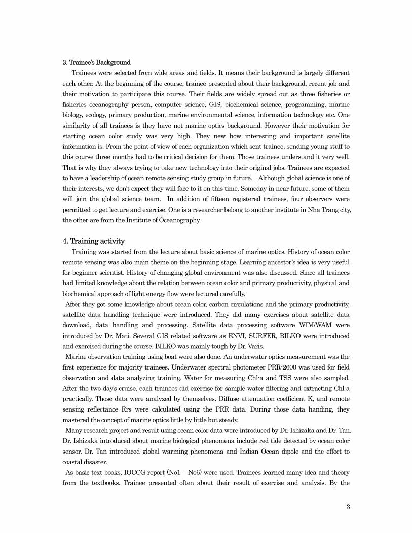
Figure 3 Rrs distribution by using NASA Protocol of 12 stations

Figure 4 The Back Scattering Spectrum

The Back scattering (Bb) was firstly derived from this algorithm. In Figure 4, the Bb spectrum showed similar slope and magnitude at all station. Therefore, this result indicated that no difference of water components in this area.

The derived Absorption spectrum by phytoplankton (Aø) showed the similar pattern. That clearly means same types of water exist in this region (Figure 5). Figure 6 showed Absorption spectrum by detritus and Gelstofs matter (Adg). The highest peak absorption found at wavelength

Figure 5 The reflectance-derived Aø(λ) spectrum of 12 stations

443 nm. Around

wavelength 670 nm, there was no effect from detritus and Gelbstofs matter because the strong absorption by water itself. The results agreed well with the in-situ measurement of SS. At station no. 7, 4, and 10, there were high SS (Figure2) because of locating near the coast. These stations were influenced by freshwater as shown in Figure 8 because of lower in salinity comparing with other stations.

5

-0.04

-0.02

0.00

0.02

0.04

0.06

0.08

0.10

0.12

412 443 490 555 670

Wavelength(nm)

Adg(

1/m

)

34567891011121314

-0.60-0.40

-0.200.00

0.200.40

0.600.80

1.001.20

1.401.60

1.80

412 443 490 555 670

Wavelength(nm)

Adg

/Aph

i(443

)

34567891011121314

33.3

33.4

33.5

33.6

33.7

33.8

3 4 5 6 7 8 9 10 11 12 13 14Station No.

Salin

ity

Figure 6 The reflectance-derived Adg(λ) spectrum of 12 stations

Figure 7 The ratio of Adg(443)/Aø(443) spectrum

The ratio of Adg(443)/Aø(443) varied from 0.21-0.61, suggesting more absorption

from phytoplankton except some stations (4, 7, 8, 9, and 10) because these ratio more than 0.4 as depicted in Figure 7.

Figure 8 Salinity of 12 stations in PSU unit

Conclusion

The Remote Sensing Reflectance showed the similar pattern of the characteristic of coastal water at all stations. There are high in chlorophyll-a, SS, and CDOM. The result showed high absorption in short wavelength area and low absorption in long wavelength area. The in-situ data set of chlorophyll-a and SS varied from 0.686-1.386 and 0.67-2.70 mg/L, respectively. The reflectance derived absorption by phytoplankton and gelstrof and Back Scattering using Semi-Analytical Algorithm showed strong effect by phytoplankton at almost station. Only station 4,7,8,9 and 10 were influenced by detritus and Gelstrof matter. This result agreed well with in-situ data set.

6

Recommendation

This study is not complete process. Next step should to compare the reflectance-derived absorption by phytoplankton and in-situ chlorophyll absorption. Acknowledgements

The author is extremely grateful to Prof. Dr. Satsaki Matsumura and Prof. Dr. Joji Ishisaka for your information about optical properties and ocean color, Dr.Mati Kahru, Dr. Chun Knee Tan, and Dr.Varis Ransi for your knowledge. References Zhong Ping Lee., Kendall L. Carter., 2003. Absorption spectrum of phytoplankton pigments derived from hyperspectral remote-sensing reflectance. Remote Sensing of Environment, 89, P361-369 IOCCG ., Remote Sensing of Ocean Color in coastal and other optically-complex waters, Report of the International Ocean-Color Coordinating Group. Volume.5, Dartmouth, Canada, IOCCG

7

Tuna longline fishing ground analysis by satellite image

Siriporn Pangsorn

Southeast Asian Fisheries Development Center: Training Department P.O. Box 97 Phrasamutchedi, Samut Prakan, 10290 Thailand

E-mail: psiriporn@seafdec.org

Abstract Ocean color remote sensing is the powerful tools for observe information from space. Chlorophyll-a and Sea Surface Temperature (SST) is the important parameters on oceanographic factors that allows a forecast of fish distribution. This study considers the relationship between tuna longline fishing ground with Monthly Mean Chlorophyll-a and Sea Surface Temperature (SST) images From Moderate Resolution Imaging Spectroradiometer-Aqua (MODIS-Aqua) in the South China Sea from the year 2003 to 2006. The results of overlaying the fishing position onto the Chlorophyll-a images shows that all the catches were obtained at a Chlorophyll-a range from 0.06-0.5 mg/m3. And in SST images shows that all the catches were obtained at a temperature range from 27.8 to 31.9oC. From this study the tuna longline catch show a relationship with the monthly mean Chlorophyll-a images that the fishing ground is formed along the chlorophyll-a front (where as Chlorophyll-a concentration have difference value). And in SST images in this area is very difficult to find the good relation with tuna fishing ground cause in this area SST is not too much change and from the study find that no tuna longline fishing grounds were observed in the area of lower SST than 27.8oC and higher than 31.9oC. This results show the possibility of using Ocean Color Remote Sensing technologies to find out the relation with tuna fishing grounds but using only Chlorophyll-a and SST information is not as accurate unless considered with the other oceanographic parameters such as fronts, current and etc. Those parameter will be providing more information to find out the distribution of tuna fishing ground in this area. Key words: Ocean color, Moderate Resolution Imaging Spectroradiometer-Aqua (MODIS-Aqua), Tuna longline, fishing ground, Chlorophyll a, Sea surface temperature Introduction

At present, ocean color satellite remote sensing can be used to measure

several parameters over the ocean surface, including Chlorophyll-a and Sea Surface Temperature (SST), that is offer the opportunity to the fisheries science. Chlorophyll a concentration and Sea Surface Temperature is the important parameters on oceanographic factors which allows a forecast of fish distribution, if we know where is a suitable water condition for the target species, this would greatly increase the chances of finding the target fish and reduce expenditure cost of fishing operation.

Tuna longline fisheries in Vietnam, there are approximately 629 longline fishing boats which are capable to fish at the offshore area of Vietnam (Dao Manh Son 2005). For tuna longline have two main fishing seasons, northeast monsoon lasts from November to the next May of the following year. And southwest one lasts from June to August. The area of fishing grounds is offshore areas of South China Sea; around Spratly Island.

This report is try to find out the fishing ground information, if have relation with Chlorophyll-a or Sea Surface Temperature data from ocean color satellite image

8

that will be useful for find the more effective fishing area for fishermen and can be reduce the cost of operation. Method

For tuna longline fishing data of Vietnam; which collected by Research

Institute for Marine Fisheries (RIMF), Hai Phong Province. This data set is available from April to September in the year 2003 till 2005 and April to May 2006, all data is in the Inter-Monsoon and Southwest Monsoon period. The data provide the information about the operating position, day of operated, total number of hooks and total catch in kilogram. After received data, calculated the catch data for CPUE in the unit as kilogram per 100 hooks and separated into 3 categories; 1. Small catch, 2. Medium catch and 3. Big catch which had CPUE value in the range of 0-6, 6.1 -12 and over 12 kg/100 hooks respectively.

Figure 1. Tuna longline fishing ground distribution

Collected by Research Institute for Marine Fisheries (RIMF), Hai Phong Province For ocean color images from Moderate Resolution Imaging

Spectroradiometer-Aqua (MODIS-Aqua), in this study using level 3 data, which resolution is 4 Km, for Monthly Mean Chlorophyll-a and Sea Surface Temperature for analyse. The MODIS-Aqua level 3 images were downloaded from Ocean Color Home Page (http://oceancolor.gsfc.nasa.gov/cgi/level3.pl).

After get the image then selected the study area from the position of catch data; in this study choose area at Longitude 102 – 122oE and Latitude 4 - 22oN and adjusted scale bar into the appropriated value of each parameter. In this study using

9

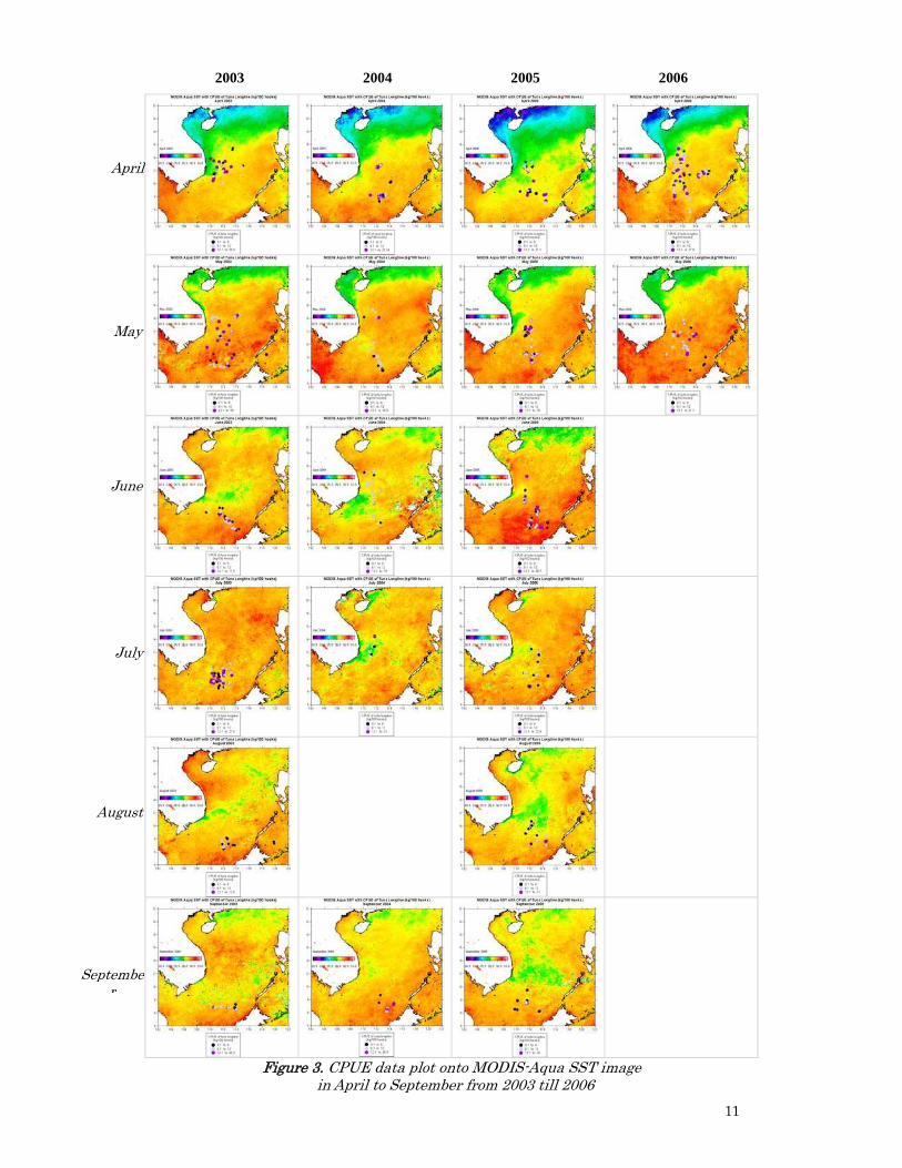
WIM software for analyze, after prepared both images of Monthly Mean Chlorophyll-a and Sea Surface Temperature then plotted CPUE data position onto those images for extract data from the images at each position. Results 1. CPUE of tuna longline and Monthly mean MODIS Aqua Chlorophyll-a images

All CPUE of tuna longline are plotted onto Chlorophyll-a images in each month and shown in Figure 2. Black, dark red and pink dot represent the CPUE data in the range value of 0-6, 6.1-12 and over 12 Kg. /100 hooks respectively. The index range of Chlorophyll-a in those images is from 0.05 to 5 mg/m3: areas with lower chlorophyll-a concentration are shown as purple color, and higher chlorophyll-a concentration are shown as blue, light blue, green, and red as shown in the color scale on the map.

From the results can find some relation between tuna fishing ground with Chlorophyll-a concentration that the fishing ground is formed along the chlorophyll-a front (where as Chlorophyll-a concentration have difference value). And no tuna longline fishing grounds were observed in the area of lower chlorophyll-a concentration than 0.06 mg/m3 and higher than 0.5 mg/m3, only few station that form in the higher concentration 0.4 to 0.5 mg/m3 with CPUE in medium catch. The fishing ground concentrated to the area with Chlorophyll-a 0.06 to 0.2 mg/m3.

And the fishing ground is move southward from central of South China Sea in April and May to southern of South China Sea in June to September due to the period of Southwest monsoon. 2. CPUE of tuna longline and MODIS Aqua Sea Surface Temperature images

CPUE of tuna longline are plotted onto SST images in each month and shown in Figure 3. The index range of SST in those images is from 20.5 to 33.8oC: areas with lower SST are shown as bluish areas, and higher SST are shown as reddish areas as shown in the color scale on the map.

From the results, the SST in this area is not change to much so its very difficult to find the relation with tuna fishing ground and no tuna longline fishing grounds were observed in the area of lower SST than 27.8oC and higher than 31.9oC, The fishing ground concentrated to the area with SST from 29 to 30.5oC.

10

2003 2004 2005 2006

Figure 2. CPUE data plot onto MODIS-Aqua Chlorophyll-a image in April to September from 2003 till 2006

September

August

April

May

June

July

11

2003 2004 2005 2006

Figure 3. CPUE data plot onto MODIS-Aqua SST image in April to September from 2003 till 2006

September

August

July

April

May

June

12

Discussion From the results, can find some relation between tuna fishing ground with Chlorophyll-a concentration that the fishing ground is formed along the chlorophyll-a front as shown in Figure 2. And the relation with the seasonal monsoon that in southwest monsoon the fishing ground is shift to southern part of South China Sea. And in this region SST is not too much change so fishing ground analysis by SST in this area is so difficult This is one method that attempts to find out the tuna fishing ground information in this area. The results of the study show the possibility to uses Ocean Color Remote Sensing techniques in fisheries issues, if we have enough data for analysis and considered with the other oceanographic parameters, such as chlorophyll front, and the habitat of target species to find out more accuracy results. Possible plan or idea in near future From the results we find some relation of tuna fishing ground with chlorophyll that the fishing grounds are formed along the chlorophyll front. This will be useful for my department to apply the use of ocean color image for fisheries science. From the study, we need to improve the methodology, i.e. find out the chlorophyll front from satellite image, and more clear information about fish habitat to find out the effective fishing area of target fish for benefits to all countries in the region. Acknowledgement

The author should like to express sincere gratitude to NIPPON Foundation and POGO that established the Visiting Professorship Program for this training course. Institute of Oceanography Nha Trang, Vietnam for provide all the facilities for this training. Prof. Dr. Satsuki Matsumura for giving his knowledge about ocean color. Dr. Venetia Stuart, Dr. Mati Kahru, Prof. Dr. Joji Ishizaka, Dr. Chun Knee Tan, Dr. Varis Ransibrahnakul and Mr. Tong Phuoc Hoang Son for giving and sharing valuable knowledge in this course. And all trainees in this course for sharing experience and discuss for all the topics in this course. Reference Kuno,M.etal. Skipjack fishing ground analysis by means of satellite remote sensing. http://oceancolor.gsfc.nasa.gov/cgi/level3.pl

13

======================================================= Marine environment and Marine Optics in Nha Trang Bay Phan Minh Thu Department of Marine Environment and Ecology – ION - Vietnam SENSE – Wageningen University – The Netherlands Background study Bachelor in Aquaculture (1997) MSc. In Integrated Tropical Coastal Zone Management (AIT - Thailand) Status work Now, doctoral student in Environmental science (Wageningen University, The Netherlands). I am also working at Institute of Oceanography, Vietnam in the field of Marine ecology and environment. I target to application of remote sensing and geography information system for environmental assessment and natural resource management. Introduction After Nha Trang becomes the most beautiful bay on the world, the economic structure in Nha Trang Bay has been changes. Before 2000, the economy in Nha Trang bay mainly targets to fishing and aquaculture, navigation and tourism, but now they rank in tourism, navigation and aquaculture. According to the department of Statistic Office (2007), the number of tourism visits was 3.83 million in 2006, being more 30% than in 2005. In addition, in Nha trang, GDP of tourism made about 46.75% of Nha Trang in 2004. In contrast, the status of marineculture in Nha Trang has been reduced both in areas and products. Marine environment have been studied in Nha Trang bay for 1970s. These studies focused to status and changes of marine environment such as DO, TSS (Total Suspended Sediment), Chl-a (Chlorophyll-a), PP (Primary Production) and nutrients. However, until now, no-data of marine optics and the relationship between marine optics and environmental factors have been identified. This report targeted to:

• Identify the distribution and changes of Chl-a and TSS in Nha trang Bay • Identify the parameters of PP which can be applied for RS (Remote sensing): • Estimate the TSS and Chl formulation for RS.

Materials and methodology The report based on secondary data collected from 1996 in the SAREC projects and monitoring station (2001 – 2006). In addition, the mini-project also collected data of TSS, Chl-a and marine optics based on 2 field trips in April and June, 2007 under POGO project in Nha Trang Bay (figure 1). Water samples were collected in the water layers at 0, 5, 10 and 15 or 20m depended on the water depth. Chl-a was measured by extraction method with acetol 90% during 24 hours at 0°C and then they were measured with the Fluorescence. TSS was identified by the weight method. Temperature and Salinity were measured with AST meter; Light: PRR 2600; and Transparency:

14

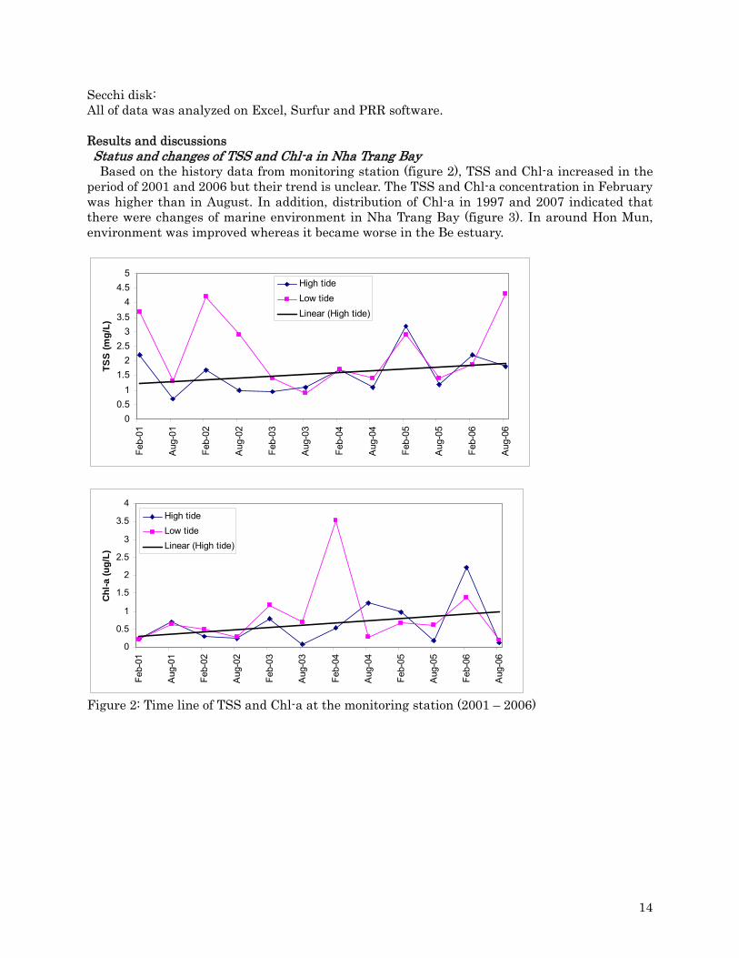
Secchi disk: All of data was analyzed on Excel, Surfur and PRR software. Results and discussions Status and changes of TSS and Chl-a in Nha Trang Bay Based on the history data from monitoring station (figure 2), TSS and Chl-a increased in the

period of 2001 and 2006 but their trend is unclear. The TSS and Chl-a concentration in February was higher than in August. In addition, distribution of Chl-a in 1997 and 2007 indicated that there were changes of marine environment in Nha Trang Bay (figure 3). In around Hon Mun, environment was improved whereas it became worse in the Be estuary.

00.5

11.5

22.5

33.5

44.5

5

Feb-

01

Aug

-01

Feb-

02

Aug

-02

Feb-

03

Aug

-03

Feb-

04

Aug

-04

Feb-

05

Aug

-05

Feb-

06

Aug

-06

TSS

(mg/

L)

High tideLow tideLinear (High tide)

0

0.5

1

1.5

2

2.5

3

3.5

4

Feb-

01

Aug

-01

Feb-

02

Aug

-02

Feb-

03

Aug

-03

Feb-

04

Aug

-04

Feb-

05

Aug

-05

Feb-

06

Aug

-06

Chl-a

(ug/

L)

High tideLow tideLinear (High tide)

Figure 2: Time line of TSS and Chl-a at the monitoring station (2001 – 2006)

15

Figure 3: Distribution of Chl in April 1997 (left) and 2007 (Right) If based on distribution of Chl-a, Nha Trang Bay had 2 regions in which Chl-a in the southern region was higher than in the northern one. Combining the status of Chl and TSS (Figure 3 and 4), water bodies in Nha Trang Bay could be divided 2 regions. In region 1 near the coastline, waters were impacted by human activities and river discharge, so this is case 2 water (high Chl, high TSS). Another region was more ocean water (case 1 water). Parameters of PP in the Nha Trang Bay To identify PP could be used 2 methods: one is direct method and another is calculating method. There are 2 models for calculating PP. The model VGPM was suggested by Berenfeld and Falskowski (1997) and MDL. The VGPM PP = 0.661625* PBopt * Zeu* Chl0 * DIRR* PAR/(PAR + 4.1) To use this model, Son and Thu (2007) found that PBopt = 8.15 (mgC/mgChl/hour). DIRR is 1 hour. Chl0 concentration was in-situ data. PAR was measured by PRR 2600 from surface water to (bottom – 2m) water layer. The results (figure 4) showed that stations 3, 4 and 8 affected river with small impact. Figure 5 indicated that light intensive in Nha Trang Bay was high and contributed to depth water layer. At the bottom layer, PAR is higher than 1% of PAR(0). Thus, to apply the VGPM, we used the depth water as the Zeu.

Figure 4: Distribution of TSS (mg/l) in April 1997

109 10 13 16 19 22

19

16

13

10

22191613109 10

10

13

16

19

127

12 7o

o

o

o

N.Trang

Hßn Tre

H.MiÕu

H.TÇm H.Mét

H.Mun

H.Nãc

H.Dun

H.Ho

H.Rïa

0 1 2 3 4km

109.15 109.2 109.25 109.3

12.16

12.18

12.2

12.22

12.24

12.26

12.28

12.3

12.32

12.34

12.36

12.38

1

2

3

4

5

6

78

9

10

11

12

1314

15

16

17

1819

109 10 13 16 19 22

19

16

13

10

22191613109 10

10

13

16

19

127

12 7o

o

o

o

N.Trang

Hßn Tre

H.MiÕu

H.TÇm H.Mét

H.Mun

H.Nãc

H.Dun

H.Ho

H.Rïa

0 1 2 3 4km

16

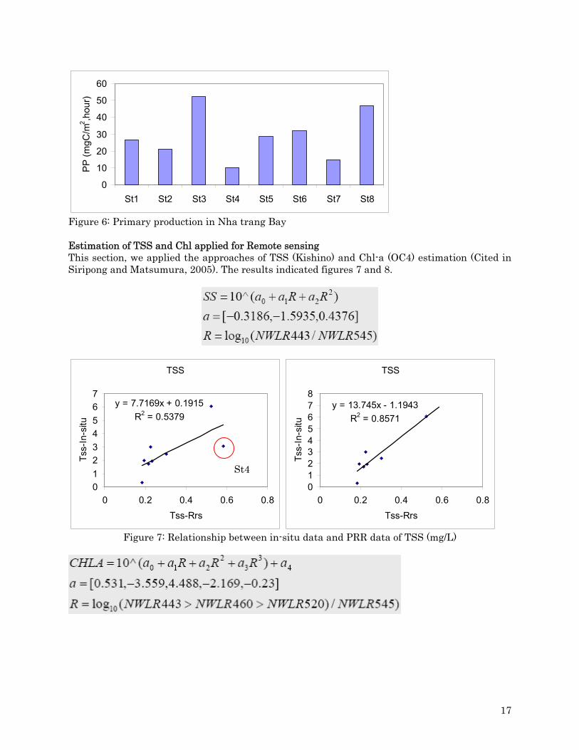
Inputted all of data to VGPM equation, primary production in Nha Trang Bay was estimated in table 1 and figure 6. Primary production ranked from 10.223 – 52.345 mgC/m2/h.

Although station 4 had the highest KPAR, strong ware and high TSS, PP was low. At station 3 had highest Chl-a, so it indicated the highest PP.

0

5

10

15

20

25

30

35

40

45

0 0.05 0.1 0.15 0.2PAR

Dep

th (m

)

St1 St2St3 St4

St5 St6St7 St8

0

5

10

15

20

25

30

35

40

0 0.1 0.2 0.3 0.4KPAR

Dep

th (m

)

St1 St2St3 St4

St5 St6St7 St8

Figure 5: PAR and KPAR in Nha Trang Bay

Table 1: Estimation of primary production with the VGPM St1 St2 St3 St4 St5 St6 St7 St8 KPAR 0.115 0.103 0.153 0.180 0.119 0.123 0.086 0.150Zeu (m) 36.5 26.0 17.8 11.0 45.5 28.2 17.4 21.0Chl0 (ug/L) 0.136 0.151 0.545 0.172 0.116 0.211 0.159 0.415PAR(0) 5265 5894 4234 6116 5940 4495 3852 4027PP (mgC/m2/h) 26.801 21.142 52.345 10.223 28.505 32.050 14.938 47.033

Figure 4: Distribution of Salinity (psu.) in 2 transects

0 5 10 15

-35

-30

-25

-20

-15

-10

-5

01234

0 5 10

-45

-40

-35

-30

-25

-20

-15

-10

-5

08 7 6 5

32.532.632.732.832.93333.133.233.333.433.533.633.733.833.93434.134.234.334.434.534.634.734.834.935

17

0

10

20

30

40

50

60

St1 St2 St3 St4 St5 St6 St7 St8

PP

(mgC

/m2 ,h

our)

Figure 6: Primary production in Nha trang Bay Estimation of TSS and Chl applied for Remote sensing This section, we applied the approaches of TSS (Kishino) and Chl-a (OC4) estimation (Cited in Siripong and Matsumura, 2005). The results indicated figures 7 and 8.

Figure 7: Relationship between in-situ data and PRR data of TSS (mg/L)

TSS

y = 7.7169x + 0.1915R2 = 0.5379

01234567

0 0.2 0.4 0.6 0.8Tss-Rrs

Tss-

In-s

itu

TSS

y = 13.745x - 1.1943R2 = 0.8571

012345678

0 0.2 0.4 0.6 0.8Tss-Rrs

Tss-

In-s

itu

St4

18

Figure 8: Relationship between in-situ data and PRR data of Chl-a (ug/L)

Figures 7 and 8 showed that with all data, the relationship of Chl-a and TSS between in-situ data with PRR data was not closed. However if data of station 4 of TSS and station 4 & 8 of Chl-a were rejected, these relationships were significant. Information of station 4 & 8 showed that these stations related with human activities and fresh water from inland, so the organic matters, specifically DOM, in these areas were high. It mean that CDOM in these station also were high. Therefore, the value of TSS and Chl calculated from PRR data were not corrected. Conclusions Based on distribution of Chl and TSS, Nha Trang bay can be divided 2 different parts PP: 10 – 52 mC/m2,hour with K: 0.086 – 0.180 m-1 OC4 only applies for Case 1 Water. CDOM affects significantly estimation of TSS and Chl Acknowledgement We would like to thank to Prof. S. Matsumura, who taught us during last three months; Mr. Trong Phuoc Hoang Son – Coordinator of POGO 2007 project for supporting; all of professors, who guided us how to apply and use techniques of remote sensing analysis in Oceanography. We also thanks to Nippon Foundation – POGO, Institute of Oceanography - Vietnam to be created condition for us to participate the training workshop. I also Prof. Leemans (WUR – The Netherlands) and IFP support for me to attend the workshop. References Behrenfeld,M.J. and Falkowski,P.G.(1997) A consumer’s guide to phytoplankton primary productivity models. Limnol. Oceanogr., 42, 1479-1491 Siripong, A., and Matsumura, S. (2005). In-water Algorithms on Chlorophyll-a, Suspended Sediments and Colored Dissolved Organic Material (CDOM)in the Upper Gulf of Thailand Using Terra, Aqua/MODIS and ADEOS-II/GLI for Validation. MODIS Workshop, 6-7 Jan. 2005. Nguyen Tac An, Vo Duy son, Phan Minh Thu (2007). Primary production models and parametric problem in various contexts of water column in Nhatrang bay-Vietnam. Scientific report. ION.

Chl

y = 0.0803x + 0.1791R2 = 0.075

00.10.20.3

0.40.50.6

0 0.5 1 1.5 2Chl-Rrs

Chl

-In-s

itu

Chl

y = 0.387x - 0.0179R2 = 0.789

00.10.20.30.40.50.60.70.8

0 0.5 1 1.5 2Chl-Rrs

Chl

-In-s

itu

St4

St8

19

THE COMPATIBILITY BETWEEN ALGORITHMS AND IN-SITU DATA OF CHLOROPHYLL-a CONCENTRATION

Tu Tuyet Hong

UTE- HoChiMinh City, VietNam

ABSTRACT

Global ocean color algorithms, used to extract chlorophyll concentration in the ocean surface, normally overestimate pigment values in coastal regions, due to optical interference of water components. The task of the report consisted of a comparison of the accuracy of two existing global ocean color algorithms for the computation of chlorophyll-a concentration in the Upper Gulf of Thailand. OC4v4 (SeaWifs) and OC3M (MODIS) are two considered empirical algorithms. The remote sensing reflectance, )(λrsR , is calculated from upwelling

radiance ),( λ+0uL and down-welling irradiance ),( λ+0dE measured by bio-spherical instrument. The uncertainty in the chlorophyll-a concentration that determined with the two algorithms was estimated by using in-situ chlorophyll-a data collected from these field-trip data, respectively. One solution to improve the algorithms is also suggested. INTRODUCTION The base of the oceanic food web is phytoplankton. The major reason that scientists measure ocean color is to study phytoplankton. Global accurate estimation of phytoplankton biomass and their primary production in the ocean is necessary to predict global climate change. Ocean color remote sensing is effective procedure to estimate chlorophyll-a concentration as an index of phytoplankton biomass widely, simultaneously and continuously.

A variety of algorithms exists for chlorophyll-a concentration. Their goal is to retrieve surface chlorophyll-a with a 30%-tolerance error. The first of these algorithms is based on the decrease of the blue to green reflectance ratio as chlorophyll is increased. It is effective in oceanic waters, determined by phytoplankton and related degradation products. However, it is inaccurate fails in coastal and inland waters, where inorganic suspended matter and dissolved and particulate non-phytoplanktonic matter also affect optical properties [2]. Another method calculates chlorophyll using the red to near infrared ratio, which is good for high concentrations, but is bad for low concentrations. The multi-band inversion of a bio-optical model is a different kind of method that has found great interest. It calculates concentrations for chlorophyll and CDOM simultaneously. The forward model relates the reflectance just below the water surface to the absorption and back scattering coefficients. Neural networks algorithm is also introduced. This must use large data sets so it is extremely expensive. In this report, two algorithms that based on the blue to green reflectance ratio, OC3M and OC4v4, are mentioned. STANDARD EMPIRICAL ALGORITHMS

What does a satellite measure? The ocean color signal, sensed by a satellite, can be quantified by using the remote-sensing reflectance. While this reflectance is just above the sea surface and defined as the ratio of upwelling radiance to down-welling irradiance just above the sea surface [3]:

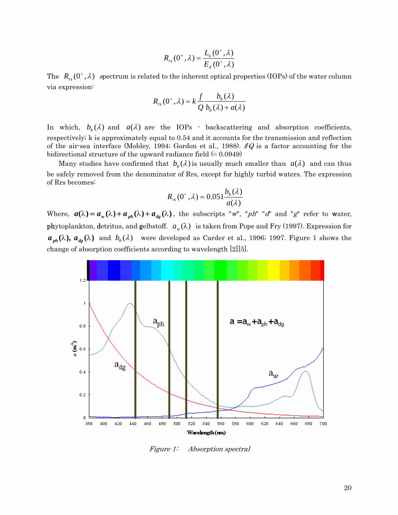
20

),0(),0(

),0(λλ

λ +

++ =

d

urs E

LR

The ),0( λ+rsR spectrum is related to the inherent optical properties (IOPs) of the water column

via expression:

)()()(

),0(λλ

λλ

abb

QfkR

b

brs +

=+

In which, )(λbb and )(λa are the IOPs - backscattering and absorption coefficients, respectively; k is approximately equal to 0.54 and it accounts for the transmission and reflection of the air-sea interface (Mobley, 1994; Gordon et al., 1988). f/Q is a factor accounting for the bidirectional structure of the upward radiance field (≈ 0.0949)

Many studies have confirmed that )(λbb is usually much smaller than )(λa and can thus be safely removed from the denominator of Rrs, except for highly turbid waters. The expression of Rrs becomes:

)()(

051.0),0(λλ

λab

R brs =+

Where, )()()()( λλλλ dgphw aaaa ++= , the subscripts "w", "ph" "d" and "g" refer to water,

phytoplankton, detritus, and gelbstoff. )(λwa is taken from Pope and Fry (1997). Expression for )(),( λλ dgph aa and )(λbb were developed as Carder et al., 1996; 1997. Figure 1 shows the

change of absorption coefficients according to wavelength [2][5].

Figure 1: Absorption spectral

21

The relationship between absorption coefficient and chlorophyll-a concentration and also the scattering coefficient is not fixed in the world ocean. So, the relationship between ocean color and chlorophyll is not invariable.

In open oceanic waters, ocean color is generally dominated by phytoplankton and roughly co-varying constituents (such as detritus and CDOM) whereas coastal waters are characterized by more than one independently varying constituent and thus have more complicated optical signatures. Ocean color modeling in optically complex waters must take into account the contribution of several independently varying constituents to the remote sensing reflectance signal. Semi-analytical algorithms have the potential to be more accurate than empirical algorithms since they simultaneously retrieve several independent relevant optical variables [1]. Most empirical algorithms relate a reflectance ratio to the chlorophyll a concentration The differences in OC3M and OC4v4 MODIS is currently producing the chlorophyll product based on the OC3M algorithm. SeaWiFS uses the OC4.v4 algorithm. Both algorithms were parameterized with the same data set used (n = 2,804) and are described in NASA TM 2000-206892, Vol.11 (O’Reilly et al., 2000). The OC4v4 (SeaWiFS) algorithm is:

432 5321649093010673366010 RRRRChl ..... −++−=

Where, R = log10(max(Rrs(443), Rrs(490), Rrs(510))/ Rrs(555)). The OC3M (MODIS) algorithm is 432 4031659045717532283010 RRRRChl ..... −++−=

where R = loopg10[max(Rrs(443), Rrs(488))/ Rrs(551)] [6]

Figure 2: The functional form of various band-ratio algorithms Assuming the atmospheric correction for SeaWiFS and MODIS/Aqua is good. We can perfectly retrieve Lw(λ). In this considering, the radiance and chlorophyll-a data products produced by SeaWiFS and MODIS/Aqua to be sometimes not the same.

22

There are systematic differences between the OC3M and OC4 algorithms.

Firstly, the shift in nominal waveband (SeaWifs 490,555 and MODIS 488,551 respectively) results in different radiance retrievals for these blue-green bands. Their spectral response functions are different. The 555/551 nm bands may have differences of up to 11%. The 412 and 443 nm shared bands have differences on the order of 1 to 3% in case 1 water. Out-of-band correction is applied to remove spectral band-pass effects in nLw(λ). After correction, the 412 and 443 nm bands are nearly identical in Case 1 water (however, the different may increase in turbid conditions). The 555/551 nm differences are reduced to around 8% Secondly, the different in the maximum-band-ratio results in differences in the functional form of each algorithm, which leads to differing estimated chlorophyll concentrations in turbid water. OC4v4 use a maximum-band-ratio that incorporates 443, 490 and 510 nm, while maximum-band-ratio in OC3M only incorporates 443 and 488. As turbidity increases, the selected maximum-band migrates from shorter (blue) to longer (green) wavelengths. In the most turbid water, OC4v4 selects 510, while OC3M remains at 488. These differences are one of reasons why MODIS image and SeaWifs image at the same time don’t look alike, perfectly.

Figure 3: SeaWifs and MODIS Cholorophyll-a concentration images at the same time don’t look alike

ESTIMATING THE CHLOROPHYLL-A BY USING ALGORITHMS Material and Method Collecting chlorophyll-a concentration and underwater spectral radiation was carried out in the ocean of the Upper Gulf of ThaiLand. Total number of data from three field trip used for analysis was 51. From water samples, the chlorophyll-a concentration, TSS (Total Suspended Sediment) and CDOM (Colored Dissolved Organic Material) was determined fluoro-metrically with a fluoro-meter. Spectral down-welling irradiance, ),( zEd λ , and upwelling radiance ),( zLu λ , were

measured by bio-spherical instruments PRR-600/610. Remote sensing reflectance )0,( +λrsR

23

were calculated from measured )0,( +λdE and )0,( +λuL for analysis

Results and Discussion The upper gulf of Thailand has complex optical properties (case 2 water) because source of waste water come from land. The algorithms were tested for the data in this study to know the overview of the relationship. The chlorophyll-a concentration calculated by OCM3 and OC4v4 was compared to in-situ chlorophyll-a concentration. Figure 4 shows the relationship between in-situ chlorophyll-a concentration and chlorophyll-a, calculated by using algorithms.

y = 2.5105x - 0.2634R2 = 0.3837

0.00

2.00

4.00

6.00

8.00

10.00

12.00

14.00

0.00 2.00 4.00 6.00 8.00 10.00 12.00 14.00

in-situ Chla (mg/m3)

OC

3M C

hl-a

(mg/

m3 )

y = 0.7221x + 0.8554R2 = 0.62

0.00

2.00

4.00

6.00

8.00

10.00

12.00

0.00 2.00 4.00 6.00 8.00 10.00 12.00

in-situ Chla (mg/m3)

OC

4v4

Chl

-a (m

g/m

3 )

Figure 4: The relationship between in-situ chlorophyll-a concentration and estimated

chlorophyll-a concentration by algorithms The R-squared value indicates the estimated values of chlorophyll-a concentration and the actual values are not close together. Some of values are dispersed, although, the OC4v4 algorithm is better than the OC3M. However, the both of model works are not very well in this case. This may be due to the presence of CDOM and TSS in the ocean water of observed area.

y = 0.9552x + 0.2049R2 = 0.9641

0.00

2.00

4.00

6.00

8.00

10.00

12.00

14.00

0.00 2.00 4.00 6.00 8.00 10.00 12.00 14.00

in-situ Chla (mg/m3)

OC

3M C

hl-a

(mg/

m3 )

y = 0.9489x + 0.2877R2 = 0.963

0.00

2.00

4.00

6.00

8.00

10.00

12.00

0.00 2.00 4.00 6.00 8.00 10.00 12.00

in-situ Chla (mg/m3)

OC

4v4

Chl

-a (m

g/m

3 )

Figure 5: The relationship between in-situ chlorophyll-a concentration and estimated chlorophyll-a concentration by algorithms after removing affect of CDOM

Looking at set of data, the coastal stations have high CDOM and also high chlorophyll. This can be viewed in the graph Rrs-wavelength using Rrs(412) as indicator of CDOM. Rrs(412) is lower while CDOM is higher and vice versa In figure 6, stations 1, 2, 3, 4, 5, 6, 7 are

24

high CDOM. In order to the estimated values of chlorophyll-a concentration at these stations can equal in-situ data, respectively, we have to manually correct them. After data are adjusted, the relationship between in-situ chlorophyll-a and chlorophyll-a by algorithms is improved significantly (see fig.5, R2 increase from 0.3837 to 9.641 for MODIS OC3M and from 0.62 to 0.963 for SeaWifs OC4v4) The both OC3M and OC4v4 algorithms use the maximum of blue to green band ratio to estimate chlorophyll-a concentration. The absorption coefficient of CDOM also appears rather high at 443, 490 and 510 wavelengths (see figure 1). So, the inaccurate of estimated chlorophyll concentration results from CDOM itself.

Figure 6: Rrs(670) is not always near zero in coastal water

The Rrs(670) (red band) is not used for detecting oceanic phenomena at oceanic water because it is nearly zero. However, coastal water include so many particles that Rrs(670) is not always near zero (see fig.6). Especially, the absorption coefficient of CDOM at 670nm wavelength is near zero (see fig.1). Moreover, recording the ultraviolet and blue wavelengths of radiation is difficult because of scattering and absorption in the atmosphere [4]. Rayleigh scattering, which affects the shorter wavelengths more severely than longer wavelengths, causes the shorter visible wavelengths (i.e. blue) to be scattered much more than longer wavelengths, so that very little of this energy is able to reach and interact with the sea surface. In other word, ocean color signal that is sensed by satellite contains smaller error at longer wavelengths Thus, Rrs(670) can be used to improve accuracy of algorithms for chlorophyll-a concentration. A suggested new algorithm for the chlorophyll-a concentration is:

Chl = f(Log (Blue/Green+C3*Red)) While in the OC4v4, Chl = f(Log (Blue/Green)). An instance of new algorithm for the chlorophyll-a concentration that tested in this present is:

432 5321649093010673366010 RRRRChl ..... −++−=

where R= log(max(Rrs(443),Rrs(r90),Rrs(510)/Rrs(555)+ 9.12*Rrs(670))

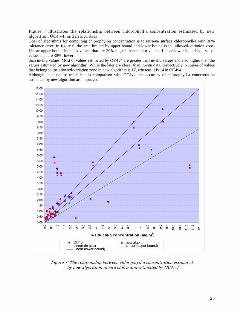
25

Figure 7 illustrates the relationship between chlorophyll-a concentration estimated by new algorithm, OC4.v4, and in-situ data. Goal of algorithms for computing chlorophyll-a concentration is to retrieve surface chlorophyll-a with 30% tolerance error. In figure 6, the area limited by upper bound and lower bound is the allowed-variation zone. Linear upper bound includes values that are 30%-higher than in-situ values. Linear lower bound is a set of values that are 30%- lower than in-situ values. Most of values estimated by OV4v4 are greater than in-situ values and also higher than the values estimated by new algorithm. While the later are closer than in-situ data, respectively. Number of values that belong to the allowed-variation zone in new algorithm is 17, whereas it is 14 in OC4v4. Although, it is not so much but in comparison with OC4v4, the accuracy of chlorophyll-a concentration estimated by new algorithm are improved

0.00

0.50

1.00

1.50

2.00

2.50

3.00

3.50

4.00

4.50

5.00

5.50

6.00

6.50

7.00

7.50

8.00

8.50

9.00

9.50

10.00

10.50

11.00

11.50

12.00

0.0

0.5

1.0

1.5

2.0

2.5

3.0

3.5

4.0

4.5

5.0

5.5

6.0

6.5

7.0

7.5

8.0

8.5

9.0

9.5

10.0

10.5

11.0

11.5

12.0

in-situ chl-a concentration (mg/m3)

OC4v4 new algorithmLinear (in-situ) Linear (upper bound)Linear (lower bound)

Figure 7: The relationship between chlorophyll-a concentration estimated by new algorithm, in-situ chlo-a and estimated by OC4.v4

26

CONCLUSION The ocean color signals are often optically complex, especially in the coastal ocean, where it is of prime importance to improve our understanding of ocean color variability. MODIS and SeaWiFS data of chlorophyll a not provide accurate absolute assessments of chlorophyll a concentration in these optically complex waters Very little improvement in the chlorophyll algorithm can be achieved without accounting for the effects of other optically active constituents. We should aim to develop an algorithm that can solve for CDOM and Chlorophyll-a simultaneously.

REFERENCES [1]. CARDER, K.L., F.R. CHEN, Z.P.LEE, S.K.HWES, and KAMYKOWSKI. Semianalytic

Moderate-resolution Imaging Spectrometer algorithms for chlorophyll-a and absorption with bio-optical domains based on nitrate-depletion temperatures. Geophys.Res. 1999.

[2]. JOJI ISHIZAKA. Ocean color. Lecture on training course NF-POGO, NhaTrang, 2007 [3]. S.MATSUMURA. IOCCG Report 3, chapters 2-3 Lecture on training course NF-POGO,

NhaTrang, VN, 2007. [4]. S.MATSUMURA Atmosphere correction. Lecture on training course NF-POGO, NhaTrang,

VN, 2007. [5]. VARIS RANSI Remote sensing reflectance and inherent optical properties. Lecture on

training course NF-POGO, NhaTrang, VN, 2007. [6]. OCEANCOLOR GROUP at NASA/GSFC. OceanColor Empirical Chlorophyll Analyses.

(http://seabass.gsfc.nasa.gov) TThhee aapppplliiccaattiioonn ooff OOcceeaann CCoolloorr RReemmoottee SSeennssiinngg ffoorr ssttuuddyy oonn SSeeaassoonnaall vvaarriiaattiioonn ooff CChhlloorroopphhyyllll--aa

ccoonncceennttrraattiioonnss aanndd rreellaattiioonnsshhiipp bbeettwweeeenn CChhll--aa wwiitthh SSeeaa SSuurrffaaccee TTeemmppeerraattuurree aanndd CCoolloorreedd DDiissssoollvveedd OOrrggaanniicc MMaatttteerr aatt tthhee VViieettnnaamm wwaatteerrss

HHooaanngg CCoonngg TTiinn

Station for Lagoon Resources Management and Environmental Studies (SLARMES) College of Sciences – Hue University

Email: hoangcongtin@gmail.com BBaacckkggrroouunndd ssttuuddyy BSc. in Biology (2001 – 2005) Master student of Ecology (2006 – 2008)

SSttaattuuss wwoorrkkss:: working for Principles in Practices (PIP): Ocean and Coastal Governance project (funded by CIDA-Canada) at Hue College of Sciences * Development and Applying GIS in zoning and planning ecosystems in Coastal zone. * Community Based Coastal Resources Management in Tam Giang Lagoon and Hue coastal zone (Community Collaboration) Abstract

Seasonal to inter annual changes in phytoplankton biomass and productivity are very important components of the total variability associated with ocean biological and biogeochemical processes (Yoder and

27

Kennelly, 2003). This study aims to find out the seasonal variation of Chl-a concentration in Northeast monsoon (NEM) and Southwest monsoon (SWM) at Vietnam waters. Find out the relationship between Chl-a concentration with SST and Rainfall in each season. II.. IInnttrroodduuccttiioonn

Vietnam is located on the Eastern seaboard of Indochinese Peninsula. In Vietnam coastal zone has many rivers, with a major river estuary for every 20 km of coast. The Red river and Mekong River have strongly influenced sediment discharge into coastal waters - 114 million tones per year, from Red river and 98 million tones per year, from Mekong River (Hoi, 1995).

Beside the difference of complex in river discharge, the difference of climate, monsoon and other oceanographic properties of this sea region have made the complex in physical, chemical and ecological characteristics and dynamic of Vietnam waters. On the other hand, Vietnam waters is the large area coverage, so there is difficulty to carry out the field survey for whole Vietnam waters area. Until recent times, Ocean color remote sensing has applied to study on Chlorophyll-a distribute in some areas of Vietnam such as Dien et. al. (2002), D.L.Tang et. al. (2003). But there is not any study on the relationship between Chl-a concentration and SST and Rainfall in Vietnam waters.

Hence, the application Ocean color remote sensing for study on Seasonal variation of Chlorophyll-a concentration and relationship between Chl-a with SST and rainfall in the Vietnam waters are more significance to fisheries and marine biological resources.

II. Data and methodology 1. Data and Materials * SeaWiFS derived Chl-a from Giovanni NASA Live Access Sever (Available at http://oceancolor.gsfc.nasa.gov). MODIS – Aqua with SST data (from 2002 – 2006) (Available at http://reason.gsfc.nasa.gov/OPS/Giovanni). * Ocean Surface Winds (QuikSCAT) Global 0.25 deg (m/s) of NASA JPL (Cal. Inst. of

Technology) (Available at http://las.pfeg.noaa.gov/oceanWatch/oceanwatch.php) * Rainfall data from Monthly Global Precipitation (GPCP)

(Available at http://disc2.nascom.nasa.gov/Giovanni/tovas/rain.GPCP.2.shtm) * CDOM (Dissolved and detrital organic matter absorption coefficient) data from GSM Modis-Aqua Optical

Monthly Global 9-km (2002 to 2006).

* Information on natural conditions, atmosphere and hydrosphere in the region of South China Sea (Bien Dong).

* Soft wave WIM-WAM and Microsoft Excel 2. Methodology * Using Wim - Wam software to analyzing SeaWiFS images. * Calculating and Statistical satellite data by using MS. Excel software.

28

III. Study sites Vietnam waters are divided into three areas:

+ Area 1: North part of Vietnam - Gulf of Tonki (22oN - 17oN; 103oE – 110oE). + Area 2: Central part of Vietnam - the central of East Sea (17oN - 12oN; 107o E – 114o E). + Area 3: South part of Vietnam - Mekong Delta and Gulf of Thailand (12oN - 7oN; 103o E – 110o E).

The study was carried out in five years from 20002 to 2006 and each year, we divide into two seasons: Northeast monsoon (NEM) from November to March and Southwest monsoon (SWM) from May to September. IV. Results and Discussions 1. Distribution and Seasonal variation of SeaWiFS-derived Chl-a in Vietnam waters The seasonal variation of Chl-a in Vietnam waters for NEM and SWM from 2002 to 2006 are illustrated by SeaWiFS maps (Fig. 2ab). Analysis of the five-year (2002-2006) composite monthly mean Chl-a images showed that there was a seasonal variability of Chl-a in NEM season. The Chl-a value high at near Red river and Mekong river estuaries (1.82 – 2.36 mg/m-3) but in the central part of Vietnam waters Chl-a value is low (0.11 – 0.35 mg m-3). In the SWM season, Chl-a value in area 1 (0.64 – 1.82 mg m-3) is higher than area 2 (0.11 – 0.29 mg m-3) and area 3 (0.44 – 0.93 mg m-3).

From

July to September at area 3, there are phenomena which high Chl-a concentration was created at near-shore of Binh Thuan province. Specially, in June 2005, upwelling occurred earlier than

Fig. 2a. Distribution and Variation of the five-year (2002-2006) composite monthly mean Chl-a images in SWM season of Vietnam waters

Fig. 2b. Distribution and Variation of the five-year (2002-2006) composite monthly mean Chl-a images in NEM season of Vietnam waters

Fig.1. Geography of the study area, Vietnam waters with three

29

Fig. 5. High Chl-a concentration (a) and low SST (b) in the central part of Vietnam waters on Nov. 2005

(a) Monthly Chl-a Nov. 2005

(b) Monthly SST Nov. 2005

normal time (July annual) and in July 2006, upwelling area extended from Binh Thuan to the north part of Vietnam - Khanh Hoa province.

In the NEM, Chl-a value in area 1 (0.39 –

1.82 mg m-3) also higher than area 2 (0.17 – 0.35 mg m-3) and 3 (0.57 – 1.37 mg m-3). The high Chl-a concentration in December to February and decrease in March (Fig. 3). Chl-a value in NEM season at all area is always higher than in the SWM season. The chl-a is higher around 10% during the NEM compared to SWM (Fig. 4). In particular, on 20th October to 2nd November 2005 at central part of Vietnam waters have a powerful typhoon brought torrential rain and 100km/h winds (BBC, 2005). So that is main cause of high Chl-a concentration in the central part of Vietnam waters on November 2005 (Fig. 5).

2. Correlation of SeaWiFS derived Chl-a and Dissolved and detrital organic matter absorption coefficient CDOM concentration is defined by light absorption coefficient per meter because chemical definitions are so complicated (S. Matsumura, 2006). In this study, digital value of SeaWiFS derived Chl-a in Vietnam waters was examined with Dissolved and detrital organic matter absorption coefficient. The result has shown that Chl-a and Dissolved and detrital organic matter absorption coefficient was highly correlated with R2 =

Area 1 Area 2 Area 3

0.793

0.948

0.162

0.238

0.733

0.837

0.00

0.10

0.20

0.30

0.40

0.50

0.60

0.70

0.80

0.90

1.00

mg/

m^3

SWM

NEM

Fig. 4. The mean of Chl-a value at three areas in SWM and NEM season

Fig. 6. Correlation between SeaWiFS-derived Chl-a (mg m-3) and Dissolved and detrital organic matter absorption

coefficient (m-1) data.

R2 = 0.8647

0

0.01

0.02

0.03

0.04

0.05

0.06

0 0.2 0.4 0.6 0.8 1SeaWiFS derived Chl-a

Dis

solv

ed a

nd d

etrit

al o

rgan

ic m

atte

r abs

orpt

ion

coef

ficie

nt (m

-1)

The distribution of Chl-a on SWM season

0.0

0.2

0.4

0.6

0.8

1.0

1.2

1.4

1.6

1.8

2.0

7 8 9 5 6 7 8 9 5 6 7 8 9 5 6 7 8 9 5 6 7 8 9

2002 2003 2004 2005 2006Time

mg/

m^3

A1_Chl-a

A2_Chl-a

A3_Chl-a

The distribution of Chl-a value on NEM season

0.0

0.20.4

0.60.8

1.0

1.21.4

1.61.8

2.0

11 12 1 2 3 11 12 1 2 3 11 12 1 2 3 11 12 1 2 3 11 12

2 0 0 2 2 0 0 3 2 0 0 4 2 0 0 5 2 0 0 6Tim e

mg/

m^3

A1_Chl-a

A2_Chl-a

A3_Chl-a

Fig. 3. The distribution of Chl-a concentration in NEM (a) and SWM (b)

a

b

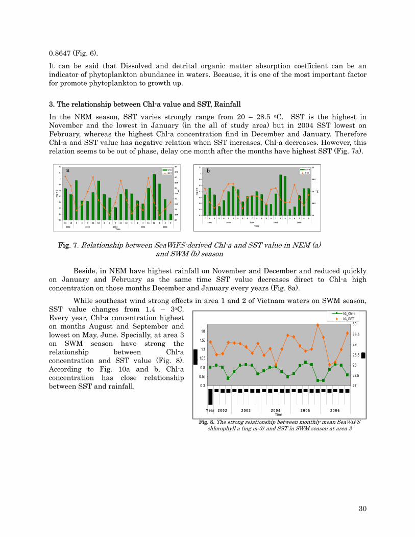
30

0.8647 (Fig. 6). It can be said that Dissolved and detrital organic matter absorption coefficient can be an indicator of phytoplankton abundance in waters. Because, it is one of the most important factor for promote phytoplankton to growth up. 3. The relationship between Chl-a value and SST, Rainfall In the NEM season, SST varies strongly range from 20 – 28.5 oC. SST is the highest in November and the lowest in January (in the all of study area) but in 2004 SST lowest on February, whereas the highest Chl-a concentration find in December and January. Therefore Chl-a and SST value has negative relation when SST increases, Chl-a decreases. However, this relation seems to be out of phase, delay one month after the months have highest SST (Fig. 7a).

Fig. 7. Relationship between SeaWiFS-derived Chl-a and SST value in NEM (a) and SWM (b) season

Beside, in NEM have highest rainfall on November and December and reduced quickly

on January and February as the same time SST value decreases direct to Chl-a high concentration on those months December and January every years (Fig. 8a).

While southeast wind strong effects in area 1 and 2 of Vietnam waters on SWM season, SST value changes from 1.4 – 3oC. Every year, Chl-a concentration highest on months August and September and lowest on May, June. Specially, at area 3 on SWM season have strong the relationship between Chl-a concentration and SST value (Fig. 8). According to Fig. 10a and b, Chl-a concentration has close relationship between SST and rainfall.

0.3

0.4

0.5

0.6

0.7

0.8

0.9

1

1.1

1.2

11 12 1 2 3 11 12 1 2 3 11 12 1 2 3 11 12 1 2 3

2002 2003 2004 2005 2006Time

mg

m-3

23

23.5

24

24.5

25

25.5

26

26.5

27

27.5

28

oC

ChlaSST

0.3

0.4

0.5

0.6

0.7

0.8

0.9

1

1.1

7 8 9 5 6 7 8 9 5 6 7 8 9 5 6 7 8 9 5 6 7 8 9

2002 2003 2004 2005 2006

Time

mg

m-3

28

28.5

29

29.5

30

oC

Chl-aSST

a b

Fig. 8. The strong relationship between monthly mean SeaWiFS chlorophyll a (mg m-3) and SST in SWM season at area 3

0.3

0.55

0.8

1.05

1.3

1.55

1.8

Y ear 2 0 0 2 2 0 0 3 2 0 0 4 2 0 0 5 2 0 0 6Time

27

27.5

28

28.5

29

29.5

30

A3_Chl-aA3_SST

31

Fig. 10a. The relationship between monthly mean SeaWiFS Chl-a and SST, Rainfall in

NEM season at Vietnam waters

Fig. 10b. The relationship between

monthly mean SeaWiFS Chl-a and SST, Rainfall in SWM season

V. Conclusions Seasonal Chl-a variation in Vietnam waters is different between the north of Vietnam (area 1) and south of Vietnam (area 3). The central of Vietnam waters is the lowest Chl-a concentration in both two seasons. This study showed that relationship between Chl-a and CDOM (Dissolved and detrital organic matter absorption coefficient) was highly correlated with R2 = 0.8647.

Fig. 9. Ocean Surface Winds (QuikSCAT) Global 0.25 deg (m/s) of NASA JPL (Cal. Inst. of Technology) during January 2006 (A) and September 2006 (B).

The changes of Chl-a value on NEM season

0.00.20.40.60.81.01.21.41.61.82.0

11 12 1 2 3 11 12 1 2 3 11 12 1 2 3 11 12 1 2 3 11 12

2 0 0 2 2 0 0 3 2 0 0 4 2 0 0 5 2 0 0 6Time

mg/

m^3

A1_Chl-a

A2_Chl-a

A3_Chl-a

The changes of Rainfall on NEM season

3

33

63

93

123

153

183

213

243

11 12 1 2 3 11 12 1 2 3 11 12 1 2 3 11 12 1 2 3 11 12

2 0 0 2 2 0 0 3 2 0 0 4 2 0 0 5 2 0 0 6

Time

mm

A1 (mm)

A2 (mm)

A3 (mm)

The changes of Chl-a value on SWM season

0.0

0.2

0.4

0.6

0.8

1.0

1.2

1.4

1.6

1.8

2.0

7 8 9 5 6 7 8 9 5 6 7 8 9 5 6 7 8 9 5 6 7 8 9

2002 2003 2004 2005 2006Time

mg/

m^3

A1_Chl-a

A2_Chl-a

A3_Chl-a

The changes of SST on NEM season

18

20

22

24

26

28

30

11 12 1 2 3 11 12 1 2 3 11 12 1 2 3 11 12 1 2 3 11 12

2 0 0 2 2 0 0 3 2 0 0 4 2 0 0 5 2 0 0 6

Time

oC

A1_SST

A2_SST

A3_SST The changes of SST on SWM season

25

26

27

28

29

30

7 8 9 5 6 7 8 9 5 6 7 8 9 5 6 7 8 9 5 6 7 8 9

2002 2003 2004 2005 2006

Time

oC

A1_SSTA2_SSTA3_SST

The changes of Rainfall on SWM season

70

120

170

220

270

320

370

7 8 9 5 6 7 8 9 5 6 7 8 9 5 6 7 8 9 5 6 7 8 9

2002 2003 2004 2005 2006

Time

mm

A1 (mm)

A2 (mm)

A3 (mm)

A

B

32

This study found time that Ch-a high concentration at north of Vietnam on January, December during NEM (> 1.05 mg m-3) and Chl-a high concentration at south of Vietnam waters from July to September during SWM (> 0.75 mg m-3).

PPoossssiibbllee ppllaann iinn nneeaarr ffuuttuurree After attending this training course, I had been receiving many knowledge and skills in

Ocean color Remote Sensing and marine oceanography conditions. In two next months (October 2008), I am going to do my master thesis in ecology specialist so my plan will be applied those knowledge into my study – besides, I want to have more opportunities to practice and study on remote sensing more in future. In order to promote applying and research on Ocean color remote sensing in Vietnam waters.

* Estimation of Primary Production in the central part of Vietnam coastal. * Applying Ocean Color Remote Sensing in monitor and manage Harmful Algae Blooms in

coastal waters.

Acknowledgements This report was done under supervisor of Prof. Satsuki Matsumura (Chulalongkorn Univ.)

who first time introduced ocean color remote sensing to us and Prof. Jogi Ishizaka (Nagasaki Uni.), Dr. Mati Kahru (Scripps Institution of Oceanography - University of California San Diego), Dr. Tan Chun Knee United Nation University and Dr. Varis Ransibrahnakul (National Oceanic Atmospheric Administration – NOAA) openned our mind about application knowledge of oceanography on ocean color remote sensing during the training course. This training course was funded The Nippon Foundation, POGO (The Partnership of Observation Global Ocean) and Nha Trang Institute of Oceanography.

We would like to thanks Mr. Tong Phuoc Hoang Son and his staffs (Nha Trang, Institute of Oceanography) for their professions and considerate organize. References BBC NEWS, 27 Sep. 2005. Available at: http://news.bbc.co.uk/2/hi/asia-pacific/4285400.stm Tran Van Dien, Dan Ling Tang, Hiroshi Kawamura. Validation of SeaWiFS-derived Ocean Color

Data and Using for study distribution and Seasonal Variation of Chlorophyll-a concentration in the Vietnam waters. Part II Remote sensing and Geographic Information Systems (GIS) Applications for Sustainable Development, p.213 – 218.

S. Matsumura, A. Siripong and T. Lirdwitayaprasit (2006). Underwater optical environment in the Upper Gulf of Thailand. Coastal Marine Science 30(1): 36-43, 2006.

Truong Xuan Luan, Tran Thi Oanh (2000), Applying Remote Sensing and GIS to Research Modern Geological Environment at the Bach Dang River Mouth Area. Remote Sensing and Geographic Information Systems (GIS) Applications for Sustainable Development, Part II. p 74 – 78.

D.L.Tang, H. Kawamura, M.A. Lee, T.V. Dien (2003), Seasonal and spatial distribution of chlorophyll-a concentration and water conditions in the Gulf of Tonki, South China Sea. Remote Sensing of Environment 85, p. 475-483.

Nguyen Chu Hoi (1995). Vietnam – National status and Approaches to Coastal Management. In “Coastal Management in the Asia-Pacific Region: Issues and Approaches”. Japan International Marine Science and Technology Federation, Tokyo, p. 209-224.

Phan Minh Thu (2006), Application of Remote Sensing and GIS tools for recognizing changes of

33

mangrove forests in Ca Mau province. International Symposium on Geo-informatics for Spatial Infrastructure Development in Earth and Allied Sciences 2006.

Kathi Kac Yapa (2000), Seasonal variability of sea surface chlorophyll-a of waters around Sri Lanka. Proc. Indian Acad. Sci. (Earth Planet. Sci.), 109, No. 4, December 2000, pp. 427-432. Printed in India.

Yoder, J. A. and M. A. Kennelly (2003): Seasonal and ENSO variability in global ocean phytoplankton chlorophyll derived from 4 years of SeaWiFS measurements. Global Biogeochem. Cycles, 17(4), 1112, doi: 10.1029/2002GB001942.

34

Developing “PRR Processing” software to process PRR data

Dinh Ngoc Dat

Dept. Remote Sensing, GIS, GPS Space Technology Institute, Hanoi, Vietnam

Abstract This study describes the method to develop a software to process calibrated data from Prr 2600 model. It’s purpose helps some scientist to calculate Prr data faster and faster. In this study, I use some method as Object Orient Programming, Database programming and Survey method to develop this software. It is called “PRR processing”. Over a period time tries to test calibrated data from some stations in Binhthuan province and KhanhHoa province. Introduction Satellite image is a source to calculate Chl-a concentration and some Inherent Optical Properties. The accuracy of result which is received after calculate image data, however, is not high because wavelengths which are received by satellite have to process atmosphere impact (atmosphere correction). At the moment, we have other method to calculate some coefficients in sea water with high accuracy, it is PRR instrument. We can save our time to process calibrated data from this instrument by automatically some steps. To solve this problem, we need to recognize structure of database which is exported from PRR instrument and to concretize some processing steps in a individual software (PRR Processing). The most important of this database is a data table so it contains wavelengths measure value. It is called calibrated data table. This software is developed by a popular programming language (Visual Basic 6). Visual Basic 6 is a simple programming language, it can help us to develop a small software easier and faster. “PRR Processing” will read the content of CalibratedData table so we choosed and process this table in some steps below: 1. Open Database and Star processing. 2. Choose Calibrated Data table and display the content of this table. Software have to recognize errors cell which occur in this table. 3. Choose Calculation to process errors data. (we can see depth graph if we want) 4. Choose one line with start row and end row in grid data (Up or Down) so Ed0 value between the period rows is not change so much. 5. Choose “Graphs of EdZ values” to draw graph for each wavelength EdZ values and get out data between the period rows which is selected in last step. 6. Choose method, depth value or period rows and unit of value to process. Press processing button to start process data is selected. 7. Choose Summarize button to calculate Chl-a and some coefficient Inherent Optical Properties. 8. To export all graphs to bitmap and Properties file (excel format) – if we want.

35

Method Object Orient Programming

Before to design interface, I designed some module to process raw data and draw graphic data so it can stay alone. It is mean that, we can use it again in other software which has same or similar structure.

Database Programming Software is built base on some rules which conform to database manage rules.

Survey, Compare and Statistic - Survey: Researching some formula to calculate Chl-a and some coefficient inherent optical properties. And then to decide choose Chl-a formula (OC4 - 2003) from Jaxa organization. - Compare: compare result from software with result from Excel file. - Statistic: Collect 12 stations data from Binhthuan field trip. Result After a small period time to develop this software according to the process was draws some results below: - Open Database

- Choose start processing

- Choose CalibratedData table to process it.

36

- Processing errors:

When user presses to Calculate button, software automatic processes all rows error first and then processes cells error If a row has there empty cell continuous, software will delete it. Formula to processes cell error:

Cell(i,j) = sqrt(cell(i-1,j)*cell(i+1,j)) i: row number

j: column number - Calculate K, Rrs values In this graph, you can see the line from row 1080 to row 1339 Ed0 values do not change so much so that I choose this line and type this values or scroll Combobox to this values:

37

After input two values start row and end row, software allows draw graph for wavelength EdZ values (“Graphs of EdZ values” button). Before, we can receive K, Rrs values, we have to choose the method (Geomean or Log function) and units divide to smooth data. RdZ values on the surface of sea water is extrapolated by Growth function below: Geomean: y = (y1i*y2i*y3i…*yni)1/n

i: column number Or Log: y = 10^(log(y1i)+log(y2i)+…+log(yni))/n

i: column number

Growth: y = bm^x

38

Table1: raw data is fixed error. Table2: Contain EdZ values after smooth and to calculate K values. Table3: Contain Rrs values and %Ed0PAR and %EdZPAR. After user chooses calculation button, software will indicate some graphs: EdZ after smooth, K values, Rrs values, Rrs surface and EdPAR%. To test all results from this software, we can compare with results is calculated in excel file by graphs of result.

1. EdZ after smooth: Prr processing

Excel

39

Vertical Profile of EdZ

0

2

4

6

8

10

12

14

16

0 20 40 60 80 100 120 140

EdZ

Dep

th(m

)

2. K values

Prr processing

Excel

Vertical Profile of Kd

0

2

4

6

8

10

12

14

16

0.00 0.05 0.10 0.15 0.20 0.25 0.30

Kd (1/m)

Dep

th(m

)

3. Rrs values Prr processing

40

Excel

Vertical Profile of Rrs

0

2

4

6

8

10

12

14

16

0.000 0.005 0.010 0.015 0.020 0.025

Dept

h(m

)

4. Rrs surface

Prr processing

Excel

Rrs at Surface of Station 5

0

0.001

0.002

0.003

0.004

0.005

0.006

Rrs380 Rrs412 Rrs443 Rrs490 Rrs555 Rrs625 Rrs665

Wavelength(nm)

41

- Calculate some coefficients of inherent optical properties.

All fomula to calculate coefficient inherent optical properties is detail in Formula column and Chl-a values is calculated according to this formula below: Chl-a = 10^(a0 + a1*R + a2*R^2 + a3*R3) + a4 With: a0 = 0.531

a1 = -3.559 a2=4.488 a3 = -2.169 a4 = -0.230

Aph[665] = (0.0176*Chl-a)^0.97 Conclusion This software is compatible with database which is exported from PRR instrument (model 2600). It can to get result data as well as to get data from excel, however, it needs small time to get result data. It is a vivacious software because user can export final data after processing to other format data as bitmap and excel file.

42

The Seasonal variation of CDOM in Mekong river mouth.

Phan Van Hoan, Danang of Science and Technology Progress Center Email: Hoanpv151079@yahoo.com

Abstract One indicator of health in estuarine and coastal ecosystems is the ability of local waters to transmit sunlight to planktonic, macrophytic, and other submerged vegetation for photosynthesis. The concentration of coloured dissolved organic matter (CDOM) is a primary factor affecting the absorption of incident sunlight in coastal and estuarine waters. In estuaries, CDOM concentrations vary due to changes in salinity gradients, inflows of industrial and domestic effluents, and the production of new dissolved organic matter from marine biologic activity. To understanding the seasonal variation of CDOM Introduction The Mekong River is one of the great rivers of Asia, ranking twelfth in the list of longest rivers of the world. It rises at about 5,000m in the Tanghla Shan Mountains, on the northeast rim of the great Tibetan Plateau, and flows for 4,200 km through or along the borders of six countries: China, Burma, Laos, Thailand, Kampuchea and Vietnam. In terms of mean annual discharge, the Mekong ranks sixth in the world. The total drainage basin of 783,000 sq.km includes 160,000 sq.km in China, 12,000 sq.km in Burma, and 611,000 sq.km in Laos, Kampuchea, Thailand and Vietnam (the lower Mekong basin). Approximately nine-tenths of Kampuchea (154,730 sq.km) lie within the lower Mekong basin. The river itself flows for 486 km across Kampuchean territory from the Lao border In the north to the Vietnamese border in the south. Leaving the southeast edge of the Korat Plateau in southern Laos and eastern Thailand, the Mekong plunges over the Khone Falls at the Laos-Kampuchea border and reaches the lowlands of northern Kampuchea after crossing a series of rapids. Below Kompong Cham, the river forms a fluviatile lowland landscape with high natural levees, broad floodplains and extensive backwater swamps, many of which remain flooded throughout the dry season. Beyond the backswamps are parallel belts of paddy fields. The mainstream habitats range from sandy-gravel bars to deep pools up to loom deep and several kilometres long, interspersed with rocky rapids. in several places between the Lao border and Phnom Penh, the river divides into two or more channels, creating large islands and extensive sand banks. The Mekong receives the waters of its last major tributary, the Tools Sap, at Phnom Penh. Immediately below this confluence, the Mekong divides to form the Mekong and the Bassac (Song Hau Giang), the two major channels of the delta. The triangular delta, with its apex at Phnom Penh, forms a vast fertile plain covering 49,520 sq.km. Some 16,000 sq.km of this delta are within Kampuchea. The Mekong river running into Vietnam is changed the name to Cuu Long river. Every year, It loads an extreme material such as CDOM, SS, Inorganic material… Material and method

The Dissolve and Detrital Organic Material absorption coefficient images get from NASA’s Giovani website (Giovani.gsfc.nasa.gov). http://reason.gsfc.nasa.gov/OPS/Giovanni/ocean.modisaUCSB.shtml The rainfall images get from NASA’s Giovani website (Giovani.gsfc.nasa.gov). http://reason.gsfc.nasa.gov/OPS/Giovanni/ocean.swfUCSB.shtml Getting whole rainfall monthly images in the Mekong river from 1998 to 2006 and

getting the Dissolve and Detrital Organic Material absorption coefficient images in the Mekong mouth river to recognize the seasonal variation.

43

Getting data Rainfall, Dissolve and Detrital Organic Material absorption coefficient make the graphs and compare the data between CDOM, rainfall to find out the variation rule of the Dissolve and Detrital Organic Material absorption coefficient. The study area.

Result and Discussion In order to getting more understanding about the seasonal variation of CDOM in Mekong mouth river, we should compare rainfall long time series data and CDOM absorption coefficient long time series data were conducted by graph. From this graph, some data can determine to divide it become 2 cases are the average value rainfall data and CDOM absorption coefficient data: Case 1 is the years from 1999 to at the end of 2001 and Case 2: from 2002 to 2006. The average peaks of rainfall about 260 mm and the average peaks of CDOM about 0.0745 m-1

The average peaks of rainfall about 238 mm and the average peaks of CDOM about 0.0706 m-1

Comparing Case 1 and Case 2 we have a rule: when the rainfall in Mekong river area increase as the Dissolve and Detrital Organic Material absorption coefficient increase and inverse. It means when freshwater discharge from Mekong river increase as the quantity of CDOM also increase. (Figure 1 shows quite clearly this relationship).

Fig. 1,a Fig.1 b Figure 1a: The relationship between rainfall and CDOM absorption coefficient. Figure 1b: the Overestimate of Satellite image.

0

50

100

150

200

250

300

2 3 4 5 6 7 8 9 10 11 12 1 2 3 4 5 6 7 8 9 10 11 12 1 2 3 4 5 6 7 8 9 10 11 12 1 2 3 4 5 6 7 8 9 10 11 12 1 2 3 4 5 6 7 8 9 10 11 12 1 2 3 4 5 6 7 8 9 10 11 12 1 2 3 4 5 6 7 8 9 10 11 12 1 2 3 4 5 6 7 8 9 10 11 12 1 2 3 4 5 6 7 8 9 10 11 12

1998 1999 2000 2001 2002 2003 2004 2005 2006

0

0.02

0.04

0.06

0.08

0.1

0.12CDOM absorption coefficient Rainfall (mm)

0

50

100

150

200

250

300

2 3 4 5 6 7 8 9 10 11 12 1 2 3 4 5 6 7 8 9 10 11 12 1 2 3 4 5 6 7 8 9 10 11 12 1 2 3 4 5 6 7 8 9 10 11 12 1 2 3 4 5 6 7 8 9 10 11 12 1 2 3 4 5 6 7 8 9 10 11 12 1 2 3 4 5 6 7 8 9 10 11 12 1 2 3 4 5 6 7 8 9 10 11 12 1 2 3 4 5 6 7 8 9 10 11 12

1998 1999 2000 2001 2002 2003 2004 2005 2006

0

0.02

0.04

0.06

0.08

0.1

0.12CDOM absorption coefficient Rainfall (mm)

Case 1

Case 2

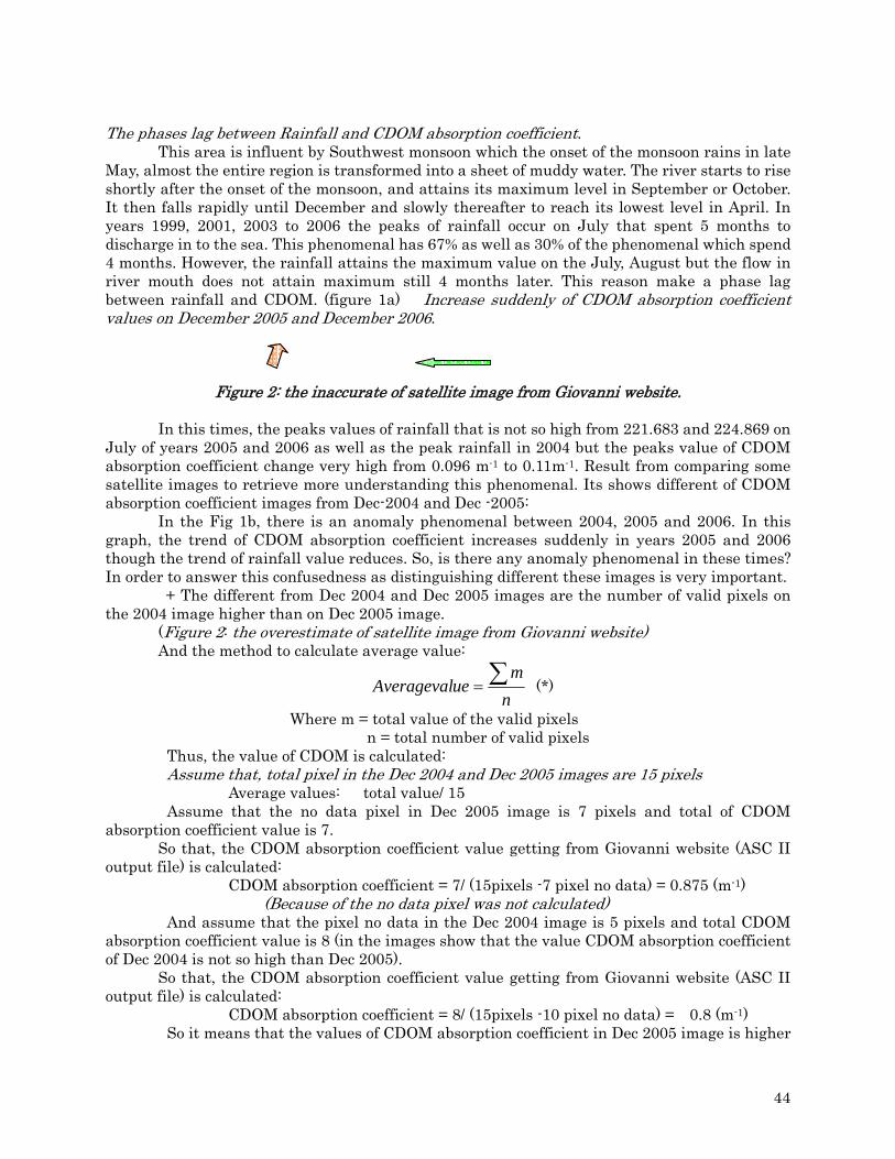
44

The phases lag between Rainfall and CDOM absorption coefficient.

This area is influent by Southwest monsoon which the onset of the monsoon rains in late May, almost the entire region is transformed into a sheet of muddy water. The river starts to rise shortly after the onset of the monsoon, and attains its maximum level in September or October. It then falls rapidly until December and slowly thereafter to reach its lowest level in April. In years 1999, 2001, 2003 to 2006 the peaks of rainfall occur on July that spent 5 months to discharge in to the sea. This phenomenal has 67% as well as 30% of the phenomenal which spend 4 months. However, the rainfall attains the maximum value on the July, August but the flow in river mouth does not attain maximum still 4 months later. This reason make a phase lag between rainfall and CDOM. (figure 1a) Increase suddenly of CDOM absorption coefficient values on December 2005 and December 2006.

Figure 2: the inaccurate of satellite image from Giovanni website.

In this times, the peaks values of rainfall that is not so high from 221.683 and 224.869 on July of years 2005 and 2006 as well as the peak rainfall in 2004 but the peaks value of CDOM absorption coefficient change very high from 0.096 m-1 to 0.11m-1. Result from comparing some satellite images to retrieve more understanding this phenomenal. Its shows different of CDOM absorption coefficient images from Dec-2004 and Dec -2005:

In the Fig 1b, there is an anomaly phenomenal between 2004, 2005 and 2006. In this graph, the trend of CDOM absorption coefficient increases suddenly in years 2005 and 2006 though the trend of rainfall value reduces. So, is there any anomaly phenomenal in these times? In order to answer this confusedness as distinguishing different these images is very important.

+ The different from Dec 2004 and Dec 2005 images are the number of valid pixels on the 2004 image higher than on Dec 2005 image.

(Figure 2: the overestimate of satellite image from Giovanni website) And the method to calculate average value:

nm

ueAverageval ∑= (*)

Where m = total value of the valid pixels n = total number of valid pixels Thus, the value of CDOM is calculated: Assume that, total pixel in the Dec 2004 and Dec 2005 images are 15 pixels Average values: total value/ 15 Assume that the no data pixel in Dec 2005 image is 7 pixels and total of CDOM absorption coefficient value is 7.

So that, the CDOM absorption coefficient value getting from Giovanni website (ASC II output file) is calculated: CDOM absorption coefficient = 7/ (15pixels -7 pixel no data) = 0.875 (m-1)

(Because of the no data pixel was not calculated) And assume that the pixel no data in the Dec 2004 image is 5 pixels and total CDOM absorption coefficient value is 8 (in the images show that the value CDOM absorption coefficient of Dec 2004 is not so high than Dec 2005).

So that, the CDOM absorption coefficient value getting from Giovanni website (ASC II output file) is calculated: CDOM absorption coefficient = 8/ (15pixels -10 pixel no data) = 0.8 (m-1) So it means that the values of CDOM absorption coefficient in Dec 2005 image is higher

45

than Dec 2004 image which is not correct. + The different of 2004 and 2006 images are explained the same. The seasonal variation of CDOM absorption The seasonal variation of CDOM absorption is very clearly because of changing mass fresh water. Familiar below, it has a phase lag between rainfall and CDOM absorption coefficient thus there is also has a phase lag seasonal variation of CDOM. The dry season in this area is from Jan to April but the mass water in Mekong river on Jan still is so high because the level of river is still influent by the very high mass water at the end of rainy season. Hence, the peak of CDOM in the dry season normally occurs on the Dec and Jan and reduces slowly thereafter to reach its lowest level in April. And in the rainy season, rainy will be increase more quickly from at the end of May to October so CDOM also increase significantly. Discussion.

Above, there are some conclusions: - When freshwater discharge from Mekong river increase as the quantity of CDOM also increase which shows clearly a relationship between rainfall and CDOM - The phase lag between Rainfall and CDOM in the Mekong mouth river influents seasonal variation of CDOM. However, these conclusions base on data that was got from Giovanni website without In stitu data. Addition, using satellite images in this report analyzes the variation of CDOM that was met some difficult such as comparing the monthly or yearly concentration of CDOM. This report concern about the seasonal variation of CDOM in the small estuary so the high resolution of images are very important but I can not find any website that provides the high resolution image. On the other hand, using images to compare the monthly concentration of CDOM does not have enough useful values (miss data) that make an integral inaccurate result. So we must have an in stitu data base and the high quality satellite images to improve the result because monitoring the effect of CDOM on the estuaries is very important. Reference Mekong river.

http://www.arcbc.org.ph/wetlands/cambodia/khm_mekriv.htm CICEET Progress Report on the Website.

http://ciceet.unh.edu/progressreports/2004/9_2004/chekalyuk03/ Meteorological of Vietnam http://www.nchmf.gov.vn/ Rainfall data http://reason.gsfc.nasa.gov/OPS/Giovanni/ocean.swfUCSB.shtml The Dissolve and Detrital Organic Material absorption coefficient

http://reason.gsfc.nasa.gov/OPS/Giovanni/ocean.modisaUCSB.shtml

0

0.02

0.04

0.06

0.08

0.1

0.12

2 3 4 5 6 1 2 3 4 5 6 1 2 3 4 5 6 1 2 3 4 5 6 1 2 3 4 5 6 1 2 3 4 5 6 1 2 3 4 5 6 1 2 3 4 5 6 1 2 3 4 5 6

1998 1999 2000 2001 2002 2003 2004 2005 2006

Dry season Rainy season

Figure 3: the seasonal variation of CDOM

46

SEASONAL VARIATION OF SURFACE TEMPERATURE AND CHL-A DISTRIBUTION IN

VIETNAM SEA LE DINH MAU Scientist, Department of Marine Physics, Institute of Oceanography, Nhatrang, Vietnam. BRIEF BACKGROUND : *> Education Background : - B.Sc. in Physical Oceanography, Hanoi University, Vietnam (1986-1990) Title of the dissertation :”Computation of wave charateristics in the South China Sea using numerical model” - M.Sc. in Physical Oceanography, Goa University, India (2000-2002) Title of the dissertation :”Wave refraction and sediment transport along Hoian coast, Central Vietnam” - Ph.D in Physical Oceanography, Goa University, India (2003-2006) Title of the Thesis :”Shore line changes in and around the Thubon River mouth, Central Vietnam” *> Main works - Studies on the characteristics of the interaction between the ocean and atmosphere in the South China Sea. - Studies on the distribution, structure and variation of hydrological fields of the South China Sea; the influence of the hydro-meteorological processes on the marine environment. - Investigation on lithodynamics for the coastal zone and the principal causes which control the processes of coastal litho-dynamics and change in nearshore morphology and shoreline. - Collection and calculation of the necessary technical parameters for design of marine structures. - Modelling and calculation of the litho-hydro-dynamics processes. Also, I have been participated in many projects of different levels : National, Ministerial and several International Co-operation project on physical oceanography in the South China Sea. ABSTRACT : This report presents the seasonal variation of sea surface temperature (SST) and Chl-a distribution in the Vietnam Sea during 2006. The average monthly SST and Chl-a were downloaded from website : http://reason.gsfc.nasa.gov/giovanni (using SeaWiFS for Chl-a; Modis for SST) and the average monthly wind velocity was download from website : ftp://ftp.ssmi.com (a Remote Sensing System Data base for Satellite Microwave Radiometers, Scatterometers, and Sounders). Study results shows that spatial distribution features of SST and Chl-a in the Vietnam Sea depend up on : monsoons, precipitation, river runoff, upwelling, and solar radiation distribution. Temporal variation features of SST and Chl-a indicated that there are 4 seasons at Vietnam Sea : NE monsoon, Transition period from Spring to Summer, SW monsoon, and Transition period from Summer to Winter. Along southern Vietnamese coast was formed a nearshore strip of low SST and high Chl-a during SW monsoon period.

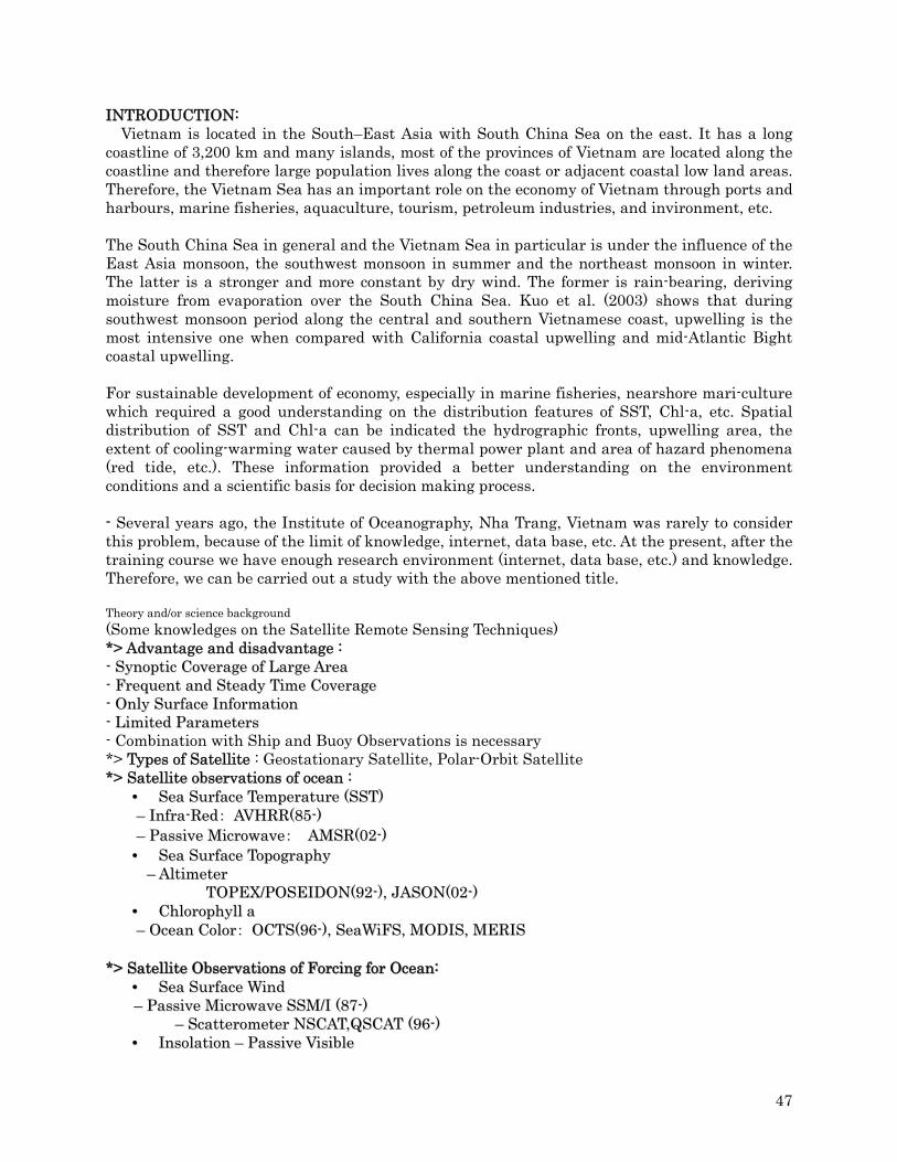
47

INTRODUCTION: Vietnam is located in the South–East Asia with South China Sea on the east. It has a long

coastline of 3,200 km and many islands, most of the provinces of Vietnam are located along the coastline and therefore large population lives along the coast or adjacent coastal low land areas. Therefore, the Vietnam Sea has an important role on the economy of Vietnam through ports and harbours, marine fisheries, aquaculture, tourism, petroleum industries, and invironment, etc. The South China Sea in general and the Vietnam Sea in particular is under the influence of the East Asia monsoon, the southwest monsoon in summer and the northeast monsoon in winter. The latter is a stronger and more constant by dry wind. The former is rain-bearing, deriving moisture from evaporation over the South China Sea. Kuo et al. (2003) shows that during southwest monsoon period along the central and southern Vietnamese coast, upwelling is the most intensive one when compared with California coastal upwelling and mid-Atlantic Bight coastal upwelling. For sustainable development of economy, especially in marine fisheries, nearshore mari-culture which required a good understanding on the distribution features of SST, Chl-a, etc. Spatial distribution of SST and Chl-a can be indicated the hydrographic fronts, upwelling area, the extent of cooling-warming water caused by thermal power plant and area of hazard phenomena (red tide, etc.). These information provided a better understanding on the environment conditions and a scientific basis for decision making process. - Several years ago, the Institute of Oceanography, Nha Trang, Vietnam was rarely to consider this problem, because of the limit of knowledge, internet, data base, etc. At the present, after the training course we have enough research environment (internet, data base, etc.) and knowledge. Therefore, we can be carried out a study with the above mentioned title. Theory and/or science background (Some knowledges on the Satellite Remote Sensing Techniques) *> Advantage and disadvantage : -- SSyynnooppttiicc CCoovveerraaggee ooff LLaarrggee AArreeaa -- FFrreeqquueenntt aanndd SStteeaaddyy TTiimmee CCoovveerraaggee -- OOnnllyy SSuurrffaaccee IInnffoorrmmaattiioonn -- LLiimmiitteedd PPaarraammeetteerrss - Combination with Ship and Buoy Observations is necessary *> Types of Satellite : Geostationary Satellite, Polar-Orbit Satellite *> Satellite observations of ocean :

•• SSeeaa SSuurrffaaccee TTeemmppeerraattuurree ((SSSSTT)) –– IInnffrraa--RReedd：： AAVVHHRRRR((8855--)) –– PPaassssiivvee MMiiccrroowwaavvee：： AAMMSSRR((0022--))

•• SSeeaa SSuurrffaaccee TTooppooggrraapphhyy –– AAllttiimmeetteerr TTOOPPEEXX//PPOOSSEEIIDDOONN((9922--)),, JJAASSOONN((0022--))

•• CChhlloorroopphhyyllll aa –– OOcceeaann CCoolloorr：： OOCCTTSS((9966--)),, SSeeaaWWiiFFSS,, MMOODDIISS,, MMEERRIISS **>> SSaatteelllliittee OObbsseerrvvaattiioonnss ooff FFoorrcciinngg ffoorr OOcceeaann::

•• SSeeaa SSuurrffaaccee WWiinndd –– PPaassssiivvee MMiiccrroowwaavvee SSSSMM//II ((8877--)) –– SSccaatttteerroommeetteerr NNSSCCAATT,,QQSSCCAATT ((9966--))

•• IInnssoollaattiioonn –– PPaassssiivvee VViissiibbllee

48

•• AAeerroossooll –– PPaassssiivvee VViissiibbllee • PPrreecciippiittaattiioonn –– PPaassssiivvee MMiiccrroowwaavvee ((ii..ee.. TTRRMMMM))

*> Challenging Sensors :

-- SSyynntthheettiicc AAppeerrttuurree RRaaddaarr ((SSAARR）） -- OOiill SSppiillll -- IInntteerrnnaall WWaavvee -- BBiioollooggiiccaall OOiill ?? HHyyppeerr SSppeeccttrraall OOcceeaann CCoolloorr •• SSeeaa SSuurrffaaccee SSaalliinniittyy ((22001100--)) •• LLaasseerr PPrrooffiilleerr

BBootthh aarree aavvaaiillaabbllee aass aaiirr--bboorrnnee sseennssoorrss bbuutt nnoott aass ssaatteelllliittee sseennssoorrss yyeett *>MMeetthhooddss ooff OOcceeaann RReemmoottee SSeennssiinngg::

++ PPaassssiivvee IInnffrraarreedd ((SSSSTT)) ++ PPaassssiivvee MMiiccrroowwaavvee ((WWiinndd VVeelloocciittyy,, RRaaiinn,, SSSSTT)) ++ AAccttiivvee MMiiccrroowwaavvee :: -- SSccaatttteerroommeetteerr ((SSeeaa SSuurrffaaccee WWiinndd DDiirreeccttiioonn && VVeelloocciittyy)) -- AAllttiimmeetteerr ((SSeeaa SSuurrffaaccee HHeeiigghhtt,, GGeeoossttrroopphhiicc CCuurrrreenntt)) -- SSyynntthheettiicc AAppeerrttuurree RRaaddeerr ((OOiill SSppiillll,, IInntteerrnnaall WWaavvee)) ++ PPaassssiivvee VViissiibbllee :: OOcceeaann CCoolloorr ((CChhll..aa,, SSSS,, CC--DDOOMM))

*> Ocean Colour Products Standard products (coastal waters)

• concentration of chlorophyll-a • suspended sediment concentration • concentration of CDOM • light attenuation coefficients

Derived products • primary production (water column and benthic) • physical dynamics (river discharges, sedimentation rates,

circulation features) *> Applications of Ocean-Colour Data 1) Quantifying ocean carbon flux (global-scale) - Users: global change programmes interested in ocean biogeochemical processes and links to global C cycle (IGBP,IOCCP) - Global primary production (using satellite-derived chl-a) 2) Ocean ecosystem - Characterise temporal and spatial variability in phytoplankton distributions (chl-a) - Directly observe effects of climate and other large-scale phenomena on phytoplankton (e.g. El-Niño - unusually warm ocean temperatures in the Equatorial Pacific vs. La Niña) - Upper ocean heat flux calculations 3) Coastal zone monitoring and management - Fisheries management, water quality, conservation, river run-off, HAB’s, sediment transport, aquaculture METHOD The study area covered the Vietnamese Sea from 1040 – 1150E; 60 – 230N. The average monthly SST and Chl-a were downloaded from the website : http://reason.gsfc.nasa.gov/giovanni (using SeaWiFS for Chl-a; Modis for SST) and the average

49

monthly wind velocity was download from website : ftp://ftp.ssmi.com (a Remote Sensing System Data base for Satellite Microwave Radiometers, Scatterometers, and Sounders). STUDY RESULTS 1. Spatial variation of SST, Chl-a, and wind velocity : Spatial distribution of SST, Chl-a, and wind velocity respecting to seasonal variation are shown in the following figures : SST (Jan.) SST (April) SST (July) SST (October) Chl-a (January) Chl-a (April) Chl-a (July) Chl-a (October) Wind (January) Wind (April) Wind (July) Wind (October) 2. Temporal variation of average monthly SST, Chl-a :

(SST) （Chl-a） ( Chl-a)

104 106 108 110 112 1146

8

10

12

14

16

18

20

22 10 (m/s)

104 106 108 110 112 1146

8

10

12

14

16

18

20

22 10 (m/s)

104 106 108 110 112 1146

8

10

12

14

16

18

20

22 10 (m/s)

104 106 108 110 112 1146

8

10

12

14

16

18

20

22 10 (m/s)

50

DISCUSSIONS From study results we can be stated as follows: *> Spatial variation of SST, Chl-a: - During NE monsoon period : in the Vietnamese Sea major wind direction was from NE, this wind field generated an anti-clockwise circulation, resulting forming a cooling water tongue along Central Vietnamese coast. High Chl-a concentration occurred in the Gulf of Tonkin and along the coast of southern coast of Vietnam. Along the cooling water tongue Chl-a concentration was low. During NE monsoon period in the study area water masses and oceanographic fronts were formed. - During SW monsoon period : at the Vietnamese Sea major wind direction was from SW, this wind field generated a famous upwelling region along southern Vietnamese coast especially along the coast of Binhthuan Province. High SST occurred in the most part of study area, especially in the Gulf of Tonkin. Low SST occurred only along Binhthuan Province coast. High Chl-a concentration occurred along the coast of the Gulf of Tonkin and along the coast of southern Vietnamese coast, since in the above regions the nutrient source was supplied from adjacent river system, the coast of Binhthuan nutrients was mainly supplied from upwelling processes. - During transition periods (April and October) : in general, wind direction was varied, the major wind direction was from E. The northern part was cooler than that of the southern part. High Chl-a concentration occurred in the Gulf of Tonkin and along southern coast of Vietnam (influence of river runoff). *> Temporal variation of average monthly SST, Chl-a : - There are 2 pick of high SST (June and September) in the Vietnamese Sea, which can be explained by intensity of solar radiation (the sun moves from southen hemisphere to northen hemisphere and comback). - There are 2 pick of high Chl-a concentration (August and December), that mean high Chl-a concentration occurred during NE and SW monsoon periods. *> Some comments : - Spatial and temporal changing gradient of SST in the northern part was larger than that of southern part. - Main fishing seasons are dring NE and SW monsoon period, and at the northern and southern part of Vietnamese Sea. POSSIBLE PLAN IN NEAR FUTURE Acquisition the physical oceanographic data such as: SST, salinity, wind data, wave, sea level, suspended sediment concentration, etc. to understanding the following oceanographic processes: + Large scale climate change events and its impact in the Vietnamese Sea: El Nino, La Nina phenomena, circulation, wave field, oceanographic fronts, interaction processes between ocean and land, internal waves, etc., and sediment transport and longtime shoreline change. + Using Ocean color is useful tool for ocenoghraphic application.

Nhatrang, 01/8/2007 Le Dinh Mau

51

===================================＝＝＝＝＝＝＝＝＝＝＝＝＝＝＝ THE APPLICATION OCEAN COLOR MODIS FOR SEASONAL VARIATION SST AND CHL-A

ON REGION SEA KHANHHOA TO BINHTHUAN

Nguyen Chi Cong Department Marine Physical Institute of Oceanography of VietNam

Email: nguyenle_cong@yahoo.com Abstract

Coastal region from Khanh Hoa to Binh Thuan province is effected by summer monsoon and winter monsoon. In the summer, coastal Binh Thuan usually happens upwelling phenomena. Many report researched on this region. When the upwelling phenomenon happens, two factors can detect easily are sea surface temperature and chlorophyll.

From ocean color images in year 2004, using Wim-wam software, we can define variation of sea surface temperature and chlorophyll in this region. Introduction The upwelling phenomenon on the sea of Binh Thuan province started in 1960s. In recent, having some results for this phenomenon but very complicated. Using ocean color remote sensing to detect SST and chlorophyll is a good method in researching oceanography. Method Source images can download from internet on the web: http://oceans.gsfc.nasa.gov daily images on the South China Sea. Using wimsoftware cut sub region include Khanh Hoa to Binh Thuan province (108.2E --> 110.5E; 10.8N--> 13.0N). After that, I composite daily image for every month from January to December of SST and chlorophyll. Result

Aver Chla Feb Aver Chla May Aver Chla Aug Aver Chla Nov

Aver SST Feb Aver SST May Aver SST Aug Aver SST Nov Figure 1: Average monthly chl_a and SST in year 2004

52

Aver winter chla Aver spring chla Aver summer chla Aver autumn chla

Aver winter SST Aver spring SST Aver summer SST Aver autumn SST Figure 2: Seasonal average chl_a and SST in year 2004

53

108.5 109 109.5 110 110.5

108.5 109 109.5 110 110.5

11

11.5

12

12.5

13

Van Ninh

Nha Trang

Huong Lien

Cam Ranh

KHANH HOA

NINH THUAN

Ninh Hoa

Ca Na

0.050.20.40.60.811.21.41.61.822.22.42.62.833.23.43.63.8

(mg/m3)

Average Chla Jan - Feb - Mar - 2004 MODIS convert

108.5 109 109.5 110 110.5

108.5 109 109.5 110 110.5

11

11.5

12

12.5

13

Van Ninh

Nha Trang

Huong Lien

Cam Ranh

KHANH HOA

NINH THUAN

Ninh Hoa

Ca Na

(mg/m3)

Average Chla Jul - Aug - Sep - 2004 MODIS convert

0.1

0.4

0.8

1.2

1.6

2

2.4

2.8

3.2

3.6

4

4.4

4.8

Aver winter chla Aver summer chla

108.5 109 109.5 110 110.5

108.5 109 109.5 110 110.5

11

11.5

12

12.5

13

11

11.5

12

12.5

13

Van Ninh

Nha Trang

Huong Lien

Cam Ranh

KHANH HOA

NINH THUAN

Ninh Hoa

Ca Na

(oC)

23.5

24

24.5

25

25.5

26

Average SST Jan - Feb - Mar - 2004 MODIS convert

108.5 109 109.5 110 110.5

108.5 109 109.5 110 110.5

10.8

11

11.2

11.4

11.6

11.8

12

12.2

12.4

12.6

12.8

13

10.8

11

11.2

11.4

11.6

11.8

12

12.2

12.4

12.6

12.8

13

Van Ninh

Nha Trang

Huong Lien

Cam Ranh

KHANH HOA

NINH THUAN

Ninh Hoa

Ca Na

(oC)

25

25.5

26

26.5

27

27.5

28

28.5

29

Average SST Jul - Aug - Sep - 2004 composite MODIS

Aver winter SST Aver summer SST Figure 3: Seasonal average chl_a and SST in year 2004 convert image format to ASCII format Table 1: Maximum, minimum, mean monthly of chl_a and SST in 2004 Chl-a Jan Feb Mar Apr May Jun Jul Aug Sep Oct Nov Dec Min 0.09 0.07 0.09 0.08 0.08 0.09 0.10 0.10 0.10 0.06 0.06 0.06 Max 3.94 2.79 1.91 2.11 1.91 3.55 2.34 8.41 4.37 3.55 2.69 3.20 Mean 0.30 0.26 0.20 0.16 0.17 0.24 0.26 0.41 0.30 0.30 0.25 0.35 SST Jan Feb Mar Apr May Jun Jul Aug Sep Oct Nov Dec

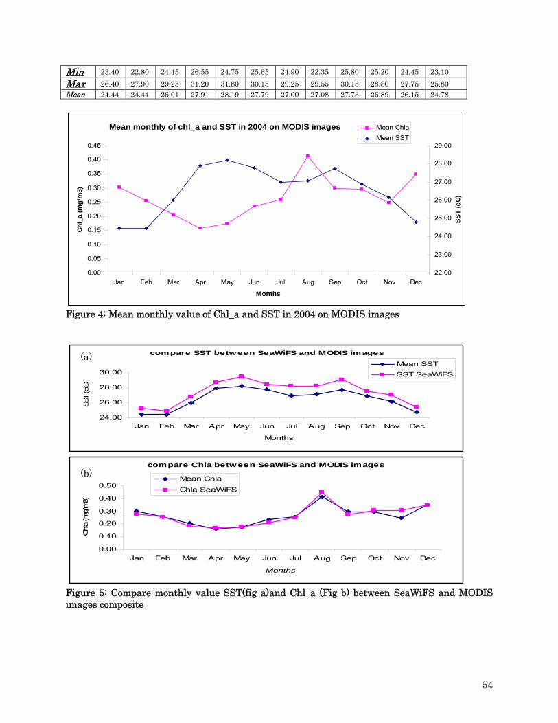
54

Min 23.40 22.80 24.45 26.55 24.75 25.65 24.90 22.35 25.80 25.20 24.45 23.10 Max 26.40 27.90 29.25 31.20 31.80 30.15 29.25 29.55 30.15 28.80 27.75 25.80 Mean 24.44 24.44 26.01 27.91 28.19 27.79 27.00 27.08 27.73 26.89 26.15 24.78

Mean monthly of chl_a and SST in 2004 on MODIS images

0.00

0.05

0.10

0.15

0.20

0.25

0.30

0.35

0.40

0.45

Jan Feb Mar Apr May Jun Jul Aug Sep Oct Nov Dec

Months

Chl_

a (m

g/m

3)

22.00

23.00

24.00

25.00

26.00

27.00

28.00

29.00

SST

(oC)

Mean ChlaMean SST

Figure 4: Mean monthly value of Chl_a and SST in 2004 on MODIS images

compare SST between SeaWiFS and MODIS images

24.00

26.00

28.00

30.00

Jan Feb Mar Apr May Jun Jul Aug Sep Oct Nov Dec

Months

SST

(oC)

Mean SST

SST SeaWiFS

compare Chla between SeaWiFS and MODIS images

0.00

0.10

0.20

0.30

0.40

0.50

Jan Feb Mar Apr May Jun Jul Aug Sep Oct Nov Dec

Months

Chla

(mg/

m3)

Mean Chla

Chla SeaWiFS

Figure 5: Compare monthly value SST(fig a)and Chl_a (Fig b) between SeaWiFS and MODIS images composite

(a)

(b)

55

Conclusion • Average chl-a minimum (0.16mg/m3) in April and Maximum (0.41mg/m3) in August. • In August, appear small region with high chl-a from MuiNe to MuiLagan. The highest

about 8.41mg/m3. • Average SST minimum in January (24.44 oC) and appear to peaks with maximum in May

(28.19 oC) and September (27.73 oC) • In the July appear small region with low SST 27.00 oC) from MuiNe to MuiLagan. In here

upwelling phenomenon usually happen annually. • The value of Chl_a seem to opposite with the value of SST. • When compare values Chl_a and SST between SeaWiFS images and MODIS images, I

see that: mean chl_a not change so much but the mean SST of the SeaWiFS higher than MODIS images.

• Using Wim software, we can export value SST & chl-a ocean color format to the ASCII format

Possible in near future

• Building data basic for the SST and Chl-a from ocean color remote sensing • Detecting factors base on ocean color • Supplying information for aquaculture • Background environment information for government

Reference:

1. Report of the International Ocean-Colour Coordinating Group. Report 1,2,3 2. Presentation of Pro. Masumura, Mr. tan, Mr. Son, Mr. Ishizaka, Mr. Kahru, Mr. Varis

Ransi. 3. Mati Kahru. May 2007. Practical Exercies with WIM and WAM. 45 pp

Information on http://las.aviso.oceanobs.com/las/servlets/dataset http://reason.gsfc.nasa.gov/Giovanni/ http://disc2.nascom.nasa.gov/Giovanni/tovas/ Analysis to build a software tool to calculate Primary Productivity from Ocean color remote sensing image

Lau Va Khin, Oceanographic Data Center Insititute of Oceanography Nha Trang

1. Introduction Primary production is the production of organic compounds from atmospheric or aquatic carbon dioxide, principally through the process of photosynthesis, with chemosynthesis being much less important. All life on earth is directly or indirectly reliant on primary production and is the base of the food chain and underlies the biogeochemical cycles of many materials. For the Ocean color remote sensing technique, a number of models and parameters have been propose to estimate vertically integrated primary productivity[1]. One of the simplest models commonly used is the vertically Generalized Production Model(VGPM) proposed by Behrenfeld and Falkowki (1997, hereafter BF). This model calculate base on Chlorophyll concentration (Chlo), sea surface temperature (SST) and photosynthetically active radiation (PAR). These are parameters, you can get from the ocean color remote sensing

56

image, here, in this paper will mention to SST from MODIS Level 3, Chlo and PAR from SeaWifs Level 3.

2. Aim - A graphic user interface software (GUI) tools to calculate primary productivity from

ocean color image of MODIS Level 3 and SeaWifs Level 3 using Vertically Generalized Production Model (VGPM).

- User can customize some parameter on VGPM 3. Method

a. Vertically Generalized Production Model The core equation describing the relationship between surface chlorophyll and depth-integrate primary production is expressed as follows:

irreusatB

opteu DZChlPAR

PARPPP1.4

66125.0+

=

Chlsat: Satellite surface chlorophyll concentration as derived from measurement of water leaving radiance (mg Chl/m3). Dirr: Daily photoperiod = f(Julia day, latitude) ? PAR: sea surface photosynthetically active radiation. Zeu: Physical depth (m) of the euphotic zone defined as the penetration depth of 1% surface irradiance based on the Beer-Lambert law. Zeu is calculated from Csat following Morel and Berthon (surface pigment, algal biomass profiles and potential production of euphotic layer: Relationship reinvertigated in view of remote sensing applications. Limnatol. Oceanograpr. 34, 1989:1545-1562):

⎪⎩

⎪⎨⎧

>

<=

−

−

102)(0.200

102)(2.568

293.0

746.0

eutotal

eutotal

eu

ZifChl

ZifChlZ

Where Chltotal

⎪⎩

⎪⎨

⎧

>

<=

0.1)(2.40

0.1)(0.38

507.0

425.0

satsat

satsat

total

ChlifChl

ChlifChlChl

BpotP : Optimal rate of daily carbon fixation within a water column, unit is [mg C (mg

Chl)-1h-1].

These are two methods to calculate BpotP as flowing:

Behrenfeld and Falkowski (1997): BpotP can be modeled according to various

temperature-dependent relationships. The relationship used for most of the global production calculations was described by

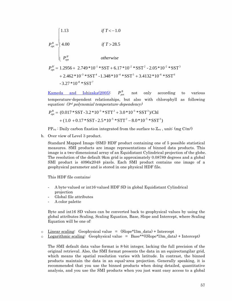
57

⎪⎪⎪

⎩

⎪⎪⎪

⎨

⎧

>

−<

=

otherwiseP

Tif

Tif

P

Bopt

Bopt

'

5.2800.4

0.113.1

78-

66-54-43-

3-22-2-1'

SST *10*3.27 - SST *10*3.4132 SST *10*1.348 - SST *10*2.462

SST *10*2.05 - SST *10*6.17 SST *10*2.749 1.2956

++

++=BoptP

Kameda and Ishizaka(2005): BpotP not only according to various

temperature-dependent relationships, but also with chlorophyll as following equation: (3rd polynomial temperature dependency)

)SST*10*.08STT*10*2.5-SST*0.17 1.0 (

)/ChlSST*10*3.0STT*10*3.2-SST*(0.017 35-25-

3-52-3

−++

+=BoptP

PPeu : Daily carbon fixation integrated from the surface to Zeu , unit: (mg C/m2) b. Over view of Level 3 product.

Standard Mapped Image (SMI) HDF product containing one of 5 possible statistical measures. SMI products are image representations of binned data products. This image is a two-dimensional array of an Equidistant Cylindrical projection of the globe. The resolution of the default 9km grid is approximately 0.08789 degrees and a global SMI product is 4096x2048 pixels. Each SMI product contains one image of a geophysical parameter and is stored in one physical HDF file.

This HDF file contains:

- A byte-valued or int16-valued HDF SD in global Equidistant Cylindrical projection

- Global file attributes - A color palette

Byte and int16 SD values can be converted back to geophysical values by using the global attributes Scaling, Scaling Equation, Base, Slope and Intercept, where Scaling Equation will be one of:

o Linear scaling: Geophysical value = (Slope*l3m_data) + Intercept o Logarithmic scaling: Geophysical value = Base**((Slope*l3m_data) + Intercept)

The SMI default data value format is 8-bit integer, lacking the full precision of the original retrieval. Also, the SMI format presents the data in an equirectangilar grid, which means the spatial resolution varies with latitude. In contrast, the binned products maintain the data in an equal-area projection. Generally speaking, it is recommended that you use the binned products when doing detailed, quantitative analysis, and you use the SMI products when you just want easy access to a global

58

image.

c. Input - SeaWifs Chlorophyll image: The value of this image was stored in DN by a byte value

or int16-value. So you have to convert back to geophysical value by using the global attributes Scaling, Scaling equation, base, slope and intercept. For SeaWifs Chlorophyy, the Scaling equation is Logarithmic scaling as following: Geophysical value= Base(Slope*DN + intercept) With: Base = 10; slope = 5.81378e-5; intercept= -2 DN Max = 65534 Geophyical value max is 64.5658

- SeaWifs PAR image: Convert to geophysical value by linear equation as following: Geophysical value = (Slope * DN) + Intercept

With: slope = 1.16275e-3; intercept= 0.0 DN Max = 65534 Geophyical value max is 76.2

- MODIS SST image: Convert to geophysical value by linear equation as following: Geophysical value = (Slope * DN) + Intercept

With: slope = 7.7185e-4; intercept= -2.0 DN Max = 65534 Geophyical value max is 45

- Dirr: f(Julia day, latitude) =12 for Vietnam sea, user can customize by GUI d. Requirement - All image have the same resolution and the same range - Image file in hdf format (this format already support by MODIS and SeaWifs) e. Output - Primary productivity image [mg C/m2] f. VGPM diagram

59

4. Discussion - Primary productivity (PP) is a very import component in coastal environment, Food, fishing

forcast,..., and with you can get free ocean color images from the Internet. So the needed of building a software tool to calculate as fast, as accuracy and free is very reasonable.

- There are also have some softwares already attached the module to calculate PP, but most of them are commercial softwares (WIM/WAM) or run on linux operating system (SEADAS), it’s very difficult got to use in developing countries (Vietnam).

- VGPM was used widely and long time ago to calculate primary productivity and also prove that it is a simplest, good and stable model.

- VGPM is very clearly model for coding a software tool. - In this paper still not define Dirr - Have not check the turbidity image. - And just a limit image format. 5. References - Ishizaka, J., E. Siswanto, T. Itoh, H. Murakami, Y. Yamaguchi, T. Ishimaru, S. Hashimoto

and T. Saino (2007): Verification of Vertically Generalized Production Model and Estimation of Primary Production in the Sagami Bay, Japan. J. Oceanogr. 64, 5１7-524.

- Nguyen Tac An, Tong Phuoc Hoang Son: Application of remote sensing for intepretation of primary productivity in South China Sea

- http://oceancolor.gsfc.nasa.gov

MODIS L3 SEAWIFS L3

SST Chl PAR

ZeuB

optP

BF

KI

Primary Productivity

Dirr

60

Seasonal variation of Chlorophyll-a concentrations, Sea Surface Temperature and the relationship with phytoplankton at Binh Thuan Province, Viet Nam. Truong Si Hai Trinh * Marine Plankton Department, Institute of oceanography, Nha Trang, Viet Nam. *Email: haitrinh-ion@vnn.vn Background BSc. In Biology (2000 – 2004) Status works: Marine Plankton Department at Institute of oceanography, Nha Trang, Viet Nam.

- Taxonomy marine zooplankton.

Introduction Red tide in Vietnamese waters has been occasionally recored from different localities over

the country, such as: Khanh Hoa province with Noctiluca scintilands in 1995 (Nguyen & Doan, 1996), Binh Thuan province with Trichodesmium species (Nguyen & Doan, 1996, Nguyen 1999).

Binh Thuan, Vietnam has been known as a province has income mostly based on seafood products (fish, cattle fishes, mollusc) and culture is mainly tiger shrimp (Tran Trong, 2001, 2002, Nguyen 2002). Bloom of micro-algae have been recorded previously and the mortalities of natural communities also recognised by local fishermen. However, only one species Trichodesmium erythraeum has been reported forming the blooms in 1993, 1995, and 1999 by scientists (Nguyen & Doan 1996, Nguyen 1999). The resent bloom of haptophyte algae Phaeocystis globosa may be the most serious red tide has been observed in the province.

The chlorophyll a (chl a) has been used as the relative measurement to phytoplankton abundance and biomass in the ocean (Martin, 2004). The goal of remote sensing of ocean colour is to derive quantitative information on the types of substances present in the water and on their concentrations, from variations in the spectral form and magnitude of the ocean colour signal. A primary goal of ocean colour remote sensing is to produce synoptic fields of chlorophyll pigment, an index of phytoplankton biomass. Method.

Binh Thuan coastal water always has bloom every year from 2000 to 2006 and only one specie Trichodesmium erythraeum has been reported.

Sea surface temperature (SST) anomalies have been used to detect changes in the oceans, such as the presence of an El Nin˜o, upwelling events, and climate predictions (Goddard et al., 2001). The change detection concepts used for temperature anomalies can also be employed with chlorophyll anomalies.

In this report, we used images from Ocean Color Time-Series Online Visualization and Analysis, this website This system is based on the GES-DISC Interactive Online Visualization and Analysis Infrastructure (Giovanni) which was developed by the GES DISC DAAC to provide users with an easy-to-use, Web-based interface for the visualization and analysis of the Earth Science data.

61

Fig 1. Binh Thuan province, Vietnam.

Result and discusion

1. Variation of Chl-a in Binh Thuan. The value of Chl-a in Binh Thuan was increase from May until have a peak and after that

decrease. In 2002, value of Chl-a had two peak at July (2.27 mg.m-3) and September (1.71 mg.m-3), and other years only has one peak at August and after that the Chl-a decrease until November (Fig 2). Maximum of Chl-a at August, 2006 with 4.46 mg/m3, in 2002, the maximum value of Chl-a was 2.27 mg.m-3, in 2003 was 2.26 mg.m-3, 2004 was 3.19 mg/m3, and 2005 was 2.55 mg.m-3. We recognized the algae bloom at this time had the maximum value of Chl-a.

0

0.5

1

1.5

2

2.5

3

3.5

4

4.5

5

I II III IV V VI VII VIII IX X XI XII Month

Chl

-a (m

g.m

-3)

20

22

24

26

28

30

32

SST

(oC)

Chl-a 2002 Chl-a 2003 Chl-a 2004 Chl-a 2005 Chl-a 2006SST-2002 SST-2003 SST-2004 SST-2005 SST-2006

Fig 2. Variation of Chl-a in Binh Thuan, 2002-2006

62

-

50

100

150

200

250

300

350

400

450

3 2 1 4 5 6 9 8 7-

5,000

10,000

15,000

20,000

25,000

30,000

BACILLARIOPHYCEAE DINOPHYCEAE PRYMNESIOPHYCEAE

Caø Naù Vónh Haûo Phöôùc Theå

Bac

illar

ioph

ycea

e &

Din

ophy

ceae

Den

sity

, x10

3 cel

ls.l-1 Prym

nesiophyceaeD

ensity, x103 cells.l -1

1.5 x 106 Surface Layer

-

50

100

150

200

250

300

350

400

450

3 2 1 4 5 6 9 8 7-

10,000

20,000

30,000

40,000

50,000

60,000

BACILLARIOPHYCEAE DINOPHYCEAE PRYMNESIOPHYCEAE

Caø Naù Vónh Haûo Phöôùc Theå

Bac

illar

ioph

ycea

e &

Din

ophy

ceae

Den

sity

, x10

3 cel

ls.l-1 Prym

nesiophyceaeD

ensity, x103 cells.l -1

Bottom Layer

Fig 3. Cell density of different phytoplankton groups during the bloom of Phaeocystis globosa in 2002 (Doan-Nhu et al. 2003)

Images in fig 2 show the Chl-a at

the south of Vietnam, and the Chl-a at Binh Thuan area lower than south area at May, June and after become higher at July, August. The area (in Binh Thuan province) had the pink color (high Chl-a) in this images show the bloom areas at this month we was recored. In 2002, a serious bloom of Phaeocystis globosa had happen during June –July period, average value of Chl-a was 1.35 mg.m-3. Wind and coast morphology would lead to the accumulation of the floating algal colonies at beaches from Phan Ri to Tuy Phong. Total cell density of bottom layer (27.8 x 106 cells L-1) was 5 fold higher than in surface layer (5.8 x 106 cells L-1), while it was only 1.5 fold on transect of Phuoc The (26.2 x 106 and

16.0 x 106 cells L-1 for surface and bottom layers, respectively). Transect of Vinh Hao showed no difference of total cell density between bottom and surface layers with rather low phytoplankton density (6.6 x 106 cells L-1) (Fig.3) (Doan-Nhu et al. 2003).

In 2004 there was a bloom with similar phenomenon as in 2002 (information from local

authorities) in July-August with a wider affected coastal waters. No data were collected. In 2005 the bloom of Phaeocystis globosa has happen again. Chlorophyll-a concentration was highest as 52 µg/L with maximum cell density to 300 x 106 cells/L (Figure 8, Nguyen-Ngoc unpublished data). There was another bloom in 2006 of the same species (Figure 8). It was not surveys on economic lost during these algal blooms but it was obvious lots for tourism by less tourists by the time when the bloom occurred.

63

Fig 8. Images from the bloom of Phaeocystis globosa in 2006. (DMP unpublished images)

On the report, we just want to know about the temporal and spatial variation of Chl-a, we take one tracsect at 11.5 N, 108.4-110.0 E and check the images in Giovani website. With this images (fig 7), it showed the co-ordinate and which month had highest Chl-a . In 2002, highest of Chl-a at June and July, 2003, 2004, 2005 and 2006 at August, the tendency of Chl-a in this transect was same with study area. 2. Variation of SST in Binh thuan

Fig 6 show some information about SST of Binh Thuan coastal. The average SST of Binh Thuan province was 27.5oC. Lowest average value at Jan (24.85oC) and highest at May (29.5oC). Highest SST in May, 2006 (30.26oC) and lowest at Jan, 2006 (24.2oC). At the time algal

27.5

12.2

26.9

12.4 813.5

164

49

69

162

82.8

109.2

0

20

40

60

80

100

120

140

160

180

0

20

40

60

80

100

120

140

160

180

Hon Rom Ham Tien Bai Ong Dia

NH 3

(4)-N

, µg.

L-1

PO

4-P, N

O2-N

, NO

3-N,

µg.

L-1

Sampling Location

PO4-P NO2-NNO3-N NH3(4)-N

0

50

100

150

200

250

300

350

-

50

100

150

200

250

300

Hon Rom Ham Tien Bai Ong Dia

Chl

orop

hyll-

a, P

haeo

phyt

in,

µg.L

-1

Sampling Location

Chlorophyll a

Phaeophytin

Mật độ tế bào

Cell

Dens

ity, x

106Ce

lls.L

-1

Figure 9.

(Above), in

situ Chl-a

and cell

density

(upper

graph)

with

nutrient

(lower

graph)

64

bloom was occur in August (2004, 2005, 2006), the average value of SST was 27.7oC. SST of Binh Thuan always lower than neighbouring area (Fig. 6) from May to September.

At the time, Binh Thuan coastal had upwelling phenomenon, and the upwelling bring the cold water from deep layer to surface and make the temperature on surface lower. Conclusion

- Use images from statelite to know about the Chl-a and SST on coastal water. - At the time had algal bloom, the images show high value of Chl-a. - No idea about the relationship between SST and Chl-a - SST of Binh thuan coastal water lower than neighbour areas because the upwelling occur

at this time (May – Sep). Future Plan

- Receive daily images about Chl-a and SST from http://oceancolor.gsfc.nasa.gov and take some information in the images about the tendency of Chl-a and give some recommend for Binh Thuan goverment about the time maybe the algal bloom occur.

Acknowledgements To complete this report, big thank for Prof. Matsumura, Dr. Tan, Dr. Varis and for all members of the training course. Thank you for all support from Marine Plankton Department, Institute of oceanography.

Appendix

65

Fig 5. The Chl-a at the south of Vietnam from 2002-2006.

66

Fig 6. The variation of SST in Binh Thuan, Vietnam, 2003-2006

67

Fig 7. Variation of Chl-a at transect 11.5N; 108.4 – 110.0

68

===============================＝＝＝＝＝＝＝＝＝＝＝＝＝＝＝ PRELIMINARY RESULTS ON APLLICATION REMOTE SENSING DATA IN MONITORING WATER SST AND CHLORPHYLL_A TO GROWTH RATE OF Kappaphycus alvarezii CULTIVATION ALONG THE COASTAL ZONE OF KHANH HOA - BINH THUAN PROVINCE

Vo Xuan Mai

Nha Trang Institute of Technology Research and Application 2 - Hung Vuong -Nha Trang City – VietNam – Email: voxuanmai@dng.vnn.vn

ABSTRACT This report introduce the relationship of Kappaphycus alvarezii, water temperature and chlorphyll_a based on the data collected from website: http://oceancolor.gsfc.nasa.gov/cgi/browse.pl ( data daily 2004) and data investigated in Nha Trang stations.(data from Departement of The Organic Materials From Sea Resources-Nha Trang Institute of Technology Research and Application)(Huynh Quang Nang, 2005-2006)

INTRODUCTION

- Kappaphycus alvarezii (Doty) Doty (main raw material for processing Kappa-Carrageenan of the world) is not found in the Viet Nam Sea so far. So in 1993 a study on transplanting of K.alvarezii ( the original seedstock from Philippines ) into the seawaters of Southern VN. And now Kappaphycus alvarezii cultivation has became a new subject in aquaculture of Viet Nam, especially in Central- South.( Huynh Quang Nang, 1996)

- Some of most important parameters that effect to growing of Kappapycus alvarezii are seawater temperature (there two main season: Hot season from April to September with the temperature ranged from more than 300C to 340C, the growth rate of K.alvarezii average ranged 3-4 %-day. Cool season from October to next March with the water temperature almost less than 300C, the growth rate of this seaweed is higher: ranged from 6-8 %-day ) (H.Q.Nang), Salinity, Chlorophyll-a (by pass primary production), nutrient, as well as bottom substract... . In order to choose a optimum areas to aquacuture, we can systematic measurement all of above parameter. But this work consume money as well as human power. The growth rate of K. alvarezii (Doty) Doty and K.striatum (Schmitz) Doty is effected by interrelation of many environmental factors. But in this report, because of I have only the data of SST , Chl_a, growth rate of two Kapaphycus species investigated in Nha Trang stations , only introduce the variation of three above factors

- Remote sensing technology can help us for reducing above mention budget by mean of automatic extraction SST and chlorophyll_a and others from ocean colour sources. USED MATERIAL AND METHOD

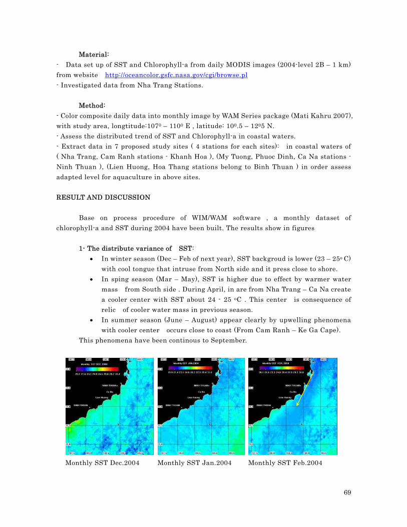
69

Material:

- Data set up of SST and Chlorophyll-a from daily MODIS images (2004-level 2B – 1 km) from website http://oceancolor.gsfc.nasa.gov/cgi/browse.pl - Investigated data from Nha Trang Stations.

Method: - Color composite daily data into monthly image by WAM Series package (Mati Kahru 2007), with study area, longtitude:1070 – 1100 E , latitude: 100.5 – 1205 N. - Assess the distributed trend of SST and Chlorophyll-a in coastal waters. - Extract data in 7 proposed study sites ( 4 stations for each sites): in coastal waters of ( Nha Trang, Cam Ranh stations - Khanh Hoa ), (My Tuong, Phuoc Dinh, Ca Na stations - Ninh Thuan ), (Lien Huong, Hoa Thang stations belong to Binh Thuan ) in order assess adapted level for aquaculture in above sites. RESULT AND DISCUSSION

Base on process procedure of WIM/WAM software , a monthly dataset of

chlorophyll-a and SST during 2004 have been built. The results show in figures 1- The distribute variance of SST:

• In winter season (Dec – Feb of next year), SST backgroud is lower (23 – 25o C) with cool tongue that intruse from North side and it press close to shore.

• In sping season (Mar – May), SST is higher due to effect by warmer water mass from South side . During April, in are from Nha Trang – Ca Na create a cooler center with SST about 24 - 25 oC . This center is consequence of relic of cooler water mass in previous season.

• In summer season (June – August) appear clearly by upwelling phenomena with cooler center occurs close to coast (From Cam Ranh – Ke Ga Cape).

This phenomena have been continous to September.

Monthly SST Dec.2004 Monthly SST Jan.2004 Monthly SST Feb.2004

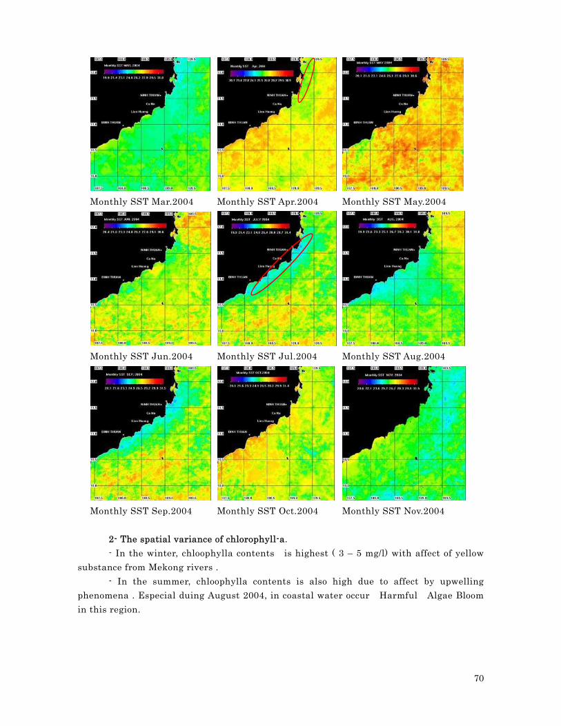
70

Monthly SST Mar.2004 Monthly SST Apr.2004 Monthly SST May.2004

Monthly SST Jun.2004 Monthly SST Jul.2004 Monthly SST Aug.2004

Monthly SST Sep.2004 Monthly SST Oct.2004 Monthly SST Nov.2004

2- The spatial variance of chlorophyll-a. - In the winter, chloophylla contents is highest ( 3 – 5 mg/l) with affect of yellow

substance from Mekong rivers . - In the summer, chloophylla contents is also high due to affect by upwelling

phenomena . Especial duing August 2004, in coastal water occur Harmful Algae Bloom in this region.

71

Monthly Chl_a Dec. 2004 Monthly Chl_a Jan. 2004 Monthly Chl_a Feb. 2004

Monthly Chl_a Mar. 2004 Monthly Chl_a Apr.2004 Monthly Chl_a May. 2004

Monthly Chl_a Jun. 2004 Monthly Chl_a Jul. 2004 Monthly Chl_a Aug. 2004

72

Monthly Chl_a Sep. 2004 Monthly Chl_a Oct. 2004 Monthly Chl_a Nov. 2004 3 - The temporal variance of SST

and Chlorophyll-a . Base on 7 sites (4 stations in each site), we will try to access adapted condition for culturing two species the Kappaphycus.

• We extracted data from monthly

images SST and chlorophyll-a • Analysis the temporal variance in each

sites and all • The results show in figures

The relationship of growth rate of K. alvarezii and K.striatum to the variation of water temperature and Chl_a showed that: - The variation of two season temperature from the data investigated in Nha Trang stations (2005-2006), they're the same as the variation of two season temperature from the data of MODIS image (2004) in other sites. - There are two season on the growth rate of K. alvarezii and K.striatum.

- In the months of low temperature (from Nov. to next Jan.) with SST average: 25.20C the daily growth rates with average: 6.06( %day-1) of K. alvarezii and average: 4.71( %day-1) of K. striatum high - In the months of higher temperature (from Apr. to next May.) with SST average: 27.70C the daily growth rates with average average: 1.04( %day-1) of K. alvarezii and average: 3.16( %day-1) of K. striatum decreased

73

0

5

10

15

20

25

30

35

Nov-05 Dec-05 Jan-06 Feb-06 Mar-06 Apr-06 May-06 Jun-06

Cool season Hot season

TºC

0

1

2

3

4

5

6

7

Gro

wth

rate

( %

day-

1)

Temp. (field work) (T°C) NT_SSTCR_SST MT-SSTPD-SST CN-SSTLH-SST HT-SSGrowth rate K.alvarezii( %day-1) Growth rate K.striatum( %day-1)

74

THE APPLICATION OCEAN COLOR REMOTE SENSING FOR DETECTING SST AND CHLOROPHYLL-A AT THE EAST SOUTH VIET NAM SEA IN THE YEAR 2005

Phan Thanh Bac

GIS and Remote Sensing Department Institute of Oceanography (Viet Nam)

ABSTRACT: The East South Vietnam sea is very important with the aquaculture, this is the place have a lot of fish at Vietnam, all of fisher man of South Vietnam have job from this place. So the poor and disease will come to them if this sea have some problem as red tide, high temperature or salinity, pollution from oil spill... The scientist always want to monitor and forecast earlier but they lost a lot of time with old methods. And with remote sensing, they will have results earlier and have decision quickly and exactly. INTRODUCTION:

Ocean color remote sensing is a new technique in Viet Nam. With this technique, scientist have image from satellite, metadata or download from website. After that they use some software detect image and analyze for their factor which they like. If we use remote sensing, we will know about some factor of sea: SST, Chlorophyll, Salinity, wind, current,… All of them may change in long time, everywhere and wide area. Remote sensing will easily support scientists who want to monitor and forecast.

In Viet Nam, almost all scientist use GIS database for management for all the factor of coastal, environment, geographical, physical ceanography… So combine image of satellite and GIS Map is easier for Vietnamese scientist. And they will have more tool using a lot of their purpose. And the local government of each province will manage easily and will have the most plan sensible for development of their province. PURPOSE:

Support for Vietnamese scientist about some factors of the ocean in large place and building database of GIS Map from satellite image data. And the monitor and forecast of the scientist will more exactly if use the data gotten from satellite image and the data gotten from Field trip or Monitoring. Support for the management of scientist about the data from remote sensing in the long time. METHOD:

Download SST and Chlorophyll-a from the level 2 of MODIS Aqua image in the year 2005. After that using Wim/Wam software for detect, composite all image and take average each month in all year long. Export data from image to ASCII data, using Microsoft Excel drawn the graph of SST and Chlorophyll for one month. Use this data in Surfer software and drawn the contour line for one month. Analyze about general trend of distribute of two factor. Drawn contour line of in-situ SST and Chlorophyll-a. Convert all satellite image and contour line to GIS map of Mapinfor software for management.

75

RESULT: - The results about SST is detected from Satellite image (from January to December 2005):

January – 2005 February – 2005 March – 2005

April – 2005 May – 2005 June – 2005

July – 2005 August – 2005 September – 2005

October -2005 November – 2005 December - 2005

76

The results about SST is converted to GIS Map (from January to December 2005):

2222.52323.52424.52525.52626.52727.52828.52929.53030.53131.532

2222.52323.52424.52525.52626.52727.52828.52929.53030.53131.532

2222.52323.52424.52525.52626.52727.52828.52929.53030.53131.532

January – 2005 February – 2005 March – 2005

2222.52323.52424.52525.52626.52727.52828.52929.53030.53131.532

2222.52323.52424.52525.52626.52727.52828.52929.53030.53131.532

2222.52323.52424.52525.52626.52727.52828.52929.53030.53131.532

April – 2005 May – 2005 June – 2005

2222.52323.52424.52525.52626.52727.52828.52929.53030.53131.532

2222.52323.52424.52525.52626.52727.52828.52929.53030.53131.532

2222.52323.52424.52525.52626.52727.52828.52929.53030.53131.532

July – 2005 August – 2005 September – 2005

2222.52323.52424.52525.52626.52727.52828.52929.53030.53131.532

2222.52323.52424.52525.52626.52727.52828.52929.53030.53131.532

2222.52323.52424.52525.52626.52727.52828.52929.53030.53131.532

October -2005 November – 2005 December - 2005

77

- The results about Chlorophyll is detected from Satellite image (from January to December 2005):

January – 2005 February – 2005 March – 2005

April – 2005 May – 2005 June – 2005

July – 2005 August – 2005 September – 2005

October -2005 November – 2005 December - 2005

78

- The results about Chlorophyll is converted to GIS Map (from January to December 2005):

0

0.5

1

1.5

2

2.5

3

3.5

4

4.5

5

5.5

6

6.5

7

7.5

0

0.5

1

1.5

2

2.5

3

3.5

4

4.5

5

5.5

6

6.5

7

7.5

0

0.5

1

1.5

2

2.5

3

3.5

4

4.5

5

5.5

6

6.5

7

7.5

January – 2005 February – 2005 March – 2005

0

0.5

1

1.5

2

2.5

3

3.5

4

4.5

5

5.5

6

6.5

7

7.5

0

0.5

1

1.5

2

2.5

3

3.5

4

4.5

5

5.5

6

6.5

7

7.5

0

0.5

1

1.5

2

2.5

3

3.5

4

4.5

5

5.5

6

6.5

7

7.5

April – 2005 May – 2005 June – 2005

0

0.5

1

1.5

2

2.5

3

3.5

4

4.5

5

5.5

6

6.5

7

7.5

0

0.5

1

1.5

2

2.5

3

3.5

4

4.5

5

5.5

6

6.5

7

7.5

0

0.5

1

1.5

2

2.5

3

3.5

4

4.5

5

5.5

6

6.5

7

7.5

July – 2005 August – 2005 September – 2005

0

0.5

1

1.5

2

2.5

3

3.5

4

4.5

5

5.5

6

6.5

7

7.5

0

0.5

1

1.5

2

2.5

3

3.5

4

4.5

5

5.5

6

6.5

7

7.5

0

0.5

1

1.5

2

2.5

3

3.5

4

4.5

5

5.5

6

6.5

7

7.5

October -2005 November – 2005 December - 2005

79

- The results is converted to ASCII and drawn to chart (from January to December 2005):

CONCLUSION:

From Satellite image we can saw chlorophyll-a is minimum in April and is maximum in September in this year. Chlorophyll-a is high from June to September and low from April to May. And SST is maximum in January and is minimum in April.

SST high in some month: March, April, May, June, July, September SST low in January, February, November, December

The sky have a lot of cloud in some month: February, April, September, October, December.

From some cause had analysis , Chlorophyll is low in April because: in this month SST high and have a lot of cloud on the sky and raining gotten at the ocean but raining won’t got at the land. So that isn’t enough nutrient and alga can’t photosynthesis.

Chlorophyll is high in September because: in August have raining on the land because this time is raining season. The water from Mekong river come to East South Vietnam sea have a lot of nutrient, SST is high and have a little cloud in this month. So that is the best environment for alga bloom in the next month (September).

Chlo

0

0.5

1

1.5

2

Jan Fer Mar Apr May Jun Jul Aug Sep Oct Nov Dec

Chlo

SST

22

23

24

25

26

27

28

29

Jan Fer Mar Apr May Jun Jul Aug Sep Oct Nov Dec

SST