feeling the heat: extreme temperatures and price stability

Working Paper Series Feeling the heat: extreme temperatures and price stability

Donata Faccia, Miles Parker, Livio Stracca

Disclaimer: This paper should not be reported as representing the views of the European Central Bank (ECB). The views expressed are those of the authors and do not necessarily reflect those of the ECB.

No 2626 / December 2021

Abstract

We contribute to the debate surrounding central banks and climate change by investigat-

ing how extreme temperatures affect medium-term inflation, the primary objective of mon-

etary policy. Using panel local projections for 48 advanced and emerging market economies

(EMEs), we study the impact of country-specific temperature shocks on a range of prices:

consumer prices, including the food and non-food components, producer prices and the GDP

deflator. Hot summers increase food price inflation in the near term, especially in EMEs.

But over the medium term, the impact across the various price indices tends to be either

insignificant or negative. Such effect is largely non-linear, being more significant for larger

shocks and at higher absolute temperatures. We also provide simulations from a two-country

model to understand the rationale behind the results. Overall, our results suggest that tem-

perature plays a non-negligible role in driving medium-term price developments. Climate

change matters for price stability.

Keywords: inflation, climate change, extreme temperatures, panel local projections.

JEL Classification Code: E03, E31, Q51, Q54.

ECB Working Paper Series No 2626 / December 2021 1

Non-Technical Summary

Climate change is the challenge of our generation, and there are increasing signs of its impact.

According to the EU Copernicus Climate Change Service, 2020 was the hottest year on record

in Europe, and the past six years comprise the hottest six on record worldwide. 2021 has

witnessed record temperatures in North America, Southern Europe and Central Asia. There

has been increasing research in recent years into the impact of these rising temperatures on

economic activity. But to date little is known about the impact on inflation – and therefore on

central banks’ primary mandate. This paper aims to address that deficit, and focuses on the

effects of temperature extremes on medium-term inflation.

For a panel of 48 advanced and emerging economies, we investigate how extreme temper-

atures affect various measures of prices: consumer prices (including the food and non-food

components), producer prices and the GDP deflator. We use data on the seasonal divergence of

temperatures from their country-level average in the middle of the 20th Century (1951-1980).

We also introduce a simple two-country New Keynesian model enriched with a role of tem-

perature in influencing productivity for agricultural goods, in order to rationalise the effect of

temperature shocks (both global and country-specific) on price developments.

We identify four key results:

1. Timing matters: extreme temperatures have differing impacts depending on when they

occur within the year. By far the largest and longest-lasting impact derives from hot

summers.

2. It is important to consider a wide range of prices and not just headline CPI. In particular,

the short-run impact from hot summers mostly arises from the impact on food prices.

This impact occurs in both advanced and emerging economies, but is stronger in the

latter group.


3. The horizon also matters: we find evidence of negative inflation dynamics in the medium

term, again particularly noticeable in emerging economies. This suggests that short-term

supply disruption in agriculture can result in more longer-lasting downward pressure on

demand.

4. Finally, we show that the impact is non-linear, both in terms of divergence from average

temperatures, and in terms of absolute temperature. This suggests that even for those

countries where the impact has been limited to date, the future may be less benign.

Overall, we find that higher temperatures over recent decades have played an increasingly

non-negligible role in driving price developments, including into the medium term. Climate

change, in other words, is already starting to bear on the primary mandate of central banks.

This provides some empirical justification for central banks to contribute to global efforts to

combat climate change.


1 Introduction

Climate change represents one of the greatest societal and economic challenges of this century

and action to combat it is becoming more urgent by the day. Human-induced climate change

is already affecting observed weather and climate extremes across the globe (IPCC, 2021). Ac-

cording to the EU Copernicus Climate Change Service, 2020 was the warmest year on record in

Europe, 0.4◦C hotter than the previous record year, which was 2019. Temperature records have

also tumbled worldwide in 2021, including in North America, Southern Europe, Arctic Russia

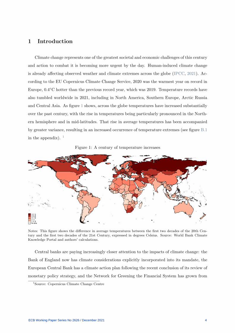
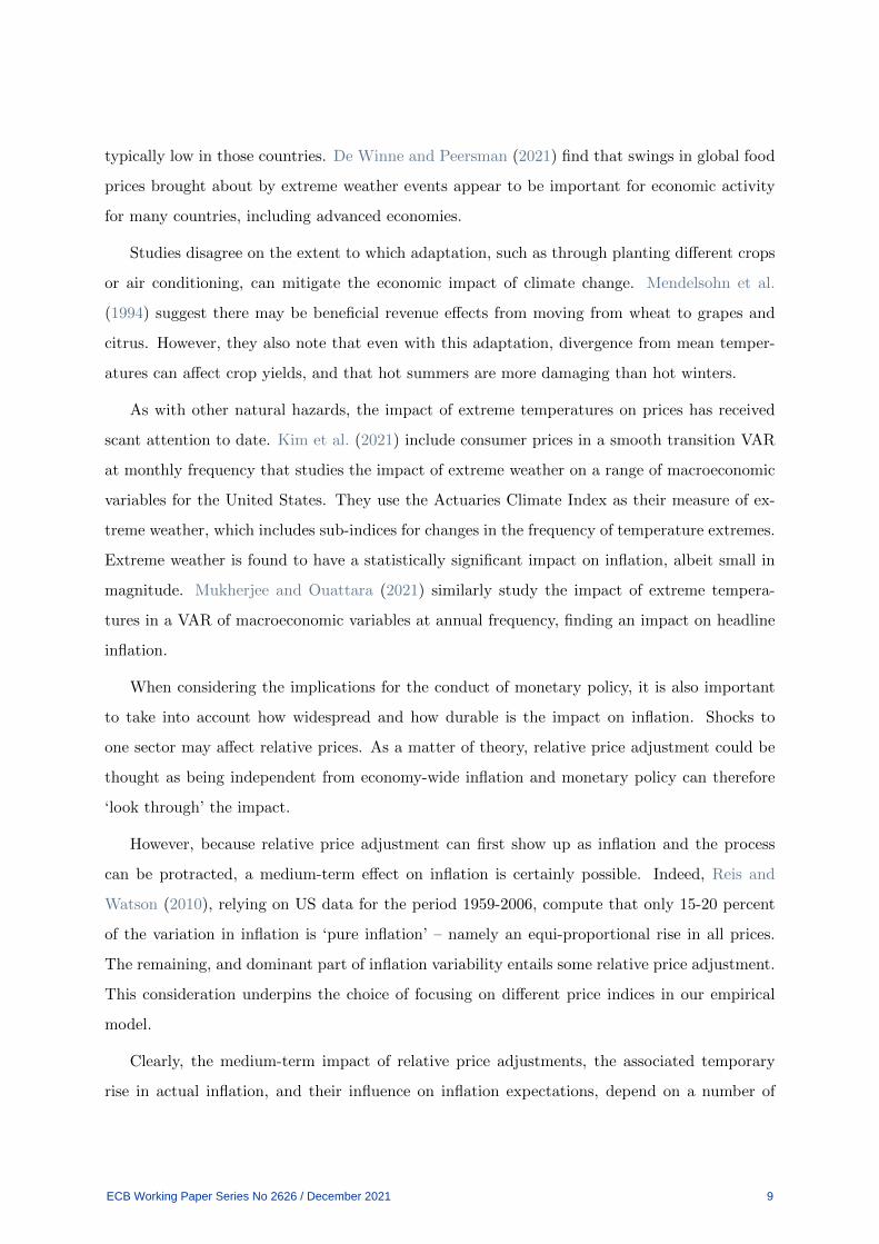
and Central Asia. As figure 1 shows, across the globe temperatures have increased substantially

over the past century, with the rise in temperatures being particularly pronounced in the North-

ern hemisphere and in mid-latitudes. That rise in average temperatures has been accompanied

by greater variance, resulting in an increased occurrence of temperature extremes (see figure B.1

in the appendix). 1

Figure 1: A century of temperature increases

Notes: This figure shows the difference in average temperatures between the first two decades of the 20th Cen-tury and the first two decades of the 21st Century, expressed in degrees Celsius. Source: World Bank ClimateKnowledge Portal and authors’ calculations.

Central banks are paying increasingly closer attention to the impacts of climate change: the

Bank of England now has climate considerations explicitly incorporated into its mandate, the

European Central Bank has a climate action plan following the recent conclusion of its review of

monetary policy strategy, and the Network for Greening the Financial System has grown from

1Source: Copernicus Climate Change Centre


8 founding central banks and supervisors in December 2017 to more than a hundred members

and observers today.

Yet despite the growing evidence of climatic impact and growing attention from policymak-

ers, the implications of climate change for monetary policy – and on its primary objective of

controlling inflation – have received little attention. Broadly speaking, there are three main

channels through which climate change can affect inflation.2 First, global warming is associated

with a greater incidence of damaging climatic events, notably windstorms, extremes of precipita-

tion and of temperature. Even if global warming is successfully restricted to 1.5◦C, these events

are still likely to become more commonplace (IPCC, 2021). Such events may impact specific

prices, notably food prices.

Second, the transition to a net zero carbon emission world is likely to involve sharp increases

in the price of carbon. That in turn is likely to affect consumer prices directly through higher

electricity, gas and petrol prices, and indirectly through increased costs of production for firms

across a broad range of sectors. Finally, higher temperatures themselves may dampen economic

activity and reduce labour productivity through higher rates of mortality, morbidity and lower

efficiency.

In this paper we focus on the first of these channels – specifically the impact of temperature

extremes on inflation – in order to address the substantial gap in the literature surrounding these

impacts. Concretely, we run panel local projections for 48 advanced and emerging economies,

regressing various quarterly price indices (CPI, its food, and non-food components, PPI, and

the GDP deflator) on measures of country-specific temperature anomalies. We also introduce a

simple two-country New Keynesian model enriched with a role for temperature in influencing

productivity for agricultural goods, in order to rationalise the effect of temperature shocks (both

common and idiosyncratic) on price developments.

We make a number of important contributions that advance our collective understanding of

the impact of extreme temperatures.

First, timing within the year matters. We do not find a significant impact of extreme

temperatures in autumn. Cold winters similarly do not have an impact. While we do find some

2Lagarde (2021) discusses these channels in detail, noting that climate change and transition policies “havemacroeconomic and financial implications and have consequences for our primary objective of price stability.”


significant impact from mild winters and springs, by far the largest – and most durable – impact

arises from hot summers.

Second, it is important to consider a wide range of prices and not just headline CPI. We

demonstrate that the higher prices arising in the short term from hot summers is mostly due

to the impact on food prices, something that has not been directly studied before. This impact

occurs in both advanced countries and emerging market economies (EMEs), although is stronger

in the latter group of countries, where it also has a much larger impact on headline CPI through

the greater weight of food in the consumption basket.

Third, the medium-term impact can be the opposite of the short-term impact, a finding of

particular importance to central banks with inflation targets centred on the medium term. We

find evidence of negative inflation dynamics in the medium term, with the results mainly driven

by developments in EMEs. In terms of economic mechanisms, the contemporaneous increase in

food price inflation could be explained by hot summers reducing food production, resulting in

supply shortages. In the medium term, demand effects may occur in less developed countries,

leading to falling prices and depressed economic activity. This is not surprising, given that in

these countries both the contribution of the agricultural sector to GDP and share of food in the

overall consumption basket are higher than in advanced economies. They are also likely to be

less integrated in the global food market – and thus more dependent on domestic agricultural

production – and less equipped with instruments aimed at mitigating the effect of temperature

shocks on food production, such as irrigation networks.

Fourth, we consider the role of adaptation and non-linearities. We find significant impacts

for hot summers, even when allowing for some adaptation to the gradual shift in mean tempera-

tures. Moreover, we find that the impact on prices is non-linear, increasing with higher absolute

temperatures and with the size of the temperature shock. This too points towards some limits

of adaptation, and as mean temperatures increase worldwide, countries that to date have had

little visible impact from hot summers may witness greater effects in future.

The paper is organised as follows. Section 2 summarises the related literature. Section 3

sketches a conceptual model to understand the impact of climate change on inflation. Section

4 describes the data. Section 5 presents the empirical model. Section 6 discusses the results.

Section 7 concludes.


2 Related literature

Over the past decade, there has been a growing literature on the impact of disasters triggered

by natural hazards – floods, droughts, windstorms and so forth – on economic activity (see e.g.

Noy, 2009; Strobl, 2011; Fomby et al., 2013; Felbermayr and Groschl, 2014). The consensus is

that such events generally reduce economic activity in the near term, particularly in develop-

ing economies and for more severe events. There is less consensus surrounding the longer-term

impact of such events, although several authors have found evidence of impacts that can last

decades (see e.g. Coffman and Noy, 2012; Hornbeck, 2012; Hsiang and Jina, 2014). The impact

of these events is generally assumed to be a supply shock – pushing down activity and pushing

up prices. But a number of studies have questioned that assumption (e.g. Batten, 2018; Cic-

carelli and Marotta, 2021). Asymmetric economic disruption can impact on demand in other

sectors, putting downward pressure on activity and prices, via a process recently described as a

‘Keynesian supply shock’ (Guerrieri et al., 2020).

The impact of such disasters on inflation, by contrast, has been much less studied. Heinen

et al. (2019) investigate the inflation impact of hurricanes on 15 Caribbean islands, calculating

the potential impact of wind and flood damage. Split by sub-component, they find a significant

contemporaneous impact on food inflation and on inflation excluding food, housing and utilities.

Severe hurricanes also affect housing and utilities inflation.

Parker (2018b) considers the impact of disasters caused by natural hazards on inflation. He

uses consumer price inflation data for 212 economies, including sub-components for food, energy,

housing and a core inflation measure that excludes these three components. The overall impact

for advanced economies is reasonably limited, but for developing economies it can be substantial

and persist for a number of years. While food price inflation typically increases, the impact can

be negative on other components for certain types of disasters resulting in an at times ambiguous

impact on overall headline inflation.

Moreover, the existing literature on the economic impact of natural hazards has focused prin-

cipally on earthquakes, windstorms, floods and droughts. The impact of extreme temperatures

on economic activity has received very little attention until recently.

Dell et al. (2012) study the impact of annual fluctuations in temperature and precipita-

tion over the period 1950-2003. They find higher temperatures depress economic growth rates


in developing economies, and impact agricultural output, industrial production and political

stability.

Acevedo et al. (2020) use annual data for 180 economies over the period 1950-2015. They

find a non-linear impact on output, with a marginally positive impact on growth for economies

where the average temperature is low, but increasingly negative impact on economies that have

relatively high average temperatures. As regards the channels of impact, their analysis suggests

that higher temperatures significantly lower labor productivity in heat-exposed sectors. On

the other hand, temperature increase have no significant effect on labour productivity in non-

heat-exposed industries, including in hot climate countries. They extrapolate their results using

climate models and estimate that output would be lower by 9 percent for the typical low-income

country by 2100.

Colacito et al. (2019) study the impact of temperatures on output in the United States,

using quarterly data over the period 1957-2012. They find a significant impact on both GDP

and for a range of economic sectors. But the impact does vary by quarter. A 1◦F increase in

summer temperatures reduces output by between 0.15 and 0.25 percentage points, but warmer

temperatures in autumn are mildly positive for GDP. The differential findings by quarter may

explain why previous results found little impact for higher income economies. In terms of

channels of impact, they find that hot summers reduce the growth rate of labour productivity,

including in non-agricultural sectors. The estimated impact of gradual warming in the United

States for a range of variables is also summarised in Hsiang et al. (2017).

Bandt et al. (2021) study the impact of climate change on 126 low and middle income

countries over the period 1960-2017, finding that a sustained 1 ◦C increase in temperature

lowers annual growth in real GDP per capita by 0.74 to 1.52 percentage points.

Several studies focus on the impact of temperature changes on a limited number of highly

exposed sectors, such as agriculture. Roberts and Schlenker (2013) study the impact on crop

yields, finding that aggregate yields are humped-shaped, with higher temperatures initially

increasing yields, before having increasingly negative effects. De Winne and Peersman (2018)

find that adverse weather impacts on agricultural production can propagate worldwide through

their effect on food commodity prices, implying potentially larger future economic disruptions

for advanced economies arising from climate change, even if the share of agriculture in GDP is


typically low in those countries. De Winne and Peersman (2021) find that swings in global food

prices brought about by extreme weather events appear to be important for economic activity

for many countries, including advanced economies.

Studies disagree on the extent to which adaptation, such as through planting different crops

or air conditioning, can mitigate the economic impact of climate change. Mendelsohn et al.

(1994) suggest there may be beneficial revenue effects from moving from wheat to grapes and

citrus. However, they also note that even with this adaptation, divergence from mean temper-

atures can affect crop yields, and that hot summers are more damaging than hot winters.

As with other natural hazards, the impact of extreme temperatures on prices has received

scant attention to date. Kim et al. (2021) include consumer prices in a smooth transition VAR

at monthly frequency that studies the impact of extreme weather on a range of macroeconomic

variables for the United States. They use the Actuaries Climate Index as their measure of ex-

treme weather, which includes sub-indices for changes in the frequency of temperature extremes.

Extreme weather is found to have a statistically significant impact on inflation, albeit small in

magnitude. Mukherjee and Ouattara (2021) similarly study the impact of extreme tempera-

tures in a VAR of macroeconomic variables at annual frequency, finding an impact on headline

inflation.

When considering the implications for the conduct of monetary policy, it is also important

to take into account how widespread and how durable is the impact on inflation. Shocks to

one sector may affect relative prices. As a matter of theory, relative price adjustment could be

thought as being independent from economy-wide inflation and monetary policy can therefore

‘look through’ the impact.

However, because relative price adjustment can first show up as inflation and the process

can be protracted, a medium-term effect on inflation is certainly possible. Indeed, Reis and

Watson (2010), relying on US data for the period 1959-2006, compute that only 15-20 percent

of the variation in inflation is ‘pure inflation’ – namely an equi-proportional rise in all prices.

The remaining, and dominant part of inflation variability entails some relative price adjustment.

This consideration underpins the choice of focusing on different price indices in our empirical

model.

Clearly, the medium-term impact of relative price adjustments, the associated temporary

rise in actual inflation, and their influence on inflation expectations, depend on a number of


factors, first and foremost the credibility of the monetary policy regime. A spike in oil prices,

for example, only has a temporary effect on overall inflation if inflation expectations are well

anchored, as illustrated for example in Choi et al. (2018). This can be seen in the discrepancy

between the large response of inflation in most industrial countries to the oil price increases in

the 1970s and the muted response in later periods, during the Great Moderation. Gelos and

Ustyugova (2017) similarly find transmission of commodity price shocks into inflation depends

on the credibility of monetary policy.

Even under a low-inflation regime, however, relative prices can be important for overall

inflation. Peersman (forthcoming), for example, finds that exogenous shifts in international

food commodity prices explain almost a third of medium-term inflation variability in the euro

area.

3 A conceptual model

To illustrate the possible channels at play and derive some baseline simulations, we introduce

a simple two country model with nominal rigidities.

There are two goods, food and the rest, both of which are tradable. Prices are assumed to

be flexible in food production, and sticky a la Calvo in the other goods. Monetary policy follows

a Taylor rule in both economies. The nominal exchange rate floats, with export and import

prices set in the currency of the producer (producer currency pricing, PCP).

The two countries are assumed to be one advanced and one emerging economy: they are

distinguished by (i) a larger weight for food and (ii) a lower responsiveness to inflation in

the Taylor rule in the emerging economy. Finally, there is imperfect risk sharing, with only

one-period nominal bonds traded between countries. Temperature influences the production of

food: high temperatures represent a negative productivity shock. Temperature is subject to

both country-specific and general shocks.

The main message from this model analysis is that the temperature shock in the home

country leads to a rise of the price of domestically produced food, but the price of other items

actually falls slightly. Overall inflation rises sharply on impact reflecting (flexible) food prices,

but the effect dies down quickly or is even slightly reversed over the medium term.

We now describe the elements of the model – many of which are standard – in more detail.


3.1 Utility

The households in both countries derive utility from consumption and disutility from labour,

U = ln(ct) −χ

2nt

2 (1)

where c is a consumption basket and n is hours worked, and the parameter χ measures the

disutility of labour.

3.2 Consumption baskets

Domestic households consume a composite consumption good defined through the CES ag-

gregator of home and foreign goods,

cit = ((1 − γ)1η c

η−1η

Ht + γ1η c

η−1η

Ft )ηη−1 (2)

where η is the elasticity of substitution between domestically and foreign produced output, γ is

the home bias parameter and PH and PF are respectively the prices of home and foreign output,

so that S = PHPF

is the terms of trade. A very similar definition holds for foreign households.

Each of cHt and cFt are themselves aggregation of two types of goods, food and non-food.3 For

example, for domestically produced goods:

cHt = ((1 − α)1ω c

ω−1ω

FoodHt + α1ω c

ωω−1

NonFoodHt)ωω−1 (3)

where ω is the elasticity of substitution between food (Food) and non-food (NonFood) goods,

and α is the consumption share of food. We calibrate the share of food to be higher in the foreign

economy. Price aggregates are defined accordingly. Note that we assume that non-food goods

are imperfectly substitutable, whereas food is close to perfectly substitutable internationally

(see below on the calibration of the model).

3Note that we use the labels ‘food’ and ‘non-food’ as a catch-all term for weather-sensitive and weather-insensitive sectors. Also note that we do not consider weather-sensitive items as upstream intermediate inputs inthe production of weather-insensitive goods (say, processed food), which would be an interesting extension of themodel.


3.3 Budget constraint

The budget constraint for the home households reads:

Ptct + bt−1Rt−1 = Wtnt + bt + Πt (4)

where Pt is the price level obtained as a composite index in the standard way, W is the nominal

wage, and b is a one-period bond, with R the gross interest rate; Π are the profits of the

intermediate goods producers, which are rebated to households. We assume prices and bonds

are invoiced in the currency of the producer; letting St be the nominal exchange rate defined in

terms of foreign currency units per domestic currency (so that an increase denotes appreciation),

then goods produced in the home economy cost PHtSt for the foreign household, and bonds

equally cost btSt.4 As a matter of convention, we assume that only the home economy can

issue bonds, so that they are always denominated in domestic currency. The PPP condition

is assumed to hold for the food sector, reflecting the fact that food commodities are largely

internationally traded.

3.4 The production side

Each intermediate good producing firm maximises profits subject to a simple linear pro-

duction technology, yj = Ajn, where j is the good type, A is productivity. Productivity for

non-food is ANF = eεit , where ε is a general productivity shock. Productivity for food, instead,

is a function of the weather and in particular of temperature, which is subject to shocks (see

below):

AF = (euit)−1 (5)

where uit is a temperature shock. In other words, higher temperature leads to a fall in agri-

cultural productivity, as found in several studies, (see e.g., recently in Colacito et al. (2019)

and Acevedo et al. (2020)). The marginal cost is defined as, for example for domestic food

production, as MCFHt = Wteuit .

Intermediate good producers are characterised by monopolistic competition and set prices

at a mark-up over marginal costs, ideally with a constant mark-up µ > 0. However, in non-food

4Exactly the opposite holds, of course, for the home economy as foreign-produced goods need to be dividedby the nominal exchange rate.


production prices are sticky a la Calvo so that, in each period, only a share θ of prices can be

adjusted. It is standard to show that this results in a price adjustment equation specified as

follows,

πjt = βEtπjt+1 +

(1 − θ)(1 − θβ)

θ(µMCjt − P jt ) (6)

where πjt , MCjt and P jt are respectively inflation, marginal cost and price level defined on the

good type j. In other words, inflation is higher, the smaller the current price level compared

with a theoretical level given by the optimal mark-up over the marginal cost.

3.5 Climate

We assume that temperature is subject to both common and country-specific shocks; note

that the latter are more important in our empirical section later on in the paper:

ut = uHt + uGt (7)

where uHt only hits the domestic economy, while uGt is a common shock leading to a rise in

temperature in both countries. Note that both shocks are assumed to be persistent in the

calibration.

3.6 Monetary policy

In both economies, monetary policy is assumed to be run according to a Taylor rule with

partial adjustment. For example for the home economy,

Rt = ρRt−1 + (1 − ρ)(1

β+ φπNonfoodt ) (8)

where φ > 1 and πNonfoodt =PNonfoodt

PNonfoodt−1

− 1 (note that we normalise the inflation target to zero

in both economies). In line with the thinking in New Keynesian models, we assume that the

central bank only reacts to the sticky price section of the price index, i.e. the non-food part.

In the foreign economy, we assume that ρ is larger, so that the central bank is less responsive

to inflation, in line with the idea that the emerging market economy has lower anti-inflationary

credibility and inflation is more volatile ex post.5

5Rudebusch (2006), for example, discusses different types of monetary policy inertia that are consistent withpartial adjustment. Here we interpret partial adjustment as pure (as opposed to optimal) inertia.


3.7 Calibration

In the baseline calibration, food and non-food goods are substitutes (ω = 3) and the share

of consumption on food is 0.1 in the advanced economy and 0.25 in the emerging economy. The

international rate of substitution, η, is set at 3 for non-food and at 10 for food (proxying for full

substitutability) and the consumption shares of domestically produced goods are 0.75 in both

countries. In terms of price setting, the mark-up is assumed to be 1.125 in both countries and

the Calvo parameter θ is set at 0.75, so that approximately one quarter of prices are set each

quarter (or that prices are changed approximately once a year). The discount rate is 0.995 and

the φ parameters in the Taylor rule are set at the conventional value of 1.5, with however the

interest rate smoothing parameter at 0 for the advanced economy and at 0.75 for the emerging

economy.

3.8 Model simulations

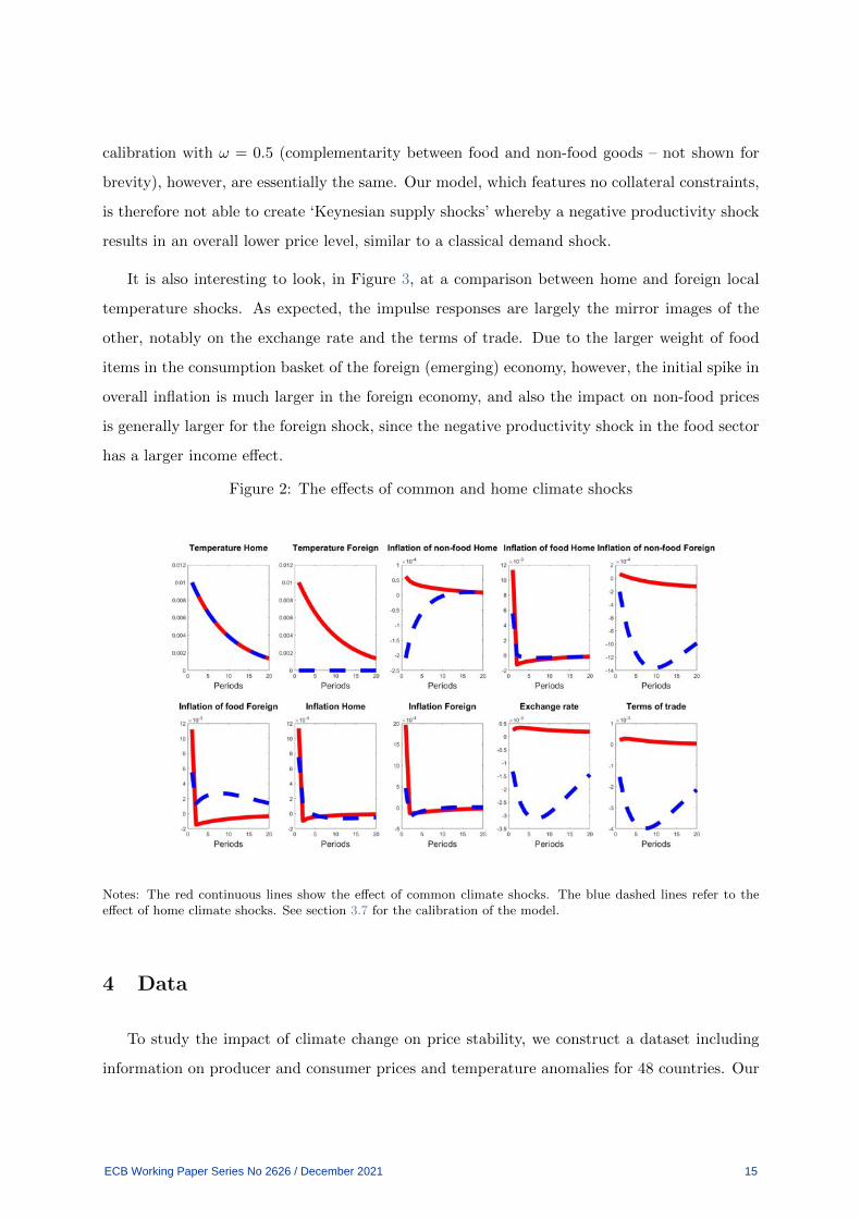
Figure 2 reports the impact of a home (blue dashed lines) and common (red solid line)

temperature shock on prices in both economies. The rise in home temperature, which is the

theoretical counterpart to our empirical exercise, results in a relatively sharp increase in home

food price inflation, almost matched by the same rise in the foreign economy, while the price of

non-food items actually falls slightly, both home and abroad. These results, and in particular

the profile of the inflation response to the temperature shocks, is a consequence of the fact that

food prices are flexible while non-food prices are sticky. The domestic currency depreciates,

which also leads to a worsening of the terms of trade. Aggregate inflation goes up sharply on

impact, given the rise in food prices which are assumed to be flexible, but the effect dies down

quickly or is even slightly reversed in the following periods. Note the difference from a common

temperature shock, for which the effect on food prices is qualitatively similar. In this case, non-

food prices increase, albeit slightly, and there is (as expected) little movement in the exchange

rate and terms of trade.

We also consider the idea of complementarity between food and non-food items, following the

intuition championed by Guerrieri et al. (2020).6 The model conclusions from this alternative

6The recent literature on ‘Keynesian supply shocks’ is also related to the idea that, when markets are incom-plete, at low levels of substitution between good types, wealth effects can drive up the aggregate demand for goodtypes even in the presence of negative endowment shocks; see Corsetti et al. (2008).


calibration with ω = 0.5 (complementarity between food and non-food goods – not shown for

brevity), however, are essentially the same. Our model, which features no collateral constraints,

is therefore not able to create ‘Keynesian supply shocks’ whereby a negative productivity shock

results in an overall lower price level, similar to a classical demand shock.

It is also interesting to look, in Figure 3, at a comparison between home and foreign local

temperature shocks. As expected, the impulse responses are largely the mirror images of the

other, notably on the exchange rate and the terms of trade. Due to the larger weight of food

items in the consumption basket of the foreign (emerging) economy, however, the initial spike in

overall inflation is much larger in the foreign economy, and also the impact on non-food prices

is generally larger for the foreign shock, since the negative productivity shock in the food sector

has a larger income effect.

Figure 2: The effects of common and home climate shocks

Notes: The red continuous lines show the effect of common climate shocks. The blue dashed lines refer to theeffect of home climate shocks. See section 3.7 for the calibration of the model.

4 Data

To study the impact of climate change on price stability, we construct a dataset including

information on producer and consumer prices and temperature anomalies for 48 countries. Our


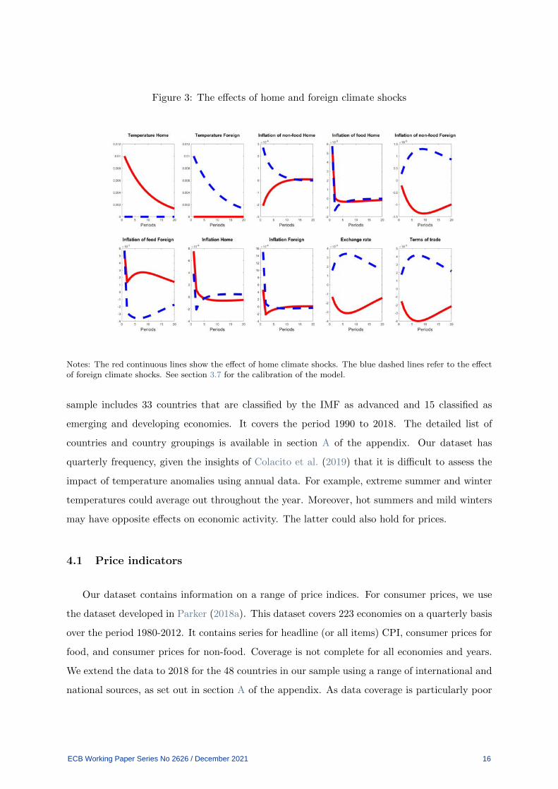
Figure 3: The effects of home and foreign climate shocks

Notes: The red continuous lines show the effect of home climate shocks. The blue dashed lines refer to the effectof foreign climate shocks. See section 3.7 for the calibration of the model.

sample includes 33 countries that are classified by the IMF as advanced and 15 classified as

emerging and developing economies. It covers the period 1990 to 2018. The detailed list of

countries and country groupings is available in section A of the appendix. Our dataset has

quarterly frequency, given the insights of Colacito et al. (2019) that it is difficult to assess the

impact of temperature anomalies using annual data. For example, extreme summer and winter

temperatures could average out throughout the year. Moreover, hot summers and mild winters

may have opposite effects on economic activity. The latter could also hold for prices.

4.1 Price indicators

Our dataset contains information on a range of price indices. For consumer prices, we use

the dataset developed in Parker (2018a). This dataset covers 223 economies on a quarterly basis

over the period 1980-2012. It contains series for headline (or all items) CPI, consumer prices for

food, and consumer prices for non-food. Coverage is not complete for all economies and years.

We extend the data to 2018 for the 48 countries in our sample using a range of international and

national sources, as set out in section A of the appendix. As data coverage is particularly poor


for some price sub-indexes before 1990, we only report results for the period 1990 to 2018 in the

rest of the paper. In addition, to ensure consistency between measures of headline CPI and of

its components, we report results for headline CPI only when information on the sub-indices is

available.

We also include two other national price measures beyond CPI: producer prices (PPI) and the

GDP deflator. These price indices permit a broader view of the impact of extreme temperatures

on economic activity by capturing transactions between businesses. Data for both are taken from

the International Financial Statistics (IFS) database published by the IMF. We also include PPI

data from national sources for five countries where it is not available for the whole period since

2000 in the IFS, as noted in section A in the appendix. Overall, compared to other databases

on global inflation as such the one developed by Ha et al. (2021), our dataset has a broader

coverage of inflation indicators at quarterly frequency for the group of countries in our sample.

In addition, our dataset includes information on CPI excluding food, which is not available in

the dataset developed by Ha et al. (2021).

4.2 Climate data

We retrieve climate data from three sources.

First, we obtain information on country-specific temperature anomalies at quarterly fre-

quency from the FAOSTAT Agri-Environmental Indicators dataset. The latter compiles infor-

mation from GISTEMP, the Global Surface Temperature Change data of the National Aeronau-

tics and Space Administration Goddard Institute for Space Studies (NASA-GISS).7 Temperature

anomalies indicate by how much temperatures deviate in a particular period from the historical

average climate, with the latter corresponding to the average of the 1951-1980 period. Weather

anomalies are calculated at station level and are subsequently aggregated up to the country

level, after correcting for a range of biases such as the station bias and heat-island effects in

urban areas.

As shown by Hansen and Lebedeff (1987), temperature anomalies are more suited to measure

climate change compared to absolute temperatures. The reason is that absolute temperatures are

7For more information on the GISTEMP dataset we refer to the data available on the GIS website (GIS, 2021)as well as to Hansen and Lebedeff (1987) and Lenssen et al. (2019).


very difficult to measure: they vary considerably in short distances depending on the location of

the weather station and thus are subject to a considerable degree of uncertainty. By correcting for

station effects before aggregating the data to the country level, temperature anomalies provide

a more reliable measure of weather changes in larger regions.

FAOSTAT provides data on seasonal temperature anomalies following the meteorological

year (which starts in December) rather than the calendar year. Therefore, in order to match data

on temperature anomalies with macroeconomic variables, we assume that the meteorological

winter (summer) in the Northern (Southern) Hemisphere – which includes the months from

December to February – corresponds to the first quarter of the year and so forth.

As shown in table 1, there has been a notable increase in temperatures for the 48 countries

in our sample compared with the period 1951–1980. For example, the median average summer

temperature increased by about 0.7◦C between the 1990s and the 2010s; a 1◦C summer anomaly

would have been just above the 75th percentile in the 1990s, but, by the 2010s, the median

anomaly was about 1.3◦C. Moreover, there has been a marked increase in the skew of the

distribution of summer temperature anomalies, with the 90th percentile increasing by around

0.8◦C over the same period.

The second data source from which we obtain data on climate variables is the World Bank

Climate Change Knowledge Portal. From this dataset, we retrieve information on absolute

temperatures at country level. These data are used in the empirical analysis to assess whether

temperature anomalies can have a different impact if temperatures exceed certain thresholds.

They are also used to construct alternative measures of temperature anomalies for robustness

checks.

Finally, we also retrieve climate data from the ifo Geological and Meteorological Events

Database (GAME), which is the data underlying Felbermayr and Groschl (2014). The GAME

dataset identifies periods of precipitation extremes and hence helps clarify to what extent the

impact on inflation is related to high temperatures as opposed to droughts.

4.3 Additional indicators

We complement our dataset with a number of additional indicators. First, we include infor-

mation on seasonally adjusted real GDP in local currency at quarterly frequency from the OECD


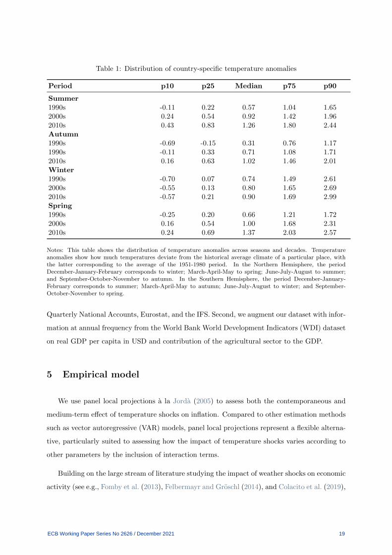
Table 1: Distribution of country-specific temperature anomalies

Period p10 p25 Median p75 p90

Summer1990s -0.11 0.22 0.57 1.04 1.652000s 0.24 0.54 0.92 1.42 1.962010s 0.43 0.83 1.26 1.80 2.44Autumn1990s -0.69 -0.15 0.31 0.76 1.171990s -0.11 0.33 0.71 1.08 1.712010s 0.16 0.63 1.02 1.46 2.01Winter1990s -0.70 0.07 0.74 1.49 2.612000s -0.55 0.13 0.80 1.65 2.692010s -0.57 0.21 0.90 1.69 2.99Spring1990s -0.25 0.20 0.66 1.21 1.722000s 0.16 0.54 1.00 1.68 2.312010s 0.24 0.69 1.37 2.03 2.57

Notes: This table shows the distribution of temperature anomalies across seasons and decades. Temperatureanomalies show how much temperatures deviate from the historical average climate of a particular place, withthe latter corresponding to the average of the 1951-1980 period. In the Northern Hemisphere, the periodDecember-January-February corresponds to winter; March-April-May to spring; June-July-August to summer;and September-October-November to autumn. In the Southern Hemisphere, the period December-January-February corresponds to summer; March-April-May to autumn; June-July-August to winter; and September-October-November to spring.

Quarterly National Accounts, Eurostat, and the IFS. Second, we augment our dataset with infor-

mation at annual frequency from the World Bank World Development Indicators (WDI) dataset

on real GDP per capita in USD and contribution of the agricultural sector to the GDP.

5 Empirical model

We use panel local projections a la Jorda (2005) to assess both the contemporaneous and

medium-term effect of temperature shocks on inflation. Compared to other estimation methods

such as vector autoregressive (VAR) models, panel local projections represent a flexible alterna-

tive, particularly suited to assessing how the impact of temperature shocks varies according to

other parameters by the inclusion of interaction terms.

Building on the large stream of literature studying the impact of weather shocks on economic

activity (see e.g., Fomby et al. (2013), Felbermayr and Groschl (2014), and Colacito et al. (2019),


among others), we treat within-country temperature fluctuations as exogenous after controlling

for country and time fixed effects; subsequently, we regress them on a range of price indicators.

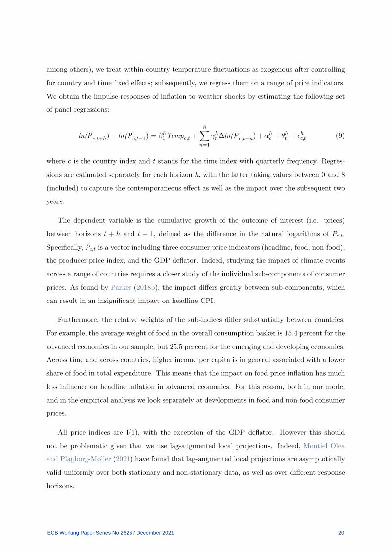
We obtain the impulse responses of inflation to weather shocks by estimating the following set

of panel regressions:

ln(P c,t+h) − ln(P c,t−1) = βh1 Tempc,t +

8∑n=1

γhn∆ln(P c,t−n) + αhc + θht + εhc,t (9)

where c is the country index and t stands for the time index with quarterly frequency. Regres-

sions are estimated separately for each horizon h, with the latter taking values between 0 and 8

(included) to capture the contemporaneous effect as well as the impact over the subsequent two

years.

The dependent variable is the cumulative growth of the outcome of interest (i.e. prices)

between horizons t + h and t − 1, defined as the difference in the natural logarithms of Pc,t.

Specifically, Pc,t is a vector including three consumer price indicators (headline, food, non-food),

the producer price index, and the GDP deflator. Indeed, studying the impact of climate events

across a range of countries requires a closer study of the individual sub-components of consumer

prices. As found by Parker (2018b), the impact differs greatly between sub-components, which

can result in an insignificant impact on headline CPI.

Furthermore, the relative weights of the sub-indices differ substantially between countries.

For example, the average weight of food in the overall consumption basket is 15.4 percent for the

advanced economies in our sample, but 25.5 percent for the emerging and developing economies.

Across time and across countries, higher income per capita is in general associated with a lower

share of food in total expenditure. This means that the impact on food price inflation has much

less influence on headline inflation in advanced economies. For this reason, both in our model

and in the empirical analysis we look separately at developments in food and non-food consumer

prices.

All price indices are I(1), with the exception of the GDP deflator. However this should

not be problematic given that we use lag-augmented local projections. Indeed, Montiel Olea

and Plagborg-Møller (2021) have found that lag-augmented local projections are asymptotically

valid uniformly over both stationary and non-stationary data, as well as over different response

horizons.


The main variable of interest, for which we report the impulse response functions (IRFs) in

the next section, is Tempc,t, a dummy variable indicating significant temperature anomalies at

country level. In the empirical analysis, we use different definitions of significant temperature

anomalies, depending on the model specification. Full details are available in table 2. For

example, when looking at the effect of hot summers in the baseline specification, the variable

Tempc,t is set to be equal to 1 when the temperature recorded in the quarter exceeds the

country’s long-run mean temperature calculated over the period 1951–1980 by at least 1.5◦C; it

is set to 0 otherwise, as there are no particularly cold summers in our dataset. In other words,

unlike e.g. Felbermayr and Groschl (2014) and Colacito et al. (2019), we assume that small

temperature fluctuations compared to historical regularities are not macro-critical.

Based on the definitions of temperature anomalies in table 2, we find that about 25% of

all quarters have a significant temperature anomaly. The share of quarters with significant

temperature anomalies varies between the two country groups. There are significant temperature

anomalies in 29.3% of the quarters in advanced economies, while the percentage drops to 14.9%

in EMEs. The same split broadly holds for significant summer temperature anomalies (28% vs.

15%). This is not surprising, as temperatures are rising faster in the latitudes where most of

advanced economies are located. Chile is the only country in the sample with no significant

temperature anomaly.

For the rest, the model is parsimonious. It includes lagged values of the dependent variable up

to the 8th lag (corresponding to the length of the forecasting horizon, following Plagborg-Møller

and Wolf (forthcoming) and Montiel Olea and Plagborg-Møller (2021)), and country (αhc ) and

time fixed effects (θht ). The aim of the fixed effects is to control for important country-invariant

factors, such as latitude, and time-specific phenomena, such as sharp swings in commodity prices

unrelated to climate. To address the serial correlation in the error term due to the inclusion of

lagged values of the dependent variable, we use Driscoll and Kraay (1998) standard errors. The

latter are robust to heteroskedasticity, autocorrelation and cross-sectional dependence.

6 Empirical evidence

We split the presentation of the results between the short and medium-term impact. Such

distinction is useful when considering the optimal response by central banks. Given the lag


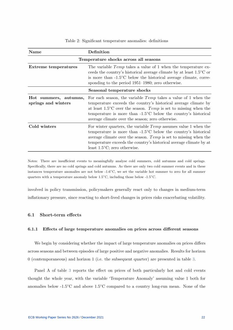
Table 2: Significant temperature anomalies: definitions

Name Definition

Temperature shocks across all seasons

Extreme temperatures The variable Temp takes a value of 1 when the temperature ex-ceeds the country’s historical average climate by at least 1.5◦C oris more than -1.5◦C below the historical average climate, corre-sponding to the period 1951–1980; zero otherwise.

Seasonal temperature shocks

Hot summers, autumns,springs and winters

For each season, the variable Temp takes a value of 1 when thetemperature exceeds the country’s historical average climate byat least 1.5◦C over the season. Temp is set to missing when thetemperature is more than -1.5◦C below the country’s historicalaverage climate over the season; zero otherwise.

Cold winters For winter quarters, the variable Temp assumes value 1 when thetemperature is more than -1.5◦C below the country’s historicalaverage climate over the season. Temp is set to missing when thetemperature exceeds the country’s historical average climate by atleast 1.5◦C; zero otherwise.

Notes: There are insufficient events to meaningfully analyse cold summers, cold autumns and cold springs.

Specifically, there are no cold springs and cold autumns. As there are only two cold summer events and in these

instances temperature anomalies are not below -1.6◦C, we set the variable hot summer to zero for all summer

quarters with a temperature anomaly below 1.5◦C, including those below -1.5◦C.

involved in policy transmission, policymakers generally react only to changes in medium-term

inflationary pressure, since reacting to short-lived changes in prices risks exacerbating volatility.

6.1 Short-term effects

6.1.1 Effects of large temperature anomalies on prices across different seasons

We begin by considering whether the impact of large temperature anomalies on prices differs

across seasons and between episodes of large positive and negative anomalies. Results for horizon

0 (contemporaneous) and horizon 1 (i.e. the subsequent quarter) are presented in table 3.

Panel A of table 3 reports the effect on prices of both particularly hot and cold events

thought the whole year, with the variable ‘Temperature Anomaly’ assuming value 1 both for

anomalies below -1.5◦C and above 1.5◦C compared to a country long-run mean. None of the


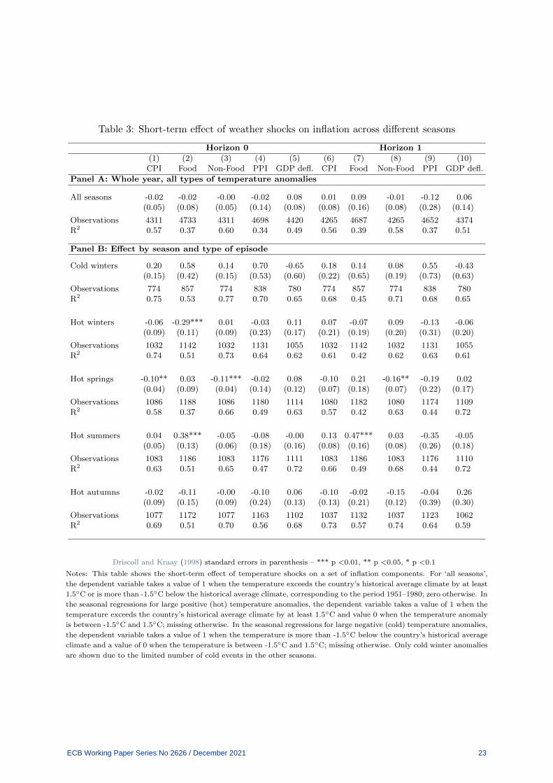
Table 3: Short-term effect of weather shocks on inflation across different seasons

Horizon 0 Horizon 1

(1) (2) (3) (4) (5) (6) (7) (8) (9) (10)CPI Food Non-Food PPI GDP defl. CPI Food Non-Food PPI GDP defl.

Panel A: Whole year, all types of temperature anomalies

All seasons -0.02 -0.02 -0.00 -0.02 0.08 0.01 0.09 -0.01 -0.12 0.06(0.05) (0.08) (0.05) (0.14) (0.08) (0.08) (0.16) (0.08) (0.28) (0.14)

Observations 4311 4733 4311 4698 4420 4265 4687 4265 4652 4374R2 0.57 0.37 0.60 0.34 0.49 0.56 0.39 0.58 0.37 0.51

Panel B: Effect by season and type of episode

Cold winters 0.20 0.58 0.14 0.70 -0.65 0.18 0.14 0.08 0.55 -0.43(0.15) (0.42) (0.15) (0.53) (0.60) (0.22) (0.65) (0.19) (0.73) (0.63)

Observations 774 857 774 838 780 774 857 774 838 780R2 0.75 0.53 0.77 0.70 0.65 0.68 0.45 0.71 0.68 0.65

Hot winters -0.06 -0.29*** 0.01 -0.03 0.11 0.07 -0.07 0.09 -0.13 -0.06(0.09) (0.11) (0.09) (0.23) (0.17) (0.21) (0.19) (0.20) (0.31) (0.20)

Observations 1032 1142 1032 1131 1055 1032 1142 1032 1131 1055R2 0.74 0.51 0.73 0.64 0.62 0.61 0.42 0.62 0.63 0.61

Hot springs -0.10** 0.03 -0.11*** -0.02 0.08 -0.10 0.21 -0.16** -0.19 0.02(0.04) (0.09) (0.04) (0.14) (0.12) (0.07) (0.18) (0.07) (0.22) (0.17)

Observations 1086 1188 1086 1180 1114 1080 1182 1080 1174 1109R2 0.58 0.37 0.66 0.49 0.63 0.57 0.42 0.63 0.44 0.72

Hot summers 0.04 0.38*** -0.05 -0.08 -0.00 0.13 0.47*** 0.03 -0.35 -0.05(0.05) (0.13) (0.06) (0.18) (0.16) (0.08) (0.16) (0.08) (0.26) (0.18)

Observations 1083 1186 1083 1176 1111 1083 1186 1083 1176 1110R2 0.63 0.51 0.65 0.47 0.72 0.66 0.49 0.68 0.44 0.72

Hot autumns -0.02 -0.11 -0.00 -0.10 0.06 -0.10 -0.02 -0.15 -0.04 0.26(0.09) (0.15) (0.09) (0.24) (0.13) (0.13) (0.21) (0.12) (0.39) (0.30)

Observations 1077 1172 1077 1163 1102 1037 1132 1037 1123 1062R2 0.69 0.51 0.70 0.56 0.68 0.73 0.57 0.74 0.64 0.59

Driscoll and Kraay (1998) standard errors in parenthesis – *** p <0.01, ** p <0.05, * p <0.1

Notes: This table shows the short-term effect of temperature shocks on a set of inflation components. For ‘all seasons’,

the dependent variable takes a value of 1 when the temperature exceeds the country’s historical average climate by at least

1.5◦C or is more than -1.5◦C below the historical average climate, corresponding to the period 1951–1980; zero otherwise. In

the seasonal regressions for large positive (hot) temperature anomalies, the dependent variable takes a value of 1 when the

temperature exceeds the country’s historical average climate by at least 1.5◦C and value 0 when the temperature anomaly

is between -1.5◦C and 1.5◦C; missing otherwise. In the seasonal regressions for large negative (cold) temperature anomalies,

the dependent variable takes a value of 1 when the temperature is more than -1.5◦C below the country’s historical average

climate and a value of 0 when the temperature is between -1.5◦C and 1.5◦C; missing otherwise. Only cold winter anomalies

are shown due to the limited number of cold events in the other seasons.


estimated coefficients is statistically significant. However, results change when we break down

annual temperature anomalies into seasons and we distinguish between hot and cold temperature

shocks (displayed in Panel B of table 3).

Starting with negative temperature anomalies, there are insufficient events to consider the

impact in spring, summer, or autumn under the baseline definition. The degree of warming

already present in our country sample over recent decades means that these events are too rare

for meaningful analysis. We do not find any significant impact on any price index at any horizon

for cold winters.

Moving to positive temperature anomalies, we do find significant impacts. Mild winters

result in a significant contemporaneous fall in food prices of -0.29 percentage points but the

effect disappears by the subsequent quarter. Mild springs result in a small fall in non-food

prices in the contemporaneous and in the subsequent quarter, which is also reflected in headline

CPI. Mild autumns do not appear to have any significant impact on any price index considered

here.

By contrast, we find a statistically significant – and economically meaningful – impact on

prices arising from hot summer events. Food prices increase by 0.38 percentage points con-

temporaneously, which is greater than a one standard deviation quarterly change in the series.

The positive impact on food prices increases further in the subsequent quarter. In terms of

economic mechanisms, the contemporaneous increase in food price inflation could be explained

by a negative effect of hot summers on food production, resulting in supply shortage effects.

In short, extreme temperatures – hot or cold – in most seasons have to date had little or

no impact on prices. The notable exception is hot summer events, where there is a significant,

meaningful and longer-lasting impact. For this reason, we focus on the effect of hot summer

temperature anomalies on prices in the remainder of this paper.

We begin by demonstrating that the short-term results are robust to a range of alternative

specifications, which are shown in table 4. For example, using four lags of the lagged inflation

rate, quarterly rather than annual fixed effects or including the lagged price level in the esti-

mation all deliver an estimated impact on food prices that are qualitatively and quantitatively

alike (columns (1) – (3)).


Results for the models presented in columns (1) – (3) of table 4 are estimated with country

fixed effects. Hence, an implicit assumption is that both the impact of temperature and lagged

inflation dynamics is homogeneous across countries. In column (4), we relax this assumption and

we show the results using the mean group estimator of Pesaran and Smith (1995). This estimator

allows the coefficients on the anomalies to vary across countries – for example permitting the

response of prices to an extreme temperature event in Canada to differ from the response in

Chile – by estimating separately for each country. The estimated coefficients are then averaged

across countries. Here again the impact is similar, albeit somewhat more pronounced at horizon

1.

Finally, we control for the potential simultaneous occurrence of droughts alongside summer

extreme temperatures, drawing from the GAME dataset. Droughts are defined as a quarter

in which the average rainfall is at least 50% below average for at least two months within the

quarter. The data show that hot summers tend to be drier on average than less warm summers

(see figure B.2 in the appendix). However, droughts are very rare events, with only 7% of

hot summers coinciding with droughts, compared with 1% for other summers. Incorporating a

dummy for drought leads to qualitatively similar results for the coefficient on extreme summer

temperatures, and the drought dummy itself is insignificant (column (5)). Note that the GAME

database ends in 2010, so does not have a complete coverage for our sample.

6.1.2 Effects of hot summer temperature anomalies on prices by level of develop-

ment

Parker (2018b) finds differing inflation impact of disasters by level of development. Results

displayed in Panel A of table 5 show that this also occurs following significant summer temper-

ature anomalies. While we do not find any significant effect in advanced economies, food price

inflation significantly increases in EMEs following a particularly hot summer. The increase in

food price inflation in emerging economies translates into an increase in the overall CPI inflation,

likely reflecting the higher share of food in the consumption basket of this country group. These

empirical results accord with the predictions from the theoretical model presented above.

While results in Panel A allow for a diverging impact of temperature anomalies on prices in

advanced and emerging market economies, they implicitly assume an homogeneous impact of


Table 4: Short-term effect of summer weather shocks on food prices – Robustness checks

(1) (2) (3) (4) (5)4 lags Qrt FE Level MGE Droughts

At horizon 0:Temperature anomaly 0.39*** 0.37*** 0.36*** 0.36** 0.49***

(0.13) (0.13) (0.14) (0.16) (0.19)Droughts 0.32

(0.61)Observations 1232 1186 1186 1186 813R2 0.49 0.54 0.51 NA 0.54

At horizon 1:Temperature anomaly 0.47*** 0.43** 0.43** 0.58** 0.66***

(0.16) (0.17) (0.16) (0.26) (0.22)Droughts 0.97

(0.70)Observations 1186 1186 1186 1186 813R2 0.49 0.53 0.52 NA 0.52

Country FE Yes Yes Yes NA YesYear FE Yes No Yes NA YesQuarter FE No Yes No NA NoLags 1st diff 4 8 8 8 8Lag level No No Yes No NoModel Std LP Std LP Std LP MGE Std LP

Standard errors in parenthesis – *** p <0.01, ** p <0.05, * p <0.1

Notes: This figure shows the short term effect of hot summer temperature anomalies on food prices across differentmodel specifications. Results reported in columns (1) – (3) and (5) are based on a standard local projection model(Std LP) a la Jorda (2005), with Driscoll and Kraay (1998) standard errors that are robust to heteroskedasticityand to serial and spatial correlation. Compared to the baseline model in equation 9, column (1) includes fourlags of the lagged inflation rate (instead of 8), column (2) considers quarterly rather than annual fixed effects,column (3) controls also for the lagged price level and column (5) adds droughts as an additional control. Resultsreported in column (4) are based on the mean group estimator (MGE) of Pesaran and Smith (1995), estimatedfor both horizon 0 and horizon 1.

lagged inflation dynamics across the whole sample. To check whether this affects the results, in

Panel B and Panel C we split the sample between the 34 advanced and 14 emerging economies

following the IMF classification. Here, we find that both country groups exhibit a positive

impact on food price growth at horizon zero. For advanced economies, the impact on CPI food

price inflation is no longer significant by horizon 1. The impact on food price inflation in EMEs

is markedly larger – 1.51 percentage points at horizon 0, and increasing to 2.55 percentage points

at horizon 1. There is also a positive impact on headline consumer prices in EMEs in line with

results displayed in Panel A. For both country groups, there is no significant impact on non-food

CPI, PPI nor the GDP deflator in the near term.

A potential explanation for the stronger and longer lasting effect of hot domestic weather


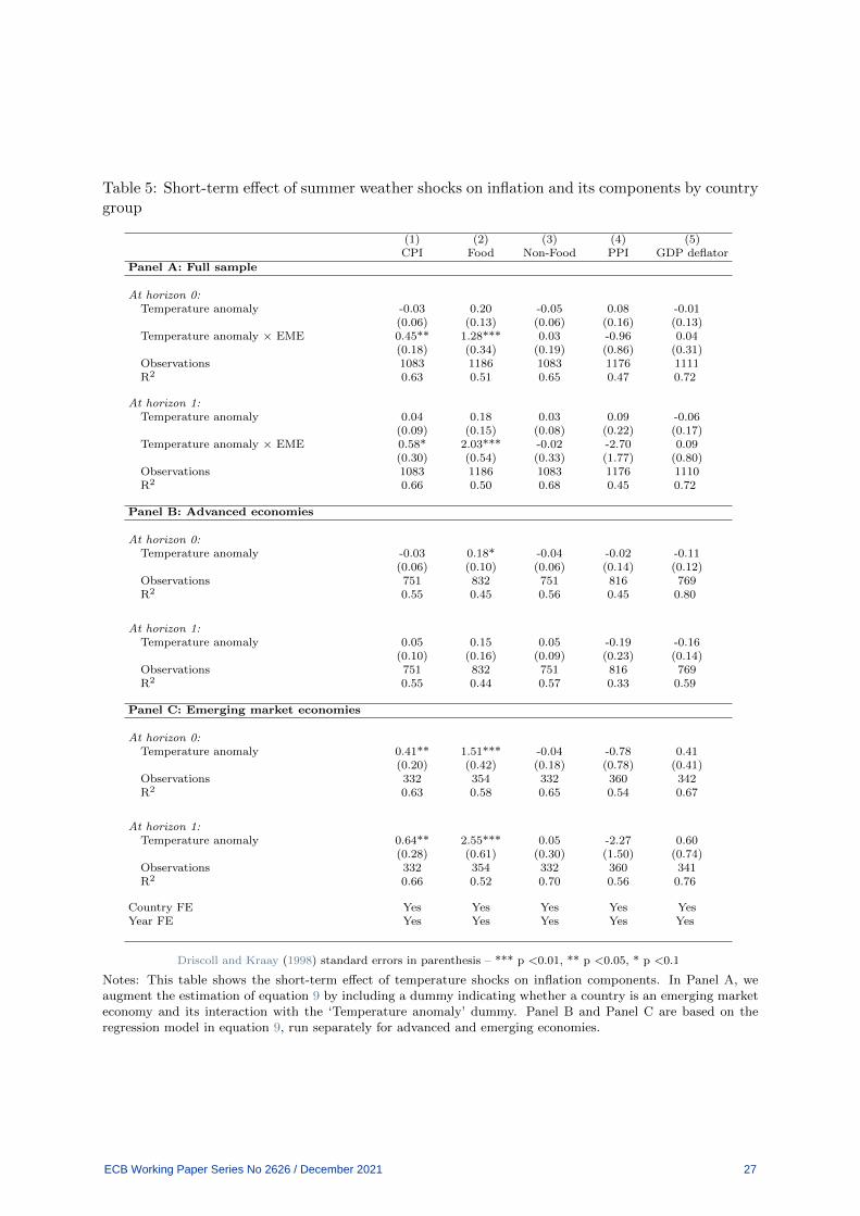
Table 5: Short-term effect of summer weather shocks on inflation and its components by countrygroup

(1) (2) (3) (4) (5)CPI Food Non-Food PPI GDP deflator

Panel A: Full sample

At horizon 0:Temperature anomaly -0.03 0.20 -0.05 0.08 -0.01

(0.06) (0.13) (0.06) (0.16) (0.13)Temperature anomaly × EME 0.45** 1.28*** 0.03 -0.96 0.04

(0.18) (0.34) (0.19) (0.86) (0.31)Observations 1083 1186 1083 1176 1111R2 0.63 0.51 0.65 0.47 0.72

At horizon 1:Temperature anomaly 0.04 0.18 0.03 0.09 -0.06

(0.09) (0.15) (0.08) (0.22) (0.17)Temperature anomaly × EME 0.58* 2.03*** -0.02 -2.70 0.09

(0.30) (0.54) (0.33) (1.77) (0.80)Observations 1083 1186 1083 1176 1110R2 0.66 0.50 0.68 0.45 0.72

Panel B: Advanced economies

At horizon 0:Temperature anomaly -0.03 0.18* -0.04 -0.02 -0.11

(0.06) (0.10) (0.06) (0.14) (0.12)Observations 751 832 751 816 769R2 0.55 0.45 0.56 0.45 0.80

At horizon 1:Temperature anomaly 0.05 0.15 0.05 -0.19 -0.16

(0.10) (0.16) (0.09) (0.23) (0.14)Observations 751 832 751 816 769R2 0.55 0.44 0.57 0.33 0.59

Panel C: Emerging market economies

At horizon 0:Temperature anomaly 0.41** 1.51*** -0.04 -0.78 0.41

(0.20) (0.42) (0.18) (0.78) (0.41)Observations 332 354 332 360 342R2 0.63 0.58 0.65 0.54 0.67

At horizon 1:Temperature anomaly 0.64** 2.55*** 0.05 -2.27 0.60

(0.28) (0.61) (0.30) (1.50) (0.74)Observations 332 354 332 360 341R2 0.66 0.52 0.70 0.56 0.76

Country FE Yes Yes Yes Yes YesYear FE Yes Yes Yes Yes Yes


Notes: This table shows the short-term effect of temperature shocks on inflation components. In Panel A, weaugment the estimation of equation 9 by including a dummy indicating whether a country is an emerging marketeconomy and its interaction with the ‘Temperature anomaly’ dummy. Panel B and Panel C are based on theregression model in equation 9, run separately for advanced and emerging economies.


shocks on price dynamics in EMEs is that these countries are likely to be less integrated in the

global food market and thus more dependent on domestic agricultural production. In addition,

in this country group the agricultural sector may be less equipped with instruments aimed at

mitigating the effect of temperature shocks on food production, such as irrigation networks.8

In this respect, columns (1) and (2) of table 6 allow for a diverging impact of summer

weather shocks on food price inflation by the importance of the agricultural sector for the

domestic economy. The thresholds for determining the importance of the agricultural sector for

the domestic economy are calculated separately for each country group given that the agriculture

GDP share varies considerably between the two. For any given year, a country is classified as

having a low agriculture GDP share if the latter is below the 33th percentile of the distribution

within its country group; it is considered as having a middle agriculture GDP share if the latter

is between the 33th percentile and the 66th percentile of the distribution within its country

group; it is considered as having a high agriculture GDP share if the latter is above the 66th

percentile of the distribution within its country group. Results reported in table 6 refer to the

impact at horizon zero (‘contemporaneous impact’).

The main findings are as follows. While the share of the agricultural sector for the domestic

economy does not play a role in advanced economies, temperature shocks have a stronger con-

temporaneous impact in emerging countries with a more rural economy. This suggests that food

prices in EMEs that are more dependent on domestic agricultural production are more affected

by domestic weather shocks. This holds if we assume that the importance of the agricultural

sector for the domestic economy is a good proxy for the importance of domestic agricultural

production in the food consumption basket.

We also investigate whether the impact of summer temperature anomalies on food price

inflation varies according to the absolute temperature level recorded in the summer in which

they happen. Indeed, it could be that a particularly hot summer compared to the country

historical average climate in, for example, the United Kingdom might be a favorable shock

for agricultural production, but could have the opposite impact in a country with a hotter

8In this respect, De Winne and Peersman (2018) find the opposite for global agricultural price and weathershocks; that is, the decline in economic activity is less in low-income countries and countries with large agriculturalsectors, which is probably the consequences of the fact that these countries are more isolated from shocks in globalmarkets. Parker (2018a) also finds a much greater impact of global developments on food prices for advancedeconomies. Dependent on the measure used, global food price inflation explains 38-54% of food price inflationvariance in advanced economies, falling to 18-24% in middle income and 10-13% in low income countries.


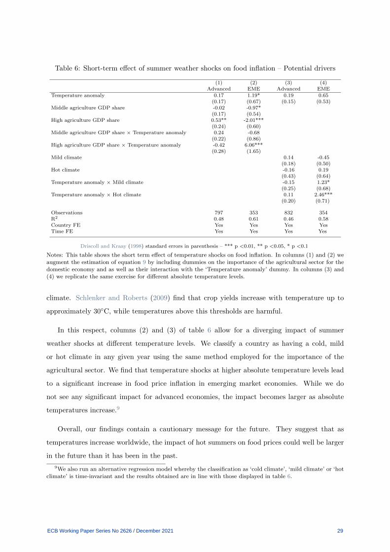
Table 6: Short-term effect of summer weather shocks on food inflation – Potential drivers

(1) (2) (3) (4)Advanced EME Advanced EME

Temperature anomaly 0.17 1.19* 0.19 0.65(0.17) (0.67) (0.15) (0.53)

Middle agriculture GDP share -0.02 -0.97*(0.17) (0.54)

High agriculture GDP share 0.53** -2.01***(0.24) (0.60)

Middle agriculture GDP share × Temperature anomaly 0.24 -0.68(0.22) (0.86)

High agriculture GDP share × Temperature anomaly -0.42 6.06***(0.28) (1.65)

Mild climate 0.14 -0.45(0.18) (0.50)

Hot climate -0.16 0.19(0.43) (0.64)

Temperature anomaly × Mild climate -0.15 1.23*(0.25) (0.68)

Temperature anomaly × Hot climate 0.11 2.46***(0.20) (0.71)

Observations 797 353 832 354R2 0.48 0.61 0.46 0.58Country FE Yes Yes Yes YesTime FE Yes Yes Yes Yes


Notes: This table shows the short term effect of temperature shocks on food inflation. In columns (1) and (2) weaugment the estimation of equation 9 by including dummies on the importance of the agricultural sector for thedomestic economy and as well as their interaction with the ‘Temperature anomaly’ dummy. In columns (3) and(4) we replicate the same exercise for different absolute temperature levels.

climate. Schlenker and Roberts (2009) find that crop yields increase with temperature up to

approximately 30◦C, while temperatures above this thresholds are harmful.

In this respect, columns (2) and (3) of table 6 allow for a diverging impact of summer

weather shocks at different temperature levels. We classify a country as having a cold, mild

or hot climate in any given year using the same method employed for the importance of the

agricultural sector. We find that temperature shocks at higher absolute temperature levels lead

to a significant increase in food price inflation in emerging market economies. While we do

not see any significant impact for advanced economies, the impact becomes larger as absolute

temperatures increase.9

Overall, our findings contain a cautionary message for the future. They suggest that as

temperatures increase worldwide, the impact of hot summers on food prices could well be larger

in the future than it has been in the past.

9We also run an alternative regression model whereby the classification as ‘cold climate’, ‘mild climate’ or ‘hotclimate’ is time-invariant and the results obtained are in line with those displayed in table 6.


6.2 Medium-term effects

6.2.1 Effects of hot summer temperature anomalies by level of development

Figure 4 reports the response of inflation to hot summer temperature anomalies up to 8

quarters following the initial shock. The results obtained show some signs of a long-lasting

effect of hot summer temperatures on prices. While food price inflation returns to the pre-shock

levels within three quarters following the shock, producer prices and the GDP deflator continue

to fall the following year.

Again, the results obtained are largely robust to a set of alternative specifications – such as

using four lags of the lagged inflation rate, including quarterly rather than annual fixed effects,

adding the lagged price level, controlling for the occurrence of droughts in the estimation, or

employing the mean group estimator. This is shown by figures B.3 – B.7 in the appendix.

We also considered the impact of hot summers temperature anomalies on inflation components

depending on past inflation levels (see figure B.8 in the appendix). We calculated the average

inflation by country over the previous five years, then split the sample by the median. In general,

the response of high inflation countries has much larger variation, in common with the positive

correlation between average inflation and inflation volatility. While the initial impact on food

prices is similar between the two groups, it grows over time for the higher inflation group and

remains more persistent. This is in keeping with the findings of Choi et al. (2018) that the

impact of relative price shocks is larger and more persistent when inflation expectations are less

well anchored.

The negative medium-term effect of summers temperature anomalies on prices is mainly

driven by developments in EMEs. Figure 5 shows that, in this country group, producer prices

start to fall following the temperature shock, with the effect becoming stronger each quarter,

both economically and statistically. On the other hand, the effect of temperature anomalies on

the GDP deflator reported in figure 4 seems to be mainly driven by developments in advanced

economies – which account for bulk of the economies in our sample – although the effect is

broadly insignificant.

In order to interpret our results, the left hand side column of figure 6 reports the impulse

responses of GDP growth to significant summer temperature anomalies. The IRFs are estimated


Figure 4: Effect of summer weather shocks on inflation and its components over the mediumterm

CPI: All Items CPI: Food

CPI: Non-Food Producer Price Index

GDP Deflator

Notes: Impulse responses to hot summer temperature anomalies at horizon 0 using the baseline specification.Shaded areas represent 68% and 90% confidence intervals computed using Driscoll and Kraay (1998) standarderrors.


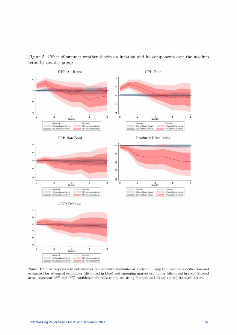
Figure 5: Effect of summer weather shocks on inflation and its components over the mediumterm, by country group



GDP Deflator

Notes: Impulse responses to hot summer temperature anomalies at horizon 0 using the baseline specification andestimated for advanced economies (displayed in blue) and emerging market economies (displayed in red). Shadedareas represent 68% and 90% confidence intervals computed using Driscoll and Kraay (1998) standard errors.


using the same model as in equation 9, with the inclusion of the level of the GDP per capita

in USD as a control to take into account catch-up effects. Our results are as follows. First,

GDP growth turns negative in emerging market economies following a hot summer temperature

anomaly. While also Dell et al. (2012), Acevedo et al. (2020) and Felbermayr and Groschl

(2014) find that hot temperatures affect economic growth negatively, these studies look at yearly

temperature fluctuations, without distinguishing across seasons. In this respect, we also run our

model for yearly temperature anomalies and we did not find a significant effect on GDP growth.

Second, we do not find evidence of dampened economic activity in advanced economies following

a hot summer temperature shock. This result is in line with the main findings of Dell et al.

(2012), Felbermayr and Groschl (2014) and Acevedo et al. (2020) (although they focus on yearly

average temperatures), while it is in contrast with those of Colacito et al. (2019) which however

focus only on the U.S. economy.10

The negative effect of temperature anomalies on prices and economic activity in the medium

term suggests that demand effects may occur in less developed countries following a particularly

hot summer. As mentioned in the previous section, this may reflect the fact that in this country

group both the contribution of the agricultural sector to GDP and share of food in the overall

consumption are higher compared to advanced economies.

6.2.2 Alternative measures of temperature anomalies

In this section, we test whether our results hold for alternative measures of temperature

anomalies.

We begin by considering whether our findings are robust to an alternative measure of signifi-

cant temperature anomalies based on World Bank data for the calendar year, which corresponds

to the frequency of the macroeconomic variables included in our dataset. As discussed in section

4, FAOSTAT provides information on seasonal temperature anomalies following the meteoro-

logical year (which starts in December) rather than the calendar one.

As a first step, we check consistency between the two data sources. Therefore, we construct

temperature anomalies relative to the 1951-1980 average based on World Bank data for the

10Also Acevedo et al. (2020) find a temporary increase in GDP growth in advanced economies in the yearfollowing a temperature increase. Similarly to our findings, such increase is temporary and weakly significant.


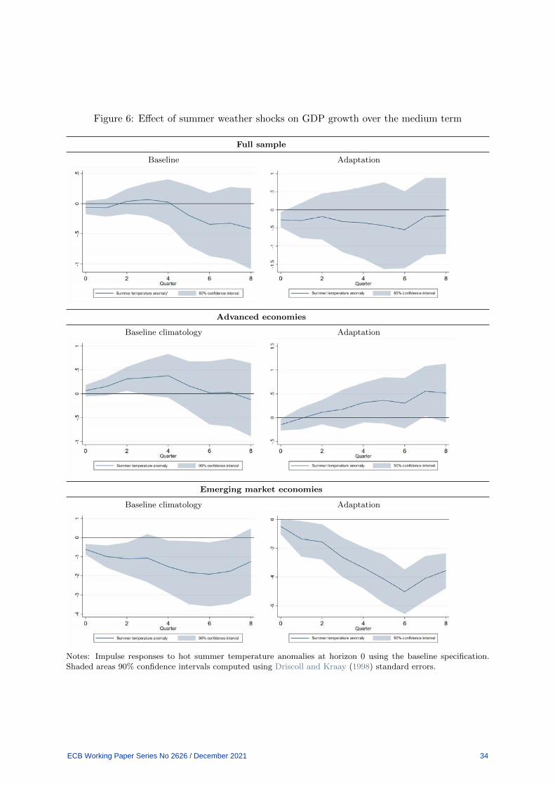
Figure 6: Effect of summer weather shocks on GDP growth over the medium term

Full sample

Baseline Adaptation

Advanced economies

Baseline climatology Adaptation

Emerging market economies

Baseline climatology Adaptation

Notes: Impulse responses to hot summer temperature anomalies at horizon 0 using the baseline specification.Shaded areas 90% confidence intervals computed using Driscoll and Kraay (1998) standard errors.


meteorological year to align with the FAOSTAT definition. As the data obtained from the

World Bank are provided in the form of monthly average temperatures, we construct anomalies

by subtracting the 1951-1980 average for the relevant month/country. Quarterly anomalies are

then derived by averaging the monthly anomalies.

As shown by figure B.9 in the appendix, temperature anomalies based on the meteorological

year are similar across the two data sources, but not perfectly matched. This is not surprising

as there are differences in the way data are compiled. Most importantly, country temperature

anomalies from FAOSTAT are more refined as they are computed by subtracting the current

absolute temperature from the 1951-80 average at station level, rather than at country level.

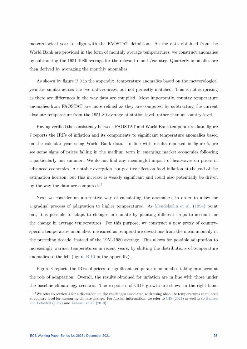
Having verified the consistency between FAOSTAT and World Bank temperature data, figure

7 reports the IRFs of inflation and its components to significant temperature anomalies based

on the calendar year using World Bank data. In line with results reported in figure 5, we

see some signs of prices falling in the medium term in emerging market economies following

a particularly hot summer. We do not find any meaningful impact of heatwaves on prices in

advanced economies. A notable exception is a positive effect on food inflation at the end of the

estimation horizon, but this increase is weakly significant and could also potentially be driven

by the way the data are computed.11

Next we consider an alternative way of calculating the anomalies, in order to allow for

a gradual process of adaptation to higher temperatures. As Mendelsohn et al. (1994) point

out, it is possible to adapt to changes in climate by planting different crops to account for

the change in average temperatures. For this purpose, we construct a new proxy of country-

specific temperature anomalies, measured as temperature deviations from the mean anomaly in

the preceding decade, instead of the 1951-1980 average. This allows for possible adaptation to

increasingly warmer temperatures in recent years, by shifting the distributions of temperature

anomalies to the left (figure B.10 in the appendix).

Figure 8 reports the IRFs of prices to significant temperature anomalies taking into account

the role of adaptation. Overall, the results obtained for inflation are in line with those under

the baseline climatology scenario. The responses of GDP growth are shown in the right hand

11We refer to section 4 for a discussion on the challenges associated with using absolute temperatures calculatedat country level for measuring climate change. For further information, we refer to GIS (2021) as well as to Hansenand Lebedeff (1987) and Lenssen et al. (2019).


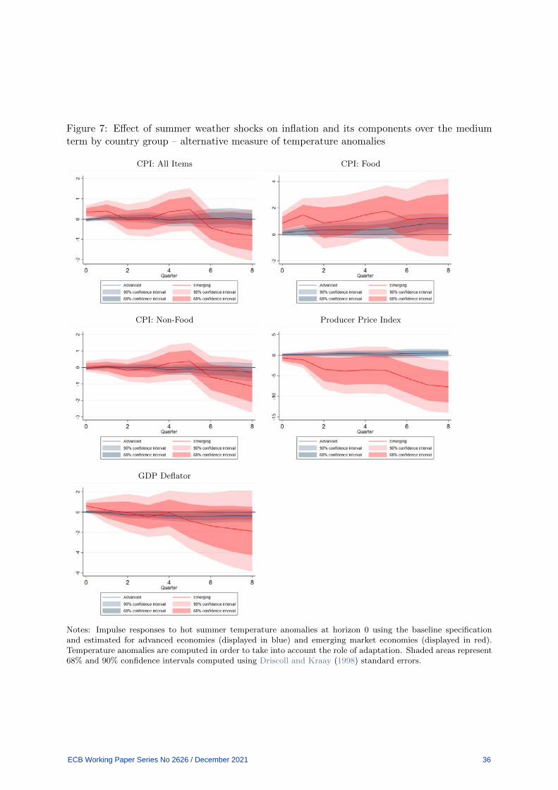
Figure 7: Effect of summer weather shocks on inflation and its components over the mediumterm by country group – alternative measure of temperature anomalies



GDP Deflator

Notes: Impulse responses to hot summer temperature anomalies at horizon 0 using the baseline specificationand estimated for advanced economies (displayed in blue) and emerging market economies (displayed in red).Temperature anomalies are computed in order to take into account the role of adaptation. Shaded areas represent68% and 90% confidence intervals computed using Driscoll and Kraay (1998) standard errors.


side column of figure 6, and demonstrate that temperature anomalies can impact output, even

when accounting for the trend increase in overall temperatures, although this is mostly a factor

in emerging economies. This highlights the need to consider not just the increase in average

temperatures arising from climate change, but also the increase in variability relative to the

mean.

Finally, we consider the impact of larger temperature anomalies. The literature on extreme

climatic events points to non-linear impacts, with larger events having proportionately greater

impacts on GDP and inflation, sometimes including changes in the direction of effect (see Fomby

et al., 2013; Felbermayr and Groschl, 2014; Parker, 2018b).

We investigate potential non-linearities by moving the threshold of the temperature anomaly

dummy variable from 1.5 ◦C to 2 ◦C, which we call hereafter ‘very hot’ summers. The higher

threshold naturally means fewer extreme events in our sample, falling to around 5% of summers

in EMEs and around 10% for advanced economies. As with the baseline case, the events have

become markedly more frequent in recent years compared with the start of our sample. These

factors combined mean that the results should be treated with a little more caution than the

main results.

Those caveats in mind, the results obtained demonstrate the existence of non-linearities. We

consider the impact of hot events, now defined as having an anomaly between 1.5 ◦C and 2 ◦C,

and very hot episodes (those with an anomaly above 2 ◦C) against a control group where neither

hot nor very hot summers occur. That means the results shown below for hot summers differ

somewhat from the baseline case shown in previous charts.

We focus on advanced economies, given the larger number of very hot events. Here, in con-

trast to the lower threshold in the baseline case, we find clear evidence of negative inflationary

pressure over the medium term (figure 9). Very hot summer temperature anomalies have a

negative medium-term impact on headline CPI, with the effect being visible in both food and

non-food sub-components. They also affect the GDP deflator. By contrast, the short-term pos-

itive impact on food prices is now clearer in the re-defined hot summers, but it is not significant

for very hot summers. These diverging results highlight the discussion earlier on the twin sup-

ply and demand impacts. For hot summers, the initial negative supply impact on food prices

is clear. But for very hot summers, the impact on all sectors may point to a more widespread

downward pressure on demand.


Figure 8: Effect of summer weather shocks on inflation and its components over the mediumterm by country group – the case of adaptation



GDP Deflator

Notes: Impulse responses to hot summer temperature anomalies at horizon 0 using the baseline specification andestimated for advanced economies (displayed in blue) and emerging market economies (displayed in red). Hotsummer temperature anomalies are calculated based on world bank data. Shaded areas represent 68% and 90%confidence intervals computed using Driscoll and Kraay (1998) standard errors.


For completeness, the impact of very hot summers in EMEs is shown in figure B.11 in the

appendix. The results for very hot summers are broadly similar to the baseline case. Given the

limited number of events and the wider confidence intervals it is, however, hard to draw strong

conclusions.

7 Conclusions

This paper is one of the first empirical contributions on the nexus between climate change and

medium-term inflation. We find a significant and meaningful impact of extreme temperatures

on a range of price indices, including consumer and producer prices and the GDP deflator. The

interpretation of these empirical results is aided by a stylised two-country New Keynesian model

enriched with a role for temperature to influence agricultural productivity.

Our analysis reaches four main conclusions. First, that the season matters. While there

are some impacts from mild winters and springs, by far the largest and most durable impact is

from hot summers. Second, the impact differs by sub-component, with the short-term impact

most notable on food prices, particularly in EMEs. Third, in terms of economic mechanisms,

the contemporaneous increase in food price inflation could be explained by a negative effect of

hot summers on food production, resulting in supply shortages. In the medium term, negative

demand effects may kick in, leading to falling prices and depressed economic activity. Fourth

and finally, our findings point to the presence of a non-linear impact of global warming on prices,

with the impact more significant for larger shocks and for higher absolute temperatures. In the

context of rising temperatures, that means countries that have to date been spared economic

impacts in the past may not be so fortunate in the future.

The results presented here consider national temperature anomalies and prices, which is the

level at which monetary policy operates. That aggregation is likely to mask greater impacts

at regional level from more intense, but more localised, events. The generalised lack of data

at sub-national level – notably of consumer price indices – makes this regional analysis more

difficult to conduct, but it would be a worthwhile continuation of the analysis presented here

should suitable data be available.

In closing, the results here provide empirical support for the attention recently paid by

central banks on climate change. While that attention has been predominantly on the financial


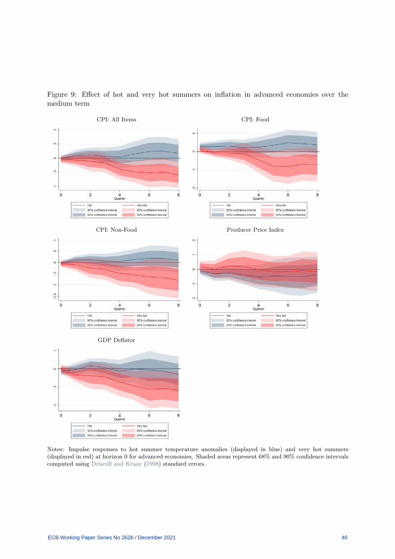
Figure 9: Effect of hot and very hot summers on inflation in advanced economies over themedium term



GDP Deflator

Notes: Impulse responses to hot summer temperature anomalies (displayed in blue) and very hot summers(displayed in red) at horizon 0 for advanced economies. Shaded areas represent 68% and 90% confidence intervalscomputed using Driscoll and Kraay (1998) standard errors.


stability implications, we find evidence that climate change is also important for the primary

objective of price stability. Hot summers can have a meaningful impact on inflation, even into

the medium term. Such events have become increasingly frequent over recent decades, and are

projected to become more frequent still. Climate change, in short, is already starting to bear

on the primary mandate of central banks.


References

Sebastian Acevedo, Mico Mrkaic, Natalija Novta, Evgenia Pugacheva, and Petia Topalova. The

effects of weather shocks on economic activity: what are the channels of impact? Journal of

Macroeconomics, 65, 2020.

Olivier De Bandt, Luc Jacolin, and Thibault Lemaire. Climate change in developing countries:

global warming effects, transmission channels and adaptation policies. Banque de France

Working Paper No. 822, 2021.

Sandra Batten. Climate change and the macro-economy: a critical review. Bank of England

Working Paper No. 706, 2018.

Sangyup Choi, Davide Furceri, Prakash Loungani, Saurabh Mishra, and Marcos Poplawski-

Ribeiro. Oil prices and inflation dynamics: evidence from advanced and developing economies.

Journal of International Money and Finance, 82:71–96, 2018.

Matteo Ciccarelli and Fulvia Marotta. Demand or supply? An empirical exploration of the

effects of climate change on the macroeconomy. ECB Working Paper No. 2608, October 2021.

Makena Coffman and Ilan Noy. Hurricane Iniki: measuring the long-term economic impact of

a natural disaster using synthetic control. Environment and Development Economics, 17(2):

187–205, 2012.

Riccardo Colacito, Bridget Hoffmann, and Toan Phan. Temperature and growth: a panel

analysis of the United States. Journal of Money, Credit and Banking, 51(2-3):313–368, 2019.

Giancarlo Corsetti, Luca Dedola, and Sylvain Leduc. International risk sharing and the trans-

mission of productivity shocks. Review of Economic Studies, 75(2):443–473, 2008.

Jasmien De Winne and Gert Peersman. Agricultural price shocks and business cycles: a global

warning for advanced economies. Ghent University Working Paper No. 18/945, 2018.

Jasmien De Winne and Gert Peersman. The adverse consequences of global harvest and weather

disruptions on economic activity. Nature Climate Change, 11(8):665–672, 2021.

Melissa Dell, Benjamin F. Jones, and Benjamin A. Olken. Temperature shocks and economic

growth: evidence from the last half century. American Economic Journal: Macroeconomics,

4(3):66–95, 2012.


John C. Driscoll and Aart C. Kraay. Consistent covariance matrix estimation with spatially

dependent panel data. The Review of Economics and Statistics, 80(4):549–560, November

1998.

Gabriel Felbermayr and Jasmin Groschl. Naturally negative: the growth effects of natural

disasters. Journal of Development Economics, 111:92–106, 2014.

Thomas Fomby, Yuki Ikeda, and Norman V. Loayza. The growth aftermath of natural disasters.

Journal of Applied Econometrics, 28(3):412–434, 2013.

Gaston Gelos and Yulia Ustyugova. Inflation responses to commodity price shocks – How and

why do countries differ? Journal of International Money and Finance, 72(C):28–47, 2017.

GIS. GISS Surface Temperature Analysis (GISTEMP), version 4. NASA Goddard Institute for

Space Studies, 2021.

Veronica Guerrieri, Guido Lorenzoni, Ludwig Straub, and Ivan Werning. Macroeconomic impli-

cations of COVID-19: can negative supply shocks cause demand shortages? NBER Working

Paper No. 26918, 2020.

Jongrim Ha, M. Ayhan Kose, and Franziska Ohnsorge. One-stop source: a global database of

inflation. World Bank Working Paper No. 9737, 2021.

James Hansen and Sergej Lebedeff. Global trends of measured surface air temperature. Journal

of Geophysical Research: Atmospheres, 92(D11):13345–13372, 1987.

Andreas Heinen, Jeetendra Khadan, and Eric Strobl. The price impact of extreme weather in

developing countries. Economic Journal, 129(619):1327–1342, 2019.

Richard Hornbeck. The enduring impact of the American dust bowl: short- and long-run

adjustments to environmental catastrophe. American Economic Review, 102(4):1477–1507,

2012.

Solomon Hsiang, Robert Kopp, Amir Jina, James Rising, Michael Delgado, Shashank Mohan,

D. J. Rasmussen, Robert Muir-Wood, Paul Wilson, Michael Oppenheimer, Kate Larsen, and

Trevor Houser. Estimating economic damage from climate change in the United States. Sci-

ence, 356(6345):1362–1369, 2017.


Solomon M. Hsiang and Amir S. Jina. The causal effect of environmental catastrophe on long-run

economic growth: evidence from 6,700 cyclones. NBER Working Paper No. 20352, 2014.

IPCC. Climate Change 2021: the physical science basis. Contribution of working group I to the

sixth assessment report of the Intergovernmental Panel on Climate Change. Technical report,

2021.

Oscar Jorda. Estimation and inference of impulse responses by local projections. American

Economic Review, 95(1):161–182, 2005.

Hee Soo Kim, Christian Matthes, and Toan Phan. Extreme weather and the macroeconomy.

Federal Reserve Bank of Richmond Working Paper Series, 2021.

Christine Lagarde. Climate change and central banking. Speech at the ILF conference on green

banking and green central banking, Jan 2021.

Nathan J.L. Lenssen, Gavin A. Schmidt, James E. Hansen, Matthew J. Menne, Avraham Persin,

Reto Ruedy, and Daniel Zyss. Improvements in the GISTEMP uncertainty model. Journal

of Geophysical Research: Atmospheres, 124(12):6307–6326, 2019.

Robert Mendelsohn, William Nordhaus, and Daigee Shaw. The impact of global warming on

agriculture: a Ricardian analysis. American Economic Review, 84(4):753–71, 1994.

Jose Luis Montiel Olea and Mikkel Plagborg-Møller. Local projection inference is simpler and

more robust than you think. Econometrica, 89(4):1789–1823, 2021.

Kriti Mukherjee and Bazoumana Ouattara. Climate and monetary policy: do temperature

shocks lead to inflationary pressures? Climatic Change, 167(3):1–21, 2021.

Ilan Noy. The macroeconomic consequences of disasters. Journal of Development Economics,

88(2):221–231, 2009.

Miles Parker. How global is ‘global inflation’? Journal of Macroeconomics, 58:174–197, 2018a.

Miles Parker. The impact of disasters on inflation. Economics of Disasters and Climate Change,

2(1):21–48, 2018b.

Geert Peersman. International food commodity prices and missing (dis)inflation in the euro

area. Review of Economics and Statistics, forthcoming.


M. Hashem Pesaran and Ron Smith. Estimating long-run relationships from dynamic heteroge-

neous panels. Journal of Econometrics, 68(1):79–113, 1995.

Mikkel Plagborg-Møller and Christian K. Wolf. Local projections and VARs estimate the same

impulse responses. Econometrica, forthcoming.

Ricardo Reis and Mark W. Watson. Relative goods’ prices, pure inflation, and the Phillips

correlation. American Economic Journal: Macroeconomics, 2(3):128–157, 2010.

Michael Roberts and Wolfram Schlenker. Identifying supply and demand elasticities of agricul-

tural commodities: implications for the US ethanol mandate. American Economic Review,

103(6):2265–95, 2013.

Glenn D. Rudebusch. Monetary policy inertia: fact or fiction? International Journal of Central

Banking, 2(4), 2006.

Wolfram Schlenker and Michael J Roberts. Non-linear temperature effects indicate severe dam-

ages to US crop yields under climate change. Proceedings of the National Academy of Sciences,

106(37):15594–15598, 2009.

Eric Strobl. The economic growth impact of hurricanes: evidence from US coastal counties. The

Review of Economics and Statistics, 93(2):575–589, 2011.


A Sample and data sources

A.1 Sample of countries and groupings

Advanced economies: Austria, Australia, Belgium, Cyprus, Czechia, Denmark, Estonia,

Iceland, Finland, France, Germany, Greece, Ireland, Israel, Italy, Japan, Korea, Latvia, Lithua-

nia, Luxembourg, Malta, Netherlands, New Zealand, Norway, Portugal, Singapore, Slovakia,

Slovenia, Spain, Sweden, Switzerland, United Kingdom, United States.

Emerging and developing economies: Bulgaria, Brazil, Chile, China, Costa Rica, Croa-

tia, Hungary, Malaysia, Mexico, Paraguay, Peru, Philippines, Poland, Thailand, Turkey.

A.2 Data sources for price indices

Consumer prices

Parker (2018a) until 2012 Q4, then:

Austria, Belgium, Bulgaria, Croatia, Cyprus, Czechia, Denmark, Estonia, Finland,

France, Germany, Greece, Hungary, Iceland, Ireland, Italy, Latvia, Lithuania, Lux-

embourg, Malta, Netherlands, Norway, Poland, Portugal, Slovakia, Slovenia, Spain,

Sweden, Switzerland, Turkey, United Kingdom: EUROSTAT.

Chile, Costa Rica, Israel, Mexico: OECD.

Australia: Australian Bureau of Statistics.

China: National Bureau of Statistics via Haver Analytics.

Japan: Statistics Japan.

Korea: Korean National Statisitcs Office via Haver Analytics.

Malaysia Department of Statistics via Haver Analytics.

New Zealand: Statistics New Zealand.

Peru: Instituto Nacional de Estadistica e Informatica.

Philippines: Philippine Statistics Authority.

Singapore: Singapore Department of Statistics.

Thailand: Department of Internal Trade, Ministry of Commerce, via Haver Analytics.


Producer price indices

International Monetary Fund’s International Financial Statistics, except:

Chile Banco Central do Chile: IPM Indice general (2007=100) to 2008 then IPP general indus-

trias (2009=100) to 2013 then IPP general industrias (2014=100).

China National Bureau of Statistics: PPI for industrial products.

Iceland Statistics Iceland: Price index of marine products to 2003 Q3, thereafter PPI (2005=100).

Peru National Institute of Statistics and Informatics (INEI): Indice General al por Mayor.

Singapore Singapore Department of Statistics: Domestic Supply Price Index - Overall Items.

Real GDP

International Monetary Fund’s International Financial Statistics

GDP deflator

International Monetary Fund’s International Financial Statistics


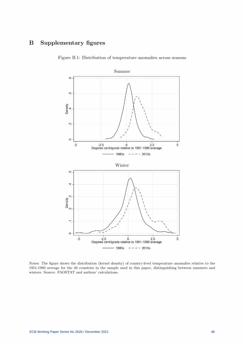
B Supplementary figures

Figure B.1: Distribution of temperature anomalies across seasons

Summer

Winter

Notes: The figure shows the distribution (kernel density) of country-level temperature anomalies relative to the1951-1980 average for the 48 countries in the sample used in this paper, distinguishing between summers andwinters. Source: FAOSTAT and authors’ calculations.


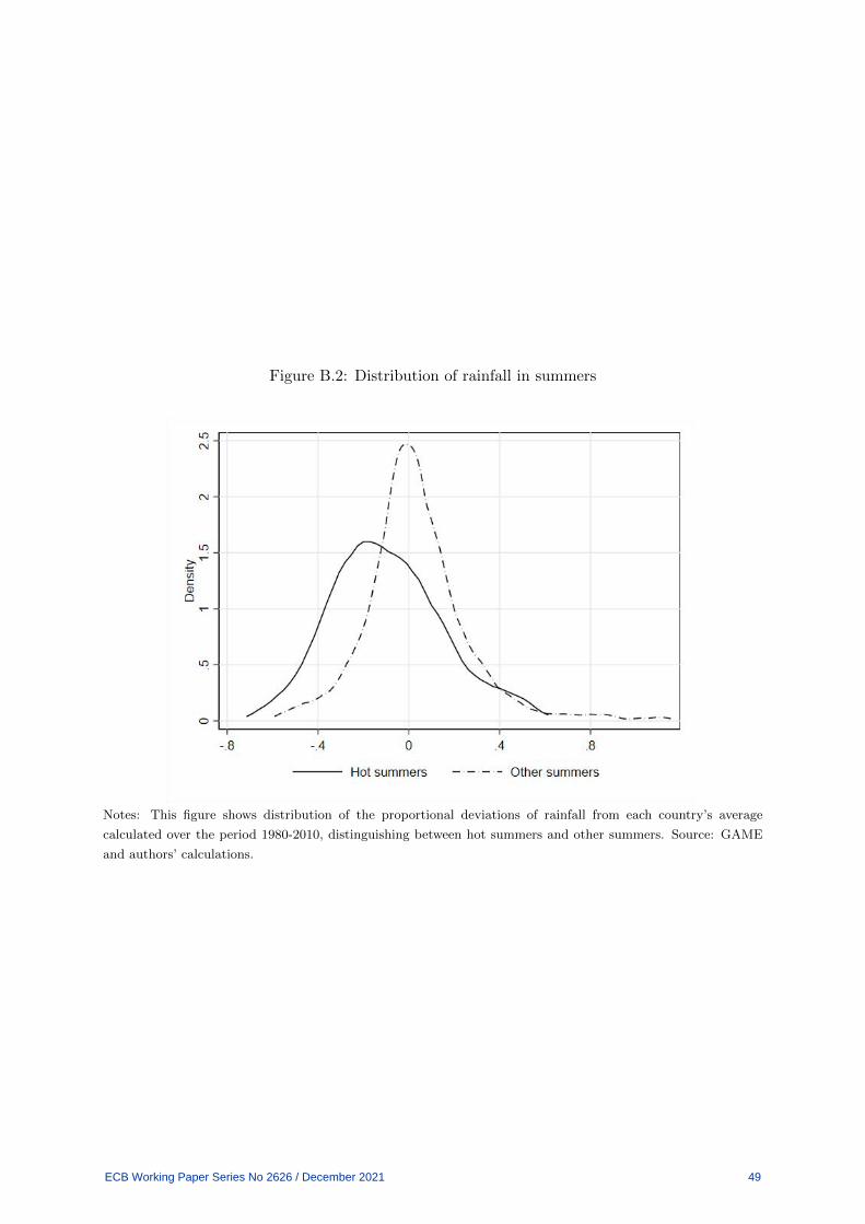
Figure B.2: Distribution of rainfall in summers

Notes: This figure shows distribution of the proportional deviations of rainfall from each country’s average

calculated over the period 1980-2010, distinguishing between hot summers and other summers. Source: GAME

and authors’ calculations.


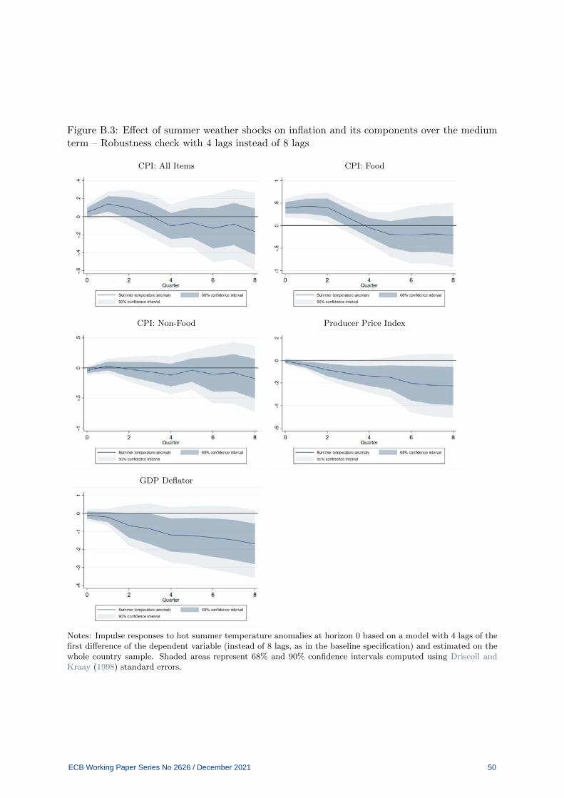
Figure B.3: Effect of summer weather shocks on inflation and its components over the mediumterm – Robustness check with 4 lags instead of 8 lags



GDP Deflator

Notes: Impulse responses to hot summer temperature anomalies at horizon 0 based on a model with 4 lags of thefirst difference of the dependent variable (instead of 8 lags, as in the baseline specification) and estimated on thewhole country sample. Shaded areas represent 68% and 90% confidence intervals computed using Driscoll andKraay (1998) standard errors.


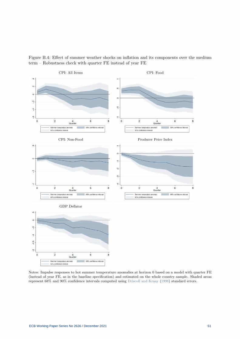
Figure B.4: Effect of summer weather shocks on inflation and its components over the mediumterm – Robustness check with quarter FE instead of year FE



GDP Deflator

Notes: Impulse responses to hot summer temperature anomalies at horizon 0 based on a model with quarter FE(instead of year FE, as in the baseline specification) and estimated on the whole country sample. Shaded areasrepresent 68% and 90% confidence intervals computed using Driscoll and Kraay (1998) standard errors.


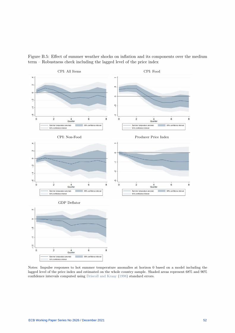
Figure B.5: Effect of summer weather shocks on inflation and its components over the mediumterm – Robustness check including the lagged level of the price index



GDP Deflator

Notes: Impulse responses to hot summer temperature anomalies at horizon 0 based on a model including thelagged level of the price index and estimated on the whole country sample. Shaded areas represent 68% and 90%confidence intervals computed using Driscoll and Kraay (1998) standard errors.


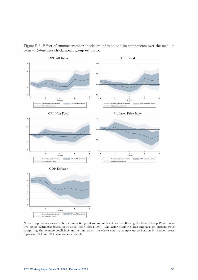
Figure B.6: Effect of summer weather shocks on inflation and its components over the mediumterm – Robustness check, mean group estimator



GDP Deflator

Notes: Impulse responses to hot summer temperature anomalies at horizon 0 using the Mean Group Panel LocalProjection Estimator based on Pesaran and Smith (1995). The latter attributes less emphasis on outliers whilecomputing the average coefficient and estimated on the whole country sample up to horizon 8. Shaded areasrepresent 68% and 90% confidence intervals.


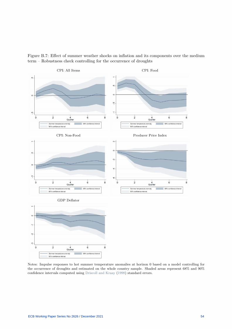
Figure B.7: Effect of summer weather shocks on inflation and its components over the mediumterm – Robustness check controlling for the occurrence of droughts



GDP Deflator

Notes: Impulse responses to hot summer temperature anomalies at horizon 0 based on a model controlling forthe occurrence of droughts and estimated on the whole country sample. Shaded areas represent 68% and 90%confidence intervals computed using Driscoll and Kraay (1998) standard errors.


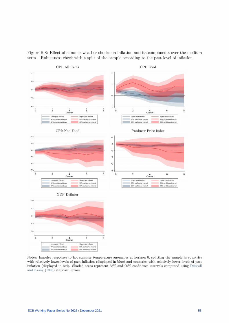
Figure B.8: Effect of summer weather shocks on inflation and its components over the mediumterm – Robustness check with a spilt of the sample according to the past level of inflation



GDP Deflator

Notes: Impulse responses to hot summer temperature anomalies at horizon 0, splitting the sample in countrieswith relatively lower levels of past inflation (displayed in blue) and countries with relatively lower levels of pastinflation (displayed in red). Shaded areas represent 68% and 90% confidence intervals computed using Driscolland Kraay (1998) standard errors.


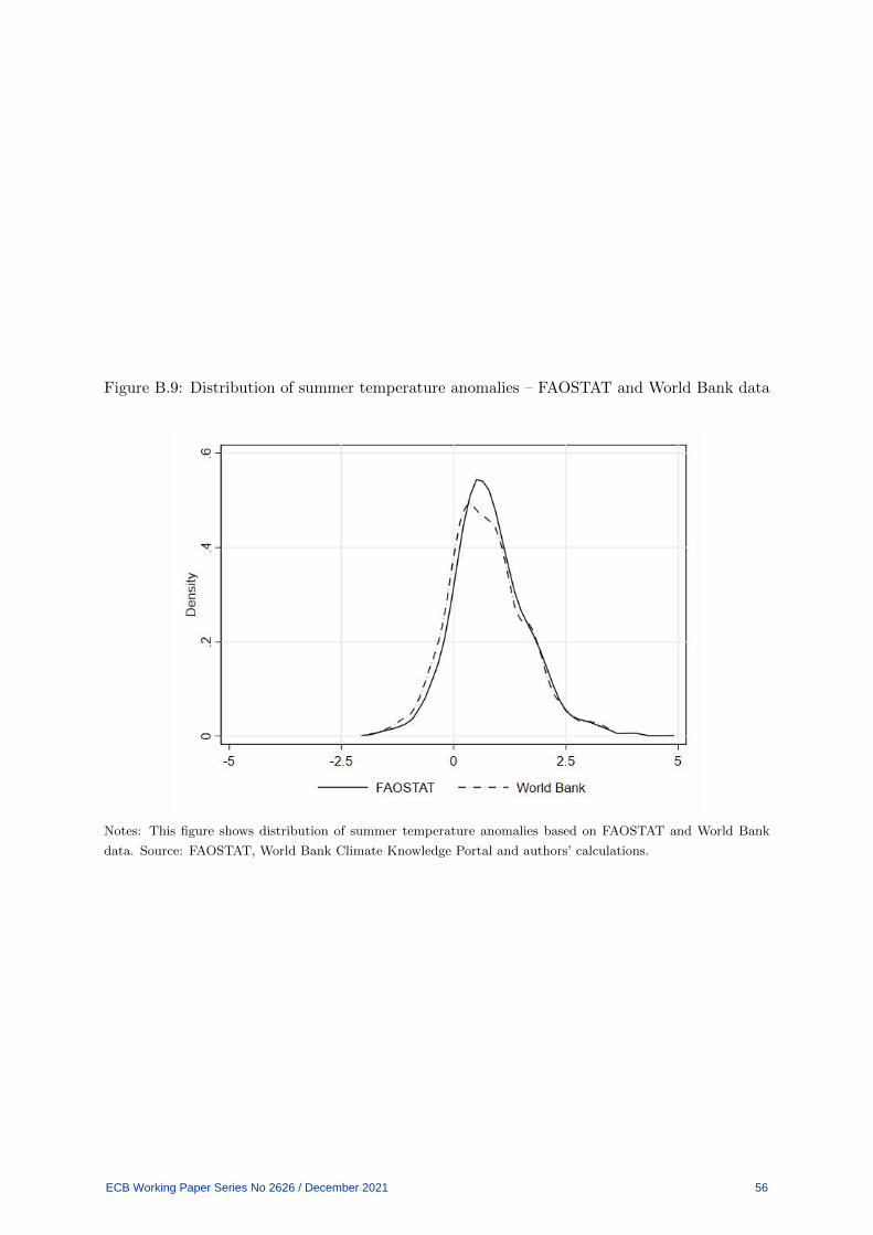
Figure B.9: Distribution of summer temperature anomalies – FAOSTAT and World Bank data

Notes: This figure shows distribution of summer temperature anomalies based on FAOSTAT and World Bank

data. Source: FAOSTAT, World Bank Climate Knowledge Portal and authors’ calculations.


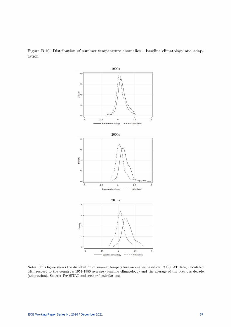
Figure B.10: Distribution of summer temperature anomalies – baseline climatology and adap-tation

1990s

2000s

2010s

Notes: This figure shows the distribution of summer temperature anomalies based on FAOSTAT data, calculatedwith respect to the country’s 1951-1980 average (baseline climatology) and the average of the previous decade(adaptation). Source: FAOSTAT and authors’ calculations.


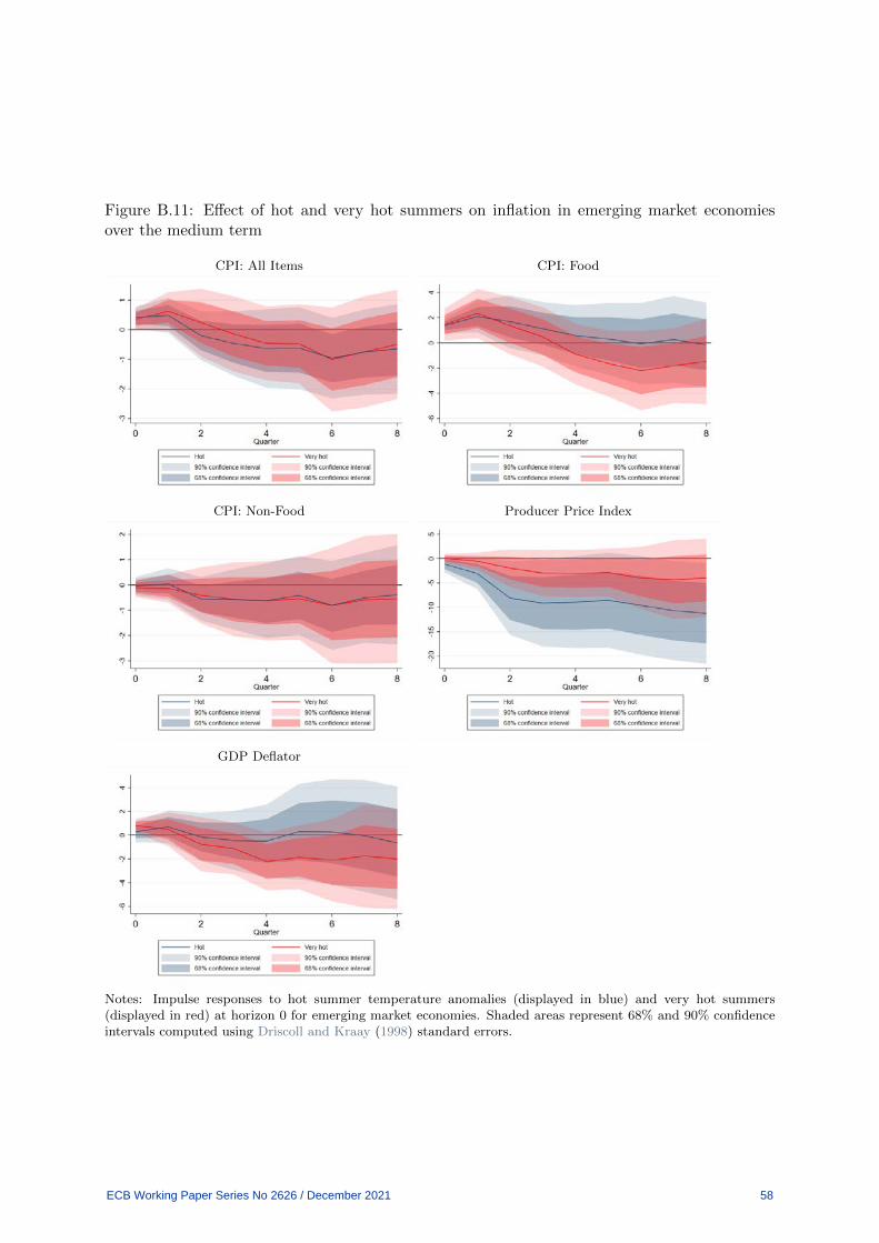
Figure B.11: Effect of hot and very hot summers on inflation in emerging market economiesover the medium term



GDP Deflator

Notes: Impulse responses to hot summer temperature anomalies (displayed in blue) and very hot summers(displayed in red) at horizon 0 for emerging market economies. Shaded areas represent 68% and 90% confidenceintervals computed using Driscoll and Kraay (1998) standard errors.


Acknowledgements We thank Philip R. Lane, Lutz Kilian, Agustín Bénétrix, Luca Dedola, Massimo Ferrari, Patrick Honohan and an anonymous referee for incisive comments and suggestions. In addition, we would like to thank participants of the 2021 CEBRA Workshop for Commodities and Macroeconomics hosted by the Federal Reserve Board and the 2021 Annual Congress of the Italian Economic Association; we would also like to thank participants of seminars at the European Central Bank and at Trinity College Dublin. Donata Faccia European Central Bank, Frankfurt am Main, Germany; email: [email protected] Miles Parker European Central Bank, Frankfurt am Main, Germany; email: [email protected] Livio Stracca European Central Bank, Frankfurt am Main, Germany; email: [email protected]

© European Central Bank, 2021

Postal address 60640 Frankfurt am Main, Germany Telephone +49 69 1344 0 Website www.ecb.europa.eu

All rights reserved. Any reproduction, publication and reprint in the form of a different publication, whether printed or produced electronically, in whole or in part, is permitted only with the explicit written authorisation of the ECB or the authors.

This paper can be downloaded without charge from www.ecb.europa.eu, from the Social Science Research Network electronic library or from RePEc: Research Papers in Economics. Information on all of the papers published in the ECB Working Paper Series can be found on the ECB’s website.

PDF ISBN 978-92-899-4913-2 ISSN 1725-2806 doi:10.2866/185550 QB-AR-21-117-EN-N

mailto:[email protected]



http://www.ecb.europa.eu/

http://www.ecb.europa.eu/

http://ssrn.com/

https://ideas.repec.org/s/ecb/ecbwps.html

http://www.ecb.europa.eu/pub/research/working-papers/html/index.en.html

feeling the heat: extreme temperatures and price stability

Documents