feature selection guided by structural information

arX

iv:1

011.

2315

v1 [

stat

.AP]

10

Nov

201

0

The Annals of Applied Statistics

2010, Vol. 4, No. 2, 1056–1080DOI: 10.1214/09-AOAS302c© Institute of Mathematical Statistics, 2010

FEATURE SELECTION GUIDED BY STRUCTURAL

INFORMATION

By Martin Slawski1,2, Wolfgang zu Castell and Gerhard Tutz

Saarland University, Helmholtz Zentrum Munchen and University ofMunich

In generalized linear regression problems with an abundant num-ber of features, lasso-type regularization which imposes an ℓ1-constrainton the regression coefficients has become a widely established tech-nique. Deficiencies of the lasso in certain scenarios, notably stronglycorrelated design, were unmasked when Zou and Hastie [J. Roy.Statist. Soc. Ser. B 67 (2005) 301–320] introduced the elastic net.In this paper we propose to extend the elastic net by admitting gen-eral nonnegative quadratic constraints as a second form of regular-ization. The generalized ridge-type constraint will typically make useof the known association structure of features, for example, by usingtemporal- or spatial closeness.

We study properties of the resulting “structured elastic net” re-gression estimation procedure, including basic asymptotics and theissue of model selection consistency. In this vein, we provide an analogto the so-called “irrepresentable condition” which holds for the lasso.Moreover, we outline algorithmic solutions for the structured elasticnet within the generalized linear model family. The rationale and theperformance of our approach is illustrated by means of simulated andreal world data, with a focus on signal regression.

1. Introduction. We consider regression problems with a linearpredictor. Let X = (X1, . . . ,Xp)

⊤ be a random vector of real-valued fea-tures/predictors and let Y be a random response variable taking values in aset Y . Given a realization x= (x1, . . . , xp)

⊤ of X, a prediction y for a specific

Received May 2009; revised October 2009.1A large fraction of this work was done while the author was at the Department of

Statistics, University of Munich and the Sylvia Lawry Centre for Multiple Sclerosis Re-search, Munich.

2Supported in part by the Porticus Foundation in the context of the InternationalSchool for Clinical Medicine and Bioinformatics.

Key words and phrases. Generalized linear model, regularization, sparsity, p≫ n, lasso,elastic net, random fields, model selection, signal regression.

This is an electronic reprint of the original article published by theInstitute of Mathematical Statistics in The Annals of Applied Statistics,2010, Vol. 4, No. 2, 1056–1080. This reprint differs from the original in paginationand typographic detail.

1

http://arxiv.org/abs/1011.2315v1

http://www.imstat.org/aoas/

http://dx.doi.org/10.1214/09-AOAS302

http://www.imstat.org

http://www.imstat.org

http://www.imstat.org/aoas/

http://dx.doi.org/10.1214/09-AOAS302

2 M. SLAWSKI, W. ZU CASTELL AND G. TUTZ

functional of the distribution of Y |X= x is obtained via a linear predictor

f(x;β0,β) = β0 + x⊤β, β = (β1, . . . , βp)⊤,

and a function ζ :R → Y such that y = ζ(f(x)). Given an i.i.d. sample

S = (xi, yi)ni=1 from (Rp × Y)n, an optimal set of coefficients β0, β =

(β1, . . . , βp)⊤ can be determined by minimization of a criterion of the form

(β0, β) = argmin(β0,β)

n∑

i=1

L(yi, f(xi;β0,β)),(1)

where L :Y ×R→R+0 is a convex loss function. The loss function is chosen

according to the specific prediction problem, so that large loss representsbad fit to the observed sample S. Approach (1) usually yields poor esti-

mates β0, β if n is not one order of magnitude larger than p. In particular,if p≫ n, approach (1) is not well-defined in the sense that there exist in-

finitely many minimizers β0, β. One way to cope with a small n/p ratio is toemploy a regularizer Ω(β). A traditional approach due to Hoerl and Ken-nard (1970) minimizes the loss in equation (1) subject to an ℓ2-constrainton β. In the situation that β is supposed to be sparse, Tibshirani (1996)proposed, under the acronym “lasso,” to work with an ℓ1-constraint, thatis, one maximizes the loss subject to Ω(β) = ‖β‖1 < s, s > 0. The latter isparticularly attractive if one is interested in feature selection, since one ob-tains estimates βj, j ∈ 1, . . . , p, which equal exactly zero, such that featurej does not contribute to prediction, for which we say that feature j is “notselected.” Continuous shrinkage [Fan and Li (2001)] and the existence of effi-cient algorithms [Efron et al. (2004), Genkin, Lewis and Madigan (2007)] fordetermining the coefficients are further virtues of the lasso. Its limitationshave recently been revealed by several researchers. Zou and Hastie (2005)pointed out that the lasso need not be unique in the p≫ n setting, wherethe lasso is able to select at most n features [Rosset, Zhu and Hastie (2004)].Furthermore, Zou and Hastie stated that the lasso does not distinguish be-tween “irrelevant” and “relevant but redundant” features. In particular, ifthere is a group of correlated features, then the lasso tends to select onearbitrary member of the group while ignoring the remainder. The combinedregularizer of the elastic net Ω(β) = α‖β‖1+(1−α)‖β‖2, α ∈ (0,1) is shownto provide remedy in this regard.

A second double regularizer—tailored to one-dimensional signal regression—is employed by the fused lasso [Tibshirani et al. (2005)], who propagateΩ(β) = α‖β‖1 + (1−α)‖Dβ‖1, where

D: Rp → R

p−1,(2)

(β1, . . . , βp)⊤ 7→ ([β2 − β1], . . . , [βp − βp−1])

⊤

FEATURE SELECTION GUIDED BY STRUCTURAL INFORMATION 3

is the first forward difference operator. The total variation regularizer is

meaningful whenever there is an order relation, notably a temporal one,

among the features. The fused lasso has a property which can be beneficial

for interpretation: it automatically clusters the features, since the sequence

β1, . . . , βp is blockwise constant.

In this paper we study a regularizer which is intermediate between the

elastic net and the fused lasso. Our regularizer combines an ℓ1-constraint

with a quadratic form:

Ω(β) = α‖β‖1 + (1−α)β⊤Λβ,(3)

where Λ= (ljj′)1≤j,j′≤p is assumed to be symmetric and positive semidefi-

nite. Setting Λ= I yields the elastic net. The inclusion of Λ aims at captur-

ing the a priori association structure (if available) of the features in more

generality than the fused lasso. Therefore, expression (3) will be referred to

as the structured elastic net regularizer. The structured elastic net estimator

is defined as


n∑

i=1

L(yi, f(xi;β0,β))

(4)subject to α‖β‖1 + (1− α)β⊤Λβ ≤ s, α ∈ (0,1), s > 0,

which is equivalent to the Lagrangian formulation


n∑

i=1

L(yi, f(xi;β0,β)) + λ1‖β‖1 + λ2β⊤Λβ,

(5)λ1, λ2 > 0.

The rest of the paper is organized as follows: in Section 2 we discuss the

choice of the matrix Λ, followed by an analysis of some important proper-

ties of our proposal (5) in Section 3. Section 4 is devoted to asymptotics and

consistency questions, motivating the introduction of the adaptive struc-

tured elastic net. Section 5 presents an algorithmic solution to compute the

minimizers (5) in the generalized linear model family. The practical per-

formance of the structured elastic net is contained in Section 6. Section

7 concludes with a discussion and an outlook. All proofs can be found in

the online supplement supporting this article [Slawski, zu Castell and Tutz

(2010)].


2. Structured features.

2.1. Motivation. A considerable fraction of contemporary regression prob-lems are characterized by a large number of features, which are either of thesame order of magnitude as the sample size or even several orders larger(p≫ n). Common instances thereof are feature sets consisting of sampledsignals, pixels of an image, spatially sampled data, or gene expression inten-sities. Beside high dimensionality of the feature space, these examples havein common that the feature set can be arranged according to an a priori as-sociation structure. If a sampled signal does not vary rapidly, the influenceof nearby sampling points on the response can be expected to be similar;correspondingly, this applies to adjacent pixels of an image, or, more gen-erally, to any other form of spatially linked features. In genomics genes canbe categorized into functional groups, or one has prior knowledge of theirfunctions and interactions within biochemical reaction chains, the so-calledpathways.

Figures 1 and 2 display two well-known examples, phoneme- and hand-written digit classification. These examples are well apt to illustrate the ideaof the structured elastic net regularizer, since it is sensible to assume thatthe prediction problem is not only characterized by smoothness with respectto a given structure, but also by sparsity: in the phoneme classification ex-ample, visually only the first hundred frequencies seem to carry informationrelevant to the prediction problem. A similar rationale applies to the secondexample, where the arc of the numeral eight in the lower half of the picture isthe eminent characteristic that admits a distinction from the numeral nine.

2.2. Gauss–Markov random fields. Given a large, but structured set offeatures, its structure can be exploited to cope with high dimensionality inregression estimation. The estimands βjpj=1 form a finite set such thattheir prior dependence structure can conveniently be described by means ofa graph G = (V,E), V = β1, . . . , βp, E ⊂ V × V . We exclude loops, thatis, (βj , βj) /∈E for all j. The edges may additionally be weighted by a func-tion w :E →R, w((βj , βj′)) =w((βj′ , βj)) for all edges in E. We will use thenotation βj ∼ βj′ to express that βj and βj′ are connected by an edge inG. The weight function can be extended to a function on V × V by settingw((βj , βj′)) =w((βj′ , βj)) = 0 if (βj , βj′) /∈E.

The graph is interpreted in terms of the Gauss–Markov random fields[Besag (1974); Rue and Held (2001)]. In our setup, the pairwise Markovproperty reads

¬βj ∼ βj′ ⇔ βj ⊥⊥ βj′ |V \ βj , βj′,(6)


Fig. 1. Phoneme data [Hastie, Buja and Tibshirani (1995)]. The upper panel shows sev-eral thousand log-periodogramms of the speech frames for the phonemes “aa” (as occuringin “dark”) and “ao” (as occuring in “water”). The classwise means are given by thick lines.We use linear logistic regression to predict the phoneme given a log-periodogramm. Thelower panel depicts the resulting coefficients when using the lasso (left panel), a first-orderdifference penalty (right panel), and a combination thereof, which we term “structuredelastic net” (middle panel).

with ⊥⊥ denoting conditional independence. Property (6) is conformed tothe following choice for the precision matrix Λ= (ljj′)1≤j,j′≤p:

ljj′ =

p∑

k=1

|w((βj , βk))|, if j = j′,

−w((βj , βj′)), if j 6= j′,

(7)

which is singular in general. If signw((βj , βj′)) ≥ 0 for all (βj , βj′) in E,then Λ as given in equation (7) is known as the combinatorial graph Lapla-cian in the spectral graph theory [Chung (1997)]. It is straightforward toverify the following properties:


Fig. 2. Handwritten digit recognition data set [Le Cun et al. (1989)]. One observationis given by a greyscale image composed of 16 × 16 pixels. The upper panel shows thecontour of the pixel-wise means for the numerals “8” and “9.” We use a training set of1500 observations of eights and nines as input for linear logistic regression. The lowerpanel depicts the coefficient surfaces for the lasso (left panel), a discrete Laplacian penaltyaccording to the grid structure (right panel), and a combination, the structured elastic net(middle panel).

•

β⊤Λβ =∑

βj∼βj′

|w(βj , βj′)|(βj − signw((βj , βj′))βj′)2 ≥ 0,(8)

where the sum is over all distinct edges in G, and “distinct” is understoodwith respect to the relation (βj , βj′) = (βj′ , βj) for all j, j

′.• If G is connected and signw((βj , βj′)) ≥ 0 for all (βj , βj′) in E, the null

space of Λ is spanned by the vector of ones 1.

While we have started in full generality, the choice w((βj , βj′)) ∈ 0,1 forall j, j′ will frequently be the standard choice in practice. In this case, thequadratic form captures local fluctuations of β w.r.t. G. As a simple example,one may take G as the path on p vertices so that expression (8) equals thesummed squared forward differences

p∑

j=2

(βj − βj−1)2 = ‖Dβ‖2 = β⊤D⊤Dβ,(9)


Fig. 3. A collection of some graphs. A path and a grid (left panel), a rooted tree (middlepanel), and an irregular graph describing a part of the so-called MAPK signaling pathway(right panel).

whereD is defined in equation (2). More complex graphical structures can begenerated from simple ones using the notion of Cartesian products of graphs[Chung (1997), page 37]. For instance (as displayed in the left panel of Figure3), the Cartesian product of a p-path and a p′-path equals a p× p′ regulargrid, in which case the standard choice of Λ is seen to be a discretizationof the Laplacian ∆ acting on functions defined on R

2. Regularizers built upfrom discrete differences have already seen frequent use in high-dimensionalregression estimation. Examples comprise penalized discriminant analysis[Hastie, Buja and Tibshirani (1995)] and spline smoothing [Eilers and Marx(1996)].

2.3. Connection to manifold regularization. As pointed out by one ofthe referees, regularizers of the form (8) are applicable to a variety of learn-ing problems in which data are supposed to be generated according to aprobability measure supported on a compact, smooth manifold M ⊂ R

p.The canonical regularization operator acting on smooth functions on M isthe Laplace–Beltrami operator ∆M [Rosenberg (1997)], which generalizesthe Laplacian for Euclidean domains. As suggested, for example, in Belkin,Niyogi and Sindwhani (2006), given a set of data points in R

p, a discreteproxy for a potential manifold structure can be obtained by computing a(possibly weighted) neighborhood graph of the points, and, in turn, a proxyfor ∆M is obtained by a discrete Laplacian of the form (7) resulting fromthe neighborhood graph.

Relating these ideas to our framework, one might think of settings whereeach of the xini=1 represents a collection of p points sampled on a compact,smooth manifold M . This is a natural extension of the introductory exam-ples in Section 2.1, where the correspondingM would be given by an intervaland a rectangle, respectively. Assuming a linear relationship between scalarresponses yini=1 and the predictors xini=1, we expect the corresponding


coefficient vector to be both sparse and smooth with respect to the mani-fold structure. Without going into detail, the approach might be useful forpredictors with geographical information. The idea is illustrated in Figure 4where M is chosen as a sphere embedded in R

3.

3. Properties.

3.1. Bayesian and geometric interpretation. In the setup of Section 1,consider the regularizer

Ω(β) = λ1‖β‖1 + λ2β⊤Λβ, λ1, λ2 > 0.

It has a nice Bayesian interpretation when the loss function L is of the form

L(y, f(x;β0,β)) = φ−1(b(f(x))− yf(x)) + c(y,φ),(10)

that is, the loss function equals the negative log-likelihood of a generalizedlinear model in canonical parametrization, which will primarily be studiedin this paper. Models of this class are characterized by [cf. McCullagh andNelder (1989)]

Y |X= x∼ simple exponential family,

y =E[Y |X= x] = µ=d

dfb(f(x)),(11)

Fig. 4. A manifold setting suitable to our regularizer. The black dots represent pointsat which the random variables Xj , j = 1, . . . , p, are realized, and the spikes normal to thesurface indicate the size of the corresponding β∗

j , j = 1, . . . , p. Except for the two groupshighlighted in the left and right panel, respectively, the coefficients equal zero. The dashedlines represent the neighborhood graph obtained by connecting each dot with its four nearestneighbors with respect to the geodesic distance on the sphere.


Fig. 5. Level sets (β1, β2) :λ1(|β1| + |β2|) + λ2(β1 − β2)2 = 1 (left panel, solid lines)

and (β1, β2) :λ1(|β1|+ |β2|)+λ2(β1+β2)2 = 1 (left panel, dashed lines) of the structured

elastic net regularizer and (β1, β2) :λ1(|β1|+ |β2|) + λ2|β1 − β2|= 1 of the fused lasso.

var[Y |X= x] = φd2

df2b(f(x)).

The form (10) is versatile, including classical linear regression with Gaus-sian errors, logistic regression for classification, and Poisson regression forcount data. Given a loss from the class (10), the regularizer Ω(β) can beinterpreted as the combined Laplace (double exponential)-Gaussian priorp(β)∝ exp(−Ω(β)), for which the structured elastic net estimator (5), pro-vided p(β0)∝ 1, is the maximum posterior (MAP) estimator given the sam-ple S. It is instructive to consider two predictors, that is, β = (β1, β2)

⊤.Figure 5 gives a geometric interpretation for the basic choices

Λ=

(1 −1−1 1

)and Λ=

(1 11 1

),

corresponding to positive- and negative prior correlation, respectively.The contour lines of the structured elastic net penalty contain elements of

a diamond and an ellipsoid. The higher λ2 in relation to λ1, the ellipsoidalpart becomes more narrower and more stretched. The sign of the off-diagonalelement of Λ determines the orientation of the ellipsoidal part.

3.2. A grouping property. For the elastic net, Zou and Hastie (2005) pro-

vided an upper bound on the absolute distances |βelastic netj − βelastic net

j′ |, j, j′ =1, . . . , p, in terms of the sample correlations, to which Zou and Hastie re-ferred to as “grouping property.” We provide similar bounds here. For whatfollows, let S be a sample as in Section 1. We introduce a design matrix


X = (xij)1≤i≤n1≤j≤p

and denote by Xj = (x1j , . . . , xnj)⊤ the realizations of pre-

dictor j in S, and the response vector is defined by y = (y1, . . . , yn)⊤. For

the remainder of this section, we assume that the responses are centered andthat the predictors are centered and standardized to unit Euclidean lengthw.r.t. the sample S, that is,

n∑

i=1

yi =

n∑

i=1

xij = 0,

n∑

i=1

x2ij = 1, j = 1, . . . , p.(12)

Proposition 1. Letting p= 2, let the loss function be of the form (10),

let ρ = X⊤1 X2 denote the sample correlation of X1 and X2, and let Λ =

12

(1 ss 1

), s ∈ −1,1. If −sβ1β2 > 0, then

|β1 + sβ1| ≤1

2λ2

√2(1 + sρ)‖y‖.

In particular, in the setting of Proposition 1, we have the implication thatif X1 =−sX2, then β1 =−sβ2.

3.3. Decorrelation. Let us now consider the important special case

L(y, f(x;β)) = (y − x⊤β)2,

which corresponds to classical linear regression. The constant term β0 isomitted, since we work with centered data. The structured elastic net esti-mator can then be written as

β = argminβ

−2y⊤Xβ+β⊤[C+ λ2Λ]β+ λ1‖β‖1, C=X⊤X,

(13)= argmin

β

−2y⊤Xβ+β⊤Cβ+ λ1‖β‖1, C=X⊤X+ λ2Λ.

Note that for standardized predictors, C equals the matrix of sample cor-relations ρjj′ =X⊤

j Xj′ , j, j′ = 1, . . . , p. With a large number of predictors or

elements ρjj′ with large |ρjj′ |, C is known to yield severely unstable ordinary

least squares (ols) estimates βolsj , j = 1, . . . , p. If the two underlying random

variables Xj and Xj′ are highly positively correlated, this will likely trans-late to high sample correlations of Xj and Xj′ , which in turn yield a strongly

negative correlation between βolsj and βols

j′ and, as a consequence, high vari-

ances var[βolsj ] and var[βols

j′ ]. In the prevalence of high correlations, perfor-mance of the lasso may degrade as well. For example, Donoho, Elad andTemlyakov (2006) showed that the lower the mutual coherence maxj,j′

j 6=j′|ρj,j′|,

the more stable is lasso estimation. The modified matrix C can be written as


C =V1/2Λ

RΛV1/2Λ

, VΛ = diag(1 + λ2∑p

k=1 |l1k|, . . . ,1 + λ2∑p

k=1 |lpk|), andthe modified correlation matrix RΛ has entries

ρΛ,jj′ =ρjj′ + λ2ljj′√

1 +∑p

k=1 |ljk|√

1 +∑p

k=1 |lj′k|, j, j′ = 1, . . . , p.

In light of Section 2, the entries of RΛ combine sample- and prior correla-tions. Decorrelation occurs if ρjj′ ≈−λ2ljj′ .

4. Consistency. The asymptotic analysis presented in this section closelyfollows the ideas of Knight and Fu (2000) and Zou (2006). Both have studiedasymptotics for the lasso in linear regression for a fixed number of predictorsunder conditions ensuring

√n-consistency and asymptotic normality of the

ordinary least squares estimator. Knight and Fu (2000) proved that the lasso

estimator βlasso is√n-consistent for the true coefficient vector β∗ provided

λn1 = O(

√n). Zou (2006) has shown that while this choice of λn

1 providesthe optimal rate for estimation, it leads to inconsistent feature selection.Define the active set as A = j :β∗

j 6= 0 and Ac = 1, . . . , p \ A and let δ

be an estimation procedure producing an estimate βδ. Then δ is said to beselection consistent if

limn→∞

P(βδj,n 6= 0) = 1 for j ∈A,

limn→∞

P(βδj,n = 0) = 1 for j ∈Ac,

where here and in the following, the sub- or superscript n indicates that thecorresponding quantity depends on the sample size n. Moreover, Zou (2006)and Zhao and Yu (2006) have shown that if λn

1 = o(n) and λn1/

√n → ∞,

the lasso has to satisfy a nontrivial condition, the so-called “irrepresentablecondition,” to be selection consistent. Zou (2006) proposed the adaptivelasso, a two-step estimation procedure, to fix this deficiency. In the following,these results will be adapted to the presence of a second quadratic penaltyterm.

Theorem 1. Define

βn = argminβ

‖yn −Xnβ‖2 + λn1‖β‖1 + λn

2β⊤Λβ.

Assume that λn1/

√n→ λ0

1 ≥ 0 and λn2/

√n→ λ0

2 ≥ 0. Consider the randomfunction

V (u) =−2u⊤w+u⊤Cu

+ λ01

p∑

j=1

uj sign(β∗j )I(β

∗j 6= 0) + |uj |I(β∗

j = 0)

+ 2λ02u

⊤Λβ∗, w∼N(0, σ2C).


Then, under conditions (C.1)–(C.3) in the online supplement,√n(βn −

β∗)D→ argminV (u).

Theorem 1 is analogous to Theorem 2 in Knight and Fu (2000) and es-

tablishes√n-consistency of βn, provided λn

1 and λn2 are O(

√n). Theorem 1

admits a straightforward extension to the class of generalized linear models[cf. equation (11)]. Let the true model be defined by

E[Y |X= x] = b′(f(x;β∗)), f(x) = x⊤β∗.

For the sake of a clearer presentation, we assume that β∗0 = 0. We study the

estimator

βn = argminβ

2φ−1n∑

i=1

b(f(xi;β))− yif(xi;β) + λn1‖β‖1 + λn

2β⊤Λβ.(14)

Theorem 2. For the estimator (14), let λn1/

√n→ λ0

1 ≥ 0 and λn2/

√n→

λ02 ≥ 0. Consider the random function

W (u) =−2u⊤w+u⊤Iu

+ λ01

p∑

j=1

uj sign(β∗j )I(β

∗j 6= 0) + |uj |I(β∗

j = 0)

+ 2λ02u

⊤Λβ∗, w∼N(0,I).

Then under conditions (G.1) and (G.2) in the online supplement,√n(βn−

β∗)D→ argminW (u).

Now let us turn to the question of selection consistency. In the setup ofTheorem 1, if λn

1 and λn2 both are O(

√n), then, using arguments similar to

those in Knight and Fu (2000) and Zou (2006), βn is shown not to be selec-tion consistent. Selection consistency can be achieved if one lets λn

1 , λn2 grow

more strongly and if the quantities C, Λ, and β∗ jointly fulfill a nontrivialcondition, which can be seen as analog to the irrepresentable condition ofthe lasso [Zou (2006), Zhao and Yu (2006)].

Theorem 3. In the situation of Theorem 1, let λn1/n→ 0, λn

1/√n→∞,

λn2/λ

n1 →R,0<R<∞ and consider the partitioning scheme

β∗ =

(β∗A

β∗Ac

), C=

(CA CAAc

CAcA CAc

)and

(15)

Λ=

(ΛA ΛAAc

ΛAcA ΛAc

),


so that here and in the following, the subscripts A and Ac refer to active andinactive set, respectively. Then, if selection consistency holds, the followingcondition must be fulfilled: there exists a sign vector sA such that

|−CAcAC−1A (sA + 2RΛAβ

∗A) + 2RΛAcAβ

∗A| ≤ 1,

where the inequality is interpreted componentwise.

While this condition is interesting from a theoretical point of view, it isimpossible to check in practice, since β∗

A is unknown.Selection consistency can be achieved by a two-step estimation strat-

egy introduced in Zou (2006) under the name adaptive lasso, which re-places ℓ1-regularization uniform in βj , j = 1, . . . , p, by a weighted variantJ(β) =

∑pj=1ωj|βj |, where the weights ωjpj=1 are determined adaptively

as a function of an “initial estimator” βinit:

ωj = |βinitj |−γ , γ > 0, j = 1, . . . , p.(16)

In terms of selection consistency, this strategy turns out to be favorable forour proposal, too.

Theorem 4. In the situation of Theorem 1, define

βadaptiven = argmin

β

‖yn −Xnβ‖2 + λn1

p∑

j=1

ωj|βj |+ λn2β

⊤Λβ,

where the weights are as in equation (16), and suppose that the initial esti-mator satisfies

rn(βn − β∗) =OP(1), rn →∞ as n→∞.

Furthermore, suppose that

rγnλn1n

−1/2 →∞, λn1n

−1/2 → 0, λn2n

−1/2 → λ02 ≥ 0

as n→∞. Then:

(1)√n(βadaptive

A,n −β∗A)

D→N(−λ02C

−1A ΛAβ

∗A,C

−1A ),

(2) limn→∞P(βadaptiveAc,n = 0) = 1.

Theorem 4 implies that the adaptive structured elastic net βadaptive is anoracle estimation procedure [Fan and Li (2001)] if the bias term in (1) van-ishes, which is the case if β∗

A resides in the null space of ΛA. Interestingly, ifΛ equals the combinatorial graph Laplacian (cf. Section 2.2), this happens ifand only if β∗

A has constant entries and A specifies a connected componentin the underlying graph.


Concerning the choice of the initial estimator, the ridge estimator hasworked well for us in practice, provided the ridge parameter is chosen ap-propriately. While γ may be treated as a tuning parameter, we have set γequal to 1 in all our data analyses. Last, we remark that while Theorem 4applies to linear regression, it can be extended to hold for generalized linearmodels, similarly as we have extended Theorem 1 to Theorem 2.

5. Computation. This section discusses aspects concerning computationand model selection for the structured elastic net estimator when the lossfunction is the negative log-likelihood of a generalized linear model (10).

5.1. Data augmentation. From the discussions in Section 3.3, it followsthat the structured elastic net for squared loss, assuming centered data, canbe recast as the lasso on augmented data

X=

(X

λ1/22 Q

)

(n+p)×p

, y=

(y

0

)

(n+p)×1

, Λ=Q⊤Q,

and, hence, algorithms available for computing the lasso, notably LARS[Efron et al. (2004)], may be applied, which computes for fixed λ2 and vary-

ing λ1 the piecewise linear solution path β(λ1;λ2). This approach is parallelto that proposed by Zou and Hastie (2005) for the elastic net. In addition,the augmented data representation is helpful when addressing uniqueness of

the structured elastic net in the p≫ n setting: if rank(X)+ rank(λ1/22 Q)≥ p

and the rows of X combined with the rows of λ1/22 Q form a linearly inde-

pendent set, C as defined in equation (13) is of full rank and, hence, thestructured elastic net is unique. Moreover, this shows that even for p≫ n,in principle, all features can be selected.

In order to fit arbitrary regularized generalized linear models, the aug-mented data representation has to be modified. Without regularization, es-timators in generalized linear models are obtained by iteratively computingweighted least squares estimators:(β(k+1)0

β(k+1)

)= ([1 X ]⊤W(k)[1 X ])−1[1 X ]⊤W(k)z(k),

z(k) = f (k) + [W(k)]−1(y−µ(k)),

f (k) = (f(k)1 , . . . , f (k)

n )⊤, f(k)i = β

(k)0 + x⊤

i β(k), i= 1, . . . , n,(17)

µ(k) = (µ(k)1 , . . . , µ(k)

n )⊤, µ(k)i = b′(f

(k)i ), i= 1, . . . , n,

W(k) = diag(w(k)1 , . . . ,w(k)

n ), w(k)i = φ−1b′′(f

(k)i ), i= 1, . . . , n.


Note that the design matrix additionally includes a constant term 1. Turningback to the structured elastic net, an adaptation of the augmented dataapproach iteratively determines

(β(k+1)0

β(k+1)

)= argmin

(β0,β)

n+p∑

i=1

w(k)i

(z(k)i − x⊤

i

(β0β

))2

+ λ1‖β‖1,

with

w(k)i =w

(k)i , i= 1, . . . , n, as in equation (17),

w(k)i = 1, i= (n+1), . . . , (n+ p),

z(k)i = z

(k)i , i= 1, . . . , n, as in equation (17),

z(k)i = 0, i= (n+1), . . . , (n+ p),

xi = (1 x⊤i )⊤ , i= 1, . . . , n,

xi = (0√λ2q

⊤i )⊤ , i= (n+1), . . . , (n+ p),

with q⊤i denoting the ith row of Q.

Alternatives to augmented data representation include cyclical coordinatedescent in the spirit of Friedman et al. (2007) and a direct modification ofGoeman’s algorithm [Goeman (2007)]. Descriptions can be a found in thefull technical report underlying this article [Slawski, zu Castell and Tutz(2009), available online].

6. Data analysis.

6.1. One-dimensional signal regression. In one-dimensional signal regres-sion, as described, for example, in Frank and Friedman (1993), one aims atthe prediction of a response given a sampled signal x⊤ = (x(t))Tt=1, wherethe indices t= 1, . . . , T , refer to different ordered sampling points. For a sam-ple S = (x1(t)Tt=1, y1), . . . , (xn(t)Tt=1, yn) of pairs consisting of sampledsignals and responses, we consider prediction models of the form

yi = ζ

(β0 +

T∑

t=1

xi(t)β(t)

), i= 1, . . . , n.

6.1.1. Simulation study. Similarly to Tutz and Gertheiss (2010), we sim-ulate signals x(t), t= 1, . . . , T , T = 100, according to

x(t) ∼5∑

k=1

bk sin(tπ(5− bk)/50−mk) + τ(t),

bk ∼ U(0,5), mk ∼U(0,2π), τ(t) ∼N(0,0.25),


with U(a, b) denoting the uniform distribution on the interval (a, b). Forthe coefficient function β∗(t), t= 1, . . . , T , we examine two cases. In the firstcase, referred to as the “bump setting,” we use

β∗(t) =

−(30− t)2 +100/200, t= 21, . . . ,39,(70− t)2 − 100/200, t= 61, . . . ,80,0, otherwise.

In the second case, referred to as the “block setting,”

β∗ = (0, . . . ,0︸︷︷︸20 times

,0.5, . . . ,0.5︸︷︷︸10 times

,1, . . . ,1︸︷︷︸10 times

,0.5, . . . ,0.5︸︷︷︸10 times

,0.25, . . . ,0.25︸︷︷︸10 times

,0, . . . ,0︸︷︷︸40 times

)⊤.

The form of the signals and coefficient functions are displayed in Figure 6.For both settings, data are simulated according to

y =

T∑

t=1

x(t)β∗(t) + ε, ε∼N(0,5).

For each out of 50 iterations, we simulate i = 1, . . . ,500 i.i.d. realizationsand divide them into three parts: a training set of size 200, a validationset of size 100, and a test set of size 200. Hyperparameters of the methodslisted below are optimized by means of the validation set. As performancemeasures, we compute the absolute distance L1(β,β) = ‖β − β‖1 of true-and estimated coefficients and the mean squared prediction error on the testset. For methods with built-in feature selection, we additionally evaluate thegoodness of selection in terms of sensitivity and specificity. For each of thetwo setups, the simulation is repeated 50 times. The following methods arecompared: ridge regression, generalized ridge regression with a first differencepenalty, P-splines according to Eilers and Marx (1999), lasso, fused lasso,elastic net, structured elastic net with a first difference penalty, adaptive

Fig. 6. The setting of the simulation study. A collection of five signals (left panel),the coefficient functions for “bump”—(middle panel) and “block” setting (right panel),respectively.


structured elastic net, where the weights ω(t) are chosen according to the

ridge estimator of the same iteration as ω(t) = 1/|βridge(t)|.Performance measures are averaged over 50 iterations and displayed in

Table 1 (bump setting) and Table 2 (block setting), respectively.For the bump setting, Figure 7 shows that the double-regularized proce-

dures employing decorrelation clearly outperform a visibly unstable lasso.Due to a favorable signal-to-noise ratio, even simplistic approaches such asridge- or generalized ridge regression show competitive performance withrespect to prediction of future observations. In pure numbers, the estima-tion of β∗(t) is satisfactory as well. However, the lack of sparsity results into“noise fitting” for those parts where β∗(t) is zero. For the two settings ex-amined here, the P-spline approach does not improve over generalized ridgeregression, because the two coefficient functions are not overly smooth. Theelastic net considerably improves over the lasso, but it lacks smoothness.Its numerical inferiority to ridge regression results from double shrinkageas discussed in Zou and Hastie (2005). The performance of the structuredelastic net is not fully satisfactory. In particular, at the changepoints fromzero- to nonzero parts, there is a tendency to widen unnecessarily the sup-port of the nonzero sections. This shortcoming is removed by the adaptivestructured elastic net, thereby confirming the theoretical result concerning

Table 1

Results for the bump setting, averaged over 50 simulations

Method L1(β, β∗) PE Sensitivity Specificity

Ridge 0.249 5.35(5.9× 10−4) (0.078)

G.ridge 0.238 5.32(9.9× 10−4) (0.076)

P-spline 0.241 5.30(16.0× 10−4) (0.077)

Lasso 0.271 5.72 0.62 0.65(23.9× 10−4) (0.079) (8.9× 10−3) (0.016)

Fused lasso 0.235 5.30 0.96 0.51(7.2× 10−4) (0.075) (5.5× 10−3) (0.010)

Enet 0.246 5.46 0.93 0.69(29.9× 10−4) (0.081) (0.013) (0.032)

S.enet 0.232 5.30 0.98 0.59(7.6× 10−4) (0.078) (7.8× 10−3) (0.029)

Ada.s.enet 0.232 5.25 0.91 0.82

(15.0× 10−4) (0.075) (21.0× 10−3) (0.020)

For annotation, see Table 2.


Table 2

Results for the block setting, averaged over 50 simulations. We make use of the followingabbreviations: “PE” for “mean squared prediction error,” “g.ridge” for “generalized

ridge,” “enet” for “elastic net,” “s.enet” for “structured elastic net,” and “ada.s.enet”for “adaptive structured elastic net.” Standard errors are given in parentheses. For each

column, the best performance is emphasized in boldface

Method L1(β, β∗) PE Sensitivity Specificity

Ridge 0.082 5.41(3.4× 10−3) (0.080)

G.ridge 0.064 5.35(1.9× 10−3) (0.078)

P-spline 0.065 5.34(1.9× 10−3) (0.077)

Lasso 0.207 6.12 0.73 0.62(3.6× 10−3) (0.089) (7.5× 10−3) (0.014)

Fused lasso 0.058 5.34 0.99 0.51(1.9× 10−3) (0.076) (7× 10−4) (0.009)

Enet 0.094 5.47 0.95 0.73(5.0× 10−3) (0.072) (6.4× 10−3) (0.083)

S.enet 0.070 5.38 0.99 0.60(5.0× 10−3) (0.080) (3.3× 10−3) (0.027)

Ada.s.enet 0.061 5.32 0.97 0.83

(3.2× 10−3) (0.69) (8.0× 10−3) (0.018)

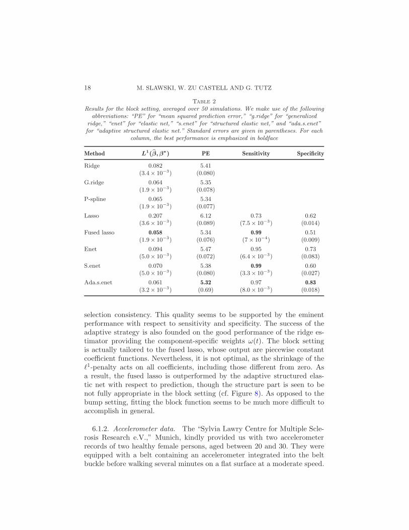
selection consistency. This quality seems to be supported by the eminentperformance with respect to sensitivity and specificity. The success of theadaptive strategy is also founded on the good performance of the ridge es-timator providing the component-specific weights ω(t). The block settingis actually tailored to the fused lasso, whose output are piecewise constantcoefficient functions. Nevertheless, it is not optimal, as the shrinkage of theℓ1-penalty acts on all coefficients, including those different from zero. Asa result, the fused lasso is outperformed by the adaptive structured elas-tic net with respect to prediction, though the structure part is seen to benot fully appropriate in the block setting (cf. Figure 8). As opposed to thebump setting, fitting the block function seems to be much more difficult toaccomplish in general.

6.1.2. Accelerometer data. The “Sylvia Lawry Centre for Multiple Scle-rosis Research e.V.,” Munich, kindly provided us with two accelerometerrecords of two healthy female persons, aged between 20 and 30. They wereequipped with a belt containing an accelerometer integrated into the beltbuckle before walking several minutes on a flat surface at a moderate speed.


Fig. 7. Estimated coefficient functions for the bump setting. The pointwise median curveover 50 iterations is represented by a solid line, pointwise 0.05- and 0.95-quantiles aredrawn in dashed lines.

The output are triaxial (vertical, horizontal, lateral) acceleration measure-ments at roughly 25,000 sampling points per person. Following Daumer et al.(2007), human gait, if defined as the temporal evolution of three-dimensionalaccelerations of the center of mass of the body, is supposed to be a quasi-periodic process. Every period defines one gait cycle/double step, whichstarts with the heel strike and ends with the heel strike of the same foot.A single step ends with the heel strike of the other foot. Therefore, a dou-ble step can be seen as a natural unit. As a consequence, decompositionof the raw signal into pieces, each representing one double step, is an inte-gral part of data preprocessing, not described in further detail here. Overall,we extract i = 1, . . . , n = 406 double steps, 242 from person B (y = 0) and164 from person A (y = 1), ending up with a sample (xi, yi)ni=1, whereeach xi = (xi(t)), t= 1, . . . , T = 102, stores the observed vertical accelerationwithin double step i, i= 1, . . . , n. For simplicity, we neglect the dependence


Fig. 8. Estimated coefficient functions for the block setting.

of consecutive double steps within the same person and treat them as inde-pendent realizations. Horizontal- and lateral acceleration are not considered,since they do not carry information relevant to our prediction problem. Weaim at the prediction of the person (A or B) given a double step pattern,and additionally at the detection of parts of the signal apt for discriminatingbetween the two persons. We randomly divide the complete sample into alearning set of size 300 and a test set of size 106, and subsequently carryout logistic regression on the training set, using the structured elastic netwith a squared first difference penalty. Hyperparameters are determined byten-fold cross-validation, and the resulting logistic regression model is usedto obtain predictions for the test set. The fused lasso with the hinge lossof support vector machines is used as competitor. A collection of results isassembled in Figure 9 and Table 3, from which one concludes that classifica-tion is an easy task, since (nearly) perfect misclassification rates on the testset are achieved. Concerning feature selection, the results of the structuredelastic net are comparable to those of the fused lasso.


Fig. 9. Coefficient functions for structured elastic net-regularized logistic regression (leftpanel) and the fused lasso support vector machine (right panel). Within each panel, theupper panel displays the overlayed double step patterns of the complete sample (406 doublesteps). The colors of the curves refer to the two persons.

6.2. Surface fitting. Figure 10 depicts the surface to be fitted on a 20×20grid. The surface can be represented by a discrete function β∗(t, u), t, u =1, . . . ,20. It consists of three nonoverlapping truncated Gaussians of differentshape and one plateau function. We have

β∗(t, u) =B(t, u) +G1(t, u) +G2(t, u) +G3(t, u),

B(t, u) =1

2I(t ∈ 10,11,12, u ∈ 3,4),(18)

G1(t, u) = max

0, exp

(−(t− 3u− 8)

(3 00 0.25

)(t− 3u− 8

))− 0.2

,

Table 3

Results of step classification for the fused lasso support vector machine and structuredelastic net-regularized logistic regression. The bound imposed on the 1-norm of β

corresponding to λ1 is denoted by t1, while t2 corresponding to λ2 denotes the boundimposed on the absolute differences

∑T

t=2 |β(t)− β(t− 1)| for the fused lasso and the

squared differences∑T

t=2(β(t)− β(t− 1))2 for the structured elastic net, respectively.Concerning the degrees of freedom of the two procedures, we take the number of nonzeroblocks for the fused lasso. For the structured elastic net, we make use of a heuristic dueto Tibshirani (1996) that rewrites the lasso fit as the weighted ridge fit; see Slawski, zu

Castell and Tutz (2009) for details

t1 t2 Test error Degrees of freedom # nonzero coefficients

Fused lasso2.5 0.5 0 9 46

Structured elastic net23 2 1 7.85 61


Fig. 10. Contours of the surface according to equation (18).

G2(t, u) = max

0, exp

(−(t− 7u− 17)

×(0.75 00 0.75

)(t− 7u− 17

))− 0.2

,

G3(t, u) = max

0, exp

(−(t− 15u− 14)

×(

0.5 −0.25−0.25 0.5

)(t− 15u− 14

))− 0.2

.

Similarly to the simulation study in Section 6.1.1, we simulate a noisyversion of the surface according to

y(t, u) = β∗(t, u) + ε(t, u), ε(t, u) i.i.d.∼ N(0,0.252), t, u= 1, . . . ,20.

For each of the 50 runs, we simulate two instances of y(t, u). The first one isused for training and the second one for hyperparameter tuning. The meansquared error for estimating β∗ is computed and averaged over 50 runs.Results are summarized in Figure 11 and Table 4. We compare ridge, gener-alized ridge with a difference penalty according to the grid structure, lasso,fused lasso with a total variation penalty along the grid, structured- andadaptive structured elastic net with the same difference penalty as for gen-eralized ridge. The elastic net coincides—up to a constant scaling factor—with the lasso/soft thresholding in the orthogonal design case and is hencenot considered.

7. Discussion. The structured elastic net is proposed as a procedure forcoefficient selection and smoothing. We have established a general notionof structured features, for which the structured elastic net is able to takeadvantage of prior knowledge as opposed to the lasso and the elastic net,


Fig. 11. Contours of the estimated surfaces for three selected methods, averaged pointwiseover 50 runs.

which are both purely data-driven. The structured elastic net may also beregarded as a computationally more convenient alternative to the fused lasso.Conceptually, generalizing the fused lasso by computing the total variationof the coefficients along a graph is straightforward. However, due to thenondifferentiability of the structure part of the fused lasso, computationmay be intractable even for moderately sized graphs.

Turning to the drawbacks of the structured elastic net, it is obviousthat model selection and computation of standard errors and, in turn, thequantification of uncertainty, are notoriously difficult. A Bayesian approach

Table 4

Results of the simulation, averaged over 50 iterations (standard errors inparentheses). The columns labeled B, G1, G2, G3, and “zero” contain themean prediction error for the corresponding region of the surface. The

abbreviations equal those in Table 2. The prediction error has been rescaledby 100

Method PE B G1 G2 G3 Zero

Ridge 1.20 0.31 0.28 0.20 0.34 0.07(0.01)

G.ridge 1.17 0.18 0.20 0.14 0.21 0.44(0.04)

Lasso 1.31 0.37 0.32 0.22 0.39 0.01

(0.01)

Fused lasso 0.67 0.14 0.12 0.08 0.15 0.18(0.02)

S.enet 0.88 0.22 0.16 0.12 0.23 0.18(0.02)

Ada.s.enet 0.56 0.15 0.09 0.08 0.18 0.06(0.02 )


promises to be superior in this regard. The lasso can be treated within aBayesian inference framework [Park and Casella (2008)], while the quadraticpart of the structured elastic net regularizer is already motivated from aBayesian perspective in this paper.

With regard to possible directions of future research, we will considerstudying the structured elastic net in combination with other loss functions,for example, the hinge loss of support vector machines or the check loss forquantile regression. The asymptotic analysis in this paper is basic in thesense that it is bound to strong assumptions, and the role of the structurepart of the regularizer and its interplay with the true coefficient vector is notwell understood yet, leaving some room for more profound investigations.

Acknowledgments. We thank the Sylvia Lawry Centre Munich e.V. forits support with the accelerometer data example, in particular, Martin Daumerfor numerous discussions, and Christine Gerges and Kathrin Thaler for pro-ducing the data. We thank Jelle Goeman for one helpful discussion abouthis algorithm and making his code publicly available as R package. We aregrateful to Angelika van der Linde and Daniel Sabanes-Bove for pointing usto several errors and typos in earlier drafts.

We thank two reviewers, an associate editor, and an area editor for theirconstructive comments and suggestions, which helped us to improve on anearlier draft.

SUPPLEMENTARY MATERIAL

Supplement to “Feature Selection guided by Structural Information”

(DOI: 10.1214/09-AOAS302SUPP; .pdf). The supplement contains proofof all statements of the main article.

REFERENCES

Belkin, M., Niyogi, P. and Sindwhani, V. (2006). Manifold regularization: A geometricframework for learning from labeled and unlabeled examples. J. Mach. Learn. Res. 72399–2434. MR2274444

Besag, J. (1974). Spatial interaction and the statistical analysis of lattice systems (withdiscussion). J. Roy. Statist. Soc. Ser. B 36 192–236. MR0373208

Chung, F. (1997). Spectral Graph Theory. AMS Publications. MR1421568Daumer, M., Thaler, K., Kruis, E., Feneberg, W., Staude, G. and Scholz, M. (2007).

Steps towards a miniaturized, robust and autonomous measurement device for the long-term monitoring of patient activity: ActiBelt. Biomed. Tech. 52 149–155.

Donoho, D., Elad, M. and Temlyakov, V. (2006). Stable recovery of sparse overcom-plete representations in the presence of noise. IEEE Trans. Inform. Theory 52 6–18.MR2237332

Efron, B., Hastie, T., Johnstone, I. and Tibshirani, R. (2004). Least angle regression(with discussion). Ann. Statist. 32 407–499. MR2060166

http://dx.doi.org/10.1214/09-AOAS302SUPP

http://www.ams.org/mathscinet-getitem?mr=2274444






Eilers, P. and Marx, B. (1996). Flexible smoothing with B-splines and penalties (withdiscussion). Statist. Sci. 11 89–121. MR1435485

Eilers, P. and Marx, B. (1999). Generalized linear regression on sampled signals andcurves: A P-spline approach. Technometrics 41 1–13.

Fan, J. and Li, R. (2001). Variable selection via nonconcave penalized likelihood and itsoracle properties. J. Amer. Statist. Assoc. 96 1348–1360. MR1946581

Frank, I. and Friedman, J. (1993). A statistical view of some chemometrics regressiontools (with discussion). Technometrics 35 109–148.

Friedman, J., Hastie, T., Hoefling, H. and Tibshirani, R. (2007). Pathwise coordinateoptimization. Ann. Appl. Statist. 2 302–332. MR2415737

Genkin, A., Lewis, D. and Madigan, D. (2007). Large-scale Bayesian logistic regressionfor text categorization. Technometrics 49 589–616. MR2408634

Goeman, J. (2007). An efficient algorithm for ℓ1-penalized estimation. Technical report,Dept. Medical Statistics and Bioinformatics, Univ. Leiden.

Hastie, T., Buja, A. and Tibshirani, R. (1995). Penalized discriminant analysis. Ann.Statist. 23 73–102. MR1331657

Hoerl, A. and Kennard, R. (1970). Ridge regression: Biased estimation for nonorthog-onal problems. Technometrics 8 27–51.

Knight, K. and Fu, W. (2000). Asymptotics for lasso-type estimators. Ann. Statist. 281356–1378. MR1805787

Le Cun, Y., Boser, B., Denker, J., Henderson, D., Howard, R., Hubbard, W. andJackel, L. (1989). Backpropagation applied to handwritten zip code recognition. Neu-ral Comput. 2 541–551.

McCullagh, P. and Nelder, J. (1989). Generalized Linear Models. Chapman & Hall,London. MR0727836

Park, T. and Casella, G. (2008). The Bayesian lasso. J. Amer. Statist. Assoc. 103 681–686.

Rosenberg, S. (1997). The Laplacian on a Riemannian Manifold. Cambridge Univ. Press,Cambridge. MR1462892

Rosset, S., Zhu, J. and Hastie, T. (2004). Boosting as a regularized path to a maximummargin classifier. J. Mach. Learn. Res. 5 941–973. MR2248005

Rue, H. and Held, L. (2001). Gaussian Markov Random Fields. Chapman & Hall/CRC,Boca Raton. MR2130347

Slawski, M., zu Castell, W. and Tutz, G. (2009). Feature selection guided by struc-tural Information. Technical report, Dept. Statistics, Univ. Munich. Available athttp://epub.ub.uni-muenchen.de/10251/.

Slawski, M., zu Castell, W. and Tutz, G. (2010). Supplement to “Feature selectionguided by structural information.” DOI: 10.1214/09-AOAS302SUPP.

Tibshirani, R. (1996). Regression shrinkage and variable selection via the lasso. J. Roy.Statist. Soc. Ser. B 58 671–686. MR1379242

Tibshirani, R., Saunders, M., Rosset, S., Zhu, J. and Knight, K. (2005). Sparsity andsmoothness via the fused lasso. J. Roy. Statist. Soc. Ser. B 67 91–108. MR2136641

Tutz, G. and Gertheiss, J. (2010). Feature extraction in signal regression: A boostingtechnique for functional data regression. J. Computat. Graph. Statist. 19 154–174.

Zhao, P. and Yu, B. (2006). On model selection consistency of the lasso. J. Mach. Learn.Res. 7 2541–2567. MR2274449

Zou, H. (2006). The adaptive lasso and its oracle properties. J. Amer. Statist. Assoc. 1011418–1429. MR2279469

Zou, H. and Hastie, T. (2005). Regularization and variable selection via the elastic net.J. Roy. Statist. Soc. Ser. B 67 301–320. MR2137327











http://epub.ub.uni-muenchen.de/10251/

http://dx.doi.org/10.1214/09-AOAS302SUPP







M. Slawski

Department of Computer Science

Saarland University

Saarbrucken

Germany

E-mail: [email protected]

W. zu Castell

Institute of Biomathematics and Biometry

Helmholtz Zentrum Munchen

Neuherberg

Germany


G. Tutz

Department of Statistics

University of Munich

Munich

Germany


mailto:[email protected]



feature selection guided by structural information

Documents