arX

iv:h

ep-t

h/96

0907

0v2

26

Sep

1996

hep-th/9609070, DUKE-TH-96-130, RU-96-80

Extremal Transitions and Five-DimensionalSupersymmetric Field Theories

David R. Morrison

Department of Mathematics, Box 90320

Duke University

Durham, NC 27708-0320 USA

drm@math.duke.edu

and

Nathan Seiberg

Department of Physics and Astronomy

Rutgers University

Piscataway, NJ 08855-0849

seiberg@physics.rutgers.edu

We study five-dimensional supersymmetric field theories with one-dimensional Coulomb

branch. We extend a previous analysis which led to non-trivial fixed points with En

symmetry (E8, E7, E6, E5 = Spin(10), E4 = SU(5), E3 = SU(3)×SU(2), E2 = SU(2)×

U(1) and E1 = SU(2)) by finding two new theories: E1 with U(1) symmetry and E0 with

no symmetry. The latter is a non-trivial theory with no relevant operators preserving the

super-Poincare symmetry. In terms of string theory these new field theories enable us to

describe compactifications of the type I′ theory on S1/Z2 with 16, 17 or 18 background D8-

branes. These theories also play a crucial role in compactifications of M-theory on Calabi–

Yau spaces, providing physical models for the contractions of del Pezzo surfaces to points

(thereby completing the classification of singularities which can occur at codimension one

in Kahler moduli). The structure of the Higgs branch yields a prediction which unifies the

known mathematical facts about del Pezzo transitions in a quite remarkable way.

September, 1996

1. Introduction

Local quantum field theories occur in string theory in two places. They describe

both the low energy excitations in string compactifications and those on D-branes [1].

Therefore, we have three distinct parallel lines of research: local quantum field theory, the

theory of D-branes, and string compactification. It is extremely interesting to understand

the relation between these three topics and to establish a complete dictionary translating

concepts from one topic to the others.

The traditional approach has been to use field theory results to learn about properties

of string theory. Recently, however, the opposite logic turned out to be fruitful. The

assumption of string duality was used to shed new light on interesting field theories [2,3].

In particular, in [3] the five-dimensional field theory on a D4-brane probe was studied.

The analysis led to the discovery of new non-trivial fixed points. As we said above, these

theories also appear in string compactifications. Here we complete the picture by relating

this new field theoretic understanding to the geometry of the compactification.

In section 2 we will review the analysis of [3] and will extend it. We will consider

U(1) and SU(2) field theories with Nf quark flavors and will describe their low energy

field theory. We will show how non-trivial fixed points with En symmetry (E8, E7, E6,

E5 = Spin(10), E4 = SU(5), E3 = SU(3)× SU(2), E2 = SU(2) × U(1) and E1 = SU(2))

can be found. We will also show that upon suitable perturbations these theories can flow

to two new theories: E1 with U(1) symmetry and E0 with no symmetry.

These results are derived using the assumption of type I/type I′/heterotic duality.

They enable us to extend the type I′ description to the entire moduli space of vacua

including vacua where at some point in space-time the coupling constant diverges [4,1].

We find that while in type I′ compactifications on S1/Z2 at weak coupling there are two

orientifolds and 16 D8-branes, at strong coupling there can be 17 or 18 D8-branes. This

can happen only when the string coupling at one or at both ends of S1/Z2 diverges.

The other application of these field theories is discussed in section 3. Five-dimensional

field theories occur in compactifications of M-theory on a Calabi–Yau threefold. Such

compactifications were studied in [5–8]. Of particular interest are the compactifications

on singular Calabi–Yau spaces. Following Strominger [9], we should understand these

singularities in terms of new degrees of freedom which become massless at that point. Such

degrees of freedom can enable one to understand transitions to different compactifications

[10]. Witten has performed such an analysis in [7] for two kinds of singularities. As in

four dimensions, the conifold singularity [9,10] was interpreted as an Abelian gauge theory

with new massless hypermultiplets and the extremal transition of [11,12] was interpreted

as an enhanced non-Abelian gauge theory.

1

Here, we complete the story by identifying the physics of the third and final type of

singularity whose geometry is that of a four-manifold within the Calabi–Yau (a so-called

“del Pezzo surface”) which shrinks to zero size at the transition point. These turn out

to be the interacting supersymmetric five-dimensional theories mentioned above.1 In such

interacting conformal field theories the notion of a particle is ill defined. Therefore, it is

meaningless to ask which particles are massless at that point in the moduli space.

The known mathematical classification of del Pezzo surfaces precisely matches the list

of interacting field theories we have found. Furthermore, the identification of the symmetry

group at the transition point as one of the En groups yields the prediction that the Higgs

branch of these theories will coincide with the corresponding instanton moduli space. That

prediction unifies the known mathematical facts about these del Pezzo transitions in a quite

remarkable way, and suggests a uniform structure which had not previously been suspected.

2. Five-dimensional supersymmetric field theories

In this section we review and extend the discussion in [3] of five-dimensional super-

symmetric field theories. The massless fields are in hypermultiplets or vector multiplets.

These theories typically have a moduli space of vacua. The scalars in the hypermultiplets

parameterize a hyper-Kahler manifold which we will refer to as the Higgs branch. The

scalars in the vector multiplets Ai parameterize the Coulomb branch. The metric on the

Coulomb branch is determined by a prepotential F(Ai) which is locally cubic

(ds)2 =∂2F

∂Ai∂AjdAidAj. (2.1)

The metric determines the kinetic terms of the scalars in the multiplets and the gauge

coupling constants for the “photons” in the vector multiplets. Since F is cubic, the metric

varies linearly. The singularities in the Coulomb branch are of two kinds. First, the moduli

space of vacua could have boundaries. Second, the space could be smooth but the metric

(2.1) could be non-differentiable. At such points the slope of the metric changes.

As in [3], we limit ourselves to theories with a one-dimensional Coulomb branch pa-

rameterized by a real scalar φ. The metric and the gauge coupling are determined by a

piecewise linear function

t(φ) =1

g2(φ)= t0 + cφ. (2.2)

1 The observation that the En theories of [3] explain the physics of del Pezzo contractions was

independently made by Vafa [13], and is being further developed by Douglas, Katz, and Vafa [14].

2

Singularities of the first kind correspond to a Coulomb branch being R+. The gauge cou-

pling near the origin is of the form (2.2). If c > 0, we could also have t0 = 0. Singularities

of the second kind have a Coulomb branch R. Around the singular point φ0 the metric is

determined by

t(φ) = t0 + c0φ + c|φ − φ0|. (2.3)

The critical behavior (the singularity) is again characterized by the value of c.

The simplest theories studied in [3], are U(1) gauge theories with Nf “electrons.” At

tree level t = t0 is independent of φ. However, a one-loop correction [7] induces non-zero

c such that

t(φ) = t0 −

Nf∑

i=1

|φ − mi| (2.4)

where mi are the electron masses. We would like to make a few comments on (2.4)

(1.) By shifting φ we can change mi such that only Nf − 1 of them are important.

(2.) The one-loop computation is divergent. Therefore, we had to absorb an additive

(non-universal) divergent renormalization in t0.

(3.) There could also be a finite correction to t0. On dimensional grounds, any such

correction must be linear in the masses mi. Using the symmetries, it must also be

proportional to∑

i mi. We can absorb such a potential contribution in t0.

(4.) The expression (2.4) makes sense only when t(φ) is non-negative. This means that t0

should be positive and the mi are constrained. Furthermore, for any t0 and mi, φ is

bounded. In other words, the moduli space always has singularities. These reflect the

lack of renormalizability of the theory, signaling that it must be embedded in another

theory at short distance.

The gauge coupling g = 1√thas negative mass dimension and therefore it is “irrelevant”

at long distance. Hence, the degrees of freedom at the singularities are the fundamental

photon and electrons.

When several masses are equal, several singularities in (2.4) coalesce. Consider the

case where all the masses are equal. Shifting φ we can set the mass to zero. The global

symmetry of the theory is then SU(Nf ) = ANf−1 (it is not U(Nf ) because the U(1) factor

is gauged). Equation (2.4) becomes

t(φ) = t0 − Nf |φ|. (2.5)

The degrees of freedom at the singularity are again the elementary photon and electrons.

There is a Higgs branch emanating from the origin. It is isomorphic to the moduli space

of SU(Nf ) instantons.

3

We will refer to these theories as ANf−1 theories reflecting their global symmetry and

their Higgs branch. We will extend this terminology to the case of Nf = 1 and will refer

to this latter theory as A0.

The second class of theories consists of SU(2) gauge theories with Nf “quarks” which

are hypermultiplets in the two-dimensional representation of the gauge group. Now the

Coulomb branch is R+ parameterized by φ ≥ 0. The one-loop computation yields

t(φ) = t0 + 16φ −

Nf∑

i=1

|φ − mi| −

Nf∑

i=1

|φ + mi|. (2.6)

We will make similar comments to the ones above, but with some crucial differences:

(1.) We cannot shift φ and therefore all the masses are physical.

(2.) The one-loop computation is again divergent and we absorbed an additive (non-

universal) divergent renormalization in t0.

(3.) There could again be finite corrections to t0. On dimensional grounds they have to

be linear in the masses mi. For Nf ≥ 2 the global SO(2Nf) symmetry of the theory

with mi = 0 prevents such corrections.

(4.) The expression (2.6) makes sense only when t(φ) is non-negative. This means that t0

should be non-negative and mi are constrained. For Nf > 8 φ is bounded. As in the

U(1) theories this reflects the lack of renormalizability of the theory signaling that it

must be embedded in another theory at short distance.

(5.) For Nf = 8 and t0 > 2∑

|mi| there is no singularity in the moduli space. If we try

to set all mi = 0 and then take the strong coupling limit t0 → 0, the metric on the

entire moduli space vanishes and hence the limit is meaningless.

(6.) The theories with Nf ≤ 7 are very interesting and will be discussed below.

The physical particles at the singularities of (2.6) with non-zero φ consist of one of

the elementary gauge bosons and one of the elementary quarks. The low energy theory is

thus the A0 theory discussed above. (Note that the singularity in t is exactly as in that

theory). If k masses are equal but do not vanish, there is a singularity with k massless

charged particles. The theory at that singularity is the Ak−1 theory,

New theories are found around φ = 0. If Nf quark masses vanish, the global symmetry

is SO(2Nf ) and we will refer to the theory as DNf. There is also another interesting U(1)

symmetry whose conserved charge is the instanton number and whose conserved current

is j = ∗(F ∧ F ). It does not act on the massless particles. Here, the massless particles at

the singularity are the three gauge bosons and Nf massless quark hypermultiplets. Also,

there is a Higgs branch isomorphic to the moduli space of SO(2Nf ) instantons emanating

from that point.

4

For Nf ≤ 7 we can consider the strong coupling limit t0 → 0. The main point of [3]

was that this limit exists. The theory at the singularity at φ = 0 is a non-trivial interacting

fixed point of the renormalization group. The notion of a particle at this point is ill defined.

For mi = 0 these theories haves ENf+1 global symmetry with E5 = Spin(10), E4 = SU(5),

E3 = SU(3)×SU(2), E2 = SU(2)×U(1) and E1 = SU(2). Clearly, their Coulomb branch

is R+. The function t is obtained from (2.6)

t(φ) = (16 − 2Nf )φ. (2.7)

Less obvious is the fact that their Higgs branch is isomorphic to the moduli space of ENf+1

instantons. (For Nf = 2 there are two separate Higgs branches—along one of them SU(3)

is broken and along the other SU(2) is broken).

It is convenient to think of the parameters in these theories as background superfields

[15]. In these theories they are scalars in background vector superfields [16] associated

with the global symmetry of the theory. This interpretation makes it obvious that they

have dimension one. The D-term equations force them to lie in the Cartan subalgebra.

Therefore, their number is the rank of the algebra. Indeed, our ANf−1 theory has Nf − 1

parameters (Nf masses, one linear combination of which can be removed by redefining φ),

and the DNftheory has Nf parameters (the Nf masses) while deformations of the gauge

coupling t0 from its non-zero value is an irrelevant parameter. In the ENf +1 theory there

are Nf + 1 parameters, namely, mi and t0.

Since the parameters t0 and mi have dimension one, the corresponding operators are

relevant at the fixed points. Turning on t0 with mi = 0 takes us to the DNftheory. Flows

between these theories are obtained by turning on some of the mi. To keep t = 0 at φ = 0

we should tune t0 to 2∑

i |mi|. Then, the parameter “t0” of the low energy theory is

t0 − 2∑

i |mi|.

Let us consider the case Nf = 1 in more detail. As we said above, for Nf ≥ 2 the

global SO(2Nf ) helped us identify t0 as an SO(2Nf ) singlet with no finite additive mass

renormalization in (2.6). For Nf = 1 the global symmetry is E2 = SU(2) × U(1). The

single mass m1 = m is associated with the U(1) factor. We would like to identify the

parameter m0 associated with the SU(2) breaking. The singularities of the gauge coupling

occur at t0 = 2|m|. Since there is no symmetry under which m changes its sign2, the

natural variable m0 can be a linear combination of t0 and m. Without loss of generality

we define

m0 = t0 − 2m (2.8)

2 The DNftheories have SO(2Nf ) but not O(2Nf ) symmetry.

5

such that

t(φ) = m0 + 2m + 16φ − |φ − m| − |φ + m|. (2.9)

This expression is valid only for m0 + 4m > 0. Since m0 is associated with the SU(2)

factor, the Weyl subgroup identifies m0 with −m0. To keep the equations simple we will

restrict m0 to be non-negative (as with φ).

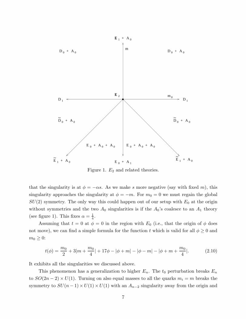
For m0 = m = 0 the theory is our E2 theory. Turning on m0 with m = 0 leads to a

flow to the trivial D1 theory. If we instead turn on m > 0 but keep m0 = 0, we flow to

the E1 theory with E1 = SU(2) global symmetry (see figure 1). At φ = m we find an A0

theory. For non-zero m0 and m > 0 we flow to the trivial D0 theory. Again, at φ = m we

find an A0 theory.

Since there is no symmetry changing the sign of m, we do not expect similar results

for m < 0. In particular, there is a singularity at m0 + 4m = 0 without a counterpart for

positive m. For m0 + 4m > 0 and m < 0 the perturbative analysis is still valid and the

low energy theory at φ = 0 is D0 and at φ = −m it is A0. The lack of m → −m symmetry

appears only in the massive modes. Therefore, we will distinguish this theory from D0 by

denoting it D0. The distinction between them becomes important only when we approach

m0 + 4m = 0. At this point the gauge coupling diverges t = 0. However, the transition to

this point is different from the transition from D0 to E1. The E1 theory has SU(2) global

symmetry while the theory at m0 + 4m = 0 has only U(1) global symmetry. Therefore,

this theory must be a new non-trivial fixed point in five dimensions. We will refer to it as

E1. Clearly it has only one relevant parameter s = m0 + 4m. Using arguments similar to

those in [3], we learn that there is no Higgs branch emanating from it.

We now explore the region m0 + 4m < 0 (as before with m0 non-negative). We do

that by turning on the only relevant parameter in E1, namely, s = m0 +4m. For s > 0 we

flow to D0. What happens for s < 0? We propose that the transition is similar to other

transitions we saw before where an A0 theory leaves the origin. The theory at the origin

is then at a new non-trivial fixed point with t = 0 at φ = 0 which we will call E0. Before

arguing that such a theory indeed exists, let us use this proposal to describe the physics

for s < 0. The global U(1) symmetry of the E1 theory acts on the particle which leaves

the origin at the transition. Therefore, there is no symmetry acting on the massless modes

in E0. This fact is consistent with the lack of relevant parameters in this theory.

The behavior near φ = 0 discussed above does not affect the A0 theory near φ = −m.

This should remain unaffected even for m0 +4m < 0 and in particular at m0 = 0 where the

global SU(2) symmetry must be restored. Now, let us track the A0 theory which leaves

the origin. It corresponds to a U(1) gauge theory with one electron with mass (at φ = 0)

−αs (α is a positive proportionality factor which we will determine momentarily) such

6

+

2

++

+ + + +

+ ++

~~

~~

EE

EEE

E

+

E

A 0D 0 A 0

D 1D 1

D 0 A 0 D 0 A

1 A 01 A 0

0 A 0 A 0 0 A 0 A 0

0 A 1

0

+1EE 0A

D 0

0m

m

Figure 1. E2 and related theories.

that the singularity is at φ = −αs. As we make s more negative (say with fixed m), this

singularity approaches the singularity at φ = −m. For m0 = 0 we must regain the global

SU(2) symmetry. The only way this could happen out of our setup with E0 at the origin

without symmetries and the two A0 singularities is if the A0’s coalesce to an A1 theory

(see figure 1). This fixes α = 1

4.

Assuming that t = 0 at φ = 0 in the region with E0 (i.e., that the origin of φ does

not move), we can find a simple formula for the function t which is valid for all φ ≥ 0 and

m0 ≥ 0:

t(φ) =m0

2+ 3|m +

m0

4| + 17φ − |φ + m| − |φ − m| − |φ + m +

m0

4|. (2.10)

It exhibits all the singularities we discussed above.

This phenomenon has a generalization to higher En. The t0 perturbation breaks En

to SO(2n− 2)× U(1). Turning on also equal masses to all the quarks mi = m breaks the

symmetry to SU(n− 1)×U(1)×U(1) with an An−2 singularity away from the origin and

7

a D0 singularity at the origin. There is another way to get to this point. First, we can

break En to SU(n) × U(1) by choosing suitable values for t0 and mi. We argue that in

this case we have an E0 theory at the origin and an An−1 theory away from the origin.

As the symmetry is further broken to SU(n− 1)×U(1)×U(1) the An−1 singularity splits

to an An−2 and an A0 singularity. This can move to the origin, be absorbed in it to turn

it into an E1 theory which can then become D0, which can then become D0 exactly as in

the other way of getting there.

As in [3], all this has a simple translation to the physics of branes in string com-

pactification. We use a D4-brane probe in the compactification of the type I′ theory on

S1/Z2. This theory is dual to the heterotic string compactified on S1. The An theories

are obtained when n + 1 background D8-branes coalesce in the interior of S1/Z2. The Dn

theories are obtained when n D8-branes are at an orientifold at the boundary of S1/Z2.

The En theories are obtained when the string coupling diverges on the boundary. The ex-

istence of the new E0 theory implies that we can have more than 16 background D8-branes

in the interior. In particular, if the theory at one of the boundaries is at E0, we can have

17 background D8-branes and if the two boundaries are at E0, we can have 18 background

D8-branes. If these 18 D8-branes coalesce, the symmetry group of the string theory is

SU(18) × U(1). In terms of the dual heterotic string the SU(18) factor comes from the

left movers and the U(1) from the right movers.3 Note that although the string coupling

diverges at the two boundaries, it can be arbitrarily weak at the point in the middle of

S1/Z2 where the background D8-branes are. Similarly, we could have one boundary with

E0 and 17 background D8-branes near an orientifold at the other boundary yielding an

SO(34)×U(1) symmetry. Again, the physics near the orientifold where the SO(34) gauge

bosons are can be arbitrarily weakly coupled.

Finally, we argue for the existence of the E0 theory. The presence of SU(18) × U(1)

and SO(34) × U(1) points in the moduli space of the heterotic string and the symmetry-

breaking pattern tell us that the type I′ theory must have corresponding points where

18 D8-branes coincide, or 17 D8-branes are at an orientifold. This also lets us reproduce

the transitions to the E1 and D0 theories, guaranteeing that our scenario for the phase

diagram and the existence of the E0 point is correct.

3 Denote by n the representation of SU(18) Kac–Moody level one whose highest weight vector

is in a representation of SU(18) constructed as an antisymmetric product of n fundamentals.

Denote its character by χn(q). Then, the partition function |χ0 +χ6 +χ12|2 + |χ3 +χ9 +χ15|

2 is

an exceptional modular invariant of a consistent conformal field theory. Denote by ψ0 and ψ1 the

characters of the two representations of SU(2) Kac–Moody level one. Then the partition function

Z = (χ0 + χ6 + χ12)ψ0 + (χ3 + χ9 + χ15)ψ1 is modular invariant. This is the partition function

of the conformal field theory based on the (17, 1) signature lattice for this SU(18) theory.

8

3. Extremal transitions in the geometry

In the previous section, we have described supersymmetric five-dimensional field the-

ories with a one-dimensional Coulomb branch, and given the D4-brane interpretation of

these theories. We now turn to the other string-theoretic application of the field theory

analysis: M-theory compactified on a Calabi–Yau threefold.

In such M-theory compactifications, the expectation values for the scalars in vec-

tor multiplets are parameterized by the Kahler classes of volume one on the Calabi–Yau

threefold [5,6,8]. The Kahler cone (i.e., the set of all Kahler classes) has various boundary

“walls,” and we should expect interesting physics as we approach such a wall since the

metric on the Calabi–Yau threefold is degenerating there. Walls along which∫

J ∧ J ∧ J

vanishes will be at infinite distance from the interior of the moduli space, since we must

divide a Kahler class J by 3

√∫J ∧ J ∧ J in order to get a class of volume one.4 Any wall

along which∫

J ∧J ∧J does not vanish corresponds to the collapse of some proper subset

of the Calabi–Yau threefold [18], for if the entire Calabi–Yau collapses, then∫

J ∧ J ∧ J

must vanish.

The possible ways that a proper subset of a Calabi–Yau threefold can collapse upon

approaching a boundary wall of the Kahler cone have been analyzed in considerable detail

in the mathematics literature. We restrict our attention to codimension-one walls, so that

approaching the wall involves tuning only a single vector multiplet expectation value; we

also assume that the complex structure on the Calabi–Yau threefold is generic (so that no

hypermultiplets need to be tuned to reach the singularity). Under these assumptions, the

possible types of “collapse” are the following:5

(1.) A collection of N disjoint P1’s can collapse to N “ordinary double points.”

(2.) A rational surface which has a “birational ruling,” N fibers of which consist of a pair

of P1’s and the remaining fibers of which are irreducible P1’s, can collapse along the

ruling to a P1 of singularities.

(3.) A “del Pezzo surface”6 which is the blowup of P1 × P1 at N points (0 ≤ N ≤ 7), or

of P2 at N + 1 points (0 ≤ N + 1 ≤ 8), can collapse to a point. (When N ≥ 1, the

two descriptions are equivalent.)

4 This is the analogue in five dimensions of Hayakawa’s criterion [17] in four dimensions, which

specifies which singularities are at finite distance in the Zamolodchikov metric.5 When the complex structure on the Calabi–Yau threefold is not generic, there are further

types of collapse which can occur, described in the appendix. We should point out here that the

possibility is left open by the literature that one or two additional cases might need to be included

along with the ones we present.6 A del Pezzo surface is a complex manifold S of complex dimension 2 whose anticanonical

divisor −KS is ample, i.e., −KS ·C > 0 for every Riemann surface C contained in S. (See [19,20],

9

Anticipating our field theory identifications, we shall refer to these three cases as AN−1,

DN , and EN+1 (or E1) respectively (where E1 is the case of P1 ×P1 blown up at 0 points,

E1 is the case of P2 blown up at 1 point, and E0 is the case of P2 blown up at 0 points).

Although the “collapse” in each of these cases is the result of a degeneration of the

metric on the Calabi–Yau, the resulting collapsed space can be described using algebraic

geometry as the solution set of a collection of polynomial equations. (The algebraic ver-

sions of such collapses are known as “extremal contractions” [22], and have been studied

extensively in the mathematics literature.) Since the singularities have an algebraic de-

scription, algebraic methods can be used to determine whether or not the collapsed space

can be smoothed out by varying the coefficients in the polynomial equations. If this is

possible, the smoothed space is again a Calabi–Yau threefold, but of a completely different

topology than the original one. The process of collapsing via an extremal contraction and

then smoothing out the resulting space to produce a new Calabi–Yau threefold is known

as an “extremal transition” [23].

It will be useful to consider a slight generalization of this setup, in which the geometry

of the contraction is similar but the contraction may occur at higher codimension in the

Kahler cone. Let S be either (1) a collection of P1’s, (2) a birationally ruled surface over

P1, or (3) a del Pezzo surface, and suppose that S is embedded in a Calabi–Yau threefold

X in such a way that there is a contraction X → X associated to some wall of the Kahler

cone of X which maps S to (1) ordinary double points, (2) a P1 of singularities, or (3) a

singular point, respectively. If the codimension of the wall of the Kahler cone is k, then

the dimension of the image of the natural map H1,1(X) → H1,1(S) is k + ǫ, where ǫ = 0

in cases (1) and (3), and ǫ = 1 in case (2).

In the AN−1 case (in this more general sense), a physical interpretation of the contrac-

tion and extremal transition was found in [9,10] when the type IIA string is compactified on

the Calabi–Yau threefold:7 there are k U(1)’s associated to the homology classes spanned

by the P1’s, there are N massive hypermultiplets charged under U(1)k which become si-

multaneously massless at the transition point, and there are N − k flat directions at the

transition which produce N − k new parameters (the Higgs branch in the field theory).

Mathematically, it was already known that this extremal transition exists [26], and that

or for a brief account in the physics literature, [21].) Every such surface is known to be either

P1 × P1, or a blowup of P2; when more than one point of P2 has been blown up the surface can

also be described as a blowup of P1 × P1.7 The analysis of [9,10] was done in type IIB language, but as has been pointed out in [24,25],

the same analysis can be applied to the type IIA string.

10

the number of new complex deformation parameters would be N − k [27,28]. (These pa-

rameters, together with their Ramond-Ramond partners, will give the Higgs branch of the

field theory.) The five-dimensional version of this transition was discussed in [7], where

it was seen that the field theory description of AN−1 type as described in the previous

section applies.

The DN theories are obtained when a birationally ruled surface over a P1 base col-

lapses. The relevant light particles arise by wrapping a two-brane over various two-cycles.

The quantization of their collective coordinates proceeds as in [7] and determines their

quantum numbers. Wrapping the two-brane over the entire collapsing fiber we find vector

multiplets in the adjoint representation of SU(2). In the case analyzed in [7] the base was

a Riemann surface of genus g and hence there were also g hypermultiplets in the adjoint

representation which we do not have. Instead, we get hypermultiplets from the 2N special

P1’s in our fiber. As in the Ak cases, every such P1 leads to one hypermultiplet which is

charged under the unbroken U(1) with the minimal unit of charge. Therefore, every pair

of P1’s leads to a hypermultiplet which is an SU(2) doublet. To summarize, the low en-

ergy spectrum is that of an SU(2) gauge theory with N hypermultiplets which are SU(2)

doublets. This is the spectrum of the DN field theories of the previous section.

When the surface S collapses, there is an effective field theory description near φ = 0

(which labels the point of collapse in the Kahler moduli space). The gauge coupling will

take the form t(φ) = t0 + cφ; since c also multiplies the Chern–Simons term in the action,

it can be calculated in terms of the intersection theory on X [5,6,8] and it turns out to

be c = 2S · S · S. (The factor of 2 is a normalization designed to match our field theory

conventions.) More generally, the second derivative of the prepotential with respect to the

field corresponding to S takes the form 2S · S · H, where H is an arbitrary divisor from

the Kahler cone on X . Expanding H in terms of a basis of H1,1(X) which contains S, we

obtain an expression for the gauge coupling of the form

t(φ) = 2S · S · (∑

αiHi + φS)

= 2S · S · (∑

αiHi) + cφ = t0 + cφ .(3.1)

Of course, any divisors Hi with S · S · Hi = 0 can be omitted from this expression.

In the simplest version of the DN theories—the ones with k = 1—there are only two

independent elements in H1,1(X) which are not orthogonal to S · S; we choose a basis for

these consisting of S and a divisor H0 with H0 · S = 1

4F , where F is a generic fiber of the

ruling. Then the gauge coupling is given by

t(φ) = 2 S · S · (t0H0 + φS) = −2KS · (t04F − φKS) = t0 + (16 − 2N)φ . (3.2)

11

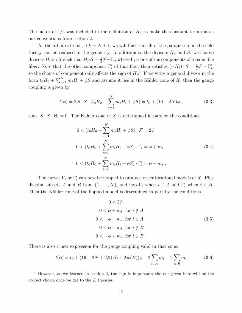
The factor of 1/4 was included in the definition of H0 to make the constant term match

our conventions from section 2.

At the other extreme, if k = N + 1, we will find that all of the parameters in the field

theory can be realized in the geometry. In addition to the divisors H0 and S, we choose

divisors Hi on X such that Hi·S = 1

2F−Γi, where Γi is one of the components of a reducible

fiber. Note that the other component Γ′i of that fiber then satisfies (−Hi) · S = 1

2F − Γ′

i,

so the choice of component only affects the sign of Hi.8 If we write a general divisor in the

form t0H0 +∑N

i=1miHi + φS and assume it lies in the Kahler cone of X , then the gauge

coupling is given by

t(φ) = 2 S · S · (t0H0 +

N∑

i=1

miHi + φS) = t0 + (16 − 2N)φ , (3.3)

since S · S · Hi = 0. The Kahler cone of X is determined in part by the conditions

0 < (t0H0 +N∑

i=1

miHi + φS) · F = 2φ

0 < (t0H0 +

N∑

i=1

miHi + φS) · Γi = φ + mi

0 < (t0H0 +N∑

i=1

miHi + φS) · Γ′i = φ − mi .

(3.4)

The curves Γi or Γ′i can now be flopped to produce other birational models of X . Pick

disjoint subsets A and B from {1, . . . , N}, and flop Γi when i ∈ A and Γ′i when i ∈ B.

Then the Kahler cone of the flopped model is determined in part by the conditions

0 < 2φ,

0 < φ + mi, for i 6∈ A

0 < −φ − mi, for i ∈ A

0 < φ − mi, for i 6∈ B

0 < −φ + mi, for i ∈ B .

(3.5)

There is also a new expression for the gauge coupling valid in that cone:

t(φ) = t0 + (16 − 2N + 2#(A) + 2#(B))φ + 2∑

i∈A

mi − 2∑

i∈B

mi (3.6)

8 However, as we learned in section 2, the sign is important; the one given here will be the

correct choice once we get to the E theories.

12

(since S ·S ·Hi decreases by 1 for i ∈ A and increases by 1 for i ∈ B when we move to the

new cone). These formulas can all be put together into a single piecewise linear function

t(φ) = 2S · S · (t0H0 +N∑

i=1

miHi + φS) = t0 + 16φ −N∑

i=1

|φ + mi| −N∑

i=1

|φ − mi| , (3.7)

valid throughout the union of all of the Kahler cones, and precisely reproducing eqn. (2.6).

This firmly establishes our identification of not only the field theory, but also the param-

eters in it.

Now we have enough data to identify the interacting field theories EN+1 in geometric

terms. We start with the DN theory, realized geometrically as above with some value of

k. Notice that the surface S in this case is actually a blowup of P1 × P1 at N points. We

assume N ≤ 7, and let t0 → 0 and φ → 0, and well as mi → 0 for any parameters mi

which are present. This means that we are approaching a part of the cone in which the

entire surface S collapses to a point, i.e., X experiences the collapse of a del Pezzo surface.

In other words, the del Pezzo contractions precisely realize the interacting five-dimensional

field theories. (We have not yet established this in the cases of E0 and E1, but we shall do

so shortly.)

As in the AN and DN cases we can examine the BPS states which approach zero mass

at the transitions. First, we could wrap various two-cycles with two-branes to find light

particles. We could also wrap a five-brane over the entire collapsing surface S to yield

a string whose tension approaches zero. This string is electric-magnetic dual to the light

particles. Such a spectrum in five dimensions was first observed in [7] for one of the del

Pezzo contractions. Having both massless particles and tensionless strings at the transition

points shows that they are not free field theories. We identify them with interacting field

theories.

Before exploring the geometry of these del Pezzo contractions further, we pause to

point out one of the striking consequences of this identification: the Higgs branches of

generic extremal transitions are given by an A, D, or E instanton moduli space. This

prediction serves to unify a collection of disparate known facts about these transitions,

which had not previously been seen as part of any pattern. Let us review what is known

mathematically.

Given S ⊂ X contracted by X → X , the mathematical question is whether X can

be smoothed by varying its equations, and if so, what is the number of new parameters,

i.e., the difference dimDef(X) − dimDef(X) between the dimensions of the deformation

spaces. (Note that this difference will coincide with the dimension of the Higgs branch in

the field theory, although strictly speaking before making such a comparison we should

13

construct the hypermultiplet moduli space in the string theory which requires the inclusion

of Ramond-Ramond partners to the complex structure moduli.) The known facts about

this mathematical question are as follows:

(1.) In the AN−1 case, as pointed out above, an extremal transition exists whenever N > k

[26] and the number of new parameters is N −k (as is seen by calculating h2,1 [27,28]).

(2.) In the DN case, assuming for simplicity that k = 1,9 an extremal transition exists

whenever N ≥ 2 [29]. The case N = 2 is somewhat special, in that the deformation

space for X is not smooth, but has two components of dimension one [30]10 (as

expected from the field theory, since D2 is not simple). Our prediction for the number

of new parameters is 2N −k−2 in general, and this is consistent with all known facts,

including the examples worked out in [12].

(3.) The EN+1 cases are rather complicated, and one must consider different values of N

separately (cf. [31]); we again assume k = 1 for simplicity.

(a.) For E1, and EN+1, 0 ≤ N + 1 ≤ 3, the singularity of X is toric and the defor-

mation theory has been worked out by Altmann [32]; the result is that there is

no smoothing for E0 or E1 (this is a classic result of Schlessinger [33] in the E0

case, which is a Z3 quotient singularity), a one-dimensional deformation space for

the cases of E1 and E2, and a deformation space with two components, one of

dimension one and one of dimension two, in the case of E3. In addition, there are

further, obstructed first-order deformations in precisely the E1 and E2 cases—the

ones with a U(1) factor in their symmetry groups.

(b.) For E4, the singularity of X is defined by a Pfaffian ideal and the theory of those

can be used to study the deformations [34,35]; the result is that a smoothing

exists.

(c.) For EN+1, 5 ≤ N + 1 ≤ 8, the singular of X is a complete intersection and the

deformation theory is relatively easy; smoothings exist in all cases.

For these del Pezzo contractions, it was observed in [21] that at least for N +1 ≥ 5, the

number of new parameters for this extremal transition should be cN+1−k, where cN+1

is the Coxeter number of the group EN+1. In fact, this statement should continue to

hold for all values of N , if properly interpreted: when the group EN+1 is not simple,

there must be two components whose dimensions are given by the Coxeter numbers

(minus k) of the two factors in the group. (One should also include an obstructed

deformation if there is a U(1) factor.) This formula is compatible with all known

calculations of dimensions of smoothing components.11

9 This is the assumption “X is Q-factorial” which sometimes appears in the mathematics

literature.10 This was only shown in an example, but it probably holds in general.11 We thank Mark Gross for discussions on this point.

14

It is quite remarkable how this prediction about the Higgs branch unifies phenomena

such as the two components or other obstructed deformations which appeared in sporadic

locations (and looked in the past like counterexamples to any regularity of behavior). It

also makes clear why the main theorems of [31] and [29] are so similar (as remarked in

[29]).

As in the DN cases, when k > 1 so that some of the field theory parameters are

realized in the string theory, the EN+1 theories will have a rich structure with various

possible flops leading to new (Kahler) cones in which the gauge coupling takes a different

form. This structure can be completely analyzed using the known combinatorial structure

of the del Pezzo surfaces. In brief, the condition which must be satisfied in order to flop

some collection of rational curves is that the del Pezzo surface can be blown down along

those curves. The Weyl group of EN+1 acts in a natural way12 on H1,1(S), and permutes

the various collections of curves which can be blown down. This can be used to write down

the complete phase diagram for each case, and of course the gauge coupling can be directly

calculated in every phase. This is essentially the same combinatorial data which we used

in the field theory, so it is not surprising that the results turn out to be the same.

We will carry this out in the case of N = 1, in order to complete our geometric

identifications of the interacting field theories by including the E1 and E0 cases.

We take a del Pezzo surface S with N = 1, embedded on a Calabi–Yau manifold X

with k = 3. The surface S can be regarded as a blowup of P2 at two points P1, P2; we let

Γ1 and Γ2 be the exceptional divisors of the blowup. There is another exceptional divisor

on S, a curve Γ3 which is the proper transform of the line passing through P1 and P2.

We also introduce three divisors Hℓ, H1, and H2, which intersect S in the classes of a

line, and the two rulings. Specifically, H1 · S = Γ2 + Γ3 is in the same class as the proper

transform of lines passing through P1, and H2 · S = Γ1 + Γ3 is in the same class as the

proper transform of lines passing through P2. We write a general divisor on X (modulo

those orthogonal to S · S) in the form

a1H1 + a2H2 + a3Hℓ . (3.8)

It is known [22] that on any del Pezzo surface, the walls of the Kahler cone are dual

to the possible exceptional curves on the surface, which in our example are precisely Γ1,

Γ2, and Γ3. Thus, the Kahler cone of X is defined by

0 < (a1H1 + a2H2 + a3Hℓ) · Γ1 = a1

0 < (a1H1 + a2H2 + a3Hℓ) · Γ2 = a2

0 < (a1H1 + a2H2 + a3Hℓ) · Γ3 = a3 .

(3.9)

12 This was known a long time ago [19,20], and provides an important clue to the EN+1 sym-

metry in the physics [21].

15

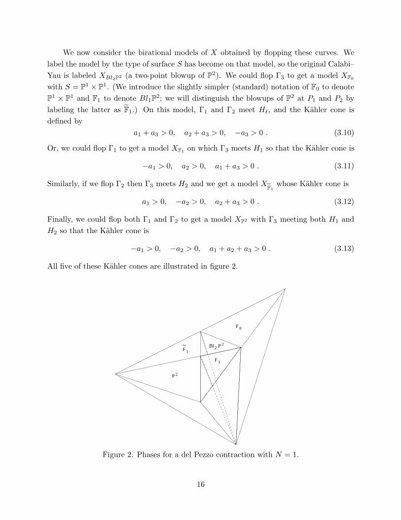
We now consider the birational models of X obtained by flopping these curves. We

label the model by the type of surface S has become on that model, so the original Calabi–

Yau is labeled XBl2P2 (a two-point blowup of P2). We could flop Γ3 to get a model XF0

with S = P1 × P1. (We introduce the slightly simpler (standard) notation of F0 to denote

P1 × P1 and F1 to denote Bl1P2; we will distinguish the blowups of P2 at P1 and P2 by

labeling the latter as F1.) On this model, Γ1 and Γ2 meet Hℓ, and the Kahler cone is

defined by

a1 + a3 > 0, a2 + a3 > 0, −a3 > 0 . (3.10)

Or, we could flop Γ1 to get a model XF1on which Γ3 meets H1 so that the Kahler cone is

−a1 > 0, a2 > 0, a1 + a3 > 0 . (3.11)

Similarly, if we flop Γ2 then Γ3 meets H2 and we get a model XF1

whose Kahler cone is

a1 > 0, −a2 > 0, a2 + a3 > 0 . (3.12)

Finally, we could flop both Γ1 and Γ2 to get a model XP2 with Γ3 meeting both H1 and

H2 so that the Kahler cone is

−a1 > 0, −a2 > 0, a1 + a2 + a3 > 0 . (3.13)

All five of these Kahler cones are illustrated in figure 2.

0

Bl 2 P 2

P

F

F 1

1

2

F~

Figure 2. Phases for a del Pezzo contraction with N = 1.

16

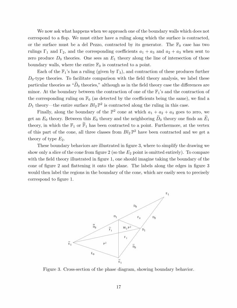
We now ask what happens when we approach one of the boundary walls which does not

correspond to a flop. We must either have a ruling along which the surface is contracted,

or the surface must be a del Pezzo, contracted by its generator. The F0 case has two

rulings Γ1 and Γ2, and the corresponding coefficients a1 + a3 and a2 + a3 when sent to

zero produce D0 theories. One sees an E1 theory along the line of intersection of those

boundary walls, where the entire F0 is contracted to a point.

Each of the F1’s has a ruling (given by Γ3), and contraction of these produces further

D0-type theories. To facilitate comparison with the field theory analysis, we label these

particular theories as “D0 theories,” although as in the field theory case the differences are

minor. At the boundary between the contraction of one of the F1’s and the contraction of

the corresponding ruling on F0 (as detected by the coefficients being the same), we find a

D1 theory—the entire surface Bl2 P2 is contracted along the ruling in this case.

Finally, along the boundary of the P2 cone at which a1 + a2 + a3 goes to zero, we

get an E0 theory. Between this E0 theory and the neighboring D0 theory one finds an E1

theory, in which the F1 or F1 has been contracted to a point. Furthermore, at the vertex

of this part of the cone, all three classes from Bl2 P2 have been contracted and we get a

theory of type E2.

These boundary behaviors are illustrated in figure 3, where to simplify the drawing we

show only a slice of the cone from figure 2 (so the E2 point is omitted entirely). To compare

with the field theory illustrated in figure 1, one should imagine taking the boundary of the

cone of figure 2 and flattening it onto the plane. The labels along the edges in figure 3

would then label the regions in the boundary of the cone, which are easily seen to precisely

correspond to figure 1.

F 1

F 1

F 0

Bl 2 P 2

P 2

D0

D1

D1

1E

0E

D0

~E1

~E1 ~

D0

~D0~

~

Figure 3. Cross-section of the phase diagram, showing boundary behavior.

17

In fact, it is this detailed correspondence which allows us to identify with confidence

the E1 and E1 field theories with the F0 = P1 × P1 and F1 = BlP P2 del Pezzo surfaces,

respectively. Further evidence that these identifications are correct is provided by the per-

fect correspondence between the mathematical deformation theory of X , and the structure

of the Higgs branch of the field theory (which is different in the two cases).

Acknowledgments

The work of D.R.M. was supported in part by NSF grant DMS-9401447, and that of

N.S. was supported in part by DOE grant DE-FG02-96ER40559. We thank M. Douglas, B.

Greene, M. Gross, S. Shenker, C. Vafa, N. Warner, and E. Witten for helpful discussions.

Appendix A. Non-generic primitive contractions

The list we have given in section 3 of possible primitive extremal contractions from a

Calabi–Yau threefold is not complete. (A “primitive” contraction is one which occurs at

codimension one in the Kahler cone.)

In the case of curves collapsing to points, in principle any terminal singularity could

occur. However, this should not happen at generic complex moduli, in light of some

results of Namikawa [36]. Although he did not state things precisely in this way, the proof

of Theorem (2.5) of [36] suggests that after a primitive extremal contraction X → X

where X has terminal singularities, one should be able to deform away the non-ordinary

double points on X while keeping the ordinary double points. The implication would be

that at generic complex moduli of X only ordinary double points should appear in such

contractions. This question deserves further study.

In the case of a divisor collapsing to a point, the original classification goes back to

Reid’s first paper on canonical singularities [37], in which it was shown that the divisor

must be a “generalized del Pezzo surface.” Such surfaces include nonsingular del Pezzo

surfaces (blowups of P2 or P1 × P1 with ample anti-canonical bundle), del Pezzo surfaces

with rational double points (which will deform to the nonsingular ones), nonnormal del

Pezzo surfaces, and cones over elliptic normal curves. As Mark Gross has pointed out

[31], the latter can only occur as exceptional divisors of primitive contractions from a

nonsingular Calabi–Yau if the degree is 1, 2, or 3, and those cones will deform to del Pezzo

surfaces of types E8, E7 and E6, respectively.

The troublesome case is the nonnormal del Pezzo surfaces [38]. They include analogous

cones over nodal or cuspidal rational curves, and Gross’s argument also limits those to the

18

three low-degree cases (which deform to E8, E7, and E6). Of the remaining possibilities,

Gross shows that only one—a nonnormal del Pezzo of degree 7, corresponding to some

sort of degenerate form of E2—could occur. We believe that this will not occur at generic

complex structure, but have no concrete evidence to support this belief.

Finally, we come to the most technically difficult case of a divisor S collapsing to a

curve, analyzed in [29]. When the curve has genus at least one, there is a deformation of X

under which the divisor ceases to be effective [18,29]; thus, this case does not occur when

the complex structure is generic. (This is also expected on physical grounds [11], since

the field theory description consists of SU(2) with charged matter in g ≥ 1 adjoints, and

possibly some fundamentals as well.) In the case of contraction to a curve of genus zero,

there is the possibility that curves being contracted are generically two P1’s which meet;

according to [29], for generic complex structure this can only happen in the case of S3 = 7,

i.e., some kind of degenerate form of D1. We believe that this case too will not occur

at generic complex structure, but have no concrete evidence to support this belief either.

(Note that [29], Example 1.5, shows that such surfaces can indeed occur on Calabi–Yau

threefolds.)

19

References

[1] For a nice review see, S. Chaudhuri, C. Johnson, and J. Polchinski, “Notes on D-

Branes,” hep-th/9602052.

[2] N. Seiberg, “IR Dynamics on Branes and Space-Time Geometry,” hep-th/9606017.

[3] N. Seiberg, “Five Dimensional SUSY Field Theories, Non-trivial Fixed Points, and

String Dynamics,” hep-th/9608111.

[4] J. Polchinski and E. Witten, “ Evidence for Heterotic – Type I Duality,” Nucl. Phys.

B460 (1996) 525–548, hep-th/9510169.

[5] A. C. Cadavid, A. Ceresole, R. D’Auria, and S. Ferrara, “Eleven-Dimensional Super-

gravity Compactified on a Calabi–Yau Threefold,” Phys. Lett. B357 (1995) 76–80,

hep-th/9506144.

[6] S. Ferrara, R.R. Khuri, and R. Minasian, “M-Theory on a Calabi–Yau Manifold,”

Phys.Lett. B375 (1996) 81–88 hep-th/9602102.

[7] E. Witten, “Phase Transitions in M-Theory and F-Theory,” hep-th/9603150.

[8] S. Ferrara, R. Minasian, and A. Sagnotti, “Low Energy Analysis of M and F Theories

on Calabi–Yau Threefolds”, hep-th/9604097.

[9] A. Strominger, “Massless Black Holes and Conifolds in String Theory,” Nucl. Phys.

B451 (1995) 97–109, hep-th/9504090.

[10] B. R. Greene, D. R. Morrison, and A. Strominger, “Black Hole Condensation and the

Unification of String Vacua,” Nucl. Phys. B451 (1995) 109–120, hep-th/9504145.

[11] S. Katz, D. R. Morrison, and M. R. Plesser, “Enhanced Gauge Symmetry in Type II

String Theory,” hep-th/9601108.

[12] P. Berglund, S. Katz, A. Klemm, and P. Mayr, “New Higgs Transitions Between Dual

N=2 String Models,” hep-th/9605154.

[13] C. Vafa, Private communication.

[14] M. Douglas, S. Katz, and C. Vafa, to appear.

[15] N. Seiberg, “Naturalness Versus Supersymmetric Non-renormalization Theorems,”

Phys. Lett. B318 (1993) 469–475, hep-ph/9309335.

[16] P. C. Argyres, M. R. Plesser, and N. Seiberg, “The Moduli Space of Vacua of N = 2

SUSY QCD and Duality in N = 1 SUSY QCD,” Nucl. Phys. B471 (1996) 159–194,

hep-th/9603042.

[17] Y. Hayakawa, “Degeneration of Calabi–Yau Manifold with Weil–Petersson Metric,”

alg-geom/9507016.

[18] P. M. H. Wilson, “The Kahler Cone on Calabi–Yau Threefolds,” Invent. Math. 107

(1992) 561–583; Erratum, ibid. 114 (1993) 231–233.

[19] M. Demazure, “Surfaces de del Pezzo, II, III, IV, V,” Seminaire sur les Singularites

des Surfaces, Lecture Notes in Math. vol. 777, Springer-Verlag, 1980, pp. 21–69.

20

[20] Yu. I. Manin, Cubic Forms: Algebra, Geometry, Arithmetic, 2nd ed., North-Holland,

Amsterdam, New York, 1986, Chapter IV.

[21] D. R. Morrison and C. Vafa, “Compactifications of F-Theory on Calabi–Yau Three-

folds (II),” Nucl. Phys. B476 (1996) 437–469, hep-th/9603161.

[22] S. Mori, “Threefolds Whose Canonical Bundles are Not Numerically Effective,” Annals

of Math. (2) 116 (1982) 133–176.

[23] D. R. Morrison, “Through the Looking Glass,” to appear.

[24] K. Becker, M. Becker, and A. Strominger, “Fivebranes, Membranes and Non-Pertur-

bative String Theory,” Nucl. Phys. B456 (1995) 130–152, hep-th/9507158.

[25] B. R. Greene, D. R. Morrison, and C. Vafa, “A Geometric Realization of Confinement,”

hep-th/9608039.

[26] R. Friedman, “Simultaneous Resolution of Threefold Double Points,” Math. Ann. 274

(1986) 671–689.

[27] H. Clemens, “Double Solids,” Adv. Math. 47 (1983) 107–230.

[28] C. Schoen, “On Fiber Products of Rational Elliptic Surfaces with Section,” Math.

Zeit. 197 (1988) 177–199.

[29] M. Gross, “Primitive Calabi–Yau Threefolds,” alg-geom/9512002.

[30] M. Gross, “The Deformation Space of Calabi–Yau n-Folds Can Be Obstructed,” Mirror

Symmetry II (B. Greene and S.-T. Yau, eds.), to appear, alg-geom/9402014.

[31] M. Gross, “Deforming Calabi–Yau Threefolds,” alg-geom/9506022.

[32] K. Altmann, “The Versal Deformation of an Isolated Toric Gorenstein Singularity,”

alg-geom/9403004.

[33] M. Schlessinger, “Rigidity of Quotient Singularities,” Invent. Math. 14 (1971) 17–26.

[34] D. Buchsbaum and D. Eisenbud, “Algebra Structures for Finite Free Resolutions and

Some Structure Theorems for Ideals of Codimension 3,” Amer. J. Math. 99 (1977)

447–485.

[35] H. Kleppe and D. Laksov, “The Algebraic Structure and Deformation of Pfaffian

Schemes,” J. Algebra 64 (1980) 167–189.

[36] Yo. Namikawa, “Stratified Local Moduli of Calabi–Yau 3-Folds,” preprint, 1995.

[37] M. Reid, “Canonical 3-Folds,” Journees de Geometrie Algebriqe d’Angers (A.

Beauville, ed.), Sitjhoff & Noordhoof, 1980, pp. 273–310.

[38] M. Reid, “Nonnormal del Pezzo Surfaces,” Publ. Res. Inst. Math. Sci. 30 (1994) 695–

727, alg-geom/9404002.

21