Extracting the Convex Hull of an UnknownInclusion in the Multilayered Material

MASARU IKEHATA∗

Department of Mathematics, Faculty of Engineering, Gunma University, Kiryu

376-8515, Japan

We consider the problem of extracting information about an unknown inclusion

embedded in a background layered material that has different constant conduc-

tivities across finitely many paralell planes, from the Dirichlet-to-Neumann map.

For the purpose we construct the exponentially growing solutions of the governing

equation for the background material. The leading coefficient of the equation has

discontinuity across finitley many planes that are paralell each other. Using the

property of those solutions, we give an extraction formula of the support function

of the inclusion from the Dirichlet-to-Neumann map.

Keywords: Inverse conducticity problem; Exponentially growing solution;Inclusion;

Dirichlet-to-Neumann map

AMS Subject Classifications: 35R30, 35R25

1. INTRODUCTION

Let Ω ⊂ Rn, n = 2, 3 be a bounded domain with Lipschitz boundary. Weconsider Ω given conductive body with the conductivity γ.We assume that : γ takes the form

γ(x) =

γ0(x), if x ∈ Ω \D,

γ0(x) + h(x), if x ∈ D

(1.1)

where D is an open subset of Ω with Lipschitz boundary and h is an essen-tially bounded matrix-valued function on D; γ0 ∈ L∞(Ω); both γ and γ0are uniformly positive definite.

∗e-mail: ikehata@math.sci.gunma-u.ac.jp

1

D is a mathematical model of an inclusion (or a defect) in the materialΩ with conductivity γ0; h(x) on D denotes the effect of appearence of D

on the original conductivity γ0. Note that we do not assume that D isconnected.

Given f ∈ H1/2(∂Ω) there exists the weak solution of the elliptic problem

∇ · γ∇u = 0 in Ω,

u = f on ∂Ω.

Define the bounded linear functional Λγf on H1/2(∂Ω) by the formula

< Λγf, g >=∫

Ωγ∇u · ∇vdx, g ∈ H1/2(∂Ω)

where v is an arbitrary function in H1(Ω) satisfying v = g on ∂Ω. The mapf 7−→ Λγf is called the Dirichlet-to-Neumann map. Physically f denotesthe voltage potential on ∂Ω and Λγf the electric current density that isinjected through ∂Ω and induces f .

Problem A Assume that γ0 is known and takes the form

γ0(x) =

γ1, if c1 < xn,

γ2, if c2 < xn < c1,...

γm, if xn < cm−1

(1.2)

where γ1, γ2, · · · , γm are known constants and m ≥ 2. Find an extractionformula of information about the location and shape of D from Λγ providedboth D and h are unknown.

We do not assume that dist (D, x |xn = cj) > 0 for all j = 1, · · · ,m−1.This means that D is a model of a defect that may exist in a neighborhoodof the plane xn = cj. One may consider this problem is a variant of theproblem posed by Calderon [1].

Let hD( · ) denote the support function of D:

Sn−1 3 ω 7−→ hD(ω) = supx∈D

x · ω.

In this paper we give an extraction formula of the value of the supportfunction of D. In order to describe the result we introduce, for δ > 0 andω ∈ Sn−1

Dω(δ) = x ∈ D |hD(ω)− δ < x · ω ≤ hD(ω).

Definition 1.1 Given ω ∈ Sn−1 we say that γ has a jump from γ0 on ∂D

from the direction ω if the following condition is satisfied:

2

there exist constants Cω > 0 and δω > 0 such that,

for almost all x ∈ Dω(δω) the lowest eigenvalue of h(x) is greater than Cω

or

for almost all x ∈ Dω(δω) the lowest eigenvalue of −h(x) is greater than Cω.

Our main result is

Theorem 1.1 Let ω ∈ Sn−1 satisfy ωn 6= 0. Assume that: γ has a jumpfrom γ0 on ∂D from the direction ω; ∂D is C2. Then one can extract hD(ω)from Λγ.

The main idea is the enclosure method developed by the author (see[4]). In case when all γj, j = 1, · · · ,m are given by a single constant, theexponential function ex·z depending on a complex vector z with z · z = 0satisfies the equation ∇ · γ0∇u = 0. Using the asymptotic behavior of thisfunction as |z| −→ ∞, one could extract hD(ω) from Λγ.

In case when γ0 is given by a smooth function on Ω, Sylvester-Uhlmann[7] constructed a solution of the equation ∇ · γ0∇u = 0 that has the form

u ∼ ex·z√γ0

as |z| −→ ∞ and proved the injectivity of the map γ0 7−→ Λγ0(global

uniqueness theorem). This type of solution is called the exponentially grow-ing solution and has yielded the reconstruction formula of γ0 itself from Λγ0

(Nachman [5], Novikov [6] and see also [8] for recent development). Notethat using this solution, one can still extract hD(ω) from Λγ (see [3]).

However, in case when γ0 has discontinuity, none consider how to con-struct such type of solution. In this paper, we construct two types of specialsolutions e±(x; γ0, z) depending on a complex vector z with z · z = 0 of theequation ∇ · γ0∇u = 0 for γ0 given by (1.2), which is a substitution of ex·z;we show how to make use of such types of solutions in a typical inverseproblem.

Their construction is analogous to that of the reflected/refracted planewave solutions caused by the presence of multilayeres having different prop-agation speeds of sound wave. The incident ”wave” is given by ex·z andenters from the top or bottom layer. We study the asymptotic behaviorof the reflected/refracted ”wave” when ±Re zn is large. To our surprise,the behavior is extremely simple compared with that of the sound wave.One can ignore multiple reflection and refraction of the incident ”wave” as±Re zn −→ ∞. These are the main part of the paper and described insections 2 and 3. The proof of main theorem and related formulae are givenin section 4.

3

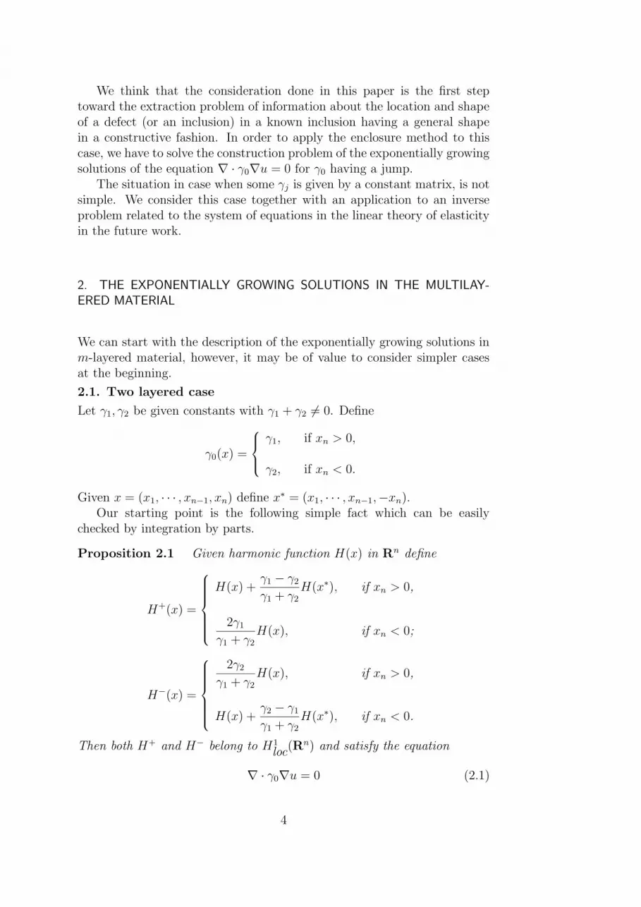
We think that the consideration done in this paper is the first steptoward the extraction problem of information about the location and shapeof a defect (or an inclusion) in a known inclusion having a general shapein a constructive fashion. In order to apply the enclosure method to thiscase, we have to solve the construction problem of the exponentially growingsolutions of the equation ∇ · γ0∇u = 0 for γ0 having a jump.

The situation in case when some γj is given by a constant matrix, is notsimple. We consider this case together with an application to an inverseproblem related to the system of equations in the linear theory of elasticityin the future work.

2. THE EXPONENTIALLY GROWING SOLUTIONS IN THE MULTILAY-

ERED MATERIAL

We can start with the description of the exponentially growing solutions inm-layered material, however, it may be of value to consider simpler casesat the beginning.

2.1. Two layered case

Let γ1, γ2 be given constants with γ1 + γ2 6= 0. Define

γ0(x) =

γ1, if xn > 0,

γ2, if xn < 0.

Given x = (x1, · · · , xn−1, xn) define x∗ = (x1, · · · , xn−1,−xn).Our starting point is the following simple fact which can be easily

checked by integration by parts.

Proposition 2.1 Given harmonic function H(x) in Rn define

H+(x) =

H(x) +γ1 − γ2

γ1 + γ2H(x∗), if xn > 0,

2γ1γ1 + γ2

H(x), if xn < 0;

H−(x) =

2γ2γ1 + γ2

H(x), if xn > 0,

H(x) +γ2 − γ1

γ1 + γ2H(x∗), if xn < 0.

Then both H+ and H− belong to H1loc(R

n) and satisfy the equation

∇ · γ0∇u = 0 (2.1)

4

in the sense:∫

γ0∇u · ∇ϕdx = 0 for all ϕ ∈ C∞0 (Rn).

H in H+ plays the role of the incident ”wave” from xn > 0; the term

γ1 − γ2

γ1 + γ2H(x∗)

denotes the reflected ”wave” from xn = 0; the term

2γ1γ1 + γ2

H(x)

denotes the refracted ”wave” passing through xn = 0.A similar comment works for H−.

Now given ω ∈ Sn−1 take ω⊥ ∈ Sn−1 perpendicular to ω. Then thefunctions

eτx·(ω+iω⊥), τ > 0

are harmonic in the whole space. Let t ∈ R. From Proposition 2.1 we knowthat both two functions indicated below satisfy the equation (2.1):

e−τteτx·(ω+iω⊥)+ =

e−τteτx·(ω+iω⊥) +γ1 − γ2

γ1 + γ2e−τteτx·(ω

∗+i(ω⊥)∗), if xn > 0,

2γ1γ1 + γ2

e−τteτx·(ω+iω⊥), if xn < 0;

e−τteτx·(ω+iω⊥)− =

2γ2γ1 + γ2

e−τteτx·(ω+iω⊥), if xn > 0,

e−τteτx·(ω+iω⊥) +γ2 − γ1

γ1 + γ2e−τteτx·(ω

∗+i(ω⊥)∗), if xn < 0.

Note that we used the relation x∗ · z = x · z∗ for vector z.It is easy to see that:

if ωn ≥ 0, then |e−τteτx·(ω+iω⊥)+| −→ 0 as τ −→∞ in x · ω < t;if ωn ≤ 0, then |e−τteτx·(ω+iω⊥)−| −→ 0 as τ −→∞ in x · ω < t.

Both functions violently behave in x · ω ≥ t as τ −→∞. So we can expectthat these functions play a similar role to e−τteτx·(ω+iω⊥).

2.2. Three layered case

Let a > b. In this subsection we consider case when γ0 may take threedifferent positive constants γ1, γ2 and γ3:

γ0(x) =

γ1, if xn > a,

γ2, if b < xn < a,

γ3, if xn < b.

5

We introduce notation

Rkl =γk − γl

γk + γl

;

Tkl =2γk

γk + γl

.

These satisfy the relations

Rkl +Rlk = 0;

Tkl −Rkl = 1.

Define two maps:

Ka : (x1, · · · , xn−1, xn) 7−→ (x1, · · · , xn−1, 2a− xn)

Kb : (x1, · · · , xn−1, xn) 7−→ (x1, · · · , xn−1, 2b− xn).

Let d = a − b(> 0). In this subsection we explain how to obtain thestatement of the following propositions heuristically, which can be easilychecked by direct computation.

Proposition 2.2 Let a complex vector z with z · z = 0 satisfy

e2dzn 6= R21R23. (2.2)

Define

e+(x; z) =

ex·z + (R12 +T21R23T12

e2dzn −R21R23)eKa(x)·z, if xn > a,

e2dznT12

e2dzn −R21R23(ex·z +R23e

Kb(x)·z), if b < xn < a,

e2dznT12T23

e2dzn −R21R23ex·z, if xn < b.

Then e+( · ; z) ∈ H1loc(R

n) and satisfies (2.1) for γ0 above.

Note that e+(x; z) has the asymptotic form as Re zn −→∞:

e+(x; z) =

ex·z1 +O(e−2(xn−a)Re zn), if xn > a,

T12ex·z1 +O(e−2(xn−b)Re zn), if b < xn < a,

T12T23ex·z1 +O(e−2dRe zn), if xn < b.

So one can expect that this function as Re zn −→∞ will play the same roleas ex·z.

6

Proposition 2.3 Let a complex vector z with z · z = 0 satisfy

e−2dzn 6= R23R21. (2.3)

Define

e−(x; z) =

e−2dznT32T21

e−2dzn −R23R21ex·z, if xn > a,

e−2dznT32

e−2dzn −R23R21(ex·z +R21e

Ka(x)·z), if b < xn < a,

ex·z + (R32 +T23R21T32

e−2dzn −R23R21)eKb(x)·z, if xn < b.

Then e−( · ; z) ∈ H1loc(R

n) and satisfies (2.1) for γ0 above.

The incident wave ex·z in xn > a produces the reflected wave R12eKa(x)·z

in xn > a and refracted wave T12ex·z in b < xn < a. Then T12e

x·z be-comes the incident wave in b < xn < a and produces the reflected waveR23T12e

Kb(x)·z in b < xn < a and refracted wave T23T12ex·z in xn < b. Then

R23T12eKb(x)·z becomes the incident wave from b < xn < a into xn > a and

produces the reflected wave R21R23T12eKbKa(x)·z in b < xn < a and refracted

wave T21R23T12eKb(x)·z in xn > a and.... These procedures are completely

same as those for the (real) wave phenomena.From the consideration above one can expect that the total waves in

xn > a, b < xn < a and xn < b, respectively become

ex·z +R12eKa(x)·z + T21R23

∞∑

j=1

aj(Kb(x)),

T12ex·z +R23T12e

Kb(x)·z +R21R23

∞∑

j=1

aj(KbKa(x)) +R23aj(KbKaKb(x)),

T23

∞∑

j=1

aj(x)

whereaj(x) = (R21R23)

j−1T12ex·ze−2(j−1)dzn .

Hereafter one can easily see that the form of these waves coincides with thatof the waves in Proposition 2.2. We omit the explanation for Proposition2.3.

2.3. The exponentially growing solutions in m-layered material

Case 1 Re zn > 0. We construct a solution of the equation (2.1) in the

7

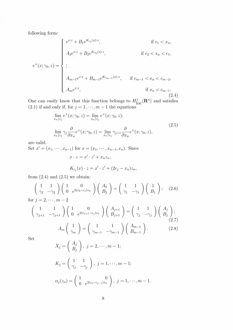
following form:

e+(x; γ0, z) =

ex·z +B1eKc1

(x)·z, if c1 < xn,

A2ex·z +B2e

Kc2(x)·z, if c2 < xn < c1,

...

Am−1ex·z +Bm−1e

Kcm−1(x)·z, if cm−1 < xn < cm−2,

Amex·z, if xn < cm−1.(2.4)

One can easily know that this function belongs to H1loc(R

n) and satisfies

(2.1) if and only if, for j = 1, · · · ,m− 1 the equations

limxn↓cj

e+(x; γ0, z) = limxn↑cj

e+(x; γ0, z);

limxn↓cj

γj∂

∂xn

e+(x; γ0, z) = limxn↑cj

γj+1∂

∂xn

e+(x; γ0, z),

(2.5)

are valid.Set x′ = (x1, · · · , xn−1) for x = (x1, · · · , xn−1, xn). Since

x · z = x′ · z′ + xnzn,

Kcj(x) · z = x′ · z′ + (2cj − xn)zn,

from (2.4) and (2.5) we obtain:(

1 1γ2 −γ2

)(

1 00 e2(c2−c1)zn

)(

A2B2

)

=

(

1 1γ1 −γ1

)(

1B1

)

; (2.6)

for j = 2, · · · ,m− 2(

1 1γj+1 −γj+1

)(

1 00 e2(cj+1−cj)zn

)(

Aj+1

Bj+1

)

=

(

1 1γj −γj

)(

Aj

Bj

)

;

(2.7)

Am

(

1γm

)

=

(

1 1γm−1 −γm−1

)(

Am−1

Bm−1

)

. (2.8)

Set

Xj =

(

Aj

Bj

)

, j = 2, · · · ,m− 1;

Kj =

(

1 1γj −γj

)

, j = 1, · · · ,m− 1;

αj(zn) =

(

1 00 e2(cj−cj−1)zn

)

, j = 1, · · · ,m− 1.

8

Then (2.6) becomes

K2α2(zn)X2 = K1

(

1B1

)

and thus

K2X2 = K2α2(−zn)K−12 K1

(

1B1

)

.

Then from (2.7) for j = 2 we obtain

K3α3(zn)X3 = K2α2(−zn)K−12 K1

(

1B1

)

and thus

K3X3 = K3α3(−zn)K−13 K2α2(−zn)K

−12 K1

(

1B1

)

.

Repeating these procedures, we obtain

Km−1Xm−1 = Km−1αm−1(−zn)K−1m−1 · · · K2α2(−zn)K

−12 K1

(

1B1

)

.

(2.9)Define

Lm−1(zn) = Km−1αm−1(−zn)K−1m−1 · · · K2α2(−zn)K

−12 .

A combination of (2.8) and (2.9) yields a system of the equations for Am

and B1:

Am

(

1γm

)

−B1Lm−1(zn)K1

(

01

)

= Lm−1(zn)K1

(

10

)

. (2.10)

Define

Pm−1(zn) =

1 −Lm−1(zn)K1

(

01

)

·(

10

)

γm −Lm−1(zn)K1

(

01

)

·(

01

)

.

(2.10) becomes

Pm−1(zn)

(

Am

B1

)

= Lm−1(zn)K1

(

10

)

. (2.11)

We study the determinant:

detPm−1(zn) = Lm−1(zn)K1

(

01

)

·(

γm

−1

)

. (2.12)

9

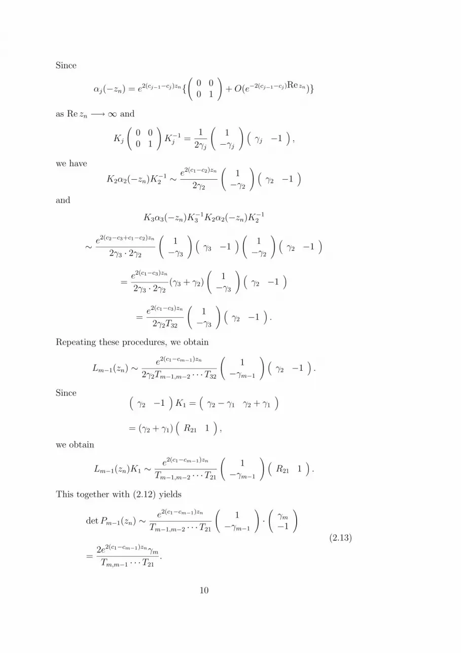
Since

αj(−zn) = e2(cj−1−cj)zn(

0 00 1

)

+O(e−2(cj−1−cj)Re zn)

as Re zn −→∞ and

Kj

(

0 00 1

)

K−1j =

1

2γj

(

1−γj

)

(

γj −1)

,

we have

K2α2(−zn)K−12 ∼ e2(c1−c2)zn

2γ2

(

1−γ2

)

(

γ2 −1)

and

K3α3(−zn)K−13 K2α2(−zn)K

−12

∼ e2(c2−c3+c1−c2)zn

2γ3 · 2γ2

(

1−γ3

)

(

γ3 −1)

(

1−γ2

)

(

γ2 −1)

=e2(c1−c3)zn

2γ3 · 2γ2(γ3 + γ2)

(

1−γ3

)

(

γ2 −1)

=e2(c1−c3)zn

2γ2T32

(

1−γ3

)

(

γ2 −1)

.

Repeating these procedures, we obtain

Lm−1(zn) ∼e2(c1−cm−1)zn

2γ2Tm−1,m−2 · · ·T32

(

1−γm−1

)

(

γ2 −1)

.

Since(

γ2 −1)

K1 =(

γ2 − γ1 γ2 + γ1)

= (γ2 + γ1)(

R21 1)

,

we obtain

Lm−1(zn)K1 ∼e2(c1−cm−1)zn

Tm−1,m−2 · · ·T21

(

1−γm−1

)

(

R21 1)

.

This together with (2.12) yields

detPm−1(zn) ∼e2(c1−cm−1)zn

Tm−1,m−2 · · ·T21

(

1−γm−1

)

·(

γm

−1

)

=2e2(c1−cm−1)znγm

Tm,m−1 · · ·T21.

(2.13)

10

Therefore we obtain

Proposition 2.4 Let m ≥ 3. There exists a positive constant Rm =Rm(γ0) such that, if Re zn > Rm, then there exists the uniqueU+ = (B1, A2, B2, · · · , Am−1, Bm−1, Am) depending on zn such that the func-tion given by (2.4) belongs to H1

loc(Rn) and satisfies ∇ · γ0∇u = 0.

Remark 2.1 Let m = 3. A direct computation yields

P2(zn) =

1 − 1

T21R21 + e2(c1−c2)zn

γ3 − γ2

T21R21 − e2(c1−c2)zn

and thus we have

detP2(zn) =2γ3

T32T21e2(c1−c2)zn −R21R23.

This explains the meaning of the condition (2.2).

Case 2 Re zn < 0.

We reduce this case to Case 1. Define

γ−0 (x) =

γm, if xn > −cm−1,

γm−1, if −cm−2 < xn < −cm−1,

...

γ1, if xn < −c1.

Using Proposition 2.4, one can construct the solution e+(x; γ−0 ,−z) of theequation ∇ · γ−0 ∇u = 0 provided Re zn < −Rm(γ

−0 ). Define

e−(x; γ0, z) = e+(−x; γ−0 ,−z).

It is clear that this belongs toH1loc(R

n) and satisfies the equation∇·γ0∇u =

0. Since K−a(−x) = −Ka(x), e−(x; γ0, z) takes the form:

e−(x; γ0, z) =

Amex·z, if xn > c1,

Am−1ex·z +Bm−1e

Kc1(x)·z, if c2 < xn < c1,

...

A2ex·z +B2e

Kcm−2(x)·z, if cm−1 < xn < cm−2,

ex·z +B1eKcm−1

(x)·z, if xn < cm−1.

(2.14)

11

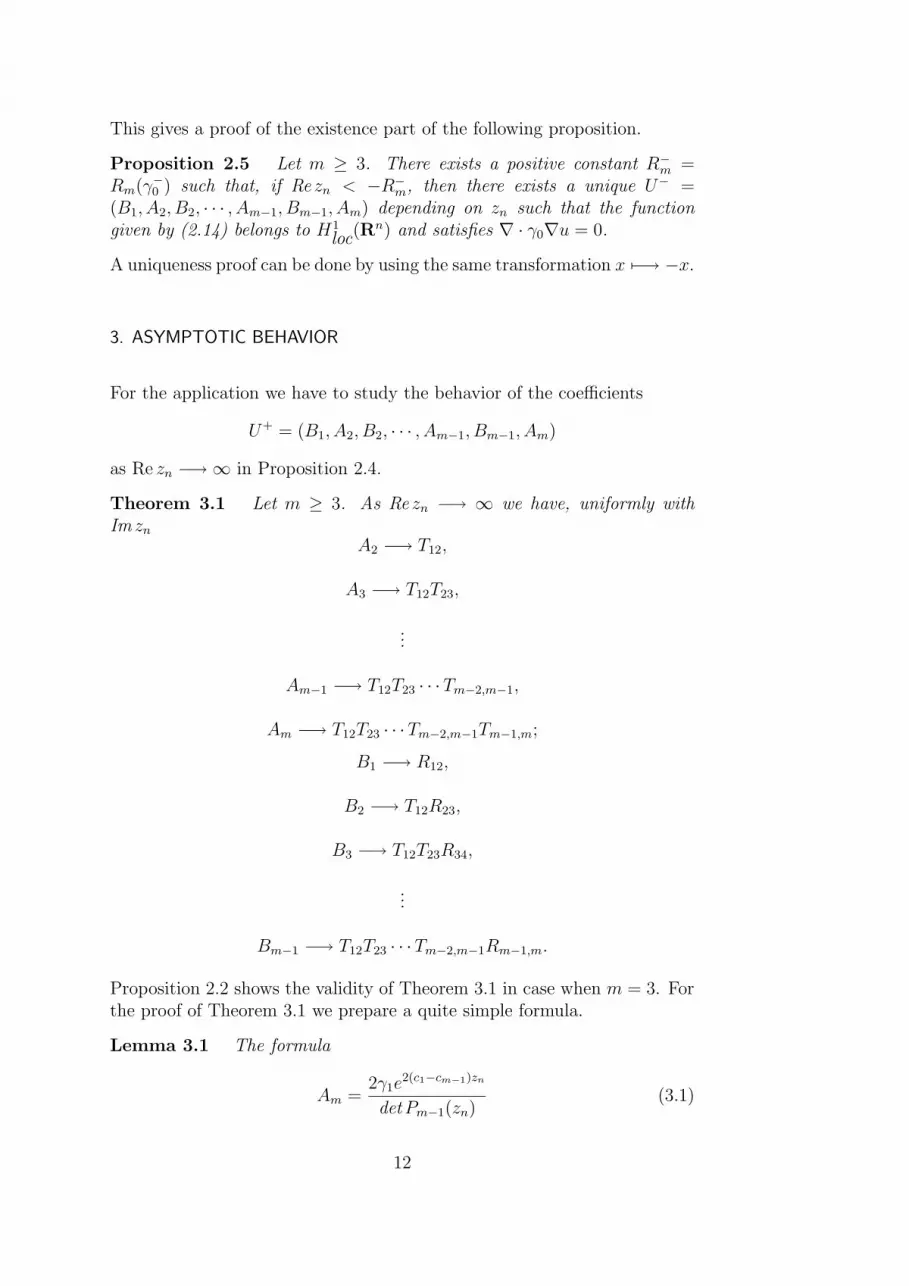
This gives a proof of the existence part of the following proposition.

Proposition 2.5 Let m ≥ 3. There exists a positive constant R−m =Rm(γ

−0 ) such that, if Re zn < −R−m, then there exists a unique U− =

(B1, A2, B2, · · · , Am−1, Bm−1, Am) depending on zn such that the functiongiven by (2.14) belongs to H1

loc(Rn) and satisfies ∇ · γ0∇u = 0.

A uniqueness proof can be done by using the same transformation x 7−→ −x.

3. ASYMPTOTIC BEHAVIOR

For the application we have to study the behavior of the coefficients

U+ = (B1, A2, B2, · · · , Am−1, Bm−1, Am)

as Re zn −→∞ in Proposition 2.4.

Theorem 3.1 Let m ≥ 3. As Re zn −→ ∞ we have, uniformly withIm zn

A2 −→ T12,

A3 −→ T12T23,

...

Am−1 −→ T12T23 · · ·Tm−2,m−1,

Am −→ T12T23 · · ·Tm−2,m−1Tm−1,m;

B1 −→ R12,

B2 −→ T12R23,

B3 −→ T12T23R34,

...

Bm−1 −→ T12T23 · · ·Tm−2,m−1Rm−1,m.

Proposition 2.2 shows the validity of Theorem 3.1 in case when m = 3. Forthe proof of Theorem 3.1 we prepare a quite simple formula.

Lemma 3.1 The formula

Am =2γ1e

2(c1−cm−1)zn

detPm−1(zn)(3.1)

12

is valid.

Proof Set

Lm−1(zn)K1 =

(

a b

c d

)

.

Then we have

Pm−1(zn) =

(

1 −b

γm −d

)

.

A combination of (2.11) and (2.12) yields

(

Am

B1

)

=1

bγm − d

(

−d b

−γm 1

)(

a

c

)

=1

bγm − d

(

−(ad− bc)−aγm + c

)

.

From this we have

Am = −det Lm−1(zn)K1detPm−1(zn)

.

Sincedet Lm−1(zn)K1 = −2γ1e2(c1−cm−1)zn ,

we obtain (3.1).

Proof of Theorem 3.1 A combination of (2.13) and (3.1) yields, as Re zn −→∞

Am −→γ1

γm

Tm,m−1 · · ·T21

=γ1

γm

2γm

γm + γm−1

2γm−1

γm−1 + γm−2

· · · 2γ2γ2 + γ1

= Tm−1,m · · ·T12.

(3.2)

Then from (2.8) we obtain

(

Am−1

Bm−1

)

=Am

2γm−1

(

γm−1 1γm−1 −1

)(

1γm

)

=Am

Tm−1,m

(

1Rm−1,m

)

.

(3.3)

A combination of (3.2) and (3.3) yields

Am−1 −→T12 · · ·Tm−1,m

Tm−1,m

= T12 · · ·Tm−2,m−1;

Bm−1 −→T12 · · ·Tm−1,mRm−1,m

Tm−1,m

= T12 · · ·Tm−2,m−1Rm−1,m.

(3.4)

13

Let 2 ≤ j ≤ m− 2. From (2.7) we have the backward recurrence formula:

Aj =Aj+1

Tj,j+1

+ e2(cj+1−cj)znBj+1

Tj,j+1

Bj =Aj+1Rj,j+1

Tj,j+1

+ e2(cj+1−cj)znBj+1

Tj,j+1

.

(3.5)

Since e2(cj+1−cj)zn = O(e−2(cj−cj+1)Re zn), using (3.5) and (3.4) we obtain thedesired conclusion for Aj, Bj with 2 ≤ j ≤ m− 2. Now from (2.6) and theresult for A2 and B2 we obtain

B1 =A2R12

T12+ e2(c2−c1)zn

B2

T12

−→ T12R12

T12= R12.

(3.6)

This completes the proof of Theorem 3.1.The proof provides an algorithm for calculatingB1, A2, B2 · · · , Am−1, Bm−1, Am:

(1) calculate Am from (3.1).(2) calculate Am−1 and Bm−1 from (3.3).(3) calculate Aj and Bj for j = 2, · · · ,m− 2 from (3.5).(4) calculate B1 from (3.6).

As a corollary of Theorem 3.1, we obtain, as Re zn −→∞

e+(x; γ0, z) ∼

ex·z, if xn > c1,

T12ex·z, if c2 < xn < c1,

T12T23ex·z, if c3 < xn < c2,

...

T12T23 · · ·Tm−2,m−1ex·z, if cm−1 < xn < cm−2,

T12T23 · · ·Tm−2,m−1Tm−1,mex·z, if xn < cm−1.

4. PROOF OF THEOREM 1.1

Given ω ∈ Sn−1 with ωn 6= 0 take ω⊥ ∈ Sn−1 perpendicular to ω. In thissection we consider only case when ωn > 0 since the argument in case whenωn < 0 is essentially same. Let τ > 0. Then z = τ(ω+iω⊥) satisfies z ·z = 0and Re zn = τωn −→∞ as τ −→∞. Let e+(x; γ0, z) be the solution of the

14

equation ∇·γ0∇u = 0 constructed in Proposition 2.4 (in case when m ≥ 3);(ex·z)+ in case when m = 2.

Define

I+ω,ω⊥(τ, t) = e−2τt < (Λγ−Λγ0)(e+( · ; γ0, z)|∂Ω), e+( · ; γ0, z)|∂Ω >, −∞ < t <∞.

Our theorem is a corollary of the following

Theorem 4.1 Let ω ∈ Sn−1 satisfy ωn > 0. Assume that γ has a jumpfrom γ0 on ∂D from the direction ω and that ∂D is C2. Then the formula

limτ−→∞

log |I+ω,ω⊥(τ, 0)|2τ

= hD(ω)

is valid. Moreover, we have:if t > hD(ω), then limτ−→∞ τn−2|I+ω,ω⊥(τ, t)| = 0;

if t < hD(ω), then limτ−→∞ τn−2|I+ω,ω⊥(τ, t)| =∞;

if t = hD(ω), then lim infτ−→∞ τn−2|I+ω,ω⊥(τ, t)| > 0.

Proof It is easy to see that if one has the estimates

|Iω,ω⊥(τ, hD(ω))| ≤ C1τ2 (4.1)

andC2

τn−2 ≤ |Iω,ω⊥(τ, hD(ω))| (4.2)

for τ ≥ τ0, where C1, C2 and τ0 > 0 are positive numbers independent of τ ,then using the trivial identity

I+ω,ω⊥(τ, t) = e−2τ(t−hD(ω))I+ω,ω⊥(τ, hD(ω)),

one obtains the desired conclusion.For the proofs of (4.1) and (4.2) we basically follow the argument in [3],

however, there are some points which should be carefully discussed.First from the inequalities in [2], we have

e−2τhD(ω)∫

Dγ0(x)γ0(x)−1 − γ(x)−1γ0(x)∇e+(x; γ0, z) · ∇e+(x; γ0, z)dx

≤ I+ω,ω⊥(τ, hD(ω))

(4.3)and

I+ω,ω⊥(τ, hD(ω))

≤ e−2τhD(ω)∫

Dγ(x)− γ0(x)∇e+(x; γ0, z) · ∇e+(x; γ0, z)dx.

(4.4)

A combination of Theorem 3.1, (4.3) and (4.4) yields (4.1).

15

For the proof of (4.2) we take a point y on ∂D such that y ·ω = hD(ω). Forsimplicity we use the convention c0 =∞ and cm = −∞.We consider two cases.

Case 1 cj < yn < cj−1 for some 1 ≤ j ≤ m.

From C2- regularity on ∂D, one can find a cone V with vertex y such thatV is an open set, V ⊂ D ∩ x | cj < xn < cj−1 and satisfies the property:

if cj < yn < cj−1 for some j ≤ m− 1, then infx∈V (xn − cj) > 0.Recalling Definition 1.1 and using a localization argument, we know thatfor the proof of (4.2) it suffices to obtain the estimate

∫

V|∇e+(x; γ0, z)|2dx ≥

C

τn−2 e2τhD(ω), τ > τ0 (4.5)

where C > 0 and τ0 > 0 are independent of τ .This estimate is proved as follows.From Theorem 3.1 one knows that there exists a positive constant C inde-pendent of τ such that:

|∇e+(x; γ0, z)|2 ≥ Cτ 2e2τx·ω1 +O(e−4(xn−cj)τωn)

for cj < xn < cj−1 for j = 1, · · · ,m− 1;

|∇e+(x; γ0, z)|2 ≥ Cτ 2e2τx·ω

for xn < cm−1. Therefore from these and the property of V mentioned abovewe have ∫

V|∇e+(x; γ0, z)|2dx ≥ C ′τ 2

∫

Ve2τx·ωdx, τ > τ0 (4.6)

where τ0 and C ′ are positive constants. Using a scalling method, it is easyto see that

τ 2∫

Ve2τx·ωdx ≥ C ′′

τn−2 e2τhD(ω) (4.7)

where C ′′ is a positive constant. From (4.6) and (4.7) we obtain (4.5).

Case 2 yn = cj for some 1 ≤ j ≤ m− 1.

From C2-regularity of ∂D, one can find an open ball (n = 3), disc (n = 2)B with y ∈ ∂B such that B ⊂ D. Since ωn > 0, one may assume that thecenter of B is located in the lower layer cj+1 < xn < cj. Then one can finda finite cone V with vertex y and a positive number ε < cj − cj+1 such thatV is an open set, V ⊂ B and V is contained in cj > xn > cj+1 + ε. Now wetake the same course as the first case.

Remark 4.1 In Case 1 it suffices to assume that ∂D is Lipschitz at thepoint y with y · ω = hD(ω) and cj < yn < cj−1. However, in Case 2 we donot know whether one can relax the regularity of ∂D at y with y ·ω = hD(ω)and yn = cj.

16

Acknowledgment

This research was partially supported by Grant-in-Aid for Scientific Re-search (C)(2) (No. 13640152) of Japan Society for the Promotion of Sci-ence.

References

[1] Calderon, A. P., On an inverse boundary value problem, in Seminaron Numerical Analysis and its Applications to Continuum Physics (W.H. Meyer and M. A. Raupp, eds.), Brazilian Math. Society, Rio deJaneiro, 1980, 65-73.

[2] Ikehata, M., Size estimation of inclusion, J. Inv. Ill-Posed Problems,6(1998), 127-140.

[3] Ikehata, M., Reconstruction of the support function for inclusion fromboundary measurements, J. Inv. Ill-Posed Problems, 8(2000), 367-378.

[4] Ikehata, M., The enclosure method and its applications, in AnalyticExtension Formulas and their Applications (Saitoh, S., Hayashi, N.and Yamamoto, M. eds.), International Society for Analysis, Applica-tions and Computation, Vol. 9(2001), pp. 87-103, Kluwer AcademicPublishers, Dordrecht.

[5] Nachman, A., Global uniqueness for a two-dimensional inverse bound-ary value problem, Ann. Math., 143(1996), 71-96.

[6] Novikov, R., Multidimensional inverse spectral problem for the equa-tion −4Ψ + (v(x) − Eu(x))Ψ = 0, Transl. Funct. Anal. and Appl.,22(1989), 263-272.

[7] Sylvester, J. and Uhlmann, G., A global uniqueness theorem for aninverse boundary value problem, Ann. Math., 125(1987), 153-169.

[8] Uhlmann, G., Developments in inverse problems since Calderon’s foun-dational paper, in Harmonic Analysis and Partial Differential Equa-tions (Christ, M., Kenig, C. E. and Sadosky, C., eds.), 1999, 295-345,The University of Chicago Press, Chicago and London.

17