extracting oscillations: neuronal coincidence detection with noisy periodic spike input

LETTER Communicated by Peter Konig

Extracting Oscillations: Neuronal Coincidence Detectionwith Noisy Periodic Spike Input

Richard KempterPhysik-Department der TU Munchen, D-85747 Garching bei Munchen, Germany

Wulfram GerstnerSwiss Federal Institute of Technology, Center of Neuromimetic Systems,EPFL-DI, CH-1015 Lausanne, Switzerland

J. Leo van HemmenPhysik-Department der TU Munchen, D-85747 Garching bei Munchen, Germany

Hermann WagnerRWTH Aachen, Institut fur Biologie II, D-52074 Aachen, Germany

How does a neuron vary its mean output firing rate if the input changesfrom random to oscillatory coherent but noisy activity? What are the crit-ical parameters of the neuronal dynamics and input statistics? To answerthese questions, we investigate the coincidence-detection properties of anintegrate-and-fire neuron. We derive an expression indicating how coin-cidence detection depends on neuronal parameters. Specifically, we showhow coincidence detection depends on the shape of the postsynaptic re-sponse function, the number of synapses, and the input statistics, and wedemonstrate that there is an optimal threshold. Our considerations canbe used to predict from neuronal parameters whether and to what extenta neuron can act as a coincidence detector and thus can convert a temporalcode into a rate code.

1 Introduction

Synchronized or coherent oscillatory activity of a population of neuronsis thought to be a vital feature of temporal coding in the brain. Oscilla-tions have been observed in the visual cortex (Eckhorn et al., 1988; Gray &Singer, 1989), the sensorimotor cortex (Murthy & Fetz, 1992), the hippocam-pus (Burgess, Recce, & O’Keefe, 1994), and the olfactory system (Freeman,1975; Davis & Eichenbaum, 1991; Wehr & Laurent, 1996). Coherent firingof neurons might be used for solving the problems of feature linking andpattern segmentation (von der Malsburg & Schneider, 1986; Eckhorn et al.,

Neural Computation 10, 1987–2017 (1998) c© 1998 Massachusetts Institute of Technology

1988 R. Kempter, W. Gerstner, J. L. van Hemmen, and H. Wagner

1988; Wang, Buhmann, & von der Malsburg, 1990; Ritz, Gerstner, Fuentes,& van Hemmen, 1994; Ritz, Gerstner, & van Hemmen, 1994) and could alsosupport attentional mechanisms (Murthy & Fetz, 1992).

Another prominent example where coherent or phase-locked activityof neurons is known to be important is the early auditory processing inmammals, birds, and reptiles (Carr, 1992, 1993). Spikes are found to be phaselocked to external acoustic stimuli with frequencies up to 8 kHz in the barnowl (Koppl, 1997). In the barn owl and various other animals, the relativetiming of spikes is used to transmit information about the azimuthal positionof a sound source. In performing this task, the degree of synchrony of twogroups of neurons is read out and transformed into a firing rate pattern,which can then be used for further processes and to control motor units. Theessential step of translating a temporal code into a rate code is performedby neurons that work as coincidence detectors.

Similarly, if neural coding in the cortex is based on oscillatory activity,then oscillations should lead to behavioral actions. Motor output requiresa mean level of activity in motor efferents of the order of, say, a hundredmilliseconds. But then somewhere in the brain, there must be a neural “unit”that transforms the temporally coded oscillatory activity into a rate-codedmean activity that is suitable for motor output. We do not want to speculatehere what this “unit” looks like. It might be composed of an array of neurons,but it is also possible that single neurons perform this transformation.

Here we focus on the question of whether the task of transforming aspike code into a rate code can be done by a single neuron. The issue of howneurons read out the temporal structure of the input and how they transformthis structure into a firing rate pattern has been addressed by several authorsand is attracting an increasing amount of interest. Konig, Engel, & Singer(1996) have argued that the main prerequisite for coincidence detectors isthat the mean interspike interval is long compared to the integration timethat neurons need to sum synaptic potentials effectively. The importance ofthe effective (membrane) time constant of neurons has also been emphasizedby Softky (1994). In addition, Abeles (1982) has shown that the value ofthe spike threshold and the number of synapses are relevant parametersas well.

Some general principles have already been outlined, but a mathematicalderivation of conditions under which neurons can act as coincidence detec-tors is still not available. In this article, we will substantiate the statementswe have already made and show explicitly the dependence of the preci-sion of neuronal coincidence detection on the shape of the postsynapticpotential, the input statistics, and the voltage threshold at which an actionpotential is generated. Specifically, we tackle the question of whether and towhat extent a neuron that receives periodically modulated input can detectthe degree of synchrony and convert a time-coded signal into a rate-codedone.

Extracting Oscillations 1989

2 Methods

This section specifies the input and briefly reviews the neuron model.

2.1 Temporal Coding of the Input. We consider a single neuron that re-ceives stochastic input spike trains through N independent channels. Inputspikes are generated stochastically and arrive at a synapse with a time-dependent T-periodic rate λin(t) = λin(t+T) ≥ 0. The probability of havinga spike in the interval [t, t+1t) is λin(t)1t as1t→ 0. In this way we obtaina nonstationary or inhomogeneous Poisson process (cf., e.g., Tuckwell, 1988,Sec. 10.8) where input spikes are more or less phase locked to a T-periodicstimulus. According to the definition of Theunissen and Miller (1995), thiskind of input is a temporal code. The average number of spikes that arriveduring one period at a synapse will be called p. The time-averaged meaninput rate is λin := 1/T

∫ t0+Tt0

dt′ λin(t′) and equals p/T.To parameterize the input, we take the function

λin(t) := p∞∑

m=−∞Gσ (t−mT), (2.1)

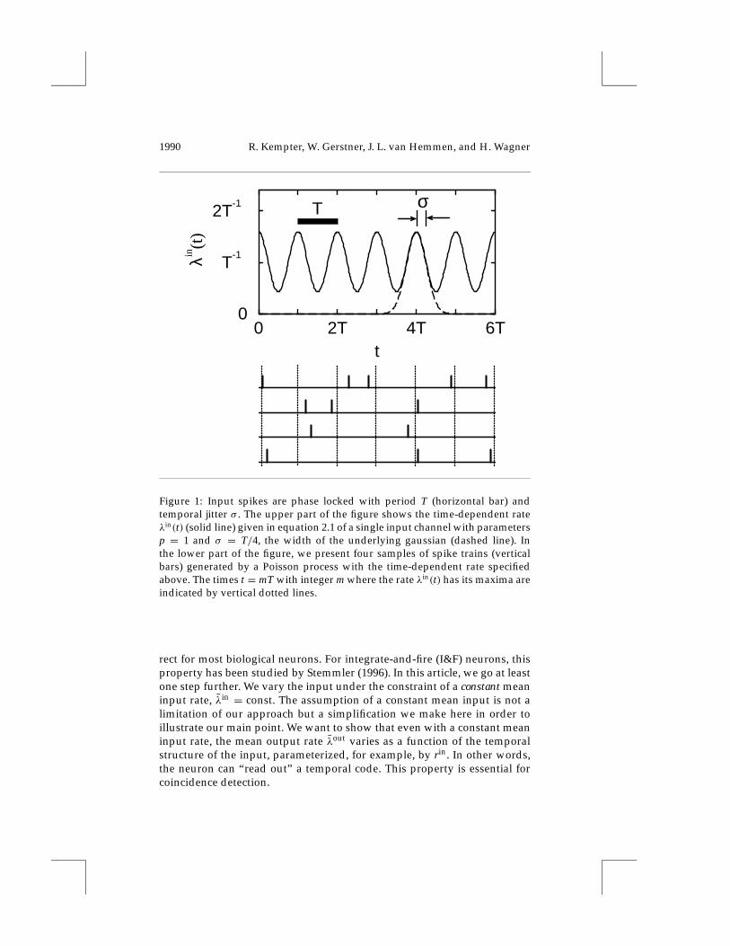
where Gσ (.) denotes a normalized gaussian distribution with zero meanand standard deviation σ > 0. In Figure 1 we present a few examples ofspike trains generated by the time-dependent rate in equation 2.1.

We assume that the neuron under consideration receives input fromN À 1 presynaptic terminals. At each input terminal, spikes arrive inde-pendently of the other terminals and with a probability density given byequation 2.1. We note that equation 2.1 is an idealization of biological spiketrains because there is no refractoriness.

The degree of synchrony of the input is parameterized by the jitter σ ∈[0,∞), the standard deviation of the gaussian distribution. In the case σ = 0,the input spikes arrive perfectly phase locked and occur only at the timestm = mT with integer m, and the number of spikes arriving at time tm hasa Poissonian distribution with parameter p. Instead of σ , we often consideranother measure of synchrony, the so-called vector strength rin (Goldberg &Brown, 1969). This measure of synchrony can be defined as the amplitudeof the first Fourier component of the periodic rate in equation 2.1 dividedby the Fourier component of order zero. For the input (see equation 2.1) wefind

rin = exp

[−1

2

(2πT

)2

σ 2

]. (2.2)

By construction, we have 0 ≤ rin ≤ 1.Many neuron models start from a gain function where the mean output

firing rate increases with increasing mean input rate. This is certainly cor-


0 2T 4T 6Tt

0

T-1

2T-1

λin(t

)T σ

Figure 1: Input spikes are phase locked with period T (horizontal bar) andtemporal jitter σ . The upper part of the figure shows the time-dependent rateλin(t) (solid line) given in equation 2.1 of a single input channel with parametersp = 1 and σ = T/4, the width of the underlying gaussian (dashed line). Inthe lower part of the figure, we present four samples of spike trains (verticalbars) generated by a Poisson process with the time-dependent rate specifiedabove. The times t = mT with integer m where the rate λin(t) has its maxima areindicated by vertical dotted lines.

rect for most biological neurons. For integrate-and-fire (I&F) neurons, thisproperty has been studied by Stemmler (1996). In this article, we go at leastone step further. We vary the input under the constraint of a constant meaninput rate, λin = const. The assumption of a constant mean input is not alimitation of our approach but a simplification we make here in order toillustrate our main point. We want to show that even with a constant meaninput rate, the mean output rate λout varies as a function of the temporalstructure of the input, parameterized, for example, by rin. In other words,the neuron can “read out” a temporal code. This property is essential forcoincidence detection.


2.2 Neuron Model and Spike Processing. We describe our neuron as anI&F unit with membrane potential u. The neuron fires if u(t) approaches thethreshold ϑ from below. This defines a firing time tn with integer n. Afteran output spike, which need not be described explicitly, the membranepotential is reset to 0. Between two firing events, the membrane voltagechanges according to the linear differential equation,

ddt

u(t) = − 1τm

u(t)+ i(t), (2.3)

where i is the total input current and τm > 0 the membrane time constant.The input is due to presynaptic activity. The spike arrival times at a givensynapse j are labeled by t f

j where f = 1, 2, . . . is a running spike index. Weassume that there are many synapses 1 ≤ j ≤ N with N À 1.

Each presynaptic spike evokes a small postsynaptic current (PSC) thatdecays exponentially with time constant τs > 0. All synapses are equalin the sense that the incoming spikes evoke PSCs of identical shape andamplitude. The total input of the neuron is then taken to be

i(t) = 1τs

N∑j=1

∑f

exp

− t− t fj

τs

θ(t− t fj ), (2.4)

where θ(.) denotes the Heaviside step function with θ(s) = 0 for s ≤ 0 andθ(s) = 1 for s > 0. We substitute equation 2.4 in 2.3 and integrate. This yieldsthe membrane potential at the hillock,

u(t) =∑

j

∑f

ε(t− t fj )

+∑nη(t− tn). (2.5)

The first term on the right in equation 2.5,

ε(s) = τm

τm − τs

[exp

(− sτm

)− exp

(− sτs

)]θ(s), (2.6)

describes the typical time course of an excitatory postsynaptic potential(EPSP). If τs = τm, we have instead of equation 2.6 the so-called alpha func-tion, ε(s) = (s/τm)· exp(−s/τm) θ(s). The argument below does not dependon the precise form of ε. The second contribution to equation 2.5,

η(s) = −ϑ exp(− sτm

)θ(s), (2.7)

accounts for the reset of the membrane potential after each output spike andincorporates neuronal refractoriness.


3 Analysis of Coincidence Detection

We are going to examine the coincidence detection properties of our modelneuron. To study the dependence of the output firing rate on the temporalstructure of the input and to answer the question of how this is influencedby neuronal parameters, we use the I&F model and the temporally codedspike input already introduced. Qualitative considerations, useful defini-tions, and illustrating simulations are presented in section 3.1. They explainthe gist of why, and how, coincidence detection works. We then return toa mathematical treatment in section 3.2 and finish with some examples insection 3.3.

3.1 The Quality of a Coincidence Detector. We now explain how theability of a neuron to act as a coincidence detector depends on the leakinessof the integrator (section 3.1.1), the threshold ϑ (section 3.1.2), the timeconstants τm and τs (section 3.1.3), and the number N of synapses as well asthe mean input rate λin (section 3.1.4).

3.1.1 Leaky or Nonleaky Integrator? The most important parameter ofthe neuron model is the membrane time constant τm. If we take the limitτm → ∞, we are left with a simple nonleaky integrator (cf. equation 2.3).In this case, the mean output rate can be calculated explicitly. Integratingequation 2.3 from the nth output spike at tn to the next one at tn+1 we obtain

ϑ = ∫ tn+1

tn dt i(t). A summation over M spikes yields

ϑ = tn+M − tn

MN λin + 1

M

tn+M∫tn

dt [i(t)−N λin], (3.1)

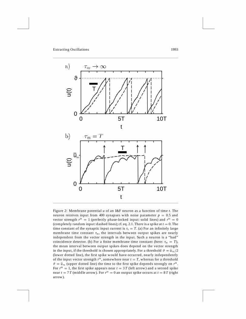
where we have separated the right-hand side into a first term that representsthe contribution of the mean input current N λin and a second term that is thefluctuation around the mean. In order to calculate the mean output rate λout,we have to consider the limit M→∞. We introduce the mean output rateby defining λout := limM→∞M/(tn+M − tn). As M → ∞, the contributionfrom the second term in the right-hand side of equation 3.1 vanishes, andwe are left with λout = Nλin/ϑ . The mean output rate is independent of theexplicit form of the time-dependent input rate λin(t), especially rin, whichis demonstrated graphically by Figure 2a.

Hence we must have a finite τm and thus a leaky integrator, if we want toend up with a coincidence detector, whose rate varies with rin. But what ismeant by a “finite” τm? The answer depends on the value of the threshold ϑ .

3.1.2 Voltage Threshold. We address the problem of how to adjust thethreshold so that an I&F neuron can be used as a coincidence detector. Let


a) �m !1

0 5T 10Tt

0

ϑu(

t) T

b) �m = T

0 5T 10Tt

0

u

u(t)

Too

Figure 2: Membrane potential u of an I&F neuron as a function of time t. Theneuron receives input from 400 synapses with noise parameter p = 0.5 andvector strength rin = 1 (perfectly phase-locked input: solid lines) and rin = 0(completely random input: dashed lines); cf. eq. 2.1. There is a spike at t = 0. Thetime constant of the synaptic input current is τs = T. (a) For an infinitely largemembrane time constant τm, the intervals between output spikes are nearlyindependent from the vector strength in the input. Such a neuron is a “bad”coincidence detector. (b) For a finite membrane time constant (here: τm = T),the mean interval between output spikes does depend on the vector strengthin the input, if the threshold is chosen appropriately. For a threshold ϑ = u∞/2(lower dotted line), the first spike would have occurred, nearly independentlyof the input vector strength rin, somewhere near t = T, whereas for a thresholdϑ = u∞ (upper dotted line) the time to the first spike depends strongly on rin.For rin = 1, the first spike appears near t = 3 T (left arrow) and a second spikenear t = 7 T (middle arrow). For rin = 0 an output spike occurs at t = 8 T (rightarrow).


us assume for the moment that the firing threshold is very high (formally,ϑ →∞), and let us focus on the temporal behavior of the membrane voltageu(t) with some input current i. The membrane potential cannot reach thethreshold so that there is neither an output spike nor a reset to baseline, andthe membrane voltage fluctuates around the mean voltage u∞ = N λin τm; seeFigure 2b. (The voltage u∞ equals u(t) as t → ∞, provided the total inputcurrent is equal to its mean value i = N λin.) We now lower the thresholdso that the neuron occasionally emits a spike. The coincidence-detectionproperties of this neuron depend on the location of the threshold ϑ relativeto u∞.

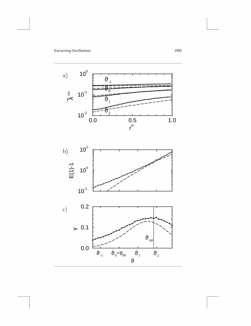
We analyze the dependence of the output firing rate on the threshold andthe input vector strength rin. As shown in Figure 3a, the mean output firingrate λout is rather insensitive to the input vector strength rin for ϑ < u∞.We therefore get a poorly performing coincidence detector. In contrast, athreshold ϑ > u∞ leads to a large variation of the mean output firing rate asa function of the input vector strength rin. Consequently we seem to obtaina better coincidence detector.

The underlying mechanism of this improvement is illustrated by Fig-ure 2b, where the trajectory of the membrane voltage u(t), after a reset attime t = 0, is shown for two cases: random and phase-locked input. Let usimagine a threshold ϑ well below u∞, say, at u∞/2. In this case, the nextspike following the one at t = 0 is triggered after a short time interval, thelength of which depends only marginally on the degree of synchrony in theinput. We are close to the regime of a nonleaky integrator. Formally, this canbe seen from eq. 2.3. Between two firings, the membrane potential alwaysstays below threshold, u(t) < ϑ . If the average current is much larger thanϑ/τm, then the first term in the right-hand side of equation 2.3 can be ne-glected, and we do have a nonleaky neuron. In contrast, let us consider thecase ϑ > u∞. The threshold ϑ can be reached only if the fluctuations of u(t)are large enough. The fluctuations consist of a statistic contribution, due tospike input (shot noise), and periodic oscillations, due to phase-locked (co-herent) input. The key observation is that with increasing synchrony in theinput, the periodic oscillations get larger and therefore the output firing rateincreases. In order to quantify this effect, we introduce a new parameter.

Definition 1. The ratio of the mean output firing rate λout for coherent inputwith vector strength rin > 0 to the rate for completely random input with vanishingvector strength is called the coherence gain E.

E(rin) := λout(rin)

λout(0), with E(rin) ≥ 1. (3.2)

A coherence gain E(rin) ≈ 1 means that the I&F neuron does not operateas a coincidence detector, whereas E(rin) À 1 hints at good coincidencedetection.


a)

0.0 0.5 1.0r

in

10-2

10-1

100

λ out

ϑ0

ϑ1

ϑ-1

ϑ2

b)

10-1

100

101

E(1

)-1

c)

ϑ-1 ϑ0=u ϑ1 ϑ2

ϑ

0.0

0.1

0.2

γ

oo

ϑopt


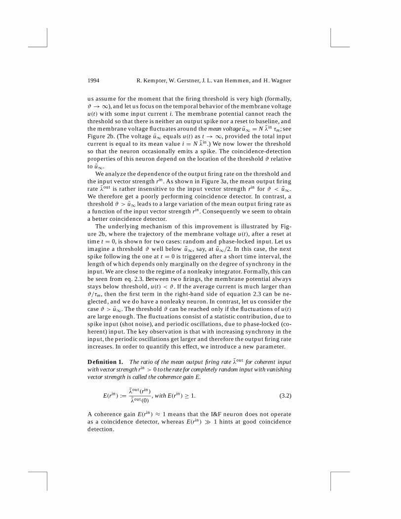
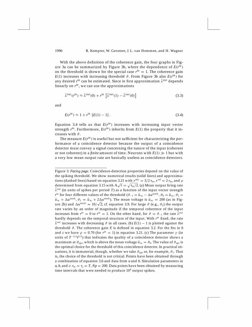
With the above definition of the coherence gain, the four graphs in Fig-ure 3a can be summarized by Figure 3b, where the dependence of E(rin)

on the threshold is shown for the special case rin = 1. The coherence gainE(1) increases with increasing threshold ϑ . From Figure 3b also E(rin) forany desired rin can be estimated. Since in first approximation λout dependslinearly on rin, we can use the approximations

λout(rin) ≈ λout(0)+ rin [λout(1)− λout(0)]

(3.3)

and

E(rin) ≈ 1+ rin [E(1)− 1] . (3.4)

Equation 3.4 tells us that E(rin) increases with increasing input vectorstrength rin. Furthermore, E(rin) inherits from E(1) the property that it in-creases with ϑ .

The measure E(rin) is useful but not sufficient for characterizing the per-formance of a coincidence detector because the output of a coincidencedetector must convey a signal concerning the nature of the input (coherentor not coherent) in a finite amount of time. Neurons with E(1)À 1 but witha very low mean output rate are basically useless as coincidence detectors.

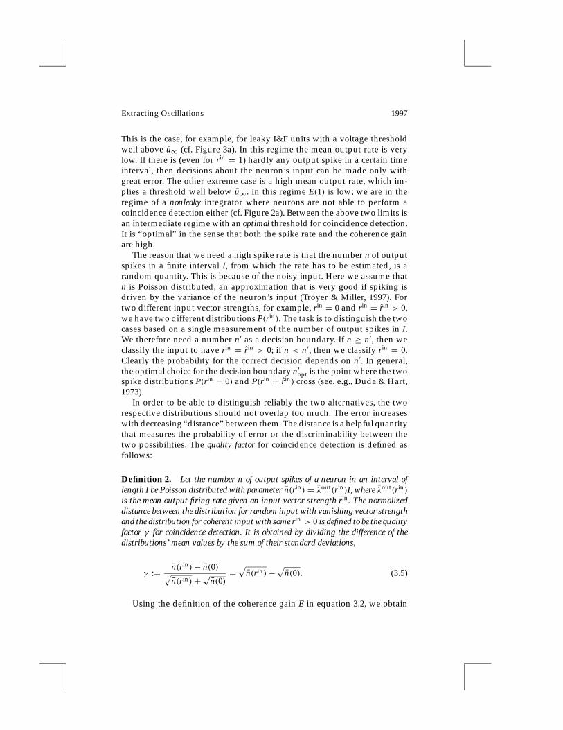
Figure 3: Facing page. Coincidence-detection properties depend on the value ofthe spiking threshold. We show numerical results (solid lines) and approxima-tions (dashed lines) based on equation 3.21 with τdec = 3/2 τm, τ ref = 2 τm, and ρdetermined from equation 3.15 with A

√τ =

√τm/2. (a) Mean output firing rate

λout (in units of spikes per period T) as a function of the input vector strengthrin for four different values of the threshold (ϑ−1 = u∞ −1ustoch, ϑ0 = u∞, ϑ1 =u∞ + 1ustoch, ϑ2 = u∞ + 21ustoch). The mean voltage is u∞ = 200 (as in Fig-ure 2b) and 1ustoch = 10/

√2; cf. equation 3.9. For large ϑ (e.g., ϑ2) the output

rate varies by an order of magnitude if the temporal coherence of the inputincreases from rin = 0 to rin = 1. On the other hand, for ϑ = ϑ−1 the rate λout

hardly depends on the temporal structure of the input. With rin fixed, the rateλout increases with decreasing ϑ in all cases. (b) E(1) − 1 is plotted against thethreshold ϑ . The coherence gain E is defined in equation 3.2. For the fits in band c we have ρ = 0.70 (for rin = 1) in equation 3.21. (c) The parameter γ (inunits of T−1/2I1/2) that indicates the quality of a coincidence detector shows amaximum at ϑopt, which is above the mean voltage u∞ = ϑ0. The value of ϑopt isthe optimal choice for the threshold of this coincidence detector. In practical sit-uations, it is immaterial, though, whether we take ϑopt or, for example, ϑ1. Thatis, the choice of the threshold is not critical. Points have been obtained througha combination of equation 3.6 and data from a and b. Simulation parameters ina, b, and c: τm = τs = T, Np = 200. Data points have been obtained by measuringtime intervals that were needed to produce 104 output spikes.


This is the case, for example, for leaky I&F units with a voltage thresholdwell above u∞ (cf. Figure 3a). In this regime the mean output rate is verylow. If there is (even for rin = 1) hardly any output spike in a certain timeinterval, then decisions about the neuron’s input can be made only withgreat error. The other extreme case is a high mean output rate, which im-plies a threshold well below u∞. In this regime E(1) is low; we are in theregime of a nonleaky integrator where neurons are not able to perform acoincidence detection either (cf. Figure 2a). Between the above two limits isan intermediate regime with an optimal threshold for coincidence detection.It is “optimal” in the sense that both the spike rate and the coherence gainare high.

The reason that we need a high spike rate is that the number n of outputspikes in a finite interval I, from which the rate has to be estimated, is arandom quantity. This is because of the noisy input. Here we assume thatn is Poisson distributed, an approximation that is very good if spiking isdriven by the variance of the neuron’s input (Troyer & Miller, 1997). Fortwo different input vector strengths, for example, rin = 0 and rin = rin > 0,we have two different distributions P(rin). The task is to distinguish the twocases based on a single measurement of the number of output spikes in I.We therefore need a number n′ as a decision boundary. If n ≥ n′, then weclassify the input to have rin = rin > 0; if n < n′, then we classify rin = 0.Clearly the probability for the correct decision depends on n′. In general,the optimal choice for the decision boundary n′opt is the point where the twospike distributions P(rin = 0) and P(rin = rin) cross (see, e.g., Duda & Hart,1973).

In order to be able to distinguish reliably the two alternatives, the tworespective distributions should not overlap too much. The error increaseswith decreasing “distance” between them. The distance is a helpful quantitythat measures the probability of error or the discriminability between thetwo possibilities. The quality factor for coincidence detection is defined asfollows:

Definition 2. Let the number n of output spikes of a neuron in an interval oflength I be Poisson distributed with parameter n(rin) = λout(rin)I, where λout(rin)

is the mean output firing rate given an input vector strength rin. The normalizeddistance between the distribution for random input with vanishing vector strengthand the distribution for coherent input with some rin > 0 is defined to be the qualityfactor γ for coincidence detection. It is obtained by dividing the difference of thedistributions’ mean values by the sum of their standard deviations,

γ := n(rin)− n(0)√n(rin)+√n(0)

=√

n(rin)−√

n(0). (3.5)

Using the definition of the coherence gain E in equation 3.2, we obtain


from equation 3.5

γ =√

I λout(0)(√

E(rin)− 1). (3.6)

Equation 3.6 shows how the quality factor γ increases with increasing I,λout(0), and E(rin). It is important to realize that λout(0) and E(rin) are notindependent variables.

Stemmler (1996) has related a quantity similar to γ to more sophisti-cated signal-detection quantities such as the “mutual information betweenthe spike counts and the presence or absence of the periodic input” andthe “probability of correct detection in the discrimination between the twoalternatives,” both of which can be expanded in powers of γ . We do notcalculate these quantities here as a function of γ . To classify the quality ofcoincidence detection, γ itself suffices.

In Figure 3c we have plotted γ as a function of the threshold ϑ . Thisgraph clearly shows that there is an optimal choice for the threshold ϑopt thatmaximizes γ . The quality factor γ as a function of the threshold ϑ generallyexhibits a maximum. We argue that γ (ϑ) approaches zero for ϑ → 0 andalso for ϑ →∞. Thus, there must be at least one maximum in between. Thecase ϑ → 0 corresponds to an infinitely high membrane time constant. Thismeans that the neuron is effectively a nonleaky integrator. For this kind ofintegrator, the mean output rate does not depend on the input structure.Thus, E = 1 and γ (ϑ)→ 0 as ϑ → 0 (cf. equation 3.6). In the case ϑ →∞,we argue that n(rin) → 0 for ϑ → ∞. Since n(rin) > n(0) it follows fromequation 3.5 that γ → 0 as ϑ →∞.

The value of the optimal threshold for coincidence detection will be esti-mated in section 3.2. As we will show there, for a high-quality factor γ , it isnot necessary that the threshold be exactly at its optimal value ϑopt. Since γdepends only weakly on the threshold, the latter is not a critical parameterfor coincidence detection. In contrast to that, γ varies strongly if we change,say, neuronal time constants.

3.1.3 Neuronal Time Constants. We now point out briefly the dependenceof the coherence gain E in equation 3.2, the rate λout(0), and the quality factorγ on the time constants τm and τs for the special case τm = τs. Figures 4a–cshow that shorter neuronal time constants yield better coincidence detectorsfor each of the four different threshold values around ϑopt. The reason forthis effect will be clarified in section 3.2.

3.1.4 Number of Synapses and Mean Input Rate. Since we have N identicaland independent synapses receiving, on the average, p spike inputs perperiod and a linear neuron model (except for the threshold process), thevariables N and p enter the problem of coincidence detection only via theproduct Np, the total number of inputs per period. The quantity Np will be


10-1

100

101

E(1

)-1

-1

01

2

0.1 1.0τm/T

10-2

10-1

100

γ

12

-1

0

10-2

10-1

100

λout (0

)

1

2

0

-1

a)

c)

b)

101

102

103

104

Np

10-2

10-1

γ

12

-10

10-1

100

101

E(1

)-1

2

10

-1

10-2

10-1

100

λout (0

)

1

2

0

-1

d)

f)

e)

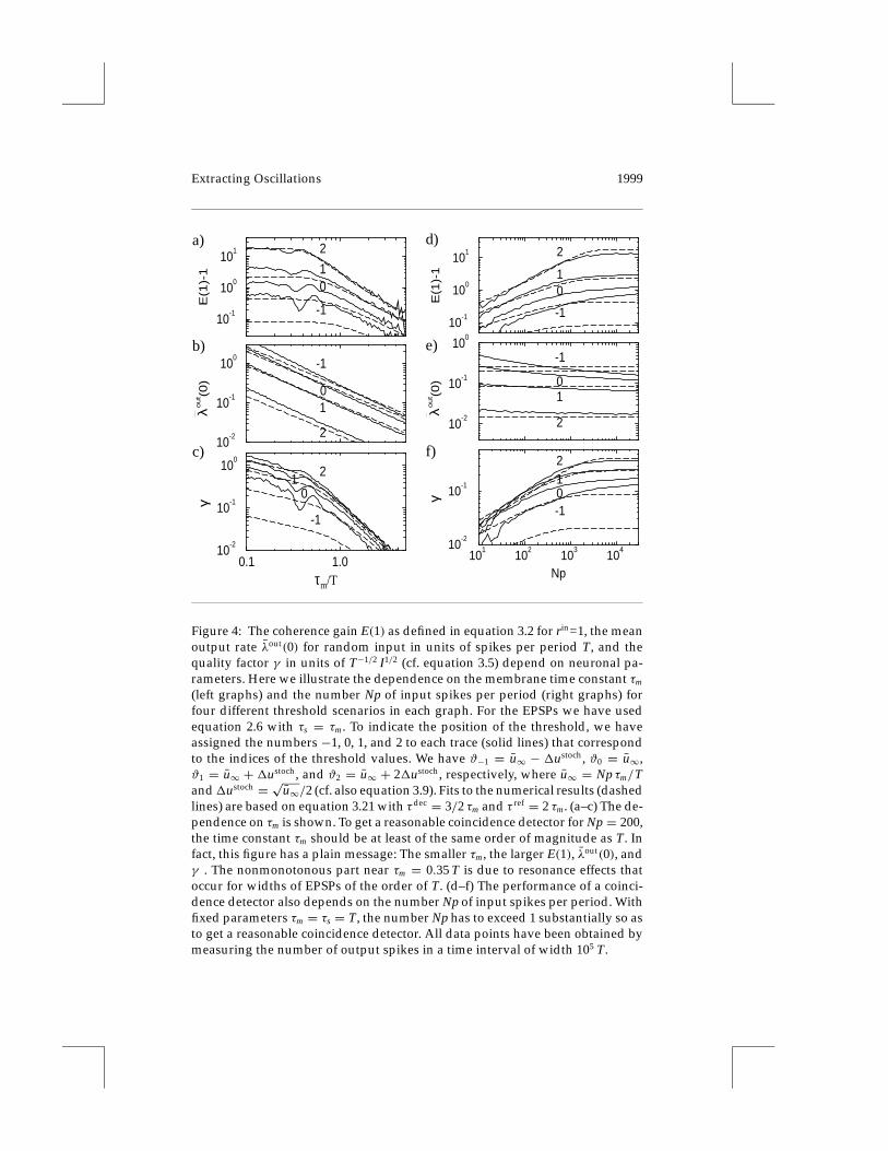
Figure 4: The coherence gain E(1) as defined in equation 3.2 for rin=1, the meanoutput rate λout(0) for random input in units of spikes per period T, and thequality factor γ in units of T−1/2 I1/2 (cf. equation 3.5) depend on neuronal pa-rameters. Here we illustrate the dependence on the membrane time constant τm

(left graphs) and the number Np of input spikes per period (right graphs) forfour different threshold scenarios in each graph. For the EPSPs we have usedequation 2.6 with τs = τm. To indicate the position of the threshold, we haveassigned the numbers −1, 0, 1, and 2 to each trace (solid lines) that correspondto the indices of the threshold values. We have ϑ−1 = u∞ − 1ustoch, ϑ0 = u∞,ϑ1 = u∞ + 1ustoch, and ϑ2 = u∞ + 21ustoch, respectively, where u∞ = Np τm/Tand1ustoch = √u∞/2 (cf. also equation 3.9). Fits to the numerical results (dashedlines) are based on equation 3.21 with τdec = 3/2 τm and τ ref = 2 τm. (a–c) The de-pendence on τm is shown. To get a reasonable coincidence detector for Np = 200,the time constant τm should be at least of the same order of magnitude as T. Infact, this figure has a plain message: The smaller τm, the larger E(1), λout(0), andγ . The nonmonotonous part near τm = 0.35 T is due to resonance effects thatoccur for widths of EPSPs of the order of T. (d–f) The performance of a coinci-dence detector also depends on the number Np of input spikes per period. Withfixed parameters τm = τs = T, the number Np has to exceed 1 substantially so asto get a reasonable coincidence detector. All data points have been obtained bymeasuring the number of output spikes in a time interval of width 105 T.


treated as a single degree of freedom. The dependence of E(1), λout(0), andγ on Np is shown in Figures 4d–f. The larger Np, the better is the neuron’sperformance as a coincidence detector (cf. section 3.2).

To summarize this section, two quantities determine the quality of acoincidence detector neuron: (1) the rate λout(0) and (2) the coherence gainE(rin), which both enter the quality factor γ in equation 3.6. Both quantitiesdepend on neuronal parameters. If, for example, the threshold is increased,then the coherence gain E is enhanced, but at the same time the rate λout(0) islowered. We note that both the coherence gain E(rin) and λout(0) are, at leastin the frame of an I&F model, determined by the neuron’s time constantsτm and τs, the period T, the mean number Np of inputs per period, and thethreshold ϑ .

3.2 Mathematical Treatment. To transfer the observations from I&F neu-rons to biological neurons, the quantities τm, τs, T, and Np have to be de-termined experimentally. To draw conclusions about the quality of a coin-cidence detector, knowledge about the spontaneous rate λout(0) and, thus,the threshold ϑ is necessary (cf. equation 3.6). But usually there is no directaccess to E(rin) or γ . To close this gap, we present a method of estimatingE(rin) and γ from experimentally available parameters.

The mathematical analysis that we present in this subsection is not lim-ited to the I&F model introduced above. We derive our results for a moregeneral class of threshold neurons whose response to an input spike canbe described by an EPSP. This class of neuron models has been called theSpike Response Model (SRM) (Gerstner & van Hemmen, 1992, 1994) and canemulate other neuron models, such as the Hodgkin-Huxley model (Kistler,Gerstner, & van Hemmen, 1997).

3.2.1 Signal-to-Noise Ratio Analysis. We perform a signal-to-noise anal-ysis of the membrane potential. Let us assume that the neuron has fired attimes {tm;m ≤ n}. We study the trajectory for tn < t < tn+1 and set

u(t) = u(t)+ δustoch(t)+ δuper(t), (3.7)

where u(t) =∑nm η(t− tm)+ u∞ is the reference trajectory of a neuron that

receives a constant input current N λin. The membrane potential u(t) followsthe trajectory u(t)+δuper(t) if it is driven by an input current N λin(t). There-fore, δustoch(t) and δuper(t) are the stochastic fluctuations and the periodicoscillations, respectively.

For the signal-to-noise ratio analysis, we de facto presuppose that thenoise is gaussian. A normal distribution is the only one that is determinedby its first and second moment, which will be used in the following anal-ysis. For a large number N of independent synapses, this is an excellentapproximation, as is shown in detail in section A.3.


We have seen before (cf. Figure 2b) that “good” coincidence-detectionproperties require a threshold ϑ above u∞. In this case, spike generationis driven by the fluctuations, not by the mean trajectory. The magnitudeof the stochastic fluctuations is determined by the mean number of inputspikes per period and the shape of the EPSP. The amplitude of the periodicfluctuations depends, in addition, on the amount rin of synchrony of thesignal. Roughly speaking, the neuron will be able to distinguish betweenthe coherent (rin > 0) and the incoherent case (rin = 0), if the total amount offluctuation is different in the two cases. The typical amplitude of the fluctu-ations will be denoted by 1ustoch and 1uper. We define an order parameter

ρ := 1uper(rin)

1ustoch(0), (3.8)

which will be related to the coherence gain E and the quality factor γ . Theparameter ρ can be considered as a signal-to-noise ratio, where the signal isgiven by the periodic modulation and the noise as the stochastic fluctuationof the membrane potential. For ρ ≈ 0 a low-coherence gain E and qualityfactor γ is to be expected; for ρ À 1 there should be a large E and γ . Toconfirm this conjecture, we relate1ustoch and1uper to the parameters of theinput and the neuron model.

The calculation of 1ustoch for rin = 0 and 1uper for rin ≥ 0 is carried outfor a class of typical EPSPs. The only requirement is that EPSPs should, asin equation 2.6, vanish for s ≤ 0, rise to a maximum, and decay thereafterback to zero (at least exponentially for s→∞). The amplitude of an EPSPwill be called A. The time window preceding any particular point in theneuron’s activity pattern during which a variation in the input could havesignificantly affected the membrane potential is called τ (without a lowerindex, in contrast to τm and τs). This is the definition of the integrationwindow of a neuron given by Theunissen and Miller (1995), which can beapproximated by the full width at half maximum of the EPSP.

The variance of the stochastic fluctuations is then proportional to theaverage number of inputs the neuron receives in a time interval τ times theamplitude A of the EPSP (for details see appendix A). For N λin τ À 1 thestandard deviation is to good approximation

1ustoch(0) ≈ A

√N λin τ

2. (3.9)

Using, for example, equation 2.6 in equation A.8, we obtain A√τ = τm/√

τm + τs.To determine the amplitude of periodic oscillations, we average over the

Poisson process of the membrane voltage in equation 2.5 and denote theaverage by angular brackets 〈.〉. From equation 3.7 we have 〈u − u〉(t) =


〈δuper〉(t), since 〈δustoch〉(t) = 0, and thus

〈δuper〉(t) = N

∞∫0

ds[λin(t− s)− λin

]ε(s). (3.10)

The amplitude 1uper of the T-periodic oscillations will be estimated by theabsolute value of the first Fourier coefficient of 〈δuper〉(t). The kth Fouriercoefficient of a T-periodic function x(t) is defined by

xk := 1T

t+T∫t

dt′ x(t′) exp(−i kω t′), with ω := 2πT. (3.11)

Now the amplitude of the periodic oscillations can be written as

1uper =∣∣∣⟨δuper

1

⟩∣∣∣ . (3.12)

To calculate the right-hand side of equation 3.12, we also have to introducethe Fourier transform of quadratically integrable functions, for example, ofthe response kernel ε defined in equation 2.6,

ε(ω) :=∞∫−∞

dt′ ε(t′) exp(−iω t′). (3.13)

Carrying out the Fourier transform in equation 3.12 and using equation 3.13,we obtain 1uper = N |λin

1 ε(ω)|, where λin1 = p/T rin = λin rin is the first

Fourier coefficient of λin defined in equation 2.1. The final result for thesignal amplitude is then

1uper = N λin rin |ε(ω)|, (3.14)

where the definition of the vector strength rin in equation 2.2 has been used.The order parameter ρ in equation 3.8 can be rewritten with equations 3.9and 3.14 in terms of experimentally accessible parameters of the input andneuronal parameters:

ρ ≈ rin√

2 N λin τ|ε(ω)|

A τ. (3.15)

One has to keep in mind that equation 3.15 contains the signal-to-noiseratio in the membrane potential and concerns only one of two aspects ofcoincidence detection. The second aspect is related to the mean output firing


rate and, thus, the threshold, which should be chosen appropriately, as wediscussed in section 3.1 (see also section 4). The order parameter ρ alonecan be used only to derive necessary conditions for coincidence detection.For small ρ, it seems unlikely that a neuron acts as a coincidence detector,but a small ρ could be compensated for by a pool of such neurons (see alsosections 3.3 and 4). We think that as a rule of thumb, one can exclude that aneuron is a coincidence detector if ρ < 0.1.

Taking advantage of equation 3.15, we now derive an expression for themean output rate λout(rin) and for γ .

3.2.2 Mean Output Rate. As we stated in the previous section, in theabsence of a firing threshold, the neuron’s membrane voltage fluctuatesaround a mean value u∞ with a standard deviation1ustoch, which is due tonoisy input. From appendix A, we also know that, to excellent approxima-tion, the voltage fluctuations are gaussian. Then the probability that at anarbitrary time the membrane voltage u is above ϑ can be estimated by

w(ϑ) = 1√2π 1ustoch

∞∫ϑ

du exp[− (u− u∞)2

2 (1ustoch)2

], (3.16)

which can be rewritten in terms of the error function,

w(ϑ) = 12

[1− erf

(ϑ − u∞√21ustoch

)]. (3.17)

If ϑ > u∞, the average time that a voltage fluctuation stays above ϑis called τdec, which is expected to be of the order of the width τ of theintegration window. The time τdec is needed for a decay of any voltagefluctuation. Therefore, the mean time interval between two events u > ϑ

can be approximated by τdec/w(ϑ).A neuron’s dynamics is such that firing occurs if the membrane volt-

age reaches the threshold ϑ from below. After firing, there is a refractoryperiod τ ref during which the neuron cannot fire. This prolongs the meanwaiting time τdec/w(ϑ) until the next event u = ϑ by an amount of τ ref.Taking refractoriness into account, the mean interspike interval τ isi can beapproximated by

τ isi ≈ τdec/w(ϑ)+ τ ref. (3.18)

The mean output rate is λout = 1/τ isi. Substituting equation 3.17 into3.18, we obtain the mean output rate for a random input,

λout(0) ={

2τdec[1− erf

(ϑ ′/√

2)]−1 + τ ref

}−1

. (3.19)


Here we have introduced the normalized threshold,

ϑ ′ = (ϑ − u∞)/1ustoch. (3.20)

If the neuron’s input has a periodic contribution, then the output rateis increased. We now calculate the rate λout(rin) for arbitrary rin ≥ 0. Thekey assumption is that we are allowed to take the oscillatory input intoaccount through a modified threshold ϑ ′ only. The periodic contributionenhances the standard deviation of the membrane potential around its meanvalue. Thus, the threshold is lowered by the normalized amplitude of theperiodic oscillations ρ(rin) of the membrane potential (cf. equation 3.8). Ageneralization of equation 3.19 leads to

λout(rin) ≈{

2τdec[1− erf

(ϑ ′ − ρ/

√2)]−1 + τ ref

}−1

. (3.21)

Since we have an expression for the mean output rate in equation 3.21, wealso have an expression for the coherence gain E and the quality factor γ(cf. equations 3.2 and 3.6). In Figure 3 the numerical results for λout, E, andγ can be fitted at least within an order of magnitude by using τdec = 3/2 τmand τ ref = 2 τm.

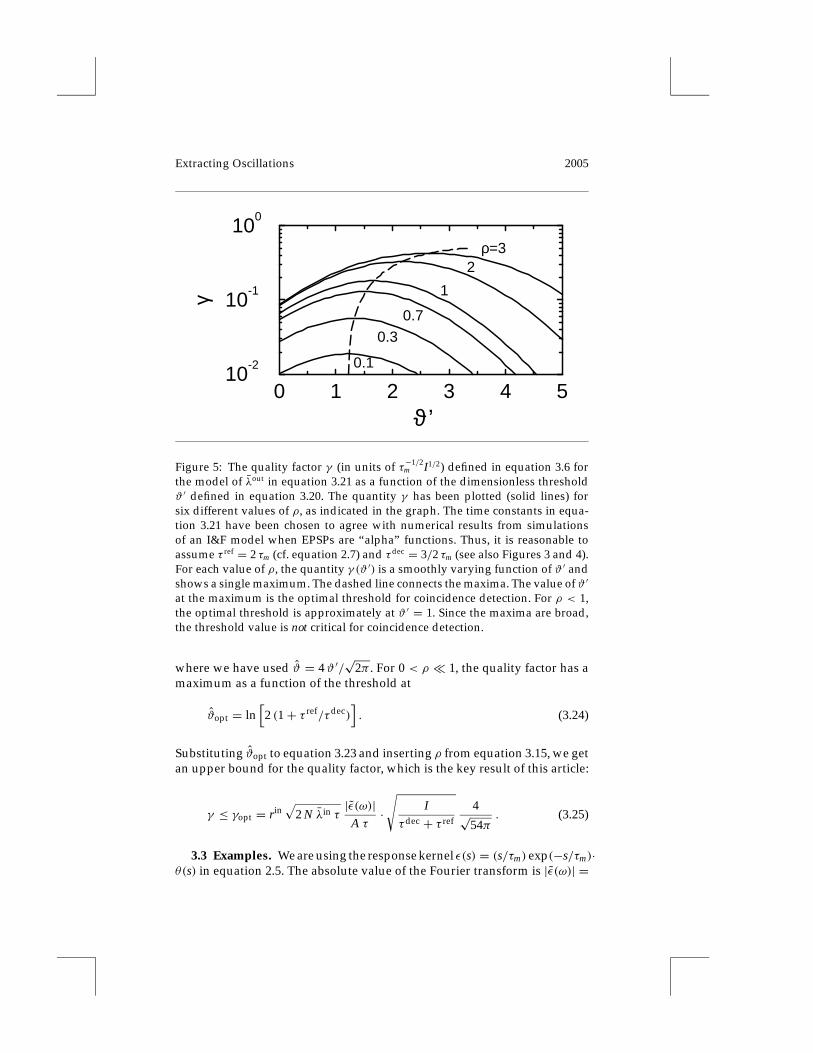
3.2.3 Quality Factor. To arrive at a better understanding of the depen-dence of the quality factor γ on the normalized threshold ϑ ′ and the signal-to-noise ratio ρ, we have plotted the result for γ (ϑ ′) in Figure 5 while takingτdec = 3/2 τm and τ ref = 2 τm (as in Figures 3 and 4) for different values ofρ. The graphs illustrate that γ varies only weakly as a function of ϑ ′, if ρ isheld constant. The maximum value is, at least for 0 < ρ < 1, close to ϑ ′ = 1.This confirms the result of Figure 3c and the conjecture that the optimalthreshold lies above the mean voltage by an amount equal to the amplitudeof the stochastic fluctuations.

To get a handy expression for γ , we use an approximation of the errorfunction (Ingber, 1982),

12

[1− erf(x)] ≈ 11+ exp

(4 x/√π) , (3.22)

which is better than 2% for all x. At least for 0 < ρ ¿ 1 we are able to derivea simple expression for γ . Using the definition for γ in equation 3.6 and alinearization in ρ, we obtain

γ = ρ√

2π

Iτdec

[1+ exp ϑ + τ ref/τdec

]−3/2exp ϑ, (3.23)


0 1 2 3 4 5ϑ’

10-2

10-1

100

γ

ρ=32

0.3

0.1

0.7

1

Figure 5: The quality factor γ (in units of τ−1/2m I1/2) defined in equation 3.6 for

the model of λout in equation 3.21 as a function of the dimensionless thresholdϑ ′ defined in equation 3.20. The quantity γ has been plotted (solid lines) forsix different values of ρ, as indicated in the graph. The time constants in equa-tion 3.21 have been chosen to agree with numerical results from simulationsof an I&F model when EPSPs are “alpha” functions. Thus, it is reasonable toassume τ ref = 2 τm (cf. equation 2.7) and τdec = 3/2 τm (see also Figures 3 and 4).For each value of ρ, the quantity γ (ϑ ′) is a smoothly varying function of ϑ ′ andshows a single maximum. The dashed line connects the maxima. The value of ϑ ′

at the maximum is the optimal threshold for coincidence detection. For ρ < 1,the optimal threshold is approximately at ϑ ′ = 1. Since the maxima are broad,the threshold value is not critical for coincidence detection.

where we have used ϑ = 4ϑ ′/√

2π . For 0 < ρ ¿ 1, the quality factor has amaximum as a function of the threshold at

ϑopt = ln[2 (1+ τ ref/τdec)

]. (3.24)

Substituting ϑopt to equation 3.23 and inserting ρ from equation 3.15, we getan upper bound for the quality factor, which is the key result of this article:

γ ≤ γopt = rin√

2 N λin τ|ε(ω)|

A τ·√

Iτdec + τ ref

4√54π

. (3.25)

3.3 Examples. We are using the response kernel ε(s) = (s/τm) exp(−s/τm)·θ(s) in equation 2.5. The absolute value of the Fourier transform is |ε(ω)| =


τm/(1+ ω2τ 2

m). From equations 3.15 and A.8 (see also the remark after equa-

tion 3.9), we then obtain the signal-to-noise ratio,

ρ =√

N λin τm2 rin

1+ ω2τ 2m. (3.26)

Let us calculate ρ for cortical neurons. Due to background activity, the(effective) membrane time constant for voltages in the neighborhood of thethreshold can be as low as 10 ms (Bernander, Douglas, Martin, & Koch,1991; cf. also Rapp, Yarom, & Segev, 1992). We assume EPSPs as “alpha”functions and N = 104 synapses firing at λin = 5 Hz. If the input has aperiodic component of 40 Hz (T = 25 ms), we calculate from equation 3.26a value of ρ = 6.1 rin. The vector strength rin can be related to the relativemodulation amplitude Arel of almost periodic correlograms by rin ≈

√Arel/2

(see appendix B), which is a good approximation for small Arel. A value ofArel ≈ 0.3 is reasonable (Gray & Singer, 1989). We find rin ≈ 0.4, and a signal-to-noise ratio of ρ ≈ 2.4. Therefore cortical neurons possess all prerequisitesnecessary for coincidence detection.

As a further application of equation 3.26, we turn to neurons in the nu-cleus laminaris of the barn owl. Model studies have shown that the laminarneurons can indeed act as coincidence detectors (Gerstner, Kempter, vanHemmen, & Wagner, 1996). These neurons have (almost) no dendritic trees.A set of parameters N = 200, τm = τs = 0.1 ms, λin = 0.5 kHz, λout = 100 Hz,and rin = 0.5 for T−1 = 5 kHz is reasonable (Carr & Konishi, 1990; Carr &Boudreau, 1991; Reyes, Rubel, & Spain, 1996). From equation 3.26, we obtainρ = 0.29. This value should be compared to the much better signal-to-noiseratio ρ ≈ 2.4 that we find for cortical neurons.

We now compare the values of the upper bound of the quality factor γoptin equation 3.25 for the two types of neurons. We take an interval of, say,I = 100 ms to get some numerical values that can be interpreted, thoughthe length of I is not important for the comparison. For cortical neuronswe assume τdec = 3/2 τm and τ ref = 2 τm, the parameters used through-out the whole article. From equation 3.25, we then obtain γopt = 1.2. Forlaminar neurons, we also assume τdec = 3/2 τm and τ ref = 2 τm, wherebyτm = 0.1 ms, and obtain γopt = 1.5. We conclude that both types of neuronshave comparable coincidence-detection properties. In laminar neurons, therelatively low number N of synapses is compensated by a high mean inputrate λin in order to achieve the same performance as cortical neurons. Inboth examples, the ratio τm/T and the input vector strength rin were almostidentical.

What does a quality factor of, say, γ = 1.5 mean? We remind readersof the definition of γ in equation 3.5. The quality factor is a quantity thatmeasures the distance between the spike count distributions for random andcoherent input. For γ = 1, the two distributions are just distinguishable, andfor γ À 1 they are well separated. The error probability or, better, the extent


to which random and coherent input can be discriminated can be calculatedfrom γ . The corresponding algorithm is the subject of further investigation.

4 Discussion

This study demonstrates the influence of the parameters of an I&F neuronon the capability of the neuron to work as a coincidence detector for pe-riodically modulated spike input. The dependence on the membrane timeconstant τm has been demonstrated in Figures 2 and 4a–c, the influence ofthe number of inputs per period Np was treated in Figures 4d–f, and therelation to the threshold ϑ has been shown in Figures 3 and 5. An orderparameter ρ for coincidence detection has been defined in equation 3.15 bydividing the amplitude of the periodic oscillations (when the neuron re-ceives phase-locked input) by the amplitude of the stochastic fluctuationsof the membrane voltage (when the neuron receives random input). Finally,ρ has been related to the quality factor γ for coincidence detection.

Our reasoning is not limited to I&F neurons. It can be applied directly toneurons whose excitatory synapses have almost equal strengths and evokesimilar EPSPs that sum up linearly, at least below the threshold. The ex-tension to a distribution of synaptic strengths and forms of EPSPs is alsostraightforward. With some additional effort, phase-locked inhibitory in-puts could also be incorporated. Our model does not include, though, non-linear effects in the dendritic tree (Softky, 1994).

The shape of the EPSP plays the most important role for coincidencedetection. More precisely, the relevant parameter is the absolute value ofthe Fourier component of the response kernel ε at the frequency of theexternal stimulus (cf. equation 3.15), which expresses the (low-pass) filteringproperty of synaptic transmission. Nevertheless, the rule of thumb holdsthat the briefer the EPSPs, the better are the coincidence-detection propertiesof the corresponding neuron. The width of the EPSP has to be at least ofthe same order of magnitude as the minimal temporal structure it shouldresolve (cf. Figure 4a).

In addition, the number of synapses and their mean activity determinewhether a neuron is able to perform coincidence detection. With T-peri-odically modulated input, our results show that the more input spikes pertime, the easier is coincidence detection (cf. Figure 4b). This is due to thefact that the ratio between the signal (= oscillations of membrane volt-age) and the noise (= random fluctuations) increases with increasing meaninput rate. The contribution of many synapses also enhances coincidence-detection properties, which is extremely important for neurons receivinga large number of inputs, such as cortical pyramidal cells with about 104

synapses or cerebellar purkinje cells with approximately 2 · 105 synapses.One can summarize the influence of the width τ of an EPSP and the

number of inputs per time a neuron receives on coincidence detection asfollows. The neuron’s “memory” extends over an interval τ back in time,


so the neuron cannot “see” earlier input spikes. They have little influenceon the membrane potential because the corresponding tails of the EPSPsare small and decay exponentially in time. (For the moment, we neglectrefractory effects.) Hence, the number of inputs in the neuron’s integrationtime window of length τ determines the state (the membrane potential) ofthe neuron. If the number of inputs in this shifting time window showsa significant T-periodic oscillation, then it is in principle possible that theneuron is able to perform coincidence detection. This is a rate-coding schemewhere the firing rate has to be measured within an averaging time window.This argument shows that the width of an EPSP, which corresponds to theaveraging time window, should be small. If it greatly exceeds one period,then averaging will be of no use at all.

For coincidence detection there is an optimal threshold value, as illus-trated by Figures 3c and 5. For optimal coincidence detection, the thresholdϑ has to surpass the mean membrane voltage u∞ = N λin τm of the neuron byan amount equal to the noise amplitude. A higher threshold implies a lowermean output firing rate, which destroys the advantage of a high-coherence-gain E. A lower threshold leads to the regime of a nonleaky integrator, whichis not at all suited to coincidence detection. Thus coincidence detection in“real” neurons requires an adaptive mechanism to control the threshold.There are several different possibilities for that. First, we could imagine acontrol loop that adjusts the threshold in the appropriate regime. This mightbe difficult to implement but could be achieved, for example, if each spikeis followed by a long-lasting hyperpolarizing afterpotential. Alternatively,we could envisage a feedback loop of inhibitory neurons that adjust themean input. A control of input strength is also possible through synapticchanges (Tsodyks & Markram, 1997; Abbott, Varela, Sen, & Nelson, 1997).Finally, it has been shown in a model study (Gerstner et al., 1996) that po-tentiation and depression of synaptic weights can balance each other so thatthe effective input strength is always normalized (see also Markram, Lubke,Frotscher, & Sackmann, 1997). However, the threshold is not a critical pa-rameter for coincidence detection, as is illustrated by the broad maximumof γ as a function of the threshold in Figures 3c and 5. The threshold alsodetermines the mean firing rate of a neuron. For reasonable firing rates, thequality factor remains of the same order of magnitude as its optimal valueγopt (cf. equation3.25).

The existence of an optimal threshold can be related to the phenomenonof stochastic resonance (Wiesenfeld & Moss, 1995) in that in the presence ofnoise, the detection of weak signals can be enhanced and there is an optimalnoise level. It seems unlikely, though, that neurons are able to change thelevel of noise in their input. A neuron has potentially the chance of adaptingits threshold to an optimal value, as we have discussed before. We haveshown that the optimal threshold for coincidence detection is, similar tostochastic resonance, always above u∞ by an amount that is of the sameorder of magnitude as the noise amplitude.


Having the parameter γ at hand, one still has to be careful with rashconclusions about a neuron’s task. Let us consider a neuron whose γ issmall. One might argue that such a neuron cannot function as a coincidencedetector, and this is certainly correct if we consider the neuron as a singleunit. But if there is a pool of neurons operating in the same pathway andreceiving the same type of input, the output of all these neurons togethercould provide a secure cue for a decision. Also, the waiting time, which isnecessary to make a correct decision with high reliability, can be reducedby using a pool of neurons. That is, the following two counting methodsare equivalent: a system can use either the output spike count of a singleneuron in an interval I or the number of spikes of L statistically independent,identical neurons operating in the same pathway during a period of timeI/L.

Although we have considered the transition from spike to rate coding,the output spikes remain phase locked to a periodic input. This means thatthe neuronal transmission always retains some of the temporal information,an aspect that we think is important to signal processing in the brain.

Appendix A: Inhomogeneous Poisson Process

In this appendix we define and analyze the inhomogeneous Poisson pro-cess. This notion has been touched on by Tuckwell (1988, pp. 218–220) andothers (e.g., Ash & Gardner, 1975, pp. 28–29), but neither of them explainsthe formalism itself or the way of computing expectation values. Since bothare used extensively, we do so here, despite the fact that the issue is treatedby Snyder and Miller (1991, secs. 2.1–2.3). Our starting assumptions in han-dling this problem are the same as those of Gnedenko (1968, sec. 51) for thehomogeneous (uniform) Poisson process, but the mathematics is different.Neither does our method resemble the Snyder and Miller approach, whichstarts from the other end, equation A.11. In the context of theoretical neu-robiology, an analysis such as this one, focusing on the local behavior of aprocess, seems to us far more natural. We proceed by evaluating the meanand the variance and finish this appendix by estimating a third moment,which is needed for the Berry-Esseen inequality, that tells us how good agaussian approximation to a sum of independent random variables is.

A.1 Definitions. Let us suppose that a certain event, in our case a spike,occurs at random instances of time. Let N(t) be the number of occurrencesof this event up to time t. We suppose that N(0) = 0, that the probability ofgetting a single event during the interval [t, t+1t) with 1t→ 0 is

Pr{N(t+1t)−N(t) = 1} = λ(t)1t , λ ≥ 0 , (A.1)

and that the probability of getting two or more events is o(1t). Finally,the process has independent increments; events in disjoint intervals are


independent. The stochastic process obeying the above conditions is aninhomogeneous Poisson process.

Under conditions on λ to be specified below, there are only finitely manyevents in a finite interval. Hence, the process lives on a space Ä of mono-tonically nondecreasing, piecewise constant functions on the positive realaxis, having finitely many unit jumps in any finite interval. The expecta-tion value corresponding to this inhomogeneous Poisson process is simplyan integral with respect to a probability measure µ on Ä, a function spacewhose existence is guaranteed by the Kolmogorov extension theorem (Ash,1972, sec. 4.4.3). A specific realization of the process, a function on the pos-itive real axis, is a “point” ω in Ä. The discrete events corresponding to ωare denoted by tf (ω) with f labeling them.

As we have seen in eq. 2.5, spikes generate postsynaptic potentials ε. Wenow compute the average, denoted by angular brackets, of the postsynapticpotentials generated by a specific neuron during the time interval [t0, t),⟨∑

f

ε(t− tf (ω))

⟩. (A.2)

Here it is understood that tf = tf (ω) depends on the realization ω andt0 ≤ tf (ω) < t. We divide the interval [t0, t) into L subintervals [tl, tl+1) oflength 1t so that at the end 1t → 0 and L → ∞ while L1t = t − t0. Wenow evaluate the integral (see equation A.2), exploiting the fact that ε is acontinuous function.

Let #{tl ≤ tf (ω) < tl+1} denote the number of events (spikes) occurringat times tf (ω) in the interval [tl, tl+1) of length 1t. In the limit 1t → 0, theexpectation value (see equation A.2) can be written

∫Ä

dµ(ω)

[∑l

ε(t− tl) #{tl ≤ tf (ω) < tl+1}], (A.3)

so that we are left with the Riemann integral,∫ t

t0

d s λ(s) ε(t− s) . (A.4)

We spell out why. The function 1I{...} is to be the indicator function of theset {. . .} in Ä; that is, 1I{...}(ω) = 1, if ω ∈ {. . .} and it vanishes if ω does notbelong to {. . .}, so it “indicates” where the set {. . .} lives. With the benefitof hindsight, we single out mutually independent sets in Ä with indicators1I{tl≤tf (ω)<tl+1} and write the expectation value (see equation A.2) in the form∫

Ä

dµ(ω)∑

l

1I{tl≤tf (ω)<tl+1}ε(t− tl) #{tl ≤ tf (ω) < tl+1} . (A.5)


Each indicator function in the sum equals

1I{tl≤tf (ω)<tl+1} = 1I{N(tl+1)−N(tl)=0} + 1I{N(tl+1)−N(tl)=1}

+1I{N(tl+1)−N(tl)≥2}. (A.6)

In view of equations A.2 and A.5, we multiply this by ε(t− tl) #{tl ≤ tf (ω) <

tl+1}, interchange integration and summation in equation A.5, and integratewith respect toµ. The first term on the right contributes nothing; the secondgives λ(tl)ε(t− tl)1t and thus produces a term in the Riemann sum leadingto equation A.4; and the last term can be neglected since it is of order o(1t).The proof of the pudding is that only a single event in the interval [tl, tl+1)

counts as1t→ 0. Since ε(t) is a function that decreases at least exponentiallyas fast as t→∞, there is no harm in taking t0 = −∞.

A.2 Second Moment and Variance. It is time to compute the secondmoment,⟨

[∑tf<t

ε(t− tf )]2

⟩. (A.7)

In a similar vein as before, we obtain, in the limit 1t→ 0,⟨ ∑tf ,t′f<t

ε(t− tf )ε(t− t′f )

⟩

=∫Ä

dµ(ω)∑l,m

1I{tl≤tf (ω)<tl+1}1I{tm≤t′f (ω)<tm+1}ε(t− tf (ω))ε(t− t′f (ω))

=∑l6=m

[λ(tl)1t λ(tm)1t] ε(t− tl)ε(t− tm)+∫Ä

dµ(ω)∑

l

1I2{tl≤tf (ω)<tl+1}ε

2(t− tl)

=∫ t

t0

∫ t

t0

d t1d t2 λ(t1)λ(t2)ε(t− t1)ε(t− t2)+∫ t

t0

d s λ(s)ε2(t− s)

=[∫ t

t0

d s λ(s)ε(t− s)]2

+∫ t

t0

d s λ(s)ε2(t− s). (A.8)

Hence the variance is the last term on the right in equation A.8. It is a simpleexercise to verify that when λ(t) ≡ λ and ε(t) ≡ 1 in equations A.4 and A.8,we regain the mean and variance of the usual Poisson distribution.

We finish the argument by computing the probability of getting k eventsin the interval [t0, t). For the usual, homogeneous Poisson process it is

Pr{N(t)−N(t0) = k} = exp[−λ(t− t0)] · [λ(t− t0)]k

k!. (A.9)


We now break up the interval [t0, t) into many subintervals [τl, τl+1)of length1t and condition with respect to the first, second, . . . , arrival. The arrivalscome one after the other, and the probability of a specific sequence of eventsin [t1, t1+1t), [t2, t2+1t), . . . , [tk, tk+1t) is made up of elementary eventssuch as

Pr{First spike in [t1, t1 +1t)}= Pr{no spike in [t0, t1)}Pr{spike in [t1, t1 +1t)}= [1− λ(τ1)1t][1− λ(τ2)1t] . . . [1− λ(t1 −1t)1t] λ(t1)1t

= exp[−∫ t1

t0

d τ λ(τ)]λ(t1)1t. (A.10)

Here we have exploited the independent-increments property and taken thelimit 1t→ 0 to obtain the last equality. Repeating the above argument forthe following events, including the no-event tail in [tk +1t, t), multiplyingthe probabilities, and summing over all possible realizations, we find

Pr{N(t)−N(t0) = k}= exp

[−∫ t

t0

d τ λ(τ)] ∫ t

t0

d tk λ(tk) . . .

∫ t3

t0

d t2 λ(t2)

∫ t2

t0

d t1 λ(t1)

= exp[−∫ t

t0

d τ λ(τ)]· 1

k!

[∫ t

t0

d s λ(s)]k

. (A.11)

In other words, N(t) − N(t0) has a Poisson distribution with parameter∫ tt0

d s λ(s). If λ(s) ≡ λ, one regains equation A.9. We now see two things.First, the appropriate condition on λ is that it be locally integrable. ThenPr{N(t) − N(t0) < ∞} = 1 as the sum of equation A.11 over all finite kadds up to one. Furthermore, N(t) − N(t′) with t0 < t′ < t has a Poissondistribution with parameter

∫ tt′ d s λ(s). Second, by rescaling time through

t := ∫ t d s λ(s) one obtains (Tuckwell, 1988; Ash & Gardner, 1975) a homoge-neous Poisson process with parameter λ = 1. This also follows more directlyfrom equation A.1. It is of no practical help for understanding neuronal co-incidence detection, though. For instance, if we use a spike train generatedby an inhomogeneous Poisson process with rate λ(t) to drive, such as aleaky I&F neuron, its mean output firing rate does depend on the temporalstructure of λ(t), as we have argued. This effect cannot be explained by sim-ply rescaling time. Another example is provided by the auditory system,where λ(t) is taken to be a periodic function of t, with the period determinedby external sound input. The cochlea, however, produces a whole range offrequency inputs, whereas time can be rescaled only once.

A.3 Berry-Esseen Estimate. Equation 2.5 tells us that the neuronal inputis a sum of independent, identically distributed random variables corre-sponding to neighboring neurons j. Neither independence nor a common


distribution is necessary, but both are quite convenient. The point is that,according to the central limit theorem, a sum of N independent randomvariables1 has a gaussian distribution as N→∞. In our case, N is definitelyfinite, so the question is: How good is the gaussian approximation? The an-swer is provided by a classical, and remarkable, result of Berry and Esseen(Lamperti, 1966, sec. 15).

We first formulate the Berry-Esseen result. Let X1,X2, . . . be independentwith a common distribution having variance σ 2 and finite third moment.Furthermore, let SN =

∑Nj=1(Xj − 〈Xj〉) be the total input, the Xj stemming

from neighboring neurons j as given by the right-hand side of equation 2.5with N as the number of synapses, and let Yσ be a gaussian with mean 0 andvariance σ 2. Then there is a constant (2π)−1/2 ≤ C < 0.8 such that, whateverthe distribution of the Xj and whatever x,∣∣∣∣Pr

{SN√

N≤ x

}− Pr{Yσ ≤ x}

∣∣∣∣ ≤ C〈|X1 − 〈X1〉|3〉σ 3√

N. (A.12)

In the present case, σ 2 directly follows from equation A.8. Computing 〈|X1−〈X1〉|3〉 is a bit nasty but it is simpler, and also provides more insight, toestimate the third moment directly by Cauchy-Schwartz so as to get rid ofthe absolute value,

〈|X1 − 〈X1〉|3〉 ≤ 〈(X1 − 〈X1〉)2〉1/2〈(X1 − 〈X1〉)4〉1/2 . (A.13)

The first term on the right equals σ ; the second is given by

〈(X1 − 〈X1〉)4〉 =∫ t

t0

d s λ(s) ε4(t− s)+ 3σ 4, (A.14)

where σ 2 = ∫ tt0

d s λ(s)ε2(t− s). Collecting terms, we can estimate the right-hand side of equation A.12, the precision of the gaussian approximationbeing determined by 1/

√N as N becomes large.

Appendix B: Cross-Correlograms and Degree of Synchrony

Here we outline the relationship between the relative modulation Arel ofcross-correlograms and the underlying degree of synchrony, rin.

A spike input generated by equation 2.1 leads to a periodic cross-corre-lation function,

C(t) ∝∞∑

m=−∞Gσ√

2(t−mT). (B.1)

1 This N directly corresponds with the number of synapses that provide the neuronalinput. There is no need to confuse it with the stochastic variable N(t) of the previoussubsection.


The relative amplitude Arel of C is to be defined below. It is estimated fromthe Fourier transform of C, which is defined in equation 3.11. The Fouriercoefficients of equation B.1 are

Ck ∝ exp[−(k σ ω)2

]with ω = 2π

T. (B.2)

For σ ω > 1 the first Fourier component dominates, all higher coefficientscan be neglected, and we can approximate equation B.1 by

C(t) ≈ C0 + 2 C1 cos(t), (B.3)

where 2 C1 is the amplitude of the first-order oscillation. Then Arel, definedas the relative modulation of the cross-correlogram (cf., e.g., Konig, Engel,& Singer, 1995), is approximated by

Arel ≈ 2 C1

C0. (B.4)

Substituting equation B.2 into B.4, we obtain

Arel ≈ 2 exp[−(σ ω)2

]. (B.5)

Using the definition of the vector strength (see equation 2.2) in B.5 andsolving for rin, we find

rin ≈√

Arel

2. (B.6)

The restriction σ ω > 1 corresponds to rin < 0.6 or Arel < 0.7.The oscillation amplitude of the cross-correlation function C(t) for spike

activity as found in various brain areas decays to zero with increasing |t|(cf. Gray & Singer, 1989) because neuronal activity is not strictly periodic.Most of the cross-correlograms can be fitted by using generalized Gaborfunctions of the form (cf., for example, Konig et al., 1995)

C(t) ∝ 1+ Arel cos(t) exp(− t2

λ2

), (B.7)

where λ is a time constant. In this case we obtain a measure of the degreeof synchrony rin also from equation B.6, which originally was derived forthe periodic case only. The transfer of the arguments from the periodic tothe nonperiodic case is reasonable if λ is of the order of a few oscillationperiods T or longer. For coincidence detection, only correlations within theintegration time τ of a neuron are important. For neurons that are able toact as coincidence detectors, τ has to be at least of the order of T, so thatreasonable coincidence detectors do not “see” the decay of the correlationfunction.


Acknowledgments

We thank Julian Eggert and Werner Kistler for stimulating discussions, help-ful comments, and a careful reading of the manuscript. We also thank JackCowan and Richard Palmer for some useful hints concerning the title. Thiswork has been supported by the Deutsche Forschungsgemeinschaft undergrant numbers He 1729/8-1 (RK) and He 1729/2-2, 8-1 (WG).

References

Abbott, L. F., Varela J. A., Sen K., & Nelson S. B. (1997). Synaptic depression andcortical gain control. Science, 275, 220–224.

Abeles, M. (1982). Role of the cortical neuron: Integrator or coincidence detector?Isr. J. Med. Sci., 18, 83–92.

Ash, R. B. (1972). Real analysis and probability. New York: Academic Press.Ash, R. B., Gardner, M. F. (1975). Topics in stochastic processes. New York: Aca-

demic Press.Bernander, O., Douglas, R. J., Martin, K. A. C., & Koch C. (1991). Synaptic back-

ground activity influences spatiotemporal integration in single pyramidalcells. Proc. Natl. Acad. Sci. USA, 88, 11569–11573.

Burgess, N., Recce, M., & O’Keefe, J. (1994). A model of hippocampal function.Neural Networks, 7, 1065–1081.

Carr, C. E. (1992). Evolution of the central auditory system in reptiles and birds.In D. B. Webster, R. R. Fay, & A. N. Popper (eds.), The evolutionary biology ofhearing (pp. 511–543). New York: Springer-Verlag.

Carr, C. E. (1993). Processing of temporal information in the brain. Ann. Rev.Neurosci., 16, 223–243.

Carr, C. E., & Boudreau, R. E. (1991). Central projections of auditory nerve fibersin the barn owl. J. Comp. Neurol., 314, 306–318.

Carr, C. E., & Konishi, M. (1990). A circuit for detection of interaural time dif-ferences in the brain stem of the barn owl. J. Neurosci., 10, 3227–3246.

Davis, J. L., & Eichenbaum, H. (Eds.). (1991). Olfaction: A model system for com-putational neuroscience. Cambridge, MA: MIT Press.

Duda, R. O., & Hart, P. E. (1973). Pattern classification and scene analysis. NewYork: Wiley.

Eckhorn, R., Bauer, R., Jordan, W., Brosch, M., Kruse, W., Munk, M., & Reitboeck,H. J. (1988). Coherent oscillations: A mechanism of feature linking in thevisual cortex? Biol. Cybern., 60, 121–130.

Freeman, W. J. (1975). Mass action in the nervous system. New York: AcademicPress.

Gerstner, W., & van Hemmen, J. L. (1992). Associative memory in a network of“spiking” neurons. Network, 3, 139–164.

Gerstner, W., & van Hemmen, J. L. (1994). Coding and information processing inneural networks. In E. Domany, J. L. van Hemmen, K. Schulten (Eds.), Modelsof neural networks II (pp. 1–93). New York: Springer-Verlag.


Gerstner, W., Kempter, R., van Hemmen, J. L., and Wagner, H. (1996). A neuronallearning rule for sub-millisecond temporal coding. Nature, 383, 76–78.

Gnedenko, B. V. (1968). The theory of probability. (4th ed.). New York: Chelsea.Goldberg, J. M., & Brown, P. B. (1969). Response of binaural neurons of dog su-

perior olivary complex to dichotic tonal stimuli: Some physiological mecha-nisms of sound localization. J. Neurophysiol., 32, 613–636.

Gray, C. M., & Singer, W. (1989). Stimulus-specific neuronal oscillations in orien-tation columns of cat visual cortex. Proc. Natl. Acad. Sci. USA, 86, 1698–1702.

Ingber, L. (1982). Statistical mechanics of neocortical interactions. I. Basic for-mulation. Physica, 5D, 83–107.

Kistler, W. M., Gerstner, W., & van Hemmen, J. L. (1997). Reduction of theHodgkin-Huxley equations to a single-variable threshold model. Neural Com-put., 9, 1015–1045.

Konig, P., Engel, A. K., & Singer, W. (1995). Relation between oscillatory activityand long-range synchronization in cat visual cortex. Proc. Natl. Acad. Sci.USA, 92, 290–294.

Konig, P., Engel, A. K., & Singer, W. (1996). Integrator or coincidence detector?The role of the cortical neuron revisited. Trends Neurosci., 19, 130–137.

Koppl, C. (1997). Phase locking to high frequencies in the auditory nerve andcochlear nucleus magnocellularis of the barn owl, tyto alba. J. Neurosci., 17,3312–3321.

Lamperti, J. (1966). Probability. New York: Benjamin.Markram, H., Lubke, J., Frotscher, M., & Sakmann, B. (1997). Regulation of

synaptic efficacy by coincidence of postsynaptic APs and EPSPs. Science, 275,213–215.

Murthy, V. N., & Fetz, E. E. (1992). Coherent 25 to 35 Hz oscillations in thesensorimotor cortex of awake behaving monkeys. Proc. Natl. Acad. Sci. USA,89, 5670–5674.

Rapp, M., Yarom, Y., & Segev, I. (1992). The impact of parallel fiber backgroudactivity on the cable properties of cerebellar pulkinje cells. Neural Comput., 4,518–533.

Reyes, A. D., Rubel, E. W., and Spain, W. J. (1996). In vitro analysis of optimalstimuli for phase-locking and time-delayed modulation of firing in aviannucleus laminaris neurons. J. Neurosci., 16, 993–1007.

Ritz, R., Gerstner, W., Fuentes, U., & van Hemmen, J. L. (1994). A biologicallymotivated and analytically soluble model of collective oscillations in thecortex. II. Application to binding and pattern segmentation. Biol. Cybern., 71,349–358.

Ritz, R., Gerstner, W., & van Hemmen, J. L. (1994). Associative binding andsegregation in a network of spiking neurons. In E. Domany, J. L. van Hem-men, K. Schulten (Eds.), Models of neural networks II (pp. 177–223). New York:Springe-Verlag.

Snyder, D. L., & Miller, M. I. (1991). Random point processes in time and space. (2nded.). New York: Springer-Verlag.

Softky, W. (1994). Sub-millisecond coincidence detection in active dendritic trees.Neuroscience, 58, 13–41.


Stemmler, M. (1996). A single spike suffices: The simplest form of stochasticresonance. Network, 7, 687–716.

Theunissen, F., & Miller, J. P. (1995). Temporal encoding in nervous systems: Arigorous definition. J. Comp. Neurosci., 2, 149–162.

Troyer, T. W., and Miller, K. D. (1997). Physiological gain leads to high ISI vari-ability in a simple model of a cortical regular spiking cell. Neural Comput., 9,971–983.

Tsodyks, M. V., & Markram, H. (1997). The neural code between neocorticalpyramidal neurons depends on neurotransmitter release probability. Proc.Natl. Acad. Sci. USA, 94, 719–723.

Tuckwell, H. C. (1988). Introduction to theoretical neurobiology: Vol. 2: Nonlinearand stochastic theories. Cambridge: Cambridge University Press.

von der Malsburg, C., & Schneider, W. (1986). A neural cocktail-party processor.Biol. Cybern., 54, 29–40.

Wang, D., Buhmann, J., von der Malsburg, C. (1990). Pattern segmentation inassociative memory. Neural Comput., 2, 94–106.

Wehr, M., & Laurent, G. (1996). Odour encoding by temporal sequences of firingin oscillating neural assemblies. Nature, 384, 162–166.

Wiesenfeld, K., & Moss, F. (1995). Stochastic resonance and the benefits of noise:From ice ages to crayfish and SQUIDs. Nature, 373, 33–36.

Received August 21, 1997; accepted March 16, 1998.

extracting oscillations: neuronal coincidence detection with noisy periodic spike input

Documents