Extracting Atmospheric Turbulence and Aerosol Characteristics

from Passive Imagery Colin N. Reinhardt*

a, D.Wayne

a, K. McBryde

a, G. Cauble

a

aSpace and Naval Warfare System Center – Pacific, San Diego, CA, USA

*corresponding author: colin.reinhardt@navy.mil; phone: 1-619-553-6668;

ABSTRACT

Obtaining accurate, precise and timely information about the local atmospheric turbulence and extinction conditions and

aerosol/particulate content remains a difficult problem with incomplete solutions. It has important applications in areas

such as optical and IR free-space communications, imaging systems performance, and the propagation of directed

energy. The capability to utilize passive imaging data to extract parameters characterizing atmospheric turbulence and

aerosol/particulate conditions would represent a valuable addition to the current piecemeal toolset for atmospheric

sensing.

Our research investigates an application of fundamental results from optical turbulence theory and aerosol extinction

theory combined with recent advances in image-quality-metrics (IQM) and image-quality-assessment (IQA) methods.

We have developed an algorithm which extracts important parameters used for characterizing atmospheric turbulence

and extinction along the propagation channel, such as the refractive-index structure parameter 2

nC , the Fried

atmospheric coherence width 0r , and the atmospheric extinction coefficient ext , from passive image data. We will

analyze the algorithm performance using simulations based on modeling with turbulence modulation transfer functions.

An experimental field campaign was organized and data were collected from passive imaging through turbulence of

Siemens star resolution targets over several short littoral paths in Point Loma, San Diego, under conditions various

turbulence intensities. We present initial results of the algorithm’s effectiveness using this field data and compare

against measurements taken concurrently with other standard atmospheric characterization equipment. We also discuss

some of the challenges encountered with the algorithm, tasks currently in progress, and approaches planned for

improving the performance in the near future.

Keywords: atmospheric propagation, passive imaging, modulation transfer function, optical turbulence, extinction,

atmospheric aerosols, image quality metrics.

1. INTRODUCTION

Obtaining accurate, precise and timely information about the local atmospheric turbulence and extinction conditions and

aerosol/particulate content remains a difficult problem with incomplete solutions. It has important applications in areas

such as optical and IR free-space communications, imaging systems performance, and the propagation of directed

energy. The capability to utilize passive imaging data to extract parameters characterizing atmospheric turbulence and

aerosol/particulate conditions would represent a valuable addition to the current piecemeal toolset for atmospheric

sensing.

Our research investigates an application of fundamental results from optical turbulence theory and aerosol extinction

theory combined with recent advances in full-/no-reference image-quality-metrics (IQM) and image-quality-assessment

(IQA) methods. We have developed an algorithm which extracts important parameters used for characterizing

atmospheric turbulence and extinction along the propagation channel, such as the refractive-index structure parameter 2

nC , the Fried atmospheric coherence width 0r , and the atmospheric extinction coefficient ext , from passive image

data of remote Siemens star resolution targets. We will analyze the algorithm performance using simulations based on

modeling with turbulence modulation transfer functions (MTF). An experimental field campaign was organized and

data were collected from passive imaging through turbulence of Siemens star resolution targets over several short littoral

paths in Point Loma, San Diego, under conditions of various turbulence intensities. We present initial results of the

algorithm’s effectiveness using this field data and compare against measurements taken concurrently with other standard

atmospheric characterization equipment. We also discuss some of the challenges encountered with the algorithm, tasks

currently in progress, and approaches planned for improving performance in the near future.

1.1 Atmospheric Optical Turbulence

Optical turbulence in the atmosphere, caused by random variations in the optical refractive index of the air due to

thermal gradients, wind, and other meteorological factors, can induce severe degradations in imaging system

performance due to blurring and loss of contrast. Although the underlying fundamental theory of turbulence is vast and

deep [1,2] in practice a few important parameters are commonly used to summarize and evaluate the turbulent intensity

and model and predict its effect on imaging. Two of the most important parameters are the refractive-index structure

parameter 2

nC and the Fried atmospheric coherence width 0r .

Fried’s parameter represents a diameter effectively describing the limiting aperture size for image resolution in the

presence of atmospheric turbulence. In other words, an imaging system with an aperture larger than r0 will have no

increased resolution due to the limiting effects of the atmospheric turbulence. Fried’s parameter ranges from millimeters

for very turbulent atmospheric channels to tens of centimeters for more benign low-turbulence channels. Fried’s

parameter is defined below, a path-averaged quantity, is given (for plane waves) by

53

22

0

0

)(sec42.0

H

h

n dzzCkr (1)

where

2k is the wavenumber and is the slant-path angle from the zenith, in radians. [3]

1.2 Atmospheric Aerosol, Molecules, and Particulates

The earth’s atmosphere is composed of a multitude of discrete aerosols, molecules, hydrometeors, and other particulates

suspended for various amounts of time and in varying ratios of concentration of various sizes, the variation occurring

both temporally and spatially on the micro- and meso-scales. As energy at optical wavelengths (10um – 300nm)

propagates through this random medium, it is both partially absorbed, scattered, and the remainder transmitted unaltered.

The term extinction is used to define the combined effects of absorption and scattering. Thus, we define the important

parameter the extinction coefficient [2]

scaabsext (2)

Similar to the turbulence effects, the aerosol effects can be modeled as a low pass spatial filter with a MTF

determined by the particle sizes along the atmospheric channel. The particles along the channel become denser as

the visibility conditions worsen; heavy fog implies lots of particles. The aerosols cause the light to be scattered and

absorbed during propagation through the atmospheric channel, the net effect is image blur, loss of contrast, and

additive noise.

2. METHODOLOGY

2.1 Modeling

Modulation Transfer Functions

The modulation transfer function (MTF) is a spatial-frequency domain representation; defined as the magnitude of the 2-

dimensional Fourier transform of the spatial point spread function (PSF). For an aberration-free imaging system, the

image quality is limited by the finite aperture of the imaging system. This has the effect of blurring or smearing the

image in the image plane. The resulting image blur is inversely proportional to the aperture size; less blur for larger

apertures. Qualitatively, the MTF can be envisioned as acting as a low-pass filter for spatial frequencies of an image. [4]

In addition to describing an image yxg , in terms of its 2D spatial (x, y) pixel coordinate intensities, it is a useful and

common analysis procedure to represent an image in terms of its equivalent spatial frequency components, or in terms of

the related spatial-angular frequency components, which are related to spatial domain by the 2D Fourier-transform

operation.

dxdyyxjyxgG sysxsysx 2exp,),( (3)

The angular-spatial-frequency [cycles/radian] is defined by ss f , where f is the imaging lens focal length [mm]

and s is the spatial frequency [cycles/mm]. This frequency-domain representation is the basis of the modulation-

transfer function (MTF) approach. There are certain fundamental conditions and simplifying assumptions which must

be made to ensure the validity of the linear-systems theory approach for relating the PSF and MTF Fourier-transform

pairs. [5]

The paradigm of image blur for a finite aperture can also be extended to model the effects of the atmospheric channel on

imaging. An image taken through an atmospheric channel experiences blurring and distortion due to the turbulence,

absorption, and scattering along the channel. The turbulence effects can be modeled by treating the atmosphere as a low

pass spatial filter with a MTF determined by Fried’s parameter r0 or equivalently the atmospheric refractive-index

structure parameter 2

nC .

From fundamental Fourier optical theory [5], the averaged long-exposure total atmospheric MTF is the multiplicative

product of several individual and independent MTFs: the detector pixel MTF, the optical system (lens) MTF, the aerosol

MTF, and the long-exposure turbulence MTF. The total atmospheric MTF is then given by

,,,,,,,,,, _ sLEturbsaerosolslensspixelstotal MTFzMTFDMTFMTFzDMTF (4)

In CCD/CMOS detector-based imaging systems, the individual pixel element dimensions detL (assuming square pixels)

along with the imaging lens focal length f define a limit to the detectable spatial frequencies, denoted as the detector

angular-spatial cutoff frequency IFOVc Lf 1detdet_ where IFOV is the instantaneous field-of-view (IFOV) of

a single detector element (pixel). Using these terms the detector pixel MTF can be defined by

det_

det_

0

sin

cs

cs

IFOVs

IFOVs

spixelMTF

(5)

The primary imaging lens aperture of the optical system also defines the diffraction-limited resolution, which is the best

achievable imaging under otherwise perfect conditions (no turbulence, aerosol, or degradations due to optical

aberrations). The diffraction-limited imaging resolution for a circular aperture is given by [6]

D

DDDDDMTF

s

ssss

slens

0

1cos2

,,

21

2

1

(6)

The so-called “classical approximation” model for the aerosol MTF [7] is a common choice to model the aerosol

absorption and scattering effects, which is given by

csaa

cscsaasaerosol

zSA

zSzAzMTF

exp

exp,,

2

(7)

where

ac is the angular-spatial cutoff-frequency, with a being the particulate radius, z is the path length, aA

and aS the wavelength-dependent atmospheric absorption and scattering coefficients, respectively. It is common

practice to define the atmospheric extinction coefficient β, which has units 1m or frequently

1km is used. Extinction

is the sum of the absorption and scattering effects.

aaa SA

The long-exposure turbulence MTF [3] is given by

35

0

_ 44.3exp,,r

MTF ssLEturb

(8)

where 0r is the Fried atmospheric coherence radius (width) parameter.

There is mature and extensive fundamental theory describing the process and physics underlying each of the individual

MTF components [4,6], which is drawn upon in selecting the specific analytical models employed on the right-hand side

of Eq. (4). However, the true elegance of the algorithm described herein lies in its versatility; as new improved models

become available, the corresponding MTF implementation details may be easily changed, thus enhancing the overall

algorithm performance.

2.2 Imaging

The imaging modality studied is that of incoherent, passive imaging. Thus the image phase is considered randomly

distributed and is not assessed, and the imaged objects are assumed to be illuminated by other natural light sources

which are also assumed to be incoherent with random phase, such as scattered ambient solar illumination.

Image Quality Assessment and Image Quality Metrics

Image quality assessment (IQA) is the task of assigning a measure that can be defined as the perceived degradation of an

image. Image quality metrics (IQM) are used to provide an objective quantitative rating or score of the quality of an

image based on a number of factors. These factors include: sharpness, noise, contrast, distortion, blur, and many others.

IQMs can be broken down into two primary categories: full-reference (FR) and no-reference (NR). FR IQMs score an

image based upon knowledge of the un-degraded source reference image. NR IQMs score an image without any prior

knowledge of the original un-degraded image. FR IQMs are more common and reliable, yet in practical applications a

prior source reference image is typically unavailable so NR IQM techniques must be used.

In this study we surveyed many current IQMs, both FR and NR. We selected the following set of two FR and two NR

IQMs to use in our image analysis algorithm simulations and data processing: MSE (FR) [8], SSIM (FR) [9], NIQE

(NR) [10], MetricQ (NR) [11].

2.3 Atmospheric Parameter Extraction Algorithm

The basic purpose of the algorithm is to extract optical characterization parameters of an atmospheric propagation

channel using an image taken through said channel. An imaging system (telescope/lens and a camera) is used to

digitally capture an image. The image will be blurred and distorted due to atmospheric effects such as turbulence and

aerosol-induced attenuation and scattering. The captured image is processed against a database of pre-generated

atmospheric transfer functions. The processed (“restored”) image is then assessed and scored with an image quality

metric. Once the processed image with the best score is found, the corresponding model parameters used to pre-distort

the image are assumed to best represent the true parameters of the atmospheric channel.

The algorithm is designed to be modular and upgradeable, not being coupled to any specific implementation of the

processing subsystems such as image restoration, image quality analysis, and atmospheric modulation transfer function

formulation. As improvements are made in the state-of-the-art in these areas, the appropriate subsystem may be

upgraded and the overall algorithm performance will improve.

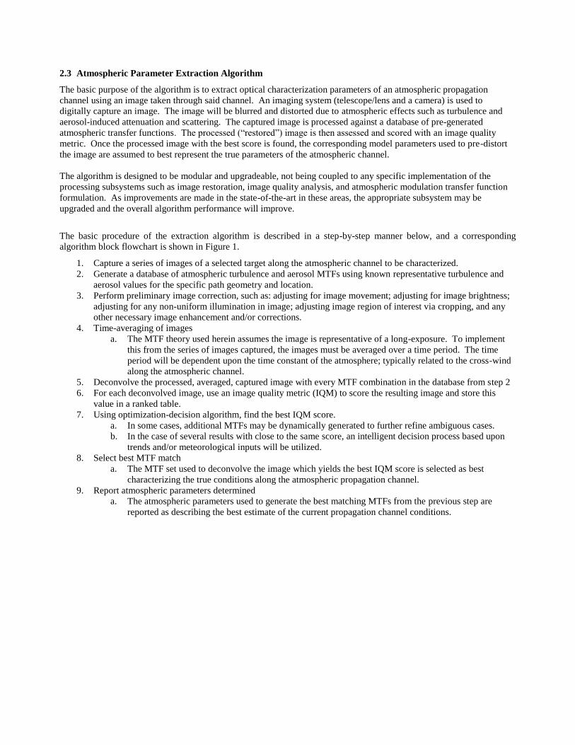
The basic procedure of the extraction algorithm is described in a step-by-step manner below, and a corresponding

algorithm block flowchart is shown in Figure 1.

1. Capture a series of images of a selected target along the atmospheric channel to be characterized.

2. Generate a database of atmospheric turbulence and aerosol MTFs using known representative turbulence and

aerosol values for the specific path geometry and location.

3. Perform preliminary image correction, such as: adjusting for image movement; adjusting for image brightness;

adjusting for any non-uniform illumination in image; adjusting image region of interest via cropping, and any

other necessary image enhancement and/or corrections.

4. Time-averaging of images

a. The MTF theory used herein assumes the image is representative of a long-exposure. To implement

this from the series of images captured, the images must be averaged over a time period. The time

period will be dependent upon the time constant of the atmosphere; typically related to the cross-wind

along the atmospheric channel.

5. Deconvolve the processed, averaged, captured image with every MTF combination in the database from step 2

6. For each deconvolved image, use an image quality metric (IQM) to score the resulting image and store this

value in a ranked table.

7. Using optimization-decision algorithm, find the best IQM score.

a. In some cases, additional MTFs may be dynamically generated to further refine ambiguous cases.

b. In the case of several results with close to the same score, an intelligent decision process based upon

trends and/or meteorological inputs will be utilized.

8. Select best MTF match

a. The MTF set used to deconvolve the image which yields the best IQM score is selected as best

characterizing the true conditions along the atmospheric propagation channel.

9. Report atmospheric parameters determined

a. The atmospheric parameters used to generate the best matching MTFs from the previous step are

reported as describing the best estimate of the current propagation channel conditions.

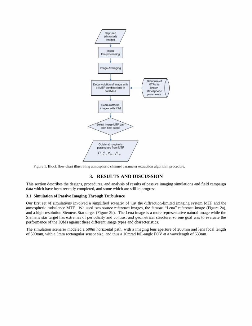
Figure 1. Block flow-chart illustrating atmospheric channel parameter extraction algorithm procedure.

3. RESULTS AND DISCUSSION

This section describes the designs, procedures, and analysis of results of passive imaging simulations and field campaign

data which have been recently completed, and some which are still in progress.

3.1 Simulation of Passive Imaging Through Turbulence

Our first set of simulations involved a simplified scenario of just the diffraction-limited imaging system MTF and the

atmospheric turbulence MTF. We used two source reference images, the famous “Lena” reference image (Figure 2a),

and a high-resolution Siemens Star target (Figure 2b). The Lena image is a more representative natural image while the

Siemens star target has extremes of periodicity and contrast and geometrical structure, so one goal was to evaluate the

performance of the IQMs against these different image types and characteristics.

The simulation scenario modeled a 500m horizontal path, with a imaging lens aperture of 200mm and lens focal length

of 500mm, with a 5mm rectangular sensor size, and thus a 10mrad full-angle FOV at a wavelength of 633nm.

Figures 2a and 2b: Simulation source reference images: (a) Lena (b) Siemens star target

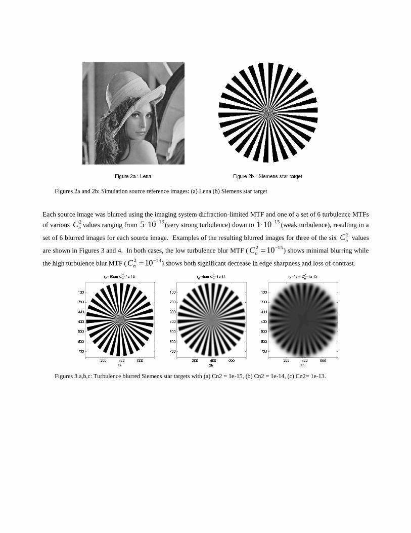
Each source image was blurred using the imaging system diffraction-limited MTF and one of a set of 6 turbulence MTFs

of various 2

nC values ranging from 13105 (very strong turbulence) down to

15101 (weak turbulence), resulting in a

set of 6 blurred images for each source image. Examples of the resulting blurred images for three of the six 2

nC values

are shown in Figures 3 and 4. In both cases, the low turbulence blur MTF (152 10nC ) shows minimal blurring while

the high turbulence blur MTF (132 10nC ) shows both significant decrease in edge sharpness and loss of contrast.

Figures 3 a,b,c: Turbulence blurred Siemens star targets with (a) Cn2 = 1e-15, (b) Cn2 = 1e-14, (c) Cn2= 1e-13.

Figures 4 a,b,c: Turbulence blurred Lena images with (a) Cn2 = 1e-15, (b) Cn2 = 1e-14, (c) Cn2= 1e-13.

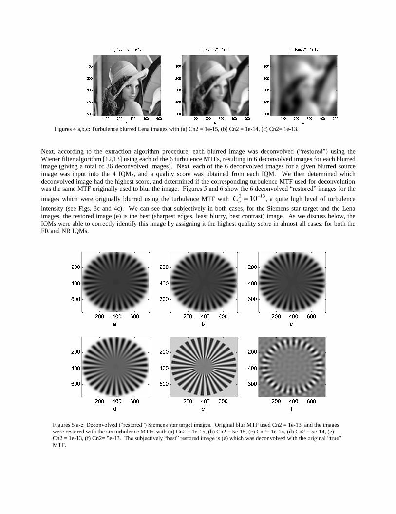
Next, according to the extraction algorithm procedure, each blurred image was deconvolved (“restored”) using the

Wiener filter algorithm [12,13] using each of the 6 turbulence MTFs, resulting in 6 deconvolved images for each blurred

image (giving a total of 36 deconvolved images). Next, each of the 6 deconvolved images for a given blurred source

image was input into the 4 IQMs, and a quality score was obtained from each IQM. We then determined which

deconvolved image had the highest score, and determined if the corresponding turbulence MTF used for deconvolution

was the same MTF originally used to blur the image. Figures 5 and 6 show the 6 deconvolved “restored” images for the

images which were originally blurred using the turbulence MTF with 132 10nC , a quite high level of turbulence

intensity (see Figs. 3c and 4c). We can see that subjectively in both cases, for the Siemens star target and the Lena

images, the restored image (e) is the best (sharpest edges, least blurry, best contrast) image. As we discuss below, the

IQMs were able to correctly identify this image by assigning it the highest quality score in almost all cases, for both the

FR and NR IQMs.

Figures 5 a-e: Deconvolved (“restored”) Siemens star target images. Original blur MTF used Cn2 = 1e-13, and the images

were restored with the six turbulence MTFs with (a) Cn2 = 1e-15, (b) Cn2 = 5e-15, (c) Cn2= 1e-14, (d) Cn2 = 5e-14, (e)

Cn2 = 1e-13, (f) Cn2= 5e-13. The subjectively “best” restored image is (e) which was deconvolved with the original “true”

MTF.

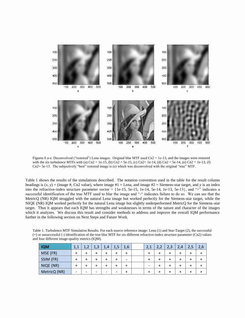
Figures 6 a-e: Deconvolved (“restored”) Lena images. Original blur MTF used Cn2 = 1e-13, and the images were restored

with the six turbulence MTFs with (a) Cn2 = 1e-15, (b) Cn2 = 5e-15, (c) Cn2= 1e-14, (d) Cn2 = 5e-14, (e) Cn2 = 1e-13, (f)

Cn2= 5e-13. The subjectively “best” restored image is (e) which was deconvolved with the original “true” MTF.

Table 1 shows the results of the simulations described. The notation convention used in the table for the result column

headings is (x, y) = (image #, Cn2 value), where image #1 = Lena, and image #2 = Siemens-star target, and y is an index

into the refractive-index structure parameter vector = {1e-15, 5e-15, 1e-14, 5e-14, 1e-13, 5e-13}, and “+” indicates a

successful identification of the true MTF used to blur the image and “-“ indicates failure to do so. We can see that the

MetricQ (NR) IQM struggled with the natural Lena image but worked perfectly for the Siemens-star target, while the

NIQE (NR) IQM worked perfectly for the natural Lena image but slightly underperformed MetricQ for the Siemens-star

target. Thus it appears that each IQM has strengths and weaknesses in terms of the nature and character of the images

which it analyzes. We discuss this result and consider methods to address and improve the overall IQM performance

further in the following section on Next Steps and Future Work.

Table 1. Turbulence MTF Simulation Results. For each source reference image: Lena (1) and Star-Target (2), the successful

(+) or unsuccessful (-) identification of the true blur MTF for six different refractive-index structure parameter (Cn2) values

and four different image-quality metrics (IQM).

IQM 1,1 1,2 1,3 1,4 1,5 1,6 2,1 2,2 2,3 2,4 2,5 2,6

MSE (FR) + + + + + + + + + + + +

SSIM (FR) + + + + + - + + + + + +

NIQE (NR) + + + + + + - + + + + +

MetricQ (NR) - - - - - + + + + + + +

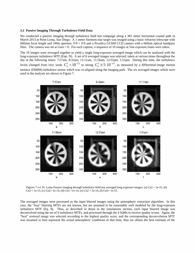
3.2 Passive Imaging Through Turbulence Field Data

We conducted a passive imaging through turbulence field test campaign along a 381 meter horizontal coastal path in

March 2013 at Point Loma, San Diego. A 1 meter Siemens-star target was imaged using a basic refractor telescope with

600mm focal length and 100m aperture, F/# = F/6 and a Prosilica GC660 CCD camera with a 660nm optical bandpass

filter. The camera was set at Gain = 0. For each capture, a sequence of 10 images at 5ms exposure times were taken.

The 10 images were averaged together to yield a single long-exposure averaged image which can be analyzed with the

long-exposure turbulence MTF (Eqn. N). A set of 6 averaged images was selected, taken at various times throughout the

day at the following times: 7:57am, 8:32am, 11:11am, 11:56am, 12:51pm, 1:51pm. During this time, the turbulence

levels changed from very weak 152 10nC to strong

142 105 nC , as measured by a differential-image motion

monitor (DIMM) turbulence sensor which was co-aligned along the imaging path. The six averaged images which were

used in the analysis are shown in Figure 7.

Figures 7 a-f: Pt. Loma Passive imaging through turbulence field test averaged long-exposure images: (a) Cn2 = 1e-15, (b)

Cn2 = 1e-15, (c) Cn2= 1e-14, (d) Cn2 =1e-14, (e) Cn2 = 5e-14, (f) Cn2= 1e-15.

The averaged images were processed as the input blurred images using the atmospheric extraction algorithm. In this

case, the “true” blurring MTFs are not known, but are assumed to be reasonably well modeled by the long-exposure

turbulence MTF (Eq. 8). Thus, as described in detail in the simulations section, each input blurred image was

deconvolved using the set of 6 turbulence MTFs, and processed through the 4 IQMs to receive quality scores. Again, the

“best” restored image was selected according to the highest quality score, and the corresponding deconvolution MTF

was assumed to best represent the actual atmospheric conditions at that time, thus we obtain the best estimate of the

corresponding refractive-index structure parameter 2

nC and the related Fried atmospheric coherence width 0r which

were used to generate that MTF. For the FR IQMs, the first image (Figure 7a) was used as a “reference” image, since it

was taken under very low turbulence conditions it represents nominally “ideal” imaging conditions.

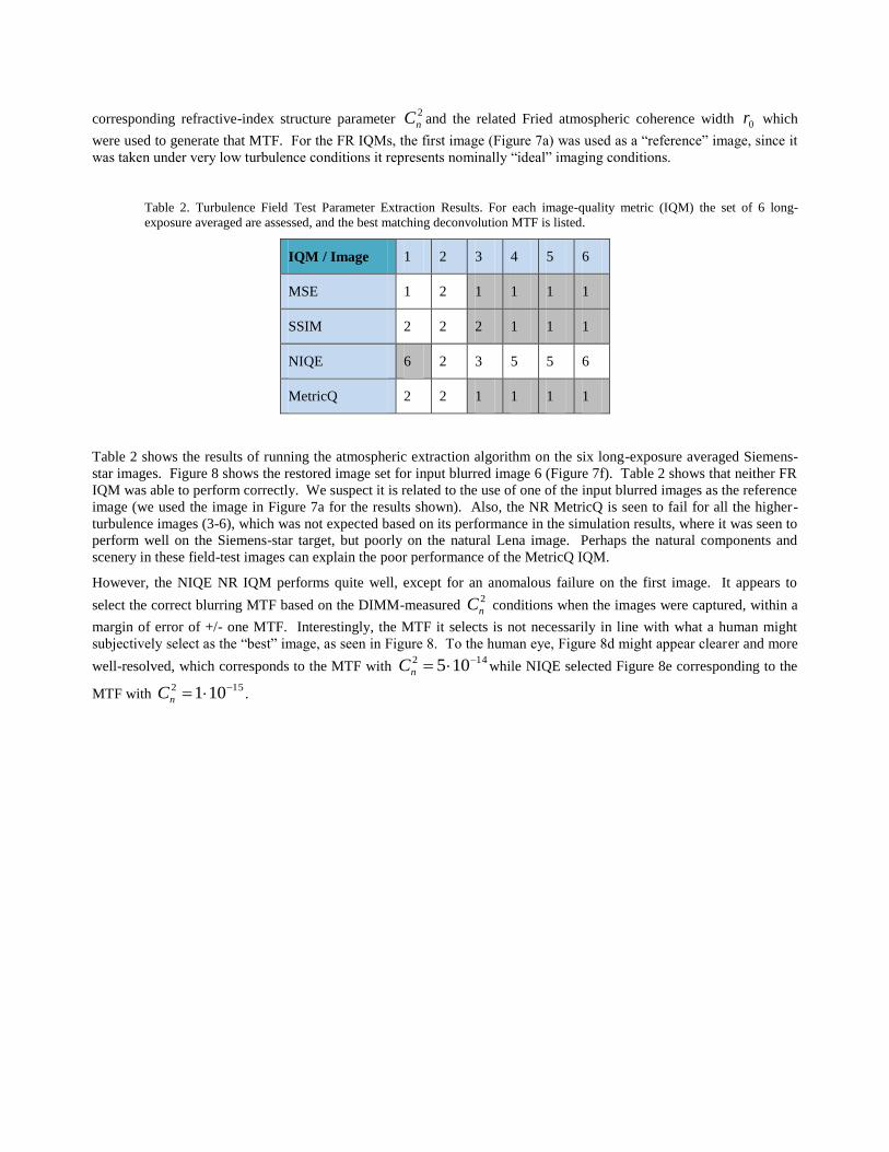
Table 2. Turbulence Field Test Parameter Extraction Results. For each image-quality metric (IQM) the set of 6 long-

exposure averaged are assessed, and the best matching deconvolution MTF is listed.

IQM / Image 1 2 3 4 5 6

MSE 1 2 1 1 1 1

SSIM 2 2 2 1 1 1

NIQE 6 2 3 5 5 6

MetricQ 2 2 1 1 1 1

Table 2 shows the results of running the atmospheric extraction algorithm on the six long-exposure averaged Siemens-

star images. Figure 8 shows the restored image set for input blurred image 6 (Figure 7f). Table 2 shows that neither FR

IQM was able to perform correctly. We suspect it is related to the use of one of the input blurred images as the reference

image (we used the image in Figure 7a for the results shown). Also, the NR MetricQ is seen to fail for all the higher-

turbulence images (3-6), which was not expected based on its performance in the simulation results, where it was seen to

perform well on the Siemens-star target, but poorly on the natural Lena image. Perhaps the natural components and

scenery in these field-test images can explain the poor performance of the MetricQ IQM.

However, the NIQE NR IQM performs quite well, except for an anomalous failure on the first image. It appears to

select the correct blurring MTF based on the DIMM-measured 2

nC conditions when the images were captured, within a

margin of error of +/- one MTF. Interestingly, the MTF it selects is not necessarily in line with what a human might

subjectively select as the “best” image, as seen in Figure 8. To the human eye, Figure 8d might appear clearer and more

well-resolved, which corresponds to the MTF with 142 105 nC while NIQE selected Figure 8e corresponding to the

MTF with 152 101 nC .

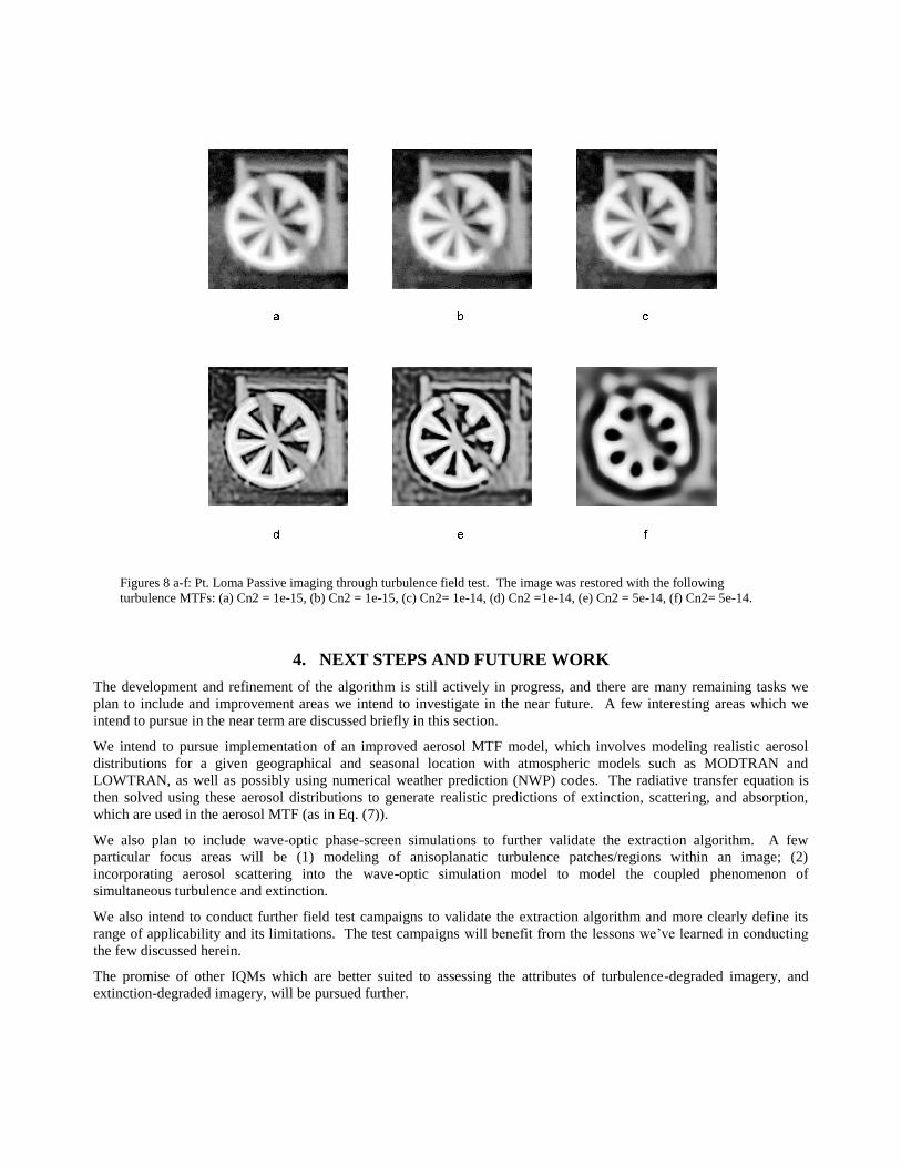
Figures 8 a-f: Pt. Loma Passive imaging through turbulence field test. The image was restored with the following

turbulence MTFs: (a) Cn2 = 1e-15, (b) Cn2 = 1e-15, (c) Cn2= 1e-14, (d) Cn2 =1e-14, (e) Cn2 = 5e-14, (f) Cn2= 5e-14.

4. NEXT STEPS AND FUTURE WORK

The development and refinement of the algorithm is still actively in progress, and there are many remaining tasks we

plan to include and improvement areas we intend to investigate in the near future. A few interesting areas which we

intend to pursue in the near term are discussed briefly in this section.

We intend to pursue implementation of an improved aerosol MTF model, which involves modeling realistic aerosol

distributions for a given geographical and seasonal location with atmospheric models such as MODTRAN and

LOWTRAN, as well as possibly using numerical weather prediction (NWP) codes. The radiative transfer equation is

then solved using these aerosol distributions to generate realistic predictions of extinction, scattering, and absorption,

which are used in the aerosol MTF (as in Eq. (7)).

We also plan to include wave-optic phase-screen simulations to further validate the extraction algorithm. A few

particular focus areas will be (1) modeling of anisoplanatic turbulence patches/regions within an image; (2)

incorporating aerosol scattering into the wave-optic simulation model to model the coupled phenomenon of

simultaneous turbulence and extinction.

We also intend to conduct further field test campaigns to validate the extraction algorithm and more clearly define its

range of applicability and its limitations. The test campaigns will benefit from the lessons we’ve learned in conducting

the few discussed herein.

The promise of other IQMs which are better suited to assessing the attributes of turbulence-degraded imagery, and

extinction-degraded imagery, will be pursued further.

5. CONCLUSION

We have presented the description of an algorithm for extracting important parameters useful for characterizing the

atmospheric turbulence and extinction conditions, based on a simple incoherent passive imaging system. The algorithm

relies on the linear-systems theory of modulation transfer functions (MTF) and models which have been defined for the

MTFs of atmospheric turbulence, aerosol extinction, diffraction-limited imaging systems, and sensor pixel elements. As

the quality of the MTF model is fundamental to the performance of the algorithm, more realistic and accurate the MTF

models will directly result in better estimates of the atmospheric parameters of interest.

The algorithm also relies on recent research into image quality metrics (IQM) used to assess the image quality, with or

without a source reference image. From our results presented above, it is clear that each IQM has its own relative

strengths and weaknesses in evaluating the degrading effects of turbulence, and no single IQM algorithm has shown

general superiority for all conditions and image types.

Lastly, the deconvolution (image restoration) procedure is tricky and sensitive in its own right. The Wiener

deconvolution filter is just one of many techniques for performing the operation, and has its own strengths and

weaknesses. It is highly sensitive to the input noise-to-signal ratio parameter, which in practice must be somehow

estimated.

We also presented some initial numerical simulation results, and the initial results of a passive-imaging through

turbulence campaign. The promise of the parameter extraction algorithm was hinted at in these results, but it was also

seen that additional work is necessary to make this algorithm a reliable and viable practical method.

REFERENCES

[1] Phillips, R. L. and Andrews, L. C., [Laser Beam Propagation through Random Media], SPIE Press, Bellingham,

WA, (2005).

[2] Ishimaru, A., [Wave Propagaton and Scattering in Random Media, a classic reissue], IEEE Press, Piscataway,

NJ, (1997).

[3] Fried, D.L., “Optical Resolution Through a Randomly Inhomogeneous Medium for Very Long and Very Short

Exposures,” JOSA 56(10), (1966).

[4] Boreman, G.D., [Modulation Transfer Function in Optical and Electro-Optical Systems], SPIE Press,

Bellingham, WA, (2001).

[5] Goodman, J., [Introduction to Fourier Optics, 3rd

edition], Roberts and Company Publishers, (2004).

[6] Kopeika, N.S., [A Systems Engineering Approach to Imaging], SPIE Press, Bellingham, WA, (1998).

[7] Sadot, D. and Kopeika, N.S., “Imaging through the atmosphere: practical instrumentation-based theory and

verification of aerosol modulation transfer function,” JOSA A 10(1), (1993).

[8] Wang, Z. and Bovik, A.C., “Mean Squared Error: Love It or Leave It?,” IEEE Signal Processing Magazine, 98,

(2009).

[9] Wang, Z., Bovik, A.C., Sheikh, H.R., and Simoncelli, E.P., “Image quality assessment: From error visibility to

structured similarity,” IEEE Trans. Image Processing, 13, pp. 600-612, (2004).

[10] Mittal, A., Soundararajan, R. and Bovik, A. C., “Making a Completely Blind Image Quality Analyzer,” IEEE

Signal Processing, (2013).

[11] Zhu, X. and Milanfar, P., “Automatic Parameter Selection for Denoising Algorithms Using a No-Reference

Measure of Image Content,” IEEE Trans. on Image Processing, 19(12), (2010).

[12] Jain, A.K., [Fundamentals of Digital Image Processing], Prentice-Hall Inc., New Jersey, (1989).

[13] Andrews, H.C. and Hunt, B.R., [Digital Image Restoration], Prentice-Hall Signal Processing Series, New

Jersey, (1977).