1

BAHIR DAR UNIVERSITY

COLLEGE OF BUSINESS AND ECONOMICS

ECONOMICS PROGRAM

EXPORT PREFORMANCE AND ECONOMIC GROWTH

IN ETHIOPIA

BY

MOGES ALEMU

JUNE, 2013

BAHIR DAR

2

BAHIR DAR UNIVERSITY

COLLEGE OF BUSINESS AND ECONOMICS

ECONOMICS PROGRAM

EXPORT PREFORMANCE AND ECONOMIC GROWTH

IN ETHIOPIA

BY

MOGES ALEMU

A SENIOR ESSAY SUBMITTED TO THE ECONOMICS PROGRAM,

BAHIR DAR UNIVERSITY, IN PARTIAL FULFILLMENT OF

THE REQUIREMENTS FOR THE

DEGREE OF BACHELOR OF ARTS ECONOMICS

ESSAY ADVISOR: TADDES EMRU

3

JUNE, 2013

BAHIR DAR

BAHIR DAR UNIVERSITY

COLLEGE OF BUSINESS AND ECONOMICS

ECONOMICS PROGRAM

Export Performance and Economic Growth in Ethiopia

By

Moges Alemu

Approved by the Board of Examiners:

Taddes Emru

Advisor Signature

Examiner Signature

Examiner Signature

4

Acknowledgment

First and for most, my gratitude goes towards the Almighty and benevolent GOD that let me stay

in life these days and enable me to conduct this study.

Secondly, my special gratitude and sincere thanks goes to my advisor Ato Taddesse Emiru for

his willingness and unreserved comment, evaluation and advice from the beginning to the end of

the research.

Thirdly, I would like also to thank to my parent, & my best friend Selamey Nega , for their

morale and financial support throughout our education to this end.

Fourthly, my greater thanks goes to instructors Surafel Melak and Getachew Yirga who are dean

of Business and Economics college and previous department head of economics respectively.

Fifthly, I would like to express my hearty appreciation and thanks my friends Endale Aynetu &

Elebe Ezezew for their read and edit un reserved time.

Sixthly, I would like to describe our greatest appreciation and thank to Ato Kasie Desie who is

an instructor in Bahir Dar University in the department of economics for his professional support

in different activities during data collection.

Finally, I would like to thanks to Abeba Hamid, who typed this paper manuscript very neatly

and carefully.

5

i

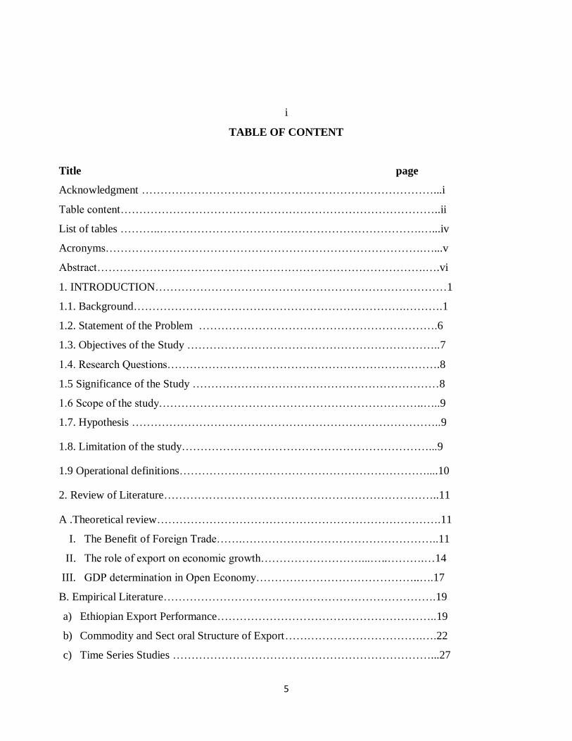
TABLE OF CONTENT

Title page

Acknowledgment ……………………………………………………………………...i

Table content…………………………………………………………………………..ii

List of tables ………..…………………………………………………………….…...iv

Acronyms………………………………………………………………………….…...v

Abstract…………………………………………………………………………….….vi

1. INTRODUCTION……………………………………………………………………1

1.1. Background……………………………………………………………….……….1

1.2. Statement of the Problem ……………………………………………………….6

1.3. Objectives of the Study …………………………………………………………..7

1.4. Research Questions……………………………………………………………….8

1.5 Significance of the Study …………………………………………………………8

1.6 Scope of the study……………………………………………………………..…..9

1.7. Hypothesis ………………………………………………………………………..9

1.8. Limitation of the study…………………………………………………………...9

1.9 Operational definitions…………………………………………………………....10

2. Review of Literature………………………………………………………………..11

A .Theoretical review………………………………………………………………….11

I. The Benefit of Foreign Trade…….……………………………………………..11

II. The role of export on economic growth………………………...…..……….…14

III. GDP determination in Open Economy……………………………………..….17

B. Empirical Literature……………………………………………………………….19

a) Ethiopian Export Performance…………………………………………………..19

b) Commodity and Sect oral Structure of Export……………………………….….22

c) Time Series Studies ……………………………………………………………...27

6

ii

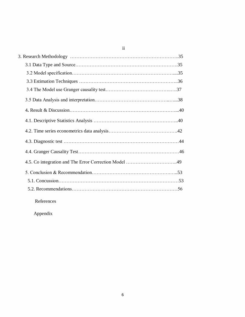
3. Research Methodology …………………………………………………………..35

3.1 Data Type and Source……………………………………………………….35

3.2 Model specification………………………………………………………....35

3.3 Estimation Techniques ……………………………………………………..36

3.4 The Model use Granger causality test…………………………………..….37

3.5 Data Analysis and interpretation………………………………………..…...38

4. Result & Discussion…………………………………………………………...40

4.1. Descriptive Statistics Analysis ……………………………………………..40

4.2. Time series econometrics data analysis…………………………………….42

4.3. Diagnostic test ………………………………………………………………44

4.4. Granger Causality Test………………………………………………………46

4.5. Co integration and The Error Correction Model …………………………..49

5. Conclusion & Recommendation………………………………………….…..53

5.1. Concussion…………………………………………………………………53

5.2. Recommendations…………………………………………………………56

References

Appendix

7

iii

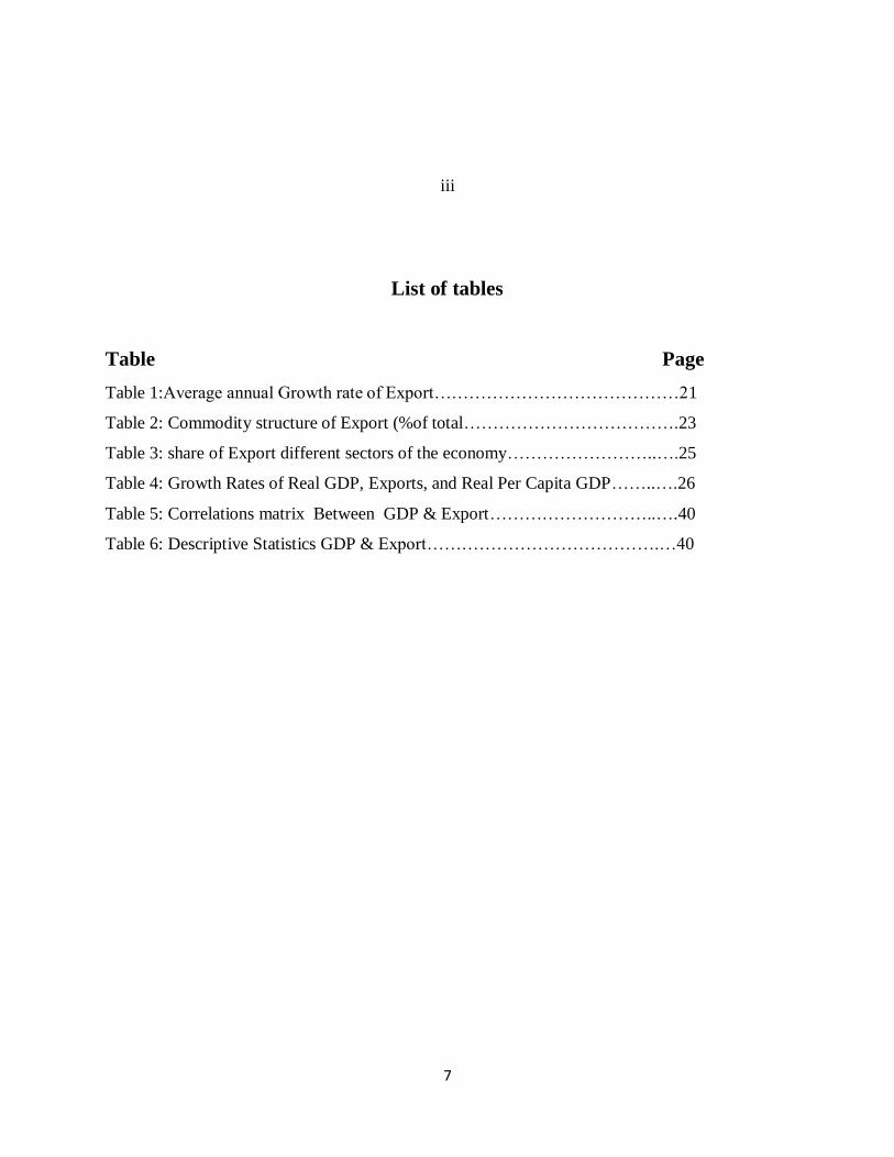
List of tables

Table Page

Table 1:Average annual Growth rate of Export……………………………………21

Table 2: Commodity structure of Export (%of total……………………………….23

Table 3: share of Export different sectors of the economy……………………..….25

Table 4: Growth Rates of Real GDP, Exports, and Real Per Capita GDP……..….26

Table 5: Correlations matrix Between GDP & Export………………………..….40

Table 6: Descriptive Statistics GDP & Export………………………………….…40

8

iv

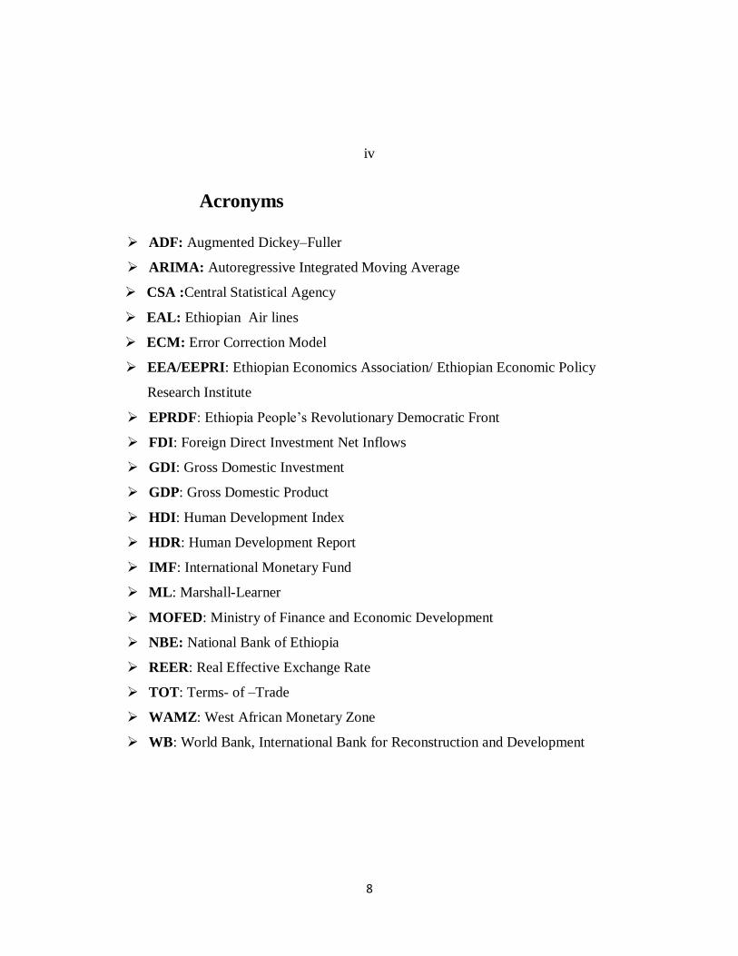
Acronyms

ADF: Augmented Dickey–Fuller

ARIMA: Autoregressive Integrated Moving Average

CSA :Central Statistical Agency

EAL: Ethiopian Air lines

ECM: Error Correction Model

EEA/EEPRI: Ethiopian Economics Association/ Ethiopian Economic Policy

Research Institute

EPRDF: Ethiopia People’s Revolutionary Democratic Front

FDI: Foreign Direct Investment Net Inflows

GDI: Gross Domestic Investment

GDP: Gross Domestic Product

HDI: Human Development Index

HDR: Human Development Report

IMF: International Monetary Fund

ML: Marshall-Learner

MOFED: Ministry of Finance and Economic Development

NBE: National Bank of Ethiopia

REER: Real Effective Exchange Rate

TOT: Terms- of –Trade

WAMZ: West African Monetary Zone

WB: World Bank, International Bank for Reconstruction and Development

9

v

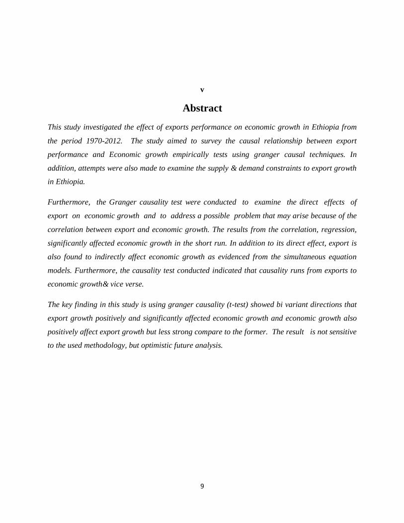
Abstract

This study investigated the effect of exports performance on economic growth in Ethiopia from

the period 1970-2012. The study aimed to survey the causal relationship between export

performance and Economic growth empirically tests using granger causal techniques. In

addition, attempts were also made to examine the supply & demand constraints to export growth

in Ethiopia.

Furthermore, the Granger causality test were conducted to examine the direct effects of

export on economic growth and to address a possible problem that may arise because of the

correlation between export and economic growth. The results from the correlation, regression,

significantly affected economic growth in the short run. In addition to its direct effect, export is

also found to indirectly affect economic growth as evidenced from the simultaneous equation

models. Furthermore, the causality test conducted indicated that causality runs from exports to

economic growth& vice verse.

The key finding in this study is using granger causality (t-test) showed bi variant directions that

export growth positively and significantly affected economic growth and economic growth also

positively affect export growth but less strong compare to the former. The result is not sensitive

to the used methodology, but optimistic future analysis.

10

vi

1. Introduction

1.1. Background of the Study

A. Overview of Economic performance

Ethiopia has experienced fast economic growth in recent years. With real GDP growth rate 11.0

%( double digit levels) since 2011/12, the country has consistently outperformed. Country’s

economy is highly vulnerable to exogenous shocks by virtue of its dependence on primary

commodities and rain fed agriculture. Ethiopia has experienced major exogenous shocks during

the past eight to nine years. These are notably droughts and adverse terms- of -trade (e.g., prices

of coffee and fuel). There is a strong correlation between weather conditions and Ethiopian

economic growth performance. (MOFD, report, 2011/12)

Ethiopian economy is based on agriculture, which accounts for 44% of gross domestic

product (GDP), 80% of exports, and 80% of total employment. However, Ethiopia's agriculture

is plagued by periodic drought, soil degradation caused by overgrazing, deforestation, high

population density, high levels of taxation and poor infrastructure this is making it difficult and

expensive to get goods to market. Yet agriculture is the country's most promising resource. A

potential exists for self-sufficiency in grains and for export development in livestock, grains,

vegetables, and fruits (MOFED, 2011/12).

11

In addition to this, many other economic activities depend on agriculture, including marketing,

processing, and export of agricultural products. Production is over time a subsistence nature, and

a large part of commodity exports are provided by the small agricultural cash-crop sector.

Principal crops include coffee, pulses (e.g., beans), oilseeds, cereals, potatoes, sugarcane, and

vegetables. Exports are almost entirely agricultural commodities, with coffee as the largest

foreign exchange earner, and its flower industry becoming a new source of revenue. Ethiopian

coffee exports represented0.9% of the world exports, and oilseeds and flowers each representing

0.5% Ethiopia is Africa's second biggest maize producer .In 2000,

Ethiopia's livestock contributed to 19% of total GDP (Wikipedia/Economy of Ethiopian free

encyclopedia retrieved on Noveber22/2012).

As of 2008, some countries that import most of their food, such as Saudi Arabia, had begun

planning the development of large tracts of arable land in developing countries such as Ethiopia.

This has raised fears of food being exported to more prosperous countries while the local

population faces its own shortage (Wikipedia/Economy of Ethiopia free encyclopedia retrieved

on Noveber22/2012).

B. Natural resource conditions

Forest products are used in construction and manufacturing and as energy sources only. Ethiopia

is endowed with distinct climatic conditions that enable it to grow diverse plant species, which

can be used for industrial and pharmaceutical purposes. Acacia, Commiphora and Boswellia

could be mentioned as one group of the various plant species grown in the arid and semi-arid

areas that yield important gums. The trend that has enhanced the growth of gum production over

the past decade has been the increasing consumption of convenience foods. As in most other

sectors of the additives industry, increasing health consciousness has tended to fuel growth for

thickeners of natural origin. Gum Olibanum derived from Boswellia, gum Myrrh, and

Oppoponex derived from Commiphora and gum Arabic derived from acacia species are the

major gum products that are mainly produced for the export market.

Ethiopian fisheries are entirely fresh water, as it has no marine coastline, and are a small part of

the economy. The mining sector is small in Ethiopia. The country has deposits

of coal, opal, gemstones, kaolin, iron ore, soda ash, and tantalum, but only gold is mined in

12

significant quantities. In 2001 gold production amounted to some 3.4 tons. Salt extraction from

salt beds in the Afar Depression, as well as from salt springs in Dire and Afder districts in the

south, is only of internal importance and only a negligible amount is exported.

On 30 August 2012 it was announced that British firm Nyota Minerals was about to become

the first foreign company to receive a mining license to extract gold from an estimated resource

of 52 tones in western Ethiopia(Wikipedia/ Economy of Ethiopia free encyclopedia retrieved on

Noveber22/2012).

Waterpower and forests are Ethiopian main energy sources. The country derives about 90

percent of its electricity needs from hydropower. Ethiopia is one of the few African countries

with a huge potential to produce hydro electric & geothermal power. Nine of its major rivers

are suitable for hydro electric power and has vast potential for geothermal energy generation.

Present produced capacities are rated at about 2000 megawatts, with planned expansion to

10,000 megawatts, and also have capacity to produce about 60,000 megawatts in different

power sources especially hydro electric and geothermal energy. It has opportunity export power

energy on the region. However, Ethiopians rely on forests for nearly all of their energy and

construction needs; the result has been deforestation of much of the highlands during the last

three decades. (Wikipedia/Economy of Ethiopia free encyclopedia retrieved on Noveber22/2012)

Less than one-half of Ethiopian towns and cities are connected to the national grid. Petroleum

requirements are met via imports of refined products, although some oil is being hauled overland

from Sudan. Oil exploration in Ethiopia has been underway for decades, ever since

Emperor HaileSelassie granted a 50-year concession to SOCONY -Vacuum in September

1945.Plans are afoot to exploit natural gas reserves in the southeastern lowlands, estimated at 4

trillion cubic feet (110×109 m

3). Exploration for gas and oil is underway in the Gambela

Region bordering Sudan.

C. Manufacturing, Transport and Communication in Ethiopia

According to (MOFED, 2010/11 report), manufacturing constitutes about 13.4 percent of the

overall economy, although it has shown some growth and diversification in recent years. Much

of it is concentrated in Addis Ababa. Food and beverages constitute some 40 percent of the

13

sector, but textiles and leather are also important, the latter especially for the export market. The

Programs from state-owned to privatize encouraging know.

Transport in Ethiopia is essential for the reason that to promote Economic growth and poverty

reduction .It includes Road, Railway, Air & Train, among these services road transport sector is

considered as the crucial one. A well developed road transport sector in developing countries

fuel up the growth process & improve market access through variety activities of the

development of a nation. During 2010/11, the Ethiopian road network reached 53,143km

(42.2%Federal&57.8% rural) with annual growth rate of 10.7% as a result of 3,662km new road

being constructed of the total 22,431km Federal roads, asphalt road constructed 37%&gravel

road63%.Ethiopia uses the ports of Djibouti connected to Addis Ababa by the Addis Ababa –

Djibouti Rail way, and to a lesser extent Port Sudan in Sudan.

In addition to this the Ethiopia government began negotiations to use the port of Berbera in

Somali land. Ethiopia Airlines is excellent contribution for the Economic growth and poverty

reduction. It has been 17 domestic Airfields &70 in international destinations. It encourages

export goods and services especially flower products. Telecommunications are provided by a

state-owned monopoly, Ethiopia Telecommunication corporation , has been under taking several

huge network expansion projects during the last few years with a view to enhancing the

development of the Telecom sector & to support the steady grow of the

country(MOFED,2010/11).

D. Tourism in Ethiopia

Ethiopia is a land with a very unique culture and heritage, with a history going back thousands

of years; it is one of the oldest nations in the world .It offers international tourist an unrivalled

choice. A country has nature gifted ranging from the peaks of the rugged semen mountains to the

deepest of the Danakil depression which is 120 meters below sea level.

On this condition, Ethiopia blessed with an abundance of natural beauty and variety of land

escapes, including Afro-Alpine, moors, and mountains deep gorges, sofomore cave (largest

cave in Africa),rift valley .etc But, Developed in the 1960s, tourism declined greatly during the

later 1970s and the 1980s under the military government. Recovery began in the 1990s, but

growth has been constrained by the lack of suitable hotels and other infrastructure, despite a

14

boom in construction of small and medium-sized hotels and restaurants, and by the impact of

drought, the 1998–2000 war with Eritrea, and the specter of terrorism. However, In 2002 more

than 156,000 tourists entered the country, many of them Ethiopians visiting from abroad ,and In

2008, the number of tourists entering the country had increased to 330,000(Wikipedia /Economy

of Ethiopian free encyclopedia retrieved on December 12/2012).

According to Mitchell and Coles (2009), even if it needs much work, tourism in Ethiopia has

bright future to grow twice the rate as the last decade for government to achieve its arrival

targets. Marketing may have a role but the fundamental constraint is that tourism in Ethiopia is

currently uncompetitive and is not that much contribute for economic growth like other Africa

countries (Egypt and Tunisia ) because of it has in the bottom 10% of performance both in Africa

and internationally. Improving this performance requires in an external marketing campaign

and enhancing competitiveness is the need to improve the quality of tourist infrastructure which

is currently very low.

In addition to this government should work with private sector to create a conducible

environment integrated with green economy development to improve the sector growth.

E. Ethiopian Export base

The major agricultural export crop is coffee, providing about 30.6%of Ethiopian foreign

exchange earnings. Coffee is critical to the Ethiopian economy. More than 15 million people

(25% of the population) derive their livelihood from the coffee sector. Other exports include live

animals, leather and leather products, chemicals, gold, pulses, oilseeds, flowers, fruits and

vegetables and chat, a leafy shrub which has psychotropic qualities when chewed (MOFED,

2010/11).

Cross-border trade by pastoralists is often informal and beyond state control and regulation.

In East Africa, over 95% of cross-border trade is through unofficial channels and the unofficial

trade of live cattle, camels, sheep and goats from Ethiopia sold to Somalia, Kenya and Djibouti

generates an estimated total value of between US $250 and US $300 million annually (100 times

more than the official figure). This trade helps lower food prices, increase food security, relieve

border tensions and promote regional integration. However, there are also risks as the

unregulated and undocumented nature of this trade runs risks, such as allowing disease to spread

15

more easily across national borders. Furthermore, the government of Ethiopia is purportedly

unhappy with lost tax revenue and foreign exchange revenues (Wikipedia/Economy of Ethiopia

free encyclopedia retrieved on December 12/2012).

On other hand, recent initiatives have sought to document and regulate this trade. Dependent on

a few vulnerable crops for its foreign exchange earnings and reliant on imported oil, Ethiopia

lacks sufficient foreign exchange. The financially conservative government has taken measures

to solve this problem, including strong import control and sharply reduced subsidies on retail

gasoline prices. Nevertheless, the largely subsistence economy is incapable of supporting high

military expenditures, drought relief, an ambitious development plan, and indispensable imports

such as oil and, therefore, must depend on foreign assistance.

In December 1999, Ethiopia signed a $1.4 billion joint venture deal with the Malaysian oil

company, PETRONAS, to develop a huge natural gas field in the Somali Region. By the year

2010, however, implementation failed to progress and PETRONAS sold its share to another oil

company. (Wikipedia/EconomyofEthiopianfreeencyclopediaretrievedonDecember12/2012)

1.2 Statement of the problem

According to Debel (2002), both internal and external factors that affect the Export performance

& Economic growth in Ethiopian economy during the past four decades. Those are:

Externally(Demand side), the fluctuation of oil prices that took place during the period 1973-74

and the export short fall associated with the world recession of 1974-75 resulted in chronic

balance of deficit problem that greatly affected the economic growth of many LDCs and

including Ethiopia. In addition, the period of the1980s was also characterized by the collapse of

commodity prices that resulted in deterioration of terms of trade of primary-commodity

exporting countries, which further deteriorate the economic performance of the country.

Therefore, export instability happens as a result of primary commodity price variation, and

concentration of trades. Such causes of export instability would consequently be detrimental to

economic growth [World Bank, 1989].

Internally (Supply side), poor climate condition, degradable soil , the prolonged war that took

place during the Derge regime, antiquated rural institutional social & Economic structure, and

16

produce less quality primary product have greatly affected the export growth. Furthermore, the

country is not self sufficient in generating the saving that is essential to realize a sustainable

economic growth, the export sector becomes very crucial for the growth performance of the

economy. (Todaro, 2003: PP, 594-596)

On other hand, the present regime design new economic policy where promote exports to

economic growth was given due to importance in the development strategy of the country.

Ethiopian exports have been growing at an average rate of 22% during the study period,

Ethiopian export sector is still small (passing US $2.7billion). Due to this, Ethiopian export is

still highly dependent on Agricultural exports. Exports of goods and services as a share of GDP

have increased from 12% in 2000/01 to 17% in 2010/ 11. Total export increase from US

$1billion in 2005/06 to US $ 2.7bilion in2010/11. It grew by 22% per year over this period

(MOFED, 2010/11).

According to MOFED (2010/11), export revenue was highly dependent on few commodities,

where Coffee, Chat, Oil Seeds, Hide Skin and Flower accounted for 78% in average. High

dependence of exports on primary exports has many drawbacks for the country. Because of the

following reasons;

First, traditional exports have been dominated by declining terms of trade which made export

earnings not to increase well enough despite increased export volumes, despite the recent spikes

in value of traditional exports. This can be revealed from the fact that unit value of exports was

116 in 1981 while it declined to 81 in 2004 showing nearly a 30% decline in 24 years (Sisay,

2010).

Secondly, traditional exports do not have much linkage effects in the economy because mostly

LDCs are sent raw product as well as have been problem of commodity and market

concentration result stiff competition.

Thirdly, the incentives provided by the new policy to promote exports could not totally

eliminate the anti-export-bias incentive structure that originated from heavy protection of the

domestic industries. As a result the export supply response was weak and the export earning

mainly resulted from coffee price boom and institutional reforms than the effect of trade and

exchange reform.

17

Finally the research will survey the above factors that affect export performance , the

contribution of export for economic growth, and analysis the constraints in this study.

1.3. Objectives of the study

1.3.1. General objectives

To assess the casual relationship between export performance and economic growth of the

country.

1.3.2 Specific objectives

To identify constraints of export performance of the country.

To analyze internal and external opportunities of export performance and

economic growth.

To examine contribution of export performance for economic growth of the

country.

To suggest possible course of action for solve the constraints.

1.4 Research Questions

a) What are the major problems that hinder export growth?

b) What is the causal relationship between the export performance and economic growth?

c) What is the efficient and productive mechanism for dynamic change in export and

economic growth?

d) What policy recommendation is survey for reduce the constraints and improve economic

growth?

1.5 Significance of the study

This study has its own contribution in the future. It helps to guide policy maker and show

solution for constraints and also the following importance.

18

To show resource based of export to the different sectors of the economy would

help the country fully exploit the benefits of the sector that is essential for

sustainable economic growth.

The government is expecting to take corrective action to improve export and

contribute for economic growth.

To provide policy recommendation in order to improve export and contribute well

develops economic growth.

It is important to other researchers need to asses in this areas, it uses as a

reference.

1.6 Scope of the study

Undertaking research on Export performance and Economic growth at international level is a

complex task in this level since it requires huge finance, time, data source and sufficient

knowledge. These constraints forced the researcher to undertake a research at national level (in

Ethiopia).

The study analysis the causal relationship between Export performance and Economic growth

during the period of 1970/71-2011/12 leaving aside the short run dynamics .It examine the

possible source of export instability, the extent to which export instability is transmitted in to the

overall economy, and the study will try to analysis what factors affect export performance

during the study period.

1.7 Hypothesis

Based on the real feature of the country, the research hypothesis is that to check the analysis of

the study.

=0

The expansions of the export base have a direct impact on the country’s economy growth.

The Export performance and Economic growth have positive relationships.

19

1.8. Limitation of the study

The paper will examine the causality relationship between Export performance and Economic

growth of the country. In doing so, the researcher faces some limitation which interims of

reduces the efficiency of the paper such as:-

Difficulties of finding accurate and sufficient data

Difficulties of getting some statistical programs for data analysis.

Some dummy variables which in turn results difficulty to interpret by this scope of

study.

Constraints of time and finance.

1.9 Operational definitions

Performance is an abstract concept and must be represented by concert measurable

phenomena.

Performance improvement is the concept of measuring the output of particular

procedure, modifying the process to increase the output and efficiency.

The Ethiopian economy is essentially agricultural -based and highly dependent on

earnings of fragmented house hold farm.

The performance of the economy is based on the performance of agricultural, services

and industries sectors. Economic growth changes year to year in the real GNP per capital.

It can take place intensively or extensively.

The expansion of infrastructure is an indicator of economic growth performance of the

country.

Export performance is relatively success or failure because of the efforts of firms or

nations domestically produced goods and services compare to other nations.

Export performance can be described in the objectives terms such as sales, profits

(marketing tools) and subjective measures such as distributor and customer satisfaction.

Export base is the opportunity that trade international market to increase Economic

growth in Ethiopia such as value add agricultural products, industrial products, cultural

20

and religion tourism ,infrastructural natural resources(Hydropower, ), use highland for

comparative advantage honey production (Bee keeping) and animal production rather

than farming, integrated with carbon trade etc .

2. Literature Review

In this paper different theoretical as well as empirical literatures that are related to the topic of

the study reviewed by different authors have been explained in a detail manner as much as

possible.

A. Theoretical review

I. The Benefits of Foreign Trade

According to classical economic theory, trade benefits a country by specialize in areas of

comparative advantage. To put that another way, a country engaged in trade specializes in what

it does best, sells it in the international market, and imports goods that cannot easily be produced

locally. Countries engaged in trade possess a surplus productive capacity that exceeds their

domestic consumption requirements.

A surplus productive capacity suitable for the export market appears to be a costless means of

acquiring imports of new productive inputs and expanding domestic economic activity (Myint,

1958). Hence, trade enables countries to benefit from their differences in factor endowments by

giving them an outlet for goods that require many of the factors in which they are relatively rich.

21

Trade enables countries to take advantage of spillovers in research and development—spillovers

that produce indispensable benefits to developing countries (Grossman and Help man 1991a,b;

Rivera-Batiz and Romer 1991).

Trade facilitates the absorption of technological improvements and global best management

practices, and it opens channels of communication that stimulate learning about production

methods, better terms of organization, product design, market conditions, and so forth (Ben-

David and Loewy 1998; Hart 1983; Lucas 1988;Tyler 1981). As Grossman and Helpman

(1991a,b) argued, technological spillovers may come through imports as easily as through

exports. One species of technology transfer is the capability of developing countries to imitate

the production of higher-quality goods developed in the advanced economies (Evenson and

Singh 1997; Fafchamps 2000). However, the idea that trade fosters economic growth through

comparative advantage, economies of scale, and specialization was challenged in the early

1970s. Morton and Tulloch (1977) argued that because production in developing countries is

highly tied with primary agricultural product.

Export agriculture product and Economic Growth in Ethiopia cultural commodities,

specialization and trade do not offer the same benefits. Rather, they would cause underdeveloped

economies to remain underdeveloped. As a result, industrialization strategy received particular

attention. In the 1950s and 1960s, many developing countries actively pursued an inward-

looking industrialization (import-substitution) policy that called for the imposition of significant

barriers to foreign trade and a substitution of domestic output for imports (using a variety of

policy instruments, such as Prebisch [1950] and Singer [1950])—as a panacea to foster their

economies and satisfy the domestic market. They thought that productivity would be higher in

the industrial sector than in other sectors.

Import substitution was believed, in the long run, to save scarce foreign currencies that would be

allocated for imports of investment goods. The strategy called for shifting resources from

imported goods toward domestically produced goods. The strategy also might have been useful

for low-income countries with a small industrial base that exported traditional primary products.

The opposite would be true for semi industrial countries whose exports already included an

increasing quantity of manufactured goods (Bhagwati 1986).

22

The growth experience of individual countries shed doubt on the strategy’s effectiveness in the

1970s. Trade deficits widened, employment ceased to grow, and the balance of payments

worsened because intermediate inputs had to be imported to supply the newly established

factories (Promfret 1997). The import-substitution strategy led to a decline in the output of

developing countries and to inefficiency and resource misallocation by reducing competitiveness

and increasing costs. A narrow domestic market also contributed to the failure of this strategy.

The theoretical underpinning of outward-orientation (where a country opens its markets to the

rest of the world and boosts its exports) relies on the effect of trade restrictions in reducing

economic growth by distorting the pattern of resource allocation and by limiting the scope of

innovation and technical progress (Edwards 1993). Under an inward-oriented strategy, scholars

argue, domestic firms lose the opportunity to benefit from economies of scale and their scope of

operation diminishes because they are encouraged to produce for the domestic market (Bhagwati

1988; Gwartney and Lawson 2002; Krueger 1978, 1995; Krugman and Obstfeld 2003).

Foreign trade, however, not only enables domestic firms to enlarge their markets and expand

through sales to the rest of the world, but also establishes new external markets and thereby

produces opportunities for industrialization and fast growth. An outward-looking strategy leads

to increased competition from abroad, which could lead to welfare gains by reducing the

deadweight losses emanating from monopolies and oligopolies—and so produce another source

of growth. Beginning in the mid- to late-1970s, many developing countries undertook trade

liberalization and pursued export-oriented strategies.

Accordingly, the composition of exports from developing economies started to shift from

primary commodities to manufactures and services. Trade liberalization induced economic

growth by facilitating technology transfer, international integration of production, and the

associated possibility of reaping scale economies, reducing price distortions, and increasing

efficiency (Gebre-Michael 2004).

Liberalization also could create an environment conducive to growth because inward orientation

inflicts both static costs (by way of resource misallocation) and dynamic costs (by raising the

incremental capital output ratios and depriving access to advanced technology).

23

On average, countries more open to international trade have a more rapid rate of economic

growth. As Gwartney and Lawson (2002) found, the most open economies in the world had

annual per capita income growth rates of 2.0 percent during the 1990s, whereas the least open

ones grew merely 0.2 percent during the same period. Frankel and Romer (1999) found that a

unit percentage rise in the ratio of international trade to GDP increased per capita income by at

least 0.05 percent.

Other studies, in contrast, concluded that the lack of openness does not constrain economic

growth in developing countries. However, countries that have positioned themselves well in

terms of their overall development performance, export patterns, skilled human resource and

well functioned institutional as well as develop physical infrastructure would be better off with

more openness than with protectionism.

Birdsall (2002, quoted in Gebre-Michael [2004]) found that although many developing

economies have been “open” for more than two decades, the value of their exports has remained

stagnant or even declined over that period—conspicuous evidence of no growth at all since 1980.

In terms of growth and poverty reduction, the performance of most natural resource production-

based countries was poor; no matter how “open” they were in their trade and economic policies.

The experience of countries that succeeded in developing domestic industries also shows that

import substitution and policies for enhancing exports and better integrating with the rest of the

world complement each other. An appropriate government policy conducive to nurturing

competitive industries and upgrading technologies in existing industries (such as policies that

encourage supply links between domestic firms and subsidiaries of multinational corporations) is

a critical factor for the industrial sector in developing countries.

II. The role of export on economic growth

Export-led growth is a trade and economic policy aiming to speed up the industrialization

process of a country by exporting goods for which the nation has a comparative advantage.

Export-led growth implies opening domestic markets to foreign competition in exchange for

market access in other countries. Export-led growth is important for mainly two reasons.

24

The first is that export-led growth can create profit, allowing a country to balance their finances,

as well as surpluses their debts as long as the facilities and materials for the export exist.

The second, much more debatable reason is that increased export growth can trigger greater

productivity, thus creating more exports in an upward spiral cycle.(Gorg $ David, 2003: pge117-

135)

The importance of this concept can be shown in the model below from: J.S.L McCombie and

A.P. Thirwall's Economic Growth and the Balance of Payments Constraint.

yB is the balance of payments constraint, meaning the relationship between

expenditures and profits

yA is the actual growth capacity of a country, which can never be more than the current

capacity

yC is the current capacity of growth, or how well the country is producing at that moment

yB=yA=yC: balance of payments equilibrium and full employments.

yB=yA<yC: balance of payments equilibrium and growing unemployment.

yB<yA=yC: increasing balance of payments deficit and full employment.

yB<yA<yC: increasing balance of payments deficit and growing unemployment.

yB>yA=yC: increasing balance of payments surplus and full employment.

yB>yA<yC: increasing balance of payments surplus and growing

unemployment(McCombie) Countries with unemployment and balance-of-payments

problems look to export-led growth because of the possibility of moving to either

situation. There are essentially two types of exports used in this context: manufactured

goods and raw materials.

Manufactured goods; the use of manufactured goods as exports are the most common

way to achieve export-led growth. However, many times these industries are competing

against industrialized countries' industries, which often include better technology, better

educated workers, and more capital to start with. Therefore, this strategy for export-led

growth must be well thought out and planned. Not only must a country find a certain

export that they manufacture well, that industry must also be able to make it in the world

market competing with industrialized industries.

25

Raw materials; using raw materials as exports are another option available to

countries. However, this strategy has a considerable amount of risk compared to

manufactured goods. The terms of trade greatly affect this plan. Over time, a country

would have to export more and more of the raw materials to import the same amount of

commodities, making the trade profits very difficult especially in LDCs.

Whether export is an engine of economic growth has been a contentious issue in the growth

literature for various reasons (see, for example, Buffie 1992; Jaffee 1985; Keesing 1967;

Riezman, Whiteman, and Summers 1996), and there are scholars who support import-

substitution strategy to foster development (Prebisch 1950; Singer 1950). Proponents of the

export-led growth theory argue for the existence of a strong correlation between exports and

economic growth; they believe that the export sector plays a key role in enhancing overall

economic performance.

Export expansion fosters higher total factor productivity growth (Krueger 1978; Ram 1987) and

better use of resources by offering the potential for economies of scale (Helpman and

Krugman1985; Sharma and Panagiotidis 2004). If there were incentives to increase investment

and improve technology, it would imply a productivity differential in favor of the export sector.

Thus, an expansion of exports, even at the cost of other sectors, will have a net positive effect on

the rest of the economy (Sharma and Panagiotidis 2004).

Exports may benefit economic growth by generating positive externalities on non exports (Feder

1983), bringing about technological progress through foreign competition (Kavoussi1984;

Moschos 1987), improved allocate efficiency, and better ability to generate dynamic comparative

advantage (Sharma and Panagiotidis 2004).

The study by Balassa (1978), supported the positive external benefits of exports (greater

capacity utilization, incentives for technological improvement, and management that is more

efficient) attributed to the competitive pressures of foreign markets. Exports ease foreign

exchange constraints to allow the import of high-quality intermediate inputs for domestic

production and exports (Chenery and Strout 1966), and thereby can provide greater access to

international markets, thus expanding the economy’s production possibilities (McKinnon 1964).

26

According to Esfahani (1991), export enables developing countries to relieve the import shortage

they may face—that is, revenue from exports fill the “foreign exchange gap” that is perceived as

a barrier to growth. Export growth also may enhance efficiency and thus lead to an increase in

real output (Jung and Marshall 1985).As depicted in figure 6.1, all things being equal, an

increase of exports will trigger a rise of income, which may lead in turn to:

1. A rise in consumption because households are richer. Consumption growth, in turn,

implies an increase of income (Keynesian multiplier).

2. A rise in employment because more production requires more labor.

3. An increase in household savings.

4. A widening tax base that aids the government by increasing tax revenue. At normal levels

of public expenditure, this means a reduced deficit or even a surplus for the government

budget.

5. An increase in imports by cover bill of exchange rate gap.

6. An increase in real interest rates, given a fixed real money supply, which depends in turn

on the central bank deliberately choosing not to increase the nominal money supply.

Sect oral exporting is an economic development strategy of many countries. Tourism service

exports in Greece are an example (Thompson and Thompson, 2010).With its thousands-year

culture and birthplace of philosophy, famous tourist hotspots as its capital Athens, the northern

Chalkidiki peninsula etc , Greece is one of the best destinations for global tourists and tourism

was found to be a long run factor to economic of the country (Dritsakis, 2004).

The Philippines is the paradigmatic example of a state that deliberately constructed policy for its

exports of labor abroad. Yang (2004) has demonstrated that Philippine families with migrant

members abroad fared considerably better than family member without migrants. The

Philippines have succeeded in developing a large scale labor export regime that provides

significant level of remittances to the Philippine economy. Remittances from abroad labor are

seen as a particularly stable source of its finance (Ratha, 2003; Kapur, 2004) so that the

Philippines try to keep labor exports as more as possible. For its important role in an economic

growth of developing countries, sect oral exports are also considered one of important economic

development strategy in Vietnam.

27

III. GDP determination in an Open Economy

Introducing international trade requires that modify the national account identity. (Henderson&

Pool ,1991:259-297 ).

GDP=C+I+G+X-M………………………….. [1]

Where, X=stands for Exports, M=Imports, GDP=National income, C+I+G=Measure spending by

domestic residents on these three categories of goods and services. Aggregate demand

decomposed according to the source of demand with in time consideration.

= + + + - )………………………………………. [2]

Where, =Output, =Consumption, = Investment, =Government spending,

= Export, =Imports. ( ) is the net Exports. This contrasts with the

alternative modeling growth from the supply side as in a neoclassical setting where growth is a

function of factor inputs &TFP. Even if, the research focus on both demand & supply side

Export performance & Economic growth. The researcher selects the demand model rather than

the supply due to actual data computed the country Economy is found Expenditure approach

measure to GDP.

The expenditure approach generates final sales of domestic product to producers, and it is

calculated by using the formula provided below.

Y (GDP) =C+I+G+X-M--------------- (1.a)

Domestic consumption is partly autonomous and partly determined by the level of national

income.

C= Ca +cY-------------------------------- (1.1b)

Where Ca= autonomous consumption, C=marginal propensity to consume

i.e the fraction of any increase income that is spent on consumption.

-An increase in consumer’s income induces an increase in their consumption.

28

_Import expenditure is also assumed to be partly auto nous and partly a positive function of the

level of domestic income:

M=Ma+mY--------------------------------------- [1.2c]

Where Ma=autonomous import expenditure and m is the marginal propensity to import, that is

the fraction of any increase income that is spent on imports. In this simple formulation import

expenditure is assumed to be a positive linear function of income.

Government expenditure and Export are assumed to be exogenous.

Substituting equation (2) and (3)in to equation(1)

Y= +cY+I+G+X-Ma+mY………………………….. [3]

Rearranging

Y-Ca+cY+I+G=X-Ma+mY……………………………….. [4]

Y-AD(Y)=Nx(Y)……………………………………………..[5]

AD= Aggregate demand which is equal to +cY+I+G and is net export defined as X-

Ma+mY

This shows that the economy would be in equilibrium where the domestic balance is equal to

external balance. Macro Economics textbooks ( Henderson& Pool ,1991:259-297 ,and

Mankiw,2009:PP ,325-338 ).

B. Empirical Review of Literature

The Ethiopia export performance, the contribution of Export to economic growth to has been

tested by different economists empirical test using time series different econometric techniques

reviewed.

a) Ethiopian Export Performance

According Ciuriak (2010), in diagnosing the demand and supply side constraints affecting

Ethiopia’s export performance observes that market structure may also diminish the positive

29

impact of devaluation, working in favors of few omnipotent global firms that dominate

international commodity markets. He notes that international commodity markets where

developing countries sell their products are dominated by a handful of buyers with considerable

power of influence that enables them to amass enormous profits and rents. Thus, such

asymmetric power of influence will likely create a situation whereby the devaluation measure

will boost the profits of multinational buyers with little of the benefit trickling down to the

Ethiopian producers.

In May 1991, the Ethiopian landscape was markedly overwhelmed by major economic and

political changes. The military junta that terrorized the country for 17 years collapsed and a

coalition of liberation front’s assumed political power. Extremely delighted with and motivated

by the fall of the communist regime in the country, delegates of Western governments and

institutions hurried to the capital Addis Ababa to sell their free market economic policies

toolkits, packaged as Structural Adjustment Programmers’ (SAP), sponsored by the International

Monetary Fund (IMF) and the World Bank (WB). Though deeply communist themselves, the

new leaders, desperately in need of resources and foreign exchange, were easily persuaded to

undertake the proposed economic reforms in exchange for low interest loans and development

aid.

Under the new reform program, foreign trade and exchange rate regimes were liberalized; prices

of domestic inputs and finished goods were decoupled from arbitrary government regulation and

interference; public sector reform that accorded autonomy to the state owned enterprises (SOEs)

was implemented; some enterprises were privatized; the financial market was reformed to allow

private sector participation in commercial banking, insurance and micro credit services; export

tariffs were abolished; export subsidies to domestic, export-oriented firms were eliminated and

were replaced by incentives that provided the duty-free importation of raw materials.

Most important, in October 1992, Ethiopian national currency, the Birr, saw a major free fall

when it was devalued by 242% from its pegged rate of 2.07 per US dollar to 5 per US dollar,

signaling the first major onslaught on the value of Birr which since then has been virtually in a

slippery slope. The authorities defended and justified such massive, one-time devaluation by

pointing to the high premium on the parallel market which was close to 238% on the eve of the

devaluation measure.

30

In May 1993, the transitional government also introduced a „Dutch auction‟ system for foreign

exchange with the objective of liberalizing the foreign exchange market. The auction system

operated side by side with the official exchange rate until the two were finally unified in July

1995. Before the unification, the dual-exchange rate regime was maintained by an amalgam of

government decree (relevant for the official rate) and quasi-market mechanism (which applied to

the auction rate).

It was expected that the new devaluation measure would enhance domestic production and

employment; eliminate the gap between the official and the parallel market rates, and improve

the country’s foreign reserves by minimizing illegal trade in smuggled goods and by re-directing

much of the unofficial remittance flow towards official intermediaries.

Though still fragile and vulnerable to the vagaries of nature and aid money, the export sector in

Ethiopia has shown tangible improvements since the country abandoned the fixed exchange rate

regime in 1991 and implemented a series of macroeconomic stabilization and adjustment

program.

For instance, real export receipts have increased fivefold between 1992 and 2009. The export

industry has also seen significant diversification away from its dependence on coffee. In 1991,

when the reform package was launched, coffee brought more than 55% of the country’s total

export revenue but by the end of 2009 its share declined to less than 35% while the shares of

other goods such as chat, flower, leather and leather products have increased substantially. The

flower industry represents the major success story, whose share registered remarkable growth

from less than 1% at the beginning of the 2000s to about 10% a decade later. Though much of

this diversification is within the same industry, the overall result shows a significant departure

from the traditional, mono-crop dominated export sector.

Assessing the performance of Ethiopian export industry is to look at the following tables&

figures that the export sector generates, particularly in agriculture where almost 80% of the

country’s exportable commodities come from.

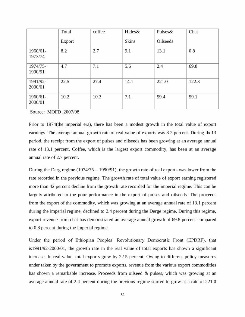
Table a).Average annual Growth rate of Export

Period Growth rate in total& Major component of Export

31

Total

Export

coffee Hides&

Skins

Pulses&

Oilseeds

Chat

1960/61-

1973/74

8.2 2.7 9.1 13.1 0.8

1974/75-

1990/91

4.7 7.1 5.6 2.4 69.8

1991/92-

2000/01

22.5 27.4 14.1 221.0 122.3

1960/61-

2000/01

10.2 10.3 7.1 59.4 59.1

Source: MOFD ,2007/08

Prior to 1974(the imperial era), there has been a modest growth in the total value of export

earnings. The average annual growth rate of real value of exports was 8.2 percent. During the13

period, the receipt from the export of pulses and oilseeds has been growing at an average annual

rate of 13.1 percent. Coffee, which is the largest export commodity, has been at an average

annual rate of 2.7 percent.

During the Derg regime (1974/75 – 1990/91), the growth rate of real exports was lower from the

rate recorded in the previous regime. The growth rate of total value of export earning registered

more than 42 percent decline from the growth rate recorded for the imperial regime. This can be

largely attributed to the poor performance in the export of pulses and oilseeds. The proceeds

from the export of the commodity, which was growing at an average annual rate of 13.1 percent

during the imperial regime, declined to 2.4 percent during the Derge regime. During this regime,

export revenue from chat has demonstrated an average annual growth of 69.8 percent compared

to 0.8 percent during the imperial regime.

Under the period of Ethiopian Peoples’ Revolutionary Democratic Front (EPDRF), that

is1991/92-2000/01, the growth rate in the real value of total exports has shown a significant

increase. In real value, total exports grew by 22.5 percent. Owing to different policy measures

under taken by the government to promote exports, revenue from the various export commodities

has shown a remarkable increase. Proceeds from oilseed & pulses, which was growing at an

average annual rate of 2.4 percent during the previous regime started to grow at a rate of 221.0

32

percent. And the revenue from Chat export has been growing at an average annual rate of 122.3

percent. Such an increase in the value of export of these commodities is mainly attributed to a

very significant growth rate recorded during the period 1991/92-1992/93. Owing to the favorable

environment created after the prolonged war that prevailed in the country, the proceeds from

these commodities escalated very sharply from the period 1991/92 to 1992/93.

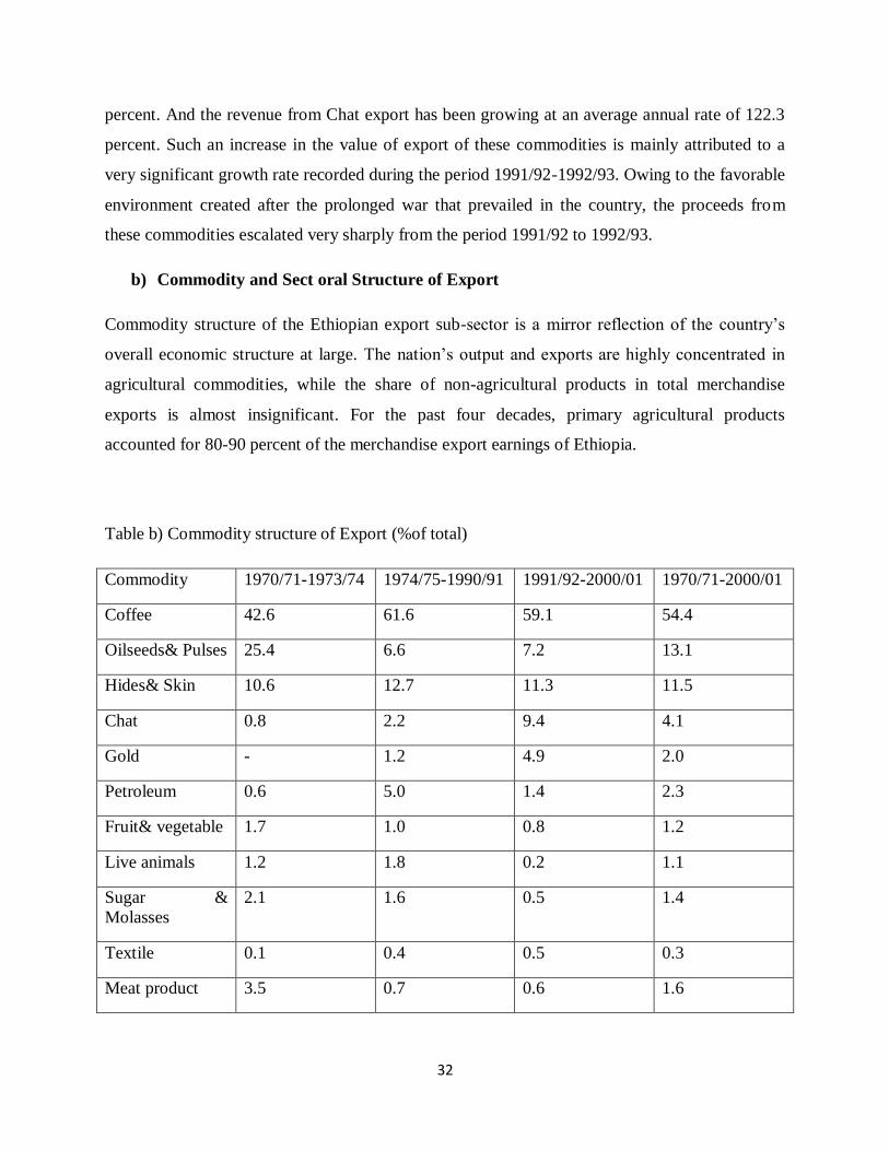
b) Commodity and Sect oral Structure of Export

Commodity structure of the Ethiopian export sub-sector is a mirror reflection of the country’s

overall economic structure at large. The nation’s output and exports are highly concentrated in

agricultural commodities, while the share of non-agricultural products in total merchandise

exports is almost insignificant. For the past four decades, primary agricultural products

accounted for 80-90 percent of the merchandise export earnings of Ethiopia.

Table b) Commodity structure of Export (%of total)

Commodity 1970/71-1973/74 1974/75-1990/91 1991/92-2000/01 1970/71-2000/01

Coffee 42.6 61.6 59.1 54.4

Oilseeds& Pulses 25.4 6.6 7.2 13.1

Hides& Skin 10.6 12.7 11.3 11.5

Chat 0.8 2.2 9.4 4.1

Gold - 1.2 4.9 2.0

Petroleum 0.6 5.0 1.4 2.3

Fruit& vegetable 1.7 1.0 0.8 1.2

Live animals 1.2 1.8 0.2 1.1

Sugar &

Molasses

2.1 1.6 0.5 1.4

Textile 0.1 0.4 0.5 0.3

Meat product 3.5 0.7 0.6 1.6

33

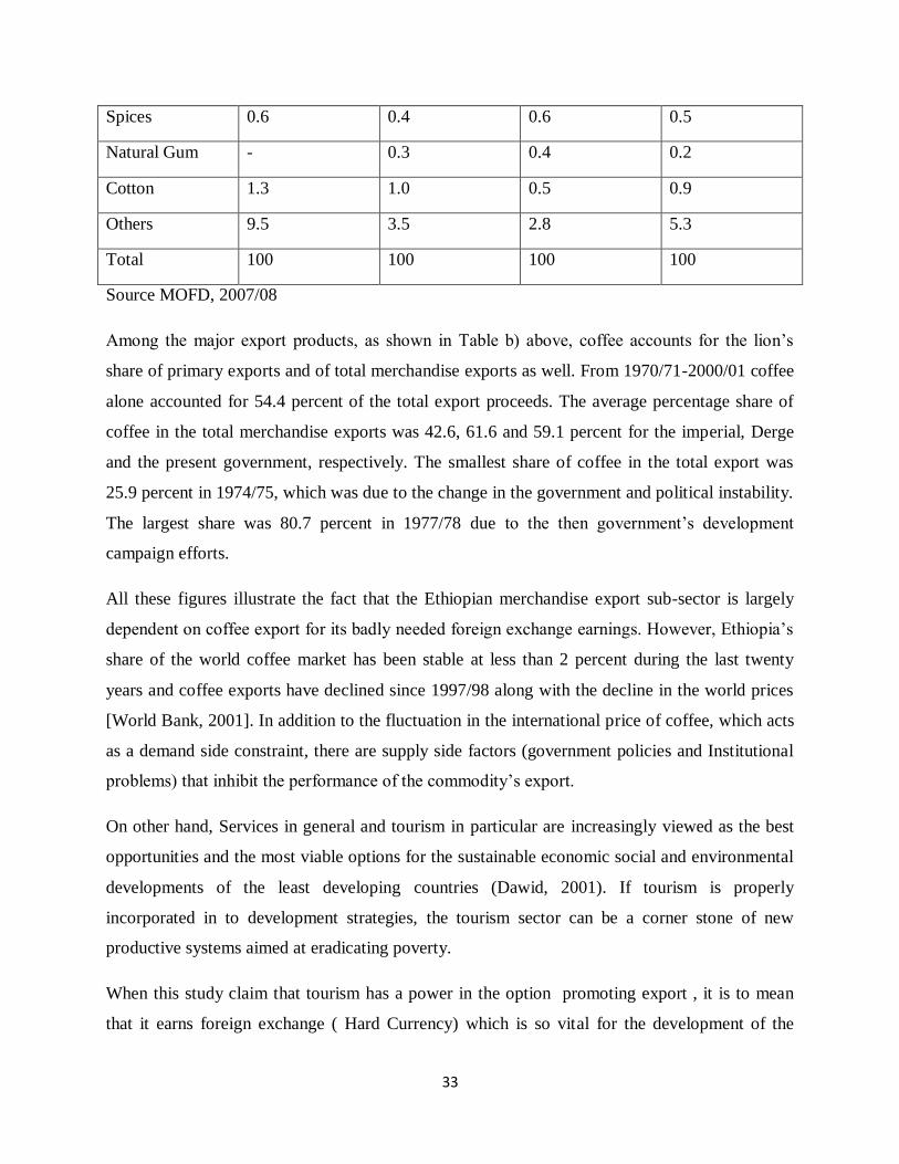
Spices 0.6 0.4 0.6 0.5

Natural Gum - 0.3 0.4 0.2

Cotton 1.3 1.0 0.5 0.9

Others 9.5 3.5 2.8 5.3

Total 100 100 100 100

Source MOFD, 2007/08

Among the major export products, as shown in Table b) above, coffee accounts for the lion’s

share of primary exports and of total merchandise exports as well. From 1970/71-2000/01 coffee

alone accounted for 54.4 percent of the total export proceeds. The average percentage share of

coffee in the total merchandise exports was 42.6, 61.6 and 59.1 percent for the imperial, Derge

and the present government, respectively. The smallest share of coffee in the total export was

25.9 percent in 1974/75, which was due to the change in the government and political instability.

The largest share was 80.7 percent in 1977/78 due to the then government’s development

campaign efforts.

All these figures illustrate the fact that the Ethiopian merchandise export sub-sector is largely

dependent on coffee export for its badly needed foreign exchange earnings. However, Ethiopia’s

share of the world coffee market has been stable at less than 2 percent during the last twenty

years and coffee exports have declined since 1997/98 along with the decline in the world prices

[World Bank, 2001]. In addition to the fluctuation in the international price of coffee, which acts

as a demand side constraint, there are supply side factors (government policies and Institutional

problems) that inhibit the performance of the commodity’s export.

On other hand, Services in general and tourism in particular are increasingly viewed as the best

opportunities and the most viable options for the sustainable economic social and environmental

developments of the least developing countries (Dawid, 2001). If tourism is properly

incorporated in to development strategies, the tourism sector can be a corner stone of new

productive systems aimed at eradicating poverty.

When this study claim that tourism has a power in the option promoting export , it is to mean

that it earns foreign exchange ( Hard Currency) which is so vital for the development of the

34

tourist destination countries. In the case of tourism, the customer visits the country to consume

the product. The problem of market access which usually happens in so many of the other

products does not exist here in tourism as it hardly encountered problems that other export

industries are experienced. More over it is free from any tariff or quota barriers due to the fact

that the consumers are meant to be there personally.

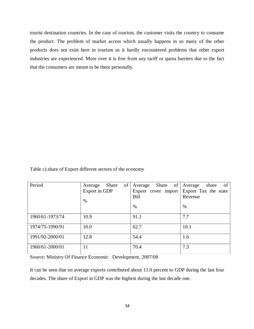
Table c).share of Export different sectors of the economy

Source: Ministry Of Finance Economic Development, 2007/08

It can be seen that on average exports contributed about 11.0 percent to GDP during the last four

decades. The share of Export in GDP was the highest during the last decade one.

Period Average Share of

Export in GDP

%

Average Share of

Export cover import

Bill

%

Average share of

Export Tax the state

Revenue

%

1960/61-1973/74 10.9 91.1 7.7

1974/75-1990/91 10.0 62.7 10.1

1991/92-2000/01 12.8 54.4 1.6

1960/61-2000/01 11 70.4 7.3

35

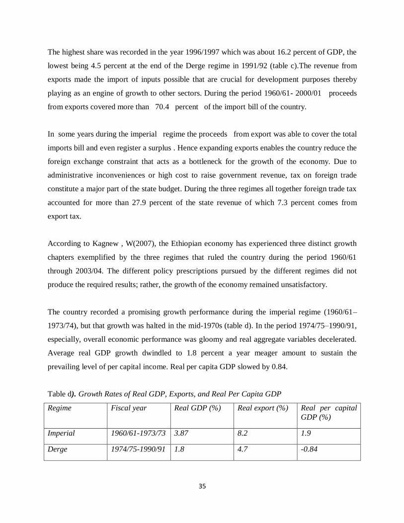
The highest share was recorded in the year 1996/1997 which was about 16.2 percent of GDP, the

lowest being 4.5 percent at the end of the Derge regime in 1991/92 (table c).The revenue from

exports made the import of inputs possible that are crucial for development purposes thereby

playing as an engine of growth to other sectors. During the period 1960/61- 2000/01 proceeds

from exports covered more than 70.4 percent of the import bill of the country.

In some years during the imperial regime the proceeds from export was able to cover the total

imports bill and even register a surplus . Hence expanding exports enables the country reduce the

foreign exchange constraint that acts as a bottleneck for the growth of the economy. Due to

administrative inconveniences or high cost to raise government revenue, tax on foreign trade

constitute a major part of the state budget. During the three regimes all together foreign trade tax

accounted for more than 27.9 percent of the state revenue of which 7.3 percent comes from

export tax.

According to Kagnew , W(2007), the Ethiopian economy has experienced three distinct growth

chapters exemplified by the three regimes that ruled the country during the period 1960/61

through 2003/04. The different policy prescriptions pursued by the different regimes did not

produce the required results; rather, the growth of the economy remained unsatisfactory.

The country recorded a promising growth performance during the imperial regime (1960/61–

1973/74), but that growth was halted in the mid-1970s (table d). In the period 1974/75–1990/91,

especially, overall economic performance was gloomy and real aggregate variables decelerated.

Average real GDP growth dwindled to 1.8 percent a year meager amount to sustain the

prevailing level of per capital income. Real per capita GDP slowed by 0.84.

Table d). Growth Rates of Real GDP, Exports, and Real Per Capita GDP

Regime Fiscal year Real GDP (%) Real export (%) Real per capital

GDP (%)

Imperial 1960/61-1973/73 3.87 8.2 1.9

Derge 1974/75-1990/91 1.8 4.7 -0.84

36

EPRDF 1991/92-2003/04 5.92 23.58 0.84

Average 1960/61-2003/04 4.21 13.04 0.41

Source MOFD,2010/11

Note: EPRDF = Ethiopian People’s Revolutionary Democratic Front; GDP = gross domestic

product.

Nation grew at about 2.8 percent annually. The ratios of government revenue and government

expenditure to GDP were 22.0 percent and 30.2 percent, respectively. This deceleration in the

economy compelled the country to resort to both domestic and foreign borrowing to finance the

mounting fiscal deficit. Large decelerations of per capital income were recorded in 1984/85 as a

result of drought/famine. In 1990/91, such decelerations were attributed to civil war and political

instability. The average growth of real GDP in the periods 1960/61–1973/74 and 1991/92–

2003/04 was 3.87 percent and 5.92 percent, respectively.

In 1992, Ethiopia embarked on a reform package intended to reverse deteriorating economic

conditions and to put the economy on a sustainable growth trajectory. Since that time, the

government has contained spending, reduced tariffs and military expenditures, improved tax

collection, reformed the investment code and the tax laws, and introduced a market-based system

to allocate urban land. It has made an effort to stimulate private sector development by launching

a privatization process and establishing a number of agencies to facilitate privatizing.

In 2008, however, the economy remains weak and sensitive to shocks, specifically drought and

commodity price instability. Real GDP skyrocketed to 7.7 percent in 2000/01, but then it

staggered at a rate of 1.2 percent in fiscal year 2001/02 and constricted by about 3.8 percent in

2002/03. Following the 2002/03 drought, agricultural production value added dropped by

12.2percent because of a 25.0 percent fall in the production of cereals, pulses, and oilseeds. Poor

growth performance in 2001/02 and the fall of agricultural production in 2002/03 caused the

average real GDP growth for the period 1997/98–2002/03 to decelerate to 2.5 percent.

c) Time Series Studies

Tyler (1981), taking a sample of 55 middle-income economies, found a positive and significant

relationship between export and income growth. Girma (1982), carried out country specific

regression analysis for Ethiopia by incorporating GDP as the dependent variable and exports as

37

the only explanatory variable. His results indicated that GDP and exports are highly correlated

with correlation coefficient of 0.962 and the coefficient of determination (R ) was 0.81.

However, his work didn’t consider the effect of other important variables that could

significantly influence economic growth.

Feder (1983) developed an analytical framework to test the export-growth relationship for 31

semi-industrial, less-developed countries, using the following variables: investment as a share of

income, rate of growth of the labor force, and rate of growth of exports (times exports as a share

of GDP). He incorporated the possibility that the marginal factor productivities are not equal in

the export and non export sectors of the economy. The regression coefficient of the export

variable was statistically highly significant. This finding led him strongly to support the

hypothesis that marginal factor productivities are higher in the export sector than in the non

export sector. Kavoussi (1984) considered 73 middle- and low-income developing countries and

found a Strong effect of export growth on output growth in both sets of countries. The effects,

however, tended to diminish according to the level of development.

According to Jung and Marshal (1985), interpretation is questionable since these regressions

provide no means of determining the direction of causality. They criticize the usual approach that

most of the studies followed (regressing real growth on contemporaneous real export growth)

and to infer support for the proposition that export growth causes output growth from the

significance of the export growth coefficient.

According to them, such an approach contains a serious methodological weakness. Although the

hypothesis of export promotion clearly implies a correlation between export and real GNP

growth, an equally plausible hypothesis is that output growth causes export growth. To

substantiate their argument they perform causality test between export and economic growth for

37 developing countries. The time series results for the countries considered provided

evidence in favor of export promotion in only four instances. Even countries like Korea,

Taiwan and Brazil whose tremendous growth was largely attributed to export growth provided

no statistical support for the export-led growth hypothesis. This strongly suggests that the

evidence in favor of export promotion is weaker than previous studies have indicated.

38

Esfahani (1987), also employed a simultaneous equation model to deal with simultaneity

problem between GDP and export growth. According to his results the positive relationship

between export and economic growth has been mainly due to the contribution of exports to the

reduction of import shortages which restrict the growth of many LDCs. Hence he tested the

export-growth relationship for a sample of 31 semi-industrialized countries from 1983-1987

using the simultaneous equation framework. His main finding was that

Other country specific studies were also conducted to test the export-growth relationship. One

of the country specific time series studies undertaken is that of Rati (1987) for a group of 88

LDCs including Ethiopia. In his study he provided estimates of two models of the export-growth

linkage for the period 1960-82. From the regression result, although coefficients of the export

variables in the two models are not significant, they have the expected sign. The weak statist ical

significance could be mainly due to the small sample size and the problem in the econometric

technique applied. In his study on the impact of exports on economic growth for Eastern and

Southern Africa countries.

Although a positive and significant relationship does emerge for slightly more than 50% of the

countries considered for majority of them the coefficients are significant at the 10% level. All of

the above studies both from cross sectional and time series have found a significant positive

impact of exports on economic growth. These studies have interpreted results in regressions

of output variables on export variables as providing support for an export promotion

development strategy.

Chow (1987), investigated the causal relationship between export growth and industrial

development during the 1960s and 1970s for eight newly industrialized countries (NIC). The

result of Sims’s causality test indicated that for most of the NICs there is a strong bi-

directional causality between the growth of exports and industrial development. He

concluded that depending on the size of the domestic market, export growth can cause

industrialization, either unidirectional, or bidirectional by influencing the development of

manufacturing industries.

Furthermore, Dodaro (1993) employed individual country time-series analysis to establish the

direction of causality between export growth and real output growth. The causality test offers a

39

very weak support for the contention that export growth promotes GDP growth. Support for the

alternate contention that GDP growth promotes export growth is also weak. Hence the evidence

is weak with respect to the alternate notion of trade as an “engine of growth” and suggests the

need to reconsider the whole relationship between exports and economic growth within the

context of LDCs.

According to Bahmani and Alse (1994), there are three major shortcomings associated with all

the time-series studies just stated?

First, growth of manufacturing industries in LDCs as a proxy for industrial development. Co

integrating properties of the variables considered. The standard Granger and Sims tests are valid

only if the time series involved are not co integrated.

Second, most economic variables like GDP and exports are non stationary which result in

spurious regression. Finally, because lack of quarterly data most of the previous studies used

annual data. If the time delay between cause and effect is small compared to the time interval

over which data is collected, however, the lack of causation could be the result of temporal

aggregation.

Accordingly, they used an alternative test for Granger causality, which is based on error-

correction models that incorporated information from the co integrated properties of the variables

involved. Using this approach they performed causality test for 9 developing countries based on

quarterly data for the period 1973I-1988IV. The results indicated that in contrast to the previous

studies when the co integrating properties of the time series are incorporated into the analysis,

bi-directional causality between export growth and output growth receives strong empirical

support in almost all countries.

According to Amoateng and Adu (1996), the export-driven economic growth hypotheses

have provided mixed results in a bi variant causality framework. The main shortcoming with the

bi variant causality analysis is the omission of other relevant variables, which could bias the

results. Hence, they introduced foreign debt service as a third variable within a tri variant

causality analysis of exports and economic growth for 35 African Countries for the period1971-

1990. They found that there is a joint feedback effect between export revenue, external debt

service and economic growth. Their main finding is that in the period 1971-90 both the export-

40

driven output growth and output growth-led export promotion hypothesis have found a strong

empirical support. For the sub-period 1983-90, however, the structural adjustment programs,

which removed economic distortions, promoted exports and encouraged repayment of the

external debt, which resulted in economic growth in the countries considered. Other

methodological frameworks have been developed by some authors to examine the relationship

between export and economic growth.

Thornton (1996), used Engle-Granger co integration and Granger causality tests in a two-

variable framework and found a positive and significant causal relationship running from exports

to economic growth in the case of Mexico. Amoateng and Amoako-Adu (1996) ran causality

tests for 35 African countries by introducing foreign debt service as a third variable within a

trivariant causality analysis of exports and economic growth. Their results showed a joint

feedback effect between export revenue, external debt service, and economic growth. The study

of Doraisami (1996) strongly supported bidirectional causality between exports and growth in

Malaysia.

Al-Yousif (1997), employed time-series analysis for four Arab Gulf countries, and the results

supported the hypothesis in the short-run but failed to find a long-run relationship (that is, did not

find co integration). Begum and Shamsuddin (1998), conducted a study of Bangladesh, and their

results indicated that exports could induce economic growth. Shan and Sun (1998) established a

vector autoregressive model in the production function context in a study of China. Finding a

bidirectional relationship, they rejected the unidirectional export-led growth hypothesis.

Nonetheless, they did find that both exports and industrial output contribute positively to each

other in China.

Begum& Shamsuddin (1998), have tested the relationship for Bangladesh for 1961-92. They

employed the ‘“Feder type”’ production function in their analysis. Their main finding was that

the sum of the productivity differential and externality effects of the export sector is positive

implying that reallocation of resources from the non-export to export sector will enhance the

productive capacity of the economy. Therefore through this effect export growth can induce

output growth.

41

Kedir (1998), estimated two models (conventional and "Feder type") of the export-growth

relationship for Ethiopia. His result confirmed a positive and significant impact of exports on

economic growth in both models. Furthermore, he run the Granger non-causality test to see the

direction of causality and found out that the positive association runs from exports to economic

growth. One immediate comment on the methodology and results is that he did not take into

account for the co integrating properties of the variables considered in the Johansen framework.

He used growth rate of the variables and hence the regression result conveys information only

about the short run dynamics. In addition, the Granger causality test did not consider the

possibility that exports and economic growth are co integrated and hence the results could be

biased. The sample size considered (1967-94) could be small to give reliable estimates. In sum,

all of the above empirical studies reviewed so far indicated that the export-economic growth

linkage is an unsettled issue that needs further investigation. Although most of the cross sectional

studies indicated that the export-economic growth nexus is predominantly positive and

significant the time series studies cast some doubt about the existence of such a relationship.

Erfani (1999) examined the causal relationship between economic performance and exports over

the period of 1965 to 1995 for several developing countries in Asia and Latin America. The

result showed the significant positive relationship between export and economic growth. This

study also provides the evidence about the hypothesis that exports lead to higher output.

Chang et al. (2000) used multivariate causality analysis incorporating imports as a factor in the

relationship between exports and output in their study of Taiwan (China). They found no support

for the export-led growth hypothesis during the period of rapid growth there (1971–95).

Nidugala (2001), using an augmented production function with export as the regress or in a study

of India, found a significant positive impact of export growth on output growth. The results

further revealed that the growth of manufactured exports had a significant positive relationship

with output growth, whereas growth of primary exports had no such influence.

Michael (2002) examined the relationship between exports, imports, and income in the economy

of Trinidad and Tobago, using Granger causality and error correction modeling. His analysis

confirmed that incomes in Trinidad and Tobago are Granger-caused by the growth of exports .A

boom in petroleum exports caused increased income and spending in the non tradable sector of

42

the economy. The results further indicated bidirectional causality between exports and imports, a

long-term bidirectional causality between imports and GDP, and unidirectional Granger

causation from exports to GDP.

Thungswan and Thompson (2002) examined the causality between exports and income in

Thailand between 1969 and 1995, using co integration and error correction models. Their results

clearly supported the export-led growth hypothesis for agricultural exports. For manufacturing

exports, they found evidence of bidirectional causality supporting both export-led growth and the

growth-driven export hypothesis; manufacturing exports had a slightly stronger effect on

absorption than did agricultural exports.

According to Debel (2002), investigated the effect of exports on economic growth in Ethiopia for

the period 1960/61-2000/01.Many researcher show Export expansion brings Economic growth

through alleviating import shortages faced by the country. Although, the results these studies are

somewhat mixed, predominately a positive and significance relationship b/n export and

economic growth is observed.

Keong, Yusop, and Liew (2003) ran a vector autoregressive model and multivariate co

integration for Malaysia and found a long-run association between the variables considered. The

results of the error correction model revealed that export, Granger caused economic growth in

the short run, and that led them to confirm the validity of the export-led growth hypothesis in

Malaysia, both in the short run and over the long term.

Shirazi (2004) studied the short run and long run relationship among real export, real import and

economic growth on the basis of co-integration and multivariate Granger causality developed

for the period 1960 to 2003.This study showed a long-run relationship among export and

economic growth and found unidirectional causality from export to output .

Mah (2005) studied the long-run causality between export and growth with the help of

significance of error correction term, ECt-1. This study also indicated that export expansion is

insufficient to explain the patterns of real economic growth.

Tang (2006) stated that there is no long run relationship among export, real Gross Domestic

product and imports. This study further shows no long-run and short-run causality between

43

export expansion and economic growth in China on the basis of Granger causality while

economic growth does Granger-cause imports in the short run.

Jordaan (2007) analyzed the causality between exports and GDP of Namibia for the period 1970

to2005. The hypothesis of growth led by export is test through Granger causality and co

integration. It tests whether there is uni-directional or bi-direction causality between export and

GDP. The results revealed that exports Granger cause GDP and GDP per capita and suggested

that the export-led growth strategy through various incentives has a positive influence on growth.

According to Kagnew .W (2007), examine export performance and economic growth in Ethiopia

during period1960/61-2003/04 using multivariate time-series approach with in production frame

work. The result show in these research export expansion brings economic growth in various

way but the pattern is still dominate by traditional produce and more on coffee whose world

price is fluctuating. One immediate comment on the methodology and results is that he did not

take into account the Granger causality test consider the possibility that exports and economic

growth are co integrated and hence the results could be biased.

Ullah et al (2009) investigated Export-led-growth by time series econometric techniques (Unit

root test, Co-integration and Granger causality through Vector Error Correction Model) over the

period of 1970 to 2008 for Pakistan. In this paper, the results reveal that export expansion leads

to economic growth. They also checked whether there is uni-directional between economic

growth& real exports. The traditional Granger causality test suggests that there is uni-directional

causality between economic growth& exports .

Elbeydi, Hamuda and Gazda (2010) investigated the relationship between exports and economic

growth for Libya for the period 1980 to 2007. The findings indicate that there exists a long-run

bi-directional causality between exports and income growth, and thus, the export promotion

policy contributes to the economic growth of Libya.

On the other hand Granger causality through vector error correction was checked with the help

of F-value of the model and t-value of the error correction term, which partially reconciles the

traditional Granger causality test.

44

In sum, all of the above empirical studies reviewed so far indicated that the export-economic

growth linkage is an unsettled issue that needs further investigation. Based on the

methodological framework will be employed, these studies can be categorized into those that

using linear multiple equation model (OLS) estimation (time series) causality test models.

This study attempts to add to the existing literature by considering altogether the methodologies

employed so far. The export performance-economic growth will be studied using the Granger

causal test (1970-2012). Furthermore, to take care of the simultaneity problem that may arise

between exports and economic growth and to see the role that trade structures play in export

growth and economic growth, simultaneous equation model will also be estimated.

3. Methodology of the Study

The research method to employ in conducting this study is a descriptive survey and using time

series data analysis for the relationship between the export performance and economic growth

.The type of research in its nature is quantitative. To achieve the objectives set, the researcher

used secondary data. Apply mathematical and statically tests to 42 years annual data to quantify

and understand the nature of time (space) varying phenomena;

Gain physical understanding of the system.

Be able to predict the future behavior. So that the methodology consider the

following important steps.

45

3.1. Data Type and Sources

The research used secondary data limited from1970-2012. The data gathered mainly through

secondary written document as well as website of National Bank ,Central Statically Agency,

Ministry of Finance Economic Development, World Bank and journals bullets are presented

in tables and percentages calculated to draw meaningful conclusions and interpretations out of

the data.

The data sources is from NBE,CSA ,MOFED and WB reports data based, survey the theory

state about this and used the pillars of the policy, previous research related to Export

performance and economic growth , books, articles, internet web and journals.

3.2. Model specification

Most of the variables are related to quantitative type. The variables are (Real GDP, export,

import, investment, government expenditure, consumption Exchange rate, Labor, Balance of

payment).

Dependent and Independent Variables Classifications:

Dependent variable: Real GDP

Independent variables, such as Export, Import, Investment, Government expenditure, and

Consumption)

proxy variables ( Balance of payment, Labor, Exchange rate)

Based on the theoretical and empirical review considerations the following model was specified

by using OLS estimation techniques.

According to Henderson & Pool (1991), to measure GDP used Expenditure approach was the

Model of this research.

The mathematical expression of the model was given as follows

GDP= f(C, I, G, X, M)

GDP(Y)= C+I+G+X-M

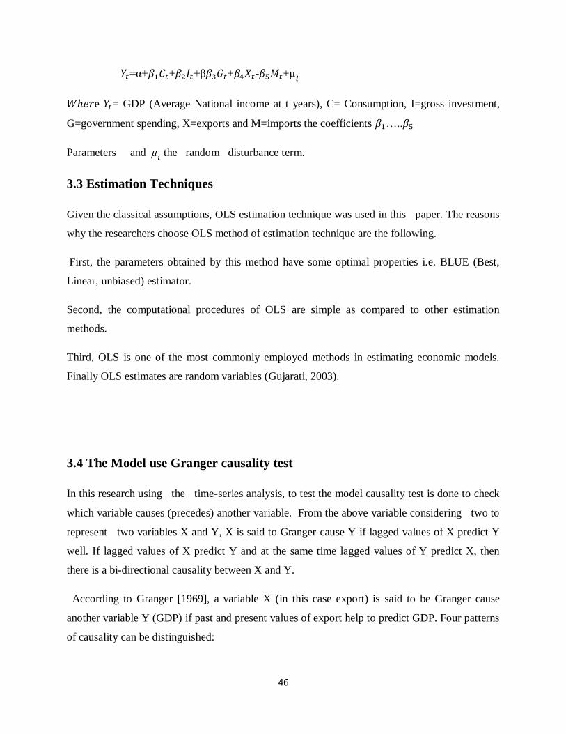
46

=α+ + +β + - +

e = GDP (Average National income at t years), C= Consumption, I=gross investment,

G=government spending, X=exports and M=imports the coefficients …..

Parameters and the random disturbance term.

3.3 Estimation Techniques

Given the classical assumptions, OLS estimation technique was used in this paper. The reasons

why the researchers choose OLS method of estimation technique are the following.

First, the parameters obtained by this method have some optimal properties i.e. BLUE (Best,

Linear, unbiased) estimator.

Second, the computational procedures of OLS are simple as compared to other estimation

methods.

Third, OLS is one of the most commonly employed methods in estimating economic models.

Finally OLS estimates are random variables (Gujarati, 2003).

3.4 The Model use Granger causality test

In this research using the time-series analysis, to test the model causality test is done to check

which variable causes (precedes) another variable. From the above variable considering two to

represent two variables X and Y, X is said to Granger cause Y if lagged values of X predict Y

well. If lagged values of X predict Y and at the same time lagged values of Y predict X, then

there is a bi-directional causality between X and Y.

According to Granger [1969], a variable X (in this case export) is said to be Granger cause

another variable Y (GDP) if past and present values of export help to predict GDP. Four patterns

of causality can be distinguished:

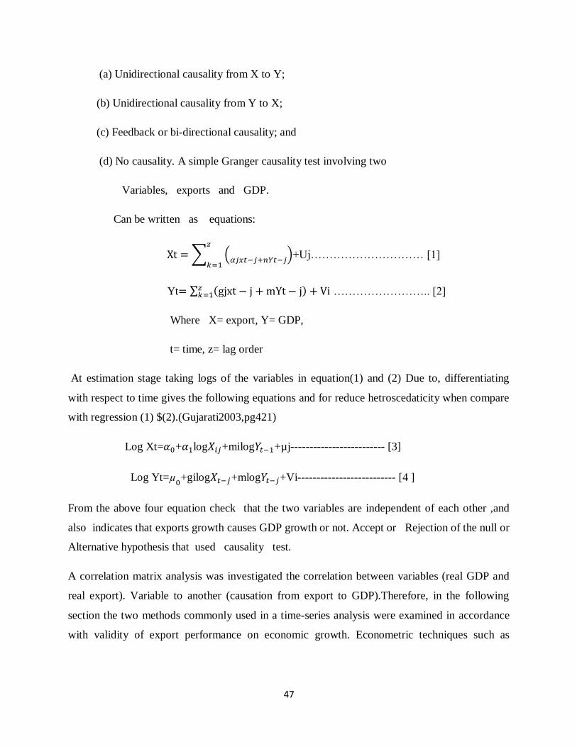
47

(a) Unidirectional causality from X to Y;

(b) Unidirectional causality from Y to X;

(c) Feedback or bi-directional causality; and

(d) No causality. A simple Granger causality test involving two

Variables, exports and GDP.

Can be written as equations:

+Uj………………………… [1]

Yt …………………….. [2]

Where X= export, Y= GDP,

t= time, z= lag order

At estimation stage taking logs of the variables in equation(1) and (2) Due to, differentiating

with respect to time gives the following equations and for reduce hetroscedaticity when compare

with regression (1) $(2).(Gujarati2003,pg421)

Log Xt= + log +milog +µj------------------------- [3]

Log Yt= +gilog +mlog +Vi-------------------------- [4 ]

From the above four equation check that the two variables are independent of each other ,and

also indicates that exports growth causes GDP growth or not. Accept or Rejection of the null or

Alternative hypothesis that used causality test.

A correlation matrix analysis was investigated the correlation between variables (real GDP and

real export). Variable to another (causation from export to GDP).Therefore, in the following

section the two methods commonly used in a time-series analysis were examined in accordance

with validity of export performance on economic growth. Econometric techniques such as

48

stationary test and Granger causality test was employed to find short-run relationship, long-run

relationship, and direction of causality between export performance and economic growth.

3.5 Data Analysis and interpretation

The Research was test classical OLS assumptions (Stationarity, heteroscedasticity, &

autocorrelation) using STATA & SPSS software, and econometrics model estimation of betas.

A. Unit Root Tests

Unit root tests will be conduct first, with real GDP and real export as the time series variables.

These variables must be stationary or co -integrate in order to avoid a spurious regression

situation and to ensure whether they are stationary or not. Augmented Dickey–Fuller (ADF) test

was conduct with critical value of 5% and 10% apply for test. The test of result based on of the

unit root test for Ethiopian annual data(1970-2012) on two series (real GDP and real export) .The

ADF test result indicate that the two series are non-stationary at levels, i.e., the results was fail

to reject the null hypothesis. Thus, to correct for the presence of unit root in the series, first and

second difference measures have been taken.

On other hand, the results of the unit root tests in the first and second difference based on ADF

test shows that, the series was stationary in the first and second difference.

A. Granger Causality Test

The causal relationship between export and economic growth of the country was analyze with

the application of Granger (1969) causality test using annual data for the period 1970 to 2012.

It indicates the hypothesis that export performance expansion Granger causes GDP is accept

null hypothesis, while the hypothesis that GDP does not Granger causes an export is reject.

These results provide evidence of bi-directional causality between export and GDP. This

implies that export growth causes economic growth and /or the reverse true.

49

4. Result and Discussion

4.1. Descriptive Statistics Analysis

A correlation matrix analysis Table (1a) was performed to investigate the correlation between

variables (real GDP and real export). The results illustrated a significant and strong positive

correlation between variables with two lags. However, strong correlation does not imply

causation from one variable to another (causation from export to GDP or vice verse).

Table.1a Correlations matrix Between GDP & Export

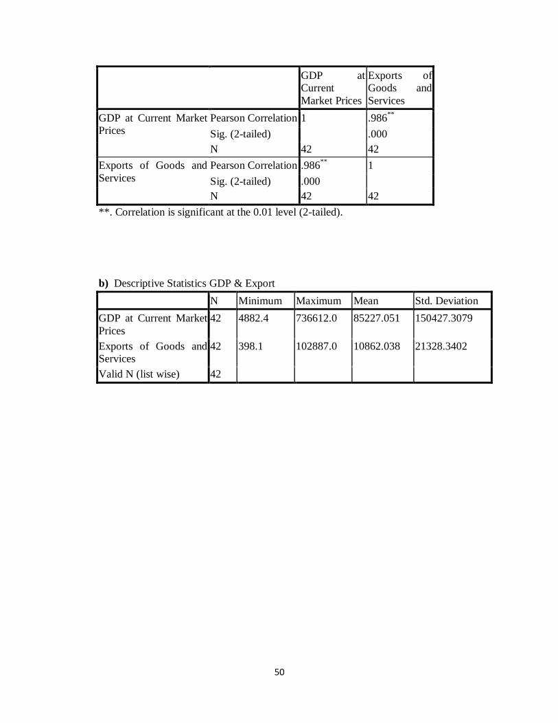
50

GDP at

Current

Market Prices

Exports of

Goods and

Services

GDP at Current Market

Prices

Pearson Correlation 1 .986**

Sig. (2-tailed) .000

N 42 42

Exports of Goods and

Services

Pearson Correlation .986**

1

Sig. (2-tailed) .000

N 42 42

**. Correlation is significant at the 0.01 level (2-tailed).

b) Descriptive Statistics GDP & Export

N Minimum Maximum Mean Std. Deviation

GDP at Current Market

Prices

42 4882.4 736612.0 85227.051 150427.3079

Exports of Goods and

Services

42 398.1 102887.0 10862.038 21328.3402

Valid N (list wise) 42

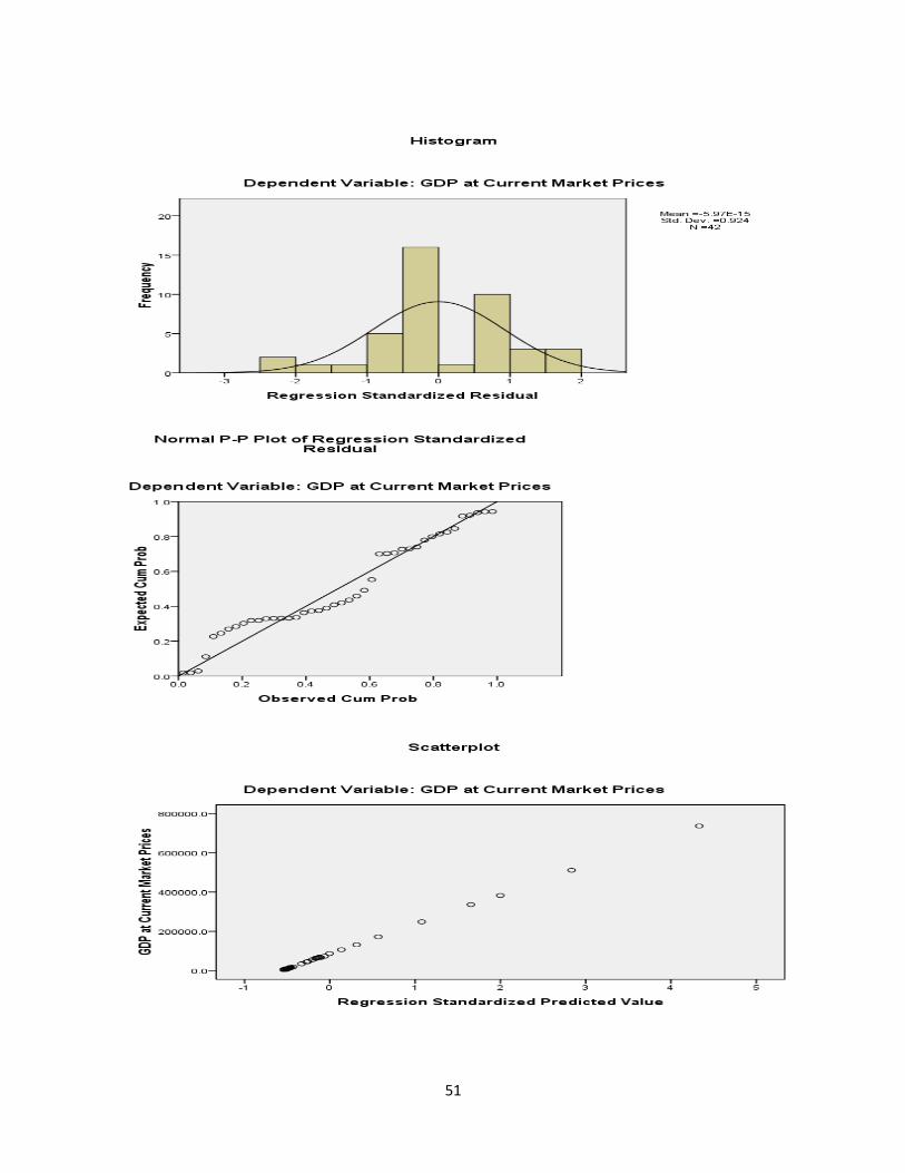
51

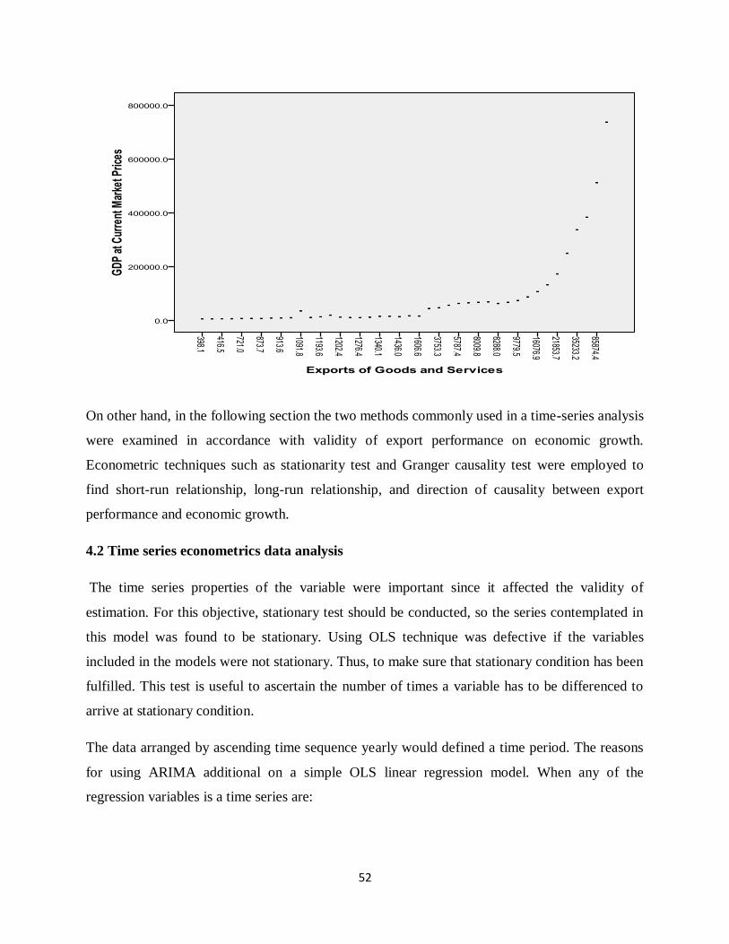
52

On other hand, in the following section the two methods commonly used in a time-series analysis

were examined in accordance with validity of export performance on economic growth.

Econometric techniques such as stationarity test and Granger causality test were employed to

find short-run relationship, long-run relationship, and direction of causality between export

performance and economic growth.

4.2 Time series econometrics data analysis

The time series properties of the variable were important since it affected the validity of

estimation. For this objective, stationary test should be conducted, so the series contemplated in

this model was found to be stationary. Using OLS technique was defective if the variables

included in the models were not stationary. Thus, to make sure that stationary condition has been

fulfilled. This test is useful to ascertain the number of times a variable has to be differenced to

arrive at stationary condition.

The data arranged by ascending time sequence yearly would defined a time period. The reasons

for using ARIMA additional on a simple OLS linear regression model. When any of the

regression variables is a time series are:

53

The fact that the value of a variable in period is typically related to lagged.

The lagged values of the dependent variable can function as independent variable.

Omitting them may cause an omitted variable bias.

From the general knowledge, it is ovices that the value at any period in a time series is related to

its values in previous time period. So that using lagged value necessary condition. Before this, to

checked the general model of the research using STATA 11 the following result were happen.

Regress GDP =α+ + +β + - + ----------------- [1.1]

To reduce hetroscadacity used ln of each variable.

lnGDP =α+ + + + - + -------------------[1.2]

The result shown the following equation

GDP =0.557+ + + + - + -------------- [1.2a]

(t) Value (9.15) (50.61) (8.94) (8.9) (3.53) (-6.7)

The result of regress the general model reveal that all parameters such as F- value, R- square

=0.99& Adjusted R -square- =0.99, t- significance, p- value all Zero and test such as stationarity

,hetroskedaticity,& auto correlation in all the values showed that statistical significant at, 90%,

95% &99%confidence interval.

The reasons that R –square & adjusted R-square.99 Because of:

i. The data used large No of observation (42 years) greater than 30 R value must

more have been explain the model.

ii. The researcher selected model theoretically the principle of Economics i.e GDP

=C+G+I+X-M is valid also empirically.

iii. All variables t- value& p-value statically significant, |t| greater than two.

iv. The individual variable test R- square less than the model i.e GDP to export into

lagged were .90 mean less explain compare to the model.

54

Interpretation :Equation the model indicate that increase by 1 unit increase by each

β’s times mean 0.83,0.15,0.12,&0.064 decrease0.17 .From this we can understand that there is

positive relationship between Export and Economic growth.

4.3 Diagnostic test

In this section, the validity of the model has been tested

Stationarity Test

The existence of unit root test is formally checked by ADF and PP tests used OLS modeling

approach. If the absolute value of calculated test statistics were less than that of critical values

(higher P-value) indicates reject the null hypothesis of non-stationarity of the variable while the

absolute value of calculated statistics are greater than that of the critical values (Lower P-value)

indicates confidently to Accept the null-hypothesis i.e. stationary of the variable .

The result showed ADF that calculated test statistics were greater than the critical value. It reveal

to accept the null –hypothesis.

When we seen ADF test the value GDP calculated test statistics is absolute value 16.15,at the

three point of critical values are -3.64,-2.95,-2.61 with 1%,5%,10% respectively. While Export

test statistics is 6.27 and the critical values within the same order -3.64,-2.95 & -

2.61respectivelly.

Moreover, Phillips-perron for test for unit root reveal outcomes for both GDP & export the same

value were calculated test statics at Z (rho), 14.46 & Z (t), 10.09 and the critical value at 1%,5%,

and 10% respectively were for the Z(rho),-18.28,-13.01&-10.52 as well as for Z(t) -3.64,-3.95 &-

2.61. According to this we should understand that at Z(rho) except 1% critical value accept the

null hypothesis . Therefore Z(t) all the calculated test statics greater than critical value the

accept the null hypothesis.

Autocorrelation Test

Autocorrelation is the situation where the value Ut (the random term at time t) is correlated with

(depends up on) its previous value. Researcher used alternative Ramsey RESET test to check

whether there is autocorrelation in the model or not.

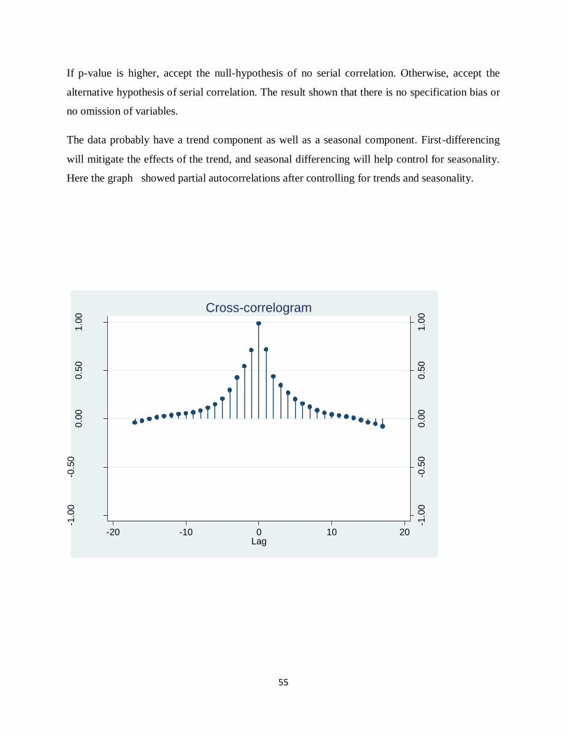
55

If p-value is higher, accept the null-hypothesis of no serial correlation. Otherwise, accept the

alternative hypothesis of serial correlation. The result shown that there is no specification bias or

no omission of variables.

The data probably have a trend component as well as a seasonal component. First-differencing

will mitigate the effects of the trend, and seasonal differencing will help control for seasonality.

Here the graph showed partial autocorrelations after controlling for trends and seasonality.

-1.0

0-0

.50

0.0

00.5

01.0

0

-1.0

0-0

.50

0.0

00.5

01.0

0

Cro

ss-c

orr

ela

tions o

f E

xport

s_of_

Goods_and_S

erv

ices a

nd G

DP

_at_

Curr

ent_

Mark

et_

Prices

-20 -10 0 10 20Lag

Cross-correlogram

56

Hetroscedasticity Test

Heteroscedasticity is created when the distribution of Ut (error term) around the explanatory is

not constant (not constant variance). It signifies that the individual variance would be different.

The nature of the variance of the error term is judged via Breush-pagan test by using the decision

rule:-

-If P-value is lower and calculated chi-square value is greater than the critical chi-square, accept

the null hypothesis of constant variance (accept constant variance). The result reveal that there

was no a problem of heteroscedasticity on this regression result.

On other hand, The result have been seen the above regression most value were significance

value, but high R –square value .In regressing a time series variable on another time series

variables one often obtain a very high R square (in excess of 0.9) b/n two variables.(Gurati,2003

pp792).For reduced the problem used Granger causal test mean that the lagged Y(GDP)

influence in X( Export) significantly and the lagged X(Export) influence Y(GDP) significantly.

In other words researcher can jointly test if the estimated lagged coefficients in the two

regressions are different from zero with F-statistic. When we seen the causal relationship

between GDP & export performance used granger causality as shown below.

4.4 Granger Causality Test

Two ways lagged regression result showed that significance R –square. When saw the two

regression compare (Q-4.1&4. 2) GDP to Export, Export to GDP in both model the values

statically viable, but the level of co integration is strong to from GDP to Export than Export to

GDP. This study examined the current issue of accelerated economic growth in Ethiopia. The

causal relationship between export performance and economic growth of the country was

analyzed with the application of Granger [1969] causality test using annual data for the period

1970 to 2012. It revealed that closer scrutiny of export growth on economic growth to achieve a

sustained economic growth.

As, Export & GDP are co integrated, a VECM (vector error correction model could have the

following form in equation (1&2)

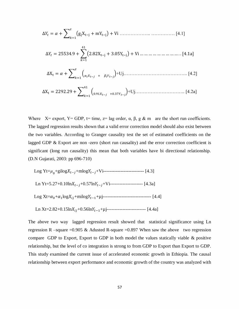
57

……………….. …………… [4.1]

+Uj………………………………….. [4.2]

+Uj………………………….. [4.2a]

Where X= export, Y= GDP, t= time, z= lag order, α, β, g & m are the short run coefficients.

The lagged regression results shown that a valid error correction model should also exist between

the two variables. According to Granger causality test the set of estimated coefficients on the

lagged GDP & Export are non -zero (short run causality) and the error correction coefficient is

significant (long run causality) this mean that both variables have bi directional relationship.

(D.N Gujarati, 2003: pp 696-710)

Log Yt= +gilog +mlog +Vi-------------------------- [4.3]

Ln Yt=5.27+0.10ln +0.57ln +Vi--------------------- [4.3a]

Log Xt= + log +milog +µj------------------------------- [4.4]

Ln Xt=2.82+0.15ln +0.56ln +µj------------------------- [4.4a]

The above two way lagged regression result showed that statistical significance using Ln

regression R –square =0.905 & Adusted R-square =0.897 When saw the above two regression

compare GDP to Export, Export to GDP in both model the values statically viable & positive

relationship, but the level of co integration is strong to from GDP to Export than Export to GDP.

This study examined the current issue of accelerated economic growth in Ethiopia. The causal

relationship between export performance and economic growth of the country was analyzed with

58

the application of Granger [1969] causality test. It revealed that closer scrutiny of export growth

on economic growth to achieve a sustained economic growth.

Interpretation: both two Questions shown that increase t by 1 increase t+1 by 0.1, 0.57 , 0.15

&0.56,mean that there is positive relationship between Export performance & Economic growth.

Chow (1987), investigated the causal relationship between export growth and Economic growth

result of granger causality test indicated that there is a strong bi- directional causality

between the growth of exports and industrial development( Economic growth). These

concluded that depending on the size of the domestic market, export growth can cause

industrialization bidirectional by influencing the development of manufacturing industries.

From this the causal relationship between export and economic growth of the country was

analyzed with the application of Granger (1969) causality test using annual data for the period

1970 to 2012. Above two questions indicates the hypothesis that export does not Granger causes

GDP is rejected, while the hypothesis that GDP does Granger causes an export is accepted.

These results provide evidence of bi-directional causality between export and GDP. This implies

that export growth causes economic growth and visceral is true. These provide evidence in

support of the export-led growth hypothesis and as well as the existence of reverse causality. The

findings also suggest that there is a need to promote export expansion policies in order to achieve

high economic growth. Correspondingly, there is also a need to devote resources on the

production of non-export goods in order to increase exports. The results of the pair wise Granger

causality test at different lag lengths (that is, Que-4.3a &4.4a) reveal that the causation is strong

from Export to GDP but less GDP to Export suggesting that export growth might affect output

growth through another channel (which could be discovered through additional research)

In multivariate time series analysis, causality test is done to check which variable causes

(precedes) another variable. Given two variables X and Y, X is said to Granger causality Y if

lagged values of X predicts Y well. If lagged values of X predict Y and at the same time lagged

values of Y predict X, then there is a bi-directional causality between X and Y.

Graphical test

59

. These reveal that the truthiness of empirical tests as well as the export growth& economic

growth trend positive relationship.

4.5 Co integration and The Error Correction Model (ECM)

Many macroeconomic time series are not stationary at levels and are most adequately

represented by first differences. Even though the individual time series are not stationary, a linear

combination of these variables could be stationary (i.e. they may be co integrated). If these

variables are co integrated, then they have a stable relationship and cannot move “too far” away

from each other.

In contrast lack of co integration suggests that such variables have no long run link, in principle

they can wonder arbitrarily far away from each other[Rao(1994)].There are two common

methods for testing co-integration and estimating the relationship among co-integrated variables.

These are the Engle- Granger (1969) and the Johansen's maximum likelihood methods.

In the Engle Granger methodology, the residuals from the long-run relationship are tested for

stationary to determine whether the variables are co integrated or not. The DF test could be

.1

.2

.3

.4

0 2 4 6 8

varbasic, lnGDP_at_Current_Market_Prices, lnGDP_at_Current_Market_Prices

95% CI orthogonalized irf

step

Graphs by irfname, impulse variable, and response variable

60

performed on the residuals to determine their order of integration. If the residuals do not appear

to be white noise, the ADF test can be used instead Testing for co-integration using the Engle-

Granger procedure has a number of weaknesses.

First the test for co integration is likely to have lower power against the alternative tests.

Second, its finite estimates of long-run relationship are potentially biased and third, inferences

cannot be drawn using standard t-statistics about the significance of the parameters of the long

run model [Harris (1995)]. In addition to the above the test procedure assumes that there is only

one co integration vector, when in fact there could be more, that is any linear combination of

these vectors is obtained when estimating a single equation.

The Johansen procedure takes care of the above shortcomings by assuming that there is multiple

co integrating vectors. The model was run export, import investment, consumption, &

Government expenditure most variables are positively related with output (results reported on the

appendix). However, import would have negative sign significant effects on economic growth.

The results suggest the need for enhancing Export and domestic investments, which currently are

low; to enhance sustainable development of the economy, and improves country’s trade balance,

owing to a shift in demand to goods produced locally from those produced abroad. These showed

that the need to shift the structure of both production and trade toward products with demand

elasticity and to high-value-added products.

The system permits us to capture the indirect impact of promoting exports in the accumulation of

foreign exchange that enables the economy to finance imports of capital goods which in turn

enhances economic growth. However, the finding that the estimated parameter of real import is

highly significant but of a negative sign indicates that much dependence on imports has

negatively affected the growth of the economy.

Growth of the GDP is an indicator of future potential and sustainability of production level. So

we expect positive impact of GDP growth on exports performance expansion. Real import tells

us that the rise in imports slows down economic growth by affecting the country’s international

reserves. It might result from the country having spent enormous amounts of foreign exchange to

purchase military armaments during the military regime.

61

Accordingly, a VECM was estimated, incorporating the short-run interactions and the speed of

adjustment toward long-run equilibrium. The short-run dynamics of the variables in the system

are influenced by the deviation from equilibrium. The model was run without the dummy. The

estimated results are reported here (t-ratios in parentheses).

The result confirms the hypothesis that exports positively and significantly affect the growth of

the Ethiopian economy. The literature relates dynamic technological spillover with manufactured

exportable products in that income-elastic goods have a larger effect on economic growth than

do agricultural goods. However, the results obtained in this study lead to skepticism of the

argument that a positive and significant link between exports and output growth is achieved only

when the country’s export basket is dominated by comparative advantage use natural resource, &

production as well as higher-value-added manufactured exports.

The results also showed that the export and economic growth link holds in the face of an inward-

oriented trade strategy. This study does not suggest that Ethiopia should continue exporting the

same traditional agricultural products that have been exported for decades. Rather, the study

strongly supports diversification of the economy away from low-value-added agricultural

products to manufactures. Diversifying the productive structure is a key strategy to foster

economic growth.

In empirical studies of exports and output growth, a major problem arises because exports are

component parts of the increase in output (Sharma and Panagiotidis 2004), and evidence found

in support of the export-led growth hypothesis could be biased by the built-in correlation

between exports and GDP. Estimating the model with other specifications not subject to this bias

(for example, by simultaneous method) may bring about a better result. There is a need, for

instance, to estimate the model (which was not attempted in this study) using the shares of

exports in GDP and investments in GDP as potentially endogenous variables in the system to

reconfirm the hypothesis.

No attempt was made to measure the extent to which the export sector is influenced by in Export

Performance and Economic Growth in Ethiopia internal supply factors and external factors. The

accuracy and consistency of data might have some effect on the validity of the results.

62

Since 1992, the economic growth policy of Ethiopian government was guided by the idea of

export-led growth. The view of export-led growth conceives growth of exports as having a

favorable impact on economic growth. According to this view, export expansion to foreign

markets improves resource allocation and production efficiency.

Export is claimed as the 'engine of growth'. The results of the study show that there is evidence

of bi-directional causality between export and economic growth for Ethiopia. Export growth

causes economic growth and vice verse true. Thus, the results are favorably comparable to those

obtained in the literature [Shan and Sun, 1998]. However, the idea of export-led growth was

anchored on the Washington consensus which emphasizes policies of trade liberalization,

privatization, market flexibility, capital mobility and fiscal austerity programs.

In the context of least developing countries these policies have been severely criticized. As

pointed out in the literature, the export-led growth paradigm shifted the focus away from

domestic market growth and placed emphasis on the international market in which developing

countries are found in “race-to-the-bottom” competition with each other. In countries where the

structural transformation has not yet realized shifting ever more output onto global markets can

distort development. Another criticism refers to the instability and fluctuation of the country’s

export earnings as a result of the competition among countries and downward price pressure.

Rivalry between countries at global markets often crowded as well as the limited type of export

base in terms number, quality & quantity in destination countries and unused comparative

advantage potentials such as using natural resource & tourism.

5. Conclusion and Recommendations

5.1. Conclusion

63

Much has been written in the literature regarding the role of the export sector in improving

economic growth. The purpose of this study was to investigate empirically the nexus of exports

and Economic growth in the Ethiopian context, using co integration by Granger causal test on

Export performance & Economic growth in year from 1970 to 2012. The study used Co

integration in granger causality time-series approach within considering real figures of GDP,

exports, consumption, gross capital formation(investment), imports, and Government

expenditure.

The inclusion of these other variables would prevent the estimates suffering from omitted-

variable bias. Consistent with expectations, export growth and Economic growth were positively

related, which supports the export expansion positive impact on economic growth hypothesis.

Ethiopia is one of the poorest countries on the African continent, despite its massive productive

land and abundant resources with immense potential for development. The fact that Ethiopia,

albeit endowed with plenty of natural and water resources, is one of the poorest countries seems

paradoxical and suggests the need to bring about a green revolution. To this end, long- and short-

term measures need to focus on developing and using water resources for agriculture, energy,

and other purposes. For a country with the largest livestock population in Africa, the production

of semi processed and finished leather products are insufficient and the tanning and leather

industry runs at partial capacity because the supply of hides and skins is inadequate but

optimistic starting using know.

The textile industry also runs at partial capacity, although the country has the capacity for high-

quality and large-volume domestic cotton production and there is a relatively cheap labor force.

Because of this under-capacity utilization of the textile industry, the country has failed to

capitalize on the opportunities offered by the U.S. African Growth Opportunities Act.

The failure of the country to expand its economy and bring about structural transformation that

would diversify the productive structure in general and the export base in particular is related to

its inability to adopt coherent strategies and more proactive policies. Despite the focus on export

diversification in the country’s development plans, the export pattern is still dominated by

traditional products and relies greatly on coffee while its world price is fluctuating.

64

All of that is symptomatic of the lack of economic transformation and an absence of structural

change in the mode of production. There is concentration both in commodity and country of

destination for Ethiopian exports. Although the export of cut flowers is increasing quickly,

success in diversifying the export base and exploiting the hitherto untapped resources is not to be

gainsaid. The country has failed to exploit its comparative advantage of geographic proximity to

the African market.

The export performance is impeded by a multitude of internal and external problems, including

feeble infrastructure, lack of physical and skilled human capital, poor export facilitation strategy,

market vagaries, climatic conditions, and some policies of the advanced economies. All these

challenges suggest that the country should spare no effort to diversify its exports on a rapid and

sustainable basis. To benefit from its accession, the country needs to strengthen its domestic

industries used the comparative advantage resource such as integrate tourism with green

economy development and increase its export competitiveness. Improving its position in the

international economy will enable it to benefit from the existing and future opportunities in the

global trading system.

Ethiopia needs to foster competitiveness so that the export sector’s capacity to make profits is

increased and domestic consumption is reduced. Furthermore, the concerned ministry bureau

needs to intensify its efforts to identify the specific key commodities in which Ethiopia has a

comparative advantage and may diversify (for instance, expanding the output of horticultural and

flower products, fruits and vegetables, and livestock products; integrated green economy with

tourism development exploiting agricultural possibilities)

On the other hand, it could produce duty-free access to important markets. To become

competitive in the leather industry, as many scholars argue, there is a need to educate the rural

population about how to take better care of skins and hides so that the quality of raw materials

supplied to tanners is improved and production capacity can be enhanced, to provide veterinary

services in rural areas so that diseases can be treated before they cause extensive damage to hides

and skins, to establish more slaughter houses to lessen damages owing to traditional slaughtering

methods, and to use the rich experience of partner countries to find solutions to the problems

encountered by the local tanners and leather commodities manufacturers.

65

Intensifying agricultural production and effectively using agricultural research, used top land for

been keeping integrate with carbon trade ,water harvesting, and small-scale irrigation for

increased yield and production are strategies of paramount importance in boosting exports and

reaching a sustainable growth trajectory.

Ensuring export diversification also demands identifying key supply constraints that handicap

the sector’s performance and taking appropriate measures to improve domestic conditions for

business development & investor participation on Tourism export development. Particular

emphasis should be given to improving problems in infrastructure, such as roads, air transport,

railways and ports, water, energy supply, rural electrification, &hotel services. Export

Performance and Economic Growth in Ethiopia and telecommunication services, organize basic

information, and other facilities. Enhancing infrastructure would contribute greatly to facilitating

export diversification and effectively competing in the international market.

Poor infrastructure is one of the stumbling blocks for attracting foreign investment. Successfully

diversifying exports is a means of extricating the country from its excessive dependence on an

inflow of foreign loans and aid and of eradicating its abysmal poverty. The government needs to

work with the business community to establish an atmosphere of mutual trust and confidence and

to persuade its members to engage in export diversification policy making.

Moreover attention also should be given to exploiting abundant natural resource such as; water

(hydro power) & mineral resources, the export of which would be a good source of foreign

exchange. Preliminary explorations have suggested that gold, platinum, phosphate, petroleum,

and metallic and chemical minerals are available in great quantities. To benefit from the global

trading system and maintain rapid economic growth, Ethiopia needs to expand the extracting and

exporting of mineral resources.

The results obtained from the regression indicate that Export base affects Economic growth

positively and significantly, both in the short run and over the long term. The use of comparative

advantage on natural resource also may help exploit & expand export performance base in terms,

number, quality& quantity commodities by compare the country potential for accelerate

economic growth.

5.2 Recommendations

66

The study suggests the need to develop new integrated policies and strategies to encourage

investments in these untapped resources. As repeatedly argued in this study and elsewhere,

success in bringing about economic transformation, increasing production, especially

comparative advantage with the natural resource; such as green economy development with

integrate tourism with bee keeping, diversifying exports, and ultimately breaking the crippling

grip of underdevelopment relies on addressing the problems of governance; avoiding

bureaucratic red tape; creating enabling supervisory, regulatory, and legal environments; and

increasing private investment, particularly in the productive sectors.

In this regard, the study suggests the ardent need for a concerted effort to improve internal

conditions and bring about structural transformation, notably diversification of the productive

structure and curtailment of supply side constraints. Building the capacity of existing

manufacturing enterprises, improving their efficiency and productivity, and setting up joint

ventures with established business in other countries to benefit from the transfer of their

expertise remain crucial actions to be taken in Ethiopia. It is impossible to imagine a vibrant

Ethiopian economy without structural transformation.

In other words, over the long run, Ethiopia should diversify its economy toward higher-value

added and income-elastic products, away from primary agricultural products. This is in line with

the widely accepted view that a country having a higher share of economic sectors with high

value added is less prone to external shocks, market vagaries, weather conditions, and unjust

competition policies. The key impediments of the manufacturing industries are structural. Thus,

the contribution of the sector to growth and transformation of the economy can be attained only

by removing the serious structural barriers that the sector has faced. Rehabilitating the domestic

manufacturing industries and encouraging both private domestic and foreign investments are

strategic issues for success that call for the attention of the government, policy makers, and other

stakeholders. The study also underlines the need to strengthen export capacity and to promote

diversification in the export sector to achieve sustainable growth. Export promotion and

diversification call for a closer look at each sector of the economy.

Hence, designing export promotion strategies, policies, and support services conducive to

stimulating competitiveness remain crucial steps. Maintaining an export-friendly, effective

exchange rate, lowering the tax burden on exports and imports of production inputs, granting

67

subsidies to exporters, providing exporters with easy access to foreign exchange for the purchase

of intermediate items, and granting exporters preferential and/or lower interest rates on bank

loans are some of the mechanisms this study suggests to encourage domestic exports capable of

competing in the world market.

Reference

A.P Thirwall (1983)Growth and Development with special referenced developing Economies

;PP 61-80,341-342

Amoateng, K. and Amako, B.(1996), " Economic growth, export and external debt causality:

the case of African countries", Applied Economics,

68

Bahmani-Oskoee, M. and Alse, J. (1994), "Export and Economic Growth: An Application

of Co integration and Error-Correction Modeling", Journal of Developing areas,

27:535-42

Balassa,B(1978) “ Exports and Economic Growth :Further Evidence”, Journal of Development

Economics:5:181-89

Chandra, R., 2002, ‘Export Growth and Economic Growth: An Investigation of Causality in

India’, Indian Economic Journal, 49, pp. 64-73.

D.Gujrati (2003) Basic Econometrics (fourth Edition) published America New York; PP, 203-

460

D.Salvator (1990) International Economics (third Editions),Macinilan published company,

New York: PP, 56-74

Debel .G (2002) Export and Economic growth in Ethiopia: an empirical investigation the school

of Graduate studies of Addis Ababa University Master of Science in Economics

(Economic policy Analysis) .

Dodaro, S. (1993), "Exports and Growth a reconsideration of causality",

The Journal of Developing Countries”, Journal of Economic Literature

Edwards (1993) “Openness, Trade liberalization, and Growth in developing countries” Journal

of Economic literature,xxxI:158-93

Feder (1982) Export and Economic growth, Journal of Development Economics vol 12.59-

73From Time series and cross-sectional data economic development

Gorg $ David (2003) Globalization and productive growth Theory and Evidence PP; 117-151

Granger .C.W.J(1969) investigation the causal relation by Econometric Models and cross-

spectral methods. Journal of Econometrics23:150-208

Hailegiogis. B.A (2010)The Effect of Export-led growth strategy on Ethiopia economy

American Journal of Economics2(3):50-56

69

Henderson & Pool (1991) Principle Of Macro Economics, (Published in Canada Brown

University: PP, 263-297

Jung and Marshal (1985) the causal relationship between Export and Economic growth

Kagnew .W (2007) Export and Economic growth in Ethiopia, World Bank Institute

Washington, Dc, 39: 177-146

Lussier(1993) Export led growth Hypothesis: Further Econometric Evidence from south Asia

countries

Mankiw (2009) Macro Economics six Editions: PP, 147-345

Michaely. M (1977) Export and Economic Growth; An empirical investigation Journal of

Development Economics,4: 49-53

Michal. P. Todaro (2003) Development Economics (Eleventh Edition) Longman published,

New York: PP, 593-624

MOFED (2010/11&2011/12) Growth Transformation plan first year report

Paul R.Kurgman (2003) International Economics Six editions PP, 93- 276,293-324

Raju, Sudhakar S. and Kurien, J., 2005, ‘Exports and Economic Growth in India:Cointegration,

Causality and Error-Correction Modeling: A Note’, Indian Journalof Economics and

Business, June,http://findarticles.com/p/articles/mi_m1TSD/is_1_4/ai_n25122014/

Ram R(1987) “Export and Economic growth: some additional evidence” Economic.

Development in developing countries Evidence, 33:415-25

Rangasamy, Logan, 2008, ‘Exports and Economic Growth: The Case of South Africa’,Journal

of International Development, 21, 5, pp. 603-617.

Shamsudin(1998) Causality between Export and Economic growth Evidence from south Asian

countries.

Sharma, A., and Panagiotidis, T., 2005, ‘An Analysis of Exports and Growth in India: Some

Empirical Evidence’, Review of Development Economics, 9, 2, pp. 232-248.Shirazi,

70

N. S. and Manap, T.A.A., 2004, ‘Export-Led Growth Hypothesis: Further Econometric

Evidence from Pakistan’, Pakistan Development Review, 43, pp. 563-581.70P. K.

Mishra

Sidiq Thurayia, 2004, ‘The Relationship between Exports and Economic Growth Experience of

Saudi Arabia and the Republic

Sisay .M (2010) Export performance and determinate in Ethiopia .published Addis Ababa,

Ethiopia

Tang, T. C., 2006, ‘New Evidence on Export Expansion, Economic Growth and Causality in

China’, Applied Economics Letters, 13, pp. 801-803.

Ullah, Zaman, Farooq and Javid., 2009, ‘Co integration and Causality between Exports and

Economic Growth in Pakistan’, European Journal of Social Sciences, 10, 2, pp. 264-

272.of Sudan’, Economic studies: The Scientific Series of the Saudi Economic

Association, V6, A11

Vohra, R., 2001, ‘Export and Economic Growth: Further Time Series Evidence from

LessDeveloped Countries’, International Advances in Economic Research, 7, 3, pp.

345-50.

Wikipedia (2012) Ethio-airlines free encyclopedia (www.google.com Ethio airlines free

encyclopedia)

Wikipedia (2012) Ethiopian Economy free encyclopedia (www.google.com Ethiopian Economy

in free encyclopedia)

World Bank (1989) Sub-Saharan Africa from Crisis to Sustainable growth: PP, 89-103

Appendex-1

Raw data GDP, Export, Import, Investment, Government expenditure& Consumption

Year

GDP at

Current

Market

Prices

Government

Expenditure

Private

Consumption Investment

Exports of

Goods and

Services

Imports

of Goods

and

Services

1963

304.0 3,629.1

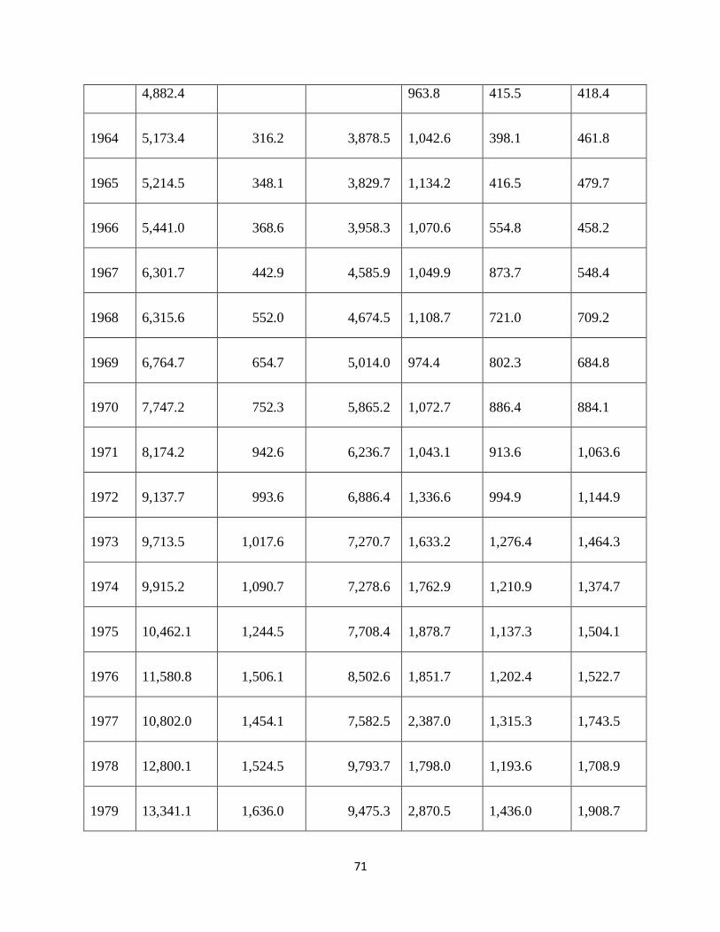
71

4,882.4 963.8 415.5 418.4

1964

5,173.4 316.2 3,878.5

1,042.6

398.1

461.8

1965

5,214.5 348.1 3,829.7

1,134.2

416.5

479.7

1966

5,441.0 368.6 3,958.3

1,070.6

554.8

458.2

1967

6,301.7 442.9 4,585.9

1,049.9

873.7

548.4

1968

6,315.6 552.0 4,674.5

1,108.7

721.0

709.2

1969

6,764.7 654.7 5,014.0

974.4

802.3

684.8

1970

7,747.2 752.3 5,865.2

1,072.7

886.4

884.1

1971

8,174.2 942.6 6,236.7

1,043.1

913.6

1,063.6

1972

9,137.7 993.6 6,886.4

1,336.6

994.9

1,144.9

1973

9,713.5 1,017.6 7,270.7

1,633.2

1,276.4

1,464.3

1974

9,915.2 1,090.7 7,278.6

1,762.9

1,210.9

1,374.7

1975

10,462.1 1,244.5 7,708.4

1,878.7

1,137.3

1,504.1

1976

11,580.8 1,506.1 8,502.6

1,851.7

1,202.4

1,522.7

1977

10,802.0 1,454.1 7,582.5

2,387.0

1,315.3

1,743.5

1978

12,800.1 1,524.5 9,793.7

1,798.0

1,193.6

1,708.9

1979

13,341.1 1,636.0 9,475.3

2,870.5

1,436.0

1,908.7

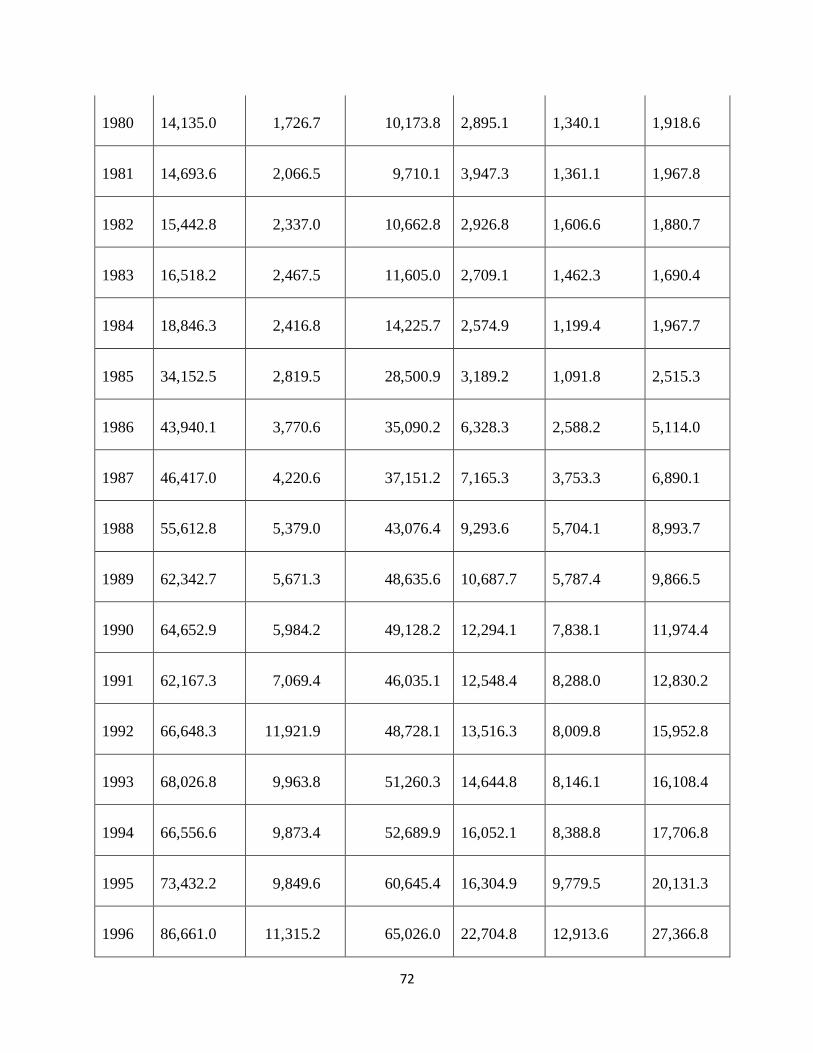
72

1980

14,135.0 1,726.7 10,173.8

2,895.1

1,340.1

1,918.6

1981

14,693.6 2,066.5 9,710.1

3,947.3

1,361.1

1,967.8

1982

15,442.8 2,337.0 10,662.8

2,926.8

1,606.6

1,880.7

1983

16,518.2 2,467.5 11,605.0

2,709.1

1,462.3

1,690.4

1984

18,846.3 2,416.8 14,225.7

2,574.9

1,199.4

1,967.7

1985

34,152.5 2,819.5 28,500.9

3,189.2

1,091.8

2,515.3

1986

43,940.1 3,770.6 35,090.2

6,328.3

2,588.2

5,114.0

1987

46,417.0 4,220.6 37,151.2

7,165.3

3,753.3

6,890.1

1988

55,612.8 5,379.0 43,076.4

9,293.6

5,704.1

8,993.7

1989

62,342.7 5,671.3 48,635.6

10,687.7

5,787.4

9,866.5

1990

64,652.9 5,984.2 49,128.2

12,294.1

7,838.1

11,974.4

1991

62,167.3 7,069.4 46,035.1

12,548.4

8,288.0

12,830.2

1992

66,648.3 11,921.9 48,728.1

13,516.3

8,009.8

15,952.8

1993

68,026.8 9,963.8 51,260.3

14,644.8

8,146.1

16,108.4

1994

66,556.6 9,873.4 52,689.9

16,052.1

8,388.8

17,706.8

1995

73,432.2 9,849.6 60,645.4

16,304.9

9,779.5

20,131.3

1996

86,661.0 11,315.2 65,026.0

22,704.8

12,913.6

27,366.8

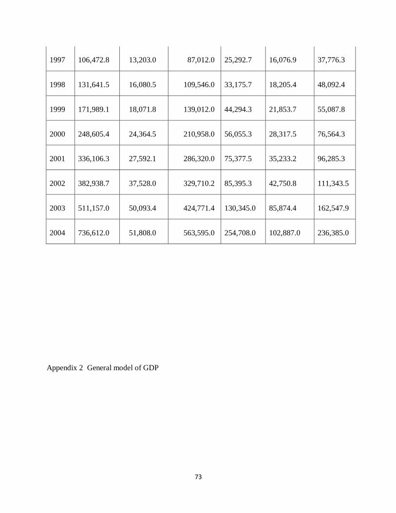
73

1997

106,472.8 13,203.0 87,012.0

25,292.7

16,076.9

37,776.3

1998

131,641.5 16,080.5 109,546.0

33,175.7

18,205.4

48,092.4

1999

171,989.1 18,071.8 139,012.0

44,294.3

21,853.7

55,087.8

2000

248,605.4 24,364.5 210,958.0

56,055.3

28,317.5

76,564.3

2001

336,106.3 27,592.1 286,320.0

75,377.5

35,233.2

96,285.3

2002

382,938.7 37,528.0 329,710.2

85,395.3

42,750.8

111,343.5

2003

511,157.0 50,093.4 424,771.4

130,345.0

85,874.4

162,547.9

2004

736,612.0 51,808.0 563,595.0

254,708.0

102,887.0

236,385.0

Appendix 2 General model of GDP

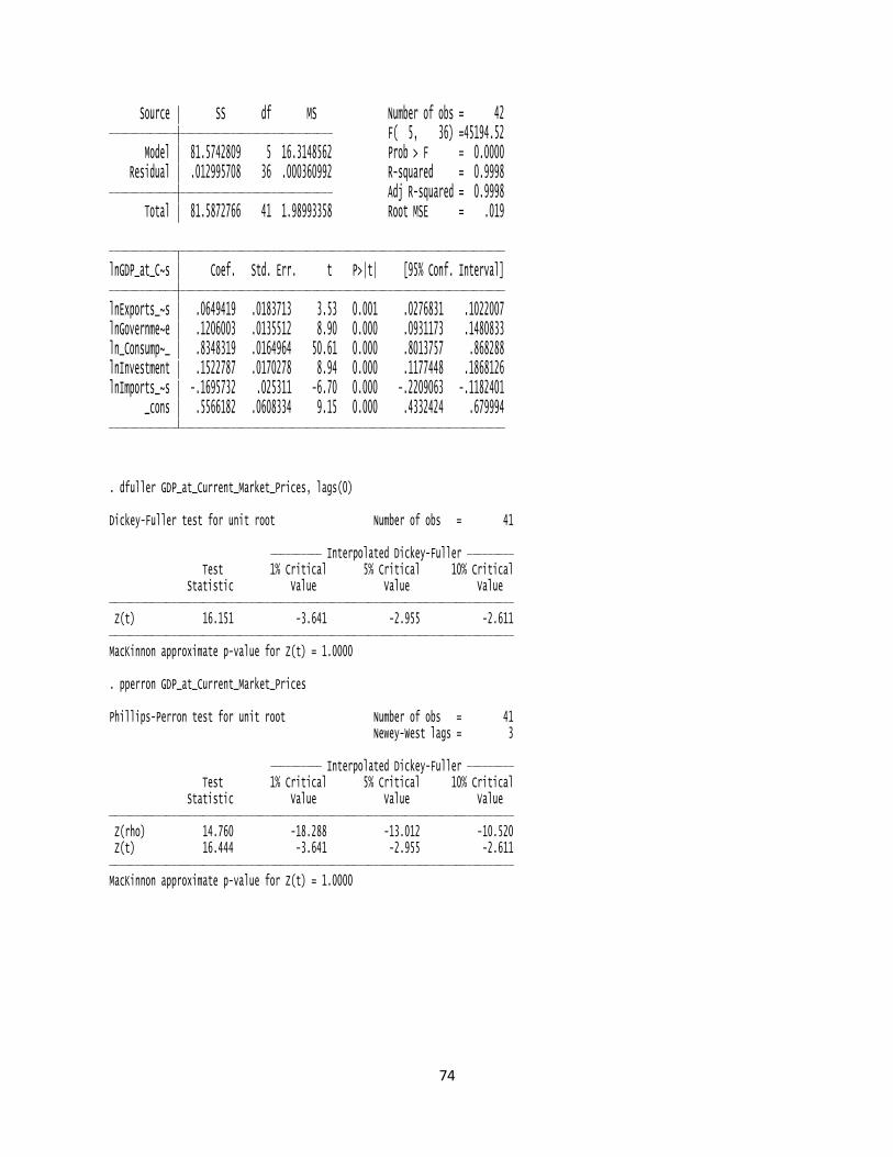
74

_cons .5566182 .0608334 9.15 0.000 .4332424 .679994lnImports_~s -.1695732 .025311 -6.70 0.000 -.2209063 -.1182401lnInvestment .1522787 .0170278 8.94 0.000 .1177448 .1868126ln_Consump~_ .8348319 .0164964 50.61 0.000 .8013757 .868288lnGovernme~e .1206003 .0135512 8.90 0.000 .0931173 .1480833lnExports_~s .0649419 .0183713 3.53 0.001 .0276831 .1022007 lnGDP_at_C~s Coef. Std. Err. t P>|t| [95% Conf. Interval]

Total 81.5872766 41 1.98993358 Root MSE = .019 Adj R-squared = 0.9998 Residual .012995708 36 .000360992 R-squared = 0.9998 Model 81.5742809 5 16.3148562 Prob > F = 0.0000 F( 5, 36) =45194.52 Source SS df MS Number of obs = 42

MacKinnon approximate p-value for Z(t) = 1.0000 Z(t) 16.444 -3.641 -2.955 -2.611 Z(rho) 14.760 -18.288 -13.012 -10.520 Statistic Value Value Value Test 1% Critical 5% Critical 10% Critical Interpolated Dickey-Fuller

Newey-West lags = 3Phillips-Perron test for unit root Number of obs = 41

. pperron GDP_at_Current_Market_Prices

MacKinnon approximate p-value for Z(t) = 1.0000 Z(t) 16.151 -3.641 -2.955 -2.611 Statistic Value Value Value Test 1% Critical 5% Critical 10% Critical Interpolated Dickey-Fuller

Dickey-Fuller test for unit root Number of obs = 41

. dfuller GDP_at_Current_Market_Prices, lags(0)

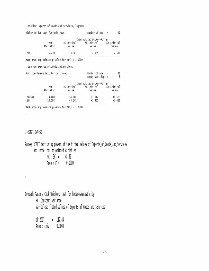
75

.

MacKinnon approximate p-value for Z(t) = 1.0000 Z(t) 10.092 -3.641 -2.955 -2.611 Z(rho) 14.460 -18.288 -13.012 -10.520 Statistic Value Value Value Test 1% Critical 5% Critical 10% Critical Interpolated Dickey-Fuller

Newey-West lags = 3Phillips-Perron test for unit root Number of obs = 41

. pperron Exports_of_Goods_and_Services

MacKinnon approximate p-value for Z(t) = 1.0000 Z(t) 6.270 -3.641 -2.955 -2.611 Statistic Value Value Value Test 1% Critical 5% Critical 10% Critical Interpolated Dickey-Fuller

Dickey-Fuller test for unit root Number of obs = 41

. dfuller Exports_of_Goods_and_Services, lags(0)

.

Prob > F = 0.0000 F(3, 36) = 48.36 Ho: model has no omitted variablesRamsey RESET test using powers of the fitted values of Exports_of_Goods_and_Services

. estat ovtest

Prob > chi2 = 0.0000 chi2(1) = 117.44

Variables: fitted values of Exports_of_Goods_and_Services Ho: Constant varianceBreusch-Pagan / Cook-Weisberg test for heteroskedasticity

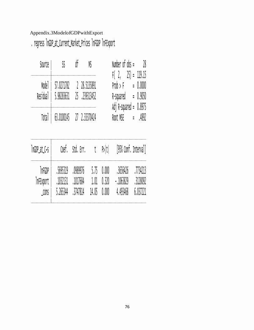
76

Appendix.3ModelofGDPwithExport

_cons 5.265344 .3747814 14.05 0.000 4.493468 6.037221 lnFExport .1032131 .1017684 1.01 0.320 -.1063829 .3128092 lnFGDP .5695319 .0989976 5.75 0.000 .3656426 .7734213 lnGDP_at_C~s Coef. Std. Err. t P>|t| [95% Conf. Interval]

Total 63.0100145 27 2.33370424 Root MSE = .4892 Adj R-squared = 0.8975 Residual 5.98283631 25 .239313452 R-squared = 0.9050 Model 57.0271782 2 28.5135891 Prob > F = 0.0000 F( 2, 25) = 119.15 Source SS df MS Number of obs = 28

. regress lnGDP_at_Current_Market_Prices lnFGDP lnFExport

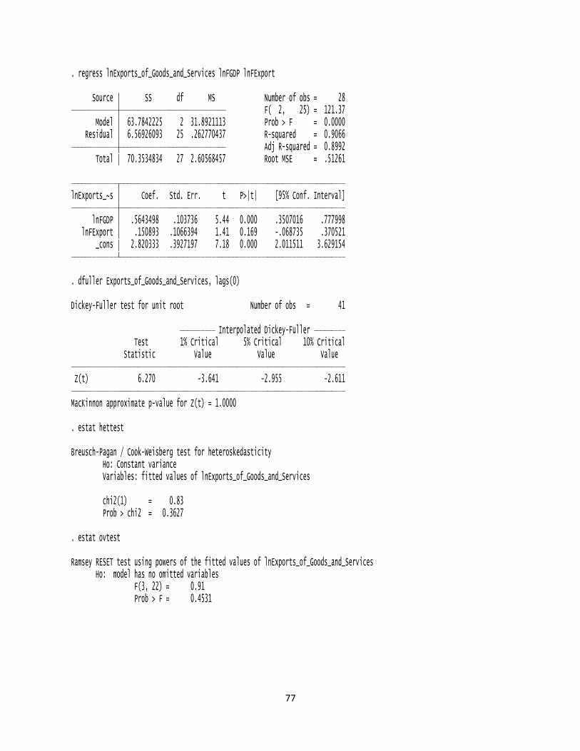
77

Prob > F = 0.4531 F(3, 22) = 0.91 Ho: model has no omitted variablesRamsey RESET test using powers of the fitted values of lnExports_of_Goods_and_Services

. estat ovtest

Prob > chi2 = 0.3627 chi2(1) = 0.83

Variables: fitted values of lnExports_of_Goods_and_Services Ho: Constant varianceBreusch-Pagan / Cook-Weisberg test for heteroskedasticity

. estat hettest

MacKinnon approximate p-value for Z(t) = 1.0000 Z(t) 6.270 -3.641 -2.955 -2.611 Statistic Value Value Value Test 1% Critical 5% Critical 10% Critical Interpolated Dickey-Fuller

Dickey-Fuller test for unit root Number of obs = 41

. dfuller Exports_of_Goods_and_Services, lags(0)

_cons 2.820333 .3927197 7.18 0.000 2.011511 3.629154 lnFExport .150893 .1066394 1.41 0.169 -.068735 .370521 lnFGDP .5643498 .103736 5.44 0.000 .3507016 .777998 lnExports_~s Coef. Std. Err. t P>|t| [95% Conf. Interval]

Total 70.3534834 27 2.60568457 Root MSE = .51261 Adj R-squared = 0.8992 Residual 6.56926093 25 .262770437 R-squared = 0.9066 Model 63.7842225 2 31.8921113 Prob > F = 0.0000 F( 2, 25) = 121.37 Source SS df MS Number of obs = 28

. regress lnExports_of_Goods_and_Services lnFGDP lnFExport