Working Paper

WP 2003-059

Project #: UM02-11 M RR C

Expectations in Micro Data: Rationality Revisited

Hugo Benítez-Silva, Debra S. Dwyer, Wayne-Roy Gayle, and Thomas J. Muench

MichiganUniversity of

ResearchRetirementCenter

“Expectations in Micro Data: Rationality Revisited”

Hugo Benítez-Silva SUNY – Stony Brook

Debra S. Dwyer SUNY – Stony Brook

Wayne-Roy Gayle University of Pittsburgh

Thomas J. Muench SUNY-Stony Brook

October 2003

Michigan Retirement Research Center University of Michigan

P.O. Box 1248 Ann Arbor, MI 48104

Acknowledgements This work was supported by a grant from the Social Security Administration through the Michigan Retirement Research Center (Grant # 10-P-98358-5). The opinions and conclusions are solely those of the authors and should not be considered as representing the opinions or policy of the Social Security Administration or any agency of the Federal Government. Regents of the University of Michigan David A. Brandon, Ann Arbor; Laurence B. Deitch, Bingham Farms; Olivia P. Maynard, Goodrich; Rebecca McGowan, Ann Arbor; Andrea Fischer Newman, Ann Arbor; Andrew C. Richner, Grosse Pointe Park; S. Martin Taylor, Gross Pointe Farms; Katherine E. White, Ann Arbor; Mary Sue Coleman, ex officio

Expectations in Micro Data: Rationality Revisited

Hugo Benítez-Silva Debra S. Dwyer

Wayne-Roy Gayle Thomas J. Muench

Abstract

An increasing number of longitudinal data sets collect expectations information regarding a variety of future individual level events and decisions, providing researchers with the opportunity to explore expectations over micro variables in detail. We provide a theoretical framework and an econometric methodology to use that type of information to test the Rational Expectations hypothesis in models of individual behavior, and present tests using two different panel data sets.

Authors’ Acknowledgements

We would like to acknowledge excellent research assistance from Huan Ni and Selcuk Eren. The Michigan Retirement Research Center (MRRC) and the TIAA-CREF Institute made this research possible through their financial support. Benítez-Silva wants to thank the Department of Economics at the University of Maryland for their hospitality during the completion of this paper. All remaining errors are the authors’.

1

1. Introduction An increasing number of large longitudinal data sets now collect expectations information regarding future

individual level events and decisions, providing researchers with the opportunity to explore expectations over micro

variables in detail. We present a theoretical framework and an econometric methodology to use that type of

information to test the Rational Expectations (RE) hypothesis in models of individual behavior. We then use the

Health and Retirement Study (HRS) and the youth cohort of the National Longitudinal Survey of Labor Market

Experience (NLSY79) to analyze retirement and education expectations, respectively. We find that these two types

of expectations are consistent with the RE hypothesis. Our results support the use of a wide variety of models in

economics that assume rational behavior.

Our definition and approach to testing the RE hypothesis will be consistent with the views expressed by the

precursors of this assumption. We will maintain that agents’ subjective beliefs about the evolution of a set of

variables of interest coincide with the objectively measurable population probability measure. This is consistent

with the characterization of Muth (1961) and Lucas (1972). The main difference is that instead of concentrating on

forecasts of market level variables we focus on how individuals form expectations over micro variables that are in

part under their control. This RE assumption at the micro level underlies a majority of the research in applied fields,

and it is the common foundation of most work in dynamic models of individual behavior. Economists are growing

increasingly interested in this type of measures as possible sources of additional variation in individual

characteristics that might reflect underlying differences in preference and beliefs parameters.

The debate over whether testing rational expectations is a worthwhile enterprise goes back almost three

decades. Prescott (1977) expressed a strong opinion against testing the hypothesis, while Simon (1979), Tobin

(1980), Revankar (1980), and Lovell (1986) considered the direct analysis of expectations an important project. The

efforts to test the hypothesis began in the context of the life cycle permanent income hypothesis in a stream of

literature that started with the work of Hall (1978), and then compared forecasts of market variables with

realizations like in Figlewski and Watchtel (1981, 1983), Kimball Dietrich and Joines (1983), de Leeuw and

McKelvey (1981 and 1984), Gramlich (1983), and more recently Davies and Lahiri (1999), and Christiansen

(2003). Finally, work by Leonard (1982) analyzed wage expectations of employers, and Fair (1993) analyzed the

question in the context of large macroeconomic models. In all these cases the concern was with market level

2

variables, and the evidence in these and many other studies is mixed. Below, we propose a slightly different

approach in line with Bernheim (1990) and Benítez-Silva and Dwyer (2003), and use panel data available through

the HRS and the NLSY79 to follow two very different cohorts of individuals planning an important decision for

people their age, retirement and education.

The conceptual model and the econometric specifications are presented in section 2. Section 3 provides

information about the data used and reports our main findings. Section 4 concludes.

2. A Model and a Test of Expectations using Individual Level Variables

Suppose an individual and an econometrician are trying to predict a variable X that the individual has decided will

be determined by a function of a sequence of random variables:

1 2( , ,..., ).TX h ω ω ω= (1)

The sequence of vector-valued variables inside the parenthesis will be observed by the individual at time periods

t=1,2,…,T. Then the individual will take action X after some or all the ωt’s have been observed.

Let 1

tt t t

ω=

Ω = be the information known at period t and let ( )1 2, ,t t tω ω ω= where all of ωt is observed by

the individual, but only 1tω is observed by the econometrician. Let then 1 1

1

t

t t tω

=Ω = . Then we can define

,tet XEX Ω= (2)

where E is the expectations operator. This is the most commonly used representation of the RE hypothesis, which

takes as the rational expectation of a variable its conditional mathematical expectation (Sargent and Wallace 1976).1

This guarantees that errors in expectations will be uncorrelated with the set of variables known at time t.

Variables included in the vector representing the information set Ω, come from models of individual

behavior and might include socio-economic and demographic characteristics. Using the law of iterated expectations

and assuming that the new information is correctly forecasted by agents (its conditional distribution not just its

mean), from (2) we get:

1 Schmalensee (1976) using experimental data emphasizes the importance of analyzing higher moments of the distribution of expectations. Due to data limitations we are unable to do so in our analysis.

3

,]|,[ 11etttttt

et XXEXEEXE =Ω=ΩΩ=Ω ++ ω (3)

where ωt+1 represents information that comes available between periods t and t+1. Then from (3) we can write the

evolution of expectations through time as

,11 ++ += tet

et XX η (4)

where ],|[ 111 tet

ett XEX Ω−= +++η and therefore E(ηt+1|Ωt)=0. Notice that ηt+1 is a function of the new information

received since period t, ωt+1. From this characterization of the evolution of expectations we can test the RE

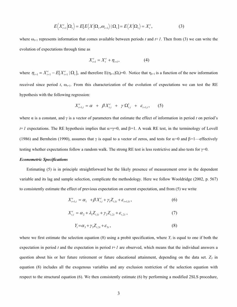
hypothesis with the following regression:

11, , , 1,

e et i t i t i t iX Xα β γ ε+ += + + Ω + , (5)

where α is a constant, and γ is a vector of parameters that estimate the effect of information in period t on period’s

t+1 expectations. The RE hypothesis implies that α=γ=0, and β=1. A weak RE test, in the terminology of Lovell

(1986) and Bernheim (1990), assumes that γ is equal to a vector of zeros, and tests for α=0 and β=1––effectively

testing whether expectations follow a random walk. The strong RE test is less restrictive and also tests for γ=0.

Econometric Specifications

Estimating (5) is in principle straightforward but the likely presence of measurement error in the dependent

variable and its lag and sample selection, complicate the methodology. Here we follow Wooldridge (2002, p. 567)

to consistently estimate the effect of previous expectation on current expectation, and from (5) we write

1, 1 , 1 ,1 1,1e et i t i t i t iX X Zα β γ ε+ += + + + , (6)

, 2 1 ,1 2 ,2 ,2et i t i t i t iX Z Zα λ γ ε= + + + , (7)

iiti ZY 33,33 εγα ++= , (8)

where we first estimate the selection equation (8) using a probit specification, where Yi is equal to one if both the

expectation in period t and the expectation in period t+1 are observed, which means that the individual answers a

question about his or her future retirement or future educational attainment, depending on the data set. Z3 in

equation (8) includes all the exogenous variables and any exclusion restriction of the selection equation with

respect to the structural equation (6). We then consistently estimate (6) by performing a modified 2SLS procedure,

4

where the first stage includes as instruments all the exogenous variables used in (8), the Inverse Mills’ ratio from

the probit equation, and any additional instruments, Z2 in (7), the validity of which will be tested.

3. Data and Empirical Results

To test the RE hypothesis on the retirement expectations of older workers we use all five available waves of the

HRS, a nationally representative longitudinal survey of 7,700 households headed by an individual aged 51 to 61 as

of the first interviews in 1992-93. We include respondents that are working, full time or part time, in any wave, and

non-employed (but searching for jobs) that report retirement plans. In each wave respondents are asked when they

plan to fully or partially depart from the labor force and whether they have thought about retirement. Most of the

people who have not thought about retirement do not report an expected age.2

To test the RE hypothesis on educational attainment expectations of the youth we use the NSLY79, a nationally

representative longitudinal survey that follows individuals over the period 1979 to 2000, who were 14 to 21 years

of age as of January 1, 1979. Interviews were conducted on an annual basis though 1994, after which they adopted

a biennial interview schedule. In the 1979, 1981, and 1982 surveys, each respondent was asked what the highest

educational grade level they expected to complete. This analysis makes use of the responses in the 1981 and 1982

waves. The sample is selected by excluding respondents of ages greater than 15 as at January 1, 1979 (to avoid

individuals that have completed their schooling), military entrants, and respondents never observed to enroll in high

school. The resulting sample size includes 2,395 respondents.

Empirical Results

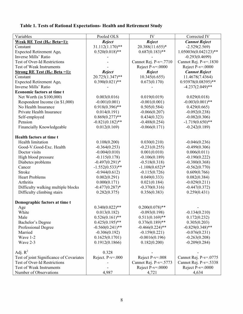
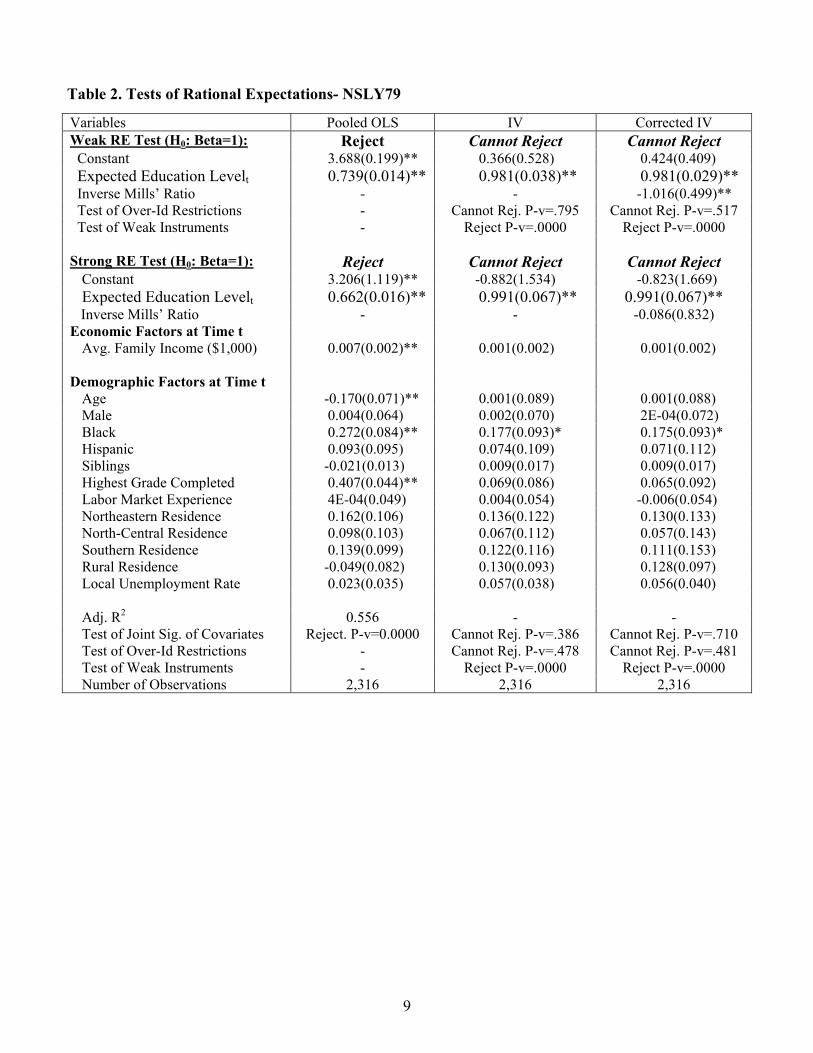
Table 1 presents the weak and strong RE tests for the sample from the HRS, and Table 2 presents the tests

for the NLSY79 sample. The HRS data support the weak and strong RE hypotheses in the augmented model that

corrects for sample selection and measurement error in the report of expected retirement age, resulting in a

selection corrected IV specification, and the NLSY79 supports the RE hypotheses in expected educational

attainment both in the IV and the corrected IV specifications.3

2 Many of them report that they will never retire. If they have not given it any thought, and they say they will never retire, we treat their expected retirement age as missing. If they give a retirement age we treat them as non-missing. We have assigned an age of 77 for those who never retire (estimated longevity). 3 The findings are robust across many specifications and empirical techniques including panel data methods.

5

We perform an F-test based on the null hypothesis that β=1 in equation (4), to test the RE hypothesis. We

obtain coefficients for β of 1.05 for the weaker test using the retirement expectations data and 0.981 using the

education expectations data, which cannot reject the hypothesis that both expectations follow a random walk. For

the pooled OLS estimation this test is effectively a unit root test, and as such, following the literature on testing unit

roots in panel data surveyed by Bond, Nauges, and Windmeijer (2002), we perform a correction to obtain the

appropriate critical value. However, this matters very little since the unit root hypothesis is soundly rejected.

For the strong test we estimate the model of equations (6) to (8), using the corrected IV procedure. The β

parameter is estimated to be equal to 0.94 in the HRS and 0.991 in the NLSY79, in both cases very precisely

estimated, and clearly failing to reject the RE hypothesis. Notice the importance in the HRS of both instrumenting

the previous period’s expectations, and controlling for sample selection. We also report in both tables tests that

show that we cannot reject that we have robust instruments and that the overidentification in the 2SLS is correct. In

fact the reported results are the product of robustly estimating the system of equations via GMM, which provides

robustness against unknown forms of heterokedasticity.

The strong test includes information available at time t that should not be significant after controlling for

time t expectations. In both samples after controlling for sample selection and measurement error we find that most

of these factors are no longer significant. The joint hypotheses that all the coefficients are equal to zero cannot be

rejected at any traditional level of significance.4

Like in Bernheim (1990), the objective behind instrumental variables estimation here is to correct for

potential measurement error in the reported expected age of retirement at time t. Since people are reporting

expectations over uncertain events, we expect some degree of reporting error that may be correlated with

unobserved factors. We use time t subjective survival to age 85 probabilities and an indicator of smoking behavior

as instruments (exclusion restrictions) for expected retirement age, and the educational attainment of the parents as

instruments (exclusion restrictions) for expected years of education. In the selection corrected IV, the inverse Mills’

ratio is an additional instrument, along with the rest of the exogenous variables from the selection equation, as

4 It is true, however, that this is trivially the case if individuals never adjust their expectations. But plenty of adjustment goes on in the data, and it seems implausible that all can be blamed on measurement error.

6

suggested by Wooldridge (2002).5 In the HRS the strongest specification is the selection corrected IV. Interestingly

in this case, this corrected IV technique seems to circumvent one of the traditional drawbacks of instrumental

variables estimation, that is, the large increase in standard errors in the IV estimates. The importance of the

selection correction in this setting, contrasts with the results by Bernheim (1990) where selection was not

important, and the inability to reject rationality was in part the product of large standard errors. In the NSLY79

although we cannot reject the presence of sample selection in the weak test, the RE results do not depend on this

additional correction.

4. Conclusions

We have tested the Rational Expectations hypothesis in the formation of expectations for retirement and

educational attainment. In both samples we cannot reject the RE hypothesis after controlling for reporting errors

and sample selection. These results support the use of the expectations variables in the growing number of data sets

that provide this type of information, and support the use of economic models that use this assumption. The results

in this analysis are meant to foster further discussion and research on the issues surrounding the role of expectations

in economic modeling.

References

Benítez-Silva, H., and D. S. Dwyer (2003): “What to Expect when you are Expecting Rationality: Testing Rational Expectations using Micro Data,” manuscript, SUNY-Stony Brook. Bernheim, B.D. (1990): “How Do the Elderly Form Expectations? An Analysis of Responses to New Information.” In Issues in the Economics of Aging. Ed. D. Wise. Chicago: University of Chicago Press, 259—285. Bond, S., C. Nauges, and F. Windmeijer (2002): “Unit Root and Identification in Autoregressive Panel Data Models: A Comparison of Alternative Tests.” IFS Working Paper. Christiansen, C. (2003): “Testing the expectations hypothesis using long-maturity forward rates,” Economics Letters, 78 175—180. Davies A., and K. Lahiri (1999): “Re-examining the rational expectations hypothesis using panel data on multi-period forecasts,” in Analysis of panels and limited dependent variable models. Edited by Cheng Hsiao, Kajal Lahiri, Lung-Fei Lee, and M. Hashem Pesaran. Cambridge University Press.

5 The exclusion restrictions in the selection equation include indicators for whether the father and mother of the respondent reached retirement age in the case of the HRS, and the results of the AFQT test in the case of the NSLY79. In the selection equation we have decided to only include covariates as of time t, we have experimented with including t+1 variables, and also a battery of residuals of the regressions of t+1 variables on their lagged values, which are then also included in the main equation. Although some coefficients in the main equation changed as a result of these modifications, the reported results were robust to this characterization of the selection process. These results are available from the authors upon request.

7

de Leeuw, F., and M.J. McKelvey (1981): “Price Expectations of Business Firms,” Brookings Papers on Economic Activity, 1981-1 299—314. de Leeuw, F., and M.J. McKelvey (1984): “Price Expectations of Business Firms: Bias in the Short and Long Run,” American Economic Review, 14 99—110. Fair, R.C. (1993): “Testing the Rational Expectations Hypothesis in Macroeconomic Models,” Oxford Economic Papers, 45-2 169—190. Figlewski, S., and P. Wachtel (1981): “The Formation of Inflationary Expectations,” Review of Economics and Statistics, 63-1 1—10. Figlewski, S., and P. Wachtel (1983): “Rational Expectations, Information Efficiency, and Tests using Survey Data,” Review of Economics and Statistics, 65-3 529—531. Gramlich, E.M. (1983): “Models of Inflation Expectations Formation: A Comparison of Household and Economic Forecasts,” Journal of Money, Credit, and Banking, 15 155—173. Hall, R. (1978): “Stochastic Implications of the Life Cycle-Permanent Income Hypothesis: Theory and Evidence,” Journal of Political Economy, 86 971—987 Kimball Dietrich, J., and D.H. Joines (1983): “Rational Expectations, Information Efficiency, and Tests using Survey Data: A comment,” Review of Economics and Statistics, 65-3 525—529 Leonard, J.S. (1982): “Wage Expectations in the Labor Market: Survey Evidence on Rationality,” Review of Economics and Statistics, 64 157—161. Lovell, M.C. (1986): “Tests of Rational Expectations Hypothesis,” American Economic Review, 76-1 110—124. Lucas, R.E. (1972): “Expectations and the Neutrality of Money,” Journal of Economic Theory, 4 103—124. Muth, J.F. (1961): “Rational Expectations and the Theory of Price Movements,” Econometrica, 29-3 315—335. Prescott, E. (1977): “Should Control Theory be Used for Economic Stabilization? Journal of Monetary Economics, Suppl. 13—38. Revankar, N.S. (1980): “Testing of the Rational Expectations Hypothesis,” Econometrica, 48-6 1347—1363. Sargent, T.J., and N. Wallace (1976): “Rational Expectations and the Theory of Economic Policy,” Journal of Monetary Economics, 2 169—183. Schmalensee, R. (1976): “An Experimental Study of Expectation Formation,” Econometrica, 44-1 17—41. Simon, H.A. (1979): “Rational Decision Making in Business Organizations,” American Economic Review, 69-4 493—513. Tobin, J. (1980): Asset Accumulation and Economic Activity. The University of Chicago Press. Wooldridge, J.M. (2002): Econometric Analysis of Cross Section and Panel Data. MIT Press.

8

Table 1. Tests of Rational Expectations- Health and Retirement Study

Variables Pooled OLS IV Corrected IV Weak RE Test (H0: Beta=1): Constant Expected Retirement Aget Inverse Mills’ Ratio Test of Over-Id Restrictions Test of Weak Instruments Strong RE Test (H0: Beta =1): Constant Expected Retirement Aget Inverse Mills’ Ratio Economic factors at time t Net Worth (in $100,000) Respondent Income (in $1,000) No Health Insurance Private Health Insurance Self-employed Pension Financially Knowledgeable Health factors at time t Health limitation Good-V.Good-Exc. Health Doctor visits High blood pressure Diabetes problems Cancer Stroke Heart Problems Arthritis Difficulty walking multiple blocks Difficulty climbing stairs Demographic factors at time t Age White Male Bachelor’s Degree Professional Degree Married Wave 1-2 Wave 2-3 Adj. R2

Test of joint Significance of Covariates Test of Over-Id Restrictions Test of Weak Instruments Number of Observations

Reject 31.112(1.170)** 0.520(0.018)**

- - -

Reject 20.725(1.347)** 0.390(0.021)**

-

0.003(0.016) -0.001(0.001)

0.918(0.396)** 0.014(0.191)

0.869(0.277)** -0.821(0.182)**

0.012(0.169)

0.108(0.200) -0.364(0.253) -0.004(0.010) -0.115(0.178)

-0.497(0.291)* -1.552(0.533)**

-0.944(0.612) 0.002(0.291) 0.000(0.171)

-0.477(0.287)* 0.282(0.375)

0.340(0.022)** 0.013(0.182)

0.526(0.161)** 0.425(0.195)** -0.560(0.241)**

-0.306(0.192) 0.1625(0.1701) 0.1912(0.1866)

0.328

Reject. P-v=.000 - -

4,987

Reject 20.388(11.655)* 0.687(0.183)**

- Cannot Rej. P-v=.7710

Reject P-v=.0000 Reject

10.345(6.655) 0.673(0.170)

-

0.019(0.019) -0.001(0.001) 0.505(0.584) -0.066(0.207) 0.434(0.323) -0.488(0.254) -0.066(0.171)

0.030(0.210) -0.231(0.255) 0.001(0.010) -0.106(0.189) -0.518(0.318)

-1.108(0.652)* -0.115(0.726) 0.049(0.333) 0.021(0.184) -0.370(0.316) 0.356(0.383)

0.200(0.078)** -0.093(0.198)

0.511(0.169)** 0.376(0.189)** -0.466(0.224)**

-0.159(0.221) -0.0016(0.196) 0.182(0.200)

-

Reject P-v=.008 Cannot Rej. P-v=.5773

Reject P-v=.0000 4,721

Cannot Reject -2.529(2.569)

1.050036(0.042123)** -0.293(0.4699)

Cannot Rej. P-v=.1830 Reject P-v=.0000

Cannot Reject 11.4678(7.4364)

0.93978(0.08395)** -4.237(2.049)**

0.029(0.018)

-0.003(0.001)** 0.429(0.665) -0.092(0.238) -0.082(0.306)

-1.719(0.650)** -0.242(0.189)

-0.046(0.236) -0.499(0.306) 0.006(0.011) -0.190(0.222) -0.380(0.368) -0.562(0.770) 0.609(0.766) 0.082(0.384) -0.029(0.211) -0.447(0.372) 0.259(0.431)

-

-0.134(0.210) 0.172(0.232) 0.305(0.203)

-0.829(0.348)** -0.076(0.231) -0.263(0.208) -0.209(0.284)

-

Cannot Rej. P-v=.0775 Cannot Rej. P-v=.5338

Reject P-v=.0000 4,634

9

Table 2. Tests of Rational Expectations- NSLY79

Variables Pooled OLS IV Corrected IV Weak RE Test (H0: Beta=1): Reject Cannot Reject Cannot Reject Constant 3.688(0.199)** 0.366(0.528) 0.424(0.409) Expected Education Levelt Inverse Mills’ Ratio

0.739(0.014)** -

0.981(0.038)** -

0.981(0.029)** -1.016(0.499)**

Test of Over-Id Restrictions - Cannot Rej. P-v=.795 Cannot Rej. P-v=.517 Test of Weak Instruments - Reject P-v=.0000 Reject P-v=.0000 Strong RE Test (H0: Beta=1): Reject Cannot Reject Cannot Reject

Constant 3.206(1.119)** -0.882(1.534) -0.823(1.669) Expected Education Levelt 0.662(0.016)** 0.991(0.067)** 0.991(0.067)**

Inverse Mills’ Ratio - - -0.086(0.832) Economic Factors at Time t

Avg. Family Income ($1,000) 0.007(0.002)** 0.001(0.002) 0.001(0.002) Demographic Factors at Time t

Age -0.170(0.071)** 0.001(0.089) 0.001(0.088) Male 0.004(0.064) 0.002(0.070) 2E-04(0.072) Black 0.272(0.084)** 0.177(0.093)* 0.175(0.093)* Hispanic 0.093(0.095) 0.074(0.109) 0.071(0.112) Siblings -0.021(0.013) 0.009(0.017) 0.009(0.017) Highest Grade Completed 0.407(0.044)** 0.069(0.086) 0.065(0.092) Labor Market Experience 4E-04(0.049) 0.004(0.054) -0.006(0.054) Northeastern Residence 0.162(0.106) 0.136(0.122) 0.130(0.133) North-Central Residence 0.098(0.103) 0.067(0.112) 0.057(0.143) Southern Residence 0.139(0.099) 0.122(0.116) 0.111(0.153) Rural Residence -0.049(0.082) 0.130(0.093) 0.128(0.097) Local Unemployment Rate 0.023(0.035) 0.057(0.038) 0.056(0.040)

Adj. R2 0.556 - - Test of Joint Sig. of Covariates Reject. P-v=0.0000 Cannot Rej. P-v=.386 Cannot Rej. P-v=.710 Test of Over-Id Restrictions - Cannot Rej. P-v=.478 Cannot Rej. P-v=.481 Test of Weak Instruments - Reject P-v=.0000 Reject P-v=.0000 Number of Observations 2,316 2,316 2,316

10

Expectations in Micro Data: Rationality Revisited Hugo Benítez-Silva, Debra S. Dwyer, Wayne-Roy Gayle, and Thomas J. Muench Appendix (submitted as supporting material only, not as part of the paper) Table A.1a. Summary Statistics. HRS.

Variables Full Sample N=23,669

Retirement Plans and Outcomes Expected retirement age Employee Self employed Financially Knowledgeable Economic factors Net worth (in $100,000) Housing wealth (in $100,000) Respondent’ Income (in $1,000) Has a private pension Health Insurance Employer provided Retiree Government Private No health insurance Health factors Health limitation Good-Very Good-Excellent Health Doctor visits Probability of living to age 85 High blood pressure Diabetes Arthritis Difficulty walking multiple blocks Difficulty climbing stairs Stroke Heart problems Cancer Smoke

Demographic factors Age Male Married Bachelor’s degree Professional degree Mother reached retirement age Father reached retirement age

64.584(6.478) 0.794(0.405) 0.173(0.378) 0.657(0.475)

2.449(5.181) 0.769(1.248)

29.213(54.304) 0.593(0.491)

0.699(0.459) 0.814(0.389) 0.082(0.274) 0.188(0.391) 0.087(0.282)

0.187(0.390) 0.866(0.340) 5.191(7.075) 0.470(0.306) 0.228(0.419) 0.060(0.238) 0.283(0.450) 0.082(0.275) 0.047(0.212) 0.003(0.052) 0.075(0.263) 0.007(0.083) 0.219(0.414)

57.197(5.222) 0.465(0.499) 0.794(0.405) 0.270(0.444) 0.101(0.301) 0.714(0.452) 0.596(0.491)

11

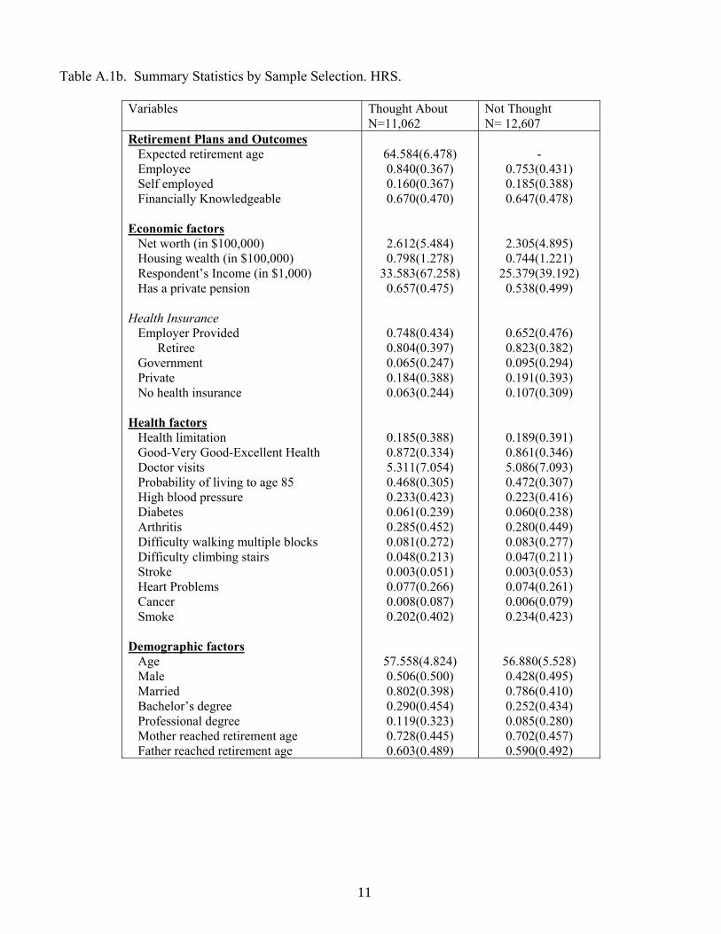
Table A.1b. Summary Statistics by Sample Selection. HRS.

Variables Thought About N=11,062

Not Thought N= 12,607

Retirement Plans and Outcomes Expected retirement age Employee Self employed Financially Knowledgeable Economic factors Net worth (in $100,000) Housing wealth (in $100,000) Respondent’s Income (in $1,000) Has a private pension Health Insurance Employer Provided Retiree Government Private No health insurance Health factors Health limitation Good-Very Good-Excellent Health Doctor visits Probability of living to age 85 High blood pressure Diabetes Arthritis Difficulty walking multiple blocks Difficulty climbing stairs Stroke Heart Problems Cancer Smoke

Demographic factors Age Male Married Bachelor’s degree Professional degree Mother reached retirement age Father reached retirement age

64.584(6.478) 0.840(0.367) 0.160(0.367) 0.670(0.470)

2.612(5.484) 0.798(1.278)

33.583(67.258) 0.657(0.475)

0.748(0.434) 0.804(0.397) 0.065(0.247) 0.184(0.388) 0.063(0.244)

0.185(0.388) 0.872(0.334) 5.311(7.054) 0.468(0.305) 0.233(0.423) 0.061(0.239) 0.285(0.452) 0.081(0.272) 0.048(0.213) 0.003(0.051) 0.077(0.266) 0.008(0.087) 0.202(0.402)

57.558(4.824) 0.506(0.500) 0.802(0.398) 0.290(0.454) 0.119(0.323) 0.728(0.445) 0.603(0.489)

-

0.753(0.431) 0.185(0.388) 0.647(0.478)

2.305(4.895) 0.744(1.221)

25.379(39.192) 0.538(0.499)

0.652(0.476) 0.823(0.382) 0.095(0.294) 0.191(0.393) 0.107(0.309)

0.189(0.391) 0.861(0.346) 5.086(7.093) 0.472(0.307) 0.223(0.416) 0.060(0.238) 0.280(0.449) 0.083(0.277) 0.047(0.211) 0.003(0.053) 0.074(0.261) 0.006(0.079) 0.234(0.423)

56.880(5.528) 0.428(0.495) 0.786(0.410) 0.252(0.434) 0.085(0.280) 0.702(0.457) 0.590(0.492)

12

Table A.2. Selection Equation Results – HRS - Probability of Thinking about Retirement

Variables Probit Marg. Effects

RE Probit Marginal Effects

Economic Factors Net wealth (in $100,000) Income (in $1,000) No Health Insurance Private Health Insurance Self-Employed Pension Financially Knowledgeable Health Factors Health limitation Good-V.Good-Exc. Health Doctor visits Probability of living to 85 Diff. walking multiple blocks Diff. climbing stairs High blood pressure Diabetes Cancer Stroke Heart problems Arthritis Demographic Factors Age Age squared Male White Bachelor’s degree Professional degree Married Mother reached retirement age Father reached retirement age Wave 1 Wave 2 Wave 3 Constant Predicted Probability Log Likelihood Pseudo-R2 Number of Observations

0.001(0.002)

0.002(0.000)** -0.21(0.034)**

-0.028(0.023) -0.024(0.028)

0.233(0.022)** -0.004(0.023)

-0.002(0.025) 0.033(0.028) 0.001(0.001) -0.004(0.030) -0.005(0.036) 0.104(0.044) 0.010(0.023) 0.006(0.039) 0.131(0.102) -0.128(0.156) -0.007(0.036) 0.044(0.022)

0.248(0.026)** -0.002(0.000)** 0.121(0.023)** -0.040(0.025) -0.007(0.028)

0.121(0.041)** 0.056(0.027)**

0.016(0.022) 0.001(0.020) -0.012(0.025)

0.1007(0.0026)**0.0855(0.0238)**-7.796(0.7489)**

0.46611

-16048.77 0.0266 23,860

0.001 0.001 -0.082 -0.011 -0.010 0.092 -0.002

-0.001 0.013 0.000 -0.001 -0.002 0.041 0.004 0.002 0.052 -0.050 -0.003 0.018

0.099 -0.001 0.048 -0.016 -0.003 0.048 0.022 0.006 0.000 -0.005 0.040

0.0340 -

0.003(0.002)

0.002(0.000)** -0.229(0.039)**

-0.026(0.026) -0.026(0.032)

0.262(0.025)** 0.000(0.026)

-0.014(0.028) 0.024(0.031) 0.001(0.001) 0.020(0.034) -0.005(0.041)

0.148(0.050)** 0.015(0.026) 0.017(0.044) 0.149(0.113) -0.192(0.185) -0.014(0.040) 0.033(0.024)

0.296(0.029)** -0.002(0.000)** 0.134(0.026)** -0.034(0.029) -0.003(0.032)

0.143(0.046)** 0.065(0.030)**

0.022(0.026) 0.004(0.023)

-0.0184(0.0282) 0.108(0.0295)** 0.0937(0.027)** -9.315(0.822)**

0.4586

-15689.41 0.0215 23,860

0.001 0.001 -0.089 -.010

-0.010 0.103 0.000

-0.006 0.009 0.000 0.008 -0.002 0.059 0.006 0.007 0.059 -0.075 -0.005 0.013

0.117 -0.001 0.053 -0.014 -0.001 0.057 0.026 0.009 0.002

-0.0073 0.0432 0.0372

-

13

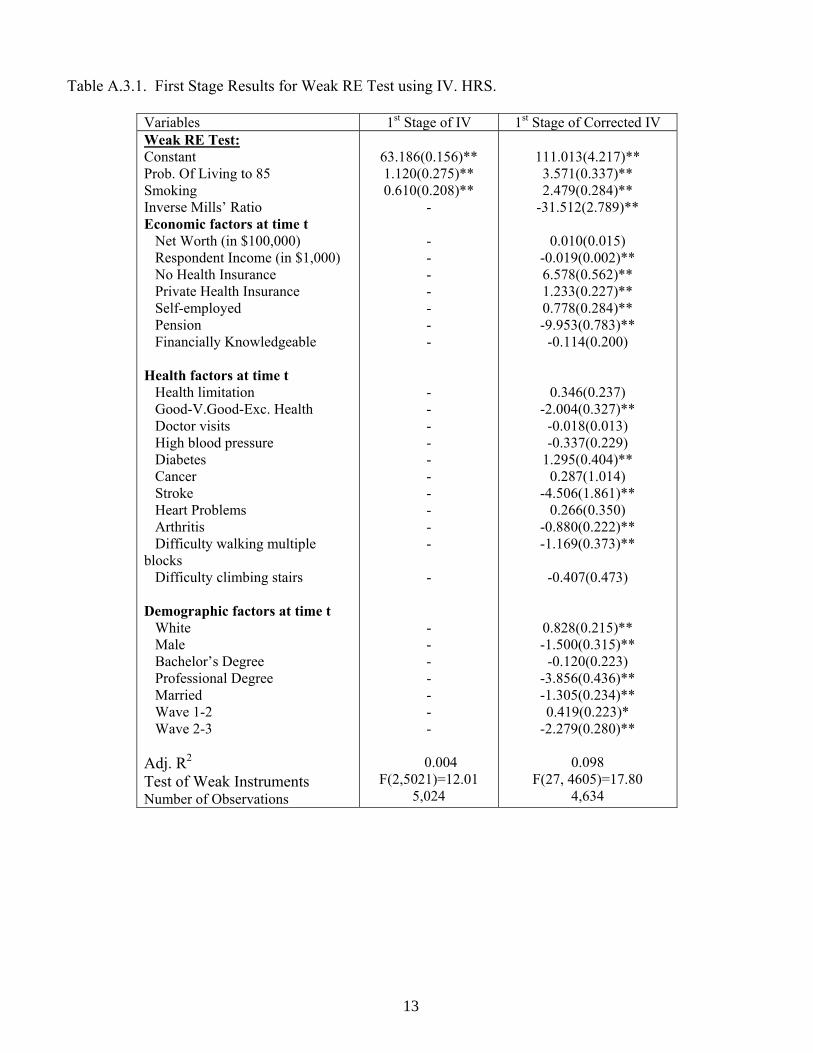
Table A.3.1. First Stage Results for Weak RE Test using IV. HRS.

Variables 1st Stage of IV 1st Stage of Corrected IV Weak RE Test: Constant Prob. Of Living to 85 Smoking Inverse Mills’ Ratio Economic factors at time t Net Worth (in $100,000) Respondent Income (in $1,000) No Health Insurance Private Health Insurance Self-employed Pension Financially Knowledgeable Health factors at time t Health limitation Good-V.Good-Exc. Health Doctor visits High blood pressure Diabetes Cancer Stroke Heart Problems Arthritis Difficulty walking multiple blocks Difficulty climbing stairs Demographic factors at time t White Male Bachelor’s Degree Professional Degree Married Wave 1-2 Wave 2-3 Adj. R2 Test of Weak Instruments Number of Observations

63.186(0.156)** 1.120(0.275)** 0.610(0.208)**

- - - - - - - - - - - - - - - - - - - - - - - - - -

0.004 F(2,5021)=12.01

5,024

111.013(4.217)**

3.571(0.337)** 2.479(0.284)**

-31.512(2.789)**

0.010(0.015) -0.019(0.002)** 6.578(0.562)** 1.233(0.227)** 0.778(0.284)** -9.953(0.783)**

-0.114(0.200)

0.346(0.237) -2.004(0.327)**

-0.018(0.013) -0.337(0.229)

1.295(0.404)** 0.287(1.014)

-4.506(1.861)** 0.266(0.350)

-0.880(0.222)** -1.169(0.373)**

-0.407(0.473)

0.828(0.215)** -1.500(0.315)**

-0.120(0.223) -3.856(0.436)** -1.305(0.234)** 0.419(0.223)*

-2.279(0.280)**

0.098 F(27, 4605)=17.80

4,634

14

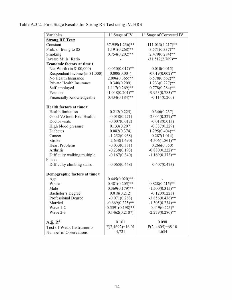
Table A.3.2. First Stage Results for Strong RE Test using IV. HRS

Variables 1st Stage of IV 1st Stage of Corrected IV Strong RE Test: Constant Prob. of living to 85 Smoking Inverse Mills’ Ratio Economic factors at time t Net Worth (in $100,000) Respondent Income (in $1,000) No Health Insurance Private Health Insurance Self-employed Pension Financially Knowledgeable Health factors at time t Health limitation Good-V.Good-Exc. Health Doctor visits High blood pressure Diabetes Cancer Stroke Heart Problems Arthritis Difficulty walking multiple blocks Difficulty climbing stairs Demographic factors at time t Age White Male Bachelor’s Degree Professional Degree Married Wave 1-2 Wave 2-3 Adj. R2 Test of Weak Instruments Number of Observations

37.959(1.236)** 1.191(0.268)** 0.754(0.202)**

-

-0.050(0.017)** 0.000(0.001)

2.096(0.365)** 0.340(0.209)

1.117(0.269)** -1.048(0.201)** 0.434(0.184)**

0.212(0.225) -0.018(0.271) -0.007(0.012) 0.133(0.207) 0.082(0.374) -1.252(0.958) -2.638(1.690) -0.033(0.331) -0.238(0.193) -0.167(0.340)

-0.065(0.448)

0.445(0.020)** 0.481(0.205)** 0.369(0.179)**

0.018(0.212) -0.071(0.283)

-0.669(0.225)** 0.5591(0.198)** 0.1462(0.2107)

0.161

F(2,4692)=16.01 4,721

111.013(4.217)**

3.571(0.337)** 2.479(0.284)**

-31.512(2.789)**

0.010(0.015) -0.019(0.002)** 6.578(0.562)** 1.233(0.227)** 0.778(0.284)** -9.953(0.783)**

-0.114(0.200)

0.346(0.237) -2.004(0.327)**

-0.018(0.013) -0.337(0.229)

1.295(0.404)** 0.287(1.014)

-4.506(1.861)** 0.266(0.350)

-0.880(0.222)** -1.169(0.373)**

-0.407(0.473)

-

0.828(0.215)** -1.500(0.315)**

-0.120(0.223) -3.856(0.436)** -1.305(0.234)** 0.419(0.223)*

-2.279(0.280)**

0.098 F(2, 4605)=68.10

4,634

15

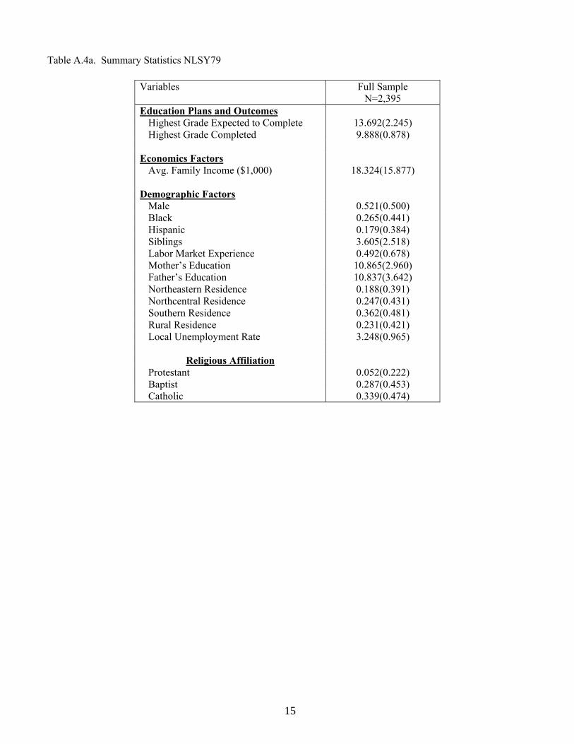
Table A.4a. Summary Statistics NLSY79

Variables Full Sample N=2,395

Education Plans and Outcomes Highest Grade Expected to Complete 13.692(2.245) Highest Grade Completed 9.888(0.878)

Economics Factors

Avg. Family Income ($1,000) 18.324(15.877) Demographic Factors

Male 0.521(0.500) Black 0.265(0.441) Hispanic 0.179(0.384) Siblings 3.605(2.518) Labor Market Experience 0.492(0.678) Mother’s Education 10.865(2.960) Father’s Education 10.837(3.642) Northeastern Residence 0.188(0.391) Northcentral Residence 0.247(0.431) Southern Residence 0.362(0.481) Rural Residence 0.231(0.421) Local Unemployment Rate 3.248(0.965)

Religious Affiliation Protestant 0.052(0.222) Baptist 0.287(0.453) Catholic 0.339(0.474)

16

Table A.4b. Summary Statistics by Sample Selection NLSY79

Variables Thought About N=2,316

Not Thought N=79

Education Plans and Outcomes Highest Grade Expected to Complete 13.692(2.245) - Highest Grade Completed 9.918(0.856) 9.013(1.044)

Economics Factors

Avg. Family Income ($1,000) 18.420(15.959) 15.491(13.034) Demographic Factors

Male 0.522(0.500) 0.468(0.502) Black 0.268(0.443) 0.190(0.395) Hispanic 0.177(0.382) 0.228(0.422) Siblings 3.611(2.521) 3.418(2.442) Labor Market Experience 0.476(0.680) 0.342(0.597) Mother’s Education 10.886(2.937) 10.266(3.533) Father’s Education 10.848(3.635) 10.494(3.846) Northeastern Residence 0.187(0.390) 0.203(0.404) Northcentral Residence 0.252(0.434) 0.089(0.286) Southern Residence 0.387(0.483) 0.114(0.320) Rural Residence 0.236(0.425) 0.076(0.267) Local Unemployment Rate 3.258(0.967) 2.962(0.854)

Religious Affiliation Protestant 0.051(0.220) 0.089(0.286) Baptist 0.290(0.454) 0.215(0.414) Catholic 0.341(0.474) 0.291(0.457)

17

Table A.5. Selection Equation Results NLSY79

Variables Probit Marginal Effects Economics Factors

Avg. Family Income ($1,000) 0.005(0.005) 2E-04 Demographic Factors

Male 0.131(0.118) 0.004 Black 0.291(0.177)* 0.008 Hispanic 0.075(0.174) 0.002 Siblings 0.044(0.026)* 0.001 Highest Grade Completed 0.499(0.066)** 0.016 Labor Market Experience 0.169(0.098)* 0.005 Northeastern Residence 0.415(0.150)** 0.010 Northcentral Residence 0.893(0.187)** 0.019 Southern Residence 1.108(0.181)** 0.031 Rural Residence 0.384(0.190)** 0.010 Local Unemployment Rate 0.150(0.070)** 0.005

Religious Affiliation Protestant -0.044(0.237) -0.001 Baptist -0.036(0.172) -0.001 Catholic 0.415(0.164)** 0.012 Constant -4.578(0.695)** - Predicted Probability 0.988 Log Likelihood -263.52 Pseudo-R2 0.241 Number of Observations 2,395 2,395

18

Table A. 6-1. First Stage Results for Weak RE Test using IV. NSLY79 Variables 1st Stage of IV 1st Stage of Corrected IV Weak RE Test:

Constant 10.838(0.170)** 11.243(1.522)** Mother’s Education 0.109(0.020)** 0.088(0.019)** Father’s Education 0.153(0.016)** 0.110(0.016)** Inverse Mills Ratio - -1.972(0.884)**

Economics Factors

Avg. Family Income ($1,000) - 0.008(0.003)** Demographic Factors

Age - -0.445(0.090)** Male - -0.030(0.082) Black - 0.290(0.109)** Hispanic - 0.474(0.144)** Siblings - -0.031(0.018)* Highest Grade Completed - 0.825(0.073)** Labor Market Experience - -0.036(0.064) Northeastern Residence - -0.092(0.151) Northcentral Residence - -0.170(0.166) Southern Residence - -0.166(0.172) Rural Residence - -0.502(0.107)** Local Unemployment Rate - -0.093(0.047)**

Adj. R2 0.128 0.263 Test of Weak Instruments F(2,2313)=171.38 F(15,2299)=47.64 Number of Observations 2,316 2,316

19

Table A. 6-2. First Stage Results for Strong RE Test using IV. NLSY79

Variables 1st Stage of IV 1st Stage of Corrected IV Weak RE Test:

Constant 10.013(1.419)** 11.243(1.522)** Mother’s Education 0.086(0.019)** 0.088(0.019)** Father’s Education 0.111(0.016)** 0.110(0.016)** Inverse Mills Ratio - -1.972(0.884)**

Economics Factors

Avg. Family Income ($1,000) 0.009(0.003)** 0.008(0.003)** Demographic Factors

Age -0.467(0.090)** -0.445(0.090)** Male 0.001(0.081) -0.030(0.082) Black 0.332(0.107)** 0.290(0.109)** Hispanic 0.549(0.130)** 0.474(0.134)** Siblings -0.024(0.018) -0.031(0.018)* Highest Grade Completed 0.936(0.053)** 0.825(0.073)** Labor Market Experience -0.004(0.062) -0.036(0.064) Northeastern Residence 0.061(0.135) -0.092(0.151) Northcentral Residence 0.058(0.131) -0.170(0.166) Southern Residence 0.094(0.127) -0.166(0.172) Rural Residence -0.444(0.104)** -0.502(0.107)** Local Unemployment Rate -0.065(0.045) -0.093(0.047)**

Adj. R2 0.262 0.263 Test of Weak Instruments F(2,2300)=72.59 F(2,2299)=73.08 Number of Observations 2,316 2,316