existence results for some quasilinear parabolic equations

,V<,nl,nuor Anulwsn. Theorv. .Merhods & Applrcomns. Vol. 13. No. 4. pp. 373-392. 1989 0362-5M.K 89 S3.OU+ .GU

Printed m Great Briraln i_ 1989 Pergamon Press plc

EXISTENCE RESULTS FOR SOME QUASILINEAR PARABOLIC EQUATIONS

LUCIO BOCCARDO

Via Bressanone 5. 00198 Roma, Italy

and

FRANCOIS MURAT and JEAN-PIERRE PUEL

Laboratoire d’Analyse Numkrique, Universite P. et M. Curie, Tour 55-65. 5hme &age, 75252 Paris Cedex 05. France

(Received 9 Seprember 1987; received for publicafion 14 April 1988)

Key wordx and phrases: Quasilinear parabolic equations. natural growth.

THIS PAPER is concerned with the Cauchy problem for an equation whose principal part is a quasilinear parabolic operator. The additional nonlinear term has at most a quadratic growth with respect to the gradient (in the space variables) of the solution. We prove the existence of a weak bounded solution under minimal regularity hypotheses, assuming the existence of a subsolution and a supersolution for the problem. The method we use is still valid in a different context, whenever the hypotheses guarantee an a priori L”-estimate. As a complement, we give in the last section the corresponding result for a parabolic quasilinear unilateral problem,

I. STATEhlENT OF THE MAIN RESULT: COhlMENTS

1.1. Notations, statement of the results Let T be a positive number, and Sz be a bounded open subset of IR”, whose boundary r is not

required to be regular. We denote by Q the cylinder

Q = ~2 x IO, TL

and by C the set

c = 1- x IO, T[.

We consider Caratheodory functions:

aij:Q x R --* IR, i,j = 1, . . . . n,

fO:QxRx~“-+IR.

If u is a function defined on Q with values in IR, we write Vu for its gradient with respect to the space variable x E Sz, and we define Aij(u) and F,(u, VU) by

Aij(U)(x, t) = aij(X, t, U(X, t)) a.e. in Q,

F&u, Vu)(x, t) = f&x, t, u(x, t), Vu(x, t)) a.e. in Q.

373

371 L. BOCCARDO, F. MURAT and J.-P. PUEL

Let ltO E L”(Q) and f, E L’(O, T, H-‘(n)) be given. We define

F(u, Vu) = Fo(u, Vu) + f,,

and we consider the following Cauchy problem

Ai, + F(u, VU) = 0 in Q, J 1

u = 0 on C, (1.1)

u(0) = no, in n.

For sake of simplicity we shall denote by A(u) the matrix (A;j(u)) and by V[A(u)Vu)] the

operator Cy,j=, a/axi[Aij(u) &4/i3xj]. We make the following hypotheses on the functions aij and fO:

3cu>o, v < E R”, v s E R ii, aii(x, t,s)<iti 2 (r/d2 a.e. in Q; (1.2)

3P>O, v s E IR, (aij(x, t, s)I 5 P a.e. in Q. (1.3)

There exists a nondecreasing function b( .) from IR’ to IR’ such that for all (x, r) E R x R”,

IS&, t, s, 01 5 b(]s])(l + lc12) a.e. in Q- (1.4)

Definition 1.1. A subsolution of problem (1.1) is a function cp E L-(0, T; IS”*“(n)) such that ap/at E L*(O, r; Z-i-‘(Cl)) + L’(Q) and

- - V. [A(cp)VpJ + F((p, Vcp) I 0 in Q, at

v, 5 0 on Z, (1.5)

~(0) 5 u0 in Q.

A supersolution of problem (1 .l) is a function IJI E L-(0, T; WIS”(!J)) such that aw/af E L*(O, R H-‘(n)) + L.‘(Q) and

w - - V. [A(I,u)VW] + F(~,u, Vy/) 2 0 in Q, at

t+u 1 0 on C, (1.6)

y/(O) 21 u0 in R.

We can now state the main result of this paper.

THEOREM 1.1. If there exist a subsolution a, and a supersolution IJI of problem (1.1) such that v, I w a.e. in Q, then there exists at least a solution u of problem (1.1) which satisfies

and

u E L*(O, T; H&2)) fl C(0, T; L’(fl)), g E L2(0, r; H-‘(a)) + L’(Q),

up 5 u I v a.e. in Q.

Quasilinear parabolic equations 375

Comments 1.2. (1) In (1.1) every term makes sense: au/at E L2(0, C H-‘(Cl)) + L’(Q);

V. [A(u)Vu] E L2(0, T; H-‘(n)); F(u, VU) E L2(0, T; H-‘(R)) + L’(Q). (Notice that u E L”(Q) because v, 5 u 5 w.) As u E C(0, c L2(sZ)), the meaning of the initial condition u(0) = u0 is clear. In fact, as it will be stated precisely in Section 2, u E C(0, T; L2(n)) is a consequence of u E L2(0, P, H:(n)) n L”(Q) and du/dt E L’(O, F, H-‘(R)) + L’(Q), and if (. , . > denotes the duality pairing between H-‘(n) and H:(Q) we have the following variational formulation

n I "T n

u(T)u(T) dx - ug u(0) dx - n i (B,, u)dt - 82udwdt

0 1 Q m

+ ,4(u) VU Vu du dt + Q I F,(u, Vu)u du dt + (f,, u) dt = 0.

YQ

(1.7)

Notice that in (1.7) we can take u = u and obtain the “energy equality”:

lU(7-)I% - 1 ~~P/UO]~~+/~ iQFu(u.VU)U~dt+STj,,U)dr=O. A(u) VU VU dudt + R

(1.8)

(2) Our result does not require any regularity assumption on the open set n nor on the functions aji and fo. In this sense it appears to be optimal

(3) It is possible to consider various extensions of problem (1. l), for example to other boundary conditions (eventually nonlinear) or to a problem with periodicity conditions in time instead

of a Cauchy problem. (4) For a given problem, one can try several methods to exhibit a subsolution and a super-

solution. Of course there is no methodology, but, usually, one should try functions which are locally “simple” (constants, linear, quadratic, exponentials, eigenfunctions of “simple” operators, solutions of auxiliary differential equations, . . .). Lef us give two useful examples.

(i) Suppose it is possible to solve on IO, r[ the following ordinary differential equations:

dt + b(- p) = 0 in (0, T)

P(O) = - IIuollm; cp I 0.

- - b(v) = 0 in (0, T) dt

(1.9)

(1.10)

v/m = II~olloo~ Iy 2 0.

Then, ifft = 0, p and IJ (which are constant in x) are clearly subsolution and supersolution of (l.l), and rp I I//.

(ii) When aij, f. and f, do not depend on t, if we know a subsolution p and a supersolution w of the associate stationary problem

- V. [A(U) Vu] + F(u, VU) = 0 in Sz, (1.11)

u = 0 on I,

376 L. BOCCARDO, F. ~~URAT and J.-P. PCEL

with cp 5 I+Y a.e. in R, then if u0 satisfies v, 5 u0 I w a.e. in Q, cp and w are subsolution and supersolution of (1.1).

(5) The result of theorem 1 .l has been announced in (161. It has recently been generalized in [ 141 to the case where the operator - V. [A(u) Vu] is replaced by an operator of Leray-Lions type - V. [A(u, Vu)] acting from P(0, Z W,‘*“(sZ)) into Lp (0, T; W-‘** (Cl)). Then the growth of the nonlinearity F0 with respect to the gradient can be of order p.

Theorem 1.1 is an extension to parabolic quasilinear equations of results obtained in the elliptic case in [5, 61 (for p = 2) and [7]. The proof given here is similar to the ones used in [5] and [7], but its extension to the parabolic case is not straightforward and requires some specific techniques.

(6) As it has already been pointed out in [16], the proof of theorem 1.1 shows in fact that whenever we have an L”(Q)-estimate on the solutions of a family of approximate equations for (l.l), these solutions converge strongly in L’(O, T; Hi(n)) to a solution of (1.1).

(7) There is an extensive literature on the study of quasilinear parabolic equations, systems and variational inequalities. Several papers are mainly concerned with the regularity properties, see e.g. [lo, 11, 18, 211. Others study the existence of a solution using as a main tool some regularity arguments (see e.g. [l, 9, 131 and [3, 4, 19, 22, 231 for the case of parabolic variational inequalities) or the fact that the nonlinearity has a growth which is strictly subquadratic with respect to the gradient [2, 8, IS]. One should also look at the references quoted in these papers.

Our method gives a direct proof which makes no use of regularity argument and which gives

an optimal result for the case of an equation and of a unilateral problem. Unfortunately, we have not been able yet to make it work for sufficiently general systems and this is an interesting and important open question.

2. PRELIMINARY RESULTS: MODIFICATION OF THE EQUATION

As in [6] we shall replace the study of (1.1) by the study of an auxiliary modified equation, the solutions of which will necessarily take values between Ed and IV.

Let us define for u E L’(0, r; H’(Q)) the truncation T(u) by

T(u) = u - (v - ij/)’ + (9 - II)+, (2.1)

and now

A,(u) = A,j(7-(UN, A(u) = taijtu))9 (2.2)

.&J, Vu) = F,(Uu), VV4). E(u, Vu) = &I, Vu) + f,. (2.3)

The coefficients A, satisfy the analogous of (1.2), (1.3), namely

v u E L2(0, r; H’(Q)), v < E IR”, i aij(u)tlirj 1 CY/<~* a.e. in Q, (2.4) i,j= 1

v u E L*(O, T; H’(i.2)), la,(U)1 I P a.e. in Q. (2.5)

The operator u -+ FO(u, Vu) maps continuously L*(O, r; H’(R)) into L’(Q) and in addition we have from (1.4) and definition 1.1,

3 B E R such that v u E L*(O, r; H’(R)), j&u, Vu)(x, r)] I B(l + ]Vu(x, t)]*) a.e. in Q. (2.6)


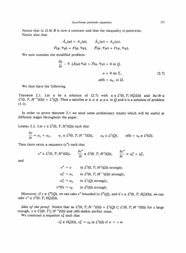
Notice that in (2.6) B is now a constant and that the inequality is pointwise. Notice also that:

A,(P) = 4j(@4> d,(Y) = Aij(V)9

&A V(o) = erp, VP), &v VW) = cry, VW).

We now consider the modified problem:

au - - V. [A(u) VU] + p(‘(u, VU) = 0 in Q, at

We then have the following.

u = 0 on E,

u(0) = ue, in R.

(2.7)

THEOREM 2.1. Let u be a solution of (2.7) with u E L’(O, T; H&I)) and au/at E

L2(0, C H-‘(Cl)) + L’(Q). Then u satisfies P I u I w a.e. in Q and u is a solution of problem (1.1).

In order to prove theorem 2.1 we need some preliminary results which will be useful at different stages throughout the paper.

LEMMA 2.2. Let v E L'(O, T; H’(n)) such that

au at = aI + a29 01~ E L2(0, T; H-‘(Q)), ~2 E L’(Q)> u(0) = vg E P(n).

Then there exists a sequence (v”) such that

and

v" E L'(O, T; H’(Q)), f$ E L’(O, T; H’(SZ)), aUn r = a: + a;,

vn + v in L’(O, T, H’(i2)) strongly,

CY; + (Y, in L’(O, T, H-‘(Cl)) strongly,

CY; -+ cY2 in L’(Q) strongly,

v”(0) -+ Ue in L2(SI) strongly.

Moreover, if v E L”(Q), we can take Y” bounded in L?‘(Q). and if v E L’(O, T; H&2)), we can take vn E L’(O, T; Hd(L2)).

Idea of the proof Notice that as ,C2(0, T; H-‘(0)) + L’(Q) c L'(0, T; H-S(Cl)) for s large enough, u E C([O, 7’1; HbS(C2)) and v(0) makes perfect sense.

We construct a sequence vi such that

vi E Hi(Cl), v: * v0 in L’(a) if n -, + 00

378

and

L. BOCCARDO. F. ~IURAT and J.-P. PCEL

This is possible by solving for example the problem:

ug = 0 on T.

Now we take u” to be the solution of

1 du” - - + un = u, n dt

u”(0) = uo”.

One can show that u” has all the properties stated in lemma 2.2.

LEMMA 2.3. Let u E L’(O, T; Hi(n)) II L”(Q) such that au/& = cr, + CY~, 01~ E L’(0, r; H-‘@)),

CY~ E L’(Q), and u(0) E L”(n). Then u E C([O, T]; Lp(sZ)), v p, 1 I p < +oo. Moreover, if w E L2(0, T; H;(a)) 0 L”(Q), awlat = p, + fi2, PI E L2(0, T; H-‘(n)), p2 E L’(Q), W(0) E

La(C2), we have

(a,, w)dt + I a2wdxdt = i

u(T)w(T) dx - u(O)w(O) dJI .Q n R

'T n

- I <PI, u)dt - &ududf, “0 I CQ

where (. , .) denotes the duality pairing between H-‘(R) and H,(R).

(2.8)

Idea of theproof. Using lemma 2.2, we approach u by a sequence v” of “regular” functions. We consider

-s

g”(t) = t ! * IU”(f)12 h7

and we show that g” is compact in W ‘* ’ 0 T) thus in C([O, r]), which proves that the function ( , ,

g(t) = + I IuU)12 h, n

belongs to C([O, T]). As we already know that u E C([O, T]; HeS(G)) for s large enough, this enables us to show that u E C([O, T]; L’(n)). Now, as u E L”(Q), the Holder inequality gives

u E C(]O, TI); L%w, vp,l~p<+w.

Formula (2.8) giving the integration by parts comes directly by approaching u and w.


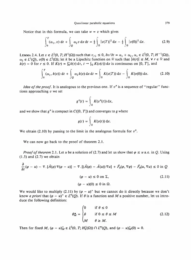
Notice that in this formula, we can take w = v which gives

3

I

II

(a,, u)df + a2vdxdt = $ Iv(r)12 d.Y - + Iv(o)(2 dr. (2.9) CQ R R

LEMMA 2.4. Let v E L2(0, Z H’(n)) such that v ,c 5 0, adat = a, + (y2, cy, E ~~(0, r; W(SZ)),

cx2 E L’(Q), u(O) E iI’( let k be a Lipschitz function on R such that Ik(r)l I M, v r E R and k(r) = 0 for r 5 0. If K(r) = j;k(r) dr, t -+ Jn K(v(t)) dx is continuous on [0, T], and

1

/

n

(a,,k(v)) dt + a2 k(v) dx dt = K(v(T)) dJz - I

K(vW) dx. (2.10) Q .fl ,fi

Idea of the proof. It is analogous to the previous one. If v” is a sequence of “regular” func-

tions approaching v we set

3

g”(t) = I K(v”(t)) h, .R

and we show that g” is compact in C([O, T]) and converges tog where

1

g(t) = I K(v(t )) d.x-. ,R

We obtain (2.10) by passing to the limit in the analogous formula for v”.

We can now go back to the proof of theorem 2.1.

Proof of theorem 2.1. Let u be a solution of (2.7) and let us show that IJ? I u a.e. in Q. Using (1.5) and (2.7) we obtain

:(a - u) - v.[A(cp) V(p - u)] - V.[(A(p) - a(u)) VU] + po(rp, V(o) - Fo(u, Vu) I 0 in Q

(cp - u) 5 0 on E, (2.11)

(9 - u)(O) 5 0 in R.

We would like to multiply (2.11) by (p - u)’ but we cannot do it directly because we don’t know a priori that (cp - u)’ E f.“(Q). If 0 is a function and A4 a positive number, let us intro- duce the following definition:

r

0 if050

eJf= 6 ifOr8rM (2.12)

M e 1 M.

Then for fixed M, (10 - u)h E L2(0, C Hi(R)) n L”(Q), and (V - u)h(O) = 0.

380 L. BOCCARDO, F. XIURAT and J.-P. PUEL

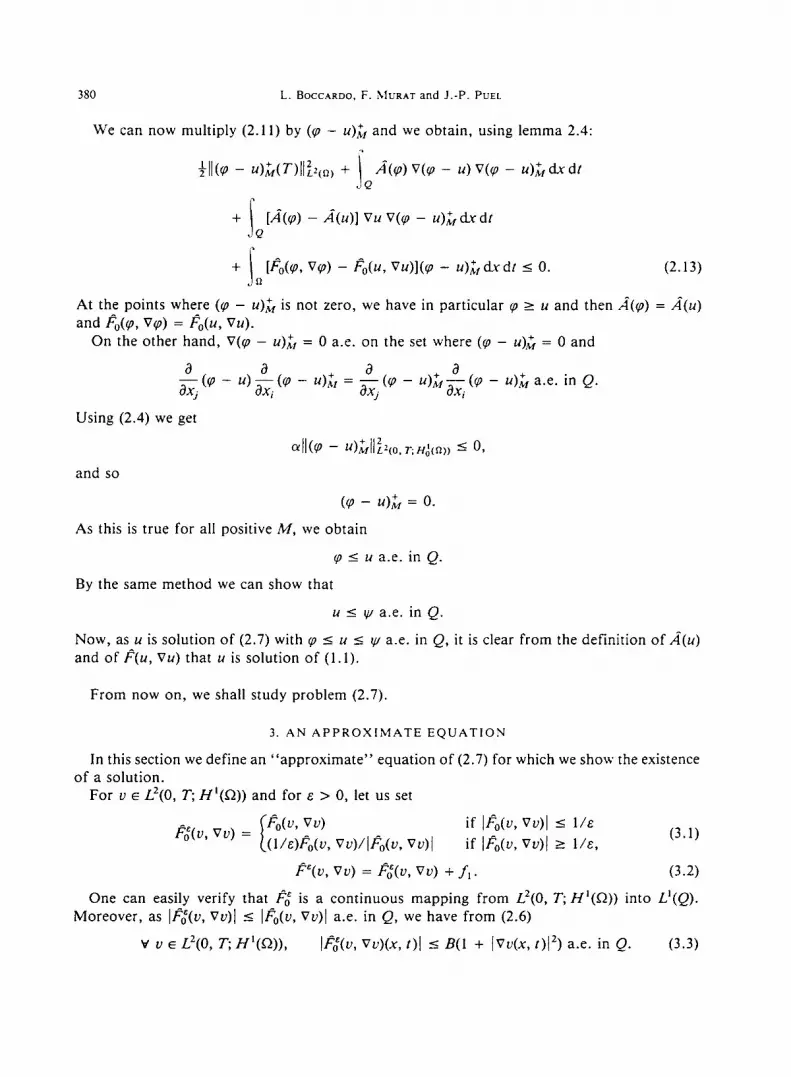
We can now multiply (2.11) by (u, - u),:, and we obtain, using lemma 2.4: -.

H(cp - 4ifV)llZq*, + i

/i(p) v(rp - u) V(rp - u)h dudt Q

+ ?:

[/i(v) - /i(u)] Vu V(CJI - u)~t,ddt Q

+ [&(p, VP) - &(u, Vu)](e~ - r&dxdt I 0. (2.13) R

At the points where (cp - u),& is not zero, we have in particular Ed 2 u and then A(cp) = A(u) and &(p, V+T) = pO(u, Vu).

On the other hand, V(y, - u)& = 0 a.e. on the set where (cp - u),& = 0 and

&(P - n)&(c - u)& = $,($J - u).&$(v - u)L a.e. in Q. J I J ,

Using (2.4) we get

and so

As this is true for all positive M, we obtain

p I u a.e. in Q.

By the same method we can show that

u 5 I+Y a.e. in Q.

Now, as u is solution of (2.7) with rp I u gr v a.e. in Q, it is clear from the definition of a(u) and of E(u, Vu) that u is solution of (1.1).

From now on, we shall study problem (2.7).

3. AN APPROXIiMATE EQUATION

In this section we define an “approximate” equation of (2.7) for which we show the existence of a solution.

For v E L*(O, T; H’(0)) and for E > 0, let us set

fq(v, Vu) = 1 eJ(u, Vu) if I&(v, Vv)l 5 l/e

(l/&)&U, Vv)/I&v, Vu)] if I&v, Vu)1 1 l/e, (3.1)

p”(v, Vu) = &I, Vu) + j-1. (3.2)

One can easily verify that & is a continuous mapping from L*(O, c H’(R)) into L’(Q). Moreover, as I&II, Vv)l 5 I&u, Vv)l a.e. in Q, we have from (2.6)

v v E L2(0, T; H’(Q)), lFt(v, Vv)(x, t)l d B(l + jVv(x, [)I*) a.e. in Q. (3.3)


For fixed E > 0, we consider the following “approximate” problem

ad - - V. [.d(u’) Vu’] + P(u’, Vu”) = 0 in Q, at

uE = 0 on IE, (3.4)

u’(O) = u0 in S2.

PROPOSITION 3.1. For every E > 0, there exists at least one solution uE of problem (3.4) such that

UE E L2(0, r; H;(cl)), g E L2(0, T; fr’(cl)).

Proof. As the initial data u0 belongs to L”(n) C L’(Q) there exists h: E L2(0, r; Hi(R)) such that &i/at E L2(0, C H-‘(!2)) and h(O) = ue. Let us set uE = U’ - U; we can rewrite problem (3.4) as follows:

at.f at + N(u”) = - $ - f, in Q,

v’ = 0 on C,

vE = 0 in Sz,

(3.5)

where

N(u) = -v. [A(ii + u) Vu] - v. [&a + u) vi21 + &a + u, vii + Vu).

One can check that the operator N satisfies the hypotheses of theorem 1.2, p. 319 of [12], which gives the existence of a solution uE of (3.5) and thus of a solution U’ of (3.4).

4. ESTIMATES IN L-(Q) AND L2(0, T;H,(C2))

4.1. Estimate in L”(Q) For E sufficiently small we show an L”(Q)-estimate for the solutions uc of (3.4).

PROPOSITION 4.1. There exists e0 > 0 such that for E I se, the solutions U’ of (3.4) satisfy

rp I uE I IJI a.e. in Q.

In particular, for e I eO, u” remains bounded in L”(Q) independently of E.

Proof As rp and w belong to L”(0, T; W’*“(Sl)) we know that F,(p, V(o) E L”(Q) and F,(w, V(v) E L”(Q). Let q, be such that

382 L. BOCCARDO, F. ML-RAT and J.-P. PUEI

Then for E 5 E,,, we have

G(9, V9) = &(9, V9) = &(9, V9),

&%C VW) = &A VW) = F,(w, VW).

Let us show, for example, that 9 I U’ a.e. in Q; the other inequality can be proved exactly in the same way. From (3.4) and (1.5) we have

ad -- at

v. [A(d) VU”] + &(I/, VU”) + fi = 0 in Q,

a9 -- at V. [a(v) Vrpl + I’,E(cp, Vrp) + f, I 0 in Q,

(U” - fp) 5 0 on C,

(u” - 9)(O) = 0 in Q.

Now we proceed as in the proof of theorem 2.1. We subtract the first equation from the second and we multiply by (9 - u”)&. We notice that

>

i [&9, V9) - &u&, Vu”)J(9 - U”)h;,ddt = 0,

Q

because at the points where (9 - u”),& # 0, for E 5 c0

&4&, VU”) = Fo(9, V9) = &9, V9) = &C, VU”).

We end up as in the proof of theorem 2.1 and we obtain

(9 - UE)+ = 0,

thus

9 5 U’ a.e. in Q.

Remark. In fact, the only result of proposition 4.1 that will be used is the L”(Q)-estimate. To obtain this estimate we strongly use here the assumptions on 9 and 9.

Other kinds of hypotheses could lead to an existence result for a family of approximate equations and an estimate in L-(Q) for their solutions. The rest of the proof of theorem 1.1 remains valid in such a context.

4.2. Estimate in L’(O,.C Hi(Q))

PROPOSITION 4.2. For E 5 E,,, the solutions U’ of (3.4) are bounded in L’(O, T; Hi(Q)) independently of E.

Proof. We start from equation (3.4)

ad -- at

V. [A(d) VU”] + &u’, VU’) + f, = 0 in Q,

uE = 0 on I,

u’(0) = u0 in R.


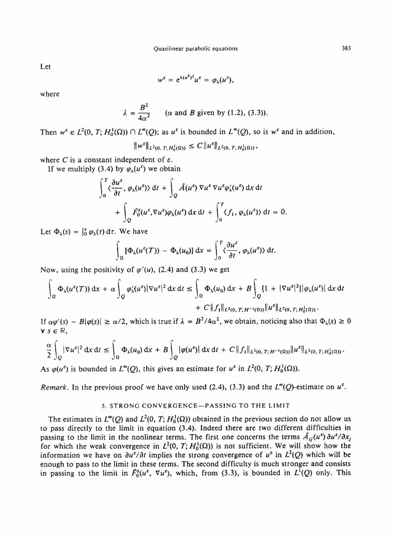
Let

where

w’ = eX(@u& = /#,j&“),

(a and B given by (1.2), (3.3)).

Then w’ E ,5’(0, T; H;(a)) n L”(Q); as u” is bounded in L”(Q), so is wE and in addition,

II WEI1 LZ(O, T; H&l,, 5 CII4IL’(O. T; H;(n), 9 where C is a constant independent of E.

If we multiply (3.4) by rpx(u”) we obtain

‘T ad

I o tat, ox> dt +

j &u’) Vu’ Vu’rp;(u’) dx dt

Q

+

s

T

f&“,Vu”)e~~(u”) dx dt + <f, ,cox(u")> dt = 0. Q 0

Let ox(s) = lf, cpx(r) dr. We have

s PWW)) - Wuo)l dx = n

oT?$ cp&“)> dt.

Now, using the positivity of q’(u), (2.4) and (3.3) we get

s @&P(T)) dx + ff

5 cp;(u”)jVu”12 d_x dt s

s %(u,) dx + B [I + IVu”~21\~M)1 dxdt

n Q R Q

+ mfillLqo. T;H-qn,,IIUEIIL~(O. T;Ff&n,, * If CUJI’(S) - Blcp(s)\ L (r/2, which is true if I = B2/4cu2, we obtain, noticing also that oh(s) L 0

VSEIR,

;

i (Vu”(2dxdt 5

Q s @x(uo) dx + B

R i l(P(nE)l d-x dt + Cl/f, 11~2~0. T;H-~~R~~~~U~~~L~~O. T;&(n), .

Q

As cp(u”) is bounded in L”(Q), this gives an estimate for uE in L2(0, Z H:(Q)).

Remark. In the previous proof we have only used (2.4), (3.3) and the L”(Q)-estimate on uE.

5. STRONG CONVERGENCE-PASSING TO THE LIMIT

The. estimates in L”(Q) and L2(0, T; Hi(n)) obtained in the previous section do not allow us to pass directly to the limit in equation (3.4). Indeed there are two different difficulties in passing to the limit in the nonlinear terms. The first one concerns the terms aii(u&) au&/ax, for which the weak convergence in L’(O, T; Hi(Q)) is not sufficient. We will show how the information we have on &P/at implies the strong convergence of u’ in L’(Q) which will be enough to pass to the limit in these terms. The second difficulty is much stronger and consists in passing to the limit in If,E(u”, Vu’), which, from (3.3), is bounded in L’(Q) only. This

384 L. BOCCARDO, F. MURAT and J.-P. PUEL

information does not allow us to pass to the limit. In order to overcome this difficulty, we will show that, because of the structure of equation (3.4), the sequence (u”) is not only bounded but actually relatively compact in L’(O, T; Hi(Q)). As it has already been pointed out in [16], this argument makes only use of (2.4), (3.3) and of L”(Q)-estimate on u’.

From proposition 4.2 we know that U’ is bounded in L2(0, T, Hi(Q)). Using (3.3), we deduce from equation (3.4) that aue/ar is bounded in L2(0, T; H-‘(n)) + L’(Q). With these two informations we obtain the following.

PROPOSITION 5.1. The sequence (u”) is relatively compact in L’(Q).

Proof. For s > 0 large enough, we have L’(R) c HeS(SZ). Then &“/at is bounded in L’(0, Z H-“(a)), and U’ is bounded in L*(O, T; Hi(n)).

As H:(n) C L’(Q) C H-“(Q), the injections being compact, proposition 5.1 follows from a compactness lemma of Aubin’s type. Such a lemma can be found for example in [ZO, chapter III, p. 2761 or in [17, section 8, corollary 41.

Let us now consider a subsequence, still denoted by U& for simplicity, such that if E -+ 0

U’ -+ u in L2(0, P, Hi(Q)) weakly.

By possibly extracting a new subsequence, we can suppose, without loss of generality using proposition 5.1, that

uc -+ u in L’(Q) strongly,

U’ + u a.e. in Q.

From proposition 4.1 we see that u E L”(Q) and

IJJ 5 u 5 (u a.e. in Q.

We now have the following essential result.

PROPOSITION 5.2. The sequence U’ converges strongly to u in L’(O, r; H,‘(R)) if E tends to 0.

Proof. We consider again equation (3.4)

ad - - V. [A(d) Vu”] + &u’, Vu”) + fi = 0 in Q, at

Let vi(s) = exszs, where J. = 16B2/(r2. We then have

uE = 0 on X 9

U&(O) = u0 in Sz.

cu(D’(.s) - 8B]&)I 2 cY/2, VSER. (5.1)


If E and 6 are two positive parameters, we rewrite (3.4) as follows

-$u’ - u*) - V.[~(U’) V(u" - u*)J + $ - V.[a(u")Vu*] + &uE,Vue) +f, = 0 in Q,

(u” - u*) = 0 on 1, (5.2)

(u” - u*)(O) = 0 in Q.

Firsr step. We multiply (5.2) by (pX(uE - u*). This is possible because (pX(nE - u*) E L2(0, T; H;(a)). If we set again D,.(s) = ji cpx(r) dr, we obtain

aguC(T) - u*(T)) dx + s /i(u”)v(uE - u*)V(u' - u*)&(u" - u*) dvdt R Q

T au* + (--, pX(uE - u*)> dt +

o at a@‘) Vu” V(e# - u*)) dx dt

Q

+ Tulv VIX(UE 5

- u*)> dt 0

=-

.i

l&P, Vu')cp,(u' - u*)dx dt Q

I B 1

[l + ~V~~~~]~rp~(u' - u*)l tidr Q

I 1

[B + 2BlV(uC - .*)I’ + ~B]VU*]~]]~~(U~ - u*)/ dwdt. Q

As mx(s) I 0 v s E IR, if Id denotes the identity matrix this gives

[z&P)&(uE - u*) - 2B]cp,(u’ - u*)] Id] V(u” - u*) V(u” - u*) dudt Q

s

T au*

I

T

+ o'ar, MU - u')> dt + /i(d) Vu* V(cp&" - u*))d_x dt + <f,, CPM - u*)> dt Q 0

n

s !

[B + ~B]VU*]~]]~@ - u*)] dxdt. Q

(5.3)

The matrix C” = a(u”)&(u” - u*) - 2Bla7,(uE - u”)] Id is positive definite because (5.1) implies

CL 1 [cq;(u” - u*) - 2B]q+E - u*)]] Id 2 (a/2) Id.

For fixed 6, let E tend to zero. We know that

uc + u a.e. in Q

u” -, u in L2(0, r; Hi(R)) weakly.

386 L. BOCCARDO. F. MURAT and J.-P. PUEL

Therefore the matrix CE converges a.e. in Q to the matrix Co defined by

Co = /i(u)(o;(u - u*) - 281(ax(u - u6)1 Id.

This convergence also occurs in [L”(Q)]“’ weak,. Because of the positive definiteness of C’, we obtain

1

lim inf I

7

C” V(U” - u*) V(u” - u6) dx dt I E-O Q !

Co v(u - u”) V(U - u*) dudt. Q

We can now pass to the limit in (5.3) when E tends to 0 and 6 is fixed. According to the above inequality, we can take the lim inf of the first term. We can pass to the limit in the second and fourth terms because

(o&P - U*) -+ px(u - u6) in L’(O, T; Hi(Q)) weakly.

This follows from the fact that rp,(u’ - u*) remains bounded in L2(0. T, Hi(Q)) and converges almost everywhere in Q towards rp,(u - u*). In order to pass to the limit in the remaining terms, we use Lebesgue’s dominated convergence theorem which implies that

a(~‘> Vu6 + A(u) Vu6 in (L’(n)Y strongly,

[B + 2BJVu6]2]]rp,(u” - U6)j + [B + ~B]VU*I~]]~~(U - u6)] in L’(Q) strongly.

We then obtain

[/i(u)p;(u - u6) - 2BIyl,(u - u*)l Id] V(u - u*) V(u - u*) dxdt +

.i

7

+ ii(u) VU*. V(rpx(u - u6)) du dt + <_f,, vx(u - u*))dt Q 0

5 .i

[B + ~B]vu*[~]~~,(u - u*)] dudt. Q

Second step. By multiplying equation (3.4) relative to the parameter 6 by px(u possible because P,,(u - u*) E L2(0, r; H,‘(0))) we get

s r ad o (at’ P,(U - u*)) dt = - /i(d) vu6 v(px(u - u*)) ti dt

Q

- <f,, rp,(u - d) dt

(5.4)

u*) (which is

_

\ F;(d, vu*)rp,(u - u6) d_x dt.

YQ

Quasilinear parabolic equations

Therefore (5.4) implies

387

? [&)9;(u - u6) - 2Bj9& - u*)[ Id] V(u - u*) V(u - u”) dxdt

Q ,3

+ 3

/f(u) vu6 V(9x(u - u”)) dx dt - 1

/i(u*)vu* v(cph(u - d))dx dt Q Q 1

I i

[B + 2BIVu*1*]/9Ju - u”)l dudt + I~;@*, @)I /9& - u6)1 dxdr Q Q

5 [2B + 3BIV~*1~][9,(u - u*)l dxdt Q

< [2B + 6BlV(u - .*)I* + ~B~VU~~]~~,(U - u*)[ dxdr. (5.5) Q

Let us notice now that

J /i(u) Vu* V(cpk(u - u*)) dxdt = - 3

&)9;(u - u*) V(u - u*) V(u - u*) ti dt Q Q

+ s /i(u) Vu V(9x(u - u6)) ti dt. Q

Similarly

- /i(u”) Vu6 V(9A(u - u”)) dxdt = &u*)9;(u - u6) V(u - ud) V(u - u6) dx dt Q Q

- s /i(d) Vu V(cox(u - u*)) dxdt. Q

Using these equalities in (5.5) and substracting from both sides ”

6B J

19x(u - u6)1 IV(u - u*)l’dxdt Q

we obtain

s [&u*)9i(u - u*) - 8BI9,(u - u*)[ Id] V(u - u*) V(u - u*) ckdl Q

+ a(u) Vu V(cpx(u - u”)) dudt - s

a(~*) Vu V(9x(u - u*)) ti dt Q Q

5 [2B + ~BIVU~~][~~(U - u*)[ dudr. (5.6) Q

From (5.1), we have, in the sense of matrices

a(u6)9i(u - u’) - 8BI9,(u - u*)l Id 1 [CY(D:(U - u*) - 8BI9,(u - u*)l] Id

2 ((~12) Id.

358 L. BOCCARDO, F. ~~I_-RAT and J.-P. PUEL

Therefore (5.6) implies

; \ ]V(u - &I* dwdt 5 - \ [A(u) - A(d)] Vu V(rpx(u - u*)) dwdt bQ UQ >

+ I (2B + 6B]Vu12]lcpx(u - u’)l dudt. JQ

If we let 6 tend to zero, we know that

qx(u - u6) -+ 0 in t*(O, r; Hi(n)) weakly, in L”(Q) weak,, and a.e. in Q,

a(u6) -+ a(u) a.e. in Q and in [L”(Q)]“’ weak,.

Using Lebesgue’s dominated convergence theorem we obtain

(5.7)

>

lim [2B + 6B/Vul’]lp,(u - u&)1 dxdt = 0 *--O I , Q

and ,

lim !

[a(u) - A( Vu V(y?x(u - u6)) du dt = 0. h--O<Q

Therefore 1

lim I

]V(u - u6)]’ tidt = 0, h-0 Q

which is the strong convergence of u6 to u in L’(O, T; Hi) when 6 -+ 0.

Remark. The proof of proposition 5.2 is quite different from the corresponding one in the elliptic case treated for example in [5, 71. In the elliptic case, the weak limit u of U& is directly in the same space as u&. But here, we don’t have enough information on au/at, which makes impossible for example the direct multiplication of (3.4) by rp,(u’ - u).

Using proposition 5.2, it is now easy to pass to the limit in equation (3.4) relative to the parameter 6.

As u6 converges strongly to u in L*(O, r; H;(n)), we have

Po(r4”, Vu6) -+ I;‘,(u, Vu) in L’(Q) strongly.

Therefore, applying Vita!i’s theorem,

Fi(u*, Vu&) + fo(u, Vu) in L’(Q) strongly.

On the other hand,

V. [A(d) Vu*] --t V. [A(u) Vu] in L*(O, T, H-‘(n)) strongly.

Thus au*/at converges strongly in L*(O, R H-‘(a)) + L’(Q), which implies that

$ E L’(O, r; H-‘(!A)> + L’(Q), au

and - - at v. [A(u) Vu] + F(u, Vu) = 0.

For s large enough, &?/at converges strongly to au/at in L’(0, T, H-‘(R)). Then u* converges strongly to u in C([O, T]; H-‘(R)), and u’(0) -+ u(O) in H-‘(R).


Therefore u satisfies (2.7), i.e.

au - - V. [A(u) VU] + fl(u, VU) = 0 in Q, at

u = 0 on 1,

u(0) = ue in G.

From lemma 2.3 we have u E C([O, T]; L’(SI)) and from theorem 2.1, u is a solution of problem (1.1). This finishes the proof of theorem 1.1.

6. A QUASILINEAR PARABOLIC UNILATERAL PROBLEM

As a complement, we present here a result concerning a quasilinear parabolic unilateral problem. For the sake of simplicity, we don’t consider the most general context and we will restrict ourselves to the zero obstacle problem in the “strong” formulation (according to the terminology of parabolic variational inequalities).

Keeping the same notations as in the previous sections, we suppose now that u0 2 0 a.e. in Sz andf, = 0, which means that for u E L’(O, T; H’(n)) fl L”(Q),

F(v, Vu) = F,(v, VU) E Lt(Q). (6.1)

We define the following convex sets:

K = (u 1 u E L’(O, Z Hd(sZ)), u 2 0 a.e. in Q) (6.2)

I? = u 1 u E K, $ E L2(0, r; H-‘(R)) + L’(Q) 1

. (6.3)

The problem we are interested in is to find u such that

($ - v. [A(U) VU] f F(u, VU), u - U> 2 0 v u E K rl L”(Q),

u E K n L”(Q), (6.4)

u(0) = uO, in Sz.

Here ( . , . > denotes the pairing between L’(O, T; H-‘&I)) + L’(Q) and L2(0, T; H&2)) fl L”(Q). Notice that the initial condition u(0) = u0 makes sense because u E z C C([O, T]; ITs(SZ)).

Remark. We impose here u E L”(Q), but what is really important is that (u - U) E L”(Q) and u E K. We need u E L”(Q) in order to have F(u, VU) E L’(Q) from (1.4).

DEFINITION 6.1. A subsolution of problem (6.4) is a function v, E L-(0, T; W’~“(SI)), such that &p/at E ~~(0, r; H-$2)) + L’(Q) and

~(0) d u0 in Sz,

9 5 0 on E, (6.5)

aq - - -7. IA VP1 + F(v, VP), (9 - at u)’ >

5 0 VUEK.

390 L. BOCTARDO. F. MURAT and J.-P. PUEL

A supersolution of problem (6.4) is a function I,Y E L-(0, r, w”m(L2)), such that aw/af E L’(O, <H-‘(R)) + L'(Q) and

w(0) 2 u0 in !CI,

w I 0 on C,

w 2 OinQ and (

aw - - V. M(W) Vy/l + F(W, VW), u 1 0 at >

Remark. If we interpret formally (6.5) and (6.6) we obtain

q(O) 5 u0 in &J,

~0 5 0 on E.

(6.6)

v u E K n L-(Q).

(6.5’)

(6.6’)

a9 950 or %- V. [A(p) Vq] + F(cp, Vcp) I 0 in Q.

w(O) 2 u0 in Sz,

y 2 0 on IL,

IJ/ZO au/

and - - at

V. [A(W) VW] + F(I,u, VW) 1 0 in Q.

We can notice that (D = 0 is always a subsolution of problem (6.4).

We can now state the existence result.

THEOREM 6.1. Suppose that there exists a subsolution cp and a supersolution w of problem (6.4) such that rp I w a.e. in Q, then there exists a solution u of (6.4) such that cp I u I w a.e. in Q. In particular, if there exists a supersolution w for (6.4), there exists a solution u of (6.4) such that 0 I u 5 w a.e. in Q.

Sketch of the proof. We rapidly sketch the proof of theorem 6.1. The details are very much similar to the ones developed in the previous sections. First of all we consider the auxiliary problem

(

au -- u at

v. [A(u) Vu] + F(u, Vu), u - >

1 0 v u E K such that (v - U) E L”(Q)

u E K, (6.7)

U(0) = Ug.

As in theorem 2.1 one can show that every solution u of (6.7) satisfies v, I u 5 I+Y a.e. in Q and is a solution of (6.4). Then we approach (6.7) by truncation and penalization by the following

391

problem defined for E > 0:

Quasilinear parabolic equations

alie - - V. [a(~‘) Vue] + E”(u”, VU”) - i (u”)- = 0 in Q, at

d = 0 on C,

u”(0) = u” in Sz.

(6.8)

We notice that w is still a supersolution of (6.8) and (o’ = - EB is a subsolution of (6.8) (B is given by (3.3)) for E I co. Then, from theorem 1.1, there exists a solution U’ of (6.8) such that (P’ I II’ I I,U a.e. in Q.

Then U’ is bounded in L”(Q) independently of E. Let rpk(s) = eXSZs; noticing that -(l/&)(u’)-cp,(u,) L 0 a.e. we obtain a bound in L’(O, Z Hi(R)) for U’ exactly as in proposition 4.2. Then multiplying (6.8) by (I/E)~I~(-(u’)-) we can show in a similar way that (I/E)(u~)- remains bounded in L2(Q). This is the only new step in the proof. The strong convergence of uE to u in L2(0, T, H:(Q)) is obtained exactly as in proposition 5.2. It is then easy to pass to the limit in (6.8) which shows that u is a solution of (6.7) and therefore of (6.4).

I.

2. 3.

4. 5.

6.

7.

8.

9. 10.

11.

12.

13.

14.

15.

16.

17. 18.

REFERENCES

AWANN H., Existence and multiplicity theorems for semilinear elliptic boundary value problems, .!luth 2. 150, 281-295 (1976). ALT H. W. & LUCKHAUS S., Quasilinear elliptic-parabolic differential equations, Math. Z. 183, 31 l-341 (1983). B~ROLI M.. Existence of a Holder continuous solution of a parabolic obstacle problem with quadratic growth nonlinearities, Boll. Un. mat. ital. 2A. 31 l-319 (1983). BIROLI M.. Nonlinear uarabolic variational inequalities, Commenfuf. tnafh. Univ. Carol. 26, 23-39 (1985). BOCCARDO L., MURAT’F. & PUEL J. P., Existence de solutions faib.les p&Cdes equations elliptiques quasilineaires a croissance quadratique, in Nonlinear partial differential equations and their appli$ftions. Coil&e de France Seminar, (Edited by H. BRASS and J. L. LtoNs), Vol. IV, pp. 19-73. Research Notes m Mathematics 8-t. Pitman, London (1983). BOCCARDO L., MURAT F. & PUEL. J. P., Resultats d’existence pour certains problemes elliptiques quasilineaires, Ann& Scu. norm. sup. Piso 11, 213-235 (1984). BOCCARDO L., MURAT F. & PUEL J. P., Existence of bounded solutions for nonlinear elliptic unilateral problems, to appear in Annali Mat. pura appl. DEUEL J. & HESS P., Nonlinear parabolic boundary value problems with upper and lower solutions, IsraelJ. Math. 29, 92-104 (1978). FREHSE J., Existence results for parabolic nonlinear problems (to appear). ,L GIAQUINTA M., Lp(O, T; W’.P(R))-regularity (p > 2) for scalar quasilinear parabolic equations, Private com- munication (1983). GIAQUINTA M. & STRUWE M., On the partial regularity of weak solutions of nonlinear parabolic systems, Math. Z. 179, 437-451 (1982). LIONS J. L.. Quefques Mkthodes de Rkolution des Probkmes aux Limifes Non LinPaires. Dunod & Gauthier Villars, Paris (1969). LADYZHENSKAYA 0. A., SOLONNIKOV V. & URALCEVA N. N., Linear and quasilinear equations of parabolic type, Trunsl. Moth. Monogr. 23,,‘Am. Math. Sot., Providence, RI (1968). MOKRANE A., Existence of bounded solutions for some nonlinear parabolic equations, Proc. R. Sot. Edinb. 107, 313-326 (1987). PUEL J. P., Existence, comportement a I’infini et stabilite dans certains problemes quasilineaires elliptiques et paraboliques d’ordre deux, Annali Scu. norm. sup. Pisp,?, 89-l 19 (1976). PUEL J. P.,/A compactness theore+m in quasilinear parabolic problems and ap#cation to aa existence %ult, Nonlinear Parabolic .Equafions; of Solufions,lProceeditiggs, Roma. Aprif 1985.’ Research Notes in Mathematics/ Pitman, SIMON J., Compact sets in the space Lp(O, T; B), Annali Mut. pura appl. 146, 65-97 (1987). STRUWE M., On the Holder continuity of bounded weak solutions of quasilinear parabolic systems, .Clonuscripta Math. 35, 125-145 (1981).

392 L. BOWARDO. F. Murtar and J.-P. PUEL

19. STRUWE hl. & VIVALDI Xl. A., On the Hdlder continuity of bounded weak solutions of quasilinear parabolic inequalities, Annali Mat. pura appl. 139. 175-190 (1985).

20. TEMAM R., Navier-Stokes Equalions. North-Holland, Amsterdam (1977). 21. TOLKSDORF P., On some parabolic variational problems with quadratic growth, Anndi Scu. norm. sup. Piso 13,

193-223 (1986). 22. VIVALDI M. A., Nonlinear parabolic variational inequalities: existence of weak solutions and regularity properties,

Communs parrial diff. Eqns (to appear). 23. VW.&LDI M. A., Existence of strong solutions for nonlinear parabolic variational inequalities, Nonlinear Analysis

11. 285-295 (1987).

existence results for some quasilinear parabolic equations

Documents