exact closed-form solutions for the static analysis of multi-cracked gradient-elastic beams in...
TRANSCRIPT

Exact closed-form solutions for the static analysis ofmulti-cracked gradient-elastic beams in bending
Marco Donaa, Alessandro Palmeria,∗, Mariateresa Lombardoa
aSchool of Civil and Building Engineering, Loughborough University, Sir Frank Gibb Building,Loughborough LE11 3TU, England
Abstract
Cracks and other forms of concentrated damage can significantly affect the per-
formance of slender beams under static and dynamic loads. The computational
model for such defects often consists of a localised reduction in the flexural stiff-
ness, which is macroscopically equivalent to a beam where the undamaged parts
are hinged at the position of the crack, with a rotational spring taking into ac-
count the residual stiffness (“discrete spring” model). It has been recently demon-
strated that this model is equivalent to an inhomogeneous Euler-Bernoulli beam
in which a Dirac’s delta is added to the bending flexibility at the position of each
damage (“flexibility crack” model). Since these models concentrate the increased
curvature at a single abscissa, a jump discontinuity appears in the field of rota-
tions. This study presents an improved representation of cracked slender beams,
based on a general class of gradient elasticity with both stress and strain gradi-
ent, which allows smoothing the singularities in the flexibility crack model. Exact
∗Corresponding authorEmail address: [email protected], [email protected]
(Alessandro Palmeri)
Preprint submitted to International Journal of Solids & Structures 12th February 2014

closed-form solutions are derived for the static response of slender gradient-elastic
beams in flexure with multiple cracks, and the numerical examples demonstrate
the effects of the nonlocal mechanical parameters (i.e. length scales of the gradient
elasticity) in this context.
Keywords: Aifantis’ strain gradient, Dirac’s delta function, Eringen’s stress
gradient, Euler-Bernoulli beam, Flexibility crack model, Hybrid gradient
elasticity, Nonlocal elasticity
Symbols and acronyms
Ci ith Integration constant, (i = 0, · · · , 5)
csch Hyperbolic cosecant= sinh−1
E Young’s modulus
EI Flexural stiffness function
Fb Damage function
H Heaviside’s unit step function
I0 Undamaged second moment of the cross section
Ki Elastic stiffness of the ith rotational spring
`ε Strain gradient length scale paramater
`σ Stress gradient length scale paramater
L Beam’s length
2

L Laplace transform operator
M Bending moment, positive if sagging
n Number of cracks
q Distributed transverse load, positive if downward
q[ j] jth anti-derivative of the load function
Q Transformed load function
s Laplace variable
sech Hyperbolic secant= cosh−1
u Transverse deflection, positive if downward
V Shear force
x Abscissa along the beam’s axis, positive to right
xi Position of the ith concentrated damage
y Horizontal coordinate along the beam’s neutral axis
βi Dimensionless severity of the ith damage
Γ = EI−1 Bending flexibility function
δ Dirac’s delta function
ε Normal strain
ρ Dimensionless microstructural parameter ratio
σ Normal stress
3

ϕ Rotation of the cross section
Φi Finite jump in the rotation’s profile at the position of the ith crack
χ Local curvature, positive is sagging
χ Effective nonlocal curvature
BCs Boundary conditions
DS Discrete spring
EB Euler-Bernoulli
UDL Uniformly distributed load
1. Introduction
One of the most popular methods used to represent the local stiffness reduction
in the analysis of cracked beams and columns is to introduce a discrete spring
(DS) at the damage position, whose stiffness coefficients can then be related to the
intensity of the damage.
Even though very simple, the DS model often represents the best trade-off
between accuracy and computational effort for many damage identification prob-
lems, particularly when the global response of the structure is of primary interest.
When the classical elasticity theory is used in conjunction with the DS model,
the effects of the damage are concentrated at a single position and, in case of a
slender Euler-Bernoulli (EB) beam in bending, a finite jump appears in the ro-
4

tations’ profile along the beam’s axis. This representation of the damage over-
simplifies the actual behaviour of the beam, which is expected to experience a
larger curvature in the neighbourhood of the damage, resulting in a smoother vari-
ation of the beam’s rotations.
In order to address this modelling issues, the solution proposed in the present
paper is based upon a convenient form of nonlocal elasticity theory, in which
both stress and strain gradients enrich the constitutive law. While in classical
elastic continua the stress at one point only depends on the strain at that the same
point, nonlocal theories allow taking into account the influence of neighbourhood
points. Such influence is particularly important to capture the size-dependent ef-
fects due to the inherent microstructural arrangement of materials and structures
at different scales. Since direct modelling of the microstructure would inevitably
results in huge computational costs, enriched elastic continua, can be resorted to,
in which additional parameters are related to microstructure (e.g. the length scale
parameters). The material is then assumed as macroscopically homogeneous, and
therefore the same equilibrium and kinematic conditions as in the classical elasti-
city theory can be used. Due to the enrichment of the constitutive law, however,
the order and the complexity of the equations increase.
Interested readers can find a general overview on the history, the developments
and main results of nonlocal models in the review paper by Askes and Aifantis [1].
Among others, Eringen’s “stress gradient” [2, 3] and Aifantis’ [4, 5] “strain gradi-
ent” elasticity theories have been successfully applied to study a variety of struc-
tural engineering problems (e.g. wave propagation [6, 7] and crack singularities
5

[8]).
Although the majority of studies on nonlocal elasticity has been carried out on
axially loaded bars and two-dimensional shell elements, an increasing attention
has been recently devoted to beams in bending, under static and dynamic loads
(e.g.[9–16]). This interest is mainly due to the development of carbon nano-tubes
(CNT) devices (albeit it should be mentioned that the same governing equations
apply at a larger scale to composite beams with interlayer slip [17]).
Comparatively, only a few authors have attempted the analysis of cracked
beams considering nonlocal elastic models and, to the best of the authors’ know-
ledge, the static problem of a gradient elastic beam with an arbitrary number of
cracks has not been treated yet. Loya et al. [18] have studied the free flexural
vibration of cracked EB nano-beams. In their work, Eringen’s nonlocal elasti-
city model has been presented to take into account the size-dependant effects, and
a simple rotational spring has been inserted to simulate the presence of a single
crack. Torabi and Dastgerdi [19] have extended this formulation to the case of
Timoshenko’s nano-beams.
It should be noted here that, while the adoption of the Eringen’s model leads
in the cited papers to less cumbersome problems (i.e. the order of governing
equations does not increase), some size-dependent effects can be overlooked (e.g.
the “cantilever paradox” highlighted by Challamel and Wang [20]), and for this
reason a more versatile gradient elasticity model is desirable. This is the case of
the so-called “hybrid gradient elasticity”, which effectively combines and gener-
alises the two theories of Eringen and Aifantis [1, 20, 21], using two length scale
6

parameters for stress and strain, both related to the microstructure (more details
are offered in Section 3).
In this paper, a new mathematical formulation is proposed, which allows de-
riving exact closed-form solutions for the linear static analysis of multi-cracked
gradient-elastic slender beams in flexure. The proposed approach combines the
hybrid stress-strain gradient-elastic constitutive law (which allows recovering clas-
sical, Eringen’s and Aifantis’ theories as particular cases) with the “flexibility
crack” model [22–24] (equivalent to the classical DS model), in which the local-
ised increase in the bending flexibility is represented through a convenient Dirac’s
delta function at the location of each crack (for clarity of presentation, this model
is firstly reviewed in Section 2 for the simplest case of classical elasticity). The
solutions so obtained account for the microstructural effects, and show a smoother
profile of rotations where the crack occurs, as demonstrated with two numerical
applications to statically determinate and indeterminate beams. The comparison
with the results obtained with the classical elasticity theory is used to quantify the
nonlocal effects.
2. Multi-damaged Euler-Bernoulli (EB) beams with classical elasticity in bend-
ing
In this section, the differential equation governing the bending deflection of the
multi-damaged EB beam is reviewed, assuming the classical elasticity model,
while the extension with a hybrid model of nonlocal elasticity will be presented
in the following sections.
7

For derivation purposes, let us consider a straight slender beam with abscissa-
dependent flexural stiffness EI(x) subjected to the distributed transverse load q(x),
x being the spatial coordinate spanning from 0 to the length L of the beam.
The equilibrium equations read:
V(x) = q[1](x) + C3 ; (1a)
M(x) = q[2](x) + C2 + C3 x , (1b)
where M(x) is the bending moment (positive if sagging); V(x) is the shear force;
q(x) is positive if downward; the superscripted number within square brackets
stands for the order of the primitive function, that is: dn f [n](x)/dxn = f (x). It can
be noticed that the two integration constants C2 and C3 are equal to the shear force
and the bending moment at x = 0 (i.e. C3 = V(0) and C2 = M(0)).
Adopting the EB beam theory, the kinematic (compatibility) equations are:
ϕ(x) = −u′(x) ; (2a)
χ(x) = ϕ′(x) = −u ′′(x) , (2b)
where the prime ′ stands for the derivative with respect to the abscissa x; u(x) is the
deflection (positive if downward); ϕ(x) is the rotation (positive if anti-clockwise);
χ(x) is the curvature of the beam.
Within the classical elasticity theory, the curvature is proportional to the bend-
ing moment through the bending flexibility Γ(x) = EI−1(x) (i.e. the inverse of the
8

flexural stiffness function):
χ(x) = Γ(x)M(x) . (3)
In our study the function Γ(x) increases locally where each damage is posi-
tioned, and the multi-cracked beam model originally proposed by Palmeri and
Cicirello [22] can be resorted to:
Γ(x) =1 + Fb(x)
E I0, (4)
in which E is the Young’s module of the material; I0 is the second moment of
the undamaged cross sectional area of the beam; the function Fb(x) describes
mathematically the localised effect of the n damages:
Fb(x) =
n∑i=1
βi δ(x − xi) , (5)
where the impulsive function δ(x − xi) is the Dirac’s delta function centred at the
position of the ith damage, x = xi, which can be formally defined as the derivative
of the Heaviside’s unit step function, i.e. δ(x− xi) = H′(x− xi), with H(x) = 0 for
x < 0; H(x) = 1 for x > 0; H(x) = 1/2 for x = 0. The intensity of the ith impulse
at the position xi is determined by the dimensionless parameter βi, which in turn
is related to the residual rotational stiffness Ki [22]:
Ki =E I0
βi L. (6)
9

Combining Eqs. (1), (2) and (3) allows deriving the second-order inhomogen-
eous differential equation ruling u(x) :
u ′′(x) = χ(x) =1
E I0[1 + Fb(x)]
[q[2](x) + C2 + C3x
], (7)
where C2 and C3 are the unknown integration constants.
3. Constitutive laws for gradient (nonlocal) elasticity
In the classical elasticity theory, the constitutive equation is represented by an al-
gebraic relationship between the stress and strain tensors at a generic point; while
the nonlocal elasticity generally involves spatial integrals, which represent some
weighted averages of the contributions of the tensors around a given point. Very
interestingly from a computational point of view, the integral equations can be
converted into some equivalent differential constitutive equations under certain
conditions [4, 9, 25]. In this context, the two main theories are those due to Erin-
gen and Aifantis [4], which enrich the classical elastic constitutive law by adding
stress or strain gradients, respectively. These two nonlocal elastic theories can be
conveniently unified through the following hybrid constitutive model [1]:
σ(x) − ` 2σ σ
′′(x) = E[ε(x) − ` 2
ε ε′′(x)
], (8)
where both stress and strain gradient terms are introduced, along with the corres-
ponding microstructural parameters `σ and `ε. It can be easily verified that for
particular values of such parameters it is possible to retrieve the Eringen’s model
10

L
Figure 1: Sketch of the nonlocal multi-cracked EB beam, showing the Cartesian coordinate system
(`σ > 0 and `ε = 0) or the Aifantis’ model (`σ = 0 and `ε > 0), as well as the
classical model without nonlocal effects (`σ = `ε ≥ 0), and this versatility makes
the hybrid gradient model particularly attractive.
Taking into account the abscissa-dependent bending flexibility Γ(x), the con-
stitutive equation in terms of bending moment M(x) and curvature χ(x) for the
hybrid gradient elastic beam can now be written as:
Γ(x) M(x) − ` 2σ
[Γ(x) M(x)
] ′′(x) = χ(x) − ` 2εχ ′′(x) . (9)
By introducing now the following relationship between the local curvature χ
and its effective nonlocal counterpart χ [20, 21]:
χ(x) = χ(x) − ` 2σχ ′′(x) , (10)
Eq. (9) takes the equivalent form:
M(x) = EI(x)[χ(x) − ` 2
εχ ′′(x)
]. (11)
This is formally equivalent to the constitutive law of a slender beam in bending
11

with gradient strain, in which however the effective curvature χ replaces χ [4].
4. Proposed multi-cracked gradient-elastic EB model
4.1. Governing equations
Similar to the case of the classical elasticity, the static response of a multi-cracked
EB beam, equipped with the hybrid gradient elasticity and subjected to transverse
loads, can be obtained by deriving the differential equation ruling the problem and
applying the pertinent BCs.
By combining Eqs. (1), (4) and (11), one obtains:
χ(x) − ` 2εχ ′′(x) =
1E I0
[1 + Fb(x)][
q[2](x) + C2 + C3 x]. (12)
Comparing Eq. (7) for the classical (local) elasticity and Eq. (12) for the hybrid
gradient-elastic beam, it appears that the order of the differential equation govern-
ing the latter problem is two-order higher (as shown in Ref [21] for the uncracked
beam). Eq. (12) can be solved by imposing the BCs χ′(0) = 0 and χ
′(L) = 0, i.e.
by assuming the stationarity of the nonlocal curvature at the beam’s ends, a con-
dition which can be rigorously derived from variational principles [21]. Eq. (10)
allows then evaluating the local curvature χ(x), whose integration delivers the ro-
tation of the beam (see Eq. (2b)):
ϕ(x) = χ[1](x) + C1 =
∫ x
0
χ(ξ) dξ + C1 ; (13)
while in turn the transversal displacement is obtained by integrating the rotation
12

(see Eq. (2a)):
u(x) = −ϕ[1](x) + C0 = −∫ x
0ϕ(ξ) dξ + C0 . (14)
As in the classical elasticity theory, the two integration constants C0 and C1
are equivalent to u(0) and ϕ(0), respectively, and can be evaluated by imposing
the BCs.
It should be noted, however, that differently from the classical elasticity the-
ory, six BCs are required overall for the hybrid gradient-elastic model: four BCs
are needed to evaluate the four integration constants (C0, C1, C2 and C3) associ-
ated with displacement, rotation, bending moment and shear force at x = 0 (see
Eqs. (1), (13) and (14)); plus two complementary BCs χ′(0) = 0 and χ
′(L) = 0,
required while integrating Eq. (11).
4.2. Exact solutions
In order to derive the mathematical solution for the problem in hand, let us apply
the Laplace transform operator L⟨ • ⟩
to both sides of Eq. (12), which yields:
L⟨ χ(x)
⟩ (1 − s2`2
ε
)+ `2
ε (C5 + C4s) =1
E I0
{L
⟨q[2](x)
⟩+
C2
s+
C3
s2 +
n∑i=1
βi e−sxi[q[2](xi) + C2 + C3 xi
] };
(15)
where s is the Laplace variable associated with the abscissa x; while C4 and C5
are the two additional integration constants, which do not appear with the classical
elasticity theory. Taking now the inverse Laplace transform of Eq. (15) , we obtain
13

the closed-form expression for the effective nonlocal curvature:
χ(x) = χ0(x) +
n∑i=1
∆ χi(x) , (16)
in which χ0(x) is the contribution due to the undamaged response:
χ0(x) = C4 cosh(
x`ε
)+ C5 sinh
(x`ε
)`ε
+1
E I0
{ [1 − cosh
(x`ε
)]C2 +
[x − sinh
(x`ε
)`ε
]C3 + Q(x)
};
(17)
while ∆ χi(x) is the individual term associated to the ith damage:
∆χi(x) =βi
E I0 `εsinh
(x − xi
`ε
) [q[2](xi) + C2 + C3 xi
]H(x − xi) . (18)
The external load q(x) appears indirectly in both contributions, namely through
the second anti-derivative q[2](x) evaluated at x = xi in Eq. (18) and through the
associated transformed function Q(x) in Eq. (17), being:
Q(x) = L −1⟨L
⟨q[2](x)
⟩1 − s2`2
ε
⟩. (19)
Combining Eqs. (16) to (19) reveals that the sought function χ(x) depends also
on the flexural stiffness of the undamaged cross section (E I0), the strain length
scale parameter (`ε), position (xi) and severity parameter (βi) of the generic dam-
age, along with the four integration constants (C2, C3, C4 and C5). The stress
length scale parameter (`σ) is introduced in the solution when the local curvature
14

Table 1: Solution procedure
1. Collect all the data for the beam and load (namely, E, I0, L, n, xi, βi, q(x), classicalBCs)
2. Evaluate:(a) q[2](x) =
∫dx
∫q(x) dx
(b) Q(x) via Eq. (19)3. Is the beam statically determinate?
(a) Yes, then go to point 4(b) No, then go to point 8
4. Evaluate the integration constants C2 and C3 from equilibrium equations:(a) C2 = M(0)(b) C3 = V(0)
5. Evaluate the integration constants C4 and C5 by setting χ′(0) = 0 and χ
′(L) = 0
6. Evaluate χ(x) via Eq. (10), and then ϕ(x) and u(x) via Eqs. (13) and (14), respectively7. Evaluate the integration constants C0 and C1 based and the kinematic constraints im-
posed by the BCs (e.g. for a cantilever beam fixed at x = 0, C0 = C1 = 0).8. Evaluate the six integration constants by applying simultaneously the six BCs.
χ(x) is evaluated (see Eq. (10)), while the other two integration constants C0 and
C1 appear with the double integration of χ(x), which gives the transverse displace-
ment (see Eqs. (13) and (14)).
Overall, independently of the number n of concentrated damages, only six
integration constants are required, without any further BC needed where the crack
is located. Importantly, for statically determinate beams, these six integration
constants do not have to be evaluated altogether, that is:
• C2 and C3 only depend on the equilibrium conditions (see Eqs. (1));
• once C2 and C3 are known, Eq. (16) allows evaluating C4 and C5, imposing
that χ ′(x) = 0 at the two ends of the beam (the resulting expressions are
15

offered within Appendix A as Eqs. (A.5) and (A.4), respectively);
• C0 and C1 then depend on compatibility considerations only (through Eqs. (13)
and (14)).
On the contrary, this cascade approach for the BCs cannot be used for statically
indeterminate beam and the six integration constants have to be evaluated alto-
gether, i.e. by solving a set of six algebraic equations with six unknown variables.
It may be worth stressing here that Eqs. (1), introduced for the classical elasti-
city theory, are valid also for the shear force and bending moment in the adopted
hybrid model of gradient elasticity. The complete procedure is summarised in
Table 1.
For illustration purposes, two numerical applications are presented and dis-
cussed in the next section, while Appendix B provides the full mathematical solu-
tion in the case where q(x) = q0 (i.e. uniformly distributed transverse load).
5. Numerical examples
In this section, two numerical applications are detailed to demonstrate the validity
of the proposed strategy of modelling and solution, also highlighting and quan-
tifying the effects of the nonlocal length scale parameters `ε and `σ on the static
response of the objective beams. Since the parameters are linked to the beam’s
microstructure, their values cannot exceed the beam’s length, i.e. 0 ≤ `ε < L and
0 ≤ `σ < L .
In the first example, a cantilever beam with a single concentrated damage and
16

subjected to a uniformly distributed load (UDL) is considered; while the second
example investigates the statically indeterminate case of a clamped-clamped beam
with three cracks under a concentrated force. The results obtained with the non-
local formulation have been compared with those of the classical elasticity theory,
which is equivalent to the adopted hybrid gradient-elastic theory when the two
length scale parameters take the same value (`ε = `σ ≥ 0).
For each example, the results are displayed in terms of non-dimensional quant-
ities, e.g. E I0 χ/(P L) (or E I0 χ/(q L2)) for the curvature and E I0 ϕ/(P L2) (or
E I0 ϕ/(q L3)) for the rotation, being P a concentrated force and q a UDL.
5.1. Example 1: Cantilever beam with uniformly distributed load (UDL) q0
In the first application, the beam is clamped at x = 0; the UDL q0 is pointing
downwards; a single crack is assumed at the position x1 = 0.4L, modelled with a
rotational spring with dimensionless parameters β1 = 0.1 (see Eq. (6)).
Following the procedure presented in Section 4, the local curvature χ, the
rotation ϕ and the displacement u are obtained for a generic set of microstruc-
tural parameters {`ε,`σ}. For the sake of completeness, the fully worked analytical
solution for a UDL and a generic number n of concentrated damages is reported in
Appendix B (this first example can be obtained as a particular case for n = 1). The
constants C0, C1, C2 and C3 are evaluated by solving the four equations that result
from applying the BCs for the internal forces at the free end (V(L) = M(L) = 0)
17
0 0.2 0.4 0.6 0.8 1
0
0.05
0.1
0.15
x/L
EI 0
qL3
u
(a)
0.36 0.4 0.44
0.02
0.025
0.03
0.035
0.04
0.045
0.05
x/L
EI 0
qL3
u
(b)
`σ = `ε
{L/5, L/50}{L/30, L/10}{L/50, L/5}
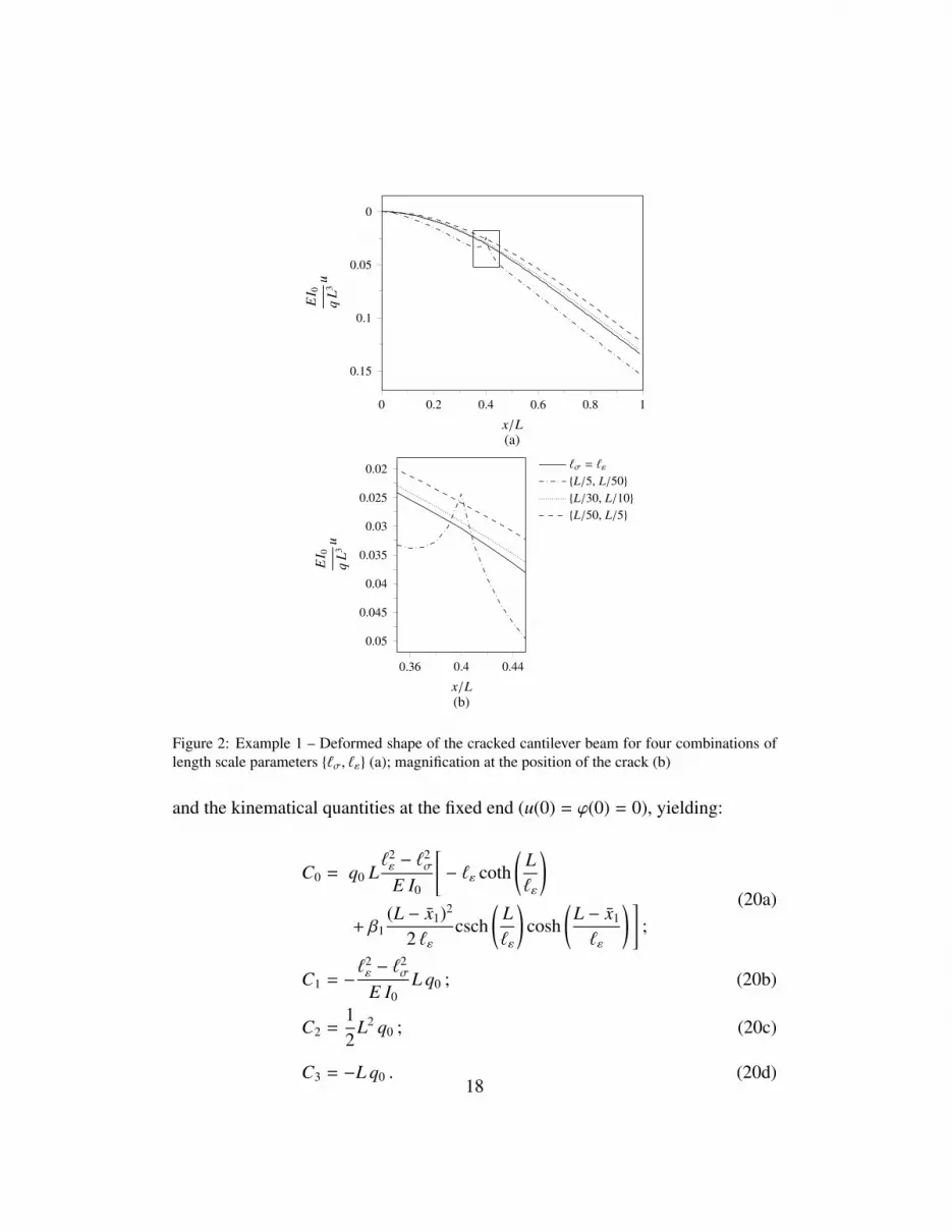
Figure 2: Example 1 – Deformed shape of the cracked cantilever beam for four combinations oflength scale parameters {`σ, `ε} (a); magnification at the position of the crack (b)
and the kinematical quantities at the fixed end (u(0) = ϕ(0) = 0), yielding:
C0 = q0 L`2ε − `2
σ
E I0
[− `ε coth
(L`ε
)+ β1
(L − x1)2
2 `εcsch
(L`ε
)cosh
(L − x1
`ε
) ];
(20a)
C1 = −`2ε − `2
σ
E I0L q0 ; (20b)
C2 =12
L2 q0 ; (20c)
C3 = −L q0 . (20d)18

0 0.2 0.4 0.6 0.8 1 1.2 1.4 1.6 1.8 20.6
0.7
0.8
0.9
1
1.1
1.2
ρ
u(L)
u ref
`σ = 0`σ = L/20`σ = L/10`σ = L/5
Figure 3: Example 1 – Normalised end-beam deflection u(L)/uref as a function of the dimension-
less ratio ρ = `σ/`ε for four different values of the stress gradient parameter `σ (Example 1)
The other constants C4 and C5 are evaluated by assuming the stationarity of
the effective nonlocal curvature at both ends of the beam (χ ′(0) = χ ′(L) = 0).
Interestingly, substituting Eqs. (20) into Eq. (B.7a) and setting β1 = 0 leads to the
same displacement function obtained by Zhang et al. [21] for a hybrid gradient-
elastic undamaged cantilever beam.
Figure 2(a) shows the effects of the length scale parameters {`ε, `σ} on the
beam’s deformed shape. For `ε > `σ > 0 (dotted line and dashed line), the tip
displacement reduces with respect to the classical continuum theory (`ε = `σ >
0, solid line); while if `ε < `σ (dot-dashed line), the beam experiences larger
displacements. In the latter case, however, the behaviour of the nonlocal beam is
physically inconsistent, as clearly evidenced by the counter-load deformations in
Figure 2(b), where the beam’s deformed shape is magnified in the neighbourhood
of the crack. Indeed, for `ε = L/50 and `σ = L/5, the beam shows an upward cusp
centred at the crack position, despite the fact that the load is downward.
19

To quantify the effects of length scale parameters on the apparent stiffness of
the beam, Figure 3 plots the displacement ratio u(L)/uref against the length scale
ratio ρ = `σ/`ε for four different values of `σ, being uref the reference value of
the tip (free-end) displacement obtained with the classical elasticity theory. For
0 < ρ < 1, the tip displacement is less than the reference value, independently of
the micro-structural parameter `σ (and, for a given ratio ρ, the larger `σ, the larger
is the discrepancy between local and nonlocal beam). It is possible to conclude
that, for the physically consistent case where 0 < ρ < 1, the nonlocal beam
always appears stiffer than the same beam with classical elasticity. Conversely,
the nonlocal beam is more flexible for ρ > 1.
Another way to show the inconsistency of the hybrid gradient-elastic model
for ρ > 1 is to evaluate the finite jump Φ1 occurring in the rotations’ profile at the
position of the concentrated damage. According to Eq. (21), the rotation ϕ(x) is
given by the superposition of two terms, namely ϕ0(x), which is continuous (see
Eq. (B.5a)), and the function ∆ϕ1(x) due to the presence of the crack at x = x1,
which is discontinuous at that position (see Eq. (B.5b)).
ϕ(x) = −u′(x) = ϕ0(x) +
n∑i=1
∆ϕi(x); (21)
Combining now Eq. (1b) and Eqs. (B.5), it can be shown that:
Φ1 =∣∣∣ϕ(x +
1 ) − ϕ(x−1 )∣∣∣ =
β1 |M(x1)|E I0
ρ2 , (22)
where the superscripted signs + and − in the argument of the rotation ϕ stand for
20

0 0.2 0.4 0.6 0.8 1
−0.2
−0.15
−0.1
−0.05
0
x/L
EI 0
qL3ϕ
(a)
0.36 0.4 0.44−0.16
−0.15
−0.14
−0.13
−0.12
x/L
EI 0
qL3ϕ
(b)
`σ = `ε
`σ = L/55`σ = L/70`σ = L/200
Figure 4: Example 1 – Rotations’ profile for a fixed value of strain length scale (`ε = L/50) andfour different values of the stress length scale `σ (a); magnification at the position of the crack (b)
the limit from the right and from the left, respectively.
Eq. (22) then reveals that the amplitude of the finite concentrated rotation pre-
dicted by the proposed model at the position of the crack increases with ρ2. For
ρ = 0 (i.e. `σ = 0 and `ε > 0), the localised jump in the rotations’ profile vanishes
completely, meaning that the beam’s curvature becomes smooth at the position of
the crack. For `σ > 0 and `ε ≥ `σ (i.e. 0 < ρ ≤ 1), the beam’s deformed shape
21

shows a finite jump at the damage position, whose amplitude ranges from zero
(the limiting case when `σ → 0) to the classical continuum solution (obtained for
`ε = `σ > 0). On the contrary, the condition `σ > `ε > 0 (i.e. ρ > 1) aggravates
the singularity, and therefore this combination of values for the microstructural
parameters should be avoided.
Based on the above considerations, the stress length `σ appears as a sensible
lower limit for the strain length `ε, and in the following the chain of inequalities
0 ≤ `σ ≤ `ε < L is always satisfied in order to avoid physically inconsistent
results. Within the above conditions, further analyses have been carried out to
investigate the effects of the two individual microstructural parameters `ε and `σ.
Figure 4 shows the rotations’ profiles for a fixed value of the strain length,
`ε = L/50, and four different values of the stress length, `σ ≤ `ε. It can be seen that
changing the parameter `σ mainly affects the rotations in the neighbourhood of the
cracks, as demonstrated by the magnified view of Figure 4(b). This comparison
confirms the prediction of Eq. (22), as the finite jump in the rotations reduces with
`σ.
Figure 5 shows the continuous part of the curvature functions χ(x) for a fixed
stress length `σ = L/50 and four different values of the strain length `ε ≥ `σ (a
Dirac’s delta of intensity Φ1 also appears at x = x1 in the mathematical expression
of χ(x), but has been hidden to make the graphical representation simpler). One
can observe that, in comparison with the classical elasticity (solid line), the hybrid
gradient model potentially provides a more accurate description of the discontinu-
ity due to a concentrated damage. In fact, while the proposed nonlocal model for
22

0 0.2 0.4 0.6 0.8 1
−0.5
−0.4
−0.3
−0.2
−0.1
0
x/L
EI 0
qL2χ
(a)
0.3 0.35 0.4 0.45 0.5
−0.35
−0.3
−0.25
−0.2
−0.15
−0.1
x/L
EI 0
qL2χ
(b)
`ε = `σ`ε = L/10`ε = L/20`ε = L/45
Figure 5: Example 1 – Curvature function for a fixed value of stress length scale (`σ = L/50) andfour different values of the stress length scale `ε (a); magnification at the position of the crack (b)
the cracked beam shows a cusp in the curvature function at the position of the
damage (whose width and hight depend on the microstructural parameters `σ and
`ε), such cusp disappears in the solution obtained with classical elasticity theory
(as the Dirac’s delta fully account for the increased deformation at x = xi).
23

0 0.2 0.4 0.6 0.8 1
0
0.001
0.002
0.003
0.004
0.005
0.006
x/L
EI 0
PL3
u
`ε = `σ`ε = L/15`ε = L/30`ε = L/45
Figure 6: Example 2 – Deformed shape of the multi-cracked clamped-clamped beam for a fixedvalue of stress length scale (`σ = L/50) and four different values of the strain length scale `ε
5.2. Example 2: Clamped-clamped beam with a point load
A similar trend of results can be observed in the second example, in which a
slender beam is clamped at both ends (x = 0 and x = L), and is loaded at
xP = 0.6 L with a concentrated force P, pointing downwards. The correspond-
ing loading function can be then expressed as q(x) = P δ(x − xP). The beam has
three cracks with the same depth, and hence the same damage factor β1 = β2 =
β3 = 1/10 and they are located at x1 = 0.1 L, x2 = 0.4 L and x3 = 0.8 L, respect-
ively. This example thus demonstrates that the proposed approach enables the
analytical solution for statically indetermined nonlocal slender beams in bending
with multiple concentrated damages (i.e. the most general case considered as part
of this study).
Figure 6 compares the deformed shape of the beam when the stress length
scale takes a given value `σ = L/50 and the strain length scale `ε ≥ `σ varies.
As in the previous example, it appears that the overall stiffness of the beam in-
24

creases with `ε, as the maximum deflection tends to reduce in comparison with
the classical elasticity theory (solid line).
Figure 7(a) shows the curvature χ for the same microstructural parameter as
in Figure 6. Interestingly, it can be observed that at the position of the point
load, xP = 0.6 L, due to the discontinuity in the shear force, the curvature of the
classical continuum solution shows a sudden change in the slope, while using the
nonlocal models the transition appears smoothed. Moreover, likewise the previous
example, the curvature has a cusp at each crack position x = xi , whose intens-
ity depends on the length scale parameters (and one of such cusps is magnified
within Fig. 7(b), to better appreciate the effect of the strain length scale `ε in this
circumstance).
The smoothing effect of the strain gradient parameter is further highlighted by
Figure 8, where the rotations’ profiles corresponding to three different values of
`ε, with `σ = 0, are plotted and compared with the classical continuum solution
(solid line, obtained for `ε = `σ). It can be seen that, being ρ = `σ/`ε = 0 for the
three nonlocal beams, the finite jumps Φi typical of the local solution disappear
(see Eq. 22); moreover, the length of the beam in which the effect of the crack is
distributed increases with `ε.
6. Concluding remarks
The current paper has offered a new formulation for the linear-elastic analysis
of nonlocal slender beams with multiple cracks under static transverse forces.
The proposed approach is based on the flexibility crack model [22] (equivalent
25

to the well-known discrete spring model), which has been extended to the hybrid
gradient-elastic constitutive law. Similar to the case of classical elasticity, each
crack is conveniently represented by means of a Dirac’s delta function, whose in-
tensity increases with the severity of the damage; in contrast, adopting the gradient
elasticity allows spreading the effects of the cracks in the neighbourhood of the
damaged abscissa, therefore providing a more realistic rotations’ profile (as con-
firmed with the numerical examples).
It has been shown that, for a given load function q(x), the solution of the
static problem depends on six integration constants only, namely: i) the classical
four constants C0, C1, C2 and C3, which are typically associated with the support
conditions of the beam; ii) two additional constants C4 and C5, which appear
in the general expression of the effective nonlocal curvature. Explicit closed-form
expressions have been provided in Appendix A for these two integration constants,
assuming the stationarity of the nonlocal effective curvature at the beam’s ends.
Importantly, since the adopted flexibility model treats the cracks as concen-
trated inhomogeneities in the bending flexibility of the beam, the size of the com-
putational problem (i.e. the number of unknowns) is independent of the number n
of cracks, for both statically determinate and indeterminate beams .
It has been theoretically found and numerically verified that the finite jump in
the rotations’ profile at the crack position is proportional to ρ2, being ρ = `σ/`ε
a dimensionless length scale ratio (i.e. the less ρ, the smoother the rotations’
profile, the more widespread the effects on the curvature of the beam); and it
has been suggested that, for the purposes of analysing cracked beams in bending,
26

physically consistent results are only obtained if 0 ≤ `σ ≤ `ε � L, being L the
length of the beam.
It has been also shown that: i) differences between predictions of local and
nonlocal elasticity theory increase with the dimensionless quantity `ε/L; ii) the
overall flexibility of the beam increases with the length scale ratio ρ and, for a
given value of ρ, with the microstructural length scales.
This set of new analytical findings allows a better understanding of how gradi-
ent elasticity theories can be effectively adopted for the analysis of cracked slender
beams. The extension of the closed-form solutions presented as part of this study
to solve dynamic and stability problems is currently being undertaken.
Appendix A. Integration constants C4 and C5
This appendix offers the closed-form expressions for the additional integration
constants C4 and C5, which appears in the solution of the multi-damaged EB beam
when the hybrid gradient-elastic constitutive law is adopted.
To derive such expressions, the BCs χ′(0) = 0 and χ
′(L) = 0 (i.e. stationar-
ity conditions at the beam’s ends) have be imposed to Eq. (12), which rules the
effective nonlocal curvature. Eqs. (16) to (18) provide the general solution for
this equation and, taking the derivative with respect to the abscissa x, the rate of
variation of the effective nonlocal curvature can be expressed as:
χ ′(x) = χ ′0(x) +
n∑i=1
∆ χ′i (x) , (A.1)
27

where:
χ ′0(x) =
C4
`εsinh
(x`ε
)+ C5 cosh
(x`ε
)+
1E I0
{C3
[1 − cosh
(x`ε
)]− C2
`εsinh
(x`ε
)+ Q′(x)
};
(A.2)
∆ χ′i (x) = − βi
E I0
[C3 xi + C2 + q[2](xi)
]×
[1`2ε
cosh(
x − xi
`ε
)H(x − xi) +
1`ε
sinh(
x − xi
`ε
)δ(x − xi)
].
(A.3)
Combining the expressions above and enforcing the BCs yields in closed form
to the sought integration constants C4 and C5:
C5 = − 1E I0
Q′(0) ; (A.4)
C4 =`ε
E I0
{C2
`ε+ C3 tanh
(L
2`ε
)+ Q′(0) coth
(L`ε
)+ −Q′(L) csch
(L`ε
)+ csch
(L`ε
) n∑i=1
∆ χ′i(L)
}.
(A.5)
It follows that the integration constant C4 depends on the other two integration
constants C2 and C3, which represent the bending moment M(0) and the shear
force V(0) at the left end of the beam, respectively. As already pointed out in
Subsection 4.2, these values can be then evaluated using equilibrium equations
only for statically determinate beams, while they are appear to be fully coupled
with all the other integration constants when the beam is statically indeterminate.
28

Appendix B. Solution for uniformly distributed load (UDL)
Aim of this appendix is to provide, as a way of example, the exact closed-form
mathematical expressions of curvature χ(x), rotation ϕ(x) and displacement u(x)
functions for a multi-cracked EB beam under the UDL q0.
To derive the sought solution, Eqs. (17) and (18) can be particularised for the
load case q(x) = q0:
χ0(x) =C2
E I0+
C3 `ε
E I0
[x`ε
+ sech(
L2 `ε
)sinh
(L − 2x
2 `ε
)]
+q0 `
2ε
2 E I0
{ (x`ε
)2
+ 2[1 − L
`εcsch
(L`ε
)cosh
(x`ε
)] };
(B.1a)
∆ χi(x) =βi
E I0 `ε
(C2 + C3 xi +
q0 x2i
2
)×
[csch
(L`ε
)cosh
(x`ε
)cosh
(L − xi
`ε
)− sinh
(x − xi
`ε
)H(x − xi)
],
(B.1b)
in which it has been taken into account that for the UDL q0: i) the second anti-
derivative is q[2](x) = q0 x2/2; and ii) the function Q(x), defined by Eq. (19), takes
the expression:
Q(x) =q0 `
2ε
2
(
x`ε
)2
+ 2[1 − cosh
(x`ε
)] . (B.2)
According to Eq. (16), the effective nonlocal curvature is given by the super-
position of the n + 1 contributions of Eqs. (B.1), and the local curvature χ(x) =
29
−u′′(x) can be successively obtained using Eq. (10), which can be applied to the
undamaged contribution χ0(x) and to the additional term associated with the ith
concentrated damage ∆ χi(x). The local curvature can be then written in a form
similar to Eq. (16):
χ(x) = χ0(x) +
n∑i=1
∆ χi(x) , (B.3)
where:
χ0(x) = χ0(x) − `2σχ′′
0 (x)
=1
E I0
(C2 + C3 x +
q0 x2
2
)+`2ε − `2
σ
E I0
{C3
`εsech
(L
2 `ε
)sinh
(L − 2x
2 `ε
)+ q0
[1 − L
`εcosh
(x`ε
)csch
(L`ε
) ]};
(B.4a)
∆ χi(x) = ∆ χi(x) − `2σ ∆ χ
′′i (x)
=βi
E I0
(C2 + C3 xi +
q0 x2i
2
)×
{`2ε − `2
σ
`3ε
[csch
(L`ε
)cosh
(x`ε
)cosh
(L − xi
`ε
)− sinh
(x − xi
`ε
)H(x − xi)
]+`2σ
`2ε
δ(x − xi) +`2σ
`ε
ddx
[sinh
(x − xi
`ε
)δ(x − xi)
]}.
(B.4b)
The two terms in the last line of Eq. (B.4b) deserve a special attention. In-
deed, the first one is an impulsive term, centred at the position of the ith crack,
x = xi, whose intensity is proportional to ρ2 =(`σ
/`ε
)2, and is responsible for
30

the finite jump in the rotations’ profile given by Eq. (22). The second term, on
the contrary, can be neglected when rotations and displacements of the nonlocal
beam are evaluated by means of successive integrations of Eq. (B.3). This can be
rigorously demonstrated, and depends on the mathematical characteristics of the
function sinh(·) that multiplies the Dirac’s delta within the square brackets to be
differentiated, namely sinh(·) has a zero value at the centre of the delta function
(x = xi) and is anti-symmetric with respect to this point.
According to Eq. (21), the rotations’ profile along the beam’s axis can be
posed as the superposition of the undamaged term ϕ0(x) and n further contribu-
tions ∆ϕi(x) due to the singularities in the beam’s bending stiffness, where each
term is obtained by integrating the corresponding curvature. The two expressions
are given by:
ϕ0(x) = C1 +C2 xE I0
+C3 x2
2 E I0+
q0 x3
6 E I0
+`2ε − `2
σ
E I0
{−C3 cosh
(L − 2x
2`ε
)sech
(L
2`ε
)+ q0
[x − L csch
(L`ε
)sinh
(x`ε
)] };
(B.5a)
∆ϕi(x) =βi
E I0
(C2 + C3 xi +
q0 x2i
2
) {H(x − xi)
+`2ε − `2
σ
`2ε
[csch
(L`ε
)sinh
(x`ε
)cosh
(L − xi
`ε
)− cosh
(x − xi
`ε
)H(x − xi)
] },
(B.5b)
and the additional integration constant is C1 = ϕ(0).
31
Similarly to Eqs. (16) and (21), the displacement function can be written as:
u(x) = u0(x) +
n∑i=1
∆ui(x) , (B.6)
The mathematical expressions for the functions u0(x) and ∆ui(x), appearing in the
right-hand side of Eq. (B.6), can be provided by integrating Eqs. (B.5) and (B.5b),
which then describes the deformed shape of the multi-damaged beam with hybrid
gradient elasticity:
u0(x) = C0 −C1 x − C2 x2
2 E I0− C3 x3
6 E I0− q0 x4
24 E I0
− `2ε − `2
σ
E I0
{C3 `ε sech
(L
2 `ε
)sinh
(L − 2x
2 `ε
)+ q0
[x2
2− `ε csch
(L`ε
)cosh
(x`ε
)] };
(B.7a)
∆ui(x) = − βi
E I0
(C2 + C3 xi +
q0 x2i
2
) {(x − xi) H (x − xi)
+`2ε − `2
σ
`ε
[csch
(L`ε
)cosh
(x`ε
)cosh
(L − xi
`ε
)− sinh
(x − xi
`ε
)H (x − xi)
]},
(B.7b)
and the additional integration constant is C0 = u(0).
Interestingly, the first line in each of Eqs. (B.5) and (B.7a) gives rotations’
profile and deformed shape of the undamaged beam with classical elasticity, re-
spectively.
32

References
1. Askes, H., Aifantis, E.C.. Gradient elasticity in statics and dynamics:
An overview of formulations, length scale identification procedures, finite
element implementations and new results. International Journal of Solids
and Structures 2011;48(13):1962–1990.
2. Eringen, A., Edelen, D.. On nonlocal elasticity. International Journal of
Engineering Science 1972;10(3):233 – 248.
3. Eringen, A.. On differential equations of nonlocal elasticity and solutions
of screw dislocation and surface waves. Journal of Applied Physics 1983;
54(9):4703–4710.
4. Aifantis, E.. Update on a class of gradient theories. Mechanics of Materials
2003;35(3):259–280.
5. Ru, C., Aifantis, E.. A simple approach to solve boundary-value problems
in gradient elasticity. Acta Mechanica 1993;101(1):59–68.
6. Lombardo, M., Askes, H.. Elastic wave dispersion in microstructured
membranes. Proceedings of the Royal Society A: Mathematical, Physical
and Engineering Science 2010;466(2118):1789–1807.
7. Wang, Q.. Wave propagation in carbon nanotubes via nonlocal continuum
mechanics. Journal of Applied Physics 2005;98(12):1–6.
33

8. Eringen, A., Speziale, C., Kim, B.. Crack-tip problem in non-local elasti-
city. Journal of the Mechanics and Physics of Solids 1977;25(5):339–355.
9. Peddieson, J., Buchanan, G., McNitt, R.. Application of nonlocal con-
tinuum models to nanotechnology. International Journal of Engineering
Science 2003;41(3-5):305–312.
10. Sudak, L.. Column buckling of multiwalled carbon nanotubes using non-
local continuum mechanics. Journal of Applied Physics 2003;94(11):7281–
7287.
11. Zhang, Y., Liu, G., Xie, X.. Free transverse vibrations of double-walled
carbon nanotubes using a theory of nonlocal elasticity. Physical Review B -
Condensed Matter and Materials Physics 2005;71(19):1–7.
12. Murmu, T., Adhikari, S., Wang, C.. Torsional vibration of carbon
nanotube-buckyball systems based on nonlocal elasticity theory. Physica
E: Low-dimensional Systems and Nanostructures 2011;43(6):1276–1280.
13. Wang, C.M., Zhang, Y.Y., Ramesh, S.S., Kitipornchai, S.. Buckling
analysis of micro- and nano-rods/tubes based on nonlocal Timoshenko beam
theory. Journal of Physics D: Applied Physics 2006;39(17):3904–3909.
14. Reddy, J.. Nonlocal theories for bending, buckling and vibration of beams.
International Journal of Engineering Science 2007;45(2-8):288–307.
15. Murmu, T., Adhikari, S.. Nonlocal vibration of carbon nanotubes with
34

attached buckyballs at tip. Mechanics Research Communications 2011;
38(1):62–67.
16. Murmu, T., Adhikari, S.. Nonlocal transverse vibration of double-
nanobeam-systems. Journal of Applied Physics 2010;108(8):083514–
083514.
17. Challamel, N., Girhammar, U.. Boundary-layer effect in composite beams
with interlayer slip. Journal of Aerospace Engineering 2010;24(2):199–209.
18. Loya, J., Lopez-Puente, J., Zaera, R., Fernandez-Saez, J.. Free transverse
vibrations of cracked nanobeams using a nonlocal elasticity model. Journal
of Applied Physics 2009;105(4):044309.
19. Torabi, K., Dastgerdi, J.. An analytical method for free vibration analysis
of Timoshenko beam theory applied to cracked nanobeams using a nonlocal
elasticity model. Thin Solid Films 2012;521(21):6595–6602.
20. Wang, C.M., Challamel, N.. The small length scale effect for a non-local
cantilever beam: a paradox solved. Nanotechnology 2008;19(34):345703.
21. Zhang, Y., Wang, C., Challamel, N.. Bending, buckling, and vibration of
micro/nanobeams by hybrid nonlocal beam model. Journal of Engineering
Mechanics 2010;136(5):562–574.
22. Palmeri, A., Cicirello, A.. Physically-based Dirac’s delta functions in the
static analysis of multi-cracked Euler-Bernoulli and Timoshenko beams. In-
ternational Journal of Solids and Structures 2011;48(14-15):2184 – 2195.
35
23. Cicirello, A., Palmeri, A.. Static analysis of Euler-Bernoulli beams with
multiple unilateral cracks under combined axial and transverse loads. Inter-
national Journal of Solids and Structures 2013;.
24. Dona, M., Palmeri, A., Cicirello, A., Lombardo, M.. A two-node multi-
cracked beam element for static and dynamic analysis of planar frames.
In: Topping, B., editor. Proceedings of the Eleventh International Con-
ference on Computational Structures Technology; Paper 257. Civil-Comp
Press,Stirlingshire, UK; 2012, .
25. Yayli, M.. Stability analysis of a gradient elastic beam using finite element
method. International Journal of Physical Science 2011;6(12):2844–2851.
36

0 0.2 0.4 0.6 0.8 1
−0.15
−0.1
−0.05
0
0.05
0.1
x/L
EI 0 PLχ
(a)
0.36 0.4 0.44
0.03
0.04
0.05
0.06
0.07
0.08
0.09
0.1
x/L
EI 0
PLχ
(b)
`ε = `σ`ε = L/15`ε = L/30`ε = L/45
Figure 7: Example 2 – Curvature function of the multi-cracked clamped-clamped beam for a fixedvalue of stress length scale (`σ = L/50) and four different values of the strain length scale `ε (a);magnification at the position of the second crack (b)
37

0 0.2 0.4 0.6 0.8 1
−0.01
0
0.01
0.02
x/L
EI 0
PL2ϕ
(a)
0.36 0.4 0.44−0.016
−0.014
−0.012
−0.01
−0.008
−0.006
x/L
EI 0
PL2ϕ
(b)
`ε = `σ`ε = L/50`ε = L/100`ε = L/200
Figure 8: Example 2 – Rotations’ profile for the multi-cracked clamped-clamped beam with fixedvalue of stress length scale (`σ = 0) and four different values of the strain length scale `ε (a);magnification at the position of the second crack (b)
38