evolutionary selection of individual expectations and aggregate outcomes in asset pricing...
TRANSCRIPT
Evolutionary Selection of Individual Expectations and
Aggregate Outcomes in Asset Pricing Experiments∗
Mikhail Anufriev† Cars Hommes‡
CeNDEF, School of Economics, University of Amsterdam,
Roetersstraat 11, NL-1018 WB Amsterdam, Netherlands
Tinbergen Institute,
Gustav Mahlerplein 117, NL-1082 MS Amsterdam, the Netherlands
First Draft: July 2007; This draft: July 2011
∗We thank the participants of the “Complexity in Economics and Finance” workshop, Leiden, Octo-
ber 2007, the “Computation in Economics and Finance” conference, Paris, June 2008, the “Learning and
Macroeconomic Policy” workshop, Cambridge, September 2008, and seminar participants at the University
of Amsterdam, Sant’Anna School of Advanced Studies (Pisa), University of New South Wales, Catholic
University of Milan, University of Warwick, Paris School of Economics, and the European University Insti-
tute (Florence) for stimulating discussions. We benefited from helpful comments by Buz Brock, Cees Diks,
John Duffy, Doyne Farmer, Frank Heinemann and Valentyn Panchenko and by two anonymous referees on
earlier versions of this paper. This work is supported by the Complex Markets E.U. STREP project 516446
under FP6-2003-NEST-PATH-1 and by the EU 7th framework collaborative project “Monetary, Fiscal and
Structural Policies with Heterogeneous Agents (POLHIA)”, grant no.225408.†Tel.: +31-20-5254248; fax: +31-20-5254349; e-mail: [email protected].‡Tel.: +31-20-5254246; fax: +31-20-5254349; e-mail: [email protected].
1

Abstract
In recent ‘learning to forecast’ experiments with human subjects (Hommes, et
al. 2005), three different patterns in aggregate price behavior have been observed:
slow monotonic convergence, permanent oscillations and dampened fluctuations. We
show that a simple model of individual learning can explain these different aggregate
outcomes within the same experimental setting. The key idea of the model is the
evolutionary selection among heterogeneous expectation rules, driven by the relative
performance of the rules. Out-of-sample predictive power of our switching model is
higher compared to the rational or other homogeneous expectations benchmarks. Our
results show that heterogeneity in expectations is crucial to describe individual fore-
casting behavior as well as aggregate price behavior.
JEL codes: C91, C92, D83, D84, E3.
Keywords: Learning, Heterogeneous Expectations, Expectations Feedback, Experimental Economics
2

1 Introduction
In an economy today’s individual decisions crucially depend upon expectations or beliefs
about future developments. For example, in speculative asset markets such as the stock
market, an investor buys (sells) stocks today when she expects stock prices to rise (fall) in
the future. Expectations affect individual decisions and the realized market outcome (e.g.,
prices and traded quantities) is an aggregation of individual behavior. A market is therefore
an expectations feedback system: market history shapes individual expectations which, in
turn, determine current aggregate market behavior and so on. How do individuals actually
form market expectations, and what is the aggregate outcome of the interaction of individual
market forecasts? To answer these questions in this paper we investigate individual learning
behavior observed in the experiments of Hommes et al. (2005b) and Hommes et al. (2008)
(HSTV05 and HSTV08, henceforth), specifically designed to study expectation feedback.
On the basis of the experimental evidence we propose a behavioral model of heterogeneous
expectations, which fits individual behavior as well as aggregate market outcomes in the
experiments quite well.
After the seminal work by Muth (1961) and Lucas (1972), it is common for economic
theory to assume that all individuals have rational expectations. In a rational world indi-
vidual expectations coincide, on average, with market realizations, and markets are efficient
with prices fully reflecting economic fundamentals (Samuelson, 1965; Fama, 1970). In the
traditional view, there is no room for market psychology and “irrational” herding behavior.
An important underpinning of the rational approach comes from an early evolutionary argu-
ment made by Friedman (1953), that “irrational” traders will not survive competition and
will be driven out of the market by rational traders, who will trade against them and earn
higher profits.
Following Simon (1957), many economists have argued that rationality imposes unrealis-
tically strong informational and computational requirements upon individual behavior and
it is more reasonable to model individuals as boundedly rational, using simple rules of thumb
in decision making. Laboratory experiments indeed have shown that individual decisions
3

under uncertainty are at odds with perfectly rational behavior, and can be much better
described by simple heuristics, which sometimes may lead to persistent biases (Tversky and
Kahneman, 1974; Kahneman, 2003; Camerer and Fehr, 2006). Models of bounded rationality
have also been applied to forecasting behavior, and several adaptive learning algorithms have
been proposed to describe market expectations. For example, Sargent (1993) and Evans and
Honkapohja (2001) advocate the use of adaptive learning in modeling expectations, where
agents learn unknown parameters of the model using econometric techniques on the past
observations. In some models (Bray and Savin, 1986) adaptive learning enforces conver-
gence to rational expectations, while in others (Bullard, 1994) learning may not converge at
all but instead lead to excess volatility and persistent deviations from rational equilibrium
similar to real markets (Shiller, 1981; DeBondt and Thaler, 1989). While most of the initial
adaptive learning models have been used in the macro-literature, several of them recently
were applied to explain various phenomena of the financial markets. The results are mixed.
Adam et al. (2008) show that when agents predict price return with least-square learning,
the moments of different time series, such as return or price-dividend ratio, become signif-
icantly closer to the actual values than under rational expectations. On the other hand,
Carceles-Poveda and Giannitsarou (2008) similarly study least-square learning in a general
equilibrium framework and find that it is not sufficient to bring moments towards plausible
values. Branch and Evans (2011) show that the model with least-square forecasting of return
and the conditional variance of return generates repeated bubbles and crashes.
Recently, models with heterogeneous expectations and evolutionary selection among fore-
casting rules have been proposed, e.g., Brock and Hommes (1997) and Branch and Evans
(2006), see Hommes (2006) for an extensive overview. By taking a larger deviation from
the rational expectation framework, these models proved to be able to match moments of
different financial variables and, therefore, generate several “stylized facts” of financial mar-
kets, such as excess volatility, volatility clustering, and fat tails of return distribution. See
Gaunersdorfer et al. (2008); Anufriev and Panchenko (2009); Franke and Westerhoff (2011),
among others. At the same time Boswijk et al. (2007) and de Jong et al. (2009) estimate the
heterogeneous expectation models on real market data and find evidence of heterogeneity.
4

Fit of the model to ’clean’ experimental data, which we perform in this paper, provide an
important further test for the heterogeneous agent models. Furthermore, we will use the
experimental data also to provide a micro-foundations for our model, since the forecasting
rules which we employ were among rules estimated in the laboratory.
Laboratory experiments with human subjects are well suited to study individual expec-
tations and how their interaction shapes aggregate market behavior (Marimon et al., 1993;
Peterson, 1993). But the results from laboratory experiments are mixed. Early experi-
ments by Smith (1962) show convergence to equilibrium, while more recent asset pricing
experiments exhibit deviations from equilibrium with persistent bubbles and crashes, see,
e.g., Smith et al. (1988) and Lei et al. (2001). It is important to recognize that in many
earlier experiments expectations only play a secondary role, being intertwined with other as-
pects, such as market architecture and trading behavior of participants. In order to provide
clean data on expectations and control all other underlying model assumptions, HSTV05 de-
signed a so-called ’learning to forecast’ experiment.1 In a typical session six human subjects
had to predict the price of an asset for 50 periods, having knowledge of the fundamen-
tal parameters (mean dividend and interest rate) and previous price realizations. Trading
is computerized, using an optimal demand schedule derived from maximization of myopic
CARA mean-variance utility, given the subject’s individual forecast. Hence, subject’s only
task in every period is to give a two period ahead point prediction for the price of the risky
asset, and their earnings are inversely related to their prediction errors. Learning to fore-
cast experimental data can be used as a test bed for various expectations hypotheses, such
as rational expectations or adaptive learning models, in any benchmark dynamic economic
model with all other assumptions controlled by the experimenter; see the discussion in Duffy
1See Hommes (2011) for an overview of learning to forecast experiments, where also earlier experiments on
expectation formation are discussed, e.g., Williams (1987) and Hey (1994) among others. The experiments in
HSTV05 and HSTV08, which we discuss in this paper, study expectations in financial markets. Experiments
in Heemeijer et al. (2009), and Bao et al. (2010) consider markets of agricultural goods in a cobweb framework,
while Adam (2007), Assenza et al. (2011) and Pfajfar and Zakelj (2010) ran experiments in a macroeconomic
environment. Anufriev et al. (2010) fit a version of the heuristic switching model to Heemeijer et al. (2009)
experiment.
5

(2008).
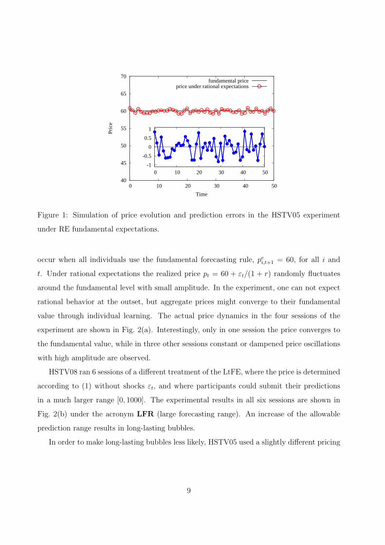
HSTV05 ran 14 sessions of the learning to forecast experiment in three different treat-
ments. In 7 sessions of one of the treatments, the outcomes were quite different, despite
identical setting. While in some sessions price convergence did occur, in other sessions prices
persistently fluctuated and temporary bubbles emerged (see Fig. 2(c) and the right panels of
Fig. 3). HSTV08 ran 6 sessions in another treatment and show that a typical outcome of the
experiment is the emergence of long-lasting bubbles followed by crashes (see Fig. 2(b)). An-
other striking and robust finding of the learning to forecast experiments is that in all sessions
individuals were able to coordinate on a common prediction rule, without any knowledge
about the forecasts of others (see Fig. 3, lower parts of the panels).
Anufriev and Hommes (2012) showed by three 50 periods ahead simulations that a simple
learning model of heterogeneous expectations can generate dynamics qualitative similar to
the three outcomes observed in some of the HSTV05 experiments. In this paper we fit the
model to all 20 different market sessions in HSTV05 and HSTV08 experiments and perform
one period ahead and out-of-sample forecasting. Our model is an extension of the evolu-
tionary selection mechanism introduced in Brock and Hommes (1997), applied to simple
predicting rules which individuals often used in the experiment. From the point of view of
the experiment’s participant several behavioral rules can plausibly be used for price predic-
tion at each time step. Participants can choose any of these rules, but at the aggregate level
the rules which generated relatively good predictions in the past will be chosen more often.
Participants also exhibit some inertia in their decisions, by temporarily sticking to their
rule. Combining these ideas we arrive at a behavioral model of learning with only three free
parameters. We show that this model fits the experimental data surprisingly well for a large
range of parameters. The model outperforms several models with homogeneous expectations
and a simple non-structural AR(2) model both in- and out-of-sample. Our model of individ-
ual learning can explain different observed aggregate patterns within the same experimental
environment (Fig. 6) and is robust with respect to changes in the experimental environments
(Fig. 8).
The fact that the model with heterogeneous expectations can explain different aggregate
6
outcomes observed within the same environment has a clear intuitive explanation. The key
feature driving the result is the path-dependent property of the nonlinear switching model. If
participants start to coordinate on an adaptive rule, the resulting (stable) price dynamics is
such that the adaptive rule performs better than other rules, reinforcing the coordination and
explaining converging and stable price behavior. When a majority of participants coordinate
on a trend-following rule, price oscillations and temporary bubbles arise. In that case trend-
following rules predict better than an adaptive rule, thus reinforcing and amplifying price
trends and temporary bubbles.
The paper is organized as follows. In Section 2 we review the findings of the laboratory
experiments of HSTV05 and HSTV08. Section 3 discusses individual behavior of participants
in the experiments, and studies the price dynamics under homogeneous forecasting rules.
A learning model based on evolutionary selection between simple forecasting heuristics is
presented in Section 4. In Section 5 we discuss how our model fits the experimental data.
Finally, Section 6 concludes.
2 Learning-to-forecast experiments
A number of computerized learning-to-forecast experiments (LtFEs) have been performed in
the CREED laboratory at the University of Amsterdam, see Hommes (2011) for an overview.
This paper proposes a theoretical explanation of the results obtained in 20 different sessions
of the LtFEs based on the asset pricing model, see HSTV05 (Hommes et al., 2005b) and
HSTV08 (Hommes et al., 2008). In each session of the experiment 6 participants were
advisers to large pension funds and had to submit point forecasts for the price of a risky
asset for 50 consecutive periods. There were two assets in the market, a risk-free asset
paying a fixed interest rate r every period, and a risky asset paying stochastic IID dividends
with mean y. Subjects knew that the price of the risky asset is determined every period
by market clearing, as an aggregation of individual forecasts of all participants. They were
also informed that the higher the forecasts are, the larger the demand for the risky asset is.
Stated differently, they knew that there was positive feedback from individual price forecasts
7
to the realized market price. Trading had been computerized with the price pt determined
in accordance with a standard mean-variance asset pricing model with heterogeneous beliefs
(Campbell et al., 1997; Brock and Hommes, 1998):
pt =1
1 + r
(pet+1 + y + εt
), t = 0, . . . , 50, (1)
where pet+1 = 16
∑6i=1 p
ei,t+1 is an average of 6 individual forecasts, and a small stochastic
term εt represents demand/supply shock. The same realizations of the shocks, drawn in-
dependently from a normal distribution with mean 0 and standard deviation 0.5, has been
used in all sessions of HSTV05. An individual forecast, pei,t+1, could be any number (with
two decimals) in the range [0, 100] to be submitted at the beginning of period t. After all
forecasts were submitted, every participant was informed about the realized price pt. The
earnings per period were determined by a quadratic scoring rule
ei,t =
1−(pt−pei,t
7
)2
if |pt − pei,t| < 7 ,
0 otherwise ,(2)
so that forecasting errors exceeding 7 would result in no reward at a given period. At the
end of the session the accumulated earnings of every participant were converted to euros (1
point computed as in (2) corresponded to 50 cents). Subjects of the experiments neither
knew the exact functional form of the market equilibrium equation (1) nor the number and
identity of other participants. They were informed about scoring rule (2) and the values
of the fundamental parameters, r and y, at the beginning of the experiment. Participants
could, therefore, compute the rational fundamental price of the risky asset, pf = y/r. The
information set of participant i at period t consisted of past prices up to pt−1, past own
predictions up to pei,t, the fundamental parameters r and y, and past own earnings.
On the basis of variations in the implementation of the experiment, four different exper-
imental settings (treatments) can be identified. The setup described above has been used in
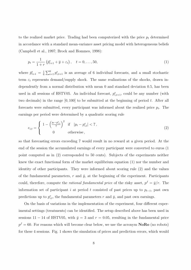
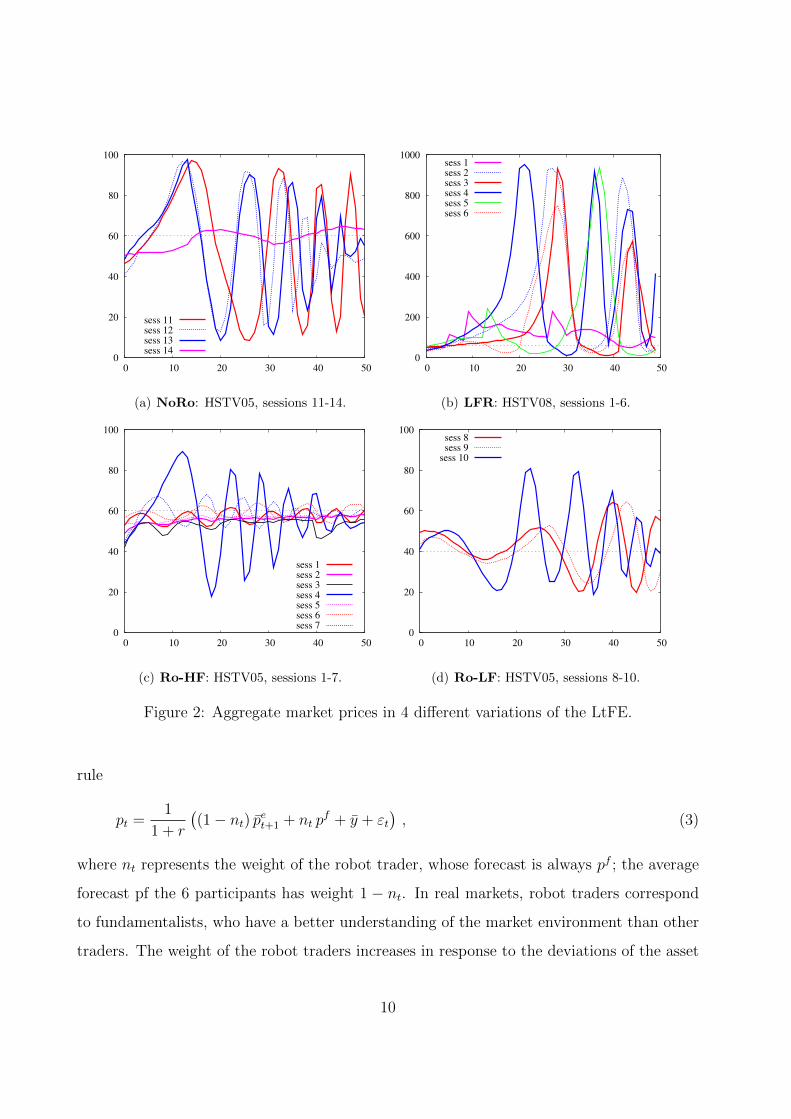
sessions 11 − 14 of HSTV05, with y = 3 and r = 0.05, resulting in the fundamental price
pf = 60. For reasons which will become clear below, we use the acronym NoRo (no robots)
for these 4 sessions. Fig. 1 shows the simulation of prices and prediction errors, which would
8
40
45
50
55
60
65
70
0 10 20 30 40 50
Pric
e
Time
fundamental priceprice under rational expectations
-1
-0.5
0
0.5
1
0 10 20 30 40 50
Figure 1: Simulation of price evolution and prediction errors in the HSTV05 experiment
under RE fundamental expectations.
occur when all individuals use the fundamental forecasting rule, pei,t+1 = 60, for all i and
t. Under rational expectations the realized price pt = 60 + εt/(1 + r) randomly fluctuates
around the fundamental level with small amplitude. In the experiment, one can not expect
rational behavior at the outset, but aggregate prices might converge to their fundamental
value through individual learning. The actual price dynamics in the four sessions of the
experiment are shown in Fig. 2(a). Interestingly, only in one session the price converges to
the fundamental value, while in three other sessions constant or dampened price oscillations
with high amplitude are observed.
HSTV08 ran 6 sessions of a different treatment of the LtFE, where the price is determined
according to (1) without shocks εt, and where participants could submit their predictions
in a much larger range [0, 1000]. The experimental results in all six sessions are shown in
Fig. 2(b) under the acronym LFR (large forecasting range). An increase of the allowable
prediction range results in long-lasting bubbles.
In order to make long-lasting bubbles less likely, HSTV05 used a slightly different pricing
9
0
20
40
60
80
100
0 10 20 30 40 50
sess 11
sess 12
sess 13
sess 14
(a) NoRo: HSTV05, sessions 11-14.
0
200
400
600
800
1000
0 10 20 30 40 50
sess 1
sess 2
sess 3
sess 4
sess 5
sess 6
(b) LFR: HSTV08, sessions 1-6.
0
20
40
60
80
100
0 10 20 30 40 50
sess 1
sess 2
sess 3
sess 4
sess 5
sess 6
sess 7
(c) Ro-HF: HSTV05, sessions 1-7.
0
20
40
60
80
100
0 10 20 30 40 50
sess 8
sess 9
sess 10
(d) Ro-LF: HSTV05, sessions 8-10.
Figure 2: Aggregate market prices in 4 different variations of the LtFE.
rule
pt =1
1 + r
((1− nt) pet+1 + nt p
f + y + εt), (3)
where nt represents the weight of the robot trader, whose forecast is always pf ; the average
forecast pf the 6 participants has weight 1 − nt. In real markets, robot traders correspond
to fundamentalists, who have a better understanding of the market environment than other
traders. The weight of the robot traders increases in response to the deviations of the asset
10

price from its fundamental level:
nt = 1− exp(− 1
200
∣∣pt−1 − pf∣∣) . (4)
This mechanism reflects the feature that in real markets there is more agreement about over-
or undervaluation of an asset when the price deviation from the fundamental level is large.2
Seven experimental sessions 1-7 had the fundamental parameters r = 0.05 and y = 3 with
fundamental price 60. For this specification an acronym Ro-HF (robots, high fundamental)
is used. As Fig. 2(c) shows, in the presence of a stabilizing robot traders the amplitude of
the oscillations decreases. Finally, in the remaining sessions 8-10, the market had a smaller
dividend y = 2, resulting in a smaller fundamental price 40, see Fig. 2(d). The oscillations
are quite large in this Ro-LF (robots and low fundamental) case.
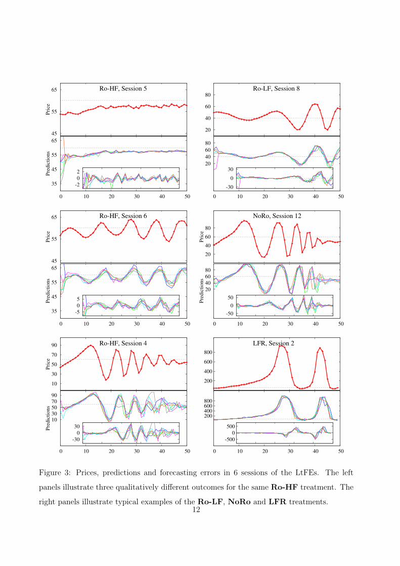
A closer look at six different sessions of the LtFEs is given in Fig. 3. The left panels show
time series of prices (upper parts of panels), individual predictions (lower parts of panels)
and forecasting errors (inner frames) for three out of seven sessions in the Ro-HF treatment.
A striking feature of this experiment is that three different qualitative patterns for aggregate
price behavior emerge within the same environment. The prices in session 5 (and 2; not
shown) converge slowly and almost monotonically to the fundamental price level. In session
6 (and 1; not shown) persistent oscillations are observed during the entire experiment. In
session 4 (and 7; not shown) prices are also fluctuating but their amplitude is decreasing.
The right panels of Fig. 3 show the price fluctuations in the typical sessions of the other
LtFEs: session 8 of Ro-LF, session 12 of NoRo and session 2 of LFR.3
Individual predictions in Fig. 3 shows another striking result of the LtFEs. In all experi-
mental sessions participants were able to coordinate their forecasting activity. The forecasts
are dispersed in the first periods but then become very close to each other. The coordina-
tion of individual forecasts has been achieved in the absence of any communication between
2In the experiments the fraction of robot trader never became larger than 0.25.3See Appendix A for similar plots in all remaining sessions. Sessions 2, 1 and 7 of Ro-HF experiment
have been analyzed in Anufriev and Hommes (2012). The dynamics in session 3 of Ro-HF was peculiar.
Similar to session 6 it started with moderate oscillations, then stabilized at a level below the fundamental,
suddenly falling significantly in period t = 40, probably due to a typing error of one of the participants.
11
35
45
55
65
0 10 20 30 40 50
Pre
dic
tions
45
55
65
Pri
ce
Ro-HF, Session 5
-2
0
2
20
40
60
80
0 10 20 30 40 50
20
40
60
80
Ro-LF, Session 8
-30
0
30
35
45
55
65
0 10 20 30 40 50
Pre
dic
tions
45
55
65
Pri
ce
Ro-HF, Session 6
-5
0
5
20
40
60
80
0 10 20 30 40 50
Pre
dic
tions
20
40
60
80
Pri
ce
NoRo, Session 12
-50
0
50
10
30
50
70
90
0 10 20 30 40 50
Pre
dic
tions
10
30
50
70
90
Pri
ce
Ro-HF, Session 4
-30
0
30
200 400 600 800
0 10 20 30 40 50
200
400
600
800
LFR, Session 2
-500
0
500
Figure 3: Prices, predictions and forecasting errors in 6 sessions of the LtFEs. The left
panels illustrate three qualitatively different outcomes for the same Ro-HF treatment. The
right panels illustrate typical examples of the Ro-LF, NoRo and LFR treatments.12

subjects and knowledge of past and present predictions of other participants.
LtFEs represent a tailored laboratory study to test different theories of expectation for-
mation. A suitable model should be able to reproduce the following findings of the HSTV05
and HSTV08 learning-to-forecast experiments:
- participants have not learned the RE fundamental forecasting rule; only in some cases
individual predictions slowly moved in the direction of the fundamental price towards
the end of the experiment;
- three different price patterns were observed in the same Ro-HF experiment: (i) slow,
(almost) monotonic convergence, (ii) persistent oscillations with almost constant am-
plitude, and (iii) large initial oscillations dampening towards the end of the experiment;
- LtFEs tend to produce long lasting bubbles followed by crashes in the LFR treatment;
The purpose of this paper is to explain these “stylized facts” simultaneously by a simple
behavioral model of individual learning.
3 Individual Forecasting Behavior
In this section we will look closer at the individual forecasting behavior in the LtFEs in order
to develop some behavioral foundations of the heterogeneous expectations model.
Which forecasting rules did individuals use in the learning to forecast experiment? Com-
parison of the RE benchmark in Fig. 1 with the lab experiments in Figs. 2 and 3 suggests
that rational expectations is not a good explanation of individual forecasting and aggregate
behavior. The REs cannot be reconciled with the oscillations of the HSTV05 experiment,
especially not in the oscillating sessions. Using individual experimental data HSTV05 esti-
mated the forecasting rules for each subject based on the last 40 periods (to allow for some
learning phase). Simple linear rules of the form
pei,t+1 = αi + βipt−1 + γi(pt−1 − pt−2) + δipei,t (5)
13

were estimated. These rules are so-called first order heuristics, since they only use the last
own forecast, the last observed price and the last observed price change to predict the future
price. Remarkably, individual forecasts are well explained by first order heuristics: for 63
out of 14× 6 = 84 participants (i.e., for 75%) an estimated linear rule falls into this simple
class with an R2 typically higher than 0.80.
The experimental evidence suggests strong coordination on a common prediction rule.
One can therefore suspect that this common rule (which, for whatever reason, turned out
to be different in different sessions) generates the resulting pattern. It is therefore useful to
first investigate price dynamics under homogeneous expectations when all participants use
the same forecasting rule. The model with homogeneous expectations is obtained when the
average pet+1 is generated by the rule of type (5) and then plugged into the corresponding pric-
ing equation: Eq. (1) for the experiment without robots or Eq. (3) for the experiments with
robots. Fig. 4 illustrates deterministic (setting the noise term εt ≡ 0) as well as stochastic
simulations of the model with the same realization of the shocks as in the experiment.
Adaptive heuristic. Participants from the converging sessions often used an adaptive
expectations rule of the form:
pet+1 = w pt−1 + (1− w) pet = pet + w (pt−1 − pet ) , (6)
with weight 0 ≤ w ≤ 1. Recall that at the moment when the forecast for the price pt+1 is
submitted, the price pt is still unknown, so that the last observed price is pt−1. At the same
time, the last forecast pet is, of course, known when forecasting pt+1. Notice also that for
w = 1, we obtain the special case of naive expectations.4
Assume that all participants use the same adaptive heuristic pet+1 = w pt−1 + (1 − w) pet
in their forecasting activity. It is easy to show (see Appendix B) that in the absence of
stochastic shock εt the dynamics will monotonically converge to the fundamental price,
independently of initial conditions. This is illustrated in Fig. 4(a) for two different values of
4The adaptive rule (6) was estimated for 5 out of 12 participants in sessions 2 and 5 of the HSTV05
experiment. Three participants had w insignificantly different from 1. Four other participants used an
AR(1) rule, pet+1 = a+ bpt−1, conditioning only on the past price with a coefficient b < 1.
14
45
50
55
60
65
70
0 10 20 30 40 50
Pri
ce
w = 0.25 w = 0.65
(a) Adaptive expectations.
45
50
55
60
65
70
0 10 20 30 40 50
γ = 0.4 γ = 0.99
(b) Weak trend-following expectations.
0
20
40
60
80
100
0 10 20 30 40 50
Pri
ce
Time
γ = 1.1 γ = 1.3
(c) Strong trend-following expectations.
45
50
55
60
65
70
0 10 20 30 40 50
Time
fixed anchor
learned anchor
(d) Anchoring and adjustment expectations.
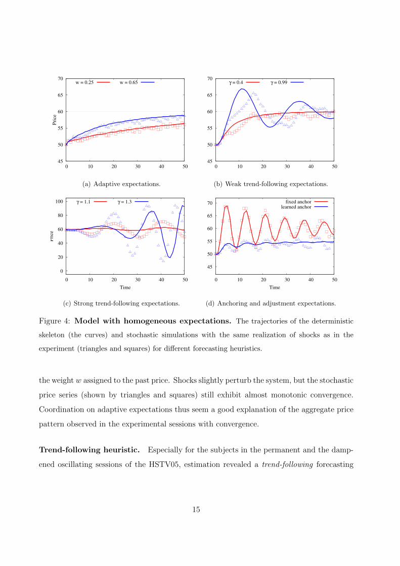
Figure 4: Model with homogeneous expectations. The trajectories of the deterministic
skeleton (the curves) and stochastic simulations with the same realization of shocks as in the
experiment (triangles and squares) for different forecasting heuristics.
the weight w assigned to the past price. Shocks slightly perturb the system, but the stochastic
price series (shown by triangles and squares) still exhibit almost monotonic convergence.
Coordination on adaptive expectations thus seem a good explanation of the aggregate price
pattern observed in the experimental sessions with convergence.
Trend-following heuristic. Especially for the subjects in the permanent and the damp-
ened oscillating sessions of the HSTV05, estimation revealed a trend-following forecasting
15
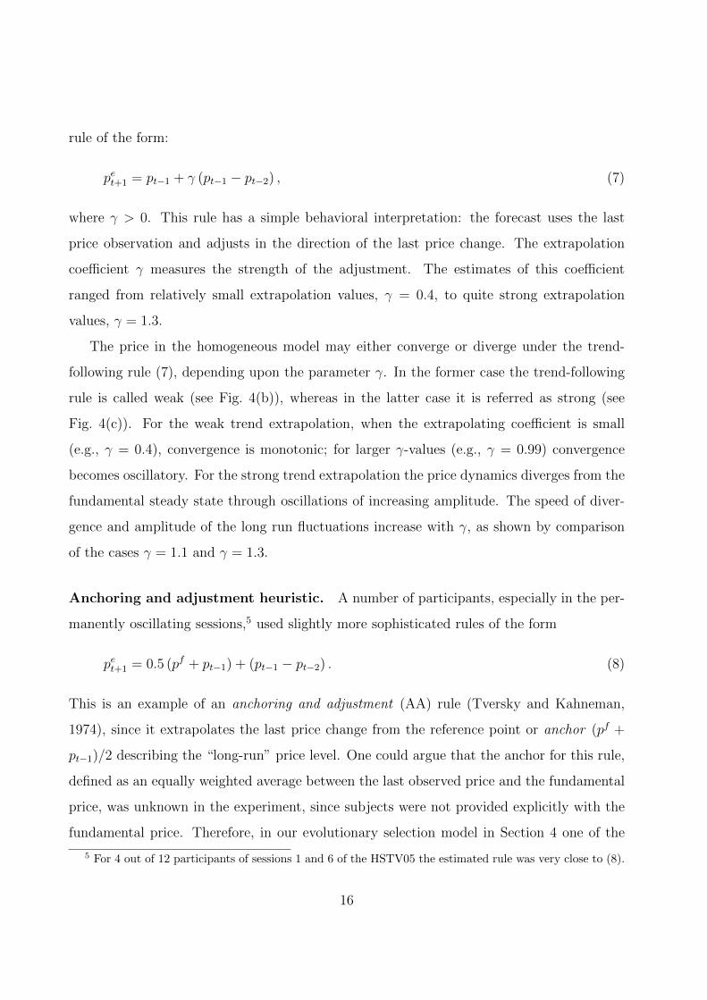
rule of the form:
pet+1 = pt−1 + γ (pt−1 − pt−2) , (7)
where γ > 0. This rule has a simple behavioral interpretation: the forecast uses the last
price observation and adjusts in the direction of the last price change. The extrapolation
coefficient γ measures the strength of the adjustment. The estimates of this coefficient
ranged from relatively small extrapolation values, γ = 0.4, to quite strong extrapolation
values, γ = 1.3.
The price in the homogeneous model may either converge or diverge under the trend-
following rule (7), depending upon the parameter γ. In the former case the trend-following
rule is called weak (see Fig. 4(b)), whereas in the latter case it is referred as strong (see
Fig. 4(c)). For the weak trend extrapolation, when the extrapolating coefficient is small
(e.g., γ = 0.4), convergence is monotonic; for larger γ-values (e.g., γ = 0.99) convergence
becomes oscillatory. For the strong trend extrapolation the price dynamics diverges from the
fundamental steady state through oscillations of increasing amplitude. The speed of diver-
gence and amplitude of the long run fluctuations increase with γ, as shown by comparison
of the cases γ = 1.1 and γ = 1.3.
Anchoring and adjustment heuristic. A number of participants, especially in the per-
manently oscillating sessions,5 used slightly more sophisticated rules of the form
pet+1 = 0.5 (pf + pt−1) + (pt−1 − pt−2) . (8)
This is an example of an anchoring and adjustment (AA) rule (Tversky and Kahneman,
1974), since it extrapolates the last price change from the reference point or anchor (pf +
pt−1)/2 describing the “long-run” price level. One could argue that the anchor for this rule,
defined as an equally weighted average between the last observed price and the fundamental
price, was unknown in the experiment, since subjects were not provided explicitly with the
fundamental price. Therefore, in our evolutionary selection model in Section 4 one of the
5 For 4 out of 12 participants of sessions 1 and 6 of the HSTV05 the estimated rule was very close to (8).
16

rules will be a modification of (8) with the fundamental price pf replaced by a proxy given
by the (observable) sample average of past prices pavt−1 = 1t
∑t−1j=0 pj, to obtain
pet+1 = 0.5 (pavt−1 + pt−1) + (pt−1 − pt−2) . (9)
We will refer to this forecasting rule with an anchor learned through a sample average of
past prices, as the learning anchoring and adjustment (LAA) heuristic.
Applying results from Appendix B to the anchoring and adjustment rule (8) we conclude
that the price dynamics of the homogeneous expectations model with AA heuristic converges
to the fundamental steady-state, but the convergence is oscillatory and slow, see Fig. 4(d).
For the stochastic simulation the convergence is even slower and the amplitude of the price
fluctuations remains more or less constant in the last 20 periods, with an amplitude ranging
from 55 to 65 comparable to that of the permanently oscillatory session 6 in the HSTV05
experiments. The small shocks εt added in the experimental design, to mimic (small) shocks
in a real market, thus seem to be important to keep the price oscillations alive. Fig. 4(d)
also shows the price dynamics of the learning anchoring and adjustment (LAA) rule (9).
Simulations under homogeneous expectations given by the LAA heuristic (9) converge to
the same fundamental steady-state as with the AA heuristic (8), but much slower and with
less pronounced oscillations. In the presence of noise, the price fluctuations under the LAA
heuristic are qualitatively similar to the fluctuations in the permanently oscillatory session
1 of the HSTV05 experiment (see, e.g., the lower left panel of Fig. 5) with prices fluctuating
below the fundamental most of the time.
Homogeneity versus heterogeneity
Different homogeneous expectation models explain the three observed patterns in the HSTV05
experiments, monotonic convergence, constant oscillations and dampened oscillations can be
reproduced. However, a model with homogeneous expectations leaves open the question why
different patterns in aggregate behavior emerged in different experimental sessions.
The behavioral model proposed in this paper is based on the idea of heterogeneity, in the
sense that several forecasting heuristics, those which we discussed above, could be used by the
17
48
50
52
54
56
58
60
0 10 20 30 40 50
Pri
ce,
Pre
dic
tio
ns
Session 2, participants 1 and 5
prediction 5prediction 1
price
52
54
56
58
60
62
64
66
0 10 20 30 40 50
Session 6, participant 1
prediction price
48
50
52
54
56
58
60
62
64
66
0 10 20 30 40 50
Pri
ce,
Pre
dic
tio
n
Time
Session 1, participant 3
prediction price
40
45
50
55
60
65
70
75
0 10 20 30 40 50
Time
Session 7, participant 3
prediction price
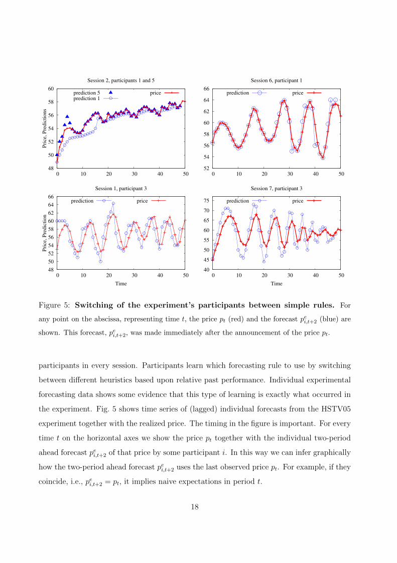
Figure 5: Switching of the experiment’s participants between simple rules. For
any point on the abscissa, representing time t, the price pt (red) and the forecast pei,t+2 (blue) are
shown. This forecast, pei,t+2, was made immediately after the announcement of the price pt.
participants in every session. Participants learn which forecasting rule to use by switching
between different heuristics based upon relative past performance. Individual experimental
forecasting data shows some evidence that this type of learning is exactly what occurred in
the experiment. Fig. 5 shows time series of (lagged) individual forecasts from the HSTV05
experiment together with the realized price. The timing in the figure is important. For every
time t on the horizontal axes we show the price pt together with the individual two-period
ahead forecast pei,t+2 of that price by some participant i. In this way we can infer graphically
how the two-period ahead forecast pei,t+2 uses the last observed price pt. For example, if they
coincide, i.e., pei,t+2 = pt, it implies naive expectations in period t.
18

In session 2, subject 5 extrapolates price changes in the early stage of the experiment
(see the upper left panel), but, starting from period t = 6, uses a simple naive rule pet+2 = pt.
In other words, in period 6, subject 5 switched from an extrapolative to a naive forecasting
rule. Subject 1 from the same group used a “smoother”, adaptive forecasting strategy, always
predicting a price between the previous forecast and the previous price realization. These
graphs suggest individual heterogeneity in forecasting strategies in the same session.
In the oscillating group 6, subject 1 used naive expectations in the first half of the
experiment (until period 24, see the upper right panel). Naive expectations however, lead
to prediction errors in an oscillating market, especially when the trend reverses. In period
25 subject 1 switches to a different, trend extrapolating prediction strategy. Thereafter, this
subject uses a trend extrapolating strategy switching back to the naive rule at periods of
expected trend reversal (e.g., in periods 27− 28, 32− 33, 37− 38, 42− 44, and 47).
Interestingly, participant 3 from another oscillating session 1 starts out predicting the
fundamental price, i.e., pet+1 = pf = 60 in the first four periods of the experiments (see the
lower left panel). But since the majority in session 1 predicted a lower price, the realized
price is much lower than the fundamental, causing participant 3 to switch to a different,
trend extrapolating strategy. Trend extrapolating predictions overshoot the realized market
price at the moments of trend reversal. Towards the end of the experiment participant 3
learned to anticipate the trend changes to some extent.
Finally, in session 7 with dampened price oscillations subject 3 started out with a strong
trend extrapolation (see the lower right panel). Despite very large prediction errors (and
thus low earnings) at the turning points, this participant sticks to strong trend extrapolation;
only in the last 4 periods some kind of adaptive expectations strategy was used.
Fig. 5 therefore suggests that individual heterogeneity in expectations within the same
session6 plays a role for explaining the observed phenomena at the aggregate level.
6Of course, high coordination of expectations means that the individual expectations were not spread
over the entire space. Appendix C provides additional details (in terms of eigenvalues) of the variety of
heuristics used in the same experimental session.
19

4 Heuristics Switching Model
In this section we present a simple model with evolutionary selection between different simple
forecasting heuristics. Before describing the model, we recall the most important “stylized
facts” which we found in the individual and aggregate experimental data:
- participants tend to base their predictions on past observations following simple fore-
casting heuristics;
- individual learning has a form of switching from one heuristic to another;
- in every session some form of coordination of individual forecasts occurs; the rule on
which individuals coordinate may be different in different sessions;
- coordination of individual forecasting rules is not perfect and some heterogeneity of
the applied rules remains at every time period.
The main idea of the model is simple.7 Assume that there exists a pool of simple predic-
tion rules (e.g., adaptive or trend-following heuristics) commonly available to the participants
of the experiment. At every time period these heuristics deliver forecasts for next period’s
price, and the realized market price depends upon these forecasts. However, the impacts of
different forecasting heuristics upon the realized prices are changing over time because the
participants are learning based on evolutionary selection: the better a heuristic performed in
the past, the higher its impact in determining next period’s price. As a result, the realized
market price and impact of the forecasting heuristics co-evolve in a dynamic process with
mutual feedback. This nonlinear evolutionary model exhibits path dependence explaining
coordination on different forecasting heuristics leading to different aggregate price behavior.
The Model
Let H denote a set of H heuristics which participants can use for price prediction. In the
beginning of period t every rule h ∈ H gives a two-period ahead point prediction for the price
7Our model is built upon the Adaptive Belief Scheme proposed in Brock and Hommes (1997) but with
memory and asynchronous updating.
20
pt+1. The prediction is described by a deterministic function fh of available information:
peh,t+1 = fh(pt−1, pt−2, . . . ; peh,t, p
eh,t−1, . . . ) . (10)
The price in period t is computed on the base of these predictions according to Eq. (1),
when the model is applied to the environment without robot traders, or to Eq. (3), when
it is applied in the environment with robots. In the latter case the fractions of robots is
determined by (4) as before. The average forecast pet+1 in the price equations becomes, in
an evolutionary model, a population weighted average of the different forecasting heuristics
pet+1 =H∑h=1
nh,t peh,t+1 , (11)
with peh,t+1 defined in (10). The weight nh,t assigned to the heuristic h is called the impact of
this heuristic. The impact is evolving over time and depends on the past relative performance
of all H heuristics, with more successful heuristics attracting more followers.
Similar to the incentive structure in the experiment, the performance measure of a fore-
casting heuristic in a given period is based on its squared forecasting error. More precisely,
the performance measure of heuristic h up to (and including) time t− 1 is given by
Uh,t−1 = −(pt−1 − peh,t−1
)2+ η Uh,t−2 . (12)
The parameter 0 ≤ η ≤ 1 represents the memory, measuring the relative weight agents
give to past errors of heuristic h. In the special case η = 0, the impact of each heuristic is
completely determined by the most recent forecasting error; for 0 < η ≤ 1 all past prediction
errors, with exponentially declining weights, affect the impact of the heuristics.
Given the performance measure, the impact of rule h is updated according to a discrete
choice model with asynchronous updating
nh,t = δ nh,t−1 + (1− δ) exp(β Uh,t−1)
Zt−1
, (13)
where Zt−1 =∑H
h=1 exp(β Uh,t−1) is a normalization factor. In the special case δ = 0,
(13) reduces to the the discrete choice model with synchronous updating used in Brock and
Hommes (1997) to describe endogenous selection of expectations. The more general case,
21

0 ≤ δ ≤ 1, gives some persistence or inertia in the impact of rule h, reflecting the fact
(consistent with the experimental data) that not all the participants update their rule in
every period or at the same time (see Hommes et al. (2005a) and Diks and van der Weide
(2005)). Hence, δ may be interpreted as the average per period fraction of individuals who
stick to their previous strategy. In the extreme case δ = 1, the initial impacts of the rules
never change, no matter what their past performance was. If 0 < δ ≤ 1, in each period
a fraction 1 − δ of participants update their rule according to the discrete choice model.
The parameter β ≥ 0 represents the intensity of choice measuring how sensitive individuals
are to differences in strategy performance. The higher the intensity of choice β, the faster
individuals will switch to more successful rules. In the extreme case β = 0, the impacts
in (13) move to an equal distribution independent of their past performance. At the other
extreme β = ∞, all agents who update their heuristic (i.e., a fraction 1 − δ) switch to the
most successful predictor.
Initialization. The model is initialized by a sequence of initial prices, whose length τ is
long enough to allow any forecasting rule in H to generate its prediction, as well as an initial
distribution {nh,0}, 1 ≤ h ≤ H of the impacts of different heuristic (summing to 1).
Given initial prices, the heuristic’s forecasts for price at time τ +2 can be computed and,
using the initial impacts of the heuristics, the price pτ+1 is determined. In the next period, the
forecasts of the heuristics are updated, the fraction of robot traders is computed if necessary,
while the same initial impacts nh,0 for the individual rules are used, since past performance
is not well defined yet. Thereafter, the price pτ+2 is computed and the initialization stage
is finished. After this initialization state the evolution of the model is well defined: first
the performance measure in (12) is updated, then, the new impacts of the heuristics are
computed according to (13), and the new prediction of the heuristics are obtained according
to (10). Finally, the new average forecast (11) and (if necessary) the new fraction of robot
traders (4) are computed, and a new price is determined by (1) or (3), respectively.
22

Table 1: Heuristics used in the evolutionary model. In simulations in Figs. 6–8 the first
four heuristics are used. The LAA heuristic is obtained from the simpler AA heuristic, by replacing
the (unknown) fundamental price pf by the sample average pavt−1.
ADA adaptive heuristic pe1,t+1 = 0.65 pt−1 + 0.35 pe1,t
WTR weak trend-following rule pe2,t+1 = pt−1 + 0.4 (pt−1 − pt−2)
STR strong trend-following rule pe3,t+1 = pt−1 + 1.3 (pt−1 − pt−2)
LAAanchoring and adjustment
pe4,t+1 = 0.5 (pavt−1 + pt−1) + (pt−1 − pt−2)rule with learned anchor
AAanchoring and adjustment
pe4,t+1 = 0.5 (pf + pt−1) + (pt−1 − pt−2)rule with fixed anchor
Example with Four Heuristics
The evolutionary model can be simulated with an arbitrary set of heuristics. Since one
of our goals is to explain the three different observed patterns in aggregate price behavior
– monotonic convergence, permanent oscillations and dampened oscillations – we keep the
number of heuristics as small as possible and consider a model with only four forecasting
rules. These rules, referred to as ADA, WTR, STR and LAA and given in Table 1, were
obtained as simple descriptions of typical individual forecasting behavior observed and esti-
mated in the experiments. As discussed in Section 3 these heuristics generate qualitatively
different dynamics, which allows one to get some non-trivial interaction between different
heuristics, so that qualitatively different patterns can be obtained.
With the four forecasting heuristics fixed, matched by experimental individual forecasting
data, there are only three free “learning” parameters in the model: β, η and δ. Provided
that these parameters are given, the HSM with four heuristics is initialized with two initial
prices, p0 and p1, and four initial impacts nh,0 used in periods t = 2 and t = 3.
23
5 Empirical Validation
The Heuristic Switching Model exhibits path-dependence and is capable of reproducing differ-
ent qualitative patterns within the same experimental environment. Anufriev and Hommes
(2012) simulate 50-period ahead forecasts (so-called “simulated paths”) of the HSM in three
sessions of the HSTV05 experiment. For a specific choice of the parameters, β = 0.4, η = 0.7
and δ = 0.9 (obtained after some trial and error simulations), but with different initial prices
and impacts of heuristics, the HSM qualitatively reproduces price behavior in sessions 2, 1
and 7, i.e., monotonic convergence, permanent oscillations and dampened oscillations.8 In
those 50-period ahead simulations the frequency and amplitude of the oscillations were dif-
ficult to match.
In this section we investigate the forecasting performance of the HSM model quantitatively
both in-sample and out-of-sample. We fit the model to 20 experimental sessions of 4 different
treatments in HSTV05 and HSTV08, providing an important test of generality of the model.
The HSM model fits all 20 sessions quite well. The section is divided in three parts. We,
first, illustrate the one-period ahead forecasts of the model visually. Then we proceed to
the rigorous evaluation of the in-sample performance of the model, and, finally, look at
out-of-sample forecasts made by the model.
5.1 One-period ahead simulations
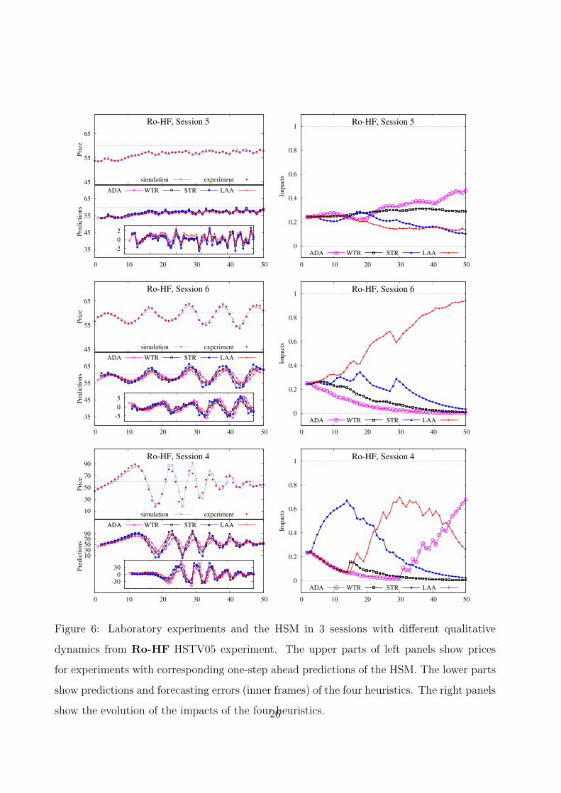
The left panels in Fig. 6 suggest that the switching model with four heuristics fits the
experimental data from the Ro-HF HSTV05 experiments quite nicely. The upper parts of
the panels compare the experimental data with the one-step ahead predictions of the HSM
for the benchmark values of parameters β = 0.4, η = 0.7 and δ = 0.9. We stress that, at this
8The initial distribution of agents over the four heuristics, i.e., initial impacts {n1,0, n2,0, n3,0, n4,0}, played
a crucial role for these price patterns. When the initial impacts of heuristics are distributed almost uniformly,
the monotonic convergence of session 2 is reproduced. Oscillations of session 1 are obtained when both WTR
and STR heuristics have relatively high initial weights (35% each). The dampened price oscillation in session
7 are reproduced when the STR rule has a large initial impact (66%).
24

stage, no fitting exercise has been performed. In each session and every period experimental
data (dots) are quite close to the prediction given by the HSM (line with squares).
In all these simulations the initial prices are chosen to coincide with the initial prices in
the first two periods in the corresponding experimental group, while the initial impacts of
all heuristics are equal to 0.25. At each step, in order to compute the heuristics’ forecasts
and update their impacts, past experimental price data are used, which is exactly the same
information that was available to participants in the experiments. The one-period ahead
forecasts can follow easily the monotonically converging patterns as well as the sustained or
dampened oscillatory patterns, starting out from a uniform initial distribution of forecasting
rules.
The lower parts of the left panels in Fig. 6 show that the heuristics forecasts are correlated,
so that the model reproduces coordination of expectations of the participants. The frames
of the lower panels display the prediction errors of the four heuristics. These errors are of
the same order as in the experiment (cf. Fig. 3).
The right panels of Fig. 6 show the transition paths of the impacts of each of the four
forecasting heuristics. In the case of monotonic convergence (session 5, upper panel), the
impacts of all four heuristics remain relatively close, although the impact of adaptive expec-
tations gradually increases and slightly dominates the other rules in the last 25 periods. In
contrast to the previous case, in experimental session 6 the two initial prices exhibited an
increasing trend. Consequently the trend-following rules and the learning anchor and adjust-
ment heuristic increase their impacts (middle panels). However, the trend rule misses the
turning points and its impact gradually decreases. The LAA heuristic with a more flexible
anchor predicts price oscillations better than the static STR and WTR rules. The impact of
the LAA heuristic gradually increases, rising to more than 80% after 40 periods. The HSM
thus explains coordination of individual forecasts on a LAA rule enforcing persistent price
oscillations around the long run equilibrium level.
Finally, in the simulations for session 4 with dampened oscillations (lower panels) the
initial price trend is so strong that the STR rule clearly dominates during the first 20 periods
of simulation. To some extent this rule enforces a trend in prices, but the presence of other
25
35
45
55
65
0 10 20 30 40 50
Pre
dic
tions
ADA WTR STR LAA
45
55
65
Pri
ce
Ro-HF, Session 5
simulation experiment
-2
0
2
0
0.2
0.4
0.6
0.8
1
0 10 20 30 40 50
Impac
ts
Ro-HF, Session 5
ADA WTR STR LAA
35
45
55
65
0 10 20 30 40 50
Pre
dic
tions
ADA WTR STR LAA
45
55
65
Pri
ce
Ro-HF, Session 6
simulation experiment
-5
0
5
0
0.2
0.4
0.6
0.8
1
0 10 20 30 40 50
Impac
ts
Ro-HF, Session 6
ADA WTR STR LAA
10 30 50 70 90
0 10 20 30 40 50
Pre
dic
tions
ADA WTR STR LAA
10
30
50
70
90
Pri
ce
Ro-HF, Session 4
simulation experiment
-30 0
30
0
0.2
0.4
0.6
0.8
1
0 10 20 30 40 50
Impac
ts
Ro-HF, Session 4
ADA WTR STR LAA
Figure 6: Laboratory experiments and the HSM in 3 sessions with different qualitative
dynamics from Ro-HF HSTV05 experiment. The upper parts of left panels show prices
for experiments with corresponding one-step ahead predictions of the HSM. The lower parts
show predictions and forecasting errors (inner frames) of the four heuristics. The right panels
show the evolution of the impacts of the four heuristics.26
35
45
55
65
0 10 20 30 40 50
Pre
dic
tions
ADA WTR STR LAA
45
55
65
Pri
ce
Ro-HF, Session 3
simulation experiment
-10
0
10
0
0.2
0.4
0.6
0.8
1
0 10 20 30 40 50
Impac
ts
Ro-HF, Session 3
ADA WTR STR LAA
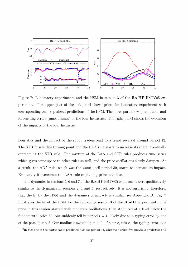
Figure 7: Laboratory experiments and the HSM in session 3 of the Ro-HF HSTV05 ex-
periment. The upper part of the left panel shows prices for laboratory experiment with
corresponding one-step ahead predictions of the HSM. The lower part shows predictions and
forecasting errors (inner frames) of the four heuristics. The right panel shows the evolution
of the impacts of the four heuristic.
heuristics and the impact of the robot traders lead to a trend reversal around period 12.
The STR misses this turning point and the LAA rule starts to increase its share, eventually
overcoming the STR rule. The mixture of the LAA and STR rules produces time series
which gives some space to other rules as well, and the price oscillations slowly dampen. As
a result, the ADA rule, which was the worst until period 30, starts to increase its impact.
Eventually it overcomes the LAA rule explaining price stabilization.
The dynamics in sessions 5, 6 and 7 of the Ro-HF HSTV05 experiment were qualitatively
similar to the dynamics in sessions 2, 1 and 4, respectively. It is not surprising, therefore,
that the fit by the HSM and the dynamics of impacts is similar, see Appendix D. Fig. 7
illustrates the fit of the HSM for the remaining session 3 of the Ro-HF experiment. The
price in this session started with moderate oscillations, then stabilized at a level below the
fundamental price 60, but suddenly fell in period t = 41 likely due to a typing error by one
of the participants.9 Our nonlinear switching model, of course, misses the typing error, but
9In fact one of the participants predicted 5.25 for period 42, whereas his/her five previous predictions all
27

nevertheless matches the overall pattern before and after the unexpected price drop.
We demonstrated that the Heuristic Switching Model fits all sessions of the Ro-HF
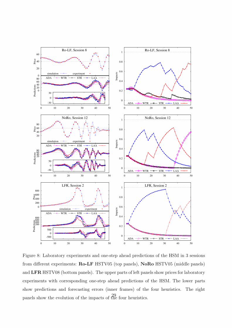
environment quite nicely. How robust are these results? Fig. 8 shows the fit and the evolution
of impacts for typical sessions from the three other treatments with modified experimental
environments. The upper panels displays session 8 of the Ro-LF HSTV05 experiment with
fundamental price of 40 instead of 60. Slowly increasing price oscillations are dominated
by the STR rule, but when the frequency of trend-reversals increases, the LAA rule takes
over again. The middle panel illustrates the HSM for session 12 of the NoRo HSTV05
experiment without robot traders. Large amplitude price oscillations, with prices almost
reaching their maximum 100 and minimum 0, arise, but prices stabilize towards the end of
the experiment. The evolution of the impacts of the four forecasting heuristics is similar to
the case of dampening price oscillations considered before (see the lower panels of Figure 6),
with the STR rule initially dominating the market, followed by the LAA rule taking over
around period 25 during price oscillations, and the ADA rule finally dominating towards
the end, when the price stabilizes. Finally, the lower panel displays session 2 of the LFR
HSTV08 experiment with large forecasting range. The asset price oscillates with very large
amplitude, with a long lasting trend of more than 25 periods with prices rising close to their
maximum 1000, after which a crash follows to values close to their minimum 0, and the
market starts oscillating. The evolution of the impacts of the four forecasting heuristics is
similar as before, with the STR rule taking the lead, increasing its share to more than 90%
after 25 periods during the long lasting price bubble. When the upper forecasting bound is
met, the trend cannot be sustained any longer and the share of the STR rule declines fast.
The LAA rule takes over and large amplitude oscillations are observed. The fact that our
nonlinear switching model nicely captures all patterns in these different groups shows that
the model is robust concerning changes of the asset pricing market environment.10
To summarize, the one-step ahead simulations of the HSM match both converging and
oscillating prices closely and produce clear differences in the evolution of impacts. In the case
were between 55.00 and 55.40. Perhaps an intention was to type 55.25.10Appendix D contains analogous plots for all other groups of the HSTV05 and HSTV08 experiments.
28
0 20 40 60 80
0 10 20 30 40 50
Pre
dic
tions
ADA WTR STR LAA 0
20
40
60
Pri
ce
Ro-LF, Session 8
simulation experiment
-30
0
30
0
0.2
0.4
0.6
0.8
1
0 10 20 30 40 50
Impac
ts
Ro-LF, Session 8
ADA WTR STR LAA
20 40 60 80
0 10 20 30 40 50
Pre
dic
tions
ADA WTR STR LAA
20
40
60
80
Pri
ce
NoRo, Session 12
simulation experiment
-50
0
50
0
0.2
0.4
0.6
0.8
1
0 10 20 30 40 50
Impac
tsNoRo, Session 12
ADA WTR STR LAA
200 400 600 800
0 10 20 30 40 50
Pre
dic
tions
ADA WTR STR LAA
0
200
400
600
800
Pri
ce
LFR, Session 2
simulation experiment
-500
0
500
0
0.2
0.4
0.6
0.8
1
0 10 20 30 40 50
Impac
ts
LFR, Session 2
ADA WTR STR LAA
Figure 8: Laboratory experiments and one-step ahead predictions of the HSM in 3 sessions
from different experiments: Ro-LF HSTV05 (top panels), NoRo HSTV05 (middle panels)
and LFR HSTV08 (bottom panels). The upper parts of left panels show prices for laboratory
experiments with corresponding one-step ahead predictions of the HSM. The lower parts
show predictions and forecasting errors (inner frames) of the four heuristics. The right
panels show the evolution of the impacts of the four heuristics.29

of monotone convergence and constant oscillations we observe a self-confirming property:
more coordination on one rule (ADA in the case of convergence and LAA in the case of
oscillations) leads to the price dynamics which reinforce this rule. For the sessions with
the dampened oscillations, one step ahead forecast produces a rich evolutionary selection
dynamics. These sessions go through three different phases where the STR, the LAA and
the ADA heuristics subsequently dominate. The STR dominates during the initial phase of
a strong trend in prices, but starts declining after it misses the first turning point of the
trend. The LAA does a better job in predicting the trend reversal but if it fails to keep the
amplitude of oscillations constant it may be taken over by a stabilizing rule as ADA.
5.2 Forecasting performance
A measure of model fit is the mean of squared errors over a simulation of the model for
one-step ahead predictions. Table 2 compares these mean squared errors (MSEs) for sev-
eral experimental sessions11 for 9 different models: the RE fundamental prediction, five
homogeneous expectations models (naive expectations, and each of the four heuristics of the
switching model), and three heterogeneous expectations models with 4 heuristics, namely,
the model with fixed fractions (corresponding to δ = 1), the switching model with benchmark
parameters β = 0.4, η = 0.7 and δ = 0.9, and, finally, the “best” switching model fitted by
minimization of the MSE over the parameter space (the last three lines in Table 2 show the
corresponding optimal parameter values).12 The MSEs for the benchmark switching model
are shown in bold and, for comparison, for each session the MSEs for the best among the
four heuristics are also shown in bold. The best among 9 models for each session is shown
in italic and it is always the best fitted HSM.
11The MSEs are computed over 47 periods for t = 4, . . . , 50 in the sessions of HSTV05 experiment and
over 46 periods, for t = 4, . . . , 49, in the sessions of HSTV08 experiments. We skip the errors of the first four
periods in order to minimize the impact of the initial conditions (i.e., the initial impacts of the heuristics)
for the HSM. Period t = 4 is the first period when the prediction is computed with both the heuristics’
forecasts and the heuristics’ impacts being updated based on the experimental data. For comparison, in all
other models we compute errors also from t = 4.12Analogous tables for the remaining sessions can be found in Appendix D.
30
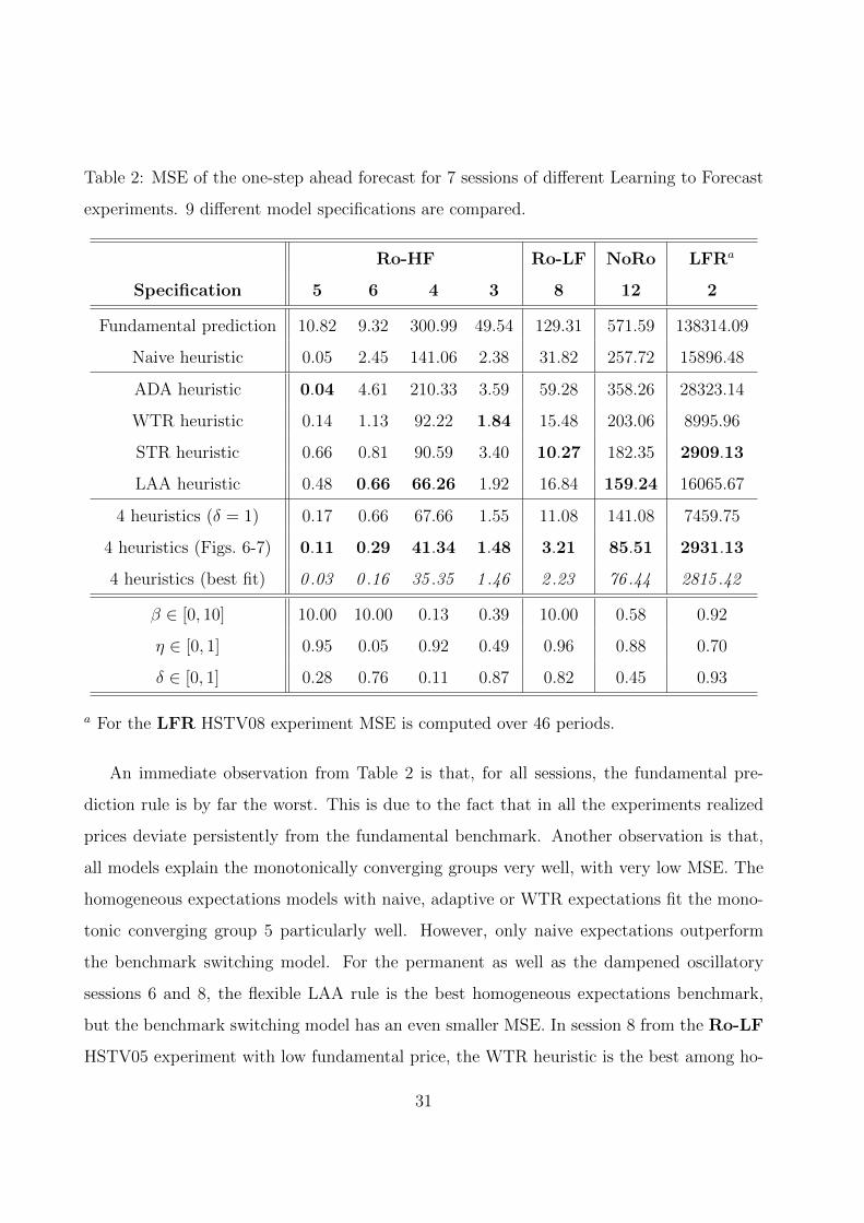
Table 2: MSE of the one-step ahead forecast for 7 sessions of different Learning to Forecast
experiments. 9 different model specifications are compared.
Ro-HF Ro-LF NoRo LFRa
Specification 5 6 4 3 8 12 2
Fundamental prediction 10.82 9.32 300.99 49.54 129.31 571.59 138314.09
Naive heuristic 0.05 2.45 141.06 2.38 31.82 257.72 15896.48
ADA heuristic 0.04 4.61 210.33 3.59 59.28 358.26 28323.14
WTR heuristic 0.14 1.13 92.22 1.84 15.48 203.06 8995.96
STR heuristic 0.66 0.81 90.59 3.40 10.27 182.35 2909.13
LAA heuristic 0.48 0.66 66.26 1.92 16.84 159.24 16065.67
4 heuristics (δ = 1) 0.17 0.66 67.66 1.55 11.08 141.08 7459.75
4 heuristics (Figs. 6-7) 0.11 0.29 41.34 1.48 3.21 85.51 2931.13
4 heuristics (best fit) 0 .03 0 .16 35 .35 1 .46 2 .23 76 .44 2815 .42
β ∈ [0, 10] 10.00 10.00 0.13 0.39 10.00 0.58 0.92
η ∈ [0, 1] 0.95 0.05 0.92 0.49 0.96 0.88 0.70
δ ∈ [0, 1] 0.28 0.76 0.11 0.87 0.82 0.45 0.93
a For the LFR HSTV08 experiment MSE is computed over 46 periods.
An immediate observation from Table 2 is that, for all sessions, the fundamental pre-
diction rule is by far the worst. This is due to the fact that in all the experiments realized
prices deviate persistently from the fundamental benchmark. Another observation is that,
all models explain the monotonically converging groups very well, with very low MSE. The
homogeneous expectations models with naive, adaptive or WTR expectations fit the mono-
tonic converging group 5 particularly well. However, only naive expectations outperform
the benchmark switching model. For the permanent as well as the dampened oscillatory
sessions 6 and 8, the flexible LAA rule is the best homogeneous expectations benchmark,
but the benchmark switching model has an even smaller MSE. In session 8 from the Ro-LF
HSTV05 experiment with low fundamental price, the WTR heuristic is the best among ho-
31

mogeneous rules but the HSM outperforms also this model. In the sessions without robots,
as in the NoRo HSTV05 treatment and especially in the LFR HSTV08 treatment, all
homogeneous models produce very large MSEs. The models often under- or overestimate
the trend and also miss the turning points of trend-reversal. The MSEs of the switching
model are much smaller in the sessions of the NoRo HSTV05 treatment and comparable
with the best homogeneous model (STR heuristic) in the LFR HSTV08 treatment. When
the learning parameters of the HSM model are chosen to minimize the MSE for the corre-
sponding session, the model produces the smallest MSE over all alternative specifications13,
though an improvement of fit with respect to the benchmark HSM is not as large as when
the benchmark HSM is compared with the best homogeneous model. This suggest that the
good fit of the switching model is fairly robust w.r.t. the model parameters.
We stress that the evolutionary Heuristic Switching Model is able to make the best
out of different heuristics. Indeed, in different sessions (and treatments) of the learning
to forecast experiment different homogeneous expectations models produce the best fit of
the price dynamics. However, the switching model produces even better fit than the best
homogeneous model.
5.3 Out-of-sample forecasting
Let us now turn to the out-of-sample validation of the model. In order to evaluate the out-
of-sample forecasting performance of the model, we first perform a grid search to find the
parameters of the model minimizing the MSE for periods t = 4, . . . , 43 and then compute the
forecasting errors of the fitted model for the remaining periods (7 in the case of the HSTV05
experiments and 6 in the case of the HSTV05 experiments). The results are reported in
the upper part of Table 3 for each session. The first two lines show the in-sample MSE of
the fitted model and the corresponding values of the parameters. The next lines give the
values of the forecasting errors. In the middle part of the table, we report the results of the
same procedure performed for the switching model with benchmark parameters. Finally,
13This holds for all 20 sessions of HSTV05 and HSTV 08 experiments, except session 5 in the LFR
HSTV08 treatment, where the STR heuristic outperforms the HSM. See Appendix D.
32
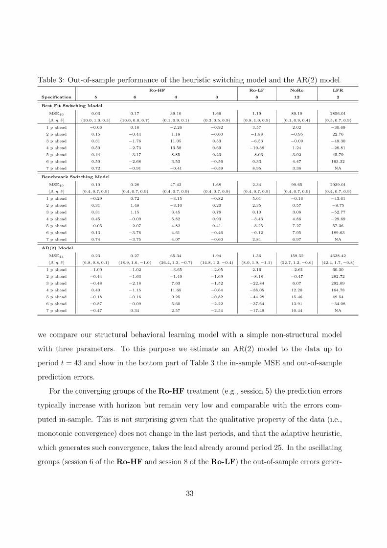
Table 3: Out-of-sample performance of the heuristic switching model and the AR(2) model.Ro-HF Ro-LF NoRo LFR
Specification 5 6 4 3 8 12 2
Best Fit Switching Model
MSE40 0.03 0.17 39.10 1.66 1.19 89.19 2856.01
(β, η, δ) (10.0, 1.0, 0.3) (10.0, 0.0, 0.7) (0.1, 0.9, 0.1) (0.3, 0.5, 0.9) (0.8, 1.0, 0.9) (0.1, 0.9, 0.4) (0.5, 0.7, 0.9)
1 p ahead −0.06 0.16 −2.26 −0.92 3.57 2.02 −30.69
2 p ahead 0.15 −0.44 1.18 −0.00 −1.88 −0.95 22.76
3 p ahead 0.31 −1.76 11.05 0.53 −6.53 −0.09 −49.30
4 p ahead 0.50 −2.73 13.58 0.69 −10.38 1.24 −28.81
5 p ahead 0.44 −3.17 8.85 0.23 −8.03 3.92 45.79
6 p ahead 0.50 −2.68 3.53 −0.56 0.33 4.47 163.32
7 p ahead 0.72 −0.91 −0.41 −0.59 8.95 3.36 NA
Benchmark Switching Model
MSE40 0.10 0.28 47.42 1.68 2.34 99.65 2939.01
(β, η, δ) (0.4, 0.7, 0.9) (0.4, 0.7, 0.9) (0.4, 0.7, 0.9) (0.4, 0.7, 0.9) (0.4, 0.7, 0.9) (0.4, 0.7, 0.9) (0.4, 0.7, 0.9)
1 p ahead −0.29 0.72 −3.15 −0.82 5.01 −0.16 −43.61
2 p ahead 0.31 1.48 −3.10 0.20 2.35 0.57 −8.75
3 p ahead 0.31 1.15 3.45 0.78 0.10 3.08 −52.77
4 p ahead 0.45 −0.09 5.82 0.93 −3.43 4.86 −29.69
5 p ahead −0.05 −2.07 4.82 0.41 −3.25 7.27 57.36
6 p ahead 0.13 −3.76 4.61 −0.46 −0.12 7.95 189.63
7 p ahead 0.74 −3.75 4.07 −0.60 2.81 6.97 NA
AR(2) Model
MSE44 0.23 0.27 65.34 1.94 1.56 159.52 4638.42
(β, η, δ) (6.8, 0.8, 0.1) (18.9, 1.6,−1.0) (26.4, 1.3,−0.7) (14.8, 1.2,−0.4) (8.0, 1.9,−1.1) (22.7, 1.2,−0.6) (42.4, 1.7,−0.8)
1 p ahead −1.00 −1.02 −3.65 −2.05 2.16 −2.61 60.30
2 p ahead −0.44 −1.63 −1.49 −1.69 −8.18 −0.47 282.72
3 p ahead −0.48 −2.18 7.63 −1.52 −22.84 6.07 292.09
4 p ahead 0.40 −1.15 11.65 −0.64 −38.05 12.20 164.78
5 p ahead −0.18 −0.16 9.25 −0.82 −44.28 15.46 49.54
6 p ahead −0.87 −0.09 5.60 −2.22 −37.64 13.91 −34.08
7 p ahead −0.47 0.34 2.57 −2.54 −17.49 10.44 NA
we compare our structural behavioral learning model with a simple non-structural model
with three parameters. To this purpose we estimate an AR(2) model to the data up to
period t = 43 and show in the bottom part of Table 3 the in-sample MSE and out-of-sample
prediction errors.
For the converging groups of the Ro-HF treatment (e.g., session 5) the prediction errors
typically increase with horizon but remain very low and comparable with the errors com-
puted in-sample. This is not surprising given that the qualitative property of the data (i.e.,
monotonic convergence) does not change in the last periods, and that the adaptive heuristic,
which generates such convergence, takes the lead already around period 25. In the oscillating
groups (session 6 of the Ro-HF and session 8 of the Ro-LF) the out-of-sample errors gener-
33

ated by the switching model are varying with the time horizon and typically larger than the
in-sample error. Even if the switching model with leading LAA heuristic captures oscillations
qualitatively, the prediction errors can become large when the oscillations predicted by the
model have different frequency than the oscillations in the experimental session, so that the
prediction goes out of phase. The prediction errors for sessions with damping oscillations
(session 4 of the Ro-HF and session 12 of the NoRo) are not very high when compared with
the in-sample errors. This is because the price in these sessions converges towards the end
of the experiment. At the end of the in-sample period, i.e., at t = 43, the switching model
already selects the ADA heuristic, which generates the same behavior as in the experiment.
Comparing the forecasting errors of the switching and AR(2) models we conclude that
the former model is better than the latter, on average. More specifically, in the converging
session 5 and oscillating session 6 of the Ro-HF treatment the out-of-sample performances
are very similar, but in all other sessions (including those which are not shown in Table 3) the
different variations of the switching model outperform the AR(2) model out-of-sample. The
non-linearity and behavioral foundation allows the HSM adapt faster than the AR(2) model
to the change in the price dynamics. In session 8 of the Ro-LF the oscillations become more
pronounced towards the end of the experiment. The HSM model captures this effect, while
AR(2) does not. As a result, the AR(2) model produces errors larger than 7 in absolute
value, which would lead to 0 earnings in the experiment, see Eq. (2), whereas the HSM does
not have such large errors.
The largest out-of-sample errors are observed in the sessions of the LFR treatment, see
also Table 8 from Appendix D. However, in all the sessions the out-of-sample errors of the
HSM are comparable and often even smaller than the in-sample errors. Furthermore, the
errors of the HSM are smaller than the analogous prediction errors of the AR(2) model.
To further investigate one- and two-period ahead out-of-sample forecasting performance,
we fit the model on a moving sample and compute an average of the corresponding squared
prediction errors. The results of this exercise for the same three models (best fit, benchmark,
and AR(2)) are presented in Table 4. The smallest forecasting errors within the same class
(e.g., one-period ahead in session 4) are shown in italic. It turns out that our nonlinear
34
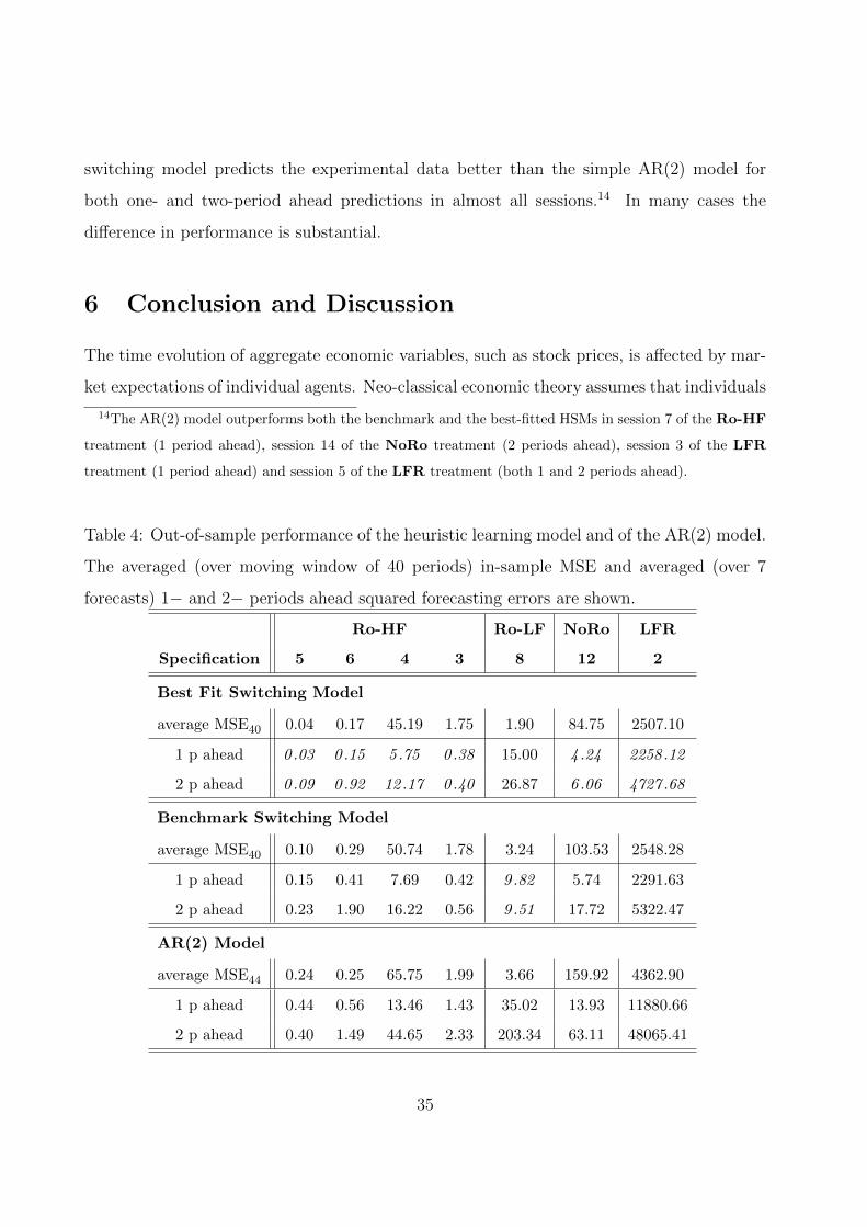
switching model predicts the experimental data better than the simple AR(2) model for
both one- and two-period ahead predictions in almost all sessions.14 In many cases the
difference in performance is substantial.
6 Conclusion and Discussion
The time evolution of aggregate economic variables, such as stock prices, is affected by mar-
ket expectations of individual agents. Neo-classical economic theory assumes that individuals
14The AR(2) model outperforms both the benchmark and the best-fitted HSMs in session 7 of the Ro-HF
treatment (1 period ahead), session 14 of the NoRo treatment (2 periods ahead), session 3 of the LFR
treatment (1 period ahead) and session 5 of the LFR treatment (both 1 and 2 periods ahead).
Table 4: Out-of-sample performance of the heuristic learning model and of the AR(2) model.
The averaged (over moving window of 40 periods) in-sample MSE and averaged (over 7
forecasts) 1− and 2− periods ahead squared forecasting errors are shown.
Ro-HF Ro-LF NoRo LFR
Specification 5 6 4 3 8 12 2
Best Fit Switching Model
average MSE40 0.04 0.17 45.19 1.75 1.90 84.75 2507.10
1 p ahead 0 .03 0 .15 5 .75 0 .38 15.00 4 .24 2258 .12
2 p ahead 0 .09 0 .92 12 .17 0 .40 26.87 6 .06 4727 .68
Benchmark Switching Model
average MSE40 0.10 0.29 50.74 1.78 3.24 103.53 2548.28
1 p ahead 0.15 0.41 7.69 0.42 9 .82 5.74 2291.63
2 p ahead 0.23 1.90 16.22 0.56 9 .51 17.72 5322.47
AR(2) Model
average MSE44 0.24 0.25 65.75 1.99 3.66 159.92 4362.90
1 p ahead 0.44 0.56 13.46 1.43 35.02 13.93 11880.66
2 p ahead 0.40 1.49 44.65 2.33 203.34 63.11 48065.41
35

form expectations rationally, thus enforcing prices to track economic fundamentals and lead-
ing to an efficient allocation of resources. Laboratory experiments with human subjects
have shown however that individuals do not behave fully rational, but instead follow simple
heuristics. In laboratory markets prices may show persistent deviations from fundamentals
similar to the large swings observed in real stock prices.
Our results show that performance-based evolutionary selection among simple forecasting
heuristics can explain coordination of individual forecasting behavior leading to three differ-
ent aggregate outcomes observed in identically organized treatments of the recent laboratory
market forecasting experiments: slow monotonic price convergence, oscillatory dampened
price fluctuations and persistent price oscillations. Furthermore, we show that the same
model fits reasonably well also other learning to forecast experiments.
In our Heuristic Switching Model forecasting strategies are selected every period from a
small population of plausible heuristics, such as adaptive expectations and trend following
rules. Individuals adapt their strategies over time, based on the relative forecasting per-
formance of the heuristics. As a result, the nonlinear evolutionary switching mechanism
exhibits path dependence and matches individual forecasting behavior as well as aggregate
market outcomes in the experiments. We showed that none of the homogeneous expectation
models constituting the HSM fits all different observed patterns. Instead different heuris-
tics fit better dynamics in different sessions. The HSM not only provide a simultaneous
explanation for the aggregate outcomes in all different sessions, but also outperforms the
best homogeneous model in almost every session. Our results are in line with recent work
on agent-based models of interaction and contribute to a behavioral explanation of market
fluctuations.
The HSM is one of the first learning models explaining different time series patterns in
the same laboratory environment. Our approach of doing this is similar to many game-
theoretical learning models (often referred as “reinforcement learning”), see, e.g., Arthur
(1991), Erev and Roth (1998) and Camerer and Ho (1999). These models were developed
as a response to experimental evidence that individuals often do not play or learn to play
equilibrium predictions such as Nash Equilibrium, or different refinements. Our market envi-
36

ronment is quite different from the strategic environments studied in game theory, however.
For example, agents in our framework do not have a well defined strategies, other than
predicting a number between 0 and 100 in two decimals. Other important differences are
that the strategies used in our switching model are state dependent and that individuals do
not know the “payoff matrix”, which moreover is changing over time in a path-depending
manner.
The model presented in this paper is one of the first models to explain individual micro-
behavior as well as aggregate macro behavior. Recently Fuster et al. (2010) propose a
somewhat similar model of “natural expectations”, which are the weighted average of a
so-called intuitive, extrapolative expectations and rational expectations. Their model can
successfully explain a number of stylized facts of macro-economic time series. Our heuristics
correspond to different plausible parametrization of their intuitive expectations, but our
approach to discipline bounded rationality is different. Instead of fixing the intuitive rule on
the basis of a mis-specified estimation of the true model as in Fuster et al. (2010), we fix the
heuristics’ parameters on the basis of experimental estimations but allow agents to change
their heuristics dynamically. Of course, fundamental expectations can be also included into
the set of the rules. In a related paper, Hommes and Lux (2011) explain learning to forecast
experiments in the classical cobweb (hog-cycle) market environment, using a heterogeneous
expectations model, where individual agents use a genetic algorithm. The GA-learning model
captures all stylized facts of the cobweb markets, both at the individual and at the aggregate
level, quite nicely across different experimental treatments.
A more systematic investigation in which market environments other than the asset
pricing framework our nonlinear heuristics switching model can explain individual forecasting
behavior as well as aggregate price behavior is beyond the scope of this paper. We conjecture,
however, that the simple Heuristics Switching Model analyzed in this paper works well in
market environments with some structure and persistence in price fluctuations, either in the
form of converging prices or in the presence of price oscillations and (temporary) trends.
In future work we intend to apply our HSM to financial data with highly irregular and
persistent time series. For this application, the set of heuristics should be augmented by
37

more sophisticated rules, those which are applied in real financial markets. Allen and Taylor
(1990) and Frankel and Froot (1990) provide evidence based on survey data, that simple
extrapolation heuristics similar to those we employ, are used in real markets. Given that
the HSM would still be able to pick and temporary amplify the self-confirming patterns in
prices such as trends, we hope that more sophisticated versions of the model could improve
the forecasting of financial markets.
38
References
Adam, K., “Experimental Evidence on the Persistence of Output and Inflation,” The Eco-
nomic Journal, 2007, 117 (520), 603–636.
, A. Marcet, and J.P. Nicolini, “Stock market volatility and learning,” Working paper
series 862, European Central Bank 2008.
Allen, H. and M.P. Taylor, “Charts, Noise and Fundamentals in the London Foreign
Exchange Market,” Economic Journal, 1990, 100, 49–59.
Anufriev, M. and C. Hommes, “Evolution of market heuristics,” Knowledge Engineering
Review, 2012. forthcoming.
and V. Panchenko, “Asset Prices, Traders’ Behavior and Market Design,” Journal of
Economic Dynamics & Control, 2009, 33, 1073 – 1090.
, C. Hommes, and R. Philipse, “Evolutionary Selection of Expectations in Positive and
Negative Feedback Markets,” CeNDEF Working Paper 2010-05, University of Amsterdam
2010.
Arthur, W.B., “Designing Economic Agents that Act like Human Agents: A Behavioral
Approach to Bounded Rationality,” American Economic Review, 1991, 81, 353–359.
Assenza, T., P. Heemeijer, C. Hommes, and D. Massaro, “Individudal expectations
and aggregate macro behavior,” CeNDEF Working Paper 2011-01, University of Amster-
dam 2011.
Bao, T., C. Hommes, J. Sonnemans, and J. Tuinstra, “Individual expectation, lim-
ited rationality and aggregate outcome,” CeNDEF Working Paper 2010-07, University of
Amsterdam 2010.
Boswijk, P., C. Hommes, and S. Manzan, “Behavioral heterogeneity in stock prices,”
Journal of Economic Dynamics and Control, 2007, 31 (6), 1938–1970.
39
Branch, W. and G. Evans, “Intrinsic Heterogeneity in Expectation Formation,” Journal
of Economic Theory, 2006, 127, 264–295.
and , “Learning about Risk and Return: A Simple Model of Bubbles and Crashes,”
American Economic Journal: Macroeconomics, 2011, 3 (3), 159–191.
Bray, M.M. and N.E. Savin, “Rational Expectations Equilibria, Learning, and Model
Specification,” Econometrica, 1986, 54 (5), 1129–1160.
Brock, W.A. and C. Hommes, “A Rational Route to Randomness,” Econometrica, 1997,
65 (5), 1059–1095.
and , “Heterogeneous Beliefs and Routes to Chaos in a Simple Asset Pricing Model,”
Journal of Economic Dynamics and Control, 1998, 22, 1235–1274.
Bullard, J.B., “Learning equilibria,” Journal of Economic Theory, 1994, 64, 468–485.
Camerer, C.F. and E. Fehr, “When Does ’Economic Man’ Dominate Social Behavior?,”
Science, 2006, 311 (5757), 47–52.
and T.-H. Ho, “Experienced-Weighted Attraction Learning in Normal Form Games,”
Econometrica, 1999, 67 (4), 827–874.
Campbell, J.Y., A.W. Lo, and A.C. MacKinlay, The Econometrics of Finanical Mar-
kets, Princeton University Press, Princeton, 1997.
Carceles-Poveda, E. and C. Giannitsarou, “Asset pricing with adaptive learning,”
Review of Economic Dynamics, 2008, 11 (3), 629 – 651.
de Jong, E., W.F.C. Verschoor, and R.C.J. Zwinkels, “Behavioural heterogeneity
and shift-contagion: Evidence from the Asian crisis,” Journal of Economic Dynamics and
Control, 2009, 33 (11), 1929 – 1944.
DeBondt, W.F.M. and R. Thaler, “Does the Stock Market Overreact?,” Journal of
Finance, 1989, 40 (3), 793–805.
40
Diks, C. and R. van der Weide, “Herding, a-synchronous updating and heterogeneity in
memory in a CBS,” Journal of Economic Dynamics and Control, 2005, 29, 741–763.
Duffy, J., “Experimental Macroeconomics,” in Steven Durlauf and Larry Blume, eds., New
Palgrave Dictionary of Economics, New York: Palgrave Macmillan, 2008.
Erev, I. and A.E. Roth, “Prediction how people play games: Reinforcement learning in
games with unique strategy equilibrium,” American Economic Review, 1998, 88, 848–881.
Evans, G.W. and S. Honkapohja, Learning and Expectations in Macroeconomics, Prince-
ton University Press, 2001.
Fama, E.F., “Efficient Capital Markets: a Review of Theory and Empirical Work,” Journal
of Finance, 1970, 25, 383–417.
Franke, R. and F. Westerhoff, “Structural Stochastic Volatility in Asset Pricing Dynam-
ics,” Working paper 78 2011.
Frankel, J.A. and K.A. Froot, “Chartists, Fundamentalists and Trading in the Foreign
Exchange Market,” American Economic Review, 1990, 80 (2), 181–185.
Friedman, M., Essays in Positive Economics, University Of Chicago Press, 1953.
Fuster, A., D. Laibson, and B. Mendel, “Natural Expectations and Macroeconomic
Fluctuations,” Journal of Economic Perspectives, 2010, 24 (4), 67–84.
Gaunersdorfer, A., C.H. Hommes, and F.O.O. Wagener, “Bifurcation routes to
volatility clustering under evolutionary learning,” Journal of Economic Behavior & Orga-
nization, 2008, 67 (1), 27 – 47.
Heemeijer, P., C. Hommes, J. Sonnemans, and J. Tuinstra, “Price stability and
volatility in markets with positive and negative expectations feedback: An experimental
investigation,” Journal of Economic Dynamics and Control, 2009, 33, 1052–1072.
41
Hey, J.D., “Expectation formation: Rational or adaptive or ...?,” Journal of Economic
Behavior and Organization, 1994, 25, 329–349.
Hommes, C., “Heterogeneous Agent Models in Economics and Finance,” in K.L. Judd and
L. Tesfatsion, eds., Handbook of Computational Economics Vol. 2: Agent-Based Compu-
tational Economics, Elsevier/North-Holland (Handbooks in Economics Series), 2006.
, “The Heterogeneous Expectations Hypothesis: Some Evidence from the Lab,” Journal
of Economic Dynamics and Control, 2011, 35 (1), 1–24.
and T. Lux, “Individual Expectations and Aggregate Behavior in Learning to Forecast
Experiments,” Macroeconomic Dynamics, 2011. forthcoming.
, H. Huang, and D. Wang, “A robust rational route to randomness in a simple asset
pricing model,” Journal of Economic Dynamics and Control, 2005, 29, 1043–1072.
, J. Sonnemans, J. Tuinstra, and H. van de Velden, “Coordination of Expectations
in Asset Pricing Experiments,” Review of Financial Studies, 2005, 18 (3), 955–980.
, , , and , “Expectations and bubbles in asset pricing experiments,” Journal of
Economic Behavior and Organization, 2008, 67 (1), 116–133.
Kahneman, D., “Maps of Bounded Rationality: Psychology for Behavioral Economics,”
American Economic Review, 2003, 93, 1449–1475.
Lei, V., C.N. Noussair, and C.R. Plott, “Nonspeculative bubbles in experimental asset
markets: lack of common knowledge of rationality vs. actual irrationality,” Econometrica,
2001, 69 (4), 831–859.
Lucas, R.E., “Expectations and the Neutrality of Money,” Journal of Economic Theory,
1972, 4, 103–124.
Marimon, R., S.E. Spear, and S. Sunder, “Expectationally Driven Market Volatility:
An Experimental Study,” Journal of Economic Theory, 1993, 61 (1), 74–103.
42
Muth, J.F., “Rational Expectations and the Theory of Price Movements,” Econometrica,
1961, 29 (3), 315–335.
Peterson, S.P., “Forecasting dynamics and convergence to market fundamentals: Evidence
from experimental asset markets,” Journal of Economic Behavior and Organization, 1993,
22 (3), 269–284.
Pfajfar, D. and B. Zakelj, “Inflation Expectations and Monetary Policy Design: Evidence
from the Laboratory,” mimeo, Tilburg University 2010.
Samuelson, P.A., “Proof that properly anticipated prices fluctuate randomly,” Manage-
ment Review, 1965, 6 (2).
Sargent, T.J., Bounded Rationality in Macroeconomics, Oxford University Press, 1993.
Shiller, R., “Do Stock Prices Move Too Much to be Justified by Subsequent Changes in
Dividends?,” American Economic Review, 1981, 71 (3), 421–436.
Simon, H.A., Models of Man: Social and Rational, John Wiley, New York, 1957.
Smith, V.L., “An Experimental Study of Competitive Market Behavior,” The Journal of
Political Economy, 1962, 70 (2), 111–137.
, G.L. Suchanek, and A.W. Williams, “Bubbles, Crashes, and Endogenous Expecta-
tions in Experimental Spot Asset Markets,” Econometrica, 1988, 56 (5), 1119–1151.
Tversky, A. and D. Kahneman, “Judgement under uncertainty: Heuristics and biases,”
Science, 1974, 185, 1124–1130.
Williams, A.W., “The Formation of Price Forecasts in Experimental Markets,” Journal of
Money, Credit and Banking, 1987, 19 (1), 1–18.
43
APPENDIX NOT FOR PUBLICATION
This Appendix consists of five sections. In Section A we illustrate aggregate price dynamics
and individual forecasting behavior in all the sessions of the HSTV05 and HSTV08 experiments not
covered in the main part of the paper. Section B collects a few results about existence and stability
of the steady states for dynamics of the models with homogeneous expectations determined by the
heuristics constituting the HSM. In Section C we return to the HSTV05 experiment and provide
an evidence of heterogeneity within sessions and between sessions on the basis in terms of stability
analysis of Section B. Finally, Section D complements Section 5 by providing the fitting results
of the HSM for all the sessions of the HSTV05 and HSTV08 experiments not covered in the main
part of the paper.
A Price and Prediction Dynamics in the Experiments
This Appendix provides a detailed view on the individual and aggregate dynamics in the HSTV05
and HSTV08 experiments. Fig. 2 of the main text provides an illustration of observed aggregate
dynamics of price in all 20 sessions. Fig. 3 of the main text displays the detailed dynamics in 6
out of 20 sessions. The dynamics of the remaining 14 sessions is shown in Figs. 9-11. For every
panel an upper part shows prices in the experiment (line) in comparison with the fundamental level
(dotted line). A lower part shows individual predictions of 6 participants with forecasting errors
in an inner frame.
The left panels of Fig. 9 show sessions 2, 1 and 7 of the HSTV05 experiment with high fundamen-
tal price and robots. The patterns of monotone convergence, constant oscillations and dampened
oscillations are similar with the corresponding patterns in sessions 5, 6 and 4 (cf. the left panels of
Fig. 3). The top right panel shows session 3 of the HSTV05 experiment, where one of the partic-
ipants presumably made a typing error. Two remaining right panels show sessions 9 and 10 from
the HSTV05 experiment with robots and low fundamental price.
Fig. 10 shows sessions 11, 13 and 14 of the HSTV05 experiment with high fundamental price
pf = 60 without “robots”.
Fig. 11 shows sessions 1 and 3 − 6 of the HSTV08 experiment with large forecasting range
[0, 1000]. In all the sessions except session 1 the large price bubble has been observed.
44
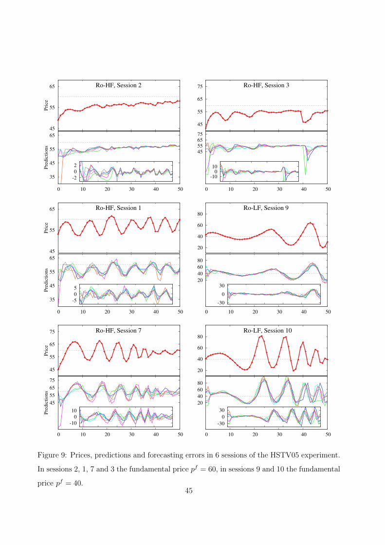
35
45
55
65
0 10 20 30 40 50
Pre
dic
tions
45
55
65
Pri
ce
Ro-HF, Session 2
-2
0
2
45
55
65
75
0 10 20 30 40 50
45
55
65
75 Ro-HF, Session 3
-10 0
10
35
45
55
65
0 10 20 30 40 50
Pre
dic
tions
45
55
65
Pri
ce
Ro-HF, Session 1
-5
0
5
20
40
60
80
0 10 20 30 40 50
20
40
60
80
Ro-LF, Session 9
-30
0
30
45
55
65
75
0 10 20 30 40 50
Pre
dic
tions
45
55
65
75
Pri
ce
Ro-HF, Session 7
-10
0
10
20
40
60
80
0 10 20 30 40 50
20
40
60
80
Ro-LF, Session 10
-30
0
30
Figure 9: Prices, predictions and forecasting errors in 6 sessions of the HSTV05 experiment.
In sessions 2, 1, 7 and 3 the fundamental price pf = 60, in sessions 9 and 10 the fundamental
price pf = 40.45
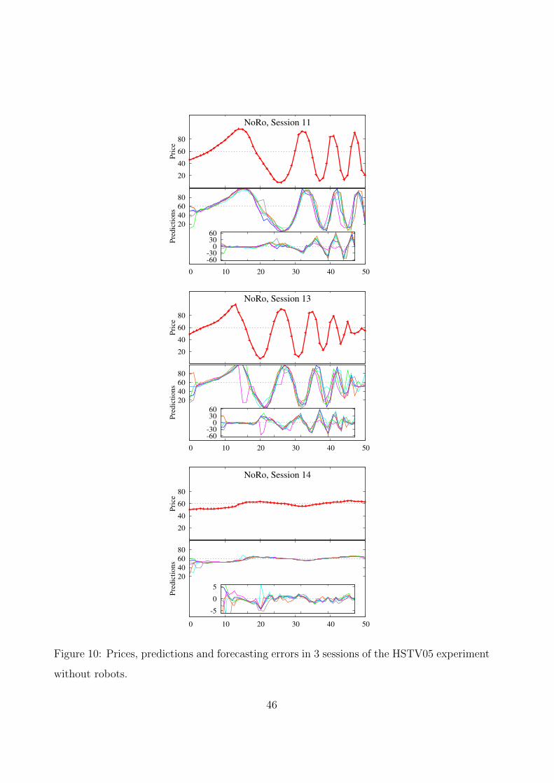
20
40
60
80
0 10 20 30 40 50
Pre
dic
tions
20
40
60
80
Pri
ce
NoRo, Session 11
-60-30
0 30 60
20
40
60
80
0 10 20 30 40 50
Pre
dic
tions
20
40
60
80
Pri
ce
NoRo, Session 13
-60-30
0 30 60
20
40
60
80
0 10 20 30 40 50
Pre
dic
tions
20
40
60
80
Pri
ce
NoRo, Session 14
-5
0
5
Figure 10: Prices, predictions and forecasting errors in 3 sessions of the HSTV05 experiment
without robots.
46
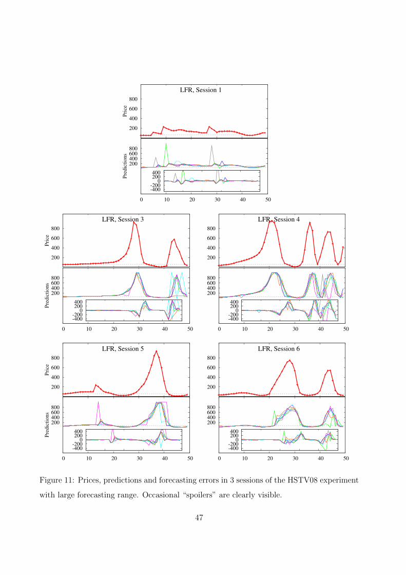
200 400 600 800
0 10 20 30 40 50
Pre
dic
tions
200
400
600
800
Pri
ce
LFR, Session 1
-400-200
0 200 400
200 400 600 800
0 10 20 30 40 50
Pre
dic
tions
200
400
600
800
Pri
ce
LFR, Session 3
-400-200
0 200 400
200 400 600 800
0 10 20 30 40 50
200
400
600
800
LFR, Session 4
-400-200
0 200 400
200 400 600 800
0 10 20 30 40 50
Pre
dic
tions
200
400
600
800
Pri
ce
LFR, Session 5
-400-200
0 200 400
200 400 600 800
0 10 20 30 40 50
200
400
600
800
LFR, Session 6
-400-200
0 200 400
Figure 11: Prices, predictions and forecasting errors in 3 sessions of the HSTV08 experiment
with large forecasting range. Occasional “spoilers” are clearly visible.
47

B Homogeneous Expectations Model
The model with homogeneous expectations is given bypet+1 = f(pt−1, pt−2, p
et ) ,
nt = 1− exp(− 1
200
∣∣pt−1 − pf∣∣) ,
pt =1
1 + r
((1− nt)pet+1 + nt p
f + y + εt).
(14)
for the experiments with robots. The first equation describes forecasting behavior with a simple
first order heuristic f as in (5), which can be either adaptive expectations (in which case f does
not depend on pt−2) or trend following expectations (in which case f does not depend on pet ).
Two other equations give the evolution of the share of “robot” traders and prices, identical to the
equations used in the experiment, cf. (3) and (4). When the robots are not present, the second
equation should be omitted and Eq. (1) should be used in place of the third.
We present below an analysis of the so-called deterministic skeleton model, setting term εt in
(14) to zero. Stochastic simulations with the same realizations of the shocks, εt, as in the experiment
are given in Fig. 4 of the main text, in order to illustrate how the noise affects price fluctuations.
In terms of deviations from the fundamental price the model can be rewritten as
pt − pf =1
1 + r
((1− nt)pet+1 + nt p
f − pf)
=1− nt1 + r
(pet+1 − pf
), (15)
Adaptive Expectations. Under adaptive expectations f is given by (6). The following result
describes the behavior of system (14) in this case.
Proposition 1. Consider the deterministic skeleton of (14) with the adaptive prediction rule (6).
This system has a unique steady-state with price equal to fundamental price, i.e., p∗ = pf . The
steady-state is globally stable for 0 < w ≤ 1, with a real eigenvalue λ, 0 < λ < 1, so that the
convergence is monotonic.
Proof. From the general relation (15) it follows that
pet+1 − pf = w (pt−1 − pf ) + (1− w) (pet − pf ) = (pet − pf )(w
1− nt−1
1 + r+ 1− w
).
The expression in the last parenthesis is a convex combination of 1 and (1−nt−1)/(1 + r) < 1. For
positive weight w such combination is always less than 1. Therefore, the dynamical system defines
48

a contraction of expectations, which then must globally converge to pf . The price realization in
this point is uniquely defined from (6) as p∗ = pf . Finally, the evolution of robot traders implies
that n∗ = 0 in this fixed-point.
Extrapolative Expectations. Consider now the dynamics of the homogeneous expectations
model with a rule given by
pet+1 = α+ β1 pt−1 + β2 pt−2 . (16)
This extrapolative rule incorporates both the trend following and the anchor and adjustment heuris-
tic as special cases. Indeed, setting α = 0, β1 = 1 + γ and β2 = −γ, the trend-following heuristics
(7) is obtained, while α = pf/2, β1 = 1.5 and β2 = −1 correspond to the anchoring and adjustment
heuristic (8).
The rules for which the forecasts are not consistent with realizations will be disregarded by
the participants, sooner or later. Therefore, we confine our attention to the rules satisfying the
following simple steady-state consistency requirement:
Definition B.1. The extrapolative rule (16) is called consistent in the steady-state p∗, if it predicts
p∗ in this steady-state.
In other words, consistent rules give unbiased predictions at the steady-state. Obviously, the ex-
trapolative rule is consistent in p∗ if and only if α = (1−β1−β2)p∗. Notice that, the trend-following
heuristic (7) is consistent at any steady-state, while the anchoring and adjustment heuristic (8) is
consistent only at the steady state with p∗ = pf .
The following result describes all possible steady-states of the asset-pricing dynamics with
consistent extrapolative heuristic, as well as their local stability.
Proposition 2. Consider the dynamics of the deterministic skeleton of (14) with extrapolative
prediction rule (16).
There exists a unique steady-state in which the rule is consistent. In this steady-state, p∗ = pf
and the fraction of robot traders n∗ = 0. The “fundamental” steady-state is locally stable if the
following three conditions are met
β2 < (1 + r)− β1 , β2 < (1 + r) + β1 , β2 > −(1 + r) . (17)
49

The steady-state generically exhibits a pitch-fork, period-doubling or Neimark-Sacker bifurcation,
if the first, second or third inequality in (17) turns into an equality, respectively. Moreover, the
dynamics is oscillating (i.e., the eigenvalues of the linearized system are complex) when
β21 + 4β2(1 + r) < 0.
Proof. Consider the steady-state (p∗, n∗) with consistent forecasting rule, and notice that (15)
implies that either p∗ = pf or 1 − n∗ = 1 + r. The second case is impossible, so p∗ = pf and,
therefore, n∗ = 0.
Using (15), the dynamics in deviations is given by
pt − pf = exp(− |pt−1 − pf |
/200) ( β1
1 + r(pt−1 − pf ) +
β2
1 + r(pt−2 − pf )
). (18)
The first term in the right hand-side is never greater than 1. Thus, dynamics of (18) is a superpo-
sition of contraction with linear process of second order
(1 + r)xt = β1 xt−1 + β2 xt−2 (19)
with xt = pt − pf . If the latter dynamics is locally stable, the steady-state pf of original dynamics
(18) will be also locally stable. Furthermore, since the exponential term in (18) is equal to 1 in
the steady-state, the linear parts of the dynamics of the last two processes are the same. Thus,
processes (18) and (19) lose stability simultaneously and through the same bifurcation type.
The Jacobian matrix of (19) in the steady-state is given by
J =
∥∥∥∥∥∥∥β1
1+rβ2
1+r
1 0
∥∥∥∥∥∥∥ .The standard conditions for the stability can be expressed through the trace Tr(J) and the deter-
minant Det(J) of this matrix, and are given by
Tr(J) < Det(J) + 1 , Tr(J) > −1−Det(J) , Det(J) < 1 . (20)
Furthermore, the dynamics is oscillatory if Tr(J)2−4 Det(J) = 0. The substitution of the values of
trace and determinant gives inequalities (17) and condition β21 +4β2(1+rf ) < 0 for the oscillations.
The bifurcation types can be determined from (20), since when one of these inequalities turns
to equality, the unit circle is crossed by a corresponding eigenvalue of the system. the second
50
inequality is violated when an eigenvalue becomes equal to −1, which implies the period-doubling
bifurcation. The violation of the last inequality in (20) implies that two complex eigenvalues cross
the unit circle. This happens under the Neimark-Sacker bifurcation. Finally, consider the first
inequality, which is violated when one eigenvalue becomes equal to 1. It turns out that at this
occasion two new steady-states are emerging, which implies that the system exhibits pitchfork
bifurcation. Indeed, any steady-state (p∗, n∗) should satisfy to
(1 + r)p∗ = (1− n∗)((1− β1 − β2)pf + (β1 + β2)p∗
)+ n∗pf + y
m
(1 + r)p∗ = pf + (β1 + β2)(p∗ − pf )(1− n∗) + y
m
(1 + r)(p∗ − pf ) = (β1 + β2)(p∗ − pf )(1− n∗)
Thus, in any non-fundamental steady-state, the fractions of robots n∗ = 1− (1+r)/(β1 +β2). Only
if this fraction belongs to the interval (0, 1) two other steady-states exist with
p∗± = pf ± 200 log(1− n∗) .
(The prediction rule is, of course, inconsistent in both steady-states.) When the first inequality
in (20) is satisfied, these two steady-state do not exist, but they appear at the moment when the
inequality changes it sign.
In general, the dynamical system (14) with homogeneous extrapolative expectations (16) may
have multiple steady-states. Proposition 2 asserts, however, that the extrapolative rule is consistent
only in the fundamental steady state pf . The stability conditions (17) are illustrated in Fig. 12 in
the parameter space (β1, β2). The dark regions contain all rules for which the extrapolative heuristic
(16) generates stable dynamics. For the pairs lying below the parabolic curve, the dynamics are
oscillating. A loss of (local) stability occurs when the pair (β1, β2) leaves the stability area and
crosses the boundary formed by the triangle. The dynamics immediately after the bifurcation
are determined by the type of bifurcation through which stability is lost. For instance, after the
pitchfork bifurcation the price diverges from its fundamental level and converges to one of two new
stable steady-states. The Neimark-Sacker bifurcation implies existence of (quasi-)periodic price
fluctuations right after the bifurcation.
51
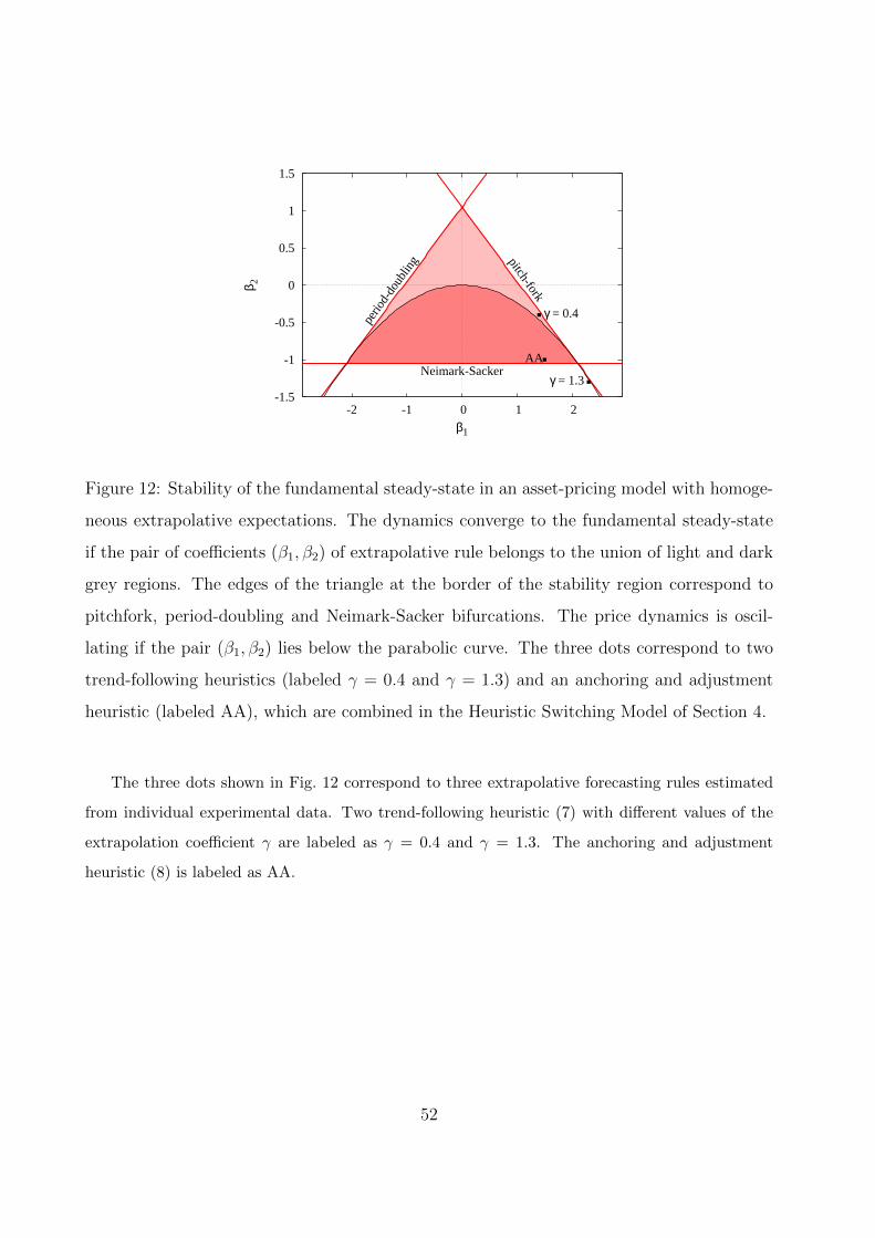
-1.5
-1
-0.5
0
0.5
1
1.5
-2 -1 0 1 2
β 2
β1
Neimark-Sackerpitch-fork
perio
d-do
ublin
g
γ = 0.4
γ = 1.3
AA
Figure 12: Stability of the fundamental steady-state in an asset-pricing model with homoge-
neous extrapolative expectations. The dynamics converge to the fundamental steady-state
if the pair of coefficients (β1, β2) of extrapolative rule belongs to the union of light and dark
grey regions. The edges of the triangle at the border of the stability region correspond to
pitchfork, period-doubling and Neimark-Sacker bifurcations. The price dynamics is oscil-
lating if the pair (β1, β2) lies below the parabolic curve. The three dots correspond to two
trend-following heuristics (labeled γ = 0.4 and γ = 1.3) and an anchoring and adjustment
heuristic (labeled AA), which are combined in the Heuristic Switching Model of Section 4.
The three dots shown in Fig. 12 correspond to three extrapolative forecasting rules estimated
from individual experimental data. Two trend-following heuristic (7) with different values of the
extrapolation coefficient γ are labeled as γ = 0.4 and γ = 1.3. The anchoring and adjustment
heuristic (8) is labeled as AA.
52

C Heterogeneity in HSTV05 Experiment
HSTV05 estimated individual forecasting rules and found that many of them can be described by
the extrapolative first order heuristics
pet+1 = α+ β1 pt−1 + β2 pt−2 .
Fig. 13 illustrates an extent of heterogeneity found in the HSTV05 experiment. For six different
sessions of the Ro-HF treatment we show all individuals whose behavior was found to be consistent
with the extrapolative heuristic.15 The dots represent the coefficients of the estimated heuristics,
with coefficient β1 shown on the horizontal axis and coefficient β2 on the vertical axis. Different
regions of the space correspond to different qualitative dynamics of the model with corresponding
homogeneous expectation rule as derived in Appendix B. The dynamics converge to the funda-
mental steady-state if the pair of coefficients (β1, β2) belongs to the union of light and dark grey
regions and diverge otherwise. The price dynamics is oscillating if the pair (β1, β2) lies below the
parabolic curve.
While the dispersion of individual forecasting rules is clear, the figure suggests some regulari-
ties. In the converging sessions 2 and 5, the majority of rules belongs to the region of monotonic
convergence. In contrast, in the oscillating sessions almost all individual rules lie in the oscillatory
region (i.e., the linear forecasting rule has complex eigenvalues). Furthermore, in sessions 1 and 6
with constant price oscillations at least two individual rules in every group are very close to the
stability border of the Neimark-Sacker bifurcation (i.e., are close to complex unit roots), while in
groups 4 and 7 with dampened oscillations both stable and unstable rules were present.
15In every group there were rules which cannot be represented by the extrapolative prediction, e.g., an
adaptive heuristic or linear rules with three lags.
53

-1.5
-1
-0.5
0
0.5
1
1.5
-2 -1 0 1 2
β2
Stability region and Ro-HF, session 5
-1.5
-1
-0.5
0
0.5
1
1.5
-2 -1 0 1 2
Stability region and Ro-HF, session 2
-1.5
-1
-0.5
0
0.5
1
1.5
-2 -1 0 1 2
β2
Stability region and Ro-HF, session 6
-1.5
-1
-0.5
0
0.5
1
1.5
-2 -1 0 1 2
Stability region and Ro-HF, session 1
-1.5
-1
-0.5
0
0.5
1
1.5
-2 -1 0 1 2
β2
β1
Stability region and Ro-HF, session 4
-1.5
-1
-0.5
0
0.5
1
1.5
-2 -1 0 1 2
β1
Stability region and Ro-HF, session 7
Figure 13: Stability of homogeneous expectations model with extrapolative rules estimated
in the experiment.
54
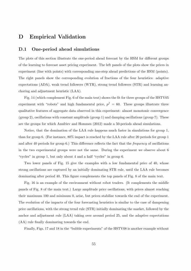
D Empirical Validation
D.1 One-period ahead simulations
The plots of this section illustrate the one-period ahead forecast by the HSM for different groups
of the learning to forecast asset pricing experiment. The left panels of the plots show the prices in
experiment (line with points) with corresponding one-step ahead predictions of the HSM (points).
The right panels show the corresponding evolution of fractions of the four heuristics: adaptive
expectations (ADA), weak trend followers (WTR), strong trend followers (STR) and learning an-
choring and adjustment heuristic (LAA).
Fig. 14 (which complement Fig. 6 of the main text) shows the fit for three groups of the HSTV05
experiment with “robots” and high fundamental price, pf = 60. These groups illustrate three
qualitative features of aggregate data observed in this experiment: almost monotonic convergence
(group 2), oscillations with constant amplitude (group 1) and damping oscillations (group 7). These
are the groups for which Anufriev and Hommes (2012) made a 50-periods ahead simulations.
Notice, that the domination of the LAA rule happens much faster in simulations for group 1,
than for group 6. (For instance, 80% impact is reached by the LAA rule after 20 periods for group 1
and after 40 periods for group 6.) This difference reflects the fact that the frequency of oscillations
in the two experimental groups were not the same. During the experiment we observe about 6
“cycles” in group 1, but only about 4 and a half “cycles” in group 6.
Two lower panels of Fig. 15 give the examples with a low fundamental price of 40, whose
strong oscillations are captured by an initially dominating STR rule, until the LAA rule becomes
dominating after period 40. This figure complements the top panels of Fig. 8 of the main text.
Fig. 16 is an example of the environment without robot traders. (It complements the middle
panels of Fig. 8 of the main text.) Large amplitude price oscillations, with prices almost reaching
their maximum 100 and minimum 0, arise, but prices stabilize towards the end of the experiment.
The evolution of the impacts of the four forecasting heuristics is similar to the case of dampening
price oscillations, with the strong trend rule (STR) initially dominating the market, followed by the
anchor and adjustment rule (LAA) taking over around period 25, and the adaptive expectations
(AA) rule finally dominating towards the end.
Finally, Figs. 17 and 18 in the “bubble experiments” of the HSTV08 is another example without
55
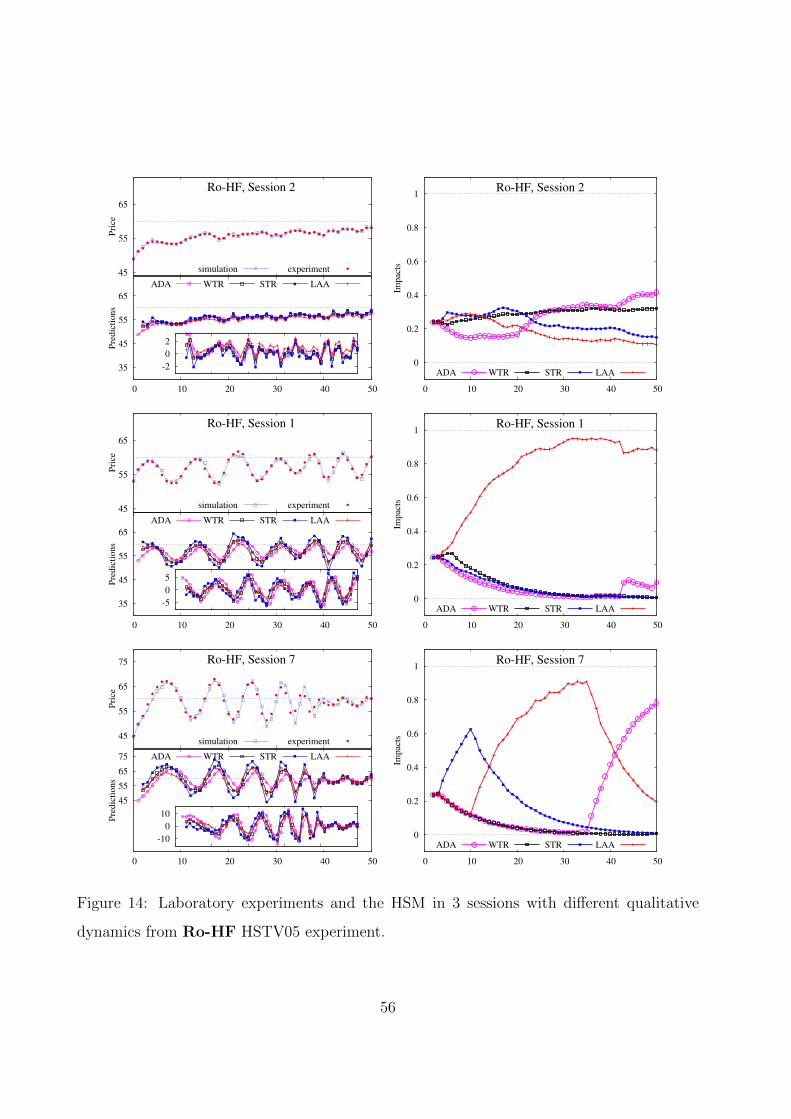
35
45
55
65
0 10 20 30 40 50
Pre
dic
tions
ADA WTR STR LAA
45
55
65
Pri
ce
Ro-HF, Session 2
simulation experiment
-2
0
2
0
0.2
0.4
0.6
0.8
1
0 10 20 30 40 50Im
pac
ts
Ro-HF, Session 2
ADA WTR STR LAA
35
45
55
65
0 10 20 30 40 50
Pre
dic
tions
ADA WTR STR LAA
45
55
65
Pri
ce
Ro-HF, Session 1
simulation experiment
-5
0
5
0
0.2
0.4
0.6
0.8
1
0 10 20 30 40 50
Impac
ts
Ro-HF, Session 1
ADA WTR STR LAA
45
55
65
75
0 10 20 30 40 50
Pre
dic
tions
ADA WTR STR LAA
45
55
65
75
Pri
ce
Ro-HF, Session 7
simulation experiment
-10
0
10
0
0.2
0.4
0.6
0.8
1
0 10 20 30 40 50
Impac
ts
Ro-HF, Session 7
ADA WTR STR LAA
Figure 14: Laboratory experiments and the HSM in 3 sessions with different qualitative
dynamics from Ro-HF HSTV05 experiment.
56
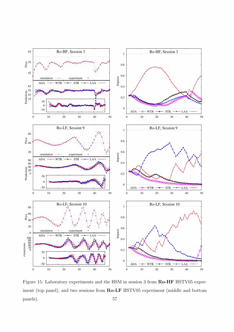
35
45
55
65
0 10 20 30 40 50
Pre
dic
tions
ADA WTR STR LAA
45
55
65
Pri
ce
Ro-HF, Session 3
simulation experiment
-10
0
10
0
0.2
0.4
0.6
0.8
1
0 10 20 30 40 50Im
pac
ts
Ro-HF, Session 3
ADA WTR STR LAA
0 20 40 60 80
0 10 20 30 40 50
Pre
dic
tions
ADA WTR STR LAA
20
40
60
Pri
ce
Ro-LF, Session 9
simulation experiment
-30
0
30
0
0.2
0.4
0.6
0.8
1
0 10 20 30 40 50
Impac
ts
Ro-LF, Session 9
ADA WTR STR LAA
0 20 40 60 80
100
0 10 20 30 40 50
Pre
dic
tions
ADA WTR STR LAA 0
20
40
60
80
Pri
ce
Ro-LF, Session 10
simulation experiment
-50
0
50
0
0.2
0.4
0.6
0.8
1
0 10 20 30 40 50
Impac
ts
Ro-LF, Session 10
ADA WTR STR LAA
Figure 15: Laboratory experiments and the HSM in session 3 from Ro-HF HSTV05 exper-
iment (top panel), and two sessions from Ro-LF HSTV05 experiment (middle and bottom
panels). 57
20 40 60 80
0 10 20 30 40 50
Pre
dic
tions
ADA WTR STR LAA
20
40
60
80
Pri
ce
NoRo, Session 11
simulation experiment
-50
0
50
0
0.2
0.4
0.6
0.8
1
0 10 20 30 40 50Im
pac
ts
NoRo, Session 11
ADA WTR STR LAA
20 40 60 80
0 10 20 30 40 50
Pre
dic
tions
ADA WTR STR LAA
20
40
60
80
Pri
ce
NoRo, Session 13
simulation experiment
-50
0
50
0
0.2
0.4
0.6
0.8
1
0 10 20 30 40 50
Impac
ts
NoRo, Session 13
ADA WTR STR LAA
35
45
55
65
0 10 20 30 40 50
Pre
dic
tions
ADA WTR STR LAA
45
55
65
Pri
ce
NoRo, Session 14
simulation experiment
-4
0
4
0
0.2
0.4
0.6
0.8
1
0 10 20 30 40 50
Impac
ts
NoRo, Session 14
ADA WTR STR LAA
Figure 16: Laboratory experiments and the HSM in three sessions from NoRo HSTV05
experiment.
58

robot traders, this time with a much larger upper-bound of 1000 (instead of 100). (See also the
bottom panel of Fig. 8 of the main text.) The asset price oscillates with very large amplitude, with
a long lasting rend of 25 periods with prices rising close to their maximum 1000, after which a crash
follows to values close to their minimum 0, and the market starts oscillating. The evolution of the
impacts of the four forecasting heuristics is similar as before, with the STR rule taking the lead,
increasing its share to more than 80% after 25 periods, then slowly declining and finally dominated
by the LAA rule with more than 60% of the share after 50 periods.
We summarize the corresponding evolution of heuristics’ impacts in Table 5.
59
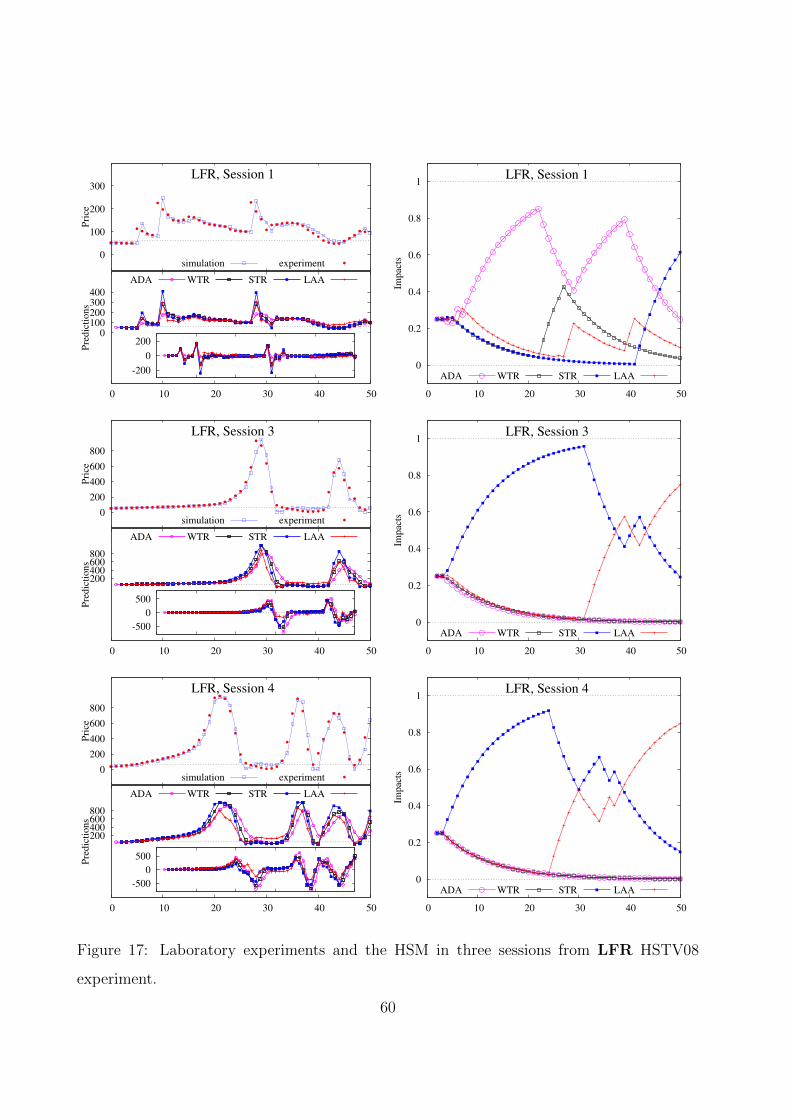
0 100 200 300 400
0 10 20 30 40 50
Pre
dic
tions
ADA WTR STR LAA
0
100
200
300
Pri
ce
LFR, Session 1
simulation experiment
-200
0
200
0
0.2
0.4
0.6
0.8
1
0 10 20 30 40 50Im
pac
ts
LFR, Session 1
ADA WTR STR LAA
200 400 600 800
0 10 20 30 40 50
Pre
dic
tions
ADA WTR STR LAA
0
200
400
600
800
Pri
ce
LFR, Session 3
simulation experiment
-500
0
500
0
0.2
0.4
0.6
0.8
1
0 10 20 30 40 50
Impac
ts
LFR, Session 3
ADA WTR STR LAA
200 400 600 800
0 10 20 30 40 50
Pre
dic
tions
ADA WTR STR LAA
0
200
400
600
800
Pri
ce
LFR, Session 4
simulation experiment
-500
0
500
0
0.2
0.4
0.6
0.8
1
0 10 20 30 40 50
Impac
ts
LFR, Session 4
ADA WTR STR LAA
Figure 17: Laboratory experiments and the HSM in three sessions from LFR HSTV08
experiment.
60
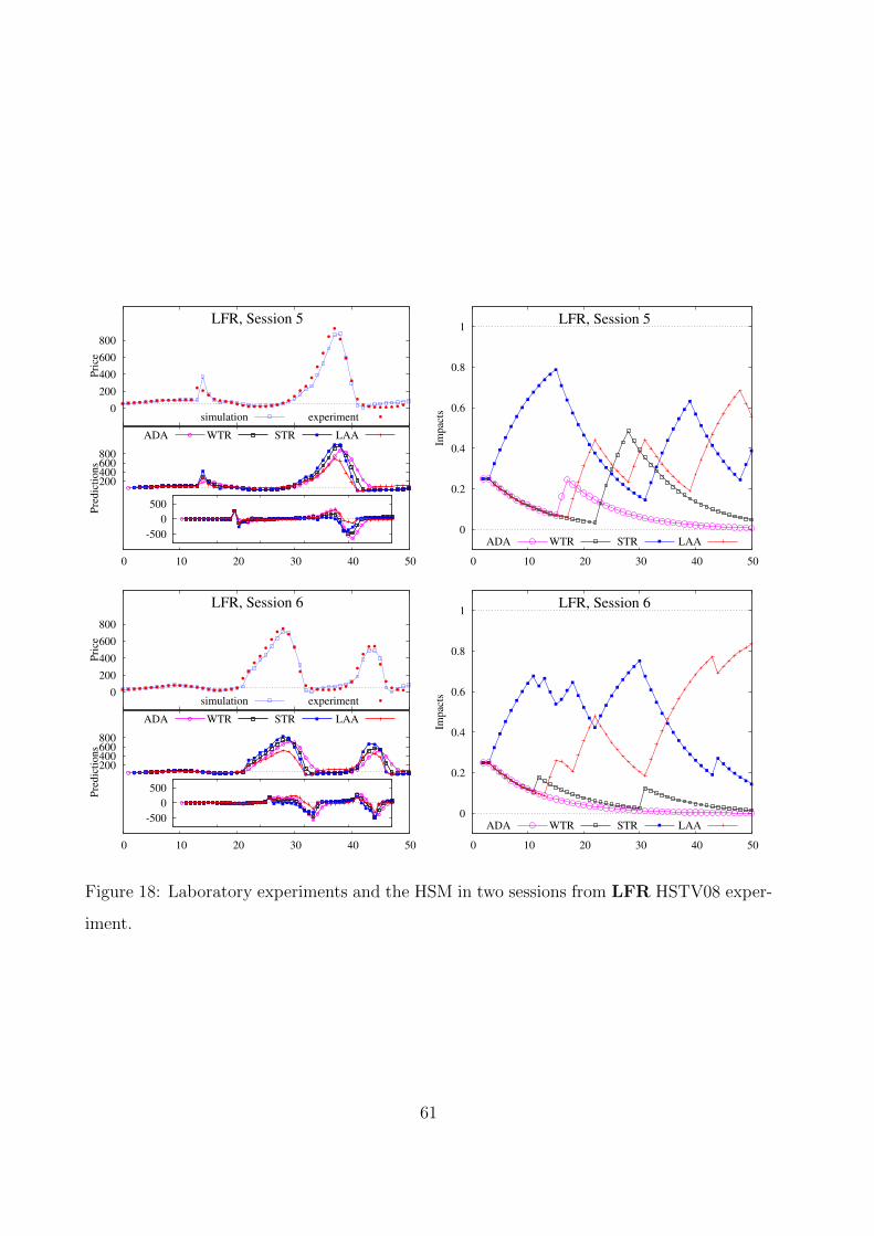
200 400 600 800
0 10 20 30 40 50
Pre
dic
tions
ADA WTR STR LAA
0
200
400
600
800
Pri
ce
LFR, Session 5
simulation experiment
-500
0
500
0
0.2
0.4
0.6
0.8
1
0 10 20 30 40 50
Impac
ts
LFR, Session 5
ADA WTR STR LAA
200 400 600 800
0 10 20 30 40 50
Pre
dic
tions
ADA WTR STR LAA
0
200
400
600
800
Pri
ce
LFR, Session 6
simulation experiment
-500
0
500
0
0.2
0.4
0.6
0.8
1
0 10 20 30 40 50
Impac
ts
LFR, Session 6
ADA WTR STR LAA
Figure 18: Laboratory experiments and the HSM in two sessions from LFR HSTV08 exper-
iment.
61

Table 5: Heuristic Switching Model in the Learning to Forecast Experiments.
type paper evolution of heuristics’ fractions figure
Ro-HF HSTV05,
sess. 5, 2
All heuristics have similar impacts leading to the monotone
convergence of price
6 (top); 14
(App. D)
HSTV05,
sess. 6, 1
WTR, STR and LAA trigger weak initial trend with LAA taking
over and leading to permanent oscillations
6 (middle); 14
(App. D)
HSTV05,
sess. 4, 7
STR dominates in the beginning leading to the strong trend. When
bubble bursts LAA takes over, but towards the end of the
experiment ADA performs even better explaining convergence
6 (bottom); 14
(App. D)
HSTV05,
sess. 3
WTR and STR overestimate strong initial trend, so that LAA takes
over. When oscillations die out, the WTR takes over but sudden
’spoiler’ (caused, presumably, by typing error) brings LAA back to
dominate
7
Ro-LF HSTV05,
sess. 8
Initially WTR and LAA perform better leading to weak oscillations
but the STR takes over and faster oscillations occur. Towards the
end LAA again takes a momentum
8 (top)
HSTV05,
sess. 9, 10
Initially STR and LAA perform better leading to strongly oscillating
dynamics. At the end LAA takes over
15 (App. D)
NoRo HSTV05,
sess. 12
STR takes over but when the upper prediction is reached the bubble
bursts and LAA rule increases its weight and takes over
8 (middle)
HSTV05,
sess. 11,
13, 14
Initially ADA and WTR performs better preventing a big bubble to
occur. No heuristic takes more than 50%
16 (App. D)
LFR HSTV08,
sess. 2
ADA dominates over all simulations. Occasional spoilers trigger
WTR and STR rules, but only to the end STR takes over
8 (bottom)
HSTV08,
sess. 1
STR takes over from the beginning and bubble grows and explodes.
Fast crash and new bubbles favor flexible LAA rule which takes over
to the end of the experiment: the second bubble is formed and burst
much faster
17 (App. D)
HSTV08,
sess. 3-6
STR takes over but bubble stops. LAA rules start to increase its
weight and prevents the highest possible bubble
18 (App. D)
62

D.2 Forecasting performance
The tables of this section supplement the results of Sections 5.2 and 5.3. We investigate the
forecasting performance of the HSM with benchmark learning parameters β = 0.4, η = 0.7 and
δ = 0.9, and compare it with the performance of other models.
Table 6 (which complements Table 2 of the main text) shows the mean squared prediction errors
of the one-step ahead forecast for different homogeneous and heterogeneous expectation models.
The best model has smallest MSE. The best among four homogeneous model corresponding to four
different heuristics is shown in bold. Also in bold we show the MSE for the HSM with benchmark
parameters. The best among all the model is shown in italic, and it is often the HSM where learning
parameters are chosen to minimize the MSE.
Tables 7 and 8 complement Table 3 of the main text. They show the out-of-sample forecasting
errors from 1- to 7-periods ahead of three different model: the HSM optimizied in-sample, the HSM
with the benchmark parameters and the AR(2) model optimized in-sample.
Finally, Table 9 (which complements Table 4 of the main text) shows the 1- and 2-periods
ahead forecasting errors averaged over moving window for the same three models. The smallest
forecasting errors within the same class are shown in italic.
63
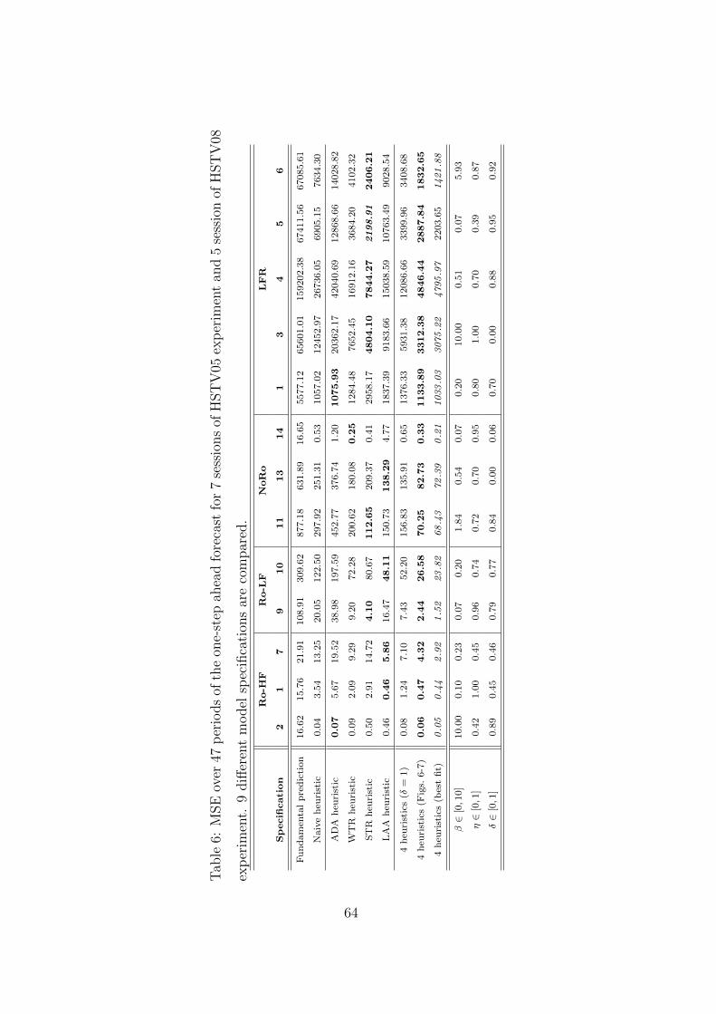
Tab
le6:
MSE
over
47p
erio
ds
ofth
eon
e-st
epah
ead
fore
cast
for
7se
ssio
ns
ofH
ST
V05
exp
erim
ent
and
5se
ssio
nof
HST
V08
exp
erim
ent.
9diff
eren
tm
odel
spec
ifica
tion
sar
eco
mpar
ed.
Ro-H
FR
o-L
FN
oR
oL
FR
Sp
ecifi
cati
on
21
79
10
11
13
14
13
45
6
Fu
nd
am
enta
lp
red
icti
on
16.6
215.7
621.9
1108.9
1309.6
2877.1
8631.8
916.6
55577.1
265601.0
1159202.3
867411.5
667085.6
1
Naiv
eh
euri
stic
0.0
43.5
413.2
520.0
5122.5
0297.9
2251.3
10.5
31057.0
212452.9
726736.0
56905.1
57634.3
0
AD
Ah
euri
stic
0.0
75.6
719.5
238.9
8197.5
9452.7
7376.7
41.2
01075.9
320362.1
742040.6
912868.6
614028.8
2
WT
Rh
euri
stic
0.0
92.0
99.2
99.2
072.2
8200.6
2180.0
80.2
51284.4
87652.4
516912.1
63684.2
04102.3
2
ST
Rh
euri
stic
0.5
02.9
114.7
24.1
080.6
7112.6
5209.3
70.4
12958.1
74804.1
07844.2
72198.91
2406.2
1
LA
Ah
euri
stic
0.4
60.4
65.8
616.4
748.1
1150.7
3138.2
94.7
71837.3
99183.6
615038.5
910763.4
99028.5
4
4h
euri
stic
s(δ
=1)
0.0
81.2
47.1
07.4
352.2
0156.8
3135.9
10.6
51376.3
35931.3
812086.6
63399.9
63408.6
8
4h
euri
stic
s(F
igs.
6-7
)0.0
60.4
74.3
22.4
426.5
870.2
582.7
30.3
31133.8
93312.3
84846.4
42887.8
41832.6
5
4h
euri
stic
s(b
est
fit)
0.05
0.44
2.92
1.52
23.82
68.43
72.39
0.21
1033.03
3075.22
4795.97
2203.6
51421.88
β∈
[0,1
0]
10.0
00.1
00.2
30.0
70.2
01.8
40.5
40.0
70.2
010.0
00.5
10.0
75.9
3
η∈
[0,1
]0.4
21.0
00.4
50.9
60.7
40.7
20.7
00.9
50.8
01.0
00.7
00.3
90.8
7
δ∈
[0,1
]0.8
90.4
50.4
60.7
90.7
70.8
40.0
00.0
60.7
00.0
00.8
80.9
50.9
2
64
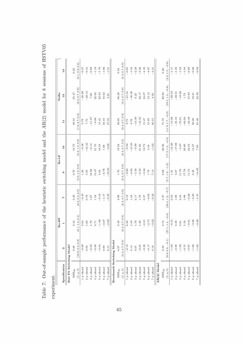
Tab
le7:
Out-
of-s
ample
per
form
ance
ofth
eheu
rist
icsw
itch
ing
model
and
the
AR
(2)
model
for
8se
ssio
ns
ofH
ST
V05
exp
erim
ent.
Ro-H
FR
o-L
FN
oR
o
Sp
ecifi
catio
n2
17
910
11
13
14
Best
Fit
Sw
itchin
gM
odel
MSE40
0.06
0.44
3.30
0.70
16.73
49.31
65.47
0.22
(β,η,δ)
(10.0,0.4,0.9)
(0.1,1.0,0.4)
(0.2,0.4,0.5)
(3.0,1.0,0.9)
(0.2,1.0,0.8)
(1.6,0.7,0.9)
(6.3,0.7,0.9)
(0.1,0.9,0.0)
1p
ahead
−0.08
0.64
−0.45
1.26
−9.38
0.79
−20.48
−0.47
2p
ahead
0.03
1.66
0.78
5.05
−12.43
7.75
−29.13
−0.41
3p
ahead
−0.02
1.79
1.87
10.26
−0.14
−11.67
7.06
−0.69
4p
ahead
−0.06
0.71
1.54
14.47
21.70
−9.06
22.02
−1.18
5p
ahead
−0.04
−1.96
−0.16
5.63
18.55
15.45
22.93
−1.78
6p
ahead
0.09
−3.67
−1.17
−6.78
1.89
50.10
10.62
−1.86
7p
ahead
0.15
−2.80
−0.25
−18.85
−2.68
37.33
2.91
−1.51
Benchm
ark
Sw
itchin
gM
odel
MSE40
0.07
0.49
4.96
1.76
19.34
49.95
66.28
0.34
(β,η,δ)
(0.4,0.7,0.9)
(0.4,0.7,0.9)
(0.4,0.7,0.9)
(0.4,0.7,0.9)
(0.4,0.7,0.9)
(0.4,0.7,0.9)
(0.4,0.7,0.9)
(0.4,0.7,0.9)
1p
ahead
−0.15
0.40
0.12
−2.60
−9.94
0.75
−21.31
−0.81
2p
ahead
0.14
1.33
1.24
−4.92
−13.50
6.78
−30.36
−1.33
3p
ahead
0.07
1.78
2.17
−5.30
−0.99
−13.39
6.23
−2.28
4p
ahead
−0.01
1.29
1.79
−2.50
21.85
−10.55
22.17
−3.36
5p
ahead
−0.28
−0.91
0.37
−2.84
19.73
15.47
24.07
−4.35
6p
ahead
−0.17
−2.75
−0.65
1.79
3.44
51.93
12.12
−4.67
7p
ahead
0.18
−2.62
−0.20
7.14
−1.62
40.15
4.03
−4.41
AR
(2)
Model
MSE44
0.23
0.74
5.37
0.68
26.06
71.70
88.69
0.48
(β,η,δ)
(8.9,0.9,−0.1)
(27.1,1.4,−0.9)
(29.4,1.2,−0.7)
(5.7,1.9,−1.0)
(17.3,1.5,−0.9)
(11.9,1.7,−0.9)
(19.1,1.5,−0.8)
(2.2,1.5,−0.6)
1p
ahead
−1.02
−0.31
0.33
1.21
−12.26
−14.28
−29.54
−1.11
2p
ahead
−0.89
0.39
1.98
5.67
−17.88
−35.16
−49.51
−1.25
3p
ahead
−1.09
0.81
2.43
11.70
−5.87
−79.01
−18.28
−1.52
4p
ahead
−0.51
1.18
1.98
17.78
20.80
−84.64
1.72
−1.04
5p
ahead
−0.87
−0.81
−0.28
11.73
24.53
−42.49
15.83
−0.86
6p
ahead
−1.66
−3.66
−2.20
0.46
12.27
30.28
18.81
−0.96
7p
ahead
−1.62
−4.28
−1.31
−14.65
7.85
61.46
22.39
−0.58
65

Tab
le8:
Out-
of-s
ample
per
form
ance
ofth
eheu
rist
icsw
itch
ing
model
and
the
AR
(2)
model
for
5se
ssio
ns
ofH
ST
V08
exp
erim
ent.
LF
R
Sp
ecifi
catio
n1
34
56
Best
Fit
Sw
itchin
gM
odel
MSE40
1257.89
2680.41
4680.75
1829.27
1123.66
(β,η,δ)
(0.1,0.7,0.8)
(10.0,1.0,0.0)
(0.5,0.7,0.9)
(0.0,0.0,0.7)
(9.5,0.9,0.9)
1p
ahead
5.01
−1.07
−65.58
35.40
23.04
2p
ahead
3.57
−10.22
−60.92
98.61
192.53
3p
ahead
1.30
−192.17
−5.62
174.59
269.56
4p
ahead
−3.71
−176.31
−52.46
232.32
151.23
5p
ahead
−14.09
−61.11
−97.41
246.92
−23.35
6p
ahead
−5.19
48.49
−249.95
214.37
−21.07
Benchm
ark
Sw
itchin
gM
odel
MSE40
1295.50
2725.92
4708.56
3031.62
1667.05
(β,η,δ)
(0.4,0.7,0.9)
(0.4,0.7,0.9)
(0.4,0.7,0.9)
(0.4,0.7,0.9)
(0.4,0.7,0.9)
1p
ahead
5.79
110.39
−54.46
33.66
−53.46
2p
ahead
3.62
271.03
−35.51
97.62
−14.42
3p
ahead
−0.48
199.30
24.19
177.89
−40.86
4p
ahead
−7.96
37.63
−51.93
244.78
−47.88
5p
ahead
−20.99
−60.19
−120.49
270.41
−18.70
6p
ahead
−14.60
−34.22
−291.43
240.07
65.18
AR
(2)
Model
MSE44
1000.42
5592.63
9088.40
2392.46
1676.52
(β,η,δ)
(39.4,0.7,−0.0)
(39.0,1.6,−0.8)
(73.3,1.6,−0.8)
(23.8,1.7,−0.8)
(23.0,1.8,−0.9)
1p
ahead
23.47
81.06
4.21
13.29
38.29
2p
ahead
29.85
249.65
148.35
38.88
245.99
3p
ahead
29.60
266.43
354.32
76.27
403.34
4p
ahead
23.57
264.61
283.81
116.87
404.23
5p
ahead
10.76
218.66
96.59
152.12
331.11
6p
ahead
16.90
102.07
−263.00
174.68
237.97
66
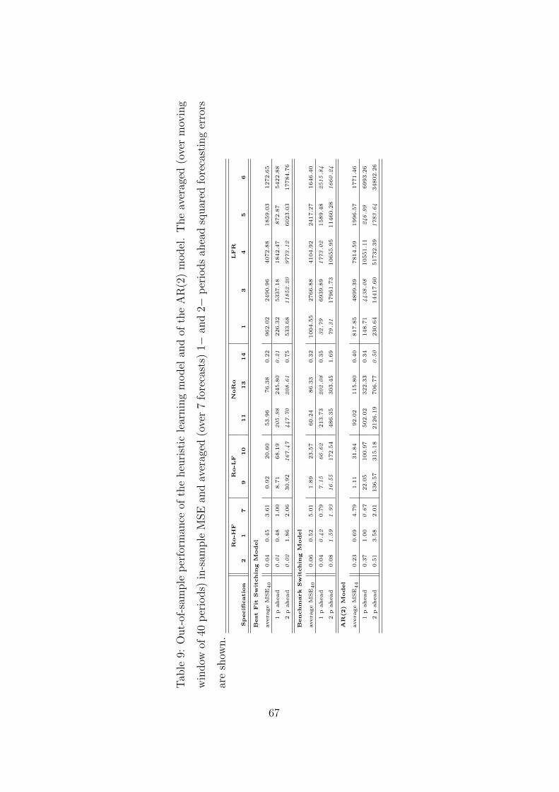
Tab
le9:
Out-
of-s
ample
per
form
ance
ofth
eheu
rist
icle
arnin
gm
odel
and
ofth
eA
R(2
)m
odel
.T
he
aver
aged
(ove
rm
ovin
g
win
dow
of40
per
iods)
in-s
ample
MSE
and
aver
aged
(ove
r7
fore
cast
s)1−
and
2−p
erio
ds
ahea
dsq
uar
edfo
reca
stin
ger
rors
are
show
n.
Ro-H
FR
o-L
FN
oR
oL
FR
Sp
ecifi
catio
n2
17
910
11
13
14
13
45
6
Best
Fit
Sw
itchin
gM
odel
avera
geM
SE40
0.04
0.45
3.61
0.92
20.60
53.96
76.38
0.22
962.02
2490.96
4072.88
1859.03
1272.65
1p
ahead
0.01
0.48
1.00
8.71
68.19
205.98
245.80
0.21
226.32
5337.18
1842.47
872.87
5422.88
2p
ahead
0.02
1.86
2.06
30.92
167.47
447.70
208.61
0.75
533.68
11852.20
9773.12
6023.03
17784.76
Benchm
ark
Sw
itchin
gM
odel
avera
geM
SE40
0.06
0.52
5.01
1.89
23.57
60.24
86.33
0.32
1004.55
2766.88
4104.92
2417.27
1646.40
1p
ahead
0.04
0.42
0.79
7.15
66.62
213.73
202.08
0.35
32.79
6939.89
1773.02
1589.48
2515.84
2p
ahead
0.08
1.59
1.93
16.55
172.54
486.35
303.45
1.69
79.31
17961.73
10655.95
11460.28
1660.24
AR
(2)
Model
avera
geM
SE44
0.23
0.69
4.79
1.11
31.84
92.02
115.80
0.40
817.85
4899.39
7814.59
1996.57
1771.46
1p
ahead
0.37
1.00
0.67
22.05
100.97
502.02
322.33
0.34
148.71
4438.08
10551.11
246.99
6993.26
2p
ahead
0.51
3.58
2.01
136.57
315.18
2126.19
706.77
0.50
230.64
14417.60
51732.39
1783.64
34802.26
67