1

EVOLUTIONARY LEARNING OF FUZZY MODELS

D.T. Pham

Manufacturing Engineering Centre,

Cardiff University

PO Box 688, Newport Road,

CF24 3TE Cardiff, UK

M. Castellani

CENTRIA - Departamento Informática,

Faculdade Ciências e Tecnologia

Universidade Nova Lisboa

Quinta da Torre,

2829-516 Caparica, Portugal

ABSTRACT

This paper presents an evolutionary algorithm for generating knowledge bases for fuzzy

logic systems. The algorithm dynamically adjusts the focus of the genetic search by

dividing the population into three sub-groups, each concerned with a different level of

knowledge base optimisation. The algorithm was tested on the identification of two

highly non-linear simulated plants. Such a task represents a challenging test for any

learning technique and involves two opposite requirements, the exploration of a large

high-dimensional search space and the achievement of the best modelling accuracy. The

algorithm achieved learning results that compared favourably with those for alternative

knowledge base generation methods.

KEYWORDS : evolutionary algorithms, fuzzy logic, systems modelling, function

approximation.

2

NOTATION:

DA-FFNN differential activation function feedforward fuzzy neural network

EA evolutionary algorithm

EP evolutionary programming

EVS evolution strategy

FL fuzzy logic

FFNN feedforward fuzzy neural network

GA genetic algorithm

KB knowledge base

MF membership function

RB rule base

rand random real number

r.m.s. error root mean square error

t time

u(k) Simulated input of the plant at control step k

y(k) Simulated output of the plant at control step k

σ standard deviation

τ time

3

1 INTRODUCTION

The study of biological nervous systems has shown that accurate and robust mappings

can be achieved by learning appropriate sets of condition-response pairs. Fuzzy logic

(FL) [1] extends the framework of classical Aristotle’s logic to achieve complex input-

output relationships via qualitative fuzzy rules. FL systems are usually implemented

through the Mamdani model [2], which is composed of four blocks, namely the fuzzifier,

the rule base (RB), the inference engine and the defuzzifier [3].

The fuzzifier transforms crisp data into fuzzy sets and is the interface between the

quantitative sensory inputs and the qualitative fuzzy mapping. A fuzzy set is defined via a

membership function (MF) that maps crisp values into fuzzy linguistic knowledge. The

core of the fuzzy system comprises the RB and the inference engine. The RB consists of

fuzzy if-then rules which describe qualitative non-linear relationships through

antecedent-consequent pairs. The inference engine processes the rules and produces the

output in the form of a fuzzy set. The defuzzifier converts the linguistic output into a

crisp value. The RB and the MFs constitute the knowledge base (KB) of the system.

FL systems are a natural candidate for identification of complex non-linear mappings.

Unfortunately, the implementation of fuzzy models has so far been hindered by the lack

of an effective learning algorithm.

4

Evolutionary algorithms (EAs) [4] [5] [6] are a class of global search techniques that

provide an ideal framework for the generation of FL systems. As well as allowing the

simultaneous optimisation of both the KB and the MFs of the solution, EAs only need a

small amount of problem domain expertise for implementation. Moreover, they do not

require properties such as the differentiability of the logic operators, unlike other

optimisation algorithms including the popular error back propagation rule [7].

The main difficulty in the evolutionary design of FL systems is due to the complexity of

the learning task, which requires the optimisation of a large number of mutually related

parameters and variables. The encoding of the fuzzy knowledge base (KB) is not

straightforward and is not suited to traditional string-like implementations. Moreover, the

simultaneous learning of the rule base (RB) and the fuzzy membership functions (MFs)

requires the definition of two different but concurrent learning strategies.

For these reasons, the implementation of evolutionary FL systems has so far relied on ad

hoc solutions, often driven by the particular problem domain. Recently, Pham and

Castellani [8] have introduced a new EA for the automatic generation of KBs for FL

systems. The FL system optimisation problem was approached in a generic manner to

facilitate the application of the results to different problems. The algorithm dynamically

optimises the search efforts allocated for the RB and the MFs optimisation by dividing

the solution population into three sub-groups, each concerned with a different level of

knowledge-base optimisation. Moreover, the evolved KB is expressed in a transparent

format that facilitates the understanding of the control policy.

5

This paper presents the application of the proposed EA to the FL modelling of two

simulated highly non-linear dynamic systems. Such a task represents a challenging test

for any learning technique. The problem involves two opposite requirements, the

exploration of a large high-dimensional search space and the achievement of the best

modelling accuracy.

The paper is organised as follows: Section 2 gives a brief introduction to EAs and

presents a review of the relevant literature on the evolutionary KB generation of FL

systems. Section 3 gives an overview of the algorithm used in this work. Section 4

describes the two simulated plants and the EA implementation. Section 5 presents the

experimental modelling results. Section 6 concludes the paper and proposes areas for

further investigation.

2 EVOLUTIONARY ALGORITHMS FOR TRAINING FUZZY SYSTE MS

2.1 Evolutionary Algorithms

The generation and optimisation of a fuzzy model is essentially a search problem, where

the solution space is represented by all the possible structures and parameters defining the

system. EAs are stochastic search algorithms that aim to find an acceptable solution when

time or computational requirements make it impractical to find the best one.

6

EAs are approximately modelled on Darwin’s theory of natural evolution. This stipulates

that a species improves its adaptation to the environment by means of a selection

mechanism that favours the reproduction of those individuals of highest fitness. The

population is made to evolve until a stopping criterion is met. At the end of the process,

the best exemplar is chosen as the solution to the problem.

In EAs, candidate solutions are encoded into variably complex structures called

chromosomes, which are composed of smaller elements called genes. The gene is the

smallest unit of information and, when defined in a quantised space, each of its allowed

values is called an allele. Following biological terminology, the encoded information

representing a solution is called a genotype, as opposed to the decoded individual that is

named phenotype.

The adaptation of an individual to the environment is defined by its ability to perform the

required task. A problem-specific fitness function is used for the quality assessment of a

candidate solution. The population is driven towards the optimal point(s) of the search

space by means of stochastic search operators inspired by the biological mechanisms of

genetic selection, mutation and recombination (crossover)crossover. Problem-specific

operators are often used to speed up the search process.

Historically, EAs originated in the mid-sixties with two parallel directions of work

leading to the fields of Evolution Strategies (EVSs) [9] [10] and Evolutionary

Programming (EP) [11] [12]. However, it was only ten years later that they gained

7

popularity following the creation of Genetic Algorithms (GAs) by Holland [13] [14] [15].

EVSs, EP and GAs represent different metaphors of biological evolution with different

representations of the candidate solutions and different genetic manipulation operators.

In the last decade, research developments in each field and the mutual exchange of ideas

blurred the boundaries between the three main branches of EAs.

EAs can be used equally for optimising the parameters of the fuzzy system, i.e. the shape

and location of the MFs and the fuzzy rule weights, or for the acquisition of the structure

of the system, i.e. the number of input and output MFs and the fuzzy RB, or for the

simultaneous generation of both. The last case is the most interesting because it requires

the least knowledge about the problem domain and it eliminates the possibility of

obtaining sub-optimal solutions related to the initial design assumptions.

2.2 EAs for concurrent membership functions and rule base learning

There are two ways of evolving the KB of fuzzy systems that have originated from earlier

studies in the broader field of Learning Classifier Systems. The Pittsburgh or “Pitt”

approach introduced by the work of Smith [16] at the University of Pittsburgh evolves the

final KB from a population of rule sets. The Michigan approach originated by the work of

Holland and Reitman [17] at Michigan University generates the optimal rule set from a

population of fuzzy rules.

8

The Pitt approach determines a more disruptive search strategy and it seems to be more

useful for off-line environments in which more radical behavioral changes are acceptable.

The use of the Pitt approach in on-line and real-time environments is also problematical

because of the difficulty of replicating the same operating conditions for the entire

population of fuzzy systems.

The Michigan approach seems to be more useful in on-line and real-time environments in

which fast evaluations are required. However, the Michigan approach is conceptually

more complex as some mechanism must be introduced to solve the credit assignment

problem between firing rules. The final outcome of the action of the fuzzy system is in

fact often the result of cooperation between competing rules.

One of the first studies into automatic optimisation of both fuzzy RB and MFs is reported

in [18]. The paper proposed a Michigan-type fuzzy learning classifier system where each

solution was encoded using a set of values defining the central point of the input and the

output MFs. The population size determined the size of the final RB.

Lee and Takagi [19] proposed a combination of FL and evolutionary techniques for the

dynamic control of GA parameters. The resulting adaptive GA was applied to the

automatic generation of the KB of a fuzzy controller for the inverted pendulum problem.

Kinzel et al. [20] used a two-step procedure for the automatic optimisation of the RB and

the MFs of a FL control system. An EA was first run to define an initial coarse policy via

9

optimisation of the fuzzy RB. After the initial step, the system was finally tuned via GA-

optimisation of the fuzzy MFs. Because of the two-step procedure adopted, the algorithm

was prone to converging to sub-optimal solutions. Two cascaded GAs were also

proposed by Heider and Drabe [21] to evolve the RB and MFs of FL systems.

Buckles et al. [22] suggested a Pitt-based fuzzy learning classifier system [16] where the

RB and the fuzzy MFs were simultaneously evolved. Data categories were clustered

using ellipsoidal MFs. Variable-length genotypes were used to encode each solution by

concatenating the encodings of the singular ellipses. Cooper and Vidal [23] proposed a

similar algorithm for the simultaneous optimisation of the RB and MFs of FL systems.

Liska and Melsheimer [24] used a three-chromosome genotype for the encoding of FL

systems. The algorithm included a final gradient-descent optimisation stage for the fine

tuning of the MFs. Ng et al. [25] [26] employed a modified GA for the optimisation of

FL controllers. In this implementation, the number of MFs and the size of the RB were

fixed and not subjected to evolution. A similar algorithm was also designed by Homaifar

and McCormick [27] and Nandi and Pratihar [28].

Shi et al. [29] designed an adaptive EA for fuzzy learning classifier syastems. The

crossover and mutation rates were tuned on-line during the genetic search, the adaptation

law being defined by a set of heuristic fuzzy rules. Solutions are encoded into integer-

based fixed-length strings defining the fuzzy rules and the shapes and ranges of the MFs.

Each rule is defined by the labels of the condition and the action terms, with a ‘don’t

10

care’ allele to mark irrelevant terms. A specific gene determines the maximum number of

rules in the RB and only rules up to that number will be decoded into the phenotype. The

ability genetically to determine the shape of each single MF and the fuzzy adaptation of

the crossover and mutation rates were the interesting features of this algorithm. On the

other handHowever, it should be noted that the RB encoding scheme is likely to generate

a sizeable amount of unused genetic material. This unwanted information will still be

processed by the EA, thus taking computational resources from the genetic search.

Moreover, pre-setting the size of the RB is a risky operation, as it may produce a sub-

optimal solution.

Pre-setting some of the parameters defining the final solution and adopting a “divide-and-

conquer” approach where learning is carried out at different stages are common solutions

to the problem of evolutionary FL system generation. As noted above, these approaches

can lead to sub-optimal solutions. Moreover, the setting of the parameters may require a

certain amount of expertise and a lengthy trial-and-error phase. On the other hand,

approaches tending to enhance the power of the learning algorithm to deal with the

complexity of FL learning (e.g., [19]) often result in very complex systems with long

running times and poorly understood dynamics.

3 PROPOSED EVOLUTIONARY ALGORITHM

In its present configuration, the algorithm is designed for the generation of Mamdani-type

FL systems through simultaneous evolution of both the rule base (RB) and MFs. The

11

adopted evolution scheme is close to the Pitt approach, where a population of FL systems

is the object of the optimisation process. As discussed above, such approach is better

suited to the case of off-line system modelling. Moreover, for the Michigan approach to

be applied to the simultaneous optimisation of the RB and the MFs, a distinct set of

condition and action terms must be associated with each fuzzy rule. This situation should

be avoided as it affects the transparency of the fuzzy KB.

The shape of the fuzzy MFs has been fixed to be a trapezoid and is not subjected to

learning. To increase KB transparency, no rule confidence factors are used in the fuzzy

inferencing. For the sake of generality, their representation was included in the genome

of the rules. Their value is set to one (i.e. full confidence, no action scaling) and it is left

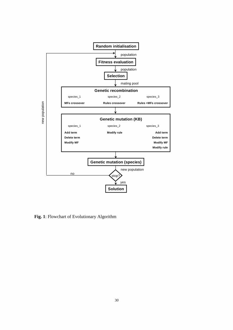
unchanged by the evolutionary procedure. A flowchart of the algorithm is given in Fig. 1.

The algorithm uses the generational replacement reproduction scheme [30], a new

selection operator [31] and a set of recombination and mutation procedures [30] dealing

with different elements of the fuzzy KB to evolve a population of FL systems. Each of

the recombination operators behaves as a two-point crossover operator [4], cutting and

pasting information defined into hypercubes of the input-output characteristic.

The algorithm uses the generational replacement reproduction scheme [30], a new

selection operator [31] and a set of crossover and mutation procedures [30] dealing with

different elements of the fuzzy KB to evolve a population of FL systems. The population

is divided into three sub-groups to which different operators are applied. A specific

integer-valued gene marks the species of each individual.

12

As previously mentioned, there are three ways of modifying the overall fuzzy mapping:

by manipulating the input and output partitions, by changing the control policy and by

performing simultaneously both operations. Accordingly, the population is divided into

three sub-groups to which the different operators are applied. A specific integer-valued

gene marks the species of each individual.

The genetic operators acting on the first sub-population work at the level of input and

output fuzzy partitions. The aim of the recombination operator is to redistribute the genes

amongst the population, looking for the most successful assembly. In this case, crossover

generates two new individuals by mixing the MFs of the two parents for each variable.

Crossover generates two new individuals by mixing the MFs of the two parents for each

variable. Each parent transmits its RB to one of the offspring. Random chromosomic

mutations can create new fuzzy terms, delete existing ones, or change the parameters

defining the location and shape of a MF. Whenever genetic manipulations modify the set

of MFs over which a RB is defined, a ‘repair’ algorithm translates the old rule conditions

and actions into the new fuzzy terms. The sub-population of fuzzy systems undergoing

this set of operations is called species_1.

The operators manipulating the second sub-population search for the optimal RB. Genetic

crossover creates two individuals by exchanging sets of rules between the two parents.

The aim of this operator is to build better performing solutions by assembling blocks of

good quality rules from the parents chromosomes. Each of the offspring inherits the input

and the output space partitions from one of its parents. The mutation operator randomly

13

changes the action of a fuzzy rule. To accommodate the new partitions, the conditions

and actions of the swapped rules are translated into new linguistic terms. The mutation

operator randomly changes the action of a fuzzy rule. This group of solutions is named

species_2.

The operators acting on the third sub-population deal with all the components of the

fuzzy KB. Genetic recombination swaps all the MFs and the rules contained in a

randomly selected portion of the input and output spaces. Mutation can take any of the

forms defined for the modification of species_1 and species_2 genotypes. This third

group of individuals is referred to as species_3.

Each of the sub-populations is used to perform a different search in the space of possible

solutions. species_1 is mainly concerned with fine tuning the fuzzy response, while the

other two species are used for increasingly more disruptive search approaches.

Information is naturally exchanged between different sub-populations through genetic

recombination which is not forbidden or strictly regulated as in ordinary niching

techniques [32]. When two individuals of different kinds are mated, the fitter solution

dominates the other, determining the species of the offspring and the type of crossover

applied. This mechanism adds a bias towards the most successful search approach.

Competition for survival is increased among the whole population of individuals, a

feature that also differs from many niching approaches.

14

A species mutation operator prevents one type of individual from taking over the entire

population. Its action has the double purpose of allowing the resurgence of temporarily

suppressed species and spreading useful genetic material over the three population

groups. The possibility of reinstating declining species allows the adaptive adjustment of

the search strategy. As an example, at the beginning of the optimisation process it may be

preferable to focus the search efforts at the RB level for a quick broad-brush definition of

the behaviour of the system. At a later stage, the fine tuning of the response may require

more computational resources to be allocated at the level of MFs optimisation.

It is important to point out that the separation of the population into three sub-groups is

aimed at the dynamic adjustment of the focus of the genetic search towards different KB

elements. In contrast with other niching techniques, the division of the population into

species is not aimed at sustaining population diversity, which is instead pursued through

the conventional balance of selection pressure and genetic mutations. Because of this

fundamental difference, the proposed algorithm cannot be regarded as adopting a

conventional niching technique.

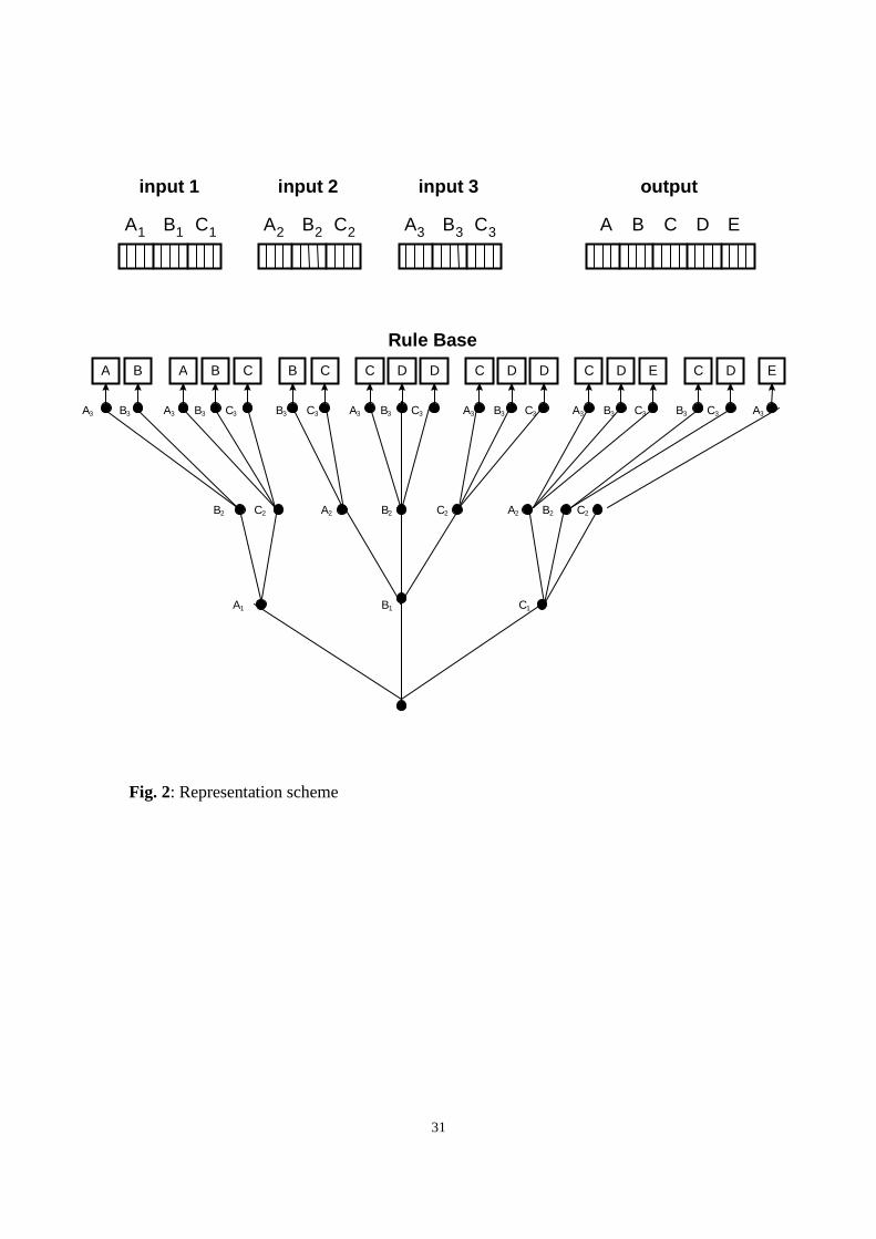
The algorithm represents candidate solutions using multi-chromosome variable-length

genotypes. Fig. 2 gives an example of an encoded solution for a FL system having three

input variables, each partitioned into three linguistic terms, and one output variable

partitioned into five fuzzy terms.

15

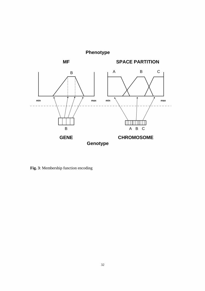
A separate chromosome is used to describe the partition of each input and output

variable, each chromosome being composed of a number of genes equal to the number of

linguistic terms. Each gene is a real-valued string encoding the parameters defining the

location and the shape of one MF. Fig. 3 details the MF encoding scheme.

The fuzzy RB is represented as a multi-level decision tree, the depth of the tree

corresponding to the dimensionality of the input space. The rule antecedent is encoded in

the full path leading to the consequent, each node being associated with a rule condition.

The nodes at the last level of the decision tree represent the rule consequent and contain a

fuzzy action for each output variable.

4 FUZZY MODELLING OF NON-LINEAR PLANTS

Two tests were performed aimed at measuring the ability of the proposed algorithm to

solve complex identification problems. Even though limited in their scope, the

investigation was expected to provide further evidence of the effectiveness and

robustness of the proposed EA.

4.1 Simulated Plants

The tests involved the modelling of two simulated highly non-linear dynamic systems.

The accuracy of the evolutionary FL model was compared by replicating the experiments

using a Differential Activation Function Feedforward Fuzzy Neural Network (DA-

FFNN) [33], a modified version of the popular FFNN by [34] [35] which automatically

16

tunes the fuzzy MFs via error back propagation. Compared to its predecessor, the DA-

FFNN allows a more precise backpropagation of the error information during the learning

phase, achieving higher modelling accuracy. The RB of the DA-FFNN was created using

the inductive rule extraction method of [36] while the number of fuzzy MFs is a system

parameter. For the sake of completeness, the first experiment also includes the modelling

results obtained using Lin’s and Lee’s original MF tuning procedure.

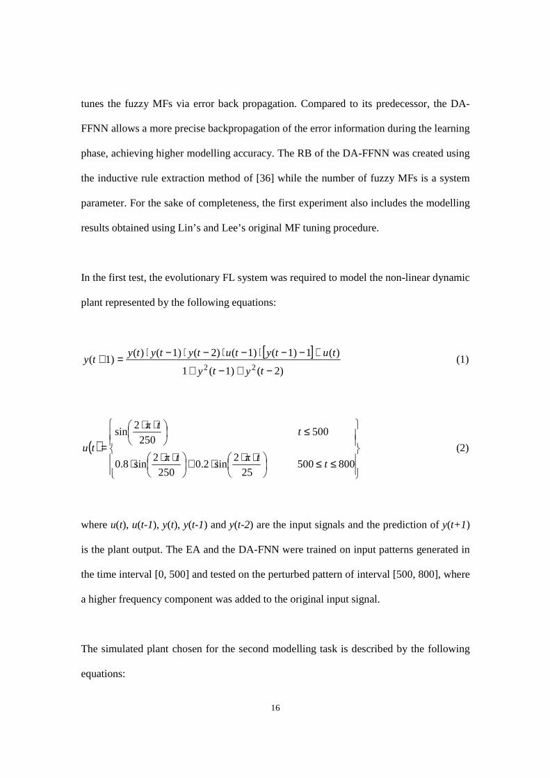
In the first test, the evolutionary FL system was required to model the non-linear dynamic

plant represented by the following equations:

[ ]2)(1)(1

)(11)(1)(2)(1)()(1)(

22 −+−+

+−−⋅−⋅−⋅−⋅=+tyty

tutytutytytyty (1)

( )

≤≤

⋅⋅⋅+

⋅⋅⋅

≤

⋅⋅

=800500

25π2

sin 2.0250π2

sin8.0

500 250π2

sin

ttt

tt

tu (2)

where u(t), u(t-1), y(t), y(t-1) and y(t-2) are the input signals and the prediction of y(t+1)

is the plant output. The EA and the DA-FNN were trained on input patterns generated in

the time interval [0, 500] and tested on the perturbed pattern of interval [500, 800], where

a higher frequency component was added to the original input signal.

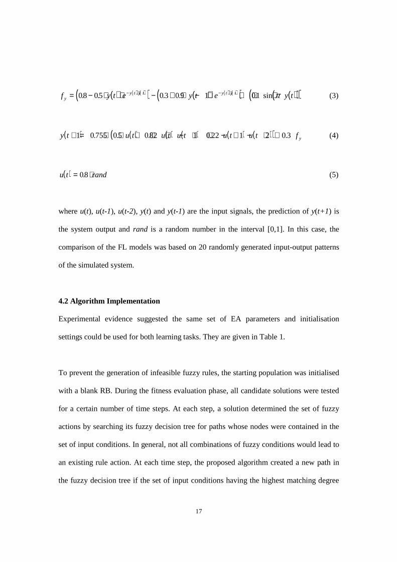
The simulated plant chosen for the second modelling task is described by the following

equations:

17

( ) ( ) ( )( ) ( ) ( ) ( )( ) ( )( )( )f y t e y t e y tyy t y t y t y t= − ⋅ ⋅ − + ⋅ − ⋅ + ⋅ ⋅− ⋅ − ⋅08 05 03 09 1 01. . . . . sinπ (3)

( ) ( ) ( ) ( ) ( ) ( )( )y t u t u t u t u t u t f y+ = ⋅ ⋅ + ⋅ ⋅ − + ⋅ − ⋅ − + ⋅1 0 755 05 082 1 0 22 1 2 0 3. . . . . (4)

( )u t rand= ⋅08. (5)

where u(t), u(t-1), u(t-2), y(t) and y(t-1) are the input signals, the prediction of y(t+1) is

the system output and rand is a random number in the interval [0,1]. In this case, the

comparison of the FL models was based on 20 randomly generated input-output patterns

of the simulated system.

4.2 Algorithm Implementation

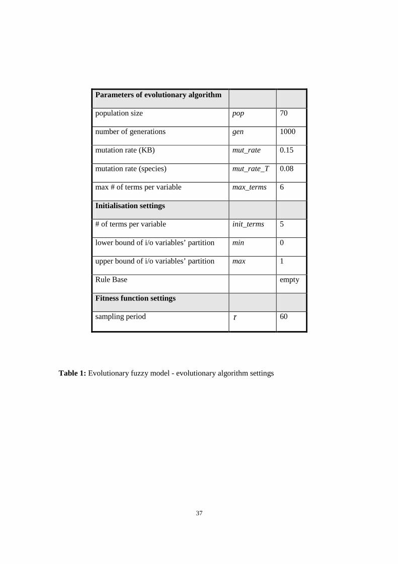
Experimental evidence suggested the same set of EA parameters and initialisation

settings could be used for both learning tasks. They are given in Table 1.

To prevent the generation of infeasible fuzzy rules, the starting population was initialised

with a blank RB. During the fitness evaluation phase, all candidate solutions were tested

for a certain number of time steps. At each step, a solution determined the set of fuzzy

actions by searching its fuzzy decision tree for paths whose nodes were contained in the

set of input conditions. In general, not all combinations of fuzzy conditions would lead to

an existing rule action. At each time step, the proposed algorithm created a new path in

the fuzzy decision tree if the set of input conditions having the highest matching degree

18

did not result in a valid action. The rule consequent was randomly determined. The aim

of the procedure was to limit the RB growth only to the most relevant instances. This

feature allowed the creation of a minimal set of fuzzy rules but also emphasised the

importance of the training procedure.

To curb the combinatorial explosion in the number of control rules further, a maximum

of 6 linguistic terms per universe of discourse was set, this figure still allowing the

generation of solutions possessing up to almost 104 fuzzy rules.

The fitness of the candidate solutions was evaluated as a measure of their root mean

square (r.m.s.) modelling error over a randomly chosen time window of 60 steps. This

value reprented a good compromise between sampling accuracy and running time.

5 RESULTS

This section presents the results of the evolutionary learning of fuzzy models for the two

plants.

5.1 Plant 1 – Learning results

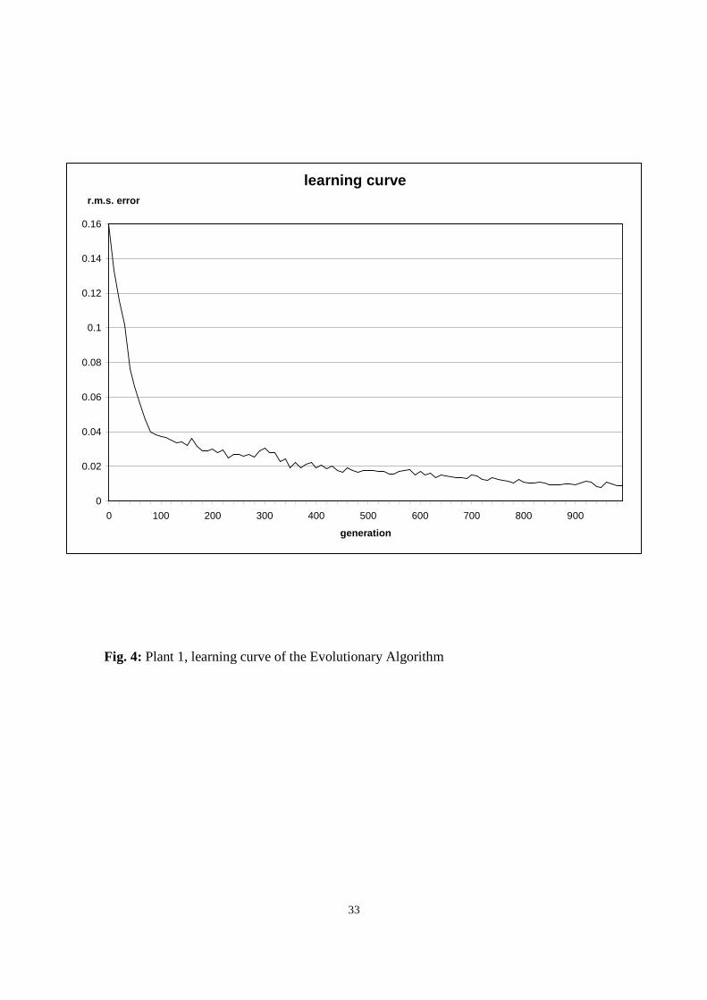
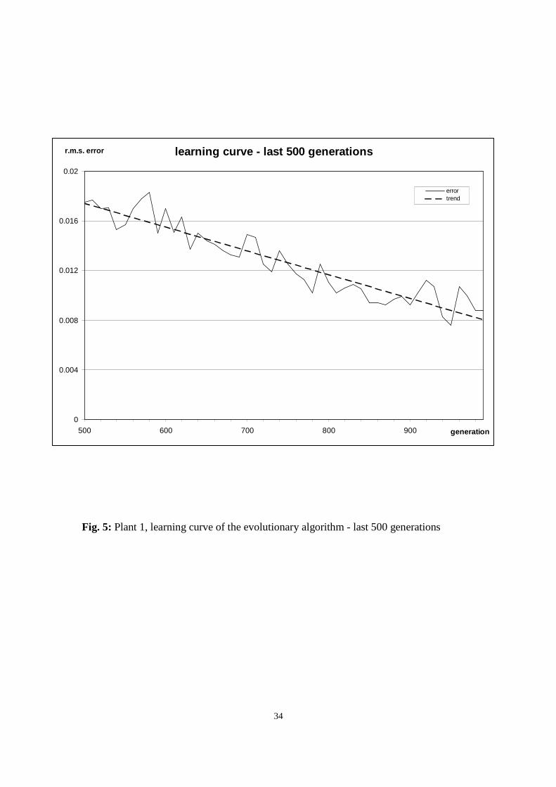
Fig. 4 shows the evolution of the average r.m.s. error of the population over the training

period. Fig. 5 focuses on the last 500 generations of the evolution period to highlight the

ongoing improvement of the performance of the population.

19

The steadiness of the learning reflects a good selection pressure after the initial large

improvement in performance. On the other hand, aAs evolution progressed, the candidate

solutions were gathering additional experience and the initially empty RB was

progressively filled. Therefore, the second half of the evolution period was the more time

consuming as more complex solutions were processed. Considering the magnitude of the

improvement during the last 500 generations, if the highest precision is not required, by

terminating the search earlier the running time of the algorithm could be drastically

reduced.

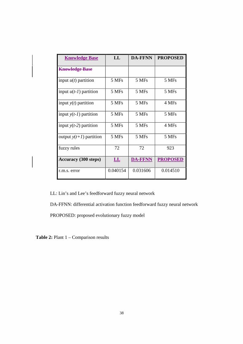
The results of the comparison are reported in Table 2 and clearly show the superior

modelling accuracy of the EA-generated fuzzy model. In particular, the measured r.m.s.

error is half of that for the DA-FFNN and three times smaller than for Lin’s and Lee’s

original FFNN, confirming the effectiveness of the proposed learning technique.

5.2 Plant 1 – Complexity of FL model

The EA-generated KB is considerably more complex, containing one order of magnitude

more rules than the induction-generated counterpart. Different reasons could explain this

dramatic difference. Besides the fact that a more precise mapping necessarily requires a

more detailed description of the approximated function, it should be noted that the size of

the RB of the DA-FFNN is partly controlled by the manual initialisation of the input and

output space partition. The inductive learning algorithm was therefore run on fuzzy space

partitions roughly tailored for a certain KB size. The freedom of the EA to organise its

own input and output spaces therefore brings a superior modelling accuracy and reduced

20

design effort at the expense of a larger RB. At the same time, it should be remembered

that no selection pressure has been exerted to evolve the most compact solution.

The setting of a maximum number of terms per universe of discourse and the allocation

of mutation probabilities that favour the reduction of fuzzy terms contribute to a degree

of control on the size of the KB. Also the rule generation procedure serves the same

purpose. Nonetheless, these methods are rather indirect ones. Following genetic

manipulations, the boundaries of some fuzzy rules may shift to areas of unfeasible input

signals, or redundant fuzzy rules and terms may be generated [37]. In those cases, a

simplification of the KB would increase the transparency of the control policy. On the

other hand, it is debatable up to which point the mapping of a five-input fuzzy system can

be transparent.

Yet, the size of the EA-generated FL system did not appear to slow the response time

down appreciably. Unless otherwise required by specific hardware or software

limitations, in case of highly dimensional complex mapping problems, focusing on the

transparency of an EA-generated KB is not likely to pay back. Where this feature was

required, it would be worthwhile investigating the possibility of introducing some EA

inspection routine with the purpose of pruning redundant fuzzy terms and rules. The

computational time allocated to this operation could be regained by the subsequent

simplification of the genetic manipulation operations.

5.3 Plant 2 – Learning results

21

The second experiment almost replicates the results obtained in the previous one. Fig. 6

shows the evolution of the average r.m.s. error of the population over the training period

while Fig. 7 focuses on the last 500 generations. The results of the comparison are

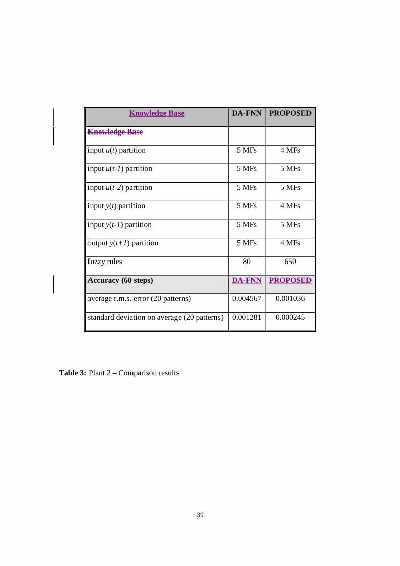
presented in Table 3.

The difference in accuracy compares here even more favourably for the proposed

algorithm which achieved a r.m.s. error measure four times smaller than the DA-FFNN.

The steeper learning curve in the first hundred generations and the smaller r.m.s.

modelling error obtained by the final solutions suggests the behaviour of the second

simulated plant was more easy to model for the FL learning algorithms.

The comparison also shows the EA technique obtaining more robust generalisation

results. The ratio between the average r.m.s. error and its standard deviation over the 20

randomly generated test patterns is in fact 0.2 for the evolutionary FL system and 0.28 for

the DA-FFNN.

Comparing the results of Table 3 with the plot of Fig. 7 shows that the performance of the

final solution is very close to the average accuracy of the population towards the end of

the search. This suggests the population is very near to convergence at that stage of the

evolution. The steadiness of the learning in the population despite the almost uniform

performance of the individuals therefore gives further evidence of the effectiveness of the

proposed selection routine. This observation was not possible in the previous experiment

as the sampling periods were different from the learning to the test phase.

22

5.4 Plant 2 – Complexity of FL model

The second experiment confirms the findings of the previous one. The size of the EA-

generated RB is smaller that the one generated in the previous modelling test. Still, it is

about 8 times larger than the corresponding one generated via rule induction for the DA-

FFNN.

The smaller size of the second EA generated KB could also provide further evidence that

the second plant was easier to model. On the other hand, it should be noted that the size

of the EA-generated KBs could vary substantially between different runs of the same

experiment. Often the size of the fluctuations in KB size was not reflected by significant

variations in performance. This supports the above formulated hypothesis of the presence

of a number of redundant fuzzy rules in the automatically generated KB.

6 CONCLUSIONS AND FURTHER WORK

A novel evolutionary technique was presented for the automatic generation of KBs for

FL systems. The algorithm was tested on two different system identification tasks, each

involving the modelling of a highly non-linear dynamic plant.

The experiments gave the opportunity of further assessing the effectiveness and

limitations of the proposed technique. The overall evaluation of the EA based on the tests

23

conducted is positive. In both cases, the algorithm achieved learning results that

compared favourably with alternative KB generation methods.

On the other hand, the algorithm probably did not evolve solutions in their most

economical representation. Experimental evidence suggests the KB developed in the

system modelling experiments were probably simplifiable. It should be noted, however,

that the current EA prototype has not been explicitly designed to optimise the

compactness of solutions.

Further work should mainly address the simplification of the KB, introducing automatic

pruning routines to cut down the size of the RB. Those routines could, for instance, focus

on merging homogeneous areas of the fuzzy response map or pruning fuzzy rules that

evolution has made obsolete or infeasible.

ACKNOWLEDGEMENTS

This research was sponsored by Hewlett-Packard and the Welsh Assembly Government

under the European Regional Development Fund programme and by the EC FP6

Network of Excellence on Innovative Production Machines and Systems (I*PROMS).

REFERENCES

[1] Zadeh, L. A. (1965), Fuzzy Sets, Information and Contr., Vol. 8, pp. 338-353.

24

[2] Mamdani, E. H. (1974), Application of fuzzy algorithms for control of simple

dynamic plant, Proc. IEE, Vol. 121 No. 12, pp. 1585-1588.

[3] Lee, C. C. (1990), Fuzzy logic in control systems: fuzzy logic controller, Part I &

Part II, IEEE Trans. Syst. Man and Cyb., Vol. 20, n. 2, pp. 404-418 & 419-435.

[4] Fogel, D. B. (2000), Evolutionary Computation: Toward a New Philosophy of

Machine Intelligence, 2nd ed., IEEE Press, New York.

[5] Eiben, A.E. and Smith, J.E. (2003), Introduction to evolutionary computing,

Springer, New York.

[6] Coello, C. A. C., Van Veldhuizen, D. A., Lamont, G. B. (2002), Evolutionary

Algorithms for Solving Multi-Objective Problems (Genetic Algorithms and

Evolutionary Computation), Plenum, New York.

[7] Rumelhart, D. E. and McClelland, J. L. (1986), Parallel Distributed Processing:

Exploration in the Micro-Structure of Cognition , Vol. 1-2, Cambridge, MIT

Press.

[8] Pham, D.T. and Castellani, M. (2002), Outline of a New Evolutionary Algorithm

for Fuzzy Systems Learning, Proc. IMechE, Part C, Vol. 216, No. 5, pp. 557-570.

[9] Rechenberg, I. (1965), Cybernetic Solution Path of an Experimental Problem,

Royal Aircr. Establ., libr. Transl., 1122, Farnborough, Hants UK.

[10] Arnold, D.V. (2002), Noisy Optimisation with Evolution Strategies, Kluwer

Academic Publishers, Boston, MA.

[11] Fogel, L. J., Owens A. J. and Walsh, M. J. (1966), Artificial Intelligence through

Simulated Evolution, Wiley, New York.

25

[12] Fogel, D. B. (1992), An Analysis of Evolutionary Programming, Proc. First Int.

Conf. on Ev. Progr., 1992, pp. 43-51.

[13] Holland, J. H. (1975), Adaptation in Natural and Artificial Systems, Ann Arbor,

MI: University of Michigan Press.

[14] De Jong, K. A. (1975), An Analysis of the Behaviour of a Class of Genetic

Adaptive Systems, Ph.D. thesis, Univ. of Michigan, Ann Arbor, MI.

[15] Gao, W. (2004), Comparison study of genetic algorithm and evolutionary

programming, Proc. 2004 Int. Conf. on Machine Learning and Cybernetics, Vol. 1,

pp. 204-209.

[16] Smith, S. F. (1980), A Learning System Based on Genetic Adaptive Algorithms,

Ph.D. thesis, Department of Computer Science, University of Pittsburgh, PA, 1980.

[17] Holland, J. H., Reitman, J. S. (1978), Cognitive Systems Based on Adaptive

Algorithms , In: D.A. Waterman, F. Hayes-Roth (Eds), Pattern-Directed Inference

Systems. New York, Academic Press.

[18] Parodi, A. and Bonelli, P. (1993), A New Approach to Fuzzy Classifier Systems,

Proc. 5th Int. Conf. on GAs and Appl., Urbana IL - 1993, pp. 223-230.

[19] Lee, M. A. and Takagi, H. (1993), Dynamic Control of Genetic Algorithms

Using Fuzzy Logic Techniques, Proc. 5th Int. Conf. on GAs and Appl., Urbana IL -

1993, pp. 76-83.

[20] Kinzel, J., Klawonn, F. and Kruse, R. (1994), Modifications of Genetic

Algorithms for Designing and Optimising Fuzzy Controllers, Proc. First IEEE

Conf. on Ev. Comp. (ICEC), Orlando FL - 1994, pp. 28-33.

26

[21] Heider, H. and Drabe, T. (1997), Fuzzy System Design with a Cascaded Genetic

Algorithm , Proc. IEEE Int. Conf. on Ev. Comp., Indianapolis IN - 1997, pp. 585-

588.

[22] Buckles, B. P., Petry, F. E., Prabhu, D., George, R. and Srikanth, R. (1994), Fuzzy

Clustering with Genetic Search, Proc. First IEEE Conf. on Ev. Comp. (ICEC),

Orlando FL - 1994, pp. 46-50.

[23] Cooper, M. G. and Vidal, J. J. (1994), Genetic Design of Fuzzy Controllers: the

Cart and Jointed-Pole Problem, Proc. 3rd IEEE Int. Conf. on Fuzzy Syst.,

Piscataway NJ - 1994, Vol. 2, pp. 1332-1337.

[24] Liska, J. and Melsheimer, S. S. (1994), Complete Design of Fuzzy Logic Systems

Using Genetic Algorithms, Proc. 3rd IEEE Int. Conf. on Fuzzy Syst., Piscataway

NJ - 1994, Vol. 2, pp. 1377-1382.

[25] Ng, K. C. and Li, Y. (1994), Design of Sophisticated Fuzzy Logic Controllers

Using Genetic Algorithms, Proc. First IEEE Conf. on Ev. Comp. (ICEC), Orlando

FL - 1994, pp. 1708-1712.

[26] Ng, K. C. and Li, Y., Murray-Smith, D. J. and Sharman, K. C. (1995), Genetic

Algorithms Applied to Fuzzy Sliding Mode Controller Design, Proc. GALESIA

First IEE/IEEE Int. Conf. on GAs in Eng. Syst.: Innovations and Appl., Sheffield

UK - 1995, pp. 220-225.

[27] Homaifar, H. and Mc Cormick, E. (1995), Simultaneous Design of Membership

Functions and Rule Sets for Fuzzy Controllers Using Genetic Algorithms, IEEE

Trans. on Fuzzy Syst., Vol. 3, No. 2, pp. 129-139.

27

[28] Nandi, A. K., Pratihar, D. K. (2004), Automatic design of fuzzy logic controller

using a genetic algorithm - To predict power requirement and surface finish in

grinding , J. of Materials Processing Techn., Vol. 148, No. 3, pp. 288-300.

[29] Shi, Y., Eberhart R. and Chen, Y. (1999), Implementation of Evolutionary Fuzzy

Systems, IEEE Trans. on Fuzzy Syst., Vol. 7, No. 2, pp. 109-119.

[30] Davis, L. (1991), Handbook of Genetic Algorithms, Van Nostrand Reinhold, New

York.

[31] Pham, D.T. and Castellani, M. (2005), A New Adaptive Selection Routine For

Evolutionary Algorithms , submitted to Proc. IMechE, Part C.

[32] Mahfoud., S. W. (1995), A comparison of parallel and sequential niching

methods, Proc. 6th Int. Conf. on GAs and Appl., Pittsburgh PA - 1995, pp. 136-143.

[33] Shankir, Y. (2000), Modified feedforward FNN with differential activati on

functions, Ph.D. thesis, Univ. of Wales, Cardiff UK.

[34] Lin, C. T. and Lee, C. S. (1991), Neural-network-based fuzzy logic control and

decision system, IEEE Trans. on Computers, Vol. 40, No. 12, pp. 1320-1336.

[35] Lin, C. T. and Lee, C. S. (1992), Real-time supervised structure/parameter

learning for fuzzy neural network, Proc. IEEE Int. Conf. on Fuzzy Syst., S. Diego

CA - 1992, pp. 1283-1290.

[36] Wang, L. X. and Mendel, J. M. (1992), Generating fuzzy rules by learning from

examples, IEEE Trans. on Syst. Man and Cybern., vol 22, nr 6, pp. 1414-1427.

[37] Pham, D.T. and Castellani, M. (2002), Evolutionary Fuzzy Logic System for

Intelligent Fibre Optic Components Assembly, Proc. IMechE, Part C, Vol. 216,

No. 5, pp. 571-581.

28

FIGURES

Fig. 1: Flowchart of Evolutionary Algorithm

Fig. 2: Representation scheme

Fig. 3: Membership function encoding

Fig. 4: Plant 1, learning curve of the Evolutionary Algorithm

Fig. 5: Plant 1, learning curve of the Evolutionary Algorithm - last 500 generations

Fig. 6: Plant 2, learning curve of the Evolutionary Algorithm

Fig. 7: Plant 2, learning curve of the Evolutionary Algorithm - last 500 generations

29

TABLES

Table 1: Evolutionary Fuzzy Logic model - Evolutionary Algorithm settings

Table 2: Plant 1 – Comparison results

Table 3: Plant 2 – Comparison results

30

Random initialisation

Solution

population

population

mating pool

new population

yes

no

new

pop

ulat

ion

stop?

Fitness evaluation

Selection

Genetic recombinationspecies_2

Rules crossover

species_1

MFs crossover

species_3

Rules +MFs crossover

Genetic mutation (KB)

Add term

Delete term

Modify MF

Modify rule

species_1 species_2 species_3

Add term

Delete term

Modify MF

Modify rule

Genetic mutation (species)

Fig. 1: Flowchart of Evolutionary Algorithm

31

A B C D EA1 B1 C1

input 1 output

Rule Base

B2 C2 A2 B2 C2A2 B2 C2

A1 B1 C1

A B

A3 B3 C3 A3 B3 C3 B3 C3 A3C3B3C3B3A3B3A3

A CB CB C DD C DD C ED C ED

A3 B3 C3

input 2

A2 B2 C2

input 3

A3 B3 C3

Fig. 2: Representation scheme

32

min

A B C

A B C

max

CHROMOSOME

min max

GENE

B

B

Genotype

Phenotype

MF SPACE PARTITION

Fig. 3: Membership function encoding

33

Fig. 4: Plant 1, learning curve of the Evolutionary Algorithm

learning curve

0

0.02

0.04

0.06

0.08

0.1

0.12

0.14

0.16

0 100 200 300 400 500 600 700 800 900

generation

r.m.s. error

34

Fig. 5: Plant 1, learning curve of the evolutionary algorithm - last 500 generations

learning curve - last 500 generations

0

0.004

0.008

0.012

0.016

0.02

500 600 700 800 900 generation

r.m.s. error

errortrend

35

Fig. 6: Plant 2, learning curve of the evolutionary algorithm

Learning curve

0

0.02

0.04

0.06

0.08

0.1

0.12

0.14

0 100 200 300 400 500 600 700 800 900

generation

r.m.s. error

error

36

Learning curve - last 500 generations

0

0.0005

0.001

0.0015

0.002

0.0025

500 600 700 800 900 generation

r.m.s. error

error

trend

Fig. 7: Plant 2, learning curve of the evolutionary algorithm - last 500 generations

37

Parameters of evolutionary algorithm

population size pop 70

number of generations gen 1000

mutation rate (KB) mut_rate 0.15

mutation rate (species) mut_rate_T 0.08

max # of terms per variable max_terms 6

Initialisation settings

# of terms per variable init_terms 5

lower bound of i/o variables’ partition min 0

upper bound of i/o variables’ partition max 1

Rule Base empty

Fitness function settings

sampling period τ 60

Table 1: Evolutionary fuzzy model - evolutionary algorithm settings

38

Knowledge Base LL DA-FFNN PROPOSED

Knowledge Base

input u(t) partition 5 MFs 5 MFs 5 MFs

input u(t-1) partition 5 MFs 5 MFs 5 MFs

input y(t) partition 5 MFs 5 MFs 4 MFs

input y(t-1) partition 5 MFs 5 MFs 5 MFs

input y(t-2) partition 5 MFs 5 MFs 4 MFs

output y(t+1) partition 5 MFs 5 MFs 5 MFs

fuzzy rules 72 72 923

Accuracy (300 steps) LL DA-FFNN PROPOSED

r.m.s. error 0.040154 0.031606 0.014510

LL: Lin’s and Lee’s feedforward fuzzy neural network

DA-FFNN: differential activation function feedforward fuzzy neural network

PROPOSED: proposed evolutionary fuzzy model

Table 2: Plant 1 – Comparison results

39

Knowledge Base DA-FNN PROPOSED

Knowledge Base

input u(t) partition 5 MFs 4 MFs

input u(t-1) partition 5 MFs 5 MFs

input u(t-2) partition 5 MFs 5 MFs

input y(t) partition 5 MFs 4 MFs

input y(t-1) partition 5 MFs 5 MFs

output y(t+1) partition 5 MFs 4 MFs

fuzzy rules 80 650

Accuracy (60 steps) DA-FNN PROPOSED

average r.m.s. error (20 patterns) 0.004567 0.001036

standard deviation on average (20 patterns) 0.001281 0.000245

Table 3: Plant 2 – Comparison results