evidence from the brew-at-home coffee market
TRANSCRIPT
Munich Personal RePEc Archive
Market Effects of New Product
Introduction: Evidence from the
Brew-at-home Coffee Market
Gayle, Philip and Lin, Ying
Kansas State University, Belhaven University
28 February 2022
Online at https://mpra.ub.uni-muenchen.de/112124/
MPRA Paper No. 112124, posted 07 Mar 2022 14:26 UTC
Market Effects of New Product Introduction:
Evidence from the Brew-at-home Coffee Marketa
Philip G. Gayle* and Ying Lin+
Forthcoming in Journal of Economics & Management Strategy
This draft: February 15, 2022 First draft: October 25, 2018
Abstract
The introduction of new products has always been an important source of economic development and improvement in consumer welfare. With retail coffee data spanning five years after the single-cup brew coffee pods were introduced to grocery chains, this paper empirically studies the market effects of new product introduction in the brew-at-home coffee market. We use a structural model of demand and supply to capture the changes in consumers’ preference for this new product over time. The demand estimates suggest that consumers’ relative preference and willingness-to-pay for the new product grew substantially over the sample periods. The analysis reveals the extent to which the introduction and growing presence of the new product simultaneously expanded the relevant market and cannibalized the sales of pre-existing substitute products (traditional auto-drip brew coffee products). Furthermore, we quantify the annually expanding welfare gains of the average consumer attributable to the new product.
Keywords: New product introduction; Willingness-to-pay; Market-expansion; Demand-cannibalization; Brew-at-home coffee market.
JEL Classification Codes: L13; D12; L66
* Kansas State University, Department of Economics, 322 Waters Hall, Manhattan, KS, 66506; Voice: 785-532-4581; Fax: 785-532-6919; Email: [email protected]; Corresponding Author. + Belhaven University, School of Business, 1500 Peachtree Street, Box 310, Jackson, MS 39202; Voice: 601-968-8982; Email: [email protected]
a For very helpful comments and suggestions, we thank the editor, Ramon Casadesus-Masanell, the co-editor, two anonymous referees, Jin Wang, Peri da Silva, Tian Xia, and participants at several seminars. Any remaining errors are our own.
1
1. Introduction
New product introduction, which often incorporates new and improved technology, has
long played a critical role in influencing not only consumers’ tastes, demand, and welfare, but also
firms’ profitability and even the overall market structure. Firms, especially those in electronics and
consumer-packaged goods (CPGs) industries (e.g., food, beverages, cleaning products, etc.),
diligently respond to consumers’ ever-changing needs and tastes by introducing new products via
either line extension or brand extension. Products in the CPGs sectors are primarily channeled
through grocery chains to households. According to Gallagher (2011), CPGs manufacturers in the
U.S. introduced more than 150,000 new products in 2010 alone.1 With market-level retail chain
packaged coffee sales data available, our empirical analysis focuses on the market of brew-at-
home coffee consumption.
In the retail packaged coffee products sector, single-cup brew coffee products were nearly
unavailable in grocery stores for brew-at-home coffee consumers prior to 2008.2 The introduction
of single-cup brewing systems, pioneered by Keurig Green Mountain, introduced a whole new
coffee segment by bringing single-cup pods into grocery chains since 2008. The rapid market
adoption of single-cup brew method fueled the sales of single-cup coffee pods3 and significantly
influencing the overall landscape of the brew-at-home coffee market.
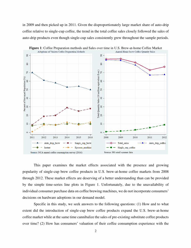
In Figure 1, on the left panel, National Coffee Association (NCA) annual national coffee
consumption survey reveals an increasing popularity of single-cup brew technology among the
surveyed population, and a declining trend in the use of traditional auto-drip brewing method from
2011 through 2016. 4 Single-cup brew method has become the second most popular coffee
preparation method after the traditional auto-drip brew method, far surpassing the preparation
methods of instant coffee and espresso machines. On the right panel of Figure 1,5 the line plots
suggest that total brew-at-home packaged coffee sales in grocery chains began a downward trend
1 More than ninety percent of new products/brands in the CPG sectors were introduced via extensions of existing brand-name products, according to Hariharan et. al. (2015). 2 Keurig single-cup brewing systems were available only in some high-end department stores in year 2003. However, they became available to households through grocery stores across the U.S. in year 2008. Since then, single-cup brew became an option for home-brew coffee consumption. See URL link: https://consumergoods.com/gmcrs-path-disruptive-innovation 3 U.S. consumers bought $3.1 billion worth of coffee pods in 2013 versus $132 million in 2008 (The Seattle Times). See URL link: https://www.seattletimes.com/business/single-serve-coffee-revolution-brews-industry-change/ 4 According to NCA, coffee brew method with single-cup systems was not surveyed until 2011. 5 The line plots are generated based on our working data sample sourced from Information Resources Inc. (IRI) academic database. Detailed discussion about the construction of the working sample is presented in the data section.
2
in 2009 and then picked up in 2011. Given the disproportionately large market share of auto-drip
coffee relative to single-cup coffee, the trend in the total coffee sales closely followed the sales of
auto-drip products even though single-cup sales consistently grew throughout the sample periods.
Figure 1: Coffee Preparation methods and Sales over time in U.S. Brew-at-home Coffee Market
This paper examines the market effects associated with the presence and growing
popularity of single-cup brew coffee products in U.S. brew-at-home coffee markets from 2008
through 2012. These market effects are deserving of a better understanding than can be provided
by the simple time-series line plots in Figure 1. Unfortunately, due to the unavailability of
individual consumer purchase data on coffee brewing machines, we do not incorporate consumers’
decisions on hardware adoptions in our demand model.
Specific in this study, we seek answers to the following questions: (1) How and to what
extent did the introduction of single-cup brew coffee products expand the U.S. brew-at-home
coffee market while at the same time cannibalize the sales of pre-existing substitute coffee products
over time? (2) How has consumers’ valuation of their coffee consumption experience with the
3
single-cup brew technology evolved over time since it was introduced to the supermarkets? (3)
What welfare effects resulted from the presence and increasing popularity of single-cup brew
technology?
To examine these questions, our research methodology begins with estimating a random
coefficients discrete-choice demand model. Assuming firms compete in prices according to a static
Nash equilibrium price-setting game, the demand estimates are subsequently used to compute
price-cost margins of the coffee products. These estimates together are used to simulate the new
market equilibrium that would result from a counterfactual experiment in which single-cup coffee
options are taken away from consumers’ choice set. Comparing actual market outcomes when
single-cup coffee options are available to consumers with counterfactual market equilibrium
outcomes when single-cup coffee options are absent enables us to address the above key research
questions.
Results from the demand estimation suggest that the average coffee drinker prefers her
coffee consumption using the single-cup brew technology over the traditional auto-drip brew
method; and this relative preference increases over time. In addition, the average consumer’s
willingness-to-pay for the single-cup brew attribute increases by more than 180% from 2008 to
2012. Counterfactually removing single-cup coffee options from consumers’ choice set predicts
to increase the price level of auto-drip coffee products, effectively suggesting the entry and
growing popularity of single-cup brew products caused an average reduction in the price level of
auto-drip products. Furthermore, this price effect tends to become larger over time.
Our empirical model predicts that the introduction and growing penetration of single-cup
products have an expansionary effect on the overall brew-at-home coffee market by attracting
consumers who would have otherwise chosen not to purchase any of the coffee products in our
analysis, while also having a demand-cannibalizing effect on the existing auto-drip brew products.
Last, the welfare analysis of the new product introduction suggests that the average consumer is
predicted to have a welfare gain of about 0.3% in 2008, which substantially increased to a welfare
gain of 2.8% in 2012. Results from the estimated compensation variation suggests that, if single-
cup coffee options were to be eliminated from consumers’ choice sets, then the average coffee
drinker needs to be compensated 13 times more in year 2012, compared with the compensation
level in year 2008. Accordingly, we monetize these predicted welfare gains and compare them to
4
estimated welfare gains attributable to new product introductions in other industries that are
documented in other studies in the literature.
The rest of the paper is organized as follows. Section 2 reviews relevant literature. Section
3 discusses data sources and variables used in the analysis. Section 4 describes the empirical model,
as well as the estimation method. Section 5 presents and discusses the empirical results. Section 6
describes the counterfactual procedure and analyzes findings from the counterfactual experiment.
Section 7 concludes the paper.
2. Related Literature
The analysis of new product introduction has been the focus of economists’ attempts to
understand its impacts on the measures of cost-of-living, such as the Consumer Price Index (CPI).6
As stated in Bresnahan and Gordon (1997), “new goods are the heart of economic progress,” and
the estimated value created by new goods provides important inference for calculating the CPI. It
is therefore important to accurately evaluate the welfare effects of new product introductions. By
analyzing the demand and welfare effects associated with the introduction of single-cup coffee
products, our paper is related to much of the previous literature examining the economic effects of
newly introduced products or technology in various industries. A few well-known papers in this
literature include: Hausman (1996); Greenstein (1997); Hausman and Leonard (2002); Petrin
(2002); Goolsbee and Petrin (2004); Brynjolfsson et.al. (2003); and Gentzkow (2007).7
However, previous literature in evaluating the economic effects of new goods particularly
focused on the price effects as well as the welfare impact of new products upon their entry. We,
instead, examine the market impacts associated with the introduction of a new product as well as
its continuing effects as the new product gradually penetrates the relevant market. Specifically, we
model consumers’ preference for the new product at each period since the product became
available to consumers. In doing so, we are able to understand how consumers’ valuation of the
new product evolved over time. In addition, we conduct two counterfactual experiments designed
6 See relevant discussions in Bresnahan and Gordon (1997), Hausman (1996), and Gentzkow (2007). 7 Hausman (1996) studied the effect of Apple Cinnamon Cheerios. Greenstein (1997) studied the effect of the technological innovation in the computer industry. Hausman and Leonard (2002) examined the effect of Kimberly-Clark bath tissue product ‘Kleenex Bath Tissue’. Petrin (2002) focused on the market effects of minivans’ introduction and Goolsbee and Petrin (2004) on the effect of direct broadcast satellites. Brynjolfsson et.al. (2003) examines the welfare effects of increased product varieties at online booksellers. Gentzkow (2007) studied the effects of online newspapers.
5
to decompose the overall impact of the new product on specific market outcome variables. For
example, in the first experiment we use the estimated model to compute the impacts on market
outcomes such as quantities demand and consumer welfare after allowing the prices of the pre-
existing products to reflect the reduced competition associated with the counterfactual absence of
the new product. The second experiment focuses on measuring the impacts on the same market
outcomes, i.e., quantities demand and consumer welfare, associated purely with the increased
product variety available to consumers due to the market presence of the new product. In order to
accurately measure the “variety effects”, the second experiment nullifies the impact of the new
product introduction on prices of the pre-existing products, i.e., “price effects” are counterfactually
nullified in the second experiment.
Our paper is also related to literature on new product introduction via brand extension8 for
multi-product firms. The introduction of new goods is a project with various risks and uncertainty,
as it requires substantial investment of time and resources and careful planning at every stage of
the new product introduction. Estimating and understanding its impacts on the consumption of
existing goods driven by consumers’ valuation between the new products and existing products
are important for designing optimal business strategies, and for investors seeking to put their
resources into projects that maximize return on their investment. For example, Aaker and Keller
(1990) studied how consumers’ evaluation of the established products/brands influence the
effectiveness of multi-product firms’ new product line design, and subsequently firms’ new
product positioning strategies. Cabral (2000) examined various effects on consumers’ willingness
to pay for a new product associated with a multi-product firm’s brand reputation stretching
decision, and how these effects together determine the multi-product firm’s optimal strategy to
launch the new product (under the same brand name vs. create a new brand). Boleslavsky et.al.
(2017) studied firms’ product demonstration design for learning consumers’ valuation when
launching new products. Similar works include Choi (1998) and Pepall and Richards (2002).
By analyzing the demand substitution features (or diversions) between the new product
and existing products, our paper also fits into the literature that examines diversion ratios, such as
Shapiro (1995, 2010) and Conlon and Mortimer (2013, 2021).
8 Brand extension or brand stretching is a common marketing strategy when a firm tries to introduce a new product under a well-established brand name. There is a large body of marketing literature focusing on the relationship between brand name and brand extension, such as Broniarczyk and Alba (1994), Pitta and Katsanis (1995), Swaminathan et.al. (2001), and Martinez and Chernatony (2004).
6
Last, our paper is also related to the coffee literature, among which only a few have studied
the relatively new single-cup coffee segment, e.g., Chintagunta et. al. (2018), Kong et. al. (2016),
Lin (2017), and Ellickson et. al. (2018). Different from previous coffee papers either on auto-drip
(ground) coffee or the single-cup system, we examine the interrelationship of the two segments.
Furthermore, we are able to provide empirical estimates of the time-varying economic effects of
the newly introduced single-cup products on the coffee market, which helps characterize how the
market effects evolved over time. The analytical framework outlined in this paper, however, is
widely applicable and implementable to other industries with new product/brand introduction,
especially in industries with frequent new product launches or product innovations. These
industries include consumer-packaged goods (e.g., food, beverages, household products, etc.),
electronics, automobiles, and many others.
3. Data
The primary data used in our empirical analysis are retail-level weekly scanner data on
consumer purchases of traditional auto-drip brew ground coffee and single-cup brew coffee
products, sourced from the Information Resources Inc. (IRI) academic database [Bronnenberg et
al. (2008)] for the period of 2008-2012. The data contain weekly observations on packages of
coffee products sold at retail grocery stores. Information in the data include: total dollars received
by a given retail store for each package of coffee product sold during the relevant week; number
of units sold of a given package; net weight of dry coffee (in ounces) contained in each package;
and a set of coffee product attributes.
We define a market as the combination of period (year-month) and the retail stores where
products are sold. A product within a market is defined as a unique combination of various
measurable non-price attributes of the product including the coffee brand to which it belongs.9
Details of the sample construction and various product attribute definitions are presented in
Appendix B.
9 For example, Folgers and Maxwell House are two distinct manufacturers of auto-drip products and single-cup products. An example of an auto-drip product sold in January 2008 at retail-store (ID=”689933”) is: Folgers’ auto-drip, non-organic, caffeine content of 1.86 gram per ounce of dry coffee, packed in a light metal tin with a net weight of 34.5 ounces, sold with store featured advertising but no promotional display. Similarly, an example of a single-cup product in the same time period and store is: Maxwell House’s single-cup, non-organic, caffeine of 1.86 gram per ounce of dry coffee, packed in a laminated bag with a net weight of 4.3 ounces, sold without any promotional activities.
7
To obtain the final working sample, we aggregate the weekly data to monthly frequency;
and therefore, the “price” variable for a defined product is the mean of those average unit prices
for this product sold during a month, and the “quantity” variable for a defined product is the total
equivalent fluid ounces sold during a month. According to the NCA annual coffee consumption
survey in 2016, individuals who consume coffee daily varies from 56% to 64% of the surveyed
population over the five sampled years, with an average of 59%. We, therefore, assume the actual
coffee quantity consumed in the data accounts for 59% of total coffee quantity that could be
potentially consumed by the entire population in a defined market. This implies the potential
market size (later denoted 𝑀𝑚𝑡) in terms of equivalent fluid ounces is equal to the market aggregate
quantity consumed in the data multiplied by the inverse of 59%.10 The observed product share
(later denoted 𝑆𝑗𝑚𝑡) is computed by dividing the quantity sold of a product in equivalent fluid
ounces by the above defined potential market size.
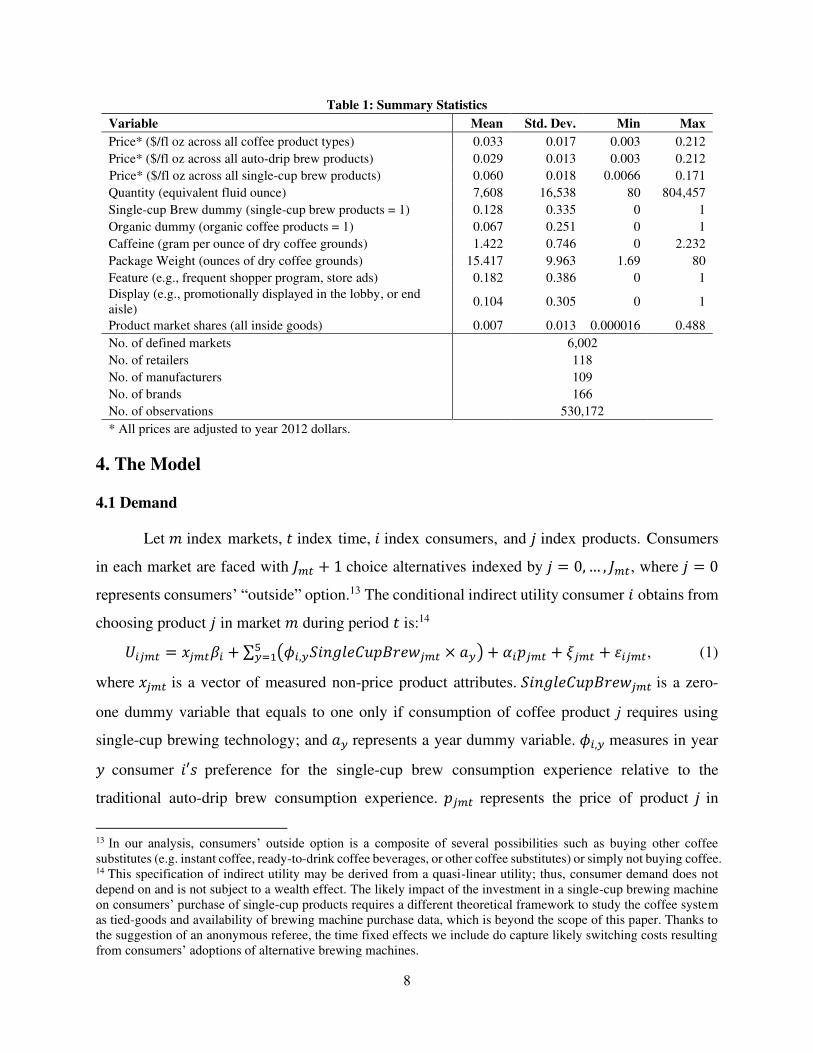
Summary statistics reported in Table 1 suggest that the average price of single-cup brew
coffee products is about twice the average price of auto-drip brew products. Product quantity sold
during a given month has an average of 7,608 equivalent fl oz, and the average product share is
0.7% in a market. Single-cup Brew is a zero-one dummy variable that takes a value of 1 if a coffee
product is designed to use the single-cup brewing technology, and a value of 0 if the product is
designed to use the traditional auto-drip brew method. The data summary shows that 12.8% of the
coffee products in the data sample are single-cup brew products. Organic is also a zero-one dummy
variable that takes a value of 1 only if a product is designated as organic coffee, and 0 otherwise.
The average caffeine contained in one ounce of dry coffee grounds is 1.42 grams across all
products in the data.11 Package Weight is a variable that measures the net weight in ounces of dry
coffee grounds contained in the package. This variable will be used to capture consumers’
preference for the product package size. “Feature” and “Display” are each zero-one dummy
variables that describe the marketing strategies used by retail stores for each product during a given
period and are considered to influence consumer brand choice and loyalty.12
10 This method of computing potential market size is similar to the “potential market factor” method in Ivaldi and Verboven (2005). 11 Caffeine is a major pharmacologically active compound in coffee beans, and it is a mild central nervous system stimulant [de Mejia and Ramirez-Mares (2014)]. Coffee, like other caffeinated soft drinks, acts as a stimulant beverage. 12 See Hwang and Thomadsen (2015), Bronnenberg et al. (2012) and Boatwright et al. (2004). Coffee is one of the most frequently promoted consumer packaged goods (CPGs) according to Boatwright et al. (2004).
8
Table 1: Summary Statistics
Variable Mean Std. Dev. Min Max
Price* ($/fl oz across all coffee product types) 0.033 0.017 0.003 0.212
Price* ($/fl oz across all auto-drip brew products) 0.029 0.013 0.003 0.212
Price* ($/fl oz across all single-cup brew products) 0.060 0.018 0.0066 0.171
Quantity (equivalent fluid ounce) 7,608 16,538 80 804,457
Single-cup Brew dummy (single-cup brew products = 1) 0.128 0.335 0 1
Organic dummy (organic coffee products = 1) 0.067 0.251 0 1
Caffeine (gram per ounce of dry coffee grounds) 1.422 0.746 0 2.232
Package Weight (ounces of dry coffee grounds) 15.417 9.963 1.69 80
Feature (e.g., frequent shopper program, store ads) 0.182 0.386 0 1
Display (e.g., promotionally displayed in the lobby, or end aisle)
0.104 0.305 0 1
Product market shares (all inside goods) 0.007 0.013 0.000016 0.488
No. of defined markets 6,002
No. of retailers 118
No. of manufacturers 109
No. of brands 166
No. of observations 530,172
* All prices are adjusted to year 2012 dollars.
4. The Model
4.1 Demand
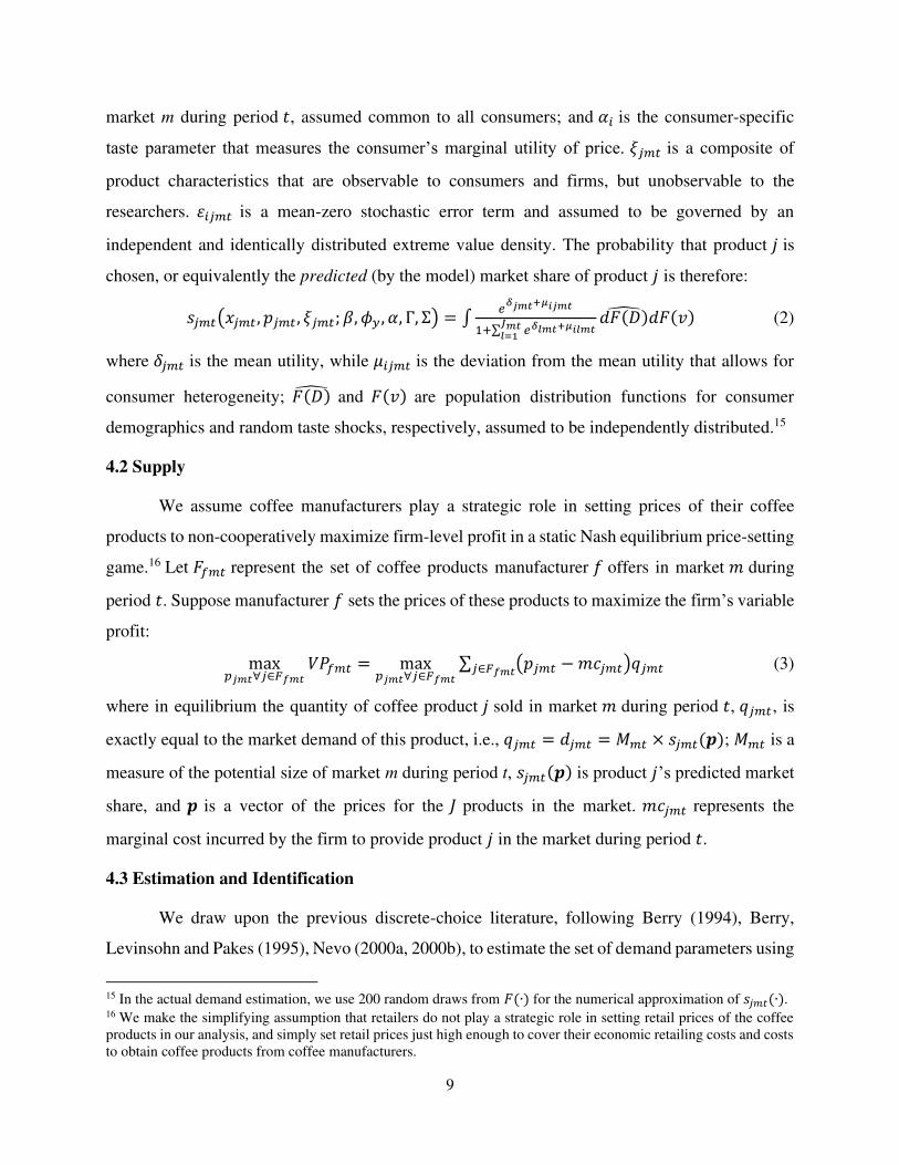
Let 𝑚 index markets, 𝑡 index time, 𝑖 index consumers, and 𝑗 index products. Consumers
in each market are faced with 𝐽𝑚𝑡 + 1 choice alternatives indexed by 𝑗 = 0, … , 𝐽𝑚𝑡, where 𝑗 = 0
represents consumers’ “outside” option.13 The conditional indirect utility consumer 𝑖 obtains from
choosing product 𝑗 in market 𝑚 during period 𝑡 is:14 𝑈𝑖𝑗𝑚𝑡 = 𝑥𝑗𝑚𝑡𝛽𝑖 + ∑ (𝜙𝑖,𝑦𝑆𝑖𝑛𝑔𝑙𝑒𝐶𝑢𝑝𝐵𝑟𝑒𝑤𝑗𝑚𝑡 × 𝑎𝑦)5𝑦=1 + 𝛼𝑖𝑝𝑗𝑚𝑡 + 𝜉𝑗𝑚𝑡 + 𝜀𝑖𝑗𝑚𝑡, (1)
where 𝑥𝑗𝑚𝑡 is a vector of measured non-price product attributes. 𝑆𝑖𝑛𝑔𝑙𝑒𝐶𝑢𝑝𝐵𝑟𝑒𝑤𝑗𝑚𝑡 is a zero-
one dummy variable that equals to one only if consumption of coffee product j requires using
single-cup brewing technology; and 𝑎𝑦 represents a year dummy variable. 𝜙𝑖,𝑦 measures in year 𝑦 consumer 𝑖′𝑠 preference for the single-cup brew consumption experience relative to the
traditional auto-drip brew consumption experience. 𝑝𝑗𝑚𝑡 represents the price of product 𝑗 in
13 In our analysis, consumers’ outside option is a composite of several possibilities such as buying other coffee substitutes (e.g. instant coffee, ready-to-drink coffee beverages, or other coffee substitutes) or simply not buying coffee. 14 This specification of indirect utility may be derived from a quasi-linear utility; thus, consumer demand does not depend on and is not subject to a wealth effect. The likely impact of the investment in a single-cup brewing machine on consumers’ purchase of single-cup products requires a different theoretical framework to study the coffee system as tied-goods and availability of brewing machine purchase data, which is beyond the scope of this paper. Thanks to the suggestion of an anonymous referee, the time fixed effects we include do capture likely switching costs resulting from consumers’ adoptions of alternative brewing machines.
9
market m during period 𝑡, assumed common to all consumers; and 𝛼𝑖 is the consumer-specific
taste parameter that measures the consumer’s marginal utility of price. 𝜉𝑗𝑚𝑡 is a composite of
product characteristics that are observable to consumers and firms, but unobservable to the
researchers. 𝜀𝑖𝑗𝑚𝑡 is a mean-zero stochastic error term and assumed to be governed by an
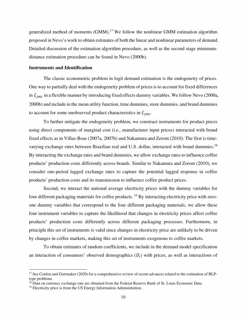
independent and identically distributed extreme value density. The probability that product 𝑗 is
chosen, or equivalently the predicted (by the model) market share of product 𝑗 is therefore: 𝑠𝑗𝑚𝑡(𝑥𝑗𝑚𝑡 , 𝑝𝑗𝑚𝑡 , 𝜉𝑗𝑚𝑡; 𝛽, 𝜙𝑦 , 𝛼, Γ, Σ) = ∫ 𝑒𝛿𝑗𝑚𝑡+𝜇𝑖𝑗𝑚𝑡1+∑ 𝑒𝛿𝑙𝑚𝑡+𝜇𝑖𝑙𝑚𝑡𝐽𝑚𝑡𝑙=1 𝑑𝐹(𝐷)̂ 𝑑𝐹(𝑣) (2)
where 𝛿𝑗𝑚𝑡 is the mean utility, while 𝜇𝑖𝑗𝑚𝑡 is the deviation from the mean utility that allows for
consumer heterogeneity; 𝐹(𝐷)̂ and 𝐹(𝑣) are population distribution functions for consumer
demographics and random taste shocks, respectively, assumed to be independently distributed.15
4.2 Supply
We assume coffee manufacturers play a strategic role in setting prices of their coffee
products to non-cooperatively maximize firm-level profit in a static Nash equilibrium price-setting
game.16 Let 𝐹𝑓𝑚𝑡 represent the set of coffee products manufacturer 𝑓 offers in market 𝑚 during
period 𝑡. Suppose manufacturer 𝑓 sets the prices of these products to maximize the firm’s variable
profit: max𝑝𝑗𝑚𝑡∀𝑗∈𝐹𝑓𝑚𝑡 𝑉𝑃𝑓𝑚𝑡 = max𝑝𝑗𝑚𝑡∀𝑗∈𝐹𝑓𝑚𝑡 ∑ (𝑝𝑗𝑚𝑡 − 𝑚𝑐𝑗𝑚𝑡)𝑞𝑗𝑚𝑡𝑗∈𝐹𝑓𝑚𝑡 (3)
where in equilibrium the quantity of coffee product 𝑗 sold in market 𝑚 during period 𝑡, 𝑞𝑗𝑚𝑡, is
exactly equal to the market demand of this product, i.e., 𝑞𝑗𝑚𝑡 = 𝑑𝑗𝑚𝑡 = 𝑀𝑚𝑡 × 𝑠𝑗𝑚𝑡(𝒑); 𝑀𝑚𝑡 is a
measure of the potential size of market m during period t, 𝑠𝑗𝑚𝑡(𝒑) is product 𝑗’s predicted market
share, and 𝒑 is a vector of the prices for the 𝐽 products in the market. 𝑚𝑐𝑗𝑚𝑡 represents the
marginal cost incurred by the firm to provide product 𝑗 in the market during period 𝑡.
4.3 Estimation and Identification
We draw upon the previous discrete-choice literature, following Berry (1994), Berry,
Levinsohn and Pakes (1995), Nevo (2000a, 2000b), to estimate the set of demand parameters using
15 In the actual demand estimation, we use 200 random draws from 𝐹(∙) for the numerical approximation of 𝑠𝑗𝑚𝑡(∙). 16 We make the simplifying assumption that retailers do not play a strategic role in setting retail prices of the coffee products in our analysis, and simply set retail prices just high enough to cover their economic retailing costs and costs to obtain coffee products from coffee manufacturers.
10
generalized method of moments (GMM).17 We follow the nonlinear GMM estimation algorithm
proposed in Nevo’s work to obtain estimates of both the linear and nonlinear parameters of demand.
Detailed discussion of the estimation algorithm procedure, as well as the second stage minimum-
distance estimation procedure can be found in Nevo (2000b).
Instruments and Identification
The classic econometric problem in logit demand estimation is the endogeneity of prices.
One way to partially deal with the endogeneity problem of prices is to account for fixed differences
in 𝜉𝑗𝑚𝑡 in a flexible manner by introducing fixed effects dummy variables. We follow Nevo (2000a,
2000b) and include in the mean utility function, time dummies, store dummies, and brand dummies
to account for some unobserved product characteristics in 𝜉𝑗𝑚𝑡.
To further mitigate the endogeneity problem, we construct instruments for product prices
using direct components of marginal cost (i.e., manufacturer input prices) interacted with brand
fixed effects as in Villas-Boas (2007a, 2007b) and Nakamura and Zerom (2010). The first is time-
varying exchange rates between Brazilian real and U.S. dollar, interacted with brand dummies.18
By interacting the exchange rates and brand dummies, we allow exchange rates to influence coffee
products’ production costs differently across brands. Similar to Nakamura and Zerom (2010), we
consider one-period lagged exchange rates to capture the potential lagged response in coffee
products’ production costs and its transmission to influence coffee product prices.
Second, we interact the national average electricity prices with the dummy variables for
four different packaging materials for coffee products. 19 By interacting electricity price with zero-
one dummy variables that correspond to the four different packaging materials, we allow these
four instrument variables to capture the likelihood that changes in electricity prices affect coffee
products’ production costs differently across different packaging processes. Furthermore, in
principle this set of instruments is valid since changes in electricity price are unlikely to be driven
by changes in coffee markets, making this set of instruments exogenous to coffee markets.
To obtain estimates of random coefficients, we include in the demand model specification
an interaction of consumers’ observed demographics (𝐷𝑖) with prices, as well as interactions of
17 See Conlon and Gortmaker (2020) for a comprehensive review of recent advances related to the estimation of BLP-type problems. 18 Data on currency exchange rate are obtained from the Federal Reserve Bank of St. Louis Economic Data. 19 Electricity price is from the US Energy Information Administration.
11
consumers’ unobserved preference shocks ( 𝑣𝑖 ) with prices, the single-cup dummy, and the
intercept, respectively. 20 The coefficients of these interaction variables serve to distinguish the
estimated substitution patterns from those implied by a simple logit model, and better capture the
heterogeneity in preferences across consumers. According to Nevo (2000b), to tie consumer
demographic variables to observed purchases, one needs to have in their data several markets with
variation in the distribution of demographics. Therefore, the random taste parameters in our
demand model can be identified based on the rich distributional variation of the demographics
obtained from Census PUMS data on a market-by-market basis, and the assumed standard normal
distribution of the unobserved preference shocks.21
To identify the coefficient that captures consumers’ income-driven heterogeneous
preference for price changes, the instrument we use is constructed by interacting the second set of
instruments for prices described above with median personal income for the population of aged
sixteen and above in the county where the relevant coffee products are sold. It is reasonable to
believe that the unobserved product characteristics contained in 𝜉𝑗𝑚𝑡 after controlling for time
fixed effects, store fixed effects, and brand fixed effects, are most likely uncorrelated with the
county-level average wealth level.
To identify the standard deviations of the random coefficients on price, the single-cup
dummy variable, and the constant term, we follow Gandhi and Houde (2020) and construct product
differentiation instruments along three dimensions.22 The differentiation measure along prices is
constructed by computing the Euclidian distance between a product’s predicted price and predicted
prices of rival products, where the predicted prices are generated from an ordinary least squares
20 A special note regarding the single-cup dummy variable in our demand model specification is that, based on discussions in Conlon and Mortimer (2013), random coefficients on categorical variables may not be identified when there is a lack of variation in price and product dummies are included in the estimation. In our paper, with the richness of price variations across products and markets, we do not have such concern. 21 Berry and Haile (2014, 2016) raised a concern regarding the identification of parameters that govern the distribution of the random coefficients. In this paper, we believe the richness and the panel structure of our data, as well as the additional information obtained from Census PUMS demographic data across more than 6002 markets makes it possible to have sufficient variations across markets that help identify the substitution parameters in the random component. A careful exploration of our data reveals that the set of available products not only varies by time periods for a given geographic area (zip code and county), but also varies by geographic areas for a given period. 22 We appreciate an anonymous referee for helpful suggestions on constructing these instrument variables, which help identify the random coefficients. For the construction of these differentiation instruments, we refer the reader to Table 12 in Gandhi and Houde (2020). The predicted prices are obtained from a reduced-form regression of prices on all the non-price product characteristics as well as the exogenous cost-shifters and fixed effects previously discussed.
12
(OLS) estimated reduced-form price regression.23 The differentiation instrument for the single-cup
dummy is the number of rival products in the market that have the same coffee type attribute
(single-cup versus auto-drip) as the given product in question.24 This instrument proxies the
amount of competition faced by each product with respect to its single-cup feature. The
differentiation instrument for the intercept is computed by interacting each product’s own
predicted price with the sum of differences between the product’s and rival products’ predicted
prices.25 It captures the fact that low quality (priced) products tend to be closer substitutes for the
outside good compared to higher quality (priced) products. The variations in these differentiation
measures induce consumer substitution along these dimensions, and thus identify the standard
deviation preference parameters for the random coefficients.
Last, we also include a standard instrument used by many empirical industrial organization
studies: the total number of coffee products offered in a market, which identifies the standard
deviation preference parameter on the intercept. The intuition is that as the number of coffee
products offered in the market increases (i.e., more inside goods become available in the market),
consumers are more likely to be induced away from the outside option to the inside goods.26
5. Empirical Results
Demand
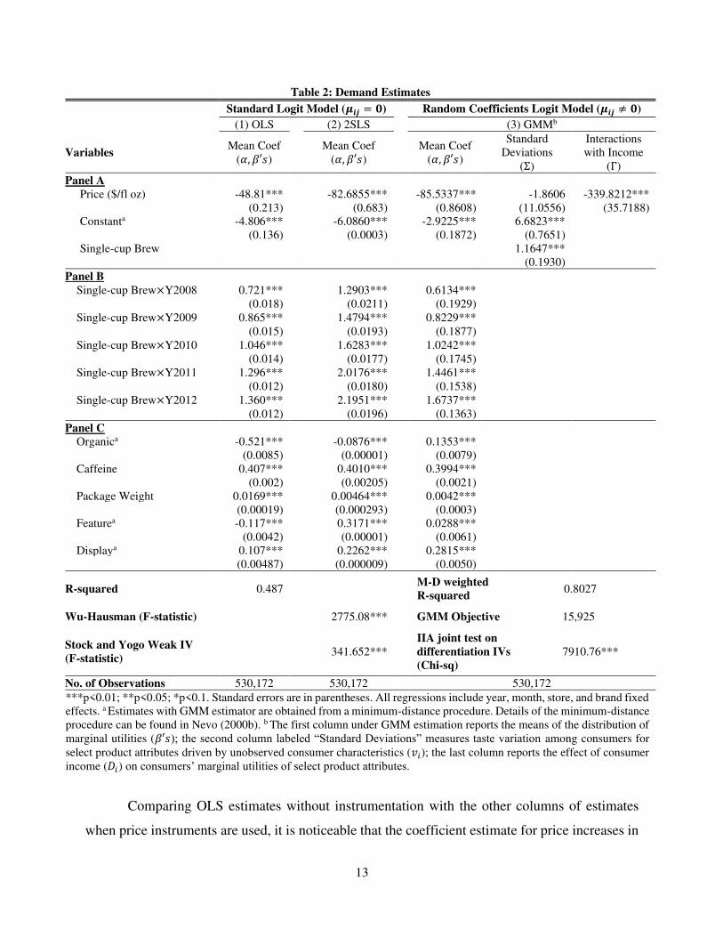
The demand model estimates are reported in Table 2. The first column reports parameter
estimates from the standard logit model using the ordinary least squares (OLS) estimator, while
the second column reports standard logit model parameter estimates using two-stage least squares
(2SLS) estimator with product prices instrumented using the set of instruments discussed in the
previous section. Parameter estimates from the random coefficients logit demand model using
generalized method of moments (GMM) are reported in the last three columns, where consumer
heterogeneity is considered by allowing the coefficient on coffee product price and other product
characteristics to vary across individual consumers.
23 As in Gandhi and Houde (2020), the Euclidian distance instrument for prices is defined as:√∑ (�̂�𝑗′𝑡 − �̂�𝑗𝑡)𝑗′≠𝑗∈𝐽𝑡 2.
24 The differentiation instrument for the discrete product attribute of whether or not the relevant product in question is
single-cup is defined as: ∑ 1{𝑥𝑗′𝑡,𝑠𝑖𝑛𝑔𝑙𝑒−𝑐𝑢𝑝 = 𝑥𝑗𝑡,𝑠𝑖𝑛𝑔𝑙𝑒−𝑐𝑢𝑝}𝑗′≠𝑗∈𝐽𝑡 . 25 The differentiation instrument for the intercept is defined as: �̂�𝑗𝑡 × (∑ (�̂�𝑗′𝑡 − �̂�𝑗𝑡)𝑗′≠𝑗∈𝐽𝑡 ). 26 See a similar argument in Sullivan (2020) and Miller and Weinberg (2017).
13
Table 2: Demand Estimates Standard Logit Model (𝝁𝒊𝒋 = 𝟎) Random Coefficients Logit Model (𝝁𝒊𝒋 ≠ 𝟎) (1) OLS (2) 2SLS (3) GMMb
Variables Mean Coef
(𝛼, 𝛽′𝑠) Mean Coef
(𝛼, 𝛽′𝑠) Mean Coef
(𝛼, 𝛽′𝑠)
Standard Deviations
(Σ)
Interactions with Income
(Γ)
Panel A Price ($/fl oz) -48.81*** -82.6855*** -85.5337*** -1.8606 -339.8212*** (0.213) (0.683) (0.8608) (11.0556) (35.7188) Constanta -4.806*** -6.0860*** -2.9225*** 6.6823*** (0.136) (0.0003) (0.1872) (0.7651) Single-cup Brew 1.1647*** (0.1930)
Panel B Single-cup Brew×Y2008 0.721*** 1.2903*** 0.6134***
(0.018) (0.0211) (0.1929) Single-cup Brew×Y2009 0.865*** 1.4794*** 0.8229***
(0.015) (0.0193) (0.1877) Single-cup Brew×Y2010 1.046*** 1.6283*** 1.0242***
(0.014) (0.0177) (0.1745) Single-cup Brew×Y2011 1.296*** 2.0176*** 1.4461***
(0.012) (0.0180) (0.1538) Single-cup Brew×Y2012 1.360*** 2.1951*** 1.6737***
(0.012) (0.0196) (0.1363)
Panel C Organica -0.521*** -0.0876*** 0.1353***
(0.0085) (0.00001) (0.0079)
Caffeine 0.407*** 0.4010*** 0.3994*** (0.002) (0.00205) (0.0021)
Package Weight 0.0169*** 0.00464*** 0.0042*** (0.00019) (0.000293) (0.0003)
Featurea -0.117*** 0.3171*** 0.0288*** (0.0042) (0.00001) (0.0061)
Displaya 0.107*** 0.2262*** 0.2815*** (0.00487) (0.000009) (0.0050)
R-squared 0.487 M-D weighted
R-squared 0.8027
Wu-Hausman (F-statistic) 2775.08*** GMM Objective 15,925
Stock and Yogo Weak IV
(F-statistic) 341.652***
IIA joint test on
differentiation IVs
(Chi-sq) 7910.76***
No. of Observations 530,172 530,172 530,172
***p<0.01; **p<0.05; *p<0.1. Standard errors are in parentheses. All regressions include year, month, store, and brand fixed effects. a Estimates with GMM estimator are obtained from a minimum-distance procedure. Details of the minimum-distance procedure can be found in Nevo (2000b). b The first column under GMM estimation reports the means of the distribution of marginal utilities (𝛽′𝑠); the second column labeled “Standard Deviations” measures taste variation among consumers for select product attributes driven by unobserved consumer characteristics (𝑣𝑖); the last column reports the effect of consumer income (𝐷𝑖) on consumers’ marginal utilities of select product attributes.
Comparing OLS estimates without instrumentation with the other columns of estimates
when price instruments are used, it is noticeable that the coefficient estimate for price increases in
14
absolute value with instrumentation. The Wu-Hausman test statistic confirms the endogeneity of
price by rejecting the exogeneity of price at the 1% level, suggesting that the OLS estimation
produces a biased and inconsistent estimate of the price coefficient. Furthermore, the Stock and
Yogo (2005) weak instrument test statistic rejects the null hypothesis that the instruments used for
price are weak.
To further investigate the possibility of weak identification problems, we follow Gandhi
and Houde (2020) and use the differentiation instruments discussed previously to perform the
Independence of Irrelevant Alternatives (IIA) hypothesis test. 27 The IIA joint test statistics
validates the ability of our product differentiation instruments to identify deviations of the random
coefficients from the standard logit preferences. We focus the remainder of our analysis on demand
estimates obtained from the random coefficients model using the GMM estimator.
We find the mean coefficient estimate for price is negative and statistically significant at
the 1% level, indicating coffee price, on average, has a negative impact on consumers’ mean utility.
All else equal, an increase in a product’s price reduces the probability that a typical coffee drinker
chooses this product. The observable variation across markets in consumer demographics
(measured by draws of consumers’ income in our study) seems to drive deviations from the mean
price sensitivity significantly, providing evidence that consumers are heterogeneous with respect
to their sensitivity to price changes of coffee products. The parameter estimate for the interaction
of unobserved variation in consumers’ tastes in the population with the constant term, which
measures heterogeneity in consumers’ valuation for the outside option, is statistically significant
at the 1% level, suggesting statistically discernable heterogeneity across consumers’ in their
valuation of the outside option.
To assess how much consumers value their coffee consumption experience using the
single-cup brewing technology relative to the traditional auto-drip method, and how their valuation
varies across time, we focus on the parameter estimates for the interactions of single-cup dummy
with the year dummies, reported in Panel B of Table 2. These parameter estimates are all positive
and statistically significant at the 1% level, suggesting a relative preference for the single-cup brew
attribute over the traditional auto-drip brewing method. In addition, this relative preference
increases year after year. To be specific, for the average coffee drinker, the single-cup consumption
27 See Gandhi and Houde (2020) for details of how to test for weak identification issues in random coefficients demand models.
15
experience has the greatest positive marginal utility in year 2012, and the smallest in year 2008.
This finding holds regardless of the estimators used according to the relevant estimates in columns
(1) and (2). What’s more, in case of the random coefficients demand model, the parameter estimate
on the interaction of unobservable variation in consumers’ tastes in the population with the Single-
cup Brew dummy reported in Panel A is statistically significant, suggesting that there is statistically
discernable heterogeneity in preferences for the single-cup brew attribute versus auto-drip brewing
method.
We now turn to discuss estimates for other product characteristics that affect consumer
choice, reported in Panel C of Table 2. For an average coffee drinker, organic coffee produces a
positive marginal utility, suggesting that, holding the impact of other demand factors constant,
organic coffee products are favored to non-organic coffee during the sample period. The other
demand-shifters all have expected demand impacts and are consistent with findings in previous
studies. For example, the coefficient estimate associated with the caffeine content variable is
positive and statistically significant, suggesting that, holding all other coffee demand factors
constant, consumers prefer coffee products that have higher caffeine content. Bonnet and Villas-
Boas (2016) found consumers have significant and negative preference for caffeine-free products;
thereby, a typical coffee drinker prefers coffee products that are not decaffeinated.
The package size, measured by the net mass weight of the package, has a statistically
significant positive marginal utility for the average consumer. This result is similar to findings in
Guadagni and Little (1998) and Ansari et al. (1995). Prendergast and Marr (1997) argue that larger
packaged consumer goods normally reflect better value to average consumers, and consumers tend
to choose larger packaged products as they are more likely to stand out on the shelf.
Last, the variables capturing the promotional activities (e.g., featured by frequent shopper
programs or advantageously displayed at the end of an aisle) both have a positive and statistically
significant coefficient estimate, suggesting that these promotional activities for a given coffee
product serve to increase consumers’ demand for the product. This finding is consistent with
results in previous studies such as Guadagni and Little (1998), Gupta (1988), Lattin and Bucklin
(1989), Grover and Srinivasan (1992), Boatwright et al. (2004), Ansari et al. (1995).28
28 These studies all provide empirical evidence that promotional activities have a positive impact on coffee demand. Gupta (1988), for example, argues that promotion enhances a brand’s value, which in turn enhances the probability of products of this brand being selected by consumers.
16
Elasticities of Demand Estimates
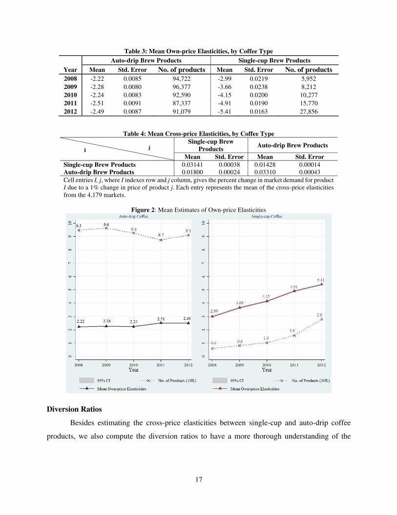
Table 3 reports the average own-price elasticities for the auto-drip and single-cup brew
coffee products in each sample year. Our demand model yields average own-price elasticity for
auto-drip brew coffee products within a given year ranging from -2.22 to -2.51 across the years in
our sample, while for single-cup brew coffee products the average own-price elasticity estimate
ranges from -2.99 to -5.41, overall greater in magnitude than the mean estimates of auto-drip
products. This result is clearly observed from the line charts in Figure 2, where we plot the absolute
values of the mean elasticities and the total number of products available in each year. The plots
in Figure 2 reveal that consumers’ price sensitivity for single-cup coffee products grew at a faster
rate than their price sensitivity for auto-drip coffee products, possibly due to the fast growth of
single-cup products available in the market. The confidence intervals in the figure show that at a
95% level of statistical confidence our model-predicted own-price elasticities are all different from
zero.
The own-price elasticity estimates of traditional auto-drip brew coffee products in this
paper tend to be slightly smaller in magnitude compared to analogous estimates obtained in some
studies: Krishnamurthi and Raj (1991) (3.6 to 8.2); Broda and Weinstein (2006) (3.1); Foster et al.
(2008) (3.65); Villas-Boas (2007b) (5.6 to 6.8); and Nakamura and Zerom (2010) (3.96).
Chintagunta et al. (2018) provide an own-price elasticity estimate of 3.6 in absolute magnitude for
single-cup brew coffee products in coffee markets in Portugal; and Ellickson et al. (2018) report
their own-price elasticity estimate for single-cup products of 2.89 in absolute value. Both estimates
are within the range of our estimated own-price elasticities for single-cup coffee products in U.S.
markets.
Compared to the own-price elasticity estimates, cross-price elasticity of demand estimates
in Table 4 are relatively small in magnitude, but all estimates are positive and statistically different
from zero, suggesting that consumers do perceive the coffee products in our sample as substitutable
both within and across the two product types.29
29 Cross-price elasticity estimates for consumer-packaged goods sold in grocery chains tend to be relatively small. For example, the estimated cross-price elasticities across ready-to-eat cereal brands in Nevo (2000b) range from 0.05 to 0.4. The cross-price elasticity estimates across bath-tissue brands in Hausman and Leonard (2002) range from 0.01 to 0.7. The cross-price elasticities across yogurt brands estimated in Villas-Boas (2007a) range from 0.018 to 0.032.
17
Table 3: Mean Own-price Elasticities, by Coffee Type Auto-drip Brew Products Single-cup Brew Products
Year Mean Std. Error No. of products Mean Std. Error No. of products
2008 -2.22 0.0085 94,722 -2.99 0.0219 5,952
2009 -2.28 0.0080 96,377 -3.66 0.0238 8,212
2010 -2.24 0.0083 92,590 -4.15 0.0200 10,277
2011 -2.51 0.0091 87,337 -4.91 0.0190 15,770
2012 -2.49 0.0087 91,079 -5.41 0.0163 27,856
Table 4: Mean Cross-price Elasticities, by Coffee Type
I j
Single-cup Brew
Products Auto-drip Brew Products
Mean Std. Error Mean Std. Error
Single-cup Brew Products 0.03141 0.00038 0.01428 0.00014 Auto-drip Brew Products 0.01800 0.00024 0.03310 0.00043
Cell entries I, j, where I indexes row and j column, gives the percent change in market demand for product I due to a 1% change in price of product j. Each entry represents the mean of the cross-price elasticities from the 4,179 markets.
Figure 2: Mean Estimates of Own-price Elasticities
Diversion Ratios
Besides estimating the cross-price elasticities between single-cup and auto-drip coffee
products, we also compute the diversion ratios to have a more thorough understanding of the
18
substitution characteristics among the two coffee types as well as with the outside option.30 Though
diversion ratios are known to be extensively examined in antitrust analyses,31 more broadly, they
provide an alternative perspective for understanding the substitution attributes in markets with
differentiated products, which Conlon and Mortimer (2021) argue cannot be captured by cross-
price elasticities.
The diversion ratio from product 𝑗 to product 𝑘, 𝐷𝑗𝑘, answers the following question: If the
price of product 𝑗 were to rise, what fraction of the customers leaving product 𝑗 would switch to
product 𝑘 (Shapiro, 1995, 2010)? For the random-coefficients logit demand model, we compute
individual 𝑖’s diversion ratio from product 𝑗 to product 𝑘 as 𝐷𝑖,𝑗𝑘 = (𝜕𝑠𝑖𝑘𝜕𝑝𝑗 ) |𝜕𝑠𝑖𝑗𝜕𝑝𝑗|⁄ for a small price
change, with individual weight function, 𝑤𝑖𝑗, described in Conlon and Mortimer (2021). So, the
diversion ratio, 𝐷𝑗𝑘, is simply the weighted-average diversion across all the sampled individuals
who consumed product 𝑗 in the given market.32 For a market with 𝐽 products, we obtain a 𝐽 × 𝐽
square matrix of weighted-average diversion ratio estimates for each product 𝑗 with respect to all
other products, 𝑘 ≠ 𝑗, offered in the market, with zeros inserted on the main diagonal of the matrix.
The individual diversion ratio from product 𝑗 to the outside option is given by: 𝐷𝑖,𝑗0 =(𝜕𝑠𝑖0𝜕𝑝𝑗 ) |𝜕𝑠𝑖𝑗𝜕𝑝𝑗|⁄ , with the above-mentioned individual weights.
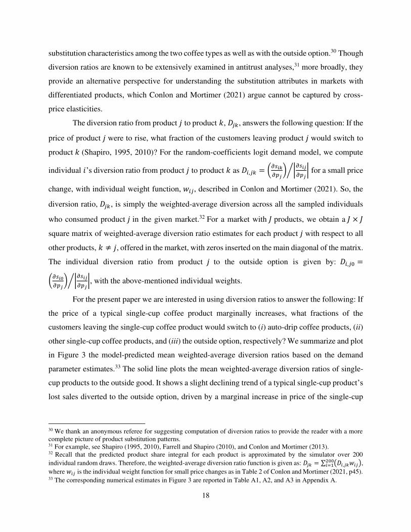
For the present paper we are interested in using diversion ratios to answer the following: If
the price of a typical single-cup coffee product marginally increases, what fractions of the
customers leaving the single-cup coffee product would switch to (i) auto-drip coffee products, (ii)
other single-cup coffee products, and (iii) the outside option, respectively? We summarize and plot
in Figure 3 the model-predicted mean weighted-average diversion ratios based on the demand
parameter estimates.33 The solid line plots the mean weighted-average diversion ratios of single-
cup products to the outside good. It shows a slight declining trend of a typical single-cup product’s
lost sales diverted to the outside option, driven by a marginal increase in price of the single-cup
30 We thank an anonymous referee for suggesting computation of diversion ratios to provide the reader with a more complete picture of product substitution patterns. 31 For example, see Shapiro (1995, 2010), Farrell and Shapiro (2010), and Conlon and Mortimer (2013). 32 Recall that the predicted product share integral for each product is approximated by the simulator over 200
individual random draws. Therefore, the weighted-average diversion ratio function is given as: 𝐷𝑗𝑘 = ∑ (𝐷𝑖,𝑗𝑘𝑤𝑖𝑗)200𝑖=1 ,
where 𝑤𝑖𝑗 is the individual weight function for small price changes as in Table 2 of Conlon and Mortimer (2021, p45). 33 The corresponding numerical estimates in Figure 3 are reported in Table A1, A2, and A3 in Appendix A.
19
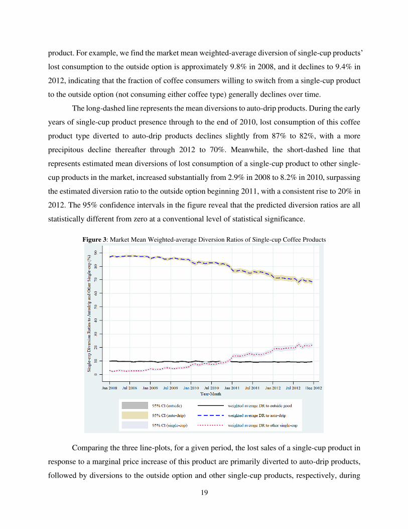
product. For example, we find the market mean weighted-average diversion of single-cup products’
lost consumption to the outside option is approximately 9.8% in 2008, and it declines to 9.4% in
2012, indicating that the fraction of coffee consumers willing to switch from a single-cup product
to the outside option (not consuming either coffee type) generally declines over time.
The long-dashed line represents the mean diversions to auto-drip products. During the early
years of single-cup product presence through to the end of 2010, lost consumption of this coffee
product type diverted to auto-drip products declines slightly from 87% to 82%, with a more
precipitous decline thereafter through 2012 to 70%. Meanwhile, the short-dashed line that
represents estimated mean diversions of lost consumption of a single-cup product to other single-
cup products in the market, increased substantially from 2.9% in 2008 to 8.2% in 2010, surpassing
the estimated diversion ratio to the outside option beginning 2011, with a consistent rise to 20% in
2012. The 95% confidence intervals in the figure reveal that the predicted diversion ratios are all
statistically different from zero at a conventional level of statistical significance.
Figure 3: Market Mean Weighted-average Diversion Ratios of Single-cup Coffee Products
Comparing the three line-plots, for a given period, the lost sales of a single-cup product in
response to a marginal price increase of this product are primarily diverted to auto-drip products,
followed by diversions to the outside option and other single-cup products, respectively, during
20
the early stage of single-cup products’ presence. However, as the single-cup coffee segment
gradually becomes mature with increased market presence and penetration over time, beginning
in 2011 the lost consumption of a single-cup product is more likely to divert to another single-cup
option available in the market rather than to the outside option. The diversion ratio to the auto-drip
option, nonetheless, is still the largest. As such, it is reasonable to conjecture that if single-cup
coffee products were to be removed from the market, those who initially consume single-cup
products are more likely to switch their consumption to auto-drip products offered in the market
than to the outside option. This suggests that the presence of single-cup coffee products partially
cannibalizes sales of auto-drip coffee products, an inference we further explore in the next section
using counterfactual analysis.
Willingness to Pay (WTP)
Discrete choice models have long been widely applied to derive estimates of willingness-
to-pay (WTP) for various measured product attributes. The WTP for a product attribute is the ratio
of the marginal utility of this attribute to the marginal utility of the cost to obtain this attribute. In
the present paper, one of our research objectives is to understand how much consumers are willing
to pay for their coffee consumption experience that uses single-cup brewing technology relative to
the traditional auto-drip brewing method. An interesting perspective of this WTP measure is to
examine how a typical consumer’s WTP estimate for this single-cup consumption attribute
changes over time. To obtain such estimates, we compute the mean individual WTP across the 200
individuals drawn in each market. The computation uses the individuals’ marginal utility
coefficient estimates on the interaction terms between the single-cup dummy variable and the year
dummies divided by their respective marginal utility coefficient estimates on price across all
markets in each of the sample years.
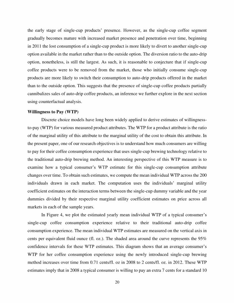
In Figure 4, we plot the estimated yearly mean individual WTP of a typical consumer’s
single-cup coffee consumption experience relative to their traditional auto-drip coffee
consumption experience. The mean individual WTP estimates are measured on the vertical axis in
cents per equivalent fluid ounce (fl. oz.). The shaded area around the curve represents the 95%
confidence intervals for these WTP estimates. This diagram shows that an average consumer’s
WTP for her coffee consumption experience using the newly introduced single-cup brewing
method increases over time from 0.71 cents/fl. oz in 2008 to 2 cents/fl. oz. in 2012. These WTP
estimates imply that in 2008 a typical consumer is willing to pay an extra 7 cents for a standard 10
21
fl. oz. cup of freshly home-brewed coffee using the single-cup brewing method, but in year 2012
this WTP increases to around 20 cents extra for a standard 10 fl. oz. cup of freshly home-brewed
coffee, corresponding to a 180% increase in WTP for the single-cup coffee consumption
experience.
Figure 4: Line Plot of Mean Individual Willingness to Pay (𝑊𝑇𝑃̅̅ ̅̅ ̅̅ ̅), by Year (all counties)
6. Counterfactual Analysis
To examine the market effects of the introduction and growing presence of single-cup brew
coffee products, we follow an approach similar to that in Petrin (2002) by counterfactually
removing the single-cup coffee products from each market.34 This exercise is operationalized by
first removing single-cup coffee products from the data sample, and then use the supply side of
our model to compute on a market-by-market basis the set of auto-drip product prices that satisfy
the remaining set of Nash equilibrium price-setting first-order conditions. By comparing this new
model-predicted price vector with the observed price vector of the pre-existing auto-drip coffee
products, we are able to understand the “price effects” that resulted from the introduction of a new
product, similar to Hausman and Leonard (2002).
To understand the impacts of the new product’s introduction and growing presence on
quantities of the pre-existing products and the outside option, as well as the associated welfare
34 Petrin (2002) evaluates the economic effects of the introduction of the minivan by counterfactually removing the minivans from the market.
22
effects, we undertake two types of comparisons. In the first counterfactual experiment (denoted as
“Counterfactual Experiment 1”), we use the new price vector obtained from the Nash-equilibrium
that is generated based on the counterfactual absence of single-cup products to compute the model-
predicted quantities demand for the auto-drip products and the outside good, respectively. The
comparison between the counterfactual equilibrium quantities evaluated at the new price levels
based on the absence of the new products and the factual model-precited quantities evaluated at
observed price levels, reveals the full demand impacts of the new product introduction on the pre-
existing products and the outside good.
In the second counterfactual experiment (denoted as “Counterfactual Experiment 2”), we
compute the counterfactual equilibrium quantities of auto-drip products and the outside good with
the absence of the new products while holding at their factual observed levels the prices of auto-
drip products. We then compare these counterfactual quantities with the factual model-predicted
quantities evaluated at observed price levels with the presence of the new products. In this exercise,
we aim to understand the pure “variety effects” of the new product introduction by nullifying the
“price effects”, i.e., in this exercise we impose the restriction that prices of the pre-existing
products are unaffected by the market presence of the new product.
In summary, counterfactual experiment 1 captures the full market impacts of the
introduction of the new products, where the full market impacts include both “price effects” and
“variety effects” as discussed in Hausman and Leonard (2002). However, counterfactual
experiment 2 captures only the extent of “variety effects” due to the introduction of the new
products. The reader is referred to Appendix C for details on how the counterfactual experiments
are formally implemented.
6.1 Predicted Changes in Prices of Auto-drip Coffee
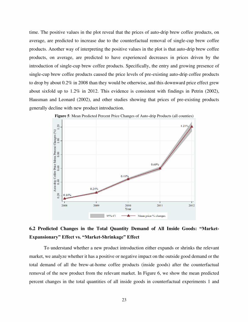
In Figure 5, we summarize and plot the time series variations in the predicted mean percent
price changes of auto-drip coffee products after we counterfactually removed the single-cup
products.35 The plot shows that, in general, the prices of auto-drip coffee products are predicted to
increase during the sample periods; and the magnitude of the price increase becomes larger over
35 Readers may refer to Table A4 in the appendix for detailed numerical estimates. We also find the predicted mean percent price changes in each time period for each of the fifteen counties studied in the data sample are all positive. As such, we can infer that the entry and presence of single-cup products is predicted to have reduced the price levels of auto-drip coffee products in each geographic market. Results for individual counties can be made available upon request.
23
time. The positive values in the plot reveal that the prices of auto-drip brew coffee products, on
average, are predicted to increase due to the counterfactual removal of single-cup brew coffee
products. Another way of interpreting the positive values in the plot is that auto-drip brew coffee
products, on average, are predicted to have experienced decreases in prices driven by the
introduction of single-cup brew coffee products. Specifically, the entry and growing presence of
single-cup brew coffee products caused the price levels of pre-existing auto-drip coffee products
to drop by about 0.2% in 2008 than they would be otherwise, and this downward price effect grew
about sixfold up to 1.2% in 2012. This evidence is consistent with findings in Petrin (2002),
Hausman and Leonard (2002), and other studies showing that prices of pre-existing products
generally decline with new product introduction.
Figure 5: Mean Predicted Percent Price Changes of Auto-drip Products (all counties)
6.2 Predicted Changes in the Total Quantity Demand of All Inside Goods: “Market-
Expansionary” Effect vs. “Market-Shrinkage” Effect
To understand whether a new product introduction either expands or shrinks the relevant
market, we analyze whether it has a positive or negative impact on the outside good demand or the
total demand of all the brew-at-home coffee products (inside goods) after the counterfactual
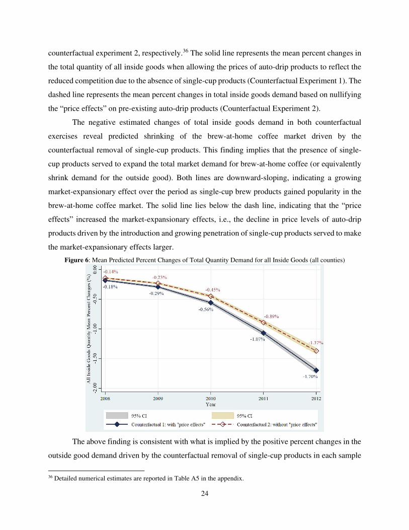
removal of the new product from the relevant market. In Figure 6, we show the mean predicted
percent changes in the total quantities of all inside goods in counterfactual experiments 1 and
24
counterfactual experiment 2, respectively.36 The solid line represents the mean percent changes in
the total quantity of all inside goods when allowing the prices of auto-drip products to reflect the
reduced competition due to the absence of single-cup products (Counterfactual Experiment 1). The
dashed line represents the mean percent changes in total inside goods demand based on nullifying
the “price effects” on pre-existing auto-drip products (Counterfactual Experiment 2).
The negative estimated changes of total inside goods demand in both counterfactual
exercises reveal predicted shrinking of the brew-at-home coffee market driven by the
counterfactual removal of single-cup products. This finding implies that the presence of single-
cup products served to expand the total market demand for brew-at-home coffee (or equivalently
shrink demand for the outside good). Both lines are downward-sloping, indicating a growing
market-expansionary effect over the period as single-cup brew products gained popularity in the
brew-at-home coffee market. The solid line lies below the dash line, indicating that the “price
effects” increased the market-expansionary effects, i.e., the decline in price levels of auto-drip
products driven by the introduction and growing penetration of single-cup products served to make
the market-expansionary effects larger.
Figure 6: Mean Predicted Percent Changes of Total Quantity Demand for all Inside Goods (all counties)
The above finding is consistent with what is implied by the positive percent changes in the
outside good demand driven by the counterfactual removal of single-cup products in each sample
36 Detailed numerical estimates are reported in Table A5 in the appendix.
25
year.37 We find the introduction of single-cup brew coffee products brings into the brew-at-home
coffee market an extra 0.24% more of the potential demand that would otherwise remain outside
the brew-at-home coffee market during 2008, and this percentage grew almost tenfold to 2.28% in
2012. As such, the introduction of single-cup brew coffee products expanded the brew-at-home
coffee market, and this market-expansionary effect grew substantially over time.
6.3 Predicted Changes in Quantity Demand of Auto-drip Products: “Demand-increasing”
Effect vs. “Demand-cannibalizing” Effect
Similarly, to understand whether a new product introduction either increases or
cannibalizes the quantity sales of the pre-existing products in the relevant market, we analyze
whether the counterfactual absence of the new product negatively or positively impacts demand
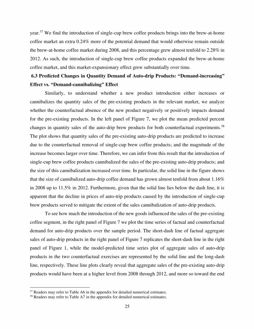
for the pre-existing products. In the left panel of Figure 7, we plot the mean predicted percent
changes in quantity sales of the auto-drip brew products for both counterfactual experiments.38
The plot shows that quantity sales of the pre-existing auto-drip products are predicted to increase
due to the counterfactual removal of single-cup brew coffee products; and the magnitude of the
increase becomes larger over time. Therefore, we can infer from this result that the introduction of
single-cup brew coffee products cannibalized the sales of the pre-existing auto-drip products; and
the size of this cannibalization increased over time. In particular, the solid line in the figure shows
that the size of cannibalized auto-drip coffee demand has grown almost tenfold from about 1.16%
in 2008 up to 11.5% in 2012. Furthermore, given that the solid line lies below the dash line, it is
apparent that the decline in prices of auto-trip products caused by the introduction of single-cup
brew products served to mitigate the extent of the sales cannibalization of auto-drip products.
To see how much the introduction of the new goods influenced the sales of the pre-existing
coffee segment, in the right panel of Figure 7 we plot the time series of factual and counterfactual
demand for auto-drip products over the sample period. The short-dash line of factual aggregate
sales of auto-drip products in the right panel of Figure 7 replicates the short-dash line in the right
panel of Figure 1, while the model-predicted time series plot of aggregate sales of auto-drip
products in the two counterfactual exercises are represented by the solid line and the long-dash
line, respectively. These line plots clearly reveal that aggregate sales of the pre-existing auto-drip
products would have been at a higher level from 2008 through 2012, and more so toward the end
37 Readers may refer to Table A6 in the appendix for detailed numerical estimates. 38 Readers may refer to Table A7 in the appendix for detailed numerical estimates.
26
of the sample period, if single-cup brew coffee products were not introduced to the brew-at-home
coffee market. The two lines representing the quantity sales of auto-drip products obtained from
the two counterfactual experiments, however, suggest small quantity differences at the aggregate
level regarding whether the “price effects” on auto-drip products are accounted for with the
counterfactual absence of single-cup brew products.
Figure 7: Quantity Demand Changes of Auto-drip Products (all counties)
In summary, the evidence provided in Figures 6 and 7 reveal that the introduction and
growing popularity of the single-cup coffee prods, which caused the creation of a whole new
segment, has not only expanded the brew-at-home coffee market (i.e., a “market-expansionary”
effect) but also cannibalized the demand for the pre-existing traditional auto-drip coffee products
(i.e., a “demand-cannibalization” effect) in each of the sample periods. Furthermore, both the sizes
of market-expansionary effect and demand-cannibalization effect are predicted to have quickly
grown over time through the end of sample period.
6.4 Consumer Welfare Analysis
We follow Nevo (2001), McFadden (1984), Small and Rosen (1981), Train (2009), and
many others and compute the change in consumer welfare associated with imposing the
27
counterfactual assumption that single-cup coffee products are no longer available in markets,
leaving consumers options of either auto-drip products or the outside good.
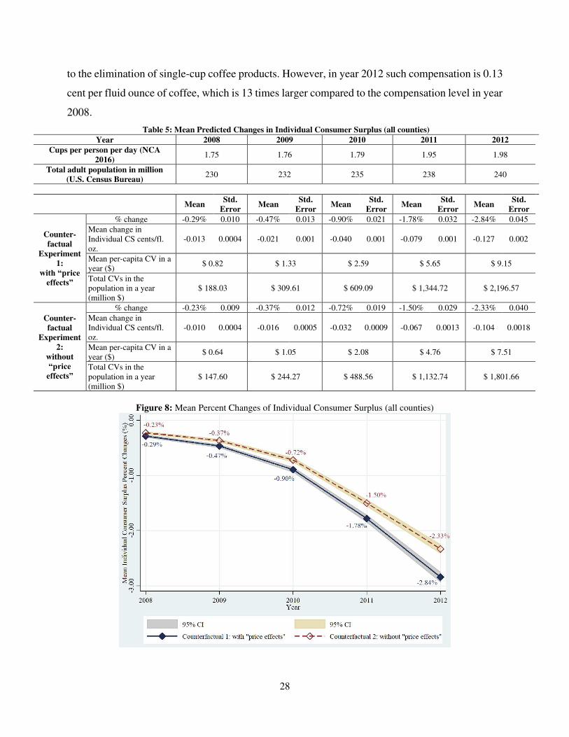
Table 5 summarizes the model-predicted effects on individual consumer welfare due to the
counterfactual elimination of single-cup brew coffee options. Specifically, the table presents the
average predicted percent changes of individual consumer surplus in each of the five years across
all geographic areas in the data sample. These estimates in the table are all negative, ranging from
-0.3% to -2.8%. The decline in estimated consumer welfare is also reflected in Figure 8.39 The
negative percent changes imply that, on average, an individual consumer is predicted to have
benefited from the new product introduction, with year-specific increases in consumer surplus that
grew ninefold from 0.3% in 2008 to 2.8% in 2012. In dollar term, the mean per-capita welfare gain
increases from $0.82 in 2008 to $9.15 in 2012. For comparative purposes, Hausman (1996) reports
estimated individual consumer surplus increases for new brand introduction in the ready-to-eat
cereal market ranging from $0.268 to $0.3136 per year. Estimated gains in consumer surplus
associated with new product introductions in various industries can be found in several studies
[e.g., Petrin (2002); and Hausman and Leonard (2002)].
According to Nevo (2000b), the indirect utility function specified in equation (1) can be
derived from a quasilinear utility function, free of wealth effects. It is reasonable to assume the
wealth effects for the retail-level packaged coffee products are small or negligible, like other
consumer packaged goods, for example, ready-to-eat cereals studied in Nevo (2000a). In this case,
consumer surplus will be very close to both compensating variation (CV) and equivalent variation,
which also means the consumer surplus estimates obtained by equation (6) approximate well the
estimates of compensating variation [see Nevo (2000b)].
In Table 5, we also report the estimated change in individual consumer surplus to
approximate mean individual compensating variations for a typical coffee drinker from 2008
through 2012. In particular, the estimates reported in the table reveal that if single-cup coffee
products are counterfactually removed from markets in year 2008, and given the prices of auto-
drip coffee products that would prevail in counterfactual experiment 1, the typical consumer needs
to be compensated 0.01 cent per fluid ounce of coffee to maintain their welfare at the level prior
39 Readers may refer to Table A8 in the appendix for detailed numerical estimates. The predicted changes in mean individual consumers surplus in each county are all negative with a downward sloping trend over the sample periods, implying the entry and presence of single-cup products is predicted to have increasingly benefited consumers in each individual local market. Results for individual counties can be made available upon request.
28
to the elimination of single-cup coffee products. However, in year 2012 such compensation is 0.13
cent per fluid ounce of coffee, which is 13 times larger compared to the compensation level in year
2008.
Table 5: Mean Predicted Changes in Individual Consumer Surplus (all counties)
Year 2008 2009 2010 2011 2012
Cups per person per day (NCA
2016) 1.75 1.76 1.79 1.95 1.98
Total adult population in million
(U.S. Census Bureau) 230 232 235 238 240
Mean Std.
Error Mean
Std.
Error Mean
Std.
Error Mean
Std.
Error Mean
Std.
Error
Counter-
factual
Experiment
1:
with “price effects”
% change -0.29% 0.010 -0.47% 0.013 -0.90% 0.021 -1.78% 0.032 -2.84% 0.045
Mean change in Individual CS cents/fl. oz.
-0.013 0.0004 -0.021 0.001 -0.040 0.001 -0.079 0.001 -0.127 0.002
Mean per-capita CV in a year ($)
$ 0.82 $ 1.33 $ 2.59 $ 5.65 $ 9.15
Total CVs in the population in a year (million $)
$ 188.03 $ 309.61 $ 609.09 $ 1,344.72 $ 2,196.57
Counter-
factual
Experiment
2:
without
“price effects”
% change -0.23% 0.009 -0.37% 0.012 -0.72% 0.019 -1.50% 0.029 -2.33% 0.040
Mean change in Individual CS cents/fl. oz.
-0.010 0.0004 -0.016 0.0005 -0.032 0.0009 -0.067 0.0013 -0.104 0.0018
Mean per-capita CV in a year ($)
$ 0.64 $ 1.05 $ 2.08 $ 4.76 $ 7.51
Total CVs in the population in a year (million $)
$ 147.60 $ 244.27 $ 488.56 $ 1,132.74 $ 1,801.66
Figure 8: Mean Percent Changes of Individual Consumer Surplus (all counties)
29
If we nullify the price adjustments of auto-drip products in the absence of single-cup
products (counterfactual experiment 2), the estimated mean compensating variation represents the
values to an average consumer associated with the additional product variety in the presence of the
new products, i.e., the “variety effects” as in Hausman and Leonard (2002).40 As shown in Table
5, the CV estimates for counterfactual experiment 2 are generally smaller in magnitude than the
ones for counterfactual experiment 1. This is because the compensating variations in
counterfactual experiment 1 represent the full effect on consumers associated with the presence of
new products, which is the sum of the “variety effect” and the “price effect” on pre-existing
products.
To better put in context the per capita compensating variation estimates, we can use these
per capita estimates to infer the monetary value of the aggregate welfare effects among the adult
population in the U.S. Accordingly, we compute the total annual compensating variations across
the adult population of the U.S. by multiplying together the following: (i) the individual
compensating variation estimate for the given year; (ii) total adult population;41 (iii) the per capita
number of cups (average cup size is 10 fluid ounces) consumed per day;42 and (iv) 365 days. The
results for counterfactual experiment 1, reported in Table 5, suggest that the entire adult population
need to be compensated by a total amount of $188 million in 2008 at the new equilibrium price
levels of traditional auto-drip coffee products in the absence of single-cup products in order to
achieve the “standard of living” when the single-cup options are available. The table also shows
that this total compensating variation increases each year and reaches a level of $2,196 million in
year 2012.
7. Conclusion
New product introductions are particularly proliferating in the “fast-moving” consumer-
packaged goods sectors. This paper aims to understand the market impacts of a new product
associated with its growing presence in the relevant market over time. Our empirical focus is the
U.S. brew-at-home coffee market in which consumers purchase various packaged coffee products
from grocery stores and brew coffee at home for their daily coffee consumption. The introduction
40 Brynjolfsson et.al. (2003) also provided empirical evidence that consumers gain dramatically with increased product variety. 41 Total U.S. population data are obtained from the U.S. Census Bureau population and housing unit estimates. 42 Survey information is obtained from the 2016 report of National Coffee Data Trends from the National Coffee Association (NCA).
30
of single-cup brew coffee products to the grocery chains has not only changed the way many brew-
at-home coffee drinkers brew and consume coffee in daily life, a change from brewing one “pot”
at a time to making one cup at a time, but also altered the overall “landscape” of the U.S. brew-at-
home coffee market.
We use a structural demand model along with an assumption that coffee manufacturers set
prices according to a static Bertrand-Nash equilibrium to enable estimating the economic effects
associated with the introduction and growing presence of single-cup brew coffee products in the
U.S. brew-at-home coffee market. The estimated model is used to implement two counterfactual
experiments that disentangle “price effects” on the pre-existing auto-drip products from pure
“variety effects” associated with market presence of the new product. As such, by counterfactually
nullifying price effects on pre-existing products, we are able to obtain separate estimates of the
impacts of the new product solely due to the product providing an additional variety available to
consumers.
From the demand estimates, we find consumers, on average, prefer consuming brewed
coffee products using the single-cup brew method instead of the traditional auto-drip brew method;
and this relative preference increased substantially over time. In addition, our model predicts that
the average coffee drinker’s willingness-to-pay for a cup of freshly brewed coffee with the new
brewing method in year 2012 is about 180% more than their willingness-to-pay in year 2008.
The counterfactual experiments predict mean decreases in the total quantity sales of all
inside goods (or equivalently increases in the demand for the outside good) and mean increases in
the quantity sales of the auto-drip products when we counterfactually eliminated the single-cup
brew product options. These predicted changes imply the presence of the single-cup brew products
not only has a market-expansionary effect on the brew-at-home coffee market, but also a demand-
cannibalization effect on the quantity sales of the pre-existing auto-drip coffee segment. In addition,
the size of market-expansionary and demand-cannibalization effects both increase in magnitude
over time as single-cup brew products grew in popularity among brew-at-home coffee drinkers.
The estimates obtained from the experiment that captures the “variety effects” after nullifying the
“price effects” are qualitatively similar to the estimates obtained from the experiment that
considers both the “variety effects” and “price effects” associated with the new product
introduction.
31
Last, we compute money-metric welfare changes to individual consumers associated with
the introduction and growing presence of single-cup brew coffee options. Our welfare estimates
suggest that consumers, on average, benefited from the new coffee product introduction, which is
consistent with findings in the literature on new product introductions in other industries.
Estimated individual compensation variations obtained from the experiment that allows the prices
of the pre-existing auto-drip products to reflect the reduced competition in the absence of the new
product suggest that: if single-cup brew options were to be removed from consumers’ choice sets,
then to maintain consumers’ valuation at the level prior to removal of these choice options requires
the average consumer be compensated a dollar amount in year 2012 that is 13 times larger than
the compensation amount in year 2008. Extending the compensating variation estimates to the
entire adult population in the U.S. suggest a compensation amount of $188 million in year 2008
compared to a substantially higher compensation amount of $2,196 million in year 2012. These
positive changes in consumer welfare are in large part due to the increased product variety caused
by the presence of single-cup products, the “variety effects”. Furthermore, the magnitude of the
“variety effects” grew over time as the new products become increasingly popular among coffee
drinkers.
It is worth pointing out some limitations of our analysis. We simplify modeling the supply
side of the market by assuming retailers play a passive role in the price-setting game. Other vertical
relationships between coffee manufacturers and retailers can be examined as a potential extension
of this current work [see, Villas-Boas (2007b) and Hellerstein and Villas-Boas (2010)]. Another
limitation of this study is the inability of modeling consumers’ hardware adoption decisions, i.e.,
consumers purchase decision of coffee brew machines, due to the unavailability of data on
purchases of coffee brew machines. Future research may consider investigating whether various
vertical contracts between manufacturers and retailers influence counterfactual predicted changes
in market outcomes obtained in our study.
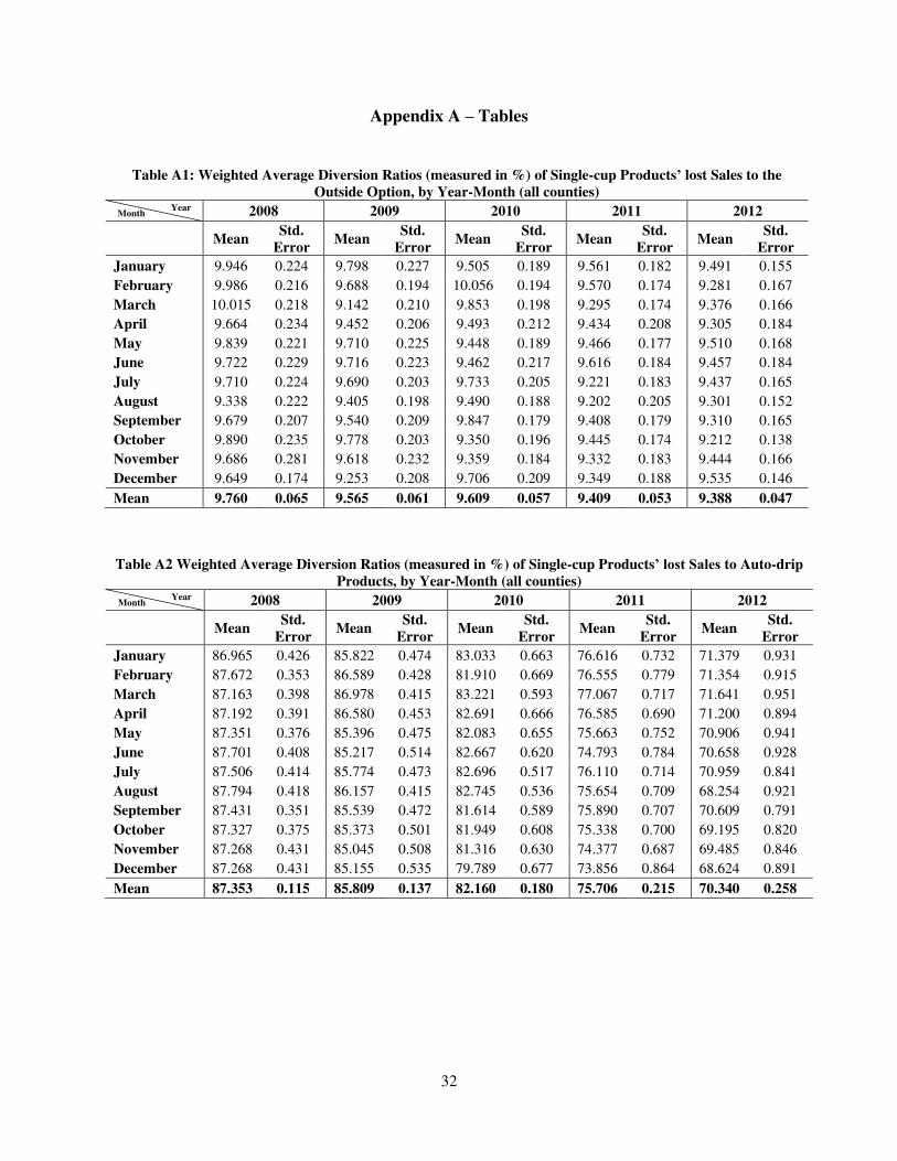
32
Appendix A – Tables
Table A1: Weighted Average Diversion Ratios (measured in %) of Single-cup Products’ lost Sales to the
Outside Option, by Year-Month (all counties)
Month Year 2008 2009 2010 2011 2012
Mean Std.
Error Mean
Std.
Error Mean
Std.
Error Mean
Std.
Error Mean
Std.
Error
January 9.946 0.224 9.798 0.227 9.505 0.189 9.561 0.182 9.491 0.155
February 9.986 0.216 9.688 0.194 10.056 0.194 9.570 0.174 9.281 0.167
March 10.015 0.218 9.142 0.210 9.853 0.198 9.295 0.174 9.376 0.166
April 9.664 0.234 9.452 0.206 9.493 0.212 9.434 0.208 9.305 0.184
May 9.839 0.221 9.710 0.225 9.448 0.189 9.466 0.177 9.510 0.168
June 9.722 0.229 9.716 0.223 9.462 0.217 9.616 0.184 9.457 0.184
July 9.710 0.224 9.690 0.203 9.733 0.205 9.221 0.183 9.437 0.165
August 9.338 0.222 9.405 0.198 9.490 0.188 9.202 0.205 9.301 0.152
September 9.679 0.207 9.540 0.209 9.847 0.179 9.408 0.179 9.310 0.165
October 9.890 0.235 9.778 0.203 9.350 0.196 9.445 0.174 9.212 0.138
November 9.686 0.281 9.618 0.232 9.359 0.184 9.332 0.183 9.444 0.166
December 9.649 0.174 9.253 0.208 9.706 0.209 9.349 0.188 9.535 0.146
Mean 9.760 0.065 9.565 0.061 9.609 0.057 9.409 0.053 9.388 0.047
Table A2 Weighted Average Diversion Ratios (measured in %) of Single-cup Products’ lost Sales to Auto-drip
Products, by Year-Month (all counties)
Month Year 2008 2009 2010 2011 2012
Mean Std.
Error Mean
Std.
Error Mean
Std.
Error Mean
Std.
Error Mean
Std.
Error
January 86.965 0.426 85.822 0.474 83.033 0.663 76.616 0.732 71.379 0.931
February 87.672 0.353 86.589 0.428 81.910 0.669 76.555 0.779 71.354 0.915
March 87.163 0.398 86.978 0.415 83.221 0.593 77.067 0.717 71.641 0.951
April 87.192 0.391 86.580 0.453 82.691 0.666 76.585 0.690 71.200 0.894
May 87.351 0.376 85.396 0.475 82.083 0.655 75.663 0.752 70.906 0.941
June 87.701 0.408 85.217 0.514 82.667 0.620 74.793 0.784 70.658 0.928
July 87.506 0.414 85.774 0.473 82.696 0.517 76.110 0.714 70.959 0.841
August 87.794 0.418 86.157 0.415 82.745 0.536 75.654 0.709 68.254 0.921
September 87.431 0.351 85.539 0.472 81.614 0.589 75.890 0.707 70.609 0.791
October 87.327 0.375 85.373 0.501 81.949 0.608 75.338 0.700 69.195 0.820
November 87.268 0.431 85.045 0.508 81.316 0.630 74.377 0.687 69.485 0.846
December 87.268 0.431 85.155 0.535 79.789 0.677 73.856 0.864 68.624 0.891
Mean 87.353 0.115 85.809 0.137 82.160 0.180 75.706 0.215 70.340 0.258
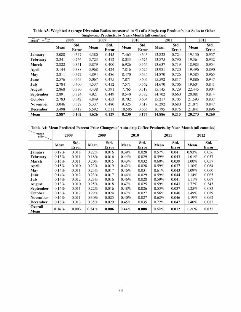
33
Table A3: Weighted Average Diversion Ratios (measured in %) of a Single-cup Product’s lost Sales to Other
Single-cup Products, by Year-Month (all counties)
Month Year 2008 2009 2010 2011 2012
Mean Std.
Error Mean
Std.
Error Mean
Std.
Error Mean
Std.
Error Mean
Std.
Error
January 3.088 0.347 4.380 0.445 7.463 0.643 13.823 0.724 19.130 0.937
February 2.341 0.266 3.723 0.412 8.033 0.675 13.875 0.790 19.364 0.932
March 2.822 0.341 3.879 0.400 6.926 0.564 13.637 0.719 18.983 0.954
April 3.144 0.388 3.968 0.424 7.816 0.625 13.981 0.720 19.496 0.890
May 2.811 0.327 4.894 0.486 8.470 0.635 14.870 0.726 19.585 0.965
June 2.576 0.363 5.067 0.475 7.871 0.605 15.592 0.817 19.886 0.947
July 2.784 0.400 4.537 0.412 7.571 0.562 14.670 0.706 19.604 0.841
August 2.868 0.390 4.438 0.391 7.765 0.517 15.145 0.729 22.445 0.904
September 2.891 0.324 4.921 0.449 8.540 0.592 14.702 0.660 20.081 0.814
October 2.783 0.342 4.849 0.453 8.702 0.604 15.217 0.705 21.593 0.837
November 3.046 0.329 5.337 0.480 9.325 0.617 16.292 0.680 21.071 0.847
December 3.498 0.417 5.592 0.511 10.505 0.665 16.795 0.876 21.841 0.896
Mean 2.887 0.102 4.626 0.129 8.230 0.177 14.886 0.215 20.273 0.260
Table A4: Mean Predicted Percent Price Changes of Auto-drip Coffee Products, by Year-Month (all counties)
Month Year
2008 2009 2010 2011 2012
Mean Std.
Error Mean
Std.
Error Mean
Std.
Error Mean
Std.
Error Mean
Std.
Error
January 0.19% 0.018 0.22% 0.016 0.39% 0.028 0.57% 0.041 0.93% 0.056 February 0.15% 0.011 0.18% 0.016 0.44% 0.029 0.59% 0.043 1.01% 0.057 March 0.16% 0.011 0.20% 0.015 0.43% 0.032 0.60% 0.039 1.00% 0.057 April 0.15% 0.010 0.23% 0.019 0.42% 0.028 0.59% 0.037 1.10% 0.064 May 0.14% 0.011 0.23% 0.017 0.46% 0.031 0.61% 0.043 1.09% 0.060 June 0.14% 0.012 0.23% 0.017 0.44% 0.029 0.59% 0.044 1.14% 0.065 July 0.14% 0.012 0.23% 0.016 0.46% 0.028 0.59% 0.041 1.11% 0.067 August 0.13% 0.010 0.25% 0.018 0.47% 0.025 0.59% 0.043 1.72% 0.345 September 0.16% 0.011 0.22% 0.016 0.48% 0.026 0.53% 0.037 1.25% 0.083 October 0.16% 0.012 0.29% 0.024 0.47% 0.027 0.56% 0.040 1.49% 0.089 November 0.16% 0.011 0.30% 0.025 0.40% 0.027 0.62% 0.046 1.19% 0.062 December 0.18% 0.013 0.35% 0.029 0.45% 0.035 0.72% 0.047 1.40% 0.083
Overall
Mean 0.16% 0.003 0.24% 0.006 0.44% 0.008 0.60% 0.012 1.21% 0.035
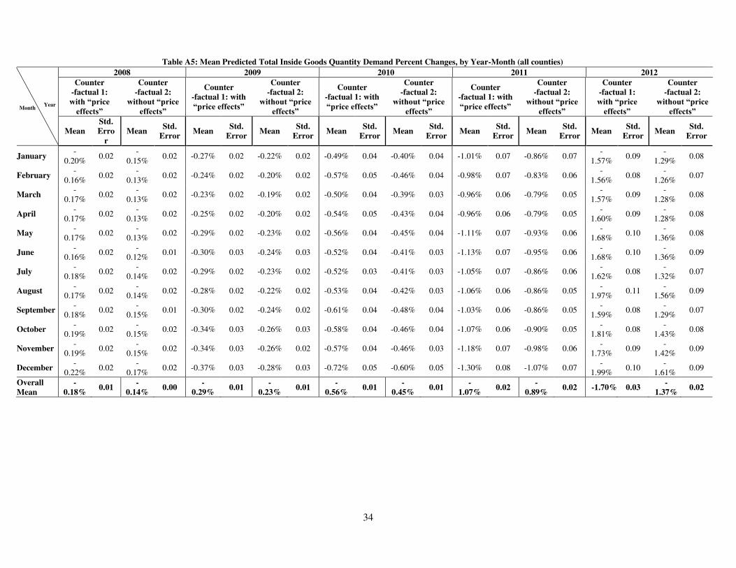
34
Table A5: Mean Predicted Total Inside Goods Quantity Demand Percent Changes, by Year-Month (all counties)
Month Year
2008 2009 2010 2011 2012
Counter
-factual 1:
with “price effects”
Counter
-factual 2:
without “price effects”
Counter
-factual 1: with
“price effects”
Counter
-factual 2:
without “price effects”
Counter
-factual 1: with
“price effects”
Counter
-factual 2:
without “price effects”
Counter
-factual 1: with
“price effects”
Counter
-factual 2:
without “price effects”
Counter
-factual 1:
with “price effects”
Counter
-factual 2:
without “price effects”
Mean
Std.
Erro
r
Mean Std.
Error Mean
Std.
Error Mean
Std.
Error Mean
Std.
Error Mean
Std.
Error Mean
Std.
Error Mean
Std.
Error Mean
Std.
Error Mean
Std.
Error
January -
0.20% 0.02
-0.15%
0.02 -0.27% 0.02 -0.22% 0.02 -0.49% 0.04 -0.40% 0.04 -1.01% 0.07 -0.86% 0.07 -
1.57% 0.09
-1.29%
0.08
February -
0.16% 0.02
-0.13%
0.02 -0.24% 0.02 -0.20% 0.02 -0.57% 0.05 -0.46% 0.04 -0.98% 0.07 -0.83% 0.06 -
1.56% 0.08
-1.26%
0.07
March -
0.17% 0.02
-0.13%
0.02 -0.23% 0.02 -0.19% 0.02 -0.50% 0.04 -0.39% 0.03 -0.96% 0.06 -0.79% 0.05 -
1.57% 0.09
-1.28%
0.08
April -
0.17% 0.02
-0.13%
0.02 -0.25% 0.02 -0.20% 0.02 -0.54% 0.05 -0.43% 0.04 -0.96% 0.06 -0.79% 0.05 -
1.60% 0.09
-1.28%
0.08
May -
0.17% 0.02
-0.13%
0.02 -0.29% 0.02 -0.23% 0.02 -0.56% 0.04 -0.45% 0.04 -1.11% 0.07 -0.93% 0.06 -
1.68% 0.10
-1.36%
0.08
June -
0.16% 0.02
-0.12%
0.01 -0.30% 0.03 -0.24% 0.03 -0.52% 0.04 -0.41% 0.03 -1.13% 0.07 -0.95% 0.06 -
1.68% 0.10
-1.36%
0.09
July -
0.18% 0.02
-0.14%
0.02 -0.29% 0.02 -0.23% 0.02 -0.52% 0.03 -0.41% 0.03 -1.05% 0.07 -0.86% 0.06 -
1.62% 0.08
-1.32%
0.07
August -
0.17% 0.02
-0.14%
0.02 -0.28% 0.02 -0.22% 0.02 -0.53% 0.04 -0.42% 0.03 -1.06% 0.06 -0.86% 0.05 -
1.97% 0.11
-1.56%
0.09
September -
0.18% 0.02
-0.15%
0.01 -0.30% 0.02 -0.24% 0.02 -0.61% 0.04 -0.48% 0.04 -1.03% 0.06 -0.86% 0.05 -
1.59% 0.08
-1.29%
0.07
October -
0.19% 0.02
-0.15%
0.02 -0.34% 0.03 -0.26% 0.03 -0.58% 0.04 -0.46% 0.04 -1.07% 0.06 -0.90% 0.05 -
1.81% 0.08
-1.43%
0.08
November -
0.19% 0.02
-0.15%
0.02 -0.34% 0.03 -0.26% 0.02 -0.57% 0.04 -0.46% 0.03 -1.18% 0.07 -0.98% 0.06 -
1.73% 0.09
-1.42%
0.09
December -
0.22% 0.02
-0.17%
0.02 -0.37% 0.03 -0.28% 0.03 -0.72% 0.05 -0.60% 0.05 -1.30% 0.08 -1.07% 0.07 -
1.99% 0.10
-1.61%
0.09
Overall
Mean
-
0.18% 0.01
-
0.14% 0.00
-
0.29% 0.01
-
0.23% 0.01
-
0.56% 0.01
-
0.45% 0.01
-
1.07% 0.02
-
0.89% 0.02 -1.70% 0.03
-
1.37% 0.02
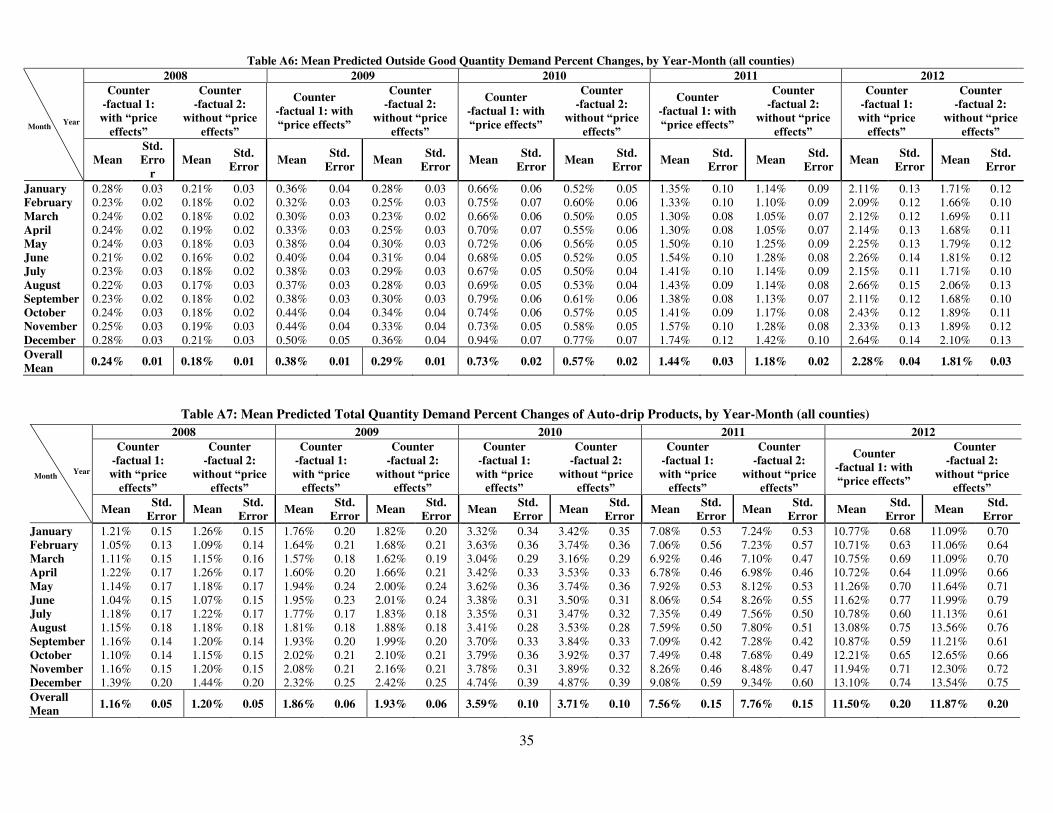
35
Table A6: Mean Predicted Outside Good Quantity Demand Percent Changes, by Year-Month (all counties)
Month Year
2008 2009 2010 2011 2012
Counter
-factual 1:
with “price effects”
Counter
-factual 2:
without “price effects”
Counter
-factual 1: with
“price effects”
Counter
-factual 2:
without “price effects”
Counter
-factual 1: with
“price effects”
Counter
-factual 2:
without “price effects”
Counter
-factual 1: with
“price effects”
Counter
-factual 2:
without “price effects”
Counter
-factual 1:
with “price effects”
Counter
-factual 2:
without “price effects”
Mean
Std.
Erro
r
Mean Std.
Error Mean
Std.
Error Mean
Std.
Error Mean
Std.
Error Mean
Std.
Error Mean
Std.
Error Mean
Std.
Error Mean
Std.
Error Mean
Std.
Error
January 0.28% 0.03 0.21% 0.03 0.36% 0.04 0.28% 0.03 0.66% 0.06 0.52% 0.05 1.35% 0.10 1.14% 0.09 2.11% 0.13 1.71% 0.12 February 0.23% 0.02 0.18% 0.02 0.32% 0.03 0.25% 0.03 0.75% 0.07 0.60% 0.06 1.33% 0.10 1.10% 0.09 2.09% 0.12 1.66% 0.10 March 0.24% 0.02 0.18% 0.02 0.30% 0.03 0.23% 0.02 0.66% 0.06 0.50% 0.05 1.30% 0.08 1.05% 0.07 2.12% 0.12 1.69% 0.11 April 0.24% 0.02 0.19% 0.02 0.33% 0.03 0.25% 0.03 0.70% 0.07 0.55% 0.06 1.30% 0.08 1.05% 0.07 2.14% 0.13 1.68% 0.11 May 0.24% 0.03 0.18% 0.03 0.38% 0.04 0.30% 0.03 0.72% 0.06 0.56% 0.05 1.50% 0.10 1.25% 0.09 2.25% 0.13 1.79% 0.12 June 0.21% 0.02 0.16% 0.02 0.40% 0.04 0.31% 0.04 0.68% 0.05 0.52% 0.05 1.54% 0.10 1.28% 0.08 2.26% 0.14 1.81% 0.12 July 0.23% 0.03 0.18% 0.02 0.38% 0.03 0.29% 0.03 0.67% 0.05 0.50% 0.04 1.41% 0.10 1.14% 0.09 2.15% 0.11 1.71% 0.10 August 0.22% 0.03 0.17% 0.03 0.37% 0.03 0.28% 0.03 0.69% 0.05 0.53% 0.04 1.43% 0.09 1.14% 0.08 2.66% 0.15 2.06% 0.13 September 0.23% 0.02 0.18% 0.02 0.38% 0.03 0.30% 0.03 0.79% 0.06 0.61% 0.06 1.38% 0.08 1.13% 0.07 2.11% 0.12 1.68% 0.10 October 0.24% 0.03 0.18% 0.02 0.44% 0.04 0.34% 0.04 0.74% 0.06 0.57% 0.05 1.41% 0.09 1.17% 0.08 2.43% 0.12 1.89% 0.11 November 0.25% 0.03 0.19% 0.03 0.44% 0.04 0.33% 0.04 0.73% 0.05 0.58% 0.05 1.57% 0.10 1.28% 0.08 2.33% 0.13 1.89% 0.12 December 0.28% 0.03 0.21% 0.03 0.50% 0.05 0.36% 0.04 0.94% 0.07 0.77% 0.07 1.74% 0.12 1.42% 0.10 2.64% 0.14 2.10% 0.13
Overall
Mean 0.24% 0.01 0.18% 0.01 0.38% 0.01 0.29% 0.01 0.73% 0.02 0.57% 0.02 1.44% 0.03 1.18% 0.02 2.28% 0.04 1.81% 0.03
Table A7: Mean Predicted Total Quantity Demand Percent Changes of Auto-drip Products, by Year-Month (all counties)
Month Year
2008 2009 2010 2011 2012
Counter
-factual 1:
with “price effects”
Counter
-factual 2:
without “price effects”
Counter
-factual 1:
with “price effects”
Counter
-factual 2:
without “price effects”
Counter
-factual 1:
with “price effects”
Counter
-factual 2:
without “price effects”
Counter
-factual 1:
with “price effects”
Counter
-factual 2:
without “price effects”
Counter
-factual 1: with
“price effects”
Counter
-factual 2:
without “price effects”
Mean Std.
Error Mean
Std.
Error Mean
Std.
Error Mean
Std.
Error Mean
Std.
Error Mean
Std.
Error Mean
Std.
Error Mean
Std.
Error Mean
Std.
Error Mean
Std.
Error
January 1.21% 0.15 1.26% 0.15 1.76% 0.20 1.82% 0.20 3.32% 0.34 3.42% 0.35 7.08% 0.53 7.24% 0.53 10.77% 0.68 11.09% 0.70 February 1.05% 0.13 1.09% 0.14 1.64% 0.21 1.68% 0.21 3.63% 0.36 3.74% 0.36 7.06% 0.56 7.23% 0.57 10.71% 0.63 11.06% 0.64 March 1.11% 0.15 1.15% 0.16 1.57% 0.18 1.62% 0.19 3.04% 0.29 3.16% 0.29 6.92% 0.46 7.10% 0.47 10.75% 0.69 11.09% 0.70 April 1.22% 0.17 1.26% 0.17 1.60% 0.20 1.66% 0.21 3.42% 0.33 3.53% 0.33 6.78% 0.46 6.98% 0.46 10.72% 0.64 11.09% 0.66 May 1.14% 0.17 1.18% 0.17 1.94% 0.24 2.00% 0.24 3.62% 0.36 3.74% 0.36 7.92% 0.53 8.12% 0.53 11.26% 0.70 11.64% 0.71 June 1.04% 0.15 1.07% 0.15 1.95% 0.23 2.01% 0.24 3.38% 0.31 3.50% 0.31 8.06% 0.54 8.26% 0.55 11.62% 0.77 11.99% 0.79 July 1.18% 0.17 1.22% 0.17 1.77% 0.17 1.83% 0.18 3.35% 0.31 3.47% 0.32 7.35% 0.49 7.56% 0.50 10.78% 0.60 11.13% 0.61 August 1.15% 0.18 1.18% 0.18 1.81% 0.18 1.88% 0.18 3.41% 0.28 3.53% 0.28 7.59% 0.50 7.80% 0.51 13.08% 0.75 13.56% 0.76 September 1.16% 0.14 1.20% 0.14 1.93% 0.20 1.99% 0.20 3.70% 0.33 3.84% 0.33 7.09% 0.42 7.28% 0.42 10.87% 0.59 11.21% 0.61 October 1.10% 0.14 1.15% 0.15 2.02% 0.21 2.10% 0.21 3.79% 0.36 3.92% 0.37 7.49% 0.48 7.68% 0.49 12.21% 0.65 12.65% 0.66 November 1.16% 0.15 1.20% 0.15 2.08% 0.21 2.16% 0.21 3.78% 0.31 3.89% 0.32 8.26% 0.46 8.48% 0.47 11.94% 0.71 12.30% 0.72 December 1.39% 0.20 1.44% 0.20 2.32% 0.25 2.42% 0.25 4.74% 0.39 4.87% 0.39 9.08% 0.59 9.34% 0.60 13.10% 0.74 13.54% 0.75
Overall
Mean 1.16% 0.05 1.20% 0.05 1.86% 0.06 1.93% 0.06 3.59% 0.10 3.71% 0.10 7.56% 0.15 7.76% 0.15 11.50% 0.20 11.87% 0.20
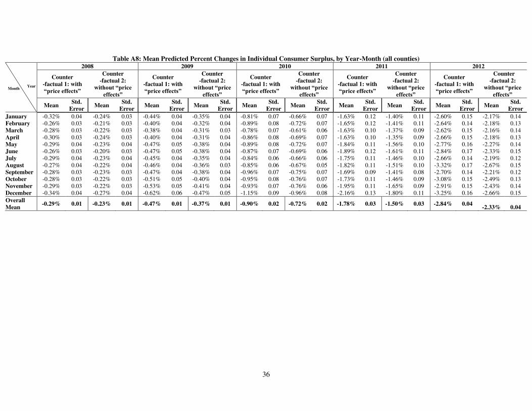
36
Table A8: Mean Predicted Percent Changes in Individual Consumer Surplus, by Year-Month (all counties)
Month Year
2008 2009 2010 2011 2012
Counter
-factual 1: with
“price effects”
Counter
-factual 2:
without “price effects”
Counter
-factual 1: with
“price effects”
Counter
-factual 2:
without “price effects”
Counter
-factual 1: with
“price effects”
Counter
-factual 2:
without “price effects”
Counter
-factual 1: with
“price effects”
Counter
-factual 2:
without “price effects”
Counter
-factual 1: with
“price effects”
Counter
-factual 2:
without “price effects”
Mean Std.
Error Mean
Std.
Error Mean
Std.
Error Mean
Std.
Error Mean
Std.
Error Mean
Std.
Error Mean
Std.
Error Mean
Std.
Error Mean
Std.
Error Mean
Std.
Error
January -0.32% 0.04 -0.24% 0.03 -0.44% 0.04 -0.35% 0.04 -0.81% 0.07 -0.66% 0.07 -1.63% 0.12 -1.40% 0.11 -2.60% 0.15 -2.17% 0.14 February -0.26% 0.03 -0.21% 0.03 -0.40% 0.04 -0.32% 0.04 -0.89% 0.08 -0.72% 0.07 -1.65% 0.12 -1.41% 0.11 -2.64% 0.14 -2.18% 0.13 March -0.28% 0.03 -0.22% 0.03 -0.38% 0.04 -0.31% 0.03 -0.78% 0.07 -0.61% 0.06 -1.63% 0.10 -1.37% 0.09 -2.62% 0.15 -2.16% 0.14 April -0.30% 0.03 -0.24% 0.03 -0.40% 0.04 -0.31% 0.04 -0.86% 0.08 -0.69% 0.07 -1.63% 0.10 -1.35% 0.09 -2.66% 0.15 -2.18% 0.13 May -0.29% 0.04 -0.23% 0.04 -0.47% 0.05 -0.38% 0.04 -0.89% 0.08 -0.72% 0.07 -1.84% 0.11 -1.56% 0.10 -2.77% 0.16 -2.27% 0.14 June -0.26% 0.03 -0.20% 0.03 -0.47% 0.05 -0.38% 0.04 -0.87% 0.07 -0.69% 0.06 -1.89% 0.12 -1.61% 0.11 -2.84% 0.17 -2.33% 0.15 July -0.29% 0.04 -0.23% 0.04 -0.45% 0.04 -0.35% 0.04 -0.84% 0.06 -0.66% 0.06 -1.75% 0.11 -1.46% 0.10 -2.66% 0.14 -2.19% 0.12 August -0.27% 0.04 -0.22% 0.04 -0.46% 0.04 -0.36% 0.03 -0.85% 0.06 -0.67% 0.05 -1.82% 0.11 -1.51% 0.10 -3.32% 0.17 -2.67% 0.15 September -0.28% 0.03 -0.23% 0.03 -0.47% 0.04 -0.38% 0.04 -0.96% 0.07 -0.75% 0.07 -1.69% 0.09 -1.41% 0.08 -2.70% 0.14 -2.21% 0.12 October -0.28% 0.03 -0.22% 0.03 -0.51% 0.05 -0.40% 0.04 -0.95% 0.08 -0.76% 0.07 -1.73% 0.11 -1.46% 0.09 -3.08% 0.15 -2.49% 0.13 November -0.29% 0.03 -0.22% 0.03 -0.53% 0.05 -0.41% 0.04 -0.93% 0.07 -0.76% 0.06 -1.95% 0.11 -1.65% 0.09 -2.91% 0.15 -2.43% 0.14 December -0.34% 0.04 -0.27% 0.04 -0.62% 0.06 -0.47% 0.05 -1.15% 0.09 -0.96% 0.08 -2.16% 0.13 -1.80% 0.11 -3.25% 0.16 -2.66% 0.15
Overall
Mean -0.29% 0.01 -0.23% 0.01 -0.47% 0.01 -0.37% 0.01 -0.90% 0.02 -0.72% 0.02 -1.78% 0.03 -1.50% 0.03 -2.84% 0.04
-2.33% 0.04
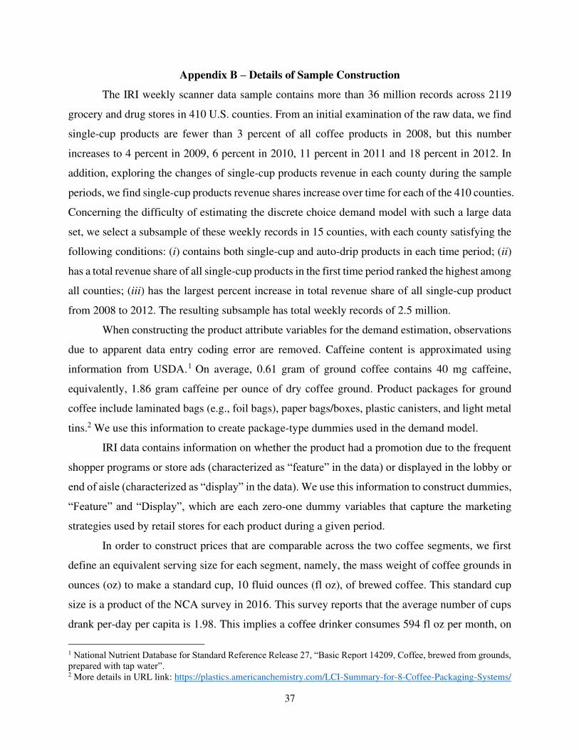
37
Appendix B – Details of Sample Construction
The IRI weekly scanner data sample contains more than 36 million records across 2119
grocery and drug stores in 410 U.S. counties. From an initial examination of the raw data, we find
single-cup products are fewer than 3 percent of all coffee products in 2008, but this number
increases to 4 percent in 2009, 6 percent in 2010, 11 percent in 2011 and 18 percent in 2012. In
addition, exploring the changes of single-cup products revenue in each county during the sample
periods, we find single-cup products revenue shares increase over time for each of the 410 counties.
Concerning the difficulty of estimating the discrete choice demand model with such a large data
set, we select a subsample of these weekly records in 15 counties, with each county satisfying the
following conditions: (i) contains both single-cup and auto-drip products in each time period; (ii)
has a total revenue share of all single-cup products in the first time period ranked the highest among
all counties; (iii) has the largest percent increase in total revenue share of all single-cup product
from 2008 to 2012. The resulting subsample has total weekly records of 2.5 million.
When constructing the product attribute variables for the demand estimation, observations
due to apparent data entry coding error are removed. Caffeine content is approximated using
information from USDA.1 On average, 0.61 gram of ground coffee contains 40 mg caffeine,
equivalently, 1.86 gram caffeine per ounce of dry coffee ground. Product packages for ground
coffee include laminated bags (e.g., foil bags), paper bags/boxes, plastic canisters, and light metal
tins.2 We use this information to create package-type dummies used in the demand model.
IRI data contains information on whether the product had a promotion due to the frequent
shopper programs or store ads (characterized as “feature” in the data) or displayed in the lobby or
end of aisle (characterized as “display” in the data). We use this information to construct dummies,
“Feature” and “Display”, which are each zero-one dummy variables that capture the marketing
strategies used by retail stores for each product during a given period.
In order to construct prices that are comparable across the two coffee segments, we first
define an equivalent serving size for each segment, namely, the mass weight of coffee grounds in
ounces (oz) to make a standard cup, 10 fluid ounces (fl oz), of brewed coffee. This standard cup
size is a product of the NCA survey in 2016. This survey reports that the average number of cups
drank per-day per capita is 1.98. This implies a coffee drinker consumes 594 fl oz per month, on
1 National Nutrient Database for Standard Reference Release 27, “Basic Report 14209, Coffee, brewed from grounds, prepared with tap water”. 2 More details in URL link: https://plastics.americanchemistry.com/LCI-Summary-for-8-Coffee-Packaging-Systems/
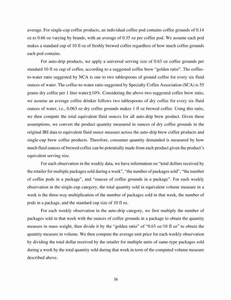
38
average. For single-cup coffee products, an individual coffee pod contains coffee grounds of 0.14
oz to 0.66 oz varying by brands, with an average of 0.35 oz per coffee pod. We assume each pod
makes a standard cup of 10 fl oz of freshly brewed coffee regardless of how much coffee grounds
each pod contains.
For auto-drip products, we apply a universal serving size of 0.63 oz coffee grounds per
standard 10 fl oz cup of coffee, according to a suggested coffee brew “golden ratio”. The coffee-
to-water ratio suggested by NCA is one to two tablespoons of ground coffee for every six fluid
ounces of water. The coffee-to-water ratio suggested by Specialty Coffee Association (SCA) is 55
grams dry coffee per 1 liter water±10%. Considering the above two suggested coffee brew ratio,
we assume an average coffee drinker follows two tablespoons of dry coffee for every six fluid
ounces of water, i.e., 0.063 oz dry coffee grounds makes 1 fl oz brewed coffee. Using this ratio,
we then compute the total equivalent fluid ounces for all auto-drip brew product. Given these
assumptions, we convert the product quantity measured in ounces of dry coffee grounds in the
original IRI data to equivalent fluid ounce measure across the auto-drip brew coffee products and
single-cup brew coffee products. Therefore, consumer quantity demanded is measured by how
much fluid ounces of brewed coffee can be potentially made from each product given the product’s
equivalent serving size.
For each observation in the weekly data, we have information on “total dollars received by
the retailer for multiple packages sold during a week”, “the number of packages sold”, “the number
of coffee pods in a package”, and “ounces of coffee grounds in a package”. For each weekly
observation in the single-cup category, the total quantity sold in equivalent volume measure in a
week is the three-way multiplication of the number of packages sold in that week, the number of
pods in a package, and the standard cup size of 10 fl oz.
For each weekly observation in the auto-drip category, we first multiply the number of
packages sold in that week with the ounces of coffee grounds in a package to obtain the quantity
measure in mass weight, then divide it by the “golden ratio” of “0.63 oz/10 fl oz” to obtain the
quantity measure in volume. We then compute the average unit price for each weekly observation
by dividing the total dollar received by the retailer for multiple units of same-type packages sold
during a week by the total quantity sold during that week in term of the computed volume measure
described above.
39
Appendix C – Formally Implementing the Counterfactual Experiments
Counterfactual Experiment 1: with “price effects”
In this exercise, once single-cup coffee products are counterfactually removed, the new
equilibrium price vector, 𝒑∗, of auto-drip products is obtained by numerically searching for the
vector of prices that satisfy the following equation: 𝒑∗ = 𝒎�̂� − [𝛀 ∗ 𝚫(𝒑∗)]−𝟏𝒔(𝒑∗) (C1)
where equation C1 is implied by the system of first-order conditions generated by the optimization
problem in equation (3) in the paper; 𝒎�̂� is the vector of recovered product-level marginal cost
estimates based on the demand parameter estimates in Table 2; 3 𝛀 is a 𝐽 × 𝐽 matrix of
appropriately positioned zeros and ones based on the manufacturers’ ownership structure of the 𝐽
products in the relevant market; 𝚫 is a 𝐽 × 𝐽 matrix of first-order derivatives of predicted product
shares with respect to prices; and 𝛀 ∗ 𝚫 is an element-by-element multiplication of the two
matrices. A comparison of the actual observed price vector 𝒑 from the data with the model-
predicted new equilibrium price vector 𝒑∗ reveals how equilibrium prices for auto-drip coffee
products are influenced by the introduction of single-cup coffee products to the brew-at-home
coffee retail market.
Let 𝐴𝐷𝑚𝑡 be the subset of brew-at-home coffee products in market 𝑚 during period 𝑡 that
are auto-drip, while 𝑆𝐶𝑚𝑡 the subset that are single-cup. We can therefore re-write product shares
predicted by the model as follows: 𝑠𝑗𝑚𝑡(𝒑; Θ̂) = 1𝑛𝑠 ∑ ( 𝑒𝛿𝑗𝑚𝑡(𝑝𝑗𝑚𝑡)+𝜇𝑖𝑗𝑚𝑡(𝑝𝑗𝑚𝑡)1+∑ 𝑒𝛿𝑙𝑡(𝑝𝑙𝑚𝑡)+𝜇𝑖𝑙𝑚𝑡(𝑝𝑙𝑚𝑡)𝑙∈𝐴𝐷𝑚𝑡 +∑ 𝑒𝛿𝑙𝑚𝑡(𝑝𝑙𝑚𝑡)+𝜇𝑖𝑙𝑚𝑡(𝑝𝑙𝑚𝑡)𝑙∈𝑆𝐶𝑚𝑡 )𝑛𝑠𝑖=1 (C2)
𝑠0𝑚𝑡(𝒑; Θ̂) = 1𝑛𝑠 ∑ ( 11+∑ 𝑒𝛿𝑙𝑚𝑡(𝑝𝑙𝑚𝑡)+𝜇𝑖𝑙𝑚𝑡(𝑝𝑙𝑚𝑡)𝑙∈𝐴𝐷𝑚𝑡 +∑ 𝑒𝛿𝑙𝑚𝑡(𝑝𝑙𝑚𝑡)+𝜇𝑖𝑙𝑚𝑡(𝑝𝑙𝑚𝑡)𝑙∈𝑆𝐶𝑚𝑡 )𝑛𝑠𝑖=1 (C3)
where, conditional on demand parameter estimates in vector Θ̂, equation (C2) yields the model-
predicted share for brew-at-home coffee product 𝑗 evaluated at the vector of actual prices, 𝒑; while
equation (C3) yields the model-predicted share of the outside good evaluated at the vector of actual
prices, 𝒑.
3 We assume cost structures of firms are not changed after the counterfactual removal of single-cup products. As stated in Villas-Boas (2007), it is a common limitation that this assumption does not consider the possibility of potential synergy effects due to joint production and distribution of both coffee product types for multi-product firms.
40
With the model-predicted new equilibrium prices for auto-drip products in hand, we then
compute model-predicted shares of auto-drip coffee products and share of the outside good based
on the following modified versions of equations (C2) and (C3): 𝑠𝑗𝑚𝑡(𝒑∗; Θ̂) = 1𝑛𝑠 ∑ ( 𝑒𝛿𝑗𝑚𝑡(𝑝𝑗𝑚𝑡∗ )+𝜇𝑖𝑗𝑚𝑡(𝑝𝑗𝑚𝑡∗ )1+∑ 𝑒𝛿𝑙𝑚𝑡(𝑝𝑙𝑚𝑡∗ )+𝜇𝑖𝑙𝑚𝑡(𝑝𝑙𝑚𝑡∗ )𝑙∈𝐴𝐷𝑚𝑡 )𝑛𝑠𝑖=1 (C4)
𝑠0𝑚𝑡(𝒑∗; Θ̂) = 1𝑛𝑠 ∑ ( 11+∑ 𝑒𝛿𝑙𝑚𝑡(𝑝𝑙𝑚𝑡∗ )+𝜇𝑖𝑙𝑚𝑡(𝑝𝑙𝑚𝑡∗ )𝑙∈𝐴𝐷𝑚𝑡 )𝑛𝑠𝑖=1 (C5)
where the term, ∑ 𝑒𝛿𝑙𝑚𝑡(𝑝𝑙𝑚𝑡)+𝜇𝑖𝑙𝑚𝑡(𝑝𝑙𝑚𝑡)𝑙∈𝑆𝐶𝑚𝑡 , is absent from the denominator in equations (C4)
and (C5) due to the counterfactual elimination of single-cup products from each market. Using
equations (C2) through (C5) along with the measure of the potential size of market m during period
t, 𝑀𝑚𝑡, we compute factual model-predicted quantities demand by 𝑑𝑗𝑚𝑡 = 𝑀𝑚𝑡 × 𝑠𝑗𝑚𝑡(𝒑; Θ̂) and 𝑑0𝑚𝑡 = 𝑀𝑚𝑡 × 𝑠0𝑚𝑡(𝒑; Θ̂), while counterfactual model-predicted quantities demand are obtained
by 𝑑𝑗𝑚𝑡∗ = 𝑀𝑚𝑡 × 𝑠𝑗𝑚𝑡(𝒑∗; Θ̂) and 𝑑0𝑚𝑡∗ = 𝑀𝑚𝑡 × 𝑠0𝑚𝑡(𝒑∗; Θ̂) , allowing price responses for
auto-drip coffee products with the introduction of single-cup products.
Counterfactual Experiment 2: without “price effects”
In this exercise, we assume the price levels of pre-existing auto-drip coffee products are
fixed at their observed price levels after the counterfactual removal of the new products; therefore,
the predicted shares of auto-drip coffee products and share of the outside good are given by the
following: �̃�𝑗𝑚𝑡(𝒑; Θ̂) = 1𝑛𝑠 ∑ ( 𝑒𝛿𝑗𝑚𝑡(𝑝𝑗𝑚𝑡)+𝜇𝑖𝑗𝑚𝑡(𝑝𝑗𝑚𝑡)1+∑ 𝑒𝛿𝑙𝑚𝑡(𝑝𝑗𝑚𝑡)+𝜇𝑖𝑙𝑚𝑡(𝑝𝑗𝑚𝑡)𝑙∈𝐴𝐷𝑚𝑡 )𝑛𝑠𝑖=1 (C6)
�̃�0𝑚𝑡(𝒑; Θ̂) = 1𝑛𝑠 ∑ ( 11+∑ 𝑒𝛿𝑙𝑚𝑡(𝑝𝑗𝑚𝑡)+𝜇𝑖𝑙𝑚𝑡(𝑝𝑗𝑚𝑡)𝑙∈𝐴𝐷𝑚𝑡 )𝑛𝑠𝑖=1 (C7)
Using equations (C6) and (C7) along with the measure of the potential market size measure, 𝑀𝑚𝑡, we then compute the counterfactual model-predicted quantities demand of the auto-drip and
the outside good by �̃�𝑗𝑚𝑡 = 𝑀𝑚𝑡 × �̃�𝑗𝑚𝑡(𝒑; Θ̂) and �̃�0𝑚𝑡 = 𝑀𝑚𝑡 × �̃�0𝑚𝑡(𝒑; Θ̂) , assuming the
prices of auto-drip products remain unchanged with the introduction of single-cup products.
41
References
Aaker, D.A. and Keller, K.L., 1990. “Consumer evaluations of brand extensions.” Journal of
Marketing, 54(1), pp.27-41.
Ansari, A., Bawa, K. and Ghosh, A., 1995. “A nested logit model of brand choice incorporating variety-seeking and marketing-mix variables.” Marketing Letters, 6(3), pp.199-210.
Berry, S., Levinsohn, J. and Pakes, A., 1995. “Automobile prices in market equilibrium.” Econometrica: Journal of the Econometric Society, pp.841-890.
Berry, S.T. and Haile, P.A., 2014. “Identification in differentiated products markets using market level data.” Econometrica, 82(5), pp.1749-1797.
Berry, S.T. and Haile, P.A., 2016. “Identification in differentiated products markets.” Annual
Review of Economics, 8, pp.27-52.
Berry, S.T., 1994. “Estimating discrete-choice models of product differentiation.” The RAND
Journal of Economics, pp.242-262.
Boatwright, P., Dhar, S. and Rossi, P.E., 2004. “The role of retail competition, demographics and account retail strategy as drivers of promotional sensitivity.” Quantitative Marketing and
Economics, 2(2), pp.169-190.
Boleslavsky, R., Cotton, C.S. and Gurnani, H., 2017. “Demonstrations and price competition in new product release.” Management Science, 63(6), pp.2016-2026.
Bonnet, C. and Villas-Boas, S.B., 2016. “An analysis of asymmetric consumer price responses and asymmetric cost pass-through in the French coffee market.” European Review of
Agricultural Economics, 43(5), pp.781-804.
Bresnahan, T.F. and Gordon, R.J. eds., 1997. “The economics of new goods.” National Bureau of Economic Research, University of Chicago Press.
Broda, C. and Weinstein, D.E., 2006. “Globalization and the Gains from Variety.” The Quarterly
Journal of Economics, 121(2), pp.541-585.
Broniarczyk, S.M. and Alba, J.W., 1994. “The importance of the brand in brand extension.” Journal of Marketing Research, 31(2), pp.214-228.
Bronnenberg, B.J., Dubé, J.P.H. and Gentzkow, M., 2012. “The evolution of brand preferences: Evidence from consumer migration.” American Economic Review, 102(6), pp.2472-2508.
Bronnenberg, B.J., Kruger, M.W. and Mela, C.F., 2008. “Database paper—The IRI marketing data set.” Marketing Science, 27(4), pp.745-748.
Brynjolfsson, E., Hu, Y. and Smith, M.D., 2003. Consumer surplus in the digital economy: Estimating the value of increased product variety at online booksellers. Management
science, 49(11), pp.1580-1596.
Cabral, L.M., 2000. “Stretching firm and brand reputation.” RAND Journal of Economics, pp.658-673.
Chintagunta, P.K., Qin, M.S. and Vitorino, M.A., 2018. “Licensing and price competition in tied-goods markets: An application to the single-serve coffee system industry.” Marketing
Science, 37(6), pp.883-911.
42
Choi, J.P., 1998. “Brand extension as informational leverage.” The Review of Economic
Studies, 65(4), pp.655-669.
Conlon, C.T. and Gortmaker, J., 2020. “Best Practices for Differentiated Products Demand Estimation with PyBLP.” The RAND Journal of Economics, Vol. 51, Issue 4, Winter 2020, pp. 1108 – 1161.
Conlon, C.T. and Mortimer, J.H., 2013. “An experimental approach to merger evaluation.” National Bureau of Economic Research (Working Paper No. 19703).
Conlon, C.T. and Mortimer, J.H., 2021. “Empirical properties of diversion ratios.” The RAND
Journal of Economics, forthcoming.
de Mejia, E.G. and Ramirez-Mares, M.V., 2014. “Impact of caffeine and coffee on our health.” Trends in Endocrinology & Metabolism, 25(10), pp.489-492.
Ellickson, P.B., Kong, P. and Lovett, M.J., 2018. “Private labels and retailer profitability: Bilateral bargaining in the grocery channel.” Available at SSRN 3045372.
Farrell Joseph & Shapiro Carl, 2010. "Antitrust Evaluation of Horizontal Mergers: An Economic Alternative to Market Definition," The B.E. Journal of Theoretical Economics, De Gruyter, vol. 10(1), pages 1-41, March.
Foster, L., Haltiwanger, J. and Syverson, C., 2008. “Reallocation, firm turnover, and efficiency: Selection on productivity or profitability?” American Economic Review, 98(1), pp.394-425.
Gallagher J, 2011. “Brands should spend less on promotions, more on innovations.” Supermarket
News 59 (15):23. Article can be retrieved from the following URL link: https://www.supermarketnews.com/center-store/brands-should-spend-less-promotions-more-innovation
Gandhi, A. and Houde, J.F., 2020. “Measuring Substitution Patterns in Differentiated-Products Industries.” National Bureau of Economic Research (Working Paper No. 26375).
Gentzkow, M., 2007. “Valuing new goods in a model with complementarity: Online newspapers.” American Economic Review, 97(3), pp.713-744.
Goolsbee, A. and Petrin, A., 2004. “The consumer gains from direct broadcast satellites and the competition with cable TV.” Econometrica, 72(2), pp.351-381.
Greenstein, S.M., 1997. “From superminis to supercomputers: Estimating surplus in the computing market.” In The economics of new goods (pp. 329-372). University of Chicago Press.
Grover, R. and Srinivasan, V., 1992. “Evaluating the multiple effects of retail promotions on brand loyal and brand switching segments.” Journal of Marketing Research, pp.76-89.
Guadagni, P.M. and Little, J.D., 1998. “When and what to buy: A nested logit model of coffee purchase.” Journal of Forecasting, 17(3‐4), pp.303-326.
Gupta, S., 1988. “Impact of sales promotions on when, what, and how much to buy.” Journal of
Marketing Research, pp.342-355.
Hariharan, V.G., Bezawada, R. and Talukdar, D., 2015. “Aggregate impact of different brand development strategies.” Management Science, 61(5), pp.1164-1182.
43
Hausman, J.A. and Leonard, G.K., 2002. “The competitive effects of a new product introduction: A case study.” The Journal of Industrial Economics, 50(3), pp.237-263.
Hausman, J.A., 1996. “Valuation of New Goods under Perfect and Imperfect Competition.” In The
Economics of New Goods (pp. 207-248). University of Chicago Press.
Hellerstein, R. and Villas-Boas, S.B., 2010. “Outsourcing and pass-through.” Journal of
International Economics, 81(2), pp.170-183.
Hwang, M. and Thomadsen, R., 2015. “How point-of-sale marketing mix impacts national-brand purchase shares.” Management Science, 62(2), pp.571-590.
Ivaldi, M. and Verboven, F., 2005. “Quantifying the effects from horizontal mergers in European competition policy.” International Journal of Industrial Organization, 23(9-10), pp.669-691.
Kong, P., Ellickson, P.B., and Lovett, M.J., (2016). “Putting the Horses Before the Cart: Harnessing the Power of Partner Brands,” Working paper, University of Rochester.
Krishnamurthi, L. and Raj, S.P., 1991. “An empirical analysis of the relationship between brand loyalty and consumer price elasticity.” Marketing Science, 10(2), pp.172-183.
Lattin, J.M. and Bucklin, R.E., 1989. “Reference effects of price and promotion on brand choice behavior.” Journal of Marketing Research, pp.299-310.
Lin, X., 2017. “Disaggregate Network Effects on Two-Sided Platforms.” Working paper, The
University of Chicago Booth School of Business.
Martinez, E. and De Chernatony, L., 2004. “The effect of brand extension strategies upon brand image.” Journal of Consumer Marketing, 21(1), pp. 39-50
McFadden, D.L., 1984. “Econometric analysis of qualitative response models.” Handbook of
econometrics, 2, pp.1395-1457.
Miller, N.H. and Weinberg, M.C., 2017. “Understanding the price effects of the MillerCoors joint venture.” Econometrica, 85(6), pp.1763-1791.
Nakamura, E. and Zerom, D., 2010. “Accounting for incomplete pass-through.” The Review of
Economic Studies, 77(3), pp.1192-1230.
Nevo, A., 2000a. “Mergers with differentiated products: The case of the ready-to-eat cereal industry.” The RAND Journal of Economics, pp.395-421.
Nevo, A., 2000b. “A practitioner's guide to estimation of random‐coefficients logit models of demand.” Journal of Economics & Management Strategy, 9(4), pp.513-548.
Nevo, A., 2001. “Measuring market power in the ready‐to‐eat cereal industry.” Econometrica, 69(2), pp.307-342.
Pepall, L.M. and Richards, D.J., 2002. “The simple economics of brand stretching.” The Journal
of Business, 75(3), pp.535-552.
Petrin, A., 2002. “Quantifying the benefits of new products: The case of the minivan.” Journal of
Political Economy, 110(4), pp.705-729.
Pitta, D.A. and Katsanis, L.P., 1995. “Understanding brand equity for successful brand extension.” Journal of Consumer Marketing. 12(4), pp. 51-64.
44
Prendergast, G.P. and Marr, N.E., 1997. “Generic products: who buys them and how do they perform relative to each other?” European Journal of Marketing, 31(2), pp.94-109.
Shapiro, C., 1995. Mergers with differentiated products. Antitrust, 10, p.23.
Shapiro, C., 2010. “The 2010 horizontal merger guidelines: From hedgehog to fox in forty years.” Antitrust LJ, 77, p.49.
Small, K.A. and Rosen, H.S., 1981. “Applied welfare economics with discrete choice models.” Econometrica: Journal of the Econometric Society, pp.105-130.
Stock, J., & Yogo, M. (2005). “Testing for Weak Instruments in Linear IV Regression.” In D. Andrews & J. Stock (Eds.), Identification and Inference for Econometric Models: Essays in Honor of Thomas Rothenberg (pp. 80-108). Cambridge: Cambridge University Press.
Sullivan, C., 2020. “The ice cream split: Empirically distinguishing price and product space collusion.” ERN: Firm Behavior (IO: Empirical) (Topic). Available at SSRN 3321948.
Swaminathan, V., Fox, R.J. and Reddy, S.K., 2001. “The impact of brand extension introduction on choice.” Journal of Marketing, 65(4), pp.1-15.
Train, K.E., 2009. “Discrete choice methods with simulation.” Cambridge University Press.
Villas-Boas, S.B., 2007a. “Vertical relationships between manufacturers and retailers: Inference with limited data.” The Review of Economic Studies, 74(2), pp.625-652.
Villas-Boas, S.B., 2007b. “Using retail data for upstream merger analysis.” Journal of Competition
Law and Economics, 3(4), pp.689-715.