Utah State University Utah State University

DigitalCommons@USU DigitalCommons@USU

All Graduate Theses and Dissertations Graduate Studies

5-2016

Evapotranspiration Estimation: A Study of Methods in the Western Evapotranspiration Estimation: A Study of Methods in the Western

United States United States

Clayton S. Lewis Utah State University

Follow this and additional works at: https://digitalcommons.usu.edu/etd

Part of the Civil Engineering Commons

Recommended Citation Recommended Citation Lewis, Clayton S., "Evapotranspiration Estimation: A Study of Methods in the Western United States" (2016). All Graduate Theses and Dissertations. 4683. https://digitalcommons.usu.edu/etd/4683

This Dissertation is brought to you for free and open access by the Graduate Studies at DigitalCommons@USU. It has been accepted for inclusion in All Graduate Theses and Dissertations by an authorized administrator of DigitalCommons@USU. For more information, please contact digitalcommons@usu.edu.

.

EVAPOTRANSPIRATION ESTIMATION: A STUDY OF METHODS

IN THE WESTERN UNITED STATES

by

Clayton S. Lewis

A dissertation submitted in partial fulfillment of the requirements of the degree

of

DOCTOR OF PHILOSOPHY

in

Civil Engineering

Approved: _________________________ Christopher M. U. Neale Major Professor _________________________ Robert W. Hill Committee Member _________________________ Jagath J. Kaluarachchi Committee Member

_________________________ Gilberto E. Urroz Committee Member _________________________ Joanna Endter-Wada Committee Member _________________________ Mark McLellan Vice President for Research and Dean of the School of Graduate Studies

UTAH STATE UNIVERSITY

Logan, Utah

2016

ii

Copyright © Clayton S. Lewis 2016

All Rights Reserved

iii

ABSTRACT

Evapotranspiration Estimation: A Study of Methods

in the Western United States

by

Clayton S. Lewis, Doctor of Philosophy

Utah State University, 2016 Major Professor: Dr. Christopher M. U. Neale Department: Civil and Environmental Engineering

This research focused on estimating evapotranspiration (i.e., the amount

of water vaporizing into the atmosphere through processes of surface

evaporation and plant transpiration) under both theoretical and actual conditions.

There were two study areas involved: one, on a large scale where 704

agriculturally-representative, electronic weather stations were used to evaluate

the drivers and calculated reference evapotranspiration of a NASA gridded

weather forcing model in the 17 western states in the contiguous U.S.; and two,

transpiration of invasive saltcedar (Tamarix sp.) in the floodplain of the lower

Colorado River, California, with Bowen ratio, eddy covariance, and groundwater

fluxes. In this study, a fire destroyed the saltcedar forest, which allowed

comparison of evapotranspiration before and after\ this event.

iv

Comparison of the input weather parameters showed some variance

between the electronic weather stations and the gridded model, but calculated

reference evapotranspiration performed well by relying on the better input and

more highly weighed variables of air temperature and downward shortwave

radiation. Only in the southern portions of California, Arizona, and New Mexico

were the evapotranspiration estimates using the gridded dataset not well

correlated with the electronic weather stations and not recommended for

prediction. Saltcedar evapotranspiration was found to match more recent and

conservative estimates for the phreatophyte than what was historically portrayed

in the literature. Horizontal advection from the surrounding desert was also

observed to affect the riparian energy balance. Annual average total

evapotranspiration before a fire varied from 0.60-1.44 meters/year to 0.25-1.00

meters/year post fire.

(132 pages)

v

PUBLIC ABSTRACT

Evapotranspiration Estimation: A Study of Methods

in the Western United States

Clayton S. Lewis Theoretical water use of well-watered vegetation in the western United

States was investigated by comparing a gridded dataset developed from satellite

and ground instruments to weather stations representative of irrigated agricultural

conditions. Since wetter environments are cooler and therefore subject to lower

levels of evaporation than the same scenario with warmer temperatures, models

derived from dryland and often populated areas overestimate potential plant

needs in semi-arid or arid conditions. Evaluation of the model revealed an

acceptable fit for air temperatures and solar radiation but with less confidence in

humidity and wind speeds. Ultimately, the last two parameters were minor

components in the calculation of reference evapotranspiration, which performed

acceptably well at an hourly time step except for some high biases in states

along the southern U.S. border. These findings substantiate application of the

model for calculation of plant water requirements 1979-present in most areas.

Actual water use of invasive saltcedar was studied along the Colorado

River in a wildlife refuge south of Palo Verde, California. Surface meteorological

towers and groundwater wells measured water fluxes from 2006 until a fire

burned the refuge and most of the equipment in August 2011. New instruments

were installed and measured the evapotranspiration of the regrowth. Change in

evapotranspiration was evidenced and models verified by a zeroed state. This

control state of no (or nearly no) vegetation was very beneficial in this study.

Saltcedar water use was assessed against other studies and the theoretical

estimates mentioned above and found to be comparable to levels required by

native vegetation.

vi

ACKNOWLEDGMENTS

I take no credit for the gain in knowledge I have received while

researching or for what is recorded in this dissertation but attribute every

enlightened thought followed by incredible fruition to my Father in Heaven.

There have been many times while sitting at my desk engaged in programming,

writing, or reading an article when unmistakable inspiration has whispered a

thought into my mind. Frequently, this occurred in the final moments of a day or

nearing the end of a project deadline after I had put in a full effort. Grateful I am

for the God who has miraculously sustained me throughout my studies at Utah

State University. I do accept responsibility for any error contained herein.

To my wife’s patience and unbeleaguered support during my years of

graduate studies and bearing of three children: Thank you, and I love you.

To Dr. Hill, my first advisor, thanks for just scratching your head when I

shared some big ideas and for instilling an engineering mindset.

To Dr. Neale, thanks for allowing me to soar untethered into the heights of

success.

To Drs. Endter-Wada and Kjelgren, thanks for the diversion coding

WaterMAPS and for the experience working with water agencies.

To Burdette Barker, Ashish Masih, Ian Ferguson, Diana Glenn, Hatim

Geli, and Marcelo Biudes, thanks for your association and help.

Clayton Lewis

vii

CONTENTS

ABSTRACT .......................................................................................................... iii

PUBLIC ABSTRACT ............................................................................................ v

ACKNOWLEDGMENTS .......................................................................................vi

CONTENTS ......................................................................................................... vii

LIST OF TABLES ................................................................................................. x

LIST OF FIGURES ...............................................................................................xi

CHAPTER

1. INTRODUCTION ....................................................................................... 1

1.1 Overview ................................................................................... 1

1.1.1 Purpose ....................................................................... 1 1.1.2 Reference Evapotranspiration ..................................... 3 1.1.3 Saltcedar Evapotranspiration ...................................... 5 1.1.4 Research Objectives ................................................... 7

1.2 Methodology .............................................................................. 8

1.2.1 Penman-Monteith Reference Evapotranspiration ...... 10 1.2.2 Bowen Ratio Energy Balance Technique .................. 12 1.2.3 Eddy Covariance Technique ..................................... 14 1.2.4 Groundwater Fluxes .................................................. 15 1.2.5 Remote Sensing Energy Balance Approach ............. 17

1.3 References .............................................................................. 18

2. COMPARISON OF THE NLDAS WEATHER FORCING MODEL TO AGROMETEOROLOGICAL MEASUREMENTS IN THE WESTERN UNITED STATES .................................................................. 23

2.1 Abstract ................................................................................... 23 2.2 Introduction ............................................................................. 24 2.3 Background ............................................................................. 24 2.4 Data Preparation ..................................................................... 28

viii

2.4.1 Retrieval .................................................................... 28 2.4.2 Weather Station Locale Filter .................................... 30

2.5 Comparison of NLDAS Data ................................................... 35

2.5.1 Weather Parameters ................................................. 35 2.5.2 Reference ET ............................................................ 38

2.6 Conclusions............................................................................. 43 2.7 Acknowledgments ................................................................... 43 2.8 References .............................................................................. 44

3. BOWEN RATIO AND EDDY COVARIANCE SYSTEM PERFORMANCE OVER SALTCEDAR UNDER DIFFERENT ATMOSPHERIC STABILITY AND ADVECTION CONDITIONS .............. 48

3.1 Abstract ................................................................................... 48 3.2 Introduction ............................................................................. 48 3.3 Theoretical Foundations .......................................................... 50 3.4 Methodology Limitations ......................................................... 52 3.5 Advection and Atmospheric Stability ....................................... 56 3.6 Site Characteristics ................................................................. 57 3.7 Data Analysis .......................................................................... 60 3.8 Results and Discussion ........................................................... 62 3.9 Summary and Conclusions ..................................................... 68 3.10 Acknowledgments ................................................................. 68 3.11 References ............................................................................ 69

4. SALTCEDAR EVAPOTRANSPIRATION PRE AND POST FIRE ............ 73

4.1 Abstract ................................................................................... 73 4.2 Introduction ............................................................................. 73 4.3 Methods .................................................................................. 75 4.4 Materials ................................................................................. 77 4.5 Data Analysis and Results ...................................................... 82 4.6 Discussion ............................................................................... 92 4.7 Conclusions............................................................................. 95 4.8 Acknowledgments ................................................................... 96 4.9 References .............................................................................. 96

5. SUMMARY AND CONCLUSIONS ......................................................... 101

5.1 Objective Fulfillment .............................................................. 102 5.2 Conclusions........................................................................... 105 5.3 References ............................................................................ 105

ix

APPENDICES .................................................................................................. 106

Appendix A: Permissions ............................................................ 107 Appendix B: Curriculum Vitae ..................................................... 116

x

LIST OF TABLES

Table Page

2.1. Electronic Weather Station Networks over Agricultural Areas for 17 States in the Western United States ........................................................ 27

2.2. Sequential Steps Taken to Programmatically Filter and Correct Electronic Weather Station Data .............................................................. 34

3.1. Advection-Corrected to Non-Corrected Fraction of Seasonal Sensible and Latent Heat Fluxes over Salt Cedar in Cibola, California, Pre and Post Fire .................................................................... 67

4.1. Averaged Groundwater Properties for Multiple Wells at 3 Sites in the Cibola National Wildlife Refuge Pre and Post Fire ............................. 91

4.2. Average Annual Groundwater ET from Multiple Wells at 3 Sites in the Cibola National Wildlife Refuge Pre and Post Fire Assuming Conservative Estimates of Specific Yield (meter/year) ............................ 92

xi

LIST OF FIGURES

Figure Page

2.1. Annual Count of Operational Agricultural Electronic Weather Stations in the Western United States (1981-2012) ................................. 27

2.2. 704 Agricultural Electronic Weather Stations Superimposed over the NASS 2012 Cropland Data Layer in the Western United States ........ 32

2.3. NLDAS and Agricultural Weather Station Scatter Plots of Hourly Solar Radiation, Air Temperature, Wind Speed, and Relative Humidity at Four Irrigated Locations in the Western United States .......... 36

2.4. IDW Interpolated R Squared of Hourly Solar Radiation, Air Temperature, Wind Speed, and Relative Humidity of the Comparison between 704 Agricultural Weather Stations and NLDAS in the Western United States ...................................................... 39

2.5. IDW Interpolated Bias of Hourly Solar Radiation, Air Temperature, Wind Speed, and Relative Humidity of the Comparison between 704 Agricultural Weather Stations and NLDAS in the Western United States ........................................................................................... 40

2.6. IDW Interpolated Root Mean Squared Error of Hourly Solar Radiation, Air Temperature, Wind Speed, and Relative Humidity of the Comparison between 704 Agricultural Weather Stations and NLDAS in the Western United States ...................................................... 41

2.7. IDW Interpolated R Squared, Bias, and Root Mean Squared Error of Hourly Short or Grass Reference Evapotranspiration of the Comparison between 704 Agricultural Weather Stations and NLDAS in the Western United States ...................................................... 42

3.1. Location of Three Surface Flux Measurement Sites over a Salt Cedar Forest within the Cibola Wildlife National Refuge near the Colorado River ......................................................................................... 59

3.2. Measurement Towers and Surrounding Salt Cedar Forest Pre and Post Fire at the Cibola National Wildlife Refuge [(A) Diablo Tower Pre Fire, 2008 (B) Slithern Tower Pre Fire, 2008 (C) SlithernTower After Fire, 2012 (D) Rebuilt Slithern Tower Post Fire, 2013] .................... 60

xii

3.3. Hourly Fraction of Bowen Ratios obtained from Eddy Covariance and Bowen Ratio Energy Balance Instrumentation over Salt Cedar at Diablo Station in Cibola, California, Pre Fire (2008-2009) ................... 63

3.4. Hourly Fraction of Bowen Ratios obtained from Eddy Covariance and Bowen Ratio Energy Balance Instrumentation over Salt Cedar at Slithern Station in Cibola, California, Post Fire (2012-2013) ................ 64

3.5. Average Hourly Fraction of Bowen Ratios obtained from Eddy Covariance and Bowen Ratio Energy Balance Instrumentation over Salt Cedar in Cibola, California, Pre and Post Fire (2008-2013) .............. 65

3.6. Average Hourly Surface Fluxes obtained from Bowen Ratio Energy Balance Instrumentation over Salt Cedar at Diablo Station in Cibola, California, Pre Fire (2008-2009) .................................................. 66

3.7. Average Hourly Surface Fluxes obtained from Bowen Ratio Energy Balance Instrumentation over Salt Cedar at Slithern Station in Cibola, California, Post Fire (2012-2013) ................................................. 66

4.1. False Color (Infrared, Red, Green) Images from the National Agriculture Imagery Program (NAIP) of the Tower Sites in the Cibola National Wildlife Refuge, (A) June 26, 2005; (B) May 25, 2009; (C) April 26 and 28, 2010; (D) April 23, 2012; (E) May 16, 2014 ......................................................................................................... 79

4.2. Tower and Groundwater Well Observation Locations within the Cibola National Wildlife Refuge ............................................................... 81

4.3. Saltcedar Regrowth in the Cibola National Wildlife Refuge Post Fire (From Top to Bottom, March 12, 2012; May 29, 2013; August 20, 2013)........................................................................................................ 82

4.4. Weekly Averaged Daily ET from Bowen Ratio Systems in the Cibola National Wildlife Refuge, (Top: 2006-2010; Bottom: 2012-2013)........................................................................................................ 84

4.5. Weekly Averaged Daily ET from Eddy Covariance Systems in the Cibola National Wildlife Refuge, (Top: 2007-2009; Bottom: 2012-2013)........................................................................................................ 86

4.6. Weekly Average Daily Groundwater Surface Elevation from Multiple Wells at 3 Sites in the Cibola National Wildlife Refuge ............................ 88

xiii

4.7. Example of 24 Hour Fourier-White Method Implementation for 3 Days at Diablo Tower Well, Cibola National Wildlife Refuge (July 1-7, 2011) .................................................................................................... 88

4.8. Weekly Averaged Daily Groundwater ET from Multiple Wells at 3 Sites in the Cibola National Wildlife Refuge, (From Top to Bottom, 2006-2010; 2011; 2012-2013) ................................................................. 91

1

CHAPTER 1

INTRODUCTION

1.1 Overview

1.1.1 Purpose

Access to, acquisition of, and allocation of potable and non-potable water

has been the motivation for colossal civil projects, numerous governmental pacts

and entities, and disputes at local and state levels. Where deficient supplies of

fresh water exist, oversight becomes even more intense. This accurately

describes conditions prevalent in the Great American Desert or western United

States. Water storage and delivery systems being essential in this arid

environment, citizens and communities have been obliged to operate jointly this

natural resource. Accordingly, development of better management practices has

been sought after to ensure equity of use. With academia thus induced, higher

institutions have answered the call with Utah State University in Logan, Utah,

being a forerunner in the field of water management and engineering. This work

sought to complement the backdrop of accomplishments by increasing

knowledge of evapotranspiration in the West. Contributors and partners in this

study were Utah State University, U.S. Bureau of Reclamation, U.S. Geological

Survey, U.S. Fish and Wildlife Service, National Oceanic and Atmospheric

Administration, National Air and Space Administration, Palo Verde Irrigation

District, Six Agencies of the Lower Colorado River, various universities across

the United States, and many organizations collecting weather data.

2

For decades, the consumptive use of water by vegetation in agricultural

and riparian lands has been studied and estimates published. As the demand

per unit of water continues to increase, managing agencies must account for

every transaction accurately or at least much closer than past rough estimates.

Currently, a multitude of researchers throughout the world are actively striving to

resolve these issues by developing and installing more advanced instrumentation

to increase temporal and spatial resolution of field measurements and by

developing new methods to assimilate datasets to create comprehensive models

of the hydrological cycle. In an effort to broaden documented knowledge of

processes pertaining to vegetative transpiration and surface evaporation, this

study investigated these three questions:

(1) Can regional reference evapotranspiration be modeled by a gridded

national weather forcing dataset in the 17-state American West while

satisfactorily agreeing with an extensive set of ground-based weather

stations?

(2) Does the Bowen ratio method of evapotranspiration estimation

produce accurate results in an advective, desert environment?

(3) What are the effects of a fire on a riparian stretch of saltcedar and the

change in evapotranspiration pre and post fire on the groundwater fluxes?

3

1.1.2 Reference Evapotranspiration

With the possibility of an enormous variety of crops and vegetation being

grown even in a specific microclimate (which are also subject to fertilizers,

irrigation, diseases, drought, variable topography and soil, and differences in

species), the task of determining consumptive use on these vegetated land

surfaces is a daunting one. Available water and nutrients, crop phenology, and

evaporative potential all need to be tracked over non-dormant periods. Since

actual evapotranspiration is currently impossible to directly measure for the

unique location and characteristics of each land cover, empirical methods to

estimate evapotranspiration—based on theory to some degree—have been

proposed. The common approach has been to account for site irregularities or

crop particularities in reductions to or additions to a single reference crop.

According to Allen et al. (1998), reference crop evapotranspiration is defined by a

“standardized vegetative surface” that reflects the “evaporation power of the

atmosphere” of observed climatic conditions. Crop growth stages, including

season initiation and termination, are described by crop coefficients (Jensen,

1968) that are the ratio of a given crop evapotranspiration to that of the estimated

reference evapotranspiration. These crop coefficients may indicate either actual

evapotranspiration or potential evapotranspiration, the latter being “the amount of

water that would be evaporated and transpired if it were available” (Thornthwaite,

1947) to which further penalties could be applied indicating actual substandard

conditions.

4

Many researchers have recommended methods to calculate reference

evapotranspiration from surface measurements which can be grouped into one of

four categories based on theory incorporated: energy balance, mass transfer, an

empirical relationship to an observed measurement, or a combination of these.

Equations such as Penman (1948), Thornthwaite (1948), Makkink (1957), Turc

(1961), Blaney and Criddle (1962), Jensen and Haise (1963), Monteith (1965),

Christiansen (1968), Priestley and Taylor (1972), Pruitt and Doorenbos (1977),

and Hargreaves et al. (1985) are examples of methods that have been applied

extensively in this discipline and results compared to disturbed point

measurements and to each other. Selection of an evapotranspiration equation

depends on weather parameters in existing datasets, their frequency, and the

overall site climate. Some equations have proven more accurate than others

with modified versions of the combination Penman-Monteith equation performing

the best worldwide (Allen et al. 1998).

Calculation of the water requirement for a given crop coincides with a

reference evapotranspiration equation, which, historically, has been the Blaney-

Criddle equation due to its reduced input of monthly average temperature and

site calibrations (Allen et al. 1998). However, enhanced spatial and temporal

estimates of reference evapotranspiration are being developed with the advent of

new technologies: the electronic weather station; increased data storage,

sampling, transfer rates, and processing capacity; better sensors; satellite

imagery; and improved modeling techniques. At present, separate standards

based on divergent and now obsolete methodologies are administered by each

5

state, which inherently poses an obstacle in shared basins. A single method to

calculate reference evapotranspiration for the whole region with tolerable

accuracy would alleviate this problem and function as a more equitable allocation

metric.

1.1.3 Saltcedar Evapotranspiration

Saltcedar, also known by the genus Tamarix, is a dense shrub or tree

native to Europe, Asia, and Africa (Baum 1978), and several species from

Eurasia were imported into the eastern United States in the nineteenth century to

build wind breaks, control erosion along stream channels, produce shade, and be

planted as ornamentals. Like the name suggests, saltcedar tolerates saline

environments and also retains salt in the glands of its tiny leaves. Upon leaf fall,

the surface is temporally salted, giving an advantage in outcompeting rival

vegetative growth. Saltcedar also exhibits further survival traits including

resistance to flooding and droughts, susceptibility to wildfires contrasted with

quick regrowth from the root crown after a burn, and propagation through high

seed production and vegetative reproduction. Once introduced into the arid and

semi-arid American West from Eastern nurseries, saltcedar proliferated along

river corridors and supplanted local riparian vegetation such as cottonwoods,

willows, and mesquite. This invasive plant is now targeted with successive

mechanical and biological mechanisms for removal. (Di Tomaso 1998, Glenn

and Nagler 2005)

6

In addition, saltcedar has been condemned for excessive consumption of

groundwater, a safeguarded commodity in the western states. Stromberg et al.

(2009) at length summarized perceptions of saltcedar water requirements by the

public, scientists, and officials over the past 60 years. Political pressure to

eradicate what was viewed as an invasive and useless pest may have biased

initial, often indirectly-derived approximations of water use, which overestimated

2-3 times what has been measured the past decade with improved methods.

These high estimates have been touted as the reason for saltcedar removal.

However, studies have not shown anticipated water savings with saltcedar

elimination, which could be due to a number of groundwater recharge factors

(Shafroth et al. 2005). Nevertheless, saltcedar at present is considered an

invasive weed using significant quantities of water. It, perhaps, matches more

closely native riparian vegetation in water consumption but outcompetes and

grows in more extensive forests in the floodplain of western U.S. river systems.

Many factors regulate saltcedar water consumption, which may include elevation,

latitude, climate, groundwater levels, drought, salinity, growth stages, and

competition. The effects of these factors on saltcedar evapotranspiration are not

fully understood, and wide-scale estimates are still reliable only within a probable

range.

Evapotranspiration of saltcedar in the southwestern U.S. has been

measured by Bowen ratio towers, eddy covariance systems, scintillometers, and

estimated using remote sensing, information from groundwater wells, lysimetry,

and sap flow techniques (Cleverly et al. 2002, Nagler et al. 2009, Taghvaeian

7

2011, Geli et al. 2012). Each of these methods contains intrinsic errors that can

be enlarged through user mismanagement and together yield uncertainties to

well over 100 percent (Sher and Quigley 2013). In the case of the Bowen ratio

energy balance, import of energy by advection can invalidate results (Perez et al.

1999) but can be verified against the more robust eddy covariance method,

although itself limited by stable atmospheric conditions and wind direction.

Tracking groundwater fluctuations will accurately illustrate withdrawals from the

saturated layer but not the magnitude, whereas remote sensing approaches can

suffer from lower temporal resolution and proper calibration. Thus, refining

accurate estimates of saltcedar water use has proved challenging and requires

careful collection and evaluation of data (Westenburg et al. 2006).

1.1.4 Research Objectives

Further research in the fields of reference evapotranspiration and riparian

saltcedar water requirements would lead to new and pertinent understandings

affecting policies both political and academic. In an attempt to answer the

previous inquiries, the following research aims were evaluated:

(1) Comparison of the North American Land Data Assimilation System

(NLDAS-2, 2013) to agricultural electronic weather station networks in the

American West for the period 1981-2012 on an hourly time step for the

meteorological parameters of solar radiation, air temperature, wind speed,

and relative humidity as well as calculated reference evapotranspiration.

8

(2) Establishment of actual evapotranspiration of saltcedar in the

advective, desert climate of the Cibola National Wildlife Refuge (CNWR,

2013) along the Lower Colorado River by analyzing groundwater, Bowen

ratio, eddy covariance, and remote sensing datasets before and after a

decimating wildfire in 2011.

Both objectives required original research and expanded scientific

knowledge in the fields of reference and saltcedar evapotranspiration. Objective

1 referred to the initial question of comparing a national gridded dataset to

ground observations, while Objective 2 satisfied the second and third questions

in Section 1.1.1 by affording multiple energy flux datasets in an advective and

arid environment overrun by saltcedar that was recently burned. Following a

format of standalone journal papers, these objectives and the underlying

questions are specifically studied in Chapters 2-4.

1.2 Methodology

In an age with science and technology advancing at a rapid rate, it may be

no surprise in the near future to be able to track or correctly determine all of

Earth’s hydrologic movements. However, current models suffer from incongruent

subsampling in representing the whole population. Examples include

measurements of an evapotranspiration weather station monitoring a wind-

whipped hillside being equated to the rather calm conditions on the opposite

side, or the altered conditions and disturbed specimens in a lysimeter or

pressurized chamber to that of a heterogeneous field, or instantaneous remote

9

sensing every two weeks, or the frequent transfer of empirical methods from one

environment to another, or even the tendency in nature for climate to change.

A number of assumptions are usually applied to satisfy either the water or

energy balance to estimate water movements on the land surface (Equations 1.1

and 1.2). Presently, texture and nutrient classifications of soil layers in both the

vertical horizons and horizontal spread are interpolations of relatively few known

samples compared to the diversity of the landscape. Measurements of water

within the soil are therefore assigned values for porosity, specific yield, and

hydraulic conductivity on a broad basis that may not coincide with reality and

distort the actual flows and storage term in Equation 1.1.

Precipitation rates are also spatially variable, especially in mountainous

terrain, which may lead to inconsistencies when extrapolated from a few gaging

stations within a basin. This leaves the last component of the water balance, that

of losses returning to the atmosphere through evapotranspiration. Since

evapotranspiration cannot yet be adequately modeled from measurements of the

other variables at a high resolution, different approaches have been studied to

determine the amount of plant transpiration and surface evaporation.

ETQQPV OUTIN −−+=∆ [ 1.1 ]

Where V∆ is the change in system volumetric storage, P is precipitation,

INQ and OUTQ are the input and output volumes from the system, and ET is

evapotranspiration.

10

One more exclusively theoretical method in obtaining evapotranspiration

would be to solve for the latent heat flux in Equation 1.2 and then convert the

consumed energy to evaporated water. A positive aspect of this approach lies in

the relatively constant and known seasonal patterns of incoming solar radiation.

Determining the net radiation, however, including the surface albedo and

scattering and reflectance of light by particles in the atmosphere, varies not only

with position but also in time. Again, the composition and water content of the soil

greatly impacts its ability to intake and release heat while the sensible heat flux,

like the latent heat flux, is not directly measured. Further, this equation

addresses plant stored energy and processes such as photosynthesis in the

storage term which is frequently neglected altogether.

ETHGRE N λ−−−=∆ [ 1.2 ]

Where E∆ is the change in system energy storage, NR is net radiation, G

is the soil heat flux, H is the sensible heat flux, and ETλ is latent heat flux.

In order to determine evapotranspiration on a site and regional basis,

research from past decades has introduced empirical procedures into Equations

1.1 and 1.2 to account for lack of necessary environmental data.

1.2.1 Penman-Monteith Reference Evapotranspiration

H. L. Penman (1948) suggested a method for determining

evapotranspiration over natural surfaces by uniting both the energy balance

(Equation 1.2) and mass transfer equations to form what is now known as the

11

“combination equation”. This semi-empirical approach used observations of

sunshine, humidity, wind speed, and temperature in addition to site specific

conditions to estimate input parameters. With further research, Monteith (1965)

improved the theoretical and empirical relations and formed Equation 1.3. This

equation eventually proved superior to 19 similar approaches and became the

world standard (Allen et al. 1998). Inclusion in this study provides a means to

estimate evapotranspiration from readily available and complete datasets that

can be compared to more complex methodologies with incomplete datasets or

precluded output.

( ) ( )

+⋅+∆⋅

−⋅⋅+−⋅∆

=

A

S

A

ASPAN

RR

ReecGR

ET1γλ

ρ [ 1.3 ]

Where ET is evapotranspiration, ∆ is the slope of the saturation vapor

pressure-temperature curve, NR is net radiation, G is the soil heat flux, Aρ

is the dry air density, Pc is the specific heat capacity of air, AR is the

aerodynamic resistance, SR is the surface resistance, Se is the saturation

vapor pressure, Ae is the saturation vapor pressure, λ is the latent heat of

vaporization, and γ is the psychrometric constant.

In an effort to normalize assumptions and create an equation appropriate

for conditions in the United States, especially the arid West, an American Society

of Civil Engineers task force agreed upon the ASCE Standardized Penman-

12

Monteith equation or Equation 1.4 (Walter, 2000). As all of the study areas are

located within the western United States, this equation was selected as the most

appropriate and accepted Penman-combination method for this research.

( ) ( )( )2

2

1273

408.0

uC

eeuT

CGRET

d

ASn

N

SZ ⋅+⋅+∆

−⋅⋅+

⋅+−⋅∆⋅=

γ

γ [ 1.4 ]

Where T is temperature, 2u is wind speed, and nC and dC are reference

constants.

1.2.2 Bowen Ratio Energy Balance Technique

While both the solar and infrared radiative fluxes and soil heat flux can be

directly measured, the partitioning of the sensible and latent heat fluxes is much

more difficult to establish and must be determined indirectly. An example already

seen was the Penman-Monteith equation, which followed the energy balance

very closely with radiation and soil heat flux terms but quickly became convoluted

in evaluation of the sensible heat flux. As the sum of the sensible and latent heat

fluxes equals the difference between the radiative and soil heat fluxes,

discovering the ratio between the sensible and latent heat fluxes would enable

calculation of the fluxes. This method is called the Bowen ratio and is shown in

Equation 1.5. Since inputs of air temperature and vapor pressure at two different

vertical heights along with air pressure can be straightforwardly obtained, this

equation is easily implemented and maintainable. There are, however, limits to

its application as the theory is idealized to the case of turbulent atmosphere,

13

horizontal and homogeneous terrain, and negligible vertical advection, which are

not always the norm in the American West (Angus and Watts 1984, Perez et al.

1999).

eTcP

ETH P

∆⋅⋅∆⋅⋅

==ελλ

β [ 1.5 ]

Where β is the Bowen ratio, H is the sensible heat flux, ETλ is latent

heat flux, P is air pressure, Pc is the specific heat capacity of air, T∆ is

the change in temperature at two heights, λ is the latent heat of

vaporization, ε is the ratio of molecular weights of water to that of dry air,

and e∆ is the change in vapor pressure at two heights.

Describing behavior of the Bowen ratio numerically can be problematic as

it approaches asymptotes or changes sign in either the numerator or

denominator. An alternative but equivalent proportion is the fraction of latent

heat flux to that of the sum of both the latent and sensible heat fluxes. This

evaporative fraction ranges between 0 and 1 and is related to the Bowen ratio

through Equation 1.6.

β+=

11EF [ 1.6 ]

Where EF is the evaporative fraction and β is the Bowen ratio.

Once the evaporative fraction is calculated, it is multiplied against the net

available energy to produce evapotranspiration as is shown in Equation 1.7.

14

λGREFET N −

⋅= [ 1.7 ]

Where ET is evapotranspiration, EF is the evaporative fraction, NR is net

radiation, G is the soil heat flux, and λ is the latent heat of vaporization.

1.2.3 Eddy Covariance Technique

Some of the science behind the eddy covariance method involves parcels

of air (eddies) circulating through the atmosphere and along the earth’s surface

of diminishing sizes. These motions transfer particles, including suspended

water molecules, from one point in the air to another. Inverse of the frequency or

the period of the eddies is proportional to their size and may vary from less than

a second per cycle to many hours. Larger eddies containing most of the energy

ultimately shrink in size and dissipate energy at higher frequencies through what

is known as an energy cascade. By reducing the Navier-Stokes equation

through a number of assumptions similar to the Penman-Monteith and Bowen

ratio methods already mentioned to a homogeneous ground cover with sufficient

fetch, evapotranspiration is derived in Equation 1.8 as the covariance between

the vertical wind component and water vapor density (Aubinet et al. 2012).

'' VZuET ρ= [ 1.8 ]

Where ET is evapotranspiration, Zu is the vertical wind component, and

Vρ is water vapor density.

15

The advantage of this method over the Bowen ratio is the measurement of

advective flux; although, it is similarly handicapped by stable atmospheric

conditions. Sampling intervals of less than a second (10 to 20 Hertz) are

required to capture the covariance of the small eddies and must be calculated

over many minutes or hours to integrate the influence of the large eddies. This

leads to (for our current systems) large data files and processing requirements as

well as instrument spikes that must be corrected. Further adjustments due to

measurement practices may involve coordinate rotations, sensor lag times,

tapering or de-trending, frequency response correction, spectral corrections, the

krypton hygrometer oxygen correction, and the Webb-Pearman-Leuning (WPL)

correction (Lee et al. 2004). Periods of stable and neutral conditions must be

identified which may be during times of strong advective conditions or

questionable measurement. With the possibility for many unaccounted errors,

careful instrument setup and operation and data post processing will produce

acceptable results for time steps representative of the underlying assumptions.

1.2.4 Groundwater Fluxes

Plant water consumption patterns beneath the vadose zone are revealed

by measuring groundwater table fluctuations. Simple and accurate devices that

gauge depth such as pressure and temperature sensors, floats, or sonic meters

are capable of logging daily or finer readings. The difference in height from one

time step to another indicates the response in storage to the sum of

inflows/outflows and water extracted by plants, these physical interactions being

16

embodied in Equation 1.9. By definition, it excludes any evapotranspiration from

precipitation or irrigation that occurs in the top layer of unsaturated soil. Because

soil is a porous medium, nominal changes in height must be multiplied by the

ratio of the drainable volume to the whole (specific yield) to obtain actual

quantities. Complexity and irregularities in soil structure that can abruptly vary

from one horizon to the next have made it difficult to determine specific yield

beyond an educated range derived from disturbed samples or documented for

the prevalent texture(s). Problematic also is the rate at which recharge occurs

due to the unknown path through the soil and the peculiarities of the source.

Groundwater-based evapotranspiration can therefore only be estimated and not

measured unless the associating factors are known.

( )HRSET YG ∆−= * [ 1.9 ]

Where GET is groundwater evapotranspiration, YS is specific yield, R is

the change in depth due to lateral recharge or depletion, and H∆ is the

change in phreatic surface elevation.

Based on research completed in southwestern Utah, or dead-center of the

study area, White (1932) recommended estimating the recharge rate by

averaging the measured change in depth for the first four hours after midnight.

This assumes that no plant transpiration takes place during this time which may

not always be the case (Dawson et al. 2007). Another approach (Soylu et al.

2012) focuses on groundwater fluctuations caused by plant withdrawals during

the day and net recharge at night by removing linear and sinusoidal trends and

17

equating the recharge to the coefficient of the sinusoidal trend. Both of these

methods perform better averaged over multiple observations, but the recharge

could also be disaggregated and applied to the individual time steps.

1.2.5 Remote Sensing Energy Balance Approach

Remote sensing obviates a critical assumption upon which the previous

four methods are founded: that a point measurement adequately represents

surrounding conditions. Instead, distant instruments transmit and/or receive

electromagnetic waves and relate wave properties from distant sources to object

features such as surface temperature and location. Levels of spatial, temporal,

spectral, and radiometric resolution of the surveillance depend on the

instrument’s field-of-view, mobility, storage, communication, and design. While

the entire globe can be monitored by a single satellite in orbit, there is an

inherent tradeoff of either a loss in spatial or temporal coverage. Uncertainty in

the measurements may emanate from alterations in the signal’s path, additional

noise, and instrument calibrations. Nevertheless, remote sensing is a valuable

asset that can be used to estimate energy balance fluxes that can be verified by

point measurements.

Research in this field of evapotranspiration estimation using remote

sensing is ongoing, with several promising methodologies. One of them, the

Two-Source model, combines the energy balance at both the canopy and soil

surfaces as shown in Equation 1.10 (Kustas et al. 2005). With Landsat imagery

available (Vogelmann et al. 2001) for the study areas, intermittent estimates of

18

instantaneous evapotranspiration can be evaluated at the time of satellite

overpass and compared to other ground-based methods. This dataset would

afford analysis of surrounding areas that could explain differences in observed

behavior between instrument stations.

( ) ( )

+−

+−

⋅⋅−−+⋅=SA

AS

A

ACPNSNC RR

TTR

TTcGRRET ρλ1 [ 1.10 ]

Where ET is evapotranspiration, λ is the latent heat of vaporization, NCR

is net radiation over the crop, NSR is net radiation over the soil, G is the

soil heat flux, ρ is the air density, Pc is the specific heat capacity of air, CT

is the canopy temperature, ST is the soil temperature, AT is the air

temperature, AR is the aerodynamic resistance, and SR is the surface

resistance.

1.3 References

Allen, R.G. 1996. Assessing integrity of weather data for reference evapotranspiration estimation. Journal of Irrigation and Drainage Engineering, 122(2), 97-106.

Allen, R.G., Pereira, L.S., Raes, D., & Smith, M. 1998. FAO Irrigation and drainage paper No. 56. Rome: Food and Agriculture Organization of the United Nations, 26-40.

Angus, D. E., & Watts, P.J. 1984. Evapotranspiration—How good is the Bowen ratio method?. Agricultural Water Management, 8(1), 133-150.

Aubinet, M., Vesala, T., & Papale, D. (Eds.). 2012. Eddy covariance: a practical guide to measurement and data analysis. Springer.

Baum, B.R. 1978. The Genus Tamarix. Israel Academy of Sciences and Humanities, Jerusalem.

19

Blaney, H.F., & Criddle, W.D. 1962. Determining consumptive use and irrigation water requirements (No. 1275). US Department of Agriculture.

Christiansen, J.E. 1968. Pan evaporation and evapotranspiration from climatic data. Proc Amer Soc Civil Eng, J Irrig Drainage Div,, 94, 243-265.

Cleverly, J.R., Dahm, C.N., Thibault, J.R., Gilroy, D.J., & Allred Coonrod, J.E. 2002. Seasonal estimates of actual evapo-transpiration from Tamarix ramosissima stands using three-dimensional eddy covariance. Journal of Arid Environments, 52(2), 181-197.

CNWR. Accessed November 12, 2013. Cibola National Wildlife Refuge | Arizona and California. U.S. Fish & Wildlife Service. <http://www.fws.gov/refuge/Cibola/>

Dawson, T.E., Burgess, S.S., Tu, K.P., Oliveira, R.S., Santiago, L.S., Fisher, J.B., Simonin, K.A., & Ambrose, A.R. 2007. Nighttime transpiration in woody plants from contrasting ecosystems. Tree Physiology, 27(4), 561-575.

Di Tomaso, J.M. 1998. Impact, biology, and ecology of saltcedar (Tamarix spp.) in the southwestern United States. Weed technology, 326-336.

Geli, H.M., Neale, C.M., Watts, D., Osterberg, J., De Bruin, H.A., Kohsiek, W., Pack, R.T., & Hipps, L.E. 2012. Scintillometer-Based Estimates of Sensible Heat Flux Using Lidar-Derived Surface Roughness. Journal of Hydrometeorology, 13(4), 1317-1331.

Glenn, E.P., & Nagler, P.L. 2005. Comparative ecophysiology of Tamarix ramosissima and native trees in western US riparian zones. Journal of Arid Environments, 61(3), 419-446.

Gollehon, N., & Quinby, W. 2000. Irrigation in the American West: Area, water and economic activity. International journal of water resources development, 16(2), 187-195.

Han, W., Yang, Z., Di, L., & Mueller, R. 2012. CropScape: A Web service based application for exploring and disseminating US conterminous geospatial cropland data products for decision support. Computers and Electronics in Agriculture, 84, 111-123.

Hargreaves, G.L., Hargreaves, G.H., & Riley, J.P. 1985. Irrigation water requirements for Senegal river basin. Journal of Irrigation and Drainage Engineering, 111(3), 265-275.

Jensen, M.E. 1968. Water consumption by agricultural plants (Chapter 1).

20

Jensen, M.E., & Haise, H.R. 1963. Estimating evapotranspiration from solar radiation. Proceedings of the American Society of Civil Engineers, Journal of the Irrigation and Drainage Division, 89, 15-41.

Lee, X., Massman, W.J., & Law, B.E. (Eds.). 2004. Handbook of micrometeorology: a guide for surface flux measurement and analysis (Vol. 29). Springer.

Legates, D.R., & McCabe, G.J. 1999. Evaluating the use of “goodness-of-fit” measures in hydrologic and hydroclimatic model validation. Water Resources Research, 35(1), 233-241.

Li, F., Kustas, W.P., Prueger, J.H., Neale, C.M., & Jackson, T.J. 2005. Utility of remote sensing-based two-source energy balance model under low-and high-vegetation cover conditions. Journal of Hydrometeorology, 6(6), 878-891.

Makkink, G.F. 1957. Testing the Penman formula by means of lysimeters. J. Inst. Water Eng, 11(3), 277-288.

Mitchell, K.E., Lohmann, D., Houser, P.R., Wood, E.F., Schaake, J.C., Robock, A., Cosgrove, B.A., Sheffield, J., Duan, Q., Luo, L., Higgins, R.W., Pinker, R.T., Tarpley, J.D., Lettenmaier, D.P., Marshall, C.H., Entin, J.K., Pan, M., Shi, W., Koren, V., Meng, J., Ramsay, B.H., & Bailey, A.A. 2004. The multi-institution North American Land Data Assimilation System (NLDAS): Utilizing multiple GCIP products and partners in a continental distributed hydrological modeling system. Journal of Geophysical Research, 109(D7), D07S90.

Monteith, J.L. 1965. Evaporation and environment. In Symp. Soc. Exp. Biol (Vol. 19, No. 205-23, p. 4).

Nagler, P.L., Morino, K., Didan, K., Erker, J., Osterberg, J., Hultine, K.R., & Glenn, E.P. 2009. Wide-area estimates of saltcedar (Tamarix spp.) evapotranspiration on the lower Colorado River measured by heat balance and remote sensing methods. Ecohydrology, 2(1), 18-33.

NLDAS-2. The North American Land Data Assimilation System Phase 2. NASA Goddard Space Flight Center and Other Collaborators. <ftp://hydro1.sci.gsfc.nasa.gov/data/s4pa//NLDAS/NLDAS_FORA0125_H.002/>

Ozdogan, M., & Gutman, G. 2008. A new methodology to map irrigated areas using multi-temporal MODIS and ancillary data: An application example in the continental US. Remote Sensing of Environment, 112(9), 3520-3537.

21

Penman, H.L. 1948. Natural evaporation from open water, bare soil and grass. Proceedings of the Royal Society of London. Series A. Mathematical and Physical Sciences, 193(1032), 120-145.

Perez, P.J., Castellvi, F., Ibanez, M., & Rosell, J.I. 1999. Assessment of reliability of Bowen ratio method for partitioning fluxes. Agricultural and Forest Meteorology, 97(3), 141-150.

Priestley, C.H.B., & Taylor, R.J. 1972. On the assessment of surface heat flux and evaporation using large-scale parameters. Monthly weather review, 100(2), 81-92.

Pruitt, W.O., & Doorenbos, J. 1977. Empirical Calibration: A Requisite for Evapotranspiration Formulae Based on Daily Or Longer Mean Climate Data?. The Committee.

Shafroth, P.B., Cleverly, J.R., Dudley, T.L., Taylor, J.P., Riper III, C.V., Weeks, E.P., & Stuart, J.N. 2005. Control of Tamarix in the western United States: implications for water salvage, wildlife use, and riparian restoration. Environmental Management, 35(3), 231-246.

Sher, A., & Quigley, M.F. (Eds.). 2013. Tamarix: A Case Study of Ecological Change in the American West. Oxford University Press.

Soylu, M.E., Lenters, J.D., Istanbulluoglu, E., & Loheide, S.P. 2012. On evapotranspiration and shallow groundwater fluctuations: A Fourier-based improvement to the White method. Water Resources Research, 48(6).

Stromberg, J.C., Chew, M.K., Nagler, P.L., & Glenn, E.P. 2009. Changing perceptions of change: the role of scientists in Tamarix and river management. Restoration Ecology, 17(2), 177-186.

Taghvaeian, S. 2011. Water and Energy Balance of a Riparian and Agricultural Ecosystem along the Lower Colorado River. (Doctoral dissertation). All Graduate Plan B and other Reports. Paper 35.

Thornthwaite, C.W. 1947. Climate and moisture conservation. Annals of the Association of American Geographers, 37(2), 87-100.

Thornthwaite, C.W. 1948. An approach toward a rational classification of climate. Geographical review, 38(1), 55-94.

Turc, L. 1961. Estimation of irrigation water requirements, potential evapotranspiration: a simple climatic formula evolved up to date. Ann. Agron, 12(1), 13-49.

22

Vogelmann, J.E., Howard, S.M., Yang, L., Larson, C.R., Wylie, B.K., & Van Driel, N. 2001. Completion of the 1990s National Land Cover Data Set for the conterminous United States from Landsat Thematic Mapper data and ancillary data sources. Photogrammetric Engineering and Remote Sensing, 67(6).

Walter I.A., Allen R.G., Elliott R., Mecham B., Jensen M.E., Itenfisu D., Howell T.A., Snyder R., Brown P., Echings S., Spofford T., Hattendorf M., Cuenca R.H.,Wright J.L. & Martin D. 2000, November. ASCE’s standardized reference evapotranspiration equation. In Proc. of the Watershed Management 2000 Conference, June.

Westenburg, C.L., Harper, D.P., & DeMeo, G.A. 2006. Evapotranspiration by Phreatophytes Along the Lower Colorado River at Havasu National Wildlife Refuge, Arizona. US Geological Survey.

White, W.N. 1932. A method of estimating ground-water supplies based on discharge by plants and evaporation from soil: Results of investigations in Escalante Valley, Utah. US Government Printing Office.

23

CHAPTER 2*

COMPARISON OF THE NLDAS WEATHER FORCING MODEL TO

AGROMETEOROLOGICAL MEASUREMENTS IN THE WESTERN UNITED

STATES

2.1 Abstract

Diverse topography and climate in the American West have stymied

efforts to accurately quantify the flux of water on the land surface at a high spatial

resolution. Observations of the processes governing the earth’s water budget

and energy balance are generally from disparate point measurements on the

ground and have lower frequency, distinction, or confidence when remotely

sensed. Combined, these terrestrial and aerial sources can offset the other’s

inherent weaknesses. At a local scale, methodologies have been developed to

estimate evapotranspiration. A systematic approach to calculating reference

evapotranspiration at a regional scale over the western United States was

explored by comparing the drivers of the North American Land Data Assimilation

System weather forcing model to 704 agriculturally representative, electronic

weather stations at an hourly time step. Parameters of solar radiation, air

temperature, wind speed, and humidity were analyzed to identify any

*Reprinted from Journal of Hydrology, Elsevier, 10.1016/j.jhydrol.2013.12.040, (Volume 510, 14 March 2014, Pages 385–392). Clayton S. Lewis, Hatim M.E. Geli, Christopher M.U. Neale. “Comparison of the NLDAS Weather Forcing Model to Agrometeorological Measurements in the western United States”, Copyright (2014), Limited License for English Reproduction.

24

uncertainties and biases. Initial inspection of the weather parameter comparisons

revealed unsatisfactory performance of one or more of the NLDAS parameters in

several regions, but this was mollified in the calculation of reference

evapotranspiration for all but the southerly portions of the study area.

2.2 Introduction

While much effort has been expended by public and private institutions to

produce evapotranspiration (ET) estimates from inconsistent methodologies,

instrumentation, and temporal and spatial scales, a standard, invariable, and

accurate procedure to calculate reference ET from satellite and ground-based

sources on a regional basis is yet to be established. The resultant medley of

approaches evinces lack of coordination in an age of instant communication,

rapid data transfers, and high computing power. Conversely, the development of

spatial weather forcing data enhanced by remote sensing has offered increased

accuracy of ET estimates at the watershed level. As part of a US Geological

Survey undertaking, the goal of this study was to ascertain the fitness of a model

of assimilated and meteorological data in representing agricultural weather

conditions for reference ET calculations in the western United States. This was

achieved by comparing observations and calculated reference ET for weather

stations located in irrigated areas in the West to the model.

2.3 Background

NLDAS, or the North American Land Data Assimilation System, is a land

surface weather forcing model covering the conterminous United States at a

25

1/8th latitude-longitude degree grid. Support for NLDAS involved participants

from the National Oceanic and Atmospheric Administration (NOAA), the National

Aeronautics and Space Administration (NASA), Princeton University, the

University of Washington, the University of Maryland, and Rutgers University.

The intent was “to provide reliable initial land surface states to coupled

atmosphere-ocean-land models in an effort to improve weather predictions” (Xia

et al., 2012b). Weather parameters in NLDAS were downscaled from the North

American Regional Reanalysis (NARR)—which has a coarser grid in the Lambert

Conformal Conic projection with a 3 hour temporal resolution—and adjusted for

differences in elevation (Cosgrove et al., 2003b). NARR is modeled from surface,

airborne, and satellite datasets and NOAA’s National Centers for Environmental

Prediction Eta Model with lateral boundaries from the antecedent Global

Reanalysis (Mesinger et al., 2006). The product of interpolating NARR was an

hourly weather forcing dataset with a pixel size around 1/3rd of NARR centered

on the continental United States. NLDAS resolution increases with latitude, and

the pixel area ranges between 44-66 square miles (112-170 square kilometers),

which is too large to adequately depict the effects of mountainous terrain on

many land surface processes. Selected weather parameters for this study were

downward shortwave radiation, air temperature, wind speed, and derived relative

humidity (from surface pressure, air temperature, and specific humidity) at an

hourly time step from January 1, 1979 through December 31, 2012. These

weather parameters are the inputs needed to calculate reference ET with the

26

ASCE Standardized Penman-Monteith equation on an hourly time step (Walter et

al., 2000).

Initial comparison of NLDAS model output revealed small differences to

observed data around the state of Oklahoma (Luo et al., 2003). Robock et al.

(2003) evaluated four land surface models (Noah, Variable Infiltration Capacity,

Sacramento Soil Moisture Accounting, and Mosaic) during the warm season

forced by NLDAS for the same area and reported inconsistencies among the

land surface models and between those models and the observed data. Xia et al.

(2012a, 2012b) recounted other studies that exposed seasonal and spatial

anomalies, especially in arid and semi-arid regions. In the model spin-up for

NLDAS, Cosgrove et al. (2003a) acknowledged that for all simulations the

southwest region advanced the slowest and never reached satisfactory levels.

Those findings prompted major improvements to NLDAS, which was upgraded to

its second phase along with many adjustments to the land surface models.

Peters‐Lidard et al. (2011) compared reference ET from both versions of NLDAS

to flux towers and to a MODIS satellite algorithm and concluded that NLDAS

displayed a high bias and overestimated reference ET in the shoulder seasons

while ignoring the effects of irrigation. These all highlight shortcomings within

NLDAS in replicating land surface processes in the differential terrain, semi-arid

climates, and irrigated agriculture that characterize the Intermountain West.

The comparison dataset chosen to validate NLDAS in the West consisted

of agricultural weather station networks managed by university, state, and federal

organizations (Table 2.1). Many of the networks had similar equipment and data

27

collection practices, but none were identical in every aspect of instrumentation,

site considerations, data corrections, and data access. Periods of record ranged

from a few months to 32 years in the interval from 1981 to 2012 with a steady

increase in the number of stations reporting per year Fig. 2.1). Only networks or

stations logging at an hourly (or more frequent) time step with observations of

solar radiation, air temperature, wind speed, and humidity were selected. These

weather stations represented open, well-watered environments and

approximated reference conditions for estimating reference ET. Thus by

comparison of these observed datasets to NLDAS any warmer, drier, or calmer

biases in NLDAS, indicative of non-reference conditions, could be detected.

Fig. 2.1. Annual count of operational agricultural electronic weather stations in the western United States (1981-2012).

0

100

200

300

400

500

600

1981 1984 1987 1990 1993 1996 1999 2002 2005 2008 2011

Num

ber o

f Sta

tions

Year

28

Table 2.1. Electronic weather station networks over agricultural areas for 17 states in the western United States.

State Network Arizona AZMET California AgriMet, CIMIS, NICE Net Colorado AWDN, CoAgMet Idaho AgriMet Kansas WDL* Montana AgriMet, NDAWN Nebraska AWDN Nevada AgriMet, NICE Net New Mexico NM* North Dakota NDAWN Oklahoma Mesonet* Oregon AgriMet South Dakota NDAWN, SDAWDN Texas Texas ET, TXHPET Utah AgWxNet Washington AgriMet, AgWeatherNet Wyoming AgriMet, AWDN, WAWN All SCAN*

*Primary purpose not agricultural.

2.4 Data Preparation

2.4.1 Retrieval

Historical data from the agricultural weather station networks were

downloaded from the supervising agencies’ websites (see references for URLs)

excepting TXHPET and WAWN who both refused repeated requisitions. Due to

variable sampling rates, observations were aggregated and converted into hourly

total solar radiation, hourly average air temperature, hourly average wind speed,

29

and hourly average relative humidity. Assuming a logarithmic vertical profile,

wind speed measurements were standardized to a height of 6.6 feet (2 meters)

above the ground. Within the study area, electronic weather stations with

relevant parameters summed to 1134 by discounting 49 sites with essentially no

record.

Hourly raster datasets from the second phase of NLDAS (Forcing File A)

were downloaded from the NASA Goddard Space Flight Center repository

(NLDAS-2). Modeled weather parameters extracted from the GRIB file format

included surface downward shortwave radiation, air temperature, specific

humidity, surface pressure, and the u and v components of wind velocity.

Emulating the NLDAS budget bilinear interpolation procedure (Cosgrove et. al

2003b), weather variables were bilinearly interpolated to the electronic weather

station coordinates for the period of record at each site. Prior to interpolation,

solar radiation and air temperature were adjusted for differences in elevation

between the NLDAS pixels and the weather station site. A lapse rate of -18.83

Fahrenheit/mile (-6.5 Celsius/kilometer) was applied to the air temperature

values while the solar radiation data were multiplied by the ratio of the weather

station’s theoretical clear-sky solar radiation (from the ASCE Standardized

Penman-Monteith equation) to that of the pixel. Mitchell et al. (2004) reported

that NLDAS specific humidity was obtained by a terrain-height adjustment of the

air temperature and surface pressure while holding the relative humidity constant

from the NARR interpolation. Because relative humidity was common to the

agricultural networks, specific humidity in the NLDAS dataset was converted to

30

relative humidity to allow for a direct comparison. Calculation of the magnitude of

the wind velocity vectors preceded the interpolation, and the result was reduced

by a logarithmic wind height adjustment from 33 feet (10 meters) to a

standardized 6.6 feet (2 meters).

2.4.2 Weather Station Locale Filter

Processing procedures were developed to eliminate electronic weather

stations not representative of agricultural climatic conditions, of which all 16

weather networks contained sites not compliant. A systematic, fine-scaled

classification was sought to identify arid station sites. Allen (1996) described a

reference ET environment as a “uniform, well-watered…surface below and

surrounding the weather equipment for a distance of 100 times the height of the

wind, air temperature and relative humidity sensors in all directions.” Normally,

the sensors on the various platforms were positioned at a height from 5 feet (1.5

meters) to 10 feet (3 meters) possibly excluding the anemometer, the wind speed

nevertheless having been adjusted to a reference plane of 6.6 feet (2 meters).

According to Allen and given the height of 10 feet (3 meters), the watered fetch

about the station need only have extended 1000 feet (300 meters). Owing to the

imprecision of station coordinates documented by a few networks (e.g.,

coordinates rounded to the hundredth decimal of a latitudinal or longitudinal

degree [ten-thousandth of a radian]) the radial distance was increased to 0.5

miles (0.8 kilometers). Site suitability was determined by categorizing nearby

features within this buffer.

31

Next, existing methods to classify cultivated regions from non-agricultural

land use were reviewed. Ozdogan and Gutman (2008) mapped irrigated areas of

the continental United States using MODIS and other sources which appeared

accurate in the West but was limited to a spatial resolution of 0.3 miles (0.5

kilometers). Similar analysis has been conducted by the USDA National

Agricultural and Statistics Service (NASS) resulting in a 100 foot (30 meter)

resolution annual product of agricultural land use within the mainland United

States since 2010. Their approach processed images from several satellites,

surveys, land cover and elevation datasets, and other ancillary data to create a

detailed inventory entitled Cropland Data Layer (Han et al., 2012). One drawback

in the 100 plus crop types was the lack of discrimination between irrigated and

non-irrigated land. The fact that one-quarter of harvested cropland in the West is

irrigated (Gollehon and Quinby, 2000) would render the majority of a reference

ET environment classification non-irrigated if based solely on the agricultural

classes. However, the weather station sites that were removed were distant from

agriculture or located in urbanized zones, which could in either case be identified

by a nonexistent or low presence of cropland within a buffered radius. By

dissolving the NASS 2012 Cropland Data Layer into two classes of agricultural

and non-agricultural (Fig. 2.2), percent agriculture was calculated within the

buffered weather station circumference and a threshold of 30 percent designated

to infer reference ET conditions. 430 of the 1134 weather stations sites did not

meet this minimum requirement and were excluded from the analysis, the

balance of representative sites totaling 704.

32

Fig. 2.2. 704 agricultural electronic weather stations superimposed over the NASS 2012 Cropland Data Layer in the western United States.

Weather Station Measurement Filter Inherent to data collected from instruments outside of laboratory settings

are a multitude of potential errors that must be resolved prior to processing.

Errors evident in the weather station data included sensor malfunctions,

miscalibrations, spikes, power failures, station maintenance, datalogger program

33

changes, animal presence, covered pyranometers, frozen anemometers due to

ice or failed bearings, inconsistent units, duplicated observations, and

mishandled data storage. Of note was the combined weather station dataset

which summed to approximately 78 million observations each of hourly solar

radiation, air temperature, wind speed, and relative humidity and spanned 17

states and a variety of climates. Since manual screening of the data was

unfeasible, removal or correction, if possible, of the suspect records was

achieved through algorithms that relied on theoretical states and empirical

Boolean logic.

In light of the large quantity of available comparison data, emphasis was

placed on deletion over correction of suspect records. Independent subroutines

(detailed in Table 2.2) were used to examine each weather parameter to apply

unit conversions and calibrations to intervals of discontinuous data suggesting

sensor drift or drop-outs and nullify unrealistic, repeated, low, high, and sparse

measurements. Apparent was the level of maintenance, post-processing, and

care by each of the networks. Most were well-kept, a few mediocre, while the

worst performance in quality assurance in every category was the Texas ET

network of which three-quarters of the weather station sites were thrown out.

Altogether, 11.5 percent of the weather station data were rejected leaving an

average of 69 million observations per weather parameter or 0.77 percent of the

total NLDAS pixels located within the study area for the same time period.

34

Table 2.2. Sequential steps taken to programmatically filter and correct electronic weather station data.

On Download Unit conversions. Disaggregate running sums. Preprocessing Duplicate time steps overwritten in array. More frequent time steps converted to hourly averages or totals. Solar Radiation Set negative values to zero. Null repeated values for 24 or more hours. Null values below threshold for 240 or more hours. Null values where no more than 24 values are valid in 120 hours. Shift time to 0 UTC. Annually calibrate to clear-sky theoretical conditions. Air Temperature Null repeated values for 4 or more hours. Null improbable values. Null peaks (or dips) in values less than 5 degrees (0.087 radians). Null outliers outside a second-order polynomial fit and range. Find discontinuities within the data and repeat within sections: Check units. Null specks in data outside 2 standard deviations of a 96 hour interval. Null specks in data outside 2 standard deviations of a 960 hour interval. Null values where no more than 12 values are valid in 96 hours. Wind Speed Find discontinuities within the data and repeat within sections: Null improbable values. Null values below threshold for 120 or more hours. Null high 24 hour intervals. Null low 24 hour intervals. Null repeated values for 4 or more hours. Null peaks (or dips) in values less than 5 degrees (0.087 radians). Null values where no more than 48 values are valid in 120 hours.

35

Relative Humidity Null improbable values. Annually calibrate to quarterly mean maximum and minimum values. Null repeated values for 4 or more hours. Null peaks (or dips) in values less than 5 degrees (0.087 radians). Null excessively low 4 hour intervals. Null specks in data outside 3.5 standard deviations of a 48 hour interval. Null low 48 hour intervals. Null values where no more than 1 value is valid in 3 hours.

2.5 Comparison of NLDAS Data

2.5.1 Weather Parameters

Observations of solar radiation, air temperature, wind speed, and relative

humidity from the winnowed weather station datasets were contrasted against

NLDAS model interpolations spatially across the western United States

(examples shown in Fig. 2.3). Goodness of fit was assessed by considering the

coefficient of determination or R2, mean error of NLDAS from the weather station

measurement, and root mean squared error and interpolated for visualization

purposes only in Fig. 2.4, Fig. 2.5, and Fig. 2.6. Legates and McCabe (1999)

warned that validation of hydroclimatic models by correlation-based measures,

specifically R2, may result in erroneously high values when the model duplicates

extreme events. However, in the case of NLDAS, day-to-day fluctuations were

dampened while local variability was absorbed in the collective nature of the

NARR grid. In line with the comparison of Luo et al. (2003) of NLDAS in

Oklahoma, weather parameters agreed well, obviously calibrated to that state,

and degenerated in the more heterogeneous climate west of the prairie states.

36

Fig. 2.3. NLDAS and agricultural weather station scatter plots of hourly solar radiation, air temperature, wind speed, and relative humidity at four irrigated locations in the western United States.

Of all the weather parameters, modeled air temperature matched

measurements the best. High correlations of R2, frequently above 0.90, and low

errors characterized the plains east of the Rocky Mountains from North Dakota to

central Texas and the drier areas of the Pacific Northwest. Lower correlations

37

were observed along the coastal areas of the Pacific and in southern Texas,

albeit still surmounting a minimum R2 of 0.77. High biases of up to 7 Fahrenheit

(4 Celsius) degrees were seen in an annular shape from southern California into

Nevada, Utah, Idaho, and down through Wyoming, Colorado, New Mexico, and

Arizona with the error in the Four Corners area conversely low.

Solar radiation was the next best performing NLDAS parameter. R2

values ranged from 0.93 to 0.77 with portions of eastern Washington, eastern

Oregon, California, Arizona, and New Mexico out-performing the eastern plain

states. Strikingly, this same area also maintained the highest bias reaching 2.9

Langley per hour (34 Watt per square meter), which could have been related to

an error in the calibration process. Only Montana showed poorly in both

correlation and deviation with some question as to the accuracy of the

AgriMet(GP) network records. Noteworthy likewise were the low biases in

southern Texas with extremely high RMSE of 12 Langley (140 Watt per square

meter).

Relative humidity corresponded closely with air temperature, itself being a

function of temperature. However, values of R2 were significantly lower for

relative humidity than for air temperature, which may be remedied by correcting

the NLDAS air temperature bias before conversion. Densely irrigated yet semi-

arid zones in eastern Washington, central California, and northern Texas

correlated better with NLDAS relative humidity than areas with less widespread

irrigation, which could be attributed to similar non-arid datasets in the NLDAS

model.

38

Correlation of wind speed, like air temperature, was highest in the eastern

prairie states reaching a modest maximum of 0.72 but of deficient quality in

mountainous regions slumping to a low of 0.14 in California. Three strips along

the eastern, central, and western portions of the study area were biased high and

were interwoven with two low expanses. NLDAS underestimated wind speed in

the northern prairie states, severest in South Dakota, and overestimated in the

coastal areas of Texas and the Pacific Northwest.

2.5.2 Reference ET

Reference ET for a short crop height (grass) was estimated by the ASCE

Standardized Penman-Monteith equation, as aforementioned. Similar

comparisons of the R2, bias, and RMSE are shown in Fig. 2.7. Performance of

reference ET was surprisingly good with the lowest R2 surpassing any of the

individual input variables. Only in the four southern states (California, Arizona,

New Mexico, and Texas) and in an anomaly in central Kansas did NLDAS-forced

reference ET appear less reliable with respect to the bias. In lieu of further

analysis, the increased quality of reference ET as opposed to its drivers could be

attributed to the selective timing of evaporation and plant transpiration which

dissipates at night and lessens in the non-growing season. Further investigation

into NLDAS may highlight poorer fits in these intervals since the land surface

models for which it was tested may have behaved similarly to calculated

reference ET in this paper.

39

Fig. 2.4. IDW interpolated R Squared of hourly solar radiation, air temperature, wind speed, and relative humidity of the comparison between 704 agricultural weather stations and NLDAS in the western United States.

40

Fig. 2.5. IDW interpolated bias of hourly solar radiation, air temperature, wind speed, and relative humidity of the comparison between 704 agricultural weather stations and NLDAS in the western United States.

41

Fig. 2.6. IDW interpolated root mean squared error of hourly solar radiation, air temperature, wind speed, and relative humidity of the comparison between 704 agricultural weather stations and NLDAS in the western United States.

42

Fig. 2.7. IDW interpolated R Squared, bias, and root mean squared error of hourly short or grass reference evapotranspiration of the comparison between 704 agricultural weather stations and NLDAS in the western United States.

43

2.6 Conclusions

Validation of the second phase of the NLDAS weather-forcing model to

agrometeorological measurements in the western United States proved good for

parameters of air temperature and solar radiation, moderately fair for humidity,

and unacceptable for wind speed. Regions with little relief fared better than

mountainous regions even though the NLDAS grid was spatially refined to site

coordinates and elevation. More arid environments had higher temperatures and

lower humidity evidential of non-reference ET surroundings. Further, local

variations were drowned out by the aggregated nature of the low-resolution input.

These findings suggest that the temporal and spatial interpolation based on the

procedures outlined by Cosgrove et al. (2003b) do not adequately reproduce

local conditions (for which they were not intended) without resolving high and low

biases and seasonal and daily fluctuations. Although reflecting the biases,

calculation of reference ET seemingly bypassed the oscillating discrepancies. A

higher-resolution product is needed to account for irrigation, terrain differences,

and microclimates in order to estimate reference ET more accurately in the highly

diverse and semi-arid American West.

2.7 Acknowledgments

Tremendous appreciation is extended to all of the agricultural weather

station networks that maintain and make accessible a dataset applicable to

scientific research. The NLDAS data used in this study were acquired as part of

the mission of NASA’s Earth Science Division and archived and distributed by

44

the Goddard Earth Sciences (GES) Data and Information Services Center

(DISC). This study was funded in part by a US Geological Survey contract

(Award No. G11AP20229) and the Utah Agricultural Experiment Station. A

special thank you is also given to Mike Hobbins for his careful review of the

manuscript.

2.8 References

Allen, R.G. 1996. Assessing integrity of weather data for reference evapotranspiration estimation. Journal of Irrigation and Drainage Engineering, 122(2), 97-106.

Cosgrove, B.A., Lohmann, D., Mitchell, K.E., Houser, P.R., Wood, E.F., Schaake, J. C., Robock, A., Sheffield, J., Duan, Q., Luo, L., Higgins, R.W., Pinker, R.T., & Tarpley, J.D. 2003a. Land surface model spin-up behavior in the North American Land Data Assimilation System (NLDAS). Journal of Geophysical Research, 108(D22), 8845.

Cosgrove, B.A., Lohmann, D., Mitchell, K.E., Houser, P.R., Wood, E.F., Schaake, J.C., Robock, R., Marshall, C., Sheffield, J., Duan, Q., Luo, L., Higgins, R W., Pinker, R.T., Tarpley, J.D., & Meng, J. 2003b. Real-time and retrospective forcing in the North American Land Data Assimilation System (NLDAS) project. Journal of Geophysical Research, 108(D22), 8842.

Gollehon, N., & Quinby, W. 2000. Irrigation in the American West: Area, water and economic activity. International journal of water resources development, 16(2), 187-195.

Han, W., Yang, Z., Di, L., & Mueller, R. 2012. CropScape: A Web service based application for exploring and disseminating US conterminous geospatial cropland data products for decision support. Computers and Electronics in Agriculture, 84, 111-123.

Legates, D.R., & McCabe, G.J. 1999. Evaluating the use of “goodness‐of‐fit” measures in hydrologic and hydroclimatic model validation. Water Resources Research, 35(1), 233-241.

Luo, L., Robock, A., Mitchell, K.E., Houser, P.R., Wood, E.F., Schaake, J.C., Lohmann, D., Cosgrove, B., Wen, F., Sheffield, J., Duan, Q., Higgins, R. W., Pinker, R.T., & Tarpley, J.D. 2003. Validation of the North American

45

Land Data Assimilation System (NLDAS) retrospective forcing over the southern Great Plains. Journal of Geophysical Research, 108(D22), 8843.

Mesinger, F., DiMego, G., Kalnay, E., Mitchell, K., Shafran, P.C., Ebisuzaki, W., Jovic, D., Woollen, J., Rogers, E., Berbery, E.H., Ek, M.B., Fan, Y., Grumbine, R., Higgins, W., Li, H., Lin, Y., Manikin, G., Parrish, D., & Shi, W. 2006. North American regional reanalysis. Bulletin of the American Meteorological Society, 87(3), 343-360.

Mitchell, K.E., Lohmann, D., Houser, P.R., Wood, E.F., Schaake, J.C., Robock, A., Cosgrove, B.A., Sheffield, J., Duan, Q., Luo, L., Higgins, R.W., Pinker, R.T., Tarpley, J.D., Lettenmaier, D.P., Marshall, C.H., Entin, J.K., Pan, M., Shi, W., Koren, V., Meng, J., Ramsay, B.H., & Bailey, A.A. 2004. The multi-institution North American Land Data Assimilation System (NLDAS): Utilizing multiple GCIP products and partners in a continental distributed hydrological modeling system. Journal of Geophysical Research, 109(D7), D07S90.

Ozdogan, M., & Gutman, G. 2008. A new methodology to map irrigated areas using multi-temporal MODIS and ancillary data: An application example in the continental US. Remote Sensing of Environment, 112(9), 3520-3537.

Peters‐Lidard, C.D., Kumar, S.V., Mocko, D.M., & Tian, Y. 2011. Estimating evapotranspiration with land data assimilation systems. Hydrological Processes, 25(26), 3979-3992.

Robock, A., Luo, L., Wood, E.F., Wen, F., Mitchell, K.E., Houser, P.R., Schaake, J.C., Lohmann, D., Cosgrove, B., Sheffield, J., Duan, Q., Higgins, R.W., Pinker, R.T., Tarpley, J.D., Basara, J.B., & Crawford, K.C. 2003. Evaluation of the North American Land Data Assimilation System over the southern Great Plains during the warm season. Journal of Geophysical Research: Atmospheres (1984–2012), 108(D22).

Walter I.A., Allen R.G., Elliott R., Mecham B., Jensen M.E., Itenfisu D., Howell T.A., Snyder R., Brown P., Echings S., Spofford T., Hattendorf M., Cuenca R.H., Wright J.L. & Martin D. 2000, November. ASCE’s standardized reference evapotranspiration equation. In Proc. of the Watershed Management 2000 Conference, June.

Xia, Y., Ek, M., Wei, H., & Meng, J. 2012a. Comparative analysis of relationships between NLDAS‐2 forcings and model outputs. Hydrological Processes, 26(3), 467-474.

Xia, Y., Mitchell, K., Ek, M., Sheffield, J., Cosgrove, B., Wood, E., Luo, L., Alonge, C., Wei, H., Meng, J., Livneh, B., Lettenmaier, D., Koren, V., Duan, Q., Mo, K., Fan, Y., & Mocko, D. 2012b. Continental‐scale water

46

and energy flux analysis and validation for the North American Land Data Assimilation System project phase 2 (NLDAS‐2): 1. Intercomparison and application of model products. Journal of Geophysical Research: Atmospheres (1984–2012), 117(D3).

North American Land Data Assimilation System (Accessed May 2013) NLDAS-2. The North American Land Data Assimilation System Phase 2. NASA

Goddard Space Flight Center and Other Collaborators. <ftp://hydro1.sci.gsfc.nasa.gov/data/s4pa//NLDAS/NLDAS_FORA0125_H.002/>

Electronic Weather Station Networks (Accessed May 2013) AgriMet-GP. The Great Plains Cooperative Agricultural Weather Network.

Bureau of Reclamation: Great Plains Region, United States Department of the Interior. <http://www.usbr.gov/gp/agrimet/>

AgriMet-PN. The Pacific Northwest Cooperative Agricultural Weather Network. Bureau of Reclamation: Pacific Northwest Region, United States Department of the Interior. <http://www.usbr.gov/pn/agrimet/>

AgWeatherNet. The Washington Agricultural Weather Network. Washington State University Irrigated Agriculture Research and Extension Center. <http://weather.wsu.edu/awn.php>

AgWxNet. Utah Agricultural Weather Network. Utah Climate Center, Utah State University. <http://climate.usurf.usu.edu/agweather.php>

AWDN. Automated Weather Data Network. High Plains Regional Climate Center, University of Nebraska-Lincoln. <http://www.hprcc.unl.edu/awdn/>

CIMIS. California Irrigation Management Information System. California Department of Water Resources, University of California at Davis. <http://www.cimis.water.ca.gov/cimis/welcome.jsp>

CoAgMet. COlorado AGricultural Meteorological nETwork. Colorado Climate Center, Colorado State University. <http://www.coagmet.colostate.edu/>

Mesonet. Oklahoma Mesonet. Oklahoma Climatological Survey, University of Oklahoma. <http://www.mesonet.org/>

NDAWN. The North Dakota Agricultural Weather Network. Department of Soil Science, North Dakota State University. <http://ndawn.ndsu.nodak.edu/>

NICE Net. Nevada Integrated Climate and Evapotranspiration Network. Division of Hydrologic Science, Desert Research Institute. <http://nicenet.dri.edu/>

47

NM. NM Climate Center. New Mexico Climate Center, New Mexico State University. <http://weather.nmsu.edu/ws/network/nmcc/>

SCAN. Soil Climate Analysis Network. Natural Resources Conservation Service, United States Department of Agriculture. <http://www.wcc.nrcs.usda.gov/scan/>

SDAWDN. South Dakota Automated Weather Data Network. South Dakota Office of Climatology, South Dakota State University. <http://climate.sdstate.edu/climate_site/ag_data.htm>

Texas ET. Texas ET Network. Texas A&M AgriLife Extension Service. <http://texaset.tamu.edu/>

TXHPET. Texas High , North, and South Plains ET Networks. Texas A&M AgriLife Research and Extension, Amarillo and Lubbock. < https://txhighplainset.tamu.edu/login.jsp>

WAWN. Wyoming Agricultural Weather Network. Department of Plant Sciences, University of Wyoming. <http://www.wawn.net/>

WDL. Weather Data Library. Kansas State University Research and Extension. <http://wdl.agron.ksu.edu/>

48

CHAPTER 3 BOWEN RATIO AND EDDY COVARIANCE SYSTEM PERFORMANCE OVER

SALTCEDAR UNDER DIFFERENT ATMOSPHERIC STABILITY AND

ADVECTION CONDITIONS

3.1 Abstract

Sonoran Desert winds near the Colorado River bordering Arizona and

California increase the potential for evapotranspiration of riparian vegetation,

including the invasive and predominant saltcedar (Tamarix ramosissima). In

2006, energy balance flux towers were positioned in the floodplain over dense

stands of saltcedar to monitor the surface energy fluxes using both eddy

covariance and Bowen ratio energy balance techniques. After a fire destroyed

both the saltcedar forest and instruments in 2011, the towers were reconstructed

and measurements resumed. Influence of sensible heat advection was

examined by comparing the sensible and latent heat fluxes measured by the

more direct eddy covariance approach to the gradient Bowen ratio technique.

The turbulent transfer coefficient for heat was found to not equate to water vapor

throughout the day, but rather as a fraction that decreased linearly at one

location pre fire and remained constant at another location post fire.

3.2 Introduction

Saltcedar species (genus Tamarix), an invasive phreatophyte in the

western hemisphere transported from Eurasia in the nineteenth century A.D.,

have been the subject of numerous ecological research studies over the past six

49

decades due to their capability to outcompete native vegetation (such as willows

and cottonwoods [genera Salix and Populus]). This shrub or tree can grow to the

height of 5-12 meters and, upon leaf fall, deposits salts accumulated on its tiny

leaves on the soil surface. Saltcedar is susceptible to fire, flooding stream

channels, and propagation through high seed production, adventitious roots, and

root crown regrowth. Being a facultative halophyte combined with its tolerance of

flooding, drought, temperature extremes, cutting, and quick reestablishment after

a fire, makes saltcedar a formidable invasive competitor. Reported excessive

consumption of groundwater has targeted saltcedar for removal, markedly in

areas that can ill afford the loss such as the arid and semi-arid portions of the

American Southwest. Estimation of evapotranspiration (ET) rates have been

calculated from diverse methodologies, including lysimeters, groundwater

fluctuations, catchment stream flow balances, sap flow techniques, transpiration

chambers, scintillometers, Bowen ratio energy balance (BREB), eddy covariance

(EC), and remote sensing. (Di Tomaso, 1998; Shafroth et al., 2005) Each of

these techniques suffers from its own assumptions and limitations whether it be

spatial heterogeneity, fetch requirements, atmospheric stability, measurement

ranges and errors, or reliance on and behavior of unknown physical properties.

For systems modeling only the vertical transfer of energy, increased ET caused

by horizontal advection of sensible heat from hotter and drier localities to cooler

and wetter oases present a plausible source of underestimation of ET in

saltcedar stands located along riparian corridors in the deserts of the

southwestern United States. Within a region infested with saltcedar along the

50

Lower Colorado River in the United States, the role of heat advection from

adjacent desert lands was studied using both BREB and EC techniques.

Particular to this paper is the comparison of results both before and after a

wildfire charred the saltcedar and blackened the landscape.

3.3 Theoretical Foundations

Radiative energy from the sun warms both the earth’s atmosphere and is

the principal driver of evaporation. Near the surface, radiation is reflected,

emitted, consumed in processes of photosynthesis and ET, converted to heat, or

stored. By neglecting the normally minor components, this phenomenon can be

modeled by Equation 3.1 as

0=−−− EHGRN λ [ 3.1 ]

Where NR is the net flux of shortwave and longwave radiation, G is the soil

heat flux,H is the sensible heat flux, and Eλ is the latent heat flux.

While it is possible to directly and independently measure all the surface

fluxes to some degree, net radiation and the soil heat flux are more easily

measured or estimated through geometrical relationships, empirical calibrations,

soil properties, and long-term averages. By determining the energy applied to

sensible heat, the remainder may be attributed to latent heat and vice versa.

Another angle would be to determine the ratio of the two and then apportion

afterwards the remaining energy calculated from Equation 3.1. This is known as

the Bowen ratio, with the following definition:

51

EHλ

β = [ 3.2 ]

where β is the Bowen ratio.

For the EC method, the sensible and latent heat fluxes are directly

calculated from high frequency wind vector and atmospheric variable

measurements, which also includes numerous corrections (Aubinet et al., 2012).

BREB Bowen ratio estimates are found by measuring air temperature and water

vapor pressure offset vertically at two heights and by assuming a gradient of

those atmospheric properties between the two positions (Perez et al., 1999).

eT

kkPC A

V

HPGRADIENT δ

δλε

β = [ 3.3 ]

where GRADIENTβ is the Bowen ratio derived from the BREB method, PC is

the specific heat of air, P is the air pressure, Hk is the turbulent or eddy

transfer coefficient for heat, AT is the air temperature, λ is the latent heat of

vaporization or sublimation of water, ε is the molecular ratio of water

vapor to air, Vk is the turbulent or eddy transfer coefficient for water vapor,

and e is the vapor pressure of water.

In practice, a fundamental simplification to Equation 3.3 is infused by

assuming the eddy transfer coefficients for water vapor and heat are equal and

hence eliminated. However, the theoretical ideal is not always upheld, and

means to check calculations is wanting. By comparing the Bowen ratios

52

obtained from both EC and BREB methodologies, the value of the ratio of the

turbulent transfer coefficients may be back calculated (Papaioannou et al., 1989).

This would assume that EC was the standard and that any difference in Bowen

ratios were due to incongruent turbulent transfer coefficients.

GRADIENT

FLUX

V

H

kk

ββ

≅ [ 3.4 ]

where FLUXβ is the Bowen ratio derived from the EC method fluxes and

Equation 3.2.

One other useful equation when working with the Bowen ratio is the

conversion to the evaporative fraction, or the fraction of latent energy to net

radiation minus the soil heat flux, and can be obtained from Equations 3.1 and

3.2 as

β+=

11EF [ 3.5 ]

where EF is the evaporative fraction.

3.4 Methodology Limitations

Idealized states, upon which EC and BREB are established, frequently do

not represent measurement site conditions. Further, the extent of the theory may

not always be satisfied by predetermined assumptions. As an example, Alfieri et

al. (2012) found that variations in surface conditions could add uncertainty into

flux measurements. These variations could lead to unbalanced energy entering

into and exiting a measurement area and not fulfill conservation of energy as a

53

closed system. For EC, “surface fluxes can be under-measured for a number of

reasons including mismatched sources of [latent and sensible heat],

inhomogeneous surface cover and soil characteristics, flux divergence or

dispersion, non-stationarity of the flow, lack of a fully developed turbulent surface

layer, flow distortion, sensor separation, topography and instrument error” (Twine

et al., 2000). These deviations can negate the statistical requirements of EC

where time averages equate to ensemble averages, thus nullifying the ergodic

hypothesis (Aubinet et al., 2012). Other disparities can be caused by a

dynamically changing flux footprint with the wind vector, which is compounded by

intervals of low turbulence and the inability to properly account for advection

(Wilson et al., 2001). Under strongly advective periods, Alfieri et al. (2012)

emphasize the discrepancy of EC measurements.

Beyond standard sensor corrections, errors in the surface energy balance

[Equation 3.1] for EC are related to low frequency fluxes, advection, and

heterogeneous terrain (Aubinet et al., 2012). In the literature, there have been

two procedures proposed to force closure: the first, to assume the remaining

energy is all unaccounted for latent heat, and the second, to partition the residual

between latent and sensible heat in proportion to the Bowen ratio. Brotzge and

Crawford (2003), in a study comparing EC and BREB, found that the lowest

closure rates for EC corresponded with a lower latent heat flux when compared

to BREB therefore strengthening the position of the first option for forcing

closure. However, many authors strongly recommend the second approach as

54

the most suitable and logical (Twine et al., 2000; Chávez et al., 2009; Aubinet et

al., 2012).

Any environmental deviation from vertically transferred, gradient, and

closely associated sensible and latent fluxes produces uncertainty in BREB

measurements (Perez et al., 1999). Horizontal fluxes must be assumed

negligible (Figuerola and Berliner, 2005), which does not characterize regions of

advection. Also, very dry conditions—when the Bowen ratio is large and

positive—exceed the accuracy of BREB equipment and increasingly amplify the

error (Angus and Watts, 1984; Fuchs and Tanner, 1970). Adequate siting of a

BREB measurement station, based on the foregoing criteria, can then be

described as a flat, well-watered, and homogeneous landscape with sufficient

fetch in every direction (Brutsaert, 1982). Heilman et al. (1989) determined from

their measurements that BREB was insensitive to poor fetch at low Bowen ratios

and required a fetch-to-instrument-height ratio of 20:1, significantly lower than the

standard practice of 100:1. When imperfectly sited, BREB measurements can be

compared to a more direct method, such as lysimeters or EC, to determine the

accuracy (Perez et al., 1999).

Some errors are inherent to BREB, which becomes unwieldy when β is

near minus one and the evaporative fraction’s denominator [Equation 3.5] goes

to zero. Tanner et al. (1987) recommended restriction to the following domain to

omit this effect.

}75.025.1|{ −≥∪−≤ βββGRADIENT [ 3.6 ]

55

Additional instrument offset errors can be eliminated by swapping the

sensors on a periodic basis between measurement heights (Fuchs and Tanner,

1970). Payero et al. (2003) presented a procedure for identifying and removing

invalid data within BREB as a function of the direction of the fluxes:

( ) 0<−

+ GRTe

Nδλδ [ 3.7 ]

Another source of error is the hypothesis that the turbulent transfer

coefficients of heat and water vapor in Equation 3.3 are equal and whose effect

may be neglected (Gavilán and Berengena, 2007). This is true for neutral

atmospheric conditions, but may not fully represent unstable or stable conditions

with significant advection of the fluxes (Motha et al., 1979; Perez et al., 1999).

Within a stable internal boundary layer, the ratio of the exchange coefficients is

most often greater than unity when the Bowen ratio is less than zero and less

than unity when the Bowen ratio is greater than zero — with opposite behavior

experienced in an unstable internal boundary layer (Bink, 1997; Lee et al., 2004).

This means that under sensible heat advection (negative Bowen ratio) and

turbulent conditions (unstable), the coefficient ratio should be less than one

resulting in an underestimation of latent heat if ignored. Even then, Todd et al.

(2000) suggested that the interaction of the exchange coefficients under those

conditions is uncertain. Under advection, flux profiles drastically alter with heat

and water vapor being transported in opposite directions (Verma et al., 1977).

56

3.5 Advection and Atmospheric Stability

Advection occurs when mass or energy is carried in a fluid from one

location to another where the property is no longer in equilibrium (Baldocchi et

al., 2000b). When dealing with near earth fluxes, this may be caused by

heterogeneity in surface roughness due to changes in height, moisture, or

temperature (Alfieri et al., 2012). Horizontal sensible heat advection ensues

when relatively hotter air is transported into a more humid and thus cooler

environment. This imported thermal energy increases the vertical latent heat flux

over the surface by subtracting from the sensible heat flux in Equation 3.1.

Regional advection is defined as a constant addition to latent heat flux above that

supplied by net radiation over an area of interest, whereas local advection

distinguishes the waning contribution of sensible heat due to a sudden surface

transition up to an asymptotic or equilibrium level some distance into a fetch

(Brakke et al., 1978; Lee et al., 2004).

BREB temperature and humidity measurements at two heights must be

located within the internal boundary layer but also high enough to account for

heterogeneity at the surface. Under advective conditions, the gradient layer does

not exist and may introduce errors in flux measurements since the evaporation

rate at the surface exceeds that at a higher level to satisfy conservation of vapor

(Monteith 1965, Baldocchi et al., 2000b). When horizontal fluxes are

inconsistent, profiles and accompanying exchange coefficients are dissimilar and

not equal, thus destroying the BREB hypothesis (Angus and Watts, 1984). Todd

et al. (2000) reported that two BREB stations with sensors at the same height

57

and location agreed closely but that changing sensor heights increased

differences. Horizontal advection in BREB measurements can be spotted when

the mean daily surface flux of vertical sensible heat is negative or through a

weaker correlation with friction velocity (Berengena and Gavilán, 2005; van

Gorsel et al. 2008).

Fluctuations in atmospheric stability, driven by diurnal and seasonal cycles

of atmospheric-surface energy interactions, affect the influence and severity of

advection (Guo and Schuepp, 1994). Under very stable conditions and little

turbulence, advection can be the principal form of energy transfer in contrast to

more frequent conditions where it takes a lesser role (Baldocchi et al., 2000a).

With only small changes in atmospheric stability, large variations in exchange

coefficients can occur (Mahrt and Ek, 1984). Additional effects include the

development of flux footprints at different observation levels yielding inconstant

Bowen ratios with height (Leclerc and Thurtell, 1990; Figuerola and Berliner,

2005). In all, advection is prevalent in arid and semiarid areas, where sensible

heat greatly enhances the latent heat flux or ET in riparian and irrigated zones

and distorts flux measurements (Berengena and Gavilán, 2005).

3.6 Site Characteristics

Encompassing 7,464 hectares along the lower Colorado River, the Cibola

National Wildlife Refuge (Cibola) is maintained by the U.S. Fish and Wildlife

Service as a habitat for migratory birds but also affords opportunities for hunting,

fishing, wildlife watching, recreation, and environmental education and research

58

(USFWS-CNWR 2014). It is located within the Sonoran Desert, exhibits high

temperatures and little precipitation, and straddles the state lines of California on

the west and Arizona on the east (Fig. 3.1). Near the shoreline of the Colorado

River are stands of native cottonwood and willow, but the floodplain has been

overrun with invasive saltcedar (Tamarix ramosissima) interspersed with native

arrowweed. With interest in quantifying saltcedar transpiration as fed by shallow

groundwater in Cibola, several universities and government agencies have

installed and monitored groundwater depth loggers, EC and BREB systems,

sctintillometers, and sap flux instruments beginning in 2006. A number of

publications have documented the groundwater fluctuations, BREB,

scintillometers, and sap flux and have been summarized recently by Glenn et al.

(2013). What has not been previously analyzed is the EC data, a more direct

approach but more difficult to calculate than BREB. Given the extremes of the

barren wasteland that surround Cibola, the likelihood of advection inducing error

in BREB measurements is high. The purpose of this study was to compare the

surface fluxes obtained from EC to validate BREB under advection, from which

numerous results have already been published.

Atmospheric measurements were recorded at three measurement towers,

depicted in Fig. 3.1, overlooking the saltcedar forest denominated Slithern,

Diablo, and Swamp. Positioning of the towers resulted in three fetch and

groundwater conditions: next to the river (Swamp), full saltcedar growth

(Slithern), and medium saltcedar growth (Diablo). Originally, all three towers had

BREB systems, but only Diablo maintained EC. In August 2011, a wildfire

59

ravaged the Refuge and decimated the saltcedar along with the towers (Fig. 3.2).

Two of the towers were rebuilt in 2012, Slithern and Diablo, and were both

equipped with EC but only Slithern was complemented with BREB. This

arrangement created two datasets for comparison between EC and BREB: at

Diablo before the fire and afterwards at Slithern measuring the regrowth.

Fig. 3.1. Location of three surface flux measurement sites over a salt cedar forest within the Cibola Wildlife National Refuge near the Colorado River.

60

Fig. 3.2. Measurement towers and surrounding salt cedar forest pre and post fire at the Cibola National Wildlife Refuge [(A) Diablo tower pre fire, 2008 (B) Slithern tower pre fire, 2008 (C) Slithern tower after fire, 2012 (D) rebuilt Slithern tower post fire, 2013].

3.7 Data Analysis

Because of the remoteness of the study site, access to the measurement

platforms and maintenance by personnel was usually limited to the saltcedar

active growing season at an intermittence of around six weeks. Raw datasets

were then collected, inspected, stored, and backed up. In consequence of the

intemperate environment were a sensor or power source to fail, gaps in the data

record would follow. This was inevitably experienced, albeit the lesser portion of

the dataset. Dataloggers and EC instruments were purchased from Campbell

Scientific, Inc. (Logan, Utah) and comprised the CSAT3 3D sonic anemometer

61

and KH20 krypton hygrometer while the BREB equipment was acquired from

Radiation and Energy Balance Systems, Inc. (Seattle, Washington).

Latent and sensible heat fluxes were calculated from the EC data using

software customized for the project. No filters were applied to the data, but

spikes for each weather parameter were removed iteratively by exceeding a

multiple of the standard deviation from the calculation period mean. From ogive

testing, an hourly calculation interval was confirmed to constitute the bulk of the

low frequency eddies derived from the 10 Hz input. Several corrections (covered

in detail by Aubinet et al., 2012), which consisted of time shifting, traditional

coordinate rotation, frequency response, high frequency, spectral, KH20 oxygen,

and WPL were conducted. Net radiation and soil heat flux were logged on a 30

minute time step (from more frequent sampling) but were downgraded

(averaged) to an hour to force closure on the sensible and latent heat fluxes.

Since the second closure option using the Bowen ratio was chosen, the Bowen

ratio was preserved.

Next, BREB surface fluxes were considered. On the tower, the

measurement arms were mounted on a vertical exchange device that rotated the

top and bottom sensors every 15 minutes. These observations were averaged to

an hour to remove the sensor offset bias and align with the EC output. Any

aggregated time steps that contained invalid readings were immediately

discarded. From the input dataset at each location, the Bowen ratio was

calculated [Equation 3.3] and was filtered by Equations 3.6 and 3.7, if applicable.

62

Latent and sensible heat flux for each hour was also output in accordance with

the calculated Bowen ratio.

Once the flux and gradient (EC and BREB) Bowen ratios were calculated,

the outputs were adjusted for the overlapping period of record at each tower. For

Diablo, an EC system was present for the years 2008-2009 and 2012-2013, but

the BREB system was destroyed in the fire so only the first portion could be

compared. At Slithern, EC data was collected in 2012-2013 with its BREB

system also expiring in the flames, but, fortunately, the BREB system was

replaced with instruments that had been used in alfalfa fields earlier in the

project. These contiguous periods at Diablo pre and Slithern post fire were

evaluated in Equation 3.4 to determine the relationship between the eddy

transfer coefficients of heat and water vapor.

3.8 Results and Discussion

Flux and gradient Bowen ratios were compared for corresponding hours at

Diablo and Slithern Towers and are plotted in Fig. 3.3 and Fig. 3.4, respectively.

Positive Bowen ratios agree linearly between the two systems but are high,

meaning BREB apportioned more energy to sensible heat than EC did. It would

be apparent from the scatter of negative Bowen ratios between EC and BREB

that BREB completely failed to account for advection, but these values almost

exclusively occurred during the nighttime hours where stable conditions

undermined the fundamental assumptions of both methodologies. These

behaviors are congruent for both locations, before and after the fire. For clarity,

63

Fig. 3.3. Hourly fraction of Bowen ratios obtained from eddy covariance and Bowen ratio energy balance instrumentation over salt cedar at Diablo station in Cibola, California, pre fire (2008-2009).

the horizontal band with no data on the gradient axis of each graph is due to the

elimination of problematic Bowen ratios as per Equation 3.6.

By dividing the EC Bowen ratios by those obtained from BREB, the

proportional relationship between the heat and water vapor turbulent transfer

coefficients was determined. These were averaged at each hourly interval and

revealed telling trends as shown in Fig. 3.5. Diablo indicates unity between the

exchange coefficients in the early morning, but the heat profile then steadily

decreases throughout the day. Such occurrence could be attributed to its closer

proximity to the desert’s edge with less dense growth to compensate for

-10

0

10

-10 0 10

β GR

AD

IEN

T (U

nitle

ss)

βFLUX (Unitless)

64

Fig. 3.4. Hourly fraction of Bowen ratios obtained from eddy covariance and Bowen ratio energy balance instrumentation over salt cedar at Slithern station in Cibola, California, post fire (2012-2013).

increasing advection throughout the day. This is contrasted with Slithern, post

fire, where the correlation is held constant at around 0.6. For both locations,

BREB underestimates latent heat flux day and night; although nighttime fluxes

have a minor bearing on the overall energy transfer.

Hourly surface fluxes were averaged at Diablo and Slithern and the

averaged hourly relationship between the turbulent transfer coefficients

subtracted to correct the latent and sensible heat fluxes (Fig. 3.6 and Fig. 3.7).

These results illustrate the difference between how EC partitioned the fluxes as

opposed to BREB. At Diablo, the uncorrected BREB latent heat flux declined

-10

0

10

-10 0 10

β GR

AD

IEN

T (U

nitle

ss)

βFLUX (Unitless)

65

throughout the day suggesting reduced saltcedar stomatal response to elevated

saturation deficit, but when the correction was included the latent and sensible

heat fluxes evened out in the later hours. This behavior diverges from what

Nagler et al. (2009) described of sap flux measurements at Diablo Tower in

2008, which more closely adhered to the BREB initial results. Latent heat flux at

Slithern increased throughout the day but kept the same curvature, lining up with

pre-fire sap flux measurements. At both sites and for both the uncorrected and

corrected values, essentially no nighttime ET was measured, which also is in

contrast to the previous authors’ results that indicate a sizeable percentage of the

total daily ET occurring at night according to the sap flux.

Fig. 3.5. Average hourly fraction of Bowen ratios obtained from eddy covariance and Bowen ratio energy balance instrumentation over salt cedar in Cibola, California, Pre and post fire (2008-2013).

-0.6

-0.4

-0.2

0

0.2

0.4

0.6

0.8

1

1 2 3 4 5 6 7 8 9 10 11 12 13 14 15 16 17 18 19 20 21 22 23 24

β FLU

X/β G

RA

DIE

NT

(Uni

tless

)

Hour Diablo (2008-2009) Slithern (2012-2013)

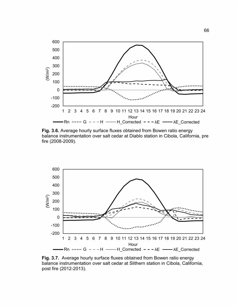
66

Fig. 3.6. Average hourly surface fluxes obtained from Bowen ratio energy balance instrumentation over salt cedar at Diablo station in Cibola, California, pre fire (2008-2009).

Fig. 3.7. Average hourly surface fluxes obtained from Bowen ratio energy balance instrumentation over salt cedar at Slithern station in Cibola, California, post fire (2012-2013).

-200

-100

0

100

200

300

400

500

600

1 2 3 4 5 6 7 8 9 10 11 12 13 14 15 16 17 18 19 20 21 22 23 24

(W/m

2 )

Hour Rn G H H_Corrected λE λE_Corrected

-200

-100

0

100

200

300

400

500

600

1 2 3 4 5 6 7 8 9 10 11 12 13 14 15 16 17 18 19 20 21 22 23 24

(W/m

2 )

Hour Rn G H H_Corrected λE λE_Corrected

67

For either measurement tower, BREB underestimated latent energy

consumption when compared to EC. Mean period fractions of the corrected and

uncorrected fluxes (listed in Table 3.1) imply that ET is estimated at 76 and 83

percent of assumed levels for Diablo and Slithern. Advection of sensible heat

flux from the surrounding Sonoran Desert is the most probable cause. Variations

in the hourly eddy transfer coefficient fraction indicate that the advection is more

of a local nature at Diablo and regional at Slithern. Of course, it would have been

helpful to compare both locations before and after the fire where canopy height

changed from around 6 meters to up to 2 meters of regrowth. This would have

distinguished the fire’s impact on the analysis, ascribing the remaining

divergence to the locality. A difference between the two sites is the tree density

that could be a function of distance from the river and groundwater salinity,

where Diablo reads twice the electrical conductivities of Slithern.

Table 3.1. Advection-corrected to non-corrected fraction of seasonal sensible and latent heat fluxes over salt cedar in Cibola, California, pre and post fire.

Station Period H λE Diablo 2008-2009 0.81 1.63

Slithern 2012-2013 0.58 1.80

68

3.9 Summary and Conclusions

Hourly estimated latent and sensible heat fluxes above saltcedar

vegetation were obtained from adjacent EC and BREB systems installed on two

separate towers in the Cibola National Wildlife Refuge, California. With the arid

environment surrounding the Colorado River, the suspicion was that sensible

heat advection would negatively affect the BREB partition of the latent heat flux.

EC and BREB datasets were prepared and used for comparison of calculated

surface fluxes. It was found that the BREB system at both locations linearly

overestimated the Bowen ratio and consequently underestimated the latent heat

flux during turbulent, daytime periods and was of no confidence at night due to

both systems being unable to measure accurately under stable conditions.

Inferred from the EC and BREB Bowen ratios, the fraction of the turbulent

transfer coefficients of heat and water vapor in the BREB Bowen ratio calculation

was shown to decrease during the day at one location and remain constant at

another, both well below unity. These lower exchange coefficients for heat

substantiated advective conditions at both towers under gradient BREB

methodology. In summary, uncorrected fluxes were found to underestimate and

misrepresent hourly contributions of the latent heat flux, or saltcedar ET.

3.10 Acknowledgments

This study was supported by the Six Agency Committee of the Colorado

River and the U.S. Bureau of Reclamation through a cooperative agreement.

Partial support was also provided by the Utah Agricultural Experiment Station

69

and the Remote Sensing Services Laboratory in the Department of Civil and

Environmental Engineering at USU. Appreciation is extended to the unnamed

field technicians and reviewers who contributed to this work.

3.11 References

Alfieri, J.G., Kustas, W.P., Prueger, J.H., Hipps, L.E., Evett, S.R., Basara, J.B., Neale, C.M., French, A.N., Colaizzi, P., Agam, N., Cosh, M.H., Chavez, J.L., & Howell, T.A. 2012. On the discrepancy between eddy covariance and lysimetry-based surface flux measurements under strongly advective conditions. Advances in Water Resources, 50, 62-78.

Angus, D.E., & Watts, P.J. 1984. Evapotranspiration—How good is the Bowen ratio method?. Agricultural Water Management, 8(1), 133-150.

Aubinet, M., Vesala, T., & Papale, D. (Eds.). 2012. Eddy covariance: a practical guide to measurement and data analysis. Springer.

Baldocchi, D.D., Meyers, T.P., & Wilson, K.B. 2000a. Correction of eddy-covariance measurements incorporating both advective effects and density fluxes. Boundary-Layer Meteorology, 97(3), 487-511.

Baldocchi, D.D., Finnigan, J., Wilson, K., Paw U, K.T. & Falge, E. 2000b. On measuring net ecosystem carbon exchange over tall vegetation on complex terrain. Boundary-Layer Meteorology, 96(1-2), 257-291.

Berengena, J., & Gavilán, P. 2005. Reference evapotranspiration estimation in a highly advective semiarid environment. Journal of irrigation and drainage engineering, 131(2), 147-163.

Bink, N.J. 1997. The ratio of eddy diffusivities for heat and water vapour under conditions of local advection. Physics and Chemistry of the Earth, 21(3), 119-122.

Brakke, T.W., Verma, S.B., & Rosenberg, N.J. 1978. Local and regional components of sensible heat advection. Journal of Applied meteorology, 17(7), 955-963.

Brotzge, J.A., & Crawford, K.C. 2003. Examination of the surface energy budget: A comparison of eddy correlation and Bowen ratio measurement systems. Journal of Hydrometeorology, 4(2).

70

Brutsaert, W. 1982. Evaporation into the atmosphere: theory, history, and applications.

Chávez, J.L., Howell, T.A., & Copeland, K.S. 2009. Evaluating eddy covariance cotton ET measurements in an advective environment with large weighing lysimeters. Irrigation science, 28(1), 35-50.

Di Tomaso, J.M. 1998. Impact, biology, and ecology of saltcedar (Tamarix spp.) in the southwestern United States. Weed technology, 326-336.

Figuerola, P.I., & Berliner, P.R. 2005. Evapotranspiration under advective conditions. International journal of biometeorology, 49(6), 403-416.

Fuchs, M., & Tanner, C.B. 1970. Error analysis of Bowen ratios measured by differential psychrometry. Agricultural Meteorology, 7, 329-334.

Gavilán, P., & Berengena, J. 2007. Accuracy of the Bowen ratio-energy balance method for measuring latent heat flux in a semiarid advective environment. Irrigation Science, 25(2), 127-140.

Glenn, E.P., Nagler, P.L., Morino, K., & Hultine, K.R. 2013. Phreatophytes under stress: transpiration and stomatal conductance of saltcedar (Tamarix spp.) in a high-salinity environment. Plant and Soil, 1-18.

Guo, Y., & Schuepp, P.H. 1994. On surface energy balance over the northern wetlands: 2. The variability of the Bowen ratio. Journal of Geophysical Research: Atmospheres (1984–2012), 99(D1), 1613-1621.

Heilman, J.L., Brittin, C.L., & Neale, C.M.U. 1989. Fetch requirements for Bowen ratio measurements of latent and sensible heat fluxes. Agricultural and Forest Meteorology, 44(3), 261-273.

Leclerc, M.Y., & Thurtell, G.W. 1990. Footprint prediction of scalar fluxes using a Markovian analysis. Boundary-Layer Meteorology, 52(3), 247-258.

Lee, X., Yu, Q., Sun, X., Liu, J., Min, Q., Liu, Y., & Zhang, X. 2004. Micrometeorological fluxes under the influence of regional and local advection: a revisit. Agricultural and forest meteorology, 122(1), 111-124.

Mahrt, L., & Ek, M. 1984. The influence of atmospheric stability on potential evaporation. J. Clim. Appl. Meteorol., 23, 222–234.

Monteith, J.L. 1965. Evaporation and environment. In Symp. Soc. Exp. Biol (Vol. 19, No. 205-23, p. 4).

71

Motha, R.P., Verma, S.B., & Rosenberg, N.J. 1979. Exchange coefficients under sensible heat advection determined by eddy correlation. Agricultural meteorology, 20(4), 273-280.

Nagler, P.L., Morino, K., Murray, R.S., Osterberg, J., & Glenn, E.P. 2009. An empirical algorithm for estimating agricultural and riparian evapotranspiration using MODIS Enhanced Vegetation Index and ground measurements of ET. I. Description of method. Remote Sensing, 1(4), 1273-1297.

Papaioannou, G., Jacovides, C., & Kerkides, P. 1989. Atmospheric stability effects on eddy transfer coefficients and on Penman's evaporation estimates. Water resources management, 3(4), 315-322.

Payero, J.O., Neale, C.M.U., Wright, J.L., & Allen, R.G. 2003. Guidelines for validating Bowen ratio data. Transactions of the ASAE, 46(4), 1051-1060.

Perez, P.J., Castellvi, F., Ibanez, M., & Rosell, J.I. 1999. Assessment of reliability of Bowen ratio method for partitioning fluxes. Agricultural and Forest Meteorology, 97(3), 141-150.

Shafroth, P.B., Cleverly, J.R., Dudley, T.L., Taylor, J.P., Riper III, C.V., Weeks, E.P., & Stuart, J.N. 2005. Control of Tamarix in the western United States: implications for water salvage, wildlife use, and riparian restoration. Environmental Management, 35(3), 231-246.

Tanner, B.D., Greene, J.P., & Bingham, G.E. 1987. A Bowen ratio design for long term measurements. American Society of Agricultural Engineers (Microfiche collection)(USA).

Todd, R.W., Evett, S.R., & Howell, T.A. 2000. The Bowen ratio-energy balance method for estimating latent heat flux of irrigated alfalfa evaluated in a semi-arid, advective environment. Agricultural and Forest Meteorology, 103(4), 335-348.

Twine, T.E., Kustas, W.P., Norman, J.M., Cook, D.R., Houser, P., Meyers, T.P., Prueger, J.H., Starks, P.J., & Wesely, M.L. 2000. Correcting eddy-covariance flux underestimates over a grassland. Agricultural and Forest Meteorology, 103(3), 279-300.

USFWS-CNWR. Accessed June 3, 2014. Cibola National Wildlife Refuge | Arizona and California. U.S. Fish & Wildlife Service. <http://www.fws.gov/refuge/Cibola/>

van Gorsel, E., Leuning, R., Cleugh, H.A., Keith, H., Kirschbaum, M.U., & Suni, T. 2008. Application of an alternative method to derive reliable estimates

72

of nighttime respiration from eddy covariance measurements in moderately complex topography. agricultural and forest meteorology, 148(6), 1174-1180.

Verma, S.B., Rosenberg, N.J., & Blad, B.L. 1977. Turbulent exchange coefficients for sensible heat and water vapor under advective conditions. Journal of Applied Meteorology, 17(3), 330-338.

Wilson, K.B., Hanson, P.J., Mulholland, P.J., Baldocchi, D.D., & Wullschleger, S.D. 2001. A comparison of methods for determining forest evapotranspiration and its components: sap-flow, soil water budget, eddy covariance and catchment water balance. Agricultural and Forest Meteorology, 106(2), 153-168.

73

CHAPTER 4

SALTCEDAR EVAPOTRANSPIRATION PRE AND POST FIRE

4.1 Abstract

Bowen ratio and eddy covariance energy balance flux towers have been

installed since 2006 in a dense salt cedar forest within the Cibola National

Wildlife Refuge, California, along the floodplain of the lower Colorado River to

monitor the evapotranspiration of saltcedar (Tamarix ramosissima). Past

research has analyzed data collected from these systems along with information

from groundwater wells, scintillometer readings, and remote sensing approaches.

In the summer of 2011, a wildfire erupted destroying both the saltcedar and

research equipment. To monitor the regrowth after the fire, groundwater

piezometers and two eddy covariance flux towers were reestablished. Additional

measurements of salt cedar water consumption were gathered, augmenting pre-

fire records. Analyzed tower and well measurements revealed a reduction of

saltcedar evapotranspiration and an increase in groundwater elevation post fire.

4.2 Introduction

Water use of saltcedar (Tamarix sp.), specifically along riparian corridors

in the southwestern United States, remains a question despite a half century of

interorganizational studies and collaborations. An exotic but naturalized

facultative phreatophyte, saltcedar has thrived where soil alkalinity, groundwater,

and surface disturbances have coexisted, which has culminated into annual

increases of areal cover and draw on water resources (Brotherson and Winkel,

74

1986; Di Tomaso, 1998). By means of superior competitive abilities, saltcedar

has threatened native plant communities and has been the target of numerous

governmental programs either to slow the advance or eradicate the species.

Many researchers have disagreed as to the predominant means of propagation

(Robinson, 1965; DeLoach et al., 2000; Glenn and Nagler, 2005; Stromberg et

al., 2009) and to the consumptive use of water (summarized in Shafroth et al.,

2005) as compared to the displaced native phreatophytes, both factors having

political and environmental implications. Regardless of the cause, saltcedar now

inhabits every major watershed in the American Southwest (Zouhar, 2003) with

an ever-expanding influence on groundwater resources.

Fire prevalence historically in the Southwest had been low in floodplains

due to presence of water and quick decomposition of potential fuel, but it has

more recently become a greater factor. Evidence points toward saltcedar’s

dense canopy, salt excretions, and resultant leaf litter that increase the possibility

of a fire. Saltcedar stands typically experience burns every 15-20 years, which

when combined with the ability to quickly resprout from the root crown have

created monospecific communities. These characteristics have enabled long-

term survivability and dominance over other native riparian vegetation. (Busch,

1995; Ellis, 2001; Lewis et al., 2003; Zouhar, 2003) Fire frequency impacts both

the surface vegetation and subsurface water supplies by affecting transpiration.

Interestingly, a study concluded that saltcedar exhibited higher midday

transpiration rates in recovering burned specimen than in controls (Busch and

Smith, 1993). If this were the case (as this subject is the foundation of this

75

paper), then to what extent, if any, would a burn impact saltcedar water use? In

answer to this question, the following analysis determines to compare saltcedar

evapotranspiration before and after a burn in the United States Southwest.

Groundwater and evapotranspiration research data of a saltcedar-infested

region bordering the Colorado River in southern California has been monitored

by groundwater and flux tower measurements since 2006. A wildfire that

ravaged the area in 2011 became a unique opportunity to conduct research,

because it transformed an actively transpiring, mature saltcedar forest within a

short interval into a blackened and barren landscape. This afforded an instant

comparison to measure the impact of no vegetation on the groundwater.

Additionally, the effects of the resurgent growth on groundwater levels were

examined. Altogether, the burn enabled a singular verification of measured

fluxes and modeled energy and water balances at the measurement sites.

4.3 Methods

Plant groundwater consumption may be estimated by measuring the

change in the phreatic surface elevation. By accounting for mass source fluxes

of inflow and outflow, the remaining dimension equates to the volumetric uptake

within the medium porosity. To determine the actual volume, the ratio of the

affected void to the total volume is multiplied. This last soil property, the specific

yield, must be known or estimated. A mathematical representation for

groundwater evapotranspiration (ET) over a period of time is presented in

Equation 4.1 below.

76

)( HRSET YG ∆−= [ 4.1 ]

where GET is groundwater evapotranspiration, YS is specific yield, R is

the change in depth due to lateral recharge or depletion, and H∆ is the

change in phreatic surface elevation.

By measuring groundwater fluctuations in a well, one of the two inner

variables in Equation 4.1 is readily obtained, which then leaves the recharge.

White (1932) documented a method, which has been widely applied, to estimate

the recharge rate for a day as the mean groundwater fluctuation for the first few

hours after midnight assuming no plant transpiration during this period. Since the

estimated day-to-day recharge rates vary sporadically and the assumption of no

nighttime transpiration contested, an alternate method was considered. Soylu et

al. (2012) proposed to calculate the recharge by detrending the oscillating diurnal

groundwater movements. Because it forms a sinusoidal function, the method

was called a “Fourier-based improvement” to the general White Method and is

replicated in Equation 4.2. C or the amplitude is functionally the recharge minus

the change in elevation deduced by removing the offset, linear, and wave trends.

This equation may be applied to time steps of periods involving one or more

days.

))(2sin()( Dtt

CBtAtFN

+++=π [ 4.2 ]

77

where )(tF is the groundwater stage at a given time t , A is the scalar

offset, B is the linear offset, C is the amplitude, Nt is the number of

increments per cycle or day, and D is the phase offset.

By derivation, C is one-half of HR ∆− , which is subsequently doubled and

multiplied by a corrective factor (an artifact of the detrending process) to estimate

groundwater ET as shown in Equation 4.3. Still required is the specific yield, but

Equation 4.3 takes on a different form than Equation 4.1 where the two

corrections may be treated as one variable and obtained through calibration.

Other transpiration measurement techniques, such as lysimetry, eddy

covariance, Bowen ratio, chambers, or sap flow, could be used for this purpose.

))(2( CkSET YG = [ 4.3 ]

where k is a scaling factor resulting from the detrending operations.

4.4 Materials

Situated along the Lower Colorado River in the middle of the Sonoran

Desert, the Cibola National Wildlife Refuge (CNWR) is preserved by the U.S.

Fish and Wildlife Service as a haven for migratory birds and other wildlife

(USFWS-CNWR 2014). CNWR encompasses the river floodplain of California

on the west and Arizona on the east and has been overrun by saltcedar (Tamarix

ramosissima). Since 2006, several universities in connection with the U.S.

Bureau of Reclamation have been investigating ET rates within the saltcedar

forests by recording sap flux, groundwater fluctuations, and tower measurements

78

using scintillometer, eddy covariance (EC), Bowen ratio (BR), and Penman

techniques. Early measurements were analyzed and published, including

groundwater ET via the standard White Method (Taghvaeian 2011). However,

an unforeseen but ultimate benefit to the study occurred when the Three Slashes

Fire burned the saltcedar in late August 2011. Because most of the equipment

had expired in the inferno, towers were reconstructed and well caps replaced in

early 2012. Measurements resumed, and the data collected characterized the

water use of the reemerging saltcedar. Although instruments and hence capital

were lost in the flames, the overarching goal of measuring saltcedar impact on

the Colorado River-supplied groundwater was enhanced by being able to

evaluate the effects of the absence of saltcedar in the floodplain. Such a

scenario would never have been permitted in the study scope, but from the point

of view of this study the fire provided an opportunity for a “natural experiment”.

Five false-color aerial photos (NAIP 2014) including the three tower sites

in the study area are shown in Fig. 4.1, which depict the saltcedar growth well

before and soon after the fire and also the regrowth. Nagler et al. (2009b)

described the study area pre fire and indicated that the plain was dominated by

invasive saltcedar with occasional patches of native arrowweed (Pluchia

sericea), mesquite (Prosopis pubescens), and quailbush (Atriplex lentiformis)

intermingled. Correspondingly, inspection post fire included the same vegetation

patterns with the exception of arrowweed covering some wide stretches. Of note

in Fig. 4.1.D is a region where the fire did not advance that had already

experienced a fire in 2006, and careful inspection of subfigure B shows the

79

regrowth. Analysis of the 2006 blaze found that a previous fire had burned

CNWR in 1991 with the sample site nearest the river experiencing the greatest

intensity (Godaire and Klinger, 2007). Confirmed at both locations precisely was

the 15-20 year proposed fire interval for saltcedar.

Fig. 4.1. False color (infrared, red, green) images from the National Agriculture Imagery Program (NAIP) of the tower sites in the Cibola National Wildlife Refuge, (A) June 26, 2005; (B) May 25, 2009; (C) April 26 and 28, 2010; (D) April 23, 2012; (E) May 16, 2014.

80

Tower sites were positioned in a dense stand of salt cedar (Slithern),

medium-density salt cedar (Diablo), and next to the river (Swamp), which were at

least the circumstances pre fire. Groundwater monitoring stations were located

next to each tower site with an additional four wells in the near proximity (Fig.

4.2). Once elevation differences were eliminated among well sites through a

high-resolution LIDAR-derived surface elevation model and considering the

overall accuracy of the groundwater loggers, measurements from the clusters of

five well sites were nearly identical (Taghvaeian, 2011). This redundancy proved

vital as the groundwater data acquisition was able to survive fire, battery failures,

and change in technicians with few gaps. Beyond the potential for fire, CNWR

has a harsh climate with summer temperatures exceeding 50 °C and desert

conditions of 80 mm average precipitation annually (of which most falls in the

winter months). Because of the extreme environment, maintenance once every

1-2 months due to site remoteness, and non-redundant tower instruments, data

gaps did occur in the surface flux measurements but were remedied as quickly

as possible.

As Fig. 4.1 and Fig. 4.2 both show, the stream nearest the station sites is

actually the old channel of the Colorado River with the engineered channel on

the east, and it is fed both by the Palo Verde Irrigation District outlet drain and

the river further upstream. The primary source of groundwater in the study area

of CNWR is the drain, and higher groundwater salinity has been observed at the

wells further from the source. Regrowth post fire around Slithern tower site is

shown in Fig. 4.3 with a high percentage of saltcedar reemerging and achieving

81

significant growth in just two years. Although not specifically sampled, the

resprouting from the root crown exceeded the 53 and 55% reported by Ellis

(2001) and echoed the observation of Zouhar (2003) that saltcedar regrowth “can

reach several feet in just a few months”.

Fig. 4.2. Tower and groundwater well observation locations within the Cibola National Wildlife Refuge.

82

Fig. 4.3. Saltcedar regrowth in the Cibola National Wildlife Refuge post fire (From Top to bottom, March 12, 2012; May 29, 2013; August 20, 2013).

4.5 Data Analysis and Results

BR and EC tower measurements were examined and corrected with the

methodology outlined in a previous publication (Lewis and Neale, 2014). It was

found that horizontal heat advection from the surrounding desert seriously

83

impaired BR ET before and after the fire. Attempts at compensating for

advection through EC-based corrections for the BR data are shown in Fig. 4.4

(on a weekly moving daily average to increase clarity of the trends). Since

Swamp never had an EC setup, its BR data and resultant ET were not corrected

and are therefore not included. What can be gleaned from the BR ET are

seasonal patterns with higher water use shifted at Slithern to later in the year

after the fire. It additionally highlights differences between an energy balance

method and a mass balance (in a later figure). Presentation of the BR results

also is important because of the many papers that have used the data previously

for comparison to sap flow, remote sensing, groundwater, and scintillometers

(Nagler et al., 2009a; Taghvaeian, 2011; Geli et al., 2012). This was mainly

because the method was common to all towers, and because the EC data had

never been fully processed. Shown in Fig. 4.5 is the weekly averaged daily EC

ET for Diablo pre fire (which has a substantial record) and for Diablo and Slithern

post fire. Energy balance closure of the EC data for Diablo and Slithern was

around 70 percent (not untypical for the environment), and the remaining energy

was proportioned to latent and sensible heat fluxes by using the Bowen ratio

(Twine et al., 2000). ASCE standardized short reference ET (Walter et al., 2000)

in Fig. 4.4, Fig. 4.5, and later figures was calculated from hourly data at a local

electronic weather station (Palo Verde II; CIMIS 2014) with missing

meteorological data filled in with adjusted values from a NASA gridded weather

forcing model (NLDAS-2).

84

Fig. 4.4. Weekly averaged daily ET from Bowen ratio systems in the Cibola National Wildlife Refuge, (Top: 2006-2010; Bottom: 2012-2013).

Preparation of the groundwater pressure and temperature readings

involved initial data screening, subtraction of atmospheric pressure, conversion

to depths, and determination of phreatic surface elevation (above mean sea

level) through well cord lengths and the LIDAR dataset that established the exact

ground elevation at each well. Readings were logged at 15-minute intervals and

were slightly offset at different well sites. These values were shifted to regular

0

2

4

6

8

10

1 31 61 91 121 151 181 211 241 271 301 331 361

0

2

4

6

8

10

1 31 61 91 121 151 181 211 241 271 301 331 361

Diablo Slithern Swamp Reference ET

Eva

potra

nspi

ratio

n (m

m/d

ay)

85

increments or to :00, :15, :30, and :45 minutes of each hour through linear

interpolation. Afterwards, pressures and temperatures were averaged for each

hour, which was the time step used for subsequent calculations. Atmospheric

pressure over CNWR was obtained by adjusting the continuous record of the

Blythe (California) airport weather station to match barometric readings from two

suspended, unsubmerged loggers in wells at Slithern tower and a nearby well

location. Because adjacent readings were analogous, groundwater elevations

were grouped by tower site and averaged. In the process, many errors could be

detected through comparison (e.g., abrupt changes in cord length after a logger

had been retrieved and replaced, bad data, incorrectly entered offsets) and either

be corrected or excluded from the averaging. Further, loss of data through

burned out wells, dead batteries, and human errors was mitigated by the similar

readings at adjacent well sites.

Final averaged groundwater elevations for each tower group are plotted in

Fig. 4.6 likewise on a weekly moving daily average. Stream elevation shown

was provided by a U.S. Bureau of Reclamation gaging station, Palo Verde Outfall

Drain, which is roughly 9 kilometers upstream from the point on the drain nearest

Slithern. Seasonal patterns of phreatophyte ET are evident as the groundwater

table recovers in the winter from summertime lower levels. Diablo and Slithern

groundwater elevations are comparable with lower elevations at Diablo expected

by its further distance inland. Swamp, being closer to the source, is affected by

the day-to-day fluctuations of the water levels in the drain but also does not drop

as low during the peak ET season. Post-fire groundwater recharge attained

86

unprecedented levels in the record and lowered only a fraction of what pre-fire

levels were during the growing season. With stream stage or inflow maintaining

typical behavior, an initial conclusion would be that surface vegetative

transpiration requirements or groundwater ET had lessened post fire.

Fig. 4.5. Weekly averaged daily ET from eddy covariance systems in the Cibola National Wildlife Refuge, (Top: 2007-2009; Bottom: 2012-2013).

0

2

4

6

8

10

1 31 61 91 121 151 181 211 241 271 301 331 361

0

2

4

6

8

10

1 31 61 91 121 151 181 211 241 271 301 331 361

Diablo Slithern Reference ET

Eva

potra

nspi

ratio

n (m

m/d

ay)

87

Amplitudinal coefficients were calculated from a least-squares fit of the

group averaged groundwater elevations to Equation 4.2. Because of the nature

of the detrending, variable lengths of data could be applied to the equation,

ranging normally from a day to a week or more. A moving calculation period of

25 hours was selected with 12 hours before and after the record of interest

(example fits in Fig. 4.7). Output was technically hourly but represented a much

longer duration. Final amplitudes were averaged for each day and doubled in

preparation to be multiplied by additional factors of specific yield and the

detrending correction in Equation 4.3.

Groundwater ET was calculated using the Fourier-based White Method

(FW) near each tower site, and the product of the specific yield and scaling factor

was determined from a least-squares fit to overlapping latent heat flux from the

EC method at Diablo and Slithern. Both EC and BR are frequently unreliable at

night where saltcedar has been documented to transpire at 12-25% or more of

total daily ET (Dawson et al., 2007; Nagler et al., 2009b; Hultine et al., 2010;

Glenn et al., 2013). Since the EC calculations displayed no ET at night, daily

estimated ET was increased by a value of one-third. This addition corresponds

to reported nighttime transpiration totaling 25% of daily values from sap flux

sensors in a previous study (Nagler et al., 2009b). Calibration for Swamp, which

never had an EC system, was obtained by matching the wintertime baseline

groundwater ET of Diablo and Slithern pre fire. Pseudo (by incorporation of the

corrective factor) specific yield values were between 0.107 and 0.125 for all three

sites (Table 4.1, which also summarizes other site properties). Well site

88

Fig. 4.6. Weekly average daily groundwater surface elevation from multiple wells at 3 sites in the Cibola National Wildlife Refuge.

Fig. 4.7. Example of 24 hour Fourier-White method implementation for 3 days at Diablo tower well, Cibola National Wildlife Refuge (July 1-7, 2011).

63.0

63.5

64.0

64.5

65.0

65.5

66.0

66.5

2006 2007 2008 2009 2010 2011 2012 2013

Ele

vatio

n (m

eter

)

Diablo Slithern Swamp Stream Stage Fire

63.40

63.45

63.50

63.55

63.60

7/1/2011 7/2/2011 7/3/2011 7/4/2011 7/5/2011 7/6/2011 7/7/2011

Ele

vatio

n (m

eter

)

Diablo F(t)

89

characterizations were obtained pre fire and included water quality testing and

soil samples. At a depth of 2-4 meters—which is where the groundwater table

fluctuated—and for all sampled soil cores near Diablo and Slithern, the texture

classification was either a sandy-loam or a loamy-sand. According to Johnson

(1967), specific yields for a corresponding grain size of fine sand are between

0.10 and 0.28 with 0.21 being the average. Loheide et al. (2005) defined a

‘readily available specific yield’ as “a function of drainage time, depth to the water

table, and the properties of the porous media” for which fluctuations of the water

table do not occur instantaneously as is suggested in a laboratory setting. These

in-field values of specific yield are therefore a fraction of the expected value. In

his work, Loheide and his associates found that for large grain sizes the readily

available specific yield was nearly equal the specific yield but for smaller grain

sizes the fraction could be as low as 40%. Assuming the averaged value for

specific yield in the study site of 0.21 and Slithern’s calculated (pseudo) specific

yield of 0.125 as the readily available specific yield, the fraction of the two would

yield 60%. This is low for the site’s sand and loam texture but not unreasonable

as it can be presupposed by a lower-than-average specific yield or a k value less

than one.

Weekly averaged daily groundwater ET for the three well groups together

with calculated short reference ET is plotted in Fig. 4.8 with years before the fire

and after the fire averaged for simplicity. Both Diablo and Slithern wells exhibited

very good agreement in the pre-fire period while groundwater ET at Swamp was

strikingly higher and followed reference ET levels during the non-dormant period.

90

Fig. 4.8. Weekly averaged daily groundwater et from multiple wells at 3 sites in the Cibola National Wildlife Refuge, (From Top to Bottom, 2006-2010; 2011; 2012-2013).

Gro

undw

ater

Eva

potra

nspi

ratio

n (m

m/d

ay)

91

Table 4.1. Averaged groundwater properties for multiple wells at 3 sites in the Cibola National Wildlife Refuge pre and post fire.

Parameter Period Unit Diablo Slithern Swamp Specific Yield 2006-2013 — 0.113a 0.125a 0.107b

Depth from Surface 2006-2013 meter 2.96 3.33 2.62 Temperature 2006-2013 °C 22.4 21.8 22.2

Electrical Conductivity 2006-2011 mS/cm 16.58 8.30 3.95 Note: Specific yield aderived from calibration to eddy covariance measurements and bestimated by matching wintertime baseline to Diablo and Slithern.

Previously, suspicion was directed towards the validity of Swamp groundwater

ET as it heavily correlated to the rise and fall of the drain stage. Yet, the fire in

August 2011 confirmed the absence of any direct coupling of the drain flow (in

addition to feeding the groundwater) on the calculated groundwater ET for all

three well groups by the sudden and sustained drop in groundwater ET post fire,

which abruptness is moderated by the weekly average in the figure.

Post fire results are congruent with previous states, and the effect of the

burn was reduced groundwater ET rates. Only at Slithern was an annual offset

present which otherwise mimicked Diablo groundwater ET. One possible

explanation is that Slithern wells were not measuring groundwater consumption

of sole saltcedar regrowth. In fact, sizeable swaths of native arrowweed, an

evergreen (Ferren et al., 1996), had occupied some areas not too far eastward of

Slithern tower. This could also explain the non-zero usage during dormant

saltcedar periods in previous years. Averaged daily groundwater ET summed to

92

annual values, both up to the fire and after, is presented in Table 4.2. Both

Diablo and Swamp have lower rates post fire at different scales, but Slithern

groundwater ET actually increases after the fire. This could be the outcome of a

greater presence of arrowweed among the saltcedar.

4.6 Discussion

Both pre and post fire, results from this study indicate that the saltcedar-

groundwater relationship in CNWR was affected by surface-to-groundwater

depth, salinity, plant phenology, and the fire. Moreover, our observations were in

agreement with Devitt et al. (1998) that “[saltcedar] has the potential to be both a

low water user and a high water user, depending on water availability, canopy

development, and atmospheric demand, and that advection can dominate energy

balances and ET in arid land riparian zones”. What was not observed were soil

hydraulic limitations (Glenn et al., 2013) and maximum or potential rates of

saltcedar ET. Overall, groundwater depth and salinity at Diablo, Slithern, and

Swamp were more important factors than surface vegetative conditions pre fire,

while post fire groundwater was not the limiting factor.

Table 4.2. Average annual groundwater ET from multiple wells at 3 sites in the Cibola National Wildlife Refuge Pre and post fire assuming conservative estimates of specific yield (meter/year).

Period Diablo Slithern Swamp Ref. ET Pre Fire (2006-2011) 0.805 0.838 1.923 1.786 Post Fire (2011-2013) 0.327 0.909 1.331 1.773

93

Previous studies in CNWR (Taghvaeian, 2011; Glenn et al., 2013)

concluded that depth to groundwater constrained saltcedar ET but could not

explain the dissimilarities among BR results and yet comparable groundwater ET

at Diablo and Slithern. Further exacerbation stemmed from Swamp groundwater

readings that revealed more than double annual groundwater ET rates at a site

only a few hundred meters closer to the drain than Slithern. Yet, the average

depths to groundwater were lowest at Swamp and 0.34 and 0.71 m higher at

Diablo and Slithern, respectively. This is in harmony with the difference seen in

saltcedar ET by Van Hylckama (1970) in groundwater depth changes of 1.5

meters to 2.1 meters and 2.1 meters to 2.7 meters. Reported shifts in saltcedar

water uptake from the phreatic to the vadose zone (Nippert et al., 2010) were not

apparent, for when the groundwater maintained a constant depth so did the

groundwater ET. This is most likely due to the lack of precipitation during the

midsummer months or a buildup of salts in the vadose zone as proposed by

Glenn et al. (2013).

Practically equal estimates of groundwater ET from measurements at

Diablo and Slithern pre-fire and longer depth to groundwater at Slithern would

void the argument for higher groundwater ET rates at Swamp if based solely on

depth to groundwater. Averaged measured groundwater electrical conductivity

was half the value at Slithern than at Diablo and less than half again at Swamp.

Both saltcedar and arrowweed have been found to tolerate the groundwater

salinities reported at the three locations in this study, but reduction of

transpiration due to higher salinity was also reported with more gradual rates for

94

saltcedar than for arrowweed (Glenn et al., 1998; Vandersande et al. 2001).

Given the opposite changes in depth to groundwater and salinity at both Diablo

and Slithern, similar groundwater ET rates should not be surprising.

Assuming the maximum specific yield of 0.28 for the sandy and loamy soil

in CNWR and that the reported annual groundwater ET for each location was

based on a specific yield of 0.10, the factor controlling the maximum probable

estimates would be 0.28 / 0.10 = 2.8. By applying this upper bound, annual

groundwater ET pre fire would range between 1.87 and 5.05 meters/year, the

original estimates being 0.81 and 1.92 meters/year. All but the highest estimate

fall within the ET rates suggested in the literature (reviewed by Shafroth et al.,

2005) and which confirms the reduction of the readily available specific yield.

More recent studies (Dahm et al., 2002; Nagler et. al., 2008; Westenburg et al.,

2006) support the eddy covariance-matched rates in Table 4.2 while the results

of Sala et al. (1996) of saltcedar ET up to twice the potential rate would

correspond with maximum specific yields. Based on evidence from the

meteorological tower measurements, this study backs the latest figures.

Reduction in saltcedar ET is a direct relationship to how well the

environment duplicates theoretical or greenhouse conditions. Groundwater ET at

Swamp visibly follows the rise and fall of the drain stage influenced by the

Colorado River and would transpire at greater rates if the drain always

maintained a higher level (in line with Devitt et al., 1997a and 1997b). The same

is true at Diablo and Slithern pre fire with late spring surges in groundwater ET

reversed by groundwater depressions. This phenomenon may also be

95

influenced by the saltcedar growth patterns, which show higher consumption in

the earlier portion of the year with a downward trend throughout the rest of the

season as evidenced before and after the fire. Following the 2011 fire,

groundwater ET became nearly zero with likely some plants that never burned

still transpiring. Fig. 4.1.D and E clearly show that post fire regrowth was much

higher around Slithern than at Diablo and corroborate the higher annual

groundwater ET post fire at Slithern while still maintaining higher groundwater

levels from lower groundwater ET rates elsewhere. Part of these annual values

was already allocated to much greater arrowweed contribution. If the offset of

1.6 mm/day were subtracted, then the annual total would become 0.324

meters/year or parallel to Diablo. This would apportion saltcedar groundwater ET

at Diablo and Slithern at 40 percent of pre-fire rates and Swamp at 70 percent.

4.7 Conclusions

Due to a 2011 burn in the CNWR, measured saltcedar water use dropped

at three locations near an agricultural drain feeding into the lower Colorado River.

Groundwater recovery was immediately evident and sustained for the next two

years. Study results concur with Di Tomaso (1998) and DeLoach et al. (2000)

that removal of saltcedar yields increases in water availability. At least in the

case of CNWR, frequent burns of the dense saltcedar forest would most likely

decrease inter-annual ET, thus providing more water downstream but would be

unlikely to eliminate the infestation. Magnitudes of saltcedar water use were

within the realm of native phreatophytes. Since measurements are ongoing,

96

future data analysis of the effects of the Mediterranean tamarisk beetle

(Diorhabda elongata, Lewis et al. 2003) on saltcedar groundwater consumption

will be interesting as the beetle migrates south along the Colorado River corridor

and will soon be present at CNWR.

4.8 Acknowledgments

This study was supported by the Six Agency Committee of the Colorado

River and the U.S. Bureau of Reclamation through a cooperative agreement.

Partial support was also provided by the Utah Agricultural Experiment Station

and the Remote Sensing Services Laboratory in the Department of Civil and

Environmental Engineering at USU.

4.9 References

Brotherson, J.D., & Winkel, V. 1986. Habitat relationships of saltcedar (Tamarix ramosissima) in central Utah. Western North American Naturalist, 46(3), 535-541.

Busch, D.E. 1995. Effects of fire on southwestern riparian plant community structure. The Southwestern Naturalist, 259-267.

Busch, D.E., & Smith, S.D. 1993. Effects of fire on water and salinity relations of riparian woody taxa. Oecologia, 94(2), 186-194.

CIMIS. Accessed August 28, 2014. California Irrigation Management Information System | California Department of Water Resources, University of California at Davis. <http://www.cimis.water.ca.gov/cimis/welcome.jsp>.

Dahm, C.N., Cleverly, J.R., Allred Coonrod, J.E., Thibault, J.R., McDonnell, D.E., & Gilroy, D.J. (2002). Evapotranspiration at the land/water interface in a semi‐arid drainage basin. Freshwater Biology, 47(4), 831-843.

Dawson, T.E., Burgess, S.S., Tu, K.P., Oliveira, R.S., Santiago, L.S., Fisher, J.B., Simonin, K.A., & Ambrose, A.R. 2007. Nighttime transpiration in woody plants from contrasting ecosystems. Tree Physiology, 27(4), 561-575.

97

DeLoach, C.J., Carruthers, R.I., Lovich, J.E., Dudley, T.L., & Smith, S.D. 2000, July. Ecological interactions in the biological control of saltcedar (Tamarix spp.) in the United States: toward a new understanding. In N. R. Spencer (Ed.), Proceedings of the X international symposium on biological control of weeds (Vol. 20001, pp. 819-8731). Bozeman^ eMontana Montana: Montana State University.

Devitt, D.A., Piorkowski, J.M., Smith, S.D., Cleverly, J.R., & Sala, A. 1997a. Plant water relations of Tamarix ramosissima in response to the imposition and alleviation of soil moisture stress. Journal of Arid Environments, 36(3), 527-540.

Devitt, D.A., Sala, A., Mace, K.A., & Smith, S.D. 1997b. The effect of applied water on the water use of saltcedar in a desert riparian environment. Journal of Hydrology, 192(1), 233-246.

Devitt, D.A., Sala, A., Smith, S.D., Cleverly, J., Shaulis, L.K., & Hammett, R. 1998. Bowen ratio estimates of evapotranspiration for Tamarix ramosissima stands on the Virgin River in southern Nevada. Water Resources Research, 34(9), 2407-2414.

Di Tomaso, J.M. 1998. Impact, biology, and ecology of saltcedar (Tamarix spp.) in the southwestern United States. Weed technology, 326-336.

Ellis, L.M. 2001. Short-term response of woody plants to fire in a Rio Grande riparian forest, Central New Mexico, USA. Biological Conservation, 97(2), 159-170.

Ferren, W.R., Fiedler, P.L., Leidy, R.A., Lafferty, K.D., & Mertes, L.A. 1996. Wetlands of California: part 2. Classification and description of wetlands of the central and southern California coast and coastal watersheds. Madroño, 43(1), 125-182.

Geli, H.M., Neale, C.M., Watts, D., Osterberg, J., De Bruin, H.A., Kohsiek, W., Pack, R.T., & Hipps, L.E. 2012. Scintillometer-Based Estimates of Sensible Heat Flux Using Lidar-Derived Surface Roughness. Journal of Hydrometeorology, 13(4), 1317-1331.

Glenn, E.P., & Nagler, P.L. 2005. Comparative ecophysiology of Tamarix ramosissima and native trees in western US riparian zones. Journal of Arid Environments, 61(3), 419-446.

Glenn, E.P., Nagler, P.L., Morino, K., & Hultine, K.R. 2013. Phreatophytes under stress: Transpiration and stomatal conductance of saltcedar (Tamarix spp.) in a high-salinity environment. Plant and soil, 371(1-2), 655-672.

98

Glenn, E., Tanner, R., Mendez, S., Kehret, T., Moore, D., Garcia, J., & Valdes, C. 1998. Growth rates, salt tolerance and water use characteristics of native and invasive riparian plants from the delta of the Colorado River, Mexico. Journal of Arid Environments, 40(3), 281-294.

Godaire, J.E., Klinger, R.E. 2007. Tree-Ring Dating of Tamarisk (Tamarix ramosissima), Cibola National Wildlife Refuge, California. U.S. Department of the Interior. Bureau of Reclamation.

Hultine, K.R., Nagler, P.L., Morino, K., Bush, S.E., Burtch, K.G., Dennison, P.E., Glenn, E.P., & Ehleringer, J.R. 2010. Sap flux-scaled transpiration by tamarisk (Tamarix spp.) before, during and after episodic defoliation by the saltcedar leaf beetle (Diorhabda carinulata). Agricultural and Forest Meteorology, 150(11), 1467-1475.

Johnson, A.I. 1967. Specific yield: compilation of specific yields for various materials. US Government Printing Office.

Lewis, C.S. and Neale, C.M. 2014. Bowen Ratio System Assessment over Saltcedar under Different Atmospheric Stability and Advective Conditions by the Eddy Covariance Technique. Unpublished manuscript.

Lewis, P.A., DeLoach, C.J., Knutson, A.E., Tracy, J.L., & Robbins, T.O. 2003. Biology of Diorhabda elongata deserticola (Coleoptera: Chrysomelidae), an Asian leaf beetle for biological control of saltcedars (Tamarix spp.) in the United States. Biological control, 27(2), 101-116.

Loheide, S.P., Butler, J.J., & Gorelick, S.M. 2005. Estimation of groundwater consumption by phreatophytes using diurnal water table fluctuations: a saturated‐unsaturated flow assessment. Water resources research, 41(7).

Nagler, P.L., Glenn, E.P., Didan, K., Osterberg, J., Jordan, F., & Cunningham, J. 2008. Wide‐Area Estimates of Stand Structure and Water Use of Tamarix spp. on the Lower Colorado River: Implications for Restoration and Water Management Projects. Restoration Ecology, 16(1), 136-145.

Nagler, P.L., Morino, K., Murray, R.S., Osterberg, J., & Glenn, E.P. 2009b. An empirical algorithm for estimating agricultural and riparian evapotranspiration using MODIS Enhanced Vegetation Index and ground measurements of ET. I. Description of method. Remote Sensing, 1(4), 1273-1297.

NAIP. Accessed June 3, 2014. National Agriculture Imagery Program | Cal-Atlas Geospatial Clearinghouse. <https://projects.atlas.ca.gov/projects/naip/>

99

Nippert, J.B., Butler Jr, J.J., Kluitenberg, G.J., Whittemore, D.O., Arnold, D., Spal, S.E., & Ward, J.K. 2010. Patterns of Tamarix water use during a record drought. Oecologia, 162(2), 283-292.

NLDAS-2. The North American Land Data Assimilation System Phase 2. NASA Goddard Space Flight Center and Other Collaborators. <ftp://hydro1.sci.gsfc.nasa.gov/data/s4pa//NLDAS/NLDAS_FORA0125_H.002/>.

Robinson, T.W. 1965. Introduction, spread and areal extent of saltcedar (Tamarix) in the western states. US Government Printing Office.

Sala, A., Smith, S.D., & Devitt, D.A. 1996. Water use by Tamarix ramosissima and associated phreatophytes in a Mojave Desert floodplain. Ecological Applications, 888-898.

Shafroth, P.B., Cleverly, J.R., Dudley, T.L., Taylor, J.P., Riper III, C.V., Weeks, E.P., & Stuart, J.N. 2005. Control of Tamarix in the western United States: implications for water salvage, wildlife use, and riparian restoration. Environmental Management, 35(3), 231-246.

Soylu, M.E., Lenters, J.D., Istanbulluoglu, E., & Loheide, S.P. 2012. On evapotranspiration and shallow groundwater fluctuations: A Fourier‐based improvement to the White method. Water Resources Research, 48(6).

Stromberg, J.C., Chew, M. K., Nagler, P.L., & Glenn, E.P. 2009. Changing perceptions of change: the role of scientists in Tamarix and river management. Restoration Ecology, 17(2), 177-186.

Taghvaeian, S. 2011. Water and energy balance of a riparian and agricultural ecosystem along the Lower Colorado River (Doctoral dissertation, UTAH STATE UNIVERSITY).

Twine, T.E., Kustas, W.P., Norman, J.M., Cook, D.R., Houser, P., Meyers, T.P., Prueger, J.H., Starks, P.J., & Wesely, M.L. 2000. Correcting eddy-covariance flux underestimates over a grassland. Agricultural and Forest Meteorology, 103(3), 279-300.

USFWS-CNWR. Accessed June 3, 2014. Cibola National Wildlife Refuge | Arizona and California. U.S. Fish & Wildlife Service. <http://www.fws.gov/refuge/Cibola/>

Van Hylckama, T.E. 1970. Water use by salt cedar. Water Resources Research, 6(3), 728-735.

100

Vandersande, M.W., Glenn, E.P., & Walworth, J.L. 2001. Tolerance of five riparian plants from the lower Colorado River to salinity drought and inundation. Journal of Arid Environments, 49(1), 147-159.

Walter, I.A., Allen, R.G., Elliott, R., Mecham, B., Jensen, M.E., Itenfisu, D., Howell, T.A., Snyder, R., Brown, P., Echings, S., Spofford, T., Hattendorf, M., Cuenca, R.H., Wright, J.L., Martin, D., 2000. ASCE’s standardized reference evapotranspiration equation. In: Proc. of the Watershed Management 2000 Conference, June.

Westenburg, C.L., Harper, D.P., & DeMeo, G.A. 2006. Evapotranspiration by Phreatophytes Along the Lower Colorado River at Havasu National Wildlife Refuge, Arizona. US Geological Survey.

White, W.N. 1932. A method of estimating ground-water supplies based on discharge by plants and evaporation from soil: Results of investigations in Escalante Valley, Utah. US Government Printing Office.

Zouhar, K. 2003. Tamarix spp. Fire Effects Information System,[Online]. US Department of Agriculture, Forest Service, Rocky Mountain Research Station, Fire Sciences Laboratory (Producer). Available: http://www.fs.fed.us/database/feis.

101

CHAPTER 5

SUMMARY AND CONCLUSIONS

Mass transfer of water on the earth’s surface through solid, liquid, and

vapor phases has been studied for millennia (Brutsaert, 1982). This has been

partly to facilitate in planning for the efficient construction and service of water

resources projects to provide irrigation, drainage, dams, other control structures,

conveyance, treatment, and potable and industrial use. Design, creation, and

maintenance of these structures and activities are planned for with available raw

materials, engineering expertise, contractors, and workforce. Cost estimates and

design flows can be calculated to some degree of certainty whereas system

removals by evaporation and transpiration remain presumptions backed by

disproportionate data (not to mention input precipitation). Advances in

measurement and prediction of evapotranspiration have occurred in the past

century through development of better evapotranspiration equations,

instrumentation, data handling, and aerial and satellite imagery. While

improvement has been continual, current evapotranspiration estimates are

beneath existing and unimplemented potential and knowhow.

Contributing to this imbalance, no doubt, are several issues. Budget

limitations, bureaucracy, and the lack of vision by its leaders are among the

foremost. As a late example, the Global Precipitation Measurement Mission

priced $978 million (GPM, 2014) and affords global coverage every 2-4 hours.

Landsat missions, equivalent in expense, have much higher resolution but a

102

return of once every 16 days (Landsat, 2014). What would it cost to mass

produce these satellites in the thousands scale to produce images every hour or

better? There would be those who would reply with an astronomical amount.

However, sound reasoning dictates an affordable price if past free market history

can be replicated (e.g., automobiles, computers, appliances, etc.). Results of

such an endeavor would be able to track water transfers on the earth’s surface

with heightened confidence.

Closer to home are legal wars over water and those privy to and against

greater water measurement. Military and privacy concerns might also prohibit

greater collection. Yet, increased knowledge of, which is acquired by

measurement of, evapotranspiration and other water processes is the only way

to more fairly and competently regulate shared water resources. In the end,

engineers and researchers grapple with the inadequate data at hand to stretch

broadened conclusions on the whole. True, current analysis is improved over

yesterday, but it still is lacking in reaching an asymptote on the reliability curve.

With better data, researchers will be able to publish figures instead of

guestimates.

5.1 Objective Fulfillment

NLDAS or the North American Land Data Assimilation System, a

historical dataset of gridded hourly weather parameters centered on the

continental United States that was derived from space, aerial, and land-based

measurements (NLDAS-2), was analyzed in Chapter 2 against an array of

103

electronic weather stations from various state and regional networks. Designed

to monitor and predict drought, NLDAS incorporates all microclimates, from

which many do not represent reference evapotranspiration conditions in an arid

environment. Hence, agricultural networks or those weather stations sited in

representative conditions from other networks were compared against NLDAS for

air temperature, relative humidity, solar radiation, wind speed, and calculated

short reference evapotranspiration. Input parameters and calculated reference

evapotranspiration from NLDAS were verified against the electronic weather

station data to verify model results. Strengthened by well-correlating air

temperature and solar radiation, reference evapotranspiration from modeled

NLDAS matched output from 704 weather stations within an accepted range of

accuracy. Although limited to the western 17 states, NLDAS annual bias was

only slightly higher than the weather station totals for most of the area.

Even though objectification was introduced through interpolations,

microscaled comparisons were not too different from an aggregated model for

hourly reference conditions. Evapotranspirative analysis over large areas is

typically calculated on a daily or instantaneously-extrapolated-to-daily time step.

Findings that NLDAS modestly compliments weather station observations

reinforce its integrity at depicting actual surface conditions. This yields a 24x

resolution over the norm that covers an expansive area in a dataset with no

missing data. From the standpoint of this study, NLDAS may be substituted for

weather station data in many areas of the Intermountain West with acceptable

accuracy.

104

Saltcedar evapotranspiration was studied in Chapters 3 and 4 in the

Cibola National Wildlife Refuge, California. Within the floodplain of the Colorado

River, meteorological instruments were positioned on towers above stands of

saltcedar with groundwater depth loggers monitoring wells below the surface. As

an exotic and proliferating species (genus Tamarix), water use of saltcedar has

been investigated by many researchers to determine comparisons to native

riparian vegetation. Due to a fire in 2011, this study reported transpiration rates

of full growth saltcedar and then of the regrowth measured from eddy covariance,

Bowen ratio, and groundwater flux methods. Decreased saltcedar transpiration

was observed post fire, and locations with higher groundwater levels and lower

salinity (i.e., nearer the stream source) transpired more. Advection of sensible

heat from the nearby desert terrain affected Bowen ratio estimates and especially

in the afternoon at one tower. Since the Bowen ratio method results were

unreliable due to advection, the eddy covariance method was used to truth the

magnitude of the calculated groundwater evapotranspiration. Although there

were many corrections in each method, calibrated saltcedar groundwater

evapotranspiration was shown to be less than short or grass reference conditions

throughout much of the studied Refuge. This benchmark places saltcedar water

use in parallel with native growth; albeit, the correspondent extent of inhabitation

remains a question.

105

5.2 Conclusions

Evapotranspiration Estimation: A Study of Methods in the Western United

States investigated evapotranspiration methods of Penman-Monteith, Bowen

ratio, eddy covariance, groundwater fluxes, and an assimilated dataset compared

to sap flow and remote sensing. While there are further measurement

techniques, these were contrasted at a large and small areal scale to

authenticate the validity of the models in the mountainous and arid American

West. In the comparisons, it was evident that, generally, much greater spatial

and temporal measurements are needed for full analysis. New ideas and better

and more instruments will certainly be introduced, which will begin to fulfill these

requirements. Nonetheless, concerted efforts to capture the detailed water cycle

through greater data acquisition are already within reach but not currently

realized. In short, this deficiency underscores ‘what could have been’ and what

can happen.

5.3 References

Brutsaert, W. 1982. Evaporation into the atmosphere: theory, history, and applications.

GPM. Accessed September 8, 2014. Goddard Space Flight Center | National Aeronautics and Space Administration. <http://www.nasa.gov/centers/goddard/news/gpm_review.html>

Landsat. Accessed September 8, 2014. Landsat Missions | U.S. Geological Survey. <http://landsat.usgs.gov/index.php>

NLDAS-2. The North American Land Data Assimilation System Phase 2. NASA Goddard Space Flight Center and Other Collaborators. <ftp://hydro1.sci.gsfc.nasa.gov/data/s4pa//NLDAS/NLDAS_FORA0125_H.002/>

106

APPENDICES

107

Appendix A

Permissions

108

ELSEVIER LICENSE TERMS AND CONDITIONS Sep 04, 2014

This is a License Agreement between Clayton S Lewis ("You") and Elsevier

("Elsevier") provided by Copyright Clearance Center ("CCC"). The license consists

of your order details, the terms and conditions provided by Elsevier, and the

payment terms and conditions.

All payments must be made in full to CCC. For payment instructions, please see information listed at the bottom of this form.

Supplier Elsevier Limited The Boulevard,Langford Lane Kidlington,Oxford,OX5 1GB,UK

Registered Company Number 1982084 Customer name Clayton S Lewis Customer address Civil and Environmental Engineering LOGAN, UT 84321 License number 3462140939180 License date Sep 04, 2014 Licensed content publisher Elsevier Licensed content publication Journal of Hydrology

Licensed content title Comparison of the NLDAS Weather Forcing Model to Agrometeorological Measurements in the western United States

Licensed content author Clayton S. Lewis,Hatim M.E. Geli,Christopher M.U. Neale Licensed content date 14 March 2014 Licensed content volume number 510

Licensed content issue number n/a Number of pages 8 Start Page 385

109

End Page 392 Type of Use reuse in a thesis/dissertation Portion full article Format both print and electronic Are you the author of this Elsevier article? Yes

Will you be translating? No

Title of your thesis/dissertation Evapotranspiration Estimation: A Study of Methods in the Western United States

Expected completion date Dec 2014 Estimated size (number of pages) 125

Elsevier VAT number GB 494 6272 12 Permissions price 0.00 USD VAT/Local Sales Tax 0.00 USD / 0.00 GBP Total 0.00 USD Terms and Conditions

INTRODUCTION

1. The publisher for this copyrighted material is Elsevier. By clicking "accept" in connection with completing this licensing transaction, you agree that the following terms and conditions apply to this transaction (along with the Billing and Payment terms and conditions established by Copyright Clearance Center, Inc. ("CCC"), at the time that you opened your Rightslink account and that are available at any time at http://myaccount.copyright.com).

GENERAL TERMS

2. Elsevier hereby grants you permission to reproduce the aforementioned material subject to the terms and conditions indicated.

3. Acknowledgement: If any part of the material to be used (for example, figures) has appeared in our publication with credit or acknowledgement to another source, permission must also be sought from that source. If such permission is not obtained then that material may not be included in your publication/copies. Suitable acknowledgement to the source must be made, either as a footnote or in a reference list at the end of your publication, as follows:

“Reprinted from Publication title, Vol /edition number, Author(s), Title of article / title of chapter, Pages No., Copyright (Year), with permission from Elsevier [OR APPLICABLE SOCIETY COPYRIGHT OWNER].” Also Lancet special credit - “Reprinted from The Lancet, Vol. number, Author(s), Title of article, Pages No., Copyright (Year), with

110

permission from Elsevier.”

4. Reproduction of this material is confined to the purpose and/or media for which permission is hereby given.

5. Altering/Modifying Material: Not Permitted. However figures and illustrations may be altered/adapted minimally to serve your work. Any other abbreviations, additions, deletions and/or any other alterations shall be made only with prior written authorization of Elsevier Ltd. (Please contact Elsevier at permissions@elsevier.com)

6. If the permission fee for the requested use of our material is waived in this instance, please be advised that your future requests for Elsevier materials may attract a fee.

7. Reservation of Rights: Publisher reserves all rights not specifically granted in the combination of (i) the license details provided by you and accepted in the course of this licensing transaction, (ii) these terms and conditions and (iii) CCC's Billing and Payment terms and conditions.

8. License Contingent Upon Payment: While you may exercise the rights licensed immediately upon issuance of the license at the end of the licensing process for the transaction, provided that you have disclosed complete and accurate details of your proposed use, no license is finally effective unless and until full payment is received from you (either by publisher or by CCC) as provided in CCC's Billing and Payment terms and conditions. If full payment is not received on a timely basis, then any license preliminarily granted shall be deemed automatically revoked and shall be void as if never granted. Further, in the event that you breach any of these terms and conditions or any of CCC's Billing and Payment terms and conditions, the license is automatically revoked and shall be void as if never granted. Use of materials as described in a revoked license, as well as any use of the materials beyond the scope of an unrevoked license, may constitute copyright infringement and publisher reserves the right to take any and all action to protect its copyright in the materials.

9. Warranties: Publisher makes no representations or warranties with respect to the licensed material.

10. Indemnity: You hereby indemnify and agree to hold harmless publisher and CCC, and their respective officers, directors, employees and agents, from and against any and all claims arising out of your use of the licensed material other than as specifically authorized pursuant to this license.

11. No Transfer of License: This license is personal to you and may not be sublicensed, assigned, or transferred by you to any other person without publisher's written permission.

12. No Amendment Except in Writing: This license may not be amended except in a

111

writing signed by both parties (or, in the case of publisher, by CCC on publisher's behalf).

13. Objection to Contrary Terms: Publisher hereby objects to any terms contained in any purchase order, acknowledgment, check endorsement or other writing prepared by you, which terms are inconsistent with these terms and conditions or CCC's Billing and Payment terms and conditions. These terms and conditions, together with CCC's Billing and Payment terms and conditions (which are incorporated herein), comprise the entire agreement between you and publisher (and CCC) concerning this licensing transaction. In the event of any conflict between your obligations established by these terms and conditions and those established by CCC's Billing and Payment terms and conditions, these terms and conditions shall control.

14. Revocation: Elsevier or Copyright Clearance Center may deny the permissions described in this License at their sole discretion, for any reason or no reason, with a full refund payable to you. Notice of such denial will be made using the contact information provided by you. Failure to receive such notice will not alter or invalidate the denial. In no event will Elsevier or Copyright Clearance Center be responsible or liable for any costs, expenses or damage incurred by you as a result of a denial of your permission request, other than a refund of the amount(s) paid by you to Elsevier and/or Copyright Clearance Center for denied permissions.

LIMITED LICENSE

The following terms and conditions apply only to specific license types:

15. Translation: This permission is granted for non-exclusive world English rights only unless your license was granted for translation rights. If you licensed translation rights you may only translate this content into the languages you requested. A professional translator must perform all translations and reproduce the content word for word preserving the integrity of the article. If this license is to re-use 1 or 2 figures then permission is granted for non-exclusive world rights in all languages.

16. Posting licensed content on any Website: The following terms and conditions apply as follows: Licensing material from an Elsevier journal: All content posted to the web site must maintain the copyright information line on the bottom of each image; A hyper-text must be included to the Homepage of the journal from which you are licensing at http://www.sciencedirect.com/science/journal/xxxxx or the Elsevier homepage for books at http://www.elsevier.com; Central Storage: This license does not include permission for a scanned version of the material to be stored in a central repository such as that provided by Heron/XanEdu.

Licensing material from an Elsevier book: A hyper-text link must be included to the Elsevier homepage at http://www.elsevier.com . All content posted to the web site must maintain the copyright information line on the bottom of each image.

112

Posting licensed content on Electronic reserve: In addition to the above the following clauses are applicable: The web site must be password-protected and made available only to bona fide students registered on a relevant course. This permission is granted for 1 year only. You may obtain a new license for future website posting.

For journal authors: the following clauses are applicable in addition to the above: Permission granted is limited to the author accepted manuscript version* of your paper.

*Accepted Author Manuscript (AAM) Definition: An accepted author manuscript (AAM) is the author’s version of the manuscript of an article that has been accepted for publication and which may include any author-incorporated changes suggested through the processes of submission processing, peer review, and editor-author communications. AAMs do not include other publisher value-added contributions such as copy-editing, formatting, technical enhancements and (if relevant) pagination.

You are not allowed to download and post the published journal article (whether PDF or HTML, proof or final version), nor may you scan the printed edition to create an electronic version. A hyper-text must be included to the Homepage of the journal from which you are licensing at http://www.sciencedirect.com/science/journal/xxxxx. As part of our normal production process, you will receive an e-mail notice when your article appears on Elsevier’s online service ScienceDirect (www.sciencedirect.com). That e-mail will include the article’s Digital Object Identifier (DOI). This number provides the electronic link to the published article and should be included in the posting of your personal version. We ask that you wait until you receive this e-mail and have the DOI to do any posting.

Posting to a repository: Authors may post their AAM immediately to their employer’s institutional repository for internal use only and may make their manuscript publically available after the journal-specific embargo period has ended.

Please also refer to Elsevier's Article Posting Policy for further information.

18. For book authors the following clauses are applicable in addition to the above: Authors are permitted to place a brief summary of their work online only.. You are not allowed to download and post the published electronic version of your chapter, nor may you scan the printed edition to create an electronic version. Posting to a repository: Authors are permitted to post a summary of their chapter only in their institution’s repository.

20. Thesis/Dissertation: If your license is for use in a thesis/dissertation your thesis may be submitted to your institution in either print or electronic form. Should your thesis be published commercially, please reapply for permission. These requirements include permission for the Library and Archives of Canada to supply single copies, on demand, of the complete thesis and include permission for UMI to supply single copies, on demand, of

113

the complete thesis. Should your thesis be published commercially, please reapply for permission.

Elsevier Open Access Terms and Conditions

Elsevier publishes Open Access articles in both its Open Access journals and via its Open Access articles option in subscription journals.

Authors publishing in an Open Access journal or who choose to make their article Open Access in an Elsevier subscription journal select one of the following Creative Commons user licenses, which define how a reader may reuse their work: Creative Commons Attribution License (CC BY), Creative Commons Attribution – Non Commercial - ShareAlike (CC BY NC SA) and Creative Commons Attribution – Non Commercial – No Derivatives (CC BY NC ND)

Terms & Conditions applicable to all Elsevier Open Access articles:

Any reuse of the article must not represent the author as endorsing the adaptation of the article nor should the article be modified in such a way as to damage the author’s honour or reputation.

The author(s) must be appropriately credited.

If any part of the material to be used (for example, figures) has appeared in our publication with credit or acknowledgement to another source it is the responsibility of the user to ensure their reuse complies with the terms and conditions determined by the rights holder.

Additional Terms & Conditions applicable to each Creative Commons user license:

CC BY: You may distribute and copy the article, create extracts, abstracts, and other revised versions, adaptations or derivative works of or from an article (such as a translation), to include in a collective work (such as an anthology), to text or data mine the article, including for commercial purposes without permission from Elsevier

CC BY NC SA: For non-commercial purposes you may distribute and copy the article, create extracts, abstracts and other revised versions, adaptations or derivative works of or from an article (such as a translation), to include in a collective work (such as an anthology), to text and data mine the article and license new adaptations or creations under identical terms without permission from Elsevier

CC BY NC ND: For non-commercial purposes you may distribute and copy the article and include it in a collective work (such as an anthology), provided you do not alter or modify

114

the article, without permission from Elsevier

Any commercial reuse of Open Access articles published with a CC BY NC SA or CC BY NC ND license requires permission from Elsevier and will be subject to a fee.

Commercial reuse includes:

• Promotional purposes (advertising or marketing)

• Commercial exploitation ( e.g. a product for sale or loan)

• Systematic distribution (for a fee or free of charge)

Please refer to Elsevier's Open Access Policy for further information.

21. Other Conditions:

v1.6 You will be invoiced within 48 hours of this transaction date. You may pay your invoice by credit card upon receipt of the invoice for this transaction. Please follow instructions provided at that time. To pay for this transaction now; please remit a copy of this document along with your payment. Payment should be in the form of a check or money order referencing your account number and this invoice number RLNK501395028. Make payments to "COPYRIGHT CLEARANCE CENTER" and send to: Copyright Clearance Center Dept 001 P.O. Box 843006 Boston, MA 02284-3006 Please disregard electronic and mailed copies if you remit payment in advance. Questions? customercare@copyright.com or +1-855-239-3415 (toll free in the US) or +1-978-646-2777.

Gratis licenses (referencing $0 in the Total field) are free. Please retain this printable license for your reference. No payment is required.

115

116

Appendix B

Curriculum Vitae

117

CURRICULUM VITAE

CLAYTON SCOTT LEWIS

Address

Office: Utah State University Civil and Environmental Engineering Engineering Innovation 206A 4110 Old Main Hill Logan, Utah 84322-4110

Home: 537 East 300 North Logan, Utah 84321-6448

Phone

Office: (435) 797-1041

Email

Academic: clayton.lewis@aggiemail.usu.edu INTERESTS Integrated solutions to complex, real world problems involving storage, processing, and transfers of huge datasets with scientific, mathematical, and spatial properties. Professional licensure. Spending time with family. EDUCATION Doctor of Philosophy Degree in Civil Engineering, Water Emphasis, (2014) Evapotranspiration Estimation: A Study of Methods in the Western United States Utah State University, Logan, Utah, USA

Master of Engineering Degree in Civil Engineering, Structural Emphasis, 2012 Utah State University, Logan, Utah, USA

Bachelor of Science Degree in Civil Engineering, 2011 Utah State University, Logan, Utah, USA

Passed Fundamentals of Engineering Exam, 2010 EMPLOYMENT

Research Assistant (2008-Present) • Developed custom research software for several water resources

engineering projects utilizing the .NET framework, ArcGIS environment,

118

SQL, and free libraries for local, state, and federal government agencies, a sampling: Determined consumptive use for the state of Utah for more than 20

land covers at 246 locations spanning a 38 year period to regulate water rights applications

Established landscape irrigation efficiencies from satellite imagery, evapotranspiration data, and property water use for municipalities and conservancy districts in Utah, which included reports and emails to customers

Calculated instantaneous actual evapotranspiration using the two source energy balance model with variable input from satellite, aerial, and point source data

Analyzed an hourly weather dataset of 704 weather stations over a 32 year period to validate a climate model and establish agricultural water use in 17 western states

Investigated potential improvements in pump scheduling, pipe capacity, and peak water demands in Moldova and Lebanon

• Delivered more than 20 presentations, many of which were marketing a software in Utah and Colorado to municipalities and water conservancy districts

• Collaboratively wrote/contributed to five major reports and others on a smaller scale

• Maintained and managed a network of over 30 electronic weather stations across the state of Utah and in California

PUBLICATIONS Lewis, C. S., Geli, H. M., & Neale, C. M. (2014). Comparison of the NLDAS Weather Forcing Model to Agrometeorological Measurements in the Western United States. Journal of Hydrology, 510, 385-392. Hill, R. W., Barker, J. B., Lewis, C. S. (2011). Crop and Wetland Consumptive Use and Open Water Surface Evaporation for Utah. Utah Agricultural Experiment Station Research Report, 213. PRESENTATIONS (Audience) City of Gillette, Wyoming City of North Salt Lake, Utah City of Thornton, Colorado Colorado Springs, Colorado Jordan Valley Water Conservancy District Logan City, Utah Multiple Municipalities in the Salt Lake County Area, Utah Multiple Municipalities in the Utah County Area, Utah Northern Colorado Water Conservancy District

119

Salt Lake City, Utah Six Agencies Committee of the Lower Colorado River (Webinar) Utah Divisions of Water Resources and Water Rights Utah State University Interdepartmental Utah State University Spring Runoff Conference Weber Basin Water Conservancy District Western Water Assessment (Webinar) SKILLSETS Computer Visual Studio, Visual Basic.NET (C#), Git, SQL (Microsoft SQL Server, SQLite, etc.), Networking, Report Generation, Campbell Scientific Dataloggers, GDAL, ArcGIS, MapWindow, RISA, SAP, AutoCAD, MATLAB, Maple, Excel, Word, Powerpoint, Access, Open Office, Dabbling in Python, Java, C++, … Languages English (Native), Russian