evaluation of time synchronisation on a research network
TRANSCRIPT
HELSINKI UNIVERSITY OF TECHNOLOGYNetworking LaboratoryTelecommunications Engineering
EVALUATION OF TIMESYNCHRONISATION ON ARESEARCH NETWORK
Master's Thesis
Carlos Muñoz Gahete
Networking LaboratoryEspoo 2008
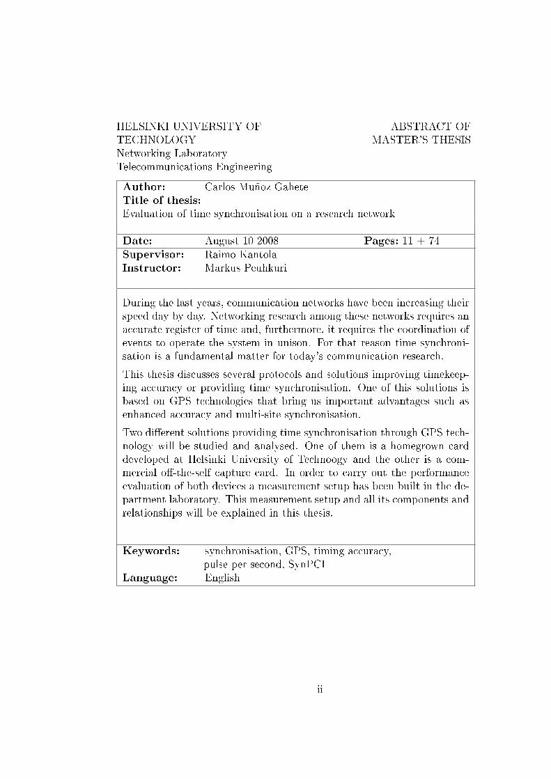
HELSINKI UNIVERSITY OF ABSTRACT OFTECHNOLOGY MASTER'S THESISNetworking LaboratoryTelecommunications EngineeringAuthor: Carlos Muñoz GaheteTitle of thesis:Evaluation of time synchronisation on a research network
Date: August 10 2008 Pages: 11 + 74Supervisor: Raimo KantolaInstructor: Markus Peuhkuri
During the last years, communication networks have been increasing theirspeed day by day. Networking research among these networks requires anaccurate register of time and, furthermore, it requires the coordination ofevents to operate the system in unison. For that reason time synchroni-sation is a fundamental matter for today's communication research.This thesis discusses several protocols and solutions improving timekeep-ing accuracy or providing time synchronisation. One of this solutions isbased on GPS technologies that bring us important advantages such asenhanced accuracy and multi-site synchronisation.Two di�erent solutions providing time synchronisation through GPS tech-nology will be studied and analysed. One of them is a homegrown carddeveloped at Helsinki University of Technoogy and the other is a com-mercial o�-the-self capture card. In order to carry out the performanceevaluation of both devices a measurement setup has been built in the de-partment laboratory. This measurement setup and all its components andrelationships will be explained in this thesis.
Keywords: synchronisation, GPS, timing accuracy,pulse per second, SynPCI
Language: English
ii
Acknowledgements
This work was done at the Helsinki University of Technology, at the Net-working Laboratory where I have enjoyed working in the international envi-ronment provided by one of the most important universities in Europe.I wish to thank my instructor Markus Peuhkuri for the help and the supporthe gave me during the execution of my thesis. I am very grateful for hissuggestions, comments and guidance. I also thank him for providing me theopportunity to work in this research project.I would like to thank my parents and my family for their endless love, en-couragement and support they gave me all through my life. I also want tothank my friends from Madrid for being there when I need them and thefriends I made in Finland who have been my second family during this year.
Espoo August 10th 2008
Carlos Muñoz Gahete
iii
Abbreviations and Acronyms
CDMA Code Division Multiple AccessCPLD Complex Programmable Logic DeviceDGPS Di�erential GPSDUCK DAG Universal Clock KitFPGA Field-Programmable Gate ArrayGPS Global Positioning SystemICMP Internet Control Message ProtocolIEEE Institute of Electrical and Electronic EngineeringIP Internet ProtocolIRIG Inter-Range Instrumentation GroupISDN Integrated Services Digital NetworkLAN Local Area NetworkMTU Maximum Transfer UnitNIC Network Interface CardNTP Network Time ProtocolOCXO Oven-Controlled Crystal OscillatorOWD One-Way DelayPCI Peripheral Component InterconnectPLL Phase-Locked LoopPPS Pulse-Per-SecondPTP Precision Time ProtocolRTT Round Trip TimeSIM Synchronisation Interface ModuleTCP Transfer Control ProtocolTCXO Temperature-Compensated Crystal OscillatorTSC Time Stamp CounterTTL Transistor-Transistor LogicUTC Coordinated Universal TimeVCO Voltage Controlled OscillatorXO Cristal Oscillator
iv
Contents
Abstract ii
Acknowledgements iii
Abbreviations and Acronyms iv
List of Tables ix
List of Figures xii
0 Resumen (Spanish) xiii0.1 Introducción . . . . . . . . . . . . . . . . . . . . . . . . . . . . xiii0.2 Entorno Tecnológico . . . . . . . . . . . . . . . . . . . . . . . xiv
0.2.1 Fuentes de incertidumbre en las medidas de tiempo . . xiv0.2.2 Uso de PPS (pulso por segundo) para sincronización . xv0.2.3 GPS . . . . . . . . . . . . . . . . . . . . . . . . . . . . xv0.2.4 Uso de una tarjeta adicional . . . . . . . . . . . . . . . xvi
0.3 Arquitectura . . . . . . . . . . . . . . . . . . . . . . . . . . . . xvii0.3.1 Diseño de la tarjeta SynPCI . . . . . . . . . . . . . . . xix0.3.2 Tarjeta DAG de Endace . . . . . . . . . . . . . . . . . xx
0.4 Análisis . . . . . . . . . . . . . . . . . . . . . . . . . . . . . . xxi0.5 Conclusiones . . . . . . . . . . . . . . . . . . . . . . . . . . . . xxi
1 Introduction 1
v
1.1 Synchronisation in Telecommunications . . . . . . . . . . . . . 11.2 Synchronisation for Networking Research . . . . . . . . . . . . 21.3 Problem Statement . . . . . . . . . . . . . . . . . . . . . . . . 21.4 Goal of the Thesis . . . . . . . . . . . . . . . . . . . . . . . . 3
2 Background 42.1 Basis and Technology of Clocks . . . . . . . . . . . . . . . . . 4
2.1.1 Quartz-Crystal Clocks . . . . . . . . . . . . . . . . . . 42.1.2 Temperature-Compensated Crystal Oscillator . . . . . 62.1.3 Oven-Controlled Crystal Oscillator . . . . . . . . . . . 62.1.4 Crystal Oscillators in Computers . . . . . . . . . . . . 6
2.2 Synchronisation over the Network . . . . . . . . . . . . . . . . 72.2.1 Network Time Protocol . . . . . . . . . . . . . . . . . . 72.2.2 Precision Time Protocol . . . . . . . . . . . . . . . . . 72.2.3 IRIG Serial Time Code . . . . . . . . . . . . . . . . . . 92.2.4 Use of Pulse-Per-Second . . . . . . . . . . . . . . . . . 10
2.3 GPS . . . . . . . . . . . . . . . . . . . . . . . . . . . . . . . . 102.3.1 Space Segment . . . . . . . . . . . . . . . . . . . . . . 112.3.2 Control Segment . . . . . . . . . . . . . . . . . . . . . 112.3.3 User Segment (GPS Receiver) . . . . . . . . . . . . . . 122.3.4 How GPS Works . . . . . . . . . . . . . . . . . . . . . 132.3.5 Triangulation . . . . . . . . . . . . . . . . . . . . . . . 132.3.6 Measuring Distance . . . . . . . . . . . . . . . . . . . . 142.3.7 Getting Perfect Timing . . . . . . . . . . . . . . . . . . 142.3.8 Error Sources . . . . . . . . . . . . . . . . . . . . . . . 152.3.9 Di�erential GPS . . . . . . . . . . . . . . . . . . . . . 18
2.4 Error Sources in Computer's Time Keeping . . . . . . . . . . . 192.5 Two-Way and One-Way Delay . . . . . . . . . . . . . . . . . . 20
3 Architecture 223.1 Environment . . . . . . . . . . . . . . . . . . . . . . . . . . . . 22
vi
3.2 System Overview . . . . . . . . . . . . . . . . . . . . . . . . . 233.3 System Components . . . . . . . . . . . . . . . . . . . . . . . 24
3.3.1 GPS Receivers . . . . . . . . . . . . . . . . . . . . . . 243.3.2 Distribution Boards . . . . . . . . . . . . . . . . . . . . 253.3.3 Procurve Switch 1800-24G . . . . . . . . . . . . . . . . 253.3.4 Tra�c Splitter . . . . . . . . . . . . . . . . . . . . . . 263.3.5 Tra�c Generator . . . . . . . . . . . . . . . . . . . . . 263.3.6 Endace DAG Card 3.7G . . . . . . . . . . . . . . . . . 283.3.7 SynPCI Card . . . . . . . . . . . . . . . . . . . . . . . 30
4 Analysis 354.1 Test Procedure . . . . . . . . . . . . . . . . . . . . . . . . . . 35
4.1.1 Network Conditions . . . . . . . . . . . . . . . . . . . . 364.1.2 Test Cases . . . . . . . . . . . . . . . . . . . . . . . . . 36
4.2 Test Results . . . . . . . . . . . . . . . . . . . . . . . . . . . . 374.2.1 DAG Card Results . . . . . . . . . . . . . . . . . . . . 374.2.2 SynPCI results . . . . . . . . . . . . . . . . . . . . . . 534.2.3 Results Summary . . . . . . . . . . . . . . . . . . . . . 664.2.4 Round Trip Time and Packet Size . . . . . . . . . . . . 674.2.5 E�ects of unsynchronisation . . . . . . . . . . . . . . . 68
5 Conclusions 715.1 Future Work . . . . . . . . . . . . . . . . . . . . . . . . . . . . 72
Bibliography 74
vii
List of Tables
1 Resumen de los resultados obtenidos . . . . . . . . . . . . . . xxii
2.1 Pulse Rates of IRIG time code formats[13] . . . . . . . . . . . 10
3.1 Trimble Thunderbolt Performance Speci�cations . . . . . . . . 253.2 Trimble Acutime Performance Speci�cations . . . . . . . . . . 25
4.1 DAG card statistics for 64 bytes packets at 10 Mbit/s . . . . . 374.2 DAG card statistics for 64 bytes packets at 200 Mbit/s . . . . 404.3 DAG card statistics for 64 bytes packets at 500 Mbit/s . . . . 424.4 DAG card statistics for 518 bytes packets at 10 Mbit/s . . . . 434.5 DAG card statistics for 518 bytes packets at 200 Mbit/s . . . . 454.6 DAG card statistics for 518 bytes packets at 500 Mbit/s . . . . 474.7 DAG card statistics for 1418 bytes packets at 10 Mbit/s . . . . 484.8 DAG card statistics for 1418 bytes packets at 200 Mbit/s . . . 504.9 DAG card statistics for 1418 bytes packets at 500 Mbit/s . . . 524.10 SynPCI card statistics for 64 bytes packets at 10 Mbit/s . . . 544.11 SynPCI card statistics for 64 bytes packets at 200 Mbit/s . . . 554.12 SynPCI card statistics for 518 bytes packets at 10 Mbit/s . . . 574.13 SynPCI card statistics for 518 bytes packets at 200 Mbit/s . . 594.14 SynPCI card statistics for 518 bytes packets at 500 Mbit/s . . 614.15 SynPCI card statistics for 1418 bytes packets at 10 Mbit/s . . 624.16 SynPCI card statistics for 1418 bytes packets at 200 Mbit/s . 644.17 SynPCI card statistics for 1418 bytes packets at 500 Mbit/s . 65
viii

4.18 Statistics summary for di�erent bit rates and packet sizes . . . 684.19 Results for Round Trip Time in relation to packet size . . . . 68
ix
List of Figures
1 Diagrama del sistema de medida . . . . . . . . . . . . . . . . . xviii2 Componentes principales del sistema de sincronización SynPCI xix3 Estructura interna de la tarjeta DAG . . . . . . . . . . . . . . xx
2.1 Frequency-temperature characteristics of various quartz cuts. . 52.2 Structure of NTP servers [3] . . . . . . . . . . . . . . . . . . . 82.3 PTP Sequence of Packets [1] . . . . . . . . . . . . . . . . . . . 92.4 GPS satellites constellation and orbits . . . . . . . . . . . . . 122.5 Timestamping process . . . . . . . . . . . . . . . . . . . . . . 19
3.1 Measurement system diagram . . . . . . . . . . . . . . . . . . 243.2 Tra�c Generator Graphical User Interface . . . . . . . . . . . 273.3 DAG card internal structure . . . . . . . . . . . . . . . . . . . 283.4 Timestamping with DAG card and conventional card. . . . . . 303.5 Measurement setup for the DAG card. . . . . . . . . . . . . . 313.6 Main components of SynPCI synchronisation system . . . . . 333.7 Measurement setup for the SynPCI card. . . . . . . . . . . . . 34
4.1 Histogram for 64 bytes packets at 10 Mbit/s captured by theDAG card . . . . . . . . . . . . . . . . . . . . . . . . . . . . . 38
4.2 Delay evolution for 64 bytes packets at 10 Mbit/s captured bythe DAG card . . . . . . . . . . . . . . . . . . . . . . . . . . . 39
4.3 Detail of the changes in the delay . . . . . . . . . . . . . . . . 394.4 Histogram for 64 bytes packets at 200 Mbit/s captured by the
DAG card . . . . . . . . . . . . . . . . . . . . . . . . . . . . . 41
x
4.5 Delay evolution for 64 bytes packets at 200 Mbit/s capturedby the DAG card . . . . . . . . . . . . . . . . . . . . . . . . . 41
4.6 Histogram for 64 bytes packets at 500 Mbit/s captured by theDAG card . . . . . . . . . . . . . . . . . . . . . . . . . . . . . 42
4.7 Delay evolution for 64 bytes packets at 500 Mbit/s capturedby the DAG card . . . . . . . . . . . . . . . . . . . . . . . . . 43
4.8 Histogram for 518 bytes packets at 10 Mbit/s captured by theDAG card . . . . . . . . . . . . . . . . . . . . . . . . . . . . . 44
4.9 Delay evolution for 518 bytes packets at 10 Mbit/s capturedby the DAG card . . . . . . . . . . . . . . . . . . . . . . . . . 44
4.10 Histogram for 518 bytes packets at 200 Mbit/s . . . . . . . . . 464.11 Delay evolution for 518 bytes packets at 200 Mbit/s captured
by the DAG card . . . . . . . . . . . . . . . . . . . . . . . . . 464.12 Histogram for 518 bytes packets at 500 Mbit/s captured by
the DAG card . . . . . . . . . . . . . . . . . . . . . . . . . . . 474.13 Delay evolution for 518 bytes packets at 500 Mbit/s captured
by the DAG card . . . . . . . . . . . . . . . . . . . . . . . . . 484.14 Histogram for 1418 bytes packets at 10 Mbit/s captured by
the DAG card . . . . . . . . . . . . . . . . . . . . . . . . . . . 494.15 Delay evolution for 1418 bytes packets at 10 Mbit/s captured
by the DAG card . . . . . . . . . . . . . . . . . . . . . . . . . 494.16 Histogram for 1418 bytes packets at 200 Mbit/s captured by
the DAG card . . . . . . . . . . . . . . . . . . . . . . . . . . . 514.17 Delay evolution for 1418 bytes packets at 200 Mbit/s captured
by the DAG card . . . . . . . . . . . . . . . . . . . . . . . . . 514.18 Histogram for 1418 bytes packets at 500 Mbit/s captured by
the DAG card . . . . . . . . . . . . . . . . . . . . . . . . . . . 524.19 Delay evolution for 1418 bytes packets at 500 Mbit/s captured
by the DAG card . . . . . . . . . . . . . . . . . . . . . . . . . 534.20 Histogram for 64 bytes packets at 10 Mbit/s captured by the
synPCI card . . . . . . . . . . . . . . . . . . . . . . . . . . . . 544.21 Delay evolution for 64 bytes packets at 10 Mbit/s captured by
the synPCI card . . . . . . . . . . . . . . . . . . . . . . . . . . 55
xi
4.22 Histogram for 64 bytes packets at 200 Mbit/s captured by thesynPCI card . . . . . . . . . . . . . . . . . . . . . . . . . . . . 56
4.23 Delay evolution for 64 bytes packets at 200 Mbit/s capturedby the synPCI card . . . . . . . . . . . . . . . . . . . . . . . . 57
4.24 Histogram for 518 bytes packets at 10 Mbit/s captured by thesynPCI card . . . . . . . . . . . . . . . . . . . . . . . . . . . . 58
4.25 Delay evolution for 518 bytes packets at 10 Mbit/s capturedby the synPCI card . . . . . . . . . . . . . . . . . . . . . . . . 58
4.26 Histogram for 518 bytes packets at 200 Mbit/s captured bythe synPCI card . . . . . . . . . . . . . . . . . . . . . . . . . . 59
4.27 Delay evolution for 518 bytes packets at 200 Mbit/s capturedby the synPCI card . . . . . . . . . . . . . . . . . . . . . . . . 60
4.28 Histogram for 518 bytes packets at 500 Mbit/s captured bythe synPCI card . . . . . . . . . . . . . . . . . . . . . . . . . . 61
4.29 Delay evolution for 518 bytes packets at 500 Mbit/s capturedby the synPCI card . . . . . . . . . . . . . . . . . . . . . . . . 62
4.30 Histogram for 1418 bytes packets at 10 Mbit/s captured bythe synPCI card . . . . . . . . . . . . . . . . . . . . . . . . . . 63
4.31 Delay evolution for 1418 bytes packets at 10 Mbit/s capturedby the synPCI card . . . . . . . . . . . . . . . . . . . . . . . . 63
4.32 Histogram for 1418 bytes packets at 200 Mbit/s captured bythe synPCI card . . . . . . . . . . . . . . . . . . . . . . . . . . 64
4.33 Delay evolution for 1418 bytes packets at 200 Mbit/s capturedby the synPCI card . . . . . . . . . . . . . . . . . . . . . . . . 65
4.34 Histogram for 1418 bytes packets at 500 Mbit/s captured bythe synPCI card . . . . . . . . . . . . . . . . . . . . . . . . . . 66
4.35 Delay evolution for 1418 bytes packets at 500 Mbit/s capturedby the synPCI card . . . . . . . . . . . . . . . . . . . . . . . . 67
4.36 Relation between packet size and round trip time . . . . . . . 694.37 Time drift for unsynchronised capture . . . . . . . . . . . . . . 70
xii
Chapter 0
Resumen (Spanish)
0.1 IntroducciónDesde el inicio de la era digital redes cada vez más rápidas han ido apare-ciendo día a día. Por este motivo la sincronización en red ha ido ganandoimportancia en el mundo de las telecomunicaciones durante los últimos 30años. El comportamiento de la mayoría de los servicios ofrecidos por losoperadores de telecomunicacines está afectado en mayor o menor medida porla calidad de su sincronización en la red.La sincronización es un aspecto muy importante dentro de las telecomuni-caciones en general, pero es aún más importante cuando nos referimos alárea de investigación, dónde la precisión en el registro del tiempo y la sin-cronización entre los distintos equipos están directamente relacionados conlos resultados de la investigación.El uso de hardware comercial es normalmente la forma más económica deconseguir sincronización. Sin embargo, esta solución raramente se ajustaperfectamente a las necesidades de la investigación, comprometiendo así susresultados.En la universidad de Helsinki (HUT) se ha desarrollado un sistema de sin-cronización de bajo coste (tarjeta SynPCI) que permite mejorar signi�cati-vamente la precisión de la sincronización, teniendo como objetivo la investi-gación en el área telemática.El objetivo de este Proyecto Fin de Carrera es el diseño y construcción deuna red de medida que permita la evaluación de la tarjeta SynPCI así comola de otro sistema de sincronización comercial, la tarjeta DAG de Endace,para posteriormente comparar sus prestaciones y obtener conclusiones acerca
xiii
del rendimiento de ambos sistemas.
0.2 Entorno TecnológicoHoy en día los ordenadores utilizan distintos protocolos para conocer eltiempo correcto con una cierta precisión. Los más simples como el daytime yel time protocol proporcionan una resolución de un segundo. Para conseguiruna mejor precisión existen dos protocolos: Network Time Protocol (NTP)diseñado para el uso en Internet, y Precision Time Protocol (PTP), apropi-ado para usarlo con dispositivos directamente conectados en una red de árealocal. Otros métodos estandarizados se han desarrollado para transmitir lainformación temporal sobre líneas dedicadas, uno de ellos es el IRIG SerialTime Code.
0.2.1 Fuentes de incertidumbre en las medidas de tiempoIncluso si suponemos que el sistema operativo sabe exactamente el tiempoactual, las medidas realizadas con su reloj podrían no ser tan precisas. Vamosa describir un simple ejemplo: queremos capturar y registrar el tiempo depaquetes provenientes de una red Ethernet usando una tarjeta de red común.Primero la tarjeta de red captura un paquete y señaliza al sistema ope-rativo con una interrupción. El sistema operativo reacciona a la señal deinterrupción y recoge el paquete de la tarjeta de red suponiendo que el busPCI esté disponible. Si no lo está, el procesador debe esperar hasta queesté disponible. Ahora, si otro paquete ha llegado mientras el bus estabaocupado, el procesador puede recoger ambos paquetes a la vez, haciendoparecer que ambos paquetes llegaron a la vez. Muchas tarjetas de red dealtas prestaciones pueden limitar el número de interrupciones para mejorarsu rendimiento, haciendo este fenómeno aún peor.Otros factores del sistema operativo, con frecuencia provocados por el retrasode las interrupciones, añaden más imprecisiones en la medida del tiempo. Porlo tanto es necesario evaluar cuidadosamente y señalar las posibles fuentesde error en las medidas.
xiv
0.2.2 Uso de PPS (pulso por segundo) para sincronizaciónUna fácil solución para poder distribuir el tiempo UTC (Tiempo UniversalCoordinado) entre un conjunto de ordenadores sería distribuir una señal PPSa cada ordenador utilizando cualquiera de los puertos paralelo o serie. Usandoel protocolo NTP se podría obtener la numeración de los segundos y el pulsoPPS señalizaría con precisión cada segundo. La ventaja de esto es su bajocoste. La construcción sería ligeramente más complicada si además queremosaislar galvánicamente el cableado entre ordenadores pero todavía por debajode 50 euros por unidad.Sin embargo, usar el puerto serie o paralelo para una sincronización precisatambién tiene sus problemas. Para empezar los puertos tienen circuitos deprotección contra descargas electrostáticas, lo que limita el tiempo de subidadel reloj. Una fuente de error más importante es el hecho de que las in-terrupciones para estos puertos tienen prioridad baja. Esto signi�ca quesi hay alguna interrupción de mayor prioridad, como lectura/escritura endisco o cualquier comunicación por Ethernet, la interrupción será retrasadahasta que la otra haya sido atendida. Además una interrupción de altaprioridad podría reemplazar a otra de baja prioridad provocando un error enla estimación del tiempo.
0.2.3 GPSLos protocolos de sincronización permiten a los ordenadores sincronizarse através de la red, sin embargo son fuertemente dependientes a la carga de lared y al número de nodos entre el equipo y la fuente de tiempo. La tecnologíaGPS permite a cualquier equipo conseguir un timing perfecto con un simplereceptor GPS.El sistema GPS es un sistema de radionavegación mundial formado por unaconstelación de 24 satélites y sus estaciones base. Estos satélites arti�cialesson utilizados como punto de referencia para calcular la posiciones en laTierra de manera muy precisa.Sin embargo, como se detalla en el desarrollo de esta tésis, el sistema GPSno solo permite conocer la posición del receptor GPS, sino que también esposible obtener una medida muy precisa del tiempo, tan precisa como que laprecisión del reloj de nuestro receptor GPS es equivalente a la de los relojesatómicos con los que están equipados los satélites.Esto no solo permite obtener una marca de tiempo extremadamente precisa,sino que además signi�ca que estaremos sincronizados con cualquier receptor
xv
GPS que obtenga el tiempo del mismo modo. Si unimos a esto el hecho deque los receptores GPS son cada vez más económicos encontramos que el usode la tecnología GPS es una solución perfecta para nuestro sistema.
0.2.4 Uso de una tarjeta adicionalComo hemos visto, existen muchas fuentes de error que afectan a la precisasincronización del hardware. El mayor problema es la incertidumbre en elretraso indeterminado causado por las interrupciones. Si es posible reduciro eliminar esta componente, la precisión se verá mejorada de modo signi�ca-tivo.Una vez más, el cambio de la prioridad de las interrupciones requeriría al-gunas modi�caciones en el hardware por lo que no es una solución adecuadapara un uso amplio. Con la señal PPS obteníamos el tiempo con precisióncada segundo, podemos cambiar esto para poder comprobar el instante detiempo actual cuando más nos interese y suponga un mínimo retraso. Basán-donos en esta información podremos hacer las correcciones adecuadas.La idea es fabricar una tarjeta añadida (SynPCI) que disponga de dos re-gistros. El primero de ellos será un contador que se resetee cada vez quees leído. El otro registro almacenará el valor del primer contador cuandose reciba una señal PPS. El reloj fuente para el primer contador será unoscilador controlado por tensión (VCO), enganchado en fase con una señalde 10 MHz proveniente de un reloj GPS.Cada vez que se dispara una interrupción de tiempo, se lee el valor de 32 bitsdel primer registro. Este valor incluye un bit indicando si ha llegado la señalPPS y un valor de 31 bits del primer contador. El tamaño del contador essu�ciente dado que es leído entre 100 y 1000 veces por segundo. El valor delkernel time-of-day xtime se actualiza de acuerdo al valor leído del registro.El indicador PPS se usa entonces para detectar si un pulso PPS ha sidorecibido entre las interrupciones del timer. Si el bit ha sido activado, entoncesse lee el otro registro y se aplica una corrección a xtime si es necesario.
¾Por qué es esto mejor que PPS?
Comparado con el uso básico de la señal PPS, la principal mejora de estemétodo es que el retraso por interrupción no tiene ningún efecto en absoluto.El tiempo entre interrupciones no puede ser mayor de 2 segundos, pero por lodemás las interrupciones pueden ocurrir en cualquier momento. Si se retrasa
xvi
el acceso al bus PCI la precisión no se ve afectada ya que el valor del contadores almacenado solo cuando se lee.
0.3 ArquitecturaPara el desarrollo de la red de medida han sido utilizados los siguientescomponentes del laboratorio del departamento de redes y comunicaciones:
� Generador/analizador de trá�co: Spirent Adtech AX/4000.
� Tarjeta capturadora: Endace DAG Card 3.7G.
� Tarjeta capturadora: SynPCI diseñada en la HUT.
� Receptor GPS: Trimble Acutime 2000.
� Receptor GPS: Trimble Thunderbolt GPS Disciplined Clock.
� Divisor de trá�co: VSS monitoring tra�c splitter.
� Procurve Switch 1800-24G
� Tarjetas de distribución de señal.
Como dijimos en la sección anterior, el propósito de este proyecto es con-�gurar una red de medida para ser capaces de analizar el comportamientode dos sistemas de sincronización diferentes. Para ello, debemos conseguiruna sincronización muy precisa entre los puntos críticos de la red, que sontanto el generador de trá�co como los ordenadores equipados con las tarjetascapturadoras.La idea es mandar un patrón de trá�co desde el generador de trá�co y re-gistrar la llegada de paquetes en los componentes que queremos analizar.Después podemos comparar estos timestamps con una fuente de referenciamás precisa. El generador de trá�co también está equipado con un analizadorde trá�co de alta calidad que podemos usar como referencia. Por esta razón serealimenta el trá�co enviado a la tarjeta capturadora de vuelta al generadorde trá�co.El generador de trá�co Spirent Adtech AX/4000 recibe una señal PPS (pulsopor segundo) y una señal de 10 MHz del receptor GPS Trimble Thunderbolta través de un cable coaxial. También recibe una comunicación serie conte-niendo información temporal desde la tarjeta que estamos evaluando.
xvii
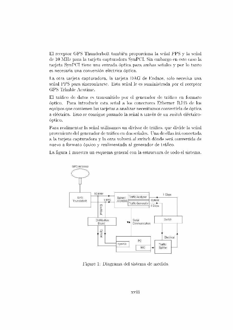
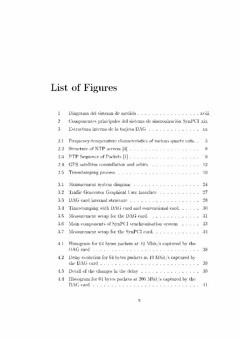
El receptor GPS Thunderbolt también proporciona la señal PPS y la señalde 10 MHz para la tarjeta capturadora SynPCI. Sin embargo en este caso latarjeta SynPCI tiene una entrada óptica para ambas señales y por lo tantoes necesaria una conversión eléctrica-óptica.La otra tarjeta capturadora, la tarjeta DAG de Endace, solo necesita unaseñal PPS para sincronizarse. Esta señal le es suministrada por el receptorGPS Trimble Acutime.El trá�co de datos es transmitido por el generador de trá�co en formatoóptico. Para introducir esta señal a los conectores Ethernet RJ45 de losequipos que contienen las tarjetas a analizar necesitamos convertirla de ópticaa eléctrica. Esto se consigue pasando la señal a través de un switch eléctrico-óptico.Para realimentar la señal utilizamos un divisor de trá�co, que divide la señalproveniente del generador de trá�co en dos señales. Una de ellas irá conectadaa la tarjeta capturadora y la otra volverá al switch dónde será convertida denuevo a formato óptico y realimentada al generador de trá�co.La �gura 1 muestra un esquema general con la estructura de todo el sistema.
Figure 1: Diagrama del sistema de medida
xviii
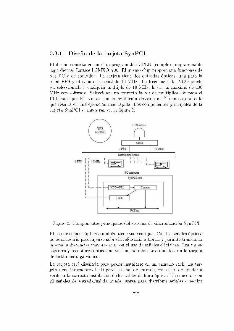
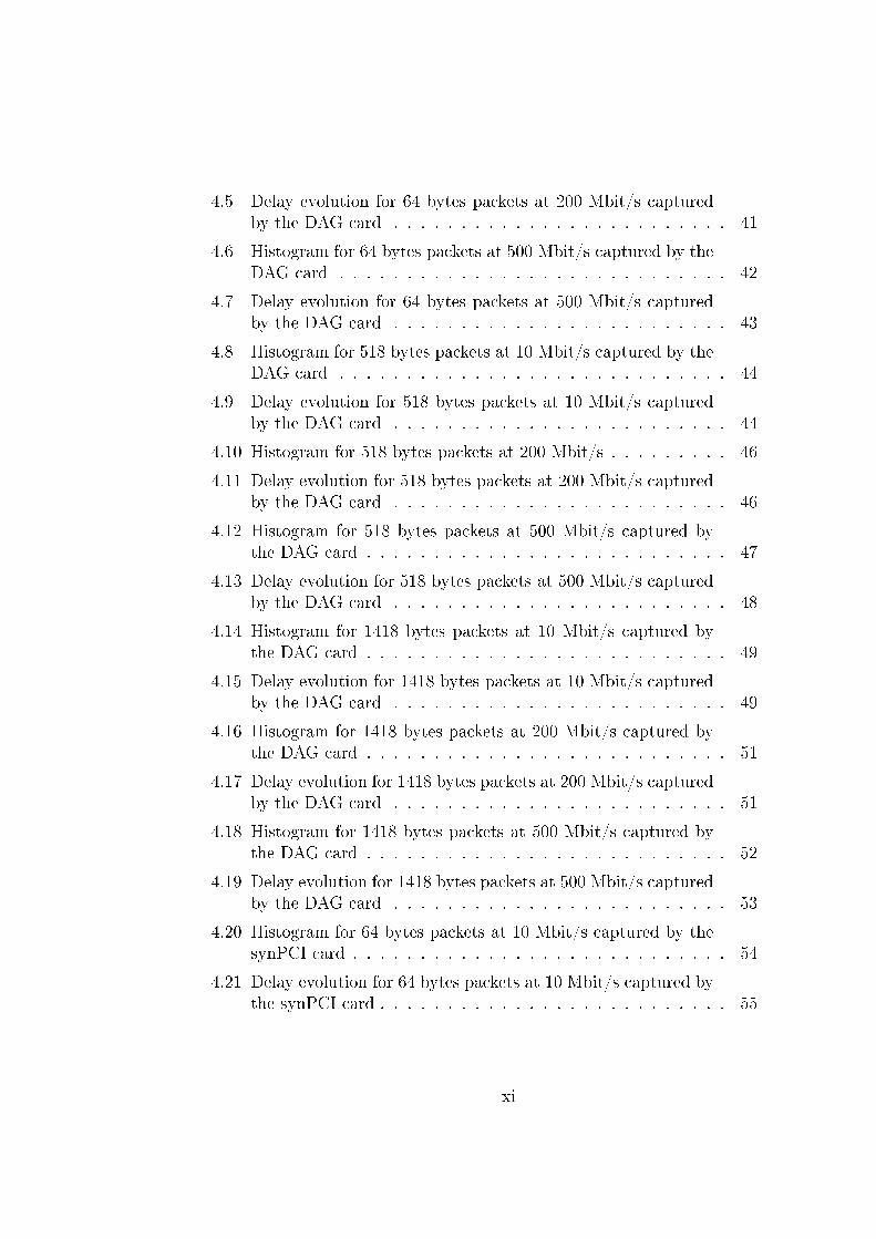
0.3.1 Diseño de la tarjeta SynPCIEl diseño consiste en un chip programable CPLD (complex programmablelogic device) Lattice LCMXO1200. El mismo chip proporciona funciones debus PC y de contador. La tarjeta tiene dos entradas ópticas, una para laseñal PPS y otra para la señal de 10 MHz. La frecuencia del VCO puedeser seleccionada a cualquier múltiplo de 10 MHz, hasta un máximo de 400MHz con software. Seleccionar un correcto factor de multiplicación para elPLL hace posible contar con la resolución deseada a 2N nanosegundos loque resulta en una ejecución más rápida. Los componentes principales de latarjeta SynPCI se muestran en la �gura 2.
Figure 2: Componentes principales del sistema de sincronización SynPCI
El uso de señales ópticas también tiene sus ventajas. Con las señales ópticasno es necesario preocuparse sobre la referencia a tierra, y permite transmitirla señal a distancias mayores que con el uso de señales eléctricas. Los trans-ceptores y receptores ópticos no son mucho más caros que dotar a la tarjetade aislamiento galvánico.La tarjeta está diseñada para poder instalarse en un armario rack. La tar-jeta tiene indicadores LED para la señal de entrada, con el �n de ayudar averi�car la correcta instalación de los cables de �bra óptica. Un conector con20 señales de entrada/salida puede usarse para distribuir señales o recibir
xix
entradas en aplicaciones futuras. Este conector y la capacidad libre del chipprogramable CPLD puede usarse para interconectarlo con otros sistemas.Además de la tarjeta SynPCI, el sistema necesita también una placa de dis-tribución que tome la señal PPS eléctrica y la señal de 10 MHz del reloj GPSy proporcione a la salida el número deseado de señales ópticas.
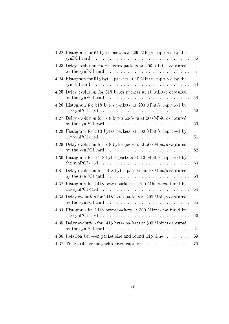
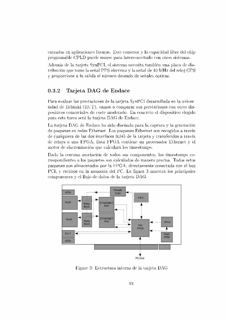
0.3.2 Tarjeta DAG de EndacePara evaluar las prestaciones de la tarjeta SynPCI desarrollada en la univer-sidad de Helsinki (HUT), vamos a comparar sus prestaciones con otros dis-positivos comerciales de coste moderado. En concreto el dispositivo elegidopara esta tarea será la tarjeta DAG de Endace.La tarjeta DAG de Endace ha sido diseñada para la captura y la generaciónde paquetes en redes Ethernet. Los paquetes Ethernet son recogidos a travésde cualquiera de las dos interfaces RJ45 de la tarjeta y transferidos a travésde relays a una FPGA. Esta FPGA contiene un procesador Ethernet y elmotor de sincronización que calculará los timestamps.Dado la cercana asociación de todos sus componentes, los timestamps co-rrespondientes a los paquetes son calculados de manera precisa. Todos estospaquetes son almacenados por la FPGA, directamente conectada con el busPCI, y escritos en la memoria del PC. La �gura 3 muestra los principalescomponentes y el �ujo de datos de la tarjeta DAG.
Figure 3: Estructura interna de la tarjeta DAG
xx
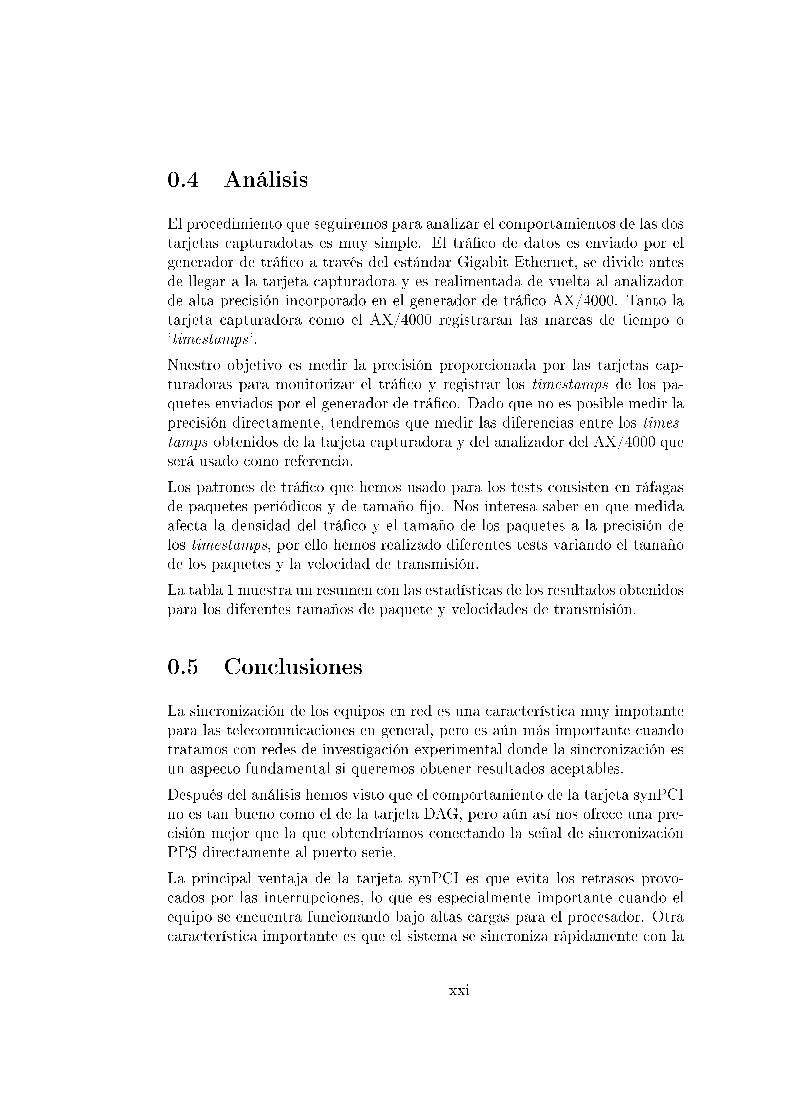
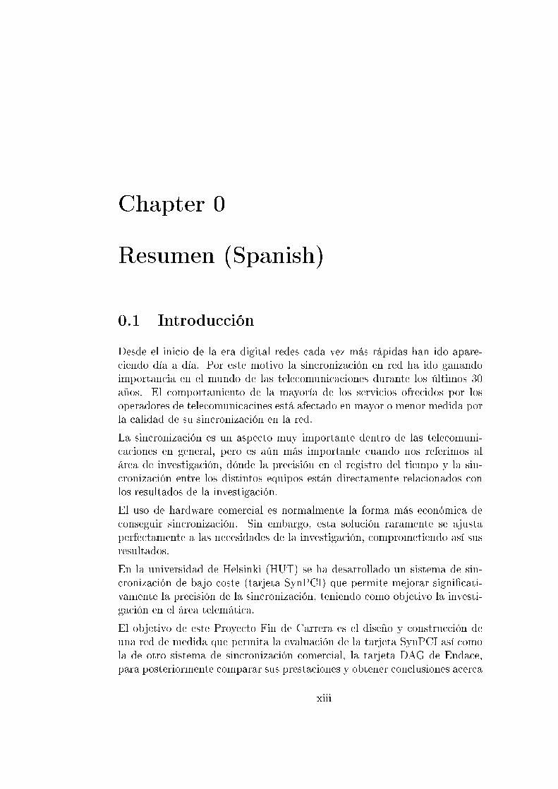
0.4 AnálisisEl procedimiento que seguiremos para analizar el comportamientos de las dostarjetas capturadotas es muy simple. El trá�co de datos es enviado por elgenerador de trá�co a través del estándar Gigabit Ethernet, se divide antesde llegar a la tarjeta capturadora y es realimentada de vuelta al analizadorde alta precisión incorporado en el generador de trá�co AX/4000. Tanto latarjeta capturadora como el AX/4000 registraran las marcas de tiempo o'timestamps '.Nuestro objetivo es medir la precisión proporcionada por las tarjetas cap-turadoras para monitorizar el trá�co y registrar los timestamps de los pa-quetes enviados por el generador de trá�co. Dado que no es posible medir laprecisión directamente, tendremos que medir las diferencias entre los times-tamps obtenidos de la tarjeta capturadora y del analizador del AX/4000 queserá usado como referencia.Los patrones de trá�co que hemos usado para los tests consisten en ráfagasde paquetes periódicos y de tamaño �jo. Nos interesa saber en que medidaafecta la densidad del trá�co y el tamaño de los paquetes a la precisión delos timestamps, por ello hemos realizado diferentes tests variando el tamañode los paquetes y la velocidad de transmisión.La tabla 1 muestra un resumen con las estadísticas de los resultados obtenidospara los diferentes tamaños de paquete y velocidades de transmisión.
0.5 ConclusionesLa sincronización de los equipos en red es una característica muy impotantepara las telecomunicaciones en general, pero es aún más importante cuandotratamos con redes de investigación experimental donde la sincronización esun aspecto fundamental si queremos obtener resultados aceptables.Después del análisis hemos visto que el comportamiento de la tarjeta synPCIno es tan bueno como el de la tarjeta DAG, pero aún así nos ofrece una pre-cisión mejor que la que obtendríamos conectando la señal de sincronizaciónPPS directamente al puerto serie.La principal ventaja de la tarjeta synPCI es que evita los retrasos provo-cados por las interrupciones, lo que es especialmente importante cuando elequipo se encuentra funcionando bajo altas cargas para el procesador. Otracaracterística importante es que el sistema se sincroniza rápidamente con la
xxi
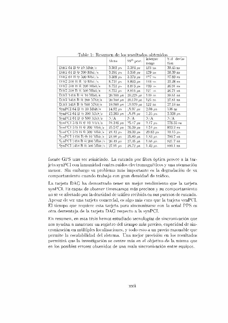
Table 1: Resumen de los resultados obtenidosMean 99th perc. interprc
rangeStd devia-tion
DAG 64 B @ 10 Mbit/s 3.303 µs 3.384 µs 185 ns 39.45 nsDAG 64 B @ 200 Mbit/s 3.291 µs 3.356 µs 129 ns 28.39 nsDAG 64 B @ 500 Mbit/s 3.309 µs 3.370 µs 127 ns 27.89 nsDAG 518 B @ 10 Mbit/s 8.731 µs 8.803 µs 148 ns 32.28 nsDAG 518 B @ 200 Mbit/s 8.753 µs 8.813 µs 120 ns 26.91 nsDAG 518 B @ 500 Mbit/s 8.755 µs 8.816 µs 121 ns 26.71 nsDAG 1418 B @ 10 Mbit/s 20.160 µs 20.228 µs 139 ns 30.61 nsDAG 1418 B @ 200 Mbit/s 20.108 µs 20.170 µs 125 ns 27.81 nsDAG 1418 B @ 500 Mbit/s 19.900 µs 19.970 µs 122 ns 27.18 nsSynPCI 64 B @ 10 Mbit/s 14.92 µs 15.97 µs 2.08 µs 736 nsSynPCI 64 B @ 200 Mbit/s 12.265 µs 15.85 µs 7.25 µs 2.328 µsSynPCI 64 B @ 500 Mbit/s N/A N/A N/A N/ASynPCI 518 B @ 10 Mbit/s 24.346 µs 25.47 µs 2.17 µs 776.35 nsSynPCI 518 B @ 200 Mbit/s 25.547 µs 26.39 µs 1.54 µs 823.2 nsSynPCI 518 B @ 500 Mbit/s 24.43 µs 39.30 µs 29.83 µs 10.15 µsSynPCI 1418 B @ 10 Mbit/s 24.90 µs 25.80 µs 1.83 µs 700.7 nsSynPCI 1418 B @ 200 Mbit/s 26.49 µs 27.35 µs 1.68 µs 821.7 nsSynPCI 1418 B @ 500 Mbit/s 27.91 µs 28.72 µs 1.42 µs 899.1 ns
fuente GPS tras ser reiniciado. La entrada por �bra óptica provee a la tar-jeta synPCI con inmunidad contra ruidos electromagnéticos y una atenuaciónmenor. Sin embargo su problema más importante es la degradación de sucomportamiento cuando trabaja con gran densidad de trá�co.La tarjeta DAG ha demostrado tener un mejor rendimiento que la tarjetasynPCI. Es capaz de obtener timestamps más precisos y su comportamientono se ve afectado por la densidad de trá�co recibida en sus puertos de entrada.Apesar de ser una tarjeta comercial, es algo más cara que la tarjeta synPCI.El tiempo que requiere esta tarjeta para sincronizarse con la señal PPS esotra desventaja de la tarjeta DAG respecto a la synPCI.En resumen, en esta tésis hemos estudiado tecnologías de sincronización quenos ayudan a mantener un registro del tiempo más preciso, capacidad de sin-cronización en múltiples localizaciones, y todo esto a un precio razonable quepermite la escalabilidad del sistema. Una mejor precisión en los resultadospermitirá que la investigación se centre más en el objetivo de la misma queen los posibles errores obtenidos de una mala sincronización entre equipos.
xxii
Chapter 1
Introduction
In digital systems, many operations must follow a precedence relationship.If some operations follow a rule of precedence, then synchronisation ensuresthat operations run in the right order. At the hardware level, synchronisationis accomplished by distributing a common timing signal to all the modules ofthe system. At a higher level of abstraction, software processes synchroniseby exchanging messages.
1.1 Synchronisation in TelecommunicationsSince the beginning of the Internet era, faster and faster networks have beencoming out day by day. For that reason, network synchronisation has gainedincreasing importance in telecommunications throughout the last 30 years.The quality of most services o�ered by telecommunications operators is af-fected directly by their network synchronisation performance, especially sincetransmission and switching became digital.Lack of synchronisation in digital switching equipments can cause timing slipsdegrading the system performance. Even if normal telephone conversationare not signi�cantly a�ected, switched data services are more problemat-ics dealing with synchronisation slips. Therefore, on circuit-switched datanetworks like ISDN, synchronisation becomes a fundamental matter for theproper behaviour of the network.[14]
1
CHAPTER 1. INTRODUCTION 2
1.2 Synchronisation for Networking ResearchIf synchronisation is a very important issue in telecommunications in general,it becomes even more important when we refer to the research area, wherecorrect timekeeping is related directly with the results of the research. Al-though sometimes a coarse accuracy for timekeeping is enough, experimentalresearch among computers connected by the fastest networks often requiresa more accurate record of time.Furthermore, if the experiment needs timekeeping in more than one device,a very precise accuracy is usually not enough and it often requires the co-ordination of events to operate the system correctly. That makes the syn-chronisation of the clocks in the network a major issue in order to reach theresearch goals and avoid error due to di�erences between clocks.Commercial o�-the-shelf hardware is usually the most economic way to achievesynchronisation. Cheap synchronisation devices provide an easy and scalablesolution, however it is seldom the most suitable alternative, compromisingthe results of the research in terms of accuracy and synchronisation.Some commercials systems can provide very accurate timestamping and syn-chronisation. However, this is a very high cost solution and in most of thecases una�ordable for research institutions, specially when synchronisationis required in a wide research network.
1.3 Problem StatementAs we said, o�-the-shelf products provide an economic solution but are rarelythe best option. At Helsinki University of Technology, an inexpensive syn-chronisation system has been developed trying to improve signi�cantly times-tamping accuracy.The system has been designed with the aim of networking research. Thisresearch includes networking experimentation using di�erent algorithms andprotocols. If we want to analyse the di�erence between these algorithm andprotocols, at least microsecond resolution is required. In order to obtainreliable results, devices related to tra�c generation and analysis are criticalpoints where synchronisation is of paramount importance.Networking experimentation usually requires to repeat the same tra�c pat-terns over and over again. Without a proper synchronisation among tra�cgenerators and analysis points, the researcher would not be able to distin-
CHAPTER 1. INTRODUCTION 3
guish signi�cant di�erences in the behaviour of algorithms from the noisegenerated by synchronisation errors.This thesis discusses di�erent protocols and systems designed to improvetimekeeping accuracy and synchronisation, analysing their advantages andlimitations. Finally it presents the solution given at Helsinki University ofTechnology consisting of one add-on card that provides accurate timestamp-ing by avoiding interrupts latency.
1.4 Goal of the ThesisThe goal of the thesis is to feed the tra�c generator and the capture cardswith GPS signals in order to achieve synchronisation among devices and builda measurement setup to collect the data. The �nal task will be to analyse andevaluate the performance of two di�erent systems in terms of synchronisationaccuracy. One of the key aspects is to identify possible sources of error anddistribution of error.
Chapter 2
Background
In this chapter we will give an overview on how common computers manageto keep their clocks synchronised and to control the timing of actions. Wewill also introduce some other protocols and methods to improve this basicsynchronisation.
2.1 Basis and Technology of ClocksFrom a theoretical point of view, the operation principle of any kind of clockconsists of a generator of oscillations and an automatic counter of such oscil-lations. With di�erent ability, the oscillator can be based indeed on (pseudo-)periodic physical phenomena of any kind: the swinging of a pendulum or awheel in mechanical clocks, the vibration of atoms in a crystal around theirminimum energy position in quartz clocks, the radiation associated withspeci�c quantum atomic transition in atomic clocks are just the best knownexamples due to their widest application but not the only ones.
2.1.1 Quartz-Crystal ClocksQuartz-crystal oscillators are based on piezoelectric e�ect: a mechanicalstrain in the crystal yields an electrical �eld and vice versa. A Crystal Oscil-lator (XO) is thus an electronic oscillator, where a quartz crystal is excitedby a periodic electrical signal at the resonance frequency (in the range from10 kHz to 1 GHz, but most commonly from 5 to 10 MHz).The resonance frequency is determined mainly by the properties of the bulkmaterial such as size, shape, elasticity, and the speed of sound in the ma-
4
CHAPTER 2. BACKGROUND 5
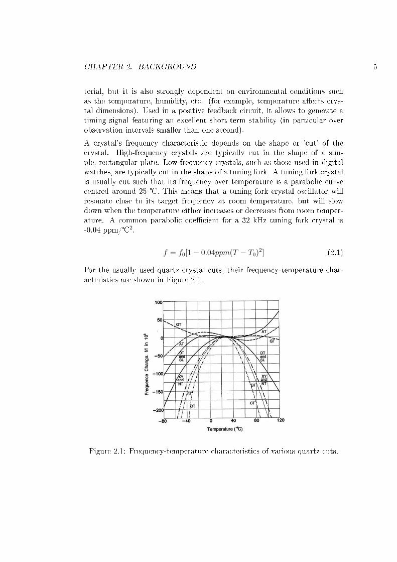
terial, but it is also strongly dependent on environmental conditions suchas the temperature, humidity, etc. (for example, temperature a�ects crys-tal dimensions). Used in a positive feedback circuit, it allows to generate atiming signal featuring an excellent short-term stability (in particular overobservation intervals smaller than one second).A crystal's frequency characteristic depends on the shape or 'cut' of thecrystal. High-frequency crystals are typically cut in the shape of a sim-ple, rectangular plate. Low-frequency crystals, such as those used in digitalwatches, are typically cut in the shape of a tuning fork. A tuning fork crystalis usually cut such that its frequency over temperature is a parabolic curvecentred around 25 �. This means that a tuning fork crystal oscillator willresonate close to its target frequency at room temperature, but will slowdown when the temperature either increases or decreases from room temper-ature. A common parabolic coe�cient for a 32 kHz tuning fork crystal is-0.04 ppm/�2.
f = f0[1− 0.04ppm(T − T0)2] (2.1)
For the usually used quartz crystal cuts, their frequency-temperature char-acteristics are shown in Figure 2.1.
Figure 2.1: Frequency-temperature characteristics of various quartz cuts.
CHAPTER 2. BACKGROUND 6
2.1.2 Temperature-Compensated Crystal OscillatorThe main problem of a plain XO is the dependence of its natural frequencyon ageing (around 10−7/day in plain models) and on the temperature (in theorder of 10−7/� or above).To overcome the latter problem, Temperature-Compensated Crystal Oscilla-tors (TCXOs) implement an automatic control on the oscillation frequencybased on the measurement of the crystal temperature. Such a trick allowsto achieve a frequency stability of 10−7 over a temperature interval from 0�to 50�. More sophisticated models by way of digital control, achieve a fre-quency stability even in the order of 10−8 in the wider temperature intervalfrom 0� to 70�.
2.1.3 Oven-Controlled Crystal OscillatorFar better than compensating temperature variations with a feedback controlis to insulate the oscillator thermically and to make it work in a constant-temperature closed environment. Such clocks are called Oven-ControlledCrystal Oscillators (OCXOs).In OCXOs, the resonator and the other temperature-sensitive elements areplaced in a controlled oven whose temperature is set as closely as possible toa point where the resonator frequency does not depend on temperature, soto minimise the e�ect of residual temperature variations. Frequency stabilityvalues exceeding 10−9/day are thus achieved. [7] [9] [15]
2.1.4 Crystal Oscillators in ComputersCommon PC computers use quartz-crystal oscillators integrated on the moth-erboard. Quartz oscillators allow computers to keep a register of time, usingdi�erent timers such as Time Stamp Counter (TSC) that provides high-resolution timestamps. However, these oscillators are directly in�uenced bythe heat dissipation coming from the motherboard and, although their accu-racy is stable in the short-term, changes of temperature destabilise accuracyin the long-term.One could think that improving stability is easily achieved using TCXO orOCXO instead of common oscillators. The problem is that these oscillatorsare not usually found embedded on common motherboards and it wouldneed a speci�c design for the mother board what takes not only time but
CHAPTER 2. BACKGROUND 7
money. Furthermore this solution does not help for time synchronisationamong di�erent computers, so we will need another solution that impliessynchronisation over the network. [11]
2.2 Synchronisation over the NetworkIn order to be in sync, computers exchange messages over the network. Withthat purpose, computers use di�erent protocols and services. Some of themjust provide us with a resolution of one second like daytime protocol. In thissection we present other more accurate protocols: Network Time Protocol(NTP), Precision Time Protocol (PTP), and the IRIG Serial Time Codes.
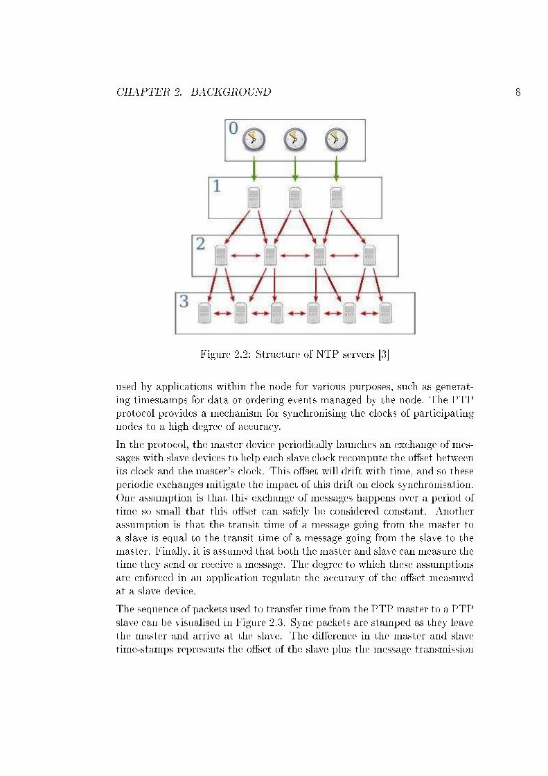
2.2.1 Network Time ProtocolThe Network Time Protocol is a protocol for synchronising the clocks of com-puter systems over packet-switched, variable-latency data networks. NTPuses UDP as its transport layer. It is designed particularly to resist thee�ects of variable latency (jitter).NTP has a tree structure as shown in Figure 2.2. Stratum 1 computers areattached to reference clocks , typically GPS clocks or atom clocks . Normallythey act as servers for timing requests from stratum 2 servers via NTP. Andthus, every stratum works as a server for the next stratum.When a computer wants to get synchronisation using NTP, it exchangespackages containing timestamps and then makes a correction of time usingthose timestamps. NTP protocol usually provides an accuracy of few mil-liseconds on a unloaded network but it is highly dependant on the networkbehaviour and the distance with the stratum 1 servers.
2.2.2 Precision Time ProtocolNetwork Time Protocol (NTP) targets large distributed computing systemswith millisecond synchronisation requirements. However, it does not ful�lthe requirements for smaller networks when a better accuracy is needed.The Precision Time Protocol (PTP) is a time-transfer protocol de�ned inthe IEEE 1588 standard. This protocol is applicable to distributed systemsconsisting of one or more nodes, communicating over some set of communica-tion media. Nodes are modelled as containing a real-time clock that may be
CHAPTER 2. BACKGROUND 8
Figure 2.2: Structure of NTP servers [3]
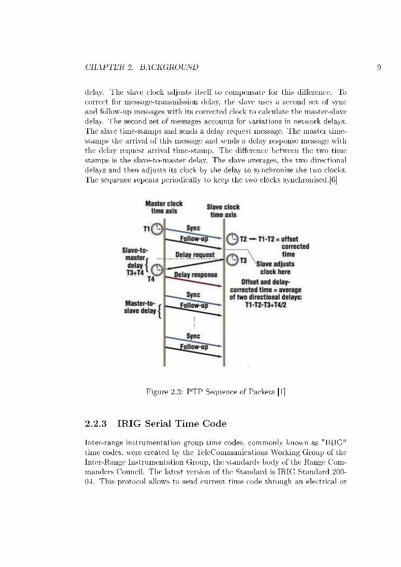
used by applications within the node for various purposes, such as generat-ing timestamps for data or ordering events managed by the node. The PTPprotocol provides a mechanism for synchronising the clocks of participatingnodes to a high degree of accuracy.In the protocol, the master device periodically launches an exchange of mes-sages with slave devices to help each slave clock recompute the o�set betweenits clock and the master's clock. This o�set will drift with time, and so theseperiodic exchanges mitigate the impact of this drift on clock synchronisation.One assumption is that this exchange of messages happens over a period oftime so small that this o�set can safely be considered constant. Anotherassumption is that the transit time of a message going from the master toa slave is equal to the transit time of a message going from the slave to themaster. Finally, it is assumed that both the master and slave can measure thetime they send or receive a message. The degree to which these assumptionsare enforced in an application regulate the accuracy of the o�set measuredat a slave device.The sequence of packets used to transfer time from the PTP master to a PTPslave can be visualised in Figure 2.3. Sync packets are stamped as they leavethe master and arrive at the slave. The di�erence in the master and slavetime-stamps represents the o�set of the slave plus the message transmission
CHAPTER 2. BACKGROUND 9
delay. The slave clock adjusts itself to compensate for this di�erence. Tocorrect for message-transmission delay, the slave uses a second set of syncand follow-up messages with its corrected clock to calculate the master-slavedelay. The second set of messages accounts for variations in network delays.The slave time-stamps and sends a delay request message. The master time-stamps the arrival of this message and sends a delay response message withthe delay request arrival time-stamp. The di�erence between the two timestamps is the slave-to-master delay. The slave averages, the two directionaldelays and then adjusts its clock by the delay to synchronise the two clocks.The sequence repeats periodically to keep the two clocks synchronised.[6]
Figure 2.3: PTP Sequence of Packets [1]
2.2.3 IRIG Serial Time CodeInter-range instrumentation group time codes, commonly known as "IRIG"time codes, were created by the TeleCommunications Working Group of theInter-Range Instrumentation Group, the standards body of the Range Com-manders Council. The latest version of the Standard is IRIG Standard 200-04. This protocol allows to send current time code through an electrical or
CHAPTER 2. BACKGROUND 10
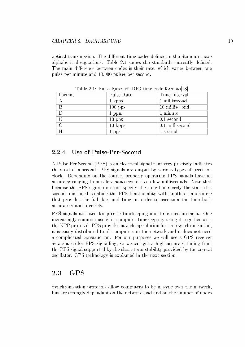
optical transmission. The di�erent time codes de�ned in the Standard havealphabetic designations. Table 2.1 shows the standards currently de�ned.The main di�erence between codes is their rate, which varies between onepulse per minute and 10.000 pulses per second.
Table 2.1: Pulse Rates of IRIG time code formats[13]Format Pulse Rate Time IntervalA 1 kpps 1 millisecondB 100 pps 10 millisecondD 1 ppm 1 minuteE 10 pps 0.1 secondG 10 kpps 0.1 millisecondH 1 pps 1 second
2.2.4 Use of Pulse-Per-SecondA Pulse Per Second (PPS) is an electrical signal that very precisely indicatesthe start of a second. PPS signals are output by various types of precisionclock. Depending on the source, properly operating PPS signals have anaccuracy ranging from a few nanoseconds to a few milliseconds. Note thatbecause the PPS signal does not specify the time but merely the start of asecond, one must combine the PPS functionality with another time sourcethat provides the full date and time, in order to ascertain the time bothaccurately and precisely.PPS signals are used for precise timekeeping and time measurement. Oneincreasingly common use is in computer timekeeping, using it together withthe NTP protocol. PPS provides us a cheap solution for time synchronisation,it is easily distributed to all computers in the network and it does not needa complicated construction. For our purposes we will use a GPS receiveras a source for PPS signalling, so we can get a high accurate timing fromthe PPS signal supported by the short-term stability provided by the crystaloscillator. GPS technology is explained in the next section.
2.3 GPSSynchronisation protocols allow computers to be in sync over the network,but are strongly dependant on the network load and on the number of nodes
CHAPTER 2. BACKGROUND 11
between the computer and the time source. In this section we explain thebasis of GPS and how we can achieve perfect timing with a simple GPSreceiver.The Global Positioning System (GPS) is a worldwide radio-navigation sys-tem formed from a constellation of 24 satellites and their ground stations.GPS uses these arti�cial satellites as reference points to calculate positionsaccurate to a matter of meters. In fact, with advanced forms of GPS youcan make measurements to better than a centimetre. GPS receivers havebeen miniaturised to just a few integrated circuits and so are becoming veryeconomical, what makes the technology accessible to virtually everyone.The GPS system can be devided into three basic segments which will bediscussed below:
� Space segment (satellites).
� Control segment (control stations).
� User segment (GPS receiver).
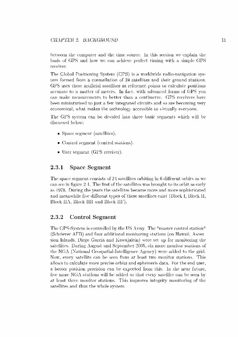
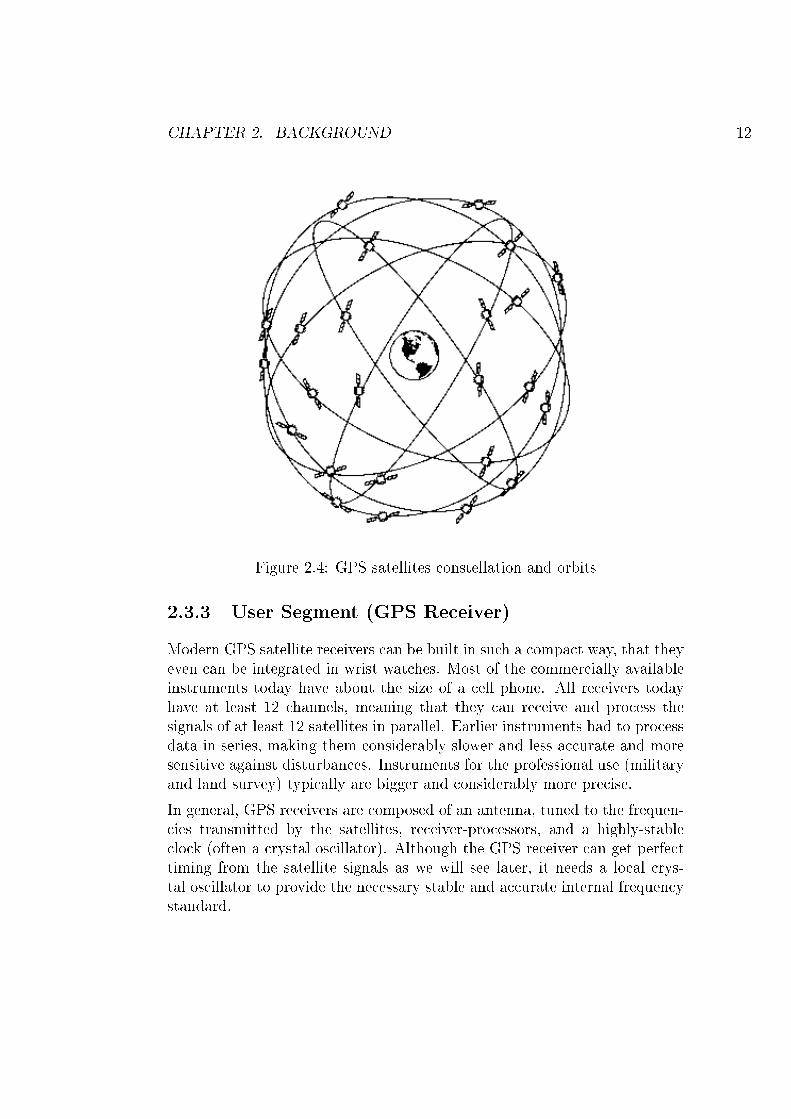
2.3.1 Space SegmentThe space segment consists of 24 satellites orbiting in 6 di�erent orbits as wecan see in �gure 2.4. The �rst of the satellites was brought to its orbit as earlyas 1978. During the years the satellites became more and more sophisticatedand meanwhile �ve di�erent types of these satellites exist (Block I, Block II,Block IIA, Block IIR und Block IIF).
2.3.2 Control SegmentThe GPS-System is controlled by the US Army. The "master control station"(Schriever AFB) and four additional monitoring stations (on Hawaii, Ascen-sion Islands, Diego Garcia and Kawajalein) were set up for monitoring thesatellites. During August and September 2005, six more monitor stations ofthe NGA (National Geospatial-Intelligence Agency) were added to the grid.Now, every satellite can be seen from at least two monitor stations. Thisallows to calculate more precise orbits and ephemeris data. For the end user,a better position precision can be expected from this. In the near future,�ve more NGA stations will be added so that every satellite can be seen byat least three monitor stations. This improves integrity monitoring of thesatellites and thus the whole system.
CHAPTER 2. BACKGROUND 12
Figure 2.4: GPS satellites constellation and orbits
2.3.3 User Segment (GPS Receiver)Modern GPS satellite receivers can be built in such a compact way, that theyeven can be integrated in wrist watches. Most of the commercially availableinstruments today have about the size of a cell phone. All receivers todayhave at least 12 channels, meaning that they can receive and process thesignals of at least 12 satellites in parallel. Earlier instruments had to processdata in series, making them considerably slower and less accurate and moresensitive against disturbances. Instruments for the professional use (militaryand land survey) typically are bigger and considerably more precise.In general, GPS receivers are composed of an antenna, tuned to the frequen-cies transmitted by the satellites, receiver-processors, and a highly-stableclock (often a crystal oscillator). Although the GPS receiver can get perfecttiming from the satellite signals as we will see later, it needs a local crys-tal oscillator to provide the necessary stable and accurate internal frequencystandard.
CHAPTER 2. BACKGROUND 13
2.3.4 How GPS WorksBasically, GPS works following these �ve steps:
1. The idea behind GPS is "triangulation" from satellites.
2. In order to triangulate, a GPS receiver calculates distance using thetravel time of satellite signals.
3. To measure travel time, GPS needs very accurate timing which isachieved with some tricks we will explain later.
4. Furthermore, you need to know the exact position of satellites in space.This can be achieved basing on high orbits and satellite monitoring.
5. Finally there are some sources of errors you must correct due to delaysthe signal experiences as it travels through the atmosphere.
2.3.5 TriangulationThe basis of GPS is to use satellites in space as reference points for locationshere on earth. By very accurately measuring our distance from three satelliteswe can "triangulate" our position anywhere on earth. We will explain thiswith an example:
1. Suppose we measure our distance from a satellite and �nd it to be18.000 meters. Knowing that we are 18.000 meters from a particularsatellite narrows down all the possible locations we could be in thewhole universe to the surface of a sphere that is centred on this satelliteand has a radius of 18.000 miles.
2. Next, say we measure our distance to a second satellite and �nd outthat it is 19.000 meters away. That tells us that we are not only onthe �rst sphere but we are also on a sphere that is 19.000 meters fromthe second satellite. Or in other words, we are somewhere on the circlewhere these two spheres intersect.
3. If we then make a measurement from a third satellite and �nd that weare 20.000 meters from that one, that narrows our position down evenfurther, to the two points where the 20.000 meters sphere cuts throughthe circle that is the intersection of the �rst two spheres.
CHAPTER 2. BACKGROUND 14
So by ranging from three satellites we can narrow our position to justtwo points in space. To decide which one is our true location we couldmake a fourth measurement. But usually one of the two points is aridiculous answer (either too far from Earth or moving at an impossiblevelocity) and can be rejected without a measurement.
2.3.6 Measuring DistanceWe saw in the last section that a position is calculated from distance mea-surements to at least three satellites. Distance can be easily calculated multi-plying the signal travel time by the speed of light. The problem is measuringthe travel time.The timing problem is tricky. First, the times are going to be extremelyshort. If a satellite were right overhead the travel time would be somethinglike 0.06 seconds. So we are going to need some really precise clocks.To make the measurement we assume that both the satellite and our receiverare generating the same pseudo-random codes at exactly the same time. Bycomparing how late the pseudo-random code of the satellite appears com-pared to the code of the receiver, we determine how long it took to reachus.Thus, if we designate the coordinates and the time sent as [xi, yi, zi, ti] wherei is the indicator for each one of the 4 satellites, and knowing the arrival timeat the receiver tri, we can calculate the transit time of the message, (tri− ti).Assuming the transmission speed is the speed of the light, c, the distancetravelled by the message is
pi = (tri − ti)c (2.2)
Once we know the position of the satellites we can triangulate the positionof the receiver as we mentioned previously.
2.3.7 Getting Perfect TimingAt the speed of light a timing error of just a thousandth of a second istranslated into 300 kilometres of error. For that reason we need very accurateand synchronised clocks in both sides.On the satellite side, timing is almost perfect because they have highly pre-cise atomic clocks on board. But on the receivers, atomic clocks are justuna�ordable.
CHAPTER 2. BACKGROUND 15
Luckily GPS allows us to get by accurate clocks in our receivers with abrilliant little trick. This trick is one of the key elements of GPS and as anadded side bene�t it means that every GPS receiver is essentially an atomic-accuracy clock.The secret to perfect timing is to make an extra satellite measurement. Ifthree perfect measurements can locate a point in 3-dimensional space, thenfour imperfect measurements can do the same thing.If our receiver's clocks were perfect, then all our satellite ranges would in-tersect at a single point (which is our position). But with imperfect clocks,a fourth measurement, done as a cross-check, will not intersect with the�rst three. That makes the receiver realises that its clock it is not perfectlysynchronised with universal time.Since any o�set from universal time will a�ect all of our measurements, thereceiver looks for a single correction factor that it can subtract from all itstiming measurements that would cause them all to intersect at a single point.That correction brings the receiver's clock back into synchronisation withuniversal time, and that is how we get an atomic accuracy clock from asimple receiver.Mathematically, if b denotes the clock error or bias, we have four unknowns,the three coordinates of the GPS receiver and the clock bias [x, y, z, b], andfour equations corresponding to the spheres of the satellites given by:
(x− xi)2 + (y − yi)
2 + (z − zi)2 = ((tri + b− ti)c)
2, i = 1, 2, 3, 4. (2.3)
Another way to express these equations is in terms of pseudo-ranges, whichare approximations to the distance travelled by the message as in equation2.2 but having in account the bias unknown. [8]
pi =√
(x− xi)2 + (y − yi)2 + (z − zi)2 − bc, i = 1, 2, 3, 4. (2.4)
To solve these equations there exists di�erent methods. The most importantis trilateration followed by one dimensional root �nding and multidimensionalNewton-Raphson calculations. [12]
2.3.8 Error SourcesUp to now we have considered our GPS system very abstractly and we havenot introduced the e�ects produced by the di�erent sources of error and
CHAPTER 2. BACKGROUND 16
interferences.
Multipath e�ect
The multipath e�ect is caused by re�ection of satellite signals (radio waves)on objects. It was the same e�ect that caused ghost images on televisionwhen antennas on the roof were still more common instead of today's satellitedishes.For GPS signals this e�ect mainly appears in the neighbourhood of largebuildings or other elevations. The re�ected signal takes more time to reachthe receiver than the direct signal. The resulting error typically lies in therange of a few meters.
Clock Inaccuracies and Rounding Errors
Despite the synchronization of the receiver clock with the satellite time dur-ing the position determination, the remaining inaccuracy of the time stillleads to an error of about 2 m in the position determination. Rounding andcalculation errors of the receiver sum up approximately to 1 m.
Relativistic E�ects
The following section shall not provide a comprehensive explanation of thetheory of relativity. In the normal life we are quite unaware of the om-nipresence of the theory of relativity. However, it has an in�uence on manyprocesses, among them is the proper functioning of the GPS system. Thisin�uence will be explained shortly in the following.As we already learnt, the time is a relevant factor in GPS navigation andmust be accurate to 20 - 30 nanoseconds to ensure the necessary accuracy.Therefore the fast movement of the satellites themselves (nearly 12000 km/h)must be considered.Whoever already dealt with the theory of relativity knows that time runsslower during very fast movements. For satellites moving with a speed of3874 m/s, clocks run slower when viewed from earth. This relativistic timedilation leads to an inaccuracy of time of approximately 7.2 microsecondsper day.The theory of relativity also says that time moves the slower the strongerthe �eld of gravitation is. For an observer on the earth surface the clock on
CHAPTER 2. BACKGROUND 17
board of a satellite is running faster (as the satellite in 20000 km height isexposed to a much weaker �eld of gravitation than the observer). And thissecond e�ect is six times stronger than the time dilation explained above.Altogether, the clocks of the satellites seem to run a little faster. The shiftof time to the observer on earth would be about 38 milliseconds per day andwould make up for an total error of approximately 10 km per day. In orderthat those error do not have to be corrected constantly, the clocks of thesatellites were set to 10.229999995453 MHz instead of 10.23 MHz but theyare operated as if they had 10.23 MHz. By this trick the relativistic e�ectsare compensated once and for all.
Atmospheric e�ects
Another source of inaccuracy is the reduced speed of propagation in thetroposphere and ionosphere. While radio signals travel with the velocity oflight in the outer space, their propagation in the ionosphere and troposphereis slower.In the ionosphere in a height of 80 - 400 km a large number of electronsand positive charged ions are formed by the ionising force of the sun. Theelectrons and ions are concentrated in four conductive layers in the ionosphere(D, E, F1, and F2 layer). These layers refract the electromagnetic waves fromthe satellites, resulting in an elongated run time of the signals.There are a couple of ways to minimise this kind of error. For one thingwe can predict what a typical delay might be on a typical day. This iscalled modelling and it helps but, of course, atmospheric conditions are rarelyexactly typical.Another way to get a handle on these atmosphere-induced errors is to com-pare the relative speeds of two di�erent signals. This "dual frequency" mea-surement is very sophisticated and is only possible with advanced receivers.Other source of error is due to re�ections of the signal in local obstructionsbefore it gets to the receiver. This is called multipath error. Good receiversuse sophisticated signal rejection techniques to minimise this problem.Fortunately all of these inaccuracies still do not add up to much of an error.And a form of GPS called "Di�erential GPS" can signi�cantly reduce theseproblems.
CHAPTER 2. BACKGROUND 18
2.3.9 Di�erential GPSDi�erential GPS (DGPS) involves the cooperation of two receivers, one thatis stationary and another that is roving around making position measure-ments. The stationary receiver is the key. It ties all the satellite measure-ments into a solid local reference.Since each of the timing signals that go into a position calculation has someerror, that calculation is going to be a compounding of those errors. Luckilythe satellites are located in high orbits far away in space so the little distanceswe travel here on earth are insigni�cant.So if two receivers are fairly close to each other, say within a few hundredkilometres, the signals that reach both of them will have travelled throughvirtually the same path in the atmosphere, and so will have virtually thesame errors.That is the idea behind di�erential GPS: We have one receiver measure thetiming errors and then provide correction information to the other receiversthat are roving around. That way virtually all errors can be eliminated fromthe system.The idea is simple. Put the reference receiver on a point that has been veryaccurately surveyed and keep it there. This reference station receives thesame GPS signals as the roving receiver but instead of working like a normalGPS receiver it attacks the equations backwards.Instead of using timing signals to calculate its position, it uses its knownposition to calculate timing. It �gures out what the travel time of the GPSsignals should be, and compares it with what they actually are. The di�er-ence is an "error correction" factor.Since the reference receiver has no way of knowing which of the many avail-able satellites a roving receiver might be using to calculate its position, thereference receiver quickly runs through all the visible satellites and computeseach of their errors. Then it encodes this information into a standard formatand transmits it to the roving receivers. The roving receivers get the com-plete list of errors and apply the corrections for the particular satellites theyare using. [2] [5] [10]
CHAPTER 2. BACKGROUND 19
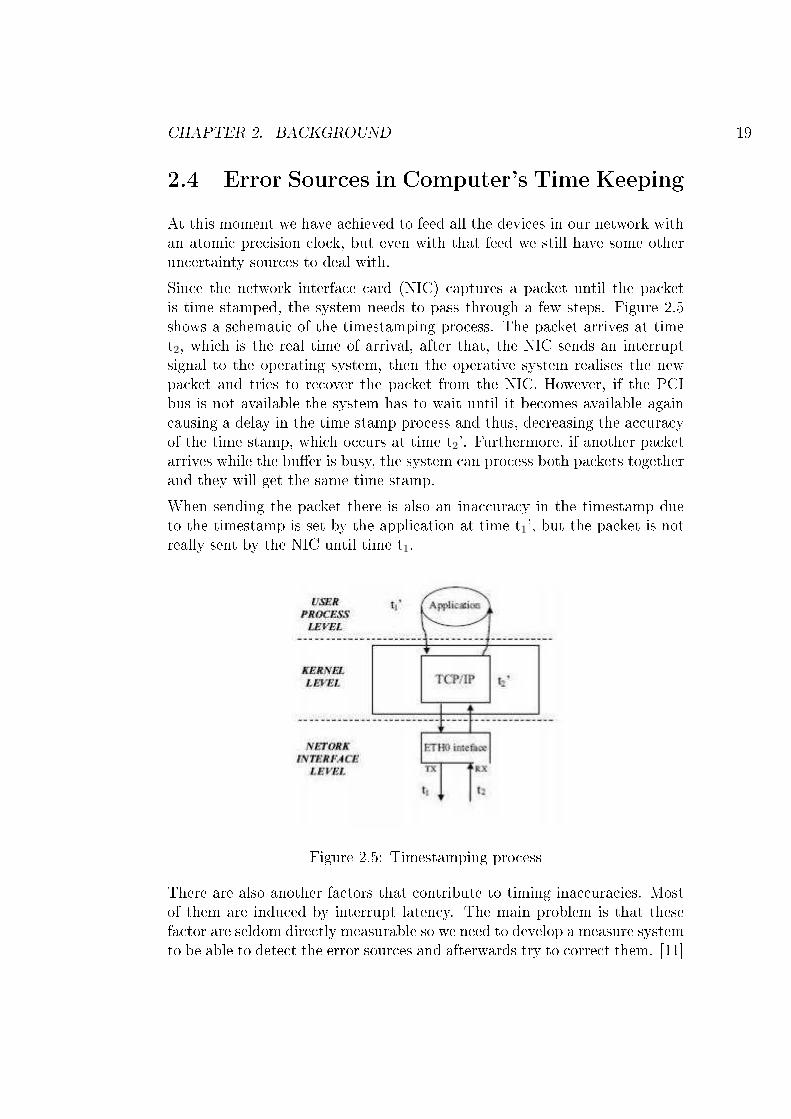
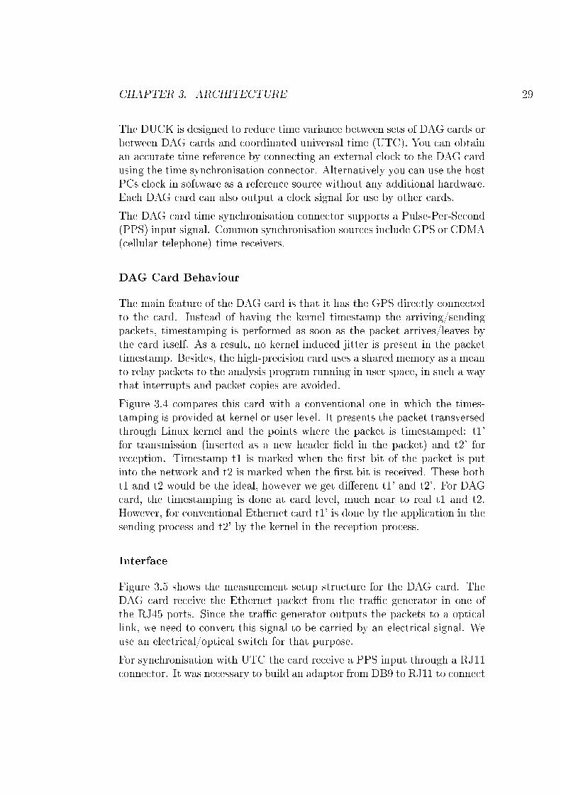
2.4 Error Sources in Computer's Time KeepingAt this moment we have achieved to feed all the devices in our network withan atomic precision clock, but even with that feed we still have some otheruncertainty sources to deal with.Since the network interface card (NIC) captures a packet until the packetis time stamped, the system needs to pass through a few steps. Figure 2.5shows a schematic of the timestamping process. The packet arrives at timet2, which is the real time of arrival, after that, the NIC sends an interruptsignal to the operating system, then the operative system realises the newpacket and tries to recover the packet from the NIC. However, if the PCIbus is not available the system has to wait until it becomes available againcausing a delay in the time stamp process and thus, decreasing the accuracyof the time stamp, which occurs at time t2'. Furthermore, if another packetarrives while the bu�er is busy, the system can process both packets togetherand they will get the same time stamp.When sending the packet there is also an inaccuracy in the timestamp dueto the timestamp is set by the application at time t1', but the packet is notreally sent by the NIC until time t1.
Figure 2.5: Timestamping process
There are also another factors that contribute to timing inaccuracies. Mostof them are induced by interrupt latency. The main problem is that thesefactor are seldom directly measurable so we need to develop a measure systemto be able to detect the error sources and afterwards try to correct them. [11]
CHAPTER 2. BACKGROUND 20
2.5 Two-Way and One-Way DelayThe two-way delay of packets is an interesting characteristic of Internet. Itprovides extensive information about state of networks and application per-formance. For network characterisation, we can get values of transmissionand propagation delays looking at the minimum two-way delay. The varia-tions of delay are related with queueing e�ects. Even we can infer topologyinformation, congestion state or route changes from two-way delay measure-ments. From an application performance point of view, large delays willmake di�cult to obtain a sustainable high bandwidth �ow because of TCPdependency on RTT (Round Trip Time).Two-way delay can be divided into several components:
� Transmission delay: the time needed to put all bits of a packet over adata link.
� Propagation delay: the time needed to propagate a bit though the datalink.
� Processing delay: the time needed to process a packet in each router.
� Queueing delay: the time needed to wait in a router queue beforetransmission.
Processing and queueing delays are stochastic random variables due to vari-ability in processing tasks in routers and in network conditions respectively.However, nowadays processing time should be almost constant except on rareoccasions because modern IP routers use hardware assisted forwarding withwire speed. Transmission and propagation delays are almost constant for acertain path, because they depend on link capacity and distance respectively.Propagation and transmission delays will give a good approximation to theminimum two-way delay and this minimum will have to be a constant value.Normally, two-way delay is approximated by RTT. Those measurements arevery easy to obtain, using ICMP Request/Reply packets through the pingtool and controlling only one of the end nodes. However, asymmetry ofpaths makes this approximation invalid because delay can be di�erent forboth directions of a path. Actually, for two way delay measurement, it doesnot matter that routes are asymmetrical. One can not divide the RTT by2 and assume that the result is a one way delay if routes are asymmetrical.
CHAPTER 2. BACKGROUND 21
Another procedure is measuring one-way delay (OWD) which is a more com-plex measurement. It requires expensive hardware but it provides a bettercharacterisation of the parameter.[4]Two-way delay does not need synchronisation since all the measures are donein the same point of the network. However, OWD does need synchronisationand it is the measure we will use in this thesis to analyse the performance ofthe di�erent devices.
Chapter 3
Architecture
This chapter shows in detail how is the architecture of the measurementsystem and provides a description of the testing environment. We will alsopresent all the di�erent devices included in the system and their character-istics.
3.1 EnvironmentFor the development of the measurement setup we have used the followingcomponents of the Department of Communications and Networks researchlaboratory:
� Tra�c generator: Spirent Adtech AX/4000.
� Capture card: Endace DAG Card 3.7G.
� Capture card: SynPCI developed in TKK.
� GPS receiver: Trimble Acutime 2000.
� GPS receiver: Trimble Thunderbolt GPS Disciplined Clock.
� VSS monitoring tra�c splitter.
� Procurve Switch 1800-24G
� Distribution boards.
22
CHAPTER 3. ARCHITECTURE 23
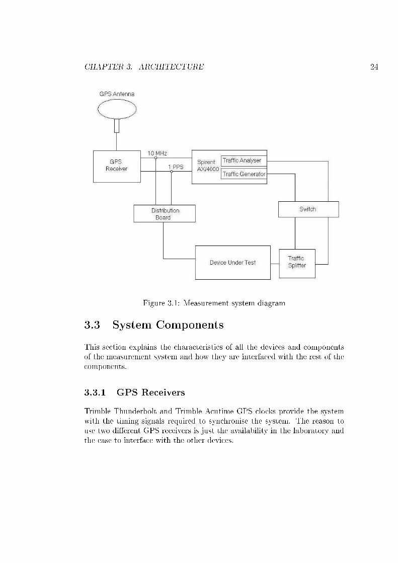
3.2 System OverviewAs we said in section 1.4 the purpose of this thesis is to build a measurementsetup to be able to analyse the performance of two di�erent synchronisationsystems. In order to do that, we have to achieve accurate synchronisationamong the critical points of the network which are the tra�c generator andthe PCs equipped with the capture cards.The idea is to send a tra�c pattern from a tra�c generator and timestampthe incoming packets in the devices we want to test. Then we can comparethis timestamps with a more accurate reference. To get this reference we usethe same tra�c generator which is also equipped with a high-quality tra�canalyser. For that reason we loop the tra�c sent to the capture card backto the tra�c generator.The Spirent Adtech AX/4000 tra�c generator receives a PPS signal and a10 MHz signal from the Trimble Thunderbolt GPS receiver trough a coaxialcable line. It also receives a serial input providing time information from thedevice under test as we will see later in section 3.3.5.Thunderbolt GPS receiver also provides both PPS and 10 MHz signals forthe SynPCI capture card. However, in this case the SynPCI card is ex-pecting optical inputs and therefore a electrical/optical conversion is needed.This conversion is performed in a distribution board that interfaces the GPSreceiver and the SynPCI card.The other capture card, Endace DAG card, only needs a PPS signal forsynchronisation. It gets it from the Trimble Acutime 2000 GPS receiver.The data transmission is output by the tra�c generator in optical format.In order to input to the RJ45 Ethernet connectors of the PCs containingthe cards we want to analyse, we need to convert this signal from optical toelectrical. We achieve that using an optical/electrical switch.To loop back the signal we use a tra�c splitter that divides the signal intotwo signals. One of them goes to the capture card and the other returnsto the switch, is converted again to optical and is fed back to the tra�cgenerator.Figure 3.1 shows the general scheme of the whole system and how it is struc-tured.
CHAPTER 3. ARCHITECTURE 24
Figure 3.1: Measurement system diagram
3.3 System ComponentsThis section explains the characteristics of all the devices and componentsof the measurement system and how they are interfaced with the rest of thecomponents.
3.3.1 GPS ReceiversTrimble Thunderbolt and Trimble Acutime GPS clocks provide the systemwith the timing signals required to synchronise the system. The reason touse two di�erent GPS receivers is just the availability in the laboratory andthe ease to interface with the other devices.
CHAPTER 3. ARCHITECTURE 25
Trimble Thunderbolt GPS Disciplined Clock
The Thunderbolt clock provides a PPS signal and a 10 MHz signal neededby the tra�c generator and the SynPCI card. Both signals are electricaland are delivered directly to the tra�c generator using a BNC connectorand through a distribution board to the SynPCI card. Table 3.1 shows itsperformance speci�cations.
Table 3.1: Trimble Thunderbolt Performance Speci�cationsPulse width 10 microsecondsPPS Accuracy (one sigma) 20 nanoseconds10 MHz Accuracy 1.16 x 10⁻¹² (one day average)
Trimble Acutime 2000
Trimble Acutime GPS Antenna is interfaced with the system using the Syn-chronisation Interface Module (SIM). The antenna sends the PPS signal withRS-422 signalling levels, the SIM outputs the same signal with TTL level.It is connected to the distribution board with a BNC connector. Table 3.2shows its performance speci�cations.
Table 3.2: Trimble Acutime Performance Speci�cationsPulse width 10 microsecondsPPS Resolution 80 nanosecondsPPS Accuracy (one sigma) 50 nanoseconds
3.3.2 Distribution BoardsThe distribution boards included in the architecture of the system have twodi�erent purposes. First of all, they provide us with the capability of sharingthe GPS signals with other devices in the laboratory, and, in the case ofthe SynPCI card, the distribution board also ful�ls the electrical/opticalconversion of both PPS and 10 MHz signal.
3.3.3 Procurve Switch 1800-24GAs we previously said, the switch is used just as a optical/electrical andviceversa converter. The Procurve Switch 1800-24G is a web-managed switch
CHAPTER 3. ARCHITECTURE 26
with 24 ports. Two of them are dual ports that can work either with aRJ45 interface or a mini-GBIC optical interface. A latency less than 3 µs isguaranteed by the manufacturer for a Gigabit Ethernet connection and 64bytes packets.
3.3.4 Tra�c SplitterIn order to split the tra�c, we will use a the VSS monitoring 10/100/10001x1 Copper Tap. It allows the uninterrupted pass through of full duplex dataover its two RJ45 tra�c ports, while the network signals are duplicated tothe transmit-only monitoring ports.Decoding the network signals this device reclocks the data and electroni-cally replicates an exact copy (including line errors) to two transmit-onlyRJ45 monitoring ports, thereby giving the user the ability to monitor a10/100/1000 copper link with a gigabit copper monitoring device.The tra�c generator sends the packets to one of the tra�c ports and thissignal is looped back through the other tra�c port. The duplicated signalis output by one of the monitoring ports and connected to capture card wewant to test.
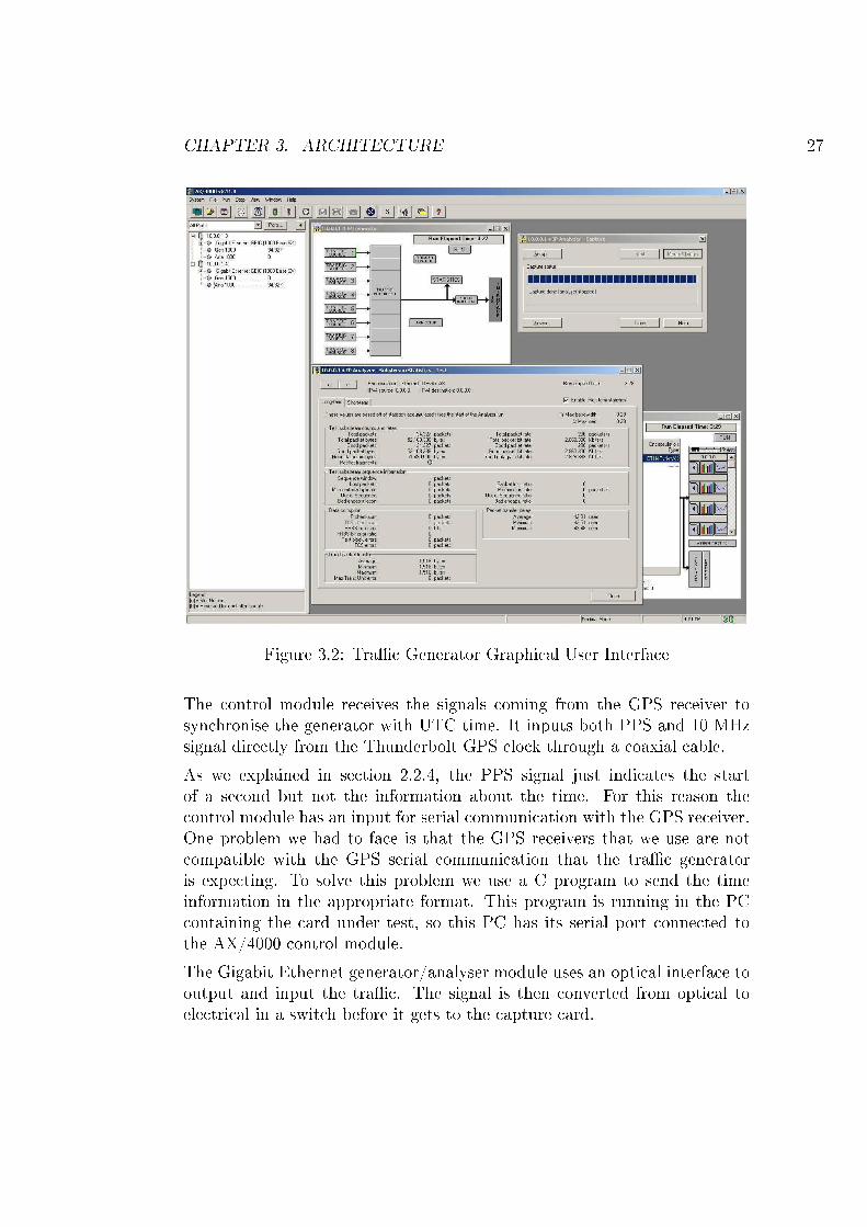
3.3.5 Tra�c GeneratorThe tra�c generator that we will use to send the packets to the deviceswe want to test is the Spirent Adtech AX/4000. AX/4000 is a modular,multi-port system capable of testing multiple transmission technologies suchas ATM, IP, Frame Relay and Ethernet simultaneously at speeds up to 10Gbit/s.The AX/4000 Generator and Generator/Analyser modules include tools forcreating unlimited tra�c variations and details. The controller software hasa very intuitive graphical user interface, that allow us to build complex traf-�c streams quickly and easily. When injected onto the network, these tra�cstreams can be "shaped" (to simulate constant or bursty tra�c) and even in-troduce error conditions. Figure 3.2 shows how the network access graphicaluser interface (NAGUI) looks like.For our purpose we will use the control module and the Gigabit Ethernetgenerator/analyser module that are installed in the AX/4000 chassis of thelaboratory. The control module allows the system to be connected to anEthernet-based LAN for access by remote users.
CHAPTER 3. ARCHITECTURE 27
Figure 3.2: Tra�c Generator Graphical User Interface
The control module receives the signals coming from the GPS receiver tosynchronise the generator with UTC time. It inputs both PPS and 10 MHzsignal directly from the Thunderbolt GPS clock through a coaxial cable.As we explained in section 2.2.4, the PPS signal just indicates the startof a second but not the information about the time. For this reason thecontrol module has an input for serial communication with the GPS receiver.One problem we had to face is that the GPS receivers that we use are notcompatible with the GPS serial communication that the tra�c generatoris expecting. To solve this problem we use a C program to send the timeinformation in the appropriate format. This program is running in the PCcontaining the card under test, so this PC has its serial port connected tothe AX/4000 control module.The Gigabit Ethernet generator/analyser module uses an optical interface tooutput and input the tra�c. The signal is then converted from optical toelectrical in a switch before it gets to the capture card.
CHAPTER 3. ARCHITECTURE 28
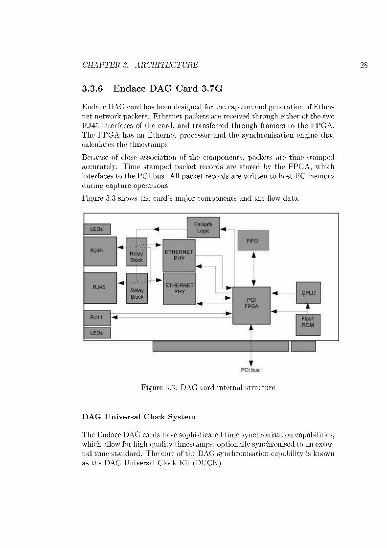
3.3.6 Endace DAG Card 3.7GEndace DAG card has been designed for the capture and generation of Ether-net network packets. Ethernet packets are received through either of the twoRJ45 interfaces of the card, and transferred through framers to the FPGA.The FPGA has an Ethernet processor and the synchronisation engine thatcalculates the timestamps.Because of close association of the components, packets are time-stampedaccurately. Time stamped packet records are stored by the FPGA, whichinterfaces to the PCI bus. All packet records are written to host PC memoryduring capture operations.Figure 3.3 shows the card's major components and the �ow data.
Figure 3.3: DAG card internal structure
DAG Universal Clock System
The Endace DAG cards have sophisticated time synchronisation capabilities,which allow for high quality timestamps, optionally synchronised to an exter-nal time standard. The core of the DAG synchronisation capability is knownas the DAG Universal Clock Kit (DUCK).
CHAPTER 3. ARCHITECTURE 29
The DUCK is designed to reduce time variance between sets of DAG cards orbetween DAG cards and coordinated universal time (UTC). You can obtainan accurate time reference by connecting an external clock to the DAG cardusing the time synchronisation connector. Alternatively you can use the hostPCs clock in software as a reference source without any additional hardware.Each DAG card can also output a clock signal for use by other cards.The DAG card time synchronisation connector supports a Pulse-Per-Second(PPS) input signal. Common synchronisation sources include GPS or CDMA(cellular telephone) time receivers.
DAG Card Behaviour
The main feature of the DAG card is that it has the GPS directly connectedto the card. Instead of having the kernel timestamp the arriving/sendingpackets, timestamping is performed as soon as the packet arrives/leaves bythe card itself. As a result, no kernel induced jitter is present in the packettimestamp. Besides, the high-precision card uses a shared memory as a meanto relay packets to the analysis program running in user space, in such a waythat interrupts and packet copies are avoided.Figure 3.4 compares this card with a conventional one in which the times-tamping is provided at kernel or user level. It presents the packet transversedthrough Linux kernel and the points where the packet is timestamped: t1'for transmission (inserted as a new header �eld in the packet) and t2' forreception. Timestamp t1 is marked when the �rst bit of the packet is putinto the network and t2 is marked when the �rst bit is received. These botht1 and t2 would be the ideal, however we get di�erent t1' and t2'. For DAGcard, the timestamping is done at card level, much near to real t1 and t2.However, for conventional Ethernet card t1' is done by the application in thesending process and t2' by the kernel in the reception process.
Interface
Figure 3.5 shows the measurement setup structure for the DAG card. TheDAG card receive the Ethernet packet from the tra�c generator in one ofthe RJ45 ports. Since the tra�c generator outputs the packets to a opticallink, we need to convert this signal to be carried by an electrical signal. Weuse an electrical/optical switch for that purpose.For synchronisation with UTC the card receive a PPS input through a RJ11connector. It was necessary to build an adaptor from DB9 to RJ11 to connect
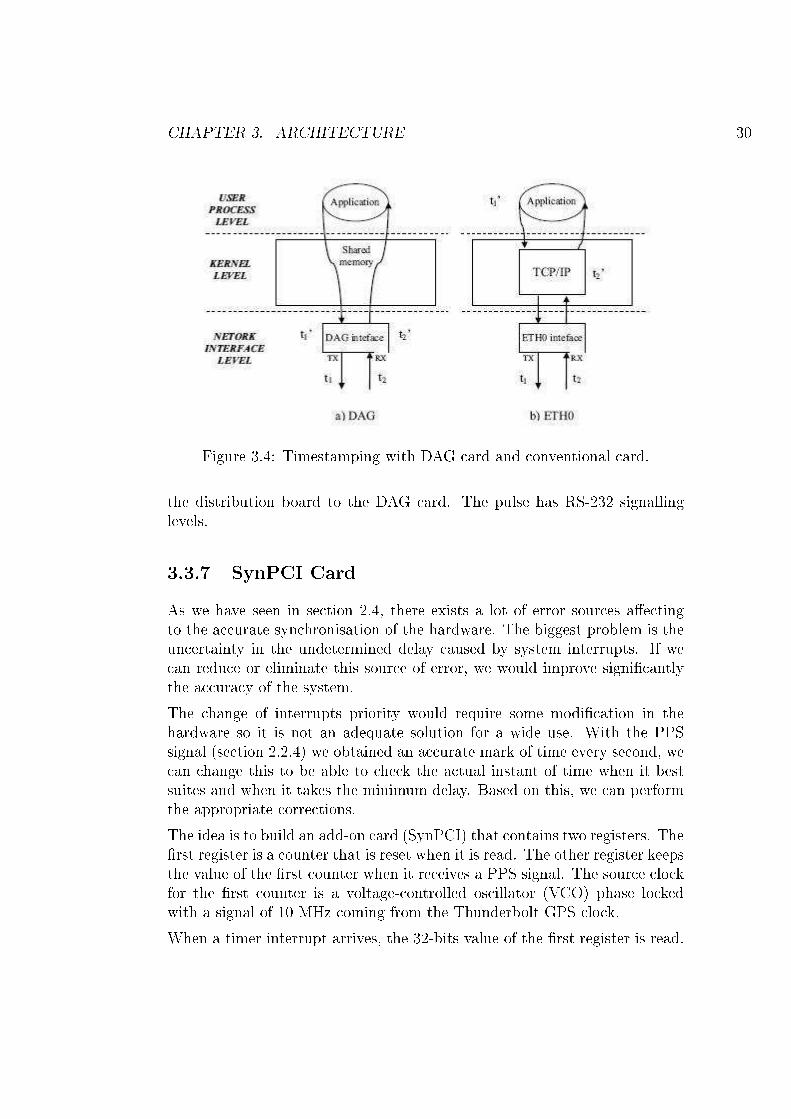
CHAPTER 3. ARCHITECTURE 30
Figure 3.4: Timestamping with DAG card and conventional card.
the distribution board to the DAG card. The pulse has RS-232 signallinglevels.
3.3.7 SynPCI CardAs we have seen in section 2.4, there exists a lot of error sources a�ectingto the accurate synchronisation of the hardware. The biggest problem is theuncertainty in the undetermined delay caused by system interrupts. If wecan reduce or eliminate this source of error, we would improve signi�cantlythe accuracy of the system.The change of interrupts priority would require some modi�cation in thehardware so it is not an adequate solution for a wide use. With the PPSsignal (section 2.2.4) we obtained an accurate mark of time every second, wecan change this to be able to check the actual instant of time when it bestsuites and when it takes the minimum delay. Based on this, we can performthe appropriate corrections.The idea is to build an add-on card (SynPCI) that contains two registers. The�rst register is a counter that is reset when it is read. The other register keepsthe value of the �rst counter when it receives a PPS signal. The source clockfor the �rst counter is a voltage-controlled oscillator (VCO) phase lockedwith a signal of 10 MHz coming from the Thunderbolt GPS clock.When a timer interrupt arrives, the 32-bits value of the �rst register is read.
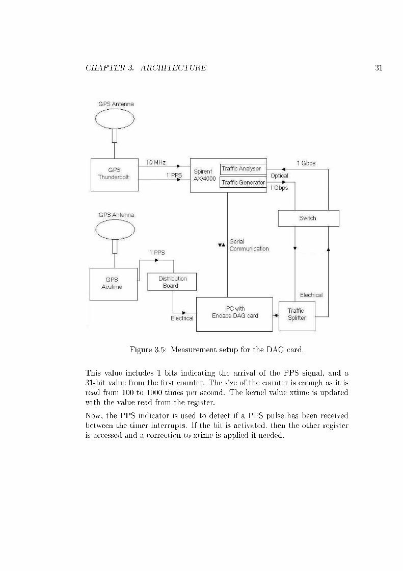
CHAPTER 3. ARCHITECTURE 31
Figure 3.5: Measurement setup for the DAG card.
This value includes 1 bits indicating the arrival of the PPS signal, and a31-bit value from the �rst counter. The size of the counter is enough as it isread from 100 to 1000 times per second. The kernel value xtime is updatedwith the value read from the register.Now, the PPS indicator is used to detect if a PPS pulse has been receivedbetween the timer interrupts. If the bit is activated, then the other registeris accessed and a correction to xtime is applied if needed.
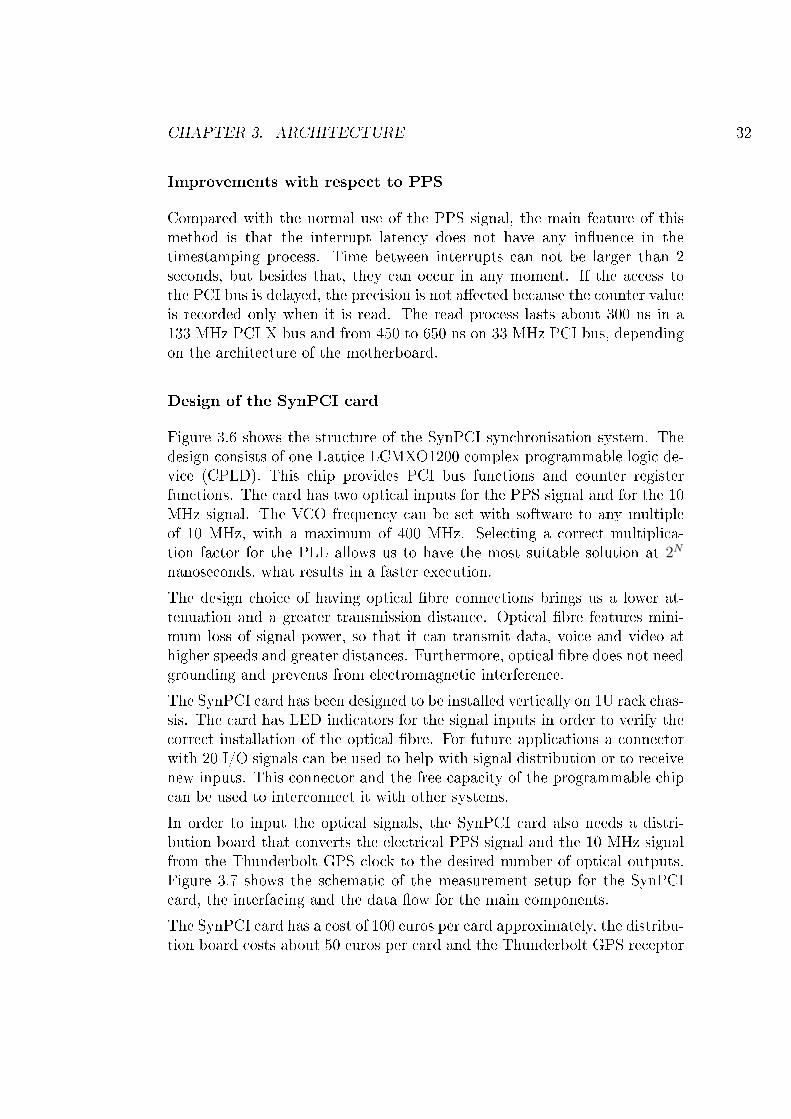
CHAPTER 3. ARCHITECTURE 32
Improvements with respect to PPS
Compared with the normal use of the PPS signal, the main feature of thismethod is that the interrupt latency does not have any in�uence in thetimestamping process. Time between interrupts can not be larger than 2seconds, but besides that, they can occur in any moment. If the access tothe PCI bus is delayed, the precision is not a�ected because the counter valueis recorded only when it is read. The read process lasts about 300 ns in a133 MHz PCI-X bus and from 450 to 650 ns on 33 MHz PCI bus, dependingon the architecture of the motherboard.
Design of the SynPCI card
Figure 3.6 shows the structure of the SynPCI synchronisation system. Thedesign consists of one Lattice LCMXO1200 complex programmable logic de-vice (CPLD). This chip provides PCI bus functions and counter registerfunctions. The card has two optical inputs for the PPS signal and for the 10MHz signal. The VCO frequency can be set with software to any multipleof 10 MHz, with a maximum of 400 MHz. Selecting a correct multiplica-tion factor for the PLL allows us to have the most suitable solution at 2N
nanoseconds, what results in a faster execution.The design choice of having optical �bre connections brings us a lower at-tenuation and a greater transmission distance. Optical �bre features mini-mum loss of signal power, so that it can transmit data, voice and video athigher speeds and greater distances. Furthermore, optical �bre does not needgrounding and prevents from electromagnetic interference.The SynPCI card has been designed to be installed vertically on 1U rack chas-sis. The card has LED indicators for the signal inputs in order to verify thecorrect installation of the optical �bre. For future applications a connectorwith 20 I/O signals can be used to help with signal distribution or to receivenew inputs. This connector and the free capacity of the programmable chipcan be used to interconnect it with other systems.In order to input the optical signals, the SynPCI card also needs a distri-bution board that converts the electrical PPS signal and the 10 MHz signalfrom the Thunderbolt GPS clock to the desired number of optical outputs.Figure 3.7 shows the schematic of the measurement setup for the SynPCIcard, the interfacing and the data �ow for the main components.The SynPCI card has a cost of 100 euros per card approximately, the distribu-tion board costs about 50 euros per card and the Thunderbolt GPS receptor
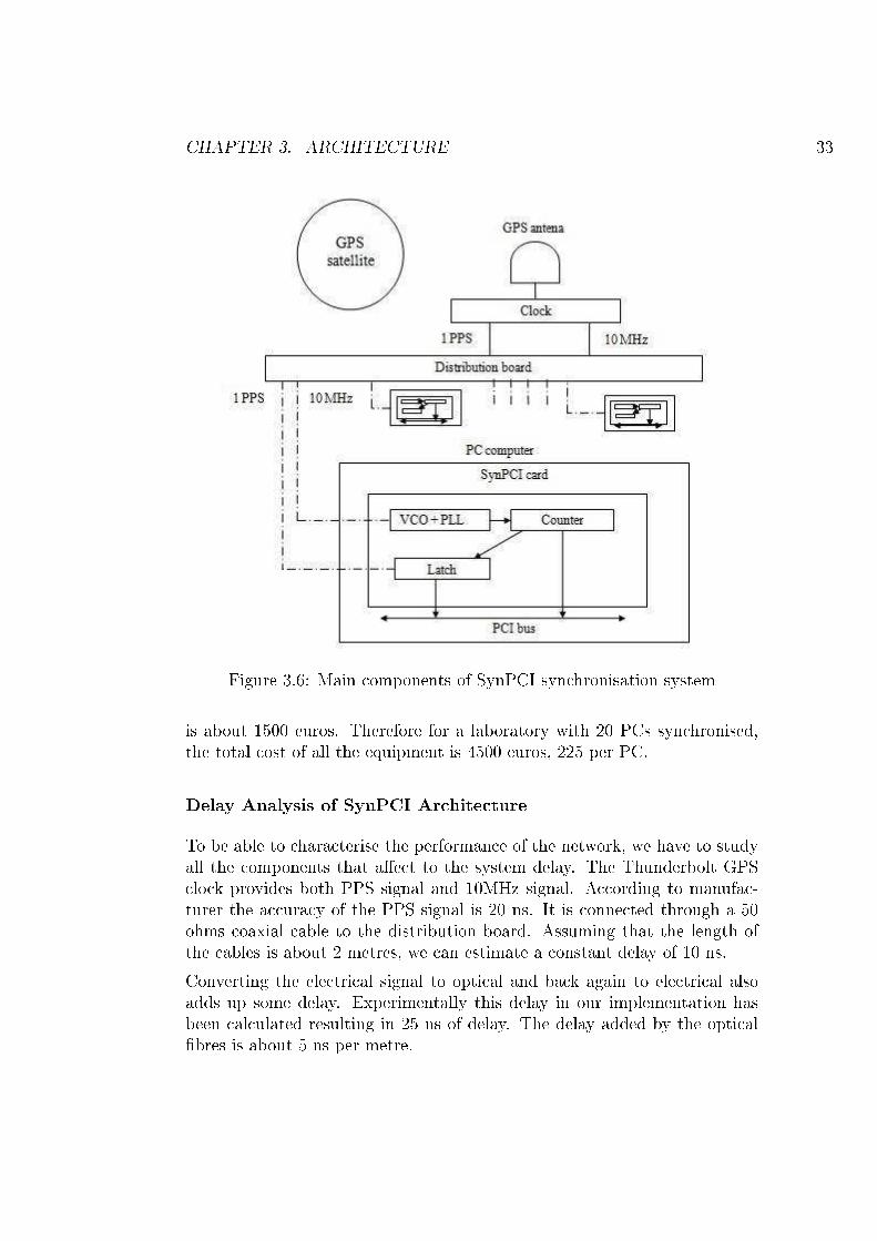
CHAPTER 3. ARCHITECTURE 33
Figure 3.6: Main components of SynPCI synchronisation system
is about 1500 euros. Therefore for a laboratory with 20 PCs synchronised,the total cost of all the equipment is 4500 euros, 225 per PC.
Delay Analysis of SynPCI Architecture
To be able to characterise the performance of the network, we have to studyall the components that a�ect to the system delay. The Thunderbolt GPSclock provides both PPS signal and 10MHz signal. According to manufac-turer the accuracy of the PPS signal is 20 ns. It is connected through a 50ohms coaxial cable to the distribution board. Assuming that the length ofthe cables is about 2 metres, we can estimate a constant delay of 10 ns.Converting the electrical signal to optical and back again to electrical alsoadds up some delay. Experimentally this delay in our implementation hasbeen calculated resulting in 25 ns of delay. The delay added by the optical�bres is about 5 ns per metre.
CHAPTER 3. ARCHITECTURE 34
Figure 3.7: Measurement setup for the SynPCI card.
Finally we can conclude that the total delay of the system produced by thesignal distribution and conversion is constant and about 85 ns considering10 metres of optical �bre. [11]
Chapter 4
Analysis
In this chapter we will present the results that have been obtained fromdi�erent measurements done for both of the devices under test. First we willexplain the test procedure, the sets of test that have been performed andtheir purpose. Then we will show the results themselves and we will analysethe meaning of this results.
4.1 Test ProcedureThe test procedure we will follow to analyse the performance of the twocapture cards is very simple. As we explained in chapter 3, the tra�c signalis sent by the tra�c generator using Gigabit Ethernet standard, split beforeit gets the capture card, and looped back again to the high-performanceanalyser of the AX/4000 tra�c generator. All the packets are timestampedin the card under test and in the AX/4000 analyser.Our aim is to measure the accuracy provided by the capture cards to monitorthe tra�c and timestamp the packets sent by the tra�c generator. Sinceit is not possible to measure the accuracy directly, we have to measure thedi�erence between the timestamps given by the capture card and the analyserused as reference.The AX/4000 network analyser allows us to capture the network packetsusing the graphic interface. From that interface we can export a text �lecontaining the timestamp information with nanosecond resolution.For the DAG card we use the command dagsnap to start capturing the tra�c.It returns a �le in erf format readable by some network protocol analyser
35
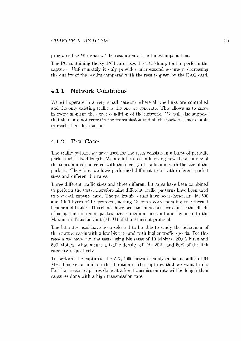
CHAPTER 4. ANALYSIS 36
programs like Wireshark. The resolution of the timestamps is 1 ns.The PC containing the synPCI card uses the TCPdump tool to perform thecapture. Unfortunately it only provides microsecond accuracy, decreasingthe quality of the results compared with the results given by the DAG card.
4.1.1 Network ConditionsWe will operate in a very small network where all the links are controlledand the only existing tra�c is the one we generate. This allows us to knowin every moment the exact condition of the network. We will also supposethat there are not errors in the transmission and all the packets sent are ableto reach their destination.
4.1.2 Test CasesThe tra�c pattern we have used for the tests consists in a burst of periodicpackets with �xed length. We are interested in knowing how the accuracy ofthe timestamps is a�ected with the density of tra�c and with the size of thepackets. Therefore, we have performed di�erent tests with di�erent packetsizes and di�erent bit rates.Three di�erent tra�c sizes and three di�erent bit rates have been combinedto perform the tests, therefore nine di�erent tra�c patterns have been usedto test each capture card. The packet sizes that have been chosen are 46, 500and 1400 bytes of IP protocol, adding 18 bytes corresponding to Ethernetheader and trailer. This choice have been taken because we can see the e�ectsof using the minimum packet size, a medium one and another near to theMaximum Transfer Unit (MTU) of the Ethernet protocol.The bit rates used have been selected to be able to study the behaviour ofthe capture cards with a low bit rate and with higher tra�c speeds. For thisreason we have run the tests using bit rates of 10 Mbit/s, 200 Mbit/s and500 Mbit/s, what means a tra�c density of 1%, 20%, and 50% of the linkcapacity respectively.To perform the captures, the AX/4000 network analyser has a bu�er of 64MB. This set a limit on the duration of the captures that we want to do.For that reason captures done at a low transmission rate will be longer thancaptures done with a high transmission rate.
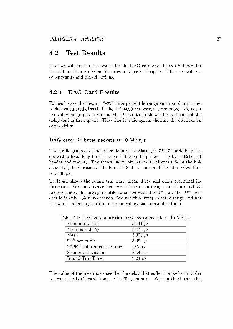
CHAPTER 4. ANALYSIS 37
4.2 Test ResultsFirst we will present the results for the DAG card and the synPCI card forthe di�erent transmission bit rates and packet lengths. Then we will seeother results and considerations.
4.2.1 DAG Card ResultsFor each case the mean, 1st-99th interpercentile range and round trip time,wich is calculated directly in the AX/4000 analyser, are presented. Moreovertwo di�erent graphs are included. One of them shows the evolution of thedelay during the capture. The other is a histogram showing the distributionof the delay.
DAG card: 64 bytes packets at 10 Mbit/s
The tra�c generator sends a tra�c burst consisting in 720874 periodic pack-ets with a �xed length of 64 bytes (46 bytes IP packet + 18 bytes Ethernetheader and trailer). The transmission bit rate is 10 Mbit/s (1% of the linkcapacity), the duration of the burst is 36.91 seconds and the interarrival timeis 55.36 µs.Table 4.1 shows the round trip time, mean delay and other statistical in-formation. We can observe that even if the mean delay value is around 3.3microseconds, the interpercentile range between the 1st and the 99th per-centile is only 185 nanoseconds. We use this interpercentile range and notthe whole range to get rid of extreme values and to avoid outliers.
Table 4.1: DAG card statistics for 64 bytes packets at 10 Mbit/sMinimum delay 3.141 µsMaximum delay 3.430 µsMean 3.303 µs99th percentile 3.384 µs1st-99th interpercentile range 185 nsStandard deviation 39.45 nsRound Trip Time 7.24 µs
The value of the mean is caused by the delay that su�er the packet in orderto reach the DAG card from the tra�c generator. We can check that this
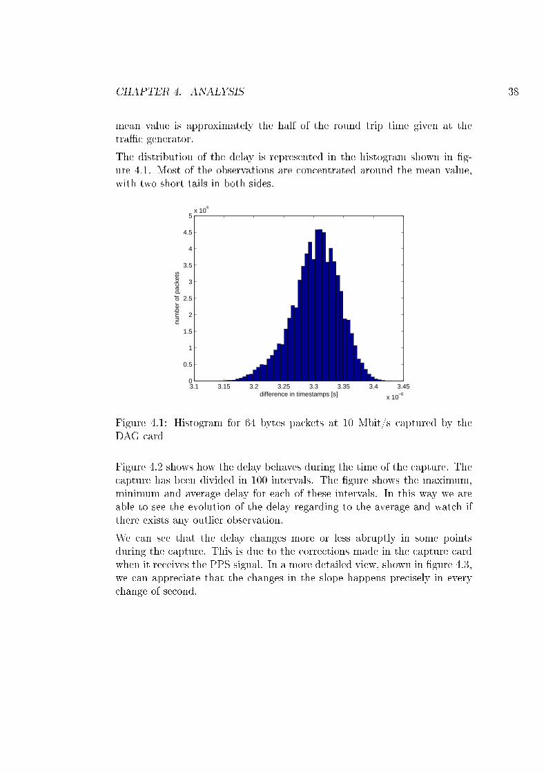
CHAPTER 4. ANALYSIS 38
mean value is approximately the half of the round trip time given at thetra�c generator.The distribution of the delay is represented in the histogram shown in �g-ure 4.1. Most of the observations are concentrated around the mean value,with two short tails in both sides.
3.1 3.15 3.2 3.25 3.3 3.35 3.4 3.45
x 10−6
0
0.5
1
1.5
2
2.5
3
3.5
4
4.5
5x 10
4
difference in timestamps [s]
num
ber
of p
acke
ts
Figure 4.1: Histogram for 64 bytes packets at 10 Mbit/s captured by theDAG card
Figure 4.2 shows how the delay behaves during the time of the capture. Thecapture has been divided in 100 intervals. The �gure shows the maximum,minimum and average delay for each of these intervals. In this way we areable to see the evolution of the delay regarding to the average and watch ifthere exists any outlier observation.We can see that the delay changes more or less abruptly in some pointsduring the capture. This is due to the corrections made in the capture cardwhen it receives the PPS signal. In a more detailed view, shown in �gure 4.3,we can appreciate that the changes in the slope happens precisely in everychange of second.
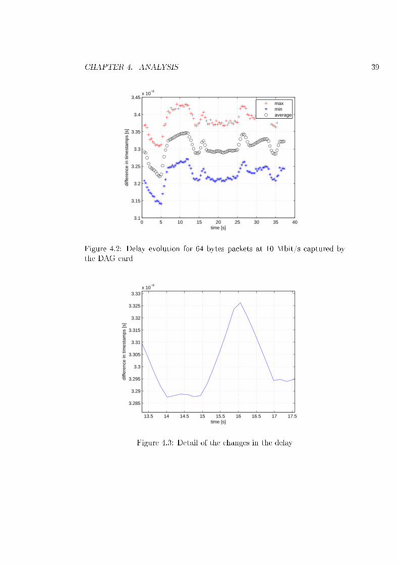
CHAPTER 4. ANALYSIS 39
0 5 10 15 20 25 30 35 403.1
3.15
3.2
3.25
3.3
3.35
3.4
3.45x 10
−6
time [s]
diffe
renc
e in
tim
esta
mps
[s]
maxminaverage
Figure 4.2: Delay evolution for 64 bytes packets at 10 Mbit/s captured bythe DAG card
13.5 14 14.5 15 15.5 16 16.5 17 17.5
3.285
3.29
3.295
3.3
3.305
3.31
3.315
3.32
3.325
3.33x 10
−6
time [s]
diffe
renc
e in
tim
esta
mps
[s]
Figure 4.3: Detail of the changes in the delay
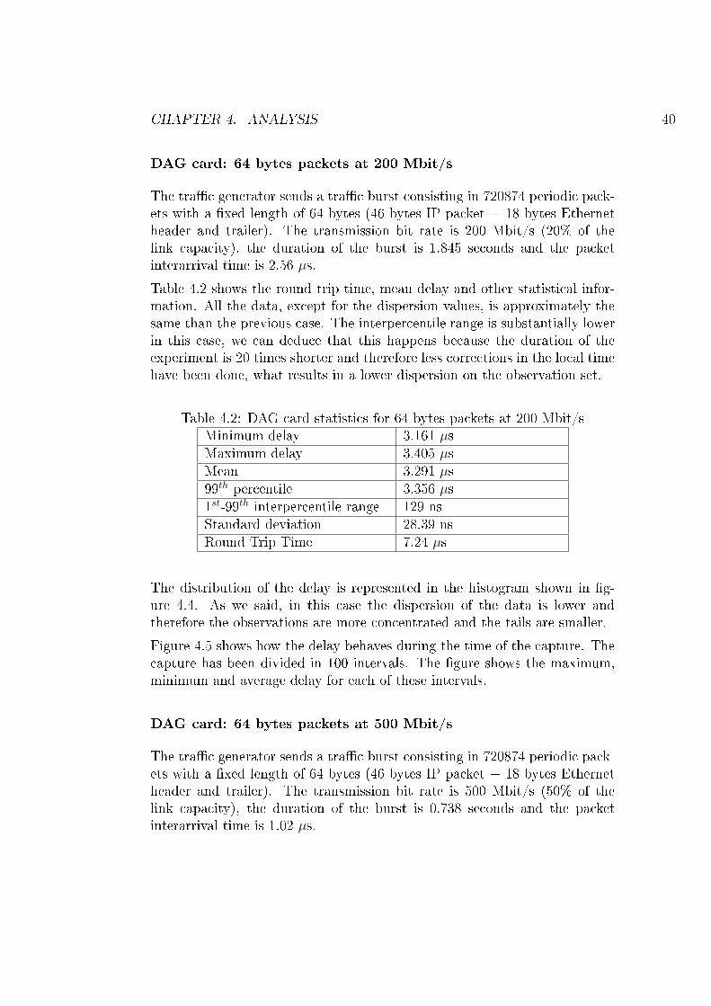
CHAPTER 4. ANALYSIS 40
DAG card: 64 bytes packets at 200 Mbit/s
The tra�c generator sends a tra�c burst consisting in 720874 periodic pack-ets with a �xed length of 64 bytes (46 bytes IP packet + 18 bytes Ethernetheader and trailer). The transmission bit rate is 200 Mbit/s (20% of thelink capacity), the duration of the burst is 1.845 seconds and the packetinterarrival time is 2.56 µs.Table 4.2 shows the round trip time, mean delay and other statistical infor-mation. All the data, except for the dispersion values, is approximately thesame than the previous case. The interpercentile range is substantially lowerin this case, we can deduce that this happens because the duration of theexperiment is 20 times shorter and therefore less corrections in the local timehave been done, what results in a lower dispersion on the observation set.
Table 4.2: DAG card statistics for 64 bytes packets at 200 Mbit/sMinimum delay 3.161 µsMaximum delay 3.405 µsMean 3.291 µs99th percentile 3.356 µs1st-99th interpercentile range 129 nsStandard deviation 28.39 nsRound Trip Time 7.24 µs
The distribution of the delay is represented in the histogram shown in �g-ure 4.4. As we said, in this case the dispersion of the data is lower andtherefore the observations are more concentrated and the tails are smaller.Figure 4.5 shows how the delay behaves during the time of the capture. Thecapture has been divided in 100 intervals. The �gure shows the maximum,minimum and average delay for each of these intervals.
DAG card: 64 bytes packets at 500 Mbit/s
The tra�c generator sends a tra�c burst consisting in 720874 periodic pack-ets with a �xed length of 64 bytes (46 bytes IP packet + 18 bytes Ethernetheader and trailer). The transmission bit rate is 500 Mbit/s (50% of thelink capacity), the duration of the burst is 0.738 seconds and the packetinterarrival time is 1.02 µs.
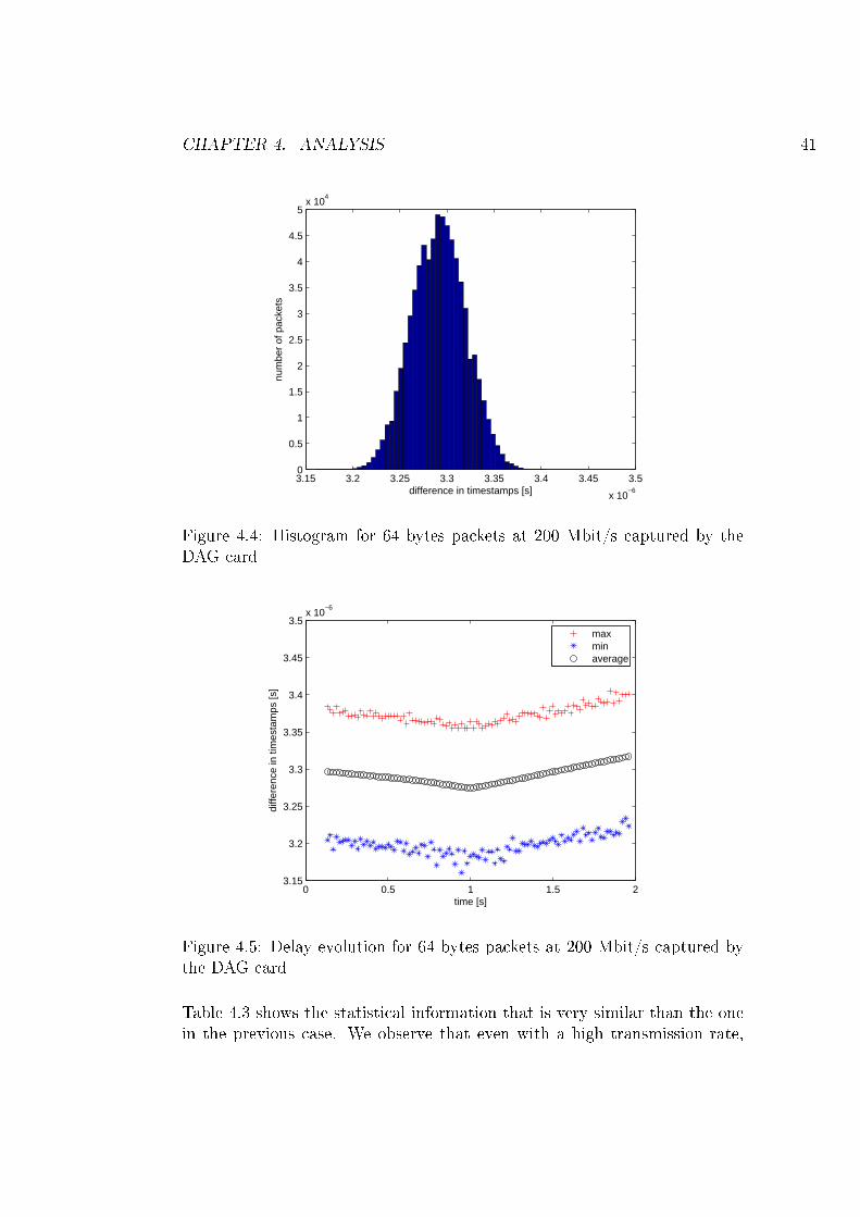
CHAPTER 4. ANALYSIS 41
3.15 3.2 3.25 3.3 3.35 3.4 3.45 3.5
x 10−6
0
0.5
1
1.5
2
2.5
3
3.5
4
4.5
5x 10
4
difference in timestamps [s]
num
ber
of p
acke
ts
Figure 4.4: Histogram for 64 bytes packets at 200 Mbit/s captured by theDAG card
0 0.5 1 1.5 23.15
3.2
3.25
3.3
3.35
3.4
3.45
3.5x 10
−6
time [s]
diffe
renc
e in
tim
esta
mps
[s]
maxminaverage
Figure 4.5: Delay evolution for 64 bytes packets at 200 Mbit/s captured bythe DAG card
Table 4.3 shows the statistical information that is very similar than the onein the previous case. We observe that even with a high transmission rate,
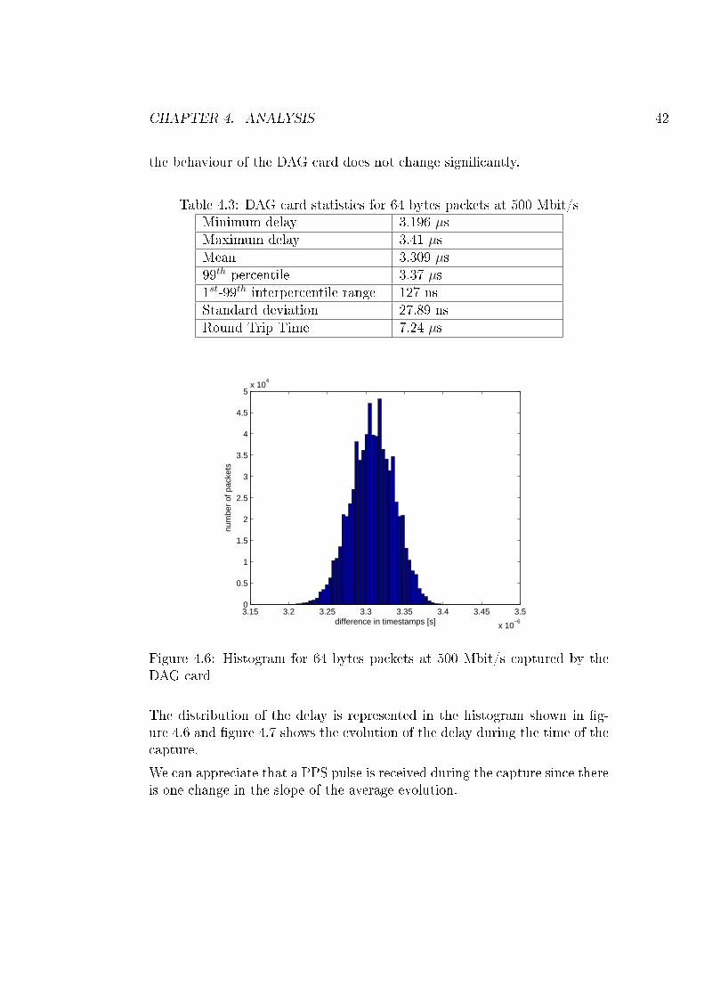
CHAPTER 4. ANALYSIS 42
the behaviour of the DAG card does not change signi�cantly.
Table 4.3: DAG card statistics for 64 bytes packets at 500 Mbit/sMinimum delay 3.196 µsMaximum delay 3.41 µsMean 3.309 µs99th percentile 3.37 µs1st-99th interpercentile range 127 nsStandard deviation 27.89 nsRound Trip Time 7.24 µs
3.15 3.2 3.25 3.3 3.35 3.4 3.45 3.5
x 10−6
0
0.5
1
1.5
2
2.5
3
3.5
4
4.5
5x 10
4
difference in timestamps [s]
num
ber
of p
acke
ts
Figure 4.6: Histogram for 64 bytes packets at 500 Mbit/s captured by theDAG card
The distribution of the delay is represented in the histogram shown in �g-ure 4.6 and �gure 4.7 shows the evolution of the delay during the time of thecapture.We can appreciate that a PPS pulse is received during the capture since thereis one change in the slope of the average evolution.
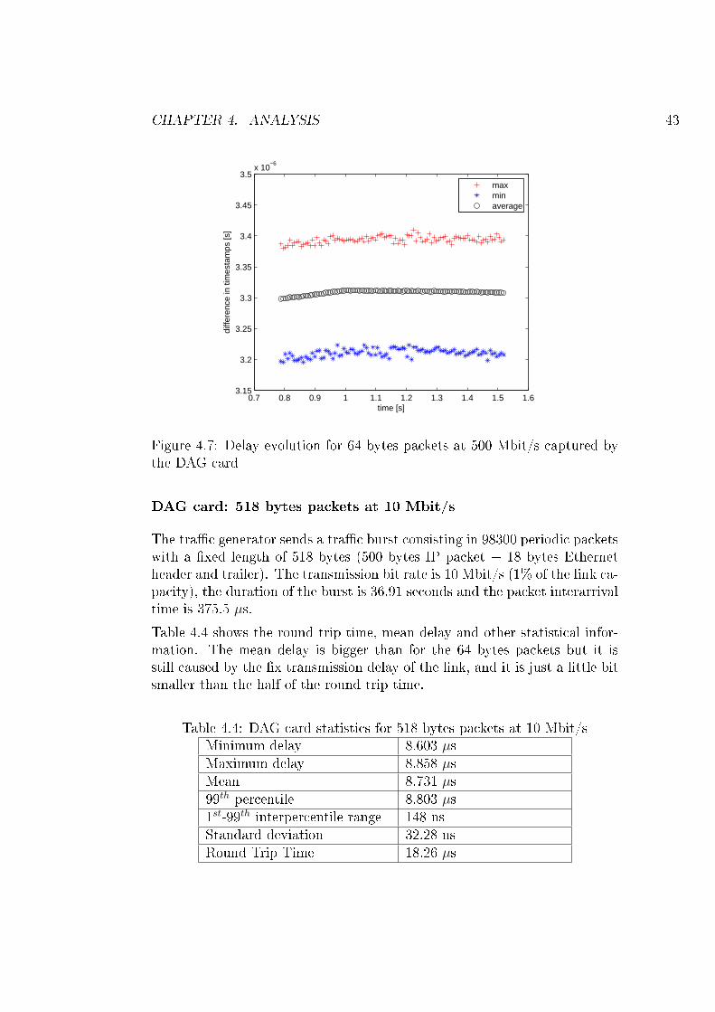
CHAPTER 4. ANALYSIS 43
0.7 0.8 0.9 1 1.1 1.2 1.3 1.4 1.5 1.63.15
3.2
3.25
3.3
3.35
3.4
3.45
3.5x 10
−6
time [s]
diffe
renc
e in
tim
esta
mps
[s]
maxminaverage
Figure 4.7: Delay evolution for 64 bytes packets at 500 Mbit/s captured bythe DAG card
DAG card: 518 bytes packets at 10 Mbit/s
The tra�c generator sends a tra�c burst consisting in 98300 periodic packetswith a �xed length of 518 bytes (500 bytes IP packet + 18 bytes Ethernetheader and trailer). The transmission bit rate is 10 Mbit/s (1% of the link ca-pacity), the duration of the burst is 36.91 seconds and the packet interarrivaltime is 375.5 µs.Table 4.4 shows the round trip time, mean delay and other statistical infor-mation. The mean delay is bigger than for the 64 bytes packets but it isstill caused by the �x transmission delay of the link, and it is just a little bitsmaller than the half of the round trip time.
Table 4.4: DAG card statistics for 518 bytes packets at 10 Mbit/sMinimum delay 8.603 µsMaximum delay 8.858 µsMean 8.731 µs99th percentile 8.803 µs1st-99th interpercentile range 148 nsStandard deviation 32.28 nsRound Trip Time 18.26 µs
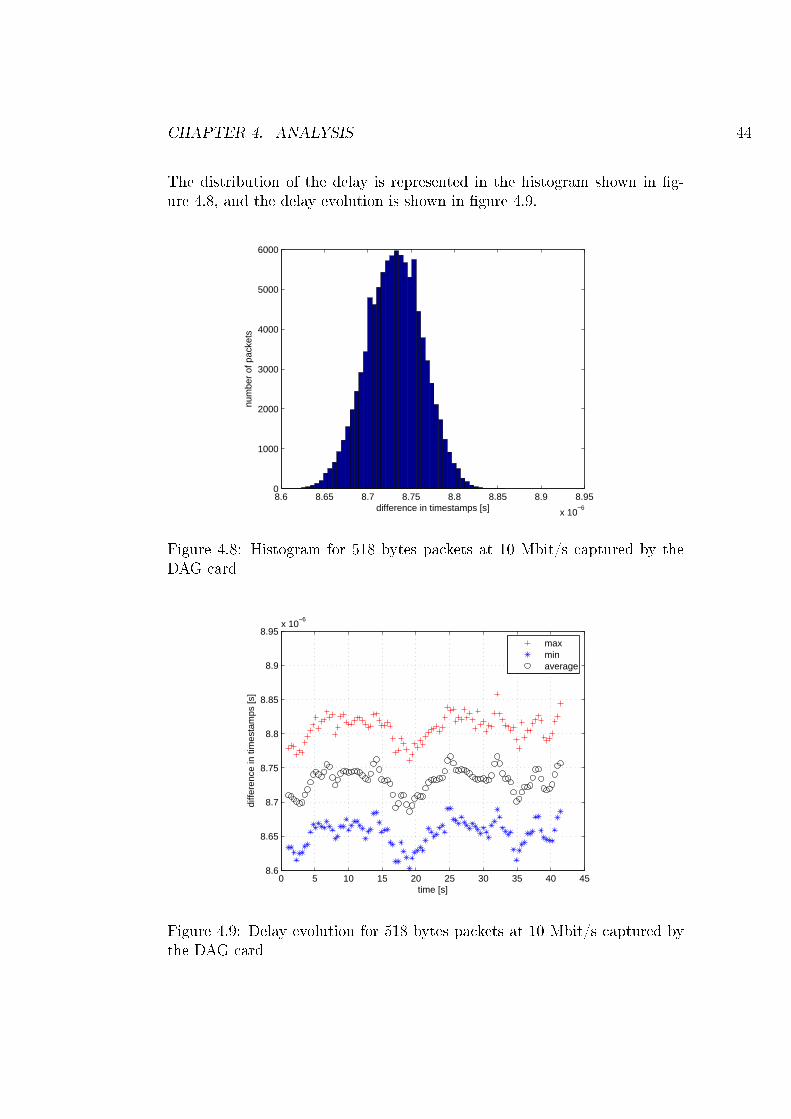
CHAPTER 4. ANALYSIS 44
The distribution of the delay is represented in the histogram shown in �g-ure 4.8, and the delay evolution is shown in �gure 4.9.
8.6 8.65 8.7 8.75 8.8 8.85 8.9 8.95
x 10−6
0
1000
2000
3000
4000
5000
6000
difference in timestamps [s]
num
ber
of p
acke
ts
Figure 4.8: Histogram for 518 bytes packets at 10 Mbit/s captured by theDAG card
0 5 10 15 20 25 30 35 40 458.6
8.65
8.7
8.75
8.8
8.85
8.9
8.95x 10
−6
time [s]
diffe
renc
e in
tim
esta
mps
[s]
maxminaverage
Figure 4.9: Delay evolution for 518 bytes packets at 10 Mbit/s captured bythe DAG card
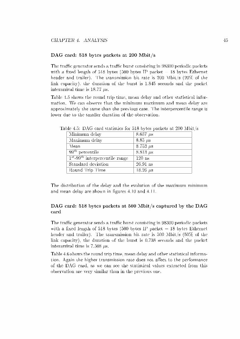
CHAPTER 4. ANALYSIS 45
DAG card: 518 bytes packets at 200 Mbit/s
The tra�c generator sends a tra�c burst consisting in 98300 periodic packetswith a �xed length of 518 bytes (500 bytes IP packet + 18 bytes Ethernetheader and trailer). The transmission bit rate is 200 Mbit/s (20% of thelink capacity), the duration of the burst is 1.845 seconds and the packetinterarrival time is 18.77 µs.Table 4.5 shows the round trip time, mean delay and other statistical infor-mation. We can observe that the minimum maximum and mean delay areapproximately the same than the previous case. The interpercentile range islower due to the smaller duration of the observation.
Table 4.5: DAG card statistics for 518 bytes packets at 200 Mbit/sMinimum delay 8.657 µsMaximum delay 8.85 µsMean 8.753 µs99th percentile 8.813 µs1st-99th interpercentile range 120 nsStandard deviation 26.91 nsRound Trip Time 18.26 µs
The distribution of the delay and the evolution of the maximum minimumand mean delay are shown in �gures 4.10 and 4.11.
DAG card: 518 bytes packets at 500 Mbit/s captured by the DAGcard
The tra�c generator sends a tra�c burst consisting in 98300 periodic packetswith a �xed length of 518 bytes (500 bytes IP packet + 18 bytes Ethernetheader and trailer). The transmission bit rate is 500 Mbit/s (50% of thelink capacity), the duration of the burst is 0.738 seconds and the packetinterarrival time is 7.508 µs.Table 4.6 shows the round trip time, mean delay and other statistical informa-tion. Again the higher transmission rate does not a�ect to the performanceof the DAG card, as we can see the statistical values extracted from thisobservation are very similar than in the previous one.
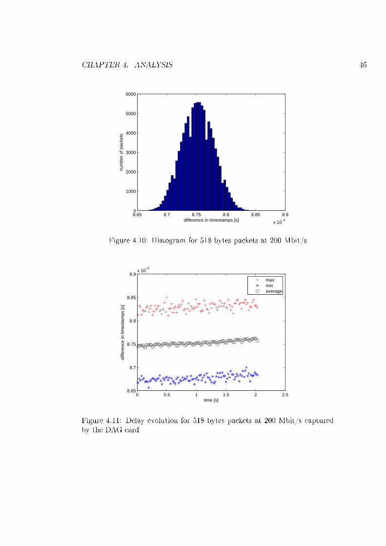
CHAPTER 4. ANALYSIS 46
8.65 8.7 8.75 8.8 8.85 8.9
x 10−6
0
1000
2000
3000
4000
5000
6000
difference in timestamps [s]
num
ber
of p
acke
ts
Figure 4.10: Histogram for 518 bytes packets at 200 Mbit/s
0 0.5 1 1.5 2 2.58.65
8.7
8.75
8.8
8.85
8.9x 10
−6
time [s]
diffe
renc
e in
tim
esta
mps
[s]
maxminaverage
Figure 4.11: Delay evolution for 518 bytes packets at 200 Mbit/s capturedby the DAG card
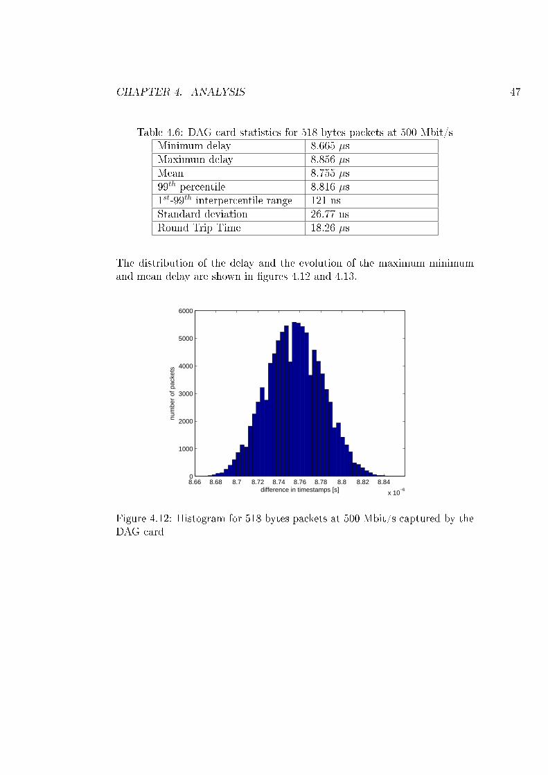
CHAPTER 4. ANALYSIS 47
Table 4.6: DAG card statistics for 518 bytes packets at 500 Mbit/sMinimum delay 8.665 µsMaximum delay 8.856 µsMean 8.755 µs99th percentile 8.816 µs1st-99th interpercentile range 121 nsStandard deviation 26.77 nsRound Trip Time 18.26 µs
The distribution of the delay and the evolution of the maximum minimumand mean delay are shown in �gures 4.12 and 4.13.
8.66 8.68 8.7 8.72 8.74 8.76 8.78 8.8 8.82 8.84
x 10−6
0
1000
2000
3000
4000
5000
6000
difference in timestamps [s]
num
ber
of p
acke
ts
Figure 4.12: Histogram for 518 bytes packets at 500 Mbit/s captured by theDAG card
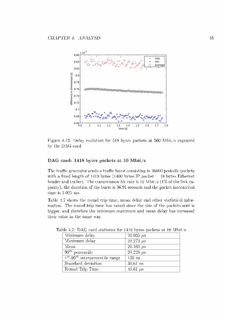
CHAPTER 4. ANALYSIS 48
0.9 1 1.1 1.2 1.3 1.4 1.5 1.6 1.7 1.88.66
8.68
8.7
8.72
8.74
8.76
8.78
8.8
8.82
8.84
8.86x 10
−6
time [s]
diffe
renc
e in
tim
esta
mps
[s]
maxminaverage
Figure 4.13: Delay evolution for 518 bytes packets at 500 Mbit/s capturedby the DAG card
DAG card: 1418 bytes packets at 10 Mbit/s
The tra�c generator sends a tra�c burst consisting in 36000 periodic packetswith a �xed length of 1418 bytes (1400 bytes IP packet + 18 bytes Ethernetheader and trailer). The transmission bit rate is 10 Mbit/s (1% of the link ca-pacity), the duration of the burst is 36.91 seconds and the packet interarrivaltime is 1.025 ms.Table 4.7 shows the round trip time, mean delay and other statistical infor-mation. The round trip time has raised since the size of the packets sent isbigger, and therefore the minimum maximum and mean delay has increasedtheir value in the same way.
Table 4.7: DAG card statistics for 1418 bytes packets at 10 Mbit/sMinimum delay 20.035 µsMaximum delay 20.273 µsMean 20.160 µs99th percentile 20.228 µs1st-99th interpercentile range 139 nsStandard deviation 30.61 nsRound Trip Time 40.61 µs
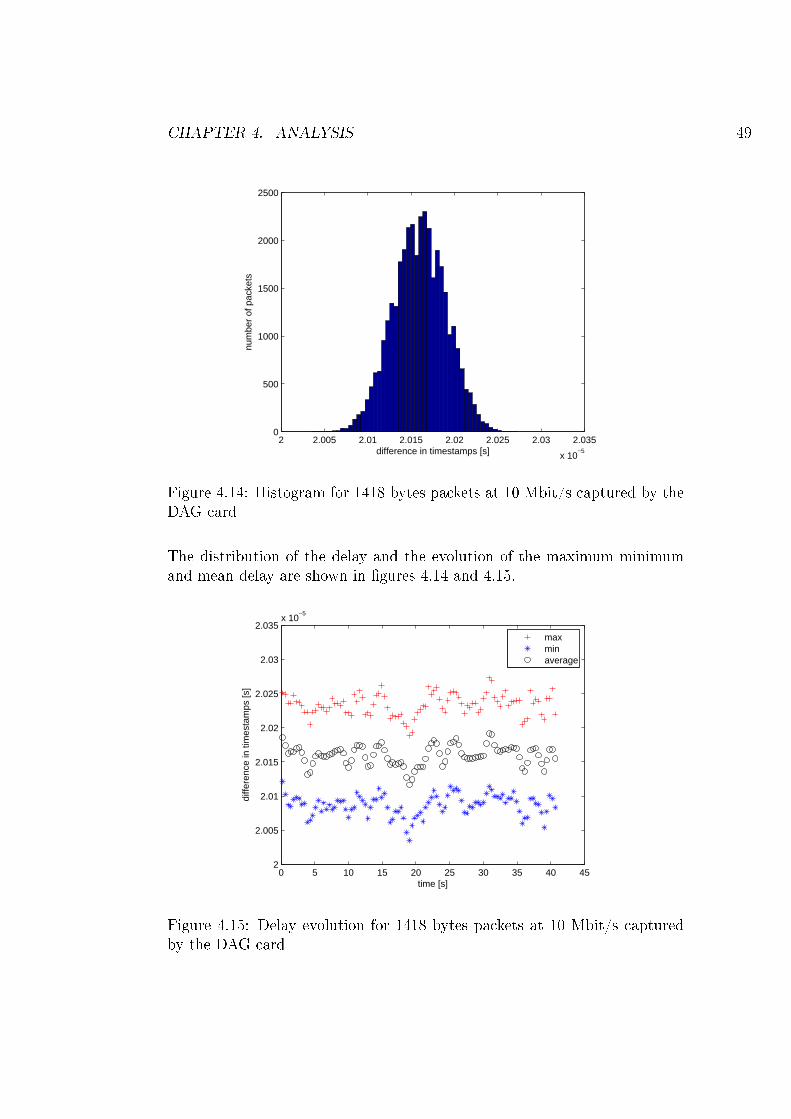
CHAPTER 4. ANALYSIS 49
2 2.005 2.01 2.015 2.02 2.025 2.03 2.035
x 10−5
0
500
1000
1500
2000
2500
difference in timestamps [s]
num
ber
of p
acke
ts
Figure 4.14: Histogram for 1418 bytes packets at 10 Mbit/s captured by theDAG card
The distribution of the delay and the evolution of the maximum minimumand mean delay are shown in �gures 4.14 and 4.15.
0 5 10 15 20 25 30 35 40 452
2.005
2.01
2.015
2.02
2.025
2.03
2.035x 10
−5
time [s]
diffe
renc
e in
tim
esta
mps
[s]
maxminaverage
Figure 4.15: Delay evolution for 1418 bytes packets at 10 Mbit/s capturedby the DAG card
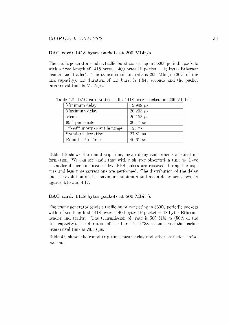
CHAPTER 4. ANALYSIS 50
DAG card: 1418 bytes packets at 200 Mbit/s
The tra�c generator sends a tra�c burst consisting in 36000 periodic packetswith a �xed length of 1418 bytes (1400 bytes IP packet + 18 bytes Ethernetheader and trailer). The transmission bit rate is 200 Mbit/s (20% of thelink capacity), the duration of the burst is 1.845 seconds and the packetinterarrival time is 51.25 µs.
Table 4.8: DAG card statistics for 1418 bytes packets at 200 Mbit/sMinimum delay 19.999 µsMaximum delay 20.203 µsMean 20.108 µs99th percentile 20.17 µs1st-99th interpercentile range 125 nsStandard deviation 27.81 nsRound Trip Time 40.61 µs
Table 4.8 shows the round trip time, mean delay and other statistical in-formation. We can see again that with a shorter observation time we havea smaller dispersion because less PPS pulses are received during the cap-ture and less time corrections are performed. The distribution of the delayand the evolution of the maximum minimum and mean delay are shown in�gures 4.16 and 4.17.
DAG card: 1418 bytes packets at 500 Mbit/s
The tra�c generator sends a tra�c burst consisting in 36000 periodic packetswith a �xed length of 1418 bytes (1400 bytes IP packet + 18 bytes Ethernetheader and trailer). The transmission bit rate is 500 Mbit/s (50% of thelink capacity), the duration of the burst is 0.738 seconds and the packetinterarrival time is 20.50 µs.Table 4.9 shows the round trip time, mean delay and other statistical infor-mation.
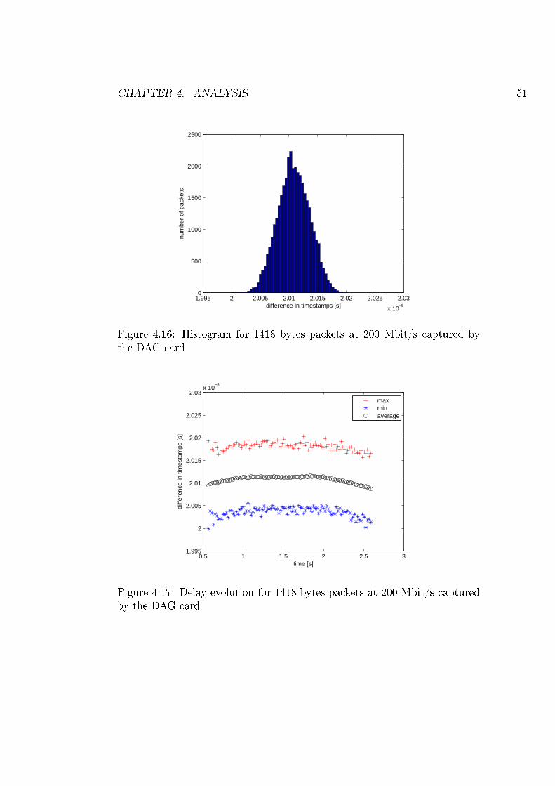
CHAPTER 4. ANALYSIS 51
1.995 2 2.005 2.01 2.015 2.02 2.025 2.03
x 10−5
0
500
1000
1500
2000
2500
difference in timestamps [s]
num
ber
of p
acke
ts
Figure 4.16: Histogram for 1418 bytes packets at 200 Mbit/s captured bythe DAG card
0.5 1 1.5 2 2.5 31.995
2
2.005
2.01
2.015
2.02
2.025
2.03x 10
−5
time [s]
diffe
renc
e in
tim
esta
mps
[s]
maxminaverage
Figure 4.17: Delay evolution for 1418 bytes packets at 200 Mbit/s capturedby the DAG card

CHAPTER 4. ANALYSIS 52
Table 4.9: DAG card statistics for 1418 bytes packets at 500 Mbit/sMinimum delay 19.813 µsMaximum delay 19.999 µsMean 19.90 µs99th percentile 19.97 µs1st-99th interpercentile range 122 nsStandard deviation 27.18 nsRound Trip Time 40.61 µs
The distribution of the delay and the evolution of the maximum minimumand mean delay are shown in �gures 4.18 and 4.19.
1.98 1.985 1.99 1.995 2 2.005
x 10−5
0
200
400
600
800
1000
1200
1400
1600
1800
2000
difference in timestamps [s]
num
ber
of p
acke
ts
Figure 4.18: Histogram for 1418 bytes packets at 500 Mbit/s captured bythe DAG card
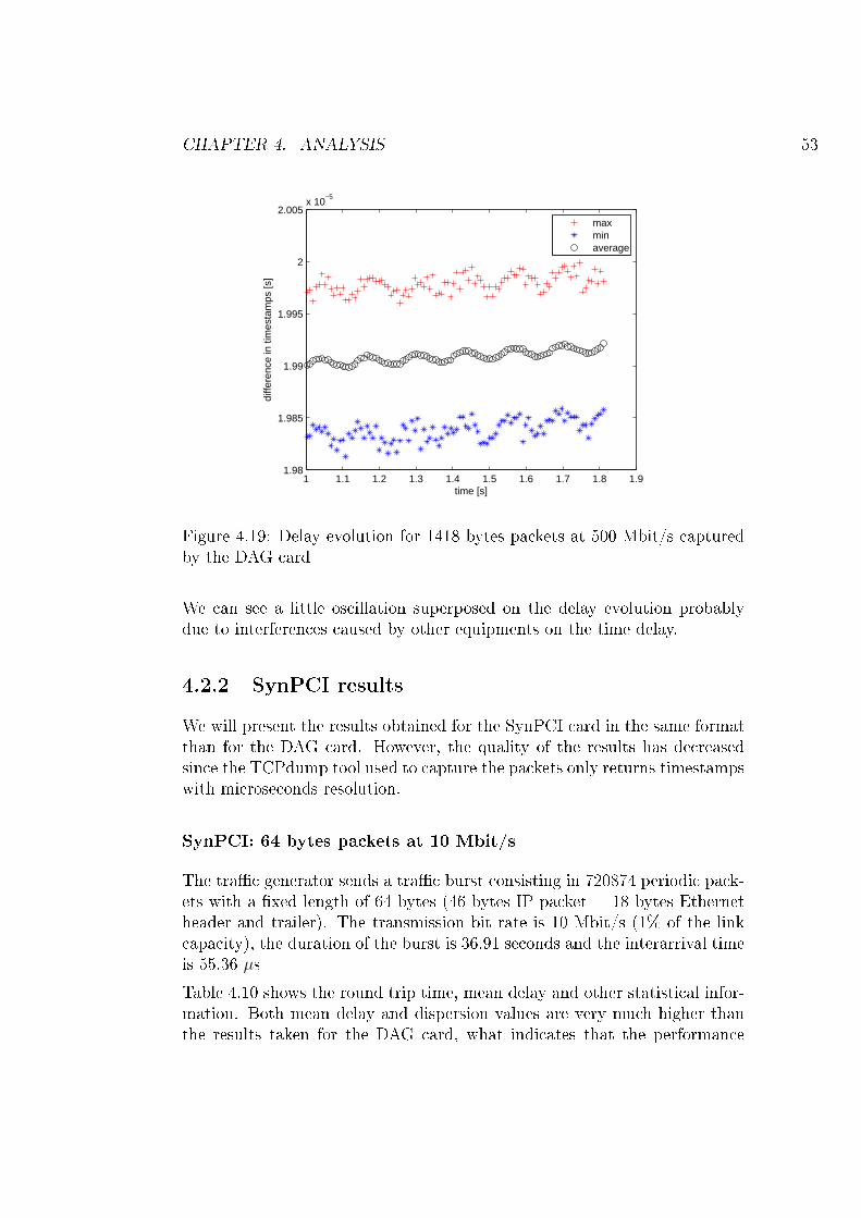
CHAPTER 4. ANALYSIS 53
1 1.1 1.2 1.3 1.4 1.5 1.6 1.7 1.8 1.91.98
1.985
1.99
1.995
2
2.005x 10
−5
time [s]
diffe
renc
e in
tim
esta
mps
[s]
maxminaverage
Figure 4.19: Delay evolution for 1418 bytes packets at 500 Mbit/s capturedby the DAG card
We can see a little oscillation superposed on the delay evolution probablydue to interferences caused by other equipments on the time delay.
4.2.2 SynPCI resultsWe will present the results obtained for the SynPCI card in the same formatthan for the DAG card. However, the quality of the results has decreasedsince the TCPdump tool used to capture the packets only returns timestampswith microseconds resolution.
SynPCI: 64 bytes packets at 10 Mbit/s
The tra�c generator sends a tra�c burst consisting in 720874 periodic pack-ets with a �xed length of 64 bytes (46 bytes IP packet + 18 bytes Ethernetheader and trailer). The transmission bit rate is 10 Mbit/s (1% of the linkcapacity), the duration of the burst is 36.91 seconds and the interarrival timeis 55.36 µsTable 4.10 shows the round trip time, mean delay and other statistical infor-mation. Both mean delay and dispersion values are very much higher thanthe results taken for the DAG card, what indicates that the performance
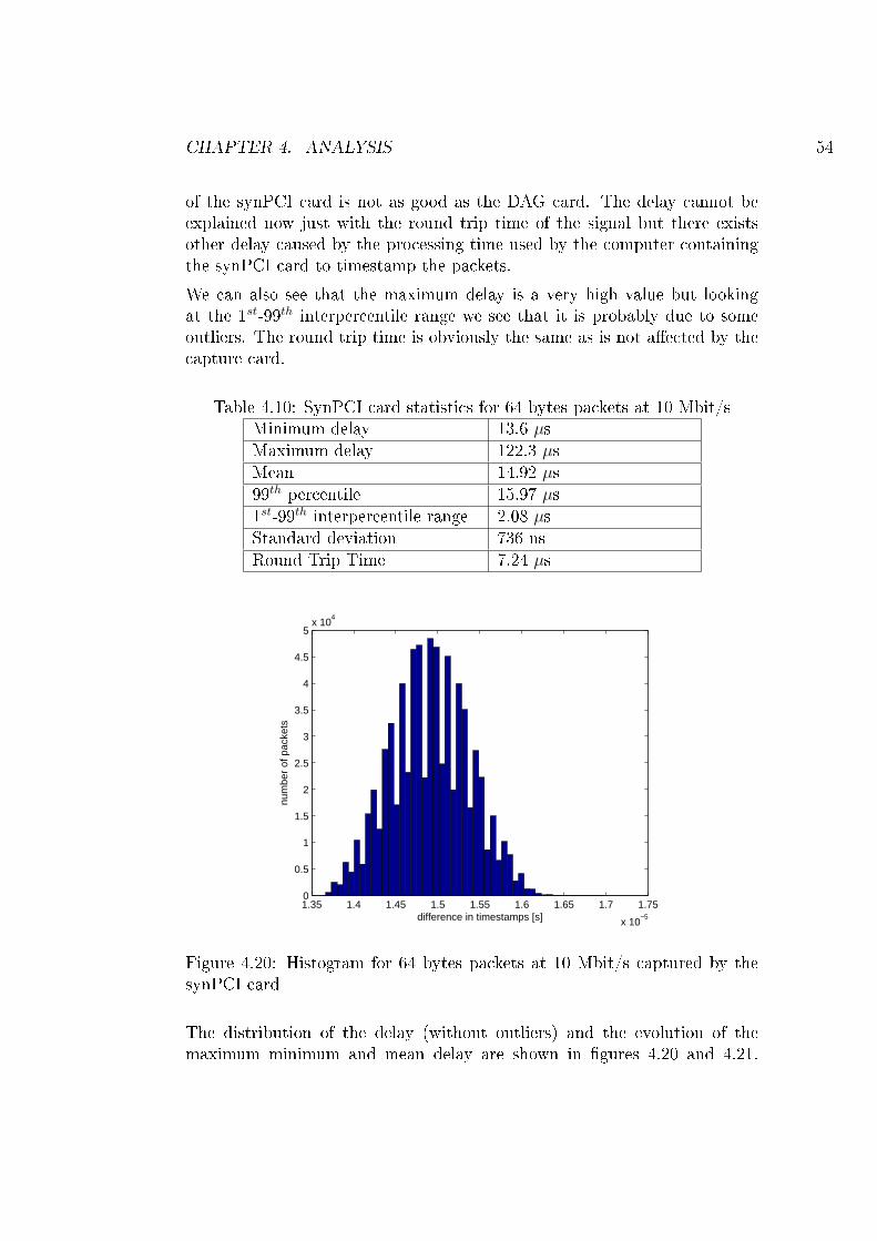
CHAPTER 4. ANALYSIS 54
of the synPCI card is not as good as the DAG card. The delay cannot beexplained now just with the round trip time of the signal but there existsother delay caused by the processing time used by the computer containingthe synPCI card to timestamp the packets.We can also see that the maximum delay is a very high value but lookingat the 1st-99th interpercentile range we see that it is probably due to someoutliers. The round trip time is obviously the same as is not a�ected by thecapture card.
Table 4.10: SynPCI card statistics for 64 bytes packets at 10 Mbit/sMinimum delay 13.6 µsMaximum delay 122.3 µsMean 14.92 µs99th percentile 15.97 µs1st-99th interpercentile range 2.08 µsStandard deviation 736 nsRound Trip Time 7.24 µs
1.35 1.4 1.45 1.5 1.55 1.6 1.65 1.7 1.75
x 10−5
0
0.5
1
1.5
2
2.5
3
3.5
4
4.5
5x 10
4
difference in timestamps [s]
num
ber
of p
acke
ts
Figure 4.20: Histogram for 64 bytes packets at 10 Mbit/s captured by thesynPCI card
The distribution of the delay (without outliers) and the evolution of themaximum minimum and mean delay are shown in �gures 4.20 and 4.21.
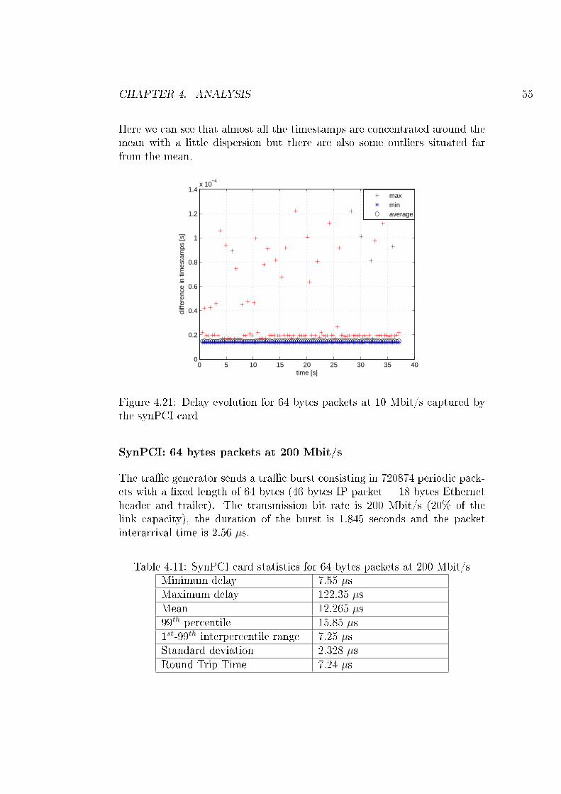
CHAPTER 4. ANALYSIS 55
Here we can see that almost all the timestamps are concentrated around themean with a little dispersion but there are also some outliers situated farfrom the mean.
0 5 10 15 20 25 30 35 400
0.2
0.4
0.6
0.8
1
1.2
1.4x 10
−4
time [s]
diffe
renc
e in
tim
esta
mps
[s]
maxminaverage
Figure 4.21: Delay evolution for 64 bytes packets at 10 Mbit/s captured bythe synPCI card
SynPCI: 64 bytes packets at 200 Mbit/s
The tra�c generator sends a tra�c burst consisting in 720874 periodic pack-ets with a �xed length of 64 bytes (46 bytes IP packet + 18 bytes Ethernetheader and trailer). The transmission bit rate is 200 Mbit/s (20% of thelink capacity), the duration of the burst is 1.845 seconds and the packetinterarrival time is 2.56 µs.
Table 4.11: SynPCI card statistics for 64 bytes packets at 200 Mbit/sMinimum delay 7.55 µsMaximum delay 122.35 µsMean 12.265 µs99th percentile 15.85 µs1st-99th interpercentile range 7.25 µsStandard deviation 2.328 µsRound Trip Time 7.24 µs
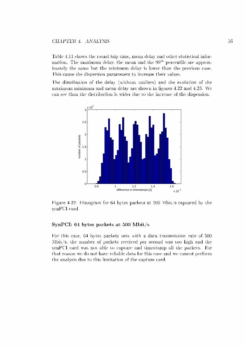
CHAPTER 4. ANALYSIS 56
Table 4.11 shows the round trip time, mean delay and other statistical infor-mation. The maximum delay, the mean and the 99th percentile are approx-imately the same but the minimum delay is lower than the previous case.This cause the dispersion parameters to increase their values.The distribution of the delay (without outliers) and the evolution of themaximum minimum and mean delay are shown in �gures 4.22 and 4.23. Wecan see than the distribution is wider due to the increase of the dispersion.
0.8 1 1.2 1.4 1.6
x 10−5
0
0.5
1
1.5
2
2.5
3x 10
4
difference in timestamps [s]
num
ber
of p
acke
ts
Figure 4.22: Histogram for 64 bytes packets at 200 Mbit/s captured by thesynPCI card
SynPCI: 64 bytes packets at 500 Mbit/s
For this case, 64 bytes packets sent with a data transmission rate of 500Mbit/s, the number of packets received per second was too high and thesynPCI card was not able to capture and timestamp all the packets. Forthat reason we do not have reliable data for this case and we cannot performthe analysis due to this limitation of the capture card.
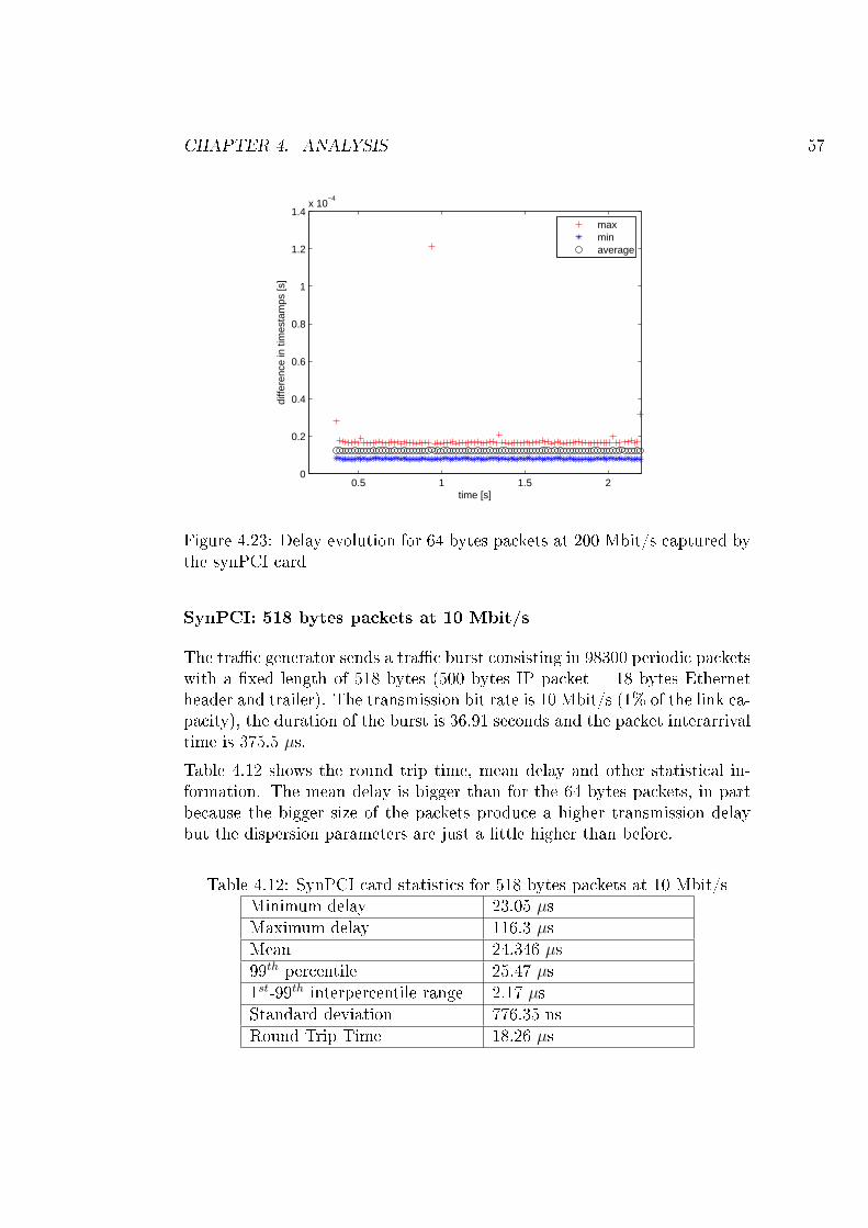
CHAPTER 4. ANALYSIS 57
0.5 1 1.5 20
0.2
0.4
0.6
0.8
1
1.2
1.4x 10
−4
time [s]
diffe
renc
e in
tim
esta
mps
[s]
maxminaverage
Figure 4.23: Delay evolution for 64 bytes packets at 200 Mbit/s captured bythe synPCI card
SynPCI: 518 bytes packets at 10 Mbit/s
The tra�c generator sends a tra�c burst consisting in 98300 periodic packetswith a �xed length of 518 bytes (500 bytes IP packet + 18 bytes Ethernetheader and trailer). The transmission bit rate is 10 Mbit/s (1% of the link ca-pacity), the duration of the burst is 36.91 seconds and the packet interarrivaltime is 375.5 µs.Table 4.12 shows the round trip time, mean delay and other statistical in-formation. The mean delay is bigger than for the 64 bytes packets, in partbecause the bigger size of the packets produce a higher transmission delaybut the dispersion parameters are just a little higher than before.
Table 4.12: SynPCI card statistics for 518 bytes packets at 10 Mbit/sMinimum delay 23.05 µsMaximum delay 116.3 µsMean 24.346 µs99th percentile 25.47 µs1st-99th interpercentile range 2.17 µsStandard deviation 776.35 nsRound Trip Time 18.26 µs
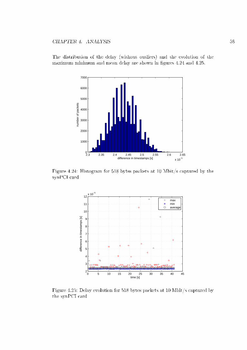
CHAPTER 4. ANALYSIS 58
The distribution of the delay (without outliers) and the evolution of themaximum minimum and mean delay are shown in �gures 4.24 and 4.25.
2.3 2.35 2.4 2.45 2.5 2.55 2.6 2.65
x 10−5
0
1000
2000
3000
4000
5000
6000
7000
difference in timestamps [s]
num
ber
of p
acke
ts
Figure 4.24: Histogram for 518 bytes packets at 10 Mbit/s captured by thesynPCI card
0 5 10 15 20 25 30 35 40 452
3
4
5
6
7
8
9
10
11
12x 10
−5
time [s]
diffe
renc
e in
tim
esta
mps
[s]
maxminaverage
Figure 4.25: Delay evolution for 518 bytes packets at 10 Mbit/s captured bythe synPCI card

CHAPTER 4. ANALYSIS 59
SynPCI: 518 bytes packets at 200 Mbit/s
The tra�c generator sends a tra�c burst consisting in 98300 periodic packetswith a �xed length of 518 bytes (500 bytes IP packet + 18 bytes Ethernetheader and trailer). The transmission bit rate is 200 Mbit/s (20% of thelink capacity), the duration of the burst is 1.845 seconds and the packetinterarrival time is 18.77 µs.Table 4.13 shows the round trip time, mean delay and other statistical in-formation. The minimum, maximum and mean delay are higher for thistransmission rate, and although the interpercentile range is lower, the stan-dard deviation is higher than for the 10 Mbit/s case.
Table 4.13: SynPCI card statistics for 518 bytes packets at 200 Mbit/sMinimum delay 24.14 µsMaximum delay 134.97 µsMean 25.547 µs99th percentile 26.39 µs1st-99th interpercentile range 1.54 µsStandard deviation 823.2 nsRound Trip Time 18.26 µs
2.4 2.45 2.5 2.55 2.6 2.65 2.7
x 10−5
0
1000
2000
3000
4000
5000
6000
7000
8000
9000
difference in timestamps [s]
num
ber
of p
acke
ts
Figure 4.26: Histogram for 518 bytes packets at 200 Mbit/s captured by thesynPCI card
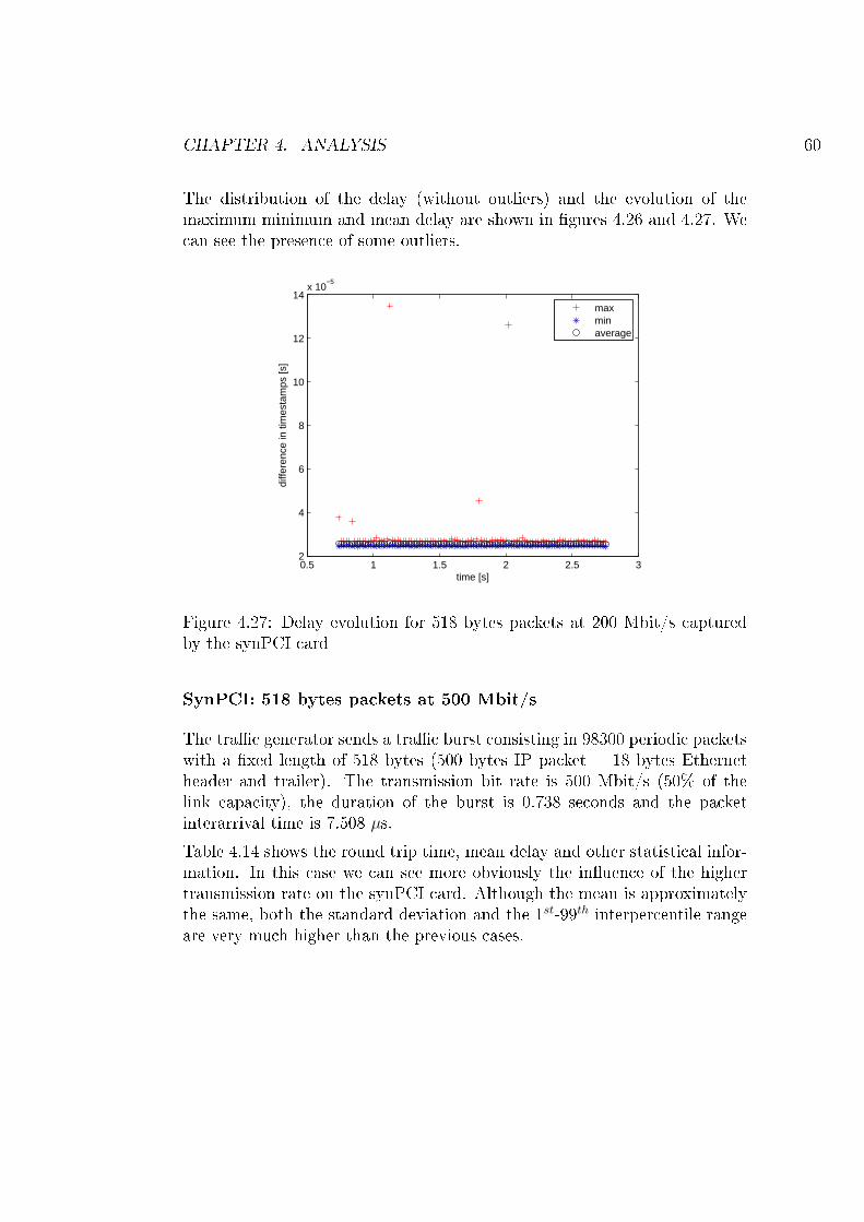
CHAPTER 4. ANALYSIS 60
The distribution of the delay (without outliers) and the evolution of themaximum minimum and mean delay are shown in �gures 4.26 and 4.27. Wecan see the presence of some outliers.
0.5 1 1.5 2 2.5 32
4
6
8
10
12
14x 10
−5
time [s]
diffe
renc
e in
tim
esta
mps
[s]
maxminaverage
Figure 4.27: Delay evolution for 518 bytes packets at 200 Mbit/s capturedby the synPCI card
SynPCI: 518 bytes packets at 500 Mbit/s
The tra�c generator sends a tra�c burst consisting in 98300 periodic packetswith a �xed length of 518 bytes (500 bytes IP packet + 18 bytes Ethernetheader and trailer). The transmission bit rate is 500 Mbit/s (50% of thelink capacity), the duration of the burst is 0.738 seconds and the packetinterarrival time is 7.508 µs.Table 4.14 shows the round trip time, mean delay and other statistical infor-mation. In this case we can see more obviously the in�uence of the highertransmission rate on the synPCI card. Although the mean is approximatelythe same, both the standard deviation and the 1st-99th interpercentile rangeare very much higher than the previous cases.
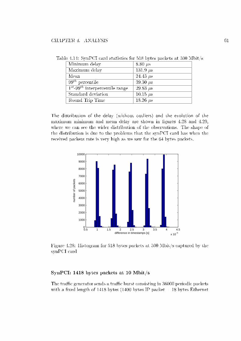
CHAPTER 4. ANALYSIS 61
Table 4.14: SynPCI card statistics for 518 bytes packets at 500 Mbit/sMinimum delay 8.80 µsMaximum delay 131.9 µsMean 24.43 µs99th percentile 39.30 µs1st-99th interpercentile range 29.83 µsStandard deviation 10.15 µsRound Trip Time 18.26 µs
The distribution of the delay (without outliers) and the evolution of themaximum minimum and mean delay are shown in �gures 4.28 and 4.29,where we can see the wider distribution of the observations. The shape ofthe distribution is due to the problems that the synPCI card has when thereceived packets rate is very high as we saw for the 64 bytes packets.
0.5 1 1.5 2 2.5 3 3.5 4 4.5
x 10−5
0
1000
2000
3000
4000
5000
6000
7000
8000
9000
10000
difference in timestamps [s]
num
ber
of p
acke
ts
Figure 4.28: Histogram for 518 bytes packets at 500 Mbit/s captured by thesynPCI card
SynPCI: 1418 bytes packets at 10 Mbit/s
The tra�c generator sends a tra�c burst consisting in 36000 periodic packetswith a �xed length of 1418 bytes (1400 bytes IP packet + 18 bytes Ethernet
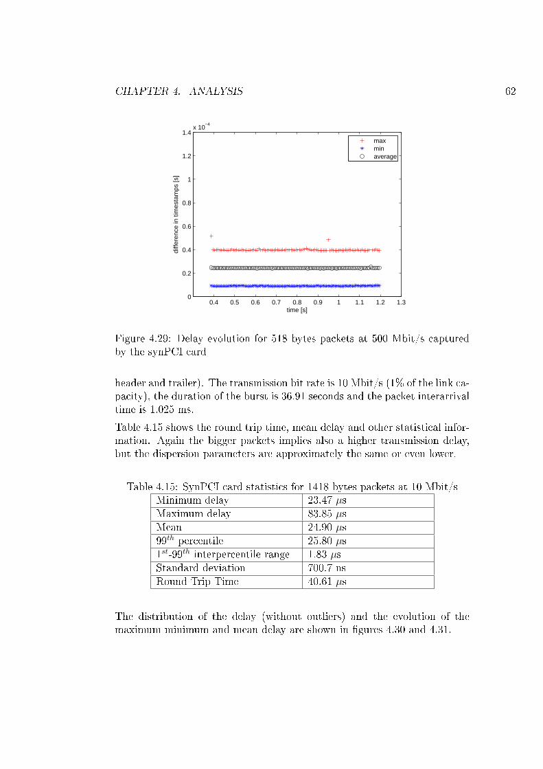
CHAPTER 4. ANALYSIS 62
0.4 0.5 0.6 0.7 0.8 0.9 1 1.1 1.2 1.30
0.2
0.4
0.6
0.8
1
1.2
1.4x 10
−4
time [s]
diffe
renc
e in
tim
esta
mps
[s]
maxminaverage
Figure 4.29: Delay evolution for 518 bytes packets at 500 Mbit/s capturedby the synPCI card
header and trailer). The transmission bit rate is 10 Mbit/s (1% of the link ca-pacity), the duration of the burst is 36.91 seconds and the packet interarrivaltime is 1.025 ms.Table 4.15 shows the round trip time, mean delay and other statistical infor-mation. Again the bigger packets implies also a higher transmission delay,but the dispersion parameters are approximately the same or even lower.
Table 4.15: SynPCI card statistics for 1418 bytes packets at 10 Mbit/sMinimum delay 23.47 µsMaximum delay 83.85 µsMean 24.90 µs99th percentile 25.80 µs1st-99th interpercentile range 1.83 µsStandard deviation 700.7 nsRound Trip Time 40.61 µs
The distribution of the delay (without outliers) and the evolution of themaximum minimum and mean delay are shown in �gures 4.30 and 4.31.
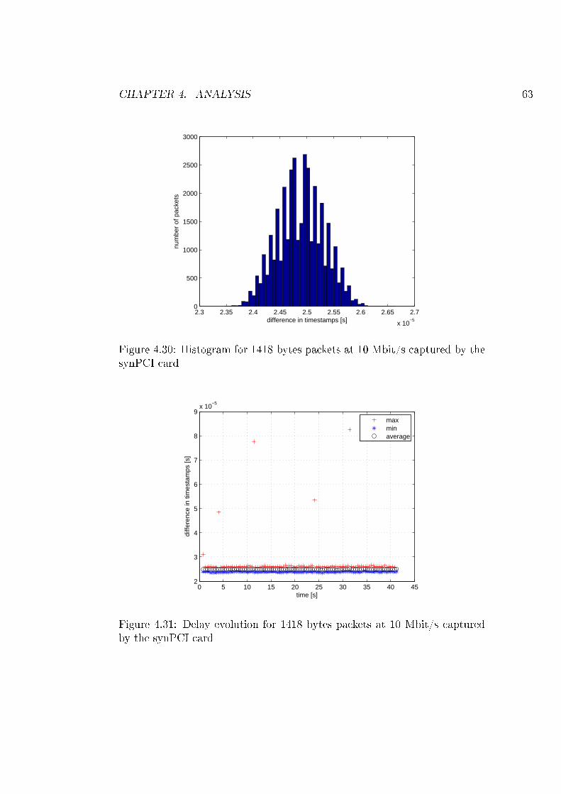
CHAPTER 4. ANALYSIS 63
2.3 2.35 2.4 2.45 2.5 2.55 2.6 2.65 2.7
x 10−5
0
500
1000
1500
2000
2500
3000
difference in timestamps [s]
num
ber
of p
acke
ts
Figure 4.30: Histogram for 1418 bytes packets at 10 Mbit/s captured by thesynPCI card
0 5 10 15 20 25 30 35 40 452
3
4
5
6
7
8
9x 10
−5
time [s]
diffe
renc
e in
tim
esta
mps
[s]
maxminaverage
Figure 4.31: Delay evolution for 1418 bytes packets at 10 Mbit/s capturedby the synPCI card
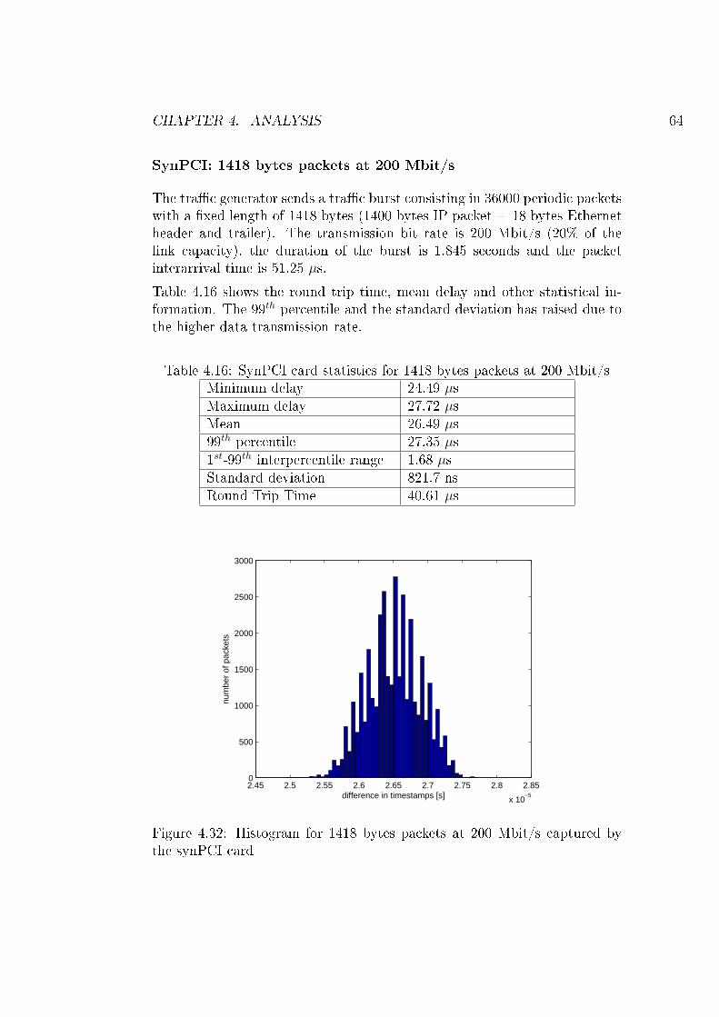
CHAPTER 4. ANALYSIS 64
SynPCI: 1418 bytes packets at 200 Mbit/s
The tra�c generator sends a tra�c burst consisting in 36000 periodic packetswith a �xed length of 1418 bytes (1400 bytes IP packet + 18 bytes Ethernetheader and trailer). The transmission bit rate is 200 Mbit/s (20% of thelink capacity), the duration of the burst is 1.845 seconds and the packetinterarrival time is 51.25 µs.Table 4.16 shows the round trip time, mean delay and other statistical in-formation. The 99th percentile and the standard deviation has raised due tothe higher data transmission rate.
Table 4.16: SynPCI card statistics for 1418 bytes packets at 200 Mbit/sMinimum delay 24.49 µsMaximum delay 27.72 µsMean 26.49 µs99th percentile 27.35 µs1st-99th interpercentile range 1.68 µsStandard deviation 821.7 nsRound Trip Time 40.61 µs
2.45 2.5 2.55 2.6 2.65 2.7 2.75 2.8 2.85
x 10−5
0
500
1000
1500
2000
2500
3000
difference in timestamps [s]
num
ber
of p
acke
ts
Figure 4.32: Histogram for 1418 bytes packets at 200 Mbit/s captured bythe synPCI card
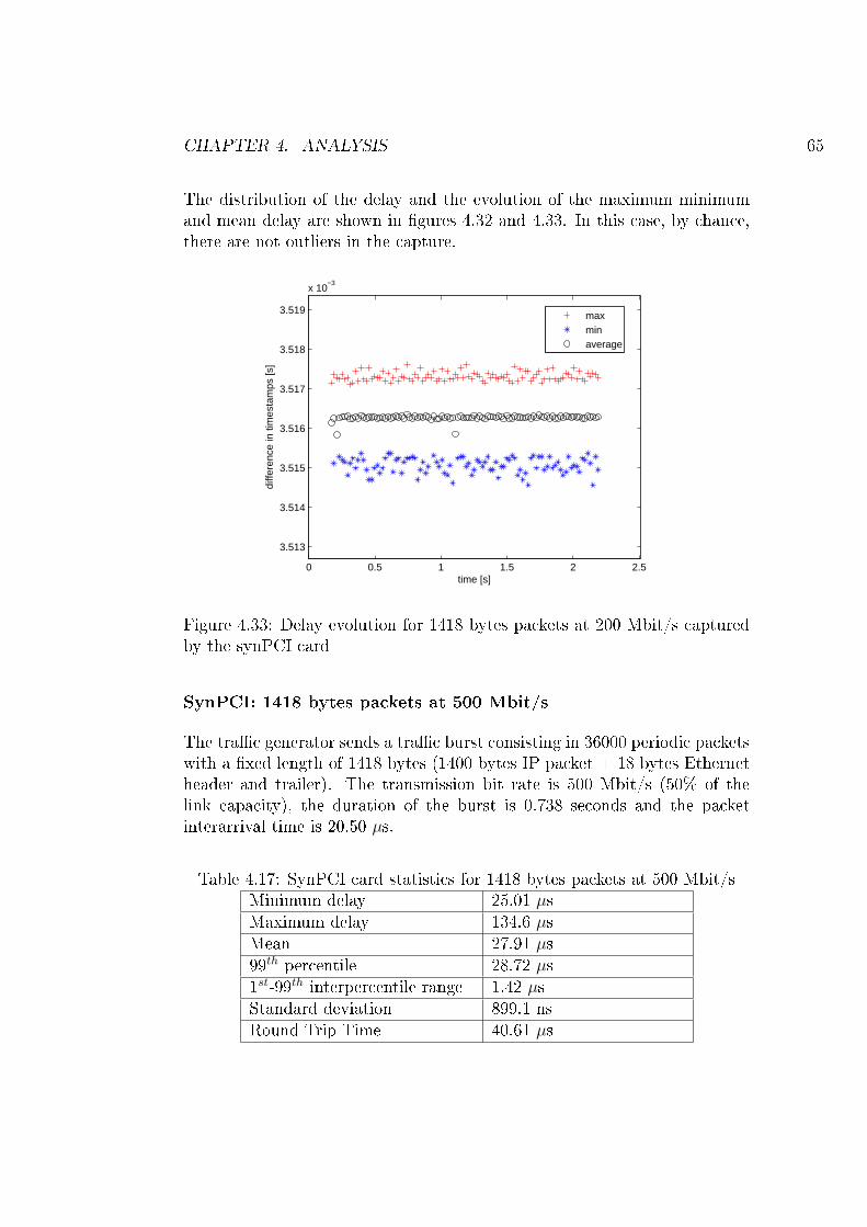
CHAPTER 4. ANALYSIS 65
The distribution of the delay and the evolution of the maximum minimumand mean delay are shown in �gures 4.32 and 4.33. In this case, by chance,there are not outliers in the capture.
0 0.5 1 1.5 2 2.5
3.513
3.514
3.515
3.516
3.517
3.518
3.519
x 10−3
time [s]
diffe
renc
e in
tim
esta
mps
[s]
maxminaverage
Figure 4.33: Delay evolution for 1418 bytes packets at 200 Mbit/s capturedby the synPCI card
SynPCI: 1418 bytes packets at 500 Mbit/s
The tra�c generator sends a tra�c burst consisting in 36000 periodic packetswith a �xed length of 1418 bytes (1400 bytes IP packet + 18 bytes Ethernetheader and trailer). The transmission bit rate is 500 Mbit/s (50% of thelink capacity), the duration of the burst is 0.738 seconds and the packetinterarrival time is 20.50 µs.
Table 4.17: SynPCI card statistics for 1418 bytes packets at 500 Mbit/sMinimum delay 25.01 µsMaximum delay 134.6 µsMean 27.91 µs99th percentile 28.72 µs1st-99th interpercentile range 1.42 µsStandard deviation 899.1 nsRound Trip Time 40.61 µs
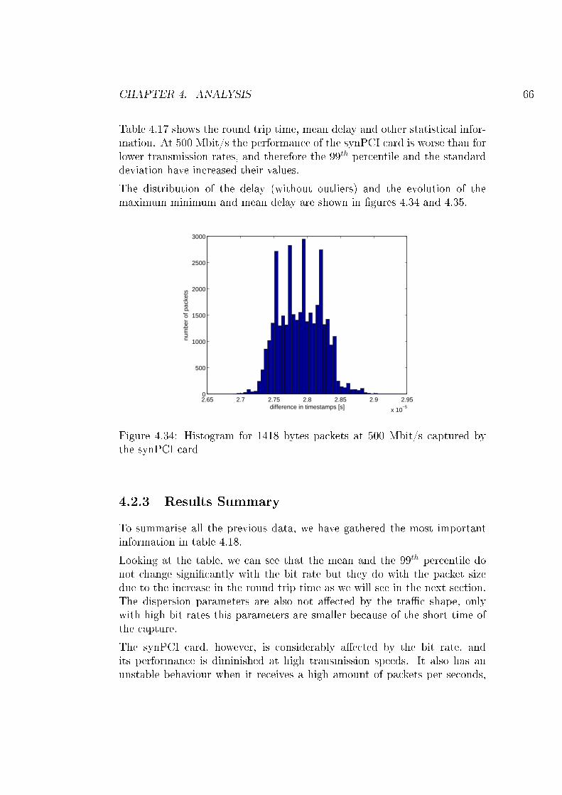
CHAPTER 4. ANALYSIS 66
Table 4.17 shows the round trip time, mean delay and other statistical infor-mation. At 500 Mbit/s the performance of the synPCI card is worse than forlower transmission rates, and therefore the 99th percentile and the standarddeviation have increased their values.The distribution of the delay (without outliers) and the evolution of themaximum minimum and mean delay are shown in �gures 4.34 and 4.35.
2.65 2.7 2.75 2.8 2.85 2.9 2.95
x 10−5
0
500
1000
1500
2000
2500
3000
difference in timestamps [s]
num
ber
of p
acke
ts
Figure 4.34: Histogram for 1418 bytes packets at 500 Mbit/s captured bythe synPCI card
4.2.3 Results SummaryTo summarise all the previous data, we have gathered the most importantinformation in table 4.18.Looking at the table, we can see that the mean and the 99th percentile donot change signi�cantly with the bit rate but they do with the packet sizedue to the increase in the round trip time as we will see in the next section.The dispersion parameters are also not a�ected by the tra�c shape, onlywith high bit rates this parameters are smaller because of the short time ofthe capture.The synPCI card, however, is considerably a�ected by the bit rate, andits performance is diminished at high transmission speeds. It also has anunstable behaviour when it receives a high amount of packets per seconds,
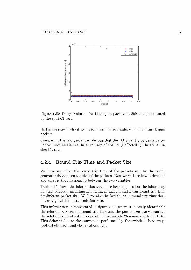
CHAPTER 4. ANALYSIS 67
0.5 0.6 0.7 0.8 0.9 1 1.1 1.2 1.3 1.42
4
6
8
10
12
14x 10
−5
time [s]
diffe
renc
e in
tim
esta
mps
[s]
maxminaverage
Figure 4.35: Delay evolution for 1418 bytes packets at 500 Mbit/s capturedby the synPCI card
that is the reason why it seems to return better results when it capture biggerpackets.Comparing the two cards it is obvious that the DAG card provides a betterperformance and it has the advantage of not being a�ected by the transmis-sion bit rate.
4.2.4 Round Trip Time and Packet SizeWe have seen that the round trip time of the packets sent by the tra�cgenerator depends on the size of the packets. Now we will see how it dependsand what is the relationship between the two variables.Table 4.19 shows the information that have been acquired at the laboratoryfor that purpose, including minimum, maximum and mean round trip timefor di�erent packet size. We have also checked that the round trip time doesnot change with the transmission rate.This information is represented in �gure 4.36, where it is easily identi�ablethe relation between the round trip time and the packet size. As we can seethe relation is lineal with a slope of approximately 25 nanoseconds per byte.This delay is due to the conversion performed by the switch in both ways(optical-electrical and electrical-optical).
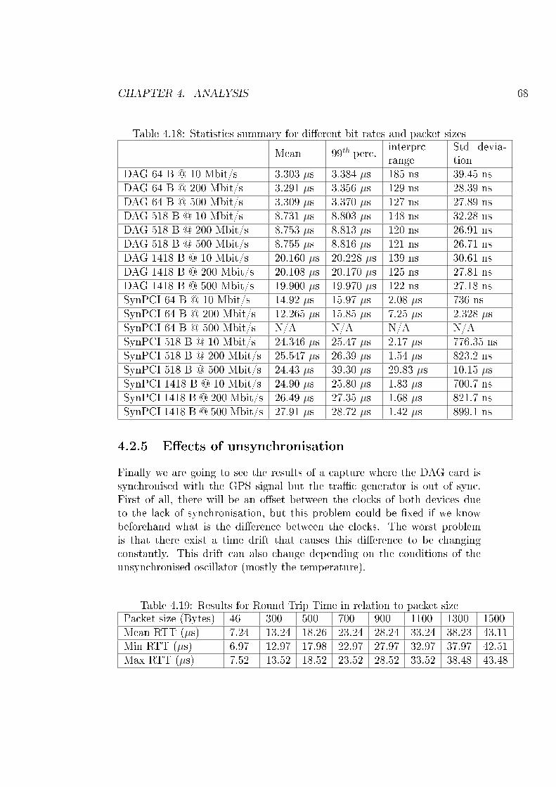
CHAPTER 4. ANALYSIS 68
Table 4.18: Statistics summary for di�erent bit rates and packet sizesMean 99th perc. interprc
rangeStd devia-tion
DAG 64 B @ 10 Mbit/s 3.303 µs 3.384 µs 185 ns 39.45 nsDAG 64 B @ 200 Mbit/s 3.291 µs 3.356 µs 129 ns 28.39 nsDAG 64 B @ 500 Mbit/s 3.309 µs 3.370 µs 127 ns 27.89 nsDAG 518 B @ 10 Mbit/s 8.731 µs 8.803 µs 148 ns 32.28 nsDAG 518 B @ 200 Mbit/s 8.753 µs 8.813 µs 120 ns 26.91 nsDAG 518 B @ 500 Mbit/s 8.755 µs 8.816 µs 121 ns 26.71 nsDAG 1418 B @ 10 Mbit/s 20.160 µs 20.228 µs 139 ns 30.61 nsDAG 1418 B @ 200 Mbit/s 20.108 µs 20.170 µs 125 ns 27.81 nsDAG 1418 B @ 500 Mbit/s 19.900 µs 19.970 µs 122 ns 27.18 nsSynPCI 64 B @ 10 Mbit/s 14.92 µs 15.97 µs 2.08 µs 736 nsSynPCI 64 B @ 200 Mbit/s 12.265 µs 15.85 µs 7.25 µs 2.328 µsSynPCI 64 B @ 500 Mbit/s N/A N/A N/A N/ASynPCI 518 B @ 10 Mbit/s 24.346 µs 25.47 µs 2.17 µs 776.35 nsSynPCI 518 B @ 200 Mbit/s 25.547 µs 26.39 µs 1.54 µs 823.2 nsSynPCI 518 B @ 500 Mbit/s 24.43 µs 39.30 µs 29.83 µs 10.15 µsSynPCI 1418 B @ 10 Mbit/s 24.90 µs 25.80 µs 1.83 µs 700.7 nsSynPCI 1418 B @ 200 Mbit/s 26.49 µs 27.35 µs 1.68 µs 821.7 nsSynPCI 1418 B @ 500 Mbit/s 27.91 µs 28.72 µs 1.42 µs 899.1 ns
4.2.5 E�ects of unsynchronisationFinally we are going to see the results of a capture where the DAG card issynchronised with the GPS signal but the tra�c generator is out of sync.First of all, there will be an o�set between the clocks of both devices dueto the lack of synchronisation, but this problem could be �xed if we knowbeforehand what is the di�erence between the clocks. The worst problemis that there exist a time drift that causes this di�erence to be changingconstantly. This drift can also change depending on the conditions of theunsynchronised oscillator (mostly the temperature).
Table 4.19: Results for Round Trip Time in relation to packet sizePacket size (Bytes) 46 300 500 700 900 1100 1300 1500Mean RTT (µs) 7.24 13.24 18.26 23.24 28.24 33.24 38.23 43.11Min RTT (µs) 6.97 12.97 17.98 22.97 27.97 32.97 37.97 42.51Max RTT (µs) 7.52 13.52 18.52 23.52 28.52 33.52 38.48 43.48
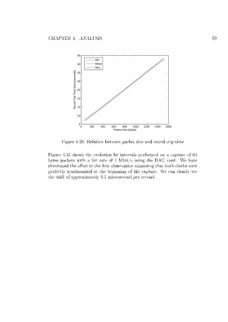
CHAPTER 4. ANALYSIS 69
0 200 400 600 800 1000 1200 1400 16005
10
15
20
25
30
35
40
45
Packet Size [bytes]
Rou
nd T
rip T
ime
[mic
rose
cond
s]
MinMeanMax
Figure 4.36: Relation between packet size and round trip time
Figure 4.37 shows the evolution by intervals performed on a capture of 64bytes packets with a bit rate of 1 Mbit/s using the DAG card. We haveeliminated the o�set in the �rst observation supposing that both clocks wereperfectly synchronised at the beginning of the capture. We can clearly seethe drift of approximately 0.1 microsecond per second.
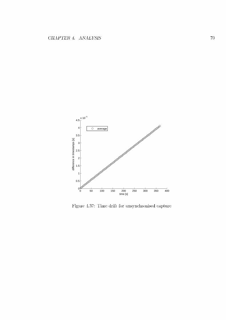
CHAPTER 4. ANALYSIS 70
0 50 100 150 200 250 300 350 4000
0.5
1
1.5
2
2.5
3
3.5
4
4.5x 10
−5
time [s]
diffe
renc
e in
tim
esta
mps
[s]
average
Figure 4.37: Time drift for unsynchronised capture
Chapter 5
Conclusions
Synchronisation over the network is a very important feature for telecom-munications in general, but it becomes even more important when we dealwith experimental research among di�erent computers and networks wheresynchronisation is a major issue in order to achieve acceptable results.In this thesis we analysed and discussed the performance of two di�erentsynchronisation devices. One commercial o�-the-shelf capture card, and an-other card developed at Helsinki University of Technology by the NetworkingLaboratory department.We have used GPS technology to get all the computers of the measurementsetup in sync. Using the satellite signal as a time reference is equivalent tohave an atomic precision clock inside the GPS receivers of the laboratory.This signal is then distributed to the devices where an accurate synchronisa-tion is needed. But this is not the only advantage that GPS synchronisationprovides, when working with multi-site networks, GPS allows us to synchro-nise all the networks no matters where are them or how far are from eachother. We only need a GPS antenna and receiver in every location.After the analysis we have seen than the performance of the synPCI card isnot as good as the DAG card, but it still provides a better accuracy than acomputer having the PPS synchronisation signal directly input to the serialport. The main advantage is that synPCI card avoids interrupt latencies,what is specially important when the computer is under heavy system load.Another remarkable feature is that it quickly gets in sync with the GPSsource after it is rebooted. The optical �bre inputs provides the synPCI cardwith immunity to electromagnetic noises and lower attenuation. However,its most important problem is that its performance is signi�cantly degradedwhen it works with dense tra�c at high transmission rate and it does not
71
CHAPTER 5. CONCLUSIONS 72
work properly when it receives a high number of packets per second.The DAG card has demonstrated to have a better performance than the syn-PCI card. It is able to provide accurate timestamps and its behaviour is notdegraded when a high bit rate burst is applied to its input ports. The DAGcard, although is a non-expensive commercial card, is still more expensivethan the synPCI card. The longer time it takes to achieve synchronisationis another disadvantage of the DAG card with respect to the synPCI card.Synchronisation is not only important in the receiving devices, but is equallyimportant in the tra�c sources and in all the network monitoring points.A lack of synchronisation in any point can degrade the results of the re-search. For wide network investigation where a high number of monitoringpoints are required, the scalability of the synchronisation devices becomes afundamental issue. The cheaper price of the devices we have studied makethem an a�ordable solution when a high number of computers need to besynchronised.To summarise, in this thesis we have studied some synchronisation technolo-gies that provides us with a better timing accuracy, multi-site synchronisationcapabilities, all of that at an a�ordable price allowing the scalability of thesystem. With accurate results network research can focus more in the subjectof the research than in inaccuracies and timing errors.
5.1 Future WorkFuture work should consist on additional evaluation of SynPCI card in widernetworks, such as multiple location networks. A patch for the tcpdump toolproviding nanosecond resolution is necessary to allow us to know better thetrue performance of the card. Finally, it would be also useful to developdrivers for other operating system.
Bibliography
[1] Bennington, J. IEEE 1588 Precision Tim-ing Protocol (PTP), Electronic Design. January 2007.http://eepn.com/locator/products/ArticleID/34270/34270.html.
[2] Dana, P. H. Global positioning system overview. Department of Ge-ography, The University of Colorado at Boulder.http://www.colorado.edu/geography/gcraft/notes/gps/gps_f.html.
[3] Esham, B. D. http://commons.wikimedia.org/wiki/Image:Network_Time_Protocol_servers_and_clients.svg.
[4] Hernández, A., and Magaña, E. One-way delay measurement andcharacterization. Universidad Pública de Navarra, Pamplona, Spain,2007.
[5] Hofmann-Wellenhof, B., Lichtenegger, H., and Collins, J.GPS Theory and Practice. New York, 2001.
[6] IEC 61588 First edition 2004-09. IEEE 1588, Precision clock syn-chronization protocol for networked measurement and control systems,2004.
[7] Kihara, M., Ono, S., and Eskelinen, P. Digital Clocks for Syn-chronization and Communications. Artech House, Inc., 2003.
[8] Langley, R. The mathematics of gps. GPS World (July/August 1991).
[9] Marrison, W. A. The evolution of the quartz crystal clock.
[10] Parkinson, B. W., and Spilker, J. J. Global Positioning System:Theory and Applications. Aiaa, 1996.
[11] Peuhkuri, M., Gröhn, A., and Simola, O. Clock synchronisationin industry-standard computer hardware. TKK Helsinki University ofTechnology.
73
BIBLIOGRAPHY 74
[12] Press, Flannery, Tekolsky, and Vetterling. NumericalRecipes, The Art of Scienti�c Computing. Cambridge University Press,1986.
[13] Range Commander's Council. Telecommunication and Tim-ing Group. IRIG Serial Time Code Formats, 2004.
[14] Stefano Bregni. Synchronization of Digital Telecommunications Net-works. John Wiley & Sons, Ltd., 2002.
[15] Vig, J. R. Introduction to quartz frequency standards. Army ResearchLaboratory, Electronics and Power Sources Directorate, October 1992.http://www.ieee-u�c.org/freqcontrol/quartz/vig/vigtoc.htm.