Inter-American Development Bank

Banco Interamericano de Desarrollo Latin American Research Network

Red de Centros de Investigación

Research Network Working Paper #R-541

An Experimental Study of Labor Market Discrimination: Gender, Social Class

and Neighborhood in Chile

by

David Bravo* Claudia Sanhueza** Sergio Urzúa***

* Centro de Microdatos, Departament de Economía, Universidad de Chile ** ILADES, Universidad Alberto Hurtado

*** Department of Economics, Northwestern University

May 2008

2

Cataloging-in-Publication data provided by the Inter-American Development Bank Felipe Herrera Library Bravo, David.

An experimental study of labor market discrimination : gender, social class and neighborhood in Chile / by David Bravo, Claudia Sanhueza, Sergio Urzúa.

p. cm. (Research Network Working papers ; R-541) Includes bibliographical references.

1. Labor market—Chile. 2. Discrimination in employment—Chile. 3. Sex discrimination in employment—Chile. I. Sanhueza, Claudia. II. Urzua, Sergio, 1977- III. Inter-American Development Bank. Research Dept. IV. Latin American Research Network. V. Title. VI. Series. HD5756.A6 .B445 2008 331.120983 B445----dc22 ©2008 Inter-American Development Bank 1300 New York Avenue, N.W. Washington, DC 20577 The views and interpretations in this document are those of the authors and should not be attributed to the Inter-American Development Bank, or to any individual acting on its behalf. This paper may be freely reproduced provided credit is given to the Research Department, Inter-American Development Bank. The Research Department (RES) produces a quarterly newsletter, IDEA (Ideas for Development in the Americas), as well as working papers and books on diverse economic issues. To obtain a complete list of RES publications, and read or download them please visit our web site at: http://www.iadb.org/res.

3

Abstract*

The objective of this paper is to study the Chilean labor market and determine the presence or absence of gender discrimination. In order to transcend the limitations of earlier works, an experimental design is used, the first of its kind in Chile. This study also allows socioeconomic discrimination associated with names and places of residence to be addressed. The study consists of sending fictitious Curriculum Vitae for real job vacancies published weekly in the Santiago newspaper El Mercurio. A range of strictly equivalent CVs in terms of qualifications and employment experience of applicants are sent out, varying only in gender, name and surname, and place of residence. The results show no significant differences in callback rates across groups, in contrast with what is found in other international studies.

* We would like to thank Andrea Moro and Hugo Ñopo for helpful comments. We also thank Verónica Flores and Bárbara Flores for their excellent research assistance as well as the outstanding performance of the Survey Unit of the Centro de Microdatos.

4

1. Introduction Gender and social discrimination in the labor market are some of the key issues in the discussion

on public policies in Latin America. However, empirical evidence and academic research on the

matter have been rather scarce until now. This is also the case in Chile.

No matter how much has been done to study labor market discrimination, either racial,

ethnic or gender, the issue of detection is still unsettled. In the usual regression analyses there are

several problems of unobservable variables that clearly bias the results (Altonji and Blank, 1999;

Neal and Johnson, 1996) and, on the other hand, experimental studies have been under

discussion for not correctly measuring discrimination (Heckman and Siegelman, 1993;

Heckman, 1998).

In Chile, despite the fact that the average years of schooling of Chilean female workers

are not statistically different from those of male workers, average wages of male workers are 25

percent higher.1 In fact, previous studies2 suggest that gender discrimination is a factor in

determining wages in the Chilean labor market. Estimates of the Blinder-Oaxaca decomposition

give “residual discrimination” a significant participation in the total wage gap.3 The evidence

also shows stable and systematic differences in the returns to education and to experience by

gender along the conditional wage distribution. Additionally, it has been shown that “residual

discrimination” is higher for women with more education and experience.

Furthermore, Chilean female labor force participation is particularly low, 38.1 percent,

compared to Latin America’s regional average of 44.7 percent.4 This is even lower for married

women and in fact, higher participation is found among separated or divorced women (Bravo,

2005). This latter fact may be interpreted as evidence of female preferences for non-market

activities.5

However, this “residual discrimination” is only a measure of how much of the wage gap

is due to unobservable factors. Therefore, these measures of discrimination are biased due to the 1 Authors’ calculations using CASEN 2003. After correcting for human capital differences and occupational choice, this gap falls to approximately 19 percent. 2 Previous studies for Chile are Bravo (2005); Montenegro (1998); Montenegro and Paredes (1999) and Paredes and Riveros (1994). 3 Bravo (2005) shows that, taking all employed workers and after controlling for years of schooling and occupation, the wage gap was 13.5 percent in 2000. Using the Blinder-Oaxaca decomposition he concludes that most of this difference was due to “residual discrimination”. 4 Source: International Labor Organization (ILO).

5

lack of relevant controls. A recent study on discrimination by social class in Chile (Núñez and

Gutiérrez, 2004) uses a dataset that reduces the role of unobserved heterogeneity across

individuals, but this dataset has several limitations.6 Furthermore, there are no attempts at

studying discrimination using either audit studies or natural experiments.

The objective of this paper is to study the Chilean labor market and determine the

presence or absence of gender discrimination. In order to transcend the limitations of earlier

works, an experimental design is used, the first of its kind in Chile. This study also makes it

possible to address socioeconomic discrimination associated with names and places of residence.

The study consists of sending fictitious Curriculum Vitae for real job vacancies published

weekly in the Santiago newspaper El Mercurio. A range of strictly equivalent CVs in terms of

qualifications and employment experience of applicants are sent out, varying only in gender,

name and surname, and place of residence. The study allows differences in call response rates to

be measured for the various demographic groups. Results are obtained for more than 11,000 CVs

sent.

The following section contains a review of the relevant literature for this study.

Meanwhile, Section 3 contains all the methodological information associated with the

implementation of the experiment, which began in the last week of March 2006. Section 4

contains a report of the main results. Lastly, Section 5 presents the main conclusions and policy

lessons.

2. Literature Review Labor market discrimination is said to arise when two identically productive workers are treated

differently on the grounds of the worker’s race or gender, when race or gender do not in

themselves have an effect on productivity (Altonji and Blank, 1999; Heckman, 1998). However,

there are never identical individuals. There are several unobservable factors that determine

individual performance in the labor market. (See Bravo, Sanhueza and Urzúa, 2008, for a review

of this literature.)

5 Contreras and Plaza (2004) also found that there are cultural factors, such as sexism, that significantly influence female labor force participation in Chile. 6 See Section 2 for a discussion.

6

The empirical literature attempts to face these problems by two alternative

methodologies: regression analysis and field experiments.7 The regression analysis is focused on

analyzing the Blinder-Oaxaca decomposition (Oaxaca, 1973; Blinder, 1973) to determine how

much of the wage differential between groups of workers, by race or gender, is unexplained. This

unexplained part is called discrimination. Developments in Chile have been centered on

regression analysis applied to the gender gap. See Paredes and Riveros (1993), Montenegro

(1999) and Montenegro and Paredes (1999) as an example. The conclusions from these studies

are very limited. They lack several control variables related to cognitive and non-cognitive

abilities and school and family environments. In addition, preferences for non-market activities

and the experience of Chilean female workers could prove to be a very important unobservable

factor. More recently, Núñez and Gutiérrez (2004) study social class discrimination in Chile

under the traditional Blinder-Oaxaca decomposition. They use a dataset that allows them to

reduce the role of unobservable factors by limiting the population under study and having better

measures of productivity.

The works cited above represent the traditional studies in this area. This paper is much

more closely related to a different line of research on labor market discrimination: experimental

studies.8 These studies originated in Europe in the 1960s and 1970s and were subsequently used

by the ILO in the 1990s. More recently, experimental techniques have been published in leading

economic journals (Bertrand and Mullainathan, 2004).

Experimental approaches can be divided into two types: audit studies and natural

experiments. The latter take advantage of unexpected changes in policies or events (Levitt, 2004;

Antonovics, Arcidiacono and Walsh, 2004, 2005; Goldin and Rouse, 2000; Newmark, Bank and

Van Nort, 1996). In Chile, as far as we know, there are no studies using these kinds of variations.

There have been two strategies used to carry out audit studies. First is the personal

approach strategy, which either sends individuals to job interviews or undertakes job applications

over the telephone. Second, there is the strategy of sending written applications for real job

vacancies.

7 See Altonji and Blank (1999) and Blank, Dabady and Citro (2004) for complete surveys on the econometric problems involving detecting discrimination in the labor market using regression analysis and field experiments. 8 Riach and Rich (2002, 2004) and Anderson, Fryer and Holt (2005) have a complete survey of these studies.

7

The first procedure is the most subject to criticism. It has been argued that it is impossible

to ensure that false applicants are identical. Also, testers were sometimes warned that they were

involved in a discrimination study, and their behavior could bias the results.9

The first experiments that used written applications were unsolicited job applications sent

to “potential employers”; these experiments tested preferential treatment in employer responses

and not the hiring decision. Later came experiments in which curriculum vitae were sent in

response to real announcements. Although the latter technique overcomes the criticisms of the

personal approaches and tests the hiring decision10 it does not overcome a common problem in

the audit studies mentioned by Heckman and Siegelman (1993) and Heckman (1998), which is

that audits are crucially dependent on the distribution of unobserved characteristics for each

racial group and the audit standardization level. Thus, there may still be unobservable factors,

which can be productivity-determining and not discrimination. Riach and Rich (2002) accepted

this criticism but pointed out that it is not easy to imagine how firms’ internal attributes11 could

enhance productivity. They conclude that, since Heckman and Siegelman (1993) do not explain

what could be behind those gaps, the argument has “not been proven.”

The present study mainly follows the line of work developed by Bertrand and

Mullainathan (2004). In their study, the authors measured the racial discrimination in the labor

market, by means of the posting of fictitious curriculum vitae for job vacancies published in

Boston and Chicago newspapers. Half of the CVs were randomly given Afro-American names

and the other half received European (“White”) names. Additionally, the effect of applicant

qualification on the racial gap was measured; for this, the CVs were differentiated between High

Qualifications and Low Qualifications.

The authors found that the curriculum vitae associated with White names received 50

percent more calls for interview than those with Afro-American names. They also found that

whites were more affected by qualification level than blacks. Additionally, the authors found

some evidence that employers were inferring social class based on applicants’ names.

9 See Heckman and Siegelman (1993). 10 It really tests the callback decision; we do not know what can happen next. 11 Such as internal promotion or other.

8

3. Experiment Design As noted above, the experiment consists of the sending out of CVs of fictitious individuals for

real job vacancies that appear weekly in the newspaper with the highest circulation in Chile.

Each week, the work team selects a total of 60 job vacancies from the Santiago newspaper El

Mercurio. ” A total of eight CVs, four corresponding to men and four to women, are sent in out

for each vacancy. The details of the experiment design are presented here below.

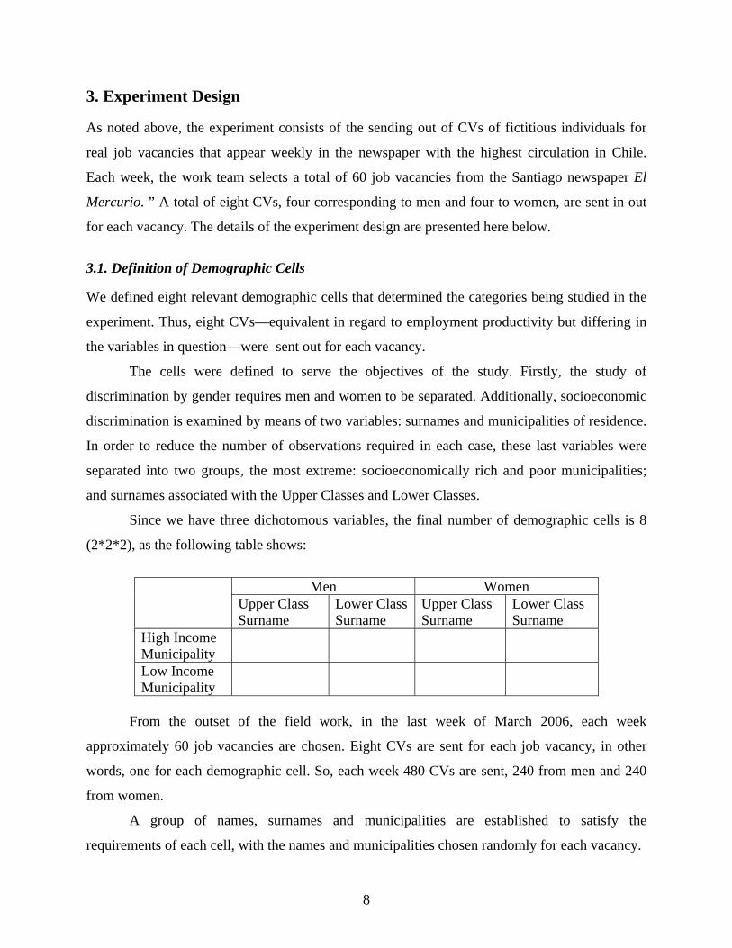
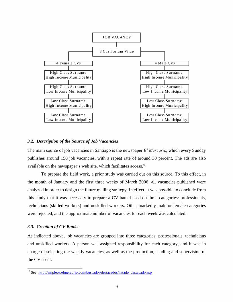
3.1. Definition of Demographic Cells We defined eight relevant demographic cells that determined the categories being studied in the

experiment. Thus, eight CVs—equivalent in regard to employment productivity but differing in

the variables in question—were sent out for each vacancy.

The cells were defined to serve the objectives of the study. Firstly, the study of

discrimination by gender requires men and women to be separated. Additionally, socioeconomic

discrimination is examined by means of two variables: surnames and municipalities of residence.

In order to reduce the number of observations required in each case, these last variables were

separated into two groups, the most extreme: socioeconomically rich and poor municipalities;

and surnames associated with the Upper Classes and Lower Classes.

Since we have three dichotomous variables, the final number of demographic cells is 8

(2*2*2), as the following table shows:

Men Women

Upper Class Surname

Lower Class Surname

Upper Class Surname

Lower Class Surname

High Income Municipality

Low Income Municipality

From the outset of the field work, in the last week of March 2006, each week

approximately 60 job vacancies are chosen. Eight CVs are sent for each job vacancy, in other

words, one for each demographic cell. So, each week 480 CVs are sent, 240 from men and 240

from women.

A group of names, surnames and municipalities are established to satisfy the

requirements of each cell, with the names and municipalities chosen randomly for each vacancy.

9

Low Class Surname Low Income Municipa lity

High Class Surname Low Income Municipa lity

Low Class Surname High Income Municipa lity

J OB VACANCY

4 Male CVs

High Class Surname High Income Municipa lity

Low Income Municipality

8 Cur r icu lum Vitae

Low Income Municipality

Low Class Surname High Income Municipality

Low Class Surname

4 Female CVs

High Class Surname

High Class Surname

High Income Municipality

3.2. Description of the Source of Job Vacancies The main source of job vacancies in Santiago is the newspaper El Mercurio, which every Sunday

publishes around 150 job vacancies, with a repeat rate of around 30 percent. The ads are also

available on the newspaper’s web site, which facilitates access.12

To prepare the field work, a prior study was carried out on this source. To this effect, in

the month of January and the first three weeks of March 2006, all vacancies published were

analyzed in order to design the future mailing strategy. In effect, it was possible to conclude from

this study that it was necessary to prepare a CV bank based on three categories: professionals,

technicians (skilled workers) and unskilled workers. Other markedly male or female categories

were rejected, and the approximate number of vacancies for each week was calculated.

3.3. Creation of CV Banks As indicated above, job vacancies are grouped into three categories: professionals, technicians

and unskilled workers. A person was assigned responsibility for each category, and it was in

charge of selecting the weekly vacancies, as well as the production, sending and supervision of

the CVs sent.

12 See: http://empleos.elmercurio.com/buscador/destacados/listado_destacado.asp

10

A data base of fictitious CVs was produced for professionals, technicians and unskilled

workers. This task was done by three different and specialized teams using models taken from

real CVs available on two public websites.13 In producing the required CVs the instruction was to

comply with the profile of the most competitive applicant for the vacancy selected. Each set of

eight CVs was constructed so that its qualification levels and employment experience were

equivalent in order to ensure that the applicants were equally eligible for the job in question.

The central element in the training of the people in charge of this was to ensure that the 8

CVs sent for each vacancy had to be equivalent in terms of qualifications and human capital. To

ensure this, the coordinators of the study were supported by a research assistant that supervised

the work over the whole period, especially, during the first weeks, until ensuring the desired

results.

3.4. Classification of Municipalities In order to facilitate the field work, the study is concentrated in the Metropolitan Urban Region,

which is divided into 34 municipalities.

To classify the municipalities in the two extreme segments a socioeconomic classification

of households based on the 2002 Census was used (the groups are, ordered from higher to lower

level: ABC1, C2, C3, D and E). Using the CASEN 2003 Survey the proportion of the population

by socioeconomic level in each municipality was computed.

For high-income municipalities, five of the six with the highest proportion of the

population in segment ABC1 were chosen (the sixth was excluded because it is a municipality

that also had a higher proportion than the rest in segments D and E). On the other hand, for the

low-income group municipalities, the 15 municipalities associated with a lower proportion of the

population in segment ABC1 and a greater proportion in segments D and E were chosen. In

order to more clearly examine the impact of the municipality of origin, all other municipalities of

intermediate socioeconomic groups were left out.

The final list of the municipalities included in each group is presented in the Table below:

13 See www.laborum.com and www.infoempleo.cl

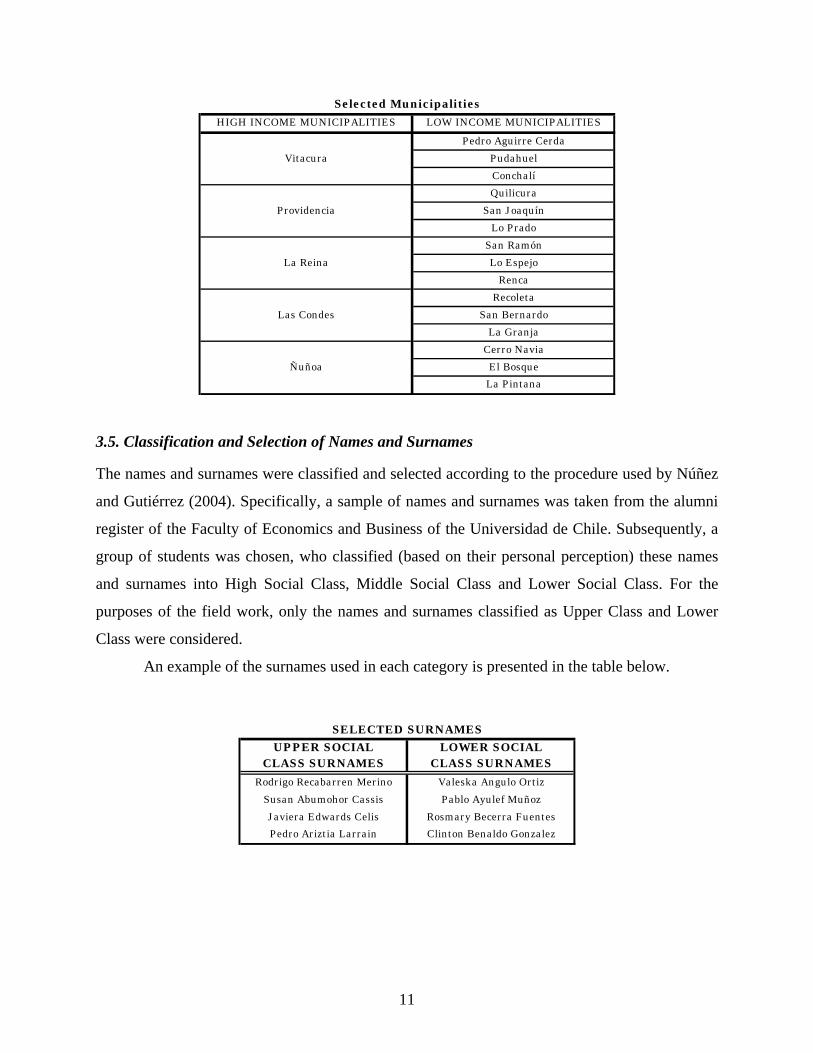
11

Ñuñoa El BosqueLa P intana

La GranjaCer ro Navia

RecoletaLas Condes San Bernardo

San RamónLa Reina Lo Espejo

Renca

Se le c te d Munic ipa lit ie sHIGH INCOME MUNICIPALITIES LOW INCOME MUNICIPALITIES

Pedro Aguir re CerdaVitacura Pudahuel

ConchalíQuilicura

Providencia San J oaquínLo Prado

3.5. Classification and Selection of Names and Surnames The names and surnames were classified and selected according to the procedure used by Núñez

and Gutiérrez (2004). Specifically, a sample of names and surnames was taken from the alumni

register of the Faculty of Economics and Business of the Universidad de Chile. Subsequently, a

group of students was chosen, who classified (based on their personal perception) these names

and surnames into High Social Class, Middle Social Class and Lower Social Class. For the

purposes of the field work, only the names and surnames classified as Upper Class and Lower

Class were considered.

An example of the surnames used in each category is presented in the table below.

J aviera Edwards Celis Rosmary Becer ra FuentesPedro Ar izt ia Lar ra in Clin ton Benaldo Gonzalez

Rodr igo Recabar ren Mer ino Valeska Angulo Or t izSusan Abumohor Cassis Pablo Ayulef Muñoz

SELECTED SURNAMESUP P ER SOCIAL LOWER SOCIAL

CLASS SURNAMES CLASS SURNAMES

12

3.6. Description of the Field Work The three people responsible indicated above handled the weekly selection of job vacancies that

appeared in El Mercurio on Sundays. They then constructed the targeted CVs for each vacancy,

compiling the competitive CVs and ensuring their equivalence so that the only differentiating

elements were the sex of the applicant, the social level, name and surname, and the municipality

of residence. Apart from the people in charge, the team was made up of three other assistants,

and the entire procedure was supervised directly by a Sociologist and an Economist who

randomly reviewed the CVs sent.

The job vacancies selected and the lot of eight CVs sent for each vacancy were entered

weekly into a specially designed web page that allowed all the vacancies to be reviewed, together

with their respective sets of CVs. The entry of that information into the web page was handled by

an information technology expert.

A central aspect of this work was receiving the calls for the CVs sent. To receive these

calls-responses, there was a fully dedicated man and woman team, ready to take the calls 24

hours a day from Monday to Sunday. There were 8 mobile telephones, each with a different

number, assigned to each of the CVs of the set; this ensured that the recruiters did not encounter

repeated telephone numbers. The people in charge of receiving the calls recorded the day, name

of the applicant, the vacancy and the phone number of the firm that selected the CV. Each report

was entered into the web page of the project, which allowed for the regular supervision of the

calls received.

In parallel, job vacancy responses were also received by e-mail, as some job vacancies

requested e-mails. For this, a generic e-mail had been created for each CV. All the e-mails

addresses created were checked every three days. As with the phone calls, the e-mails were

reported and entered into the web page of the project.

3.7 Identity of Fictitious Applicants Once the names and surnames were classified by categories (Upper Class and Lower Class), they

were then mixed so as to not use real names. Additionally, each fictitious applicant had a

fictitious RUT14 and an exclusive e-mail address. To ensure the equivalence of each set of CVs,

14 National Identification Number.

13

the age of the applicants was set at between 30 and 35 years of age, and applicants were listed as

married with at least one child and no more than two children.

3.8 Ensuring the Equivalence of Fictitious Applicants between Cells In order to ensure the equivalence of the eight fictitious applications sent for each vacancy, the

other variables included in the CVs were controlled for similarity. For this, the following

decisions were made:

• As regards the educational background of the applicants, those with university

education were considered Universidad de Chile graduates and where

necessary, they had postgraduate studies from the same University.

• The school of the applicant and the home address were determined by the

applicant’s municipality of residence. A bank of school names of each

municipality was used for this purpose. However, to ensure homogeneous

schooling the eight CVs sent must belong to the same category of

socioeconomic background as the school.15

• Additionally, each CV of the set of eight had a unique telephone number that

was different from the other seven; however, these may repeat themselves

among different groups of CVs.

• The employment experience of the applicants was equivalent within each

category (professional, technician, unskilled worker) but different from other

categories. Thus, professionals with greater time spent in the educational

system had fewer years of employment experience; meanwhile, unskilled

workers had a longer track record in the labor market. To maintain this

equivalence, we also set the number of jobs that each applicant has had in the

various categories and their employment history continuity (absence of

employment gaps).

15 This is a discrete variable that describes the level of income of the majority of the school population.

14

Cate gory Em ploym e n t Expe rie n ce

Nu m be r of jobs

Professiona ls 7 to 12 years 2 to 3Technicians 8 to 13 years 4 to 5

Unskilled workers 12 to 17 years 5 to 7

• Postgraduate studies of applicants were equivalent within the set of eight CVs

that were sent for each vacancy. Within the set of eight CVs, postgraduate

studies must be from the same university (Universidad de Chile) and in very

similar areas or even identical areas. Training courses must also be from

equivalent institutions (Technical Institutes) and in similar or identical areas.

• As a general rule, high-quality CVs were sent for each vacancy. In other

words, the variables of employment history, education and training were

drawn up to be attractive to firms.

• The pay expectations required, which generally had to be included in job

applications, were based on actual remuneration information of professionals

and technicians (from the web page www.futurolaboral.cl). The starting point

was pay levels required by a good candidate (of percentile 75 of that

distribution), expected remuneration was subsequently reduced to average

levels. Each set of eight CVs sent for a vacancy had the same reference pay

level and varied only slightly (in some cases it was given as a range and in

others as a specific reference).

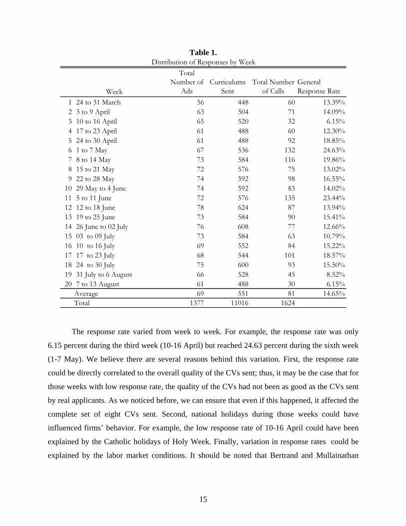
4. Findings The CV mailing process started in the last week of March. As we can note from Table 1, on

average, 69 vacancies had been applied for weekly, with a total of 11,016 CVs sent during the 20

weeks of the project, and a response rate of 14.65 percent. This rate was higher than that

obtained by Bertrand and Mullainathan (2004).

15

Table 1.

Total Number of

AdsCurriculums

SentTotal Number

of CallsGeneral Response Rate

1 24 to 31 March 56 448 60 13.39%2 3 to 9 April 63 504 71 14.09%3 10 to 16 April 65 520 32 6.15%4 17 to 23 April 61 488 60 12.30%5 24 to 30 April 61 488 92 18.85%6 1 to 7 May 67 536 132 24.63%7 8 to 14 May 73 584 116 19.86%8 15 to 21 May 72 576 75 13.02%9 22 to 28 May 74 592 98 16.55%

10 29 May to 4 June 74 592 83 14.02%11 5 to 11 June 72 576 135 23.44%12 12 to 18 June 78 624 87 13.94%13 19 to 25 June 73 584 90 15.41%14 26 June to 02 July 76 608 77 12.66%15 03 to 09 July 73 584 63 10.79%16 10 to 16 July 69 552 84 15.22%17 17 to 23 July 68 544 101 18.57%18 24 to 30 July 75 600 93 15.50%19 31 July to 6 August 66 528 45 8.52%20 7 to 13 August 61 488 30 6.15%

Average 69 551 81 14.65%Total 1377 11016 1624

Distribution of Responses by Week

Week

The response rate varied from week to week. For example, the response rate was only

6.15 percent during the third week (10-16 April) but reached 24.63 percent during the sixth week

(1-7 May). We believe there are several reasons behind this variation. First, the response rate

could be directly correlated to the overall quality of the CVs sent; thus, it may be the case that for

those weeks with low response rate, the quality of the CVs had not been as good as the CVs sent

by real applicants. As we noticed before, we can ensure that even if this happened, it affected the

complete set of eight CVs sent. Second, national holidays during those weeks could have

influenced firms’ behavior. For example, the low response rate of 10-16 April could have been

explained by the Catholic holidays of Holy Week. Finally, variation in response rates could be

explained by the labor market conditions. It should be noted that Bertrand and Mullainathan

16

(2004) reported similar variations in their response rates, apparently associated withdifferent

labor market conditions.

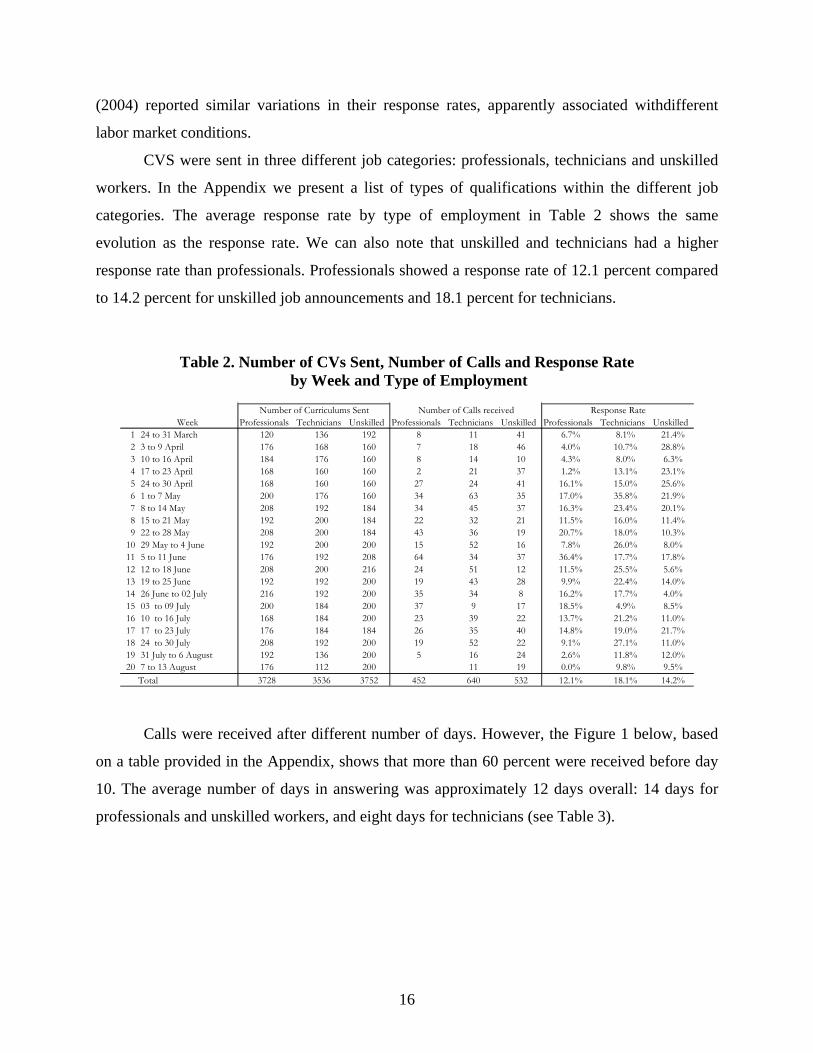
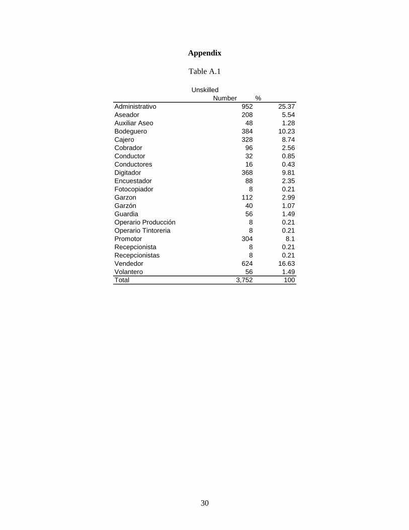
CVS were sent in three different job categories: professionals, technicians and unskilled

workers. In the Appendix we present a list of types of qualifications within the different job

categories. The average response rate by type of employment in Table 2 shows the same

evolution as the response rate. We can also note that unskilled and technicians had a higher

response rate than professionals. Professionals showed a response rate of 12.1 percent compared

to 14.2 percent for unskilled job announcements and 18.1 percent for technicians.

Table 2. Number of CVs Sent, Number of Calls and Response Rate by Week and Type of Employment

Week Professionals Technicians Unskilled Professionals Technicians Unskilled Professionals Technicians Unskilled1 24 to 31 March 120 136 192 8 11 41 6.7% 8.1% 21.4%2 3 to 9 April 176 168 160 7 18 46 4.0% 10.7% 28.8%3 10 to 16 April 184 176 160 8 14 10 4.3% 8.0% 6.3%4 17 to 23 April 168 160 160 2 21 37 1.2% 13.1% 23.1%5 24 to 30 April 168 160 160 27 24 41 16.1% 15.0% 25.6%6 1 to 7 May 200 176 160 34 63 35 17.0% 35.8% 21.9%7 8 to 14 May 208 192 184 34 45 37 16.3% 23.4% 20.1%8 15 to 21 May 192 200 184 22 32 21 11.5% 16.0% 11.4%9 22 to 28 May 208 200 184 43 36 19 20.7% 18.0% 10.3%

10 29 May to 4 June 192 200 200 15 52 16 7.8% 26.0% 8.0%11 5 to 11 June 176 192 208 64 34 37 36.4% 17.7% 17.8%12 12 to 18 June 208 200 216 24 51 12 11.5% 25.5% 5.6%13 19 to 25 June 192 192 200 19 43 28 9.9% 22.4% 14.0%14 26 June to 02 July 216 192 200 35 34 8 16.2% 17.7% 4.0%15 03 to 09 July 200 184 200 37 9 17 18.5% 4.9% 8.5%16 10 to 16 July 168 184 200 23 39 22 13.7% 21.2% 11.0%17 17 to 23 July 176 184 184 26 35 40 14.8% 19.0% 21.7%18 24 to 30 July 208 192 200 19 52 22 9.1% 27.1% 11.0%19 31 July to 6 August 192 136 200 5 16 24 2.6% 11.8% 12.0%20 7 to 13 August 176 112 200 11 19 0.0% 9.8% 9.5%

Total 3728 3536 3752 452 640 532 12.1% 18.1% 14.2%

Number of Curriculums Sent Number of Calls received Response Rate

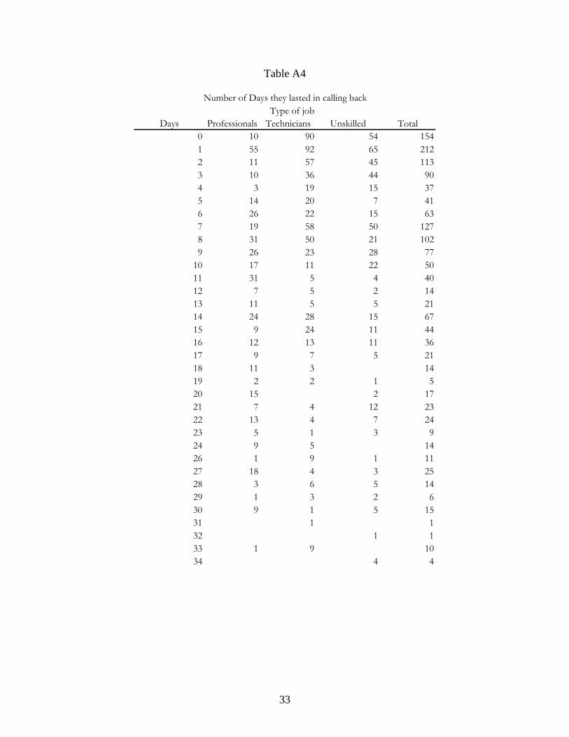
Calls were received after different number of days. However, the Figure 1 below, based

on a table provided in the Appendix, shows that more than 60 percent were received before day

10. The average number of days in answering was approximately 12 days overall: 14 days for

professionals and unskilled workers, and eight days for technicians (see Table 3).

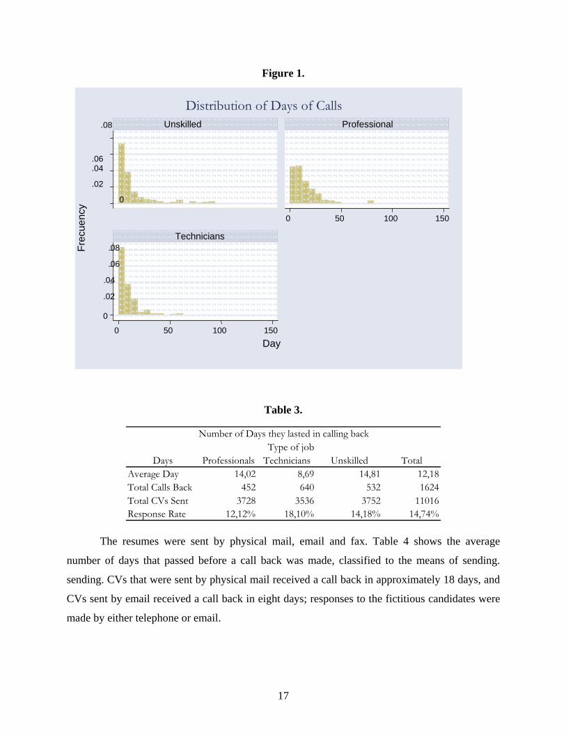
17

Figure 1.

Table 3.

Days Professionals Technicians UnskilledAverage Day 14,02 8,69 14,81 12,18Total Calls Back 452 640 532 1624Total CVs Sent 3728 3536 3752 11016Response Rate 12,12% 18,10% 14,18% 14,74%

Number of Days they lasted in calling backType of job

Total

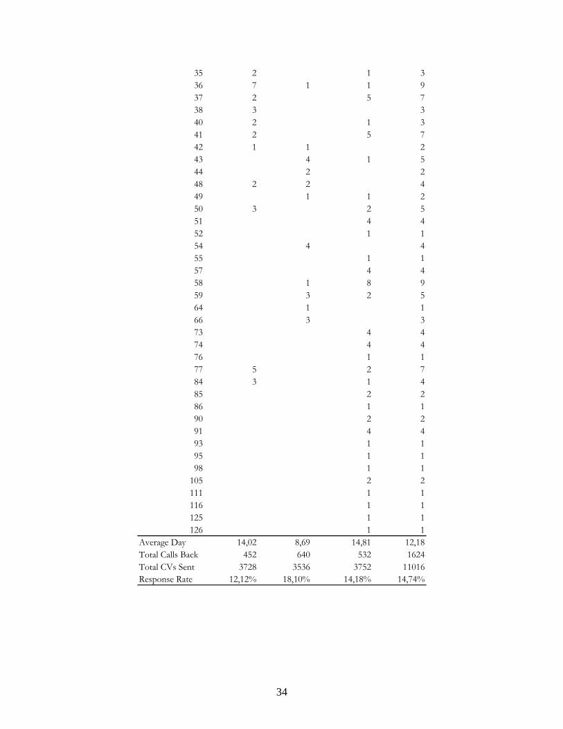
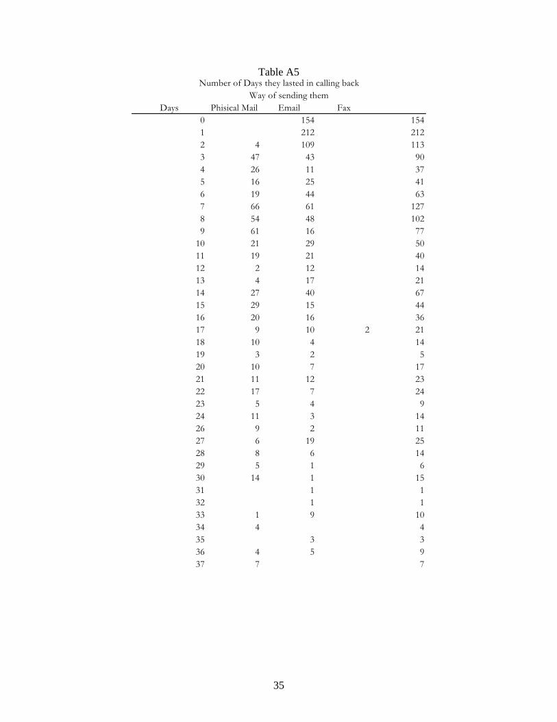
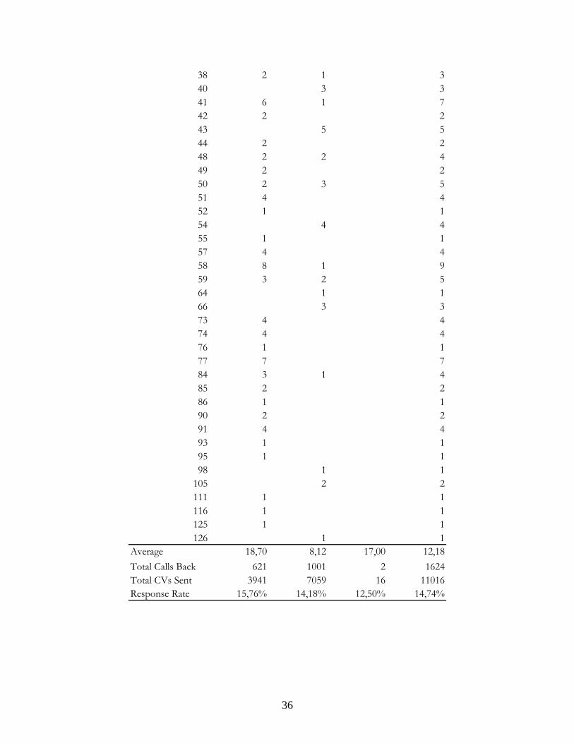
The resumes were sent by physical mail, email and fax. Table 4 shows the average

number of days that passed before a call back was made, classified to the means of sending.

sending. CVs that were sent by physical mail received a call back in approximately 18 days, and

CVs sent by email received a call back in eight days; responses to the fictitious candidates were

made by either telephone or email.

0

.02

.04

.06

.08

0

.02

.04

.06

.08

0 50 100 150

0 50 100 150

Unskilled Professional

Technicians

Frec

uenc

y

Day

Distribution of Days of Calls

18

Table 4.

Days Phisical Mail Email FaxAverage 18,70 8,12 17,00 12,18Total Calls Back 621 1001 2 1624Total CVs Sent 3941 7059 16 11016Response Rate 15,76% 14,18% 12,50% 14,74%

Number of Days they lasted in calling backWay of sending them

Total

We will now examine the average response rate by the three dimensions considered in

this paper.

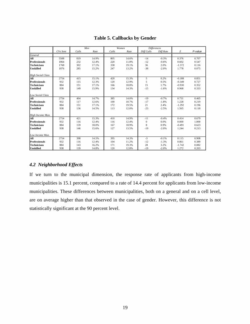
4.1 Gender Effects When we consider gender based-information, the response rates show very similar levels: 14.9

percent for men and 14.6 percent for women. This difference is small and not statistically

significant (applying a test where the null hypothesis is the equality of the two proportions). In

other words, men and women seem to have the same probability of being called for an

interview.

When the gender-based difference is examined within the Upper Class group (by

surnames), women registered a slightly higher response rate than men (15.3 percent versus 15.1

percent). Among CVs with Lower Class surnames, however, men received higher response rates

(14.7 percent versus 14 percent for women). These differences, however, were not statistically

significant.

19

Table 5. Callbacks by Gender

CVs Sent Calls Rate Calls Rate Diff Calls Diff Rate Z P-value

GeneralAll 5508 819 14.9% 805 14.6% -14 -0.3% 0.376 0.707Professionals 1864 232 12.4% 220 11.8% -12 -0.6% 0.602 0.547Technicians 1768 302 17.1% 338 19.1% 36 2.0% -1.572 0.116Unskilled 1876 285 15.2% 247 13.2% -38 -2.0% 1.778 0.075

High Social ClassAll 2754 415 15.1% 420 15.3% 5 0.2% -0.188 0.851Professionals 932 115 12.3% 120 12.9% 5 0.5% -0.349 0.727Technicians 884 151 17.1% 166 18.8% 15 1.7% -0.930 0.352Unskilled 938 149 15.9% 134 14.3% -15 -1.6% 0.968 0.333

Low Social ClassAll 2754 404 14.7% 385 14.0% -19 -0.7% 0.731 0.465Professionals 932 117 12.6% 100 10.7% -17 -1.8% 1.228 0.219Technicians 884 151 17.1% 172 19.5% 21 2.4% -1.292 0.196Unskilled 938 136 14.5% 113 12.0% -23 -2.5% 1.565 0.118

High Income Mun.All 2754 421 15.3% 410 14.9% -11 -0.4% 0.414 0.679Professionals 932 116 12.4% 116 12.4% 0 0.0% 0.000 1.000Technicians 884 159 18.0% 167 18.9% 8 0.9% -0.491 0.623Unskilled 938 146 15.6% 127 13.5% -19 -2.0% 1.244 0.213

Low Income Mun.All 2754 398 14.5% 395 14.3% -3 -0.1% 0.115 0.908Professionals 932 116 12.4% 104 11.2% -12 -1.3% 0.861 0.389Technicians 884 143 16.2% 171 19.3% 28 3.2% -1.742 0.082Unskilled 938 139 14.8% 120 12.8% -19 -2.0% 1.272 0.203

WomenMen Differences

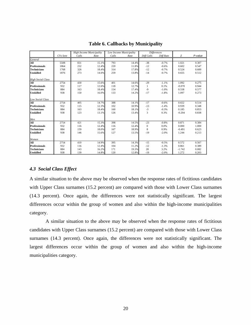
4.2 Neighborhood Effects If we turn to the municipal dimension, the response rate of applicants from high-income

municipalities is 15.1 percent, compared to a rate of 14.4 percent for applicants from low-income

municipalities. These differences between municipalities, both on a general and on a cell level,

are on average higher than that observed in the case of gender. However, this difference is not

statistically significant at the 90 percent level.

20

Table 6. Callbacks by Municipality

CVs Sent Calls Rate Calls Rate Diff Calls Diff Rate Z P-valueGeneralAll 5508 831 15.1% 793 14.4% -38 -0.7% 1.021 0.307Professionals 1864 232 12.4% 220 11.8% -12 -0.6% 0.602 0.547Technicians 1768 326 18.4% 314 17.8% -12 -0.7% 0.524 0.600Unskilled 1876 273 14.6% 259 13.8% -14 -0.7% 0.655 0.512

High Social ClassAll 2754 430 15.6% 401 14.6% -29 -1.1% 1.092 0.275Professionals 932 117 12.6% 118 12.7% 1 0.1% -0.070 0.944Technicians 884 163 18.4% 154 17.4% -9 -1.0% 0.558 0.577Unskilled 938 150 16.0% 133 14.2% -17 -1.8% 1.097 0.273

Low Social ClassAll 2754 405 14.7% 388 14.1% -17 -0.6% 0.652 0.514Professionals 932 115 12.3% 102 10.9% -13 -1.4% 0.939 0.348Technicians 884 163 18.4% 160 18.1% -3 -0.3% 0.185 0.853Unskilled 938 123 13.1% 126 13.4% 3 0.3% -0.204 0.838

MenAll 2754 421 15.3% 398 14.5% -23 -0.8% 0.871 0.384Professionals 932 116 12.4% 116 12.4% 0 0.0% 0.000 1.000Technicians 884 159 18.0% 167 18.9% 8 0.9% -0.491 0.623Unskilled 938 146 15.6% 127 13.5% -19 -2.0% 1.244 0.213

WomenAll 2754 410 14.9% 395 14.3% -15 -0.5% 0.572 0.567Professionals 932 116 12.4% 104 11.2% -12 -1.3% 0.861 0.389Technicians 884 143 16.2% 171 19.3% 28 3.2% -1.742 0.082Unskilled 938 139 14.8% 120 12.8% -19 -2.0% 1.272 0.203

Low Income MunicipalityHigh Income Municipality Differences

4.3 Social Class Effect A similar situation to the above may be observed when the response rates of fictitious candidates

with Upper Class surnames (15.2 percent) are compared with those with Lower Class surnames

(14.3 percent). Once again, the differences were not statistically significant. The largest

differences occur within the group of women and also within the high-income municipalities

category.

A similar situation to the above may be observed when the response rates of fictitious

candidates with Upper Class surnames (15.2 percent) are compared with those with Lower Class

surnames (14.3 percent). Once again, the differences were not statistically significant. The

largest differences occur within the group of women and also within the high-income

municipalities category.

21

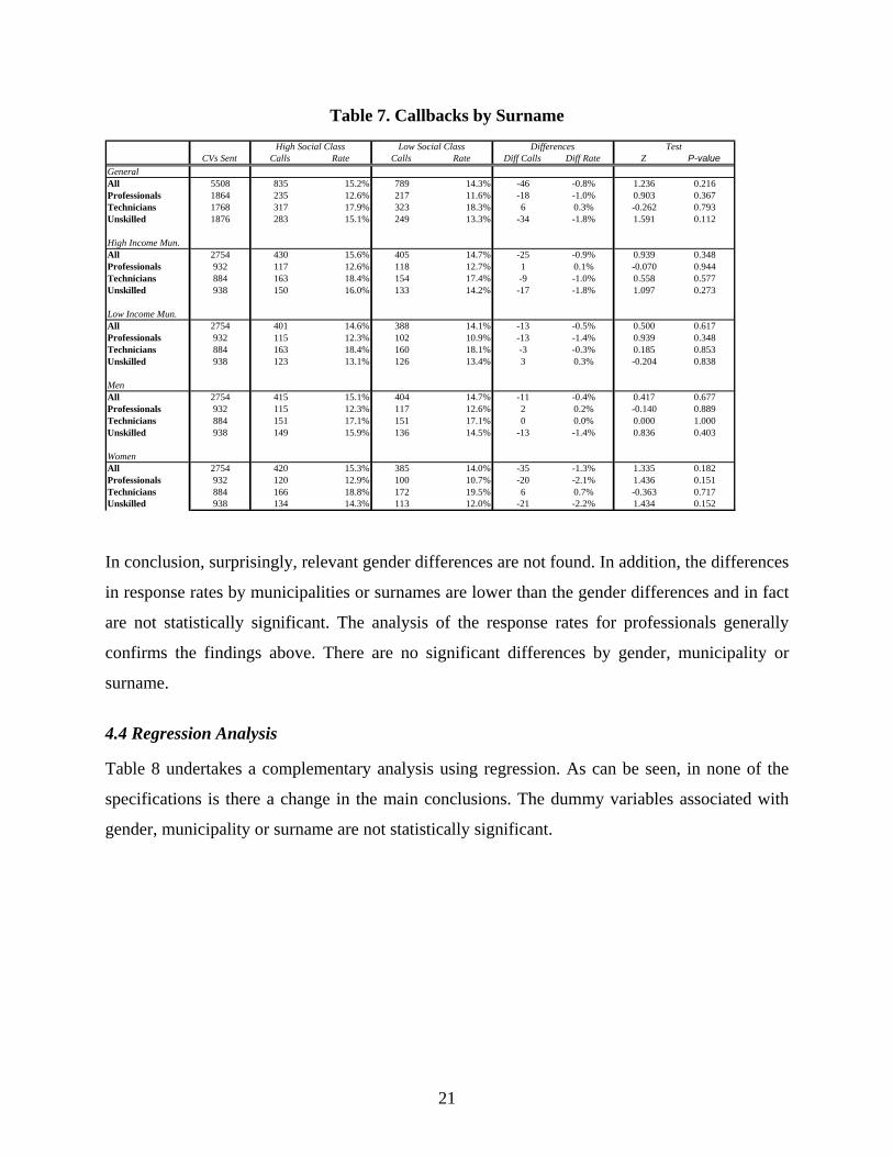
Table 7. Callbacks by Surname

CVs Sent Calls Rate Calls Rate Diff Calls Diff Rate Z P-valueGeneralAll 5508 835 15.2% 789 14.3% -46 -0.8% 1.236 0.216Professionals 1864 235 12.6% 217 11.6% -18 -1.0% 0.903 0.367Technicians 1768 317 17.9% 323 18.3% 6 0.3% -0.262 0.793Unskilled 1876 283 15.1% 249 13.3% -34 -1.8% 1.591 0.112

High Income Mun.All 2754 430 15.6% 405 14.7% -25 -0.9% 0.939 0.348Professionals 932 117 12.6% 118 12.7% 1 0.1% -0.070 0.944Technicians 884 163 18.4% 154 17.4% -9 -1.0% 0.558 0.577Unskilled 938 150 16.0% 133 14.2% -17 -1.8% 1.097 0.273

Low Income Mun.All 2754 401 14.6% 388 14.1% -13 -0.5% 0.500 0.617Professionals 932 115 12.3% 102 10.9% -13 -1.4% 0.939 0.348Technicians 884 163 18.4% 160 18.1% -3 -0.3% 0.185 0.853Unskilled 938 123 13.1% 126 13.4% 3 0.3% -0.204 0.838

MenAll 2754 415 15.1% 404 14.7% -11 -0.4% 0.417 0.677Professionals 932 115 12.3% 117 12.6% 2 0.2% -0.140 0.889Technicians 884 151 17.1% 151 17.1% 0 0.0% 0.000 1.000Unskilled 938 149 15.9% 136 14.5% -13 -1.4% 0.836 0.403

WomenAll 2754 420 15.3% 385 14.0% -35 -1.3% 1.335 0.182Professionals 932 120 12.9% 100 10.7% -20 -2.1% 1.436 0.151Technicians 884 166 18.8% 172 19.5% 6 0.7% -0.363 0.717Unskilled 938 134 14.3% 113 12.0% -21 -2.2% 1.434 0.152

Low Social Class Differences TestHigh Social Class

In conclusion, surprisingly, relevant gender differences are not found. In addition, the differences

in response rates by municipalities or surnames are lower than the gender differences and in fact

are not statistically significant. The analysis of the response rates for professionals generally

confirms the findings above. There are no significant differences by gender, municipality or

surname.

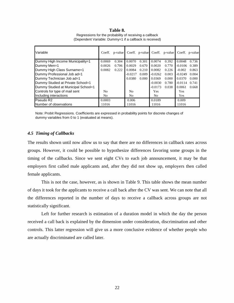
4.4 Regression Analysis Table 8 undertakes a complementary analysis using regression. As can be seen, in none of the

specifications is there a change in the main conclusions. The dummy variables associated with

gender, municipality or surname are not statistically significant.

22

Table 8.

Variable Coeff. p-value Coeff. p-value Coeff. p-value Coeff. p-value

Dummy High Income Municipality=1 0.0069 0.304 0.0070 0.301 0.0074 0.392 0.0048 0.736Dummy Men=1 0.0026 0.706 0.0029 0.670 0.0020 0.770 -0.0106 0.389Dummy High Class Surname=1 0.0082 0.222 0.0084 0.210 0.0082 0.226 -0.002 0.863Dummy Professional Job ad=1 -0.0217 0.009 -0.0262 0.003 -0.0249 0.004Dummy Technician Job ad=1 0.0380 0.000 0.0369 0.000 0.0370 0.000Dummy Studied at Private School=1 -0.0030 0.780 -0.0114 0.741Dummy Studied at Municipal School=1 -0.0173 0.038 0.0061 0.668Controls for type of mail sent No No Yes YesIncluding interactions No No No YesPseudo R2 0.0003 0.006 0.0189 0.009Number of observations 11016 11016 11016 11016

Note: Probit Regressions. Coefficients are expressed in probability points for discrete changes ofdummy variables from 0 to 1 (evaluated at means).

Regressions for the probability of receiving a callback(Dependent Variable: Dummy=1 if a callback is received)

4.5 Timing of Callbacks The results shown until now allow us to say that there are no differences in callback rates across

groups. However, it could be possible to hypothesize differences favoring some groups in the

timing of the callbacks. Since we sent eight CVs to each job announcement, it may be that

employers first called male applicants and, after they did not show up, employers then called

female applicants.

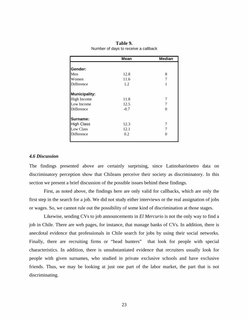
This is not the case, however, as is shown in Table 9. This table shows the mean number

of days it took for the applicants to receive a call back after the CV was sent. We can note that all

the differences reported in the number of days to receive a callback across groups are not

statistically significant.

Left for further research is estimation of a duration model in which the day the person

received a call back is explained by the dimension under consideration, discrimination and other

controls. This latter regression will give us a more conclusive evidence of whether people who

are actually discriminated are called later.

23

Table 9.

Mean Median

Gender:Men 12.8 8Women 11.6 7Difference 1.2 1

Municipality:High Income 11.8 7Low Income 12.5 7Difference -0.7 0

Surname:High Class 12.3 7Low Class 12.1 7Difference 0.2 0

Number of days to receive a callback

4.6 Discussion The findings presented above are certainly surprising, since Latinobarómetro data on

discriminatory perception show that Chileans perceive their society as discriminatory. In this

section we present a brief discussion of the possible issues behind these findings.

First, as noted above, the findings here are only valid for callbacks, which are only the

first step in the search for a job. We did not study either interviews or the real assignation of jobs

or wages. So, we cannot rule out the possibility of some kind of discrimination at those stages.

Likewise, sending CVs to job announcements in El Mercurio is not the only way to find a

job in Chile. There are web pages, for instance, that manage banks of CVs. In addition, there is

anecdotal evidence that professionals in Chile search for jobs by using their social networks.

Finally, there are recruiting firms or “head hunters” that look for people with special

characteristics. In addition, there is unsubstantiated evidence that recruiters usually look for

people with given surnames, who studied in private exclusive schools and have exclusive

friends. Thus, we may be looking at just one part of the labor market, the part that is not

discriminating.

24

Additionally, we use a different experimental design than Bertrand and Mullainathan

(2004). We argue, however, that our methodology is more robust. While we constructed equally

qualified CVs and then assigned names, those authors took samples of CVs from the real world

and assigned them different name using the same share of population groups as in the real world.

This difference has two major implications that may in turn raise additional questions. First,

constructing a world that does not exist fact helps us to have a real exogenous variation. Second,

this world may differ so much from the real world that employers could have applied a kind of

positive discrimination. They could have thought “if this person, under these circumstances,

reaches such level of education and experience, she or he must be good applicant.”

Finally, it is still surprising that, although Bertrand and Mullainathan (2004) found

statistically significant differences among surnames associated with African-American versus

white population groups, we did not find similar results in our study. This may mean that

discrimination in the United States is deeper than in Chile, which, unlike other Latin American

countries such as Bolivia, Peru or Brazil, does not display a great deal of racial diversity. The

country’s population is overwhelmingly of European descent, with only a small percentage of

indigenous population. In addition, the type of discrimination we are looking at it may indeed be

related to historical factors of inequality of opportunities rather than subjective discrimination.

5. Conclusions The objective of this paper is to study the Chilean labor market and determine the presence or

absence of gender discrimination. In order to transcend the limitations of earlier works, an

experimental design is used, the first of its kind in Chile. This design also makes it possible to

address socioeconomic discrimination associated with names and places of residence in the

Chilean labor market to be tackled.

The study consists of sending fictitious Curriculum Vitae for real job vacancies published

weekly in the Santiago newspaper El Mercurio. A range of strictly equivalent CVs in terms of

qualifications and employment experience of applicants was sent out, only varying in gender,

name and surname, and place of residence. The study allows differences in call response rates to

be measured for the various demographic groups.

We find no statistically significant differences in callbacks for any of the groups we

explore: gender, socioeconomic background and place of residence. The findings are surprising

25

and generate new questions. We discuss several issues that may be behind these findings. In

particular, we are only considering one step in the hiring process, the callback, and not the

complete behavior of the labor market. We leave for further research the use of duration models

to estimate different effects of the timing of the call.

26

References Adimark. “Mapa Socioeconómico de Chile: Nivel socioeconómico de los hogares del país

basado en datos del Censo.” Santiago, Chile: Adimark.

Altonji, J., and R. Blank. 1999. “Race and Gender in the Labor Market.” In: O. Ashenfelter and

D. Card, editors. Handbook of Labor Economics. Volume 3. Amsterdam, The

Netherlands: North Holland.

Anderson, L., R. Fryer and C. Holt. 2006. “Discrimination: Experimental Evidence from

Psychology and Economics.” In: W. Rogers, editor. Handbook on the Economics and

Discrimination. Cheltenham, United Kingdom: Elgar.

Antonovics, K., Peter Arcidiacono and R. Walsh. 2004. “Competing Against the Opposite Sex.”

Economics Working Paper Series 2003-08. San Diego, United States: University of

California at San Diego.

----. 2005. “Games and Discrimination: Lessons from The Weakest Link.” Journal of Human

Resources 40(4): 918-947.

Arenas, A. J. Behrman and D. Bravo. 2004. “Characteristics of and Determinants of the Density

of Contributions in a Private Social Security System.” Working Paper 077. Ann Arbor,

United States: University of Michigan, Michigan Retirement Research Center.

Becker, G. 1971. The Economics of Discrimination. Second edition. Chicago, United States:

University of Chicago Press.

----. 1991. A Treatise on the Family. Enlarged edition. Cambridge, United States: Harvard

University Press.

Bertrand, M., and S. Mullainathan. 2004. “Are Emily and Greg More Employable than Lakisha

and Jamal? A Field Experiment on Labor Market Discrimination.” American Economic

Review 94(4): 991-1013.

Blank, R., M. Dabady and Constance Citro, editors. 2004. Measuring Racial Discrimination:

Panel on Methods for Assessing Discrimination. Washington, DC, United States:

National Academies Press.

Blinder, A. 1973. “Wage Discrimination: Reduced Form and Structural Estimates.” Journal of

Human Resources 7(4): 436-55.

27

Bravo, D. 2004. “Análisis y principales resultados: Primera Encuesta de Protecciòn Social.”

Santiago, Chile: Universidad de Chile, Departamento de Economía, and Ministerio del

Trabajo y Previsión Social.

----. 2005. “Elaboración, Validación y Difusión de Índice Nacional de Calidad del Empleo

Femenino.” Report prepared for the Secretary of Gender (Ministerio Servicio Nacional

de la Mujer). Santiago, Chile: Universidad de Chile: Centro de Microdatos.

Contreras, D., and G. Plaza. 2004. “Participación Femenina en el Mercado Laboral Chileno.

¿Cuánto importan los factores culturales?” Santiago, Chile: Universdiad de Chile:

Departamento de Economía.

Contreras, D., and E. Puentes. 2001. “Is Gender Wage Discrimination Decreasing In Chile?

Thirty Years Of ‘Robust’ Evidence.” Santiago, Chile: Universdiad de Chile:

Departamento de Economía.

Fernandez, R., A. Fogli and C. Olivetti. 2004. “Preference Formation and The Rise Of Women’s

Labor Force Participation: Evidence From WWII.” NBER Working Paper 10589.

Cambridge, United States: National Bureau of Economic Research.

Goldin, C., and C. Rouse. 2000. “Orchestrating Impartiality: The Impact of ‘Blind’ Auditions on

Female Musicians.” American Economic Review 90(4): 715-741.

Heckman, J. 1998. “Detecting Discrimination.” Journal of Economic Perspectives 12(2): 101-

116.

Heckman, J., and P. Siegelman. 1993. “The Urban Institute Audit Studies: Their Methods and

Findings.” In: M. Fix and R. Struyk, editors. Clear and Convincing Evidence: Measure of

Discrimination in America. Washington, DC, United States: Urban Institute Press.

Heckman, J., J. Stixrud and S. Urzúa. 2006. “The Effects of Cognitive and Noncognitive

Abilities on Labor Market Outcomes and Social Behavior.” Journal of Labor Economics

24(3): 411-482.

Levitt, S. 2004. “Testing Theories of Discrimination. Evidence from ‘The Weakest Link.’”

Journal of Law and Economics 47: 431-452.

List, J. 2003. “The Nature and Extent of Discrimination in the Marketplace: Evidence from the

Field.” Quarterly Journal of Economics 119(1): 49-89.

Montenegro, C. 1999. “Wage Distribution in Chile: Does Gender Matter? A Quantile Regression

Approach.” Santiago, Chile: Universidad de Chile. Mimeographed document.

28

Montenegro, C., and R. Paredes. 1999. “Gender Wage Gap and Discrimination: A Long-Term

View Using Quantile Regression.” Santiago, Chile: Universidad de Chile. Mimeographed

document.

Moreno, M. et al. 2004. “Gender and Racial Discrimination in Hiring. A Pseudo-Audit Study for

Three Selected Occupations in Metropolitan Lima.” IZA Discussion Paper 979. Bonn,

Germany: Institute for the Study of Labor (IZA).

Neal, D.A., and W.R. Johnson. A. and William R. and Johnson. 1996. “The Role of Premarket

Factors in Black-White Wage Differences.” Journal of Political Economy 104(5): 869-

895.

Newmark, D., Roy J. Bank and K.D. Van Nort. 1996. “Sex Discrimination in Restaurant Hiring:

An Audit Study.” Quarterly Journal of Economics 111(3): 915-941.

Núñez, J., and R. Gutiérrez. 2004. “Classism, Discrimination and Meritocracy in the Labor

Market: The Case of Chile.” Documento de Trabajo 208. Santiago, Chile: Universidad de

Chile: Departamento de Economia.

Ñopo, H. 2004. “Matching as a Tool to Decompose Wage Gaps.” IZA Discussion Paper 981.

Bonn, Germany: Institute for the Study of Labor (IZA).

Oaxaca, R. 1973. “Male-Female Wage Differentials in Urban Labor Markets.” International

Economic Review 14(3): 693-709.

O’Neil, J.E., and D.M. M. O’Neil. 2005. “What Do Wage Differentials Tell Us about Labor

Market Discrimination.” NBER Working Paper 11240. Cambridge, United States:

National Bureau of Economic Research.

Paredes, R., and L. Riveros. 1994. “Gender Wage Gaps in Chile: A Long-Term View: 1958-

1990.” Estudios de Economía 21(Número especial).

Riach, P., and J. Rich. 2002. “Field Experiments of Discrimination in the Marketplace.”

Economic Journal 112: 480-518.

----. 2004. “Deceptive Field Experiments of Discrimination: Are they Ethical?” KYKLOS 57(3):

457-470.

Rosenberg, M. 1965. Society and the Adolescent Self-Image. Princeton, United States: Princeton

University Press.

29

Rotter, J.B. 1966. “Generalized Expectancies for Internal versus External Control of

Reinforcement.” Psychological Monographs 80. Washington, DC, United States:

American Psychological Association.

30

Appendix

Table A.1

Number %Administrativo 952 25.37Aseador 208 5.54Auxiliar Aseo 48 1.28Bodeguero 384 10.23Cajero 328 8.74Cobrador 96 2.56Conductor 32 0.85Conductores 16 0.43Digitador 368 9.81Encuestador 88 2.35Fotocopiador 8 0.21Garzon 112 2.99Garzón 40 1.07Guardia 56 1.49Operario Producción 8 0.21Operario Tintoreria 8 0.21Promotor 304 8.1Recepcionista 8 0.21Recepcionistas 8 0.21Vendedor 624 16.63Volantero 56 1.49Total 3,752 100

Unskilled

31

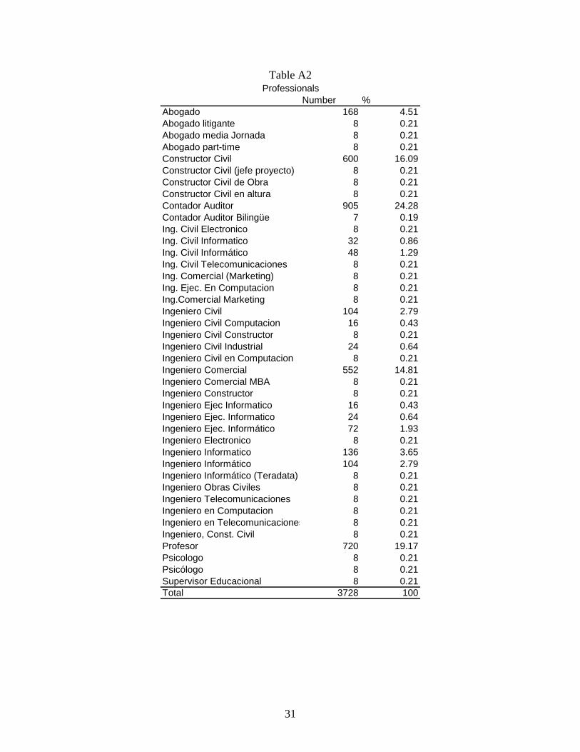
Table A2

Number %Abogado 168 4.51Abogado litigante 8 0.21Abogado media Jornada 8 0.21Abogado part-time 8 0.21Constructor Civil 600 16.09Constructor Civil (jefe proyecto) 8 0.21Constructor Civil de Obra 8 0.21Constructor Civil en altura 8 0.21Contador Auditor 905 24.28Contador Auditor Bilingüe 7 0.19Ing. Civil Electronico 8 0.21Ing. Civil Informatico 32 0.86Ing. Civil Informático 48 1.29Ing. Civil Telecomunicaciones 8 0.21Ing. Comercial (Marketing) 8 0.21Ing. Ejec. En Computacion 8 0.21Ing.Comercial Marketing 8 0.21Ingeniero Civil 104 2.79Ingeniero Civil Computacion 16 0.43Ingeniero Civil Constructor 8 0.21Ingeniero Civil Industrial 24 0.64Ingeniero Civil en Computacion 8 0.21Ingeniero Comercial 552 14.81Ingeniero Comercial MBA 8 0.21Ingeniero Constructor 8 0.21Ingeniero Ejec Informatico 16 0.43Ingeniero Ejec. Informatico 24 0.64Ingeniero Ejec. Informático 72 1.93Ingeniero Electronico 8 0.21Ingeniero Informatico 136 3.65Ingeniero Informático 104 2.79Ingeniero Informático (Teradata) 8 0.21Ingeniero Obras Civiles 8 0.21Ingeniero Telecomunicaciones 8 0.21Ingeniero en Computacion 8 0.21Ingeniero en Telecomunicaciones 8 0.21Ingeniero, Const. Civil 8 0.21Profesor 720 19.17Psicologo 8 0.21Psicólogo 8 0.21Supervisor Educacional 8 0.21Total 3728 100

Professionals

32

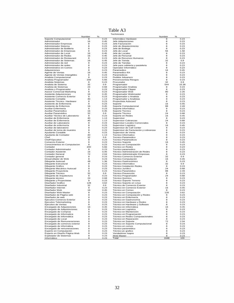
Table A3 Number % Number %

Soporte Computacional 8 0.23 Informático Hardware 8 0.23Administrador 16 0.45 Jefe Adquisiciones 8 0.23Administrador Empresas 8 0.23 Jefe Facturación 8 0.23Administrador Sistema 8 0.23 Jefe de Abastecimiento 8 0.23Administrador de Botilleria 8 0.23 Jefe de Bodega 8 0.23Administrador de Empresas 8 0.23 Jefe de Local 56 1.58Administrador de Local 16 0.45 Jefe de Locales 8 0.23Administrador de Redes 16 0.45 Jefe de Personal 8 0.23Administrador de Restaurant 8 0.23 Jefe de Recursos Humanos 8 0.23Administrador de Sistemas 16 0.45 Jefe de Tienda 32 0.9Administrador de red 8 0.23 Jefe de Tiendas 8 0.23Administrador de redes 8 0.23 Jefe para cafeteria y pasteleria 8 0.23Administrativo en Comex 8 0.23 Operador Informático 8 0.23Adquisiciones 8 0.23 Paramedico 16 0.45Agente de Ventas 16 0.45 Paramedico RX 8 0.23Agente de Ventas Intangibles 8 0.23 Paramedicos 8 0.23Analista Computacional 8 0.23 Pedidor Aduanero 8 0.23Analista Programador 200 5.66 Prevencionista Riesgos 8 0.23Analista Sistemas 8 0.23 Procurador 32 0.9Analista de Sistema 32 0.9 Programador 544 15.38Analista de Sistemas 24 0.68 Programador Analista 8 0.23Analista o Programador 8 0.23 Programador Clipper 8 0.23Asesor Comercial Marketing 8 0.23 Programador Web 80 2.26Asistente Adquisiciones 16 0.45 Programador Webmaster 8 0.23Asistente Comercio Exterior 8 0.23 Programador o Analista 8 0.23Asistente Contable 40 1.13 Programador y Analistas 8 0.23Asistente Técnico Hardware 8 0.23 Proyectista Autocard 8 0.23Asistente de Enfermeria 8 0.23 Soporte 16 0.45Asistente de Enfermos 16 0.45 Soporte Computacional 88 2.49Auxiliar Enfermería 8 0.23 Soporte Informático 8 0.23Auxiliar Paramedico 16 0.45 Soporte Tecnico 8 0.23Auxiliar Paramédico 32 0.9 Soporte Técnico 24 0.68Auxiliar Técnico de Laboratorio 8 0.23 Soporte en Redes 16 0.45Auxiliar de Enfermeria 40 1.13 Supervisor 8 0.23Auxiliar de Enfermería 40 1.13 Supervisor Cobranzas 24 0.68Auxiliar de Laboratorio 8 0.23 Supervisor Locales Comerciales 8 0.23Auxiliar de enfermería 8 0.23 Supervisor Logístico 16 0.45Auxiliar de laboratorio 8 0.23 Supervisor de Call Center 8 0.23Auxiliar de toma de muestra 8 0.23 Supervisor de Facturación y cobranzas 8 0.23Ayudante Contable 8 0.23 Supervisor de Venta 8 0.23Ayudante de Contador 40 1.13 Tecnico Informatico 8 0.23Chef 32 0.9 Tecnico Paramedico 8 0.23Cheff Ejecutivo 8 0.23 Tecnico Paramedicos 8 0.23Comercio Exterior 8 0.23 Tecnico Soporte 16 0.45Conocimientos en Computacion 8 0.23 Tecnico en Computación 8 0.23Contador 200 5.66 Tecnico en Redes 8 0.23Contador Administrador 8 0.23 Tecnico paramedico 8 0.23Contador Asistente 16 0.45 Técnico Administración de Redes 8 0.23Contador General 72 2.04 Técnico Administrador Empresas 8 0.23Contador general 8 0.23 Técnico Comercio Exterior 32 0.9Desarrollador de Web 8 0.23 Técnico Computación 16 0.45Dibujante Autocad 48 1.36 Técnico Gastronómico 8 0.23Dibujante Estructural 8 0.23 Técnico Informático 32 0.9Dibujante Gráfico 8 0.23 Técnico Instalación Redes 8 0.23Dibujante Mecánico Autocad 8 0.23 Técnico Jurídico 24 0.68Dibujante Proyecticta 8 0.23 Técnico Paramédico 88 2.49Dibujante Técnico 32 0.9 Técnico Prevención 8 0.23Dibujante de Arquitectura 8 0.23 Técnico Programador 24 0.68Dibujante técnico 24 0.68 Técnico Químico 8 0.23Dibujante y Proyectistas 8 0.23 Técnico Soporte Terreno 8 0.23Diseñador Gráfico 128 3.62 Técnico Soporte en Linux 8 0.23Diseñador Industrial 32 0.9 Técnico de Comercio Exterior 8 0.23Diseñador Internet 8 0.23 Técnico en Comercio Exterior 16 0.45Diseñador Web 16 0.45 Técnico en Comex 8 0.23Diseñador Web Master 8 0.23 Técnico en Computación 128 3.62Diseñador de Página web 8 0.23 Técnico en Computación y Redes 8 0.23Diseñador de web 8 0.23 Técnico en Enfermería 8 0.23Ejecutivo Comercio Exterior 8 0.23 Técnico en Gastronomía 8 0.23Ejecutivo Telemarketing 8 0.23 Técnico en Hardware y Redes 8 0.23Ejecutivo de Ventas 8 0.23 Técnico en Hardware y Software 8 0.23Encargado de Adquisiciones 16 0.45 Técnico en Informática 16 0.45Encargado de Adquisisciones 8 0.23 Técnico en Logística 8 0.23Encargado de Compras 8 0.23 Técnico en Mantención 8 0.23Encargado de Informatica 8 0.23 Técnico en Programación 8 0.23Encargado de Informática 8 0.23 Técnico en Redes Computacionales 8 0.23Encargado de Local 8 0.23 Técnico en Reparación 8 0.23Encargado de Remuneraciones 8 0.23 Técnico en Soporte 72 2.04Encargado de comercio exterior 8 0.23 Técnico en Soporte Computacional 8 0.23Encargado de informática 8 0.23 Técnico en comex 8 0.23Encargado de remuneraciones 8 0.23 Técnico paramédico 8 0.23Experto en Computación 8 0.23 Técnico pc grafico 8 0.23Experto en Diseño Página Web 8 0.23 Vendedores Isapre 8 0.23Explotador de Sistemas 8 0.23 Web Master 8 0.23Informático 8 0.23 Total 1648 100

Technicians

33

Table A4

Days Professionals Technicians Unskilled0 10 90 54 1541 55 92 65 2122 11 57 45 1133 10 36 44 904 3 19 15 375 14 20 7 416 26 22 15 637 19 58 50 1278 31 50 21 1029 26 23 28 77

10 17 11 22 5011 31 5 4 4012 7 5 2 1413 11 5 5 2114 24 28 15 6715 9 24 11 4416 12 13 11 3617 9 7 5 2118 11 3 1419 2 2 1 520 15 2 1721 7 4 12 2322 13 4 7 2423 5 1 3 924 9 5 1426 1 9 1 1127 18 4 3 2528 3 6 5 1429 1 3 2 630 9 1 5 1531 1 132 1 133 1 9 1034 4 4

Number of Days they lasted in calling backType of job

Total

34

35 2 1 336 7 1 1 937 2 5 738 3 340 2 1 341 2 5 742 1 1 243 4 1 544 2 248 2 2 449 1 1 250 3 2 551 4 452 1 154 4 455 1 157 4 458 1 8 959 3 2 564 1 166 3 373 4 474 4 476 1 177 5 2 784 3 1 485 2 286 1 190 2 291 4 493 1 195 1 198 1 1

105 2 2111 1 1116 1 1125 1 1126 1 1

Average Day 14,02 8,69 14,81 12,18Total Calls Back 452 640 532 1624Total CVs Sent 3728 3536 3752 11016Response Rate 12,12% 18,10% 14,18% 14,74%

35

Table A5

Days Phisical Mail Email Fax0 154 1541 212 2122 4 109 1133 47 43 904 26 11 375 16 25 416 19 44 637 66 61 1278 54 48 1029 61 16 77

10 21 29 5011 19 21 4012 2 12 1413 4 17 2114 27 40 6715 29 15 4416 20 16 3617 9 10 2 2118 10 4 1419 3 2 520 10 7 1721 11 12 2322 17 7 2423 5 4 924 11 3 1426 9 2 1127 6 19 2528 8 6 1429 5 1 630 14 1 1531 1 132 1 133 1 9 1034 4 435 3 336 4 5 937 7 7

Number of Days they lasted in calling backWay of sending them

36

38 2 1 340 3 341 6 1 742 2 243 5 544 2 248 2 2 449 2 250 2 3 551 4 452 1 154 4 455 1 157 4 458 8 1 959 3 2 564 1 166 3 373 4 474 4 476 1 177 7 784 3 1 485 2 286 1 190 2 291 4 493 1 195 1 198 1 1

105 2 2111 1 1116 1 1125 1 1126 1 1

Average 18,70 8,12 17,00 12,18Total Calls Back 621 1001 2 1624Total CVs Sent 3941 7059 16 11016Response Rate 15,76% 14,18% 12,50% 14,74%