essays on equality of opportunity and public policy ... - ddd-uab
TRANSCRIPT
ADVERTIMENT. Lʼaccés als continguts dʼaquesta tesi queda condicionat a lʼacceptació de les condicions dʼúsestablertes per la següent llicència Creative Commons: http://cat.creativecommons.org/?page_id=184
ADVERTENCIA. El acceso a los contenidos de esta tesis queda condicionado a la aceptación de las condiciones de usoestablecidas por la siguiente licencia Creative Commons: http://es.creativecommons.org/blog/licencias/
WARNING. The access to the contents of this doctoral thesis it is limited to the acceptance of the use conditions setby the following Creative Commons license: https://creativecommons.org/licenses/?lang=en
Essays on equality of opportunity and public policy
Gonzalo Salas
Supervised by Xavier Ramos
Dissertation Submitted to the Departament of Applied Economics at the Universitat Autònoma de Barcelona in partial fulfillment of the requirements for the degree of
Doctor of Philosophy in the subjet of Economics

ii

iii
Acknowledgements
I would like to give special thanks to my PhD director Xavier Ramos for his excellent advise and support. His academic insight, flexibility and patience has been invaluable. His observations and comments helped me to establish the direction of the research and identify the important and the superfluous. Also I would like to express my gratitude to Andrea Vigorito for her support throughout the process.
Special thanks has to go my partner Paula for sharing this experience with me and for her love and patience. I also thank my friends and parents. They were my support during this period. Finally, I thank the financial support of the Fundación Carolina and Instituto de Economía - Universidad de la República.

iv
v
Contents
General Introduction ..................................................................................................... 1
Preferences for redistribution: perceptions of fairness and equality of opportunity ........ 7
1.1 Introduction .................................................................................................................... 8
1.2 Preferences for redistribution and equality of opportunities ........................................... 11
1.3 The data ....................................................................................................................... 14
1.4 The conceptual framework and empirical strategy......................................................... 20
1.5 Baseline results ............................................................................................................ 24
1.6 Equality of opportunities and preferences for redistribution .......................................... 28
1.6.1 Preferences for redistribution according to income level in adolescence .................. 31
1.6.2 Preferences for redistribution according to labor, education and health circumstances ....................................................................................................................................... 34
1.7 Sensitivity of the results................................................................................................ 39
1.7.1 Sense of fairness and mobility................................................................................. 40
1.7.2 Altruism and reciprocity ......................................................................................... 47
Reference ............................................................................................................................ 52
Annex ................................................................................................................................. 55
Early childhood development, school attendance and parenting .................................. 57
2.1 Introduction ................................................................................................................... 58
2.2 Literature review ........................................................................................................... 62
2.3 Conceptual framework and identification strategy.......................................................... 65
2.3.1 Conceptual framework ............................................................................................ 65
2.3.2 Identification .......................................................................................................... 67
2.4 Description of the data ................................................................................................... 74
2.4.1 Characteristics of the child development tests ......................................................... 75
2.4.2 Parenting practices .................................................................................................. 79
2.4.3 Other characteristics of the mothers, children and the household ............................. 81
2.5 Main results .................................................................................................................. 83
2.5.1 Demand for schools ................................................................................................ 83
2.5.2 Variation in the MTE of school attendance ............................................................. 86
2.6 Conclusions ................................................................................................................. 102
References ........................................................................................................................ 105
Annex ............................................................................................................................... 109
vi
Inequality of opportunity, cash transfer and educational performance ........................ 125
3.1 Introduction ................................................................................................................. 126
3.2 Details of the PANES Program .................................................................................... 130
3.3 Empirical Strategy ....................................................................................................... 131
3.3.1 Measuring inequality of opportunity and the effects of the CT .............................. 131
3.3.2 Measuring effort ................................................................................................... 133
3.3.3 The circumstances ................................................................................................ 134
3.3.4 Econometric strategy and identification ............................................................... 138
3.3.5 Inequality of opportunity in the entire population ................................................. 140
3.4 Data ............................................................................................................................ 140
3.5 The impact of CTs on inequality of opportunity ........................................................... 144
3.5.1 PANES impact on inequality of opportunity in dropping out from the education system ........................................................................................................................... 146
3.5.2 PANES impact on inequality of opportunity in repetition due to poor grade .......... 152
3.5.3 Placebo Estimates ................................................................................................ 158
3.6 Conclusions ................................................................................................................ 159
Reference .......................................................................................................................... 162
Annex ............................................................................................................................... 166
Conclusions .............................................................................................................. 169
General Introduction
A good part of the discussion that economists and philosophers have had in recent decades is about the meaning of distributive justice and is synthesized by Amartya Sen (1995), who notes that there is a question underlying the differences: equality of what? Consequently, the meaning of equal treatment of individuals includes a range of interpretations from guaranteeing a set of fundamental rights (Nozick, 1988), an equitable set of means (Rawls, 1971), the development of basic capabilities (Sen, 1995), and equal access to the same opportunities (Roemer, 1993).
This thesis is structured around the notion of equal opportunities, a concept first proposed by Arneson (1989), whose philosophical foundations are deeply influenced by the proposals of Rawls (1971) and his theory of “Justice as Fairness”. In this context he established which principles should guide the system in the basic structure of society, related to basic liberties and social and economic inequalities. From this perspective there is no justification for the existence of differentiating circumstances arising from luck or natural endowment, while everything which is under the control of the person is the responsibility of the individual and society should not concern itself with establishing compensatory mechanisms. In this sense, Roemer (1998) notes that public policy should be responsible for leveling the playing field by equaling the opportunities and starting conditions of the people in order to be able to access an advantage. In the different chapters of this thesis I aim to contribute to different areas of this field by providing empirical evidence for the case of Uruguay.
Ferreira and Gignoux (2011) state that the concept of equality of opportunities is an interesting one for at least three reasons. First, it is appealing for those who design public policies in the sense that the objectives of public action are not necessarily focused on eliminating all inequality in the results obtained by individuals, but on reducing the inequality of opportunities that they face. Second, the degree of the inequality of opportunities may affect the attitude of the population towards the inequality of outcomes, in the sense that it affects beliefs about social fairness and attitudes towards redistribution. Finally, inequality of opportunities may help us to understand the added performance of the economy, as worse rates of economic growth may be associated with the lack of recognition of the effort made by individuals.
In this thesis I aim to address the first two aforementioned topics, focusing on the link between equality of opportunities and public policy. The public policies that are analyzed put a focus on education, explicitly in some cases and indirectly in others. I consider an income transfer program, the Plan de Atención Nacional a la Emergencia
2 General Introdution
Social (PANES), and a policy oriented to early childhood based on increasing places in public schools. In the literature reviewed the studies that casually link targeted public policies with inequality of opportunities are scarce (Ham, 2010; Van der gaer, 2011), with a greater number of studies focusing on analyzing the impact of policies oriented to early childhood (for example, Baker et al, 2008; Urzúa & Veramendi, 2011; Conti & Heckman, 2012; Felfe & Lalive, 2014). In the latter case there is less emphasis on the effects on equality of opportunities, so it is not possible to attribute responsibility to the children for their performance. However, in Andreoli, Havnes & Lefranc (2014) an effort was made to link the literature based on equality of opportunities and the expansion of public schools aimed at early childhood.
The remaining chapter focuses on the study of preferences for redistributive policies considering different normative approaches that have been used to measure equality of opportunity. There are also several papers that have attempted to understand the role played by the perceptions of fairness of individuals in the aforementioned preferences (Fong, 2001; Alesina & Angeletos, 2005; Alesina & Giuliano, 2009). In the first chapter of this thesis I attempt to link these two areas, which have a string subjective element, with greater precision. Specifically, I study the extent to which preferences for redistribution may be determined by heterogeneous individual perceptions about inequality of opportunity. Particular emphasis is placed on the theoretical arguments underlying the idea that perceptions of fairness influence the utility of individuals, where they see their preferences for redistribution reflected. Unlike the chapters which precede it, and which focus on explanations based on the altruism of people, in this chapter the argument shifts towards the reciprocity generated by the interaction among individuals. This last element associates the role played by the sense of fairness with the identity of the people (Akerlof & Kranton, 2010), and is therefore formed from the interaction with the peer group.
In addition, this first chapter attempts to contribute to the literature by making a broader interpretation of perceptions of fairness based on equality of opportunities, distinguishing perceptions based on the income generating process (effort or circumstances) that are commonly used in the literature, from the ethical criteria considered by each individual when defining the optimal level of equality, for example if based on responsibility-sensitive egalitarianism. In the chapter I also introduce heterogeneous beliefs associated with different areas of life by considering egalitarianism in the labor market, health and education. The final contribution is methodological and is justified by the interpretation given to the formation of beliefs based on the identity of the people. For this reason the explanation of the perceptions of fairness is considered endogenous, which is why the explanation of the sense of fairness is introduced in the first stage of the estimates through the average sense of fairness of the peer group.
In the second chapter I examine a specific public policy, preschool education, and its effects on inequality measured from child development. As already mention, in this stage of life it is not possible to attribute responsibilities to children (Brunori et al.,
General Introdution 3
2012) meaning that all of the inequality observed is a consequence of the child’s circumstances and, therefore, there are ethical justifications for total compensation. I also analyze how school attendance interacts with the parenting practices encouraged by parents in the household. These two types of investments, sending children to school and parenting practices, are the main factors that shape the behavior of children in early childhood, their cognitive and non-cognitive skills, and are also strong predictors of the future performance of children in school and the workplace (Heckman et al., 2013). The way in which preschool attendance, according to different parenting practices, affects inequality is a priori undetermined. Good parenting practices can enhance the acquisition of skills at school, the latter being a source that increases inequalities in child development. On the other hand, preschool attendance can act as a mechanism which offsets what happens in households with risky parenting practices, and therefore reduce inequality. Identifying how these interactions operate is one of the aims of this chapter and the main contribution that I hope to make.
The causal effects of preschool attendance on child development are identified from the estimated Marginal Treatment Effects (Heckman & Vytlacil, 2001a). Following Felfe & Lalive (2014) the number of places in each neighborhood in the city of Montevideo has been included as an exclusion restriction, to which I have added the perception of each adult on the matching of supply and demand of school places available in their area of residence. I have not found any evidence regarding the extent of the dispersion of different measures of child development, which are shown in this chapter, in the literature reviewed. Given their potential intra-generational consequences, such measures constitute an interesting approach to the inequality of opportunities of a cohort of children. The paper culminates by simulating the effects of an expansion of the public supply of schools through the treatment effects of the relevant policy (Heckman & Vytlacil, 2001b). Targeted and universal criteria are used and the impacts of these policies in terms of equality and efficiency are discussed.
Finally, in the third chapter I analyze the impacts of the PANES program on inequality of opportunity. This policy was implemented between 2005 and 2007 and impacted almost 10% of the population. Inequality of opportunity is measured from two types of educational performance: high school dropout and repetition. In order to do this, from the proposal of Ramos & Van der gaer (2012) to measure inequality of opportunity from an ex ante perspective, I quantify what proportion of the effects on educational performance offset unfavorable circumstances. This analysis focuses on the low-income population, as it is this group on which the policy focuses and which allows us to identify causal effects by comparing with a control group. To this end I applied the difference in differences method, exploiting heterogeneities associated with the effort of students. However, I also analyzed what happens with the general population as I also had information on the performances of children and teenagers who did not apply for the program. In this case possible associated externalities are not considered, for example, peer effects.
4 General Introdution
From the first chapter I conclude that residential segregation constitutes a powerful regulatory basis for the formation of the preferences of individuals. Redistributive policies may be more viable as the aforementioned segregation decreases and the interaction among individuals with heterogeneous origins is enhanced. The chapter discusses the background to the approach to the perceptions of fairness held by individuals, and shows that it is important to consider not only the factors that the individuals believe influence the income generating process, but also the perceived levels of optimal equality and how they change in the different orbits of life.
In the second and third chapters there is evidence of the importance of the policies studied, as well as their complementarity. In the first potential impacts emerge in the long term on intragenerational mobility while the second shows short term effects. Regarding the increase in educational supply simulated in the second chapter, there is a significant improvement in child development in the whole population, which is achieved with universal expansion. The average effects are higher with this type of policy than with targeted policies, which demonstrates the dynamic complementarity between advantages from the household (due to parenting practices) and those promoted in schools. The advantage of the universal policy is reversed when taking into account changes in inequality, where greater impacts of an expansion policy focused on the neighborhoods with the worst socioeconomic performances are derived.
The third chapter shows that the PANES program reduces inequality of opportunity when considering repetition due to low grades and high school dropout as disadvantages, the reduction being more significant with the second disadvantage. However, these changes in inequality of opportunities occur with falls in school dropout and simultaneous increases in repetition. The latter is explained because the proportion of repeaters of students belonging to the types with the best performance, those with a high previous GPA, increases after the program. That is, the smallest gap involving the fall in inequality of opportunity is the result of the worsening of students who were better before. This is explained by a change in composition, and the fact that the program managed to keep more of these students in the education system but fails to improve their academic performance. Finally, there is a specific improvement for students who made a greater previous effort, of 3% in school dropout and a little over 1% in repetition due to low grades.
This result shows the potential and the weaknesses of the policy. The threat of the loss of the benefit, as well as the change in the opportunity cost of studying, succeeds in keeping young people in the education system, but other types of policies are necessary to ensure that remaining in the school then translates to actual academic achievement.
All three chapters utilize information from Uruguay. There are two reasons for this. The first is related to the evolution in recent years of a set of variables that affect the wellbeing of the population, educational performance and income inequality, which make this country an outlier in the context of Latin America. Inequality in Uruguay has historically been the lowest in the region and in recent years has shown significant drops
General Introdution 5
which place it among the lowest levels since records began. On the other hand, disaffiliation from the education system has not stopped growing and has done so with a particular intensity in the last fifteen years. This combination of factors, coupled with the strong economic growth which has also been seen in recent years, have placed the need to design specific public policies aimed at keeping adolescents in the education system, and which transcends those mechanisms based exclusively on increasing access to resources, at the center of public debate.
The second reason for choosing the case of Uruguay is the availability of exceptionally rich sources of data in comparison with the information available for other countries with similar relative development. As mentioned, in the first chapter I analyze the link between the preferences for redistributive policies and the perceptions of fairness of the individuals in different orbits of life. In this case I use the third wave of the Longitudinal Survey of Well-being in Uruguay (ELBU in Spanish). In this panel it was possible to introduce a set of questions which were specific for this study, which allowed a novel approach to the sense of fairness which individuals hold. In the second chapter I used the Nutrition, Child Development and Health Survey (ENDIS in Spanish) which contains a broad spectrum of information about the cognitive and non-cognitive skills of children, as well as other items which are not common in data bases, such as parenting practices. Finally, in the third chapter information is combined from two administrative records, the first being the PANES register that collects information on the beneficiaries and non-beneficiaries of that income transfer program, while the second register contains information about the performance and attendance of all middle school students.

Chapter 1
Preferences for redistribution: perceptions of fairness and equality of opportunity
Abstract
In this paper I analyze the existence of heterogeneity in individuals’ perceptions of fairness and how they affect preferences for redistribution. Through a novel set of questions, it is possible to capture the egalitarianism sensitive to reponsibility and explore the extent to which efficiency criteria operate in the formation of a sense of fairness. Whether or not the ethical criteria of individuals vary according to the domain of life considered is investigated, as well as how opportunities experienced modify perceptions of fairness. In addition, the article attempts to eliminate potential endogeneity problems, associating the sense of fairness to the identity of individuals. The results confirm the existence of heterogeneous perceptions of justice. It is found that there are differences in the ethical criteria which guide the formation of a sense of fairness according to the dimensions in which it is evaluated, and that ignoring them would amplify the role played by this channel. Egalitarianism sensitive to reponsibility primarily operates within the labor market. Finally there is evidence of greater diversity in the perceptions of fairness when reciprocity is assumed between individuals instead of altruism.
8 Preferences for redistribution: perceptions of fairness and equality of opportunity
1.1 Introduction
In democratic societies the viability of public policies is conditioned by voter preferences. In political economics texts this topic has been extensively analyzed in relation to the incidence of the median voter in the mechanisms of public choice (Black, 1948; Downs, 1957). In recent years a new branch has been introduced into this literature that analyzes the factors that affect the formation of preferences for income redistribution. The heterogeneity in these preferences constitutes a core problem if they are a source of conflict with respect to the appropriateness of a particular fiscal or income transfer policy (Schwarze & Härpfer, 2007). In this paper heterogeneous perceptions of fairness are introduced and their consequences on the preferences of the citizens for more or less redistributive policies are analyzed.
Alesina & Angeletos (2005) demonstrate that one of the channels that impacts the claims of individuals for more or less redistribution is their beliefs about fairness and how far society is from levels which can be considered optimal. Among the various existing standard approaches, that which considers equality of opportunity as a space for evaluation is the most appropriate to explain the preferences of the population for redistribution (Alesina & LaFerrera, 2005; Ferreira & Gignoux, 2010). Since the initial contribution of Alesina, Glaeser & Sacerdote (2001) several empirical studies have shown that there is a relationship between the importance that individuals believe that effort has in determining income, to the detriment of luck, and the preferences they have for redistribution (Fong 2001; Corneo & Grüner, 2002; Alesina & LaFerrara, 2005; Kuhn, 2010; and Isaksson & Lindskog, 2009). In this paper aims to contribute to this branch of the literature. I analyze whether the channel associated with perceptions of fairness shows heterogeneities in the way in which equality of opportunity is interpreted, in the domain of life used to evaluate whether a particular distribution is fair or not, and in the opportunities experienced by individuals throughout their lives.
At the time of introducing perceptions of fairness, the theoretical literature on preferences has shown various deviations from the standard model based on self-interest, including models based on altruism and reciprocity (Fehr & Schmidt, 2006). Preferences for redistribution constitute a special case of social preferences, where the channel of fairness is derived from approaches based on altruism. For example, in the model of Alesina & Angeletos (2005) the channel of fairness is obtained by a parameter that reflects preferences for an altruistic redistribution originating from the desire to correct the effect of luck on income. In this paper it is assumed that perceptions of fairness constitute a component of the indentity of individuals (Akerlof & Kranton, 2010), and, therefore, that the formation of beliefs about what is fair and what is not is based on the principle of reciprocity. In this case the preferences depend on the intentions attributable to the rest of the individuals, that is to say that the preferences for more or less redistributive policies will be linked to beliefs about why a group of individuals chose one action or another. For
Chapter 1 9
example, the motives that lead individuals to not seek employment, not educate themselves, or not seek a certain medical treatment that they need.
Taking an approach of this nature has certain consequences for the empirical approach. Firstly, as indicated by Akerlof & Kranton (2000), reference groups play a fundamental role in forming the identity of individuals. This aspect is used in this paper to try to eliminate potential endogeneity problems arising from subjective statements from individuals both in the dependent and independent variables which reflect the sense of fairness. To do this the average perceptions of fairness of the peer group are introduced to explain the formation of the individual’s perception of fairness. While in recent years there have been experiments to observe preferences for redistribution and identify the role played by perceptions of fairness (Durante, Putterman & van der Weele, 2013) or unequal access to education (Fischbacher, Eisenkopf & Föllmi-Heusi, 2010), this paper is the first to address the endogeneity problems of perceptions of fairness through the use of instrumental variables.
A derivation that arises from assuming that perceptions of fairness depend on the interaction of individuals is that it is possible that there are multiple individual beliefs depending on the domain of life in which this interraction occurs. In particular, a dimension in which a sense of fairness can be evaluated can be considered as a merit good by individuals. This paper allows for different roles to be assigned to effort and circumstances in different domains of life. As such the sense of fairness is evaluated by differentiating the dimensions of education, health and work. In other words, it is posible that the ethical standards that guide individuals’ preferences are established differently in each of these spheres of life. It is expected that the population forms its sense of fairness heterogeneously. The factor involved which lead to the sense of fairness releted to health problem differ from the factor considered by individuals when evaluating participation in the labor market in relation to the role of public policy in compensating economic inequality or not.
The heterogeneity with which individuals form their sense of fairness does not only depend on the dimension being evaluated. Equality of opportunities can be interpreted in a different way. In the papers reviewed, the questions that are introduced to explain preferences for redistribution relate to the causes that determine the success of individuals (Fong, 2001), the factors that explain the remuneration of individuals (Kuhn, 2010; Isaksson & Lindskog, 2009) or the reasons why individuals succeed (Alesina & Giulianno, 2009; Alesina & LaFerrara, 2005; Corneo & Grüner, 2002). In these cases the responses are exclusive and are divided into effort, luck and, on some occasions, abilities and intelligence. These papers implicitly assume that the sense of fairness based on equality of opportunity implies that inequalities arising from these circumstances must be compensated for.
This, however, is just one of the ways in which equality of opportunity can be understood (Ramos & Van de gaer, 2012). In this paper a broader interpretation is used. On the one hand a positive criterion is introduced, related to beliefs on the way the income
10 Preferences for redistribution: perceptions of fairness and equality of opportunity
generating process is adopted, as in previous papers. In this case it is indicated whether there is inequality of opportunity or not depending on whether the beliefs are based on whether the income is the consequence of individual effort or not. Secondly, a normative criterion is used to define the optimal level of equality, that is, what inequalities are considered legitimate by individuals (Almås, 2008). For this, two ethical criteria are explored that indicate to what extent aspects of efficiency operate in the sense of fairness of individuals, while egalitarianism sensitive to responsibility is considered through a novel set of questions. This makes it possible to interpret if the preference for more redistributive policies goes hand in hand with the pursuit of maximizing aggregate utility (egalitarianism sensitive to efficiency), if the objective is to reward the efforts of individuals (egalitarianism sensitive to responsibility), or if neither of these egalitarianisms operate, and perceptions on equality of opportunities are valid, consistent with public policies aiming to compensate for unfavorable circumstances, for a given level of effort. This aspect is extremely important to the success of public policy. If different perceptions of fairness coexist in a society and their distribution is relatively uniform in the population, then policies which require a certain temporal consistency, as their effects are observable in the medium term, may fail as a result of the fluctuations that may be generated by the electoral cycle.
Regarding the incidence of opportunities experienced on preferences for redistribution, the literatura has indicated that public policy can be interpreted as a form of insurance if past low mobility is the best predictor of the levels of future mobility (Picketty, 1995; Alesina & Giuliano, 2009). This argument is consistent with variations in preferences for redistribution based on individual circumstaces. However, it is also possible that an individual’s past history conditions the formation of perceptions of what they consider to be fair or not. In this paper I examine whether perceived and experienced opportunities interact in the formation of preferences for more or less redistributive policies. It is expected that family trajectories condition the preferences of individuals for different levels of redistribution to the extent that the links that are established in the household with public policy are different. It is very likely that there is a high correlation between the circumstances of individuals and the formation of their sense of fairness, if what they understand as fair arises from the interactive processes of individuals with their peer groups which, generally, have similar family trajectories. Ultimately, whether or not the role played by perceptions of fairness in preferences for redistribution varies depending on whether the individual circumstances were positive or negative, is evaluated.
The study was carried out for Uruguay on a database called Longitudinal Survey of Well-being in Uruguay (Estudio Longitudinal del Bienestar en Uruguay – ELBU – in Spanish). This contains three sets, the first of these corresponds to 2004 and the last was collected between 2011 and 2012. While it would be desirable to make the estimates with longitudinal data, only in the last set are the respondents asked about their preferences for redistribution. In the literatura reviewed, only one paper (Alesina & LaFerrara, 2005) used longitudinal data from the PSID information, although the information to analyze the role played by the sense of fairness is only available for one year. Siedler & Sonnenberg (2012)
Chapter 1 11
use the SOEP to analyze the role of income mobility in preferences for redistribution, with information of the dependent variable only for 2005. A similar strategy is developed in this paper, with the goal of verifying whether the inclusion of mobility variables alters the results.
The rest of the paper is organized as follows. In section 1.2, papers that explore the main determinants of preferences for redistribution are outlined, with emphasis on the channel associated to the sense of justice. Section 1.3 describes the data source and the main variables used, section 1.4 is related to the theoretical framework and empirical strategy. In the following three sections, the main results are presented, first the determinants of preference for redistribution in the baseline and whether these results are altered based on opportunities experienced (section 1.5). Then the results obtained when the prevalence of egalitarianism sensitive to responsibility or the prevalence of efficiency criteria is identified, are presented. In the latter case I also analyze how the interaction operates between experienced and perceived opportunities (section 1.6). In section 1.7, I analyze the sensitivity of the results to the introduction of intergenerational and intragenerational mobility, and to the identification of altruistic principles and reciprocity. Finally, the last section presents the conclusions of the paper.
1.2 Preferences for redistribution and equality of opportunities
This paper attempts to approach the problem of preference for redistribution from the perspective of equality of opportunities. The majority of the papers in the recent literature on preferences for redistribution (PR) are based on the economic policy model preoposed by Meltzer & Richards (1981). In this model individuals are only concerned with their own consumption, while having different productivity (푥) associated with the proportion of time 푛 allocated to work. Meanwhile, the government collects linear taxes and makes fixed sum transfers associated with the average productivity of individuals so as to maintain balanced public accounts. In the model, consumption is determined by the sum of private income after taxes and the transfers received. The equilibrium tax rate is that which maximizes consumption for the decisive voter, the voter with mediam productivity. In this model the magnitude of the tax is determined by the desire for changes in the distribution, such that the current income constitutes a good predictor of the attitude of individuals to redistribution. The main conclusion to be drawn is that the poor individuals will be those who primarily support redistributive policies.
This aspect is relativized by Alesina, Di Tella & MacCulloch (2005), who study how individual well-being affects the levels of inequality prevailing in society. They compare what happens in two societies with a similar relative development (USA and EU) and found that the levels of tolerance for inequality are determined, in part, by the perception that individuals have on the levels of social mobility prevailing in each society. This result is consistent with the hypothesis of the "upward mobility perspective" by which the poor
12 Preferences for redistribution: perceptions of fairness and equality of opportunity
individuals can oppose high rates of redistribution if they anticipate that their children will move towards the upper reaches of the income distribution (Bénabou & Ok, 2001). In addition to future mobility perspectives, past history of mobility can affect the desire of individuals for different redistributive policies. In this sense Picketty (1995) indicates that individuals who are unaware of their upward mobility possibilities may differ in their desire for redistribution as a result of past experience. Similarly, Alesina & Giuliano (2009) indicate that individual stories of hardship may make the individuals more risk averse, while redistributive policies may be desired by these individuals if they are interpreted as insurance. This channel, regularly cited in the literature, will be taken into account in this paper. It will explore whether the good or bad circumstances of the individual affect the formation of a sense of fairness and, therefore, if they indirectly explain the preferences of the population for income redistribution.
Other determinants have been mentioned in the literature that affect the formation of preferences for redistribution, a comprehensive discussion of which is detailed in Alesina & Giuliano (2009). The authors indicate different channels in which empirical evidence has been found. One of these relates to the different emphasis that can coexist in a culture on the merits of equality. Moreover, the indoctrination of society as well as the transmition of "distorted" visions of reality by parents may also influence the preferences and demands of individuals for greater or lesser public intervention. Finally, the authors mention three other channels: the structure of the family, which may make them more or less dependent on government intervention; the desire to act in accordance with public values; and the perception that each individual has about what is fair and what is not.
The last of these channels will be the focus of this paper. On this point, Alesina & Angeletos (2005) indicate that redistributive policies are conditioned by the attitude of individuals to distributive fairness, while Bénabou & Tirol (2011) indicate that the perception of whether work related income is the result of the effort or luck may explain the preferences of individuals for more or less redistributive policies. Along the same line, Fong (2001) indicates that individual beliefs about the determinants of wages have a significant effect on redistributive demands, and Corneo & Grüner (2002) demonstrate that the idiosyncratic beliefs of individuals on the contribution of family background and effort, affect economic success.
In a perspective close to that of this paper, Durante et al. (2013) highlight the importance of taking into account, within the ethical criteria that influence the desires for redistribution, the way in which the causes of inequality are perceived before government intervention. Isaksson & Lindskog (2009) indicate that if individuals believe that the factors for which they are responsible are the main determinants of income, they will consider income distribution to be fairer and will be less likely to support redistributive policies. Finally, Krawczyk (2010) links preferences for redistribution to equality of opportunities and indicates that the way in which inequality is perceived may be associated with the diverging probability of achieving higher social status or with the determinants of success being considered unjustified, for example – if they do not depend on individual effort.
Chapter 1 13
The last perspective lies in a perspective commonly called "procedural utility", that is, when the utility is not seen as a result but as a process (Benz, 2007), and differs from the standard utilitarian theory which assumes that the utility of an action depends solely on its consequences and not the intentions behind that action. The approach used in this paper to analyze the link between the channel of fairness and preferences for redistribution assumes that the reciprocal behavior of individuals is a source that contributes to the formation of the intention of fairness (Falk, Fehr & Fieschbacher, 2008), which emerges from the interaction with other individuals (Akerloff & Kranton, 2010), as individuals evaluate actions rowards others and not just the consequences (Benz, 2007).
From the equality of opportunities approach there is no justification for the existence of differentiating circumstances originating from luck or natural endowment, as such the individual is responsible for everything which is under their control and it should not be compensated for. In this sense, Roemer (1998) notes that public policy should be responsible for leveling the playing field, matching the starting conditions of individuals in order to be able to access an advantage, which can be measured in terms of health, education or income.
Under this general framework, where unfairness is identified as inequalities originating from the circumstances of individuals, there have been different interpretations of the role to be played by effort, which allows for the building of a taxonomy with the different variants of this approach (Ramos & Van de gaer, 2012). One of these differentiates the role of public policy based on whether or not to consider the behavior of individuals at the time of identifying the unfair component in the inequality, that is, whether to compensate individuals for inequalities originating from circumstances, independent of the effort made (Van de gaer, 1993), or whether to compensate inequality that exists between individuals making the same effort (Roemer, 1998).
A second distinction arises from considering the extent to which the efficient allocation of resources has to be taken into account when choosing one policy or another to make opportunities more equal, naming the approach that shares this criterion as utilitarian as opposed to the liberal approach (Fleurbaey, 2011). Both approaches, utilitarian and liberal, prioritize the most disadvantaged but differ in the treatment they provide to the inequalities that arise as a consequence of making different levels of effort. From the utilitarian approach, differences due to effort are not a reason for concern, on the contrary, with two individuals with a similar disadvantage, this approach promotes the most efficient policy, that is, that which rewards those who contribute more to increasing aggregate utility. Finally, from the liberal approach, the external treatment received by an individual through various policies is independent of the amount of effort made.
These variations in the possible ways in which perceptions of fairness are determined have implications on the intertemporal consistency of public policy. It is likely that different societies agree that it is necessary to seek equality of opportunities with the goal of allowing individuals to determine their own lives and manage their destiny. However, interpreting equality of opportunities differently can be a source of conflict when choosing
14 Preferences for redistribution: perceptions of fairness and equality of opportunity
one public policy or another. The heterogeneity with which what is fair or not is perceived can redound to different desires regarding the extent to which the government should intervene, or the areas in which they should do so. In these cases, the implementation of specific policies, whose effects can be observed in the medium term, will be subject to the sway of the society’s electoral cycle. If individuals form their perceptions of fairness from interaction with their peer group, and these groups have similar family backgrounds, then these conflicts will be more important in societies where the weight of circumstances is greater when explaining income inequality.
1.3 The data
The source of information being used is the panel on ELBU conducted in Uruguay. This panel is representative, for the whole country, of households which, in 2004, had children attending the first grade of public school.1 In Uruguay public school coverage in that year was 90% among children attending the first grade. In the first set of the panel 3266 people were interviewed, with almost 1800 residing in the metropolitan area (Montevideo and Canelones). In 2006 the second set was developed, exclusively interviewing households in the metropolitan area, and obtaining the information of 1327 people, which represents an attrition of 26% the panel. The third set was applied between September 2011 and March 2012, and is also representative for the whole country, with 2174 people interviewed.
The last set of the survey contains information relevant to the development of this paper, not only because it reveals the preferences of the population for income redistribution policies, but also because individuals are questioned about their perceptions of fairness with a wide range of questions, and their different circumstances are investigated.
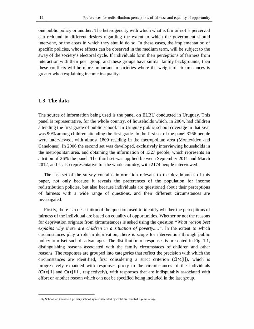
Firstly, there is a description of the question used to identify whether the perceptions of fairness of the individual are based on equality of opportunities. Whether or not the reasons for deprivation orignate from circumstances is asked using the question “What reason best explains why there are children in a situation of poverty.....”. In the extent to which circumstances play a role in deprivation, there is scope for intervention through public policy to offset such disadvantages. The distribution of responses is presented in Fig. 1.1, distinguishing reasons associated with the family circumstaces of children and other reasons. The responses are grouped into categories that reflect the precision with which the circumstances are identified, first considering a strict criterion (Circ[I]), which is progressively expanded with responses proxy to the circumstances of the individuals (Circ[II] and Circ[III], respectively), with responses that are indisputably associated with effort or another reason which can not be specified being included in the last group.
1 By School we know to a primary school system attended by children from 6-11 years of age.
Chapter 1 15
Fig. 1.1 – Distribution of responses about the reasons behind of poverty Note: The categories are the following: 1 “The parents are uneducated”, 2 “The grandparents were also poor”, 3 “The parents suffer from discrimination”, 4 “The parents suffer from illnesses or disabilities”, 5 “The parents do not earn enough”, 6 “It is due to the inequalities that exist in society”, 7 “They live in difficult neighborhoods”, 8 “They cannot access adequate housing”, 9 “There must have been a break or loss in the family”, 10 “The transfers are not high enough”, 11 “The parents suffer from alcoholism, drug addiction…”, 12 “The parents must have been unemployed for a long time”, 13 “There are many children in that family”, 14 “The parents do not work enough hours”, 15 “The parents do not want to work”, 16 “Other”, 17 “None of the above”
In addition, the population interviewed were asked for their opinion about the causes of
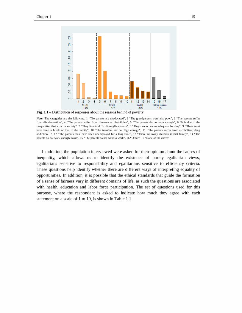
inequality, which allows us to identify the existence of purely egalitarian views, egalitarians sensitive to responsibility and egalitarians sensitive to efficiency criteria. These questions help identify whether there are different ways of interpreting equality of opportunities. In addition, it is possible that the ethical standards that guide the formation of a sense of fairness vary in different domains of life, as such the questions are associated with health, education and labor force participation. The set of questions used for this purpose, where the respondent is asked to indicate how much they agree with each statement on a scale of 1 to 10, is shown in Table 1.1.
16 Preferences for redistribution: perceptions of fairness and equality of opportunity
Table 1.1 Questions used to identify different perceptions about equality of opportunities according to different advantages
Labor participation
Education The State should provide financial support (…) and
guarantee access to university (…)
Health
Egalitarianism (Eg)
The State should guarantee a minimum income to all unemployed workers, whether they are actively seeking employment or not
To all the young people who need it
Medical treatment should be provided to everyone who needs it regardless of whether the illness or disease is the consequence of actions or decisions taken by the individual
Egalitarianism sensitive to responsibility (Eg-Re)
Unemployment benefit may cause harmful effects because the recipient has less incentive to seek employment, as such this type of benefit should only be provided to jobseekers who conclusively demonstrate that they are seeking, and are unable to find, employment
Only to young people who dedicate more time during the day to their studies and need financial support
Access to different types of organ transplants is, in general, restricted depending on the availability or organs and often the waiting time is too long, which can lead to the death of the patient. When selecting people to be treated, those whose disease is the consequence of smoking habits or the consumption of alcohol should be discarded from the list of potential beneficiaries
Egalitarianism sensitive to efficiency (Eg-Ef)
The best employment policy is one which allows the most productive workers to get jobs which are appropriate for their qualifications independent of whether the least productive employees are employed or not
Only to young people who obtained the highest qualifications in high school and need financial support
Some medical treatments are very expensive, for example implanting a pacemaker, and are more beneficial for younger people, who have more years to live, than for older adults. Given that the number of implants that can be performed is limited, treatment should be restricted to people under the age of 50
Note: When asking the question, the respondent is requested to indicate how much they agree with each statement on a scale of 1 to 10, 1 being strongly disagree and 10 being strongly agree
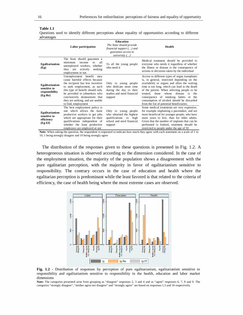
The distribution of the responses given to these questions is presented in Fig. 1.2. A
heterogeneous situation is observed according to the dimension considered. In the case of the employment situation, the majority of the population shows a disagreement with the pure egalitarian perception, with the majority in favor of egalitarianism sensitive to responsibility. The contrary occurs in the case of education and health where the egalitarian perception is predominant while the least favored is that related to the criteria of efficiency, the case of health being where the most extreme cases are observed.
Fig. 1.2 - Distribution of responses by perception of pure egalitarianism, egalitarianism sensitive to responsibility and egalitarianism sensitive to responsibility in the health, education and labor market dimensions Note: The categories presented arise from grouping as “disagree” responses 2, 3 and 4 and as “agree” responses 6, 7, 8 and 9. The categories “strongly disagree”, “neither agree nor disagree” and “strongly agree” are based on responses 1,5 and 10 respectively.
Chapter 1 17
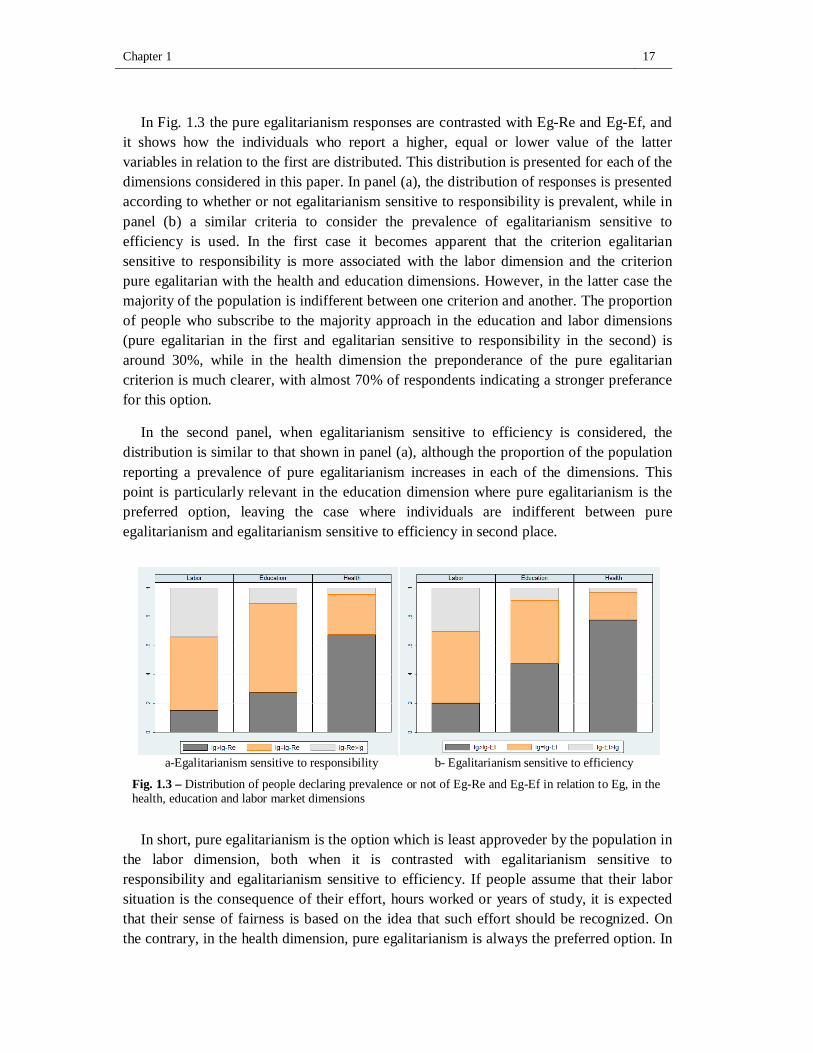
In Fig. 1.3 the pure egalitarianism responses are contrasted with Eg-Re and Eg-Ef, and it shows how the individuals who report a higher, equal or lower value of the latter variables in relation to the first are distributed. This distribution is presented for each of the dimensions considered in this paper. In panel (a), the distribution of responses is presented according to whether or not egalitarianism sensitive to responsibility is prevalent, while in panel (b) a similar criteria to consider the prevalence of egalitarianism sensitive to efficiency is used. In the first case it becomes apparent that the criterion egalitarian sensitive to responsibility is more associated with the labor dimension and the criterion pure egalitarian with the health and education dimensions. However, in the latter case the majority of the population is indifferent between one criterion and another. The proportion of people who subscribe to the majority approach in the education and labor dimensions (pure egalitarian in the first and egalitarian sensitive to responsibility in the second) is around 30%, while in the health dimension the preponderance of the pure egalitarian criterion is much clearer, with almost 70% of respondents indicating a stronger preferance for this option.
In the second panel, when egalitarianism sensitive to efficiency is considered, the distribution is similar to that shown in panel (a), although the proportion of the population reporting a prevalence of pure egalitarianism increases in each of the dimensions. This point is particularly relevant in the education dimension where pure egalitarianism is the preferred option, leaving the case where individuals are indifferent between pure egalitarianism and egalitarianism sensitive to efficiency in second place.
a-Egalitarianism sensitive to responsibility b- Egalitarianism sensitive to efficiency
Fig. 1.3 – Distribution of people declaring prevalence or not of Eg-Re and Eg-Ef in relation to Eg, in the health, education and labor market dimensions
In short, pure egalitarianism is the option which is least approveder by the population in the labor dimension, both when it is contrasted with egalitarianism sensitive to responsibility and egalitarianism sensitive to efficiency. If people assume that their labor situation is the consequence of their effort, hours worked or years of study, it is expected that their sense of fairness is based on the idea that such effort should be recognized. On the contrary, in the health dimension, pure egalitarianism is always the preferred option. In
18 Preferences for redistribution: perceptions of fairness and equality of opportunity
this case there is a widespread belief in the role played by circumstances and/or luck, whether it be inheriting an illness or simply suffering an illness. In the case of education, the prevalence of both egalitarianism sensitive to responsibility and egalitarianism sensitive to efficiency are the criteria with the lowest number of followers, in the first case due to the strong influence of people who are indifferent to both criteria and in the second the greater preponderance of preference for pure egalitarianism.
A lot of papers introduce a variable that refers to the role played by effort in the mobility perceived by the individual. This variable is commonly known as subjective mobility, and is collected in the survey by the question "Do you believe that an individual who is born poor and works hard can become rich in Uruguay?". According to Alesina and LaFerrera (2005), in order to correctly estimate the effect of opinions about the role of a sense of fairness in preferences for redistribution, it is necessary to incorporate the perspective of mobility, for this reason this variable is incorporated in the various estimates. Additionally, in a set of estimates objective mobility variables are introduced to see if a sense of fairness does not capture ommitted factors associated with the past experience of individuals. In this regard an intergenerational mobility variable is considered which identifies whether the educational level of the respondent exceeds that of both the father and the mother, as well as an intergenerational mobility variable that collects the variation in per capita household income between 2004 and 2011.
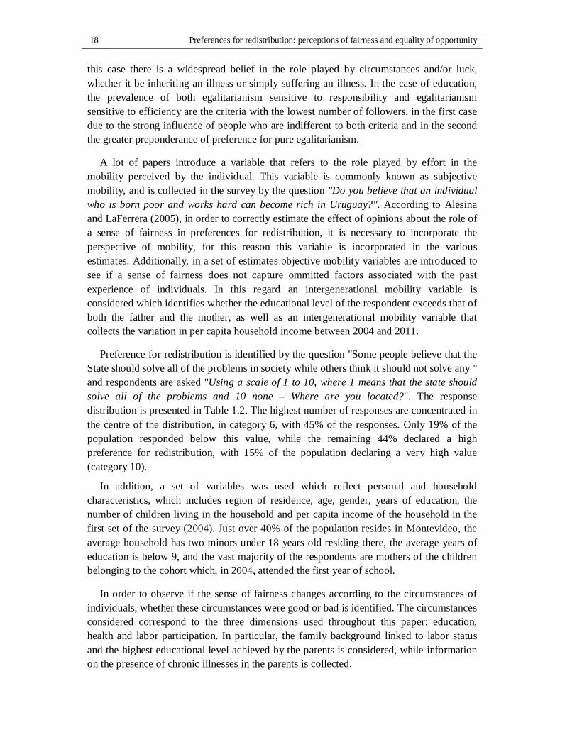
Preference for redistribution is identified by the question "Some people believe that the State should solve all of the problems in society while others think it should not solve any " and respondents are asked "Using a scale of 1 to 10, where 1 means that the state should solve all of the problems and 10 none – Where are you located?". The response distribution is presented in Table 1.2. The highest number of responses are concentrated in the centre of the distribution, in category 6, with 45% of the responses. Only 19% of the population responded below this value, while the remaining 44% declared a high preference for redistribution, with 15% of the population declaring a very high value (category 10).
In addition, a set of variables was used which reflect personal and household characteristics, which includes region of residence, age, gender, years of education, the number of children living in the household and per capita income of the household in the first set of the survey (2004). Just over 40% of the population resides in Montevideo, the average household has two minors under 18 years old residing there, the average years of education is below 9, and the vast majority of the respondents are mothers of the children belonging to the cohort which, in 2004, attended the first year of school.
In order to observe if the sense of fairness changes according to the circumstances of individuals, whether these circumstances were good or bad is identified. The circumstances considered correspond to the three dimensions used throughout this paper: education, health and labor participation. In particular, the family background linked to labor status and the highest educational level achieved by the parents is considered, while information on the presence of chronic illnesses in the parents is collected.
Chapter 1 19
Table 1.2 Descriptive statistics
Obs. No data Mean Standard
Deviation Min Max
Preferences for redistribution Very low 2125 49 0.04 0.19 0 1
2 2125 49 0.01 1.01 0 1 3 2125 49 0.03 0.17 0 1 4 2125 49 0.05 0.21 0 1 5 2125 49 0.06 0.24 0 1 6 2125 49 0.45 0.50 0 1 7 2125 49 0.06 0.24 0 1 8 2125 49 0.08 0.27 0 1 9 2125 49 0.07 0.25 0 1
Very high 2125 49 0.15 0.35 0 1
Subjective Mobility (1=High, 0=Other) 2120 54 0.09 0.29 0 1 Intergenerational Mobility (1=High, 0=Other) 2062 112 0.43 0.49 0 1
Variation of per capita income 1983 191 2290 4082 -25282 39434 Per capita income (2004) 2114 60 3476 3477 2.30 32458 Age 2008 166 41.97 7.77 25 70 Gender (1=Male, 0=Female) 2079 95 0.12 0.32 0 1 Region (1=Montevideo, 0=Other) 2174 0 0.41 0.49 0 1 Years of education 2062 112 8.98 3.60 0 18 Number of children under 18 in the household 2077 97 2.33 1.04 1 4 Circumstances
Education (1=Poor, 0=Good) 2032 142 0.74 0.44 0 1 Labor (1=Poor, 0=Good) 2061 113 0.81 0.39 0 1
Health (1=Poor, 0=Good) 2077 97 0.52 0.50 0 1 Entering adolescence
(1=Poor, 0=Good) 2156 18 0.61 0.49 0 1
Note: Based on the ELBU
In general it is observed that family backgrounds are not good. In the case of education, 74% have poor circumstances, if identifying cases in which the father failed to complete the basic cycle of secondary education (9 years of education), which is the number of years of compulsory education in Uruguay. In the case of working conditions, the circumstances are identified as good if the father has mosty worked in jobs commonly referred to as “white collar” (civil servants, technicians, professionals or office workers) in relation to “blue collar” work (agricultural, service workers or vendors, operators or machine or equipment operators, member of the armed forces or other unskilled work). This latter group contains job categories associated with worse working conditions in terms of income, social protection and social recognition, and was the case for 81% of the respondents.
In the case of the health condition of the father, the survey includes a set of possible illnesses or conditions (hypertension, asthma, diabetes, celiac, heart, other chronic, or psychological), and indicates that the condition is good if none of them are reported. In this case almost 52% reported that the health background is bad. In addition the survey also includes another circumstance, but of a general and subjective nature. The repondents are asked how they perceive their economic situation in adolescence, with a scale of 1 (very bad) to 10 (very good). The response distribution is mainly concentrated in the lower part: over 60% reported a value of lower than or equal to 4, which was identified in this paper as a bad circumstance.
20 Preferences for redistribution: perceptions of fairness and equality of opportunity
The last set of variables used refer to subjective and objective mobility. In the first case less than 10% understand that mobility is high. In the case of objective mobility variables ot is observed, from the intergenerational perspective, that over 40% obtain an educational level superior to that of their parents, while when an intergenerational mobility perspective is assumed it is noted that, on average, household income increases, in real terms, by 66% between 2004 and 2011.
1.4 The conceptual framework and empirical strategy
In the model proposed by Alesina & Angeletos (2005) individual preferences are the result of the difference between the private utility derived from individual consumption, 푢 , and the disutility emerging from social outcomes which are considered unfair, Ω, such that 푈 = 푢 − 휚 ∙ Ω. In this case, if 휚 ≥ 0 they will notice the intensity of the social demand for justice arising from the desire to correct the effect of luck on income. On the other hand, the authors define social unfairness as the distance between current utility and the
utility considered fair, u , such that Ω = ∫ (u −u ) .
This measure, which collects the criteria of altruistic redistribution, is utilized by Alesina & Giuliano (2009). In this case inequality (푄 ) can operate on the utility function indirectly, through consumption, or directly. In the first case there are potential opposing effects. A negative relationship is possible between utility and inequality as a result of the externalities of education and crime rate, and positive relationship through potential incentives associated with the requirements of greater effort, 푢(푐 ). In the direct channel the role played by inequality will depend on the individual’s religion, race, cultural differences (ℎ ) and, especially, the perception of fairness they have (푄 ,∗). In this paper it is assumed that these aspects are relatively invariant in time and form the identity of the individual. The case that concerns us is the sense of fairness of individuals, which may affect preferences for redistribution positively or negatively depending on the gap between the level of inequality that would exist if it were caused entirely by differences in effort and the level observed in reality.
In the specification of the baseline considered in this paper the utility function, which reflects preferences for redistribution, is a variant of that proposed by Alesina & Giuliano (2009) and is expressed as:
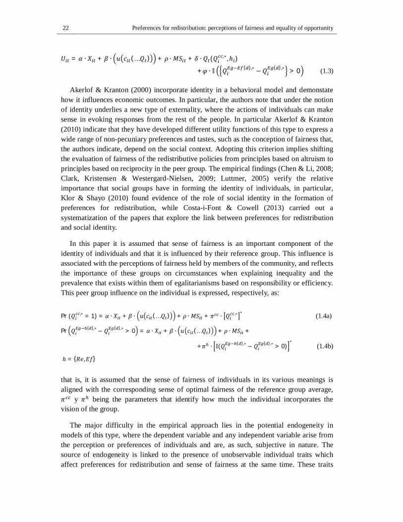
푈 = 훼 ∙ 푋 + 훽 ∙ 푢 푐 (…푄 ) + 휌 ∙ 푀푆 + 훿 ∙ 푄 푄 ,∗, ℎ (1.1)
where 훿 reflects the weight given to the cannel directly from the inequality, particularly taking into account the difference between the observed inequality and the level of inequality that would exist in the absence of the effects of circumstances or luck. This parameter reflects the weight given to the inequality generating process, that is, the belief
Chapter 1 21
that individuals have about the causes of inequality. If this parameter is nonzero then perceptions of fairness will be based on equality of opportunity, and if it is positive it will be understood that the desire for greater government intervention is based on the need to compensate inequality arising from circumstances. Parameter 휌 indicates the weight of subjective mobility and, finally, 훼 reflects the weight of the rest of the individual variables that influence preference for redistribution (푋 ).
Two variants of the utility function are proposed in order to reflect the ethical criteria that approximate the optimal levels of inequality desired by individuals. The first aims to capture whether there is an egalitarian sensitive to responsibility vision and the second whether there is an egalitarian sensitive to efficiency vision. In both cases different dimensions are discussed (푑) on which these visions can operate. That is to say, it is an attempt to analyze if there are differences in the egalitarianism desired by the individual, if it is more sensitive to responsibility or efficiency criteria, when considering how the labor market, education or health functions.
In the first case, the perception of the role of circumstances is accompanied by a measure that identifies whether the optimal level of a sense of fairness takes individual responsibility into account, which is obtained when the value reported for egalitarianism sensitive to responsibility (퐸푔 − 푅푒) is greater than the pure egalitarian vision of fairness(퐸푔), considering each of the d dimensions. In this case the utility function of individual i is expressed as:
푈 = 훼 ∙ 푋 + 훽 ∙ 푢 푐 (…푄 ) + 휌 ∙ 푀푆 + 훿 ∙ 푄 (푄 ,∗,ℎ )
+훾 ∙ 핀 푄 { },∗ − 푄 { },∗ > 0 (1.2)
where 핀 is an indicatrix function that takes the value of 1 when the inequality shown in brackets is true. When the value of 훾 is zero the prevalence of egalitarianism sensitive to responsibility is discarded and, therefore, it is assumed that the notion of fairness implies that only inequalities arising from circumstances should be compensated. Whether this parameter is poitive or negative will indicate whether individual beliefs about fairness incorporate effort in the process of evaluating the role of redistributive policies. In this regard parameters 훿 and 훾 must be analyzed together, for example when parameter 훾 is negative it is assumed that the sense of fairness channel is lower than that assumed in the baseline, and it will be in the presence of a vision of equality of opportunities that emphasizes reward for effort made. Therefore, it should be tested, to verify that both criteria operate jointly in preferences for redistribution, that 훿 + 훾 ≠ 0.
In the second case it is assumed that individuals may take efficiency criteria into account, which can alter the optimal levels of inequality of opportunities. Again, it is identified whether there is an egalitarian sensitive to efficiency vision (퐸푔 − 퐸푓) when their optimal values are greater than the optimal of the purely egalitarian vision. The parameter associated to the prevalence of this criterion, 휑, has a similar interpretation to parameter 훾. In this way we obtain a utility function augmented by efficiency criteria:
22 Preferences for redistribution: perceptions of fairness and equality of opportunity
푈 = 훼 ∙ 푋 + 훽 ∙ 푢 푐 (…푄 ) + 휌 ∙ 푀푆 + 훿 ∙ 푄 (푄 ,∗,ℎ )
+휑 ∙ 핀 푄 { },∗ −푄 { },∗ > 0 (1.3)
Akerlof & Kranton (2000) incorporate identity in a behavioral model and demonstate how it influences economic outcomes. In particular, the authors note that under the notion of identity underlies a new type of externality, where the actions of individuals can make sense in evoking responses from the rest of the people. In particular Akerlof & Kranton (2010) indicate that they have developed different utility functions of this type to express a wide range of non-pecuniary preferences and tastes, such as the conception of fairness that, the authors indicate, depend on the social context. Adopting this criterion implies shifting the evaluation of fairness of the redistributive policies from principles based on altruism to principles based on reciprocity in the peer group. The empirical findings (Chen & Li, 2008; Clark, Kristensen & Westergard-Nielsen, 2009; Luttmer, 2005) verify the relative importance that social groups have in forming the identity of individuals, in particular, Klor & Shayo (2010) found evidence of the role of social identity in the formation of preferences for redistribution, while Costa-i-Font & Cowell (2013) carried out a systematization of the papers that explore the link between preferences for redistribution and social identity.
In this paper it is assumed that sense of fairness is an important component of the identity of individuals and that it is influenced by their reference group. This influence is associated with the perceptions of fairness held by members of the community, and reflects the importance of these groups on circumstances when explaining inequality and the prevalence that exists within them of egalitarianisms based on responsibility or efficiency. This peer group influence on the individual is expressed, respectively, as:
Pr(푄 ,∗ = 1) = 훼 ∙ 푋 + 훽 ∙ 푢 푐 (…푄 ) + 휌 ∙ 푀푆 + 휋 ∙ 푄 ,∗ ∗ (1.4a)
Pr 푄 { },∗ − 푄 { },∗ > 0 = 훼 ∙ 푋 + 훽 ∙ 푢 푐 (…푄 ) + 휌 ∙ 푀푆 +
+휋 ∙ 핀(푄 { },∗ − 푄 { },∗ > 0)∗ (1.4b)
ℎ = {푅푒,퐸푓}
that is, it is assumed that the sense of fairness of individuals in its various meanings is aligned with the corresponding sense of optimal fairness of the reference group average, 휋 y 휋 being the parameters that identify how much the individual incorporates the vision of the group.
The major difficulty in the empirical approach lies in the potential endogeneity in models of this type, where the dependent variable and any independent variable arise from the perception or preferences of individuals and are, as such, subjective in nature. The source of endogeneity is linked to the presence of unobservable individual traits which affect preferences for redistribution and sense of fairness at the same time. These traits
Chapter 1 23
may be associated with how individuals were raised and the beliefs transmitted by parents, for example conveying views on inequality and social mobility in order to influence their incentives (Bénabou & Tirole, 2006).
This type of endogeneity, generated by the presence of subjective variables in both the dependent and independent variable, has hardly been discussed in the literature. In Stuzter (2004) instrumental variables are introduced in an estimation where it is analyzed how income aspirations affect happiness reported. In this paper the author uses two different instruments to explain aspirations: the average income of the community and the proportion of rich people living in that community. That is, it is assumed that the social group with which the individual interacts affects their aspirations. However, in general terms the literature has not made too much progress in determining whether the formation of the reference groups is endogenous or if the choice of the group is random, as there is empirical evidence on both sides (Clark & Senik, 2010).
Given the wealth of information available on the community in which the respondents lived and the significant verified residential segregation in Uruguay (Macadar, Calvo, Pellegrino & Vigorito, 2002; Cervini & Gallo, 2001), information about the reference group is used as an instrument in the estimation. Recall that all respondents have at least one child with high school age who attended the first grade in 2004. On the other hand, while it is not exploited at the time of making the estimates, the database used contains longitudinal data from which it is possible to identify the educational center which the child attended in 2004 (first set from the survey). The educational center attended by the child of the respondent is the variable used as a proxy of the community, and is the variable on which the average sense of justice is calculated.
Therefore the estimations are made through Two-Stage Least Squares (2SLS). The first stage of the estimation seeks to identify the effects on the individual’s sense of fairness, as shown in equations (1.4a) and (1.4b). This aspect, which refers to the identity of the individual, is a structural element of the individual permeated by the opinions of members of the community to which they belong. Therefore, the average sense of fairness of the community is the instrument used for equations (1.1), (1.2), and (1.3), in which preference for redistribution is explained.
Another aspect that this paper seeks to answer is whether circumstances alter the way in which the cannel of fairness operates on the demand for redistribution. For this, specific estimates are made for individuals with good and bad circumstances, and it is observed whether there are consistent divergences among the three dimensions considered (labor market, education and health). With this strategy I aim to conclude if the differences in the perception of fairness are determined by opportunities experienced, and whether such differences are sensitive to the dimension considered.
24 Preferences for redistribution: perceptions of fairness and equality of opportunity
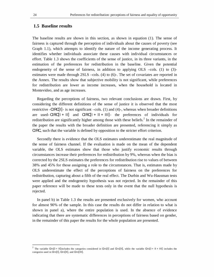
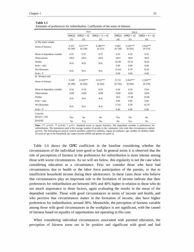
1.5 Baseline results
The baseline results are shown in this section, as shown in equation (1). The sense of fairness is captured through the perception of individuals about the causes of poverty (see Graph 1.1), which attempts to identify the nature of the income generating process. It identifies whether individuals associate these causes with individual circumstances or effort. Table 1.3 shows the coefficients of the sense of justice, in its three variants, in the estimation of the preferences for redistribution in the baseline. Given the potential endogeneity of the sense of fairness, in addition to applying OLS –cols. (1) to (3)- estimates were made through 2SLS –cols. (4) to (6)-. The set of covariates are reported in the Annex. The results show that subjective mobility is not significant, while preferences for redistribution are lower as income increases, when the household is located in Montevideo, and as age increases.
Regarding the perceptions of fairness, two relevant conclusions are drawn. First, by considering the different definitions of the sense of justice it is observed that the most restrictive -CIRC[I]- is not significant –cols. (1) and (4)-, whereas when broader definitions are used-CIRC[I + II] and CIRC[I + II + III]- the preferences of individuals for redistribution are significantly higher among those with these beliefs.2 In the remainder of the paper the results with the broader definition are presented, referencing it simply as CIRC, such that the variable is defined by opposition to the stricter effort criterion.
Secondly there is evidence that the OLS estimates underestimate the real magnitude of the sense of fairness channel. If the evaluation is made on the mean of the dependent variable, the OLS estimates show that those who justify economic results through circumstances increase their preferences for redistribution by 9%, whereas when the bias is corrected by the 2SLS estimates the preferences for redistribution rise to values of between 38% and 45% for those assigning a role to the circumstances. That is, estimates made by OLS underestimate the effect of the perceptions of fairness on the preferences for redistribution, capturing about a fifth of the real effect. The Durbin and Wu-Hausman tests were applied and the endogeneity hypothesis was not rejected. In the remainder of this paper reference will be made to these tests only in the event that the null hypothesis is rejected.
In panel b) in Table 1.3 the results are presented exclusively for women, who account for almost 90% of the sample. In this case the results do not differ in relation to what is shown in panel a), where the entire population is used. In the absence of evidence indicating that there are systematic differences in perceptions of fairness based on gender, in the remainder of this paper the results for the whole population are presented.
2 The variable Circ[I + II]includes the categories considered in Circ[I] and Circ[II], while the variable Circ[I + II + III] includes the categories used in Circ[I], Circ[II], and Circ[III].
Chapter 1 25
Table 1.3 Estimates of preferences for redistribution. Coefficients of the sense of fairness
OLS 2SLS CIRC[I] CIRC[I + II] CIRC[I + II + II] CIRC[I] CIRC[I + II] CIRC[I + II + II] (1) (2) (3) (4) (5) (6)
a) The entire simple
Sense of fairness 0.257 0.571*** 0.584*** 0.601 2.535*** 2.632*** [0.180] [0.158] [0.155] [0.728] [0.592] [0.574]
Mean of dependent variable 6.55 6.55 6.55 6.55 6.55 6.55 Observations 1853 1853 1853 1853 1853 1853 Durbin N/A N/A N/A 43.49 19.53 18.41 Prob > chi2 0.00 0.00 0.00 Wu-Hausman N/A N/A N/A 21.64 8.79 16.41
Prob > F 0.00 0.00 0.00 b) Women only
Sense of fairness 0.249 0.528*** 0.553*** 0.735 2.454*** 2.544*** [0.189] [0.166] [0.164] [0.726] [0.590] [0.570]
Mean of dependent variable 6.54 6.54 6.54 6.54 6.54 6.54 Observations 1658 1658 1658 1658 1658 1658 Durbin N/A N/A N/A 34.6 17.44 16.86
Prob > chi2 0.00 0.00 0.00 Wu-Hausman
N/A N/A N/A 17.61 8.39 16.19
Prob > F 0.00 0.00 0.00
Controls Circ(II + III) Yes No No Yes No No Circ(III) No Yes No No Yes No
Note: *** p<0.01, ** p<0.05, * p<0.1. Standard errors in square brackets. The dependent variable is preferences for redistribution. The instrument used is the average number of people in the community who state that circumstances explain poverty. The following are used as control variables: subjective mobility, región of residence, age, number of children under 18 years of age in the household, per capita income (2004) and gender (in panel a).
Table 1.4 shows the CIRC coefficient in the baseline considering whether the
circumstances of the individual were good or bad. In general terms it is observed that the role of perceptions of fairness in the preferences for redistribution is more intense among those with worse circumstances. As we will see below, this regularity is not the case when considering education as a circumstance. First we consider those who have bad circumstances due to health or the labor force participation of the parents, or due to insufficient household income during their adolescence. In these cases those who believe that circumstances play an important role in the formation of income indicate that their preferences for redistribution are between 36% and 40% higher in relation to those who do not attach importance to these factors, again evaluating the results in the mean of the dependent variable. Those with good circumstances in terms of income and health, and who perceive that circumstances matter in the formation of income, also have higher preferences for redistribution, around 38%. Meanwhile, the perception of fairness variable among those with good circumstances in the workplace is not significant, with the cannel of fairness based on equality of opportunities not operating in this case.
When considering individual circumstances associated with parental education, the perception of fairness turns out to be positive and significant with good and bad
26 Preferences for redistribution: perceptions of fairness and equality of opportunity
circumstances, with the greater magnitude among those with better circumstances. In fact, it is in these estimates where the differences in preferences for redistribution as a result of CIRC are greater among both groups. In this case CIRC has an impact of 48% among those with good circumstances, while this effect is around 35% (similar to those with good circumstances in income and health) among those with bad circumstances.
Finally, in columns (3) and (6) the estimates made for the entire population are presented, incorporating the interaction between CIRC and a dichotomous variable which identifies whether the circumstances are bad (BC). In all cases, when the estimate is made by 2SLS it is observed that the CIRCvariable is positive and significant. Also, the interaction of CIRC with the dichotomous variable which identifies bad circumstances, which has a negative sign, is compensated almost completely with the bad circumstances variable that shows a positive effect on preferences for redistribution. The only case where there is more than one point of difference between both effects is that shown by circumstances in education. In this case the effect that collects the interaction of the two variables slightly predominates, which accounts for the greatest preferences for redistribution of individuals with better circumstances, which is consistent with the comments in the preceding paragraphs. In addition, the results show that, beyond the homogeneous and positive effect of CIRC in all circumstances, a significant and positive effect is observed in those who do not share a sense of fairness based on CIRC but have bad circumstances.
In short, perceptions about the role of curcumstances positively affect preferences for redistribution. This link is stronger among those with worse circumstances in the majority of the dimensions. It was expected that unfavorable circumstances would be associated with greater preferences for redistribution, to the extent that the low levels of mobility observed in Uruguay (Calonico, 2006) represent a barrier for the people aiming to perform well throughout their lives. The only exception observed was when the circumstances in education are considered. In this case the effect of perceptions of fairness on preferences for redistribution is greater among those with better circumstances. One hypothesis that may explain this difference could be from the greater value that this population has for education. If so, these individuals may be more inclined to support government intervention, if it is understood that a natural consequence of this is an increase in public spending on education, or even generating incentives for the greater participation of children and adolescents in the education system through income transfers which are conditional on the attendance of children at educational centers.
Chapter 1 27
Table 1.4 Preference of redistribution estimates according to individual circumstances. Coefficients of the sense of fairness
OLS 2SLS Circumstance Circumstance
Good Bad All Good Bad All (1) (2) (3) (4) (5) (6)
a) Circumstance: Entering adolescence
CIRC 0.659** 0.540*** 0.668** 2.370*** 2.699*** 6.502*** [0.272] [0.191] [0.267] [0.893] [0.737] [1.649]
CIRC ∙ BC -0.121 -5.954*** [0.328] [1.650]
BC 0.557* 5.594***
[0.310] [1.455] Observations 717 1135 1852 717 1135 1852 Durbin N/C N/C N/C 4.64 13.41 18.20 Prob > chi2 0.03 0.00 0.00 Wu-Hausman N/C N/C N/C 4.58 11.28 16.27 Prob > F 0.03 0.00 0.00 b) Circumstance: Education
CIRC 0.499* 0.568*** 0.489* 3.090*** 2.345*** 9.577*** [0.295] [0.184] [0.287] [1.148] [0.612] [2.719]
CIRC ∙ BC 0.080 -8.991*** [0.341] [2.713]
BC 0.050 7.979***
[0.321] [2.417] Observations 471 1271 1742 471 1271 1742 Durbin N/C N/C N/C 5.63 11.69 17.14 Prob > chi2 0.02 0.00 0.00 Wu-Hausman N/C N/C N/C 5.03 11.46 16.54 Prob > F 0.03 0.00 0.00 c) Circumstance: Labor Market
CIRC 0.589 0.505*** 0.605 2.555 2.393*** 11.791*** [0.410] [0.176] [0.396] [1.620] [0.636] [4.134]
CIRC ∙ BC -0.094 -
11.275*** [0.434] [4.131]
BC 0.144 10.145***
[0.418] [3.780] Observations 349 1607 1776 349 1607 1776 Durbin N/C N/C N/C 2.43 12.01 15.24 Prob > chi2 0.12 0.00 0.00 Wu-Hausman N/C N/C N/C 2.22 10.60 13.60 Prob > F 0.14 0.00 0.00 d) Circumstance: Health
CIRC 0.601*** 0.552** 0.590*** 2.521*** 2.354*** 4.468*** [0.220] [0.221] [0.223] [0.885] [0.748] [1.256]
CIRC ∙ BC -0.080 -3.950*** [0.314] [4.625]
BC -0.019 3.302***
[0.295] [1.110] Observations 849 933 1782 849 933 1782 Durbin N/C N/C N/C 6.79 7.65 15.13 Prob > chi2 0.01 0.00 0.00 Wu-Hausman N/C N/C N/C 5.87 7.19 13.59 Prob > F 0.01 0.01 0.00 Note: *** p<0.01, ** p<0.05, * p<0.1. Standard errors in square brackets. The dependent variable is preferences for redistribution. The instrument used is the average number of people in the community who report that circumstances explain poverty. The following are used as control variables: subjective mobility, region of residence, age, number of children under 18 in the household, per capita income (2004) and gender; in the case of the specifications, a dichotomous variable is included for the entire simple which identifies bad circumstances. The mean of the dependent variable is around 6.5 in all cases. Table 1.5 shows some frequencies that attempt to justify this hypothesis. Valuations
made by respondents about the future educational performance of their children are compared. The responses by respondents with good and bad circumstances in education
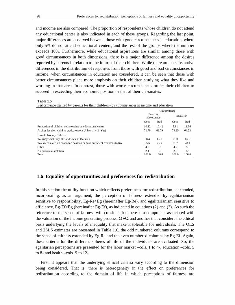
28 Preferences for redistribution: perceptions of fairness and equality of opportunity
and income are also compared. The proportion of respondents whose children do not attend any educational center is also indicated in each of these groups. Regarding the last point, major differences are observed between those with good circumstances in education, where only 5% do not attend educational centers, and the rest of the groups where the number exceeds 10%. Furthermore, while educational aspirations are similar among those with good circumstances in both dimensions, there is a major difference among the desires reported by parents in relation to the future of their children. While there are no substantive differences in the distribution of responses from those with good and bad circumstances in income, when circumstances in education are considered, it can be seen that those with better circumstances place more emphasis on their children studying what they like and working in that area. In contrast, those with worse circumstances prefer their children to succeed in exceeding their economic position or that of their classmates.
Table 1.5 Performance desired by parents for their children - by circumstances in income and education Circumstance
Entering
adolescence Education
Good Bad Good Bad
Proportion of children not attending an educational center 10.12 10.42 5.81 11.36 Aspires for their child to graduate from University (1=Yes) 71.78 63.79 74.25 64.53 I would like my child … To study what they like and work in that area 68.4 66.2 71.0 65.6 To exceed a certain economic position or have sufficient resources to live 25.6 26.7 21.7 28.1 Other 4.0 3.9 4.7 3.3 No particular ambition 2.1 3.3 2.6 2.9 Total 100.0 100.0 100.0 100.0
1.6 Equality of opportunities and preferences for redistribution
In this section the utility function which reflects preferences for redistribution is extended, incorporating, as an argument, the perception of fairness extended by egalitarianism sensitive to responsibility, Eg-Re>Eg (hereinafter Eg-Re), and egalitarianism sensitive to efficiency, Eg-Ef>Eg (hereinafter Eg-Ef), as indicated in equations (2) and (3). As such the reference to the sense of fairness will consider that there is a component associated with the valuation of the income generating process, CIRC, and another that considers the ethical basis underlying the levels of inequality that make it tolerable for individuals. The OLS and 2SLS estimates are presented in Table 1.6, the odd numbered columns correspond to the sense of fairness extended by Eg-Re and the even numbered columns by Eg-Ef. Again, these criteria for the different spheres of life of the individuals are evaluated. So, the egalitarian perceptions are presented for the labor market –cols. 1 to 4-, education –cols. 5 to 8- and health –cols. 9 to 12-.
First, it appears that the underlying ethical criteria vary according to the dimension being considered. That is, there is heterogeneity in the effect on preferences for redistribution according to the domain of life in which perceptions of fairness are
Chapter 1 29
evaluated. When egalitarianism is incoporated into the labor market, it is observed that within perceptions about the role played by equality of opportunities, there is an emphasis on individual responsibility. When considering egalitarianism in education, perceptions of fairness correspond to egalitarianism sensitive to both responsibility and efficiency. In these cases considering only the perception about the role of circumstances would overestimate the role of the sense of fairness when explaining preferences for redistribution. When Eg-Re prevails in the workplace it is observed that the effect of the sense of fairness falls from 38% to 24%, with the effect being similar when considering egalitarianism in the education dimension, where the effect is reduced to 21%. In the latter case Eg-Ef is also significant although the test of joint significance of CIRC and Eg-Ef do not allow us to reject the null hypothesis, therefore the role of the sense of fairness in preferences for redistribution is diluted to offset both effects. This group believes that the circumstances affect the income generating process but that the government should not redistribute because they aspire to maximize aggregate utility.
The case of identifying egalitarian perceptions in the health dimension is distinct. In this case Eg-Ef is not significant. Similar to that which occurs with Eg-Ef in education, Eg-Re in health is significant but its introduction causes a significant fall which dilutes the effect of the cannel of fairness. The effect was 38% when only considering CIRC. That is, in all three dimensions, individuals believe the a sense of fairness based on equality of opportunities involves rewarding effort, and in the case of education, also rewarding efficient performance.
In the following sections the same specifications are presented but, in addition, it is identified whether the population had good or bad circumstances. In section 1.6.1 emphasis is put on the circumstances associated with entering adolescence. In this case the egalitarian perceptions in the three domains of life (work, education and health) are considered, and the differences arising from evaluating the egalitarianism in each of these dimensions are observed. The following section (1.6.2) focuses on showing the effects on preferences for redistribution when the rest of the circumstances are taken into acount. For each case, the egalitarianism in the same domain of life as that used to measure the circumstances is considered. As such, when the circumstances are observed in the labor market, the egalitarianism is also evaluated in the labor market, and the same when the circumstances are identified in education and health. In both sections, the columns marked by the letter (a) correspond to estimates for the population with good circumstances and letter (b) bad circumstances. Finally, in the column marked by letter (c) the entire population is considered, introducing one variable that identifies bad circumstances in the estimation, and another in which this variable interacts with egalitarianism.
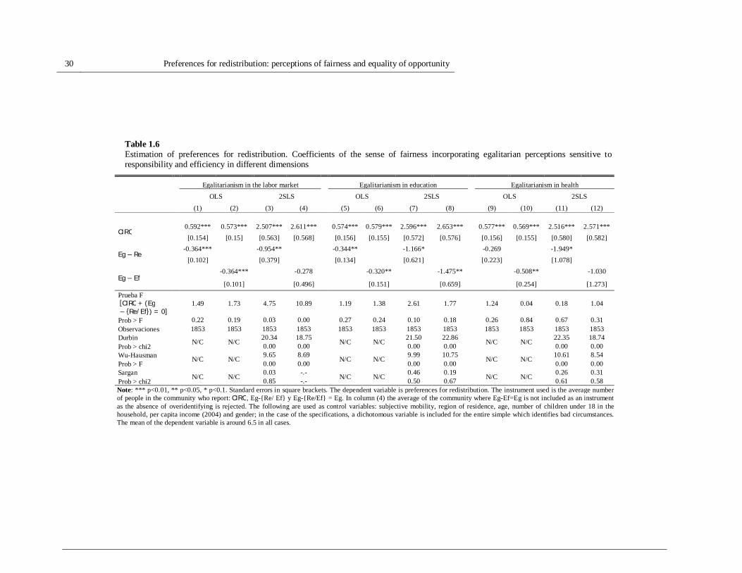
30 Preferences for redistribution: perceptions of fairness and equality of opportunity
Table 1.6 Estimation of preferences for redistribution. Coefficients of the sense of fairness incorporating egalitarian perceptions sensitive to responsibility and efficiency in different dimensions
Egalitarianism in the labor market Egalitarianism in education Egalitarianism in health OLS 2SLS OLS 2SLS OLS 2SLS (1) (2) (3) (4) (5) (6) (7) (8) (9) (10) (11) (12)
CIRC 0.592*** 0.573*** 2.507*** 2.611*** 0.574*** 0.579*** 2.596*** 2.653*** 0.577*** 0.569*** 2.516*** 2.571*** [0.154] [0.15] [0.563] [0.568] [0.156] [0.155] [0.572] [0.576] [0.156] [0.155] [0.580] [0.582]
Eg − Re -0.364*** -0.954** -0.344** -1.166* -0.269 -1.949* [0.102] [0.379] [0.134] [0.621] [0.223] [1.078]
Eg − Ef -0.364*** -0.278 -0.320** -1.475** -0.508** -1.030
[0.101] [0.496] [0.151] [0.659] [0.254] [1.273] Prueba F [CIRC + (Eg− {Re/Ef}) = 0] 1.49 1.73 4.75 10.89 1.19 1.38 2.61 1.77 1.24 0.04 0.18 1.04
Prob > F 0.22 0.19 0.03 0.00 0.27 0.24 0.10 0.18 0.26 0.84 0.67 0.31 Observaciones 1853 1853 1853 1853 1853 1853 1853 1853 1853 1853 1853 1853 Durbin N/C N/C 20.34 18.75 N/C N/C 21.50 22.86 N/C N/C 22.35 18.74 Prob > chi2 0.00 0.00 0.00 0.00 0.00 0.00 Wu-Hausman N/C N/C 9.65 8.69 N/C N/C 9.99 10.75 N/C N/C 10.61 8.54 Prob > F 0.00 0.00 0.00 0.00 0.00 0.00 Sargan N/C N/C 0.03 -.- N/C N/C 0.46 0.19 N/C N/C 0.26 0.31 Prob > chi2 0.85 -.- 0.50 0.67 0.61 0.58 Note: *** p<0.01, ** p<0.05, * p<0.1. Standard errors in square brackets. The dependent variable is preferences for redistribution. The instrument used is the average number of people in the community who report:CIRC, Eg-{Re/ Ef} y Eg-{Re/Ef} = Eg. In column (4) the average of the community where Eg-Ef=Eg is not included as an instrument as the absence of overidentifying is rejected. The following are used as control variables: subjective mobility, region of residence, age, number of children under 18 in the household, per capita income (2004) and gender; in the case of the specifications, a dichotomous variable is included for the entire simple which identifies bad circumstances. The mean of the dependent variable is around 6.5 in all cases.
Chapter 1 31
1.6.1 Preferences for redistribution according to income level in adolescence
In this section estimates of preferences for redistribution are presented, differentiating the population with low and high income in adolescence, while introducing the criteria of egalitarianism in the three domains of life considered (see Table 1.7a). The results show that egalitarianism sensitive to responsibility is only significant and with a negative sign in the labor market when the circumstances are bad. Therefore, when the sense of fairness is evaluated in this dimension, the effect on preference for redistribution is greater among those with good circumstances, as only the CIRC componente is significant. In this last case the increase in preferences for redistribution is 38% compared to its mean value. In contrast, those with bad circumstances show that the sense of fairness gives a role to effort at the point where CIRC and Eg-Re are compensated, not affecting the sense of fairness in preferences for redistribution. In the remaining specifications, whether it be for high or low income, egalitarianism sensitive to responsibility is not significant.
In the cases where the entire population is considered, and interactions between the sense of fairness and low income (LY) are introduced, we observe differential effects generated as a result of the various circumstances independent of the dimension in which egalitarianism is evaluated. In these cases the component of the cannel of fairness associated with offsetting inequality arising from circumstances is linked to the population which had low income in adolescence. Those who prefer greater redistribution are located in this group. On the other hand, among those with good circumstances, the notion of equality of opportunity does not operate, this group believes in egalitariansim sensitive to responsibility and this results in a desire for less redistributive policies.
When estimates are made for those with high or low income in adolescence and Eg-Ef is considered, no significant effects of this last variable are found. In the case where the interactions in the entire simple are introduced, similar results are observed to those shown with Eg-Re regarding offsetting unfavorable circumstances. It is among those with bad circumstances that this channel of fairness applies, and who subsequently become those with greater preferences for redistribution. Furthermore, and unlike what happens with Eg-Re, egalitarianism sensitive to efficiency is not significant in any case.
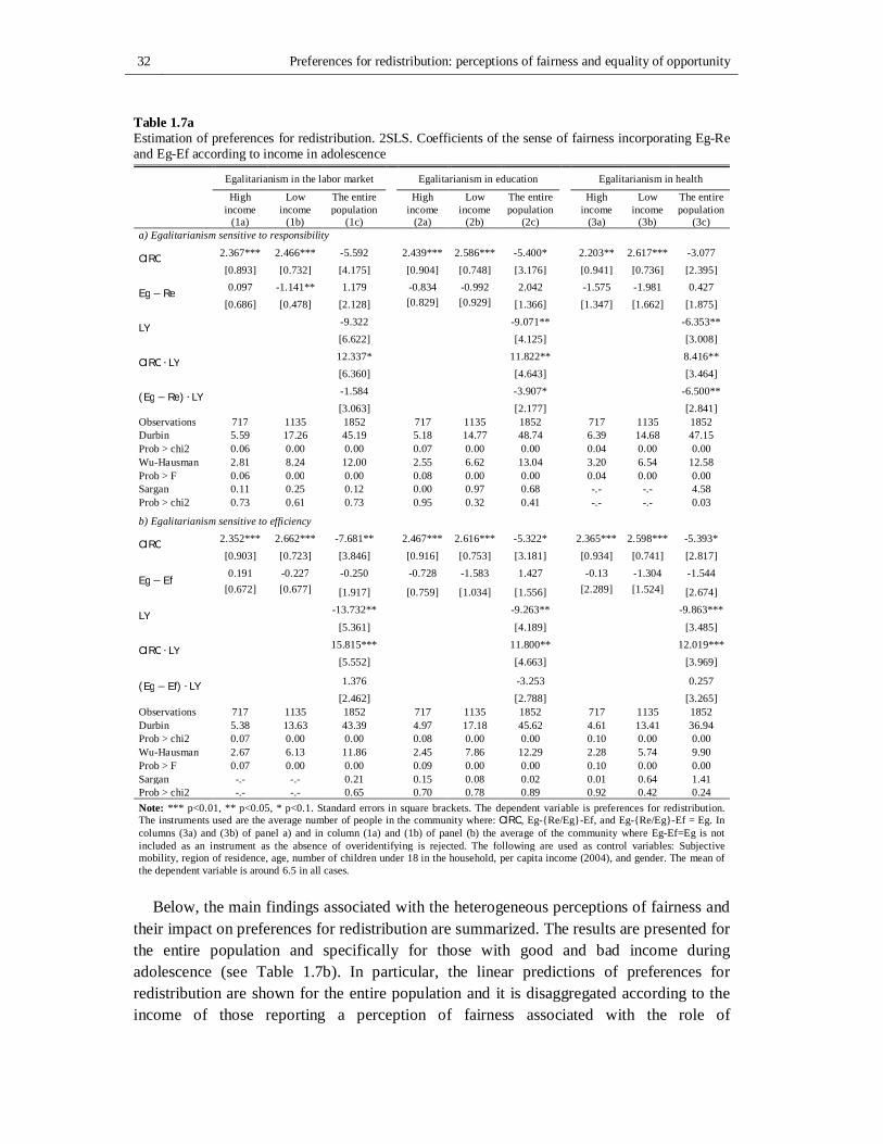
32 Preferences for redistribution: perceptions of fairness and equality of opportunity
Table 1.7a Estimation of preferences for redistribution. 2SLS. Coefficients of the sense of fairness incorporating Eg-Re and Eg-Ef according to income in adolescence
Egalitarianism in the labor market Egalitarianism in education Egalitarianism in health
High income
Low income
The entire population High
income Low
income The entire population High
income Low
income The entire population
(1a) (1b) (1c) (2a) (2b) (2c) (3a) (3b) (3c) a) Egalitarianism sensitive to responsibility
CIRC 2.367*** 2.466*** -5.592 2.439*** 2.586*** -5.400* 2.203** 2.617*** -3.077 [0.893] [0.732] [4.175] [0.904] [0.748] [3.176] [0.941] [0.736] [2.395]
Eg − Re 0.097 -1.141** 1.179 -0.834 -0.992 2.042 -1.575 -1.981 0.427 [0.686] [0.478] [2.128] [0.829] [0.929] [1.366] [1.347] [1.662] [1.875]
LY -9.322 -9.071** -6.353** [6.622] [4.125] [3.008]
CIRC ∙ LY 12.337* 11.822** 8.416** [6.360] [4.643] [3.464]
(Eg − Re) ∙ LY -1.584 -3.907* -6.500**
[3.063] [2.177] [2.841] Observations 717 1135 1852 717 1135 1852 717 1135 1852 Durbin 5.59 17.26 45.19 5.18 14.77 48.74 6.39 14.68 47.15 Prob > chi2 0.06 0.00 0.00 0.07 0.00 0.00 0.04 0.00 0.00 Wu-Hausman 2.81 8.24 12.00 2.55 6.62 13.04 3.20 6.54 12.58 Prob > F 0.06 0.00 0.00 0.08 0.00 0.00 0.04 0.00 0.00 Sargan 0.11 0.25 0.12 0.00 0.97 0.68 -.- -.- 4.58 Prob > chi2 0.73 0.61 0.73 0.95 0.32 0.41 -.- -.- 0.03
b) Egalitarianism sensitive to efficiency
CIRC 2.352*** 2.662*** -7.681** 2.467*** 2.616*** -5.322* 2.365*** 2.598*** -5.393* [0.903] [0.723] [3.846] [0.916] [0.753] [3.181] [0.934] [0.741] [2.817]
Eg − Ef 0.191 -0.227 -0.250
-0.728 -1.583 1.427 -0.13 -1.304 -1.544
[0.672] [0.677] [1.917] [0.759] [1.034] [1.556] [2.289] [1.524] [2.674]
LY -13.732** -9.263** -9.863***
[5.361] [4.189] [3.485]
CIRC ∙ LY 15.815*** 11.800** 12.019*** [5.552] [4.663] [3.969]
(Eg − Ef) ∙ LY 1.376 -3.253 0.257 [2.462] [2.788] [3.265]
Observations 717 1135 1852 717 1135 1852 717 1135 1852 Durbin 5.38 13.63 43.39 4.97 17.18 45.62 4.61 13.41 36.94 Prob > chi2 0.07 0.00 0.00 0.08 0.00 0.00 0.10 0.00 0.00 Wu-Hausman 2.67 6.13 11.86 2.45 7.86 12.29 2.28 5.74 9.90 Prob > F 0.07 0.00 0.00 0.09 0.00 0.00 0.10 0.00 0.00 Sargan -.- -.- 0.21 0.15 0.08 0.02 0.01 0.64 1.41 Prob > chi2 -.- -.- 0.65 0.70 0.78 0.89 0.92 0.42 0.24 Note: *** p<0.01, ** p<0.05, * p<0.1. Standard errors in square brackets. The dependent variable is preferences for redistribution. The instruments used are the average number of people in the community where: CIRC, Eg-{Re/Eg}-Ef, and Eg-{Re/Eg}-Ef = Eg. In columns (3a) and (3b) of panel a) and in column (1a) and (1b) of panel (b) the average of the community where Eg-Ef=Eg is not included as an instrument as the absence of overidentifying is rejected. The following are used as control variables: Subjective mobility, region of residence, age, number of children under 18 in the household, per capita income (2004), and gender. The mean of the dependent variable is around 6.5 in all cases.
Below, the main findings associated with the heterogeneous perceptions of fairness and
their impact on preferences for redistribution are summarized. The results are presented for the entire population and specifically for those with good and bad income during adolescence (see Table 1.7b). In particular, the linear predictions of preferences for redistribution are shown for the entire population and it is disaggregated according to the income of those reporting a perception of fairness associated with the role of
Chapter 1 33
circumstances, with egalitarianism sensitive to responsibility, and with egalitarianism sensitive to efficiency (row labeled W/SF). With the aim of observing the extent of the changes in preferences for redistribution originating from perceptions of fairness, the results with those who did not report these perceptions (row labeled WO/SF). The same is done in Table 8b when considering the rest of the circumstances.
The general results arising from Tables 1.3 and 1.6 are presented in panel A, and they are compared with the results that consider good and bad circumstances according to income (panel B), and which arise from the estimates presented in Tables 1.4 and 1.7a. When no variables associated with the interpretation that individuals make of egalitarianism are introduced, there is always a significant and positive effect of the perceptions of fairness base on the belief that it is necessary to offset inequality arising from circumstances. Considering the scale of 1 to 10 in preferences for redistribution, the predictions of individuals WO/SF have a value of 4.3 points, whereas in the case of W/SF the predictions have a value of 6.9. Moreover, in the latter case differences are observed in the predictions between those with good and bad circumstances, the predictions of the preferences for redistribution being 7.1 and 6.5 respectively.
In columns 2 and 6, egalitarianism sensitive to responsibility (CIRC + Eg − Re) and egalitarianism sensitive to efficiency (CIRC + Eg− Ef) in the labor market are added to the role assigned to circumstances. If both ethical criteria are compared it is observed that when effort criteria are introduced to determine tolerable inequality, the predicted values of preferences for redistribution are lower than when the criteria takes the efficiency of the results into account. However, in no case is Eg-Ef significant. In the general specification equality of opportunity operates on egalitarianism sensitive to responsibility, and as a whole positively affects preferences for redistribution. In the case where circumstances are good, both egalitarianisms operate, although the effect on preferences for redistribution is reduced.
Continuing with the circumstances associated with income, if egalitarianisms in the dimensions of education (cols 3 and 7) and health (cols 4 and 8) are considered, similar results are observed. In these cases only CIRC is significant. When Eg-Ef is introduced, the predictions are higher, both with the good and bad circumstances, although the gap generated by the cannel of fairness is similar in both egalitarianisms. These results are different to the general case where the egalitarianisms were significant and the effects of the sense of fairness were offset when Eg-Ef was evaluated in education and Eg-Re in health.
Finally, the differences between the predictions which consider Eg-Re and Eg-Ef are presented. For this, an average of the predictions is made considering the egalitarianisms in all of the dimensions (cols 5 and 9). In this way the different intensities with which the sense of fairness affects preferences for redistribution is observed according to the circumstances. In all cases it is observed that with W/SF the predicted values are higher when considering Eg-Ef than with Eg-Re. The situation is reversed in the group WO/SF as the higher values are found when Eg-Re is introduced into the estimates. Both situations make the gap in preferences for redistribution between the groups W/SF and WO/SF greater when Eg-Ef is considered. If circumstances are taken into account, it is observed
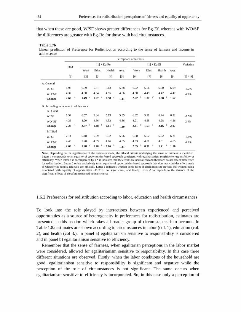
34 Preferences for redistribution: perceptions of fairness and equality of opportunity
that when these are good, W/SF shows greater differences for Eg-Ef, whereas with WO/SF the differences are greater with Eg-Re for those with bad circumstances.
Table 1.7b Linear prediction of Preference for Redistribution according to the sense of fairness and income in adolescence
Perceptions of fairness
CIRC
[1] + Eg-Re [1] + Eg-Ef Variation
Work Educ. Health Avg. Work Educ. Health Avg. [1] [2] [3] [4] [5] [6] [7] [8] [9] [5] / [9]
A. General
W/ SF 6.92 6.39 5.81 5.13 5.78 6.72 5.56 6.00 6.09 -5.2%
WO/ SF 4.32 4.90 4.54 4.55 4.66 4.50 4.49 4.42 4.47 4.3%
Change 2.60 b 1.49 a 1.27 a 0.58 a* 1.11 2.22 b 1.07 a* 1.58 b 1.62
B. According to income in adolescence B.I Good
W/ SF 6.54 6.57 5.84 5.13 5.85 6.62 5.91 6.44 6.32 -7.5%
WO/ SF 4.26 4.20 4.36 4.52 4.36 4.21 4.28 4.28 4.26 2.4% Change 2.28 b 2.37 b 1.48 b 0.61 b 1.49 2.41 b 1.63 b 2.16 b 2.07
B.II Bad
W/ SF 7.14 6.48 6.09 5.32 5.96 6.98 5.62 6.02 6.21 -3.9%
WO/ SF 4.45 5.20 4.69 4.66 4.85 4.63 4.71 4.61 4.65 4.3% Change 2.69 b 1.28 d 1.40 b 0.66 b 1.11 2.35 b 0.91 b 1.41 b 1.56
Note: Depending on the significance of the estimates made, the ethical criteria underlying the sense of fairness is identified. Letter a corresponds to an equality of opportunities based approach consistent with egalitarianism sensitive to responsibility or efficiency. When letter a is accompanied by a * it indicates that the effects are neutralized and therefore do not affect preference for redistribution. Letter b refers exclusively to an equality of opportunities based approach that does not consider effort made or whether the results achieved are efficient. Letter c indicates whether some form of egalitarianism prevails but without being associated with equality of opportunities -CIRC is not significant-, and finally, letter d corresponds to the absence of the significant effects of the aforementioned ethical criteria.
1.6.2 Preferences for redistribution according to labor, education and health circumstances
To look into the role played by interactions between experienced and perceived opportunities as a source of heterogeneity in preferences for redistribution, estimates are presented in this section which takes a broader group of circumstances into account. In Table 1.8a estimates are shown according to circumstances in labor (col. 1), education (col. 2), and health (col 3.). In panel a) egalitarianism sensitive to responsibility is considered and in panel b) egalitarianism sensitive to efficiency.
Remember that the sense of fairness, when egalitarian perceptions in the labor market were considered, allowed for egalitarianism sensitive to responsibility. In this case three different situations are observed. Firstly, when the labor conditions of the household are good, egalitarianism sensitive to responsibility is significant and negative while the perception of the role of circumstances is not significant. The same occurs when egalitarianism sensitive to efficiency is incorporated. So, in this case only a perception of
Chapter 1 35
fairness guided by egalitarianism sensitive to responsibility (generating a fall of 29.1% in preferences for redistribution) or guided by egalitarianism sensitive to efficiency (generating a fall of 37% in preferences for redistribution) operates, although the ethical criterion is not based on an equality of opportunities approach.
Secondly, when circumstances in the labor market are bad, two different situations arise. The channel of fairness operates through CIRC, generating increases in preferences for redistribution of 35%. When egalitarianism sensitive to responsibility is introduced this is significant, generating less demand for redistributive policies among those who ascribe to this approach, while egalitarianism sensitive to efficiency does not play any role in this population group.
When the axis of the egalitarian perceptions and circumstances moves from the labor market to education (col. 2), the sense of fairness adjusted by egalitarianism operates in households with the worst circumstances. When the circumstances in education are good the sense of fairness is associated exclusively to offsetting unfavorable circumstances, increasing preferences for redistribution by between 36 and 49% through this channel. In cases where circumstances are bad, both egalitarianism sensitive to responsibility and egalitarianism sensitive to efficiency are significant, reducing the role played by the sense of fairness when explaining preferences for redistribution. As already mentioned, it is possible that those with worse circumstances under-value the importance of education, either due to the intergenerational transmission of values or because they perceive that they receive no benefit from educational policies.
Finally, when the entire sample is considered and the interactions between bad circumstances and the sense of fairness are introduced, there are two relevant results. Firstly, the CIRC component of the sense of fairness is always significant and positive, and is partially offset by the interaction of bad circumstances. This indicates that the specific effect of CIRC on preferences for redistribution among those with worse circumstances is lower than among those with good circumstances. This partly explains why there is a direct and positive effect of bad circumstances (BC). The remaining component of the sense of fairness has greater heterogeneities. Firstly, Eg-Re and Eg-Ef are never significant in the health dimension. However, in education there are always significant effects that are offset for those with bad circumstances and negatively affect preferences for redistribution when circumstances are good. In the case of egalitarianisms in the labor market, there is a combination of the above results, similar to health when considering egalitarianism sensitive to efficiency, and to education with egalitarianism sensitive to responsibility.
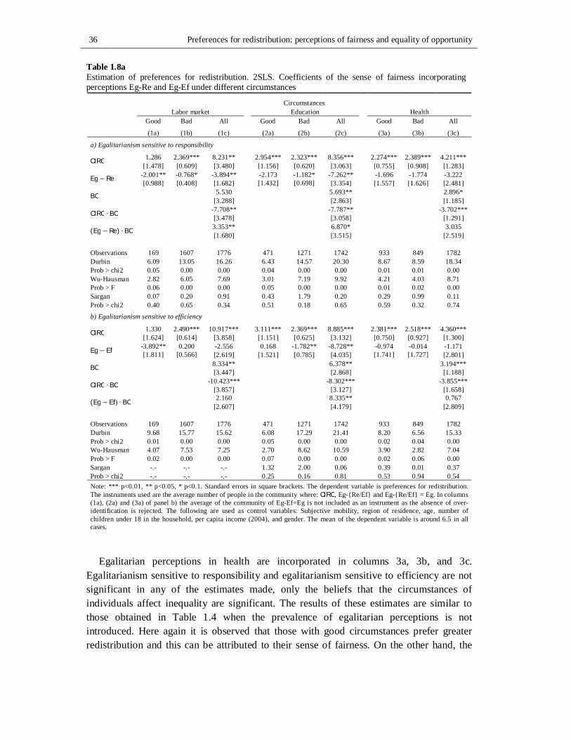
36 Preferences for redistribution: perceptions of fairness and equality of opportunity
Table 1.8a Estimation of preferences for redistribution. 2SLS. Coefficients of the sense of fairness incorporating perceptions Eg-Re and Eg-Ef under different circumstances
Circumstances Labor market Education Health Good Bad All Good Bad All Good Bad All (1a) (1b) (1c) (2a) (2b) (2c) (3a) (3b) (3c)
a) Egalitarianism sensitive to responsibility
CIRC 1.286 2.369*** 8.231** 2.954*** 2.323*** 8.356*** 2.274*** 2.389*** 4.211*** [1.478] [0.609] [3.480] [1.156] [0.620] [3.063] [0.755] [0.908] [1.283]
Eg − Re -2.001** -0.768* -3.894** -2.173 -1.182* -7.262** -1.696 -1.774 -3.222 [0.988] [0.408] [1.682] [1.432] [0.698] [3.354] [1.557] [1.626] [2.481]
BC 5.530 5.693** 2.896* [3.288] [2.863] [1.185]
CIRC ∙ BC -7.708** -7.787** -3.702*** [3.478] [3.058] [1.291]
(Eg − Re) ∙ BC 3.353** 6.870* 3.035 [1.680] [3.515] [2.519]
Observations 169 1607 1776 471 1271 1742 933 849 1782 Durbin 6.09 13.05 16.26 6.43 14.57 20.30 8.67 8.59 18.34 Prob > chi2 0.05 0.00 0.00 0.04 0.00 0.00 0.01 0.01 0.00 Wu-Hausman 2.82 6.05 7.69 3.01 7.19 9.92 4.21 4.03 8.71 Prob > F 0.06 0.00 0.00 0.05 0.00 0.00 0.01 0.02 0.00 Sargan 0.07 0.20 0.91 0.43 1.79 0.20 0.29 0.99 0.11 Prob > chi2 0.40 0.65 0.34 0.51 0.18 0.65 0.59 0.32 0.74
b) Egalitarianism sensitive to efficiency
CIRC 1.330 2.490*** 10.917*** 3.111*** 2.369*** 8.885*** 2.381*** 2.518*** 4.360*** [1.624] [0.614] [3.858] [1.151] [0.625] [3.132] [0.750] [0.927] [1.300]
Eg − Ef -3.892** 0.200 -2.556 0.168 -1.782** -8.728** -0.974 -0.014 -1.171 [1.811] [0.566] [2.619] [1.521] [0.785] [4.035] [1.741] [1.727] [2.801]
BC 8.334** 6.378** 3.194*** [3.447] [2.868] [1.188]
CIRC ∙ BC -10.423*** -8.302*** -3.855*** [3.857] [3.127] [1.658]
(Eg − Ef) ∙ BC 2.160 8.335** 0.767 [2.607] [4.179] [2.809]
Observations 169 1607 1776 471 1271 1742 933 849 1782 Durbin 9.68 15.77 15.62 6.08 17.29 21.41 8.20 6.56 15.33 Prob > chi2 0.01 0.00 0.00 0.05 0.00 0.00 0.02 0.04 0.00 Wu-Hausman 4.07 7.53 7.25 2.70 8.62 10.59 3.90 2.82 7.04 Prob > F 0.02 0.00 0.00 0.07 0.00 0.00 0.02 0.06 0.00 Sargan -.- -.- -.- 1.32 2.00 0.06 0.39 0.01 0.37 Prob > chi2 -.- -.- -.- 0.25 0.16 0.81 0.53 0.94 0.54 Note: *** p<0.01, ** p<0.05, * p<0.1. Standard errors in square brackets. The dependent variable is preferences for redistribution. The instruments used are the average number of people in the community where: CIRC, Eg-{Re/Ef} and Eg-{Re/Ef} = Eg. In columns (1a), (2a) and (3a) of panel b) the average of the community of Eg-Ef=Eg is not included as an instrument as the absence of over-identification is rejected. The following are used as control variables: Subjective mobility, region of residence, age, number of children under 18 in the household, per capita income (2004), and gender. The mean of the dependent variable is around 6.5 in all cases.
Egalitarian perceptions in health are incorporated in columns 3a, 3b, and 3c.
Egalitarianism sensitive to responsibility and egalitarianism sensitive to efficiency are not significant in any of the estimates made, only the beliefs that the circumstances of individuals affect inequality are significant. The results of these estimates are similar to those obtained in Table 1.4 when the prevalence of egalitarian perceptions is not introduced. Here again it is observed that those with good circumstances prefer greater redistribution and this can be attributed to their sense of fairness. On the other hand, the
Chapter 1 37
demand for greater redistribution from those with worse circumstances is associated with the opportunities they have experienced.
Linear predictions of references for redistribution are presented in Table 8b. The first shows the results obtained if no egalitarianism is considered. In general it is observed that there is an effect of perceptions based on the role of circumstance, except in the case where circumstances in the labor market are good. In the latter case the sense of fairness does not operate on preferences for redistribution. When the results are compared with specifications which include some egalitarianism in the perception of fairness, it appears that simply assuming the circumstances-effort dichotomy to measure perceptions of fairness magnifies the effect of this channel. For example, in the case of egalitarianism in the labor market it is observed that the effect of the channel of fairness on preferences for redistribution is 2.6 points when neither egalitarianism sensitive to responsibility nor egalitarianism sensitive to efficiency (col. 1) are considered. However, when egalitarianism sensitive to responsibility is introduced (col. 2) the effect of this channel is reduced to 1.5 points. Introducing egalitarianism sensitive to efficiency (col. 3) does not modify the results shown in the case where only CIRC is used as a channel.
Opportunities experienced affect perceived opportunities. Identifying the circumstances of the people causes, in many cases, both egalitarianism sensitive to responsibility and egalitarianism sensitive to efficiency to lose significance when explaining preferences for redistribution. Among those with good circumstances in education, good and bad circumstances in health, the channel of fairness only operates through perceptions on the role of circumstances. The same occurs with good and bad circumstances in income, regardless of the domain of life in which egalitarianism is evaluated. This is true except when egalitarisnism is introduced in education and the circumstances are bad. In these cases perceptions based on circumstances like the egalitarianisms are significant, compensating the effect of both components of the sense of fairness.
The heterogeneity introduced by incorporating different types of egalitarianism is more evident when considering the circumstances of the individuals. In general, preferences for redistribution are again higher among those with bad circumstances and with a sense of fairness close to equality of opportunities. When no egalitarianism is considered, the preferences for redistribution of these subgroups were very similar and the predicted values were around 7 points (col. 1). With egalitarianism sensitive to responsibility the predictions are always higher when the circumstances are bad, although the values are around 6 points, with a difference of almost a point with good circumstances in education and the labor market. When Eg-Ef is considered the results are similar in the labor market. In addition, if bad circumstances in the different dimensions are considered, the predicted levels of preferences for redistribution are highest when considering circumstances in the labor market. In cases where egalitarianism operates in the health and education dimensions, the relationship is inverted and preferences for redistribution are higher among those with good circumstances.
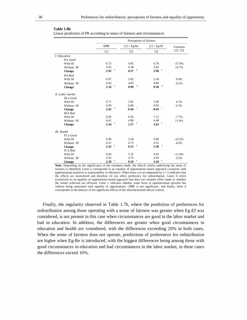
38 Preferences for redistribution: perceptions of fairness and equality of opportunity
Table 1.8b Linear prediction of PR according to sense of fairness and circumstances
Perceptions of fairness
CIRC [1] + Eg-Re [1] + Eg-Ef Variation [2] / [3] [1] [2] [3]
I. Education II.a Good With SF 6.75 4.95 6.78 -27.0% Without SF 3.83 4.38 3.82 14.7% Change 2.92 b 0.57 b 2.96 b II.b Bad With SF 6.97 5.82 5.34 9.0% Without SF 4.63 4.83 4.84 -0.2% Change 2.34 b 0.99 a* 0.50 a* II. Labor market III.a Good With SF 6.71 5.62 5.40 4.1% Without SF 4.09 6.06 6.03 0.5% Change 2.62 d -0.44 c -0.63 c III.b Bad With SF 6.95 6.56 7.11 -7.7% Without SF 4.61 4.99 4.48 11.4% Change 2.34 b 1.57 b 2.63 b III. Health IV.a Good With SF 6.96 5.28 6.90 -23.5% Without SF 4.51 4.73 4.52 4.6% Change 2.45 b 0.55 b 2.38 b IV.b Bad With SF 6.83 5.31 6.03 -11.9% Without SF 4.55 4.75 4.59 3.5% Change 2.28 b 0.56 b 1.44 b Note: Depending on the significance of the estimates made, the ethical criteria underlying the sense of fairness is identified. Letter a corresponds to an equality of opportunities based approach consistent with egalitarianism sensitive to responsibility or efficiency. When letter a is accompanied by a * it indicates that the effects are neutralized and therefore do not affect preference for redistribution. Letter b refers exclusively to an equality of opportunities based approach that does not consider effort made or whether the results achieved are efficient. Letter c indicates whether some form of egalitarianism prevails but without being associated with equality of opportunities -CIRC is not significant-, and finally, letter d corresponds to the absence of the significant effects of the aforementioned ethical criteria.
Finally, the regularity observed in Table 1.7b, where the prediction of preferences for redistribution among those operating with a sense of fairness was greater when Eg-Ef was considered, is not present in this case when circumstances are good in the labor market and bad in education. In addition, the differences are greater when good circumstances in education and health are considered, with the differences exceeding 20% in both cases. When the sense of fairness does not operate, predictions of preferences for redistribution are higher when Eg-Re is introduced, with the biggest differences being among those with good circumstances in education and bad circumstances in the labor market, in these cases the differences exceed 10%.
Chapter 1 39
1.7 Sensitivity of the results
In this section the robustness of the results is verified by considering the role of mobility in preferences for redistribution and making a more precise approximation to the processes of forming the sense of fairness. In section 1.7.1 estimates are made considering objective mobility indicators (푀푂) among the independent variables, both intergenerational 푀푂 and intragenerational (푀푂 ). The aim is to study whether the role played
by the sense of fairness when explaining preferences for redistribution is modified as a result of changes experienced by the individuals in relation to their parents or throughout their own lives. Secondly, (section 1.7.2) I attempt to identify with greater precision whether social preferences are based on reciprocity or, alternatively, if they are based on altruistic motives. For this, it is assumed that the peer group would only be affect the formation of a sense of fairness in the first case.
In order to test whether the role played by the sense of fairness is modified when objective mobility variables are introduced, the specifications used in the previous sections are increased. For example, in the case of the baseline specification a utility function is estimated with the following characteristics:
푈 = 훼 ∙ 푋 + 훽 ∙ 푢 푐 (…푄 ) + 휌 ∙ 푀푆 + 훿∗ ∙ 푄 푄 ,∗,ℎ + 휂 ∙ 푀푂 (1.5)
where 훿∗ is the new parameter that identifies whether the cannel of fairness operates in the formation of preferences for redistribution, while j indicates whether the measure of the mobility used is inter or intragenerational. Additionally, the possibility that the sense of fairness is determined, in part, by the levels of individual mobility is enabled, so a set of estimates is incorporated where the mobility variable interacts with the sense of fairness.
The second aspect considered in this section is associated with the formation of the sense of fairness. This formation may be determined by altruistic motives or reciprocity, and, as has been already mentioned, only in the case where reciprocity plays a role does the peer group intervene. In the survey used in this paper respondents were asked – Who do you consider will contribute more to a change in your life? and seven possible answers are provided: you, the national government, a group of people, religion, your family, the local government and another person. In this section it is assumed that those who responded a group of people or another person are probably those who form their sense of fairness through interaction with their peer group.
When attempting to closer approximate the process of forming social preferences, whether for altruistic motives or reciprocity, the interaction of variables which reflect the sense of fairness is incorporated into a new specification with a dichotomous variable which identies whether this is formed by criteria of reciprocity (θ ). A variable is also introduced where the sense of fairness interacts with the complement of the criterion of reciprocity (1 − θ ) in which it is assumed that the formation of the sense of fairness is
40 Preferences for redistribution: perceptions of fairness and equality of opportunity
closer to altruistic motives. The specifications which reflect the role played by altruistic social preferences and based on reciprocity, for the case where egalitarianism sensitive to responsibility is considered, is expressed as:
푈 = 훼 ∙ 푋 + 훽 ∙ 푢 푐 (…푄 ) + 휌 ∙푀푆 + 훿 ∙ 푄 (푄 ,∗, ℎ )
+휑 ∙ 핀 푄 { },∗ − 푄 { },∗ > 0 ∙ 휃 +휑 ∙ 핀 푄 { },∗ − 푄 { },∗ > 0 ∙ (1− 휃 ) (1.6) Throughout this paper it has been considered that the formation of social preferences
arose from reciprocity, which is why interaction with the peer group was a relevant normative source for all individuals. For this reason in all estimates it is assumed that the endogeneity of the sense of fairness was corrected taking the perception on the sense of fairness declared by the peers into account. In this section the role of the peer group is confined to the group where reciprocity plays a role in the formation of the sense of fairness and, therefore, is used to deal with endogeneity problems only in this case. In other words, it is assumed that when the origin of social preferences is linked to altruistic motives, the peer group plays no role.
1.7.1 Sense of fairness and mobility
In this paper it has been indicated that the sense of fairness is an identifying feature of individuals and, therefore, should be relatively stable over time. However, it is possible that variations in income can cause changes in the reported levels of fairness, which I will attempt to verify in this section. Additionally, the sense of fairness may contain effects which should be attributed to intergenerational mobility. In order to verify that the inclusion of a variable of this nature does not modify the findings presented in the previous sections, estimates were made where inter and intragenerational mobility were introduced. At the same time the role played by mobility in the formation of the sense of fairness of individuals is studied, which corresponds to the first stage of the different estimates made in the previous section.
The inclusion of inter and intragenerational mobility is done seperately and is presented in Table 1.9, the intragenerational mobility is included in the odd numbered columns and the intergenerational mobility in the even numbered columns. The estimates are also made without including the egalitarian perceptions sensitive to responsibility and efficiency –panel A- and including them successively in the labor market –panel B-, in education –panel C- and in health –panel D-. The first thing which is apparent is that mobility negatively affects preferences for redistribution when egalitarian perceptions are not included. In these cases perceptions of the role of circumstances maintain their level and significance, around 40% of the mean of the dependent variable. In the case of intragenerational mobility, each additional unit of variation in income implies a fall of 2.5% in preferences for redistribution, while those with a higher level of education than
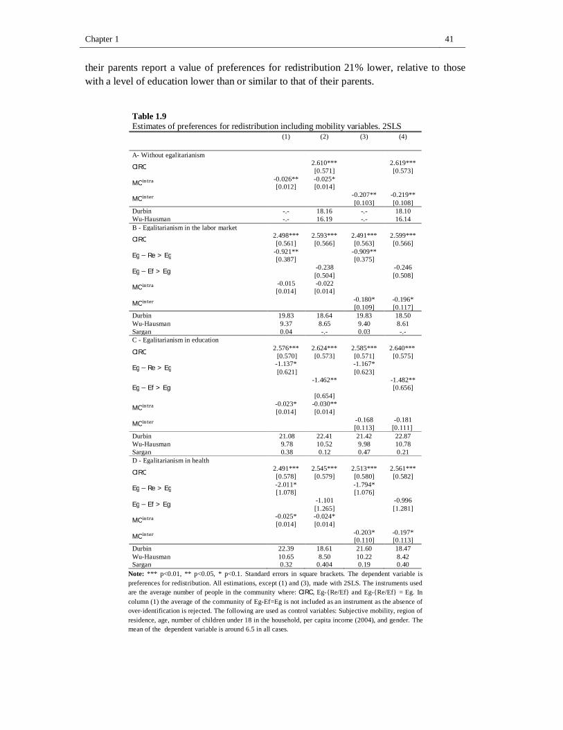
Chapter 1 41
their parents report a value of preferences for redistribution 21% lower, relative to those with a level of education lower than or similar to that of their parents.
Note: *** p<0.01, ** p<0.05, * p<0.1. Standard errors in square brackets. The dependent variable is preferences for redistribution. All estimations, except (1) and (3), made with 2SLS. The instruments used are the average number of people in the community where: CIRC, Eg-{Re/Ef} and Eg-{Re/Ef} = Eg. In column (1) the average of the community of Eg-Ef=Eg is not included as an instrument as the absence of over-identification is rejected. The following are used as control variables: Subjective mobility, region of residence, age, number of children under 18 in the household, per capita income (2004), and gender. The mean of the dependent variable is around 6.5 in all cases.
Table 1.9 Estimates of preferences for redistribution including mobility variables. 2SLS
(1) (2) (3) (4)
A- Without egalitarianism
CIRC 2.610*** 2.619*** [0.571] [0.573]
MO -0.026** -0.025* [0.012] [0.014]
MO -0.207** -0.219** [0.103] [0.108]
Durbin -.- 18.16 -.- 18.10 Wu-Hausman -.- 16.19 -.- 16.14 B - Egalitarianism in the labor market
CIRC 2.498*** 2.593*** 2.491*** 2.599*** [0.561] [0.566] [0.563] [0.566]
Eg − Re > Eg -0.921** -0.909** [0.387] [0.375]
Eg − Ef > Eg -0.238 -0.246 [0.504] [0.508]
MO -0.015 -0.022 [0.014] [0.014]
MO -0.180* -0.196* [0.109] [0.117]
Durbin 19.83 18.64 19.83 18.50 Wu-Hausman 9.37 8.65 9.40 8.61 Sargan 0.04 -.- 0.03 -.- C - Egalitarianism in education
CIRC 2.576*** 2.624*** 2.585*** 2.640*** [0.570] [0.573] [0.571] [0.575]
Eg − Re > Eg -1.137* -1.167* [0.621] [0.623]
Eg − Ef > Eg -1.462** -1.482**
[0.654] [0.656]
MO -0.023* -0.030** [0.014] [0.014]
MO -0.168 -0.181 [0.113] [0.111]
Durbin 21.08 22.41 21.42 22.87 Wu-Hausman 9.78 10.52 9.98 10.78 Sargan 0.38 0.12 0.47 0.21 D - Egalitarianism in health
CIRC 2.491*** 2.545*** 2.513*** 2.561*** [0.578] [0.579] [0.580] [0.582]
Eg − Re > Eg -2.011* -1.794* [1.078] [1.076]
Eg − Ef > Eg -1.101 -0.996 [1.265] [1.281]
MO -0.025* -0.024* [0.014] [0.014]
MO -0.203* -0.197* [0.110] [0.113]
Durbin 22.39 18.61 21.60 18.47 Wu-Hausman 10.65 8.50 10.22 8.42 Sargan 0.32 0.404 0.19 0.40
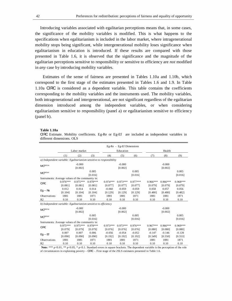
42 Preferences for redistribution: perceptions of fairness and equality of opportunity
Introducing variables associated with egalitarian perceptions means that, in some cases, the significance of the mobility variables is modified. This is what happens to the specifications when egalitarianism is included in the labor market, where intragenerational mobility stops being significant, while intergenerational mobility loses significance when egalitarianism in education is introduced. If these results are compared with those presented in Table 1.6, it is observed that the significance and the magnitude of the egalitarian perceptions sensitive to responsibility or sensitive to efficiency are not modified in any case by introducing mobility variables.
Estimates of the sense of fairness are presented in Tables 1.10a and 1.10b, which correspond to the first stage of the estimates presented in Tables 1.6 and 1.9. In Table 1.10a CIRC is considered as a dependent variable. This table contains the coefficients corresponding to the mobility variables and the instruments used. The mobility variables, both intragenerational and intergenerational, are not significant regardless of the egalitarian dimension introduced among the independent variables, or when considering egalitarianism sensitive to responsibility (panel a) or egalitarianism sensitive to efficiency (panel b).
Table 1.10a CIRC Estimate. Mobility coefficients. Eg-Re or Eg-Ef are included as independent variables in different dimensions. OLS
Eg-Re - Eg-Ef Dimensions Labor market Education Health
(1) (2) (3) (4) (5) (6) (7) (8) (9) a) Independent variable: Egalitarianism sensitive to responsibility
MO -0.000 -0.000 -0.000 [0.002] [0.002] [0.002]
MO 0.005 0.005 0.005 [0.016] [0.016] [0.016]
Instruments: Average values of the community in:
CIRC 0.976*** 0.975*** 0.978*** 0.974*** 0.973*** 0.977*** 0.966*** 0.966*** 0.968*** [0.081] [0.081] [0.081] [0.077] [0.077] [0.077] [0.079] [0.079] [0.079]
Eg − Re 0.012 0.014 0.014 -0.060 -0.059 -0.059 0.058 0.057 0.056 [0.104] [0.104] [0.104] [0.129] [0.129] [0.129] [0.480] [0.480] [0.482]
Observations 1881 1881 1871 1881 1881 1871 1881 1881 1871 R2 0.10 0.10 0.10 0.10 0.10 0.10 0.10 0.10 0.10 b) Independent variable: Egalitarianism sensitive to efficiency
MO -0.000 -0.000 -0.000 [0.002] [0.002] [0.002]
MO 0.005 0.005 0.005 [0.016] [0.016] [0.016]
Instruments: Average values of the community in:
CIRC 0.975*** 0.975*** 0.978*** 0.973*** 0.973*** 0.976*** 0.967*** 0.966*** 0.969*** [0.079] [0.079] [0.079] [0.076] [0.076] [0.076] [0.080] [0.080] [0.080]
Eg − Ef 0.007 0.007 0.006 -0.056 -0.054 -0.052 -0.147 -0.146 -0.128 [0.090] [0.090] [0.090] [0.192] [0.192] [0.192] [0.549] [0.550] [0.553]
Observations 1881 1881 1871 1881 1881 1871 1881 1881 1871 R2 0.10 0.10 0.10 0.10 0.10 0.10 0.10 0.10 0.10 Note: *** p<0.01, ** p<0.05, * p<0.1. Standard errors in square brackets. The dependent variable is the perception of the role of circumstances in explaining poverty –CIRC -. First stage of the 2SLS estimates presented in Table 1.6.
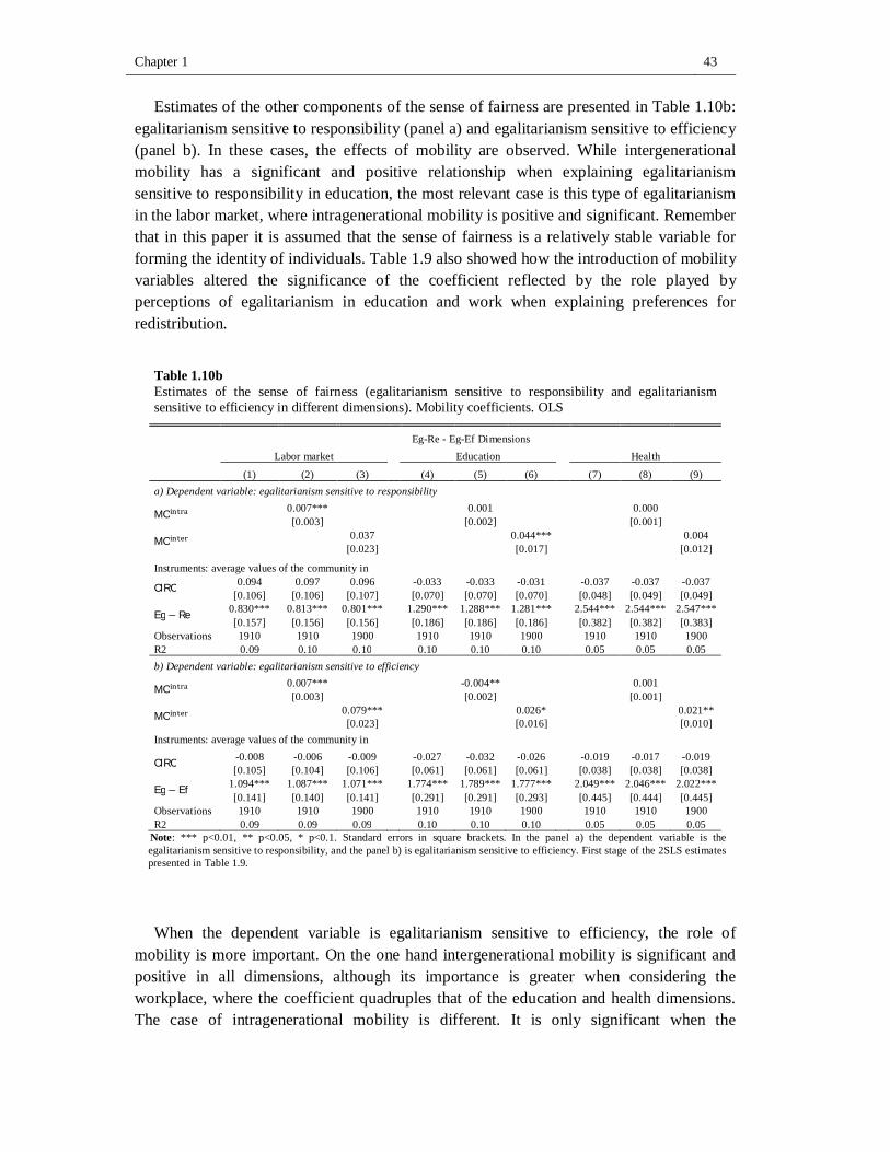
Chapter 1 43
Estimates of the other components of the sense of fairness are presented in Table 1.10b: egalitarianism sensitive to responsibility (panel a) and egalitarianism sensitive to efficiency (panel b). In these cases, the effects of mobility are observed. While intergenerational mobility has a significant and positive relationship when explaining egalitarianism sensitive to responsibility in education, the most relevant case is this type of egalitarianism in the labor market, where intragenerational mobility is positive and significant. Remember that in this paper it is assumed that the sense of fairness is a relatively stable variable for forming the identity of individuals. Table 1.9 also showed how the introduction of mobility variables altered the significance of the coefficient reflected by the role played by perceptions of egalitarianism in education and work when explaining preferences for redistribution.
Table 1.10b Estimates of the sense of fairness (egalitarianism sensitive to responsibility and egalitarianism sensitive to efficiency in different dimensions). Mobility coefficients. OLS
Eg-Re - Eg-Ef Dimensions Labor market Education Health
(1) (2) (3) (4) (5) (6) (7) (8) (9) a) Dependent variable: egalitarianism sensitive to responsibility
MO 0.007*** 0.001 0.000 [0.003] [0.002] [0.001]
MO 0.037 0.044*** 0.004 [0.023] [0.017] [0.012]
Instruments: average values of the community in
CIRC 0.094 0.097 0.096 -0.033 -0.033 -0.031 -0.037 -0.037 -0.037 [0.106] [0.106] [0.107] [0.070] [0.070] [0.070] [0.048] [0.049] [0.049]
Eg − Re 0.830*** 0.813*** 0.801*** 1.290*** 1.288*** 1.281*** 2.544*** 2.544*** 2.547*** [0.157] [0.156] [0.156] [0.186] [0.186] [0.186] [0.382] [0.382] [0.383]
Observations 1910 1910 1900 1910 1910 1900 1910 1910 1900 R2 0.09 0.10 0.10 0.10 0.10 0.10 0.05 0.05 0.05 b) Dependent variable: egalitarianism sensitive to efficiency
MO 0.007*** -0.004** 0.001 [0.003] [0.002] [0.001]
MO 0.079*** 0.026* 0.021** [0.023] [0.016] [0.010]
Instruments: average values of the community in
CIRC -0.008 -0.006 -0.009 -0.027 -0.032 -0.026 -0.019 -0.017 -0.019 [0.105] [0.104] [0.106] [0.061] [0.061] [0.061] [0.038] [0.038] [0.038]
Eg − Ef 1.094*** 1.087*** 1.071*** 1.774*** 1.789*** 1.777*** 2.049*** 2.046*** 2.022*** [0.141] [0.140] [0.141] [0.291] [0.291] [0.293] [0.445] [0.444] [0.445]
Observations 1910 1910 1900 1910 1910 1900 1910 1910 1900 R2 0.09 0.09 0.09 0.10 0.10 0.10 0.05 0.05 0.05
Note: *** p<0.01, ** p<0.05, * p<0.1. Standard errors in square brackets. In the panel a) the dependent variable is the egalitarianism sensitive to responsibility, and the panel b) is egalitarianism sensitive to efficiency. First stage of the 2SLS estimates presented in Table 1.9.
When the dependent variable is egalitarianism sensitive to efficiency, the role of mobility is more important. On the one hand intergenerational mobility is significant and positive in all dimensions, although its importance is greater when considering the workplace, where the coefficient quadruples that of the education and health dimensions. The case of intragenerational mobility is different. It is only significant when the
44 Preferences for redistribution: perceptions of fairness and equality of opportunity
dependent variable is egalitarianism sensitive to efficiency in the labor market and in education, although the sign is positive in the first case and negative in the second. In other words, the greatest variation in income is associated with higher egalitarianism sensitive to efficiency in the labor market and less egalitarianism sensitive to efficiency in education.
Ultimately there is evidence of the effects of variation of income in egalitarianism sensitive to responsibility when this component of the sense of fairness is evaluated in the labor market, and in egalitarianism sensitive to efficiency if it is evaluated in the labor market and education. Within the labor market it is observed that individuals become more sensitive to results being efficient, and value effort incrementally as their income increases. When fairness is evaluated in this dimension there is a stable component associated with perceptions of the role of circumstances, however the sense of fairness viewed globally varies as a consequence of changes in income. Greater variations in income result in lower preferences for redistribution.
In order to show the role played by intragenerational mobility in egalitarianism sensitive to efficiency and responsibility more clearly, Fig. 1.4 shows the evolution of the prediction of both egalitarianisms according to the vigintile of the variation in income. It is clear that when egalitarianism is applied to the labor market (panel a) it is observed that after the initial stages of stability (and fall in the case of egalitarianism sensitive to efficiency), perception of the importance of both egalitarianisms grows continuously with the variation in income. Throughout, the level of egalitarianism sensitive to responsibility is higher in relation to egalitarianism sensitive to efficiency, although the latter increases at a higher rate from the eighth vigintile. Thus, higher mobility increases the importance of egalitarianism in the labor market when explaining preferences for redistribution.
The predictions of egalitarianism in education (panel b) and health (panel c) have substantially lower and more stable levels. Egalitarianism in education shows different developments in relation to intragenerational mobility, depending on whether egalitarianism sensitive to responsibility or sensitive to efficiency is considered. In the case of egalitarianism sensitive to responsibility it is observed that the trajectory is a relatively stable U-shape, while egalitarianism sensitive to efficiency decreases with the variation in income, mainly in the first stages of the distribution of these variations. In fact, those with low intragenerational mobility show high levels (and very similar) of egalitarianism if either of the two criteria are considered. On the other hand, large differences are observed among those with high intragenerational mobility, with egalitarianism sensitive to responsibility perceptions being higher compared to egalitarianism sensitive to efficiency.
In the case of health, differences are also observed in the evolution of both egalitarianisms based on changes in income, but with levels very close to zero. Egalitarianism sensitive to responsibility is relatively stable throughout, with values oscillating between 0.06 and 0.07. Egalitarianism sensitive to efficiency increases with intragenerational mobility, but at very low levels ranging from 0.035 in the first vigintile to 0.05 in the last.
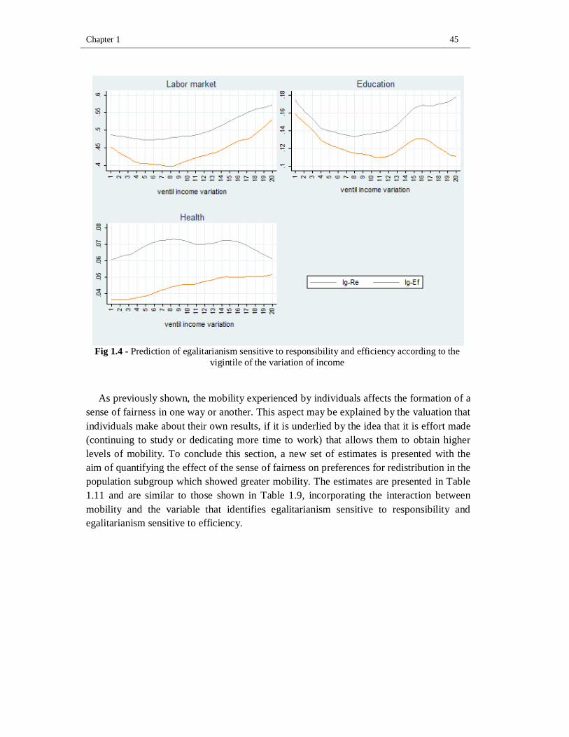
Chapter 1 45
Fig 1.4 - Prediction of egalitarianism sensitive to responsibility and efficiency according to the
vigintile of the variation of income
As previously shown, the mobility experienced by individuals affects the formation of a
sense of fairness in one way or another. This aspect may be explained by the valuation that individuals make about their own results, if it is underlied by the idea that it is effort made (continuing to study or dedicating more time to work) that allows them to obtain higher levels of mobility. To conclude this section, a new set of estimates is presented with the aim of quantifying the effect of the sense of fairness on preferences for redistribution in the population subgroup which showed greater mobility. The estimates are presented in Table 1.11 and are similar to those shown in Table 1.9, incorporating the interaction between mobility and the variable that identifies egalitarianism sensitive to responsibility and egalitarianism sensitive to efficiency.
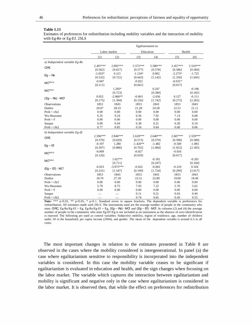
46 Preferences for redistribution: perceptions of fairness and equality of opportunity
Table 1.11 Estimates of preferences for redistribution including mobility variables and the interaction of mobility with Eg-Re or Eg-Ef. 2SLS
Egalitariansim in:
Labor market Education Health
(1) (2) (3) (4) (5) (6)
a) Independent variable Eg-Re
CIRC 2.497*** 2.892*** 2.575*** 2.580*** 2.457*** 2.510*** [0.562] [0.627] [0.577] [0.578] [0.586] [0.584]
Eg − Re -1.033* 0.121 -1.134* 0.002 -2.273* -1.725 [0.532] [0.721] [0.643] [1.142] [1.330] [1.645]
MO -0.047 -0.022 -0.031* [0.111] [0.041] [0.017]
MO 1.283* 0.247 -0.196 [0.723] [0.289] [0.182]
(Eg − Re) ∙ MO 0.052 -2.860** -0.003 -2.656 0.127 -0.111 [0.175] [1.394] [0.156] [1.742] [0.273] [2.265]
Observations 1853 1843 1853 1843 1853 1843 Durbin 20.07 28.33 21.28 24.58 22.51 21.11 Prob > chi2 0.00 0.00 0.00 0.00 0.00 0.00 Wu-Hausman 6.35 9.24 6.56 7.92 7.14 6.68 Prob > F 0.00 0.00 0.00 0.00 0.00 0.00 Sargan 0.09 0.04 0.38 0.21 0.28 0.19 Prob > chi2 0.77 0.85 0.54 0.64 0.60 0.66
b) Independent variable Eg-Ef
CIRC 2.596*** 2.846*** 2.618*** 2.640*** 2.607*** 2.559*** [0.570] [0.629] [0.573] [0.579] [0.598] [0.580]
Eg − Ef -0.197 1.280 -1.426** -1.482 -0.500 -1.083 [0.597] [0.886] [0.702] [1.084] [1.653] [2.185]
MO -0.009 -0.027 -0.016 [0.126] [0.029] [0.017]
MO 1.627** -0.181 -0.201 [0.711] [0.247] [0.160]
(Eg − Ef) ∙ MO -0.023 -3.975*** -0.022 -0.002 -0.210 0.104 [0.231] [1.547] [0.190] [1.724] [0.299] [2.617]
Observations 1853 1843 1853 1843 1853 1843 Durbin 18.70 27.18 22.51 22.89 19.00 18.49 Prob > chi2 0.00 0.00 0.00 0.00 0.00 0.00 Wu-Hausman 5.79 8.75 7.03 7.22 5.76 5.62 Prob > F 0.00 0.00 0.00 0.00 0.00 0.00 Sargan -.- -.- 0.11 0.21 0.63 0.40 Prob > chi2 -.- -.- 0.74 0.65 0.43 0.53 Note: *** p<0.01, ** p<0.05, * p<0.1. Standard errors in square brackets. The dependent variable is preferences for redistribution. All estimates made with 2SLS. The instruments used are the average number of people in the community who state: CIRC, Eg-Re/Eg-Ef > Eg, Eg-Re/Eg-Ef = Eg, (Eg − Re) ∙MO and (Eg − Ef) ∙ MO . In columns (2) and (4) the average number of people in the community who state Eg-Ef=Eg is not included as an instrument as the absence of over-identification is rejected. The following are used as control variables: Subjective mobility, region of residence, age, number of children under 18 in the household, per capita income (2004), and gender. The mean of the dependent variable is around 6.5 in all cases.
The most important changes in relation to the estimates presented in Table 8 are observed in the cases where the mobility considered is intergenerational. In panel (a) the case where egalitarianism sensitive to responsibility is incorporated into the independent variables is considered. In this case the mobility variable ceases to be significant if egalitarianism is evaluated in education and health, and the sign changes when focusing on the labor market. The variable which captures the interaction between egalitarianism and mobility is significant and negative only in the case where egalitarianism is considered in the labor market. It is observed then, that while the effect on preferences for redistribution
Chapter 1 47
increases as a result of the perceptions of fairness based on the income generating process and greater intergenerational mobility, the effect is partially offset for those whose perceptions of fairness are also close to egalitarianism senstive to responsibility and with high intergenerational mobility. In the latter case the demand for redistributive policies is reduced. This is similar to what occurs in the case where the independent variable is egalitarianism sensitive to efficiency (panel b), with the magnitude of the coefficient being higher where perceptions of egalitarianism in the labor market interact with intergenerational mobility.
1.7.2 Altruism and reciprocity
This paper has referenced throughout that perceptions of fairness are introduced in the utility function as these are a factor associated with the identity of individuals. For this it was also asssumed that the formation of the sense of fairness is based on reciprocity. However, previous studies associate sense of fairness to the altruistic attitudes of individuals. Both elements could affect the formation of the sense of fairness, but only the criterion based on reciprocity is constructed from interaction with the peer group. Table 12 shows estimates of preferences for redistribution considering whether the sense of fairness is associated with the principle of reciprocity or altruism. For this, I introduce the interaction between the variables used to capture the sense of fairness and the proxy variable of reciprocity (θ) on the one hand, and the proxy of altruism (1 − θ) on the other. As mentioned in the estimates, only instruments for the variable which captures the interaction of the sense of fairness and the proxy of reciprocity are used, as it is this group which should be influenced by the peer group.
The first column, where the sense of fairness without considering any type of egalitarianism is introduced, shows that the role of CIRC is more important among those whose behavior is based on reciprocity than in the case where the behavior is based on altruistic motives. For the former, preferences for redistribution increased almost 70% compared to the mean of the dependent variable, while for the latter it is just 40%. The next six columns introduce egalitarianism sensitive to responsibility (even columns) and egalitarianism sensitive to efficiency (odd columns). The first thing which is observed is that among those who form their sense of fairness from an altruistic perspective, the underlying ethical criterion is one which posits offsetting inequalities which arise from circumstances, as only CIRC · (1− θ) is significant. In these cases preferences for redistribution increase between 35% and 40%.
When perceptions of fairness are introduced into the utility function as a consequence of the reciprocity of individuals, more heterogeneous results are observed. Firstly, the perspective of justice is associated with the notion equality of opportunities sensitive to responsibility and efficiency if egalitarianism is evaluated in the labor market. However, the joint significance hypothesis of the variables CIRC · θ and Ig − Re · θ is rejected. On
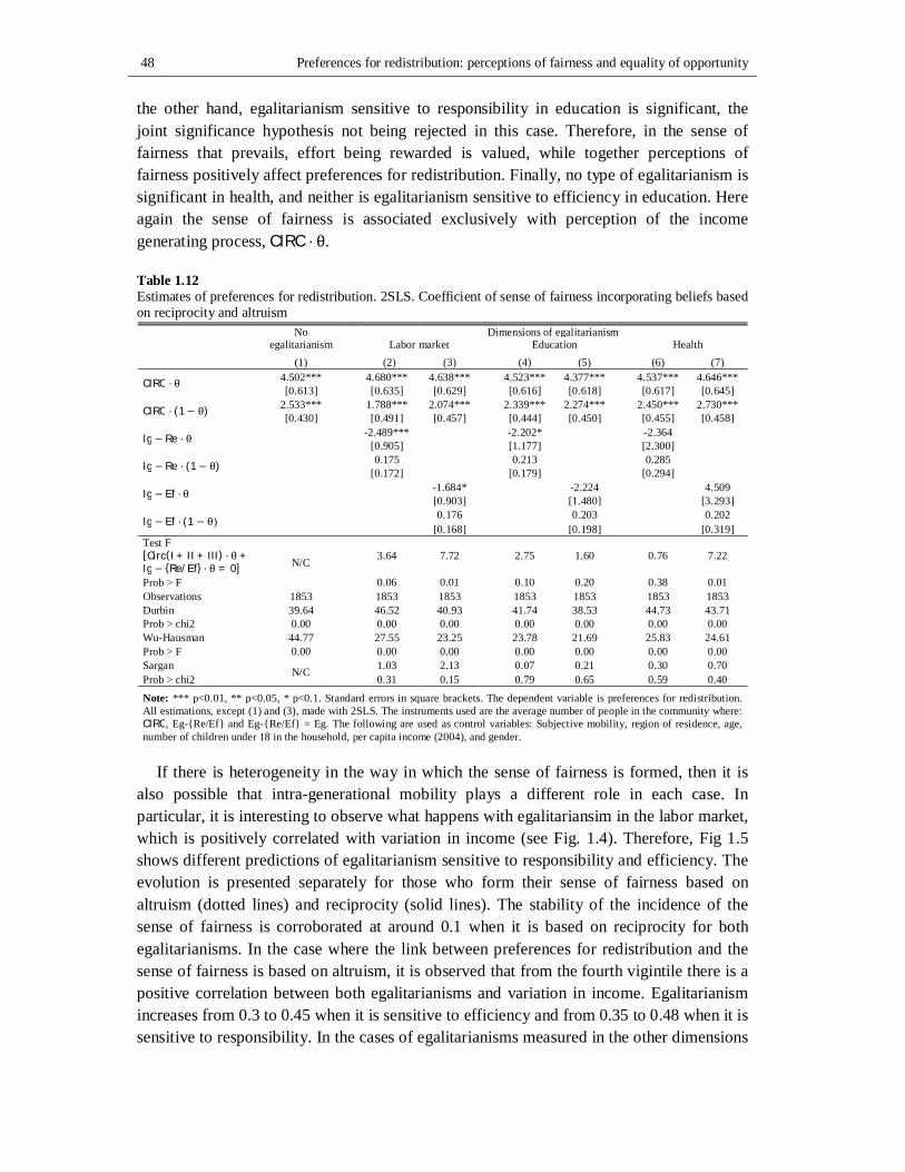
48 Preferences for redistribution: perceptions of fairness and equality of opportunity
the other hand, egalitarianism sensitive to responsibility in education is significant, the joint significance hypothesis not being rejected in this case. Therefore, in the sense of fairness that prevails, effort being rewarded is valued, while together perceptions of fairness positively affect preferences for redistribution. Finally, no type of egalitarianism is significant in health, and neither is egalitarianism sensitive to efficiency in education. Here again the sense of fairness is associated exclusively with perception of the income generating process, CIRC · θ. Table 1.12 Estimates of preferences for redistribution. 2SLS. Coefficient of sense of fairness incorporating beliefs based on reciprocity and altruism
No egalitarianism
Dimensions of egalitarianism Labor market Education Health (1) (2) (3) (4) (5) (6) (7)
CIRC · θ 4.502*** 4.680*** 4.638*** 4.523*** 4.377*** 4.537*** 4.646*** [0.613] [0.635] [0.629] [0.616] [0.618] [0.617] [0.645]
CIRC · (1− θ) 2.533*** 1.788*** 2.074*** 2.339*** 2.274*** 2.450*** 2.730*** [0.430] [0.491] [0.457] [0.444] [0.450] [0.455] [0.458]
Ig − Re · θ -2.489*** -2.202* -2.364 [0.905] [1.177] [2.300]
Ig − Re · (1− θ) 0.175 0.213 0.285 [0.172] [0.179] [0.294]
Ig − Ef · θ -1.684* -2.224 4.509 [0.903] [1.480] [3.293]
Ig − Ef · (1 − θ) 0.176 0.203 0.202 [0.168] [0.198] [0.319]
Test F [Circ(I + II + III) · θ +Ig − {Re/Ef} · θ = 0] N/C 3.64 7.72 2.75 1.60 0.76 7.22
Prob > F 0.06 0.01 0.10 0.20 0.38 0.01 Observations 1853 1853 1853 1853 1853 1853 1853 Durbin 39.64 46.52 40.93 41.74 38.53 44.73 43.71 Prob > chi2 0.00 0.00 0.00 0.00 0.00 0.00 0.00 Wu-Hausman 44.77 27.55 23.25 23.78 21.69 25.83 24.61 Prob > F 0.00 0.00 0.00 0.00 0.00 0.00 0.00 Sargan N/C
1.03 2.13 0.07 0.21 0.30 0.70 Prob > chi2 0.31 0.15 0.79 0.65 0.59 0.40
Note: *** p<0.01, ** p<0.05, * p<0.1. Standard errors in square brackets. The dependent variable is preferences for redistribution. All estimations, except (1) and (3), made with 2SLS. The instruments used are the average number of people in the community where: CIRC, Eg-{Re/Ef} and Eg-{Re/Ef} = Eg. The following are used as control variables: Subjective mobility, region of residence, age, number of children under 18 in the household, per capita income (2004), and gender.
If there is heterogeneity in the way in which the sense of fairness is formed, then it is
also possible that intra-generational mobility plays a different role in each case. In particular, it is interesting to observe what happens with egalitariansim in the labor market, which is positively correlated with variation in income (see Fig. 1.4). Therefore, Fig 1.5 shows different predictions of egalitarianism sensitive to responsibility and efficiency. The evolution is presented separately for those who form their sense of fairness based on altruism (dotted lines) and reciprocity (solid lines). The stability of the incidence of the sense of fairness is corroborated at around 0.1 when it is based on reciprocity for both egalitarianisms. In the case where the link between preferences for redistribution and the sense of fairness is based on altruism, it is observed that from the fourth vigintile there is a positive correlation between both egalitarianisms and variation in income. Egalitarianism increases from 0.3 to 0.45 when it is sensitive to efficiency and from 0.35 to 0.48 when it is sensitive to responsibility. In the cases of egalitarianisms measured in the other dimensions
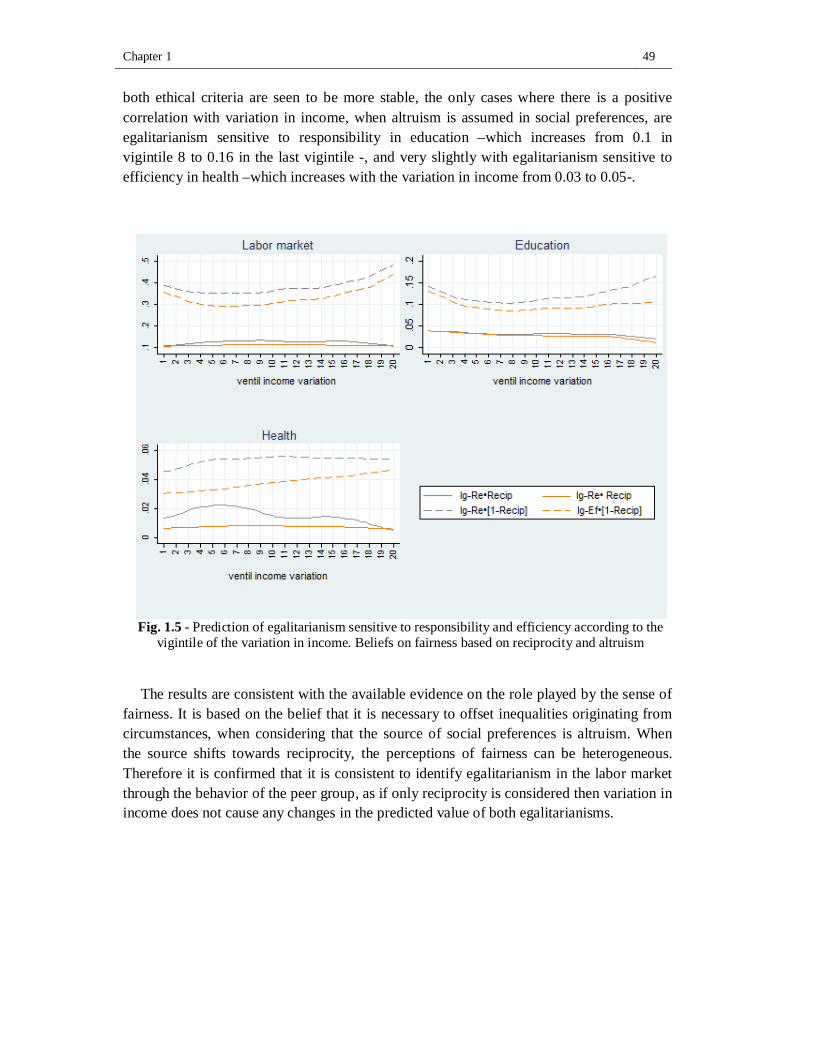
Chapter 1 49
both ethical criteria are seen to be more stable, the only cases where there is a positive correlation with variation in income, when altruism is assumed in social preferences, are egalitarianism sensitive to responsibility in education –which increases from 0.1 in vigintile 8 to 0.16 in the last vigintile -, and very slightly with egalitarianism sensitive to efficiency in health –which increases with the variation in income from 0.03 to 0.05-.
Fig. 1.5 - Prediction of egalitarianism sensitive to responsibility and efficiency according to the
vigintile of the variation in income. Beliefs on fairness based on reciprocity and altruism The results are consistent with the available evidence on the role played by the sense of
fairness. It is based on the belief that it is necessary to offset inequalities originating from circumstances, when considering that the source of social preferences is altruism. When the source shifts towards reciprocity, the perceptions of fairness can be heterogeneous. Therefore it is confirmed that it is consistent to identify egalitarianism in the labor market through the behavior of the peer group, as if only reciprocity is considered then variation in income does not cause any changes in the predicted value of both egalitarianisms.
50 Preferences for redistribution: perceptions of fairness and equality of opportunity
1.8 Conclusions In this paper the role of perceptions of fairness in preferences for redistribution is explored. Both elements are known from the subjective statements of individuals, so the channel of fairness is potentially endogenous. This aspect is corroborated in the workplace, showing that introducing perceptions of fairness assuming exogeneity overestimates the real magnitude of the channel. Moreover it accurately reveals the beliefs of individuals about what they understand to be fair and not, allowing for heterogeneity in the way in which egalitarianism is conceptualized. For this egalitarianism sensitive to responsibility and sensitive to efficiency are introduced into the estimates. In general the results show that there is a perception of fairness based on equality of opportunities sensitive to the role played by responsibility. This component reduces the magnitude of the channel of fairness which would be obtained if only perceptions about the role played by circumstances in economic results were considered.
It is also demonstrated that it is necessary to consider two other types of heterogeneities when exploring the role played by the sense of fairness. On the one hand, individuals generate their beliefs in different domains of life and therefore vary the way in which they interpret what is fair or not when evaluating egalitarianism in the labor market, education and health. While in the labor market individuals believe that effort should be rewarded, in health they understand that inequalities should be offset considering only those which arise from circumstances. On the other hand it is observed that perceived opportunities are associated with opportunities experienced. The effect of the different egalitarianisms is diluted in general when considering subgroups with similar circumstances. In these cases a sense of fairness that demands offsetting inequalities arising from circumstances prevails, except for those coming from households with good performances in the workplace, in which case individuals do not have a sense of fairness based on equality of opportunities. In this group it is understood that inequalities are the consequence solely of effort and, therefore, demand less government intervention. In addition, the circumstances affect the degree of demand for redistributive policies. In general individuals with bad circumstances reported a greater preference for redistribution.
It is corroborated that greater inter-generational mobility negatively affects preferences for redistribution. This is not the case with intra-generacional mobility. The latter variable directly affects the preferences for redistribution of a population subgroup. In this paper it is demonstrated that while sense of fairness is an identifying feature of individuals, it oscillates depending on the variation in income when egalitarianism in the labor market is considered. Individuals who report greater variation in income throughout their lives are more likely to feel a preference for egalitarianism sensitive to responsibility in the labor market, which implies lower preferences for redistributive policies. The same applies to egalitarianism sensitive to efficiency in the labor market. However, this element is relativized when the sources through which perceptions of fairness are introduced into the utility function are distinguished, with this link between sense of fairness and variation in income being associated with social preferences based on altruism.
Chapter 1 51
These results may be relevant when thinking about the design of public policy that is better accepted among the population and are sustainable over time. If educational level attained and hours dedicated to work tasks are an indirect approximation of effort made, it is probable that new tax policy designs, based on greater taxes for higher work income will face more barriers than proposals which focus on increasing taxes on capital. The reason for this is that the source of capital income is generally unknown and may be associated with the lottery in which all individuals participate from birth.
Finally, and most importantly, the longer processes of educational and residential segregation which characterize the Uruguayan society are maintained, with similar reference groups between themselves and different from the rest, the lower the probability that the population accepts more redistributive policies will be. The interaction with people from different social backgrounds is a powerful normative source, which contributes to forming a sense of fairness which emphasizes elements beyond the control of the people.
52 Preferences for redistribution: perceptions of fairness and equality of opportunity
Reference
Akerlof G. & R. Kranton (2000). “Economics and identity”, Quarterly Journal of Economics 115(3): 715–753
Akerlof G. & R. Kranton (2010). Identity Economics: How Our Identities Shape Our Work, Wages, and Well-Being. Princeton University Press, New Jersey
Alesina A. & G. Angeletos (2005). “Fairness and Redistribution”, American Economic Review 95(4): 960-980
Alesina A., R. Di Tella, & R. MacCulloch (2005). “Inequality and happiness: are Europeans and Americans different?”, Journal of Public Economics 88(9-10): 2009-2042
Alesina A. & P. Giuliano (2009). “Preference for redistribution” Handbook of Social Economics
Alesina A, E. Glaeser & B. Sacerdote (2001). “Why doesn’t the United States have a European-style welfare state?”, Brookings Papers on Economic Activity, 187–254
Alesina A. & E. LaFerrera (2005). “Ethnic Diversity and Economic Performance”, Journal of Economic Literature 43(3): 762-800
Almås I. (2008). “Equalizing income versus equalizing opportunity: a comparison of the United States and Germany”. In Bishop J. and B. Zheng (ed.) Inequality and Opportunity: Papers from the Second ECINEQ Society Meeting (Research on Economic Inequality, Volume 16). Emerald Group Publishing Limited, 129 - 156
Bénabou R. & E. Ok (2001). “Social Mobility and the demand for redistribution: the poum hypothesis”, The Quarterly Journal of Economics 116(2): 447-487
Bénabou R. & J. Tirole (2006). “Belief in a Just World and Redistributive Politics”, The Quarterly Journal of Economics 121(2): 699-746
Bénabou R. & J. Tirol (2011). “Identity, Morals and Taboos: Beliefs as Assets”, The Quarterly Journal of Economics 126(2): 805-855
Benz M. (2007). “The Relevance of Procedural Utility for Economics”. In B. Frey and A. Stutzer (ed.) Economics and Psychology. The MIT Press. Cambridge: Massachusetts
Black D. (1948). “On the Rationale of Group Decision-making”, Journal of Political Economy 56: 23-34
Calonico S. (2006). “Pseudo-Panel Analysis of Earnings Dynamics and Mobility in Latin America”, Mimeographed document. Washington, DC, United States: Inter-American Development Bank, Research Department
Chapter 1 53
Cervini M. & M. Gallo (2001). “Un análisis de exclusión social: la segregación residencial entre los barrios de Montevideo. 1986-1998”, Trabajo monográfico de la Facultad de Ciencias Económicas y de Administración, UdelaR
Chen Y. & S. Li (2008). “Group identity and social preferences”, American Economic Review 99(1): 431–457
Clark A., N. Kristensen, & N. Westergard-Nielsen (2009). “Job Satisfaction and Co- Worker Wages: Status or Signal?”, The Economic Journal 119(536): 430-447
Clark A. & C. Senik (2010). “Will GDP growth increase happiness in developing countries?”, PSE Working Papers halshs-00564985, HAL
Corneo G. & H. Gruner (2002). “Individual Preferences for Political Redistribution”, Journal of Public Economics 83(1): 83–107
Costa-i-Font J. & F. Cowell (2013). “Social Identity and Redistributive Preferences: A Survey”, CESifo Working Paper Series 4440. CESifo Group Munich. Avaible in: http://www.cesifo-group.de/portal/page/portal/DocBase_Content/WP/WP-CESifo_Working_Papers/wp-cesifo-2013/wp-cesifo-2013-10/cesifo1_wp4440.pdf
Downs A. (1957). An Economic Theory of Democracy. Harper Collin. New York
Durante R., L. Putterman & J. van der Weele (2013). “Preferences for Redistribution and Perception of Fairness: An Experimental Study”, Working Papers 2013-7, Brown University, Department of Economics
Falk A., E. Fehr & U. Fieschbacher (2008). “Testing Theories of Fairness – Intentions Matter”, Games and Economic Behavior 62(1):287-308
Ferreira F. & J. Gignoux (2011). “The Measurement of Inequality of Opportunity: Theory and an Application to Latin America” Review of Income and Wealth 57(4): 622-657
Fehr E. & K. Schmidt (2006). “The Economics of Fairness, Reciprocity and Altruism - Experimental Evidence and New Theories”, Handbook on the Economics of Giving, Reciprocity and Altruism
Fischbacher U., G Eisenkopf & F. Föllmi-Heusi (2010). “Unequal Opportunities and Distributive Justice”, Research Paper Series 57. Thurgau Institute of Economics at the University of Konstanz
Fleurbaey M. (2011). “Four approaches to equal opportunity”. In C. Knight y Z. Stemplowska (ed.) Responsibility and Distributive Justice. Oxford University Press. Oxford
Fong C. (2001). “Social preferences, self-interest, and the demand for redistribution”, Journal of Public Economics 82(2): 225–246
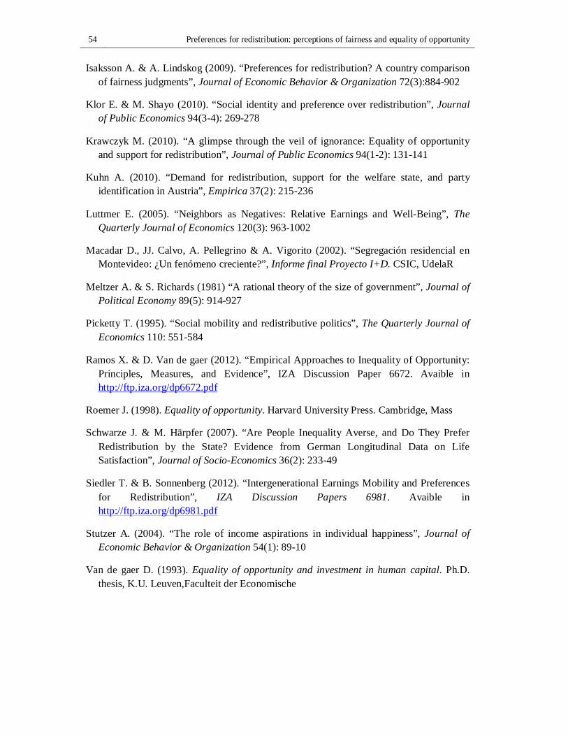
54 Preferences for redistribution: perceptions of fairness and equality of opportunity
Isaksson A. & A. Lindskog (2009). “Preferences for redistribution? A country comparison of fairness judgments”, Journal of Economic Behavior & Organization 72(3):884-902
Klor E. & M. Shayo (2010). “Social identity and preference over redistribution”, Journal of Public Economics 94(3-4): 269-278
Krawczyk M. (2010). “A glimpse through the veil of ignorance: Equality of opportunity and support for redistribution”, Journal of Public Economics 94(1-2): 131-141
Kuhn A. (2010). “Demand for redistribution, support for the welfare state, and party identification in Austria”, Empirica 37(2): 215-236
Luttmer E. (2005). “Neighbors as Negatives: Relative Earnings and Well-Being”, The Quarterly Journal of Economics 120(3): 963-1002
Macadar D., JJ. Calvo, A. Pellegrino & A. Vigorito (2002). “Segregación residencial en Montevideo: ¿Un fenómeno creciente?”, Informe final Proyecto I+D. CSIC, UdelaR
Meltzer A. & S. Richards (1981) “A rational theory of the size of government”, Journal of Political Economy 89(5): 914-927
Picketty T. (1995). “Social mobility and redistributive politics”, The Quarterly Journal of Economics 110: 551-584
Ramos X. & D. Van de gaer (2012). “Empirical Approaches to Inequality of Opportunity: Principles, Measures, and Evidence”, IZA Discussion Paper 6672. Avaible in http://ftp.iza.org/dp6672.pdf
Roemer J. (1998). Equality of opportunity. Harvard University Press. Cambridge, Mass
Schwarze J. & M. Härpfer (2007). “Are People Inequality Averse, and Do They Prefer Redistribution by the State? Evidence from German Longitudinal Data on Life Satisfaction”, Journal of Socio-Economics 36(2): 233-49
Siedler T. & B. Sonnenberg (2012). “Intergenerational Earnings Mobility and Preferences for Redistribution”, IZA Discussion Papers 6981. Avaible in http://ftp.iza.org/dp6981.pdf
Stutzer A. (2004). “The role of income aspirations in individual happiness”, Journal of Economic Behavior & Organization 54(1): 89-10
Van de gaer D. (1993). Equality of opportunity and investment in human capital. Ph.D. thesis, K.U. Leuven,Faculteit der Economische
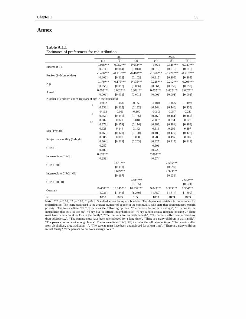
Chapter 1 55
Annex
Table A.1.1 Estimates of preferences for redistribution OLS 2SLS (1) (2) (3) (4) (5) (6)
Income (t-1) -0.048*** -0.052*** -0.053*** -0.024 -0.048*** -0.049***
[0.014] [0.014] [0.013] [0.016] [0.015] [0.015]
Region (1=Montevideo) -0.406*** -0.419*** -0.418*** -0.350*** -0.420*** -0.410***
[0.102] [0.102] [0.102] [0.112] [0.109] [0.108]
Age -0.179*** -0.175*** -0.175*** -0.228*** -0.212*** -0.208***
[0.056] [0.057] [0.056] [0.061] [0.059] [0.059]
Age^2 0.002*** 0.002*** 0.002*** 0.002*** 0.002*** 0.002*** [0.001] [0.001] [0.001] [0.001] [0.001] [0.001]
Number of children under 18 years of age in the household
2 -0.052 -0.058 -0.059 -0.040 -0.075 -0.079 [0.132] [0.132] [0.132] [0.144] [0.140] [0.139]
3 -0.162 -0.161 -0.160 -0.242 -0.247 -0.241 [0.156] [0.156] [0.156] [0.169] [0.161] [0.162]
>3 0.007 0.020 0.018 -0.037 0.031 0.020
[0.173] [0.174] [0.174] [0.189] [0.184] [0.183]
Sex (1=Male) 0.128 0.144 0.142 0.111 0.206 0.197
[0.169] [0.170] [0.170] [0.180] [0.177] [0.177]
Subjective mobility (1=high) 0.086 0.067 0.068 0.288 0.197 0.207
[0.204] [0.203] [0.203] [0.225] [0.215] [0.214]
CIRC[I] 0.257 0.601
[0.180] [0.728]
Intermediate CIRC[I] 0.678*** 2.890*** [0.158] [0.574]
CIRC[I+II] 0.571*** 2.535*** [0.158] [0.592]
Intermediate CIRC[I+II] 0.629*** 2.923*** [0.187] [0.659]
CIRC[I+II+II] 0.584*** 2.632*** [0.155] [0.574]
Constant 10.408*** 10.345*** 10.332*** 9.843*** 9.399*** 9.304***
[1.236] [1.241] [1.239] [1.350] [1.314] [1.309] N 1853 1853 1853 1853 1853 1853
Note: *** p<0.01, ** p<0.05, * p<0.1. Standard errors in square brackets. The dependent variable is preferences for redistribution. The instrument used is the average number of people in the community who state that circumstances explain poverty. The intermediate CIRC[I] includes the following options: “The parents do not earn enough”, “It is due to the inequalities that exist in society”, “They live in difficult neighborhoods”, “They cannot access adequate housing”, “There must have been a break or loss in the family”, “The transfers are not high enough”, “The parents suffer from alcoholism, drug addiction…”, “The parents must have been unemployed for a long time”, “There are many children in that family”, “The parents do not work enough hours”. The intermediate CIRC[I+II] includes the following options: “The parents suffer from alcoholism, drug addiction…”, “The parents must have been unemployed for a long time”, “There are many children in that family”, “The parents do not work enough hours”.
56 Preferences for redistribution: perceptions of fairness and equality of opportunity
Table A.1.2 Estimates of preferences for redistribution. Women
OLS 2SLS (1) (2) (3) (4) (5) (6) Income (t-1) -0.048*** -0.052*** -0.052*** -0.031* -0.051*** -0.052*** [0.015] [0.015] [0.015] [0.017] [0.016] [0.016] Region (1=Montevideo) -0.380*** -0.394*** -0.392*** -0.331*** -0.396*** -0.390*** [0.107] [0.107] [0.107] [0.117] [0.113] [0.113] Age -0.173*** -0.170*** -0.169*** -0.231*** -0.217*** -0.214*** [0.061] [0.061] [0.060] [0.067] [0.065] [0.064] Age^2 0.002*** 0.002*** 0.002*** 0.003*** 0.002 0.002*** [0.001] [0.001] [0.001] [0.001] [0.001] [0.001]
2 -0.043 -0.051 -0.053 -0.045 -0.093 -0.098 [0.140] [0.140] [0.140] [0.152] [0.148] [0.147]
3 -0.171 -0.175 -0.172 -0.250 -0.274 -0.266 [0.166] [0.166] [0.166] [0.178] [0.171] [0.172]
>3 -0.021 -0.008 -0.009 -0.081 -0.019 -0.022 [0.182] [0.182] [0.182] [0.197] [0.192] [0.191]
Subjective mobility (1=high) 0.231 0.210 0.213 0.388 0.293 0.306 [0.220] [0.219] [0.219] [0.239] [0.230] [0.228] CIRC[I] 0.249 0.735 [0.189] [0.726] Intermediate CIRC[I] 0.640*** 2.779*** [0.167] [0.574] CIRC[I+II] 0.528*** 2.454*** [0.166] [0.590] Intermediate CIRC[I+II] 0.638*** 2.815*** [0.197] [0.662] CIRC[I+II+II] 0.553*** 2.544*** [0.164] [0.570] Constant 10.315*** 10.270*** 10.249*** 9.929*** 9.574*** 9.503*** [1.319] [1.320] [1.318] [1.433] [1.389] [1.384] N 1658 1658 1658 1658 1658 1658
Note: *** p<0.01, ** p<0.05, * p<0.1. Standard errors in square brackets. The dependent variable is preferences for redistribution. The instrument used is the average number of people in the community who state that circumstances explain poverty. The intermediate CIRC[I] includes the following options: “The parents do not earn enough”, “It is due to the inequalities that exist in society”, “They live in difficult neighborhoods”, “They cannot access adequate housing”, “There must have been a break or loss in the family”, “The transfers are not high enough”, “The parents suffer from alcoholism, drug addiction…”, “The parents must have been unemployed for a long time”, “There are many children in that family”, “The parents do not work enough hours”. The intermediate CIRC[I+II] includes the following options: “The parents suffer from alcoholism, drug addiction…”, “The parents must have been unemployed for a long time”, “There are many children in that family”, “The parents do not work enough hours”.
Chapter 2
Early childhood development, school attendance and parenting
Abstract
School attendance may either reinforce or compensate the effect of parenting practices on children’s development. In this paper I use a unique dataset for Uruguay to study the impact of school attendance on child development for children aged 2 and 3, and analyze heterogeneous effects based on parents’ parenting practices. Marginal Treatment Effects suggest school attendance to increase the gap in children’s development that results from parenting practices, and these effects being more significant for girls. In addition, simulation exercises indicate that a universal increase in educational supply is more efficient than an expansion that targets households with greater socioeconomic vulnerability, but that the targeted policy achieves better results in reducing inequality in the different dimensions of child development.
58 Early childhood development, school attendance and parenting
2.1 Introduction
The aim of this paper is to study how school attendance during early childhood affects the opportunities of children, measured through the development of their motor skills, and their cognitive and non-cognitive skills. The role played by different circumstances is expected to modify its impact on child development as a result of school attendance. In particular, school attendance can mold the child’s behavior, often reinforcing the stimuli received at home and in other cases compensating for them. For this reason special attention will be paid to the views of parents regarding parenting practices, as these views are a central circumstance in the early development of the child. Children aged from 18 to 48 months are considered while it is observed whether there are differences between boys and girls, in terms of the beliefs of the parents being oriented to the reproduction of traditional gender roles that result in varying degrees of stimulation.
Interventions in early childhood are vital instruments to “level the playing field” throughout the entire life cycle. Conti & Heckman (2012) indicate that improving the performance of children in the first few months of their lives is extremely important due to the potential dynamic effects that are generated in this stage. This is because current skills depend on the stock of accumulated skills, while the productivity of the investments made in early childhood is higher when skills that have already been acquired are higher. Investments may correspond, for example, to the time dedicated by parents to raising their children or to sending their children to school, and they are expected to have greater effects on children with high cognitive and non-cognitive skills.
The foundations of the neural substrates are established during the first years of life, as well as the psychomotor, cognitive, communicative and emotional processes which fully develop throughout childhood and adolescence, and while these foundations are not closed after these early years, it is much more difficult to develop them in later childhood (Center on the Developing Child, 2007). The highest return generated by investments in the earliest stages of life is explained in Bernal & Camacho (2010) and is based on five aspects: the greater development of the brain, being the most critical period in the neuronal development; dynamic learning development, which has implications for future performance; the deceleration of the dynamic interactions of skills which occurs during adolescence; the great malleability of psychosocial development (curiosity, persistence, self-control, etc.) that interacts with the cognitive development; the high returns derived from interventions at this stage, which will be enjoyed for many years.
In this paper two ways in which school attendance can affect child development are postulated. A first effect reflects the dynamic interactions of skills, based on the complementarity of parenting practices and school attendance. In this case the stimulation received at home from appropriate parenting practices leads to children benefitting more from school attendance, increasing the gap to children who receive inappropriate parenting practices. A second effect is associated with reduced care time from other sources (mother,
Chapter 2 59
father and other family members), which is replaced by time spent at school (Felfe & Lalive, 2014). The direction of the latter depends on the quality of parenting practices of the parents, and of those provided by the school. If hours of passive activities at home, such as hours spent in front of a screen, are replaced with school attendance, the effect on child development will probably be positive. In this case school attendance increases the average quality care time initially provided by the parents, offsetting heterogeneities caused by inappropriate parenting practices. However, it is also possible that time spent at school replaces active time at home, which is cognitively stimulating for the child. In this case the effect is unknown and will depend on the relative degree of stimulation from the school and the home. In this paper I will attempt to identify which types of practices are enhanced and which are offset by school attendance.
Studies carried out in recent years are conclusive regarding the medium-term impact of interventions in early childhood. The paradigmatic case is the Perry Preschool program, aimed at children of African descent, 3-4 years of age and with low IQs. The papers of Heckman, Moon, Pinto, Savelyev & Yavitz (2010) and Conti et al. (2012) show that such interventions lead to better performances in adolescence and adulthood in education, employment and healthy practices, as well as a lower involvement in criminal activities. Heckman, Pinto & Savelyev (2013) attempted to identify the channels that explain such results, that is, the abilities which are modified by the program. The study showed that the improvements achieved in cognitive skills are quickly diluted, but not in the case of personality traits, which last over time. The findings also provide evidence of differential effects between boys and girls.
From the expansion of the number of schools dedicated to early childhood in Norway, Andreoli, Havnes & Lefranc (2014) proposed to explicitly measure the changes that occurred in inequality of opportunity. They considered a reform which took place in 1975 and observed the performances in adulthood of those who were children at the time of the reform. The authors found heterogeneous effects according to the socioeconomic status of the parents. Children from poor backgrounds were those who obtained greater benefits as a result of the policy, allowing them to conclude that the policy equalized opportunities in early childhood.
In addition, several authors have suggested that the provision of additional financial resources to poor families does not necessarily translate directly to increased investments and improvements in the development of the children (Conti & Heckman, 2012; Carneiro, Cunha, Galasso & López Garcia, 2013), with the actual parenting being a central factor in explaining the way in which these resources are utilized. Conti & Heckman (2012) indicated that the quality of parenting is fundamental to achieving improvements in the welfare of children. Subsequent investments, such as in primary education, while unquestionably providing tools to help promote the welfare of children, will be affected by the pre-existing conditions of the child. Carneiro et al. (2013) suggested that a better understanding of the determinants of parental behavior is necessary, as well as understanding how the beliefs of those parents are related to the effectiveness of different
60 Early childhood development, school attendance and parenting
styles of parenting, to the benefits of spending time with the children, and to the skills they possess in their role as parents. In this view it is essential that public interventions begin during the first months of life in order to improve the child’s development directly, or indirectly by altering the beliefs of the parents.
As in Carneiro et al. (2013), the beliefs of parents about parenting practices and aspirations regarding the level of education that their children will achieve in the future are included in the explanation of child development. As already mentioned, I aim to establish how parenting practices affect childhood development, identifying inappropriate practices which are offset by school attendance. There are very few papers that address the link between parenting practices and childhood development from an empirical perspective, and even fewer that consider the potential interactions between parenting practices and school attendance in order to explain the cognitive and non-cognitive skills of children. In addition, some circumstances are considered which are regularly used in the literature, such as the educational level of the mother and the income and composition of the household, and others which are less common such as the child’s birth weight, the nutritional situation and the non-presence of the father within the household.
In the paper of Cabella & Nathan (2014) inappropriate parenting practices were identified in the following dimensions: setting limits and rules, controlling the child’s behavior, parental cooperation, parental participation in decision-making and the emotional context of the parenting. To these I added parental discrimination between boys and girls, which identifies conservative views on education and the roles to be fulfilled by the children. Special attention is paid to the link between the differential risk of these beliefs and the development of boys and girls, as they may reflect different types of stimuli in the household.
For the empirical approach I used the Health, Nutrition and Child Development Survey (ENDIS, by Spanish name) carried out by the National Institute of Statistics (Uruguay) between October 2013 and February 2014. The ENDIS is representative of children who were between 6 and 48 months old at the time of the survey. Childhood development is analyzed using two instruments, the Child Behavior Checklist (CBCL), which collects information on the non-cognitive skills of the child from a set of socio-emotional characteristics, and the Age and Stages Questionnaire, Third Edition (ASQ-3), which contains information that can be associated with the cognitive, non-cognitive and motor skills of the child. Exploiting this source of information, which is uncommon in countries with a low degree of relative development, allows us to analyze the impact of school attendance on child development.
To identify the causal effects I follow the proposal of Heckman & Vytlacil (2001a). Using the Marginal Treatment Effect (MTE) it is possible to observe the average causal effect on child development of sending children to school in the cases where the parents are indifferent between sending their children to those schools or not (Felfe & Lalive, 2014). It is then considered how the causal effects are modified with the characteristics
Chapter 2 61
observed in the children and the household, as well as the unobservable characteristics that reflect the costs of the parents for sending their children to school. In the first stage the probability of the child attending school is determined, using the number of places offered in the public and private sub-sectors in each of the 62 neighborhoods in Montevideo as an exclusion restriction, as well as the number of children residing in those neighborhoods (potential demand). A further restriction is included in the estimate: The perception of the respondents about the balance between the supply and demand of schools dedicated to early childhood in one’s neighborhood of residence. As will be mentioned later this perception reflects, in part, the assessment of the quality of the schools relative to the quality of the care offered in the household.
Given that it is not possible to attribute responsibility to children for their performance at that age, all of the inequality that is identified is considered illegitimate and constitutes a restriction on the opportunities of the children. This justifies the implementation of public policies aiming to eliminate all of the sources that generate heterogeneity in the outcomes of children. The paper ends by simulating a reform in the supply of public pre-school education. In Uruguay education is compulsory from the age of 4, where attendance is 91.2% of all children (DNPS-MIDES, 2014). In this paper different scenarios are simulated, with expansions of the public supply aimed at children aged 2 and 3 years old. In order to estimate the effects of this reform I followed the proposal of Heckman & Vytlacil (2001b) to calculate the Policies Relevant Treatment Effect (PRTE).
Identifying heterogeneous effects from the parenting practices is one of the contributions of this paper. The role of parenting practices in child development has been studied very little empirically, and the interactions with the school attendance of children even less so. Parenting practices and school attendance are different types of investments that can be made by parents. These investments can be complementary, if children with greater stimuli in the household take advantage of the contributions made by the schools or, on the contrary, attendance can have a compensating effect on the inequality generated in households which is associated with parenting practices.
Secondly, in this paper I will measure inequality in child development, which is a novel aspect in the relevant literature. This aspect is a substantive element for understanding intra and intergenerational mobility, as it is one of the main channels that can amplify or restrict the opportunities that children will have in the medium term in education and the workplace. In the paper I also discuss which educational supply expansion policies (universal or targeted) have a greater impact in terms of distribution, as well as from an efficiency based perspective (better average results of children). As such the paper contributes by providing useful information for policymakers, given the limited existing evidence in middle-income countries, on the link between school attendance and early child development.3 The gap in the literature that I am attempting to fill in this paper is of the more general interest of discussing the differential effects of universal and targeted
3 An exception are the papers of Urzúa and Veramendi (2011) and Noboa-Hidalgo and Urzúa (2012) for the case of Chile.
62 Early childhood development, school attendance and parenting
policies, an aspect which has not been addressed empirically by taking early child development as a measure of performance.
The main finding is that school attendance and parenting practices play mostly a complementary role. Greater investment in parenting practices in the household result in better use of the stimuli offered in the school in cognitive and motor skills. This type of effect is seen mainly among girls. School attendance also offsets childrens’ development gaps associated with the education level of the mother, both with cognitive and non-cognitive skills and motor skills. Finally, our simulation exercises suggest that universal public educational supply expansion policies for children aged 2 and 3 are more efficient than targeted policies, but less good at reducing inequalities.
The rest of the chapter is organized as follows. In section 2 I review the literature that shows the link between school attendance and child development and I also discuss some results that show how parenting practices influence child development. In the following section I present the conceptual framework and the identification strategy which, as mentioned, is based on the MTE. In section 4 I present the data and section 5 contains the main results. The chapter ends with some conclusions, where I mention some gaps which exist in the literature and which form part of an agenda for future research based on intergenerational mobility and equality of opportunities.
2.2 Literature review
In this section I review the literature associated with the determinants of early child development, with an emphasis on the role of school attendance and parenting practices in the household.
Several papers have studied the effects of programs which focus on early child development. In Heckman & Kautz (2014) different types of interventions carried out in this stage of life are reviewed, particularly before entering into formal schooling. They distinguished two types of interventions: the first relates to small-scale programs that provide socio-emotional and cognitive stimuli directly, either by giving instructions to young mothers or providing care in a center to a specific population (for example, Perry Preschool or Abecedarian). The second type relates to larger-scale programs which have generally been implemented in the schools themselves and are relatively less expensive than the first type (for example, Head Start or Chicago CPC). The authors indicate that in the literature the latter type of programs were found to have a lesser impact. On the other hand, there is evidence that those who participate in Project STAR perform better than their peers, although the effect is diluted over time. The same result was found for cognitive skills in the Perry Preschool program, demonstrating the importance of evaluating the impact of the programs in the medium and long term.
Chapter 2 63
The evidence is less abundant when it comes to analyzing the effects of preschool attendance on child development. The decision of parents to send their children to school is voluntary and clearly endogenous. The absence of experimental data requires the design of an alternative to capture the unobservable components that influence that decision. For example, Urzúa & Veramendi (2011) studied the impact of school attendance on different variables that approximate child development. They made estimates with instrumental variables, considering distance from the household to the school and the average number of children attending schools per municipality as instruments. Felfe & Lalive (2014) adopted a Marginal Treatment Effect (MTE) structure and used the proportion of children attending school within the cohort in each of the school districts in Germany as an exclusion restriction.
Urzúa & Veramendi (2011) reviewed a set of studies and indicated that the effects of the preschools can be positive or negative depending on the quality of the school, the time spent by parents looking after their children, and the characteristic of the parents and the children themselves. In their study they found, for the case of Chile, a positive effect of attendance in the TEPSI test (Psychomotor Development Test) on children over 2, which the authors suggest approximates cognitive skills. They also stated that the effects are consistently positive in relation to cognitive skills, and not in relation to non-cognitive skills. Also based on information about Chilean children, Noboa-Hidalgo & Urzúa (2012) found that school attendance improves emotional regulation and motor skills. However, the authors found negative effects in the areas of memory and the interaction between children and adults. However this paper refers to children younger than those considered in my paper.
Baker, Gruber & Milligan (2008) analyzed the introduction of a subsidy in Quebec to allow broad access to the care system. The authors found no impact on cognitive skills and observed negative effects on non-cognitive skills (aggressiveness and hyperactivity) and motor skills. The latter is explained by the difficulties brought about by the first interactions with other children. Using the same source of information and for the same program, Lefebvre, Merrigan & Verstraete (2006) found no impact on cognitive skills at 4 years of age, with a negative impact on these skills when the children reach 5 years of age. The authors’ hypothesis is that the effects are due to the high exposure of the children to the school due to their lack of time schedule flexibility.
In the literature reviewed heterogeneous effects are found depending on the socioeconomic condition of the household. For the Italian case, Del Boca, Pronzato & Sorrenti (2015) found that the benefits of attending schools at an early age are more significant in regions with policies that favour families with fewer resources. Loeb, Bridges, Bassok, Fuller, & Rumberger (2007) indicate that children from poorer households show a linear association with the hours spent in the preschool, that is, the greater the number of hours the greater the gain in cognitive skills. This does not occur with children from homes with better economic conditions, in which cases a moderate intensity in the treatment is what produces better results. Felfe & Lalive (2014) found that
64 Early childhood development, school attendance and parenting
school attendance had a significant effect on language and motor skills in children less than 3 years of age with disadvantaged background (low education of the mother or immigrant parents). An effect was also observed in a component that approximates non-cognitive skills, socio-emotional maturity. With a similar information source and also in the case of children with parents from other countries, Dustmann, Raute, & Schönberg (2013) found that school attendance reduces problems in language and motor skills. Finally, Magnuson, Ruhm, & Waldfogel (2007) found that the school readiness benefits are greater for children from more disadvantaged homes, with no differences found on a socioeconomic level in the incidence of behavioral problems.
Some studies focus on the optimal age at which children should begin schooling and whether there is an ideal number of hours per week. Loeb et al. (2007) found that the exposure of children to preschool generates a 0.1 standard deviation increase in cognitive skills, but also that behavioral problems increase. The largest effects are found when the child begins preschool between 2 and 3 years of age, with the most significant behavioral problems being observed for children who begin preschool aged less than 1 year old. Magnuson et al. (2007) studied the effects of school attendance on the cognitive and social skills of children, taking into account the intensity and the length of time the child attended the school. They found that preschool attendance improved school readiness in reading and mathematics, but is also associated with increased behavioral problems in the classroom. The authors used the component of the CBCL called externalized problems to identify behavioral problems, which I will also use in this paper. Belsky (2002) found a linear, positive relationship between the time spent taking care of the child in a school and the externalized behavior. Children who spent more hours and/or months attending school displayed greater behavioral problems, including elevated levels of aggression and being less effective in controlling their impulses.
Parenting practices could be of the utmost importance when explaining the levels of development in childhood. The resources invested by parents in their children, not only those derived from money or time, but also in terms of love and affection, play a substantial role in the cognitive, emotional and social development of children (Coleman, 1988; Gibson-Davis, 2008). Several authors have discussed how the beliefs of parents about the best way to raise their children affect child development. In some cases it is shown that parenting styles can directly affect the abilities of children. According to Bornstein (2001), the ideas of the parents about the best way to raise their children lead to different styles of parenting. The authoritarian style, which is associated with a high level of structure and control of the children, implying strong disciplinary strategies and low levels of affection and communication, is linked to children who are more hostile with the peers and who are more dependent on their parents. On the other hand, the permissive style combines a high level of affection and balanced control, and is associated with positive child development. Finally the author describes a third style associated with authoritative parents. In these cases the children perform well in standardized tests, with the children being friendlier with peers, more independent and assertive, more cooperative with their parents and more achievement-oriented. Authoritarian and permissive parents share a
Chapter 2 65
common characteristic in that they minimize the opportunities for their children to deal with stress.
Parents who believe that intelligence is malleable also believe that they are capable of affecting the academic achievements of their children and have higher educational aspirations for them (Wentzel, 1998). Bandura (1995) introduced the idea of self-efficacy in parenting, referring to people who believe in their ability to succeed in a particular situation. This aspect may have an impact on child development, even in cases where parents have the same beliefs about how to raise their children but different views about their own ability to turn their beliefs into concrete practices. According to Schellenbach, Whitman & Borkowski (1992), mothers who feel more competent in their role are less demanding and develop their expectations more appropriately. Brody, Flor & Morgan Gibson (1999) indicate that the beliefs of parents about their self-efficacy are related to their parenting objectives, and result in better academic and social skills for their children.
Finally Doyle et al. (2013) studied the impact of investments made in the first 18 months of life on adolescence. The authors studied a program of visits to households, in Ireland, which focused on educating parents on child health and development, stimulating a healthy lifestyle, affirming the maternal perceptions of the self-efficacy of their parenting practices and encouraging positive parenting practices. They found that the program had effects on parenting practices but with a weaker impact on child development. In the latter point it was observed that there were effects on socio-personal dimensions as well as on fine and gross motor skills. On a similar note Walker, Chang, Powell & Grantham-McGregor (2005) found, for Jamaica, that a program offering psychosocial stimulation to children aged from 9 to 24 months with nutritional problems generated positive effects in cognitive skills and educational performance at the age of 17-18.
2.3 Conceptual framework and identification strategy
2.3.1 Conceptual framework
From the proposal made by Heckman & Vytlacil (2001a), in order to estimate the Marginal Treatment Effects (MTE), I will attempt to identify the effects of exposing children to a school, treatment variable (퐷 = 1), on child development, 푌 . Variable j corresponds to the extent of child development used, which may correspond to the cognitive or non-cognitive skills and the motor skills of the child.
The MTE is the effect of the treatment associated with individuals who are indifferent between being and not being treated, and becomes especially relevant when the effects of the treatment are heterogeneous. In this paper I introduce parenting practices as a relevant factor in explaining child development, and I explore whether its incidence can be
66 Early childhood development, school attendance and parenting
enhanced or offset by the role played by the school. For this reason the heterogeneity of the effects of attending school is a central aspect.
푌 is defined as the child development in s of the treated children and 푌 the development of untreated children. The equations that explain the levels of development of treated and untreated children are expressed as:
푌 = 푋 ∙ 훽 + 푆 ∙ 휁 + 푊 ∙ 휂 + 푈 (2.1) 푌 = 푋 ∙ 훽 + 푆 ∙ 휁 + 푊 ∙ 휂 + 푈 (2.2)
where X is a vector of characteristics of the child and the family, S represents the parenting practices and W is a vector of fixed effects of the neighborhoods where the school is located.
The effect of the treatment is presented in equation (2.3). It also depends on the characteristics of the child and the family, on the unobservable components of child development (푈 −푈 )
푌 − 푌 = 푋 ∙ 훽 − 훽 + 푆 ∙ (휁 − 휁 ) + 푊 ∙ (휂 − 휂 ) + 푈 − 푈 (2.3)
The decisions to send children to school are modeled as follows:
퐷 = 퐼(푍 ∙ 훾 − 푉 > 0) (2.4)
In this case function I takes a value of one if the inequality indicated in the parentheses
is met, and zero if not. The selection depends on a set of observable characteristics, Z, which do not include parenting practices, and on unobservable components. The parameter 푉 is probably correlated with 푈 and 푈 , that is, between the unobservable components of the decisions of the parents and those corresponding with the performance of the children. Beyond the intergenerational transmission of skills, which probably makes the unobservable components correlated; the preferences of the parents for sending their children to school reflects the valuation they have of education. This element is probably associated with the stimulation that the parents give their children at home, an unobservable component that affects child development.
Introducing an exclusion restriction, z, in the estimation of the probability of attending school (Heckman, 1979) is a necessary condition to be able to identify the causal effects of
Chapter 2 67
attending school on child development.4 There are two assumptions that must be established in order for instrument z to be adequate: 퐶표푣(퐷, 푧) ≠ 0 (relevance of the instrument) and 푧 ⊥ 푌 ,푌 (exogenous instrument).
To do this in the first stage a propensity score 푃(푍) is estimated:
푃(푍) ≡ Pr(퐷 = 1|푍) = Pr(푍 ∙ 훾 − 푉 > 0) = Pr(퐹 (푍) > 푉) = 퐹 (푍 ∙ 훾) (2.5)
where 퐹 (∙) is the cumulative density of the unobservable characteristics V, and 푈 =퐹 | (푉) represents different quantiles of V and by construction is evenly distributed, 푈 ∼ 푈푛푖푓[0,1]. In short the MTE is expressed as:
푀푇퐸 = 퐸[푌 − 푌 |푋 = 푥, 푆 = 푠;푈 = 푢 ]
Similar to the interpretation in Felfe and Lalive (2014), in the context of this article 푈
reflects the preferences of parents for early school attendance or the need for schools. The likelihood of children attending school is expected to decrease as 푈 increases.
The MTE measures how early school attendance affects child development for children whose unobservable determinants of attending school is the same as their propensity score. It is a marginal effect in the sense that the parents of those children are indifferent between sending them to school at an early age or not. The MTE for children whose unobservable component is 푈 is expressed as:
퐸(푌 − 푌 푋, 푆,푈 = 푃(푍)) = 푋 ∙ 훽 − 훽 + 푆 ∙ (휁 − 휁 ) + 퐸(푈 − 푈 푋, 푆,푈 = 푃(푍)) (2.6)
2.3.2 Identification
Several papers that have studied the effects of school attendance on child development have used different variants of the supply of local education as an exclusion restriction, for example Felfe & Lalive (2014) considered the average attendance at care centers in school districts in Germany (private centers with public subsidies 79% of the total cost of center), Urzúa & Veramendi (2011) considered the capacity of public centers in the municipalities of Chile, and also for the case of Chile, Noboa-Hidalgo & Urzúa (2012) introduced the changes in the number of public care centers at the municipal level.
4 Heckman and Vytlacil (2007) show that for the OLS estimate, in addition to the standard selection bias derived from the correlation between the treatment and the unobservable component of control and treated individuals in the estimate of the performances, 푈 , there is a second source of bias associated with the presence of the treatment in the error term of the reduced form. This implies, in this case, that the decision of parents to send their children to school is determined by unobservable gains that are derived from this decision.
68 Early childhood development, school attendance and parenting
With similar criteria to the previous cases, in this paper I consider the supply of preschools as an exclusion restriction. This study separately incorporates the supply of public and private schools as an exclusion restriction, identifying the existing links between the number of places of both types and preschool attendance. A potential weakness of this instrument could be the criteria used by policy makers to select the location of these schools. If these criteria are linked to the relative income of the average population of each neighborhood, then supply will most likely be higher in the areas where the poorest children reside. If this were the case then the instrument could be correlated with the level of child development and would not be useful. In this section I aim to show that this association is weak in the case of Montevideo in Uruguay. On the other hand it is expected that there is a certain lag in the construction of schools in response to the demographic changes that occur in each of the neighborhoods, and this potential lag in the coverage of the schools allows us to further relativize the endogeneity of the supply of schools.
In order to identify the above restriction the fact that the ENDIS reports the child’s neighborhood of residence and the neighborhood of the school which the children attend is considered. In order to obtain the supply of education for this age group in the different neighborhoods I used the records of the Ministry of Education and Culture, which contains information regarding the number of preschools, both public and private (approved), as well as their geographical location. In order to calculate the number of places available, I used the parameters established by the national regulations. For children aged from 12 to 24 months it is considered that the maximum number of children that can attend per group is 12, regardless of whether the center is public or private. For classes for children aged from 24 to 47 months, two types of public centers are considered separately: Child and Family Care Centers (CAIF, by Spanish name) and kindergartens. According to the regulations a limit of 15 children per group has been established for the first type (centers covering children aged up to 36 months), while a limit of 30 children has been established for the second type (these centers generally cover children aged up to 36 months). In private centers a limit of 20 children per group has been established, as the majority of these institutions indicate on their websites.
Fig. 2.1 shows the number of children in the 24 to 47 month age group residing in each neighborhood as well as the number of public places in the enabled institutions. The frequency of poor children for the same age group is also included. The information is presented in four panels, the first corresponds to neighborhoods where the relationship between public places and children is less than 10%, that is, where supply is very low; the second and third panels indicate the cases where the relationship is intermediate, between 10% and 20% and between 20% and 30%; while the last panel shows a slightly higher relationship, more than 30% of the potential demand is covered.
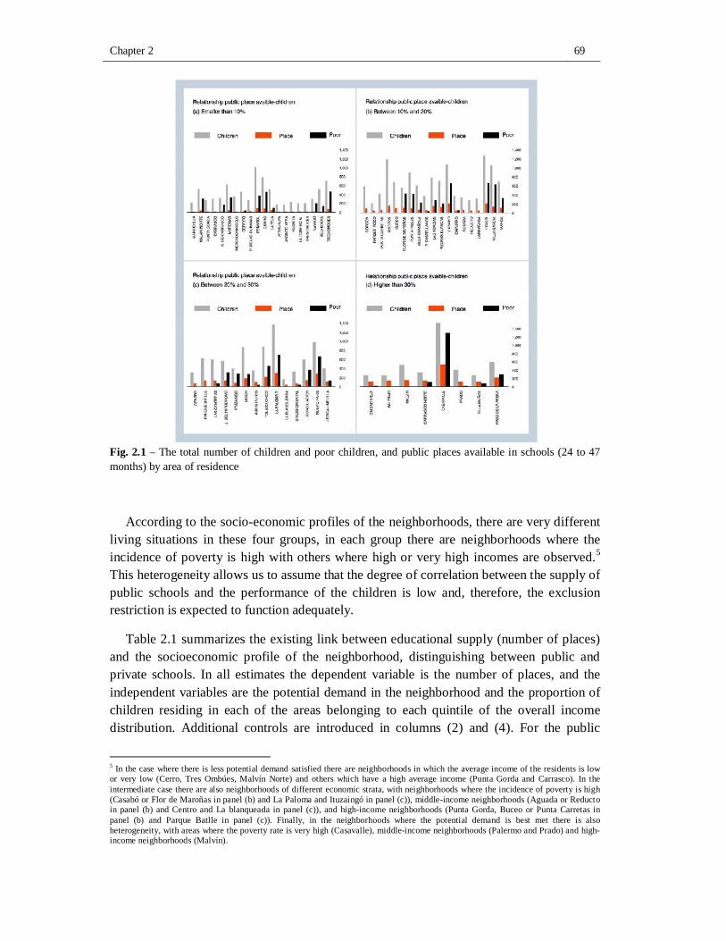
Chapter 2 69
Fig. 2.1 – The total number of children and poor children, and public places available in schools (24 to 47 months) by area of residence
According to the socio-economic profiles of the neighborhoods, there are very different living situations in these four groups, in each group there are neighborhoods where the incidence of poverty is high with others where high or very high incomes are observed.5 This heterogeneity allows us to assume that the degree of correlation between the supply of public schools and the performance of the children is low and, therefore, the exclusion restriction is expected to function adequately.
Table 2.1 summarizes the existing link between educational supply (number of places) and the socioeconomic profile of the neighborhood, distinguishing between public and private schools. In all estimates the dependent variable is the number of places, and the independent variables are the potential demand in the neighborhood and the proportion of children residing in each of the areas belonging to each quintile of the overall income distribution. Additional controls are introduced in columns (2) and (4). For the public
5 In the case where there is less potential demand satisfied there are neighborhoods in which the average income of the residents is low or very low (Cerro, Tres Ombúes, Malvín Norte) and others which have a high average income (Punta Gorda and Carrasco). In the intermediate case there are also neighborhoods of different economic strata, with neighborhoods where the incidence of poverty is high (Casabó or Flor de Maroñas in panel (b) and La Paloma and Ituzaingó in panel (c)), middle-income neighborhoods (Aguada or Reducto in panel (b) and Centro and La blanqueada in panel (c)), and high-income neighborhoods (Punta Gorda, Buceo or Punta Carretas in panel (b) and Parque Batlle in panel (c)). Finally, in the neighborhoods where the potential demand is best met there is also heterogeneity, with areas where the poverty rate is very high (Casavalle), middle-income neighborhoods (Palermo and Prado) and high-income neighborhoods (Malvín).
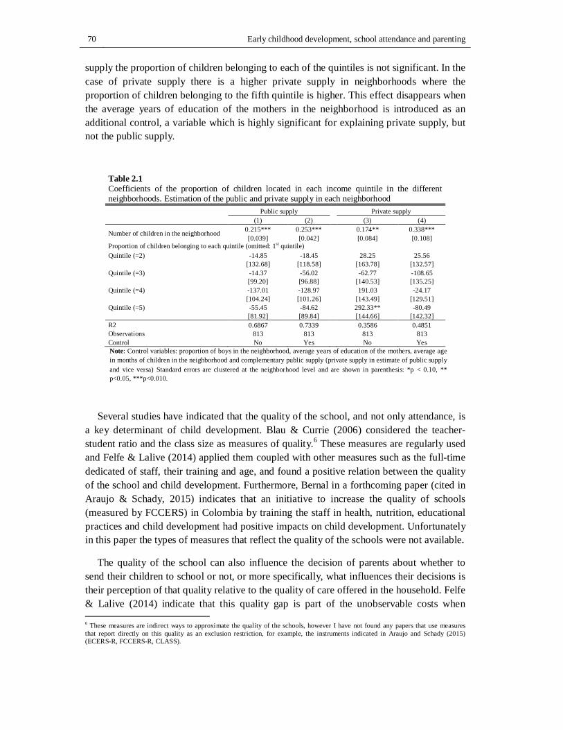
70 Early childhood development, school attendance and parenting
supply the proportion of children belonging to each of the quintiles is not significant. In the case of private supply there is a higher private supply in neighborhoods where the proportion of children belonging to the fifth quintile is higher. This effect disappears when the average years of education of the mothers in the neighborhood is introduced as an additional control, a variable which is highly significant for explaining private supply, but not the public supply.
Table 2.1 Coefficients of the proportion of children located in each income quintile in the different neighborhoods. Estimation of the public and private supply in each neighborhood
Public supply Private supply (1) (2) (3) (4)
Number of children in the neighborhood 0.215*** 0.253*** 0.174** 0.338*** [0.039] [0.042] [0.084] [0.108]
Proportion of children belonging to each quintile (omitted: 1st quintile) Quintile (=2) -14.85 -18.45 28.25 25.56 [132.68] [118.58] [163.78] [132.57] Quintile (=3) -14.37 -56.02 -62.77 -108.65 [99.20] [96.88] [140.53] [135.25] Quintile (=4) -137.01 -128.97 191.03 -24.17 [104.24] [101.26] [143.49] [129.51] Quintile (=5) -55.45 -84.62 292.33** -80.49 [81.92] [89.84] [144.66] [142.32] R2 0.6867 0.7339 0.3586 0.4851 Observations 813 813 813 813 Control No Yes No Yes Note: Control variables: proportion of boys in the neighborhood, average years of education of the mothers, average age in months of children in the neighborhood and complementary public supply (private supply in estimate of public supply and vice versa) Standard errors are clustered at the neighborhood level and are shown in parenthesis: *p < 0.10, ** p<0.05, ***p<0.010.
Several studies have indicated that the quality of the school, and not only attendance, is a key determinant of child development. Blau & Currie (2006) considered the teacher-student ratio and the class size as measures of quality.6 These measures are regularly used and Felfe & Lalive (2014) applied them coupled with other measures such as the full-time dedicated of staff, their training and age, and found a positive relation between the quality of the school and child development. Furthermore, Bernal in a forthcoming paper (cited in Araujo & Schady, 2015) indicates that an initiative to increase the quality of schools (measured by FCCERS) in Colombia by training the staff in health, nutrition, educational practices and child development had positive impacts on child development. Unfortunately in this paper the types of measures that reflect the quality of the schools were not available.
The quality of the school can also influence the decision of parents about whether to send their children to school or not, or more specifically, what influences their decisions is their perception of that quality relative to the quality of care offered in the household. Felfe & Lalive (2014) indicate that this quality gap is part of the unobservable costs when 6 These measures are indirect ways to approximate the quality of the schools, however I have not found any papers that use measures that report directly on this quality as an exclusion restriction, for example, the instruments indicated in Araujo and Schady (2015) (ECERS-R, FCCERS-R, CLASS).
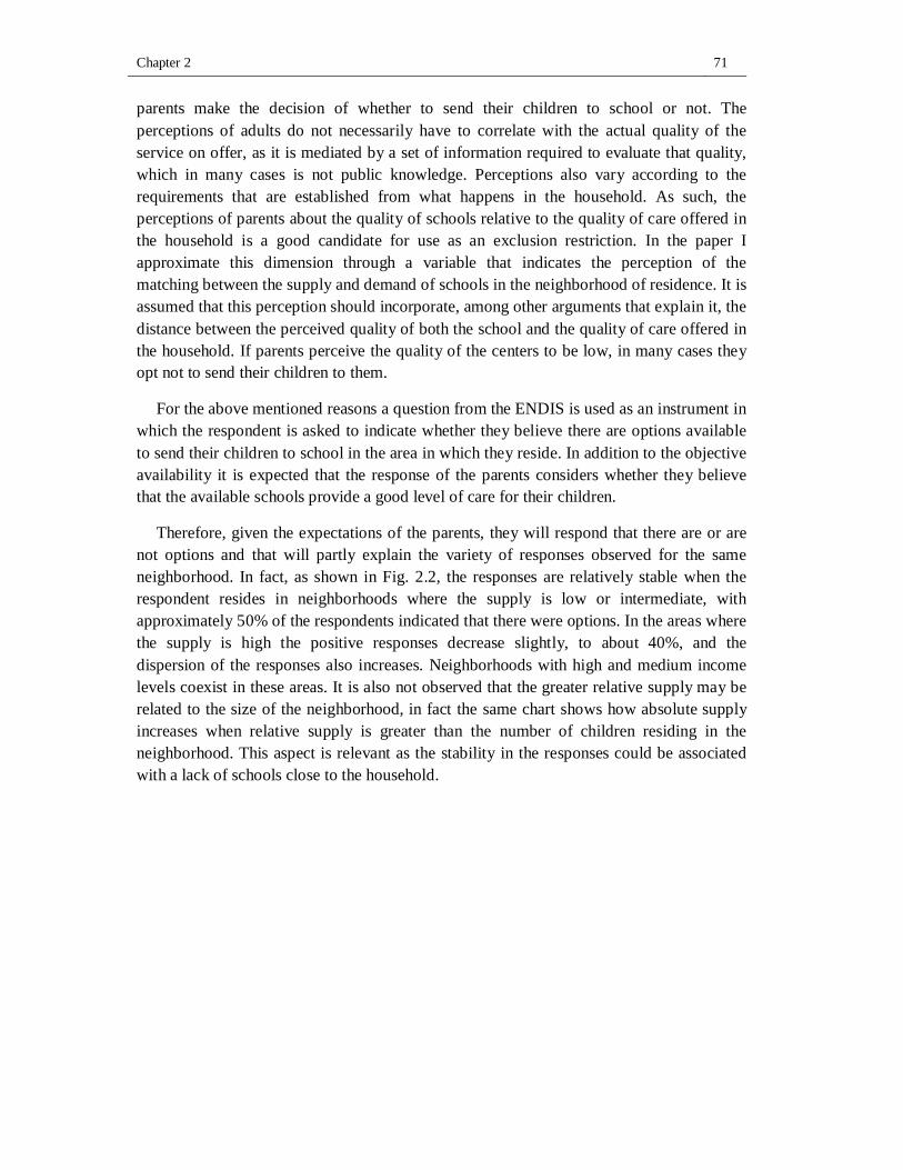
Chapter 2 71
parents make the decision of whether to send their children to school or not. The perceptions of adults do not necessarily have to correlate with the actual quality of the service on offer, as it is mediated by a set of information required to evaluate that quality, which in many cases is not public knowledge. Perceptions also vary according to the requirements that are established from what happens in the household. As such, the perceptions of parents about the quality of schools relative to the quality of care offered in the household is a good candidate for use as an exclusion restriction. In the paper I approximate this dimension through a variable that indicates the perception of the matching between the supply and demand of schools in the neighborhood of residence. It is assumed that this perception should incorporate, among other arguments that explain it, the distance between the perceived quality of both the school and the quality of care offered in the household. If parents perceive the quality of the centers to be low, in many cases they opt not to send their children to them.
For the above mentioned reasons a question from the ENDIS is used as an instrument in which the respondent is asked to indicate whether they believe there are options available to send their children to school in the area in which they reside. In addition to the objective availability it is expected that the response of the parents considers whether they believe that the available schools provide a good level of care for their children.
Therefore, given the expectations of the parents, they will respond that there are or are not options and that will partly explain the variety of responses observed for the same neighborhood. In fact, as shown in Fig. 2.2, the responses are relatively stable when the respondent resides in neighborhoods where the supply is low or intermediate, with approximately 50% of the respondents indicated that there were options. In the areas where the supply is high the positive responses decrease slightly, to about 40%, and the dispersion of the responses also increases. Neighborhoods with high and medium income levels coexist in these areas. It is also not observed that the greater relative supply may be related to the size of the neighborhood, in fact the same chart shows how absolute supply increases when relative supply is greater than the number of children residing in the neighborhood. This aspect is relevant as the stability in the responses could be associated with a lack of schools close to the household.
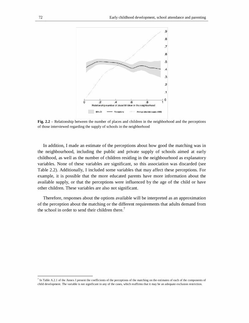
72 Early childhood development, school attendance and parenting
Fig. 2.2 – Relationship between the number of places and children in the neighborhood and the perceptions of those interviewed regarding the supply of schools in the neighborhood
In addition, I made an estimate of the perceptions about how good the matching was in the neighbourhood, including the public and private supply of schools aimed at early childhood, as well as the number of children residing in the neighbourhood as explanatory variables. None of these variables are significant, so this association was discarded (see Table 2.2). Additionally, I included some variables that may affect these perceptions. For example, it is possible that the more educated parents have more information about the available supply, or that the perceptions were influenced by the age of the child or have other children. These variables are also not significant.
Therefore, responses about the options available will be interpreted as an approximation of the perception about the matching or the different requirements that adults demand from the school in order to send their children there.7
7 In Table A.2.1 of the Annex I present the coefficients of the perceptions of the matching on the estimates of each of the components of child development. The variable is not significant in any of the cases, which reaffirms that it may be an adequate exclusion restriction.
Chapter 2 73
Table 2.2 Estimates of perception of the goodness of matching in the neighborhood
Public supply 0.001 0.001 [0.0003] [0.0003]
Private supply -0.0001 -0.00001 [0.0003] [0.0004]
Private supply² (/ 1000) 0.0002 0.0002 [0.0005] [0.0006]
Number of children in the neighborhood -0.00001 -0.00004 [0.0001] [0.0001]
Years of education of the mother -0.009 [0.006]
Months -0.002 [0.003]
Mother alone (1=Yes) -0.014 [0.045]
Other child in the household
< 4 years (1=Yes) 0.015 [0.041]
Between 4 and 12 years 0.012 [0.038]
Constant 0.410*** 0.554*** [0.046] [0.104]
Observation 813 801 R2 0.014 0.019
Note: Standard errors are shown in parenthesis: *p < 0.10, ** p<0.05, ***p<0.010.
The estimates are made considering these exclusion restrictions and from which we can identify the expected gains resulting from participation in the school, and which are generated by a change in the supply and quality of the school. That is, they capture how a change in the latter variables (which approximate the policy in effect) affects early child development. The reduced form to estimate is:
퐸(푌 |푋, 푆,푃(푍) = 푃) = 푋 ∙ 훽 + 푆 ∙ 휁 + 푃 ∙ 푋 ∙ 훽 − 훽 + 푃 ∙ 푆 ∙ (휁 − 휁 ) + 휅 , (푃) (2.7)
The conditional independence of 푈 in relation to Z implies that 퐸 푈 푋,푆,푃(푍) =
푃 = 0, where the restriction Z may be excluded from the potential results. The conditional independence of 푈 ,푈 ,푈 in relation to Z also implies that:
퐸 퐷(푈 − 푈 ) 푋, 푆,푃(푍) = 푃 = 푃 ∙ 퐸 푈 −푈 푋, 푆,푃(푧) = 푃 ≡ 휅 , 푃 (2.8)
where 휅 , (푃) is an unknown function that measures how the effect of the treatment due to
unobservable characteristics, 푈 − 푈 , varies with the preferences for attending schools, 푈 . Therefore 휅 , (푃) depends on the propensity score in two ways. First, if 푃 increases it
74 Early childhood development, school attendance and parenting
means that a growing proportion of the children attend school in early childhood, such that the result of the reduced form reflects more of the unobserved component of the treatment effect, 퐸 푈 − 푈 푋,푆,푃(푍) = 푃 . Second, the increase of 푃 implies increased parental preferences for attending schools at an early age,푈 . This in turn changes the unobserved component of the treatment effect, 퐸 푈 − 푈 푋,푆,푃(푍) = 푃 , if there is a correlation between the preferences for sending children to school in the early years of life and early child development.
Finally, the partial derivative of the reduced form regarding the propensity score is calculated (Heckman & Vytlacil, 2001a):
퐸 푌 − 푌 푋, 푆,푈 = 푃(푧) = , , ( ) = 푋 ∙ 훽 − 훽 + 푆 ∙ (휁 − 휁 ) + , ( ) (2.9)
This derivative is called Local Instrumental Variables (LIV) and is what identifies the
MTE. The last component , ( )= 퐸(푈 − 푈 푋, 푆,푈 = 푃(푍)) is estimated using a
local nonparametric regression.
2.4 Description of the data
The information source used is the ENDIS carried out by the National Institute of Statistics (Uruguay) between October 2013 and February 2014. This survey has extensive information on child welfare, such as the development, nutritional status and health of the children. It also has information on child feeding practices, their school attendance, the reproductive history, the employment history of the mother and the parenting practices. The ENDIS can also be joined with the Continuous Household Survey (ECH, by Spanish name), which allows for a wide range of data on the socio-economic status of household members.
The ENDIS is representative of children between 0 and 4 years of age, with 2665 adults having been interviewed (97% mothers) corresponding to 3077 children.8 Psychometric tests were performed to measure child development: TEPSI, EEDP, ASQ-SE, ASQ-3, and the CBCL. The last two were the ones used in this paper. These tests were performed by psychomotor students as they combined questions to the mothers of the children with direct observation, and were performed for a subset of the population, residents of households in Montevideo, which covers 1163 children.
8 Throughout the paper I make reference to the mother of the child or to the respondent indistinctly, when strictly speaking in 3% of the cases the relationship with the child is different.
Chapter 2 75
In this paper I restrict the sample to children over 17 months old, this being the age at which we begin to observe child participation in schools.9 For this age group 773 adults were interviewed in the ENDIS. 41.8% of children between 18 and 48 months old attend school, which reflects the population that will be identified as treated. Below I will discuss the main features of the CBCL and the ASQ-3, then I will summarize the most relevant aspects of the variables used to measure parenting practices and, finally, I will describe the rest of the variables used in this paper.
2.4.1 Characteristics of the child development tests
The in-depth analysis of early childhood development implies taking many dimensions into account. It is generally recommended to form a set of instruments to give robustness to the measurement of the different spheres of life of children: communication, fine and gross motor skills, emotions, expression, understanding of situations and vocabulary, vocalization and verbalization, empathy, interests, playing, muscle tone, grasping and manipulation of objects, autonomy, acceptance of rules and limits, obedience, exploration of environment, shyness or extraversion, ability to form and strengthen ties, ability to enjoy different activities, alimentation, looking after one’s own body, hyperactivity, concentration, daydreaming, imagination (Cabella et al., 2015). In this paper I use two instruments with good psychometric characteristics and international standardization, the CBCL and the ASQ-3. These tests allow us to capture several of the above mentioned spheres.
The CBCL integrates a system called ASEBA to evaluate of the psychopathology of children (Achenbach & Rescorla, 2000). It is one of most commonly used instruments to evaluate the mental health of children at a population level. It applies to children who are between 18 and 66 months of age, and includes the socio-emotional and personality traits of the child. It consists of 100 items with frequent symptoms or behaviors understood as common problems in childhood. The problems are given a value of two if they are understand by the parents as being frequent, and zero if they are not, a value of one corresponding to an intermediate situation.
From this indicator we can calculate global indicators, empirical syndromes and scales. Specifically we can distinguish internalized and externalized problems, which refer to symptoms or behaviors that are predominantly expressed inside or outside of oneself (Achenbach, 1978).
The internalized problems (36 items) are those symptoms which include mood and depression disorders, anxiety disorders, somatic complaints and withdrawal. Another part of the test relates to the externalized problems (25 items) of the child, which covers
9 In Uruguay classes begin in March, although in preschools entry may occur in any month for these age groups. The ENDIS was applied between October 2013 and February 2014. That is, children who were at least 12 months old in March were considered.
76 Early childhood development, school attendance and parenting
behavioral disorders, hyperactivity disorders, impulsive behavior, problems with rules and uncontrolled aggression. All of these aspects identify the child’s personality traits which are called non-cognitive skills in the economic literature.
The first version of the ASQ-3 was developed in 1995 and today it is widely used internationally to monitor child development indicators (Squires et al., 2009). It was designed to be applied by the parents themselves and can be used by evaluators with basic training.
Table 2.3 Characteristics of the ASQ-3 and the CBCL
Instrument Dimensions Ranges Reference population Age of
child in months
Cases Normal Monitoring
/limit Risk/ Clinic Mean Standard
deviation
ASQ-3
Communication
z > -1 -1 < z < -2 z < -2
42.3 - 53.8 10.3 - 16.0
1 to 47 1163
Gross motor skills 50.3 - 55.8 8.0 - 11.4
Fine motor skills 43.5 - 52.7 8.3 - 15.6
Problem solving 46.0 - 52.8 9.7 - 11.9
Socio-personal 46.9 - 52.8 8.7 - 11.9
CBCL
Totals probs. PT < 52 51 >PT< 61 PT > 60 33.4 18.8
18 to 47 781 Externalized probs. PE < 21 20 >PE< 25 PE > 24 13.1 7.8
Internalized probs. PI < 14 13 >PI< 18 PI > 17 8.7 6.3 Note: In the CBCL the thresholds of the column ranges correspond to the 83 and 90 percentiles of the reference population. The mean values and standard deviations of the reference population in the ASQ-3 depend on the age in months of the child. Given that children under 18 months are not considered in this paper, the age groups in months used are: 17-18, 19-20, 21-22, 23-24, 25-27, 28-30, 31-33, 34-38, 39-44, and 45-47. For example, in those ranges the mean values for the communication component are, respectively, 42.3, 48.1, 49.9, 52.2, 50.4, 53.8, 49.4, 51.9, 50.0 and 52.9.
The ASQ-3 contains five components that approximate the cognitive and non-cognitive skills of children, as well as the development of their motor skills. It allows us to identify results in fine and gross motor, communication, socio-personal and problem solving skills. The last of these components approximates the cognitive abilities of the children, while the socio-personal component includes elements that could be associated with non-cognitive skills. In the dimension of communication cognitive and non-cognitive skills are combined. The ASQ-3 is a test aimed at children less than 66 months old, with the questions being varied according to the months of age, in accordance with their maturation process. Thirty items are applied in each age group, six for each of the areas, with a value of ten points when the item is fully achieved, five when it is partially achieved, and zero when it is not achieved. In each area the scores are added up and they are compared with a scoreboard containing the expected scores based on the age of the child.
Both the CBCL and the ASQ-3 can be standardized based on the expected mean values and standard deviations, while it is possible to identify risk/clinical and monitoring/limit situations. A summary of the tests with the dimensions they cover and the thresholds is
Chapter 2 77
presented in Table 1. This table also shows the mean values and standard deviations of the reference population of the CBCL and a range of values in the ASQ-3 showing the highest and lowest values, depending on the age of the child.
Table 2.4 shows the descriptive statistics of the tests used. The standardized values of children over 17 months are considered. The higher scores in the CBCL identify greater problems of the child, while in the ASQ-3 the better performances are associated with higher values.
Table 2.4 Descriptive statistics of the CBCL and the ASQ-3
N Mean Standard Dev Min. Max.
ASQ-3
Communication 768 0.038 0.954 -4.079 1.211
Gross motor skills 784 0.189 0.893 -4.958 0.874
Fine motor skills 775 -0.132 1.087 -4.438 1.284
Problem solving 762 -0.080 1.005 -4.398 1.383
Socio-personal 780 0.067 0.922 -4.336 1.209
CBCL
Total probs. 773 -0.465 0.961 -1.777 3.862
Externalized probs. 773 -0.169 1.108 -1.679 3.705
Internalized probs. 773 -0.564 0.807 -1.381 3.381
The average scores of the different tests by sex and the school attendance of children are shown below. Fig. 2.3 corresponds to the ASQ-3 tests, panel (a) corresponding to boys and girls that attend school, while panel (b) refers to children who do not attend. First it is worth noting the large differences between boys and girls, particularly in the components of communication and socio-personal. The scores of girls are higher regardless of school attendance. In the case of communication the score of girls is 0.35 and 0.05 depending on attendance (0.16 average), while that of boys is 0.14 and -0.28 (-0.09 average). In socio-personal the scores are 0.2 and 0.25 (0.22) for girls and -0.04 and -0.12 (-0.09) for boys. It is different in the case of gross motor skills, where there are small differences for the boys and girls who attend school, and the score of the boys is actually higher when they do not attend. The averages of those who attend and those who do not are 0.18 for girls and 0.20 for boys.
As for the differences associated with attendance, those who attended obtained higher scores in almost all cases, the exception being girls in the socio-personal component. The figure shows that the score variation as a result of attendance is clearly higher in the case of boys. For example, in the communication component the score for boys increases from -0.29 to 0.14 when comparing boys who do not attend with those who do, while for girls this variation is from 0.05 to 0.35. The same is observed for the other components. The
78 Early childhood development, school attendance and parenting
differential role that attendance can play in developing the skills of boys and girls is one of the aspects that will be studied in the next section, as it constitutes one of the hypotheses to be studied in this paper.
Fig. 2.3 – Average score of the ASQ-3 for boys and girls by school attendance
In the case of the CBCL the variability is much lower (Fig. 2.4). The differences between boys and girls are mainly observed externalized problems. Among those who attend school, the score is -0.24 for girls and -0.17 for boys. The better performance of children is repeated among those who do not attend, in this case the score is -0.18 for girls and 0.09 for boys (-0.20 and -0.13 averages for those who attend and those who do not).
In the case of internalized problems it is observed that school attendance reverses the better performance of girls, whose score remains relatively stable between -0.56 and -0.59, in favor of boys who move from -0.49 when they do not attend to -0.63. However, as a whole the scores are very similar, -0.57 for girls and -0.55 for boys.
Chapter 2 79
Fig. 2.4 – Average score of the CBCL for boys and girls by school attendance
2.4.2 Parenting practices
Parenting practices are understood as parental attitudes or behaviors which aim to create a certain emotional climate (Darling & Steinberg, 1993). These attitudes refer to the ways in which parents interact with their children and to the specific behaviors they adopt to achieve certain objectives in their socialization, for example helping children with their homework, controlling the amount of time they spend watching television, or spanking them or shouting at them (Cabella & Nathan, 2014). These practices are not generally observable and even less quantifiable.10 For this reason it is common to analyze the opinions of the parents about the appropriateness of certain practices, that is, beliefs about the normative criteria that should be considered for appropriate parenting. In addition, it is common to enquire about the concrete form that the attitudes of the parents take when raising their children. Both cases should naturally show a strong correlation with the practices themselves, with the understanding that they are good approximations of the link they establish with their children and of the elements they try to stimulate in their socialization process. Finally, the third aspect to consider is parental cooperation and the participation of the parents in the decision making process. These three aspects, that shape the way in which the children are raised in their homes, are the ones that will be considered in this paper.
I use the typology proposed in Cabella & Nathan (2014) in which they identified different dimensions of beliefs about parenting practices: i) daily limits and rules; ii) parental cooperation and consistency in raising children; iii) parental participation in decision-making regarding children; iv) parenting practices related to controlling the
10 Some tests allow us to identify parenting practices such as the Home Inventory, unfortunately in the ENDIS this type of information is not available.
80 Early childhood development, school attendance and parenting
child’s behavior, v) emotional context of parenting. To these I have added a sixth dimension associated with parental discrimination between boys and girls.
For the operationalization of this typology I use the respondent’s approval rating on certain statements and questions concerning parental cooperation and participation in decision-making regarding their children. The number of questions used in each dimension varies from 3 in the emotional context of parenting and parental discrimination between boys and girls, to 11 in parental cooperation. In between are controlling the child’s behavior (6 questions), daily limits and rules (5 questions) and parental participation (4 questions).
The variables included in each of these dimensions are presented in Table A.2.2 in the Annex. An example of a question that identifies risk in daily limits and rules is when parents agree with the statement “Loving a child more means letting them do anything they want”. Other examples for each of the dimensions are: “At home, the father and the mother are not jointly responsible for looking after the child” (parental cooperation); “Decisions about the child’s education are not taken together” (parental participation); “Many times the whims of children get on my nerves and I end up hitting them or shouting at them” (controlling the child’s behavior); “I am not used to singing them songs to...” (emotional context of parenting); “Girls need to be taught that a woman’s place is at home” (parental discrimination between boys and girls).
For the estimates I built a dichotomous variable in each dimension that identifies the risk situation of the children. To this end I consider whether the risk responses given by the parents are above the median of the distribution of responses in each dimension. Fig. 2.5 shows the distribution of risk responses in each of the dimensions of parenting practices considered. The threshold that identifies the risk in each distribution is indicated by a dotted line. In the dimensions emotional context of parenting and parental discrimination between boys and girls around 80% do not give risky responses, so children whose parents give risky responses in at least one item will be identified as risky. In the cases of parental participation and daily limits and rules, 40% show no risk at all. In these cases even children whose parents give a risky response will be considered risk free in terms of parenting practices, which corresponds to 43% in the first dimension and over 80% in the second.
Chapter 2 81
Fig. 2.5 – Proportion of children by number of risky responses in each dimension of parenting practices Note: The dotted line indicates 50% of the median risky responses. The left side indicates the proportion of children who are identified as being free of risk while the right side indicates children considered to be at risk in each dimension
Greater heterogeneity is observed in controlling the child’s behavior but above all in parental cooperation. In this latter dimension, which has eleven items, the cumulative distribution increases at a very similar rate, between 5% and 15% for each additional risky response. In this case a home is identified as having risky practices when the number of risky responses is greater than six, with 59.8% of the children residing in homes with no risk in parental cooperation. Finally, in the case of controlling the child’s behavior a home is identified as having risky practices when the number of risky responses is greater than two, with 58% of the children residing in homes with no risk in this practice.
2.4.3 Other characteristics of the mothers, children and the household
This section concludes by presenting the mean of the variables used in the estimates for the total number of children, and for those considered treated and non-treated (Table 2.5). In addition the difference between these two groups is presented and it is indicated whether this difference is significant. The characteristics are separated according to whether they correspond to the child, the mother or the household. In the case of the child four variables are included. No significant differences are observed related to the sex and height for the age of the child. In the first case the sample is composed of 45% children, with 77% not
82 Early childhood development, school attendance and parenting
having deficit problems. In this case a more demanding criterion is used by considering neither those with severe deprivation (less than two standard deviations) nor moderate (less than one standard deviation). The differences are significant in the months and low birth weight. Children who attend school are, on average, 31 months old while those who do not attend are 28 months old. On the other hand, the proportion of children born with a low birth weight (less than 2500 grams) is higher among the control group (10%) than those treated (6%).
Among the characteristics of the mothers significant differences are observed in terms of the educational aspirations regarding their children, mainly when considering the option to attend university, around 76% of those treated chose this option, while only 65% of the control group did. The most significant differences are related to the mother’s years of education. The mothers of children who attend school (treated) have on average 11.8 years of education, while the mothers of untreated children have on average 9.9 years of education. The age at which the mother had the child in question is also significant, with the proportion of respondents who had their child under the age of 20 being the highest for the control group (19% vs 11.4%) and the proportion who had their child between 20 and 38 years of age being the highest for the treated group (82.8% vs 72.6%).
Table 2.5 Descriptive statistics of the characteristics of the children, the mothers and the household of the controlled and treated children Total Treated Control Dif. t a. Characteristics of the child Sex (1=Boy) 0.440 0.467 0.419 0.048 1.35 Age in months 29.78 31.40 28.49 2.91 5.48 *** Low birth weight 0.087 0.064 0.106 -0.042 -2.11 ** Height for the age (1=normal) 0.772 0.778 0.768 0.010 0.32 b. Characteristics of the mother Years of education of the mother 10.73 11.80 9.88 1.92 6.86 *** Age at which she had the child
< 20 years 0.156 0.114 0.190 -0.076 -2.98 *** Between 20 and 38 years 0.771 0.828 0.726 0.102 3.44 ***
> 38 years 0.073 0.058 0.084 -0.026 -1.40 Educational aspirations of the mother
Last 3 years of High School 0.237 0.205 0.262 -0.057 -1.88 * University 0.699 0.758 0.652 0.106 3.29 ***
c. Characteristics of the household Mother alone (1=Yes) 0.271 0.275 0.267 0.008 0.25 Other child in the household < 4 years (1=Yes) 0.338 0.244 0.413 -0.169 -5.11 *** Number of people in the household 1.509 1.426 1.576 -0.150 -6.31 *** Number of children between 4 - 12 years 0.739 0.567 0.876 -0.309 -4.55 *** 1st Quintile 0.156 0.097 0.203 -0.106 -4.17 *** 2nd Quintile 0.149 0.119 0.172 -0.053 -2.10 ** 3rd Quintile 0.189 0.156 0.216 -0.060 -2.20 ** 4th Quintile 0.194 0.403 0.170 0.233 1.97 ** 5th Quintile 0.311 0.409 0.238 0.171 5.10 ***
In the case of the characteristics of the household only the absence of the father is not significant when comparing treated and untreated children. On average the father does not live in the household in 27% of the cases. The rest of the variables that relate to the configuration of the household consider the larger size of the households of untreated
Chapter 2 83
children, that is when considering both whether there is another child under 4 years of age residing there, and the number of children between 4 and 12 years of age, and the logarithm of the number of people. The difference between the control group and the treated group is also significant according to the quintile of the income distribution in the child’s household. It should be noted that this variable is lagged by a period; it was collected in the ECH between a year and a year and a half before the ENDIS, and as such does not correspond to the same attendance period. It is observed that the greater proportion of treated children reside in households in quintiles four and five, while the majority of the control group are in the remaining quintiles of the income distribution. In order to balance the sample between the observable characteristics the observations that are not located in the common support which is identified are removed from the propensity score.
2.5 Main results
The results of this research are divided into three sections. First I explain what the determinants of the demand for schools are. I analyze how the exclusion restrictions operate and build a balanced sample between the treated and untreated population. Secondly I present the variation of the MTE based on the unobserved heterogeneity of the decisions to send children to school and a set of characteristics of the mother and the child himself, with particular emphasis on parenting practices. Finally I simulate the effect of an expansion of the supply of public schools aimed at children aged 2 and 3 years, observing the changes in the impacts on child development, both from variations in the levels of inequality and in the deprivation associated with cognitive and non-cognitive and motor skills.
2.5.1 Demand for schools
In order to estimate the demand for schools I used a logit model, with the dependent variable being school attendance (Table 2.6). Independent variables are included which reflect structural aspects of the child or which are not expected to change in the short term. It was found that some characteristics of the mother are strong predictors: education and age at which they had the child. With respect to the last variable it is observed that the probability of children attending school is higher among those who had their child between 20 and 38 years of age, when comparing with extreme ages (mothers under 20 and over 38). Educational aspirations are more mildly associated with the decision to send children school. The main difference lies between those who aspire for their children to reach up to 9 years of formal education (basic high school) and those who aspire to a higher
84 Early childhood development, school attendance and parenting
educational level. In the latter case the probability that the child attends school in early childhood increases.
Variables associated with the structure of the household are also significant, as they allow us to identify the presence of alternative care resources. The absence of the father shows a positive association, with the link with the presence of older or younger children in the household being negative. The presence of older children in the household can provide care alternatives for younger children, while the presence of other children in the same age group may generate economies of scale in care within the household.
Other variables like the quintile of per capita household income in a previous period (2012 or 2013) or the total number of household members are not significant. The same is also true of one of the characteristics of the child, their birth weight. Finally, as expected, the age of the child in months has a positive and highly significant relationship, while the sex of the child is also significant, with attendance being more likely among boys.
The exclusion restrictions included in the estimates are all significant. The greater the supply of public schools (number of places) in the child’s neighborhood of residence the higher the school attendance. The opposite occurs in the case of private schools, which has a parabolic relationship. In the first case there is a direct interpretation, the availability of places increases the likelihood of children getting places in those schools. In the case of private schools the relationship may show the socio-economic characteristics of the neighborhood (see Table 2.1). The highest concentration of this type of institution is found in higher income neighborhoods, where it is common that households have other resources to postpone sending children to schools. As expected the number of children residing in the neighborhood is negatively related with attendance, capturing the potential demand for schools. Finally, the perceptions of the children’s mothers on the availability of schools is introduced, in order to obtain the variability within the neighborhood at the level of the household in relation to the restrictions children face to access the schools. Beyond the absence or existence of schools in the neighborhood, this variable appears to represent the perceptions of the children’s mothers about the quality of the schools. Not all of the schools are a part of the set of options that parents consider sending their children to. In the estimates it is found that where perceptions about the availability of schools are high, attendance is higher. 11
11 The same estimate was made without considering the perceptions on the matching in the neighborhood (PGMN). The prediction with and without the PGMN of the mean PSM shows no significant differences, and there are also no significant differences in the prediction of the PSM for different population subgroups (see Table A.2.3 of the Annex). Additionally, in Fig. A.2.1 of the Annex I present the distribution of the PSM with and without the variable PGMN.
Chapter 2 85
Table 2.6 Estimated attendance at schools
Logit Marginal effect
(1) (2)
Perception of the goodness of matching in the neighborhood (1=Good) 0.480** 0.116** [0.195] [0.047]
Public supply 0.003** 0.0007** [0.001] [0.0003]
Private supply -0.004** -0.0009** [0.002] [0.0004]
Private supply² 0.000*** 0.000*** [0.000] [0.000]
Number of children in the neighborhood -0.001** -0.0003** [0.0005] [0.0001]
Sex (1=Male) 0.287* 0.069* [0.174] [0.042]
Months 0.080*** 0.019*** [0.015] [0.003]
Low birth weight (<2500g) -0.396 -0.092 [0.331] [0.073]
Years of education of the mother 0.086*** 0.021*** [0.031] [0.007]
Age at which she had the child (omitted: under 20 years)
Between 20 & 38 years 0.786*** 0.178*** [0.240] [0.051]
Over 38 years 0.587 0.145 [0.396] [0.098]
Educational aspirations for the child (omitted: < Basic high school)
University 0.737* 0.170* [0.433] [0.094]
Last 3 years of High School 0.679* 0.167* [0.392] [0.096]
Mother alone (1=Yes) 0.333* 0.081* [0.201] [0.049]
Other child in the household
< 4 years (1=Yes) -0.748*** -0.174*** [0.200] [0.044]
Between 4 and 12 years -0.607*** -0.145*** [0.207] [0.050]
Number of people in the household 0.122 0.029 [0.422] [0.102]
Quintile of per capita income (omitted: 1st quintile)
Quintile (=2) 0.264 0.065 [0.382] [0.095]
Quintile (=3) 0.027 0.007 [0.328] [0.080]
Quintile (=4) 0.436 0.107 [0.378] [0.094]
Quintile (=5) 0.098 0.024 [0.377] [0.092]
Constant -4.577*** [0.859]
R2 0.129 Observations 789
Note: Estimated standard errors with clusters of the neighborhood of residence are shown with square brackets. *p<0.10, **p<0.05, ***p<0.01
86 Early childhood development, school attendance and parenting
The sample is restricted such that there are observations of the treated population
(children who attend school) and the untreated population (those who do not attend) in the probability of being treated. This involves excluding 1% of the observations. Fig. 2.6 shows the distribution of those treated (solid line) and untreated (dotted line), identifying the common support which both groups have 0.067 to 0.920.
Fig. 2.6 – kernel density function of the probability of being treated according to the degree of treatment
Note: The solid line reflects the treated population and the dotted line the untreated population
2.5.2 Variation in the MTE of school attendance
A. Unobservable heterogeneity of decisions to send children to school
Using the specification given in equation (2.7), the full results of which are presented for the different tests in Table A.2.4 of the Annex, the MTE were built as indicated in equation (2.9). The variables used in the estimation are expressed as variations from the mean, so that the variables that interact with the logit prediction collect the MTE for children with average characteristics. Standard errors are calculated using clusters at the neighborhood level.
Figures 2.7 and 2.8 show the variation of the MTE with respect to the unobservable component that explains the child’s school attendance, 푈 , which is interpreted following the work of Felfe and Lalive as unobserved costs for sending their children to school. Higher values of 푈 reflect the greater cost for the parents (that is lower unobservable preferences) of sending their children to school.12 Felfe & Lalive (2014) indicate that higher unobservable costs for the parents of sending their children to school may be
12 These estimates were made considering all children aged over 17 months, residing in Montevideo, who were present in the ENDIS, after excluding children who were not located in the common support estimated in the propensity score. This includes 47 households where two children aged between 18 and 47 months resided. The same estimates were made excluding these households, with no change in the results.
Chapter 2 87
associated with at least three aspects: (i) an assessment of the benefits of care available in the household vis-a-vis care offered by the school, (ii) the need for specific care not provided by the schools, and (iii) the perception of the parents about the stimuli provided in the schools, which may be assumed to be less if there is a high heterogeneity among the children’s peers. In this paper I contemplate, among the observable variables, the first of the motives when introducing perceptions about the matching as an exclusion restriction. If the relationship between 푈 and the MTE is positive in the different tests (the lower the preferences of parents for sending their children to school the lower the effects of that attendance), we should find that the slope is positive in the CBCL and negative in the ASQ-3.
The variation of the MTE associated with the total problems of the CBCL is not significant in any stretch of 푈 (Fig. 2.7). The same is true when considering externalized and internalized problems. These results differ from some findings in the literature reviewed (Loeb et al., 2007; Baker et al., 2008, Magnusson et al., 2007), which indicate that preschool attendance increases behavioral problems, particularly when this begins before the age of 4.
In the case of the ASQ-3 the results are heterogeneous, in some components there is no effect of school attendance, while in others there are positive effects (Fig. 2.8). However, in the latter cases the variability derived from the unobservable heterogeneity is low, when a steeper negative slope is expected. As indicated in Felfe & Lalive (2014) the decreasing pattern of the MTE indicates that demand for schools is a function of expected returns. Parents who expect their children to benefit from attending school look to send them there in the early years.
88 Early childhood development, school attendance and parenting
Fig. 2.7 – Variation of the MTE of the CBCL according to unobservable characteristics
Consistent with what happens with the CBCL, the socio-personal component is not significant in any part of the 푈 . The same applies to most of the unobserved heterogeneity of the motor skills (fine and gross), where school attendance has no significant effects. This result is consistent with that of Felfe & Lalive (2014), but contrasts with Noboa-Hidalgo & Urzúa (2012). In a small section, when unobservable costs are low, the effect of attendance on fine motor skills is negative. Baker et al. (2008) found this result for the case of Quebec, and they state that it can be explained by the difficulties that arise as a result of the first interaction with other children.
The problem solving component is a special case, a variable which approximates the cognitive skills of the child. In this case the effects are positive throughout and the values decrease slightly, from 0.8 std when unobservable costs are low to 0.75 std when they are high. Positive effects of attendance are also observed in communication, although they are stable at 0.7 std across all the unobservable costs. This aspect suggests the absence of heterogeneity in the effects of attendance on this component. These results are in line with some of the reviewed literature, in particular that linked to middle-income countries. Urzúa & Veramendi (2011) indicate that school attendance has positive effects on cognitive skills, which in this paper are approximated by this components of the ASQ-3.
Chapter 2 89
Fig. 2.8 – Variation of the MTE of the ASQ-3 according to unobservable characteristics
B. Parenting practices
In this section I present the variations of the MTE based on the risks observed in the different dimensions of parenting practices. Parenting practices identified are associated with risk in six dimensions: daily limits and rules, controlling the child’s behavior, parental cooperation, parental participation in decision-making, emotional context of parenting and parental discrimination between boys and girls. Both school attendance and proper parenting practices are investments made by parents which, as already mentioned, can operate as a supplement or substitute. I also present estimates for boys and girls in an attempt to identify whether the interactions between parenting practices and school attendance is mediated by the sex of the child.
As seen below, in fine motor and personal-social performance school attendance enhances good parenting practices in daily rules and limits and in parental discrimination. The same occurs when considering the performance of internalized problems and the good practices associated with the affective context of parenting. However, in the personal-social component, it is also found that school attendance offsets the effects of households with risky parenting practices related to parental participation. Furthermore the greatest
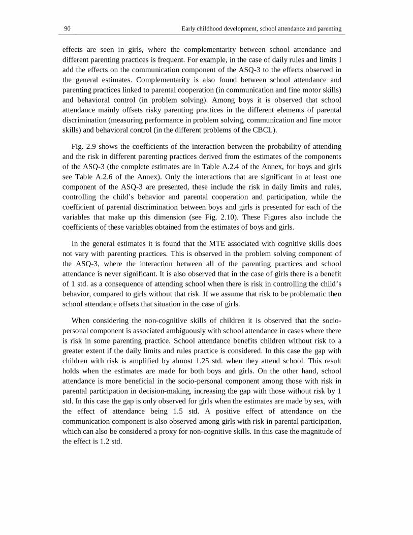
90 Early childhood development, school attendance and parenting
effects are seen in girls, where the complementarity between school attendance and different parenting practices is frequent. For example, in the case of daily rules and limits I add the effects on the communication component of the ASQ-3 to the effects observed in the general estimates. Complementarity is also found between school attendance and parenting practices linked to parental cooperation (in communication and fine motor skills) and behavioral control (in problem solving). Among boys it is observed that school attendance mainly offsets risky parenting practices in the different elements of parental discrimination (measuring performance in problem solving, communication and fine motor skills) and behavioral control (in the different problems of the CBCL).
Fig. 2.9 shows the coefficients of the interaction between the probability of attending and the risk in different parenting practices derived from the estimates of the components of the ASQ-3 (the complete estimates are in Table A.2.4 of the Annex, for boys and girls see Table A.2.6 of the Annex). Only the interactions that are significant in at least one component of the ASQ-3 are presented, these include the risk in daily limits and rules, controlling the child’s behavior and parental cooperation and participation, while the coefficient of parental discrimination between boys and girls is presented for each of the variables that make up this dimension (see Fig. 2.10). These Figures also include the coefficients of these variables obtained from the estimates of boys and girls.
In the general estimates it is found that the MTE associated with cognitive skills does not vary with parenting practices. This is observed in the problem solving component of the ASQ-3, where the interaction between all of the parenting practices and school attendance is never significant. It is also observed that in the case of girls there is a benefit of 1 std. as a consequence of attending school when there is risk in controlling the child’s behavior, compared to girls without that risk. If we assume that risk to be problematic then school attendance offsets that situation in the case of girls.
When considering the non-cognitive skills of children it is observed that the socio-personal component is associated ambiguously with school attendance in cases where there is risk in some parenting practice. School attendance benefits children without risk to a greater extent if the daily limits and rules practice is considered. In this case the gap with children with risk is amplified by almost 1.25 std. when they attend school. This result holds when the estimates are made for both boys and girls. On the other hand, school attendance is more beneficial in the socio-personal component among those with risk in parental participation in decision-making, increasing the gap with those without risk by 1 std. In this case the gap is only observed for girls when the estimates are made by sex, with the effect of attendance being 1.5 std. A positive effect of attendance on the communication component is also observed among girls with risk in parental participation, which can also be considered a proxy for non-cognitive skills. In this case the magnitude of the effect is 1.2 std.
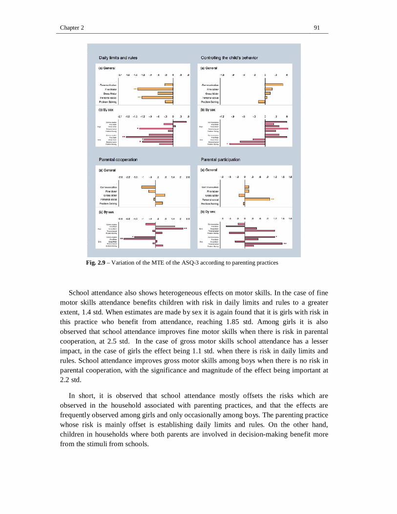
Chapter 2 91
Fig. 2.9 – Variation of the MTE of the ASQ-3 according to parenting practices
School attendance also shows heterogeneous effects on motor skills. In the case of fine motor skills attendance benefits children with risk in daily limits and rules to a greater extent, 1.4 std. When estimates are made by sex it is again found that it is girls with risk in this practice who benefit from attendance, reaching 1.85 std. Among girls it is also observed that school attendance improves fine motor skills when there is risk in parental cooperation, at 2.5 std. In the case of gross motor skills school attendance has a lesser impact, in the case of girls the effect being 1.1 std. when there is risk in daily limits and rules. School attendance improves gross motor skills among boys when there is no risk in parental cooperation, with the significance and magnitude of the effect being important at 2.2 std.
In short, it is observed that school attendance mostly offsets the risks which are observed in the household associated with parenting practices, and that the effects are frequently observed among girls and only occasionally among boys. The parenting practice whose risk is mainly offset is establishing daily limits and rules. On the other hand, children in households where both parents are involved in decision-making benefit more from the stimuli from schools.
92 Early childhood development, school attendance and parenting
By incorporating the parental discrimination dimension as a parenting practice there is the intuition that there should be some heterogeneous effect, particularly in the specific estimates of boys and girls. In these estimates the variable which identifies the risk associated with parental discrimination (grouping the three components of this dimension) is not significant when it interacts with the probability of attending school. The absence of effects could be hiding heterogeneous effects within the dimension. For this reason I made new estimates incorporating risk in parental discrimination, for each the variables used to build this dimension. That is to say whether parents identify differences depending on sex when raising their children in: looking after themselves, education on their position in the household and giving orders in the household (see Tables A.2.5 and A.2.7 of the Annex). The first variable identifies risk if the mother provides a positive response to the statement “Boys must be taught to look after themselves and girls to look after someone else”, the second “Boys must be educated so that they know how to be in charge of their house”, and the third “Girls must be taught that a woman’s place is in the home”.
These variables show more than levels of discrimination in that they show conservative perceptions about the gender roles that boys and girls should undertake in the household. Therefore the existence of risk in this dimension should not only be thought of as affecting the development of girls, it reflects the possibility that the stimuli provided to boys and girls are different, but not that the stimuli received by boys is good. This is what is shown in Fig. 2.10 where the coefficients of the aforementioned variables interacted with the probability of attending school are presented.
It can broadly be stated that there is a similar pattern in the variables looking after oneself and giving orders in the household. In these cases school attendance benefits children whose parents do not declare risky practices to a greater extent, and benefits are observed in both practices in the problem solving component, reaching nearly 5 std. in giving orders in the household and over 2.5 std. in looking after oneself. Meanwhile boys with risk in the dimension associated with giving orders in the household also have a better performance in fine motor skills and communication (in these components the general estimates are also significant, at 2.8 std. and 3.5 std.). Finally, the general estimates show that when there is no risk of the parents having discriminatory attitudes regarding the position that men and women should have in the household, children attending school achieve better levels of performance in fine motor and socio-personal skills, approximately 3.7 and 1.9 std. respectively.
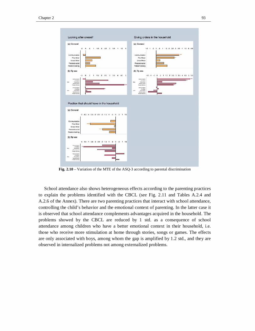
Chapter 2 93
Fig. 2.10 – Variation of the MTE of the ASQ-3 according to parental discrimination
School attendance also shows heterogeneous effects according to the parenting practices to explain the problems identified with the CBCL (see Fig. 2.11 and Tables A.2.4 and A.2.6 of the Annex). There are two parenting practices that interact with school attendance, controlling the child’s behavior and the emotional context of parenting. In the latter case it is observed that school attendance complements advantages acquired in the household. The problems showed by the CBCL are reduced by 1 std. as a consequence of school attendance among children who have a better emotional context in their household, i.e. those who receive more stimulation at home through stories, songs or games. The effects are only associated with boys, among whom the gap is amplified by 1.2 std., and they are observed in internalized problems not among externalized problems.
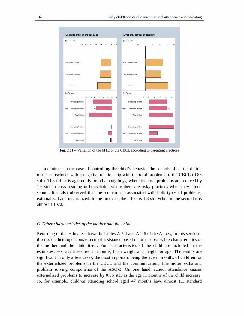
94 Early childhood development, school attendance and parenting
Fig. 2.11 – Variation of the MTE of the CBCL according to parenting practices
In contrast, in the case of controlling the child’s behavior the schools offset the deficit of the household, with a negative relationship with the total problems of the CBCL (0.83 std.). This effect is again only found among boys, where the total problems are reduced by 1.6 std. in boys residing in households where there are risky practices when they attend school. It is also observed that the reduction is associated with both types of problems, externalized and internalized. In the first case the effect is 1.3 std. While in the second it is almost 1.1 std.
C. Other characteristics of the mother and the child
Returning to the estimates shown in Tables A.2.4 and A.2.6 of the Annex, in this section I discuss the heterogeneous effects of assistance based on other observable characteristics of the mother and the child itself. Four characteristics of the child are included in the estimates: sex, age measured in months, birth weight and height for age. The results are significant in only a few cases, the most important being the age in months of children for the externalized problems in the CBCL and the communication, fine motor skills and problem solving components of the ASQ-3. On one hand, school attendance causes externalized problems to increase by 0.06 std. as the age in months of the child increase, so, for example, children attending school aged 47 months have almost 1.1 standard
Chapter 2 95
deviations more than children aged 24 months who attend. These results are in line with those found in Belsky (2002), Loeb et al. (2007) and Magnuson et al. (2007). The opposite happens in the components of the ASQ-3. In this case older children attending school get a higher score than younger children, with the magnitude of the effect being around 0.05 std. for each additional month. It is possible that in this case the age is capturing time in the school, which, as indicated previously, may increase the behavioral problems of the child. When observing how this is affected by school attendance according to the age in months of the children and sex is taken into account, it is observed that the effects are concentrated in boys. In the case of the ASQ-3 these effects occur in all of the components except socio-personal.
School attendance has a differential effect between boys and girls in gross motor skills, the girls achieved a score 0.75 std. lower than the boys. Among girls it is shown that school attendance has differential effects among those who had a low birth weight and those who did not. Girls with a low birth weight benefit less from school attendance and obtain a higher score, between 2 and 3 std. in gross motor skills, communication and socio-personal.
The variation of the MTE from the characteristics of the mother is more significant. School attendance offsets the differences in child development originating from the higher education of the mother. This occurs with fine motor skills and externalized problems. In the first case the score is reduced by 0.31 standard deviations for each additional year of education of the mother. Regarding externalized problems the effects are around 0.12 standard deviations. Similar effects are found in several components of the ASQ-3 when estimates are made for the case of boys, communication, problem solving and fine motor skills; which is not the case for girls where the effects are only seen in fine motor skills. These results are in line with those found by Felfe & Lalive (2014) who indicated that school attendance closed, in part, the gap generated by the education of the mother.
Few effects are found based on the age that the mother had her child. In the case of the socio-personal component, school attendance is associated with higher scores for children as the age at which the mother had the child increases. When considering the same component of the ASQ-3 it is observed that school attendance offsets the potential effects of educational aspirations, while children whose parents want their children to go to university obtained almost 2.5 std. less than the rest of the children. A similar effect in magnitude and direction is found for girls for both the socio-personal and communication components.
Variation of the MTE by household composition is not clearly observed. For example there is no evidence of differential effects of school attendance based on the absence of the father. However, when considering exclusively boys, school attendance allows children residing with both parents to increase their score in gross motor skills by almost 2 std. in relation to children who do not attend. When children do not reside with another child less than 4 years old the problems identified by the CBCL are lower in the case of attending
96 Early childhood development, school attendance and parenting
school, which is evident in internalized problems where the effect is almost 1 std. Similar effects are found when the estimates are made specifically for boys. Attendance affects the socio-personal component of the ASQ-3 in the same direction but when considering the presence of children aged 4-12. When there are no children in this age group residing in the same household the score of those who attend school is 0.8 std. higher on average, 1.6 std. in the case of boys. This effect, which in this case is found in the socio-personal component and the CBCL, is linked to the non-cognitive skills of the child, and possibly reflects a certain complementarity between the resources to stimulate the child in the household (for example, in terms of time dedicated to the child and his care) and school attendance.
Finally, as with the results found in Magnuson et al. (2007), it is observed that school attendance shows differential effects depending on the socio-economic situation of the children, especially when analyzing what occurs with boys and girls. In the case of problem solving, for example, differences are not observed among girls, whereas boys who attend school and reside in households whose income is above the first quintile obtain better scores than those in the lowest quintile. The magnitude of the effect does not change between the second and fifth quintile, and is around 4 std. Meanwhile, in other components of the ASQ-3 it is found that school attendance leads to better scores for children belonging to the higher strata of the income distribution, in the case of boys in gross motor skills and communication, and in girls in socio-personal, with the magnitude of the effects being greatest in the fifth quintile, reaching 3.5 std. in the first two cases and 2.7 std. in the third case. Attendance in the CBCL operates in the same way depending on the economic condition of the household; girls who do not reside in the first quintile get a lower score, almost 3 std., while the boys who obtain the lowest score reside in the fifth quintile, 2.6 std.
D. The effect of the expansion of schools for children aged 2 and 3
In this section I simulate an expansion of the supply of schools for children aged 2 and 3. The specific design of the reform is based on making more places available in order to bridge the gap in each neighborhood with the coverage of children aged 4, when attendance is mandatory. Figure 2.12 shows the potential demand satisfied for children aged 4 and for the group comprising children aged 2 and 3. The upper quadrants include the neighborhoods where the potential demand satisfied is higher for children aged 4 than for children aged 2 and 3, the first graph shows the neighborhoods where the gap is at least 3 times more, while the second graph includes neighborhoods where while the coverage for children aged 4 is higher, it does not triple the coverage of children aged 2 and 3. In these cases the gap between the existing supply is evident in both age groups, with the public supply for children aged 4 being close to 50% of the total of all children residing in the respective neighborhood, while for children aged 2 and 3 the number is around 30%.
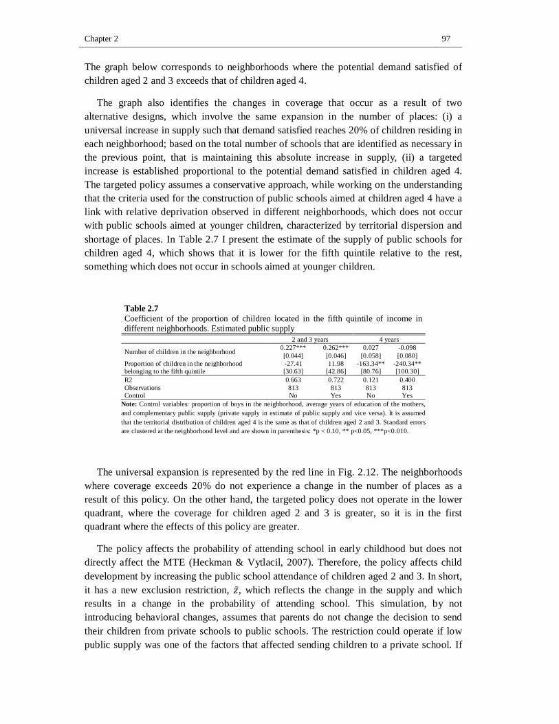
Chapter 2 97
The graph below corresponds to neighborhoods where the potential demand satisfied of children aged 2 and 3 exceeds that of children aged 4.
The graph also identifies the changes in coverage that occur as a result of two alternative designs, which involve the same expansion in the number of places: (i) a universal increase in supply such that demand satisfied reaches 20% of children residing in each neighborhood; based on the total number of schools that are identified as necessary in the previous point, that is maintaining this absolute increase in supply, (ii) a targeted increase is established proportional to the potential demand satisfied in children aged 4. The targeted policy assumes a conservative approach, while working on the understanding that the criteria used for the construction of public schools aimed at children aged 4 have a link with relative deprivation observed in different neighborhoods, which does not occur with public schools aimed at younger children, characterized by territorial dispersion and shortage of places. In Table 2.7 I present the estimate of the supply of public schools for children aged 4, which shows that it is lower for the fifth quintile relative to the rest, something which does not occur in schools aimed at younger children.
Table 2.7 Coefficient of the proportion of children located in the fifth quintile of income in different neighborhoods. Estimated public supply 2 and 3 years 4 years
Number of children in the neighborhood 0.227*** 0.262*** 0.027 -0.098 [0.044] [0.046] [0.058] [0.080]
Proportion of children in the neighborhood belonging to the fifth quintile
-27.41 11.98 -163.34** -240.34** [30.63] [42.86] [80.76] [100.30]
R2 0.663 0.722 0.121 0.400 Observations 813 813 813 813 Control No Yes No Yes
Note: Control variables: proportion of boys in the neighborhood, average years of education of the mothers, and complementary public supply (private supply in estimate of public supply and vice versa). It is assumed that the territorial distribution of children aged 4 is the same as that of children aged 2 and 3. Standard errors are clustered at the neighborhood level and are shown in parenthesis: *p < 0.10, ** p<0.05, ***p<0.010.
The universal expansion is represented by the red line in Fig. 2.12. The neighborhoods where coverage exceeds 20% do not experience a change in the number of places as a result of this policy. On the other hand, the targeted policy does not operate in the lower quadrant, where the coverage for children aged 2 and 3 is greater, so it is in the first quadrant where the effects of this policy are greater.
The policy affects the probability of attending school in early childhood but does not directly affect the MTE (Heckman & Vytlacil, 2007). Therefore, the policy affects child development by increasing the public school attendance of children aged 2 and 3. In short, it has a new exclusion restriction, 푧̃, which reflects the change in the supply and which results in a change in the probability of attending school. This simulation, by not introducing behavioral changes, assumes that parents do not change the decision to send their children from private schools to public schools. The restriction could operate if low public supply was one of the factors that affected sending children to a private school. If
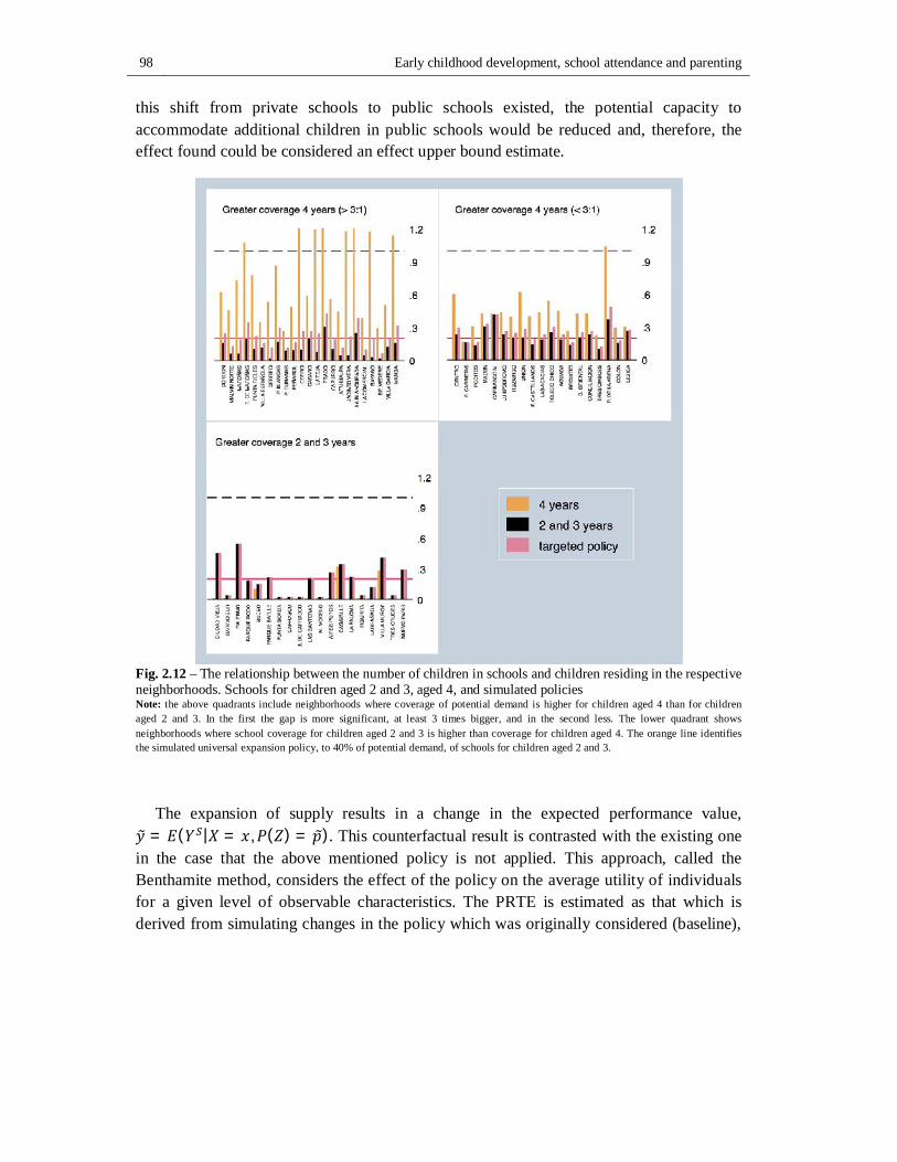
98 Early childhood development, school attendance and parenting
this shift from private schools to public schools existed, the potential capacity to accommodate additional children in public schools would be reduced and, therefore, the effect found could be considered an effect upper bound estimate.
Fig. 2.12 – The relationship between the number of children in schools and children residing in the respective neighborhoods. Schools for children aged 2 and 3, aged 4, and simulated policies Note: the above quadrants include neighborhoods where coverage of potential demand is higher for children aged 4 than for children aged 2 and 3. In the first the gap is more significant, at least 3 times bigger, and in the second less. The lower quadrant shows neighborhoods where school coverage for children aged 2 and 3 is higher than coverage for children aged 4. The orange line identifies the simulated universal expansion policy, to 40% of potential demand, of schools for children aged 2 and 3.
The expansion of supply results in a change in the expected performance value, 푦 = 퐸(푌 |푋 = 푥,푃(푍) = 푝). This counterfactual result is contrasted with the existing one in the case that the above mentioned policy is not applied. This approach, called the Benthamite method, considers the effect of the policy on the average utility of individuals for a given level of observable characteristics. The PRTE is estimated as that which is derived from simulating changes in the policy which was originally considered (baseline),
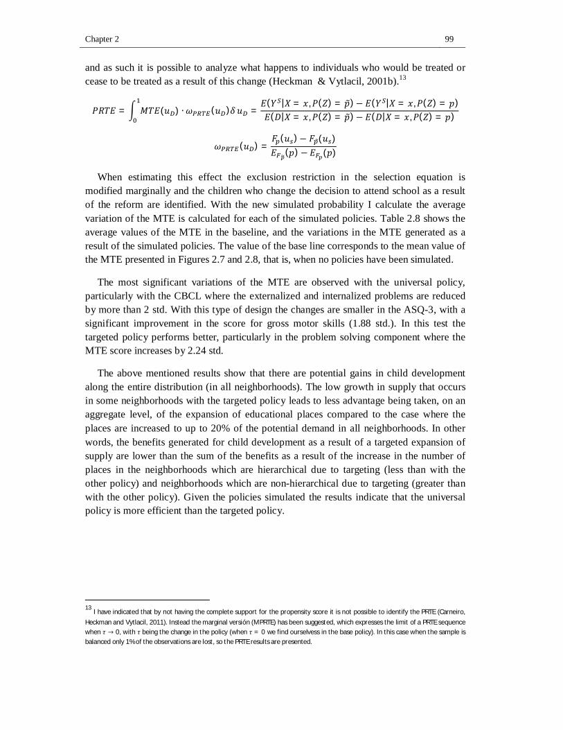
Chapter 2 99
and as such it is possible to analyze what happens to individuals who would be treated or cease to be treated as a result of this change (Heckman & Vytlacil, 2001b).13
푃푅푇퐸 = 푀푇퐸(푢 ) ∙ 휔 (푢 )훿 푢 =퐸(푌 |푋 = 푥,푃(푍) = 푝)− 퐸(푌 |푋 = 푥,푃(푍) = 푝)퐸(퐷|푋 = 푥,푃(푍) = 푝)− 퐸(퐷|푋 = 푥,푃(푍) = 푝)
휔 (푢 ) =퐹 (푢 )− 퐹 (푢 )퐸 (푝)−퐸 (푝)
When estimating this effect the exclusion restriction in the selection equation is modified marginally and the children who change the decision to attend school as a result of the reform are identified. With the new simulated probability I calculate the average variation of the MTE is calculated for each of the simulated policies. Table 2.8 shows the average values of the MTE in the baseline, and the variations in the MTE generated as a result of the simulated policies. The value of the base line corresponds to the mean value of the MTE presented in Figures 2.7 and 2.8, that is, when no policies have been simulated.
The most significant variations of the MTE are observed with the universal policy, particularly with the CBCL where the externalized and internalized problems are reduced by more than 2 std. With this type of design the changes are smaller in the ASQ-3, with a significant improvement in the score for gross motor skills (1.88 std.). In this test the targeted policy performs better, particularly in the problem solving component where the MTE score increases by 2.24 std.
The above mentioned results show that there are potential gains in child development along the entire distribution (in all neighborhoods). The low growth in supply that occurs in some neighborhoods with the targeted policy leads to less advantage being taken, on an aggregate level, of the expansion of educational places compared to the case where the places are increased to up to 20% of the potential demand in all neighborhoods. In other words, the benefits generated for child development as a result of a targeted expansion of supply are lower than the sum of the benefits as a result of the increase in the number of places in the neighborhoods which are hierarchical due to targeting (less than with the other policy) and neighborhoods which are non-hierarchical due to targeting (greater than with the other policy). Given the policies simulated the results indicate that the universal policy is more efficient than the targeted policy.
13
I have indicated that by not having the complete support for the propensity score it is not possible to identify the PRTE (Carneiro, Heckman and Vytlacil, 2011). Instead the marginal versión (MPRTE) has been suggested, which expresses the limit of a PRTE sequence when 휏 → 0, with 휏being the change in the policy (when 휏 = 0 we find ourselvess in the base policy). In this case when the sample is balanced only 1% of the observations are lost, so the PRTE results are presented.
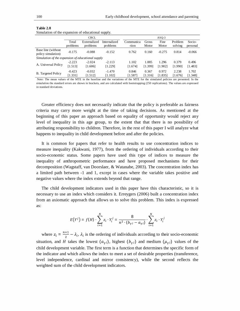
100 Early childhood development, school attendance and parenting
Table 2.8 Simulation of the expansion of educational supply. CBCL ASQ-3
Total
problems Externalized
problems Internalized
problems Communica-tion
Gross Motor
Fine Motor
Problem solving
Socio-personal
Base line (without policy simulation) -0.175 -0.088 -0.152 0.762 0.160 -0.275 0.814 -0.066
Simulation of the expansion of educational supply
A. Universal Policy -2.223 -2.024 -2.113 1.102 1.885 1.296 0.379 0.496 [1.513] [1.606] [1.229] [1.674] [1.399] [1.902] [1.990] [1.483]
B. Targeted Policy -0.423 -0.032 -1.470 0.846 0.367 0.972 2.238 1.702 [1.331] [1.512] [1.102] [1.587] [1.316] [1.835] [1.676] [1.348]
Note: The mean values of the MTE in the baseline and the variations of the MTE for the simulated policies are presented. In the simulation the standard errors are shown in brackets, and are calculated with bootstrapping (250 replications). The values are expressed in standard deviations.
Greater efficiency does not necessarily indicate that the policy is preferable as fairness criteria may carry more weight at the time of taking decisions. As mentioned at the beginning of this paper an approach based on equality of opportunity would reject any level of inequality in this age group, to the extent that that there is no possibility of attributing responsibility to children. Therefore, in the rest of this paper I will analyze what happens to inequality in child development before and after the policies.
It is common for papers that refer to health results to use concentration indices to measure inequality (Kakwani, 1977), from the ordering of individuals according to their socio-economic status. Some papers have used this type of indices to measure the inequality of anthropometric performance and have proposed mechanisms for their decomposition (Wagstaff, van Doorslaer, & Watanabe, 2003). The concentration index has a limited path between -1 and 1, except in cases where the variable takes positive and negative values where the index extends beyond that range.
The child development indicators used in this paper have this characteristic, so it is necessary to use an index which considers it. Erreygers (2006) built a concentration index from an axiomatic approach that allows us to solve this problem. This index is expressed as:
퐸 푌 = 푓(퐻) ∙ 푧 ∙ 푌 =8
푛 ∙ (푏 − 푎 )∙ 푧 ∙ 푌
where 푧 = − 휆 , 휆 is the ordering of individuals according to their socio-economic situation, and 퐻 takes the lowest (푎 ), highest (푏 ) and medium (휇 ) values of the child development variable. The first term is a function that determines the specific form of the indicator and which allows the index to meet a set of desirable properties (transference, level independence, cardinal and mirror consistency), while the second reflects the weighted sum of the child development indicators.
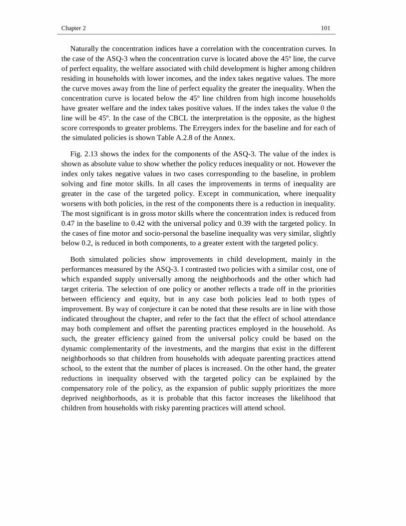
Chapter 2 101
Naturally the concentration indices have a correlation with the concentration curves. In the case of the ASQ-3 when the concentration curve is located above the 45º line, the curve of perfect equality, the welfare associated with child development is higher among children residing in households with lower incomes, and the index takes negative values. The more the curve moves away from the line of perfect equality the greater the inequality. When the concentration curve is located below the 45º line children from high income households have greater welfare and the index takes positive values. If the index takes the value 0 the line will be 45º. In the case of the CBCL the interpretation is the opposite, as the highest score corresponds to greater problems. The Erreygers index for the baseline and for each of the simulated policies is shown Table A.2.8 of the Annex.
Fig. 2.13 shows the index for the components of the ASQ-3. The value of the index is shown as absolute value to show whether the policy reduces inequality or not. However the index only takes negative values in two cases corresponding to the baseline, in problem solving and fine motor skills. In all cases the improvements in terms of inequality are greater in the case of the targeted policy. Except in communication, where inequality worsens with both policies, in the rest of the components there is a reduction in inequality. The most significant is in gross motor skills where the concentration index is reduced from 0.47 in the baseline to 0.42 with the universal policy and 0.39 with the targeted policy. In the cases of fine motor and socio-personal the baseline inequality was very similar, slightly below 0.2, is reduced in both components, to a greater extent with the targeted policy.
Both simulated policies show improvements in child development, mainly in the performances measured by the ASQ-3. I contrasted two policies with a similar cost, one of which expanded supply universally among the neighborhoods and the other which had target criteria. The selection of one policy or another reflects a trade off in the priorities between efficiency and equity, but in any case both policies lead to both types of improvement. By way of conjecture it can be noted that these results are in line with those indicated throughout the chapter, and refer to the fact that the effect of school attendance may both complement and offset the parenting practices employed in the household. As such, the greater efficiency gained from the universal policy could be based on the dynamic complementarity of the investments, and the margins that exist in the different neighborhoods so that children from households with adequate parenting practices attend school, to the extent that the number of places is increased. On the other hand, the greater reductions in inequality observed with the targeted policy can be explained by the compensatory role of the policy, as the expansion of public supply prioritizes the more deprived neighborhoods, as it is probable that this factor increases the likelihood that children from households with risky parenting practices will attend school.
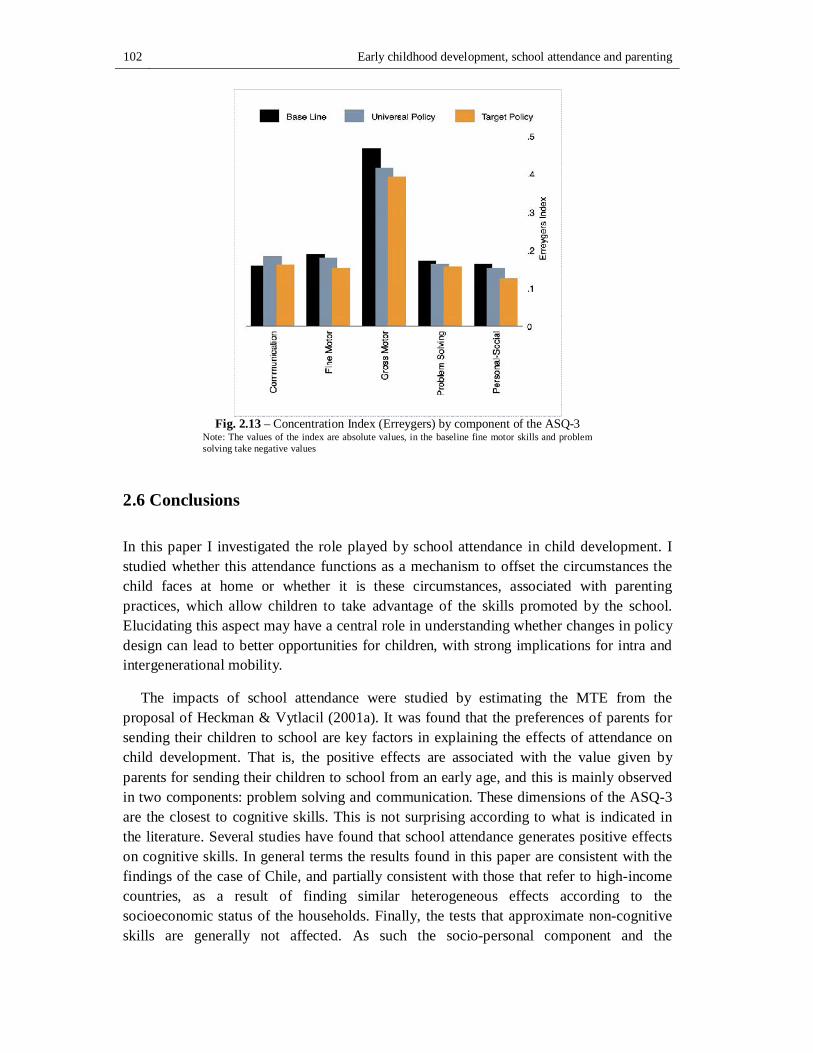
102 Early childhood development, school attendance and parenting
Fig. 2.13 – Concentration Index (Erreygers) by component of the ASQ-3
Note: The values of the index are absolute values, in the baseline fine motor skills and problem solving take negative values
2.6 Conclusions
In this paper I investigated the role played by school attendance in child development. I studied whether this attendance functions as a mechanism to offset the circumstances the child faces at home or whether it is these circumstances, associated with parenting practices, which allow children to take advantage of the skills promoted by the school. Elucidating this aspect may have a central role in understanding whether changes in policy design can lead to better opportunities for children, with strong implications for intra and intergenerational mobility.
The impacts of school attendance were studied by estimating the MTE from the proposal of Heckman & Vytlacil (2001a). It was found that the preferences of parents for sending their children to school are key factors in explaining the effects of attendance on child development. That is, the positive effects are associated with the value given by parents for sending their children to school from an early age, and this is mainly observed in two components: problem solving and communication. These dimensions of the ASQ-3 are the closest to cognitive skills. This is not surprising according to what is indicated in the literature. Several studies have found that school attendance generates positive effects on cognitive skills. In general terms the results found in this paper are consistent with the findings of the case of Chile, and partially consistent with those that refer to high-income countries, as a result of finding similar heterogeneous effects according to the socioeconomic status of the households. Finally, the tests that approximate non-cognitive skills are generally not affected. As such the socio-personal component and the
Chapter 2 103
internalized and externalized problems (CBCL) are not modified as a result of attendance when the preferences of the parents change. This differs from the findings of several papers that show negative effects on non-cognitive skills, mainly when considering attendance for children under 4 years old (Urzúa & Veramendi, 2011; Loeb et al., 2007; Magnuson et al., 2007).
A novel aspect of this paper arises when considering the interactions between school attendance and parenting practices. While effects on non-cognitive skills are not observed when considering heterogeneity in the preferences of parents, they are when the parenting practices vary. School attendance mainly operates by offsetting risks generated at home by parenting practices, and does so mainly among girls. The paper concludes by showing what the impacts would be of an expansion of educational supply for children aged 2 and 3. Two alternative designs are proposed, one is targeted based on the distribution of schools by neighborhood similar to the distribution of educational places for children aged 4, and the other which increases the number of places universally to cover 20% of potential demand. It was found that both policies lead to improvements in terms of efficiency and equity, with the targeted policy being preferable in terms of equity and the universal policy in terms of efficiency.
The source of information used for this study, the ENDIS, is the first wave of a panel which aims to follow a cohort. In 2015 the second wave of this survey began to be carried out and a third wave is planned within three years. As such this paper is the first in a series of studies which aim to analyze the microeconomic foundations of intergenerational mobility, as well as the intertemporal determinants of inequality of opportunity. Many studies have shown that policies aimed at early childhood level the playing field, so the performances in this age group are strong predictors of what happens in youth and adolescence in both the educational system and the workplace. However, we know little about the impact on these performances of what had occurred previously in the household. According to the findings in this paper parenting practices are a strong source of heterogeneities in the skills that children develop and affect the subsequent investments made by the parents. Knowledge about these issues is still developing, and the field of study is very broad to identify how these practices may or may not lead down a path which is difficult to change in the future trajectories of children.
In the scarce evidence found for middle-income countries, positive effects have been found of school attendance on cognitive and motor skills, with the results for non-cognitive skills being ambiguous. The results are more abundant for countries whose average incomes are higher. In these countries no effects have been found on the general population or the effects have been negative on both cognitive and non-cognitive skills. When the studies explore heterogeneous effects there are positive impacts for disadvantaged groups (parents with a poor socioeconomic status, low education or immigrants) mainly on cognitive and motor skills. This suggests that in these cases school attendance may succeed in closing gaps, allowing for a greater accumulation of skills in children from more disadvantaged households. Therefore, upon finding that the empirical
104 Early childhood development, school attendance and parenting
evidence indicates that there are average effects on the general population of middle-income countries, and also on the most disadvantaged groups of high-income countries, the question arises of whether there is a child development threshold from which school attendance stops generating additional effects. The indication of an affirmative response would be observed if the average characteristics of the population of middle-income countries resemble the most disadvantages groups of high-income countries. This paper does not provide an answer to this question, still an open issue for future research.
Chapter 2 105
References
Achenbach, T. (1978). The Child Behavior Profile: I. Boys aged 6–11. Journal of Consulting and Clinical Psychology, 46(3): 478-488.
Achenbach T. & L. Rescorla (2000). Manual for the ASEBA Preschool Forms & Profiles: An Integrated System of Multi-informant Assessment; Child Behavior Checklist for Ages 1 1/2-5; Language Development Survey; Caregiver-Teacher Report Form. University of Vermont.
Andreoli F, T. Havnes & A. Lefranc (2014). “Equalization of opportunity: Definitions, implementable conditions and application to early-childhood policy evaluation”, Mimeo
Araujo C & N. Schady (2015). “Los jardines de cuidado infantil: la calidad es lo que cuenta”. In Berlinski S. and N. Schady Los primeros años. El bienestar infantil y el papel de las políticas públicas. BID.
Baker M., J. Gruber & K. Milligan (2008). Universal child care, maternal labor supply, and family well-being. Journal of Political Economy 116(4), 709–74.
Bandura A. (1995). Self-efficacy in changing societies. Cambridge University Press.
Belsky J. (2002). “Quantity Counts: Amount of Child Care and Children’s Socioemotional Development”, Journal of Developmental and Behavioral Pediatrics, 23: 167-170.
Bernal R. & A. Camacho (2010). “La importancia de los programas para la primera infancia en Colombia”, Documentos CEDE, 20.
Blau D. & J. Currie (2006). “Pre-school, day care, and after-school care: who's minding the kids?”. Handbook of the Economics of Education, 2:1163-1278.
Bornstein M. (2001). Parenting: Science and Practice. Parenting, 1(1-2).
Brody G., D. Flor & N. Morgan Gibson (1999). “Linking Maternal Efficacy Beliefs, Developmental Goals, Parenting Practices, and Child Competence in Rural Single-Parent African American Families”, Child Development, 70(5): 1197–1208.
Cabella, W. & M. Nathan (2014). “Cambio familiar, parentalidades y bienestar en la infancia y la adolescencia”. In INAU, Parentalidades y cambios familiares. Enfoques teóricos y prácticos. Montevideo: INAU.
Cabella W., M. De Rosa, E. Failache, P. Fitermann, N. Katzkowicz, M. Medina, J. Mila, M. Nathan, A. Nocetto, I. Pardo, I. Perazzo, G. Salas, C. Salmentón, C. Severi & A. Vigorito (2015). Salud, nutrición y desarrollo en la primera infancia en Uruguay. Primeros resultados de la ENDIS. INE/UdelaR/OPP/MSP/MIDES/UCC. Available in: http://www.ine.gub.uy/documents/10181/35704/SALUD,+NUTRICI%C3%93N+Y+DE
106 Early childhood development, school attendance and parenting
SARROLLO+EN+LA+PRIMERA+INFANCIA+EN+URUGUAY+PRIMEROS+RESULTADOS+DE+LA+ENDIS/7be3f504-ebb9-4427-bb5d-cb4d9f242a7b
Carneiro P., F. Cunha, E. Galasso & I. López Garcia (2013). “The role of beliefs in parental investments and child development: Evidence from a parenting intervention in Chile”. Mimeo.
Carneiro P., J. Heckman & E. Vytlacil (2011). “Estimating marginal returns to education”. American Economic Review, 101: 2754-2781.
Center on the Developing Child (2007). A Science-Based Framework for Early Childhood Policy. Available in: www.developingchild.harvard.edu.
Coleman J. (1988). “Social capital in the creation of human capital”, American Journal of Sociology, 94: 95 – 120.
Conti G. & J. Heckman (2012). "The Economics of Child Well-Being," NBER Working Papers 18466.
Conti G., C. Hansman, J. Heckman, M. Novak, A. Ruggiero & S. Suomi (2012) “Primate Evidence on the Late Health Effects of Early Life Adversity”, NBER Working Paper Nº 18002.
Darling N. & L. Steinberg (1993). “Parenting style as context: An integrative model”. Psychological bulletin, 113(3), 487.
Del Boca D., C. Pronzato & G. Sorrenti (2015). “When rationing plays a role: selection criteria in the Italian early child care system” Families and Societies WP 47.
DNPS-MIDES (2014). Cuidados como sistema. Propuestas para un modelo solidario y corresponsable de cuidados en Uruguay. Dirección Nacional de Políticas Sociales, Ministerio de Desarrollo Social.
Doyle O., C. Harmon, J. Heckman, C. Logue & S. Moon (2013). “Mesuring Investment in Human Capital Formation: An Experimental Analysis of Early Life Outcomes” NBER Working Papers 19316.
Dustmann C., A. Raute & U. Schöenberg (2013). Does universal child care matter? evidence from a large expansion in pre-school education. mimeo, UCL.
Erreygers G. (2006). Correcting the Concentration Index. University of Antwerp. Antwerp, Belgium.
Felfe C. & R. Lalive (2014). “Does Early Care Help or Hurt Children´s Development”. IZA DP N.º 8484.
Gibson-Davis C. (2008). “Family Structure Effects on Maternal and Paternal Parenting in Low-Income Families”. Journal of Marriage and Family 70: 452–465.
Chapter 2 107
Heckman J. (1979). "Sample selection bias as a specification error", Econometrica 153-161.
Heckman J., S. Moon, R. Pinto, P. Savelyev & A. Yavitz (2010). “The rate of return to the High Scope Perry Preschool Program”. Journal of Public Economics, 94(1-2), 114-128.
Heckman J., R. Pinto & P. Savelyev (2013). “Understanding the mechanisms through which an influential early childhood program boosted adult outcomes”. American Economic Review, 103(6): 2052–86.
Heckman J. & T. Kautz (2014). “Fostering and measuring skills interventions that improve character and cognition”. In J. J. Heckman, J. E. Humphries and T. Kautz (Eds.) The GED Myth: Education, Achievement Tests, and the Role of Character in American Life, Ch. 9. Chicago, IL: University of Chicago Press.
Heckman, J. & E. Vytlacil (2001a). “Local instrumental variables”· In Hsiao C., K. Morimune and J. Powell (Eds.) Nonlinear Statistical Modeling: Proceedings of the Thirteenth International Symposium in Economic Theory and Econometrics: Essays in Honor of Takeshi Amemiya, 1-46. New York: Cambridge University Press.
Heckman, J. & E. Vytlacil (2001b). “Policy relevant treatment effects”. American Economic Review, 91(2), 107-11.
Heckman, J. & E. Vytlacil (2007). “Econometric evaluation of social programs. Using the marginal treatment effect to organize alternative econometric estimators to evaluate social programs and to forecast their effects in new environments”. In J. Heckman and E. Leamer (Eds.) Handbook of the Econometrics, vol. 6B:4875–5144, New York.
Kakwani N. (1977). “Measurement of Tax Progressivity: An International Comparison”, Economic Journal 87(345): 71–80.
Lefebvre P., P. Merrigan & M. Verstraete (2006). “Impact of Early Childhood Care and Education on Children's Preschool Cognitive Development: Canadian Results from a Large Scale Quasi-Experiment”. CIPRÉE WP 06-36.
Loeb S., M. Bridges, D. Bassok, B. Fuller, & R. Rumberger (2007). “How much is too much? The influence of preschool centers on children's social and cognitive development”. Economics of Education review, 26(1): 52-66.
Magnuson K., C. Ruhm & J. Waldfogel (2007). “Does Prekindergarten Improve School Preparation and Performance? Economics of Education Review, 26, 33-51.
Noboa-Hidalgo G. & S. Urzúa (2012). “The Effects of Participation in Public Child Care Centers: Evidence from Chile”. Journal of Human Capital, 6(1).
Schellenbach C., T. Whitman & J. Borkowski (1992). "Toward an integrative model of adolescent parenting". Human Development, 35(2): 81-99.
108 Early childhood development, school attendance and parenting
Squires, J. Briker & D. Twombly. (2002). The ASQ: SE user´s guide: for the Ages & Stages Questionnaires, social-emotional: a parent-completed, child-monitoring program for social-emotional behaviors, Paul H. Brookes Baltimore, Md.
Urzúa S. & G. Veramendi (2011). "The Impact of Out-of-Home Childcare Centers on Early Childhood Development". Research Department Publications 4723, IADB.
Wagstaff A., E. van Doorslaer, & N. Watanabe (2003). “On Decomposing the Causes of Health Sector Inequalities, with an Application to Malnutrition Inequalities in Vietnam”. Journal of Econometrics, 112(1): 219–27.
Walker S., S. Chang, C. Powell & S. Grantham-McGregor (2005). “Effects of early childhood psychosocial stimulation and nutritional supplementation on cognition and education in growth-stunted Jamaican children: prospective cohort study”. The Lancet, 366(9499): 1804-1807.
Wentzel K. (1998). "Social relationships and motivation in middle school: The role of parents, teachers, and peers". Journal of educational Psychology, 90(2).
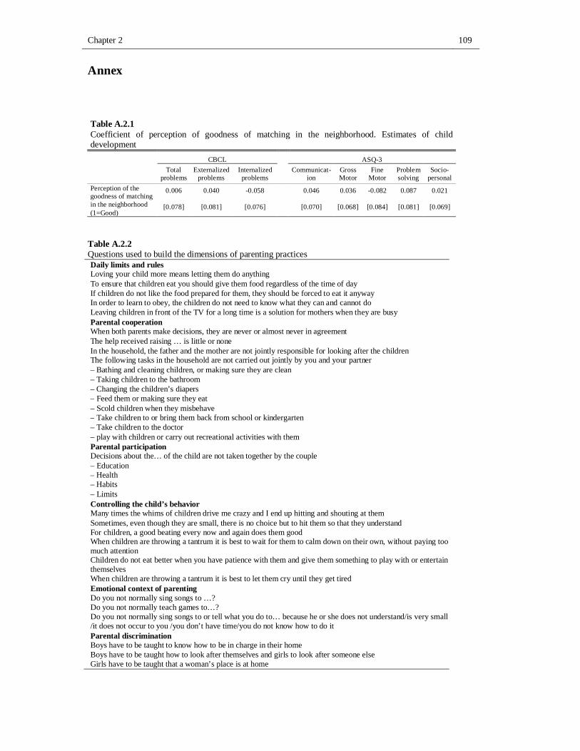
Chapter 2 109
Annex
Table A.2.1 Coefficient of perception of goodness of matching in the neighborhood. Estimates of child development
CBCL ASQ-3 Total
problems Externalized
problems Internalized
problems Communicat- ion
Gross Motor
Fine Motor
Problem solving
Socio-personal
Perception of the goodness of matching in the neighborhood (1=Good)
0.006 0.040 -0.058 0.046 0.036 -0.082 0.087 0.021
[0.078] [0.081] [0.076] [0.070] [0.068] [0.084] [0.081] [0.069]
Table A.2.2 Questions used to build the dimensions of parenting practices Daily limits and rules Loving your child more means letting them do anything To ensure that children eat you should give them food regardless of the time of day If children do not like the food prepared for them, they should be forced to eat it anyway In order to learn to obey, the children do not need to know what they can and cannot do Leaving children in front of the TV for a long time is a solution for mothers when they are busy Parental cooperation When both parents make decisions, they are never or almost never in agreement The help received raising … is little or none In the household, the father and the mother are not jointly responsible for looking after the children The following tasks in the household are not carried out jointly by you and your partner – Bathing and cleaning children, or making sure they are clean – Taking children to the bathroom – Changing the children’s diapers – Feed them or making sure they eat – Scold children when they misbehave – Take children to or bring them back from school or kindergarten – Take children to the doctor – play with children or carry out recreational activities with them Parental participation Decisions about the… of the child are not taken together by the couple – Education – Health – Habits – Limits Controlling the child’s behavior Many times the whims of children drive me crazy and I end up hitting and shouting at them Sometimes, even though they are small, there is no choice but to hit them so that they understand For children, a good beating every now and again does them good When children are throwing a tantrum it is best to wait for them to calm down on their own, without paying too much attention Children do not eat better when you have patience with them and give them something to play with or entertain themselves When children are throwing a tantrum it is best to let them cry until they get tired Emotional context of parenting Do you not normally sing songs to …? Do you not normally teach games to…? Do you not normally sing songs to or tell what you do to… because he or she does not understand/is very small /it does not occur to you /you don’t have time/you do not know how to do it Parental discrimination Boys have to be taught to know how to be in charge in their home Boys have to be taught how to look after themselves and girls to look after someone else Girls have to be taught that a woman’s place is at home
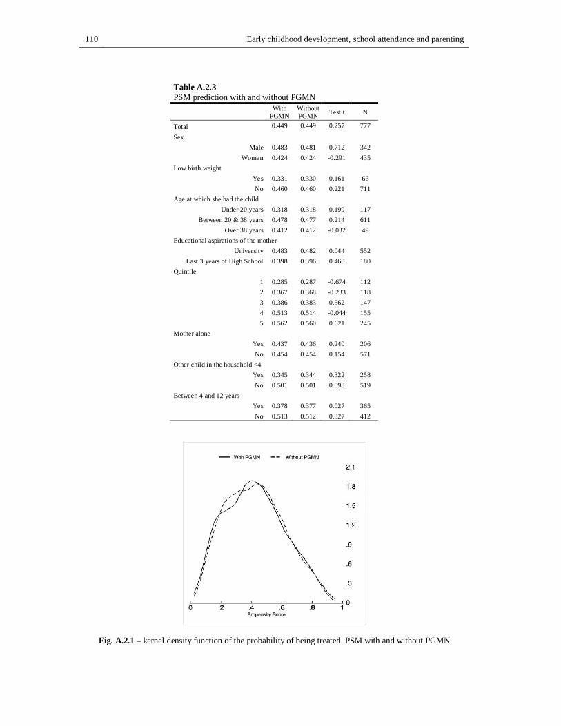
110 Early childhood development, school attendance and parenting
Table A.2.3 PSM prediction with and without PGMN
With
PGMN Without PGMN Test t N
Total 0.449 0.449 0.257 777
Sex Male 0.483 0.481 0.712 342
Woman 0.424 0.424 -0.291 435 Low birth weight
Yes 0.331 0.330 0.161 66 No 0.460 0.460 0.221 711
Age at which she had the child Under 20 years 0.318 0.318 0.199 117
Between 20 & 38 years 0.478 0.477 0.214 611 Over 38 years 0.412 0.412 -0.032 49
Educational aspirations of the mother University 0.483 0.482 0.044 552
Last 3 years of High School 0.398 0.396 0.468 180 Quintile
1 0.285 0.287 -0.674 112 2 0.367 0.368 -0.233 118 3 0.386 0.383 0.562 147 4 0.513 0.514 -0.044 155 5 0.562 0.560 0.621 245
Mother alone Yes 0.437 0.436 0.240 206 No 0.454 0.454 0.154 571
Other child in the household <4 Yes 0.345 0.344 0.322 258 No 0.501 0.501 0.098 519
Between 4 and 12 years Yes 0.378 0.377 0.027 365 No 0.513 0.512 0.327 412
Fig. A.2.1 – kernel density function of the probability of being treated. PSM with and without PGMN
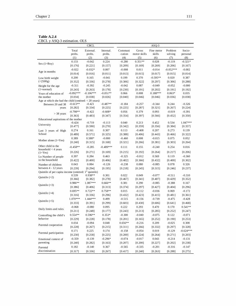
Chapter 2 111
Table A.2.4 CBCL y ASQ-3 estimation. OLS
CBCL ASQ-3
Total probs.
External. probs.
Internal. probs.
Communi-cation
Gross motor skills
Fine motor skills
Problem solving
Socio-personal
(1) (2) (3) (4) (5) (6) (7) (8)
Sex (1=Boy) 0.133 -0.042 0.224 -0.280 0.351** 0.028 -0.119 -0.321*
[0.176] [0.221] [0.157] [0.209] [0.169] [0.269] [0.206] [0.167]
Age in months -0.022 -0.032* 0.007 -0.008 0.011 -0.014 -0.052*** -0.002 [0.014] [0.016] [0.011] [0.013] [0.015] [0.017] [0.015] [0.014]
Low birth weight (<2500g)
0.200 0.165 -0.041 0.199 0.370 -0.595** 0.020 0.387 [0.352] [0.336] [0.278] [0.306] [0.322] [0.297] [0.306] [0.288]
Height for the age (1=normal)
-0.311 -0.392 -0.245 -0.042 0.087 -0.049 -0.052 -0.000 [0.243] [0.263] [0.178] [0.230] [0.191] [0.202] [0.191] [0.192]
Years of education of the mother
-0.092*** -0.106*** -0.051** 0.066 0.008 0.188*** 0.063* 0.035 [0.034] [0.038] [0.026] [0.040] [0.046] [0.046] [0.036] [0.038]
Age at which she had the child (omitted: < 20 years) Between 20 and 38
years -0.613** -0.421 -0.487** -0.184 -0.257 -0.344 0.244 -0.326 [0.282] [0.334] [0.225] [0.225] [0.287] [0.321] [0.267] [0.224]
> 38 years -0.798** -0.422 -0.608* 0.056 0.379 0.093 -0.019 -0.391 [0.363] [0.483] [0.347] [0.354] [0.397] [0.566] [0.452] [0.350]
Educational aspirations of the mother
University -0.424 -0.719 -0.113 0.040 0.213 0.452 0.534 1.047*** [0.477] [0.590] [0.270] [0.342] [0.359] [0.356] [0.384] [0.357]
Last 3 years of High School
0.274 0.161 0.307 0.113 -0.408 0.207 0.273 0.139 [0.489] [0.571] [0.325] [0.388] [0.406] [0.443] [0.466] [0.322]
Mother alone (1=Yes) 0.389 0.588* -0.000 -0.460 0.008 -0.015 0.075 0.052
[0.240] [0.315] [0.168] [0.321] [0.266] [0.381] [0.303] [0.264] Other child in the household < 4 years (1=Yes)
-0.458** -0.285 -0.489*** 0.111 0.155 -0.240 0.254 0.016
[0.226] [0.271] [0.169] [0.215] [0.192] [0.264] [0.217] [0.206] Ln Number of people in the household
0.397 0.284 0.463 -0.325 -0.012 0.569 0.119 -0.360 [0.422] [0.400] [0.406] [0.402] [0.366] [0.432] [0.400] [0.302]
Number of children between 4 - 12 years
0.043 0.084 -0.126 -0.238 0.080 -0.085 0.078 0.326 [0.239] [0.294] [0.195] [0.218] [0.245] [0.315] [0.246] [0.237]
Quintile of per capita income (omitted: 1st quintile)
Quintile (=2) 0.539 0.938** 0.301 0.022 0.049 -0.077 -0.511 -0.310
[0.366] [0.382] [0.278] [0.467] [0.341] [0.407] [0.429] [0.352]
Quintile (=3) 0.986** 1.087*** 0.666** 0.381 0.290 -0.085 -0.388 0.167 [0.386] [0.406] [0.313] [0.374] [0.297] [0.427] [0.404] [0.296]
Quintile (=4) 0.695** 0.722** 0.758** 0.015 -0.112 -0.036 0.069 -0.172 [0.316] [0.336] [0.296] [0.432] [0.423] [0.415] [0.481] [0.361]
Quintile (=5) 1.070*** 1.444*** 0.499 -0.515 -0.156 -0.739 -0.475 -0.428 [0.333] [0.391] [0.299] [0.603] [0.430] [0.606] [0.641] [0.468]
Daily limits and rules -0.068 -0.080 0.095 0.222 0.293 0.470 0.170 0.541** [0.211] [0.248] [0.177] [0.243] [0.213] [0.285] [0.252] [0.247]
Controlling the child’s behavior
0.554** 0.596** 0.353* -0.300 -0.040 -0.075 0.122 -0.071 [0.229] [0.228] [0.178] [0.201] [0.165] [0.252] [0.190] [0.253]
Parental cooperation 0.034 -0.094 0.048 0.656** -0.216 0.209 -0.025 0.308
[0.228] [0.267] [0.215] [0.311] [0.266] [0.332] [0.297] [0.328]
Parental participation 0.171 0.225 0.174 -0.158 -0.054 0.019 -0.129 -0.624***
[0.230] [0.258] [0.225] [0.200] [0.224] [0.264] [0.271] [0.203] Emotional context of parenting
-0.359 -0.139 -0.296* -0.074 -0.017 0.043 -0.214 -0.131 [0.240] [0.282] [0.163] [0.207] [0.200] [0.227] [0.202] [0.238]
Parental discrimination
0.182 -0.140 0.367 -0.565 -0.335 -0.201 -0.316 -0.147 [0.317] [0.336] [0.267] [0.417] [0.240] [0.263] [0.288] [0.275]
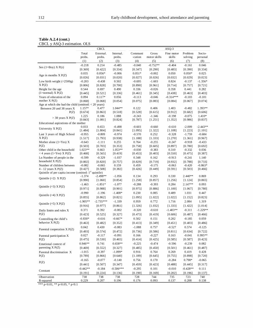
112 Early childhood development, school attendance and parenting
Table A.2.4 (cont.) CBCL y ASQ-3 estimation. OLS
CBCL ASQ-3 Total probs.
External. probs.
Internal. probs.
Communi-cation
Gross motor skills
Fine motor skills
Problem solving
Socio-personal
(1) (2) (3) (4) (5) (6) (7) (8)
Sex (1=Boy) X P(z) -0.218 0.214 -0.485 -0.040 -0.752** -0.404 -0.161 0.046 [0.369] [0.422] [0.334] [0.347] [0.290] [0.483] [0.390] [0.334]
Age in months X P(Z) 0.035 0.056* -0.006 0.051* -0.002 0.050 0.050* 0.025 [0.026] [0.031] [0.020] [0.027] [0.026] [0.032] [0.029] [0.023]
Low birth weight (<2500g) X P(Z)
-0.203 -0.438 0.502 -0.695 -1.603 0.824 -0.137 -1.356* [0.806] [0.828] [0.700] [0.890] [0.961] [0.714] [0.757] [0.721]
Height for the age (1=normal) X P(Z)
0.544 0.697 0.490 0.336 -0.026 0.358 0.441 0.282 [0.445] [0.521] [0.336] [0.461] [0.345] [0.438] [0.463] [0.403]
Years of education of the mother X P(Z)
0.094 0.117* 0.056 -0.113 -0.046 -0.314*** -0.103 -0.101 [0.068] [0.068] [0.054] [0.075] [0.083] [0.084] [0.067] [0.074]
Age at which she had the child (omitted: < 20 years) Between 20 and 38 years X
P(Z) 1.157* 0.477 1.044** 0.122 0.406 1.403 -0.482 1.393** [0.674] [0.863] [0.518] [0.528] [0.615] [0.912] [0.682] [0.606]
> 38 years X P(Z) 1.225 0.186 1.088 -0.243 -1.346 -0.198 -0.075 1.410* [0.843] [1.081] [0.824] [0.787] [1.251] [1.352] [0.986] [0.837]
Educational aspirations of the mother
University X P(Z) 0.033 0.653 -0.498 -0.603 -0.660 -0.610 -2.009 -2.443** [1.484] [1.804] [0.841] [1.095] [1.322] [1.108] [1.223] [1.101]
Last 3 years of High School X P(Z)
-0.955 -0.809 -0.974 -0.570 0.252 -0.328 -1.759 -0.684 [1.517] [1.793] [0.938] [1.188] [1.333] [1.270] [1.361] [0.967]
Mother alone (1=Yes) X P(Z)
-0.643 -1.111 0.255 0.764 -0.255 -0.247 -0.918 -0.433 [0.503] [0.703] [0.353] [0.758] [0.605] [0.897] [0.780] [0.692]
Other child in the household < 4 years (1=Yes) X P(Z)
1.023** 0.663 1.053** -0.030 -0.383 0.310 -0.332 0.036 [0.468] [0.565] [0.419] [0.453] [0.403] [0.550] [0.475] [0.387]
Ln Number of people in the household X P(Z)
-0.599 -0.329 -1.037 0.348 0.162 -0.913 -0.241 1.140 [0.802] [0.820] [0.757] [0.829] [0.719] [0.932] [0.788] [0.733]
Number of children between 4 - 12 years X P(Z)
-0.082 -0.065 0.159 0.459 -0.175 -0.063 -0.420 -0.863* [0.427] [0.508] [0.382] [0.426] [0.449] [0.591] [0.503] [0.466]
Quintile of per capita income (omitted: 1st quintile)
Quintile (=2) X P(Z) -1.374 -2.498** -1.056 0.134 0.293 0.330 2.440** 0.869 [0.990] [1.060] [0.854] [1.258] [0.857] [1.256] [1.124] [0.865]
Quintile (=3) X P(Z) -1.463 -1.851* -1.077 -0.288 -0.393 0.284 2.147** 0.093 [0.971] [0.988] [0.901] [0.975] [0.886] [1.100] [1.067] [0.780]
Quintile (=4) X P(Z) -0.990 -1.196 -1.408* 0.230 0.085 0.489 1.031 0.447 [0.855] [0.862] [0.821] [1.095] [1.022] [1.022] [1.152] [0.823]
Quintile (=5) X P(Z) -1.905** -2.735*** -1.339 0.959 0.772 1.716 2.084 1.319 [0.916] [0.977] [0.861] [1.326] [1.032] [1.333] [1.422] [1.014]
Daily limits and rules X P(Z)
0.371 0.392 -0.002 -0.320 -0.610 -1.403** -0.311 -1.229** [0.423] [0.525] [0.327] [0.473] [0.419] [0.606] [0.487] [0.466]
Controlling the child’s behavior X P(Z)
-0.830* -0.616 -0.667* 0.502 0.151 0.202 -0.185 0.059 [0.463] [0.482] [0.352] [0.413] [0.349] [0.451] [0.403] [0.486]
Parental cooperation X P(Z) 0.042 0.430 -0.083 -1.088 0.757 -0.527 0.574 -0.125
[0.493] [0.574] [0.472] [0.736] [0.586] [0.811] [0.634] [0.722] Parental participation X P(Z)
0.027 -0.117 -0.091 0.166 -0.227 0.163 -0.041 0.995** [0.475] [0.530] [0.465] [0.414] [0.425] [0.585] [0.587] [0.423]
Emotional context of parenting X P(Z)
0.946** 0.741 0.658** -0.225 -0.474 -0.596 -0.239 0.082 [0.469] [0.552] [0.327] [0.485] [0.450] [0.501] [0.461] [0.487]
Parental discrimination X P(Z)
-1.015 -0.397 -1.099* 0.916 0.764 0.269 0.419 0.428 [0.789] [0.866] [0.640] [1.189] [0.645] [0.755] [0.898] [0.720]
P(Z) -0.165 -0.077 -0.140 0.756 0.170 -0.284 0.798* -0.065 [0.441] [0.507] [0.347] [0.459] [0.423] [0.488] [0.445] [0.317]
Constant -0.442** -0.184 -0.506*** -0.295 0.101 -0.010 -0.428** 0.111 [0.191] [0.224] [0.136] [0.190] [0.169] [0.202] [0.196] [0.137]
Observation 738 738 738 728 744 735 723 740 R-squared 0.229 0.207 0.196 0.176 0.093 0.137 0.208 0.138 *** p<0.01, ** p<0.05, * p<0.1
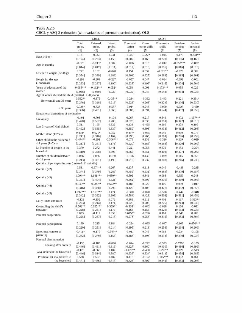
Chapter 2 113
Table A.2.5 CBCL y ASQ-3 estimation (with variables of parental discrimination). OLS
CBCL ASQ-3
Total probs.
External. probs.
Interal. probs.
Communi-cation
Gross motor skills
Fine motor skills
Problem solving
Socio-personal
(1) (2) (3) (4) (5) (6) (7) (8)
Sex (1=Boy) 0.131 -0.055 0.231 -0.337 0.322* -0.045 -0.173 -0.344** [0.174] [0.223] [0.155] [0.207] [0.166] [0.270] [0.186] [0.168]
Age in months -0.023 -0.033* 0.007 -0.006 0.013 -0.012 -0.053*** -0.002 [0.014] [0.017] [0.011] [0.012] [0.016] [0.016] [0.016] [0.013]
Low birth weight (<2500g) 0.222 0.182 -0.028 0.154 0.332 -0.626** -0.028 0.389 [0.354] [0.339] [0.283] [0.301] [0.325] [0.283] [0.315] [0.301]
Height for the age (1=normal)
-0.299 -0.389 -0.237 -0.057 0.047 -0.084 -0.098 -0.001 [0.263] [0.287] [0.190] [0.228] [0.196] [0.216] [0.204] [0.204]
Years of education of the mother
-0.095*** -0.112*** -0.052* 0.054 0.003 0.173*** 0.055 0.029 [0.036] [0.040] [0.027] [0.039] [0.047] [0.048] [0.034] [0.038]
Age at which she had the child (omitted: < 20 years)
Between 20 and 38 years -0.562** -0.379 -0.435** -0.284 -0.362 -0.443 0.221 -0.391* [0.276] [0.328] [0.215] [0.223] [0.268] [0.324] [0.276] [0.230]
> 38 years -0.728* -0.336 -0.557 -0.014 0.243 -0.000 -0.023 -0.459 [0.366] [0.481] [0.365] [0.383] [0.391] [0.544] [0.457] [0.359]
Educational aspirations of the mother
University -0.401 -0.708 -0.104 0.067 0.217 0.549 0.472 1.137*** [0.478] [0.582] [0.285] [0.328] [0.338] [0.391] [0.342] [0.315]
Last 3 years of High School 0.311 0.195 0.322 0.133 -0.425 0.260 0.204 0.199
[0.492] [0.565] [0.337] [0.359] [0.393] [0.433] [0.412] [0.298]
Mother alone (1=Yes) 0.438* 0.621* 0.052 -0.497* -0.035 0.040 0.090 0.076 [0.241] [0.316] [0.164] [0.296] [0.265] [0.381] [0.296] [0.259]
Other child in the household < 4 years (1=Yes)
-0.474** -0.291 -0.506*** 0.079 0.139 -0.326 0.229 -0.029 [0.217] [0.261] [0.171] [0.220] [0.185] [0.268] [0.220] [0.209]
Ln Number of people in the household
0.379 0.272 0.441 -0.221 0.055 0.679 0.133 -0.304 [0.410] [0.388] [0.398] [0.365] [0.351] [0.408] [0.377] [0.292]
Number of children between 4 - 12 years
0.026 0.076 -0.150 -0.196 0.130 -0.039 0.115 0.358 [0.243] [0.301] [0.195] [0.210] [0.237] [0.308] [0.246] [0.238]
Quintile of per capita income (omitted: 1st quintile)
Quintile (=2) 0.531 0.974** 0.267 0.137 0.118 0.040 -0.483 -0.245 [0.374] [0.379] [0.289] [0.455] [0.331] [0.389] [0.379] [0.357]
Quintile (=3) 1.004** 1.141*** 0.650** 0.502 0.341 0.066 -0.359 0.243 [0.391] [0.404] [0.321] [0.362] [0.305] [0.430] [0.360] [0.305]
Quintile (=4) 0.636** 0.700** 0.672** 0.182 0.029 0.106 0.059 -0.047 [0.316] [0.338] [0.299] [0.420] [0.408] [0.427] [0.462] [0.356]
Quintile (=5) 1.092*** 1.513*** 0.474 -0.370 -0.070 -0.578 -0.447 -0.348 [0.342] [0.392] [0.309] [0.584] [0.423] [0.603] [0.591] [0.454]
Daily limits and rules -0.122 -0.155 0.076 0.182 0.318 0.408 0.137 0.523** [0.203] [0.244] [0.174] [0.225] [0.208] [0.275] [0.243] [0.239]
Controlling the child’s behavior
0.568** 0.625*** 0.359** -0.308* -0.042 -0.088 0.166 -0.091 [0.228] [0.231] [0.176] [0.168] [0.158] [0.229] [0.183] [0.235]
Parental cooperation 0.033 -0.112 0.058 0.615** -0.236 0.161 -0.049 0.283 [0.225] [0.257] [0.213] [0.278] [0.253] [0.315] [0.283] [0.304]
Parental participation 0.169 0.215 0.184 -0.224 -0.065 -0.047 -0.109 -
0.670*** [0.220] [0.251] [0.214] [0.195] [0.218] [0.256] [0.264] [0.206]
Emotional context of parenting
-0.411* -0.179 -0.347** -0.011 0.046 0.063 -0.234 -0.105 [0.232] [0.279] [0.156] [0.188] [0.194] [0.234] [0.209] [0.237]
Parental discrimination
Looking after oneselft -0.130 -0.186 -0.080 -0.044 -0.222 -0.583 -0.729* -0.103 [0.446] [0.461] [0.319] [0.627] [0.360] [0.430] [0.416] [0.399]
Give orders in the household -0.125 -0.565 0.182 -1.420** -0.400 -1.295** -0.626 -0.513 [0.446] [0.514] [0.380] [0.636] [0.334] [0.611] [0.438] [0.585]
Position that should have in the household
0.588 0.507 0.487 0.116 -0.172 1.115*** 0.302 0.464 [0.471] [0.486] [0.313] [0.423] [0.302] [0.341] [0.283] [0.298]
114 Early childhood development, school attendance and parenting
Table A.2.5 (cont.) CBCL y ASQ-3 estimation (with variables of parental discrimination). OLS
CBCL ASQ-3 Total probs.
External. probs.
Interal. probs.
Communi-cation
Gross motor skills
Fine motor skills
Problem solving
Socio-personal
(1) (2) (3) (4) (5) (6) (7) (8)
Sex (1=Boy) X P(z) -0.208 0.234 -0.489 0.043 -0.701** -0.292 -0.074 0.066 [0.371] [0.428] [0.334] [0.343] [0.285] [0.475] [0.353] [0.340]
Age in months X P(Z) 0.036 0.056* -0.005 0.048* -0.004 0.046 0.049 0.023 [0.026] [0.030] [0.019] [0.025] [0.027] [0.030] [0.030] [0.023]
Low birth weight (<2500g) X P(Z)
-0.243 -0.459 0.474 -0.598 -1.555 0.854 -0.012 -1.378* [0.814] [0.836] [0.713] [0.878] [0.960] [0.697] [0.759] [0.739]
Height for the age (1=normal) X P(Z)
0.528 0.690 0.484 0.349 0.056 0.448 0.538 0.286 [0.484] [0.569] [0.361] [0.440] [0.358] [0.444] [0.484] [0.429]
Years of education of the mother X P(Z)
0.101 0.129* 0.058 -0.088 -0.040 -0.289*** -0.089 -0.096 [0.071] [0.072] [0.055] [0.073] [0.084] [0.086] [0.064] [0.075]
Age at which she had the child (omitted: < 20 years) Between 20 and 38 years
X P(Z) 1.050 0.390 0.939* 0.338 0.598 1.602* -0.442 1.518**
[0.664] [0.841] [0.505] [0.537] [0.586] [0.915] [0.699] [0.632]
> 38 years X P(Z) 1.071 -0.018 0.989 -0.183 -1.065 -0.027 -0.122 1.544* [0.847] [1.062] [0.860] [0.874] [1.237] [1.347] [1.016] [0.880]
Educational aspirations of the mother
University X P(Z) -0.159 0.486 -0.599 -0.667 -0.662 -0.873 -1.874 -2.722*** [1.483] [1.789] [0.898] [1.077] [1.203] [1.182] [1.145] [0.931]
Last 3 years of High School X P(Z)
-1.152 -0.994 -1.072 -0.597 0.286 -0.480 -1.589 -0.901 [1.520] [1.790] [0.978] [1.139] [1.247] [1.282] [1.258] [0.835]
Mother alone (1=Yes) X P(Z)
-0.718 -1.151 0.168 0.865 -0.178 -0.340 -0.922 -0.503 [0.526] [0.710] [0.369] [0.715] [0.605] [0.892] [0.762] [0.670]
Other child in the household < 4 years (1=Yes) X P(Z)
1.052** 0.683 1.077** 0.032 -0.358 0.460 -0.275 0.133
[0.454] [0.549] [0.423] [0.465] [0.396] [0.555] [0.479] [0.391] Ln Number of people in the household X P(Z)
-0.567 -0.307 -0.995 0.171 0.037 -1.085 -0.255 1.040 [0.785] [0.812] [0.743] [0.759] [0.688] [0.915] [0.760] [0.720]
Number of children between 4 - 12 years X P(Z)
-0.046 -0.044 0.201 0.375 -0.255 -0.157 -0.491 -0.916*
[0.434] [0.521] [0.386] [0.408] [0.436] [0.577] [0.502] [0.468] Quintile of per capita income (omitted: 1st quintile)
Quintile (=2) X P(Z) -1.374 -2.606** -0.978 -0.169 0.068 -0.053 2.326** 0.619 [1.007] [1.062] [0.890] [1.218] [0.845] [1.192] [1.018] [0.883]
Quintile (=3) X P(Z) -1.541 -2.014* -1.062 -0.600 -0.549 -0.151 2.023** -0.137 [1.012] [1.034] [0.934] [0.956] [0.908] [1.107] [0.964] [0.830]
Quintile (=4) X P(Z) -0.889 -1.191 -1.230 -0.149 -0.235 0.117 0.995 0.114 [0.863] [0.875] [0.839] [1.067] [1.003] [1.039] [1.095] [0.842]
Quintile (=5) X P(Z) -1.947** -2.884*** -1.276 0.629 0.550 1.331 1.989 1.079 [0.931] [0.978] [0.886] [1.274] [1.020] [1.316] [1.319] [1.017]
Daily limits and rules X P(Z)
0.456 0.518 0.024 -0.256 -0.616 -1.262** -0.249 -1.164** [0.401] [0.508] [0.315] [0.428] [0.406] [0.579] [0.462] [0.453]
Controlling the child’s behavior X P(Z)
-0.861* -0.676 -0.679* 0.515 0.170 0.255 -0.261 0.119 [0.462] [0.486] [0.350] [0.361] [0.336] [0.403] [0.394] [0.454]
Parental cooperation X P(Z)
0.013 0.436 -0.124 -1.027 0.788 -0.474 0.600 -0.066 [0.491] [0.555] [0.470] [0.690] [0.559] [0.777] [0.610] [0.679]
Parental participation X P(Z)
0.049 -0.080 -0.099 0.304 -0.210 0.303 -0.064 1.085** [0.458] [0.518] [0.452] [0.405] [0.406] [0.565] [0.574] [0.423]
Emotional context of parenting X P(Z)
1.057** 0.829 0.762** -0.345 -0.600 -0.652 -0.210 0.017 [0.453] [0.543] [0.314] [0.456] [0.437] [0.511] [0.473] [0.487]
Parental discrimination Looking after oneselft X
P(Z) -0.128 -0.188 0.047 -0.286 0.841 1.865 1.261 0.543 [1.228] [1.293] [0.863] [1.807] [0.845] [1.317] [1.436] [1.104]
Give orders in the household X P(Z)
-0.240 0.849 -0.721 3.547** 0.594 2.807* 1.705 1.208 [1.253] [1.510] [1.053] [1.520] [0.922] [1.564] [1.129] [1.365]
Position that should have in the household X P(Z)
-1.400 -1.322 -1.071 -0.709 -0.182 -3.699*** -0.904 -1.915*** [1.260] [1.287] [0.876] [1.085] [0.835] [1.040] [0.808] [0.712]
P(Z) -0.127 -0.028 -0.122 0.751 0.131 -0.294 0.867* -0.087 [0.442] [0.508] [0.340] [0.468] [0.415] [0.499] [0.448] [0.300]
Constant -0.458** -0.206 -0.513*** -0.295 0.115 -0.013 -0.459** 0.117 [0.195] [0.226] [0.134] [0.190] [0.168] [0.205] [0.196] [0.131]
Observations 737 737 737 727 743 734 722 739 R-squared 0.231 0.210 0.197 0.190 0.102 0.157 0.217 0.145 *** p<0.01, ** p<0.05, * p<0.1
Chapter 2 115
Table A.2.6a. CBCL y ASQ-3 estimation by sex. Girls. OLS
CBCL ASQ-3 Total probs.
External. probs.
Interal. probs.
Communi-cation
Gross motor skills
Fine motor skills
Problem solving
Socio-personal
(1) (2) (3) (4) (5) (6) (7) (8)
Age in months -0.009 -0.012 0.010 0.015 0.036* 0.020 -0.032 0.001 [0.017] [0.017] [0.014] [0.014] [0.021] [0.025] [0.025] [0.014]
Low birth weight (<2500g)
-0.082 -0.032 -0.257 0.491 0.895 -0.481 0.244 0.463
[0.471] [0.473] [0.320] [0.296] [0.541] [0.404] [0.428] [0.300] Height for the age (1=normal)
-0.346 -0.513 -0.257 0.071 0.442 -0.099 0.115 0.058
[0.317] [0.363] [0.253] [0.251] [0.360] [0.315] [0.357] [0.252] Years of education of the mother
-0.106** -0.114** -0.058 -0.004 0.051 0.148*** 0.038 0.027
[0.048] [0.052] [0.040] [0.038] [0.067] [0.047] [0.046] [0.044] Age at which she had the child (omitted: < 20 years)
Between 20 and 38 years
-1.008*** -0.788* -0.688** -0.199 -0.034 -0.332 0.327 -0.121 [0.348] [0.398] [0.302] [0.289] [0.382] [0.403] [0.324] [0.360]
> 38 years -1.467*** -1.644*** -0.610* -0.150 0.319 -0.349 -0.467 0.025 [0.411] [0.521] [0.364] [0.445] [0.616] [0.691] [0.731] [0.518]
Educational aspirations of the mother
University -0.593 -0.604 -0.439 0.531* 0.642 0.011 0.681 1.495*** [0.693] [0.813] [0.371] [0.309] [0.513] [0.526] [0.449] [0.373]
Last 3 years of High School
0.404 0.394 0.274 0.155 -0.445 -0.790 0.259 0.440 [0.742] [0.818] [0.428] [0.475] [0.660] [0.709] [0.523] [0.458]
Mother alone (1=Yes)
-0.001 0.130 -0.161 -0.132 -0.174 -0.315 0.076 0.157 [0.296] [0.359] [0.229] [0.401] [0.362] [0.464] [0.322] [0.332]
Other child in the household < 4 years (1=Yes)
-0.060 0.184 -0.420 0.205 -0.096 -0.737*** 0.021 -0.175
[0.334] [0.353] [0.268] [0.242] [0.337] [0.264] [0.365] [0.253] Ln Number of people in the household
-0.172 -0.066 0.110 -1.358*** 0.009 0.623 0.160 -1.061**
[0.511] [0.524] [0.459] [0.436] [0.608] [0.531] [0.441] [0.436] Number of children between 4 - 12 years
0.387 0.319 0.114 -0.223 -0.262 -0.309 -0.331 -0.028
[0.268] [0.298] [0.250] [0.220] [0.343] [0.422] [0.358] [0.301] Quintile of per capita income (omitted: 1st quintile)
Quintile (=2) 0.642 1.139* 0.109 0.231 -0.251 0.024 -0.247 -0.594 [0.533] [0.573] [0.424] [0.470] [0.505] [0.405] [0.451] [0.470]
Quintile (=3) 1.219** 1.578*** 0.547 0.379 0.140 -0.292 -0.076 -0.046 [0.514] [0.559] [0.399] [0.384] [0.371] [0.428] [0.557] [0.343]
Quintile (=4) 0.931* 0.957* 0.705* 0.045 -0.233 0.851** 0.852 -0.670 [0.514] [0.524] [0.408] [0.453] [0.613] [0.395] [0.551] [0.425]
Quintile (=5) 0.863 1.210** 0.308 0.365 -0.350 0.044 0.341 -1.071** [0.543] [0.570] [0.444] [0.569] [0.560] [0.540] [0.730] [0.528]
Daily limits and rules
-0.227 -0.150 -0.097 0.642** 0.592** 0.790** 0.308 0.504 [0.295] [0.327] [0.230] [0.293] [0.287] [0.345] [0.374] [0.329]
Controlling the child’s behavior
0.225 0.340 0.166 -0.163 0.239 -0.091 0.402 0.198
[0.293] [0.320] [0.236] [0.201] [0.235] [0.272] [0.277] [0.248] Parental cooperation
0.118 -0.085 0.104 0.943*** 0.053 0.880** 0.062 0.196 [0.294] [0.319] [0.194] [0.345] [0.322] [0.435] [0.314] [0.339]
Parental participation
0.095 0.110 0.203 -0.685** -0.058 -0.040 -0.261 -0.792** [0.284] [0.347] [0.225] [0.296] [0.301] [0.320] [0.358] [0.312]
Emotional context of parenting
-0.381 -0.326 -0.222 -0.401* -0.196 -0.132 -0.385 -0.315
[0.370] [0.395] [0.263] [0.215] [0.257] [0.332] [0.257] [0.236] Parental discrimination
0.274 0.054 0.267 -0.508 -0.010 -0.370 -0.111 0.145
[0.422] [0.447] [0.322] [0.479] [0.320] [0.415] [0.549] [0.424]
116 Early childhood development, school attendance and parenting
Table A.2.6a (cont.) CBCL y ASQ-3 estimation by sex. Girls. OLS
CBCL ASQ-3 Total probs.
External. probs.
Interal. probs.
Communi-cation
Gross motor skills
Fine motor skills
Problem solving
Socio-personal
(1) (2) (3) (4) (5) (6) (7) (8)
Age in months X P(Z) -0.010 -0.016 -0.019 0.014 -0.040 0.019 0.046 0.022 [0.037] [0.040] [0.028] [0.030] [0.039] [0.050] [0.047] [0.027]
Low birth weight (<2500g) X P(Z)
0.871 0.199 1.471 -1.811* -3.248** 0.042 -1.026 -1.800* [1.229] [1.234] [0.952] [0.965] [1.579] [1.065] [1.081] [0.969]
Height for the age (1=normal) X P(Z)
0.612 0.914 0.478 0.289 -0.501 0.259 0.595 -0.002 [0.623] [0.784] [0.496] [0.537] [0.733] [0.636] [0.859] [0.570]
Years of education of the mother X P(Z)
0.147 0.146 0.111 0.092 -0.127 -0.163* -0.029 -0.063 [0.111] [0.113] [0.100] [0.078] [0.142] [0.083] [0.090] [0.085]
Age at which she had the child (omitted: < 20 years) Between 20 and 38
years X P(Z) 1.774* 0.718 1.336* 0.177 -0.007 1.043 -0.753 0.667 [0.956] [1.265] [0.791] [0.679] [0.881] [1.028] [0.994] [1.114]
> 38 years X P(Z) 2.363** 2.482 0.696 -0.063 -1.104 0.544 0.325 -0.161 [1.104] [1.537] [0.969] [1.136] [1.633] [1.585] [1.684] [1.479]
Educational aspirations of the mother
University X P(Z) 0.769 0.387 0.989 -2.221** -1.143 1.208 -2.358 -2.948* [2.133] [2.461] [1.273] [1.061] [2.077] [1.657] [1.643] [1.516]
Last 3 years of High School X P(Z)
-0.396 -0.833 0.309 -1.274 0.811 2.263 -1.585 -0.768 [2.214] [2.486] [1.341] [1.381] [2.230] [2.027] [1.802] [1.609]
Mother alone (1=Yes) X P(Z)
0.417 0.066 0.806 0.308 0.354 0.899 -0.799 -0.398 [0.617] [0.755] [0.550] [1.024] [0.819] [1.241] [0.856] [0.752]
Other child in the household < 4 years (1=Yes) X P(Z)
0.190 -0.124 0.868 -0.449 0.189 1.185* -0.220 0.397
[0.702] [0.781] [0.609] [0.590] [0.604] [0.697] [0.706] [0.599] Ln Number of people in the household X P(Z)
0.717 0.194 0.055 2.522*** -0.157 -1.166 -0.082 3.087*** [1.081] [1.162] [0.925] [0.885] [1.287] [1.215] [0.953] [0.961]
Number of children between 4 - 12 years X P(Z)
-0.746 -0.402 -0.360 0.192 0.680 0.450 0.348 -0.162
[0.523] [0.563] [0.499] [0.417] [0.607] [0.915] [0.699] [0.649] Quintile of per capita income (omitted: 1st quintile)
Quintile (=2) X P(Z) -1.639 -2.988* -0.546 -0.462 1.164 0.256 0.764 1.943 [1.601] [1.747] [1.456] [1.422] [1.366] [1.340] [1.255] [1.244]
Quintile (=3) X P(Z) -2.128 -2.999* -0.893 -0.586 -0.381 0.272 0.234 0.434 [1.512] [1.619] [1.398] [1.042] [1.199] [1.331] [1.465] [1.003]
Quintile (=4) X P(Z) -1.595 -1.794 -1.144 -0.114 0.372 -1.677 -1.303 1.952* [1.472] [1.471] [1.362] [1.198] [1.339] [1.158] [1.430] [1.131]
Quintile (=5) X P(Z) -1.819 -2.641* -0.939 -1.285 1.181 -0.315 -0.613 2.740** [1.530] [1.513] [1.455] [1.426] [1.318] [1.331] [1.764] [1.218]
Daily limits and rules X P(Z)
0.724 0.616 0.172 -0.952 -1.142* -1.841** -0.550 -1.204* [0.664] [0.708] [0.562] [0.715] [0.611] [0.872] [0.754] [0.657]
Controlling the child’s behavior X P(Z)
-0.089 -0.021 -0.260 0.396 -0.333 0.606 -0.984* -0.691 [0.587] [0.655] [0.473] [0.415] [0.520] [0.584] [0.585] [0.479]
Parental cooperation X P(Z)
-0.374 0.078 -0.162 -1.678* 0.138 -2.510** 0.610 -0.190 [0.616] [0.652] [0.445] [0.857] [0.771] [1.113] [0.722] [0.782]
Parental participation X P(Z)
0.078 -0.053 -0.009 1.198* -0.372 0.538 0.353 1.493** [0.658] [0.806] [0.492] [0.700] [0.614] [0.671] [0.843] [0.699]
Emotional context of parenting X P(Z)
1.038 1.339 0.459 0.641 0.028 0.418 0.384 0.260 [0.793] [0.857] [0.572] [0.508] [0.605] [0.706] [0.716] [0.587]
Parental discrimination X P(z)
-0.569 -0.230 -0.316 0.563 -0.021 0.481 -0.240 -0.077 [1.181] [1.240] [0.885] [1.570] [0.745] [1.043] [1.561] [1.078]
P(Z) 0.487 0.661 0.202 0.358 0.202 -0.667 0.332 -0.400 [0.678] [0.680] [0.546] [0.466] [0.563] [0.587] [0.721] [0.507]
Constant -
0.733*** -0.488* -0.664*** 0.057 0.122 0.282 -0.077 0.419** [0.252] [0.253] [0.197] [0.176] [0.227] [0.229] [0.300] [0.178]
Observations 413 413 413 404 414 410 402 410 R-squared 0.280 0.266 0.256 0.293 0.177 0.245 0.198 0.183 *** p<0.01, ** p<0.05, * p<0.1
Chapter 2 117
Table A.2.6b CBCL y ASQ-3 estimation by sex. Boys. OLS
CBCL ASQ-3 Total probs.
External. probs.
Interal. probs.
Communi-cation
Gross motor skills
Fine motor skills
Problem solving
Socio-personal
(1) (2) (3) (4) (5) (6) (7) (8)
Age in months -0.033 -0.051* 0.002 -0.035 -0.040** -0.065** -0.092*** -0.016 [0.021] [0.028] [0.018] [0.025] [0.016] [0.028] [0.023] [0.022]
Low birth weight (<2500g) 0.130 0.064 -0.055 -0.462 0.004 -0.251 -0.074 0.228 [0.507] [0.451] [0.547] [0.641] [0.329] [0.528] [0.459] [0.560]
Height for the age (1=normal)
-0.227 -0.055 -0.316 0.347 -0.210 0.423 0.173 0.080 [0.363] [0.417] [0.261] [0.392] [0.285] [0.384] [0.319] [0.323]
Years of education of the mother
-0.126** -0.135** -0.092* 0.193*** -0.063 0.162** 0.119** 0.095 [0.060] [0.065] [0.048] [0.067] [0.058] [0.075] [0.056] [0.071]
Age at which she had the child (omitted: < 20 years)
Between 20 and 38 years 0.249 0.452 0.022 0.129 -0.411 -0.495 0.036 -0.081 [0.334] [0.334] [0.301] [0.326] [0.349] [0.498] [0.466] [0.379]
> 38 years 0.082 0.775 -0.219 0.192 -0.051 0.189 0.293 -0.509 [0.607] [0.709] [0.546] [0.495] [0.490] [0.785] [0.727] [0.578]
Educational aspirations of the mother
University -0.555 -1.031* -0.114 -0.553 -0.134 0.894 0.546 0.374 [0.516] [0.547] [0.395] [0.688] [0.346] [0.692] [0.602] [0.508]
Last 3 years of High School -0.213 -0.341 -0.044 0.105 -0.286 0.998 0.314 -0.276 [0.611] [0.686] [0.471] [0.589] [0.339] [0.750] [0.672] [0.440]
Mother alone (1=Yes) 0.696* 0.827* 0.237 -0.710 0.746** 0.143 -0.098 0.237 [0.380] [0.452] [0.336] [0.566] [0.331] [0.611] [0.491] [0.534]
Other child in the household < 4 years (1=Yes)
-0.803** -0.632 -0.702** 0.017 0.457* 0.704 0.679** 0.092 [0.350] [0.414] [0.302] [0.335] [0.269] [0.435] [0.290] [0.362]
Ln Number of people in the household
0.938 0.700 0.751 0.746 0.244 0.225 -0.016 0.664 [0.676] [0.676] [0.593] [0.682] [0.376] [0.672] [0.650] [0.422]
Number of children between 4 - 12 years
-0.302 -0.059 -0.432 -0.122 0.350 0.056 0.543 0.748* [0.352] [0.436] [0.311] [0.404] [0.318] [0.514] [0.411] [0.381]
Quintile of per capita income (omitted: 1st quintile)
Quintile (=2) 0.500 0.725 0.765* -0.327 0.713 -0.873 -0.943 0.335 [0.669] [0.796] [0.412] [0.883] [0.453] [0.611] [0.728] [0.659]
Quintile (=3) 0.713 0.440 0.947* -0.102 0.781* -0.625 -1.050* 0.666 [0.586] [0.627] [0.509] [0.615] [0.448] [0.707] [0.602] [0.612]
Quintile (=4) 0.293 0.227 0.779* -0.225 0.343 -1.240 -1.054 0.300 [0.497] [0.551] [0.465] [0.789] [0.450] [0.782] [0.743] [0.575]
Quintile (=5) 1.721*** 2.096*** 0.944* -1.890** 0.494 -1.491* -1.299 0.293 [0.504] [0.554] [0.507] [0.829] [0.636] [0.850] [0.865] [0.747]
Daily limits and rules -0.104 -0.265 0.375 -0.366 -0.127 -0.215 0.034 0.588 [0.388] [0.484] [0.312] [0.413] [0.285] [0.492] [0.386] [0.419]
Controlling the child’s behavior
0.971*** 0.976** 0.592** -0.459 -0.221 -0.317 -0.135 -0.340 [0.347] [0.385] [0.249] [0.363] [0.238] [0.396] [0.358] [0.323]
Parental cooperation -0.045 -0.098 -0.051 0.493 -0.860** -0.533 -0.075 0.523 [0.340] [0.388] [0.374] [0.588] [0.425] [0.574] [0.515] [0.572]
Parental participation 0.365 0.549 0.025 0.193 -0.357 0.455 0.147 -0.771*
[0.403] [0.471] [0.325] [0.476] [0.312] [0.435] [0.460] [0.415] Emotional context of parenting
-0.567* -0.350 -0.444* 0.342 0.284 0.169 -0.184 0.096 [0.301] [0.336] [0.230] [0.421] [0.227] [0.390] [0.386] [0.342]
Parental discrimination 0.023 -0.525 0.466 -0.721 -0.586* -0.532 -0.836** -0.339 [0.445] [0.509] [0.375] [0.565] [0.301] [0.561] [0.402] [0.578]
118 Early childhood development, school attendance and parenting
Table A.2.6b (cont.) CBCL y ASQ-3 estimation by sex. Boys. OLS
CBCL ASQ-3 Total probs.
External. probs.
Internal. probs.
Communi-cation
Gross motor skills
Fine motor skills
Problem solving
Socio-personal
(1) (2) (3) (4) (5) (6) (7) (8)
Age in months X P(Z) 0.078** 0.114** 0.014 0.097** 0.069** 0.103** 0.090** 0.049 [0.036] [0.048] [0.032] [0.044] [0.032] [0.050] [0.043] [0.042]
Low birth weight (<2500g) X P(Z)
-0.381 -0.479 0.191 0.708 -0.468 0.761 0.269 -0.974 [0.891] [0.886] [1.113] [1.361] [1.051] [1.112] [0.860] [1.244]
Height for the age (1=normal) X P(Z)
0.301 0.045 0.570 -0.420 0.396 -0.451 -0.329 0.229 [0.599] [0.707] [0.428] [0.684] [0.496] [0.704] [0.633] [0.640]
Years of education of the mother X P(Z)
0.130 0.152 0.090 -0.347*** 0.061 -0.308** -0.224** -0.195 [0.100] [0.107] [0.076] [0.103] [0.091] [0.132] [0.097] [0.123]
Age at which she had the child (omitted: < 20 years) Between 20 and 38 years
X P(Z) -0.622 -1.156 -0.007 -0.699 0.515 1.801 -0.297 1.014 [0.743] [0.838] [0.638] [0.793] [0.823] [1.304] [1.057] [0.878]
> 38 years X P(Z) -0.471 -2.248 0.492 -0.728 -0.580 -0.567 -0.847 1.961 [1.443] [1.647] [1.247] [0.988] [1.859] [2.162] [1.693] [1.226]
Educational aspirations of the mother
University X P(Z) 0.170 1.583 -1.227 1.188 -0.685 -2.373 -2.273 -1.586
[1.758] [2.109] [1.109] [1.946] [0.945] [1.655] [1.613] [1.235] Last 3 years of High School X P(Z)
-0.467 0.141 -1.332 0.047 -0.702 -2.410 -2.186 -0.332 [1.905] [2.302] [1.233] [2.005] [0.985] [1.784] [1.769] [1.134]
Mother alone (1=Yes) X P(Z)
-1.559** -1.842* -0.521 1.159 -1.981** -1.051 -0.769 -0.918 [0.708] [0.938] [0.669] [1.235] [0.889] [1.391] [1.179] [1.234]
Other child in the household < 4 years (1=Yes) X P(Z)
1.637** 1.209 1.415** 0.410 -0.805 -1.238 -0.854 -0.016
[0.778] [0.921] [0.683] [0.701] [0.657] [0.893] [0.639] [0.657] Ln Number of people in the household X P(Z)
-1.708 -0.992 -1.682 -1.953 -0.195 -0.667 -0.117 -0.971 [1.334] [1.354] [1.160] [1.441] [0.916] [1.428] [1.258] [0.946]
Number of children between 4-12 years X P(Z)
0.449 0.025 0.657
0.442 -0.775 -0.370 -1.257 -1.629**
[0.686] [0.828] [0.618]
[0.799] [0.555] [0.890] [0.799] [0.664]
Quintile of per capita income (omitted: 1st quintile)
Quintile (=2) X P(Z) -1.145 -1.991 -1.911* 1.097 -1.178 2.201 4.066** -0.739 [1.500] [1.844] [0.981] [2.217] [1.221] [1.793] [1.655] [1.602]
Quintile (=3) X P(Z) -0.588 -0.331 -1.475 1.042 -1.148 2.053 4.255*** -0.969 [1.367] [1.524] [1.210] [1.612] [1.231] [1.665] [1.479] [1.458]
Quintile (=4) X P(Z) 0.036 -0.083 -1.383 1.161 -0.939 3.258* 3.727** -0.805
[1.031] [1.230] [0.969] [1.796] [1.154] [1.660] [1.464] [1.372]
Quintile (=5) X P(Z) -2.629** -3.464*** -2.030* 3.746** -0.541 3.634* 4.323** -0.204 [1.014] [1.193] [1.022] [1.774] [1.344] [1.833] [1.728] [1.688]
Daily limits and rules X P(Z)
0.401 0.668 -0.412 0.526 0.109 -0.352 -0.187 -1.328* [0.698] [0.913] [0.553] [0.660] [0.634] [0.889] [0.732] [0.710]
Controlling the child’s behavior X P(Z)
-1.597** -1.310* -1.086** 0.610 0.401 0.241 0.300 0.643 [0.654] [0.758] [0.483] [0.687] [0.486] [0.707] [0.722] [0.562]
Parental cooperation X P(Z)
0.388 0.666 0.090 -0.770 2.224** 1.554 0.549 -0.211 [0.786] [0.913] [0.857] [1.218] [0.950] [1.322] [1.066] [1.244]
Parental participation X P(Z)
-0.299 -0.631 0.090 -0.259 0.479 -0.730 -0.609 1.199 [0.757] [0.899] [0.634] [0.867] [0.564] [0.839] [0.854] [0.762]
Emotional context of parenting X P(Z)
1.269** 0.979 0.987** -0.907 -1.058* -0.943 -0.225 -0.273 [0.603] [0.700] [0.440] [0.885] [0.588] [0.839] [0.846] [0.765]
Parental discrimination X P(Z)
-1.186 0.103 -1.826* 1.683 1.486 1.244 2.010* 1.168 [1.055] [1.252] [0.964] [1.270] [0.926] [1.398] [1.054] [1.499]
P(Z) -0.794 -0.591 -0.624 1.084 0.724 0.447 1.416*** 0.234 [0.539] [0.684] [0.481] [0.682] [0.556] [0.738] [0.479] [0.665]
Constant -0.116 0.099 -0.270 -0.665** -0.204 -0.505 -0.858*** -0.203 [0.249] [0.312] [0.213] [0.321] [0.258] [0.347] [0.217] [0.314]
Observations 325 325 325 324 330 325 321 330 R-squared 0.280 0.251 0.225 0.200 0.132 0.195 0.315 0.143 *** p<0.01, ** p<0.05, * p<0.1
Chapter 2 119
Table A.2.7a CBCL y ASQ-3 estimation by sex (with variables of parental discrimination). Girls. OLS
CBCL ASQ-3 Total probs.
External. probs.
Interal. probs.
Communi-cation
Gross motor skills
Fine motor skills
Problem solving
Socio-personal
(1) (2) (3) (4) (5) (6) (7) (8)
Age in months -0.011 -0.013 0.009 0.013 0.039* 0.018 -0.031 0.002 [0.016] [0.017] [0.014] [0.013] [0.022] [0.025] [0.025] [0.014]
Low birth weight (<2500g)
-0.084 -0.055 -0.250 0.453 0.856 -0.524 0.175 0.467 [0.464] [0.468] [0.310] [0.282] [0.544] [0.394] [0.430] [0.302]
Height for the age (1=normal)
-0.362 -0.549 -0.273 0.046 0.435 -0.212 0.040 0.070 [0.333] [0.395] [0.254] [0.251] [0.370] [0.321] [0.386] [0.257]
Years of education of the mother
-0.101** -0.110** -0.050 -0.007 0.039 0.147*** 0.031 0.024 [0.050] [0.054] [0.042] [0.040] [0.070] [0.052] [0.047] [0.043]
Age at which she had the child (omitted: < 20 years)
Between 20 and 38 years -0.898** -0.670 -0.589** -0.311 -0.246 -0.501 0.281 -0.178 [0.340] [0.404] [0.270] [0.279] [0.349] [0.407] [0.350] [0.376]
> 38 years -1.362*** -1.518*** -0.523 -0.233 0.066 -0.507 -0.506 -0.054 [0.403] [0.519] [0.346] [0.443] [0.621] [0.699] [0.750] [0.547]
Educational aspirations of the mother
University -0.590 -0.629 -0.443 0.537 0.656 -0.003 0.567 1.572*** [0.678] [0.765] [0.396] [0.343] [0.518] [0.553] [0.442] [0.306]
Last 3 years of High School
0.426 0.413 0.270 0.177 -0.462 -0.860 0.193 0.455 [0.727] [0.775] [0.432] [0.489] [0.660] [0.717] [0.541] [0.435]
Mother alone (1=Yes) 0.095 0.225 -0.064 -0.202 -0.316 -0.379 0.022 0.142 [0.297] [0.370] [0.240] [0.389] [0.365] [0.463] [0.342] [0.322]
Other child in the household < 4 years (1=Yes)
-0.035 0.231 -0.390 0.206 -0.179 -0.770*** 0.036 -0.227 [0.338] [0.358] [0.274] [0.219] [0.343] [0.268] [0.357] [0.262]
Ln Number of people in the household
-0.273 -0.176 0.000 -1.274*** 0.210 0.815 0.186 -0.977** [0.521] [0.522] [0.474] [0.445] [0.599] [0.547] [0.448] [0.440]
Number of children between 4 - 12 years
0.368 0.301 0.106 -0.177 -0.236 -0.200 -0.317 -0.023 [0.284] [0.311] [0.253] [0.219] [0.343] [0.430] [0.363] [0.299]
Quintile of per capita income (omitted: 1er quintil)
Quintile (=2) 0.620 1.118* 0.084 0.246 -0.169 0.074 -0.208 -0.588 [0.538] [0.561] [0.446] [0.436] [0.497] [0.379] [0.400] [0.462]
Quintile (=3) 1.201** 1.557*** 0.539 0.370 0.199 -0.218 -0.067 -0.029 [0.521] [0.552] [0.416] [0.360] [0.369] [0.410] [0.520] [0.343]
Quintile (=4) 0.768 0.770 0.552 0.144 0.060 1.039*** 0.856* -0.566 [0.521] [0.514] [0.423] [0.419] [0.617] [0.346] [0.488] [0.419]
Quintile (=5) 0.745 1.091* 0.178 0.379 -0.099 0.108 0.386 -0.995* [0.568] [0.584] [0.475] [0.569] [0.561] [0.543] [0.655] [0.521]
Daily limits and rules -0.215 -0.147 -0.079 0.620** 0.601** 0.731** 0.320 0.493 [0.275] [0.314] [0.216] [0.275] [0.281] [0.335] [0.350] [0.331]
Controlling the child’s behavior
0.256 0.394 0.185 -0.145 0.187 -0.124 0.444 0.150 [0.295] [0.328] [0.235] [0.192] [0.243] [0.268] [0.271] [0.241]
Parental cooperation 0.101 -0.127 0.102 0.902*** 0.101 0.857** 0.050 0.219 [0.318] [0.343] [0.205] [0.314] [0.317] [0.410] [0.307] [0.336]
Parental participation 0.096 0.128 0.196 -0.648** -0.043 0.011 -0.201 -0.808***
[0.268] [0.327] [0.222] [0.279] [0.303] [0.313] [0.340] [0.290] Emotional context of parenting
-0.467 -0.406 -0.296 -0.321 -0.090 -0.043 -0.357 -0.302 [0.384] [0.424] [0.256] [0.231] [0.277] [0.352] [0.273] [0.252]
Parental discrimination
Looking after oneselft 0.151 -0.140 0.183 -0.489 0.016 -0.895** -0.258 -0.085 [0.549] [0.599] [0.369] [0.556] [0.424] [0.406] [0.572] [0.478]
Give orders in the household
0.030 0.118 0.120 0.016 -0.225 -0.097 -0.326 0.297 [0.647] [0.653] [0.537] [0.582] [0.609] [0.454] [0.619] [0.588]
Position that should have in the household
0.250 0.026 0.199 -0.485 -0.091 0.234 -0.197 0.216 [0.595] [0.639] [0.374] [0.420] [0.507] [0.492] [0.464] [0.488]
120 Early childhood development, school attendance and parenting
Table A.2.7a (cont.) CBCL y ASQ-3 estimation by sex (with variables of parental discrimination). Girls. OLS
CBCL ASQ-3 Total probs.
External. probs.
Interal. probs.
Communi-cation
Gross motor skills
Fine motor skills
Problem solving
Socio-personal
(1) (2) (3) (4) (5) (6) (7) (8)
Age in months X P(Z) -0.009 -0.015 -0.019 0.016 -0.042 0.020 0.045 0.022 [0.037] [0.040] [0.028] [0.029] [0.040] [0.049] [0.047] [0.028]
Low birth weight (<2500g) X P(Z)
0.863 0.247 1.438 -1.705* -3.171** 0.155 -0.859 -1.820* [1.215] [1.227] [0.933] [0.928] [1.571] [1.040] [1.068] [0.979]
Height for the age (1=normal) X P(Z)
0.628 0.975 0.497 0.307 -0.473 0.538 0.742 0.000 [0.664] [0.844] [0.517] [0.512] [0.789] [0.636] [0.895] [0.583]
Years of education of the mother X P(Z)
0.138 0.141 0.094 0.098 -0.110 -0.172* -0.011 -0.063 [0.114] [0.115] [0.103] [0.081] [0.147] [0.092] [0.093] [0.083]
Age at which she had the child (omitted: < 20 years) Between 20 and 38 years X
P(Z) 1.524 0.451 1.104 0.398 0.516 1.362 -0.646 0.813
[0.958] [1.295] [0.732] [0.655] [0.805] [1.035] [1.055] [1.144]
> 38 years X P(Z) 2.140* 2.199 0.530 0.057 -0.545 0.931 0.387 0.021 [1.091] [1.533] [0.921] [1.136] [1.653] [1.592] [1.728] [1.514]
Educational aspirations of the mother
University X P(Z) 0.731 0.432 1.021 -2.360* -1.349 1.189 -2.052 -
3.269** [2.101] [2.301] [1.372] [1.218] [1.998] [1.669] [1.717] [1.283]
Last 3 years of High School X P(Z)
-0.480 -0.875 0.325 -1.445 0.655 2.396 -1.363 -0.979 [2.163] [2.323] [1.384] [1.512] [2.176] [2.060] [1.926] [1.468]
Mother alone (1=Yes) X P(Z) 0.178 -0.143 0.545 0.443 0.722 1.027 -0.656 -0.329 [0.622] [0.774] [0.562] [0.989] [0.834] [1.241] [0.908] [0.752]
Other child in the household < 4 years (1=Yes) X P(Z)
0.172 -0.205 0.852 -0.446 0.303 1.272* -0.280 0.483 [0.712] [0.801] [0.619] [0.530] [0.603] [0.707] [0.688] [0.620]
Ln Number of people in the household X P(Z) 0.901 0.420 0.238 2.367*** -0.575 -1.595 -0.091
2.880***
[1.080] [1.148] [0.925] [0.875] [1.263] [1.240] [0.943] [0.967] Number of children between 4 - 12 years X P(Z)
-0.721 -0.385 -0.347 0.117 0.646 0.293 0.307 -0.159 [0.543] [0.581] [0.504] [0.412] [0.596] [0.924] [0.709] [0.641]
Quintile of per capita income (omitted: 1st quintile)
Quintile (=2) X P(Z) -1.592 -2.866 -0.553 -0.400 0.886 -0.040 0.806 1.801 [1.661] [1.763] [1.555] [1.316] [1.308] [1.180] [1.131] [1.207]
Quintile (=3) X P(Z) -2.059 -2.888* -0.885 -0.480 -0.600 -0.019 0.308 0.263 [1.591] [1.656] [1.484] [1.000] [1.126] [1.153] [1.371] [0.988]
Quintile (=4) X P(Z) -1.282 -1.371 -0.904 -0.219 -0.267 -2.161** -1.184 1.626 [1.502] [1.459] [1.422] [1.118] [1.323] [0.946] [1.271] [1.100]
Quintile (=5) X P(Z) -1.597 -2.360 -0.739 -1.259 0.632 -0.553 -0.589 2.482** [1.568] [1.523] [1.518] [1.367] [1.298] [1.215] [1.600] [1.204]
Daily limits and rules X P(Z) 0.734 0.616 0.187 -0.912 -1.156* -1.708* -0.589 -1.180* [0.620] [0.675] [0.534] [0.634] [0.618] [0.865] [0.708] [0.659]
Controlling the child’s behavior X P(Z)
-0.149 -0.139 -0.287 0.341 -0.222 0.720 -1.082* -0.582 [0.596] [0.673] [0.473] [0.406] [0.527] [0.582] [0.571] [0.464]
Parental cooperation X P(Z) -0.275 0.193 -0.076 -1.591* -0.041 -2.508** 0.597 -0.276 [0.651] [0.683] [0.456] [0.799] [0.780] [1.052] [0.731] [0.784]
Parental participation X P(Z) 0.088 -0.074 0.010 1.125* -0.416 0.439 0.246 1.519**
[0.625] [0.768] [0.486] [0.665] [0.620] [0.670] [0.807] [0.651] Emotional context of parenting X P(Z)
1.170 1.469* 0.560 0.496 -0.117 0.217 0.316 0.284 [0.802] [0.878] [0.542] [0.494] [0.659] [0.740] [0.743] [0.618]
Parental discrimination X P(Z)
Looking after oneselft X P(Z) -0.660 -0.176 -0.369 -0.057 0.212 2.306* -0.024 0.686 [1.415] [1.413] [1.041] [2.267] [1.114] [1.276] [2.100] [1.261]
Give orders in the household X P(Z)
0.535 0.024 0.482 -0.104 -0.547 0.265 0.744 -1.398 [1.828] [1.945] [1.569] [1.900] [1.741] [1.353] [1.911] [1.887]
Position that should have in the household X P(Z)
-0.734 0.137 -0.800 1.266 0.066 -1.639 0.520 -0.516 [1.658] [1.803] [1.058] [0.973] [1.160] [1.300] [1.124] [1.292]
P(Z) 0.558 0.703 0.292 0.361 0.042 -0.620 0.296 -0.463 [0.700] [0.709] [0.558] [0.454] [0.592] [0.610] [0.758] [0.494]
Constant -0.760*** -0.507* -0.697*** 0.053 0.185 0.263 -0.068 0.446** [0.261] [0.265] [0.202] [0.170] [0.238] [0.241] [0.309] [0.175]
Observations 412 412 412 403 413 409 401 409 R-squared 0.281 0.268 0.258 0.302 0.185 0.261 0.204 0.186 *** p<0.01, ** p<0.05, * p<0.1
Chapter 2 121
Table A.2.7b CBCL y ASQ-3 estimation by sex (with variables of parental discrimination). Boys. OLS
CBCL ASQ-3 Total probs.
External. probs.
Interal. probs.
Communi-cation
Gross motor skills
Fine motor skills
Problem solving
Socio-personal
(1) (2) (3) (4) (5) (6) (7) (8)
Age in months -0.036* -0.050* -0.001 -0.020 -0.036** -0.052** -0.093*** -0.010 [0.020] [0.027] [0.017] [0.026] [0.016] [0.024] [0.022] [0.021]
Low birth weight (<2500g)
0.253 0.183 0.031 -0.495 0.052 -0.231 -0.090 0.202 [0.507] [0.393] [0.580] [0.649] [0.378] [0.536] [0.475] [0.605]
Height for the age (1=normal)
-0.137 -0.038 -0.200 0.187 -0.290 0.348 0.172 0.039 [0.349] [0.397] [0.252] [0.375] [0.302] [0.347] [0.251] [0.306]
Years of education of the mother
-0.130** -0.146** -0.092* 0.187*** -0.070 0.155** 0.119** 0.084 [0.055] [0.063] [0.047] [0.067] [0.060] [0.077] [0.057] [0.078]
Age at which she had the child (omitted: < 20 years) Between 20 and 38
years 0.058 0.251 -0.115 0.067 -0.380 -0.672 -0.079 -0.168
[0.329] [0.337] [0.283] [0.335] [0.323] [0.523] [0.413] [0.413]
> 38 years -0.054 0.694 -0.354 0.216 -0.058 0.031 0.208 -0.553 [0.631] [0.685] [0.590] [0.462] [0.504] [0.684] [0.615] [0.634]
Educational aspirations of the mother
University -0.573 -1.049* -0.122 -0.348 -0.083 1.017 0.405 0.416 [0.508] [0.549] [0.386] [0.651] [0.353] [0.722] [0.597] [0.494]
Last 3 years of High School
-0.328 -0.508 -0.100 0.235 -0.251 1.017 0.086 -0.307 [0.603] [0.664] [0.471] [0.596] [0.350] [0.731] [0.633] [0.431]
Mother alone (1=Yes) 0.827** 1.006** 0.303 -0.486 0.779** 0.539 0.050 0.435 [0.359] [0.469] [0.315] [0.531] [0.336] [0.609] [0.415] [0.531]
Other child in the household < 4 years (1=Yes)
-0.831** -0.636 -0.741** -0.010 0.496* 0.584 0.609* 0.029
[0.343] [0.424] [0.291] [0.361] [0.282] [0.446] [0.316] [0.403] Ln Number of people in the household
0.865 0.593 0.720 0.894 0.212 0.282 -0.128 0.626 [0.578] [0.587] [0.546] [0.597] [0.389] [0.650] [0.615] [0.440]
Number of children between 4 - 12 years
-0.148 0.110 -0.337 -0.130 0.340 0.125 0.665* 0.758* [0.367] [0.462] [0.301] [0.383] [0.309] [0.523] [0.391] [0.388]
Quintile of per capita income (omitted: 1st quintile)
Quintile (=2) 0.251 0.562 0.515 -0.036 0.865* -0.711 -1.090 0.404 [0.719] [0.884] [0.408] [0.850] [0.460] [0.553] [0.686] [0.660]
Quintile (=3) 0.714 0.578 0.842* 0.347 0.870* -0.228 -1.011* 0.808 [0.603] [0.670] [0.503] [0.676] [0.473] [0.723] [0.582] [0.604]
Quintile (=4) 0.173 0.245 0.575 0.091 0.465 -1.001 -1.034 0.390 [0.537] [0.635] [0.476] [0.805] [0.477] [0.837] [0.748] [0.548]
Quintile (=5) 1.665*** 2.163*** 0.800 -1.656* 0.604 -1.337 -1.318 0.327 [0.523] [0.624] [0.481] [0.830] [0.654] [0.807] [0.820] [0.734]
Daily limits and rules -0.158 -0.352 0.368 -0.441 -0.093 -0.272 0.013 0.610 [0.371] [0.477] [0.307] [0.401] [0.281] [0.473] [0.382] [0.402]
Controlling the child’s behavior
0.928*** 0.961** 0.539** -0.526 -0.198 -0.386 -0.106 -0.318 [0.327] [0.363] [0.250] [0.318] [0.229] [0.350] [0.362] [0.300]
Parental cooperation -0.094 -0.174 -0.074 0.409 -0.924** -0.664 -0.083 0.441 [0.336] [0.403] [0.369] [0.556] [0.428] [0.571] [0.497] [0.552]
Parental participation 0.346 0.474 0.053 -0.100 -0.381 0.169 0.127 -0.878**
[0.391] [0.472] [0.307] [0.507] [0.318] [0.406] [0.456] [0.426] Emotional context of parenting
-0.576** -0.354 -0.455** 0.462 0.271 0.228 -0.286 0.096 [0.269] [0.299] [0.218] [0.379] [0.225] [0.342] [0.376] [0.321]
Parental discrimination
Looking after oneselft -1.586* -1.738* -1.072** 0.401 -0.070 -0.751 -1.947*** -0.574 [0.805] [0.888] [0.510] [0.615] [0.599] [0.701] [0.618] [0.755]
Give orders in the household
-0.732 -1.469** -0.127 -2.193** -0.371 -2.203** -1.063** -1.182 [0.611] [0.692] [0.538] [1.036] [0.579] [1.067] [0.483] [0.852]
Position that should have in the household
0.774 0.874 0.567 0.507 -0.262 1.525* 0.571 0.751
[0.696] [0.689] [0.581] [0.663] [0.326] [0.782] [0.570] [0.734]
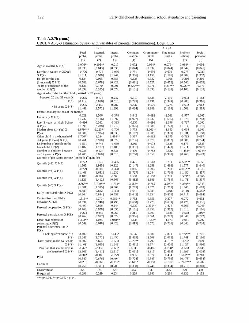
122 Early childhood development, school attendance and parenting
Table A.2.7b (cont.) CBCL y ASQ-3 estimation by sex (with variables of parental discrimination). Boys. OLS
CBCL ASQ-3 Total probs.
External. probs.
Interal. probs.
Communi-cation
Gross motor skills
Fine motor skills
Problem solving
Socio-personal
(1) (2) (3) (4) (5) (6) (7) (8)
Age in months X P(Z) 0.076** 0.105** 0.017 0.072 0.064* 0.079* 0.088** 0.036 [0.033] [0.043] [0.030] [0.044] [0.032] [0.044] [0.042] [0.041]
Low birth weight (<2500g) X P(Z)
-0.706 -0.775 -0.056 0.731 -0.636 0.609 0.275 -0.929 [1.011] [0.908] [1.247] [1.386] [1.150] [1.176] [0.902] [1.352]
Height for the age (1=normal) X P(Z)
0.134 0.005 0.358 -0.138 0.532 -0.306 -0.310 0.310 [0.582] [0.678] [0.423] [0.691] [0.527] [0.652] [0.540] [0.603]
Years of education of the mother X P(Z)
0.136 0.170 0.091 -0.329*** 0.071 -0.297** -0.229** -0.179 [0.092] [0.105] [0.074] [0.101] [0.093] [0.138] [0.100] [0.135]
Age at which she had the child (omitted: < 20 years) Between 20 and 38 years X
P(Z) -0.275 -0.778 0.242 -0.519 0.438 2.136 -0.093 1.182 [0.712] [0.816] [0.610] [0.795] [0.797] [1.349] [0.988] [0.916]
> 38 years X P(Z) -0.205 -2.155 0.787 -0.847 -0.576 -0.275 -0.692 2.012 [1.448] [1.572] [1.298] [1.024] [1.889] [2.114] [1.508] [1.319]
Educational aspirations of the mother
University X P(Z) 0.029 1.506 -1.378 0.842 -0.692 -2.561 -1.977 -1.605 [1.737] [2.116] [1.097] [1.927] [0.932] [1.656] [1.678] [1.283]
Last 3 years of High School X P(Z)
-0.416 0.362 -1.393 -0.136 -0.696 -2.396 -1.737 -0.202 [1.890] [2.288] [1.219] [2.025] [0.988] [1.723] [1.814] [1.191]
Mother alone (1=Yes) X P(Z)
-1.879*** -2.225** -0.700 0.773 -2.063** -1.853 -1.068 -1.301 [0.686] [0.974] [0.638] [1.167] [0.905] [1.399] [1.031] [1.188]
Other child in the household < 4 years (1=Yes) X P(Z)
1.706** 1.244 1.484** 0.397 -0.912 -1.075 -0.713 0.087 [0.761] [0.910] [0.679] [0.736] [0.679] [0.882] [0.686] [0.724]
Ln Number of people in the household X P(Z)
-1.561 -0.743 -1.639 -2.166 -0.078 -0.638 0.173 -0.825 [1.187] [1.177] [1.103] [1.351] [0.966] [1.423] [1.211] [0.947]
Number of children between 4 - 12 years X P(Z)
0.236 -0.224 0.531 0.400 -0.788 -0.532 -1.458* -1.674** [0.705] [0.850] [0.615] [0.760] [0.558] [0.900] [0.768] [0.673]
Quintile of per capita income (omitted: 1st quintile)
Quintile (=2) X P(Z) -0.772 -1.879 -1.436 0.471 -1.518 1.791 4.223*** -0.959 [1.565] [1.985] [0.922] [2.147] [1.251] [1.686] [1.577] [1.640]
Quintile (=3) X P(Z) -0.729 -0.802 -1.328 0.086 -1.315 1.208 4.086*** -1.313 [1.468] [1.651] [1.232] [1.727] [1.284] [1.710] [1.450] [1.457]
Quintile (=4) X P(Z) 0.188 -0.287 -0.971 0.508 -1.190 2.739 3.599** -1.066 [1.123] [1.412] [0.963] [1.812] [1.181] [1.784] [1.471] [1.337]
Quintile (=5) X P(Z) -2.565** -3.700*** -1.731* 3.255* -0.765 3.290* 4.280** -0.343 [1.081] [1.355] [0.969] [1.765] [1.375] [1.755] [1.640] [1.663]
Daily limits and rules X P(Z) 0.489 0.812 -0.408 0.641 0.089 -0.196 -0.119 -1.333* [0.664] [0.884] [0.559] [0.642] [0.634] [0.874] [0.717] [0.684]
Controlling the child’s behavior X P(Z)
-1.513** -1.270* -0.989** 0.732 0.359 0.377 0.272 0.632 [0.637] [0.740] [0.490] [0.608] [0.473] [0.639] [0.726] [0.531]
Parental cooperation X P(Z) 0.497 0.806 0.144 -0.637 2.331** 1.824 0.569 -0.049 [0.768] [0.928] [0.835] [1.161] [0.958] [1.312] [1.013] [1.196]
Parental participation X P(Z) -0.224 -0.446 0.066 0.311 0.503 -0.185 -0.568 1.402* [0.762] [0.917] [0.629] [0.966] [0.561] [0.777] [0.844] [0.772]
Emotional context of parenting X P(Z)
1.333** 1.025 1.048** -1.138 -1.057* -1.073 -0.041 -0.297 [0.549] [0.648] [0.423] [0.815] [0.573] [0.780] [0.840] [0.738]
Parental discrimination X P(Z)
Looking after oneselft X P(Z)
3.402 3.674 2.443* -0.347 0.880 2.801 4.799*** 1.701 [2.048] [2.272] [1.450] [1.485] [1.509] [2.012] [1.741] [2.186]
Give orders in the household X P(Z)
0.607 2.654 -0.583 5.220** 0.792 4.516* 2.623* 3.009 [1.401] [1.665] [1.241] [2.481] [1.574] [2.620] [1.427] [1.996]
Position that should have in the household X P(Z)
-1.477 -2.439 -0.652 -1.938 -0.486 -4.728* -1.563 -2.638 [2.665] [2.411] [2.312] [2.051] [1.113] [2.658] [1.596] [2.008]
P(Z) -0.342 -0.186 -0.279 0.935 0.574 0.454 1.660*** 0.210 [0.540] [0.676] [0.494] [0.724] [0.543] [0.759] [0.478] [0.654]
Constant -0.291 -0.069 -0.397* -0.611* -0.150 -0.517 -0.957*** -0.202 [0.250] [0.311] [0.209] [0.338] [0.248] [0.354] [0.210] [0.310]
Observations 325 325 325 324 330 325 321 330 R-squared 0.296 0.269 0.234 0.229 0.140 0.230 0.332 0.153 *** p<0.01, ** p<0.05, * p<0.1
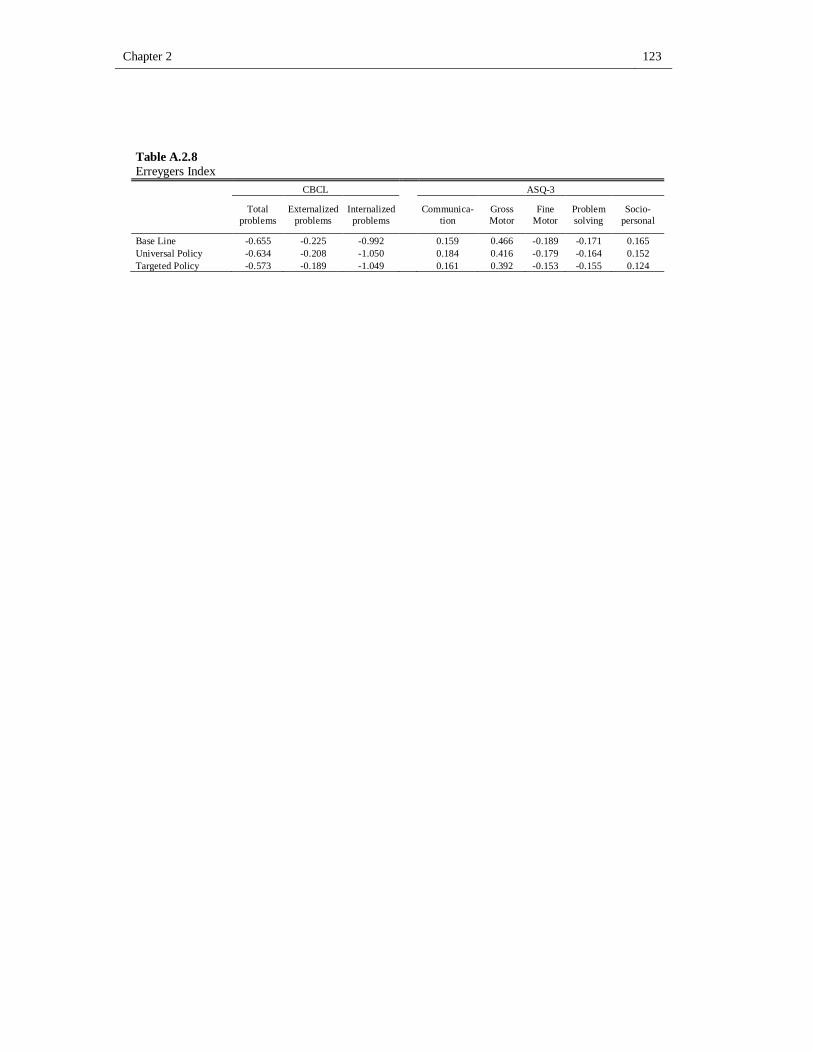
Chapter 2 123
Table A.2.8 Erreygers Index CBCL ASQ-3
Total problems
Externalized problems
Internalized problems Communica-
tion Gross Motor
Fine Motor
Problem solving
Socio-personal
Base Line -0.655 -0.225 -0.992 0.159 0.466 -0.189 -0.171 0.165 Universal Policy -0.634 -0.208 -1.050 0.184 0.416 -0.179 -0.164 0.152 Targeted Policy -0.573 -0.189 -1.049 0.161 0.392 -0.153 -0.155 0.124

Chapter 3
Inequality of opportunity, cash transfer and educational performance
Abstract
In this paper I analyze the impact of a cash transfer program, PANES, on equality of opportunities. I use different educational performance indicators of adolescents as advantage variable. Through the use of administrative records I make estimates using the difference in differences method, incorporating heterogeneous effects according to the effort made by each student. Effort is measured by the number of days that the student attended school in the previous school year. I found that the program succeeded in reducing dropout for some types, but that these reductions did not lead to higher academic achievement. In fact, the change of composition generated by the greater retention of students in the educational system leads, in some cases, to repetition due to poor grades increasing after the program. Inequality of opportunity measured from repetition due to poor grades is reduced as a result of the increase in repetition in the types with the best circumstances due to the aforementioned change of composition. When considering school dropout I found that inequality of opportunities increased, as the types with better circumstances improve in this area. The paper culminates by extending the results to the entire population (and not only treated and control). I found that the direction of the changes in inequality of opportunities is the same, although the magnitude of the variation is lower.
126 Inequality of opportunity, cash transfer and educational performance
3.1 Introduction
The search for equal treatment of persons has been promoted from diverse concepts that differentially emphasize rights (Nozick, 1988), capabilities (Sen, 1995) and opportunity (Arneson, 1989). This paper analyzes the effects of a public policy, the Social Emergency Attention Plan (Programa de Atención a la Emergencia Social - PANES), implemented in Uruguay. It is assumed that access to a set of opportunities must be guaranteed, and, therefore, that one of the roles of the public policy must be to offset those inequalities that originate from the life circumstances of each individual. Specifically, the impact of a Cash Transfer (CT) program on the different educational performance of adolescents is studied, from the approach of Equality of Opportunities (EOp).
One interest feature of evaluating a social program from the perspective of EOp is that, unless you possess a completely egalitarian vision, the objectives of public action are not generally intended to eliminate all outcome inequality, but aim to eliminate those inequalities that escape individual responsibility, which should be compensated for by society (Ferreira & Gignoux, 2011a). However, there are few papers that attempt to measure the success of a policy based on the degree of the Inequality of Opportunity (IOp) that it reduces. This issue is expected to constitute the main contribution of this paper.
From the theoretical point of view, it has been argued that public policies can alter the range of opportunities that individuals face. Roemer (1993) introduced the category type to refer to groups of individuals sharing the same circumstances, for instance people who have a similar family background, individual traits or other aspects that are beyond their control and cannot be modified (by them). The author assumes that, within each type, advantage is determined by the effects of public policies and by effort. In this case, for EOp to hold, public policies might be designed in order to allow individuals, with the same relative effort, to access to the same advantage. On the other hand, Peragine (2004) define the notion of tranches for measuring IOp, a concept which refers to a group of individuals who share the same level of effort. In this case the IOp corresponds to the inequality which arises from a reference value of the advantage variable in each type.
In recent years there have been discussions as to which is the most appropriate way to evaluate the distribution of results from the perspective of EOp (Bossert, 1995; Fleurbaey, 2008; Roemer & Trannoy, 2013; Ferreira & Peragine, 2015; Ramos & Van de gaer, 2016). In parallel the literature that attempts to evaluate public policies has grown considerably (Fiszbein & Schady, 2009). However, the majority of empirical studies in the field of EOp have focused on finding appropriate measures for situations considered to be unfair, without paying too much attention to the impact that public policies have on EOp.
The first studies that have addressed the effects of public policy on EOp analyzed what happened in the context of tax policy. Roemer et al. (2003) studied different high income countries, and found that that tax regimes are more equalizing in northern Europe, even going beyond equal circumstances. In Aaberge, Colombino & Roemer (2003) optimal tax
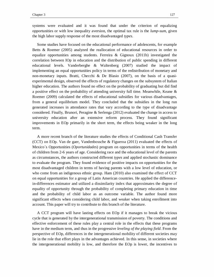
Chapter 3 127
systems were evaluated and it was found that under the criterion of equalizing opportunities or with low inequality aversion, the optimal tax rule is the lump-sum, given the high labor supply response of the most disadvantaged types.
Some studies have focused on the educational performance of adolescents, for example Betts & Roemer (2005) analyzed the reallocation of educational resources in order to equalize opportunities among students. Ferreira & Gignoux (2011b) investigated the correlation between IOp in education and the distribution of public spending in different educational levels. Vanderberghe & Waltenberg (2007) studied the impact of implementing an equal opportunities policy in terms of the redistribution of monetary and non-monetary inputs. Bratti, Checchi & De Blasio (2007), on the basis of a quasi-experimental design, observed the effects of regulatory changes on the subsystem of Italian higher education. The authors found no effect on the probability of graduating but did find a positive effect on the probability of attending university full time. Meanwhile, Keane & Roemer (2009) calculated the effects of educational subsidies for various disadvantages, from a general equilibrium model. They concluded that the subsidies in the long run generated increases in attendance rates that vary according to the type of disadvantage considered. Finally, Brunori, Peragine & Serlenga (2012) evaluated the change in access to university education after an extensive reform process. They found significant improvements in EOp primarily in the short term, the effects being weaker in the long term.
A more recent branch of the literature studies the effects of Conditional Cash Transfer (CCT) on EOp. Van de gaer, Vandenbossche & Figueroa (2011) evaluated the effects of Mexico´s Opportunities (Oportunidades) program on opportunities in terms of the health of children from 2-6 years of age. Considering race and the educational level of the parents as circumstances, the authors constructed different types and applied stochastic dominance to evaluate the program. They found evidence of positive impacts on opportunities for the most disadvantaged children in terms of having parents with a low level of education, or who come from an indigenous ethnic group. Ham (2010) also examined the effect of CCT on equal opportunities for a group of Latin American countries. He applied the difference-in-differences estimator and utilized a dissimilarity index that approximates the degree of equality of opportunity through the probability of completing primary education in time and the probability of child labor as an outcome variable. The author found more significant effects when considering child labor, and weaker when taking enrollment into account. This paper will try to contribute to this branch of the literature.
A CCT program will have lasting effects on EOp if it manages to break the vicious cycle that is generated by the intergenerational transmission of poverty. The conditions and effective enforcement of these rules play a central role in the effects that these programs have in the medium term, and thus in the progressive leveling of the playing field. From the perspective of EOp, differences in the intergenerational mobility of different societies may lie in the role that effort plays in the advantages achieved. In this sense, in societies where the intergenerational mobility is low, and therefore the EOp is lower, the incentives to
128 Inequality of opportunity, cash transfer and educational performance
exert more effort will also be lower, to dissociate the link between the benefit achieved and the effort made. Therefore, the design of a public policy from an EOp perspective must include instruments to offset unfair inequalities with others that promote effort. CCT programs combine these aspects so the study of them is of great interest for this approach.
Evaluating the impact of CCT or CT programs on equality of opportunities is not easy and requires knowledge of the performance of the entire population and not just the beneficiary population and those used as the control. By not considering the entire population in the analysis it is possible to draw incorrect conclusions about the virtues of a policy, if the direction of the effects between the most vulnerable groups (treated and control) is different from the changes which take place with inequality of opportunities in terms of the general population.
A simple example can help to illustrate the difficulties that would arise from focusing exclusively on the most vulnerable population. Imagine a society where individuals can be grouped into five types, and where the average value thereof, before the intervention, is {1,2,3,4,5}. For simplicity assume that the program affects individuals located in the first three types. In this example it would be the case that before the intervention, inequality of opportunities, measured by the Gini index, would reach 0.26 in the entire population, and only 0.22 when considering the types where the beneficiaries of the program are located. For this example we assume two alternative scenarios that could be caused by the transfer: (i) the type where the average performance is 2 improves, and changes to 3 as a result of the program (scenario A); (ii) there is an improvement in the type with an average performance of 3, which changes to 4 as a result of the program (scenario B). In scenario A the inequality among the most vulnerable population falls to 0.19 while in scenario B it increases to 0.28. This could lead us to conclude that the policy reflected in scenario B does not contribute to reducing inequality of opportunities and this is not the case. When analyzing what happens to the inequality across the entire population it is observed that inequality falls in both scenarios A and B, in the first case to 0.225 and in the second to 0.25. Carrying out the analysis first among the treated and control populations before then extending it to the entire population is the second contribution that I attempt to make in this paper.
Uruguay, the country where the program to be analyzed was developed, suffered a severe economic crisis in 2002, which meant that between 2005 and 2007 the PANES program was implemented. The beginning of the last decade showed a significant deterioration in educational performance, with an increase in both dropout rate and repetition. As can be seen in Fig. 3.1, the years 2005 and 2006 appear to be an inflection point in the level of repetition from the education system while in 2006 there was a decrease in the dropouts for students who attend in 3rd and 4th grade. Uruguay also shows high inequality in educational performance, measured by the PISA test results, which encompasses the location in relative terms when measuring inequality of opportunity in education (Ferreira & Gignoux, 2011b).
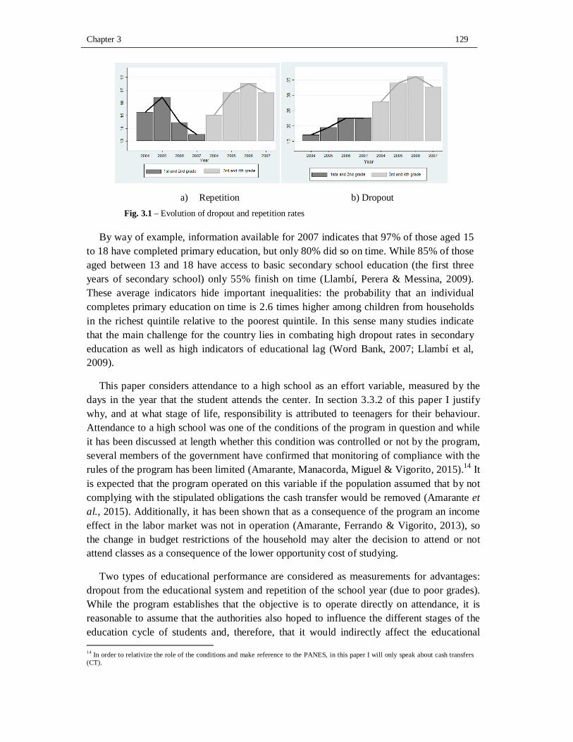
Chapter 3 129
a) Repetition b) Dropout Fig. 3.1 – Evolution of dropout and repetition rates
By way of example, information available for 2007 indicates that 97% of those aged 15
to 18 have completed primary education, but only 80% did so on time. While 85% of those aged between 13 and 18 have access to basic secondary school education (the first three years of secondary school) only 55% finish on time (Llambí, Perera & Messina, 2009). These average indicators hide important inequalities: the probability that an individual completes primary education on time is 2.6 times higher among children from households in the richest quintile relative to the poorest quintile. In this sense many studies indicate that the main challenge for the country lies in combating high dropout rates in secondary education as well as high indicators of educational lag (Word Bank, 2007; Llambí et al, 2009).
This paper considers attendance to a high school as an effort variable, measured by the days in the year that the student attends the center. In section 3.3.2 of this paper I justify why, and at what stage of life, responsibility is attributed to teenagers for their behaviour. Attendance to a high school was one of the conditions of the program in question and while it has been discussed at length whether this condition was controlled or not by the program, several members of the government have confirmed that monitoring of compliance with the rules of the program has been limited (Amarante, Manacorda, Miguel & Vigorito, 2015).14 It is expected that the program operated on this variable if the population assumed that by not complying with the stipulated obligations the cash transfer would be removed (Amarante et al., 2015). Additionally, it has been shown that as a consequence of the program an income effect in the labor market was not in operation (Amarante, Ferrando & Vigorito, 2013), so the change in budget restrictions of the household may alter the decision to attend or not attend classes as a consequence of the lower opportunity cost of studying.
Two types of educational performance are considered as measurements for advantages: dropout from the educational system and repetition of the school year (due to poor grades). While the program establishes that the objective is to operate directly on attendance, it is reasonable to assume that the authorities also hoped to influence the different stages of the education cycle of students and, therefore, that it would indirectly affect the educational 14 In order to relativize the role of the conditions and make reference to the PANES, in this paper I will only speak about cash transfers (CT).

130 Inequality of opportunity, cash transfer and educational performance
performance analyzed in this paper. Ultimately it is assumed that the program can operate on these results in two ways: through the indirect effects that are produced by increased attendance to an educational center and, the direct effects that can arise as a result of reduced economic constraints in the household and, therefore, a reduction in the time that adolescents have to spend on tasks that compete with their studies.
The paper is structured as follows. The second section presents the details of the program, while the third part refers to the empirical strategy emphasizing identification criteria and the methodology used to measure inequality of opportunity. In the fourth section the information source is described and the variables used are discussed. The fifth section focuses on the main findings of the study, ending with the main discussion points and the conclusions.
3.2 Details of the PANES Program
PANES was designed with the aim of lessening the effects of the economic crisis in Uruguay in 2002. In that year GDP fell by 15%, unemployment increased from 12% to 18% and poverty from 20% to 32%. In this context several instruments of the existing social security system at the time were redesigned, and in April 2005 PANES came into effect. This program was presented as transient and ended in December 2007.
The objectives of the program can be divided into providing direct assistance to households that suffered a rapid decline in living standards and the strengthening of the human and social capital of the poor to enable them to escape poverty by themselves (Manacorda, Miguel, & Vigorito, 2011). PANES also presented multiple components, the most important of which corresponded to a transfer of income (called ingreso ciudadano in Uruguay) of approximately 60 Euros monthly at the value of April 2005, an amount independent of the number of household members. In addition households with children received a food card (in-kind transfer) that varied monthly between 10 and 35 Euros per month, depending on the number of children in the household.15
In order to remain in the program it was indicated that the beneficiaries had to meet a set of conditions, such as school attendance for children, and periodic health checks for children and pregnant women. While it was announced that these conditions would be required, they were hardly monitored (Amarante et al., 2015). Finally, the possibility was offered to beneficiaries to participate in job training sub-programs as well as transitional employment. The population that participated was selected among the beneficiaries of PANES and received an income above that of the ingreso ciudadano.
The target population of this program was the first quintile of poor households. A first criterion for selecting beneficiaries was to identify households whose incomes were below
15 In April 2005 the official minimum salary was approximately 120 Euro a month.
Chapter 3 131
a threshold. Under this criterion only 5% of households which applied were rejected. The program design included a second criterion for selecting beneficiaries. This criterion consisted of a questionnaire that sought information on a group of characteristics of household members as well as housing characteristics. From the information on socio-economic aspects such as educational environment, housing characteristics and access to durable goods, researchers at the University of the Republic produced a vulnerability index based on a Probit model (Amarante, Arim & Vigorito, 2005). This index, in standardized terms, took values between -0.2 and 1, identifying positive values of this index for the potential beneficiaries of the program. Ultimately, of the 190,000 households that applied, 102,000 were selected, representing 10% of Uruguayan households.
One of the main virtues that have been identified from PANES is its good focus, it being one of the most important among similar programs applied in Latin America. In terms of horizontal efficiency PANES reached 50.3% if the target population is considered and 63% if the population that applied to receive the benefit is taken into account, while in terms of vertical efficiency, 57.3% of the beneficiary population met the entry conditions required by law (Amarante, Burdín, Manacorda & Vigorito, 2008). Manacorda et al. (2011) also demonstrated that the implementation of the program was very clean, as among the candidates virtually all potential beneficiaries benefitted from the program, concluding that the application of the selection criteria was as strict as was stipulated in the law.
3.3 Empirical Strategy
3.3.1 Measuring inequality of opportunity and the effects of the CT
The criteria for evaluating the inequality of outcome from the IOp perspective can be built based on two principles: the principle of compensation and the principle of reward. The first demands that inequality due to circumstances must be eliminated, while the second discusses how effort between individuals with identical circumstances must be rewarded. In addition, within the principle of compensation two methodological alternatives are available which turn out to be mutually incompatible, which have been called ex–ante and ex–post approaches (Fleurbaey & Peragine, 2013). While the first of these approaches focuses on prospects, that is, it requires EOp if all individuals face the same set of opportunities, the second approach looks at the outcomes among different individuals with the same effort characteristics.
This paper takes the principle of compensation as a criterion for evaluating IOp. With this objective a finite population given by 푘 ∈ {1, … ,푁} is considered, where N is sufficiently large. Each individual is characterized by a set of attributes {푆 ,퐶 ,푅 } which respectively reflect the advantage of the individual, their circumstances and their effort. In this paper the advantage variables considered correspond to educational outcomes.
132 Inequality of opportunity, cash transfer and educational performance
Ramos & Van de gaer (2012) postulate that the advantage of the individual can be modeled taking into account their circumstances, effort, unobservable variables, 푢 , and a random term, 휁 , such that
푆 = 푔(퐶 ,푅 ,푢 , 휁 )
The function 푔(. )is unknown. By imposing a functional form to estimate this function,
you have 푔(퐶 ,푅 , 푒 ), where 푒 captures the effects of both 푢 and 휁 , while an estimate of 푆 can be obtained by imposing 푒 equal to zero.
Measuring IOp can be done directly or indirectly (Pistolesi, 2009). Direct measures indicate how much inequality is maintained when inequality only exists due to circumstances, while indirect measurements consider how much inequality is maintained after opportunities have been equalized, that is, when you eliminate all inequality among individuals that make the same effort. Ramos & Van de gaer (2016) demonstrate that different direct measures have a dual counterfactual on indirect measurements. The authors suggest that indirect measures are instruments that allow us to answer how much of the inequality of outcome is due to IOp, but do not allow us to measure the IOp per se, this is limited to direct measures.
In this article We use a direct method to measure inequality of educational opportunities, 퐼(푆 ). We have built a counterfactual distribution in which all individuals belonging to the same type have the same set of opportunities (the average of the type), which, naturally, does not depend on effort.
The counterfactual distribution eliminates any inequality among individuals who make the same effort. Therefore, ex–ante inequality of opportunity is being measured, which implies ex–post equality of opportunities when faced with the absence of ex–ante inequality of opportunity. To this end, we will use a measurement proposed by Ramos & Van de gaer (2012), who give more flexibility to the proposal made in Ferreira & Gignoux (2011a), by considering the covariance between circumstances and effort in the estimate. Naturally using this measure requires knowledge of the effort of the individuals. In this case, to measure the inequality of opportunities we must build a counterfactual distribution, which is defined as:
푆 =1
|푁 .|푔(퐶 ,푅 , 0)
∈ .
Where 푁 . = {푖 ∈ 푁|퐶 = 퐶 } is the set of individuals who share the circumstance 퐶 , that
is, individuals which can be found in the same type.
When income transfer is introduced the function to estimate incorporates a new parameter,Φ , which captures the effect of the program. In this case a new estimate is obtained, 푆ϕ = 푔(퐶 ,푅 , Φ , 0), where the vector of educational performance reflects
Chapter 3 133
inequality of opportunity with the effects of the program, expressed as 푆ϕ = | .|
∑ 푔(퐶 ,푅 , Φ , 0)∈ . .
A new distribution is built assuming that the effect of the program does not operate, Φ . In this case a new distribution of inequality of educational opportunities is calculated, 푆ϕ, = | .|
∑ 푔(퐶 ,푅 , Φ , 0)∈ . .
The contribution of PANES to the change in the IOp arises from the difference between the distributions predicted with and without the effect of the program, Λ = 퐼 푆ϕ − 퐼 푆ϕ .
Finally, as the advantage variables used are dichotomous the procedure proposed by Trannoy, Sandy, Jusot & Devaux (2010) is followed. They suggested using linear prediction to measure inequality. For the measurement of inequality the Theil and Gini indices are used. For the purposes of this paper I have not found arguments that favour using one type of inequality index over another, or which indicate that the use of any particular index would generate some kind of problem. As such, the selection of these indices is justified solely on the grounds of comparability with other studies that measure inequality of opportuity.
Measuring EOp in education faces two significant problems when assuming an egalitarian perspective sensitive to responsibility. Firstly it implies considering if the talents should be rewarded or considered as a circumstance that should be compensated. Secondly we must ask whether we can consider students to be responsible for their effort decisions (Brunori et al., 2012). In the following sections the position to be adopted in this paper with respect to these points will be commented on, specifying the criteria used to measure effort and indicating what circumstances are considered in this paper.
3.3.2 Measuring effort
Many studies identify students´ effort as one of the main determinants that influence educational performance. For example, Stinebrickner & Stinebrickner (2007), Bonesrønning (2008) and Guney (2009) use the time dedicated to study as an effort variable. As already mentioned it is necessary to establish a criterion that allows us to identify when it is possible to hold students accountable for their choices, and when not. In the cited studies a relationship between educational performance and effort is established both for students in the first years of secondary education and for university students.
Based on the proposal of Trannoy (1999), Brunori et al. (2012) indicate that children cannot be completely responsible for their actions when they are very small (if they are less than 푡∗ years of age). Once it is possible to hold them accountable for their decisions, the distribution of educational outcomes should be evaluated by balancing the compensation and reward criteria. Brunori et al. (2012) suggest that a good benchmark for
134 Inequality of opportunity, cash transfer and educational performance
this discussion is the legal literature on criminal responsibility. In this sense the authors suggest that the age at which teenagers should be held responsible for their actions is 14 in the Italian case. The Uruguayan case implies a gradual involvement in the penal system starting at the age of 12, with the general rules applying from 18 years of age. The rules governing child and adolescent labor constitute another possible benchmark. According to the ILO (2005) child labor, in terms of activities that should be abolished by the State, refers to children under 12 years of age engaged in light work, children between 12 and 15 years of age engaged in non-dangerous work, and children between 15 and 18 years of age engaged in dangerous work. In the case of Uruguay the working age population is considered to be those who are 14 years of age of over. Finally, the age of consent is the minimum age of a person is considered to be legally competent to consent to sexual acts. The age of consent in Uruguay stands at 15 years, and there is an intermediate status between 12 and 15 years of age.
In this paper it is assumed that students are responsible for their choices (푡∗)from the 2nd year of secondary education, which means that the student starts the school year, if there is no lag, at 13 or 14 years of age. The number of days in the year that the student attends the educational center is considered as an effort variable. The relevance of attendance to an educational center as a determinant of educational performance is discussed in Balfanz, Herzog & Mac Iver (2007) who show that low achievement in reading and mathematics, unsatisfactory behavior and low attendance rates reflect a reduction in effort and are predictive of dropout from the education system. On the other hand, several authors suggest that high rates of absenteeism are indicative of the students´ abandonment of the educational process (Alexander, Entwisle & Horsey, 1997; Kane, 2006; Balfanz et al., 2007), suggesting that students have interests that compete with education, or that there are financial constraints in the household that impede the student from systematically attending the educational center, which results in low achievements that discourage the student from remaining in the education system (Alexander et al., 1997). Schoeneberger (2011), on the other hand, states that students lose skills when attendance is erratic and see themselves as incapable of continuing to study.
3.3.3 The circumstances
In addition to effort, a wide range of variables have been used in the literature to explain poor grades and dropout from the education system (Webbik, 2005; Bradley & Lenton, 2007; Bonesrønning, 2008; Babcock & Betts, 2009; Martins & Veiga, 2010; Guney, 2009). This section explains the choice of some of these variables in the extent that they can be to interpret as circumstances of the student. In this sense individual and family circumstances are identified, as well as contextual circumstances and circumstances of the educational center, which can operate at different stages of the student´s educational trajectory.
Chapter 3 135
It is assumed that individual and family circumstances have an influence throughout the entire educational trajectory, although with greater importance in the first years of middle education. In general, the household characteristics that the literature indicates affect educational performance are associated with the social origins of the individual (Todd & Wolpin, 2006). In this sense the grades obtained by children are expected to be higher if the father or mother are employed full time or have a higher educational level, assuming that in those cases their ability to transfer knowledge is greater as well as their ability to assist their children in doing the homework given by the teacher. Bradley & Lenton (2007) argue that these characteristics can affect the decision to drop out of the school system to the extent that approximates the value the parents attach to education or to an income effect. This paper proposes to use the educational level of the household through a dichotomous variable that reflects if there is a household member who has spent more than 10 years in formal education.
Additionally an index of durable goods is considered as a circumstance in order to approximate household wealth. Zhao & Glewwe (2010) indicate that per capita household expenditure affects attendance to an educational center if, as a result of low income, the demand for education is reduced, due to the budget constraints of the parents operating as a limitation on the possibilities of investing in education. To build the durable goods index I performed a factor analysis from variables that indicate ownership of the following items: heater, shower, cooker, microwave oven, refrigerator, freezer, washing machine, dishwasher, gas heater, electric heater, television, video, cable TV, computer, automobile and telephone. The weight of the factors used is presented in Table A.1 of the Annex.
In different studies it is indicated that among the personal circumstances that affect educational performance, innate abilities must be included. These variables are generally omitted and, thus combined with the error term. From the EOp perspective, various studies have adopted a residual approach where the observed variables are beyond individual control and are considered unfair, while the remaining variability is not (Brunori et al., 2012), interpreting the observed IOp as a lower bound estimate of the real IOp (Checchi & Peragine, 2010).
However, other studies have used observable characteristics of children to approximate their innate abilities, for example Zhao & Glewwe (2010) partially explain abilities by differences in gender, age and nutrition. Other studies use scores obtained in previous years as a proxy for intelligence and/or innate abilities of the students (Bradley & Lenton, 2007; Guney, 2009) to explain dropout from the education system. In a chain of thought closer to the motivation for this paper Brunori et al. (2012) indicate that, given that the accumulation of cognitive abilities are highly influenced by abilities that have already been acquired, one must consider the educational outcomes in 푡∗ as one of the circumstances that influence educational achievement. Based on this argument, in this paper, the GPA achieved in the 1st and 2nd year of high school, will be considered as one of the circumstances of educational performance achieved by students in the 3rd and 4th year of secondary education. We do not believe that this variable reflects only innate abilities, but
136 Inequality of opportunity, cash transfer and educational performance
that it is the result of a combination of these abilities and processes of socialization. It will, nevertheless, be treated as a circumstance to the extent that students generally study in the 1st and 2nd grades when they are under 15 years old. As mentioned in the previous section, responsibility for decisions taken cannot be attributed to students of this age.
If parents are unable to choose the characteristics of the school, assuming for example that there is only one school available, the variables associated with the educational center become exogenous for the household.16 This supposition is pertinent for the beneficiary population of the program analyzed here as well as for those who applied for the program and were not accepted, given that all of them attend public institutions, which are assigned based on the place of residence of the child. As noted by Zhao & Glewwe (2010) financial constraints faced by a household make it unlikely that they will relocate in order to be in the vicinity of an educational center with better characteristics.
Several authors have proposed considering a measure to contemplate the student-teacher ratio at the time of explaining the attendance of students to educational centers, an aspect that I will attempt to include in the estimates presented in this paper. Stiefel, Varne, Iatarola & Fruchter (2000) mention that the size of the school may adversely affect results due to inefficient administration, stemming from the larger size of the institution, from the loss of parental participation in larger schools, and as a consequence of a more formal educational setting. For this reason the number of students that attend the educational center in the same grade is included as a circumstance. Another complementary circumstance that attempts to indirectly approximate the characteristics of the educational centers is also introduced. This is a dichotomous variable that identifies the country´s capital (Montevideo) from the other regions. This is justified because in Montevideo classes are overpopulated in relation to the rest of the regions, and therefore have fewer teachers per student, as a result of which worse educational outcomes are expected. In addition, both regions have differences associated with the functioning of the labor market (mainly in wages). Some authors have shown how what is happening in the labor market affects decisions to stay in the education system or not, by altering the opportunity cost of studying (Zhao & Glewwe, 2010; Jones, Toma & Zimmer, 2008).
The types are built from three of these circumstances, while the rest are included as controls in the estimates. Two different ways of making the groupings are used in order to make estimates for different purposes. The base estimates are made based on the circumstances considered to be the most suitable (Criterion A), considering the treated and control populations. Secondly, and based on the circumstances that are available for the entire population (Criterion B), estimates are made that show the overall effect of the program on inequality of opportunities.
The circumstances included in Criterion A consider two dichotomous variables at the household level, if there is a household member residing there with over 10 years of
16 When parents can alter the quality of the school by choosing, selection bias is possible if unobservable characteristics of the children and households, which affect the outcomes, are correlated with unobservable factors that determine the choice of school.
Chapter 3 137
education and if the index of durable goods is located above the median. At the individual level there are two groups that identify the GPA average in the en 1st and 2nd grades, considering those who average lower or higher than 7.17
With the years of education the aim is to capture the presence of an environment within the household which is more inclined towards the teenager remaining in the school system. The threshold selected (a household member with 10 or more years of education) allows us to identify the minimum number of years necessary for the teenager to show some degree of upward intergenerational mobility, given that in this paper I consider the educational performance in the 3rd and 4th grades (9 and 10 years of education respectively). The durable goods index is an approximation of the wealth or permanent income of the household, and attempts to identify the long term socio-economic conditions that may have conditioned, in previous stages, the process of accumulating skills (and not restrict it, with the income for example, to the present conditions). The GPA identifies the teenager’s skills which are innate or acquired previously, that is, at times when it is not possible to attribute responsibility to them for their achievements.
As mentioned, other variables recognized by the literature as being important to explain the educational performance of teenagers, and which can be considered as circumstances, refer to the characteristics of the school attended by the teenager. While this information is available, I opted not to include it when forming Criterion A, thus not increasing the total number of types used with the consequent reduction of observations available per cell. The characteristics of the school and its size are considered as a circumstance within Criterion B.
The distribution of the population by types is presented in Table 3.1. 8 types were built with these criteria, whose distribution is rather uniform, i.e similar number of individuals located in each cell. It can, however, be seen that the high GPA of the 1st and 2nd grades (the categories identified with even numbers) concentrates slightly more of the population, reaching 17% among those with better circumstances (Type 8 Criterion A).
In Criterion B the GPA variable is maintained, and a dichotomous variable referring to the area of residence (Montevideo and the rest of the country) is included as well as another that takes the size of the educational center into account (greater or less than the median size). Two distributions are presented in the table, that corresponding to the sample used for the evaluation and that which refers to the entire population. The sample shows that the weight of the first four types the greater proportion of the population, the type that corresponds to students residing outside of Montevideo. In this population the highest concentration is in Type 4, which corresponds to numerous educational centers and students with high grades. In the case of the total population the prevalence of the types associated with the area outside Montevideo is maintained, but with slightly lower numbers (69.6% vs 77.3%). 17 GPA scores take values between 1 and 12, with 6 being the minimum passing grade.
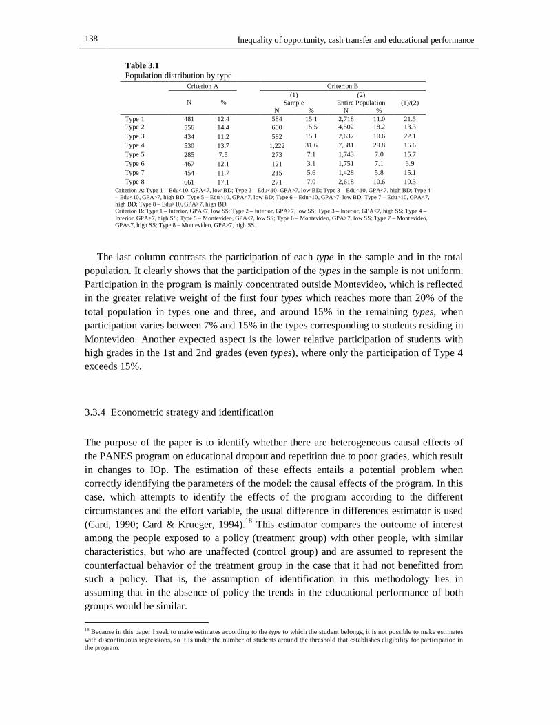
138 Inequality of opportunity, cash transfer and educational performance
Table 3.1 Population distribution by type
Criterion A Criterion B
N % (1) Sample
(2) Entire Population (1)/(2)
N % N % Type 1 481 12.4 584 15.1 2,718 11.0 21.5 Type 2 556 14.4 600 15.5 4,502 18.2 13.3 Type 3 434 11.2 582 15.1 2,637 10.6 22.1 Type 4 530 13.7 1,222 31.6 7,381 29.8 16.6 Type 5 285 7.5 273 7.1 1,743 7.0 15.7 Type 6 467 12.1 121 3.1 1,751 7.1 6.9 Type 7 454 11.7 215 5.6 1,428 5.8 15.1 Type 8 661 17.1 271 7.0 2,618 10.6 10.3
Criterion A: Type 1 – Edu<10, GPA<7, low BD; Type 2 – Edu<10, GPA>7, low BD; Type 3 – Edu<10, GPA<7, high BD; Type 4 – Edu<10, GPA>7, high BD; Type 5 – Edu>10, GPA<7, low BD; Type 6 – Edu>10, GPA>7, low BD; Type 7 – Edu>10, GPA<7, high BD; Type 8 – Edu>10, GPA>7, high BD. Criterion B: Type 1 – Interior, GPA<7, low SS; Type 2 – Interior, GPA>7, low SS; Type 3 – Interior, GPA<7, high SS; Type 4 – Interior, GPA>7, high SS; Type 5 – Montevideo, GPA<7, low SS; Type 6 – Montevideo, GPA>7, low SS; Type 7 – Montevideo, GPA<7, high SS; Type 8 – Montevideo, GPA>7, high SS.
The last column contrasts the participation of each type in the sample and in the total population. It clearly shows that the participation of the types in the sample is not uniform. Participation in the program is mainly concentrated outside Montevideo, which is reflected in the greater relative weight of the first four types which reaches more than 20% of the total population in types one and three, and around 15% in the remaining types, when participation varies between 7% and 15% in the types corresponding to students residing in Montevideo. Another expected aspect is the lower relative participation of students with high grades in the 1st and 2nd grades (even types), where only the participation of Type 4 exceeds 15%.
3.3.4 Econometric strategy and identification
The purpose of the paper is to identify whether there are heterogeneous causal effects of the PANES program on educational dropout and repetition due to poor grades, which result in changes to IOp. The estimation of these effects entails a potential problem when correctly identifying the parameters of the model: the causal effects of the program. In this case, which attempts to identify the effects of the program according to the different circumstances and the effort variable, the usual difference in differences estimator is used (Card, 1990; Card & Krueger, 1994).18 This estimator compares the outcome of interest among the people exposed to a policy (treatment group) with other people, with similar characteristics, but who are unaffected (control group) and are assumed to represent the counterfactual behavior of the treatment group in the case that it had not benefitted from such a policy. That is, the assumption of identification in this methodology lies in assuming that in the absence of policy the trends in the educational performance of both groups would be similar. 18 Because in this paper I seek to make estimates according to the type to which the student belongs, it is not possible to make estimates with discontinuous regressions, so it is under the number of students around the threshold that establishes eligibility for participation in the program.
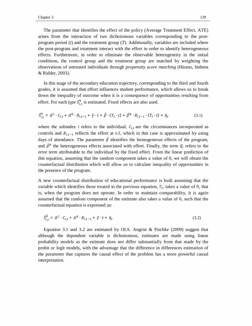
Chapter 3 139
The parameter that identifies the effect of the policy (Average Treatment Effect, ATE) arises from the interaction of two dichotomous variables corresponding to the post-program period (t) and the treatment group (T). Additionally, variables are included where the post-program and treatment interact with the effort in order to identify heterogeneous effects. Furthermore, in order to eliminate the observable heterogeneity in the initial conditions, the control group and the treatment group are matched by weighting the observations of untreated individuals through propensity score matching (Hirano, Imbens & Ridder, 2003).
In this stage of the secondary education trajectory, corresponding to the third and fourth grades, it is assumed that effort influences student performance, which allows us to break down the inequality of outcome when it is a consequence of opportunities resulting from effort. For each type 푆 ,
ϕ is estimated. Fixed effects are also used. 푆 ,
ϕ = 훼 ∙ 퐶 , + 훼 ∙ 푅 , + 훾 ∙ 푡 + 훽 ∙ (푇 ∙ 푡) + 훽 ∙ 푅 , ∙ (푇 ∙ 푡) + 휂̂ (3.1) where the subindex i refers to the individual, 퐶 , are the circumstances incorporated as controls and 푅 , reflects the effort at t-1, which in this case is approximated by using days of attendance. The parameter 훽 identifies the homogeneous effects of the program, and 훽 the heterogeneous effects associated with effort. Finally, the term 휂 refers to the error term attributable to the individual by the fixed effect. From the linear prediction of this equation, assuming that the random component takes a value of 0, we will obtain the counterfactual distribution which will allow us to calculate inequality of opportunities in the presence of the program.
A new counterfactual distribution of educational performance is built assuming that the variable which identifies those treated in the previous equation, 푇 , takes a value of 0, that is, when the program does not operate. In order to maintain comparability, it is again assumed that the random component of the estimate also takes a value of 0, such that the counterfactual equation is expressed as:
푆 ,ϕ = 훼 ∙ 퐶 , + 훼 ∙ 푅 , + 훾 ∙ 푡 + 휂̂ (3.2)
Equation 3.1 and 3.2 are estimated by OLS. Angrist & Pischke (2009) suggest that
although the dependent variable is dichotomous, estimates are made using linear probability models as the estimate does not differ substantially from that made by the probit or logit models, with the advantage that the difference in differences estimation of the parameter that captures the causal effect of the problem has a more powerful causal interpretation.
140 Inequality of opportunity, cash transfer and educational performance
3.3.5 Inequality of opportunity in the entire population
In order to consider inequality of opportunities across the entire population, that is all students in the 3rd and 4th grade, and evaluate the changes that arise as a result of the program, it is necessary to add information about non-applicants (NA) of the program. This will allow us to account for possible measurement biases that occur when considering only the most vulnerable groups.
To this end I made the estimates of the educational performance of the NA population, those which are neither in the treated not the control groups. The intention is to have a prediction comparable to that obtained in equations 3.1 and 3.2 for the NA group and therefore be able to calculate the inequality of opportunities with and without the effect of the program in the entire population (EP). The equation to estimate the NA group is expressed as:
푆 , = 훼 ∙ 퐶 , + 훼 ∙ 푅 , + 훾 ∙ 푡 + 휂 (3.3)
The linear prediction of this estimate is what is called the distribution of the non-applicants,푆 , . The new counterfactual distribution for the entire population is expressed as the sum of the distribution of the performances of the non-applicants and the treated and control groups. In the latter distribution I consider the cases where the program operates and does not operate (eq. 3.1 and 3.2). 푆 ,
ϕ, = 푆 ,ϕ + 푆 , (3.4)
푆 ,ϕ, = 푆 ,
ϕ + 푆 , (3.5) The effect of the program on the entire population is expressed as the difference in
inequality of the sum of the mean values of each of the types, Λ = 퐼 푆ϕ, − 퐼 푆ϕ,
3.4 Data
The information used in this paper comes from two administrative records, which can be combined using the ID number of the person. They are: the PANES Administrative Record (PAR) and the Secondary Education Record (SER).
The PAR information is primarily from 2005, although part of it corresponds to 2006 and to a lesser extent to 2007, depending on the moment when individuals enrolled in the program. This record is used as a tool to select the beneficiaries of the program through the application of the vulnerability index. It is therefore possible to identify the beneficiaries of the program (treatment group) and those who applied but were not selected (control group). While the program design does not reflect a pure experiment, it does allow us to
Chapter 3 141
have a very good causal design to evaluate the effect of the policy on equality of opportunity.
To complement the PAR data, this is combined with information from the SER, which contains data on the educational performance of students in secondary education. This cycle starts at 11 or 12 years of age after 6 years of primary education. In turn, this stage of the education cycle is divided into two, the first three years correspond to the basic cycle and the last three to the diversified baccalaureate (called bachillerato diversificado, BD, in Uruguay). Once admitted to the BD the student chooses, in the second year, between different options: social sciences and humanities, biological sciences, scientific, and art and expression. This paper focuses exclusively on the educational results of the first four years of the second cycle of secondary education, in which students study what is called the “common core” of the second cycle. This choice is due to the fact that in the last two years of the bachillerato general attendance information is not revealed, as there is no overall general course assessment, but individual assessment by subject studied.
The years in which data is available are between 2004 and 2007, therefore information exists for the period before PANES was implemented (2004) and two years after it (2006 and 2007). This allows us to build a panel with the educational data of adolescents. Specific information is provided on the number of days the student attends the high school, which constitutes the effort variable to be used in this paper. It also has information on the Grade Point Average (GPA) the student obtained in the year, allowing us to identify if the student repeated due to poor grade which is one of the outcomes to be analyzed. Finally it is possible to identify, based on the administrative records for the current year and in the subsequent years after the period analyzed in this paper, if the student dropped out of the education system. In this way a variable is built which indicates whether the year being observed is the last in which the student remains in the education system or even if they abandoned their studies during the year, which constitutes the second educational performance analyzed.
The number of people in the PAR database is 709,360 and the number of households is 189,747 which, when combined with the SER database, is reduced to 112,961 secondary education students inhabiting 43,255 households. This number corresponds to those students who studied any of the 1st to 4th grades between 2004 and 2007. The paper focuses on the cohort of students who entered secondary education in 2004 without educational lag, which corresponds to 4,342 students, with 5,374 children being old enough to enter but did not due to educational lag or because they dropped out during primary education. As mentioned in section 3.3.2 of this paper, it is assumed possible to attribute responsibility to teenagers from the age of 15, as such educational performance is analyzed in the 3rd and 4th years of secondary education. In these grades 3,820 cases were observed of which 780 students dropped out.
A summary of the mean values of the educational performance used and their standard deviations are presented in Table 3.2. The effort variable is also presented in this table, as
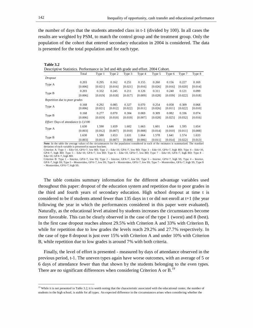
142 Inequality of opportunity, cash transfer and educational performance
the number of days that the students attended class in t-1 (divided by 100). In all cases the results are weighted by PSM, to match the control group and the treatment group. Only the population of the cohort that entered secondary education in 2004 is considered. The data is presented for the total population and for each type.
Table 3.2 Descriptive Statistics. Performance in 3rd and 4th grade and effort. 2004 Cohort. Total Type 1 Type 2 Type 3 Type 4 Type 5 Type 6 Type 7 Type 8 Dropout Type A 0.203 0.295 0.162 0.251 0.155 0.260 0.156 0.227 0.169
[0.006] [0.021] [0.016] [0.021] [0.016] [0.026] [0.016] [0.020] [0.014]
Type B 0.203 0.332 0.245 0.211 0.126 0.311 0.240 0.121 0.099
[0.006] [0.019] [0.018] [0.017] [0.009] [0.028] [0.039] [0.022] [0.018] Repetition due to poor grades
Type A 0.168 [0.006]
0.292 [0.021]
0.085 [0.012]
0.327 [0.022]
0.070 [0.011]
0.254 [0.026]
0.058 [0.011]
0.309 [0.022]
0.068 [0.010]
Type B 0.168 0.277 0.070 0.304 0.069 0.309 0.082 0.336 0.074
[0.006] [0.019] [0.010] [0.019] [0.007] [0.028] [0.025] [0.032] [0.016] Effort: Days of attendance (t-1)/100
Type A 1.630 1.590 1.659 1.602 1.663 1.601 1.646 1.595 1.654
[0.003] [0.012] [0.007] [0.010] [0.008] [0.014] [0.010] [0.011] [0.008]
Type B 1.630 1.580 1.653 1.631 1.664 1.578 1.641 1.574 1.633
[0.003] [0.011] [0.007] [0.008] [0.006] [0.011] [0.014] [0.022] [0.013] Note: In the table the average values of the circumstances for the population considered in each of the estimates is summarized. The standard deviation of each variable is presented in square brackets. Criterion A: Type 1 – Edu<10, GPA<7, low BD; Type 2 – Edu<10, GPA>7, low BD; Type 3 – Edu<10, GPA<7, high BD; Type 4 – Edu<10, GPA>7, high BD; Type 5 – Edu>10, GPA<7, low BD; Type 6 – Edu>10, GPA>7, low BD; Type 7 – Edu>10, GPA<7, high BD; Type 8 – Edu>10, GPA>7, high BD. Criterion B: Type 1 – Interior, GPA<7, low SS; Type 2 – Interior, GPA>7, low SS; Type 3 – Interior, GPA<7, high SS; Type 4 – Interior, GPA>7, high SS; Type 5 – Montevideo, GPA<7, low SS; Type 6 – Montevideo, GPA>7, low SS; Type 7 – Montevideo, GPA<7, high SS; Type 8 – Montevideo, GPA>7, high SS.
The table contains summary information for the different advantage variables used throughout this paper: dropout of the education system and repetition due to poor grades in the third and fourth years of secondary education. High school dropout at time t is considered to be if students attend fewer than 135 days in t or did not enroll at t+1 (the year following the year in which the performances considered in this paper were evaluated). Naturally, as the educational level attained by students increases the circumstances become more favorable. This can be clearly observed in the case of the type 1 (worst) and 8 (best). In the first case dropout reaches almost 29.5% with Criterion A and 33% with Criterion B, while for repetition due to low grades the levels reach 29.2% and 27.7% respectively. In the case of type 8 dropout is just over 15% with Criterion A and under 10% with Criterion B, while repetition due to low grades is around 7% with both criteria.
Finally, the level of effort is presented - measured by days of attendance observed in the previous period, t-1. The uneven types again have worse outcomes, with an average of 5 or 6 days of attendance fewer than that shown by the students belonging to the even types. There are no significant differences when considering Criterion A or B.19
19 While it is not presented in Table 3.2, it is worth noting that the characteristic associated with the educational center, the number of students in the high school, is stable for all types. An expected difference in the circumstances arises when considering whether the
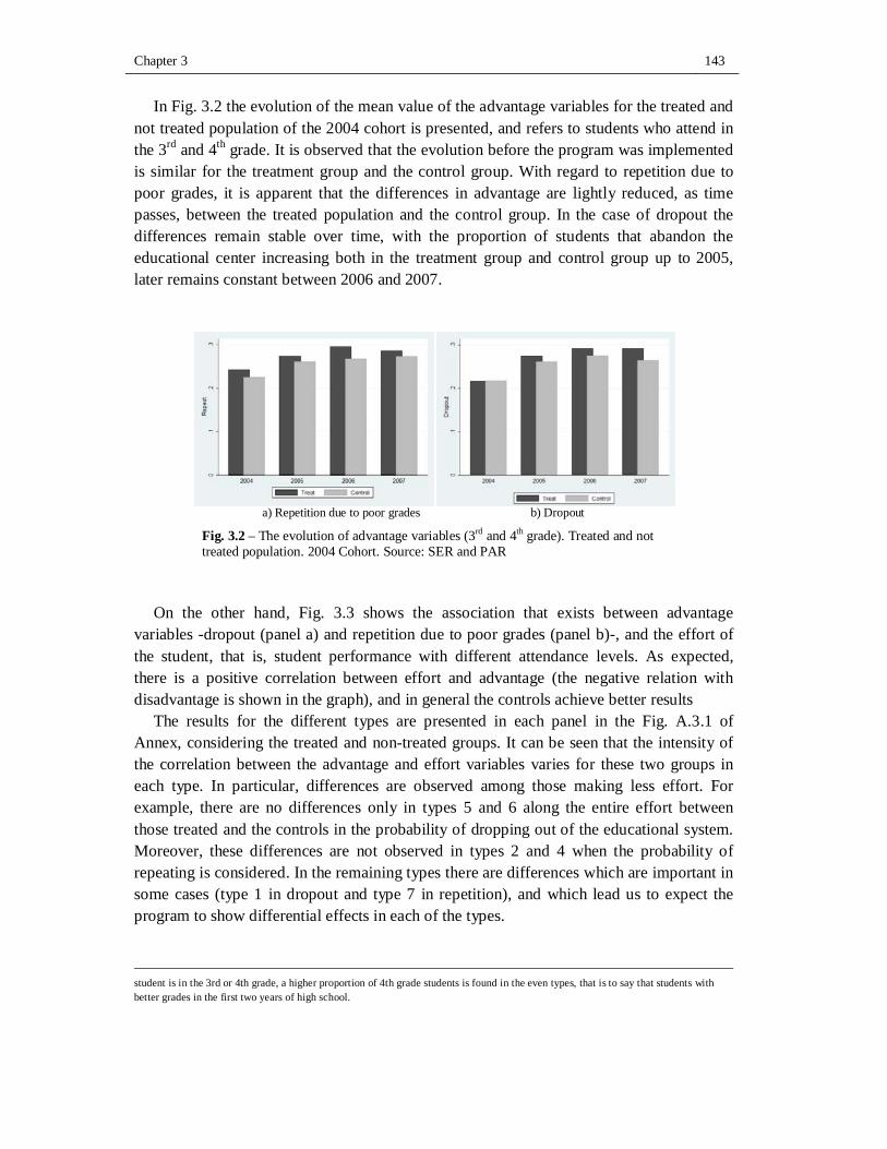
Chapter 3 143
In Fig. 3.2 the evolution of the mean value of the advantage variables for the treated and not treated population of the 2004 cohort is presented, and refers to students who attend in the 3rd and 4th grade. It is observed that the evolution before the program was implemented is similar for the treatment group and the control group. With regard to repetition due to poor grades, it is apparent that the differences in advantage are lightly reduced, as time passes, between the treated population and the control group. In the case of dropout the differences remain stable over time, with the proportion of students that abandon the educational center increasing both in the treatment group and control group up to 2005, later remains constant between 2006 and 2007.
a) Repetition due to poor grades b) Dropout
Fig. 3.2 – The evolution of advantage variables (3rd and 4th grade). Treated and not treated population. 2004 Cohort. Source: SER and PAR
On the other hand, Fig. 3.3 shows the association that exists between advantage variables -dropout (panel a) and repetition due to poor grades (panel b)-, and the effort of the student, that is, student performance with different attendance levels. As expected, there is a positive correlation between effort and advantage (the negative relation with disadvantage is shown in the graph), and in general the controls achieve better results
The results for the different types are presented in each panel in the Fig. A.3.1 of Annex, considering the treated and non-treated groups. It can be seen that the intensity of the correlation between the advantage and effort variables varies for these two groups in each type. In particular, differences are observed among those making less effort. For example, there are no differences only in types 5 and 6 along the entire effort between those treated and the controls in the probability of dropping out of the educational system. Moreover, these differences are not observed in types 2 and 4 when the probability of repeating is considered. In the remaining types there are differences which are important in some cases (type 1 in dropout and type 7 in repetition), and which lead us to expect the program to show differential effects in each of the types.
student is in the 3rd or 4th grade, a higher proportion of 4th grade students is found in the even types, that is to say that students with better grades in the first two years of high school.
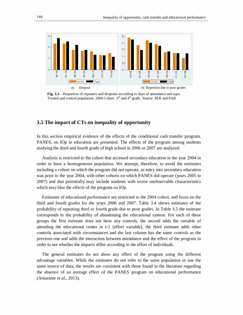
144 Inequality of opportunity, cash transfer and educational performance
a) Dropout b) Repetition due to poor grades
Fig. 3.3 – Proportion of repeaters and dropouts according to days of attendance and type. Treated and control population. 2004 Cohort. 3rd and 4th grade. Source: SER and PAR
3.5 The impact of CTs on inequality of opportunity
In this section empirical evidence of the effects of the conditional cash transfer program, PANES, on IOp in education are presented. The effects of the program among students studying the third and fourth grade of high school in 2006 or 2007 are analyzed.
Analysis is restricted to the cohort that accessed secondary education in the year 2004 in order to have a homogeneous population. We attempt, therefore, to avoid the estimates including a cohort on which the program did not operate, as entry into secondary education was prior to the year 2004, with other cohorts on which PANES did operate (years 2005 to 2007) and that potentially may include students with worse unobservable characteristics which may blur the effects of the program on IOp.
Estimates of educational performance are restricted to the 2004 cohort, and focus on the third and fourth grades for the years 2006 and 2007. Table 3.4 shows estimates of the probability of repeating third or fourth grade due to poor grades. In Table 3.5 the estimate corresponds to the probability of abandoning the educational system. For each of these groups the first estimate does not have any controls, the second adds the variable of attending the educational center in t-1 (effort variable), the third estimate adds other controls associated with circumstances and the last column has the same controls as the previous one and adds the interaction between attendance and the effect of the program in order to see whether the impacts differ according to the effort of individuals.
The general estimates do not show any effect of the program using the different advantage variables. While the estimates do not refer to the same population or use the same source of data, the results are consistent with those found in the literature regarding the absence of an average effect of the PANES program on educational performance (Amarante et al., 2013).
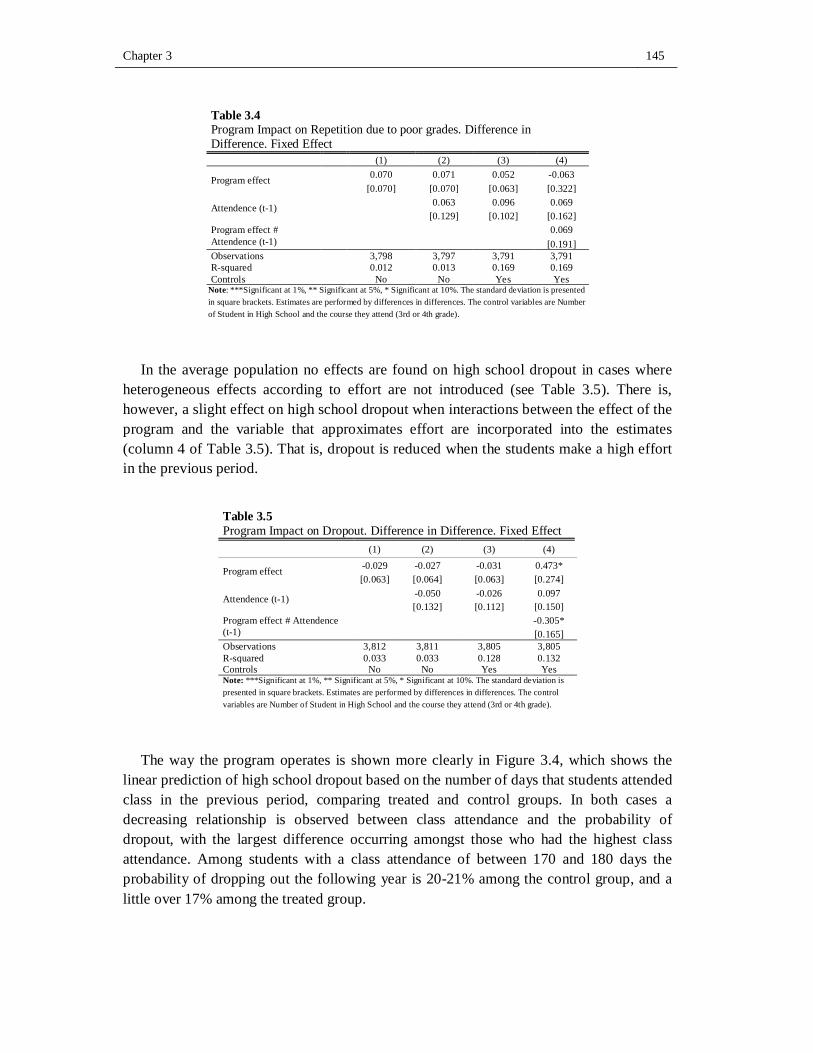
Chapter 3 145
Table 3.4 Program Impact on Repetition due to poor grades. Difference in Difference. Fixed Effect
(1) (2) (3) (4)
Program effect 0.070 0.071 0.052 -0.063
[0.070] [0.070] [0.063] [0.322]
Attendence (t-1) 0.063 0.096 0.069
[0.129] [0.102] [0.162] Program effect # Attendence (t-1) 0.069
[0.191] Observations 3,798 3,797 3,791 3,791 R-squared 0.012 0.013 0.169 0.169 Controls No No Yes Yes
Note: ***Significant at 1%, ** Significant at 5%, * Significant at 10%. The standard deviation is presented in square brackets. Estimates are performed by differences in differences. The control variables are Number of Student in High School and the course they attend (3rd or 4th grade).
In the average population no effects are found on high school dropout in cases where heterogeneous effects according to effort are not introduced (see Table 3.5). There is, however, a slight effect on high school dropout when interactions between the effect of the program and the variable that approximates effort are incorporated into the estimates (column 4 of Table 3.5). That is, dropout is reduced when the students make a high effort in the previous period.
Table 3.5 Program Impact on Dropout. Difference in Difference. Fixed Effect
(1) (2) (3) (4)
Program effect -0.029 -0.027 -0.031 0.473* [0.063] [0.064] [0.063] [0.274]
Attendence (t-1) -0.050 -0.026 0.097 [0.132] [0.112] [0.150]
Program effect # Attendence (t-1)
-0.305* [0.165]
Observations 3,812 3,811 3,805 3,805 R-squared 0.033 0.033 0.128 0.132 Controls No No Yes Yes Note: ***Significant at 1%, ** Significant at 5%, * Significant at 10%. The standard deviation is presented in square brackets. Estimates are performed by differences in differences. The control variables are Number of Student in High School and the course they attend (3rd or 4th grade).
The way the program operates is shown more clearly in Figure 3.4, which shows the linear prediction of high school dropout based on the number of days that students attended class in the previous period, comparing treated and control groups. In both cases a decreasing relationship is observed between class attendance and the probability of dropout, with the largest difference occurring amongst those who had the highest class attendance. Among students with a class attendance of between 170 and 180 days the probability of dropping out the following year is 20-21% among the control group, and a little over 17% among the treated group.
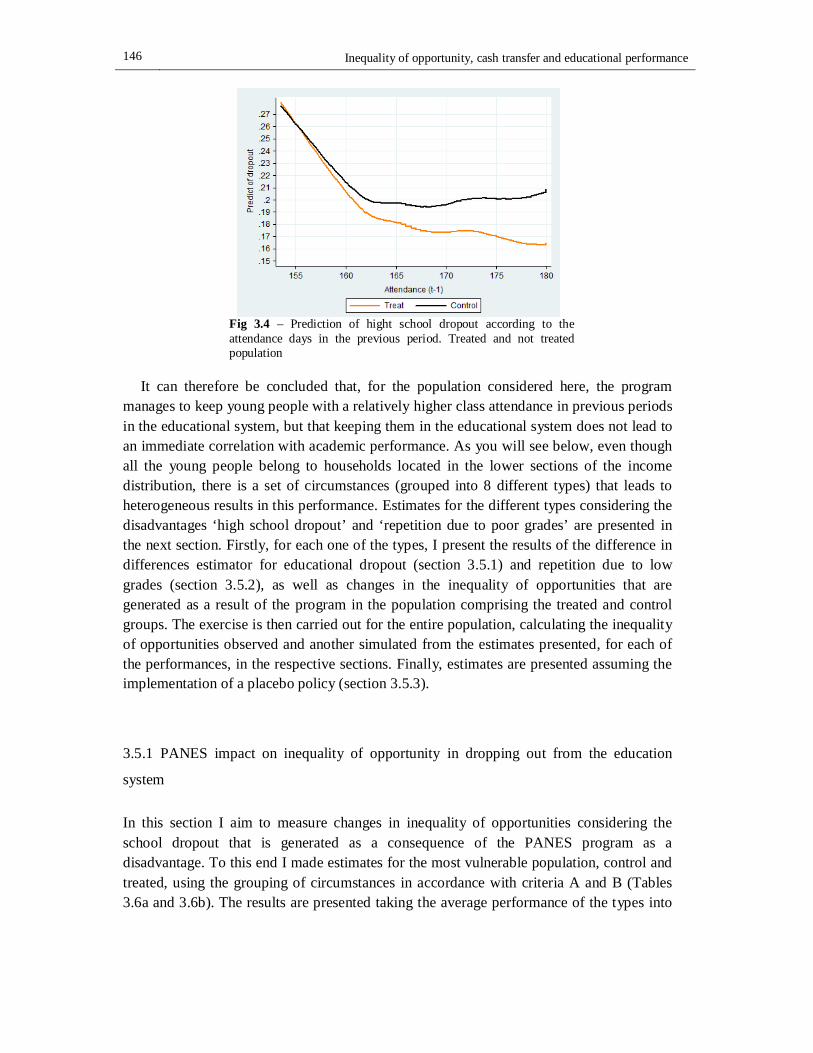
146 Inequality of opportunity, cash transfer and educational performance
Fig 3.4 – Prediction of hight school dropout according to the attendance days in the previous period. Treated and not treated population
It can therefore be concluded that, for the population considered here, the program
manages to keep young people with a relatively higher class attendance in previous periods in the educational system, but that keeping them in the educational system does not lead to an immediate correlation with academic performance. As you will see below, even though all the young people belong to households located in the lower sections of the income distribution, there is a set of circumstances (grouped into 8 different types) that leads to heterogeneous results in this performance. Estimates for the different types considering the disadvantages ‘high school dropout’ and ‘repetition due to poor grades’ are presented in the next section. Firstly, for each one of the types, I present the results of the difference in differences estimator for educational dropout (section 3.5.1) and repetition due to low grades (section 3.5.2), as well as changes in the inequality of opportunities that are generated as a result of the program in the population comprising the treated and control groups. The exercise is then carried out for the entire population, calculating the inequality of opportunities observed and another simulated from the estimates presented, for each of the performances, in the respective sections. Finally, estimates are presented assuming the implementation of a placebo policy (section 3.5.3).
3.5.1 PANES impact on inequality of opportunity in dropping out from the education
system
In this section I aim to measure changes in inequality of opportunities considering the school dropout that is generated as a consequence of the PANES program as a disadvantage. To this end I made estimates for the most vulnerable population, control and treated, using the grouping of circumstances in accordance with criteria A and B (Tables 3.6a and 3.6b). The results are presented taking the average performance of the types into
Chapter 3 147
account.20 Therefore, Table 3.6a includes the types with a worse average performance, and which have a low GPA at t-1 (types 1, 3, 5 and 7) as a common characteristic, while the students with a better performance are presented in Table 3.6b (those with a high GPA at t-1, types 2, 4, 6 and 8). The order of the types, which is based on average dropout, is maintained with both criteria A and B.
The most significant effects of the program are found in Criterion A when the teenager comes from a home with better circumstances in terms of wealth and education. In this group, when the teenager had a poor performance in the previous period, as measured by the GPA, the program succeeded in retaining those who made a high effort in the school, while the positive effects on teenagers with a high GPA occur regardless of previous effort. Heterogeneous effects from effort are also observed in teenagers with a high GPA. This is the case of those who, while coming from households with a high educational background, have low levels of wealth. In this group a reduction in school dropout, as a result of the program, is only achieved among those who showed high levels of effort. These results are commented on in greater detail below.
Table 3.6a shows the first four types corresponding to young people with low GPA. For young people living in households where the adults do not have a high level of education and those residing outside of Montevideo no effects of the program are observed. As mentioned, the only significant effect of the program on school dropout is observed for those residing in households with better (other) circumstances: high educational levels among the adults residing there and with a high durable goods index. The positive effects of the program are heterogeneous, based on previous attendance, with a reduction in high school dropout among those who had previously shown a greater predisposition to remaining within the educational system. Among the students with higher class attendance in the previous period (180 days) the program reduces high school dropout by 4.5% (0.848-0.496*1.8), while the effect disappears for those with more than 10 days of non-attendance in the previous period (0.848-0.496*1.7).
Table 3.6b includes type four which corresponds to young people with high GPA. The greater effects of the program are observed with Criterion A. No effects are found only for those residing in households where the adults have a low level of education and a low wealth indicator (durable goods index).
20 The average dropout rate of each type was presented in Table 3.2.
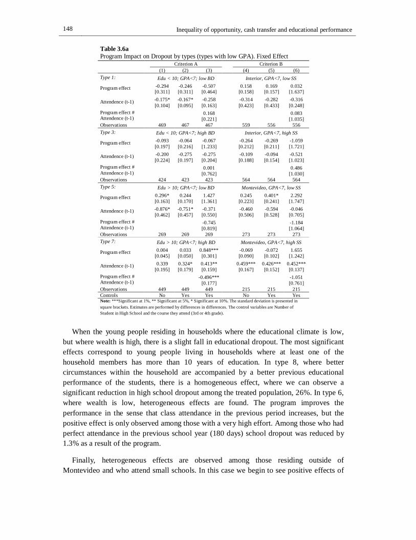
148 Inequality of opportunity, cash transfer and educational performance
Table 3.6a Program Impact on Dropout by types (types with low GPA). Fixed Effect
Criterion A Criterion B
(1) (2) (3) (4) (5) (6) Type 1: Edu < 10; GPA<7; low BD Interior, GPA<7, low SS
Program effect -0.294 -0.246 -0.507 0.158 0.169 0.032 [0.311] [0.311] [0.464] [0.158] [0.157] [1.637]
Attendence (t-1) -0.175* -0.167* -0.258 -0.314 -0.282 -0.316 [0.104] [0.095] [0.163] [0.423] [0.433] [0.248]
Program effect # Attendence (t-1)
0.168 0.083 [0.221] [1.035]
Observations 469 467 467 559 556 556 Type 3: Edu < 10; GPA<7; high BD Interior, GPA<7, high SS
Program effect -0.093 -0.064 -0.067 -0.264 -0.269 -1.059 [0.197] [0.216] [1.233] [0.212] [0.211] [1.721]
Attendence (t-1) -0.200 -0.275 -0.275 -0.109 -0.094 -0.521 [0.224] [0.197] [0.204] [0.188] [0.154] [1.023]
Program effect # Attendence (t-1)
0.001 0.486 [0.762] [1.030]
Observations 424 423 423 564 564 564 Type 5: Edu > 10; GPA<7; low BD Montevideo, GPA<7, low SS
Program effect 0.296* 0.244 1.427 0.245 0.401* 2.292 [0.163] [0.170] [1.361] [0.223] [0.241] [1.747]
Attendence (t-1) -0.876* -0.751* -0.371 -0.460 -0.594 -0.046 [0.462] [0.457] [0.550] [0.506] [0.528] [0.705]
Program effect # Attendence (t-1)
-0.745 -1.184 [0.819] [1.064]
Observations 269 269 269 273 273 273 Type 7: Edu > 10; GPA<7; high BD Montevideo, GPA<7, high SS
Program effect 0.004 0.033 0.848*** -0.069 -0.072 1.655 [0.045] [0.050] [0.301] [0.090] [0.102] [1.242]
Attendence (t-1) 0.339 0.324* 0.413** 0.459*** 0.426*** 0.452*** [0.195] [0.179] [0.159] [0.167] [0.152] [0.137]
Program effect # Attendence (t-1)
-0.496*** -1.051 [0.177] [0.761]
Observations 449 449 449 215 215 215 Controls No Yes Yes No Yes Yes Note: ***Significant at 1%, ** Significant at 5%, * Significant at 10%. The standard deviation is presented in square brackets. Estimates are performed by differences in differences. The control variables are Number of Student in High School and the course they attend (3rd or 4th grade).
When the young people residing in households where the educational climate is low,
but where wealth is high, there is a slight fall in educational dropout. The most significant effects correspond to young people living in households where at least one of the household members has more than 10 years of education. In type 8, where better circumstances within the household are accompanied by a better previous educational performance of the students, there is a homogeneous effect, where we can observe a significant reduction in high school dropout among the treated population, 26%. In type 6, where wealth is low, heterogeneous effects are found. The program improves the performance in the sense that class attendance in the previous period increases, but the positive effect is only observed among those with a very high effort. Among those who had perfect attendance in the previous school year (180 days) school dropout was reduced by 1.3% as a result of the program.
Finally, heterogeneous effects are observed among those residing outside of Montevideo and who attend small schools. In this case we begin to see positive effects of
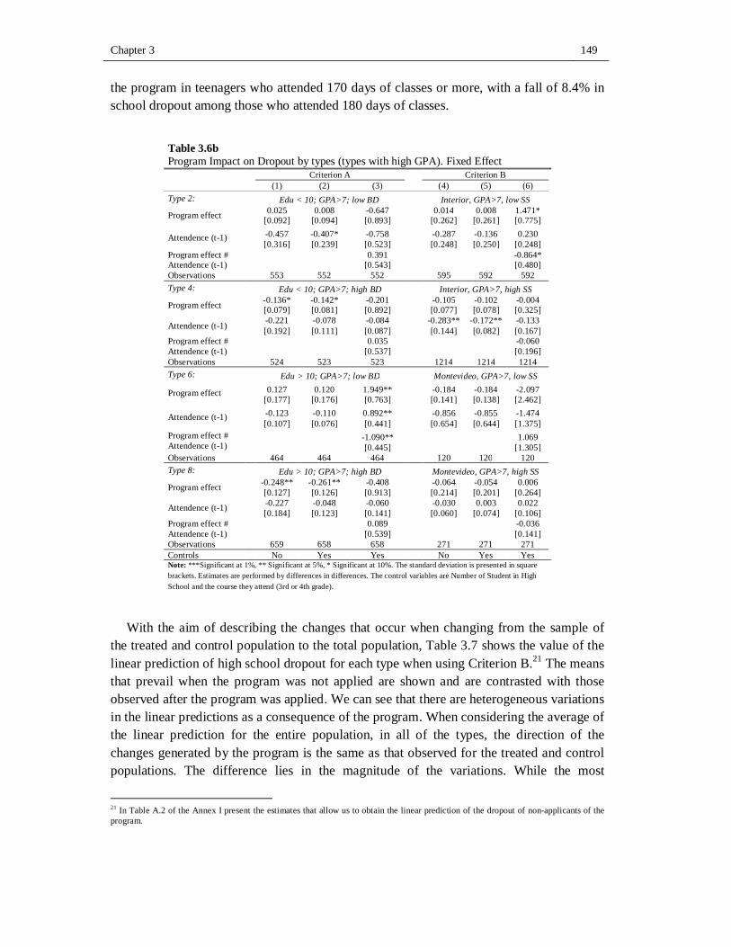
Chapter 3 149
the program in teenagers who attended 170 days of classes or more, with a fall of 8.4% in school dropout among those who attended 180 days of classes.
Table 3.6b Program Impact on Dropout by types (types with high GPA). Fixed Effect
Criterion A Criterion B
(1) (2) (3) (4) (5) (6) Type 2: Edu < 10; GPA>7; low BD Interior, GPA>7, low SS
Program effect 0.025 0.008 -0.647 0.014 0.008 1.471* [0.092] [0.094] [0.893] [0.262] [0.261] [0.775]
Attendence (t-1) -0.457 -0.407* -0.758 -0.287 -0.136 0.230 [0.316] [0.239] [0.523] [0.248] [0.250] [0.248]
Program effect # Attendence (t-1)
0.391 -0.864* [0.543] [0.480]
Observations 553 552 552 595 592 592 Type 4: Edu < 10; GPA>7; high BD Interior, GPA>7, high SS
Program effect -0.136* -0.142* -0.201 -0.105 -0.102 -0.004 [0.079] [0.081] [0.892] [0.077] [0.078] [0.325]
Attendence (t-1) -0.221 -0.078 -0.084 -0.283** -0.172** -0.133 [0.192] [0.111] [0.087] [0.144] [0.082] [0.167]
Program effect # Attendence (t-1)
0.035 -0.060 [0.537] [0.196]
Observations 524 523 523 1214 1214 1214 Type 6: Edu > 10; GPA>7; low BD Montevideo, GPA>7, low SS
Program effect 0.127 0.120 1.949** -0.184 -0.184 -2.097 [0.177] [0.176] [0.763] [0.141] [0.138] [2.462]
Attendence (t-1) -0.123 -0.110 0.892** -0.856 -0.855 -1.474 [0.107] [0.076] [0.441] [0.654] [0.644] [1.375]
Program effect # Attendence (t-1)
-1.090** 1.069 [0.445] [1.305]
Observations 464 464 464 120 120 120 Type 8: Edu > 10; GPA>7; high BD Montevideo, GPA>7, high SS
Program effect -0.248** -0.261** -0.408 -0.064 -0.054 0.006 [0.127] [0.126] [0.913] [0.214] [0.201] [0.264]
Attendence (t-1) -0.227 -0.048 -0.060 -0.030 0.003 0.022 [0.184] [0.123] [0.141] [0.060] [0.074] [0.106]
Program effect # Attendence (t-1)
0.089 -0.036 [0.539] [0.141]
Observations 659 658 658 271 271 271 Controls No Yes Yes No Yes Yes Note: ***Significant at 1%, ** Significant at 5%, * Significant at 10%. The standard deviation is presented in square brackets. Estimates are performed by differences in differences. The control variables are Number of Student in High School and the course they attend (3rd or 4th grade).
With the aim of describing the changes that occur when changing from the sample of the treated and control population to the total population, Table 3.7 shows the value of the linear prediction of high school dropout for each type when using Criterion B.21 The means that prevail when the program was not applied are shown and are contrasted with those observed after the program was applied. We can see that there are heterogeneous variations in the linear predictions as a consequence of the program. When considering the average of the linear prediction for the entire population, in all of the types, the direction of the changes generated by the program is the same as that observed for the treated and control populations. The difference lies in the magnitude of the variations. While the most
21 In Table A.2 of the Annex I present the estimates that allow us to obtain the linear prediction of the dropout of non-applicants of the program.
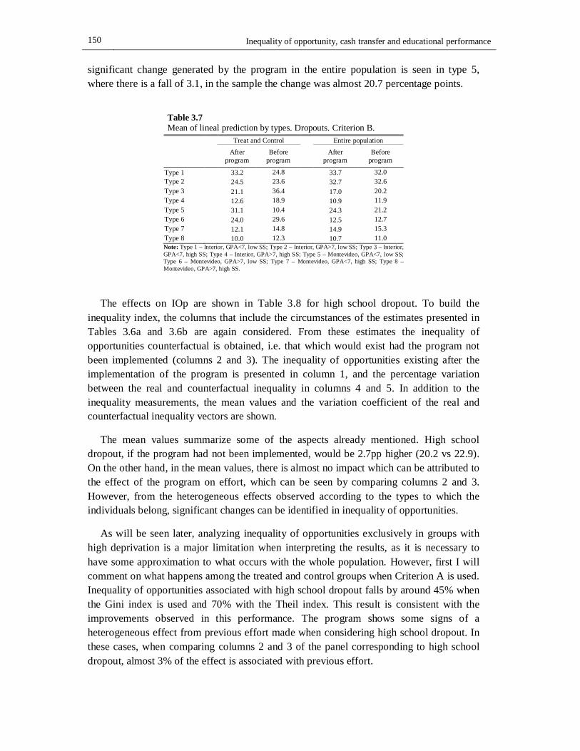
150 Inequality of opportunity, cash transfer and educational performance
significant change generated by the program in the entire population is seen in type 5, where there is a fall of 3.1, in the sample the change was almost 20.7 percentage points.
Table 3.7 Mean of lineal prediction by types. Dropouts. Criterion B. Treat and Control Entire population
After program
Before program
After program
Before program
Type 1 33.2 24.8 33.7 32.0 Type 2 24.5 23.6 32.7 32.6 Type 3 21.1 36.4 17.0 20.2 Type 4 12.6 18.9 10.9 11.9 Type 5 31.1 10.4 24.3 21.2 Type 6 24.0 29.6 12.5 12.7 Type 7 12.1 14.8 14.9 15.3 Type 8 10.0 12.3 10.7 11.0 Note: Type 1 – Interior, GPA<7, low SS; Type 2 – Interior, GPA>7, low SS; Type 3 – Interior, GPA<7, high SS; Type 4 – Interior, GPA>7, high SS; Type 5 – Montevideo, GPA<7, low SS; Type 6 – Montevideo, GPA>7, low SS; Type 7 – Montevideo, GPA<7, high SS; Type 8 – Montevideo, GPA>7, high SS.
The effects on IOp are shown in Table 3.8 for high school dropout. To build the inequality index, the columns that include the circumstances of the estimates presented in Tables 3.6a and 3.6b are again considered. From these estimates the inequality of opportunities counterfactual is obtained, i.e. that which would exist had the program not been implemented (columns 2 and 3). The inequality of opportunities existing after the implementation of the program is presented in column 1, and the percentage variation between the real and counterfactual inequality in columns 4 and 5. In addition to the inequality measurements, the mean values and the variation coefficient of the real and counterfactual inequality vectors are shown.
The mean values summarize some of the aspects already mentioned. High school dropout, if the program had not been implemented, would be 2.7pp higher (20.2 vs 22.9). On the other hand, in the mean values, there is almost no impact which can be attributed to the effect of the program on effort, which can be seen by comparing columns 2 and 3. However, from the heterogeneous effects observed according to the types to which the individuals belong, significant changes can be identified in inequality of opportunities.
As will be seen later, analyzing inequality of opportunities exclusively in groups with high deprivation is a major limitation when interpreting the results, as it is necessary to have some approximation to what occurs with the whole population. However, first I will comment on what happens among the treated and control groups when Criterion A is used. Inequality of opportunities associated with high school dropout falls by around 45% when the Gini index is used and 70% with the Theil index. This result is consistent with the improvements observed in this performance. The program shows some signs of a heterogeneous effect from previous effort made when considering high school dropout. In these cases, when comparing columns 2 and 3 of the panel corresponding to high school dropout, almost 3% of the effect is associated with previous effort.
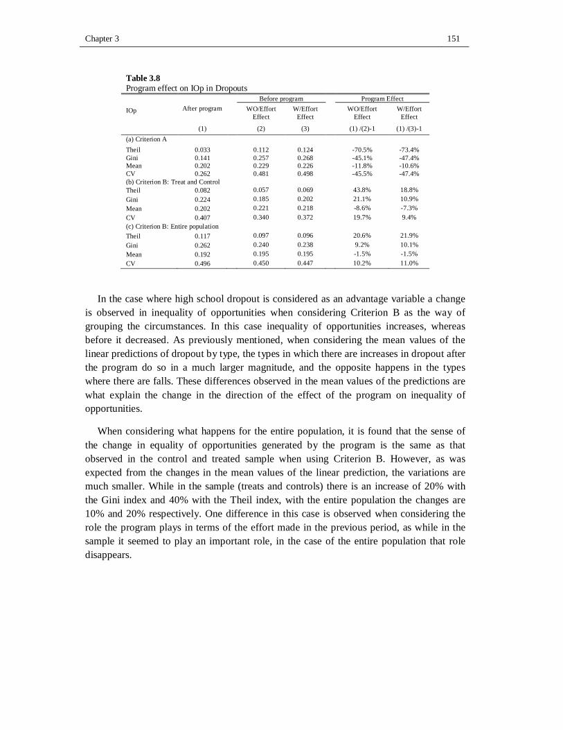
Chapter 3 151
Table 3.8 Program effect on IOp in Dropouts
IOp After program Before program Program Effect WO/Effort
Effect W/Effort
Effect WO/Effort Effect
W/Effort Effect
(1) (2) (3) (1) /(2)-1 (1) /(3)-1 (a) Criterion A Theil 0.033 0.112 0.124 -70.5% -73.4% Gini 0.141 0.257 0.268 -45.1% -47.4% Mean 0.202 0.229 0.226 -11.8% -10.6% CV 0.262 0.481 0.498 -45.5% -47.4% (b) Criterion B: Treat and Control Theil 0.082 0.057 0.069 43.8% 18.8% Gini 0.224 0.185 0.202 21.1% 10.9% Mean 0.202 0.221 0.218 -8.6% -7.3% CV 0.407 0.340 0.372 19.7% 9.4% (c) Criterion B: Entire population Theil 0.117 0.097 0.096 20.6% 21.9% Gini 0.262 0.240 0.238 9.2% 10.1% Mean 0.192 0.195 0.195 -1.5% -1.5% CV 0.496 0.450 0.447 10.2% 11.0%
In the case where high school dropout is considered as an advantage variable a change is observed in inequality of opportunities when considering Criterion B as the way of grouping the circumstances. In this case inequality of opportunities increases, whereas before it decreased. As previously mentioned, when considering the mean values of the linear predictions of dropout by type, the types in which there are increases in dropout after the program do so in a much larger magnitude, and the opposite happens in the types where there are falls. These differences observed in the mean values of the predictions are what explain the change in the direction of the effect of the program on inequality of opportunities.
When considering what happens for the entire population, it is found that the sense of the change in equality of opportunities generated by the program is the same as that observed in the control and treated sample when using Criterion B. However, as was expected from the changes in the mean values of the linear prediction, the variations are much smaller. While in the sample (treats and controls) there is an increase of 20% with the Gini index and 40% with the Theil index, with the entire population the changes are 10% and 20% respectively. One difference in this case is observed when considering the role the program plays in terms of the effort made in the previous period, as while in the sample it seemed to play an important role, in the case of the entire population that role disappears.

152 Inequality of opportunity, cash transfer and educational performance
3.5.2 PANES impact on inequality of opportunity in repetition due to poor grade
Beyond keeping students in the educational system, the aim of public policy is for students to successfully complete the compulsory education cycle. Keeping the students within the educational system is a necessary condition for them to complete different academic activities, but not sufficient, the program could be ‘neutral’ in allowing students to achieve this goal. In fact, it is possible that the success of the policy in keeping teenagers in the educational system has the flip side that the average educational performance actually gets worse, due to the change in composition of the population attending the educational system. Therefore in this section I will analyze the effects of the PANES program on repetition due to poor grades.
While Table 3.4 shows that the program had no impact on school repetition, it is possible that there are specific effects on some types which could lead to consequences in measuring inequality of opportunity. The impacts of the PANES program on repetition due to poor grades for the different types are presented in Tables 3.9a and 3.9c. Again, the first table presents the types with a low GPA and the second those with a better GPA at t-1.
When students have a low GPA at t-1 and Criterion A is used, the program has virtually no effects. There is only one exception. In the case of type 7, young people residing in households with better circumstances (high educational levels among the adults residing there and with high wealth), the repetition due to poor grades is reduced on average for the whole group. Remember that when considering this type, school dropout had declined, mainly for those who had made a high effort in the previous period. In this sense, the program succeeded in simultaneously improving both performances.
With Criterion B heterogeneous effects are observed in very different groups, types 1 and 7. In the first case reside outside Montevideo and attend a small school, while in the second case they reside in Montevideo and attend larger schools. In type 1 it is observed that the repetition rate increases with previous effort, while in type 7 the levels of repetition are reduced as a result of the program, and to a greater extent when the previous effort is higher. In both types no effects of the program on school dropout were observed.
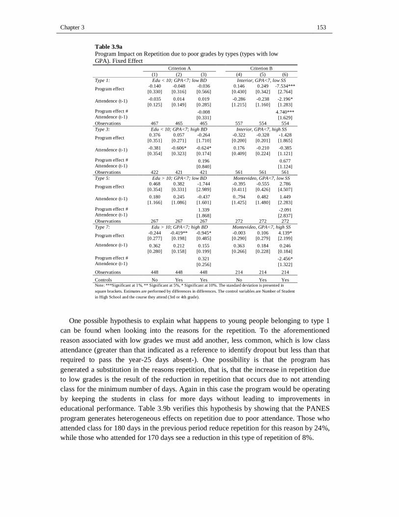
Chapter 3 153
Table 3.9a Program Impact on Repetition due to poor grades by types (types with low GPA). Fixed Effect
Criterion A Criterion B
(1) (2) (3) (4) (5) (6) Type 1: Edu < 10; GPA<7; low BD Interior, GPA<7, low SS
Program effect -0.140 -0.048 -0.036 0.146 0.249 -7.534*** [0.330] [0.316] [0.566] [0.430] [0.342] [2.764]
Attendence (t-1) -0.035 0.014 0.019 -0.286 -0.238 -2.196* [0.125] [0.149] [0.285] [1.215] [1.160] [1.283]
Program effect # Attendence (t-1)
-0.008 4.740*** [0.331] [1.629]
Observations 467 465 465 557 554 554 Type 3: Edu < 10; GPA<7; high BD Interior, GPA<7, high SS
Program effect 0.376 0.057 -0.264 -0.322 -0.328 -1.428 [0.351] [0.271] [1.710] [0.200] [0.201] [1.865]
Attendence (t-1) -0.381 -0.606* -0.624* 0.176 -0.210 -0.385 [0.354] [0.323] [0.174] [0.409] [0.224] [1.121]
Program effect # Attendence (t-1)
0.196 0.677 [0.840] [1.124]
Observations 422 421 421 561 561 561 Type 5: Edu > 10; GPA<7; low BD Montevideo, GPA<7, low SS
Program effect 0.468 0.382 -1.744 -0.395 -0.555 2.786 [0.354] [0.331] [2.989] [0.411] [0.426] [4.507]
Attendence (t-1) 0.180 0.245 -0.437 0..794 0.482 1.449 [1.166] [1.086] [1.601] [1.425] [1.480] [2.283]
Program effect # Attendence (t-1)
1.339 -2.091 [1.868] [2.837]
Observations 267 267 267 272 272 272 Type 7: Edu > 10; GPA<7; high BD Montevideo, GPA<7, high SS
Program effect -0.244 -0.419** -0.945* -0.003 0.106 4.139* [0.277] [0.198] [0.485] [0.290] [0.279] [2.199]
Attendence (t-1)
0.362 0.212 0.155 0.363 0.184 0.246 [0.280] [0.158] [0.199] [0.266] [0.228] [0.184]
Program effect # Attendence (t-1)
0.321 -2.456* [0.256] [1.322]
Observations 448 448 448 214 214 214 Controls No Yes Yes No Yes Yes Note: ***Significant at 1%, ** Significant at 5%, * Significant at 10%. The standard deviation is presented in square brackets. Estimates are performed by differences in differences. The control variables are Number of Student in High School and the course they attend (3rd or 4th grade).
One possible hypothesis to explain what happens to young people belonging to type 1 can be found when looking into the reasons for the repetition. To the aforementioned reason associated with low grades we must add another, less common, which is low class attendance (greater than that indicated as a reference to identify dropout but less than that required to pass the year-25 days absent-). One possibility is that the program has generated a substitution in the reasons repetition, that is, that the increase in repetition due to low grades is the result of the reduction in repetition that occurs due to not attending class for the minimum number of days. Again in this case the program would be operating by keeping the students in class for more days without leading to improvements in educational performance. Table 3.9b verifies this hypothesis by showing that the PANES program generates heterogeneous effects on repetition due to poor attendance. Those who attended class for 180 days in the previous period reduce repetition for this reason by 24%, while those who attended for 170 days see a reduction in this type of repetition of 8%.
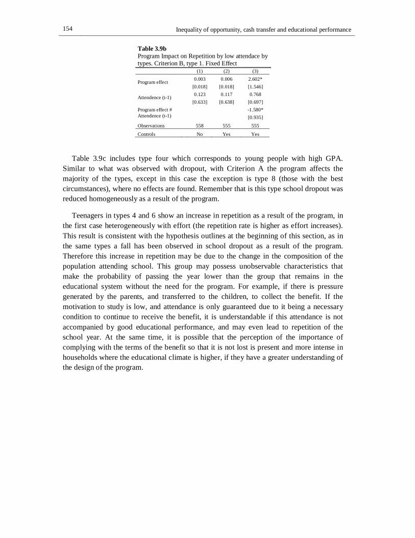
154 Inequality of opportunity, cash transfer and educational performance
Table 3.9b Program Impact on Repetition by low attendace by types. Criterion B, type 1. Fixed Effect (1) (2) (3)
Program effect 0.003 0.006 2.602* [0.018] [0.018] [1.546]
Attendence (t-1) 0.123 0.117 0.768 [0.633] [0.638] [0.697]
Program effect # Attendence (t-1)
-1.580* [0.935]
Observations 558 555 555
Controls No Yes Yes
Table 3.9c includes type four which corresponds to young people with high GPA. Similar to what was observed with dropout, with Criterion A the program affects the majority of the types, except in this case the exception is type 8 (those with the best circumstances), where no effects are found. Remember that is this type school dropout was reduced homogeneously as a result of the program.
Teenagers in types 4 and 6 show an increase in repetition as a result of the program, in the first case heterogeneously with effort (the repetition rate is higher as effort increases). This result is consistent with the hypothesis outlines at the beginning of this section, as in the same types a fall has been observed in school dropout as a result of the program. Therefore this increase in repetition may be due to the change in the composition of the population attending school. This group may possess unobservable characteristics that make the probability of passing the year lower than the group that remains in the educational system without the need for the program. For example, if there is pressure generated by the parents, and transferred to the children, to collect the benefit. If the motivation to study is low, and attendance is only guaranteed due to it being a necessary condition to continue to receive the benefit, it is understandable if this attendance is not accompanied by good educational performance, and may even lead to repetition of the school year. At the same time, it is possible that the perception of the importance of complying with the terms of the benefit so that it is not lost is present and more intense in households where the educational climate is higher, if they have a greater understanding of the design of the program.
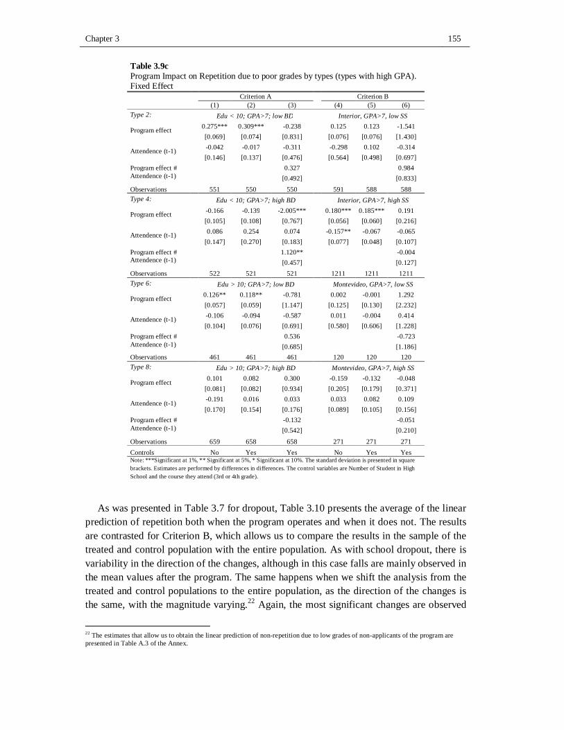
Chapter 3 155
Table 3.9c Program Impact on Repetition due to poor grades by types (types with high GPA). Fixed Effect
Criterion A Criterion B
(1) (2) (3) (4) (5) (6) Type 2: Edu < 10; GPA>7; low BD Interior, GPA>7, low SS
Program effect 0.275*** 0.309*** -0.238 0.125 0.123 -1.541 [0.069] [0.074] [0.831] [0.076] [0.076] [1.430]
Attendence (t-1) -0.042 -0.017 -0.311 -0.298 0.102 -0.314 [0.146] [0.137] [0.476] [0.564] [0.498] [0.697]
Program effect # Attendence (t-1)
0.327 0.984 [0.492] [0.833]
Observations 551 550 550 591 588 588 Type 4: Edu < 10; GPA>7; high BD Interior, GPA>7, high SS
Program effect -0.166 -0.139 -2.005*** 0.180*** 0.185*** 0.191 [0.105] [0.108] [0.767] [0.056] [0.060] [0.216]
Attendence (t-1) 0.086 0.254 0.074 -0.157** -0.067 -0.065 [0.147] [0.270] [0.183] [0.077] [0.048] [0.107]
Program effect # Attendence (t-1)
1.120** -0.004 [0.457] [0.127]
Observations 522 521 521 1211 1211 1211 Type 6: Edu > 10; GPA>7; low BD Montevideo, GPA>7, low SS
Program effect 0.126** 0.118** -0.781 0.002 -0.001 1.292 [0.057] [0.059] [1.147] [0.125] [0.130] [2.232]
Attendence (t-1) -0.106 -0.094 -0.587 0.011 -0.004 0.414 [0.104] [0.076] [0.691] [0.580] [0.606] [1.228]
Program effect # Attendence (t-1)
0.536 -0.723 [0.685] [1.186]
Observations 461 461 461 120 120 120 Type 8: Edu > 10; GPA>7; high BD Montevideo, GPA>7, high SS
Program effect 0.101 0.082 0.300 -0.159 -0.132 -0.048 [0.081] [0.082] [0.934] [0.205] [0.179] [0.371]
Attendence (t-1) -0.191 0.016 0.033 0.033 0.082 0.109 [0.170] [0.154] [0.176] [0.089] [0.105] [0.156]
Program effect # Attendence (t-1)
-0.132 -0.051 [0.542] [0.210]
Observations 659 658 658 271 271 271 Controls No Yes Yes No Yes Yes Note: ***Significant at 1%, ** Significant at 5%, * Significant at 10%. The standard deviation is presented in square brackets. Estimates are performed by differences in differences. The control variables are Number of Student in High School and the course they attend (3rd or 4th grade).
As was presented in Table 3.7 for dropout, Table 3.10 presents the average of the linear prediction of repetition both when the program operates and when it does not. The results are contrasted for Criterion B, which allows us to compare the results in the sample of the treated and control population with the entire population. As with school dropout, there is variability in the direction of the changes, although in this case falls are mainly observed in the mean values after the program. The same happens when we shift the analysis from the treated and control populations to the entire population, as the direction of the changes is the same, with the magnitude varying.22 Again, the most significant changes are observed
22 The estimates that allow us to obtain the linear prediction of non-repetition due to low grades of non-applicants of the program are presented in Table A.3 of the Annex.
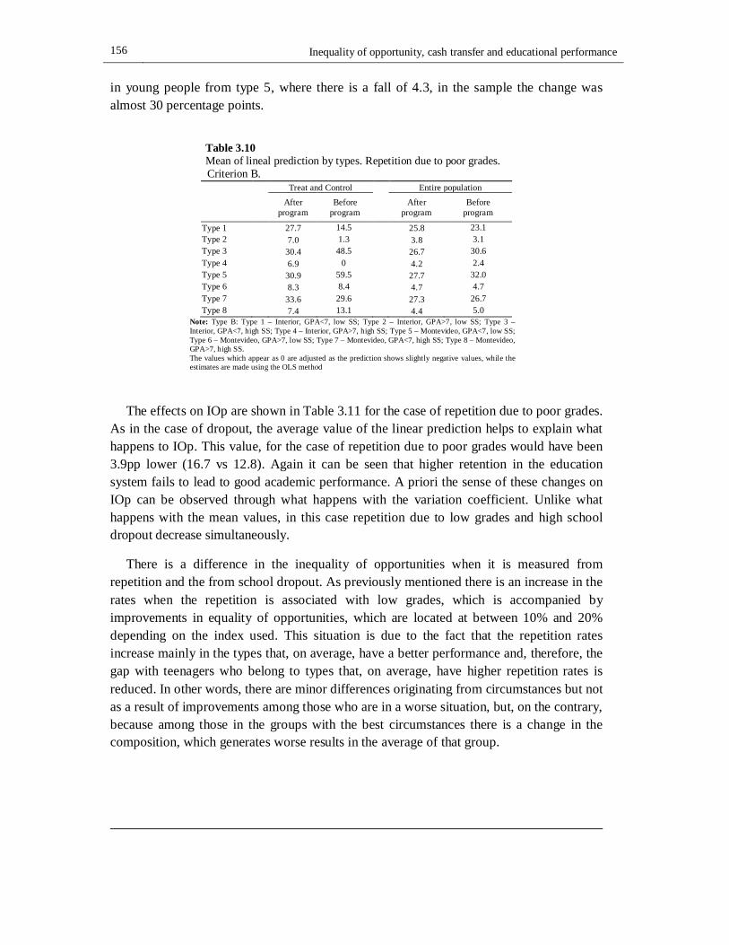
156 Inequality of opportunity, cash transfer and educational performance
in young people from type 5, where there is a fall of 4.3, in the sample the change was almost 30 percentage points.
Table 3.10 Mean of lineal prediction by types. Repetition due to poor grades. Criterion B. Treat and Control Entire population
After program
Before program
After program
Before program
Type 1 27.7 14.5 25.8 23.1 Type 2 7.0 1.3 3.8 3.1 Type 3 30.4 48.5 26.7 30.6 Type 4 6.9 0 4.2 2.4 Type 5 30.9 59.5 27.7 32.0 Type 6 8.3 8.4 4.7 4.7 Type 7 33.6 29.6 27.3 26.7 Type 8 7.4 13.1 4.4 5.0
Note: Type B: Type 1 – Interior, GPA<7, low SS; Type 2 – Interior, GPA>7, low SS; Type 3 – Interior, GPA<7, high SS; Type 4 – Interior, GPA>7, high SS; Type 5 – Montevideo, GPA<7, low SS; Type 6 – Montevideo, GPA>7, low SS; Type 7 – Montevideo, GPA<7, high SS; Type 8 – Montevideo, GPA>7, high SS. The values which appear as 0 are adjusted as the prediction shows slightly negative values, while the estimates are made using the OLS method
The effects on IOp are shown in Table 3.11 for the case of repetition due to poor grades. As in the case of dropout, the average value of the linear prediction helps to explain what happens to IOp. This value, for the case of repetition due to poor grades would have been 3.9pp lower (16.7 vs 12.8). Again it can be seen that higher retention in the education system fails to lead to good academic performance. A priori the sense of these changes on IOp can be observed through what happens with the variation coefficient. Unlike what happens with the mean values, in this case repetition due to low grades and high school dropout decrease simultaneously.
There is a difference in the inequality of opportunities when it is measured from repetition and the from school dropout. As previously mentioned there is an increase in the rates when the repetition is associated with low grades, which is accompanied by improvements in equality of opportunities, which are located at between 10% and 20% depending on the index used. This situation is due to the fact that the repetition rates increase mainly in the types that, on average, have a better performance and, therefore, the gap with teenagers who belong to types that, on average, have higher repetition rates is reduced. In other words, there are minor differences originating from circumstances but not as a result of improvements among those who are in a worse situation, but, on the contrary, because among those in the groups with the best circumstances there is a change in the composition, which generates worse results in the average of that group.
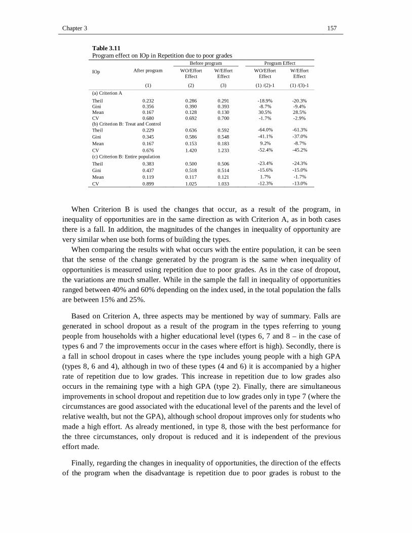
Chapter 3 157
Table 3.11 Program effect on IOp in Repetition due to poor grades
IOp After program Before program Program Effect WO/Effort
Effect W/Effort
Effect WO/Effort Effect
W/Effort Effect
(1) (2) (3) (1) /(2)-1 (1) /(3)-1 (a) Criterion A Theil 0.232 0.286 0.291 -18.9% -20.3% Gini 0.356 0.390 0.393 -8.7% -9.4% Mean 0.167 0.128 0.130 30.5% 28.5% CV 0.680 0.692 0.700 -1.7% -2.9% (b) Criterion B: Treat and Control Theil 0.229 0.636 0.592 -64.0% -61.3% Gini 0.345 0.586 0.548 -41.1% -37.0% Mean 0.167 0.153 0.183 9.2% -8.7% CV 0.676 1.420 1.233 -52.4% -45.2% (c) Criterion B: Entire population Theil 0.383 0.500 0.506 -23.4% -24.3% Gini 0.437 0.518 0.514 -15.6% -15.0% Mean 0.119 0.117 0.121 1.7% -1.7% CV 0.899 1.025 1.033 -12.3% -13.0%
When Criterion B is used the changes that occur, as a result of the program, in inequality of opportunities are in the same direction as with Criterion A, as in both cases there is a fall. In addition, the magnitudes of the changes in inequality of opportunity are very similar when use both forms of building the types.
When comparing the results with what occurs with the entire population, it can be seen that the sense of the change generated by the program is the same when inequality of opportunities is measured using repetition due to poor grades. As in the case of dropout, the variations are much smaller. While in the sample the fall in inequality of opportunities ranged between 40% and 60% depending on the index used, in the total population the falls are between 15% and 25%.
Based on Criterion A, three aspects may be mentioned by way of summary. Falls are generated in school dropout as a result of the program in the types referring to young people from households with a higher educational level (types 6, 7 and 8 – in the case of types 6 and 7 the improvements occur in the cases where effort is high). Secondly, there is a fall in school dropout in cases where the type includes young people with a high GPA (types 8, 6 and 4), although in two of these types (4 and 6) it is accompanied by a higher rate of repetition due to low grades. This increase in repetition due to low grades also occurs in the remaining type with a high GPA (type 2). Finally, there are simultaneous improvements in school dropout and repetition due to low grades only in type 7 (where the circumstances are good associated with the educational level of the parents and the level of relative wealth, but not the GPA), although school dropout improves only for students who made a high effort. As already mentioned, in type 8, those with the best performance for the three circumstances, only dropout is reduced and it is independent of the previous effort made.
Finally, regarding the changes in inequality of opportunities, the direction of the effects of the program when the disadvantage is repetition due to poor grades is robust to the
158 Inequality of opportunity, cash transfer and educational performance
criteria used to build the types and the population considered (decreases in all cases). However, there are variations in the magnitude of the effects. The effect on inequality of opportunities when considering high school dropout is sensitive to the selection of circumstances used to build the types, with no changes observed in the direction of the effect when changing from the treated and control populations to the entire population of students.
3.5.3 Placebo Estimates
To verify the robustness of the results it is necessary to corroborate that the identification assumptions implicit in the estimates of difference in differences are met. For this reason placebo estimates are made which allow us to rule out the effects found being the consequence of tendencies prior to the implementation of the program. The placebo estimates were suggested in Bertrand, Duflo & Mullainathan (2004) to test the robustness of the estimates of difference-in-differences. In order to rule out the existence of prior tendencies, information prior to the implementation of the program is considered. In order to attribute causal effects to the policy in question, in this case the PANES program, it is necessary that in the cases where effects are found, the placebo policy is not significant.
The information prior to the implementation of the program consists of data from the year 2004, information for 2005 and 2006 are also included for the population that entered in later years, and it is assumed that there is an artificial policy for 2006. The placebo of the treated group is identified from the people who entered the program after July 2006. By limiting the number of previous periods it is not possible to verify the robustness of the estimates when considering heterogeneous effects. The set of placebo regressions are presented in Table 3.12. In this table only the coefficients of interest are presented. Panel (a) corresponds to dropouts, while panel (b) refers to repeating due to poor grades.
In all of the cases where real impacts of the program were found, no effects of the placebo policy were observed. This ensures the robustness of the results both for dropout and repetition due to low grades. These results are found when the types are built with both Criterion A and Criterion B. In some types effects of the placebo policy are observed, however in these types the estimates that reflect the impact of the PANES program do not show significant results. As such it is not possible to attribute results to the presence of a previous trend. What happens with type 4 of Criterion A is of particular interest. In this case it is observed that the placebo policy, when considering repetition due to low grades, is significant and has a negative effect. This effect disappears when considering the real policy. At the same time it is found that in this type the PANES program reduces school dropout. This can be seen as a clear example of changes in the composition generated by the program. Prior to it being implemented, repetition showed a fall, once the program is in effect more teenagers remain in the education system, and this stops the fall in repetition which had previously been observed.
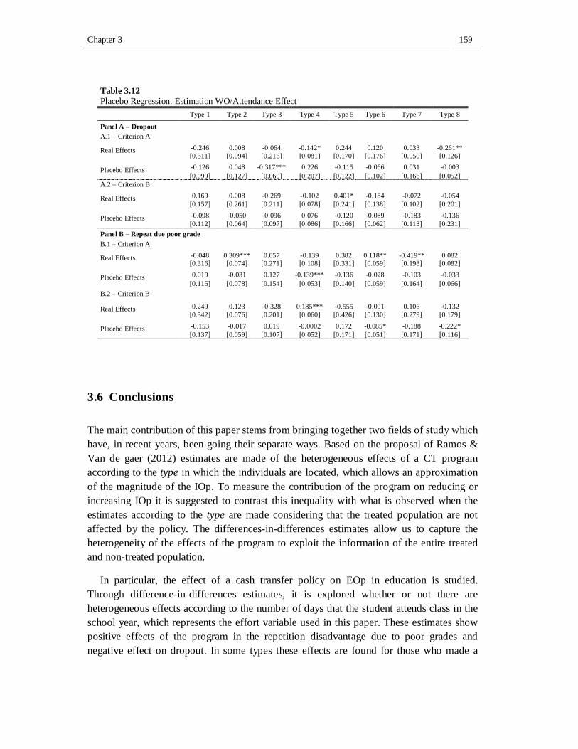
Chapter 3 159
Table 3.12 Placebo Regression. Estimation WO/Attendance Effect Type 1 Type 2 Type 3 Type 4 Type 5 Type 6 Type 7 Type 8
Panel A – Dropout A.1 – Criterion A
Real Effects -0.246 0.008 -0.064 -0.142* 0.244 0.120 0.033 -0.261** [0.311] [0.094] [0.216] [0.081] [0.170] [0.176] [0.050] [0.126]
Placebo Effects -0.126 0.048 -0.317*** 0.226 -0.115 -0.066 0.031 -0.003 [0.099] [0.127] [0.060] [0.207] [0.122] [0.102] [0.166] [0.052]
A.2 – Criterion B
Real Effects 0.169 0.008 -0.269 -0.102 0.401* -0.184 -0.072 -0.054 [0.157] [0.261] [0.211] [0.078] [0.241] [0.138] [0.102] [0.201]
Placebo Effects -0.098 -0.050 -0.096 0.076 -0.120 -0.089 -0.183 -0.136 [0.112] [0.064] [0.097] [0.086] [0.166] [0.062] [0.113] [0.231]
Panel B – Repeat due poor grade B.1 – Criterion A
Real Effects -0.048 0.309*** 0.057 -0.139 0.382 0.118** -0.419** 0.082 [0.316] [0.074] [0.271] [0.108] [0.331] [0.059] [0.198] [0.082]
Placebo Effects 0.019 -0.031 0.127 -0.139*** -0.136 -0.028 -0.103 -0.033 [0.116] [0.078] [0.154] [0.053] [0.140] [0.059] [0.164] [0.066]
B.2 – Criterion B
Real Effects 0.249 0.123 -0.328 0.185*** -0.555 -0.001 0.106 -0.132 [0.342] [0.076] [0.201] [0.060] [0.426] [0.130] [0.279] [0.179]
Placebo Effects -0.153 -0.017 0.019 -0.0002 0.172 -0.085* -0.188 -0.222* [0.137] [0.059] [0.107] [0.052] [0.171] [0.051] [0.171] [0.116]
3.6 Conclusions
The main contribution of this paper stems from bringing together two fields of study which have, in recent years, been going their separate ways. Based on the proposal of Ramos & Van de gaer (2012) estimates are made of the heterogeneous effects of a CT program according to the type in which the individuals are located, which allows an approximation of the magnitude of the IOp. To measure the contribution of the program on reducing or increasing IOp it is suggested to contrast this inequality with what is observed when the estimates according to the type are made considering that the treated population are not affected by the policy. The differences-in-differences estimates allow us to capture the heterogeneity of the effects of the program to exploit the information of the entire treated and non-treated population.
In particular, the effect of a cash transfer policy on EOp in education is studied. Through difference-in-differences estimates, it is explored whether or not there are heterogeneous effects according to the number of days that the student attends class in the school year, which represents the effort variable used in this paper. These estimates show positive effects of the program in the repetition disadvantage due to poor grades and negative effect on dropout. In some types these effects are found for those who made a
160 Inequality of opportunity, cash transfer and educational performance
high effort in the previous period. The estimates are robust when a placebo policy is introduced.
The main result shows that inequality of opportunities is reduced significantly as a result of the program, both in terms of high school dropout and repetition (Criterion A). However, these changes in inequality of opportunities occur with falls in school dropout and simultaneous increases in repetition. This result shows the potential and the weaknesses of the policy. The threat of the loss of the benefit, as well as the change in the opportunity cost of studying, succeeds in keeping young people in the education system, but other types of policies are necessary to ensure that remaining in the school then translates to actual academic achievement. An example could be accompanying or support policies which provide additional support to beneficiaries of the program, and/or measures that relax the criterion for repetition by differing the evaluation period.
One limitation in this type of study is only considering inequality for a population with significant deprivation, so it is verified whether the results are consistent by looking at the entire population. Data restrictions oblige us to group individuals into types based on other circumstances. The sense of the changes in inequality of opportunities is maintained when repetition due to poor grades is considered as a disadvantage. In the case of high school dropout there are changes in the direction of the variation of inequality of opportunities, while with the circumstances identified in the criterion we call A inequality of opportunities is reduced, when the circumstances available for the entire population are considered (Criterion B) an increase occurs. However, this change does not obey the passage from the most vulnerable population to the entire population. When the estimates are made only for the treated and control group from criterion B, an increase in inequality of opportunities is also observed.
Therefore, we conclude that while there are no changes in the direction of inequality of opportunities when the group to which that inequality is calculated is modified, the estimates are sensitive to the selection of circumstances for configuring the types. On the other hand, it appears that beyond the direction in which inequality of opportunities changes after the transfer applied, the magnitudes of the changes are modified substantially, with the effects having a lesser magnitude when considering the entire population.
Naturally the objectives of policy makers are not focused on improving the relative position of those who are treated in relation to those who are not. It is improving inequality of opportunities in the entire population which constitutes a potential goal. In this sense, if we consider the results for the entire population, we can conclude that the program reduced dropout in the types that are relatively better, that is to say those who are best positioned to change their behavior as a result of the transfer. As mentioned this effect causes a change in the composition of the population which is maintained in the educational system and is located in the better types. Thus, while there is a direct effect, which is the explicit objective of the policy, while avoiding the disaffiliation of the educational system this is
Chapter 3 161
not accompanied by accompanying policies for the students so that this assistance translates into performance. It is not, therefore, surprising that the improvement in the assistance leads to higher repetition rates in the types with better circumstances. This is the reason why it generates an improvement in equality of opportunities.
This paper makes two methodological contributions by linking the literature on the evaluation of the impact of social programs with the inequality of opportunities. The first has to do with the need for information on the whole population in order to calibrate the magnitude of the effects, which would reduce the potential of tools with greater internal validity, such as those based on discontinuous designs. However, the direction of the variations does not appear to be affected, so, to the extent that it has a sufficient number of observations for each type at the point of entering the programs (which can be difficult), this instrument should not be discarded to understand the direction of the changes that occur as a result of the policy in terms of equality of opportunities. Secondly, it is necessary to verify that the measurement of inequality of opportunities is robust to the circumstances selected to form the types. This element transcends the study of the impact of public policies although, naturally, the theoretical basis of the circumstances selected to form the types is the central element to be considered.
162 Inequality of opportunity, cash transfer and educational performance
Reference
Aaberge R., U. Colombino & J. Roemer (2003). “Optimal taxation according to equality of opportunity: a microeconometric simulation analysis”, ICER Working Papers
Alexander K., D. Entwisle & C. Horsey (1997). “From first grade forward: Early foundations of high school dropout”, Sociology of Education 70:87–107
Amarante V., M. Manacorda, E. Miguel & A. Vigorito (2015). “Do Cash Transfers Improve Birth Outcome? Evidence from Matched Vital Statistics, Social Security and Program Data”, forthcoming American Economic Journal: Economic Policy
Amarante, V., Arim, R., & Vigorito, A. (2005). Metodología para la selección de participantes en el Plan de Atención Nacional a la Emergencia Social. Report prepared for MIDES. Unpublished
Amarante V., M. Ferrando, & A. Vigorito (2013). “Teenage School Attendance and Cash Transfers: An Impact Evaluation of PANES”, Economía 14(1): 61-102
Amarante V., G. Burdın, M. Manacorda, & A. Vigorito (2008). “Informe de evaluación intermedia del PANES”, Informe preparado para el MIDES, Montevideo
Angrist J. & S. Pischke (2009). Mostly Harmless Econometrics: An empiricist’s companion Princeton: Princeton University Press
Arneson R. (1989). “Equality and equal opportunity for welfare”, Philosophical Studies 56(1): 77–93
Babcock P. & J. Betts (2009). “Reduced-class distinctions: Effort, ability, and the education production function”, Journal of Urban Economics 65(3): 314-322
Balfanz R., L. Herzog & D Mac Iver (2007). “Preventing student disengagement and keeping students on the graduation path in urban middle-grades schools: Early identification and effective interventions”, Educational Psychologist 42 (4): 223–35
Bertrand M., E. Duflo & S. Mullainathan (2004). “How Much Should We Trust Difference in Differences Estimates?”, The Quarterly Journal of Economics 119(1): 249-275
Betts J. & J. Roemer (2005). “Equalizing opportunity for racial and socioeconomic groups in the united states through educational finance reform”. In P. Peterson (ed.), Schools and the Equal Opportunity Problem. Cambridge, MA: MIT Press
Bonesrønning H. (2008). “The effect of grading practice on gender differences in academic performance”, Bulletin of Economic Research: 245–264
Bossert W. (1995). “Redistribution mechanisms based on individual characteristics”, Mathematical Social Sciences 29: 1-17
Chapter 3 163
Bradley S. & P. Lenton (2007). “Dropping out of post-compulsory education in the UK: an analysis of determinants and outcomes”, Journal of Population Economics 20(2): 299-328
Bratti M., D. Checchi, & G. De Blasio (2007). “Does the expansion of higher education increase the equality of educational opportunities? Evidence from Italy”, Labour 22: 53-88
Brunori P., V. Peragine & L. Serlenga (2012). “Fairness in education: The Italian university before and after the reform” Economics of Education Review 31:764-777
Card D. (1990). "The impact of the Mariel boatlift on the Miami labor market" Industrial and Labor Relations Review 43(2): 245-257
Card D. & A. Krueger (1994). "Minimum Wages and Employment: A Case Study of the Fast-Food Industry in New Jersey and Pennsylvania" American Economic Review 84(4): 772-93
Checchi D. & V. Peragine (2010). "Inequality of opportunity in Italy", Journal of Economic Inequality 8(4): 429-450
Ferreira F. & J. Gignoux (2011a). “The Measurement of Inequality of Opportunity: Theory and an Application to Latin America”, Review of Income and Wealth 57(4): 622–657
Ferreira F. & J. Gignoux (2011b). “The Measurement of Educational Inequality: Achievement and Opportunity”, Policy Research Working Paper 5873, The World Bank
Ferreira F. & V. Peragine (2015). “Equality of Opportunity. Theory and Evidence”, Policy Research Working Paper 7217, The World Bank
Fiszbein A. & N. Schady (2009). Conditional Cash Transfers: Reducing Present and Future Poverty, volume 1. World Bank Policy Research Report.
Fleurbaey M. & V. Peragini (2013). "Ex Ante Versus Ex Post Equality of Opportunity", Economica 80(317): 118-130
Fleurbaey M. (2008). “Fairness, Responsibility and Welfare”. Oxford: Oxford University Press
Guney Y. (2009). “Exogenous and endogenous factors impacting student performance in undergraduate accounting modules”, Accounting Education 18(1): 51-73
Ham A. (2010). “The Effect of Conditional Cash Transfers on Educational Opportunities: Experimental Evidence from Latin America”, Documento de Trabajo 109, CEDLAS
Hirano K., G. Imbens & G. Ridder (2003). “Efficient estimation of average treatment effects using the estimated propensity score”, Econometrica 71(4): 1161-1189
ILO (2005). “Una alianza global contra el trabajo forzado”, Informe global con arreglo al seguimiento de la Declarción de la OIT relativa a los principios y derechos fundamentales en el trabajo
164 Inequality of opportunity, cash transfer and educational performance
Jones J., E. Toma & R. Zimmer (2008). “School attendance and district and school size”, Economics of Education Review 27:140–148
Kane, J. (2006). “School exclusions and masculine, working-class identities”, Gender and Education 18:673–685
Keane M. & J. Roemer (2009). “Assessing policies to equalize opportunity using an equilibrium model of educational and occupational choices”, Journal of Public Economics 93(7-8): 879–898
Llambí C., M. Perera & P. Messina (2009). “Desigualdad de oportunidades y el rol del sistema educativo en los logros de los jóvenes uruguayos”. In Estudios de la Edición 2008 del Fondo Concursable Carlos Filgueira. Infancia, Adolescencia y Políticas Sociales, pages 39 –118. Infamilia-Ministerio de Desarrollo Social
Manacorda M., E. Miguel, E. & A. Vigorito (2011). “Government Transfers and Political Support”, American Economic Journal: Applied Economics 3(3): 1-28
Martins L. & P. Veiga (2010). “Do inequalities in parents' education play an important role in PISA students' mathematics achievement test score disparities?”, Economics of Education Review 29(6): 1016-1033
Morley S. & D. Coady (2003). “From Social Assistance to Social Development: A Review of Targeted Education Subsidies in Developing Countries”, International Food Policy Research Institute, Washington, D.C
Nozick R. (1988). Anarquía, Estado y utopía. Ciudad de México: Fondo de cultura económico
Peragine V. (2004). "Measuring and implementing equality of opportunity for income" Social Choice and Welfare 22(1): 187-210
Pignataro G. (2011). “Equality of opportunity: Policy and measurement paradigms”, Journal of Economic Surveys
Pistolesi N. (2009). “Inequality of opportunity in the land of opportunities, 1968-2001”, Journal of Economic Inequality 7:411-433.
Ramos X. & D. Van de gaer (2012). “Empirical Approaches to Inequality of Opportunity: Principles, Measures and Evidence”, IZA DP No. 6672
Ramos, X. & D. Van de gaer (2016). “Approaches to Inequality of Opportunity: Principles, Measures, and Evidence”, Journal of Economic Surveys, forthcoming
Roemer J. (1993). “A pragmatic theory of responsibility for the egalitarian planner” Philosophy and public affairs 22:146-166
Roemer J., R. Aaberge, U. Colombino, J. Fritzell, S. Jenkins, A. Lefranc, I. Marx, M. Page, E. Pommer, & J. Ruiz-Castillo (2003). “To what extent do fiscal regimes equalize
Chapter 3 165
opportunities for income acquisition among citizens?” Journal of Public Economics 87(3): 539-565
Roemer J. & A. Trannoy (2013). “Equality of Opportunity”, Cowles Foundation Disscusion Paper Nº1921
Schoeneberger J. (2011). “Longitudinal Attendance Patterns: Developing High School Dropouts”, The Clearing House 85:7–14
Sen A. (1995). Nuevo examen de la desigualdad, Madrid, Alianza
Stiefel L., R. Varne, P. Iatarola & N. Fruchter (2000). “High school size: Effects on budgets and performance in New York City”, Educational Evaluation and Policy Analysis 22(1): 27–39
Stinebrickner T. & R. Stinebrickner (2007). “The causal effect of studying on academic performance”, NBER working papers series 13341
Todd, P & K. Wolpin (2006). “Assessing the impact of a school subsidy program in Mexico: using a social experiment to validate a dynamic behavioral model of child schooling and fertility”, American Economic Review 96 (5): 1384–1417
Trannoy A. (1999). “L’ègalisation des savoirs de base: l’èclairage des thèories èconomiques de la responsabilitè et des contrats”, Justice et Education 55–76
Trannoy, A., T. Sandy, F. Jusot & M. Devaux (2010). “Inequality of opportunities in health in France: a first pass”, Health Economics 19(8): 921-938
Van de gaer D., J. Vandenbossche & J. Figueroa (2011). “Children's health opportunities and project evaluation: Mexico's oportunidades program”, F.E.B. working paper 11/749
Vanderberghe V. & F. Waltenberg (2007). “What does it take to achieve equality of opportunity in education? An empirical investigation based on Brazilian data”, Economics of Education Review 26: 710–724
Webbik D. (2005). “Causal Effects in Education”, Journal of Economic Surveys 19(4): 535–560
Word Bank (2007). “Uruguay: equidad y calidad de la educación básica”, Informe Nº 38082
Zhao M. & P. Glewwe (2010). “What determines basic school attainment in developing countries? Evidence from rural China”, Economics of Education Review 29(3): 451-460
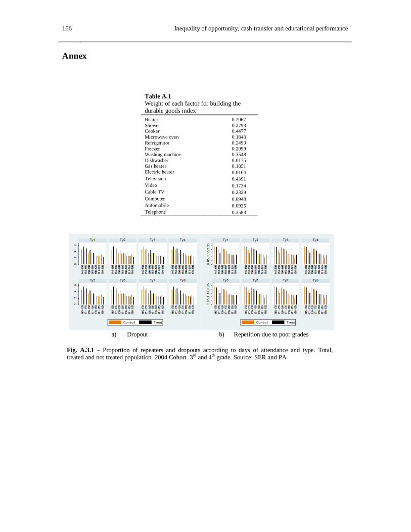
166 Inequality of opportunity, cash transfer and educational performance
Annex
Table A.1 Weight of each factor for building the durable goods index
Heater 0.2067 Shower 0.2793 Cooker 0.4477 Microwave oven 0.1843 Refrigerator 0.2490 Freezer 0.2099 Washing machine 0.3548 Dishwasher 0.0175 Gas heater 0.1851 Electric heater 0.0164 Television 0.4391 Video 0.1734 Cable TV 0.2329 Computer 0.0948 Automobile 0.0925 Telephone 0.3583
a) Dropout b) Repetition due to poor grades
Fig. A.3.1 – Proportion of repeaters and dropouts according to days of attendance and type. Total, treated and not treated population. 2004 Cohort. 3rd and 4th grade. Source: SER and PA
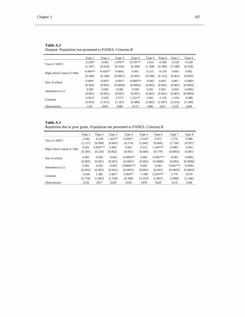
Chapter 3 167
Table A.2 Dropout. Population not presented to PANES. Criterion B
Type 1 Type 2 Type 3 Type 4 Type 5 Type 6 Type 7 Type 8
Year (1=2007) -2.299* -0.901 1.076** 0.570*** 1.614 -0.348 -0.529 -0.199 [1.397] [0.624] [0.524] [0.208] [1.268] [0.396] [1.188] [0.528]
High school course (1=4th) -0.984** -0.450** 0.0001 0.001 0.115 -0.156 -0.001 0.002 [0.388] [0.188] [0.0001] [0.001] [0.296] [0.123] [0.001] [0.003]
Size of school 0.004* 0.002* -0.001* -0.0005** -0.002 0.001 0.001 -0.0003 [0.002] [0.001] [0.0005] [0.0002] [0.002] [0.001] [0.001] [0.0005]
Attendence (t-1) -0.001 -0.001 -0.001 -0.001 0.001 0.001 -0.001 -0.0002 [0.001] [0.001] [0.001] [0.001] [0.001] [0.001] [0.001] [0.0003]
Constant -6.952* -2.625 2.272* 1.222** 3.601 -1.129 -1.356 -0.489 [3.814] [1.671] [1.187] [0.486] [3.482] [1.097] [2.676] [1.190]
Observations 2147 3920 2049 6173 1486 1631 1218 2349
Table A.3 Repetition due to poor grade. Population not presented to PANES. Criterion B
Type 1 Type 2 Type 3 Type 4 Type 5 Type 6 Type 7 Type 8
Year (1=2007) -2.092 -0.238 1.425** 0.439** -3.316* 0.973 2.770 0.088 [2.117] [0.694] [0.663] [0.174] [1.942] [0.668] [1.730] [0.597]
High school course (1=4th) 0.655 0.959*** 0.002 0.001 0.313 1.410*** 0.0001 -0.001 [0.593] [0.210] [0.002] [0.001] [0.460] [0.179] [0.0003] [0.001]
Size of school 0.002 -0.001 -0.001 -0.0004** 0.004 -0.002*** -0.003 -0.0001 [0.003] [0.001] [0.001] [0.0001] [0.003] [0.0008] [0.002] [0.0006]
Attendence (t-1) 0.002 -0.001 -0.002 -0.0006*** 0.002 -0.001 -0.002*** -0.0002 [0.002] [0.001] [0.001] [0.0002] [0.001] [0.001] [0.0005] [0.0003]
Constant -3.636 1.586 2.981* 0.968** -7.449 5.433*** 5.770 0.076 [5.754] [1.863] [1.528] [0.398] [5.353] [1.861] [3.896] [1.346]
Observations 2128 3917 2028 6165 1478 1629 1214 2348

168
Conclusions
In recent years there has been a significant increase in the literature attempting to measure inequality of opportunity. Some papers have attempted to quantify the effects of public policies on this type of inequality, particularly from the study of different tax systems, which has mainly been carried out in developed countries. Studies on the impact of other public policies on inequality of opportunity are not so common, especially in less developed countries. The thesis aims to contribute to the debate on the viability and impact of public policies, with an emphasis on what happens with inequality of opportunity.
I analyze one policy that may impact equality of opportunity in the long term, the increase in the number of public places available in schools aimed at early childhood, and another that may offset educational performance in the short term through income transfers. In the first case performance is measured from child development, while in the second I study a set of results in secondary education. I also analyze the population’s beliefs about the factors that lead to heterogeneity in income distribution, whether it is effort or circumstances, including, as a novelty, beliefs on the levels of equality that are considered optimal, when individuals have egalitarian criteria that are sensitive to responsibility or efficiency. This belief is recognized in the literature as one of the most important factors behind the decisions of the population to support or not support government programs aimed at changing the income distribution.
The first chapter of this thesis shows that the formation of beliefs about equal opportunities is based on reciprocity criteria and, therefore, that interaction with peers is fundamental. As such it is concluded that knowledge of heterogeneous life situations may be a powerful foundation for viable redistributive policies, and such interaction could be promoted by reducing residential segregation. In addition, in this chapter I demonstrate that considering only the income generating process as a way of measuring individuals’ perceptions of fairness overestimates the role played by this channel. Finally, I show that there is heterogeneity in the desirable optimal equality according to different domains of life. These differences are generated because people believe that effort better explains inequality in the labor market, while circumstances do so when considering inequalities in health, with education being an intermediate case.
In the second chapter I analyze the impact of school attendance on child development. I establish, as a novelty, the interaction between that attendance and parenting practices employed in the household. By using standardized tests to measure the cognitive, non-cognitive and motor skills of the children, the paper found that the MTE decreases slightly with the unobservable costs of sending the children to school in one component of the
170
ASQ-3: problem solving (always with positive effects). On the other hand, a positive effect was observed in the communication component of the same test, and this effect is independent of the unobservable costs. Regarding non-cognitive skills, approximated by the externalized problems of the CBCL, I found that school attendance does not change such problems among the children.
By analyzing the interaction with parenting practices it can be shown that school attendance complements appropriate parenting practices. As such, school attendance amplifies the gaps generated in the household, measured by several tests that approximate child development. This effect is particularly intensive among girls. Finally, I simulate an expansion of the supply of public school places for children aged 2 and 3, using two criteria: (i) a universal increase in supply in the different neighborhoods of Montevideo, and (ii) a targeted increase considering the current supply for children aged 4, which are concentrated in neighborhoods with worse socioeconomic performances. The simulations show that a universal increase produces better results in the average population when contrasted with a targeted increase, but that the latter policy reduces early childhood development inequality to a greater extent.
Finally, in the last chapter, I study how an income transfer policy affects inequality of opportunity measured by two types of educational performance: school dropout and repetition due to low grades. Using difference in differences estimates, I found that inequality of opportunity measured by repetition was reduced, although this is as a result of the repetition of teenagers with better circumstances increasing after the program. This can be explained by the fact that the program manages to reduce dropout in this group, but that this achievement does not translate to better academic performance. The paper culminates by analyzing changes in inequality of opportunities at the level of the entire population, as there are administrative records of all teenagers who attended secondary education. By carrying out the aforementioned extension the results remain the same, although the magnitude of the variation in inequality of opportunities is lesser.
