Journal of Hydrology (2006) 330, 641–650

ava i lab le a t www.sc iencedi rec t . com

journal homepage: www.elsevier .com/ locate / jhydrol

Errors and uncertainty in physically-basedrainfall-runoff modelling of catchment change effects

John Ewen, Greg O’Donnell *, Aidan Burton, Enda O’Connell

School of Civil Engineering and Geosciences, Cassie Building, University of Newcastle, Newcastle upon Tyne NE1 7RU, UK

Received 28 January 2005; received in revised form 17 April 2006; accepted 18 April 2006

Summary The error in physically-based rainfall-runoff modelling is broken into components,and these components are assigned to three groups: (1) model structure error, associated withthe model’s equations; (2) parameter error, associated with the parameter values used in theequations; and (3) run time error, associated with rainfall and other forcing data. The errorcomponents all contribute to ‘‘integrated’’ errors, such as the difference between simulatedand observed runoff, but their individual contributions cannot usually be isolated becausethe modelling process is complex and there is a lack of knowledge about the catchment andits hydrological responses. A simple model of the Slapton Wood Catchment is developed withina theoretical framework in which the catchment and its responses are assumed to be knownperfectly. This makes it possible to analyse the contributions of the error components whenpredicting the effects of a physical change in the catchment. The standard approach to predict-ing change effects involves: (1) running ‘‘unchanged’’ simulations using current parametersets; (2) making adjustments to the sets to allow for physical change; and (3) running ‘‘chan-ged’’ simulations. Calibration or uncertainty-handling methods such as GLUE are used to obtainthe current sets based on forcing and runoff data for a calibration period, by minimising or cre-ating statistical bounds for the ‘‘integrated’’ errors in simulations of runoff. It is shown thatcurrent parameter sets derived in this fashion are unreliable for predicting change effects,because of model structure error and its interaction with parameter error, so caution is neededif the standard approach is to be used when making management decisions about change incatchments.

�c 2006 Elsevier B.V. All rights reserved.

KEYWORDSModel error;Uncertainty;Catchment modelling;Rainfall-runoff modelling;Land use change

0d

022-1694/$ - see front matter �c 2006 Elsevier B.V. All rights reservedoi:10.1016/j.jhydrol.2006.04.024

* Corresponding author. Tel.: +44 191 222 6424.E-mail address: G.M.O’Donnell@ncl.ac.uk (G. O’Donnell).

Introduction

The physical processes that control runoff generation andflow routing in catchments are complex and highly variable.Rainfall-runoff models therefore invariably have imperfect

.

642 J. Ewen et al.

structures and use imperfect data, so from a mathematicalpoint of view it is impossible to validate a rainfall-runoffmodel (Oreskes et al., 1994) or to carry out a full analysisof errors. In calibration, and in error and uncertainty analy-ses, rainfall-runoff modellers usually work only with ‘‘inte-grated’’ errors, such as the difference between thesimulated and observed runoff at the catchment outlet.These ‘‘integrated’’ errors are the result of errors intro-duced at all stages of the modelling process, including thedesign and construction stages, and of the processing ofthese errors during simulations.

The parameters in physically-based models representphysical properties that are defined in terms of small-scale physics, such as hydraulic conductivity defined interms of Darcy’s law. This explains why physically-basedmodels are sometimes used to predict the effects of phys-ical change in catchments: (1) there is a direct link be-tween the parameters and the physical processes andproperties; and (2) the sensitivity to the parameters is(assumed to be) accurate in physically-based modelling,because of the physical basis (e.g. see De Roo et al.,2001; Dunn and MacKay, 1995, 1996; Ewen and Parkin,1996; Lukey et al., 2000; Nandakumar and Mein, 1997;Niehoff et al., 2002; Parkin et al., 1996; Storck et al.,1998).

In their most basic form, predictions of change involvecomparing an ‘‘unchanged’’ and a ‘‘changed’’ simulationfor the same time period: one simulation assuming that a gi-ven change had not taken place prior to the start of the per-iod and the other assuming that it had.

An error classification is developed here so that ‘‘inte-grated’’ error can be treated as if it comprises several errorcomponents, and a form of ‘‘partial analysis’’ (see Kuhnelet al., 1991) is used to investigate the nature and effectof some of these components. The object in ‘‘partial anal-ysis’’ is to bypass some of the difficulties of a problem, inthis case the impossibility of validation, but to retain the es-sence of the important features. A simple one-parameterphysically-based model is created and is assumed be an ex-act and complete (i.e. perfect) representation of the Slap-ton Wood Catchment, and this perfect model is run togive perfect values for runoff and for the change in runoffassociated with a physical change in the catchment. Anapproximate model of the catchment is then created andthe error components analysed when this model is used tomake predictions for runoff and the effects of catchmentchange on runoff.

This is a simple and direct approach, when comparedto the mathematical and statistical approaches sometimesused to study errors in rainfall-runoff modelling (e.g. seeDuan et al., 2002). The aim is to demonstrate one ofthe fundamental problems involved in estimating the‘‘integrated’’ error in predictions of catchment change.Once the problem has been demonstrated, conclusionsare drawn about the usefulness or otherwise of some ofthe mathematical and statistical approaches. As part ofthe demonstration, the generalized likelihood uncertaintyestimation method (GLUE, Beven and Binley, 1992) is usedto estimate the uncertainty in (i.e. a likely range for) the‘‘integrated’’ error in predictions of catchment changemade using the approximate Slapton Wood CatchmentModel.

Error components

Errors are introduced at every stage of the modelling pro-cess, and most introduced errors will affect the ‘‘inte-grated’’ error. To give a simple example, a mistake intyping in a parameter value (e.g. typing ‘‘3’’ instead of‘‘30’’) might contribute to the ‘‘integrated’’ error. Its con-tribution will depend on how its effect propagates throughthe model calculations and interacts with the model struc-ture, the other model parameters, the forcing data, andthe other errors. The term ‘‘forcing data’’ is used in thedefinition of the error components in a catch-all sense, toinclude data directly or indirectly used in calculating rain-fall, evaporation, and boundary heads and flows, and alsoany observed or synthetic response data (e.g. assimilationdata) which are used to help control the simulations.

Table 1 shows only one of several ways that ‘‘inte-grated’’ error can be broken into components, in threegroups: (1) model structure error, associated with the mod-el’s equations; (2) parameter error, associated with theparameter values used in the equations; and (3) run time er-ror, associated with forcing data. The sources for the com-ponents are listed in order in the table. For model structureerror, for example, starting from the ‘‘truth’’ about thecatchment, the first component (M1) is associated withassuming the ‘‘truth’’ can be represented in an abstractform, as a model. Then there is simplification (M2), to apractical form. Next there is approximation (M3), includingthe introduction of discrete time and space scales. The onlyother error component assigned in Table 1 to model struc-ture error is mistakes (M4) made in designing and construct-ing the model. The following are a few notes about the errorcomponents:

M1 It is a philosophical question whether any model canexactly represent the truth, so even the best possiblemodel might give ‘‘integrated’’ error

M2 From conceptual and mathematical simplificationM3 From using approximate numerical solutions, finite

timesteps, etcM4 From conceptual, mathematical and programming

mistakes made by the modellerP1 From incomplete or erroneous calibration data

(i.e. forcing and response data used in calibration)P2 From the calibration process, to compensate for model

structure errorP3 From not using the optimum parameter valuesP4 From mistakes made by the modeller in setting

parameter values (the typing error described abovecontributes to component P4)

R1 From incomplete and erroneous forcing dataR2 From mistakes in forcing data made by the modeller

and from mistakes in the way the model is used andthe results interpreted

In a general sense, the ‘‘integrated’’ error for any simu-lation is the sum of the model structure error, parametererror, and run time error, but there can be interactionsbetween the error components, so this is not a simple sum-mation of positive numbers. Consider, for example, a cali-brated model which gives accurate simulations, but for

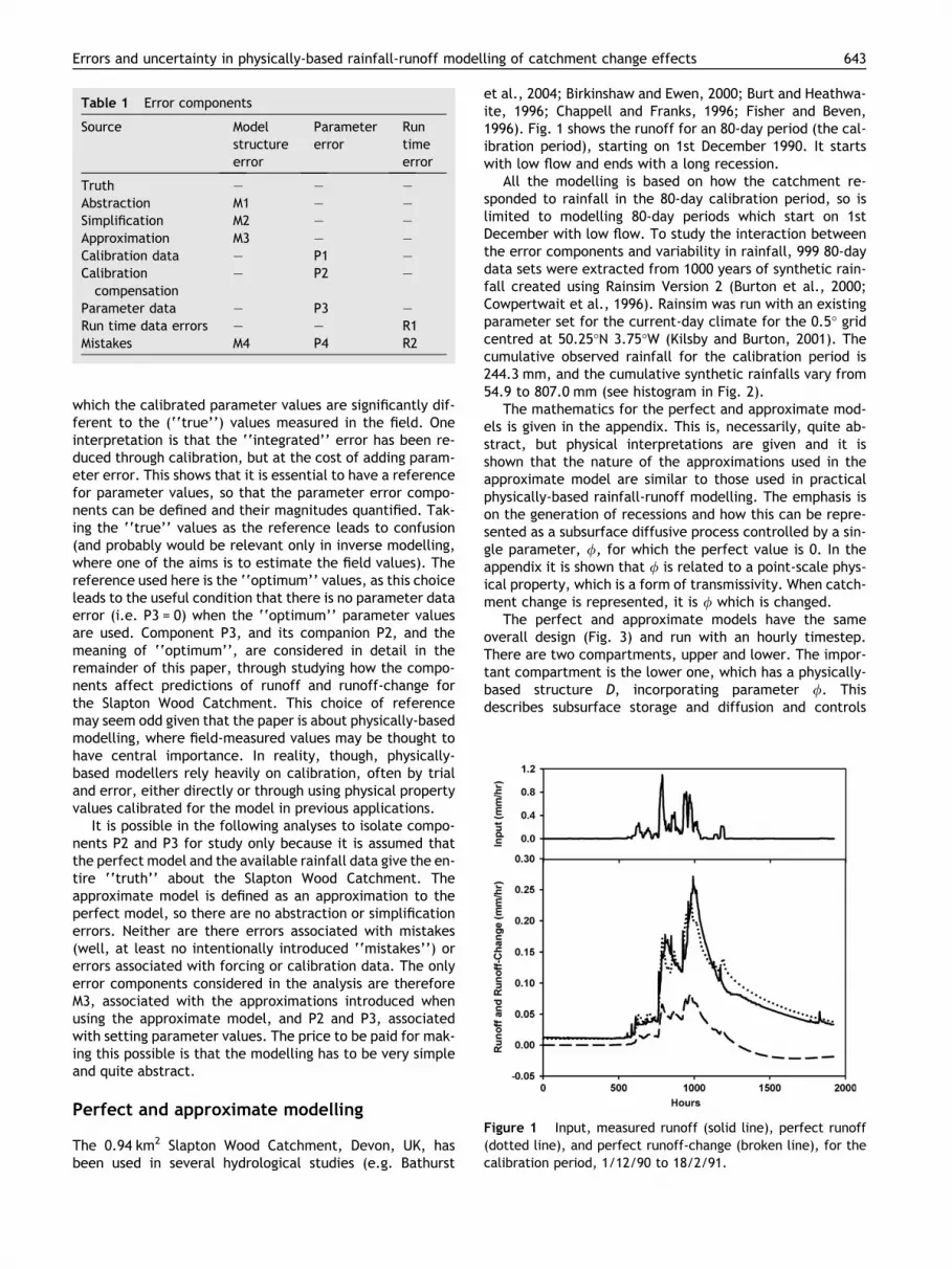
Figure 1 Input, measured runoff (solid line), perfect runoff(dotted line), and perfect runoff-change (broken line), for thecalibration period, 1/12/90 to 18/2/91.

Table 1 Error components

Source Modelstructureerror

Parametererror

Runtimeerror

Truth – – –Abstraction M1 – –Simplification M2 – –Approximation M3 – –Calibration data – P1 –Calibrationcompensation

– P2 –

Parameter data – P3 –Run time data errors – – R1Mistakes M4 P4 R2

Errors and uncertainty in physically-based rainfall-runoff modelling of catchment change effects 643

which the calibrated parameter values are significantly dif-ferent to the (‘‘true’’) values measured in the field. Oneinterpretation is that the ‘‘integrated’’ error has been re-duced through calibration, but at the cost of adding param-eter error. This shows that it is essential to have a referencefor parameter values, so that the parameter error compo-nents can be defined and their magnitudes quantified. Tak-ing the ‘‘true’’ values as the reference leads to confusion(and probably would be relevant only in inverse modelling,where one of the aims is to estimate the field values). Thereference used here is the ‘‘optimum’’ values, as this choiceleads to the useful condition that there is no parameter dataerror (i.e. P3 = 0) when the ‘‘optimum’’ parameter valuesare used. Component P3, and its companion P2, and themeaning of ‘‘optimum’’, are considered in detail in theremainder of this paper, through studying how the compo-nents affect predictions of runoff and runoff-change forthe Slapton Wood Catchment. This choice of referencemay seem odd given that the paper is about physically-basedmodelling, where field-measured values may be thought tohave central importance. In reality, though, physically-based modellers rely heavily on calibration, often by trialand error, either directly or through using physical propertyvalues calibrated for the model in previous applications.

It is possible in the following analyses to isolate compo-nents P2 and P3 for study only because it is assumed thatthe perfect model and the available rainfall data give the en-tire ‘‘truth’’ about the Slapton Wood Catchment. Theapproximate model is defined as an approximation to theperfect model, so there are no abstraction or simplificationerrors. Neither are there errors associated with mistakes(well, at least no intentionally introduced ‘‘mistakes’’) orerrors associated with forcing or calibration data. The onlyerror components considered in the analysis are thereforeM3, associated with the approximations introduced whenusing the approximate model, and P2 and P3, associatedwith setting parameter values. The price to be paid for mak-ing this possible is that the modelling has to be very simpleand quite abstract.

Perfect and approximate modelling

The 0.94 km2 Slapton Wood Catchment, Devon, UK, hasbeen used in several hydrological studies (e.g. Bathurst

et al., 2004; Birkinshaw and Ewen, 2000; Burt and Heathwa-ite, 1996; Chappell and Franks, 1996; Fisher and Beven,1996). Fig. 1 shows the runoff for an 80-day period (the cal-ibration period), starting on 1st December 1990. It startswith low flow and ends with a long recession.

All the modelling is based on how the catchment re-sponded to rainfall in the 80-day calibration period, so islimited to modelling 80-day periods which start on 1stDecember with low flow. To study the interaction betweenthe error components and variability in rainfall, 999 80-daydata sets were extracted from 1000 years of synthetic rain-fall created using Rainsim Version 2 (Burton et al., 2000;Cowpertwait et al., 1996). Rainsim was run with an existingparameter set for the current-day climate for the 0.5� gridcentred at 50.25�N 3.75�W (Kilsby and Burton, 2001). Thecumulative observed rainfall for the calibration period is244.3 mm, and the cumulative synthetic rainfalls vary from54.9 to 807.0 mm (see histogram in Fig. 2).

The mathematics for the perfect and approximate mod-els is given in the appendix. This is, necessarily, quite ab-stract, but physical interpretations are given and it isshown that the nature of the approximations used in theapproximate model are similar to those used in practicalphysically-based rainfall-runoff modelling. The emphasis ison the generation of recessions and how this can be repre-sented as a subsurface diffusive process controlled by a sin-gle parameter, /, for which the perfect value is 0. In theappendix it is shown that / is related to a point-scale phys-ical property, which is a form of transmissivity. When catch-ment change is represented, it is / which is changed.

The perfect and approximate models have the sameoverall design (Fig. 3) and run with an hourly timestep.There are two compartments, upper and lower. The impor-tant compartment is the lower one, which has a physically-based structure D, incorporating parameter /. Thisdescribes subsurface storage and diffusion and controls

Figure 2 Relative frequency of cumulative rainfall, andcumulative input versus cumulative rainfall, for the 1000periods.

644 J. Ewen et al.

the runoff, q. The structure in the upper compartment, U, isnot physically based, but its role, in an abstract sense, issimply to manipulate the rainfall, r, to supply the input, i,to the lower compartment.

In total there are three structures: a structure for U,which is used for both the perfect and approximate model-ling, and the perfect and approximate structures for D. Run-off measurements for the calibration period were usedwhen designing and parameterising the perfect model, tomake it as physically realistic as possible within the con-straints of simple modelling. This involved creating struc-ture U and the perfect structure D, and calibrating themboth (i.e. calibrating the ‘‘perfect’’ model) against therainfall and runoff measurements for the calibration period.Mathematically, the approximate structure for D is a re-duced version of the perfect structure for D, and has thesame single parameter, /. To make it practical to test everypossibility when calibrating the approximate model, it is as-sumed that / has a resolution of 0.01 and a limited range,�1 6 / 6 1. This means that / can take only 201 differentvalues (i.e. �1,�0.99,�0.98, . . .,0.99,1).

In the analyses, the runoff simulated by the perfectmodel is assumed to be the ‘‘true’’ runoff, so the runoff

Figure 3 Schematic of Slapton Wood Catchment Model.

measurements were discarded once the perfect model wascreated. The measured and perfect runoff for the calibra-tion period can be compared in Fig. 1, which also showsthe input to the lower compartment. The efficiency (E)for the comparison is 0.930: E ¼ 1� r2

e=r2o, where r2

e isthe variance of the residuals and r2

o the variance of the mea-sured runoff.

Fig. 1 also shows the difference (i.e. the perfect runoff-change) associated with increasing / by 0.3, found by takingthe difference in runoff between perfect simulations with /= 0.3 and / = 0. This increase causes the runoff to be higher(positive runoff-change) during the wet period and lower(negative runoff-change) during the second part of therecession. All the results for runoff-change in the analysesare for a change in / of 0.3. This change corresponds toan approximate doubling in the value of the point-scalephysical property.

Predicting runoff

Fig. 4 shows that efficiency varies systematically with /when using the approximate model to predict the runoffin the calibration period. It is 0.795 at the perfect value(/ = 0) and 0.909 at the optimum, / = 0.23. The ‘‘inte-grated’’ error (as given by the efficiency deficit) is thereforeat a minimum at / = 0.23. This bias of 0.23 can be explainedpartly by the difference between the (linear) unit hydro-graphs for the perfect and approximate models (see Appen-dix) and partly by the interaction between the rainfalltimeseries and the efficiency, E, which is a non-linearsum. If one of the 999 synthetic rainfall periods is selectedand used instead of the calibration period, then the result-ing E plot will be similar in shape to that in Fig. 4, but theoptimum / can be different. Fig. 5 shows the optimum /for each of the 1000 periods. It varies from 0.2 to 0.64, sois always significantly greater than the perfect value, /= 0. The optimum is 0.23 for only 97 of the periods.

Calibrating rainfall-runoff models always implicitly in-volves a form of compensation, in which part of the effectof model structure error is compensated for by ‘‘falsely’’adjusting the model’s parameters. For the calibration

Figure 4 Efficiencies for runoff (solid line) and runoff-change(broken line) for the calibration period.

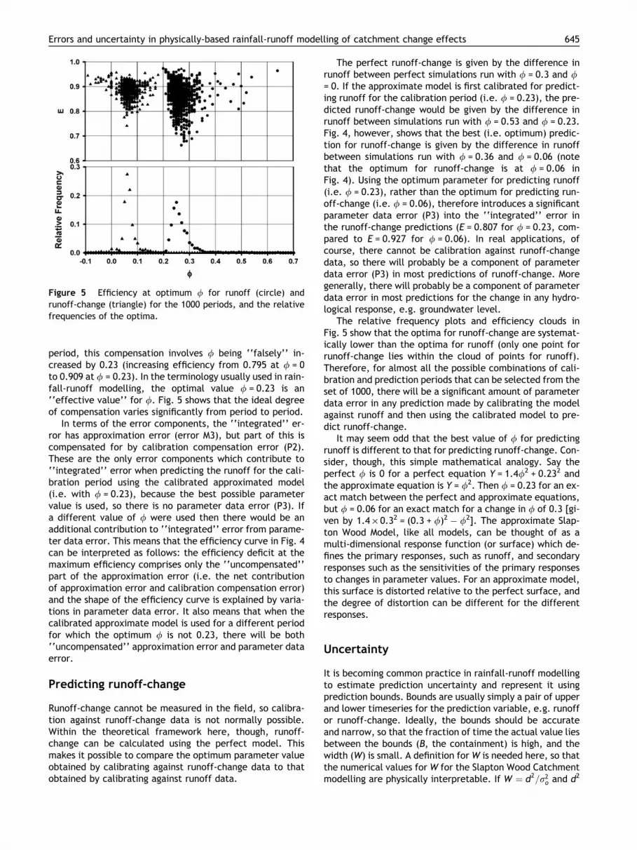
Figure 5 Efficiency at optimum / for runoff (circle) andrunoff-change (triangle) for the 1000 periods, and the relativefrequencies of the optima.

Errors and uncertainty in physically-based rainfall-runoff modelling of catchment change effects 645

period, this compensation involves / being ‘‘falsely’’ in-creased by 0.23 (increasing efficiency from 0.795 at / = 0to 0.909 at / = 0.23). In the terminology usually used in rain-fall-runoff modelling, the optimal value / = 0.23 is an‘‘effective value’’ for /. Fig. 5 shows that the ideal degreeof compensation varies significantly from period to period.

In terms of the error components, the ‘‘integrated’’ er-ror has approximation error (error M3), but part of this iscompensated for by calibration compensation error (P2).These are the only error components which contribute to‘‘integrated’’ error when predicting the runoff for the cali-bration period using the calibrated approximated model(i.e. with / = 0.23), because the best possible parametervalue is used, so there is no parameter data error (P3). Ifa different value of / were used then there would be anadditional contribution to ‘‘integrated’’ error from parame-ter data error. This means that the efficiency curve in Fig. 4can be interpreted as follows: the efficiency deficit at themaximum efficiency comprises only the ‘‘uncompensated’’part of the approximation error (i.e. the net contributionof approximation error and calibration compensation error)and the shape of the efficiency curve is explained by varia-tions in parameter data error. It also means that when thecalibrated approximate model is used for a different periodfor which the optimum / is not 0.23, there will be both‘‘uncompensated’’ approximation error and parameter dataerror.

Predicting runoff-change

Runoff-change cannot be measured in the field, so calibra-tion against runoff-change data is not normally possible.Within the theoretical framework here, though, runoff-change can be calculated using the perfect model. Thismakes it possible to compare the optimum parameter valueobtained by calibrating against runoff-change data to thatobtained by calibrating against runoff data.

The perfect runoff-change is given by the difference inrunoff between perfect simulations run with / = 0.3 and /= 0. If the approximate model is first calibrated for predict-ing runoff for the calibration period (i.e. / = 0.23), the pre-dicted runoff-change would be given by the difference inrunoff between simulations run with / = 0.53 and / = 0.23.Fig. 4, however, shows that the best (i.e. optimum) predic-tion for runoff-change is given by the difference in runoffbetween simulations run with / = 0.36 and / = 0.06 (notethat the optimum for runoff-change is at / = 0.06 inFig. 4). Using the optimum parameter for predicting runoff(i.e. / = 0.23), rather than the optimum for predicting run-off-change (i.e. / = 0.06), therefore introduces a significantparameter data error (P3) into the ‘‘integrated’’ error inthe runoff-change predictions (E = 0.807 for / = 0.23, com-pared to E = 0.927 for / = 0.06). In real applications, ofcourse, there cannot be calibration against runoff-changedata, so there will probably be a component of parameterdata error (P3) in most predictions of runoff-change. Moregenerally, there will probably be a component of parameterdata error in most predictions for the change in any hydro-logical response, e.g. groundwater level.

The relative frequency plots and efficiency clouds inFig. 5 show that the optima for runoff-change are systemat-ically lower than the optima for runoff (only one point forrunoff-change lies within the cloud of points for runoff).Therefore, for almost all the possible combinations of cali-bration and prediction periods that can be selected from theset of 1000, there will be a significant amount of parameterdata error in any prediction made by calibrating the modelagainst runoff and then using the calibrated model to pre-dict runoff-change.

It may seem odd that the best value of / for predictingrunoff is different to that for predicting runoff-change. Con-sider, though, this simple mathematical analogy. Say theperfect / is 0 for a perfect equation Y = 1.4/2 + 0.232 andthe approximate equation is Y = /2. Then / = 0.23 for an ex-act match between the perfect and approximate equations,but / = 0.06 for an exact match for a change in / of 0.3 [gi-ven by 1.4 · 0.32 = (0.3 + /)2 � /2]. The approximate Slap-ton Wood Model, like all models, can be thought of as amulti-dimensional response function (or surface) which de-fines the primary responses, such as runoff, and secondaryresponses such as the sensitivities of the primary responsesto changes in parameter values. For an approximate model,this surface is distorted relative to the perfect surface, andthe degree of distortion can be different for the differentresponses.

Uncertainty

It is becoming common practice in rainfall-runoff modellingto estimate prediction uncertainty and represent it usingprediction bounds. Bounds are usually simply a pair of upperand lower timeseries for the prediction variable, e.g. runoffor runoff-change. Ideally, the bounds should be accurateand narrow, so that the fraction of time the actual value liesbetween the bounds (B, the containment) is high, and thewidth (W) is small. A definition for W is needed here, so thatthe numerical values for W for the Slapton Wood Catchmentmodelling are physically interpretable. If W ¼ d2=r2

o and d2

646 J. Ewen et al.

is the mean square of half the distance between the bounds,thenW = 1 corresponds to bounds which have a spread equalto the spread of the prediction variable (e.g. runoff) aboutits mean. Bounds which are narrow will have W values ofmuch less than 1 (typically 0.2 or less).

The most widely used method for handling uncertainty isprobably the GLUE method (Beven and Binley, 1992). Theprocess of applying GLUE is usually, essentially, as follows.Parameter sets are chosen at random and are ranked basedon their efficiency (or some other measure of quality) whenused to simulate runoff for a calibration period. The mostefficient parameter sets (e.g. with E greater than somespecified threshold value) are then taken as being ‘‘behav-ioural’’ and the rest are eliminated as being ‘‘non-behav-ioural’’. When making a prediction for a predictionperiod, simulations are run for all the ‘‘behavioural’’parameter sets and bounds are created using the simulatedrunoff. This is all carried out within a statistical framework,giving a link between the properties of the bounds and anystatistical properties attributed to the parameter spacefrom which the random choices are made, such as probabil-ity distributions for the parameter values.

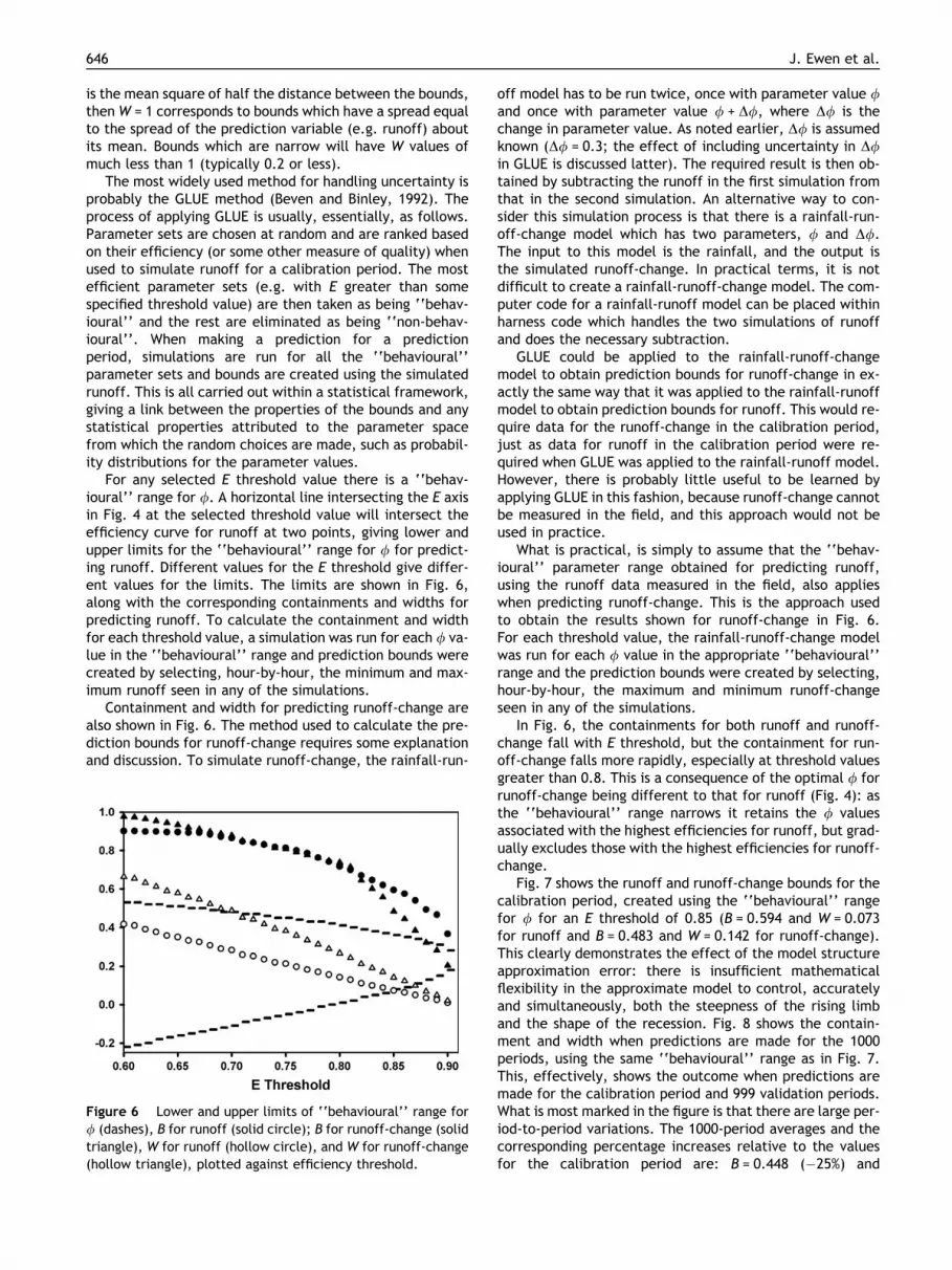
For any selected E threshold value there is a ‘‘behav-ioural’’ range for /. A horizontal line intersecting the E axisin Fig. 4 at the selected threshold value will intersect theefficiency curve for runoff at two points, giving lower andupper limits for the ‘‘behavioural’’ range for / for predict-ing runoff. Different values for the E threshold give differ-ent values for the limits. The limits are shown in Fig. 6,along with the corresponding containments and widths forpredicting runoff. To calculate the containment and widthfor each threshold value, a simulation was run for each / va-lue in the ‘‘behavioural’’ range and prediction bounds werecreated by selecting, hour-by-hour, the minimum and max-imum runoff seen in any of the simulations.

Containment and width for predicting runoff-change arealso shown in Fig. 6. The method used to calculate the pre-diction bounds for runoff-change requires some explanationand discussion. To simulate runoff-change, the rainfall-run-

Figure 6 Lower and upper limits of ‘‘behavioural’’ range for/ (dashes), B for runoff (solid circle); B for runoff-change (solidtriangle), W for runoff (hollow circle), and W for runoff-change(hollow triangle), plotted against efficiency threshold.

off model has to be run twice, once with parameter value /and once with parameter value / + D/, where D/ is thechange in parameter value. As noted earlier, D/ is assumedknown (D/ = 0.3; the effect of including uncertainty in D/in GLUE is discussed latter). The required result is then ob-tained by subtracting the runoff in the first simulation fromthat in the second simulation. An alternative way to con-sider this simulation process is that there is a rainfall-run-off-change model which has two parameters, / and D/.The input to this model is the rainfall, and the output isthe simulated runoff-change. In practical terms, it is notdifficult to create a rainfall-runoff-change model. The com-puter code for a rainfall-runoff model can be placed withinharness code which handles the two simulations of runoffand does the necessary subtraction.

GLUE could be applied to the rainfall-runoff-changemodel to obtain prediction bounds for runoff-change in ex-actly the same way that it was applied to the rainfall-runoffmodel to obtain prediction bounds for runoff. This would re-quire data for the runoff-change in the calibration period,just as data for runoff in the calibration period were re-quired when GLUE was applied to the rainfall-runoff model.However, there is probably little useful to be learned byapplying GLUE in this fashion, because runoff-change cannotbe measured in the field, and this approach would not beused in practice.

What is practical, is simply to assume that the ‘‘behav-ioural’’ parameter range obtained for predicting runoff,using the runoff data measured in the field, also applieswhen predicting runoff-change. This is the approach usedto obtain the results shown for runoff-change in Fig. 6.For each threshold value, the rainfall-runoff-change modelwas run for each / value in the appropriate ‘‘behavioural’’range and the prediction bounds were created by selecting,hour-by-hour, the maximum and minimum runoff-changeseen in any of the simulations.

In Fig. 6, the containments for both runoff and runoff-change fall with E threshold, but the containment for run-off-change falls more rapidly, especially at threshold valuesgreater than 0.8. This is a consequence of the optimal / forrunoff-change being different to that for runoff (Fig. 4): asthe ‘‘behavioural’’ range narrows it retains the / valuesassociated with the highest efficiencies for runoff, but grad-ually excludes those with the highest efficiencies for runoff-change.

Fig. 7 shows the runoff and runoff-change bounds for thecalibration period, created using the ‘‘behavioural’’ rangefor / for an E threshold of 0.85 (B = 0.594 and W = 0.073for runoff and B = 0.483 and W = 0.142 for runoff-change).This clearly demonstrates the effect of the model structureapproximation error: there is insufficient mathematicalflexibility in the approximate model to control, accuratelyand simultaneously, both the steepness of the rising limband the shape of the recession. Fig. 8 shows the contain-ment and width when predictions are made for the 1000periods, using the same ‘‘behavioural’’ range as in Fig. 7.This, effectively, shows the outcome when predictions aremade for the calibration period and 999 validation periods.What is most marked in the figure is that there are large per-iod-to-period variations. The 1000-period averages and thecorresponding percentage increases relative to the valuesfor the calibration period are: B = 0.448 (�25%) and

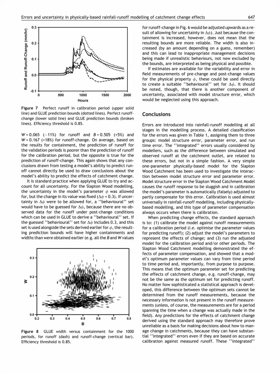
Figure 7 Perfect runoff in calibration period (upper solidline) and GLUE prediction bounds (dotted lines). Perfect runoff-change (lower solid line) and GLUE prediction bounds (brokenlines). Efficiency threshold is 0.85.

Errors and uncertainty in physically-based rainfall-runoff modelling of catchment change effects 647

W = 0.065 (�11%) for runoff and B = 0.505 (+5%) andW = 0.167 (+18%) for runoff-change. On average, based onthe results for containment, the prediction of runoff forthe validation periods is poorer than the prediction of runofffor the calibration period, but the opposite is true for theprediction of runoff-change. This again shows that any con-clusions drawn from testing a model’s ability to predict run-off cannot directly be used to draw conclusions about themodel’s ability to predict the effects of catchment change.

It is standard practice when applying GLUE to try and ac-count for all uncertainty. For the Slapton Wood modelling,the uncertainty in the model’s parameter / was allowedfor, but the change in its value was fixed (D/ = 0.3). If uncer-tainty in D/ were to be allowed for, a ‘‘behavioural’’ setwould have to be guessed for D/, because there are no ob-served data for the runoff under post-change conditionswhich can be used in GLUE to derive a ‘‘behavioural’’ set. Ifthe guessed ‘‘behavioural’’ set for D/ includes 0.3, and thisset is used alongside the sets derived earlier for/, the result-ing prediction bounds will have higher containments andwidths than were obtained earlier (e.g. all the B andW values

Figure 8 GLUE width versus containment for the 1000periods, for runoff (dash) and runoff-change (vertical bar).Efficiency threshold is 0.85.

for runoff-change in Fig. 6 would be adjusted upwards as a re-sult of allowing for uncertainty in D/). Just because the con-tainment is increased, however, does not mean that theresulting bounds are more reliable. The width is also in-creased (by an amount depending on a guess, remember)and this can lead to inappropriate management decisionsbeing made if unrealistic behaviours, not now excluded bythe bounds, are interpreted as being physical and possible.

If estimates are available for the variability and error infield measurements of pre-change and post-change valuesfor the physical property /, these could be used directlyto create a suitable ‘‘behavioural’’ set for D/. It shouldbe noted, though, that there is another component ofuncertainty, associated with model structure error, whichwould be neglected using this approach.

Conclusions

Errors are introduced into rainfall-runoff modelling at allstages in the modelling process. A detailed classificationfor the errors was given in Table 1, assigning them to threegroups: model structure error, parameter error, and runtime error. The ‘‘integrated’’ errors usually considered bymodellers, such as the difference between simulated andobserved runoff at the catchment outlet, are related tothese errors, but not in a simple fashion. A very simpleone-parameter physically-based model for the SlaptonWood Catchment has been used to investigate the interac-tion between model structure error and parameter error.Model structure error in the Slapton Wood Catchment Modelcauses the runoff response to be sluggish and in calibrationthe model’s parameter is automatically (falsely) adjusted topartly compensate for this error. Calibration is used almostuniversally in rainfall-runoff modelling, including physically-based modelling, and this type of parameter compensationalways occurs when there is calibration.

When predicting change effects, the standard approachis to: (1) calibrate the model against runoff measurementsfor a calibration period (i.e. optimise the parameter valuesfor predicting runoff); (2) adjust the model’s parameters torepresent the effects of change; and (3) run the adjustedmodel for the calibration period and/or other periods. TheSlapton Wood Catchment modelling demonstrated the ef-fects of parameter compensation, and showed that a mod-el’s optimum parameter values can vary from time periodto time period and, importantly, from purpose to purpose.This means that the optimum parameter set for predictingthe effects of catchment change, e.g. runoff-change, maynot be the same as the optimum set for predicting runoff.No matter how sophisticated a statistical approach is devel-oped, this difference between the optimum sets cannot bedetermined from the runoff measurements, because thenecessary information is not present in the runoff measure-ments (unless, of course, the measurements are for a periodspanning the time when a change was actually made in thefield). Any predictions for the effects of catchment changederived using the standard approach may therefore proveunreliable as a basis for making decisions about how to man-age change in catchments, because they can have substan-tial ‘‘integrated’’ errors even if they are based on accuratecalibration against measured runoff. These ‘‘integrated’’

648 J. Ewen et al.

errors arise from assuming (wrongly) that the effect ofparameter compensation will be exactly the same when pre-dicting catchment change as when predicting runoff.

The argument usually made for using an uncertainty-han-dling method such as GLUE instead of calibration is that itimproves the reliability of any conclusions or decisionswhich are based on predictions. It does this by giving an esti-mate for the likely range of the ‘‘integrated’’ error for thepredictions, as prediction bounds. Two measures were de-fined for the quality of GLUE prediction bounds: the con-tainment, B, which is the fraction of time that the actualresponse lies between the prediction bounds, and the widthof the bounds, W. For the bounds to be reliable, the con-tainment must be high and the width must be small (to re-duce the likelihood that inappropriate managementdecisions will be made). This means that reliability dependson both B and W.

Viewed solely in terms of the mechanics of its applica-tion, and leaving to one side any arguments about theunderlying statistical theory, GLUE simply extends the con-cept of calibration. Instead of finding just a single (optimal)set of parameter values, several sets (the ‘‘behavioural’’sets) are found. The choice of the efficiency threshold inGLUE is subjective, and it essentially behaves like a tuningknob, which can be turned up or down to adjust the numberof ‘‘behavioural’’ sets, with the consequence of adjusting Band W. If the knob is turned to one extreme, so there is onlyone ‘‘behavioural’’ set, this set will simply be the optimalset that would be obtained by calibration. By viewing GLUEfrom this perspective, as an extension of calibration, it canbe concluded that GLUE is unreliable as a basis for makingdecisions about catchment change, for exactly the samereason that calibration is unreliable.

It is possible to use systematic methods to select the effi-ciency threshold, using runoff data for a calibration period.For example, the tuning knob can be adjusted until it givessome prescribed containment (e.g. 95% containment). How-ever, even if such an approach proves reliable when predict-ing runoff, in validation tests, it may be unreliable forpredicting the effects of catchment change using the stan-dard approach, because of the parameter compensationproblem.

Predictions of change made using a rainfall-runoff modeldepend on the model structure, and in particular on theway that the structure controls the change in runoff associ-ated with changes in the values of the model’s parameters.If data are available for the effects of catchment change onrunoff, these sensitivities to parameter change can be testedand the structures of existing models can be improved, ornew structures developed. There are, though, very few datasets for catchment change (e.g. see O’Connell et al., 2005),so it is difficult to see how significant progress can be madein developing and improving model structures unless thereare major programmes of fieldwork where data sets are col-lected for a wide range of different catchments and changes.

Appendix. Perfect and approximate modelling

Schematically, the perfect and approximate models canboth be represented by Fig. 3, where the inputs, outputs

and internal exchanges are as follows: r rainfall, e evapora-tion, i input to the lower compartment, and q runoff. Theupper compartment, containing structure U, describes sur-face and near-surface processes, including infiltration, per-colation, evaporation, and storage, while the lowercompartment, containing structure D, is physically basedand describes subsurface storage and diffusion (i.e. the pro-cess giving rise to the exponential decay recessions seen inthe runoff measurements).

The simplest physical, distributed equation which de-scribes diffusive behaviour is the heat equation, so treatingthe input, i, as if it is uniform recharge, the perfect struc-ture for D is chosen to be:

os

ot¼ k

o2s

ox2þ i; ðA:1Þ

where, in appropriate units: i(t) (mm/h) is the input, k (m2/h) the (uniform) physical characteristic, s(x,t) (mm) the lo-cal storage, t (h) time, and x (m) is distance. The local stor-age is assumed to be initially zero, and the boundaryconditions are s(0,t) = 0, and os/ox(L,t) = 0, where L (m)is a length. A physical interpretation is that there is point-scale diffusion and the catchment comprises a set of similarhillslopes, where L is hillslope length and k is a form oftransmissivity. For this interpretation, there is a subsurfacewatershed at x = L and the head is constant at the dischargepoint, x = 0.

The volumetric runoff rate per unit catchment area(mm/h) is:

q ¼ kL�1os

oxat x ¼ 0: ðA:2Þ

One of the unusual features of this model is that q can beevaluated exactly using a simple analogue, as the sum ofthe discharges from an infinite set of parallel buckets (i.e.linear reservoirs). Numbering the buckets n = 1,2,3, . . .:

q ¼ bþX1n¼1

qn; ðA:3Þ

where qn is the discharge rate for bucket n, and b(=0.01 mm/h) has been added to account for baseflow (va-lue taken directly from Fig. 1).

The storage equation for bucket n is:

dsndt¼ bni� ab�1n sn; ðA:4Þ

where a = 2k/L2 (h�1) (calibrated perfect value:ap = 1.5 · 10�3 h�1), and,

bn ¼8

p2ð2n� 1Þ2: ðA:5Þ

This bucket analogue was derived by working backwardsfrom the series solution for the heat equation given in Car-slaw and Jaeger (1959). It can be seen that the input tobucket n is fraction bn of the total input and the rate of dis-charge is linearly proportional to the bucket storage, sn.Only the largest buckets play a significant role, because bn

falls rapidly with n (b1 = 0.81057; b2 = 0.09006;b3 = 0.03242; . . .; b50 = 0.00008). To ensure that the perfectrepresentation is accurate it includes the first 50 buckets.The other buckets (numbers 51,52, . . .) are small and drainvery quickly, so they are assumed to be bypassed, in that

Errors and uncertainty in physically-based rainfall-runoff modelling of catchment change effects 649

their input will appear immediately as discharge. Just over0.4% of the total input will bypass these small buckets. Thisapproach conserves mass but introduces timing errors.These errors will be extremely small, however, as any waterstored in the small buckets has a very short half-life. Thelongest half-life for any bypassed bucket is 132 s.

Eq. (A.4) can be solved and an equation derived for thedischarge from the buckets. The discharge during the(N + 1)th hour from bucket n is:

qNþ1n ¼ sNn þ bni

Nþ1 � sNþ1n ; ðA:6Þ

where sNn is the storage in bucket n at time N, s0n ¼ 0, and

sNþ1n ¼ a�1b2ni

Nþ1 þ sNn � a�1b2ni

Nþ1� �e�a=bn : ðA:7Þ

For convenience, in the perfect and approximate modelsthe parameter / is used in place of a, where a = ap10

/ (so0 is the perfect value for /).

Mathematically, the approximate structure for D is a re-duced version of the perfect structure, comprising only asingle bucket (b1 = 1 and bm = 0 where m 5 1). A physicalinterpretation for the approximate structure D is that thepoint-scale diffusion and hillslope analogies for the perfectstructure still apply, but the storage is always linearly dis-tributed such that the gradient everywhere is 2s/L.

There is similarity between the way the single bucket isused as an approximation for the heat equation and theway that finite-difference equations are used as approxima-tions to the governing equations in distributed physically-based models (DPBMs) such as SHETRAN (Ewen et al.,2000). In both cases, the approximations assume that stor-age is distributed linearly over large scales. For the singlebucket, this scale is the catchment scale, and for DPBMs itis the grid scale, typically several hundred metres. A bucketis also a suitable choice as the approximate structure be-cause buckets are used quite widely in rainfall-runoff mod-elling (Beven, 2001), singly and in many differentcombinations. A parallel pair of fast and slow draining buck-ets is used, for example, in the PDM model (Moore andClarke, 1981).

Figure A1 Perfect (solid line) and approximate (broken line)approximate (dotted line) changes in unit hydrograph for an increa

Both the perfect and approximate structures for D arelinear so it is possible to visualise the model structure erroras the difference between the approximate and perfect unithydrographs. The hydrographs in Fig. A1 were calculated bysetting / = 0 in the approximate and perfect models, run-ning simulations with i = 1 in the first hour and i = 0 thereaf-ter, and then subtracting the baseflow, b, from thesimulated discharges. The small buckets in the perfectstructure drain quickly causing an initial rapid fall in theperfect hydrograph, so the approximate hydrograph is flat-ter than the perfect hydrograph. This results in the runoffresponses for the approximate model being more sluggishthan those for the perfect model. Fig. A1 also shows thechange in the hydrographs for an increase in / from 0 to0.3. For both hydrographs, the change is initially positive(the higher is / the less sluggish the runoff responses),but goes negative after about 400 hours.

For both the perfect and approximate models, the input,i, is calculated as follows:

AN ¼ Min 1;XN

j¼N�335rj=120

!ðA:8Þ

and

iN ¼XN

j¼N�23ðAjÞ2rj=24; ðA:9Þ

where N is the hour number. A physical interpretation isthat the 24-h averaging damps high-frequency responsesand the 336-h summation represents the wetting-up of thesurface, which is assumed fully wet (i.e. the wetness factor,A, equals 1) if the cumulative rainfall over the previous336 h equals or exceeds 120 mm. The cumulative input forthe calibration period is 123 mm, and it varies from 1 to671 mm for the 999 synthetic rainfalls (Fig. 2). To be consis-tent with the initial condition for runoff (i.e. that there islow flow) it is assumed that the rainfall is zero for 335 hprior to the start of the simulation period, even where the

unit hydrographs for / = 0, and perfect (dot-dash line) andse in / of 0.3.

650 J. Ewen et al.

synthetic rainfall record shows that there is rainfall duringthis period.

References

Bathurst, J.C., Ewen, J., Parkin, G., O’Connell, P.E., Cooper, J.D.,2004. Validation of catchment models for predicting land-useand climate change impacts. 3. Blind validation for internal andoutlet responses. Journal of Hydrology 287, 74–94.

Beven, K.J., 2001. Rainfall-Runoff Modelling: The Primer. Wiley,Chichester, UK.

Beven, K., Binley, A., 1992. The future of distributed models: modelcalibration and uncertainty prediction. Hydrological Processes 6,279–298.

Birkinshaw, S.J., Ewen, J., 2000. Modelling nitrate transport in theSlapton Wood catchment using SHETRAN. Journal of Hydrology230, 18–33.

Burt, T.P., Heathwaite, A.L., 1996. The hydrology of the Slaptoncatchments. Field Studies 8, 543–557.

Burton, A., Besford, A., Kilsby, C.G., O’Connell, P.E., 2000. Annex2: development of a new version of rainsim. In: O’Connell, P.E.(Ed.), Final Report by Partner 4 of the FRAMEWORK Project (EUEnvironment and Climate Research Programme, Project ENV4-CT97-0529), pp. 15–24.

Carslaw, H.S., Jaeger, J.C., 1959. Conduction of Heat in Solids.Oxford University Press, Oxford, UK.

Chappell, N.A., Franks, S.W., 1996. Property distributions and flowstructure in the Slapton Wood catchment. Field Studies 8, 559–575.

Cowpertwait, P.S.P., O’Connell, P.E., Metcalfe, A.V., Mawdsley,J.A., 1996. Stochastic point processmodelling of rainfall. I. Singlesite fitting and validation. Journal of Hydrology 175, 17–46.

De Roo, A., Odijk, M., Schmuck, G., Koster, E., Lucieer, A., 2001.Assessing the effects of land use changes on floods in the Meuseand Oder catchments. Physics and Chemistry of the Earth (B) 26(7-8), 593–599.

Duan, Q., Gupta, H.V., Sorooshian, S., Rousseau, A.N., Turcotte,R., 2002. Calibration of Watershed Models. Water Science andApplications Series, vol. 6. American Geophysical Union, Wash-ington, DC, USA.

Dunn, S.M., MacKay, R., 1995. Spatial variation in evapotranspira-tion and the influence of land use on catchment hydrology.Journal of Hydrology 171, 49–73.

Dunn, S.M., MacKay, R., 1996. Modelling the hydrological impacts ofopen ditch drainage. Journal of Hydrology 179, 37–66.

Ewen, J., Parkin, G., 1996. Validation of catchment models forpredicting land-use and climate change impacts: 1. Method.Journal of Hydrology 175, 583–594.

Ewen, J., Parkin, G., O’Connell, P.E., 2000. SHETRAN: distributedriver basin flow and transport modeling system. AmericanSociety of Civil Engineers Journal of Hydrologic Engineering 5(3), 250–258.

Fisher, J., Beven, K.J., 1996. Modelling of stream flow at SlaptonWood using TOPMODEL within an uncertainty estimation frame-work. Field Studies 8, 577–584.

Kilsby, C.G., Burton, A., 2001. Chapter 4: Rainfall modelling. In:Kilsby, C.G. (Ed.), Final Report of WRINCLE Project (EUEnvironment and Climate Research Programme, Project ENV4-CT97-0452), pp. 47–53.

Kuhnel, V., Dooge, J.C.I., O’Kane, J.P.J., Romanowicz, R.J., 1991.II. Partial analysis applied to scale problems in surface moisturefluxes. Surveys in Geophysics 12, 221–247.

Lukey, B.T., Sheffield, J., Bathurst, J.C., Hiley, R.A., Mathys, N.,2000. Test of the SHETRAN technology for modelling the impactof reforestation on badlands runoff and sediment yield at Draix,France. Journal of Hydrology 235, 44–62.

Moore, R.J., Clarke, R.T., 1981. A distribution function approach torainfall runoff modelling. Water Resources Research 17, 1367–1382.

Nandakumar, N., Mein, R.G., 1997. Uncertainty in rainfall-runoffmodel simulations and the implications for predicting thehydrologic effects of land-use change. Journal of Hydrology192, 211–232.

Niehoff, D., Fritsch, U., Bronstert, A., 2002. Land-use impacts onstorm-runoff generation: scenarios of land-use change andsimulation of hydrological response in a meso-scale catchmentin SW-Germany. Journal of Hydrology 267, 80–93.

O’Connell, P.E., Beven, K.J., Carney, J.N., Clements, R.O., Ewen,J., Fowler, H., Harris, G.L., Hollis, J., Morris, J., O’Donnell,G.M., Packman, J.C., Parkin, A., Quinn, P.F., Rose, S.C.,Shepherd, M., Tellier, S., 2005. Review of impacts of rural landuse and management on flood generation: impact study report.Department of Environment, Food and Rural Affairs, Researchand Development Technical Report FD2114/TR, Defra FloodManagement Division, London.

Oreskes, N., Shrader-Frechette, K., Belitz, K.N., 1994. Verification,validation and confirmation of numerical models in the earthsciences. Science 263, 641–646.

Parkin, G., O’Donnell, G.M., Ewen, J., Bathurst, J.C., O’Connell,P.E., Lavabre, J., 1996. Validation of catchment models forpredicting land-use and climate change impacts: 2. Case studyfor a Mediterranean catchment. Journal of Hydrology 175, 595–613.

Storck, P., Bowling, L., Wetherbee, P., Lettenmaier, D., 1998.Application of a GIS-based distributed hydrology model forprediction of forest harvest effects on peak stream flow in thePacific Northwest. Hydrological Processes 12, 889–904.