erdc/cerl tr-13-3, advanced bridge capacity and
TRANSCRIPT

ERD
C/CE
RL T
R-13
-3
Advanced Bridge Capacity and Structural Integrity Assessment Methodology
Cons
truc
tion
Engi
neer
ing
Res
earc
h La
bora
tory
Matthew B. Gries, Ryan K. Giles, Daniel A. Kuchma, Billie F. Spencer, Lawrence A. Bergman, and James Wilcoski
March 2013
Approved for public release; distribution is unlimited.

The US Army Engineer Research and Development Center (ERDC) solves the nation’s toughest engineering and environmental challenges. ERDC develops innovative solutions in civil and military engineering, geospatial sciences, water resources, and environmental sciences for the Army, the Department of Defense, civilian agencies, and our nation’s public good. Find out more at www.erdc.usace.army.mil.
To search for other technical reports published by ERDC, visit the ERDC online library at http://acwc.sdp.sirsi.net/client/default.

ERDC/CERL TR-13-3 March 2013
Advanced Bridge Capacity and Structural Integrity Assessment Methodology
James Wilcoski
Construction Engineering Research Laboratory US Army Engineer Research and Development Center 2902 Newmark Drive Champaign, IL 61822
Matthew B. Gries*, Ryan K. Giles*, Daniel A. Kuchma*, B. F. Spencer*, and Lawrence A. Bergman‡ *Department of Civil and Environmental Engineering ‡Department of Aerospace Engineering University of Illinois Urbana, IL 61801
Final report
Approved for public release; distribution is unlimited.
Prepared for Defense Advanced Research Projects Agency Arlington, VA 22203-1714
Under ARPA Order AV47/00, “Advanced Bridge Capacity and Integrity Assessment”
ERDC/CERL TR-13-3 iv
Abstract
The bridge is a basic element of all surface transportation networks. In military theaters of operation, transportation routes that cross bridges are essential for deploying personnel, supplies, and heavy equipment, as well as for facilitating communications. It is essential that the structural capaci-ty of each bridge along a military route be assessed in order to avoid over-loading the bridge or unnecessarily hindering military operations by over-estimating or underestimating its capacity. For reinforced concrete structures, information about the number, size, and orientation of steel reinforcement is necessary to make a strength assessment. Since rein-forcement is not visible externally, making an accurate assessment without design drawings is extremely difficult.
The objective of this project was to develop more reliable means of in-field capacity assessment of reinforced concrete bridges by making improved estimates of the level of longitudinal and shear reinforcement. The pro-posed assessment procedure is based on comparing measured structural response under controlled loading conditions to predicted structural re-sponse from analysis. This report presents results from a preliminary sen-sitivity study of the analytically predicted response of simply supported reinforced concrete T-beam girders that have varying levels of longitudinal and shear reinforcement.
DISCLAIMER: The contents of this report are not to be used for advertising, publication, or promotional purposes. Citation of trade names does not constitute an official endorsement or approval of the use of such commercial products. All product names and trademarks cited are the property of their respective owners. The findings of this report are not to be construed as an official Department of the Army position unless so designated by other authorized documents. DESTROY THIS REPORT WHEN NO LONGER NEEDED. DO NOT RETURN IT TO THE ORIGINATOR.

ERDC/CERL TR-13-3 v
Contents Abstract ................................................................................................................................................... iv
Figures and Tables ................................................................................................................................ vii
Preface ..................................................................................................................................................... x
1 Introduction ..................................................................................................................................... 1 1.1 Background .................................................................................................................... 1 1.2 Objective ........................................................................................................................ 2 1.3 Approach ........................................................................................................................ 2 1.4 Scope ............................................................................................................................. 5 1.5 Mode of technology transfer ......................................................................................... 6
2 Bridge and Parameter Selection .................................................................................................. 7 2.1 Selection of 1964 reinforced T-beam bridge ............................................................... 7 2.2 Loadings ......................................................................................................................... 9 2.3 Design requirements ................................................................................................... 13 2.4 ERDC bridge evaluation procedure ............................................................................ 17
2.4.1 Capacity evaluation ................................................................................................... 17 2.4.2 Multi-resolution assessment .................................................................................... 23
2.5 Final bridge parameters .............................................................................................. 24
3 Static Modeling and Analysis ..................................................................................................... 27 3.1 Analytical tools ............................................................................................................. 27
3.1.1 Response-2000 ........................................................................................................ 28 3.1.2 VecTor2 ...................................................................................................................... 29 3.1.3 Membrane-2000 ....................................................................................................... 33
3.2 Models used in assessment ....................................................................................... 35 3.2.1 Continuum model ...................................................................................................... 35 3.2.2 Sectional models ....................................................................................................... 36
3.3 Predicted responses .................................................................................................... 38 3.3.1 Continuum model ...................................................................................................... 38 3.3.2 Sectional model ........................................................................................................ 39
4 Dynamic Modeling and Analysis ................................................................................................. 44 4.1 Analytical tools and model .......................................................................................... 44
4.1.1 Vehicle model ............................................................................................................ 45 4.1.2 Beam model .............................................................................................................. 45 4.1.3 Model verification...................................................................................................... 52
4.2 Predicted responses .................................................................................................... 56
5 Survey of Sensor Technologies ................................................................................................... 68 5.1 Accelerometers ............................................................................................................ 68
ERDC/CERL TR-13-3 vi
5.2 Extensometers ............................................................................................................. 70 5.3 GPS sensors ................................................................................................................ 71 5.4 Laser trackers .............................................................................................................. 74 5.5 Photogrammetry .......................................................................................................... 76 5.6 Instrumented speed bumps ........................................................................................ 79 5.7 Inclinometers ............................................................................................................... 80 5.8 Strain gages ................................................................................................................. 82
6 Efficacy of Approach .................................................................................................................... 84 6.1 Assessment scenarios ................................................................................................ 84
6.1.1 Quick reconnaissance .............................................................................................. 84 6.1.2 Detailed reconnaissance .......................................................................................... 84
6.2 Example problem ......................................................................................................... 86 6.2.1 Description ................................................................................................................ 87 6.2.2 Capacity assessment from measuring dynamic response ..................................... 88 6.2.3 Capacity assessment from measuring static response .......................................... 91
6.3 Real-time assessment applications ........................................................................... 92
7 Discussion ..................................................................................................................................... 93 7.1 Assumptions and limitations ...................................................................................... 93
7.1.1 Structure type and condition .................................................................................... 93 7.2 Future work .................................................................................................................. 95
7.2.1 Experimental validation of predictive analysis for single girder structures ........... 96 7.2.2 Sensor technology development .............................................................................. 98 7.2.3 Experimental validation of predictive analysis for multi-girder structures ............ 99 7.2.4 Procedure and software development ..................................................................... 99
8 Conclusions .................................................................................................................................101
References ......................................................................................................................................... 102
Report Documentation Page
ERDC/CERL TR-13-3 vii
Figures and Tables
Figures
Figure 1. 1964 Russian-designed Afghanistan bridge (BCDI 2009). ................................................... 8 Figure 2. Cross section diagram of selected bridge (ERDC-GSL 2009). ............................................... 8 Figure 3. Exposed reinforcement at mid-span due to explosive hit (BCDI 2009). ............................... 8 Figure 4. Cross section of analyzed girder (all units millimeters). ......................................................... 9 Figure 5. M1-Abrams tank load distribution (James Ray, ERDC). ....................................................... 10 Figure 6. HETS load distribution (James Ray, ERDC). ........................................................................... 10 Figure 7. AASHTO HS20-44 Truck (Precast/Prestressed Concrete Institute 2003). ......................... 11 Figure 8. California Permit Truck (Caltrans 2008). ............................................................................... 11 Figure 9. Illustration comparing continuum and sectional analysis tools (Vecchio and Collins 1986). ........................................................................................................................................... 27 Figure 10. Response-2000 results output. ........................................................................................... 28 Figure 11. MFCT for membrane elements. ............................................................................................ 32 Figure 12. MCFT prediction versus results from shell membrane tests conducted at the University of Toronto (image courtesy of Michael Collins). ................................................................... 34 Figure 13. Structures idealized as an assemblage of membrane elements (Vecchio and Collins 1986). ........................................................................................................................................... 34 Figure 14. VecTor2 2D continuum finite element model. .................................................................... 35 Figure 15. Three-dimensional rendering of structure from VecTor2 post-processing. ...................... 35 Figure 16. Section definition in Response-2000. ................................................................................. 37 Figure 17. Sample membrane element from Membrane-2000. ......................................................... 38 Figure 18. Net midspan displacement v. tank location. ....................................................................... 39 Figure 19. Tank influence lines for moving tank for midspan moment (left) and shear force at the left support (right). ............................................................................................................... 40 Figure 20. Moment v. curvature. ............................................................................................................ 41 Figure 21. Moment v. top strain. ............................................................................................................. 41 Figure 22. Moment v. bottom strain. ...................................................................................................... 42 Figure 23. Shear stress v. shear strain. ................................................................................................. 43 Figure 24. Diagram of a quarter car model on a beam with a bump. ................................................. 45 Figure 25. Example showing assumed modes adding to form the deflected shape. ....................... 47 Figure 26. Derivation of EI(x) for critical level of longitudinal steel under HS20-44 load history. ....................................................................................................................................................... 49 Figure 27. EI(x) for all different levels of reinforcement and load histories. ........................................ 49 Figure 28. (a) bump function where α = 0.05 m, β = 0.38 m, and γ = 4.45 m; (b) first derivative of the bump function. ............................................................................................................. 51 Figure 29. Comparison of the acceleration at the beam center for models that contain 8, 15 and 25 modes. ................................................................................................................................... 54 Figure 30. Displacement at bridge center with a moving load. ........................................................... 55

ERDC/CERL TR-13-3 viii
Figure 31. Screenshots from animation showing vehicle crossing the beam with the beam's dynamic response (blue line) and the equivalent position static deflection (red line). ........................................................................................................................................................... 57 Figure 32. Example relationship for determining amount of longitudinal reinforcement using measured natural frequency and assumed previous maximum load. ..................................... 60 Figure 33. First mode for HS20-44 truck minimum steel beam as determined using the 15 assumed mode model compared with the first assumed mode function. ................................... 61 Figure 34. Second mode for HS20-44 truck minimum steel beam as determined using the 15 mode assumed model compared with the second assumed mode function. ...................... 61 Figure 35. Third mode for HS20-44 truck minimum steel beam as determined using the 15 assumed mode model compared with the third assumed mode function. ................................. 62 Figure 36. Fourth mode for HS20-44 truck minimum steel beam as determined using the 15 assumed mode model compared with the fourth assumed mode function. ............................... 62 Figure 37. Fifth mode for HS20-44 truck minimum steel beam as determined using the 15 assumed mode model compared with the fifth assumed mode function. .................................. 63 Figure 38. Sixth mode for HS20-44 truck minimum steel beam as determined using the 15 assumed mode model compared with the sixth assumed mode function. ................................. 63 Figure 39. Typical response at the bridge center due to HMMWV driving over a bump at a distance L/3 from the end of the beam. ............................................................................................... 65 Figure 40. Diagram showing typical resistive (left) and capacitive (right) accelerometer. ................ 69 Figure 41. Diagram showing typical piezoelectric shear accelerometer. ............................................ 70 Figure 42. Types of displacement transducers used in structural testing laboratories .................... 71 Figure 43. Commercial GPS sensor board for use with wireless sensor platform. ............................ 72 Figure 44. SMR reflector. ..........................................................................................................................74 Figure 45. Flight path of laser beam. ......................................................................................................74 Figure 46. Phase shift in laser beam paths. ......................................................................................... 75 Figure 47. Photogrammetric method for coordinate measurement. ................................................... 77 Figure 48. Photogrammetric method for the study of the crack-opening process in prestressed concrete beams (Hegger 2004). ....................................................................................... 77 Figure 49. Measuring the shape of a concrete wall by photogrammetric methods .......................... 78 Figure 50. Crack detection by photogrammetric methods. ................................................................. 78 Figure 51. The determination of crack patterns using photometric methods. ................................... 79 Figure 52. EL inclinometer showing the physical relationship between the vial, pins, and fluid (“The Electrolytic Tilt Sensor,” Sensors, May 1, 2000). ................................................................ 81 Figure 53. Concrete surface strain gauges on a prestressed concrete girder ................................... 83 Figure 54. Overview of multi-resolution assessment strategy ............................................................. 85 Figure 55. Predicted modal frequencies for given percent differences from minimum steel and the measured response of Bridge 1 ............................................................................................... 89 Figure 56. Predicted modal frequencies for given percent differences from minimum steel and the measured response of Bridge 2 ............................................................................................... 90 Figure 57. Predicted modal frequencies for given percent differences from minimum steel and the measured response of Bridge 3 ............................................................................................... 90 Figure 58. Interpretation of example static response .......................................................................... 91
ERDC/CERL TR-13-3 ix
Figure 59. Proposed test setup for experimental verification of the dynamic predictive analysis (Biello, Bergman and Kuchma 2004). .................................................................................... 98
Tables
Table 1. FM3-34.343 Table 5-1; Special-Crossing Considerations (US Army 2002). ........................ 12 Table 2. Comparison of ACI shear provisions 1956 and 2008............................................................ 16 Table 3. Timeline of major ACI and AASHTO developments. ................................................................ 16 Table 4. FM3-34.343 Table B-2; shear live load effect based on span and MLC (US Army 2002)......................................................................................................................................................... 21 Table 5. FM3-34.343 Table B-3; shear live load effect based on span and MLC (US Army 2002)......................................................................................................................................................... 22 Table 6. Final parameters for flexural and shear reinforcement levels. .............................................. 26 Table 7. Midspan deflection v. tank location.......................................................................................... 39 Table 8. Shear response comparison of sectional models. ................................................................. 43 Table 9. Comparison of natural frequencies (Hz) for dynamic models with varying numbers of assumed modes. ................................................................................................................. 53 Table 10. Comparison of output based on the number of assumed modes included in the dynamic model. ........................................................................................................................................ 53 Table 11. Comparison of dynamic model and static solution. ............................................................. 56 Table 12. Natural frequencies from the 15 assumed mode dynamic model for bridges previously loaded with a HS20-44 truck. ............................................................................................... 58 Table 13. Natural frequencies from the 15 assumed mode dynamic model for bridges previously loaded with a California permit truck. .................................................................................. 58 Table 14. Comparison of natural frequencies for bridges with the same steel content but different cracking states. ......................................................................................................................... 58 Table 15. Response at bridge center to HMMWV excitation over bump at L/3 from the end of the bridge for HS20-44 previous load................................................................................................ 65 Table 16. Response at bridge center to HMMWV excitation over bump at L/3 from the end of the bridge for California Permit previous load. .................................................................................. 66 Table 17. Comparing response at bridge center to HMMWV excitation over bump at L/3 from the end of the bridge for minimum reinforcement. ...................................................................... 66 Table 18. Static response example—tensile strain at midspan. .......................................................... 71 Table 19 - Estimated and Measured Natural Frequencies (Hz) for the example problem ................ 89

ERDC/CERL TR-13-3 x
Preface
This study was conducted for the Defense Advanced Research Projects Agency (DARPA) under ARPA Order AV47/00, PBAS Transaction Num-ber 09000Z01307, DARPA/STO “Advanced Bridge Capacity and Integrity Assessment”, accepted January 2009. The technical monitor was Dr. Jo-seph Durek, DARPA Strategic Technology Office.
The work was performed by the Materials and Structures Branch (CF-M) of the Facilities Division (CF), US Army Engineer Research and Develop-ment Center – Construction Engineering Research Laboratory (ERDC-CERL). Portions of the study were performed by the Department of Civil and Environmental Engineering and the Department of Aerospace Engi-neering at the University of Illinois at Urbana-Champaign. At the time of publication, Vicki L. Van Blaricum was Chief, CEERD-CF-M; L. Michael Golish was Chief, CEERD-CF; and Martin J. Savoie was the Technical Di-rector for Installations. The Deputy Director of ERDC-CERL was Dr. Kirankumar Topudurti and the Director was Dr. Ilker Adiguzel.
COL Kevin J. Wilson was the Commander of ERDC, and Dr. Jeffery P. Holland was the Director.
ERDC/CERL TR-13-3 1
1 Introduction 1.1 Background
Bridges, particularly short-span highway bridges, are basic elements of nearly all contemporary transportation networks. In military theatres of operation, transportation routes that cross bridges are essential for de-ploying personnel, supplies, and heavy equipment, as well as for facilitat-ing communications. It is essential that the structural capacity of each bridge along a route be known to avoid overload and subsequent damage or failure.
Typically, when a military convoy approaches an unfamiliar bridge in the field, a reconnaissance team consisting of several enlisted men who are not necessarily trained engineers moves quickly ahead of the convoy to survey the bridge and provide as much physical data in the shortest time possible to make an assessment of its capacity. The acquired information may be limited in quantity and variable in quality and will almost certainly be in-sufficient to make an accurate, reliable assessment of capacity, particularly within the 2 to 6 man-hours currently allowed for reconnaissance and as-sessment in the field. Because parameters important to bridge capacity as-sessment are often not accessible through cursory inspection, assessments are based on conservative assumptions that generally underestimate load-carrying capacity (US Army 2002, Ray and Butler 2004). Underestimates of load-carrying capacity unnecessarily hinder military operations by re-quiring an alternate route or limiting the size of vehicle class.
Current assessment procedures can best be described according to three scenarios. The first, detailed reconnaissance, generally requires hours to complete, including time on the bridge by personnel with demonstrated engineering knowledge to take measurements and perform an inspection. This may also include real-time consultation with personnel at the US Ar-my Corps of Engineers Reachback Operations Center (UROC), located in Vicksburg, MS. The outcome is an evaluation of the bridge using a multi-metric approach. The second, quick reconnaissance, is less intensive, usu-ally performed by personnel lacking extensive engineering training. The outcome is a less-detailed evaluation of the bridge, lacking the higher level of confidence of the detailed approach. The third, no reconnaissance, is based on “classification-by-correlation” using a database compiled from
ERDC/CERL TR-13-3 2
detailed and quick reconnaissance of similar bridges, as described in Ray and Butler (2004). In the first two procedures, some degree of access to the bridge is required. However, in the theatre of operation, it may be cru-cial for time spent on the bridge by the reconnaissance team to be mini-mized. Current assessment procedure mostly involves measurement and inspection to provide bridge geometry and damage estimates.
For reinforced concrete bridges, accurate information about the as-built details of the structure is especially important. In steel structures, the structural elements are generally visible externally; thus, visual inspection and measurement of structural members provide much of the critical in-formation needed to make an accurate structural assessment when as-built drawings are not available. However, in reinforced concrete struc-tures, complete information about the number, size, and orientation of steel reinforcements is necessary in order to make a complete strength as-sessment. Since reinforcement is not visible externally, making an accu-rate assessment without as-built construction drawings is extremely diffi-cult.
Thus, to prevent loss or damage of equipment and costly delays due to structural failures, the military requires the means to estimate the levels of longitudinal and shear reinforcement during the assessment procedure, from which bending moment and shear capacities—and ultimately the mil-itary load-carrying capacity of the bridge—can be determined. With mili-tary vehicles ranging in weight from approximately 3 tons for an armored High Mobility Multipurpose Wheeled Vehicle (HMMWV) to nearly 140 tons for the Heavy Equipment Transporter System (HETS), the ability to provide rapid and accurate assessment of bridge capacity is integral to mission planning.
1.2 Objective
The objective of this project was to conduct a preliminary analytical study of methods for assessing the capacity of a bridge based on the measured response of the bridge to crossing by a single army vehicle. These methods should be applicable to the needs of a detailed reconnaissance of about 8 hours.
1.3 Approach
This analysis encompassed the following steps:

ERDC/CERL TR-13-3 3
1. Select a representative bridge to use in this study. The selected bridge structure should represent the type of bridge in the field for which there is significant uncertainty about capacity. A prime candidate for this is a bridge of reinforced concrete construction as the capacity of these types of structures is controlled by the provided amount of rein-forcement, which cannot be directly measured. Concrete bridges are more prevalent in the regions of interest than are steel bridges, and the capacity of steel bridges can be roughly estimated from their externally measureable geometry.
2. Conduct analytical investigations on the response (static and dynamic) of the selected bridges to determine the degree of precision in poten-tially measurable bridge response characteristics needed to more accu-rately assess the capacity of bridges. The static analytical models must be capable of capturing the inelastic behavior of concrete and rein-forcement materials as well as the complexity of the external geometry and internal reinforcement placements. The dynamic models must be able to account for non-uniform stiffness characteristics along the length of a bridge structure. The predicted aspects of bridge response are to include displacements, strains, and natural frequencies that can be measured by conventional sensors. In addition, they are to include other aspects of predictable response, including cracking patterns and distributions of stiffness that currently cannot be readily measured by traditional sensors.
3. Assess the precision of the promising sensing technologies for field ap-plications. This assessment is to include a review and summary of the capabilities and applications of both conventional and emerging tech-nologies.
4. Assess the feasibility of using the measured response and characteris-tics of bridge structures combined with numerical methods to deter-mine bridge condition and capacity. This is to include the development of bridge reconnaissance scenarios and assessment methodologies.
In order to make improved estimates of the levels of longitudinal and shear reinforcement in the structure, it is critical to understand which quantities are known and unknown. The noted assumptions underlying the project identify that the known quantities consist of the member geometry and de-mands imposed on the analyzed girder. The isolated unknown quantities are the levels of shear and longitudinal reinforcement. To accurately assess the level of reinforcement, this project compares predicted member re-sponse to member response measured in the field. Member response in-
ERDC/CERL TR-13-3 4
cludes behavior such as deflections, curvature, strains, and accelerations due to vibration. The predicted member response for assumed levels of rein-forcement is determined through the use of nonlinear analysis programs, which are described in further detail in sections 3.1 and 4.1. The nonlinear analysis tools are capable of analyzing both static and dynamic member re-sponse. The determination of member response is obtained through the use of various sensor technologies such as extensometers, laser measurement systems, and accelerometers. A survey of current sensor technologies is pro-vided in section 5.
In order to more clearly understand the aim of this project and how it would potentially be implemented in the field, the following procedural steps are defined:
1. Determine critical demand – Identify the most-demanding vehicle that the military would like to have cross the bridge. The load rating needs to be identified based on the largest demand that will be imposed on the structure; this includes identifying the maximum bending moment and shear demand as a combination of dead and live loads. Finding these demands may necessitate the use of impact factors to account for dynamic amplification and factors of safety for dead and live loads.
2. Assess critical level of longitudinal and shear reinforcement – Identify the minimal allowable level of reinforcement that would allow passage of the critical demand. Identification of the critical level of reinforce-ment mimics the procedure followed in (Ray and Garner 2009), which is described in section 2.4.1.
3. Predict member response – Predict the response of the bridge girder loaded with a less-demanding vehicle than the vehicle identified in Step 1 through nonlinear static and dynamic analysis. In addition to predicting the response of a member with the critical level of rein-forcement, predictive analyses are performed for levels of reinforce-ment greater than and less than the critical level to create a gradient of responses.
4. Measure member response – In the field, the vehicle used in the pre-dictive analysis is driven over the structure and the actual member re-sponse is measured through the use of sensors. Key aspects of the re-sponse include deflections, strains, accelerations, and cracking patterns.
5. Compare measured and predicted responses – By comparing the measured responses to the predicted responses, insight is gained into
ERDC/CERL TR-13-3 5
whether the level of reinforcement in the structure is above or below the critical level needed for the passage of a specific convoy.
Once the necessary information regarding the level of reinforcement in the structure has been obtained, current methods of assessing the bridge’s ad-equacy for military passage are acceptable. This project follows the proce-dure from (Ray and Garner 2009) to create a hypothetical but reasonably applicable situation for Steps 1 and 2, and then performs the detailed anal-ysis associated with Step 3. The project proceeds to make inferences re-garding the feasibility of Steps 4 and 5.
1.4 Scope
In order to place appropriate bounds on this preliminary numerical study to isolate key variables and identify areas of high potential for future re-search and development, the scope of this study was limited with a num-ber of assumptions. The class of structures analyzed in this project was limited to simply supported reinforced concrete T-beam girders, as pre-sented further in section 2.1. This class of structures was selected, with in-put from the ERDC Geotechnical and Structures Laboratory (ERDC-GSL) due to its applicability to diverse geographic locations. Additionally, simp-ly supported T-beam girders allow for more direct insight into the behav-ioral response of the structure due to its boundary conditions. It is possible that the concepts and analyses explored in this report could be expanded to applications for other types of structures such as bridges with reinforced concrete girders that are continuous over multiple spans.
In addition to the class of structure, it is assumed in this study that there exists complete information regarding the geometry of the member. Specifi-cally, it is assumed that the span length and cross section dimensions are all known. Programmatically, in terms of field applications, there would have to be sufficient access to the structure to obtain this information. It is also assumed that moment and shear demands on the structure are known. This knowledge requires sufficient understanding of both the dead and live load demands. For dead load, this means that the self weight is calculated from the known cross section geometry, and the superimposed dead load is un-derstood based on asphalt overlays, railings, sidewalks, etc. For live load, the vehicle axle loads and axle spacing are known. Based on distribution factors and influence lines, the demands that these vehicles impose on the structure are known. More detailed discussion regarding the limitations and

ERDC/CERL TR-13-3 6
assumptions associated with this project are outlined in section 7.2 of this report.
1.5 Mode of technology transfer
The methods presented in this report for assessing the capacity of bridges in military operations could be developed in further studies. A prototype could be tested and evaluated in realistic military operations in conjunc-tion with the UROC as the methods presented in this report closely com-plement the work currently done by UROC. The UROC could also provide training for soldiers in the use of the eventual fielded system.
ERDC/CERL TR-13-3 7
2 Bridge and Parameter Selection 2.1 Selection of 1964 reinforced T-beam bridge
In order to effectively study differences in bridge behavior due to the level of reinforcement, a specific bridge was selected to serve as the basis for analy-sis. Based on discussions with DARPA and ERDC-GSL, it was determined that the analyzed bridge should represent structures commonly encoun-tered in military operations, but should not be exclusive to a specific geo-graphic location. That is, the selected structure should provide insight into bridge evaluation that can be applied to a general class of bridges. To this end, it was determined that analysis of simply supported T-beam girders would be most appropriate. Bridges with simply supported T-beam girders are common along developed highway routes throughout the world. While this report explores behavior that is applicable to a number of geographic locations, the most recent and applicable source of data regarding existing reinforced concrete bridges experienced in military operations comes from Afghanistan.
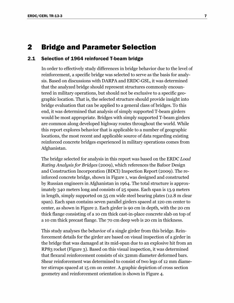
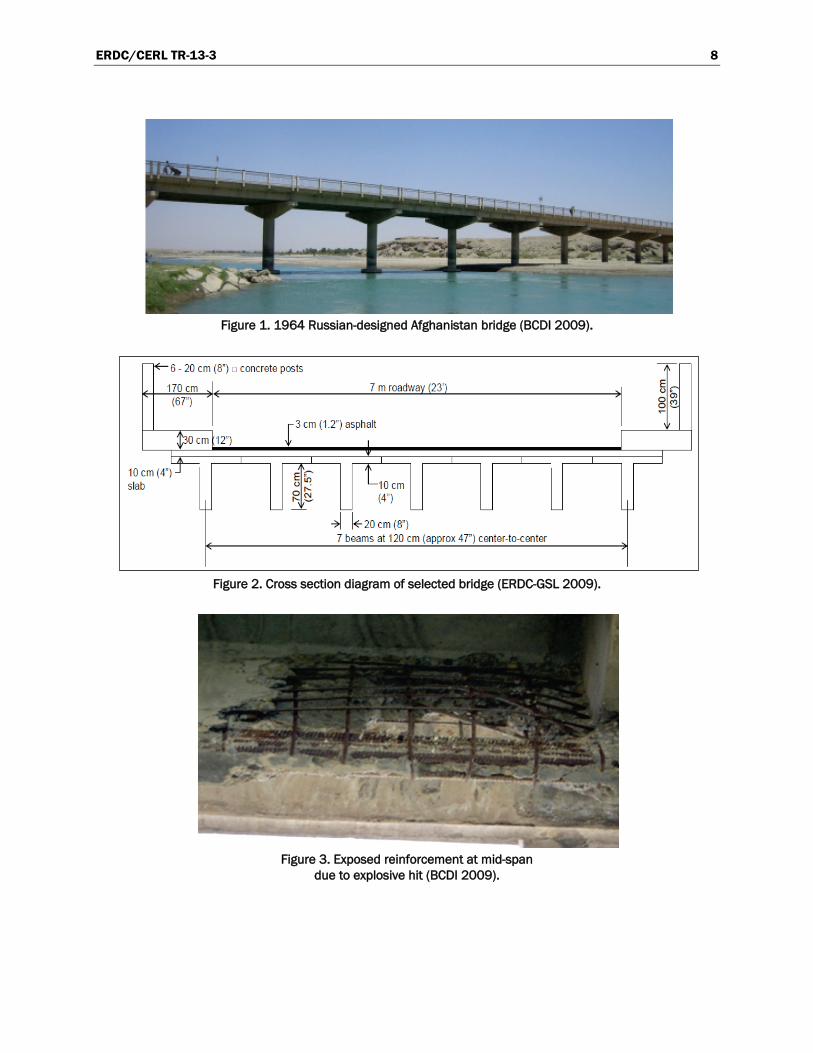
The bridge selected for analysis in this report was based on the ERDC Load Rating Analysis for Bridges (2009), which references the Bafoor Design and Construction Incorporation (BDCI) Inspection Report (2009). The re-inforced concrete bridge, shown in Figure 1, was designed and constructed by Russian engineers in Afghanistan in 1964. The total structure is approx-imately 340 meters long and consists of 25 spans. Each span is 13.9 meters in length, simply supported on 55 cm wide steel bearing plates (12.8 m clear span). Each span contains seven parallel girders spaced at 120 cm center to center, as shown in Figure 2. Each girder is 90 cm in depth, with the 20 cm thick flange consisting of a 10 cm thick cast-in-place concrete slab on top of a 10 cm thick precast flange. The 70 cm deep web is 20 cm in thickness.
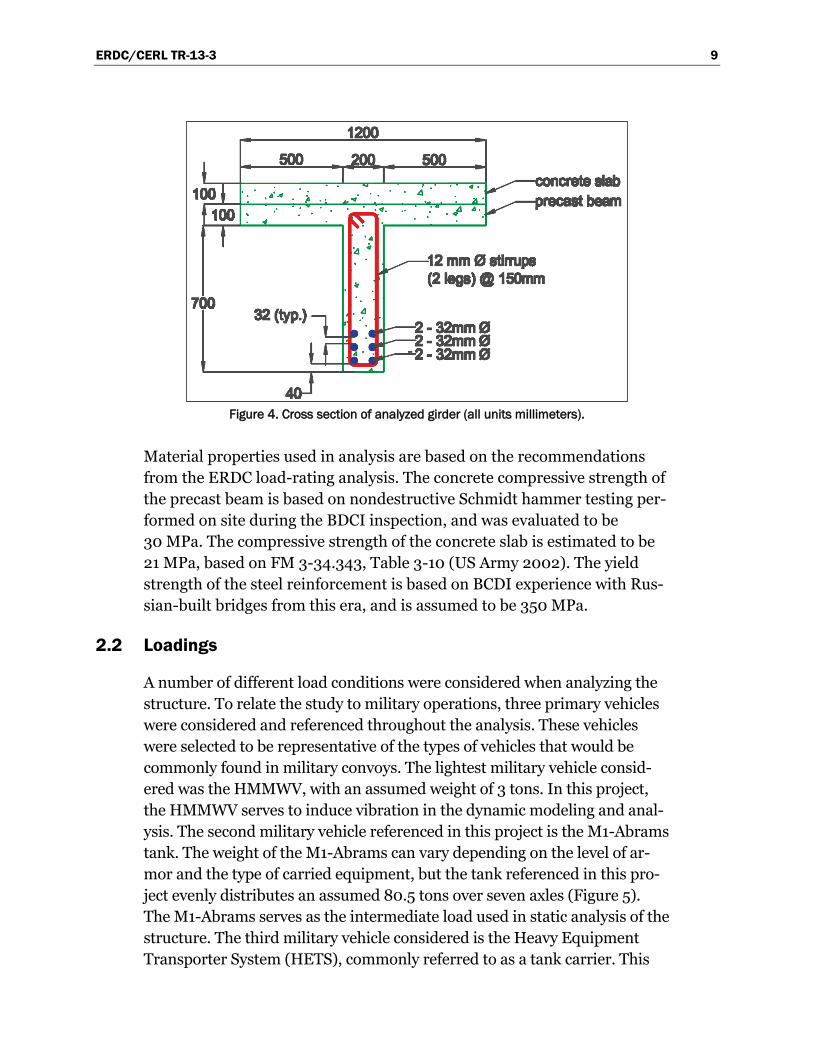
This study analyses the behavior of a single girder from this bridge. Rein-forcement details for the girder are based on visual inspection of a girder in the bridge that was damaged at its mid-span due to an explosive hit from an RP83 rocket (Figure 3). Based on this visual inspection, it was determined that flexural reinforcement consists of six 32mm diameter deformed bars. Shear reinforcement was determined to consist of two legs of 12 mm diame-ter stirrups spaced at 15 cm on center. A graphic depiction of cross section geometry and reinforcement orientation is shown in Figure 4.
ERDC/CERL TR-13-3 8
Figure 1. 1964 Russian-designed Afghanistan bridge (BCDI 2009).
Figure 2. Cross section diagram of selected bridge (ERDC-GSL 2009).
Figure 3. Exposed reinforcement at mid-span
due to explosive hit (BCDI 2009).
ERDC/CERL TR-13-3 9
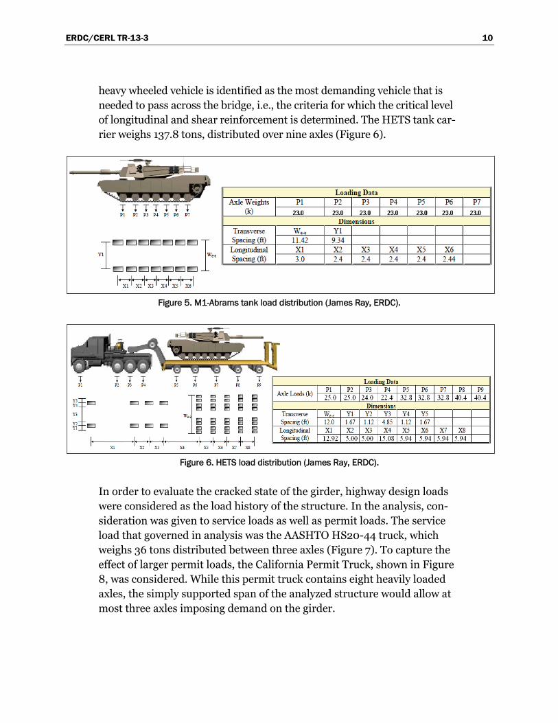
Figure 4. Cross section of analyzed girder (all units millimeters).
Material properties used in analysis are based on the recommendations from the ERDC load-rating analysis. The concrete compressive strength of the precast beam is based on nondestructive Schmidt hammer testing per-formed on site during the BDCI inspection, and was evaluated to be 30 MPa. The compressive strength of the concrete slab is estimated to be 21 MPa, based on FM 3-34.343, Table 3-10 (US Army 2002). The yield strength of the steel reinforcement is based on BCDI experience with Rus-sian-built bridges from this era, and is assumed to be 350 MPa.
2.2 Loadings
A number of different load conditions were considered when analyzing the structure. To relate the study to military operations, three primary vehicles were considered and referenced throughout the analysis. These vehicles were selected to be representative of the types of vehicles that would be commonly found in military convoys. The lightest military vehicle consid-ered was the HMMWV, with an assumed weight of 3 tons. In this project, the HMMWV serves to induce vibration in the dynamic modeling and anal-ysis. The second military vehicle referenced in this project is the M1-Abrams tank. The weight of the M1-Abrams can vary depending on the level of ar-mor and the type of carried equipment, but the tank referenced in this pro-ject evenly distributes an assumed 80.5 tons over seven axles (Figure 5). The M1-Abrams serves as the intermediate load used in static analysis of the structure. The third military vehicle considered is the Heavy Equipment Transporter System (HETS), commonly referred to as a tank carrier. This
ERDC/CERL TR-13-3 10
heavy wheeled vehicle is identified as the most demanding vehicle that is needed to pass across the bridge, i.e., the criteria for which the critical level of longitudinal and shear reinforcement is determined. The HETS tank car-rier weighs 137.8 tons, distributed over nine axles (Figure 6).
Figure 5. M1-Abrams tank load distribution (James Ray, ERDC).
Figure 6. HETS load distribution (James Ray, ERDC).
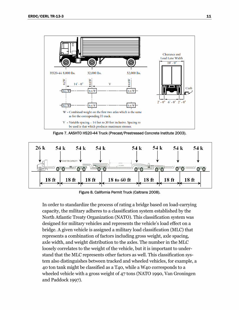
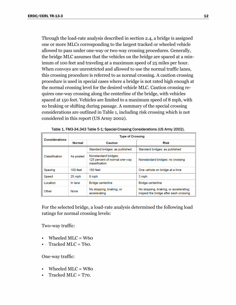
In order to evaluate the cracked state of the girder, highway design loads were considered as the load history of the structure. In the analysis, con-sideration was given to service loads as well as permit loads. The service load that governed in analysis was the AASHTO HS20-44 truck, which weighs 36 tons distributed between three axles (Figure 7). To capture the effect of larger permit loads, the California Permit Truck, shown in Figure 8, was considered. While this permit truck contains eight heavily loaded axles, the simply supported span of the analyzed structure would allow at most three axles imposing demand on the girder.
ERDC/CERL TR-13-3 11
Figure 7. AASHTO HS20-44 Truck (Precast/Prestressed Concrete Institute 2003).
Figure 8. California Permit Truck (Caltrans 2008).
In order to standardize the process of rating a bridge based on load-carrying capacity, the military adheres to a classification system established by the North Atlantic Treaty Organization (NATO). This classification system was designed for military vehicles and represents the vehicle’s load effect on a bridge. A given vehicle is assigned a military load classification (MLC) that represents a combination of factors including gross weight, axle spacing, axle width, and weight distribution to the axles. The number in the MLC loosely correlates to the weight of the vehicle, but it is important to under-stand that the MLC represents other factors as well. This classification sys-tem also distinguishes between tracked and wheeled vehicles, for example, a 40 ton tank might be classified as a T40, while a W40 corresponds to a wheeled vehicle with a gross weight of 47 tons (NATO 1990, Van Groningen and Paddock 1997).
ERDC/CERL TR-13-3 12
Through the load-rate analysis described in section 2.4, a bridge is assigned one or more MLCs corresponding to the largest tracked or wheeled vehicle allowed to pass under one-way or two-way crossing procedures. Generally, the bridge MLC assumes that the vehicles on the bridge are spaced at a min-imum of 100 feet and traveling at a maximum speed of 25 miles per hour. When convoys are unrestricted and allowed to use the normal traffic lanes, this crossing procedure is referred to as normal crossing. A caution crossing procedure is used in special cases where a bridge is not rated high enough at the normal crossing level for the desired vehicle MLC. Caution crossing re-quires one-way crossing along the centerline of the bridge, with vehicles spaced at 150 feet. Vehicles are limited to a maximum speed of 8 mph, with no braking or shifting during passage. A summary of the special crossing considerations are outlined in Table 1, including risk crossing which is not considered in this report (US Army 2002).
Table 1. FM3-34.343 Table 5-1; Special-Crossing Considerations (US Army 2002).
For the selected bridge, a load-rate analysis determined the following load ratings for normal crossing levels:
Two-way traffic:
• Wheeled MLC = W60 • Tracked MLC = T60.
One-way traffic:
• Wheeled MLC = W80 • Tracked MLC = T70.
ERDC/CERL TR-13-3 13
Similarly, a load-rate analysis determined the following load ratings for caution crossing levels:
One-way traffic:
• Wheeled MLC =W90 • Tracked MLC = T80.
The HETS rates from a class W96 up to a class W100 are based on the standard classification methodology for assigning a vehicle an MLC. How-ever, it is recognized that the methodology may be overly conservative for this specific vehicle due to its multi-axle and multi-wheeled configuration. To determine a more accurate rating for the HETS, an extensive 3 year study was performed by the US Military Traffic Management Command Transportation Engineering Agency (MTMCTEA) in partnership with the Federal Highway Administration (FHWA) and through a contract with New Mexico State University (NMSU). This study performed over 400 computer simulation analyses to determine the critical bending moments on bridges ranging in span from 20 to 140 feet. Bridge dimensions for the computer analyses were determined through the evaluation of a large database of ex-isting bridges. Results from analyses were verified through field tests con-ducted by NMSU and the Texas and Colorado Departments of Transporta-tion. Based on this study, for a bridge of the same span as the selected structure, the equivalent MLC for the HETS is W49 (Ray and Garner 2009, Minor and Woodward 1999).
2.3 Design requirements
The standards and codes by which bridges and other reinforced concrete structures were designed and constructed have evolved as understanding of reinforced concrete structures has developed through research and de-sign experience. The two principal codes currently used in the United States for design of reinforced concrete structures are the American Con-crete Institute (ACI) Building Code and the American Association of State Highway and Transportation Officials (AASHTO) LRFD Highway Bridge Specifications. Current highway bridge design in the United States is based on AASHTO design standards, which makes reference to a number of the provisions in the ACI Building Code.
When looking at the changes in ACI design since its first publication in 1910, changes are seen both in an overall design philosophy as well as spe-

ERDC/CERL TR-13-3 14
cific changes in addressing reinforcement requirements, especially for shear resistance. Prior to 1963, the ACI code exclusively used working stress design as its design philosophy. The working stress design limits the maximum elastically computed stresses at service loads to be less than the material strengths by a factor of safety. This approach assumes that ulti-mate limit states such as rupture, formation of plastic mechanism, insta-bility, or fatigue, are automatically satisfied. However, MacGregor and Wight (2005) point out that this is not necessarily the case, and note the following major drawbacks to working stress design:
• inability to account for variability of loads and resistance • lack of knowledge of the level of safety (with respect to ultimate limit
states) • inability to deal with load combinations where loading rates are not the
same.
In 1963, the ACI code introduced the ultimate strength design approach in addition to the working stress design approach. In ultimate strength de-sign, factored load combinations and capacity-reduction factors are ap-plied to proportion members based on calculations of ultimate strength. In addition to developing a stronger sense of the overall safety of members, serviceability is accounted for through provisions for control of deflections and cracking under service loads. After its introduction in 1963, ultimate strength design quickly became the preferred method of design and work-ing stress design was eventually moved into an appendix and finally re-moved from the ACI code entirely in 2002.
Prior to the 1951 ACI provisions, ACI shear provisions recognized that shear resistance in beams and girders consisted of both a reinforcement and con-crete component. The concrete component of shear resistance was based on experimental tests of members with little to no web reinforcement, and its allowable stress for longitudinal reinforcement with no special anchorage conditions was limited to 0.02𝑓′𝑐. Thus, the shear force resisted by the con-crete was equal to 0.02𝑓′𝑐𝑏(𝑗𝑑) where 𝑏 is the width of the web and 𝑗𝑑 is the flexural lever arm. If stirrups are used to resist shear, the required vertical shear reinforcement area is determined by
'
vv
V sAf jd
(2-1)
ERDC/CERL TR-13-3 15
where
vA = total area of web reinforcement within a distance s (i.e., combined area of legs of stirrup)
'V = total shear minus the contribution from concrete s = spacing of stirrups (≤ d/2) vf = tensile unit yield stress of steel shear reinforcement.
Additionally, a limit on the allowable shear stress at service loads was im-posed to prevent a diagonal crushing failure before the yielding of the stir-rups. However, it is important to note that through 1951, no shear rein-forcement was required if the shear stress at a section was less than the resistance contribution from concrete. That is, no provisions existed for a required minimum level of shear reinforcement. A required minimum level of shear reinforcement of 0.15% was introduced in the 1956 code as a direct response to a 1955 shear failure of beams in the warehouse at the Wilkins Air Force Depot in Shelby, OH (Ramirez 2009). The requirement for a min-imum level of shear reinforcement has been modified over the years as re-search in response to the 1955 shear failure has refined the level of under-standing of shear behavior in beams. Currently, the minimum required level of shear reinforcement is expressed as 0.75�𝑓′𝑐 𝑓𝑦� (ACI Committee 318 2008). The current minimum requirement is significantly lower than that in 1956, as shown in Table 2, reflecting that the 1956 provision was a conserva-tive response to the 1955 failure and that refinement of the code has result-ed in a less-stringent requirement today.
In addition to changes in the minimum level of shear reinforcement, the allowable design value for the concrete contribution to shear resistance has also evolved. Today, the concrete unit stress, 𝑣𝑐 = 2�𝑓′𝑐 (ACI Committee 318 2008) is considerably larger than the value in 1956, as seen in Table 2.
The AASHTO Highway Bridge Specifications have slowly adopted ACI provisions. Two important milestones in the history of the AASHTO provi-sions as they relate to current practice include the introduction of the HS20-44 design vehicle in 1944 and the full adoption of the ACI shear provisions in 1973. Prior to 1973, bridges designed by AASHTO specifica-tions were not necessarily consistent in their design approaches.

ERDC/CERL TR-13-3 16
Table 2. Comparison of ACI shear provisions 1956 and 2008.
Table 3. Timeline of major ACI and AASHTO developments.
In trying to understand the design requirements to which a bridge was de-signed and constructed, one would need to have an understanding of the age of the structure as well as to what standard the bridge was designed. Different countries and governments have adopted various codes; some countries have developed their own design standards, some have adopted the US standards, while other less-developed regions have no formalized design standards or practices. It is also important to note that the infra-structure in many nations was developed by foreign interests, thus a struc-ture located in one country may have been designed to a standard or code adopted by a foreign country. Even within a particular region, different sec-tions of highways may have been funded by different sources and thus de-signed by different codes of practice. Additionally, as discussed in the con-text of ACI and AASHTO code history, the standards to which a structure is developed is very time sensitive. Shear requirements for beams and girders
1956 2008 1956 20080.02f'c 2√(f'c) 0.15% 0.75√(f'c)/fy*
3000 60.0 109.5 0.15% 0.07%3500 70.0 118.3 0.15% 0.07%4000 80.0 126.5 0.15% 0.08%4500 90.0 134.2 0.15% 0.08%5000 100.0 141.4 0.15% 0.09%5500 110.0 148.3 0.15% 0.09%6000 120.0 154.9 0.15% 0.10%
*fy = 60000 psi
Concrete Contribution to Shear Resistance, vc (psi)
Minimum Level of Shear Reinforcement (%)
ACI Comparison 1956 - 2008
f'c (psi)
Year AASHO/AASHTO Highway Bridge Specifications
First published code 1910
1914 AASHO founded
1944 HS 20-44 loading introduced
Minimum shear reinforcement introduced 1956
Introduction of limit state designRevisions to min. shear
1974 Fully adopted ACI shear provisions
Working-stress design
1963
ACI Building Code
Ultimate strength design
ERDC/CERL TR-13-3 17
designed to ACI standards vary significantly before and after 1956. Due to difficulty in determining a structure’s age from visual inspection, knowing which version of a given code was used in design is further complicated. In short, determining the code of practice used in the design of a bridge is dif-ficult without having detailed information about when and by whom the structure was designed and constructed.
2.4 ERDC bridge evaluation procedure
2.4.1 Capacity evaluation
For the selected structure, a load-rate analysis has been performed in ac-cordance with standard AASHTO and ACI provisions. In this document, nominal load-carrying capacity for shear and bending moment are com-puted. Once the nominal capacity of the structure is determined, the ca-pacity available to resist live load can be evaluated in terms of military load classification. This load-rate analysis procedure finds the capacity of the structure available to carry live load through the following equation (AASHTO 1994)
** *C A D
LA l DF
1
2 1 (2-2)
where
L = live load effect (the available capacity to resist live load, 𝑀𝐿𝐿 or 𝑉𝐿𝐿)
C = member ultimate capacity (𝑀𝑢 or 𝑉𝑢) D = dead load demand (𝑀𝐷𝐿 or 𝑉𝐷𝐿) A1 = dead load factor of safety
A2 = live load factor of safety
l1 = impact factor DF = distribution factor.
In the next section an example calculation for the level of reinforcement described in section 2.1 is presented. US customary units are utilized throughout this example in order to present empirical ACI equations in their more recognizable form.
ERDC/CERL TR-13-3 18
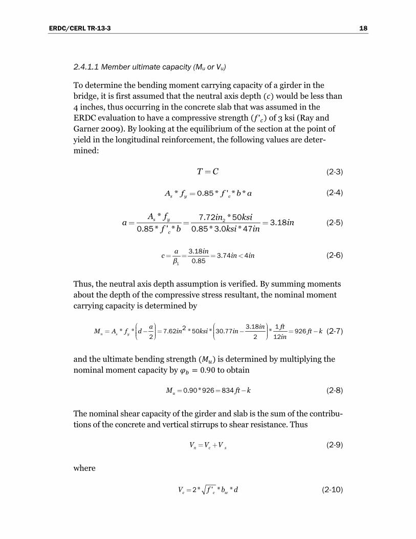
2.4.1.1 Member ultimate capacity (Mu or Vu)
To determine the bending moment carrying capacity of a girder in the bridge, it is first assumed that the neutral axis depth (𝑐) would be less than 4 inches, thus occurring in the concrete slab that was assumed in the ERDC evaluation to have a compressive strength (𝑓’𝑐) of 3 ksi (Ray and Garner 2009). By looking at the equilibrium of the section at the point of yield in the longitudinal reinforcement, the following values are deter-mined:
T C (2-3)
* . * ' * *s y cA f f b a0 85 (2-4)
* . *
.. * ' * . * . *
s y
c
A f in ksia in
f b ksi in 27 72 50
3 180 85 0 85 3 0 47
(2-5)
..
.a inc in inβ
1
3 18 3 74 40 85
(2-6)
Thus, the neutral axis depth assumption is verified. By summing moments about the depth of the compressive stress resultant, the nominal moment carrying capacity is determined by
.* * . * * . *n s y
a in ftM A f d in ksi in ft k
in
3 18 127 62 50 30 77 926
2 2 12 (2-7)
and the ultimate bending strength (𝑀𝑢) is determined by multiplying the nominal moment capacity by 𝜑𝑏 = 0.90 to obtain
. *uM ft k 0 90 926 834 (2-8)
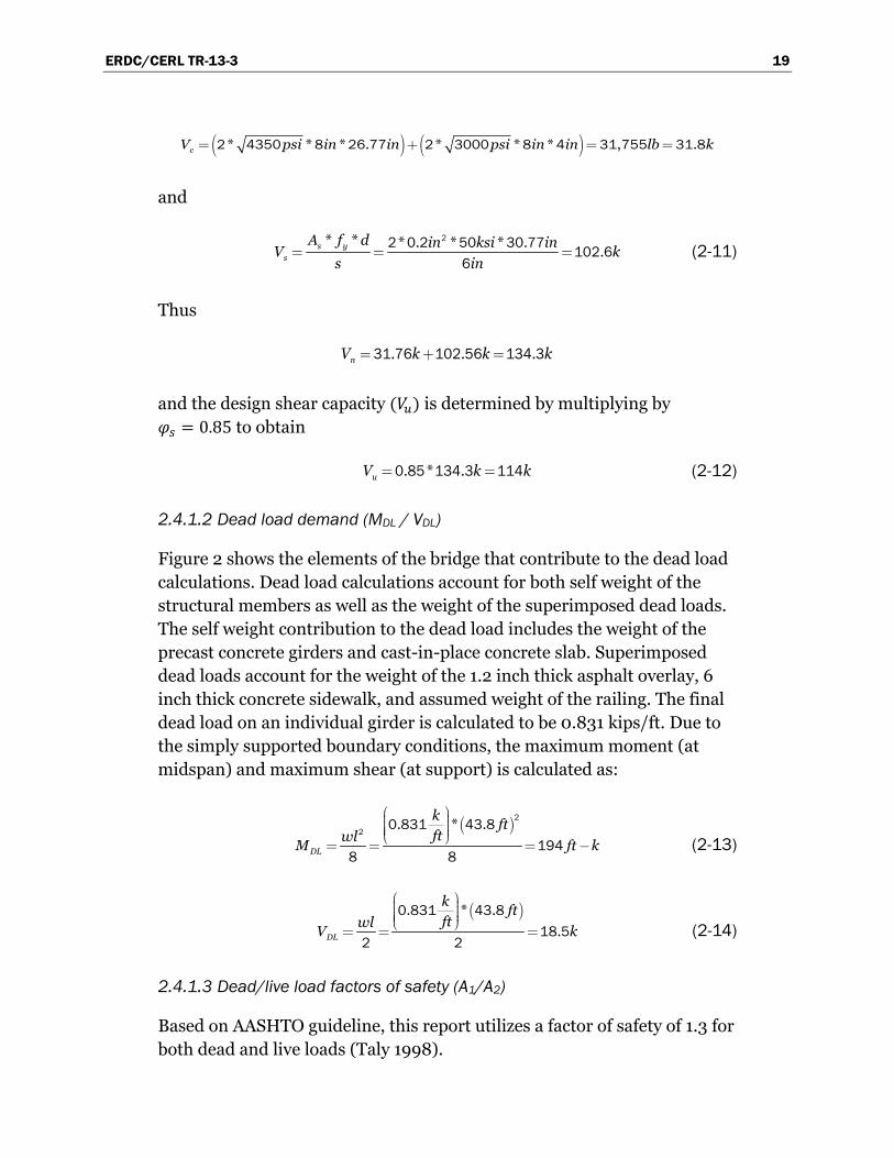
The nominal shear capacity of the girder and slab is the sum of the contribu-tions of the concrete and vertical stirrups to shear resistance. Thus
n c sV V V (2-9)
where
* ' * *c c wV f b d2 (2-10)
ERDC/CERL TR-13-3 19
* * * . * * * , .cV psi in in psi in in lb k 2 4350 8 26 77 2 3000 8 4 31 755 31 8
and
* * * . * * .
.s ys
A f d in ksi inV ks in
22 0 2 50 30 77 102 6
6 (2-11)
Thus
. . .nV k k k 31 76 102 56 134 3
and the design shear capacity (𝑉𝑢) is determined by multiplying by 𝜑𝑠 = 0.85 to obtain
. * .uV k k 0 85 134 3 114 (2-12)
2.4.1.2 Dead load demand (MDL / VDL)
Figure 2 shows the elements of the bridge that contribute to the dead load calculations. Dead load calculations account for both self weight of the structural members as well as the weight of the superimposed dead loads. The self weight contribution to the dead load includes the weight of the precast concrete girders and cast-in-place concrete slab. Superimposed dead loads account for the weight of the 1.2 inch thick asphalt overlay, 6 inch thick concrete sidewalk, and assumed weight of the railing. The final dead load on an individual girder is calculated to be 0.831 kips/ft. Due to the simply supported boundary conditions, the maximum moment (at midspan) and maximum shear (at support) is calculated as:
. * .
DL
k ftftwlM ft k
2
20 831 43 8
1948 8
(2-13)
. * .
.DL
k ftftwlV k
0 831 43 8
18 52 2
(2-14)
2.4.1.3 Dead/live load factors of safety (A1/A2)
Based on AASHTO guideline, this report utilizes a factor of safety of 1.3 for both dead and live loads (Taly 1998).
ERDC/CERL TR-13-3 20
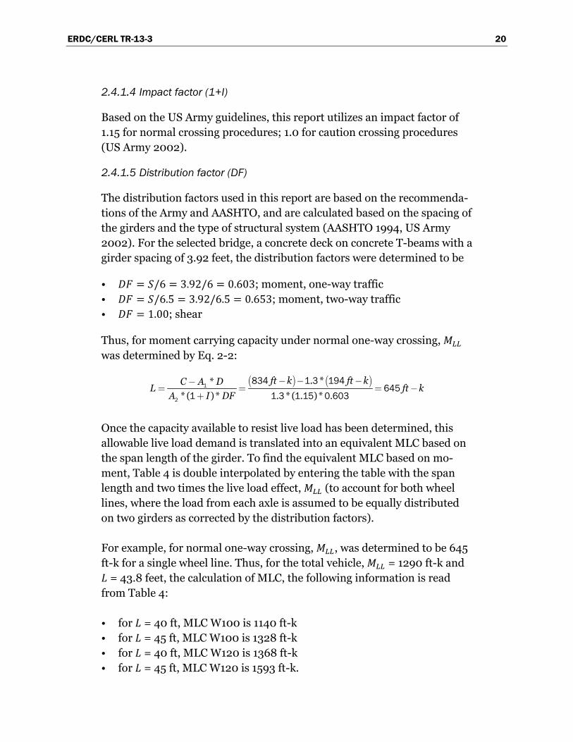
2.4.1.4 Impact factor (1+I)
Based on the US Army guidelines, this report utilizes an impact factor of 1.15 for normal crossing procedures; 1.0 for caution crossing procedures (US Army 2002).
2.4.1.5 Distribution factor (DF)
The distribution factors used in this report are based on the recommenda-tions of the Army and AASHTO, and are calculated based on the spacing of the girders and the type of structural system (AASHTO 1994, US Army 2002). For the selected bridge, a concrete deck on concrete T-beams with a girder spacing of 3.92 feet, the distribution factors were determined to be
• 𝐷𝐹 = 𝑆/6 = 3.92/6 = 0.603; moment, one-way traffic • 𝐷𝐹 = 𝑆/6.5 = 3.92/6.5 = 0.653; moment, two-way traffic • 𝐷𝐹 = 1.00; shear
Thus, for moment carrying capacity under normal one-way crossing, 𝑀𝐿𝐿 was determined by Eq. 2-2:
. **
* ( ) * . * ( . ) * .ft k ft kC A D
L ft kA I DF
1
2
834 1 3 194645
1 1 3 1 15 0 603
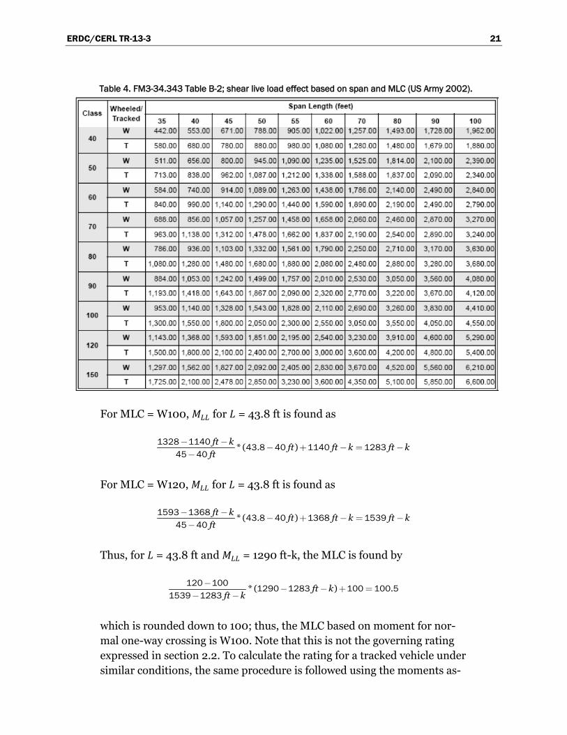
Once the capacity available to resist live load has been determined, this allowable live load demand is translated into an equivalent MLC based on the span length of the girder. To find the equivalent MLC based on mo-ment, Table 4 is double interpolated by entering the table with the span length and two times the live load effect, 𝑀𝐿𝐿 (to account for both wheel lines, where the load from each axle is assumed to be equally distributed on two girders as corrected by the distribution factors).
For example, for normal one-way crossing, 𝑀𝐿𝐿, was determined to be 645 ft-k for a single wheel line. Thus, for the total vehicle, 𝑀𝐿𝐿 = 1290 ft-k and 𝐿 = 43.8 feet, the calculation of MLC, the following information is read from Table 4:
• for 𝐿 = 40 ft, MLC W100 is 1140 ft-k • for 𝐿 = 45 ft, MLC W100 is 1328 ft-k • for 𝐿 = 40 ft, MLC W120 is 1368 ft-k • for 𝐿 = 45 ft, MLC W120 is 1593 ft-k.
ERDC/CERL TR-13-3 21
Table 4. FM3-34.343 Table B-2; shear live load effect based on span and MLC (US Army 2002).
For MLC = W100, 𝑀𝐿𝐿 for 𝐿 = 43.8 ft is found as
* ( . )ft k ft ft k ft k
ft
1328 1140 43 8 40 1140 128345 40
For MLC = W120, 𝑀𝐿𝐿 for 𝐿 = 43.8 ft is found as
* ( . )ft k ft ft k ft k
ft
1593 1368 43 8 40 1368 153945 40
Thus, for 𝐿 = 43.8 ft and 𝑀𝐿𝐿 = 1290 ft-k, the MLC is found by
* ( ) .ft kft k
120 100 1290 1283 100 100 51539 1283
which is rounded down to 100; thus, the MLC based on moment for nor-mal one-way crossing is W100. Note that this is not the governing rating expressed in section 2.2. To calculate the rating for a tracked vehicle under similar conditions, the same procedure is followed using the moments as-
ERDC/CERL TR-13-3 22
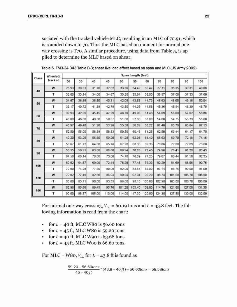
sociated with the tracked vehicle MLC, resulting in an MLC of 70.91, which is rounded down to 70. Thus the MLC based on moment for normal one-way crossing is T70. A similar procedure, using data from Table 5, is ap-plied to determine the MLC based on shear.
Table 5. FM3-34.343 Table B-3; shear live load effect based on span and MLC (US Army 2002).
For normal one-way crossing, 𝑉𝐿𝐿 = 60.19 tons and 𝐿 = 43.8 feet. The fol-lowing information is read from the chart:
• for 𝐿 = 40 ft, MLC W80 is 56.60 tons • for 𝐿 = 45 ft, MLC W80 is 59.20 tons • for 𝐿 = 40 ft, MLC W90 is 63.68 tons • for 𝐿 = 45 ft, MLC W90 is 66.60 tons.
For MLC = W80, 𝑉𝐿𝐿 for 𝐿 = 43.8 ft is found as
. .* ( . ) . .
tons ft tons tonsft
59 20 56 60 43 8 40 56 60 58 5845 40

ERDC/CERL TR-13-3 23
For MLC = W90, 𝑉𝐿𝐿 for 𝐿 = 43.8 ft is found as
. .* ( . ) . .
tons ft tons tonsft
66 60 63 68 43 8 40 63 69 65 9145 40
Thus, for 𝐿 = 43.8 ft and 𝑉𝐿𝐿 = 60.19 tons, the MLC is found to be
*( . . ) .. .
tons tonstons
90 80 60 19 58 58 80 82 2765 91 58 58
which is rounded down to 80. Thus, the MLC based on shear for normal one-way crossing is W80. The MLC rating for shear is less than that for moment, thus the shear-based rating controls, as seen in section 2.2 (Ray and Garner 2009). Similarly, the MLC for a tracked vehicle is calculated as 73.00, which is rounded down to 70. Thus the MLC for normal, one-way crossing of a tracked vehicle based on shear is T70.
2.4.2 Multi-resolution assessment
ERDC researchers have developed a methodology to rapidly assess a large number of bridges that is applicable to any geographic region (Ray and Butler 2004). The problem this paper sought to address was the US mili-tary need to assess hundreds of bridges along convoy routes with little in-formation about individual bridges. The approach uses a system of three discrete levels of assessment resolution (low, medium, and high) and em-ploys a learning algorithm to improve low-resolution assessments to me-dium-resolution status. A description of the levels of assessment resolu-tion follows.
Low-resolution assessments are the first level of assessment, and they are performed on every bridge of interest. Information about a bridge’s loca-tion, route classification, and number and length of spans is gathered through aerial intelligence. Assessments that can be made at this resolu-tion are based on correlations between design loads and military loads. Due to the very limited amount of information collected about the struc-ture, low-resolution assessments are less accurate and more conservative than the other two levels.
High-resolution assessments are the most complete of the three levels, and they are performed only on a select number of structures. Through onsite inspection and a review of complete structural dimensions, a thorough un-
ERDC/CERL TR-13-3 24
derstanding of the structural makeup and condition of the bridge is ob-tained. However, reinforcement details often are not known. This is a severe limitation, and it is addressed in the proposed multi-resolution assessment methodology. From this information, a live load capacity assessment can be made, similar to the procedure outlined previously in section 2.4. High-resolution assessments are the most desirable because they provide greater accuracy that results in a higher load-carrying capacity in nearly all cases. However, when details of the structural components are not available or on-site inspection of the structure is not possible, a high-resolution assessment cannot be performed.
Medium-resolution assessments serve to provide less conservative but more accurate assessments than a low-resolution assessment in cases where a high-resolution assessment is not possible. Medium-resolution assessments are achieved by upgrading a low-resolution assessment by a process called machine learning. Machine learning infers regional construction and condi-tion tendencies from existing high-resolution assessments. The adaptive al-gorithm in the machine-learning process outlined in Ray (2004) determines bridge similarity based on span length, distance between bridges, and route type. Once similarity has been confirmed between an under-documented bridge and one that has undergone high-resolution assessment, a medium-resolution assessment of the first bridge is established.
The accuracy of medium-resolution assessments improve as more regional data are collected. The proposed multi-resolution methodology hinges on the availability of a sufficient number of high-resolution assessments, which require a full understanding of a bridge’s structural integrity. Ray (2004) and the proposed assessment methodology complement the objec-tives of the current report. One potential application of the proposed in-field assessment procedure studied in this report is to help provide infor-mation about structural element details, namely the level of flexural and shear reinforcement needed to make a high-resolution assessment.
2.5 Final bridge parameters
For this numerical study, the desired passable vehicle was selected to be the 137.8 ton HETS under a one-way caution crossing. As described in sec-tion 1.3, this requires the calculation of the minimum level of longitudinal and shear reinforcement required for passage of the desired vehicle. This critical level of reinforcement is determined using the capacity evaluation procedure described in section 2.4.1. In addition to finding the critical lev-
ERDC/CERL TR-13-3 25
el of longitudinal and shear reinforcement, analysis is performed on mod-els with levels of reinforcement both above and below the critical level of reinforcement to produce a gradient of responses. For this study, the sen-sitivity of changing the level of longitudinal and shear reinforcement was investigated by varying the level of reinforcement +/-10% from the critical level of reinforcement required for passage of the HETS.
In varying the level of flexural reinforcement, the cross section shown in Figure 4 served as the basis of the model. The number and spacing of lon-gitudinal reinforcement was held constant, and only the cross-sectional area of the bars was varied to produce the different levels of reinforce-ment. Based on the capacity evaluation approach outlined in the previous section, the critical level of reinforcement for passage of the HETS was de-termined to require six 509 mm2 bars, corresponding to a steel ratio of 0.362%. Note that this critical level of reinforcement is less than the six 804 mm2 depicted in Figure 4. From this critical level of longitudinal rein-forcement, a variation of +/-10% of the area of steel in the critical case was analyzed.
For determining the levels of shear reinforcement for this project, the size and type of stirrups were based on the representative structure described in section 2.1. Two legs of 12mm diameter stirrups were considered, as seen in Figure 4. To vary the level of shear reinforcement, only the spacing of the stirrups was changed for analysis. Based on the capacity evaluation procedure in section 2.4.1, a stirrup spacing of 200 mm was determined to be the maximum required for passage of the HETS vehicle. In contrast, the spacing shown in Figure 4 was less than this maximum, with a value of 150 mm. Parametric variation of the level of shear reinforcement consisted of increasing and decreasing the spacing of the stirrups to create a steel ratio equal to the critical level +/-10%. A summary of the parametric varia-tion in longitudinal and shear reinforcement is found in Table 6.
In addition to varying the level of longitudinal and shear reinforcement, it is necessary to consider the effect of cracking on the flexural stiffness of the structure for dynamic analysis. In reinforced concrete, cracking is a direct result of the largest load imposed on a member. For bridges, cracking in the girder is due to the combination of static dead loads and vehicular live loads. Thus, cracking results from the largest load in a girder’s load history. For this study, two different load histories are considered to understand the sensitivity of flexural stiffness to cracking in the dynamic model. The first
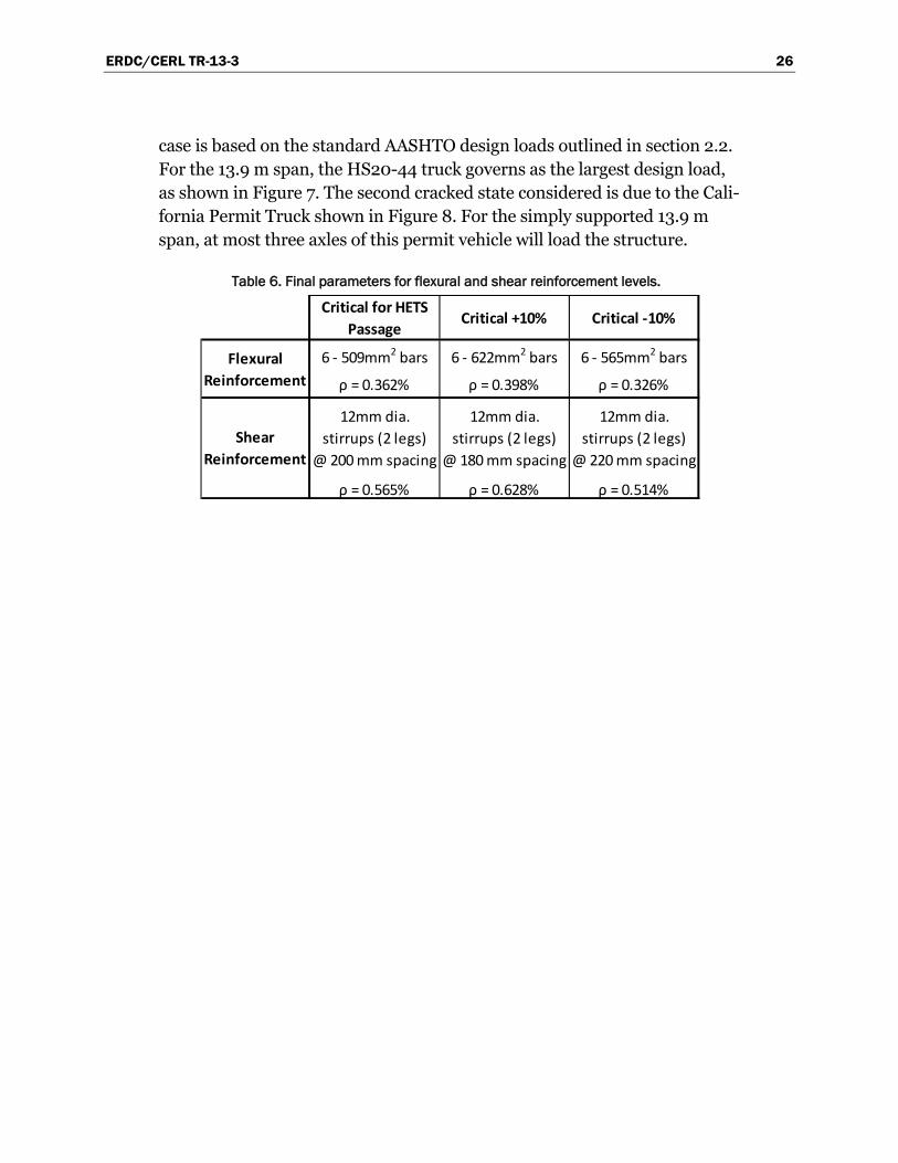
ERDC/CERL TR-13-3 26
case is based on the standard AASHTO design loads outlined in section 2.2. For the 13.9 m span, the HS20-44 truck governs as the largest design load, as shown in Figure 7. The second cracked state considered is due to the Cali-fornia Permit Truck shown in Figure 8. For the simply supported 13.9 m span, at most three axles of this permit vehicle will load the structure.
Table 6. Final parameters for flexural and shear reinforcement levels.
Critical for HETS Passage
Critical +10% Critical -10%
6 - 509mm2 bars 6 - 622mm2 bars 6 - 565mm2 bars
ρ = 0.362% ρ = 0.398% ρ = 0.326%
12mm dia. stirrups (2 legs)
@ 200 mm spacing
12mm dia. stirrups (2 legs)
@ 180 mm spacing
12mm dia. stirrups (2 legs)
@ 220 mm spacing
ρ = 0.565% ρ = 0.628% ρ = 0.514%
Flexural Reinforcement
Shear Reinforcement
ERDC/CERL TR-13-3 27
3 Static Modeling and Analysis 3.1 Analytical tools
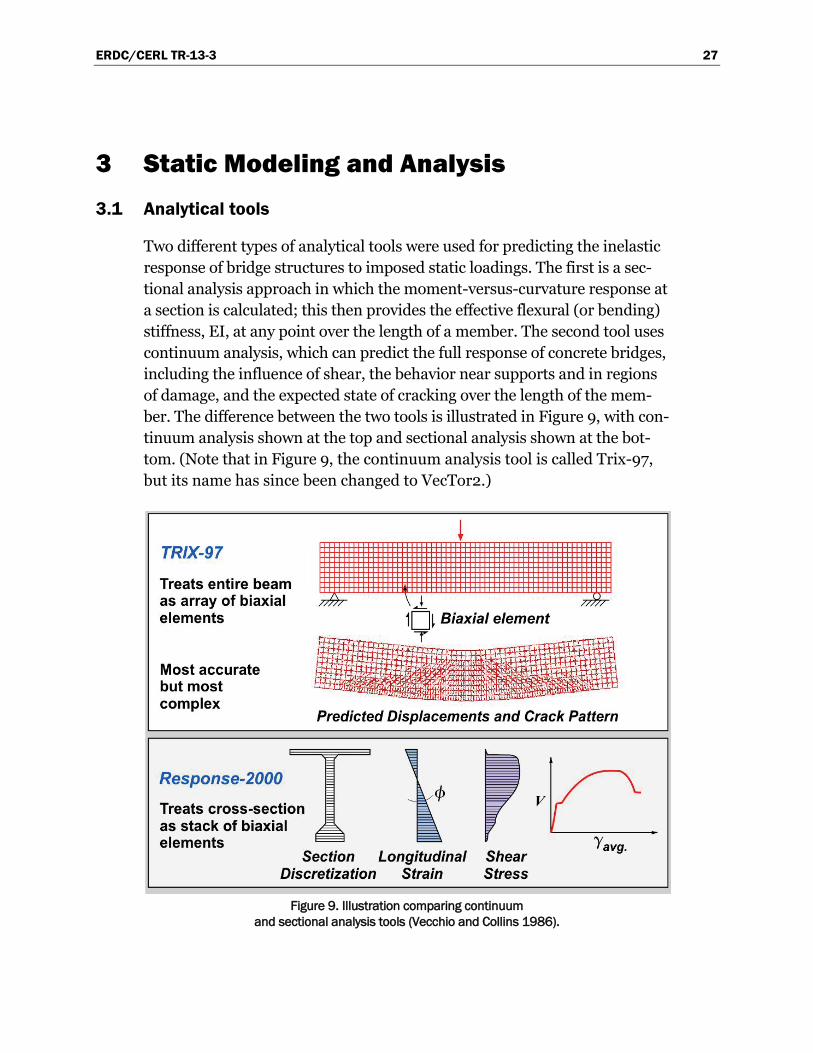
Two different types of analytical tools were used for predicting the inelastic response of bridge structures to imposed static loadings. The first is a sec-tional analysis approach in which the moment-versus-curvature response at a section is calculated; this then provides the effective flexural (or bending) stiffness, EI, at any point over the length of a member. The second tool uses continuum analysis, which can predict the full response of concrete bridges, including the influence of shear, the behavior near supports and in regions of damage, and the expected state of cracking over the length of the mem-ber. The difference between the two tools is illustrated in Figure 9, with con-tinuum analysis shown at the top and sectional analysis shown at the bot-tom. (Note that in Figure 9, the continuum analysis tool is called Trix-97, but its name has since been changed to VecTor2.)
Figure 9. Illustration comparing continuum
and sectional analysis tools (Vecchio and Collins 1986).
ERDC/CERL TR-13-3 28
3.1.1 Response-2000
Response-2000 is able to predict the complete moment-curvature response of a section, which involves a multistep iterative process. At the lowest level, a multilayer analysis methodology is used to evaluate the axial load and moment acting on a section for any strain gradient over the height. This is done by calculating the state of stress in concrete and in the reinforcement at each individual layer over the height of a section using nonlinear consti-tutive relationships and then employing equilibrium to determine the forces in each layer and, thereby, the forces (axial load and moment) acting on a section. There is one unique combination of axial load and moment for a single variation in longitudinal strain over the depth of the member. For a beam with no axial load, it is necessary to iterate on the curvature for any individual top strain to obtain one point on the moment-curvature re-sponse. Repeating this process for many levels of top strain provides a com-plete moment-curvature response for a section.
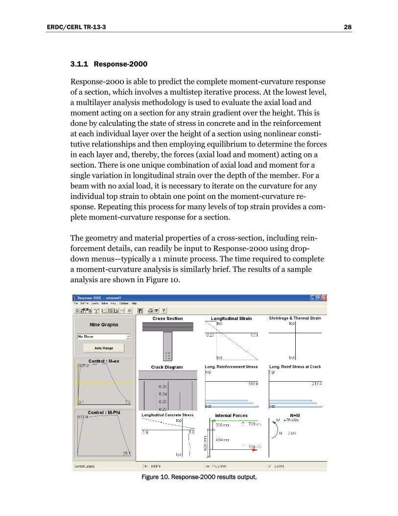
The geometry and material properties of a cross-section, including rein-forcement details, can readily be input to Response-2000 using drop-down menus—typically a 1 minute process. The time required to complete a moment-curvature analysis is similarly brief. The results of a sample analysis are shown in Figure 10.
Figure 10. Response-2000 results output.
ERDC/CERL TR-13-3 29
The lower-left image in the shaded area of Figure 10 presents the calculat-ed moment-curvature response, and the one directly above it shows the moment-longitudinal strain at the centroidal axis of the section. Each of the other nine images to the right of these presents the section condition for one particular level of moment.
Beginning at the upper-left of these nine images, “Cross Section” presents the overall state of stress on an illustration of the cross-section. The shaded region represents the uncracked portion of the section while the unshaded region is the cracked portion of the section. The location of the reinforce-ment is also shown in this section and the color of the reinforcing bars is used to indicate the points of yielding and strain hardening. The next image to the right presents the profile of “Longitudinal Strain” over the depth of the member for the target axial load level (typically N=0 for a beam). Mov-ing right, the effect of “Shrinkage and Thermal Strains” also can be consid-ered, but in this example they were taken as zero. The “Crack Diagram” pre-sents the predicted depth and width of flexural cracking. The next two graphics to the right present the average stress in the longitudinal rein-forcement and also that at a crack. The average stress is less than the stress at a crack due to the tension stiffening effect of the concrete that is still bonded to the reinforcement between cracks. In the last row, “Longitudinal Concrete Stress” presents the concrete stress over the depth of the section based on the distribution of “Longitudinal Strain” presented in the top-middle image. As shown, the compressive stress is zero when the longitudi-nal strain is zero and then increases with compressive straining in a nonlin-ear manner. “Internal Forces” presents the centers of the compressive and tensile forces that are acting on the section and the distance between these forces. The axial load and moment acting on this section, “N+M”, can then be respectively calculated as the sum of these forces and the force coupling of these forces (Bentz 2000).
3.1.2 VecTor2
VecTor2, formerly known as Trix-97, is a nonlinear, two-dimensional (2D) continuum finite element analysis (FEA) program for reinforced and pre-stressed concrete structures that employs the modified compression field theory (MCFT). The available materials in the program consist of reinforced concrete elements with or without smeared and discrete rebars. It should be noted that the behavior models of MCFT are not bound with any specific constitutive relationship. Rather, they can be combined with any set of real-istic constitutive relationships. Therefore, VecTor2 provides several differ-
ERDC/CERL TR-13-3 30
ent models for each material behavior. There is no specific guideline for the selection of constitutive models; the selection is completely up to user, and this may produce some subjectivity in the analytic result.
The element library of VecTor2 can be divided into three categories:
1. planar triangular, rectangular and quadrilateral elements for modeling reinforced concrete.
2. a linear truss element for modeling discrete reinforcing bars 3. an element for bond-slip modeling between concrete and reinforcing
bars, which has the non-dimensional link and contact element.
Note that all elements are of linear order, which means the strain field within an element is constant (Wong and Vecchio 2002). Therefore, for regions of complex stress distribution, a sufficiently fine mesh should be implemented to ensure quality results.
In order to solve a nonlinear problem, VecTor2 adopts the secant stiffness solution method. This is possible because the strain-stress relation of rein-forced concrete is independent of loading history. During the iteration, the strain state is assumed first. Then, the assumption makes it possible to de-termine the corresponding constitutive relationship, from which the secant stiffness matrix becomes available immediately. The advantage of the meth-od is that a linear elastic FEA program can be used without much modifica-tion.
The behavior of structural concrete is highly nonlinear in general, and thus it is usually the case that more than 10 input parameters are needed for each material type in order to reproduce the complex behavior. Although VecTor2 also requires a large number of input parameters to be set, since it is a structural concrete analysis-oriented program, it provides default values for most material properties calculated from the basic set of meas-urable properties (e.g., 𝑓’𝑐 ,𝑓𝑦 ,𝑑𝑏 of rebars, etc.) according to the relation-ships suggested by codes of practice or researchers.
A post-processor, Augustus, provides many options for viewing the pre-dicted behavior. The output options include deformation, strains and stresses of reinforced concrete and discrete rebars, stress at crack surfaces, width and direction of cracks, which are vital signs used for determination of structural health. Remembering that MCFT and VecTor2 are based on
ERDC/CERL TR-13-3 31
the smeared-crack concept, the locations and width of cracks represent av-erage response of the structure and not real, discrete local cracks.
In order to understand the predictive capability of VecTor2 it is necessary to understand MCFT, which is the underlying behavioral model used in the program. The MCFT was proposed by Vecchio and Collins (1986) as an extension of its predecessor, compression field theory (Mitchell and Collins 1974). Later, the MCFT progressed into a new version of the theo-ry, disturbed stress field model (DSFM) (F. Vecchio 2000, Vecchio, Lai, et al. 2001, F. Vecchio 2001). The MCFT and DSFM were implemented in the Nonlinear Finite Element Analysis of Reinforced Concrete (NLFEARC) program VecTor2, which was written and has been improved by Vecchio and his colleagues (Wong and Vecchio 2002). Since the MCFT was not based on any specific constitutive relationships, this review does not in-clude any specific constitutive relationships. For a more comprehensive review of the MCFT and VecTor2, see Collins and Mitchell (1991), ACI Committee 445 (1998), or Wong and Vecchio (2002).
The MCFT is an analytical model for the response of 2D membrane struc-tures subjected to in-plane normal and shear stresses. The model accounts for the average stress-strain relationships in cracked concrete and per-forms an equilibrium check of conditions at crack locations.
MCFT makes the following important assumptions:
1. The external normal and shear stress are uniform along the sides of an element.
2. The reinforced concrete element is independent of loading history (i.e., one strain state can have only one stress state).
3. For an element of which area spans a few cracks, average stress-strain relationship can be used. The tracks of individual cracks are not fol-lowed.
4. Reinforcement is modeled as smeared and is taken as perfectly bonded to surrounding concrete.
5. Reinforcement is uniformly distributed in an element. 6. Cracked concrete is an orthotropic material. 7. In cracked concrete, the directions of principal strains and stresses co-
incide with each other (but this assumption was abandoned in DSFM). 8. The direction of a crack is the same as the direction of principal tensile
strain.
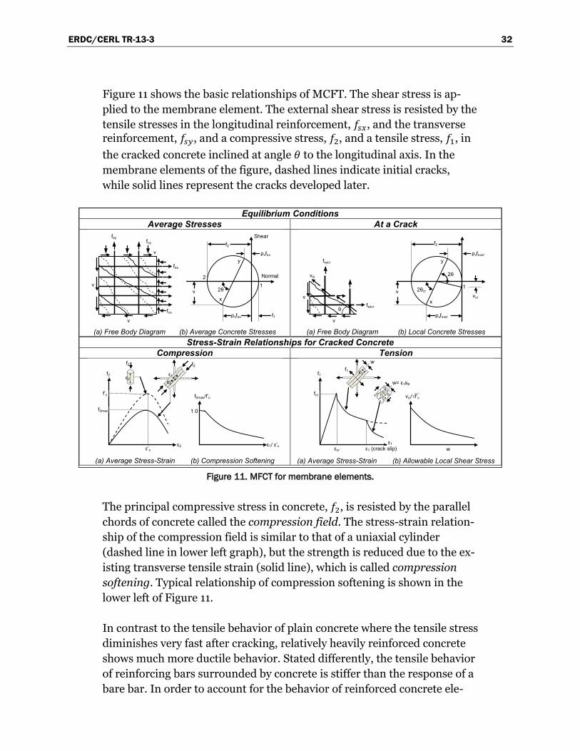
ERDC/CERL TR-13-3 32
Figure 11 shows the basic relationships of MCFT. The shear stress is ap-plied to the membrane element. The external shear stress is resisted by the tensile stresses in the longitudinal reinforcement, 𝑓𝑠𝑥, and the transverse reinforcement, 𝑓𝑠𝑦, and a compressive stress, 𝑓2, and a tensile stress, 𝑓1, in the cracked concrete inclined at angle 𝜃 to the longitudinal axis. In the membrane elements of the figure, dashed lines indicate initial cracks, while solid lines represent the cracks developed later.
Figure 11. MFCT for membrane elements.
The principal compressive stress in concrete, 𝑓2, is resisted by the parallel chords of concrete called the compression field. The stress-strain relation-ship of the compression field is similar to that of a uniaxial cylinder (dashed line in lower left graph), but the strength is reduced due to the ex-isting transverse tensile strain (solid line), which is called compression softening. Typical relationship of compression softening is shown in the lower left of Figure 11.
In contrast to the tensile behavior of plain concrete where the tensile stress diminishes very fast after cracking, relatively heavily reinforced concrete shows much more ductile behavior. Stated differently, the tensile behavior of reinforcing bars surrounded by concrete is stiffer than the response of a bare bar. In order to account for the behavior of reinforced concrete ele-
Equilibrium Conditions Average Stresses At a Crack
(a) Free Body Diagram (b) Average Concrete Stresses
(a) Free Body Diagram (b) Local Concrete Stresses
Stress-Strain Relationships for Cracked Concrete Compression Tension
(a) Average Stress-Strain (b) Compression Softening
(a) Average Stress-Strain (b) Allowable Local Shear Stress
εcr
fcr
f1
ε1
νci/√f’c
ε1 f1 w
w= ε1sθ
w
ε1 (crack slip) ε’c
f’c
f2max
f2
ε2
ε2 f2 f2
ε2
1.0 f2max/f’c
ε1/ ε’c
ε1
ν
ν
fsycr
fsxcr
f2
ν
ρxfsxcr
x
y
1
ρyfsycr
2θcr
νci
θ
2θ
νci
ν
ν
fsy fcy
ν
fsx
fcx
f2
ν
Shear
Normal
ρxfsx f1
x
y
2 1
ρyfsy
2θ
ERDC/CERL TR-13-3 33
ment, the tension stiffening relationship is used in MCFT as presented in the lower right part of Figure 11. By considering tension stiffening rela-tionship with the stiffness of bare bar, the stiffer tensile response of the reinforced concrete can be modeled properly.
The principal tensile stress is resisted by the combination of reinforcement and tensile stress of concrete in terms of tension stiffening. However, at the crack surface, the stresses in the reinforcing bars increase in order to satisfy the equilibrium condition because the tensile stress of concrete al-most reduces instantly. If the reinforcing bars have yielded and thus do not have sufficient strength to resist the tensile stress, shear stress devel-ops at the crack surface in terms of aggregate interlocking. The capacity of shear stress reduces as the width of the crack increases. Therefore, for large crack widths, the tensile capacity of concrete should be reduced in order to account for shear slip failure at crack surface. The crack width is calculated by the product of average tensile strain of concrete and average crack spacing, which is usually calculated based on the CEB-FIP model code 90 (CEB-FIB 1993)
Besides the compressive and tensile behavior models described above, several behavior models have been added to the prototype of MCFT in or-der to improve the accuracy of analysis (e.g., Poisson effect, strength en-hancement due to the confinement effect, tension softening).
3.1.3 Membrane-2000
Membrane-2000 utilizes the MCFT to analyze reinforced concrete mem-branes subjected to in-plane shear forces and axial loads (Bentz 2000). Un-like VecTor2, which allows for analysis of a 2D continuum model consisting of multiple membrane elements, Membrane-2000 analyzes a single mem-brane element similar to the original derivation of the MCFT. For more in-formation on Membrane-2000 and its capabilities, please refer to its user manual (Bentz 2001).
The MCFT was developed from and is validated by a large number of tests on reinforced concrete elements subjected to shear as well as combinations of shear and normal actions. An example of the predictive capability of the MCFT is presented in Figure 12 for four elements that range widely in terms of levels of reinforcement.
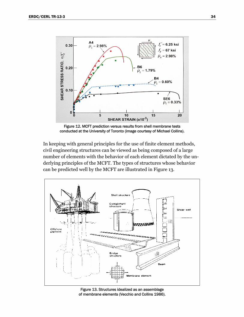
ERDC/CERL TR-13-3 34
Figure 12. MCFT prediction versus results from shell membrane tests
conducted at the University of Toronto (image courtesy of Michael Collins).
In keeping with general principles for the use of finite element methods, civil engineering structures can be viewed as being composed of a large number of elements with the behavior of each element dictated by the un-derlying principles of the MCFT. The types of structures whose behavior can be predicted well by the MCFT are illustrated in Figure 13.
Figure 13. Structures idealized as an assemblage
of membrane elements (Vecchio and Collins 1986).
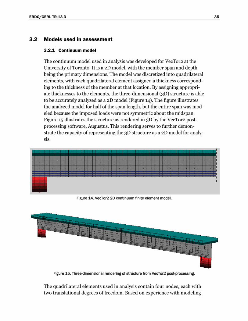
ERDC/CERL TR-13-3 35
3.2 Models used in assessment
3.2.1 Continuum model
The continuum model used in analysis was developed for VecTor2 at the University of Toronto. It is a 2D model, with the member span and depth being the primary dimensions. The model was discretized into quadrilateral elements, with each quadrilateral element assigned a thickness correspond-ing to the thickness of the member at that location. By assigning appropri-ate thicknesses to the elements, the three-dimensional (3D) structure is able to be accurately analyzed as a 2D model (Figure 14). The figure illustrates the analyzed model for half of the span length, but the entire span was mod-eled because the imposed loads were not symmetric about the midspan. Figure 15 illustrates the structure as rendered in 3D by the VecTor2 post-processing software, Augustus. This rendering serves to further demon-strate the capacity of representing the 3D structure as a 2D model for analy-sis.
Figure 14. VecTor2 2D continuum finite element model.
Figure 15. Three-dimensional rendering of structure from VecTor2 post-processing.
The quadrilateral elements used in analysis contain four nodes, each with two translational degrees of freedom. Based on experience with modeling
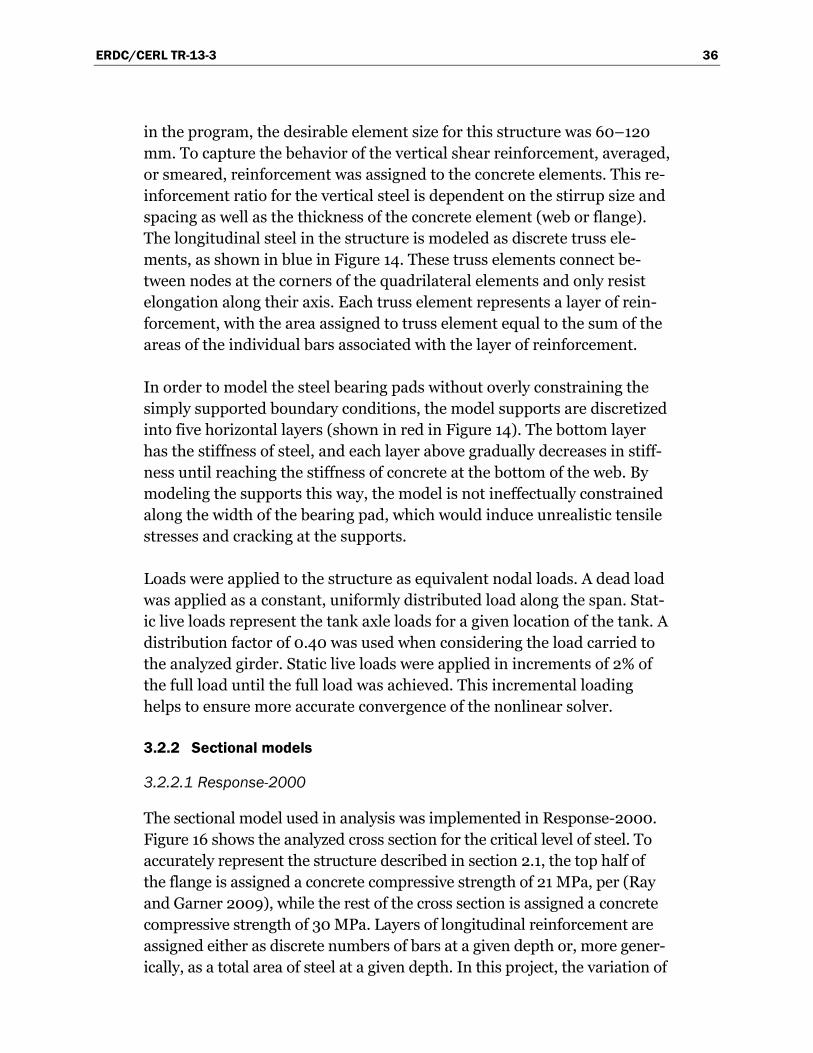
ERDC/CERL TR-13-3 36
in the program, the desirable element size for this structure was 60–120 mm. To capture the behavior of the vertical shear reinforcement, averaged, or smeared, reinforcement was assigned to the concrete elements. This re-inforcement ratio for the vertical steel is dependent on the stirrup size and spacing as well as the thickness of the concrete element (web or flange). The longitudinal steel in the structure is modeled as discrete truss ele-ments, as shown in blue in Figure 14. These truss elements connect be-tween nodes at the corners of the quadrilateral elements and only resist elongation along their axis. Each truss element represents a layer of rein-forcement, with the area assigned to truss element equal to the sum of the areas of the individual bars associated with the layer of reinforcement.
In order to model the steel bearing pads without overly constraining the simply supported boundary conditions, the model supports are discretized into five horizontal layers (shown in red in Figure 14). The bottom layer has the stiffness of steel, and each layer above gradually decreases in stiff-ness until reaching the stiffness of concrete at the bottom of the web. By modeling the supports this way, the model is not ineffectually constrained along the width of the bearing pad, which would induce unrealistic tensile stresses and cracking at the supports.
Loads were applied to the structure as equivalent nodal loads. A dead load was applied as a constant, uniformly distributed load along the span. Stat-ic live loads represent the tank axle loads for a given location of the tank. A distribution factor of 0.40 was used when considering the load carried to the analyzed girder. Static live loads were applied in increments of 2% of the full load until the full load was achieved. This incremental loading helps to ensure more accurate convergence of the nonlinear solver.
3.2.2 Sectional models
3.2.2.1 Response-2000
The sectional model used in analysis was implemented in Response-2000. Figure 16 shows the analyzed cross section for the critical level of steel. To accurately represent the structure described in section 2.1, the top half of the flange is assigned a concrete compressive strength of 21 MPa, per (Ray and Garner 2009), while the rest of the cross section is assigned a concrete compressive strength of 30 MPa. Layers of longitudinal reinforcement are assigned either as discrete numbers of bars at a given depth or, more gener-ically, as a total area of steel at a given depth. In this project, the variation of
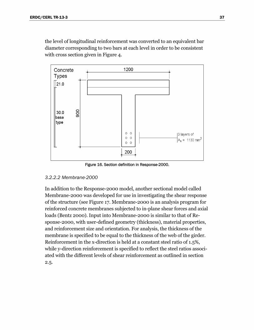
ERDC/CERL TR-13-3 37
the level of longitudinal reinforcement was converted to an equivalent bar diameter corresponding to two bars at each level in order to be consistent with cross section given in Figure 4.
Figure 16. Section definition in Response-2000.
3.2.2.2 Membrane-2000
In addition to the Response-2000 model, another sectional model called Membrane-2000 was developed for use in investigating the shear response of the structure (see Figure 17. Membrane-2000 is an analysis program for reinforced concrete membranes subjected to in-plane shear forces and axial loads (Bentz 2000). Input into Membrane-2000 is similar to that of Re-sponse-2000, with user-defined geometry (thickness), material properties, and reinforcement size and orientation. For analysis, the thickness of the membrane is specified to be equal to the thickness of the web of the girder. Reinforcement in the x-direction is held at a constant steel ratio of 1.5%, while y-direction reinforcement is specified to reflect the steel ratios associ-ated with the different levels of shear reinforcement as outlined in section 2.5.
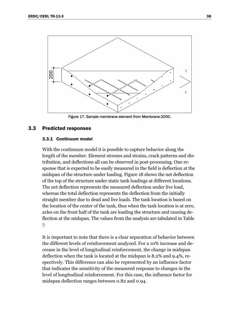
ERDC/CERL TR-13-3 38
Figure 17. Sample membrane element from Membrane-2000.
3.3 Predicted responses
3.3.1 Continuum model
With the continuum model it is possible to capture behavior along the length of the member. Element stresses and strains, crack patterns and dis-tribution, and deflections all can be observed in post-processing. One re-sponse that is expected to be easily measured in the field is deflection at the midspan of the structure under loading. Figure 18 shows the net deflection of the top of the structure under static tank loadings at different locations. The net deflection represents the measured deflection under live load, whereas the total deflection represents the deflection from the initially straight member due to dead and live loads. The tank location is based on the location of the center of the tank, thus when the tank location is at zero, axles on the front half of the tank are loading the structure and causing de-flection at the midspan. The values from the analysis are tabulated in Table 7.
It is important to note that there is a clear separation of behavior between the different levels of reinforcement analyzed. For a 10% increase and de-crease in the level of longitudinal reinforcement, the change in midspan deflection when the tank is located at the midspan is 8.2% and 9.4%, re-spectively. This difference can also be represented by an influence factor that indicates the sensitivity of the measured response to changes in the level of longitudinal reinforcement. For this case, the influence factor for midspan deflection ranges between 0.82 and 0.94.
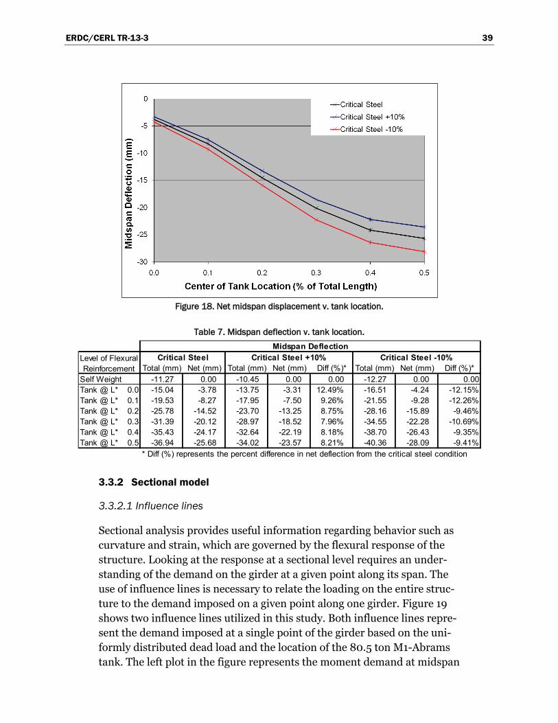
ERDC/CERL TR-13-3 39
Figure 18. Net midspan displacement v. tank location.
Table 7. Midspan deflection v. tank location.
3.3.2 Sectional model
3.3.2.1 Influence lines
Sectional analysis provides useful information regarding behavior such as curvature and strain, which are governed by the flexural response of the structure. Looking at the response at a sectional level requires an under-standing of the demand on the girder at a given point along its span. The use of influence lines is necessary to relate the loading on the entire struc-ture to the demand imposed on a given point along one girder. Figure 19 shows two influence lines utilized in this study. Both influence lines repre-sent the demand imposed at a single point of the girder based on the uni-formly distributed dead load and the location of the 80.5 ton M1-Abrams tank. The left plot in the figure represents the moment demand at midspan
Total (mm) Net (mm) Total (mm) Net (mm) Diff (%)* Total (mm) Net (mm) Diff (%)*Self Weight -11.27 0.00 -10.45 0.00 0.00 -12.27 0.00 0.00Tank @ L* 0.0 -15.04 -3.78 -13.75 -3.31 12.49% -16.51 -4.24 -12.15%Tank @ L* 0.1 -19.53 -8.27 -17.95 -7.50 9.26% -21.55 -9.28 -12.26%Tank @ L* 0.2 -25.78 -14.52 -23.70 -13.25 8.75% -28.16 -15.89 -9.46%Tank @ L* 0.3 -31.39 -20.12 -28.97 -18.52 7.96% -34.55 -22.28 -10.69%Tank @ L* 0.4 -35.43 -24.17 -32.64 -22.19 8.18% -38.70 -26.43 -9.35%Tank @ L* 0.5 -36.94 -25.68 -34.02 -23.57 8.21% -40.36 -28.09 -9.41%
* Diff (%) represents the percent difference in net deflection from the critical steel condition
Critical Steel +10% Critical Steel -10% Midspan Deflection
Level of Flexural Reinforcement
Critical Steel
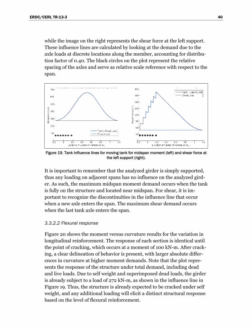
ERDC/CERL TR-13-3 40
while the image on the right represents the shear force at the left support. These influence lines are calculated by looking at the demand due to the axle loads at discrete locations along the member, accounting for distribu-tion factor of 0.40. The black circles on the plot represent the relative spacing of the axles and serve as relative scale reference with respect to the span.
Figure 19. Tank influence lines for moving tank for midspan moment (left) and shear force at
the left support (right).
It is important to remember that the analyzed girder is simply supported, thus any loading on adjacent spans has no influence on the analyzed gird-er. As such, the maximum midspan moment demand occurs when the tank is fully on the structure and located near midspan. For shear, it is im-portant to recognize the discontinuities in the influence line that occur when a new axle enters the span. The maximum shear demand occurs when the last tank axle enters the span.
3.3.2.2 Flexural response
Figure 20 shows the moment versus curvature results for the variation in longitudinal reinforcement. The response of each section is identical until the point of cracking, which occurs at a moment of 100 kN-m. After crack-ing, a clear delineation of behavior is present, with larger absolute differ-ences in curvature at higher moment demands. Note that the plot repre-sents the response of the structure under total demand, including dead and live loads. Due to self weight and superimposed dead loads, the girder is already subject to a load of 272 kN-m, as shown in the influence line in Figure 19. Thus, the structure is already expected to be cracked under self weight, and any additional loading will elicit a distinct structural response based on the level of flexural reinforcement.
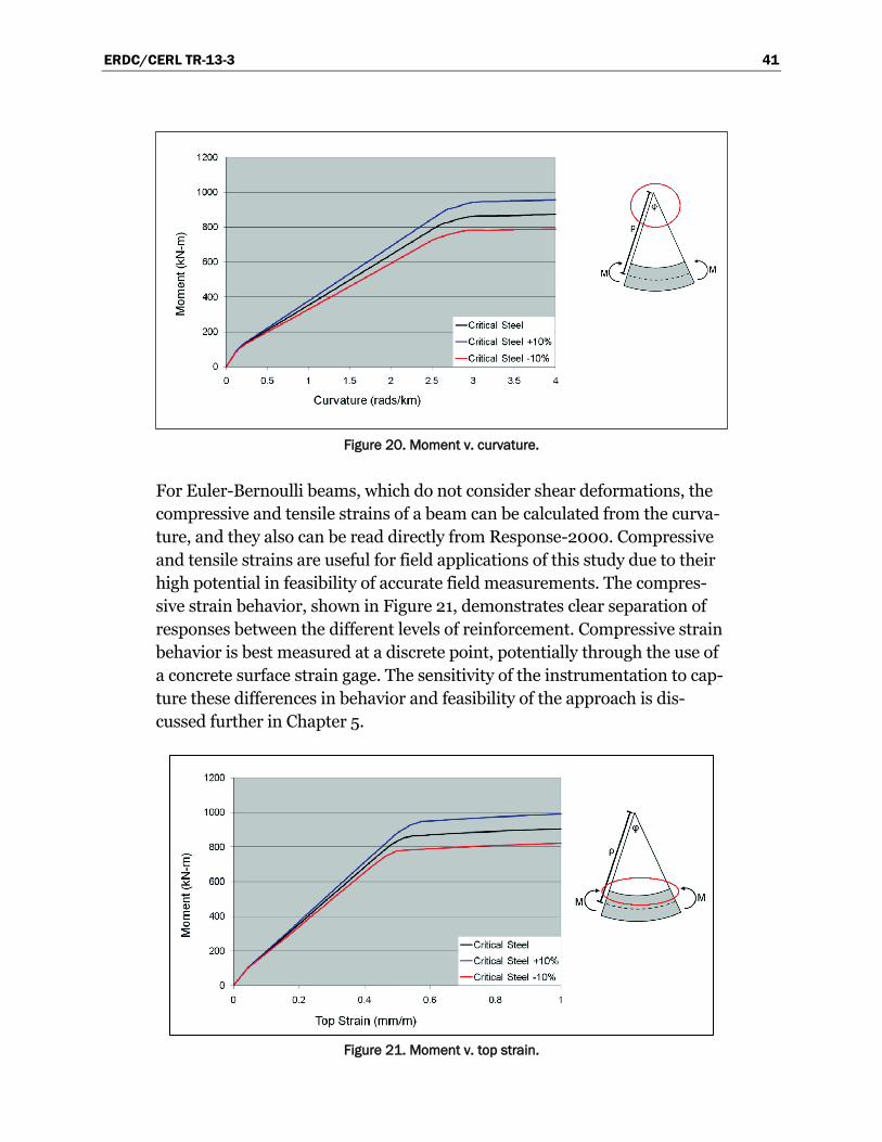
ERDC/CERL TR-13-3 41
Figure 20. Moment v. curvature.
For Euler-Bernoulli beams, which do not consider shear deformations, the compressive and tensile strains of a beam can be calculated from the curva-ture, and they also can be read directly from Response-2000. Compressive and tensile strains are useful for field applications of this study due to their high potential in feasibility of accurate field measurements. The compres-sive strain behavior, shown in Figure 21, demonstrates clear separation of responses between the different levels of reinforcement. Compressive strain behavior is best measured at a discrete point, potentially through the use of a concrete surface strain gage. The sensitivity of the instrumentation to cap-ture these differences in behavior and feasibility of the approach is dis-cussed further in Chapter 5.
Figure 21. Moment v. top strain.
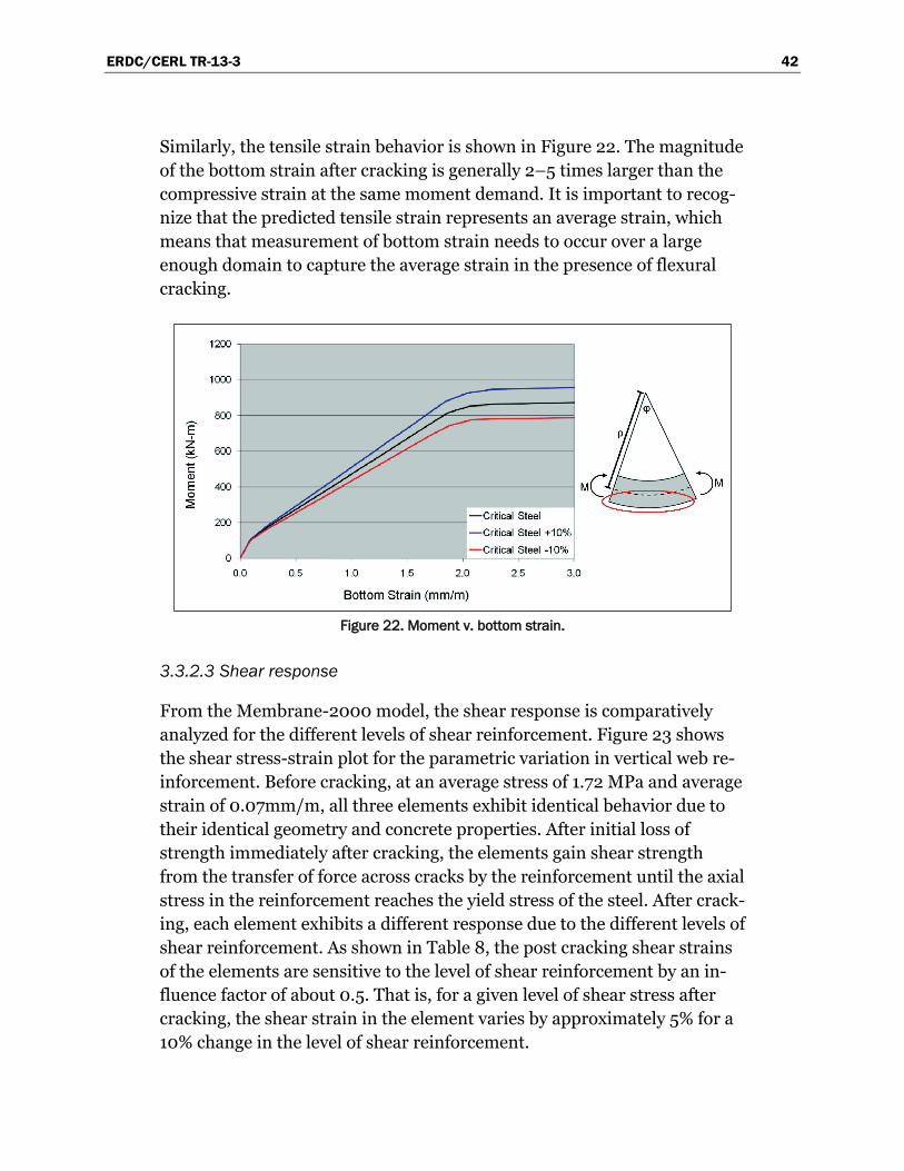
ERDC/CERL TR-13-3 42
Similarly, the tensile strain behavior is shown in Figure 22. The magnitude of the bottom strain after cracking is generally 2–5 times larger than the compressive strain at the same moment demand. It is important to recog-nize that the predicted tensile strain represents an average strain, which means that measurement of bottom strain needs to occur over a large enough domain to capture the average strain in the presence of flexural cracking.
Figure 22. Moment v. bottom strain.
3.3.2.3 Shear response
From the Membrane-2000 model, the shear response is comparatively analyzed for the different levels of shear reinforcement. Figure 23 shows the shear stress-strain plot for the parametric variation in vertical web re-inforcement. Before cracking, at an average stress of 1.72 MPa and average strain of 0.07mm/m, all three elements exhibit identical behavior due to their identical geometry and concrete properties. After initial loss of strength immediately after cracking, the elements gain shear strength from the transfer of force across cracks by the reinforcement until the axial stress in the reinforcement reaches the yield stress of the steel. After crack-ing, each element exhibits a different response due to the different levels of shear reinforcement. As shown in Table 8, the post cracking shear strains of the elements are sensitive to the level of shear reinforcement by an in-fluence factor of about 0.5. That is, for a given level of shear stress after cracking, the shear strain in the element varies by approximately 5% for a 10% change in the level of shear reinforcement.
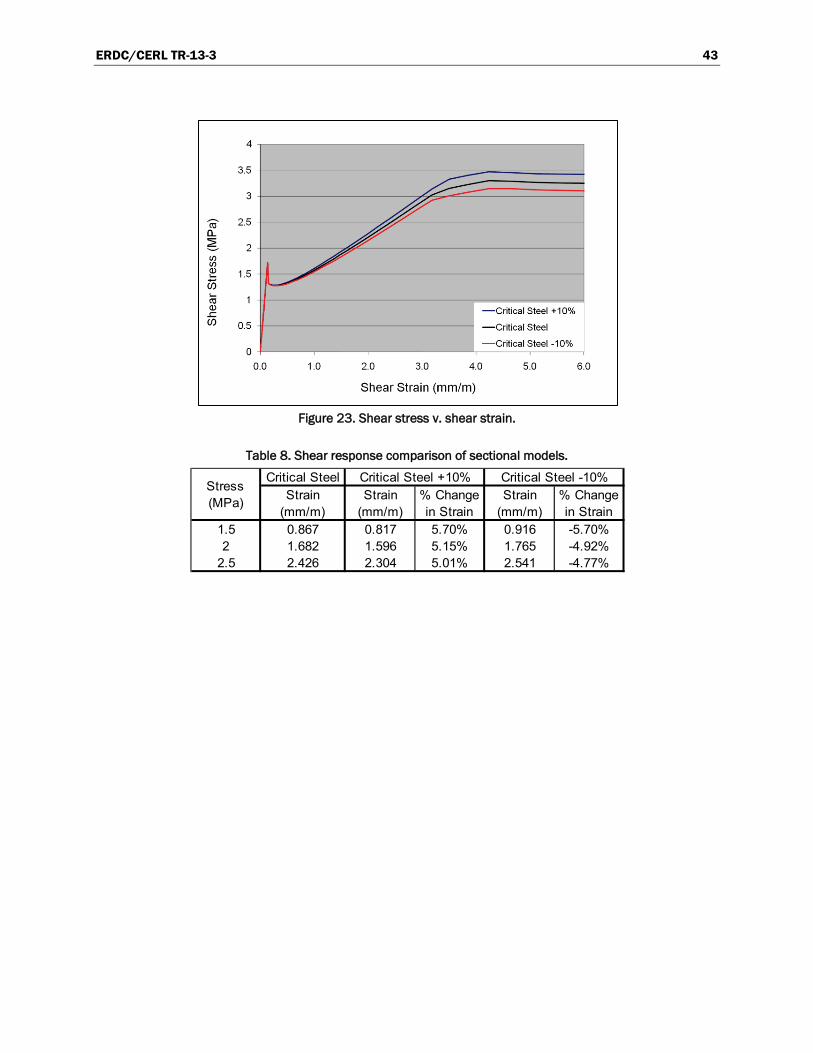
ERDC/CERL TR-13-3 43
Figure 23. Shear stress v. shear strain.
Table 8. Shear response comparison of sectional models.
Critical SteelStrain
(mm/m)Strain
(mm/m)% Change in Strain
Strain (mm/m)
% Change in Strain
1.5 0.867 0.817 5.70% 0.916 -5.70%2 1.682 1.596 5.15% 1.765 -4.92%
2.5 2.426 2.304 5.01% 2.541 -4.77%
Critical Steel +10% Critical Steel -10%Stress (MPa)
ERDC/CERL TR-13-3 44
4 Dynamic Modeling and Analysis
Measuring the dynamic response of a structure provides an additional source of information that can help to determine the structure’s internal makeup. Vibrations are measured to perform a system identification of the structure from which the natural frequencies and mode shapes are deter-mined. The identified dynamic properties are dependent on the stiffness of the structure as determined by the structure’s internal makeup. The loca-tion and amount of reinforcement in a concrete bridge affect the stiffness of the structure. By comparing measured responses to those from a dy-namic model of the structure, the model can be updated to match the measured characteristics, thereby giving a better understanding of the likely makeup of the structure.
4.1 Analytical tools and model
Dynamic measurements and the subsequent system identification are de-pendent on a source of vibration sufficient to cause a measureable re-sponse. The type of reinforced concrete bridges being analyzed are short, stiff structures that are less responsive to ambient excitation caused by winds. Bridge traffic loads under normal operating conditions can provide sufficient excitation to carry out system identification. For military situa-tions specific to this project, the bridge would be closed to normal traffic. While the bridge is under analysis, a military vehicle could be sent across to provide excitation. Installing a speed bump on the bridge can cause an excitation that, depending on speed of the vehicle and dimensions of the bump, induces an impulse response in the bridge. An impulse excitation is ideal as it excites the entire frequency domain so that all the natural fre-quencies of the bridge can be measured simultaneously. In order to model the reinforced concrete bridge and vehicle system properly, considerations for the properties of the bridge and the interaction of the vehicle and bridge need to be considered.
In order to analyze the dynamic characteristics of the reinforced concrete beams being studied, a dynamic model was created in MATLAB. The mod-el used the characteristics of the beams as determined by applying the static techniques in Chapter 3.
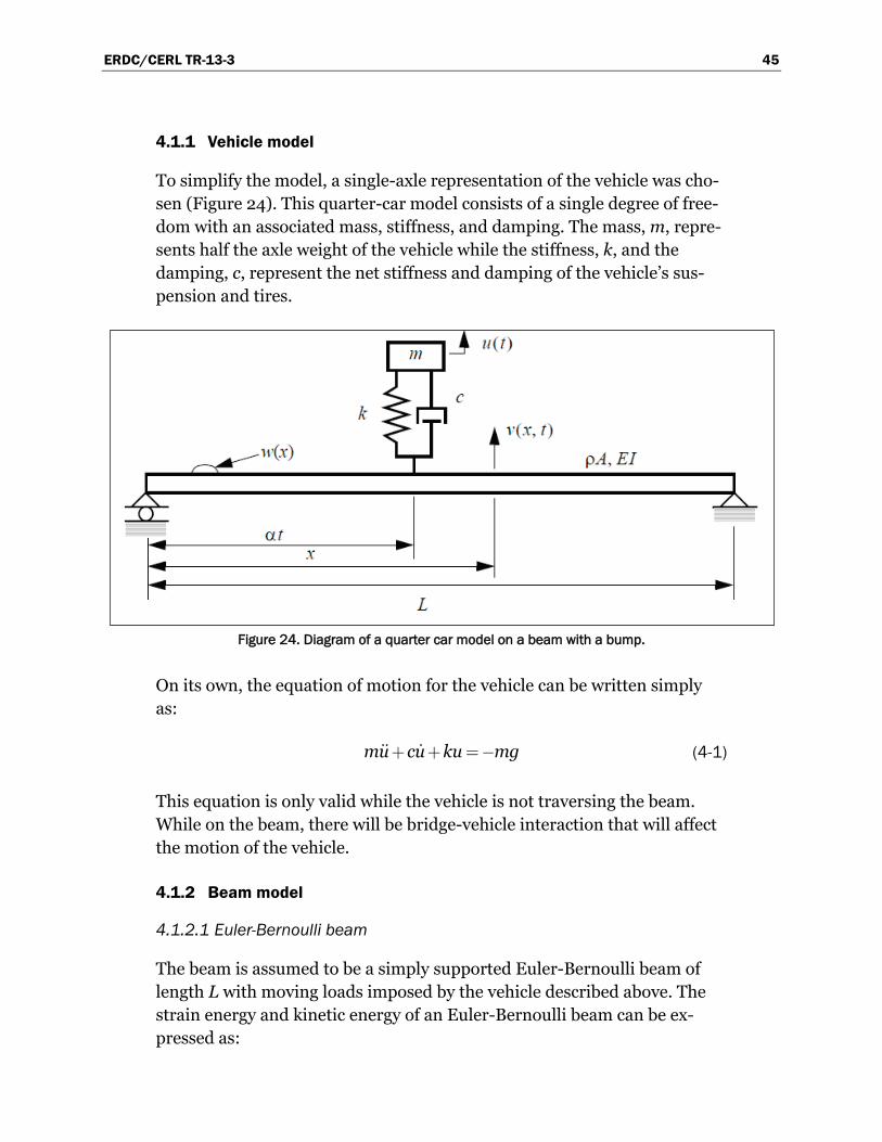
ERDC/CERL TR-13-3 45
4.1.1 Vehicle model
To simplify the model, a single-axle representation of the vehicle was cho-sen (Figure 24). This quarter-car model consists of a single degree of free-dom with an associated mass, stiffness, and damping. The mass, m, repre-sents half the axle weight of the vehicle while the stiffness, k, and the damping, c, represent the net stiffness and damping of the vehicle’s sus-pension and tires.
Figure 24. Diagram of a quarter car model on a beam with a bump.
On its own, the equation of motion for the vehicle can be written simply as:
mu cu ku mg (4-1)
This equation is only valid while the vehicle is not traversing the beam. While on the beam, there will be bridge-vehicle interaction that will affect the motion of the vehicle.
4.1.2 Beam model
4.1.2.1 Euler-Bernoulli beam
The beam is assumed to be a simply supported Euler-Bernoulli beam of length L with moving loads imposed by the vehicle described above. The strain energy and kinetic energy of an Euler-Bernoulli beam can be ex-pressed as:
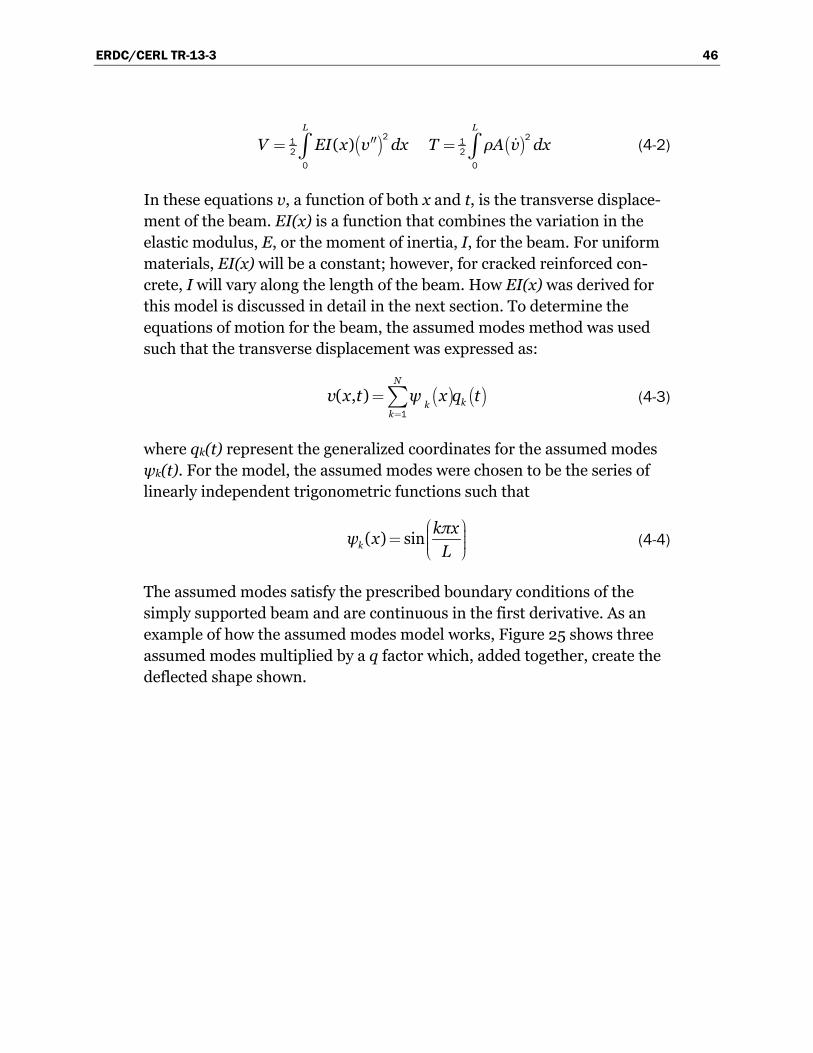
ERDC/CERL TR-13-3 46
( ) L L
V EI x v dx T ρA v dx 2 21 1
2 20 0
(4-2)
In these equations v, a function of both x and t, is the transverse displace-ment of the beam. EI(x) is a function that combines the variation in the elastic modulus, E, or the moment of inertia, I, for the beam. For uniform materials, EI(x) will be a constant; however, for cracked reinforced con-crete, I will vary along the length of the beam. How EI(x) was derived for this model is discussed in detail in the next section. To determine the equations of motion for the beam, the assumed modes method was used such that the transverse displacement was expressed as:
( , )N
kkk
v x t ψ x q t
1
(4-3)
where qk(t) represent the generalized coordinates for the assumed modes ψk(t). For the model, the assumed modes were chosen to be the series of linearly independent trigonometric functions such that
( ) sinkkπxψ x
L
(4-4)
The assumed modes satisfy the prescribed boundary conditions of the simply supported beam and are continuous in the first derivative. As an example of how the assumed modes model works, Figure 25 shows three assumed modes multiplied by a q factor which, added together, create the deflected shape shown.
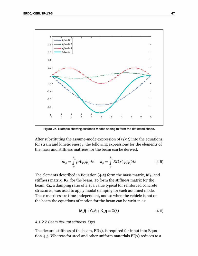
ERDC/CERL TR-13-3 47
Figure 25. Example showing assumed modes adding to form the deflected shape.
After substituting the assume-mode expression of v(x,t) into the equations for strain and kinetic energy, the following expressions for the elements of the mass and stiffness matrices for the beam can be derived.
( )L L
ij i j ij i jm ρAψ ψ dx k EI x ψ ψ dx 0 0
(4-5)
The elements described in Equation (4-5) form the mass matrix, Mb, and stiffness matrix, Kb, for the beam. To form the stiffness matrix for the beam, Cb, a damping ratio of 4%, a value typical for reinforced concrete structures, was used to apply modal damping for each assumed mode. These matrices are time-independent, and so when the vehicle is not on the beam the equations of motion for the beam can be written as:
( )b b b t M q C q K q G (4-6)
4.1.2.2 Beam flexural stiffness, EI(x)
The flexural stiffness of the beam, EI(x), is required for input into Equa-tion 4-5. Whereas for steel and other uniform materials EI(x) reduces to a
0 1 2 3 4 5 6 7 8 9 10-1
-0.8
-0.6
-0.4
-0.2
0
0.2
0.4
0.6
0.8
1
q1*Mode 1
q2*Mode 2
q3*Mode 3
Deflection

ERDC/CERL TR-13-3 48
constant EI, the depth and location of cracking in reinforced concrete cause the moment of inertia of the beam to change along its length. Typi-cally, designers will use an effective moment of inertia, 𝐼𝑒, as a single value in calculating deflections and other serviceability considerations. Values of 𝐼𝑒 are bound by the uncracked gross moment of inertia, 𝐼𝑔, and the cracked moment of inertia, 𝐼𝑐𝑟. Different methods for determining 𝐼𝑒 have been proposed and evaluated in research throughout the years (Wickline, Cousins and Seda-Sanabria 2003, ACI Committee 435 1966).
In this project, the extent of cracking along the beam was considered by looking at the influence lines of two different vehicles, the HS20-44 AASHTO design vehicle and the California permit truck, as discussed in section 2.2. The influence line needed to represent the largest moment im-posed at each point along the beam for the vehicle crossing the bridge. In other words, each point on the influence line represents the largest mo-ment demand “felt” by the structure in its load history. For each point along the influence line, the curvature (𝜑) of the beam can be determined from the moment-curvature plot in Figure 20. From this information, the flexural stiffness at each point along the beam is evaluated by:
( )
( )( )
M xEI xφ x
(4-7)
Figure 26 demonstrates the calculation of EI(x) for the beam with the criti-cal level of reinforcement with an HS20-44 load history. In the curvature plot, there is an evident abrupt change in behavior near the ends of the span, for example at x = 0.57m. This change in behavior demonstrates that the beam is not flexurally cracked for the first 0.57 m from the support. This behavior is further demonstrated in the EI(x) plot, where in this region, EI(x) is equal to EIg(x), the flexural stiffness of the uncracked gross section.
This procedure of calculating EI(x) along the beam was performed for the three levels of reinforcement under the two different load histories, as shown in Figure 27. As seen in the figure, the majority of the cracking in the beams is controlled primarily by the level of reinforcement rather than the load history.
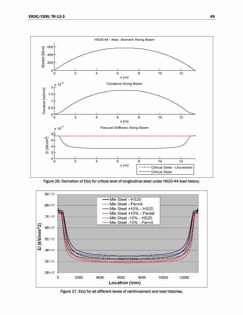
ERDC/CERL TR-13-3 49
Figure 26. Derivation of EI(x) for critical level of longitudinal steel under HS20-44 load history.
Figure 27. EI(x) for all different levels of reinforcement and load histories.
0 2 4 6 8 10 120
200
400
600
HS20-44 - Max. Moment Along Beam
x [m]
Mom
ent [
kN-m
]
0 2 4 6 8 10 120
0.5
1
1.5
2x 10
-6
x [m]
Curv
atur
e [ra
d/m
m]
Curvature Along Beam
0 2 4 6 8 10 120
2
4
6
8
x 1011
x [m]
EI [k
N-m
m2 ]
Flexural Stiffness Along Beam
Critical Steel - UncrackedCritical Steel
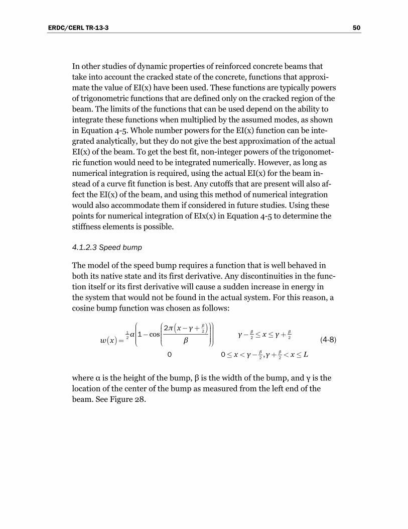
ERDC/CERL TR-13-3 50
In other studies of dynamic properties of reinforced concrete beams that take into account the cracked state of the concrete, functions that approxi-mate the value of EI(x) have been used. These functions are typically powers of trigonometric functions that are defined only on the cracked region of the beam. The limits of the functions that can be used depend on the ability to integrate these functions when multiplied by the assumed modes, as shown in Equation 4-5. Whole number powers for the EI(x) function can be inte-grated analytically, but they do not give the best approximation of the actual EI(x) of the beam. To get the best fit, non-integer powers of the trigonomet-ric function would need to be integrated numerically. However, as long as numerical integration is required, using the actual EI(x) for the beam in-stead of a curve fit function is best. Any cutoffs that are present will also af-fect the EI(x) of the beam, and using this method of numerical integration would also accommodate them if considered in future studies. Using these points for numerical integration of EIx(x) in Equation 4-5 to determine the stiffness elements is possible.
4.1.2.3 Speed bump
The model of the speed bump requires a function that is well behaved in both its native state and its first derivative. Any discontinuities in the func-tion itself or its first derivative will cause a sudden increase in energy in the system that would not be found in the actual system. For this reason, a cosine bump function was chosen as follows:
cos
,
ββ β
β β
π x γα γ x γ
βw x
x γ γ x L
21
2 2 2
2 2
21
0 0
(4-8)
where α is the height of the bump, β is the width of the bump, and γ is the location of the center of the bump as measured from the left end of the beam. See Figure 28.
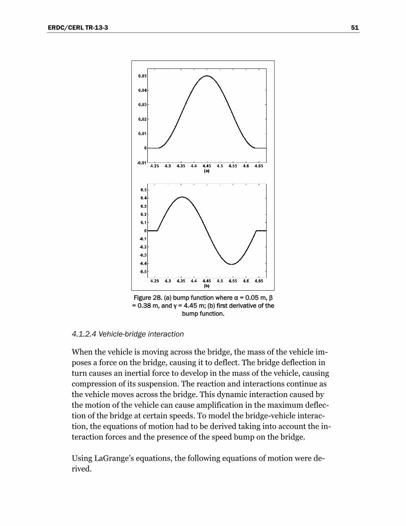
ERDC/CERL TR-13-3 51
Figure 28. (a) bump function where α = 0.05 m, β
= 0.38 m, and γ = 4.45 m; (b) first derivative of the bump function.
4.1.2.4 Vehicle-bridge interaction
When the vehicle is moving across the bridge, the mass of the vehicle im-poses a force on the bridge, causing it to deflect. The bridge deflection in turn causes an inertial force to develop in the mass of the vehicle, causing compression of its suspension. The reaction and interactions continue as the vehicle moves across the bridge. This dynamic interaction caused by the motion of the vehicle can cause amplification in the maximum deflec-tion of the bridge at certain speeds. To model the bridge-vehicle interac-tion, the equations of motion had to be derived taking into account the in-teraction forces and the presence of the speed bump on the bridge.
Using LaGrange’s equations, the following equations of motion were de-rived.
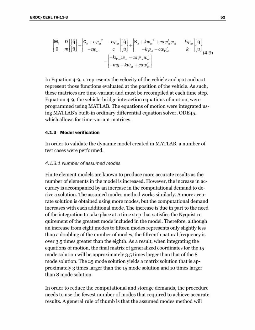
ERDC/CERL TR-13-3 52
b b αt αt b αt αt αt αt
αt αt αt
αt αt αt αt
αt αt
cψ cψ kψ cαψ ψ kψ
m u u ucψ c kψ cαψ k
kψ w cαψ w
mg kw cαw
M 0 q q qC K0
2 2
(4-9)
In Equation 4-9, α represents the velocity of the vehicle and ψαt and ωαt represent those functions evaluated at the position of the vehicle. As such, these matrices are time-variant and must be recompiled at each time step. Equation 4-9, the vehicle-bridge interaction equations of motion, were programmed using MATLAB. The equations of motion were integrated us-ing MATLAB’s built-in ordinary differential equation solver, ODE45, which allows for time-variant matrices.
4.1.3 Model verification
In order to validate the dynamic model created in MATLAB, a number of test cases were performed.
4.1.3.1 Number of assumed modes
Finite element models are known to produce more accurate results as the number of elements in the model is increased. However, the increase in ac-curacy is accompanied by an increase in the computational demand to de-rive a solution. The assumed modes method works similarly. A more accu-rate solution is obtained using more modes, but the computational demand increases with each additional mode. The increase is due in part to the need of the integration to take place at a time step that satisfies the Nyquist re-quirement of the greatest mode included in the model. Therefore, although an increase from eight modes to fifteen modes represents only slightly less than a doubling of the number of modes, the fifteenth natural frequency is over 3.5 times greater than the eighth. As a result, when integrating the equations of motion, the final matrix of generalized coordinates for the 15 mode solution will be approximately 3.5 times larger than that of the 8 mode solution. The 25 mode solution yields a matrix solution that is ap-proximately 3 times larger than the 15 mode solution and 10 times larger than 8 mode solution.
In order to reduce the computational and storage demands, the procedure needs to use the fewest number of modes that required to achieve accurate results. A general rule of thumb is that the assumed modes method will

ERDC/CERL TR-13-3 53
generally yield accurate natural frequencies for the first half of the number of modes used. This is due to the higher modes being used to account for the infinite number of modes that are not included in the model. Never-theless, the calculated modes will become more accurate as the number of modes included is increased. Table 9 shows the convergence of the first four natural frequencies as the number of assumed modes included in the model increases.
Table 9. Comparison of natural frequencies (Hz) for dynamic models with varying numbers of assumed modes.
Since the beam motion is dominated by the first mode, additional modes need only be included until the solution converges. Table 10 shows, to three significant digits, the maximum negative displacement, velocity, and accel-eration at the center of the beam for a model where a vehicle passes over a bump located at a distance L/3 from the approach end. The only parameter changed was the number of assumed modes used in the computation. By using 15 modes, the solution does not differ significantly from higher-mode solutions and it can still be calculated using a desktop computer in a rea-sonable amount of time. Figure 29 shows the calculated results for the ac-celeration at the beam center when the moving vehicle crosses the bump for models that included 8, 15 or 25 modes.
Table 10. Comparison of output based on the number of assumed modes included in the dynamic model.
8 15 251st (Hz) 5.338 5.338 5.3382nd (Hz) 21.77 21.77 21.773rd (Hz) 49.65 49.58 49.584th (Hz) 89.09 88.93 88.93
Natural Frequency
Assumed Modes Included in Model
8 15 25Displacement mm -1.322 -1.322 -1.322
Velocity mm/s -7.566 -7.567 -7.568Acceleration mg -22.63 -22.87 -22.66
Assumed Modes IncludedUnitMeasurement
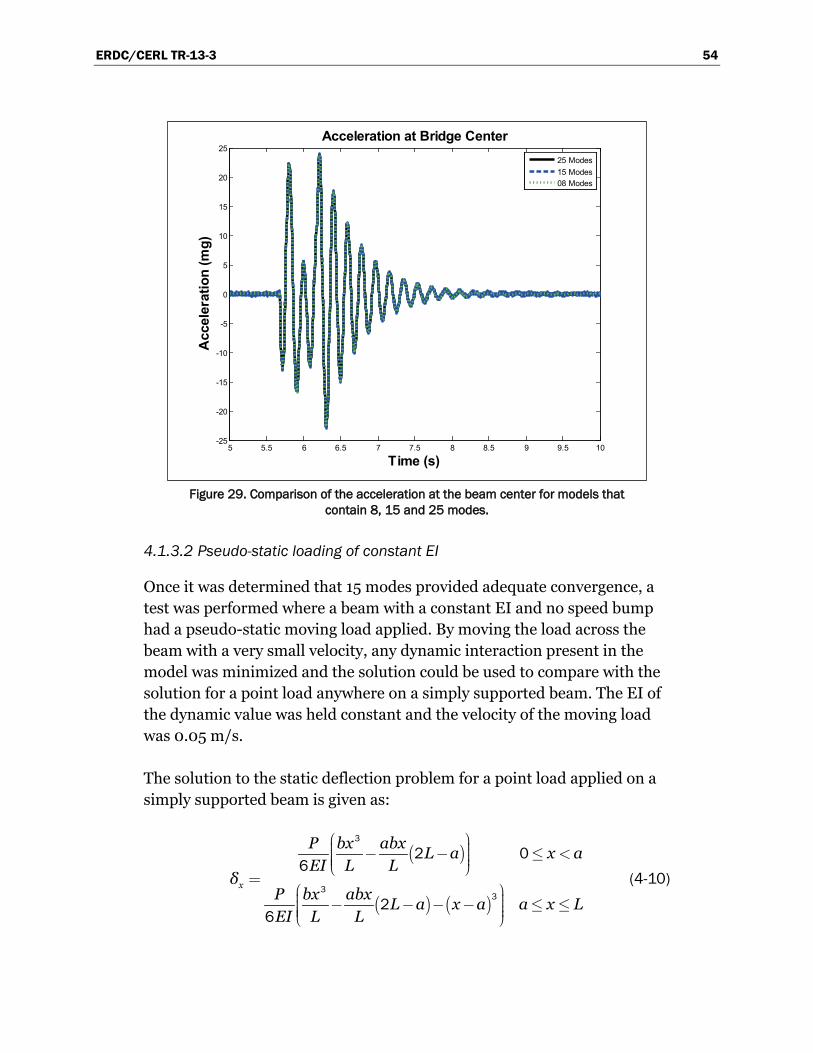
ERDC/CERL TR-13-3 54
Figure 29. Comparison of the acceleration at the beam center for models that
contain 8, 15 and 25 modes.
4.1.3.2 Pseudo-static loading of constant EI
Once it was determined that 15 modes provided adequate convergence, a test was performed where a beam with a constant EI and no speed bump had a pseudo-static moving load applied. By moving the load across the beam with a very small velocity, any dynamic interaction present in the model was minimized and the solution could be used to compare with the solution for a point load anywhere on a simply supported beam. The EI of the dynamic value was held constant and the velocity of the moving load was 0.05 m/s.
The solution to the static deflection problem for a point load applied on a simply supported beam is given as:
x
P bx abx L a x aEI L L
δP bx abx L a x a a x LEI L L
3
33
2 06
26
(4-10)
5 5.5 6 6.5 7 7.5 8 8.5 9 9.5 10-25
-20
-15
-10
-5
0
5
10
15
20
25Acceleration at Bridge Center
Time (s)
Acc
eler
atio
n (m
g)
25 Modes15 Modes08 Modes
ERDC/CERL TR-13-3 55
where P is the point load, a is the distance from the left of the beam to the point load, b is the distance from the point load to the right of the beam, and x is the point where the deflection is being calculated. For comparison to the dynamic model, a=αt where α is the velocity of the moving load, b=L-a, and x=L/2.
Figure 30 shows the deflection of the center of the beam as calculated us-ing the dynamic model as the load moves across and the solution if the load had been applied at the equivalent point on the static beam. The two solutions matched up well, confirming the formulation of the equations of motion and the integration techniques for the EI of the beam.
Figure 30. Displacement at bridge center with a moving load.
Table 11 shows the calculated values of displacement at the quarter and third points of the beam for both the dynamic and static models. The val-ues are equivalent to a reasonable number of significant digits.
0 50 100 150 200 250-0.5
-0.45
-0.4
-0.35
-0.3
-0.25
-0.2
-0.15
-0.1
-0.05
0
0.05Response at Bridge Center
Time (s)
mm
Dynamic ModelStatic Solution
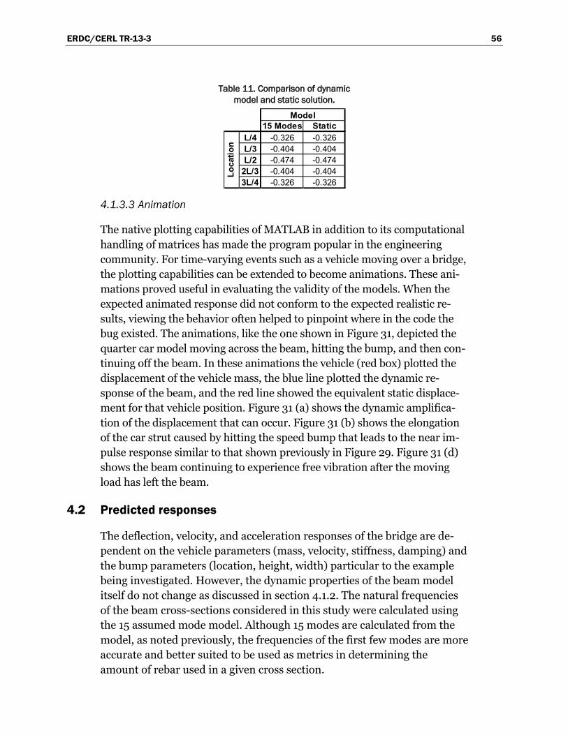
ERDC/CERL TR-13-3 56
Table 11. Comparison of dynamic model and static solution.
4.1.3.3 Animation
The native plotting capabilities of MATLAB in addition to its computational handling of matrices has made the program popular in the engineering community. For time-varying events such as a vehicle moving over a bridge, the plotting capabilities can be extended to become animations. These ani-mations proved useful in evaluating the validity of the models. When the expected animated response did not conform to the expected realistic re-sults, viewing the behavior often helped to pinpoint where in the code the bug existed. The animations, like the one shown in Figure 31, depicted the quarter car model moving across the beam, hitting the bump, and then con-tinuing off the beam. In these animations the vehicle (red box) plotted the displacement of the vehicle mass, the blue line plotted the dynamic re-sponse of the beam, and the red line showed the equivalent static displace-ment for that vehicle position. Figure 31 (a) shows the dynamic amplifica-tion of the displacement that can occur. Figure 31 (b) shows the elongation of the car strut caused by hitting the speed bump that leads to the near im-pulse response similar to that shown previously in Figure 29. Figure 31 (d) shows the beam continuing to experience free vibration after the moving load has left the beam.
4.2 Predicted responses
The deflection, velocity, and acceleration responses of the bridge are de-pendent on the vehicle parameters (mass, velocity, stiffness, damping) and the bump parameters (location, height, width) particular to the example being investigated. However, the dynamic properties of the beam model itself do not change as discussed in section 4.1.2. The natural frequencies of the beam cross-sections considered in this study were calculated using the 15 assumed mode model. Although 15 modes are calculated from the model, as noted previously, the frequencies of the first few modes are more accurate and better suited to be used as metrics in determining the amount of rebar used in a given cross section.
15 Modes StaticL/4 -0.326 -0.326L/3 -0.404 -0.404L/2 -0.474 -0.474
2L/3 -0.404 -0.4043L/4 -0.326 -0.326
Model
Loca
tion
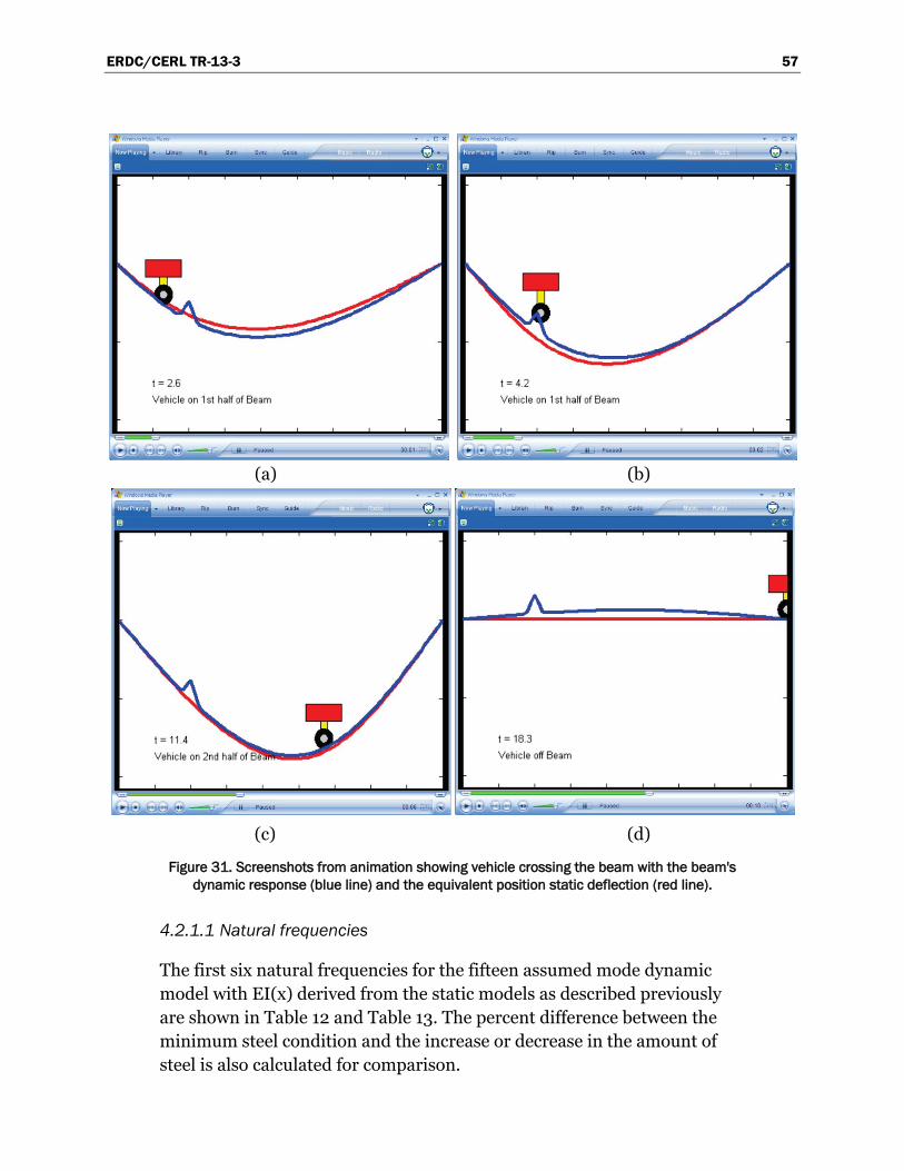
ERDC/CERL TR-13-3 57
(a) (b)
(c) (d)
Figure 31. Screenshots from animation showing vehicle crossing the beam with the beam's dynamic response (blue line) and the equivalent position static deflection (red line).
4.2.1.1 Natural frequencies
The first six natural frequencies for the fifteen assumed mode dynamic model with EI(x) derived from the static models as described previously are shown in Table 12 and Table 13. The percent difference between the minimum steel condition and the increase or decrease in the amount of steel is also calculated for comparison.
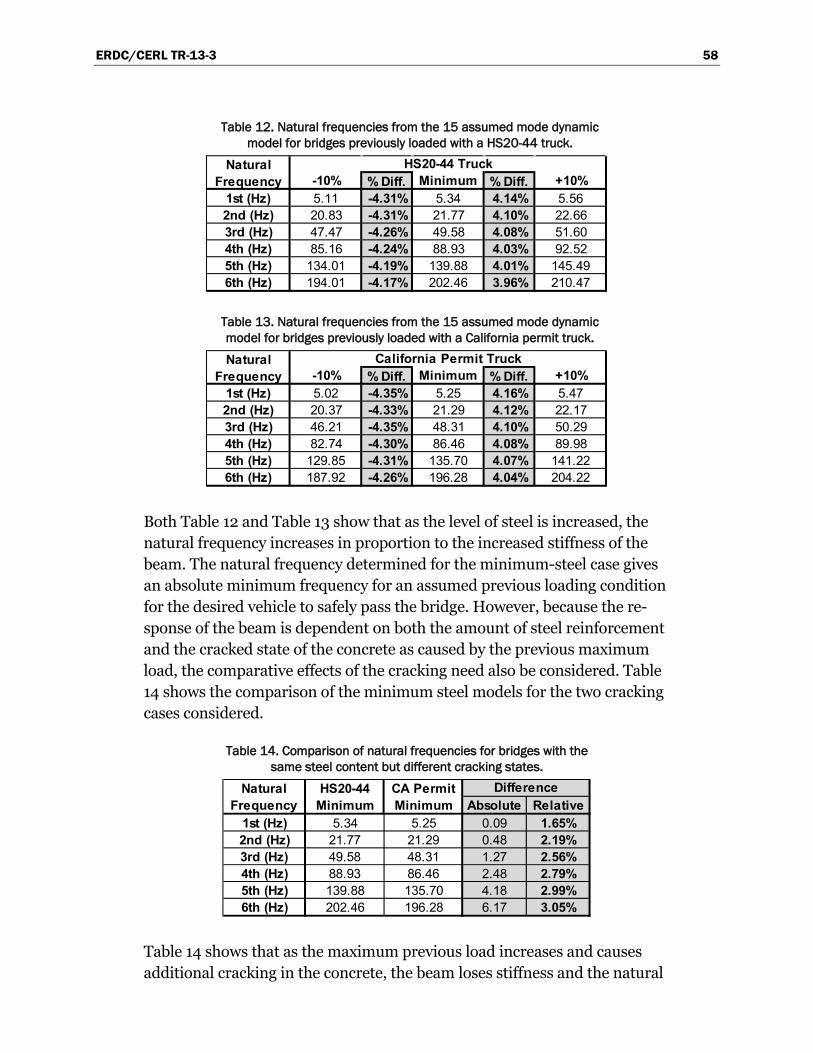
ERDC/CERL TR-13-3 58
Table 12. Natural frequencies from the 15 assumed mode dynamic model for bridges previously loaded with a HS20-44 truck.
Table 13. Natural frequencies from the 15 assumed mode dynamic model for bridges previously loaded with a California permit truck.
Both Table 12 and Table 13 show that as the level of steel is increased, the natural frequency increases in proportion to the increased stiffness of the beam. The natural frequency determined for the minimum-steel case gives an absolute minimum frequency for an assumed previous loading condition for the desired vehicle to safely pass the bridge. However, because the re-sponse of the beam is dependent on both the amount of steel reinforcement and the cracked state of the concrete as caused by the previous maximum load, the comparative effects of the cracking need also be considered. Table 14 shows the comparison of the minimum steel models for the two cracking cases considered.
Table 14. Comparison of natural frequencies for bridges with the same steel content but different cracking states.
Table 14 shows that as the maximum previous load increases and causes additional cracking in the concrete, the beam loses stiffness and the natural
-10% % Diff. Minimum % Diff. +10%1st (Hz) 5.11 -4.31% 5.34 4.14% 5.562nd (Hz) 20.83 -4.31% 21.77 4.10% 22.663rd (Hz) 47.47 -4.26% 49.58 4.08% 51.604th (Hz) 85.16 -4.24% 88.93 4.03% 92.525th (Hz) 134.01 -4.19% 139.88 4.01% 145.496th (Hz) 194.01 -4.17% 202.46 3.96% 210.47
Natural Frequency
HS20-44 Truck
-10% % Diff. Minimum % Diff. +10%1st (Hz) 5.02 -4.35% 5.25 4.16% 5.472nd (Hz) 20.37 -4.33% 21.29 4.12% 22.173rd (Hz) 46.21 -4.35% 48.31 4.10% 50.294th (Hz) 82.74 -4.30% 86.46 4.08% 89.985th (Hz) 129.85 -4.31% 135.70 4.07% 141.226th (Hz) 187.92 -4.26% 196.28 4.04% 204.22
Natural Frequency
California Permit Truck
HS20-44 CA PermitMinimum Minimum Absolute Relative
1st (Hz) 5.34 5.25 0.09 1.65%2nd (Hz) 21.77 21.29 0.48 2.19%3rd (Hz) 49.58 48.31 1.27 2.56%4th (Hz) 88.93 86.46 2.48 2.79%5th (Hz) 139.88 135.70 4.18 2.99%6th (Hz) 202.46 196.28 6.17 3.05%
Natural Frequency
Difference
ERDC/CERL TR-13-3 59
frequencies decrease. The percent change caused by a change in flexural steel, shown in Table 12 and Table 13, is greater than that caused by the change in cracking conditions, shown in Table 14. Although the 4% percent change caused by a 10% change in the amount of steel reinforcement does not seem significantly greater than the 2% change seen in the first two natu-ral frequencies in Table 14, the magnitude of the cracking change is much greater than a 10% increase. Therefore, if the amount of cracking can be predicted to a reasonable value and modeled, the natural frequencies for a bridge containing the minimum amount of reinforcement can be calculated. Any deviation from these calculated values can then be reasonably assumed to be caused by the amount of steel in the structure and not cracking in the bridge. The greater sensitivity of the dynamic properties of the bridge to the amount of flexural reinforcement and not the cracked state of the concrete permits the development of a method to determine the amount of rein-forcement from a measured response.
As previously stated, the natural frequency of the bridge depends on both parameters used in the study: loading history and amount of reinforcement. However, if the previous maximum load can be determined or assumed, there is potential for determining the amount of reinforcement in the beam based on a measured natural frequency. Figure 32 illustrates how this method would work. In Figure 32, the blue and green lines represent two possible measured frequencies for the first mode of the beam. In this case, Frequency 1 is the lower value and Frequency 2 is the higher of the two. Each line represents the combinations of maximum load and reinforcement steel that will yield that given frequency. From modeling, the relationship between the previous maximum load and the amount of steel reinforcement is known. If for Frequency 1 shown by the blue line, a certain maximum previous load is determined (red dotted line), then the amount of rein-forcement can be determined. However if a greater maximum load is de-termined for the same frequency value (dark purple dotted line), then a greater amount of reinforcement was present. This is because the in-creased amount of cracking will cause the stiffness to decrease to a greater degree, and the original beam must have been stiffer for the resultant fre-quency to be the same as the case with a lesser maximum previous load. For the same loading conditions but different measured frequencies (dark and light purple dotted lines), the bridges would have different amounts of reinforcement present. By running the model with the assumed maximum previous load, curves could be developed for determining the amount of steel present for a given beam and measured natural frequencies. Using
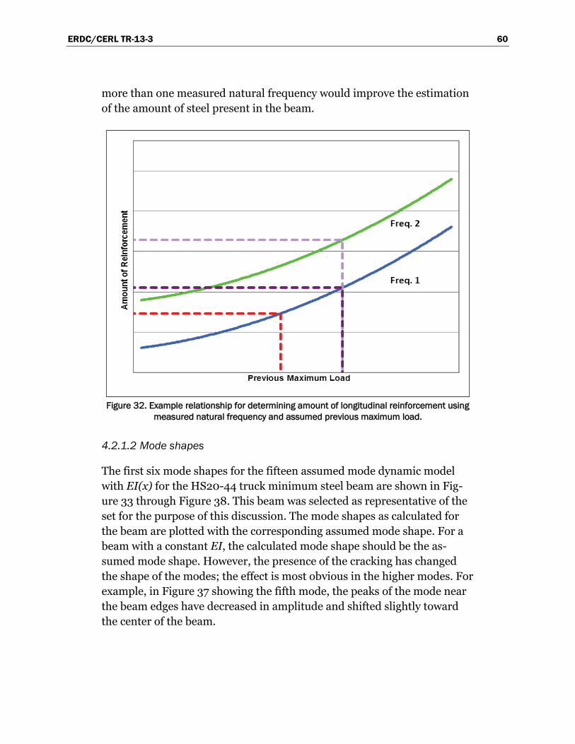
ERDC/CERL TR-13-3 60
more than one measured natural frequency would improve the estimation of the amount of steel present in the beam.
Figure 32. Example relationship for determining amount of longitudinal reinforcement using
measured natural frequency and assumed previous maximum load.
4.2.1.2 Mode shapes
The first six mode shapes for the fifteen assumed mode dynamic model with EI(x) for the HS20-44 truck minimum steel beam are shown in Fig-ure 33 through Figure 38. This beam was selected as representative of the set for the purpose of this discussion. The mode shapes as calculated for the beam are plotted with the corresponding assumed mode shape. For a beam with a constant EI, the calculated mode shape should be the as-sumed mode shape. However, the presence of the cracking has changed the shape of the modes; the effect is most obvious in the higher modes. For example, in Figure 37 showing the fifth mode, the peaks of the mode near the beam edges have decreased in amplitude and shifted slightly toward the center of the beam.
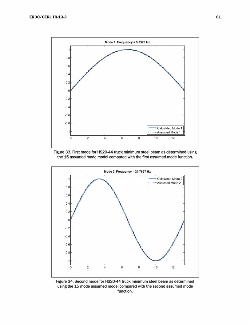
ERDC/CERL TR-13-3 61
Figure 33. First mode for HS20-44 truck minimum steel beam as determined using
the 15 assumed mode model compared with the first assumed mode function.
Figure 34. Second mode for HS20-44 truck minimum steel beam as determined using the 15 mode assumed model compared with the second assumed mode
function.
0 2 4 6 8 10 12
-1
-0.8
-0.6
-0.4
-0.2
0
0.2
0.4
0.6
0.8
1
Mode 1 Frequency = 5.3378 Hz
Calculated Mode 1Assumed Mode 1
0 2 4 6 8 10 12
-1
-0.8
-0.6
-0.4
-0.2
0
0.2
0.4
0.6
0.8
1
Mode 2 Frequency = 21.7657 Hz
Calculated Mode 2Assumed Mode 2
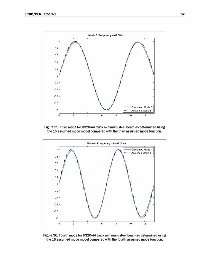
ERDC/CERL TR-13-3 62
Figure 35. Third mode for HS20-44 truck minimum steel beam as determined using
the 15 assumed mode model compared with the third assumed mode function.
Figure 36. Fourth mode for HS20-44 truck minimum steel beam as determined using
the 15 assumed mode model compared with the fourth assumed mode function.
0 2 4 6 8 10 12
-1
-0.8
-0.6
-0.4
-0.2
0
0.2
0.4
0.6
0.8
1
Mode 3 Frequency = 49.58 Hz
Calculated Mode 3Assumed Mode 3
0 2 4 6 8 10 12
-1
-0.8
-0.6
-0.4
-0.2
0
0.2
0.4
0.6
0.8
1
Mode 4 Frequency = 88.9326 Hz
Calculated Mode 4Assumed Mode 4
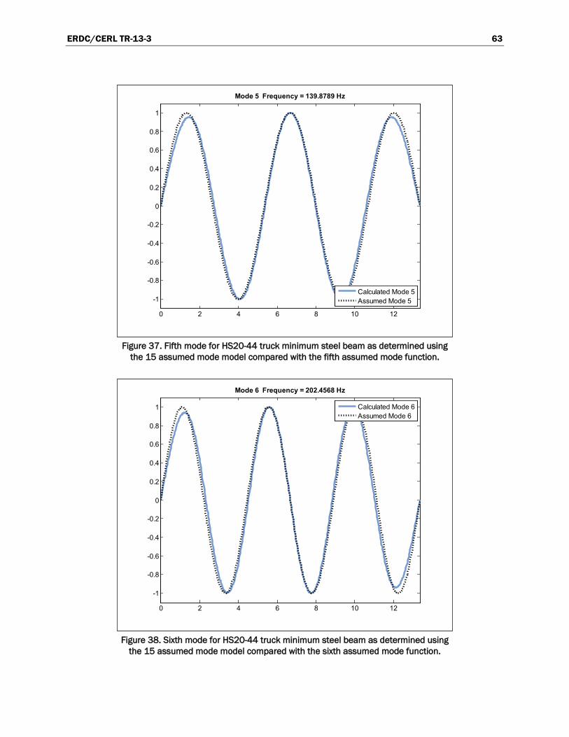
ERDC/CERL TR-13-3 63
Figure 37. Fifth mode for HS20-44 truck minimum steel beam as determined using
the 15 assumed mode model compared with the fifth assumed mode function.
Figure 38. Sixth mode for HS20-44 truck minimum steel beam as determined using
the 15 assumed mode model compared with the sixth assumed mode function.
0 2 4 6 8 10 12
-1
-0.8
-0.6
-0.4
-0.2
0
0.2
0.4
0.6
0.8
1
Mode 5 Frequency = 139.8789 Hz
Calculated Mode 5Assumed Mode 5
0 2 4 6 8 10 12
-1
-0.8
-0.6
-0.4
-0.2
0
0.2
0.4
0.6
0.8
1
Mode 6 Frequency = 202.4568 Hz
Calculated Mode 6Assumed Mode 6
ERDC/CERL TR-13-3 64
4.2.1.3 Response to excitation
The response of the bridge is dependent on how the bridge is excited. Field experiments on long-span bridges often depend on ambient vibration from wind or traffic for excitation. Short-span bridges, which are more common, are usually stiffer than their long-span counterparts and often need an ex-ternal source of excitation to achieve a measured response. Shakers with at-tached masses are useful in providing a controlled excitation in prescribed frequency ranges. Attaching cables to the bridge to apply a force to the bridge and then suddenly releasing the cables can cause an impulse loading that can also be used to determine the system properties of the bridge. However, these methods of excitation can be laborious to both mount and calibrate.
For a military operation, the required speed and ease of reconnaissance also must be considered in designing the experimental methods. A vehicle of known mass and speed driven over a speed bump of known height and width can cause a near impulse excitation of the bridge. The installation of the speed bump and operation of the vehicle are less technically demand-ing than other excitation techniques. For these reasons, the presence of a bump was included in the model as described previously. A bump 30 cm wide, 5 cm tall, and placed at a distance L/3 from the end of the beam was used in the study.
The military nature of the problem led to the selection of the High Mobility Multipurpose Wheeled Vehicle (HMMWV, or Humvee) for use in the mod-el. The HMMWV is used by the military in many different forms for many different purposes. Lighter, unarmored vehicles are used for general-purpose transport in safer regions while heavier, armored vehicles are often mounted with weapons in combat areas. Due to the ubiquitous use of the HMMWV, equipping one of known properties for a bridge reconnaissance mission is not unreasonable. In this study, a light HMMWV moving at a speed of 0.75 m/s with an axle weight of 2340 kg, a suspension stiffness of 50 kN/m, and a suspension damping of 12 kNs/m was modeled.
Using these parameters, the response of the structure and vehicle were computed. Using the assumed modes method, the response at any point on the beam can easily be computed. Figure 39 shows the response of the HS20-44 minimum steel bridge to the bump and vehicle parameters de-scribed above.
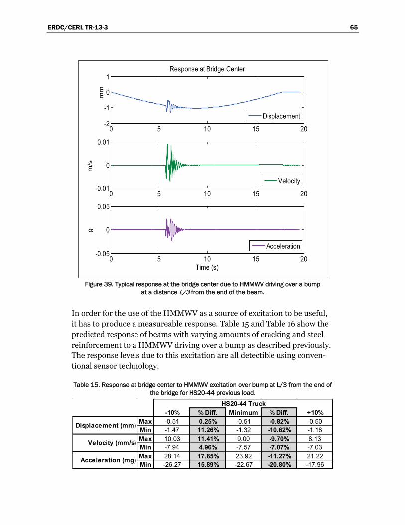
ERDC/CERL TR-13-3 65
Figure 39. Typical response at the bridge center due to HMMWV driving over a bump
at a distance L/3 from the end of the beam.
In order for the use of the HMMWV as a source of excitation to be useful, it has to produce a measureable response. Table 15 and Table 16 show the predicted response of beams with varying amounts of cracking and steel reinforcement to a HMMWV driving over a bump as described previously. The response levels due to this excitation are all detectible using conven-tional sensor technology.
Table 15. Response at bridge center to HMMWV excitation over bump at L/3 from the end of the bridge for HS20-44 previous load.
0 5 10 15 20-2
-1
0
1Response at Bridge Center
mm
Displacement
0 5 10 15 20-0.01
0
0.01
m/s
Velocity
0 5 10 15 20-0.05
0
0.05
Time (s)
g
Acceleration
-10% % Diff. Minimum % Diff. +10%Max -0.51 0.25% -0.51 -0.82% -0.50Min -1.47 11.26% -1.32 -10.62% -1.18Max 10.03 11.41% 9.00 -9.70% 8.13Min -7.94 4.96% -7.57 -7.07% -7.03Max 28.14 17.65% 23.92 -11.27% 21.22Min -26.27 15.89% -22.67 -20.80% -17.96
HS20-44 Truck
Displacement (mm)
Velocity (mm/s)
Acceleration (mg)
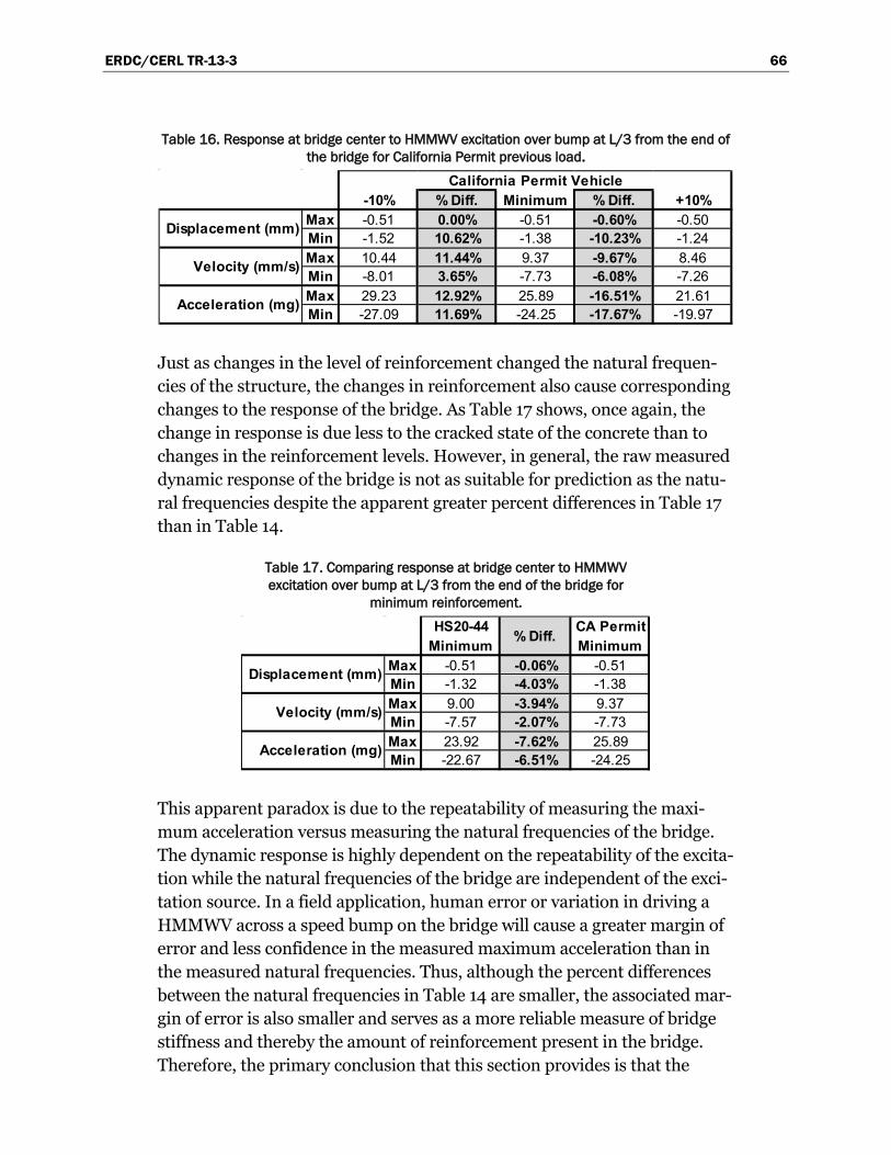
ERDC/CERL TR-13-3 66
Table 16. Response at bridge center to HMMWV excitation over bump at L/3 from the end of the bridge for California Permit previous load.
Just as changes in the level of reinforcement changed the natural frequen-cies of the structure, the changes in reinforcement also cause corresponding changes to the response of the bridge. As Table 17 shows, once again, the change in response is due less to the cracked state of the concrete than to changes in the reinforcement levels. However, in general, the raw measured dynamic response of the bridge is not as suitable for prediction as the natu-ral frequencies despite the apparent greater percent differences in Table 17 than in Table 14.
Table 17. Comparing response at bridge center to HMMWV excitation over bump at L/3 from the end of the bridge for
minimum reinforcement.
This apparent paradox is due to the repeatability of measuring the maxi-mum acceleration versus measuring the natural frequencies of the bridge. The dynamic response is highly dependent on the repeatability of the excita-tion while the natural frequencies of the bridge are independent of the exci-tation source. In a field application, human error or variation in driving a HMMWV across a speed bump on the bridge will cause a greater margin of error and less confidence in the measured maximum acceleration than in the measured natural frequencies. Thus, although the percent differences between the natural frequencies in Table 14 are smaller, the associated mar-gin of error is also smaller and serves as a more reliable measure of bridge stiffness and thereby the amount of reinforcement present in the bridge. Therefore, the primary conclusion that this section provides is that the
-10% % Diff. Minimum % Diff. +10%Max -0.51 0.00% -0.51 -0.60% -0.50Min -1.52 10.62% -1.38 -10.23% -1.24Max 10.44 11.44% 9.37 -9.67% 8.46Min -8.01 3.65% -7.73 -6.08% -7.26Max 29.23 12.92% 25.89 -16.51% 21.61Min -27.09 11.69% -24.25 -17.67% -19.97
Displacement (mm)
Velocity (mm/s)
Acceleration (mg)
California Permit Vehicle
HS20-44 CA PermitMinimum Minimum
Max -0.51 -0.06% -0.51Min -1.32 -4.03% -1.38Max 9.00 -3.94% 9.37Min -7.57 -2.07% -7.73Max 23.92 -7.62% 25.89Min -22.67 -6.51% -24.25
% Diff.
Displacement (mm)
Velocity (mm/s)
Acceleration (mg)

ERDC/CERL TR-13-3 67
HMMWV excitation, which the military could readily adopt, would provide sufficient excitation to evaluate the natural frequencies of the bridge. It is then, by using the measured natural frequencies, that the levels of rein-forcement can be determined using the method described above. An exam-ple of this approach is given in section 6.2.
ERDC/CERL TR-13-3 68
5 Survey of Sensor Technologies
The proposed assessment procedure requires that the sensor technology used to capture the in-field behavior is capable of making precise meas-urements and is feasible for implementation. It is not the aim of this study to make definitive statements on the application of available sensor tech-nologies. However, it is useful to provide a survey of current technologies that have potential application to the field and to offer insight into poten-tially useful sensor technologies that are either in development or do not currently exist. Accordingly, this chapter provides a brief survey of some of the useful technologies that may be applied to static and dynamic meas-urements in the field.
5.1 Accelerometers
Acceleration has proved a useful metric in many engineering disciplines. For example, seismic engineers have used accelerometers to measure ground accelerations during an earthquake. Acceleration is a more useful metric to seismic engineers than displacement, as the design forces acting on the structure are equal to the mass of the structure multiplied by its ac-celeration. Accelerometers need to be tailored to fit the application. Some existing sensors can measure many times the force of gravity down to a few hundred-thousandths of the force of gravity.
All accelerometers contain a seismic mass that moves within the sensor to cause a detectible change in an electrical property, which indicates accelera-tion. The size of the mass influences not only the sensitivity of the mecha-nism but also its usable range and fragility. As such, the size of the seismic mass and its support need to be tuned to the appropriate sizes for the in-tended application. Accelerometers for geological monitoring tend to be larger (e.g., greater than one cubic inch) to detect the small vibrations of small seismic events while also having sufficient range to record a major earthquake. Smaller, less delicate accelerometers are better-suited for la-boratory or field applications and still provide sufficient sensitivity and range. Microelectromechanical systems (MEMS) accelerometers have been developed that are also suitable for most structural dynamic applications while being small enough to fit on a circuit board.
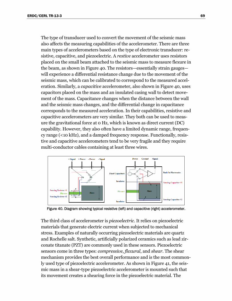
ERDC/CERL TR-13-3 69
The type of transducer used to convert the movement of the seismic mass also affects the measuring capabilities of the accelerometer. There are three main types of accelerometers based on the type of electronic transducer: re-sistive, capacitive, and piezoelectric. A restive accelerometer uses resistors placed on the small beam attached to the seismic mass to measure flexure in the beam, as shown in Figure 40. The resistors—essentially strain gauges—will experience a differential resistance change due to the movement of the seismic mass, which can be calibrated to correspond to the measured accel-eration. Similarly, a capacitive accelerometer, also shown in Figure 40, uses capacitors placed on the mass and an insulated casing wall to detect move-ment of the mass. Capacitance changes when the distance between the wall and the seismic mass changes, and the differential change in capacitance corresponds to the measured acceleration. In their capabilities, resistive and capacitive accelerometers are very similar. They both can be used to meas-ure the gravitational force at 0 Hz, which is known as direct current (DC) capability. However, they also often have a limited dynamic range, frequen-cy range (<10 kHz), and a damped frequency response. Functionally, resis-tive and capacitive accelerometers tend to be very fragile and they require multi-conductor cables containing at least three wires.
Figure 40. Diagram showing typical resistive (left) and capacitive (right) accelerometer.
The third class of accelerometer is piezoelectric. It relies on piezoelectric materials that generate electric current when subjected to mechanical stress. Examples of naturally occurring piezoelectric materials are quartz and Rochelle salt. Synthetic, artificially polarized ceramics such as lead zir-conate titanate (PZT) are commonly used in these sensors. Piezoelectric sensors come in three types: compressive, flexural, and shear. The shear mechanism provides the best overall performance and is the most common-ly used type of piezoelectric accelerometer. As shown in Figure 41, the seis-mic mass in a shear-type piezoelectric accelerometer is mounted such that its movement creates a shearing force in the piezoelectric material. The
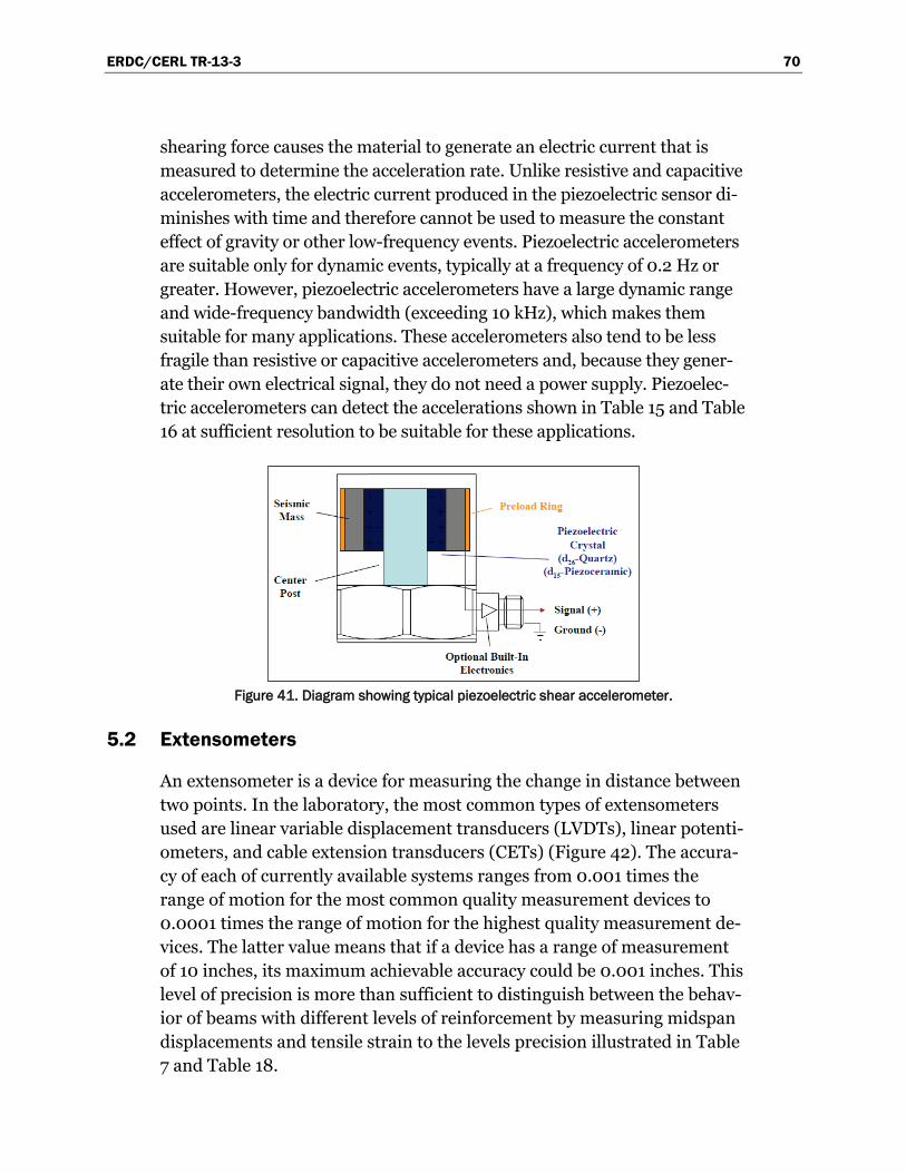
ERDC/CERL TR-13-3 70
shearing force causes the material to generate an electric current that is measured to determine the acceleration rate. Unlike resistive and capacitive accelerometers, the electric current produced in the piezoelectric sensor di-minishes with time and therefore cannot be used to measure the constant effect of gravity or other low-frequency events. Piezoelectric accelerometers are suitable only for dynamic events, typically at a frequency of 0.2 Hz or greater. However, piezoelectric accelerometers have a large dynamic range and wide-frequency bandwidth (exceeding 10 kHz), which makes them suitable for many applications. These accelerometers also tend to be less fragile than resistive or capacitive accelerometers and, because they gener-ate their own electrical signal, they do not need a power supply. Piezoelec-tric accelerometers can detect the accelerations shown in Table 15 and Table 16 at sufficient resolution to be suitable for these applications.
Figure 41. Diagram showing typical piezoelectric shear accelerometer.
5.2 Extensometers
An extensometer is a device for measuring the change in distance between two points. In the laboratory, the most common types of extensometers used are linear variable displacement transducers (LVDTs), linear potenti-ometers, and cable extension transducers (CETs) (Figure 42). The accura-cy of each of currently available systems ranges from 0.001 times the range of motion for the most common quality measurement devices to 0.0001 times the range of motion for the highest quality measurement de-vices. The latter value means that if a device has a range of measurement of 10 inches, its maximum achievable accuracy could be 0.001 inches. This level of precision is more than sufficient to distinguish between the behav-ior of beams with different levels of reinforcement by measuring midspan displacements and tensile strain to the levels precision illustrated in Table 7 and Table 18.
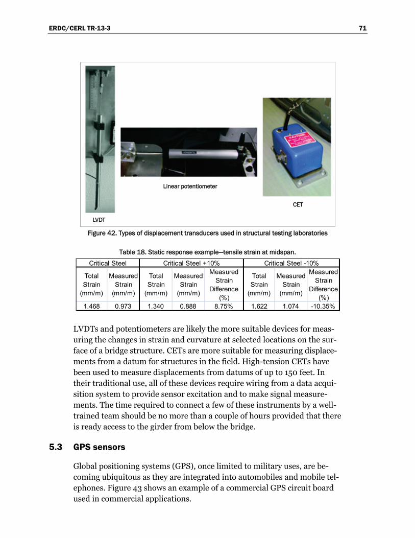
ERDC/CERL TR-13-3 71
Figure 42. Types of displacement transducers used in structural testing laboratories
Table 18. Static response example—tensile strain at midspan.
LVDTs and potentiometers are likely the more suitable devices for meas-uring the changes in strain and curvature at selected locations on the sur-face of a bridge structure. CETs are more suitable for measuring displace-ments from a datum for structures in the field. High-tension CETs have been used to measure displacements from datums of up to 150 feet. In their traditional use, all of these devices require wiring from a data acqui-sition system to provide sensor excitation and to make signal measure-ments. The time required to connect a few of these instruments by a well-trained team should be no more than a couple of hours provided that there is ready access to the girder from below the bridge.
5.3 GPS sensors
Global positioning systems (GPS), once limited to military uses, are be-coming ubiquitous as they are integrated into automobiles and mobile tel-ephones. Figure 43 shows an example of a commercial GPS circuit board used in commercial applications.
Total Strain
(mm/m)
Measured Strain
(mm/m)
Total Strain
(mm/m)
Measured Strain
(mm/m)
Measured Strain
Difference (%)
Total Strain
(mm/m)
Measured Strain
(mm/m)
Measured Strain
Difference (%)
1.468 0.973 1.340 0.888 8.75% 1.622 1.074 -10.35%
Critical Steel +10% Critical Steel -10%Critical Steel
LVDT
CET
Linear potentiometer
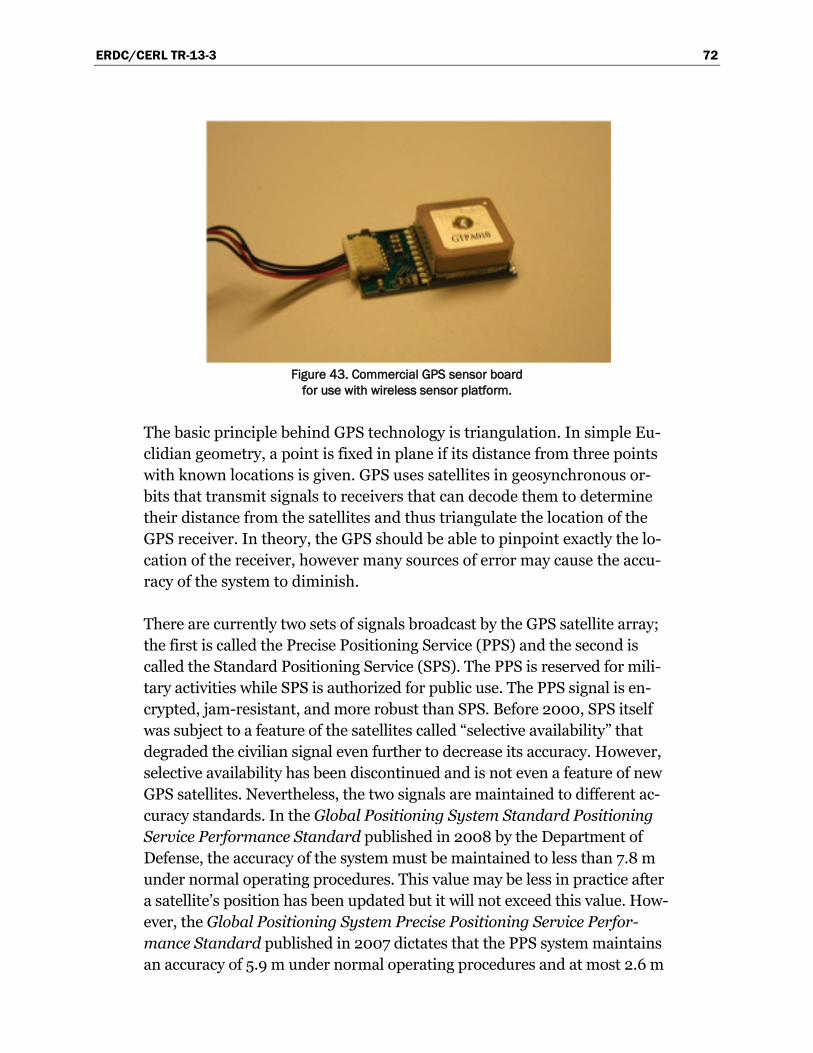
ERDC/CERL TR-13-3 72
Figure 43. Commercial GPS sensor board
for use with wireless sensor platform.
The basic principle behind GPS technology is triangulation. In simple Eu-clidian geometry, a point is fixed in plane if its distance from three points with known locations is given. GPS uses satellites in geosynchronous or-bits that transmit signals to receivers that can decode them to determine their distance from the satellites and thus triangulate the location of the GPS receiver. In theory, the GPS should be able to pinpoint exactly the lo-cation of the receiver, however many sources of error may cause the accu-racy of the system to diminish.
There are currently two sets of signals broadcast by the GPS satellite array; the first is called the Precise Positioning Service (PPS) and the second is called the Standard Positioning Service (SPS). The PPS is reserved for mili-tary activities while SPS is authorized for public use. The PPS signal is en-crypted, jam-resistant, and more robust than SPS. Before 2000, SPS itself was subject to a feature of the satellites called “selective availability” that degraded the civilian signal even further to decrease its accuracy. However, selective availability has been discontinued and is not even a feature of new GPS satellites. Nevertheless, the two signals are maintained to different ac-curacy standards. In the Global Positioning System Standard Positioning Service Performance Standard published in 2008 by the Department of Defense, the accuracy of the system must be maintained to less than 7.8 m under normal operating procedures. This value may be less in practice after a satellite’s position has been updated but it will not exceed this value. How-ever, the Global Positioning System Precise Positioning Service Perfor-mance Standard published in 2007 dictates that the PPS system maintains an accuracy of 5.9 m under normal operating procedures and at most 2.6 m
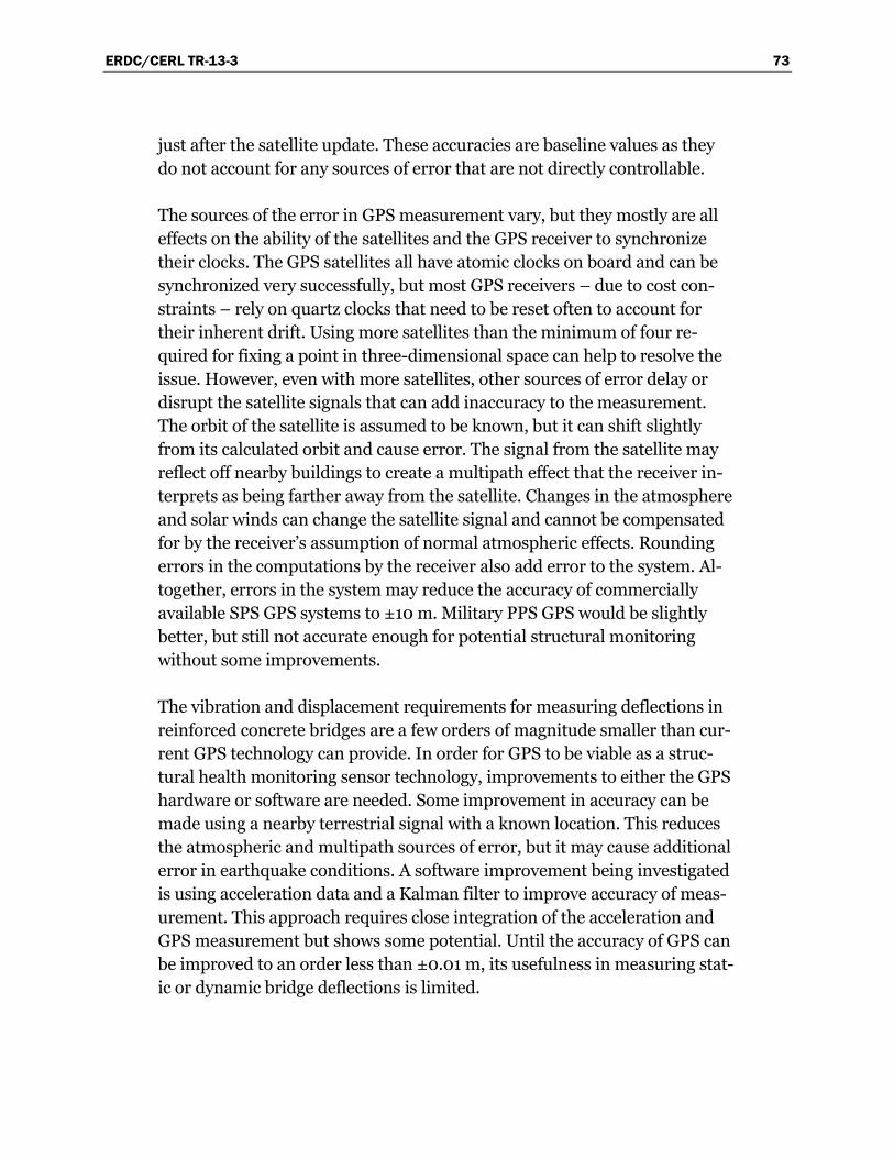
ERDC/CERL TR-13-3 73
just after the satellite update. These accuracies are baseline values as they do not account for any sources of error that are not directly controllable.
The sources of the error in GPS measurement vary, but they mostly are all effects on the ability of the satellites and the GPS receiver to synchronize their clocks. The GPS satellites all have atomic clocks on board and can be synchronized very successfully, but most GPS receivers – due to cost con-straints – rely on quartz clocks that need to be reset often to account for their inherent drift. Using more satellites than the minimum of four re-quired for fixing a point in three-dimensional space can help to resolve the issue. However, even with more satellites, other sources of error delay or disrupt the satellite signals that can add inaccuracy to the measurement. The orbit of the satellite is assumed to be known, but it can shift slightly from its calculated orbit and cause error. The signal from the satellite may reflect off nearby buildings to create a multipath effect that the receiver in-terprets as being farther away from the satellite. Changes in the atmosphere and solar winds can change the satellite signal and cannot be compensated for by the receiver’s assumption of normal atmospheric effects. Rounding errors in the computations by the receiver also add error to the system. Al-together, errors in the system may reduce the accuracy of commercially available SPS GPS systems to ±10 m. Military PPS GPS would be slightly better, but still not accurate enough for potential structural monitoring without some improvements.
The vibration and displacement requirements for measuring deflections in reinforced concrete bridges are a few orders of magnitude smaller than cur-rent GPS technology can provide. In order for GPS to be viable as a struc-tural health monitoring sensor technology, improvements to either the GPS hardware or software are needed. Some improvement in accuracy can be made using a nearby terrestrial signal with a known location. This reduces the atmospheric and multipath sources of error, but it may cause additional error in earthquake conditions. A software improvement being investigated is using acceleration data and a Kalman filter to improve accuracy of meas-urement. This approach requires close integration of the acceleration and GPS measurement but shows some potential. Until the accuracy of GPS can be improved to an order less than ±0.01 m, its usefulness in measuring stat-ic or dynamic bridge deflections is limited.
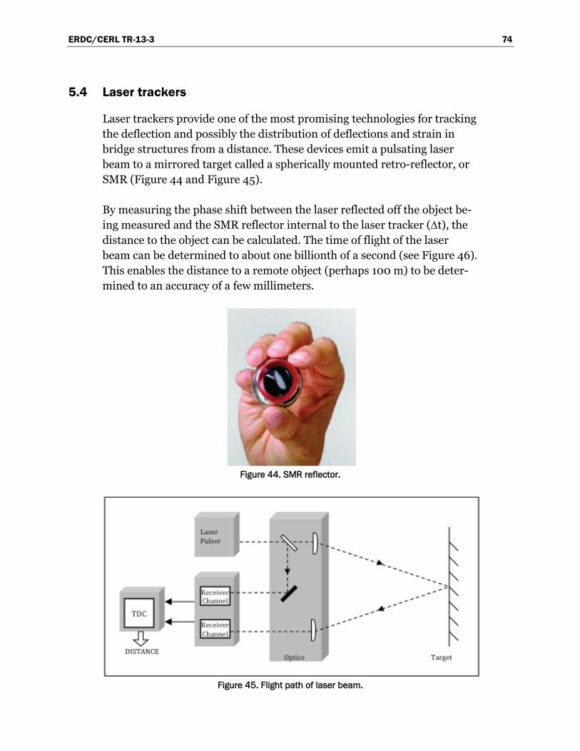
ERDC/CERL TR-13-3 74
5.4 Laser trackers
Laser trackers provide one of the most promising technologies for tracking the deflection and possibly the distribution of deflections and strain in bridge structures from a distance. These devices emit a pulsating laser beam to a mirrored target called a spherically mounted retro-reflector, or SMR (Figure 44 and Figure 45).
By measuring the phase shift between the laser reflected off the object be-ing measured and the SMR reflector internal to the laser tracker (∆t), the distance to the object can be calculated. The time of flight of the laser beam can be determined to about one billionth of a second (see Figure 46). This enables the distance to a remote object (perhaps 100 m) to be deter-mined to an accuracy of a few millimeters.
Figure 44. SMR reflector.
Figure 45. Flight path of laser beam.
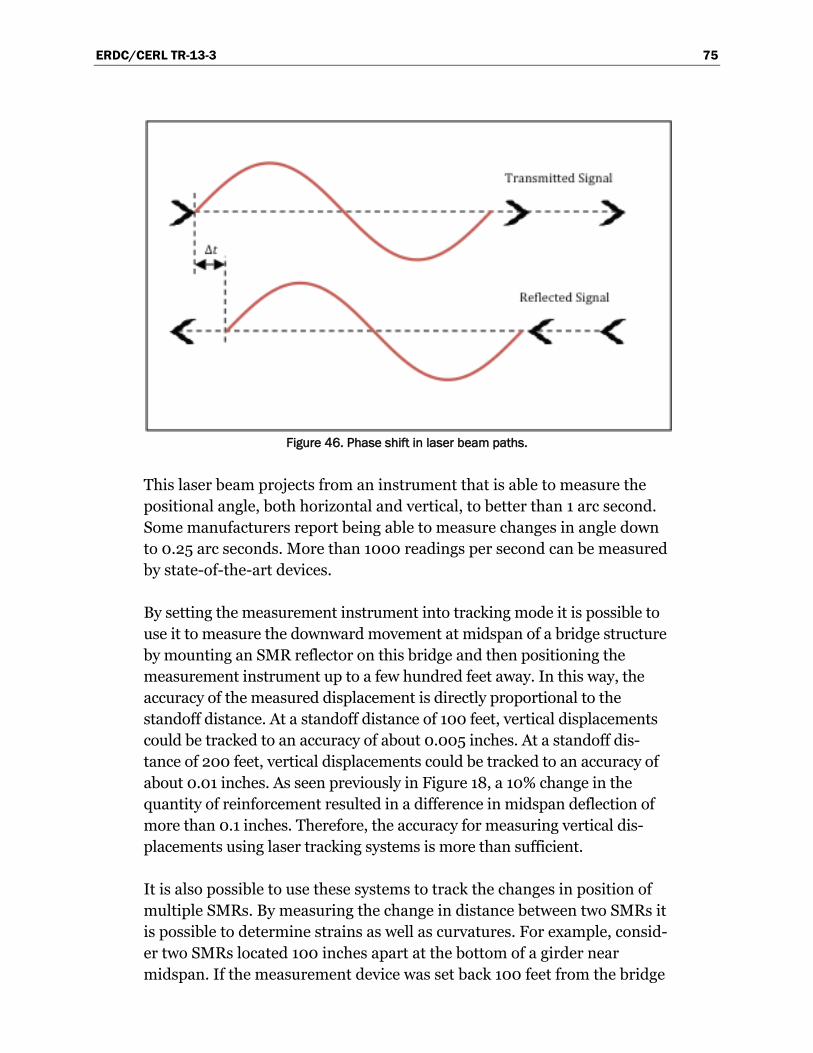
ERDC/CERL TR-13-3 75
Figure 46. Phase shift in laser beam paths.
This laser beam projects from an instrument that is able to measure the positional angle, both horizontal and vertical, to better than 1 arc second. Some manufacturers report being able to measure changes in angle down to 0.25 arc seconds. More than 1000 readings per second can be measured by state-of-the-art devices.
By setting the measurement instrument into tracking mode it is possible to use it to measure the downward movement at midspan of a bridge structure by mounting an SMR reflector on this bridge and then positioning the measurement instrument up to a few hundred feet away. In this way, the accuracy of the measured displacement is directly proportional to the standoff distance. At a standoff distance of 100 feet, vertical displacements could be tracked to an accuracy of about 0.005 inches. At a standoff dis-tance of 200 feet, vertical displacements could be tracked to an accuracy of about 0.01 inches. As seen previously in Figure 18, a 10% change in the quantity of reinforcement resulted in a difference in midspan deflection of more than 0.1 inches. Therefore, the accuracy for measuring vertical dis-placements using laser tracking systems is more than sufficient.
It is also possible to use these systems to track the changes in position of multiple SMRs. By measuring the change in distance between two SMRs it is possible to determine strains as well as curvatures. For example, consid-er two SMRs located 100 inches apart at the bottom of a girder near midspan. If the measurement device was set back 100 feet from the bridge
ERDC/CERL TR-13-3 76
and a measurement accuracy of 1 arc second is assumed, then the strain can be determined down to 50 micro strain. Figure 21 and Figure 22 show this is just about the level of accuracy needed to distinguish a change in reinforcement amount of about 10%.
5.5 Photogrammetry
In recent years, new noncontact optical methods have been developed for measuring the shape, condition, and displacement of objects. These sys-tems use long-established photogrammetric principles for obtaining useful information from photographs. Cost reductions for high-resolution digital cameras and optics have spurred this development.
One example of how these methods are used is in coordinate measurement machines (CMMs), which provide similar functionality as a laser tracker but offer certain advantages and disadvantages. The main advantage in the field is that it is not necessary to place a target, such as a SMR, on the bridge; in-stead, the technology can use any stable pre-existing mark on a girder. The main disadvantage is that significant post-processing of images may be re-quired to assess displacements. Depending on the quality of the structural marker, errors may result in post-processing. The accuracy of this system for making displacement measurements can be up to one ten-thousandth of the camera’s field of view. For example, if the field of view in the captured image is 100 inches, then displacements may be determined to within about 0.01 in.
The number of cameras needed to make a measurement depends on the type of measurement to be made. If dimensional information is already available about the object, then it is possible to measure vector displace-ments with only one camera. If dimensional information is not available, then at least two cameras are needed. Accuracy will increase with the number of cameras. Figure 47 illustrates how the position of multiple points on an object are recorded on the image space of the camera sensor.
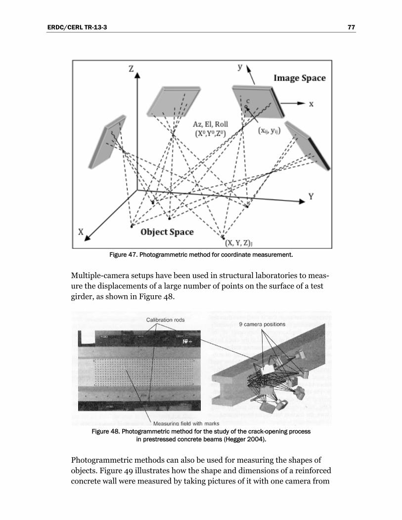
ERDC/CERL TR-13-3 77
Figure 47. Photogrammetric method for coordinate measurement.
Multiple-camera setups have been used in structural laboratories to meas-ure the displacements of a large number of points on the surface of a test girder, as shown in Figure 48.
Figure 48. Photogrammetric method for the study of the crack-opening process
in prestressed concrete beams (Hegger 2004).
Photogrammetric methods can also be used for measuring the shapes of objects. Figure 49 illustrates how the shape and dimensions of a reinforced concrete wall were measured by taking pictures of it with one camera from
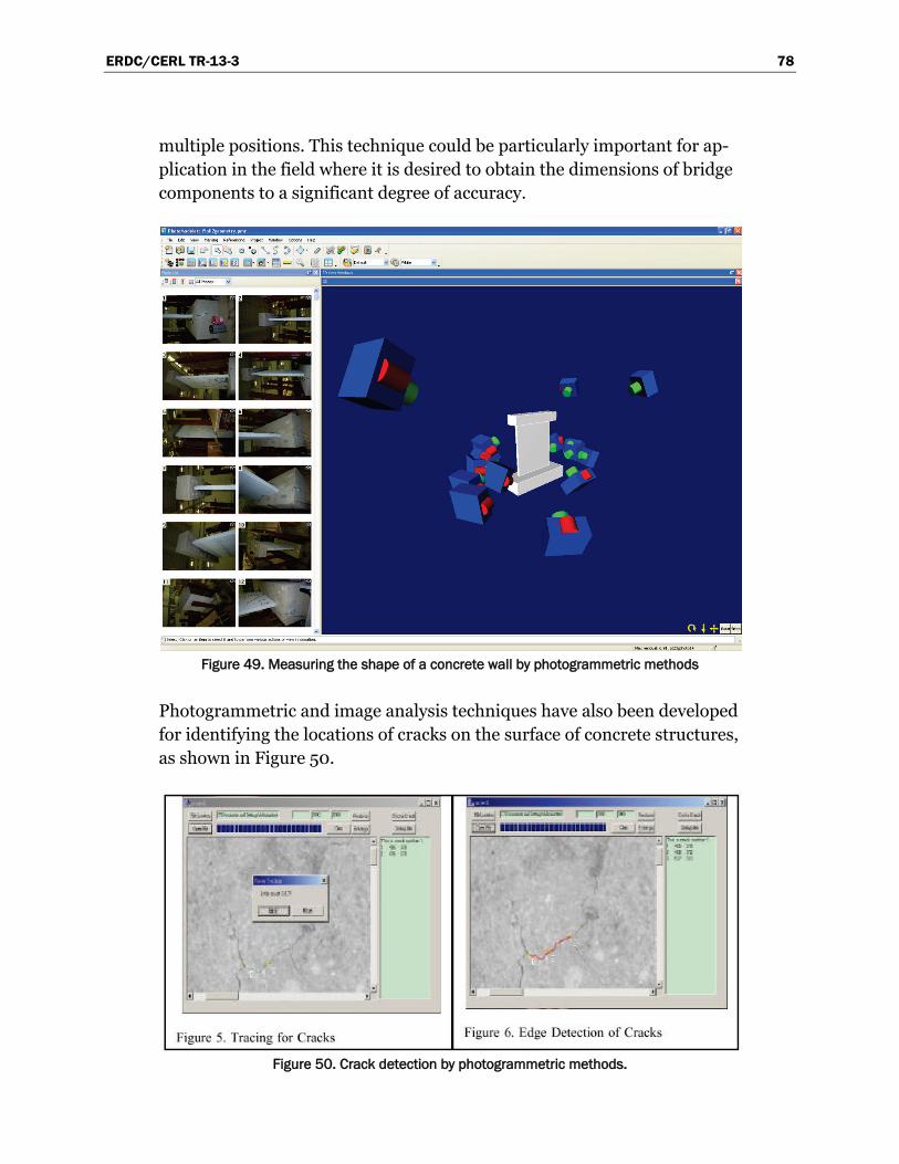
ERDC/CERL TR-13-3 78
multiple positions. This technique could be particularly important for ap-plication in the field where it is desired to obtain the dimensions of bridge components to a significant degree of accuracy.
Figure 49. Measuring the shape of a concrete wall by photogrammetric methods
Photogrammetric and image analysis techniques have also been developed for identifying the locations of cracks on the surface of concrete structures, as shown in Figure 50.
Figure 50. Crack detection by photogrammetric methods.
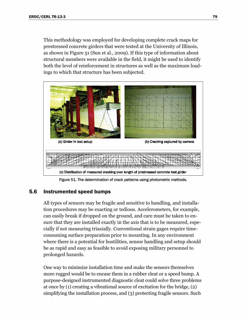
ERDC/CERL TR-13-3 79
This methodology was employed for developing complete crack maps for prestressed concrete girders that were tested at the University of Illinois, as shown in Figure 51 (Sun et al., 2009). If this type of information about structural members were available in the field, it might be used to identify both the level of reinforcement in structures as well as the maximum load-ings to which that structure has been subjected.
Figure 51. The determination of crack patterns using photometric methods.
5.6 Instrumented speed bumps
All types of sensors may be fragile and sensitive to handling, and installa-tion procedures may be exacting or tedious. Accelerometers, for example, can easily break if dropped on the ground, and care must be taken to en-sure that they are installed exactly in the axis that is to be measured, espe-cially if not measuring triaxially. Conventional strain gages require time-consuming surface preparation prior to mounting. In any environment where there is a potential for hostilities, sensor handling and setup should be as rapid and easy as feasible to avoid exposing military personnel to prolonged hazards.
One way to minimize installation time and make the sensors themselves more rugged would be to encase them in a rubber cleat or a speed bump. A purpose-designed instrumented diagnostic cleat could solve three problems at once by (1) creating a vibrational source of excitation for the bridge, (2) simplifying the installation process, and (3) protecting fragile sensors. Such
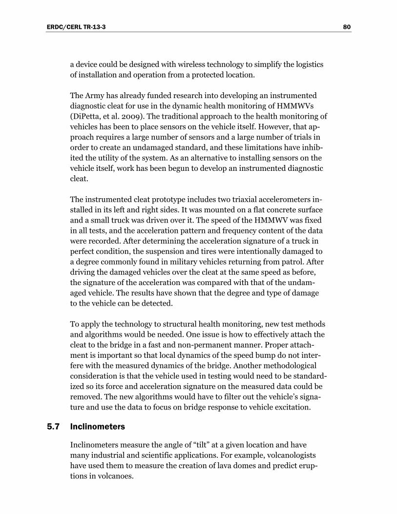
ERDC/CERL TR-13-3 80
a device could be designed with wireless technology to simplify the logistics of installation and operation from a protected location.
The Army has already funded research into developing an instrumented diagnostic cleat for use in the dynamic health monitoring of HMMWVs (DiPetta, et al. 2009). The traditional approach to the health monitoring of vehicles has been to place sensors on the vehicle itself. However, that ap-proach requires a large number of sensors and a large number of trials in order to create an undamaged standard, and these limitations have inhib-ited the utility of the system. As an alternative to installing sensors on the vehicle itself, work has been begun to develop an instrumented diagnostic cleat.
The instrumented cleat prototype includes two triaxial accelerometers in-stalled in its left and right sides. It was mounted on a flat concrete surface and a small truck was driven over it. The speed of the HMMWV was fixed in all tests, and the acceleration pattern and frequency content of the data were recorded. After determining the acceleration signature of a truck in perfect condition, the suspension and tires were intentionally damaged to a degree commonly found in military vehicles returning from patrol. After driving the damaged vehicles over the cleat at the same speed as before, the signature of the acceleration was compared with that of the undam-aged vehicle. The results have shown that the degree and type of damage to the vehicle can be detected.
To apply the technology to structural health monitoring, new test methods and algorithms would be needed. One issue is how to effectively attach the cleat to the bridge in a fast and non-permanent manner. Proper attach-ment is important so that local dynamics of the speed bump do not inter-fere with the measured dynamics of the bridge. Another methodological consideration is that the vehicle used in testing would need to be standard-ized so its force and acceleration signature on the measured data could be removed. The new algorithms would have to filter out the vehicle’s signa-ture and use the data to focus on bridge response to vehicle excitation.
5.7 Inclinometers
Inclinometers measure the angle of “tilt” at a given location and have many industrial and scientific applications. For example, volcanologists have used them to measure the creation of lava domes and predict erup-tions in volcanoes.
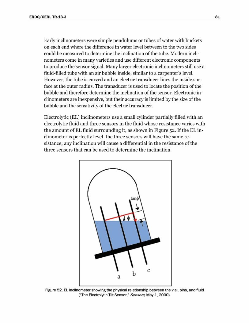
ERDC/CERL TR-13-3 81
Early inclinometers were simple pendulums or tubes of water with buckets on each end where the difference in water level between to the two sides could be measured to determine the inclination of the tube. Modern incli-nometers come in many varieties and use different electronic components to produce the sensor signal. Many larger electronic inclinometers still use a fluid-filled tube with an air bubble inside, similar to a carpenter’s level. However, the tube is curved and an electric transducer lines the inside sur-face at the outer radius. The transducer is used to locate the position of the bubble and therefore determine the inclination of the sensor. Electronic in-clinometers are inexpensive, but their accuracy is limited by the size of the bubble and the sensitivity of the electric transducer.
Electrolytic (EL) inclinometers use a small cylinder partially filled with an electrolytic fluid and three sensors in the fluid whose resistance varies with the amount of EL fluid surrounding it, as shown in Figure 52. If the EL in-clinometer is perfectly level, the three sensors will have the same re-sistance; any inclination will cause a differential in the resistance of the three sensors that can be used to determine the inclination.
Figure 52. EL inclinometer showing the physical relationship between the vial, pins, and fluid
(“The Electrolytic Tilt Sensor,” Sensors, May 1, 2000).
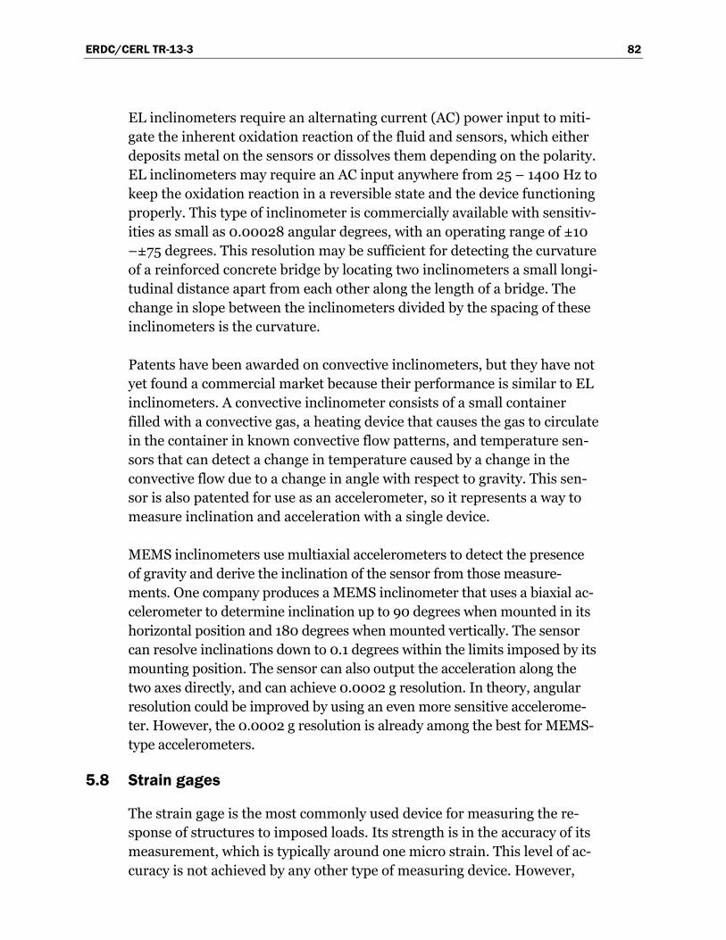
ERDC/CERL TR-13-3 82
EL inclinometers require an alternating current (AC) power input to miti-gate the inherent oxidation reaction of the fluid and sensors, which either deposits metal on the sensors or dissolves them depending on the polarity. EL inclinometers may require an AC input anywhere from 25 – 1400 Hz to keep the oxidation reaction in a reversible state and the device functioning properly. This type of inclinometer is commercially available with sensitiv-ities as small as 0.00028 angular degrees, with an operating range of ±10 –±75 degrees. This resolution may be sufficient for detecting the curvature of a reinforced concrete bridge by locating two inclinometers a small longi-tudinal distance apart from each other along the length of a bridge. The change in slope between the inclinometers divided by the spacing of these inclinometers is the curvature.
Patents have been awarded on convective inclinometers, but they have not yet found a commercial market because their performance is similar to EL inclinometers. A convective inclinometer consists of a small container filled with a convective gas, a heating device that causes the gas to circulate in the container in known convective flow patterns, and temperature sen-sors that can detect a change in temperature caused by a change in the convective flow due to a change in angle with respect to gravity. This sen-sor is also patented for use as an accelerometer, so it represents a way to measure inclination and acceleration with a single device.
MEMS inclinometers use multiaxial accelerometers to detect the presence of gravity and derive the inclination of the sensor from those measure-ments. One company produces a MEMS inclinometer that uses a biaxial ac-celerometer to determine inclination up to 90 degrees when mounted in its horizontal position and 180 degrees when mounted vertically. The sensor can resolve inclinations down to 0.1 degrees within the limits imposed by its mounting position. The sensor can also output the acceleration along the two axes directly, and can achieve 0.0002 g resolution. In theory, angular resolution could be improved by using an even more sensitive accelerome-ter. However, the 0.0002 g resolution is already among the best for MEMS-type accelerometers.
5.8 Strain gages
The strain gage is the most commonly used device for measuring the re-sponse of structures to imposed loads. Its strength is in the accuracy of its measurement, which is typically around one micro strain. This level of ac-curacy is not achieved by any other type of measuring device. However,
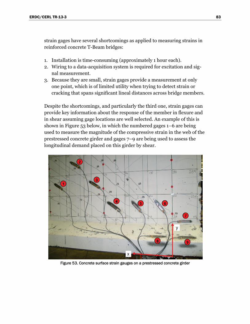
ERDC/CERL TR-13-3 83
strain gages have several shortcomings as applied to measuring strains in reinforced concrete T-Beam bridges:
1. Installation is time-consuming (approximately 1 hour each). 2. Wiring to a data-acquisition system is required for excitation and sig-
nal measurement. 3. Because they are small, strain gages provide a measurement at only
one point, which is of limited utility when trying to detect strain or cracking that spans significant lineal distances across bridge members.
Despite the shortcomings, and particularly the third one, strain gages can provide key information about the response of the member in flexure and in shear assuming gage locations are well selected. An example of this is shown in Figure 53 below, in which the numbered gages 1–6 are being used to measure the magnitude of the compressive strain in the web of the prestressed concrete girder and gages 7–9 are being used to assess the longitudinal demand placed on this girder by shear.
Figure 53. Concrete surface strain gauges on a prestressed concrete girder
ERDC/CERL TR-13-3 84
6 Efficacy of Approach 6.1 Assessment scenarios
The various assessment scenarios may be categorized in terms of the reason for the assessment, its importance, the level of information needed, and the time required for collecting it. Two different types of assessment scenarios are discussed in this chapter: quick and detailed reconnaissance. Both sce-narios require fairly complete information on the overall structural geome-try and types of materials used. Measurements needed, for example, include the length and width of each span, dimensions of cross sections, and num-ber of sections across the width of each span. Fortunately, photogrammetric principles make it possible to collect this information using high-resolution digital photographs.
6.1.1 Quick reconnaissance
Quick reconnaissance is expected to require 1–3 hours. The capacity as-sessment is most likely to be based on either the frequency of the bridge’s response to a military vehicle passing over an instrumented speed bump and/or the midspan deflection of the bridge due to the passage of a heavy military vehicle of known mass while no other vehicles are on the bridge. It is envisioned that the field team will enter the geometric details for the bridge, as derived from digital photography, into a computer program using a graphical user interface before the reconnaissance. The program will then provide charts showing capacity versus frequency and capacity versus midspan displacement. In cases where data are missing, conservative as-sumptions will be made, which may underestimate the load-carrying ca-pacity of the bridge. If the results of this reconnaissance indicate that the bridge has more than adequate capacity for supporting the desired military loads, then no additional assessments may be needed. Otherwise, a more detailed assessment is required.
6.1.2 Detailed reconnaissance
Detailed reconnaissance may be needed for two reasons. One reason is that the results of a quick reconnaissance may indicate that the bridge may not have sufficient capacity to support passage of the desired military ve-hicles. The other reason is to collect high-resolution information about the
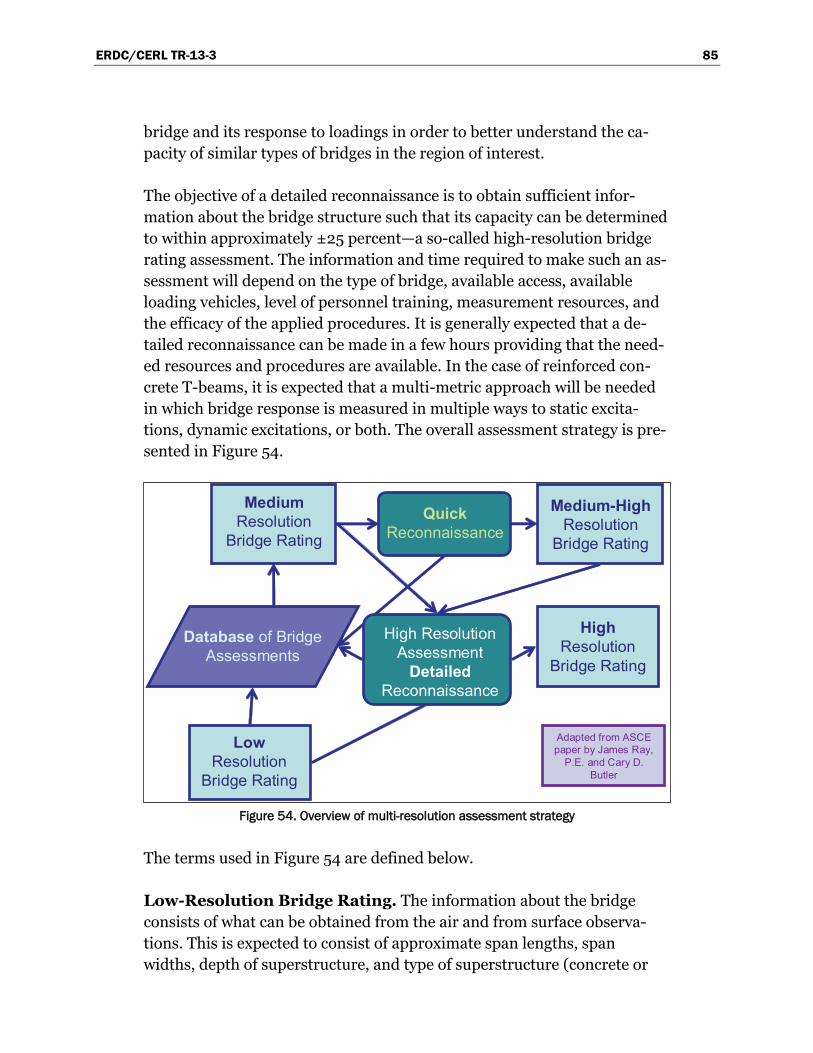
ERDC/CERL TR-13-3 85
bridge and its response to loadings in order to better understand the ca-pacity of similar types of bridges in the region of interest.
The objective of a detailed reconnaissance is to obtain sufficient infor-mation about the bridge structure such that its capacity can be determined to within approximately ±25 percent—a so-called high-resolution bridge rating assessment. The information and time required to make such an as-sessment will depend on the type of bridge, available access, available loading vehicles, level of personnel training, measurement resources, and the efficacy of the applied procedures. It is generally expected that a de-tailed reconnaissance can be made in a few hours providing that the need-ed resources and procedures are available. In the case of reinforced con-crete T-beams, it is expected that a multi-metric approach will be needed in which bridge response is measured in multiple ways to static excita-tions, dynamic excitations, or both. The overall assessment strategy is pre-sented in Figure 54.
Figure 54. Overview of multi-resolution assessment strategy
The terms used in Figure 54 are defined below.
Low-Resolution Bridge Rating. The information about the bridge consists of what can be obtained from the air and from surface observa-tions. This is expected to consist of approximate span lengths, span widths, depth of superstructure, and type of superstructure (concrete or
LowResolution
Bridge Rating
High Resolution Assessment
Detailed Reconnaissance
Medium Resolution
Bridge Rating
HighResolution
Bridge Rating
Database of Bridge Assessments
Medium-High Resolution
Bridge Rating
QuickReconnaissance
Adapted from ASCE paper by James Ray,
P.E. and Cary D. Butler
ERDC/CERL TR-13-3 86
steel). This information by itself is rarely enough to assess the load-carrying capacity of a bridge structure with sufficient accuracy.
Medium-Resolution Bridge Rating. When only low-resolution infor-mation is available, then the estimated capacity of a bridge can be im-proved based on correlations with other bridge structures of similar form and age for which more complete information is available.
Medium-High-Resolution Bridge Rating. The resolution of the rat-ing based on a quick reconnaissance is characterized as medium-high. In the case of reinforced concrete T-beams, only the midspan displacement and/or frequencies of vibration of the bridge structure may be measured. An advantage of a quick reconnaissance is that it should require only a few hours to complete. A quality rating is achieved through the quick recon-naissance in conjunction with the measured bridge response to applied loads.
High-Resolution Bridge Rating (±25%). A high-resolution bridge rating is possible when sufficiently detailed information is available about the bridge geometry. In addition to the low-resolution information, this includes the dimensions of cross-sections and reasonable estimates (±25%) of the amounts of reinforcement and other structural details. The estimates of reinforcement could come from the measurement approach presented in this report or from other sources.
When only low-resolution information is available and no reconnaissance has been done to measure bridge response to loads, then the load-carrying capacity must be based on the “classification-by-correlation” method of military classification (Ray and Butler 2004).
6.2 Example problem
In order to perform the load-carrying capacity assessment using the pro-cedure outlined in section 1.3, in-field measured response of the structure under known loads must be captured for comparison with the predicted response from nonlinear analysis. The assessment procedure described in this report assumes that full access to the structure is possible for purposes of instrumentation. In general, both dynamic and static loads are imposed. Dynamic excitation through induced vibrations can be performed by run-ning a light military vehicle over a speed bump. A lighter military vehicle, such as a 3 ton HMMWV, is feasible for this test because relative differ-
ERDC/CERL TR-13-3 87
ences in response due to different levels of reinforcement are not sensitive to scaling. That is, the percent difference between responses for different levels of reinforcement is not affected by overall magnitude of the re-sponse. A heavier vehicle such as the 80.5 ton M1-Abrams tank is ideal for measuring static responses such as displacements and strains. While the influence factor for a given static response for members with different lev-els of reinforcement is fairly consistent, the measurable differences of stat-ic response require a larger imposed load than the dynamic response. The following example illustrates one potential way to use dynamic and static tests to perform a capacity assessment. It is important to note that while the example details one type of measurement of both dynamic and static testing, increasing the number and types of measurements increases the confidence in the assessment.
6.2.1 Description
Without advanced knowledge of the capacity of the structure, this assess-ment procedure anticipates that the dynamic testing would be performed first. In the dynamic test, the vehicle utilized is the HMMWV. Since this 3 ton vehicle is lighter than a typical highway design vehicle such as the 36 ton AASHTO HS20-44 truck, the effect of this vehicle’s weight and dynam-ic amplification is not expected to cause any damage as it crosses the struc-ture. In addition to safely crossing the structure, using a vehicle that is lighter than the expected vehicles in the structure’s load history is critical to ensure that the flexural stiffness input to the predictive analysis is not inaccurate as a result of further cracking during the dynamic test. To in-duce vibration with the vehicle, the test utilizes a pre-instrumented speed bump like the one described in section 5.6. The first step to performing the dynamic test is to place the instrumented speed bump on the girder, which requires that it be fully adhered to the deck surface. The hypothetical speed bump design used in this analysis has a 5 cm tall by 30 cm wide half-cosine profile. After the speed bump is securely adhered to the sur-face, the test vehicle moves over the structure at a velocity of 0.75 m/s (1.7 mph) and the data are captured by the instrumentation. The speed and placement of the vehicle can be adapted to best suit the modeled charac-teristics of the bridge to obtain the best results possible.
Once the dynamic test is complete, a first assessment on the level of rein-forcement can be inferred. From this first dynamic assessment, it can be determined whether safe passage of the M1-Abrams tank can be expected for use in the static test. If the results from the dynamic test indicate that
ERDC/CERL TR-13-3 88
the tank is safe for passage, the static load test can proceed. The instru-mentation used in this example is designed to capture the average tensile strain on the bottom fiber at the midspan of the girder. Due to flexural cracking, the average tensile strain is determined through a measurement taken over a domain along the bottom fiber, as opposed to measurement at a discrete point. For this reason, a strain gage cannot be used, so either an extensometer or targets for use with laser or photogrammetric means are adhered to the bottom fiber at the midspan. After stopping the tank at midspan and waiting for any vibrations to diminish, the strain measure-ment is recorded.
6.2.2 Capacity assessment from measuring dynamic response
Measuring the dynamic response of a bridge for system identification can be a metric in either a quick or detailed reconnaissance. As previously de-scribed, the ubiquitous HMMWV driven over a speed bump is likely to be used as a source of excitation to obtain dynamic measurements.
The first step in the dynamic approach is to use the measured dimensions of the bridge, the desired loading, and the static models to obtain the esti-mated natural frequencies of the bridge. Then, after measuring the dynam-ic response of the bridge to HMMWV excitation, the data are analyzed to determine the measured natural frequencies. The estimated and measured responses are then compared to determine whether the desired load can safely pass over the bridge.
Consider, for example, three random bridges along a given route that have the same external dimensions used in this study, but unknown internal reinforcement. Dynamic measurements using a HMMWV could be made to determine the natural frequencies of the bridges. If the load that needs to pass over the bridge is an HS20-44, the estimated response, assuming the absolute minimum reinforcement and ±10% of the minimum steel needed to carry the load, can be determined as shown in Table 12 (section 4.2) for another bridge. The values equivalent to those in Table 12 can be plotted to form a curve showing a variation in the bridge modes with re-spect to the amount of steel. The natural frequencies of the three random bridges in this example can be measured and then plotted on the curves, determined using the percentage of minimum steel required, to find out how much steel the random bridge in likely to have. Table 19 shows the estimated response for the minimum steel required for an HS20-44 load and the measured response for the three random bridges in this example.
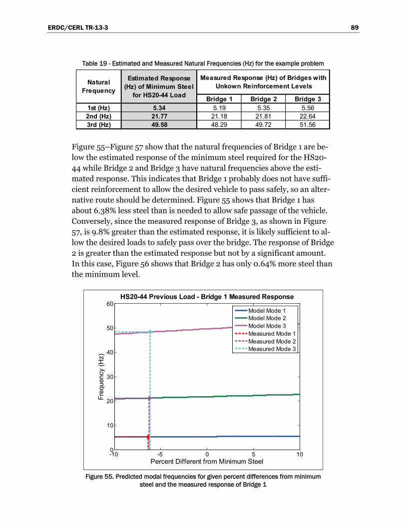
ERDC/CERL TR-13-3 89
Table 19 - Estimated and Measured Natural Frequencies (Hz) for the example problem
Figure 55–Figure 57 show that the natural frequencies of Bridge 1 are be-low the estimated response of the minimum steel required for the HS20-44 while Bridge 2 and Bridge 3 have natural frequencies above the esti-mated response. This indicates that Bridge 1 probably does not have suffi-cient reinforcement to allow the desired vehicle to pass safely, so an alter-native route should be determined. Figure 55 shows that Bridge 1 has about 6.38% less steel than is needed to allow safe passage of the vehicle. Conversely, since the measured response of Bridge 3, as shown in Figure 57, is 9.8% greater than the estimated response, it is likely sufficient to al-low the desired loads to safely pass over the bridge. The response of Bridge 2 is greater than the estimated response but not by a significant amount. In this case, Figure 56 shows that Bridge 2 has only 0.64% more steel than the minimum level.
Figure 55. Predicted modal frequencies for given percent differences from minimum
steel and the measured response of Bridge 1
Bridge 1 Bridge 2 Bridge 31st (Hz) 5.34 5.19 5.35 5.562nd (Hz) 21.77 21.18 21.81 22.643rd (Hz) 49.58 48.29 49.72 51.56
Natural Frequency
Estimated Response (Hz) of Minimum Steel
for HS20-44 Load
Measured Response (Hz) of Bridges with Unkown Reinforcement Levels
-10 -5 0 5 100
10
20
30
40
50
60
Percent Different from Minimum Steel
Freq
uenc
y (H
z)
HS20-44 Previous Load - Bridge 1 Measured Response
Model Mode 1Model Mode 2Model Mode 3Measured Mode 1Measured Mode 2Measured Mode 3
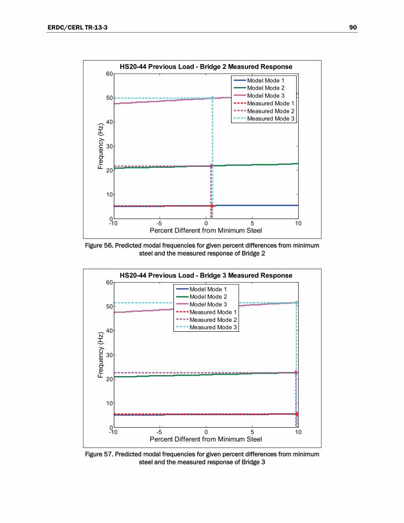
ERDC/CERL TR-13-3 90
Figure 56. Predicted modal frequencies for given percent differences from minimum
steel and the measured response of Bridge 2
Figure 57. Predicted modal frequencies for given percent differences from minimum
steel and the measured response of Bridge 3
-10 -5 0 5 100
10
20
30
40
50
60
Percent Different from Minimum Steel
Freq
uenc
y (H
z)
HS20-44 Previous Load - Bridge 2 Measured Response
Model Mode 1Model Mode 2Model Mode 3Measured Mode 1Measured Mode 2Measured Mode 3
-10 -5 0 5 100
10
20
30
40
50
60
Percent Different from Minimum Steel
Freq
uenc
y (H
z)
HS20-44 Previous Load - Bridge 3 Measured Response
Model Mode 1Model Mode 2Model Mode 3Measured Mode 1Measured Mode 2Measured Mode 3
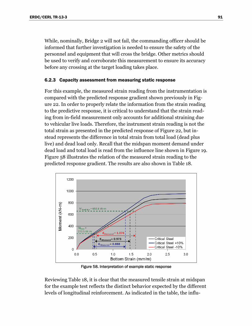
ERDC/CERL TR-13-3 91
While, nominally, Bridge 2 will not fail, the commanding officer should be informed that further investigation is needed to ensure the safety of the personnel and equipment that will cross the bridge. Other metrics should be used to verify and corroborate this measurement to ensure its accuracy before any crossing at the target loading takes place.
6.2.3 Capacity assessment from measuring static response
For this example, the measured strain reading from the instrumentation is compared with the predicted response gradient shown previously in Fig-ure 22. In order to properly relate the information from the strain reading to the predictive response, it is critical to understand that the strain read-ing from in-field measurement only accounts for additional straining due to vehicular live loads. Therefore, the instrument strain reading is not the total strain as presented in the predicted response of Figure 22, but in-stead represents the difference in total strain from total load (dead plus live) and dead load only. Recall that the midspan moment demand under dead load and total load is read from the influence line shown in Figure 19. Figure 58 illustrates the relation of the measured strain reading to the predicted response gradient. The results are also shown in Table 18.
Figure 58. Interpretation of example static response
Reviewing Table 18, it is clear that the measured tensile strain at midspan for the example test reflects the distinct behavior expected by the different levels of longitudinal reinforcement. As indicated in the table, the influ-

ERDC/CERL TR-13-3 92
ence factor of level of longitudinal reinforcement on measured tensile strain is in the range of 0.85–1.05.
6.3 Real-time assessment applications
It is expected that there may be situations in which a crossing is consid-ered necessary over a span for which the capacity is in doubt. In this type of situation it is advisable to monitor the response of the bridge, such as midspan displacement, as heavy military loadings slowly begin to cross the bridge. Based only on the depth of supporting beams and the displacement pattern as a function of the load position, it is possible to identify whether or not the bridge can support each heavy military vehicle or if more than one vehicle may cross at the same time.
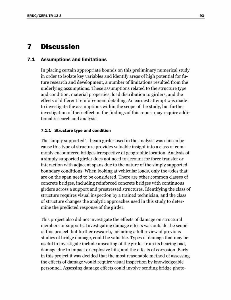
ERDC/CERL TR-13-3 93
7 Discussion 7.1 Assumptions and limitations
In placing certain appropriate bounds on this preliminary numerical study in order to isolate key variables and identify areas of high potential for fu-ture research and development, a number of limitations resulted from the underlying assumptions. These assumptions related to the structure type and condition, material properties, load distribution to girders, and the effects of different reinforcement detailing. An earnest attempt was made to investigate the assumptions within the scope of the study, but further investigation of their effect on the findings of this report may require addi-tional research and analysis.
7.1.1 Structure type and condition
The simply supported T-beam girder used in the analysis was chosen be-cause this type of structure provides valuable insight into a class of com-monly encountered bridges irrespective of geographic location. Analysis of a simply supported girder does not need to account for force transfer or interaction with adjacent spans due to the nature of the simply supported boundary conditions. When looking at vehicular loads, only the axles that are on the span need to be considered. There are other common classes of concrete bridges, including reinforced concrete bridges with continuous girders across a support and prestressed structures. Identifying the class of structure requires visual inspection by a trained technician, and the class of structure changes the analytic approaches used in this study to deter-mine the predicted response of the girder.
This project also did not investigate the effects of damage on structural members or supports. Investigating damage effects was outside the scope of this project, but further research, including a full review of previous studies of bridge damage, could be valuable. Types of damage that may be useful to investigate include unseating of the girder from its bearing pad, damage due to impact or explosive hits, and the effects of corrosion. Early in this project it was decided that the most reasonable method of assessing the effects of damage would require visual inspection by knowledgeable personnel. Assessing damage effects could involve sending bridge photo-
ERDC/CERL TR-13-3 94
graphs from the field to the Corps of Engineers Reachback Operations Center (UROC) for remote evaluation.
7.1.1.1 Member geometry
This report assumes that the member geometry, including dimensions of the gross cross section and span, is known. The degree to which the mem-ber geometry is known may be affected by the level of access to the struc-ture. The issue of how uncertainty about member dimensions affects re-sults is not investigated in this study.
7.1.1.2 Material properties
This report assumes that the compressive strength of the concrete (𝑓’𝑐) and the yield strength of the reinforcing steel (𝑓𝑦) are known. A parametric study was performed to verify that small (≤10%) variations in material properties would not affect results. It was assumed that the compressive strength of concrete can be accurately assessed using nondestructive means, but this technique requires full access to the structure. Analysis in-dicated that the predicted response of the structure is not affected by a ±10% parametric variation of concrete stiffness and strength.
The modulus of elasticity of reinforcement varies little. It is not intended that the loading of the structure would result in yielding of the reinforce-ment. Thus, as long as the estimate of yield strength is reasonably accurate and conservative, small variations in the steel strength will not affect re-sults. Because there is no direct way to nondestructively test the yield strength of steel that is cast in concrete, yield strength predictions may need to be based on knowledge of regional construction practices.
7.1.1.3 Reinforcement detailing
This project studied variations in the amount of reinforcement based on longitudinal bar size and vertical stirrup spacing, but it did not investigate other possible reinforcement details. For example, older bridge structures may not utilize vertically oriented stirrups as the principal means of resist-ing shear. The bending of longitudinal bars at angles of 30–60 degrees was common in many structures built in the early to mid-1900s. Additionally, this project looked at cases in which the longitudinal reinforcement is placed continuously along the length of the member. The longitudinal re-inforcement must be designed to resist the moment along the span; how-
ERDC/CERL TR-13-3 95
ever, because the moment is usually largest near midspan, the reinforce-ment required near the ends of the girder is less than at midspan. For economy, the top layers of reinforcement may not run the entire span, in-stead having cutoff locations to reduce the amount of steel where there is lower moment demand.
7.1.1.4 Load distribution
This project assumes that the demand imposed on the analyzed girder is known. The dead and live loads are known with high levels of confidence. Dead loads are calculated based on common densities of construction ma-terials and known structure geometry. Live loads are known because the axle spacing and loads are known for the vehicles crossing the bridge. What is assumed in this study, though, is the distribution of these load demands to individual girders. In order to accurately predict the behavior of the girder under the procedure outlined in this report, it is necessary to know what percentage of the imposed loads is transferred to the measured girder. The distribution factors used in this report are based on AASHTO guidelines as well as practical experience. The precision of distribution fac-tors continues to be an active area of research, and the uncertainty associ-ated with distribution assumptions may warrant further investigation.
7.1.1.5 Beam flexural stiffness, EI(x)
The flexural rigidity factor used in the dynamic model was based on calcu-lating the curvature at discrete points along the beam, as described in sec-tion 4.1. Curvature was determined based on sectional analysis for mo-ment distribution from an influence line for the assumed largest vehicle in the bridge’s load history. It is expected that this method would underesti-mate the flexural rigidity of the beam because it ignores the tensile contri-bution of the concrete between cracks (ACI Committee 435 1966). The ex-tent to which this method underestimates the flexural rigidity has not been determined in this study.
7.2 Future work
This preliminary numerical study focused on assessing whether the amount of reinforcement in concrete bridges, and therefore the load-carrying capac-ity, could be determined from the measured response of these structures to static and/or dynamic loadings. The results of this study illustrate that many different aspects of a bridge’s response, including its deflections, cur-
ERDC/CERL TR-13-3 96
vatures, and frequencies, present distinctly different behavior that enable its load-carrying capacity to be determined to within approximately 20%. The-se results constitute a significant improvement over current methods of in-field assessment that rely mainly on the external geometry of these struc-tures for estimating capacity. This study also reveals that, while convention-al instrumentation technology is able to measure many important response characteristics, the use of emerging instrumentation technologies may greatly improve the ability to more quickly and accurately assess the load-carrying capacity of bridges. Next-generation improvements in measure-ment capabilities are expected to be based on optics and laser technologies.
Because this study was a purely analytical effort and relied on assumptions discussed in the previous section, further sensitivity analysis and experi-mental validation are necessary. Further development of the proposed ca-pacity assessment methodology will involve the following tasks:
1. experimental validation of the analytical predictions documented here 2. identification and development of suitable sensor technologies to sup-
port the methodology 3. experimental validation of predictive analysis for a multi-girder struc-
ture 4. development and validation of a general procedure for assessing con-
crete bridge load-carrying capacity, including a software implementa-tion.
These items are discussed in more detail in the sections that follow.
7.2.1 Experimental validation of predictive analysis for single girder structures
7.2.1.1 Static testing
A series of load tests should be conducted on simple-span, single-girder reinforced concrete T-beams configured as a reduced-scale model of the T-beams in the bridge structures described throughout this report. The test structure, although reduced in scale, should be sufficiently large that standard concrete and reinforcement materials may be used without modification for scaling effects. It is expected that four different levels of flexural reinforcement and three different levels of shear reinforcement would be needed for this study. Conventional instrumentation technolo-gies should be used to measure the deflections, curvatures, slopes, and

ERDC/CERL TR-13-3 97
strains over the length of the structure. The measured response should be compared with the full analytical predictions to assess the accuracy and limitations of the numerical models. Loads could be applied with actua-tors. The expected loading and measurement procedure would be:
1. Increase load to first cracking. 2. Mark cracks and record in photographs. 3. Make other surface measurements. 4. Unload the beam to assess flexural stiffness. 5. Repeat steps 1–4 , each time increasing the load over the previous larg-
est load until failure occurs (probably 10 or more cycles).
7.2.1.2 Dynamic testing
This evaluation could begin with tests on reduced-scale linear elastic phys-ical concrete models. These beams should be affixed with instrumented speed-bumps, and then the structural response to moving loads should be measured. The measured responses would be compared with the predic-tions of numerical models to assess their accuracy and limitations. A setup for making similar types of evaluations has been used by researchers at the University of Illinois, and is presented in Figure 59 (Biello, Bergman and Kuchma 2004).
In addition, the frequency of vibration of the reduced-scale reinforced concrete T-beams could be measured at various levels of deformation and cracking over the loading history. This would provide an assessment as to how the dynamic response of these structures can be used to determine the extent of cracking and level of provided longitudinal reinforcement.
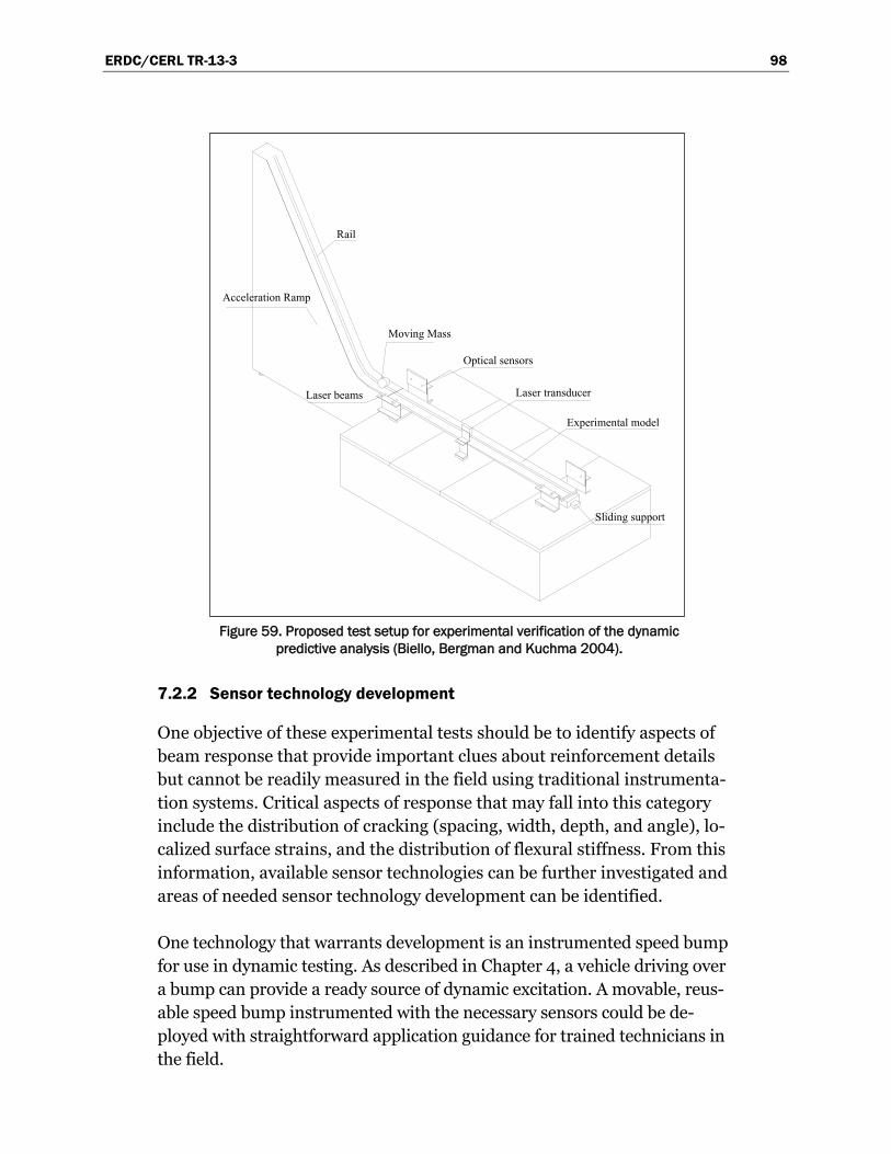
ERDC/CERL TR-13-3 98
Figure 59. Proposed test setup for experimental verification of the dynamic
predictive analysis (Biello, Bergman and Kuchma 2004).
7.2.2 Sensor technology development
One objective of these experimental tests should be to identify aspects of beam response that provide important clues about reinforcement details but cannot be readily measured in the field using traditional instrumenta-tion systems. Critical aspects of response that may fall into this category include the distribution of cracking (spacing, width, depth, and angle), lo-calized surface strains, and the distribution of flexural stiffness. From this information, available sensor technologies can be further investigated and areas of needed sensor technology development can be identified.
One technology that warrants development is an instrumented speed bump for use in dynamic testing. As described in Chapter 4, a vehicle driving over a bump can provide a ready source of dynamic excitation. A movable, reus-able speed bump instrumented with the necessary sensors could be de-ployed with straightforward application guidance for trained technicians in the field.
Acceleration Ramp
Moving Mass
Optical sensors
Laser beams
Rail
Laser transducer
Experimental model
Sliding support
ERDC/CERL TR-13-3 99
Assessing the shear capacity of bridges is difficult without knowing the size and location of shear reinforcement. One possible solution, if the level of access permits, would be to locate the shear reinforcement using ground-penetrating radar (GPR). This technology is currently used in construction practices to locate reinforcement before drilling into a reinforced concrete member. In laboratory tests, GPR has not yet proven capable of identifying the diameter of reinforcement with sufficient accuracy for application to this project, but it has shown promise in locating reinforcement (Zhan and Xie 2009); (Chang, Lin and Lien 2009); (He, et al. 2009). By using GPR to lo-cate vertical stirrup spacing, a conservative assumption on stirrup diameter (#3 bars) and number of legs (2) could be made to more safely and accu-rately assess the shear capacity of the structure in lieu of measuring shear response under controlled loading.
7.2.3 Experimental validation of predictive analysis for multi-girder structures
Once the reliability of the predictive analysis procedures are assessed and verified for a single girder structure, verification of the procedure for mul-ti-girder structures will be needed. Validation could be performed either on an existing bridge in collaboration with a state department of transpor-tation or on a scaled structure built for controlled laboratory testing. If an existing structure were used, it should be a relatively new structure so the research team can obtain important properties that are often not known about the completed structure. Examples of these properties include measured material strengths, as-built geometry, shrinkage strains, and bearing conditions. Assessment of a multi-girder structure offers an op-portunity to identify missing elements and shortcomings of the numerical models that may arise from some of the simplifying assumptions described in section 7.1. Testing the multi-girder structure, whether in the controlled laboratory environment or on an existing full-scale structure, would re-quire further investigation into load-distribution factors.
7.2.4 Procedure and software development
Once experimental testing has validated the predictive analysis techniques and measurement capabilities, a formal procedure and the required com-putational tools need to be developed. Depending on the specific field ap-plication, the available time and level of access to the structure will limit the formal procedure. One assumption of this preliminary numerical study indicates that time and access constraints are not yet considered. In order

ERDC/CERL TR-13-3 100
to implement the procedure, trained field technicians would need compu-tational tools for data input and predictive analysis output. Ideally, these tools would consist of a portable computer with a clean, transparent user interface for input of member geometry, material strength, load condi-tions, etc. Predictive analysis could be performed directly on the computer or by transmitting the input for remote processing on another computer.
ERDC/CERL TR-13-3 101
8 Conclusions
The results of this study indicate that there is high potential for improving current methods for assessing the capacity of reinforced concrete bridges through comparison of predictive analysis and measured behavior under known loads. This report documents a preliminary numerical study de-signed to isolate key variables and identify areas of high potential for fu-ture research and development. Within the assumptions noted in section 7.1, the results are particularly promising for identifying the amount of flexural reinforcement in the structure. The flexural response—both dis-placement and strains—of girders with different levels of reinforcement exhibits both a consistent reinforcement influence factor and a measure-able difference with currently available sensor precision.
Shear response, however, is more difficult to capture due to the very small magnitude of the response, such as shear strain. As discussed in section 2.3, common shear reinforcement design requirements have evolved, and many bridges were built before minimum shear reinforcement requirements were introduced. Since shear failure is brittle in nature, it is dangerous to not have an accurate assessment of shear capacity when loading a structure with heavy vehicles such as a HETS tank carrier. Other possible solutions may need to be explored if further developments of the shear assessment approaches in this study are shown to be inadequate in the experimental validation tests. In the absence of a direct or indirect way to measure shear reinforcement, the remaining option would be to calculate what the shear reinforcement should have been based on the assessed flexural capacity, pattern of loading, and the age of the structure (which helps in selecting the applicable code of practice for making these calculations).
It is important to understand that, unlike the results of predictive analysis, field measurement data will tend to reflect a degree of variability and, therefore, uncertainty. However, with improvements in sensor reliability and understanding of load distribution to individual girders, confidence in measured behaviors will increase. Measurement of load response should include recording a variety of different behaviors (strains, displacements, vibrations), different types of tests (static and dynamic), and repetition of each test. By obtaining data for different tests, statistical correlations can increase confidence in the capacity assessment made from the procedure.

ERDC/CERL TR-13-3 102
References AASHTO. American Association of State Highway Transportation Officials Manual for
Condition Evaluation of Bridges. 2nd. Washington, D.C., 1994.
ACI Committee 318. "Building Code Requirements for Structural Concrete (ACI 318-08) and Commentary." American Concrete Institute,, 2008.
ACI Committee 435. "Deflections of Reinforced Concrete Flexural Members." Journal of the American Concrete Institute, June 1966: 637-674.
ACI Committee 445. "Recent Approaches to Shear Design of Structural Concrete." ASCE Journal of Structural Engineering 124, no. 12 (December 1998).
Bafoor Design and Construction Incorporation. "Structural Inspection and Repair/Replacement Proposal, Bridge ????, ????, Afghanistan." for the U.S Army Corps of Engineers, Afghanistan District, 2009.
Bentz, Evan C. "Response-2000 Manual." September 2001. http://www.ecf.utoronto.ca/~bentz/manual2/final.pdf (accessed April 18, 2010).
Bentz, Evan C. "Sectional Analysis of Reinforced Concrete Members." Department of Civil Engineering, University of Toronto, 2000.
Biello, C., L. Bergman, and D.A. Kuchma. "Experimental Investigation of a Small Scale Bridge Model Under a Moving Mass." ASCE Journal of Structural Engineering 130 (May 2004): 799-804.
Caltrans. "Post-Tensioned Box Girder LRFD Design Example." Prestressed Concrete Committee, Division of Engineering Services, 2008.
CEB-FIB. "Model Code 1990." Laussane: Comité Euro-International du Béton, 1993. 437.
Chang, Che Way, Chen Hua Lin, and Sheng Lien Lien. "Measurement radius of reinforcing steel bar in concrete using digital image GPR." Construction and Building Materials, 2009: 1057-1063.
Collins, M. P., and D. Mitchell. Prestressed Concrete Structures. Englewood Cliffs, New Jersey: Prentice Hall, 1991.
DiPetta, T., Koester, D., Adams, D.E., Gothamy, J., Decker, P., Lamb, D., and Gorsich, D. Health Monitoring for Condition-Based Maintenance of a HMMWV using an Instrumented Diagnostic Cleat. Warrendale, PA: SAE International, April 20, 2009.
Gries, M., R. Giles, D. Kuchma, B. Spencer, and L. Bergman. "Advanced Bridge Capacity and Structural Integrity Assessment." University of Illinois at Urbana-Champaign, Final project report to USA-CERL (in progress), 2010.
He, Xian-Qi, Zi-Qiang Zhu, Qun-Yi Liu, and Guang-Yin Lu. "Review of GPR Rebar Detection." PIERS Proceedings. Beijing, 2009. 804-813.

ERDC/CERL TR-13-3 103
Hegger, Josef. ACI Structural Journal 101, no. 2 (March-April 2004).
MacGregor, James G., and James K. Wight. Reinforced Concrete: Mechanics and Design. 4th. Upper Saddle River, NJ: Pearson Prentice Hall, 2005.
Minor, John, and Clinton Woodward. "Bridge Analysis Study, Phase II & Phase III." New Mexico State University;, 1999.
Mitchell, D., and M. P. Collins. "Diagonal Compression Field Theory - A Rational Model for Structural Concrete in Pure Torsion." ACI Journal 71, no. 8 (1974): 396-408.
NATO. "Standard NATO Agreement 2021." Computation of Bridge, Raft, Ferry, and Vehicle Classifications. 1990.
Precast/Prestressed Concrete Institute. "Chapter 7: Loads & Load Distribution." Chap. 7 in PCI Bridge Design Manual. Chicago, 2003.
Ramirez, J.A. "Recent Approaches to Shear Design." ACI-ASCE Committee 445. 2009.
Ray, James C., and Sharon B. Garner. Load Rating Analysis for Bridges. Unpublished, US Army Engineer Research and Development Center (ERDC), Vicksburg, MS: Engineer Research and Development Center, Geotechnical and Structures Laboratory, 2009.
Ray, James, and Cary D. Butler. "Rapid and Global Bridge Assessment for the Military." ASCE Journal of Bridge Engineering, November 2004: 550-557.
Taly, Narendra. Design of Modern Highway Bridges. New York: McGraw-Hill, 1998.
US Army. "FM3-34.343." Military Nonstandard Fixed Bridging. Washington, DC: Headquarters, Department of the Army, 2002.
Van Groningen, Charles N., and Robert A. Paddock. "SmartBridge: A Tool for Estimating the Military Load Classification." Decision and Information Sciences Division, Argonne National Laboratory, Argonne, IL, 1997.
Vecchio, F.J. "Disturbed Stress Field Model for Reinforced Concrete: Formulation." ASCE Journal of Structural Engineering 126, no. 8 (September 2000): 1070-1077.
Vecchio, F.J. "Disturbed Stress Field Model for Reinforced Concrete: Implementation." ASCE Journal of Structural Engineering 127, no. 1 (January 2001): 12-20.
Vecchio, F.J., D. Lai, W. Shim, and J. Ng. "Disturbed Stress Field Model for Reinforced Concrete: Validation." ASCE Journal of Structural Engineering 127, no. 4 (April 2001): 350-358.
Vecchio, Frank J., and Michael P. Collins. "The Modified Compression-Field Theory for Reinforced Concrete Elements Subjected to Shear." ACI Journal, March-April 1986: 219-231.

ERDC/CERL TR-13-3 104
Wickline, Joseph E., Thomas E. Cousins, and Yazmin Seda-Sanabria. "ERDC/GSL TR-03-12: A Study of Effective Moment of Inertia Models for Full-Scale Reinforced Concrete T-Beams Subjected to a Tandem-Axle Load Configuration." Geotechnical and Structures Laboratory, Engineering Research and Development Center, 2003.
Wong, P.S., and F. J. Vecchio. "VecTor2 & Formworks User's Manual." Vector Analysis Group. August 2002. http://www.civ.utoronto.ca/vector/user_manuals/manual1.pdf (accessed April 18, 2010).
Zhan, Runtao, and Huicai Xie. "GPR measurement of the diameter of steel bars in concrete specimens based on the stationary wavelet transform." Insight - Non-Destructive Testing and Condition Monitoring 51, no. 3 (March 2009): 151-155.

REPORT DOCUMENTATION PAGE Form Approved
OMB No. 0704-0188 Public reporting burden for this collection of information is estimated to average 1 hour per response, including the time for reviewing instructions, searching existing data sources, gathering and maintaining the data needed, and completing and reviewing this collection of information. Send comments regarding this burden estimate or any other aspect of this collection of information, including suggestions for reducing this burden to Department of Defense, Washington Headquarters Services, Directorate for Information Operations and Reports (0704-0188), 1215 Jefferson Davis Highway, Suite 1204, Arlington, VA 22202-4302. Respondents should be aware that notwithstanding any other provision of law, no person shall be subject to any penalty for failing to comply with a collection of information if it does not display a currently valid OMB control number. PLEASE DO NOT RETURN YOUR FORM TO THE ABOVE ADDRESS.
1. REPORT DATE (DD-MM-YYYY) March 2013
2. REPORT TYPE Final
3. DATES COVERED (From - To)
4. TITLE AND SUBTITLE Advanced Bridge Capacity and Structural Integrity Assessment Methodology
5a. CONTRACT NUMBER
5b. GRANT NUMBER
5c. PROGRAM ELEMENT NUMBER
6. AUTHOR(S) Matthew B. Gries, Ryan K. Giles, Daniel A. Kuchma, Billie F. Spencer, Lawrence A. Bergman, and James Wilcoski
5d. PROJECT NUMBER ARPA Order AV47/00
5e. TASK NUMBER
5f. WORK UNIT NUMBER 09000Z01307
7. PERFORMING ORGANIZATION NAME(S) AND ADDRESS(ES) U.S. Army Engineer Research and Development Center Construction Engineering Research Laboratory P.O. Box 9005 Champaign, IL 61826-9005
8. PERFORMING ORGANIZATION REPORT NUMBER
ERDC/CERL TR-13-3
9. SPONSORING / MONITORING AGENCY NAME(S) AND ADDRESS(ES) Defense Advanced Research Projects Agency Strategic Technology Office 3701 North Fairfax Drive Arlington, VA 22203-1714
10. SPONSOR/MONITOR’S ACRONYM(S) DARPA
11. SPONSOR/MONITOR’S REPORT NUMBER(S)
12. DISTRIBUTION / AVAILABILITY STATEMENT Approved for public release; distribution is unlimited.
13. SUPPLEMENTARY NOTES
14. ABSTRACT
The bridge is a basic element of all surface transportation networks. In military theaters of operation, transportation routes that cross bridges are essential for deploying personnel, supplies, and heavy equipment, as well as for facilitating communications. It is essen-tial that the structural capacity of each bridge along a military route be assessed in order to avoid overloading the bridge or unneces-sarily hindering military operations by overestimating or underestimating its capacity. For reinforced concrete structures, information about the number, size, and orientation of steel reinforcement is necessary to make a strength assessment. Since reinforcement is not visible externally, making an accurate assessment without design drawings is extremely difficult.
The objective of this project was to develop more reliable means of in-field capacity assessment of reinforced concrete bridges by making improved estimates of the level of longitudinal and shear reinforcement. The proposed assessment procedure is based on comparing measured structural response under controlled loading conditions to predicted structural response from analysis. This re-port presents results from a preliminary sensitivity study of the analytically predicted response of simply supported reinforced con-crete T-beam girders that have varying levels of longitudinal and shear reinforcement.
15. SUBJECT TERMS reinforced concrete bridges, structural engineering, load-carrying capacity, rapid assessment, military operations
16. SECURITY CLASSIFICATION OF: 17. LIMITATION OF ABSTRACT
18. NUMBER OF PAGES
19a. NAME OF RESPONSIBLE PERSON
a. REPORT
Unclassified
b. ABSTRACT
Unclassified
c. THIS PAGE
Unclassified 112 19b. TELEPHONE NUMBER (include area code)
Standard Form 298 (Rev. 8-98) Prescribed by ANSI Std. 239.18