equivariant schubert calculus and jeu de taquin
TRANSCRIPT

arX
iv:1
207.
3209
v1 [
mat
h.C
O]
13
Jul 2
012
EQUIVARIANT SCHUBERT CALCULUS AND JEU DE TAQUIN
HUGH THOMAS AND ALEXANDER YONG
ABSTRACT. We introduce edge labeled Young tableaux. Our main results provide a cor-responding analogue of [Schutzenberger ’77]’s theory of jeu de taquin. These are appliedto the equivariant Schubert calculus of Grassmannians. Reinterpreting, we present new(semi)standard tableaux to study factorial Schur polynomials, after [Biedenharn-Louck’89], [Macdonald ’92] and [Goulden-Greene ’94] and others.
Consequently, we obtain new combinatorial rules for the Schubert structure coefficients,complementing work of [Molev-Sagan ’99], [Knutson-Tao ’03], [Molev ’08] and [Kreiman’09]. We also describe a conjectural generalization of one of our rules to the equivariantK-theory of Grassmannians, extending work of [Thomas-Yong ’07]. This conjecture con-cretely realizes the “positivity” known to exist by [Anderson-Griffeth-Miller ’08]. It pro-vides an alternative to the conjectural rule of Knutson-Vakil reported in [Coskun-Vakil ’06].
1. INTRODUCTION
1.1. Overview. The main goal of this paper is to introduce edge labeled Young tableaux,together with a corresponding analogue of the theory of jeu de taquin. We apply them tothe setting of equivariant Schubert calculus of Grassmannians. This paper may also beinterpreted as extending (semi)standard tableaux for use with the closely related familyof factorial Schur polynomials.
The classical theory of jeu de taquin, initiated by M.-P. Schutzenberger [Sc77], has beenof significance in combinatorial representation theory. One outcome of this theory is acombinatorial rule for the Littlewood-Richardson coefficients. Perhaps more importantly,it provides a systematic and flexible means to elegantly reconcile a variety of importanttableau algorithms. It achieves this using a simple sliding law.
The Littlewood-Richardson coefficients compute Schubert calculus of Grassmannians.More precisely, they are structure coefficients for multiplication with respect to the Schu-bert basis of the ordinary cohomology ring of Grassmannians. Since a Grassmannianadmits the action of the torus T of invertible diagonal matrices, one can instead studythe richer T -equivariant cohomology ring and its Schubert calculus. While Littlewood-Richardson rules were already available for this setting [KnTa03], further ideas are neededto (provably) extend them to other Lie types or finer cohomology theories. In addition, todate, jeu de taquin is the only combinatorial model that admits a root-system uniform rulefor Schubert calculus on minuscule G/P ’s [ThYo06]. These are our principal reasons forseeking new combinatorial models that extend jeu de taquin.
1.2. Schubert calculus of Grassmannians. Let X = Gr(k,Cn) denote the Grassmannianof k-dimensional planes in Cn. If λ = (n−k ≥ λ1 ≥ λ2 ≥ · · · ≥ λk ≥ 0) is a Young diagramcontained in the rectangle Λ := k × (n− k), the associated Schubert variety is defined by
Xλ :={V ∈ Gr(k,Cn)| dim(V ∩ F n−k+i−λi) ≥ i, 1 ≤ i ≤ k
},
Date: July 13, 2012.
1

where F d = span(en, en−1, . . . , en−d+1). With this convention, codim(Xλ) = |λ| =∑
i λi.
Let T ⊆ GLn be the torus of invertible diagonal matrices. Since Xλ is T -stable underthe action of T on X , Xλ admits an equivariant Schubert class σλ in HT (X) = the T -equivariant cohomology ring of X . Now, HT (X) is a module over HT (pt) := Z[t1, . . . , tn],and these classes form an additive HT (pt)-basis of HT (X). The expansion
(1) σλ · σµ =∑
ν
Cνλ,µσν ,
defines the equivariant Schubert structure coefficients Cνλ,µ ∈ Z[t1, . . . , tn]. In fact, Cν
λ,µ =0 unless |λ| + |µ| ≥ |ν|. In the case of equality, Cν
λ,µ ∈ N are the Littlewood-Richardsoncoefficients; these compute the number of points of X in g1 ·Xλ∩ g2 ·Xµ∩ g3∩Xν∨ , whereg1, g2, g3 are generic elements of GLn and ν∨ is the 180-degree rotation of the complementof ν inside Λ.
W. Graham [Gr01] proved that the polynomials Cνλ,µ have positive coefficients when
expressed in the variables βi := ti − ti+1. This positivity is evident in the statement ofA. Knutson-T. Tao’s combinatorial puzzle rule [KnTa03]. Later, alternative tableau ruleswere given by V. Kreiman [Kr10] and A. Molev [Mo09] (in these rules, the positivity isnot hard to prove). See also the work of P. Zinn-Justin [Zi09].
1.3. (Semi)standard tableaux with edge labels. Our work depends on a new kind ofYoung tableaux. Let Y denote the set of Young diagrams (drawn in English notation).Given λ, ν ∈ Y with λ contained in ν, denote the skew shape by ν/λ. A horizontal edgeof ν/λ is a horizontally-oriented line segment which either lies along the upper or lowerboundary of ν/λ, or which separates two boxes of ν/λ.
An equivariant filling of ν/λ assigns one of the labels 1, 2, . . . , ℓ to each box of ν/λ anda (possibly empty) subset of {1, 2, . . . , ℓ} to each horizontal edge of ν/λ. An equivariantfilling is semistandard if every box label is:
• weakly smaller than the label in the box immediately to its right;• strictly smaller than any label in its southern edge and the label in the box imme-
diately below it; and• strictly larger than any label in its northern edge and the label in the box immedi-
ately above it.
(No condition is placed on the labels of adjacent edges.) The filling is standard if thelabels used are 1, 2, . . . , ℓ, and each label is used exactly once.
Let EqSYT(ν/λ, ℓ) and EqSSYT(ν/λ, ℓ) respectively be the set of equivariant standard andsemistandard tableaux whose entries come from {1, 2, . . . , ℓ}. For example:
1 6
7
4 8
3, 5 2and
1 1
6
6 7
3, 5 2, 4
7
which are in EqSYT((4, 2, 2)/(2, 1), 8) and EqSSYT((4, 2, 2)/(2, 1), 8), respectively.
Those T ∈ EqSYT(ν/λ, |ν/λ|), where each horizontal edge has no labels, are in obviousbijection with (ordinary) standard Young tableaux. In this latter case, we also call T an or-dinary standard tableau. (We will drop “equivariant” for fillings unless confusion might
2

arise.) Finally, an ordinary standard Young tableau of shape µ is row superstandard if itis filled by 1, 2, . . . , µ1 in the first row, µ1 +1, µ1 +2, . . . , µ1 + µ2 in the second row, etc. LetTµ denote the row superstandard Young tableau of shape µ.
1.4. Equivariant jeu de taquin (first version). Our first version of equivariant jeu detaquin omits some features (and complexity) of the main construction of Section 2. Nev-ertheless, this version already suffices to compute the polynomials Cν
λ,µ. Moreover, it sug-gests generalizations. Specifically, we present a conjectural generalization to equivariantK-theory in Section 4. It also suggests a first step towards an extension to minusculeG/P ’s (further discussion may appear elsewhere), cf. [ThYo06].
A box x ∈ λ is an inner corner of ν/λ if it is maximally southeast in λ. Given an innercorner x and T ∈ EqSYT(ν/λ, ℓ), compare the label in the box immediately to the right ofx and the smallest label on the southern edge of x, or the label in the box immediatelybelow x, if no label appears on that edge. The smaller of the labels is moved into x, eitherby vacating a box or moving a label from the southern edge of x. If no labels can be usedor if an edge label is moved, the process terminates. Otherwise, some adjacent box hasbeen vacated, and we repeat the above process until termination. Call the result Ejdtx(T ),the equivariant jeu de taquin slide into x. Clearly, Ejdtx(T ) is also a standard tableau.
Define the equivariant rectification of T , denoted Erect(T ), to be the result of applyingthe sequence Ejdtx(1), Ejdtx(2), . . . , Ejdtx(|λ|) starting with T , where x(1), x(2), . . . , x(|λ|) arethe boxes of λ, read along columns, from bottom to top, and right to left.
Example 1.1. Let ν/λ = (4, 3, 1)/(3, 1, 1) ⊆ Λ = 3× 4 and
T = 3
5 6
4
1 2
We use “•” to indicate the boxes being slid into during the steps of Erect(T ). The rectifi-cation of the third column given by:
(2)
• 3
5 6
2 3
5 6
4
1 2
4
17→
The rectification of the second column given by:
(3)
• 2 3
5 6
1 2 3
5 6
4
1
4
7→
and finally the rectification of the first column given by:
(4)
1 2 3
5 6
•
1 2 3
• 5 6
4
• 1 2 3
4 5 6
1 2 3 •
4 5 6
4
7→ 7→ 7→ · · · 7→
the last tableau being T(3,3). Here the “ 7→ · · · 7→” refers to slides moving the • right in thefirst row. �
3

We now define the weight wt(T ) ∈ Z[t1, . . . , tn] of a standard tableau T . Each box x ∈ Λis assigned a weight β(x) = tm − tm+1 where m is the “Manhattan distance” from thesouthwest corner (point) of Λ to the northwest corner (point) of x (i.e., the length of anynorth and east lattice path between the corners); see Example 1.3. We say an edge label lpasses through a box x if it occupies x during the equivariant rectification of the columnof T in which l begins. Suppose that the boxes passed are x1, x2, . . . , xs. Moreover, oncethe rectification of a column is complete, suppose the filled boxes strictly to the right ofthe box xs are y1, . . . , yt. Then set
factor(l) = (β(x1) + β(x2) + · · ·+ β(xs)) + (β(y1) + β(y2) + · · ·+ β(yt)).
If after rectification of a column, the label l still remains an edge label, factor(l) is declaredto be zero. Otherwise, note that since the boxes x1, . . . , xs, y1, . . . , yt form a hook inside ν,factor(i) = te − tf with e < f . Now define
wt(T ) :=∏
l
factor(l),
where the product is over all edge labels l of T .
Theorem 1.2. The equivariant Schubert structure coefficient is given by the polynomial
Cνλ,µ =
∑
T
wt(T ),
where the sum is over all T ∈ EqSYT(ν/λ, |µ|) such that Erect(T ) = Tµ.
Since each factor(l) is a positive sum of the indeterminates βi = ti − ti+1, Theorem 1.2expresses Cν
λ,µ as a polynomial with positive coefficients in the βi’s. It is not hard to seethat Theorem 1.2 expresses Cν
λ,µ as a squarefree polynomial in the “positive root” variablesαij = βi + βi+1 + · · ·+ βj−1, also a feature of the puzzle rule of [KnTa03].
Example 1.3. Continuing Example 1.1, the Manhattan distances for Λ = 3× 5 are:
3 4 5 6 72 3 4 5 61 2 3 4 5
.
There are three edge labels of T :
• For the edge label 2, we have factor(2) = (t5 − t6) + (t6 − t7) = t5 − t7 since theedge label passes through one box, and after the third column is rectified (2), the3 lies to its right.
• For the edge label 1, we have factor(1) = (t4−t5)+(t5−t6)+(t6−t7) = t4−t7 sincethe edge label passes through one box, and after the second column is rectified (3),
the 2 3 lies to its right.• For the edge label 4, we have factor(4) = (t1− t2)+(t2− t3)+(t3− t4)+(t4− t5) =t1 − t5 since the edge label passes through two boxes, and after the first column is
rectified (4), 5 6 lies to its right.
Therefore, wt(T ) = (t5 − t7)(t4 − t7)(t1 − t5). �
In Schutzenberger’s jeu de taquin theory, one is free to slide at different inner corners.His theory’s “first fundamental theorem” is that rectification does not depend on thesechoices. The above equivariant jeu de taquin avoids this issue altogether by insisting on a
4

specific order of rectification. Even more, the classical theory’s “second fundamental the-orem” asserts the number of tableaux that rectify to a given target tableau is independentof the choice of target tableau. In contrast, we insist on using row superstandard tableauxas our targets.
The above rigid definition of jeu de taquin makes nonobvious to us how to directlyprove Theorem 1.2. Although one can biject the rule of Theorem 1.2 with earlier rules,our original reason for starting this project was to find a model that could ultimatelyextend to other equivariant contexts where earlier rules are unavailable.
Therefore, our problem was to find a more flexible version of equivariant jeu de taquinpossessing features of the fundamental theorems. Our solution is described in Section 2.It has some aspects that are distinctly different than the classical jeu de taquin (and ourfirst version of equivariant jeu de taquin):
• More than one label can move during a swap.• Labels can move downwards during a swap.• Row semistandardness can be violated after a swap (although at most one such
violation occurs at any given time, and it is eliminated at the end of a sequence ofswaps that defines a slide).
Our main result shows that the order of rectification is independent of the choices, ifone rectifies to a “highest weight tableau” and starts with a tableau that is “lattice”. Fromthis, we derive an essentially independent proof of Theorem 1.2.
1.5. Organization. In Section 2, we describe our flexible version of jeu de taquin as wellas stating and proving our main results. Section 3 uses the results of Section 2 to give twoadditional formulations of the equivariant Littlewood-Richardson rule. We then deduceTheorem 1.2. In Section 4, we formulate a conjectural formula for equivariant K-theoryof Grassmannians. Concluding remarks are given in Section 5.
2. EQUIVARIANT JEU DE TAQUIN (FLEXIBLE VERSION)
To describe our flexible version of equivariant jeu de taquin, it is more convenient towork with semistandard fillings than with standard fillings.
Starting with a semistandard filling T of a skew shape ν/λ, choose an inner corner x
and mark it with a •. We now define the equivariant slide of T into x. As in classical jeude taquin, the slide proceeds by a sequence of swaps, as the • moves through the tableau.
However, the result of a slide is not necessarily a single tableau, but rather a formal sumof tableaux, with coefficients in Z[β1, . . . , βn−1], where βi = ti− ti+1. The way this arises inthe course of the sequence of swaps is that sometimes a swap will produce two tableaux.One of them has no •, and it contributes directly to the output (with a coefficient), whilethe other still has a •, which we continue to swap.
2.1. Definitions of the equivariant swaps. Let x ∈ T be as above. Suppose y is the boxto the immediate right of x, and z is the box immediately below x. Let b be the smallestneighbouring label below x (either the smallest one on the lower edge of x or the one inthe box z) and let r be the label in y. Define N T
x,l to be the number of occurences of a labell in columns weakly to the right of the box x in T .
There are four kinds of swaps (I)–(IV) that we use:
5

(I) “vertical swap”: b ≤ r (or there is no r) and b is a box label of z: T ′ is obtained by exchanging
• and b, i.e., T =• r
b7→ b r
•= T ′.
Output: T ′.
(II) “expansion swap”: b ≤ r and b is a label of the lower edge of x: T ′ is obtained by moving b
into x; the • is eliminated. T ′′ is obtained by moving b to the top edge of x (and • remainsin place). In this case,
•7→ β(x) · b +
•= β(x) · T ′ + T ′′
b
b
Output: β(x) · T ′ + T ′′.
(III) “resuscitation swap”: b > r (or there is no b), and the largest label u on the upper edge of xsatisfies u = r: In this case, T ′ is obtained by having u = r replace the • in x, replace r by •in y, and placing r on the lower edge of y. This move locally looks like:
T =• r
7→r •
= T ′
r
r
Output: T ′.
(IV) “horizontal swap”: b > r (or there is no b), and (III) does not apply: Define Z to be the setof consecutive integers {r, r+ 1, . . . ,m} where m is chosen largest so that:
(i) m < b and m is at least as large as the entry in the box to the left of x;(ii) N T
y,l = N Ty,r for all r ≤ l ≤ m.
(iii) {r+ 1, . . . ,m} are labels on the lower edge of y.
Set, Z ′ = Z \ {m}, W = U ∪ Z ′ and Y ′ = Y \ Z. Then locally the swap is:
(5) T =• r
7→m •
= T ′
U
b Y b Y ′
W
That is, T ′ is the result of moving m into x and putting the smaller entries of Z in theupper edge of x. Conclude by placing • into y.
Output: T ′.
Example 2.1 (of swap (IV)). We have
• 13 2, 3
7→12 •3 3
where Z = {1, 2}.
On the other hand:1
• 17→ 1
1 •2 2
where the edge label “2” is not in Z because of (IV)(ii).
In addition, the following swap (IV) is valid, even though it “breaks” row semistan-dardness in the “obvious” sense:
• 1 17→
2 • 12 2
1
2Note that the next swap will also be of type (IV), “fixing” the broken semistandardness inthe second row. Claims 2.8 and 2.9 below explain how this example generalizes. �
6

We now describe Eqjdtx(T ) (as opposed to the “Ejdtx(T )” of Section 1). Begin by re-placing T by the result of swapping at x. The result is a formal sum of terms of the formω · S where ω ∈ Z[β1, . . . , βn−1], and S is a tableau. If a tableau U in this formal sum eitherhas no •, or the • has no neighbouring labels southeast, then do nothing. Otherwise, letx′ be the box containing the • of U and replace U by swapping at x′. Repeat until no moretableaux need replacement. Now erase all any •’s from the tableaux in the formal sum.We need to show (under assumptions) that Eqjdtx(T ) is a well-defined algorithm.
Call a tableau T with at most a single • really good if:
(a) it is semistandard, once one ignores the • (i.e., the rows are weakly increasing andthe columns are strictly increasing);
(b) the label of the box directly left of the box with the • is weakly less than the smallestlabel on the edge below the • (if the latter label exists), i.e.,
ℓ •b
(ℓ ≤ b);
(c) the label of the box directly right of the box with the bullet is weakly larger thanthe largest label on the edge above the • (if the latter exists), i.e.,
• ru
(u ≤ r).
(Note that the latter two conditions would be automatic if the • were a numerical label.)Call T nearly bad if (b) and (c) above hold, and (a) holds except that the label to theimmediate left of the • may be larger than the label to the immediate right of •. We willsay T is good if it is either really good or nearly bad; otherwise T is bad.
The third swap in Example 2.1 demonstrates that swap (IV) can turn a really goodtableau to a nearly bad one. In fact, in Section 2.4 we see only swap (IV) can cause nearbadness.
2.2. Statement of the main results. An equivariant filling T is lattice if for a given col-umn c and label l (that may not be in column c), the number of occurrences of l in columnsweakly to the right of column c weakly exceeds the occurences of l+ 1 in that region.
The appropriate class of tableaux to apply our Eqjdt swaps to are the lattice and semi-standard tableaux, in the sense that Eqjdt preserves this class:
Proposition 2.2. Suppose T is semistandard and lattice, and that x is an inner corner. ThenEqjdtx(T ) is well-defined as an algorithm: it terminates in a finite number of steps, and outputsa formal sum of semistandard and lattice tableaux. Each intermediate tableau in the calculation ofEqjdtx(T ) is good and lattice.
Assuming this proposition (the proof being delayed until Section 2.3), we define (an)equivariant rectification. Given T , pick an inner corner x and replace T by the formalsum Eqjdtx(T ). Now, for each U appearing in Eqjdtx(T ), which has an inner corner x′,replace U by Eqjdtx′(U). Repeat until no such U exists. Let Eqrect(T ) be the resultingformal sum of equivariant semistandard tableaux. We will call the choices of x and ofeach x′ the rectification order.
Call a straight shape tableau regular if does not have any edge labels; it is irregularotherwise. The regular tableau Sµ whose i-th row uses only the labels i is called a highestweight tableau. The content of a tableau T is µ = (µ1, µ2, . . . ) if T has µ1 1’s, µ2 2’s, etc.
7

For T of content µ, Eqrect(T ) is µ−highest weight if Sµ is the only regular tableau thatappears. (We allow the possibility that no regular tableau appears at all.)
Let us also define the a priori weight of a good and lattice tableau T , denoted byapwt(T ). Declare apwt(T ) = 0 if:
(i) there is an edge label i weakly above the upper edge of the box x in row i (in itscolumn), and it is not possible to apply a resuscitation swap (III) to T such that imoves into x; or
(ii) there is a box label i located strictly higher than row i.
We will say that a label satisfying (i) or (ii) is too high. It will also be convenient to saythat a label i is nearly too high if it lies on the upper edge of a box in row i but is not toohigh (i.e., a resuscitation swap (III) applies to T and moves i into x).
Now suppose neither (i) nor (ii) holds. Given an edge label i, suppose it lies on thelower edge of a box x in row r. (If i is on a top edge of Λ then r = 0.) Define apfactor(i)as follows:
(6) apfactor(i) = tMan(x) − tMan(x)+r−i+1+# of i’s strictly to the right of x.
where Man(x) is the Manhattan distance as defined in Section 1.
Finally, let
apwt(T ) =∏
i is an edge label of T
apfactor(i).
We are now ready to state our main result, a partial analogue of the fundamental theo-rems of jeu de taquin.
Theorem 2.3. Let T be a lattice semistandard tableau of content µ. Then:
(I) Eqrect(T ) is µ-highest weight for any choice of rectification order.(II) The coefficient of Sµ in Eqrect(T ) is invariant under these choices.
(III) The coefficient in (II) is apwt(T ).
Remark 2.4. In the classical theory, T rectifies to Sµ if and only if T is lattice and has contentµ. However, in our setting, analogues of these two conditions are no longer equivalent.Specifically, it is possible for a non-lattice tableau to become lattice using the equivariantswaps. For example, the starting tableau T below is not lattice, but Eqjdtx(T ) is:
T =• 2 2
7→2 • 2
7→2 2 •
= Eqjdtx(T )1 1 1 1 1 1
Therefore, we proceed to develop an equivariant Littlewood-Richardson rule using thesecond of the two classically equivalent conditions.
In order to develop a rule using an analogue of the first condition, one needs swappingrules with the property that non-lattice fillings stay non-lattice after a swap. It seems tous that such rules would be more complicated than our current rules. �
8

Example 2.5. In the following rectification (inside Λ = 2×2), we suppress the computationsconcerning tableaux with labels that are too high (i.e., will rectify to a irregular tableau):
T =•
7→ β31
•+
•
1
1
1 1
1
7→ β3
β1• 1
1+
• 1
+ · · ·1
7→ β1β31 1
•+ β3
β21 1 +
• 1
+ · · ·1
7→ (β1β3 + β2β3)1 1 + β3
1 •+ · · ·1
7→ (β1β3 + β2β3)1 1 + β3
β3
1 1 + 1 •
+ · · ·
1
7→ (β1β3 + β2β3 + β23)
1 1 + · · · = Eqrect(T )
Hence Eqrect(T ) is (2)-highest weight. Now, apwt(T ) = (β1 + β2 + β3)β3 which equalsthe coefficient of S(2) in Eqrect(T ). These two facts agree with parts (I) and (III) of Theo-rem 2.3, respectively. �
2.3. Proof of Proposition 2.2. Suppose we start the computation of Eqjdtx(T ), giving riseto a sequence of swaps of tableaux:
T = T (0) 7→ T (1) 7→ · · · 7→ T (i).
(If we use swap (II) a “branching” occurs in the computation. The above sequence repre-sents one of the paths of the computation.)
We argue by induction that each successive tableau is good and lattice; the base case isthe hypothesis on T . If T (i) either has no • or no labels southeast of • then this is one ofthe tableaux appearing in Eqjdtx(T ). Otherwise, we must show that we can apply exactlyone of the swaps (I)–(IV) to obtain S ′ = T (i+1) which is good and lattice.
There are two cases, depending on whether S = T (i) is really good or nearly bad.
Case 1: S is really good: We break our argument into several claims.
Claim 2.6. If it is possible to apply one of the swaps (I)–(IV) to S then the result is good.
Proof. Suppose the vertical swap (I) is applied. Thus, S locally looks like
S = d • e
f g h,
9

where g ≤ e (and there is no label on the edge above the g). Thus we obtain S ′ =
d g e
f • h. To check that S ′ is really good, one only needs d ≤ g (if d exists). If d ex-
ists, so must f and d < f ≤ g (since S is good), as needed.
Next, suppose the expansion swap (II) is applied, thus
S = d • e
f g hy
where y is the smallest label on its edge and y ≤ e. If S ′ is the result of having the y jumpto the top edge, then S ′ is really good since S is really good and, as we have assumed,y ≤ e. Also, we know d ≤ y (again since S is good) and hence if S ′ is the result of replacing• by y, then S ′ is really good.
If a resuscitation swap (III) is used, we would have:
S =p q t
m • r
s f hb
r 7→ S ′ =p q t
m r •
s f hrb
where u = r is the largest label on its edge. Since S is really good, m ≤ r. Hence S ′ isreally good.
Finally, suppose we use a horizontal swap (IV) to arrive at S ′. Thus:
S = d • r w
s f h vb
U
Y 7→ S ′ = d m • w
s f h vY ′b
W
Recall Z = {r, r + 1, . . . ,m} is the set of labels that move from the third column to thesecond (relative to our local picture). Removal of these labels clearly keeps the thirdcolumn of S ′ semistandard since the third column of S is assumed to be semistandard.By the really goodness of S and the assumption that (III) does not apply, it follows that themaximal element immediately above the • in S is strictly less than r. These considerations,and condition (IV)(i), imply the semistandardness of the second column of S ′. Now, (IV)(i)allows, at worst, the possibility that S ′ is nearly bad, i.e., that w < m. However, even inthat case, S ′ is good (by definition). �
Claim 2.7. Exactly one of the swaps (I)–(IV) is applicable.
Proof. In the case b ≤ r (or r does not exist), one can apply either a vertical or expansionswap but not both. Thus suppose b > r (or there is no b). Locally, we have
S =a • r
.
u
b Y
(The argument is the same if b is the label of the box below the •.) Since S is good wehave u ≤ r. If u = r then one can apply a resuscitation move (III) (and, by definition, nota horizontal swap (IV)).
Hence we may assume u < r < b. Now, (IV) is always possible since the set Z in thedefinition of (IV) is nonempty by the given inequalities and the assumption a ≤ r (sinceS is really good). �
10
We also need to show S ′ is lattice. This will be argued after Case 2 since the proof onlyassumes S is good.
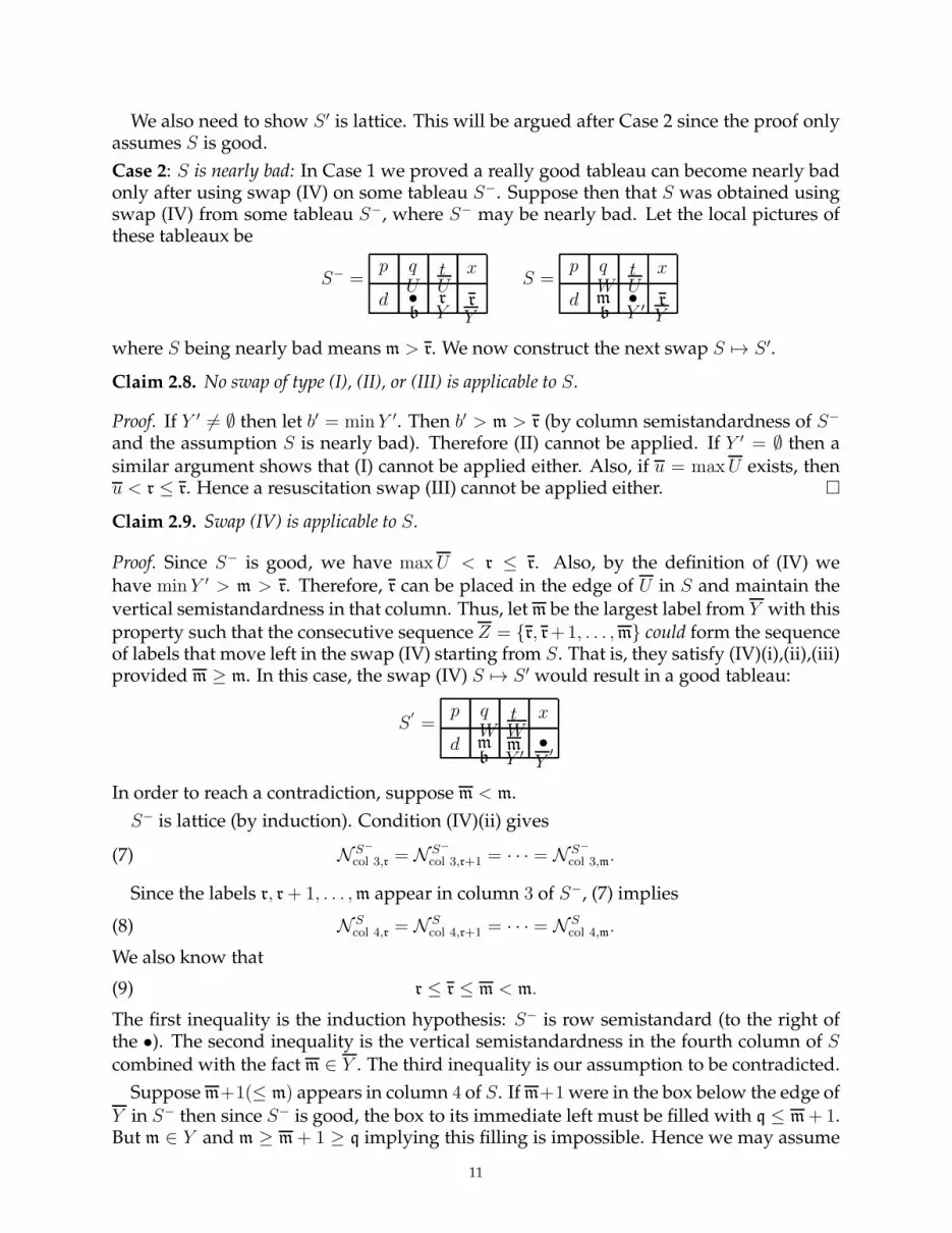
Case 2: S is nearly bad: In Case 1 we proved a really good tableau can become nearly badonly after using swap (IV) on some tableau S−. Suppose then that S was obtained usingswap (IV) from some tableau S−, where S− may be nearly bad. Let the local pictures ofthese tableaux be
S− =p q t x
d • r rb
U U
Y Y
S =p q t x
d m • rb
W U
Y ′Y
where S being nearly bad means m > r. We now construct the next swap S 7→ S ′.
Claim 2.8. No swap of type (I), (II), or (III) is applicable to S.
Proof. If Y ′ 6= ∅ then let b′ = minY ′. Then b′ > m > r (by column semistandardness of S−
and the assumption S is nearly bad). Therefore (II) cannot be applied. If Y ′ = ∅ then asimilar argument shows that (I) cannot be applied either. Also, if u = maxU exists, thenu < r ≤ r. Hence a resuscitation swap (III) cannot be applied either. �
Claim 2.9. Swap (IV) is applicable to S.
Proof. Since S− is good, we have maxU < r ≤ r. Also, by the definition of (IV) wehave minY ′ > m > r. Therefore, r can be placed in the edge of U in S and maintain thevertical semistandardness in that column. Thus, let m be the largest label from Y with thisproperty such that the consecutive sequence Z = {r, r+1, . . . ,m} could form the sequenceof labels that move left in the swap (IV) starting from S. That is, they satisfy (IV)(i),(ii),(iii)provided m ≥ m. In this case, the swap (IV) S 7→ S ′ would result in a good tableau:
S′
=p q t x
d m m •b
W W
Y ′Y
′
In order to reach a contradiction, suppose m < m.
S− is lattice (by induction). Condition (IV)(ii) gives
(7) N S−
col 3,r = N S−
col 3,r+1 = · · · = N S−
col 3,m.
Since the labels r, r+ 1, . . . ,m appear in column 3 of S−, (7) implies
(8) N Scol 4,r = N S
col 4,r+1 = · · · = N Scol 4,m.
We also know that
(9) r ≤ r ≤ m < m.
The first inequality is the induction hypothesis: S− is row semistandard (to the right ofthe •). The second inequality is the vertical semistandardness in the fourth column of Scombined with the fact m ∈ Y . The third inequality is our assumption to be contradicted.
Suppose m+1(≤ m) appears in column 4 of S. If m+1 were in the box below the edge ofY in S− then since S− is good, the box to its immediate left must be filled with q ≤ m+ 1.But m ∈ Y and m ≥ m+ 1 ≥ q implying this filling is impossible. Hence we may assume
11

m + 1 ∈ Y . Then this, together with (8) and (9), imply m + 1(≤ m < minY ′) should havebeen included in Z, contradicting the definition of m.
Therefore m + 1 does not appear in column 4 of S−. Then let X be the subtableau ofS− using the boxes in columns weakly to the right of column 4 of S−. Then X has thelabels r, . . . ,m+ 1 in equal numbers, is lattice in those labels, and does not have m + 1 inits leftmost column. This is impossible, another contradiction. Hence, in fact, m ≤ m asdesired. This means S ′ is at worst nearly bad and therefore good, as desired. �
Summarizing, if S is nearly bad then it was obtained by a horizontal swap (IV) fromeither a really good S− or a nearly bad S− whose near badness occurs in the same rowbut one step to the right.
To complete both Cases 1 and 2, it remains to prove:
Claim 2.10. Any swap T 7→ T ′ starting from a good and lattice T , results in T ′ being lattice.
Proof. None of the swaps (I), (II) nor (III) can turn a lattice tableau into a non-latticetableau, since in each case the set of labels in each column stays the same. Therefore,suppose that a horizontal swap (IV) destroys latticeness.
Consider the local diagram (5). The labels that move from the second column to thefirst column (with respect to our local diagram) are Z = {r, r+ 1, . . . ,m}.
The violation of latticeness must occur in the second column (and nowhere else in T ′),since it is the only column such that the multiset of entries weakly to its right has changed.An offending label l + 1 (i.e., one such that N T ′
y,l+1 > N T ′
y,l ) is not weakly less than n (theneighboring label of • to the north) since none of those labels moved. Also, l+1 6∈ Z sincethey do not appear in the second column of T ′. Moreover l + 1 ≤ m + 1 since the labelsm + 1 and larger have not moved. Thus the offending label must be l + 1 = m + 1, i.e.,N T ′
y,m+1 > N T ′
y,m. Hence, there must be a m+ 1 in the second column.
We cannot have m+ 1 as a box label in the box immediately below y, because then thebox label in the neighbor to the left would also be m + 1 (other values would violate theprerequisite (IV)(i) or that T is good). Since m does not already occur in the first columnof T , the assumption that T ′ is not lattice implies T fails the lattice condition for the labelm+ 1, at the first column, contrary to our assumption that T is lattice.
Therefore, m + 1 is on the lower edge of y. Why does it not lie in the set Z? Thereason must be failure of the prerequisite (IV)(i) or (IV)(ii). If it is condition (IV)(i), thenthere must already be a m + 1 in the first column, and again we conclude T is not lattice,contrary to our assumption. If it violates condition (IV)(ii), then that means N T
y,m+1 < N Ty,r
(since T is lattice). However, since swap (IV) was used, by (IV)(ii) we see
N Ty,m = N T
y,r > N Ty,m+1.
Since N T ′
y,m = N Ty,m−1, N T ′
y,m+1 = N Ty,m+1 and all the numbers involved are integers, we have
N T ′
y,m ≥ N T ′
y,m+1 and so m+1 satisfies the lattice condition in T ′ after all, a contradiction. �
Concluding, we have shown that after each swap we obtain a good and lattice tableau.Moreover, given such a tableau, exactly one of the swaps (I)-(IV) is applicable. Theseswaps have the property of either eliminating the •, moving the • strictly east or south, orstrictly decreasing the number of labels southeast of the •. Hence after a finite number of
12

steps, each tableau will have either no • or a single • on an outer corner (which can thenbe erased). Hence the Eqjdt algorithm is well-defined and terminates as desired. �
2.4. Proof of Theorem 2.3. Having established the well-definedness of Eqjdt in Proposi-tion 2.2, the next proposition is the remaining main step in our proof of Theorem 2.3.
Proposition 2.11. Let T be a good and lattice tableau arising in the process of computing Eqjdt
starting from a semistandard and lattice tableau. If T 7→ T ′ is the result of one of the swaps (I),(III) or (IV) then apwt(T ) = apwt(T ′). In the case of the expansion swap (II), if T 7→ β(x)T ′+T ′′
then we have apwt(T ) = β(x)apwt(T ′) + apwt(T ′′).
Proof. We analyze each of the swaps (I)-(IV) in turn:
Vertical swap (I): Only the box label b moves (up by one square). Hence if any label wastoo high in T , it will also be too high in T ′. So we may assume no label is too high in T .In addition, since we use (I), no labels of T are even nearly too high. Hence no labels inT ′ other than perhaps b can be even nearly too high. Thus, if b is not too high in T ′, thenthe computation of each apfactor will be the same in T and T ′.
Suppose b becomes too high in T ′. Since the swap does not destroy the lattice or good-ness properties, there must be some b − 1 to the right of the b, which must therefore bestrictly higher than the new position of the b. But this implies that the b− 1 was too highin T , contrary to our assumption.
Since the edge labels are in the same positions in T and T ′, it now follows that apwt(T ) =apwt(T ′), as desired.
Expansion swap (II): Recall T ′ is the tableau obtained by moving b into the box x, “emittingthe weight” β(x), whereas T ′′ is the tableau obtained by b “jumping over” x. Thus, if Thas any labels that are too high, this will be true of both T ′ and T ′′, in which case
0 = apwt(T ) = β(x)apwt(T ′) + apwt(T ′′) = β(x) · 0 + 0,
as desired. Hence we may assume no labels of T are too high.
Case 1: The b in T ′′ is not too high: Note that the b in T ′ is also not too high: we couldonly have b too high in T ′ if b was at the top edge of the box in row b in T . However,since it was not resuscitated, it would have been too high in T , a contradiction. Thus thehighest b can be in T ′ is row b. The apfactor of all edge labels other than the b are thesame in T, T ′ and T ′′. (No label could become nearly too high in T ′′ except possibly b.) So,it remains to prove that
(10) apfactorT (b) = β(x) + apfactorT ′′(b)
Since the box above b in T ′′ has Manhattan distance Man(x) + 1, we have by (6) that
apfactorT ′′(b) = tMan(x)+1 − tMan(x)+1+(r−1)−b+1+# of b’s strictly to the right of x in T ′′.
But the number of b’s strictly to the right of our b in T ′′ equals the number of b’s strictlyto the right of b in T . Thus, since β(x) = tMan(x) − tMan(x)+1, (10) follows immediately.
Case 2: The b in T ′′ is too high: Since b is not too high in T , b in T ′′ is on the upper edge ofa box in row b. This label is too high because it cannot be resuscitated. Consider the boxy to the immediate right of x in T (or T ′′). For us to have done an expansion step T → T ′′,if there is a label r in y of T , it must satisfy r ≥ b. However, if r > b then since y is in rowb we can conclude r is too high in T , a contradiction of our assumption about T .
13

Thus y either has no box label (explaining why we can’t do a resuscitation) or y containsb. If the former is true then apfactorT (b) = β(x) since there can be no b’s strictly to theright of x (by the goodness and highness assumptions). So we are done in this situation.Hence assume y contains b. Thus the resuscitation swap (III) was possible after all in T ′′,contradicting our assumption that the b in T ′′ is too high.
Resuscitation swap (III): Only two labels move, namely u = r and r go downwards. Sup-pose a label n on the top edge of box y in T is too high but becomes only nearly toohigh in T ′. Hence y must be in row n. But since swap (III) was applied, by semis-tandardness, n < u = r. Hence u = r must be too high in both T and T ′ and thusapwt(T ) = apwt(T ′) = 0. Thus we may assume this does not happen. It is therefore clearthat no other labels, except possibly u = r and r can be too high in T and become not toohigh in T ′. Hence we assume all labels of T except possibly u = r and r are not too high.
If u = r is on the upper edge of a box in row u then it must be only nearly too high inT , since by assumption we can apply a resuscitation swap (III) to bring that label down-wards. If u = r were any higher in T (and thus too high), it would be still too high in T ′.Thus we may assume it was not too high in T . Thus r must be not too high. Summarizing,we can assume that no label of T is too high.
Since u = r and r move down when T → T ′, no labels of T ′ are too high. Since the setof labels in each column is the same, it follows that apwt(T ) = apwt(T ′) provided that
(11) apfactorT (u) = apfactorT ′(r).
(Recall we argued above that no labels other than u can be nearly too high in T or T ′.)
There is a box above x, say w. By (6) we have
apfactorT (u) = tMan(w) − tMan(w)+row(w)−u+1+∆T
x,u,
where ∆Tx,u is the number of u’s strictly to the right of x in T .
Also by (6)
apfactorT ′(r) = tMan(y) − tMan(y)+row(y)−r+1+∆T ′
y,r.
where ∆T ′
y,r is the number of r’s strictly to the right of y in T ′.
Noting that
Man(w) = Man(y)
row(w) = row(y)− 1
∆T ′
y,r = ∆Tx,u=r − 1
we conclude (11) is true.
Horizontal swap (IV): If any label of T is too high then since labels are moving weaklyupwards, that label will also be too high in T ′. Thus, we may assume that no label of Tis too high. We did not resuscitate u = maxU , nor labels on the upper edge of y. Hencelabels on these edges are not even nearly too high in T .
Recall Z = {r, r + 1, . . . ,m} are the labels that moved during the swap (IV). If m = r,then r is the only label that moves, and moreover it simply moves directly to the left frombox y to box x. So if r was not too high in T , nor is it too high in T ′. Next suppose m > r.Now r moves into the upper edge of x. Since r + 1 ∈ Y and r + 1 is not too high in T , wesee x and y are in row R ≥ r + 1. Similarly, in fact x and y must be in row R ≥ m, since
14

otherwise m would be too high. Consequently, in T ′, all of the labels in Z are still not toohigh.
We also need to rule out the possibility that an edge-label which is too high in T couldbecome nearly too high in T ′ (because the next step after T ′ would be a swap (III) resus-citating it). Suppose locally the picture looks like
(12)T = • r r
Y
rU7→ m • r
Y ′
rW= T ′
If T ′ is really good then m ≤ r, but m > r by the vertical semistandardness of T , a contra-diction. Otherwise if T ′ is nearly bad, then the next swap is (IV) not (III), by Claim 2.8.Thus, again T ′ cannot be of the form in (12).
Consider any edge label i that did not change in the swap T → T ′. Note apfactor(i)and apfactorT ′(i) could only differ if the number of i’s strictly to the right of the given ichanges as we compare T and T ′. However, there could not be a nonzero change, by thedefinition of the swap (IV).
We now establish a weight-preserving correspondence between the edge labels of Twhich moved and the edge labels of T ′ which resulted from the move; specifically,
apfactorT ′(l) = apfactorT (l+ 1)
for l = r, r + 1, . . . ,m − 1, using (6). To see this, first note that in each case l is in a onehigher row in T ′ than in T . Therefore it remains to show
N Ty,l+1 = N T ′
x,l .(13)
Now by (IV)(ii) we have
(14) N Ty,r = N T
y,r+1 = · · · = N Ty,m.
Finally, by (IV)(i), we know there were no l’s in the column of x in T , so
(15) N T ′
x,l = N Ty,l.
Now (14) and (15) combined immediately gives (13). �
Conclusion of the proof of Theorem 2.3: By Proposition 2.2, any tableau in Eqrect(T ) (un-der any rectification order) is semistandard and lattice. The only regular, semistandard,lattice tableaux of straight shape are the highest weight tableaux. Since T is lattice thenEqrect(T ) (with respect to any order) will be a sum of tableaux that are lattice and whichhave the same multiset of labels as T . Hence the only regular tableau that can appear is Sµ.Any irregular U that appears in Eqrect(T ) has apwt(U) = 0. Hence, by Proposition 2.11,the coefficient of Sµ in Eqrect(T ) is apwt(T ) and the theorem holds. �
3. EQUIVARIANT JEU DE TAQUIN COMPUTES SCHUBERT CALCULUS
LetDν
λ,µ =∑
T
[Sµ] Eqrect(T ) =∑
T
apwt(T )
where the sums are over all lattice and semistandard tableaux T of shape ν/λ and contentµ such that Eqrect(T ) is µ-highest weight. (By the arguments of Section 2, the last con-dition can be replaced by apwt(T ) 6= 0.) Also, here [Sµ] Eqrect(T ) means the coefficient
15

of Sµ under some (or, as we proved in Theorem 2.3, any) rectification order. (The secondequality is Theorem 2.3(III).)
We now connect these polynomials to the Schubert structure coefficients:
Theorem 3.1. Dνλ,µ = Cν
λ,µ
The Eqrect method of computing Dνλ,µ generates each monomial of this polynomial (as
expressed in the variables βi) separately. This is somewhat different than other rules forthese polynomials, which express the answer (as the apwt computation does) by combin-ing many of these monomials into one.
Our proof follows the same general strategy used in [KnTa03]. However the techni-cal details are, naturally, significantly different. Although we can state the rule Dν
λ,µ =∑T apwt(T ) without development of Eqjdt, our proof relies on this construction.
Proposition 3.2. Dλλ,µ = Cλ
λ,µ.
We delay the proof of the above proposition until after the proof of Theorem 3.1.
For completeness, we restate and prove the following recurrence from [MoSa99, Propo-sition 3.4] and also observed by A. Okounkov; see also [KnTa03, Proposition 2].
Lemma 3.3. We have
(16)∑
λ+
Cνλ+,µ = Cν
λ,µ · wt(ν/λ) +∑
ν−
Cν−
λ,µ
where
• λ+ is obtained by adding an outer corner to λ;• ν− is obtained by removing an outer corner of ν; and• wt(ν/λ) =
∑x∈ν/λ β(x).
Proof. The equivariant Pieri rule states
(17) σ(1) · σλ =∑
λ+
σλ+ + wt(λ)σλ ∈ HT (X).
Equation (17) is proved in [KnTa03, Proposition 2]. To repeat the argument, it followsfrom the classical Pieri rule combined with the localization computation Cλ
λ,(1) = wt(λ);
this localization computation is easily recovered from the earlier results discussed in Sec-tion 3.1. Hence
σ(1) · (σλ · σµ) = σ(1) ·
(∑
ν
Cνλ,µσν
)=∑
ν
Cνλ,µσ(1) · σν
=∑
ν
Cνλ,µwt(ν)σν +
∑
ν
Cνλ,µ
∑
ν+
σν+ .
Also,
(σ(1) · σλ) · σµ =
(wt(λ)σλ +
∑
λ+
σλ+
)· σµ = wt(λ)σλ · σµ +
∑
λ+
σλ+ · σµ
= wt(λ)∑
ν
Cνλ,µσν +
∑
λ+
∑
ν
Cνλ+,µσν .
16

Now, σ(1) · (σλ · σµ) = (σ(1) · σλ) · σµ since HT is an associative ring. Thus taking thecoefficient of σν on both sides of this identitiy gives the conclusion. �
Proof of Theorem 3.1: Suppose that {Dνλ,µ} satisfies
(18)∑
λ+
Dνλ+,µ = Dν
λ,µ · wt(ν/λ) +∑
ν−
Dν−
λ,µ
and we have established Proposition 3.2 (as done in Section 3.1). Then, by induction on|ν| − |λ| ≥ 0, the recurrence (18) together with the initial condition Dλ
λ,µ = Cλλ,µ uniquely
determine Dνλ,µ; cf. [KnTa03, Corollary 1]. Hence, by Lemma 3.3 it follows thatDν
λ,µ = Cνλ,µ.
This would complete the proof of the theorem.
Hence it remains to show that the polynomials {Dνλ,µ} satisfy (18). Let Dν
λ,µ denote theset of witnessing lattice and semistandard tableaux that rectify to Sµ. Fix λ+ and considerT ∈ Dν
λ+,µ. Let x = λ+/λ and consider the tableaux {S : [S] Eqjdtx(T ) 6= 0}. Among these
S, exactly one is of shape ν−/λ (for some ν−). For this S we have ωS = 1 and S ∈ Dν−
λ,µ.The other S appearing in the formal sum arise from an expansion of an edge label into abox y in ν/λ and ωS = β(y); also S ∈ Dν
λ,µ. By construction, no other kinds of tableaux canappear. (In this paragraph, we have tacitly used Proposition 2.2.)
It remains to show that:
(a) Given W ∈ Dν−
λ,µ there is a unique λ+ and a unique T ∈ Dνλ+,µ such that
[W ] Eqjdtx(T ) = 1.
(b) Given W ∈ Dνλ,µ and a box b ∈ ν/λ there is a unique λ+ and a unique T ∈ Dν
λ+,µ
such that
[W ] Eqjdtx(T ) = β(b).
In order to prove (a) and (b), we need to develop a notion of reverse Eqjdt. In (a), wewish to argue that from W and the box b = ν/ν− there is a unique sequence of tableaux
(19) T = U (−N) 7→ · · · 7→ U (−1) 7→ U (0) = W,
(for some N) where each U (−j) is a good and lattice tableau. Moreover, U (−j) 7→ U (−j+1)
means U (−j+1) is obtained from U (−j) by one of the swaps (I)-(IV) into the box of U (−j)
containing the •. In (b) we wish to make the same argument, except that U (0) is obtainedfrom W by moving the label in b to the lower edge of b, and a • is placed in b.
Now, (a) and (b) follow from three claims.
Claim 3.4. Suppose U = U (−i) is a really good and lattice tableau with • in box b and locally near
b we label the boxes as U =· · · a
c b
. If box a or box c has a label, or if the upper edge of b has a
label, then there exists a unique good and lattice tableau V with • in box d ∈ {a, b, c} such thatV → U , using one of the swaps (I)–(IV).
Proof of Claim 3.4: There are two main cases, depending on whether the upper edge of b isempty or not.
17

Case 1: Locally U looks likez y w
x • q, where the upper edge of the box b containing • is empty,
but other edges are possibly nonempty.
(Subcase 1a: x ≤ y or x does not exist): Since U is good, we have z < x ≤ y ≤ w < q. If
V =z • w
x y qthen V is (really) good and also lattice since U is lattice. Moreover, since
y ≤ w then we can apply the vertical swap (I) to give U . Hence it remains to show thatthere are no other possible choices of V .
Clearly a expansion swap (II) could not result in U since we assume the edge immedi-ately above the • in U is empty. Also, swaps (III) and (IV) are not possible if x does notexist. Thus, we assume x exists.
If resuscitation (III) results in U then the box with x in U had a • in V , and the u = x ison the top edge of this box in V . But y ≥ x implies V is not semistandard in the secondcolumn.
Finally, if a horizontal swap (IV) resulted in U , then
V =z y w
• r qY
where x ∈ {r}∪Y . However, since x ≤ y, we have a violation of vertical semistandardnessin the second column of V . Hence, (IV) could not have used either.
(Subcase 1b: x > y, or y does not exist): If y does not exist then clearly the vertical swap (I)
did not result in U . If y exists then the same is true since we would have V =z • w
x y q:
but since x > y then we obtain a violation of semistandardness in the second row.
As in subcase 1a, the expansion swap (II) cannot produce U since we have assumedthat the edge directly above the • in U is empty.
Resuscitation (III) can happen if
V =z y w
• x qx
and x is the least label in the edge below the • in U . Note V is good and lattice since Uhas these properties. Clearly, there is at most one way to reverse using (III).
On the other hand, if a reversal using (III) is not possible, then we aim to construct ahorizontal swap V ′ 7→ U where
V ′ =z y w
• r q,
Ax ∈ {r} ∪ A, and in the notation of swap (IV) we have m = x. More precisely, supposeone can find a set of labels r = x − d, x − d + 1, . . . , x − 1, x (for some d ≥ 0) wherex− d, x− d+ 1, . . . , x− 1 are labels in the edge above the box containing x in U and
N Ucol 1,x−i = N U
col 1,x
18

for 1 ≤ i ≤ d. Further suppose if those labels are moved where A is (and combined withlabels already on that edge in U) then V ′ is good. In this case, take d to be maximal amongall choices satisfying these conditions and define A and thus V ′ in this manner.
Subclaim 3.5. If d ≥ 0 exists then V ′ is lattice.
Proof. U is lattice (by the induction hypothesis) and only two columns of U change toconstruct V ′. Thus, if V ′ is not lattice, the failure of latticeness can be blamed on one ofthese two columns. It cannot be the first column of the local picture of V ′ since we movedlabels rightward and thus N U
col 1,t = N V ′
col 1,t for any label t. If there is a problem in the
second column, it would have to be that N V ′
col 2,x−d > N V ′
col 2,x−d−1, so assume this holds.
Since U is lattice we have N Ucol 1,x−d−1 ≥ N U
col 1,x−d. In combination with our assumption,
it must be that N Ucol 1,x−d−1 = N U
col 1,x−d, and x − d − 1 appears in column 1 of U . It mustappear either in the edge above x or in the box above it. We also note that x−d−1 cannotappear in column 2 of U , since if it did, we would have N U
col 3,x−d−1 < N Ucol 3,x−d, contrary
to the assumption that U is lattice.
Suppose first that x − d − 1 appears in the first column of U in the box above x. Thatis to say, using our labelling of entries of U defined above, that z = x − d − 1. Nowconsider the value y. Since we have assumed that V ′ is good, we must have y < x − d,and semistandardness requires y ≥ z = x − d − 1. So y = x − d − 1, but that contradictsour argument above that x− d− 1 does not appear in column 2 of U .
Now suppose that x− d− 1 appears on the edge above x. Since we know that x− d− 1does not appear in column 2, we could have chosen r = x − d − 1 rather than r = x − d,which contradicts the fact that d was chosen to be maximal.
We have found a contradiction based on our assumption that V ′ was not lattice, so itmust be that V ′ is lattice. �
Subclaim 3.6. Suppose V ′ is good, lattice and V ′ 7→ U is obtained by swap (IV). Then V ′ is
unique (and hence V ′ = V ′ as just constructed above).
Proof. The only question is whether in our given construction of V ′ we can instead use
0 ≤ d′ < d in place of d. That is, we construct V ′ by moving fewer labels right than wecould have, i.e., we move r = x − d′, x − d′ + 1, . . . , x − 1, x = z. If we do this then notethat V ′ is not lattice since
N V ′
col 2,x−d′ = N Ucol 1,x−d′ = N U
col 1,x−d′−1 = N V ′
col 2,x−d′−1 + 1.
(The first equality holds since there is no x − d′ in column 2 of U .) Hence we find
N V ′
col 2,x−d′ > N V ′
col 2,x−d′−1, so V ′ is not lattice. �
Subclaim 3.7. If V and V ′ are good and lattice then they cannot both result in U , using swaps(III) and (IV) respectively.
Proof. If (III) could be applied to V to give U then
U =z y w
x • qx
where the edge label x is the least label on its edge. However, then V ′ is ruled out sincewe must have two x’s in the second column of V ′, a contradiction. �
19

Subclaim 3.8. One can actually reverse from U using either (III) or (IV).
Proof. Let γ be the smallest label on the edge directly below the • in U . It satisfies x ≤ γ(since U is good). If γ = x we saw (III) is applicable: V 7→ U where V is good and lattice. Ifγ > x(> y) then since x ≤ q (since U is really good) the construction of V ′ can be achieved,and we saw V ′ is good and lattice, as desired. �
Case 2: Suppose
U = d e f
x • ty
where y is the largest label in its edge.
Subcase 2a: x ≤ y: Clearly a vertical swap (I) could not have produced U . If a resuscitationswap (III) produced U then V looks locally like
V =• xx y
where semistandardness requires y < x. This contradicts the assumption of this subcase.On the other hand, if a horizontal swap (IV) produced U then
V = d e f
• r ty
Awhere x ∈ {r} ∪A, which by vertical semistandardness implies that x > y, which is againa contradiction.
Finally, consider
(20)V = d e f
x • ty
where y is the least label on its edge (the other labels being those on the same edge of U .)Clearly V is good and lattice (since we assume x ≤ y and U is good and lattice) and anexpansion swap (II) produces U .
Subcase 2b: x > y: Clearly U did not arise from a vertical swap (I). Next, suppose anexpansion swap (II) produced U . Then V is of the form (20), where y is the least elementon its edge. But y < x, so V is not good.
A resuscitation swap (III) can produce U if
V = d e f
• x tx y 7→ U = d e f
x • tx
y
Suppose the resuscitation swap (III) is not possible starting with V . We need to con-struct a unique
V ′ = d e f
• x ty
Ysuch that V ′ is good and lattice, and V ′ 7→ U using (IV). The arguments are exactly thesame as in subcase 1b.
20

We have now completed our proof of Claim 3.4. �
Claim 3.9. In the process of reversing from W , if we arrive at a tableau U = U (−i) that is nearlybad, then the forward step U 7→ U⋆ = U (−i+1) was a horizontal swap.
Proof. By assumption, locally we have
U =z y w
x • q
j k m
,
where x > q. We show that U 7→ U⋆ could not be swaps (I), (II) and (III).
Suppose U 7→ U⋆ is swap (I). Then k ≤ q. But then U⋆ is not good since x > k and x andk are adjacent in U⋆; this is a contradiction. Similarly, we could not have used swap (II).Finally, if swap (III) was used, then q = u where u is the largest label in the upper edge ofthe box in U with the •. But x > q = u means that, again, U∗ would not be good. �
Claim 3.4 tells us how to reverse from W until we arrive at a nearly bad tableau U .Claim 3.9 says that we can only arrive at a nearly bad tableau by (reversing) a horizontalswap (IV). The remaining claim below explains how to reverse from a nearly bad tableau:
Claim 3.10. Suppose we are in the process (19) of reversing from W and we arrive at a nearly badU = U (−i). Then there is a good and lattice tableau V such that V 7→ U is a swap (IV). If V isnearly bad, the defect occurs in the same row as the defect of U , but one square to the left.
Proof. By Claim 3.9 we may suppose U 7→ U⋆ = U (−i+1), where the local pictures are
U =z y w
x • qYCB
A T U⋆ =z y w
x f •Y ′CB
WA
and x > q (since U is nearly bad).
We need to show that we can take some of the labels of A and move them right so as toconstruct
V =z y w
• r qYC ′B
A′ T
where all the conditions on being good (but possibly nearly bad) are met, and V 7→ Uusing (IV).
We have x ≤ f < minC (since U⋆ is good). Also, x > q and U 7→ U⋆ occurs, so x >q > maxT . Hence x can be placed into C’s edge and maintain vertical semistandardnessin that column. Note that r = x is not possible since then V is bad. Let A = {ak < ak−1 <. . . < a1} where a1 < x (by column semistandardness). We need to show there exists j ≥ 1satisfying the following conditions:
• aj , aj−1, . . . , a1, x forms an interval,• N U
col 1,aj= N U
col 1,x,
• aj is strictly larger than the maximum entry of T (or y, if T is empty).
21

Then choose j to be maximal subject to those conditions. We want to establish that aj ≤ qso that we can set r = aj and C ′ = C ∪ {aj−1, . . . , a1, x}, and have V be good.
Now, since U 7→ U⋆ using swap (IV) we know q + 1, q + 2, . . . , f − 1, f ∈ Y . Moreover,by the prerequisite (IV)(ii) we have N U⋆
col 2,i = N U⋆
col 2,q for q ≤ i ≤ f . Using this, togetherwith the fact that q < x ≤ f , and the fact that the first column of U and U⋆ are thesame, we deduce that there exists an x − 1 in column 1 of U : otherwise we find thatN U⋆
col 1,x−1 < N U⋆
col 1,x so that U⋆ is not lattice (contradicting our induction hypothesis). Ifx − 1 6∈ A it must be z. But then y ≥ x − 1 which contradicts that U 7→ U⋆ is possible.Hence x− 1 ∈ A. Continuing this same reasoning implies x− 2, x− 3, . . . , q + 1, q ∈ A. Itthen follows that aj ≤ q, so V is good.
We now check that V 7→ U . The only concern is if x + 1 ∈ C ′, so that x + 1 mightalso move left when we apply the horizontal swap (IV), so that we do not arrive at Uafter all. However, if this were true then N V
col 2,x = N Vcol 2,x+1. This would imply that
N Ucol 2,x < N U
col 2,x+1, violating the lattice property of U .
It remains to check that V is lattice. Recall U is lattice (by the induction hypothesis)and V and U agree except in two columns. Since we are moving labels to the right fromcolumn 1 of U into column 2, if V is not lattice we have N V
col 2,aj> N V
col 2,aj−1.
In order for this to happen, we must have an aj − 1 in column 1 of U . Further, theremust be no aj − 1 in column 2 of U , since otherwise N U
col 2,aj−1 > N Ucol 2,aj
, and U is not
lattice, contrary to our assumption.
Hence, it must be true that N Ucol 1,aj
= N Ucol 1,aj−1. Moreover, in fact aj−1 ∈ A: Otherwise
in U , z = aj − 1. Since y 6= aj − 1, by U ’s goodness, y ≥ aj implying V 7→ U is impossible,and thus violating the definition of aj . Therefore we should also have moved aj − 1(=aj+1) in our construction of V . This contradicts the maximality of j.
Summarizing, V is good, but possibly nearly bad: It might be that r is strictly smallerthan the first numerical label to its left (if it exists). However, in this case, the near badnesshas moved one square left, as claimed. �
Conclusion of the proof of the Theorem 3.1: First suppose we are considering the case (b) andour initial tableau U (0) that we are reversing from is obtained from W by pushing the labelin box b to its lower edge. Then U (0) is really good and lattice. So we are in the situationof Claim 3.4 and can take a first step in the reversal process (19). If this reversal resultsafter some steps in a nearly bad tableau, then we can utilize Claim 3.9 and Claim 3.10. Ateach step we obtain a good tableau with strictly fewer labels northwest of the •. Thus, byinduction, we eventually arrive at the situation that the • has no labels northwest of it.This happens when • arrives at an outer corner of λ. Call the final tableau T of shape λ+.Then T is good (thus semistandard) and lattice. Moreover, the final position of • and Titself was uniquely determined from U (0). This completes the proof for (b). The argumentfor (a) is the same, except we start with U (0) = W . �
3.1. Proof of Proposition 3.2. We now show that Cλλ,µ = Dλ
λ,µ, a fact we needed in theabove proof of Theorem 3.1.
For λ ⊆ Λ = k × (n− k), the Grassmannian permutation associated to λ is the permu-tation π(λ) ∈ Sn uniquely defined by π(λ)i = i + λk−i+1 for 1 ≤ i ≤ k and which has atmost one descent, which (if it exists) appears at position k.
22

Let w′, v′ ∈ Sn be the Grassmannian permutations for the conjugate shapes λ′, µ′ ⊆(n − k) × k. The following identity relates Cλ
λ,µ to the localization at eµ of the class σλ, asexpressed in terms of a specialization of the double Schubert polynomial. It is well knownto experts; it can be proved (in the conventions we use) by, e.g., combining [KnTa03,Lemma 4] and [WoYo12, Theorem 4.5]:
Cλλ,µ(Grk(C
n)) = Sv′(tw′(1), . . . , tw′(n); t1, . . . , tn).
Here p(t1, . . . , tn) is the polynomial obtained from p(t1, . . . , tn) under the substitutiontj 7→ tn−j+1. We refer the reader to [Ma01] for background about Schubert polynomials;however, we will only use a subset of the theory, which we describe now.
Since v′ is Grassmannian, we have
Sv′(X ; Y ) =∑
T
SSYTwt(T )
where the sum is over all (ordinary) semistandard Young tableau T of shape µ′ withentries bounded above by n − k. Here SSYTwt(T ) =
∏b∈µ′(xval(b) − yval(b)+j(b)) where
j(b) = col(b) − row(b). This formula is well-known (see, e.g., a more general form in[KnMiYo09, Theorem 5.8]).
The Schubert polynomial Sv′ for a Grassmannian permutation v′ can also be iden-tified as the factorial Schur function sµ′ (cf. [BiLo89, Ma92, GoGr94]): One has (see,e.g., [Kr10, Section 2]), after (re)conjugating the shapes, that if we take λ, µ ⊆ Λ thensλ · sµ =
∑ν⊆Λ C
νλ,µ(tj 7→ −yj)sν . We will not need this identification.
Let SSYTeqwt(T ) be the result of the substitution xj 7→ tw′(j), yj 7→ tj . Define A to be theset of semistandard and lattice tableaux T of shape λ/λ and content µ such that apwt(T ) 6=0. Define B to be the set of semistandard tableaux U of shape µ′ where SSYTeqwt(U) 6= 0.
It remains to prove the following:
Claim 3.11. There is a weight-preserving bijection φ : A → B where if T ∈ A then apwt(T ) =
SSYTeqwt(φ(T )).
Proof. Define φ as follows. Label the columns of Λ = k × (n − k) by (n − k), (n − k) −1, . . . , 3, 2, 1 from left to right. Given T , let col(T ) be the word c1c2 · · · c|µ| obtained byrecording the column indices of the 1’s (from left to right), 2’s (from left to right) etc. Nowlet φ(T ) be obtained by placing this word into the boxes of shape µ′ from bottom to topalong columns, and from left to right (noting there are µi labels i in T for each i). We havea candidate inverse map φ−1 : B → A obtained by reading U ∈ B in the same way andplacing edge labels on the bottom edge of λ/λ: the placement of the i’s is determined bythe labels in column i of U .
Example 3.12. Let n = 7, k = 3, λ = (4, 2, 1) and µ = (4, 2). Then T , together with thecolumn labels 1, . . . , 4 and φ(T ) are depicted below:
4 3 2 1
T =
1, 2
1, 2
1 1 7→ φ(T ) =1 32 434
Here we had col(T ) = 432143.
23

We compute
apwt(T ) = (t1 − t7)(t3 − t7)(t5 − t7)(t6 − t7)(t1 − t4)(t3 − t4),
where the first four factors correspond to the labels 1 of T from left to right and the lasttwo factors correspond to the labels 2 of T from left to right. Now,
SSYTwt(φ(T )) = (x4 − y1)(x3 − y1)(x2 − y1)(x1 − y1)(x4 − y4)(x3 − y4),
where the factors correspond to the entries of φ(T ) as read up columns from left to right(i.e., consistent with the order of factors of apwt(T ) above).
Since λ′ = (3, 2, 1, 1) and µ′ = (2, 2, 1, 1) we have w′ = 2357146 and v′ = 2356147 (oneline notation). So substituting, we get
SSYTeqwt(φ(T )) = (t7 − t1)(t5 − t1)(t3 − t1)(t2 − t1)(t7 − t4)(t5 − t4).
Finally, the reader can check SSYTeqwt(T ) = apwt(T ), in agreement with the Claim. �
(φ−1 is well-defined and is weight-preserving): Let U ∈ B. Since φ−1(U) is of shapeλ/λ, it is vacuously standard. The fact that U is semistandard easily implies that φ−1(U)is lattice.
We check that the weight assigned to a label ℓ in box b and column c = col(b) of Uis the same as the apfactor assigned to the corresponding label c in φ−1(U). The label ℓgets assigned the weight SSYTeqfactor = tλ′
(n−k)−ℓ+1+ℓ − tℓ+j(b). Hence we must show the
equality of these two quantities:
SSYTeqfactor(ℓ) = tn−(λ′
(n−k)−ℓ+1+ℓ)+1 − tn−(ℓ+j(b))+1, and
apfactor(c) = tMan(x) − tMan(x)+r−c+1+# of c’s strictly to the right of x,
where here x is the bottom edge of λ in column ℓ from the right edge of Λ and r =λ′(n−k)−ℓ+1.
Now, counting the number of columns and rows which separate x from the bottom-leftcorner of Λ, we have
Man(x) = ((n− k)− ℓ) + (k − λ′(n−k)−ℓ+1 + 1) = n− (λ′
(n−k)−ℓ+1 + ℓ) + 1.
Thus, the first term of SSYTeqfactor(ℓ) and apfactor(c) agree. To compare the secondterms note that
Man(x) + r − c+ 1 +# of c’s strictly to the right of x =
[n− (λ′(n−k)−ℓ+1 + ℓ) + 1] + λ′
(n−k)−ℓ+1 − c+ 1 +# of c’s strictly to the right of x
= n− ℓ+ 1− c+ 1 +# of c’s strictly to the right of x
Hence it suffices to show
−j(b) = −c+ 1 +# of c’s strictly to the right of x,
or equivalently,row(b)− 1 = # of c’s strictly to the right of x.
However, this final equality is clear by the definition of φ−1.
Thus 0 6= SSYTeqwt(U) = apwt(φ−1(U)) and we are done.
(φ is well-defined and weight-preserving): Let T ∈ A. By construction, φ(T ) is strictlyincreasing along columns.
24

Now suppose φ(T ) is not weakly increasing along rows. Thus there is a violation be-tween columns c+1 and c. We may suppose c+1 is the leftmost column of Λ, recalling thereverse labelling of columns; the general argument is similar. Now suppose the violationoccurs M rows from the top. Hence in T , the M-th label 1 (counting from the right) is ina column strictly to the left of the label M-th label 2. Then it must be true that T is notlattice.
Hence φ(T ) is a semistandard tableau of shape µ′. The same computations showing φ−1
is weight preserving shows 0 6= apwt(T ) = SSYTeqwt(φ(T )) and so the desired conclusionshold. �
3.2. Proof of Theorem 1.2. Let C be the set of lattice semistandard tableaux S of shape ν/λwhose content is µ and apwt(S) 6= 0. Also, let D be the set of tableaux from Theorem 1.2.Define a map Φ : C → D as follows: given S ∈ C relabel the µ1 labels 1 that appear by1, 2, . . . , µ1, from left to right; then relabel the µ2 (original) labels 2 by µ1+1, µ1+2, . . . , µ1+µ2, etc. This map is clearly reversible. Theorem 1.2 follows from:
Proposition 3.13. Φ : C → D is a weight preserving bijection: apwt(S) = wt(Φ(S)).
Proof. (Φ is well-defined): Since S ∈ C is semistandard, clearly T = Φ(S) is standard.
Let Tµ[i] be the set of labels in row i of Tµ. By construction, the labels of Tµ[i] form ahorizontal strip in T . The following is an easy induction using the definition of Ejdt:
Claim 3.14. The labels of Tµ[i] form a horizontal strip in each tableau arising in the process ofcolumn rectifying T .
Translating the assumption that S is lattice, for any column c of T , the number of la-bels from Tµ[i] appearing in columns weakly to the right of column c weakly exceeds thenumber from Tµ[i + 1] in the same region, for any i ≥ 1. Mildly abusing terminology, wesay that T is also lattice.
Claim 3.15. Each tableau appearing in the column rectification of T is lattice.
Proof. Suppose that in the process of column rectification we arrive at a tableau U (whichmay have a • in the middle of it) which is lattice and the next swap U 7→ U ′ breaks
latticeness. Then this swap must locally look like U = a b• cd e
7→ a bc •d e
= U ′ where c ∈ Tµ[i]
moving left causes more labels of Tµ[i+ 1] than of Tµ[i] to appear weakly right of column2 of U ′. So there must be a label ℓ of Tµ[i+1] in column 2 of U (and of U ′), since otherwiseU is not lattice, a contradiction.
Suppose e does not exist. Then since U is standard, ℓ cannot exist, a contradiction.Hence we assume e and thus d exists. By standardness of U and Claim 3.14, e(= ℓ) ∈Tµ[i + 1]. Notice that no label of column 1 of U can be in Tµ[i] since we would contradictClaim 3.14 (applied to U ′). Now d > c (since otherwise the swap would not have beenused). So by standardness and Claim 3.14 (applied to U), d ∈ Tµ[i + 1]. But then U wasnot lattice in column 1 to begin with. This is our final contradiction. �
Write T (k) for the tableau that consists of the k rightmost columns of the column rectifi-cation of the k rightmost columns of T .
25

Claim 3.16. The i-th row of T (k) is a consecutive sequence of integers from Tµ[i], ending withµ1 + · · ·+ µi(= maxTµ[i]).
Proof. The argument is by induction on k ≥ 0. The base case k = 0 is trivial. Suppose afterrectifying the k − 1 rightmost columns of T , T (k−1) has the claimed form. Now we arerectifying column k (from the right). Suppose we are Ejdt sliding into a square x in row Rand the slide Ejdtx is a horizontal one (i.e., a label moves left). Observe that in this case,the • must only move right in the same row until the slide completes: otherwise, by theform of T (k−1), it must be that the rows R and R+1 of T (k) are of the same length, and therightmost label of row R + 1 moves up into row R; however this contradicts Claim 3.15.
Suppose the labels in the column we are presently rectifying are ℓ1 < ℓ2 < . . . < ℓt. Nowℓm ∈ Tµ[im] where i1 < i2 < . . . < it. By the form of T (k−1), it is easy to see ℓm completesat row im. Now, by Claim 3.14 it follows that ℓm is the largest label of Tµ[im] that does notappear in T (k−1). This completes the induction step. �
Claim 3.16 immediately shows Erect(T ) = Tµ, as desired.
(Φ−1 is well-defined): Let T ∈ D. Let S = Φ−1(T ); proving well definedness means weneed to show S is semistandard, lattice and apwt(S) 6= 0 (the content of of S being µ is byconstruction).
Claim 3.17. The labels Tµ[i] form a horizontal strip in T , as well as in each tableau T ′ in thecolumn rectification of T .
Proof. Suppose j and j + 1 appear in the same row of Tµ. Then we claim that j + 1 isstrictly east (and, by standardness of T , thus weakly north) of j in T (respectively, T ′).Otherwise, if this is false, it remains false after each Ejdt step. This implies Erect(T ) 6= Tµ,a contradiction. �
Given Claim 3.17, the semistandardness of S is clear.
Next we argue that S is lattice. Otherwise, there is a column c and label i such thatN S
col c,i+1 > N Scol c,i. We may assume c is rightmost with this property. Hence T is not
lattice.
Claim 3.18. Assuming (for the sake of contradiction) that T is not lattice, it follows that afterevery swap in the process that column rectifies T to Tµ, the resulting tableau is also not lattice.
Proof. Without loss of generality, it suffices to argue about the first swap applied to T . Ifthe result T ◦ is lattice then there is a label ℓ ∈ Tµ[i + 1] in column c of T that moved to
the column c − 1. Locally, the swap looks like a b• ℓ
→ a bℓ •
. By Claim 3.17, the labels of
Tµ[i + 1] form a horizontal strip in T . Hence a, b 6∈ Tµ[i + 1]. Also, no label in column cis in Tµ[i] since otherwise there is a violation of latticeness strictly to the right of columnc that is not fixed by this swap. Now, some label m in column c − 1 is in Tµ[i] (since wehave fixed non-latticeness by the swap). This m cannot be below the • since ℓ > m so mwould move into the • instead of ℓ. Hence a = m. Now what about b? We have excludedthe possibility that b ∈ Tµ[i]∪ Tµ[i+1]. However, by standardness of T , there are no otherpossibilities for b. This is a contradiction and T ◦ is not lattice. �
Thus, by Claim 3.18, Tµ is not lattice, a contradiction. Hence S is lattice.
26

Finally, in the weight preservation argument below, we see apwt(S) = wt(T ). Thus wehave apwt(S) 6= 0 since by construction wt(T ) 6= 0.
(Φ and Φ−1 are weight preserving): Suppose T ∈ D and we consider a label ℓ in thatcolumn which finishes in row i. Claim 3.16 (and its proof) shows that the labels to the right(and in the same row) of ℓ (once it completed rectifying in its column) are precisely thoseto its right in Tµ, and moreover than any edge label rises exactly to its row in Tµ (althoughit may move left in that row in subsequent column rectifications). Hence by the definitionof apfactor, if ℓ′ is the corresponding label in S = Φ−1(T ) then factor(ℓ) = apfactor(ℓ′).So wt(T ) = apfactor(Φ−1(T )). Thus Φ−1 is weight-preserving. Reversing the argumentshows Φ is weight preserving. �
4. CONJECTURAL EXTENSION TO EQUIVARIANT K-THEORY
The ring KT (Gr(k,Cn)) has a KT (pt)-basis of equivariant K-theory classes σKλ indexed
by λ ⊆ Λ. Here KT (pt) := Z[t±11 , t±1
2 , . . . , t±1n ] is the Laurent polynomial ring in t1, . . . , tn.
Consequently, the equivariant K-theory Schubert structure coefficients are defined bythe expansion
(21) σKλ · σK
µ =∑
ν
Kνλ,µσ
Kν ,
where Kνλ,µ ∈ Z[t±1
1 , t±12 , . . . , t±1
n ].
Earlier, a puzzle conjecture for these Laurent polynomials was given by A. Knutson-R. Vakil and reported in [CoVa06]. One aspect of their conjecture is that it does not spe-cialize to K-theory puzzle rules (compare Sections 3 and 5 of [CoVa06] and see specifi-cally the remarks of the fourth paragraph of the latter section). In contrast, our conjecturetransparently recovers the jeu de taquin rules for K-theory, T -equivariant cohomology andordinary cohomology, by “turning off” parts of our construction.
Recently, A. Knutson [Kn10] obtained a puzzle rule for an equivariant K-theory prob-lem different than the one considered here (or in the Knutson-Vakil puzzle conjecture).
4.1. Statement of the equivariant K-theory rule. To state our conjectural generalizationof Theorem 1.2, we need to broaden the class of equivariant tableaux. The ideas containedbelow also generalize the notions concerning increasing tableau that we gave in our earlierpaper [ThYo07], where a jeu de taquin rule for K-theory of Grassmannians was proved.
An equivariant increasing tableau is an equivariant filling of ν/λ by the labels 1, 2, . . . , ℓsuch that each label in a box is:
• strictly smaller than the label in the box immediately to its right;• strictly smaller than the label in its southern edge, and the label in the box imme-
diately below it; and• strictly larger than the label in the northern edge.
Moreover, any subset of the boxes of ν/λ may be marked by a “⋆”, subject to:
• if the labels i and i+1 appear as box labels in the same row of T , then only the boxcontaining i+ 1 may be marked by a “⋆”.
Let EqINC(ν/λ, ℓ) denote the set of all equivariant increasing tableaux.
27

Example 4.1. If ν/λ = (3, 2)/(2) and ℓ = 3 the first two tableaux below are in EqINC(ν/λ, ℓ)while the third is not:
1
1⋆ 3⋆2
2
1 2⋆2
2
1⋆ 2⋆2
�
We also need an extension of the algorithms Ejdt and Erect defined in Section 1.
A short ribbon R is a connected skew shape that does not contain a 2 × 2 subshapeand where each row and column contains at most two boxes. An alternating ribbon is afilling of R by two symbols, say α and β such that
• adjacent boxes are filled differently;• all edges except the (unique) southmost edge are empty; and• if the southmost edge is filled, it is filled with a different symbol than the symbol
the in box above it.
Example 4.2. The two types of alternating ribbons are of the form:
α β
α β
α β
andα β
α β
α ββ
(where in the tableau on the right, the edge label β is the smallest label on that edge).
We define switch(R) to be the alternating ribbon of the same shape but where eachbox is instead filled with the other symbol. If the southmost edge was filled by one ofthese symbols, that symbol is deleted. If R is a ribbon consisting of a single box withonly one symbol used, then switch does nothing to it. We also define switch to act on askew shape consisting of multiple connected components, each of which is a alternatingribbon, by acting on each separately.
Example 4.3. Applying switch to either of the alternating ribbons above gives
β α
β α
β α
Given T ∈ KEqInc(ν/λ, ℓ), consider an inner corner x ∈ λ which we label with a •. Eraseall ⋆’s appearing in T . Consider the alternating ribbon made of • and 1. (It is allowed forthe southmost edge of R1 in T consists of the label 1 and other labels as well.) Applyswitch to R1. Now let R2 be the union of ribbons consisting of • and 2, and proceed asbefore. Repeat this process until the •’s have been switched past all the numerical labelsin T ; the final placement of these labels gives KEjdtx(T ). Finally, define KErect(T ) bysuccessively applying KEjdt in the column rectification order.
Example 4.4. Erasing the ⋆’s in
T = 2
1⋆ 4gives 2
1 43
1
3
1
28

There is nothing to do to rectify the third column. Rectifying the second column isachieved in one step:
• 2
1 47→ 1 2
1 43
1
3
while rectifying the first column demands three steps:
• 1 2
1 47→ 1 • 2
• 47→ 1 2 •
• 47→ 1 2 •
3 43 3 3
which gives the final tableau T(2,2). �
While the definition of KErect above does not depend on the markings of boxes of T by⋆, these markings play a role in our modification of the equivariant weight wt(T ) definedin Section 1.3. We say that a label s ∈ T is a special label if it is either
• an edge label; or• lies in a box that has been marked by a ⋆.
To each special label s we associate a Laurent binomial factorK(s): given a box x define a
weight β(x) = tm/tm+1 where m is the “Manhattan distance” as defined in Section 1. Notethat at most one of the labels “s” or “s⋆” can appear in a column. Moreover, each step ofthe rectification moves an s at most one step north (and it remains in the same column).Therefore one can precisely say a special label s passes through a box x if it occupies itduring the K-equivariant rectification of the column that s initially occupies and if s didnot initially begin in x. (This notion of “pass” reduces to our original notion in Section 1.4if s is an edge label.) Now, let x1, . . . , xs be the boxes passed through by s and y1, . . . , yt bethe numerically labelled boxes in the same row as xs and strictly to its right. Set
factorK(s) = 1−s∏
i=1
β(xi)t∏
j=1
β(yj).
We apply the convention that if any special label s does not move during the rectificationof the column that it initially sits in, then factorK(s) = 0. Now set
wtK(T ) =∏
s
factorK(s),
where the product is over all special labels s.
Example 4.5. Assume that in Example 4.4, we are working in Gr(2,C5). There are threespecial labels:
• The edge label “1” in the second column gives factor(1) = 1− t3t4· t4t5= 1− t3
t5since
it passes through one box during the rectification of column 2, and ends in a row
with a single labelled box 2 to its right.• The marked label “1⋆” gives factor(1⋆) = 1− t2
t3· t3t4= 1− t2
t4since it passes through
one box and has one box 2 to its right after rectifying column 1.
29

• The edge label “3” gives factor(3) = 1− t1t2· t2t3= 1− t1
t3since it passes through one
box and has one box 4 to its right when the rectification of column 1 is complete.
Hence wtK(T ) =(1− t3
t5
)(1− t2
t4
)(1− t1
t3
). �
Lastly, given T we define
sgn(T ) = (−1)#⋆’s in T + #labels in T − |µ|(22)
= (−1)#⋆’s in T + #edge labels in T + |ν|−|λ|−|µ|
Example 4.6. Continuing Example 4.4 we have sgn(T ) = (−1)1+2+5−2−4 = (−1)2 = 1.
Conjecture 4.7. The equivariant K-theory Schubert structure coefficient is
Kνλ,µ =
∑
T
sgn(T ) · wtK(T )
where the sum is over all T ∈ EqINC(ν/λ, |µ|) such that KErect(T ) = Tµ.
Conjecture 4.7 manifests the equivariant K-theory positivity proved (for all generalizedflag varieties G/P ) by [AnGrMi08]. Let zi :=
titi+1
− 1. Note that for j > i,
(23) 1−titj
= −(zi + 1) · · · (zj−1 + 1) + 1.
Thus
sgn(T ) · wtK(T ) = (−1)|ν|−|λ|−|µ|((−1)#⋆’s in T + #edge labels in T · wtK(T )
).
Notice wtK(T ) is a product of (#⋆’s in T +#edge labels in T )-many factors of the form (23)and also (zi+1) · · · (zj−1+1)−1 is manifestly positive in the variables {zi}. Hence Conjec-ture 4.7 expresses Kν
λ,µ · (−1)|ν|−|λ|−|µ| as a manifestly positive polynomial in the variables
{zi}; this is the positivity of [AnGrMi08], after the substitution zi 7→ eβi − 1.
We have computer verified this conjecture for all Gr(k,Cn) for n ≤ 5 as well as a num-ber of cases for larger n.
5. FINAL REMARKS
We are attempting to extend ideas in this paper to prove Conjecture 4.7. Specifically, wedesire an analogue of the results of Section 2. This would specialize to a “semistandard”version of the results of [ThYo07].
One can reformulate Theorem 1.2 to avoid edge labels. In this version, a bullet • ina box can either be replaced by a label using a classical jeu de taquin slide or it can bereplaced by a label not already present in the tableau, at the cost of the weight associatedwith the box containing the •.
We mentioned that the equivariant cohomology of Grassmannians is controlled by mul-tiplication of factorial Schur polynomials. A. Molev-B. Sagan [MoSa99] introduced a gen-eralization of this (geometrically relevant to “triple Schubert calculus”, see [KnTa03]).The ideas of Section 2 also generalize to provide a jeu de taquin rule for the Molev-Sagancoefficients.
30

ACKNOWLEDGMENTS
We thank Allen Knutson and Mark Shimozono for helpful conversations. HT wassupported by an NSERC Discovery Grant. AY was supported by NSF grants and by aCAS/Beckman fellowship at UIUC’s Center for Advanced Study. This project was par-tially completed at the Fields Institute, and at the 2010 workshop on localization tech-niques in equivariant cohomology at the American Institute for Mathematics.
REFERENCES
[AnGrMi08] D. Anderson, S. Griffeth and E. Miller, Positivity and Kleiman transversality in equivariant K-theory of homogeneous spaces, J. European Mathematical Society, vol. 13 (2011), pp. 57–84.
[BiLo89] L. Biedenharn and J. Louck, A new class of symmetric polynomials defined in terms of tableaux,Adv. Appl. Math. 10 (1989), 396–438.
[CoVa06] I. Coskun and R. Vakil, Geometric positivity in the cohomology of homogeneous spaces and general-ized Schubert calculus, in “Algebraic Geometry — Seattle 2005” Part 1, 77–124, Proc. Sympos.Pure Math., 80, Amer. Math. Soc., Providence, RI, 2009.
[GoGr94] I. Goulden and C. Greene, A new tableau representation for supersymmetric Schur functions, J. Al-gebra 170 (1994), 687–703.
[Gr01] W. Graham, Positivity in equivariant Schubert calculus, Duke Math. J., 109 (2001), no. 3, 599–614.[Kn10] A. Knutson, Puzzles, positroid varieties, and equivariant K-theory of Grassmannians, preprint
2010. arXiv:1008.4302[KnMiYo09] A. Knutson, E. Miller and A. Yong, Grobner geometry of vertex decompositions and of flagged
tableaux, J. Reine Angew. Math. 630 (2009), 1–31.[KnTa03] A. Knutson and T. Tao, Puzzles and (equivariant) cohomology of Grassmannians, Duke Math. J.
119 (2003), no. 2, 221–260.[Kr10] V. Kreiman, Equivariant Littlewood-Richardson skew tableaux, Trans. Amer. Math. Soc 362 (2010),
no. 5, 2589–2617.[Ma92] I. G. Macdonald, Schur functions: theme and variations, in “Actes 28-e Seminaire Lotharingien”,
I.R.M.A., Strasbourg, 1992, 5–39.[Ma01] L. Manivel, Symmetric functions, Schubert polynomials and degeneracy loci, American Mathemat-
ical Society, Providence, RI, 2001.[Mo09] A. Molev, Littlewood-Richardson polynomials, J. Algebra 321 (2009), no. 11, 3450–3468.[MoSa99] A. Molev and B. Sagan, A Littlewood-Richardson rule for factorial Schur functions, Trans. Amer.
Math. Soc. 351 (1999), no. 11, 4429–4443.[Sc77] M.-P. Schutzenberger, Combinatoire et representation du groupe symetrique (Actes Table Ronde
CNRS, Univ. Louis-Pasteur Strasbourg, Strasbourg, 1976), pp. 59–113. Lecture Notes in Math.,Vol. 579, Springer, Berlin, 1977.
[ThYo06] H. Thomas and A. Yong, A combinatorial rule for (co)minuscule Schubert calculus, Adv. Math.222 (2009), no. 2, 596–620.
[ThYo07] , A jeu de taquin theory for increasing tableaux, with applications to K-theoretic Schubertcalculus, Algebra Number Theory 3 (2009), no. 2, 121–148.
[WoYo12] A. Woo and A. Yong, A Grobner basis for Kazhdan-Lusztig ideals, to appear in Amer. J. Math.,2012.
[Zi09] P. Zinn-Justin, Littlewood-Richardson coefficients and integrable tilings, Electronic J. Combina-torics 16 (2009), Issue 1.
DEPARTMENT OF MATHEMATICS AND STATISTICS, UNIVERSITY OF NEW BRUNSWICK, FREDERICTON,NEW BRUNSWICK, E3B 5A3, CANADA
E-mail address: [email protected]
DEPARTMENT OF MATHEMATICS, UNIVERSITY OF ILLINOIS AT URBANA-CHAMPAIGN, URBANA, IL61801, USA
E-mail address: [email protected]
31