environment, human development and economic growth after liberalisation : an analysis of indian...
TRANSCRIPT
MPRAMunich Personal RePEc Archive
Environment, Human Development andEconomic Growth after Liberalisation:An Analysis of Indian States
Sacchidananda Mukherjee and Debashis Chakraborty
Madras School of Economics, Chennai, Tamil Nadu, India, IndianInstitute of Foreign Trade, New Delhi, India
July 2007
Online at http://mpra.ub.uni-muenchen.de/6472/MPRA Paper No. 6472, posted 28. December 2007 15:32 UTC
Environment, Human Development andEnvironment, Human Development andEnvironment, Human Development andEnvironment, Human Development andEnvironment, Human Development andEconomic Growth after Liberalisation:Economic Growth after Liberalisation:Economic Growth after Liberalisation:Economic Growth after Liberalisation:Economic Growth after Liberalisation:
An Analysis of Indian StatesAn Analysis of Indian StatesAn Analysis of Indian StatesAn Analysis of Indian StatesAn Analysis of Indian States
Sacchidananda MukherjeeResearch Scholar, Madras School of Economics,
Gandhi Mandapam Road, Chennai – 600 025, Tamil Nadu, IndiaPhone: +91 44 2235 2157, 2230 0304, 2230 0307, Cell: +91 9840699343
Fax: +91 44 2235 2155, 2235 4847Email: [email protected]
and
Debashis ChakrabortyAssistant Professor, Indian Institute of Foreign Trade, IIFT Bhawan
B-21, Qutab Institutional Area, New Delhi – 110016, IndiaPhone: +91 11 2696 5051, 2696 5124, Cell: +91 9818447900
Fax: +91 11 2685 3956, 2686 7841Email: [email protected]
WORKING PAPER 16/2007 MADRAS SCHOOL OF ECONOMICSGandhi Mandapam Road
July 2007 Chennai 600 025India
Phone: 2230 0304/ 2230 0307/2235 2157Price: Rs.35 Fax : 2235 4847 /2235 2155
Email : [email protected]: www.mse.ac.in
ENVIRONMENT, HUMAN DEVELOPMENT ANDECONOMIC GROWTH AFTER LIBERALISATION:
AN ANALYSIS OF INDIAN STATES
Sacchidananda Mukherjee and Debashis Chakraborty
Abstract
Economic growth does not necessarily ensure environmentalsustainability for a country. The relationship between the two is far morecomplicated for developing countries like India, given the dependence ofa large section of the population on natural resources for livelihood. Underthis backdrop, the current study attempts to analyze the relationships amongEnvironmental Quality (EQ), Human Development (HD) and EconomicGrowth (EG) for 14 major Indian States during post liberalisation period(1991-2004). Further, for understanding the changes in EQ with theadvancement of economic liberalisation, the analysis is carried out bydividing the sample period into two: Period A (1990–1996) and Period B(1997–2004). For both the sub-periods, 63 environmental indicators havebeen clustered under eight broad environmental groups and an overallindex of EQ using the HDI methodology. The EQ ranks of the States exhibitvariation over time, implying that environment has both spatial and temporaldimensions. Ranking of the States across different environmental criteria(groups) show that different States possess different strengths andweaknesses in managing various aspects of EQ. The HDI rankings of theStates for the two periods are constructed by the HDI technique followingthe National Human Development Report 2001 methodology. We attemptto test for the Environmental Kuznets Curve hypothesis through multivariateOLS regression models, which indicate presence of non-linear relationshipbetween several individual environmental groups and per capita net statedomestic product (PCNSDP). The relationship between EQ and economicgrowth however does not become clear from the current study.The regression results involving individual environment groups and HDIscore indicate a slanting N-shaped relationship. The paper concludes thatindividual States should adopt environmental management practices basedon their local (at the most disaggregated level) environmental information.Moreover, since environmental sustainability and human well-being arecomplementary to each other, individual States should attempt to translatethe economic growth to human well-being.
Keywords: Environmental Quality; Economic Liberalisation; EconomicGrowth; Human Development; India.
1. Introduction
The economic reform process initiated in 1991 has played a
major role in shaping India’s overall as well as its sub-regional economic
growth so far. First, the unshackling of domestic industries, coupled
with the shift towards export-oriented economic philosophy caused an
industrialisation drive across the Indian States. Second, the easing of
FDI approval system provided ample opportunities for States with
enterprising governments to strike their own growth curves by
encouraging investment and thereby ensuring industrialisation within
their territories. Third, in the post-1991 period the policy objective of
achieving balanced growth no longer remained a driving concern, and
thus the possibility of increasing industrial concentration in strategic
locations. Fourth, the States characterised by better infrastructural
conditions grew at a much higher rate as compared to the natural-
resource rich economies (Bhandari and Khare, 2002).
The enhanced growth is likely to raise the general level of
human development (HD) in the current period, which in turn may
influence future economic growth (EG) potential positively. However,
increasing industrialization or urbanization on the other hand, if not
associated with requisite level of governance, can considerably influence
the environmental sustainability of the State in question (Gulati and
Sharma, undated; Indian NGOs, undated). The adverse impact could
either come through natural resource depletion and/or adverse health
consequences of environmental degradation, e.g., air or water pollution
(Brandon and Hommann, 1995).
1
Acknowledgements
Earlier versions of the paper have been presented at the National
Seminar on ‘National Environment Policy 2006: Objectives, Strategies
and Implementation’, organized by Department of Economics, Jamia
Milia Islamia (on 21 February 2007) and at the National Conference on
‘Making Growth Inclusive with Special Reference to Imbalance in
Regional Development’ jointly organized by Department of Economics,
Jammu University and Indian Institute of Advanced Studies, Shimla
(on 12 March 2007). We thank all the participants in these two
conferences for their helpful comments. We are especially grateful to
Prof. Paul P. Appasamy, Prof. U. Shankar, Dr. Vinish Kathuria and Dr. Ajit
Menon for their detailed suggestions on an earlier draft of our paper.
We however are fully responsible for all errors remaining.
2 3
It can be further argued that with increasing level of HD, public
awareness on environmental sustainability increase in a particular State,
which in turn will influence its pattern of governance.1 In other words,
States with higher HDI should ideally be ranked higher in terms of
environmental performance. The relationship between economic growth,
measured through per capita net state domestic product (PCNSDP),
and environmental performance might be more complex in nature. In
general, higher income level is conducive for ensuring higher HD, and
therefore should ideally be favourable for maintaining environmental
sustainability (World Bank, 2006). However, some States might also
choose to grow in the short run by hosting a number of environmentally
damaging but fast-growing industries within their territories, with
obvious consequences on local environment.
Globally, the environmental regulation-avoiding attitude of
producers often leads to concentration of polluting industries in locations
characterized by lax environmental norms (‘Pollution Haven Hypothesis
- PHH’). Usually it is argued that the developed country producers
relocate their polluting units in newly industrializing developing countries
(Eskeland and Harrison, 2003).2 Similarly within a country, relocation
along that line from ‘cleaner’ States to the ‘dirtier’ States may be noticed
for various reasons.3
Working with the Indian scenario, while negative environmental
performance by transnational corporations during 1980s (Jha, 1999)
and higher FDI inflow in relatively more polluting sectors in the post-
liberalization period have been reported (Gamper-Rabindran and Jha,
2004); several studies rejected the existence of PHH (Dietznbacher
and Mukhopadhyay, 2007; Jena et al, 2005). In long run the PHH may
or may not become a reality in some Indian States.4 However, that is
beyond the scope of the current exercise.
The efficiency of environmental governance and pollution-
abatement is currently a much-researched area (Costantini and
Salvatore, 2006; Dam, 2004; Kathuria, 2004; Kathuria and Sterner,
2005; Murty et al, 2003; Parikh, 2004; Sankar, 1998; Santhakumar,
2001; Somanathan and Sterner, 2003; Sood and Arora, 2006).
The intervention of Supreme Court in India has been quite successful
in this regard (Antony, 2001; World Bank, 2006), although the limitation
1 Jalan et al (2003) show that raising the level of schooling of woman in an urbanhousehold from 0 to 10 years approximately doubles willingness to pay for improveddrinking water quality. This is equivalent to increasing the household’s wealth levelfrom the first to the third wealth quartile.
2 Gallagher (2004) cautioned that without environmental laws, regulations, and thewillingness and capacity to enforce them, trade-led growth will lead to increases inenvironmental degradation. By citing the example of post-NAFTA environmentalcondition of Mexico, he concluded that environmental regulations and enforcementare not generally decisive in most firms’ location decision and therefore Governmentswill not be jeopardizing their access to FDI by enacting strong environmentallegislation and enforce it.
3 For instance, a recent study conducted by the Delhi-based NGO, InternationalResources, for the Maharashtra Pollution Control Board has shown that althoughMaharashtra is the biggest producer of electronic waste in India, the more hazardousrecycling of these products (e.g. – extraction of copper, gold, breaking-up of cathode-ray tubes etc.) is actually undertaken in Delhi. This particular choice of recyclinglocation comes from the fact that the extracted materials are important inputs forthe copper and gold business in Moradabad and Meerat respectively, both close toDelhi (Dastidar, 2006).
4 Though import of hazardous waste for processing or reusing as raw material isallowed, with environmental consequence within Indian territories. However recently29 categories of hazardous waste have completely been banned for import andexport (Sharma, 2005).
4 5
of that approach has also been highlighted (Venkatachalam, 2005).5
Programmes like joint forest management (JFM) can also be mentioned
here, with direct involvement of stakeholders, which has helped natural
resource management to a great extent (CBD, undated; Balooni, 2002).6
Apart from the internal factors like economic liberalisation,
external factors have also influenced the environmental scenario in
India significantly. Trade and Environment remained an important issue
for discussion at the WTO forums since the inception of the multilateral
body in 1995 and standard-setting has been a continuous process.
Indian firms, especially doing business in sectors like textile, marine
products, leather, chemicals etc., have often complained that the
environmental compliance norms for exporting to EU and US are too
stringent.7 Nonetheless, owing to sanctions and regular factory visits
by importing country officials, the compliance level in India has increased
over the years for several industries (Tewari and Pillai, 2005; Sankar,
2006; Schjolden, 2000), with obvious positive implications on the
domestic environment.8 On the other hand, pollution level in upcoming
sectors like electronics components industry is on the rise (Saqib et al,
2001).
In this background, on the basis of a secondary data analysis, the
current paper attempts to analyze the relationship of environmental
quality with human development and economic growth separately for
14 major Indian States over 1991-2004. For a closer analysis of the
impact of the reform element on environmental quality of the States,
the sample period is bifurcated into two sub-periods - Period A (1990–
1996) and Period B (1997–2004) respectively. This period marks an
evolving attitude of the country towards environment, although in a
gradual manner.9 The paper is organized as follows. A brief literature
survey on environmental sustainability, human development and
economic growth is followed by the discussion on the methodology
adopted in this paper, the results and the policy observations
respectively.
5 For instance, setting up of the Local Area Environmental Committees (LAECs) withthe active participation of the local people for inspection, monitoring of day-to-daydevelopment in hazardous waste affected sites; the Supreme Court MonitoringCommittee (SCMC) on Hazardous Waste has ensured strict compliance of theHazardous Wastes (Management and Handling) Rules, 1989 on the part of theindustries or any other agency involved in Hazardous Waste generation, collection,treatment and disposal.
6 Sankar (1998) argues that the government may ensure participation of communitybased organizations in management of local commons as well as in the enforcementof environmental laws and rules.
7 In 1989-90 Germany banned the import of leather items containing more than 5mg/kg of Pentachlorophenol (PCP). It again banned the import of leather (andtextiles) treated with azo dyes (benzidine) in 1994 (Chakraborty and Singh, 2005).In case of marine products, the requirement to clean the floors of the processingunits with mineral waters has been too stringent (Kaushik and Saqib, 2001).
8 However, environmental NTBs significantly affect Indian exports (Bhattacharyya,1999; Chaturvedi and Nagpal, 2002; Mehta, 2005), and it is believed that too muchemphasis on environmental standards might lead to loss of comparative advantagefor India (Mukhopadhyay and Chakraborty, 2005).
9 India introduced the Environment (Protection) Act and the Hazardous Wastes(Management and Handling) Rules in 1986 and 1989 respectively and became amember of Basel Convention in 1992. However, the national rules on hazardouswastes were brought into conformity with Basel norms only in 2000 (Sharma, 2005;Divan and Rosencranz, 2002).
6 7
2. Literature Review
2.1 Environmental Sustainability
Determining the appropriate methodology for arriving at meaningful
environmental indices is a debated research question (Ebert and Welsch,
2004; Zhou et al., 2006). It has generally been observed that using a
composite environmental index summarizes the environment condition
of a region or country or state,10 and is more meaningful than individual
indicators (Rogers et al., 1997; Adriaanse et al., 1995; Adriaanse, 1993,
Esty et al, 2005; WWF, 2002; CBD, undated; Jones et al., 2002; RIVM/
UNEP, undated). However the methodology and selection of variables
for construction of environmental index vary considerably across these
studies.
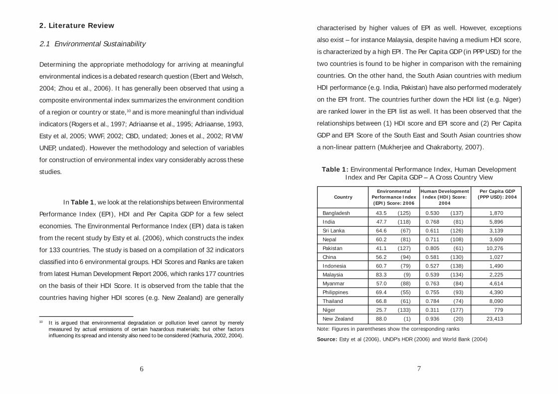
In Table 1, we look at the relationships between Environmental
Performance Index (EPI), HDI and Per Capita GDP for a few select
economies. The Environmental Performance Index (EPI) data is taken
from the recent study by Esty et al. (2006), which constructs the index
for 133 countries. The study is based on a compilation of 32 indicators
classified into 6 environmental groups. HDI Scores and Ranks are taken
from latest Human Development Report 2006, which ranks 177 countries
on the basis of their HDI Score. It is observed from the table that the
countries having higher HDI scores (e.g. New Zealand) are generally
characterised by higher values of EPI as well. However, exceptions
also exist – for instance Malaysia, despite having a medium HDI score,
is characterized by a high EPI. The Per Capita GDP (in PPP USD) for the
two countries is found to be higher in comparison with the remaining
countries. On the other hand, the South Asian countries with medium
HDI performance (e.g. India, Pakistan) have also performed moderately
on the EPI front. The countries further down the HDI list (e.g. Niger)
are ranked lower in the EPI list as well. It has been observed that the
relationships between (1) HDI score and EPI score and (2) Per Capita
GDP and EPI Score of the South East and South Asian countries show
a non-linear pattern (Mukherjee and Chakraborty, 2007).
Table 1: Environmental Performance Index, Human DevelopmentIndex and Per Capita GDP – A Cross Country View
Environmental Human Development Per Capita GDPCountry Performance Index Index (HDI) Score: (PPP USD): 2004
(EPI) Score: 2006 2004
Bangladesh 43.5 (125) 0.530 (137) 1,870
India 47.7 (118) 0.768 (81) 5,896
Sri Lanka 64.6 (67) 0.611 (126) 3,139
Nepal 60.2 (81) 0.711 (108) 3,609
Pakistan 41.1 (127) 0.805 (61) 10,276
China 56.2 (94) 0.581 (130) 1,027
Indonesia 60.7 (79) 0.527 (138) 1,490
Malaysia 83.3 (9) 0.539 (134) 2,225
Myanmar 57.0 (88) 0.763 (84) 4,614
Philippines 69.4 (55) 0.755 (93) 4,390
Thailand 66.8 (61) 0.784 (74) 8,090
Niger 25.7 (133) 0.311 (177) 779
New Zealand 88.0 (1) 0.936 (20) 23,413
Note: Figures in parentheses show the corresponding ranks
Source: Esty et al (2006), UNDP’s HDR (2006) and World Bank (2004)
10 It is argued that environmental degradation or pollution level cannot by merelymeasured by actual emissions of certain hazardous materials; but other factorsinfluencing its spread and intensity also need to be considered (Kathuria, 2002, 2004).
8 9
2.2 Relationships between Environmental Quality and EconomicGrowth
The literature on the relationship between Per Capita Income
(PCI) or the PCNSDP in case of States within a country, and pollution or
environmental degradation generally attempts to verify the existence
of an inverted U-shaped curve in the PCI vs. pollution plane
(‘Environmental Kuznets Curve’). The relationship implies that with the
rise in PCI, environmental degradation continues up to a certain level
of PCI, but improves afterwards as with prosperity, countries shift to
cleaner production technologies or spend more resources on pollution
abatement (Esty and Porter, 2001-02; Andreoni and Levinson, 2001).
Recent empirical studies show that while some local pollutants like
Sulphur dioxide (SO2), Suspended Particulate Matter (SPM), Carbon
monoxide (CO) etc. support EKC hypothesis; other pollutants exhibit
either monotonicity or N-shaped curve (Dinda, 2004; Stern, 1998).
Studies based on both ambient concentration of pollutants (Baldwin,
1995; Grossman and Krueger, 1995; Selden and Song, 1994; Panayatou,
1993; Shafik and Bandyopadhyay, 1992; Pezzey, 1989) or the actual
emissions of pollutants (Bruvoll and Medin, 2003; de Bruyn et al., 1998;
Carson et al., 1997) also support the EKC hypothesis.
It is argued that working with a composite indicator of
pollutants, as a proxy of actual EQ scenario, scores over selection of a
single pollutant in determination of the EKC relationship (Mukherjee
and Kathuria, 2006), although only a handful of studies have adopted
that approach so far. Jha and Bhanu Murthy (2001) created an
Environmental Degradation Index (EDI) for 174 countries and compared
that with the Human Development Index (HDI) instead of the PCI. The
study found an inverse link between EDI and HDI, which supported the
existence of an inverted N-shaped global EKC rather than an inverted
U-shaped one.
In Indian context, Mukherjee and Kathuria (2006) explored
the EKC relationship for 14 major Indian States over 1990-2001 by
considering 63 environmental variables, arranged under eight broad
environmental groups. The ranking of the States on a constructed
Environmental Quality Index (EQI) were determined by using the factor
analysis method. The results indicate that the relationship between EQ
and PCNSDP is slanting S-shaped, indicating that the economic growth
has occurred in Indian States mostly at the cost of EQ. It was observed
that except Bihar, all the States are on the upward sloping portion of
the EKC. Kadekodi and Venkatachalam (2005) noted evidence of a
strong linkage between various natural resources and environment with
income and the status of livelihood and concluded that the causal
relationship between poverty and environment works in both directions.11
The research has also highlighted the importance of poverty alleviation
while minimising the human health and environmental costs of economic
growth (Nadkarni, 2000) and the possibility of entering into a long-run
vicious circle of environmental degradation, greater inequality and lower
growth (Dutt and Rao, 1996) in that process.
11 However the study noted a mixed effect of improvement in human development onvarious individual pollution indicators in different states.
10 11
2.3 Relationship between Environment and Human Well-being
It is observed from the literature on environmental impacts of
structural adjustment programme that if the victims of depletion and
degradation of natural environment are not identified and compensated
by the beneficiaries, the vulnerable sections face additional economic
hardship, which may fuel inequality further (Dasgupta, 2001). It has
been argued by Boyce (2003) that, “social and economic inequalities
can influence both the distribution of the costs and benefits from
environmental degradation and the extent of environmental protection.
When those benefit from environmentally degrading economic activities
are powerful relative to those who bear the costs, environmental
protection is generally weaker than when the reverse is true.” The
analysis suggests that socio-economic inequality leads to environmental
inequality, which may consequently affect the overall extent of
environmental quality. Therefore any attempt to reduce inequalities
would eventually result in environmental protection.
It is increasingly believed that environmental problems should
no longer be viewed as the side effects of development process. On
the contrary, a new approach focusing on promotion of their integration
need to be adopted (Ginkel et al., 2001). The objective has been met
through Target 9 of the United Nations’ Millennium Development Goals
(MDGs),12 which demands that environmental conservation and
conservation of natural resources from quantitative depletion and
qualitative degradation, should be an integral part of any economic
and development policy.
Melnick et al. (2005) highlight the critical importance of
achieving environmental sustainability to meet the MDGs with respect
to poverty, illiteracy, hunger, gender inequality, unsafe drinking water
and environmental degradation. They argue that achieving
environmental sustainability requires carefully balancing human
development activities while maintaining a stable environment that
predictably and regularly provides resources and protects people from
natural calamities.
2.4 Relationship between Economic Growth and HumanDevelopment
The literature suggests a two-way relationship between EG
and HD, implying that nations may enter either into a virtuous cycle of
high growth and large HD gains, or a vicious cycle of low growth and
low HD improvement (Ranis, 2004). It is also observed that higher
initial level of HD corresponds to positive effects on institutional quality
and indirectly on EG (Costantini and Salvatore, 2006). The study by
Agarwal and Samanta (2006) involving 31 developing countries,
observed that EG is not correlated with social progress, structural
adjustment or governance. Nevertheless, all of them might have an
impact on the EQ within a country like India, where a two-way causality
between EG and HD is observed, indicating possibilities of vicious cycles
(Ghosh, 2006), which might have environmental repercussions.
12 “Integrate the principles of sustainable development into country policies andprogrammes and reverse the losses of environmental resources” - Target 9 of theUN’s MDGs.
12 13
The UNDP annually publishes an extensive analysis of global
HD situation in the Human Development Report (HDR) along with
country rankings. However, it is often argued that the UNDP HD
indicators are perhaps too narrow in nature, and inclusion of certain
important socio-economic variables would enrich the analysis further.
The Latent Variable Approach adopted by Nagar and Basu (2001)
involving 174 countries confirms that with inclusion of additional socio-
economic variables, the alternate HD rankings differ significantly from
the official UNDP ranking.
While India’s HD ranking remained in the low HD category
throughout nineties, in 2002 it graduated to medium HD category with
the HDI score of 0.577, as compared to the corresponding figure of
0.439 in 1990. India’s global HDI rank has improved from 132 in 1999
to 127 in 2003.13 Recently in association with UNDP, the Government of
India has started analysing the State-wise HD status. The National
Human Development Report 2001, brought out by the Planning
Commission (Government of India, 2002), is worth mentioning in this
regard. While the report ranked Kerala, Punjab and Tamil Nadu as the
toppers; Bihar, Madhya Pradesh and Uttar Pradesh were at the other
extreme in HD scale. The alternate index developed by Guha and
Chakraborty (2003), in line with Nagar and Basu (2001), however
showed that inclusion of other socio-economic variables changes the
State rankings to some extent. For instance, Tamil Nadu, ranked third
by NHDR, slides down the ladder to the eighth place according to the
alternate index.
3. Methodology and Data
3.1 Environmental Quality Index (EQI)
The EQI for the States is postulated to be linearly dependent
on a set of observable indicators and has been determined by adopting
the HDI method, by putting the selected variables under eight broad
categories mentioned in Table 2. The idea is that all the 63
environmental variables, when combined, give a composite EQI ranking
of the States, unobservable otherwise. We assume Xij to be the value
of the ith indicator for jth State of India with respect to X (or environmental
quality), where X consists of a large number of indicators varying from
6 to 12 (see Appendix 3). As defined earlier, X’s are AIRPOL, INDOOR,
GHGS, ENERGY, FOREST, WATER, NPSP and LAND respectively.
In line with the HDI method, we transform the indicators into
their standardised form, by which the adjusted values of Xij (i.e., EXij’s)
to be used for the analysis become:
or
where, Xi* and Xi** are the minimum and maximum values for
the ith indicator of environmental quality X respectively.14 Now, EQIXj,
i.e., the environmental quality index score for the jth State with respect
to each individual environmental quality X (which constitutes of n number
of indicators, n varies from 6 to 12), is arrived at by summing the EXijs
over i by using the following formula:
∑=
=n
iijj EX
nEQIX
1
1
13 In relative sense, India’s position actually does not look that bad as UNDP considered130 and 177 countries in 1990 and 2003 respectively.
)()( *****iiijiij XXXXEX −−=)()( ****
iiiijij XXXXEX −−=
1 The variables for which these two alternate formulas are used are specified at theend of Appendix 3.
14 15
In a similar manner, EQIj, i.e., the overall environmental quality
index score for the jth State, is arrived at by summing the EXijs for all X
over i by using the following formula:
XEXN
EQIN
iijj ∀= ∑
=
=
63
1
1
The obtained EQIs measure the environmental well-being of
the States, i.e., the States with higher score are characterised by cleaner
environment. The EQIjs (where j=1 to 14), thus arrived, is therefore
used to obtain the REQIjs (the rank of the jth State), where the States
having higher EQIj are assigned higher rank.
3.2 Human Development Index (HDI)
Following the principle of the NHDR 2001 methodology
(Government of India, 2002), for calculation of the Human Development
Index (HDI), we consider three variables, namely - inflation and
inequality adjusted per capita consumption expenditure (X1); and
composite indicator of educational attainment (X2) and composite
indicator on health attainment (X3). With this formulation, following
the HDI method, the HDI score for the jth State is given by:
∑=
=3
131
iij XHDI
where, Xi represents the normalized values of the three
indicators selected for construction of the HDI score, obtained by using
the following formula:
)()( ****iiiiji XXXXX −−=
where Xij refers to attainment of the ith indicator by the jth State
and Xi** and Xi* are the scaling maximum and minimum values of the
indicators respectively (i = 1 to 3).
Although UNDP considers Real GDP Per Capita in PPP USD for
generating the HDI, the NHDR 2001 (2002) has preferred total inflation
and inequality adjusted per capita consumption expenditure of a State
(i.e., Rural and Urban Combined) over that for the analysis. Here the
monthly per capita consumption expenditure data obtained from NSSO
for two periods (1993-94 and 1999-2000), adjusted for inequality using
estimated Gini Ratios, and further adjusted for inflation to bring themto 1983 prices by using deflators derived from State specific poverty
line (Raju, undated). We follow the NHDR methodology in our analysis
and consider total inflation and inequality adjusted per capita
consumption expenditure of a State as an explanatory variable.
The composite indicator on educational attainment (X2) isarrived at by considering two variables, namely literacy rate for the
age group of 7 years and above (e1) and adjusted intensity of formal
education (e2). The idea is that literacy rate being an overall ratio alone
may not indicate the actual scenario, and the drop-out rate, needs to
be incorporated in the formula. We consider the data on literacy ratefor two periods, namely - 1991 and 2001. The adjusted Intensity of
Formal Education data is used for two periods – 1993 and 2002. The
following weightage is assigned for the two variables so as to determine
the composite indicator:
[ ])65.0()35.0( 212 ×+×= eeX
16 17
The adjusted Intensity of Formal Education is estimated as
weighted average of the enrolled students from class I to class XII
(where weights being 1 for Class I, 2 for Class II and so on) to the total
enrolment in Class I to Class XII. This is adjusted by proportion of total
enrolment to population in the age group 6-18 (Raju, undated).
According to the formula suppose Ei be the number of children (rural
and urban combined) enrolled in ith standard in 2002, i= 1 for Class I to
12 for Class XII. Then WAE becomes the Weighted Average of the
Enrolment from Class I to Class XII:
∑
∑
=
=
×= 12
1
12
1
i
ii
i
EiWAE
Now, let TE be the total enrolment of Children from Class I to
Class XII in 2002. Then by definition, we have:
∑=
=12
1iiETE
Hence, the Intensity of Formal Education (IFE) for children
(rural and urban combined) in 2002 becomes:
100×=TE
WAEIFE
From the IFE, we can determine the Adjusted Intensity of
Formal Education (AIFE) for children (rural and urban combined) in
2002 by using the following formula:
CPTEIFEAIFE ×=
Where PC represents the Population of Children (rural and urban
combined) in the age group 6 to 18 years in 2001.
The Composite indicator on health attainment (X3) is arrived at
by considering two variables, namely Life Expectancy (LE) at age one
(h1) and the reciprocal of Infant Mortality Rate (IMR) as the second
variable (h2). For h1, which measures the life expectancy at age 1 (Rural
and Urban Combined), the two data points considered for the two periods
are 1990-94 and 1998-2002 respectively. On the other hand, the IMR
(Per Thousand) data is considered for two periods, namely - 1992 and
2000. The following weightage is assigned for the two variables so as to
determine the composite indicator used for calculation of the HDI:
[ ])35.0()65.0( 213 ×+×= hhX
3.3 Economic Growth (EG)
Economic growth in the current analysis is measured by the
PCNSDP of the States at constant (1993-94) prices. PCNSDP for the
Period A is the average PCNSDP for the period 1993-94 to 1995-96 and
for Period B, it is the average PCNSDP over 1997-98 to 1999-2000. The
average is taken to smoothen out uneven fluctuations. To understand
the size of the economy and growth pattern of each of the 14 States,
we have classified the States into three categories with respect to their
Gross State Domestic Product (GSDP) at constant 1993-94 prices, e.g.,
high income States (having GSDP: greater than 3rd Quartile), medium
income States (GSDP: 1st to 3rd Quartile) and low income States (GSDP:
less than 1st Quartile), for early 1990s (1993-96), late 1990s (1997-
2000) and early years of new millennium (2001-2005).
18 19
Mukherjee and Chakraborty (2007) noted that during early 1990s
(1993-96), on an average middle income states (e.g. - Gujarat, Rajasthan,
Karnataka and West Bengal) were growing faster than others. However,
during late 1990s (1997-2000), except for low income States (e.g. –
Kerala, Haryana, Bihar and Orissa), growth rate slowed down, indicating
a stagnation. On the other hand, during early 2000s (2000-2004), the
difference in economic growth rate across the States having different
level of income has gone down and barring few exceptions (Rajasthan
and West Bengal) both for low and medium income States the growth
rate generally slowed down as compared to the late 1990s level.
3.4 Data
In order to obtain State level secondary information on
environment and natural resources from published government reports
and other databases for both the time periods selected in our analysis,
i.e., Period A (1990-96) and Period B (1997-2004), the sample is restricted
only to 14 major Indian States, namely - Andhra Pradesh (AP), Bihar
(BH), Gujarat (GJ), Haryana (HR), Karnataka (KR), Kerala (KL), Madhya
Pradesh (MP), Maharashtra (MH), Orissa (OR), Punjab (PB), Rajasthan
(RJ), Tamil Nadu (TN), Uttar Pradesh (UP) and West Bengal (WB). Now
the data available for various environmental indicators in India are not
always necessarily compatible with the time period selected by us, given
the varying date and frequency of their publication. To resolve this issue,
we have chosen only those indicators with at least two observations,
where one of these observations is located within the boundary of the
two sample periods. The selected indicators have then been normalized
using appropriate measures of size / scale of the States – geographical
area, population and GSDP at current prices.
Here we need to distinguish between two key concepts, namely
- endowment effect and efficiency in natural resource management
effect. The depletion and degradation of natural resources and
occurrence of environmental pollution is chiefly concerned with
environmental management. On the other hand, the initial endowments
of natural resources (forests, land and water) are determined by
geographical, climatic and ecological factors. Quite understandably,
the former is comparatively more influenced by human activities. By
calculating the change in the natural resource position with respect to
a base year we can isolate the two effects.15 The current study focuses
on the environmental management efficiency effect as well as the size
effect of the States.
The data sources for our analysis on EQ and descriptions of
the actual data series used to construct each group are listed in
Appendix 2 and 3 respectively. A total of 63 variables have been
selected for the analysis, placed under eight broad categories, which
are summarized in Table 2.
15 For instance, a higher index for Orissa as compared to Punjab by merely rankingthe forest resources of the two States (by taking the percentage of geographicalarea under forests land) comes from the fact that Punjab possess very little of theselected variable to begin with. Therefore the analysis does not imply that forestconservation practices of the former are in any way better than the same of thelatter. Ranking the change in their forest area (as a percentage of geographicalarea) during any two periods would be the ideal exercise for comparing their forestconservation practices.
20 21
Table 2: Description of the Environmental Groups
Groups Description Number ofvariables
AIRPOL Air Pollution 6
INDOOR Indoor Air Pollution Potential 9
GHGS Green House Gases (GHGs) Emissions 6
ENERGY Pollution from Energy Generation and Consumption 6
FOREST Depletion and Degradation of Forest Resources 8
WATER Depletion and Degradation of Water Resources 12
NPSP Nonpoint Source Water Pollution Potential 10
LAND Pressure and Degradation of Land Resources 6
Total 63
For the analysis on education, we use the data available from
the “7th All India Educational Survey (AIES): All India School Education
Survey (AISES)”, published by NCERT (2002). On the health front, IMR
data is taken from Sample Registration System (SRS) Bulletins; Registrar
General of India, New Delhi and LE data is taken from Indiastat database
website (www.indiastat.com). The data on EG of the States is obtained
from EPW Research Foundation Database Software and RBI’s Database
on Indian Economy.
4. The Results
4.1 EQI
In Table 3, we present the EQ scores and rankings of the
States for Period A, both for individual categories as well as for the
composite index. It is observed that Kerala, Karnataka and Maharashtra
were the toppers during this period, while Uttar Pradesh, Punjab and
Haryana had been the laggards. Interestingly the topper Kerala, despite
a good performance in AIRPOL, GHGS, ENERGY, WATER and NPSP,
fared among the laggards in case of INDOOR, LAND and FOREST.
Karnataka had good performance in case of AIRPOL and GHGS, while
maintaining moderate performance in other categories. The third ranking
of Maharashtra, an industrialized state, is justified by the fact that the
State performed appreciably in several categories like INDOOR, GHGS,
LAND and NPSP, however the performance with respect to ENERGY,
WATER, FOREST and AIRPOL was not that satisfactory. Looking at the
other extreme, we can see that the overall rankings of laggards like
Haryana and Uttar Pradesh were influenced by their performance in
sub-categories like LAND, NPSP etc. It is observed that while some
major States like Madhya Pradesh (tenth) and West Bengal (ninth)
placed in the lower segment, others like Gujarat (sixth) and Andhra
Pradesh (seventh) had performed moderately well. Interestingly, a
relatively poorer State, Orissa, obtained the fourth rank, owing to
comparatively better performance in case of AIRPOL, ENERGY and
WATER.
22 23
Table 4 provides the EQ scores and ranking of the States for
Period B. As in the earlier case, we see that Kerala, Karnataka and
Maharashtra retained their positions at the top (although the latter
two interchange their positions), while Haryana, Bihar and Punjab now
turned out to be the laggards. It is observed that the toppers improved
their position in certain sub-categories (Kerala in AIRPOL, INDOOR,
GHGS, FOREST; Karnataka in ENERGY, FOREST etc.). However, their
performance deteriorated in certain key areas as well. For instance,
the lower ranking of Karnataka in AIRPOL in Period B can be explained
by rapid urbanization, industrialization and vehicular pollution.16 Its
relative performance on WATER also raises concern. On the other hand
the laggards continued to perform poorly in several sub-categories
(e.g. - Punjab – AIRPOL, GHGS, ENERGY, LAND, WATER and NPSP;
Bihar - AIRPOL, INDOOR, GHGS, LAND, FOREST and NPSP; Haryana –
ENERGY, LAND, WATER and NPSP). Energy management and forest
conservation should be the first two priority areas for environmental
management in Maharashtra. For Karnataka, conservation of land and
water should be priority areas for environmental management.
Stat
esAI
RPO
LIN
DO
OR
GH
GS
ENER
GY
LAN
DW
ATER
FOR
EST
NPS
PEQ
I SC
OR
E
(1)
(2)
(3)
(4)
(5)
(6)
(7)
(8)
(9)
Andh
ra P
rade
sh0.
876
(4)
0.32
0(1
1)0.
685
(5)
0.52
4(8
)0.
592
(5)
0.53
5(6
)0.
506
(13)
0.48
9(8
)0.
544
(7)
Biha
r0.
647
(8)
0.12
9(1
4)
0.46
7(1
1)0.
555
(7)
0.50
2(1
0)0.
604
(5)
0.51
5(1
2)0.
467
(11)
0.48
0(1
1)
Guj
arat
0.43
2(1
2)0.
643
(3)
0.61
7(7
)0.
282
(13)
0.61
6(4
)0.
482
(9)
0.59
4(6
)0.
630
(2)
0.54
5(6
)
Har
yana
0.78
3(6
)0.
574
(4)
0.49
4(9
)0.
450
(12)
0.18
3(1
3)0.
381
(13)
0.67
1(2
)0.
333
(13)
0.47
5(1
2)
Karn
atak
a0.
912
(1)
0.43
5(5
)0.
901
(1)
0.67
3(5
)0.
535
(7)
0.51
6(7
)0.
573
(9)
0.54
1(6
)0.
607
(2)
Kera
la0.
874
(5)
0.32
7(1
0)0.
870
(3)
0.70
9(3
)0.
520
(8)
0.69
6(3
)0.
517
(11)
0.55
9(5
)0.
617
(1)
Mad
hya
Prad
esh
0.48
3(1
1)0.
367
(8)
0.35
5(1
3)0.
468
(10)
0.71
9(1
)0.
695
(4)
0.15
8(1
4)
0.59
7(4
)0.
493
(10)
Mah
aras
htra
0.65
3(7
)0.
715
(2)
0.69
7(4
)0.
473
(9)
0.65
2(2
)0.
514
(8)
0.58
1(8
)0.
599
(3)
0.60
5(3
)
Oris
sa0.
909
(2)
0.22
8(1
2)0.
350
(14
)0.
771
(1)
0.54
3(6
)0.
760
(1)
0.58
4(7
)0.
516
(7)
0.57
8(4
)
Punj
ab0.
644
(9)
0.80
3(1
)0.
427
(12)
0.27
4(1
4)
0.18
1(1
4)
0.24
4(1
4)
0.84
0(1
)0.
267
(14
)0.
456
(13)
Raja
stha
n0.
631
(10)
0.39
7(7
)0.
881
(2)
0.62
2(6
)0.
637
(3)
0.46
5(1
0)0.
520
(10)
0.64
2(1
)0.
577
(5)
Tam
il N
adu
0.89
6(3
)0.
412
(6)
0.65
6(6
)0.
458
(11)
0.51
3(9
)0.
381
(12)
0.61
2(4
)0.
478
(10)
0.52
5(8
)
Utt
ar P
rade
sh0.
152
(14
)0.
222
(13)
0.60
0(8
)0.
682
(4)
0.36
3(1
2)0.
447
(11)
0.62
0(3
)0.
478
(9)
0.44
3(1
4)
Wes
t Be
ngal
0.24
8(1
3)0.
357
(9)
0.47
3(1
0)0.
758
(2)
0.36
9(1
1)0.
699
(2)
0.61
1(5
)0.
442
(12)
0.50
8(9
)
Tab
le 3
: En
viro
nmen
tal Q
ualit
y Sc
ores
and
Ran
ks o
f th
e St
ates
: 19
90-1
996
Stat
esAI
RPO
LIN
DO
OR
GH
GS
ENER
GY
LAN
DW
ATER
FOR
EST
NPS
PEQ
I SC
OR
E
(1)
(2)
(3)
(4)
(5)
(6)
(7)
(8)
(9)
Andh
ra P
rade
sh0.
876
(4)
0.32
0(1
1)0.
685
(5)
0.52
4(8
)0.
592
(5)
0.53
5(6
)0.
506
(13)
0.48
9(8
)0.
544
(7)
Biha
r0.
647
(8)
0.12
9(1
4)
0.46
7(1
1)0.
555
(7)
0.50
2(1
0)0.
604
(5)
0.51
5(1
2)0.
467
(11)
0.48
0(1
1)
Guj
arat
0.43
2(1
2)0.
643
(3)
0.61
7(7
)0.
282
(13)
0.61
6(4
)0.
482
(9)
0.59
4(6
)0.
630
(2)
0.54
5(6
)
Har
yana
0.78
3(6
)0.
574
(4)
0.49
4(9
)0.
450
(12)
0.18
3(1
3)0.
381
(13)
0.67
1(2
)0.
333
(13)
0.47
5(1
2)
Karn
atak
a0.
912
(1)
0.43
5(5
)0.
901
(1)
0.67
3(5
)0.
535
(7)
0.51
6(7
)0.
573
(9)
0.54
1(6
)0.
607
(2)
Kera
la0.
874
(5)
0.32
7(1
0)0.
870
(3)
0.70
9(3
)0.
520
(8)
0.69
6(3
)0.
517
(11)
0.55
9(5
)0.
617
(1)
Mad
hya
Prad
esh
0.48
3(1
1)0.
367
(8)
0.35
5(1
3)0.
468
(10)
0.71
9(1
)0.
695
(4)
0.15
8(1
4)
0.59
7(4
)0.
493
(10)
Mah
aras
htra
0.65
3(7
)0.
715
(2)
0.69
7(4
)0.
473
(9)
0.65
2(2
)0.
514
(8)
0.58
1(8
)0.
599
(3)
0.60
5(3
)
Oris
sa0.
909
(2)
0.22
8(1
2)0.
350
(14
)0.
771
(1)
0.54
3(6
)0.
760
(1)
0.58
4(7
)0.
516
(7)
0.57
8(4
)
Punj
ab0.
644
(9)
0.80
3(1
)0.
427
(12)
0.27
4(1
4)
0.18
1(1
4)
0.24
4(1
4)
0.84
0(1
)0.
267
(14
)0.
456
(13)
Raja
stha
n0.
631
(10)
0.39
7(7
)0.
881
(2)
0.62
2(6
)0.
637
(3)
0.46
5(1
0)0.
520
(10)
0.64
2(1
)0.
577
(5)
Tam
il N
adu
0.89
6(3
)0.
412
(6)
0.65
6(6
)0.
458
(11)
0.51
3(9
)0.
381
(12)
0.61
2(4
)0.
478
(10)
0.52
5(8
)
Utt
ar P
rade
sh0.
152
(14
)0.
222
(13)
0.60
0(8
)0.
682
(4)
0.36
3(1
2)0.
447
(11)
0.62
0(3
)0.
478
(9)
0.44
3(1
4)
Wes
t Be
ngal
0.24
8(1
3)0.
357
(9)
0.47
3(1
0)0.
758
(2)
0.36
9(1
1)0.
699
(2)
0.61
1(5
)0.
442
(12)
0.50
8(9
)
16 In several major Karnataka cities suspended particulate matter (SPM) and respirablesuspended particulate matter (RSPM) are far above the permissible limits (TheHindu, 2005, 2006).N
ote:
fig
ures
in t
he p
aren
thes
is s
how
the
ran
ks
24 25
We can compare the relative performance of the States on EQ
scale during the two time periods looking at their ranks. It is observed
that although the overall position of the better performing States
remained unchanged, there had been some interesting movements of
their ranking within the sub-categories. For instance, Maharashtra’s
rank declined in LAND and FOREST,17 while it improved its performance
in WATER. Karnataka had been subjected to greater variations - while
its ranking improved in ENERGY and FOREST, but declined for AIRPOL,
INDOOR and WATER. Kerala on the other hand improved its relative
performance in a number of sub-categories (notably FOREST).18
Nonetheless, its score got affected by the decline in its ranking in
categories like WATER.19 Looking across categories, it is observed that
Punjab and Uttar Pradesh experienced a sharp decline in their ranking
in case of FOREST, indicating degradation on that front.
Stat
esAI
RPO
LIN
DO
OR
GH
GS
ENER
GY
LAN
DW
ATER
FOR
EST
NPS
PEQ
I SC
OR
E
(1)
(2)
(3)
(4)
(5)
(6)
(7)
(8)
(9)
Andh
ra P
rade
sh0.
802
(3)
0.49
8(7
)0.
553
(5)
0.58
5(5
)0.
617
(3)
0.47
9(9
)0.
781
(9)
0.47
4(9
)0.
580
(6)
Biha
r0.
433
(12)
0.14
1(1
4)
0.42
8(1
0)0.
574
(7)
0.43
6(1
0)0.
675
(2)
0.48
0(1
3)0.
422
(12)
0.45
5(1
3)
Guj
arat
0.31
0(1
3)0.
718
(3)
0.54
7(6
)0.
231
(13)
0.65
3(1
)0.
539
(8)
0.76
9(1
0)0.
599
(4)
0.56
4(7
)
Har
yana
0.71
5(5
)0.
714
(4)
0.54
2(7
)0.
362
(10)
0.08
8(1
4)
0.33
2(1
3)0.
790
(7)
0.27
8(1
4)
0.47
2(1
2)
Karn
atak
a0.
684
(6)
0.61
0(6
)0.
885
(1)
0.67
9(3
)0.
568
(7)
0.46
5(1
1)0.
807
(5)
0.56
3(6
)0.
636
(3)
Kera
la0.
791
(4)
0.46
7(8
)0.
882
(2)
0.64
4(4
)0.
534
(9)
0.54
1(7
)0.
942
(1)
0.59
8(5
)0.
656
(1)
Mad
hya
Prad
esh
0.51
0(1
0)0.
453
(10)
0.30
2(1
4)
0.34
9(1
2)0.
647
(2)
0.68
9(1
)0.
230
(14
)0.
627
(1)
0.49
7(1
0)
Mah
aras
htra
0.67
6(7
)0.
771
(2)
0.68
2(4
)0.
428
(9)
0.57
8(6
)0.
606
(5)
0.73
1(1
1)0.
615
(2)
0.64
1(2
)
Oris
sa0.
823
(2)
0.18
9(1
3)0.
381
(11)
0.74
5(2
)0.
612
(4)
0.67
3(3
)0.
864
(2)
0.52
7(7
)0.
593
(5)
Punj
ab0.
600
(9)
0.81
2(1
)0.
349
(13)
0.21
1(1
4)
0.11
8(1
3)0.
273
(14
)0.
789
(8)
0.27
9(1
3)0.
434
(14
)
Raja
stha
n0.
670
(8)
0.45
9(9
)0.
807
(3)
0.56
4(8
)0.
603
(5)
0.47
0(1
0)0.
804
(6)
0.61
4(3
)0.
606
(4)
Tam
il N
adu
0.94
9(1
)0.
624
(5)
0.37
6(1
2)0.
361
(11)
0.56
7(8
)0.
356
(12)
0.84
2(3
)0.
483
(8)
0.55
5(8
)
Utt
ar P
rade
sh0.
471
(11)
0.30
5(1
2)0.
518
(8)
0.58
4(6
)0.
366
(11)
0.56
6(6
)0.
507
(12)
0.45
8(1
0)0.
473
(11)
Wes
t Be
ngal
0.21
2(1
4)
0.41
7(1
1)0.
476
(9)
0.79
4(1
)0.
347
(12)
0.61
0(4
)0.
825
(4)
0.42
2(1
1)0.
522
(9)
Tabl
e 4
: En
viro
nmen
tal Q
ualit
y Sc
ores
and
Ran
ks o
f th
e St
ates
: 19
97-2
004
17 Rithe and Fernandes (2002) argued that Maharashtra has achieved the currentlevel of industrialization at the cost of the loss of much of its forests. However, thefindings of Kadekodi and Venkatachalam (2005) do not support this.
18 Apart from the Government regulations, exporter firms increasingly adoptedenvironment-friendly processes to comply with strict norms in export markets(e.g. - marine industries in Kochi), which had a significant positive influence on theenvironment of the State.
19 Nair (2006) noted that depletion of the groundwater table due to indiscriminatesand mining, shrinkage in natural forest cover and reclamation of wetland andpaddy fields are major environmental challenges that Kerala is facing today.N
ote:
fig
ures
in t
he p
aren
thes
is s
how
the
ran
ks
26 27
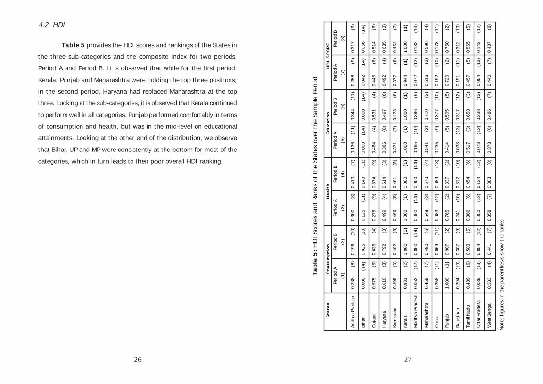
4.2 HDI
Table 5 provides the HDI scores and rankings of the States in
the three sub-categories and the composite index for two periods,
Period A and Period B. It is observed that while for the first period,
Kerala, Punjab and Maharashtra were holding the top three positions;
in the second period, Haryana had replaced Maharashtra at the top
three. Looking at the sub-categories, it is observed that Kerala continued
to perform well in all categories. Punjab performed comfortably in terms
of consumption and health, but was in the mid-level on educational
attainments. Looking at the other end of the distribution, we observe
that Bihar, UP and MP were consistently at the bottom for most of the
categories, which in turn leads to their poor overall HDI ranking.
Sta
tes
Con
sum
pti
onH
ealt
hEd
uca
tion
HD
I S
CO
RE
Perio
d A
Perio
d B
Perio
d A
Perio
d B
Perio
d A
Perio
d B
Perio
d A
Perio
d B
(1)
(2)
(3)
(4)
(5)
(6)
(7)
(8)
Andh
ra P
rade
sh0.
338
(8)
0.19
6(1
0)0.
300
(8)
0.41
0(7
)0.
136
(11)
0.34
4(1
1)0.
258
(9)
0.31
7(9
)
Biha
r0.
000
(14
)0.
025
(13)
0.12
5(1
1)0.
143
(11)
0.00
0(1
4)
0.00
0(1
4)
0.04
2(1
4)
0.05
6(1
4)
Guj
arat
0.57
5(5
)0.
636
(4)
0.27
5(9
)0.
374
(9)
0.48
4(4
)0.
531
(4)
0.44
5(6
)0.
514
(6)
Har
yana
0.61
0(3
)0.
792
(3)
0.49
9(4
)0.
614
(3)
0.36
6(8
)0.
497
(6)
0.49
2(4
)0.
635
(3)
Karn
atak
a0.
295
(9)
0.40
2(8
)0.
466
(5)
0.48
1(5
)0.
371
(7)
0.47
8(8
)0.
377
(8)
0.45
4(7
)
Kera
la0.
831
(2)
1.00
0(1
)1.
000
(1)
1.00
0(1
)1.
000
(1)
1.00
0(1
)0.
944
(1)
1.00
0(1
)
Mad
hya
Prad
esh
0.05
2(1
2)0.
000
(14
)0.
000
(14
)0.
000
(14
)0.
165
(10)
0.39
6(9
)0.
072
(12)
0.13
2(1
3)
Mah
aras
htra
0.45
9(7
)0.
490
(6)
0.54
9(3
)0.
570
(4)
0.54
1(2
)0.
710
(2)
0.51
6(3
)0.
590
(4)
Oris
sa0.
258
(11)
0.06
9(1
1)0.
083
(12)
0.08
9(1
3)0.
235
(9)
0.37
7(1
0)0.
192
(10)
0.17
8(1
1)
Punj
ab1.
000
(1)
0.90
7(2
)0.
765
(2)
0.83
7(2
)0.
414
(5)
0.50
5(5
)0.
726
(2)
0.75
0(2
)
Raja
stha
n0.
294
(10)
0.30
7(9
)0.
241
(10)
0.31
2(1
0)0.
038
(13)
0.31
7(1
2)0.
191
(11)
0.31
2(1
0)
Tam
il N
adu
0.48
9(6
)0.
583
(5)
0.36
6(6
)0.
454
(6)
0.51
7(3
)0.
658
(3)
0.45
7(5
)0.
565
(5)
Utt
ar P
rade
sh0.
039
(13)
0.05
4(1
2)0.
050
(13)
0.13
4(1
2)0.
073
(12)
0.23
8(1
3)0.
054
(13)
0.14
2(1
2)
Wes
t Be
ngal
0.58
3(4
)0.
441
(7)
0.35
8(7
)0.
383
(8)
0.37
8(6
)0.
486
(7)
0.44
0(7
)0.
437
(8)
Tab
le 5
: H
DI
Scor
es a
nd R
anks
of
the
Stat
es o
ver
the
Sam
ple
Perio
d
Not
e: f
igur
es in
the
par
enth
esis
sho
w t
he r
anks
28 29
Comparison of the relative performance of the States on HDI
during the two time periods covered in our analysis shows interesting
results. We observe that there had not been major changes in the
overall HDI Score of the States, and in all cases their ranks changed by
one unit only. Some changes in the relative positions of the States in
terms of consumption can be noted, reflecting their relative growth
pattern, but in case of education and health the relative positions of
fifty percent of the States remained unchanged. We observe that the
aggregate picture do not always show the dynamics of different
components of HDI, e.g., for MP aggregate HDI Score had gone up
from 0.072 to 0.132, however its consumption score had gone down
from 0.052 to 0.000. A declining trend in the HDI is noticed for AP as
well. For MP, since health status remained unchanged it is only the
improvement in education, which had driven its HDI score up. Movement
in consumption expenditure is interesting; it had gone down both for
poor States like Orissa (insignificant poverty reduction over NSSO 50th
(1993-94) and 55th (1999-2000) round) and moderate performers like
West Bengal (9 percent poverty reduction over NSSO 50th and 55th
round). One reason may perhaps be that the decline in income inequality
(Gini ratio) in these two States over 1993-94 to 1999-00 (Government
of India, 2002) had been marginal.
4.3 Cross-Period Analysis between HDI and EQI
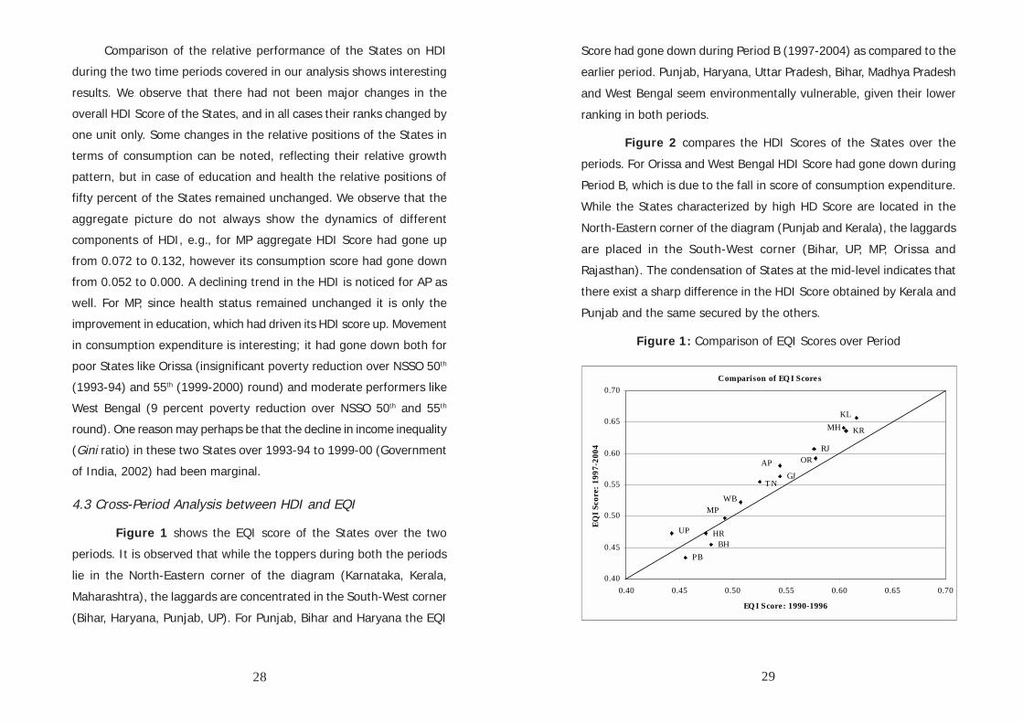
Figure 1 shows the EQI score of the States over the two
periods. It is observed that while the toppers during both the periods
lie in the North-Eastern corner of the diagram (Karnataka, Kerala,
Maharashtra), the laggards are concentrated in the South-West corner
(Bihar, Haryana, Punjab, UP). For Punjab, Bihar and Haryana the EQI
Score had gone down during Period B (1997-2004) as compared to the
earlier period. Punjab, Haryana, Uttar Pradesh, Bihar, Madhya Pradesh
and West Bengal seem environmentally vulnerable, given their lower
ranking in both periods.
Figure 2 compares the HDI Scores of the States over the
periods. For Orissa and West Bengal HDI Score had gone down during
Period B, which is due to the fall in score of consumption expenditure.
While the States characterized by high HD Score are located in the
North-Eastern corner of the diagram (Punjab and Kerala), the laggards
are placed in the South-West corner (Bihar, UP, MP, Orissa and
Rajasthan). The condensation of States at the mid-level indicates that
there exist a sharp difference in the HDI Score obtained by Kerala and
Punjab and the same secured by the others.
Figure 1: Comparison of EQI Scores over Period
Comparison of EQ I Scores
RJ
GJAP OR
KR
KLMH
T N
MPWB
BHHRUP
PB
0.40
0.45
0.50
0.55
0.60
0.65
0.70
0.40 0.45 0.50 0.55 0.60 0.65 0.70
EQ I Score: 1990-1996EQ
I Sco
re: 1
997-
2004
30 31
Figure 2: Comparison of HDI Scores over Period
4.4 EQI and HDI
Figure 3 plots the EQI and HDI Scores of the 14 States during
Period A. While the States located in the North-East corner of the Figure
characterized States with both high EQI and HDI scores, States placed
in South-West corner represents those with worst performance on both
counts. The States positioned in the North-West corner of the figure on
the other hand indicates the States performing appreciably in terms of
EQI, but not in terms of HDI. We can see that Kerala and Maharashtra
are clearly the top performers on both counts while Bihar and UP are
located at the other extreme. Orissa and Rajasthan on the other hand
had performed poorly in terms of HDI (placed below the first quartile),
despite putting up a commendable performance on EQ front. Looking
at the other major States it is observed that while AP had performed
moderately well in terms of EQI, its accomplishment in terms of HDI
was rather limited. Other major States like Gujarat and Tamil Nadu
were moderately placed on both counts. Karnataka on the other hand
despite being a top performer in terms of EQI fared moderately on the
HDI front (placed below the second quartile line). The HDI had been
quite high for northern States like Punjab and Haryana (characterized
by a vibrant agricultural and industrial sector), but they secured a lower
place on the EQI scale, primarily owing to overexploitation of natural
resources.20
Figure 3: HDI Score Vs. EQI Score (1990-1996)
Comparison of HDI Scores
MPUP
MHHRTNGJ
BH
APRJ
KR WB
OR
PB
KL
0.0
0.3
0.5
0.8
1.0
0.0 0.3 0.5 0.8 1.0
HDI Score: 1990-1996
HD
I Sco
re: 1
997-
2004
20 Sidhu (2002) notes that in Punjab more than nine lakh tube wells are being suppliedelectricity free of cost, leading to indiscriminate use. This in turn is causingunderground water to deplete at a rate of 23 centimeter per annum, which infuture would require submersible pumps to be installed, meaning that only richfarmers could afford to bear the expenditure. Apart from severe environmentalconsequences, this is expected to fuel rural inequality further. Bhullar and Sidhu(2006) have also reported disregard to environmental sustainability for short runincome and productivity gain in Punjab, which has resulted in overexploitation ofland and water resources.
HDI Score Vs. EQ I Score: Period A
UP
BHMP
ORRJ
AP
WBTN
KR MH
GJ
HR
KL
PB
0.40
0.45
0.50
0.55
0.60
0.65
0.00 0.10 0.20 0.30 0.40 0.50 0.60 0.70 0.80 0.90 1.00
HDI Score: Period A
EQI S
core
: Per
iod
A
32 33
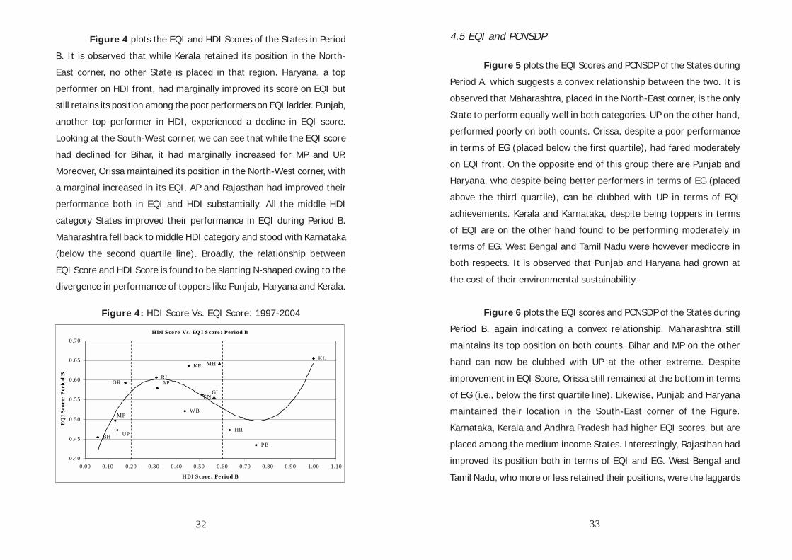
Figure 4 plots the EQI and HDI Scores of the States in Period
B. It is observed that while Kerala retained its position in the North-
East corner, no other State is placed in that region. Haryana, a top
performer on HDI front, had marginally improved its score on EQI but
still retains its position among the poor performers on EQI ladder. Punjab,
another top performer in HDI, experienced a decline in EQI score.
Looking at the South-West corner, we can see that while the EQI score
had declined for Bihar, it had marginally increased for MP and UP.
Moreover, Orissa maintained its position in the North-West corner, with
a marginal increased in its EQI. AP and Rajasthan had improved their
performance both in EQI and HDI substantially. All the middle HDI
category States improved their performance in EQI during Period B.
Maharashtra fell back to middle HDI category and stood with Karnataka
(below the second quartile line). Broadly, the relationship between
EQI Score and HDI Score is found to be slanting N-shaped owing to the
divergence in performance of toppers like Punjab, Haryana and Kerala.
Figure 4: HDI Score Vs. EQI Score: 1997-2004
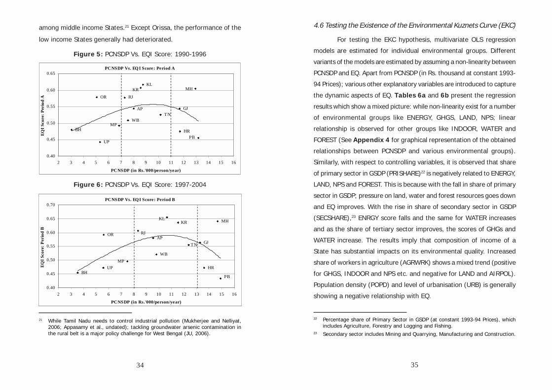
4.5 EQI and PCNSDP
Figure 5 plots the EQI Scores and PCNSDP of the States during
Period A, which suggests a convex relationship between the two. It is
observed that Maharashtra, placed in the North-East corner, is the only
State to perform equally well in both categories. UP on the other hand,
performed poorly on both counts. Orissa, despite a poor performance
in terms of EG (placed below the first quartile), had fared moderately
on EQI front. On the opposite end of this group there are Punjab and
Haryana, who despite being better performers in terms of EG (placed
above the third quartile), can be clubbed with UP in terms of EQI
achievements. Kerala and Karnataka, despite being toppers in terms
of EQI are on the other hand found to be performing moderately in
terms of EG. West Bengal and Tamil Nadu were however mediocre in
both respects. It is observed that Punjab and Haryana had grown at
the cost of their environmental sustainability.
Figure 6 plots the EQI scores and PCNSDP of the States during
Period B, again indicating a convex relationship. Maharashtra still
maintains its top position on both counts. Bihar and MP on the other
hand can now be clubbed with UP at the other extreme. Despite
improvement in EQI Score, Orissa still remained at the bottom in terms
of EG (i.e., below the first quartile line). Likewise, Punjab and Haryana
maintained their location in the South-East corner of the Figure.
Karnataka, Kerala and Andhra Pradesh had higher EQI scores, but are
placed among the medium income States. Interestingly, Rajasthan had
improved its position both in terms of EQI and EG. West Bengal and
Tamil Nadu, who more or less retained their positions, were the laggards
HDI Score Vs. EQ I Score : Pe riod B
PB
KL
HR
GJ
MHKR
T N
W B
APRJ
OR
MP
BH UP
0.40
0.45
0.50
0.55
0.60
0.65
0.70
0.00 0.10 0.20 0.30 0.40 0.50 0.60 0.70 0.80 0.90 1.00 1.10
HDI Score : Pe riod B
EQ
I Sc
ore:
Per
iod
B
34 35
among middle income States.21 Except Orissa, the performance of the
low income States generally had deteriorated.
Figure 5: PCNSDP Vs. EQI Score: 1990-1996
Figure 6: PCNSDP Vs. EQI Score: 1997-2004
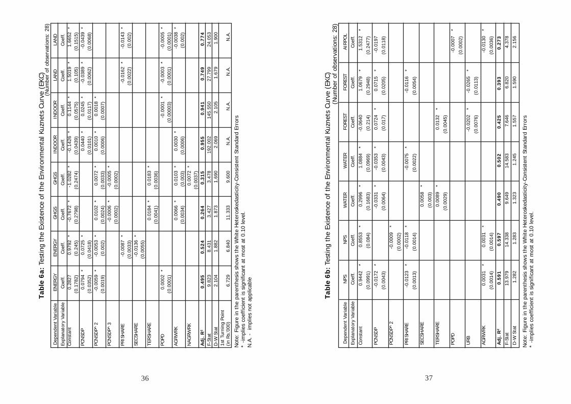
4.6 Testing the Existence of the Environmental Kuznets Curve (EKC)
For testing the EKC hypothesis, multivariate OLS regression
models are estimated for individual environmental groups. Different
variants of the models are estimated by assuming a non-linearity between
PCNSDP and EQ. Apart from PCNSDP (in Rs. thousand at constant 1993-
94 Prices); various other explanatory variables are introduced to capture
the dynamic aspects of EQ. Tables 6a and 6b present the regression
results which show a mixed picture: while non-linearity exist for a number
of environmental groups like ENERGY, GHGS, LAND, NPS; linear
relationship is observed for other groups like INDOOR, WATER and
FOREST (See Appendix 4 for graphical representation of the obtained
relationships between PCNSDP and various environmental groups).
Similarly, with respect to controlling variables, it is observed that share
of primary sector in GSDP (PRISHARE)22 is negatively related to ENERGY,
LAND, NPS and FOREST. This is because with the fall in share of primary
sector in GSDP; pressure on land, water and forest resources goes down
and EQ improves. With the rise in share of secondary sector in GSDP
(SECSHARE),23 ENRGY score falls and the same for WATER increases
and as the share of tertiary sector improves, the scores of GHGs and
WATER increase. The results imply that composition of income of a
State has substantial impacts on its environmental quality. Increased
share of workers in agriculture (AGRWRK) shows a mixed trend (positive
for GHGS, INDOOR and NPS etc. and negative for LAND and AIRPOL).
Population density (POPD) and level of urbanisation (URB) is generally
showing a negative relationship with EQ.
PCNSDP Vs. EQ I Score: Period A
KRKL
AP GJTN
RJ
MPWB
UP
BH
OR
MH
PBHR
0.40
0.45
0.50
0.55
0.60
0.65
2 3 4 5 6 7 8 9 10 11 12 13 14 15 16
PCNSDP (in Rs.'000/person/year)
EQI S
core
: Per
iod
A
PCNSDP Vs. EQI Score: Period B
HR
PB
MH
OR
BHUP
WBMP
RJ
TN GJAP
KLKR
0.40
0.45
0.50
0.55
0.60
0.65
0.70
2 3 4 5 6 7 8 9 10 11 12 13 14 15 16
PCNSDP (in Rs.'000/person/year)
EQI S
core
: Per
iod
B
21 While Tamil Nadu needs to control industrial pollution (Mukherjee and Nelliyat,2006; Appasamy et al., undated); tackling groundwater arsenic contamination inthe rural belt is a major policy challenge for West Bengal (JU, 2006).
22 Percentage share of Primary Sector in GSDP (at constant 1993-94 Prices), whichincludes Agriculture, Forestry and Logging and Fishing.
23 Secondary sector includes Mining and Quarrying, Manufacturing and Construction.
36 37
Dep
ende
nt V
aria
ble
ENER
GY
ENER
GY
GH
GS
GH
GS
IND
OO
R
IND
OO
R
LAN
D
LAN
D
Expl
anat
ory
Varia
ble
Coef
f. C
oeff.
Co
eff.
Coef
f. Co
eff.
Coef
f. Co
eff.
Coef
f.
Cons
tant
0.28
27
0.97
92*
-0.7
672
*-1
.028
2*
-0.1
426
*0.
1144
*1.
5019
*1.
6652
*
(0.1
782)
(0
.245
)
(0.2
798)
(0
.247
4)
(0.0
439)
(0
.057
5)
(0.1
05)
(0
.151
5)
PCN
SDP
0.07
94*
0.07
25*
0.04
40*
0.02
45*
-0.0
389
*-0
.043
9*
(0
.035
2)(0
.041
8)
(0.0
101)
(0
.011
7)
(0.0
062)
(0
.006
8)
PCN
SDP^
2-0
.005
9*
-0.0
053
*0.
0102
*0.
0072
*0.
0010
*0.
0018
*
(0.0
019)
(0
.002
)
(0.0
024)
(0
.003
3)
(0.0
006)
(0
.000
7)
PCN
SDP^
3
-0.0
006
*-0
.000
5*
(0.0
002)
(0
.000
2)
PRIS
HAR
E
-0
.008
7*
-0.0
162
*-0
.014
3*
(0
.003
3)
(0.0
022)
(0
.002
)
SECS
HAR
E
-0.0
136
*
(0
.005
5)
TER
SHAR
E
0.
0184
*0.
0183
*
(0.0
041)
(0
.003
6)
POPD
0.00
02*
-0.0
001
*-0
.000
3*
-0.0
005
*
(0.0
001)
(0.0
0003
)
(0.0
001)
(0
.000
1)
AGR
WR
K
0.
0066
*0.
0103
*0.
0030
*
-0
.003
8*
(0
.003
4)
(0.0
03)
(0
.000
6)
(0.0
02)
N
AGR
WR
K
0.
0072
*
(0.0
037)
A
dj.
R2
0.4
95
0
.52
4
0.2
64
0
.31
5
0.9
55
0
.94
1
0.7
49
0
.77
4
F-St
at9.
823
8.43
1
3.42
7
3.47
8
192.
002
14
5.55
0
27.7
99
24.0
53
D-W
Sta
t2.
104
1.
882
1.
873
1.
690
2.
069
2.
105
1.
679
1.
900
1s
t Tu
rnin
g Po
int
(in
Rs.
’000
)6.
729
6.
840
11
.333
9.
600
N
.A.
N
.A.
N
.A.
N
.A.
Tab
le 6
a: T
estin
g th
e Ex
iste
nce
of t
he E
nviro
nmen
tal K
uzne
ts C
urve
(EK
C)
Not
e: F
igur
e in
the
par
enth
esis
sho
ws
the
Whi
te H
eter
oske
dast
icity
-Con
sist
ent
Stan
dard
Err
ors
* -im
plie
s co
effic
ient
is s
igni
fican
t at
mos
t at
0.1
0 le
vel.
N.A
. -
impl
ies
not
appl
icab
le
Dep
ende
nt V
aria
ble
NPS
N
PS
WAT
ER
WAT
ER
FOR
EST
FOR
EST
AIR
POL
Ex
plan
ator
y Va
riabl
eCo
eff.
Coef
f. Co
eff.
Coef
f. Co
eff.
Coef
f. Co
eff.
Cons
tant
0.94
42*
0.85
53*
0.29
96*
1.08
84*
-0.0
640
1.
0679
*1.
5312
*
(0
.099
1)
(0.0
84)
(0
.168
3)
(0.0
969)
(0
.214
)
(0.2
948)
(0
.247
7)
PCN
SDP
-0.0
172
*
-0
.033
1*
-0.0
353
*0.
0724
*0.
0715
*-0
.019
7
(0
.004
3)
(0.0
064)
(0
.004
3)
(0.0
17)
(0
.020
5)
(0.0
118)
PCN
SDP^
2
-0
.000
9*
(0
.000
2)
PRIS
HAR
E-0
.012
3*
-0.0
118
*
-0
.007
5*
-0.0
116
*
(0
.001
3)
(0.0
014)
(0
.002
2)
(0.0
054)
SECS
HAR
E
0.
0058
*
(0
.003
)
TER
SHAR
E
0.
0089
*
0.
0132
*
(0
.002
9)
(0.0
045)
POPD
-0.0
007
*
(0
.000
2)
UR
B
-0
.020
2*
-0.0
265
*
(0
.007
6)
(0.0
113)
AGR
WR
K0.
0031
*0.
0031
*
-0
.013
0*
(0
.001
4)
(0.0
014)
(0
.003
6)
Ad
j. R
20
.59
1
0.5
97
0
.49
0
0.5
02
0
.42
5
0.3
93
0
.27
3
F-St
at13
.979
14
.338
9.
649
14
.583
7.
646
6.
820
4.
378
D-W
Sta
t1.
282
1.
283
1.
323
1.
245
1.
557
1.
590
2.
156
Tab
le 6
b:
Test
ing
the
Exis
tenc
e of
the
Env
ironm
enta
l Kuz
nets
Cur
ve (
EKC)
(Num
ber
of o
bser
vatio
ns:
28)
Not
e: F
igur
e in
the
par
enth
esis
sho
ws
the
Whi
te H
eter
oske
dast
icity
-Con
sist
ent
Stan
dard
Err
ors
* -im
plie
s co
effic
ient
is s
igni
fican
t at
mos
t at
0.1
0 le
vel.
(Num
ber
of o
bser
vatio
ns:
28)
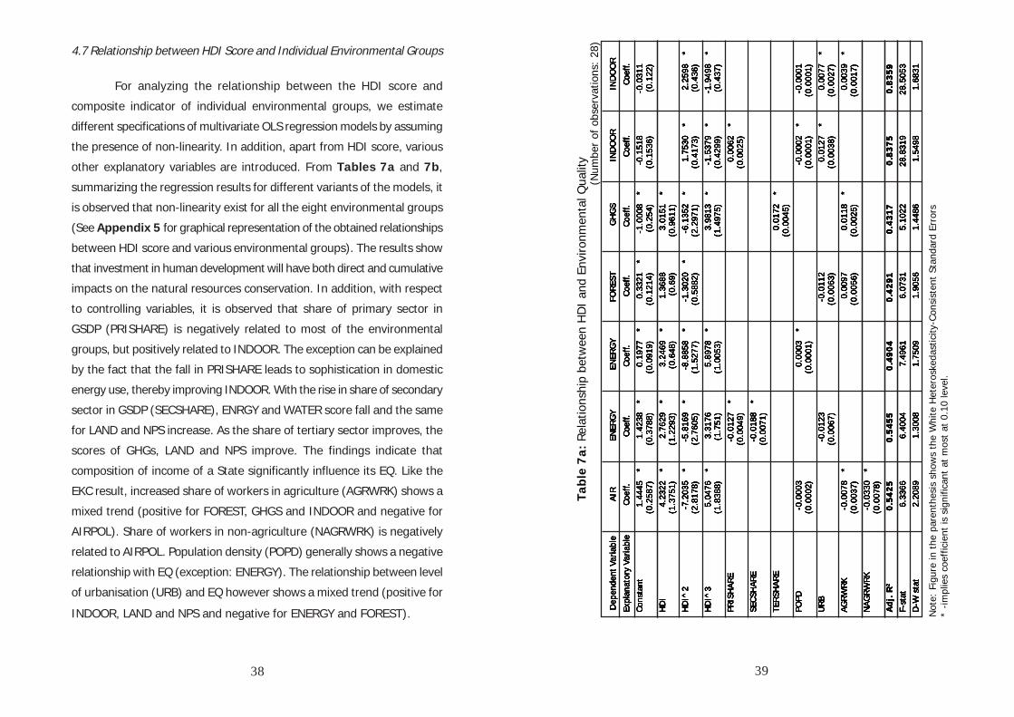
38
4.7 Relationship between HDI Score and Individual Environmental Groups
For analyzing the relationship between the HDI score and
composite indicator of individual environmental groups, we estimate
different specifications of multivariate OLS regression models by assuming
the presence of non-linearity. In addition, apart from HDI score, various
other explanatory variables are introduced. From Tables 7a and 7b,
summarizing the regression results for different variants of the models, it
is observed that non-linearity exist for all the eight environmental groups
(See Appendix 5 for graphical representation of the obtained relationships
between HDI score and various environmental groups). The results show
that investment in human development will have both direct and cumulative
impacts on the natural resources conservation. In addition, with respect
to controlling variables, it is observed that share of primary sector in
GSDP (PRISHARE) is negatively related to most of the environmental
groups, but positively related to INDOOR. The exception can be explained
by the fact that the fall in PRISHARE leads to sophistication in domestic
energy use, thereby improving INDOOR. With the rise in share of secondary
sector in GSDP (SECSHARE), ENRGY and WATER score fall and the same
for LAND and NPS increase. As the share of tertiary sector improves, the
scores of GHGs, LAND and NPS improve. The findings indicate that
composition of income of a State significantly influence its EQ. Like the
EKC result, increased share of workers in agriculture (AGRWRK) shows a
mixed trend (positive for FOREST, GHGS and INDOOR and negative for
AIRPOL). Share of workers in non-agriculture (NAGRWRK) is negatively
related to AIRPOL. Population density (POPD) generally shows a negative
relationship with EQ (exception: ENERGY). The relationship between level
of urbanisation (URB) and EQ however shows a mixed trend (positive for
INDOOR, LAND and NPS and negative for ENERGY and FOREST). Dep
ende
nt V
aria
ble
AIR
ENER
GY
ENER
GY
FOR
EST
G
HG
SIN
DO
OR
IN
DO
OR
Ex
plan
ator
y Va
riabl
eCo
eff.
Coef
f. Co
eff.
Coef
f. Co
eff.
Coef
f. Co
eff.
Cons
tant
1.44
45*
1.42
38*
0.19
77*
0.33
21*
-1.0
008
*-0
.151
8
-0.0
311
(0.2
587)
(0
.378
8)
(0.0
919)
(0
.121
4)
(0.2
54)
(0
.153
6)
(0.1
22)
HD
I4.
2322
*2.
7629
*3.
2469
*1.
3688
3.
0151
*
(1.3
751)
(1
.229
3)
(0.6
48)
(0
.69)
(0
.961
1)
HD
I^2
-7.2
035
*-5
.816
9*
-8.8
858
*-1
.302
0*
-6.1
352
*1.
7530
*2.
2598
*
(2.8
178)
(2
.760
5)
(1.5
277)
(0
.588
2)
(2.2
971)
(0
.417
3)
(0.4
36)
HD
I^3
5.04
76*
3.31
76
5.89
78*
3.98
13*
-1.5
379
*-1
.949
8*
(1
.838
8)
(1.7
51)
(1
.005
3)
(1.4
975)
(0
.429
9)
(0.4
37)
PRIS
HAR
E
-0
.012
7*
0.00
62*
(0
.004
9)
(0.0
025)
SECS
HAR
E
-0
.018
8*
(0
.007
1)
TER
SHAR
E
0.
0172
*
(0.0
045)
PO
PD-0
.000
3
0.00
03*
-0.0
002
*-0
.000
1
(0
.000
2)
(0.0
001)
(0
.000
1)
(0.0
001)
U
RB
-0.0
123
-0
.011
2
0.01
27*
0.00
77*
(0
.006
7)
(0.0
063)
(0
.003
8)
(0.0
027)
AG
RW
RK
-0.0
078
*
0.
0097
0.
0118
*
0.
0039
*
(0.0
037)
(0
.005
6)
(0.0
025)
(0
.001
7)
NAG
RW
RK
-0.0
330
*
(0.0
078)
A
dj.
R2
0.5
42
5
0.5
45
5
0.4
90
4
0.4
29
1
0.4
31
7
0.8
37
5
0.8
35
9
F-st
at6.
3366
6.
4004
7.
4961
6.
0731
5.
1022
28
.831
9
28.5
053
D
-W s
tat
2.20
89
1.30
08
1.75
09
1.90
56
1.44
86
1.54
98
1.68
31
Tab
le 7
a: R
elat
ions
hip
betw
een
HD
I an
d En
viro
nmen
tal Q
ualit
y
Dep
ende
nt V
aria
ble
AIR
ENER
GY
ENER
GY
FOR
EST
G
HG
SIN
DO
OR
IN
DO
OR
Ex
plan
ator
y Va
riabl
eCo
eff.
Coef
f. Co
eff.
Coef
f. Co
eff.
Coef
f. Co
eff.
Cons
tant
1.44
45*
1.42
38*
0.19
77*
0.33
21*
-1.0
008
*-0
.151
8
-0.0
311
(0.2
587)
(0
.378
8)
(0.0
919)
(0
.121
4)
(0.2
54)
(0
.153
6)
(0.1
22)
HD
I4.
2322
*2.
7629
*3.
2469
*1.
3688
3.
0151
*
(1.3
751)
(1
.229
3)
(0.6
48)
(0
.69)
(0
.961
1)
HD
I^2
-7.2
035
*-5
.816
9*
-8.8
858
*-1
.302
0*
-6.1
352
*1.
7530
*2.
2598
*
(2.8
178)
(2
.760
5)
(1.5
277)
(0
.588
2)
(2.2
971)
(0
.417
3)
(0.4
36)
HD
I^3
5.04
76*
3.31
76
5.89
78*
3.98
13*
-1.5
379
*-1
.949
8*
(1
.838
8)
(1.7
51)
(1
.005
3)
(1.4
975)
(0
.429
9)
(0.4
37)
PRIS
HAR
E
-0
.012
7*
0.00
62*
(0
.004
9)
(0.0
025)
SECS
HAR
E
-0
.018
8*
(0
.007
1)
TER
SHAR
E
0.
0172
*
(0.0
045)
PO
PD-0
.000
3
0.00
03*
-0.0
002
*-0
.000
1
(0
.000
2)
(0.0
001)
(0
.000
1)
(0.0
001)
U
RB
-0.0
123
-0
.011
2
0.01
27*
0.00
77*
(0
.006
7)
(0.0
063)
(0
.003
8)
(0.0
027)
AG
RW
RK
-0.0
078
*
0.
0097
0.
0118
*
0.
0039
*
(0.0
037)
(0
.005
6)
(0.0
025)
(0
.001
7)
NAG
RW
RK
-0.0
330
*
(0.0
078)
A
dj.
R2
0.5
42
5
0.5
45
5
0.4
90
4
0.4
29
1
0.4
31
7
0.8
37
5
0.8
35
9
F-st
at6.
3366
6.
4004
7.
4961
6.
0731
5.
1022
28
.831
9
28.5
053
D
-W s
tat
2.20
89
1.30
08
1.75
09
1.90
56
1.44
86
1.54
98
1.68
31
(Num
ber
of o
bser
vatio
ns:
28)
Not
e: F
igur
e in
the
par
enth
esis
sho
ws
the
Whi
te H
eter
oske
dast
icity
-Con
sist
ent
Stan
dard
Err
ors
* -im
plie
s co
effic
ient
is s
igni
fican
t at
mos
t at
0.1
0 le
vel.
39
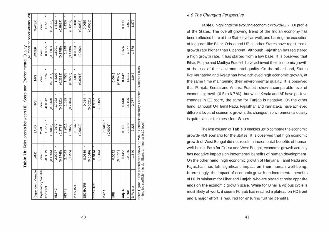
4.8 The Changing Perspective
Table 8 highlights the evolving economic growth-EQ-HDI profile
of the States. The overall growing trend of the Indian economy has
been reflected here at the State level as well, and barring the exception
of laggards like Bihar, Orissa and UP, all other States have registered a
growth rate higher than 6 percent. Although Rajasthan has registered
a high growth rate, it has started from a low base. It is observed that
Bihar, Punjab and Madhya Pradesh have achieved their economic growth
at the cost of their environmental quality. On the other hand, States
like Karnataka and Rajasthan have achieved high economic growth, at
the same time maintaining their environmental quality. It is observed
that Punjab, Kerala and Andhra Pradesh show a comparable level of
economic growth (6.5 to 6.7 %); but while Kerala and AP have positive
changes in EQ score, the same for Punjab is negative. On the other
hand, although UP, Tamil Nadu, Rajasthan and Karnataka, have achieved
different levels of economic growth, the changes in environmental quality
is quite similar for these four States.
The last column of Table 8 enables us to compare the economic
growth-HDI scenario for the States. It is observed that high economic
growth of West Bengal did not result in incremental benefits of human
well-being. Both for Orissa and West Bengal, economic growth actually
has negative impacts on incremental benefits of human development.
On the other hand, high economic growth of Haryana, Tamil Nadu and
Rajasthan has left significant impact on their human well-being.
Interestingly, the impact of economic growth on incremental benefits
of HD is minimum for Bihar and Punjab, who are placed at polar opposite
ends on the economic growth scale. While for Bihar a vicious cycle is
most likely at work, it seems Punjab has reached a plateau on HD front
and a major effort is required for ensuring further benefits.Dep
ende
nt V
aria
ble
LAN
D L
AND
NPS
N
PS
WAT
ER
WAT
ER
Expl
anat
ory
Varia
ble
Coef
f.Co
eff.
Coef
f.Co
eff.
Coef
f.Co
eff.
Co
nsta
nt-0
.301
9
1.25
17*
-0.0
512
0.
7769
*0.
8395
*1.
0513
*
(0.1
865)
(0
.083
6)
(0.0
959)
(0
.109
7)
(0.0
807)
(0
.216
5)
HD
I^2
-2.9
027
*-2
.267
7*
-1.7
022
*-1
.829
3*
-1.8
201
*-1
.543
3*
(0
.774
5)
(0.3
768)
(0
.262
2)
(0.3
335)
(0
.375
5)
(0.5
667)
H
DI^
32.
7043
*2.
2011
*1.
685
*1.
7538
*1.
749
*1.
4337
*
(0.7
55)
(0
.362
7)
(0.2
704)
(0
.322
3)
(0.4
138)
(0
.623
9)
PRIS
HAR
E
-0
.014
7*
-0.0
083
*-0
.005
3*
-0.0
081
*
(0.0
022)
(0
.001
8)
(0.0
02)
(0
.003
7)
SECS
HAR
E0.
0139
*
0.
014
*
-0
.005
7
(0
.004
6)
(0.0
021)
(0
.005
5)
TER
SHAR
E0.
0114
*
0.
0077
*
(0.0
04)
(0
.002
)
POPD
-0.0
003
*
(0.0
001)
U
RB
0.00
72
0.00
49
(0
.005
1)
(0.0
029)
A
dj.
R2
0.6
27
0
.75
8
0.6
60
0
.64
2
0.3
74
0.3
70
F-
stat
10.0
85
22.1
78
14.1
06
13.1
17
6.37
7
4.97
2
D-W
sta
t1.
640
2.
228
2.
077
1.
847
1.
878
1.
877
Tab
le 7
b:
Rela
tions
hip
betw
een
HD
I Sc
ore
and
Envi
ronm
enta
l Qua
lity
(Num
ber
of o
bser
vatio
ns:
28)
Not
e: F
igur
e in
the
par
enth
esis
sho
ws
the
Whi
te H
eter
oske
dast
icity
-Con
sist
ent
Stan
dard
Err
ors
* -im
plie
s co
effic
ient
is s
igni
fican
t at
mos
t at
0.1
0 le
vel.
40 41
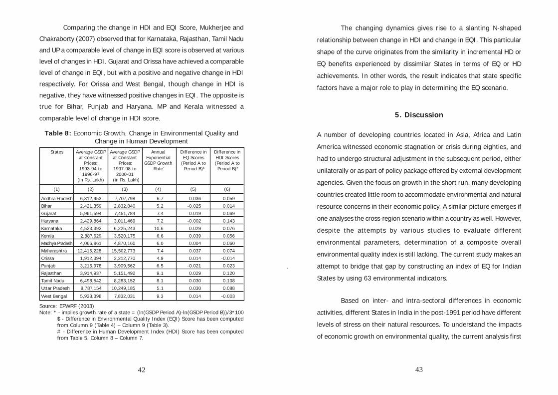
Comparing the change in HDI and EQI Score, Mukherjee and
Chakraborty (2007) observed that for Karnataka, Rajasthan, Tamil Nadu
and UP a comparable level of change in EQI score is observed at various
level of changes in HDI. Gujarat and Orissa have achieved a comparable
level of change in EQI, but with a positive and negative change in HDI
respectively. For Orissa and West Bengal, though change in HDI is
negative, they have witnessed positive changes in EQI. The opposite is
true for Bihar, Punjab and Haryana. MP and Kerala witnessed a
comparable level of change in HDI score.
Table 8: Economic Growth, Change in Environmental Quality andChange in Human Development
States Average GSDP Average GSDP Annual Difference in Difference inat Constant at Constant Exponential EQ Scores HDI Scores
Prices: Prices: GSDP Growth (Period A to (Period A to1993-94 to 1997-98 to Rate* Period B)$ Period B)#
1996-97 2000-01(in Rs. Lakh) (in Rs. Lakh)
(1) (2) (3) (4) (5) (6)
Andhra Pradesh 6,312,953 7,707,798 6.7 0.036 0.059
Bihar 2,421,359 2,832,840 5.2 -0.025 0.014
Gujarat 5,961,594 7,451,784 7.4 0.019 0.069
Haryana 2,429,864 3,011,469 7.2 -0.002 0.143
Karnataka 4,523,392 6,225,243 10.6 0.029 0.076
Kerala 2,887,629 3,520,175 6.6 0.039 0.056
Madhya Pradesh 4,066,861 4,870,160 6.0 0.004 0.060
Maharashtra 12,415,228 15,502,773 7.4 0.037 0.074
Orissa 1,912,394 2,212,770 4.9 0.014 -0.014
Punjab 3,215,978 3,909,562 6.5 -0.021 0.023
Rajasthan 3,914,937 5,151,492 9.1 0.029 0.120
Tamil Nadu 6,498,542 8,283,152 8.1 0.030 0.108
Uttar Pradesh 8,787,154 10,249,185 5.1 0.030 0.088
West Bengal 5,933,398 7,832,031 9.3 0.014 -0.003
Source: EPWRF (2003)Note: * - implies growth rate of a state = (ln(GSDP Period A)-ln(GSDP Period B))/3*100
$ - Difference in Environmental Quality Index (EQI) Score has been computedfrom Column 9 (Table 4) – Column 9 (Table 3).# - Difference in Human Development Index (HDI) Score has been computedfrom Table 5, Column 8 – Column 7.
The changing dynamics gives rise to a slanting N-shaped
relationship between change in HDI and change in EQI. This particular
shape of the curve originates from the similarity in incremental HD or
EQ benefits experienced by dissimilar States in terms of EQ or HD
achievements. In other words, the result indicates that state specific
factors have a major role to play in determining the EQ scenario.
5. Discussion
A number of developing countries located in Asia, Africa and Latin
America witnessed economic stagnation or crisis during eighties, and
had to undergo structural adjustment in the subsequent period, either
unilaterally or as part of policy package offered by external development
agencies. Given the focus on growth in the short run, many developing
countries created little room to accommodate environmental and natural
resource concerns in their economic policy. A similar picture emerges if
one analyses the cross-region scenario within a country as well. However,
despite the attempts by various studies to evaluate different
environmental parameters, determination of a composite overall
environmental quality index is still lacking. The current study makes an
attempt to bridge that gap by constructing an index of EQ for Indian
States by using 63 environmental indicators.
Based on inter- and intra-sectoral differences in economic
activities, different States in India in the post-1991 period have different
levels of stress on their natural resources. To understand the impacts
of economic growth on environmental quality, the current analysis first
42 43
constructs the environmental quality index for the 14 major Indian
States and look for its possible relationship with economic growth. This
paper also attempts to capture the relationship between environmental
sustainability and human well-being – as measured by the Human
Development Index. To capture the temporal aspects of environmental
quality and to understand the dynamics of economic liberalization
process, the entire period of our study has been divided into two broad
time periods – Period A (1990-1996) and Period B (1997-2004).
It is observed that different States possess different strengths
and weaknesses in managing various aspects of EQ. For instance, while
Maharashtra is in the second position in terms of EQI during period B,
and fares satisfactorily in terms of INDOOR and NPSP; it’s performance
on ENERGY and FOREST is not that satisfactory. On the other hand,
Punjab, the state at the bottom in terms of overall EQI and ENERGY
and WATER, is actually topper for INDOOR. It also shows that there are
scopes for the States to learn from each other about different aspects
of environmental management. Therefore, adoption of a ‘one-size-fits-
all’ National Environmental Policy at the country-level might have limited
impact on the local environmental quality. In other words, individual
States should adopt environmental management practices based on
their local (at the most disaggregated level) environmental information.
Furthermore, over time performance of an individual State varies across
the environmental criteria, which shows that environmental management
practices should take into account this dynamic nature of environment,
and review their environmental status or achievement regularly.
The analysis on the relationship between economic growth and EQ
does not reveal a very clear picture during the two time periods under
consideration. For different States, the impacts of economic restructuring
process, as adopted by them during 1990s, have affected the
environmental quality differently. It is observed that while States like
Maharashtra has performed well on both counts, growth in northern
States like Punjab and Haryana has taken place mostly at the cost of
EQ. On the other hand Orissa, despite being a low-income State,
performed well during both period A and B in terms of EQ. The results
indicate that laggards like Bihar and MP have also achieved their
economic growth at the cost of their EQ. On the other hand a few
States like Karnataka and Rajasthan have achieved economic growth
and also maintained their environment well. The obtained results again
indicate that individual States should adopt special environmental
measures, based on their environmental impacts assessment of major
economic activities, to achieve sustainable economic growth.
The formal testing for the existence of Environmental Kuznets
Curve (EKC) through multivariate OLS regression models are estimated
by assuming non-linearity in the relationship between PCNSDP and the
composite score of the defined environmental sub-categories. It is
observed that while for a few categories an inverted U-shaped
relationship exists between PCNSDP and individual indicator of
environmental quality (e.g. – GHGS, LAND, ENERGY, NPS),24 a linear
24 However it goes against the popular EKC hypothesis, which shows invertedU-shaped relationship between PCI and environmental degradation (pollution) insteadof environmental quality.
44 45
relationship exist for other categories (INDOOR, WATER, FOREST) and
no relationship in case of AIRPOL. The absence of the EKC in the Indian
framework can be explained by the mixed performance of the States
across environmental groups – e.g., worse EQ for economically advanced
Punjab and better EQ for economically lagging Orissa.
Estimation of multivariate OLS regression models between
individual EQ Scores and HDI Score indicate presence of non-linear
relationships (in most cases, slanting N-shaped and parabolic in case
of FOREST). The results originate from the concentration of several
States in low HDI-Low EQ category (Bihar, UP) and high EQ-mid HDI
category (AP, Rajasthan) on one hand, and presence of the outliers
like Orissa (high EQ-Low HDI) on one hand and Punjab and Haryana
(high HDI-Low EQ) on the other. The result indicates the need to re-
examine the methodology for calculating the HD achievements of the
States. Perhaps, the HD ranking of States like Punjab and Haryana has
been influenced too heavily by their high per capita consumption
expenditure. Broad-basing the HD index by incorporating other social
achievements might reveal interesting results.
A few policy issues need to be highlighted here. First, the
increment in HD indicators and economic growth can effectively increase
the demand for a better environment, and therefore provide a demand
side solution to the problem of environmental sustainability. Second, in
contrary to popular belief, industrial pollution is not the source of all
the problems. In Punjab and Haryana, it seems that the thrust on
agriculture is increasingly becoming a serious concern. Third, given
the need to arrive at local State-level solutions, there seems to be
enough scope to involve local communities with direct interest in certain
initiatives (e.g. - JFM). Fourth, it is difficult to comment on the choice
of optimal level of income and its composition for a State, which would
be in line with the objective of sustainable development. For instance,
we observe a high level of EQ for a poor State like Orissa, which clearly
is a result of unutilised resources. Fifth, as has been observed, improved
governance can play a key role (e.g. – Supreme Court intervention) in
ensuring sustainable development, and there is increasing need for
implementing that in environmentally vulnerable States. Finally, here
we focus only on the economic growth of the Indian States during the
two periods (1990-96 and 1997-2004) and look into its relationship
with EQ. However, income inequality varies across Indian States and it
has often been observed that inequality has increased in the post-
reform period (Deaton and Dreze, 2002). An area of future research
can be to analyse the relationship between income inequality of the
States, their EQ and HD achievements.
Finally, a few limitations of the study are as follows. We have
confined our analysis only to 14 major Indian States, the constraint
being the availability of various secondary environmental information
for both the time periods under consideration. Given the fact that a
number of Indian States are currently in the process of preparing their
environmental profile, one future area of research would be to extend
the analysis to the remaining States. The analysis can be further
extended by dividing the post-1997 period into more sub-groups, as
permitted by availability of newer data points.
46 47
References
Adriaanse, A. (1993), “Environmental Policy Performance Indicators: A Study of the
Development of Indicators for Environmental Policy in the Netherlands”, SDU
Publishers, The Hague.
Adriaanse, A., D. Bryant, A.L. Hammond, E. Rodeburg, and R. Woodward (1995),
“Environmental Indicators: A Systematic Approach to Measuring and Reporting
on Environmental Policy Performance in the Context of Sustainable
Development”, World Resources Institute, Washington D.C.
Agarwal, M and S. Samanta (2006), “Structural adjustment, governance, economic
growth and social progress”, Journal of International Trade & Economic
Development, Vol. 15, No. 3, pp. 387 – 401.
Andreoni, J. and A. Levinson (2001), “The simple analytics of the Environmental Kuznets
curve”, Journal of Public Economics, Vol. 80, No.1, pp. 269–286.
Antony, M. J. (2001), “Landmark Judgements on Environmental Protection”, Indian
Social Institute, New Delhi.
Appasamy, P., P. Nelliyat, N. Jayakumar and R. Manivasagan (undated), “Economic
Assessment of Environmental Damage: A Case Study of Industrial Water
Pollution in Tiruppur”, Environmental Economics Research Committee Working
Paper Series: IPP-1, available at http://coe.mse.ac.in/eercrep/fullrep/ipp/
IPP_FR_Paul_Appasamy.pdf.
Baldwin, R. (1995), “Does sustainability require growth?”, in Goldin, I. and Winters,
L.A. (Eds.): The Economics of Sustainable Development, Cambridge University
Press, Cambridge, UK, pp. 19–47.
Balooni, K. (2002), “Participatory Forest Management in India - An Analysis of Policy
Trends amid ‘Management Change”, Policy Trend Report 2002: 88-113, The
Institute for Global Environmental Strategies (IGES), Japan, available at
www.iges.or.jp/en/fc/pdf/report5/PTR0207.pdf.
Bhandari, Laveesh and Aarti Khare (2002), “The Geography of Post-1991 India Economy”,
Global Business Review, Vol. 3, No. 2, pp. 321-340.
Bhattacharyya, B. (1999), “Non-Tariff Measures on Indian Exports: An Assessment”,
Occasional Paper No. 16, Indian Institute of Foreign Trade, New Delhi.
Bhullar, A.S. and R.S. Sidhu (2006), “Integrated Land and Water Use: A Case Study of
Punjab”, Economic and Political Weekly, December 30, pp. 5353-5357.
Boyce, J.K. (2003), “Inequality and Environmental Protection”, Working Paper Series No.
52, Political Economy Research Institute, University of Massachusetts, Amherst.
Brandon, Carter and Kirsten Hommann (1995), “The Cost of Inaction: Valuing the
Economy-Wide Cost of Environmental Degradation in India”, paper presented
at the “Modelling Global Sustainability” conference held in United Nations
University, Tokyo, October 1995.
Bruvoll, A. and Medin, H. (2003) “Factors behind the environmental Kuznets curve: A
decomposition of the changes in air pollution”, Environmental and Resource
Economics, Vol. 24, No. 1, pp. 27–48.
Carson, R.T., Y. Jeon, and D. R. McCubbin (1997) “The relationship between air pollution
emissions and income: US data”, Environment and Development Economics,
Vol. 2, No. 4, pp. 433–450.
Centre for Science and Environment (CSE), “State of India’s Environment”, various
issues of Citizen’s Reports, New Delhi.
Chakraborty, P. and J. Singh (2005), “Leather Bound: A Comprehensive Guide for SMEs”,
The Energy and Resources Institute, New Delhi.
Chaturvedi, Sachin and Gunjan Nagpal (2002), “WTO and Product related Environmental
Standards: Emerging Issues and Policy Options before India”, RIS Discussion
Paper No. 36, New Delhi.
Convention on Biological Diversity (CBD) (Undated), “Global Biodiversity Outlook, United
Nations Environment Program”, Montreal, Quebec, Canada, available at http:/
/www.biodiv.org/gbo/annex.asp?ann=1
Convention on Biological Diversity (CBD) (undated), “Case study on Joint Forest
Management (JFM) as an example of non-monetary positive incentive”,
available at www.biodiv.org/doc/case-studies/inc/cs-inc-india-forest-en.doc.
Costantini, V. and M. Salvatore (2006), “Environment, Human Development and Economic
Growth”, The Fondazione Eni Enrico Mattei, Note di Lavoro Series, February
2006, available at http://www.feem.it/NR/rdonlyres/CA11D877-29E3-462F-
A591-7738FBD508F0/1891/3506.pdf
48 49
Dam, S. (2004), “Green Laws for Better Health: The Past that was and the Future that
may be – Reflections from the Indian Experience”, Georgetown International
Environmental Law Review, Vol. 16, No. 4, pp. 593-615.
Dasgupta, P. (2001), “Human Well-Being and the Natural Environment”, Oxford University
Press, New Delhi.
Dastidar, Avishek G. (2006), “Maharashtra ‘outsources’ toxic e-waste to Delhi”, Hindustan
Times, December 30.
Deaton, A. and J. Dreze (2002), “Poverty and Inequality in India: A Re-Examination”,
Economic and Political Weekly, September 7, pp. 3729-3748.
de Bruyn, S.M., J.C.J.M. van den Berg and J.B. Opschoor (1998) “Economic growth and
emissions: reconsidering the empirical basis of Environmental Kuznets Curve”,
Ecological Economics, Vol. 25, No. 2, pp. 161–175.
Dietzenbacher, Erik and Kakali Mukhopadhyay (2007), “An Empirical Examination of the
Pollution Haven Hypothesis for India: Towards a Green Leontief Paradox?”,
Environmental and Resource Economics, Vol. 36, No. 4, pp. 427-449.
Dinda, S. (2004), “Environmental Kuznets curve hypothesis: a survey”, Ecological
Economics, Vol. 49, No. 4, pp. 431–455.
Divan, Shyam and Armin Rosencranz (2002), “Environmental Law and Policy in India:
Cases, Materials and Statutes”, Second Edition, Oxford University Press, New
Delhi.
Dutt, A. K. and J.M. Rao (1996), “Growth, Distribution, and the Environment: Sustainable
Development in India”, World Development, Vol. 24, No. 2. pp. 287-305.
Ebert, Udo and Heinz Welsch (2004), “Meaningful environmental indices: a social choice
approach”, Journal of Environmental Economics and Management, Vol. 47,
pp. 270–283.
EPWRF (2003), “Domestic Product of State of India: 1960–1961 to 2000–2001”, DatabaseSoftware, Economic and Political Weekly Research Foundation, Mumbai.
Eskeland, G.S. and A.E. Harrison (2003), “Moving to greener pastures? Multinationals
and the pollution haven hypothesis”, Journal of Development Economics, Vol.
70, No. 1, pp. 1-23.
Esty, D.C., M.A. Levy, T. Srebotnjak, A. de Sherbinin, C.H. Kim and B. Anderson (2006),
“Pilot 2006 Environmental Performance Index”, Yale Center for Environmental
Law and Policy and Center for International Earth Science Information Network
(CIESIN), available at http://www.yale.edu/ epi/2006EPI_Report_Full.pdf
Esty, D.C., M. A. Levy, T. Srebotnjak and A. de Sherbinin (2005), “2005 Environmental
Sustainability Index: Benchmarking National Environmental Stewardship”, Yale
Center for Environmental Law & Policy, New Haven.
Esty, D.C. and M.E. Porter (2001-02), “Ranking National Environmental Regulation and
Performance: A Leading Indicator of Future Competitiveness?”, Chapter 2.1,
p. 78-100, Harvard Business School, Global Competitiveness Report, available
at http://www.isc.hbs.edu/GCR_20012002_Environment.pdf
Gallagher, K.P (2004), “Free Trade and the Environment: Mexico, NAFTA,
and Beyond”, available at http://ase.tufts.edu/gdae/Pubs/rp/
NAFTAEnviroKGAmerProgSep04.pdf
Ginkel, Hans van, Brendan Barrett, Julius Court and Jerry Velasquez (edited) (2001),
“Human Development and the Environment: Challenges for the United Nations
in the New Millennium”, United Nations University Press, Tokyo, Japan.
Gamper-Rabindran, Shanti and Shreyasi Jha (2004), “Environmental Impact of India’s
Trade Liberalization”, available at http://unpan1.un.org/intradoc/groups/public/
documents/APCITY/ UNPAN024230.pdf
Garg, A. and P.R. Shukla (2002), “Emission Inventory of India”, Tata McGraw-Hill
Publishing Company Limited, New Delhi.
Ghosh, Madhusudan (2006), “Economic Growth and Human Development in Indian
States”, Economic and Political Weekly, July 29, pp. 3321-3329.
Government of India (2002), Planning Commission, “National Human Development
Report, 2001”, March 2002.
Grossman, G.M. and Krueger, A.B. (1995), “Economic growth and the environment”,
Quarterly Journal of Economics, Vol. 110, No. 2, pp. 353–378.
Guha, A. and D. Chakraborty (2003), “Relative Positions of Human Development Index
Across Indian States: Some Exploratory Results”, Artha Beekshan, Vol. 11,
No. 4, pp. 166-181.
50 51
Gulati, S.C. and Suresh Sharma (undated), “Population pressure and Deforestation in
India”, Population Research Centre, Institute of Economic Growth, available
at http://iegindia.org/dis_scg_17.pdf
Indian NGOs (undated), “Environment Overview”, avai lable at http://
www.indianngos.com/issue/ environment/overview.htm
Jadavpur University (JU) (2006), “Groundwater Arsenic Contamination in West Bengal”, School
of Environmental Studies, available at http://www.soesju.org/arsenic/wb.htm
Jalan, Jyotsna, E. Somanathan and Saraswata Chaudhuri (2003), “Awareness and the
Demand for Environmental Quality: Drinking Water in Urban India”, Economics
Discussion Paper No. 03-05, Indian Statistical Institute, New Delhi.
Jena, P.R., N. C. Sahu and B. Rath (2005), “Does Trade Liberalisation Create Pollution
Haven? An Indian Experience”, paper presented at the “International Conference
on Environment and Development: Developing Countries Perspective”, April 7-
8, 2005, ITD, SIS, Jawaharlal Nehru University, New Delhi.
Jha, R. and Bhanu Murthy, K.V. (2001), “An Inverse Global Environmental Kuznets
Curve”, Departmental Working Papers: 2001–2002, Division of Economics,
RSPAS, Australian National University, Canberra, Australia.
Jha, V. (1999), “Investment Liberalization and Environmental Protection: Conflicts and
Compatibilities in the Case of India”, Occasional Paper No. 1, Cross Border
Environmental Management Project, CHP: Copenhagen Business School.
Jones, L., Fredricksen, L. and Wates, T. (2002), “Environmental Indicators”, 5th ed.,
The Fraser Institute, available at http://www.fraserinstitute.ca/shared/
readmore.asp?snav=pb&id=314.
Kadekodi, Gopal K. and L. Venkatachalam (2005), “Human Development, Environment
and Poverty Nexus in India”, Institute for Social and Economic Change, Report
prepared for the United Nations Development Programme, New Delhi.
Kathuria, V. and T. Sterner (2005), “Monitoring and Enforcement: Is Two-Tier Regulation
Robust? – A case study of Ankleshwar, India”, April 2005, available at http:/
/www.hgu.gu.se/files/nationalekonomi/ personal/thomas%20sterner/
kathuria.sterner%20ecological%20economics%20revised.pdf
Kathuria, Vinish (2004), “Informal Regulation of Pollution in a Developing Country:
Empirical Evidence from India”, Working Paper No. 6-04, South Asian Network
for Development and Environmental Economics (SANDEE), Kathmandu, Nepal.
Kathuria, V. (2002) “Vehicular pollution control in Delhi, India”, Transportation Research,
Part D: Transport and Environment, Vol. 7D, No. 5, pp. 373–387.
Kathuria, V. (2004) “Impact of CNG on vehicular pollution in Delhi: a note”, Transportation
Research, Part D: Transport and Environment, Vol. 9D, No. 5, pp. 409–417.
Kaushik, A and M. Saqib (2001), “Environmental Requirements and India’s Exports: An
Impact Analysis”, Rajiv Gandhi Institute for Contemporary Studies (RGICS)
Working Paper No. 25, New Delhi.
Mehta, R. (2005), “Non-Tariff Barriers affecting India’s Exports”, RIS Discussion Paper
No. 97, New Delhi.
Melnick, D., J. McNeely, Y. K. Navarro, G. Schmidt-Traub and R.R. Sears (2005),
“Environment and human well-being: a practical strategy”, UN Millennium
Project, Task Force on Environmental Sustainability, available at http://
www.unmillenniumproject.org/documents/Environment-complete-lowres.pdf
Mukherjee, S. and D. Chakraborty (2007), “Environment, Human Development and
Economic Growth of Indian States after Liberalisation”, presented at the National
Conference on ‘Making Growth Inclusive with Special Reference to Imbalance
in Regional Development’ jointly organized by Department of Economics, Jammu
University and Indian Institute of Advanced Studies, March 12, 2007.
Mukherjee, S. and P. Nelliyat (2006), “Groundwater Pollution and Emerging Environmental
Challenges of Industrial Effluent Irrigation in Mettupalayam Taluk, Tamil Nadu”,
Working Paper No. 7/2006, Madras School of Economics, Chennai.
Mukherjee, S. and V. Kathuria (2006), “Is Economic Growth Sustainable? Environmental
Quality of Indian States After 1991”, International Journal of Sustainable
Development, Vol. 9, No. 1, pp. 38-60.
Mukhopadhyay, K. and D. Chakraborty (2005), “Is liberalization of trade good for the
environment? Evidence from India”, Asia-Pacific Development Journal, Vol.
12, No. 1, pp. 109-136, available at http://www.unescap.org/pdd/publications/
apdj_12_1/5_kakali.pdf.
Murty, M. N., S. C. Gulati and A. Banerjee (2003), “Health Benefits from Urban Air
Pollution Abatement in the Indian Subcontinent”, Institute of Economic Growth
Working Paper, New Delhi.
52 53
Nadkarni, M.V. (2000), “Poverty, environment, development: a many patterned nexus”,
Economic and Political Weekly, April 1, pp. 1184–1190.
Nagar, A.L., and S.R. Basu (2001), “Weighing Socio-Economic Indicators of Human
Development: A Latent Variable Approach”, Working Paper, National Institute
of Public Finance and Policy, New Delhi.
Nair, G.K. (2006), “Water scarcity hits parts of south Kerala”, The Hindu, March 31,
available at http://www.thehindubusinessline.com/2006/03/31/stories/
2006033101981900.htm
NCERT (2002), “7th All India Educational Survey (AIES): All India School Education
Survey (AISES)”, National Council of Educational Research and Training
(NCERT), Ministry of Human Resource Development (MHRD), Government of
India, New Delhi, available at http://www.7thsurvey.ncert.nic.in/
Panayatou, T. (1993), “Empirical Tests and Policy Analysis of Environmental Degradation
at Different Stages of Economic Development”, World Employment Research
Programme, Working Paper No. WP238, Technology and Employment
Programme, International Labour Office, Geneva.
Parikh, J. (2004), “Environmentally Sustainable Development in India”, available at
http://scid.stanford.edu/ events/India2004/JParikh.pdf
Pezzey, J. (1989), “Economic Analysis of Sustainable Growth and Sustainable
Development”, Environment Department Working Paper No 15, The World
Bank, Washington DC.
Raju, S. Durai (Undated), “Measurement of Human Development – District Level”,
available at http://www.undp.org.in/hdrc/events/Aggregates/Goa/2
Ranis, Gustav, “Human Development and Economic Growth”, Center Discussion Paper
No. 887, Economic Growth Center, Yale University, May 2004, available at
http://www.econ.yale.edu/growth_pdf/ cdp887.pdf
Rithe, Kishor and Ashish Fernandes (2002), “Maharashtra’s tiger troubles”, April, available
at www.satpuda.org/maharashtratiger.doc
RIVM/UNEP (Undated), “Global Environment Outlook (GEO-3)”, National Institute of
Public Health and the Environment (RIVM), UNEP, Bilthoven, The Netherlands,
available at http://arch.rivm.nl/ env/int/geo/
Rogers, P., K.F. Jalal, B.N. Lohani, G.M. Owens, C-C. Yu, M. Christia and J.B. Dufournaud
(1997), “Measuring Environmental Quality in Asia”, Harvard University Press
and ADB, London, UK.
Sankar, U. (2006), “Trade Liberalisation and Environmental Protection Responses of
Leather Industry in Brazil, China and India,” Economic and Political Weekly,
June 17, pp. 2470-2477.
___ (1998), “Laws and Institutions relating to Environmental Protection in India”,
presented at the Conference on ‘The Role of Law and Legal Institutions in
Asian Economic Development’, Rotterdam, November 1998, available at http:/
/www.mse.ac.in/pub/op_sankar.pdf
Santhakumar, V. (2001), “Will Public Interest Litigations and Citizens’ Actions Lead to
Sustainable Development? An economic analysis with empirical cases from
India”, available at http://www.ccsindia.org/ccsindia/santhakumar.doc
Saqib, Mohd., Yashika Singh and Ritu Kumar (2001), “Stimulating Sustainable Trade in
Electronics: Challenges, Realities and Strategies for the Indian Components
Sector”, Rajiv Gandhi Institute for Contemporary Studies (RGICS), New Delhi.
Schjolden, A. (2000), “Leather tanning in India: Environmental regulations and firms’
Compliance”, F.I.L. Working Papers, No. 21, available at http://
www.cicero.uio.no/media/1677.pdf
Selden, T.M. and Song, D.S. (1994), “Environmental quality and development: is there
a Kuznets curve for air pollution emissions?” Journal of Environmental
Economics and Management, Vol. 27, No. 2, pp. 147–162.
Shafik, N. and Bandyopadhyay, S. (1992), “Economic Growth and Environmental Quality:
Time-Series and Cross-Country Evidence”, World Bank Policy Research Working
Paper No. 904, The World Bank, Washington DC.
Sharma, D.C. (2005), “By Order of the Court: Environmental Cleanup in India”,
Environmental Health Perspectives, Vol. 113, No. 6, pp. A394-A397.
Sidhu, H S., “Crisis in Agrarian Economy in Punjab: Some Urgent Steps”, Economic and
Political Weekly, July 27– August 2, 2002, pp. 3132-38.
Somanathan, J.E. and T. Sterner (2003), “Environmental Policy Instruments and
Institutions in Developing Countries”, Initiative for Policy Dialogue Working
Paper Series, Columbia University, available at http://www0.gsb.columbia.edu/
ipd/pub/EnvironmentalPolicyInstruments.pdf.
54 55
Sood, Atul and Bimal Arora (2006), “The Political Economy of Corporate Responsibility
in India”, Technology, Business and Society – Paper No. 18, United Nations
Research Institute for Social Development, Geneva, Switzerland.
Stern, D.I. (1998) “Progress on the Environmental Kuznets curve”, Environment and
Development Economics, Vol. 3, No. 2, pp. 175–198.
Tewari, M. and P. Pilai (2005), “Global standards and environmental compliance in India’s
leather industry”, Oxford Development Studies, Vol 33, No. 2, pp. 245-267.
The Hindu (2006), “Air pollution the bane of Davangere”, Wednesday, October 4, available
at http://www.hindu.com/2006/10/04/stories/2006100414400300.htm
(2005), “Air quality around hospitals, schools deteriorating: SPM levels are
at least 25 per cent more than standard values”, November 18, available at
http://www.hindu.com/2005/11/18/stories /2005111817640300.htm
UNDP, “Human Development Report”, various issues, available at http://hdr.undp.org/,
United Nations Development Programme, New York, USA.
Venkatachalam, L. (2005), “Damage Assessment and Compensation to Farmers: Lessons
from Verdict of Loss of Ecology Authority in Tamil Nadu”, Economic and Political
Weekly, April 9, 2005.
World Bank (2006), “India: Strengthening Institutions for Sustainable Growth”, Country
Environmental Analysis (India CEA), September 2006, available at
http://siteresources.worldbank.org/INDIAEXTN/ Resources/295583-
1176163782791/complete.pdf
World Bank (2004), “World Development Indicator - 2004”, available at
http://www.worldbank.org/data/ countrydata/countrydata.html
World Wildlife Fund (WWF) (2002), “WWF’s Living Planet Report 2002", WWF
International, Switzerland, available at http://www.panda.org/news_facts/
publications/general/living planet/lpr02.cfm
Zhou, P., B.W. Ang, K.L. Poh (2006), “Comparing aggregating methods for constructing
the composite environmental index: an objective measure”, Ecological
Economics, Vol. 59, pp. 305-311.
Appendix 1: Abbreviations used in Text
AGRWRK Percentage of Agricultural Workers in Total WorkersAIES All India Educational SurveyAIFE Adjusted Intensity of Formal EducationAISES All India School Education SurveyAP Andhra PradeshBH BiharCBD Convention on Biological DiversityCH4 MethaneCO Carbon monoxideCPCB Central Pollution Control BoardCSO Central Statistical OrganisationEDI Environmental Degradation IndexEG Economic GrowthEKC Environmental Kuznets CurveEPI Environmental Performance IndexEQ Environmental QualityEQI Environmental Quality IndexEU European UnionFDI Foreign Direct InvestmentGDP Gross Domestic ProductGHGs Green House GasesGJ GujaratGSDP Gross State Domestic ProductHD Human DevelopmentHDI Human Development IndexHDR Human Development ReportHR HaryanaHSD High Speed DieselHT Hindustan TimesIFE Intensity of Formal EducationIMR Infant Mortality RateJFM Joint Forest ManagementJU Jadavpur UniversityK KeroseneKL KeralaKR KarnatakaLAECs Local Area Environmental CommitteesLDO Light Diesel OilLE Life ExpectancyLPG Liquefied Petroleum GasMDGs Millennium Development GoalsMG Motor GasolineMH MaharashtraMP Madhya Pradesh
56 57
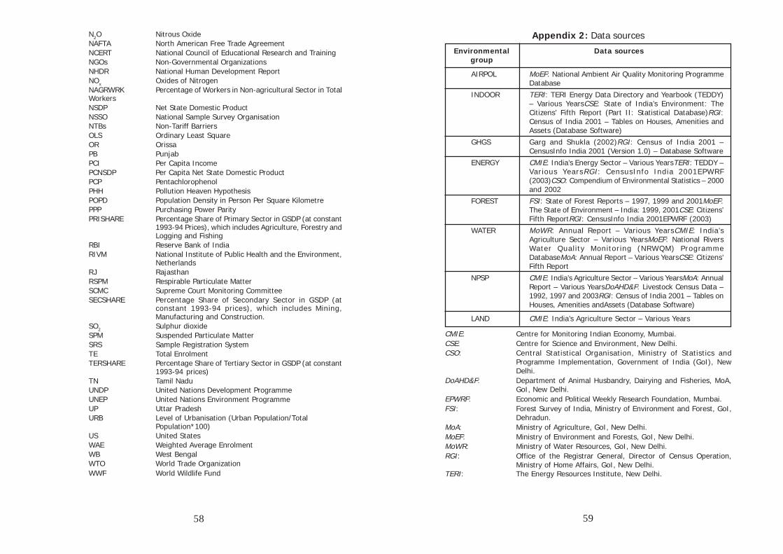
N2O Nitrous OxideNAFTA North American Free Trade AgreementNCERT National Council of Educational Research and TrainingNGOs Non-Governmental OrganizationsNHDR National Human Development ReportNOx Oxides of NitrogenNAGRWRK Percentage of Workers in Non-agricultural Sector in TotalWorkersNSDP Net State Domestic ProductNSSO National Sample Survey OrganisationNTBs Non-Tariff BarriersOLS Ordinary Least SquareOR OrissaPB PunjabPCI Per Capita IncomePCNSDP Per Capita Net State Domestic ProductPCP PentachlorophenolPHH Pollution Heaven HypothesisPOPD Population Density in Person Per Square KilometrePPP Purchasing Power ParityPRISHARE Percentage Share of Primary Sector in GSDP (at constant
1993-94 Prices), which includes Agriculture, Forestry andLogging and Fishing
RBI Reserve Bank of IndiaRIVM National Institute of Public Health and the Environment,
NetherlandsRJ RajasthanRSPM Respirable Particulate MatterSCMC Supreme Court Monitoring CommitteeSECSHARE Percentage Share of Secondary Sector in GSDP (at
constant 1993-94 prices), which includes Mining,Manufacturing and Construction.
SO2 Sulphur dioxideSPM Suspended Particulate MatterSRS Sample Registration SystemTE Total EnrolmentTERSHARE Percentage Share of Tertiary Sector in GSDP (at constant
1993-94 prices)TN Tamil NaduUNDP United Nations Development ProgrammeUNEP United Nations Environment ProgrammeUP Uttar PradeshURB Level of Urbanisation (Urban Population/Total
Population*100)US United StatesWAE Weighted Average EnrolmentWB West BengalWTO World Trade OrganizationWWF World Wildlife Fund
Appendix 2: Data sources
Environmental Data sourcesgroup
AIRPOL MoEF: National Ambient Air Quality Monitoring ProgrammeDatabase
INDOOR TERI: TERI Energy Data Directory and Yearbook (TEDDY)– Various YearsCSE: State of India’s Environment: TheCitizens’ Fifth Report (Part II: Statistical Database)RGI:Census of India 2001 – Tables on Houses, Amenities andAssets (Database Software)
GHGS Garg and Shukla (2002)RGI: Census of India 2001 –CensusInfo India 2001 (Version 1.0) – Database Software
ENERGY CMIE: India’s Energy Sector – Various YearsTERI: TEDDY –Various YearsRGI: CensusInfo India 2001EPWRF(2003)CSO: Compendium of Environmental Statistics – 2000and 2002
FOREST FSI: State of Forest Reports – 1997, 1999 and 2001MoEF:The State of Environment – India: 1999, 2001CSE: Citizens’Fifth ReportRGI: CensusInfo India 2001EPWRF (2003)
WATER MoWR: Annual Report – Various YearsCMIE: India’sAgriculture Sector – Various YearsMoEF: National RiversWater Quality Monitoring (NRWQM) ProgrammeDatabaseMoA: Annual Report – Various YearsCSE: Citizens’Fifth Report
NPSP CMIE: India’s Agriculture Sector – Various YearsMoA: AnnualReport – Various YearsDoAHD&F: Livestock Census Data –1992, 1997 and 2003RGI: Census of India 2001 – Tables onHouses, Amenities andAssets (Database Software)
LAND CMIE: India’s Agriculture Sector – Various Years
CMIE: Centre for Monitoring Indian Economy, Mumbai.CSE: Centre for Science and Environment, New Delhi.CSO: Central Statistical Organisation, Ministry of Statistics and
Programme Implementation, Government of India (GoI), NewDelhi.
DoAHD&F: Department of Animal Husbandry, Dairying and Fisheries, MoA,GoI, New Delhi.
EPWRF: Economic and Political Weekly Research Foundation, Mumbai.FSI: Forest Survey of India, Ministry of Environment and Forest, GoI,
Dehradun.MoA: Ministry of Agriculture, GoI, New Delhi.MoEF: Ministry of Environment and Forests, GoI, New Delhi.MoWR: Ministry of Water Resources, GoI, New Delhi.RGI: Office of the Registrar General, Director of Census Operation,
Ministry of Home Affairs, GoI, New Delhi.TERI: The Energy Resources Institute, New Delhi.
58 59
Appendix 3: Descriptions of Environmental Groups (Variables)and Indicators
AIR POLLUTION (12 indicators)• Maximum Concentration of NO2, SO2 and SPM in Residential and Industrial Area
(µg/m3): 1990-1995 and 1996-2000 *
INDOOR AIR POLLUTION POTENTIAL (18 indicators)· Monthly Per-Capita Expenditure (MPCE) on Fuel & Lighting (Rs./month/head)
Rural and Urban Areas: 1993-94 and 1999-2000 $
• Percentage of Rural Households using Bio-fuels (Firewoods and chips, Dung cake)as primary source of energy (Traditional & Commercial) for cooking (%): 1993-1994 and 1999-2000 *
• Percentage of Urban Households using Bio-fuels (Firewoods and chips) as primarysource of energy (Traditional) for cooking (%): 1993-1994 and 1999-2000 *
• Percentage of Rural and Urban Households Do Not Have Access to Electricity:1991 and 2001 *
• Achievement in Installation of Biogas Plants: Upto 1994-95 and Upto 2001-2002 $
• Kerosene as a Primary Source of Energy for Lighting for Rural and Urban Households(%): 1993-94 and 1999-2000 *
GREEN HOUSE GASES EMISSIONS (12 indicators)• CO2 Equivalent GHGs (CO2, CH4, N2O) Emissions (Kg. /Person): 1990 and 1995 *
• CO2 Equivalent GHGs (CO2, CH4, N2O) Emissions (Tons/Rs. Lakh of GSDP atConstant 1980-81 Prices): 1990 and 1995 *
• CO2 Equivalent GHGs (CO2, CH4, N2O) Emissions (Tons/hectare of Reporting Areaof Land Utilisation): 1990 and 1995 *
• Other GHGs (NOx, SO2) Emissions (Kg. /Person): 1990 and 1995 *
• Other GHGs (NOx, SO2) Emissions (Tons/Rs. Lakh of GSDP at Constant 1980-81Prices): 1990 and 1995 *
• Other GHGs (NOx, SO2) Emissions (Tons/hectare of Reporting Area of LandUtilisation): 1990 and 1995 *
POLLUTION FROM ENERGY GENERATION AND CONSUMPTION (12 indicators)
• Annual Percentage Increase in Motor Vehicles Number (given geographical area)during 1991-92 to 1995-96 and during 1995-96 to 2000-2001 *
• Average Per Capita Consumption of LPG, MG, Kerosene, HSD & LDO (in Kg. perperson): 1993-94 to 1996-97 and 1997-98 to 2000-2001 *
• Average Petroleum Consumption (in tonnes) Per Rs. Lakh of GSDP (at constant1993-94 Prices): 1993-94 to 1996-97 and 1997-98 to 2000-2001 *
• Average Thermal Electricity Generation as a Percentage of Total ElectricityGeneration (%): 1990-91 to 1995-96 and 1996-97 to 1999-2000 *
• Average Electricity Consumption (in KwH) per Rs. Lakh of GSDP at Constant (1993-94) Prices: 1993-94 to 1995-96 and 1996-97 to 1999-2001 *
• Average Per Capita Consumption of Electricity (in KwH/Person): 1990-91 to 1995-96 and 1996-97 to 1999-2000 *
DEPLETION AND DEGRADATION OF FOREST RESOURCES (16 indicators)
• Change in Forest Cover (Dense and Open Forest) as Percentage of GeographicalArea (in percentage points): 1995 to 1997 and 1999-2001 $
• Change in Per Capita Forest Cover (Dense Forest, Open Forest, Mangrove, Scrub)(in Hectare): 1995 to 1997 and 1999 to 2001 $
• Change in Recorded Forest Area as a Percentage of Total Geographical Area:1997 to 1999 and 1999 to 2001 $
• Change in Common Property Forest Area@ as Percentage of Total Recorded ForestArea: 1997 to 1999 and 1999 to 2001 $
• Change in Common Property Forest Area@ as a Percentage of Geographical Area:1997 to 1999 and 1999 to 2001 $
• Change in Per Capita Availability of Recorded Forest Area (Person/ha): 1997 to1999 and 1999 to 2001$
• Change in Per Capita Availability of Common Property Forest Area (in Person/ha):1997 to 1999 and 1999 to 2001$
• Change in Protected Area (National Park & Sanctuary) as a Percentage of TotalGeographical Area: 1997 to 1999 and 1999 to 2001 $
Note: @ - Common Property Forest Area = Protected + Unclassed Forest Area
DEPLETION AND DEGRADATION OF WATER RESOURCES (24 indicators)
• Level of groundwater development (%): 1996 and 2004 *
• Percentage of Irrigated Area Irrigated by Surface Water Sources (Canals & Tanks):1992-93 and 1998-99 $
• Inland Surface Water Resources (% of geographical area): 1995 and 2001 $
• Major & Medium Irrigation Potential Created (Developed) upto the end of the 8thPlan (1992-1997) as a Percentage of Ultimate Irrigation Potential of the State *
• Major & Medium Irrigation Potential Utilised as a Percentage of Irrigation PotentialCreated Upto March 1997 *
• Minor Irrigation Potential Created (Developed) upto the end of the 8th Plan (1992-1997) as a Percentage of Ultimate Irrigation Potential of the State *
• Minor Irrigation Potential Utilised as a Percentage of Irrigation Potential CreatedUpto March 1997 *
• Major & Medium Irrigation Potential Created (Developed) upto the end of the 9thPlan (1997-2002) as a Percentage of Ultimate Irrigation Potential of the State *
• Major & Medium Irrigation Potential Utilised as a Percentage of Irrigation PotentialCreated Upto March 2002 *
• Minor Irrigation Potential Created (Developed) upto the end of the 9th Plan (1997-2002) as a Percentage of Ultimate Irrigation Potential of the State *
• Minor Irrigation Potential Utilised as a Percentage of Irrigation Potential CreatedUpto March 2002 *
• Average Gross Irrigated as a Percentage of Total Cropped Area (%): 1992-93 to1995-96 and 1996-97 to 1999-2000 *
60 61
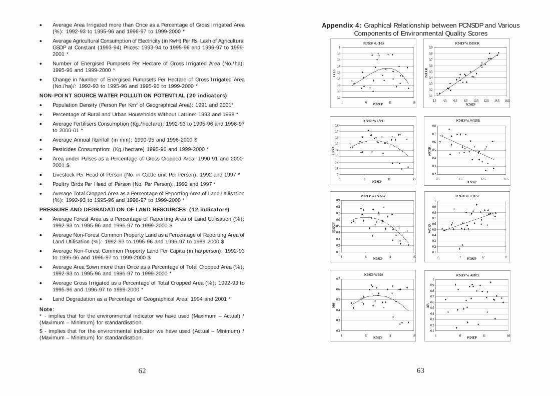
• Average Area Irrigated more than Once as a Percentage of Gross Irrigated Area(%): 1992-93 to 1995-96 and 1996-97 to 1999-2000 *
• Average Agricultural Consumption of Electricity (in KwH) Per Rs. Lakh of AgriculturalGSDP at Constant (1993-94) Prices: 1993-94 to 1995-96 and 1996-97 to 1999-2001 *
• Number of Energised Pumpsets Per Hectare of Gross Irrigated Area (No./ha):1995-96 and 1999-2000 *
• Change in Number of Energised Pumpsets Per Hectare of Gross Irrigated Area(No./ha)/: 1992-93 to 1995-96 and 1995-96 to 1999-2000 *
NON-POINT SOURCE WATER POLLUTION POTENTIAL (20 indicators)
• Population Density (Person Per Km2 of Geographical Area): 1991 and 2001*
• Percentage of Rural and Urban Households Without Latrine: 1993 and 1998 *
• Average Fertilisers Consumption (Kg./hectare): 1992-93 to 1995-96 and 1996-97to 2000-01 *
• Average Annual Rainfall (in mm): 1990-95 and 1996-2000 $
• Pesticides Consumption: (Kg./hectare) 1995-96 and 1999-2000 *
• Area under Pulses as a Percentage of Gross Cropped Area: 1990-91 and 2000-2001 $
• Livestock Per Head of Person (No. in Cattle unit Per Person): 1992 and 1997 *
• Poultry Birds Per Head of Person (No. Per Person): 1992 and 1997 *
• Average Total Cropped Area as a Percentage of Reporting Area of Land Utilisation(%): 1992-93 to 1995-96 and 1996-97 to 1999-2000 *
PRESSURE AND DEGRADATION OF LAND RESOURCES (12 indicators)
• Average Forest Area as a Percentage of Reporting Area of Land Utilisation (%):1992-93 to 1995-96 and 1996-97 to 1999-2000 $
• Average Non-Forest Common Property Land as a Percentage of Reporting Area ofLand Utilisation (%): 1992-93 to 1995-96 and 1996-97 to 1999-2000 $
• Average Non-Forest Common Property Land Per Capita (in ha/person): 1992-93to 1995-96 and 1996-97 to 1999-2000 $
• Average Area Sown more than Once as a Percentage of Total Cropped Area (%):1992-93 to 1995-96 and 1996-97 to 1999-2000 *
• Average Gross Irrigated as a Percentage of Total Cropped Area (%): 1992-93 to1995-96 and 1996-97 to 1999-2000 *
• Land Degradation as a Percentage of Geographical Area: 1994 and 2001 *
Note:* - implies that for the environmental indicator we have used (Maximum – Actual) /(Maximum – Minimum) for standardisation.
$ - implies that for the environmental indicator we have used (Actual – Minimum) /(Maximum – Minimum) for standardisation.
Appendix 4: Graphical Relationship between PCNSDP and VariousComponents of Environmental Quality Scores
PCNSDP Vs. GHGS
0.2
0.3
0.4
0.5
0.6
0.7
0.8
0.9
1
1 6 11 16PCNSDP
GHGS
PCNSDP Vs. LAND
0
0.1
0.2
0.3
0.4
0.5
0.6
0.7
0.8
1 6 11 16PCNSDP
LAND
PCNSDP Vs. WATER
0.2
0.3
0.4
0.5
0.6
0.7
0.8
2.5 7.5 12.5 17.5PCNSDP
WAT
ER
PCNSDP Vs. INDOOR
0.1
0.2
0.3
0.4
0.5
0.6
0.7
0.8
0.9
2.5 4.5 6.5 8.5 10.5 12.5 14.5 16.5PCNSDP
INDO
OR
PCNSDP Vs. FOREST
0.10.2
0.30.40.5
0.60.70.8
0.91
2 7 12 17PCNSDP
WAT
ER
PCNSDP Vs. AIRPOL
0.10.2
0.30.4
0.50.6
0.70.8
0.91
1 6 11 16PCNSDP
AIR
PCNSDP Vs. ENERGY
0.1
0.2
0.3
0.4
0.5
0.6
0.7
0.8
0.9
1 6 11 16PCNSDP
ENER
GY
PCNSDP Vs. NPS
0.2
0.3
0.4
0.5
0.6
0.7
1 6 11 16PCNSDPNP
S
62 63
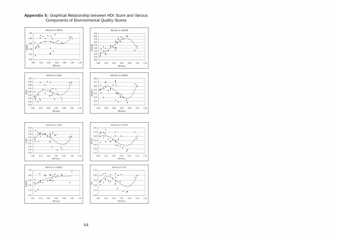
Appendix 5: Graphical Relationship between HDI Score and VariousComponents of Environmental Quality Scores
HDI Score Vs. AIRPOL
0.00
0.20
0.40
0.60
0.80
1.00
0.00 0.20 0.40 0.60 0.80 1.00 1.20HDI Score
AIRP
OLHDI Score Vs. INDOOR
0.000.100.200.300.400.500.600.700.800.90
0.00 0.20 0.40 0.60 0.80 1.00 1.20HDI Score
INDO
OR
HDI Score Vs. GHGS
0.200.300.400.500.600.700.800.901.00
0.00 0.20 0.40 0.60 0.80 1.00 1.20HDI Score
GHGS
HDI Score Vs. ENERGY
0.15
0.25
0.35
0.450.55
0.65
0.75
0.85
0.00 0.20 0.40 0.60 0.80 1.00 1.20HDI Score
ENER
GY
HDI Score Vs. LAND
0.000.100.200.300.400.500.600.700.80
0.00 0.20 0.40 0.60 0.80 1.00 1.20HDI Score
LAND
HDI Score Vs. W AT ER
0.20
0.30
0.40
0.50
0.60
0.70
0.80
0.00 0.20 0.40 0.60 0.80 1.00 1.20HDI Score
WAT
ER
HDI Score Vs. FOREST
0.00
0.20
0.40
0.60
0.80
1.00
0.00 0.20 0.40 0.60 0.80 1.00 1.20HDI Score
FORE
ST
HDI Score Vs. NP S
0.20
0.30
0.40
0.50
0.60
0.70
0.00 0.20 0.40 0.60 0.80 1.00 1.20HDI Score
NPS
64