arX

iv:1

008.

5253

v1 [

quan

t-ph

] 3

1 A

ug 2

010

Entanglement and nonlocality of one- and two-mode

combination squeezed state∗

Li-yun Hu1†, Xue-xiang Xu1,2, Qin Guo1, and Hong-yi Fan2

1College of Physics & Communication Electronics, Jiangxi Normal University, Nanchang 330022, China2Department of Physics, Shanghai Jiao Tong University, Shanghai 200030, China

October 16, 2018

Abstract

We investigate the entanglement and nonlocality properties of one- and two-modecombination squeezed vacuum state (OTCSS, with two-parameter λ and γ) by analyzingthe logarithmic negativity and the Bell’s inequality. It is found that this state exhibitslarger entanglement than that of the usual two-mode squeezed vacuum state (TSVS),and that in a certain regime of λ, the violation of Bell’s inequality becomes more obvious,which indicates that the nonlocality of OTCSS can be stronger than that of TSVS. Asan application of OTCSS, the quantum teleportaion is examined, which shows thatthere is a region spanned by λ and γin which the fidelity of OTCSS channel is largerthan that of TSVS.

Keywords: Entanglement, nonlocality, IWOP technique, teleportation

PACS number(s): 42.50.Dv, 03.65.Wj, 03.67.Mn

1 Introduction

Entanglement between quantum systems plays a key role in quantum information process-ing, such as quantum teleportation, dense coding, and quantum cloning. In recent years,various entangled states have brought considerable attention and interests of physicists be-cause of their potential uses in quantum communication [1, 2]. For instance, the two-modesqueezed state is a typical entangled state of continuous variable and exhibits quantum en-tanglement between the idle-mode and the signal-mode in a frequency domain manifestly.Theoretically, the two-mode squeezed state is constructed by the two-mode squeezing op-erator S = exp[λ(a1a2 − a†1a

†2)] [3–5] acting on the two-mode vacuum state |00〉,

S |00〉 = sechλ exp[

−a†

1a†

2 tanhλ]

|00〉 , (1)

where λ is a squeezing parameter, the disentangling of S can be obtained by using SU(1,1)

Lie algebra, [a1a2, a†1a

†2] = a†1a1 + a†2a2 + 1, or by using the entangled state representation

∗Work supported by a grant from the Key Programs Foundation of Ministry of Education ofChina (No. 210115) and the Research Foundation of the Education Department of Jiangxi Provinceof China (No. GJJ10097).

†Corresponding author. E-mail: hlyun2008@126.com.

1

|η〉 [6–8], which was constructed according to the idea of Einstein, Podolsky and Rosen intheir argument that quantum mechanics is incomplete [9].

Using the relation between Bosonic operators and the coordinate Qi, momentum Pi, Qi =(ai + a†i )/

√2, Pi = (ai − a†i )/(

√2i), and introducing the two-mode quadrature operators

of light field, x1 = (Q1 +Q2)/2, x2 = (P1 + P2)/2, the variances of x1 and x2 in the stateS |00〉 are in the standard form

〈00| S†x22S |00〉 = 1

4e−2λ, 〈00|S†x21S |00〉 = 1

4e2λ, (2)

thus we get the standard squeezing for the two quadrature: x1 → 1

2eλx1, x2 → 1

2e−λx2.

On the other hand, the two-mode squeezing operator can also be recast into the formS = exp [iλ (Q1P2 +Q2P1)] . Then some interesting questions naturally rise: what is theproperty of the following operator

V = exp [−i (λ1Q1P2 + λ2Q2P1)] , (3)

with two parameters λ1 = λeγ , λ2 = λe−γ , λ > 0? What is the normally ordered expansionof V and what is the state V |00〉? What are the entanglement and nonlocality propertiesof V |00〉? When γ = 0, Eq.(3) just reduces to the usual two-mode squeezing operator S.Thus we can consider V as a generalized two-mode squeezing operator and V |00〉 as one-and two-mode combination squeezed vacuum state (OTCSS).

In this paper, we investigate entanglement properties and quantum nonlocality of V |00〉in terms of logarithmic negativity and the Bell’s inequality, respectively. Subsequently, weconsider its application in the field of quantum teleportation by using the characteristic-function formula. It is shown that this state exhibits larger entanglement than that of theusual two-mode squeezed vacuum state (TSVS); and in a certain smaller regime of λ, thatthe nonlocality of this state can be stronger than that of TSVS due to the presence of γ.In addition, application to quantum teleportation with OTCSS is also considered, whichshows that there is a region spanned by λ and γ in which the fidelity of OTCSS channel islarger than that of TSVS.

Our paper is arranged as follows. In section 2, we derive the normal ordering form ofone- and two-mode combination squeezing operator by using the technique of integrationwithin an ordered product (IWOP) of operators. In section 3, using the Weyl ordering formof single-mode Wigner operator and the order-invariance of Weyl ordered operators undersimilar transformations, we derive analytically the Wigner function of V |00〉. Sections 4and 5 are devoted to investigating the entanglement properties and the nonlocal propertiesOTCSS by using the Bell’s inequality and the logarithmic negativity, respectively. An ap-plication to quantum teleportation with OTCSS is involved in section 6. We end with themain conclusions of our work.

2 The normal ordering form of V and fluctuations in V |00〉

In order to know V |00〉 , we need to derive the normal ordering form of the unitary operatorV by virtue of the IWOP technique [10–12]. Using the Baker-Hausdorff formula,

eABe−A = B + [A,B] +1

2![A, [A,B]] +

1

3![A, [A, [A,B]]] + · · · , (4)

2

and noticing that

i [λ1Q1P2 + λ2Q2P1, Q1] = λ2Q2, (5)

i [λ1Q1P2 + λ2Q2P1, Q2] = λ1Q1, (6)

i [λ1Q1P2 + λ2Q2P1, P1] = −λ1P2, (7)

i [λ1Q1P2 + λ2Q2P1, P2] = −λ2P1, (8)

we have

V −1Q1V = Q1 cosh λ+Q2e−γ sinhλ, (9)

V −1Q2V = Q2 cosh λ+Q1eγ sinhλ, (10)

V −1P1V = P1 coshλ− P2eγ sinhλ, (11)

V −1P2V = P2 coshλ− P1e−γ sinhλ. (12)

Thus, in order to keep the eigenvalues invariant under the V transformation, i..e.,

V −1QkV |q1q2〉′ = qk |q1q2〉′ , (k = 1, 2), (13)

the base vector must be changed to

|q1q2〉′ = V −1 |q1q2〉 =∣

∣

∣

∣

Λ−1

(

q1q2

)⟩

,Λ =

(

coshλ e−γ sinhλeγ sinhλ coshλ

)

, (14)

where |q1q2〉 = |q1〉 ⊗ |q2〉, and |qk〉 is the coordinate eigenstate,

|qk〉 = π−1/4 exp[−1

2q2 +

√2qa† − 1

2a†2] |0〉 . (15)

Using the completeness raltion∫∞−∞ dq1dq2 |q1, q2〉 〈q1, q2| = 1, we have

V −1 =

∫ ∞

−∞dq1dq2

∣

∣

∣

∣

Λ−1

(

q1q2

)⟩

〈q1, q2| , (16)

which leads to

V =

∫ ∞

−∞dq1dq2

∣

∣

∣

∣

Λ

(

q1q2

)⟩

〈q1, q2| . (17)

Actually, one can check (17) by V −1V = V V −1 = 1. Further using the vacuum projec-tor |00〉 〈00| =: exp[−a†a − b†b] : ( : : denoting normal ordering), as well as the IWOPtechnique, we can put V into the normal ordering form [13],

V =2√Lexp

{

1

L

[(

b†2 − a†2)

sinh2 λ sinh 2γ + 2a†b† sinh 2λ cosh γ]

}

: exp

{

4

L

[(

a†a+ b†b)

cosh λ+(

b†a− a†b)

sinhλ sinh γ]

− a†a− b†b}

:

exp

{

1

L

[

(

b2 − a2)

sinh2 λ sinh 2γ − 2a†b† sinh 2λ cosh γ]

}

, (18)

where L = 4(

1 + sinh2 γ tanh2 λ)

cosh2 λ. Eq. (18) is just the normal ordering form of V . Itis obviously to see that when γ = 0, Eq.(18) just reduces to the usual two-mode squeezing

3

operator. Operating V on the two-mode vacuum state |00〉, we obtain the squeezed vacuumstate,

V |00〉 = 2√Lexp

{

1

L

[(

b†2 − a†2)

sinh2 λ sinh 2γ + 2a†b† sinh 2λ cosh γ]

}

|00〉 . (19)

On the other hand, by using the transformations Eqs.(9)-(12), one can derive the vari-ances of x1 and x2 in the state V |00〉 [13]

⟨

(∆x1)2⟩

=1

4

(

cosh 2λ+ 2 sinh2 λ sinh2 γ + sinh 2λ cosh γ)

, (20)

⟨

(∆x2)2⟩

=1

4

(

cosh 2λ+ 2 sinh2 λ sinh2 γ − sinh 2λ cosh γ)

, (21)

which indicate that the variances are not only dependent on parameter λ, but also on

parameter γ. When γ = 0, Eqs.(20) and (21) reduce to⟨

(∆x1)2⟩

= 1

4e2λ, and

⟨

(∆x2)2⟩

=1

4e−2λ, corresponding to the usual TSVS. In particular, by modulating the two parameters

(λ and γ), we can realize that

⟨

(∆x1)2⟩

>1

4e2λ,

⟨

(∆x2)2⟩

<1

4e−2λ, (22)

whose condition is given by

0 < tanhλ <1

1 + cosh γ, λ > 0, (23)

which mean that the OTCSS may exhibit stronger squeezing in one quadrature than that ofthe TSVS while exhibiting weaker squeezing in another quadrature when the condition (23)satisfied. Then, can the OTCSS exhibits stronger nonlocality or more observable violationof Bell’s inequality? In the following, we pay our attention to these two aspects.

3 Wigner function of V |00〉

Wigner distribution functions [14–16] of quantum states are widely studied in quantumstatistics and quantum optics. Now we derive the expression of the Wigner function ofV |00〉 . Here we take a new method to do it. Recalling that in Ref. [17–19] we have intro-duced the Weyl ordering form of single-mode Wigner operator ∆1 (q1, p1),

∆1 (q1, p1) =:

:δ (q1 −Q1) δ (p1 − P1)

:

:, (24)

its normal ordering form is

∆1 (q1, p1) =1

π: exp

[

− (q1 −Q1)2 − (p1 − P1)

2]

: , (25)

where the symbols : : and :

:

:

:denote the normal ordering and the Weyl ordering, respec-

tively. Note that the order of Bose operators a1 and a†1 within a normally ordered product

and a Weyl ordered product can be permuted. That is to say, even though [a1, a†1] = 1, we

can have : a1a†1 : =: a†1a1 : and :

:a1a

†1:

:= :

:a†1a1

:

:.

4

For one- and two-mode combination squeezed vacuum state V |00〉, its Wigner functionis given by

W (q1, p1; q2, p2) = tr

[

V |00〉 〈00|V −1∆1 (q1, p1)∆2 (q2, p2)]

= 〈00|U |00〉 , (26)

where U = V −1∆1 (q1, p1)∆2 (q2, p2)V. Further using Eq.(24), noticing that the Weyl or-dering has a remarkable property, i.e., the order-invariance of Weyl ordered operators undersimilar transformations [17–19], which means

V −1 :

:(◦ ◦ ◦) :

:V =

:

:V −1 (◦ ◦ ◦)V :

:, (27)

as if the “fence” :

:

:

:did not exist, thus U can be cast into the following form (see appendix

A),

U = V −1 :

:δ (q1 −Q1) δ (p1 − P1) δ (q2 −Q2) δ (p2 − P2)

:

:V

= ∆1

(

q1 coshλ− q2e−γ sinhλ, p1 cosh λ+ p2e

γ sinhλ)

×∆2

(

q2 coshλ− q1eγ sinhλ, p2 cosh λ+ p1e

−γ sinhλ)

. (28)

So the Wigner function of V |00〉 is given by

W (q1, p1; q2, p2) =1

π2exp

{

−m1

(

q21 + p22)

−m2

(

p21 + q22)

+ 2 (q1q2 − p1p2)m3

}

, (29)

where

m1 = cosh2 λ+ e2γ sinh2 λ, m2 = cosh2 λ+ e−2γ sinh2 λ, m3 = cosh γ sinh 2λ.

In particular, when γ = 0, Eq.(29) becomes

W (q1, p1; q2, p2) =1

π2exp

{

−(

p21 + p22 + q21 + q22)

cosh 2λ

+2 (q1q2 − p1p2) sinh 2λ} , (30)

which is just the Wigner function of the usual TSVS.

4 Entanglement properties of V |00〉

In this section, we consider the entanglement properties of V |00〉. It is well known that atwo-mode Gaussian state can be completely characterized by its first and second statisticalmoments and the covariance matrix of elements σ. In general, the first statistical momentscan be adjusted by local displacements without affecting entanglement, thus they they willcan be set to be zero without loss of generality and the behavior of the covariance matrix σ isall important for the study of entanglement. There are several quantitative measurements ofquantum entanglement proposed [20–22]. For a two-mode Gaussian state, the entanglementis best characterized by the logarithmic negativity EN , a quantity evaluated in terms of thesymplectic eigenvalues of σ [23, 24].

In order to evaluate the entanglement of V |00〉 , we reform Eq.(29) as follows in terms ofphase space quadrature variables,

5

W (q1, p1; q2, p2) =1

π2exp

[

−1

2

(

q1 p1 q2 p2)

σ−1(

q1 p1 q2 p2)T

]

, (31)

where the covariance matrix σ of this OTCSS is [25]

σ =

(

u wwT v

)

, u =1

2

(

m2 00 m1

)

, v =1

2

(

m1 00 m2

)

, w =1

2

(

m3 00 −m3

)

.

(32)In particular, when γ = 0, m1 = m2 = cosh 2λ, m3 = sinh 2λ, Eq.(32) just reduces to theso-called standard form of covariance matrix for TSVS [24].

The condition for entanglement of a Gaussian state is derived from the partially trans-posed density matrix (PPT criterion) [24], according to the smallest symplectic eigenvaluens of the partially transposed state, ns < 1

2, i.e., ns >

1

2means the a two-mode Gaussian

state is separable, where ns is defined as

ns = min [n+, n−] , (33)

and n± is given by [26]

n± =

√

∆ (σ)± (∆ (σ)2 − 4 det σ)1/2

2, (34)

where ∆ (σ) = ∆ (σ) = detu+ det v − 2 detw.

Using Eqs.(32)-(34), the corresponding sympletic eigenvalues n± are then given by

n± =1

2(√m1m2 ±m3) . (35)

One the other hand, the corresponding quantification of entanglement is given by the log-arithmic negativity EN defined as [20,26,27],

EN = max [0,− ln 2ns] . (36)

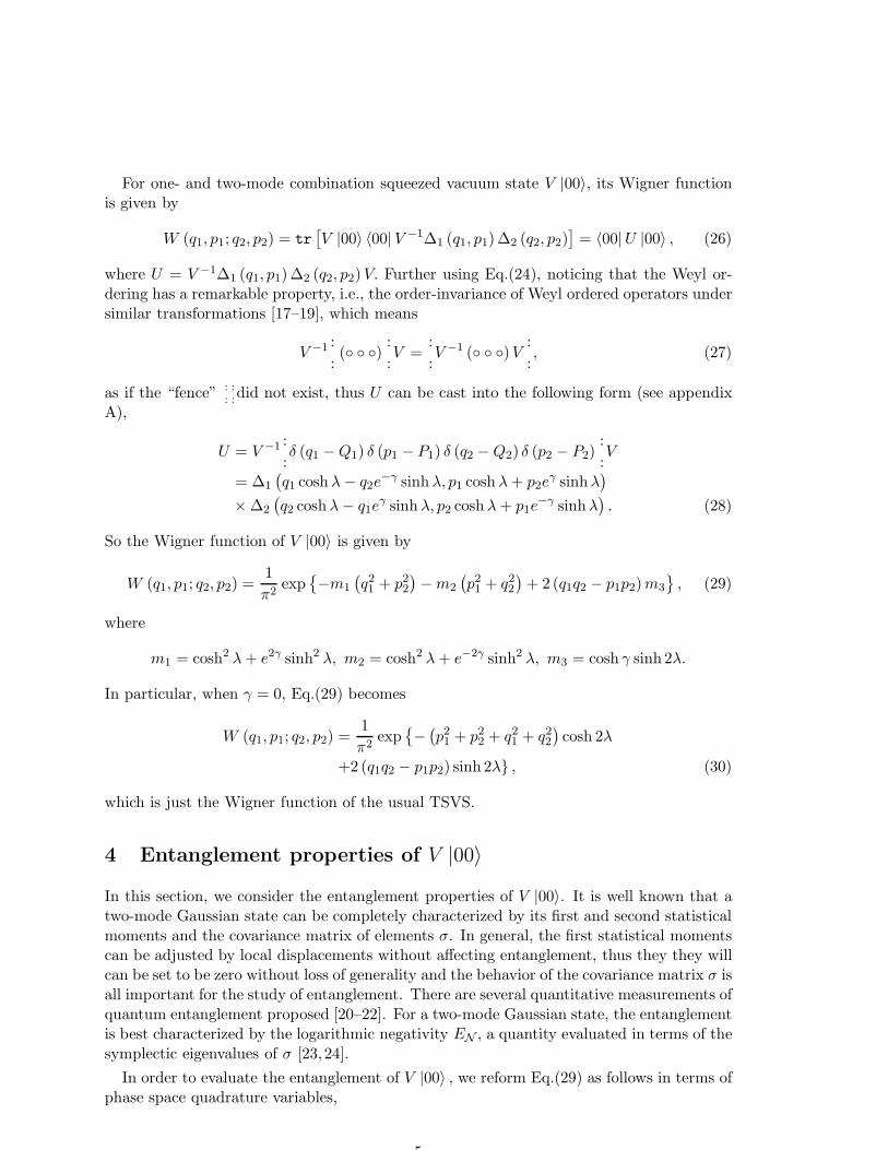
From Eqs.(32), (35) and (36), one can clearly see that the logarithmic negativity EN isdependent on λ and γ. In figure 1, we plot the logarithmic negativity EN as a function ofparameters λ and γ. From Fig.1, we clearly see a new feature, i.e., in presence of parameterγ, the logarithmic negativity becomes larger than that of tha usual squeezed state (γ = 0).

5 Violations of Bell’s inequality for V |00〉

We now turn our attention to the nonlocal properties of V |00〉 in terms of the Bell’s in-equality. For a two-mode continuous variable system, the Bell’s inequality is given, usingcorrelations between parity measurement, by

|B| ≡∣

∣

∣

⟨

Πab(

α′, β′)+ Πab(

α, β′)+ Πab(

α′, β)

− Πab (α, β)⟩∣

∣

∣6 2, (37)

6

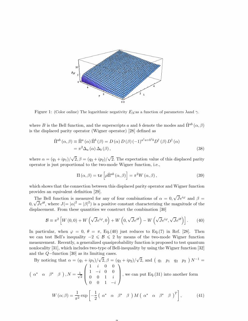
Figure 1: (Color online) The logarithmic negativity EN as a function of parameters λand γ.

where B is the Bell function, and the superscripts a and b denote the modes and Πab (α, β)is the displaced parity operator (Wigner operator) [28] defined as

Πab (α, β) ≡ Πa (α) Πb (β) = D (α)D (β) (−1)a†a+b†bD† (β)D† (α)

= π2∆a (α)∆b (β) , (38)

where α = (q1 + ip1)/√2, β = (q2 + ip2)/

√2. The expectation value of this displaced parity

operator is just proportional to the two-mode Wigner function, i.e.,

Π (α, β) = tr

[

ρΠab (α, β)]

= π2W (α, β) , (39)

which shows that the connection between this displaced parity operator andWigner functionprovides an equivalent definition [29].

The Bell function is measured for any of four combinations of α = 0,√Jeiϕ and β =

0,√Jeiθ, where J(= |α|2 = |β|2) is a positive constant characterizing the magnitude of the

displacement. From these quantities we construct the combination [30]

B ≡ π2[

W (0, 0) +W(√

Jeiϕ, 0)

+W(

0,√Jeiθ

)

−W(√

Jeiϕ,√Jeiθ

)]

. (40)

In particular, when ϕ = 0, θ = π, Eq.(40) just reduces to Eq.(7) in Ref. [28]. Thenwe can test Bell’s inequality −2 6 B 6 2 by means of the two-mode Wigner functionmeasurement. Recently, a generalized quasiprobability function is proposed to test quantumnonlocality [31], which includes two-type of Bell-inequality by using the Wigner function [32]and the Q−function [30] as its limiting cases.

By noticing that α = (q1 + ip1)/√2, β = (q2 + ip2)/

√2, and

(

q1 p1 q2 p2)

N−1 =

(

α∗ α β∗ β)

, N = 1√2

1 i 0 01 −i 0 00 0 1 i0 0 1 −i

, we can put Eq.(31) into another form

W (α;β) =1

π2exp

[

−1

2

(

α∗ α β∗ β)

M(

α∗ α β∗ β)T

]

, (41)

7

B

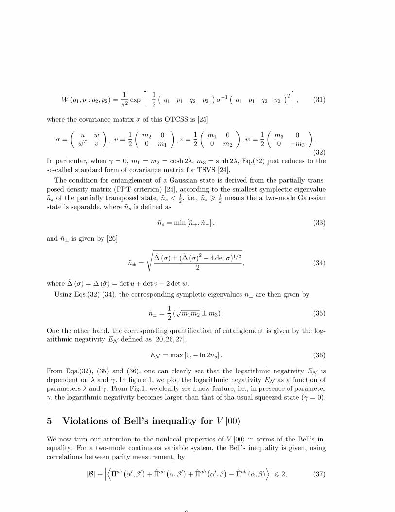
Figure 2: (Color online) Plot of the Bell function Bas a function of parameters λand J , for

γ = 0, θ = π, ϕ = 0. Only values exceeding the bound imposed by local theories are shown.

where M is a 4× 4 Hermitian matrix

M =

m1 −m2 m1 +m2 −2m3 0m1 +m2 m1 −m2 0 −2m3

−2m3 0 m2 −m1 m1 +m2

0 −2m3 m1 +m2 m2 −m1

. (42)

Substituting Eq.(41) into Eq.(40) we have

B = 1 + exp[

−2J cosh2 λ− 2J(

e2γ cos2 ϕ+ e−2γ sin2 ϕ)

sinh2 λ]

+ exp[

−2J cosh2 λ− 2J(

e2γ sin2 θ + e−2γ cos2 θ)

sinh2 λ]

− exp{

−4J cosh2 λ− 2J(

cos2 ϕ+ sin2 θ)

e2γ sinh2 λ

−2J(

sin2 ϕ+ cos2 θ)

e−2γ sinh2 λ+ 4J cos (θ + ϕ) cosh γ sinh 2λ}

, (43)

Thus we can say that V |00〉 is quantum mechanically nonlocal as |B| > 2, and the non-locality is stronger with the increase of |B|. From Eq.(43) one can see that the degree ofnonlocality not only depends on the coherent amplitude J , on the phases θ and ϕ, but alsoon the parameter γ. In particular, when ϕ = 0, θ = π, Eq.(43) just reduces to

B = 1 + exp[

−2J(

cosh2 λ+ e2γ sinh2 λ)]

+ exp[

−2J(

cosh2 λ+ e−2γ sinh2 λ)]

− exp[

−4J(

cosh2 λ+ cosh 2γ sinh2 λ)

− 4J cosh γ sinh 2λ]

, (44)

which further becomes Eq.(7) in Ref. [28] with γ = 0.

In figure 2, we plot Bell function in the space spanned by parameters J and λ with γ = 0(corresponding to the usual squeezed vacuum state). From Fig. 2, one can clearly see thatthe result (43) violates the upper bound imposed by local theories. With the increase of λ,the violation of Bell’s inequality becomes more observable for smaller J .

As depicted in Fig. 3, the Bell function also violates the upper bound in the spacespanned by parameters γ and λ with given α, β values. From Fig.3, one can see that for agiven small γ, the violation of Bell’s inequality becomes more observable with the increase

8

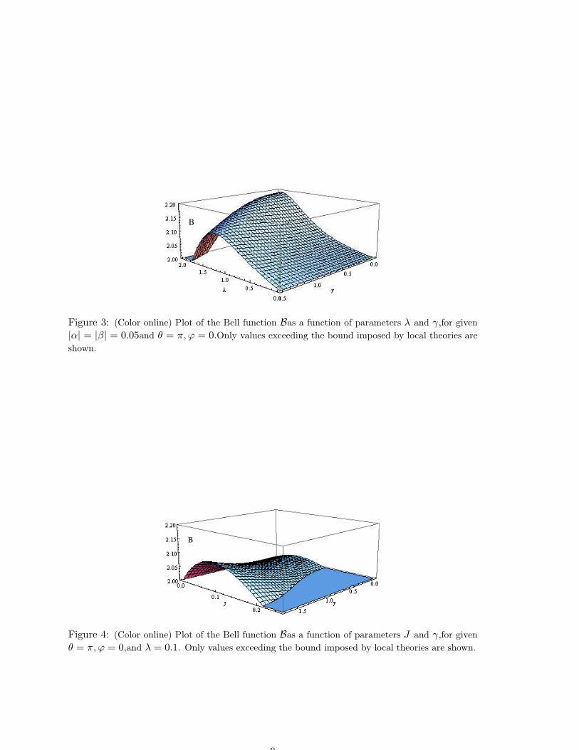
B

Figure 3: (Color online) Plot of the Bell function Bas a function of parameters λ and γ,for given|α| = |β| = 0.05and θ = π, ϕ = 0.Only values exceeding the bound imposed by local theories are

shown.

B

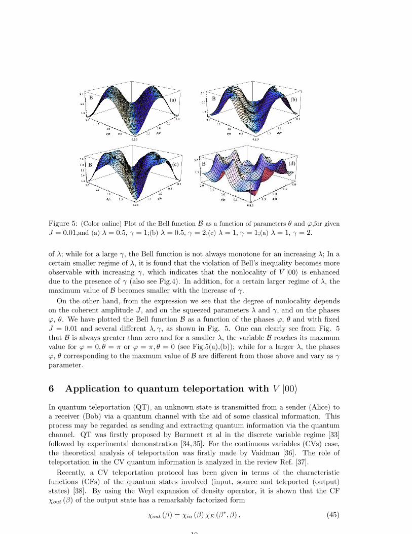
Figure 4: (Color online) Plot of the Bell function Bas a function of parameters J and γ,for givenθ = π, ϕ = 0,and λ = 0.1. Only values exceeding the bound imposed by local theories are shown.

9

B B (b)(a)

(d)B(c)B

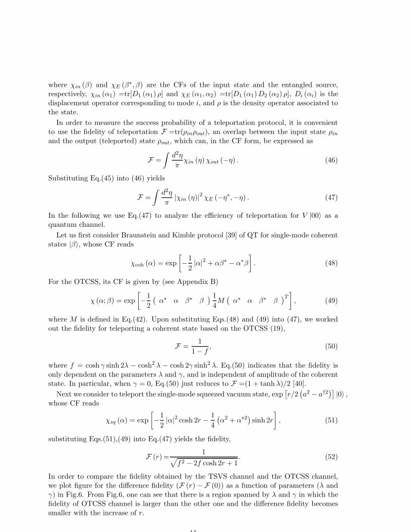
Figure 5: (Color online) Plot of the Bell function B as a function of parameters θ and ϕ,for givenJ = 0.01,and (a) λ = 0.5, γ = 1;(b) λ = 0.5, γ = 2;(c) λ = 1, γ = 1;(a) λ = 1, γ = 2.

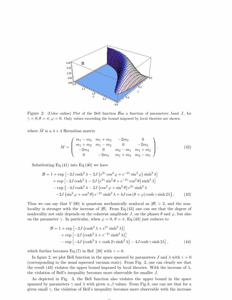
of λ; while for a large γ, the Bell function is not always monotone for an increasing λ; In acertain smaller regime of λ, it is found that the violation of Bell’s inequality becomes moreobservable with increasing γ, which indicates that the nonlocality of V |00〉 is enhanceddue to the presence of γ (also see Fig.4). In addition, for a certain larger regime of λ, themaximum value of B becomes smaller with the increase of γ.

On the other hand, from the expression we see that the degree of nonlocality dependson the coherent amplitude J , and on the squeezed parameters λ and γ, and on the phasesϕ, θ. We have plotted the Bell function B as a function of the phases ϕ, θ and with fixedJ = 0.01 and several different λ, γ, as shown in Fig. 5. One can clearly see from Fig. 5that B is always greater than zero and for a smaller λ, the variable B reaches its maxmumvalue for ϕ = 0, θ = π or ϕ = π, θ = 0 (see Fig.5(a),(b)); while for a larger λ, the phasesϕ, θ corresponding to the maxmum value of B are different from those above and vary as γparameter.

6 Application to quantum teleportation with V |00〉In quantum teleportation (QT), an unknown state is transmitted from a sender (Alice) toa receiver (Bob) via a quantum channel with the aid of some classical information. Thisprocess may be regarded as sending and extracting quantum information via the quantumchannel. QT was firstly proposed by Barnnett et al in the discrete variable regime [33]followed by experimental demonstration [34, 35]. For the continuous variables (CVs) case,the theoretical analysis of teleportation was firstly made by Vaidman [36]. The role ofteleportation in the CV quantum information is analyzed in the review Ref. [37].

Recently, a CV teleportation protocol has been given in terms of the characteristicfunctions (CFs) of the quantum states involved (input, source and teleported (output)states) [38]. By using the Weyl expansion of density operator, it is shown that the CFχout (β) of the output state has a remarkably factorized form

χout (β) = χin (β)χE (β∗, β) , (45)

10

where χin (β) and χE (β∗, β) are the CFs of the input state and the entangled source,respectively, χin (α1) =tr[D1 (α1) ρ] and χE (α1, α2) =tr[D1 (α1)D2 (α2) ρ], Di (αi) is thedisplacement operator corresponding to mode i, and ρ is the density operator associated tothe state.

In order to measure the success probability of a teleportation protocol, it is convenientto use the fidelity of teleportation F =tr(ρinρout), an overlap between the input state ρinand the output (teleported) state ρout, which can, in the CF form, be expressed as

F =

∫

d2η

πχin (η)χout (−η) . (46)

Substituting Eq.(45) into (46) yields

F =

∫

d2η

π|χin (η)|2 χE (−η∗,−η) . (47)

In the following we use Eq.(47) to analyze the efficiency of teleportation for V |00〉 as aquantum channel.

Let us first consider Braunstein and Kimble protocol [39] of QT for single-mode coherentstates |β〉, whose CF reads

χcoh (α) = exp

[

−1

2|α|2 + αβ∗ − α∗β

]

. (48)

For the OTCSS, its CF is given by (see Appendix B)

χ (α;β) = exp

[

−1

2

(

α∗ α β∗ β) 1

4M

(

α∗ α β∗ β)T

]

, (49)

where M is defined in Eq.(42). Upon substituting Eqs.(48) and (49) into (47), we workedout the fidelity for teleporting a coherent state based on the OTCSS (19),

F =1

1− f, (50)

where f = cosh γ sinh 2λ − cosh2 λ − cosh 2γ sinh2 λ. Eq.(50) indicates that the fidelity isonly dependent on the parameters λ and γ, and is independent of amplitude of the coherentstate. In particular, when γ = 0, Eq.(50) just reduces to F =(1 + tanhλ)/2 [40].

Next we consider to teleport the single-mode squeezed vacuum state, exp[

r/2(

a2 − a†2)]

|0〉 ,whose CF reads

χsq (α) = exp

[

−1

2|α|2 cosh 2r − 1

4

(

α2 + α∗2) sinh 2r]

, (51)

substituting Eqs.(51),(49) into Eq.(47) yields the fidelity,

F (r)=1

√

f2 − 2f cosh 2r + 1. (52)

In order to compare the fidelity obtained by the TSVS channel and the OTCSS channel,we plot figure for the difference fidelity (F (r)−F (0)) as a function of parameters (λ andγ) in Fig.6. From Fig.6, one can see that there is a region spanned by λ and γ in which thefidelity of OTCSS channel is larger than the other one and the difference fidelity becomessmaller with the increase of r.

11

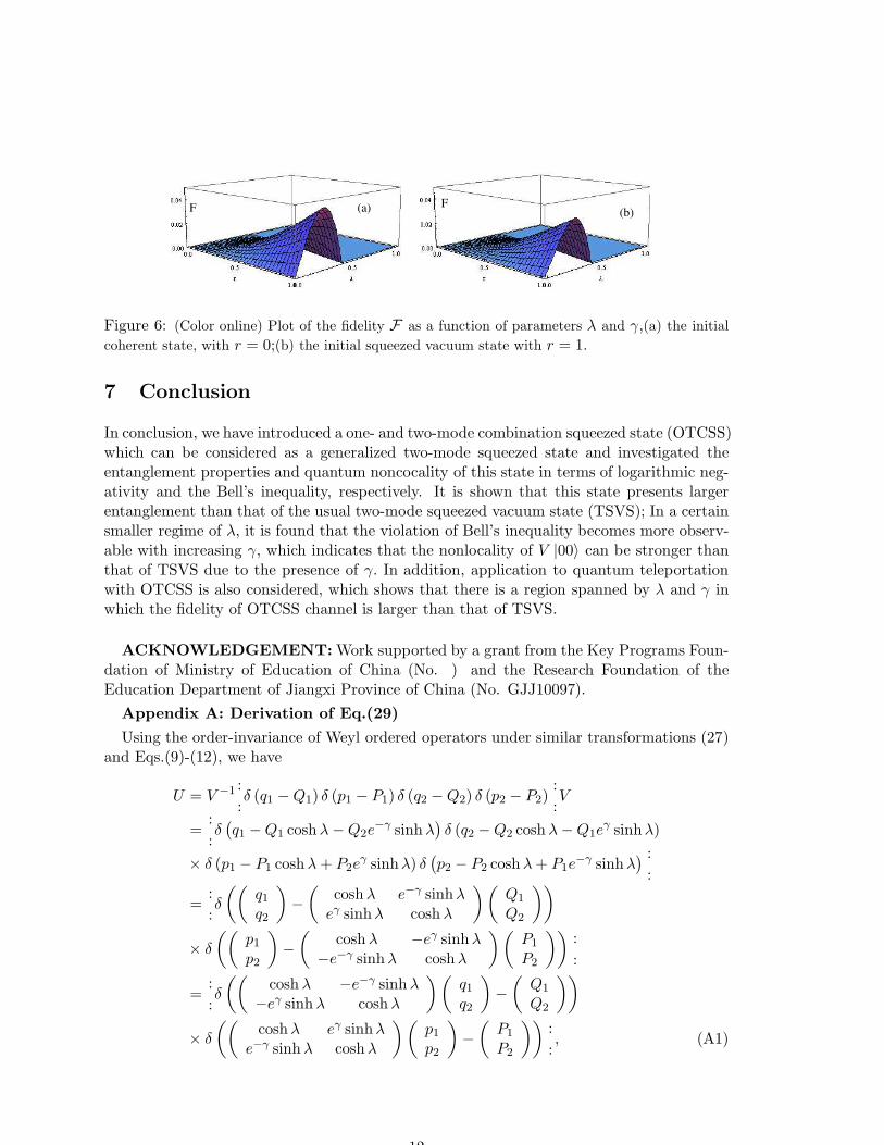
FF (a) (b)

Figure 6: (Color online) Plot of the fidelity F as a function of parameters λ and γ,(a) the initial

coherent state, with r = 0;(b) the initial squeezed vacuum state with r = 1.

7 Conclusion

In conclusion, we have introduced a one- and two-mode combination squeezed state (OTCSS)which can be considered as a generalized two-mode squeezed state and investigated theentanglement properties and quantum noncocality of this state in terms of logarithmic neg-ativity and the Bell’s inequality, respectively. It is shown that this state presents largerentanglement than that of the usual two-mode squeezed vacuum state (TSVS); In a certainsmaller regime of λ, it is found that the violation of Bell’s inequality becomes more observ-able with increasing γ, which indicates that the nonlocality of V |00〉 can be stronger thanthat of TSVS due to the presence of γ. In addition, application to quantum teleportationwith OTCSS is also considered, which shows that there is a region spanned by λ and γ inwhich the fidelity of OTCSS channel is larger than that of TSVS.

ACKNOWLEDGEMENT:Work supported by a grant from the Key Programs Foun-dation of Ministry of Education of China (No. ) and the Research Foundation of theEducation Department of Jiangxi Province of China (No. GJJ10097).

Appendix A: Derivation of Eq.(29)

Using the order-invariance of Weyl ordered operators under similar transformations (27)and Eqs.(9)-(12), we have

U = V −1 :

:δ (q1 −Q1) δ (p1 − P1) δ (q2 −Q2) δ (p2 − P2)

:

:V

=:

:δ(

q1 −Q1 coshλ−Q2e−γ sinhλ

)

δ (q2 −Q2 cosh λ−Q1eγ sinhλ)

× δ (p1 − P1 coshλ+ P2eγ sinhλ) δ

(

p2 − P2 coshλ+ P1e−γ sinhλ

) :

:

=:

:δ

((

q1q2

)

−(

coshλ e−γ sinhλeγ sinhλ cosh λ

)(

Q1

Q2

))

× δ

((

p1p2

)

−(

cosh λ −eγ sinhλ−e−γ sinhλ coshλ

)(

P1

P2

))

:

:

=:

:δ

((

cosh λ −e−γ sinhλ−eγ sinhλ coshλ

)(

q1q2

)

−(

Q1

Q2

))

× δ

((

coshλ eγ sinhλe−γ sinhλ coshλ

)(

p1p2

)

−(

P1

P2

))

:

:, (A1)

12

which indicates that (comparing with Eq.(24))

U =:

:δ(

q1 coshλ− q2e−γ sinhλ−Q1

)

δ (p1 cosh λ+ p2eγ sinhλ− P1)

× δ (q2 cosh λ− q1eγ sinhλ−Q2) δ

(

p2 coshλ+ p1e−γ sinhλ− P2

) :

:= Eq.(29). (A2)

Thus the Wigner function of V |00〉 is

W (q1, p1; q2, p2) =1

π2exp

{

−(

q1 coshλ− q2e−γ sinhλ

)2 − (q2 cosh λ− q1eγ sinhλ)2

− (p1 coshλ+ p2eγ sinhλ)2 −

(

p2 cosh λ+ p1e−γ sinhλ

)2}

= (29). (A3)

Appendix B: Derivation of characteristic function of V |00〉For two-mode quantum state V |00〉, its characteristic function is given by

χ (q1, p1; q2, p2) = tr

[

V |00〉 〈00|V −1D1 (q1, p1)D2 (q2, p2)]

= 〈00|V −1D1 (q1, p1)D2 (q2, p2)V |00〉 , (B1)

whereDi (qi, pi) (i = 1, 2) are the displacement operators, defined byDi (qi, pi) = exp [i (piQi − qiPi)] .

Noticing that the Weyl ordering of Di (qi, pi) is itself, Di (qi, pi) =:

:Di (qi, pi)

:

:, and that

a remarkable property of the invariance of Weyl ordered operators under similar transfor-mations (27), we have

V −1D1 (q1, p1)D2 (q2, p2)V

= V −1 :

:exp [i (p1Q1 − q1P1)] exp [i (p2Q2 − q2P2)]

:

:V

=:

:exp

[

i(

p1(

Q1 coshλ+Q2e−γ sinhλ

)

− q1 (P1 coshλ− P2eγ sinhλ)

)]

× exp[

i(

p2 (Q2 coshλ+Q1eγ sinhλ)− q2

(

P2 cosh λ− P1e−γ sinhλ

))] :

:

=:

:exp

[

i(

p′1Q1 − q′1P1

)]

exp[

i(

p′2Q2 − q′2P2

)] :

:= D1

(

q′1, p′1

)

D2

(

q′2, p′2

)

, (B2)

where

q′1 = q1 coshλ− q2e−γ sinhλ, p′1 = p1 cosh λ+ p2e

γ sinhλ,

q′2 = q2 coshλ− q1eγ sinhλ, p′2 = p2 cosh λ+ p1e

−γ sinhλ. (B3)

Then substituting Eqs.(B2), (B3) into Eq.(B1) we can directly obtain the CF of V |00〉 ,

χ (q1, p1; q2, p2) = 〈00|D1

(

q′1, p′1

)

D2

(

q′2, p′2

)

|00〉

= exp

[

−1

2

(

q1 p1 q2 p2)

σ(

q1 p1 q2 p2)T

]

, (B4)

or

χ (α;β) = exp

[

−1

2

(

α∗ α β∗ β)

σ(

α∗ α β∗ β)T

]

, (B5)

13

where

σ =1

2

m1 0 −m3 00 m2 0 m3

−m3 0 m2 00 m3 0 m1

, σ = NσNT =1

4M. (B6)

When γ = 0, (m1 +m2) → 2 cosh 2λ,m3 → sinh 2λ,we have

χ (α;β) = exp

[

−1

2

(

|α|2 + |β|2)

cosh 2λ+1

2(α∗β∗ + αβ) sinh 2λ

]

, (B7)

which is just the CF of the usual TSVS.

References

[1] D. Bouwmeester et al., The Physics of Quantum Information, (Springer, Berlin) 2000.

[2] M. A. Nielsen and I. L. Chuang, Quantum Computation and Quantum Information

(Cambridge University Press) 2000.

[3] V. Buzek, J. Mod. Opt. 37 (1990) 303.

[4] R. Loudon, P. L. Knight, J. Mod. Opt. 34 (1987) 709.

[5] V. V. Dodonov, J. Opt. B: Quantum Semiclass. Opt. 4 (2002) R1.

[6] Hong-yi Fan and J. R. Klauder, Phys. Rev. A 49 (1994) 704.

[7] Hong-yi Fan and Y. Fan, Phys. Rev. A 54 (1996) 958.

[8] Li-yun Hu and Hong-yi Fan, Europhys. Lett. 85 (2009) 60001.

[9] A. Einstein, B. Poldolsky and N. Rosen, Phys. Rev. 47 (1935) 777.

[10] Li-yun Hu and Hong-yi Fan, Phys. Rev. A 80 (2009) 022115; Opt. Commun. 282 (2009)3734.

[11] Hong-yi Fan and Li-yun Hu, Opt. Commun. 281 (2008) 1629; 281 (2008) 5571.

[12] Hong-yi Fan, J Opt B: Quantum Semiclass. Opt. 5 (2003) R147

[13] Hong-yi Fan, Phys. Rev. A 41 (1990) 1526.

[14] E. P. Wigner, Phys. Rev. 40 (1932) 749.

[15] R. F. O’Connell and E. P. Wigner, Phys. Lett. A 83 (1981) 145.

[16] W. P. Schleich, Quantum Optics in Phase Space, Wiley-VCH, Berlin, 2001.

[17] Hong-yi Fan, J. Phys. A 25 (1992) 3443; Hong-yi Fan, Y. Fan, Int. J. Mod. Phys. A17 (2002) 701.

[18] Hong-yi Fan, Mod. Phys. Lett. A 15 (2000) 2297.

[19] Hong-yi Fan, Ann. Phys. (New York) 323 (2008) 500; 323 (2008) 1502.

14

[20] G. Vidal and R. F. Werner, Phys. Rev. A 65 (2002) 032314.

[21] J. Eisert and M. B. Plenio, J. Mod. Opt. 46 (1999) 145.

[22] S. Virmani and M. B. Plenio, Phys. Lett. A 268 (2000) 31.

[23] L. M. Duan, G. Giedke, J. O. Cirac, and P. Zoller, Phys. Rev. Lett. 84 (2000) 2722.

[24] R. Simon, Phys. Rev. Lett. 84 (2000) 2726.

[25] J. Williamson, Am. J. Math. 58 (1936) 141; V. I. Arnold, Mathematical Methods ofClassical Mechanics (Springer-Verlag, New York, 1978).

[26] A. Serafini, F. Illuminati, M. G. A. Paris, and S. De Siena, Phys. Rev. A 69 (2004)022318.

[27] G. Adesso, A. Serafini, and F. Illuminati, Phys. Rev. A. 70 (2004) 022318.

[28] K. Banasek and K. Wodkiewicz, Phys. Rev. A. 58 (1998) 4345.

[29] K. Banasek and K. Wodkiewicz, Phys. Rev. Lett. 76 (1996) 4344; S. Wallentowitz andW. Volgel, Phys. Rev. A. 53 (1996) 4528.

[30] J. F. Clauser, M. A. Horne, A. Shimony, and R. A. Holt, Phys. Rev. Lett. 23 (1969)880.

[31] S-W Lee, H. Jeong, and D. Jaksch, Phys. Rev. A. 80 (2009) 022104.

[32] J. F. Clauser, and M. A. Horne, Phys. Rev. D. 10 (1974) 526.

[33] C. H. Bennett, G. Brassard, C. Crepeau, R. Jozsa, A. Peres, and W. K. Wootters,Phys. Rev. Lett. 70 (1993) 1895.

[34] D. Bouwmeester, J. W. Pan, K. Mattle, M. Eibl, H.Weinfurther, and A. Zeilinger,Nature (London) 390 (1997) 575.

[35] D. Boschi, S. Branca, F. De Martini, L. Hardy, and S. Popescu, Phys. Rev. Lett. 80(1998) 1121.

[36] L. Vaidmain, Phys. Rev. A 49 (1994) 1473.

[37] S. L. Braunstein and P. van Loock, Rev. Mod. Phys. 77 (2005) 513.

[38] P. Marian and T. A. Marian, Phys. Rev. A. 74 (2006) 042306.

[39] S. L. Braunstein and H. J. Kimble, Phys. Rev. Lett. 80 (1998) 869.

[40] Y. Yang, and F-L. Li, Phys. Rev. A. 80 (2009) 022315.

15