enhancements to slide-by detection with linear

APPLICATION INFORMATIONAN296200MCO-0000930AP-1063

ENHANCEMENTS TO SLIDE-BY DETECTION WITH LINEAR SENSORS

By Dominic Palermo Allegro MicroSystems

ABSTRACTThis application note presents a modified solution to magnetic sensing in long stroke applications. Through the incorporation of a microcontroller, a lower cost solution can be realized with fewer linear sensors than previously existing arc tangent solutions. The method explained in this document requires a one-time initialization test to calibrate the software for optimal performance in each application. Once this calibration is completed, a complete end-of-line solution can be implemented.

INTRODUCTIONThis document will discuss an enhanced methodology for long stroke (or “slide-by”) applications with linear sensors. Historically, long stroke applications require a relatively large magnet and multiple linear or angle Hall-effect sensors. This enhanced methodology shows how linear Hall-effect sensors can be optimized to use a significantly smaller magnet with fewer sensors. This is critical for customers desiring a low-cost solution with minimal space for a mounted magnet.

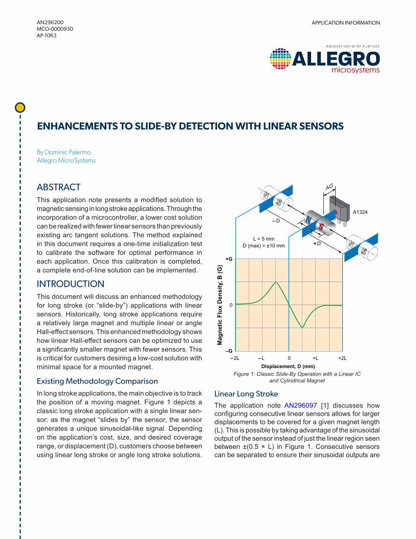
Existing Methodology ComparisonIn long stroke applications, the main objective is to track the position of a moving magnet. Figure 1 depicts a classic long stroke application with a single linear sen-sor: as the magnet “slides by” the sensor, the sensor generates a unique sinusoidal-like signal. Depending on the application’s cost, size, and desired coverage range, or displacement (D), customers choose between using linear long stroke or angle long stroke solutions.

Mag

netic

Flu

x D

ensi

ty, B

(G)

+G

0

–G– L– 2L +2L0 +L

Displacement, D (mm)

– D

+ D

A1324

L = 5 mmD (max) = ±10 mm

AG

L

Figure 1: Classic Slide-By Operation with a Linear IC and Cylindrical Magnet

Linear Long StrokeThe application note AN296097 [1] discusses how configuring consecutive linear sensors allows for larger displacements to be covered for a given magnet length (L). This is possible by taking advantage of the sinusoidal output of the sensor instead of just the linear region seen between ±(0.5 × L) in Figure 1. Consecutive sensors can be separated to ensure their sinusoidal outputs are

https://www.allegromicro.com/en/insights-and-innovations/technical-documents/hall-effect-sensor-ic-publications/hall-effect-system-with-two-linear-sensor-ics

2955 PERIMETER ROAD • MANCHESTER, NH 03103 • USA+1-603-626-2300 • FAX: +1-603-641-5336 • ALLEGROMICRO.COM


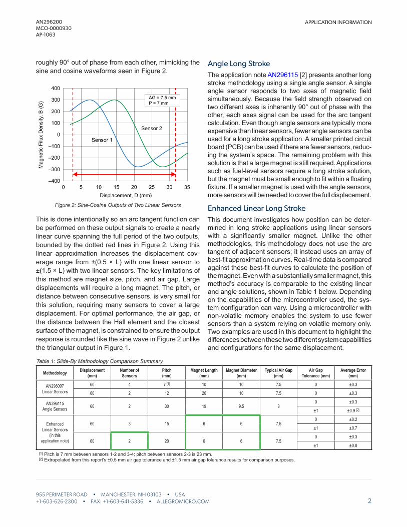
roughly 90° out of phase from each other, mimicking the sine and cosine waveforms seen in Figure 2.

Displacement, D (mm)

Mag

netic

Filu

x D

ensi

ty, B

(G)

400

300

200

100

0

–100

–200

–300

–4000 5 10 15 20 25 30 35

AG = 7.5 mmP = 7 mm

Sensor 1

Sensor 2

Figure 2: Sine-Cosine Outputs of Two Linear Sensors

This is done intentionally so an arc tangent function can be performed on these output signals to create a nearly linear curve spanning the full period of the two outputs, bounded by the dotted red lines in Figure 2. Using this linear approximation increases the displacement cov-erage range from ±(0.5 × L) with one linear sensor to ±(1.5 × L) with two linear sensors. The key limitations of this method are magnet size, pitch, and air gap. Large displacements will require a long magnet. The pitch, or distance between consecutive sensors, is very small for this solution, requiring many sensors to cover a large displacement. For optimal performance, the air gap, or the distance between the Hall element and the closest surface of the magnet, is constrained to ensure the output response is rounded like the sine wave in Figure 2 unlike the triangular output in Figure 1.

Angle Long StrokeThe application note AN296115 [2] presents another long stroke methodology using a single angle sensor. A single angle sensor responds to two axes of magnetic field simultaneously. Because the field strength observed on two different axes is inherently 90° out of phase with the other, each axes signal can be used for the arc tangent calculation. Even though angle sensors are typically more expensive than linear sensors, fewer angle sensors can be used for a long stroke application. A smaller printed circuit board (PCB) can be used if there are fewer sensors, reduc-ing the system’s space. The remaining problem with this solution is that a large magnet is still required. Applications such as fuel-level sensors require a long stroke solution, but the magnet must be small enough to fit within a floating fixture. If a smaller magnet is used with the angle sensors, more sensors will be needed to cover the full displacement.

Enhanced Linear Long StrokeThis document investigates how position can be deter-mined in long stroke applications using linear sensors with a significantly smaller magnet. Unlike the other methodologies, this methodology does not use the arc tangent of adjacent sensors; it instead uses an array of best-fit approximation curves. Real-time data is compared against these best-fit curves to calculate the position of the magnet. Even with a substantially smaller magnet, this method’s accuracy is comparable to the existing linear and angle solutions, shown in Table 1 below. Depending on the capabilities of the microcontroller used, the sys-tem configuration can vary. Using a microcontroller with non-volatile memory enables the system to use fewer sensors than a system relying on volatile memory only. Two examples are used in this document to highlight the differences between these two different system capabilities and configurations for the same displacement.

Table 1: Slide-By Methodology Comparison Summary

Methodology Displacement (mm)

Number of Sensors

Pitch(mm)

Magnet Length(mm)

Magnet Diameter(mm)

Typical Air Gap(mm)

Air Gap Tolerance (mm)

Average Error (mm)

AN296097Linear Sensors

60 4 7 [1] 10 10 7.5 0 ±0.3

60 2 12 20 10 7.5 0 ±0.3

AN296115Angle Sensors 60 2 30 19 9.5 8

0 ±0.3

±1 ±0.9 [2]

EnhancedLinear Sensors

(in this application note)

60 3 15 6 6 7.50 ±0.2

±1 ±0.7

60 2 20 6 6 7.50 ±0.3

±1 ±0.8[1] Pitch is 7 mm between sensors 1-2 and 3-4; pitch between sensors 2-3 is 23 mm. [2] Extrapolated from this report’s ±0.5 mm air gap tolerance and ±1.5 mm air gap tolerance results for comparison purposes.

https://allegromicro.com/en/insights-and-innovations/technical-documents/hall-effect-sensor-ic-publications/slide-by-sensing-for-long-stroke-applications-using-allegro-angle-sensors



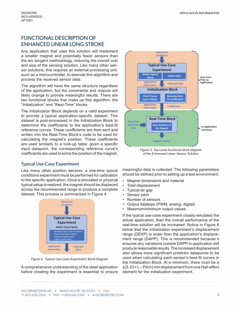
FUNCTIONAL DESCRIPTION OF ENHANCED LINEAR LONG STROKEAny application that uses this solution will implement a smaller magnet and potentially fewer sensors than the arc tangent methodology, reducing the overall cost and size of the sensing solution. Like many other sen-sor solutions, this requires an external processing unit, such as a microcontroller, to execute this algorithm and process the received sensor data. The algorithm will have the same structure regardless of the application, but the constraints and outputs will likely change to provide meaningful results. There are two functional blocks that make up this algorithm: the “Initialization” and “Real-Time” blocks. The Initialization Block depends on a valid experiment to provide a typical application-specific dataset. This dataset is post-processed in the Initialization Block to determine the coefficients to the application’s best-fit reference curves. These coefficients are then sent and written into the Real-Time Block’s code to be used for calculating the magnet’s position. These coefficients are used similarly to a look-up table: given a specific input datapoint, the corresponding reference curve’s coefficients are used to solve the position of the magnet.

Post-Process Input Dataset

Ini�aliza�on Block

Real-Time Block

Typical Use-Case Experiment

Collected Data

Applica�on Informa�on

Define Typical Setup

Typical UseCondi�ons

Magnet Posi�on

Generate Best-Fit Coefficients

Real-Time Applica�on

DataSolve Posi�on of

the Magnet

One-Time

Applica�on

In-Applica�on Func�ons

Coefficients


Collect DataPrior to

Figure 3: Top-Level functional block diagram of the Enhanced Linear Sensor Solution

Typical Use-Case ExperimentLike many other position sensors, a one-time typical conditions experiment must be performed for calibration to the specific application. Once a simulated or physical typical setup is realized, the magnet should be displaced across the recommended range to produce a complete dataset. This process is summarized in Figure 4.

Typical Use-Case Experiment

• Replicate Typical Use Condi�ons• Physical/Simulated Setup• Increase Displacement• Collect Output Data

Collected Data

Define Typical Setup

Typical Use Condi�ons


Figure 4: ‘Typical Use-Case Experiment’ Block Diagram

A comprehensive understanding of the ideal application before creating the experiment is essential to ensure

meaningful data is collected. The following parameters should be defined prior to setting up a test environment: • Magnet dimensions and material• Total displacement• Typical air gap• Sensor pitch• Number of sensors• Output datatype (PWM, analog, digital)• Maximum/minimum output valuesIf the typical use-case experiment closely emulates the actual application, then the overall performance of the real-time solution will be increased. Notice in Figure 6 below that the initialization experiment’s displacement range (DEXP) is wider than the application’s displace-ment range (DAPP). This is recommended because it ensures any variations outside DAPP in-application still produce reasonable results. The increased displacement also allows more significant predictor datapoints to be used when calculating each sensor’s best-fit curves in the Initialization Block. At a minimum, there must be a ±(5.33 × L – Pitch) mm displacement from one Hall-effect element for the initialization experiment.



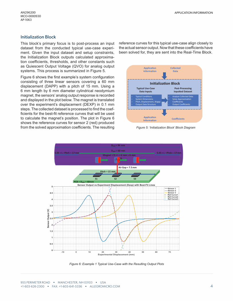
Initialization BlockThis block’s primary focus is to post-process an input dataset from the conducted typical use-case experi-ment. Given the input dataset and setup constraints, the Initialization Block outputs calculated approxima-tion coefficients, thresholds, and other constants such as Quiescent Output Voltage (QVO) for analog output systems. This process is summarized in Figure 5.Figure 6 shows the first example’s system configuration consisting of three linear sensors covering a 60 mm displacement (DAPP) with a pitch of 15 mm. Using a 6 mm length by 6 mm diameter cylindrical neodymium magnet, the sensors’ analog output response is recorded and displayed in the plot below. The magnet is translated over the experiment’s displacement (DEXP) in 0.1 mm steps. The collected dataset is processed to find the coef-ficients for the best-fit reference curves that will be used to calculate the magnet’s position. The plot in Figure 6 shows the reference curves for sensor 2 (red) produced from the solved approximation coefficients. The resulting

reference curves for this typical use-case align closely to the actual sensor output. Now that these coefficients have been solved for, they are sent into the Real-Time Block.

Typical Use-CaseData Inputs

• Typical Condi�ons• System Dimensions• Pitch, Displacement, Airgap• Output Data Structure

• Analyze Collected Data• Solve Approxima�on

Coefficients• Output Coefficients

Post-Processing Inpu�ed Dataset

Ini�aliza�on Block

Collected Data



Coefficients

Figure 5: ‘Initialization Block’ Block Diagram

Air Gap = 7.5 mm

Magnet = D × L = 6 mm × 6 mm

DAPP = 60 mm

S1 S2 S3

Pitch = 15 mm

DEXP = 94 mm

5.33 × L – Pitch = 17 mm 5.33 × L – Pitch = 17 mm

DL

PCB = DAPP = 60mm

Figure 6: Example 1 Typical Use-Case with the Resulting Output Plots



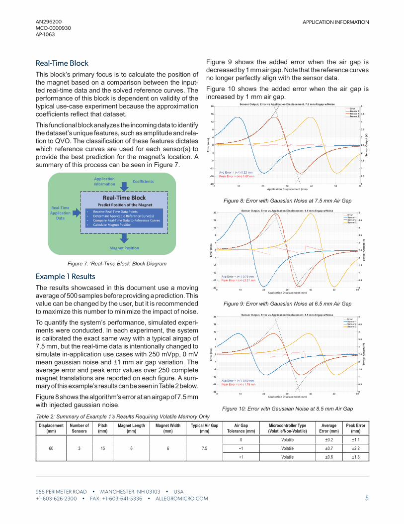
Real-Time BlockThis block’s primary focus is to calculate the position of the magnet based on a comparison between the input-ted real-time data and the solved reference curves. The performance of this block is dependent on validity of the typical use-case experiment because the approximation coefficients reflect that dataset. This functional block analyzes the incoming data to identify the dataset’s unique features, such as amplitude and rela-tion to QVO. The classification of these features dictates which reference curves are used for each sensor(s) to provide the best prediction for the magnet’s location. A summary of this process can be seen in Figure 7.

• Receive Real-Time Data Points• Determine Applicable Reference Curve(s)• Compare Real-Time Data to Reference Curves• Calculate Magnet Posi�on

Predict Posi�on of the MagnetReal-Time Block


Magnet Posi�on

Coefficients

Real-TimeApplica�on

Data

Figure 7: ‘Real-Time Block’ Block Diagram

Example 1 ResultsThe results showcased in this document use a moving average of 500 samples before providing a prediction. This value can be changed by the user, but it is recommended to maximize this number to minimize the impact of noise.To quantify the system’s performance, simulated experi-ments were conducted. In each experiment, the system is calibrated the exact same way with a typical airgap of 7.5 mm, but the real-time data is intentionally changed to simulate in-application use cases with 250 mVpp, 0 mV mean gaussian noise and ±1 mm air gap variation. The average error and peak error values over 250 complete magnet translations are reported on each figure. A sum-mary of this example’s results can be seen in Table 2 below.Figure 8 shows the algorithm’s error at an airgap of 7.5 mm with injected gaussian noise.

Figure 9 shows the added error when the air gap is decreased by 1 mm air gap. Note that the reference curves no longer perfectly align with the sensor data.Figure 10 shows the added error when the air gap is increased by 1 mm air gap.

Figure 8: Error with Gaussian Noise at 7.5 mm Air Gap

Figure 9: Error with Gaussian Noise at 6.5 mm Air Gap

Figure 10: Error with Gaussian Noise at 8.5 mm Air GapTable 2: Summary of Example 1’s Results Requiring Volatile Memory Only

Displacement (mm)

Number of Sensors

Pitch(mm)

Magnet Length(mm)

Magnet Width(mm)

Typical Air Gap(mm)


Microcontroller Type(Volatile/Non-Volatile)

Average Error (mm)

Peak Error(mm)

60 3 15 6 6 7.5

0 Volatile ±0.2 ±1.1

–1 Volatile ±0.7 ±2.2

+1 Volatile ±0.6 ±1.8



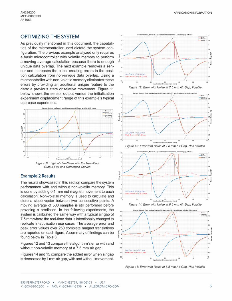
OPTIMIZING THE SYSTEMAs previously mentioned in this document, the capabili-ties of the microcontroller used dictate the system con-figuration. The previous example analyzed only requires a basic microcontroller with volatile memory to perform a moving average calculation because there is enough unique data overlap. The next example removes a sen-sor and increases the pitch, creating errors in the posi-tion calculation from non-unique data overlap. Using a microcontroller with non-volatile memory eliminates these errors by providing an additional unique feature to the data: a previous state or relative movement. Figure 11 below shows the sensor output versus the initialization experiment displacement range of this example’s typical use-case experiment.

Figure 11: Typical Use-Case with the Resulting Output Plot and Reference Curves

Example 2 ResultsThe results showcased in this section compare the system performance with and without non-volatile memory. This is done by adding 0.1 mm net magnet movement to each calculation. Non-volatile memory is used to calculate and store a slope vector between two consecutive points. A moving average of 500 samples is still performed before providing a prediction. In the following experiments, the system is calibrated the same way with a typical air gap of 7.5 mm where the real-time data is intentionally changed to replicate in-application use cases. The average error and peak error values over 250 complete magnet translations are reported on each figure. A summary of findings can be found below in Table 3.Figures 12 and 13 compare the algorithm’s error with and without non-volatile memory at a 7.5 mm air gap.Figures 14 and 15 compare the added error when air gap is decreased by 1 mm air gap, with and without movement.

Figure 12: Error with Noise at 7.5 mm Air Gap, Volatile

Figure 13: Error with Noise at 7.5 mm Air Gap, Non-Volatile





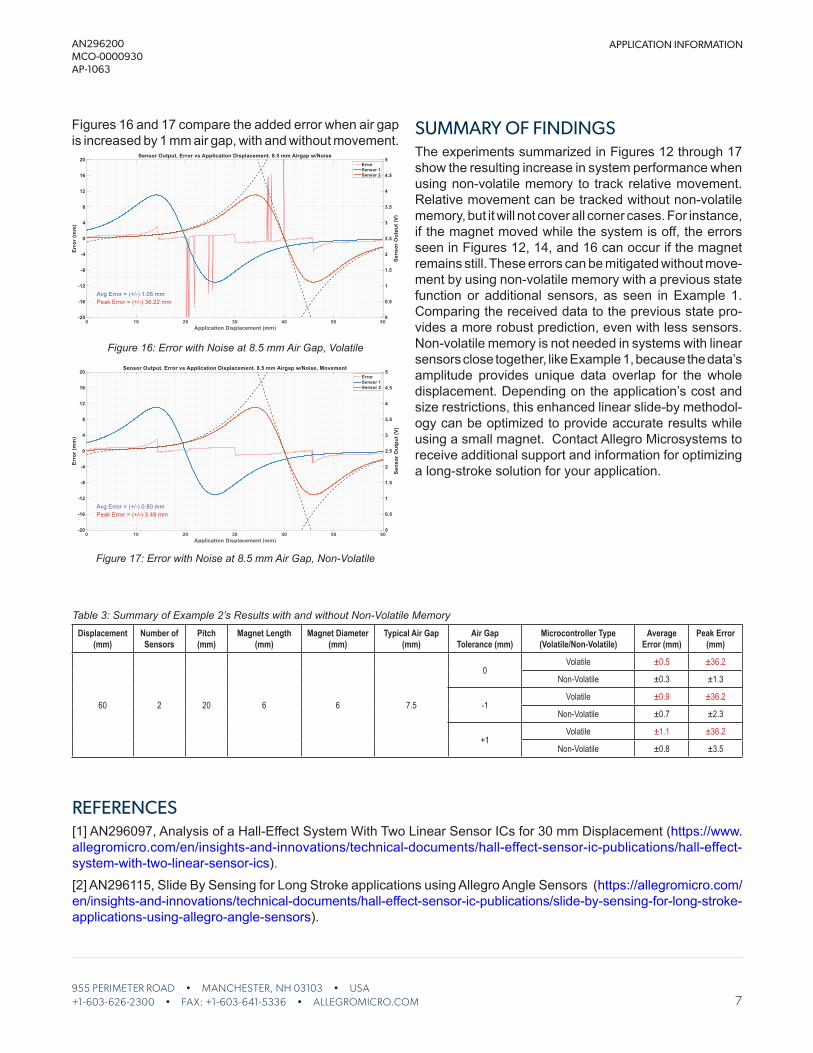
Figures 16 and 17 compare the added error when air gap is increased by 1 mm air gap, with and without movement.



SUMMARY OF FINDINGSThe experiments summarized in Figures 12 through 17 show the resulting increase in system performance when using non-volatile memory to track relative movement. Relative movement can be tracked without non-volatile memory, but it will not cover all corner cases. For instance, if the magnet moved while the system is off, the errors seen in Figures 12, 14, and 16 can occur if the magnet remains still. These errors can be mitigated without move-ment by using non-volatile memory with a previous state function or additional sensors, as seen in Example 1. Comparing the received data to the previous state pro-vides a more robust prediction, even with less sensors. Non-volatile memory is not needed in systems with linear sensors close together, like Example 1, because the data’s amplitude provides unique data overlap for the whole displacement. Depending on the application’s cost and size restrictions, this enhanced linear slide-by methodol-ogy can be optimized to provide accurate results while using a small magnet. Contact Allegro Microsystems to receive additional support and information for optimizing a long-stroke solution for your application.

Table 3: Summary of Example 2’s Results with and without Non-Volatile MemoryDisplacement

(mm)Number of Sensors

Pitch(mm)

Magnet Length(mm)

Magnet Diameter(mm)

Typical Air Gap(mm)


Microcontroller Type(Volatile/Non-Volatile)

Average Error (mm)

Peak Error(mm)

60 2 20 6 6 7.5

0Volatile ±0.5 ±36.2

Non-Volatile ±0.3 ±1.3

-1Volatile ±0.9 ±36.2


+1Volatile ±1.1 ±36.2


REFERENCES[1] AN296097, Analysis of a Hall-Effect System With Two Linear Sensor ICs for 30 mm Displacement (https://www.allegromicro.com/en/insights-and-innovations/technical-documents/hall-effect-sensor-ic-publications/hall-effect-system-with-two-linear-sensor-ics).[2] AN296115, Slide By Sensing for Long Stroke applications using Allegro Angle Sensors (https://allegromicro.com/en/insights-and-innovations/technical-documents/hall-effect-sensor-ic-publications/slide-by-sensing-for-long-stroke-applications-using-allegro-angle-sensors).









Copyright 2020, Allegro MicroSystems.The information contained in this document does not constitute any representation, warranty, assurance, guaranty, or inducement by Allegro to the customer with respect to the subject matter of this document. The information being provided does not guarantee that a process based on this information will be reliable, or that Allegro has explored all of the possible failure modes. It is the customer’s responsibility to do sufficient qualification testing of the final product to ensure that it is reliable and meets all design requirements.Copies of this document are considered uncontrolled documents.

Revision HistoryNumber Date Description Responsibility

– August 11, 2020 Initial release Dominic Palermo

enhancements to slide-by detection with linear

Documents