Encyclopaedia of Complexity Results for Finite-Horizon MarkovDecision Process Problems�Martin Mundhenk y Judy Goldsmith z Christopher Lusena x Eric Allender {August 21, 1997AbstractThe computational complexity of �nite horizon policy evaluation and policy existenceproblems are studied for several policy types and representations of Markov decision pro-cesses. In almost all cases, the problems are shown to be complete for their complexityclasses; classes range from nondeterministic logarithmic space and probabilistic logarith-mic space (highly parallelizable classes) to exponential space. In many cases, this workshows that problems that already were widely believed to be hard to compute are probablyintractable (complete for NP, NPPP, or PSPACE), or provably intractable (EXPTIME-complete or worse). The major contributions of the paper are to pinpoint the complexityof these problems; to isolate the factors that make these problems computationally com-plex; to show that even problems such as median-policy or average-policy evaluation maybe intractable; and the introduction of natural NPPP-complete problems.1 IntroductionMarkov decision processes are used in the natural and social sciences and engineering to modela vast array of systems. (Puterman's book [32] has excellent discussions of applications.) Theyare used in a variety of applied computer science �elds, including control theory, robotics, expertsystems, learning theory, and data mining to model assembly lines, robot location problems,medical diagnosis and treatment experts, and many other systems.Markov Decision Processes (MDPs) model controlled stochastic processes. Such a processhas states, an external agent or controller that can choose actions (here assumed to be chosen�A preliminary version of some of this work appeared as [27].yUniversit�at Trier, FB IV { Informatik, D-54286 Trier, Germany, mundhenk@ti.uni-trier.de. Supported inpart by the O�ce of the Vice Chancellor for Research and Graduate Studies at the University of Kentucky, andby the Deutsche Forschungsgemeinschaft (DFG), grant Mu 1226/2-1.zDept. of Computer Science, University of Kentucky, Lexington KY 40506-0046, goldsmit@cs.engr.uky.edu.Supported in part by NSF grant CCR-9315354 and CCR-9610348.xDept. of Computer Science, University of Kentucky, Lexington KY 40506-0046, lusena@cs.engr.uky.edu.Supported in part by NSF grant CCR-9315354 and CCR-9610348.{Department of Computer Science, Rutgers University, Piscataway, NJ 08855, USA,allender@cs.rutgers.edu. Supported in part by NSF grant CCR-9509603. Portions of this work wereperformed while at the Institute of Mathematical Sciences, Chennai (Madras), India, and at the Wilhelm-Schickard Institut f�ur Informatik, Universit�at T�ubingen (supported by DFG grant TU 7/117-1).1

at discrete time intervals) which have probabilistic e�ects, and rewards associated with eachstate-action pair. The process is assumed to run (in the cases considered here) for a �xed �nitetime, approximately equal to the size of the system or its representation.There are several computational questions associated with the use of MDPs. We do notaddress the questions that arise in designing MDP models of stochastic processes. Rather, weaddress the computational complexity, given an MDP and speci�cations for a controller, of�nding a good or optimal controller. Goodness is measured in terms of the expected reward,and the speci�cations on the system and the controller include the amount of feedback thatthe controller gets from the system (observability), the length of time that the process will run(horizon), the amount of memory the controller has, and the form of the input and output.Is the system fully speci�ed, or is it represented by some sort of function (here, circuits) thatcomputes the probabilities as needed? Similarly for the controller itself.For instance, partially observable MDPs (POMDPs) model everything from robot locationproblems to medical treatment [38]. Unfortunately, the optimal policies for POMDPs aregenerally expressible as functions from initial segments of the history of a process (a series ofobservations, giving partial or full information about the state at previous and current times,and | implicitly | of actions taken). This is unfortunate because (as practitioners alreadysuspected, and we prove), the problem of �nding optimal policies for POMDPs is PSPACE-hard.In this paper, we primarily consider the policy evaluation problem (given an MDP and apolicy, what is the expected reward accrued by that policy over the given horizon), and thepolicy existence problem (given an MDP, is there a policy with expected reward greater than0). Linear programming has been used to decide these two problems for certain forms of MDPsand certain types of policies since 1960 [15]; in 1987, Papadimitriou and Tsitsiklis [30] showedthat in fact certain policy existence problems in these cases are P-complete. The complexity ofthese problems is quite sensitive to details in the speci�cation. We show that a seemingly similarproblem, based on maximization rather than minimization, is complete for nondeterministiclogspace (Corollary 5.2), whereas a more analogous P-completeness result can be found inTheorem 6.1.In most other cases, however, we show that the decision problems considered here arecomplete for classes thought or known to be above P, such as NP, PSPACE, and even ashigh as EXPSPACE. Thus, the contribution this paper makes to the �elds of control theory,economics, medicine, etc., are largely negative: there are unlikely to be any e�cient algorithmsfor �nding the optimal policies for the general MDP problems.However, there is good news in this bad news. We prove what many practitioners alreadysuspected. This gives strength to the call for approximations, and the search for special casesthat are in fact computationally simpler than the general case.For instance, there is interest in the AI community in so-called \structured," or succinctlyrepresented MDPs [10, 13, 25]. These representations arise when one can make use of struc-tures in the state space to provide small descriptions of very large systems [10]. Whereas thosesystems are not tractable by classical methods, there is some hope { expressed in di�erentalgorithmic approaches { that many special cases of these structured POMDPs can be solvedmore e�ciently. Boutillier, et al., in [10] conjecture that �nding optimal policies for structuredPOMDPs is infeasible. We prove this conjecture by showing that in many cases the complexity2

Evaluation Existence Evaluation (nonneg) Existence (nonneg)Partially-observableStationary PL 4.5 NP 6.4 NL 5.1 NP 5.4Time-dependent PL 4.5 NP 6.5 NL 5.1 NL 5.3History-dependent PSPACE 6.6 NL 5.3Fully-observableStationary PL 4.5 ? NL 5.1 NL 5.2Time-dependent PL 4.5 P 6.1 NL 5.1 NL 5.2UnobservableStationary PL 4.5 PL 6.2 NL 5.1 NL 5.2Time-dependent PL 4.5 NP 6.3 NL 5.1 NL 5.2Table 1: Completeness results for Flat MDPsEvaluation Existence Evaluation (nonneg) Existence (nonneg)Partially-observableStationary PSPACE 4.7 NEXP 6.8 PSPACE 5.5; NP 5.6� NEXP 5.10Time-dependent PSPACE 4.8 NEXP 6.8 PSPACE 5.5; NP 5.6 PSPACE 5.11History-dependent EXPSPACE 6.8 PSPACE 5.11Fully-observableStationary PSPACE 4.7 ? PSPACE 5.9Time-dependent PSPACE 4.8 EXP 6.7 PSPACE 5.9UnobservableStationary PSPACE 4.7 PSPACE 6.9 NP 5.7 PSPACE 5.8Time-dependent PSPACE 4.8 NEXP 6.10 NP 5.7 PSPACE 5.8Table 2: Completeness results for Succinct MDPs� The di�erence depends on whether the horizon is polynomial in the size of the input or in thenumber of states.of our decision problems increases exponentially if succinct descriptions [19, 37] for POMDPsare considered. For example, policy existence problems for POMDPs with nonnegative re-wards are NL-complete under straightforward descriptions. Using succinct descriptions, thecompleteness increases to PSPACE. We also consider a new intermediate notion of compressedrepresentations and get intermediate complexity results, e.g. NP-completeness for the aboveexample.The results of this paper are summarized in Tables 1{3. The numbers next to complexityclasses indicate the relevant theorems. The history-dependent cases for fully-observable andunobservable MDPs have been omitted, since those cases are identical to the time-dependentones.Given the widespread use and consideration of MDPs, there has been surprisingly littlework on the computational complexity of �nding good policies. There have certainly beenalgorithms presented and analyzed, but we will not generally survey them here. For that, we3

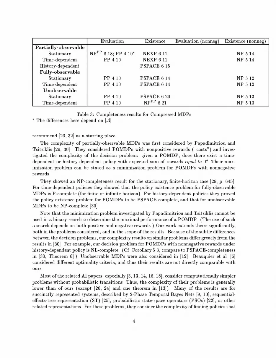
Evaluation Existence Evaluation (nonneg) Existence (nonneg)Partially-observableStationary NPPP 6.18; PP 4.10� NEXP 6.11 NP 5.14Time-dependent PP 4.10 NEXP 6.11 NP 5.14History-dependent PSPACE 6.15Fully-observableStationary PP 4.10 PSPACE 6.14 NP 5.12Time-dependent PP 4.10 PSPACE 6.14 NP 5.12UnobservableStationary PP 4.10 PSPACE 6.20 NP 5.13Time-dependent PP 4.10 NPPP 6.21 NP 5.13Table 3: Completeness results for Compressed MDPs� The di�erences here depend on jAj.recommend [26, 32] as a starting place.The complexity of partially-observable MDPs was �rst considered by Papadimitriou andTsitsiklis [29, 30]. They considered POMDPs with nonpositive rewards (\costs") and inves-tigated the complexity of the decision problem: given a POMDP, does there exist a time-dependent or history-dependent policy with expected sum of rewards equal to 0? Their max-imization problem can be stated as a minimization problem for POMDPs with nonnegativerewards.They showed an NP-completeness result for the stationary, �nite-horizon case [29, p. 645].For time-dependent policies they showed that the policy existence problem for fully-observableMDPs is P-complete (for �nite or in�nite horizon). For history-dependent policies they provedthe policy existence problem for POMDPs to be PSPACE-complete, and that for unobservableMDPs to be NP-complete [30].Note that the minimization problem investigated by Papadimitriou and Tsitsiklis cannot beused in a binary search to determine the maximal performance of a POMDP. (The use of sucha search depends on both positive and negative rewards.) Our work extends theirs signi�cantly,both in the problems considered, and in the scope of the results. Because of the subtle di�erencesbetween the decision problems, our complexity results on similar problems di�er greatly from theresults in [30]. For example, our decision problem for POMDPs with nonnegative rewards underhistory-dependent policy is NL-complete. (Cf. Corollary 5.3, compare to PSPACE-completenessin [30, Theorem 6].) Unobservable MDPs were also considered in [12]. Beauquier et al. [6]considered di�erent optimality criteria, and thus their results are not directly comparable withours.Most of the related AI papers, especially [3, 13, 14, 16, 18], consider computationally simplerproblems without probabilistic transitions. Thus, the complexity of their problems is generallylower than of ours (except [20, 24] and one theorem in [13]). Many of the results are forsuccinctly represented systems, described by 2-Phase Temporal Bayes Nets [9, 10], sequential-e�ects-tree representation (ST) [25], probabilistic state-space operators (PSOs) [22], or otherrelated representations. For these problems, they consider the complexity of �nding policies that4

are of size polynomial in either the size of the representation, or the number of states | leadingto di�erent complexities, in certain cases. (For instance, Littman showed that the general planexistence problem is EXP-complete, but if plans are limited to size polynomial in the size ofthe planning domain, then the problem is PSPACE-complete [25]; the PSPACE-completenesswas proved independently in [20].) Sometimes the stochasticity of the system does not addcomputational complexity. For instance, Bylander [13] showed that the time-dependent policyexistence problem for unobservable, succinct MDPs with nonnegative rewards is PSPACE-complete, even if the transitions are restricted to be deterministic. In Theorem 5.8 we showPSPACE-completeness of the stochastic version of this problem.De�nitions of Markov decision processes and policies appear in Section 2. The followingsection addresses computational issues, especially the representation of MDPs. In each ofthe next three sections, we consider at, then succinctly represented, then compressed MDPs:Section 4 presents the complexity of policy evaluation problems for general MDPs; Section 5concerns both policy evaluation and policy existence problems for MDPs with nonnegativerewards; Section 6 is on policy existence problems for general MDPs. In Section 7, we alsoconsider the question, does a givenMDP have a policy with expected reward exactly r? Section 8considers the complexity of testing the median and average policies of an MDP.2 De�nitions and Preliminaries2.1 Complexity Theory: Counting ClassesFor de�nitions of complexity classes, reductions, and standard results from complexity theorywe refer to [28]. In the interest of completeness, in this section we give a short description ofthe probabilistic and counting complexity classes we use in this work.The class #L [2] is the class of functions f such that, for some nondeterministic logarith-mically space-bounded machine N , the number of accepting paths of N on x equals f(x). Theclass #P is de�ned analogously as the class of functions f such that, for some nondeterministicpolynomial-time-bounded machine N , the number of accepting paths of N on x equals f(x).Probabilistic logspace, PL, is the class of sets A for which there exists a nondeterministiclogarithmically space-bounded machineN such that x 2 A if and only if the number of acceptingpaths of N on x is greater than its number of rejecting paths. In apparent contrast to P-complete sets, sets in PL are decidable using very fast parallel computations [21]. Probabilisticpolynomial time, PP, is de�ned analogously. A classic PP-complete problem isMajsat: givena Boolean formula, do the majority of assignments satisfy it?For polynomial-space-bounded computations, PSPACE equals probabilistic PSPACE, and#PSPACE (de�ned analogously to #L and #P) is the same as the class of polynomial-space-computable functions [23]. (Note that some functions in #PSPACE produce output of expo-nential length.)For any complexity classes C and C 0 the class CC0 consists of those sets that are C-Turingreducible to sets in C 0, i.e., sets that can be accepted with resource bounds speci�ed by C,using some problem in C 0 as a subroutine (oracle) with instantaneous output. For any classC � PSPACE, it is the case that NPC�PSPACE, and therefore NPPSPACE=PSPACE; seePapadimitriou's textbook [28]. 5

Another useful result is that the class NPPP equals the \�NPm " closure of PP [34], which canbe seen as the closure of PP under polynomial-time disjunctive reducibility with an exponentialnumber of queries (each of the queries computable in polynomial time from its index in the listof queries).2.2 Markov Decision ProcessesA Markov decision process (MDP) describes a controlled stochastic system by its states andthe consequences of actions on the system. It is denoted as a tuple M = (S; s0;A;O; t; o; r),where� S, A and O are �nite sets of states, actions and observations,� s0 2 S is the initial state,� t : S � A � S ! [0; 1] is the state transition function, where t(s; a; s0) is the probabilitythat state s0 is reached from state s on action a (where �s02St(s; a; s0) 2 f0; 1g for everys 2 S; a 2 A),� o : S ! O is the observation function, where o(s) is the observation made in state s,� r : S �A ! Z is the reward function, where r(s; a) is the reward gained by taking actiona in state s.If states and observations are identical, i.e. O = S and o is the identity function (or abijection), then the MDP is called fully-observable. Another special case is unobservable MDPs,where the set of observations contains only one element, i.e. in every state the same observa-tion is made and therefore the observation function is constant. Without restrictions on theobservability, an MDP is called partially-observable.12.3 Policies and PerformancesA policy describes how to act depending on observations. We distinguish three types of policies.� A stationary policy �s (for M) is a function �s : O ! A, mapping each observation to anaction.� A time-dependent policy �t is a function �t : O�N ! A, mapping each pair hobservation,timei to an action.� A history-dependent policy �h is a function �h : O� ! A, mapping each �nite sequence ofobservations to an action.1Note that making observations probabilistically does not add any power to MDPs. Any probabilisticallyobservable MDP can be turned into one with deterministic observations with only a polynomial increase in itssize. 6

Notice that, for an unobservable MDP, a history-dependent policy is equivalent to a time-dependent one. Thus, our theorems do not address the case of history-dependent policies forunobservable MDPs.Let M = (S; s0;A;O; t; o; r) be an MDP. A trajectory � for M is a �nite sequence ofstates � = �1; �2; : : : ; �m (m � 0, �i 2 S). The probability prob�(M; �) of a trajectory � =�1; �2; : : : ; �m under policy � is� prob�(M; �) = �m�1i=1 t(�i; �(o(�i)); �i+1), if � is a stationary policy,� prob�(M; �) = �m�1i=1 t(�i; �(o(�i); i); �i+1), if � is a time-dependent policy, and� prob�(M; �) = �m�1i=1 t(�i; �(o(�1) � � �o(�i)); �i+1), if � is a history-dependent policy.The reward rew�(M; �) of trajectory � under � is the sum of its rewards, i.e. rew�(M; �) =�m�1i=1 r(�i; �(�)) dependent on the type of policy. The performance of a policy � for �nite-horizon k with initial state � is the expected sum of rewards received on the next k steps byfollowing the policy �, i.e. perf(M;�; k; �) =P�2�(�;k) prob�(M; �) � rew�(M; �), where �(�; k)is the set of all length k trajectories beginning with state �. The �-value val�(M; k) of M forhorizon k isM 's maximal performance under a policy � of type � for horizon k when started inits initial state, i.e. val�(M; k) = max�2�� perf(M; s0; k; �), where �� is the set of all � policies.For simplicity, we assume that the size of an MDP is determined by the size n of its statespace. We assume that there are no more actions than states, and that each state transitionprobability is given as binary fraction with n bits and each reward is an integer of at most n bits.This is no real restriction, since adding unreachable \dummy" states allows one to use morebits for transition probabilities and rewards. Also, it is straightforward to transform an MDPM with non-integer rewards to M 0 with integer rewards such that val�(M; k) = c � val�(M 0; k)for some constant c.3 Representations and Computational Questions3.1 Flat MDPsThere are various ways an MDP can be represented. We begin by considering problem instancesthat are represented in a straightforward way. Namely an MDP with n states is represented bya set of n�n tables for the transition function (one table for each action) and a similar table forthe reward function. We assume that the number of actions and the number of bits needed tostore each transition probability or reward does not exceed n, so such a representation requiresO(n4) bits. In the same way, stationary policies can be encoded as lists with n entries, andtime-dependent policies for horizon n as n � n tables.The � policy evaluation problem for MDPs is the set of all pairs (M;�) consisting of aPOMDP M = (S;O; s0;A; o; t; r) and an � policy � with performance perf(M; s0; jSj; �)> 0.The � policy existence problem for MDPs is the set of all MDPs M = (S;O; s0;A; o; t; r),for which there exists an � policy � with performance perf(M; s0; jSj; �)> 0.Notice that there are jOjh possible histories for an MDP with time horizon h. If jOj > 1,this means that one cannot fully specify a history-dependent policy in space polynomial in7

the size of S. Therefore, we do not generally consider the history-dependent policy evaluationproblem in this paper. Since we generally assume that h � jSj, time-dependent policies do notcause such problems.3.2 Succinct MDPsSuccinct representations of MDPs arise when the system being modeled has su�cient structure,e.g., when a state is modelled by the states of n variables, and for each action, the state of eachvariable depends on only a few of the variables. This is true, for instance, when a system ismodeled as a Bayes belief net, or when actions are given in the STRIPS model [13, 20, 24].Changing the way in which MDPs (and policies) are represented may change the com-plexities of the considered problems too. We focus on the concept of succinct representations,which was introduced independently in [19, 37]. POMDPs having very regular structure arisein many practical and theoretical areas of computer science, and often it is most natural torepresent these processes very compactly. For example, the transition tables of a POMDP withn states and actions can be represented by a Boolean circuit C with 4dlogne input bits suchthat C(s; a; s0; l) outputs the l-th bit of t(s; a; s0). Encodings of those circuits are no larger thanthe straightforward matrix encodings. But for POMDPs with su�cient structure, the circuitencodings may be much smaller, namely O(logn), i.e., the logarithm of the size of the statespace. In this case, we say that the problem has a succinct representation. It is easy to seethat in going from straightforward to succinct encodings, the complexity of the correspond-ing decision problems increases at most exponentially. More importantly (and less obviously),there are many problems for which this exponential increase in complexity is inherent (see [5]for conditions). For most of the problems considered here, the completeness proofs for the atPOMDPs translate upward to the respective succinctly represented POMDPs.The � policy evaluation problem for partially-observable sMDPs is the set of all pairs (M;�)consisting of a succinctly represented POMDP M = (S;O; s0;A; o; t; r) and a succinctly repre-sented � policy �, such that perf(M; s0; jSj; �)> 0.The � policy existence problem for partially-observable sMDPs is the set of all succinctlyrepresented POMDPs M = (S;O; s0;A; o; t; r), for which there exists an � policy �, such thatperf(M; s0; jSj; �)> 0.3.3 Compressed MDPsIn this section, we introduce what we believe is a better model of the type of \succinct"MDPs that are of interest in practice. This model, which we call \compressed MDPs," isintermediate between the at representation and the succinct representation introduced inthe preceding subsection. Note for instance that the transition probabilities t(s; a; s0) in the\succinct" representation potentially have exponentially-many bits of precision. It is hardto think of situations when this amount of precision would be known, and thus it is not aserious restriction to consider only succinctly represented MDPs where the circuits representingthe transition tables have multiple output gates from which on input s; a; s0 the transitionprobability t(s; a; s0) can be read. (Thus, in particular, only polynomially-many bits of precisionare considered. That is, because the number of output gates is bounded by the size of the circuit,8

for an MDP with n states, encoded by a circuit of size c logn, the transition probabilities mustbe written using roughly logn bits (in their standard representation).) The issue of bit-counts intransition probabilities has arisen before; it occurs, for instance, in [6, 35]. It is also importantto note that our probabilities are speci�ed by single bit-strings, rather than as rationals speci�edby two bit-strings.Since the \succinct" MDPs considered in practice frequently arise in the context of planning,it is much more likely that one will be interested in the reward after only a polynomial numberof steps (since there will not be time to run the policy for an exponential number of steps).This motivates restricting the horizon to be logarithmic in the size of the state space.It turns out that the number of bits needed to represent the actions and rewards contributesto the complexity too. Since there are so many factors, the problem descriptions are moreinvolved than in the at or succinct cases.The � policy evaluation problem for partially-observable compressed MDP[f(n)] with g(n)horizon is the set of all pairs (M;�) consisting of a partially-observable succinctly encodedMDP M = (S;O; s0;A; o; t; r) where each transition probability and reward takes log jSj manybits and jAj � f(jSj), and an � policy �, such that perf(M; s0; g(jSj); �)> 0.The policy existence problems are expressed similarly.If f or g is the identity function, we omit it in the problem description.4 Policy Evaluation Problems4.1 Flat MDPsThe standard polynomial time algorithm for evaluating a given policy for a given POMDP usesdynamic programming [30, 32]. We show that for POMDPs this evaluation can be performedquickly in parallel. Eventually this yields the policy evaluation problem being complete for PL.We begin with a technical lemma about matrix powering, and show that each entry (Tm)(i;j) ofthe mth power of a nonnegative integer square matrix T can be computed in #L, if the powerm is at most the dimension n of the matrix.Lemma 4.1 (cf. [36]) Let T be an n� n matrix of nonnegative binary integers, each of lengthn, and let 1 � i; j � n, 0 � m � n. The function mapping (T;m; i; j) to (Tm)(i;j) is in #L.We review the relations between the function class #L and the class of decision problems PL.GapL is the class of functions representable as di�erences of #L functions, GapL = #L �#L,and PL is the class of sets A, for which there is a GapL function f such that for every x, x 2 Ai� f(x) > 0 (see [1]). We use these results to prove the following.Lemma 4.2 The stationary policy evaluation problem for partially-observable MDPs is in PL.Proof Let M = (S; s0;A;O; t; o; r) be a POMDP, and let � be a stationary policy, i.e. amapping from O to A. We show that perfs(M; s0; jSj; �)> 0 can be decided in PL.We transform M to an unobservable MDPM with the same states and rewards as M , havingthe same performance as M under policy �. Since � is a stationary policy, this can be achieved9

by \hard-wiring" the actions chosen by � into the MDP. Then M = (S; s0; fag;O; t; o; r)where t(s; a; s0) = t(s; �(o(s)); s0) and r(s; a) = r(s; �(o(s))). Since M has only one action,the only policy to consider is the constant function mapping each observation to that actiona. It is clear that M under policy � has the same performance as M under (constant) policya, i.e. perf(M; s0; jSj; �) = perf(M; s0; jSj; a). This performance can be calculated using arecursive de�nition of perf, namely perf(M; i;m; a) = r(i; a)+Pj2S t(i; a; j)�perf(M; j;m�1; a)and perf(M; i; 0; a) = 0.The state transition probabilities are given as binary fractions of length h = jSj. In orderto get an integer function for the performance, de�ne the function p as p(M; i; 0) = 0 andp(M; i;m) = 2hmr(i; a) +Pj2S p(M; j;m� 1) � 2ht(i; a; j). One can show thatperf(M; i;m; a) = p(M; i;m) � 2�hm :Therefore, perf(M; s0; jSj; a)> 0 i� p(M; s0; jSj) > 0.In order to complete the proof using the characterization of PL mentioned above, we haveto show that the function p is in GapL.Let T be the matrix obtained from the transition matrix of M by multiplying all entries by2h, i.e. T(i;j) = t(i; a; j) � 2h. The recursion in the de�nition of p can be resolved, and we getp(M; i;m) = mXk=1Xj2S(T k�1)(i;j) � r(j; a) � 2(m�k+1)�h :Each T(i;j) is logspace computable from the input M . From Lemma 4.1 we get that (T k�1)(i;j) 2#L. The reward function is part of the input too, thus r is in GapL (note that rewards maybe negative integers). Because GapL is closed under multiplication and polynomial summation(see [1]), it follows that p 2 GapL. 2Since unobservable and fully observable MDPs are a special case of POMDPs, we get thefollowing corollary.Corollary 4.3 The stationary policy evaluation problems for unobservable and fully observableMDPs are in PL.Lemma 4.4 The stationary policy evaluation problem for unobservable MDPs is PL-hard.Proof Consider A 2 PL. Then there exists a probabilistic logspace machine N acceptingA, and a polynomial p such that each computation of N on x uses at most p(jxj) randomdecisions [21]. Now, �x some input x. We construct an unobservable MDP M(x) with onlyone action, which models the behavior of N on x. Each state of M(x) is a pair consistingof a con�guration of N on x (there are polynomially many) and an integer used as a counterfor the number of random moves made to reach this con�guration (there are at most p(jxj)many). Also, we add a �nal \trap" state reached from states containing a halting con�gurationor from itself. The state transition function of M(x) is de�ned according to the state transitionfunction of N on x, so that each halting computation of N on x corresponds to a length p(jxj)trajectory of M(x) and vice versa. The state transition function is de�ned so that each halting10

computation of N on x corresponds to a length p(jxj) trajectory of M(x) and vice versa. Thereward function is chosen such that rew(�) �prob(�) equals 1 for trajectories � corresponding toaccepting computations (independent of their length), or �1 for rejecting computations, or 0otherwise. Since x 2 A if and only if the number of accepting computations of N on x is greaterthan the number of rejecting computations, it follows that x 2 A if and only if the number oftrajectories � of length jSj for M(x) with rew(�) � prob(�) = 1 is greater than the number oftrajectories � with rew(�) � prob(�) = �1, which is equivalent to perf(M(x); s0; jSj; a)> 0. 2Because the above reduction function constructs an MDP having only one action, the samehardness proof applies for time-dependent policies, and also for partially and fully observableMDPs.Theorem 4.5 The stationary and time-dependent policy evaluation problems for partially-ob-servable, fully observable, and unobservable MDPs are PL-complete.Proof Completeness of the stationary case follows from the above Lemmas 4.2 and 4.4. Becauseevery stationary policy is a time-dependent policy too, hardness of the time-dependent casefollows from Lemma 4.4. It remains to show that the time-dependent case is contained in PL.Let M = (S; s0;A;O; t; o; r) be a partially-observable MDP, and let � be a stationary policy,i.e. a mapping from O�f0; : : : ; jSj�1g to A. Essentially, we proceed in the same way as in theabove proof. The main di�erence is that the transformation from M to M is more involved.We construct M by making jSj copies of M such that all transitions from the ith copy go tothe i + 1st copy, and all these transitions correspond to the transition chosen by � in the ithstep. The rest of the proof proceeds as in the proof of Lemma 4.2. 24.2 Succinct MDPsPut succinctly, all results from Section 4.1 translate to succinctly represented MDPs. The �rstresult which we translate is Lemma 4.1. In Lemma 4.1, we considered the problem of matrixpowering form�m matrices; here, we consider powering a succinctly-represented matrix of sizeO(2m). In space logarithmic in the size of the matrix, we can apply the the algorithm positedin Lemma 4.1; since the input is size O(m), this means that the problem is in #PSPACE.Lemma 4.6 Let T be a 2m � 2m matrix of nonnegative integers, each consisting of 2m bits,1 � i; j � 2m, and 0 � s � m. Let T be represented by a Boolean circuit C with 2m+ dlogmeinput bits, such that C(a; b; r) outputs the r-th bit of T(a;b). The function mapping (T; s; i; j) to(T s)(i;j) is in #PSPACE.As a consequence, we can prove the policy evaluation problems for succinctly representedMDPs is exponentially more complex than for the at ones.Theorem 4.7 The stationary policy evaluation problems for unobservable, fully, and partiallyobservable sMDPs are PSPACE-complete. 11

Proof In order to show that the problem is in PSPACE, we can use the same techniqueas in the proof of Lemma 4.2 yielding here that the problem is in PPSPACE (=probabilisticPSPACE). Ladner [23] showed that FPSPACE = #PSPACE, from which it follows thatPPSPACE = PSPACE.Showing PSPACE-hardness is even easier than showing PL-hardness in the proof of Theo-rem 4.4, because here we deal with a deterministic class. We can transform the computationsof a polynomial space bounded machine on input x directly into a succinct representation of adeterministic MDP. 2The same complexity holds for time-dependent policies.Theorem 4.8 The time-dependent policy evaluation problem for unobservable, fully, and par-tially observable sMDPs are PSPACE-complete.4.3 Compressed MDPsRemember that #P is the class of functions f for which there exists a nondeterministic polyno-mial time bounded Turing machine N such that f(x) equals the number of accepting compu-tations of N on x, and that FP � #P � FPSPACE. The matrix powering problem for integermatrices with \small" entries is in #P, using the same proof idea as for Lemma 4.1.Lemma 4.9 Let T be a 2m � 2m matrix of nonnegative integers, each consisting of m bits,1 � i; j � 2m, and 0 � s � m. Let T be represented by a Boolean circuit C with 2m+ dlogmeinput bits, such that C(a; b; r) outputs the r-th bit of T(a;b). The function mapping (T; s; i; j) to(T s)(i;j) is in #P.As a consequence, the complexity of the policy evaluation problems can be shown to bebetween NP and PSPACE. (Remember that n represents the size of the state space, not thesize of the input.)Theorem 4.10 The stationary and time-dependent policy evaluation problems for unobserv-able, fully, and partially-observable compressed MDP[logn] and logn horizon are PP-complete.The proof is similar to that of Theorem 4.5.5 MDPs with Nonnegative RewardsThe policy evaluation and existence problems for MDPs with nonnegative rewards are gen-erally easier than for MDPs with unrestricted rewards. In fact, these problems reduce in astraightforward way to graph accessibility problems. In order to determine whether an MDPhas performance greater than 0 under a given policy, it su�ces to �nd one \path" with posi-tive probability through the given POMDP that is consistent with the given policy and yieldsreward > 0. Moreover, the transition probabilities and rewards do not need to be calculatedexactly. 12

Note that earlier work, for instance Papadimitriou and Tsitsiklis' [30] considered a di�erentproblem than we do here, with strikingly di�erent complexity. They considered MDPs withnonpositive rewards, and asked whether there was a policy with expected reward 0. In orderfor such a policy to exist, there must be no trajectory consistent with that policy that hasnon-zero reward. Thus, their question has a \for all" avor to it, whereas ours has a \thereexists" avor; in order for one of our policies to have expected positive reward (when thereare no negative rewards), there must be some trajectory consistent with that policy that haspositive expected reward.5.1 Flat MDPsTheorem 5.1 The stationary and time-dependent policy evaluation problems for partially-ob-servable, fully-observable, and unobservable MDPs with nonnegative rewards are complete forNL.Proof AnMDPM (any observability) and a stationary policy � can be interpreted as a directedgraph: the vertices are states of the MDP, and an edge exists from si to sj i� t(si; �(o(si)); sj >0. Then perf(M;�) > 0 i� the set of vertices R = fsi : r(si; �(o(si))) > 0g is reachable froms0. If � is time-dependent, then the vertices of the graph are state-time pairs.Given a graph reachability problem, it can easily be interpreted as a existence problem foran MDP with only one action (all edges from a given vertex have equal probability). The MDPhas only one policy, and that policy has positive expected value i� the sink node is reachablein the original graph. Since there is only one possible policy, observability is irrelevant. 2Corollary 5.2 The stationary, time-dependent and history-dependent policy existence problemsfor fully-observable or unobservable MDPs with nonnegative rewards are NL-complete.Proof For fully-observable or unobservable MDPs with nonnegative rewards the existenceproblem is as easy as the evaluation problem. As we've seen, the expected reward for a policy� is greater than 0 if and only if at least one trajectory �0; : : : ; �m consistent with � existsfor which the action chosen by � for �m yields a reward greater than 0. It is clear that eachsuch � can be changed to a policy for which there exists a consistent trajectory with positivereward, where no state appears twice in that trajectory. The latter bounds the length of thetrajectories to be considered by the number of the states of the MDP. Therefore, the policyexistence problems can be shown to be equivalent to graph reachability problems, from whichwe can conclude NL-completeness. 2Corollary 5.3 The time-dependent and history-dependent policy existence problems for partially-observable MDPs with nonnegative rewards are NL-complete.For POMDPs the same argument works for time- or history-dependent policy existenceproblems. In order to create a consistent trajectory, at any step of the process the next ac-tion can be chosen without taking former observations and actions into account; each partialtrajectory has its own unique history. 13

For stationary policies, the same action must be chosen whenever the same observationis made. Logspace is not su�cient to handle this problem. On the other hand, we can useobservations to store information. This allows us to express NP-complete problems.Theorem 5.4 The stationary policy existence problem for POMDPs with nonnegative rewardsis NP-complete.Proof Membership in NP is straightforward, because a policy can be guessed and evaluatedin polynomial time. To show NP-hardness, we reduce the NP-complete satis�ability problem� to it. Let �(x1; : : : ; xn) be such a formula with variables x1; : : : ; xn and clauses C1; : : : ; Cm,where clause Cj = (lv(1;j) _ lv(2;j) _ lv(3;j)) for li 2 fxi;:xig. We say that variable xi appearsin Cj with signum 0 (resp. 1) if :xi (resp. xi) is a literal in Cj . Without loss of generality,we assume that every variable appears at most once in each clause. The idea is to constructan POMDP M(�) having one state for each appearance of a variable in a clause. The set ofobservations is the set of variables. Each action corresponds to an assignment of a value to avariable. The transition function is deterministic. The process starts with the �rst variable inthe �rst clause. If the action chosen in a certain state satis�es the corresponding literal, theprocess proceeds to the �rst variable of the next clause, or with reward 1 to the �nal state, ifall clauses were considered. If the action does not satisfy the literal, the process proceeds to thenext variable of the clause, or with reward 0 to the �nal state. The partition of the state spaceinto observation classes guarantees that the same assignment is made for every appearance ofthe same variable. Therefore, the value of M(�) equals 1 i� � is satis�able.Formally, from �, we construct a POMDP M(�) = (S; s0;A;O; t; o; r) withS = f(i; j) j 1 � i � n; 1 � j � mg [ fF; Tgs0 = (v(1; 1); 1); A = f0; 1g; O = fx1; : : : ; xn; F; Tgt(s; a; s0) = 8>>>>>>>>>>>>>>>><>>>>>>>>>>>>>>>>: 1; if s = (v(i; j); j); s0 = (1; j + 1); j < m; 1 � i � 3;and xv(i;j) appears in Cj with signum a1; if s = (v(i;m); m); s0 = T; 1 � i � 3;and xv(i;m) appears in Cm with signum a1; if s = (v(i; j); j); s0 = (v(i+ 1; j); j); 1� i < 3;and xv(i;j) appears in Cj with signum 1� a1; if s = (v(3; j); j); s0 = F;and xv(3;j) appears in Cj with signum 1� a1; if s = s0 = F or s = s0 = T0; otherwiser(s; a) = ( 1; if t(s; a; T ) = 1; s 6= T0; otherwise ; o(s) = 8><>: xi; if s = (i; j)T; if s = TF; if s = F :Note that all transitions in M(�) are deterministic, and every trajectory has value 0 or 1.There is a correspondence between policies for M(�) and assignments of values to the variablesof �, such that policies under which M(�) has value 1 correspond to satisfying assignments for�, and vice versa. 214

5.2 Succinct MDPs with nonnegative rewardsNote that we take our �nite horizon length relative to the size of the state space, which maybe exponential in the size of the representation of the POMDP. The following theorems followfrom our observations on the relationship of policy evaluation problems to graph reachability,and facts about succinctly represented graphs.Theorem 5.5 The stationary and time-dependent policy evaluation problems for partially-ob-servable sMDPs with nonnegative rewards are PSPACE-complete.The proof follows from that of Theorem 5.1.Theorem 5.6 The logn-horizon stationary and time-dependent policy evaluation problems forpartially-observable sMDPs with nonnegative rewards are NP-complete.Proof Notice that the horizon is roughly the size of the input, so that a trajectory can beguessed in polynomial time, and then checked for consistency, positive probability, and positivereward.The proof of NP-hardness is a reduction from Sat. Given a Boolean formula � with vvariables, we create a partially-observable MDP with 2v+1 states and one action, a. The states0 represents the null assignment, and each of the next 2v states represents an assignment;t(s0; a; si) is either 1=2v, if 0 < i < 2v + 2, or 0 otherwise. The reward r(si; a) equals 1 i� theith truth assignment satis�es �. The unique policy � has expected reward > 0 i� there is asatisfying assignment for �. 2Corollary 5.7 The stationary and time-dependent policy evaluation problems for unobservablesMDPs with nonnegative rewards for horizon logn are complete for NP.Because the policy existence problem is so close to the the policy evaluation problem in theabsence of both positive and negative rewards, we get the following results.Theorem 5.8 The stationary and time-dependent policy existence problems for unobservablesMDPs with nonnegative rewards are complete for PSPACE.This also follows from Corollary 5.2.Theorem 5.9 The policy existence problems for stationary, time-dependent, or history-dependentpolicies for fully-observable sMDPs with nonnegative rewards are PSPACE-complete.This follows from Corollary 5.2, or alternatively from Theorem 5.5.Theorem 5.10 The stationary policy existence problem for succinct POMDPs with nonnega-tive rewards is NEXP-complete. 15

Proof One can use a succinct 3Sat input like that in [28, pp 493{5] to construct a succinctversion of the POMDP used in the reduction for Theorem 5.4. 2Theorem 5.11 The time- or history-dependent policy existence problems for succinct POMDPswith nonnegative rewards are PSPACE-complete.This follows from Corollary 5.3.5.3 Compressed MDPs with nonnegative rewardsTheorem 5.12 The logn-horizon stationary, time-dependent and history-dependent policy ex-istence problems for fully-observable compressed MDPs with nonnegative rewards are NP-complete.Proof Membership in NP follows using similar arguments as those used for Theorem 5.2.Hardness for NP follows from the fact that an NP computation tree can be represented asan MDP with only one action, where nondeterministic computation steps are probabilistictransitions between states. Reaching an accepting state yields a positive reward. 2Examination of the proof shows that it carries over in the unobservable case, since the MDPhas only one action.Corollary 5.13 The logn-horizon stationary and time-dependent policy existence problems forcompressed unobservable MDPs with nonnegative rewards are NP-complete.The argument used for Theorem 5.6 works for compressed POMDPs with nonnegativerewards as well as for succinct POMDPs.Theorem 5.14 The logn-horizon stationary, time-dependent and history-dependent policy ex-istence problems for compressed POMDPs with nonnegative rewards are NP-complete.Proof NP-hardness follows from Theorem 5.12, (since fully-observable MDPs are POMDPs),or alternatively from the fact that the reduction in the proof of Theorem 5.6 was in fact to acompressed POMDP. Membership in NP follows as in the proof of Theorem 5.6. 26 Policy Existence Problems6.1 Flat MDPsTo decide the performance of a policy for a POMDP with positive and negative rewards, a full\tree" of trajectories has to be evaluated, instead of one trajectory, and the weighted averageof their values computed.The computation of optimal policies for fully-observable MDPs is a well-studied optimiza-tion problem. The maximal performance of any in�nite-horizon stationary policy for a fully-observable Markov decision process can be solved by linear programming techniques in poly-nomial time. Dynamic programming can be used for the �nite horizon time-dependent policycase. 16

Theorem 6.1 The time-dependent and history-dependent policy existence problems for fully-observable MDPs are P-complete.Because the proof is a straightforward modi�cation of a proof in [30], we omit it here.The exact complexity of the policy existence problem for stationary, fully-observable MDPswith �nite horizon is not known. From [30] it follows that it is P-hard, and it is easily seen tobe in NP. But completeness results are not known.It turns out that for unobservable MDPs and for stationary policies, the evaluation and theexistence problem are of the same complexity, whereas this is not the case for time-dependentpolicies. For fully-observable and partially-observable MDPs, the policy existence problemshave the same complexity for both stationary and time-dependent policies.Theorem 6.2 The stationary policy existence problem for unobservable MDPs is PL-complete.Proof First we show that the problem is in PL. Let M be an unobservable MDP with set ofactions A. Because M is unobservable, every policy for M is a constant function a 2 A. Thenthere exists a policy under whichM has performance greater than 0 if and only if for some a 2 A,M under a has performance greater than 0. Thus the policy-existence problem for stationaryunobservable MDPs logspace disjunctively reduces to the stationary policy evaluation problemfor unobservable MDPs. From Lemma 4.2 and the closure of PL under logspace disjunctivereductions (see [1]), it follows that the policy existence problem is in PL.In order to show PL-hardness, note that for MDPs with only one action there is no di�erencebetween the complexity of the policy evaluation problem and the policy existence problem. Inthe proof proof of Lemma 4.4, every PL computation was logspace reduced to an unobservableMDP with one action. This proves PL-hardness of the policy existence problem. 2The time-dependent policy existence problem for unobservable MDPs turns out to be NP-complete.Theorem 6.3 The time-dependent policy existence problem for unobservable MDPs is NP-complete.Papadimitriou and Tsitsiklis proved a similar theorem [30]. Their MDPs had only non-positive rewards, and their formulation of the decision problem was whether there is a policywith reward 0. However, our result can be proven by a proof very similar to theirs showing areduction from 3Sat.Proof That it is in NP follows from the fact that a policy with performance > 0 can be guessedand checked in polynomial time. NP-hardness follows from the following reduction from 3Sat.At the �rst step, a clause is chosen randomly. At step i + 1, the assignment of variable i isdetermined. Because the process is unobservable, it is guaranteed that each variable gets thesame assignment in all clauses. If a clause was satis�ed by this assignment, it will gain reward1, if not, the reward will be �m, where m is the number of clauses of the formula. Therefore,if all clauses are satis�ed, the time-dependent value of the MDP is positive, otherwise negative.We formally de�ne the reduction. Let � be a formula with n variables x1; : : : ; xn and mclauses C1; : : : ; Cm. We say that xi appears in Cj with signum 1, if xi 2 Cj , and with signum0, if :xi 2 Cj . De�ne the unobservable MDP M(�) = (S; s0;A; t; r) where17

S = f(i; j) j 1 � i � n; 1 � j � mg [ fs0; T; FgA = f0; 1gt(s; a; s0) = 8>>>>>>><>>>>>>>: 1m ; if s = s0; a = 0; s0 = (1; j); 1� j � m1; if s = (i; j); s0 = T; xi appears in Cj with signum a1; if s = (i; j); s0 = (i+ 1; j); i < n; xi doesn't appear in Cj with signum a1; if s = (n; j); s0 = F; xn doesn't appear in Cj with signum a1; if s = s0 = F or s = s0 = T; a = 0 or a = 10; otherwiser(s; a) = 8><>: 1; if t(s; a; T ) > 0 and s 6= T�m; if t(s; a; F ) > 0 and s 6= F0; otherwise :The correctness of the reduction follows by the above discussion. 2For POMDPs with unrestricted rewards we obtain completeness results for all policy exis-tence problems. Contrary to the results for time- and history-dependent policies, surprisingly,the complexity of the existence problem for stationary partially-observable MDPs does notdepend on whether the rewards are nonnegative or unrestricted. Instead, POMDPs seem toobtain their expressive power by history-dependent policies.Corollary 6.4 The stationary policy existence problem for POMDPs is NP-complete.Proof Hardness follows directly from Theorem 5.4, by generalization since a restricted rewardMDP is also an unrestricted reward MDP. Membership in NP follows because one can, inpolynomial time, guess a policy, then evaluate it in PL � P . 2Corollary 6.5 The time-dependent policy existence problem for POMDPs is NP-complete.This follows by generalization on Theorem 6.3, since an unobservable MDP is also a POMDP.Whereas for fully-observable MDPs the existence problems for time-dependent and history-dependent policies are equally hard to solve, for POMDPs the complexity is di�erent.Theorem 6.6 The history-dependent policy existence problem for POMDPs is PSPACE-com-plete.The proof of Theorem 6.6 is a straightforward modi�cation of the proof by Papadimitriouand Tsitsiklis [30, Theorem 6], where the rewards for reaching the satisfying resp. unsatisfying�nal state are changed appropriately.6.2 Succinct MDPsNote that we still take the size of the state space as our �nite horizon, which may be exponentialin the size of the representation of the MDP.Theorem 6.7 The time- or history-dependent policy existence problems for fully-observablesMDPs are EXP-complete. 18

Theorem 6.8 The stationary and time-dependent policy existence problems for partially-observablesMDPs are NEXP-complete. The history-dependent policy existence problem for succinct POMDPsis EXPSPACE-complete.The arguments used to prove the following results are direct translations of those used inthe proofs of Theorem 6.2 and Theorem 6.3. In fact, the proof of the following theorem refersback to the proof of Theorem 4.7.Theorem 6.9 The stationary policy existence problem for unobservable sMDPs is PSPACE-complete.Theorem 6.10 The time-dependent policy existence problem for unobservable sMDPs is NEXP-complete.6.3 Compressed MDPsTheorem 6.11 The logn-horizon stationary and time-dependent policy existence problems forcompressed POMDPs are NEXP-complete.Proof Membership in NEXP follows from Theorem 6.8. To show NEXP-hardness, we sketcha reduction from the succinct version of 3Sat, shown to be NEXP-complete in [31], to the sta-tionary case. The reduction is similar to that of Theorem 6.3. where a formula was transformedinto a POMDP which \checks" all clauses of the formula in parallel, works here. We put allstates which stand for appearances of the same variable into one observation class and leaveout considerations of variables in a clause where they do not appear. Then each trajectory oflength at least 4 checks a clause, which satis�es the horizon bound. 2Theorem 6.12 The logn-horizon stationary, time-dependent and history-dependent policy ex-istence problems for fully-observable compressed MDPs are PSPACE-hard.Proof We consider the case for stationary policies at �rst. To prove hardness, we show apolynomial time reduction from Qbf, the validity problem for quanti�ed Boolean formulae.Informally, from a formula � with n variables we construct a fully-observable MDP with2n+1 � 1 states, where every state represents an assignment of Boolean values to the �rst ivariables (0 � i � n) of �. Transitions from state s can reach the two states representingassignments that extend s by assigning a value to the next unassigned variable. If this variableis bound by an existential quanti�er, then the action taken in s assigns a value to that variable;otherwise the transition is random and independent of the action. Reward 1 is gained for everyaction after a state representing a satisfying assignment for the formula is reached. If a staterepresenting an unsatisfying assignment is reached, reward �(2n) is gained. Then the valueof this MDP is positive i� the formula is true. A succinct representation of the MDP can becomputed in time polynomial in the size of the formula.This construction proves the same lower bound for the other types of policies, since everystate except the last one appears at most once in every (consistent) trajectory. 219

Theorem 6.13 The logn-horizon history-dependent policy existence problem for fully-observ-able compressed MDPs is in PSPACE.Proof We show that this problems is in NPSPACE = PSPACE. In PSPACE, an entirehistory-dependent policy cannot be speci�ed, even for horizon logn, since logn is roughly thesize of the input. However, a policy can be guessed.The set of possible histories (i.e., sequences of length � logn of observations) forms a tree;a policy can be speci�ed by labeling the edges of that tree with actions. Such a policy can beguessed one branch at a time; in order to maintain consistency, one need only keep track of thecurrent branch.The number of observations is bounded by the number, n, of states of the MDP. Therefore,there are nlogn branches in this tree.To evaluate a policy, for each branch through the policy tree, one must evaluate each possiblesequence of states; if a sequence is consistent with the sequence of observations and actions,then its probability and its expected reward are calculated. The probability of each transitioncan be represented with logn bits; the product of logn such requires (logn)2 bits. Rewardsrequire logn bits, and are accumulated (potentially) at each transition. The total reward for agiven trajectory, therefore, requires at most (logn)3 bits.There are at most nlogn trajectories, each of which is considered for each of the nlognbranches of the policy tree. Therefore, the total expected reward is the sum of n2 logn numbers,each represented by at most (logn)3 bits. Thus, the sum can be represented by at most 2(logn)5bits. This is polynomial in the size of the input (i.e., logn). 2Corollary 6.14 The logn-horizon stationary, time-dependent, and history-dependent policyexistence problems for fully-observable compressed MDPs are PSPACE-complete.Theorem 6.15 The logn-horizon history-dependent policy existence problem for compressedPOMDPs is PSPACE-complete.The exact complexity of the time-dependent policy existence problem for compressed POMDPsremains open.Theorem 6.16 The logn-horizon time-dependent policy existence problem for compressedPOMDPs is PSPACE-hard and is in NEXP.Proof Hardness follows from Theorem 6.12. Containment in NEXP follows from the standardguess-and-check approach. 2For the complexity of policy existence problems for unobservable MDPs, the number ofactions of the MDP is important. Remember that in the proof of Theorem 6.2, we used thefact that the policy existence problem disjunctively reduces to the policy evaluation problem:for a given MDP M we computed a set of pairs (M; a) for every action a. If the set of actionsis as large as the set of states, this reduction can no longer be performed in time polynomial inlogn. 20

Theorem 6.17 The stationary policy existence problem for unobservable compressed MDP[logn]swith logn horizon is PP-complete.Proof Hardness for PP follows from the hardness proof of Lemma 4.10. To show containmentin PP, we use arguments similar to those in the proof of Lemma 4.2. It is convenient to use theclass GapP, which is the class of functions that are the di�erence of two #P functions. We makeuse of the fact that A 2 PP if and only if there exists a GapP function f such that for everyx, x 2 A if and only if f(x) > 0 (see [17]). One can show that the function p from the proofof Lemma 4.2, is in GapP under these circumstances, because the respective matrix poweringis in GapP (see the proofs of Lemmas 4.9 and 4.1), and GapP is closed under multiplicationand summation. Finally, PP is closed under polynomial-time disjunctive reducibility [7], whichcompletes the proof. 2Omitting the restriction on the number of actions, the complexity of the problem rises toNPPP.Theorem 6.18 The stationary policy existence problem for unobservable compressed MDPwith logn horizon is �pm-complete for NPPP.Proof To see that this problem is in NPPP, remember that the corresponding policy evalu-ation problem is PP-complete, by Theorem 4.10. For the existence question, one can guess a(polynomial-sized) policy, and verify that it has expected reward > 0 by consulting a PP oracle.To show NPPP-hardness, one needs that NPPP equals the �npm closure of PP [34], which canbe seen as the closure of PP under polynomial-time disjunctive reducibility with an exponentialnumber of queries (each of the queries computable in polynomial time from its index in the listof queries).Let A 2 NPPP. Then there is some PP relation, R, such that x 2 A () 9P y R(x; y)(where 9P y means there is some polynomial p such that 9y ^ jyj � p(jxj)). Let M be thePP-machine for R(x; y). Then one can model the computation of M(x; y) as a logn-horizonpolicy evaluation problem for an unobservable sMDP, as in the proof of Theorem 6.17. ThesMDP depends only on M and x; the input itself supplies the policy. For a �xed x, then, eachy speci�es a policy. Thus x 2 A if and only if there is a y such that R(x; y), i.e., such thatthe policy speci�ed by x and y has expected value > 0. Thus the policy existence problem iscomplete for NPPP. 2From Toda's result that PH � PPP [33] and Theorem 6.18 we have the following.Corollary 6.19 The stationary policy existence problem for unobservable sMDPs and lognhorizon is �pm-hard for PH.If the horizon increases to the size of the state space (which may be exponential in thesize of the MDP's representation), we get completeness for PSPACE. Note that the PSPACE-completeness does not depend on the existence of negative as well as positive rewards; thenonnegative rewards case is PSPACE-complete as well (see Theorem 5.8).Theorem 6.20 The stationary policy existence problem for unobservable compressed MDPsis PSPACE-complete. 21

Proof Containment in PSPACE follows from Theorem 6.9. Note that in the proof of Theo-rem 4.7 a polynomially space bounded computation was transformed into a deterministic sMDPwith nonnegative rewards and only one action. The same proof applies here too. 2As a consequence we obtain that the policy existence problem for atMDPs with exponentialhorizon is in PSPACE. This was originally proved in [25].The complexity gap between the stationary and the time-dependent policy existence prob-lems for compressed MDP[logn]s is as big as that for at MDPs, but the di�erence no longerdepends on the number of actions.Theorem 6.21 The time-dependent policy existence problem for unobservable compressed MDPswith logn horizon is NPPP-complete.Hardness follows from Theorem 6.18, and membership in NPPP from Theorem 4.10.Theorem 6.22 The time-dependent policy existence problem for unobservable compressed MDP[logn]swith logn horizon is NPPP-complete.7 Exact Policy Existence ProblemsThe exact � policy existence problem for � MDPs is the set of all pairs (M; k) of a � MDPM = (S;O; s0;A; o; t; r) and a rational k, for which there exists an � policy � with performanceperf(M; s0; jSj; �) = k.There are several notable instances where the exact policy existence problem has a di�erentcomplexity than the general policy existence problem. For instance, we have been unable todetermine the complexity of the �nite horizon stationary policy existence problem for fully-observable MDPs. (The in�nite horizon case is known to be P-complete [30]; as noted in theintroduction, the �nite horizon problem is only known to be P-hard and in NP.) However, wecan determine the complexity of the exact policy existence problem, as follows.Theorem 7.1 The exact stationary policy existence problem for fully-observable ( at) MDPsis NP-complete.Proof It is clear that the problem is in NP. In order to show its completeness, we givea reduction from the NP-complete problem PARTITION. The instances of PARTITION arefunctions f : [n]! N for arbitrary [n] = f1; 2; : : : ; ng. Such an instance belongs to PARTITIONi� for a subset A � [n] it holds that 2Pa2A f(a) =Pb2[n] f(b).Let g : [m] ! N be an instance of PARTITION. From g, we construct a fully-observableMDP M with state set S = [m + 1], initial state s0 = 1, actions A = fin; outg, transitionfunctiont(s; a; t) = ( 1; if t = minfs+ 1; m+ 1g, a 2 fin; outg0; otherwise,and reward function 22

r(s; a) = ( g(s); if a = in and s � m0; if a = out or s = m+ 1.Every stationary policy � for M determines a subset A = fi j �(i) = ing of [m], such thatperf(M; s0; jSj; �) =Pa2A g(a). Therefore, g 2 PARTITION i�M has a stationary policy withreward exactly 12Pb2[n] g(b). 2Notice that, in the MDP constructed in this proof, transitions depend only on time, not onthe action chosen. Thus, the proof holds for unobservable and partially observable MDPs, andalso for time-dependent policies.Corollary 7.2 The exact stationary and time-dependent policy existence problems partially-and fully-observable ( at) MDPs and the time-dependent policy existence problem for unobserv-able MDPs are NP-complete.8 Median and Average PerformancesWe now ask whether most of the policies for an MDP (in fact, we focus on POMDPs) havepositive performance, and also, whether we can expect to get a positive performance if we picka policy randomly. The �rst of these problems, called the policy median problem, is intuitivelyharder than the policy existence problem, because we need to count policies with positiveperformance. We show that it is complete for PP both for stationary and time-dependentpolicies. The second problem (the policy average problem) turns out to be harder than thepolicy existence problem for stationary policies, but easier for time-dependent policies.Theorem 8.1 The stationary policy median problem for POMDPs is PP-complete.Proof We show that the problem is in PP. Given a POMDP M , guess a policy, calculate thevalue of M under that policy, and accept i� that value is greater than 0. Because every policyis guessed with the same probability, this nondeterministic computation has more acceptingthan rejecting paths i� the median policy of M is greater than 0.To show PP-completeness, we give a reduction from the PP-complete set Majsat. ABoolean formula � is in Majsat i� more than half of all assignments satisfy �. Given �, weconstruct a POMDP M(�) as in the proof of Theorem 5.4. Because of the bijection betweenstationary policies and assignments, we obtain that � is in Majsat i� M(�) has value 1 undermore than half of all policies. Since M(�) has value 0 or 1 under any policy, we obtain thatthe median of M(�) is greater than 0 i� � is in Majsat. 2Theorem 8.2 The stationary policy average problem for POMDPs is PP-complete.Proof In order to prove PP-hardness, we apply the same technique as in the proof of Theo-rem 8.1, but we change the reward function of the POMDPM(�) constructed from the formula� in a way such that M has value 1 under every stationary policy corresponding to a satisfyingassignment, and value �1 (instead of 0) under every other policy. Then the average of M(�) isgreater than 0 i� � is in Majsat. 23

Lemma 4.2 shows that for every POMDPM and policy � there exists a logspace polynomial-time nondeterministic computation such that the number of accepting paths minus the numberof rejecting paths in this computation equals the value ofM under � multiplied by some constantdependent only on M . To show that the average problem is in PP, instead of generatingone computation path for each policy, we now generate such a computation tree for everypolicy. (Note that it is necessary to write down each policy, requiring polynomial rather thanlogarithmic space.) Then this whole computation has more accepting than rejecting paths i�the average value of all policies is greater than 0. 2Theorem 8.3 The time-dependent policy median problem for POMDPs is PP-complete.Proof Containment in PP can be shown using the same idea as in the stationary case. Toshow PP-hardness, we use a similar argument as for the stationary case. We showed how toreduce 3Sat to the existence problem for time-dependent policies for POMDPs by giving atransformation from formulae � to POMDP M(�) such that � is satis�able i� there exists atime-dependent policy under which M(�) has performance greater than 0. Because we have abijective correspondence between time-dependent policies and assignments such that M(�) haspositive value under a policy i� � is satis�ed by the correponding assignment, it follows that �is in Majsat i� the median of M(�) under time-dependent policy is positive. 2The time-dependent policy average problem for POMDPs has complexity even lower thanthe existence problem { we locate it in PL. The di�erence between time-dependent and station-ary policies is that it is not necessary, in a trajectory for a time-dependent policy, to rememberprevious choices. Thus, the space requirements drop dramatically.Theorem 8.4 The time-dependent policy average problem for POMDPs is PL-complete.Proof We start with showing that the problem is in PL. Let M be a POMDP. Imagine Mas a graph with vertices labeled by states of M and edges labeled by actions between verticescorresponding to the state transition function ofM . Every path �1 �!a1 �2 �!a2 � � � �!an�1 �n witht(�i; ai; �i+1) > 0 (i = 1; : : : ; n � 1) is consistent with some time-dependent policy. Actually,every such path is consistent with exactly jAj(jOj�1)(n�1) time-dependent policies (since a time-dependent policy is simply a sequence of n � 1 functions from O to A). Because every policyhas equal probability, the average performance can be computed by computing the averageperformance of all paths as above. Let av(i;m) denote the average performance of all pathsthrough the graph for M starting from state i after m steps. This can be calculated asav(i;m) = 1jAjXa2A0@r(i; a) +Xj2S t(i; a; j) � av(j;m� 1)1A :Because we are interested only in whether av(i;m) is greater than 0, we can multiply both sideswith jAj2jSjm without changing the sign of the average. Then we obtainav(i;m) � jAj2jSjm = Xa2A0@2jSjmr(i; a) +Xj2S 2jSjt(i; a; j) � 2jSj(m�1)av(j;m� 1)1A :24

Note that the right hand side of the equation now only deals with integer values. We arguethat av(i;m) is in GapL (de�ned in [36]), i.e. the class of integer functions f for which existlogspace nondeterministic Turing machines Nf such that the number of accepting paths minusthe number of rejectin paths Nf on input x equals f(x). The functions r and t are part of theinput, and GapL is closed under all operations used on the right hand side of the equation [1].Therefore it follows that av(i;m) � jAj2jSjm is computable in GapL. Thus the problem whetherav(i;m) � jAj2jSjm is greater than 0 is decidable in PL. (This follows using a characterizationof PL by GapL from [1]).Hardness for PL follows using the standard simulation technique, where rejecting computa-tions have reward �1 and accepting computations have reward 1 (weighted depending on thelength of the computation). 2Note that the time-dependent policy average problem for fully-observable MDPs can beshown to have the same complexity using the same arguments as above.9 Discussion and Open QuestionsOne general lesson that can be drawn from our results is that there is no simple relationshipamong the policy existence problems for stationary, time-dependent, and history-dependentpolicies. Although it is trivially true that if a good stationary policy exists, then good time-and history-dependent policies exist, is is not always the case that one of these problems iseasier than the other. (For instance, in Theorem 6.6 and Corollaries 6.4 and 6.5, we seethat the policy existence problem for history-dependent policies can be more di�cult than forstationary and time-dependent policies, and in Theorems 6.2 and 6.3, the time-dependent caseis more di�cult than the stationary case. This contrasts with the situtation in Corollary 5.3and Theorem 5.4 and in Theorems 6.11 and 6.15, where the policy-existence problem is moredi�cult for stationary policies than for history-dependent policies.)There are a few problems that have not yet been categorized by completeness. However,the major open questions are of the form: What now? Now that we have proved that theseproblems are di�cult to compute, heuristics are needed in order to manage them. In particular,there are no known heuristics for NPPP-complete problems; surprisingly, these problems arisefrequently, at least in the AI/planning literature. (See [20] for more examples.)AcknowledgementsWe would like to thank Anne Condon, Andy Klapper, Matthew Levy, and especially MichaelLittman for discussions and suggestions on this material.References[1] E. Allender and M. Ogihara. Relationships among PL, #L, and the determinant. Theo-retical Informatics and Applications, 30(1):1{21, 1996.25

[2] C. �Alvarez and B. Jenner. A very hard log-space counting class. Theoretical ComputerScience, 107:3{30, 1993.[3] C. B�ackstr�om. Expressive Equivalence of Planning Formalisms. Arti�cial Intelligence,76:17{34, 1995.[4] J.L. Balc�azar. The complexity of searching implicit graphs. Arti�cial Intelligence, 86:171{188, 1996.[5] J.L. Balc�azar, A. Lozano, and J. Tor�an. The complexity of algorithmic problems on succinctinstances. In R. Baeza-Yates and U. Manber, editors, Computer Science, pages 351{377.Plenum Press, 1992.[6] D. Beauquier, D. Burago, and A. Slissenko. On the complexity of �nite memory policiesfor Markov decision processes. In Mathematical Foundations of Computer Science, pages191{200. Lecture Notes in Computer Science Vol. 969, Springer-Verlag, 1995.[7] R. Beigel, N. Reingold and D. Spielman, PP is closed under intersection. Journal ofComputer and System Sciences, 50:191-202, 1995.[8] A. Borodin, S. Cook, and N. Pippenger. Parallel computation for well-endowed rings andspace-bounded probabilistic machines. Information and Control, 58:113{136, 1983.[9] C. Boutilier, T. Dean, and S. Hanks. Planning under uncertainty: Structural assumptionsand computational leverage. In Proceedings of the Second European Workshop on Planning,1995.[10] C. Boutilier, R. Dearden, and M. Goldszmidt. Exploiting structure in policy construction.In 14th International Conference on AI, 1995.[11] C. Boutilier and D. Poole. Computing optimal policies for partially observable decisionprocesses using compact representations, 1994.[12] D. Burago, M. de Rougemont, and A. Slissenko. On the complexity of partially observedMarkov decision processes. Theoretical Computer Science, 157(2):161{183, 1996.[13] T. Bylander. The computational complexity of propositional STRIPS planning. Arti�cialIntelligence, 69:165{204, 1994.[14] D. Chapman. Planning for conjunctive goals. Arti�cial Intelligence, 32:333{379, 1987.[15] F. D'Epenoux. A probabilistic production and inventory problem. AManagement Science,10:98-108, 1963.[16] K. Erol, J. Hendler, and D. Nau. Complexity results for hierarchical task-network planning.Annals of Mathematics and Arti�cial Intelligence, 1996.[17] S. Fenner, L. Fortnow, and S. Kurtz. Gap-de�nable counting classes. Journal of Computerand System Sciences, 48(1):116{148, 1994.26

[18] K. Erol, D. Nau, and V. S. Subrahmanian. Complexity, decidability and undecidabilityresults for domain-independent planning. Arti�cial Intelligence, 76:75{88, 1995.[19] H. Galperin and A. Wigderson. Succinct representation of graphs. Information and Con-trol, 56:183{198, 1983.[20] J. Goldsmith, M. Littman, and M. Mundhenk. The complexity of plan existence andevaluation in probabilistic domains. Proc. 13th Annual Conference on Uncertainty inArti�cial Intelligence, 182{189, 1997.[21] H. Jung. On probabilistic time and space. In Proceedings 12th ICALP, pages 281{291.Lecture Notes in Computer Science, Vol. 194, Springer-Verlag, 1985.[22] N. Kushmerick, S. Hanks, and D.S.Weld. An algorithm for probabilistic planning. Arti�cialIntelligence, 76:239{286, 1995.[23] R. Ladner. Polynomial space counting problems. SIAM Journal on Computing, 18:1087{1097, 1989.[24] M.L. Littman. Probabilistic STRIPS planning is EXPTIME-complete. Technical ReportCS-1996-18, Duke University Department of Computer Science, November 1996.[25] M.L. Littman. Probabilistic propositional planning: Representations and complexity. Proc.14th National Conference on Arti�cial Intelligence, AAAI Press/The MIT Press, 1997.[26] W.S. Lovejoy. A survey of algorithmic methods for partially observed Markov decisionprocesses. Annals of Operations Research, 28:47{66, 1991.[27] M. Mundhenk, J. Goldsmith, and E. Allender. The complexity of policy evaluation for�nite-horizon partially-observable Markov decision processes. Proc. MFCS '97, 1997.[28] C.H. Papadimitriou. Computational Complexity. Addison-Wesley, 1994.[29] C.H. Papadimitriou and J.N. Tsitsiklis. Intractable problems in control theory. SIAMJournal of Control and Optimization, 24, pages 639{654, 1986.[30] C.H. Papadimitriou and J.N. Tsitsiklis. The complexity of Markov decision processes.Mathematics of Operations Research, 12(3):441{450, 1987.[31] C.H. Papadimitriou and M. Yannakakis. A note on succinct representations of graphs.Information and Control, 71:181{185, 1986.[32] M.L. Puterman. Markov decision processes. John Wiley & Sons, New York, 1994.[33] S. Toda. PP is as hard as the polynomial-time hierarchy. SIAM Journal on Computing,20:865{877, 1991.[34] J. Tor�an. Complexity classes de�ned by counting quanti�ers. Journal of the ACM,38(3):753{774, 1991.[35] P. Tseng. Solving h-horizon, stationary Markov decision problems in time proportional tolog h. Operations Research Letters, 9, pages 287{297, September 1990.27

[36] V. Vinay. Counting auxiliary pushdown automata and semi-unbounded arithmetic circuits.In Proc. 6th Structure in Complexity Theory Conference, pages 270{284. IEEE, 1991.[37] K. W. Wagner. The complexity of combinatorial problems with succinct input represen-tation. Acta Informatica, 23:325{356, 1986.[38] R. Washington. Incremental Markov-model planning.http://www.cis.upenn.edu/�rwash/papers/inc-markov.html (submitted for review).

28