emulated digital cnn-um solution of partial differential equations

INTERNATIONAL JOURNAL OF CIRCUIT THEORY AND APPLICATIONSInt. J. Circ. Theor. Appl. 2006; 34:445–470Published online in Wiley InterScience (www.interscience.wiley.com). DOI: 10.1002/cta.363

Emulated digital CNN-UM solution of partialdifferential equations

Zoltan Nagy∗,†, Zsolt Voroshazi and Peter Szolgay‡

Department of Image Processing and Neurocomputing, University of Veszprem, Egyetem u. 10,H-8200 Veszprem, Hungary

SUMMARY

We present here new cellular neural/non-linear networks (CNN)-based emulated digital architecturesspecifically designed for the solution of different partial differential equations (PDE). The array structureand local connectivity of the CNN paradigm make it a natural framework to describe the behaviourof locally interconnected dynamical systems. Solution of the PDE is carried out by a spatio-temporaldynamics, which can be computed in real-time on analogue CNN-UM chips, but the accuracy of thesolution is low. Additionally, solution of PDEs on a CNN-UM architecture often requires a multi-layerstructure and non-linear templates which is partially or not supported on the current analogue VLSI CNN-UM chips. To overcome these obstacles while preserving high computing performance a configurableemulated digital CNN-UM can be used where the main parameters (accuracy, template size and numberof layers) are configurable. Additionally, the symmetry of the finite difference operators makes it possibleto specialize the emulated digital CNN-UM architecture to solve a specific type of PDE, which resultsin higher performance. Emulated digital CNN-UM processors use fixed-point numbers to carry outcomputations, and by decreasing the precision the speed of the computations can be improved. Hence, asimple algorithm is introduced to determine the optimal fixed-point precision and maximize computingperformance. Copyright q 2006 John Wiley & Sons, Ltd.

Received 10 June 2005; Revised 17 March 2006

KEY WORDS: cellular neural networks; emulated digital CNN-UM; reconfigurable architectures; partialdifferential equations; ocean modelling; retina modelling

1. INTRODUCTION

Though the scaling-down covers the problem of increasing computational needs, there are someproblems which are difficult to solve on traditional digital computers. Typical examples are patternrecognition, data organization, clustering and solution of partial differential equations. Neuralnetworks are proved to be more feasible for these applications than digital computers but they

∗Correspondence to: Zoltan Nagy, Department of Image Processing and Neurocomputing, University of Veszprem,Egyetem u. 10, H-8200 Veszprem, Hungary.

†E-mail: [email protected]‡Also affiliated to: Analogic and Neural Computing Laboratory, Computer and Automation Institute of HAS, Kendeu. 13-17, H-1111 Budapest, Hungary.

Copyright q 2006 John Wiley & Sons, Ltd.

446 Z. NAGY, Z. VOROSHAZI AND P. SZOLGAY

are not used expansively in industrial applications because of the imperfections of the neuralhardware. The most important drawback of a general neural network is that quick reprogrammingis not possible, which restricts its use in very specific applications. Additionally, assuming afully connected neural network is a major obstacle of the implementation because the complexityincreases exponentially with the number of processors.

Cellular neural networks [1] solve this interconnection bottleneck by arranging the processingelements in a square grid and connecting each cell to its local neighbourhood. This approachmakes it possible to integrate large number of analogue processors on a single chip. CNN wasfound to be very efficient in real-time image and signal-processing tasks where the computation iscarried out by some kind of spatio-temporal phenomena. But the limited accuracy of the currentanalogue VLSI CNN chips [2] does not make it possible to solve partial differential equationsaccurate enough to use the results in engineering applications.

By using a digital architecture such as the Falcon [3] or the CASTLE [4] architecture toemulate the CNN dynamics these limitations can be solved but the speed of these architectures isone order smaller than its analogue counterparts. Designing a full custom digital VLSI architectureis very time consuming and costly, especially when small number of chips is manufactured. Thedevelopment costs of an emulated digital CNN architecture can be reduced by using programmabledevices during the implementation. The main advantage of the use of reconfigurable devices isthat it makes the design and implementation of a digital architecture without any concern aboutthe manufacturing technology possible. Additionally, technology changes become easier becauseonly small portions of the design should be redesigned or no redesign is required at all.

Performance of the previously described CNN implementations along with simulation runtimeson different microprocessor architectures are summarized in Table I. All of the runtimes arecorresponding to equivalent 128× 128 sized images. The simplest way to simulate the CNN stateequations is a software simulator running on desktop microprocessors such as Intel’s Pentium 4 [5]or AMD’s Athlon 64 [6] series processors but these simulators are very slow. The performance canbe increased by using conventional digital signal processors (DSP). It is very interesting that todayhighest performance DSP processor, the Texas Instruments TMS320C6455 [7] running on 1 GHzclock frequency, can perform a B template operation as fast as the ACE16k analogue VLSI CNNchip. The recently announced IBM Cell architecture [8], which is optimized for high-performancemultimedia processing seems to be very efficient in the solution of the CNN state equations. Itcan outperform the analogue VLSI implementation even in the case of feedback convolutions.

CNN can be used very efficiently in the solution of partial differential equations and complexdynamical systems. But usually a multi-layer CNN structure or non-linear templates are requiredin these applications, which are still unsupported or have several limitations in the recent analogueCNN-UM implementations. Additionally, the usefulness of the analogue VLSI solution is limitedby its relatively low computing precision. These issues can be solved by using emulated digitalCNN-UM architectures because its capabilities can be extended to emulate multi-layer CNNstructure or use non-linear templates. Additionally, the symmetrical nature of the various spatialdifference operators makes it possible to optimize the general CNN-UM architecture for eachpartial differential equation. Implementation of these specialized architectures requires smallerarea and has higher performance. Fast and efficient implementation of these extended emulateddigital architectures on high density, high-performance programmable logic devices require ahigh-level hardware description language. Implementing the emulated digital architectures onreconfigurable devices makes it possible to use the same hardware environment in completelydifferent applications.

Copyright q 2006 John Wiley & Sons, Ltd. Int. J. Circ. Theor. Appl. 2006; 34:445–470DOI: 10.1002/cta

EMULATED DIGITAL CNN-UM SOLUTION OF PDEs 447

TableI.Com

parisonof

thevariousCNN

implem

entatio

ns.

IBM

Intel

AMD

ACE16

k∗C-TON

CAST

LE

DSP

FALCON

Cell

Pentium

4Athlon64

Implem

entatio

nAnalogu

e/Emulated

Cellwise

HW

+SW

Digital

type

mixed

sign

aldigital

emulated

Software

FPGA

heterogeno

usSo

ftware

Software

VLSI

digital

multi-processor

Date

2001

2005

2004

2004

2005

2005

2005

2005

Implem

entatio

n0.35

�m0.18

�m0.35

�m0.09

�m0.09

�m0.09

�mSO

I0.09

�m0.09

�mSO

Itechno

logy

128×12

812

8×96

2×3proc.

TMS3

20C64

55XC4V

SX55

>4GHz

3.8GHz

2.4GHz

features

array6W

array0.5W

array

DSP

@1GHz

@50

0Mhz

Grey-scale

8�s

2�s

16�s

19.5

�s0.60

8�s

1.2

�s67

8�s

805

�sconvolution

(Btemplate)

Grey-scale

15�s

100

�s90

�s20

5�s

6.5

�s12

.8�s

7461

�s88

58�s

convolution

(Atemplate)



In Section 2 the state equation of a simple dynamical system is solved to compare the accuracyof different numerical methods. This simple example makes it possible to develop algorithmsto determine the optimal fixed-point precision (bit width) required during the computations. InSections 3 and 4 the state equation of a two-dimensional ocean model and a CNN-based retinamodel are solved. For the solution specialized emulated digital processor arrays are designed andthe optimal fixed-point precision is determined.

2. SIMPLE EXAMPLE: MECHANICAL VIBRATING SYSTEM

Using finite difference approximation the solution of a PDE can be reduced to a solution of a set ofordinary differential equations. This set of ODEs can be mapped to a CNN array. The emulation ofa CNN dynamics on a digital architecture requires discretization in time and a suitable numericalODE solver method. The accuracy of three single step algorithms was compared in Reference [9].In our case the following three methods will be examined: the forward-Euler method, which iswidely used in CNN simulation and the second- and fourth-order Runge–Kutta method [10]. Tocompare the accuracy of the different methods the state equation of a simple dynamical system issolved. However, the solution of this state equation is not challenging it provides a good startingpoint for our examinations because it has an analytical solution.

The formula for the Euler method is

un+1 = un + h f (tn, un) + O(h2) (1)

which advances a solution from tn to tn+1 = tn + h. However, the method is very simple it hassome disadvantages:

(i) it is not very accurate when compared to other methods run at the equivalent step-size, and(ii) it is not very stable either.

The classical second- and fourth-order Runge–Kutta method has the following form:

k1 = h f (tn, un)

k2 = h f

(tn + h

2, un + k1

2

)

un+1 = un + k2 + O(h3)

(2)

k1 = h f (tn, un)

k2 = h f

(tn + h

2, un + k1

2

)

k3 = h f

(tn + h

2, un + k2

2

)

k4 = h f (tn + h, un + k3)

un+1 = un + k16

+ k23

+ k33

+ k46

+ O(h5)

(3)



m1 m2 m3 m4 m5

c1 c2 c3 c4 c5 c6

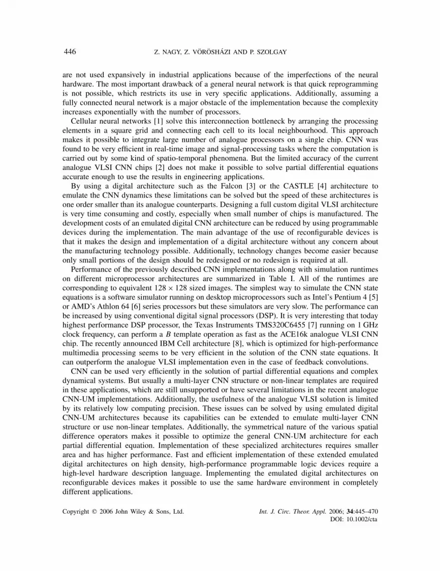
Figure 1. A simple mechanical vibrating system.

These methods require computing 2 and 4 times as many derivatives as the forward-Euler casebut we shall see that the extra computation is worthwhile.

The main issue when these equations are solved on an emulated digital CNN-UM is the requiredprecision (bit width) of the state values to get accurate results. To examine the accuracy of thedifferent fixed-point solutions the state equation of a simple dynamical system, shown in Figure 1,is solved.

This simple mechanical vibrating system contains five bodies which are connected by springs.The motion of the bodies is described by the following set of equations. (For simplicity, we assumeunit mass and unit spring constants.)

x1 = −2x1 + x2

xi = xi−1 − 2xi + xi+1, i = 2, 3, 4

x5 = x4 − 2x5

xi (0) = X0, xi (0)= V0, 1� i � 5

(4)

This set of state equations can be solved exactly and the solution has the following general form:

xi (t) =5∑j=1

Bi, j cos(� j t) (5)

where the � values are the eigenfrequencies of the system and the B values depend on the initialconditions. In our test case, the initial parameters were set to 0 except for the central element whichhad an initial displacement of 1. The solution of the system is plotted in Figure 2. According tothe initial conditions the values of the B matrix and the � eigenfrequencies of the system are thefollowing:

B =

⎡⎢⎢⎢⎢⎢⎢⎢⎣

0.16667 0 −0.33333 0 0.16667

−0.28868 0 0 0 0.28868

0.33333 0 0.33333 0 0.33333

−0.28868 0 0 0 0.28868

0.16667 0 −0.33333 0 0.16667

⎤⎥⎥⎥⎥⎥⎥⎥⎦

, � =

⎡⎢⎢⎢⎢⎢⎢⎢⎣

1.9319

1.7321

1.4142

1

0.51764

⎤⎥⎥⎥⎥⎥⎥⎥⎦

(6)

The state equations of the mechanical vibrating system can be solved on a line of 2-layer CNNcells where the first layer is the displacement and the second is the velocity of the given body.The following two templates are required for the computation:

A12 = 1, A21 = [1 −2 1] (7)



0 2 4 6 8 10 12 14 16–1

–0.8

–0.6

–0.4

–0.2

0

0.2

0.4

0.6

0.8

1

Time (s)

Pos

ition

m1m2m3

Figure 2. The analytical solution of the mechanical vibrating system.

1.0E-14

1.0E-13

1.0E-12

1.0E-11

1.0E-10

1.0E-09

1.0E-08

1.0E-07

1.0E-06

1.0E-05

1.0E-04

1.0E-03

1.0E-02

1.0E-01

-3 -4 -5 -6 -7 -8 -9 -10 -11 -12 -13 -14 -15 -16 -17 -18 -19 -20

Timestep (log2(h))

Err

or

RK4 RK2 Euler

Figure 3. Error of the different numerical methods.

The state equation of this CNN array is solved by using the previously described numericalmethods. To compare the different solutions the first 16 seconds of the analytical solution iscomputed using a 0.125 s timestep and the numerical and exact solutions were compared only inthese 128 points. The amplitude of the displacement of every body is always inside the [−1,+1]range. The absolute maximum difference between the exact and the numerical solution usingdifferent timesteps is shown in Figure 3.

As we could expect, the forward-Euler method has the largest errors and the higher-ordermethods perform better. On the other hand, the second- and fourth-order Runge–Kutta methods



1.0E-141.0E-131.0E-121.0E-111.0E-101.0E-091.0E-081.0E-071.0E-061.0E-051.0E-041.0E-031.0E-021.0E-01

-3 -4 -5 -6 -7 -8 -9 -10 -11 -12 -13 -14 -15 -16 -17 -18 -19 -20

Timestep (log2(h))

Err

or

FP64 8 bit 16 bit 24 bit 32 bit 40 bit

48 bit 56 bit

Figure 4. Error of the fourth-order Runge–Kutta method using different state precision.

have a much better convergence as the step-size is decreased. In the case of the fourth-orderRunge–Kutta method the accuracy of the solution cannot be increased if the timestep value issmaller than 2−11 because the rounding errors and the error of the method are in the samerange. In spite of the fact that the fourth-order Runge–Kutta method requires 4 times morecomputations and memory, it is worthwhile to implement it if accurate simulation of the dynamicsis required.

After a suitable ODE solver method is selected the next question is the required precision ofthe FPGA implementation because floating-point arithmetic requires huge area and by using fixed-point arithmetic large amount of resources can be saved or traded for performance. The absolutemaximum difference between the exact and the different numerical solutions using different stateprecision and timestep values are plotted in Figure 4.

In case of fixed-point computation, the error of the different numerical methods has a verysimilar behaviour. For large step-sizes the errors of the fixed and floating-point computations areequal. If the step-size is reduced further the error grows again because in these cases the roundingerrors are larger than the error of the numerical method. This effect is more obvious if the errorvalues are plotted as a function of the different precision values as shown in Figure 5. These resultsshow that an optimal bit width can be found for every timestep where the error of the floating-pointand the fixed-point solutions are identical and the bit width is minimal. The optimal bit widths fordifferent timestep values and simulation runtimes are plotted in Figure 6.

In the case of the forward-Euler and the second-order Runge–Kutta methods, very low fixed-point precision is required to get similar results than the floating-point solution; however, thesemethods are not very accurate. To get better results the fourth-order Runge–Kutta method shouldbe used, which requires about 2 times larger bit width but it is still more efficient than the lower-order methods. In a typical engineering application the simulation time and the desired accuracyof the solution are given in advance. According to the required accuracy the timestep value and



1.0E-13

1.0E-12

1.0E-11

1.0E-10

1.0E-09

1.0E-08

1.0E-07

1.0E-06

1.0E-05

1.0E-04

1.0E-03

1.0E-02

1.0E-01

8 12 16 20 24 28 32 36 40 44 48 52 56

Precision (bit)

Err

or

-4 -6 -8 -10 -12

-14 -16 -18 -20

Figure 5. Error of the fourth-order Runge–Kutta method using different timestep values.

0

10

20

30

40

50

60

-3 -4 -5 -6 -7 -8 -9 -10 -11 -12 -13 -14 -15 -16 -17 -18 -19 -20

Timestep (log2(h))

Pre

cisi

on

(b

it)

RK4 RK2 Euler

Figure 6. Optimal bit width for the different numerical methods.

the required bit width for every method can be selected. The comparison of the performance ofthe different methods in this case is summarized in Table II.

In our example the required accuracy was set to 10−4. In this case the required timesteps are 2−4

and 2−9 for the fourth- and second-order Runge–Kutta method while the forward-Euler methodrequires 2−17. In the case of the second-order Runge–Kutta and the forward-Euler method 32 and8192 times more iterations must be computed compared to the fourth-order Runge–Kutta method



Table II. Comparison of the different methods in case of an equalsolution accuracy (10−4).

Runge–Kutta Runge–Kutta Forwardfourth-order second-order Euler

Timestep (log2(h)) −4 −9 −17Iteration number 1 32 8192Derivative computation 4 2 1State width 32 bit 32 bit 36 bitNumber of processors 1 2 3.555Clock cycle time 1 1 1.125Performance 1 2 3.16Computation time 1 16 2592

due to the required smaller timestep. But in the case of the fourth-order Runge–Kutta method 4times more derivatives should be computed than the forward-Euler case. The area of the processoris determined by the state width and the number of derivative computations, thus 2 and 3.5 timesmore processors can be implemented on the same area if the second-order Runge–Kutta and theforward-Euler method are used. The clock cycle time is also affected by the state width thusthe performance of the lower-order methods on a unit area is 2 and 3.1 times larger than thefourth-order Runge–Kutta method. But the higher performance of the lower-order methods doesnot result in smaller computation time because much more iterations must be computed due tothe smaller timestep. In spite of the larger area and state width requirements of the fourth-orderRunge–Kutta method, the computation can be carried out 16 and 2592 times faster.

Unfortunately, the exact solution is usually not available which makes it hard to determine theoptimal fixed-point precision. In these cases only the floating-point results can be used as a referenceto determine the error of the fixed-point solution. The difference between the floating-point andthe fixed-point solutions is shown in Figure 7.

As the precision is increased, the difference between the two solutions decreases but how canwe tell the optimal bit width for the fixed-point solution? In Figure 7, the difference between theexact and floating-point solution is also plotted (FP64) but in this case the error of the differentfixed-point computations crosses this line instead of following it. But these solutions are not moreaccurate than the floating-point solution as shown in Figure 4.

Simple algorithm to determine the optimal bit width of the fixed-point computation. Let usassume that the error � of the floating-point solution is given in advance (it is usually true inengineering applications). The optimal bit width can be determined if several fixed-point solutionsare computed and the bit width is increased in each iteration until the difference between thefloating-point and fixed-point results is smaller than �. The determined precision of the state valuescan be used in case of other initial conditions provided that the results are in the same range asthe reference solution.

Another interesting question is to determine the limits of the floating-point solution. The accuracyof the solution of our simple example cannot be smaller than 10−14 as shown in Figure 4. Whathappens if the bit width of the fixed-point solution is increased well beyond 56 bit? To answer thisquestion the accuracy of the floating-point solution is decreased to 32 bit from 64 bit. In this caseonly the 32 bit floating-point results should be computed and compared to the previously computedfixed-point results and we do not have to use special library functions to handle bit widths larger



1.0E-16

1.0E -14

1.0E-12

1.0E-10

1.0E-08

1.0E-06

1.0E-04

1.0E-02

-3 -4 -5 -6 -7 -8 -9 -10 -11 -12 -13 -14 -15 -16 -17 -18 -19 -20

Timestep (log2(h))

Err

or


48 bit 56 bit

Figure 7. Difference between the 64 bit floating-point and the fixed-point solutions in the case of thefourth-order Runge–Kutta method using different state precision values.

than 56 bits. The error of the fixed-point computations compared to the 32 bit floating-point resultsis shown in Figure 8. The difference between the exact solution and the 32 bit floating-pointcomputation is also shown (FP32).

According to the narrower mantissa the 32 bit floating-point solution is very inaccurate comparedto the 64 bit floating-point results and the smallest error is in the order of 10−7. If the step-size isdecreased to improve the accuracy, the error of the solution increases due to the larger roundingerrors during the computation. If these inaccurate results are used as a reference solution in thecomputation of the error of the fixed-point solutions, the error values are very similar to theprevious case if the precision is smaller than 28 bit. If the precision is increased, the error valuesare identical to the error of the 32 bit floating-point results. This effect is more visible if theerror values are plotted as a function of the computational precision as shown in Figure 9. If theprecision is larger than 32 bit the error function is a horizontal line for all timesteps but thesefixed-point solutions are more accurate as shown in Figure 4.

Simple algorithm to determine the optimal bit width of the fixed-point computation when itsaccuracy is equal to the floating point solution: In this case the break-point of the error functionsshould be determined by increasing the precision until the error value remains the same. In thiscase, the fixed-point solution is at least as accurate as the floating-point solution.

In this section, the state equation of a simple dynamical system is solved and the accuracy ofthree numerical methods was examined. The results showed that high-order methods can be veryefficient if the dynamical behaviour of the system should be computed accurately in spiteof the fact that these methods require more computation per timestep. The state equation of thissystem is solved by using fixed-point numbers. The results showed that only moderate precision(28–32 bit) is required during the computation and the results are very close to the exact solutionof the system. Two simple heuristic methods are introduced to determine the optimal fixed-point



1.0E-07

1.0E-06

1.0E-05

1.0E-04

1.0E-03

1.0E-02

1.0E-01

-3 -4 -5 -6 -7 -8 -9 -10 -11 -12 -13 -14 -15 -16 -17 -18 -19 -20

Timestep (log2(h))

Err

or


48 bit 56 bit

Figure 8. Difference between the 32 bit floating-point and the fixed-point solutions in the case of thefourth-order Runge–Kutta method using different state precision values.

1.0E-07

1.0E-06

1.0E-05

1.0E-04

1.0E-03

1.0E-02

1.0E-01

8 12 16 20 24 28 32 36 40 44 48 52 56

Precison (bit)

Err

or

-4 -6 -8 -10 -12

-14 -16 -18 -20

Figure 9. Difference between the 32 bit floating-point and the fixed-point solutions in the case of thefourth-order Runge–Kutta method using different timestep values.

precision. The first method requires a priori information about the desired error of the solutionwhile the second method sets the precision so that the solution of the system using fixed-pointnumbers will be as accurate as the floating-point solution.



3. BAROTROPIC OCEAN MODEL

Simulation of compressible and incompressible fluids is one of the most exciting areas of thesolution of PDEs because these equations appear in many important applications in aerodynamics,meteorology and oceanography. In this section, a CNN-UM simulation of ocean currents will bepresented. The governing equations of the ocean model are derived from the Navier–Stokes equa-tions of incompressible fluids. CNN-UM solution of the Navier–Stokes equations was describedin Reference [11]. But the non-linearity of the state equations does not make it possible to utilizethe huge computing power of the current analogue CNN-UM chips. By using an emulated digitalCNN-UM the known limitations of the analogue chips such as low precision, small array size andnoise sensitivity can be solved. To improve the performance of our solution the cell model of thearchitecture is modified to handle the non-linearity of the model.

Building a universal ocean model that can accurately describe the state of the ocean on allspatial and temporal scales is very difficult [12]. Thus, ocean-modelling efforts can be diversifiedinto different classes, some concerned only with the turbulent surface boundary layers, some withcontinental shelves and some with the circulation in the whole ocean basin. Fine resolution modelscan be used to provide real-time weather forecasts for several weeks. These forecasts are veryimportant to the fishing industry, ship routing and search and rescue operations. The more coarseresolution models are very efficient in long-term global climate simulations such as simulating ElNino effects of the Pacific Ocean.

In general, ocean models describe the response of the variable density ocean to atmosphericmomentum and heat forcing. In the simplest barotropic ocean model a region of the ocean’s watercolumn is vertically integrated to obtain one value for the vertically different horizontal currents.The more accurate models use several horizontal layers to describe the motion in the deeper regionsof the ocean. Though these models are more accurate investigation of the barotropic ocean modelis not worthless because it is relatively simple, easy to implement and it provides a good basis forthe more sophisticated three-dimensional layered models.

The governing equations of the barotropic ocean model on a rotating Earth can be derived fromthe Navier–Stokes equations of incompressible fluids. Using Cartesian co-ordinates these equationshave the following form [12, 13]:

duxdt

= 2� sin �uy − gH��

�x+ �wx − �bx + A∇2ux − ux

H

�ux�x

− uy

H

�ux�y

Coriolis Pressure Lateral Advectionviscosity (8)

duy

dt= −2� sin �ux − gH

��

�y+ �wy − �by + A∇2uy − ux

H

�uy

�x− uy

H

�uy

�y(9)

d�

dt= −�ux

�x− �uy

�y(10)

where � is the height above mean sea level, ux and uy are volume transports in the x and ydirections, respectively. In the Coriolis term � is the angular rotation of the Earth and � is thelatitude. The pressure term contains H(x, y), which is the depth of the ocean and the gravitational



acceleration g. The wind and bottom stress components in both x and y directions are representedby �wx , �wy , �bx and �by , respectively. The lateral viscosity is denoted by A.

The circulation in the ocean is generally the result of the wind stress at the ocean’s surface andthe source sink mass flows at the basin boundaries. In our investigation steady wind was used toforce our model. In this case, the ocean will generally arrive at a steady circulation after an initialtransient behaviour.

Solution of Equations (8)–(10) on a CNN-UM architecture requires finite difference approxi-mation on a uniform square grid. The spatial derivatives can be approximated by the followingwell-known finite difference schemes and CNN templates:

��x

≈ 1

2�x

⎡⎢⎣0 0 0

1 0 −1

0 0 0

⎤⎥⎦= Adx (11)

��y

≈ 1

2�x

⎡⎣0 1 00 0 00 −1 0

⎤⎦= Ady (12)

∇2 ≈ 1

�x2

⎡⎢⎣0 1 0

1 −4 1

0 1 0

⎤⎥⎦= An (13)

By using these templates the pressure and lateral viscosity terms can be easily computed on CNN-UM architecture. However, the computation of the advection terms requires the following non-linearCNN template, which cannot be implemented on the present analogue CNN-UM architectures:

ux, i j��x

≈ ux, i j2�x

⎡⎢⎣0 0 0

1 0 −1

0 0 0

⎤⎥⎦ = Ax, x, i j (14)

Most ocean models arrange the time-dependent variables ux , uy and � on a staggered grid calledC-grid. In this case, the pressure p and height H variables are located at the centre of the meshboxes, and mass transports ux and uy are at the centre of the box boundaries facing the x andy directions, respectively. In this case, the state equation of the ocean model can be solved by aone layer CNN but the required template size is 5× 5 and space variant templates should be used.Another approach is to use 3 layers for the 3 time-dependent variables. In this case, the CNN-UMsolution can be described by the following set of equations:

dux, i jdt

= fi j uy, i j − gHi j∑

Adx� + �wx, i j − �′ux, i j

+ Ai j∑

Anux − 1

Hi j

(∑Ax, x, i j ux + ∑

Ax, y, i j uy)

(15)



duy, i j

dt= − fi j ux, i j − gHi j

∑Ady� + �wy, i j − �′uy, i j

+ Ai j∑

Anuy − 1

Hi j

(∑Ay, x, i j ux + ∑

Ay, y, i j uy)

(16)

d�i jdt

= −∑Adxux − ∑

Adyuy (17)

At the edges of the model the normal and tangential components of the flow are zero: the formermeans that there is no flow through the boundary while the later means that there is no slip at thesolid boundary. To achieve these conditions fixed boundary conditions are used in the case of uxand uy . In the case of the elevation � zero-flux boundary conditions are used because the watercan move freely at the boundary.

Using Equations (15)–(17) and templates (11)–(14) an analogic algorithm can be constructed tosolve the state equation of the barotropic ocean model. However, the non-linear advection terms donot allow us to implement our algorithm on the present analogue CNN-UM chips. The non-linearbehaviour can be modelled by using software simulation but this solution does not differ from thetraditional approach and does not provide any performance advantage.

The Falcon-emulated digital CNN-UM architecture can be modified to handle the non-lineartemplates required in the advection terms of the ocean model. The required blocks are an additionalmultiplier to compute the non-linearity and a memory unit to store the required ux, i j or uy, i jvalues. Of course this modification requires the redesign of the whole control unit of the processor.However, this modified Falcon architecture can run the analogic algorithm of the ocean model,its performance would not be significant because six templates should be run to compute the nextstep of the ocean model. The performance can be greatly improved by designing a specializedarithmetic unit, which can compute these templates fully parallel. Instead of building a generalCNN-UM architecture which can handle the required non-linear templates, an array of specializedcells is designed which can solve the state equation of the discretized ocean model directly.

To emulate the behaviour of the specialized cells the continuous state equations (15)–(17) mustbe discretized in time. In the solution, the leapfrog method is used but in this case we have anupper limit on the �t timestep. The maximal value of the timestep can be computed by using theCourant–Friedrichs–Levy (CFL) stability condition.

�t<�x/cw (18)

where �t is the timestep, �x is the distance between the grid points and cw is the speed of thesurface gravity waves typically cw =√

gH .Computation of the derivatives of ux and uy is the most complicated part of the arithmetic unit.

The proposed structure to compute the derivative of ux is shown in Figure 10. Similar circuit isrequired to compute the derivative of uy according to Equation (16).

This complex arithmetic unit can compute the derivatives and update the cell’s state value inone clock cycle but it requires pipelining to achieve high clock speeds. The values of �x and�t are restricted to be integer powers of two. In this case, multiplication and division by thesevalues can be done by shifts. This simple trick makes it possible to eliminate several multipliersfrom the arithmetic unit and greatly reduces the area requirements. The multiplication of g withHi j in the pressure term and the reciprocal of Hi j in the advection term are constant during thecomputation thus these values are computed in advance. This solution requires additional memory



Figure 10. Structure of the arithmetic unit.

both on- and off-chip but the required computing precision and the area of the arithmetic unit canbe significantly reduced.

The proposed architecture is implemented on our RC200 prototyping board from Celoxica Ltd.The XC2V1000 FPGA on this card can host one arithmetic unit which makes it possible to computea new cell value in one clock cycle (Figure 11). Unfortunately, the board has 72-bit wide data bus,so 6 clock cycles are required to read a new cell value and to store the results if 36-bit precision isused. The performance can be increased by reducing the array size and implementing six memoryunits which use the arithmetic unit alternately. In this case 6 clock cycles are required to compute 6new cell values and the utilization of the arithmetic unit is 100%. The performance of the system islimited by the speed of the on-board memory resulting in a maximum clock frequency of 90 MHz.In this case the performance of the chip is 90 million cell update/s. The size of the memory is also alimiting factor because the state and constant values must fit into the 4 Mbyte memory of the board.The size of the cell array is restricted to 256× 256 cells by the limited amount of on-board memory;however, the XC2V1000 FPGA can be used to work with 1024 or even 2048-cell wide arrays.

By using the new Virtex-4SX devices with larger and faster memory the performance of thearchitecture can reach 500 MHz clock rate and can compute a new cell value in each clockcycle. Additionally the huge amount of on-chip memory and multiplier on the largest XC4VSX55FPGA makes it possible to implement 12 separate arithmetic units. These arithmetic units work inparallel and the cumulative performance is 4800 million cell update/s. On the other hand, the largenumber of arithmetic units make it possible to implement more sophisticated and more accurateocean models. The performance of the different implementations compared to an AMD Athlon64 3200+ processor running on 2 GHz clock frequency is shown in Figure 12.



0

5

10

15

20

25

30

35

40

45

10 12 14 16 18 20 22 24 26 28 30 32 34 36

Precison (bit)

Nu

mb

er o

f p

roce

sso

rs

XC2V1000 XC2VP125 XC4VSX55

Figure 11. Number of implementable arithmetic units on different FPGAs.

1

10

100

1000

10000

10 12 14 16 18 20 22 24 26 28 30 32 34 36

Precision (bit)

Sp

eed

up

XC4VSX55 XC2VP125 XC2V1000 RC200

Figure 12. Speed-up of the architecture compared to an AMD Athlon 64 3200+ microprocessor.

The performance of the emulated digital solution of the model is very encouraging even byusing the mid-sized XC2V1000 FPGA on our prototyping board the computation is accelerated by60 times. Using the currently available largest FPGA, the XC4VSX55, the speed-up is 3200-foldwhen 36-bit precision is used.

To evaluate the accuracy of the fixed-point solution a simple model is used. The size of themodelled ocean is 2097 km, the boundaries are closed, the grid size is 256× 256 and the grid



(b)(a)

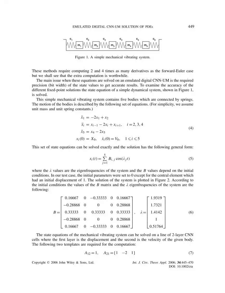
Figure 13. Results in the case of a seamount: (a) flow values; and (b) elevation.

resolution is 8192 m. The model is forced by a steady wind blowing from west and its valueis constant along the x direction. The wind speed in the y direction is described by a reversedparabolic curve where the speed is zero at the edges and 8 m/s in the centre. Several differentbottom topographies were used during the computation such as flat bottom, underwater ridge andseamount. The results of the 36 bit fixed-point computations after 72 h of simulation time using32 s timestep in the seamount case are shown in Figure 13.

The 36 bit fixed-point computations are very close to the 64 bit floating-point results but ourquestion is what the optimal fixed-point precision is. To answer this question the model is simulatedby using different precisions for all bottom topographies. The result of the fixed-point computationsis compared to the 64 bit floating-point results and the absolute maximum difference between thetwo solutions is shown in Figure 14.

If the precision is smaller than 12 bit, the state of the ocean model does not change. By slightlyincreasing the accuracy the state of the model will change but the error of the flow is in thesame range as the flow value itself. To achieve 10% accuracy at least 22-bit precision is required;however, in this case, the error of the elevation is still too high compared to its maximum value. Ifthe precision is further increased, the accuracy of the solution increases quickly but seemingly theerror cannot be decreased if the precision is larger than 30 bit. This behaviour is very similar tothe results obtained in the previous section and the error of the fixed-point solution in these casesis smaller than the error of the 64-bit floating-point solution. Though 30 bits of precision seemto be enough for the computation of the flow values the elevation of the ocean model should becomputed more accurately to achieve similar accuracy to the 64-bit floating-point solution.

The state equation of a barotropic ocean model with realistic input parameters was solvedby using CNN architecture. The Falcon-emulated digital CNN-UM processor was optimized tosolve the governing equations of the model. Due to the optimization the area requirements of thearithmetic unit are significantly reduced while its computing power is increased. The proposedarchitecture was implemented on a mid-sized FPGA with one million equivalent system gates onour RC200 prototyping board. The performance of this solution is limited by the speed of thememories and the width of the memory bus. But even this restricted solution is 60 times fasterthan an AMD Athlon 64 3200+. If larger FPGA and wider memory bus are used, 3200-foldperformance increase can be achieved even if 36-bit precision is used.



1.0E-05

1.0E-04

1.0E-03

1.0E-02

1.0E-01

1.0E+00

10 12 14 16 18 20 22 24 26 28 30 32 34 36

Precision (bit)

Err

or

Case1 Case2 Case3 Case4

Case5 Case6(a)

1.0E-05

1.0E-04

1.0E-03

1.0E-02

1.0E-01

1.0E+00

10 12 14 16 18 20 22 24 26 28 30 32 34 36

Precision (bit)

Err

or


Case5 Case6(b)

1.0E-07

1.0E-06

1.0E-05

1.0E-04

1.0E-03

1.0E-02

10 12 14 16 18 20 22 24 26 28 30 32 34 36

Precision (bit)

Err

or


Case5 Case6(c)

Figure 14. Error of the: (a) horizontal flow ux ; (b) vertical flow uy ; and (c) elevation in the case ofdifferent bottom topographies.

4. RETINA MODEL

The visual system is the most important sensory organ for humans as well as mammals. Its firstand best-known part is the retina, which is a preprocessor and it sends visual information to thebrain via several parallel channels. The framework of mammalian retinal modelling via multi-layerCNN was published in Reference [14]. Determination of the model parameters requires very highcomputing power and accurate solution. On the current multi-layer analogue VLSI chips only thebasic building blocks of the retina model can be implemented [15]. Additionally the size of thecell array is relatively small.

The basic building blocks of the retina model are the abstract neurons which are organized intotwo-dimensional layers [16]. The main components of the abstract neuron are the cell body, thesynapses and the output transfer function. The cell body has a first- or second-order dynamicswhich is described by the following differential equations:

�ln xln = −xln + ∑

kl∈SnC�n,kl x

ln,kl + ∑

∀m∈Sy1∑

kl∈Smf rnm(G�

nm,kl ylm) +

∑∀m∈Sy2

xrnm + ∑∀m∈Sy3

(xrnm − r xdnm) − sx jn (19)



� jn x

jn = −x j

n + xln (20)

yln = f on (xln) (21)

C�n = �

⎡⎢⎣1 2 1

2 −12 2

1 2 1

⎤⎥⎦ (22)

G�nm,i j = 1∑

∀k,l G�nm(k, l)

e−√

i2+ j2/� (23)

where

• xln and x jn are the states of the second-order abstract neuron

• y is non-linear output of the abstract neuron• �l and � j are time constants of the layers• f r and f o are receptor and the output transfer function• Sn and Sm are local neighbourhood of the neuron• C is diffusion-type template• � is coupling parameter of the layer• G is Gauss-type template• � is sigma parameter of the receptor• Sy1, Sy2 and Sy3 are the plain, delayed and desensitized receptor set, respectively• r is the ratio parameter• s is the feedback gain.

Subsequent layers supply the input of the next layer through synapses. The abstract neuron hasreceptors to implement these synapses. The three different types of receptors are plain, delayedand desensitizing. The differential equations of the receptors are the following:

�rnm xrnm = −xrnm + ∑

kl∈Smf rnm(G�

nm,kl ylm) (24)

�dnm xdnm = −xdnm + xrnm (25)

where

• xln and x jn are the states of the receptor and the desensitized receptor

• �r and �d are delay and the desensitizing speed of the receptor.

The light-adapted mammalian retina model consists of several parts. The main parts are theouter retina model and the different ganglion models. The outer retina is a uniform block, whichtransforms the stimulus to the ganglion models. The ganglion models contain three functionalblocks: the excitation pattern generator, the inhibitory subsystem and the ganglion cell model.This middle abstraction-level model can be transformed to a low-level multi-layer CNN structureas shown in Figure 15. Each layer has its own time constant and connections. The inter-layerconnections are zero neighbourhood neuron to neuron links that have linear or rectifier transferfunctions.



ConeCone2

Horizontal

Input

Bip. Excit.Desensitized

AmacrineFB

Ganglion

- +Bip.Inhib.Desens.

Bip. Excit.Receptor

Bip.Inhib.Rec.

AmacrineFF

�

�

�

��

�

�

�

�

�

�

�

�

�

�

�

�

Figure 15. The structure of one retina channel.

To model one channel of the retina 10 CNN layers are required. This structure cannot bedirectly implemented on the recent analogue VLSI CNN-UM chips. Some features of the modelcan be demonstrated on the CACE1K [15] two-layer complex kernel CNN-UM chip but onlyapproximation of the complete model is possible. Additionally, the size of the array is just 32× 32cells, which is much smaller than the required 180× 135-sized cell array. The relatively lowaccuracy of the chip does not make it possible to utilize its high computing power during themodel building and parameter tuning steps of the retina modelling.

The Falcon-ML emulated digital CNN-UM architecture can be used to emulate a multi-layerCNN structure. The number of layers and the accuracy of the computation are configurable [3].The Falcon-ML architecture is designed to emulate a fully connected multi-layer CNN structurethus its hardware complexity increases quadratically as the number of layers are increased. In ourcase at least 10 layers should be emulated which means that 100 inter- and intra-layer connectionsand 300 multipliers (in case of nearest-neighbour templates) are required. Implementation of sucha huge arithmetic unit is not possible on the currently available reconfigurable chips thereforesome optimizations are required.

The main blocks of the optimized architecture are shown in Figure 16. The memory unit isvery similar to the memory unit of the Falcon-ML architecture. Depending on the template size itstores a one or two row high belt from the given layer to reduce I/O requirements of the processor.The template memory is modified and it contains only those parameters that are necessary to per-form the computations. The arithmetic unit is completely redesigned to make efficient computationof the multi-layer dynamics possible.

By examining the parameters of the mammalian retina model we find that most of the inter-layerconnections are zero, some of them are zero neighbourhood templates and only a few feedbackconnections require a nearest-neighbour template [14]. Additionally, the diffusion- and Gauss-typetemplates are symmetrical which makes further optimizations possible.

The block level structure of the optimized arithmetic unit is shown in Figure 17. According toEquations (19), (20), (24) and (25) the computation of the derivatives can be divided into three parts:

• computation with the zero neighbourhood connections,• computation with the diffusion-type template,• computation with the Gauss-type templates.



Memory unit

Coeff. Memory

Arithmetic unit

StateIn

StateOut

Input

Control

Figure 16. The structure of the optimized Falcon-ML architecture.

Diffusion type

Gauss type

Inter- Layer

Sh

ift

Reg

.Iterate

StateOut

Old StateInput from Memory unit

Figure 17. Structure of the optimized arithmetic unit.

The simplest element of the arithmetic unit is the inter-layer block which computes the inter- andintra-layer zero neighbourhood connections. This unit contains one multiplier for each connectionand the multiplied values are summed by an adder tree.

Due to the symmetry properties of the diffusion-type template the computation can be performedby the circuit shown in Figure 18. Multiplication with 2 and −12 is carried out by shifts and onlyone multiplier is required to compute the template operation. This solution reduces the number ofrequired multipliers from 3 to 1. Additionally, the number of clock cycles required to compute anew value is also reduced from 3 to 1 clock cycle, which significantly increases the computingperformance of the processor.

The Gauss-type template is also symmetrical but the ratio of the coefficient values is not aninteger value. Therefore, at first, the equally weighted state values are summed then these partialresults are multiplied; finally, the multiplied values are summed. By using the circuit shown inFigure 19. The number of multipliers is still three but the length of the computation cycle isreduced to 1 clock cycle.



+

x i+1,j+1 x i+1,j-1

, ,∈∑ l

n kl n klkl Sn

C x

+

x i-1,j+1 x i-1,j-1

+

+

x i,j+1 x i,j-1

+

x i+1,j x i-1,j

+

+

+

x i,j

Reg.

Reg.

-

*

<<1

<<1

<<2

�

�

Figure 18. Structure of the optimized arithmetic unit to compute the diffusion-type template.

+

yi+1,j+1 yi+1,j-1

11,nmGσ

, ,∈∑ l

nm kl n klkl Sm

G yσ

+

yi-1,j+1 yi-1,j-1

+

+

yi,j+1 yi,j-1

+

yi+1,j yi-1,j

+

+

yi,j

+

* *

*S

hif

t re

g.

10,nmGσ

00,nmGσ

Figure 19. Structure of the optimized arithmetic unit to compute the Gauss-type template.

The optimized Falcon-ML processor uses the forward-Euler method to compute the dynamics ofthe retina model. The Iterate block of the arithmetic unit sums the computed parts of the derivativeand computes the new state value of the cell. The timestep value h is restricted to be an integerpower of two. This makes it possible to do the multiplication with h by shifts and does not requirean additional multiplier.

Implementation and testing of the previously described arithmetic unit can be very time con-suming. But using rapid prototyping techniques and high-level hardware description languagessuch as Handel-C from Celoxica [17] makes it possible to develop the optimized arithmetic unitmuch faster compared to the conventional VHDL-based RTL level approach.

The proposed specialized Falcon-ML architecture will be implemented on the RC2000 boardfrom Celoxica Inc. [17]. This board contains a Virtex-II 6000 FPGA [18] and 24MB SRAMmemory, which is organized in six 36 bit wide independent banks. Utilization of the dedicated



0%

10%

20%

30%

40%

50%

60%

18 bit 20 bit 22 bit 24 bit 26 bit 28 bit 30 bit 32 bit 34 bit 36 bit

Precision (bit)

Uti

lizat

ion

BRAM XC2V6000 BRAM XC2VP125

BRAM XC4VSX55 MULT18X18 XC2V6000

MULT18X18 XC2VP125 MULT18X18 XC4VSX55

Figure 20. Device utilization.

memory (BRAM) and multiplier elements (MULT18X18) on this and the currently available largestFPGA the XC4VSX55 are summarized in Figure 20.

In both cases only a small fraction of the available resources is utilized. This makes it possibleto implement several Falcon-ML processors to speed up the computations. In the case of theVirtex-II 6000 FPGA 2 or 3 while on the Virtex-4 SX 55 FPGA even 9 processor cores canbe implemented. The performance of the architecture is scaled linearly according to the numberof processors. Computing performance compared to the speed of an Athlon 64 microprocessorrunning on 2 GHz clock frequency is shown in Figure 21. The results show that even in the caseof the Virtex-II 6000 FPGA more than 600 times higher computing performance can be achieved.By using the currently available largest FPGA the computations can be carried out more than 3000times faster.

The high computing performance of the Virtex-4 SX FPGA makes real-time emulation of oneretina channel possible. The clock frequency of the architecture can reach 400MHz and one clockcycle is required to compute a new cell value. The cumulative performance of the 9 implementableprocessors is 3.6 billion cell iteration/s. According to the parameters published in [14] mostchannels of the retina can be emulated by using 2−7 ms timestep. If the speed of the input video is30 frames/s, approximately 4266 iterations must be computed on each frame; this means 128 000iterations in every second. The maximum number of emulated cells can be computed by dividingthe performance of the processor by the required number of iterations. In our case the result is28 125 cells, which is approximately a 165× 165-sized cell array.

Additionally, the large number of implementable processors makes it possible to emulate morethan one channel of the retina. In this case, only one outer retina block is required and the processoris extended to emulate additional excitation, inhibition and ganglion blocks. The modular structureof the memory and the arithmetic unit makes this extension possible. The Handel-C high-levelhardware description language makes implementation and testing of the new processor much fasterand simpler than the conventional VHDL-based approach.



0

1000

2000

3000

4000

5000

6000

18 bit 20 bit 22 bit 24 bit 26 bit 28 bit 30 bit 32 bit 34 bit 36 bit

Precision (bit)

Sp

eed

up

XC2V6000 XC2VP125 XC4VSX55

Figure 21. Performance compared to an Athlon 64 microprocessor.

Unfortunately, addition of new layers to the model significantly increases the required I/Obandwidth and several clock cycles are required to load the state values and save the results.Though the arithmetic unit can compute a new cell value in every clock cycle this high computingpower cannot be utilized because several dummy cycles must be inserted until the I/O operationsare performed. Due to the architectural properties of the Virtex-II and Virtex-II Pro FPGAs thememory units must be configured 1024 elements wide. In most cases, much smaller cell array sizeis required hence the memory unit is also underutilized. To improve the utilization of the memoryand the arithmetic unit virtual processors are implemented. These virtual processors are chainedone after another and each of them works on a different forward-Euler iteration. In the case ofthe memory unit data of the different virtual memory units are stored on subsequent addresses.Similarly, the arithmetic unit is used by the different virtual arithmetic units in subsequent clockcycles.

Implementation of the virtual processors requires very small additional area. In most cases, onlyshift registers are required, which can be very efficiently implemented on the FPGA. By usingvirtual processors the utilization of the memory and the arithmetic unit can be improved whichresults in higher performance.

Performance of the processor can be significantly improved by lowering the computationalprecision. But low precision results in inaccurate solution. We should find a balance betweencomputing precision and solution accuracy. A simple test case is computed by using differentcomputing precision to approximate the accuracy of the results. The input of the model wasthe usual white flash, the simulation time was 2 s and the responses of several channel typesare computed. The results of the different fixed-point computations are compared to the 64 bitfloating point results. The absolute maximum difference between the different solutions is shownin Figure 22.

In case of very low precision the error values are very high because the model does not respond tothe input and remains in steady state. At least 16–18-bit precision is required to get some responseon the output of the model. If the precision is further improved, the error of the solution is quickly



1.0E-04

1.0E-03

1.0E-02

1.0E-01

1.0E+00

10 12 14 16 18 20 22 24 26 28 30 32 34 36

Precision (bit)

Err

or

OffBriskL OffBriskTr OnBist OnBriskTrN OnSluggish

Figure 22. Difference between the 64 bit floating-point and the different fixed-point results.

decreasing. If the dynamics of the retina model should be computed accurately, 30-bit precisionis required while qualitatively correct results can be obtained by using 20–22-bit precision.

A new emulated digital architecture based on the Falcon-ML architecture was designed to solvethe state equation of the mammalian retina model. The modular structure of the processor makes itpossible to implement specialized processors rapidly to emulate different types of retina channel(s)on the RC2000 prototyping board.

The computing precision of the processor is configurable which makes it possible to make atrade-off between area and performance. Even by using moderate precision the fixed-point resultsare very close to the floating-point results. If the precision is increased to 30 bit, the accuracy ofthe fixed-point solution is comparable to the accuracy of the floating-point results. This makes itpossible to use the proposed architecture during the model building and parameter tuning steps ofthe retina modelling where fast and accurate solution of the model is required.

In the currently available largest FPGA, computations can be carried out 3000 times faster thanon the AMD Athlon 64 microprocessor running on 2 GHz clock frequency. The high computingperformance of the processor makes real-time emulation possible in case of one retina channeland moderate-sized (165× 165) cell arrays.

5. CONCLUSIONS

In this paper, the solution of PDEs on emulated digital CNN-UM architectures was examined.However, several previous studies proved the effectiveness of the CNN solution of PDEs, inmost cases these results cannot be applied in the solution of real-life problems because of theimperfections of the analogue CNN chips. Emulated digital CNN-UM architectures can be used toovercome the limitations of the analogue VLSI CNN chips. Our results show that the forward-Eulermethod, which is widely used in the computation of the CNN dynamics on digital architectures,is not perfect in the solution of spatially discretized PDEs. By using more sophisticated numerical



methods PDEs can be solved orders of magnitude faster. But these architectures use fixed-pointnumbers during the solution of the CNN state equation because it requires less area than floating-point arithmetic. Additionally, performance of the emulated digital CNN-UM architectures can besignificantly improved by decreasing the computing precision. Therefore, it is very important toexamine the accuracy of the solution in the case of low computing precision. Comparison of thefloating-point and the fixed-point solutions showed that fixed-point arithmetic can be used veryefficiently in the solution of PDEs. The results of the floating-point and the fixed-point solutionsare very close even if low precision (20–24 bit) is used. If the precision is increased to 30–34 bit,the fixed-point computations are as accurate as the 64 bit floating-point results while it requiresmuch less amount of computing resources in implementation.

The symmetrical nature of the spatial difference operators makes it possible to optimize theFalcon-emulated digital CNN-UM architecture to solve a specific PDE. The resulting new ar-chitecture requires less area while its computing performance is increased. Performance of theemulated digital solution is 2–3 orders faster than the software simulation. In some cases this hugecomputing power makes real-time emulation of physical systems possible.

REFERENCES

1. Chua LO, Yang L. Cellular neural networks: theory and applications. IEEE Transactions on Circuits and Systems1998; 35:1257–1290.

2. Linan G, Domınguez-Castro R, Espejo S, Rodrıguez-Vazquez A. ACE16k: a programmable focal plane visionprocessor with 128× 128 resolution. Proceedings of the 15th European Conference on Circuit Theory and Design,vol. 1, 2001; 345–348.

3. Nagy Z, Szolgay P. Configurable multi-layer CNN-UM emulator on FPGA. IEEE Transactions on Circuits andSystems I: Fundamental Theory and Applications 2003; 50:774–778.

4. Keresztes P, Zarandy A, Roska T, Szolgay P, Hıdvegi T, Jonas P, Katona A. An emulated digital CNNimplementation. International Journal of VLSI Signal Processing 1999; 23:291–303.

5. Intel Products Homepage. [Online] http://www.intel.com, 2005.6. AMD Products Homepage. [Online] http://www.amd.com, 2005.7. Texas Instruments Products Homepage. [Online] http://www.ti.com, 2005.8. Kahle JA, Day MN, Hofstee HP, Johns CR, Maeurer TR, Shippy D. Introduction to the cell multiprocessor. IBM

Journal of Research and Development. [Online] http://www.research.ibm.com/journal/rd/494/kahle.html, 2005.9. Harrer H, Schuler A, Amelunxen E. Comparison of different numerical integration methods for simulating cellular

neural networks. Proceedings of the 1st IEEE International Workshop on Cellular Neural Networks and theirApplications, 1990; 151–159.

10. Press WH, Teukolsky SA, Vetterling WT, Flannery BP. Numerical Recipes in C. [Online] http://www.library.cornell.edu/nr/bookcpdf.html, 1992.

11. Roska T, Kozek T, Wolf D, Chua LO. Solving partial differential equations by CNN. Proceedings of EuropeanConference on Circuits Theory and Design, 1992.

12. Kantha L, Piacsek S. Ocean Models. [Online] http://csep1.phy.ornl.gov/CSEP/OM/OM.html, 2004.13. Robertson R, Padman L, Egbert GD. Tides in the weddell sea. [Online] http://www.esr.org/antarctic/barotropic.

html, 1998.14. Balya D, Roska B, Roska T, Werblin FS. A CNN framework for modeling parallel processing in a mammalian

retina. International Journal of Circuit Theory and Applications 2002; 30:363–393.15. Rekeczky Cs, Serrano-Gotarredona T, Roska T, Rodrıguez-Vazquez A. A stored program 2nd order/3-layer

complex cell CNN-UM. Proceedings of the 6th IEEE International Workshop on Cellular Neural Networks andtheir Applications, 2000; 219–224.

16. Balya D, Roska B, Roska T, Werblin FS. A CNN model framework and simulator for biological sensory systems.Proceedings of the 15th European Conference on Circuit Theory and Design, 2001; 357–360.

17. Celoxica Ltd. homepage. [Online] http://www.celoxica.com, 2005.18. Xilinx products homepage. [Online] http://www.xilinx.com, 2005.


emulated digital cnn-um solution of partial differential equations

Documents