embedded code generation from high-level heterogeneous
TRANSCRIPT
HAL Id: tel-00329534https://tel.archives-ouvertes.fr/tel-00329534
Submitted on 12 Oct 2008
HAL is a multi-disciplinary open accessarchive for the deposit and dissemination of sci-entific research documents, whether they are pub-lished or not. The documents may come fromteaching and research institutions in France orabroad, or from public or private research centers.
L’archive ouverte pluridisciplinaire HAL, estdestinée au dépôt et à la diffusion de documentsscientifiques de niveau recherche, publiés ou non,émanant des établissements d’enseignement et derecherche français ou étrangers, des laboratoirespublics ou privés.
Embedded Code Generation from High-levelHeterogeneous Components
Christos Sofronis
To cite this version:Christos Sofronis. Embedded Code Generation from High-level Heterogeneous Components. Net-working and Internet Architecture [cs.NI]. Université Joseph-Fourier - Grenoble I, 2006. English.�tel-00329534�

UNIVERSITY JOSEPH FOURIER – GRENOBLE 1
T H E S I S
To obtain the grade of
UJF DOCTOR
Speciality: ≪ COMPUTER SYSTEMS AND COMMUNICATIONS ≫
(INFORMATIQUE : SYSTEMES ET COMMUNICATION)
by
CHRISTOS SOFRONIS
Embedded Code Generation fromHigh-level Heterogeneous Components
Under the supervision of:
Paul Caspi & Stavros TripakisPrepared in the VERIMAG Laboratory
members of the jury
Yassine Lakhnech President
Christoph Kirsch Reviewer
Alberto Sangiovanni-Vincentelli Reviewer
Thierry Le Sergent Examinator
Paul Caspi Director
Stavros Tripakis Director
November 2006

ii

✳✳✳st♦✉❝ ❣♦♥❡Ð❝ ♠♦✉ ❆❥❤♥❼ ❦❛✐ ❉❤♠➔tr❤
iii

iv
Ithaca
When you set out on your journey to Ithaca,
pray that the road is long,
full of adventure, full of knowledge.
The Lestrygonians and the Cyclops,
the angry Poseidon do not fear
You will never find such as these on your path,
if you do not carry them within your soul,
if your soul does not set them up before you.
And if you find her poor, Ithaca has not deceived you.
Wise as you have become, with so much experience,
you must already have understood what Ithacas mean.
Constantine P. Cavafy (1911)
■❥❼❦❤
❙❛ ❜❣❡✐❝ st♦ ♣❤❣❛✐♠ì ❣✐❛ t❤♥ ■❥❼❦❤✱♥❛ ❡Ôq❡s❛✐ ♥❛ ❡Ð♥❛✐ ♠❛❦rÔ❝ ♦ ❞rì♠♦❝✱❣❡♠❼t♦❝ ♣❡r✐♣èt❡✐❡❝✱ ❣❡♠❼t♦❝ ❣♥➳s❡✐❝✳❚♦✉❝ ▲❛✐str✐❣ì♥❛❝ ❦❛✐ t♦✉❝ ❑Ô❦❧✇♣❛❝✱t♦♥ ❥✉♠✇♠è♥♦ P♦s❡✐❞➳♥❛ ♠❤ ❢♦❜❼s❛✐✳❚èt♦✐❛ st♦ ❞rì♠♦ s♦✉ ♣♦tè ❞❡♥ ❥❛ ❜r❡✐❝✱❛♥ ❞❡♥ t♦✉❝ ❦♦✉❜❛♥❡Ð❝ ♠❡❝ st❤♥ ②✉q➔ s♦✉✱❛♥ ❤ ②✉q➔ s♦✉ ❞❡♥ t♦✉❝ st➔♥❡✐ ❡♠♣rì❝ s♦✉✳
❑✐ ❛♥ ♣t✇q✐❦➔ t❤♥ ❜r❡✐❝✱ ❤ ■❥❼❦❤ ❞❡ s❡ ❣è❧❛s❡✳✬❊ts✐ s♦❢ì❝ ♣♦✉ è❣✐♥❡❝✱ ♠❡ tìs❤ ♣❡Ðr❛✱➔❞❤ ❥❛ t♦ ❦❛t❼❧❛❜❡❝ ❤ ■❥❼❦❡❝ t✐ s❤♠❛Ð♥♦✉♥✳
❑✇♥st❛♥tÐ♥♦❝ P✳ ❑❛❜❼❢❤❝ ✭✶✾✶✶✮
v

vi
Acknowledgments
This PhD thesis has been a three years journey for me and I must do the impossible task to
acknowledge in few words all the people that have helped and influenced me through all this
period both in my academic as well as in my personal life.
First of all I would like to thank both my supervisors Paul Caspi and Stavros Tripakis for
their constant help and for giving me new stimulus to continue my work. Moreover Stavros,
who has been more than a supervisor for me, tried a great deal to make me understand the world
of research. I would like to thank also the reviewers and the jury for their careful reading and
valuable comments.
Special thanks goes to Joseph Sifakis and all people in VERIMAG that hosted me “seam-
lessly”, meaning that all this time, although I was far from my home country, I didn’t experience
any problem. Special thanks goes also to the Region Rhone-Alpes for funding this thesis.
During this thesis, I met many people and had many discussions about my work. In partic-
ular, I would like to thank Norman Scaife for the implementation of the SF2LUS tool and his
collaboration on integrating both S2L and SF2LUS tools. Dietmar Kant, Thierry Le Sergent and
Jean-Louis Colaco for their collaboration and tips during the implementation of the S2L tool.
Finally Pontus Bostrom who provided me great feedback while using our tool-chain and helped
me debugging and extending it.
However the thesis was not only the time in the lab in front of a computer, that’s why I want
to specially thank the people in Grenoble that made my life more interesting, through all those
interactions. So, thank you Lemonia, all the friends at VERIMAG namely Dejan, Thao, Alex,
Marcelo, Radu, the football team (we are the champions!).
I would like to send my thoughts to my little Mikko and Dimitra and their little brothers and
sisters. I wish the best for their future that already looks brilliant.
Last but not least I send my thoughts to all my friends back to Greece, namely Nikos, Giorgos
(all of them), Alkis, Miltos, Antonis, Ilias, Kostis, my friends from this “cult” city Koropi:
Pavlos, Giannis, Dimosthenis and of course Aristel, Panagiotel... and Mariel.
Finally, I would like to thank Ana Maric by dedicating to her my favorite quotation: “life is
hilariously cruel”.
And of course, the best of my gratitude for their support goes to my sister Vicky and my
parents Athina and Dimitris.
I thank you all and I wish you the best luck...
vii

viii
Abstract
The work described in this thesis is done in the context of a long term effort at VERIMAG labora-
tory to build a complete model based tool-chain for the design and implementation of embedded
systems. We follow a layered approach that distinguishes the application level from the architec-
tural/implementation level. The application is described in a high-level language that is indepen-
dent of implementation details. The application is then mapped to a specified architecture using
a number of techniques so that the desired properties of the high level description are preserved.
In this thesis, the application is described in SIMULINK/STATEFLOW, a wide-spread model-
ing language that has become a de-facto standard in many industrial domains, such as automotive.
At the architectural level we consider single-processor, multi-tasking software implementations.
Multi-tasking means that the application software is divided into a number of processes that are
scheduled by a real-time operating system, according to some preemptive scheduling policy, such
as static-priority or earliest deadline first.
Between these two layers we add an intermediate representation layer, based on the syn-
chronous language LUSTRE, developed at VERIMAG for the last 25 years. This intermediate
layer permits us to take advantage of a number of tools developed for LUSTRE, such as simula-
tors, model-checkers, test generators and code generators.
In a first part of the thesis, we study how to translate automatically SIMULINK/STATEFLOW
models into LUSTRE. For SIMULINK this is mostly straightforward, however it still requires
sophisticated algorithms for the inference of type and timing information. The translation of
STATEFLOW is much harder for a number of reasons; first STATEFLOW presents a number of
semantically “unsafe” features, including non-termination of a synchronous cycle or dependence
of semantics on the graphical layout. Second, STATEFLOW is an automata-based, imperative
language, whereas LUSTRE is a dataflow language. For the first set of problems we propose a
number of statically verifiable conditions that define a “safe” subset of STATEFLOW. For the
second set of problems we propose a set of techniques to encode automata and sequential code
into dataflow equations.
In the second part of the thesis, we study the problem of implementing synchronous designs
in the single-processor multi-tasking architecture described above. The crucial issue is how to
implement inter-task communication so that the semantics of the synchronous design are pre-
served. Standard implementations, using single buffers protected by semaphores to ensure atom-
icity, or other, lock-free, protocols proposed in the literature do not preserve the synchronous
semantics. We propose a new buffering scheme that preserves the synchronous semantics and is
also lock-free. We also show that this scheme is optimal in terms of buffer usage.
ix

x
Resume
Le travail decrit dans cette these fait partie d’un effort de recherche au laboratoire VERIMAG pour
creer une chaıne d’outils basee sur modeles (model-based) pour la conception et l’implantation
des systemes embarquees. Nous utilisons une approche en trois couches, qui separent le niveau
d’application du niveau implantation/architecture. L’application est decrite dans un langage de
haut niveau qui est independante des details d’implantation. L’application est ensuite transferee
a l’architecture d’execution en utilisant des techniques specifiques pour que les proprietes de-
mandees soient bien preservees.
Dans cette these, l’application est decrite en SIMULINK/STATEFLOW, un langage de
modelisation tres repandu dans le milieu de l’industrie, comme celui de l’automobile. Au niveau
de l’architecture, nous considerons des implantation sur une plate-forme ”mono-processeur” et
”multi-taches”. Multi-taches signifie que l’application est repartie en un nombre des taches qui
sont ordonnees par un systeme d’exploitation temps-reel (RTOS) en fonction d’une politique
d’ordonnancement preemptive comme par exemple la priorite statique (static-priority SP) ou la
date-limite la plus proche en priorite (earliest deadline first EDF).
Entre ces deux couches, on rajoute une couche de representation intermediaire basee sur le
langage de programmation synchrone Lustre, developpe a VERIMAG durant les 25 dernieres
annees. Cette representation intermediaire permet de profiter des nombreux outils egalement
developpes a VERIMAG tels que des simulateurs, des generateurs de tests, des outils de
verification et des generateurs de code.
Dans la premiere partie de cette these, on etudie comment realiser une traduction automatique
de modele SIMULINK/STATEFLOW en modeles Lustre. Cote SIMULINK, le probleme est rela-
tivement simple mais necessite neanmoins l’utilisation d’algorithmes sophistiques pour inferer
correctement les informations de temps et de types (de signaux) avant de generer les variables
correspondantes dans le programme Lustre. La traduction de STATEFLOW est plus difficile a
cause d’un certain nombre de raisons ; d’abord STATEFLOW present un certain nombre de com-
portements ”non-sur” tels que la non-terminaison d’un cycle synchrone ou des semantiques qui
dependent de la disposition graphique des composants sur un modele. De plus STATEFLOW
est un langage imperatif, tandis que Lustre un langage de flots de donnees. Pour le premier
probleme nous proposons un ensemble de conditions verifiables statiquement servant a definir
un sous-ensemble ”sur” de STATEFLOW. Pour le deuxieme type de problemes nous proposons
un ensemble de techniques pour encoder des automates et du code sequentiel en equations de
flots de donnees.
Dans la deuxieme partie de la these, on etudie le probleme de l’implantation de programmes
xi

synchrones dans l’architecture mono-processeur et multi-tache decrite plus haut. Ici, l’aspect
le plus important est comment implanter les communications entre taches de maniere a ce que
la semantique synchrone du systeme soit preservee. Des implantations standards, utilisant des
buffers de taille un, proteges par des semaphores pour assurer l’atomicite, ou d’autres proto-
coles ”lock-free” proposes dans la litterature ne preservent pas la semantique synchrone. Nous
proposons un nouveau schema de buffers, qui preserve la semantique synchrone tout en etant
egalement ”lock-free”. Nous montrons de plus que ce schema est optimal en terme d’utilisation
des buffers.
xii
Contents
Acknowledgements vii
Abstract ix
Resume xii
1 Introduction 1
2 Model-based design at VERIMAG 7
3 The Synchronous Programming Language LUSTRE 11
3.1 The LUSTRE language . . . . . . . . . . . . . . . . . . . . . . . . . . . . . . . 11
3.2 LUSTRE compiler and code generation . . . . . . . . . . . . . . . . . . . . . . . 14
4 Analysis and Translation of Discrete-Time SIMULINK to LUSTRE 17
4.1 SIMULINK Translation Objectives . . . . . . . . . . . . . . . . . . . . . . . . . 17
4.2 Differences of SIMULINK and LUSTRE . . . . . . . . . . . . . . . . . . . . . . 17
4.3 The Goals and Limitations of the Translation . . . . . . . . . . . . . . . . . . . 18
4.4 Type inference . . . . . . . . . . . . . . . . . . . . . . . . . . . . . . . . . . . . 21
4.4.1 Types in LUSTRE . . . . . . . . . . . . . . . . . . . . . . . . . . . . . . 21
4.4.2 Types in SIMULINK . . . . . . . . . . . . . . . . . . . . . . . . . . . . 22
4.4.3 Type Inference and Translation . . . . . . . . . . . . . . . . . . . . . . . 23
4.5 Clock inference . . . . . . . . . . . . . . . . . . . . . . . . . . . . . . . . . . . 24
4.5.1 Time in LUSTRE . . . . . . . . . . . . . . . . . . . . . . . . . . . . . . 24
4.5.2 Time in SIMULINK . . . . . . . . . . . . . . . . . . . . . . . . . . . . . 25
4.5.3 Clock Inference . . . . . . . . . . . . . . . . . . . . . . . . . . . . . . . 33
4.6 Translation . . . . . . . . . . . . . . . . . . . . . . . . . . . . . . . . . . . . . 36
4.7 Related Work . . . . . . . . . . . . . . . . . . . . . . . . . . . . . . . . . . . . 43
4.8 Conclusions . . . . . . . . . . . . . . . . . . . . . . . . . . . . . . . . . . . . . 44
5 Analysis and Translation of STATEFLOW to LUSTRE 45
5.1 A short description of STATEFLOW . . . . . . . . . . . . . . . . . . . . . . . . . 45
5.2 Semantical issues with STATEFLOW . . . . . . . . . . . . . . . . . . . . . . . . 47
5.3 Simple conditions identifying a “safe” subset of STATEFLOW . . . . . . . . . . . 50
xiii
5.4 Translation into LUSTRE . . . . . . . . . . . . . . . . . . . . . . . . . . . . . . 53
5.4.1 Encoding of states . . . . . . . . . . . . . . . . . . . . . . . . . . . . . 53
5.4.2 Compiling transition networks . . . . . . . . . . . . . . . . . . . . . . . 55
5.4.3 Hierarchy and parallel AND states . . . . . . . . . . . . . . . . . . . . . 59
5.4.4 Inter-level and inner transitions . . . . . . . . . . . . . . . . . . . . . . 60
5.4.5 Action language translation . . . . . . . . . . . . . . . . . . . . . . . . 65
5.4.6 Event broadcasting . . . . . . . . . . . . . . . . . . . . . . . . . . . . . 68
5.4.7 History junctions . . . . . . . . . . . . . . . . . . . . . . . . . . . . . . 72
5.4.8 Translation fidelity . . . . . . . . . . . . . . . . . . . . . . . . . . . . . 72
5.5 Which subset of STATEFLOW do we translate . . . . . . . . . . . . . . . . . . . 73
5.6 Enlarging the “safe” subset by model-checking . . . . . . . . . . . . . . . . . . 73
5.7 Related Work . . . . . . . . . . . . . . . . . . . . . . . . . . . . . . . . . . . . 76
5.8 Conclusions . . . . . . . . . . . . . . . . . . . . . . . . . . . . . . . . . . . . . 77
6 The SIMULINK/STATEFLOW to LUSTRE Translator: Tool and Case Studies 79
6.1 Tool . . . . . . . . . . . . . . . . . . . . . . . . . . . . . . . . . . . . . . . . . 79
6.1.1 The S2L tool . . . . . . . . . . . . . . . . . . . . . . . . . . . . . . . . 79
6.1.2 The SF2LUS tool . . . . . . . . . . . . . . . . . . . . . . . . . . . . . . 83
6.1.3 SS2LUS tool architecture and usage . . . . . . . . . . . . . . . . . . . . 88
6.2 Case Studies . . . . . . . . . . . . . . . . . . . . . . . . . . . . . . . . . . . . . 89
6.2.1 Warning processing system . . . . . . . . . . . . . . . . . . . . . . . . . 89
6.2.2 Steer-by-wire controller . . . . . . . . . . . . . . . . . . . . . . . . . . 92
6.2.3 A car alarm monitoring system . . . . . . . . . . . . . . . . . . . . . . . 94
6.2.4 A mixed SIMULINK/STATEFLOW case study . . . . . . . . . . . . . . . 99
7 Preservation of Synchronous Semantics under Preemptive Scheduling 103
7.1 Motivation . . . . . . . . . . . . . . . . . . . . . . . . . . . . . . . . . . . . . . 103
7.2 An inter-task communication model . . . . . . . . . . . . . . . . . . . . . . . . 106
7.3 Execution on static-priority or EDF schedulers . . . . . . . . . . . . . . . . . . . 107
7.3.1 Execution under preemptive scheduling policies . . . . . . . . . . . . . . 107
7.3.2 A “simple” implementation . . . . . . . . . . . . . . . . . . . . . . . . 108
7.3.3 Problems with the “simple” implementation . . . . . . . . . . . . . . . . 109
7.4 Semantics-preserving implementation: the one-reader case . . . . . . . . . . . . 111
7.4.1 The low-to-high buffering protocol . . . . . . . . . . . . . . . . . . . . 112
7.4.2 The high-to-low buffering protocol . . . . . . . . . . . . . . . . . . . . 112
7.4.3 The high-to-low buffering protocol with unit-delay . . . . . . . . . . . . 114
7.4.4 Some examples under EDF scheduling . . . . . . . . . . . . . . . . . . 116
7.4.5 Application to general task graphs . . . . . . . . . . . . . . . . . . . . . 120
7.5 Semantics-preserving implementation: the general case . . . . . . . . . . . . . . 122
7.5.1 The Dynamic Buffering Protocol . . . . . . . . . . . . . . . . . . . . . . 124
7.5.2 Application of DBP to general task graphs . . . . . . . . . . . . . . . . . 128
7.5.3 Application of DBP to tasks with known arrival pattern . . . . . . . . . . 129
7.6 Periods in consecutive powers of two . . . . . . . . . . . . . . . . . . . . . . . . 129
xiv
7.6.1 Non-atomic case . . . . . . . . . . . . . . . . . . . . . . . . . . . . . . 129
7.6.2 Atomic case . . . . . . . . . . . . . . . . . . . . . . . . . . . . . . . . . 130
7.7 Proof of correctness . . . . . . . . . . . . . . . . . . . . . . . . . . . . . . . . . 132
7.7.1 Proof of correctness using model-checking . . . . . . . . . . . . . . . . 132
7.7.2 Proof of correctness of the dynamic buffering protocol . . . . . . . . . . 139
7.8 Buffer requirements: lower bounds and optimality of DBP . . . . . . . . . . . . 142
7.8.1 Lower bounds on buffer requirements and optimality of DBP in the worst
case . . . . . . . . . . . . . . . . . . . . . . . . . . . . . . . . . . . . . 143
7.8.2 Optimality of DBP for every arrival/execution pattern . . . . . . . . . . . 145
7.8.3 Exploiting knowledge about future task arrivals . . . . . . . . . . . . . . 148
7.9 Related Work . . . . . . . . . . . . . . . . . . . . . . . . . . . . . . . . . . . . 149
7.10 Conclusions . . . . . . . . . . . . . . . . . . . . . . . . . . . . . . . . . . . . . 152
8 Conclusions and Perspectives 153
Appendixes 159
A Help messages by the S2L and SF2LUS tools 159
B One-to-one translation of a SIMULINK model to XML 165
Bibliography 175
xv

xvi
List of Figures
2.1 Model Based Design architecture. . . . . . . . . . . . . . . . . . . . . . . . . . 9
3.1 A LUSTRE program is a deterministic Mealy machine. . . . . . . . . . . . . . . 12
3.2 A LUSTRE node example. . . . . . . . . . . . . . . . . . . . . . . . . . . . . . 15
3.3 A counter in LUSTRE. . . . . . . . . . . . . . . . . . . . . . . . . . . . . . . . . 15
3.4 The C code for the example of the counter. . . . . . . . . . . . . . . . . . . . . . 16
4.1 The set of SIMULINK blocks that are currently handled by S2L. . . . . . . . . . . 20
4.2 A type error in SIMULINK. . . . . . . . . . . . . . . . . . . . . . . . . . . . . . 22
4.3 A SIMULINK model producing a strange error. . . . . . . . . . . . . . . . . . . . 26
4.4 Illustration of the “GCD rule”. . . . . . . . . . . . . . . . . . . . . . . . . . . . 27
4.5 A triggered subsystem. . . . . . . . . . . . . . . . . . . . . . . . . . . . . . . . 28
4.6 Illustration of the rising trigger. . . . . . . . . . . . . . . . . . . . . . . . . . . . 28
4.7 An enabled subsystem. . . . . . . . . . . . . . . . . . . . . . . . . . . . . . . . 29
4.8 A SIMULINK model with a counter inside an enabled subsystem. . . . . . . . . . 29
4.9 A strange behavior of the model of Figure 4.8. . . . . . . . . . . . . . . . . . . . 31
4.10 Example of clock inference. . . . . . . . . . . . . . . . . . . . . . . . . . . . . 35
4.11 Mux - Demux example. . . . . . . . . . . . . . . . . . . . . . . . . . . . . . . . 39
4.12 SIMULINK system A with subsystem B. . . . . . . . . . . . . . . . . . . . . . . 40
4.13 A Zero-Order Hold block modifying the period of its input. . . . . . . . . . 42
5.1 Stack overflow . . . . . . . . . . . . . . . . . . . . . . . . . . . . . . . . . . . 48
5.2 Example of backtracking . . . . . . . . . . . . . . . . . . . . . . . . . . . . . . 48
5.3 Example of non-confluence . . . . . . . . . . . . . . . . . . . . . . . . . . . . . 49
5.4 “Early return logic” problem . . . . . . . . . . . . . . . . . . . . . . . . . . . . 50
5.5 The example of Figure 5.3 corrected to be confluent . . . . . . . . . . . . . . . . 52
5.6 A simple STATEFLOW chart . . . . . . . . . . . . . . . . . . . . . . . . . . . . 53
5.7 Simple LUSTRE encoding of the example . . . . . . . . . . . . . . . . . . . . . 54
5.8 Alternative LUSTRE encoding of the example . . . . . . . . . . . . . . . . . . . 56
5.9 A STATEFLOW chart with a junction . . . . . . . . . . . . . . . . . . . . . . . . 56
5.10 Code generated for the junctions example . . . . . . . . . . . . . . . . . . . . . 58
5.11 Chaining together transition-valid computations . . . . . . . . . . . . . . . . . . 59
5.12 A for-loop implemented in STATEFLOW junctions and its expansion . . . . . . 59
xvii
5.13 A model with parallel (AND) and exclusive (OR) decompositions . . . . . . . . 60
5.14 LUSTRE code fragments for parallel and hierarchical states . . . . . . . . . . . . 61
5.15 Computation of parallel state variables . . . . . . . . . . . . . . . . . . . . . . . 62
5.16 A model with inter-level transitions . . . . . . . . . . . . . . . . . . . . . . . . 62
5.17 A model with inner transitions . . . . . . . . . . . . . . . . . . . . . . . . . . . 63
5.18 Inter-level transitions with action order distortion . . . . . . . . . . . . . . . . . 64
5.19 LUSTRE code fragments for inter-level transitions . . . . . . . . . . . . . . . . . 67
5.20 Transformation of pseudo-LUSTRE . . . . . . . . . . . . . . . . . . . . . . . . . 68
5.21 Counter function for temporal logic . . . . . . . . . . . . . . . . . . . . . . . . 69
5.22 A model with non-confluent parallel states requiring event broadcasting . . . . . 70
5.23 Code showing event stack . . . . . . . . . . . . . . . . . . . . . . . . . . . . . . 71
5.24 Saving and restoring history values . . . . . . . . . . . . . . . . . . . . . . . . . 72
5.25 Simple observer in STATEFLOW . . . . . . . . . . . . . . . . . . . . . . . . . . 73
5.26 An observer for parallel state confluence . . . . . . . . . . . . . . . . . . . . . . 74
5.27 An observer for event stack overflow . . . . . . . . . . . . . . . . . . . . . . . . 75
5.28 Code for event broadcast with error detection . . . . . . . . . . . . . . . . . . . 76
6.1 The S2L tool architecture. . . . . . . . . . . . . . . . . . . . . . . . . . . . . . . 80
6.2 The main window of the GUI version of the S2L tool. . . . . . . . . . . . . . . . 82
6.3 The cancel warning subsystem. . . . . . . . . . . . . . . . . . . . . . . . . 90
6.4 Contents of the cancel warning subsystem. . . . . . . . . . . . . . . . . . . 91
6.5 A small fragment of the LUSTRE program generated by S2L from the warning
processing system model. . . . . . . . . . . . . . . . . . . . . . . . . . . . . . . 93
6.6 The steer-by-wire controller model (root system). . . . . . . . . . . . . . . . . . 94
6.7 Parts of the steer-by-wire controller model. . . . . . . . . . . . . . . . . . . . . 95
6.8 Parts of the steer-by-wire controller model. . . . . . . . . . . . . . . . . . . . . 96
6.9 An alarm controller for a car . . . . . . . . . . . . . . . . . . . . . . . . . . . . 97
6.10 Abstracted and corrected version of the alarm controller . . . . . . . . . . . . . . 98
6.11 The SIMULINK part of the kiiku verification example . . . . . . . . . . . . . . . 100
6.12 The STATEFLOW part of the kiiku verification example . . . . . . . . . . . . . . 101
7.1 Two periodic tasks. . . . . . . . . . . . . . . . . . . . . . . . . . . . . . . . . . 104
7.2 In the semantics, xjm = yi
k+1, whereas in the implementation, xjm = yi
k. . . . . . . 110
7.3 In the semantics, xjm = yi
k−1, whereas in the implementation, xjm = yi
k−2. . . . . 110
7.4 In the semantics, xjm = yi
k, whereas in the implementation, xjm = yi
k+1. . . . . . . 111
7.5 Low-to-high buffering protocol. . . . . . . . . . . . . . . . . . . . . . . . . . . 113
7.6 A typical low-to-high communication scenario. . . . . . . . . . . . . . . . . . . 113
7.7 High-to-low buffering protocol. . . . . . . . . . . . . . . . . . . . . . . . . . . . 115
7.8 A typical high-to-low communication scenario. . . . . . . . . . . . . . . . . . . 115
7.9 High-to-low buffering protocol with unit delay. . . . . . . . . . . . . . . . . . . 117
7.10 A typical high-to-low with unit delay communication scenario. . . . . . . . . . . 117
7.11 The scenario of Figure 7.6 possibly under EDF: τi is not preempted. . . . . . . . 118
7.12 The scenario of Figure 7.8 possibly under EDF: τj is not preempted. . . . . . . . 119
xviii
7.13 The scenario of Figure 7.10 possibly under EDF: τj is not preempted. . . . . . . 120
7.14 Equal absolute deadlines example. . . . . . . . . . . . . . . . . . . . . . . . . . 121
7.15 A task graph. . . . . . . . . . . . . . . . . . . . . . . . . . . . . . . . . . . . . 123
7.16 Applicability of the DBP protocol. . . . . . . . . . . . . . . . . . . . . . . . . . 123
7.17 The protocol DBP. . . . . . . . . . . . . . . . . . . . . . . . . . . . . . . . . . 125
7.18 A task graph with one writer and three readers. . . . . . . . . . . . . . . . . . . 126
7.19 The execution of the tasks. . . . . . . . . . . . . . . . . . . . . . . . . . . . . . 127
7.20 The values of the DBP pointers during execution. . . . . . . . . . . . . . . . . . 127
7.21 Multiperiodic events with consecutive periods in powers of 2 . . . . . . . . . . . 130
7.22 Multiperiodic events with consecutive periods in powers of 2, atomic reads . . . 131
7.23 Architecture of the model used in model-checking. . . . . . . . . . . . . . . . . 133
7.24 Assumptions modeling static-priority scheduling: p1 > p2. . . . . . . . . . . . . 134
7.25 Assumptions modeling EDF scheduling: d1 < d2. . . . . . . . . . . . . . . . . . 135
7.26 The ideal semantics described in LUSTRE: the case τ1 → τ2. . . . . . . . . . . . 135
7.27 The low-to-high protocol described in LUSTRE. . . . . . . . . . . . . . . . . . . 136
7.28 Model checking described in LUSTRE. . . . . . . . . . . . . . . . . . . . . . . . 137
7.29 Single buffer scheme for periods in powers of 2 . . . . . . . . . . . . . . . . . . 138
7.30 Illustration used in the proof of DBP. . . . . . . . . . . . . . . . . . . . . . . . . 140
7.31 N + 1 buffers are necessary in the worst case (N is the number of readers). . . . 143
7.32 Worst-case scenario for N +1 buffers: N lower-priority readers without unit-delay.144
7.33 First worst-case scenario for N + 2 buffers: N lower-priority readers without
unit-delay and at least one higher-priority reader (with unit-delay). . . . . . . . . 144
7.34 Second worst-case scenario for N + 2 buffers: N = N1 + N2, N1 lower-priority
readers without unit-delay and N2 lower-priority readers with unit-delay. . . . . . 145
7.35 The protocol DBP. . . . . . . . . . . . . . . . . . . . . . . . . . . . . . . . . . 148
A.1 The help message provided by the S2L tool. . . . . . . . . . . . . . . . . . . . . 160
A.2 The help message provided by the SF2LUS tool. . . . . . . . . . . . . . . . . . . 163
B.1 The initial model file of the example of the translation to XML. . . . . . . . . . . 166
B.2 The resulting XML file. . . . . . . . . . . . . . . . . . . . . . . . . . . . . . . . 167
xix

xx

List of Tables
3.1 Boolean flows and their clocks. . . . . . . . . . . . . . . . . . . . . . . . . . . . 12
3.2 Example for the use of pre and ->. . . . . . . . . . . . . . . . . . . . . . . . . 14
3.3 Example of use of when and current . . . . . . . . . . . . . . . . . . . . . . 14
4.1 Signals and systems in SIMULINK and LUSTRE. . . . . . . . . . . . . . . . . . . 17
4.2 Types of some SIMULINK blocks. . . . . . . . . . . . . . . . . . . . . . . . . . 23
4.3 Clock calculus of LUSTRE. . . . . . . . . . . . . . . . . . . . . . . . . . . . . . 25
4.4 Sample time signatures in SIMULINK. . . . . . . . . . . . . . . . . . . . . . . . 34
xxi

xxii
Chapter 1
Introduction
Context of this thesis
The technological evolution we are experiencing the last decades has resulted in using more and
more “computerized” devices for an entire spectrum of tasks, from the simple everyday tasks to
the most sophisticated and complicated ones, which is far from the classical perception of what
we used to call “computer”. Moreover the constantly reducing size of these systems results to
finding usage even in the most unthinkable (for the past decades) places, providing the market
with a big number of small devices that we may call “gadgets”. More than 98% of processors
today are in such systems, and are no longer visible to the customer as computers in the classical
sense.
Other examples can be found in consumer electronics such as mobile phones, house electrical
appliances or in more “heavy” industries like automotive, railway, avionics and aerospace. We
call all these systems embedded systems. More precisely, when we consider high-risk application
domains, like the avionics or the automotive, those systems are called safety-critical embedded
systems. In this specific area of embedded and real-time systems the basic requirement is high-
quality design and being able to guarantee a set of correctness properties.
The design of such systems is a difficult task. In this context, the model-based design
paradigm has been established as an important paradigm for the development of modern embed-
ded software. The main principle of the paradigm is to use models (with formal or semi-formal
semantics) all along the development cycle, from design, to analysis, to implementation. Using
models rather than, say, building prototypes is essential for keeping the development costs man-
ageable. However, models alone are not enough. Especially in the safety-critical domain, they
need to be accompanied by powerful tools for analysis (e.g., model-checking) and implemen-
tation (e.g., code generation). Automation here is the key: high system complexity and short
time-to-market make model reasoning a hopeless task, unless it is largely automatized.
The benefits of model-based design are many. First, high-level models raise the level of
abstraction, allowing the designer to focus on the essential functions of the system rather than
implementation details. This in turn makes possible to build larger and more complex systems.
Analysis tools, such as simulation or model-checking tools, are crucial at this stage. Bugs that
are found early in the design process are easier and less expensive to fix.
1
Chapter 1. Introduction
At some point the implementation phase begins, during which the system is actually built.
By “system” we mean hardware, software or both. One may consider also the environment as
part of the system and thus of the whole implementation process1. In the hardware industry the
implementation phase is closely coupled with the modeling and analysis phase. Powerful EDA
tools, stemming from a rich body of research on logic synthesis and similar topics, are used for
gate synthesis, circuit layout, routing, etc. Such tools are largely responsible for the proliferation
of electronics and their constant increase in performance.
In the software industry the situation is not as clear. On one hand, high-level models are not
as widespread. After all, the software itself is a model and simulation can be done by executing
the software. Testing and debugging are common-place (in fact, very time-consuming) but they
are done at the implementation level, that is, on the target software. Implementation is automated
using the most classical tools in computer science: compilers. The situation is changing, how-
ever: languages such as SIMULINK/STATEFLOW2, UML3 and others, as well as corresponding
software-synthesis facilities are used more and more. Currently, software synthesis is mostly re-
stricted to separate code generation for parts of the system. The integration of the different pieces
of code is usually done “manually” and is source of many problems, since the implementation
often exhibits unexpected behavior: deadlocks, missed data values, etc. These problems arise be-
cause the implementation method (in this case, code generation followed by manual integration)
does not guarantee that the original behavior (high-level semantics) is preserved.
The reason high-level semantics are generally not preserved by straightforward implementa-
tion methods is the fact that high-level design languages often use “ideal” semantics, such as con-
current, zero-time execution (as well as communication) of an unlimited number of components.
It is essential to use such ideal semantics in order to keep the level of abstraction sufficiently high.
On the other hand, these assumptions break down upon implementation: components take time
to execute; communication is also not free; neither is concurrency: scheduling is needed when
many software components are executed on the same processor and communication is needed
between components executing on separate hardware platforms.
As a result, implementations often exhibit a very different behavior than the original high-
level model. This is a problem, because it means that the results obtained by analyzing the
model (e.g., model satisfies a given property) may not hold at the implementation level. In
turn this implies that testing and verification need to be repeated at the implementation level.
This is clearly a waste of resources. In order to avoid this, we need to address the issue of the
preservation of properties of the high-level model, when moving towards the implementation.
This is the vision that motivates this thesis. To contribute to the effort of building a complete
model-based tool-chain that starts with high-level design languages and allows automatic, as
much as possible, synthesis of embedded code that, by construction, preserves crucial properties
of the high-level model.
This is an ambitious goal and, naturally, we had to look at only some parts of the entire
problem. In particular, our main focus has been the class of embedded control applications, and
1 This is especially important in control applications where the environment is the object to be controlled and
the one the controller needs to be adapted to.2 MATLAB, SIMULINK and STATEFLOW are trademarks of the MathWorks Inc.: http://www.mathworks.com.3 From the Object Management Group: http://www.uml.org/
2 Verimag — November 2006 Christos Sofronis
mostly those coming from domains such as automotive. Many of our choices, such as the choice
of which high-level design languages to consider, are a result of this context.
Our work has been performed in the context of two European projects, the project “NEXT
TTA”4 and the project “RISE”5. We should also say that our work has been part of an on-going
team effort at the VERIMAG laboratory for a number of years. This effort is explained in more
detail in Chapter 2.
Before proceeding to list the contributions of this thesis, let us briefly describe the state of
the art in what concerns model-based design.
State of the art
In the domains that we are mostly interested, that is the safety-critical applications like the au-
tomotive and avionic industries, the use of the SIMULINK/STATEFLOW toolkit by MathWorks is
considered as the de-facto standard.
SIMULINK offers to the designer a graphical interface that allows to combine blocks from
a number of libraries and interconnect them using signals. These blocks may perform basic
operations (like addition or multiplication) or more advanced ones (like transfer functions or
integration). SIMULINK can model discrete as well as continuous behavior making it feasible
for the designer to model not only the system but also the physical environment where this
system will be embedded. Thus the designer can simulate the interaction of his system and
the environment to check for the correctness and to measure the performance. Coupled with
SIMULINK there is the STATEFLOW tool that provides automata-based design capabilities. Other
products of MathWorks are the REAL-TIME WORKSHOP and REAL-TIME WORKSHOP EM-
BEDDED CODER code generators, that produce, starting from a SIMULINK/STATEFLOW model,
imperative code for given target execution platforms. Other companies also provide third-party
tools for SIMULINK/STATEFLOW, such as the TARGETLINK library and code generator from
dSpace.
SIMULINK/STATEFLOW started purely as a simulation environment and lacks many desir-
able features of programming languages. It has a multitude of semantics (depending on user-
configurable options), informally and sometimes only partially documented. Although commer-
cial code generators exist for SIMULINK/STATEFLOW, these present major restrictions. For ex-
ample, TARGETLINK does not generate code for blocks of the “Discrete” library of SIMULINK,
but only for blocks of the dSpace-provided SIMULINK library, and currently handles only mono-
periodic systems. Another issue not addressed by these tools is the preservation of semantics.
Indeed, the relation between the behavior of the generated code and the behavior of the simulated
model is unclear. Often, speed and memory optimization are given more attention than semantic
consistency. We describe in detail the short-comings of current code-generators for SIMULINK
in Section 7.9.
4 The project’s title is “High-Confidence Architecture for Distributed Control Applications” and for more infor-
mation refer to the official web-page http://www.vmars.tuwien.ac.at/projects/nexttta5 “RISE” stands for “Reliable Innovative Software for Embedded Systems” and more information can be found
in http://www.esterel-technologies.com/rise/
Christos Sofronis Ph.D Thesis 3
Chapter 1. Introduction
SCADE, a product of Esterel Technologies, Inc., is another design environment for embed-
ded software. SCADE uses a graphical user interface for design capture, similar to SIMULINK.
However, at the heart of the tool lies a backbone language, LUSTRE [HCRP91], which is a syn-
chronous language with formal semantics, developed at the VERIMAG laboratory for the past
twenty years. SCADE features model-checking capabilities with its “plug-in” from Prover 6, a
very important feature in the domain of safety-critical applications. Moreover, SCADE is en-
dowed with a DO178B-level-A7 code generator which allows it to be used in highest criticality
applications. SCADE has been used in important European avionic projects (Airbus A340-600,
A380, Eurocopter) and is also becoming a de-facto standard in this field.
Besides these and other commercial products8, there is a number of related offerings from
the academic world. Synchronous languages is one set of such offerings [BCE+03]. These lan-
guages appeared at approximately the same time in the eighties and include LUSTRE [HCRP91],
ESTEREL [BG92] and SIGNAL [GGBM91]. Synchronous languages share a number of com-
mon characteristics, among which a deterministic, synchronous automaton semantics, much
like that of a Mealy machine. These languages were conceived early-on as high-level pro-
gramming languages, targeted at embedded software. Code generation for these languages
has thus been one of the main concerns, and a lot of effort has been devoted in this direc-
tion [HCRP91, BG92, GGBM91].
With a different focus, and larger scope, the Metropolis project [BWH+03] offers a frame-
work that implements the platform-based design paradigm. In this paradigm, function (i.e., high-
level model) and architecture (i.e., execution platform) are clearly separated. Metropolis offers
a modeling framework to capture both. It also provides mechanisms, essentially by means of
action synchronization, for mapping the function onto the architecture. This mapping (currently
chosen by the user) essentially defines an implementation choice. By trying out and evaluating
different mappings, the user can explore different implementation choices.
The PTOLEMY project9 is another framework mostly focusing in modeling, and in particu-
lar in heterogeneous formalisms, that use radically different models of computation. Examples
of such formalisms range from Kahn process networks [Kah74] to Communicating Sequential
Processes (CSP) [Hoa85] to hybrid automata [ACH+95]. How to compose such heterogeneous
models in a coherent manner is a non-trivial problem, and the main focus of PTOLEMY.
Contributions of this thesis
State-of-the-art offerings are limited in a number of ways. Some solutions, for instance
SIMULINK, lack in formal semantics and provide little analysis capabilities except simulation10.
6 http://www.prover.com7 DO-178B, Software Considerations in Airborne Systems and Equipment Certification is a standard for software
development, which was developed by RTCA and EUROCAE. The FAA accepts use of DO-178B as a means of
certifying software in avionics.8 e.g., Telelogic’s TAU, supporting UML and SysML (http://www.telelogic.com/Products/tau/), ETAS’ ASCET
automotive platform, and more9 http://ptolemy.eecs.berkeley.edu [BHLM94]
10 A recent plug-in to SIMULINK is the “Verification and Validation” tool-box which performs input stimuli
generation and checks model coverage. The third-party tool Reactis, by Reactive Systems, has similar functionality.
4 Verimag — November 2006 Christos Sofronis
Others, for instance synchronous languages, provide relatively restricted modeling frameworks.
Finally, most solutions provide very limited code generation capabilities (essentially single-
processor, single-tasking) with little or no guarantees on preservation of properties of the high-
level model.
With this work, we hope to provide remedies to some of these shortcomings. Our work has
been done in the context of a long-term effort at the VERIMAG laboratory aiming to build a
complete tool-chain for the design and the implementation of safety-critical embedded systems
(see Chapter 2 for details). The contributions that this thesis brings to this effort are the following:
• We provide a method to translate (discrete-time) SIMULINK to LUSTRE. SIMULINK of-
fers an excellent high-level modeling framework, that is widespread in a number of ap-
plication domains, in particular, in the automotive domain. Our work provides a way to
link SIMULINK to a number of tools available for LUSTRE, including formal analysis tools
such as model-checkers and test generators. The translation also allows to use the code
generation capabilities for LUSTRE as well as the new techniques developed in this thesis
(see below). This translation is presented in Chapter 4.
• We provide a method to translate STATEFLOW to LUSTRE. STATEFLOW offers enhanced
modeling capabilities to SIMULINK. Together they offer a heterogeneous modeling frame-
work based on a combination of block diagrams and state machines. Apart from our trans-
lation to LUSTRE, we also provide static analysis techniques for STATEFLOW, that permit
to guarantee absence of critical errors in a model, such as non-termination of a simulation
cycle. This translation is presented in Chapter 5.
• We provide tools that implement the above translation methods. We also describe a few
case studies we have treated using these tools. The tools and case studies are presented in
Chapter 6.
• We provide a method to generate code from synchronous models onto single-processor,
multi-tasking execution platforms. Our method is proved to be semantics-preserving, in
the sense that the executable software has the same behavior as the “ideal” synchronous
model. Our method is also optimal with respect to memory requirements. The method is
presented in Chapter 7.
Organization of this document
The rest of this document is organized as follows. Chapter 2 describes the overall model-based
design effort at VERIMAG, in the context of which this work has been performed. In Chapter 3
we provide the basics of the LUSTRE synchronous programming language, which is a crucial
element in this overall approach. In Chapters 4 and 5 we study the translation of SIMULINK
and STATEFLOW, respectively, to LUSTRE. In Chapter 6 we present the implementation of these
translation methods in the tool SS2LUS, and also describe some case studies where this tool has
been used. Finally in Chapter 8 we present the conclusions of this work and possible future
directions.
Christos Sofronis Ph.D Thesis 5

Chapter 1. Introduction
6 Verimag — November 2006 Christos Sofronis
Chapter 2
Model-based design at VERIMAG
This thesis is in the context of almost 10 years efforts in VERIMAG to build a complete model
based tool-chain for the design and implementation of embedded systems. Moreover we focus
in the embedded systems that are used in high-risk application domains such as the automotive
and the aeronautics, where security is the most important requirement.
Designing according to the model based approach refers to using high-level abstractions to
conceptualize a system. Those high-level abstractions may be software platforms or models that
abstract the real implementation details and provide the designer with means to focus in certain
aspects of his design. Most of the times it is better to provide the designer with a methodology
that abstracts the communications between tasks of his model. Having a more general tool is
redundant and complicates the design in this case.
We propose a layered approach that distinguishes the application and the architecture in
which the execution will take place. In this sense, our approach follows the paradigm of platform-
based design [SV02], implemented in other frameworks such as Metropolis [BWH+03].
In our flavor of this approach we add another layer between the application and the architec-
ture layers. This layer that serves as an intermediate representation, is the LUSTRE synchronous
programming language, developed in VERIMAG for the last 25 years. We choose LUSTRE first
because of the vast knowledge of its mechanisms available within VERIMAG and also because
it permits us to take advantage of a number of tools developed for it, such as simulators, model-
checkers, test generators and code generators. A more detailed description of LUSTRE is pro-
vided in Chapter 3.
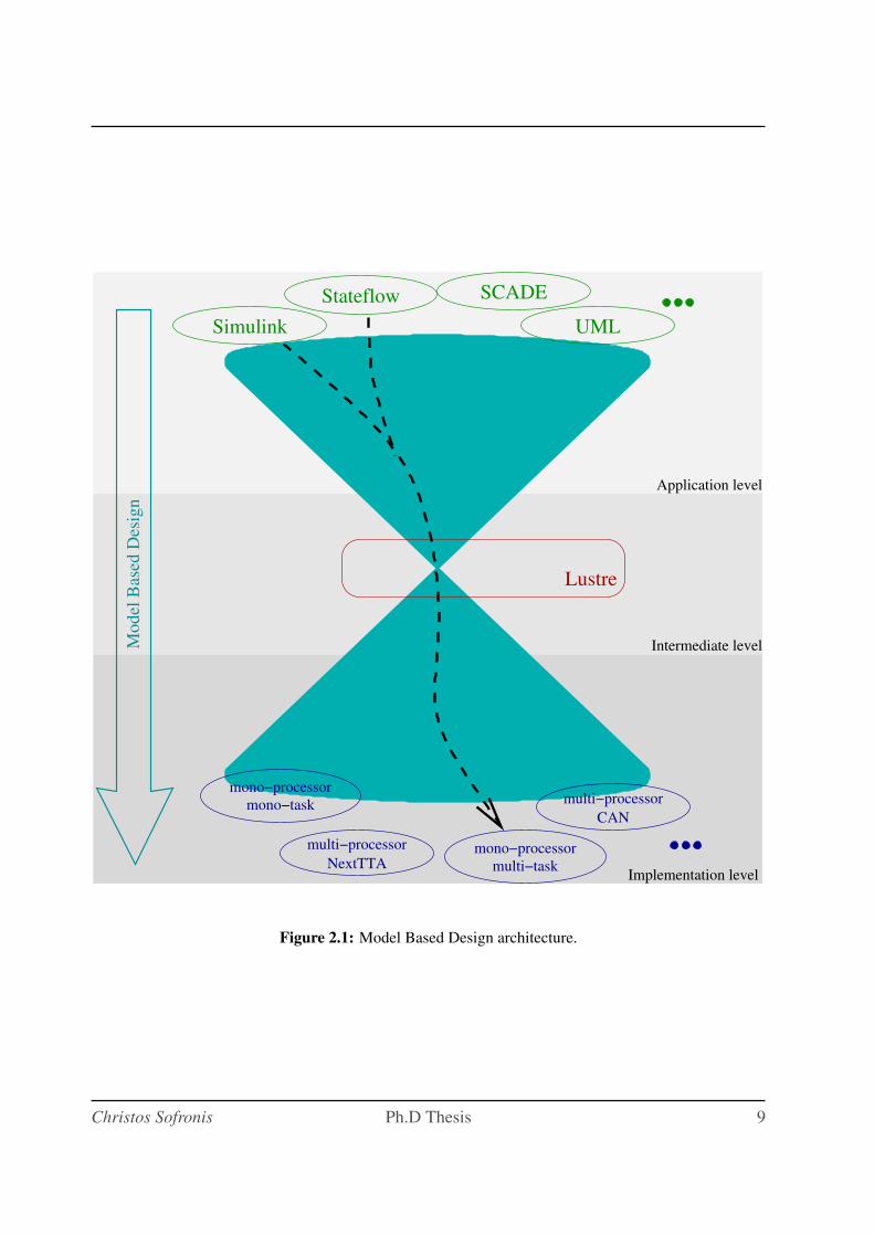
The model based approach we propose is the three-layered one we can see in Figure 2.1. As
said earlier, the LUSTRE language serves as an intermediate level between the top and the bottom
pyramids.
The top level is the application layer and contains all the tools, platforms and models that can
be used to facilitate the design of a system. In this area we can find SIMULINK, STATEFLOW,
UML or other formalisms and mathematical representations.
In the middle level we position LUSTRE, into which we translate the models produced in
the top level. Then we use the model-checking capabilities of LUSTRE to verify and validate
our design and thus, be sure that we the system respects always some safety properties. The
importance of the latter is significant since, as we saw earlier, the target applications are the ones
7
Chapter 2. Model-based design at VERIMAG
in the domains of automotive, aerospace and more general in high-risk applications.
The bottom level is the one of the actual execution of the system. In this layer we have all
the possible execution architectures and we can choose according to our needs. This contains
centralized or distributed architectures using single-tasking or multi-tasking software, various
hardware platforms as well as various communication media.
An on-going effort at VERIMAG aims at enriching the top and bottom layers, adding more
high-level description languages and more low-level execution platforms, to the capabilities of
our current tools. The first compiler of the LUSTRE language [HCRP91] covers implementa-
tion of LUSTRE on a mono-processor and single-task execution platform. The work of Adrian
Curic [Cur05, CCM+03] covers implementation of LUSTRE (and an extended LUSTRE lan-
guage) to a distributed synchronous execution platform, called the Time-Triggered Architecture
(TTA) [Kop97], where nodes communicate via the Time-Triggered Protocol (TTP) [KG94].
Our work contributes to the previous efforts as depicted by the dashed lines in Figure 2.1.
First, we provide a translation from SIMULINK to LUSTRE that we study in Chapter 4. We also
study the translation of STATEFLOW to LUSTRE in Chapter 5. Finally, we study the implemen-
tation of LUSTRE (and synchronous languages in general) on a mono-processor, multi-tasking
execution platform in Chapter 7.
We hope that future works will further enhance the picture by considering other high-level
languages (e.g., UML [Gro01]) and more execution platforms.
8 Verimag — November 2006 Christos Sofronis
Model
Bas
ed D
esig
n
Stateflow
Simulink
multi−processor
CAN
mono−processor
multi−task
multi−processor
NextTTA
mono−processor
mono−task
UML
SCADE
Application level
Intermediate level
Implementation level
Lustre
Figure 2.1: Model Based Design architecture.
Christos Sofronis Ph.D Thesis 9

Chapter 2. Model-based design at VERIMAG
10 Verimag — November 2006 Christos Sofronis
Chapter 3
The Synchronous Programming Language
LUSTRE
LUSTRE [CPHP87, HCRP91] is a synchronous dataflow programming language that has been
designed and developed in VERIMAG laboratory 25 years ago, following the merging of the
synchronous and the dataflow paradigms. On top of the language there is a number of tools
that constitute the LUSTRE platform. These tools take advantage of the formal foundations of
LUSTRE to provide model-checking capabilities and test generation. There is also the compiler
of producing imperative C code, that respects the semantics of the language. Finally there are
tools for the simulation of the system on design.
Moreover, SCADE, the industrial counterpart of LUSTRE, was founded by Esterel Tech-
nologies, Inc.. SCADE, having LUSTRE as backbone, provides graphical user interface to the
designer and also has a certified compiler1, which is very important in the area of aeronautics
and automotive industries. We can measure the importance of SCADE, and thus of LUSTRE,
by counting the number of companies already using it as a basis for their design. The last big
success of SCADE is its use for the development of the latest project of Airbus, the A380 carrier
airplane.
In this Chapter, we demonstrate the principles of LUSTRE and also give some examples of
usage. Furthermore, we discuss the C code generation capabilities of the LUSTRE compiler. We
do not intent to provide a full-fledged cover of the area, in which case the reader should refer
to [BCGH93, BCE+03].
3.1 The LUSTRE language
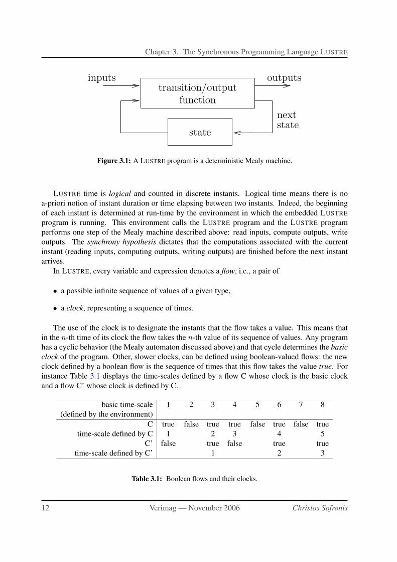
A LUSTRE program models essentially a deterministic Mealy machine, as illustrated in Fig-
ure 3.1. The machine has a (possibly infinite) set of states, a (possibly infinite) set of inputs and
a (possibly infinite) set of outputs. Given the current state and the current input the transition
function and output function compute the next state and the current output, respectively.
1 certified with the DO-178B certification on level A
11
Chapter 3. The Synchronous Programming Language LUSTRE
state
transition/outputfunction
inputs outputs
nextstate
Figure 3.1: A LUSTRE program is a deterministic Mealy machine.
LUSTRE time is logical and counted in discrete instants. Logical time means there is no
a-priori notion of instant duration or time elapsing between two instants. Indeed, the beginning
of each instant is determined at run-time by the environment in which the embedded LUSTRE
program is running. This environment calls the LUSTRE program and the LUSTRE program
performs one step of the Mealy machine described above: read inputs, compute outputs, write
outputs. The synchrony hypothesis dictates that the computations associated with the current
instant (reading inputs, computing outputs, writing outputs) are finished before the next instant
arrives.
In LUSTRE, every variable and expression denotes a flow, i.e., a pair of
• a possible infinite sequence of values of a given type,
• a clock, representing a sequence of times.
The use of the clock is to designate the instants that the flow takes a value. This means that
in the n-th time of its clock the flow takes the n-th value of its sequence of values. Any program
has a cyclic behavior (the Mealy automaton discussed above) and that cycle determines the basic
clock of the program. Other, slower clocks, can be defined using boolean-valued flows: the new
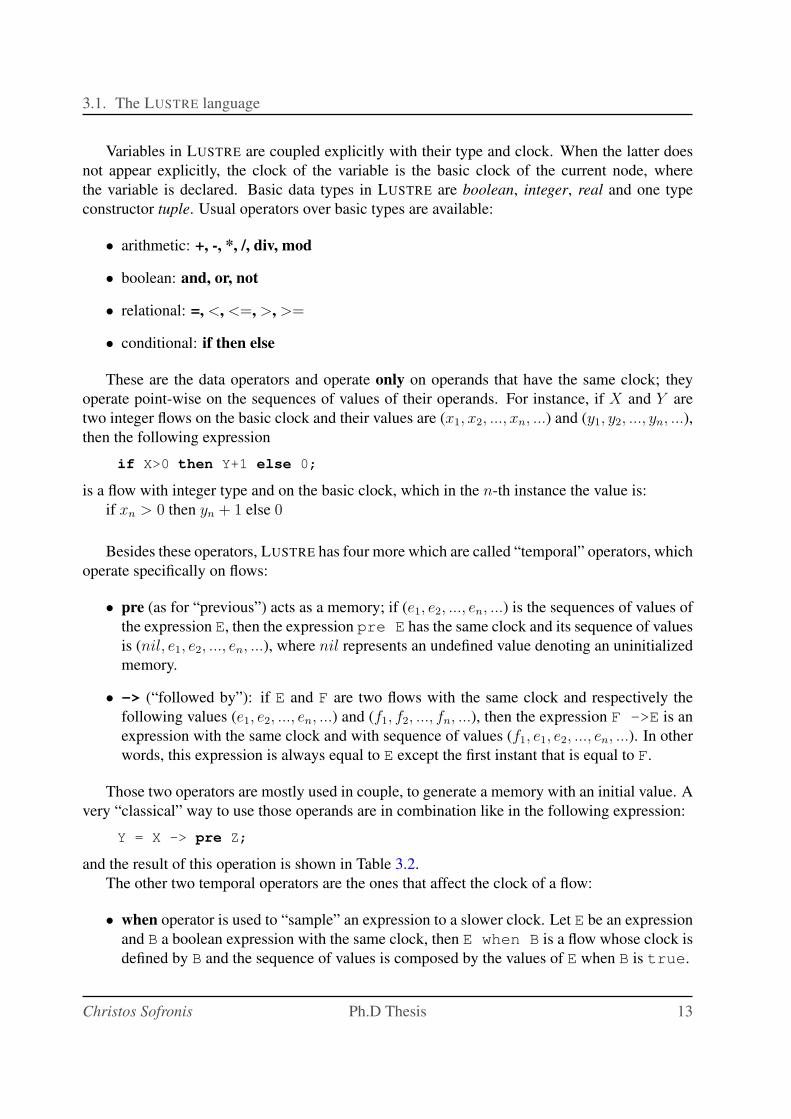
clock defined by a boolean flow is the sequence of times that this flow takes the value true. For
instance Table 3.1 displays the time-scales defined by a flow C whose clock is the basic clock
and a flow C’ whose clock is defined by C.
basic time-scale 1 2 3 4 5 6 7 8
(defined by the environment)
C true false true true false true false true
time-scale defined by C 1 2 3 4 5
C’ false true false true true
time-scale defined by C’ 1 2 3
Table 3.1: Boolean flows and their clocks.
12 Verimag — November 2006 Christos Sofronis
3.1. The LUSTRE language
Variables in LUSTRE are coupled explicitly with their type and clock. When the latter does
not appear explicitly, the clock of the variable is the basic clock of the current node, where
the variable is declared. Basic data types in LUSTRE are boolean, integer, real and one type
constructor tuple. Usual operators over basic types are available:
• arithmetic: +, -, *, /, div, mod
• boolean: and, or, not
• relational: =, <, <=, >, >=
• conditional: if then else
These are the data operators and operate only on operands that have the same clock; they
operate point-wise on the sequences of values of their operands. For instance, if X and Y are
two integer flows on the basic clock and their values are (x1, x2, ..., xn, ...) and (y1, y2, ..., yn, ...),then the following expression
if X>0 then Y+1 else 0;
is a flow with integer type and on the basic clock, which in the n-th instance the value is:
if xn > 0 then yn + 1 else 0
Besides these operators, LUSTRE has four more which are called “temporal” operators, which
operate specifically on flows:
• pre (as for “previous”) acts as a memory; if (e1, e2, ..., en, ...) is the sequences of values of
the expression E, then the expression pre E has the same clock and its sequence of values
is (nil, e1, e2, ..., en, ...), where nil represents an undefined value denoting an uninitialized
memory.
• -> (“followed by”): if E and F are two flows with the same clock and respectively the
following values (e1, e2, ..., en, ...) and (f1, f2, ..., fn, ...), then the expression F ->E is an
expression with the same clock and with sequence of values (f1, e1, e2, ..., en, ...). In other
words, this expression is always equal to E except the first instant that is equal to F.
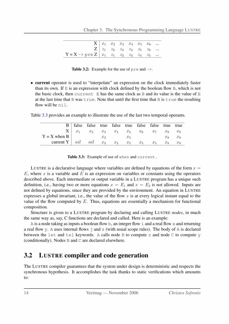
Those two operators are mostly used in couple, to generate a memory with an initial value. A
very “classical” way to use those operands are in combination like in the following expression:
Y = X -> pre Z;
and the result of this operation is shown in Table 3.2.
The other two temporal operators are the ones that affect the clock of a flow:
• when operator is used to “sample” an expression to a slower clock. Let E be an expression
and B a boolean expression with the same clock, then E when B is a flow whose clock is
defined by B and the sequence of values is composed by the values of E when B is true.
Christos Sofronis Ph.D Thesis 13
Chapter 3. The Synchronous Programming Language LUSTRE
X x1 x2 x3 x4 x5 x6 ...
Z z1 z2 z3 z4 z5 z6 ...
Y = X -> pre Z x1 z1 z2 z3 z4 z5 ...
Table 3.2: Example for the use of pre and ->.
• current operator is used to “interpolate” an expression on the clock immediately faster
than its own. If E is an expression with clock defined by the boolean flow B, which is not
the basic clock, then current E has the same clock as B and its value is the value of E
at the last time that B was true. Note that until the first time that B is true the resulting
flow will be nil.
Table 3.3 provides an example to illustrate the use of the last two temporal operants.
B false false true false true false false true true
X x1 x2 x3 x4 x5 x6 x7 x8 x9
Y = X when B x3 x5 x8 x9
current Y nil nil x3 x3 x5 x5 x5 x8 x9
Table 3.3: Example of use of when and current .
LUSTRE is a declarative language where variables are defined by equations of the form x =E, where x is a variable and E is an expression on variables or constants using the operators
described above. Each intermediate or output variable in a LUSTRE program has a unique such
definition, i.e., having two or more equations x = E1 and x = E2 is not allowed. Inputs are
not defined by equations, since they are provided by the environment. An equation in LUSTRE
expresses a global invariant, i.e., the value of the flow x is at every logical instant equal to the
value of the flow computed by E. Thus, equations are essentially a mechanism for functional
composition.
Structure is given to a LUSTRE program by declaring and calling LUSTRE nodes, in much
the same way as, say, C functions are declared and called. Here is an example:
A is a node taking as inputs a boolean flow b, an integer flow i and a real flow x and returning
a real flow y. A uses internal flows j and z (with usual scope rules). The body of A is declared
between the let and tel keywords. A calls node B to compute z and node C to compute y
(conditionally). Nodes B and C are declared elsewhere.
3.2 LUSTRE compiler and code generation
The LUSTRE compiler guarantees that the system under design is deterministic and respects the
synchronous hypothesis. It accomplishes the task thanks to static verifications which amounts
to:
14 Verimag — November 2006 Christos Sofronis
3.2. LUSTRE compiler and code generation
node A(b: bool; i: int; x: real)
returns (y: real);
var j: int; z: real;
let
j = if b then 0 else i;
z = B(j, x);
y = 0.0 -> (if b then pre z else C(z));
tel
Figure 3.2: A LUSTRE node example.
• Definition checking: every local and output variable should have one and only one equa-
tional definition.
• Clock consistency.
• Absence of cycles in definitions: Any cycle should use at least one pre operator.
This latter check, in LUSTRE, is done by statically rejecting any program that contains a cycle
in the instantaneous dependencies relation. This, syntactic, method of rejecting designs is some
times too restrictive, since a further boolean causality check could prove that the program has
one and only one solution for any given input.
Moreover to the above static checks, the LUSTRE compiler can generate code to be executed
in a target platform. The first such implementation is the code generation for a mono-processor
and mono-thread implementation. Thus, the compiler can generate a monolithic program in the
imperative C language. The principle to associate an imperative program to LUSTRE, is to con-
struct an infinite loop whose body implements the inputs to outputs transformations performed
at any cycle of the node.
The two basic steps are: (1) introduce variables for implementing the memory needed by
the pre operators and (2) sort the equations in order to respect data-dependencies. Note that a
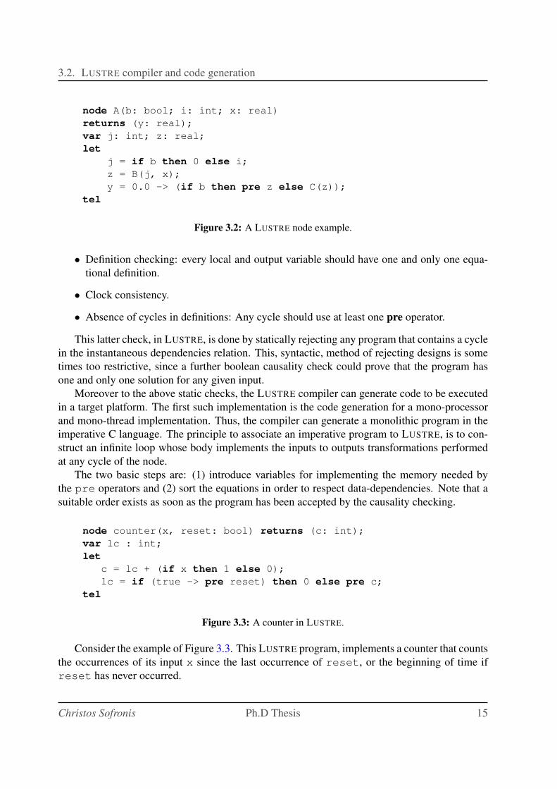
suitable order exists as soon as the program has been accepted by the causality checking.
node counter(x, reset: bool) returns (c: int);
var lc : int;
let
c = lc + (if x then 1 else 0);
lc = if (true -> pre reset) then 0 else pre c;
tel
Figure 3.3: A counter in LUSTRE.
Consider the example of Figure 3.3. This LUSTRE program, implements a counter that counts
the occurrences of its input x since the last occurrence of reset, or the beginning of time if
reset has never occurred.
Christos Sofronis Ph.D Thesis 15
Chapter 3. The Synchronous Programming Language LUSTRE
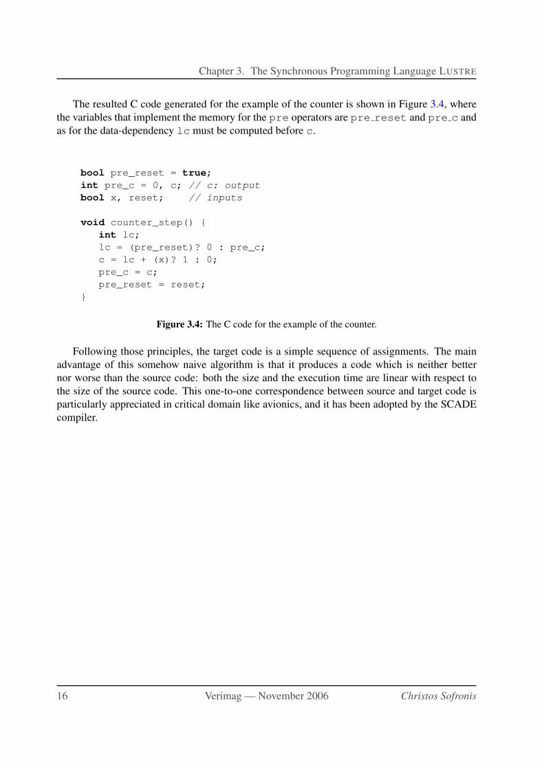
The resulted C code generated for the example of the counter is shown in Figure 3.4, where
the variables that implement the memory for the pre operators are pre reset and pre c and
as for the data-dependency lc must be computed before c.
bool pre_reset = true;
int pre_c = 0, c; // c: output
bool x, reset; // inputs
void counter_step() {
int lc;
lc = (pre_reset)? 0 : pre_c;
c = lc + (x)? 1 : 0;
pre_c = c;
pre_reset = reset;
}
Figure 3.4: The C code for the example of the counter.
Following those principles, the target code is a simple sequence of assignments. The main
advantage of this somehow naive algorithm is that it produces a code which is neither better
nor worse than the source code: both the size and the execution time are linear with respect to
the size of the source code. This one-to-one correspondence between source and target code is
particularly appreciated in critical domain like avionics, and it has been adopted by the SCADE
compiler.
16 Verimag — November 2006 Christos Sofronis

Chapter 4
Analysis and Translation of Discrete-Time
SIMULINK to LUSTRE
4.1 SIMULINK Translation Objectives
SIMULINK and LUSTRE are languages manipulating signals and systems. Signals are functions
of time. Systems take as input signals and produce as output other signals. In SIMULINK, which
has a graphical language, the signals are the “wires” connecting the various blocks. In LUSTRE,
the signals are the program variables, called flows. In SIMULINK, the systems are the built-in
blocks (e.g., adders, gains, transfer functions) as well as composite blocks, called subsystems. In
LUSTRE, the systems are the various built-in operators as well as user-defined operators called
nodes.
In the sequel, we use the following terminology. We use the term block for a basic SIMULINK
block (e.g., adder, gain, transfer function) and the term subsystem for a composite SIMULINK
block. We will use the term system for the root subsystem. We use the term operator for a basic
LUSTRE operator and the term node for a LUSTRE node.
4.2 Differences of SIMULINK and LUSTRE
We will try now to elaborate on the differences of SIMULINK and LUSTRE languages as a first
step towards the translation from the former to the latter. They are both data-flow programming
languages that allow the representation of multi-periodic sampled systems as well as discrete
Simulink Lustre
Signals “wires” connecting blocks variables (flows)
Systems Sum, Gain, Unit Delay, ..., subsystems +, pre, when, current, ..., nodes
Table 4.1: Signals and systems in SIMULINK and LUSTRE.
17
Chapter 4. Analysis and Translation of Discrete-Time SIMULINK to LUSTRE
event systems. However, despite their similarities, they also differ in many ways:
• LUSTRE has a discrete-time semantics, whereas SIMULINK has a continuous-time seman-
tics1. It is important to note that even the blocks of SIMULINK belonging to the “Discrete
library” produce piecewise-constant continuous-time signals. Thus, in general, it is pos-
sible to feed the output of a continuous-time block into the input of a discrete-time block
and vice-versa.
• LUSTRE has a unique, precise semantics. The semantics of SIMULINK depends on the
choice of a simulation method. For instance, some models are accepted if one chooses a
variable-step integration solver and rejected with a fixed-step solver.
• LUSTRE is a strongly-typed language with explicit types for each flow. Explicit types
are not mandatory in SIMULINK. However, they can be set using, for instance, the Data
Type Converter block or an expression such as single(1.2) which specifies the constant 1.2having type single. The differences of the typing mechanisms of SIMULINK and LUSTRE
are discussed in more detail in Section 4.4.
• LUSTRE is modular in certain aspects, while SIMULINK is not. In particular, concern-
ing timing aspects, a SIMULINK model allows a subsystem to “run faster” (be sampled
at a higher rate) than its parent system. In this sense, SIMULINK is not modular since
the subsystem contains implicit inputs (i.e., sample times). The differences of the timing
mechanisms of SIMULINK and LUSTRE are discussed in more detail in Section 4.5.2.
• Hierarchy in SIMULINK is present both at the definition and at the execution levels. This
means that subsystems are drawn graphically within their parent systems, to form a tree-
like hierarchy. The same hierarchy is used to determine the order of execution of nodes.
In LUSTRE, the execution graph is hierarchical (nodes calling other nodes), while the
definition of nodes is “flat” (that is, following the style of C rather than, say, Pascal, where
procedures can be declared inside other procedures). The differences of the structure of
SIMULINK and LUSTRE are discussed in more detail in Section 4.6.
4.3 The Goals and Limitations of the Translation
The ultimate objective of the translation is to automatize the implementation of embedded
controllers as much as possible. We envisage a tool chain where controllers are designed in
SIMULINK, translated to LUSTRE, and implemented on a given platform using the LUSTRE C
code generator and a C compiler for this platform. Other tools, for instance, for worst-case exe-
cution time (WCET) analysis, code distribution, schedulability analysis and scheduling, etc., can
also assist the implementation process, especially when targeting distributed execution platforms
(e.g., see [CCM+03]).
1 In the sense that LUSTRE signals are functions from the set of natural numbers to sets of values and SIMULINK
signals are functions from the set of positive real numbers to sets of values.
18 Verimag — November 2006 Christos Sofronis
4.3. The Goals and Limitations of the Translation
The basic assumption is that the embedded controller to be implemented is designed in
SIMULINK using the discrete-time part of the model. Thus, we only translate the discrete-time
part of a SIMULINK model. Of course, controllers can be modeled in continuous time as well.
This is typically done in control theory, so that analytic results for the closed-loop system can be
obtained (e.g., regarding its stability). Analytical results can also be obtained using the sampled-
data control theory. In any case, the implemented controller must be discrete-time. How to obtain
this controller is a control problem which is clearly beyond the scope of this paper. According
to classical text-books [AW84], there are two main ways of performing this task: either design
a continuous-time controller and sample it or sample the environment and design a sampled
controller.
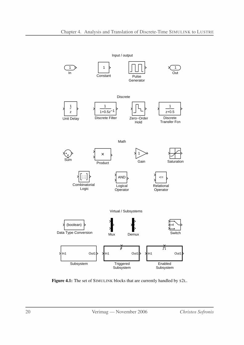
Concretely, the subset of SIMULINK we translate includes blocks of the “Discrete” library
such as “Unit-delay”, “Zero-order hold”, “Discrete filter” and “Discrete transfer function”,
generic mathematical operators such as sum, gain, logical and relational operators, other useful
operators such as switches, and, finally, subsystems including triggered and enabled subsystems.
The subset of SIMULINK currently handled by our method and tool (called S2L) is shown in
Figure 4.1.
Other goals and limitations of our translation are the following.
1. We aim at a translation method that preserves the semantics of SIMULINK. This means
that the original SIMULINK model and the generated LUSTRE program should have the
same observable output behavior, given same inputs, modulo precisely defined conditions.
Since SIMULINK semantics depends on the simulation method, we restrain ourselves only
to one method, namely, “solver: fixed-step, discrete” and “mode: auto”. We also assume
that the LUSTRE program is run at the time period the SIMULINK model was simulated.
Thus, an outcome of the translation must be the period at which the LUSTRE program shall
be run (see also Section 4.5).
2. We do not translate S-functions or Matlab functions. Although such functions can be help-
ful, they can also create side-effects, which is something to be avoided and contrary to
the “functional programming” spirit of LUSTRE. Notice, however, that our tool does not
“block” or rejects the input model when the latter contains such functions. It translates
them into external function calls, like other “unknown” SIMULINK blocks (see also item
5, below).
3. As the SIMULINK models to be translated are in principle controllers embedded in larger
models containing both discrete and continuous parts, we assume that for every input of
the model to be translated (i.e., every input of the controller) the sampling time is explicitly
specified. This also helps the user to see the boundaries of the discrete and the continuous
parts in the original model.
4. In accordance with the first goal, we want the LUSTRE program produced by the translator
to type-check if and only if the original SIMULINK model type-checks (i.e., is not rejected
by SIMULINK because of type errors). However, the behavior of the type checking mech-
anism of SIMULINK depends on the simulation method and the “Boolean logic signals”
Christos Sofronis Ph.D Thesis 19
Chapter 4. Analysis and Translation of Discrete-Time SIMULINK to LUSTRE
Input / output
Discrete
Math
Virtual / Subsystems
1
Out
Zero−OrderHold
z
1
Unit Delay
In1 Out1
TriggeredSubsystem
Switch
Sum
In1 Out1
Subsystem
Saturation
<=
RelationalOperator
PulseGenerator
Product
Mux
AND
LogicalOperator
1
Gain
In1 Out1
EnabledSubsystem
1
1+0.5z −1
Discrete Filter
1
z+0.5
DiscreteTransfer Fcn
Demux
Demux
(boolean)
Data Type Conversion
1
Constant
Combinatorial Logic
1
In
Figure 4.1: The set of SIMULINK blocks that are currently handled by S2L.
20 Verimag — November 2006 Christos Sofronis
4.4. Type inference
flag (BLS). Thus, apart from the simulation method which must be set as stated in item 1,
we also assume that BLS is on. When set, BLS imposes that inputs and outputs of logical
blocks (and, or, not) be of type boolean. Not only this is good modeling and programming
practice, it also makes type inference more precise (see also Section 4.4) and simplifies
the verification of the translated SIMULINK models using LUSTRE-based model-checking
tools.
We also set the “algebraic loop” detection mechanism of SIMULINK to the strictest degree,
which rejects models with such loops. These loops correspond to cyclic data dependencies
in the same instant in LUSTRE. The LUSTRE compiler rejects such programs.
5. For reasons of traceability, the translation must preserve the hierarchy of the SIMULINK
model as much as possible. We achieve this by suitable naming, as explained in Sec-
tion 4.6.
6. The translator must “try its best”. This means that it must be able to handle as larger a
part of the SIMULINK model as possible, potentially leaving some parts un-translated. But
it should not “block” or reject models simply because there are some parts in them that
the translator does not “know” how to translate. We achieve this by taking advantage of
the possibility to include external data types and external functions in a LUSTRE program.
The translator generates external function code for every “unknown” block.
It should also be noted that SIMULINK is a product evolving in time. This evolution has
an impact on the semantics of the tool, as mentioned earlier. For instance, earlier versions
of SIMULINK had weaker type-checking rules. We have developed and tested our translation
method and tool with Matlab version 6.5.0 release 13 (Jun 18, 2002), SIMULINK Block Library
5.0.1. All examples given in the thesis refer to this version as well. However any SIMULINK
model created with a MATLAB release between r12 and r13 is treated and translated correctly.
4.4 Type inference
Type inference is a prior step to translation per se. It is necessary in order to infer the types of
signals in the SIMULINK model and use them to associate types of variables in the generated
LUSTRE program. In this section, we explain the typing mechanisms of LUSTRE and SIMULINK
and then present the type inference technique we use. The type rules for SIMULINK that are
stated here are with respect to the simulation method and flag options mentioned in Section 4.3.
4.4.1 Types in LUSTRE
LUSTRE is a strongly typed language, meaning that every variable has a declared type and op-
erations have precise type signatures. For instance, we cannot add an integer with a boolean or
even an integer with a real. However, predefined casting operators such as int2real can be
used to transform the type of a variable in a “safe” way.
Christos Sofronis Ph.D Thesis 21
Chapter 4. Analysis and Translation of Discrete-Time SIMULINK to LUSTRE
1
Out1
single(23.4)
Constant1
int8(10)
Constant
int8int8
single
int8
int8
Figure 4.2: A type error in SIMULINK.
Basic types in LUSTRE are bool for boolean, int for integer and real. Composite types
are essentially records of fixed size, constructed with the type operator. For instance,
type type_rrb = {real, real, bool};
declares the new type type rrb as the tuple of two reals and one boolean. The LUSTRE com-
piler ensures that operations between flows with different types do not take place. For example,
var x: int; y: real; z: real;
z = x + y;
results into a type error and the program is rejected.
It should be noted that constants in LUSTRE also have types. Thus, 0 is zero of type int,
whereas 0.0 is zero of type real. true and false are constants of type bool.
4.4.2 Types in SIMULINK
In SIMULINK, types need not be explicitly declared. Nevertheless, SIMULINK does have typing
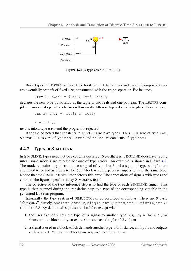
rules: some models are rejected because of type errors. An example is shown in Figure 4.2.
The model contains a type error since a signal of type int8 and a signal of type single are
attempted to be fed as inputs to the Sum block which expects its inputs to have the same type.
Notice that the SIMULINK simulator detects this error. The annotations of signals with types and
colors in the figure is performed by SIMULINK itself.
The objective of the type inference step is to find the type of each SIMULINK signal. This
type is then mapped during the translation step to a type of the corresponding variable in the
generated LUSTRE program.
Informally, the type system of SIMULINK can be described as follows. There are 9 basic
“data types”, namely, boolean, double, single, int8, uint8, int16, uint16, int32
and uint32. By default, all signals are double, except when:
1. the user explicitly sets the type of a signal to another type, e.g., by a Data Type
Converter block or by an expression such as single(23.4); or
2. a signal is used in a block which demands another type. For instance, all inputs and outputs
of Logical Operator blocks are required to be boolean.
22 Verimag — November 2006 Christos Sofronis
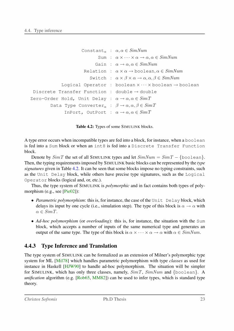
4.4. Type inference
Constantα : α, α ∈ SimNum
Sum : α × · · · × α → α, α ∈ SimNum
Gain : α → α, α ∈ SimNum
Relation : α × α → boolean, α ∈ SimNum
Switch : α × β × α → α, α, β ∈ SimNum
Logical Operator : boolean× · · · × boolean → boolean
Discrete Transfer Function : double → double
Zero-Order Hold, Unit Delay : α → α, α ∈ SimT
Data Type Converterα : β → α, α, β ∈ SimT
InPort, OutPort : α → α, α ∈ SimT
Table 4.2: Types of some SIMULINK blocks.
A type error occurs when incompatible types are fed into a block, for instance, when a boolean
is fed into a Sum block or when an int8 is fed into a Discrete Transfer Function
block.
Denote by SimT the set of all SIMULINK types and let SimNum = SimT − {boolean}.
Then, the typing requirements imposed by SIMULINK basic blocks can be represented by the type
signatures given in Table 4.2. It can be seen that some blocks impose no typing constraints, such
as the Unit Delay block, while others have precise type signatures, such as the Logical
Operator blocks (logical and, or, etc.).
Thus, the type system of SIMULINK is polymorphic and in fact contains both types of poly-
morphism (e.g., see [Pie02]):
• Parametric polymorphism: this is, for instance, the case of the Unit Delay block, which
delays its input by one cycle (i.e., simulation step). The type of this block is α → α with
α ∈ SimT .
• Ad-hoc polymorphism (or overloading): this is, for instance, the situation with the Sum
block, which accepts a number of inputs of the same numerical type and generates an
output of the same type. The type of this block is α × · · · × α → α with α ∈ SimNum.
4.4.3 Type Inference and Translation
The type system of SIMULINK can be formalized as an extension of Milner’s polymorphic type
system for ML [Mil78] which handles parametric polymorphism with type classes as used for
instance in Haskell [HJW90] to handle ad-hoc polymorphism. The situation will be simpler
for SIMULINK, which has only three classes, namely, SimT , SimNum and {boolean}. A
unification algorithm (e.g. [Rob65, MM82]) can be used to infer types, which is standard type
theory.
Christos Sofronis Ph.D Thesis 23
Chapter 4. Analysis and Translation of Discrete-Time SIMULINK to LUSTRE
For the type inference, we extract from the SIMULINK model the type equations for every
signal transformation , using “fresh” type variables for every signal. As signal transformation,
we mean all the blocks and subsystems, even though the ones that have no inputs or no outputs.
After extracting all those equations, we solve them using Robinson’s Unification algorithm U .
The type of a SIMULINK subsystem (or root system) A is defined given the types of the
subsystems or blocks composing A, using a standard function composition rule.
As we shall see in Section 4.6 our translation preserves the structure of SIMULINK. In par-
ticular, every SIMULINK signal s is mapped to a variable xs in the generated LUSTRE program.
Once the type of s is inferred using the above method, the type of xs is determined. This is done
as follows.
• If the type of s is boolean then the type of xs is bool.
• If the type of s is int8, uint8, int16, uint16, int32 or uint32 then the type of
xs is int.
• If the type of s is single or double then the type of xs is real.
• If the type of s is α then the type of xs is real.
The last case is consistent with the fact that the default type in SIMULINK is double.
4.5 Clock inference
As with type inference, clock inference is a prior step to translation. It is necessary in order
to infer timing information of the SIMULINK model and use this information during generation
of the LUSTRE program. In this section, we explain the timing mechanisms of LUSTRE and
SIMULINK and then present our clock inference technique. Notice that the timing rules for
SIMULINK that are stated
here are with respect to the simulation method and flag options mentioned in Section 4.3.
4.5.1 Time in LUSTRE
As mentioned in Chapter 3, LUSTRE time is logical and counted in discrete instants. Associated
with each LUSTRE flow x is a Boolean flow bx, called the clock of x, specifying the instants
when x is defined: x is defined at instant i iff bx(i) = true. For example, if x is defined at
i = 0, 2, 4, ... then bx = true false true false · · ·. We say that “x runs on clock bx”.
Input variables are by definition defined at every instant: their clock is called the basic clock,
represented by the Boolean flow true. “Slower” clocks are obtained from the basic clock using
the when operator. For example, if x is an input then the flow y defined only at even instants
can be generated by the following LUSTRE code:
cl_half = true -> not pre(cl_half) ;
y = x when cl_half ;
24 Verimag — November 2006 Christos Sofronis
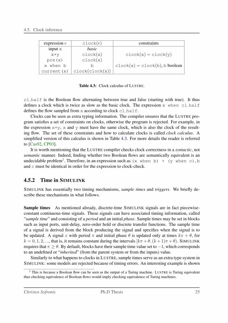
4.5. Clock inference
expression e clock(e) constraints
input x basic
x+y clock(x) clock(x) = clock(y)pre(x) clock(x)x when b b clock(x) = clock(b), b boolean
current(x) clock(clock(x))
Table 4.3: Clock calculus of LUSTRE.
cl half is the Boolean flow alternating between true and false (starting with true). It thus
defines a clock which is twice as slow as the basic clock. The expression x when cl half
defines the flow sampled from x according to clock cl half.
Clocks can be seen as extra typing information. The compiler ensures that the LUSTRE pro-
gram satisfies a set of constraints on clocks, otherwise the program is rejected. For example, in
the expression x+y, x and y must have the same clock, which is also the clock of the result-
ing flow. The set of these constraints and how to calculate clocks is called clock calculus. A
simplified version of this calculus is shown in Table 4.3. For more details the reader is referred
to [Cas92, CP03].
It is worth mentioning that the LUSTRE compiler checks clock correctness in a syntactic, not
semantic manner. Indeed, finding whether two Boolean flows are semantically equivalent is an
undecidable problem2. Therefore, in an expression such as (x when b) + (y when c), b
and c must be identical in order for the expression to clock-check.
4.5.2 Time in SIMULINK
SIMULINK has essentially two timing mechanisms, sample times and triggers. We briefly de-
scribe these mechanisms in what follows.
Sample times As mentioned already, discrete-time SIMULINK signals are in fact piecewise-
constant continuous-time signals. These signals can have associated timing information, called
“sample time” and consisting of a period and an initial phase. Sample times may be set in blocks
such as input ports, unit-delay, zero-order hold or discrete transfer functions. The sample time
of a signal is derived from the block producing the signal and specifies when the signal is to
be updated. A signal x with period π and initial phase θ is updated only at times kπ + θ, for
k = 0, 1, 2, ..., that is, it remains constant during the intervals [kπ + θ, (k + 1)π + θ). SIMULINK
requires that π ≥ θ. By default, blocks have their sample time value set to −1, which corresponds
to an undefined or “inherited” (from the parent system or from the inputs) value.
Similarly to what happens to clocks in LUSTRE, sample times serve as an extra type system in
SIMULINK: some models are rejected because of timing errors. An interesting example is shown
2 This is because a Boolean flow can be seen as the output of a Turing machine. LUSTRE is Turing equivalent
thus checking equivalence of Boolean flows would imply checking equivalence of Turing machines.
Christos Sofronis Ph.D Thesis 25
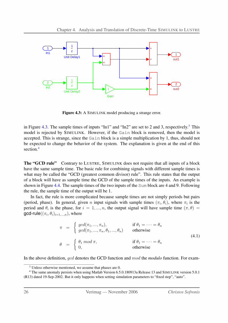
Chapter 4. Analysis and Translation of Discrete-Time SIMULINK to LUSTRE
2
out2
1
out1
z
1
Unit Delay2
z
1
Unit Delay1
1
Gain
2
In2
1
In1
Figure 4.3: A SIMULINK model producing a strange error.
in Figure 4.3. The sample times of inputs “In1” and “In2” are set to 2 and 3, respectively.3 This
model is rejected by SIMULINK. However, if the Gain block is removed, then the model is
accepted. This is strange, since the Gain block is a simple multiplication by 1, thus, should not
be expected to change the behavior of the system. The explanation is given at the end of this
section.4
The “GCD rule” Contrary to LUSTRE, SIMULINK does not require that all inputs of a block
have the same sample time. The basic rule for combining signals with different sample times is
what may be called the “GCD (greatest common divisor) rule”. This rule states that the output
of a block will have as sample time the GCD of the sample times of the inputs. An example is
shown in Figure 4.4. The sample times of the two inputs of the Sum block are 4 and 9. Following
the rule, the sample time of the output will be 1.
In fact, the rule is more complicated because sample times are not simply periods but pairs
(period, phase). In general, given n input signals with sample times (πi, θi), where πi is the
period and θi is the phase, for i = 1, ..., n, the output signal will have sample time (π, θ) =gcd-rule((πi, θi)i=1,...,n), where
π =
{
gcd(π1, ..., πn),gcd(π1, ..., πn, θ1, ..., θn)
if θ1 = · · · = θn
otherwise
θ =
{
θ1 mod π,0,
if θ1 = · · · = θn
otherwise
(4.1)
In the above definition, gcd denotes the GCD function and mod the modulo function. For exam-
3 Unless otherwise mentioned, we assume that phases are 0.4 The same anomaly persists when using Matlab Version 6.5.0.180913a Release 13 and SIMULINK version 5.0.1
(R13) dated 19-Sep-2002. But it only happens when setting simulation parameters to “fixed step”, “auto”.
26 Verimag — November 2006 Christos Sofronis
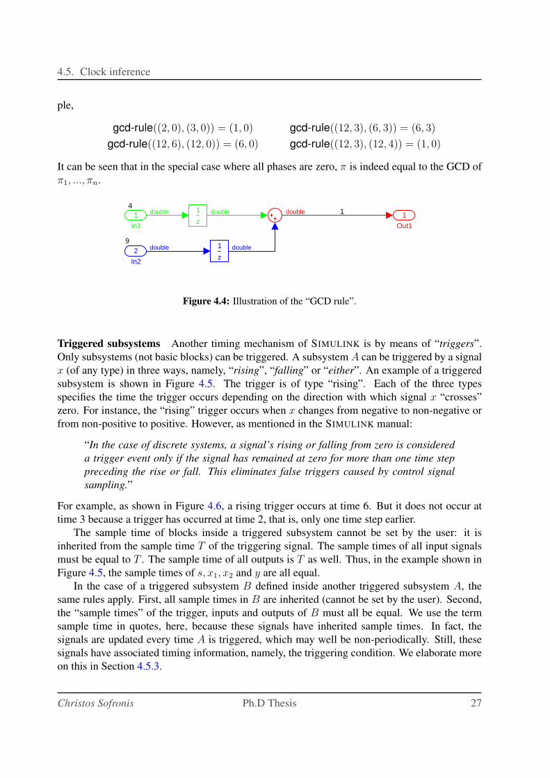
4.5. Clock inference
ple,
gcd-rule((2, 0), (3, 0)) = (1, 0) gcd-rule((12, 3), (6, 3)) = (6, 3)
gcd-rule((12, 6), (12, 0)) = (6, 0) gcd-rule((12, 3), (12, 4)) = (1, 0)
It can be seen that in the special case where all phases are zero, π is indeed equal to the GCD of
π1, ..., πn.
4
9
1 1
Out1
z
1
z
1
2
In2
1
In1
double
double
doubledouble
double
Figure 4.4: Illustration of the “GCD rule”.
Triggered subsystems Another timing mechanism of SIMULINK is by means of “triggers”.
Only subsystems (not basic blocks) can be triggered. A subsystem A can be triggered by a signal
x (of any type) in three ways, namely, “rising”, “falling” or “either”. An example of a triggered
subsystem is shown in Figure 4.5. The trigger is of type “rising”. Each of the three types
specifies the time the trigger occurs depending on the direction with which signal x “crosses”
zero. For instance, the “rising” trigger occurs when x changes from negative to non-negative or
from non-positive to positive. However, as mentioned in the SIMULINK manual:
“In the case of discrete systems, a signal’s rising or falling from zero is considered
a trigger event only if the signal has remained at zero for more than one time step
preceding the rise or fall. This eliminates false triggers caused by control signal
sampling.”
For example, as shown in Figure 4.6, a rising trigger occurs at time 6. But it does not occur at
time 3 because a trigger has occurred at time 2, that is, only one time step earlier.
The sample time of blocks inside a triggered subsystem cannot be set by the user: it is
inherited from the sample time T of the triggering signal. The sample times of all input signals
must be equal to T . The sample time of all outputs is T as well. Thus, in the example shown in
Figure 4.5, the sample times of s, x1, x2 and y are all equal.
In the case of a triggered subsystem B defined inside another triggered subsystem A, the
same rules apply. First, all sample times in B are inherited (cannot be set by the user). Second,
the “sample times” of the trigger, inputs and outputs of B must all be equal. We use the term
sample time in quotes, here, because these signals have inherited sample times. In fact, the
signals are updated every time A is triggered, which may well be non-periodically. Still, these
signals have associated timing information, namely, the triggering condition. We elaborate more
on this in Section 4.5.3.
Christos Sofronis Ph.D Thesis 27
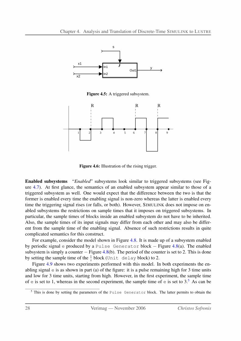
Chapter 4. Analysis and Translation of Discrete-Time SIMULINK to LUSTRE
s
x1
x2
yIn1
In2Out1
Figure 4.5: A triggered subsystem.
�✁ ✂✄ ☎✆ ✝✞ ✟✠ ✡ ✡☛ ☞✌✍✎✏✑
R R R
1 2 3 4 5 6 7 8 9
Figure 4.6: Illustration of the rising trigger.
Enabled subsystems “Enabled” subsystems look similar to triggered subsystems (see Fig-
ure 4.7). At first glance, the semantics of an enabled subsystem appear similar to those of a
triggered subsystem as well. One would expect that the difference between the two is that the
former is enabled every time the enabling signal is non-zero whereas the latter is enabled every
time the triggering signal rises (or falls, or both). However, SIMULINK does not impose on en-
abled subsystems the restrictions on sample times that it imposes on triggered subsystems. In
particular, the sample times of blocks inside an enabled subsystem do not have to be inherited.
Also, the sample times of its input signals may differ from each other and may also be differ-
ent from the sample time of the enabling signal. Absence of such restrictions results in quite
complicated semantics for this construct.
For example, consider the model shown in Figure 4.8. It is made up of a subsystem enabled
by periodic signal e produced by a Pulse Generator block − Figure 4.8(a). The enabled
subsystem is simply a counter − Figure 4.8(b). The period of the counter is set to 2. This is done
by setting the sample time of the 1z
block (Unit delay block) to 2.
Figure 4.9 shows two experiments performed with this model. In both experiments the en-
abling signal e is as shown in part (a) of the figure: it is a pulse remaining high for 3 time units
and low for 3 time units, starting from high. However, in the first experiment, the sample time
of e is set to 1, whereas in the second experiment, the sample time of e is set to 3.5 As can be
5 This is done by setting the parameters of the Pulse Generator block. The latter permits to obtain the
28 Verimag — November 2006 Christos Sofronis
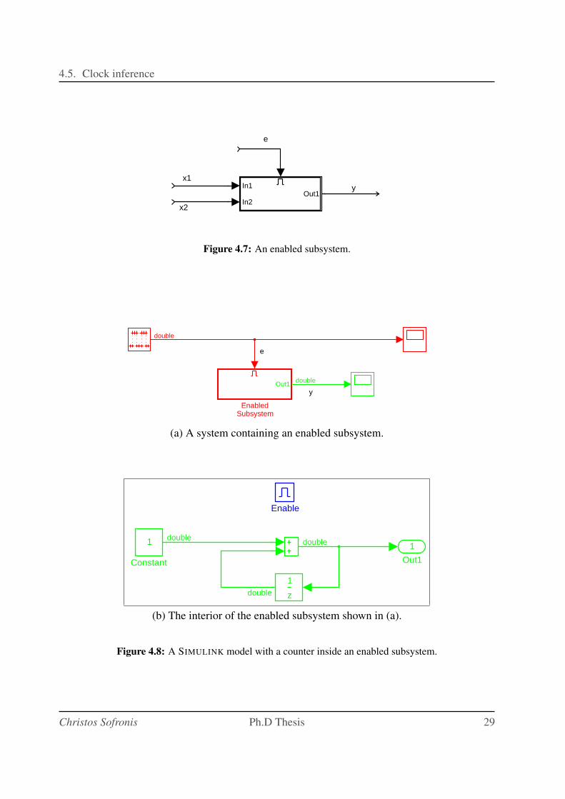
4.5. Clock inference
e
x1
x2
yIn1
In2Out1
Figure 4.7: An enabled subsystem.
y
e
Out1
EnabledSubsystem
double
double
(a) A system containing an enabled subsystem.
1
Out1
z
1
1
Constant
Enable
double double
double
(b) The interior of the enabled subsystem shown in (a).
Figure 4.8: A SIMULINK model with a counter inside an enabled subsystem.
Christos Sofronis Ph.D Thesis 29
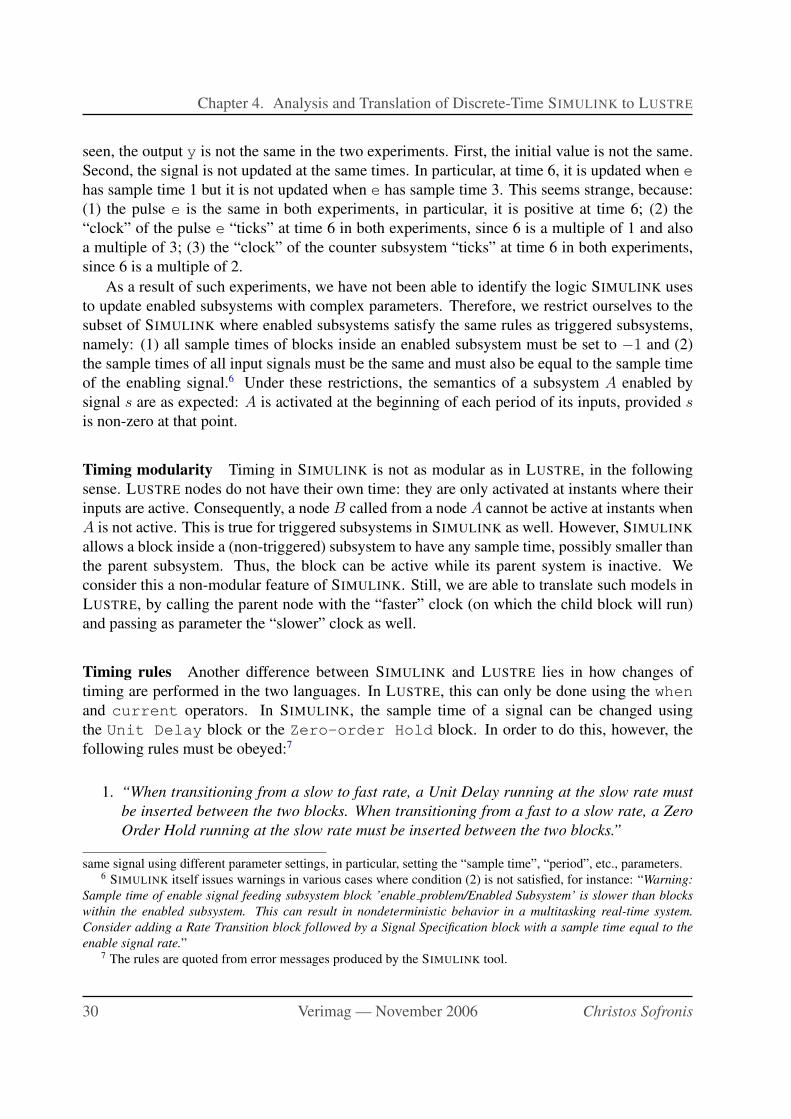
Chapter 4. Analysis and Translation of Discrete-Time SIMULINK to LUSTRE
seen, the output y is not the same in the two experiments. First, the initial value is not the same.
Second, the signal is not updated at the same times. In particular, at time 6, it is updated when e
has sample time 1 but it is not updated when e has sample time 3. This seems strange, because:
(1) the pulse e is the same in both experiments, in particular, it is positive at time 6; (2) the
“clock” of the pulse e “ticks” at time 6 in both experiments, since 6 is a multiple of 1 and also
a multiple of 3; (3) the “clock” of the counter subsystem “ticks” at time 6 in both experiments,
since 6 is a multiple of 2.
As a result of such experiments, we have not been able to identify the logic SIMULINK uses
to update enabled subsystems with complex parameters. Therefore, we restrict ourselves to the
subset of SIMULINK where enabled subsystems satisfy the same rules as triggered subsystems,
namely: (1) all sample times of blocks inside an enabled subsystem must be set to −1 and (2)
the sample times of all input signals must be the same and must also be equal to the sample time
of the enabling signal.6 Under these restrictions, the semantics of a subsystem A enabled by
signal s are as expected: A is activated at the beginning of each period of its inputs, provided sis non-zero at that point.
Timing modularity Timing in SIMULINK is not as modular as in LUSTRE, in the following
sense. LUSTRE nodes do not have their own time: they are only activated at instants where their
inputs are active. Consequently, a node B called from a node A cannot be active at instants when
A is not active. This is true for triggered subsystems in SIMULINK as well. However, SIMULINK
allows a block inside a (non-triggered) subsystem to have any sample time, possibly smaller than
the parent subsystem. Thus, the block can be active while its parent system is inactive. We
consider this a non-modular feature of SIMULINK. Still, we are able to translate such models in
LUSTRE, by calling the parent node with the “faster” clock (on which the child block will run)
and passing as parameter the “slower” clock as well.
Timing rules Another difference between SIMULINK and LUSTRE lies in how changes of
timing are performed in the two languages. In LUSTRE, this can only be done using the when
and current operators. In SIMULINK, the sample time of a signal can be changed using
the Unit Delay block or the Zero-order Hold block. In order to do this, however, the
following rules must be obeyed:7
1. “When transitioning from a slow to fast rate, a Unit Delay running at the slow rate must
be inserted between the two blocks. When transitioning from a fast to a slow rate, a Zero
Order Hold running at the slow rate must be inserted between the two blocks.”
same signal using different parameter settings, in particular, setting the “sample time”, “period”, etc., parameters.6 SIMULINK itself issues warnings in various cases where condition (2) is not satisfied, for instance: “Warning:
Sample time of enable signal feeding subsystem block ’enable problem/Enabled Subsystem’ is slower than blocks
within the enabled subsystem. This can result in nondeterministic behavior in a multitasking real-time system.
Consider adding a Rate Transition block followed by a Signal Specification block with a sample time equal to the
enable signal rate.”7 The rules are quoted from error messages produced by the SIMULINK tool.
30 Verimag — November 2006 Christos Sofronis

4.5. Clock inference
0 5 10 15−1
0
1
2
Time offset: 0
(a) The enabling signal e.
0 5 10 150
1
2
3
4
5
6
7
Time offset: 0
(b) The output y when enable e has period 1.
0 5 10 150
1
2
3
4
5
6
7
Time offset: 0
(c) The output y when enable e has period 3.
Figure 4.9: A strange behavior of the model of Figure 4.8.
Christos Sofronis Ph.D Thesis 31
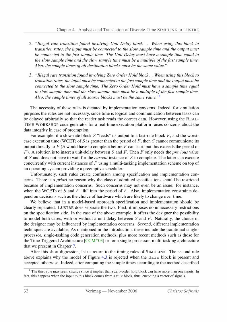
Chapter 4. Analysis and Translation of Discrete-Time SIMULINK to LUSTRE
2. “Illegal rate transition found involving Unit Delay block ... When using this block to
transition rates, the input must be connected to the slow sample time and the output must
be connected to the fast sample time. The Unit Delay must have a sample time equal to
the slow sample time and the slow sample time must be a multiple of the fast sample time.
Also, the sample times of all destination blocks must be the same value.”
3. “Illegal rate transition found involving Zero Order Hold block ... When using this block to
transition rates, the input must be connected to the fast sample time and the output must be
connected to the slow sample time. The Zero Order Hold must have a sample time equal
to slow sample time and the slow sample time must be a multiple of the fast sample time.
Also, the sample times of all source blocks must be the same value.”8
The necessity of these rules is dictated by implementation concerns. Indeed, for simulation
purposes the rules are not necessary, since time is logical and communication between tasks can
be delayed arbitrarily so that the reader task reads the correct data. However, using the REAL-
TIME WORKSHOP code generator for a real-time execution platform raises concerns about the
data integrity in case of preemption.
For example, if a slow-rate block S “feeds” its output to a fast-rate block F , and the worst-
case execution time (WCET) of S is greater than the period of F , then S cannot communicate its
output directly to F (S would have to complete before F can start, but this exceeds the period of
F ). A solution is to insert a unit-delay between S and F . Then F only needs the previous value
of S and does not have to wait for the current instance of S to complete. The latter can execute
concurrently with current instances of F using a multi-tasking implementation scheme on top of
an operating system providing a preemptive scheduler.
Unfortunately, such rules create confusion among specification and implementation con-
cerns. There is a priori no reason why the class of admitted specifications should be restricted
because of implementation concerns. Such concerns may not even be an issue: for instance,
when the WCETs of S and F “fit” into the period of F . Also, implementation constraints de-
pend on decisions such as the choice of hardware which are likely to change over time.
We believe that in a model-based approach specification and implementation should be
clearly separated. LUSTRE does separate the two. First, it imposes no unnecessary restrictions
on the specification side. In the case of the above example, it offers the designer the possibility
to model both cases, with or without a unit-delay between S and F . Naturally, the choice of
the designer may be influenced by implementation concerns. Second, different implementation
techniques are available. As mentioned in the introduction, these include the traditional single-
processor, single-tasking code generation methods, plus more recent methods such as those for
the Time Triggered Architecture [CCM+03] or for a single-processor, multi-tasking architecture
that we present in Chapter 7.
After this short digression, let us return to the timing rules of SIMULINK. The second rule
above explains why the model of Figure 4.3 is rejected when the Gain block is present and
accepted otherwise. Indeed, after computing the sample times according to the method described
8 The third rule may seem strange since it implies that a zero-order hold block can have more than one inputs. In
fact, this happens when the input to this block comes from a Mux block, thus, encoding a vector of signals.
32 Verimag — November 2006 Christos Sofronis
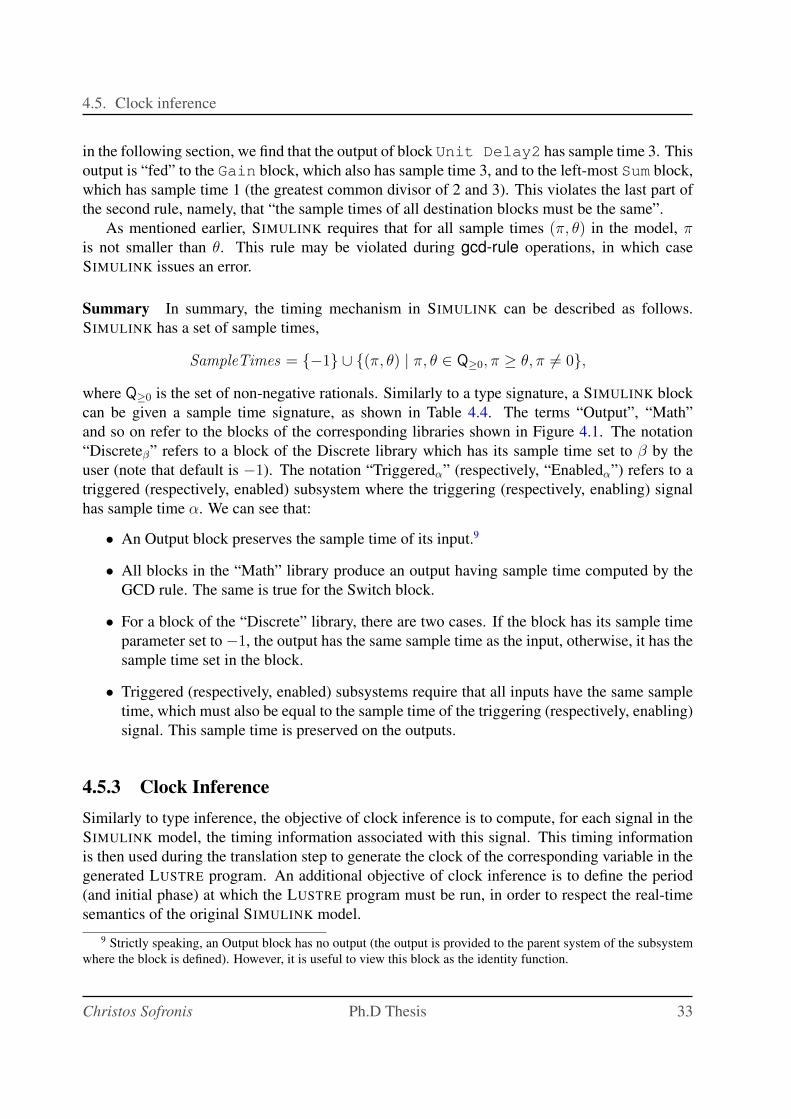
4.5. Clock inference
in the following section, we find that the output of block Unit Delay2 has sample time 3. This
output is “fed” to the Gain block, which also has sample time 3, and to the left-most Sum block,
which has sample time 1 (the greatest common divisor of 2 and 3). This violates the last part of
the second rule, namely, that “the sample times of all destination blocks must be the same”.
As mentioned earlier, SIMULINK requires that for all sample times (π, θ) in the model, πis not smaller than θ. This rule may be violated during gcd-rule operations, in which case
SIMULINK issues an error.
Summary In summary, the timing mechanism in SIMULINK can be described as follows.
SIMULINK has a set of sample times,
SampleTimes = {−1} ∪ {(π, θ) | π, θ ∈ Q≥0, π ≥ θ, π 6= 0},
where Q≥0 is the set of non-negative rationals. Similarly to a type signature, a SIMULINK block
can be given a sample time signature, as shown in Table 4.4. The terms “Output”, “Math”
and so on refer to the blocks of the corresponding libraries shown in Figure 4.1. The notation
“Discreteβ” refers to a block of the Discrete library which has its sample time set to β by the
user (note that default is −1). The notation “Triggeredα” (respectively, “Enabledα”) refers to a
triggered (respectively, enabled) subsystem where the triggering (respectively, enabling) signal
has sample time α. We can see that:
• An Output block preserves the sample time of its input.9
• All blocks in the “Math” library produce an output having sample time computed by the
GCD rule. The same is true for the Switch block.
• For a block of the “Discrete” library, there are two cases. If the block has its sample time
parameter set to −1, the output has the same sample time as the input, otherwise, it has the
sample time set in the block.
• Triggered (respectively, enabled) subsystems require that all inputs have the same sample
time, which must also be equal to the sample time of the triggering (respectively, enabling)
signal. This sample time is preserved on the outputs.
4.5.3 Clock Inference
Similarly to type inference, the objective of clock inference is to compute, for each signal in the
SIMULINK model, the timing information associated with this signal. This timing information
is then used during the translation step to generate the clock of the corresponding variable in the
generated LUSTRE program. An additional objective of clock inference is to define the period
(and initial phase) at which the LUSTRE program must be run, in order to respect the real-time
semantics of the original SIMULINK model.
9 Strictly speaking, an Output block has no output (the output is provided to the parent system of the subsystem
where the block is defined). However, it is useful to view this block as the identity function.
Christos Sofronis Ph.D Thesis 33
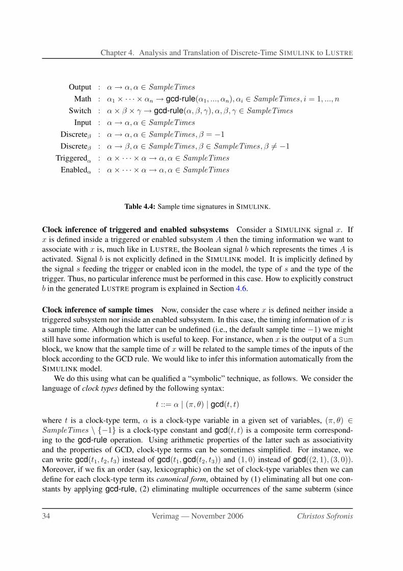
Chapter 4. Analysis and Translation of Discrete-Time SIMULINK to LUSTRE
Output : α → α, α ∈ SampleTimes
Math : α1 × · · · × αn → gcd-rule(α1, ..., αn), αi ∈ SampleTimes , i = 1, ..., n
Switch : α × β × γ → gcd-rule(α, β, γ), α, β, γ ∈ SampleTimes
Input : α → α, α ∈ SampleTimes
Discreteβ : α → α, α ∈ SampleTimes , β = −1
Discreteβ : α → β, α ∈ SampleTimes , β ∈ SampleTimes , β 6= −1
Triggeredα : α × · · · × α → α, α ∈ SampleTimes
Enabledα : α × · · · × α → α, α ∈ SampleTimes
Table 4.4: Sample time signatures in SIMULINK.
Clock inference of triggered and enabled subsystems Consider a SIMULINK signal x. If
x is defined inside a triggered or enabled subsystem A then the timing information we want to
associate with x is, much like in LUSTRE, the Boolean signal b which represents the times A is
activated. Signal b is not explicitly defined in the SIMULINK model. It is implicitly defined by
the signal s feeding the trigger or enabled icon in the model, the type of s and the type of the
trigger. Thus, no particular inference must be performed in this case. How to explicitly construct
b in the generated LUSTRE program is explained in Section 4.6.
Clock inference of sample times Now, consider the case where x is defined neither inside a
triggered subsystem nor inside an enabled subsystem. In this case, the timing information of x is
a sample time. Although the latter can be undefined (i.e., the default sample time −1) we might
still have some information which is useful to keep. For instance, when x is the output of a Sum
block, we know that the sample time of x will be related to the sample times of the inputs of the
block according to the GCD rule. We would like to infer this information automatically from the
SIMULINK model.
We do this using what can be qualified a “symbolic” technique, as follows. We consider the
language of clock types defined by the following syntax:
t ::= α | (π, θ) | gcd(t, t)
where t is a clock-type term, α is a clock-type variable in a given set of variables, (π, θ) ∈SampleTimes \ {−1} is a clock-type constant and gcd(t, t) is a composite term correspond-
ing to the gcd-rule operation. Using arithmetic properties of the latter such as associativity
and the properties of GCD, clock-type terms can be sometimes simplified. For instance, we
can write gcd(t1, t2, t3) instead of gcd(t1, gcd(t2, t3)) and (1, 0) instead of gcd((2, 1), (3, 0)).Moreover, if we fix an order (say, lexicographic) on the set of clock-type variables then we can
define for each clock-type term its canonical form, obtained by (1) eliminating all but one con-
stants by applying gcd-rule, (2) eliminating multiple occurrences of the same subterm (since
34 Verimag — November 2006 Christos Sofronis
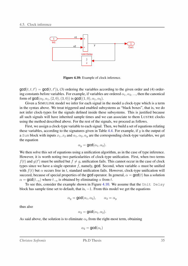
4.5. Clock inference
x1
x2 y1
Out1
z
1
Unit Delay
1
In1
Figure 4.10: Example of clock inference.
gcd(t, t, t′) = gcd(t, t′)), (3) ordering the variables according to the given order and (4) order-
ing constants before variables. For example, if variables are ordered α1, α2, ..., then the canonical
form of gcd(α2, α1, (2, 0), (3, 0)) is gcd((1, 0), α1, α2).
Given a SIMULINK model we infer for each signal in the model a clock-type which is a term
in the syntax above. We treat triggered and enabled subsystems as “black boxes”, that is, we do
not infer clock-types for the signals defined inside these subsystems. This is justified because
all such signals will have inherited sample times and we can associate to them LUSTRE clocks
using the method described above. For the rest of the signals, we proceed as follows.
First, we assign a clock-type variable to each signal. Then, we build a set of equations relating
these variables, according to the signatures given in Table 4.4. For example, if y is the output of
a Sum block with inputs x1, x2 and α1, α2, αy are the corresponding clock-type variables, we get
the equation
αy = gcd(α1, α2).
We then solve this set of equations using a unification algorithm, as in the case of type inference.
However, it is worth noting two particularities of clock-type unification. First, when two terms
f(t) and g(t′) must be unified but f 6= g, unification fails. This cannot occur in the case of clock
types since we have a single operator f , namely, gcd. Second, when variable α must be unified
with f(t) but α occurs free in t, standard unification fails. However, clock-type unification will
succeed, because of special properties of the gcd operator. In general, α = gcd(t) has a solution
α = gcd(t−α) where t−α is obtained by eliminating α from t.
To see this, consider the example shown in Figure 4.10. We assume that the Unit Delay
block has sample time set to default, that is, −1. From this model we get the equations
αy = gcd(α1, α2), α2 = αy
thus also
α2 = gcd(α1, α2).
As said above, the solution is to eliminate α2 from the right-most term, obtaining
α2 = gcd(α1)
Christos Sofronis Ph.D Thesis 35
Chapter 4. Analysis and Translation of Discrete-Time SIMULINK to LUSTRE
or
α2 = α1.
Thus, unification succeeds in this case with α1 = α2 = αy.
Clock-type unification may fail, for instance, when trying to unify constant clock-types that
differ. One situation where this occurs is when two inputs of, say, a triggered subsystem have
different sample times, thus, violating the signature shown in Table 4.4. When unification fails,
the SIMULINK model is rejected due to timing errors.
The solution provided by the unification algorithm when the latter succeeds is to be inter-
preted as follows. For signals with inferred clock-types which are constants (π, θ), we know
exactly their sample time. For signals with inferred clock-types which are variables α1, α2, ...,their sample times are unknown and can be anything. The rest of the signals will have a clock-
type of the form gcd(αi, αj, ...) or gcd((π, θ), αi, αj, ...). The sample times of such signals are
not known, however, they are subject to constraints expressed by the GCD rule.
4.6 Translation
The type and clock inference steps are independent and can be performed in any order. Once
this is done, the translation itself is performed, in a hierarchical manner. The SIMULINK model
is organized as a tree, where the children of a subsystem (or system) are the subsystems (or
blocks) directly appearing in it. The translation is performed following this hierarchy in a
bottom-up fashion, that is, starting from the basic blocks which form the leaves of the hierar-
chy tree. SIMULINK signals are mapped into LUSTRE flows. SIMULINK blocks are translated as
input/output equations between signals, either by using predefined LUSTRE operators, in the case
of simple blocks, or by calling LUSTRE nodes, which capture the functionality of more complex
blocks. SIMULINK subsystems are also translated by declaring and calling LUSTRE nodes.
Naming In accordance with the goal of traceability and in order to preserve the hierarchical
structure of the SIMULINK model in the generated LUSTRE program, each LUSTRE node is
named with the corresponding path of names in the SIMULINK tree. For example, a subsystem
B contained in a subsystem A will be translated into a LUSTRE node named NameofA B where
NameofA is the name of the LUSTRE node corresponding to subsystem A.
When a signal in SIMULINK has a name, the name is preserved during the translation. How-
ever, it is often the case that signals in SIMULINK are not named (they are simply “wires” con-
necting two blocks). In such a case, the name given to the corresponding LUSTRE variable
reflects the block which produces the signal. For example, if an unnamed signal is produced by
a block named Sum1 then the corresponding LUSTRE variable will be named Sum1 out.
Translation of basic SIMULINK blocks Simple SIMULINK blocks are translated into prede-
fined LUSTRE operators. In particular:
• The Sum block is translated using the + and - LUSTRE operators.
36 Verimag — November 2006 Christos Sofronis
4.6. Translation
• The Product and Gain blocks are translated using the * and / LUSTRE operators and
constants.
• The Logical Operator block is translated using the Boolean LUSTRE operators and,
or, not.
• The Relational Operator block is translated using the LUSTRE comparison opera-
tors <, >, <=, >=, =, <>.
• The Unit Delay block is translated using the LUSTRE operators pre and ->. In par-
ticular, if x and y are the input and output of the block and init is the initial value
(a constant) specified in the dialog box of the block, then the following LUSTRE code is
generated:
y = init -> pre(x) ;
• A Zero-Order Hold block with sample time set to −1 is the identity function, thus no
special code needs to be generated. If the sample time of the block is set, then the block is
translated using a when statement, possibly preceded by a current statement. The latter
is needed in the case where the input signal is not running on the basic clock. For example,
consider the model of Figure 4.13 and assume that the sample time of the Zero-Order
Hold block is 3. Thus, the output has sample time 3 as well. First, suppose that the sample
time of the input is 1 and that this also corresponds to the basic clock. Then, the translation
would be:
y = x when clock_3_0 ;
Second, suppose that the sample time of the input is 2, in which case the sample time
corresponding to the basic clock is 1. Then, the translation would be:
x_ = if clock_2_0 then current(x) else 0 -> pre(x_) ;
y = x_ when clock_3_0 ;
• A Constant block is translated into the corresponding constant. Here, the type infor-
mation of the output of the block is used. For example, the output of constant block 0 is
translated to false if it has type boolean, to 0 if it has type int and to 0.0 if it has
type real. This is because in LUSTRE constants are not overloaded with many types.
• The Saturation block truncates its input according to bounds provided by the user. It is
translated using if-then-else statements. For instance, if the upper and lower bounds
are 0.5 and −0.5 then the generated LUSTRE code is like:
Saturation = if In1 > 0.5 then 0.5
else if In1 < -0.5 then -0.5
else In1 ;
Christos Sofronis Ph.D Thesis 37
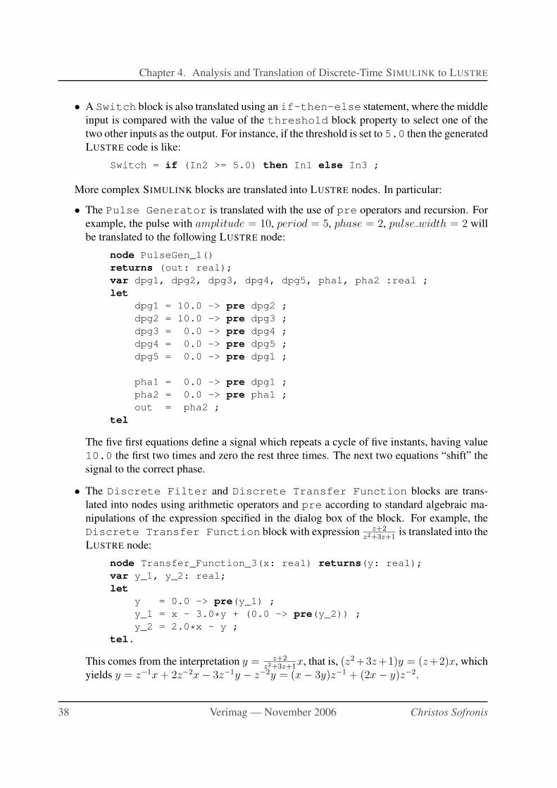
Chapter 4. Analysis and Translation of Discrete-Time SIMULINK to LUSTRE
• A Switch block is also translated using an if-then-else statement, where the middle
input is compared with the value of the threshold block property to select one of the
two other inputs as the output. For instance, if the threshold is set to 5.0 then the generated
LUSTRE code is like:
Switch = if (In2 >= 5.0) then In1 else In3 ;
More complex SIMULINK blocks are translated into LUSTRE nodes. In particular:
• The Pulse Generator is translated with the use of pre operators and recursion. For
example, the pulse with amplitude = 10, period = 5, phase = 2, pulse width = 2 will
be translated to the following LUSTRE node:
node PulseGen_1()
returns (out: real);
var dpg1, dpg2, dpg3, dpg4, dpg5, pha1, pha2 :real ;
let
dpg1 = 10.0 -> pre dpg2 ;
dpg2 = 10.0 -> pre dpg3 ;
dpg3 = 0.0 -> pre dpg4 ;
dpg4 = 0.0 -> pre dpg5 ;
dpg5 = 0.0 -> pre dpg1 ;
pha1 = 0.0 -> pre dpg1 ;
pha2 = 0.0 -> pre pha1 ;
out = pha2 ;
tel
The five first equations define a signal which repeats a cycle of five instants, having value
10.0 the first two times and zero the rest three times. The next two equations “shift” the
signal to the correct phase.
• The Discrete Filter and Discrete Transfer Function blocks are trans-
lated into nodes using arithmetic operators and pre according to standard algebraic ma-
nipulations of the expression specified in the dialog box of the block. For example, the
Discrete Transfer Function block with expression z+2z2+3z+1
is translated into the
LUSTRE node:
node Transfer_Function_3(x: real) returns(y: real);
var y_1, y_2: real;
let
y = 0.0 -> pre(y_1) ;
y_1 = x - 3.0*y + (0.0 -> pre(y_2)) ;
y_2 = 2.0*x - y ;
tel.
This comes from the interpretation y = z+2z2+3z+1
x, that is, (z2 +3z+1)y = (z+2)x, which
yields y = z−1x + 2z−2x − 3z−1y − z−2y = (x − 3y)z−1 + (2x − y)z−2.
38 Verimag — November 2006 Christos Sofronis
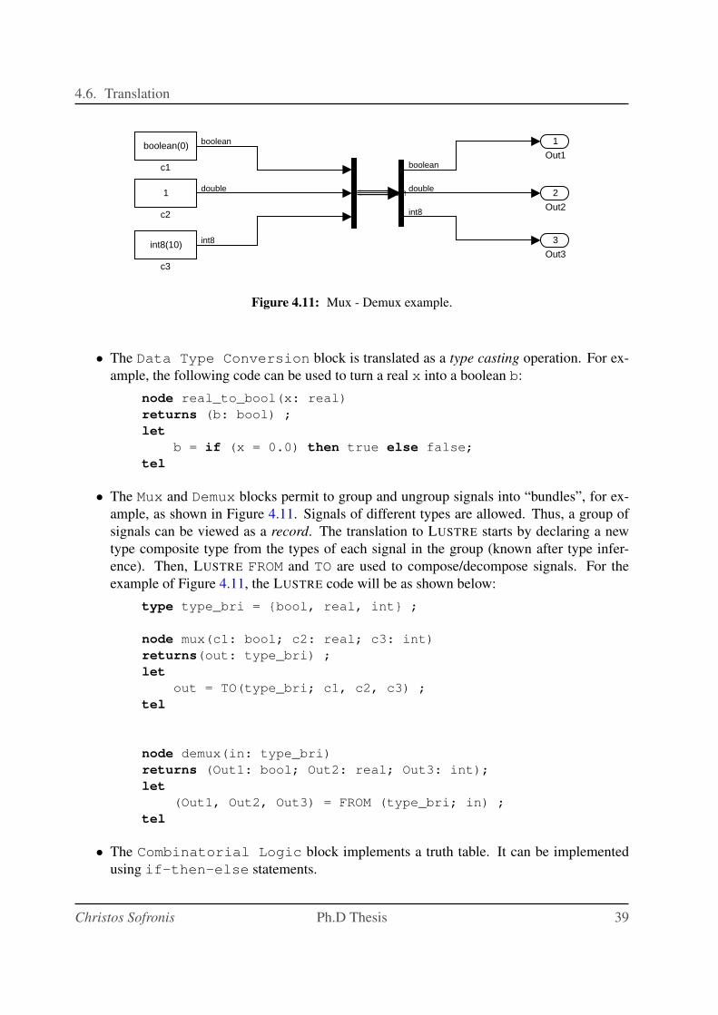
4.6. Translation
3
Out3
2
Out2
1
Out1
int8(10)
c3
1
c2
boolean(0)
c1
Demux
boolean
double
int8
boolean
double
int8
Figure 4.11: Mux - Demux example.
• The Data Type Conversion block is translated as a type casting operation. For ex-
ample, the following code can be used to turn a real x into a boolean b:
node real_to_bool(x: real)
returns (b: bool) ;
let
b = if (x = 0.0) then true else false;
tel
• The Mux and Demux blocks permit to group and ungroup signals into “bundles”, for ex-
ample, as shown in Figure 4.11. Signals of different types are allowed. Thus, a group of
signals can be viewed as a record. The translation to LUSTRE starts by declaring a new
type composite type from the types of each signal in the group (known after type infer-
ence). Then, LUSTRE FROM and TO are used to compose/decompose signals. For the
example of Figure 4.11, the LUSTRE code will be as shown below:
type type_bri = {bool, real, int} ;
node mux(c1: bool; c2: real; c3: int)
returns(out: type_bri) ;
let
out = TO(type_bri; c1, c2, c3) ;
tel
node demux(in: type_bri)
returns (Out1: bool; Out2: real; Out3: int);
let
(Out1, Out2, Out3) = FROM (type_bri; in) ;
tel
• The Combinatorial Logic block implements a truth table. It can be implemented
using if-then-else statements.
Christos Sofronis Ph.D Thesis 39
Chapter 4. Analysis and Translation of Discrete-Time SIMULINK to LUSTRE
BA
2
A_Out2
1
A_Out1
B_In1
B_In2
B_Out
3
A_In3
2
A_In2
1
A_In1
Figure 4.12: SIMULINK system A with subsystem B.
Translation of subsystems and subsystem calls A SIMULINK subsystem is translated into a
LUSTRE node, possibly containing calls to other nodes. The LUSTRE node has the same inputs
and outputs as the SIMULINK subsystem, plus, sometimes, the clock of some of its inputs (this is
done for modularity). Here is an example of such a translation. Consider the SIMULINK model
shown in Figure 4.12, with subsystems A and B. The LUSTRE code generated for this example
is as shown below:
node A(A_in1, A_in2, A_in3 : real)
returns (A_out1, A_out2 : real) ;
let
A_out1 = B(A_in1, A_in2) ;
A_out2 = ...
tel
node B(B_in1, B_in2 : real)
returns (B_out : real) ;
...
An example where it is necessary to pass clock information as input to the LUSTRE node is given
in Section 6.2.1.
Translation of triggered subsystem calls If the subsystem to be called is a triggered subsys-
tem such as the one shown in Figure 4.5, special code needs to be added in order to capture the
timing behavior according to the trigger. We illustrate how this is done in the case of a “rising”
trigger. The translation method is similar for the other two types of triggers.
First, as mentioned in Section 4.5.3, we must explicitly define in LUSTRE the Boolean flow
representing the trigger, which is implicit in SIMULINK. This is performed using three auxiliary
40 Verimag — November 2006 Christos Sofronis
4.6. Translation
LUSTRE nodes rising bool, rising int and rising real. These nodes are indepen-
dent from the SIMULINK model and can be predefined in a library. There is one node for each
possible type of the triggering signal s, because LUSTRE does not currently support polymor-
phism. We only present rising int here. The other two nodes are defined similarly.
node rising_int (s : int)
returns (rise_trigger : bool);
var neg_to_nonneg, nonpos_to_pos, not_before : bool ;
let
rise_trigger = neg_to_nonneg or (nonpos_to_pos and not_before) ;
neg_to_nonneg = false -> (pre(s < 0) and (s >= 0)) ;
nonpos_to_pos = false -> (pre(s <= 0) and (s > 0)) ;
not_before = false -> not pre(rise_trigger) ;
tel
The node takes as input an integer flow and returns a Boolean flow which is true whenever
there is a rising trigger on s. The local variables neg to nonneg and nonpos to pos rep-
resent the situations where the signal s rises from negative to zero or positive and from negative
or zero to positive, respectively. The local variable not before ensures that in situations such
as the one shown in Figure 4.6 there is no trigger produced when it should not.
Then, the LUSTRE code generated when calling a triggered subsystem A like the one of
Figure 4.5 is as follows (we assume that variables x1 and x2 are of type int):
var trig : bool;
trig = rising_int(s) ;
x1t = x1 when trig ;
x2t = x2 when trig ;
yt = A(x1t, x2t) ;
y = if trig then current(yt) else (0 -> pre(y)) ;
Variables x1t and x2t are obtained by “sampling” the inputs only at times dictated by the
trigger. Consequently, node A is activated only at those times as well, and its output yt has
the same clock, that is, trig. To obtain output y which must have the same clock (sample
time) of the inputs x1 and x2, we must perform a current operation. However, a simple
current is not enough, since it may leave y undefined for the initial instants when the trigger
is potentially false. This is why we use the if-then-else construct in the equation defining
y. This construct ensures that the value of y is equal to 0 until the first time trig becomes true.
Translation of enabled subsystem calls The LUSTRE code generated when calling an enabled
subsystem is the same as when calling a triggered subsystem, except that flow trig is replaced
by flow enab, defined as follows:
var enab : bool;
enab = if (e > 0) then true else false ;
where e is the signal feeding the Enable icon.
Christos Sofronis Ph.D Thesis 41
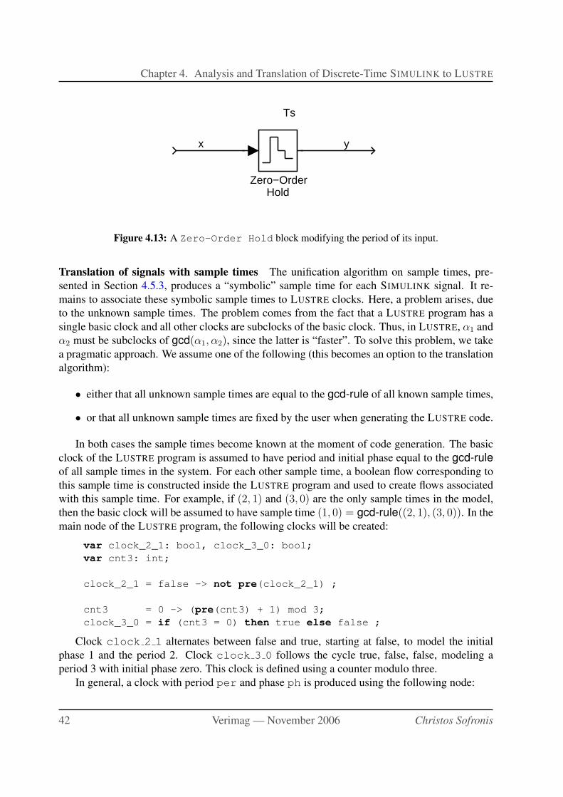
Chapter 4. Analysis and Translation of Discrete-Time SIMULINK to LUSTRE
Ts
x y
Zero−OrderHold
Figure 4.13: A Zero-Order Hold block modifying the period of its input.
Translation of signals with sample times The unification algorithm on sample times, pre-
sented in Section 4.5.3, produces a “symbolic” sample time for each SIMULINK signal. It re-
mains to associate these symbolic sample times to LUSTRE clocks. Here, a problem arises, due
to the unknown sample times. The problem comes from the fact that a LUSTRE program has a
single basic clock and all other clocks are subclocks of the basic clock. Thus, in LUSTRE, α1 and
α2 must be subclocks of gcd(α1, α2), since the latter is “faster”. To solve this problem, we take
a pragmatic approach. We assume one of the following (this becomes an option to the translation
algorithm):
• either that all unknown sample times are equal to the gcd-rule of all known sample times,
• or that all unknown sample times are fixed by the user when generating the LUSTRE code.
In both cases the sample times become known at the moment of code generation. The basic
clock of the LUSTRE program is assumed to have period and initial phase equal to the gcd-rule
of all sample times in the system. For each other sample time, a boolean flow corresponding to
this sample time is constructed inside the LUSTRE program and used to create flows associated
with this sample time. For example, if (2, 1) and (3, 0) are the only sample times in the model,
then the basic clock will be assumed to have sample time (1, 0) = gcd-rule((2, 1), (3, 0)). In the
main node of the LUSTRE program, the following clocks will be created:
var clock_2_1: bool, clock_3_0: bool;
var cnt3: int;
clock_2_1 = false -> not pre(clock_2_1) ;
cnt3 = 0 -> (pre(cnt3) + 1) mod 3;
clock_3_0 = if (cnt3 = 0) then true else false ;
Clock clock 2 1 alternates between false and true, starting at false, to model the initial
phase 1 and the period 2. Clock clock 3 0 follows the cycle true, false, false, modeling a
period 3 with initial phase zero. This clock is defined using a counter modulo three.
In general, a clock with period per and phase ph is produced using the following node:
42 Verimag — November 2006 Christos Sofronis
4.7. Related Work
node make_clock(per: int; ph: int)
returns( clock: bool );
var cnt: int;
let
cnt = (per - ph) -> (pre(cnt) + 1) mod period ;
clock = if (cnt = 0) then true else false ;
tel
The above clocks are used during LUSTRE code generation as follows. Consider the Zero-
Order Hold block of Figure 4.13 and assume that the sample time of input x is (1, 0) and the
sample time set to the zero-order hold block is (2, 1). Then the sample time of the output y is
also (2, 1) and the generated LUSTRE code is as follows:
y = x when clock_2_1 ;
If, instead of a Zero-Order Hold block we had, say, a Discrete Transfer Function block, the
LUSTRE code would be:
y = DTF(x when clock_2_1) ;
where DTF is the LUSTRE node implementing the Discrete Transfer Function block.
Now consider the Sum block of Figure 4.4 and assume that the sample times of inputs x1 and
x2 are (2, 1) and (3, 0), respectively. Also assume as a first case that the basic clock is (1, 0).Then the sample time of the output y is (1, 0) and the generated LUSTRE code is as follows:
x1t = if clock_2_1 then current(x1) else (0 -> pre(x1t)) ;
x2t = if clock_3_0 then current(x2) else (0 -> pre(x2t)) ;
y = x1t + x2t ;
x1 and x2 have been previously produced using the when operator on the appropriate clocks.
Then, x1t and x2t are on the basic clock and so is the output y. The if-then-else con-
struct is used with the current operator as previously, to ensure well-defined initial values.
As a second case, assume that (1, 0) is not the basic clock but a subclock. Then y must be
obtained as
y = (x1t + x2t) when clock_1_0 ;
4.7 Related Work
Before concluding this Chapter, we comment on some work related to its contents.
[BFM+05] study the translation between SIMULINK and the language supported by the AS-
CET tool-set by the ETAS group. ASCET’s language is closer to the implementation level than
LUSTRE, in the sense that the basic entities are tasks scheduled by a real-time operating system
(RTOS).
[TNTBS00] report on an approach to co-simulate discrete controllers modeled in the syn-
chronous language Signal [GGBM91] along with continuous plants modeled in SIMULINK.
[CHLrA02] present tools for co-simulation of process dynamics, control task execution and net-
work communication in a distributed real-time control system. [SBCR01] use a model-checker
Christos Sofronis Ph.D Thesis 43
Chapter 4. Analysis and Translation of Discrete-Time SIMULINK to LUSTRE
to verify a SIMULINK/STATEFLOW model from the automotive domain, however, they translate
their model manually to the input language of the model-checker.
A number of approaches are based in extending SIMULINK with libraries of predefined blocks
and then using SIMULINK as a front-end or simulator. The hybrid-system model-checker Check-
Mate uses such an approach [SRKC00, CK03]. [KSHP02] extend SIMULINK with the capability
of expressing designs in the time-triggered language Giotto [HHK01].
[JZW+00] report on translating SIMULINK to the SPI model, a model of concurrent processes
communicating with FIFO queues or registers. The focus seems to be the preservation of value
over-writing which can occur in multi-rate systems when a “slower” node receives input from a
“fast” one.
[JB03] report on MAGICA, a type-inference engine for Matlab. The focus is on deriving
information such as whether variables have real or imaginary values, array sizes for non-scalars,
and so on.
[ASK04] propose a method to translate SIMULINK/STATEFLOW models into hybrid automata
using graph transformations.
4.8 Conclusions
We have presented a method for translating a discrete-time subset of SIMULINK models into
LUSTRE programs. The translation is done in three steps: type and clock inference, followed by
a hierarchical bottom-up translation. We have implemented the method in a tool called S2L and
applied it to two embedded controller applications from the automotive domain. The interest of
our tool is that it opens the way to the use of formal and certified verification and implementation
tools attached to the LUSTRE tool chain. Also, in the process of translation, we explained and
formalized the typing and timing mechanisms of SIMULINK.
Perhaps the most significant drawback of our approach is its dependency on syntax and se-
mantics of SIMULINK models. New versions of SIMULINK appear as often as every six months
and sometimes major changes are made with respect to previous versions. This situation seems
difficult to avoid given the relative “monopoly” of SIMULINK/STATEFLOW in the control de-
sign landscape. Another weakness of our tool is its incompleteness: several unsafe constructs
of SIMULINK are not translated. Yet this can be seen as the price to pay for having a sound
translation.
44 Verimag — November 2006 Christos Sofronis
Chapter 5
Analysis and Translation of STATEFLOW to
LUSTRE
In this Chapter we will analyze STATEFLOW and go through a faithful translation towards LUS-
TRE, trying to preserve the semantics that we define in the next Sections.
Before we can attempt to define which features of STATEFLOW are suitable for translation
into LUSTRE, we have to illustrate some of the semantical issues with STATEFLOW, which are
also likely to cause problems with our translator. These issues range from “serious” ones, such as
non-termination of a simulation step or stack overflow, to more “minor” ones, such as dependence
of the semantics upon the positions of objects in the STATEFLOW diagram. First, we briefly
describe the STATEFLOW language and informally explain its semantics (for a formal semantics,
see [HR04]).
5.1 A short description of STATEFLOW
STATEFLOW is a graphical language resembling Statecharts [Har87]. The semantics of STATE-
FLOW are embodied in the interpretation algorithm of the STATEFLOW simulator1. A STATE-
FLOW chart has a hierarchical structure, where states can be refined into either exclusive (OR)
states connected with transitions or parallel (AND) states, which are not connected. It is impor-
tant to note that parallel states are not executed concurrently, but sequentially. Figure 5.13 shows
an example: A and B are parallel states (with parent the root state), while all their child states
are exclusive. A transition can be a complex (possibly cyclic) flow graph made of segments join-
ing connective junctions. Each segment can bear a complex label with the following syntax (all
fields are optional):
E[C]{Ac}/At
where E is an event, C is the condition (i.e., guard), Ac is the condition action and At is the
transition action. Ac and At are written in the action language of STATEFLOW, which contains
1 This is documented in a 900-page long User’s Guide STATEFLOW and STATEFLOW Coder, User’s Guide,
Version 5. Available at http://www.mathworks.com/products/stateflow/ From this guide we have borrowed our
terminology.
45

Chapter 5. Analysis and Translation of STATEFLOW to LUSTRE
assignments, emissions of events, and so on. The order of execution of those actions is stated
later. Actions written in the action language can also be associated to states. A state can have an
entry action, a during action, an exit action and on event E actions, where E is an event.
The interpretation algorithm is triggered every time an event arrives from SIMULINK or from
within the STATEFLOW model itself.2 The algorithm then executes the following steps:
Search for active states: this search is performed hierarchically, from top to bottom. At each
level of hierarchy, when there are parallel states, the search order is a graphical two di-
mensional one: states are searched from top to bottom and from left to right, in order to
impose determinism upon the STATEFLOW semantics.
Search for valid transitions: once an active state is found, its output transitions are searched
for a valid one to follow, with respect to several criteria: the event of the transition must be
present and its condition must be true. As mentioned earlier, both the event on a transition
and the condition are optional, in which case those criteria are not checked. The goal is to
find a transition which is valid all the way from the source state to the destination state. In
particular, when the transition is multi-segment, the condition actions of each segment are
executed while searching and traversing the transition graph, even if the condition does not
hold. The search order is again deterministic: transitions are searched according to the 12
o’clock rule.3
Execute a valid transition: once a valid transition is found, STATEFLOW follows these steps:
execute the exit action of the source state, set the source state to inactive, execute the
transition actions of the transition path, set the destination state to active and finally execute
the entry action of the destination state.
Idling: when an active state has no valid output transitions an active state performs its during
action and the state remains active.
Termination: occurs when there are no active states.
It should be emphasized that each of the executions runs to completion and this makes the be-
havior of the overall algorithm very complex. In particular, when any of the actions consists
of broadcasting an event, the interpretation algorithm for that event is also run to completion
before execution proceeds. This means that the interpretation algorithm is recursive and uses a
stack. However, as we will see, the stack does not store the full state, which leads to problems of
side effect (Section 5.2). Also, without care, the stack may overflow (Section 5.2).
Interface between SIMULINK model and STATEFLOW chart
Every STATEFLOW model resides inside a SIMULINK system and more precisely it is introduced,
in the SIMULINK model, using the “Chart” block from the “sflib” library (that may be invoked
2 The SIMULINK event is often a SIMULINKtrigger, although it can also be the simulation step of the global
SIMULINK-STATEFLOW model.3 Notice that this is considered harmful even in the STATEFLOW documentation, where it is stated: “Do not
design your STATEFLOW diagram based on the expected execution order of transitions.”
46 Verimag — November 2006 Christos Sofronis
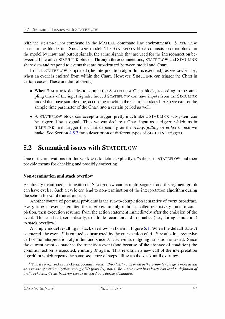
5.2. Semantical issues with STATEFLOW
with the stateflow command in the MATLAB command line environment). STATEFLOW
charts run as blocks in a SIMULINK model. The STATEFLOW block connects to other blocks in
the model by input and output signals, the same signals that are used for the interconnection be-
tween all the other SIMULINK blocks. Through these connections, STATEFLOW and SIMULINK
share data and respond to events that are broadcasted between model and Chart.
In fact, STATEFLOW is updated (the interpretation algorithm is executed), as we saw earlier,
when an event is emitted from within the Chart. However, SIMULINK can trigger the Chart in
certain cases. These are the following
• When SIMULINK decides to sample the STATEFLOW Chart block, according to the sam-
pling times of the input signals. Indeed STATEFLOW can have inputs from the SIMULINK
model that have sample time, according to which the Chart is updated. Also we can set the
sample time parameter of the Chart into a certain period as well.
• A STATEFLOW block can accept a trigger, pretty much like a SIMULINK subsystem can
be triggered by a signal. Thus we can declare a Chart input as a trigger, which, as in
SIMULINK, will trigger the Chart depending on the rising, falling or either choice we
make. See Section 4.5.2 for a description of different types of SIMULINK triggers.
5.2 Semantical issues with STATEFLOW
One of the motivations for this work was to define explicitly a “safe part” STATEFLOW and then
provide means for checking and possibly correcting
Non-termination and stack overflow
As already mentioned, a transition in STATEFLOW can be multi-segment and the segment graph
can have cycles. Such a cycle can lead to non-termination of the interpretation algorithm during
the search for valid transition step.
Another source of potential problems is the run-to-completion semantics of event broadcast.
Every time an event is emitted the interpretation algorithm is called recursively, runs to com-
pletion, then execution resumes from the action statement immediately after the emission of the
event. This can lead, semantically, to infinite recursion and in practice (i.e., during simulation)
to stack overflow.4
A simple model resulting in stack overflow is shown in Figure 5.1. When the default state Ais entered, the event E is emitted as instructed by the entry action of A. E results in a recursive
call of the interpretation algorithm and since A is active its outgoing transition is tested. Since
the current event E matches the transition event (and because of the absence of condition) the
condition action is executed, emitting E again. This results in a new call of the interpretation
algorithm which repeats the same sequence of steps filling up the stack until overflow.
4 This is recognized in the official documentation: “Broadcasting an event in the action language is most useful
as a means of synchronization among AND (parallel) states. Recursive event broadcasts can lead to definition of
cyclic behavior. Cyclic behavior can be detected only during simulation.”
Christos Sofronis Ph.D Thesis 47
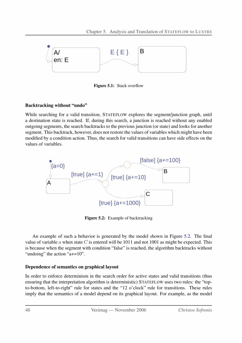
Chapter 5. Analysis and Translation of STATEFLOW to LUSTRE
A/en: E
BE { E }
Figure 5.1: Stack overflow
Backtracking without “undo”
While searching for a valid transition, STATEFLOW explores the segment/junction graph, until
a destination state is reached. If, during this search, a junction is reached without any enabled
outgoing segments, the search backtracks to the previous junction (or state) and looks for another
segment. This backtrack, however, does not restore the values of variables which might have been
modified by a condition action. Thus, the search for valid transitions can have side effects on the
values of variables.
A
C
B{a=0}
[false] {a+=100}
[true] {a+=10}[true] {a+=1}
[true] {a+=1000}
Figure 5.2: Example of backtracking
An example of such a behavior is generated by the model shown in Figure 5.2. The final
value of variable a when state C is entered will be 1011 and not 1001 as might be expected. This
is because when the segment with condition “false” is reached, the algorithm backtracks without
“undoing” the action “a+=10”.
Dependence of semantics on graphical layout
In order to enforce determinism in the search order for active states and valid transitions (thus
ensuring that the interpretation algorithm is deterministic) STATEFLOW uses two rules: the “top-
to-bottom, left-to-right” rule for states and the “12 o’clock” rule for transitions. These rules
imply that the semantics of a model depend on its graphical layout. For example, as the model
48 Verimag — November 2006 Christos Sofronis
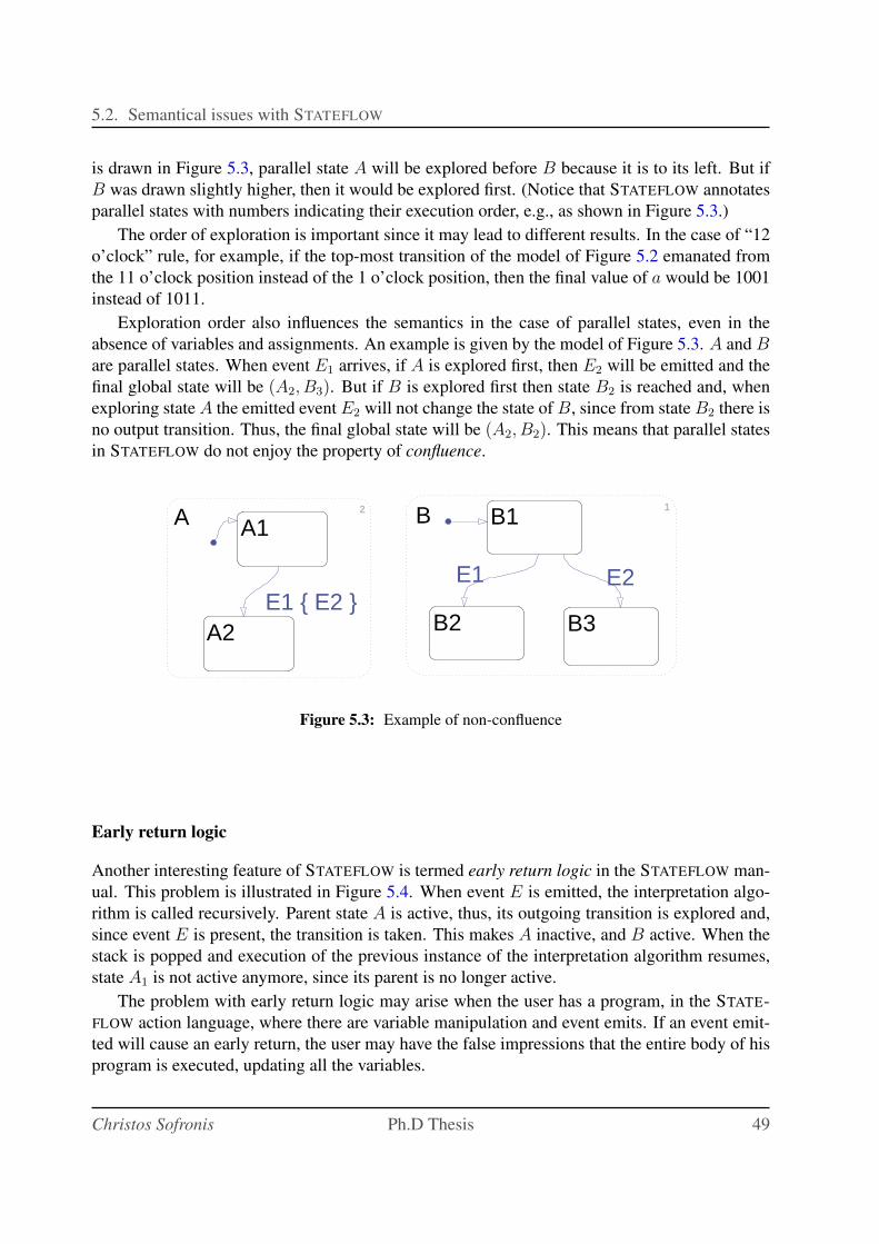
5.2. Semantical issues with STATEFLOW
is drawn in Figure 5.3, parallel state A will be explored before B because it is to its left. But if
B was drawn slightly higher, then it would be explored first. (Notice that STATEFLOW annotates
parallel states with numbers indicating their execution order, e.g., as shown in Figure 5.3.)
The order of exploration is important since it may lead to different results. In the case of “12
o’clock” rule, for example, if the top-most transition of the model of Figure 5.2 emanated from
the 11 o’clock position instead of the 1 o’clock position, then the final value of a would be 1001
instead of 1011.
Exploration order also influences the semantics in the case of parallel states, even in the
absence of variables and assignments. An example is given by the model of Figure 5.3. A and Bare parallel states. When event E1 arrives, if A is explored first, then E2 will be emitted and the
final global state will be (A2, B3). But if B is explored first then state B2 is reached and, when
exploring state A the emitted event E2 will not change the state of B, since from state B2 there is
no output transition. Thus, the final global state will be (A2, B2). This means that parallel states
in STATEFLOW do not enjoy the property of confluence.
B 1A 2 B1A1
B2 B3A2
E2E1E1 { E2 }
Figure 5.3: Example of non-confluence
Early return logic
Another interesting feature of STATEFLOW is termed early return logic in the STATEFLOW man-
ual. This problem is illustrated in Figure 5.4. When event E is emitted, the interpretation algo-
rithm is called recursively. Parent state A is active, thus, its outgoing transition is explored and,
since event E is present, the transition is taken. This makes A inactive, and B active. When the
stack is popped and execution of the previous instance of the interpretation algorithm resumes,
state A1 is not active anymore, since its parent is no longer active.
The problem with early return logic may arise when the user has a program, in the STATE-
FLOW action language, where there are variable manipulation and event emits. If an event emit-
ted will cause an early return, the user may have the false impressions that the entire body of his
program is executed, updating all the variables.
Christos Sofronis Ph.D Thesis 49
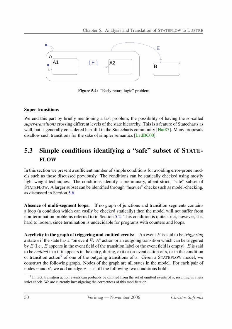
Chapter 5. Analysis and Translation of STATEFLOW to LUSTRE
A
BA1 A2
E
{ E }
Figure 5.4: “Early return logic” problem
Super-transitions
We end this part by briefly mentioning a last problem; the possibility of having the so-called
super-transitions crossing different levels of the state hierarchy. This is a feature of Statecharts as
well, but is generally considered harmful in the Statecharts community [Har87]. Many proposals
disallow such transitions for the sake of simpler semantics [LvdBC00].
5.3 Simple conditions identifying a “safe” subset of STATE-
FLOW
In this section we present a sufficient number of simple conditions for avoiding error-prone mod-
els such as those discussed previously. The conditions can be statically checked using mostly
light-weight techniques. The conditions identify a preliminary, albeit strict, “safe” subset of
STATEFLOW. A larger subset can be identified through “heavier” checks such as model-checking,
as discussed in Section 5.6.
Absence of multi-segment loops: If no graph of junctions and transition segments contains
a loop (a condition which can easily be checked statically) then the model will not suffer from
non-termination problems referred to in Section 5.2. This condition is quite strict, however, it is
hard to loosen, since termination is undecidable for programs with counters and loops.
Acyclicity in the graph of triggering and emitted events: An event E is said to be triggering
a state s if the state has a “on event E: A” action or an outgoing transition which can be triggered
by E (i.e., E appears in the event field of the transition label or the event field is empty). E is said
to be emitted in s if it appears in the entry, during, exit or on-event action of s, or in the condition
or transition action5 of one of the outgoing transitions of s. Given a STATEFLOW model, we
construct the following graph. Nodes of the graph are all states in the model. For each pair of
nodes v and v′, we add an edge v → v′ iff the following two conditions hold:
5 In fact, transition action events can probably be omitted from the set of emitted events of s, resulting in a less
strict check. We are currently investigating the correctness of this modification.
50 Verimag — November 2006 Christos Sofronis

5.3. Simple conditions identifying a “safe” subset of STATEFLOW
1. There is an event E which is emitted in v and triggering v′.
2. Either v = v′ or the first common parent state of v and v′ is a parallel state.
The idea is that v can emit event E which can then trigger v′, but only if v and v′ can be active at
the same time. If the graph above has no directed cycle then the model will not suffer from stack
overflow problems.
Absence of assignments in intermediate segments: In order to avoid side effects due to lack
of “undo”, we can simply check that all variable assignments in a multi-segment transition appear
either in transition actions (which are executed only once a destination state has been reached) or
in the condition action of the last segment (whose destination is a state and not a junction). This
ensures that even in case the algorithm backtracks, no variable has been modified. An alternative
is to avoid backtracking altogether, as is done with the following check.
Conditions of outgoing junction segments form a cover: In order to ensure absence of back-
tracking when multi-segment transitions are explored, we can check that for each junction, the
disjunction of all conditions in outgoing segments is the condition true. If segments also carry
triggering events, we must ensure that all possible emitted events are covered as well.
Conditions of outgoing junction segments are disjoint: In order to ensure that the STATE-
FLOW model does not depend on the 12 o’clock rule, we must check that for each state or junc-
tion, the conditions of its outgoing transitions are pair-wise disjoint. This implies at most one
transition is enabled at any given time. In the presence of triggering events, we can relax this by
performing the check for each group of transitions associated with a single event E (or having
no triggering event).
It should be noted that checking whether STATEFLOW conditions are disjoint or form a cover
is an undecidable problem, because of the generality of these conditions. From a STATEFLOW
design, we can extract very easily the logical properties expressing that a set of conditions are
disjoint and form a cover. These logical properties can be transmitted as a proof obligation to
some external tool such as a theorem prover. However, for most practical cases, recognizing
common sub-expressions is sufficient for establishing that some conditions are disjoint and form
a cover.
Checks for confluence: In order to ensure that the semantics of a given STATEFLOW model
does not depend on the order of exploring two parallel states A and B, we must check two things.
First, that A and B do not access the same variable x (both write x or one reads and the other
writes x). But this is not sufficient, as shown in Section 5.2, because event broadcasting alone
can cause problems. A simple solution is to check that in the aforementioned graph of triggering
and emitted events, there is no edge v → v′ such that v belongs to A and v′ to B or vice-versa.
This is exactly the problem of Figure 5.3, where one of the edges in the above mentioned
graph of triggering and emitted events is the A1 → B1; the emitted event in the outgoing tran-
sition form A1 to A2 is the same event E that is triggering event for the state B1 (because the
Christos Sofronis Ph.D Thesis 51
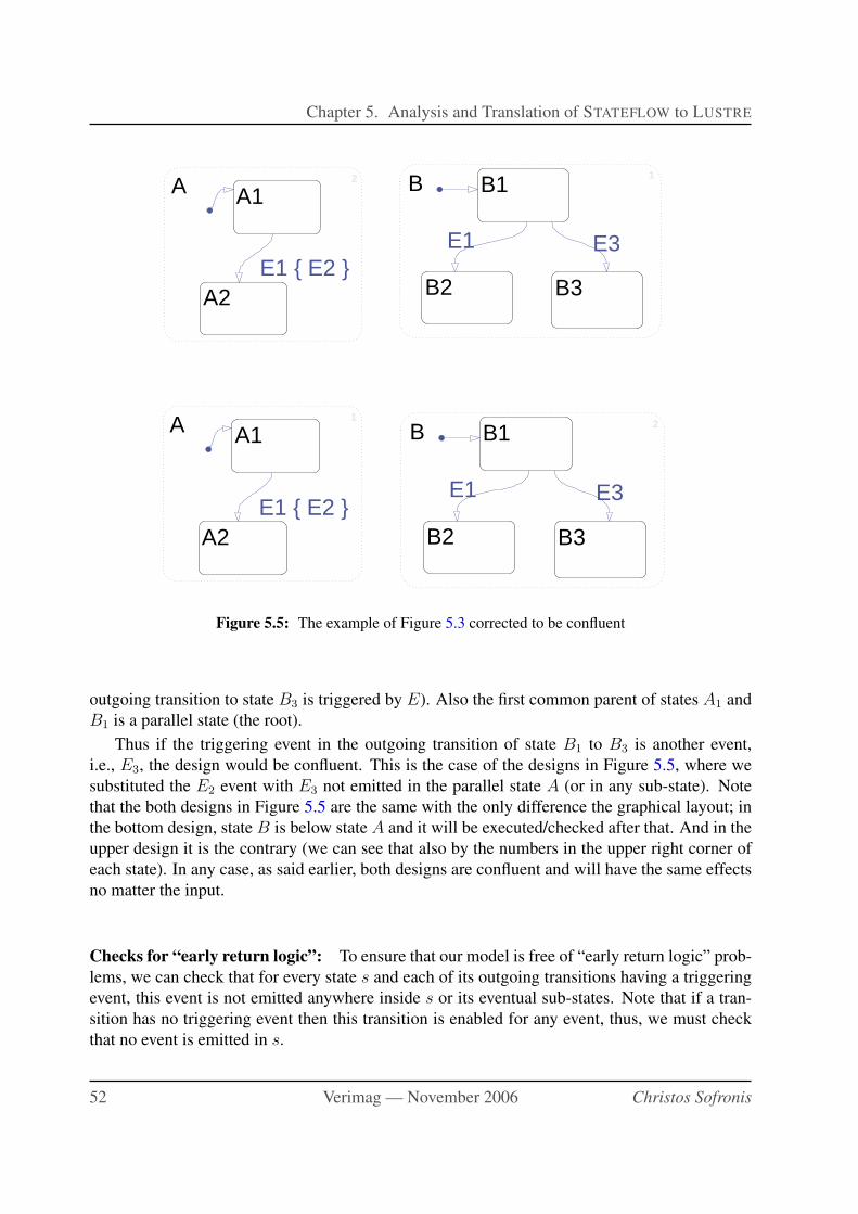
Chapter 5. Analysis and Translation of STATEFLOW to LUSTRE
B 1A 2 B1A1
B2 B3A2
E1 E3E1 { E2 }
A 1
B 2B1A1
B2 B3A2
E1 E3E1 { E2 }
Figure 5.5: The example of Figure 5.3 corrected to be confluent
outgoing transition to state B3 is triggered by E). Also the first common parent of states A1 and
B1 is a parallel state (the root).
Thus if the triggering event in the outgoing transition of state B1 to B3 is another event,
i.e., E3, the design would be confluent. This is the case of the designs in Figure 5.5, where we
substituted the E2 event with E3 not emitted in the parallel state A (or in any sub-state). Note
that the both designs in Figure 5.5 are the same with the only difference the graphical layout; in
the bottom design, state B is below state A and it will be executed/checked after that. And in the
upper design it is the contrary (we can see that also by the numbers in the upper right corner of
each state). In any case, as said earlier, both designs are confluent and will have the same effects
no matter the input.
Checks for “early return logic”: To ensure that our model is free of “early return logic” prob-
lems, we can check that for every state s and each of its outgoing transitions having a triggering
event, this event is not emitted anywhere inside s or its eventual sub-states. Note that if a tran-
sition has no triggering event then this transition is enabled for any event, thus, we must check
that no event is emitted in s.
52 Verimag — November 2006 Christos Sofronis
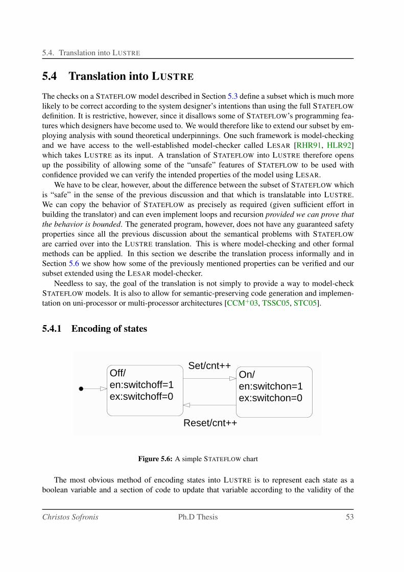
5.4. Translation into LUSTRE
5.4 Translation into LUSTRE
The checks on a STATEFLOW model described in Section 5.3 define a subset which is much more
likely to be correct according to the system designer’s intentions than using the full STATEFLOW
definition. It is restrictive, however, since it disallows some of STATEFLOW’s programming fea-
tures which designers have become used to. We would therefore like to extend our subset by em-
ploying analysis with sound theoretical underpinnings. One such framework is model-checking
and we have access to the well-established model-checker called LESAR [RHR91, HLR92]
which takes LUSTRE as its input. A translation of STATEFLOW into LUSTRE therefore opens
up the possibility of allowing some of the “unsafe” features of STATEFLOW to be used with
confidence provided we can verify the intended properties of the model using LESAR.
We have to be clear, however, about the difference between the subset of STATEFLOW which
is “safe” in the sense of the previous discussion and that which is translatable into LUSTRE.
We can copy the behavior of STATEFLOW as precisely as required (given sufficient effort in
building the translator) and can even implement loops and recursion provided we can prove that
the behavior is bounded. The generated program, however, does not have any guaranteed safety
properties since all the previous discussion about the semantical problems with STATEFLOW
are carried over into the LUSTRE translation. This is where model-checking and other formal
methods can be applied. In this section we describe the translation process informally and in
Section 5.6 we show how some of the previously mentioned properties can be verified and our
subset extended using the LESAR model-checker.
Needless to say, the goal of the translation is not simply to provide a way to model-check
STATEFLOW models. It is also to allow for semantic-preserving code generation and implemen-
tation on uni-processor or multi-processor architectures [CCM+03, TSSC05, STC05].
5.4.1 Encoding of states
Off/en:switchoff=1ex:switchoff=0
On/en:switchon=1ex:switchon=0
Set/cnt++
Reset/cnt++
Figure 5.6: A simple STATEFLOW chart
The most obvious method of encoding states into LUSTRE is to represent each state as a
boolean variable and a section of code to update that variable according to the validity of the
Christos Sofronis Ph.D Thesis 53
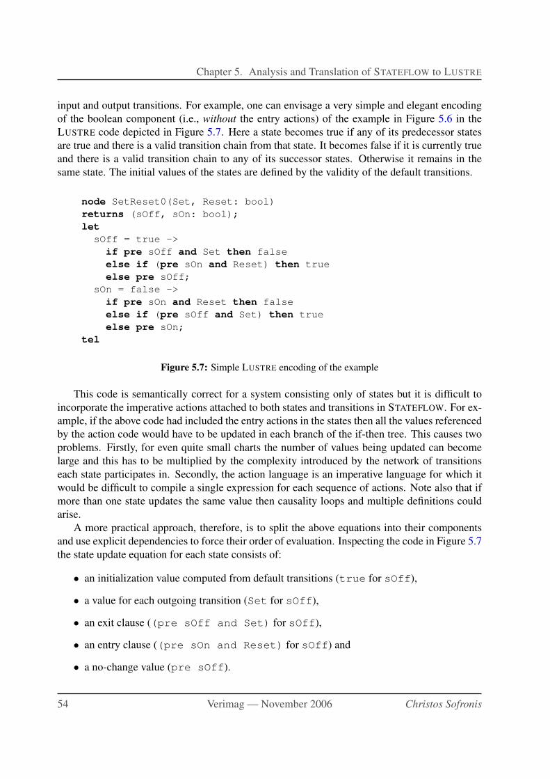
Chapter 5. Analysis and Translation of STATEFLOW to LUSTRE
input and output transitions. For example, one can envisage a very simple and elegant encoding
of the boolean component (i.e., without the entry actions) of the example in Figure 5.6 in the
LUSTRE code depicted in Figure 5.7. Here a state becomes true if any of its predecessor states
are true and there is a valid transition chain from that state. It becomes false if it is currently true
and there is a valid transition chain to any of its successor states. Otherwise it remains in the
same state. The initial values of the states are defined by the validity of the default transitions.
node SetReset0(Set, Reset: bool)
returns (sOff, sOn: bool);
let
sOff = true ->
if pre sOff and Set then false
else if (pre sOn and Reset) then true
else pre sOff;
sOn = false ->
if pre sOn and Reset then false
else if (pre sOff and Set) then true
else pre sOn;
tel
Figure 5.7: Simple LUSTRE encoding of the example
This code is semantically correct for a system consisting only of states but it is difficult to
incorporate the imperative actions attached to both states and transitions in STATEFLOW. For ex-
ample, if the above code had included the entry actions in the states then all the values referenced
by the action code would have to be updated in each branch of the if-then tree. This causes two
problems. Firstly, for even quite small charts the number of values being updated can become
large and this has to be multiplied by the complexity introduced by the network of transitions
each state participates in. Secondly, the action language is an imperative language for which it
would be difficult to compile a single expression for each sequence of actions. Note also that if
more than one state updates the same value then causality loops and multiple definitions could
arise.
A more practical approach, therefore, is to split the above equations into their components
and use explicit dependencies to force their order of evaluation. Inspecting the code in Figure 5.7
the state update equation for each state consists of:
• an initialization value computed from default transitions (true for sOff),
• a value for each outgoing transition (Set for sOff),
• an exit clause ((pre sOff and Set) for sOff),
• an entry clause ((pre sOn and Reset) for sOff) and
• a no-change value (pre sOff).
54 Verimag — November 2006 Christos Sofronis
5.4. Translation into LUSTRE
Explicitly separating these components allows us to insert the action code at the correct point
in the computation of a reaction. This results in the rather dense encoding shown in Figure 5.8.
Here, the code has been split into several sections.
• Initial values. These are the initial values for all variables, false for states and the
initial value from the data dictionary for STATEFLOW variables. Mention that after the
first, initial cycle, those variables have the pre value of the corresponding variable, which
is the previous state (on or off) of the corresponding state (in the STATEFLOW graph)
• Transition validity. In this section the values for the transitions are computed. For con-
venience in the translator these are actually calls to predefined nodes generated in advance
from the transitions’ events and actions. Note that the test for the activity of the source
state is included in the transition’s validity test. In the example of Figure 5.8, for reasons
of simplicity, the validity of the links appears inside the node.
• State exits. Any states which are true and have a valid outgoing transition are set to
false.
• Exit actions. The code for any exiting state’s exit actions is computed. This section also
includes during actions for states which remain active and on actions also for active states.
• Transition actions. The code for the transition actions is executed. Note that the exiting
state’s value is false while this occurs.
• State entries. Any states which are false and have a valid incoming transition are set to
true.
• Entry actions. Entering states action code is executed with the state’s variable now true.
This sequence corresponds to the sequence of events in STATEFLOW’s interpretation algo-
rithm. Note that by “transition valid” we do not mean that the transition is valid with respect
to the current context but that this is a transition which will be traversed in the current reaction.
Thus the arbitration between competing outgoing transitions has to be resolved by the transition
valid computation.
There are some additional complications in the code shown in Figure 5.8, for instance the use
of the init and term flags which are used to control initialization and termination of subgraphs
but these are discussed in the later sections.
5.4.2 Compiling transition networks
Figure 5.9 shows a STATEFLOW chart with a junction. Junctions in STATEFLOW do not have a
physical state and can be thought of as nodes in an if-then tree. This is thus the most sensible
encoding of junctions. One problem, however, is that junction networks can be sourced from
more than one state and/or a single state can have more than one output to the same junction.
Christos Sofronis Ph.D Thesis 55
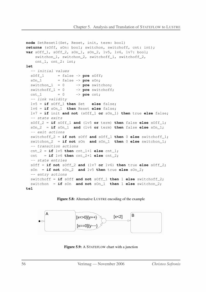
Chapter 5. Analysis and Translation of STATEFLOW to LUSTRE
node SetReset1(Set, Reset, init, term: bool)
returns (sOff, sOn: bool; switchon, switchoff, cnt: int);
var sOff_1, sOff_2, sOn_1, sOn_2, lv5, lv6, lv7: bool;
switchon_1, switchon_2, switchoff_1, switchoff_2,
cnt_1, cnt_2: int;
let
-- initial values
sOff_1 = false -> pre sOff;
sOn_1 = false -> pre sOn;
switchon_1 = 0 -> pre switchon;
switchoff_1 = 0 -> pre switchoff;
cnt_1 = 0 -> pre cnt;
-- link validity
lv5 = if sOff_1 then Set else false;
lv6 = if sOn_1 then Reset else false;
lv7 = if init and not (sOff_1 or sOn_1) then true else false;
-- state exits
sOff_2 = if sOff_1 and (lv5 or term) then false else sOff_1;
sOn_2 = if sOn_1 and (lv6 or term) then false else sOn_1;
-- exit actions
switchoff_2 = if not sOff and sOff_1 then 0 else switchoff_1;
switchon_2 = if not sOn and sOn_1 then 0 else switchon_1;
-- transition actions
cnt_2 = if lv5 then cnt_1+1 else cnt_1;
cnt = if lv6 then cnt_2+1 else cnt_2;
-- state entries
sOff = if not sOff_2 and (lv7 or lv6) then true else sOff_2;
sOn = if not sOn_2 and lv5 then true else sOn_2;
-- entry actions
switchoff = if sOff and not sOff_1 then 1 else switchoff_2;
switchon = if sOn and not sOn_1 then 1 else switchon_2;
tel
Figure 5.8: Alternative LUSTRE encoding of the example
A B
[x==0]{y−−}
[x<>0]{y++} [x<2]
Figure 5.9: A STATEFLOW chart with a junction
56 Verimag — November 2006 Christos Sofronis
5.4. Translation into LUSTRE
These can be handled quite easily if one allows a certain amount of code duplication, the common
subnetwork for two joining outgoing transitions being compiled twice.
We could devise a very natural scheme for LUSTRE to handle this but again it becomes dif-
ficult to insert the condition and transition actions into the if-then tree in LUSTRE. Figure
5.10 shows the actual code generated6. The functions cv{678}_ not shown compute the con-
dition code for their respective transitions. Note how the cv8 call is duplicated between lv6
and lv7 . Essentially, the junction tree is turned into a flattened representation with two flags,
“end” which signifies the termination of the tree (either a destination state or a terminal junc-
tion) and “exit” which is true if the terminal was a state. One slight inefficiency is the use of
these flags to defeat further computation after the termination point is reached (the not end
clauses). These two flags correspond to the End, No and Fire transition values in [HR04], the
semantics of our junction processing is identical to the semantics described therein.
There is also a slight problem with the “transition valid” section in the code shown in Figure
5.8. For the example shown there can only ever be one transition valid flag true at each instant
but when a state has (potentially competing) outgoing transitions there has to be some kind of
arbitration between them, hopefully using the same arbitration as STATEFLOW itself. In fact the
statements are chained together with a common flag which indicates when a valid transition has
been found. This is called the ok variable and a revised transition validity computation section
is shown in Figure 5.11. In fact we need a separate ok flag for each subgraph, this is explained
later when inter-level transitions are discussed.
A more serious problem is that junction networks can have loops which results in unbounded
recursion and therefore a loss of synchronous semantics. Figure 5.12 shows a simple for-loop.
There are a number of possibilities for handling this.
Junctions as states. An easy solution would be to give junctions a physical state in the exe-
cuting LUSTRE program. This effectively moves the non-termination problem outward into the
code calling the STATEFLOW model but also moves the burden of the proof of non-termination to
the client code. This has been implemented in our translator where we also provide an additional
status flag called “valid” as an output which is true only if the current state is not a junction.
In theory, the client code could loop over the STATEFLOW code until this flag becomes true at
which point the other outputs are also valid.
Loop unrolling with external proof obligations. This is unsatisfactory from the point of view
of using the translator as a development tool. We would prefer to simply impose a synchronous
semantics upon STATEFLOW and outlaw such constructs if they cannot be proven to be bounded.
Given a synchronous semantics for STATEFLOW we have to outlaw such constructs in the general
case. It is possible, however, to unroll such loops (Figure 5.12 also shows the expansion of the
simple loop) without loss of generality, provided bounds can be proven on the number of itera-
tions. This means we can generate proof obligations for external tools such as Nbac [JHR99]. If
6 Our code examples have been condensed for brevity and use abbreviated variable names. cv means “condition
valid”, lv “transition valid”, ca “condition action” and su “state update”
Christos Sofronis Ph.D Thesis 57
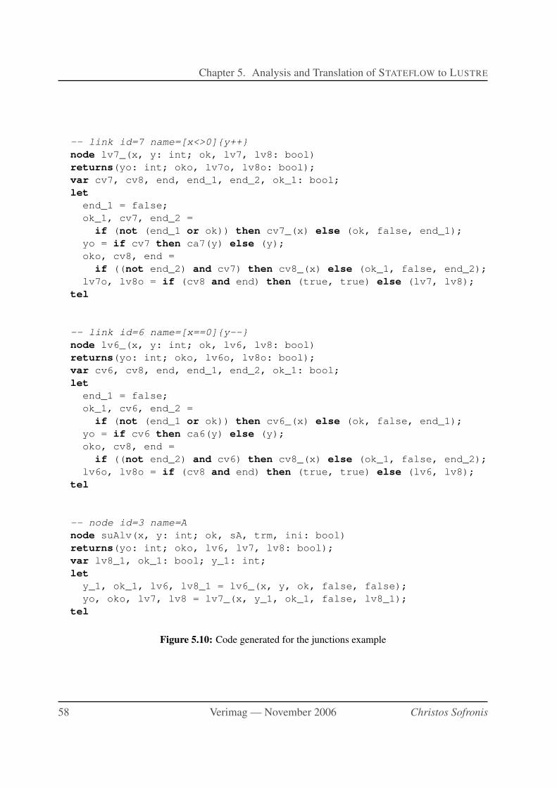
Chapter 5. Analysis and Translation of STATEFLOW to LUSTRE
-- link id=7 name=[x<>0]{y++}
node lv7_(x, y: int; ok, lv7, lv8: bool)
returns(yo: int; oko, lv7o, lv8o: bool);
var cv7, cv8, end, end_1, end_2, ok_1: bool;
let
end_1 = false;
ok_1, cv7, end_2 =
if (not (end_1 or ok)) then cv7_(x) else (ok, false, end_1);
yo = if cv7 then ca7(y) else (y);
oko, cv8, end =
if ((not end_2) and cv7) then cv8_(x) else (ok_1, false, end_2);
lv7o, lv8o = if (cv8 and end) then (true, true) else (lv7, lv8);
tel
-- link id=6 name=[x==0]{y--}
node lv6_(x, y: int; ok, lv6, lv8: bool)
returns(yo: int; oko, lv6o, lv8o: bool);
var cv6, cv8, end, end_1, end_2, ok_1: bool;
let
end_1 = false;
ok_1, cv6, end_2 =
if (not (end_1 or ok)) then cv6_(x) else (ok, false, end_1);
yo = if cv6 then ca6(y) else (y);
oko, cv8, end =
if ((not end_2) and cv6) then cv8_(x) else (ok_1, false, end_2);
lv6o, lv8o = if (cv8 and end) then (true, true) else (lv6, lv8);
tel
-- node id=3 name=A
node suAlv(x, y: int; ok, sA, trm, ini: bool)
returns(yo: int; oko, lv6, lv7, lv8: bool);
var lv8_1, ok_1: bool; y_1: int;
let
y_1, ok_1, lv6, lv8_1 = lv6_(x, y, ok, false, false);
yo, oko, lv7, lv8 = lv7_(x, y_1, ok_1, false, lv8_1);
tel
Figure 5.10: Code generated for the junctions example
58 Verimag — November 2006 Christos Sofronis
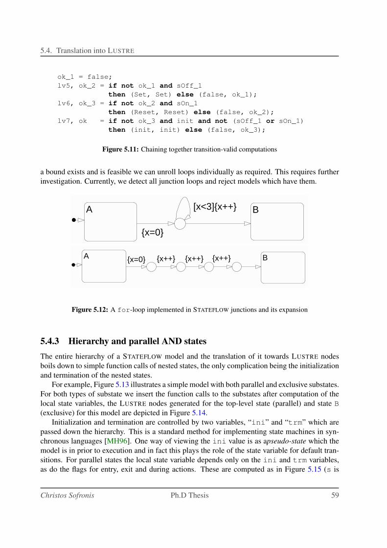
5.4. Translation into LUSTRE
ok_1 = false;
lv5, ok_2 = if not ok_1 and sOff_1
then (Set, Set) else (false, ok_1);
lv6, ok_3 = if not ok_2 and sOn_1
then (Reset, Reset) else (false, ok_2);
lv7, ok = if not ok_3 and init and not (sOff_1 or sOn_1)
then (init, init) else (false, ok_3);
Figure 5.11: Chaining together transition-valid computations
a bound exists and is feasible we can unroll loops individually as required. This requires further
investigation. Currently, we detect all junction loops and reject models which have them.
A B
{x=0}
[x<3]{x++}
A B{x=0} {x++} {x++}{x++}
Figure 5.12: A for-loop implemented in STATEFLOW junctions and its expansion
5.4.3 Hierarchy and parallel AND states
The entire hierarchy of a STATEFLOW model and the translation of it towards LUSTRE nodes
boils down to simple function calls of nested states, the only complication being the initialization
and termination of the nested states.
For example, Figure 5.13 illustrates a simple model with both parallel and exclusive substates.
For both types of substate we insert the function calls to the substates after computation of the
local state variables, the LUSTRE nodes generated for the top-level state (parallel) and state B
(exclusive) for this model are depicted in Figure 5.14.
Initialization and termination are controlled by two variables, “ini” and “trm” which are
passed down the hierarchy. This is a standard method for implementing state machines in syn-
chronous languages [MH96]. One way of viewing the ini value is as apseudo-state which the
model is in prior to execution and in fact this plays the role of the state variable for default tran-
sitions. For parallel states the local state variable depends only on the ini and trm variables,
as do the flags for entry, exit and during actions. These are computed as in Figure 5.15 (s is
Christos Sofronis Ph.D Thesis 59
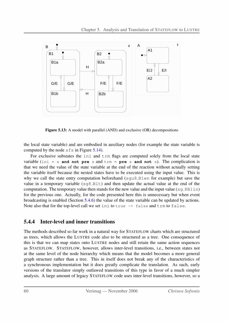
Chapter 5. Analysis and Translation of STATEFLOW to LUSTRE
B 2 A 1
A1
A2
B1 B2
B1a
B1b
B2a
B2b
E/J E/IH
F/E F/EG/E G/E
H
Figure 5.13: A model with parallel (AND) and exclusive (OR) decompositions
the local state variable) and are embodied in auxiliary nodes (for example the state variable is
computed by the node sfs in Figure 5.14).
For exclusive substates the ini and trm flags are computed solely from the local state
variable (ini = s and not pre s and trm = pre s and not s). The complication is
that we need the value of the state variable at the end of the reaction without actually setting
the variable itself because the nested states have to be executed using the input value. This is
why we call the state entry computation beforehand (sgu8 B1en for example) but save the
value in a temporary variable (sg8 B1t) and then update the actual value at the end of the
computation. The temporary value then stands for the new value and the input value (sg 8B1in)
for the previous one. Actually, for the code presented here this is unnecessary but when event
broadcasting is enabled (Section 5.4.6) the value of the state variable can be updated by actions.
Note also that for the top-level call we set ini to true -> false and trm to false.
5.4.4 Inter-level and inner transitions
The methods described so far work in a natural way for STATEFLOW charts which are structured
as trees, which allows the LUSTRE code also to be structured as a tree. One consequence of
this is that we can map states onto LUSTRE nodes and still retain the same action sequences
as STATEFLOW. STATEFLOW, however, allows inter-level transitions, i.e., between states not
at the same level of the node hierarchy which means that the model becomes a more general
graph structure rather than a tree. This in itself does not break any of the characteristics of
a synchronous implementation but it does greatly complicate the translation. As such, early
versions of the translator simply outlawed transitions of this type in favor of a much simpler
analysis. A large amount of legacy STATEFLOW code uses inter-level transitions, however, so a
60 Verimag — November 2006 Christos Sofronis
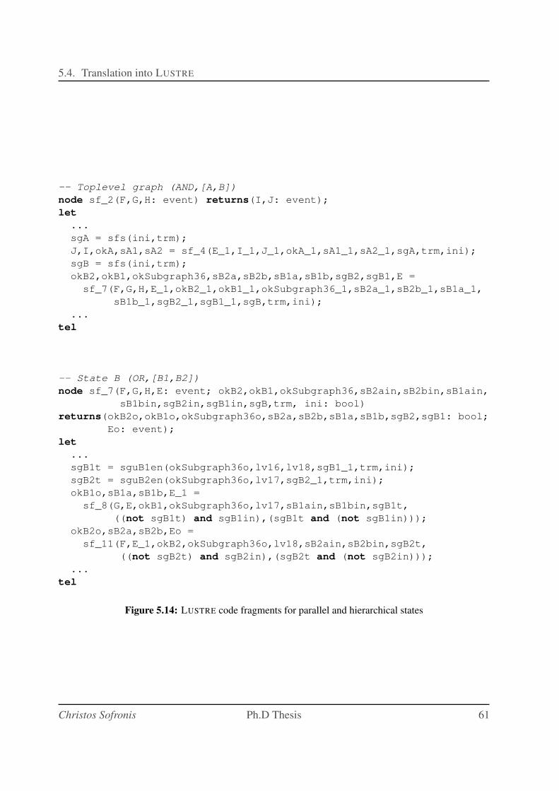
5.4. Translation into LUSTRE
-- Toplevel graph (AND,[A,B])
node sf_2(F,G,H: event) returns(I,J: event);
let
...
sgA = sfs(ini,trm);
J,I,okA,sA1,sA2 = sf_4(E_1,I_1,J_1,okA_1,sA1_1,sA2_1,sgA,trm,ini);
sgB = sfs(ini,trm);
okB2,okB1,okSubgraph36,sB2a,sB2b,sB1a,sB1b,sgB2,sgB1,E =
sf_7(F,G,H,E_1,okB2_1,okB1_1,okSubgraph36_1,sB2a_1,sB2b_1,sB1a_1,
sB1b_1,sgB2_1,sgB1_1,sgB,trm,ini);
...
tel
-- State B (OR,[B1,B2])
node sf_7(F,G,H,E: event; okB2,okB1,okSubgraph36,sB2ain,sB2bin,sB1ain,
sB1bin,sgB2in,sgB1in,sgB,trm, ini: bool)
returns(okB2o,okB1o,okSubgraph36o,sB2a,sB2b,sB1a,sB1b,sgB2,sgB1: bool;
Eo: event);
let
...
sgB1t = sguB1en(okSubgraph36o,lv16,lv18,sgB1_1,trm,ini);
sgB2t = sguB2en(okSubgraph36o,lv17,sgB2_1,trm,ini);
okB1o,sB1a,sB1b,E_1 =
sf_8(G,E,okB1,okSubgraph36o,lv17,sB1ain,sB1bin,sgB1t,
((not sgB1t) and sgB1in),(sgB1t and (not sgB1in)));
okB2o,sB2a,sB2b,Eo =
sf_11(F,E_1,okB2,okSubgraph36o,lv18,sB2ain,sB2bin,sgB2t,
((not sgB2t) and sgB2in),(sgB2t and (not sgB2in)));
...
tel
Figure 5.14: LUSTRE code fragments for parallel and hierarchical states
Christos Sofronis Ph.D Thesis 61
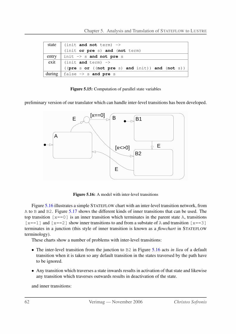
Chapter 5. Analysis and Translation of STATEFLOW to LUSTRE
state (init and not term) ->
(init or pre s) and (not term)
entry init -> s and not pre s
exit (init and term) ->
((pre s or ((not pre s) and init)) and (not s))
during false -> s and pre s
Figure 5.15: Computation of parallel state variables
preliminary version of our translator which can handle inter-level transitions has been developed.
B
A
B1
B2
[x==0]E
[x<>0] E
E
Figure 5.16: A model with inter-level transitions
Figure 5.16 illustrates a simple STATEFLOW chart with an inter-level transition network, from
A to B and B2. Figure 5.17 shows the different kinds of inner transitions that can be used. The
top transition [x==0] is an inner transition which terminates in the parent state A, transitions
[x==1] and [x==2] show inner transitions to and from a substate of A and transition [x==3]
terminates in a junction (this style of inner transition is known as a flowchart in STATEFLOW
terminology).
These charts show a number of problems with inter-level transitions:
• The inter-level transition from the junction to B2 in Figure 5.16 acts in lieu of a default
transition when it is taken so any default transition in the states traversed by the path have
to be ignored.
• Any transition which traverses a state inwards results in activation of that state and likewise
any transition which traverses outwards results in deactivation of the state.
and inner transitions:
62 Verimag — November 2006 Christos Sofronis
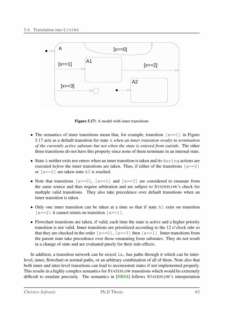
5.4. Translation into LUSTRE
A
A1
A2
[x==0]
[x==1] [x==2]
[x==3]
Figure 5.17: A model with inner transitions
• The semantics of inner transitions mean that, for example, transition [x==1] in Figure
5.17 acts as a default transition for state A when an inner transition results in termination
of the currently active substate but not when the state is entered from outside. The other
three transitions do not have this property since none of them terminate in an internal state.
• State A neither exits nor enters when an inner transition is taken and its during actions are
executed before the inner transitions are taken. Thus, if either of the transitions [x==0]
or [x==2] are taken state A2 is reached.
• Note that transitions [x==0], [x==1] and [x==3] are considered to emanate from
the same source and thus require arbitration and are subject to STATEFLOW’s check for
multiple valid transitions. They also take precedence over default transitions when an
inner transition is taken.
• Only one inner transition can be taken at a time so that if state A1 exits on transition
[x==2] it cannot return on transition [x==1].
• Flowchart transitions are taken, if valid, each time the state is active and a higher priority
transition is not valid. Inner transitions are prioritized according to the 12 o’clock rule so
that they are checked in the order [x==0], [x==3] then [x==1]. Inner transitions from
the parent state take precedence over those emanating from substates. They do not result
in a change of state and are evaluated purely for their side-effects.
In addition, a transition network can be mixed, i.e., has paths through it which can be inter-
level, inner, flowchart or normal paths, or an arbitrary combination of all of them. Note also that
both inner and inter-level transitions can lead to inconsistent states if not implemented properly.
This results in a highly complex semantics for STATEFLOW transitions which would be extremely
difficult to emulate precisely. The semantics in [HR04] follows STATEFLOW’s interpretation
Christos Sofronis Ph.D Thesis 63
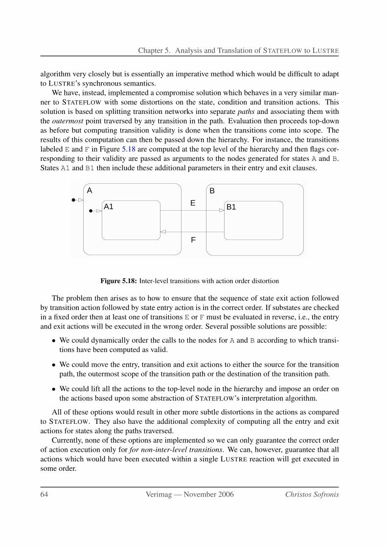
Chapter 5. Analysis and Translation of STATEFLOW to LUSTRE
algorithm very closely but is essentially an imperative method which would be difficult to adapt
to LUSTRE’s synchronous semantics.
We have, instead, implemented a compromise solution which behaves in a very similar man-
ner to STATEFLOW with some distortions on the state, condition and transition actions. This
solution is based on splitting transition networks into separate paths and associating them with
the outermost point traversed by any transition in the path. Evaluation then proceeds top-down
as before but computing transition validity is done when the transitions come into scope. The
results of this computation can then be passed down the hierarchy. For instance, the transitions
labeled E and F in Figure 5.18 are computed at the top level of the hierarchy and then flags cor-
responding to their validity are passed as arguments to the nodes generated for states A and B.
States A1 and B1 then include these additional parameters in their entry and exit clauses.
A B
A1 B1E
F
Figure 5.18: Inter-level transitions with action order distortion
The problem then arises as to how to ensure that the sequence of state exit action followed
by transition action followed by state entry action is in the correct order. If substates are checked
in a fixed order then at least one of transitions E or F must be evaluated in reverse, i.e., the entry
and exit actions will be executed in the wrong order. Several possible solutions are possible:
• We could dynamically order the calls to the nodes for A and B according to which transi-
tions have been computed as valid.
• We could move the entry, transition and exit actions to either the source for the transition
path, the outermost scope of the transition path or the destination of the transition path.
• We could lift all the actions to the top-level node in the hierarchy and impose an order on
the actions based upon some abstraction of STATEFLOW’s interpretation algorithm.
All of these options would result in other more subtle distortions in the actions as compared
to STATEFLOW. They also have the additional complexity of computing all the entry and exit
actions for states along the paths traversed.
Currently, none of these options are implemented so we can only guarantee the correct order
of action execution only for for non-inter-level transitions. We can, however, guarantee that all
actions which would have been executed within a single LUSTRE reaction will get executed in
some order.
64 Verimag — November 2006 Christos Sofronis
5.4. Translation into LUSTRE
Inter-level transitions
The basic scheme, however, is relatively easy to implement for inter-level transitions provided
we are careful to compute the correct arguments (transitions) to the substate nodes.
The only major complication is the computation of the ok value for inter-level transitions.
Because of the presence of default transitions we need an ok flag for each substate because the
computation of transition validity is disjoint for each default transition taken within the hierarchy.
We also need a separate ok flag for each parallel state because transition computations are also
disjoint between parallel states. Luckily, STATEFLOW outlaws inter-level transitions between
parallel states but we still need a flag for each subgraph because of default transitions. This
means that we need to associate an ok value with each transition (in fact we associate it with the
flag for its source graph) so that the transition is only valid if both its validity flag and associated
ok flag are true.
Figure 5.19 shows the code produced for Figure 5.16. This is a direct implementation of the
scheme described above. Points to note about this code include:
• transitions 8 (default for A), 9 (A to junction), 10 (B2 to A), 12
(junction to B) and 13 (junction to B2) are all computed at the top-level, of
which 9, 10 and 13 are passed to the node for subgraph B,
• the node for state B augments these with the transitions 11 (B1 to B2) and 14 (default
for B1),
• the complex predicate for the default transition to state B1 has to take into account whether
state B is being entered by inter-level transition 13 or normal transition 12,
• the distortions in the actions (state A enters before B2 exits if transition 10 is taken) and
• the computation of the ok flags, for example, transition 12 uses okTop whereas transition
10 uses okB.
Inner transitions
Although we have treated inter-level and inner transitions separately here, they are intimately
interlinked due to the possibility of a single path through a transition network having transitions
of both types. It is even possible for a single transition to be of both types. In some ways, inner
transitions are simpler than inter-level transitions since they are nearly local (only involving the
immediate parent state) but are more complicated in the way they interact with other transitions
at the same level.
5.4.5 Action language translation
There are two basic options for translating the simple imperative language implemented by
STATEFLOW into the synchronous language LUSTRE. One possibility would be to generate C
code from the action code and use the external function call facility of LUSTRE to call the action
Christos Sofronis Ph.D Thesis 65
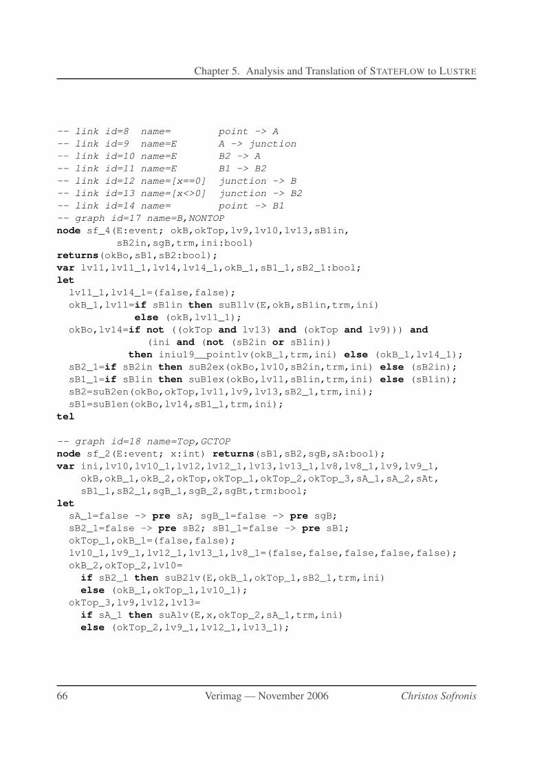
Chapter 5. Analysis and Translation of STATEFLOW to LUSTRE
-- link id=8 name= point -> A
-- link id=9 name=E A -> junction
-- link id=10 name=E B2 -> A
-- link id=11 name=E B1 -> B2
-- link id=12 name=[x==0] junction -> B
-- link id=13 name=[x<>0] junction -> B2
-- link id=14 name= point -> B1
-- graph id=17 name=B,NONTOP
node sf_4(E:event; okB,okTop,lv9,lv10,lv13,sB1in,
sB2in,sgB,trm,ini:bool)
returns(okBo,sB1,sB2:bool);
var lv11,lv11_1,lv14,lv14_1,okB_1,sB1_1,sB2_1:bool;
let
lv11_1,lv14_1=(false,false);
okB_1,lv11=if sB1in then suB1lv(E,okB,sB1in,trm,ini)
else (okB,lv11_1);
okBo,lv14=if not ((okTop and lv13) and (okTop and lv9))) and
(ini and (not (sB2in or sB1in))
then iniu19__pointlv(okB_1,trm,ini) else (okB_1,lv14_1);
sB2_1=if sB2in then suB2ex(okBo,lv10,sB2in,trm,ini) else (sB2in);
sB1_1=if sB1in then suB1ex(okBo,lv11,sB1in,trm,ini) else (sB1in);
sB2=suB2en(okBo,okTop,lv11,lv9,lv13,sB2_1,trm,ini);
sB1=suB1en(okBo,lv14,sB1_1,trm,ini);
tel
-- graph id=18 name=Top,GCTOP
node sf_2(E:event; x:int) returns(sB1,sB2,sgB,sA:bool);
var ini,lv10,lv10_1,lv12,lv12_1,lv13,lv13_1,lv8,lv8_1,lv9,lv9_1,
okB,okB_1,okB_2,okTop,okTop_1,okTop_2,okTop_3,sA_1,sA_2,sAt,
sB1_1,sB2_1,sgB_1,sgB_2,sgBt,trm:bool;
let
sA_1=false -> pre sA; sgB_1=false -> pre sgB;
sB2_1=false -> pre sB2; sB1_1=false -> pre sB1;
okTop_1,okB_1=(false,false);
lv10_1,lv9_1,lv12_1,lv13_1,lv8_1=(false,false,false,false,false);
okB_2,okTop_2,lv10=
if sB2_1 then suB2lv(E,okB_1,okTop_1,sB2_1,trm,ini)
else (okB_1,okTop_1,lv10_1);
okTop_3,lv9,lv12,lv13=
if sA_1 then suAlv(E,x,okTop_2,sA_1,trm,ini)
else (okTop_2,lv9_1,lv12_1,lv13_1);
66 Verimag — November 2006 Christos Sofronis
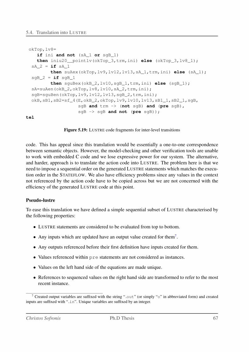
5.4. Translation into LUSTRE
okTop,lv8=
if ini and not (sA_1 or sgB_1)
then iniu20__pointlv(okTop_3,trm,ini) else (okTop_3,lv8_1);
sA_2 = if sA_1
then suAex(okTop,lv9,lv12,lv13,sA_1,trm,ini) else (sA_1);
sgB_2 = if sgB_1
then sguBex(okB_2,lv10,sgB_1,trm,ini) else (sgB_1);
sA=suAen(okB_2,okTop,lv8,lv10,sA_2,trm,ini);
sgB=sguBen(okTop,lv9,lv12,lv13,sgB_2,trm,ini);
okB,sB1,sB2=sf_4(E,okB_2,okTop,lv9,lv10,lv13,sB1_1,sB2_1,sgB,
sgB and trm -> (not sgB) and (pre sgB),
sgB -> sgB and not (pre sgB));
tel
Figure 5.19: LUSTRE code fragments for inter-level transitions
code. This has appeal since this translation would be essentially a one-to-one correspondence
between semantic objects. However, the model-checking and other verification tools are unable
to work with embedded C code and we lose expressive power for our system. The alternative,
and harder, approach is to translate the action code into LUSTRE. The problem here is that we
need to impose a sequential order on the generated LUSTRE statements which matches the execu-
tion order in the STATEFLOW. We also have efficiency problems since any values in the context
not referenced by the action code have to be copied across but we are not concerned with the
efficiency of the generated LUSTRE code at this point.
Pseudo-lustre
To ease this translation we have defined a simple sequential subset of LUSTRE characterised by
the following properties:
• LUSTRE statements are considered to be evaluated from top to bottom.
• Any inputs which are updated have an output value created for them7.
• Any outputs referenced before their first definition have inputs created for them.
• Values referenced within pre statements are not considered as instances.
• Values on the left hand side of the equations are made unique.
• References to sequenced values on the right hand side are transformed to refer to the most
recent instance.
7 Created output variables are suffixed with the string “ out” (or simply “o” in abbreviated form) and created
inputs are suffixed with “ in”. Unique variables are suffixed by an integer.
Christos Sofronis Ph.D Thesis 67
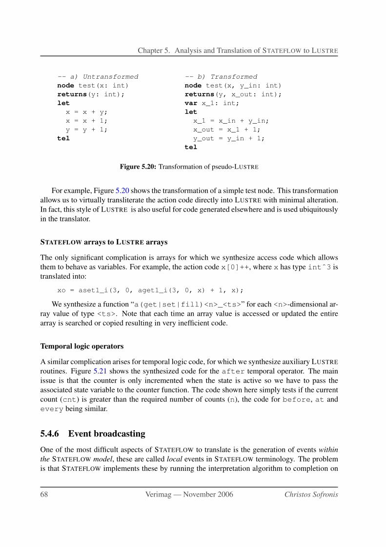
Chapter 5. Analysis and Translation of STATEFLOW to LUSTRE
-- a) Untransformed -- b) Transformed
node test(x: int) node test(x, y_in: int)
returns(y: int); returns(y, x_out: int);
let var x_1: int;
x = x + y; let
x = x + 1; x_1 = x_in + y_in;
y = y + 1; x_out = x_1 + 1;
tel y_out = y_in + 1;
tel
Figure 5.20: Transformation of pseudo-LUSTRE
For example, Figure 5.20 shows the transformation of a simple test node. This transformation
allows us to virtually transliterate the action code directly into LUSTRE with minimal alteration.
In fact, this style of LUSTRE is also useful for code generated elsewhere and is used ubiquitously
in the translator.
STATEFLOW arrays to LUSTRE arrays
The only significant complication is arrays for which we synthesize access code which allows
them to behave as variables. For example, the action code x[0]++, where x has type intˆ3 is
translated into:
xo = aset1_i(3, 0, aget1_i(3, 0, x) + 1, x);
We synthesize a function “a(get|set|fill)<n>_<ts>” for each <n>-dimensional ar-
ray value of type <ts>. Note that each time an array value is accessed or updated the entire
array is searched or copied resulting in very inefficient code.
Temporal logic operators
A similar complication arises for temporal logic code, for which we synthesize auxiliary LUSTRE
routines. Figure 5.21 shows the synthesized code for the after temporal operator. The main
issue is that the counter is only incremented when the state is active so we have to pass the
associated state variable to the counter function. The code shown here simply tests if the current
count (cnt) is greater than the required number of counts (n), the code for before, at and
every being similar.
5.4.6 Event broadcasting
One of the most difficult aspects of STATEFLOW to translate is the generation of events within
the STATEFLOW model, these are called local events in STATEFLOW terminology. The problem
is that STATEFLOW implements these by running the interpretation algorithm to completion on
68 Verimag — November 2006 Christos Sofronis
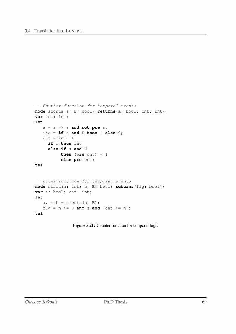
5.4. Translation into LUSTRE
-- Counter function for temporal events
node sfcnts(s, E: bool) returns(a: bool; cnt: int);
var inc: int;
let
a = s -> s and not pre s;
inc = if a and E then 1 else 0;
cnt = inc ->
if a then inc
else if s and E
then (pre cnt) + 1
else pre cnt;
tel
-- after function for temporal events
node sfaft(n: int; s, E: bool) returns(flg: bool);
var a: bool; cnt: int;
let
a, cnt = sfcnts(s, E);
flg = n >= 0 and s and (cnt >= n);
tel
Figure 5.21: Counter function for temporal logic
Christos Sofronis Ph.D Thesis 69
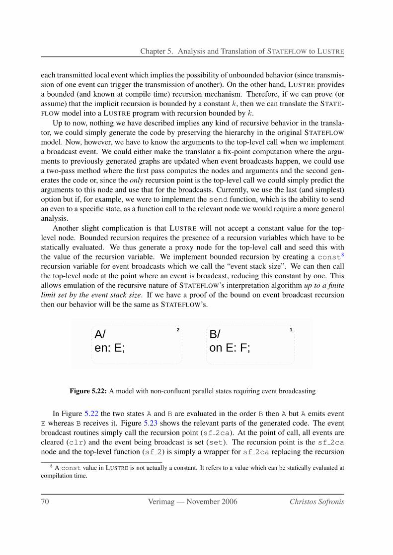
Chapter 5. Analysis and Translation of STATEFLOW to LUSTRE
each transmitted local event which implies the possibility of unbounded behavior (since transmis-
sion of one event can trigger the transmission of another). On the other hand, LUSTRE provides
a bounded (and known at compile time) recursion mechanism. Therefore, if we can prove (or
assume) that the implicit recursion is bounded by a constant k, then we can translate the STATE-
FLOW model into a LUSTRE program with recursion bounded by k.
Up to now, nothing we have described implies any kind of recursive behavior in the transla-
tor, we could simply generate the code by preserving the hierarchy in the original STATEFLOW
model. Now, however, we have to know the arguments to the top-level call when we implement
a broadcast event. We could either make the translator a fix-point computation where the argu-
ments to previously generated graphs are updated when event broadcasts happen, we could use
a two-pass method where the first pass computes the nodes and arguments and the second gen-
erates the code or, since the only recursion point is the top-level call we could simply predict the
arguments to this node and use that for the broadcasts. Currently, we use the last (and simplest)
option but if, for example, we were to implement the send function, which is the ability to send
an even to a specific state, as a function call to the relevant node we would require a more general
analysis.
Another slight complication is that LUSTRE will not accept a constant value for the top-
level node. Bounded recursion requires the presence of a recursion variables which have to be
statically evaluated. We thus generate a proxy node for the top-level call and seed this with
the value of the recursion variable. We implement bounded recursion by creating a const8
recursion variable for event broadcasts which we call the “event stack size”. We can then call
the top-level node at the point where an event is broadcast, reducing this constant by one. This
allows emulation of the recursive nature of STATEFLOW’s interpretation algorithm up to a finite
limit set by the event stack size. If we have a proof of the bound on event broadcast recursion
then our behavior will be the same as STATEFLOW’s.
B/on E: F;
1A/en: E;
2
Figure 5.22: A model with non-confluent parallel states requiring event broadcasting
In Figure 5.22 the two states A and B are evaluated in the order B then A but A emits event
E whereas B receives it. Figure 5.23 shows the relevant parts of the generated code. The event
broadcast routines simply call the recursion point (sf 2ca). At the point of call, all events are
cleared (clr) and the event being broadcast is set (set). The recursion point is the sf 2ca
node and the top-level function (sf 2) is simply a wrapper for sf 2ca replacing the recursion
8 A const value in LUSTRE is not actually a constant. It refers to a value which can be statically evaluated at
compilation time.
70 Verimag — November 2006 Christos Sofronis
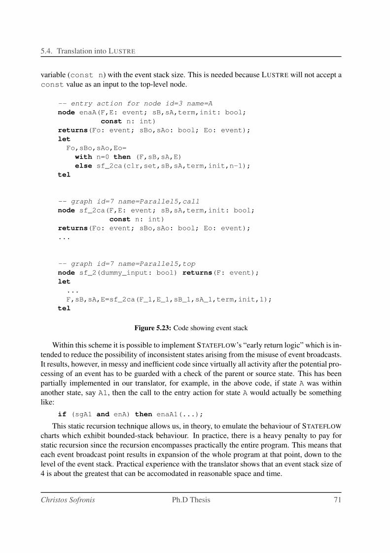
5.4. Translation into LUSTRE
variable (const n) with the event stack size. This is needed because LUSTRE will not accept a
const value as an input to the top-level node.
-- entry action for node id=3 name=A
node enaA(F,E: event; sB,sA,term,init: bool;
const n: int)
returns(Fo: event; sBo,sAo: bool; Eo: event);
let
Fo,sBo,sAo,Eo=
with n=0 then (F,sB,sA,E)
else sf_2ca(clr,set,sB,sA,term,init,n-1);
tel
-- graph id=7 name=Parallel5,call
node sf_2ca(F,E: event; sB,sA,term,init: bool;
const n: int)
returns(Fo: event; sBo,sAo: bool; Eo: event);
...
-- graph id=7 name=Parallel5,top
node sf_2(dummy_input: bool) returns(F: event);
let
...
F,sB,sA,E=sf_2ca(F_1,E_1,sB_1,sA_1,term,init,1);
tel
Figure 5.23: Code showing event stack
Within this scheme it is possible to implement STATEFLOW’s “early return logic” which is in-
tended to reduce the possibility of inconsistent states arising from the misuse of event broadcasts.
It results, however, in messy and inefficient code since virtually all activity after the potential pro-
cessing of an event has to be guarded with a check of the parent or source state. This has been
partially implemented in our translator, for example, in the above code, if state A was within
another state, say A1, then the call to the entry action for state A would actually be something
like:
if (sgA1 and enA) then enaA1(...);
This static recursion technique allows us, in theory, to emulate the behaviour of STATEFLOW
charts which exhibit bounded-stack behaviour. In practice, there is a heavy penalty to pay for
static recursion since the recursion encompasses practically the entire program. This means that
each event broadcast point results in expansion of the whole program at that point, down to the
level of the event stack. Practical experience with the translator shows that an event stack size of
4 is about the greatest that can be accomodated in reasonable space and time.
Christos Sofronis Ph.D Thesis 71
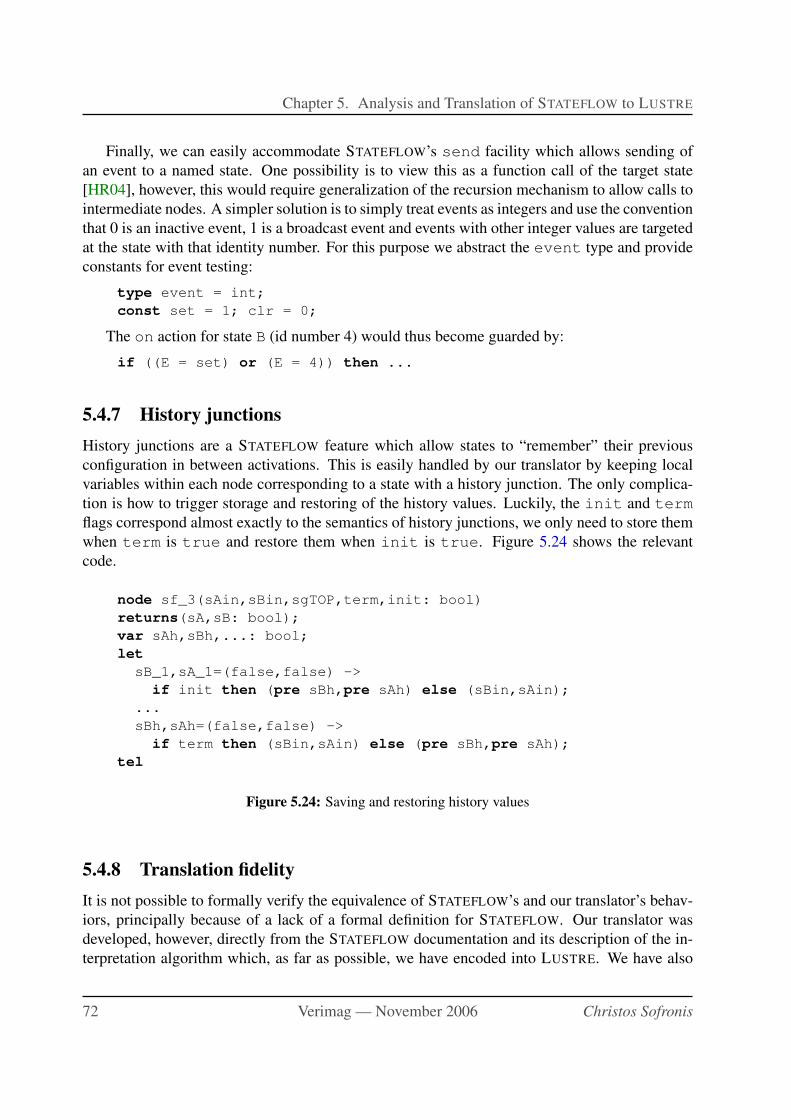
Chapter 5. Analysis and Translation of STATEFLOW to LUSTRE
Finally, we can easily accommodate STATEFLOW’s send facility which allows sending of
an event to a named state. One possibility is to view this as a function call of the target state
[HR04], however, this would require generalization of the recursion mechanism to allow calls to
intermediate nodes. A simpler solution is to simply treat events as integers and use the convention
that 0 is an inactive event, 1 is a broadcast event and events with other integer values are targeted
at the state with that identity number. For this purpose we abstract the event type and provide
constants for event testing:
type event = int;
const set = 1; clr = 0;
The on action for state B (id number 4) would thus become guarded by:
if ((E = set) or (E = 4)) then ...
5.4.7 History junctions
History junctions are a STATEFLOW feature which allow states to “remember” their previous
configuration in between activations. This is easily handled by our translator by keeping local
variables within each node corresponding to a state with a history junction. The only complica-
tion is how to trigger storage and restoring of the history values. Luckily, the init and term
flags correspond almost exactly to the semantics of history junctions, we only need to store them
when term is true and restore them when init is true. Figure 5.24 shows the relevant
code.
node sf_3(sAin,sBin,sgTOP,term,init: bool)
returns(sA,sB: bool);
var sAh,sBh,...: bool;
let
sB_1,sA_1=(false,false) ->
if init then (pre sBh,pre sAh) else (sBin,sAin);
...
sBh,sAh=(false,false) ->
if term then (sBin,sAin) else (pre sBh,pre sAh);
tel
Figure 5.24: Saving and restoring history values
5.4.8 Translation fidelity
It is not possible to formally verify the equivalence of STATEFLOW’s and our translator’s behav-
iors, principally because of a lack of a formal definition for STATEFLOW. Our translator was
developed, however, directly from the STATEFLOW documentation and its description of the in-
terpretation algorithm which, as far as possible, we have encoded into LUSTRE. We have also
72 Verimag — November 2006 Christos Sofronis
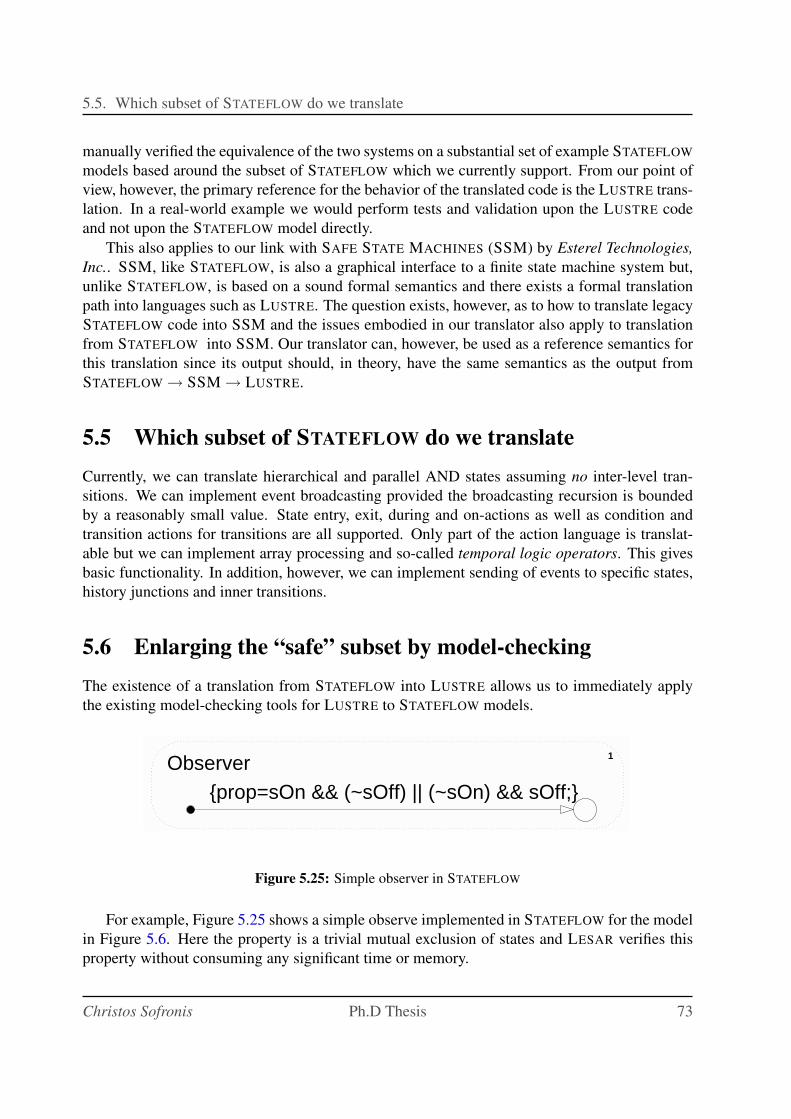
5.5. Which subset of STATEFLOW do we translate
manually verified the equivalence of the two systems on a substantial set of example STATEFLOW
models based around the subset of STATEFLOW which we currently support. From our point of
view, however, the primary reference for the behavior of the translated code is the LUSTRE trans-
lation. In a real-world example we would perform tests and validation upon the LUSTRE code
and not upon the STATEFLOW model directly.
This also applies to our link with SAFE STATE MACHINES (SSM) by Esterel Technologies,
Inc.. SSM, like STATEFLOW, is also a graphical interface to a finite state machine system but,
unlike STATEFLOW, is based on a sound formal semantics and there exists a formal translation
path into languages such as LUSTRE. The question exists, however, as to how to translate legacy
STATEFLOW code into SSM and the issues embodied in our translator also apply to translation
from STATEFLOW into SSM. Our translator can, however, be used as a reference semantics for
this translation since its output should, in theory, have the same semantics as the output from
STATEFLOW → SSM → LUSTRE.
5.5 Which subset of STATEFLOW do we translate
Currently, we can translate hierarchical and parallel AND states assuming no inter-level tran-
sitions. We can implement event broadcasting provided the broadcasting recursion is bounded
by a reasonably small value. State entry, exit, during and on-actions as well as condition and
transition actions for transitions are all supported. Only part of the action language is translat-
able but we can implement array processing and so-called temporal logic operators. This gives
basic functionality. In addition, however, we can implement sending of events to specific states,
history junctions and inner transitions.
5.6 Enlarging the “safe” subset by model-checking
The existence of a translation from STATEFLOW into LUSTRE allows us to immediately apply
the existing model-checking tools for LUSTRE to STATEFLOW models.
Observer 1
{prop=sOn && (~sOff) || (~sOn) && sOff;}
Figure 5.25: Simple observer in STATEFLOW
For example, Figure 5.25 shows a simple observe implemented in STATEFLOW for the model
in Figure 5.6. Here the property is a trivial mutual exclusion of states and LESAR verifies this
property without consuming any significant time or memory.
Christos Sofronis Ph.D Thesis 73
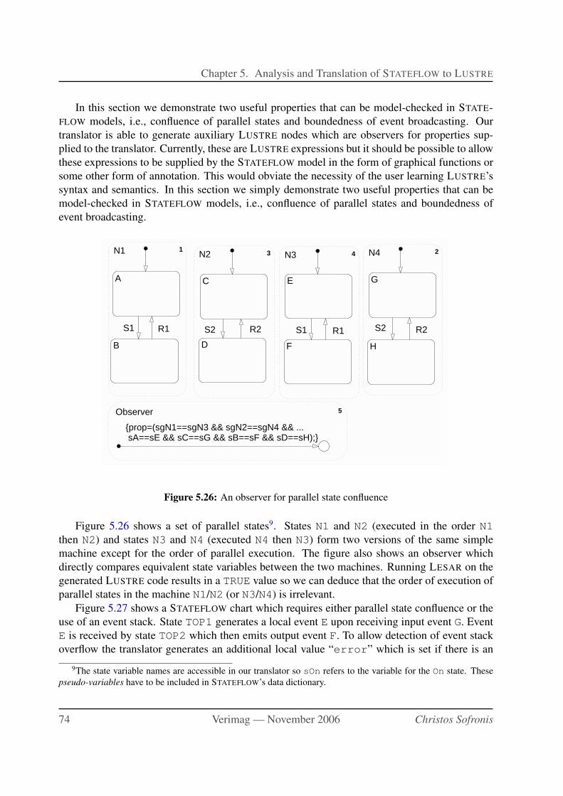
Chapter 5. Analysis and Translation of STATEFLOW to LUSTRE
In this section we demonstrate two useful properties that can be model-checked in STATE-
FLOW models, i.e., confluence of parallel states and boundedness of event broadcasting. Our
translator is able to generate auxiliary LUSTRE nodes which are observers for properties sup-
plied to the translator. Currently, these are LUSTRE expressions but it should be possible to allow
these expressions to be supplied by the STATEFLOW model in the form of graphical functions or
some other form of annotation. This would obviate the necessity of the user learning LUSTRE’s
syntax and semantics. In this section we simply demonstrate two useful properties that can be
model-checked in STATEFLOW models, i.e., confluence of parallel states and boundedness of
event broadcasting.
N2 3 N3 4N1 1 N4 2
Observer 5
F
EA GC
DB H
R1S1 R2S2R1S1R2S2
{prop=(sgN1==sgN3 && sgN2==sgN4 && ... sA==sE && sC==sG && sB==sF && sD==sH);}
Figure 5.26: An observer for parallel state confluence
Figure 5.26 shows a set of parallel states9. States N1 and N2 (executed in the order N1
then N2) and states N3 and N4 (executed N4 then N3) form two versions of the same simple
machine except for the order of parallel execution. The figure also shows an observer which
directly compares equivalent state variables between the two machines. Running LESAR on the
generated LUSTRE code results in a TRUE value so we can deduce that the order of execution of
parallel states in the machine N1/N2 (or N3/N4) is irrelevant.
Figure 5.27 shows a STATEFLOW chart which requires either parallel state confluence or the
use of an event stack. State TOP1 generates a local event E upon receiving input event G. Event
E is received by state TOP2 which then emits output event F. To allow detection of event stack
overflow the translator generates an additional local value “error” which is set if there is an
9The state variable names are accessible in our translator so sOn refers to the variable for the On state. These
pseudo-variables have to be included in STATEFLOW’s data dictionary.
74 Verimag — November 2006 Christos Sofronis
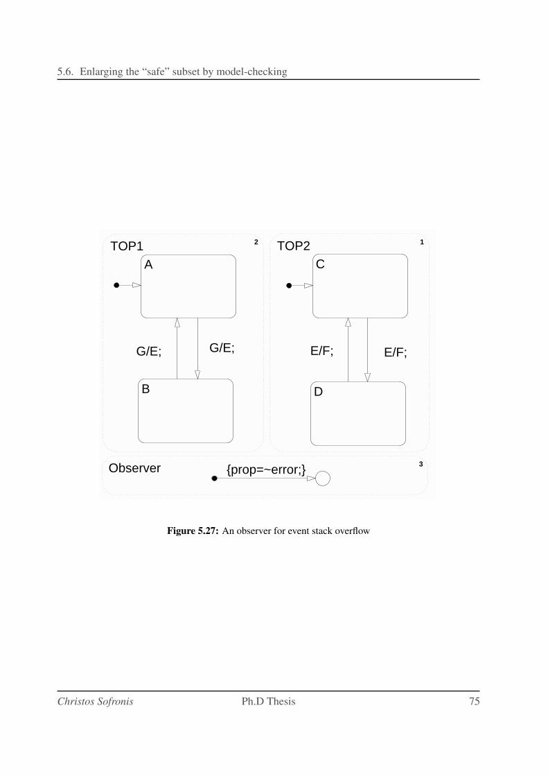
5.6. Enlarging the “safe” subset by model-checking
Observer 3
TOP1 2 TOP2 1
C
B D
A
E/F; E/F;G/E; G/E;
{prop=~error;}
Figure 5.27: An observer for event stack overflow
Christos Sofronis Ph.D Thesis 75
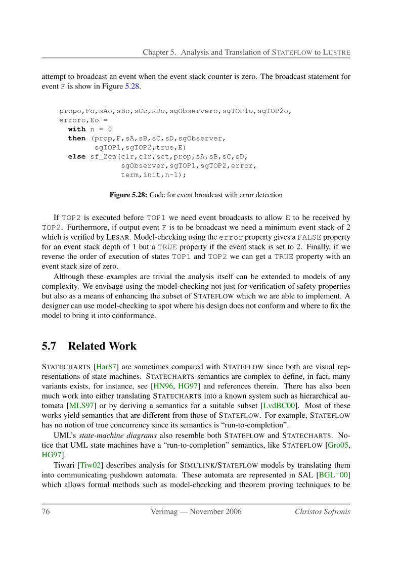
Chapter 5. Analysis and Translation of STATEFLOW to LUSTRE
attempt to broadcast an event when the event stack counter is zero. The broadcast statement for
event F is show in Figure 5.28.
propo,Fo,sAo,sBo,sCo,sDo,sgObservero,sgTOP1o,sgTOP2o,
erroro,Eo =
with n = 0
then (prop,F,sA,sB,sC,sD,sgObserver,
sgTOP1,sgTOP2,true,E)
else sf_2ca(clr,clr,set,prop,sA,sB,sC,sD,
sgObserver,sgTOP1,sgTOP2,error,
term,init,n-1);
Figure 5.28: Code for event broadcast with error detection
If TOP2 is executed before TOP1 we need event broadcasts to allow E to be received by
TOP2. Furthermore, if output event F is to be broadcast we need a minimum event stack of 2
which is verified by LESAR. Model-checking using the error property gives a FALSE property
for an event stack depth of 1 but a TRUE property if the event stack is set to 2. Finally, if we
reverse the order of execution of states TOP1 and TOP2 we can get a TRUE property with an
event stack size of zero.
Although these examples are trivial the analysis itself can be extended to models of any
complexity. We envisage using the model-checking not just for verification of safety properties
but also as a means of enhancing the subset of STATEFLOW which we are able to implement. A
designer can use model-checking to spot where his design does not conform and where to fix the
model to bring it into conformance.
5.7 Related Work
STATECHARTS [Har87] are sometimes compared with STATEFLOW since both are visual rep-
resentations of state machines. STATECHARTS semantics are complex to define, in fact, many
variants exists, for instance, see [HN96, HG97] and references therein. There has also been
much work into either translating STATECHARTS into a known system such as hierarchical au-
tomata [MLS97] or by deriving a semantics for a suitable subset [LvdBC00]. Most of these
works yield semantics that are different from those of STATEFLOW. For example, STATEFLOW
has no notion of true concurrency since its semantics is “run-to-completion”.
UML’s state-machine diagrams also resemble both STATEFLOW and STATECHARTS. No-
tice that UML state machines have a “run-to-completion” semantics, like STATEFLOW [Gro05,
HG97].
Tiwari [Tiw02] describes analysis for SIMULINK/STATEFLOW models by translating them
into communicating pushdown automata. These automata are represented in SAL [BGL+00]
which allows formal methods such as model-checking and theorem proving techniques to be
76 Verimag — November 2006 Christos Sofronis
5.8. Conclusions
applied to these models. Essentially, the system is treated as a special hybrid automaton and
algebraic loops involving STATEFLOW charts are not considered.
[Nee01] presents the data model of SIMULINK and STATEFLOW as a UML class diagram.
Hamon and Rushby have developed a structural operational semantics for STATE-
FLOW [HR04] for which they have an interpreter to allow comparison with STATEFLOW. Their
subset of STATEFLOW seems to have been inspired by the Ford guidelines [For99], for instance
loops are forbidden in event broadcasting and local events can only be sent to parallel states.
They have other restrictions as well, such as forbidding transitions out of parallel states but in
general support most of the STATEFLOW definition including inter-level transitions. They also
have a translator into the SAL system which allows various model-checking techniques to be
applied to STATEFLOW.
5.8 Conclusions
In this Chapter we studied the translation of STATEFLOW to LUSTRE. Although the behavior
of STATEFLOW is deterministic, it may lead to problematic designs, for instance, such that a
simulation cycle does not terminate or where tiny changes in the graphical layout may modify
the behavior of the model. To handle these issues we proposed a set of conditions, that can
be checked statically, that guarantee that a STATEFLOW model will be free of the semantical
problems described.
Besides the analysis of STATEFLOW and those static rules, we have provided a method to
translate a STATEFLOW Chart into the synchronous programming language LUSTRE. This trans-
lation can be used in many different ways. First of all, for code generation, using one of the code
generators available for LUSTRE. The translation can also be used for verification of STATEFLOW
models, using LUSTRE’s model-checker Lesar. We can use verification to check not only general
properties about the model but also specific properties, for instance, those related to semantical
issues above (e.g., check the confluence of a set of states).
The translation algorithms presented in this and the previous Chapter have been implemented
in a prototype tool called SF2LUS. This is presented in the Chapter that follows.
Christos Sofronis Ph.D Thesis 77
Chapter 5. Analysis and Translation of STATEFLOW to LUSTRE
78 Verimag — November 2006 Christos Sofronis
Chapter 6
The SIMULINK/STATEFLOW to LUSTRE
Translator: Tool and Case Studies
We implemented the algorithms discussed in Chapter 4 and Chapter 5, in prototype tools that
translate SIMULINK and STATEFLOW into LUSTRE. Those tools are the S2L and SF2LUS re-
spectively, and on top of them we added a coordination system able to translate a model that
contains both SIMULINK and STATEFLOW parts. This latter, mostly scripting, tool is called
SS2LUS as for Simulink-Stateflow-to-Lustre.
The tools can be downloaded free of charge, after signing an academic license1. To date, the
tool has been distributed to five different users and we have a collaboration with most of them in
terms of bugs and new features needed.
In this Chapter we study certain aspects of the implementation of those tools and the way
they interact. Moreover, we demonstrate their use on a number of real models we tested during
implementation phase.
Note that in Appendix A, we provide the output of the tools when invoked using the --help
flag. This output contains the main information about the tools and all the possible invocation
arguments.
6.1 Tool
6.1.1 The S2L tool
In Chapter 4, we studied all the aspects of the translation from SIMULINK to LUSTRE. Alongside
to studying those methods and algorithms we implemented them in a prototype tool that achieves
the goals of this translation, modulo all the constraints that are discussed in Section 4.3.
This tool is named S2L as for Simulink-to-Lustre translation and it is a tool written using the
Java programming language. Though the initial implementation was back and forth compatible
with older Java versions, in the latest updates of the tool, we used the latest addition of Java, the
1 For more information refer to the official website of the tool following the Simulink, Stateflow link in the
following web page: http://www-verimag.imag.fr/SYNCHRONE
79
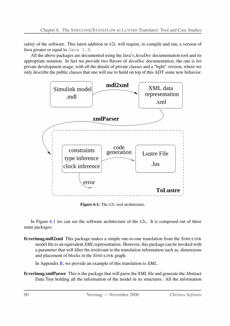
Chapter 6. The SIMULINK/STATEFLOW to LUSTRE Translator: Tool and Case Studies
safety of the software. This latest addition in S2L will require, to compile and run, a version of
Java greater or equal to Java 1.5.
All the above packages are documented using the Java’s JavaDoc documentation tool and its
appropriate notation. In fact we provide two flavors of JavaDoc documentation, the one is for
private development usage, with all the details of private classes and a “light” version, where we
only describe the public classes that one will use to build on top of this ADT some new behavior.
Simulink model.mdl
constraintstype inferenceclock inference
error
generationcode
XML data
.lus
Lustre File
representation.xml
ToLustre
xmlParser
mdl2xml
Figure 6.1: The S2L tool architecture.
In Figure 6.1 we can see the software architecture of the S2L. It is composed out of three
main packages:
fr.verimag.mdl2xml This package makes a simple one-to-one translation from the SIMULINK
model file to an equivalent XML representation. However, this package can be invoked with
a parameter that will filter the irrelevant to the translation information such as, dimensions
and placement of blocks in the SIMULINK graph.
In Appendix B, we provide an example of this translation to XML.
fr.verimag.xmlParser This is the package that will parse the XML file and generate the Abstract
Data Tree holding all the information of the model in its structures. All the information
80 Verimag — November 2006 Christos Sofronis
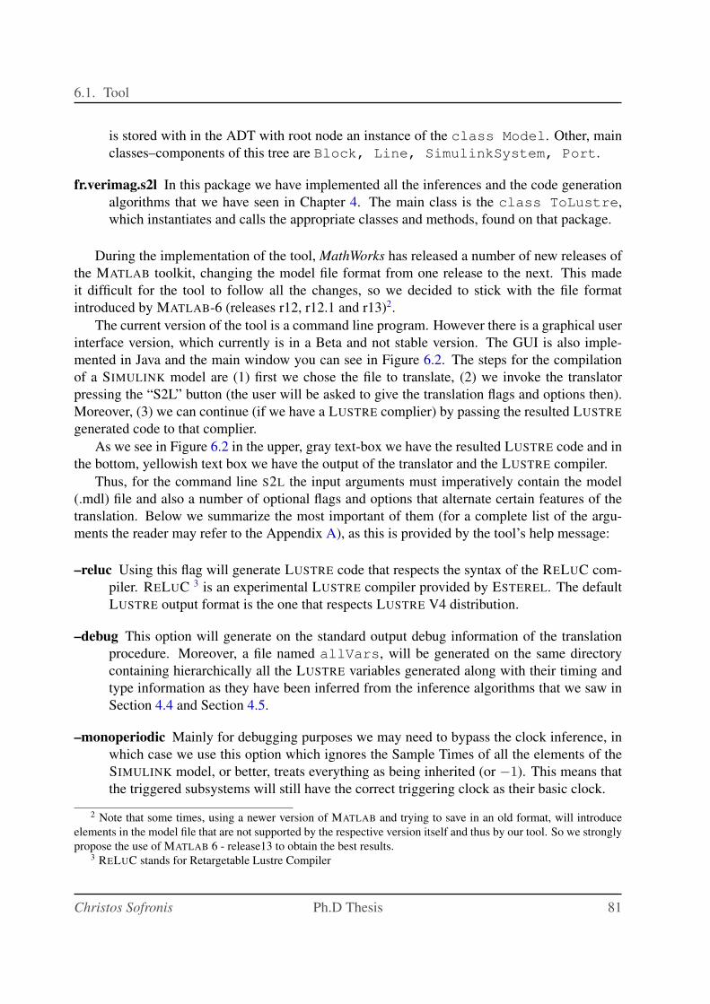
6.1. Tool
is stored with in the ADT with root node an instance of the class Model. Other, main
classes–components of this tree are Block, Line, SimulinkSystem, Port.
fr.verimag.s2l In this package we have implemented all the inferences and the code generation
algorithms that we have seen in Chapter 4. The main class is the class ToLustre,
which instantiates and calls the appropriate classes and methods, found on that package.
During the implementation of the tool, MathWorks has released a number of new releases of
the MATLAB toolkit, changing the model file format from one release to the next. This made
it difficult for the tool to follow all the changes, so we decided to stick with the file format
introduced by MATLAB-6 (releases r12, r12.1 and r13)2.
The current version of the tool is a command line program. However there is a graphical user
interface version, which currently is in a Beta and not stable version. The GUI is also imple-
mented in Java and the main window you can see in Figure 6.2. The steps for the compilation
of a SIMULINK model are (1) first we chose the file to translate, (2) we invoke the translator
pressing the “S2L” button (the user will be asked to give the translation flags and options then).
Moreover, (3) we can continue (if we have a LUSTRE complier) by passing the resulted LUSTRE
generated code to that complier.
As we see in Figure 6.2 in the upper, gray text-box we have the resulted LUSTRE code and in
the bottom, yellowish text box we have the output of the translator and the LUSTRE compiler.
Thus, for the command line S2L the input arguments must imperatively contain the model
(.mdl) file and also a number of optional flags and options that alternate certain features of the
translation. Below we summarize the most important of them (for a complete list of the argu-
ments the reader may refer to the Appendix A), as this is provided by the tool’s help message:
–reluc Using this flag will generate LUSTRE code that respects the syntax of the RELUC com-
piler. RELUC 3 is an experimental LUSTRE compiler provided by ESTEREL. The default
LUSTRE output format is the one that respects LUSTRE V4 distribution.
–debug This option will generate on the standard output debug information of the translation
procedure. Moreover, a file named allVars, will be generated on the same directory
containing hierarchically all the LUSTRE variables generated along with their timing and
type information as they have been inferred from the inference algorithms that we saw in
Section 4.4 and Section 4.5.
–monoperiodic Mainly for debugging purposes we may need to bypass the clock inference, in
which case we use this option which ignores the Sample Times of all the elements of the
SIMULINK model, or better, treats everything as being inherited (or −1). This means that
the triggered subsystems will still have the correct triggering clock as their basic clock.
2 Note that some times, using a newer version of MATLAB and trying to save in an old format, will introduce
elements in the model file that are not supported by the respective version itself and thus by our tool. So we strongly
propose the use of MATLAB 6 - release13 to obtain the best results.3 RELUC stands for Retargetable Lustre Compiler
Christos Sofronis Ph.D Thesis 81
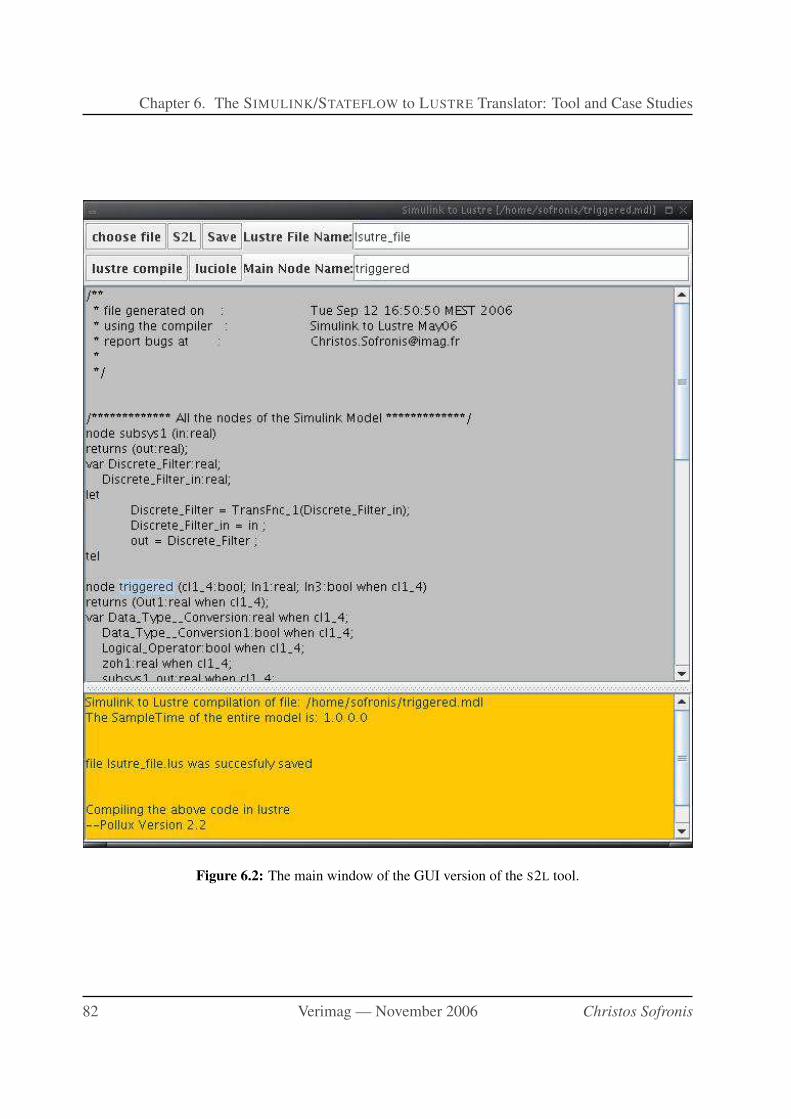
Chapter 6. The SIMULINK/STATEFLOW to LUSTRE Translator: Tool and Case Studies
Figure 6.2: The main window of the GUI version of the S2L tool.
82 Verimag — November 2006 Christos Sofronis
6.1. Tool
–choose-system In a big and complex system, we may want to translate only a small part hidden
in the tree structure of subsystems. Using this flag we interactively choose the subsystem
that will be the root node of the translation to LUSTRE.
–no-main By default, S2L, will generate a folding node that encapsulates the main node in the
generated LUSTRE file. This helps on generating internal clocks and associating them
to input/output LUSTRE variables and thus giving a “cleaner” interface to the user that no
longer he has to cope with timing relation between inputs. However, this may be redundant
if there is no timing variance between inputs and/or outputs, thus using this option will skip
this step.
–xml Using this option, the tool only generates the XML representation of the SIMULINK model
and stops the execution.
The result of invoking S2L is to generate a LUSTRE program in a .lus file (usually with the
same file name, unless explicitly stated). Moreover, the tool outputs the period that the LUSTRE
program should be run at, so that the translation corresponds to the source model. As we have
seen in Section 4.5, this is a result of the clock inference algorithm.
However, if during any stage of the translation there is an error, then the translation is aborted
and an error message is printed on the standard output. Note also, that the code generation
is done on-the-fly, which means that every node that is generated is written and flushed to the
output file, so that in any undesired exception, we will still have the LUSTRE code generated up
to the occurrence of this exception.
6.1.2 The SF2LUS tool
The translation of STATEFLOW to LUSTRE studied in Chapter 5 has been implemented in the
SF2LUS tool. This tool has been implemented by Norman Scaife, a post-doc at Verimag from
2003 to 2005. SF2LUS is written in Objective Caml (OCaml).
SF2LUS does not use intermediate XML representation and the ADT is parsed immediately
out of the model file. On the other hand SF2LUS provides more options to toggle features of the
translation and produce detailed debugging output. Note that the tool initially was conceived to
parse the STATEFLOW part of a model and construct a graphical representation of it. Then various
methods for generating code were implemented and the final version, actually implements all the
features we have studied in the previous chapter.
The input to the tool is a STATEFLOW model. The tool supports the MATLAB 7 release 14
and if the file format remains the same in the next versions of the tool, it will support them also.
Output from the tool is primarily LUSTRE V4. This version of LUSTRE includes bounded
iteration using the when construct in conjunction with statically-evaluated constants and proved
very useful in structuring STATEFLOW’s unbounded iterations such as event broadcasts and junc-
tion loops. In general, however, it is intended that SF2LUS be used in conjunction with the
planned STATEFLOW analysis tool to allow the elimination of unbounded recursion either by
automated transformation or by manual editing of the STATEFLOW chart.
Christos Sofronis Ph.D Thesis 83
Chapter 6. The SIMULINK/STATEFLOW to LUSTRE Translator: Tool and Case Studies
Other outputs include preliminary versions of SCADE [Est] which allows STATEFLOW
charts to be included as source code into the SCADE suite of tools by Esterel Technologies,
Inc., RELUC which is a commercial version of LUSTRE also by ESTEREL and some minor
support required by the abstract interpretation tool NBAC (via LUS2NBAC provided in the LUS-
TRE distribution). These output formats are only partially supported, however. Note that the
LUSTRE output itself can be used as input to a variety of tools including the model-checker
LESAR [RHR91, HLR92].
Hereafter we discuss the principle options of the translator, invoked in command line as
arguments.
Output language
Four output languages are currently supported, triggered by the following options:
-pollux Generate LUSTRE V4 output. This is the default mode and the most fully supported.
-nbac Generate NBAC output. NBAC is almost completely compatible with LUSTRE V4 via
the LUS2NBAC utility supplied with the LUSTRE distribution. This option simply triggers
emulation of the integer modulus function which seems to be missing from NBAC.
-reluc Use RELUC modifications. Again, since the SF2LUS translator uses only a small sub-
set of LUSTRE the output is almost compatible with RELUC. Currently, this option trig-
gers some additional parenthesization which seems to be needed. Currently, arrays and
the event stack are not supported since RELUC does not have LUSTRE’s static recursion
mechanism.
-scade Use SCADE modifications. There are some syntactic differences between SCADE and
LUSTRE, some of which can be ironed out by a simple transformation on the output. These
involve constructs such as:
(x,y) = if p then f(a,b) else (c,d);
which are not supported by SCADE. Again, there are no arrays or event stack.
Namespace management
Namespace management in the SF2LUS translator is not fixed, for several reasons:
• There is the tension between providing human-readable LUSTRE output without making
the code too verbose.
• Different users may have different preferences as to what is readable, depending upon their
intended usage of the resulting code.
• It is difficult to translate namespaces accurately between two such widely differing lan-
guages as STATEFLOW and LUSTRE. It is simple to convert names from one syntax space
to another but doing so while retaining the flavor of the original language is difficult.
84 Verimag — November 2006 Christos Sofronis
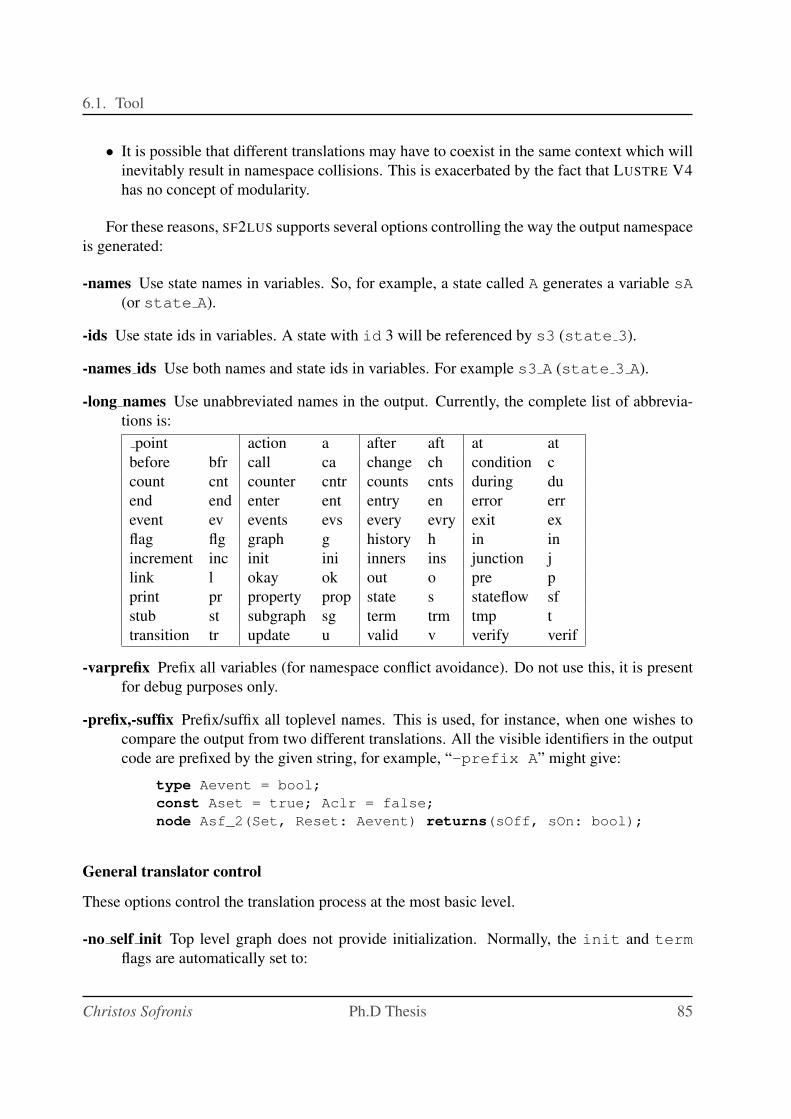
6.1. Tool
• It is possible that different translations may have to coexist in the same context which will
inevitably result in namespace collisions. This is exacerbated by the fact that LUSTRE V4
has no concept of modularity.
For these reasons, SF2LUS supports several options controlling the way the output namespace
is generated:
-names Use state names in variables. So, for example, a state called A generates a variable sA
(or state A).
-ids Use state ids in variables. A state with id 3 will be referenced by s3 (state 3).
-names ids Use both names and state ids in variables. For example s3 A (state 3 A).
-long names Use unabbreviated names in the output. Currently, the complete list of abbrevia-
tions is:
point action a after aft at at
before bfr call ca change ch condition c
count cnt counter cntr counts cnts during du
end end enter ent entry en error err
event ev events evs every evry exit ex
flag flg graph g history h in in
increment inc init ini inners ins junction j
link l okay ok out o pre p
print pr property prop state s stateflow sf
stub st subgraph sg term trm tmp t
transition tr update u valid v verify verif
-varprefix Prefix all variables (for namespace conflict avoidance). Do not use this, it is present
for debug purposes only.
-prefix,-suffix Prefix/suffix all toplevel names. This is used, for instance, when one wishes to
compare the output from two different translations. All the visible identifiers in the output
code are prefixed by the given string, for example, “-prefix A” might give:
type Aevent = bool;
const Aset = true; Aclr = false;
node Asf_2(Set, Reset: Aevent) returns(sOff, sOn: bool);
General translator control
These options control the translation process at the most basic level.
-no self init Top level graph does not provide initialization. Normally, the init and term
flags are automatically set to:
Christos Sofronis Ph.D Thesis 85
Chapter 6. The SIMULINK/STATEFLOW to LUSTRE Translator: Tool and Case Studies
init = true -> false;
term = false;
at the top level of the code. This option disables this behavior but is only present for
debugging the translator.
-ess Event stack size. This sets the depth of the event stack, see Section 5.4.6 for usage informa-
tion and caveats.
-sends Enable sends to specific states. This option triggers some additional processing which
allows STATEFLOW’s send function to be implemented. Note that events become inte-
gers which may affect subsequent analysis and that currently this feature is only partially
implemented. See Section 5.4.6.
-junc states Treat junctions as states. When this is set junctions are given a physical state (called
j<ID> or junction_<ID>) and the chart can stay in a junction after a reaction. An
additional output boolean (v or valid) is generated which is true if and only if the
current state is not a junction. See Section 5.4.2.
-errstate Add error processing to event broadcasts. This generates an extra output boolean
variable (err or error) which is set to true if an event is broadcast at the lowest level
of the event stack. This logic is switched off if the event stack size is zero.
-unroll Unroll loops according to loop counters. Using the annotations in the STATEFLOW chart
described in Section 5.4.2 transition networks involving loops are unfolded a fixed number
of times resulting in a loop-free chart. The unrolling algorithm is currently very primitive
and has complexity problems.
Data management
Handling MATLAB’s workspace is complicated by the fact that it is stored in a binary format
which external tools cannot read. Hence, the translator has to make some assumptions about
the workspace which it communicates via the .mws file. Note also that this file provides the
means of communication with the S2L tool also. These options allow some additional control
over workspace values:
-create missing Add missing data to data dictionary. If a chart contains a reference to a vari-
able not in STATEFLOW’s data dictionary then it can be automatically created. All such
variables have to have the same scope and type, however.
-missing scope Scope for missing data (default: INPUT_DATA). Recognized values are:
r13/r14 INPUT_EVENT OUTPUT_EVENT LOCAL_EVENT
OUTPUT_DATA INPUT_DATA LOCAL_DATA
TEMPORARY_DATA CONSTANT_DATA
r14 FUNCTION_INPUT_DATA FUNCTION_OUTPUT_DATA PARAMETER_DATA
86 Verimag — November 2006 Christos Sofronis
6.1. Tool
-missing datatype Data type for missing data (default: double). Known values are (not all
are supported):
double single int8 int16
int32 uint8 uint16 uint32
boolean fixpt ml
-no constants Omit workspace constants from output. This is used by SS2LUS and prevents
SF2LUS from including constants defined in the MATLAB workspace file from being in-
cluded. The output is not legal LUSTRE since the constants are expected to be provided
by S2L.
Time
The STATEFLOW implicit time variable t is slightly problematical since LUSTRE does not have
any notion of absolute time. For stand-alone STATEFLOW-generated LUSTRE code the following
options allow t to be generated automatically assuming a fixed time difference between reac-
tions. If time is not emulated here then it is assumed to be an input to the chart. The MATLAB
workspace file contains an entry indicating whether t is an input or not.
-emulate time Provide internal time value. References to STATEFLOW’s time value are imple-
mented internally in the LUSTRE code according to the following two options.
-start time Start time for emulated time (default: 0.0). The value of t at reaction zero.
-time increment Time increment for emulated time (default: 1.0). The t variable is incre-
mented by this amount at the start of each reaction.
Observers
One of the main uses of the SF2LUS translator is in the proof of safety properties. The following
options support this activity:
-observe Add observer node for given expression. Generate a single LUSTRE node observing
the expression given as a string of LUSTRE code. State variables can be observed provided
the -states_visible option is set.
-no observers Don’t read observer file. By default, SF2LUS looks for a file <file>.obs
when given a model file <file>.mdl. If it exists it is assumed to be a file containing
observable expressions, one per line. LUSTRE-style comments (--) are permitted.
-consistency Add a state consistency observer. This option causes an observer for the state
variables to be generated. The observer is called consistency_<CID> and is mostly
used to verify the translation process, see Section 5.6. The -states_visible option
is set automatically.
Christos Sofronis Ph.D Thesis 87
Chapter 6. The SIMULINK/STATEFLOW to LUSTRE Translator: Tool and Case Studies
-counters Add loop counters to junction networks. An additional integer output for each
junction in the chart is generated. The counters are called cntrj<ID> where <ID>
is the id number for the junction. Each counter is incremented when its junction
is entered during transition path analysis. Currently, maximum values are not main-
tained so the values have to be checked after each reaction. In addition, an observer
(called loop_counters_<CID>) is generated for all the junctions annotated as in Sec-
tion 5.4.2. The -junc_states option is set automatically.
Debugging features
Finally there is a number of options used to help in debugging the translator. Some may be of
use in debugging STATEFLOW charts, however. Given the large number and the specialization of
those options, we recall the reader to refer to the tool usage itself for further information.
6.1.3 SS2LUS tool architecture and usage
In this Section we will present the SS2LUS tool, which translates models composed by both a
SIMULINK and a STATEFLOW part. SS2LUS, written in the shell’s scripting language, invokes
the two tools S2L and SF2LUS and interface them in a “clean” manner: whenever S2L finds a
STATEFLOW block, it submits it to SF2LUS which translates it into a LUSTRE node and returns
this node (body plus type signature) back to S2L. Thus, SS2LUS is a mechanism that combine
the functionality of those two independent tools and accepts he following inputs:
• The SIMULINK/STATEFLOW model to be translated to LUSTRE. This is a .mdl file and it
must be generated by a MATLAB release between r12 and r14.
• Arguments to be passed to S2L.
The output is a LUSTRE program (a .lus file) and the period that the LUSTRE program
must be executed, which as we have seen in Section 4.5, it is the output of the clock inference
algorithm. Also the above discussed .mws file is generated in the current directory.
The procedure of the translation is to call the module to translate the STATEFLOW part and
generate the LUSTRE code in a temporary file. Upon correct execution and translation of the
STATEFLOW part4 there is the translation of the SIMULINK part. However in that case, there is a
primitive exploration of the STATEFLOW part, from S2L to extract the inputs and outputs of the
STATEFLOW chart, so that the correct node call is generated.
Upon successful completion of the SIMULINK translation also, we append the LUSTRE code
of the temporary file and we have the LUSTRE program that corresponds to the initial model.
Though the independent tools have several parameters and flags to alternate features of the
translations, the global tool have restricted this usage to the default, which is the intersection so
that both tools can cooperate. However, one may use the tools independently and generate the
glue code between them manually, i.e., the code that will call the STATEFLOW part from within
the SIMULINK part.
4 In any case that an error occurs, an error message is printed and translation is aborted
88 Verimag — November 2006 Christos Sofronis
6.2. Case Studies
6.2 Case Studies
In this section we present four case studies of the use of the above tools. We have used S2L to
translate two SIMULINK models provided by the Audi automotive constructor in the context of
the European IST project “NEXT TTA”.5 The first model defines a warning processing system
and is part of a larger controller used by Audi in production vehicles. The second model is a
larger steer-by-wire controller. Both models have been given to Verimag for internal project
purposes and cannot be made public due to intellectual property restrictions. Thus, we only
present parts of these models.
In Section 6.2.3, we present a case study that we have created to test the SF2LUS translator
and in Section 6.2.4 there is an case study of our overall translator, which generates one LUSTRE
program out of a model composed by both a SIMULINK and a STATEFLOW part.
6.2.1 Warning processing system
The objective of the system is to recognize if a car is moving towards its physical limits and to
generate a warning to the driver. However, the warning may be canceled because of a number of
conditions ensuring that the car is not in a dangerous situation.
The main subsystem is called cancel warning and is shown in Figure 6.3. The subsystem
has ten inputs and five outputs. Inputs warning 1 in and warning 2 in are generated on
the same electronic control unit (ECU) and are sampled with a rate of 20 milliseconds (ms).
Each warning is a boolean, representing an a-priori need to issue a warning. The input signals
warning 1 amp in and warning 2 amp in are the amplitudes of the warnings. They are
8-bit signals sampled with a rate of 20 ms. The rest of the input signals (signal 1, signal 2,
. . . ) are used to compute the warning permission no warning and they have a sampling rate
of 4 ms. The outputs of the main subsystem are the warning signals and their amplitudes (with
the sampling rate of 20 ms) as well as the warning permission (with the sampling rate of 4 ms).
The cancel warning subsystem is itself composed of a number of subsystems and basic
blocks, as shown in Figure 6.4. The subsystem no warning conditions is supposed to
check a number of conditions which cancel the warning. Depending on its output, the subsystem
eliminate warning filters the warning. The subsystem warning filter blocks one of
the warning signals if the other one is already active. The subsystem warning duration en-
sures that a warning which has been issued will be sustained long enough in order to be perceived
by the user.
The entire SIMULINK model has a hierarchy depth of 6 layers (including the top-level sys-
tem). It contains 20 subsystems and more than 200 total components (including subsystems,
basic SIMULINK blocks, as well as input/output port blocks).
Translating the entire SIMULINK model to LUSTRE using the S2L tool takes less than a
second. The resulting LUSTRE program is 718 lines long. A small part of the program is shown
in Figure 6.5. It contains the signature of the LUSTRE node corresponding to the subsystem
5 http://www.vmars.tuwien.ac.at/projects/nexttta/
Christos Sofronis Ph.D Thesis 89
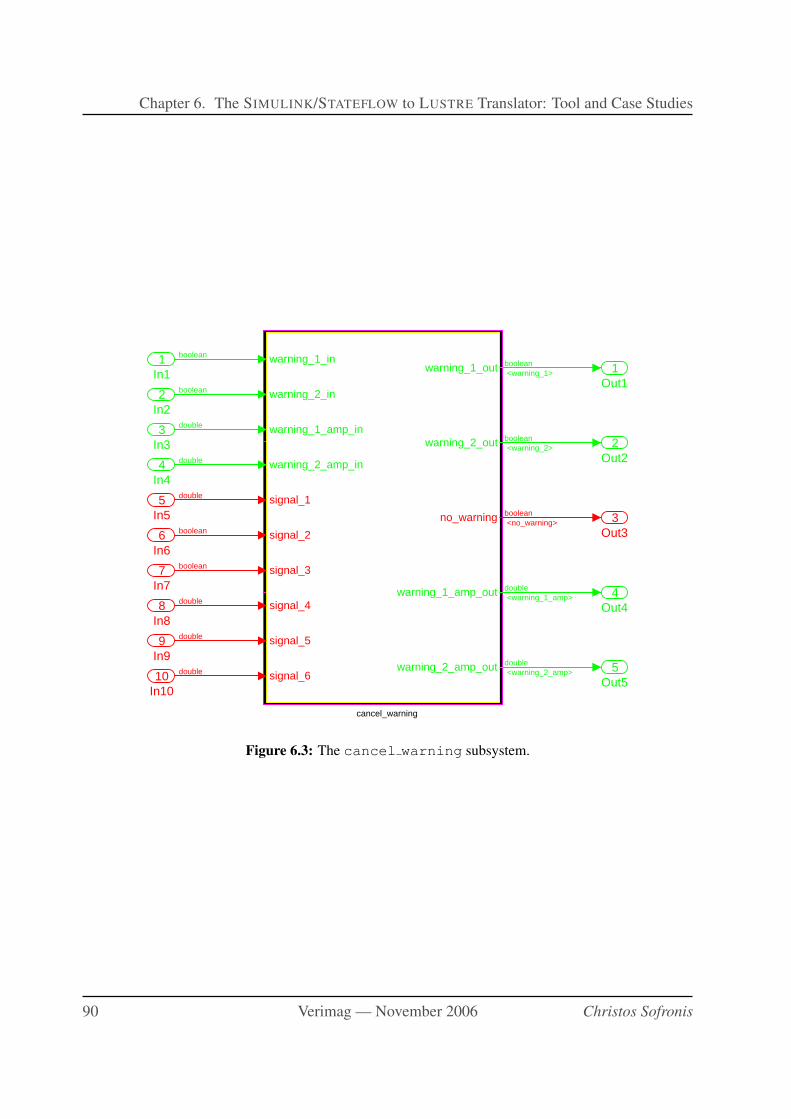
Chapter 6. The SIMULINK/STATEFLOW to LUSTRE Translator: Tool and Case Studies
cancel_warning
5Out5
4Out4
3Out3
2Out2
1Out1
warning_1_in
warning_2_in
warning_1_amp_in
warning_2_amp_in
signal_1
signal_2
signal_3
signal_4
signal_5
signal_6
warning_1_out
warning_2_out
no_warning
warning_1_amp_out
warning_2_amp_out10
In10
9In9
8In8
7In7
6In6
5In5
4In4
3In3
2In2
1In1
boolean
boolean
double
double
double
boolean
boolean
double
double
double
boolean<warning_1>
boolean<warning_2>
boolean<no_warning>
double<warning_1_amp>
double<warning_2_amp>
Figure 6.3: The cancel warning subsystem.
90 Verimag — November 2006 Christos Sofronis
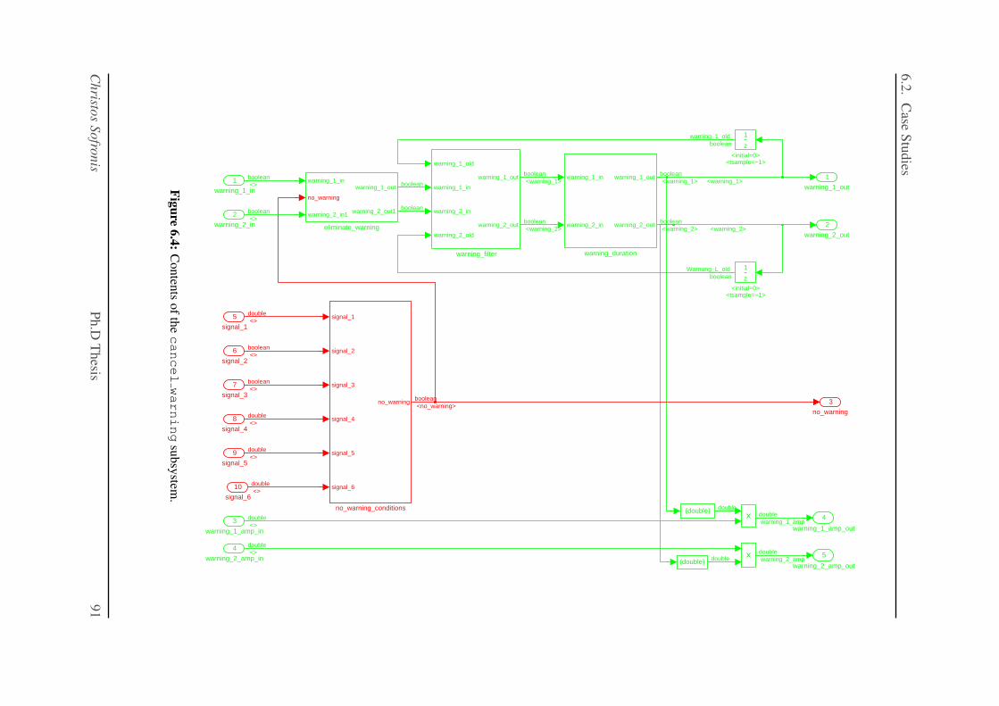
6.2
.C
aseS
tudies
5
warning_2_amp_out
4
warning_1_amp_out
3
no_warning
2
warning_2_out
1
warning_1_out
warning_1_old
warning_1_in
warning_2_in
warning_2_old
warning_1_out
warning_2_out
warning_filter
warning_1_in
warning_2_in
warning_1_out
warning_2_out
warning_duration
signal_1
signal_2
signal_3
signal_4
signal_5
signal_6
no_warning
no_warning_conditions
warning_1_in
no_warning
warning_2_in1
warning_1_out
warning_2_out1
eliminate_warning
z
1
<initial=0><tsample=−1>
z
1
<initial=0><tsample=−1>
(double)
(double)
10
signal_6
9
signal_5
8
signal_4
7
signal_3
6
signal_2
5
signal_1
4
warning_2_amp_in
3
warning_1_amp_in
2
warning_2_in
1
warning_1_in<warning_1>
boolean<warning_1>
<warning_2>boolean<warning_2>
boolean<warning_1>
boolean<warning_2>
booleanwarning_1_old
booleanWarnung_L_old
boolean<>
double<>
boolean<>
boolean<>
double<>
double<>
double<>
double<>
double<>
double
double
doublewarning_1_amp
doublewarning_2_amp
boolean<no_warning>
boolean<>
boolean
booleanFig
ure
6.4
:C
onten
tsof
thecancelwarning
subsy
stem.
Christo
sSofro
nis
Ph.D
Thesis
91
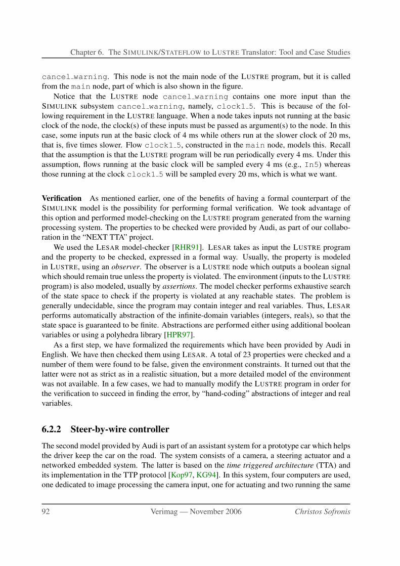
Chapter 6. The SIMULINK/STATEFLOW to LUSTRE Translator: Tool and Case Studies
cancel warning. This node is not the main node of the LUSTRE program, but it is called
from the main node, part of which is also shown in the figure.
Notice that the LUSTRE node cancel warning contains one more input than the
SIMULINK subsystem cancel warning, namely, clock1 5. This is because of the fol-
lowing requirement in the LUSTRE language. When a node takes inputs not running at the basic
clock of the node, the clock(s) of these inputs must be passed as argument(s) to the node. In this
case, some inputs run at the basic clock of 4 ms while others run at the slower clock of 20 ms,
that is, five times slower. Flow clock1 5, constructed in the main node, models this. Recall
that the assumption is that the LUSTRE program will be run periodically every 4 ms. Under this
assumption, flows running at the basic clock will be sampled every 4 ms (e.g., In5) whereas
those running at the clock clock1 5 will be sampled every 20 ms, which is what we want.
Verification As mentioned earlier, one of the benefits of having a formal counterpart of the
SIMULINK model is the possibility for performing formal verification. We took advantage of
this option and performed model-checking on the LUSTRE program generated from the warning
processing system. The properties to be checked were provided by Audi, as part of our collabo-
ration in the “NEXT TTA” project.
We used the LESAR model-checker [RHR91]. LESAR takes as input the LUSTRE program
and the property to be checked, expressed in a formal way. Usually, the property is modeled
in LUSTRE, using an observer. The observer is a LUSTRE node which outputs a boolean signal
which should remain true unless the property is violated. The environment (inputs to the LUSTRE
program) is also modeled, usually by assertions. The model checker performs exhaustive search
of the state space to check if the property is violated at any reachable states. The problem is
generally undecidable, since the program may contain integer and real variables. Thus, LESAR
performs automatically abstraction of the infinite-domain variables (integers, reals), so that the
state space is guaranteed to be finite. Abstractions are performed either using additional boolean
variables or using a polyhedra library [HPR97].
As a first step, we have formalized the requirements which have been provided by Audi in
English. We have then checked them using LESAR. A total of 23 properties were checked and a
number of them were found to be false, given the environment constraints. It turned out that the
latter were not as strict as in a realistic situation, but a more detailed model of the environment
was not available. In a few cases, we had to manually modify the LUSTRE program in order for
the verification to succeed in finding the error, by “hand-coding” abstractions of integer and real
variables.
6.2.2 Steer-by-wire controller
The second model provided by Audi is part of an assistant system for a prototype car which helps
the driver keep the car on the road. The system consists of a camera, a steering actuator and a
networked embedded system. The latter is based on the time triggered architecture (TTA) and
its implementation in the TTP protocol [Kop97, KG94]. In this system, four computers are used,
one dedicated to image processing the camera input, one for actuating and two running the same
92 Verimag — November 2006 Christos Sofronis
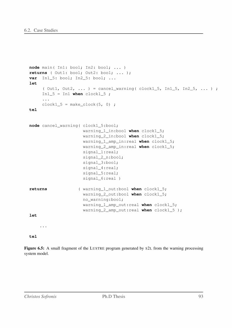
6.2. Case Studies
node main( In1: bool; In2: bool; ... )
returns ( Out1: bool; Out2: bool; ... );
var In1_5: bool; In2_5: bool; ...
let
( Out1, Out2, ... ) = cancel_warning( clock1_5, In1_5, In2_5, ... ) ;
In1_5 = In1 when clock1_5 ;
...
clock1_5 = make_clock(5, 0) ;
tel
node cancel_warning( clock1_5:bool;
warning_1_in:bool when clock1_5;
warning_2_in:bool when clock1_5;
warning_1_amp_in:real when clock1_5;
warning_2_amp_in:real when clock1_5;
signal_1:real;
signal_2_n:bool;
signal_3:bool;
signal_4:real;
signal_5:real;
signal_6:real )
returns ( warning_1_out:bool when clock1_5;
warning_2_out:bool when clock1_5;
no_warning:bool;
warning_1_amp_out:real when clock1_5;
warning_2_amp_out:real when clock1_5 );
let
...
tel
Figure 6.5: A small fragment of the LUSTRE program generated by S2L from the warning processing
system model.
Christos Sofronis Ph.D Thesis 93
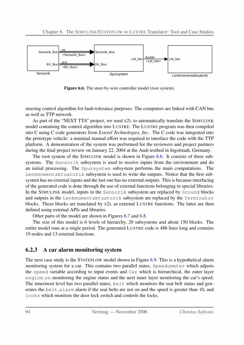
Chapter 6. The SIMULINK/STATEFLOW to LUSTRE Translator: Tool and Case Studies
Sensorik_Bus
BV_Bus
LM_Nm
Spursystem
Sensorik_Bus
BV_Bus
Sensorik
LM_Nm
Lenkmomentaktuatorik
3{3}<BV_Bus>
{3}<Sensorik_Bus>
double<LM_Nm>
Figure 6.6: The steer-by-wire controller model (root system).
steering control algorithm for fault-tolerance purposes. The computers are linked with CAN bus
as well as TTP network.
As part of the “NEXT TTA” project, we used S2L to automatically translate the SIMULINK
model containing the control algorithm into LUSTRE. The LUSTRE program was then compiled
into C using C code generators from Esterel Technologies, Inc.. The C code was integrated into
the prototype vehicle: a minimal manual effort was required to interface the code with the TTP
platform. A demonstration of the system was performed for the reviewers and project partners
during the final project review on January 22, 2004 at the Audi testbed in Ingolstadt, Germany.
The root system of the SIMULINK model is shown in Figure 6.6. It consists of three sub-
systems. The Sensorik subsystem is used to receive inputs from the environment and do
an initial processing. The Spursystem subsystem performs the main computations. The
Lenkmomentaktuatorik subsystem is used to write the outputs. Notice that the first sub-
system has no external inputs and the last one has no external outputs. This is because interfacing
of the generated code is done through the use of external functions belonging in special libraries.
In the SIMULINK model, inputs in the Sensorik subsystem are replaced by Ground blocks
and outputs in the Lenkmomentaktuatorik subsystem are replaced by the Terminator
blocks. These blocks are translated by S2L as external LUSTRE functions. The latter are then
defined using external APIs and libraries.
Other parts of the model are shown in Figures 6.7 and 6.8.
The size of this model is 6 levels of hierarchy, 20 subsystems and about 150 blocks. The
entire model runs at a single period. The generated LUSTRE code is 486 lines long and contains
19 nodes and 13 external functions.
6.2.3 A car alarm monitoring system
The next case study is the STATEFLOW model shown in Figure 6.9. This is a hypothetical alarm
monitoring system for a car. This contains two parallel states, Speedometer which adjusts
the speed variable according to input events and Car which is hierarchical, the outer layer
engine on monitoring the engine status and the next inner layer monitoring the car’s speed.
The innermost level has two parallel states, belt which monitors the seat belt status and gen-
erates the belt alarm alarm if the seat belts are not on and the speed is greater than 10, and
locks which monitors the door lock switch and controls the locks.
94 Verimag — November 2006 Christos Sofronis
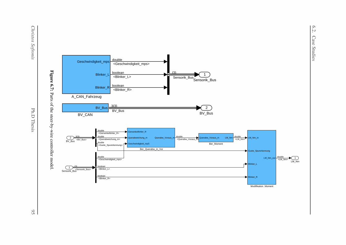
6.2
.C
aseS
tudies
2
BV_Bus
1
Sensorik_Bus
BV_Bus
BV_CAN
Geschwindigkeit_mps
Blinker_L
Blinker_R
A_CAN_Fahrzeug
{3}Sensorik_Bus
double<Geschwindigkeit_mps>
3{3}BV_Bus
boolean<Blinker_L>
boolean<Blinker_R>
1
LM_Nm
LM_Nm_in
Guete_Spurerkennung
Blinker_L
Blinker_R
LM_Nm_out
Modifikation_Moment
Gierwinkelfehler_R
Querabweichung_m
Geschwindigkeit_mpS
Querabw_Voraus_m
Ber_Querabw_in_Vor
Querabw_Voraus_m LM_Nm
Ber_Moment
2
BV_Bus
1
Sensorik_Bus
double<Geschwindigkeit_mps>
double<Querabweichung_m>
double<Gierwinkelfehler_R>
double<Querabw_Voraus_m>
boolean<Blinker_R>
double<Guete_Spurerkennung>
3{3}<BV_Bus>
{3}<Sensorik_Bus>
double<LM_Nm>
double<LM_Nm>
boolean<Blinker_L>
Fig
ure
6.7
:P
artsof
the
steer-by-w
ireco
ntro
llerm
odel.
Christo
sSofro
nis
Ph.D
Thesis
95
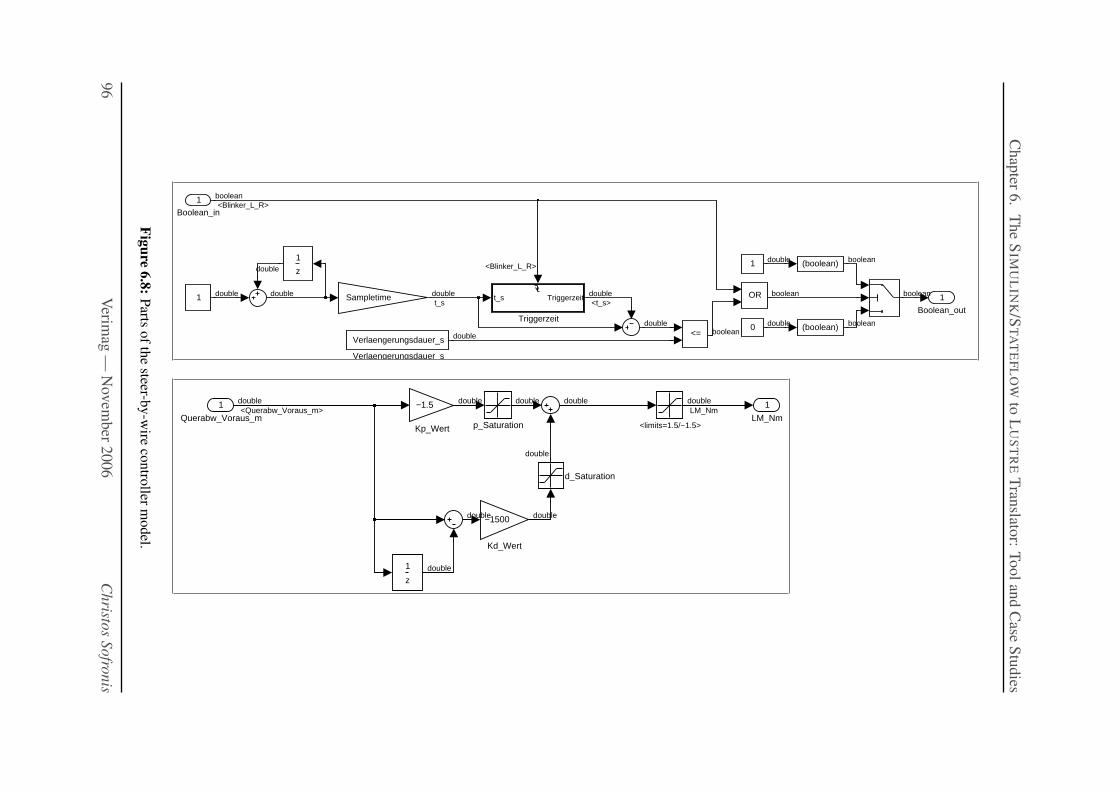
Chap
ter6.
The
SIM
UL
INK
/ST
AT
EF
LO
Wto
LU
ST
RE
Tran
slator:
Tool
and
Case
Stu
dies
1
Boolean_out
Verlaengerungsdauer_s
Verlaengerungsdauer_s
z
1
t_s Triggerzeit
Triggerzeit
<=
ORSampletime
(boolean)
(boolean)1
0
1
1
Boolean_in
double
double
double doublet_s
double
double
<Blinker_L_R>
boolean<Blinker_L_R>
double<t_s>
booleandouble
double
boolean
boolean
boolean
boolean
1
LM_Nmp_Saturation
d_Saturation
z
1
<limits=1.5/−1.5>
−1.5
Kp_Wert
−1500
Kd_Wert
1
Querabw_Voraus_m
double doubleLM_Nm
double<Querabw_Voraus_m>
double
double
double double
double
double
Fig
ure
6.8
:P
artsof
the
steer-by-w
ireco
ntro
llerm
odel.
96
Verim
ag—
Novem
ber
2006
Christo
sSofro
nis
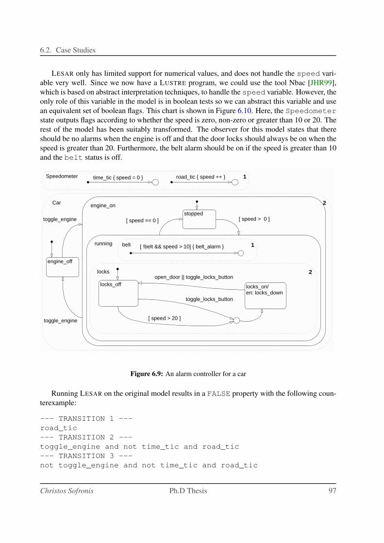
6.2. Case Studies
LESAR only has limited support for numerical values, and does not handle the speed vari-
able very well. Since we now have a LUSTRE program, we could use the tool Nbac [JHR99],
which is based on abstract interpretation techniques, to handle the speed variable. However, the
only role of this variable in the model is in boolean tests so we can abstract this variable and use
an equivalent set of boolean flags. This chart is shown in Figure 6.10. Here, the Speedometer
state outputs flags according to whether the speed is zero, non-zero or greater than 10 or 20. The
rest of the model has been suitably transformed. The observer for this model states that there
should be no alarms when the engine is off and that the door locks should always be on when the
speed is greater than 20. Furthermore, the belt alarm should be on if the speed is greater than 10
and the belt status is off.
Car 2
Speedometer 1
engine_off
engine_on
running
stopped
belt 1
locks 2
locks_off locks_on/en: locks_down
time_tic { speed = 0 } road_tic { speed ++ }
toggle_engine
toggle_locks_button
[ !belt && speed > 10] { belt_alarm }
[ speed == 0 ] [ speed > 0 ]
toggle_engine [ speed > 20 ]
open_door || toggle_locks_button
Figure 6.9: An alarm controller for a car
Running LESAR on the original model results in a FALSE property with the following coun-
terexample:
--- TRANSITION 1 ---
road_tic
--- TRANSITION 2 ---
toggle_engine and not time_tic and road_tic
--- TRANSITION 3 ---
not toggle_engine and not time_tic and road_tic
Christos Sofronis Ph.D Thesis 97
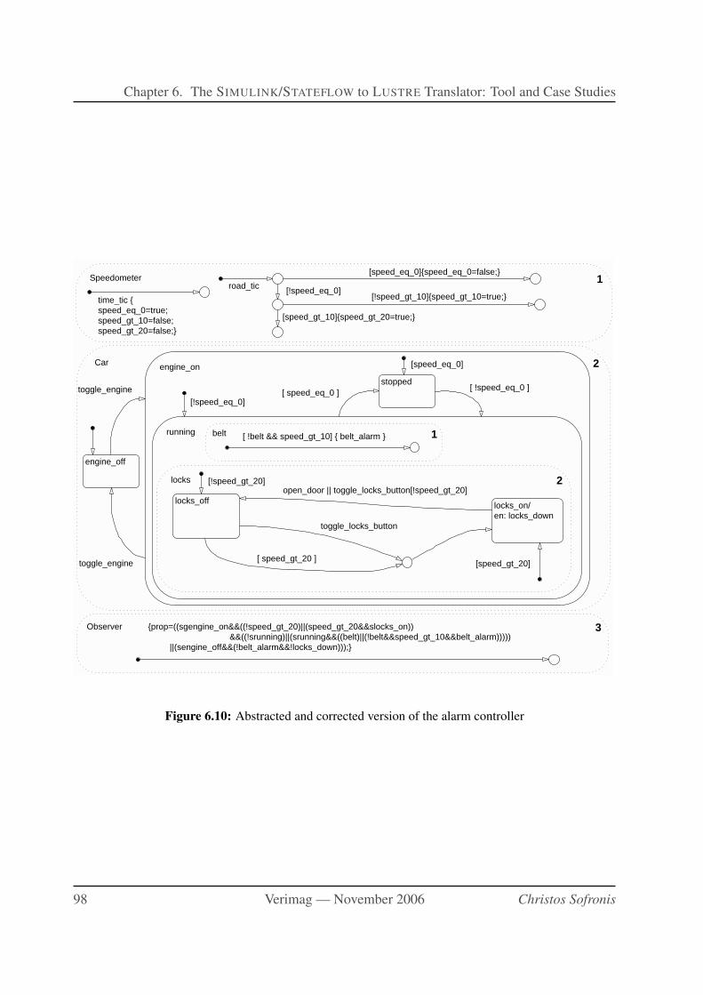
Chapter 6. The SIMULINK/STATEFLOW to LUSTRE Translator: Tool and Case Studies
Observer 3
Car 2
Speedometer 1
engine_off
engine_on
running
stopped
locks 2
belt 1
locks_on/en: locks_down
locks_off
road_tic
[speed_eq_0]{speed_eq_0=false;}
[!speed_eq_0]time_tic {speed_eq_0=true;speed_gt_10=false;speed_gt_20=false;}
[!speed_gt_10]{speed_gt_10=true;}
[speed_gt_10]{speed_gt_20=true;}
[speed_eq_0]
[ speed_eq_0 ][ !speed_eq_0 ]
[!speed_eq_0]
toggle_engine
[ !belt && speed_gt_10] { belt_alarm }
[!speed_gt_20]
toggle_engine
open_door || toggle_locks_button[!speed_gt_20]
toggle_locks_button
[ speed_gt_20 ][speed_gt_20]
{prop=((sgengine_on&&((!speed_gt_20)||(speed_gt_20&&slocks_on)) &&((!srunning)||(srunning&&((belt)||(!belt&&speed_gt_10&&belt_alarm))))) ||(sengine_off&&(!belt_alarm&&!locks_down)));}
Figure 6.10: Abstracted and corrected version of the alarm controller
98 Verimag — November 2006 Christos Sofronis
6.2. Case Studies
What the model-checker has spotted is that if the engine is switched on while the car is mov-
ing (not an impossibility by any means) then it is possible to reach a state where the speed
is greater than 20 and not be in the locks on state. The solution is simple, split up the
default transitions in the engine on and locks states (for example, [speed_eq_0] and
[!speed_eq_0]) so that the correct state is reached depending upon the initial conditions
when these states are entered. These additional default transitions are shown in Figure 6.10. The
new model gives a TRUE LESAR property with the observer shown.
This model is perhaps not a realistic application but even with such a simple model the prop-
erties verified by LESAR are not intuitively obvious. It is also not very well-written STATEFLOW
since the use of conditions on default transitions is warned against in the STATEFLOW documen-
tation. The point, however, is that given suitable observers and verification by model-checking,
even badly written STATEFLOW can be used with confidence.
6.2.4 A mixed SIMULINK/STATEFLOW case study
The last case study we present is a model that combines both a SIMULINK part and a STATEFLOW
part. One of the users of our distributed platform is the group in Turku Center for Computer
Science in Finland. They have used our translator, and its model checking capabilities, for their
research in combining SIMULINK/STATEFLOW with mode-automata.
This model has been kindly provided to us by Pontus Bostrom of the Department of Computer
Science of Abo Akademi, Finland. It is a part of the model used in [BM06] to investigate the
suitability of a formalization proposed in that work.
The model represents a digital hydraulics system. The system consists of a hydraulic cylinder
that moves a load mass either to a desired position or with a desired speed. The speed of the load
mass is controlled by the pressure on each side of the piston in the cylinder. A digital controller
controls the pressures in the cylinder using a system of on/off valves. The SIMULINK model
is illustrated in Figure 6.11 and the STATEFLOW part is the Mode switching block in the
middle of the SIMULINK diagram. The STATEFLOW controller (shown in Figure 6.12) has the
following three modes stopped, extending and retracting.
Using our tool-chain, we managed to translate this model to LUSTRE and then to ensure that
the invariant in each mode is maintained by the transitions. The initial model contains more than
50 Blocks and the hierarchy is not very deep composed of only of the two subsystems we see in
Figure 6.11 as long as with one STATEFLOW Chart. The translated LUSTRE code has a length of
400 lines and contains as many as 30 LUSTRE nodes.
Christos Sofronis Ph.D Thesis 99
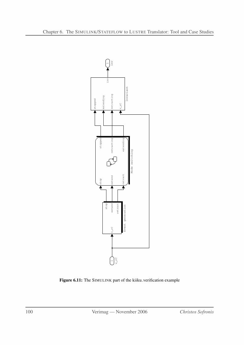
Chapter 6. The SIMULINK/STATEFLOW to LUSTRE Translator: Tool and Case Studies
1
inv
stop
extend
retract
stopped
retracting
extending
Mode switching
stopped
extending
retracting
v_rC
inv
Invariant
v_rC
stop
extend
retract
Event generation
1
v_rC
Figure 6.11: The SIMULINK part of the kiiku verification example
100 Verimag — November 2006 Christos Sofronis
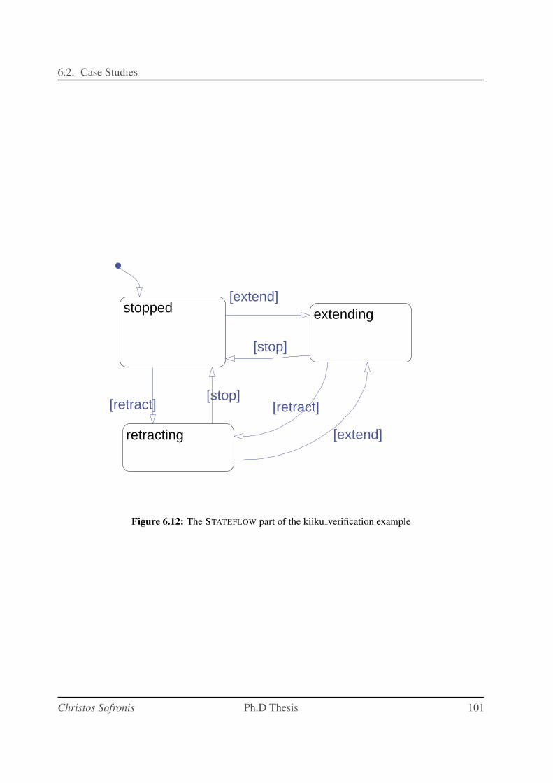
6.2. Case Studies
stopped extending
retracting
[extend]
[stop]
[retract]
[extend]
[stop][retract]
Figure 6.12: The STATEFLOW part of the kiiku verification example
Christos Sofronis Ph.D Thesis 101
Chapter 6. The SIMULINK/STATEFLOW to LUSTRE Translator: Tool and Case Studies
102 Verimag — November 2006 Christos Sofronis

Chapter 7
Preservation of Synchronous Semantics
under Preemptive Scheduling
7.1 Motivation
In this Chapter we study the problem of code generation from synchronous high-level languages
such as SIMULINK or LUSTRE to a single-processor, multi-tasking architecture. This is in the
context of the tool-chain presented in Chapter 2 (Figure 2.1).
Before we enter into the study of this problem, we should motivate the need for consider-
ing this type of architectures, and multi-tasking code generation in particular. After all, single-
processor code generation methods for synchronous models exist, and in fact are the oldest: the
classic single-task code generation methods (see Section 3.2 and [HCRP91]). These methods
generate the simplest kind of code, that presents a number of advantages. For instance, it does
not require a real-time operating system (RTOS) with multi-tasking capabilities (i.e., a scheduler
to allocate the processor to the different tasks). Why then worry about multi-tasking implemen-
tations?
To understand this, let us examine more in detail the difference between the single-task and
the multi-task implementation, from where we will see the motivation for the work presented in
this Chapter. It is true that the generation of a single, monolithic program out of a synchronous
program is simple as we saw in Section 3.2, but there is a major drawback, mostly when the
synchronous program has parts running in different periods. In this case, the single-task im-
plementation may fail the schedulability check, whereas the counterpart multi-tasking one will
succeed.
We demonstrate the above using a simple example. Consider a synchronous program con-
sisting of two parts, or tasks, P1 and P2, that must be executed every (, i.e., their periods are) 10
ms and every 100 ms, respectively. Suppose the worst-case execution time (WCET) of P1 and
P2 is 2 ms and 10 ms, respectively, as shown in Figure 7.1. Then, generating a single task P that
includes the code of both P1 and P2 would be problematic. P would have to be executed every
10 ms, since this is required by P1. Inside P , P2 would be executed only once every 10 times
(e.g., using an internal counter modulo 10). Assuming that the WCET of P is the sum of the
103
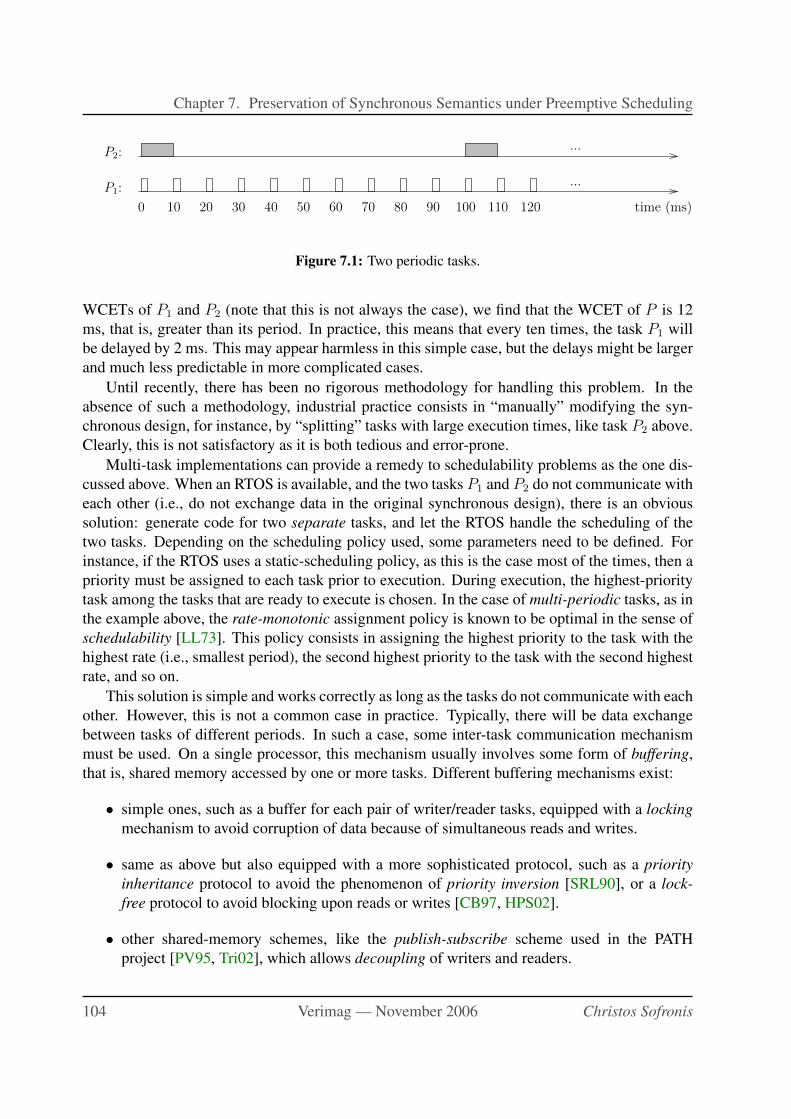
Chapter 7. Preservation of Synchronous Semantics under Preemptive Scheduling
P1:
0 10 20 30 40 50 60 70 80 90 100 110 120 time (ms)
...
...P2:
Figure 7.1: Two periodic tasks.
WCETs of P1 and P2 (note that this is not always the case), we find that the WCET of P is 12
ms, that is, greater than its period. In practice, this means that every ten times, the task P1 will
be delayed by 2 ms. This may appear harmless in this simple case, but the delays might be larger
and much less predictable in more complicated cases.
Until recently, there has been no rigorous methodology for handling this problem. In the
absence of such a methodology, industrial practice consists in “manually” modifying the syn-
chronous design, for instance, by “splitting” tasks with large execution times, like task P2 above.
Clearly, this is not satisfactory as it is both tedious and error-prone.
Multi-task implementations can provide a remedy to schedulability problems as the one dis-
cussed above. When an RTOS is available, and the two tasks P1 and P2 do not communicate with
each other (i.e., do not exchange data in the original synchronous design), there is an obvious
solution: generate code for two separate tasks, and let the RTOS handle the scheduling of the
two tasks. Depending on the scheduling policy used, some parameters need to be defined. For
instance, if the RTOS uses a static-scheduling policy, as this is the case most of the times, then a
priority must be assigned to each task prior to execution. During execution, the highest-priority
task among the tasks that are ready to execute is chosen. In the case of multi-periodic tasks, as in
the example above, the rate-monotonic assignment policy is known to be optimal in the sense of
schedulability [LL73]. This policy consists in assigning the highest priority to the task with the
highest rate (i.e., smallest period), the second highest priority to the task with the second highest
rate, and so on.
This solution is simple and works correctly as long as the tasks do not communicate with each
other. However, this is not a common case in practice. Typically, there will be data exchange
between tasks of different periods. In such a case, some inter-task communication mechanism
must be used. On a single processor, this mechanism usually involves some form of buffering,
that is, shared memory accessed by one or more tasks. Different buffering mechanisms exist:
• simple ones, such as a buffer for each pair of writer/reader tasks, equipped with a locking
mechanism to avoid corruption of data because of simultaneous reads and writes.
• same as above but also equipped with a more sophisticated protocol, such as a priority
inheritance protocol to avoid the phenomenon of priority inversion [SRL90], or a lock-
free protocol to avoid blocking upon reads or writes [CB97, HPS02].
• other shared-memory schemes, like the publish-subscribe scheme used in the PATH
project [PV95, Tri02], which allows decoupling of writers and readers.
104 Verimag — November 2006 Christos Sofronis
7.1. Motivation
None of these buffering schemes, however, guarantees preservation of the original syn-
chronous semantics1. This means that the sequence of outputs produced by some task at the
implementation may not be the same as the sequence of outputs produced by the same task at
the original synchronous program. Small discrepancies between semantics and implementation
can sometimes be tolerated, for instance, when the task implements a robust controller which has
built-in mechanisms to compensate for errors. In other applications, however, such discrepan-
cies may result in totally wrong results, with catastrophic consequences. Having a method that
guarantees equivalence of semantics and implementation is then crucial. It also implies that the
effort spent in simulation or verification of the synchronous program need not be duplicated for
the implementation. This is an extremely important cost factor and hereafter we provide standard
methods and algorithms to overcome this problem and preserve the semantics in a communica-
tion between tasks in a preemptive scheduling execution platform.
As we show later in Section 7.3.3, ”naive” inter-process communication schemes do not pre-
serve the synchronous semantics. In particular, such schemes are not deterministic: depending
on the execution time of the tasks, the data sent from a task to another might be different.
One might say that strict preservation of the synchronous semantics is not really necessary.
After all, in control applications controllers are usually designed to be robust to various types of
data variability, including data loss, jitter, sensor inaccuracies, etc. Two answers can be given
to this claim. First, controllers contain more and more ”discrete logic”, which is not robust (a
single bit-flip may change the course of an if-then-else statement). Second, echos from the in-
dustry indicate that determinism is an important requirement. For instance, recent versions of
the SIMULINK code-generator REAL-TIME WORKSHOP provide options to ”ensure determin-
istic data transfer” (see the ”Related work” section for references). Our contacts with Esterel
Technologies reveal similar concerns.
Decomposition of a synchronous program into tasks
In the rest of this chapter we will be assuming an abstract model of a synchronous program based
on a set of communicating tasks where each task has its own triggering event (see Section 7.2).
The question arises, then, how to go from a synchronous model such as SIMULINK or LUSTRE
to this abstract model of tasks. In other words, how to decompose a synchronous program into a
set of tasks.
The decomposition procedure can be quite complicated involving WCET (worst-case execu-
tion time) estimation and schedulability analysis (i.e., checking that the tasks meet their dead-
lines, given a specified scheduling policy). Decomposition is indeed a topic on its own, and we
do not attempt to cover it in this work. Instead, we discuss a simple decomposition method, often
encountered in practice. Clearly this is a topic for future research.
The simple method boils down to grouping together all the different parts of the code that
are triggered by the same event, into separate tasks, one task for each such event. This event
1 Many of these schemes guarantee a freshest-value semantics, where the reader always gets the latest value
produced by the writer. Freshness is desirable in some cases, in particular in control applications, where the more
recent the data, the more accurate they are.
Christos Sofronis Ph.D Thesis 105
Chapter 7. Preservation of Synchronous Semantics under Preemptive Scheduling
may be a periodic one (i.e., the “tick” of a periodic clock) or an aperiodic one (e.g., linked to the
crank-shaft angle in an engine-control application).
We illustrate the above decomposition method on an example. Consider the SIMULINK
model in Figure 6.4, Section 6.2.1. This system has two different periods: red blocks and signals
have a period of 4 milliseconds (ms) and green ones have a period of 20 ms.
In this case, we can simply decompose this system in two tasks: the “red” task with period 4
ms will contain all red blocks, and the “green” task with period 20 ms will contain all the green
blocks. In this example the red task communicates data to the green task, but not vice-versa.
Notice that if the green task also needed to communicate data to the red one, there would be a
problem, namely, a dependency cycle, at those instants where both tasks are active (i.e., every 20
ms). In such cases this simple decomposition method does not work, and more refined methods
are necessary.
7.2 An inter-task communication model
We consider a set of tasks, T = {τ1, τ2, ...}. The set need not be finite, which allows the modeling
of, for example, dynamic creation of tasks.
To model inter-task communication, we consider a set of data-flow links of the form (i, j, p),with i, j ∈ {1, 2, ...} and p ∈ {−1, 0}. If p = 0 then we write τi → τj , otherwise, we write
τi−1→ τj . The tasks and links result in what we shall call a task graph. For each i, j pair, there
can only be one link, so we cannot have both τi → τj and τi−1→ τj .
Intuitively, a link (i, j, p) means that task τj receives data from task τi. If p = 0 then τj
receives the last value produced by τi, otherwise, it receives the one-before-last value (i.e., there
is a “unit delay” in the link from τi to τj). In both cases, it is possible that the first time that τj
occurs2 there is no value available from τi (either because τi has not occurred yet, or because it
has occurred only once and p = −1). To cover such cases, we will assume that for each task τi
there is a default output value yi0. Then, in cases such as the above, τj uses this default value.
Notice that links model data-flow, and not precedences between tasks.
We allow for cycles in the graph of links, provided these cycles are not zero-delay, that is,
provided there is at least one link (i, j,−1) in every cycle. Notice that we could allow zero-delay
cycles if we made an assumption on the arrival patterns of tasks, namely, that all tasks in a zero-
delay cycle cannot occur at the same time. However, it is often the case that tasks occur at the
same time. For instance, two periodic tasks with the same initial phase, will “meet” at multiples
of the least common multiplier of their periods.
Synchronous, zero-time semantics
We associate with this model an “ideal”, zero-time semantics. For each task τi we associate a set
of occurrence times Ti = {ti1, ti2, ...}, where tik ∈ R≥0 and tik < tik+1 for all k. Because of the
2 As we shall see shortly, we define an “ideal” zero-time semantics where a task executes and produces its result
as the same time it is released. We can thus say “task τi occurs”.
106 Verimag — November 2006 Christos Sofronis
7.3. Execution on static-priority or EDF schedulers
zero-time assumption, the occurrence time captures the release, start and finish times of a task.
The release time refers to the time the task becomes ready for execution. The start time refers to
the time the task starts execution. The end time refers to the time the task finishes execution. In
the next section, we will distinguish these three times.
We make no assumption on the occurrence times of a task. This allows us to capture all
possible situations, namely, where a task is periodic (i.e., released at multiples of a given period)
or where a task is aperiodic or sporadic. Also note that for two tasks i and j, we might have
tik = tjm, which means that i and j may occur at the same time. The absence of zero-delay cycles
ensures that the semantics will still be well-defined in such a case.
Given time t ≥ 0, we define ni(t) to be the number of times that τi has occurred until t, that
is:
ni(t) = |{t′ ∈ Ti | t′ ≤ t}|.
We denote inputs of tasks by x’s and outputs by y’s. Let yik denote the output of the k-th
occurrence of τi. Given a link τi → τj , xi,jk denotes the input that the k-th occurrence of τj
receives from τi. The ideal semantics specifies that this input is equal to the output of the last
occurrence of τi before τj , that is:
xi,jk = yi
ℓ, where ℓ = ni(tjk).
Notice that if τi has not occurred yet then ℓ = 0 and the default value yi0 is used.
If the link has a unit delay, that is, τi−1→ τj , then:
xi,jk = yi
ℓ, where ℓ = max{0, ni(tjk) − 1}.
Some examples of the ideal semantics are provided in the next section, where we also show
potential problems that arise during implementation.
7.3 Execution on static-priority or EDF schedulers
7.3.1 Execution under preemptive scheduling policies
We consider the situation where tasks are implemented as stand-alone processes executing on
a single processor equipped with a real-time operating system (RTOS). The RTOS implements
a scheduling policy to determine which of the ready tasks (i.e., tasks released but not yet com-
pleted) is to be executed at a given point in time. In this work, we consider two scheduling
policies:
• Static-priority: each task τi is assigned a unique priority pi. The task with the highest
(greatest) priority among the ready tasks executes. We assume no two tasks have the same
priority, that is, i 6= j ⇒ pi 6= pj . This implies that at any given time, there is a unique task
that may be executed. In other words, the scheduling policy is deterministic, in the sense
that for a given pattern of release and execution times, there is a unique behavior.
Christos Sofronis Ph.D Thesis 107
Chapter 7. Preservation of Synchronous Semantics under Preemptive Scheduling
• Earliest-deadline first or EDF: each task is assigned a unique (relative) deadline (in short,
deadline). We assume no two tasks have the same deadline, that is, i 6= j ⇒ di 6= dj .
The task with the smallest absolute deadline among the ready tasks executes. The absolute
deadline of a task is equal to r + d, where r is the release time of the task and d is the
deadline. However, there is a case, that the scheduler cannot make a deterministic choice.
This is examined thoroughly in Section 7.4.4, providing a solution and explanation using
an example.
In the ideal semantics, task execution takes zero time. In reality, this is not true. A task is
released and becomes ready. At some later point it is chosen by the scheduler to execute. Until it
completes execution, it may be preempted a number of times by other tasks. To capture this, we
distinguish, as explained above, the release time of a task τi from the time τi begins execution
and from the time τi ends execution. For the k-th occurrence of τi, these three times will be
denoted rik, bi
k and eik, respectively.
Throughout this Chapter, we make only one assumption concerning the release times of the
different tasks, namely, that the tasks are schedulable. Schedulability means that no task ever
violates its absolute deadline, that is, that the release of a task cannot be prior to the completion
of the previous instance, if there exists any, of the same task. Therefore, in the static-priority case,
we assume that the absolute deadline is the next release time of the task, that is, the absolute
deadline of the k-th occurrence of τi is rik+1. In the EDF case, if di is the deadline of τi, then the
absolute deadline of the k-th occurrence of τi is rik + di.
Obviously, schedulability depends on the assumptions made on the release times and execu-
tion times of tasks. Checking schedulability is beyond the scope of this work. A large amount
of work exists on schedulability analysis techniques for different sets of assumptions: see, for
instance, the seminal paper of Liu and Layland [LL73], the books [HKO+93, SSRB98], or more
recent schedulability methods based on timed automata model-checking [FY04]. Notice, how-
ever, that our assumption of schedulability is not related to a specific schedulability analysis
method: it cannot be, since we make no assumptions on release times and execution times of
tasks.
7.3.2 A “simple” implementation
Our purpose is to implement the set of tasks so that the ideal semantics are preserved by the
implementation. It is worth examining a few examples in order to see that a “simple” implemen-
tation does not preserve the ideal semantics.
What we call simple implementation is a buffering scheme where, for each link τi → τj , there
is a buffer Bi,j used to store the data produced by τi and consumed by τj . This buffer must ensure
data integrity: a task writing on the buffer might be preempted before it finishes writing, leaving
the buffer in an inconsistent state. To avoid this, we will assume that the simple implementation
scheme uses atomic reads and writes, so that a task writing to or reading from a buffer cannot be
preempted before finishing.
For links with unit delays, of the form τi−1→ τj , the simple implementation scheme uses a
double buffer (B0i,j, B
1i,j). B1
i,j is used to store the current value written by the producer (i.e., the
108 Verimag — November 2006 Christos Sofronis
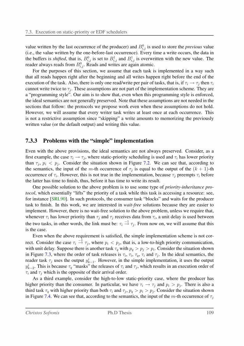
7.3. Execution on static-priority or EDF schedulers
value written by the last occurrence of the producer) and B0i,j is used to store the previous value
(i.e., the value written by the one-before-last occurrence). Every time a write occurs, the data in
the buffers is shifted, that is, B0i,j is set to B1
i,j and B1i,j is overwritten with the new value. The
reader always reads from B0i,j . Reads and writes are again atomic.
For the purposes of this section, we assume that each task is implemented in a way such
that all reads happen right after the beginning and all writes happen right before the end of the
execution of the task. Also, there is only one read/write per pair of tasks, that is, if τi → τj then τi
cannot write twice to τj . These assumptions are not part of the implementation scheme. They are
a “programming style”. Our aim is to show that, even when this programming style is enforced,
the ideal semantics are not generally preserved. Note that these assumptions are not needed in the
sections that follow: the protocols we propose work even when these assumptions do not hold.
However, we will assume that every writer task writes at least once at each occurrence. This
is not a restrictive assumption since “skipping” a write amounts to memorizing the previously
written value (or the default output) and writing this value.
7.3.3 Problems with the “simple” implementation
Even with the above provisions, the ideal semantics are not always preserved. Consider, as a
first example, the case τi → τj , where static-priority scheduling is used and τi has lower priority
than τj , pi < pj . Consider the situation shown in Figure 7.2. We can see that, according to
the semantics, the input of the m-th occurrence of τj is equal to the output of the (k + 1)-thoccurrence of τi. However, this is not true in the implementation, because τj preempts τi before
the latter has time to finish, thus, before it has time to write its result.
One possible solution to the above problem is to use some type of priority-inheritance pro-
tocol, which essentially “lifts” the priority of a task while this task is accessing a resource: see,
for instance [SRL90]. In such protocols, the consumer task “blocks” and waits for the producer
task to finish. In this work, we are interested in wait-free solutions because they are easier to
implement. However, there is no wait-free solution to the above problem, unless we require that,
whenever τi has lower priority than τj and τj receives data from τi, a unit delay is used between
the two tasks, in other words, the link must be: τi−1→ τj . From now on, we will assume that this
is the case.
Even when the above requirement is satisfied, the simple implementation scheme is not cor-
rect. Consider the case τi−1→ τj , where pi < pj , that is, a low-to-high priority communication,
with unit delay. Suppose there is another task τq with pq > pj > pi. Consider the situation shown
in Figure 7.3, where the order of task releases is τi, τi, τq, τi and τj . In the ideal semantics, the
reader task τj uses the output yik−1. However, in the simple implementation, it uses the output
yik−2. This is because τq “masks” the releases of τi and τj , which results in an execution order of
τi and τj which is the opposite of their arrival order.
As a third example, consider the high-to-low static-priority case, where the producer has
higher priority than the consumer. In particular, we have τi → τj and pi > pj . There is also a
third task τq with higher priority than both τi and τj , pq > pi > pj . Consider the situation shown
in Figure 7.4. We can see that, according to the semantics, the input of the m-th occurrence of τj
Christos Sofronis Ph.D Thesis 109
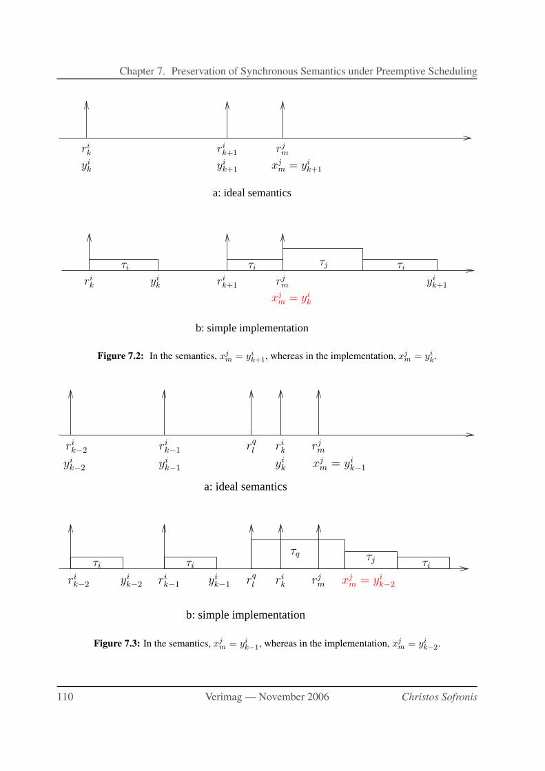
Chapter 7. Preservation of Synchronous Semantics under Preemptive Scheduling
a: ideal semantics
b: simple implementation
rik
yik
rik+1
yik+1
rjm
xjm = yi
k+1
rik
τi
yik
τiτj τi
rik+1
rjm yi
k+1
xjm = yi
k
Figure 7.2: In the semantics, xjm = yi
k+1, whereas in the implementation, xjm = yi
k.
a: ideal semantics
b: simple implementation
rikr
q
l rjm
xjm = yi
k−1yi
k
rik−2
yik−2
rik−1
yik−1
τi τi
τq
τiτj
rik−2
rq
l rik rj
mrik−1
yik−2
yik−1
xjm = yi
k−2
Figure 7.3: In the semantics, xjm = yi
k−1, whereas in the implementation, xjm = yi
k−2.
110 Verimag — November 2006 Christos Sofronis
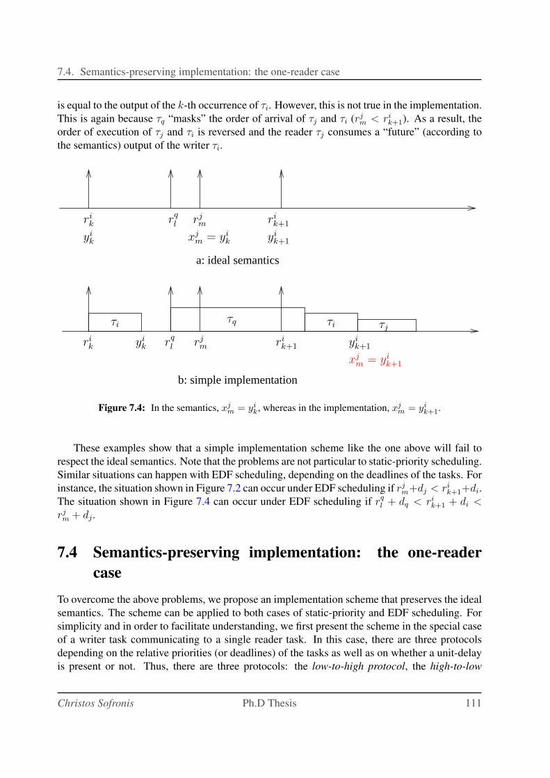
7.4. Semantics-preserving implementation: the one-reader case
is equal to the output of the k-th occurrence of τi. However, this is not true in the implementation.
This is again because τq “masks” the order of arrival of τj and τi (rjm < ri
k+1). As a result, the
order of execution of τj and τi is reversed and the reader τj consumes a “future” (according to
the semantics) output of the writer τi.
a: ideal semantics
b: simple implementation
rik
yik
rq
l rjm ri
k+1
xjm = yi
k yik+1
τj
rik+1
yik+1
xjm = yi
k+1
τiτiτq
rq
l rjmri
k yik
Figure 7.4: In the semantics, xjm = yi
k, whereas in the implementation, xjm = yi
k+1.
These examples show that a simple implementation scheme like the one above will fail to
respect the ideal semantics. Note that the problems are not particular to static-priority scheduling.
Similar situations can happen with EDF scheduling, depending on the deadlines of the tasks. For
instance, the situation shown in Figure 7.2 can occur under EDF scheduling if rjm+dj < ri
k+1+di.
The situation shown in Figure 7.4 can occur under EDF scheduling if rql + dq < ri
k+1 + di <rjm + dj .
7.4 Semantics-preserving implementation: the one-reader
case
To overcome the above problems, we propose an implementation scheme that preserves the ideal
semantics. The scheme can be applied to both cases of static-priority and EDF scheduling. For
simplicity and in order to facilitate understanding, we first present the scheme in the special case
of a writer task communicating to a single reader task. In this case, there are three protocols
depending on the relative priorities (or deadlines) of the tasks as well as on whether a unit-delay
is present or not. Thus, there are three protocols: the low-to-high protocol, the high-to-low
Christos Sofronis Ph.D Thesis 111
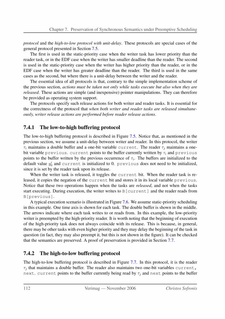
Chapter 7. Preservation of Synchronous Semantics under Preemptive Scheduling
protocol and the high-to-low protocol with unit-delay. These protocols are special cases of the
general protocol presented in Section 7.5.
The first is used in the static-priority case when the writer task has lower priority than the
reader task, or in the EDF case when the writer has smaller deadline than the reader. The second
is used in the static-priority case when the writer has higher priority than the reader, or in the
EDF case when the writer has greater deadline than the reader. The third is used in the same
cases as the second, but where there is a unit-delay between the writer and the reader.
The essential idea of all protocols is that, contrary to the simple implementation scheme of
the previous section, actions must be taken not only while tasks execute but also when they are
released. These actions are simple (and inexpensive) pointer manipulations. They can therefore
be provided as operating system support.
The protocols specify such release actions for both writer and reader tasks. It is essential for
the correctness of the protocol that when both writer and reader tasks are released simultane-
ously, writer release actions are performed before reader release actions.
7.4.1 The low-to-high buffering protocol
The low-to-high buffering protocol is described in Figure 7.5. Notice that, as mentioned in the
previous section, we assume a unit-delay between writer and reader. In this protocol, the writer
τi maintains a double buffer and a one-bit variable current. The reader τj maintains a one-
bit variable previous. current points to the buffer currently written by τi and previous
points to the buffer written by the previous occurrence of τi. The buffers are initialized to the
default value yi0 and current is initialized to 0. previous does not need to be initialized,
since it is set by the reader task upon its release.
When the writer task is released, it toggles the current bit. When the reader task is re-
leased, it copies the negation of the current bit and stores it in its local variable previous.
Notice that these two operations happen when the tasks are released, and not when the tasks
start executing. During execution, the writer writes to B[current] and the reader reads from
B[previous].
A typical execution scenario is illustrated in Figure 7.6. We assume static-priority scheduling
in this example. One time axis is shown for each task. The double buffer is shown in the middle.
The arrows indicate where each task writes to or reads from. In this example, the low-priority
writer is preempted by the high-priority reader. It is worth noting that the beginning of execution
of the high-priority task does not always coincide with its release. This is because, in general,
there may be other tasks with even higher priority and they may delay the beginning of the task in
question (in fact, they may also preempt it, but this is not shown in the figure). It can be checked
that the semantics are preserved. A proof of preservation is provided in Section 7.7.
7.4.2 The high-to-low buffering protocol
The high-to-low buffering protocol is described in Figure 7.7. In this protocol, it is the reader
τj that maintains a double buffer. The reader also maintains two one-bit variables current,
next. current points to the buffer currently being read by τj and next points to the buffer
112 Verimag — November 2006 Christos Sofronis
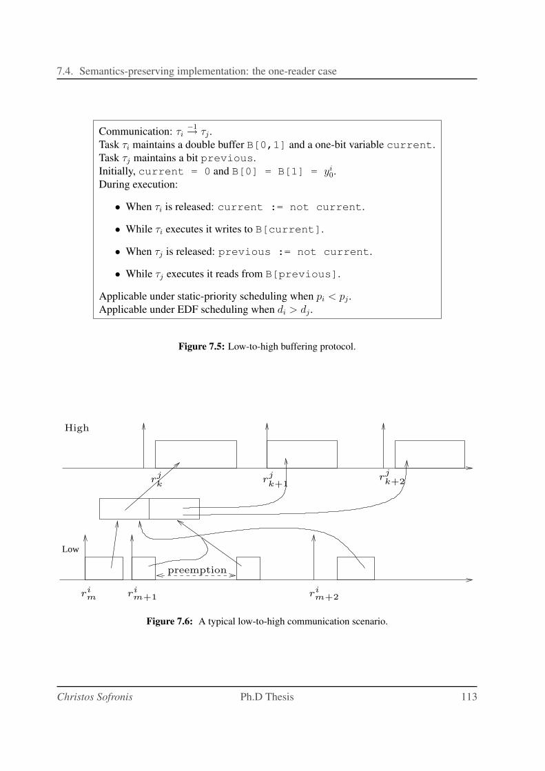
7.4. Semantics-preserving implementation: the one-reader case
Communication: τi−1→ τj .
Task τi maintains a double buffer B[0,1] and a one-bit variable current.
Task τj maintains a bit previous.
Initially, current = 0 and B[0] = B[1] = yi0.
During execution:
• When τi is released: current := not current.
• While τi executes it writes to B[current].
• When τj is released: previous := not current.
• While τj executes it reads from B[previous].
Applicable under static-priority scheduling when pi < pj .
Applicable under EDF scheduling when di > dj .
Figure 7.5: Low-to-high buffering protocol.
Low
High
rjk
rjk+2r
jk+1
rim+2r
im+1r
im
preemption
Figure 7.6: A typical low-to-high communication scenario.
Christos Sofronis Ph.D Thesis 113
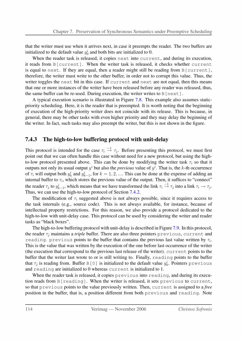
Chapter 7. Preservation of Synchronous Semantics under Preemptive Scheduling
that the writer must use when it arrives next, in case it preempts the reader. The two buffers are
initialized to the default value yi0 and both bits are initialized to 0.
When the reader task is released, it copies next into current, and during its execution,
it reads from B[current]. When the writer task is released, it checks whether current
is equal to next. If they are equal, then a reader might still be reading from B[current],
therefore, the writer must write to the other buffer, in order not to corrupt this value. Thus, the
writer toggles the next bit in this case. If current and next are not equal, then this means
that one or more instances of the writer have been released before any reader was released, thus,
the same buffer can be re-used. During execution, the writer writes to B[next].
A typical execution scenario is illustrated in Figure 7.8. This example also assumes static-
priority scheduling. Here, it is the reader that is preempted. It is worth noting that the beginning
of execution of the high-priority writer does not coincide with its release. This is because, in
general, there may be other tasks with even higher priority and they may delay the beginning of
the writer. In fact, such tasks may also preempt the writer, but this is not shown in the figure.
7.4.3 The high-to-low buffering protocol with unit-delay
This protocol is intended for the case τi−1→ τj . Before presenting this protocol, we must first
point out that we can often handle this case without need for a new protocol, but using the high-
to-low protocol presented above. This can be done by modifying the writer task τi so that it
outputs not only its usual output yi but also the previous value of yi. That is, the k-th occurrence
of τi will output both yik and yi
k−1, for k = 1, 2, .... This can be done at the expense of adding an
internal buffer to τi, which stores the previous value of the output. Then, it suffices to “connect”
the reader τj to yik−1, which means that we have transformed the link τi
−1→ τj into a link τi → τj .
Thus, we can use the high-to-low protocol of Section 7.4.2.
The modification of τi suggested above is not always possible, since it requires access to
the task internals (e.g., source code). This is not always available, for instance, because of
intellectual property restrictions. For this reason, we also provide a protocol dedicated to the
high-to-low with unit-delay case. This protocol can be used by considering the writer and reader
tasks as “black boxes”.
The high-to-low buffering protocol with unit-delay is described in Figure 7.9. In this protocol,
the reader τj maintains a triple buffer. There are also three pointers previous, current and
reading. previous points to the buffer that contains the previous last value written by τi.
This is the value that was written by the execution of the one before last occurrence of the writer
(the execution that correspond to the previous last release of the writer). current points to the
buffer that the writer last wrote to or is still writing to. Finally, reading points to the buffer
that τj is reading from. Buffer B[0] is initialized to the default value yi0. Pointers previous
and reading are initialized to 0 whereas current is initialized to 1.
When the reader task is released, it copies previous into reading, and during its execu-
tion reads from B[reading]. When the writer is released, it sets previous to current,
so that previous points to the value previously written. Then, current is assigned to a free
position in the buffer, that is, a position different from both previous and reading. Note
114 Verimag — November 2006 Christos Sofronis
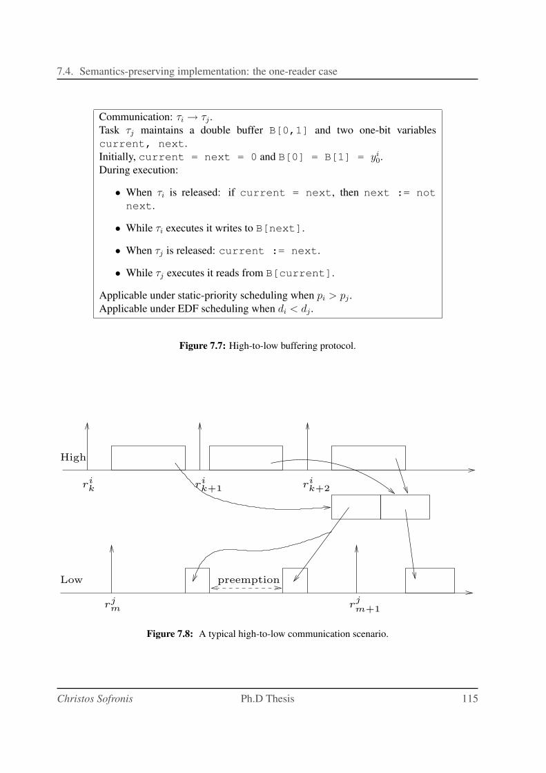
7.4. Semantics-preserving implementation: the one-reader case
Communication: τi → τj .
Task τj maintains a double buffer B[0,1] and two one-bit variables
current, next.
Initially, current = next = 0 and B[0] = B[1] = yi0.
During execution:
• When τi is released: if current = next, then next := not
next.
• While τi executes it writes to B[next].
• When τj is released: current := next.
• While τj executes it reads from B[current].
Applicable under static-priority scheduling when pi > pj .
Applicable under EDF scheduling when di < dj .
Figure 7.7: High-to-low buffering protocol.
Low
High
rik r
ik+1
rik+2
rjm r
jm+1
preemption
Figure 7.8: A typical high-to-low communication scenario.
Christos Sofronis Ph.D Thesis 115
Chapter 7. Preservation of Synchronous Semantics under Preemptive Scheduling
that after the first execution the previous pointer will still point in the first buffer which has
the default value.
7.4.4 Some examples under EDF scheduling
All examples we have given so far have assumed static-priority scheduling. It is probably easier
for the reader to be persuaded of the correctness of the protocols in the static-priority case, before
going to the other scheduling policy, the EDF.
In this section, we provide some informal arguments and examples to justify intuitively why
the protocols can also be applied to EDF. Notice that, a priori, one might think that the protocols
are not applicable to EDF, for the following reason. Under EDF, the priorities of tasks change
dynamically. On the other hand, the above protocols have been designed assuming a static
priority assignment to the writer and the reader. Indeed, if the two priorities are swapped, a
different protocol must be used. These facts could lead one to conclude that, under EDF, the
buffering scheme needs to be dynamic as well.
Fortunately, this is not the case: the buffering scheme can be defined statically, that is, before
execution begins. In particular, the buffering scheme depends on the relative deadlines di and dj
of the writer τi and the reader τj , respectively.
• If di > dj then the low-to-high buffering scheme is used. Again, we assume a unit-delay
between τi and τj , in order to avoid the problem of Figure 7.2.
• If di < dj and τi → τj , then the high-to-low buffering scheme is used.
• If di < dj and τi−1→ τj , then the high-to-low with unit-delay scheme is used.
The case di > dj implies that, if τj is released before τi then τi cannot preempt τj , neither
can it start before τi ends. Indeed, rjk ≤ ri
m and dj < di implies rjk + dj < ri
m + di, that is, the
absolute deadline of τj is smaller than that of τi. Therefore, we have a situation which is “almost
the same” as the low-to-high static-priority case. The difference is that in the static-priority case
τj always preempts τi, whereas in the EDF case this might not happen. Therefore, in order to
guarantee the correctness of the scheme, we must examine this last possibility, to ensure that
nothing goes wrong.
Figure 7.11 illustrates what might happen when τj does not preempt τi as it normally would in
the low-to-high static-priority scenario. One can see that this poses no problems for the buffering
scheme. In fact, the situation is as if the k-th instance of τj was released after the (m + 1)-thinstance of τi finished.
Let us now turn to the case di < dj . This case implies that, if τi is released before τj then
τj cannot preempt τi, neither can it start before τi ends. Indeed, rik ≤ rj
m and di < dj implies
rik + di < rj
m + dj , that is, the absolute deadline of τi is smaller than that of τj . Therefore, we
have a situation which is “almost the same” as the high-to-low priority case. The difference is
that in the high-to-low priority case τi always preempts τj , whereas in the EDF case this might
not happen. As before, we must examine this possibility.
116 Verimag — November 2006 Christos Sofronis
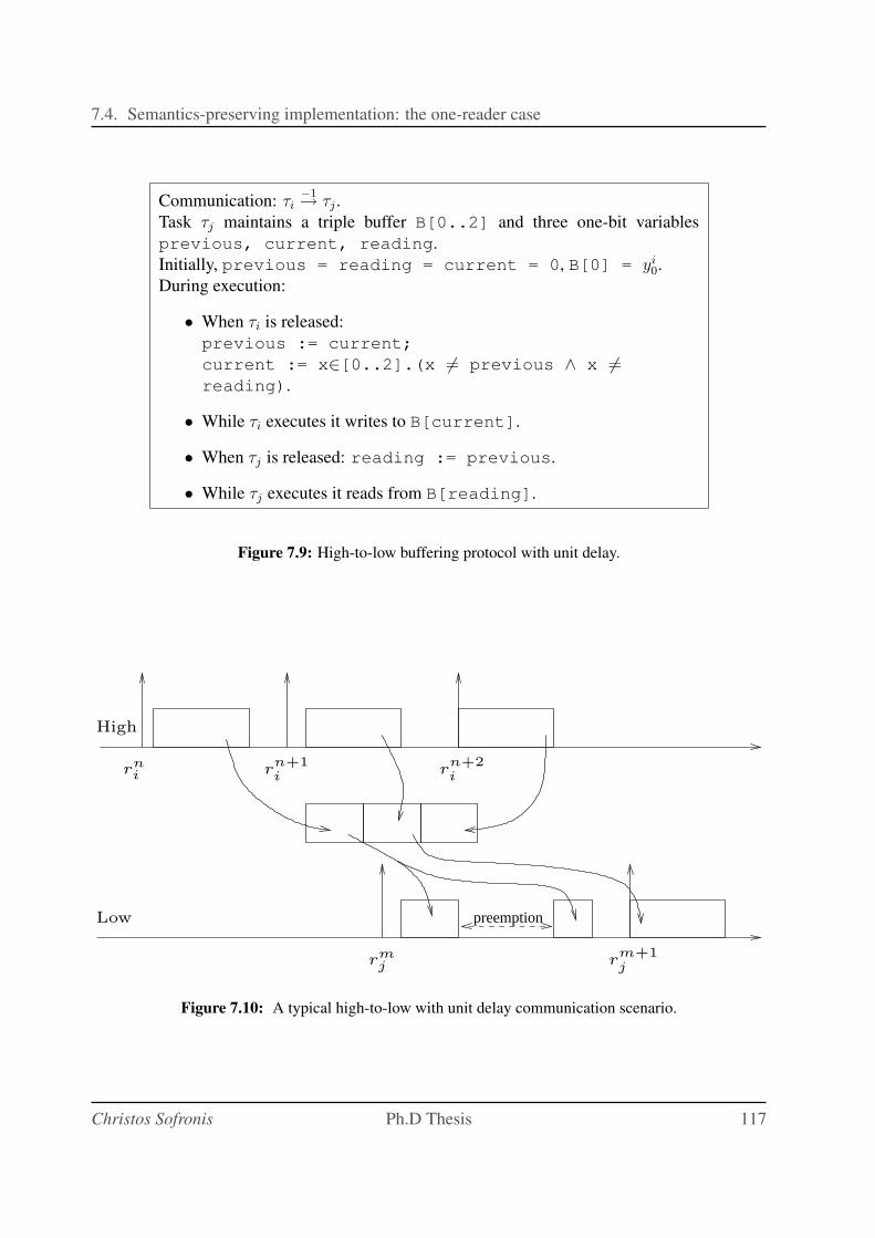
7.4. Semantics-preserving implementation: the one-reader case
Communication: τi−1→ τj .
Task τj maintains a triple buffer B[0..2] and three one-bit variables
previous, current, reading.
Initially, previous = reading = current = 0, B[0] = yi0.
During execution:
• When τi is released:
previous := current;
current := x∈[0..2].(x 6= previous ∧ x 6=reading).
• While τi executes it writes to B[current].
• When τj is released: reading := previous.
• While τj executes it reads from B[reading].
Figure 7.9: High-to-low buffering protocol with unit delay.
preemptionLow
High
rmj
rni r
n+1
ir
n+2
i
rm+1
j
Figure 7.10: A typical high-to-low with unit delay communication scenario.
Christos Sofronis Ph.D Thesis 117
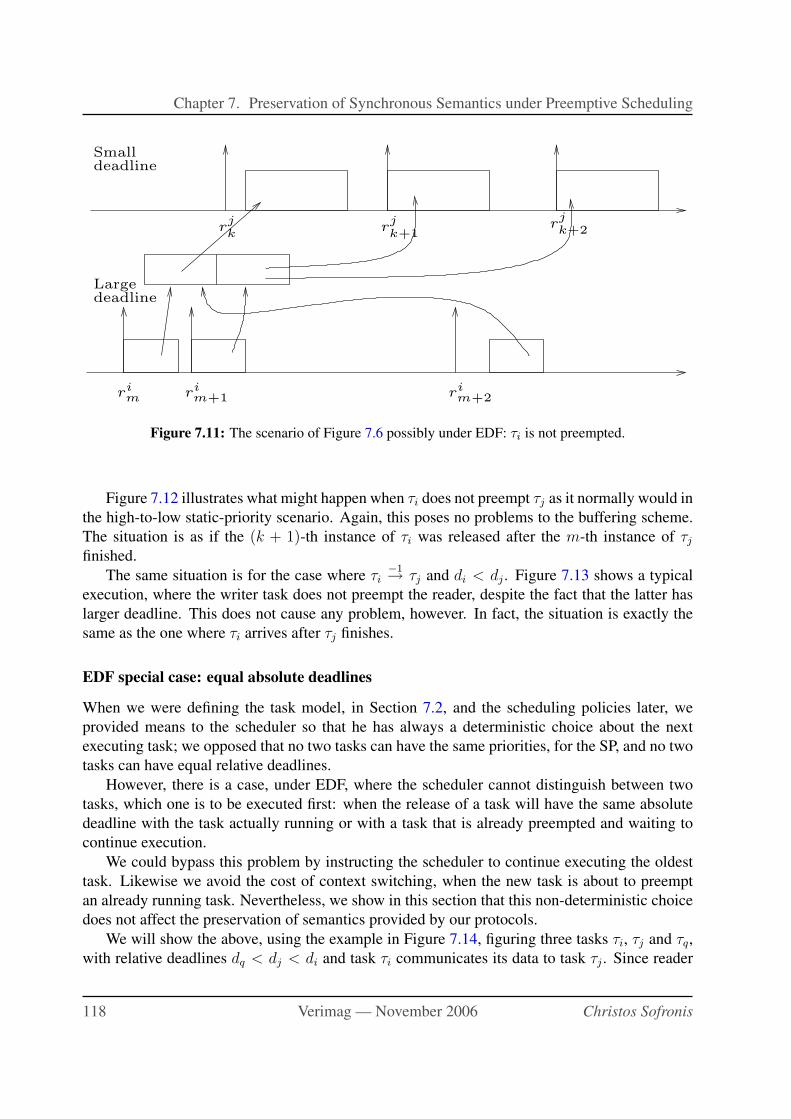
Chapter 7. Preservation of Synchronous Semantics under Preemptive Scheduling
deadlineLarge
Smalldeadline
rjk
rjk+2r
jk+1
rim+2r
im+1r
im
Figure 7.11: The scenario of Figure 7.6 possibly under EDF: τi is not preempted.
Figure 7.12 illustrates what might happen when τi does not preempt τj as it normally would in
the high-to-low static-priority scenario. Again, this poses no problems to the buffering scheme.
The situation is as if the (k + 1)-th instance of τi was released after the m-th instance of τj
finished.
The same situation is for the case where τi−1→ τj and di < dj . Figure 7.13 shows a typical
execution, where the writer task does not preempt the reader, despite the fact that the latter has
larger deadline. This does not cause any problem, however. In fact, the situation is exactly the
same as the one where τi arrives after τj finishes.
EDF special case: equal absolute deadlines
When we were defining the task model, in Section 7.2, and the scheduling policies later, we
provided means to the scheduler so that he has always a deterministic choice about the next
executing task; we opposed that no two tasks can have the same priorities, for the SP, and no two
tasks can have equal relative deadlines.
However, there is a case, under EDF, where the scheduler cannot distinguish between two
tasks, which one is to be executed first: when the release of a task will have the same absolute
deadline with the task actually running or with a task that is already preempted and waiting to
continue execution.
We could bypass this problem by instructing the scheduler to continue executing the oldest
task. Likewise we avoid the cost of context switching, when the new task is about to preempt
an already running task. Nevertheless, we show in this section that this non-deterministic choice
does not affect the preservation of semantics provided by our protocols.
We will show the above, using the example in Figure 7.14, figuring three tasks τi, τj and τq,
with relative deadlines dq < dj < di and task τi communicates its data to task τj . Since reader
118 Verimag — November 2006 Christos Sofronis
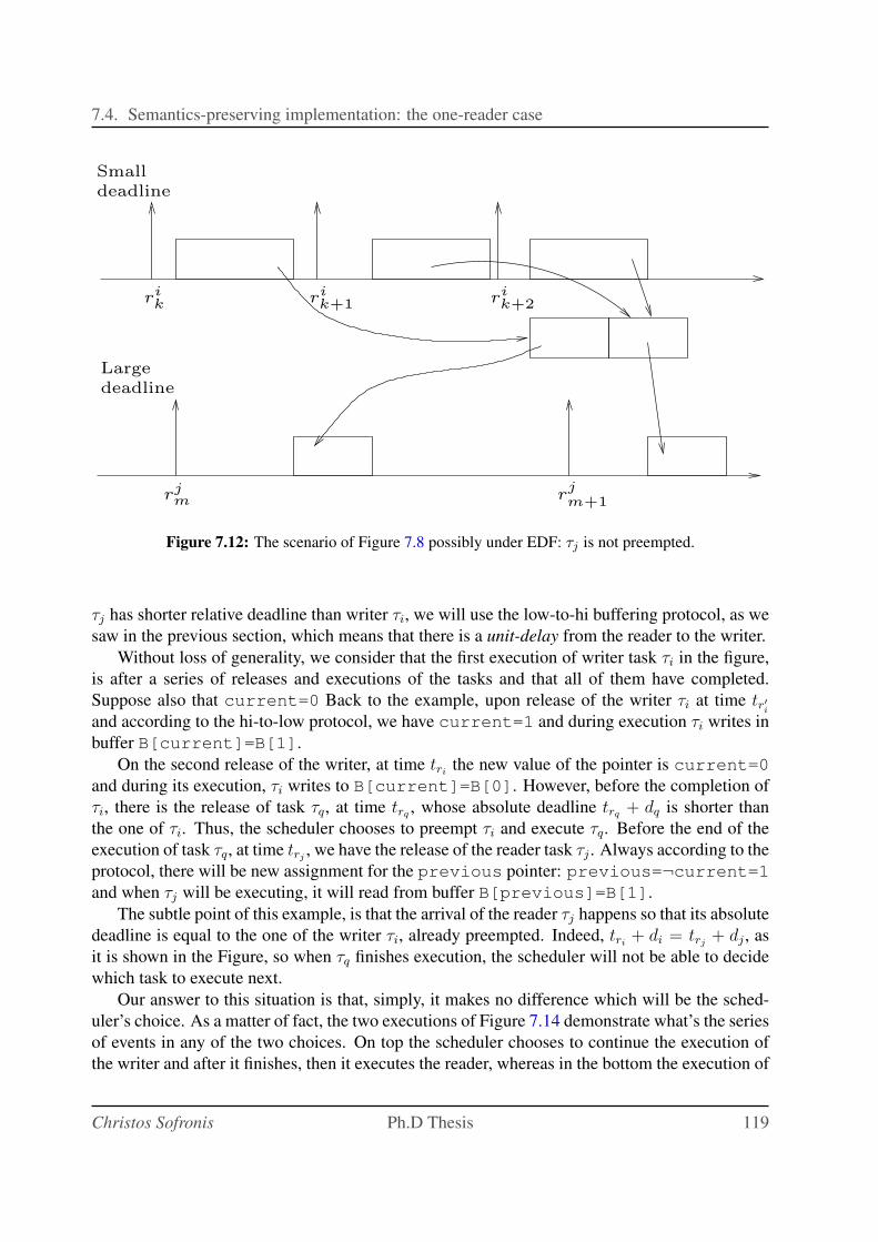
7.4. Semantics-preserving implementation: the one-reader case
Small
deadline
deadline
Large
rjm r
jm+1
rik+1
rik+2
rik
Figure 7.12: The scenario of Figure 7.8 possibly under EDF: τj is not preempted.
τj has shorter relative deadline than writer τi, we will use the low-to-hi buffering protocol, as we
saw in the previous section, which means that there is a unit-delay from the reader to the writer.
Without loss of generality, we consider that the first execution of writer task τi in the figure,
is after a series of releases and executions of the tasks and that all of them have completed.
Suppose also that current=0 Back to the example, upon release of the writer τi at time tr′i
and according to the hi-to-low protocol, we have current=1 and during execution τi writes in
buffer B[current]=B[1].
On the second release of the writer, at time trithe new value of the pointer is current=0
and during its execution, τi writes to B[current]=B[0]. However, before the completion of
τi, there is the release of task τq, at time trq, whose absolute deadline trq
+ dq is shorter than
the one of τi. Thus, the scheduler chooses to preempt τi and execute τq. Before the end of the
execution of task τq, at time trj, we have the release of the reader task τj . Always according to the
protocol, there will be new assignment for the previous pointer: previous=¬current=1and when τj will be executing, it will read from buffer B[previous]=B[1].
The subtle point of this example, is that the arrival of the reader τj happens so that its absolute
deadline is equal to the one of the writer τi, already preempted. Indeed, tri+ di = trj
+ dj , as
it is shown in the Figure, so when τq finishes execution, the scheduler will not be able to decide
which task to execute next.
Our answer to this situation is that, simply, it makes no difference which will be the sched-
uler’s choice. As a matter of fact, the two executions of Figure 7.14 demonstrate what’s the series
of events in any of the two choices. On top the scheduler chooses to continue the execution of
the writer and after it finishes, then it executes the reader, whereas in the bottom the execution of
Christos Sofronis Ph.D Thesis 119
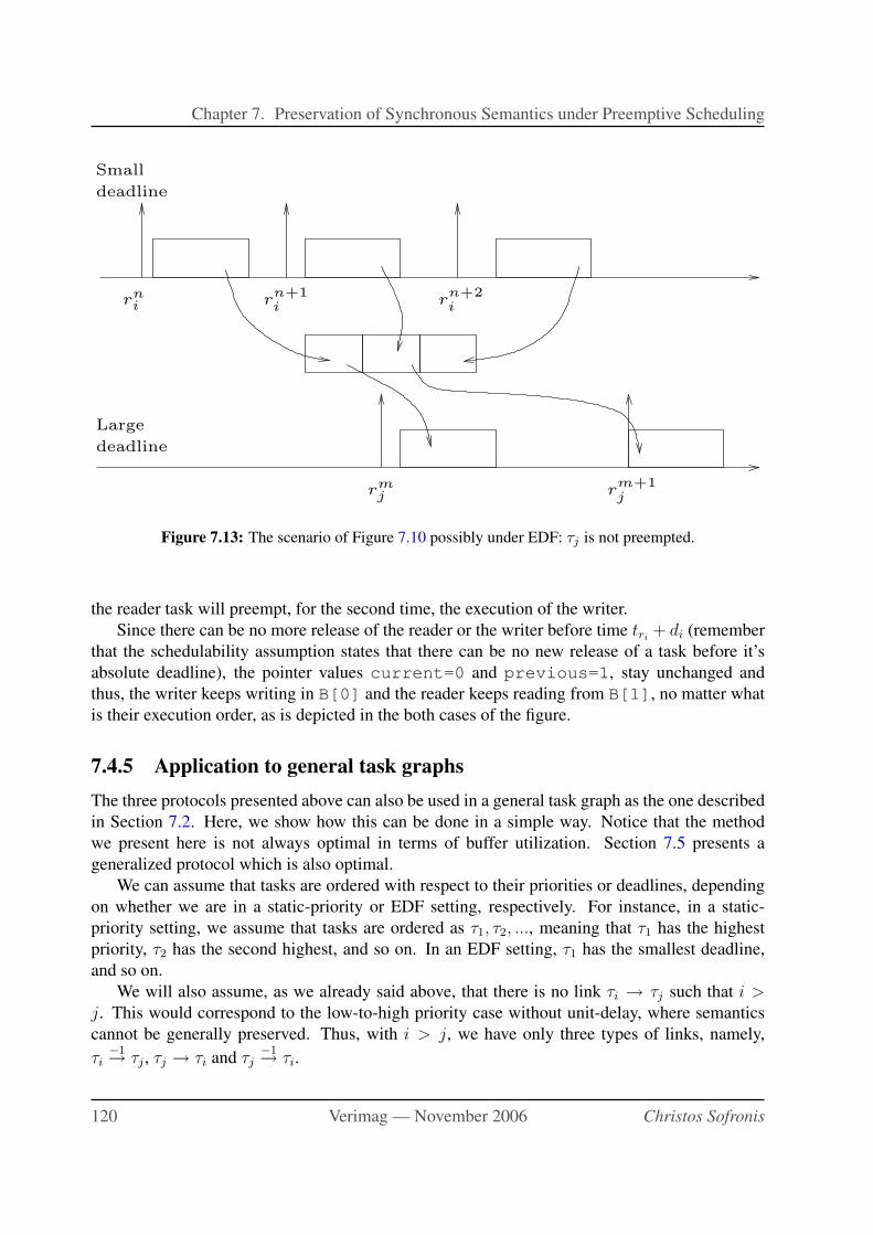
Chapter 7. Preservation of Synchronous Semantics under Preemptive Scheduling
Large
deadline
rmj
rni r
n+1
ir
n+2
i
rm+1
j
Small
deadline
Figure 7.13: The scenario of Figure 7.10 possibly under EDF: τj is not preempted.
the reader task will preempt, for the second time, the execution of the writer.
Since there can be no more release of the reader or the writer before time tri+ di (remember
that the schedulability assumption states that there can be no new release of a task before it’s
absolute deadline), the pointer values current=0 and previous=1, stay unchanged and
thus, the writer keeps writing in B[0] and the reader keeps reading from B[1], no matter what
is their execution order, as is depicted in the both cases of the figure.
7.4.5 Application to general task graphs
The three protocols presented above can also be used in a general task graph as the one described
in Section 7.2. Here, we show how this can be done in a simple way. Notice that the method
we present here is not always optimal in terms of buffer utilization. Section 7.5 presents a
generalized protocol which is also optimal.
We can assume that tasks are ordered with respect to their priorities or deadlines, depending
on whether we are in a static-priority or EDF setting, respectively. For instance, in a static-
priority setting, we assume that tasks are ordered as τ1, τ2, ..., meaning that τ1 has the highest
priority, τ2 has the second highest, and so on. In an EDF setting, τ1 has the smallest deadline,
and so on.
We will also assume, as we already said above, that there is no link τi → τj such that i >j. This would correspond to the low-to-high priority case without unit-delay, where semantics
cannot be generally preserved. Thus, with i > j, we have only three types of links, namely,
τi−1→ τj , τj → τi and τj
−1→ τi.
120 Verimag — November 2006 Christos Sofronis
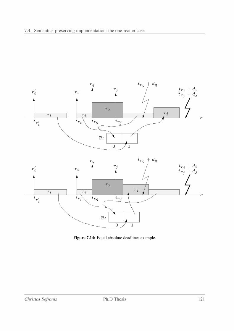
7.4. Semantics-preserving implementation: the one-reader case
rj
rj
τi
ri trj+ dj
tri+ di
trj+ dj
tri+ di
rq
τj
rq
ri
τq
τi
τq
τj
τi
τi
trq + dq
trq + dq
tritrq trj
tritrq trj
tr′
i
tr′
i
r′
i
r′
i
0 1
B:
B:
0 1
Figure 7.14: Equal absolute deadlines example.
Christos Sofronis Ph.D Thesis 121
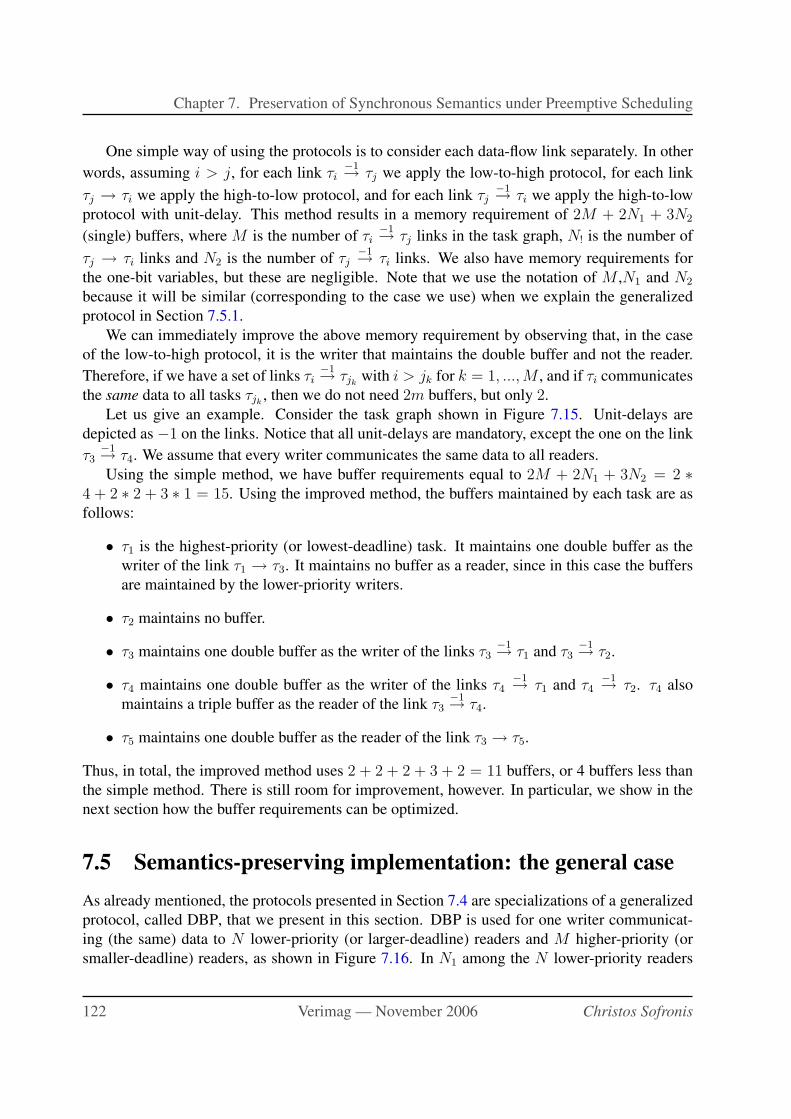
Chapter 7. Preservation of Synchronous Semantics under Preemptive Scheduling
One simple way of using the protocols is to consider each data-flow link separately. In other
words, assuming i > j, for each link τi−1→ τj we apply the low-to-high protocol, for each link
τj → τi we apply the high-to-low protocol, and for each link τj−1→ τi we apply the high-to-low
protocol with unit-delay. This method results in a memory requirement of 2M + 2N1 + 3N2
(single) buffers, where M is the number of τi−1→ τj links in the task graph, N! is the number of
τj → τi links and N2 is the number of τj−1→ τi links. We also have memory requirements for
the one-bit variables, but these are negligible. Note that we use the notation of M ,N1 and N2
because it will be similar (corresponding to the case we use) when we explain the generalized
protocol in Section 7.5.1.
We can immediately improve the above memory requirement by observing that, in the case
of the low-to-high protocol, it is the writer that maintains the double buffer and not the reader.
Therefore, if we have a set of links τi−1→ τjk
with i > jk for k = 1, ...,M , and if τi communicates
the same data to all tasks τjk, then we do not need 2m buffers, but only 2.
Let us give an example. Consider the task graph shown in Figure 7.15. Unit-delays are
depicted as −1 on the links. Notice that all unit-delays are mandatory, except the one on the link
τ3−1→ τ4. We assume that every writer communicates the same data to all readers.
Using the simple method, we have buffer requirements equal to 2M + 2N1 + 3N2 = 2 ∗4 + 2 ∗ 2 + 3 ∗ 1 = 15. Using the improved method, the buffers maintained by each task are as
follows:
• τ1 is the highest-priority (or lowest-deadline) task. It maintains one double buffer as the
writer of the link τ1 → τ3. It maintains no buffer as a reader, since in this case the buffers
are maintained by the lower-priority writers.
• τ2 maintains no buffer.
• τ3 maintains one double buffer as the writer of the links τ3−1→ τ1 and τ3
−1→ τ2.
• τ4 maintains one double buffer as the writer of the links τ4−1→ τ1 and τ4
−1→ τ2. τ4 also
maintains a triple buffer as the reader of the link τ3−1→ τ4.
• τ5 maintains one double buffer as the reader of the link τ3 → τ5.
Thus, in total, the improved method uses 2 + 2 + 2 + 3 + 2 = 11 buffers, or 4 buffers less than
the simple method. There is still room for improvement, however. In particular, we show in the
next section how the buffer requirements can be optimized.
7.5 Semantics-preserving implementation: the general case
As already mentioned, the protocols presented in Section 7.4 are specializations of a generalized
protocol, called DBP, that we present in this section. DBP is used for one writer communicat-
ing (the same) data to N lower-priority (or larger-deadline) readers and M higher-priority (or
smaller-deadline) readers, as shown in Figure 7.16. In N1 among the N lower-priority readers
122 Verimag — November 2006 Christos Sofronis
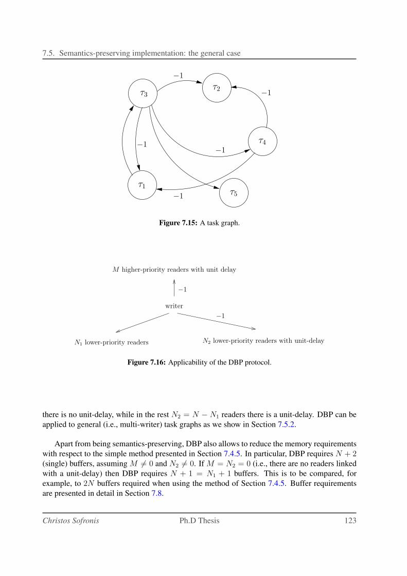
7.5. Semantics-preserving implementation: the general case
τ5
τ1
τ3
τ2
τ4
−1
−1
−1
−1
−1
Figure 7.15: A task graph.
N1 lower-priority readers N2 lower-priority readers with unit-delay
writer
M higher-priority readers with unit delay
−1
−1
Figure 7.16: Applicability of the DBP protocol.
there is no unit-delay, while in the rest N2 = N − N1 readers there is a unit-delay. DBP can be
applied to general (i.e., multi-writer) task graphs as we show in Section 7.5.2.
Apart from being semantics-preserving, DBP also allows to reduce the memory requirements
with respect to the simple method presented in Section 7.4.5. In particular, DBP requires N + 2(single) buffers, assuming M 6= 0 and N2 6= 0. If M = N2 = 0 (i.e., there are no readers linked
with a unit-delay) then DBP requires N + 1 = N1 + 1 buffers. This is to be compared, for
example, to 2N buffers required when using the method of Section 7.4.5. Buffer requirements
are presented in detail in Section 7.8.
Christos Sofronis Ph.D Thesis 123
Chapter 7. Preservation of Synchronous Semantics under Preemptive Scheduling
7.5.1 The Dynamic Buffering Protocol
DBP is shown in Figure 7.17. The figure shows the protocol in the case where M 6= 0 or
N2 6= 0, that is, the case where there are links with unit-delay. If M = N2 = 0 then the protocol
is actually simpler: the pointer previous is not needed and instead of N + 2 = N1 + 2, only
N1 + 1 buffers are needed.
The operation of DBP is as follows. The writer τw maintains all buffers and pointers except
the pointers of the higher-priority readers P[i]. The current pointer points to the position
that the writer last wrote to. The previous pointer points to the position that the writer wrote
to before that. R[i] points to the position that τi must read from.
The key point is that when the writer is released, a free position in the buffer array must
be found, and this is where the writer must write to. By free we mean a position which is not
currently in use by any reader, as defined by the predicate free(j). Finding a free j ∈ [1..N +2] amounts to finding some j which is different from previous (because B[previous] may
be used by the higher-priority reader or a possible lower-priority with unit-delay reader may need
to copy its value) and also different from all R[i] (because B[R[i]] is used, or will be used,
by the lower-priority reader τi). Notice that such a j always exists, by the pigeon-hole principle:
there are N + 2 possible values for j and up to N + 1 possible values for previous and all
R[i].
Finding a free position is done in the second instruction executed upon the release of the
writer. The first instruction updates the previous pointer. This pointer is copied by each
higher-priority reader τ ′i , when released, into its local variable P[i]. τ ′
i then reads from
B[P[i]].
When a lower-priority reader τi is released, we have two cases: (i) either τi is one of the
N1 readers that are linked without a unit-delay, or (ii) τi is one of the N2 readers that are linked
with unit-delay. In case (i) τi needs the last value written by the writer. In case (ii) τi needs the
previous value. Pointer R[i] is set to the needed value. Besides this pointer assignment the
rest of the procedure remains the same for both kinds of lower-priority readers. While executing,
τi reads from B[R[i]]. When τi finishes execution, R[i] is set to null. This is done for
optimization purposes, so that buffers can be re-used as early as possible. Notice that even if this
operation is removed, DBP will still be correct and it will use at most N + 2 buffers. However,
DBP will be sub-optimal, in the sense that the buffer pointed to by R[i] will not be freed until
the next release of τi. With the above operation present, the buffer is freed earlier, namely, when
the current release of τi finishes.
Notice that DBP also relies on the fact that no more than one instance of every task can be
active at any point in time, which follows from the schedulability assumption. In more detail,
there can be no more than one pointer per lower-priority task, which allow us to use the pigeon
hole principle as we did before.
Like the protocols discussed in the previous section, DBP also specifies release actions for
both writer and reader tasks. In case of simultaneous release of more than one tasks, we re-
quire that the release actions of the writer task are performed before the release actions of the
simultaneously released readers. The actions of the readers can be performed in any order.
Another major contribution of the above algorithm is that it does not take into account any
124 Verimag — November 2006 Christos Sofronis
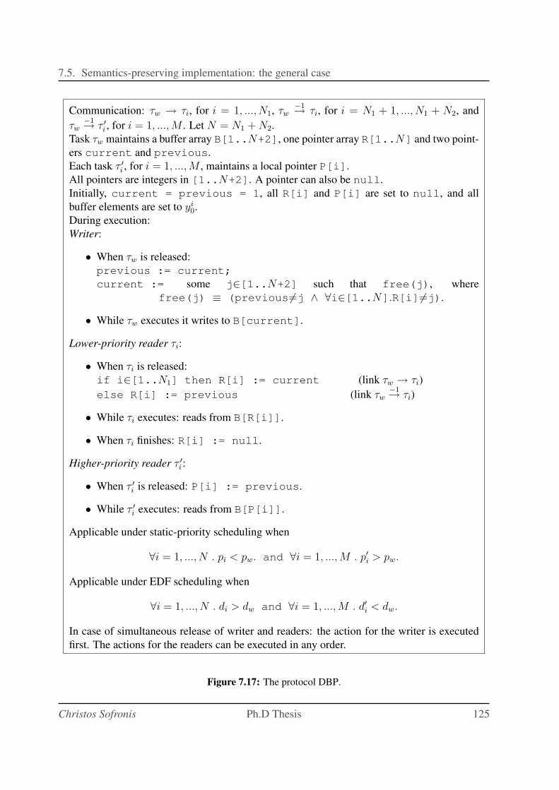
7.5. Semantics-preserving implementation: the general case
Communication: τw → τi, for i = 1, ..., N1, τw−1→ τi, for i = N1 + 1, ..., N1 + N2, and
τw−1→ τ ′
i , for i = 1, ...,M . Let N = N1 + N2.
Task τw maintains a buffer array B[1..N+2], one pointer array R[1..N] and two point-
ers current and previous.
Each task τ ′i , for i = 1, ...,M , maintains a local pointer P[i].
All pointers are integers in [1..N+2]. A pointer can also be null.
Initially, current = previous = 1, all R[i] and P[i] are set to null, and all
buffer elements are set to yi0.
During execution:
Writer:
• When τw is released:
previous := current;
current := some j∈[1..N+2] such that free(j), where
free(j) ≡ (previous6=j ∧ ∀i∈[1..N].R[i]6=j).
• While τw executes it writes to B[current].
Lower-priority reader τi:
• When τi is released:
if i∈[1..N1] then R[i] := current (link τw → τi)
else R[i] := previous (link τw−1→ τi)
• While τi executes: reads from B[R[i]].
• When τi finishes: R[i] := null.
Higher-priority reader τ ′i :
• When τ ′i is released: P[i] := previous.
• While τ ′i executes: reads from B[P[i]].
Applicable under static-priority scheduling when
∀i = 1, ..., N . pi < pw. and ∀i = 1, ...,M . p′i > pw.
Applicable under EDF scheduling when
∀i = 1, ..., N . di > dw and ∀i = 1, ...,M . d′i < dw.
In case of simultaneous release of writer and readers: the action for the writer is executed
first. The actions for the readers can be executed in any order.
Figure 7.17: The protocol DBP.
Christos Sofronis Ph.D Thesis 125
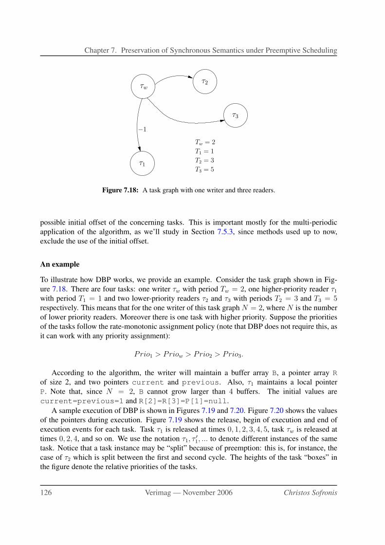
Chapter 7. Preservation of Synchronous Semantics under Preemptive Scheduling
−1
τ2
τ1
τ3
T1 = 1
T2 = 3
T3 = 5
Tw = 2
τw
Figure 7.18: A task graph with one writer and three readers.
possible initial offset of the concerning tasks. This is important mostly for the multi-periodic
application of the algorithm, as we’ll study in Section 7.5.3, since methods used up to now,
exclude the use of the initial offset.
An example
To illustrate how DBP works, we provide an example. Consider the task graph shown in Fig-
ure 7.18. There are four tasks: one writer τw with period Tw = 2, one higher-priority reader τ1
with period T1 = 1 and two lower-priority readers τ2 and τ3 with periods T2 = 3 and T3 = 5respectively. This means that for the one writer of this task graph N = 2, where N is the number
of lower priority readers. Moreover there is one task with higher priority. Suppose the priorities
of the tasks follow the rate-monotonic assignment policy (note that DBP does not require this, as
it can work with any priority assignment):
Prio1 > Priow > Prio2 > Prio3.
According to the algorithm, the writer will maintain a buffer array B, a pointer array R
of size 2, and two pointers current and previous. Also, τ1 maintains a local pointer
P. Note that, since N = 2, B cannot grow larger than 4 buffers. The initial values are
current=previous=1 and R[2]=R[3]=P[1]=null.
A sample execution of DBP is shown in Figures 7.19 and 7.20. Figure 7.20 shows the values
of the pointers during execution. Figure 7.19 shows the release, begin of execution and end of
execution events for each task. Task τ1 is released at times 0, 1, 2, 3, 4, 5, task τw is released at
times 0, 2, 4, and so on. We use the notation τ1, τ′1, ... to denote different instances of the same
task. Notice that a task instance may be “split” because of preemption: this is, for instance, the
case of τ2 which is split between the first and second cycle. The heights of the task “boxes” in
the figure denote the relative priorities of the tasks.
126 Verimag — November 2006 Christos Sofronis
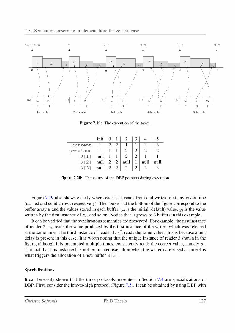
7.5. Semantics-preserving implementation: the general case
B0: B1: B2: B3: B4:y0 y1 y0 y1 y1y2 y2 y1 y1y2 y3
τ′′
1τ′
1τ1
τw τ2 τ3
τ′
w τ3τ2
τ′′′
1τ′
2 τ3
τ′′′′
1τ′′
w τ3
τw, τ1, τ2, τ3 τ1 τw, τ1 τw, τ1 τ1, τ3τ1, τ2
10 2 3 4 5
1 2 1 2 1 2 31 21 2
2nd cycle 3rd cycle 4th cycle 5th cycle1st cycle
Figure 7.19: The execution of the tasks.
init 0 1 2 3 4 5
current 1 2 2 1 1 3 3
previous 1 1 1 2 2 2 2
P[1] null 1 1 2 2 1 1
R[2] null 2 2 null 1 null null
R[3] null 2 2 2 2 2 3
Figure 7.20: The values of the DBP pointers during execution.
Figure 7.19 also shows exactly where each task reads from and writes to at any given time
(dashed and solid arrows respectively). The “boxes” at the bottom of the figure correspond to the
buffer array B and the values stored in each buffer: y0 is the initial (default) value, y1 is the value
written by the first instance of τw, and so on. Notice that B grows to 3 buffers in this example.
It can be verified that the synchronous semantics are preserved. For example, the first instance
of reader 2, τ2, reads the value produced by the first instance of the writer, which was released
at the same time. The third instance of reader 1, τ ′′1 , reads the same value: this is because a unit
delay is present in this case. It is worth noting that the unique instance of reader 3 shown in the
figure, although it is preempted multiple times, consistently reads the correct value, namely y1.
The fact that this instance has not terminated execution when the writer is released at time 4 is
what triggers the allocation of a new buffer B[3].
Specializations
It can be easily shown that the three protocols presented in Section 7.4 are specializations of
DBP. First, consider the low-to-high protocol (Figure 7.5). It can be obtained by using DBP with
Christos Sofronis Ph.D Thesis 127
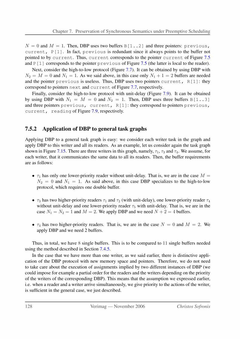
Chapter 7. Preservation of Synchronous Semantics under Preemptive Scheduling
N = 0 and M = 1. Then, DBP uses two buffers B[1..2] and three pointers: previous,
current, P[1]. In fact, previous is redundant since it always points to the buffer not
pointed to by current. Thus, current corresponds to the pointer current of Figure 7.5
and P[1] corresponds to the pointer previous of Figure 7.5 (the latter is local to the reader).
Next, consider the high-to-low protocol (Figure 7.7). It can be obtained by using DBP with
N2 = M = 0 and N1 = 1. As we said above, in this case only N1 + 1 = 2 buffers are needed
and the pointer previous is useless. Thus, DBP uses two pointers current, R[1]: they
correspond to pointers next and current of Figure 7.7, respectively.
Finally, consider the high-to-low protocol with unit-delay (Figure 7.9). It can be obtained
by using DBP with N1 = M = 0 and N2 = 1. Then, DBP uses three buffers B[1..3]
and three pointers previous, current, R[1]: they correspond to pointers previous,
current, reading of Figure 7.9, respectively.
7.5.2 Application of DBP to general task graphs
Applying DBP to a general task graph is easy: we consider each writer task in the graph and
apply DBP to this writer and all its readers. As an example, let us consider again the task graph
shown in Figure 7.15. There are three writers in this graph, namely, τ1, τ3 and τ4. We assume, for
each writer, that it communicates the same data to all its readers. Then, the buffer requirements
are as follows:
• τ1 has only one lower-priority reader without unit-delay. That is, we are in the case M =N2 = 0 and N1 = 1. As said above, in this case DBP specializes to the high-to-low
protocol, which requires one double buffer.
• τ3 has two higher-priority readers τ1 and τ2 (with unit-delay), one lower-priority reader τ4
without unit-delay and one lower-priority reader τ5 with unit-delay. That is, we are in the
case N1 = N2 = 1 and M = 2. We apply DBP and we need N + 2 = 4 buffers.
• τ4 has two higher-priority readers. That is, we are in the case N = 0 and M = 2. We
apply DBP and we need 2 buffers.
Thus, in total, we have 8 single buffers. This is to be compared to 11 single buffers needed
using the method described in Section 7.4.5.
In the case that we have more than one writer, as we said earlier, there is distinctive appli-
cation of the DBP protocol with new memory space and pointers. Therefore, we do not need
to take care about the execution of assignments implied by two different instances of DBP (we
could impose for example a partial order for the readers and the writers depending on the priority
of the writers of the corresponding DBP). This means that the assumption we expressed earlier,
i.e. when a reader and a writer arrive simultaneously, we give priority to the actions of the writer,
is sufficient in the general case, we just described.
128 Verimag — November 2006 Christos Sofronis

7.6. Periods in consecutive powers of two
7.5.3 Application of DBP to tasks with known arrival pattern
We have seen that the three protocols, described in Section 7.4, are correct for any arrival pat-
tern. The same holds for DBP as well. In this section we examine the application of DBP to
applications where the triggering pattern of tasks is known, for instance, multi-periodic applica-
tions where each task is periodic with a known period. We will see that in this case DBP can be
optimized, taking advantage of the additional knowledge on the arrival patterns. In this section
we discuss a time optimization, which aims at turning DBP into a static rather than dynamic
protocol. In Section 7.8 we discuss memory optimizations.
DBP, being a dynamic protocol in general, implies an overhead, namely, searching for a free
buffer to use every time the writer is released. To this overhead must be added the time to allocate
a buffer on-the-fly, or the “waste” of memory in case buffers are pre-allocated. We can do better
if we know the arrival pattern of the tasks, by providing a static schedule. This can be done
by simulating the DBP with the, a priori known, release times of the reader(s) and writer tasks.
During simulation we keep track where the writer stores data on every execution and from where
the reader(s) read from, on every execution as well. Those positions are instructed by DBP and
more precisely, for the writer it is the current pointer and for the reader task τi it is the pointer
R[i].
This simulation must be done until the hyper-period of the tasks. In the case where the tasks
are multi-periodic, this hyper-period Th is the least common multiplier of all periods. If tasks
are not multi-periodic then we will have to find a point where the arrival pattern starts repeating.
If that point doesn’t exist either, we will have to keep track for the entire possible execution of
the system. This last one, of course, may be very inefficient in case the execution is not short,
causing the static schedule to be enormous in terms of memory (to remember where the readers
and writer read from and writes to).
7.6 Periods in consecutive powers of two
We further investigate special cases of applications for which the periods are powers of two.
We also consider one additional factor, whether we have atomic reads and writes or not. If data
transfer is instantaneous then we can further optimize the system since the scheduling constraints
allow earlier release of buffer space.
7.6.1 Non-atomic case
Consider n tasks, τ1, ..., τn, such that task τi has period Ti = 2i−1 and a priority which is in
inverse order of period. Suppose each task sends data to all lower-priority tasks. For three tasks
of periods T1 = 1, T2 = 2 and T3 = 4, this gives the situation shown in Figure 7.21.
We assume that for simultaneous occurrences, the higher-priority task takes precedence and
thus transmits its data to the co-incidentally occurring lower-priority task. Thus the first emission
of τ1 (r1a) is required by both τ2 and τ3. Furthermore, the data is required to persist until the
end of the period of τ3, i.e., until r3a’. However, the same emission is required by τ2 and this
Christos Sofronis Ph.D Thesis 129
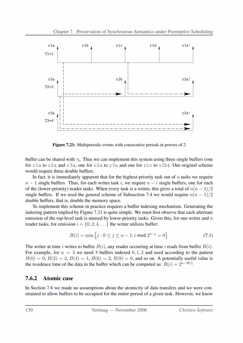
Chapter 7. Preservation of Synchronous Semantics under Preemptive Scheduling
T1=1
T2=2
r3a
r2a
r1a r1b r1c r1d
r2b
T3=4
r3a’
r2a’
r1a’
Figure 7.21: Multiperiodic events with consecutive periods in powers of 2
buffer can be shared with τ3. Thus we can implement this system using three single buffers (one
for r1a to r2a and r3a, one for r2a to r3a and one for r1c to r2b). Our original scheme
would require three double buffers.
In fact, it is immediately apparent that for the highest-priority task out of n tasks we require
n − 1 single buffers. Thus, for each writer task i, we require n − i single buffers, one for each
of the (lower-priority) reader tasks. When every task is a writer, this gives a total of n(n − 1)/2single buffers. If we used the general scheme of Subsection 7.4 we would require n(n − 1)/2double buffers, that is, double the memory space.
To implement this scheme in practice requires a buffer indexing mechanism. Generating the
indexing pattern implied by Figure 7.21 is quite simple. We must first observe that each alternate
emission of the top-level task is unused by lower-priority tasks. Given this, for one writer and nreader tasks, for emission i = {0, 2, 4, . . .} the writer utilizes buffer:
B(i) = min{
j : 0 ≤ j ≤ n − 1, i mod 2n−j = 0}
(7.1)
The writer at time i writes to buffer B(i), any reader occurring at time i reads from buffer B(i).For example, for n = 3 we need 3 buffers indexed 0, 1, 2 and used according to the pattern
B(0) = 0, B(2) = 2, B(4) = 1, B(6) = 2, B(8) = 0, and so on. A potentially useful value is
the residence time of the data in the buffer which can be computed as: R(i) = 2n−B(i).
7.6.2 Atomic case
In Section 7.6 we made no assumptions about the atomicity of data transfers and we were con-
strained to allow buffers to be occupied for the entire period of a given task. However, we know
130 Verimag — November 2006 Christos Sofronis
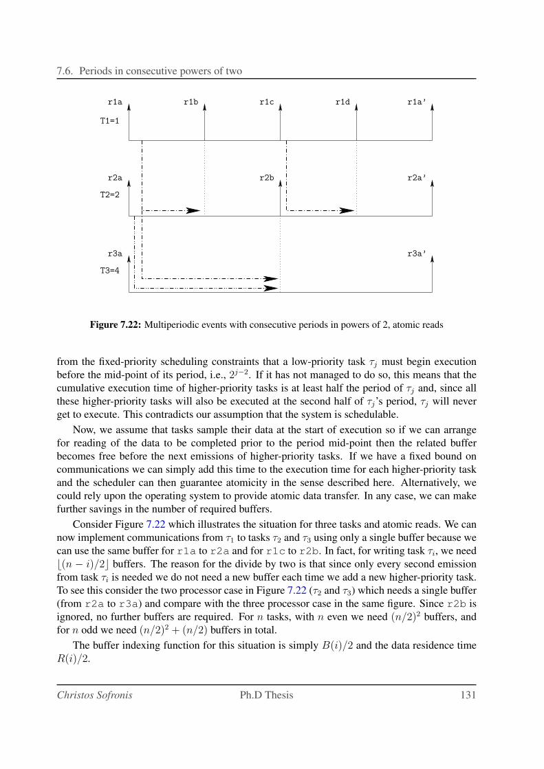
7.6. Periods in consecutive powers of two
T1=1
T2=2
r3a
r2a
r1a r1b r1c r1d
r2b
T3=4
r3a’
r2a’
r1a’
Figure 7.22: Multiperiodic events with consecutive periods in powers of 2, atomic reads
from the fixed-priority scheduling constraints that a low-priority task τj must begin execution
before the mid-point of its period, i.e., 2j−2. If it has not managed to do so, this means that the
cumulative execution time of higher-priority tasks is at least half the period of τj and, since all
these higher-priority tasks will also be executed at the second half of τj’s period, τj will never
get to execute. This contradicts our assumption that the system is schedulable.
Now, we assume that tasks sample their data at the start of execution so if we can arrange
for reading of the data to be completed prior to the period mid-point then the related buffer
becomes free before the next emissions of higher-priority tasks. If we have a fixed bound on
communications we can simply add this time to the execution time for each higher-priority task
and the scheduler can then guarantee atomicity in the sense described here. Alternatively, we
could rely upon the operating system to provide atomic data transfer. In any case, we can make
further savings in the number of required buffers.
Consider Figure 7.22 which illustrates the situation for three tasks and atomic reads. We can
now implement communications from τ1 to tasks τ2 and τ3 using only a single buffer because we
can use the same buffer for r1a to r2a and for r1c to r2b. In fact, for writing task τi, we need
⌊(n − i)/2⌋ buffers. The reason for the divide by two is that since only every second emission
from task τi is needed we do not need a new buffer each time we add a new higher-priority task.
To see this consider the two processor case in Figure 7.22 (τ2 and τ3) which needs a single buffer
(from r2a to r3a) and compare with the three processor case in the same figure. Since r2b is
ignored, no further buffers are required. For n tasks, with n even we need (n/2)2 buffers, and
for n odd we need (n/2)2 + (n/2) buffers in total.
The buffer indexing function for this situation is simply B(i)/2 and the data residence time
R(i)/2.
Christos Sofronis Ph.D Thesis 131
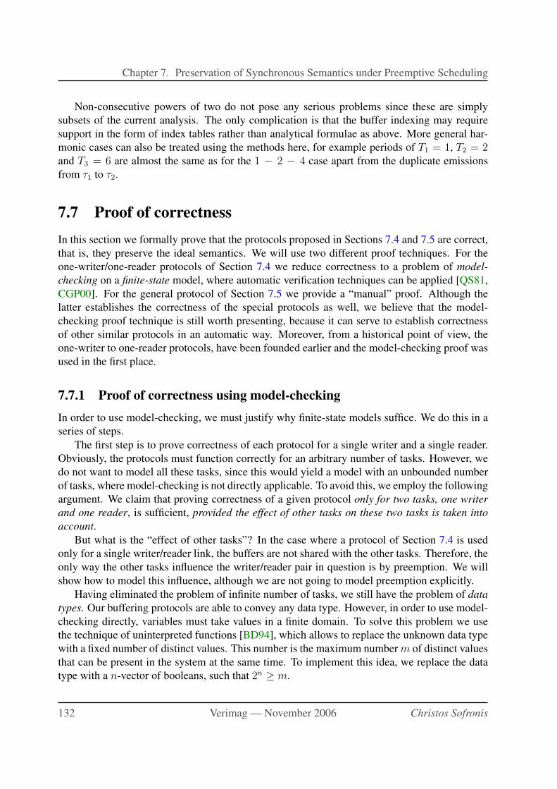
Chapter 7. Preservation of Synchronous Semantics under Preemptive Scheduling
Non-consecutive powers of two do not pose any serious problems since these are simply
subsets of the current analysis. The only complication is that the buffer indexing may require
support in the form of index tables rather than analytical formulae as above. More general har-
monic cases can also be treated using the methods here, for example periods of T1 = 1, T2 = 2and T3 = 6 are almost the same as for the 1 − 2 − 4 case apart from the duplicate emissions
from τ1 to τ2.
7.7 Proof of correctness
In this section we formally prove that the protocols proposed in Sections 7.4 and 7.5 are correct,
that is, they preserve the ideal semantics. We will use two different proof techniques. For the
one-writer/one-reader protocols of Section 7.4 we reduce correctness to a problem of model-
checking on a finite-state model, where automatic verification techniques can be applied [QS81,
CGP00]. For the general protocol of Section 7.5 we provide a “manual” proof. Although the
latter establishes the correctness of the special protocols as well, we believe that the model-
checking proof technique is still worth presenting, because it can serve to establish correctness
of other similar protocols in an automatic way. Moreover, from a historical point of view, the
one-writer to one-reader protocols, have been founded earlier and the model-checking proof was
used in the first place.
7.7.1 Proof of correctness using model-checking
In order to use model-checking, we must justify why finite-state models suffice. We do this in a
series of steps.
The first step is to prove correctness of each protocol for a single writer and a single reader.
Obviously, the protocols must function correctly for an arbitrary number of tasks. However, we
do not want to model all these tasks, since this would yield a model with an unbounded number
of tasks, where model-checking is not directly applicable. To avoid this, we employ the following
argument. We claim that proving correctness of a given protocol only for two tasks, one writer
and one reader, is sufficient, provided the effect of other tasks on these two tasks is taken into
account.
But what is the “effect of other tasks”? In the case where a protocol of Section 7.4 is used
only for a single writer/reader link, the buffers are not shared with the other tasks. Therefore, the
only way the other tasks influence the writer/reader pair in question is by preemption. We will
show how to model this influence, although we are not going to model preemption explicitly.
Having eliminated the problem of infinite number of tasks, we still have the problem of data
types. Our buffering protocols are able to convey any data type. However, in order to use model-
checking directly, variables must take values in a finite domain. To solve this problem we use
the technique of uninterpreted functions [BD94], which allows to replace the unknown data type
with a fixed number of distinct values. This number is the maximum number m of distinct values
that can be present in the system at the same time. To implement this idea, we replace the data
type with a n-vector of booleans, such that 2n ≥ m.
132 Verimag — November 2006 Christos Sofronis
7.7. Proof of correctness
The general architecture of the model we shall use for model-checking is shown in Fig-
ure 7.23. The model has four components. An event generator component which produces the
events of the tasks. A component modeling the ideal semantics. A component modeling the
behavior of the buffering protocol. A preservation monitor component which compares the two
behaviors and checks whether they are “equivalent” (where the notion of equivalence is to be
defined).
The above described approach, using the model based paradigm, is interesting because it
provides means to verify the preservation of semantics in a larger extend. One can use this
scheme to generate sequences of inputs and compare the results of the protocol in question with
respect to an automaton representing some “ideal” behavior, or some behavior under test.
preservationmonitor
ideal semantics
event generator
buffering protocolexecution with a
Figure 7.23: Architecture of the model used in model-checking.
Event generator model
A task τi is modeled by three events, ri, bi and ei, corresponding to the release, beginning of
execution and end of execution of (an instance of) the task, respectively. In the ideal semantics,
these three events occur simultaneously. In the real implementation, these events follow a cyclic
order
ri → bi → ei → ri → bi → ei → · · · ,
which corresponds to two facts. First, that each task instance is first released, then starts execution
and finally ends execution. Second, that when a new instance is released the previous instance
has finished, which is our schedulability assumption. Notice that although preemption may occur
between bi and ei, they are not modeled explicitly.
The scheduling policy is captured by placing restrictions on the possible interleavings of the
above events. Let us first show how to model static-priority scheduling. Let τ1 be the high-
priority task and τ2 be the low-priority task. Then, we know that neither b2 nor e2 can occur
between r1 and e1. Indeed, τ2 cannot start before τ1 finishes. Also, if τ2 has already started when
r1 occurs then it is preempted, thus, will not finish before τ1 finishes. These ordering restrictions
can be modeled using the finite-state automaton shown in Figure 7.24.3
The automaton has five states. The state labeled “false” corresponds to the violation of the
static-priority scheduling assumption. In other words, the legal orderings of the events ri, bi, ei
3 For simplicity, the automaton shown in the figure assumes that no two events can occur simultaneously. This
assumption can be lifted but it results in a more complicated automaton which is not shown.
Christos Sofronis Ph.D Thesis 133
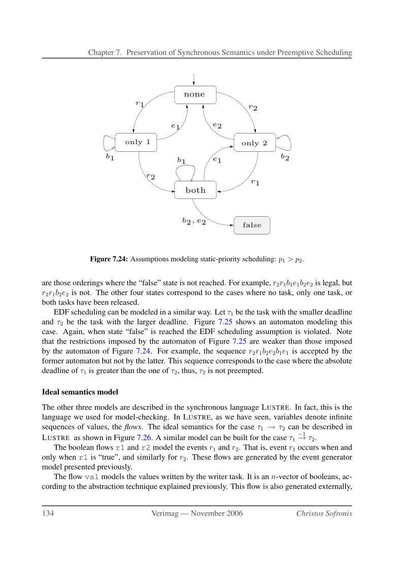
Chapter 7. Preservation of Synchronous Semantics under Preemptive Scheduling
both
none
e1e2
r2
only 1 only 2
r1
e1
r2
false
r1
b2, e2
b1b1 b2
Figure 7.24: Assumptions modeling static-priority scheduling: p1 > p2.
are those orderings where the “false” state is not reached. For example, r2r1b1e1b2e2 is legal, but
r2r1b2e2 is not. The other four states correspond to the cases where no task, only one task, or
both tasks have been released.
EDF scheduling can be modeled in a similar way. Let τ1 be the task with the smaller deadline
and τ2 be the task with the larger deadline. Figure 7.25 shows an automaton modeling this
case. Again, when state “false” is reached the EDF scheduling assumption is violated. Note
that the restrictions imposed by the automaton of Figure 7.25 are weaker than those imposed
by the automaton of Figure 7.24. For example, the sequence r2r1b2e2b1e1 is accepted by the
former automaton but not by the latter. This sequence corresponds to the case where the absolute
deadline of τ1 is greater than the one of τ2, thus, τ2 is not preempted.
Ideal semantics model
The other three models are described in the synchronous language LUSTRE. In fact, this is the
language we used for model-checking. In LUSTRE, as we have seen, variables denote infinite
sequences of values, the flows. The ideal semantics for the case τ1 → τ2 can be described in
LUSTRE as shown in Figure 7.26. A similar model can be built for the case τ1−1→ τ2.
The boolean flows r1 and r2 model the events r1 and r2. That is, event r1 occurs when and
only when r1 is “true”, and similarly for r2. These flows are generated by the event generator
model presented previously.
The flow val models the values written by the writer task. It is an n-vector of booleans, ac-
cording to the abstraction technique explained previously. This flow is also generated externally,
134 Verimag — November 2006 Christos Sofronis
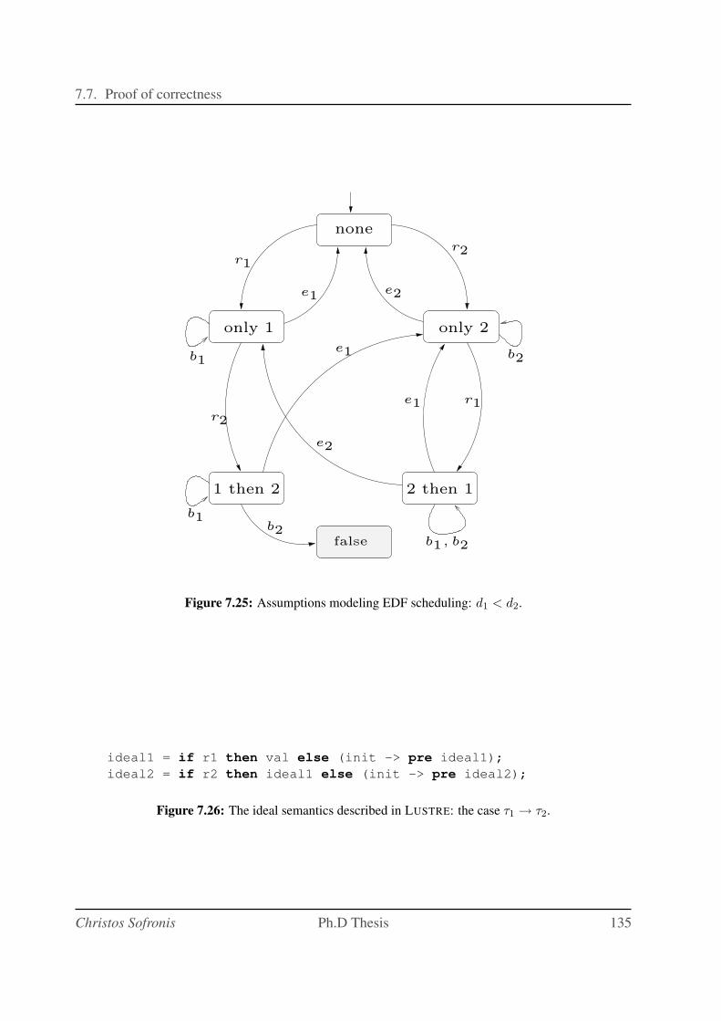
7.7. Proof of correctness
only 2
none
only 1
2 then 11 then 2
r1
false
b2
e2
r2
e1
e1
r1e1
e2
r2
b2
b1, b2
b1
b1
Figure 7.25: Assumptions modeling EDF scheduling: d1 < d2.
ideal1 = if r1 then val else (init -> pre ideal1);
ideal2 = if r2 then ideal1 else (init -> pre ideal2);
Figure 7.26: The ideal semantics described in LUSTRE: the case τ1 → τ2.
Christos Sofronis Ph.D Thesis 135
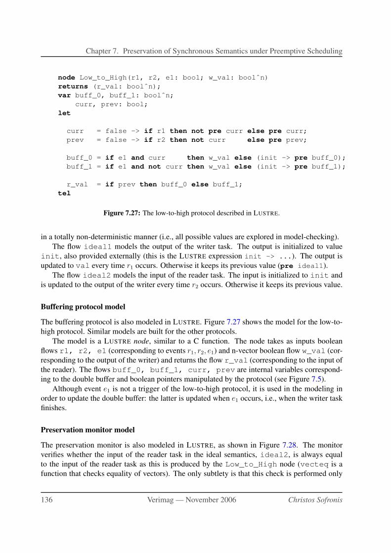
Chapter 7. Preservation of Synchronous Semantics under Preemptive Scheduling
node Low_to_High(r1, r2, e1: bool; w_val: boolˆn)
returns (r_val: boolˆn);
var buff_0, buff_1: boolˆn;
curr, prev: bool;
let
curr = false -> if r1 then not pre curr else pre curr;
prev = false -> if r2 then not curr else pre prev;
buff_0 = if e1 and curr then w_val else (init -> pre buff_0);
buff_1 = if e1 and not curr then w_val else (init -> pre buff_1);
r_val = if prev then buff_0 else buff_1;
tel
Figure 7.27: The low-to-high protocol described in LUSTRE.
in a totally non-deterministic manner (i.e., all possible values are explored in model-checking).
The flow ideal1 models the output of the writer task. The output is initialized to value
init, also provided externally (this is the LUSTRE expression init -> ...). The output is
updated to val every time r1 occurs. Otherwise it keeps its previous value (pre ideal1).
The flow ideal2 models the input of the reader task. The input is initialized to init and
is updated to the output of the writer every time r2 occurs. Otherwise it keeps its previous value.
Buffering protocol model
The buffering protocol is also modeled in LUSTRE. Figure 7.27 shows the model for the low-to-
high protocol. Similar models are built for the other protocols.
The model is a LUSTRE node, similar to a C function. The node takes as inputs boolean
flows r1, r2, e1 (corresponding to events r1, r2, e1) and n-vector boolean flow w_val (cor-
responding to the output of the writer) and returns the flow r_val (corresponding to the input of
the reader). The flows buff_0, buff_1, curr, prev are internal variables correspond-
ing to the double buffer and boolean pointers manipulated by the protocol (see Figure 7.5).
Although event e1 is not a trigger of the low-to-high protocol, it is used in the modeling in
order to update the double buffer: the latter is updated when e1 occurs, i.e., when the writer task
finishes.
Preservation monitor model
The preservation monitor is also modeled in LUSTRE, as shown in Figure 7.28. The monitor
verifies whether the input of the reader task in the ideal semantics, ideal2, is always equal
to the input of the reader task as this is produced by the Low_to_High node (vecteq is a
function that checks equality of vectors). The only subtlety is that this check is performed only
136 Verimag — November 2006 Christos Sofronis
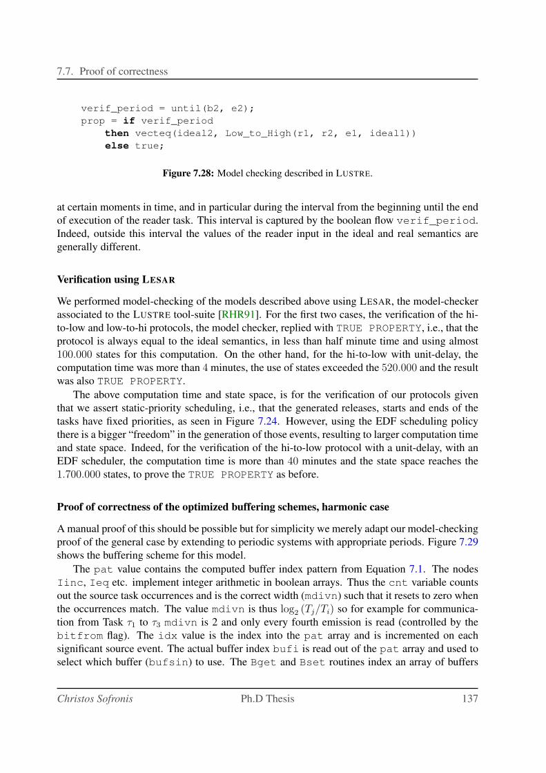
7.7. Proof of correctness
verif_period = until(b2, e2);
prop = if verif_period
then vecteq(ideal2, Low_to_High(r1, r2, e1, ideal1))
else true;
Figure 7.28: Model checking described in LUSTRE.
at certain moments in time, and in particular during the interval from the beginning until the end
of execution of the reader task. This interval is captured by the boolean flow verif_period.
Indeed, outside this interval the values of the reader input in the ideal and real semantics are
generally different.
Verification using LESAR
We performed model-checking of the models described above using LESAR, the model-checker
associated to the LUSTRE tool-suite [RHR91]. For the first two cases, the verification of the hi-
to-low and low-to-hi protocols, the model checker, replied with TRUE PROPERTY, i.e., that the
protocol is always equal to the ideal semantics, in less than half minute time and using almost
100.000 states for this computation. On the other hand, for the hi-to-low with unit-delay, the
computation time was more than 4 minutes, the use of states exceeded the 520.000 and the result
was also TRUE PROPERTY.
The above computation time and state space, is for the verification of our protocols given
that we assert static-priority scheduling, i.e., that the generated releases, starts and ends of the
tasks have fixed priorities, as seen in Figure 7.24. However, using the EDF scheduling policy
there is a bigger “freedom” in the generation of those events, resulting to larger computation time
and state space. Indeed, for the verification of the hi-to-low protocol with a unit-delay, with an
EDF scheduler, the computation time is more than 40 minutes and the state space reaches the
1.700.000 states, to prove the TRUE PROPERTY as before.
Proof of correctness of the optimized buffering schemes, harmonic case
A manual proof of this should be possible but for simplicity we merely adapt our model-checking
proof of the general case by extending to periodic systems with appropriate periods. Figure 7.29
shows the buffering scheme for this model.
The pat value contains the computed buffer index pattern from Equation 7.1. The nodes
Iinc, Ieq etc. implement integer arithmetic in boolean arrays. Thus the cnt variable counts
out the source task occurrences and is the correct width (mdivn) such that it resets to zero when
the occurrences match. The value mdivn is thus log2 (Tj/Ti) so for example for communica-
tion from Task τ1 to τ3 mdivn is 2 and only every fourth emission is read (controlled by the
bitfrom flag). The idx value is the index into the pat array and is incremented on each
significant source event. The actual buffer index bufi is read out of the pat array and used to
select which buffer (bufsin) to use. The Bget and Bset routines index an array of buffers
Christos Sofronis Ph.D Thesis 137
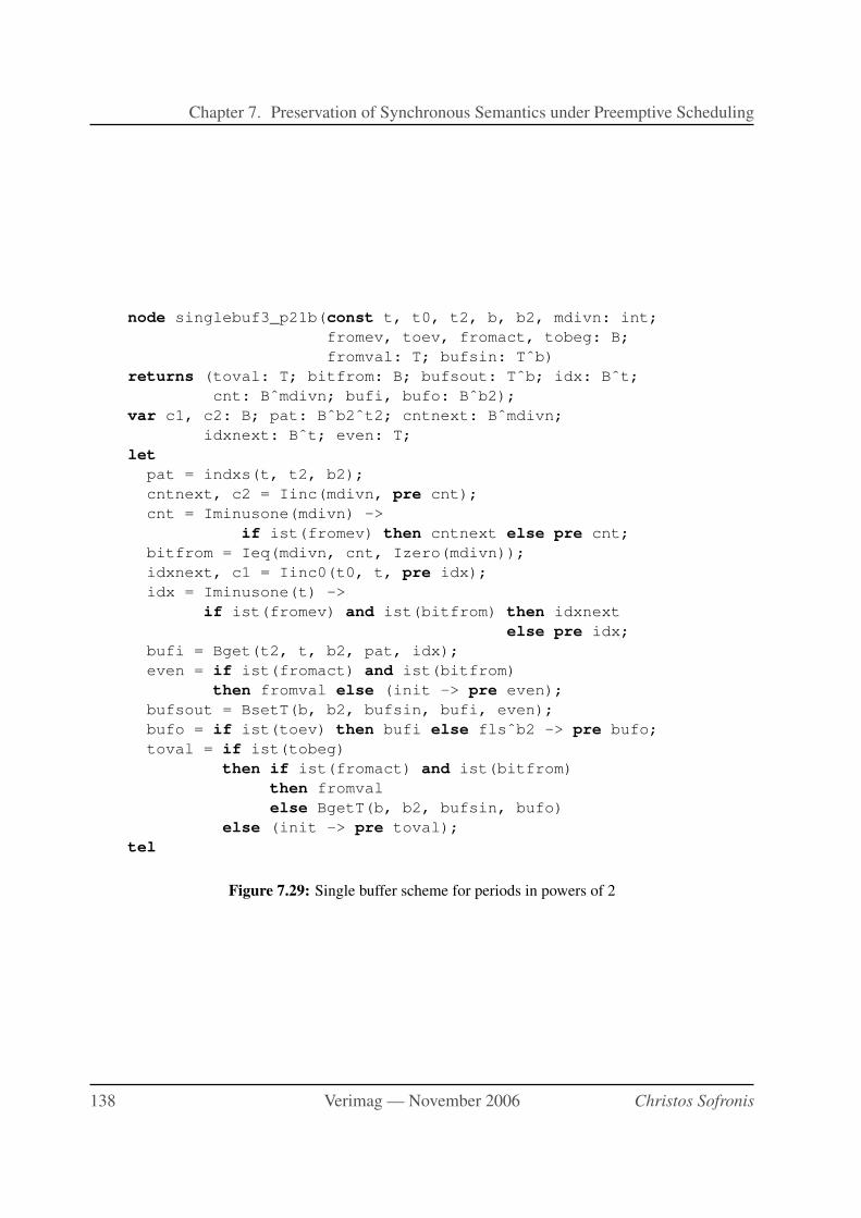
Chapter 7. Preservation of Synchronous Semantics under Preemptive Scheduling
node singlebuf3_p21b(const t, t0, t2, b, b2, mdivn: int;
fromev, toev, fromact, tobeg: B;
fromval: T; bufsin: Tˆb)
returns (toval: T; bitfrom: B; bufsout: Tˆb; idx: Bˆt;
cnt: Bˆmdivn; bufi, bufo: Bˆb2);
var c1, c2: B; pat: Bˆb2ˆt2; cntnext: Bˆmdivn;
idxnext: Bˆt; even: T;
let
pat = indxs(t, t2, b2);
cntnext, c2 = Iinc(mdivn, pre cnt);
cnt = Iminusone(mdivn) ->
if ist(fromev) then cntnext else pre cnt;
bitfrom = Ieq(mdivn, cnt, Izero(mdivn));
idxnext, c1 = Iinc0(t0, t, pre idx);
idx = Iminusone(t) ->
if ist(fromev) and ist(bitfrom) then idxnext
else pre idx;
bufi = Bget(t2, t, b2, pat, idx);
even = if ist(fromact) and ist(bitfrom)
then fromval else (init -> pre even);
bufsout = BsetT(b, b2, bufsin, bufi, even);
bufo = if ist(toev) then bufi else flsˆb2 -> pre bufo;
toval = if ist(tobeg)
then if ist(fromact) and ist(bitfrom)
then fromval
else BgetT(b, b2, bufsin, bufo)
else (init -> pre toval);
tel
Figure 7.29: Single buffer scheme for periods in powers of 2
138 Verimag — November 2006 Christos Sofronis
7.7. Proof of correctness
using boolean arrays as indices. The appropriate buffer is then written to (bufsout) and the
buffer index is latched for the receiving process in bufo. The correct value is then read out of
the buffer when the receiving task begins execution (tobeg).
This model-checks correctly for n = 3 but is too big to verify for T4 = 8. Partial verification
is possible and all subsets are true for n = 4. Since there are no irregularities in this construction
(each case is built by extending the previous one in a regular way) we can conclude that the
scheme is correct for all n. For systems with contiguous priorities in powers of 2 we can thus
implement our buffering mechanism using the same number of single buffers as we would need
double buffers in the general case.
Buffering for consecutive powers of two, atomic case
Using the same code as in Figure 7.29, but replacing the buffer pattern pat with the buffer
pattern implied by B(i)/2 and updating the priority conditions to reflect the new scheduling
constraints model-checks correctly for the n = 3 case. Again, we are only able to partially verify
the mechanism for four tasks.
Model-checking can also be used to prove correctness of the optimized versions, however,
this can be done a priori only for a given, rather than arbitrary, set of tasks. We have followed this
approach and modeled the buffering schemes for the harmonic multi-periodic case (Sections 7.6
and 7.6.2). In both cases, we have managed to model-check completely only systems of n = 3tasks. The model gets too large for LESAR to handle for n = 4. We did manage, however, to
partially verify the n = 4 case, selecting various subsets of the model and proving them correct.
Since there are no irregularities in these schemes (each case is built by extending the previous
one in a regular way) we can expect the scheme to be correct for all n.
7.7.2 Proof of correctness of the dynamic buffering protocol
In this section we will prove the correctness of the protocol DBP (Section 7.5.1). In this case,
model-checking is not directly applicable, since we have an arbitrary number of reader tasks.
Instead, we provide a “manual” proof.
What we want to prove is semantical preservation, that is, that for any possible arrival pattern
and values written by the writer, the values read by the readers in the ideal semantics are equal
to the values read by the readers in the implementation, assuming DBP is used. More formally,
consider a reader τi and let ti be the time when an arbitrary instance of τi is released. We denote
this instance by τ tii . Let t′i ≥ ti be the time when τ ti
i reads. Let τw be the writer task. For the
moment, let us assume that τw is released at least twice before time ti. We relax this assumption
later in this section.
Let t ≤ ti be the last time before ti that an instance of τw was released. We denote this
instance by τ tw. Let te > t be the time that τ t
w produces its output and finishes. Let y(t) be the
output of τ tw. Let t′ < t be the last time before t that an instance of the writer τw was released.
This instance is denoted τ t′
w . It finishes execution at time t′e > t′. Let y(t′) be the output of τ t′
w .
Figure 7.30 illustrates the notation defined above. Notice that the order of events shown in the
figure is just one of the possible orders.
Christos Sofronis Ph.D Thesis 139
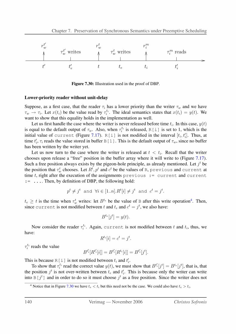
Chapter 7. Preservation of Synchronous Semantics under Preemptive Scheduling
τ tw writes
te ti t′i
τmi reads
rmi
t′ t
rtwrt′
w
t′e
τ t′
w writes
Figure 7.30: Illustration used in the proof of DBP.
Lower-priority reader without unit-delay
Suppose, as a first case, that the reader τi has a lower priority than the writer τw and we have
τw → τi. Let x(ti) be the value read by τ tii . The ideal semantics states that x(ti) = y(t). We
want to show that this equality holds in the implementation as well.
Let us first handle the case where the writer is never released before time ti. In this case, y(t)is equal to the default output of τw. Also, when τ ti
i is released, R[i] is set to 1, which is the
initial value of current (Figure 7.17). R[i] is not modified in the interval [ti, t′i]. Thus, at
time t′i, τi reads the value stored in buffer B[1]. This is the default output of τw, since no buffer
has been written by the writer yet.
Let us now turn to the case where the writer is released at t < ti. Recall that the writer
chooses upon release a “free” position in the buffer array where it will write to (Figure 7.17).
Such a free position always exists by the pigeon-hole principle, as already mentioned. Let jt be
the position that τ tw chooses. Let Rt, pt and ct be the values of R, previous and current at
time t, right after the execution of the assignments previous := current and current
:= .... Then, by definition of DBP, the following hold:
pt 6= jt and ∀i ∈ [1..n].Rt[i] 6= jt and ct = jt.
te ≥ t is the time when τ tw writes: let Bte be the value of B after this write operation4. Then,
since current is not modified between t and te and ct = jt, we also have:
Bte [jt] = y(t).
Now consider the reader τ tii . Again, current is not modified between t and ti, thus, we
have:
Rti [i] = ct = jt.
τ tii reads the value
Bt′i [Rt′
i [i]] = Bt′i [Rti [i]] = Bt′
i [jt].
This is because R[i] is not modified between ti and t′i.To show that τ ti
i read the correct value y(t), we must show that Bt′i [jt] = Bte [jt], that is, that
the position jt is not over-written between te and t′i. This is because only the writer can write
into B[jt] and in order to do so it must choose jt as a free position. Since the writer does not
4 Notice that in Figure 7.30 we have te < ti but this need not be the case. We could also have te > ti.
140 Verimag — November 2006 Christos Sofronis
7.7. Proof of correctness
arrive in the interval [te, ti], it suffices to show that free(jt) is false in the interval [ti, t′i]. This
is because R[i] equals jt in all this interval.
Lower-priority reader with unit-delay
Suppose, next, that the reader τi has a lower priority than the writer τw and we have a link with
a unit-delay: τw−1→ τi. Again, let x(ti) be the value read by τ ti
i . The ideal semantics states that
x(ti) = y(t′). We want to show that this equality holds in the implementation as well.
Let us first handle the case where the writer is released not more than once before time ti.In this case, y(t′) is equal to the default output of τw. Also, when τ ti
i is released, R[i] is set
to 1, which is the value of previous at this point. Indeed, either the writer has never been
released yet and previous is equal to its initial value 1, or the writer has been released once
and previous is set to the initial value of current, which is also 1. R[i] is not modified in
the interval [ti, t′i]. Thus, at time t′i, τi reads the value stored in buffer B[1]. If the writer has not
been released before ti then B[1] holds the default output of τw. If the writer has been released
once before ti then it has not written to B[1]: to do so, it must choose 1 as a free position to
assign to current, however, 1 is not free because previous=1.
Let us now turn to the case where the writer is released twice before ti. Upon arrival of the
writer at time t′, a free position in the buffer array is chosen to write to: let this position be jt′ .
Let also Rt′ , pt′ and ct′ be the values of R, previous and current at time t′, right after the
execution of the assignments to previous and current. Then, by definition of DBP, the
following hold:
pt′ 6= jt′ and ∀i ∈ [1..n].Rt′ [i] 6= jt′ and ct′ = jt′ .
t′e ≥ t′ is the time when τ t′
w writes: let Bt′e be the value of B after this write operation. Then,
since current is not modified between t′ and t′e and ct′ = jt′ , we also have:
Bt′e [jt′ ] = y(t′).
On the next arrival of the writer at time t, new assignments will be made to the pointers
previous and current. Let jt be the new free position chosen. Let Rt, pt and ct be the
values of R, previous and current at time t, right after the assignments to previous and
current. Then, the following hold (mention also that current = ct′ = jt′ remains unchanged
from time t′e and until before the assignments at time t):
pt = ct′ and pt 6= jt and ∀i ∈ [1..n].Rt[i] 6= jt and ct = jt
When the reader arrives at time ti, R[i] is set to previous. previous is not modified
between t and ti, thus, the value of R[i] at time ti is equal to pt:
Rti [i] = pt = ct′ = jt′ .
R[i] is not modified between ti and t′i. Thus, τ tii reads the value
Bt′i [Rt′
i [i]] = Bt′i [Rti [i]] = Bt′
i [jt′ ].
Christos Sofronis Ph.D Thesis 141
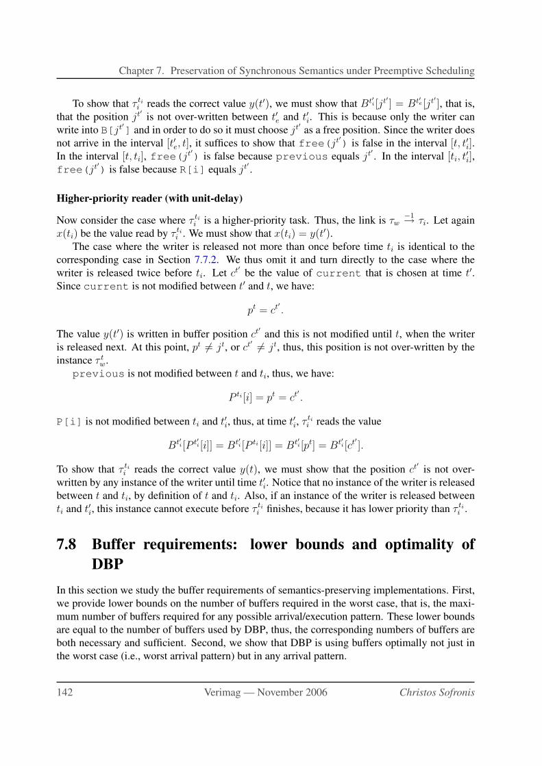
Chapter 7. Preservation of Synchronous Semantics under Preemptive Scheduling
To show that τ tii reads the correct value y(t′), we must show that Bt′
i [jt′ ] = Bt′e [jt′ ], that is,
that the position jt′ is not over-written between t′e and t′i. This is because only the writer can
write into B[jt′] and in order to do so it must choose jt′ as a free position. Since the writer does
not arrive in the interval [t′e, t], it suffices to show that free(jt′) is false in the interval [t, t′i].In the interval [t, ti], free(jt′) is false because previous equals jt′ . In the interval [ti, t
′i],
free(jt′) is false because R[i] equals jt′ .
Higher-priority reader (with unit-delay)
Now consider the case where τ tii is a higher-priority task. Thus, the link is τw
−1→ τi. Let again
x(ti) be the value read by τ tii . We must show that x(ti) = y(t′).
The case where the writer is released not more than once before time ti is identical to the
corresponding case in Section 7.7.2. We thus omit it and turn directly to the case where the
writer is released twice before ti. Let ct′ be the value of current that is chosen at time t′.Since current is not modified between t′ and t, we have:
pt = ct′ .
The value y(t′) is written in buffer position ct′ and this is not modified until t, when the writer
is released next. At this point, pt 6= jt, or ct′ 6= jt, thus, this position is not over-written by the
instance τ tw.
previous is not modified between t and ti, thus, we have:
P ti [i] = pt = ct′ .
P[i] is not modified between ti and t′i, thus, at time t′i, τ tii reads the value
Bt′i [P t′
i [i]] = Bt′i [P ti [i]] = Bt′
i [pt] = Bt′i [ct′ ].
To show that τ tii reads the correct value y(t), we must show that the position ct′ is not over-
written by any instance of the writer until time t′i. Notice that no instance of the writer is released
between t and ti, by definition of t and ti. Also, if an instance of the writer is released between
ti and t′i, this instance cannot execute before τ tii finishes, because it has lower priority than τ ti
i .
7.8 Buffer requirements: lower bounds and optimality of
DBP
In this section we study the buffer requirements of semantics-preserving implementations. First,
we provide lower bounds on the number of buffers required in the worst case, that is, the maxi-
mum number of buffers required for any possible arrival/execution pattern. These lower bounds
are equal to the number of buffers used by DBP, thus, the corresponding numbers of buffers are
both necessary and sufficient. Second, we show that DBP is using buffers optimally not just in
the worst case (i.e., worst arrival pattern) but in any arrival pattern.
142 Verimag — November 2006 Christos Sofronis
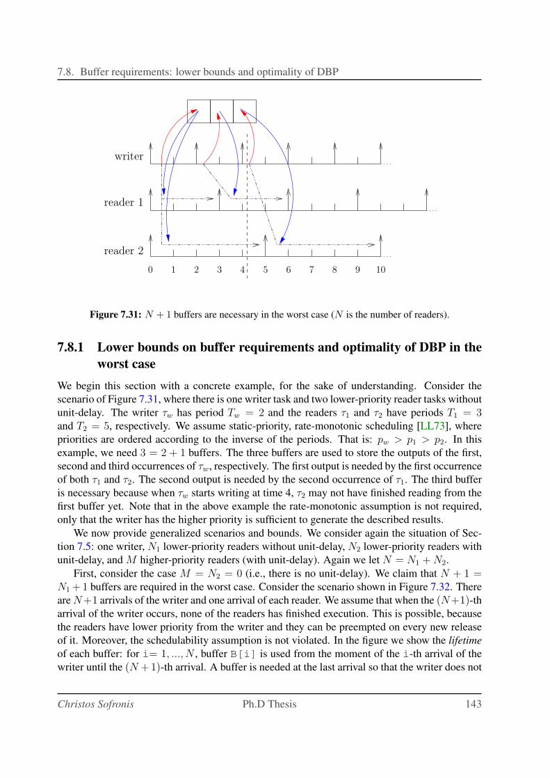
7.8. Buffer requirements: lower bounds and optimality of DBP
108 976543210
writer
reader 1
reader 2
Figure 7.31: N + 1 buffers are necessary in the worst case (N is the number of readers).
7.8.1 Lower bounds on buffer requirements and optimality of DBP in the
worst case
We begin this section with a concrete example, for the sake of understanding. Consider the
scenario of Figure 7.31, where there is one writer task and two lower-priority reader tasks without
unit-delay. The writer τw has period Tw = 2 and the readers τ1 and τ2 have periods T1 = 3and T2 = 5, respectively. We assume static-priority, rate-monotonic scheduling [LL73], where
priorities are ordered according to the inverse of the periods. That is: pw > p1 > p2. In this
example, we need 3 = 2 + 1 buffers. The three buffers are used to store the outputs of the first,
second and third occurrences of τw, respectively. The first output is needed by the first occurrence
of both τ1 and τ2. The second output is needed by the second occurrence of τ1. The third buffer
is necessary because when τw starts writing at time 4, τ2 may not have finished reading from the
first buffer yet. Note that in the above example the rate-monotonic assumption is not required,
only that the writer has the higher priority is sufficient to generate the described results.
We now provide generalized scenarios and bounds. We consider again the situation of Sec-
tion 7.5: one writer, N1 lower-priority readers without unit-delay, N2 lower-priority readers with
unit-delay, and M higher-priority readers (with unit-delay). Again we let N = N1 + N2.
First, consider the case M = N2 = 0 (i.e., there is no unit-delay). We claim that N + 1 =N1 +1 buffers are required in the worst case. Consider the scenario shown in Figure 7.32. There
are N+1 arrivals of the writer and one arrival of each reader. We assume that when the (N+1)-tharrival of the writer occurs, none of the readers has finished execution. This is possible, because
the readers have lower priority from the writer and they can be preempted on every new release
of it. Moreover, the schedulability assumption is not violated. In the figure we show the lifetime
of each buffer: for i= 1, ..., N , buffer B[i] is used from the moment of the i-th arrival of the
writer until the (N +1)-th arrival. A buffer is needed at the last arrival so that the writer does not
Christos Sofronis Ph.D Thesis 143
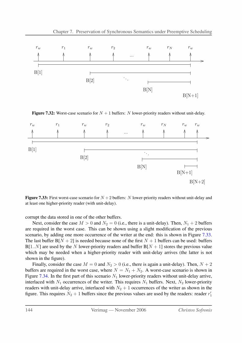
Chapter 7. Preservation of Synchronous Semantics under Preemptive Scheduling
rw rwr1 r2 rw
...
rN rw
B[N]
B[2]
B[1]
B[N+1]
. . .
Figure 7.32: Worst-case scenario for N + 1 buffers: N lower-priority readers without unit-delay.
rw rwr1 r2 rw
...
rN rw
B[N]
B[2]
B[1]
B[N+1]
rw
B[N+2]
. . .
Figure 7.33: First worst-case scenario for N +2 buffers: N lower-priority readers without unit-delay and
at least one higher-priority reader (with unit-delay).
corrupt the data stored in one of the other buffers.
Next, consider the case M > 0 and N2 = 0 (i.e., there is a unit-delay). Then, N1 + 2 buffers
are required in the worst case. This can be shown using a slight modification of the previous
scenario, by adding one more occurrence of the writer at the end: this is shown in Figure 7.33.
The last buffer B[N + 2] is needed because none of the first N + 1 buffers can be used: buffers
B[1..N ] are used by the N lower-priority readers and buffer B[N + 1] stores the previous value
which may be needed when a higher-priority reader with unit-delay arrives (the latter is not
shown in the figure).
Finally, consider the case M = 0 and N2 > 0 (i.e., there is again a unit-delay). Then, N + 2buffers are required in the worst case, where N = N1 + N2. A worst-case scenario is shown in
Figure 7.34. In the first part of this scenario N1 lower-priority readers without unit-delay arrive,
interlaced with N1 occurrences of the writer. This requires N1 buffers. Next, N2 lower-priority
readers with unit-delay arrive, interlaced with N2 + 1 occurrences of the writer as shown in the
figure. This requires N2 + 1 buffers since the previous values are used by the readers: reader r′1
144 Verimag — November 2006 Christos Sofronis
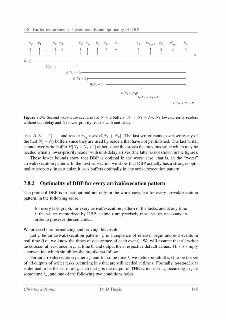
7.8. Buffer requirements: lower bounds and optimality of DBP
rw rw
.
.
.
... ...
B[1]
B[N1]
r′
N2r′
N2−1rwrwrwrN1
rwr1rw rwr′
1r′
2
B[N1 + 1]
B[N1 + 2]
B[N1 + 3]
B[N1 + N2]
B[N1 + N2 + 1]
B[N1 + N2 + 2]
.
.
.
Figure 7.34: Second worst-case scenario for N + 2 buffers: N = N1 + N2, N1 lower-priority readers
without unit-delay and N2 lower-priority readers with unit-delay.
uses B[N1 + 1], ..., and reader r′N2uses B[N1 + N2]. The last writer cannot over-write any of
the first N1 + N2 buffers since they are used by readers that have not yet finished. The last writer
cannot over-write buffer B[N1 +N2 +1] either, since this stores the previous value which may be
needed when a lower-priority reader with unit-delay arrives (the latter is not shown in the figure).
These lower bounds show that DBP is optimal in the worst case, that is, in the “worst”
arrival/execution pattern. In the next subsection we show that DBP actually has a stronger opti-
mality property, in particular, it uses buffers optimally in any arrival/execution pattern.
7.8.2 Optimality of DBP for every arrival/execution pattern
The protocol DBP is in fact optimal not only in the worst case, but for every arrival/execution
pattern, in the following sense:
for every task graph, for every arrival/execution pattern of the tasks, and at any time
t, the values memorized by DBP at time t are precisely those values necessary in
order to preserve the semantics.
We proceed into formalizing and proving this result.
Let ρ be an arrival/execution pattern: ρ is a sequence of release, begin and end events in
real-time (i.e., we know the times of occurrence of each event). We will assume that all writer
tasks occur at least once in ρ, at time 0, and output their respective default values. This is simply
a convention which simplifies the proofs that follow.
For an arrival/execution pattern ρ and for some time t, we define needed(ρ, t) to be the set
of all outputs of writer tasks occurring in ρ that are still needed at time t. Formally, needed(ρ, t)is defined to be the set of all y such that y is the output of THE writer task τw occurring in ρ at
some time tw, and one of the following two conditions holds:
Christos Sofronis Ph.D Thesis 145
Chapter 7. Preservation of Synchronous Semantics under Preemptive Scheduling
1. There exists a link τw → τi, task τi is released in ρ after tw and before the next occurrence
of τw (if it exists), and τi finishes after t.
2. There exists a link τw−1→ τi, there is a second occurrence of τw in ρ at time t′w, where
tw < t′w, τi is released after t′w and before the next occurrence of τw (if it exists), and τi
finishes after t.
We assume that outputs y are indexed by the writer identifier and occurrence number, so that
no two outputs are equal and needed(ρ, t) contains all values that have been written. This is not
a restricting assumption since in the general case the domain of output values will be infinite,
thus, there is always a scenario where all outputs are different.
needed(ρ, t) captures precisely the minimal set of values that must be memorized by any
protocol so that semantics are preserved. Another way of looking at the definitions above is that
needed(ρ, t) contains all outputs whose lifetime extends from some point before t to some point
after t. Notice that needed(ρ, t) is clairvoyant in the sense that it can “see” in the future, after
time t. For instance, needed(ρ, t) “knows” whether a reader τi will occur after time t or not, and
if so, whether this will be before the next occurrence of τw.
Obviously, a real implementation cannot be clairvoyant, unless it has some knowledge
of the arrival/execution pattern. This motivates us to define another set of outputs, denoted
maybeneeded(ρ, t). The latter contains all outputs that may be needed, given the knowledge up
to time t. Formally, maybeneeded(ρ, t) is defined to be the set of all y such that y is the output
of some writer task τw occurring in ρ at some time tw, and one of the following two conditions
holds:
1. There exists a link τw → τi, such that, if there is a second occurrence of τw in ρ at time t′w,
with tw < t′w < t, then there is an occurrence of τi at time ti, with tw < ti < t′w, and τi
finishes after t.
2. There exists a link τw−1→ τi, such that, if there is a second and a third occurrence of τw in
ρ at times t′w and t′′w, with tw < t′w < t′′w < t, then there is an occurrence of τi at time ti,with t′w < ti < t′′w, and τi finishes after t.
The intuition is that y may be needed because the reader task τi may perform a read operation,
say, right after time t. It should be clear that for any ρ and t, needed(ρ, t) ⊆ maybeneeded(ρ, t).We want to compare the values stored by DBP to the above sets. To this end, we define
DBPused(ρ, t) as the set of all values stored in some buffer B[i] of DBP at time t, when DBP is
executed on the arrival/execution pattern ρ, such that free(i) is false5 (recall that the predicate
free is defined in Figure 7.17).
We then have the following result.
5 When implementing DBP, there is the option of pre-allocating the worst-case number of buffers or allocating
buffers on-the-fly, that is, during execution, as necessary. This is a usual time vs. space trade-off. To avoid such
implementation considerations, we have included in the above definition of DBPused(ρ, t) the requirement that
free(i) be false, which means that, even if B[i] has been pre-allocated, its contents are not needed anymore.
146 Verimag — November 2006 Christos Sofronis
7.8. Buffer requirements: lower bounds and optimality of DBP
Theorem 1 For any arrival/execution pattern ρ and any time t,
DBPused(ρ, t) ⊆ maybeneeded(ρ, t).
Proof:
Consider some y in DBPused(ρ, t). There must be some position j such that free(j) is
false and the value of B[j] at time t is y. This value was written by the writer τw at time tw < t.We reason by cases:
1. free(j) is false because previous=j. This means that there is a reader task τi com-
municating with τw with a unit-delay link τw−1→ τi. We must show that Condition 2 in
the definition of maybeneeded(ρ, t) holds. We consider the following cases, depending on
how many times τw was released before t:
• τw is not released before t. This means that previous = j = 1 and B[j] holds
the default value y0.
• τw is released only once before t. When this happens, previous is set to current
which is equal to 1, since this is the first release of τw. Thus, again B[j] holds the
default value y0.
• τw is released at least twice before t, and the last two times where at tw < t′w < t. At
t′w, previous is set to current which equals j at that point. Thus, B[j] holds
the value y written by the instance of τw released at tw.
In none of the three cases above there is more than one occurrence of τw after tw, thus
Condition 2 in the definition of maybeneeded(ρ, t) holds.
2. free(j) is false because there is some i ∈ [1..N1] such that R[i]=j. This means
that the reader τi communicates with τw via a link without unit-delay, τw → τi. Since
R[i] 6=null, τi is released at least once before t and it has not finished at time t. Suppose
τi is released last at time ti < t. When this happens, R[i] is set to current which
equals j at that point. Condition 1 in the definition of maybeneeded(ρ, t) holds since tw is
the last occurrence (if any) of the writer before time ti and τi finishes after time t.
3. free(j) is false because there is some i∈ [N1 + 1..N1 + N2] such that R[i]=j. This
means that the reader τi communicates with τw via a link with unit-delay, τw−1→ τi. This
case is similar to Case 1 above.
The above result shows that DBP never stores redundant data, only data that may be needed.
In the absence of any knowledge about the future (which is unknown if arrival/execution patterns
are not known), this is the best that can be achieved, if we are to preserve semantics. However,
we can also show that DBP is not too far from the ideal case.
Christos Sofronis Ph.D Thesis 147
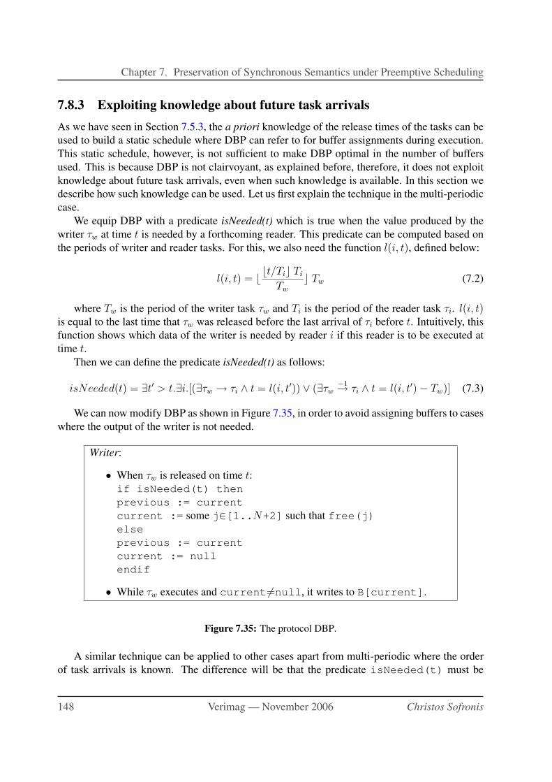
Chapter 7. Preservation of Synchronous Semantics under Preemptive Scheduling
7.8.3 Exploiting knowledge about future task arrivals
As we have seen in Section 7.5.3, the a priori knowledge of the release times of the tasks can be
used to build a static schedule where DBP can refer to for buffer assignments during execution.
This static schedule, however, is not sufficient to make DBP optimal in the number of buffers
used. This is because DBP is not clairvoyant, as explained before, therefore, it does not exploit
knowledge about future task arrivals, even when such knowledge is available. In this section we
describe how such knowledge can be used. Let us first explain the technique in the multi-periodic
case.
We equip DBP with a predicate isNeeded(t) which is true when the value produced by the
writer τw at time t is needed by a forthcoming reader. This predicate can be computed based on
the periods of writer and reader tasks. For this, we also need the function l(i, t), defined below:
l(i, t) = ⌊⌊t/Ti⌋ Ti
Tw
⌋ Tw (7.2)
where Tw is the period of the writer task τw and Ti is the period of the reader task τi. l(i, t)is equal to the last time that τw was released before the last arrival of τi before t. Intuitively, this
function shows which data of the writer is needed by reader i if this reader is to be executed at
time t.Then we can define the predicate isNeeded(t) as follows:
isNeeded(t) = ∃t′ > t.∃i.[(∃τw → τi ∧ t = l(i, t′)) ∨ (∃τw−1→ τi ∧ t = l(i, t′) − Tw)] (7.3)
We can now modify DBP as shown in Figure 7.35, in order to avoid assigning buffers to cases
where the output of the writer is not needed.
Writer:
• When τw is released on time t:if isNeeded(t) then
previous := current
current := some j∈[1..N+2] such that free(j)
else
previous := current
current := null
endif
• While τw executes and current6=null, it writes to B[current].
Figure 7.35: The protocol DBP.
A similar technique can be applied to other cases apart from multi-periodic where the order
of task arrivals is known. The difference will be that the predicate isNeeded(t) must be
148 Verimag — November 2006 Christos Sofronis
7.9. Related Work
defined in a different way: when a writer is released at time tw, we check if there is a release of a
reader between time tw and time t′w − 1, where t′w is the next release of writer after tw. If there is
such a release of a reader, then isNeeded(tw)=true and the standard procedure is followed.
is the above redundant???
In addition to the previous, as we saw in Section 7.5.3, DBP protocol can be applied to
tasks with known arrival patterns as well. In that case the predicate isNeeded(t) is given
by a known function with respect to relative arrivals of readers and the writer; when a writer
is released at time tw, we check if there is the release of a reader between time tw and time
t′w − 1, where t′w is the next release of writer after tw. If there is such a release of a reader, then
isNeeded(t)=true and the standard procedure is followed.
7.9 Related Work
Before we conclude this Chapter, we discuss a number of related works. First we present the
code generation method that the tool REAL-TIME WORKSHOP applies for SIMULINK and its
current limitations. Next, we discuss the paper [BFMSV05] extensively, since it includes the
closest work to ours. Finally, we discuss a number of other related works.
Code generation for SIMULINK/STATEFLOW models using REAL-TIME WORKSHOP.
The documentation of MathWorks’ code generator REAL-TIME WORKSHOP claims that the tool
builds code that reproduces the deterministic behavior of the model, provided tasks are peri-
odic and periods are multiples of each other6. The documentation does not describe how this is
achieved, however, evidence can be found in some restrictions imposed on multi-rate SIMULINK
diagrams. For instance, SIMULINK requires that a rate-transition block must be inserted every
time we have different rates between two connected blocks.
A Rate-transition block behaves as a unit-delay block, in the case where a “slow” writer
communicates data to a “fast” reader. In this case the block executes in the rate of the writer
but with the priority of the reader. The block will copy the output of the writer and provide it to
the reader upon his execution. Also a delay of 1 will be added in that communication, i.e., the
reader will always read the previous last result of the writer. On the other hand if a “fast” writer
sends data to a “slow” reader the rate-transition block acts like a zero-order hold block , i.e., it
is executed in the rate of the reader but with the priority of the writer, thus having always the
correct value needed by the writer.
However, this solution imposes the use of multi-periodic tasks and moreover that the reader
and the writer always have multiple periods, otherwise this solution fails. Note also, that the
above solution implies that the scheduling is done according to the rate monotonic priority
scheme [LL73], where the faster one task is executed, the higher priority it has.
6 Quoting from Section “Mapping Model Execution to the Target Environment” of [Mat]: “A correctly executing
application will generate deterministic results that are identical to the results produced by the model in simulation.
To achieve correct execution, the model’s sample rates must be mapped into corresponding tasks executing in the
target environment.” See the section titled “Models with Multiple Sample Rates” of the Real-Time Workshop user
guide, available at http://www.mathworks.com/access/helpdesk/help/toolbox/rtw/ug/.
Christos Sofronis Ph.D Thesis 149
Chapter 7. Preservation of Synchronous Semantics under Preemptive Scheduling
Our solution is more general since it applies also to event-triggered applications, to arbitrary
priority assignments, as well as to the EDF scheduling algorithm. Moreover, our solution is
memory-optimal when extended to many readers and writers.
Memory bounds on the implementation of synchronous programs. [BFMSV05] presents
work similar in spirit to ours, however, with a number of differences. The main focus
of [BFMSV05] is to provide upper bounds on the memory required by any inter-task communi-
cation protocol so that the synchronous semantics are preserved. Our emphasis is instead on the
development of communication schemes that achieve optimal memory bounds.
More specifically, the differences between the two works are the following. First, regarding
the setting:
• We work with a known scheduling policy (static-priority or EDF). In [BFMSV05], no
assumption is made about the scheduling policy.
• We require no knowledge of the minimum inter-arrival time (MIT) or deadline of tasks.
However, we do require schedulability. In [BFMSV05], it is assumed that the MIT and
deadline of each task is known. Schedulability is also assumed, in the sense that the dead-
line of each task is respected. The deadline of a task can be greater than its MIT, which
means that the schedulability assumption in [BFMSV05] is weaker than ours.
• We assume that all tasks run on a single processor. In [BFMSV05], no a-priori assumption
is made about the execution platform.
Then, regarding the memory requirements:
• We provide protocols that use buffers optimally.
• The bounds provided in [BFMSV05] are generally not tight. For example, in a static-
priority (SP) setting with one writer and N = 2 readers, where both readers have lower
priority than the writer, where the periods are Tw = 2, T1 = 3, T2 = 5, and the deadlines
are equal to the periods, we require 3 buffers whereas the upper bound calculated by the
formulas provided in [BFMSV05] is 4.
Finally, regarding the communication schemes:
• DBP is lock-free, meaning that tasks do not block on reads or writes: the only thing that can
suspend execution of a task is preemption by another, higher-priority task. DBP requires
atomic manipulations of global pointers upon task releases. These can be handled by the
operating system or by some special interrupt-handling routine with the highest priority.
• [BFMSV05] considers single-processor, “multi-processor” (many processors with central-
ized pointer manipulations) or “distributed” (many processors with decentralized pointer
manipulations) implementations. For single-processor implementations, both lock-free
and locking methods are considered. In the lock-free methods, the assumption is that
150 Verimag — November 2006 Christos Sofronis
7.9. Related Work
scheduling ensures that the producer has always higher priority than the consumer. This
implies that there can be no cycles in the graph of producers/consumers and that this graph
is topologically ordered in order to assign the priorities. The main impact of this assump-
tion is that a consumer task which comes after a long chain of producers will have a very
low priority, thus, it cannot handle “urgent” events. In contrast, in our work we make no
assumption on the relative priorities of producer and consumer, provided that a unit delay
is present when the producer has lower priority than the consumer.
In summary, one can say that the setting of [BFMSV05] is more general than ours, however,
it also requires more knowledge (minimum inter-arrival times, deadlines). Our protocol has
optimal memory requirements while the upper bounds provided in [BFMSV05] are not tight
(this is to be expected given that their setting is more general).
Other Related Work. [LM87] introduces the synchronous dataflow model (SDF) and provides
methods for static scheduling and code generation on single-processor or multi-processor archi-
tectures. This work has been extended in a number of directions, including buffer optimizations
(e.g., see [BML96, MB04]). SDF can be viewed as a subclass of the model we consider in this
paper, in the sense that only multi-periodic designs can be described in SDF. On the other hand,
SDF descriptions are more high-level and must generally be unfolded into a more basic model
such as ours. A major difference with our work, however, is that [LM87, BML96, MB04] aim for
static, cyclic schedules, whereas we aim for multi-task applications that use dynamic, preemptive
scheduling.
[Nat06] considers the problem of minimizing the cost of adding unit-delay or zero-order-hold
blocks in SIMULINK diagrams. The main difference with our work is that the focus of [Nat06]
is cost minimization and not preservation of semantics. Indeed, by adding or removing blocks as
the above, the semantics generally change. In contrast, we start from a fixed set of such blocks
and do not attempt a modification. We only perform optimizations at the implementation level
and not at the design level.
[RB04] proposes a method of distribution of synchronous programs and preserves the ideal
semantics by introducing delays in the early (high-level) design stages.
Our work is also related to a set of papers that propose lock-free inter-task communication
schemes, for instance [CB97, HPS02]. Although our methods are lock-free (only manipulations
of pointers are atomic, writes and reads need not be), it is different from the protocols proposed in
the above works. The latter preserve the integrity and often also the “freshness” of data, meaning
that the reader consumes the latest complete value produced by the writer. This value does not
always correspond to the value defined by the zero-time semantics. Another difference, which is
the basic characteristic of our work, is that the protocols are based on pointer manipulations that
happen upon task release, and not task execution, as is the case of the above protocols.
We should also note that our work has different objectives from the research done in the con-
text of real-time scheduling theory (e.g., see [LL73, HKO+93, ABD+95, SSRB98]). Real-time
scheduling theory is concerned with checking schedulability of a set of tasks in various settings.
Our concern is not schedulability, but preservation of semantics. We assume that the system is
Christos Sofronis Ph.D Thesis 151
Chapter 7. Preservation of Synchronous Semantics under Preemptive Scheduling
schedulable (something that can be checked using existing scheduling techniques such as those
in the works cited above) and we develop preservation schemes that rely on this assumption.
7.10 Conclusions
In this Chapter we studied the problem of semantics-preserving implementations of synchronous
programs on single-processor, multi-tasking execution platforms with preemptive scheduling
policies such as static-priority or EDF. We proposed a set of buffering protocols for inter-task
communication that preserve the synchronous semantics, that is, guarantee that the behavior of
the executed code will be the same (in terms of streams of output values) to the behavior of the
synchronous program. We proved this using model-checking as well as “manual” techniques.
We also proved that our generalized protocol (for the many writers-many readers case), DBP, is
optimal with respect to memory requirements.
152 Verimag — November 2006 Christos Sofronis
Chapter 8
Conclusions and Perspectives
The success of the SIMULINK/STATEFLOW toolkit is largely a result of the fact that a designer
can model the system coupled with the environment and simulate its execution. This success
shows that the industry of embedded control systems needs a complete approach starting from the
high-level conceptualization of the system until the final implementation in the target platform.
Such an approach raises a number of important issues, especially in the domain of safety-
critical applications (avionics and automotive being two examples). We need model-checking
capabilities for verification purposes and when moving towards the execution platform, we need
an implementation methodology that preserves properties of the high-level design. Moreover,
efficiency of implementations in terms of memory usage or time performance is a must.
This is exactly the problem that this thesis treats and proposes solutions to. Indeed we pro-
pose a complete chain from top to bottom for the design and implementation of embedded control
systems. This is a three-layered approach, starting from the design using a high-level modeling
and simulation tool, in particular SIMULINK/STATEFLOW, and going down to the execution in a
single-processor, multi-tasking preemptive platform, while preserving the synchronous seman-
tics of the model all-along. We use LUSTRE as an intermediate language, because it provides a
formal modeling framework, rich with tools such as model-checkers, test-generators and code-
generators.
This work opens many directions for future research. Some general directions, in the context
of the overall model-based design effort at VERIMAG, are the following:
• Enlarging the set of high-level models in the picture of Figure 2.1. We have considered
SIMULINK and STATEFLOW. Another high-level modeling formalism (or rather, collec-
tion of formalisms) is the Unified Modeling Language (UML) and its various extensions,
such as SysML1. This language, coming from the software engineering domain rather than
control, addresses somewhat different concerns, which explains the interest of the industry
in it. At the same time, UML brings different challenges to an automated, semantics-
preserving implementation process, and this, independently of whether LUSTRE is consid-
ered or not as an intermediate point.
1 see http://www.omgsysml.org/
153
Chapter 8. Conclusions and Perspectives
• Enlarging the set of execution platforms. We now understand relatively well the imple-
mentation of synchronous models on single-processor platforms, single-tasking or multi-
tasking. Some initial work has been also done for distributed platforms, such as the Time-
Triggered Architecture or TTA [CCM+03], which is a synchronous execution platform,
and for multi-periodic applications. A lot remains however to be done in this direction.
For instance, we still need to cover loosely synchronous [BCG+02] or asynchronous ar-
chitectures with preemptive scheduling for more general task arrival patterns. Also we can
study the implementation in a distributed architecture equipped with a CAN or Flexray
bus, or a network of different buses connected through gateways.
Some directions more specifically related to the work done in this thesis are the following:
• Our translation method from SIMULINK to LUSTRE is restricted to the discrete-time part
of SIMULINK. A natural extension would be to consider continuous-time SIMULINK as
well. This is not a trivial problem, as it includes in essence the entire issue of relating
continuous-time and discrete-time systems, with the theory of sampling and other major
control-theoretic results. Some recent work in this direction has been done in [CB02,
KC06].
• Both translations of SIMULINK and STATEFLOW are “one-way”, in two senses: first, we
do not currently translate LUSTRE into SIMULINK (or STATEFLOW), and second, we do
not map the results provided by LUSTRE-based tools such as the LESAR model-checker
back to the original model. Both limitations are serious, in particular the second one, since
it obliges the user to “look under the hood”, so to speak, and inspect the results of the
analysis at the LUSTRE level. This requires familiarity with the LUSTRE language, which
SIMULINK/STATEFLOW users often lack.
• Our study of static analysis methods for STATEFLOW is only preliminary. In particular, the
techniques proposed in Chapter 5 have not been implemented. They should be, as well as
tested on a number of case studies. This would provide feedback in order to validate and
improve these methods.
• Another, more ambitious goal, is to develop dynamic model-checking algorithms for State-
flow, that are specific for the semantical problems of STATEFLOW (e.g., stack-overflow or
confluence). Model-checking for STATEFLOW is generally undecidable and so is check-
ing these properties, however, optimizations with respect to general model-checking algo-
rithms are probably possible.
• The prototype tool S2L that implements the algorithms studied in Chapter 4 can be further
extended to translate more blocks from the SIMULINK library that initially were not con-
sidered. In addition to that, newer releases of SIMULINK add new features and change the
input file representation of the model. Further study should be done in such additions and
incorporate those changes in the tool.
154 Verimag — November 2006 Christos Sofronis
• The buffering protocols we proposed in Chapter 7 rely on support from the operating sys-
tem, in particular regarding the management of pointers to the buffers upon arrivals of
task-triggering events. Methods to implement this mechanism on current RTOSs in an
efficient way (i.e., with minimal overhead) should be studied. One possibility for imple-
menting the mechanism without changing the RTOS kernel is to build special high-priority
interrupt handling routines that are executed upon arrival of the triggering events and ma-
nipulate the pointers. This solution should be evaluated with respect to others, in particular
those that rely on a modification of the kernel.
• In Chapter 7, we proposed only a simple and limited method to decompose synchronous
programs into tasks. This problem should be studied thoroughly.
• In the context of multi-tasking implementation of synchronous programs on preemptive
execution platforms, we can consider relaxing the schedulability assumption, to allow mul-
tiple instances of the same task to be active at the same time.
• More generally, our multi-tasking implementation scheme relies on external methods and
tools for scheduling and schedulability analysis. We can consider connecting the two in
a “feedback loop”, where information from the scheduler and schedulability analyzer is
provided to the code generator, in order to optimize the final solution.
Christos Sofronis Ph.D Thesis 155
Chapter 8. Conclusions and Perspectives
156 Verimag — November 2006 Christos Sofronis

Appendixes
157

Appendix A
Help messages by the S2L and SF2LUS tools
The help message provided by the S2L tool when this one is invoked from command line is the
one appearing in the Figure A.1
While the output of the SF2LUS program gives the following help message:
159
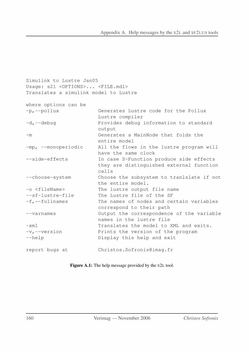
Appendix A. Help messages by the S2L and SF2LUS tools
Simulink to Lustre Jan05
Usage: s2l <OPTIONS>... <FILE.mdl>
Translates a simulink model to Lustre
where options can be
-p,--pollux Generates Lustre code for the Pollux
Lustre compiler
-d,--debug Provides debug information to standard
output
-m Generates a MainNode that folds the
entire model
-mp, --monoperiodic All the flows in the lustre program will
have the same clock
--side-effects In case S-Function produce side effects
they are distinguished external function
calls
--choose-system Choose the subsystem to tranlslate if not
the entire model.
-o <fileName> The lustre output file name
--sf-lustre-file The Lustre file of the SF
-f,--fullnames The names of nodes and certain variables
correspond to their path
--varnames Output the correspondence of the variable
names in the lustre file
-xml Translates the model to XML and exits.
-v,--version Prints the version of the program
--help Display this help and exit
report bugs at [email protected]
Figure A.1: The help message provided by the S2L tool.
160 Verimag — November 2006 Christos Sofronis
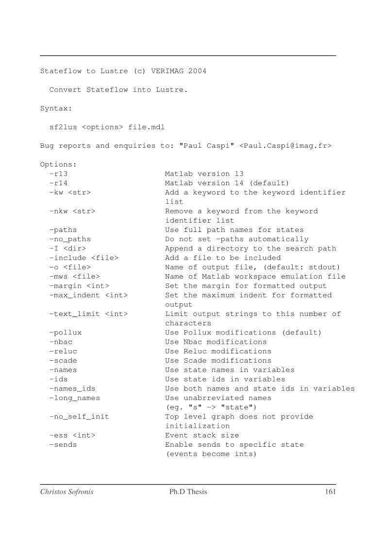
Stateflow to Lustre (c) VERIMAG 2004
Convert Stateflow into Lustre.
Syntax:
sf2lus <options> file.mdl
Bug reports and enquiries to: "Paul Caspi" <[email protected]>
Options:
-r13 Matlab version 13
-r14 Matlab version 14 (default)
-kw <str> Add a keyword to the keyword identifier
list
-nkw <str> Remove a keyword from the keyword
identifier list
-paths Use full path names for states
-no_paths Do not set -paths automatically
-I <dir> Append a directory to the search path
-include <file> Add a file to be included
-o <file> Name of output file, (default: stdout)
-mws <file> Name of Matlab workspace emulation file
-margin <int> Set the margin for formatted output
-max_indent <int> Set the maximum indent for formatted
output
-text_limit <int> Limit output strings to this number of
characters
-pollux Use Pollux modifications (default)
-nbac Use Nbac modifications
-reluc Use Reluc modifications
-scade Use Scade modifications
-names Use state names in variables
-ids Use state ids in variables
-names_ids Use both names and state ids in variables
-long_names Use unabrreviated names
(eg. "s" -> "state")
-no_self_init Top level graph does not provide
initialization
-ess <int> Event stack size
-sends Enable sends to specific state
(events become ints)
Christos Sofronis Ph.D Thesis 161
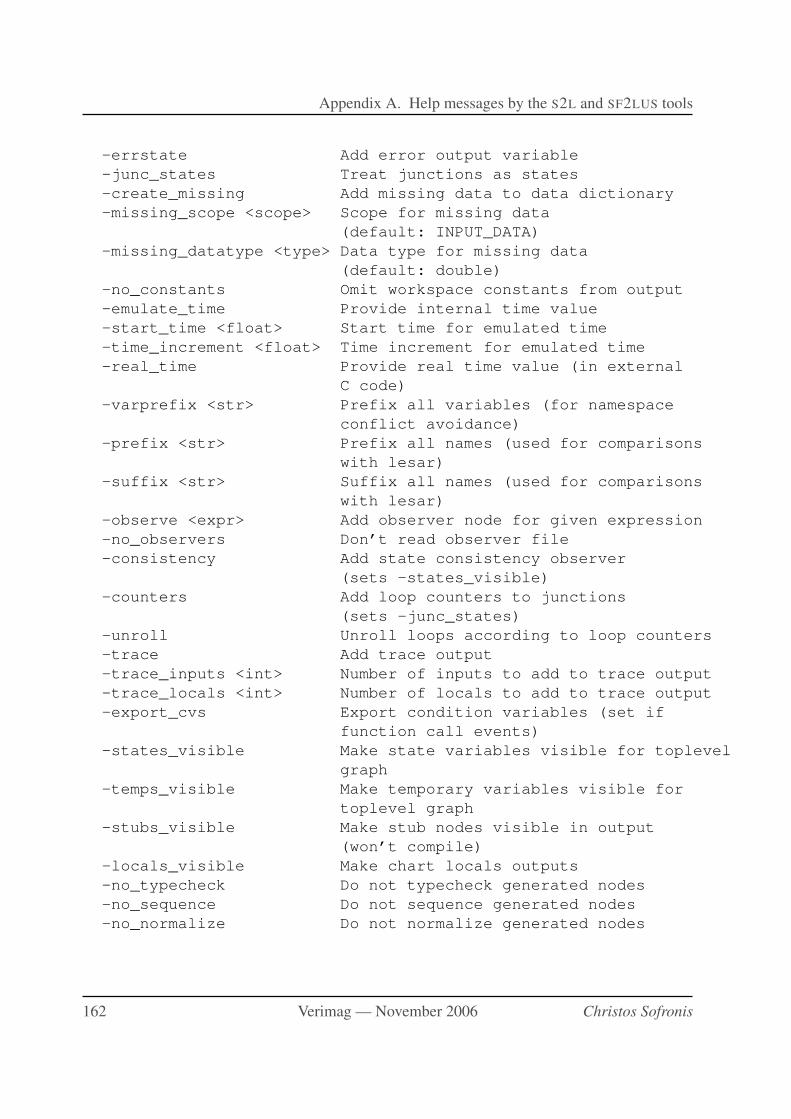
Appendix A. Help messages by the S2L and SF2LUS tools
-errstate Add error output variable
-junc_states Treat junctions as states
-create_missing Add missing data to data dictionary
-missing_scope <scope> Scope for missing data
(default: INPUT_DATA)
-missing_datatype <type> Data type for missing data
(default: double)
-no_constants Omit workspace constants from output
-emulate_time Provide internal time value
-start_time <float> Start time for emulated time
-time_increment <float> Time increment for emulated time
-real_time Provide real time value (in external
C code)
-varprefix <str> Prefix all variables (for namespace
conflict avoidance)
-prefix <str> Prefix all names (used for comparisons
with lesar)
-suffix <str> Suffix all names (used for comparisons
with lesar)
-observe <expr> Add observer node for given expression
-no_observers Don’t read observer file
-consistency Add state consistency observer
(sets -states_visible)
-counters Add loop counters to junctions
(sets -junc_states)
-unroll Unroll loops according to loop counters
-trace Add trace output
-trace_inputs <int> Number of inputs to add to trace output
-trace_locals <int> Number of locals to add to trace output
-export_cvs Export condition variables (set if
function call events)
-states_visible Make state variables visible for toplevel
graph
-temps_visible Make temporary variables visible for
toplevel graph
-stubs_visible Make stub nodes visible in output
(won’t compile)
-locals_visible Make chart locals outputs
-no_typecheck Do not typecheck generated nodes
-no_sequence Do not sequence generated nodes
-no_normalize Do not normalize generated nodes
162 Verimag — November 2006 Christos Sofronis
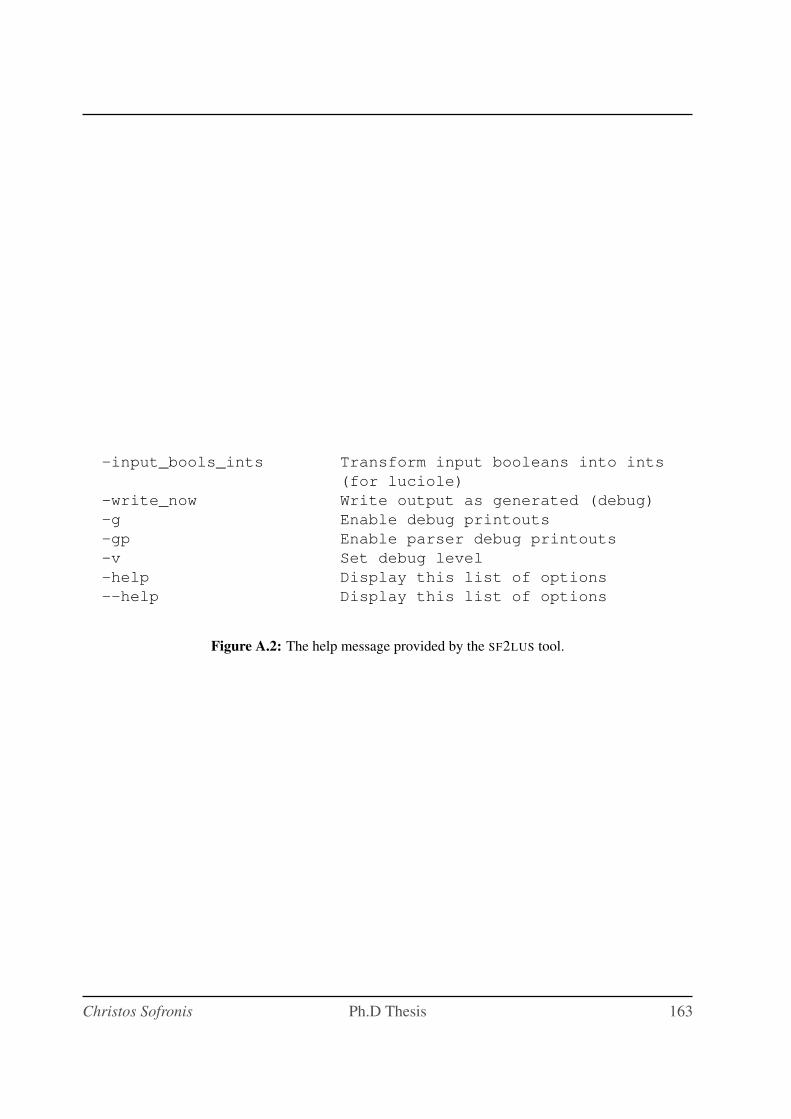
-input_bools_ints Transform input booleans into ints
(for luciole)
-write_now Write output as generated (debug)
-g Enable debug printouts
-gp Enable parser debug printouts
-v Set debug level
-help Display this list of options
--help Display this list of options
Figure A.2: The help message provided by the SF2LUS tool.
Christos Sofronis Ph.D Thesis 163

Appendix A. Help messages by the S2L and SF2LUS tools
164 Verimag — November 2006 Christos Sofronis
Appendix B
One-to-one translation of a SIMULINK
model to XML
As mentioned in Chapter 4, the first step of the S2L tool is the translation of the SIMULINK
model to an equivalent (in the sense of the information contained in both representations) XLM
document. This is done with the use of the fr.verimag.mdl2xml package as we saw in the
tool’s architecture in Figure 6.1. In this Appendix we demonstrate an example for this translation.
Figure B.1 shows a SIMULINK model file. However, since the length of that file (and there-
fore of the translated XML file) is too big we provide only some segments of them. Figure B.2
shows XML file that represents the SIMULINK model file (and that will be fed to the S2L tool to
continue with the translation to LUSTRE).
We can see clearly from this example that the produced XML file does not contain in-
formation that are irrelevant to the translation to LUSTRE, such the ScreenColor and
PaperOrientation properties of the source file, or the Position of the blocks. How-
ever, this is an option that can be disabled and produce an XML that is completely identical in
terms of information.
165
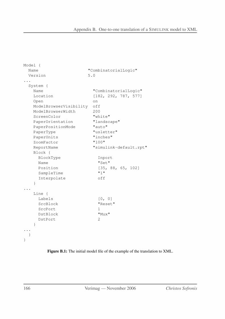
Appendix B. One-to-one translation of a SIMULINK model to XML
Model {
Name "CombinatorialLogic"
Version 5.0
...
System {
Name "CombinatorialLogic"
Location [182, 292, 787, 577]
Open on
ModelBrowserVisibility off
ModelBrowserWidth 200
ScreenColor "white"
PaperOrientation "landscape"
PaperPositionMode "auto"
PaperType "usletter"
PaperUnits "inches"
ZoomFactor "100"
ReportName "simulink-default.rpt"
Block {
BlockType Inport
Name "Set"
Position [35, 88, 65, 102]
SampleTime "1"
Interpolate off
}
...
Line {
Labels [0, 0]
SrcBlock "Reset"
SrcPort 1
DstBlock "Mux"
DstPort 2
}
...
}
}
Figure B.1: The initial model file of the example of the translation to XML.
166 Verimag — November 2006 Christos Sofronis
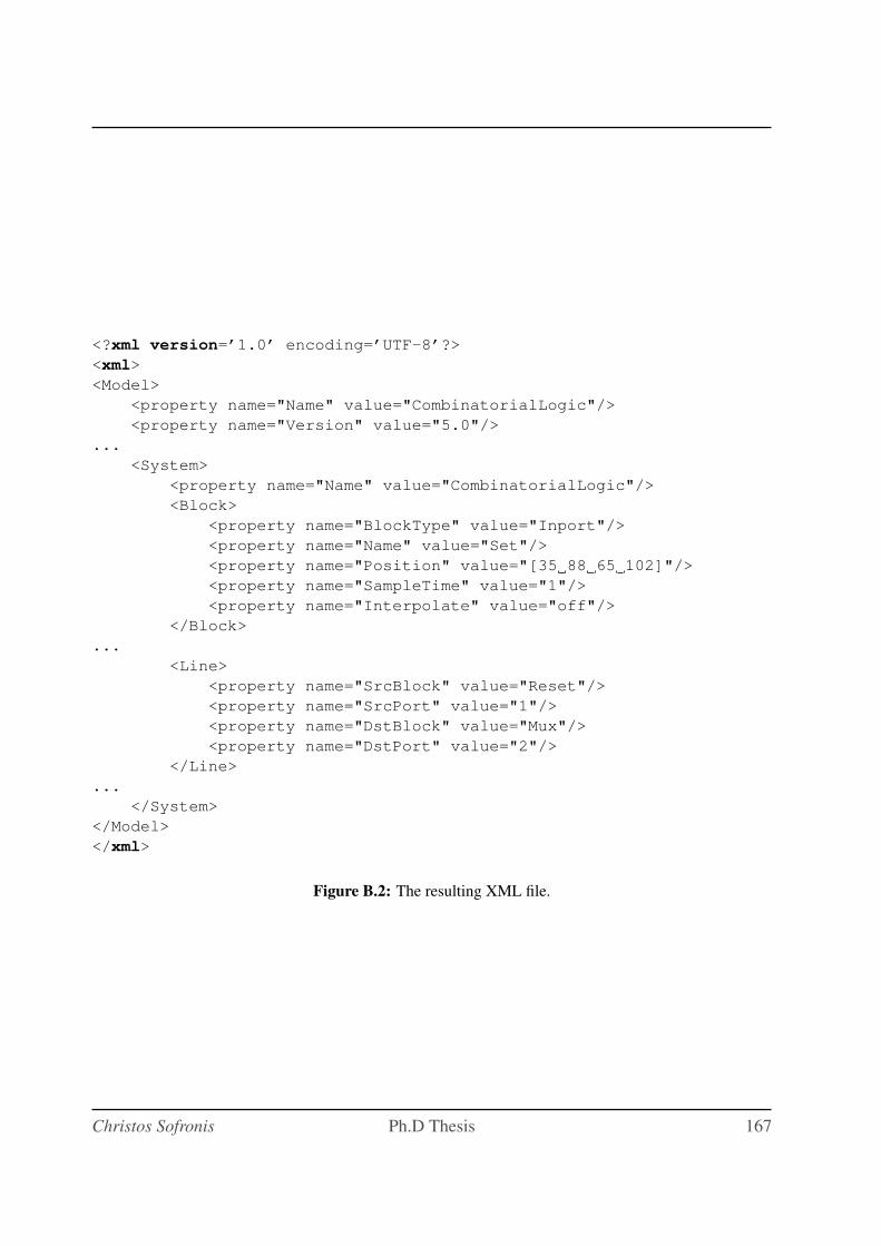
<?xml version=’1.0’ encoding=’UTF-8’?>
<xml>
<Model>
<property name="Name" value="CombinatorialLogic"/>
<property name="Version" value="5.0"/>
...
<System>
<property name="Name" value="CombinatorialLogic"/>
<Block>
<property name="BlockType" value="Inport"/>
<property name="Name" value="Set"/>
<property name="Position" value="[35 88 65 102]"/>
<property name="SampleTime" value="1"/>
<property name="Interpolate" value="off"/>
</Block>
...
<Line>
<property name="SrcBlock" value="Reset"/>
<property name="SrcPort" value="1"/>
<property name="DstBlock" value="Mux"/>
<property name="DstPort" value="2"/>
</Line>
...
</System>
</Model>
</xml>
Figure B.2: The resulting XML file.
Christos Sofronis Ph.D Thesis 167

Appendix B. One-to-one translation of a SIMULINK model to XML
168 Verimag — November 2006 Christos Sofronis
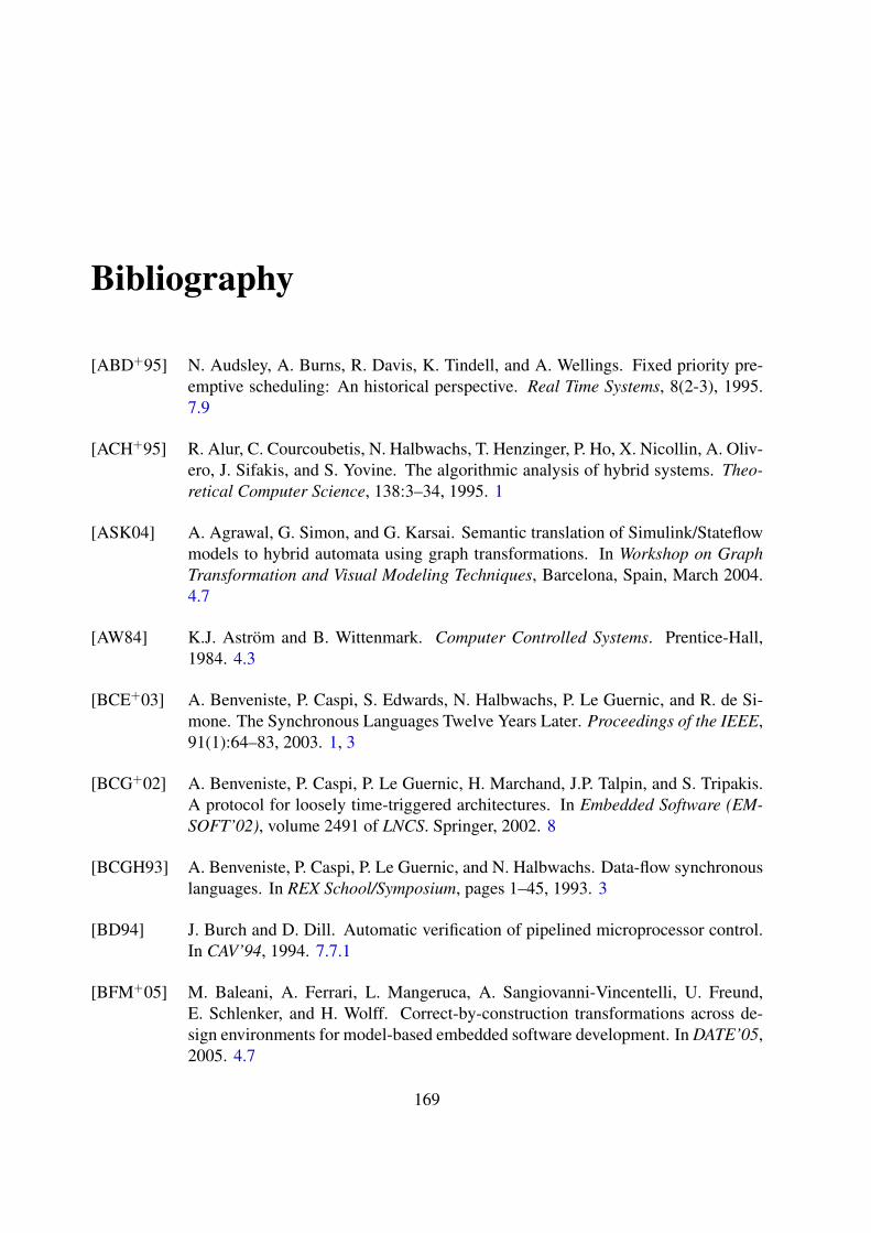
Bibliography
[ABD+95] N. Audsley, A. Burns, R. Davis, K. Tindell, and A. Wellings. Fixed priority pre-
emptive scheduling: An historical perspective. Real Time Systems, 8(2-3), 1995.
7.9
[ACH+95] R. Alur, C. Courcoubetis, N. Halbwachs, T. Henzinger, P. Ho, X. Nicollin, A. Oliv-
ero, J. Sifakis, and S. Yovine. The algorithmic analysis of hybrid systems. Theo-
retical Computer Science, 138:3–34, 1995. 1
[ASK04] A. Agrawal, G. Simon, and G. Karsai. Semantic translation of Simulink/Stateflow
models to hybrid automata using graph transformations. In Workshop on Graph
Transformation and Visual Modeling Techniques, Barcelona, Spain, March 2004.
4.7
[AW84] K.J. Astrom and B. Wittenmark. Computer Controlled Systems. Prentice-Hall,
1984. 4.3
[BCE+03] A. Benveniste, P. Caspi, S. Edwards, N. Halbwachs, P. Le Guernic, and R. de Si-
mone. The Synchronous Languages Twelve Years Later. Proceedings of the IEEE,
91(1):64–83, 2003. 1, 3
[BCG+02] A. Benveniste, P. Caspi, P. Le Guernic, H. Marchand, J.P. Talpin, and S. Tripakis.
A protocol for loosely time-triggered architectures. In Embedded Software (EM-
SOFT’02), volume 2491 of LNCS. Springer, 2002. 8
[BCGH93] A. Benveniste, P. Caspi, P. Le Guernic, and N. Halbwachs. Data-flow synchronous
languages. In REX School/Symposium, pages 1–45, 1993. 3
[BD94] J. Burch and D. Dill. Automatic verification of pipelined microprocessor control.
In CAV’94, 1994. 7.7.1
[BFM+05] M. Baleani, A. Ferrari, L. Mangeruca, A. Sangiovanni-Vincentelli, U. Freund,
E. Schlenker, and H. Wolff. Correct-by-construction transformations across de-
sign environments for model-based embedded software development. In DATE’05,
2005. 4.7
169
Bibliography
[BFMSV05] M. Baleani, A. Ferrari, L. Mangeruca, and A. Sangiovanni-Vincentelli. Efficient
embedded software design with synchronous models. In 5th ACM International
Conference on Embedded Software (EMSOFT’05), pages 187 – 190, 2005. 7.9,
7.9
[BG92] G. Berry and G. Gonthier. The Esterel synchronous programming language: de-
sign, semantics, implementation. Science of Computer Programming, 19(2):87–
152, 1992. 1
[BGL+00] S. Bensalem, V. Ganesh, Y. Lakhnech, C. Munoz, S. Owre, H. Rueß, J. Rushby,
V. Rusu, H. Saıdi, N. Shankar, E. Singerman, and A. Tiwari. An overview of SAL.
In C. Michael Holloway, editor, LFM 2000: Fifth NASA Langley Formal Meth-
ods Workshop, pages 187–196, Hampton, VA, jun 2000. NASA Langley Research
Center. 5.7
[BHLM94] J. Buck, S. Ha, E. Lee, and D. Messerschmitt. Ptolemy: A framework for simulat-
ing and prototyping heterogenous systems. Int. Journal in Computer Simulation,
4(2), 1994. 9
[BM06] P. Bostrom and L. Morel. Mode-Automata in Simulink/Stateflow. Technical Re-
port 772, Turku Centre for Computer Science, 2006. 6.2.4
[BML96] S. S. Bhattacharyya, P. K. Murthy, and E. A. Lee. Software Synthesis from Dataflow
Graphs. Kluwer, 1996. 7.9
[BWH+03] F. Balarin, Y. Watanabe, H. Hsieh, L. Lavagno, R. Passerone, and A. Sangiovanni-
Vincentelli. Metropolis: An integrated electronic system design environment.
IEEE Computer, 36:45–52, 2003. 1, 2
[Cas92] P. Caspi. Clocks in dataflow languages. Theoretical Computer Science, 94:125–
140, 1992. 4.5.1
[CB97] J. Chen and A. Burns. A three-slot asynchronous reader-writer mechanism for mul-
tiprocessor real-time systems. Technical Report YCS-286, Department of Com-
puter Science, University of York, May 1997. 7.1, 7.9
[CB02] P. Caspi and A. Benveniste. Toward an approximation theory for computer-
ized control. 2nd ACM International Conference on Embedded Software (EM-
SOFT’02), pages 294–304, 2002. 8
[CCM+03] P. Caspi, A. Curic, A. Maignan, C. Sofronis, S. Tripakis, and P. Niebert. From
Simulink to SCADE/Lustre to TTA: a layered approach for distributed embed-
ded applications. In Languages, Compilers, and Tools for Embedded Systems
(LCTES’03). ACM, 2003. 2, 4.3, 4.5.2, 5.4, 8
[CGP00] E. Clarke, O. Grumberg, and D. Peled. Model Checking. MIT Press, 2000. 7.7
170 Verimag — November 2006 Christos Sofronis
Bibliography
[CHLrA02] A. Cervin, D. Henriksson, B. Lincoln, and K.-E. rArzen. Jitterbug and Truetime:
Analysis tools for real-time control systems. In 2nd Workshop on Real-Time Tools,
2002. 4.7
[CK03] A. Chutinan and B.H. Krogh. Computational techniques for hybrid system verifi-
cation. IEEE Trans. Automatic Control, 48(1), 2003. 4.7
[CP03] J.L. Colaco and M. Pouzet. Clocks as first class abstract types. In Embedded
Software (EMSOFT’03), volume 2855 of LNCS. Springer, 2003. 4.5.1
[CPHP87] P. Caspi, D. Pilaud, N. Halbwachs, and J. Plaice. Lustre: a declarative language
for programming synchronous systems. In 14th ACM Symp. POPL, 1987. 3
[Cur05] A. Curic. Implementing Lustre Programs on Distributed Platforms with Real-Time
Constraints. PhD thesis, University Joseph Fourier, Grenoble, France, 2005. 2
[Est] Esterel Technologies, Inc. SCADE Language - Reference Manual 2.1. 6.1.2
[For99] Ford. Structured Analysis Using Matlab/Simulink/Stateflow - Modeling Style
Guidelines. Technical report, Ford Motor Company, 1999. 5.7
[FY04] E. Fersman and W. Yi. A generic approach to schedulability analysis of real-time
tasks. Nordic J. of Computing, 11(2):129–147, 2004. 7.3.1
[GGBM91] P. Le Guernic, T. Gautier, M. Le Borgne, and C. Le Maire. Programming real-time
applications with Signal. Proc. of the IEEE, 79(9):1321–1336, 1991. 1, 4.7
[Gro01] Open Management Group. Response to the OMG RFP for schedulability, perfor-
mance, and time revised submission. OMG Document number: ad/2001-06-14,
June 18, 2001. 2
[Gro05] Open Management Group. Unified Modeling Language: Superstructure, version
2.0, 2005. Available at http://www.omg.org/cgi-bin/doc?formal/05-07-04. 5.7
[Har87] D. Harel. Statecharts: A Visual Formalism for Complex Systems. Science of
Computer Programming, 8(3):231–274, June 1987. 5.1, 5.2, 5.7
[HCRP91] N. Halbwachs, P. Caspi, P. Raymond, and D. Pilaud. The synchronous dataflow
programming language lustre. Proceedings of the IEEE, 79(9), September 1991.
1, 2, 3, 7.1
[HG97] David Harel and Eran Gery. Executable object modeling with statecharts. Com-
puter, 30(7):31–42, 1997. 5.7
[HHK01] T. Henzinger, B. Horowitz, and C. Kirsch. Giotto: A time-triggered language for
embedded programming. In EMSOFT’01, volume 2211 of LNCS. Springer, 2001.
4.7
Christos Sofronis Ph.D Thesis 171
Bibliography
[HJW90] P. Hudak, S. Peyton Jones, and P. Wadler. Report on the programming language
haskell, a non strict purely functional language (version 1.2). ACM SIGPLAN
Notices, 27(5), 1990. 4.4.3
[HKO+93] M.G. Harbour, M.H. Klein, R. Obenza, B. Pollak, and T. Ralya. A Practitioner’s
Handbook for Real-Time Analysis: Guide to Rate-Monotonic Analysis for Real-
Time Systems. Kluwer, 1993. 7.3.1, 7.9
[HLR92] N. Halbwachs, F. Lagnier, and C. Ratel. Programming and verifying real-time
systems by means of the synchronous data-flow programming language Lustre.
IEEE Transactions on Software Engineering, Special Issue on the Specification
and Analysis of Real-Time Systems, September 1992. 5.4, 6.1.2
[HN96] David Harel and Amnon Naamad. The STATEMATE semantics of statecharts.
ACM Transactions on Software Engineering and Methodology, 5(4):293–333,
1996. 5.7
[Hoa85] C.A.R. Hoare. Communicating Sequential Processes. Prentice Hall, 1985. 1
[HPR97] N. Halbwachs, Y.-E. Proy, and P. Roumanoff. Verification of real-time systems
using linear relation analysis. Formal Methods in System Design, 11(2):157–185,
August 1997. 6.2.1
[HPS02] H. Huang, P. Pillai, and K. Shin. Improving wait-free algorithms for interprocess
communication in embedded real-time systems. In USENIX’02, 2002. 7.1, 7.9
[HR04] G. Hamon and J. Rushby. An operational semantics for Stateflow. In Fundamental
Approaches to Software Engineering (FASE), volume 2984 of LNCS, pages 229–
243, Barcelona, Spain, 2004. Springer. 5, 5.4.2, 5.4.4, 5.4.6, 5.7
[JB03] P.G. Joisha and P. Banerjee. The MAGICA type inference engine for MATLAB.
In Compiler Construction (CC). LNCS 2622, Springer, 2003. 4.7
[JHR99] B. Jeannet, N. Halbwachs, and P. Raymond. Dynamic partitioning in analyses of
numerical properties. In Static Analysis Symposium, pages 39–50, 1999. 5.4.2,
6.2.3
[JZW+00] M. Jersak, D. Ziegenbein, F. Wolf, K. Richter, R. Ernst, F. Cieslog, J. Teich,
K. Strehl, and L. Thiele. Embedded system design using the SPI workbench. In
Proc. of the 3rd International Forum on Design Languages, 2000. 4.7
[Kah74] G. Kahn. The semantics of a simple language for parallel programming. In Proc.
of the IFIP Congress, 1974. 1
[KC06] C. Kossentini and P. Caspi. Approximation, sampling and voting in hybrid com-
puting systems. In HSCC, pages 363–376, 2006. 8
172 Verimag — November 2006 Christos Sofronis
Bibliography
[KG94] H. Kopetz and G. Grunsteidl. TTP – a protocol for fault-tolerant real-time systems.
IEEE Computer, 27(1):14–23, January 1994. 2, 6.2.2
[Kop97] H. Kopetz. Real-Time Systems Design Principles for Distributed Embedded Appli-
cations. Kluwer, 1997. 2, 6.2.2
[KSHP02] C.M. Kirsch, M.A. Sanvido, T.A. Henzinger, and W. Pree. A Giotto-based heli-
copter control system. In EMSOFT’02. LNCS 2491, Springer, 2002. 4.7
[LL73] C.L. Liu and J. Layland. Scheduling algorithms for multiprogramming in a hard
real-time environment. Journal of the ACM, 20(1):46–61, January 1973. 7.1, 7.3.1,
7.8.1, 7.9, 7.9
[LM87] E. Lee and D. Messerschmitt. Synchronous data flow. Proceedings of the IEEE,
75(9):1235–1245, 1987. 7.9
[LvdBC00] G. Luttgen, M. von der Beeck, and R. Cleaveland. A Compositional Approach
to Statecharts Semantics. In D.Rosenblum, editor, Proceedings of the 8th ACM
SIGSOFT international symposium on Foundations of software engineering, pages
120–129. ACM Press, 2000. 5.2, 5.7
[Mat] The Mathworks Inc. Developing Embedded Targets for Real-Time Workshop R©Embedded Coder (R13). 6
[MB04] P. K. Murthy and S. S. Bhattacharyya. Buffer merging — a powerful technique
for reducing memory requirements of synchronous dataflow specifications. ACM
Transactions on Design Automation of Electronic Systems, 9(2):212–237, April
2004. 7.9
[MH96] F. Maraninchi and N. Halbwachs. Compiling ARGOS into boolean equations. In
Proc. 4th Int. School and Symposium “Formal Techniques in Real Time and Fault
Tolerant Systems” FTRTFT, pages 72–89, Uppsala, Sweden, 1996. 5.4.3
[Mil78] R. Milner. A theory of type polymorphism in programming. Journal of Computer
and System Sciences, 17:384–375, 1978. 4.4.3
[MLS97] E. Mikk, Y. Lakhnech, and M. Siegel. Hierarchical Automata as a Model for
Statecharts. In Asian Computing Science Conference (ASIAN’97), number 1345 in
Lecture Notes in Computer Science. Springer, December 1997. 5.7
[MM82] A. Martelli and U. Montanari. An efficient unification algorithm. ACM Trans. on
Progr. Lang. and Systems, 4(2), 1982. 4.4.3
[Nat06] M. Di Natale. Optimizing the multitask implementation of multirate Simulink
models. In 12th IEEE Real-Time and Embedded Technology and Applications
Symposium (RTAS’06), 2006. To appear. 7.9
Christos Sofronis Ph.D Thesis 173
Bibliography
[Nee01] S. Neema. Simulink and Stateflow data model. Technical report, ISIS, Vanderbilt
University, 2001. 5.7
[Pie02] B. Pierce. Types and Programming Languages. MIT Press, 2002. 4.4.2
[PV95] A. Puri and P. Varaiya. Driving safely in smart cars. In IEEE American Control
Conference, 1995. 7.1
[QS81] J.P. Queille and J. Sifakis. Specification and verification of concurrent systems in
CESAR. In 5th Intl. Sym. on Programming, volume 137 of LNCS, 1981. 7.7
[RB04] J. Romberg and A. Bauer. Loose synchronization of event-triggered networks for
distribution of synchronous programs. Proceedings of the fourth ACM interna-
tional conference on Embedded software, pages 193–202, 2004. 7.9
[RHR91] C. Ratel, N. Halbwachs, and P. Raymond. Programming and verifying critical
systems by means of the synchronous data-flow programming language Lustre. In
ACM-SIGSOFT Conference on Software for Critical Systems, 1991. 5.4, 6.1.2,
6.2.1, 7.7.1
[Rob65] J.A. Robinson. A machine-oriented logic based on the resolution principle. Journal
of the ACM, 12(1), 1965. 4.4.3
[SBCR01] S. Sims, K. Butts, R. Cleaveland, and S. Ranville. Automated validation of soft-
ware models. In ASE, 2001. 4.7
[SRKC00] B.I. Silva, K. Richeson, B.H. Krogh, and A. Chutinan. Modeling and verifying
hybrid dynamical systems using CheckMate. In ADPM, 2000. 4.7
[SRL90] L. Sha, R. Rajkumar, and J. Lehoczky. Priority inheritance protocols: An approach
to real-time synchronization. IEEE Trans. Computers, September 1990. 7.1, 7.3.3
[SSRB98] J. Stankovic, M. Spuri, K. Ramamritham, and G. Buttazzo. Deadline Scheduling
For Real-Time Systems: EDF and Related Algorithms. Kluwer Academic Publish-
ers, 1998. 7.3.1, 7.9
[STC05] C. Sofronis, S. Tripakis, and P. Caspi. A memory-optimal buffering protocol for
preservation of synchronous semantics under preemptive scheduling. In 6th ACM
International Conference on Embedded Software (EMSOFT’06), 2005. 5.4
[SV02] A. Sangiovanni-Vincentelli. Defining platform-based design. EEDesign of EE-
Times, February 2002. 2
[Tiw02] A. Tiwari. Formal semantics and analysis methods for Simulink Stateflow models.
Technical report, SRI International, 2002. 5.7
174 Verimag — November 2006 Christos Sofronis
Bibliography
[TNTBS00] S. Tudoret, S. Nadjm-Tehrani, A. Benveniste, and J.-E. Stromberg. Co-simulation
of hybrid systems: Signal-Simulink. In FTRTFT, volume 1926 of LNCS. Springer,
2000. 4.7
[Tri02] S. Tripakis. Description and schedulability analysis of the software architecture
of an automated vehicle control system. In Embedded Software (EMSOFT’02),
volume 2491 of LNCS. Springer, 2002. 7.1
[TSSC05] S. Tripakis, C. Sofronis, N. Scaife, and P. Caspi. Semantics-preserving and
memory-efficient implementation of inter-task communication on static-priority
or EDF schedulers. In 5th ACM International Conference on Embedded Software
(EMSOFT’05), pages 353 – 360, 2005. 5.4
Christos Sofronis Ph.D Thesis 175

Bibliography
176 Verimag — November 2006 Christos Sofronis