electromagnetic metamaterials: transmission line theory and
TRANSCRIPT

ELECTROMAGNETICMETAMATERIALS

ELECTROMAGNETICMETAMATERIALS:TRANSMISSION LINETHEORY ANDMICROWAVEAPPLICATIONS
The Engineering Approach
CHRISTOPHE CALOZ
Ecole Polytechnique de Montreal
TATSUO ITOH
University of California at Los Angeles
A JOHN WILEY & SONS, INC., PUBLICATION

Copyright 2006 by John Wiley & Sons, Inc. All rights reserved.
Published by John Wiley & Sons, Inc., Hoboken, New Jersey.
Published simultaneously in Canada.
No part of this publication may be reproduced, stored in a retrieval system, or transmitted in any
form or by any means, electronic, mechanical, photocopying, recording, scanning, or otherwise,
except as permitted under Section 107 or 108 of the 1976 United States Copyright Act, without
either the prior written permission of the Publisher, or authorization through payment of the
appropriate per-copy fee to the Copyright Clearance Center, Inc., 222 Rosewood Drive, Danvers,
MA 01923, (978) 750-8400, fax (978) 750-4470, or on the web at www.copyright.com. Requests
to the Publisher for permission should be addressed to the Permissions Department, John Wiley &
Sons, Inc., 111 River Street, Hoboken, NJ 07030, (201) 748-6011, fax (201) 748-6008, or online at
http://www.wiley.com/go/permission.
Limit of Liability/Disclaimer of Warranty: While the publisher and author have used their best
efforts in preparing this book, they make no representations or warranties with respect to the
accuracy or completeness of the contents of this book and specifically disclaim any implied
warranties of merchantability or fitness for a particular purpose. No warranty may be created or
extended by sales representatives or written sales materials. The advice and strategies contained
herein may not be suitable for your situation. You should consult with a professional where
appropriate. Neither the publisher nor author shall be liable for any loss of profit or any other
commercial damages, including but not limited to special, incidental, consequential, or other
damages.
For general information on our other products and services or for technical support, please contact
our Customer Care Department within the United States at (800) 762-2974, outside the United
States at (317) 572-3993 or fax (317) 572-4002.
Wiley also publishes its books in a variety of electronic formats. Some content that appears in print
may not be available in electronic formats. For more information about Wiley products, visit our
web site at www.wiley.com.
Library of Congress Cataloging-in-Publication Data:
Caloz, Christophe, 1969-
Electromagnetic metamaterials : transmission line theory and microwave applications :
the engineering approach / Christophe Caloz, Tatsuo Itoh.
p.cm.
“Wiley-Interscience publication.”
Includes bibliographical references and index.
ISBN-10: 0-471-66985-7 (alk.paper)
ISBN-13: 978-0-471-66985-2 (alk.paper)
1. Magnetic materials. 2. Nanostructured materials. 3. Microwave transmission lines. I.
Itoh, Tatsuo. II. Title.
TK454.4.M3C36 2006
620.1′18—dc22
2005048976
Printed in the United States of America.
10 9 8 7 6 5 4 3 2 1

To Dominique, Maxime, and Raphael
Christophe

CONTENTS
Preface xiii
Acknowledgments xv
Acronyms xvii
1 Introduction 1
1.1 Definition of Metamaterials (MTMs) and Left-Handed (LH) MTMs, 1
1.2 Theoretical Speculation by Viktor Veselago, 3
1.3 Experimental Demonstration of Left-Handedness, 4
1.4 Further Numerical and Experimental Confirmations, 9
1.5 “Conventional” Backward Waves and Novelty of LH MTMs, 10
1.6 Terminology, 12
1.7 Transmission Line (TL) Approach, 12
1.8 Composite Right/Left-Handed (CRLH) MTMs, 16
1.9 MTMs and Photonic Band-Gap (PBG) Structures, 17
1.10 Historical “Germs” of MTMs, 20
References, 22
2 Fundamentals of LH MTMs 27
2.1 Left-Handedness from Maxwell’s Equations, 28
2.2 Entropy Conditions in Dispersive Media, 33
2.3 Boundary Conditions, 38
vii

viii CONTENTS
2.4 Reversal of Doppler Effect, 39
2.5 Reversal of Vavilov-Cerenkov Radiation, 41
2.6 Reversal of Snell’s Law: Negative Refraction, 43
2.7 Focusing by a “Flat LH Lens”, 46
2.8 Fresnel Coefficients, 48
2.9 Reversal of Goos-Hanchen Effect, 50
2.10 Reversal of Convergence and Divergence in Convex and Concave
Lenses, 51
2.11 Subwavelength Diffraction, 53
References, 57
3 TL Theory of MTMs 59
3.1 Ideal Homogeneous CRLH TLs, 59
3.1.1 Fundamental TL Characteristics, 60
3.1.2 Equivalent MTM Constitutive Parameters, 67
3.1.3 Balanced and Unbalanced Resonances, 70
3.1.4 Lossy Case, 74
3.2 LC Network Implementation, 79
3.2.1 Principle, 79
3.2.2 Difference with Conventional Filters, 83
3.2.3 Transmission Matrix Analysis, 85
3.2.4 Input Impedance, 100
3.2.5 Cutoff Frequencies, 103
3.2.6 Analytical Dispersion Relation, 106
3.2.7 Bloch Impedance, 113
3.2.8 Effect of Finite Size in the Presence of Imperfect
Matching, 115
3.3 Real Distributed 1D CRLH Structures, 119
3.3.1 General Design Guidelines, 120
3.3.2 Microstrip Implementation, 122
3.3.3 Parameters Extraction, 124
3.4 Experimental Transmission Characteristics, 127
3.5 Conversion from Transmission Line to Constitutive Parameters, 131
References, 131
4 Two-Dimensional MTMs 133
4.1 Eigenvalue Problem, 134
4.1.1 General Matrix System, 134
4.1.2 CRLH Particularization, 138
4.1.3 Lattice Choice, Symmetry Points, Brillouin Zone, and 2D
Dispersion Representations, 139
4.2 Driven Problem by the Transmission Matrix Method (TMM), 143
4.2.1 Principle of the TMM, 144
4.2.2 Scattering Parameters, 145

CONTENTS ix
4.2.3 Voltage and Current Distributions, 147
4.2.4 Interest and Limitations of the TMM, 154
4.3 Transmission Line Matrix (TLM) Modeling Method, 154
4.3.1 TLM Modeling of the Unloaded TL Host Network, 155
4.3.2 TLM Modeling of the Loaded TL Host Network (CRLH), 158
4.3.3 Relationship between Material Properties and the TLM Model
Parameters, 159
4.3.4 Suitability of the TLM Approach for MTMs, 161
4.4 Negative Refractive Index (NRI) Effects, 162
4.4.1 Negative Phase Velocity, 162
4.4.2 Negative Refraction, 163
4.4.3 Negative Focusing, 165
4.4.4 RH-LH Interface Surface Plasmons, 167
4.4.5 Reflectors with Unusual Properties, 169
4.5 Distributed 2D Structures, 170
4.5.1 Description of Possible Structures, 171
4.5.2 Dispersion and Propagation Characteristics, 173
4.5.3 Parameter Extraction, 178
4.5.4 Distributed Implementation of the NRI Slab, 183
References, 190
5 Guided-Wave Applications 192
5.1 Dual-Band Components, 193
5.1.1 Dual-Band Property of CRLH TLs, 193
5.1.2 Quarter-Wavelength TL and Stubs, 197
5.1.3 Passive Component Examples: Quadrature Hybrid and
Wilkinson Power Divider, 201
5.1.3.1 Quadrature Hybrid, 201
5.1.3.2 Wilkinson Power Divider, 202
5.1.4 Nonlinear Component Example: Quadrature Subharmonically
Pumped Mixer, 205
5.2 Enhanced-Bandwidth Components, 210
5.2.1 Principle of Bandwidth Enhancement, 211
5.2.2 Rat-Race Coupler Example, 215
5.3 Super-compact Multilayer “Vertical” TL, 217
5.3.1 “Vertical” TL Architecture, 219
5.3.2 TL Performances, 221
5.3.3 Diplexer Example, 225
5.4 Tight Edge-Coupled Coupled-Line Couplers (CLCs), 227
5.4.1 Generalities on Coupled-Line Couplers, 228
5.4.1.1 TEM and Quasi-TEM Symmetric Coupled-Line
Structures with Small Interspacing: Impedance
Coupling (IC), 228
5.4.1.2 Non-TEM Symmetric Coupled-Line Structures with
Relatively Large Spacing: Phase Coupling (PC), 232

x CONTENTS
5.4.1.3 Summary on Symmetric Coupled-Line Structures, 233
5.4.1.4 Asymmetric Coupled-Line Structures, 234
5.4.1.5 Advantages of MTM Couplers, 235
5.4.2 Symmetric Impedance Coupler, 235
5.4.3 Asymmetric Phase Coupler, 245
5.5 Negative and Zeroth-Order Resonator, 249
5.5.1 Principle, 249
5.5.2 LC Network Implementation, 251
5.5.3 Zeroth-Order Resonator Characteristics, 253
5.5.4 Circuit Theory Verification, 256
5.5.5 Microstrip Realization, 258
References, 259
6 Radiated-Wave Applications 261
6.1 Fundamental Aspects of Leaky-Wave Structures, 262
6.1.1 Principle of Leakage Radiation, 262
6.1.2 Uniform and Periodic Leaky-Wave Structures, 266
6.1.2.1 Uniform LW Structures, 266
6.1.2.2 Periodic LW Structures, 268
6.1.3 Metamaterial Leaky-Wave Structures, 269
6.2 Backfire-to-Endfire (BE) Leaky-Wave (LW) Antenna, 270
6.3 Electronically Scanned BE LW Antenna, 275
6.3.1 Electronic Scanning Principle, 276
6.3.2 Electronic Beamwidth Control Principle, 277
6.3.3 Analysis of the Structure and Results, 279
6.4 Reflecto-Directive Systems, 282
6.4.1 Passive Retro-Directive Reflector, 283
6.4.2 Arbitrary-Angle Frequency Tuned Reflector, 286
6.4.3 Arbitrary-Angle Electronically Tuned Reflector, 287
6.5 Two-Dimensional Structures, 290
6.5.1 Two-Dimensional LW Radiation, 290
6.5.2 Conical-Beam Antenna, 292
6.5.3 Full-Space Scanning Antenna, 296
6.6 Zeroth Order Resonating Antenna, 297
6.7 Dual-Band CRLH-TL Resonating Ring Antenna, 300
6.8 Focusing Radiative “Meta-Interfaces”, 304
6.8.1 Heterodyne Phased Array, 305
6.8.2 Nonuniform Leaky-Wave Radiator, 310
References, 313
7 The Future of MTMs 316
7.1 “Real-Artificial” Materials: the Challenge of Homogenization, 316
7.2 Quasi-Optical NRI Lenses and Devices, 319
7.3 Three-Dimensional Isotropic LH MTMs, 323

CONTENTS xi
7.4 Optical MTMs, 328
7.5 “Magnetless” Magnetic MTMs, 329
7.6 Terahertz Magnetic MTMs, 330
7.7 Surface Plasmonic MTMs, 331
7.8 Antenna Radomes and Frequency Selective Surfaces, 338
7.9 Nonlinear MTMs, 339
7.10 Active MTMs, 341
7.11 Other Topics of Interest, 341
References, 342
Index 347

PREFACE
This book is essentially the fruit of a research work carried out at University
of California, Los Angeles (UCLA), from 2002 to 2004 in the context of a
Multidisciplinary University Research Initiative (MURI) program. The main par-
ticipants in this program, in addition to the authors, were John Pendry (Imperial
College), David Smith (formerly University of California, San Diego (UCSD),
now Duke University), Sheldon Schultz (UCSD), Xiang Zhang (formerly UCLA,
now University of California, Berkeley), Gang Chen (formerly UCLA, now Mas-
sachusetts Institute of Technology (MIT)), John Joannopoulos (MIT) and Eli
Yablonovitch (UCLA).
During these years of infancy for metamaterials (MTMs), which emerged from
the first experimental demonstration of a left-handed (LH) structure in 2000, the
vast majority of the groups involved in research on MTMs had been focusing
on investigating from a physics point of view the fundamental properties of
LH media predicted by Veselago in 1967. Not following this trend, the authors
adopted an engineering approach, based on a generalized transmission line (TL)
theory, with systematic emphasis on developing practical applications, exhibiting
unprecedented features in terms of performances or functionalities. This effort
resulted in the elaboration of the powerful composite right/left-handed (CRLH)
MTM concept, which led to a suite of novel guided-wave, radiated-wave, and
refracted-wave devices and structures.
This book presents electromagnetic MTMs and their applications in the gen-
eral framework of CRLH TL MTMs. Chapter 1 introduces MTMs from a his-
torical perspective and points out their novelty compared with conventional
periodic backward-wave media. Chapter 2 exposes the fundamentals of ideal1
1“Ideal” designates here perfectly homogeneous and isotropic volumic (left-handedness along the
three directions of space) materials.
xiii

xiv PREFACE
LH MTMs, including the antiparallelism existing between phase/group veloc-
ities, the frequency dispersion required from entropy conditions, the modified
boundary conditions, the modified Fresnel coefficients, the reversal of classical
phenomena [Doppler effect, Vavilov-Cerenkov radiation, Snell’s law (negative
refractive index, NRI), Goos-Hanchen effect, lenses convergence/divergence],
and focusing by a flat “lens” and subwavelength diffraction. Chapter 3 estab-
lishes the foundations of CRLH structures, in three progressive steps: ideal TL,
LC network, and real distributed structure. Chapter 4 extends theses founda-
tions to the two-dimensional (2D) case, develops a transmission matrix method
(TMM) and a transmission line method (TLM) techniques to address the prob-
lem of finite-size 2D MTMs excited by arbitrary sources, illustrates by TLM
simulations a few NRI effects occurring in 2D MTMs (backward-wave propa-
gation, negative refraction by a RH-LH interface, a LH slab, a LH prism, inner
reflection of Gaussian beams in a LH prism, and a LH “perfectly absorbing reflec-
tor”), and describes real distributed implementations of 2D MTMs. Chapter 5
presents guided-wave applications of CRLH TL MTMs, including dual-band
components, enhanced-bandwidth components, a super-compact multilayer “ver-
tical” structure, tight edge-coupled directional couplers, and negative/zeroth-order
resonators. Chapter 6 presents radiated-wave applications of CRLH TL MTMs,
including 1D or 2D frequency-scanned and electronically scanned leaky-wave
antennas and reflecto-directive systems. Finally, future challenges and prospects
of MTMs, including homogenized MTMs, quasi-optical NRI lenses, 3D isotropic
LH structures, optical MTMs, magnetless magnetic MTMs, surface plasmonic
MTMs, MTMs antenna radomes and frequency selective surfaces, nonlinear, and
active MTMs, are discussed in Chapter 7.
It is hoped that the engineering approach of MTMs presented in this book
will pave the way for a novel generation of microwave and photonic devices and
structures.
C. Caloz and T. Itoh
Monteal, Quebec, and Los Angeles, California

ACKNOWLEDGMENTS
Many researchers have contributed to the realization of this book.
The authors thank all the master’s and Ph.D. students of UCLA who have
been involved in this work: Anthony Lai, Sungjoon Lim, I-Hsiang Lin, Catherine
Allen, Lei Liu, Simon Otto, Chen-Jung Lee, and Marc de Vincentis.
In addition, the authors express their gratitude to several visiting scholars
of UCLA, who had various degrees of participation in this research, including
Hiroshi Okabe (Hitachi Central Research Laboratory), Yasushi Horii (Kansai
University), Taisuke Iwai (Fujitsu’s Research Labs), and Dal Ahn (Soonchun-
hyang University). Special thanks are addressed to Atsushi Sanada (Yamagushi
University), who played a major role in the development of several concepts and
applications presented in the book.
Finally, very special thanks are addressed to Wolfgang Hoefer, University
of Victoria, British Columbia, who kindly accepted to contribute to this work
by authoring two sections in Chapter 4 on the transmission line method (TLM)
analysis of 2D metamaterials.
This work was part of the MURI program “Scalable and Reconfigurable Elec-
tromagnetic Metamaterials and Devices.” It was supported by the Department
of Defense (program N00014-01-1-0803) and monitored by the U.S. Office of
Naval Research.
C. C. and T. I.
xv

ACRONYMS
ATR Attenuated total reflection
BCs Boundary conditions
BE Backfire-to-endfire
BWO Backward-wave oscillator
BZ Brillouin zone
CRLH Composite right/left-handed
CLC Coupled-line coupler
DB Dual-band
DPDS Dual-passband dual-stopband
FDTD Finite-difference time domain
FEM Finite-element method
FSS Frequency selective surface
GVD Group velocity dispersion
IC Impedance coupling or coupler
LH Left-handed
LTCC Low-temperature cofired ceramics
LW Leaky-wave
MIM Metal-insulator-metal
MTM Metamaterial
MLV Multilayered vertical
MoM Method of moments
MRI Magnetic resonance imaging
MSBVW Magnetostatic backward volume wave
NRI Negative refractive index
OPL Optical path length
xvii

xviii ACRONYMS
PC Phase coupling or coupler
PCB Printed circuit board
PBCs Periodic boundary conditions
PBG Photonic band-gap
PPWG Parallel-plate waveguide
PLH Purely left-handed
PRH Purely right-handed
QH Quadrature hybrid
RH Right-handed
RCS Radar cross section
RDS Reflecto-directive system
RRC Rat-race coupler
SHPM Subharmonically pumped mixer
SP Surface plasmon
SPM Self-phase modulation
SRR Split-ring resonator
TE Transverse electric
TEM Transverse electric-magnetic
TH Thin-wire
TL Transmission line
TLM Transmission line method
TM Transverse magnetic
TMA Transfer matrix algorithm
TMM Transmission matrix method
TWT Traveling-Wave Tube
UWB Ultra wideband
ZOR Zeroth-order resonator

1INTRODUCTION
Chapter 1 introduces electromagnetic metamaterials (MTMs) and left-handed
(LH) MTMs from a general prospect. Section 1.1 defines them. Section 1.2
presents the theoretical speculation by Viktor Veselago on the existence of “sub-
stances with simultaneously negative ε and µ” in 1967, which is at the origin of
all research on LH MTMs. Section 1.3 describes the first experimental demonstra-
tion of left-handedness in 2000 by Smith et al., and Section 1.4 lists a number of
further numerical, theoretical, and experimental confirmations of the fundamen-
tal properties of LH structures. The difference between “conventional” backward
waves, known for many decades, and LH waves, as well as the essential novelty
of LH MTMs, are explained in Section 1.5. Section 1.6 discusses the different
terminologies used in the literature to designate LH MTMs. Next, Section 1.7
introduces the transmission line (TL) approach of LH MTMs, which has consti-
tuted a decisive step toward microwave applications, and Section 1.8 presents, in
a concise manner, the generalized composite right/left-handed (CRLH) concept
upon which the whole book is based. Finally, Section 1.9 points out the essen-
tial difference existing between photonic crystals or photonic band-gap (PBG)
structures, more conventionally simply called “periodic structures”, and MTMs.
1.1 DEFINITION OF METAMATERIALS (MTMs)
AND LEFT-HANDED (LH) MTMs
Electromagnetic metamaterials (MTMs) are broadly defined as artificial effec-
tively homogeneous electromagnetic structures with unusual properties not readily
Electromagnetic Metamaterials: Transmission Line Theory and Microwave Applications,By Christophe Caloz and Tatsuo ItohCopyright 2006 John Wiley & Sons, Inc.
1

2 INTRODUCTION
available in nature. An effectively homogeneous structure is a structure whose
structural average cell size p is much smaller than the guided wavelength λg .
Therefore, this average cell size should be at least smaller than a quarter of
wavelength, p < λg/4. We will refer to the condition p = λg/4 as the effective-
homogeneity limit or effective-homogeneity condition1, to ensure that refractive
phenomena will dominate over scattering/diffraction phenomena when a wave
propagates inside the MTM medium. If the condition of effective-homogeneity is
satisfied, the structure behaves as a real material in the sense that electromagnetic
waves are essentially myopic to the lattice and only probe the average, or effec-
tive, macroscopic and well-defined constitutive parameters, which depend on the
nature of the unit cell; the structure is thus electromagnetically uniform along the
direction of propagation. The constitutive parameters are the permittivity ε and
the permeability µ, which are related to the refractive index n by
n = ±√εrµr , (1.1)
where εr and µr are the relative permittivity and permeability related to the
free space permittivity and permeability by ε0 = ε/εr = 8.854 · 10−12 and µ0 =µ/µr = 4π · 10−7, respectively. In (1.1), sign ± for the double-valued square
root function has been a priori admitted for generality.
The four possible sign combinations in the pair (ε, µ) are (+, +), (+, −),
(−, +), and (−, −), as illustrated in the ε − µ diagram of Fig 1.1. Whereas the
first three combinations are well known in conventional materials, the last one
[(−, −)], with simultaneously negative permittivity and permeability, corresponds
to the new class of left-handed (LH) materials.2 LH materials, as a consequence
of their double negative parameters, are characterized by antiparallel phase and
group velocities, or negative refractive index (NRI) [negative sign in Eq. (1.1)],
as will be shown in Chapter 2.
LH structures are clearly MTMs, according to the definition given above,
since they are artificial (fabricated by human hands), effectively homogeneous
(p < λg/4), and exhibit highly unusual properties (εr , µr < 0). It should be
noted that, although the term MTM has been used most often in reference to
LH structures in the literature, MTMs may encompass a much broader range of
1This limit corresponds to a rule of thumb effectiveness condition. Microwave engineers often use the
limit p = λg/4, where p is the size of the component considered, to distinguish lumped components
(p < λg/4) from quasi-lumped components (λg/4 < p < λg/2) and distributed components (p >
λg/2) [1]. In the lumped case, the phase variation of the signal from the input to the output of the
component is negligible, and the component may therefore be considered as a localized (sizeless)
element. In contrast, in the distributed case, phase variation along the component cannot be ignored,
and the component must consequently be considered as a transmission line section. MTMs are thus
“distributed structures constituted of lumped elements.”2It should be noted that thin ferrimagnetic films biased in the plane of the film support magnetostatic
backward volume wave (MSBVW) in the direction of bias, which may be seen as a LH phenomenon
(Section 2.1) in a real material. However, this phenomenon is strictly dependent on the thin slab
shape of the film and could not exist per se in a bulk ferrite and is therefore not an isotropic LH
effect.

THEORETICAL SPECULATION BY VIKTOR VESELAGO 3
ε
µ
r
r
r
r
I.
ε > 0, µ > 0:
n = +√εµ ∈ R, n > 0
isotropic dielectrics
right-handed (RH) /
forward-wave propagation
II.
ε < 0, µ > 0:
n = √εµ ∈ I, n < 0
plasmas (ω < ωpe)
metals at optical frequencies
evanescent wave
III.
ε < 0, µ < 0:
n = −√εµ ∈ R, n < 0
Veselago’s materials
left-handed (LH) /
backward-wave propagation
IV.
ε > 0, µ < 0:
n = √εµ ∈ I, n < 0
ferrites (ω < ωpm )
(ferrimagnetic materials)
evanescent wave
Fig. 1.1. Permittivity-permeability (ε − µ) and refractive index (n) diagram. The time
dependence e+jωt , associated with the outgoing wave function e−jβr or incoming wave
function e+jβr , where β is the propagation constant, β = nk0 (k0 = ω/c: free space
wavenumber, ω: angular frequency, c: speed of light), is assumed. The angular frequen-
cies ωpe and ωpm represent the electric and magnetic plasma frequencies, respectively. R,
purely real. I, purely imaginary.
structures.3 However, LH structures have been by far the most popular of the
MTMs, due to their exceptional property of negative refractive index (Chapter 2).
This book mainly deals with this class of MTMs and, more precisely, with
composite right/left-handed (CRLH) MTMs (Section 1.8), which constitute a
generalization of LH MTMs.
1.2 THEORETICAL SPECULATION BY VIKTOR VESELAGO
The history of MTMs started in 1967 with the visionary speculation on the
existence of “substances with simultaneously negative values of ε and µ” (fourth
3Examples are MTMs with only one of the two constitutive parameters negative, anisotropic MTMs,
or any type of functional effective engineered structure. In addition, many existing materials obtained
by novel nanotechnology and chemistry processes may be regarded as MTMs.

4 INTRODUCTION
quadrant in Fig 1.1) by the Russian physicist Viktor Veselago [3].4 In his paper,
Veselago called these “substances” LH to express the fact that they would allow
the propagation of electromagnetic waves with the electric field, the magnetic
field, and the phase constant vectors building a left-handed triad, compared with
conventional materials where this triad is known to be right-handed (Section 2.1).
Several fundamental phenomena occurring in or in association with LH media
were predicted by Veselago:
1. Necessary frequency dispersion of the constitutive parameters (Section 2.2).
2. Reversal of Doppler effect (Section 2.4).
3. Reversal of Vavilov-Cerenkov radiation (Section 2.5).
4. Reversal of the boundary conditions relating the normal components of the
electric and magnetic fields at the interface between a conventional/right-
handed (RH) medium and a LH medium (Section 2.3).
5. Reversal of Snell’s law (Section 2.6).
6. Subsequent negative refraction at the interface between a RH medium and
a LH medium (Section 2.6).
7. Transformation of a point source into a point image by a LH slab
(Section 2.6).
8. Interchange of convergence and divergence effects in convex and concave
lenses, respectively, when the lens is made LH (Section 2.6).
9. Plasmonic expressions of the constitutive parameters in resonant-type LH
media (Section 1.3).
Veselago concluded his paper by discussing potential real (natural) “sub-
stances” that could exhibit left-handedness. He suggested that “gyrotropic sub-
stances possessing plasma and magnetic properties” (“pure ferromagnetic metals
or semiconductors”), “in which both ε and µ are tensors” (anisotropic structures),
could possibly be LH.5 However, he recognized, “Unfortunately, . . . , we do not
know of even a single substance which could be isotropic and have µ < 0,”
thereby pointing out how difficult it seemed to realize a practical LH structure.
No LH material was indeed discovered at that time.
1.3 EXPERIMENTAL DEMONSTRATION OF LEFT-HANDEDNESS
After Veselago’s paper, more than 30 years elapsed until the first LH material was
conceived and demonstrated experimentally. This LH material was not a natural
substance, as expected by Veselago, but an artificial effectively homogeneous
4This paper was originally published in Russian in 1967 and then translated into English in 1968.
In this translation, the date of 1964 is indicated by mistake as the publication year of the original
Russian version.5This is indeed the case, in a restricted sense, of ferrite films supporting MSBVWs, as pointed out
in note 2.

EXPERIMENTAL DEMONSTRATION OF LEFT-HANDEDNESS 5
p
z
(a)
p
y
(b)
Fig. 1.2. First negative-ε/positive-µ and positive-ε/negative-µ MTM (p ≪ λg), consti-
tuted only by standard metals and dielectrics, proposed by Pendry. (a) Thin-wire (TW)
structure exhibiting negative-ε/positive-µ if E‖z [6]. (b) Split-ring resonator (SRR) struc-
ture exhibiting positive-ε/negative-µ if H⊥y [7].
structure (i.e., a MTM), which was proposed by Smith and colleagues at Uni-
versity of California, San Diego (UCSD) [4].6 This structure was inspired by the
pioneering works of Pendry at Imperial College, London. Pendry introduced the
plasmonic-type negative-ε/positive-µ and positive-ε/negative-µ structures shown
in Fig 1.2, which can be designed to have their plasmonic frequency in the
microwave range.7 Both of these structures have an average cell size p much
smaller than the guided wavelength λg (p ≪ λg) and are therefore effectively
homogeneous structures, or MTMs.
The negative-ε/positive-µ MTM is the metal thin-wire (TW) structure shown
in Fig 1.2(a). If the excitation electric field E is parallel to the axis of the wires
(E‖z), so as to induce a current along them and generate equivalent electric dipole
moments,8 this MTM exhibits a plasmonic-type permittivity frequency function
of the form [5, 6]
εr(ω) = 1 −ω2
pe
ω2 + jωζ= 1 −
ω2pe
ω2 + ζ 2+ j
ζω2pe
ω(ω2 + ζ 2), (1.2)
where ωpe =√
2πc2/[p2 ln(p/a)] (c: speed of light, a: radius of the wires) is the
electric plasma frequency, tunable in the GHz range, and ζ = ε0(pωpe/a)2/πσ
6The fact that this first LH MTM was artificial, as all the other LH MTMs known to date!, does
not at all exclude that natural substances exhibiting left-handedness could be discovered some day.
Because left-handedness is allowed by fundamental physics laws in artificial structures, there is no
reason why it would not be also possible in natural substances.7This is distinct from conventional gas and metal plasmas, which have their plasma frequency far
above the microwave range, preventing negative ε at microwave frequencies.8If the electric field E is perfectly parallel to the axis of the wires (z), a maximum of effect is
obtained. If it is exactly perpendicular to the wires, we have a situation of cross polarization, where
no effect is produced. In the intermediate situation where the electric field is oblique with respect to
the wires, a reduced effect occurs, decreasing as the angle with the wires increases.

6 INTRODUCTION
(σ : conductivity of the metal) is a damping factor due to metal losses. It clearly
appears in this formula that
Re(εr) < 0, for ω2 < ω2pe − ζ 2, (1.3a)
which reduces if ζ = 0 to
εr < 0, for ω < ωpe . (1.3b)
On the other hand, permeability is simply µ = µ0, since no magnetic material
is present and no magnetic dipole moment is generated. It should be noted that
the wires are assumed to be much longer than wavelength (theoretically infinite),
which means that the wires are excited at frequencies situated far below their
first resonance.
The positive-ε/negative-µ MTM is the metal split-ring resonator (SRR) struc-
ture9 shown in Fig 1.2(b). If the excitation magnetic field H is perpendicular
to the plane of the rings (H⊥y), so as to induce resonating currents in the
loop and generate equivalent magnetic dipole moments,10 this MTM exhibits a
plasmonic-type permeability frequency function of the form [7]
µr(ω) = 1 − Fω2
ω2 − ω20m + jωζ
= 1 − Fω2(ω2 − ω20m)
(ω2 − ω20m)2 + (ωζ )2
+ jFω2ζ
(ω2 − ω20m)2 + (ωζ )2
,
(1.4)
where F = π(a/p)2 (a: inner radius of the smaller ring), ω0m = c√
3p
π ln(2wa3/δ)
(w: width of the rings, δ: radial spacing between the rings) is a magnetic res-
onance frequency, tunable in the GHz range, and ζ = 2pR′/aµ0 (R′: metal
resistance per unit length) is the damping factor due to metal losses. It should
be noted that the SRR structure has a magnetic response despite the fact that
it does not include magnetic conducting materials due to the presence of artifi-
cial magnetic dipole moments provided by the ring resonators. Eq. (1.4) reveals
that a frequency range can exist in which Re(µr) < 0 in general (ζ = 0). In the
loss-less case (ζ = 0), it appears that
µr < 0, for ω0m < ω <ω0m√1 − F
= ωpm , (1.5)
where ωpm is called the magnetic plasma frequency. An essential difference
between the plasmonic expressions of ε and µ is that the latter is of resonant
9One single ring in the unit cell produces qualitatively identical effects, but the magnetic activity,
effective permeability and bandwidth, is enhanced by the presence of a second ring due to larger
overall current and slightly different overlapping resonances.10A remark analogous to that of note 8 holds here under the substitutions E → H and z → y.

EXPERIMENTAL DEMONSTRATION OF LEFT-HANDEDNESS 7
L1
R1
C1L2
R2C2
Cm
n
(a)
L
RC
(b)
Fig. 1.3. Equivalent circuit model of SRRs. (a) Double SRR configuration (e.g., [7]).
(b) Single SRR configuration.
nature [µ(ω = ω0m) = ∞], whereas the former is a nonresonant expression. The
resonance of the structure is due to the resonance of its SRRs, given in [7] by
ω20m = 3pc2/[π ln(2w/δ]a3) (p: period, c = 1/
√ε0µ0: speed of light, w: width
of the rings, δ: spacing between the rings).
The equivalent circuit of a SRR is shown in Fig 1.3 [8]. In the double ring
configuration [Fig 1.3(a)], capacitive coupling and inductive coupling between
the larger and smaller rings are modeled by a coupling capacitance (Cm) and by
a transformer (transforming ratio n), respectively. In the single ring configuration
[Fig 1.3(b)], the circuit model is that of the simplest RLC resonator with resonant
frequency ω0 = 1/√
LC. The double SRR is essentially equivalent to the single
SRR if mutual coupling is weak, because the dimensions of the two rings are
very close to each other, so that L1 ≈ L2 ≈ L and C1 ≈ C2 ≈ C, resulting in
a combined resonance frequency close to that of the single SRR with same
dimensions but with a larger magnetic moment due to higher current density.
In [4], Smith et al. combined the TW and SRR structures of Pendry into
the composite structure shown in Fig 1.4(a), which represented the first exper-
imental LH MTM prototype. The arguments in [4] consisted of the following:
1) designing a TW structure and a SRR structure with overlapping frequency
ranges of negative permittivity and permeability; 2) combining the two struc-
tures into a composite TW-SRR structure, which is shown in Fig 1.4(a); and 3)
launching an electromagnetic wave e−jβr through the structure and concluding
from a fact that a passband (or maximum transmission coefficient, experimen-
tally) appears in the frequency range of interest proves that the constitutive
parameters are simultaneously negative in this range on the basis of the fact
that β = nk0 = ±√εrµr has to be real in a passband.
Although the arguments of [4] were questionable, because it ignored the fact
that coupling interactions between the two constituent structures could yield prop-
erties totally different from the superposition of the properties of each structure
taken separately,11 a vivid experimental demonstration of the LH nature of the
TW-SRR was provided in [10]. In this paper, the TW-SRR structure of Fig 1.4(b)
11In fact, this structure was really “working” only due to the judicious position of the wires in the
symmetry center of the rings, which canceled interactions between the two structures due to induced

8 INTRODUCTION
xy
z
(a)
x
y
z
(b)
Fig. 1.4. First experimental LH structures, constituted of TWs and SRRs, introduced by
the team of UCSD. (a) Monodimensionally LH structure of [4]. (b) Bidimensionally LH
structure of [10].
Fig. 1.5. Experimental setup used in [10] for the demonstration of left-handedness of
the TW-SRR structure of Fig 1.4(b) at around 5 GHz. “The sample and the microwave
absorber were placed between top and bottom parallel, circular aluminum plates spaced
1.2 cm apart. The radius of the circular plates was 15 cm. The black arrows represent
the microwave beam as would be refracted by a positive index sample. The detector was
rotated around the circumference of the circle in 1.5
steps, and the transmitted power
spectrum was measured as a function of angle, θ , from the interface normal. The detector
was a waveguide to coaxial adapter attached to a standard X-band waveguide, whose
opening was 2.3 cm in the plane of the circular plates. θ as shown is positive in this
figure.” From [10], Science; reprinted with permission.
was cut into a wedge-shaped piece of MTM and inserted into the experimental
apparatus depicted in Fig 1.5. Left-handedness of the TW-SRR structure was
evidenced by the fact that a maximum of the transmission coefficient was mea-
sured in the negative angle (below the normal in the figure) with respect to the
currents with opposite signs in the SRRs and TWs [9]. Note that there an other possible symmetry
location for the TWs is in the midplanes between the SRRs.

FURTHER NUMERICAL AND EXPERIMENTAL CONFIRMATIONS 9
interface of the wedge, whereas a maximum in the positive angle (above the
normal) was measured, as expected, when the wedge was replaced by a regular
piece of teflon with identical shape. The result reported was in qualitative and
quantitative agreement with Snell’s law, which reads
k1 sin θ1 = k2 sin θ2, (1.6a)
or, if the two media are isotropic (so that k1 = n1k0 and k2 = n2k0),
n1 sin θ1 = n2 sin θ2, (1.6b)
where ki , ni , and θi represent the wavenumber, refractive index, and angle of
the ray from the normal to the interface, respectively, in each of the two media
considered (i = 1, . . . , 2).
The MTMs described here are anisotropic12 and characterized by uniaxial
permittivity and permeability tensors
[ε] =
εxx 0 0
0 εyy 0
0 0 εzz
, (1.7a)
[µ] =
µxx 0 0
0 µyy 0
0 0 µzz
. (1.7b)
The structure shown in Fig 1.4(a) is monodimensionally LH, since only one
direction is allowed for the doublet (E, H); we have εxx (ω < ωpe) < 0 and εyy =εzz > 0, µxx (ω0m < ω < ωpm) < 0 and µyy = µzz > 0. The structure shown in
Fig 1.4(b) is bidimensionally LH because, although E has to be directed along
the axis of the wires, two directions are possible for H; then [ε] is unchanged,
but µxx , µyy < 0 for ω0m < ω < ωpm and µzz > 0.
1.4 FURTHER NUMERICAL AND EXPERIMENTAL
CONFIRMATIONS
In the few years after the first experimental demonstration of a LH structure by
Smith et al., a large number of both theoretical and experimental reports con-
firmed the existence and main properties of LH materials predicted by Veselago.13
Characterization of the TW-SRR LH structures in terms of constitutive param-
eter functions similar to Eqs. (1.2) and (1.4) was provided by Smith et al. in
[12], [13], and [14] and was then abundantly rediscussed and refined by various
12It is worth noting that various spatial filtering effects may be obtained from this anisotropic
MTM [11].13In 2002, some controversies temporarily cast doubt on these novel concepts [15, 16, 17]. However,
these controversies were quickly shown to be based on physics misconceptions (e.g., [35]).

10 INTRODUCTION
TABLE 1.1. Verification of Main Properties and
Fundamental Physics of LH MTMs by Different
Approaches and Different Groups.
Type of Investigation References
Numerical FDTD Ziolkowski et al. [27, 28]
Numerical FEM Caloz et al. [29]
Numerical TMA Markos et al. [20, 21]
Numerical TLM So and Hoefer [30, 31]
Theoretical EM Lindell et al. [32], Kong et al.
[33, 34], Smith et al. [35],
McCall et al. [36]
Experimental
(bulk) TW-SRR
Shelby et al. [10], Greegor
et al. [22], Ziolkowski [26],
Marques et al. [25]
Theoretical TL Eleftheriades et al. [37, 38],
Caloz and Itoh [39, 40],
Oliner [41, 42]
Experimental
(planar) TL
Iyer et al. [43], Caloz and Itoh
[40], Sanada et al. [44]
groups, all confirming the LH nature of these structures (e.g., [18, 19, 20, 21,
22, 23, 24, 25, 26]).
Table 1.1 presents a list of key reports verifying, by different approaches, the
main properties and fundamental physics of LH MTMs. The main numerical
methods used are finite-difference time-domain (FDTD), finite-elements method
(FEM), transfer matrix algorithm (TAM), and transmission line method (TLM).
The theoretical verifications are subdivided into fundamental electromagnetic
(EM) theory and transmission line (TL) theory approaches. Experimental demon-
strations are provided both in TW-SRR bulk structures and planar TL-type
structures.
1.5 “CONVENTIONAL” BACKWARD WAVES AND NOVELTY
OF LH MTMs
Propagation of waves with antiparallel phase and group velocity is not a new
phenomenon. It has been known for many years in the physics and microwave
communities in various contexts. Back in the late 1940s, Brillouin and Pierce uti-
lized the series-capacitance/shunt-inductance equivalent circuit model shown in
Fig 1.6, which constitutes the starting point of the CRLH TL theory and applica-
tions presented in this book, to describe such antiparallel phase/group velocities
propagation, and used the term backward waves to designate the corresponding
waves [45, 46].14 For Brillouin, backward waves referred to negative space
14We may also add Malyuzhinets, who also used the same LC model, after Brillouin and Pierce, in
the description of the radiation condition in backward-wave media [47].

“CONVENTIONAL” BACKWARD WAVES AND NOVELTY OF LH MTMs 11
Fig. 1.6. Equivalent circuit model for a line supporting a backward wave.
harmonics contributing in the Fourier series expansion of fields in periodic
structures, while for Pierce and colleagues backward waves were related to the
phenomenon of backward amplification in traveling wave tubes (TWT).15 Several
classical textbooks describing backward waves are available [48, 49].
However, in both Brillouin’s and Pierce’s cases, and it seems in all other
known occurrences of backward-wave phenomena in the literature, perhaps with
the exception of magnetostatic backward volume waves (MSBVWs) [2], back-
ward waves are associated with either space harmonics or higher-order modes of
the structures. Therefore, these structures have a period typically of the order of
one-half the guided wavelength (p ≈ λg/2), or multiple of half the guided wave-
length for higher space harmonics or higher modes (p ≈ nλg/2). Consequently,
propagation along these conventional backward-wave structures are dominated
by diffraction/scattering phenomena, so that they cannot be characterized by con-
stitutive parameters ε and µ.16 Extended to 2D or 3D, if possible, they would not
exhibit the electromagnetic behavior of real materials, as for instance refractive
properties obeying to simple laws such as Snell’s law.
In contrast, LH MTMs are operating in their fundamental mode (effectively
homogeneous), where p ≪ λg , so that effective macroscopic ε and µ can be
rigorously defined. They are thus behaving as “real” materials. In fact, as long as
p < λg/4, the difference between a LH MTM and a natural dielectric material
(such as glass or Teflon) is only quantitative. In the case of the natural dielectric
material, the structural units inducing a given permittivity value are the consti-
tutive molecules, which are of the order of the Angstrom, while in the case of
current LH materials, the structural units are of the order of the centimeter in
the microwave range; thus, in the microwave L − X bands, the electrical size of
the structural unit in the former case is of the order of p/λg ≈ 10−9 while it is
of the order of p/λg ≈ 10−1 − 10−2 in the latter case. But qualitatively, similar
refractive phenomena occur in LH MTMs as in conventional dielectrics. This
is the point at which the fundamental originality of LH-MTMs lies: LH-MTMs
represent artificial structures behaving in the same manner as conventional bulk
dielectrics, hence the term “material” in meta-materials, but with negative con-
stitutive parameters. The subsequent and fundamental originality of LH MTMs
15Backward-wave oscillators (BWOs), which are realized by coupling some of the output power
of a TWT back into its input, also exhibit backward-wave properties reminiscent to those of LH
structures.16In this regard, they can be termed “structures” but not artificial “materials” or MTMs.

12 INTRODUCTION
is that, due to their effective homogeneity, they can be extended to 2D and
potentially 3D isotropic MTMs.
1.6 TERMINOLOGY
To date, there is no consensus regarding the terminology designating MTMs with
simultaneously negative permittivity and permeability. Several equivalent termi-
nologies have been used, each of which presenting advantages and disadvantages:
• Left-handed (LH) (e.g., [3, 12, 19, 20, 34, 40])—This is the terminology
originally suggested by Veselago in [3]. It has the advantage of being related
to the most fundamental property of these structures, which is antiparallel
phase and group velocities (Section 2.1), and to be universal (applicable to
1D, 2D, and 3D structures). Some authors feel that the term “left-handed”
could be confused with left-handed chiral materials, which may be consid-
ered a weakness of this term.
• Double-negative (DNG) (e.g., [28, 53])—In this case, the aforementioned
potential confusion is not possible. However, this term does not tell what is
negative and may be therefore seen as not self-consistent.
• Negative-refractive-index (NRI) (e.g., [38, 41])—NRI certainly represents
a meaningful term for 2D or 3D structures and also has the advantage of
emphasizing the effectively homogeneous nature of LH MTMs. However,
it looses its sense in 1D LH structures, where propagation angles are not
involved.
• Backward-wave (BW) (e.g., [32, 54])—The asset of this term may be that it
points out the existence of antiparallel phase/group velocities, well known
in conventional structures but fails to inform on the material (effectively
homogeneous) nature of LH MTMs (Section 1.5).
• Veselago medium (e.g., [50, 51])—This choice pays tribute to the visionary
idea of Veselago but does not provide any information on the properties of
the medium.
• Negative phase velocity medium (NPV) (e.g., [52])—In our opinion, this
term may be the best of all from a semantic point of view, but it has been
so little used that it may be premature to adopt it definitely, unless some sort
of consensus can be made between the main protagonists of MTM research.
In this book, we have made the choice of the terminology left-handed (LH)
MTM.
1.7 TRANSMISSION LINE (TL) APPROACH
Although very exciting from a physics point of view, the initial TW-SRR MTMs
(Fig 1.4) seem of little practical interest for engineering applications because

TRANSMISSION LINE (TL) APPROACH 13
these structures are resonant, and consequently exhibit high loss and narrow
bandwidth.17 A structure made of resonating elements generally does not consti-
tute a good transmission medium for a modulated signal because of the quality
factor intrinsically associated with each resonator [57]. In a resonator, the loaded
quality factor Ql is related to the unloaded quality factor Qu and external quality
factor Qe by the relation
1
Ql
= 1
Qu
+ 1
Qe
, (1.8)
which expresses the fact that the total transmission18 loss (∝ 1/Ql) through a res-
onator is equal to the sum of the dielectric/ohmic losses in the resonator (∝ 1/Qu)
and the coupling losses in the transitions with the external (source/load) circuits
(∝ 1/Qe). The loaded quality factor, which is the quantity actually measured and
eventually relevant in terms of transmission, is also obtained from the magnitude
of the transmission parameter (S21) as
Ql = fr
B, (1.9)
where fr is the resonance frequency and B is the −3-dB bandwidth (in Hz),
while the unloaded quality factor is defined as
Qu = ωaverage energy stored in resonator
power dissipated in resonator. (1.10)
These textbook formulas show that, for given dielectric (dielectric loss ∝ tan δ)
and metal (ohmic loss ∝ 1/σ , σ : conductivity) materials, there is an unavoidable
trade-off between bandwidth and transmission level. Minimum transmission loss,
or equivalently maximum Ql , is achieved at the resonance frequency fr by min-
imizing the bandwidth B, according to Eq. (1.9), because in this case very little
power is dissipated in the cavity since its bandwidth is extremely narrow so that
Qu is maximized, according to Eq. (1.10)19. So, in this case, good transmission
characteristics can be obtained. But bandwidth is so restricted that a modulated
signal, even with a modest bandwidth, cannot be transmitted without distortion
17The insertion loss reported in [13] for the first TW-SRR structure was higher than 30 dB! Opti-
mization of coupling mechanisms later improved the transmission characteristics of this structure.
For instance, minimum transmission loss of around 1 dB over a 3-dB fractional bandwidth of 6.5%
for a 3-cell structure was reported in [22]. Unfortunately, such performances are still not acceptable
for microwave engineering applications.18We are considering here a two-port TL-type (series) resonator system because we are interested
in transmission characteristics through the structure. In such a system, a maximum in the magnitude
of the transmission parameter (S21) occurs at the resonance [57]. A perfectly loss-less resonating
two-port system would correspond to Ql = ∞, implying Qu = ∞ and Qe = ∞.19This consideration is based on the assumption, generally reasonable, that Qe ≫ Qu, so that Ql is
mostly dependent on Qu, from (1.8).

14 INTRODUCTION
through the resonating structure. Bandwidth can naturally be increased, but this
immediately results in a decrease of Ql according to Eq. (1.9) and therefore
in an increase of transmission loss. In conclusion, a modulated signal cannot
be transmitted efficiently through a resonating propagation medium. Although
this statement is a very basic fact of resonators theory, it might not have been
sufficiently appreciated in the physics community investigating MTMs.
Due to the weaknesses of resonant-type LH structures, there was a need for
alternative architectures. Therefore, recognizing the analogy between LH waves
and conventional backward waves (Section 1.5), three groups introduced, almost
simultaneously in June 2002, a transmission line (TL) approach of metamaterials:
Eleftheriades et. al [37, 55], Oliner [41] and Caloz et al. [39, 56].
In fact, hypothetical “backward-wave” uniform TLs, without any suggestion
for a practical implementation!, had been briefly described in a few textbooks,
such as [48]. The incremental circuit model for such a TL, which is essentially
the dual20 of a conventional right-handed (RH) series-L/shunt-C TL, is shown in
Fig 1.7.21,22
The fundamental characteristics of the TL of Fig 1.7 are straightforwardly
derived by elementary TL theory. Let us consider here for simplicity the loss-
less case, the lossy case being rigorously treated in Chapter 3. The complex
L′L (H·m)
C′L (F·m)
Z′ = 1/(jωC′L)
Z′ = 1/(jωL′L)
z → 0
Fig. 1.7. Incremental circuit model for a hypothetical uniform LH TL.
20In this book, the term “dual” is considered in a broad sense, although more specific definitions
are preferred by some electromagnetic theoreticians. The series-C/shunt-L prototype is called the
dual of the series-L/shunt-C prototype, since it represents the fundamental “complement” to it, as
corroborated by the fact is associated with negative refractive index as a complement of positive
refractive index.21In the present book, primes are used to represent reactances related to per-unit-length immittances,
i.e., per-unit-length impedances Z′ in /m and admittances Y ′ in S/m.22Note the units of L′
L (H·m) and C ′L (F·m) ensuring that Z′ and Y ′ correspond to per-unit-
length immittances in /m and S/m, respectively. We have Z() = 1/[jωCL(F)] → Z′(/m) =1/[jωCL(F)z] = 1/[jωC ′
L(F·m)] where C ′L = CL · z; similarly, Y(S) = 1/[jωLL(H)] →
Y ′(S/m) = 1/[jωLL(H)z] = 1/[jωL′L(H · m)] where L′
L = LL · z.

TRANSMISSION LINE (TL) APPROACH 15
propagation constant γ , the propagation constant β, the characteristic impedance
Zc, the phase velocity vp, and the group velocity vg of the TL are given by
γ = jβ =√
Z′Y ′ = 1
jω√
L′LC′
L
= −j1
ω√
L′LC′
L
, (1.11a)
β = − 1
ω√
L′LC′
L
< 0, (1.11b)
Zc =√
Z′
Y ′ = +√
L′L
C′L
> 0, (1.11c)
vp = ω
β= −ω2
√
L′LC′
L < 0, (1.11d)
vg =(
∂β
∂ω
)−1
= +ω2√
L′LC′
L > 0. (1.11e)
The last two equations immediately and unambiguously show that phase and
group velocities in such a TL would be antiparallel, vp − ‖vg . The phase veloc-
ity vg , associated with the direction of phase propagation or wave vector β, is
negative, whereas the group velocity vg , associated with the direction of power
flow or Poynting vector S, is positive (Section 2.1). Thus, the TL of Fig 1.7 is
LH, according to the definition given in Section 1.2.
These considerations revealed that a LH TL medium could be engineered in
a structural manner by conceiving LC structures corresponding to the model of
Fig 1.6 in condition that the average cell size p would be much smaller than the
guided wavelength λg (p ≪ λg). If this could be accomplished, a nonresonant
type, in the frequency range of interest, LH medium would be obtained. Such
a design was shown to be perfectly realizable. The first practical LH TL was
the microstrip structure shown in Fig 1.8(a) [39], with a 2D version of it in
Fig 1.8(a).
Because of their nonresonant nature, TL MTMs can be designed to exhibit
simultaneously low loss and broad bandwidth. Low loss is achieved by a “bal-
anced” design (Section 1.8) of the structure and good matching to the excitation
ports, whereas broad-bandwidth is a direct consequence of the TL nature of the
structure and can be controlled by its LC parameters, which determine the cutoff
frequency of the resulting high-pass structure. Another advantage of TL MTM
structures is that they can be engineered in planar configurations, compatible
with modern microwave integrated circuits (MICs). Finally, TL MTM structures
can benefit from the efficient and well-established TL theory for the efficient
design of microwave applications. Over 25 novel devices, with unique features
or superior performances compared with conventional devices, have already been
demonstrated [58, 59] and are described in the Chapters 3, 5 and 7.

16 INTRODUCTION
(a) (b)
Fig. 1.8. Planar transmission line (TL) LH structures in microstrip technology constituted
of series interdigital capacitors and shunt stub inductors. The gray areas represent the
ground planes, and the black surfaces represent metal. (a) 1D (e.g., [39, 40]). (b) 2D
(similar to [44]).
1.8 COMPOSITE RIGHT/LEFT-HANDED (CRLH) MTMs
The concept of composite right/left-handed (CRLH) MTM, introduced by Caloz
et al. in [58], is the cornerstone of the theory and applications presented in this
book and is therefore extensively developed in the next chapters. However, this
section already introduces this concept as a broad-band generalization of LH
MTMs and provides a quick explanation of its essence.
The TL structures shown in Fig 1.8 are constituted of series (interdigital)
capacitors CL and shunt (stub) inductors LL, intended to provide left-handedness
from the explanations of the previous section. However, as a wave propagates
along the structures, the associated currents and voltages induce other natural
effects. As currents flow along CL, magnetic fluxes are induced and therefore a
series inductance LR is also present; in addition, voltage gradients exist between
the upper conductors and the ground plane, which corresponds to a shunt capac-
itance CR . As a consequence, a purely LH (PLH) structure does not exist, even
in a restricted frequency range, since a real LH structure necessarily includes
(LR, CR) contributions in addition to the (LL, CL) reactances. This was the moti-
vation for the introduction of the term “composite right/left-handed” (CRLH),
allowing to account for the exact natural of practical LH media [58, 60].
The essential characteristics of a CRLH TL MTM can be inferred from analysis
of the equivalent circuit of Fig 1.9(a). At low frequencies, LR and CR tend to be
short and open, respectively, so that the equivalent circuit is essentially reduced
to the series-CL/shunt-LL circuit, which is LH since it has antiparallel phase and
group velocities; this LH circuit is of highpass nature; therefore, below a certain
cutoff, a LH stopband is present. At high frequencies, CL and LL tend to be
short and open, respectively, so that the equivalent circuit is essentially reduced
to the series-LR/shunt-CR circuit, which is RH since it has parallel phase and
group velocities; this LH circuit is of lowpass nature; therefore, above a certain
cutoff, a RH stopband is present. In general, the series resonance ωse and shunt

MTMs AND PHOTONIC BAND-GAP (PBG) STRUCTURES 17
LR CL
CR LL
φ < π/2
ωse
ωsh
(a)
0βp
ω
−π +π
ωse
ωshω0
PLH
PRH
CRLH
CRLH
LH GAP
RH GAP
ωcR
ωcL
(b)
Fig. 1.9. Fundamentals of composite right/left-handed (CRLH) MTMs. (a) Unit cell
TL prototype. (b) Dispersion diagram. The curves for a purely LH (PLH) structure
(LR = CR = 0) and for a purely RH (PRH) structure (LL = CL = ∞) are also shown
for comparison. Here, we have represented the case ωse < ωsh , but ωse > ωsh is naturally
also possible, depending on the LC parameters (Section 3.1).
resonance ωsh are different, so that a gap exists between the LH and the RH
ranges. However, if these resonances are made equal, or are “balanced,” this gap
disappears, and an infinite-wavelength (λg = 2π/|β|) propagation is achieved
at the transition frequency ω0. Despite its filter nature, the CRLH structure is
never operated at the edges of the Brillouin zone, where p ≈ λg/2, but only in
the vicinity of the transition frequency, where effective-homogeneity is ensured
(p < λg/4). Note that, although a CRLH structure has both a LH range and a RH
range, the dispersion curve in each of these ranges significantly differs from that
of the PLH and PRH structures, respectively, because of the combined effects of
LH and RH contributions at all frequencies.
1.9 MTMs AND PHOTONIC BAND-GAP (PBG) STRUCTURES
The essential difference between MTM and photonic band gap (PBG) (or pho-
tonic crystals) structures has already been implicitly mentioned in Section 1.5
in connection with periodic structures. This section provides a more detailed
explanation of this difference.
Photonic crystals [61] and PBG [62] structures are usually operated at fre-
quencies where the lattice period p is of the order of a multiple of half a guided
wavelength, p ≈ nλg/2. In this case, as illustrated in Fig 1.10(a), the waves scat-
tered by adjacent layers of the lattice interfere constructively for some specific
angles of incidence. Therefore, net rejection of the incoming energy, correspond-
ing to zero group velocity, occurs at these angles. This phenomenon is similar to

18 INTRODUCTION
Bragg diffraction in X-ray optics [63] and is sometimes referred to as “Bragg-
like” diffraction. The Bragg condition for maximum diffraction is given by
2p sin θ = mλg, m = 0, 1, 2, . . . , (1.12)
where it is clearly seen that the Bragg angles are function of frequency (via λg).
This condition, with β = 2π/λg , is equivalent to
β(ω) = mπ
p sin θ(ω), m = 0, 1, 2, . . . , (1.13)
where the function β(ω) [or, more commonly, its inverse ω(β)] is the dispersion
relation, from which the dispersion diagram is computed. The points of the
dispersion curves ω(β) where the Bragg condition is met have a zero slope (or
tangent), since the slope of ω(β) corresponds to the group velocity, vg = dω/dβ,
which is zero there. This means that Bragg points delimit the stop bands or
band gaps in the dispersion diagram. The CRLH TL structure, whose dispersion
diagram is shown in Fig 1.9(b), has two Bragg points: one is the highpass LH
gap cutoff ωcL and the other one is the lowpass RH gap cutoff ωcR . At each
of these two points, we have |β|p = π ; i.e., p = π/|β|, which corresponds to
(1.13) with m = 1.23 These points correspond to resonating and noneffectively
homogeneous frequencies, and are therefore not in the range of MTM operation
of the CRLH structure.24
Whereas in a PBG structure period is of the order of wavelength [Fig 1.10(a)],
period (or average period) in a MTM is much smaller than wavelength
(p/λg ≪ 1), as shown in Fig 1.10(b). Therefore, interference effects cannot take
place in a MTM because the phase difference between adjacent cells is negligi-
ble. Instead, the wave simply travels through the material in a straight line, only
probing average or effective constitutive parameters. This is what happens in the
vicinity of the axis β = 0 ( spectral point) in a CRLH TL structure [Fig 1.9(b)].
In the balanced case, we have perfectly homogeneous transmission (p/λg = 0).
In the unbalanced case, we have the two resonances ωse and ωsh . However, these
resonances are not Bragg resonances but zeroth-order resonances (Section 5.5), in
the sense that they are infinite wavelength (β = 0, fundamental mode) resonances.
Thus, a photonic crystal or PBG structure is operated in the Bragg regime,
where periodicity plays a crucial role and the structure is strongly inhomogeneous,
whereas a MTM is operated in the long wavelength regime, where the lattice
does not need to be periodic and the structure is homogeneous. Consequently,
(diffraction/scattering) properties of photonic crystals are essentially determined
by the lattice,25 while the (refractive) properties of MTM are determined by the
nature of the unit cell, as detailed Section 3.1 [Eqs. (3.23) and (3.25)].
23In fact, m = −1 for the LH resonance, as it will be explained in Section 5.5.24At these frequencies, the structure is a PBG but not a MTM.25For instance, change the lattice of a 2D photonic crystal from square to hexagonal, without changing
the unit cell or basis, results in dramatic changes in the PBG structure (dispersion diagram), whereas
a change of the basis only hardly affects the PBG structure [61].

MTMs AND PHOTONIC BAND-GAP (PBG) STRUCTURES 19
p
λg
θ
(a)
p
θ
λg ≫ p
(b)
Fig. 1.10. Difference between the Bragg-scattering and long wavelength regimes.
(a) Bragg regime, p ≈ λg/2, usually prevailing in photonic crystals or PBG structures.
(b) Long wavelength regime, p ≪ λg , prevailing in MTMs.
Despite the fundamental differences pointed out above, several reports men-
tioning “negative refraction” in photonic crystals have been presented [64, 65, 66,
67].26 The important distinction to make between these “refraction-like”crystals
and LH MTMs is the following. A photonic crystal exhibits many higher-order
modes (or bands) ωm(β)27 with negative gradients ∇βmω (m: mode index). For
this reason, the corresponding mth Fourier spectral contribution to the total field
[Subsection 3.2.6, Eq. (3.107)] “propagates” with a phase in the opposite direc-
tion than that of power, which can result in NRI-like fields outside the photonic
crystal (e.g., in a photonic crystal prism [67]). However, this “wave” βm is only
one Fourier component in the total physical field and is not this field itself. The
physical field experiences scattering, not refraction, within the medium, as clearly
shown in various reported simulations. No negative focusing would be possible
26It may be noted that the more careful term “refraction-like behavior” is used in [65].27Note that β is a vector (hence the overline) if the dimension is superior than one. In the general 3D
case, we have β = βx x + βy y + βzz, where x, y, z denote unit vectors along the direction x, y, z,
respectively.

20 INTRODUCTION
inside a photonic crystal. In terms of engineering applications, this approach to
obtain LH-like effects does not seem judicious because 1) such effects are more
difficult to obtain in Bragg structures than in effectively homogeneous struc-
tures; 2) Bragg regime does not allow refractive effects inside the structure; and
3) Bragg structures necessarily result in large-size components since the unit cell
itself is already very large, p ∼ mλg/2.
1.10 HISTORICAL “GERMS” OF MTMs
In the previous sections, we reported the most significant milestones in the emer-
gence of the new field of MTMs and more particularly of LH or CRLH MTMs.
However, MTMs are related to such fundamental aspects of electromagnetic sci-
ence and engineering that they necessarily had a few more or less diffuse “germs”
in previous history. For instance in [68], Tretyakov presented an interesting “his-
torical perspective,” which uncovers some of these germs.28 We give now a
historical perspective partly inspired by this paper.
The earliest known speculation on negative refraction was made by Mandelsh-
tam back in 1944 [69]. In this paper, Mandelshtam noticed that, given two media
(labeled 1 and 2), for a given incidence angle θ1 of the wave at the interface,
Snell’s law [Eq. (1.6a)] admits, mathematically, two solutions: not only the con-
ventional solution θ2 but also the “unusual” solution π − θ229. Regarding this
second solution, Mandelshtam wrote:
“Demanding [as before] that the energy in the second medium propagates from theboundary, we arrive to the conclusion that the phase must propagate towards theboundary and, consequently, the propagation direction of the refracted wave willmake with the normal the angle π − θ2. This derivation appears to be unusual, butof course there is no wonder because the phase velocity still tells us nothing aboutthe direction of the energy transfer.”
Although we note that Mandelshtam made no reference to negative refraction
and did note carry out an in-depth study of this phenomenon, it is manifest that
his argument refers to the same phenomenon. This fact reduces in no ways the
pioneering merit of Veselago, who first addressed in 1967 the problem of LH
materials in a systematic manner; Veselago may be considered as the father of LH
MTMs with his decisive contribution of establishing their fundamental properties
and predicting their unusual effects [3] (Section 1.2).
The year after his initial speculation (1945), with reference to Lamb (1904)
who “gave examples of fictitious one-dimensional media with negative group
velocity,” Mandelshtam presented physical examples of structures supporting
waves with “negative group velocity,” such as structures with periodically varying
28The perspective of [68], as mentioned in the paper, is not systematic and therefore not necessarily
exhaustive. It is likely that even former “germs” of MTMs have existed under various forms.29This solution first seems to correspond to a ray in the half-plane of the reflection, but this solution
is necessarily in medium 2, as Mandelshtam explained in the statement given here.

HISTORICAL “GERMS” OF MTMs 21
effective permittivity [70]. However, these structures were not MTMs in the sense
defined in Section 1.1 but merely periodic structures, similar to those presented
for example in [45, 46] at the same period, based on space harmonics excitation.
Maybe the first report of a hypothetical medium with simultaneously negative
permittivity and permeability is the paper by Sivukhin in 1957 [71]. In this
paper, Sivukhin noticed that a media with double negative parameters would be
backward media, but this observation was still far from LH MTMs, as he pointed
out “media with ε < 0 and µ < 0 are not known. The question on the possibility
of their existence has not been clarified.”
As far as the TL approach of MTMs is concerned (Section 1.7), it has already
been mentioned in Section 1.5 that LH TL circuit models with series capacitance
and shunt inductances were used by several authors, such as for instance Brillouin
and Pierce [45, 46], back in the 1940s in the context of periodic structures and
microwave tubes. Malyuzhinets, in 1951, even showed a TL model similar to
the CRLH TL model (Section 1.8) [47]. However, none of these approaches
pertained to MTMs, as they were systematically used to describe space harmonics
of periodic structures, as opposed to a fundamental propagation mode, and its
seems that there was no clue at that time regarding how to design effective
LH and CRLH TL structures. Moreover, most of the MTMs and CRLH MTM
concepts presented in this book were apparently unknown. It should be noted
that some authors, such as for instance Ramo et al., showed the PLH TL in
their textbooks as a hypothetical effectively homogeneous TL, but without any
suggestion on the existence or design of such TLs [48].
There is no doubt that the periodic slow-wave, backward-wave structures stud-
ied and developed in the 1940s and 1950s included important germs of MTMs
and LH MTMs [45, 46, 47, 72]. It is worth noting that Silin discussed in 1959
the phenomenon of “negative refraction” in connection with periodic slow-wave
structures (although the definition of a refractive index in a periodic structure
operated in the Bragg regime is questionable, as pointed out in Section 1.9)
[73]. Nowadays, there is still considerable effort in conceiving MTMs based on
Bragg-regime periodic structures.
From the above reference with Mandelshtam, we see that Veselago was not
the first to postulate the existence of LH media in [3], but it is an established fact
that he was the first to conduct a systematic study of these media and to predict
their most fundamental properties.
After Veselago, there has been made really no attempt to design a LH MTM
before Smith et al. [4, 10]. However, resonant-type single ε negative and single
µ negative structures, which are the constitutive elements of the SRR/TW LH
MTMs (Section 1.3), have been reported under various forms long before the
systematic studies of Pendry in [5] (ε < 0) and [6] (µ < 0), who first developed
a unified approach of these structure as effective media or MTMs. It seems that
a wire medium, similar to the TW medium, was first described in the 1950s as
a material for microwave lenses [74, 75]. Variants of the SRR were presented
in the textbook by Schelkunoff and Friis published in 1952 [76], although these
SRRs were not considered there as the artificial particles of a magnetic medium

22 INTRODUCTION
(as introduced by Pendry in [6]). Media with loops of various shapes (e.g., omega,
helix, spiral) were abundantly reported in the 1980s and 1990s in the investigation
of artificial chiral and bi-isotropic materials for microwave applications [77].
These chiral materials are effective media and are therefore MTMs according
to our definition (Section 1.1); negative permeability was identified theoretically
and experimentally and described in several papers about chiral media. It is worth
noting that a chiral medium with double-ring structure implants very similar to
the SRRs was presented [78]. To conclude these remarks on relations between
chiral and LH MTMs let us also note that backward waves have been recently
shown to be supported by materials with positive parameters if chirality is present
[79, 80].
REFERENCES
1. J.-S. G. Hong, M. J. Lancaster. Microstrip Filters for RF/Microwave Applications,
Wiley-Interscience, 2001.
2. D. D. Stancil. Theory of Magnetostatic Waves, Springer-Verlag, 1993.
3. V. Veselago. “The electrodynamics of substances with simultaneously negative values
of ε and µ,” Soviet Physics Uspekhi, vol. 10, no. 4, pp. 509–514, Jan., Feb. 1968.
4. D. R. Smith, W. J. Padilla, D. C. Vier, S. C. Nemat-Nasser, and S. Schultz. “Com-
posite medium with simultaneously negative permeability and permittivity,” Phys.
Rev. Lett., vol. 84, no. 18, pp. 4184–4187, May 2000.
5. J. B. Pendry, A. J. Holden, W. J. Stewart, and I. Youngs. “Extremely low frequency
plasmons in metallic mesostructure,” Phys. Rev. Lett., vol. 76, no. 25, pp. 4773–4776,
June 1996.
6. J. B. Pendry, A. J. Holden, D. J. Robbins, and W. J. Stewart. “Low frequency plas-
mons in thin-wire structures,” J. Phys. Condens. Matter, vol. 10, pp. 4785–4809,
1998.
7. J. B. Pendry, A. J. Holden, D. J. Robbins, and W. J. Stewart. “Magnetism from con-
ductors and enhanced nonlinear phenomena,” IEEE Trans. Micr. Theory. Tech., vol. 47,
no. 11, pp. 2075–1084, Nov. 1999.
8. M. Makimoto and S. Yamashita. Microwave Resonators and Filters Communications:
Theory, Design and Applications, Springer, 2000.
9. D. R. Smith, D. C. Vier, N. Kroll, and S. Schultz. “Direct calculation of permeability
and permittivity for a left-handed metamaterial,” App. Phys. Lett., vol. 77, no. 14,
pp. 2246–2248, Oct. 2000.
10. R. A. Shelby, D. R. Smith, and S. Schultz. “Experimental verification of a negative
index of refraction,” Science, vol. 292, pp. 77–79, April 2001.
11. D. R. Smith and D. Schurig. “Electromagnetic wave propagation in media with indef-
inite permittivity and permeability tensors,” Phys. Rev. Lett., vol. 90, pp. 077405:1–4,
Feb. 2003.
12. D. R. Smith, D. C. Vier, N. Kroll, and S. Schultz. “Direct calculation of permeability
and permittivity for a left-handed metamaterial,” App. Phys. Lett., vol. 77, no. 14,
pp. 2246–2248, Oct. 2000.

REFERENCES 23
13. D. R. Smith and N. Kroll. “Negative refractive index in left-handed materials,” Phys.
Rev. Lett., vol. 85, no. 14, pp. 2933–2936, Oct. 2000.
14. R. A. Shelby, D. R. Smith, S. C. Nemat-Nasser, and S. Schultz. “Microwave trans-
mission through a two-dimensional, isotropic, left-handed metamaterial,” App. Phys.
Lett., vol. 78, no. 4, pp. 489–491, Jan. 2001.
15. M. Garcia, and M. Nieto-Vesperinas. “Left-handed materials do not make a perfect
lens,” Phys. Rev. Lett., vol. 88, no. 20, pp. 207403:1–4, Jan. 2002.
16. M. Garcia, and M. Nieto-Vesperinas. “Is there an experimental verification of a neg-
ative index of refraction yet?,” Optics Lett., vol. 27, no. 11, pp. 885–887, June 2002.
17. P. M. Valanju, R. M. Walser, and A. P. Valanju. “Wave refraction in negative-index
media: always positive and very inhomogeneous,” Phys. Rev. Lett., vol. 88, no. 18,
pp. 187401:1–4, 2002.
18. P. Gay-Balmaz and O. J. F. Martin. “Electromagnetic resonances in individual and
coupled split-ring resonators,” J. App. Phys., vol. 92, no. 5, pp. 2929–2936, Sept.
2002.
19. R. Marques, F. Median, and R. Rafii-El-Idrissi. “Role of bianisotropy in negative
permeability and left-handed metamaterials,” Phys. Rev. B, vol. 65, pp. 144440:1–6,
2002.
20. P. Markos and C. M. Soukoulis. “Numerical studies of left-handed materials and
arrays of split ring resonators,” Phys. Rev. E, vol. 65, pp. 036622:1–8, 2002.
21. P. Markos and C. M. Soukoulis. “Transmission studies of left-handed materials,”
Phys. Rev. B, vol. 65, pp. 033401:1–4, 2002.
22. R. B. Greegor, C. G. Parazzoli, K. Li, B. E. C. Koltenbah, and M. Tanielian. “Exper-
imental determination and numerical simulation of the properties of negative index
of refraction materials,” Optics Express, vol. 11, no. 7, pp. 688–695, April 2003.
23. E. Ozbay, K. Aydin, E. Cubukcu, and M. Bayindir. “Transmission and reflection prop-
erties of composite double negative metamaterials in free space,” IEEE Trans. Anten-
nas Propagat., vol. 51, no. 10, pp. 2592–2595, Oct. 2003.
24. C. R. Simovski, P. A. Belov, and S. He. “Backward wave region and negative mate-
rial parameters of a structure formed by lattices of wires and split-ring resonators,”
IEEE Trans. Antennas Propagat., vol. 51, no. 10, pp. 2582–2591, Oct. 2003.
25. R. Marques, F. Mesa, J. Martel, and F. Median. “Comparative analysis of edge- and
broadside-coupled split ring resonators for metamaterial: design, theory and experi-
ments,” IEEE Trans. Antennas Propagat., vol. 51, no. 10, pp. 2572–2581, Oct. 2003.
26. R. W. Ziolkowski. “Design, fabrication, and testing of double negative metamateri-
als,” IEEE Trans. Antennas Propagat., vol. 51, no. 7, pp. 1516–1529, July 2003.
27. R. W. Ziolkowski and E. Heyman. “Wave propagation in media having negative per-
mittivity and permeability” Phys. Rev. E, vol. 64, pp. 056625:1–15, 2001.
28. R. W. Ziolkowski. “Pulsed and CW gaussian beam interactions with double negative
metamaterial slabs,” Optics Express, vol. 11, no. 7, pp. 662–681, April 2003.
29. C. Caloz, C. C. Chang, and T. Itoh. “Full-wave verification of the fundamental prop-
erties of left-handed materials (LHMs) in waveguide configurations” J. App. Phys.,
vol. 90, no. 11, pp. 5483–5486, Dec. 2001.
30. P. P. M. So and W. J. R. Hoefer. “Time domain TLM modeling of metamaterials
with negative refractive index,” IEEE-MTT Int’l Symp., pp. 1779–1782, Fort Worth,
TX, June 2004.

24 INTRODUCTION
31. P. P. M. So, H. Du, and W. J. R. Hoefer. “Modeling of metamaterials with nega-
tive refractive index using 2D-shunt and 3D-SCN TLM networks,” IEEE Trans.
Microwave Theory Tech., pp. 1496–1505 vol. 53, no. 4, April. 2005.
32. I. V. Lindell, S. A. Tretyakov, K. I. Nikoskinen, and S. Ilvonen. “BW media –media
with negative parameters, capable of supporting backward waves,” Micr. Opt. Technol.
Lett., vol. 31, no. 2, pp. 129–133, Oct. 2001.
33. J. A. Kong, B.-I. Wu, and Y. Zhang. “A unique lateral displacement of a Gaussian
beam transmitted through a slab with negative permittivity and permeability,” Micr.
Opt. Technol. Lett., vol. 33, no. 2, pp. 136–139, April 2002.
34. J. Pacheco, T. M. Grzegorzcyk, B.-I. Wu, Y. Zhang, and J. A. Kong. “Wave propa-
gation in homogeneous isotropic frequency-dispersive left-handed media,” Phys. Rev.
Lett., vol. 89, no. 25, pp. 257401:1–4, Dec. 2002.
35. D. R. Smith, D. Schurig, and J. B. Pendry. “Negative refraction of modulated elec-
tromagnetic waves,” App. Phys. Lett., vol. 81, no. 15, pp. 2713–2715, Oct. 2002.
36. M. W. McCall, A. Lakhtakia, and W. S. Weiglhofer. “The negative index of refrac-
tion demystified,” Eur. J. Phys., vol. 23, pp. 353–359, 2002.
37. A. K. Iyer and G. V. Eleftheriades. “Negative refractive index metamaterials support-
ing 2-D waves,” in IEEE-MTT Int’l Symp., vol. 2, Seattle, WA, pp. 412–415, June
2002.
38. G. V. Eleftheriades, A. K. Iyer, and P. C. Kremer. “Planar negative refractive index
media using periodically L-C loaded transmission lines,” IEEE Trans. Microwave
Theory Tech., vol. 50, no. 12, pp. 2702–2712, Dec. 2002.
39. C. Caloz and T. Itoh. “Application of the transmission line theory of left-handed (LH)
materials to the realization of a microstrip LH transmission line,” in Proc. IEEE-AP-S
USNC/URSI National Radio Science Meeting, vol. 2, San Antonio, TX, pp. 412–415,
June 2002.
40. C. Caloz and T. Itoh. “Transmission line approach of left-handed (LH) structures
and microstrip realization of a low-loss broadband LH filter,” IEEE Trans. Antennas
Propagat., vol. 52, no. 5, pp. 1159–1166, May 2004.
41. A. A. Oliner. “A periodic-structure negative-refractive-index medium without res-
onant elements,” in URSI Digest, IEEE-AP-S USNC/URSI National Radio Science
Meeting, San Antonio, TX, pp. 41, June 2002.
42. A. A. Oliner. “A planar negative-refractive-index medium without resonant elements,”
in IEEE-MTT Int’l Symp., Philadelphia, PA, pp. 191–194, June 2003.
43. A. K. Iyer, P. C. Kremer, and G. V. Eleftheriades. “Experimental and theoretical ver-
ification of focusing in a large, periodically loaded transmission line negative refrac-
tive index metamaterial,” Optics Express, vol. 11, no. 7, pp. 696–708, April 2003.
44. A. Sanada, C. Caloz, and T. Itoh. “Planar distributed structures with negative refrac-
tive index,” IEEE Trans. Microwave Theory Tech., vol. 52, no. 4, pp. 1252–1263,
April 2004.
45. L. Brillouin. Wave Propagation in Periodic Structures, McGraw-Hill, 1946.
46. J. R. Pierce. Traveling-Wave Tubes, D. Van Nostrand, 1950.
47. G. D. Malyuzhinets. “A note on the radiation principle,” Zhurnal Technicheskoi Fiziki,
vol. 21, pp. 940–942, 1951 [in Russian].
48. S. Ramo, J. R. Whinnery and T. Van Duzer. Fields and Waves in Communication
Electronics, Third Edition, John Wiley & Sons, 1994.

REFERENCES 25
49. J. A. Kong. Electromagnetic Wave Theory, Second Edition, EMW Pub., 2000.
50. P. A. Belov. “Backward waves and negative refraction in uniaxial dielectrics with
negative dielectric permittivity along the anisotropy axis,” Microwave Opt. Technol.
Lett., vol. 37, no. 4, pp. 259–263, March 2003.
51. D. Felbacq and A. Moreau. “Direct evidence of negative refraction media with neg-
ative ε and µ,” J. Opt. A, vol. 5, pp. L9–L11, 2003.
52. A. Lakhtakia. “Positive and negative Goos-H anchen shifts and negative phase-velocity
mediums (alias left-handed materials),” Int. J. Electron. Commun., vol. 58, no. 3,
pp. 229–231, 2004.
53. A. Alu and N. Engheta. “Guided modes in a waveguide filled with a pair of single-
negative (SNG), double-negative (DNG) and/or double-positive (DPS) layers,” IEEE
Trans. Microwave Theory Tech., vol. 52, no. 1, pp. 192–210, Jan. 2004.
54. S. A. Tretyakov, S. I. Maslovski, I. S. Nefedov, M. K. Karkkainen. “Evanescent
modes stored in cavity resonators with backward-wave slabs,” Microwave Opt. Tech-
nol. Lett., vol. 38, no. 2, pp. 153–157, May 2003.
55. A. Grbic and G. V. Eleftheriades. “A backward-wave antenna based on negative
refractive index L-C networks,” in Proc. IEEE-AP-S USNC/URSI National Radio
Science Meeting, vol. 4, San Antonio, TX, pp. 340–343, June 2002.
56. C. Caloz, H. Okabe, T. Iwai, and T. Itoh. “Anisotropic PBG surface and its transmis-
sion line model,” in URSI Digest, IEEE-AP-S USNC/URSI National Radio Science
Meeting, San Antonio, TX, pp. 224, June 2002.
57. R. E. Collin. Foundations for Microwave Engineering, Second Edition, McGraw-Hill,
1992.
58. C. Caloz and T. Itoh. “Novel microwave devices and structures based on the transmis-
sion line approach of meta-materials,” in IEEE-MTT Int’l Symp., vol. 1, Philadelphia,
PA, pp. 195–198, June 2003.
59. A. Lai, C. Caloz and T. Itoh. “Transmission line based metamaterials and their
microwave applications,” Microwave Mag., vol. 5, no. 3, pp. 34–50, Sept. 2004.
60. A. Sanada, C. Caloz and T. Itoh. “Characteristics of the composite right/left-handed
transmission lines,” IEEE Microwave Wireless Compon. Lett., vol. 14, no. 2,
pp. 68–70, Feb. 2004.
61. J. D. Joannopoulos, R. D. Meade, J. N. Winn. Photonic Crystals, Princeton Univer-
sity Press, 1995.
62. “Special issue on photonic band-gap structures,” Trans. Microwave Theory Tech.,
vol. 47, no. 11, Nov. 1999.
63. C. Kittel. Introduction to Solid State Physics, Seventh Edition, Wiley, 1995.
64. B. Gralak, S. Enoch, and G. Tayeb. “Anomalous refractive properties of photonic
crystals,” J. Opt. Soc. Am., vol. 17, no. 6, pp. 1012–1020, June 2000.
65. M. Notomi. “Theory of light propagation in strongly modulated photonic crystals:
refraction-like behavior in the vicinity of the photonic band gap,” Phys. Rev. B,
vol. 62, no. 16, pp. 10696–10705, Oct. 2000.
66. C. Luo, S. G. Johnson, J. D. Joannopoulos, and J. B. Pendry. “All-angle negative
refraction without negative effective index,” Phys. Rev. B, vol. 65, pp. 201104:1–4,
2002.
67. P. V. Parimi, W. T. Lu, P. Vodo, J. Sokoloff, J. S. Devov, and S. Sridhar. “Negative
refraction and left-handed electromagnetism in microwave photonic crystals,” Phys.
Rev. Lett., vol. 92, no. 12, pp. 127401:1–4, June 2004.

26 INTRODUCTION
68. S. A. Tretyakov. “Research on negative refraction and backward-wave media: a his-
torical perspective,” in Proc. Latsis Symposium, Lausanne, Switzerland, pp. 30–35,
March 2005.
69. L. I. Mandelshtam. “Lecture on some problems of the theory of oscillations,” in
Complete Collection of Works, vol. 5, Moscow: Academy of Sciences, pp. 428–467,
1944 [in Russian].
70. L. I. Mandelshtam. “Group velocity in a crystal lattice,” in Zhurnal Eksperimentalnoi
i Teoreticheskoi Fiziki, vol. 15, n. 9, pp. 476–478, 1945 [in Russian].
71. D. V. Sivukhin. “The energy of electromagnetic waves in dispersive media,” in Opt.
Spektrosk., vol. 3, pp. 308–312, 1957.
72. R. G. E. Hutter. Beam and Wave Electronics in Microwave Tubes, Van Nostrand,
1960.
73. R. A. Silin. “Waveguiding properties of two-dimensional periodical slow-wave sys-
tems,” in Voprosy Radioelectroniki, Electronika, vol. 4, pp. 11–33, 1959.
74. J. Brown. “Artificial dielectrics,” in Progress in Dielectrics, vol. 2, pp. 195–225,
1960.
75. W. Rotman. “Plasma simulation by artificial and parallel plate media,” in IRE Trans.
Ant. Propagat., vol. 10, pp. 82–95, 1962.
76. S. A. Schelkunoff and H. T. Friis. Antennas: Theory and Practice, John Wiley &
Sons, 1952.
77. A. H. Sihvola, A. J. Viitanen, I. V. Lindell, and S. A. Tretyakov. Electromagnetic
Waves in Chiral and Bi-Isotropic Media, Artech House, 1994.
78. M. V. Kostin and V. V. Shevchenko. “Artificial magnetics based on double circular
elements,” in Proc. Bioanisotropics ’94, Perigueux, France, pp. 46–56, 1994.
79. S. Tretyakov, I. Nefedov, A. Sihvola, S. Maslovski, and C. Simovski. “Waves and
energy in chiral nihility,” Journal of Electromagnetic Waves and Applications, vol. 17,
no. 7, pp. 695–706, 2003.
80. J. Pendry. “A chiral route to negative refraction,” Science, vol. 306, pp. 1353–1955,
2004.

2FUNDAMENTALS OF LH MTMs
Chapter 2 presents a concise overview on the fundamental theory of left-handed
(LH) metamaterials (MTMs). Whereas this theory is of paramount importance in
the study of any MTM or MTM-based structure, most of the MTM properties
discussed here have not been directly exploited in practical applications yet.1
However, it is useful still to describe them, for the sake of both completeness
and illustration of the richness and wealth of potential applications, probably
extending far beyond those presented in this book.
Section 2.1 shows how the antiparallelism existing between the phase and group
velocities in a LH medium is inferred from Maxwell’s equations and leads to
negative refractive index (NRI). Section 2.2 demonstrates that a LH medium is
necessarily frequency-dispersive and establishes the subsequent necessary entropy
conditions on the LH constitutive parameters. Section 2.3 describes the modified
boundary conditions at the interface between a right-handed (RH) medium and
a LH medium compared with those at the boundary between two RH media.
The next sections describe the reversals of the Doppler effect (Section 2.4) and
the Vavilov-Cerenkov radiation (Section 2.5) occurring in LH media. The most
important phenomenon, which is the reversal of Snell’s law associated with NRI,
1We are referring essentially to refractive properties of 2D (or possibly 3D) MTM (Section 7.3),
which are still mostly restricted to concepts at the time of this writing. This is in contrast to the
properties exploited in the majority of the applications presented in this book, which are generally
based on the CRLH TL concept (Section 1.8), not necessarily requiring refractive properties (at least
not in 1D structures, where angles are not involved).
Electromagnetic Metamaterials: Transmission Line Theory and Microwave Applications,By Christophe Caloz and Tatsuo ItohCopyright 2006 John Wiley & Sons, Inc.
27

28 FUNDAMENTALS OF LH MTMs
is presented in Section 2.6, which is followed by a section describing the LH “flat
lens” (Section 2.7). Fresnel coefficients are given and discussed in Section 2.8. The
next two sections describe the reversal of the Goos-Hanchen effect (Section 2.9) at
a RH-LH interface and the reversal of the convergence/divergence effects induced
by (curved) LH convex/concave lenses (Section 2.10). Finally, the concept of
subwavelength diffraction is described in Section 2.11.
2.1 LEFT-HANDEDNESS FROM MAXWELL’S EQUATIONS
A LH material is an electromagnetic medium with simultaneously negative per-
mittivity ε and permeability µ. We will show that the double negative nature of
the constitutive parameters, ε and µ, results in the propagation of electromagnetic
waves exhibiting antiparallel phase and group velocities2 or LH waves. For this
purpose, we start by writing Maxwell’s equations3
∇ × E = −∂B
∂t− Ms, (Faraday’s law) (2.1a)
∇ × H = ∂D
∂t+ Js, (Ampere’s law) (2.1b)
∇ · D = e, (electric Gauss’ law) (2.1c)
∇ · B = m, (magnetic Gauss’ law) (2.1d)
where E (V/m) is the electric field intensity, H (A/m) is the magnetic field
intensity, D (C/m2) is the electric flux density, B (W/m2) is the magnetic flux
density, Ms (V/m2) is the (fictitious) magnetic current density, Js (A/m2) is the
electric current density, e (C/m3) is the electric charge density, and m (C/m3)
is the (fictitious) magnetic charge density. In addition, if the medium is linear
(ε, µ not depending on E or H ) and nondispersive4 (ε, µ not depending on ω),
the vectors in the pairs [D, E] and [B,H] are related by the constitutive equations
D = ε0E + P = ε0(1 + χe)E = ε0εrE = εE, (2.2a)
B = µ0H + M = µ0(1 + χm)H = µ0µrH = µH, (2.2b)
2Antiparallel vectors are collinear vectors with opposite signs, i.e., opposite directions.3For the sake of generality, we consider here generalized symmetrical Maxwell’s equations, including
fictitious magnetic current density and magnetic charge density. Fictitious magnetic conductivity will
also be admitted in the constitutive relations.4In fact, LH media are necessarily dispersive, as shown in Section 2.2, where the corresponding
constitutive relations and subsequent entropy conditions will be derived. However, Eqs. (2.2) are
approximately true in a weakly dispersive media. (In practice, many dispersive media can be con-
sidered weakly dispersive.) In this section, we will assume weakly nondispersive LH media before
presenting a rigorous discussion including dispersion in Section 2.2.

LEFT-HANDEDNESS FROM MAXWELL’S EQUATIONS 29
where P = ε0χe and M = µ0χm are the electric and magnetic polarizations,
respectively, χe and χm are the electric and magnetic susceptibilities, respec-
tively, ε0 = 8.854 · 10−12 (F/m) and µ0 = 4π · 10−7 (H/m) are the permittivity
and permeability of free space, respectively, and εr = 1 + χe and µr = 1 + χm
are the permittivity and permeability, respectively, of the material considered.
The latter can be written in the form
εr = ε′ − jε′′ = ε′ (1 − j tan δe) , tan δe = ωε′′ + σe
ωε′ , (2.3a)
µr = µ′ − jµ′′ = µ′ (1 − j tan δm) , tan δm = ωµ′′ + σm
ωµ′ . (2.3b)
In the last two equations, the imaginary parts of ε and µ account for losses:
ωε′′ represents loss due to dielectric damping, σe loss due to finite electric conduc-
tivity, ωµ′′ loss due to magnetic damping, and σm loss due to finite (fictitious)
magnetic conductivity. Assuming harmonic fields with the time dependence5
e+jωt and defining the corresponding generic phasor F(r) as
F(r, t) = Re[F(r)e+jωt
], (2.4)
where F represents any of the physical quantities in Eq. (2.1), Maxwell’s equ-
ations and the constitutive equations can be written as
∇ × E = −jωµH − Ms, (2.5a)
∇ × H = jωεE + J s, (2.5b)
∇ · D = ρe, (2.5c)
∇ · B = ρm, (2.5d)
and
D = εE, (2.6a)
B = µH, (2.6b)
respectively. Let us consider now the plane wave
E = E0e−jβ·r , (2.7a)
H = E0
ηe−jβ·r , (2.7b)
5The dependence e+jωt is the convention of engineers, whereas physicists generally use the phasor
time dependence e−iωt . Conversion from one formulation to the other can be accomplished by
the imaginary variable substitution i → −j . Particular care must be taken to this divergence of
conventions in the study of LH media, where sign often plays a crucial role.

30 FUNDAMENTALS OF LH MTMs
where η = |E|/|H | denotes the wave impedance. Because any physical quantity
can be expressed as a superposition of plane waves by virtue of the Fourier
transform, consideration of an isolated plane wave will provide information
on the fundamental response of the medium. This information is straightfor-
wardly obtained by substituting the plane wave expressions (2.7) into the first
two Maxwell’s equations [Eq. (2.5)].
For simplicity, let us consider a loss-less medium6 (ε′′ = µ′′ = 0) in regions
without sources (Ms = J s = 0). In the case of a RH medium, ε, µ > 0, and
therefore
β × E = +ωµH, (2.8a)
β × H = −ωεE, (2.8b)
which builds the familiar right-handed triad (E, H, β) shown in Fig 2.1(a). In
contrast, in the case of a LH medium, ε, µ < 0, and therefore, since |ε| = −ε > 0
and |µ| = −µ > 0,
β × E = −ω|µ|H, (2.9a)
β × H = +ω|ε|E, (2.9b)
which builds the unusual left-handed triad (E, H, β) shown in Fig 2.1(b).
E H
β
S
(a)
E H
β
S
(b)
Fig. 2.1. Electric field–magnetic field–wave vector triad (E,H, β) and Poynting vec-
tor S for an electromagnetic wave, as prescribed by Maxwell’s equations [Eq. (2.1)]
and Poynting’s theorem [Eq. (2.19)], respectively. (a) Conventional, right-handed (RH)
medium, where ε, µ > 0. (b) Left-handed (LH) medium, where ε, µ < 0.
6The following argument holds in the lossy case, because ε′′ and µ′′ represent an attenuation factor
in Eq. (2.7), which is related to the evanescent nature of the wave and therefore does not affect
phase in any way.

LEFT-HANDEDNESS FROM MAXWELL’S EQUATIONS 31
Thus, frequency being always a positive quantity, the phase velocity
vp = ω
ββ,
(β = β/|β|
)(2.10)
in a LH medium [Eq. (2.8)] is opposite to the phase velocity in a RH medium
[Eq. (2.9)]. Moreover, because the wave number β is known to be positive in
a RH medium (outward propagation from the source), it is negative in a LH
medium (inward propagation to the source):
RH medium: β > 0 (vp > 0), (2.11a)
LH medium: β < 0 (vp < 0). (2.11b)
For generality, Eqs. (2.8) and (2.9) can be compacted into the single relation
β × E = sω|µ|H, (2.12a)
β × H = −sω|ε|E, (2.12b)
where s is a “handedness” sign function defined as
s =
+1 if the medium is RH,
−1 if the medium is LH.(2.13)
It follows from Eq. (2.9) [or Eq. (2.12) with s = −1] and Fig 2.1(b) that, in LH
medium phase, which is related to phase velocity vp, propagates backward to the
source in the opposite direction than that of power, related to group velocity vg .
With the adopted time dependence e+jωt and assuming that power propagates
in the direction of positive values of the space variable r , this backward-wave
propagation implies that the fields have a time-space dependence
E, H ≈ e+j (ωt+|n|k0r). (2.14)
In this expression, transverse electromagnetic (TEM) propagation, prevailing
in a homogeneous and isotropic medium, has been implicitly assumed, so that the
propagation constant has only one component that is equal to the wave number
kn in the medium
β = kn = nk0 = nω
c, (2.15)
where
n = ±√εrµr (2.16)
is the refractive index [Eq. (1.1)]. In a LH medium, since β < 0, we must have
from Eqs. (2.15) and (2.16) a negative index of refraction (NRI), n < 0 (so that

32 FUNDAMENTALS OF LH MTMs
|n| = −n). This demonstrates that the index of refraction is negative in a medium
with negative permittivity and permeability. The index of refraction can thus be
written in general as
n = s√
εrµr , (2.17)
where Eq. (2.13) was used.
To better understand the implications of the above observations, let us consider
also the Poynting theorem, which reads for the volume shown in Fig 2.2 [1]
Ps = P0 + Pl + 2jω(We − Wm), (2.18a)
where
Ps = −1
2
∫
V
(E · J ∗
s + H∗ · Ms
)dv, (2.18b)
P0 = 1
2
∮
S
E × H∗ · ds, (2.18c)
Pl = σe
2
∫
V
|E|2dv + σm
2
∫
V
|H |2dv + ω
2
∫
V
(ε′′|E|2 + µ′′|H |2
)dv, (2.18d)
We = 1
4Re
∫
V
E · D∗dv, (2.18e)
Wm = 1
4Re
∫
V
H · B∗dv. (2.18f)
This theorem expresses the complex power Ps in a volume V delivered by
the sources Ms and J s in terms of the complex power flow P0 out of the closed
surface S delimiting V , the time-average dissipated power Pl in V due to elec-
tric/magnetic conductivities, dielectric and magnetic losses, and the time average
E, H
µ, ε, σ
V
S
J s, Ms
dS
Fig. 2.2. Volume V formed by the closed surface S and containing the field intensities
E, H and the sources J s , Ms .

ENTROPY CONDITIONS IN DISPERSIVE MEDIA 33
electric and magnetic energy stored in V , We, and Wm, respectively. The power
flow P0 is related to the Poynting vector S, defined as7
S = E × H∗, (2.19)
The Poynting vector S, associated with the power flow P0 in Eq. (2.18c), is
oriented toward the direction of propagation of energy over time and is therefore
parallel to the group velocity
vg = ∇βω, (2.20)
which may be broadly defined as the velocity of a modulated signal in a distor-
tionless medium. Thus, in contrast to the wave vector β, the Poynting vector is
not dependent on the constitutive parameters of the medium (ε and µ), but only
on E and H . This conclusion completes the characterization of the RH and LH
media (Fig 2.1), which may be summarized as follows, considering positive the
direction of the power flow
RH medium: vp > 0 (β > 0) and vg > 0, (2.21a)
LH medium: vp < 0 (β < 0) and vg > 0. (2.21b)
The fact that phase velocity is negative (vp < 0) might seem troubling at
first glance. However, this appears more acceptable if one remembers that phase
velocity simply corresponds to the propagation of a perturbation and not of
energy [2]. In contrast, a negative group velocity (vg < 0) would violate causal-
ity, as it would correspond to transfer of energy toward the source! If often
negative-gradient dispersion curves ω(β) associated with positive values of β
(i.e., apparently negative group velocity modes) are observed in standard rep-
resentations of dispersion diagrams, these curves should be interpreted as the
eigen-solutions of the wave equation corresponding to the situation where the
source placed at the other end of the medium (energy transfer from positive to
negative values of the space variable).
2.2 ENTROPY CONDITIONS IN DISPERSIVE MEDIA
In this section, we will show that a LH medium, in contrast to a RH medium, is
necessarily frequency dispersive, and we will derive a corresponding frequency-
domain dispersion condition, called the entropy condition, which must be satisfied
by the LH constitutive parameters ε and µ.
A frequency-dispersive or simply dispersive medium is a medium in which
the propagation constant (β) is a nonlinear function of frequency, which results in
7This expression also holds in a LH (dispersive) medium, as shown in Section 2.2.

34 FUNDAMENTALS OF LH MTMs
frequency-dependent group velocity and leads to distortion of modulated signals.8
This implies from Eqs. (2.15) and (2.16) that either ǫr or µr (or both) have to
be functions of frequency. An equivalent, more fundamental, definition is the
following: dispersive medium is a medium in which the relation between D/B
and E/H9 is a dynamic relation with “memory” rather than an instantaneous
relation. The field intensities E/H “create” the flux densities D/B by inducing
oscillation of the bound electrons in the atoms of the medium. These electrons
respond to the excitation (E/H) with various delays to produce the collective
response (D/B) of the system. As a consequence, a time delay exists between the
cause and the effect, and arbitrary field intensities E(t)/H(t) induce flux densities
D(t)/B(t) that are superpositions (assuming a linear medium) of the effects of
E(t ′)/H(t ′) at all times t ′ ≤ t . This corresponds to the convolutions10
D(r, t) = ε(t) ∗ E(r, t) =∫ t
−∞ε(t − t ′)E(r, t ′)dt ′, (2.22a)
B(r, t) = µ(t) ∗ H(r, t) =∫ t
−∞µ(t − t ′)H(r, t ′)dt ′. (2.22b)
Using the Fourier transform pair
f (t) = 1
2π
∫ +∞
−∞f (ω)e+jωtdω, (2.23a)
f (ω) =∫ +∞
−∞f (t)e−jωtdt, (2.23b)
we thus have
D(r, ω) = ε(ω) · E(r, ω), (2.24a)
B(r, ω) = µ(ω) · H(r, ω). (2.24b)
8Frequency dispersion in a LH TL medium is clearly apparent in the fundamental relations of
Eq. (1.11) and in Fig 1.9(b).9In this section, the notation x/y is a shorthand for “x, respectively, y,” and does not mean x divided
by y.10We could make the following analogy with road traffic. The flux F(r, t) of vehicles at different
points r of a freeway’s network as a function of time t depends on the traffic intensity at earlier times
I(r, t ′) (t ′ < t) weighted by the capacity c(t) of the network to absorb traffic in time: F(r, t ′) =∫ t
−∞ c(t − t ′)I(r, t ′)dt ′. If the network had the capacity to absorb traffic instantaneously, the flux of
cars at a given time t would depend only on the traffic intensity at the same time, i.e., c(t) = cδ(t −t ′), and therefore we would have F(r, t) = cI(r, t). If the network is capable of absorbing traffic
very fast, the flux of vehicles is at any time fairly proportional to traffic intensity, F(r, t) ≈ cI(r, t);
the response of the network is almost instantaneous, and the system is therefore said to be weakly
dispersive. If in contrast the network cannot “follow” the traffic intensity, which generally results in
a jam, the flux of vehicles strongly depends on the “history” of traffic along the network; we then
have a strongly dispersive system, where c(t ′) is a function exhibiting a slowly decreasing tail for
t ′ < t toward smaller values of t ′ [with c(t ′ > t) = 0].
ENTROPY CONDITIONS IN DISPERSIVE MEDIA 35
Eqs. (2.22) show that, even for time harmonic excitations E and H, ∂/∂t = jω
in a dispersive medium. Therefore, the full time dependence of the different
quantities must be retained. The Poynting vector [Eq. (2.19)], expressed in terms
of the real fields E/H, can then be shown to read as
S(r, t) = E(r, t) × H(r, t). (2.25)
This relation is formally identical to (2.19), except for the absence of the
complex conjugate “∗”, which has become meaningless because all fields are
now real quantities. The fact that this relation still holds in a dispersive medium
can be demonstrated in the following manner. The continuity of the tangential
components of E/H at the boundary between two media induces the continuity
of the normal component of S at this interface. Because one of the two media
considered can be nondispersive while the other one is assumed dispersive, the
normal component of S, by continuity, is not affected by dispersion in the dis-
persive medium. It follows that the tangential components of S, although not
continuous, are also unaffected by dispersion.11 Therefore, the expression (2.19)
established for a nondispersive medium still holds in the more general case of
a dispersive medium, where it is more generally (also for nonharmonic fields)
written as Eq. (2.25).
The rate of change of the energy per volume in a body V (see Fig 2.2) is ∇ · S.
With the use of Eq. (2.25), the sourceless Maxwell’s equations (fields considered
at locations where no source is present) (2.1a) (Ms = 0) and (2.1b) (Js = 0) and
the identity ∇ · (A × B) = (∇ × A) · B − (∇ × B) · A, this quantity becomes
∇ · S = −[E · ∂D
∂t+ H · ∂B
∂t
]. (2.26)
At this point, some kind of assumption on the nature of the fields intensities
has to be made in order to derive a useful expression in the frequency domain.
Let us therefore consider quasi-harmonic fields with mean frequency ω0. We can
write such fields F (standing for E, H, D or B) in terms of the phasor F (standing
for E, H , D or B) [Eq. (2.4)]
F = Re[F(t)e+jω0t
]= Re
[F
]= F + F
∗
2,
[F = F(t)e+jω0t
](2.27)
where here F(t) is function slowly varying in time in comparison with e+jω0t ,
so that the field F has a narrow spectrum centered around the mean value of ω0,
and F (standing for E, H, D or B) is the product of the phasor F by the harmonic
function e+jω0t . Inserting this expression for E, H, D, and B into Eq. (2.26)
11Dispersion characteristics are naturally common to all the components of the fields. For instance,
in the case of a plane wave, the same dependence e−jβ(ω)r is present in all the components.

36 FUNDAMENTALS OF LH MTMs
and noting that the products E · ∂D/∂t , E∗ · ∂D∗
/∂t , H · ∂B/∂t and H∗ · ∂B∗
/∂t
vanish when averaged over time, we obtain
∇ · S = −1
4
[E · ∂D
∗
∂t+ E
∗ · ∂D
∂t+ H · ∂B
∗
∂t+ H
∗ · ∂B
∂t
]. (2.28)
To develop the derivatives ∂D∗/∂t , ∂D/∂t , and subsequently ∂B
∗/∂t , ∂B/∂t ,
let us expand D in its Fourier series
D = D(t)e+jω0t =[∑
ω′Dω′e+jω′t
]e+jω0t =
∑
ω′Dω′e+j (ω0+ω′)t
=∑
ω′ε(ω0 + ω′)Eω′e+j (ω0+ω′)t ,
(2.29)
where we remember that only terms with ω′ ≪ ω0 will subsist in the series due
to the assumption of slow time variation of the phasor D. The derivative of the
above expression reads
∂D
∂t=
∑
ω′f (ω0 + ω′)Eω′e+j (ω0+ω′)t , with f (ω) = jωε(ω), (2.30)
where f (ω) may be approximated by its Taylor expansion around ω = ω0, since
ω′ ≪ ω0: f (ω) = f (ω0) +[df (ω)/dω
]ω=ω0
(ω − ω0) or f (ω0 + ω′) = f (ω0) +f (ω0)ω
′. We then have
∂D
∂t=
∑
ω′
[f (ω0)Eω′e+j (ω0+ω′)t + f (ω0)ω
′Eω′e+j (ω0+ω′)t]
= f (ω0)
[∑
ω′Eω′e+jω′t
]e+jω0t + f (ω0)
[∑
ω′ω′Eω′e+jω′t
]e+jω0t
= f (ω0)Ee+jω0t − j f (ω0)∂E
∂te+jω0t
= f (ω0)E − j f (ω0)∂E
∂te+jω0t
= jω0ε(ω0)E +[d(ωε)
dω
]
ω=ω0
∂E
∂te+jω0t .
(2.31)
Omitting henceforward the subscript 0, we have thus for ∂D/∂t
∂D
∂t= jωε(ω)E + d(ωε)
dω
∂E
∂te+jωt , (2.32)

ENTROPY CONDITIONS IN DISPERSIVE MEDIA 37
and similarly for ∂B/∂t
∂B
∂t= jωµ(ω)H + d(ωµ)
dω
∂H
∂te+jωt . (2.33)
Substituting these expressions in Eq. (2.28) and neglecting the imaginary parts
of ε(ω) and µ(ω) yields then
∇ · S = −1
4
d(ωε)
dω
[E
∗ · ∂E
∂t+ E · ∂E
∗
∂t
]+ d(ωµ)
dω
[H
∗ · ∂H
∂t+ H · ∂H
∗
∂t
]
= −1
4
d(ωε)
dω
∂
∂t
[E · E
∗] + d(ωµ)
dω
∂
∂t
[H · H
∗](2.34)
since E · E∗ = E · E∗
and H · H∗ = H · H ∗
. Rewriting this expression in terms
of the real fields E/H, we obtain the mean value of the electromagnetic part of
the internal energy per unit volume of the medium, W = −∫
∇ · S dt , as12
W = 1
4
[d(ωε)
dωE2 + d(ωµ)
dωH2
]. (2.35)
If there is no dispersion, ε and µ are constants, and Eq. (2.35) reduces to
W = εE2 + µH 2
4, (2.36)
which corresponds, as expected, to the sum W = W e + Wm of the time average
electric and magnetic energies stored in the volume V , where W e = εE2/4 and
Wm = µH2/4 according to Eqs. (2.18e) and (2.18f), respectively.
If the external supply of electromagnetic energy to the body is cut off, absorp-
tion ultimately converts the energy W entirely into heat. By the law of entropy,
specifying that the entropy of a system is an ever increasing quantity, there must
be evolution and not absorption of heat [3]. We therefore must have
W > 0, (2.37)
which leads in the general (dispersive) case to the inequalities
d(ωε)
dω> 0, (2.38a)
d(ωµ)
dω> 0, (2.38b)
12It should be kept in mind that this relation is valid only for fields whose amplitude varies sufficiently
slowly with time in comparison with e+jω0t .

38 FUNDAMENTALS OF LH MTMs
since E2 > 0 and H2 > 0. Eq. (2.37) is called the entropy condition, which is
seen to be different in the general case of a dispersive medium [Eq. (2.35)]
than in the particular case of a nondispersive medium [Eq. (2.36)].13 Eqs. (2.38)
are the general entropy conditions for the constitutive parameters. These entropy
conditions show that simultaneously negative ε and µ are physically impossible
in a nondispersive medium since they would violate the law of entropy. They
also show that, in contrast in a dispersive medium, simultaneously negative ε and
µ are allowed, as long as the frequency dependent ε and µ satisfy the conditions
of Eqs. (2.38). For this to be achieved, ε and µ must be positive in some parts
of their spectrum, to compensate for the negative parts, which shows that a LH
medium is necessarily dispersive.
2.3 BOUNDARY CONDITIONS
The boundary conditions (BCs) at the interface between two media, which are
directly derived from Maxwell equations and therefore clearly hold also in the
case of LH media, read
n · (D2 − D1) = ρes , (2.39a)
n · (B2 − B1) = ρms , (2.39b)
n × (E2 − E1) = −Ms, (2.39c)
n × (H 2 − H 1) = J s, (2.39d)
where ρse is the electric surface charge density on the interface, ρsm is the
magnetic (fictitious) surface charge density on the interface, and n is a unit
vector normal to the interface pointing from medium 1 to medium 2. The first
two equations of (2.39) state that, in the absence of charges (ρes = ρem = 0) at
the interface, the normal components of D and B are continuous, whereas the
last two questions of (2.39) state that, in the absence of sources (J s = Ms = 0) at
the interface, the normal tangential components of E and H are continuous, i.e.,
D1n = D2n, (2.40a)
B1n = B2n, (2.40b)
E1t = E2t , (2.40c)
H1t = H2t , (2.40d)
where the indexes n and t stand for normal and tangential, respectively.
Let us consider now the specific case of an interface between a RH and a LH
media, illustrated in Fig 2.3 (medium 1: LH, medium 2: RH). The relations of
13In a nondispersive medium, the entropy conditions simply read ε > 0 and µ > 0.

REVERSAL OF DOPPLER EFFECT 39
Medium 1: RH, ε1, µ1
Medium 2: LH, ε2, µ2
nH1n
H2n
H1t
H2t
E1tE1t
E2tE2t
Fig. 2.3. Boundary conditions at the interface between a RH medium and a LH medium.
Eqs. (2.40) reveal the following. The BCs on the tangential components of E/H
are unaffected at this interface, since the relations on the tangential components
do not depend on ε, µ. In contrast, the BCs on the normal components are
necessarily changed, since they involve ε, µ with changes in signs. By assuming
that the LH medium is weakly dispersive and that therefore the constitutive
relations (2.2) or (2.6) are approximately valid, we obtain the following BCs at
a RH/LH interface:
E1n = − ε2
|ε1|E2n, (2.41a)
H1n = − µ2
|µ1|H2n, (2.41b)
E1t = E2t , (2.41c)
H1t = H2t . (2.41d)
Thus the tangential components of E/H remain continuous while their normal
components become antiparallel at the interface between a RH medium and a LH
medium. The BCs on the normal components of E/H can be written in general,
for and interface between arbitrary RH-LH media, as follows:
E1n = s1s2
|ε2||ε1|
E2n, (2.42a)
H1n = s1s2
|µ2||µ1|
H2n, (2.42b)
where si (i = 1, 2) represents the sign of handedness of the medium i, as defined
in Eq. (2.13).
2.4 REVERSAL OF DOPPLER EFFECT
Consider a source S in motion along a direction z and radiating omnidirectionally
an electromagnetic wave with angular frequency ω, as illustrated in Fig 2.4. In

40 FUNDAMENTALS OF LH MTMs
SO zvs
(a)
SO zvs
(b)
Fig. 2.4. Doppler effect. (a) Conventional, in a RH medium ( ω > 0). (b) Reversed, in
a LH medium ( ω < 0).
the far-field of the source,14 the radiated fields have the form [4]
E(z, t), H(z, t) ∝ ejϕ(ω,t)
r, with ϕ(ω, t) = ωt − βr, (2.43)
where β represents the wave number in the medium in which S moves and
radiates and r the standard radial variable of the spherical coordinates system.
Let us consider what happens to the radiated wave along the direction of the
motion of the source, i.e., for r = z (in θ = 0). If the sources moves toward
positive values of z with a velocity vs = z/t , its position as a function of time is
z = vs t . Consequently, the phase seen by an observer O located at the left-hand
side of S (i.e., looking at S toward positive values of z) may be developed as
follows along the z axis:
ϕ = ωt − βvs t = ω
(1 − β
ωvs
)t = ω
(1 − vs
vp
)t = ω
(1 − s
vs
|vp|
)t, (2.44)
since ω/β = vp according to Eq. (2.10). The coefficient of t is the Doppler
frequency ωDoppler, which is the difference of the frequency ω of the motionless
(vs = 0) source and the Doppler frequency shift ω,
ωDoppler = ω − ω, with ω = svs
|vp| , (2.45)
where s is the handedness sign function defined in Eq. (2.13). In a RH medium,
ω > 0 since s = +1, and therefore the frequency measured by the observer
looking at the receding source is shifted downward or “red-shifted,” as illus-
trated in Fig 2.4(a); on the other hand, an observer located on the right-hand
side of the source, i.e., seeing a proceeding source, would measure a frequency
shifted upward or “blue-shifted,” because the sign of vs would be changed for
that observer [6]. In a LH medium, because s = −1, the whole phenomenon is
14The far-field region is defined as r > 2D2/λ, where D is the largest size of the source (antenna) [4].

REVERSAL OF VAVILOV-CERENKOV RADIATION 41
reversed, as shown in Fig 2.4(b): The Doppler frequency of a receding source is
blue-shifted, whereas that of a proceeding source is red-shifted. This phenomenon
of reversal of Doppler effect in a LH medium was pointed out by Veselago back
in 1967 as an immediate consequence of left-handedness [5] (Section 1.2).
2.5 REVERSAL OF VAVILOV-CERENKOV RADIATION
In his paper [5], Veselago also pointed out that a LH medium would induce
reversal of Vavilov-Cerenkov radiation (Section 1.2). Vavilov-Cerenkov radia-
tion is the visible electromagnetic radiation emitted by liquids and solids when
bombarded by fast-moving electron beams with high velocity. For simplicity, let
us consider a single electron e− of charge q moving at the velocity ve along a
direction z, as illustrated in Fig 2.5. The current density for this charge is
J(r, t) = zqveδ(x)δ(y)δ(z − vet), (2.46)
where z is a unit vector directed along the direction z. By solving the wave
equation for this source in the cylindrical coordinate system, one obtains the
electric field intensity solution [7]
E(r) = − q
8πωε
[zk2 − j
ω
ve
∇]
H(1)0 (kρρ)e−jωz/ve
kρρ≫1= − q
8πωε
√2jkρ
πρ
[ρ
ω
ve
− zkρ
]e−j (kρρ+ωz/ve),
(2.47a)
e− z
k0
k0
kρ
kρ
β
β
vg
ve
θ
θ
r
r
(a)
e− z
k0
k0
kρ
kρ
β
β
vg
ve
θ
θ
r
r
(b)
Fig. 2.5. Vavilov-Cerenkov radiation. vg would represent the group velocity of the beam
including the electron. (a) Conventional, in a RH medium (θ > 0). (b) Reversed, in a LH
medium (θ < 0).

42 FUNDAMENTALS OF LH MTMs
where
kρ =√
k2 − β2, with β = ω
ve
. (2.47b)
Due to its wave nature, “the isolated electron considered is the wave” and
therefore the phase velocity vp = ω/β of the wave along z is the same thing as
the velocity of the electron, vp = ve. This is the reason why we have β = ω/ve
in the above relations.15
It is worth noting that the phenomenon of Vavilov-Cerenkov radiation is fun-
damentally similar to the phenomenon of leakage radiation in traveling-wave
antennas (Section 6.1). The link between the two descriptions may be under-
stood by considering the fact that a beam of electrons in motion is equivalent
to an electric current (i = dq/dt). From this point of view, a transmission line
supporting a fast-wave (vp > c) (leaky-wave structure) is equivalent to a trans-
mission medium supporting a beam of fast-wave electrons (ve > c). This analogy
can be further extended to an array of antennas [4] where the phase difference
ϕ = −βp between the elements (separated by a distance p) may be considered
equivalent to a wave propagating along the array with the velocity vp = ω/β [8].
Examination of Eq. (2.47) explains the phenomena observed by Cerenkov in
his experiments [7]:
• Since radiation requires kρ ∈ R (propagation along the direction perpendic-
ular to the direction of motion of the beam), radiation can occur only in the
frequency range where k > β = ω/ve, i.e., ve > ω/k = c. Thus, radiation
occurs only at frequencies where the velocity of the electrons is larger than
the speed of light. If ve < c, kρ is imaginary, and therefore exponential
decay of the fields occurs in the direction perpendicularly to the beam. In
the leaky-wave approach, the dispersion or ω − β diagram is plotted along
with the air lines ω = ±k0c, delimiting the “radiation cone” (Section 6.1).
When the structure is excited at a point (ω, β) of the dispersion lying inside
this cone, the wave in the direction of the line is called a fast wave, because
vp > c, and leakage radiation occurs; when the structure is excited at a point
lying outside this region, the wave is called a slow wave, because vp < c,
and the wave is purely guided along the line, without radiation.
• Vavilov-Cerenkov radiation is directive, with a radiation angle depending
on the velocity of the electrons. This radiation angl can be straightforwardly
15This fact is the most essential distinction between the Doppler “event” (Section 2.4) and the
Vavilov-Cerenkov “event.” In the case of the Doppler effect, the source in motion considered is not
a relativistic particle, such as an electron, but macroscopic object (e.g., an antenna), the velocity (of
motion) of which, vs , has no relation with the phase velocity vp of the wave it radiates (vp = ve).
Otherwise, the Doppler effect and the Vavilov-Cerenkov radiation would be the same phenomenon!
Another fundamental difference is that, in the case of Vavilov-Cerenkov, radiation occurs only if
the source velocity is larger than the velocity of light, ve = vp > c (fast-wave), whereas in the case
of Doppler, radiation is a mechanism totally independent from the motion of the object, which can
therefore occur for any source velocity vs .

REVERSAL OF SNELL’S LAW: NEGATIVE REFRACTION 43
determined with the help of Fig 2.5(a)
θ = sin−1
(β
k0
)= sin−1
(c
ve
). (2.48)
It is clear in this relation that, if ve < c, the angle θ is imaginary, consistent
with the fact that there is no radiation in this case. This relation is exactly
identical to that used in leaky-wave antennas (Section 6.1, Eq. 6.3).
• With regard to the polarization, E lies in the plane determined by k and
z. In addition, we have E ⊥ k0 since k0 · E = 0. The following intuitive
explanation is provided in [7] to explain this polarization. When the charged
particle is at rest, the electric field points radially, whereas when the particle
moves the field lines are bent at an angle proportional to the velocity of the
particle, eventually breaking away from the charge to produce radiation
when ve > c.
From the above explanations and in particular Eq. (2.48), it is obvious that,
in a RH medium, Vavilov-Cerenkov radiation occurs at positive θ angles (in the
half-plane in the direction of motion of the particle), since β > 0, as shown in
Fig 2.5(a). If in contrast the medium is LH, β < 0, radiation occurs at negative
θ angles (in fact also the half-plane in the direction of motion of the particle but
opposite to the group velocity of the beam including it). To better understand
the meaning of this reversal of Vavilov-Cerenkov radiation, a source generating
a modulated beam of electrons should be considered. In this case, if the source
emits electrons toward positive values of z, power (vg) would naturally propagate
toward positive z, whereas the electron wave would propagate backward in the
LH medium.
A theoretical study of Vavilov-Cerenkov radiation in a LH medium is presented
in [9]. The conclusions of this paper correspond point by point to those obtained
for the CRLH backfire-to-endfire leaky-wave antenna, which will be presented
in Section 6.2.
2.6 REVERSAL OF SNELL’S LAW: NEGATIVE REFRACTION
One of the most remarkable property of LH media is their negative refractive
index (NRI), already demonstrated in Section 2.1. In this section, we will show
the consequences of NRI when the LH medium is interfaced with a RH medium.
Let us consider the classical problem of a plane wave incident upon the bound-
ary between two homogeneous media, illustrated in Fig 2.6. In general, from the
incident wave, e−jki ·r , in medium 1, a reflected wave, e−jkr ·r , in medium 1,
and a transmitted (or refracted) wave in medium 2, e−jkt ·r , are generated. The
boundary condition [Eq. (2.41)] requires that the tangential components of E
and H be continuous at z = 0 for all x and y. Calling the magnitudes of the

44 FUNDAMENTALS OF LH MTMs
tangential incident, reflected, and transmitted electric field16 Ei,tan , Er,tan and
Et,tan , respectively, we must have (at z = 0) in all possible cases
Ei,tane−j (kix x+kiy y) + Er,tane−j (krx x+kry y) = Et,tane−j (ktx x+kty y), (2.49)
since the total field is the sum of the incident and reflected field in medium 1
and the transmitted field in medium 2. The only way that this equation can be
satisfied for all x and y (of the interface) is to have Ei,tan + Er,tan = Et,tan , and
therefore
kix = krx = ktx = kx, (2.50a)
kiy = kry = kty = ky, (2.50b)
which show that the tangential component of the wave number ktan = kx x + ky y
is continuous at the interface between two media
k1,tan = k2,tan . (2.51)
This relation is the phase matching-condition, which is a direct consequence
of the continuity of the tangential components of E and H and which also holds
at the interface between a RH medium and a LH medium since the continuity of
E and H is conserved in this case (Section 2.3). Another information provided
by the phase matching condition is that the incident, reflected, and transmitted
wave vectors must all lie in the plane of incidence, which is the plane determined
by ki and the normal to the interface (z axis).
The tangential components of the wave numbers can be expressed as a function
of their corresponding angle with the help of Fig 2.6. For instance, for the x
components we have
kix = ki sin θi, krx = kr sin θr , ktx = kt sin θt , (2.52)
where the wave numbers are
ki = ω√
εr1µr1
c= ωn1
c= kr = k1, kt = ω
√εr2µr2
c= ωn2
c= k2. (2.53)
Eqs. (2.51) and (2.52) applied to the incident and reflected waves lead to
the relation ki sin θi = kr sin θr , which, with Eq. (2.53), yields Snell’s law of
reflection
θr = θi . (2.54)
This law is unchanged at the interface between a RH medium and a LH
medium, because it relates fields in the same medium. Eqs. (2.51) and (2.52)
16Of course, the magnetic field can also be considered instead of the electric field.

REVERSAL OF SNELL’S LAW: NEGATIVE REFRACTION 45
x
zθi
θr θt
k1x k2x
ki
kr
kt
kix
krx ktx
kiz
krz
ktz
medium 1 medium 2
Fig. 2.6. Phase-matching at the boundary between two media. The angles θi , θr , and θt
are the incident, reflected, and transmitted (or refracted) angles, respectively.
applied to the incident and transmitted waves lead to the relation ki sin θi =kt sin θt , which, with Eq. (2.53), yields Snell’s law of refraction
n1 sin θ1 = n2 sin θ2. (2.55)
This law is modified at the interface between a RH medium and a LH medium,
due to the apparition of a negative sign in the refractive index of the LH medium
(Section 2.1). Snell’s law of refraction may be written in the more general form
s1|n1| sin θ1 = s2|n2| sin θ2, (2.56)
where it also appears that if the two media are LH, Snell’s law is unchanged due
to mutual cancelation of the two minus signs of the two refractive indexes. Form
(2.56), the reversal of Snell’s law at the interface between a RH medium and a LH
medium, illustrated in Fig 2.7, is manifest. A wave incident upon the interface
between two media with same handedness (e.g., RH) experiences conventional
positive refraction, characterized by a positive17 refraction angle [Fig 2.7(a)],
whereas a ray at the interface between two media of different handednesses
(RH and LH) undergoes negative refraction, corresponding to negative refraction
angle or NRI [Fig 2.7(b)].
17This is based on the convention that positive angles correspond to the counter-clockwise direction
or rotation.

46 FUNDAMENTALS OF LH MTMs
θi
θt
S1
S2
k1,tan k2,tan
k1,norm k2,norm
k1
k2
medium 1
(e.g., RH)medium 1
(e.g., RH)
(a)
θiθt
S1
S2k1,tan k2,tan
k1,norm k2,norm
k1k2
medium 1
(e.g., RH)medium 1
(e.g., LH)
(b)
Fig. 2.7. Refraction of an electromagnetic wave at the interface between two different
media. (a) Case of two media of same handedness (either RH or LH): positive refraction.
(b) Case of two media of different handedness (one RH and the other one LH): negative
refraction.
As a consequence of phase matching [Eq. (2.51)] and of the sign of the refrac-
tive index [Eq. (2.17)] in each of the two media, it is immediately apparent in
Fig 2.7, that although the normal components of the wave vector knorm are par-
allel at a RH/RH or LH/LH interface they are antiparallel at a RH/LH interface.
The relation between the normal components of the wave vectors at the interface
may be written in the general form
s1|n1| · |k2,norm| = s2|n2| · |k1,norm|. (2.57)
Fig 2.7 also shows the Poynting vectors Si which, according to Section 2.1,
are parallel and antiparallel to the wave vector in RH medium and LH medium,
respectively.
Various NRI effects will be illustrated by full-wave simulated fields distribu-
tions in Section 4.4, including the focusing effect induced by a flat lens, which
is presented in the following section.
2.7 FOCUSING BY A “FLAT LH LENS”
By applying Snell’s law [Eq. (2.56)] twice to a LH slab sandwiched between
two RH media, also called a LH “lens,”18 we obtain the double focusing effect
18This structure, although producing focusing, is not stricto senso a lens, considering that in principle
a lens transforms a spherical wave into a plane wave, or vice versa, and not into another spherical
wave, as it is the case for the LH slab.

FOCUSING BY A “FLAT LH LENS” 47
l d
s
d − l
θR θL
source focus refocus
RH (nR)RH (nR)LH (nL)
nL = −nR
➀➀ ➁
Fig. 2.8. Double focusing effect in a “flat lens,” which is a LH slab of thickness d
and refractive index nL sandwiched between two RH media of refractive index nR with
nL = −nR .
depicted in Fig 2.819 [5]: two radiated rays with equal symmetric angles from
a source at the distance l from the first interface are negatively refracted under
an angle of same magnitude to meet at a distance s in the slab; then they focus
again after a second negative refraction in the second RH medium at the distance
d − l from the second interface, where s is obtained by simple trigonometric
considerations as
s = ltan θR
tan |θL| , (2.58)
where the angle θR is the incidence angle and θL is obtained by Snell’s law
[Eq. (2.56)], θL = − sin−1[(nR/nL) sin θR
]. Formula (2.58) shows that if the
two media have the same electromagnetic density, that is, refractive indexes of
same magnitude (nL = −nR), focus is obtained at the mirror image of the source,
s = l, since |θL| = θR from Snell’s law.
Let us now, instead of two isolated symmetric plane waves (Fig 2.8), consider
a collection of plane waves (or rays), or more generally a cylindrical (2D problem)
or spherical (3D problem) electromagnetic wave, as typically radiated by a point
source. It is then necessary to have the two media with the same electromagnetic
density to achieve good focusing. In this case, each pair l of symmetric rays
with incidence angle θR,l focus at the same point, because θL,l = θR,l , ∀l, so that
19The motivation for using a slab with double interface, as opposed to single interface, for focusing
is that it is assumed that the electromagnetic waves cannot be detected and manipulated inside the
LH material but only in the air regions, as in the case of a conventional optical lens. However, this
assumption is not necessarily pertinent in microwaves, as one could envision to detect and utilize a
wave focused inside the LH structure.

48 FUNDAMENTALS OF LH MTMs
source focal point
medium 1
nR
medium 2
nL = −nR
(a)
source focal region
medium 1
nR
medium 2
nL = −nR
(b)
Fig. 2.9. Problem of spherical aberration. (a) When the two media have the same elec-
tromagnetic density nL = −nR , a pure focal point is formed. (b) When the two media
have different electromagnetic densities nL = −nR , spherical aberration occurs.
the focal distances are the same for all pairs of rays, sl = s ∀m, according to
Eq. (2.58), as illustrated in Fig 2.9(a). If the electromagnetic densities of the two
media are different (|nL| = nR), then rays with different incidence angles refract
to different focal points because the ratios tan θR,l/ tan |θL,l | of the different pairs
of rays are all different, leading to different focal distances sl . In that case,
spherical aberration [11], illustrated in Fig 2.9(a), occurs, and the focal point
degenerates into a diffuse focal spot with area increasing with the contrast of
refractive indexes, |nL|/nR
2.8 FRESNEL COEFFICIENTS
In this section, we will see how Fresnel coefficients (reflection coefficient R
and transmission coefficient T ) at an interface between two arbitrary media are
affected when one of the two media is LH. For simplicity, we restrict ourselves
to the case of loss-less media [i.e., with zero imaginary parts of their constitutive
parameters, according to Eq. (2.3)]. The reflection and transmission coefficients
for parallel polarization (E parallel to the plane of incidence, also called E, TMz,
p) and perpendicular polarization (E perpendicular to the plane of incidence,
also called H, TEz, s) are given, with reference to Fig 2.6, by [10]
R‖ = εr1k2z − εr2k1z
εr1k2z + εr2k1z
= η2 cos θ2 − η1 cos θ1
η2 cos θ2 + η1 cos θ1
, (2.59a)
T‖ = 2(εr1εr2µr2/µr1)k1z
εr1k2z + εr2k1z
= 2η2 cos θ1
η2 cos θ2 + η1 cos θ1
, (2.59b)

FRESNEL COEFFICIENTS 49
R⊥ = µr2k1z − µr1k2z
µr2k1z + µr1k2z
= η2 cos θ1 − η1 cos θ2
η2 cos θ1 + η1 cos θ2
, (2.59c)
T⊥ = 2µr2k1z
µr2k1z + µr1k2z
= 2η2 cos θ1
η2 cos θ1 + η1 cos θ2
, (2.59d)
where ηi (i = 1, 2) is the intrinsic impedance of medium i (i = 1, 2)
ηi =√
µi
εi
. (2.60)
These formulas, by setting kz2 = −|kz2| [Fig 2.7(b)], εr2 = −|εr2|, and µr2 =−|µr2|, show that the Fresnel coefficients at a RH/LH interface are equal in
magnitude to the Fresnel coefficients at a RH/RH interface. The reason for con-
servation of the magnitude of the Fresnel coefficients is that these coefficients
depend only on the tangential components of the fields, which are unchanged
from a RH/RH interface to a RH/LH interface, as shown in Eqs. (2.41c) and
(2.41d). In addition, the Fresnel coefficients at a RH/LH interface are also equal in
phase to the Fresnel coefficients at a RH/RH interface, except for the transmission
coefficient for parallel polarization T‖, the phase of which is reversed.20
Whereas the indexes of refraction (2.17), related to the product of the permit-
tivity and the permeability, determine the angle of transmission by Snell’s law,
the intrinsic impedances (2.60), related to the ratio of the permeability to the
permittivity, determine the amount of reflection and transmission. Fresnel coef-
ficients are therefore matching parameters, which are of particular importance
in microwave and millimeter-wave structures. This observation emphasizes the
following fact for the LH slab of Section 2.7 (Fig 2.8). In order to have “perfect”
focusing, we must use a LH slab not only with the same refractive index as the
index of the sandwiching RH media, to avoid spherical aberration, but also with
the same intrinsic impedance, to obtain perfect transmission without reflection,
as seen in Eq. (2.59) (where θ1 = θ2 for all pairs of symmetric rays if |n2| = n1).
This means that we must have both same products and same ratios of permittivity
and permeability and we therefore must have
ε1 = ε2, (2.61a)
and
µ1 = µ2, (2.61b)
which obviously represents a much more important design constraint than the
isolated condition n2 = −n1. This is one of the reasons why focusing by a flat
lens (Section 2.7) is relatively difficult to achieve.
20Note that it would be the phase of the transmission coefficient for perpendicular polarization T⊥that would be reversed in the complementary configuration of a RH slab in a LH environment.

50 FUNDAMENTALS OF LH MTMs
2.9 REVERSAL OF GOOS-HANCHEN EFFECT
The Goos-Hanchen effect is the displacement d of a beam of light, or more
generally of an electromagnetic wave, impinging on a planar interface with an
optically rarer dielectric material under an angle where total reflection occurs.
This phenomenon was first conjectured by Newton [14] and later demonstrated
experimentally by Goos and Hanchen [15].
Let us rewrite the reflection coefficients given in Section 2.8 in the form
R‖ = 1 − (εr2/εr1)(k1z/k2z)
1 + (εr2/εr1)(k1z/k2z), (2.62a)
R⊥ = −1 − (µr2/µr1)(k1z/k2z)
1 + (µr2/µr1)(k1z/k2z), (2.62b)
which is more tractable for the argument of this section. In the Goos-Hanchen
effect, the incidence medium (medium 1) is rarer (has smaller electromagnetic
density or magnitude of refractive index) than the medium with which it is
interfaced (medium 2) (i.e., n1 > n2) and the incidence angle is larger than the
critical angle (θi > θc > sin−1 |n2/n1|), so that total internal reflection occurs.
In this case, the normal component of the wave vector is real in the incidence
medium and imaginary in the other medium21
k1z = p1 =√
n1k20 − k2
x, (2.63a)
k2z = −jq2 = −j
√k2x − n2k
20, (2.63b)
where x is a variable along the plane of the interface, p1 ∈ R, p1 > 0, assuming
that medium 1 is RH, to ensure outgoing propagation away from the source, and
q2 ∈ R, q2 > 0 to ensure exponential decay away form the source. With these
relations, the reflection coefficients (2.62) may be written in polar form as [16]
R‖ = |R‖|ejϕ‖ with ϕ‖ = −2 tan−1
(εr2
εr1
p1
q2
)= −2 tan−1(ξ‖), (2.64a)
R⊥ = |R⊥|ejϕ⊥ with ϕ⊥ = π − 2 tan−1
(µr2
µr1
p1
q2
)= π − 2 tan−1(ξ⊥),
(2.64b)
where p1, q2 in ϕ‖ and ϕ⊥ are functions of kx via Eq. (2.63). The Goos-Hanchen
shifts can be computed from these relations as
d‖ = −∂ϕ‖∂kx
= − 2
1 + ξ 2‖
εr2
εr1
kx
p1q2
[1 −
(p1
q2
)2]
, (2.65a)
21The two media are assumed here to be loss-less for simplicity.

REVERSAL OF CONVERGENCE AND DIVERGENCE 51
incident beam reflected beam
d > 0
x
(a)
incident beam reflected beam
d < 0
x
(b)
Fig. 2.10. Goos-Hanchen effect. (a) Conventional case, at the interface between two RH
media. (b) Reversed effect, at the interface between a RH medium and a LH medium.
d⊥ = −∂ϕ⊥∂kx
= − 2
1 + ξ 2⊥
µr2
µr1
kx
p1q2
[1 −
(p1
q2
)2]
, (2.65b)
where, according to (2.63),
(p1
q2
)2
= n1k20 − k2
x
k2x − n2k
20
> 0, (2.66)
since p1, q2 ∈ R and p1, q2 > 0. These relations with Eq. (2.64) reveal the fol-
lowing phenomenon. If both media are RH, p1/q2 > 1 since n1, n2 > 0 and
n1 > n2, so that d‖ and d⊥ are positive quantities (i.e., with the same sign as
kx), according to Eq. (2.65). This corresponds to the positive shift of the beam
observed by Goos and Hanchen, which is depicted in Fig 2.10(a).
If in contrast, medium 2 is replaced by a LH medium, the signs of εr2 and
µr2 are reversed. Consequently, for parameters still satisfying the inequality of
Eq. (2.66) after n2 has been replaced by −|n2|, negative phase shifts are obtained
for d‖ and d⊥, as illustrated in Fig 2.10(b). Thus the Goos-Hanchen effect has
been reversed [16, 17]. It should be noted that for parallel polarization medium
2 does not need to be LH but may only have negative permittivity (and positive
permeability) and that, similarly, for parallel polarization medium 2 does not need
to be LH but may only have negative permeability (and positive permittivity).
Goos-Hanchen shifts occurring in layered structures with negative refraction
were analyzed by Shadrivov et al. in [18].
2.10 REVERSAL OF CONVERGENCE AND DIVERGENCE
IN CONVEX AND CONCAVE LENSES
Due to their effectively homogeneous nature, in the frequency range of inter-
est, MTMs represent a new paradigm to perform “conventional optics in non
conventional materials at microwave frequencies,” where in principle simple ray

52 FUNDAMENTALS OF LH MTMs
RH slab
LH slab
(a)
RH slab
LH slab
(b)
Fig. 2.11. Convergence and divergence induced by RH and LH (curved) lenses in air.
(a) A LH convex lens is diverging, whereas a RH convex lens is converging. (b) A LH
concave lens is converging, whereas a RH concave lens is diverging.
optics laws directly apply [11], as already shown in Sections 2.6, 2.7, 2.8, and
2.9. In practice, a typical limitation could be the too large electrical size of the
unit cell p/λg at frequencies too far from the phase origin, where p/λg = 022
(Section 1.8). At those frequencies, some amount of diffraction or scattering is
produced, which alters the purity of refraction.
All conventional ray optics may be revisited under the light of the unusual and
exotic effects achieved with LH lenses [12, 13]. For instance, Fig 2.11 depicts
the reversal of the convergence and divergence effects of convex (parabolic)
and concave (hyperbolic) lenses, respectively, when the conventional RH lens
is replaced by a LH lens [5]. The diverging effect of the convex lens and the
converging effect of the converging lens are readily understood from simply
ray optics based on Snell’s law [Eq. (2.56)]. In practice, curved interface (e.g.,
parabolic or hyperbolic) with a LH MTM may be obtained only in a staircase
fashion due to the structural nature of the MTM. However, if p/λg ≪ 1, the
scattering effects of this interface “quantization” are negligible.
Among the potential benefits of replacing conventional (RH) lenses by LH
lenses, we may mention the following example [20]. The focal length in a thin
lens is given by [11]
f = R
|n − 1| , (2.67)
where R is the radius of curvature of the surface of the lens. From this formula,
it appears that, for a given R, a lens with an index of n = −1 would have the
22As pointed out in Section 1.5, the rule of thumb p < λg/4 ensures predominance of refracted effects
over diffraction/scattering effects, but at p ≈ λg/4 there is nevertheless some amount of spurious
scattering. Scattering may be considered negligible at frequencies where p < λg/10, λg/15.

SUBWAVELENGTH DIFFRACTION 53
same focal length as a lens of index n = +3. By the same reasoning, we see,
by comparing a RH lens and a LH lens with same index magnitude, that the LH
lens would have a smaller focal length and would therefore be more compact.
Another observation from the focal length formula is that a RH lens of n = +1
would not focus electromagnetic waves (since f = ∞), whereas a LH lens with
the same density, n = −1, would, with a focal length of f = R/2.
2.11 SUBWAVELENGTH DIFFRACTION
In [19], Pendry suggested that the subwavelength diffraction limit encountered
in conventional lenses could be overcome by Veselago’s LH “flat lens” (Fig 2.8)
with εr = µr = −1, and therefore n = −1. In this section, we reproduce the argu-
ment of [19], explain this phenomenon in the perspective of surface plasmons,
and also point out the practical limitations of such a subwavelength lens.
Consider an infinitesimal dipole of frequency ω in front of a lens with axis
z, as illustrated in Fig 2.12. The electric field produced by this source may be
expressed in term of the 2D Fourier expansion
E(r, t) = E(r)ejωt =∑
m
∑
kx ,ky
Em(kx, ky)e−j (kxx+kyy+kzz−ωt), (2.68)
with, from the wave equation,
kiz = pi − jqi =
√k2i − (k2
x + k2y) if k2
x + k2y = k2
ρ < k2i ,
−j
√(k2
x + k2y) − k2
i if k2x + k2
y = k2ρ > k2
i ,
(2.69a)
where ki is the wave number in the medium i (i = 1, 2; 1: air, 2: lens)
ki = (ω/c)√
εri µri . (2.70)
All of the information on the image (included in a x − y plane) to be focused
by the lens are included in their spectral components kx and ky , also referred
to as spatial frequencies. By Fourier transform between the spatial (x, y) to the
spectral (kx, ky) domains of the image, the meaning of the spatial frequencies
kρ , associated with the image wavelength λρ = 2π/kρ , is readily understood.
Small kρs correspond to bulk features of the image, while large kρs correspond
to detailed features of the image. The information on the image is carried to
the lens in the air region by a wave propagating along z. Considering the z
dependence of this wave, e−jkzz (kz = k1z, air region), we see from Eq. (2.69)
that, if kρ < k0 or equivalently λρ > λ0, then kz is real; therefore, the wave really
propagates along z and the contents of the image are transmitted to the lens, which
accomplishes focusing. This is the situation illustrated in Fig 2.12(a). In contrast,

54 FUNDAMENTALS OF LH MTMs
z
(a)
z
(b)
z
(c)
z
(d)
Fig. 2.12. Imaging subwavelength limit and subwavelength diffraction (the lenses are
assumed to be in air). Reproduced from [20]. (a) Conventional (RH) lens for incident prop-
agating waves, corresponding to low-spatial frequency components (bulk features) of the
source kρ < k0: focusing occurs. (b) Conventional (RH) focusing lens for incident evanes-
cent waves, corresponding to high-spatial frequency components (details) of the source
kρ > k0: source information does not reach the source. (c) LH slab with εr = µr = −1 for
incident propagating waves, corresponding to low-spatial frequency components: focusing
occurs. (d) LH slab with εr = µr = −1 for incident evanescent waves, corresponding to
high-spatial frequency components: information reaches the source due to energy enhance-
ment related to surface plasmon resonance at each of the two interfaces.
if kρ > k0 or λρ < λ0, kz is imaginary; therefore, the wave is evanescent along
z and the contents of the image either do not reach the lens or are strongly
attenuated when reaching the location of focus. This is the situation illustrated in
Fig 2.12(b). These considerations show that a conventional lens operates lowpass
filter in terms of spatial frequencies of the image at the input of the system: bulk
features of the image, transported by propagating components of the wave, are
well transmitted, whereas details, included in the evanescent components of the
wave, are lost in the transmission process. The spatial frequency limit is given
as kρ = k0, or equivalently λρ = λ0. This is the fundamental diffraction limit of
conventional optics, which may be formulated as follows: the resolution of an
optical system is limited by the wavelength of the wave transporting the image
≈ λρ,min = 2π
kρ,max
= 2π
k0
= 2πc
ω= λ0. (2.71)
Let us now show how Pendry demonstrated that this diffraction limit could,
theoretically, be overcome in a LH slab with εr and µr = −1. In this case,

SUBWAVELENGTH DIFFRACTION 55
|k1z| = |k2z|, and we have from Eq. (2.69),23 where the subscripts 1 and 2 refer
to air and to the LH medium of the slab, respectively,
k2z = p2 = −k1z = −p1 if k1z, k2z ∈ R (propagating wave), (2.72a)
k2z = p2 = +k1z = p1 if k1z, k2z ∈ I (evanescent wave), (2.72b)
where the first relation accounts for NRI of the wave when it is propagating and
the second relation ensures exponential decay of the wave when it is evanescent
(R stands for purely real and I for purely imaginary).
The Fresnel coefficients from medium 1 to medium 2 and from medium 2
to medium 1 are given by Eq. (2.59). Let us for instance consider the case of
perpendicular polarization. We have
R1→2‖ = µr2k2z − µr1k1z
µr2k2z + µr1k1z
= r, T 1→2‖ = 2µr2k1z
µr2k2z + µr1k1z
= t, (2.73a)
R2→1‖ = µr1k1z − µr2k2z
µr1k1z + µr2k2z
= r ′, T 2→1‖ = 2µr1k2z
µr1k1z + µr2k2z
= t ′. (2.73b)
It is then possible to compute the total transmission and reflection coefficients
by summing the multiple reflections events
T‖ = t t ′e−jk2zd + t t ′r ′2e−j3k2zd + t t ′r ′4e−j5k2zd + . . . = t t ′e−jk2zd
1 − r ′2e−j2k2zd,
(2.74a)
R‖ = r + t t ′r ′e−jk2zd + t t ′r ′3e−j3k2zd + . . . = r + t t ′r ′e−j2k2zd
1 − r ′2e−j2k2zd. (2.74b)
Let us now consider the overall transmission coefficient. By inserting
Eq. (2.73) into Eq. (2.74a), we obtain with Eq. (2.72b) in the case of an evanes-
cent wave
Tevan.(LH)‖ = lim
µr1→+1
µr2→−1
t t ′e−jk2zd
1 − r ′2e−j2k2zd
= limµr1→+1
µr2→−1
2µr2k1z
µr2k2z + µr1k1z
2µr1k2z
µr1k1z + µr2k2z
e−jk2zd
1 −(
µr1k1z−µr2k2z
µr1k1z+µr2k2z
)2
e−j2k2zd
= −2k1z
−k2z + k1z
2k2z
k1z − k2z
e−jk2zd
1 −(
k1z+k2z
k1z−k2z
)2
e−j2k2zd
23Again, we consider a loss-less slab for simplicity.

56 FUNDAMENTALS OF LH MTMs
= −4k1zk2z
(k1z − k2z)2
e−jk2zd
1 −(
k1z+k2z
k1z−k2z
)2
e−j2k2zd
(k2z=k1z=kz)= e+jkzd(kz=−ja)= e+qd (q ∈ R, q > 0). (2.75)
This result shows that an evanescent wave is enhanced by a LH slab, as illus-
trated in Fig 2.12(d).24 This enhancement phenomenon is simply due to the
excitation of a resonance mode of each of the interface, called a surface plas-
mon.25 Thus, subwavelength details (λρ < ≈ λ0) of the image can be focused
by the LH slab. Bulk features of the image are clearly transmitted, as already
shown in Section 2.7 and illustrated in Fig 2.12(c).
For the sake of completeness, let us consider what happens if the evanescent
wave would be incident upon RH slab (for which we have k2z = k1z = −jq for
exponential decay at infinity)
Tevan.(RH)‖ = lim
µr1→+1
µr2→+1
t t ′e−jk2zd
1 − r ′2e−j2k2zd
= limµr1→+1
µr2→+1
2µr2k1z
µr2k2z + µr1k1z
2µr1k2z
µr1k1z + µr2k2z
e−jk2zd
1 −(
µr1k1z−µr2k2z
µr1k1z+µr2k2z
)2
e−j2k2zd
= 2k1z
k2z + k1z
2k2z
k1z + k2z
e−jk2zd
1 −(
k1z−k2z
k1z+k2z
)2
e−j2k2zd
= 4k1zk2z
(k1z + k2z)2
e−jk2zd
1 −(
k1z−k2z
k1z+k2z
)2
e−j2k2zd
(k2z=k1z=kz)= e−jkzd(kz=−jq)= e−qd (q ∈ R, q > 0) (2.76)
We see that, in this case, the typically expected exponential decay is observed.
Subwavelength diffraction with a εr = µr = −1 LH slab suggests the theoret-
ical idea of infinite resolution focusing. In practice, the severe constraint that the
lens must have exactly εr = µr = −1 limits this phenomenon. If this condition is
not satisfied, spherical aberration (Section 2.7) and mismatch losses (Section 2.8)
24The same conclusion is straightforwardly obtained in the case of perpendicular polarization, where
the fact that µr1 → +1 εr2 → −1 is used in the derivations.25MTM surface plasmons are illustrated by full-wave simulated fields in Section 4.4.4 and discussed
in the perspective of potential novel applications in Section 4.5.1.

REFERENCES 57
occur and ruin the theoretical interest of the lens. Such limitations are discussed
in several papers (e.g., [21, 22]). Subwavelength focusing was demonstrated
experimentally in the SRR-TW structure by Lagarkov et al. in [22] and in a 2D
planar transmission line structure by Grbic et al. in [23]. In [24], regeneration
of evanescent waves from a silver (εr ≈ −1) superlens was demonstrated exper-
imentally.26 Note that performance is predicted from alternating parallel sided
layers of n = −1 and n = +1 material, which also acts as a “lens” [25, 26].
REFERENCES
1. M. D. Pozar. Microwave Engineering, Third Edition, John Wiley & Sons, 2004.
2. L. Brillouin. Wave Propagation and Group Velocity, Academic Press, 1960.
3. E. M. Lifshitz, L. D. Landau, and L. P. Pitaevskii. Electrodynamics of Continuous
Media: Volume 8, Second Edition, Butterworth-Heinemann, 1984.
4. J. D. Kraus and R. J. Marhefka. Antennas, Third Edition, McGraw Hill, 2001.
5. V. Veselago. “The electrodynamics of substances with simultaneously negative values
of ε and µ,” Soviet Physics Uspekhi, vol. 10, no. 4, pp. 509–514, Jan.-Feb. 1968.
6. R. J. Doviak, D. S. Zrnic, and R. J. Doviak. Doppler Radar and Weather Observa-
tions, Second Edition, Academic Press, 1993.
7. J. A. Kong. Electromagnetic Wave Theory, Second Edition, John Wiley & Sons, 1990.
8. C. Caloz and T. Itoh. “Array factor approach of leaky-wave antennas and application
to 1D/2D composite right/left-handed (CRLH) structures,” IEEE Microwave Wireless
Compon. Lett., vol. 14, no. 6, pp. 274–276, June 2004.
9. J. L, T. M. Grzegorczyk, Y. Zhang, J. Pacheo, B.-I. Wu, J. A. Kong, and M. Chen.
“Cerenkov radiation in materials with negative permittivity and permeability,” Optics
Express, vol. 11, no. 7, pp. 723–734, April 2003.
10. A. Ishimaru. Electromagnetic Wave Propagation, Radiation, and Scattering, Prentice
Hall, 1991.
11. M. Born and E. Wolf. Principles of Optics, Seventh Edition, Cambridge University
Press, 2002.
12. D. Schurig and D. R. Smith. “Universal description of spherical aberration free lenses
composed of positive or negative index media,” Phys. Rev. E, eprint physics/0307088,
2003.
13. D. Schurig and D. R. Smith. “Negative index lens aberrations,” Phys. Rev. E, eprint
physics/0403147 v1, 2003.
14. H. K. V. Lotsch. “Beam displacement at total reflection: the Goos-Hanchen effect,”
I. Optik, vol. 32, pp. 116–137, 1970.
15. F. Goos and H. Hanchen. “Ein neuer und fundamentaler Versuch zur Totalreflexion,”
Ann. Phys. Lpz, vol. 1, pp. 333–346, 1947.
26A slab with only εr = −1 represents a simplification of the “perfect lens” (p-polarized fields),
which is possible when all length scales are much smaller than the wavelength of light (quasistatic
limit) [19]. Subwavelength resolution is then possible in principle for example with thin silver films,
which exhibit a permittivity equal to −1 in the visible region of the spectrum, although losses still
represent a severe limitations in this approach.

58 FUNDAMENTALS OF LH MTMs
16. A. Lakhtakia. “Positive and negative Goos-Hanchen shifts and negative phase-velocity
mediums (alias left-handed materials),” Int. J. Electron. Commun., vol. 58, no. 3,
pp. 229–231, 2004.
17. P. R. Berman. “Goos-Hanchen shift in negatively refractive media,” Phys. Rev. E,
vol. 66, pp. 067603:1–3, 2002.
18. I. V. Shadrivov, R. W. Ziolkowski, A. A. Zharov, and Y. S. Kivshar. “Excitation of
guided waves in layered structures with negative refraction,” Optics Express, vol. 13,
no. 2, pp. 481–492, Jan. 2003.
19. J. B. Pendry. “Negative refraction makes a perfect lens,” Phys. Rev. Lett., vol. 85,
no. 18, pp. 3966–3969, Oct. 2000.
20. D. R. Smith and J. B. Pendry. “Reversing light: negative refraction,” Physics Today,
pp. 1-8, Dec. 2003.
21. D. R. Smith, D. Schurig, M. Rosenbluth, and S. Schultz. “Limitations on subdiffrac-
tion imaging with a negative refractive index slab,” App. Phys. Lett., vol. 82, no. 10,
pp. 1506–1508, March 2003.
22. A. N. Lagarkov and V. N. Kissel. “Near-perfect imaging in a focusing system based
ona left-handed-material plate,” Phys. Rev. Lett., vol. 92, no. 7, pp. 077401:1–4,
Feb. 2004.
23. A. Grbic and G. Eleftheriades. “Overcoming the diffraction limit with a planar left-
handed transmission-line lens,” Phys. Rev. Lett., vol. 92, no. 11, pp. 117403:1–4,
March 2004.
24. N. Fang, Z. Liu, T.-J. Yen, and X. Zhang. “Regenerating evanescent waves from a
silver superlens,” Optics Express, vol. 11, no. 7, pp. 682–687, March 2004.
25. E. Shamonina, V. A. Kalinin, K. H. Ringhofer, and L. Solymar. “Imaging compres-
sion and Poynting vector streamlines for negative permittivity materials,” Electron.
Lett., vol. 37, no. 20, pp. 1243–1244, Sept. 2001.
26. S. .A. Ramakrishna, J. B. Pendry, M. C. K. Wiltshire, and W. J. Stewart. “Imaging
the near field,” J. Mod. Opt., vol. 50, pp. 1419–1430, 2003.

3TL THEORY OF MTMs
Chapter 3 presents the fundamental TL theory of MTMs. Because MTMs are
effectively homogeneous structures (Section 1.1), they can be essentially modeled
by one-dimensional (1D) transmission lines (TLs), whose propagation direction
represents any direction in the material. Therefore, this chapter deals exclusively
with 1D MTM, while a complementary theory for 2D MTMs is provided in
Chapter 4.
As for the case of conventional RH materials [4], TL theory (Section 1.7)
provides an insightful and powerful tool for the analysis and design of LH or,
more generally, CRLH MTMs (Section 1.8) [1, 2, 3]. The TL approach of MTMs,
along with the CRLH MTM concept, represents the foundation for most of the
applications presented in this book.
The TL theory of 1D MTMs is presented here in three progressive steps,
starting with the ideal TL model (Section 3.1), continuing on to the ideal LC
network implementation (Section 3.2), and culminating with the real dispersive
LC material (Section 3.3).
3.1 IDEAL HOMOGENEOUS CRLH TLs
A stricto senso homogeneous1 TL is perfectly uniform, i.e., a TL that has invariant
cross section along the direction of propagation. The TL is in addition called ideal
1Here “stricto senso homogeneous” is opposed to “only effectively homogeneous but structurally
inhomogeneous” (constituted of cells much smaller than guided wavelength).
Electromagnetic Metamaterials: Transmission Line Theory and Microwave Applications,By Christophe Caloz and Tatsuo ItohCopyright 2006 John Wiley & Sons, Inc.
59

60 TL THEORY OF MTMs
z
z
i(z, t), I (z)
v(z, t), V (z)
Fig. 3.1. Representation of an ideal (transmitting from ω = 0 to ω → ∞) homogeneous
(perfectly uniform) TL in the form of its incremental model (length z → 0) with time-
domain or steady-state voltage/currents, v(z, t)/i(z, t) and V (z)/I (z), respectively.
if it can transmit signals at all frequencies, from zero to infinity. Fig 3.1 shows
a representation of an ideal homogeneous TL.
Although RH homogeneous TLs are commonly used (e.g., coaxial or microstrip
lines), LH or CRLH homogeneous TLs do not seem to be possible, due to the
unavailability of real homogeneous LH or CRLH materials. However, it is possible
to construct effectively homogeneous artificial LC TL structures, or MTM TLs, that
perfectly mimic ideal TLs in a restricted range of frequencies (Section 3.2). Despite
the nonexistence of ideal homogeneous CRLH TLs, the analysis of such TLs is
extremely useful because it provides insight regarding the fundamental aspects of
CRLH MTMs with very simple relations (e.g., Section 1.7) and, more importantly,
because it really describes the fundamental characteristics of MTMs due to their
effective-homogeneity. The difference between a perfectly homogeneous TL and
an effectively homogeneous TL is that in the former case we have an incremental
length z → 0, whereas in the latter case we must consider the restriction
z ≪ λg
(
at least z <λg
4
)
, (3.1)
where λg represents the guided wavelength and z is typically equal the average
unit cell size p.2
In this section, we present the fundamentals of ideal CRLH TLs. Details of
TL principles are available in classical textbooks such as [4, 6, 7, 8]. For the
sake of simplicity, we will first consider the case of a loss-less CRLH TL.
3.1.1 Fundamental TL Characteristics
The model for a loss-less CRLH TL is shown in Fig 3.2. It consists of a per-unit
length impedance Z′ (/m) constituted by a RH per-unit-length inductance L′R
2The average unit cell size is called the lattice constant for crystals in solid state physics [5]. However,
crystals are generally periodic (hence p is the period in crystals) structures, whereas MTMs may be
nonperiodic (Fig 3.28).

IDEAL HOMOGENEOUS CRLH TLs 61
z
L′Rz
C′Rz L′
L/z
C′L/z
Z′
Y ′
Z′R Z′
L
Y ′R Y ′
L
Fig. 3.2. Equivalent circuit model for the ideal CRLH TL.
(H/m) in series with a LH times-unit-length capacitance C′L (F·m) and a per-unit-
length admittance Y ′ (S/m) constituted by a RH per-unit-length capacitance C′R
(F/m) in parallel with a LH times-unit-length inductance L′L (H·m)
Z′ = j
(
ωL′R − 1
ωC′L
)
, (3.2a)
Y ′ = j
(
ωC′R − 1
ωL′L
)
. (3.2b)
If the LH immittances are zero, Z′L = −j/(ωC′
L) = 0 (or C′L = ∞) and Y ′
L =−j/(ωL′
L) = 0 (or L′L = ∞), only the RH immittances Z′
R = jωL′R and Y ′
R =jωC′
R remain and the model of Fig 3.2 reduces to the conventional RH TL model.
In contrast, if it is the RH immittances, which are zero (L′R = 0 and C′
R = 0), the
model of Fig 3.2 includes only the elements C′L and L′
L and becomes the dual of
the RH TL model. For convenience, we call the TL including only L′R and C′
R
a purely RH (PRH) TL, and we call the TL including only L′L and C′
L a purely
left-handed (LRH) TL. If all four immittances Z′R, Z′
L, Y ′R, Y ′
L are nonzero, all
of the elements L′R, C′
L, C′R, L′
L contribute to the transmission characteristic and
the line is called CRLH.
As already pointed out in Section 1.8, a purely LH TL cannot exist physi-
cally because, even if we intentionally provide only series capacitance and shunt
inductance, parasitic series inductance and shunt capacitance effects, increasing
with increasing frequency, will unavoidably occur due to currents flowing in the
metallizations and voltage gradients developing between the metal patterns of the
trace and the ground plane. Thus, the CRLH model represents the most general
MTM structure possible.
The behavior of the CRLH TL can be anticipated by the following asymptotic
considerations. At low frequencies (ω → 0), Z′R → 0, Y ′
R → 0, so that the CRLH
TL becomes equivalent to a PLH TL (L′R = C′
R = 0). At high frequencies (ω →∞), Z′
L → 0, Y ′L → 0, so that the CRLH TL becomes equivalent to A PRH TL

62 TL THEORY OF MTMs
(L′L = C′
L = 0). At all other frequencies, the transmission characteristics depend
on the combination of LH and RH contributions.
In order to carry out rigorous analysis of the CRLH TL, we start with the
generalized telegraphist’s equations for steady-state sinusoidal waves based on
cosine phasors
dV
dz= −Z′I = −jω
(
L′R − 1
ω2C′L
)
I, (3.3a)
dI
dz= −Y ′V = −jω
(
C′R − 1
ω2L′L
)
V, (3.3b)
where V and I are the position-dependent voltage and currents [V = V (z) and
I = I (z)] along the line, respectively. By solving simultaneously Eqs. (3.3a) and
(3.3b), we obtain the wave equations for V and I
d2V
dz2− γ 2 = 0, (3.4a)
d2I
dz2− γ 2 = 0, (3.4b)
where γ (1/m) is the complex propagation constant. γ is expressed in terms of
the per-unit-length immittances Z′ and Y ′ as
γ = α + jβ =√
Z′Y ′, (3.5)
and is associated with the +z/ − z-propagating (e−γ z/e+γ z) traveling wave solu-
tions
V (z) = V +0 e−γ z + V −
0 e+γ z, (3.6a)
I (z) = I+0 e−γ z + I−
0 e+γ z = γ
Z′(
V +0 e−γ z − V −
0 e+γ z)
. (3.6b)
The second equality in Eq. (3.6b) was obtained by taking the derivative of
Eq. (3.6a) and equating the resulting expression with Eq. (3.3a). The character-
istic impedance Zc (), relating the voltage and current on the line as V +0 /I+
0 =Zc = −V −
0 /I−0 , is then obtained in terms of Z′ and Y ′ by comparing the two
expressions of Eq. (3.6b) and using Eq. (3.5)
Zc = Rc + jXc = Z′
γ=√
Z′
Y ′ = Zc(ω), (3.7)
For convenience, we now introduce the variables
ω′R = 1
√
L′RC′
R
(rad·m)/s, (3.8a)

IDEAL HOMOGENEOUS CRLH TLs 63
ω′L = 1
√
L′LC′
L
rad/(m·s), (3.8b)
κ = L′RC′
L + L′LC′
R (s/rad)2, (3.8c)
and the series and shunt resonance frequencies
ωse = 1√
L′RC′
L
rad/s, (3.9a)
ωsh = 1√
L′LC′
R
rad/s, (3.9b)
respectively. By inserting Eq. (3.2) into Eq. (3.5) and using Eq. (3.8), we obtain
the following explicit expression for the complex propagation constant
γ = α + jβ = js(ω)
√
(
ω
ω′R
)2
+(
ω′L
ω
)2
− κω′2L , (3.10)
where s(ω) is the following sign function,
s(ω) =
−1 if ω < min(ωse, ωsh) LH range,
+1 if ω > max(ωse, ωsh) RH range,(3.11)
which will be shortly further explained. Note that, because of the presence of
the negative sign in the radicand of Eq. (3.10), the propagation constant γ is not
necessarily purely imaginary γ = jβ (pass band); it can be purely real γ = α
(stop band) in some frequency ranges despite the fact that the line is loss-less.
The CRLH dispersion/attenuation relation (3.10) is plotted in Fig 3.3. Fig 3.3(a)
shows the CRLH dispersion and attenuation curves for energy propagation along
both the positive and negative z directions, whereas Fig 3.3(b) shows these curves
in comparison with the dispersion curves of the corresponding PRH and PLH
TLs. This second graph shows how the CRLH dispersion curves tends to the PLH
and PRH dispersion curves at lower and higher frequencies, respectively. We also
note the presence of the predicted CRLH gap. This gap is due to the different
series and shunt resonances (ωse, ωsh ); when it occurs, the CRLH TL is said to be
unbalanced. Section 3.1.3 will show that, when these two frequencies are equal, in
which case the line will be called balanced, the CRLH gap closes up with nonzero
group velocity.
The sign function of Eq. (3.11) is easily understood by considering Fig 3.3(a).
If ω < min(ωse, ωsh), the phase velocity (slope of the line segment from origin
to curve) and group velocity (slope of the curve) have opposite signs (i.e., they
are antiparallel, vp − ‖vg), meaning that the TL is LH and that β is therefore
negative. In contrast, in the RH range ω > max(ωse, ωsh), the phase and group

64 TL THEORY OF MTMs
β, α
ω
β+LH
β+RH
β−LH
β−RH
α+α−
min(ωse, ωsh)
max(ωse, ωsh)
ω0
(a)
β, α
ω
min(ωse, ωsh)
max(ωse, ωsh)
ω0
βLH
βRH
α
βPLH βPRH
(b)
Fig. 3.3. Dispersion/attenuation diagrams computed by Eq. (3.10) for a CRLH TL. The
labels “RH” and “LH” indicate the RH and LH frequency branches, respectively. (a)
Energy propagation along +z and −z directions. (b) Comparison of the CRLH, PLH
(βPLH ) and PRH (βPRH ) TLs for energy propagation along the +z direction (vg > 0).
velocities have the same sign (vp‖vg), meaning that the TL is RH and that β is
therefore positive. Thus, the real dispersion diagram for propagation of energy
(vg) in the +z direction is the one shown in Fig 3.3(b), which is flipped around
the ω axis if propagation of energy occurs in the −z direction.
The frequency of maximum attenuation ω0 can be derived as the root of the
derivative of the complex propagation constant (3.10)
dγ
dω= js(ω)
ω/ω′2R − ω′2
L/ω3
√
(
ω/ω′R
)2 +(
ω′L/ω
)2 − κω′2L
= 0, (3.12)

IDEAL HOMOGENEOUS CRLH TLs 65
yielding
ω0 =√
ω′Rω′
L = 1
4√
L′RC′
RL′LC′
L
. (3.13)
The CRLH characteristic impedance is obtained explicitly by inserting Eq. (3.2)
into Eq. (3.7) with Eq. (3.9)
Zc = ZL
√
(ω/ωse)2 − 1
(ω/ωsh)2 − 1, (3.14)
where ZL is the PLH impedance
ZL =√
L′L
C′L
, (3.15)
and we also introduce for completeness and later convenience the PRH impedance
ZR =√
L′R
C′R
. (3.16)
It should be noted in Eq. (3.14) that the characteristic impedance has a zero
and a pole at ω = ωse and ω = ωsh , respectively,
Zc(ω = ωse) = 0, (3.17a)
Zc(ω = ωsh) = ∞, (3.17b)
corresponding to the series and shunt resonances, respectively. The CRLH impe-
dance is plotted in Fig 3.4. As seen in Eq. (3.14), this impedance is purely
imaginary in the gap, which extends from min(ωse, ωsh) to max(ωse, ωsh).3
Because the characteristic impedance is a function of frequency, the CRLH TL
can only be matched in a restricted frequency band, in general.
The other fundamental transmission quantities (defined only in the passband),
guided wavelength λg , phase velocity vp, and group velocity vg , of the CRLH
TL are readily derived from Eq. (3.10)
λg = 2π
|β| = 2π√
(ω/ω′R)2 + (ω′
L/ω)2 − κω′2L
, (3.18)
3It is interesting to observe that the resonances ωse and ωsh cannot be discriminated in the expression
(3.10) for the propagation constant γ , but that they can be discriminated in the expression (3.14)
for the characteristic impedance Zc. In other words, by considering only the dispersion diagram
(Fig 3.3), we cannot tell which of the two resonances is ωse or ωsh , whereas in the characteristic
impedance graph (Fig 3.4) we can immediately identify the zero of Zc as ωse and its pole as ωsh .

66 TL THEORY OF MTMs
Zc/ZL
ω
ωsh
ωse
ω0
Rc,LH
Rc,RH
Xc,LH
ωsh
ωse1
Fig. 3.4. Characteristic impedance [Eq. (3.14)] of the CRLH TL in the case ωsh < ωse .
The labels “RH” and “LH” indicate the RH and LH frequency branches, respectively.
vp = ω
β= s(ω)
ω√
(ω/ω′R)2 + (ω′
L/ω)2 − κω′2L
, (3.19)
vg =(
dβ
dω
)−1
=
∣
∣
∣ωω′−2
R − ω−3ω′2L
∣
∣
∣
√
(ω/ω′R)2 + (ω′
L/ω)2 − κω′2L
. (3.20)
Fig 3.5 shows the phase and group velocities for the PLH and CRLH TLs.
In the PRH TL, these velocities are well known to be constant and equal,
vPRHp = ω′
R and vPRHg = ω′
R . In the PLH TL, we find from Eqs. (3.19) and
(3.20), with L′R = C′
R = 0, that vPLHp = −ω2/ω′
L and vPLHg = ω2/ω′
L, showing
that phase velocity is negative and that the phase and group velocities are there-
fore antiparallel [Fig 3.5(a)], as expected. It appears that these PLH velocities
are unbounded at high frequencies [vp, vg(ω → ∞) → ∞]. The fact that vg is
ω
vp/ω′R, vg/ω
′R
vp
vg
+1
−1
(a)
ω
vp/ω′R, vg/ω
′R
vp
vp
vgvg
+1
−1
(b)
Fig. 3.5. Phase velocity [Eq. (3.19)] and group velocity [Eq. (3.20)]. (a) PLH TL (L′R =
C ′R = 0). (b) General (unbalanced) CRLH TL.

IDEAL HOMOGENEOUS CRLH TLs 67
unbounded seems to violate Einstein’s relativity according to which no modulated
signal could propagate faster than the speed of light c = 1/√
ε0µ0.4 This con-
tradiction is automatically suppressed if we appropriately consider the parasitic
RH contributions existing in a physical LH medium and recognize thereby that
any LH medium is in effect a CRLH medium, where phase and group velocities
are bounded at high frequencies to the velocity of the RH contributions only,
vPRHp,g = ω′
R [Fig 3.5(b)], that would be equal to the velocity of light c if we had
pure LH elements interconnected by air-filled waveguides.
3.1.2 Equivalent MTM Constitutive Parameters
The CRLH TL parameters (LR, CR, LL, CL) of the previous subsection can be
related to the constitutive parameters (ε and µ) of a real material exhibiting
the same propagation characteristics by mapping the telegraphist’s equations
[Eq. (3.3)] to Maxwell equations [Eq. (2.5)]. Such a mapping is rigorously possi-
ble only if the electromagnetic waves in the MTM are propagating in a transverse
electromagnetic mode (TEM), where the longitudinal components of the electric
and magnetic fields are both zero (Ez = 0 and Hz = 0, z direction of the TL)
because it is only under this condition that Maxwell’s equations exhibits the same
form as the telegraphist’s equations. To derive explicitly the MTM equivalent
constitutive parameters, let us consider the example of the (TEM) parallel-plate
waveguide structure shown in Fig 3.65 [7] filled with a hypothetical CRLH mate-
rial. Maxwell equations [Eq. (2.5)] in this problem take the simple form
dEy
dz= −Z′Hx = −jωµHx, (3.21a)
dHx
dz= −Y ′Ey = −jωεEy . (3.21b)
These equations are identical to the telegraphist’s equations [Eq. (3.3)] if the
following mapping
Ey → V, (3.22a)
Hx → I, (3.22b)
4Note however that this statement needs to be considered with caution. Although vg rigorously
represents the velocity of propagation of energy in a nondispersive medium (where β is a linear
function of ω and therefore vg = (dβ/dω)−1 = is a constant), it is not the case in a dispersive
medium, such as a PLH medium (Section 2.2). This is obvious if we consider that a pulse propagating
through a nondispersive medium may be so distorted, due to frequency-dispersive group delay
tg = −dφ/dω = fct(ω), that it may be unrecognizable at the output of the medium, so that the
group velocity could not even be defined. The appropriate energy velocity to use would then be
the front velocity, described in [9]. In conclusion, vg can be considered to represent the velocity of
propagation of energy only in a weakly nondispersive medium.5It will be shown in Section 4.5.1 that a CRLH TEM parallel-plate waveguide structure can indeed
be realized in practice with a strip-line type mushroom architecture.

68 TL THEORY OF MTMs
x
y
z
E = Ey
H = Hx
β
ℓ
ε,µ
CRLH
Fig. 3.6. Parallel-plate waveguide structure filled with a CRLH material excited in the
fundamental TEM mode.
ω
εr , µr
C′R/ε0
L′R/µ0
ωsh ωse
εr µr
(a)
ω
ωsh ωsen
Re(nLH )
Re(nRH )
Im(n)
c√
(L′RC′
R)
(b)
Fig. 3.7. Constitutive parameters of a CRLH material (case ωsh < ωse). (a) Permittivity
and permeability computed by Eq. (3.23). (b) Refractive index computed by Eq. (3.25).
and
µ = µ(ω) = L′R − 1
ω2C′L
, (3.23a)
ε = ε(ω) = C′R − 1
ω2L′L
, (3.23b)
where µ = µrµ0 (H/m) and ε = εrε0 (F/m)6. Eqs. (3.23) represent the equivalent
constitutive parameters of a CRLH TL MTM.
6These expression are valid in the loss-less case. In the presence of losses, associated with series
resistance R′ and shunt admittance G′ in the CRLH model (Section 3.1.4), ε and µ naturally become
complex [Eq. 2.3]. If losses are weak, the expressions in Eq. (3.23) are approximately equal to the
real parts of ε and µ, ε′, and µ′. The imaginary parts of ε and µ, ε′′, and µ′′ are generally positive
for passive materials.

IDEAL HOMOGENEOUS CRLH TLs 69
At highest frequencies, the equivalent parameters [Eq. (3.23)] tend to the PRH
TL nondispersive equivalent parameters µ(ω → ∞) = L′R and ε(ω → ∞) =
C′R; at lowest frequencies, they tend to the PLH TL dispersive equivalent param-
eters, µ(ω → 0) = −1/(ω2C′L) and ε(ω → 0) = −1/(ω2L′
L). It can be easily
verified that the CRLH TL equivalent parameters [Eq. (3.23)] satisfy the entropy
condition for dispersive media [Eq. (2.35)]
W = ∂ (ωε)
∂ωE2 + ∂ (ωµ)
∂ωH 2
=(
C′R + 1
ω2L′L
)
E2 +(
L′R + 1
ω2C′L
)
H 2 > 0,
(3.24)
since all the quantities in this expression are positive. We can finally derive the
CRLH TL equivalent refractive index as
n = n(ω) = √µrεr = c
√µε
= cs(ω)
ω
√
(
ω
ω′R
)2
+(
ω′L
ω
)2
− κω′2L ,
(3.25)
according to Eq. (3.10). This equivalent refractive index is related to the (TEM)
propagation constant β by
β = nk0, (3.26)
where k0 = ω/c. Thus, the refractive index of a given material can be computed
either by Eq. (3.25) after the CRLH TL LC parameters (LR, CR, LL, CL) have
been extracted (Section 3.3.3) or from the dispersion relation β(ω), obtained ana-
lytically or by full-wave analysis using periodic boundary conditions, by (3.26),
n = β/k0.
The constitutive parameters [Eq. (3.23)] and refractive index [Eq. (3.25)] are
plotted in Fig 3.7. Inspection of (3.23) and of Fig 3.7(a) reveals that µ(ω) is
negative when ω < ωse and that ε(ω) is negative when ω < ωsh . Therefore, in the
general case where ωse = ωsh , only one of the two quantities µ and ε is negative
in the gap, from min(ωse, ωsh) to max(ωse, ωsh), which leads by Eq. (3.25) to
the expected imaginary refractive index βgap = j Im(n)k0 = −jα associated with
the attenuation constant α = −Im(n)k0. If ωsh < ωse (case of Fig 3.7), only µ is
negative in the gap, and the gap may therefore by referred to as a magnetic gap;
if in contrast ωsh < ωse , only ε is negative in the gap, and the gap may therefore
be referred to as an electric gap.
Another interesting observation is that the magnitude of the refractive index
is smaller than one close to the frequencies ωse and ωsh (passbands) [Fig 3.7(b)].
Consequently, the phase velocity of the wave vp = c/n is larger than the velocity
of light in these frequency regions, a phenomenon sometimes referred to as
superluminal propagationinxxSuperluminal propagation7
7This phenomenon of superluminal propagation is somewhat different from that occurring in waveg-
uides [6]. In a waveguide, the phase velocity vp is larger than the velocity of light and than the

70 TL THEORY OF MTMs
3.1.3 Balanced and Unbalanced Resonances
The CRLH TL exhibits interesting properties in the particular case where the
series and shunt resonant frequencies (3.9a) and (3.9b) are equal
ωse = ωsh , (3.27a)
or equivalently
L′RC′
L = L′LC′
R, (3.27b)
or equivalently
ZL = ZR, (3.27c)
where ZL and ZR were defined in Eqs. (3.15) and (3.16), respectively. This case
is called the balanced case and is opposed to the general unbalanced case (implic-
itly assumed in the previous section), where the series and shunt resonances are
different
ωse = ωsh . (3.28)
Let us first focus on the unbalanced case and inspect the corresponding charac-
teristic impedance, represented in Fig 3.4. When the TL is fed by a signal with
either frequency ω = ωse or ω = ωsh , we have zero immittances from Eq. (3.2)
Z′(ω = ωse) = 0, (3.29a)
and
Y ′(ω = ωsh) = 0, (3.29b)
introducing a zero and a pole, respectively, in the characteristic impedance (3.14)
Zc(ω = ωse) = 0, (3.30a)
and
Zc(ω = ωsh) = ∞. (3.30b)
group velocity vg from the relation vp = c2/vg where causality requires vg < c. This relation does
not hold in the CRLH TL, as it may be seen in Eqs. (3.19) and (3.20) and in Fig 3.5. In addition,
superluminal phase velocity in a waveguide is due to the fact that the waves are non-TEM and travel
along the structure in a zigzagging manner as the superposition of two plane waves, each propagating
in fact with the velocity c; vp > c because vp refers to the effective direction of propagation along
the axis of the guide and not to the real, zigzagging, direction of propagation of the physical waves.
In contrast, propagation is TEM in a CRLH TL. Therefore, the effective and physical directions of
propagation are the same, and superluminal propagation really refers to propagation of the phase of
the physical wave.

IDEAL HOMOGENEOUS CRLH TLs 71
These impedances conditions correspond to zero group velocities (vg = 0)
from Eq. (3.20) or zero slopes in the dispersion diagram, i.e., TL resonances,
and result in the emergence of a stop band or gap, despite the assumed absence
of loss. We have indeed from Eq. (3.14), assuming ports with constant and real
impedance,
Zc[0 < ω < min(ωse, ωsh)] ∈ R (LH pass band), (3.31a)
Zc[min(ωse, ωsh) < ω < min(ωseωsh)] ∈ I, (el. or mag. gap), (3.31b)
Zc[ω > max(ωse, ωsh)] ∈ R, (RH pass band). (3.31c)
In contrast, in the balanced case (ωse = ωsh = ω0), we observe in Eq. (3.14)
that the zero ωse and the pole ωsh in the characteristic impedance cancel each
other,8 suppressing resonance effect. As a consequence, the gap closes up and
the characteristic impedance becomes a frequency-independent quantity
Zc = ZL = ZR. (3.32)
This means that the balanced condition allows matching over an infinite band-
width.9
Let us examine what happens now for the propagation constant in the balanced
case. The expression for κ in Eq. (3.8c) becomes
κ =√
L′RC′
R
(
C′L
√
L′R
C′R
+ L′L
√
C′R
L′R
)
= 2
ω′Rω′
L,, (3.33)
so that κω′2L = ω′
L/ω′R , and the radicand in Eq. (3.10) forms a square, leading to
the simplified propagation constant
β = ω
ω′R
− ω′L
ω, (3.34)
exhibiting the root
ω0 =√
ω′Rω′
L, (3.35)
which is identical to Eq. (3.13). This indicates that the frequency of maximum
gap attenuation of the unbalanced CRLH TL [Eq. (3.13)] becomes the frequency
of gap-less transition between the LH and RH ranges if the line is balanced. This
frequency ω0 is called the transition frequency.
8After suppression of the 0/0 indetermination by L’Hospital rule.9In real LC network implementations (Section 3.2), the balanced condition will correspond to optimal
matching condition over the passband of the resulting passband filter.

72 TL THEORY OF MTMs
Eq. (3.34) shows that, in a balanced CRLH TL, the propagation constant is
simply expressed as the sum of the propagation constants of a (linear and positive)
PRH TL
βPRH = ω
ω′R
= ω
√
L′RC′
R (3.36)
and of a (negative and hyperbolic) PLH TL
βPLH = −ω′L
ω= − 1
ω√
L′LC′
L
. (3.37)
Finally, the refractive index [Eq. (3.25)] takes the simpler form
n = c
(
1
ω′R
− ω′L
ω2
)
, (3.38)
where negative sign for ω < ω0 and positive sign for ω > ω0 are immediately
apparent. In addition, we note that the refractive index is zero at the transition
frequency ω0, which corresponds to infinite phase velocity and infinite guided
wavelength.
The balanced transmission characteristics of Eqs. (3.34) and (3.32) correspond
to the simplified circuit model shown in Fig 3.8.
The balanced CRLH TL has a number of advantages over the unbalanced
CRLH TL, which may be summarized as follows:
• Its model is simpler than that of the general unbalanced model of Fig 3.2
because series combined LH and RH contributions are decoupled from each
other.
z
L′Rz
C′Rz L′
L/z
C′L/z
βR, ZcR βL, ZcL
Fig. 3.8. Simplified equivalent circuit model for the unit cell of an ideal CRLH TL under
the condition of balanced resonances (compared with the general case unbalanced circuit
model shown in Fig 3.2).

IDEAL HOMOGENEOUS CRLH TLs 73
• In contrast to the unbalanced TL, the balanced TL is gapless (no stop band).
This can be seen by the fact that β in Eq. (3.34) is purely real and Zc in
Eq. (3.32) is purely real at all frequencies from ω = 0 to ω = ∞, whereas
the unbalanced TL exhibits a usually undesired stop band in the frequency
range extending from min(ωse, ωsh) to max(ωse, ωsh), where γ in Eq. (3.10)
and Zc in Eq. (3.14) are purely real and imaginary, respectively.
• The characteristic impedance of the balanced TL is a constant frequency
independent quantity, Zc = const [Eq. (3.14)]. As a consequence, the bal-
anced TL can be matched over a broad bandwidth, whereas the unbalanced
TL can only be matched over a restricted bandwidth (strictly to one single
frequency).
• In the unbalanced case, the gap, delimited by the series and shunt resonances
ωse and ωsh at γ = 0 (i.e., β = α = 0) (Fig 3.3), is associated with zero
group velocity. In contrast, in the balanced case, there is no such gap and
the group velocity [Eq. (3.20)], which reduces to
vg = ω2ω′R
ω2 + ω′Rω′
L
, (3.39)
is nonzero at ω0
vg(ω = ω0) = ω′R
2= ω2
0
2ω′L
, (3.40)
that is
vg(ω = ω0) = vg,R(ω = ω0)
2= vg,L(ω = ω0)
2, (3.41)
where vg,R and vg,L represent the group velocities of the PRH and PLH TLs,
respectively. This unique property of nonzero group velocity at the transition
frequency is a key feature of of CRLH structures, which is exploited in
several applications presented in this book. Note also that the phase velocity
[Eq. (3.19)] in the balanced CRLH TL takes the form
vp = ω2ω′R
ω2 − ω′Rω′
L
, (3.42)
and exhibits a pole at ω = ω0 =√
ω′Rω′
L where vg = ω′R/2.
• Because the transition frequency ω0 associated with the fundamental mode
[Eq. (3.34)], supports wave propagation (vg = 0) with β = 0, it is called
the phase origin of the CRLH TL. At this frequency, the phase shift along
a line of length ℓ is zero (φ = −βℓ = 0). When frequency is decreased
below ω0 toward zero, the phase becomes positive, increases progressively,
and tends to infinity as φ(ω → 0) = −βd → +ω′Lℓ/ω; when frequency is
increased above ω0 toward infinity, the phase becomes negative, increases
progressively in magnitude, and tends to infinity as φ(ω → ∞) = −βd →−ωℓ/ω′
R.

74 TL THEORY OF MTMs
• Translating the previous point in terms of guided wavelength, we have for
the balanced CRLH TL10
λg = 2π
|β| = 2π
|ω/ω′R − ω′
L/ω| . (3.43)
This equation shows that guided wavelength in a CRLH TL exhibits the
following behavior. At low frequencies, λg , which is essentially of LH
nature, is small. As frequency is increased, λg increases roughly linearly
(exactly linearly in a PLH TL) with frequency. This proportionality between
guided wavelength and frequency, which is characteristic of a LH medium, is
unusual, but perfectly physical, as be shown in Section 3.4. At the transition
frequency ω0, λg = ∞, which means that the electrical length of the line
is zero, θ = ℓ/λg = 0. When frequency is further increased into the RH
range, λg starts to decrease and decreases roughly hyperbolically (exactly
hyperbolically in a PLH TL) with frequency, as in conventional TLs.
The propagation constant, characteristic impedance, constitutive parameters,
refractive index and phase/group velocities shown in Figs. 3.3(a), 3.4, 3.7, and
3.5(b) for the unbalanced case are plotted in Fig 3.9 for the balanced case.
Table 3.1 summarizes the main results for the balanced CRLH TL in comparison
with the corresponding PRH and PLH TLs.
3.1.4 Lossy Case
The lossy CRLH TL model is shown in Fig 3.10. In this model, the per-unit-
length immittances [Eq. (3.2)] can be written
Z′ = R′ + jX′ with X′ =(
ωL′R − 1
ωC′L
)
, (3.44a)
Y ′ = G′ + jB ′ with B ′ = j
(
ωC′R − 1
ωL′L
)
. (3.44b)
Hence, the complex propagation constant and characteristic impedance read
γ = α + jβ =√
Z′Y ′ =√
(R′G′ − X′B ′) − j (R′B ′ + G′X′), (3.45)
Zc = R0 + jX0 =√
Z′
Y ′ =√
R′ + jX′
G′ + jB ′ , (3.46)
respectively, which reduce to their loss-less counterparts of Eqs. (3.10) and (3.14)
when R′ = G′ = 0. The effects of losses in RH TL structures are well known.
To obtain some insight into the effects of losses in the CRLH TL (particularly
in the LH range), we will first consider, for simplicity, the PLH TL, which is a
10This point is also true for the unbalanced case in the passbands.

IDEAL HOMOGENEOUS CRLH TLs 75
β
ω
ω0 = ωsh = ωse
ββPLH
βPRH
(a)
ω
Zc/ZL
= Zc/ZR
ω0
1
(b)
ω
ω0εr , µr
C′R/ε0
L′R/µ0
εr
µr
(c)
ω
ω0n
n∞nR = c
√
L′RC′
R
(d)
ωω0
+1
−1
1/2
vp,g/ω′R
vp
vp
vg
(e)
Fig. 3.9. Characteristics of a balanced CRLH material. (a) Propagation constant β
[Eq. (3.34)], compared with those of PLH βPLH [Eq. (3.37)] and of PRH βPRH (3.36)
materials, respectively. (b) Characteristic impedance Zc [Eq. (3.32)]. (c) Relative permit-
tivity εr and permeability µr [Eq. (3.23)]. (d) Refractive index [Eq. (3.38)]. (e) Phase and
group velocities [Eqs. (3.39) and (3.42)].
good approximation of the CRLH TL at low frequencies. Using Eq. (3.45) with
L′R = C′
R = 0 in Eq. (3.44), we obtain the propagation constant γL for the PLH
lossy TL
γL = −j
√
1 − R′G′(ω/ω′L)2 + jω(C′
LR′ + L′LG′)
ω/ω′L
= αL + jβL, (3.47)

TABLE 3.1. Summary of the Fundamental Characteristics of Ideal PLH, PRH, and Balanced CRLH TLs.
Quantity PRH PLH CRLH (balanced)
Model
z
L′Rz
C′Rz
z
L′L/z
C ′L/z
z
L′Rz
C ′Rz L′
L/z
C ′L/z
β =√
Z′Y ′ ω/ω′R , with ω′
R = 1/√
L′RC ′
R −ω′L/ω, with ω′
L = 1/√
L′LC ′
L ω/ω′R − ω′
L/ω
ω − β diagram
ω
β
−βc +βc
ω
β
−βc +βc
ω
β
−βc +βc
ω0 =√
ω′Rω′
L
λg = 2π/|β| 2πω′R/ω 2πω/ω′
L 2π/∣
∣ω/ω′R − ω′
L/ω∣
∣
vp = ω
βω′
R −ω2/ω′L
(
ω2ω′R
)
/(
ω2 − ω′Rω′
L
)
vg =(
dβ
dω
)−1
ω′R ω2/ω′
L
(
ω2ω′R
)
/(
ω2 + ω′Rω′
L
)
Zc = Z′
Y ′ ZcR =√
L′R/C′
R ZcL =√
L′L/C ′
L Z0C = ZcR = ZcL
ε C′R −1/
(
ω2L′L
)
C′R − 1/
(
ω2L′L
)
µ L′R −1/
(
ω2C ′L
)
L′R − 1/
(
ω2C ′L
)
n = ±c√
εµ c/ω′R −cω′
L/ω2 c(
1/ω′R − ω′
L/ω2)
76

IDEAL HOMOGENEOUS CRLH TLs 77
z
L′R
C′R L′
L
C′L
Z′
Y ′
R′
G′
Fig. 3.10. Equivalent circuit model for the ideal lossy CRLH TL.
which has both a real and an imaginary part at all frequencies (α = 0 and β = 0,
∀ω). In practical low-frequency microwave structures, ohmic and dielectric losses
are relatively small, and the parameters
A = R′G′(ω/ω′L)2 (3.48)
B = ω(C′LR′ + L′
LG′) (3.49)
are typically such that A ≪ B < 1. Therefore, A can be neglected, and the
remaining square root may be approximated by its first order Taylor expansion,
so that
γL = −j1
ω/ω′L
[
1 + j
2(C′
LR′ + L′LG′)
]
, (3.50)
from which
βL ≈ −ω′L
ω, (3.51a)
αL ≈ 1
2
[
R′Y0 + G′Zc
]
, (3.51b)
where Zc = ZL =√
L′L/C′
L and Y0 = YL = 1/Zc. We observe that a weakly
lossy LH TL exhibits the same propagation constant as a loss-less LH TL
[Eq. (3.34)] and the same attenuation factor as that of the conventional RH TL
[6]. These two facts are not surprising since the loss mechanism is the same in
a LH TL as in a RH TL. By the same order of approximation, we find that the
characteristic impedance [Eq. (3.46)] becomes
Zc =√
R′ − j/(ωC′L)
G′ − j (ωL′L)
ω→0≈√
L′L
C′L
, (3.52)

78 TL THEORY OF MTMs
ω
α, ββ0
β1 α1
β2 α2
(a)
ω
Rc,0
Rc,1Xc,1
Rc,2
Rc,2
Xc,2Zc/ZL
1
(b)
Fig. 3.11. Effects of losses in an ideal PLH lossy TL. (a) Dispersion and attenuation.
(b) Characteristic impedance. The indexes “0,” “1,” “2” refer to a loss-less, weakly lossy,
and strongly lossy TL, respectively.
which is identical to that of the loss-less LH TL [Eq. (3.32)]. Thus, a weakly
lossy LH TL behaves essentially in the same manner as a loss-less LH TL. The
same will naturally apply to a weakly lossy CRLH TL, including both LH and
RH contributions.
The propagation constant and characteristic impedance of the PLH lossy TL
are shown in Fig 3.11. It can be seen that the introduction of losses reduces
group velocity over a bandwidth, which increases as the amount of losses is
increased and nullifies the real part of the characteristic impedance at the tran-
sition frequency. As expected from Eq. (3.52), Zc(ω → 0) = ZL and Zc(ω →∞) = √
R′/G′.The propagation constant [Eq. (3.45)] and characteristic impedance [Eq. (3.46)]
of the CRLH lossy TL are shown in Figs. 3.12 and 3.13 for the balanced and
unbalanced cases, respectively. We find from Eq. (3.44) that in the CRLH TL
X′(ω0) = B ′(ω0) = 0, so that from Eq. (3.46) Zc(ω0) = √R′/G′. This value can
ω
α, β
β0
β0
β1
β1
α1
α1
β2
β2 α2
α2
ω0
(a)
ω
ω0Rc,0
Rc,1
Rc,1
Xc,1
Rc,2
Rc,2Xc,2 Zc/ZL
1
(b)
Fig. 3.12. Effects of losses in the ideal balanced CRLH TL. (a) Dispersion and attenua-
tion. (b) Characteristic impedance. The indexes “0,” “1,” “2” refer to a loss-less, weakly
lossy, and strongly lossy TL, respectively.

LC NETWORK IMPLEMENTATION 79
ω
ω0
ωse
ωsh
α, ββ0
β0
α0β1
β1
α1
α1
β2
β2
α2
α2
(a)
ω
ω0
ωse
ωsh
Rc,0
Rc,0
Xc,0
Rc,1
Rc,1
Xc,1Rc,2
Rc,2
Xc,2
Zc/ZL1
(b)
Fig. 3.13. Effects of losses in the ideal unbalanced CRLH TL for ωsh < ωse . (a) Dis-
persion and attenuation. (b) Characteristic impedance. The indexes “0,” “1,” “2” refer to
a loss-less, weakly lossy, and strongly lossy TL, respectively.
be shown to represent a minimum of Zc in the balanced case (Fig 3.12). We also
observe that, in the unbalanced case, X′(ωse) = 0, leading to a minimum value of
Zc at ω = ωsh .
3.2 LC NETWORK IMPLEMENTATION
The ideal CRLH TL described in Section 3.1 is not readily available from nature,
but an effectively homogeneous CRLH TL operative in a restricted frequency
range11 can be realized the form of a ladder network circuit structure.
3.2.1 Principle
This network is obtained by cascading the LC unit cell shown in Fig 3.14 so as
to obtain the ladder network shown in Fig 3.15.12 The unit cell consists of an
impedance Z () constituted by a RH inductance LR (H) in series with a LH
capacitance CL (F) and of an admittance Y (S) constituted by a RH capacitance
CR (F) in parallel with a LH inductance LL (H)
Z = j
(
ωLR − 1
ωCL
)
= j(ω/ωse)
2 − 1
ωCL
, (3.53a)
Y = j
(
ωCR − 1
ωLL
)
= j(ω/ωsh)2 − 1
ωLL
, (3.53b)
11“Restricted” means here that there is limitation to the frequency range of the passband (in contrast to
what we have in the ideal homogeneous TL case). However, this frequency range can be controlled
by the LC parameter values (Section 3.2.5) and is incomparably larger to that of resonant-type
structures (Section 1.3).12Although periodicity is not mandatory in MTMs, we will generally consider periodic implemen-
tations for simplicity, which does not represent any restriction since only the average lattice size
matters in terms of macroscopic parameters of MTMs (Fig 3.28).

80 TL THEORY OF MTMs
Z
Y
ZR ZL
YR YL
LR CL
CR LL
φ
(a)
LR CL
CR LL
φ
βPRH βPLH
(b)
Fig. 3.14. Unit cell of an LC CRLH TL. (a) General (unbalanced). (b) Balanced
(LRCL = LLCR).
Fig. 3.15. Periodic ladder network implementation of a general (unbalanced) LC CRLH
TL.
where the series and shunt resonance ωse and ωsh are defined in a manner similar
to that for the ideal homogeneous case in Eq. (3.9)
ωse = 1√LRCL
, (3.54a)
ωsh = 1√LLCR
. (3.54b)
We note the phase shift induced by the unit cell is noted φ. It should be
understood that, whereas the infinitesimal models of Figs. 3.2 and 3.8 are asso-
ciated with a physical length z (m), the circuit models of Figs. 3.14 and 3.15
are dimensionless and their size can be described only in terms of their electrical
length θ = |φ| (rad).13 However, in a practical circuital implementation, the
inductors and capacitors will occupy a physical length, varying with the tech-
nology used (Section 3.3).14 If the footprint of the unit cell of Fig. 3.14 is p in
13The electrical length is a positive quantity by definition [7].14For example, in microstrip technology, the capacitors CL can be implemented as interdigital capac-
itors and the inductors LL can be implemented as stub inductors (Section 3.3).

LC NETWORK IMPLEMENTATION 81
length, then we can write the immittances along z as
Z
p= j
[
ω
(
LR
p
)
− 1
ω(CLp)
]
, (3.55a)
Y
p= j
[
ω
(
CR
p
)
− 1
ω(LLp)
]
. (3.55b)
Comparison of Eqs. (3.2) and (3.55) reveals that, if p = z → 0, the immit-
tances for the length p become Z/p → Z′, Y/p → Y ′, which means that the LC
implementation of Fig 3.14(a) is equivalent to the incremental model of Fig 3.2.
The model of Fig 3.2 represents only a z-long piece of TL, and a real line
of total length ℓ is naturally obtained by repeating this section an appropriate
number of times N , such that ℓ = Nz.15 Thus, cascading N LC unit cells as
in the network of Fig 3.15 results in a TL equivalent to an ideal CRLH TL16
of length ℓ under the condition p → 0, as illustrated in Fig 3.16. This is called
the homogeneity condition because it ensures that the artificial TL is equiva-
lent to the ideal homogeneous TL. In practice, this condition can be translated
into the rule-of-thumb effective-homogeneity condition, p < λg/4, introduced
in Section 1.1. The homogeneity condition ensures the absence of Bragg-like
ppp
ℓ = Np
ℓ
1 2 N
γ, Zc
Fig. 3.16. Equivalence between a periodic ladder network and an ideal TL of length ℓ
obtained in the limit p = z → 0. If p = 0 but p < λg/4, the network still represents a
good approximation of the ideal TL in a restricted frequency range.
15If z → 0 and ℓ is finite, then N → ∞. But in practice the homogeneity condition z < λg/4
is sufficient, so that an artificial TL can always be realized with a finite number of cells in a given
frequency range.16The reason why we need to synthesize such a line is of course the fact that it does not exist
naturally.

TABLE 3.2. Summary of the Main Characteristics of LC Network PLH, PRH, and Balanced CRLH TLs With Very Small Unit Cell
Electrical Length |φ| ≪ π/2 (approximation from ideal homogeneous case valid for φ → 0).
Quantity PRH PLH CRLH (balanced)
Model
φ
LR
CR
φ
LL
CL
φ
LR
CR LL
CL
Filter type
ωωcRS21
Lowpass
ωωcLS21
Highpass
ωωωcL ω0 ωcRS21
Band-Pass
ωc ωcR = 2ωR , with ωR = 1/√
LRCR ωcL = ωL/2, with ωL = 1/√
LLCL ω0 = √ωRωL = 1/ 4
√LRCRLLCL
Zc ZcR = √LR/CR ZcL = √
LL/CL Z0C = ZcR = ZcL
L′, C ′ for
N cells TL
of length ℓ
C′R = CRN/d, L′
R = LRN/ℓ C′L = CLd/N,L′
L = LLd/N Same values
φ
φR = −arctan
[
ωκR
2 − (ω/ωR)2
]
with κR = LR/Zc + CRZc
φR < 0: phase lag
φL = −arctan
[
ωκL
1 − 2 (ω/ω0)2
]
with κL = LL/Zc + CLZc
φL > 0: phase advance
φc ≈ φR + φL
tg = − dφ
dω(group delay)
tgR = − κR
[
2 + (ω/ωR)2]
κ2Rω2 +
[
2 − (ω/ωR)2]2
tgL = − κL
[
1 + 2 (ω/ωL)2]
κ2Lω2 +
[
1 − 2 (ω/ωL)2]2
tgC ≈ tgR + tgL
82

LC NETWORK IMPLEMENTATION 83
interferences (or resonances) along the discontinuities of the line.17 In the limit
p → 0, all the results presented in Section 3.1 apply to the LC implementation,
which is the object of this section.
In the present section, we consider only dimensionless LC ladder network
constituted of ideal18 inductors and capacitors, where the homogeneity condition
becomes |φ| → 0 or |φ| < π/2, since φ = βp = 2πp/λg; real CRLH TL
structures will be presented in Section 3.3.
Table 3.2 summarizes the main approximate characteristics of PRH, PLH, and
CRLH LC network TLs obtained from the limit case of their ideal homogeneous
counterparts, valid for very small unit cell electrical length, |φ| ≪ π/2. Exact
relations for larger electrical length (but still smaller than π/2) will be derived
further in this section.
3.2.2 Difference with Conventional Filters
Considered over all frequencies from ω = 0 to ω → ∞, the CRLH networks of
Figs. 3.2 and 3.8 are obviously band-pass filters. When ω → 0, |Z| → 1/(ωCL) →∞ and |Y | → 1/(ωLL) → ∞, and therefore we have a stopband due to the high-
pass nature of the LH elements; when ω → ∞, |Z| → ωLR → ∞ and |Y | →ωCR → ∞, and therefore we have a stopband due to the lowpass nature of the RH
elements. Between these two stop bands, a perfectly matched passband can exist
under the balanced condition (Section 3.1.3), which we will extend in this section
to the case of the LC network implementation. Thus, an LC network implemen-
tation of a CRLH TL is a band-pass filter, in the sense that it has LH highpass
low-frequency and RH lowpass high-frequency stop bands, but it exhibits the very
specific behavior of a CRLH TL, fully characterizable in terms of its propagation
constant β and characteristic impedance Zc, in its passband. These exact expres-
sions for the cutoff frequencies delimiting the operational bandwidth will be derived
in Section 3.2.5.
Because CRLH TLs may look at the first sight similar to conventional filters
[10], let us now point out the essential distinctions existing between these two
types of structures:
• A LH MTM structure exhibits a specific phase response, of the type Eq. (3.10)
or Eq. (3.34),19 leading to LH transmission at lower frequencies and RH trans-
mission at higher frequencies. Conventional filters are generally designed to
meet magnitude specifications and do not exhibit a LH range.20
17As a consequence, the LC components are electrically very small and are called lumped.18The term “ideal” refers here to constant, nonfrequency-dependent elements.19These expressions are for the ideal TL. The corresponding formulas for the ladder network
implementation will be derived in this section.20The proof of this statement is out of the scope of this book and is specific to the filter prototype
considered. It may be done analytically. It may also be done heuristically in a circuit simulator
by distributing voltage probes along the filter and exciting it with a harmonic signal switched on
at a specific time; it can then be verified that (for standard filters) the observers closer to the

84 TL THEORY OF MTMs
• A MTM structure is intended to be used as a transmission line or trans-
mission structure. Only the passband is directly useful. The stopbands are
usually parasitic effects limiting the operation bandwidth of the MTM. Thus,
the filtering characteristic of the network are generally not used in MTM as
in filters.
• A MTM structure is constituted of unit cells satisfying the homogeneity
condition |φ| < π/2. Conventional filters do not generally satisfy this con-
dition; they may have node-to-node phase shifts larger than π/2. In fact, a
MTM with φ ≪ π/2, or z ≪ λg/4, would be an ideal (perfectly homo-
geneous) material, in the same manner as conventional dielectrics, made of
molecules with dimensions many orders of magnitude smaller than wave-
length. The only reason while z may be close to λg/4 at some frequencies
in today’s MTMs is the unavailability of more effective structures.
• A MTM structure can be 2D or 3D and behave as bulk media, whereas
conventional filters are 1D and behave as electric circuits.
• A MTM structure can be made of identical cells, whereas in a conventional
filter each “cell” has generally different LC values to match the specifications
of a given prototype.
In connection with the last point, it is important to emphasize that MTMs
do not require periodicity, as will be shown in Fig 3.28. Although they are
generally implemented in periodic configurations, the reason for periodicity is
not physics but convenience. From a fabrication point of view, it is easier
to design and build a MTM by repeating periodically a unique cell than by
using a collection of different cells. From an analysis point of view, making
the MTM periodic allows one to use the well-established and powerful theory
of periodic structures, whereas a nonuniform architecture would be much more
difficult to analyze, without exhibiting different properties. The fact that peri-
odicity is not a necessity in MTMs is obvious when considering the ideal TL
(Section 3.1). This TL is nonperiodic in nature and supports a unique mode,
shown in Figs. 3.3 and 3.9(a). In a periodic LC ladder network implementa-
tion, this mode will represent the fundamental mode of the periodic structure
(Section 3.2.6). If periodicity is suppressed, the different space harmonics dis-
appear and only this mode is left. Another way of understanding this fact is to
consider that in the limit p → 0, all space harmonics are shifted to very high
frequencies, outside the frequency range of interest, leaving only the fundamental
CRLH of the ideal TL. Thus a MTM, as defined in this book, is fundamentally
different from photonic crystals or PBG structures, as already pointed out in
Section 1.9.
output see, at all frequencies, the first maxima of the wave after at later times than the observers
closer to the input, which indicates RH positive phase velocity. Note that these considerations
are even not relevant in the case of the vast majority of conventional filters, where the phase
shift of some “cells” of the structure are typically not inferior to the effective-homogeneity limit
φ < π/2 for a propagating wave, characterizable by a propagation constant β, to be defined (see
third bullet).

LC NETWORK IMPLEMENTATION 85
3.2.3 Transmission Matrix Analysis
The transmission characteristics of an N -cell ladder network TL can be conve-
niently computed by using the [ABCD] or transmission matrix formalism [7].
The [ABCD] matrix for the two-port network represented in Fig 3.17 relates
the input current and voltage to the output current and voltage in the follow-
ing manner
[
Vin
Iin
]
=[
A B
C D
] [
Vout
Iout
]
, (3.56)
or
[
Vout
Iout
]
= 1
AD − BC
[
D −B
−C A
] [
Vin
Iin
]
, (3.57)
where it can be shown, after conversion from ABCD parameters to scattering or
S parameters, that A = D if the two-port is symmetric (S11 = S22), AD − BC =1 if the two-port is reciprocal (S21 = S12), and A, D ∈ R and B, C ∈ I if the
two-port is loss-less.
It is well known and can be easily verified that the [ABCD] matrix of the cas-
cade connection of N two-port networks, [ANBNCNDN ], is equal to the product
of the [ABCD] matrices representing the individual two-ports, [AkBkCkDk]
[
AN BN
CN DN
]
=N∏
k=1
[
Ak Bk
Ck Dk
]
, (3.58)
which reduces to
[
AN BN
CN DN
]
=[
A B
C D
]N
(3.59)
if all the cells are identical, [AkBkCkDk] = [ABCD], ∀k. The [ABCD] matrix
for an asymmetric two-port network consisting of a series impedance Z and shunt
admittance Y [7] is thus given by
[
A B
C D
]
asym
=[
1 Z
0 1
] [
1 0
Y 1
]
=[
1 + ZY Z
Y 1
]
, (3.60)
MMVin
Iin
Vout
Iout
Fig. 3.17. Representation of a two-port network by the [ABCD] matrix.

86 TL THEORY OF MTMs
and takes for the CRLH unit cell of Fig 3.14(a) the specific form
[
A B
C D
]CRLH
asym
=
1 − χ j(ω/ωse)
2 − 1
ωCL
j(ω/ωsh )2 − 1
ωLL
1
, (3.61)
where ωse and ωsh were defined in Eq. (3.54) and
χ = ZY =(
ω
ωR
)2
+(ωL
ω
)2
− κω2L, with (3.62a)
ωR = 1√LRCR
rad/s, (3.62b)
ωL = 1√LLCL
rad/s, (3.62c)
κ = LRCL + LLCR (s/rad)2. (3.62d)
The balanced condition for the LC network, as the counterpart of the ideal
homogeneous TL expression (3.27), reads
ωse = ωsh or LRCL = LLCR or ZL = ZR, (3.63)
where this time ωse and ωsh are given by Eqs. (3.54a) and (3.54b), respectively,
and ZR = √LR/CR , ZL = √
LL/CL. Following developments similar to those
in Eqs. (3.33) and (3.34), we obtain thus κ(ωse = ωsh) = 2/ (ωRωL) and
χ (ωse = ωsh) =(
ω
ωR
− ωL
ω
)2
(balanced resonances). (3.64)
Z/2Z/2
Y
ZR/2ZR/2 ZL/2ZL/2
YR YL
LR/2LR/2 2CL2CL
CR LL
φ
Fig. 3.18. Symmetric unit cell of an LC CRLH TL with identical infinitesimal immit-
tances as the asymmetric unit cell of Fig 3.14(a).

LC NETWORK IMPLEMENTATION 87
Although the network TL of Fig 3.15, constituted by the repetition of the unit
cell of Fig 3.14(a), is equivalent to the homogeneous TL represented in Fig 3.2
in the limit φ → 0, in practice φ = 0 and the asymmetry of the unit cell
of Fig 3.14(a) will introduce mismatch effects at the connections with external
ports, as it will be explained shortly. For this reason, the symmetric unit cell
shown in Fig 3.18,21 including the same infinitesimal immittances as those of
the symmetric unit cell of Fig 3.14(a), is generally preferable for MTM.
In the case of a symmetric T -network of the type shown in Fig 3.18, the
[ABCD] matrix reads
[
A B
C D
]
sym
=[
1 Z/2
0 1
] [
1 0
Y 1
] [
1 Z/2
0 1
]
=
1 + ZY
2Z
(
1 + ZY
4
)
Y 1 + ZY
2
,
(3.65)
leading to the symmetric CRLH unit cell matrix
[
A B
C D
]CRLH
sym
=
1 − χ
2j(ω/ωse)
2 − 1
ωCL
[
1 − χ
4
]
j(ω/ωsh)2 − 1
ωLL
1 − χ
2
. (3.66)
Fig 3.19 compares asymmetric and symmetric CRLH TL networks. It is obvi-
ous that the asymmetric configuration [Fig 3.19(a)] has different input and output
impedances (Zin = Zout), whereas these impedances are equal (Zin = Zout) in the
symmetric configuration [Fig 3.19(b)]. As a consequence, the asymmetric net-
work would require different port impedances for matching, which is impractical,
and the symmetric network is recommended instead.
Once the matrix [ANBNCNDN ] for an N -cell network TL has been estab-
lished, the corresponding scattering parameters Sij ,N for terminations of impe-
dance Zc can be computed by using the well-known formula [7]
[
S11,N S12,N
S21,N S22,N
]
= 1
AN + BN/Zc + CNZc + DN
·
[
AN + BN/Zc − CNZc − DN 2(ANDN − BNCN )
2 −AN + BN/Zc − CNZc + DN
]
,
(3.67)
21This is a T -network configuration. It is clear that the equivalent -network configuration could
also be used instead.

88 TL THEORY OF MTMs
Y YY
ZZZ
Zin Zout
(a)
Z/2Z/2Z/2Z/2Z/2Z/2
Y YYZZ
Zin Zout
(b)
Fig. 3.19. Example of a three-cell network TL. (a) With asymmetric unit cell. (b) With
symmetric unit cell.
where S11,N = S22,N in the asymmetric configuration of Fig 3.19(a) and S11,N =S22,N in the symmetric configuration of Fig 3.19(b). The propagation constant
β and attenuation constant α of the network TL can be computed from the
transmission parameter
S21,N = |S21,N |ejϕ(S21,N ) = e−αde−jβℓ, (3.68)
where ℓ represents the total physical length of the TL in a specific implementation,
and read
β = −ϕunwrapped(S21,N )/ℓ + ξ, (3.69a)
α = − ln |S21,N |/ℓ. (3.69b)
Although the computation of α by Eq. (3.69b) is straightforward, the compu-
tation of β comprises two difficulties. First, due to periodicity of the complex
exponential function, the phase of S21,N , ϕ(S21,N ), generally appears as a curve
varying between −π and +π , whereas the dispersion characteristic β(ω) is a
continuous function of frequency. It is therefore necessary to unwrap the phase
ϕ(S21,N ) in order to restore the continuous nature of β. Unwrapping means
connecting the discontinuous −π to +π segments into a continuous curve,
ϕunwrapped(ω), in frequency. Second, practical network TLs are in effect band-pass
filters, as pointed out in Section 3.2.2. Consequently, the phase origin, defined as
the frequency where the electrical length of the TL zero (or θ = |β|ℓ = ℓ/λg = 0)
cannot be determined immediately, due to phase ambiguity. The exact shape of
the dispersion curve is obtained by phase unwrapping, but the phase offset from
the unwrapped curve to the real physical dispersion, noted ξ in Eq. (3.69a),
is not known a priori. To illustrate this problematic, we will first consider the

LC NETWORK IMPLEMENTATION 89
conventional PRH case, then the PLH case, and finally we will examine the
balanced and unbalanced CRLH cases.
The transmission characteristics of the PRH network TL, described in the first
column of Table 3.2 and corresponding to the homogeneous TL described in the
first column of Table 3.1, are shown in Fig 3.20. The PRH network TL is a
lowpass filter with cutoff frequency
f PRHc = 1
π√
LRCR
= ωR
πor ωPRH
c = 2ωR, (3.70)
which will be derived in Section 3.2.5. Sufficiently below this cutoff, namely
when the homogeneity condition |φR| < π/2 (where φR is the electrical
frequency (GHz)
|S1
1|,|
S2
1|(
dB
)
S21
S11
f PRHc
f PRHh
(a)
frequency (GHz)
ϕ(S
21)
(deg
)
(b)
frequency (GHz)
ϕ(S
21)
(deg
)
(c)
θ = βp (rad)
freq
uen
cy(G
Hz)
(d)
Fig. 3.20. PRH (symmetric unit cell) network TL (lowpass) characteristics computed by
(3.67) and (3.66) with LL = CL = 0 for the parameters N = 10, LR = 2.5 nH, CR = 1
pF, Zc = 50 (ZR = √LR/CR = Zc, matched condition). (a) Magnitude of S21,N and
S11,N . (b) Phase of S21,N . (c) Unwrapped phase of S21,N (phase lag). (d) Dispersion
relation computed by (3.69a). The −10 dB cutoff frequency is f −10dBcR = 6.32 GHz and
the homogeneity limit is fRh = 4.50 GHz. The cutoff frequency computed by (3.97b) is
fcR = 6.37 GHz.

90 TL THEORY OF MTMs
length of the unit cell) is satisfied, the network exhibits a broad passband where
it is essentially equivalent to a homogeneous RH TL. The electrical length φR
is obtained from Eq. (3.67) (with N = 1) with Eq. (3.66)22
φR = ϕ(S21,R) = − arctan
ω
2
LR
ZcR
[
1 − 1
4
(
ω
ωR
)2]
+ CRZcR
1 − 1
2
(
ω
ωR
)2
.
(3.71)It can be easily verified that
φR(ω ≪ ωR) ≈ −ω
2
(
LR
ZcR
+ ZcRCR
)
= −ω√
LRCR, (3.72)
where the result of Eq. (3.74) has been used in anticipation to establish the
second equality, which is the counterpart of Eq. (3.36). Thus, φR(ω = 0) = 0,
which means that ω = 0 is the phase origin of the PRH network. In addition,
φR(ω ≪ ωR) < 0, which indicates that the PRH network exhibits phase lag.
When frequency is increased from ω = 0, φR remains negative until it reaches
its pole
ω = ωPRHh =
√2ωR, (3.73)
above which it becomes positive. But this pole ωPRHh precisely corresponds to the
limit of the homogeneity condition (hence the subscript h), |φR| = π/2, which
leads to the statement that the PRH network TL exhibits phase lag over the whole
MTM frequency range of interest, which extends from ω = 0 to ω = ωPRHh . In
this range, the characteristic impedance is simply given by
ZcR =√
LR
CR
. (3.74)
Note that at cutoff φR(ω = ωPRHc = 2ωR) = arctan (CRωRZc) = arctan(1) =
+π/4, corresponding in fact to a cumulated phase of −π/2 − π/4 = −3π/4.
In the PRH network TL, phase unwrapping of S21 [Fig 3.20(c)] is straight-
forward, as we know that the phase origin is zero. The phase of S21 has not
much significance above cutoff, since it corresponds there only to residual trans-
mitted power, usually below the noise floor of measurement instruments. The
positive linear dispersion curve β(ω) of the PRH network TL can be observed
in Fig 3.20(d). It should also be noted in Fig 3.20(a) that the return loss S11
exhibits N − 1 reflection peaks, where N is the number of cells constituting the
22The electrical length φR appearing in Table 3.2 is for the asymmetric unit cell. It is equal to that
of the symmetric cell in the limit ω/ωR → 0.

LC NETWORK IMPLEMENTATION 91
network. Labeling these peaks by the index k, where k = 1, 2, . . . , N − 1, the
kth peak starting from ω = 0 corresponds to a weak resonance of the combina-
tion of k + 1 cells and is located at the frequency where the total phase shift
along the line is φRk = −90 − (k − 1) · 180
.23 The magnitude of these reflec-
tion peaks decreases as frequency is decreased because the phase discontinuities
are progressively reduced until the condition of perfect homogeneity is reached
at ω = 0. At low frequencies, the peaks are equidistant as a consequence of the
fact that the unit cell electrical length is proportional to frequency (φR ∝ ω)
according to Eq. (3.72).
The transmission characteristics of the PLH network TL, described in the
second column of Table 3.2 and corresponding to the homogeneous TL described
in the second column of Table 3.1, are shown in Fig 3.21. The PLH network TL
is a highpass filter with cutoff frequency
f PLHc = 1
4π√
LLCL
= ωL
4πor ωPLH
c = ωL/2, (3.75)
which will be derived in Section 3.2.5. Sufficiently above this cutoff, namely
when the homogeneity condition |φL| < π/2 (where φL is the electrical
length of the unit cell) is satisfied, the network exhibits a broad passband where
it is essentially equivalent to a homogeneous LH TL. The electrical length φL
is obtained from Eq. (3.67) (with N = 1) with (3.66)24
φL = ϕ(S21,L) = + arctan
1
2ω
1
ZcLCL
[
1 − 1
4
(ωL
ω
)2]
+ ZcL
LL
1 − 1
2
(ωL
ω
)2
,
(3.76)It can be easily verified that
φL(ω ≫ ωL) ≈ 1
2ω
(
1
ZcCL
+ Zc
LL
)
= 1
ω√
LLCL
, (3.77)
where the result of Eq. (3.79) has been used in anticipation to establish the sec-
ond equality, which is the counterpart of Eq. (3.37). Thus, φL(ω → ∞ = 0),
which means that ω → ∞ is the phase origin of the PLH network. In addi-
tion, φL(ω ≫ ωL) > 0, which indicates that the PLH network exhibits phase
advance. When frequency is decreased from ω → ∞, φL remains positive until
it reaches its pole
ω = ωPLHh = ωL√
2, (3.78)
23Alternately, the N zeros of S11,N , which are associated with perfect transmission, occur at φRk =−(k − 1) · 180
, k = 1, 2, . . . , N .
24The unit cell electrical length φL appearing in Table 3.2 is for the asymmetric unit cell. It is
equal to the of the symmetric cell in the limit ω/ωL → ∞.

92 TL THEORY OF MTMs
frequency (GHz)
|S1
1|,|
S2
1|(
dB
)
S21
S11
f PLHc f PLH
h
(a)
frequency (GHz)
ϕ(S
21)
(deg
)
(b)
frequency (GHz)
ϕ(S
21)
(deg
)
(c)
θ = βp (rad)
freq
uen
cy(G
Hz)
(d)
Fig. 3.21. PRH (symmetric unit cell) network TL (highpass) characteristics computed by
(3.67) and (3.66) with LR = CR = 0 for the parameters N = 10, LL = 2.5 nH, CL = 1
pF, Zc = 50 (ZL = √LL/CL = Zc, matched condition). (a) Magnitude of S21,N and
S11,N . (b) Phase of S21,N . (c) Unwrapped phase of S21,N (phase advance). (d) Dispersion
relation computed by (3.69a). The −10 dB cutoff frequency is f −10dBcL = 1.60 GHz, and
the homogeneity limit is fLh = 2.25 GHz. The cutoff frequency computed by (3.97a) is
fcL = 1.59 GHz.
below which it becomes negative. But this pole ωPLHh precisely corresponds to
the limit of the homogeneity condition (hence the subscript h), |φL| = π/2,
which leads to the statement that the PLH network TL exhibits phase advance
over the whole MTM frequency range of interest, which extends from ω → ∞to ω = ωPLH
h . In this range, the characteristic impedance is simply given by
Zc =√
LL
CL
. (3.79)
Note that at cutoff φL(ω = ωPLHc = ωL/2) = − arctan
[
Zc/(LLωL)]
=− arctan(1) = −π/4, corresponding in fact to a cumulated phase of +π/2 +π/4 = +3π/4.

LC NETWORK IMPLEMENTATION 93
In the PLH network TL, phase unwrapping of S21 [Fig 3.21(c)] has to start at
ω = ∞, as we know that the phase origin is infinity. The phase of S21 has not
much signification below cutoff, since it corresponds only to residual transmitted
power, usually below the noise floor of measurement instruments. The negative
hyperbolic dispersion curve β(ω) of the PLH network TL can be observed in
Fig 3.21(d). It should also be noted in Fig 3.21(a) that the return loss S11 exhibits
N − 1 reflection peaks, where N is the number of cells constituting the network.
Labeling these peaks by the index k, where k = 1, 2, . . . , N − 1, the kth peak
starting from ω → ∞ corresponds to a weak resonance of the combination of
k + 1 cells and is located at the frequency where the total phase shift along the
line is φRk = +90 + (k − 1) · 180
.25 The magnitude of these reflection peaks
progressively decreases as frequency is increased because the phase disconti-
nuities are progressively reduced until the condition of perfect homogeneity is
reached at ω → ∞. The distance between the peaks is decreasing as frequency is
decreased as a consequence of the fact that the electrical length is inversely pro-
portional to frequency (φL ∝ 1/ω) according to Eq. (3.77).26 In other words,
there is dramatic phase accumulation toward cutoff; this is a useful slow-wave
effect, possibly associated with very low loss, which can be exploited in several
practical applications, such as for instance phase shifters and diplexers.
Figs. 3.22 and 3.23 show the transmission characteristics of the CRLH TL
network for the balanced and unbalanced cases, respectively. The CRLH TL
network is qualitatively a combination of the PRH and PLH network TLs. It is
thus a band-pass filter in condition that the LH highpass cutoff frequency fcL is
smaller than the RH lowpass cutoff frequency fcR , fcL < fcR .27 It can be easily
anticipated from the study of the homogeneous CRLH TL that the CRLH TL
network will also exhibit a low-frequency LH range and a high-frequency RH
range, without or with interposed gaps between these two range, depending on
whether the resonances are balanced or not (Section 3.1).
The exact LH highpass and RH lowpass cutoff frequencies of a general (unbal-
anced) CRLH TL network have relatively complex forms, which will be derived
in Section 3.2.5 and will be given by Eq. (3.94). In the particularly useful bal-
anced case, these cutoff frequencies will be shown to take the simpler forms
f balcL = fR
∣
∣
∣
∣
∣
1 −√
1 + fL
fR
∣
∣
∣
∣
∣
, (3.80a)
f balcR = fR
(
1 +√
1 + fL
fR
)
, (3.80b)
25Alternately, the N zeros of S11,N , which are associated with perfect transmission, occur at φLk =(k − 1) · 180
, k = 1, 2, . . . , N .
26The peaks would appear equidistant at high frequency if the abscissa would be switched from ω
to 1/ω.27It will be shown in Section 3.2.5 that these cutoff frequencies are different from the cutoff fre-
quencies f PRHc of the PRH and f PRH
c of the PLH TLs, but relatively close to them. Another note is
that no passband exists if fcL > fcR .

94 TL THEORY OF MTMs
frequency (GHz)
|S1
1|,|
S2
1|(
dB
)
S21
S11
fcL fcRf0
(a)
frequency (GHz)
ϕ(S
21)
(deg
)
(b)
frequency (GHz)
ϕ(S
21)
(deg
)
(c)
θ = βp (rad)
freq
uen
cy(G
Hz)
(d)
Fig. 3.22. Balanced CRLH (symmetric unit cell) network TL (band-pass) characteristics
computed by Eqs. (3.67) and (3.66) for the parameters N = 10, LR = 2.5 nH, CR =1 pF, LL = 2.5 nH, CL = 1 pF, Zc = 50 (ZL = √
LL/CL = ZR = √LR/CR = Zc,
matched condition). (a) Magnitude of S21,N and S11,N . (b) Phase of S21,N . (c) Unwrapped
phase of S21,N . (d) Dispersion relation computed by Eq. (3.69a). The −10 dB cutoff
frequencies are f −10dBcL = 1.32 GHz and f −10dB
cR = 7.64 GHz, and the transition frequency
is f0 = 1/ 4√
LRCRLLCL = 3.18 GHz. The cutoff frequencies computed by Eq. (3.96) are
fcL = 1.32 GHz and fcR = 7.68 GHz.
where fR = 1/(2π√
LRCR) and fL = 1/(2π√
LLCL). The electrical length φC
of the unit cell is obtained from Eq. (3.67) (with N = 1) with Eq. (3.66)
φC = ϕ(S21,C)
= − arctan
1
ω
(ω/ωse)2 − 1
CLZc
(
1 − χ
4
)
+ Zc
ωLL
[
(ω/ωsh )2 − 1]
2 − χ
,
(3.81)

LC NETWORK IMPLEMENTATION 95
frequency (GHz)
|S1
1|,|
S2
1|(
dB
)
S21
S11
fcL fcR
f0
fsh fse
(a)
frequency (GHz)
ϕ(S
21)
(deg
)
(b)
frequency (GHz)
ϕ(S
21)
(deg
)
(c)
θ = βp (rad)
freq
uen
cy(G
Hz)
(d)
Fig. 3.23. Unbalanced CRLH TL (symmetric unit cell) network (band-pass with
gap) characteristics computed by Eqs. (3.67) and (3.66) for the parameters N = 10,
LR = 2 nH, CR = 1 pF, LL = 2.5 nH, CL = 0.75 pF, Zc = 50 , ZR = √LR/CR =
44.72, (ZL = √LL/CL = 57.54 . (a) Magnitude of S21,N and S11,N . (b) Phase
of S21,N . (c) Unwrapped phase of S21,N (ZR = Zc and ZL = Zc, mismatched case).
(d) Dispersion relation computed by Eq. (3.69a). The frequencies of interest are f −10dBcL =
1.51 GHz, f −3dBsh = 3.06 GHz, f0 = 1/ 4
√LRCRLLCL = 3.62 GHz, f −3dB
se = 4.27 GHz
and f −10dBcR = 8.64 GHz. The cutoff frequencies computed by Eq. (3.94) are fcL =
1.51 GHz and fcR = 8.69 GHz.
where the different parameters were defined in (3.54) and (3.62). Let us now
consider the frequencyω0
ω0 = √ωRωL = 1
4√
LRCRLLCL
= √ωseωsh , (3.82)
corresponding to the homogeneous TL formulas (3.13) (maximum gap attenuation
for unbalanced case) and (3.35) (gap-less transition frequency between the LH
and RH ranges for balanced case). In the case of balanced resonances, ωse = ωsh

96 TL THEORY OF MTMs
(or LRCL = LLCR = LC), we have ω0 = ωse = ωsh . It follows that
φC(ω = ω0) = 0, (3.83)
which indicates that ω = ω0 is the phase origin of the CRLH network, cor-
responding to the phase origin of the homogeneous CRLH TL described in
Section 3.1.3. It can be further established28 that under the balanced condition
φC(ω → ω0) ≈ −[
ω√
LRCR − 1
ω√
LLCL
]
, (3.84)
leading for an N -cell TL to the total phase shift φC = N · φC
φC(ω → ω0) ≈ −N
[
ω√
LRCR − 1
ω√
LLCL
]
. (3.85)
The matching condition, similar to Eq. (3.32),
Zc = ZL = ZR, with ZL =√
LL
CL
and ZR =√
LR
CR
, (3.86)
where Zc is the characteristic impedance of the CRLH TL network, was assumed
in the derivation of this expression, which is the counterpart of the dispersion
relation (3.34). As expected, the LC CRLH TL network is equivalent to the
homogeneous CRLH TL in the frequency range centered at ω0 [Eq. (3.84)].
Fig 3.22 illustrates the problematic of matching in a CRLH TL. If the line is
balanced, it is intrinsically optimally matched over the whole bandwidth of the
structure, as expected from Eq. (3.14) (with ωse = ωsh ) and shown in Fig 3.24(a).
If the line is unbalanced [Figs. 3.24(b), 3.24(c) and 3.24(d)], mismatching occurs.
In the case of Fig 3.24(b), the ports impedance is equal to the geometric average
of the LH and RH impedances, Zc = √ZLZR; consequently, mismatch is rela-
tively comparable in both the LH and the RH bands. In the case of Fig 3.24(c), we
have Zc = ZL and therefore matching is favored in the LH band, while the RH
band is penalized; the converse situation occurs in Fig 3.24(d), where Zc = ZR.
It can be easily verified that φC > 0 (phase advance) for ω < ω0 (LH range)
and φC < 0 (phase lag) for ω > ω0 (RH range). The frequencies limiting the
range of validity of the homogeneity condition |φC | < π/2, ωhL and ωhR could
be calculated analytically as the root of 2 − χ in Eq. (3.81) but will be determined
easier from the dispersion relations to be derived in the Section 3.2.6.
Since the phase origin of the CRLH TL is ω0, it is obvious that phase unwrap-
ping should be performed around this frequency, indicated by a dot in Fig 3.22(b),
as shown in Fig 3.22(c). It is then an easy matter to compute the actual disper-
sion relation, plotted in Fig 3.22(d), which is identical to that of the homogeneous
28This requires recognizing that χ (ωse = ωsh) << 1 in the case ωL ≪ ω ≪ ωR , which prevails
around ω = ω0, according to Eq. (3.64).

LC NETWORK IMPLEMENTATION 97
frequency (GHz)
|S1
1|,|
S2
1|(
dB
)
S11
S21
(a)
frequency (GHz)
|S1
1|,|
S2
1|(
dB
)
S11
S21
(b)
frequency (GHz)
|S1
1|,|
S2
1|(
dB
)
S11
S21
(c)
frequency (GHz)
|S1
1|,|
S2
1|(
dB
)
S11
S21
(d)
Fig. 3.24. Insertion and return losses in a 10-cell CRLH TL in different matched/
mismatched condition. (a) Matched case, with LR = 1.25 nH, CR = 0.5 pF, LL = 1.25
nH, CL = 0.5 pF, i.e., ZL = √LL/CL = 50 , ZR = √
LR/CR = 50 , and ports
impedance Zc = 50 . (b) Mismatched case, with LR = 0.25 nH, CR = 2.0 pF, LL = 0.5
nH, CL = 1.0 pF, i.e., ZL = √LL/CL = 22.4 , ZR = √
LR/CR = 11.2 , and ports
impedance Zav = √ZLZR = 15.8 . (c) Mismatched case with the same TL parameters
as in (b) but port impedance Zc = ZL = 22.4 . (d) Mismatched case with the same TL
parameters as in (b) but port impedance Zc = ZR = 11.2 .
CRLH TL [Fig 3.9(a)] in the vicinity of ω0 and which will be derived rigorously
for all frequencies in Section 3.2.6. The reflection peaks in Fig 3.22(a) follow
the same rules as those for the PLH and PRH network TLs except that ω → ∞and ω = 0 phase origins are replaced by the phase origin ω = ω0.
The characteristics of the unbalanced CRLH TL shown in Fig 3.23 are a
priori of lesser interest than those of the balanced CRLH TL. But in practice,
the balanced condition ωse = ωsh may be sometimes difficult to satisfy exactly,
and a small mismatch gap may therefore exist. The width and depth of this
gap are proportional to the ratio max(ωse)/ min(ωsh ) and may be consequently
acceptable if ωse and ωsh are reasonably close to each other. Moreover, in some
applications, only the LH range or only the RH range of the line may be needed.

98 TL THEORY OF MTMs
It will then be appropriate to design the line such that ZL = Zc or ZR = Zc,
where Zc represents the port impedance, to obtain good matching in the band of
interest by sacrificing the other unused band. The properties of the homogeneous
CRLH TL established in Section 3.1 also apply to the unbalanced CRLH TL
network in the vicinity of ω0 and will be rigorously derived in Section 3.2.6.
The phase origin and frequency evolution of the PLH, PRH, and CRLH TLs
are shown in Fig 3.25. The phase origin translations from ω = 0 in the RH TL
to ω → ∞ in the LH TL and to ω = ω0 in the CRLH TL are directly related
to the conventional conversions from lowpass to highpass and to band-pass filter
prototypes [10].
The single-tone time domain analyses of Fig 3.26 demonstrate the positive,
negative, and infinite phase velocity vg in the PRH, PRH, and CRLH (at the
ρ
φ
ρ = 1
PRH
PLH
PRH TL (φL < 0)
PLH TL (φR > 0)
ω = 0
φR = 0
ω → ∞φL = 0
ω ↑
ω ↓
(a)
ρ
φ
ρ = 1
CRLH
RH range (φC < 0)
LH range (φC > 0)
ω ↑
ω ↓
ω = ω0
φc = 0
(b)
Fig. 3.25. Phase origin and phase evolution in frequency (S21(ω) = ρejφ(ω)) for the
different (matched) TLs in the Smith chart. (a) PRH and PLH TLs. (b) CRLH TL.

LC NETWORK IMPLEMENTATION 99
time (ns)
volt
age
mag
nit
ude 1
23
45
(a)
time (ns)
volt
age
mag
nit
ude 12
3
4
5
(b)
time (ns)
volt
age
mag
nit
ude
1
2
34
5
(c)
Fig. 3.26. Propagation of a single-tone (or harmonic) wave (f = 3.81 GHz) in the time
domain. The labels 1, 2, . . . , 5 on the curves indicate the number of the node at which
the voltage is calculated in increasing order from the input (5 first nodes for each 10-
cell TL). (a) PRH TL of Fig 3.20; phase lag (φR < 0), corresponding to positive phase
velocity (vPRHp > 0). (b) PLH TL of Fig 3.21; phase advance (φL > 0), corresponding to
negative phase velocity (vPLHp < 0). (c) CRLH TL of Fig 3.22; here, because the f = f0
(phase origin of the CRLH TL), phase is stationary (φC = 0), which corresponds to
infinite group velocity (vp → ∞) (but vg = 0).
transition frequency) TLs, respectively. The results for the CRLH TL operated in
the RH and LH ranges are qualitatively similar to those for the PRH [Fig 3.26(a)]
and for the PLH [Fig 3.26(b)], respectively. The stationary phase behavior (β =0) observed in the case of the CRLH TL at the transition frequency is not related
to a standing wave regime since propagation occurs along the line (Fig 3.22,
vg = 0), but to the fact that this frequency corresponds to the phase origin (φC =0) of the line.
The two-tone time domain analyses of Fig 3.27 demonstrate the fact that the
phase velocity vp and group velocity vg (envelope) are parallel and antiparallel
in the PRH (or CRLH in the RH range) and in the PLH (or CRLH in the LH
range), respectively.

100 TL THEORY OF MTMs
time (ns)
volt
age
mag
nit
ude
vp vg
(a)
time (ns)
volt
age
mag
nit
ude
vp vg
(b)
Fig. 3.27. Propagation of a two-tone (bi-harmonic) wave (f1 = f0 − f and f2 = f0 +f , with f0 = 3.81 GHz and f = 200 MHz) in the time domain. (a) PRH TL of
Fig 3.20; positive group delay (vPRHg > 0) associated with positive phase velocity (vPRH
p >
0). (b) PLH TL of Fig 3.21; positive group delay (vPLHg > 0) associated with negative
phase velocity (vPLHp < 0).
TABLE 3.3. Random LC Values for the Nonuniform LC Network of Fig 3.28.
k LRk (nH) CRk (pF) LLk (nH) CLk (pF)
1 2.1 8.3 3.0 1.2
2 1.8 7.2 3.5 1.4
3 2.3 9.1 2.7 1.1
4 3.8 1.5 1.6 0.7
5 3.1 1.2 2.0 0.8
6 3.4 1.4 1.8 0.7
7 4.9 2.0 1.3 0.5
8 2.8 1.1 2.2 0.9
9 2.2 8.7 2.9 1.2
10 4.3 1.7 1.5 0.6
Finally, Fig 3.28 demonstrates that periodicity in a CRLH is not a necessity,
by comparing a periodic or uniform (all cells identical) with a nonperiodic or
nonuniform CRLH TL constituted of cells of random LC values (Table 3.3). Very
similar transmission characteristics are observed in the nonperiodic TL due to
the fact that each unit cell satisfies the homogeneity condition. The agreement is
perfect at the phase origin, f = f0, the two TLs are rigorously identical because
perfectly homogeneous (φ = 0).
3.2.4 Input Impedance
Consider the general infinite periodic ladder network transmission line shown
Fig 3.29. Because the line is infinite and periodic, the input impedance Zin is the

LC NETWORK IMPLEMENTATION 101
frequency (GHz)
S2
1(d
B) P
NP
(a)
frequency (GHz)
S1
1(d
B)
P
NP
(b)
frequency (GHz)
ϕ(S
21)
(deg
)
P
NP
(c)
Fig. 3.28. Comparison between a periodic (P) (or uniform) and a nonperiodic (NP) (or
nonuniform) CRLH TLs with N = 10 unit cells. The P TL has the parameters LR = 2.5
nH, CR = 1 pF, LL = 2.5 nH, CL = 1 pF, corresponding to the transition frequency
f0 = 3.81 GHz and characteristic impedance Zc = 50 (same parameters as in Fig 3.22).
The NP TL has different LC parameters for each kth unit cell (N = 1, 2, . . . , 10) obtained
randomly with the three constraints φk(ω0) = 0,√
LRk /CRk = Zc, and√
LLk/CLk =Zc; these parameters are given in Table 3.3. (a) Magnitude of S21. (b) Magnitude of S11.
(c) Cumulated phase of S21.
ZZZZZ
Y Y YY
Zin Zin Zin ZinZin
Fig. 3.29. Input impedance of an infinite periodic ladder network transmission line.

102 TL THEORY OF MTMs
same at each node. Therefore,
Zin = Z +[(
1
Y
)
‖Zin
]
= Z + Zin/Y
1/Y + Zin
, (3.87)
were Z and Y represent arbitrary complex immittances. This yields a quadratic
equation in Zin with solution
Zin = Z ±√
Z2 + 4(Z/Y )
2= Z
2
[
1 ±√
1 + 4
ZY
]
= Rin + jXin. (3.88)
Because MTMs are constituted of electrically small unit cells, the immittances
Z and Y of Eq. (3.53) are small and the input impedance (3.88) simplifies to
Zin ≈√
Z
Y. (3.89)
In the balanced CRLH TL, the RH and LH contributions split into RH and LH
series-connected subcircuits, as shown in Fig 3.14(b), with total phase shift φC =φR + φL. The unit cell is electrically small if |φC | is small, |φC | → 0.
This homogeneity condition is automatically satisfied if both the phase lab φR =ω
√LRCR of the RH subcircuit and the phase advance φL = −1/
(
ω√
LLCL
)
of the LH subcircuit are small, φR → 0 and φL → 0. These two conditions
require that LR, CR → 0 and LL, CL → ∞, which implies according to Eq. (3.53)
that Z → 0 and Y → 0, as expected.29 Because under the balanced condition we
also have ωse = 1/√
LRCL = ωsh = 1/√
LLCR , we obtain from Eq. (3.89) the
purely real frequency-independent input impedance
Zin ≈√
LR
CR
= ZR =√
LL
CL
= ZL. (3.90)
The above rationale only holds in a limited frequency range. If ω → 0,
φR → 0 and φL → ∞, and if ω → ∞, φR → ∞ and φL → 0. There-
fore, the condition φC can be satisfied in neither of these two extreme cases.
In reality, as frequency decreases or increases, resonances occur at some point,
resulting in a passband behavior with low-frequency LH gap and high-frequency
RH gap, immediately apparent in the circuit model of Figs. 3.14 and 3.15. The
relation of Eq. (3.89) is clearly not valid anymore at these extreme frequencies,
29It is clear that |φC | → 0 is also achieved with large equal-magnitude values of φR and φL,
but the physical size of the resulting practical implementation is then of the order of or larger than
the guided wavelength and is therefore not a MTM any more. So, this case is of no interest here.

LC NETWORK IMPLEMENTATION 103
and we must consider the general relation of Eq. (3.88), which becomes with
Eq. (3.53) for the CRLH TL
Zin = j
[
(ω/ωse)2 − 1
2ωCL
]
1 ±√
1 − 4 (ω/ωL)2
[
(ω/ωse)2 − 1
] [
(ω/ωsh)2 − 1]
, (3.91)
simplifying in the balanced case to
Zin = j1
2ωCL
[
(ω/ω0)2 − 1
]
±√
[
(ω/ω0)2 − 1
]2 − 4 (ω/ωL)2
, (3.92)
from which we retrieve the φc → 0 limit impedance (3.89) at the transition
frequency Zin = ZR = ZL.
3.2.5 Cutoff Frequencies
The cutoff frequencies of an infinite periodic TL can be determined from inspec-
tion of the input impedance [Eq. (3.88)]. To support propagation, a TL needs
to have an input impedance Zin = Rin + jXin with a nonzero real part, Rin = 0,
assuming real (nonzero) impedance terminations, such as typically Z0 = 50 .30
The line is then matched if Zin = Z0. In the loss-less case, Z is purely imag-
inary [e.g., ZPRH = jωLR and ZPLH = 1/(jωCL)], and therefore the condition
Rin = 0 is satisfied only at frequencies where the radicand of Zin in Eq. (3.88),
R = 1 + 4/(ZY ) is negative, yielding an imaginary root, which, combined with
Z, produces the real part Rin. Thus, the range in which R is negative, is a pass-
band and the range in which R is positive is a stopband. The zeros of R = 0,
corresponding to ZY = −4, and the poles of R, corresponding to ZY = 0, repre-
sent the changes in sign of R, and therefore correspond to the cutoff frequencies.
In a CRLH network TL, R in Eq. (3.91) exhibits two roots, which are obtained
by solving the biquadratic equation
ω4 −
ω2se + ω2
sh + 4
(
ω20
ωL
)2
ω2 + ω40 = 0, (3.93)
where we have substituted (ωseωsh)2 = ω40 from Eq. (3.82), yielding the solutions
ω = ωcL = ω0
√
√
√
√
[
κ + (2/ωL)2]
ω20 −
√
[
κ + (2/ωL)2]2
ω40 − 4
2, (3.94a)
30If Rin = 0, then Zin = jXin and the reflection coefficient at the port connection is |Ŵ| = |(jXin −Zc)/(jXin + Zc)| =
√
X2in + Z2
c /
√
X2in + Z2
c = 1.

104 TL THEORY OF MTMs
ω = ωcR = ω0
√
√
√
√
[
κ + (2/ωL)2]
ω20 +
√
[
κ + (2/ωL)2]2
ω40 − 4
2, (3.94b)
where κ was defined in (3.62c) as κ = LRCL + LLCR . In the unbalanced case,
we have in addition in Eq. (3.91) the two poles
ω = ωse, (3.95a)
ω = ωsh , (3.95b)
corresponding to the cutoff frequencies of the gap. In the balanced case (ωse =ωsh = ω0), the poles in Eq. (3.91) are canceled by zeros, corresponding to closure
of the gap. Moreover, the remaining cutoff frequencies take the simpler form
ωbalcL = ωR
∣
∣
∣
∣
1 −√
1 + ωL
ωR
∣
∣
∣
∣
, (3.96a)
ωbalcR = ωR
(
1 +√
1 + ωL
ωR
)
. (3.96b)
In applications requiring only phase lag/advance compensation (e.g., dual-
band components, Section 5.1), a real CRLH structure is not required. Instead,
a RH and quasi-LH lines can be simply cascaded for a net CRLH phase effect,
as shown in Fig 3.30. In this case, by superposition, the highpass cutoff is
exclusively related to the PLH section and the lowpass cutoff is exclusively
related to the PRH section, whereas in a real CRLH TL (Fig 3.15) phase inter-
actions imply that the RH elements and LH elements slightly affect the highpass
and lowpass cutoffs, respectively. The cutoff frequencies of the PRH and PLH
TLs are easily obtained by repeating the above procedure with the immittances
Z = jωLR, Y = jωCR and Z = −j/(ωLL), Y = −j/(ωCL), respectively. The
results are
ωPLHcL = ωL
2, (3.97a)
ωPRHcR = 2ωR. (3.97b)
Fig. 3.30. Periodic ladder network implementation of a balanced LC CRLH TL.

LC NETWORK IMPLEMENTATION 105
In the typical situation where ωL ≪ ωR so that the available bandwidth is
sufficient, the square root in the expressions for cutoff of the balanced CRLH
TL may be approximated by its first order Taylor expansion√
1 + ωL/ωR ≈1 + (ωL/ωR)/2, leading to the approximations of (3.96)
ωbalcL (ωL ≪ ωR) ≈ ωL
2, (3.98a)
ωbalcR (ωL ≪ ωR) ≈ 2ωR + ωL
2≈ 2ωR, (3.98b)
which shows that the simple formulas (3.97) provide convenient rule-of-thumb
estimation of the usable bandwidth to the engineer, Eq. (3.97a) being more accu-
rate than (3.97b) to which the term ωL/2 should be added for the same order
estimate as that of (3.97a).
In practice, no transmission line or structure is infinite. If the number of
sections is small (N < 2, 3), cutoffs can even not be defined absolutely because of
the weak-slope edges of the bands. However, the formulas derived in this section
provide very accurate cutoff frequencies for a larger number of cells (N > 3 to 5),
where the cutoffs are so sharp that they are unambiguously definable in absolute
terms. The evolution of the cutoff as a function of the number of cells is illustrated
in Fig 3.31. The excellent accuracy of the infinite-structure approximation for a
sufficiently large number of cells can be verified in Figs. 3.20 to 3.23, where the
infinite-approximation cutoff frequencies computed by Eqs. (3.94), (3.96), (3.97)
are indicated in the captions in comparison with the −10 dB cutoffs obtained for
the finite-size structure.
0 1 2 3 4 5 6 7 8 9 10−60
−50
−40
−30
−20
−10
0
10
frequency (GHz)
|S2
1|(
dB
)
11
3
3
5 5
10 10
Fig. 3.31. Magnitude of S21 in the CRLH TL with the LC parameters of Fig 3.22 for
different numbers N of unit cells, N = 1, 3, 5, 10.

106 TL THEORY OF MTMs
3.2.6 Analytical Dispersion Relation
Consider an arbitrary infinite periodic structure, as depicted in Fig 3.32. The
fields of a wave propagating along such a structure at any point z may differ
from the fields one period p farther, at the point z + p, only by a complex
constant C = e−γp, where γ = γ (ω) = α(ω) + jβ(ω) includes the phase shift
e−jβ(ω)p, related to the propagation constant β(ω), and the attenuation e−α(ω)p ,
related to the attenuation coefficient α(ω), which are experienced by the wave
along the distance p. This fact can be formulated mathematically as
ψ(z + p)
ψ(z)= ψ(z + 2p)
ψ(z + p)= ψ(z + np)
ψ[z + (n − 1)p]= C = e−γp,∀n. (3.99)
Recursively applying this relation from n = 0, we obtain the sequence ψ(z +p) = Cψ(z), ψ(z + 2p) = Cψ(z + p) = C2ψ(z), . . ., from which we infer the
generic term
ψ(z + np) = Cnψ(z) = e−γ npψ(z) (∀n). (3.100)
This relation represents the periodic boundary condition (PBCs) prevailing in a
periodic structure. The wave function ψ(z) may be written from Eq. (3.100)
ψ(z) = ψ(z + np)e+γ np. (3.101)
When multiplied by e+γ z, this expression becomes ψ(z)e+γ z = ψ(z + np)
e+γ (z+np), which indicates that the function defined by
ξγ (z) = ψ(z)e+γ z (3.102)
is a periodic function of period p for any complex propagation constant γ .
Consequently, this function can be expanded in Fourier series
ξγ (z) =+∞∑
n=−∞ξγ ne
−j (2nπ/p)z, (3.103)
n = −3 −2 −1 0 +1 +2 n − 1 n
p
z
ψ[z + (n − 1)p] ψ(z + np)
Fig. 3.32. Arbitrary infinite periodic structure.

LC NETWORK IMPLEMENTATION 107
with the Fourier expansion coefficients
ξγ n = 1
2π
∫ +π
−π
ξγ (z)e+j (2nπ/p)z dz. (3.104)
By inserting the expansion Eq. (3.103) into Eq. (3.102), we finally obtain the
following expression for the waveform in a periodic structure with period p
ψγ (z) = e−α(ω)z
+∞∑
n=−∞ξγ ne
−j[β(ω)+2nπ/p]z = e−α(ω)z
+∞∑
n=−∞ξγ ne
−jβnz, (3.105)
where
βn = β(ω) + 2nπ
p, (3.106)
and the subscript γ has been introduced to emphasize the fact that the wave form
ψ is associated with the propagation constant β(ω) and the attenuation constant
α(ω), representing the dispersion and attenuation relation, respectively, of the
periodic structure. The expression of Eq. (3.105) was obtained by considering
only a positive-going wave C = e−γp. In general, if reflections are present, both
positive-going C+ = e−γp and negative-going C− = e+γp waves exist along the
line, which yields the more general expression
ψγ (z) = e−α(ω)z
+∞∑
n=−∞ξ+γ ne
−jβnz + e+α(ω)z
+∞∑
n=−∞ξ−γ ne
+jβnz. (3.107)
This expression is the mathematical representation of Bloch-Floquet’s theorem,31
which states that the wave in a periodic structure consists of the superposition
of an infinite number of plane waves, called space harmonics or Bloch-Floquet’s
waves. The wave β0 = β(ω) is called the fundamental, whereas the waves βn
with n < 0 and n > 0 are called the negative and positive space harmonics,
respectively.
To illustrate the dispersion characteristics β(ω) of periodic structures, con-
sider the classical problem of a rectangular waveguide periodically loaded with
capacitive diaphragms, depicted in Fig 3.33(a). At frequencies below cutoff of
the first higher order mode T E11 or T M11, where only the dominant mode
T E10 with propagation constant βTE 10=√
k20 − (π/a)2 propagates between the
diaphragms32, the dispersion relation for this structure is given by cos(βp) =31This theorem was first proved by Floquet in the 1D case and is therefore generally called “Floquet’s
theorem” in 1D electromagnetic structures. However, in solid-state physics [5], involving electronic
waves propagating in 3D crystals, the name “Bloch’s theorem” is used most often. To conciliate the
two terminologies, we are referring to this theorem as the “Bloch-Floquet’s” theorem.32This implies that the spacing p between the diaphragms or period is large enough so that the
evanescent modes excited at the discontinuity of each diaphragm have decayed to a negligible value
at the positions of the adjacent diaphragms.

108 TL THEORY OF MTMs
a
b
ph x
y
z
(a)
0
1
2
3
4
5
6
7
βp (rad)
kp=
ωp/c
(rad
)
−4π −2π 0 +2π +4π
−2+ −1− −1+ 0− 0+ +1− +1+ +2−
β10
β11
(b)
0
1
2
3
4
5
6
7
βp (rad)
kp=
ωp/c
(rad
)
−4π −2π 0 +2π +4π
−2+ −1− −1+ 0− 0+ +1− +1+ +2−
β10
β11
(c)
0
1
2
3
4
5
6
7
βp (rad)
kp=
ωp/c
(rad
)
−4π −2π 0 +2π +4π
−2+ −1− −1+ 0− 0+ +1− +1+ +2−
β10
β11
(d)
Fig. 3.33. Rectangular waveguide periodically loaded with capacitive diaphragms.
(a) Structure. (b)-(c) Dispersion diagrams (solid lines) for different parameters. The short-
dashed lines indicate the dominant TE 10 mode and the TE 11 or TM 11 modes of the empty
waveguide. The long-dashed lines are related to the space harmonics βn (3.106), with
the subscript + for positive-going waves and the subscript − for negative-going waves.
(b) Parameters: a = 22.86 mm, b = 5.08 mm, h = 3.81 mmm, p = 10 mm. The cutoffs
for TE 10 and TE ,M11 are 1.37 rad and 6.34 rad, respectively. (c) Very large waveguide
width: a = 1000 mm, and other parameters as in (b). The cutoffs for TE 10 and TE ,M11
are 0.03 rad and 6.18 rad, respectively. (d) Negligible diaphragm height: h = 0.001 mm,
and other parameters as in (c).
cos(βTE 10p) − B
2sin(βTE 10
p) [11], where B is the normalized shunt susceptance
of the diaphragm given by the low-frequency formula B = 4bβTE10π
ln[
sec(
πh2b
)]
[12]. Dispersion diagrams computed by this formula are plotted in Figs. 3.33(b)–
3.33(d). In conformity with (3.107), these diagrams are periodic in βp with
period 2π (or periodic in β with period 2π/p), so that the dispersion diagram
can be restricted to the Brillouin zone (BZ) [5] βp ∈ [0, 2π] without any loss of
information.
Fig 3.33(b) represents a practical case of a periodically loaded rectangular
waveguide, exhibiting a typical structure of alternating passbands and stopbands.
The first (lowest) periodic mode shares the cutoff of the TE 10 mode, (kp)TE 10c =

LC NETWORK IMPLEMENTATION 109
πp/a. Due to the assumption of mono/dominant-mode propagation, the computed
curves are really meaningful only up to cutoff of the first higher-order mode
TE 11 or TM 11, (kp)TE ,M11c =
√
(π/a)2 + (π/b)2p. In Fig 3.33(c), the resonant
dimension a of the waveguide has been increased so much that the structure of
Fig 3.33(a) has become essentially equivalent to a periodically-loaded parallel-
plate waveguide (PPWG) structure. Consequently, the cutoff (kp)TE 10c = πp/a
has decreased to zero and the TE 10 mode has degenerated into the TEM mode
β = ±ω/c of the PPWG structure at low frequencies. In Fig 3.33(d), we have
in addition decreased the height h of the diaphragms to such a small value
that the structure of Fig 3.33(a) is now essentially equivalent to a simple PPWG
structure (with negligible periodic perturbation). As a consequence, the dispersion
curves cannot be distinguished any more from the space harmonics curves. In
fact, if h is exactly zero (no diaphragms), Bloch-Floquet analysis is artificial and
unappropriate, because it yields a discrete spectrum of modes, whereas the PPWG
structure is perfectly continuous. Therefore, the dispersion curves of Fig 3.33(d)
reduce exclusively to fundamental the mode n = 0± in Eq. (3.106) (thick curves),
corresponding to the PPWG TEM mode, k = ±β = ±ω/c.
The phase and group velocities of the space harmonics [Eq. (3.107)] are straight-
forwardly obtained from their propagation constants βn given in Eq. (3.106)
vpn = ω
βn
= ω
β + 2nπ/p, vgn = 1
dβn/dω= 1
dβ/dω= vg0 . (3.108)
These expressions show that the different space harmonics have different phase
velocities vpn but share the same group velocity vgn = vg0 , ∀n (slope in the ω − β
diagram). The phase velocities can be either positive or negative, corresponding to
forward and backward waves, respectively, and their magnitudes can range from
zero to infinity. The group velocity vg0 , corresponding to the energy velocity in
a moderately dispersive medium, is always smaller than the velocity of light c.
In 2D or 3D structures, it may be advantageous to use the solid-state physics
techniques [5] based on the direct lattice and reciprocal lattice concepts, the
former representing the (infinite) set of vectors defining the spatial domain lattice
sites and the latter representing the (infinite) set of vectors defining the spectral
domain lattice sites. In this formalism, Eq. (3.107) takes the compact and general
(any dimension and any lattice type) form
ψ γ (r) = e−α·r ∑
Gψ β+ Gej ( β+ G), (3.109)
where G is the generic vector for the reciprocal lattice and the complex propa-
gation constant is a vector γ = α + j β [5].
To determine the dispersion relation or dispersion diagram of a periodic LC
network TL (such as PRH, PRH or CRLH TLs), we apply PBCs of Eq. (3.100)
to the unit cell of the line represented by its [ABCD] matrix, as shown in
Fig 3.34. As a consequence, the output current and voltage variables, related to

110 TL THEORY OF MTMs
p
Vin
Iin
Vout = Vine−γp
Iout = Iine−γp
[
A B
C D
]
Fig. 3.34. Application of PBCs to a two-port network represented by its unit cell
[ABCD] matrix to describe an infinite periodic network structure. The physical length of
the unit cell or period is p.
the input current and voltage by the propagation term e−γp, where γ = α + jβ
is the complex propagation constant of the wave traveling along the line, can be
eliminated
[
A B
C D
] [
Vin
Iin
]
= ψ
[
Vin
Iin
]
, with ψ = e+γp. (3.110)
This is an eigensystem with eigenvalues ψn = e+γnp (n = 1, 2), yielding γn =ln[ψn(ω)]/p. The propagation constant β(ω) and attenuation constant α(ω) at
each frequency ω can be computed numerically from these eigenvalues by
αn(ω) = Re[γn(ω)], (3.111a)
βn(ω) = ±Im[γn(ω)]. (3.111b)
The dispersion/attenuation diagrams are then be obtained by computing the dis-
crete solutions for β and α over the Brillouin zone [5]. To derive an analytical
dispersion relation, we rewrite the eigensystem of Eq. (3.110) in the form of the
following homogeneous linear system
[
A − eγp B
C D − eγp
] [
Vin
Iin
]
=[
0
0
]
, (3.112)
which must have a zero determinant to provide a nontrivial solution
AD − (A + D)eγp + e2γp − BC = 0. (3.113)
This leads, using either Eq. (3.60) or Eq. (3.65) for the T network unit cell, to
the general determinantal equation
4 sinh2(γp
2
)
− ZY = 0. (3.114)
The particular relation for the CRLH TL can be obtained by replacing the immit-
tances Z and Y by their CRLH expressions as in Eq. (3.66), noting that ZY = χ

LC NETWORK IMPLEMENTATION 111
and using the identity sinh(x/2) = [cosh(x) − 1]/2, which yields
γ = 1
pcosh−1
(
1 − χ
2
)
, (3.115)
where χ was defined in Eq. (3.62a). Eq. (3.115) can be split into the following
two equations
α = 1
pcosh−1
(
1 − χ
2
)
if χ < 0 (stopband), (3.116a)
β = 1
pcos−1
(
1 − χ
2
)
if χ > 0 (passband). (3.116b)
Eq. (3.115) constitutes the dispersion relation of a CRLH TL, which is solved
for the different values of β in the Brillouin zone to yield the eigenfrequencies
ωn(β) (n = 1, 2) building up the dispersion diagram. Note that, if the electrical
length of the unit cell is small, |φ| = |βp| ≪ 1, which is always assumed in
MTMs, we obtain cos(βp) ≈ 1 − (βp)2/2 using Taylor expansion approximation
to the second order, and Eq. (3.116b) becomes
1 − (βp)2
2≈ 1 − χ
2, (3.117)
or
β = s(ω)
p
√
(
ω
ωR
)2
+(ωL
ω
)2
− κω2L = s(ω)
√
(
ω
ω′R
)2
+(
ω′L
ω
)2
− κ ′ω′2L ,
(3.118)which, if the balanced condition ωse = ωsh is satisfied, simplifies to
β = 1
p
(
ω
ωR
− ωL
ω
)
=(
ω
ω′R
− ω′L
ω
)
. (3.119)
In Eq. (3.118), the sign function s(ω), to be determined by physics considera-
tions, is introduced because of the loss of sign information due to the double-
valued square root function. The second equalities in Eqs. (3.118) and (3.119)
are obtained by noticing that for p = z → 0
ωRp = p√LRCR
= 1√(LR/p)(CR/p)
= 1√
L′RC′
R
= ω′R, (3.120a)
ωL
p= 1
p√
LRCR
= 1√(LLp)(CLp)
= 1√
L′LC′
L
= ω′L, (3.120b)
κ
(
ωL
p
)2
= (LRCL + LLCR)ω′2L =
[
LR
p· CLp + LLp · CR
p
]
ω′2L
= (L′RC′
L + L′LC′
R)ω′2L = κ ′ω′2
L .
(3.120c)

112 TL THEORY OF MTMs
The expressions of Eqs. (3.118) and (3.119) are exactly identical to Eqs. (3.10) and
(3.34), respectively, which confirms the fact, already proven in Section 3.2.3, that
the CRLH LC network TL is equivalent to the homogeneous CRLH TL for small
electrical lengths. The dispersion relation of Eq. (3.115), obtained by solving the
eigenvalue problem of Eq. (3.110) for an infinite periodic structure with PBCs,
provides results equivalent to those of Eq. (3.69a), obtained from the phase of the
transmission parameter S21 of a network of finite length when the number of cells N
is large enough. This relation is ideal when the LC parameters of the structure under
consideration are known, for instance after parameters extraction (Section 3.3.3),
because it immediately provides the information on the sign s(ω) of β and on the
transition frequency in the balanced CRLH TL or frequency of maximum gap atten-
uation in the unbalanced CRLH TL, ω0. However, because this relation pertains to
an infinite structure, it is not appropriate for some practical LC network imple-
mentations to include too small of a number of cells. In this case, the relation of
Eq. (3.69a) can be used instead, but with the difficulties of ω0 determination, for
phase unwrapping, and of β sign determination, discussed in Section 3.2.3.
The dispersion relation of Eq. (3.115) is plotted in Fig 3.35 and can be com-
pared with the results obtained by phase unwrapping of S21 shown in Figs 3.23
and 3.22. The curves for the homogeneous TL are also shown in Fig 3.35 for
comparison. The (loss-less) homogeneous CRLH TL exhibits a gap only between
min(ωse, ωsh) and max(ωse, ωsh) in the unbalanced case (Section 3.1), whereas
the CRLH TL network always exhibits a low-frequency LH stopband and a
high-frequency RH stopband (Section 3.2).
The phase and group velocities of the infinite periodic CRLH network TL
derived from Eq. (3.116b) read
vp = ω
β= ωp
cos−1
1 − 12
[
(ω/ωR)2 + (ωL/ω)2 − κω2L
] (3.121)
00
1
2
3
4
5
6
7
8
9
10
βp
freq
uen
cy(G
Hz)
−π +π
α
α
αβ
βh
(a)
00
1
2
3
4
5
6
7
8
9
10
βp
freq
uen
cy(G
Hz)
−π +π
α
α
β
βh
(b)
Fig. 3.35. Dispersion/attenuation diagram for the CRLH TL computed by Eq. (3.115).
The results for the homogeneous case, βh, and αh [see Eqs. (3.10)/(3.34) and
Figs. 3.3/3.9(a))] are also shown. (a) Balanced case with parameters of Fig 3.22.
(b) Unbalanced case with parameters of Fig 3.23.

LC NETWORK IMPLEMENTATION 113
and
vg =(
dβ
dω
)−1
= p sin(βp)
(ω/ω2R) − (ω2
L/ω3), (3.122)
and exhibit shapes essentially similar to those shown for the homogeneous case
in Figs. 3.5 and 3.9(e) in the vicinity of ω0. In the balanced case (ωse = ωsh )
at the transition frequency ω0 = √ωRωL, the expression of Eq. (3.122) gives an
indetermination of the type 0/0, since β = 0 and (ω0/ω2R) − (ω2
L/ω30) = 0. This
indetermination can be removed by applying L’Hospital rule
vg(ω = ω0)]
ωse=ωsh= p2 cos(βp)(dω/dβ)−1
(1/ω2R) + 3(ωL/ω−2
0 )2
]
ωse=ωsh
= ωRp
2=
vPRHg (ω0)
2
= ω20p
2ωL
=vPLH
p (ω0)
2,
(3.123)
in agreement with the result of Eq. (3.41) obtained for the homogeneous CRLH TL.
Finally, the characteristic impedance can be written, from Eq. (3.14) with
LR → L′Rp, CR → C′
Rp, LL → L′L/p, CL → C′
L/p,
Zc = ZL
√
(ω/ωse)2 − 1
(ω/ωsh)2 − 1, (3.124)
with ωse /ωsh defined in Eq. (3.54) and ZR/ZL defined in Eqs. (3.16)/(3.15).
3.2.7 Bloch Impedance
A last concept of importance in periodic TL structures is the one of Bloch
impedance [7, 8]. We have defined in Eqs. (3.7) and (3.14) the characteristic
impedance of an ideal CRLH TL as the square root of the ratio of the immit-
tances of an infinitesimal section z of line, Zc = √Z′/Y ′. In an LC network
implementation of a TL, such a quantity cannot be defined uniquely stricto senso
because of the discontinuities of the network. This is obvious by considering that
the ratio of voltages and currents in the network of Fig 3.15 vary along the unit
cell of Fig 3.14. However, if the network is periodic, this ratio is constant at the
terminals of the unit cell at any kth point of the TL. This constant is called the
Bloch impedance ZB and is obtained from Eq. (3.112)
ZB = Vk
Ik
= Vin
Iin
= − B
A − eγp= −D − eγp
C(). (3.125)

114 TL THEORY OF MTMs
By solving Eq. (3.113) for eγp, with AD − BC = 1 assuming a reciprocal unit
cell, we get eγp =[
(A + D) ±√
(A + D)2 − 4]
/2 and we obtain the explicit
form of the Bloch impedance as a function of the ABCD parameters
ZB± = −2B
A − D ∓√
(A + D)2 − 4= (A − D) ±
√
(A + D)2 − 4
2C, (3.126)
which reduces to
ZB± = ±B√A2 − 1
= ±√
D2 − 1
C, (3.127)
if the unit cell is symmetric (A = D). In these expressions, the ± solutions
correspond to positively and negatively traveling waves, respectively. In practical
truncated periodic network TLs terminated in a load impedance Zload, matching is
naturally achieved by avoiding reflection at the end of the periodic structure, that
is by the conjugate-matching condition ZB = Z∗L, and the reflection coefficient
at the load is given by
γL = Zload − ZB
Zload + ZB
. (3.128)
The relation between the Bloch impedance and the characteristic impedance
in MTMs can be best understood by considering the periodic Z/2 − Y − Z/2
T -network TL with the general [ABCD] matrix of Eq. (3.65) for the unit cell.
The Bloch impedance [Eq. (3.127)] then takes the form
ZB = Z(1 + ZY/4)√
(ZY/2)2 + ZY=√
(ZY/2)2 + ZY
Y. (3.129)
Since, in a MTM, the physical length p of the unit cell is very small, the
corresponding admittances Z and Y are very small as well. At the limit, p =z → 0, we have thus Z, Y → 0 and the Bloch impedance becomes
limp→0
ZB = limp→0
√
Z
Y= lim
p→0
√
Z/p
Y/p=√
Z′
Y ′ = Zc, (3.130)
where Zc is the characteristic impedance of the ideal TL defined in Eq. (3.7).
This indicates that the Bloch impedance for a periodic network reduces to the
characteristic impedance of the homogeneous TL in the homogeneity limit. In
practice, ZB may slightly differ from Zc and should be the quantity used for
matching, according to Eq. (3.128).

LC NETWORK IMPLEMENTATION 115
The Bloch impedance [Eq. (3.126)] for the particular case of the symmetric
unit cell CRLH network TL of Fig 3.18 becomes with Eq. (3.66)
ZB± = ±j [(ω/ωse)2 − 1](1 − χ/4)/(ωCL)√
χ(χ/4 − 1), (3.131)
which can also be written with Eq. (4.11) as
ZB = ZL
√
√
√
√
(ω/ωse)2 − 1
(ω/ωsh)2 − 1−
ωL
2ω
[
(
ω
ωse
)2
− 1
]2
, (3.132)
where, as in the characteristic impedance, ωse and ωsh [see Eq. (3.17)] correspond
to a zero and a pole, respectively. It can be verified that
ZB(ω = ω0) = ZL
√
(ω0/ωse)2 − 1
(ω0/ωsh)2 − 1, and ZB = Zc if ωse = ωsh ,
(3.133)
since the electrical length is zero at the transition frequency, and that ZPRHB (ω =
0) = √LR/CR = Zc and ZPLH
B (ω → ∞) = √LL/CL = Zc, as expected from
the fact that the phase origins of the PRH and PLH TLs are at the origin and at
infinity, respectively.
3.2.8 Effect of Finite Size in the Presence of Imperfect Matching
In Sections 3.2.4 to 3.2.7, we treated the CRLH TL as an infinitely periodic
structure, claiming that PBCs yielded in general accurate results also for finite-
size TLs. This was indeed verified for the cutoff frequencies in Figs. 3.20 to
3.23 and for the dispersion diagrams in Fig 3.35. However, if the TL becomes
electrically very small, its dispersion characteristics may significantly depart from
those of the corresponding infinitely periodic structure if the TL is imperfectly
matched to its ports imperfect matching.
If the structure is perfectly matched to its terminations, the wave propagating
along it does not “see” the terminations and can therefore not distinguish a finite-
size structure from an infinite structure. Thus, a finite-size perfectly matched
periodic structure exhibits exactly the same propagation characteristics as its
infinitely periodic counterpart. In contrast, if there is some amount of mismatch
between the TL and the terminations, the resulting standing wave regime affects
the dispersion characteristics of the line.
To illustrate this phenomenon, let us consider a periodic TL constituted by
the repetition of N identical TL sections perfectly matched to each other, as
illustrated in Fig 3.36. Fig 3.37 shows the transmission characteristics of this
line in the case of perfect matching [Figs. 3.37(a) and 3.37(b)] and in the case

116 TL THEORY OF MTMs
...1 2 3 N − 1 N
Zs ZL
Zin
β, Zc, φ
Fig. 3.36. Finite-size TL constituted by the repetition of N TL sections and terminated
by a source of impedance Zs and a load of impedance ZL. Each section is characterized
by a propagation constant β, a characteristic impedance Zc, and an electrical length φ.
of strong mismatch [Figs. 3.37(c) and 3.37(d)] for different numbers of sections.
For simplicity, we will consider a TL made of PRH sections.33
The case of perfect matching is trivial. Because there is no reflection at the
terminations, transmission is total (|S21 = 0| dB) for any number of sections and
the effective phase per section, obtained by unwrapping the phase of S21 and
dividing it by the number of sections N ,
φeff = ϕunwrapped (S21) /N, (3.134)
is the same for all Ns. In other words, the effective phase per section is equal
to the electrical length of the isolated section. Moreover, the phase curve is a
straight line for PRH sections since PRH TLs are dispersionless.
It should be noted that relation of Eq. (3.134) is equivalent to Eq. (3.69a)
after the LC network has been implemented into a specific technology so that
a physical length of the line ℓ can be defined (Section 3.3). Thus, the effective
phase φeff is directly related to the effective propagation constant βeff along
the line in a real structure.
The case of mismatch is more subtle. In general, the voltage or current along
a TL can be expressed as the sum of an incident and a reflected wave [7],
ψ(z) = ψ+e−jβz + ψ−e+jβz = ψ+e−jβz[
1 + Ŵ+2jβz
L
]
(3.135)
where ŴL is the reflection coefficient at the load
ŴL = ψ−
ψ+ . (3.136)
33In this case, the phase origin is at DC and unwrapping from DC is straightforward. In the case of
CRLH sections, phase unwrapping has to be performed around the nonzero phase origin frequency f0
given by Eq. (3.82), as shown in Eq. (3.69a). Another difference between PRH and CRLH sections
is that the dispersion curve is a straight line in the former case while it is a curve the type shown in
Fig 3.22(d) in the latter case.

LC NETWORK IMPLEMENTATION 117
frequency (GHz)
|S2
1|(
dB
)
1 2 3 10
(all curves superimposed)
(a)
frequency (GHz)
φ
(deg
)
1
2
3
10
(all curves superimposed)
(b)
frequency (GHz)
|S2
1|(
dB
)
1 2 3 10
(c)
frequency (GHz)
φ
(deg
)
1
2
3
10
(d)
Fig. 3.37. Transmission characteristics of the finite size periodic TL represented in
Fig 3.36 for different number of cells N = 1, 2, 3, 10, each of which is an ideal PRH TL
with electrical length φ = 90
(intensionally a large value, at the limit of homogeneity,
to emphasize the effect of mismatch) at the frequency f = 1 GHz and with characteristic
impedance Zc = 50 . (a) Perfectly matched case (Zs = ZL = Zc) transmission coeffi-
cient |S21|. (b) Perfectly matched case effective phase per unit length φeff . (c) Strongly
mismatched case S21 with Zs = ZL = 10 and Zc = 50 (ŴZc→Zs ,Zt = −0.67).
(d) Strongly mismatched case (also with Zt = 10 ) effective phase per unit length φeff .
The first expression in Eq. (3.135) may also be rearranged in terms of the
superposition of a traveling wave and a standing wave as
ψ(z) = (ψ+ − ψ−)e−jβz + 2ψ− cos(βz). (3.137)
At frequencies where the electrical length of the total TL is φtot = mπ
(m ∈ N), the input impedance is equal to the load impedance Zin = ZL, since
m complete turns have been accomplished in the Smith chart from the load.
Consequently, if the source impedance is equal to the load impedance Zs =ZL, the TL is perfectly matched; only the traveling wave exists from ψ− = 0
in Eq. (3.137), so that S11 = 0 and |S21| = 1. At frequencies where φtot =π/2 + mπ (m ∈ N), the impedance is inverted with respect to the load (quarter

118 TL THEORY OF MTMs
wavelength transformation), Zin = Z2c/ZL, which results in maximum mismatch,
given by S11 = (Zin − Zs)/(Zin + Zs) = (Z2c/ZL − Zs)/(Z
2c/ZL + Zs), which
is equal to S22 when Zs = ZL. Therefore, ψ− is nonzero and maximum, and
the physical wave along the TL is a combination of a traveling wave and a
standing wave according to Eq. (3.137). As a consequence, in the presence of
mismatch, the physical or effective propagation constant along the line, related
to Eq. (3.134) by βeff = −φeff /ℓ for a physical length ℓ, will be different from
the propagation constant of the perfectly matched TL. This is clearly apparent
in the comparison of Figs. 3.37(b) and 3.37(d). Whereas the effective phase per
section of the perfectly matched TL is a unique straight curve, the effective phase
per section of the mismatched TL exhibits ripples, with a period following the
period of the magnitude oscillations and varying with the number of sections
constituting the TL.34 However, the average slope is identical to that of the
perfectly matched TL because the mismatched TL phase is necessarily identical
to that of the matched TL at the frequencies of perfect transmission. As N is
increased, the electrical length of the TL in a given frequency range of interest
(e.g., DC to 2.0 GHz in Fig 3.37) is increased, which results in increase in the
period and decrease in the magnitude of the phase oscillations. Therefore, the
effective propagation constant (and effective phase) of a mismatched TL tends to
the same straight phase curve as that of the matched TL the number of sections
tends to infinity, limN→∞ βeff (N) = β, ∀N .
The exact relation between βeff and β of the isolated sections can be derived
by writing the wave form as
ψ(z) = ψ+e−γeff z, with γeff = αeff + jβeff , (3.138)
and equating this expression to the second expression in Eq. (3.135). This yields,
by taking the magnitude and the phase of the resulting equation, the effective
(distorted) attenuation and propagation coefficients for a TL of length ℓ as
αeff = ln∣
∣1 + ŴLe+2jβd∣
∣
d, (3.139a)
βeff = β + ∠(
1 + ŴLe+2jβd)
d. (3.139b)
which are represented in Fig 3.38. The oscillations in the phase response can
be related to the space harmonics [Eq. (3.106)] of the infinitely periodic struc-
ture. As N → ∞, all the space harmonics (infinite number) contribute in the
Bloch-Floquet expansion [Eq. (3.105)], and this results in a periodic-structure
continuous (nonwiggly) dispersion curve, as typically obtained by application of
PBCs.
34These ripples correspond physically to periodic increase and decrease of the effective phase velocity
in frequency. When animated in the time domain along the line axis, this fact results in a kind of
“hiccup” effect in the wave motion.

REAL DISTRIBUTED 1D CRLH STRUCTURES 119
Re
Im
1
eαeff
ℓ
(
βeff − β)
ℓ
2βℓ
1 + ŴLe+2jβℓ
Fig. 3.38. Representation of the effective attenuation constant αeff and propagation con-
stant βeff given by Eq. (3.139) as a function of the isolated line sections propagation
constant β.
It should be noted that the situation shown in Figs. 3.37(c) and 3.37(d) cor-
responds to strongly exaggerated mismatch to emphasize the effect. In practice,
excellent matching can be obtained in balanced CRLH structures by satisfying
the matching condition of Eq. (3.86), and the ripples observed in Fig 3.37(c)
are so negligibly small that they cannot even be observed for typical number of
unit cells (N > 10) (e.g., Fig 3.44). An example of a practical situation where
the effects of finite size MTMs have to be understood and taken into account
is the design of low-directivity leaky-wave antennas (Chapter 6). If a relatively
fat beam is required, the aperture of the radiator needs to be small and therefore
the length of the leaky-wave structure is small. In this case, the radiation angle
predicted from the propagation constant by application of PBCs may be signifi-
cantly different from the real radiation angle, especially if mismatch is significant,
because the effective propagation constant is different from the infinitely peri-
odic structure propagation constant due to the contribution of standing waves. It is
then preferable to use Eq. (3.134), after full-wave determination of the scattering
parameters of the unit cell, rather than resorting to PBCs.
3.3 REAL DISTRIBUTED 1D CRLH STRUCTURES
Let us first recall that, in most applications, the balanced (ωse = ωsh ) CRLH
design is preferable to the unbalanced (ωse = ωsh ) CRLH design because there
is no gap at the transition between the LH and RH ranges. Therefore, we will
first consider the balanced case here. However, imperfections in the actual design
may introduce some amount of unbalance, in which case the formulas derived
for the unbalanced CRLH TL can be used.

120 TL THEORY OF MTMs
3.3.1 General Design Guidelines
Consider the periodic CRLH LC network TL of Fig 3.15 with the unit cell of
Fig 3.14.35 Typical guidelines for the design of a real CRLH TL structure may
be the following:
• First select an appropriate transition frequency, as given by Eq. (3.82)
ω0 = 14√
LRCRLLCL
= √ωRωL = √
ωseωsh , (3.140)
where we defined
ωR = 1√LRCR
, ωL = 1√LLCL
, ωse = 1√LRCL
, ωsh = 1√LLCR
.
(3.141)The transition frequency ω0 will play various roles depending on the appli-
cation, but it generally represents the center of the operational bandwidth.
• Apply the matching condition of Eq. (3.86) to ports of impedance Z0
ZR =√
LR
CR
= Z0, (3.142a)
ZL =√
LL
CL
= Z0. (3.142b)
• Eqs. (3.140) and (3.142) represent three equations in the four unknowns LR ,
CR , LL, and CL. Thus, there is one remaining degree of freedom for one
of these four variables, which may be exploited to meet some technological
constraint or application requirement, such as bandwidth. The bandwidth
was shown to extend from the highpass LH cutoff frequency ωcL to the
lowpass RH cutoff frequency ωcR given by Eq. (3.96)
ωcL = ωR
∣
∣
∣
∣
1 −√
1 + ωL
ωR
∣
∣
∣
∣
, (3.143a)
ωcR = ωR
(
1 +√
1 + ωL
ωR
)
, (3.143b)
in the balanced case and by the more complicated formulas of Eq. (3.94) in
the unbalanced case. Note that these cutoffs do not depend on the number of
35This design procedure to be presented here will be extendable to structures with more complicated
unit cells, such tunable structures, including varactors with biasing networks (Section 6.4.3).

REAL DISTRIBUTED 1D CRLH STRUCTURES 121
cells but only on the value of the LC parameters. The fractional bandwidth
may thus be written as
FBW = 2(ωcR − ωcL)
(ωcL + ωcR), (3.144)
which may constitute the fourth equation to determine LR , CR , LL, and CL.
• Choose an appropriate number of cells N for the specific application. For
instance, in leaky-wave (LW) antenna, directivity depends on the radiation
aperture and hence on the total length of the line ℓ = N · p, where p is the
length of the unit cell, so that N will have to be properly adjusted for the
desired directivity (Chapter 6).
• At this step, we have determined the set of parameters LR, CR, LL, CL and
the number of cells N . The network model of Figs. 3.15 and 3.14, yielding
transmission characteristics of the type shown in Figs. 3.22 or 3.23, are
therefore readily available to evaluate in a fast and efficient manner the
potential performances of the future device, as will be largely illustrated in
Chapters. 5 and 6.
• The network can now be implemented practically by generating the induc-
tances LR, LL and capacitances CR, CL with real inductors and capacitors.
Two main options are available for these reactive elements: surface mount
technology (SMT) chip components or distributed36 components. The SMT
chip have important limitations for MTMs: 1) they are limited to low fre-
quencies (typically 3 − 6 GHz, depending on their values) due to their
self-resonance; 2) they are available only in discrete values provided by
manufacturers; 3) they cannot be implemented in MIC/MMIC-compatible
technologies; 4) their EM characteristics are difficult to control; 5) they
cannot be conveniently used for radiation applications; 6) they lead to
circuit-type structures while we eventually want to create materials, which
should be manufactured by semiconductor or nanotechnology processes in
the future. For these reasons, distributed components are generally prefer-
able. A technology has to be selected for the implementation of the line.
This technology can be microstrip, coplanar waveguide, stripline, or any
other type.
• Once a technology has been chosen, we have to decide how to fabricate the
inductors and capacitors. For instance in microstrip technology, inductors
can be implemented in the form of spiral inductor strips or simply stub strips,
while capacitors may be implemented in interdigital or metal-insulator-metal
(MIM) structures. Unfortunately, only very inaccurate synthesis formulas
are available for distributed inductors and capacitors, and we will therefore
36Here “distributed” refers to components that are metal package-less “patterned” (e.g., interdigi-
tal capacitors and spiral inductors), as opposed to discrete (commercial) commercial chip (SMT)
components. However, we must be very careful to understand that these distributed components are
“electromagnetically discrete” in the sense that their size is smaller than λg/4.

122 TL THEORY OF MTMs
not describe them in detail. A comprehensive text on these components is
available in [13]. Eventually, an accurate design requires full-wave simula-
tions. LC parameters are then extracted, following the procedure that will
be presented in Section 3.3.3, and inserted into the LC network model. The
design procedure may have to be reiterated a few times to produce and
optimal design. Although synthesis only by iterative-analysis is available, a
good extraction model provides the tools for accurate and efficient design.
• The characteristic parameters of the effectively homogeneous CRLH net-
work TL are finally determined by the relations
L′R = LR
p, C′
R = CR
p, L′
L = LL · p, C′L = CL · p, (3.145)
where p still represents the physical length of the unit cell. For instance, the
C′L of a MIM capacitor will be typically smaller than that of an interdigital
capacitor, because a given capacitance (e.g., 1 pF) can be obtained with a
smaller length in an MIM structure (with small interspacing and high per-
mittivity) than in an interdigital structure where only weak edge coupling
is present. Once the characteristic parameters have been found, the approx-
imate homogeneous TL analysis of Section 3.1 can be used if necessary.
3.3.2 Microstrip Implementation
Fig 3.39 depicts a typical microstrip CRLH TL constituted by interdigital capac-
itors and stub inductors shorted to the ground plane by a via.37 This structure is
the first distributed TL MTM structure. It was introduced by Caloz et al. in 2002
[14, 15] and subsequently used in various applications [16, 17]. The unit cell,
centered in the plane defined by the axis of the stub, represents a T network con-
stituted by two impedance branches with capacitance 2CL and inductance LR/238
and by an admittance branch with inductance LL and capacitance CR .This T-
network is modeled by the equivalent circuit of Fig 3.18. The contributions CL
and LL are provided by the interdigital capacitors and stub inductors whereas the
contributions CR and LR come from their parasitic reactances (see Section 3.3.3)
and have an increasing effect with increasing frequency. The parasitic inductance
LR is due to the magnetic flux generated by the currents flowing along the dig-
its of the capacitor and the parasitic capacitance CR is due to the parallel-plate
voltage gradients existing between the trace and the ground plane.
Many other lumped (using SMT chip components) or distributed imple-
mentations (stripline, CPW, etc.) are possible for CRLH TLs. For instance, in
37The interdigital capacitor could be replaced by an MIM capacitor and the stub inductor could be
replaced by a spiral inductor for more compact unit cell footprint.38In fact, there is simply a capacitance of value CL and an inductance of value LR between each stub,
corresponding in effect to the series connection of two capacitors of value 2CL and two inductors
of value LR/2, except at each end of the line (last cell), where actual capacitors of value 2CL with
inductance LR/2 are used.

REAL DISTRIBUTED 1D CRLH STRUCTURES 123
z
ground plane
stub
via
interdigital
capacitor
Fig. 3.39. Microstrip CRLH TL using interdigital capacitors and shorted stub inductors
[14, 15].
Sections 5.1 and 5.2, applications using lumped-element implementations are
presented, whereas Section 5.3 describes a multilayer structure with propagation
perpendicular to the plane of the substrate.
It should be noted that the structure of Fig 3.39 is open to air. Consequently,
because the CRLH dispersion curves (e.g., Fig 3.35) penetrate into the fast-wave
region of the dispersion diagram, defined by vp = ω/β > ω/k0 = c, the line
is potentially radiative, a characteristic that will exploited in leaky-wave (LW)
antenna applications, to be presented in Chapter 6. In the case of guided-wave
applications, radiation should be minimized by mismatching the line to the air
impedance (Zairc = √
µ0/ε0 = 376.7 ) as much as possible.
First approximation formulas for the inductance LL and capacitance CL may
be obtained as follows. The shorted stub corresponds to a shorted TL, with input
impedance Zsiin = jZsi
c tan(βsiℓsi), where Zsic , βsi, and ℓsi represent the character-
istic impedance, the propagation constant, and the length of stub, respectively.
Equating this expression with the ideal impedance of an inductor, jωLL, we
obtain the following low-frequency approximation for the inductance of the stub
LL ≈ Zsic
ωtan(βsiℓsi), (3.146)
which is seen to be frequency dependent.39 One (among other) rough approxi-
mation for the capacitance of the interdigital capacitor is the empirical formula
CL ≈ (εr + 1)ℓic[(N − 3)A1 + A2] (pF), (3.147)
39It is obvious that if the electrical length of the shorted stub is longer than π/2, |φsi| = βsiℓ > π/2,
the reactance of the stub becomes negative and therefore capacitive. In that case, an open stub, with
impedance Zosin = −jZos
c cot(βosℓ), must be considered instead, yielding LL = −Zosc cot(βosℓ)/ω,
where cot(βosℓ) < 0. Using an open stub represents the disadvantage of requiring a longer strip
(but this strip may be meandered to minimize length) and a virtual large-value ground capacitor
(Section 6.6). The advantage of the open stub is that it does not require a via conductor.

124 TL THEORY OF MTMs
with
A1 = 4.409 tanh
[
0.55
(
h
wic
)0.45]
· 10−6 (pF/µm), (3.148a)
A2 = 9.92 tanh
[
0.52
(
h
wic
)0.5]
· 10−6 (pF/µm), (3.148b)
where ℓic, wic, and h represent the length of the capacitor, the overall width of
its finger, and the height of the substrate, respectively.
The approximate formulas of Eqs. (3.146) and (3.147) may be used only
as a starting guess for design.40 In the next section, we will present a more
accurate approach based on parameters extraction from full-wave simulation or
measurement.
3.3.3 Parameters Extraction
For the purpose of extraction of the parameters LR , CR , LL, and CL in the
CRLH implementation of Fig 3.39, we consider the unit cell shown in Fig 3.40.
The equivalent circuit of this unit cell, constituted by the series connection of
the interdigital capacitor and the shorted stub inductor, is shown in Fig 3.41(a),
whereas Fig 3.41(b) shows an auxiliary T − network that will be used for
extraction.
First, the scattering parameters of the interdigital capacitor and of the stub
inductor, taken separately, are determined by either full-wave simulation or mea-
surement. For this purpose, a short section of microstrip TL has to be added at
each end of the component to ensure extinction of the higher-order modes gen-
erated by the coaxial connector-to-microstrip transition discontinuity. Because
the most important properties of MTMs are related to phase, it is essentially to
zwc
ws
ℓc ℓs
p
Fig. 3.40. Unit cell of the microstrip CRLH TL of Fig 3.39 for parameters extraction.
40For further information on detailed modeling of quasi-lumped components, the reader is referred
to textbooks such as [13].

REAL DISTRIBUTED 1D CRLH STRUCTURES 125
interdigital capacitor (ic)
Lics Cic
s
CicpCic
p
stub inductor (si)
LsisLsi
s
Csip Lsi
p
(a)
interdigital capacitor (ic)
Y ic
Zic
Y icY ic
stub inductor (si)
ZicT
Zsi Zsi
Y si
(b)
Fig. 3.41. Circuit models for the parameters extraction of the unit cell of Fig 3.40. (a)
Equivalent circuit. (b) Auxiliary equivalent and T networks.
de-embed the component, that is, to subtract the phase shifts due to the addi-
tional microstrip lines by appropriate reference plane positioning or calibration
(e.g., TRL calibration). Practically, if the lengths of these lines are ℓ1 and ℓ2, the
de-embedded transmission parameters is
Sde−embedded21 = S
sim/meas
21 e−jφµstrip, (3.149)
with
φµstrip = −k0√
εeff (ℓ1 + ℓ2), (3.150)
where εeff is the effective permittivity of the microstrip lines. Failing to de-emb
the components will result in an erroneous unit cell, with extra lines at the ends,
inducing a wrong phase lag in addition to the phase shift [Eq. (3.81)] of the
actual CRLH structure.
The scattering or S parameters of the interdigital capacitor and sub inductors
are then converted into admittance or Y parameters and impedance or Z param-
eters, respectively, using standard conversion formulas [7]. The corresponding T
and matrixes, that we note[
Y ic
]
and[
ZsiT
]
, are related to the elements of the
circuits in Fig 3.41 as follows
[
Y ic
]
=[
Y ic11 Y ic
12
Y ic12 Y ic
22
]
=
1
Zic + Y ic− 1
Zic
− 1
Zic
1
Zic + Y ic,
(3.151)

126 TL THEORY OF MTMs
with
Zic = j
[
ωLics − 1
ωCics
]
, (3.152a)
Y ic = jωCicp , (3.152b)
and
[
ZsiT
]
=[
Zsi11 Zsi
12
Zsi12 Zsi
22
]
=
1
Y si + Zsi− 1
Y si
− 1
Y si
1
Y si + Zsi
, (3.153)
where
Y si = j
[
ωCsip − 1
ωLsip
]
, (3.154a)
Zsi = jωLsis . (3.154b)
Next, we have to determine the LC parameters in Fig 3.41(a). These param-
eters are obtained by comparison of Figs. 3.41(a) and 3.41(b). Determination of
the expressions of the isolated reactances Cicp and Lsi
s is immediate, whereas cal-
culations of the reactances Lics - Cic
s and Csip -Lsi
p , appearing resonant/antiresonant
tanks, require derivation with respect to ω to provide one additional equation for
determination of all unknowns. The results are
Cicp =
(
Y ic11
)−1 +(
Y ic21
)−1
jω, (3.155a)
Lics = 1
2jω
[
ω∂(1/Y ic
21)
∂ω− 1
Y ic21
]
, (3.155b)
Cics = 2
jω
[
ω∂(1/Y ic
21)
∂ω+ 1
Y ic21
]
, (3.155c)
and
Lsis =
(
Zsi11
)−1 +(
Zsi21
)−1
jω, (3.156a)
Csip = 1
2jω
[
ω∂(1/Zsi
21)
∂ω+ 1
Zsi21
]
, (3.156b)
Lsip = 2
jω
[
ω∂(1/Zsi
21)
∂ω− 1
Zsi21
]
. (3.156c)

EXPERIMENTAL TRANSMISSION CHARACTERISTICS 127
Finally, neglecting the extremely small inductance Lsis , we obtain the four
CRLH parameters
LR = Lics , (3.157a)
CR = 2Cicp + Csi
p , (3.157b)
LL = Lsip, (3.157c)
CL = Cics . (3.157d)
It should be noted that this parameter extraction procedure considers complex
S, Y , and Z parameters. Therefore, it is a rigorous technique describing both the
magnitude and the phase behavior of the waves traveling along the structure.41
A second important point to note is that the expressions for the extracted
parameters depend on frequency, since Eqs. (3.155) and (3.156) are explicit func-
tions of ω, as well as the Y and Z parameters. Consequently, a frequency at which
extraction is performed, or extraction frequency, ωe, must be chosen. If the whole
bandwidth (LH and RH) of the CRLH structure is used, a judicious choice for
the extraction frequency is the transition frequency ω0. Performing extraction
at other frequencies will yield slightly different responses. Fortunately, these
variations are moderate, and it will be shown in the next section that using con-
stant values for LR , CR , LL and CL provides remarkably accurate results, which
is consistent with our implicit assumption of nondispersive reactances42 in the
previous sections.
3.4 EXPERIMENTAL TRANSMISSION CHARACTERISTICS
Fig 3.42 shows a typical prototype of a CRLH microstrip structure, and Fig 3.43
shows the frequency characteristics of such a structure both for a balanced
[Fig 3.43(a)] and an unbalanced [Fig 3.43(b)] designs. Although it does not
include higher order modes between adjacent cells, the LC network model exhibits
excellent agreement with experimental and full-wave simulation results over a
very broad bandwidth. This confirms that the three-step TL approach developed
41In this sense, this procedure is more elaborated than wide-spread magnitude curve fitting techniques,
which may provide inaccurate results in terms of phase.42There is no contradiction in stating that a structure is dispersive and constituted of nondispersive
elements. The CRLH is intrinsically dispersive since, as seen in Eqs. (3.10) or Eq. (3.115), the
CRLH propagation constant is a nonlinear function of frequency, and therefore group delay is
frequency dependent. This dispersion is a physical requirement, expressed by the entropy condition
of [Eq. (2.35)]. However, there is no requirement for the LC parameters involved in Eqs. (3.10)
and (3.115) to be frequency-dependent. So, a physical CRLH structure is always dispersive but
may constituted by nondispersive reactances in the frequency range of interest. Dispersion in CRLH
structures (in particular in the LH range) comes from the unusual way the L and C components are
arranged (series C / shunt L instead of series L / shunt C) in the unit cell.

128 TL THEORY OF MTMs
Fig. 3.42. Top view of a microstrip CRLH prototype of the type of Figs. 3.39 and 3.40.
This prototypes includes N = 24 cells.
frequency (GHz)
|S2
1|(
dB
)
|S1
1|(
dB
)experimentcircuit sim.full-wave sim.
(a)
frequency (GHz)
|S2
1|(
dB
)
|S1
1|(
dB
)
(b)
Fig. 3.43. Frequency characteristics of the microstrip CRLH structure of Figs. 3.39 and
3.42 obtained by measurement, by full-wave (MoM) simulation, and by circuit simulation
using Eqs. (3.151) to (3.157). (a) N = 9-cell balanced design with parameters (Fig 3.40):
p = 6.1 mm, ℓc = 5.0 mm, wc = 2.4 mm, ℓs = 8.0 mm, ws = 1.0 mm, width of digits
0.15 mm, and all spacings 0.1 mm. Extracted parameters: LR = 2.45 nH, CR = 0.50 pF,
LL = 3.38 nH, CL = 0.68 pF; ZL/ZR = 1.01, f0 = 3.9 GHz. (b) N = 7-cell unbalanced
design with parameters (Fig 3.40): p = 12.2 mm, ℓc = 10.0 mm, wc = 4.8 mm, ℓs =6.0 mm, ws = 2.0 mm, width of digits 0.3 mm, and all spacings 0.2 mm. Extracted
parameters: LR = 2.22 nH, CR = 1.55 pF, LL = 1.39 nH, CL = 1.57 pF; ZL/ZR = 0.46,
fse = 2.3 GHz, f0 = 3.0 GHz, fsh = 3.4 GHz. In both (a) and (b) designs, the number
of pairs of interdigited fingers is 5 and the substrate used is Rogers RT/duroid 5880 with
dielectric constant εr = 2.2 and thickness h = 62 mil (loss tangent = 0.0009).
in this chapter, ideal TL (Section 3.1), LC network (Section 3.2), and real dis-
tributed structure (Section 3.3), is appropriate to describe TL MTMs.
The experimental dispersion relation for the balanced CRLH microstrip struc-
ture of Fig 3.43(a), obtained by Eq. (3.69a) with the phase unwrapping technique
exposed in Section 3.2.3, is shown in Fig 3.44. In addition, the analytical homo-
geneous TL relation of Eq. (3.34) (Section 3.1) and LC network relation of
Eq. (3.116b) (Section 3.2.6) are also shown for comparison. Results obtained

EXPERIMENTAL TRANSMISSION CHARACTERISTICS 129
00
1
2
3
4
5
6
7
8
9
10
βp (rad)
freq
uen
cy(G
Hz)
−π +π
exp. (3.69a)LC (3.116b)
hom. (3.34)
Fig. 3.44. Experimental dispersion diagram obtained by Eq. (3.69a) with phase unwrap-
ping, compared with the analytical homogeneous TL relation (3.34) and LC network
relation (3.116b) for balanced CRLH the microstrip structure of Fig 3.43(a). The thick
dots show results obtained from near-field.
from near-field measurement on top of the structure are also shown.43 Remarkable
agreement may be observed between experiments and the theoretical predic-
tions.
The nature of propagation in the CRLH microstrip structure is quasi-TEM,44
which means that the components of the electric and magnetic field in the
direction of propagation (longitudinal components) are much smaller than the
components perpendicular to this direction (transverse components). The field
distribution is essentially the same as in the conventional microstrip structure
[7, 8], with electric field dominantly perpendicular to the strip and magnetic
field circulating around it, except in the cross section through the stub inductors,
where the magnetic field has a circulating longitudinal component around the
43The following method is used [18]. A component of the field ψ is near-field measured at
K different points zk along the structure, which provides the data ψmeas (zk) (k = 1, . . . , K).
In addition, the general wave form of a propagating wave is considered, at the same points,
ψth (zk) = ψ+(ω)e−jβ(ω)zk + ψ+(ω)e−jβ(ω)zk (k = 1, . . . , K); at each frequency ωl this expression
has the two unknowns ψ+(ωl) and ψ−(ωl), in addition to the sought dispersion point β(ωl).
Next, the difference between the measured and theoretical fields is defined as the error function
ǫ(zk)(ω) = ψmeas (zk) − ψth (zk) (k = 1, . . . , K). This represents an overdetermined system (2
unknowns/K > 2 equations), which can be solved by standard singular value decomposition (SVD)
in order to determine ψ+(ωl) and ψ−(ωl) for a given guess value β(ωl). By searching (in the range
of interest within the Brillouin zone) the value of β(ωl) minimizing |ǫ(zk)(ω)| with an appropriate
root-searching procedure such as Newton-Raphson, each value β(ωl) can be obtained easily, which
leads, by scanning frequency, to the dispersion relation β(ω).44Otherwise, the LC model presented in this chapter, which is based on the assumption of TEM
propagation, would provide so accurate results and would thus have to be further elaborated.

130 TL THEORY OF MTMs
2.9 3.4 3.9 4.4 4.9
(a)
2.9 3.4 3.9 4.4 4.9
(b)
Fig. 3.45. Distribution of the magnitude of the electric field in the transverse plane of the
line of Figs. 3.43(a) and 3.44 just above the structure. (a) Simulation (MoM). (b) Near-
field measurement with a vertical monopole. The authors thank Drs. Laurin and Ouardirhi,
Ecole Polytechnique de Montreal, for performing these near-field measurements.
part of the stub exceeding the width of the capacitor (section ℓs − ws referring
to Fig 3.40).
The variations of he dispersion curves [Figs. 3.3(a), 3.35 and 3.44] induced
by variations of the microstrip design parameters are the following.45 If the sub-
strate thickness is increased, CR is decreased and LR is increased, in a factor
roughly proportional to the factor of thickness increase. The value of LL is
increased as LR , whereas CL is weakly affected because most of the quasi-static
electric field generating the capacitance is concentrated between the fingers of
the interdigital capacitors. Consequently, the RH lowpass cutoff fcR tends to be
relatively unchanged, whereas the LH highpass cutoff fcL tends to be lowered,
which results into wider CRLH bandwidth. In addition, ωsh is weakly changed
while ωse is decreased. If the permittivity of the substrate is increased, CR is
increased proportionally, whereas LR and LL are unchanged, and CL may be
slightly decreased due to higher concentration of the electric field inside the sub-
strate to the ground plane. The consequences are a significant decrease in fcR and
minor decrease in fcL, resulting in reduction of the CRLH bandwidth, significant
decrease in ωsh , and minor decrease in ωse .
Finally, Fig 3.45 demonstrates the guided wavelength behavior described in
Section 3.1.3. Both full-wave and experimental results show how guided wave-
length increases with frequency in the LH range, becomes very large near the
transition frequency (theoretically infinite at exactly f = f0), and then decreases
as frequency increases in the RH range.
45The consideration of per-unit-length capacitance and inductance in a conventional wide microstrip
line may help to understand these trends: C = εw/h and L = µh/w, where ε and µ are the per-
mittivity and permeability of the substrate, respectively, h is the thickness of the substrate, and w is
the width of the line.

REFERENCES 131
TABLE 3.4. Conversion between the Material Constitutive Parameters εr, µr and
the CRLH (balanced) TL Parameters β,Zc of a Material.
εr , µr β,Zc LR, CR, LL, CL
εr , µr –εr =
√
n
ηr
= cβ
ωZc
µr = nηr = cβZc
ω
via β and Zc
↓
β,Zc
β = nω
c= √
εrµr
ω
c
Zc = ηrη0 = √µr/εrη0
–
β(LR, CR, LL, CL)
Zc =√
LR
CR
=√
LL
CL
LR, CR,
LL, CL
LR
CR
= LL
CL
(∗)=(
µr
εr
)2
β−1(CR, CL) with (∗)
+ 1 degree of freedom
LR
CR
= LL
CL
(∗∗)= Z2c
β−1(CR, CL) with (∗∗)
+ 1 degree of freedom
–
The relation β = β(LR, CR, LL, CL) is available from the dispersion diagram computed by
Eq. (3.116b). The inverse of this function, β−1(LR, CR, LL, CL) is found numerically after applying
the two conditions on ηr or Zc and using the available degree of freedom.
3.5 CONVERSION FROM TRANSMISSION LINE
TO CONSTITUTIVE PARAMETERS
With the fundamental constitutive parameters and TL relations
n = √εrµr (3.158a)
η = ηrη0 =√
µr
εr
η0, with η0 =√
µ0
ε0
, (3.158b)
β = nk0 = ω
c, (TEM assumption), (3.158c)
Zc = nk0 =√
L
C, (3.158d)
the conversion formulas between the constitutive material parameters (εr , µr),
the TL MTM parameters (β, Zc), and the LC CRLH network implementation
of the TL MTM (LR, CR, LL, CL) are easily found as given in Table 3.4.
REFERENCES
1. C. Caloz and T. Itoh. “Novel microwave devices and structures based on the transmis-
sion line approach of meta-materials,” IEEE-MTT Int’l Symp., vol. 1, pp. 195–198,
Philadelphia, PA, June 2003.

132 TL THEORY OF MTMs
2. A. Sanada, C. Caloz, and T. Itoh. “Characteristics of the composite right/left-handed
transmission lines,” IEEE Microwave Wireless Compon. Lett., vol. 14, no. 2, pp.
68–70, February 2004.
3. C. Caloz, A. Sanada, and T. Itoh. “A novel composite right/left-handed coupled-line
directional coupler with arbitrary coupling level and broad bandwidth” IEEE Trans.
Microwave Theory Tech., vol. 52, no. 3, pp. 980–992, March 2004.
4. L. B. Felsen and N. Marcuvitz. Radiation and Scattering of Waves, Reissue edition,
Ieee/Oup Series on Electronic Wave Theory, 1996.
5. C. Kittel. Introduction to Solid State Physics, Eighth Edition, Wiley, 2005.
6. S. Ramo, J. R. Whinnery, and T. Van Duzer. Fields and Waves in Communication
Electronics, Third Edition, John Wiley & Sons, 1994.
7. M. D. Pozar. Microwave Engineering, Third Edition, John Wiley & Sons, 2004.
8. R. E. Collin. Foundations for Microwave Engineering, Second Edition, McGraw-Hill,
1992.
9. L. Brillouin. Wave Propagation and Group Velocity, Academic Press, 1960.
10. G. L. Matthaei, L. Young, and E. M. T. Jones. Microwave Filters, Impedance-
Matching Networks, and Coupling Structures, Artech House, Dedham, 1964.
11. R. E. Collin. Field Theory of Guided Waves, Second Edition, Wiley-Interscience,
1991.
12. N. Marcuvitz. Waveguide Handbook, McGraw-Hill, London, 1951.
13. I. Bahl. Lumped Elements for RF and Microwave Circuits, Artech House, Boston,
2003.
14. C. Caloz, H. Okabe, T. Iwai, and T. Itoh. “Transmission line approach of left-handed
(LH) materials,” USNC/URSI National Radio Science Meeting, San Antonio, TX,
vol. 1, p. 39, June 2002.
15. C. Caloz and T. Itoh. “Transmission line approach of left-handed (LH) structures
and microstrip realization of a low-loss broadband LH filter,” IEEE Trans. Antennas
Propagat., vol. 52, no. 5, May 2004.
16. C. Caloz, A. Sanada, and T. Itoh. “Microwave applications of transmission-line based
negative refractive index structures,” in Proc. of Asia-Pacific Microwave Conf., Seoul,
Korea, vol. 3, pp. 1708–1713, Nov. 2003.
17. A. Lai, C. Caloz and T. Itoh. “Transmission line based metamaterials and their micro-
wave applications,” Microwave Mag., vol. 5, no. 3, pp. 34–50, Sept. 2004.
18. Z. Ouardirhi and J.-J. Laurin. “A new near-field based noncontacting measurement
technique for S-parameters,” Int. Conf. Electromag. Near Field Caract.(ICONIC),
Rouen, France, pp. 147–152, June 2003.

4TWO-DIMENSIONAL MTMs
The TL theory and fundamental properties of CRLH MTMs structures have been
established in Chapter 3 for the 1D case. Chapter 4 extends these 1D concepts
to 2D structures, or metasurfaces, where additional refractive effects involving
angles, such as those described in Chapter 2, occur.1
Due to effective-homogeneity, the theory of ideal homogeneous 2D MTMs
is absolutely identical to that developed in Section 3.1 for the 1D case, where
the direction of propagation in the 1D TL can represent any direction in the
2D structure and is not replicated here. In contrast, the analysis of 2D LC, or
more generally TL, network structures,2 where a discrete TL unit cell is defined,
somewhat differs from that of 1D TL network structures, given in Section 3.2
and is therefore presented.
Because the fundamental properties of CRLH MTMs have already been estab-
lished in Chapter 3, this chapter only deals with numerical methods for 2D MTMs
and with illustration of refractive effects computed by these methods.
Section 4.1 solves the 2D TL network eigenvalue problem, where no source
is present and periodic boundary conditions (PBCs) are applied along two
1This book does not include 3D MTMs structures, as they have been little explored to date. But
the TL analysis for future 3D MTMs is straightforward from that of 2D MTM, requiring only
introduction of an additional TL axis and extension of the Brillouin zone domain to 3D spectral
domain [1].2Some principles of modeling of 2D and 3D TL networks are presented in [2], but this book provides
neither the explicit dispersion relations for unbounded networks nor the propagation characteristics
for finite-size networks and is therefore found of little use for MTMs.
Electromagnetic Metamaterials: Transmission Line Theory and Microwave Applications,By Christophe Caloz and Tatsuo ItohCopyright 2006 John Wiley & Sons, Inc.
133

134 TWO-DIMENSIONAL MTMs
orthogonal directions at the edges of the unit cell. Section 4.2 solves the
driven-solution problem, where the frequency characteristics of a finite-size
M × N -cell structure are determined in terms of scattering parameters, by a sim-
ple 2D transmission matrix method (TMM) algorithm. A more sophisticated and
powerful transmission line method (TLM) approach, particularly well suited for
TL MTMs, is presented in Section 4.3. Some refractive effects, such as cylindri-
cal wave propagation, negative refraction and negative focusing, RH/LH surface
plasmons (SPs) and LH prism reflection and LH perfect absorbing reflection,
are illustrated in Section 4.4. Finally, Section 4.5 is dedicated to real distributed
meta-structures.
Since, as pointed out in Chapter 3, it is both a computational and fabrica-
tion advantage to treat MTMs as periodic structures (even if they are not, see
Fig 3.28), the configuration considered in this chapter are periodic. However,
extension to aperiodic and anisotropic structures is straightforward.
4.1 EIGENVALUE PROBLEM
The resolution of the 2D TL network CRLH eigenvalue problem, leading to an
analytical formula for the dispersion relation, is very similar to that presented
in Section 3.2.6 for the 1D case [3, 4]. Fig 4.1 shows the unit cell of a 2D TL,
where the four impedance branches and the admittance branch are represented
by their [ABCD] matrix. This unit cell is the 2D counterpart of the 1D unit cell
of Fig 3.34. An essential difference between the 2D and 1D cells however is that
the complex propagation constant γ , and corresponding propagation constant β
and attenuation constant α are vectors in the 2D case
γ = α + jβ = kx x + ky y. (4.1)
4.1.1 General Matrix System
We will consider a general structure where all the immittances are arbitrary,3 and
particularize it later to the case of the CRLH 2D network, which exhibits the unit
cell shown in Fig 4.2 and is shown in Fig 4.3.
Using the [ABCD] matrix [Eq. (3.56)] and its inverse [Eq. (3.57)], we can
relate the input voltages and currents to the output voltages and currents to obtain
five different expressions for the center node voltage V0
V i0x = V0 = Di
xVx − B ixIx
AixD
ix − B i
xCix
, (4.2a)
V i0y = V0 =
DiyVy − B i
yIy
AiyD
iy − B i
yCiy
, (4.2b)
V o0x = V0 =
(
AoxVx + Bo
x Ix
)
e−jkxpx , (4.2c)
3This can also be useful for other structures than MTMs, such as general periodic structures, operated
in the Bragg regime.

EIGENVALUE PROBLEM 135
x
y
V0I5
I ishV o
sh
Ash Bsh
Csh Dsh
Aix
B ixCi
xDi
x
V ix = Vx
I ix = Ix
V i0x
I1
Aox
BoxCo
xDo
x
V ox = Vxe
−jkxpx
I ox = Ixe
−jkxpx
V o0x
I2
Aiy
B iy
Ciy
Diy
V iy = Vy
I iy = Iy
V i0y
I3
Aoy
Boy
Coy
Doy
V oy = Vye
−jkypy
I oy = Iye
−jkypy
V o0y
I4
Fig. 4.1. Unit cell of a general 2D periodic network TL. The output currents and voltages
are related to the input currents and voltages by PBCs [Eq. (3.100)]. The periods along
x and y are px and py , respectively. If the network is constituted of ideal and therefore
dimensionless, LC components, the phase shifts φx = −kxpx and φy = −kypy have to
be considered instead of the wavenumbers kx and ky , which are then undefined.
V o0y = V0 =
(
AoyVy + Bo
y Iy
)
e−jkypy , (4.2d)
V osh = V0 = −BshI i
sh
AshDsh − BshCsh
, (4.2e)
where PBCs were used, with periods px and py along x and y, respectively. In
addition, Kirchoff’s current law may be applied at the center node, yielding
5∑
k=1
Ik = −CixVx + Ai
xIx
AixD
ix − B i
xCix
+−Ci
yVy + AiyIy
AiyD
iy − B i
yCiy
−(
CoxVx + Do
xIx
)
e−jkxpx −(
CoyVy + Do
yIy
)
e−jkypy
+ AshI ish
AshDsh − BshCsh
= 0.
(4.3)
Eq. (4.2) together with Eq. (4.3) represents a linear system of six equations in the
six unknowns Vx , Ix , Vy , Iy , I ish , and V0. By eliminating I i
sh from Eq. (4.3) and
equating each of the expressions from Eq. (4.2a) to Eq. (4.2d) with the resulting
expression for Eq. (4.2e) to also eliminate V0, we obtain the following linear

136 TWO-DIMENSIONAL MTMs
x
y Z/2
Z/2Z/2
Z/2
Y
LR/2
LR/2
LR/2
LR/2
2CL2CL
2CL2CL
CR LL
Fig. 4.2. Unit cell of a CRLH 2D periodic network TL. This is the 2D counterpart of
the CRLH 1D unit cell shown in Fig. 3.18.
x
y
Fig. 4.3. 2D CRLH periodic network consisting by the repetition of the unit cell of
Fig 4.2 along both the x and y directions.

EIGENVALUE PROBLEM 137
matrix system
[M]
Vx
Ix
Vy
Iy
=
0
0
0
0
, (4.4a)
where
[M] =
α − DixAsh
Bshix
β + B ixAsh
Bshix
γ δ
α β γ −Di
yAsh
Bshiy
δ +B i
yAsh
Bshiy
α − AoxAshex
Bsh
β − BoxAshex
Bsh
γ δ
α β γ −Ao
yAshey
Bsh
δ −Bo
yAshey
Bsh
,
(4.4b)with
α = −Coxex − Ci
x
ix
, β = −Doxex − Ai
x
ix
, γ = −Coyey −
Ciy
iy
δ = −Doyey −
Aiy
iy
,
(4.4c)
iu = Ai
uDiu − B i
uCiu (u = x, y), (4.4d)
ex = e−jkxpx , and ey = e−jkypy . (4.4e)
This system admits a nontrivial solution if
det [M] = det
[M(kx, ky;ω)]
= 0, (4.5)
which is in general a transcendental equation yielding the eigenfrequencies ωn
(kx, ky) or the dispersion relation when the spectral parameters (kx, ky), defin-
ing the propagation constant β = kx x + ky y,4 sweep the edge of the irreducible
BZ [1].
Eq. (4.4) is a completely general relation that can be solved, numerically or
analytically with some further developments, for any kind of periodic 2D net-
work, either perfectly isotropic (with four identical series branches), orthogonally
anisotropic (different periods px and py [4], or different impedances along x and
y, or arbitrary (four different series branches).
4Although this expression is different from Eq. (4.1), it can also represent the general lossy case ifβ is allowed to be complex. Then, we can write β = β ′ − j α′, which results, by setting α = 0 in
Eq. (4.1), into γ ′ = α′ + j β ′, where the primes can be left out.

138 TWO-DIMENSIONAL MTMs
4.1.2 CRLH Particularization
Let us now consider the case of an isotropic network with impedances Z/2
branches and admittance Y , such as the CRLH network of Fig 4.2. In this case,
Eq. (4.5) is dramatically simplified after substitution of the appropriate ABCD
parameters [5]
Aix = Ai
y = Aox = Ao
y = 1,
B ix = B i
y = Box = Bo
y = Z/2,
Cix = Ci
y = Cox = Co
y = 0,
Dix = Di
y = Dox = Do
y = 1,
Ash = 1, Bsh = 0, Csh = Y, Dsh = 1,
iu = 1, (u = x, y) (reciprocal network branches),
(4.6)
from which we obtain, after some calculations,
(
1 − e−jkxpx)2
e−jkxpx+(
1 − e−jkypy)2
e−jyypy− ZY = 0. (4.7)
This equation with the substitutions ku → βu − jαu (u = x, y) clearly reduces
to the 1D dispersion relation [Eq. (3.114)] if kx = 0 or ky = 0. In the particular
case of the CRLH network TL of Fig 4.2, it becomes, with the immittances of
Eq. (3.53),
(
1 − e−jkxpx)2
e−jkxpx+(
1 − e−jkypy)2
e−jyypy+ χ = 0, (4.8)
which can also be written
sin2
(
kxpx
2
)
+ sin2
(
kypy
2
)
− χ
4= 0, (4.9)
or
2 − cos (kxpx) − cos(
kypy
)
− χ
2= 0, (4.10)
where we recall χ defined in Eq. (3.62a)
χ =(
ω
ωR
)2
+(ωL
ω
)2
− κω2L, with (4.11a)
ωR = 1√LRCR
rad/s, (4.11b)
ωL = 1√LLCL
rad/s, (4.11c)
κ = LRCL + LLCR (s/rad)2. (4.11d)

EIGENVALUE PROBLEM 139
4.1.3 Lattice Choice, Symmetry Points, Brillouin Zone, and 2D Dispersion
Representations
In Figs. 4.1 to 4.3, a square or rectangular lattice network interconnection was
implicitly assumed. In 2D, a triangular (hexagonal) lattice network is also pos-
sible [6].5 However, the triangular lattice yields results identical to those of the
square lattice in effectively homogeneous media such as MTMs.6 Consequently,
we naturally choose the simpler, square lattice network here.7
In a square lattice, the direct (or spatial) lattice, shown in Fig 4.4(a), is rep-
resented by the generic vector Ruv
Ruv = ua1 + va2, (u, v ∈ Z), (4.12a)
where
a1 = px x and a2 = py y, (4.12b)
while the reciprocal (or spectral) lattice, shown in Fig 4.4(b), is represented by
the generic vector Ghk
Ghk = hb1 + kb2, (h, k ∈ Z), (4.13a)
x
y
a1
a2
px
py
(a)
x
y
b1
b2
2π/px
2π/py
Ŵ X
X M
BZ
irreducible BZ
(b)
Fig. 4.4. Square lattices for a 2D structure. (a) Direct (spatial) lattice. (b) Reciprocal
(spectral) lattice. The extension to a non square rectangular lattice (px = py) is straight-
forward.
5In 3D, even more diverse and complex lattices, such as simple cubic, face-centered cubic, and
body-centered cubic lattices, well-known in solid-state physics, are possible [1].6This statement does not naturally apply to photonic crystals and PBG structures, where different
lattices exhibit very different properties.7Similarly, in 3D structures, the simplest, simple-cubic lattice would be the most indicated.

140 TWO-DIMENSIONAL MTMs
where
b1 = kx x =(
2π
px
)
x and b2 = ky y =(
2π
py
)
y. (4.13b)
Fig 4.4(b) also shows the Brillouin zone (BZ) of the periodic lattice, which
corresponds to one (spectral) period centered at the origin of the Floquet function
ξ(x, y) = ψ(x, y)ekxx+kyy , given in Eq. (3.102) for the 1D case. This Brillouin
zone is the square surface [−π/px < kx < +π/px, −π/py < ky < +π/py], and
the dispersion relation is a 2D function ωn(kx, ky), where n labels the number of
the mode. However, due to symmetry, this square surface can be reduced, without
loss of information, to the triangular surface shown in the figure, which is called
the irreducible Brillouin zone. For computation of the dispersion diagram, this
irreducible zone is generally further reduced to the segment Ŵ − X − M − Ŵ
because this segment includes the most important symmetry points Ŵ, X (and Y
in case of anisotropy) and M , where maximum diffraction occurs in the Bragg
regime [1]. These symmetry points are given by
Ŵ : β = 0, (4.14a)
X : β = π
px
x
(
Y : β = π
py
y
)
(4.14b)
M : β = π
(
1
px
x + 1
py
y
)
. (4.14c)
The wavenumbers kx and ky along the BZ can be derived analytically from
Eq. (4.10)
Ŵ − X (0 < kxpx < π, ky = 0) : kx = 1
px
cos−1(
1 − χ
2
)
, (4.15a)
X − M (kxpx = π, 0 < kypy < π) : ky = 1
py
cos−1(
3 − χ
2
)
, (4.15b)
M − Ŵ (0 < kupu < π, u = x, y) : ku = 1
pu
cos−1(
1 − χ
4
)
, (4.15c)
and the eigenfrequencies at the symmetry points can also be determined from
Eq. (4.8)
ωŴ1 = min(ωse, ωsh), ωŴ2 = max(ωse, ωsh), (4.16a)
ωX1
ωX2
=
√
√
√
√ω2
se + ω2sh
2+ 2ω2
R ∓√
(
ω2se + ω2
sh
2+ 2ω2
R
)2
− (ωseωsh)2,
(4.16b)

EIGENVALUE PROBLEM 141
ωM1
ωM2
=
√
√
√
√ω2
se + ω2sh
2+ 4ω2
R ∓√
(
ω2se + ω2
sh
2+ 4ω2
R
)2
− (ωseωsh)2.
(4.16c)Figs. 4.5 and 4.6 show the balanced and unbalanced dispersion relation of the
CRLH network TL of Figs. 4.2 and 4.3 in different representations, the conven-
tional Ŵ − X − M − Ŵ diagram, the 2D curve fn(kx, ky) and the isofrequency
maps over the BZ. These figures can be compared with the 1D-case dispersion
diagrams of Fig 3.35 and are verified to be exactly identical to them on the
Ŵ − X segment.
The isofrequency maps of Figs. 4.5 and 4.6 clearly show the difference
between the long-wavelength regime, of interest in MTMs, close to the transition
0
1
2
3
4
5
6
7
8
9
10
11
12
0
1
2
3
4
5
6
7
8
9
10
11
12
0
1
2
3
4
5
6
7
8
9
10
11
12
β
freq
uen
cy(G
Hz)
f0f0
ŴŴ XX MM
(a)
0
1
2
3
4
5
6
7
8
9
10
11
12
freq
uen
cy(G
Hz)
−π
−π
00+π
+π kxky
(b)
1.2
1.2
1.2
1.2
1.3
1.3
1.3
1.3
1.5
1.5
1.5
1.5
1.5
1.5
1.5
1.5
1.7
1.7
1.7
1.7
1.7
1.7
2
2
2
2
2.5
2.5
3
kx
ky
(c)
4.55
5
6
6
6
7
7
7
7
7
8
8
8
8
8
8
9
9
9
9
9
9
9
9
10
10
10
10
11
11
11
11
kx
ky
(d)
Fig. 4.5. Dispersion diagram for a 2D balanced CRLH network TL computed by
Eq. (4.8) with the parameters of Figs. 3.22 and 3.35(b). (a) Conventional representation
along the irreducible BZ. (b) 3D representation of the function ωn(kx , ky) (n = 1, 2) over
the BZ. (c) Isofrequency curves for f < f0. (d) Isofrequency curves for f > f0.

142 TWO-DIMENSIONAL MTMs
0
1
2
3
4
5
6
7
8
9
10
11
12
0
1
2
3
4
5
6
7
8
9
10
11
12
0
1
2
3
4
5
6
7
8
9
10
11
12
β
freq
uen
cy(G
Hz)
fsefse
fshfsh
ŴŴ XX MM
(a)
0
1
2
3
4
5
6
7
8
9
10
11
12
freq
uen
cy(G
Hz)
−π
−π
00+π
+π kxky
(b)
1.3
1.3
1.3
1.3
1.5
1.5
1.5
1.5
1.5
1.5
1.5
1.5
2
2
22
2.5
2.5
2.8
2.8
3.1
kx
ky
(c)
5
5
6
6
6
7
7
7
7
7
8
8
8
8
8
8
9
9
9
9
9
9
9
9
kx
ky
(d)
Fig. 4.6. Dispersion diagram for a 2D unbalanced CRLH network TL computed by
Eq. (4.8) with the parameters of Figs. 3.23 and 3.35(a). (a) Conventional representation
along the irreducible BZ. (b) 3D representation of the function ωn(kx , ky) (n = 1, 2) over
the BZ. (c) Isofrequency curves for f < fsh. (d) Isofrequency curves for f > fse.
frequency at the Ŵ point, and the Bragg regime. In the former case, the isofre-
quency curves are regular circles, indicating azimuthal isotropy and homogeneity,
whereas in the latter case, either in the low LH band or in the high RH band,
the circles are degenerated into non azimuthally symmetric contours (with 90
rotational symmetry), indicating anisotropy.8
The refractive index can be immediately obtained from the dispersion relation
of [Eq. (4.10)]
n) = c0β
ω=
c0
ωpcos−1
(
1 − χ
2
)
(Ŵ − X)
c0
ωpcos−1
(
1 − χ
4
)
(M − Ŵ).
(4.17)
8Consider for instance the frequency 3 GHz in Fig 4.5. At this frequency, propagation is allowed
along the diagonal axes of the structure but prohibited along its main axes.

DRIVEN PROBLEM BY THE TRANSMISSION MATRIX METHOD (TMM) 143
0 1 2 3 4 5 6 7 8 9 10 11 12−5
−4
−3
−2
−1
0
1
2
frequency (GHz)
refr
acti
ve
ind
exn
Ŵ − X Ŵ − M
(a)
0 1 2 3 4 5 6 7 8 9 10 11 12−5
−4
−3
−2
−1
0
1
2
frequency (GHz)
refr
acti
ve
ind
exn
Ŵ − X Ŵ − M
(b)
Fig. 4.7. Refractive index (real part) computed by Eq. (4.17). (a) Balanced design of
Fig 4.5. (b) Unbalanced design of Fig 4.6.
The refractive index was not given for the X − M spectral segment because
this segment corresponds to Bragg regime (px = λg/2 and py = 0, . . . , λg/2),
where the medium is inhomogeneous and the refractive index can therefore not
be defined. The refractive indexes of the balanced and unbalanced designs of
Figs. 4.5 and 4.6 are plotted in Figs. 4.7(a) and 4.7(b), respectively. It can be
seen that the refractive index along the Ŵ − X and Ŵ − M are exactly equal
at the transition frequency (balanced case), where perfect effective-homogeneity
is achieved, and tend to become progressively more and more different as we
move away from the transition frequency, which indicates increasing anisotropy,
as observed in the isofrequency charts of Figs. 4.5 and 4.6. As already pointed
out for 1D CRLH structures in Chapter 3, the magnitude of the refractive index
is smaller then 1 in the vicinity of the transition frequency (superluminal prop-
agation) and is zero at the transition frequency in the balanced case, which
corresponds to infinite phase velocity and infinite guided wavelength.
4.2 DRIVEN PROBLEM BY THE TRANSMISSION MATRIX
METHOD (TMM)
Because the electrical length of the unit cell in a MTM is very small com-
pared with guided wavelength, a piece of MTM with overall size of a few
guided wavelengths includes a very large number of cells.9 Determining the
propagation characteristics of such a MTM structure [β(x, y) and n(x, y)] is
a conceptually simple and computationally fast problem (sourceless, eigenvalue
problem) consisting in computing the dispersion relation for the corresponding
infinitely periodic structure by PBCs analysis of one unit cell only, as presented in
Section 4.1. In contrast, determining the response of a practical finite-size MTM
9For instance, a 2D structure of overall size 10λg × 10λg with unit cell of period px = py = p =λg/10 includes 10,000 cells; if the more homogeneous solution px = py = p = λg/100 could be
attained, the total number if cells would increase to 1,000,000!

144 TWO-DIMENSIONAL MTMs
to a given source is a problem (driven problem) for which analysis and design
by conventional numerical methods may extremely difficult, if possible at all!,
due to the huge number of cells that need to be considered. New numerical tools
are therefore needed to solve practical problems and develop useful applications
of 2D (and possibly also 3D) MTMs.
In this section, we present a transmission matrix method (TMM) capable of
dealing with finite-size 2D networks TLs. This method is essentially an extension
of [7].
4.2.1 Principle of the TMM
Consider the arbitrary 2D (or planar) metastructure, depicted in Fig 4.8(a), con-
stituted by a square lattice of periodic or nonperiodic unit cells.10 The TMM
consists of the division of the structures into columns of unit cells, each of which
being represented by a general circuit model, as shown in Fig 4.8(b),11 similar
to that of Figs. 4.1 and 4.2. First, the generalized transmission matrix, relating
dx dy
h
1 2
2
M
Nnn· · · · · ·
.
.
.
.
.
.
.
.
.
in
in
out
out
(a)
h
px py
Z2Z2
Z2Z2
Y
(b)
Fig. 4.8. Principle of the transmission matrix method (TMM). (a) Arbitrary 2D metas-
tructure and decomposition in column cells. (b) Unit cell and its general T network
equivalent circuit. The unit cell for a CRLH structure is the one shown in Fig 4.2.
10The TMMs can also be used for conventional continuous RH structures, such as for instance
microstrip or parallel-plate waveguide structures [7]. In this case, the structure is “sampled” or
divided into an arbitrary lattice with small unit cell electrical length satisfying the homogeneity
condition.11Although we will consider here only a T -network unit cell circuit, for consistency with the models
of Figs. 4.1 and 4.2, a network model is naturally also possible [7].

DRIVEN PROBLEM BY THE TRANSMISSION MATRIX METHOD (TMM) 145
the input voltages and currents to the output voltages and currents of this column
cell, is established. The transmission matrix of the complete structure is then
obtained by simple multiplication of the column cells constituting the network,
in the same manner as for simple two-port networks [5]. Next, this transmission
matrix is converted into the scattering matrix of the structure, which provides the
scattering coefficient for any combination of ports at the edges of the structure.
Finally, for a source exciting the structure, at an arbitrary point (edge or inter-
nal), a “folded” equivalent network is established and the overall current/voltage
distributions are determined by letting the observer points scan the structure.
4.2.2 Scattering Parameters
The equivalent network for a column cell with termination impedances Ztv is
shown in Fig 4.9. A column cell constituted of M unit cells can be represented
by a 2M × 2M transmission matrix [T ] associated with M input ports and M
output ports[
[Vin]
[Iin]
]
= [T ] ·[
[Vout]
[Iout]
]
, (4.18a)
where
[Vin] =
V1
V2
...
VM
, [Iin] =
I1
I2
...
IM
, (4.18b)
[Vout] =
VM+1
VM+2
...
V2M
, [Iout] =
IM+1
IM+2
...
I2M
, (4.18c)
and
[T ] =[
[A] [B]
[C] [D]
]
. (4.18d)
By decomposing the column cell into three distinct subcolumn cells, as shown
in Fig 4.9, we can easily obtain the transmission matrix [T ] as the product of
the three matrixes corresponding to the three subcell columns
[T ] =[
[A] [B]
[C] [D]
]
= [Th] · [Tv] · [Th] , (4.19a)
where
[Th] =[
[I ] (Z/2) [I ]
[O] [I ]
]
(4.19b)
[Tv] =[
[I ] [O]
[X] [I ]
]
(4.19c)

146 TWO-DIMENSIONAL MTMs
Z
Z
Z
Z/2
Z/2
Z/2
Z/2
Z/2
Z/2
Z/2
Z/2
Y
Y
Y
Ztv
Ztv
V1
V2
VM
VM+1
VM+2
V2M
I1
I2
IM
IM+1
IM+2
I2M
[Th][Th] [Tv]
Fig. 4.9. Equivalent circuit T network for a column (M × 1) cell and corresponding
decomposition into three subcolumn cells.
with
[X] =
Ya Yb 0 · · · 0 0 0
Yb Yc Yb · · · 0 0 0
0 Yb Yc · · · 0 0 0...
......
. . ....
......
0 0 0 · · · Yc Yb 0
0 0 0 · · · Yb Yc Yb
0 0 0 · · · 0 Yb Ya
(4.19d)
and
Ya = Y + 1
Z+ 1
Z/2 + Ztv
, Yb = − 1
Z, Yc = Y + 2
Z, (4.19e)

DRIVEN PROBLEM BY THE TRANSMISSION MATRIX METHOD (TMM) 147
and where [I ] and [O] represent the M × M unit and zero matrixes, respectively.
Note that the information on the vertical connections and terminations Ztv is
included in the submatrix [X] via the admittance Ya only. If the structure is open-
ended (Ztv = ∞), the only modification is to remove the term 1/(Z/2 + Ztv ) in
Ya , since no current is flowing in the termination branch. The transmission matrix
of the total structure constituted of N columns is then simply obtained by taking
the N th power of transmission matrix of the column cell
[Ttot] = [T ]N =[
[Atot] [Btot]
[Ctot] [Dtot]
]
, (4.20)
where the matrixes [Atot], [Btot], [Ctot], and [Dtot] are all of size M × M . It
appears that the TMM is not an “isotropically 2D method,” in the sense that
the product of Eq. (4.20) of the individual transmission matrixes is performed
only along one direction from one input edge to the opposite output edge of the
structure. However, the network is really 2D and arbitrary terminations Ztv can
be used at the other two edges. Therefore, in effect, fully 2D problems can be
handled by the TMM.
In a simple two-port network, the conversion formulas between the transmis-
sion matrix and the impedance matrix are Z11 = A/C, Z12 = (AD − BC )/C,
Z21 = 1/C and Z22 = D/C, where AD − BC = 1 in the case of a reciprocal
network [5]. The extension of these formulas to the impedance matrix of the 2D
network structure yields
[Ztot] =[
[Z11] [Z12]
[Z21] [Z22]
]
=[
[Atot] · [Ctot]−1 [Ctot]
−1
[Ctot]−1 [Ctot]
−1 · [Dtot]
]
. (4.21)
The scattering matrix of the complete structure is then obtained by the con-
ventional conversion formula [5]
[Stot] =[
[Ztot] /Zc + [I ]]
·[
[Ztot] /Zc − [I ]]−1
, (4.22)
where Zc represents the characteristic impedance of the ports.
Fig 4.10 shows an M × N = 12 × 12-cell network structure, and Fig 4.11
compares a few scattering parameters obtained by Eq. (4.22) and by a standard
circuit simulator for this network in the CRLH case. Eq. (4.22) is exact, and
therefore the results obtained are perfectly superimposed with those obtained by
a standard circuit simulator.
4.2.3 Voltage and Current Distributions
The technique just described provides the scattering parameters for ports located
at the edges of the structure. In MTM applications, we also need to probe the

148 TWO-DIMENSIONAL MTMs
1
2
3
4
5
6
7
8
9
10
11
12
13
14
15
16
17
18
19
20
21
22
23
24
Fig. 4.10. 2D M × N = 12 × 12-cell network structure with ports designation for TMM
analysis. Each 4-port block corresponds to the unit cell shown in Fig 4.2 for a CRLH
MTM. The horizontal termination impedances at the left and at the right of the structure
are Zth , while the vertical termination impedances at the bottom and at the top of the
structure are Ztv .
inside of the structure to determine the refractive characteristics of the propagat-
ing waves. This can be accomplished with the help of the transmission matrix
representations of Fig 4.12.12
We consider the case of an M × N network with a voltage (or current) source
located at any point of it, at the kth row between ith and (i + 1)th column,
and we wish to determine the resulting voltages and currents at any point of
the network. This operation will be performed column by column, as suggested
in Fig 4.12(a), where the observer (load RL) is located between the (i + m)th
and (i + m + 1)th columns of the network. The equivalent “folded” network
representation of Fig 4.12(b), which represents the source and the load at each
end of the network and the parts of the network on each side of the source-to-load
network by shunt networks, should ease the forthcoming developments.
Refer to Fig 4.12(b). First, the input and output matrixes [Tin ] and [Tout ] are
modified into the matrixes[
T ′in
]
and[
T ′out
]
including the horizontal terminations
12The formulation that will be presented is not unique. For instance, the currents and voltages are
determined between the nodes of the network, but they could also be determined at the nodes by
a different decomposition than that of Fig 4.9. However, the results will not differ between the
different formulations if the homogeneity condition is satisfied.

DRIVEN PROBLEM BY THE TRANSMISSION MATRIX METHOD (TMM) 149
(a) (b)
(c) (d)
Fig. 4.11. Scattering parameters (solid lines) for a 2D M × N = 12 × 12-cell CRLH
MTM with parameters LR = LL = 2.5 nH, CL = CR = 1 pF, Zth = 50, Ztv = ∞. Dots
(perfectly superimposed with the TMM curves) are the results obtained with a standard
circuit simulator. (a) S1,1. (b) S3,9. (c) S6,6. (d) S6,24.
Zth13
[
T ′in
]
= [Tin ] · [Tt ] , (4.23a)[
T ′out
]
= [Tout ] · [Tt ] , (4.23b)
where
[Tt ] =[
[I ] [O]
Zth [I ] [I ]
]
. (4.24)
Then, by matricially applying Kirchoff’s currents law at the input and output
nodes, we obtain the currents at the reference planes A and A′ located at each
side of the center section [Tc]
[I1] = [Iin ] − [I2] , (4.25a)
where[I2] = [Yin ] · [Vin ] , (4.25b)
13Note that the terminations Zth appear in shunt.

150 TWO-DIMENSIONAL MTMs
[Tin ] [Tc] [Tout ]
Vs
kth
(M × i) (M × m) (M × o)
i + m + o = N Rs
ZthZth
ZL
∼
[Vin ]
[Iin ]
[Vout ]
[Iout ]
scanning
(a)
[Tin ]
[Tc]
[Tout ]
[
T ′in
] [
T ′out
]
Vs
Rs
ZthZth
ZL
∼
[Vin ]
[Iin ]
[Vout ] [Iout ][I1]
[I2]
[I3]
[I4]A A′
(b)
Fig. 4.12. Transmission matrix representations used to determine the currents and volt-
ages at any (inside) node of the structure with source arbitrary location of the source
(kth row and between ith and (i + 1)st column of the network). (a) Original network,
including M inputs and M outputs, divided into an input network Tin (left-hand side of
the source), a center network Tc (between the source and the observer column) and an
output network Tout (right-hand of the observer column). The locations of the source and
the observer can be interchanged. (b) Equivalent “folded” representation facilitating the
TMM analysis.
and[I3] = [Iout ] + [I4] , (4.26a)
where[I4] = [Yout ] · [Vout ] . (4.26b)
Note that in the case of a single excitation (one point in the network), illustrated
in Fig 4.12, the vector [Iin ] reduces to a vector with all elements set to zero except

DRIVEN PROBLEM BY THE TRANSMISSION MATRIX METHOD (TMM) 151
for the kth row where the excitation is applied. But multiple column excitations,
corresponding to the existence of multiple nonzero elements in [Iin ], can also
be straightforwardly considered if necessary. The case of sources distributed
between different columns can be handled by superposition of the corresponding
single-column excitation cases.
The admittance matrixes [Yin ] and [Yout ] in Eqs. (4.25) and (4.26) can be
derived from the definition of the impedance parameter of a 2-port network
(with input/output ports labeled 1/2), 1/Z11 = I1/V1
]
I2=0, which translates
here into [Z22]−1 = [I2] / [V2][Iie=0] = [Yin ] and [Z44]−1 = [I4] / [V4][Ioe=0] =[Yout ], where [Iie] and [Ioe] represent the currents, effectively zero, at the outputs
of the matrixes[
T ′in
]
and[
T ′out
]
, respectively. Using conventional conversion
formulas from Z to ABCD parameters [5] then yields
[Yin ] =[
T ′iA
]−1 ·[
T ′iC
]
, (4.27a)
[Yout ] =[
T ′oC
]
·[
T ′oA
]−1, (4.27b)
where the M × M A and C blocks of the transmission matrixes
[
T ′in
]
=[ [
T ′iA
] [
T ′iB
]
[
T ′iC
] [
T ′iD
]
]
(4.28a)
and[
T ′out
]
=[ [
T ′oA
] [
T ′oB
]
[
T ′oC
] [
T ′oD
]
]
. (4.28b)
have been used. By inserting Eq. (4.27) into Eqs. (4.25) and (4.26) and noting
that [V1] = [Vin ], [V3] = [Vout ], we obtain the following relation between the
input and output current voltages at the planes A and A′
[
[I ] [O]
− [Yin ] [I ]
]
·[
[Vin ]
[Iin ]
]
= [Tc]
[
[I ] [O]
[Yout ] [I ]
]
·[
[Vout ]
[Iout ]
]
, (4.29)
or[
[Vin ]
[Iin ]
]
= [Tio] ·[
[Vout ]
[Iout ]
]
, (4.30a)
where[Tio] = [TY i] · [Tc] · [TYo] , (4.30b)
with
[TY i] =[
[I ] [O]
[Yi] [I ]
]
, (4.31a)
[TYo] =[
[I ] [O]
[Yo] [I ]
]
. (4.31b)

152 TWO-DIMENSIONAL MTMs
Eq. (4.30) constitutes the key transmission relation between the source (input)
and the observer (output). In a practical MTM problem, we will typically consider
a fixed source and scan the network by moving the observer from the input to
the output column of the full network represented in Fig 4.12(a), as suggested
by the arrows in this figure.
In general, Eq. (4.30) represents a linear system of 2M equations with 4M un-
knowns, Vin,1, . . . , Vin,M , Iin,1, . . . , Iin,M , Vout,1, . . . , Vout,M , Iout,1, . . . , Iout,M .
The number of unknowns can be reduced by a factor 2 with the boundary con-
dition equations
Iin,i
= 0 if i = k
= 0 if i = k, (4.32a)
Vin,k = Vs − RsIin,k, (4.32b)
Vout,i = ZLIout,i, ∀i = 1, . . . , M, (4.32c)
where k still corresponds to the index of the row where the excitation is applied.
By combining Eqs. (4.30) and (4.32), we obtain after some algebraic develop-
ments, denoting the elements of [Tio] in Eq. (4.30) tij for convenience,
[vsol ] =[
[R]−ZL [I ]
− [I ]
]−1
· [vexc] , (4.33)
where
[R] =
t11 t12 · · · t1,M t1,M+k − Rs t1,k
t21 t22 · · · t2,M t2,M+k − Rs t2,k
...... · · · . . .
...
t2M,1 t2M,2 · · · t2M,M t2M,M+k − Rs t2M,k
,
t thi,k column
skipped
(4.34)
where the column[
t thi,k
]
has been skipped in [R] (2M × M matrix), with the
solution and excitation vectors
[vsol ] =
Vin,1
Vin,2
...
Vin,M
Iin,k
Iout,1
Iout,2
...
Iout,M−1
Iout,M
Vin,k
skipped
and [vexc] = −Vs
t1k
t2k
...
tM−1,k
tM,k
tM+1,k
tM+2,k
...
t2M−1,k
t2M,k
, (4.35)

DRIVEN PROBLEM BY THE TRANSMISSION MATRIX METHOD (TMM) 153
1.0 GHz 1.5 GHz 2.0 GHz 2.5 GHz 3.0 GHz 3.13 GHz 4.0 GHz
5.0 GHz 6.0 GHz 7.0 GHz 8.0 GHz 9.0 GHz 10.0 GHz 12.0 GHz
Fig. 4.13. TMM current distribution along an M × N = 31 × 31-cell 2D CRLH MTM
(source placed in the center of the structure) with the same parameters as in Fig 4.5,
where fcL = 1.32 GHz, f0 = 3.18 GHz and fcR = 7.68 GHz.
where the row Vin,k, known from Eq. (4.32b), has been skipped in the first half of
the vector [vsol ] (2M × 1 vector). Eq. (4.33) provides the solution to the problem
of determining the currents and voltages at any point of a 2D MTM network.
Fig 4.13 shows current distributions obtained by the TMM from Eq. (4.33).
These distributions verify the guided wavelength behavior described in Section
3.1.3. Below the highpass LH cutoff frequency fcL, there is a stopband and
consequently no propagation. Just above fcL, propagation starts to occur, but it
is very anisotropic due to the fact the isofrequency dispersion curves are not
circular (Fig 4.5(c)). When frequency increases toward the transition frequency
f0 (LH range), guided wavelength increases progressively and, correspondingly,
propagation becomes more isotropic. Close to f0, guided wavelength is extremely
large (in principle ∞ exactly at f0). When frequency is further increased above
f0 (RH range), guided wavelength decreases again. Far from f0, anisotropy is
observed again (Fig 4.5(d)). Finally, above the lowpass RH cutoff frequency fcL,
we have another stopband and there is therefore no more propagation.
Finally, Fig 4.14 shows an illustration of the negative focusing effect (Section
2.6) at the interface between a RH medium and a LH medium obtained by TMM
analysis.
RH RH RHLH LHLH
6.0 GHz 7.45 GHz 8.5 GHz
Fig. 4.14. Negative focusing at the interface between a RH and CRLH medium (in
its LH range) observed by TMM-computed phase at three different frequencies. The
parameters are nRH = 0.007, and nLH (6.0 GHz) = −0.015, nLH (7.45 GHz) = −0.007,
nLH (8.5 GHz) = −0.003.

154 TWO-DIMENSIONAL MTMs
4.2.4 Interest and Limitations of the TMM
The main interest of the TMM is the fact that it provides a simple and straight-
forward 2D extension (M × N -ports) of the transmission matrix principles well-
known in 1D networks (two-port). It is a fast technique, which can be applied eas-
ily to CRLH MTMs, once the parameters LR, CR, LL, CL, have been extracted
(Section 4.5.3).
However, as the size of the structure becomes very large, the TMM in the
formulation presented becomes unstable, due to the emergence of ill-conditioned
matrixes, and alternative formulations of the TMM have to be considered to
handle the problem.14
In addition, the TMM is a frequency domain technique. As such, it does not
provide direct information on the “real-life” wave propagation in time, while
time-domain visualization of field behavior is often very useful in MTM phe-
nomena.
A more elaborate method, which is both intrinsically stable and time-domain
based, the transmission line matrix (TLM) method, is presented in the next
section.
4.3 TRANSMISSION LINE MATRIX (TLM) MODELING METHOD15
As pointed out in the previous section, the modeling of large 2D CRLH arrays,
such as the network shown in Fig 4.3, can be a daunting task. A practical problem
could easily contain thousands or even millions of cells, the boundaries could be
of complex shape, and the properties of the medium could be inhomogeneous. To
handle such large problems with so many unknowns, one must express the wave
properties of the individual cells in the simplest possible way. Such a simplifi-
cation is indeed possible, provided that the guided wavelength in the network is
much larger than the cell dimensions, which is the homogeneity condition always
valid in MTMs by definition (Section 1.1).
Consider the unit cell of a 2D CRLH network shown in Fig 4.2. If we remove,
for the time being, the series capacitors 2CL in the four branches, and the shunt
inductor LL across the node, we are left with the PRH (Sections 1.7 and 3.1.1) LC
host network shown in Fig 4.15(a), which can be approximated by two orthogonal
shunt-connected TL sections, as shown in Fig 4.15(b).
At wavelengths much larger than the cell size ℓ, the inductance L′ and
capacitance C′ per unit length of the TL sections, henceforth called “link lines”,
are related to the lumped elements of the LC network as
L′ ≈ LR
ℓand C′ ≈ CR
ℓ. (4.36)
14Such methods may typically consist in partitioning the too large matrices into smaller matrixes
and applying iterative techniques for the matrix inversion process. These methods can be imple-
mented relatively easily, but they are considered out of the scope of this book and are therefore not
presented here.15This section was written by Wolfgang Hoefer, University of Victoria, British Columbia, Canada.

TRANSMISSION LINE MATRIX (TLM) MODELING METHOD 155
(a) (b)
Fig. 4.15. Unit cells used as basis of the TLM. (a) LC network obtained by removing
the series capacitors and the shunt inductor from the unit cell of the CRLH shown in
Fig 4.2. (b) Approximation of that LC network by two orthogonal shunt-connected TL
sections.
The phase velocity and characteristic impedance of the link lines are
vp = 1√L′C′ ≈ ℓ√
LRCR
and Zc =√
L′
C′ ≈√
LR
CR
. (4.37)
We can reconstitute the CRLH properties by embedding the series capacitors
and the shunt inductor into the TL model in Fig 4.15(b). We will show that this
TL model allows us to describe wave propagation in such a structure with high
computational efficiency and that this forms the basis for an efficient, versatile,
and robust numerical technique known as the Transmission Line Matrix (TLM)
modeling method [8].
4.3.1 TLM Modeling of the Unloaded TL Host Network
The key advantage in replacing the lumped element host cell by a pair of shunt-
connected nondispersive TLs resides in their ability to transmit short impulses
without distortion and to scatter the impulses at the shunt nodes according to a
simple local scattering algorithm; this approach was first proposed by Johns and
Beurle in 1971 [9]. Inspired by earlier work on TL networks to experimentally
characterize waveguide discontinuities [10], Johns and Beurle developed a time
domain algorithm to track the propagation and scattering of very short impulses in
such a network. They showed that the impulses correctly sampled electromagnetic
field propagation in 2D space and time. Frequency domain information can be
extracted from the impulse response of the network via discrete or fast Fourier
transform. Johns and Beurle referred to this technique as transmission line matrix
(TLM) modeling, where the term “matrix” refers to the physical array of TLs
and not to a mathematical object.

156 TWO-DIMENSIONAL MTMs
(a) (b) (c)
Fig. 4.16. Elementary process of impulse propagation and scattering in a 2D TLM cell.
(a) Incident impulses enter the cell at t = kt . (b) Scattering occurs at t = (k + 1/2)t .
(c) Reflected impulses leave (and new impulses enter) the cell at t = (k + 1)t . The cell
size is ℓ × ℓ. The numbering of the ports is indicated in (b).
Fig 4.16 shows the elementary process of impulse propagation and scattering
in a 2D TLM cell.
The time interval t is the time required for the impulses to travel across a
distance ℓ along the TLs (link lines). The scattering event is best described by
a matrix equation relating the reflected voltage impulses at time (k + 1)t to the
incident voltage impulses at the previous time step kt
k+1[v]r = [S] · k[v]i, (4.38)
where [S] is the impulse scattering matrix of the shunt node given by
[S] = 1
2
−1 1 1 1
1 −1 1 1
1 1 −1 1
1 1 1 −1
, (4.39)
and k+1[v]r and k[v]i are the vectors of reflected and incident voltage impulses,
respectively,
k+1[v]r =
k+1vr1
k+1vr2
k+1vr3
k+1vr4
and k[v]r =
kvr1
kvr2
kvr3
kvr4
. (4.40)
The subscripts 1 to 4 designate the port number as indicated in Fig 4.16(b).
When the reflected impulses leave the cell, four impulses k+1[v]i are incident

TRANSMISSION LINE MATRIX (TLM) MODELING METHOD 157
simultaneously upon each node from its four neighbors. This transfer process
can also be written in matrix form as
k+1[v]i = [C] · k+1[v]r∗, (4.41)
where [C] is the connection matrix describing the topology of the network. For
the 2D TLM shunt network, we have
[C] = 1
2
0 0 1 0
0 0 0 1
1 0 0 0
0 1 0 0
, (4.42)
and k+1[v]i and k+1[v]r are the vectors of the voltage impulses incident on a node
situated at point (x, y) and of the voltage impulses reflected from the neighboring
nodes toward it,
k+1[v]i =
k+1vi1(x, y)
k+1vi2(x, y)
k+1vi3(x, y)
k+1vi4(x, y)
and k+1[v]r∗ =
k+1vr1(x, y + 1)
k+1vr2(x + 1, y)
k+1vr3(x, y − 1)
k+1vr4(x − 1, y)
. (4.43)
When Eqs. (4.39) and (4.41) are executed alternately for all nodes in an
unbounded network consisting of such cells, an explicit update process results.
Fig 4.17 shows the result of this algorithm for three consecutive time steps. At
the initial step, a short impulse of 1 V is injected at the center node. The impulses
spread out at successive time steps. In the general case, multiple excitations in
space and time can be applied and tracked using this algorithm.
In a physical network, the propagation of impulses between nodes is a continu-
ous process, but in the computational model the state of the network is considered
(a) (b) (c)
Fig. 4.17. Three consecutive scatterings in a two-dimensional TLM network excited by
a unit voltage impulse. (a) Initial impulse excitation. (b) First update. (c) Second update.

158 TWO-DIMENSIONAL MTMs
only at discrete points in space (nodes) and time (steps). In other words, TLM is
a discretized procedure, yielding impulsive “samples” in space and time of the
continuous wave function it models.
The node voltage at time kt is the sum of the incident and reflected impulses
kVnode
(
1 − 1
2
)
(
kvi1 + kv
i2 + kv
i3 + kv
i4
)
= 1
2
4∑
m=1
kvim. (4.44)
The time and space envelope of the node voltages emulates a continuous
(analog) wave function. It is quite obvious that the rather simple and robust
TLM update algorithm is much faster than a solution in which a large system
of analog network equations is solved, particularly when the number of cells is
very large.
4.3.2 TLM Modeling of the Loaded TL Host Network (CRLH)
To model the unit cell of the CLRH material in Fig 4.2, we must extend the
TLM algorithm such that it can account for the series capacitances CL and shunt
inductance LL embedded in the host cell. The best way to accomplish this is
to represent the capacitance in each branch by an open-circuited TL stub, and
the inductance by a short-circuited stub, as shown in Fig 4.18. All stubs have
the same length ℓ/2 so that the impulses scattered into the stubs return to
the node in synchronism with the impulses incident from neighboring nodes.
Fig. 4.18. Modified 2D shunt TLM cell of size ℓ × ℓ equipped with four open-
circuited series stubs and one short-circuited shunt stub that model the reactive elements
2CL and LL of the CLRH cell. Scattered impulses and line characteristic impedances are
also defined in this figure.

TRANSMISSION LINE MATRIX (TLM) MODELING METHOD 159
The characteristic impedances of these stubs are related to CL and LL by the
following expressions
Zs = ℓ
4CLvp
and Zp = 2LLvp
ℓ, (4.45)
where vp is the phase velocity on the stub and link lines. These expressions are
approximately valid for electrically short TLs (ℓ/λm ≪ 1).
The voltage impulse scattering matrix of this 9-port junction is of the form
k
v1
v3
v4
vs1
vs2
vs3
vs4
vp
r
=
p d d d e −d −d −d p
d a d d −d e −d −d p
d d a d −d −d e −d p
d d a −d −d −d −d e p
f −g −g −g b g g g −q
−g f −g −g g b g g −q
−g −g f −g g g b g −q
−g −g −g f g g g b −q
h h h h −h −h −h −h c
·
k
v1
v3
v4
vs1
vs2
vs3
vs4
vp
i
(4.46)The elements of this scattering matrix have been derived in [11] and will
thus not be repeated here. The connection matrix [C] given in Eq. (4.42) is
not changed by the stubs. Hence, by replacing the impulse scattering matrix of
Eq. (4.39) by the expanded scattering matrix of Eq. (4.46), we obtain a numerical
CLRH model with the same wave properties and dispersion characteristics as the
lumped periodic network of Fig 4.3, provided that the cell size is small compared
with the wavelength on the network.
4.3.3 Relationship between Material Properties and the TLM Model
Parameters
It is convenient to relate the parameters of the TLM model to the constitutive
parameters of the MTM by considering the generic network model of 2D wave
propagation in an isotropic homogeneous medium shown in Fig 4.19.
The series and shunt elements Z′ and Y ′, specified in units of complex
impedance (/m) and complex shunt admittance per unit length (S/m), are related
to the constitutive parameters µ and ε of the medium by the following equiva-
lences
jωµ = Z′ and jωε = Y ′. (4.47)
For infinitesimal cell size, the network equations and the 2D Maxwell equations
for the TM-to-y case are isomorphic when the following identities are introduced
Ey ≡ vy, Hx ≡ −iz, Hz ≡ ix . (4.48)

160 TWO-DIMENSIONAL MTMs
Fig. 4.19. Unit cell of a generic 2D distributed network that models a continuous medium
at low frequencies. The elements are labeled in units of impedance and susceptance per
unit length, respectively.
A regular material with positive constitutive parameters µn and εn is repre-
sented by Fig 4.15 if
jωµn = Z′ = jωLR/ℓ and jωεn = Y ′ = jωCR/ℓ, (4.49)
resulting in the following relationships
LR = µnℓ and CR = εnℓ. (4.50)
However, in the case of a CRLH MTM with constitutive parameters µm and
εm that is modeled by the equivalent network in Fig 4.2, we obtain
jωµm = Z′ = jω
ℓ
(
LR − 1
ω2CL
)
, jωεm = Y ′ = jω
ℓ
(
LR − 1
ω2LL
)
,
(4.51)and we can now determine the reactive loading elements from the parameters of
the MTM and the host network
CL = − 1
ω2 (ℓµm − LR)= − 1
ω2ℓ (µm − µn), (4.52a)
LL = − 1
ω2 (ℓεm − CR)= − 1
ω2ℓ (εm − εn), (4.52b)
where µn and εn are the intrinsic effective constitutive parameters of the host
network without the embedded lumped elements. Note that the presence of the ω2

TRANSMISSION LINE MATRIX (TLM) MODELING METHOD 161
term in the denominator of Eqs. (4.52a) and (4.52b) does not imply that CL and
LL are dispersive. ω is a design parameter that is chosen a priori, but, once the
design frequency has been selected, the resulting µm and εm are indeed frequency
dispersive.
Alternatively, the MTM properties can be defined in terms of the refractive
index nm and intrinsic impedance Zcm which yield µm and εm by means of the
following expressions
µm = nmZcm
cand εm = nm
Zcmc. (4.53)
Eqs. (4.52) and (4.53) complement the TL-material relations summarized in
Table 3.4.
Finally, we must select the cell size ℓ of the discrete network; it should be
much smaller than the guided wavelength at the highest frequency of interest.
The choice should satisfy the condition
2πℓ
λm
= βℓ = ℓω√
µmεm ≪ 1. (4.54)
With Eqs. (4.52a) and (4.52b), we can now determine the lumped elements that
must be embedded into the TLM cell with the chosen size ℓ, and Eqs. (4.37) and
(4.43) yield the parameters of the link and stub lines of the TLM implementation
shown in Fig 4.18.
4.3.4 Suitability of the TLM Approach for MTMs
The TLM algorithm of numerical analysis is based on a network model of
Maxwell’s field equations. It is thus a natural candidate for modeling the field
properties of MTMs that are realized as loaded TL networks. Indeed, the modi-
fied TLM algorithm presented here is a numerical incarnation of the 2D CRLH
arrays shown in Fig 4.3, and it therefore exhibits all the salient wave properties
of these arrays.
Faustus Scientific Corporation [12] has incorporated the above algorithm as a
standard material property feature in the commercial electromagnetic simulator
MEFiSTo. The computational efficiency, accuracy, resolution, and flexibility of
the TLM model and its implementation in MEFiSTo provide powerful CAD capa-
bilities. The MEFiSTo tool is indeed a virtual test bed for researching, visualizing,
and demonstrating the properties of media with negative refractive index and for
developing innovative components based on CLRH materials. The combination
of time domain modeling and interactive computer graphics allows us to observe
processes that, previously, could only be imagined or described in abstract math-
ematical language; it enriches the perception to an extent rarely achieved by other
tools in science or engineering and enhances our creative potential by leveraging
the synergy of intellect, intuition, and experience.

162 TWO-DIMENSIONAL MTMs
The next section presents a number of examples and field plots for MTMs
refractive effects computed by TLM with MEFiSTo. These examples demonstrate
the wave properties of the loaded TL model of 2D CLRH materials and confirm
Veselago’s [13] and Pendry’s [14] theoretical predictions. In particular, the phe-
nomena of negative phase velocity and negative refraction in CLRH MTMs will
be demonstrated.
4.4 NEGATIVE REFRACTIVE INDEX (NRI) EFFECTS16
It should be noted that, while the figures that will be shown in this section pro-
vide informative snapshots of field distributions at a given time, only a transient
dynamic computer simulation can fully convey the complex field evolution in
space and time, particularly the slow buildup of the plasmon-like surface wave
resonances that can form at the interface between regular media and MTMs.
Such transient simulations clearly illustrate the physics of wave propagation in
MTMs and clarify some of the controversies that gave rise to heated exchanges
on the subject of the “perfect lens” by Pendry [14]. Readers who wish to down-
load movies of these numerical experiments or wish to explore the features of
the simulator MEFiSTo may visit the web site of Faustus Scientific Corporation
[12]. MEFiSTo also has a full 3D MTM modeling capability; the theoretical
foundations of that algorithm can be found in [15].
4.4.1 Negative Phase Velocity
We first demonstrate the phenomenon of negative phase velocity (Sections 1.1,
2.1 and 3.1) by transmitting a uniform monochromatic plane wave through a slab
of MTM, as shown in Fig. 4.20. At 10 GHz, the refractive index of the MTM is
designed to be nm = −2, (µr = −2, εr = −2), and its characteristic impedance
is 377 . The slab is embedded in air, and the 10-GHz plane wave source is
located on the left. The wave impedance of the slab is thus matched to the air, but
its phase velocity is negative and half that in air. The electric field is polarized
in the z-direction.
Fig 4.21 shows two snapshots of the electric field propagating across the MTM
slab shown in Fig 4.20. The power flows from left to right in all subsections;
the phase velocity, however, is positive in the air sections and negative in the
MTM. Note that it takes many periods of oscillation before the steady-state shown
in Fig 4.21 is reached. Quantitative analyses of the above waveforms and their
displacement clearly show that
1. The wavelength in the MTM is half that in air.
2. Its phase velocity is negative and half that in air.
3. All subsections are matched since no scattering occurs at the material inter-
faces.

NEGATIVE REFRACTIVE INDEX (NRI) EFFECTS 163
Fig. 4.20. Metamaterial slab (refractive index nm = −2 and wave impedance Zcn =377 at 10-GHz) embedded in air. A z-polarized uniform 10 GHz TEM wave is incident
normally from the left.
Fig. 4.21. Two snapshots of the electric field that propagates across the air and MTM
sections at 10 GHz. Trace 1 changes into trace 2 after 10 ps. Clearly, the wave pattern
in the air regions has shifted toward the right, while the pattern in the MTM has moved
toward the left by half that distance. No scattering occurs at the interfaces by virtue of
the impedance match. (Waveforms generated with the MEFiSTo-3D Pro Electromagnetic
Simulator by Faustus Scientific Corporation.)
This simple experiment validates the accurate modeling of the characteristic
impedance and the negative phase velocity by the modified TLM algorithm. The
material and modeling parameters for this example are given in Table 4.1.
4.4.2 Negative Refraction
The phenomenon of negative refraction (Section 2.6) at an air-MTM interface is
demonstrated in Fig 4.22. A monochromatic Gaussian beam is incident from the
top upon a MTM slab at an angle of 14.17 The MTM has the same properties
as in the previous example (n = −2, Z = 377 ). The beam is refracted at an
angle of −7, as predicted by Snell’s law. The impedance match between the
media and the compression of the wavelength in the MTM slab are also clearly
visible.
16This section was written by Wolfgang Hoefer, University of Victoria, British Columbia, Canada.17Note that the problem of incidence of a Gaussian beam on LH interfaces has also been studied by
Ziolkowski with the FDTD [16].

164 TWO-DIMENSIONAL MTMs
TABLE 4.1. Material and Modeling Parameters for the 1D Example Shown in
Figs. 4.21 and 4.20.
Parameter Symbol Value Dim.
Air
Permeability µn = µ0 1.2566E − 06 H/m
Permittivity εn = ε0 8.8542E − 12 F/m
Refractive index nn 1
Phase velocity c 2.9979E + 08 m/s
Wave impedance η0 3.7673E + 02
MTM
Permeability µn = −2µ0 −2.5133E − 06 H/m
Permittivity εn = −2ε0 −1.7708E − 11 F/m
Refractive index nn −2
Phase velocity −c/2 −1.4990E + 08 m/s
Wave impedance η0 3.7673E + 02
TL model
Frequency f 10 GHz
Cell size (Mesh) ℓ 0.5 mm
Shunt inductance LL 1.9072E − 08 H
Series capacitance CL 1.3438E − 13 F
Fig. 4.22. Negative refraction of a monochromatic Gaussian beam incident on a MTM
interface at an angle of 14. The refracted angle is 14
predicted by Snell’s law. (Field pat-
tern generated with the MEFiSTo-3D Pro Electromagnetic Simulator by Faustus Scientific
Corporation.)

NEGATIVE REFRACTIVE INDEX (NRI) EFFECTS 165
(a) (b)
Fig. 4.23. Refraction of a monochromatic Gaussian beam. (a) Regular prism with εr =µr = n = 1.4142. (b) MTM prism with εr = µr = n = −1. (Field pattern generated with
the MEFiSTo-3D Pro Electromagnetic Simulator by Faustus Scientific Corporation.)
A similar numerical experiment is depicted in Fig 4.23. Two prisms are shown
side by side. The prism on the left is made of regular dielectric (εr = µr = n =1.4142), and the prism on the right is made of MTM (εr = µr = n = −1.00).
Both prisms are embedded in air. Identical monochromatic Gaussian beams, inci-
dent from the bottom, are refracted at the upper slanted face of the prisms. The
incident angle at the upper surface is 13.5
in both cases. The refracted angle is
+19.3
for the regular prism (a) and -13.5
for the MTM prism (b), as predicted
by Snell’s law. Both Figs. 4.22 and 4.23 not only confirm Veselago’s prediction
of negative refraction, but they also quantitatively validate the CRLH 2D network
model against Snell’s law.
4.4.3 Negative Focusing
The previous examples clearly demonstrate that the negative refractive index of
a MTM causes a monochromatic beam to change direction in such a way that
the refracted angle is negative. Closer inspection of Figs. 4.22 and 4.23(b) also
reveals a slight focusing of the Gaussian beams. To show this focusing effect
(Sections 2.6 and 2.7) more clearly, we consider the refraction of a cylindrical
wave at a plane air-MTM interface, when the source is only a short distance away
from that interface, perhaps of the order of one wavelength or less. This situation
is shown in Fig 4.24 where two rays emanating from the source are incident on
the interface between two semi-infinite media. Refracted rays are shown for the
two cases of positive and negative refractive index of +2 and −2, respectively,
as predicted by Snell’s law. The situation is actually more complex than the ray
diagram suggests since the interface is in the near-field of the source. Fig 4.25

166 TWO-DIMENSIONAL MTMs
Fig. 4.24. Refraction of two rays of a cylindrical wave incident on an air-material inter-
face for a positive (dashed line) and a negative refractive index of +2 and −2, respectively,
as predicted by Snell’s law. In the second case, a focusing effect is predicted [see also
Fig 4.25(b)].
(a) (b)
Fig. 4.25. Refraction of a 10 GHz cylindrical wave emanating from a point source in air
at 9.5 mm from the air-material interface (white line). The TLM grid size is 0.5 mm.
(a) Regular (RH) material with positive refractive index nm = +2 (µr = εr = +2).
(b) MTM (LH) with negative refractive index nm = −2 (µr = εr = −2). (Field pattern
generated with the MEFiSTo-3D Pro Electromagnetic Simulator by Faustus Scientific Cor-
poration.)
shows the full-wave 2D solution for both cases. The instantaneous electric field
normal to the plane of incidence is shown, and the focusing effect in the LH
material is clearly visible. The guided wavelength is identical in both materials
since the magnitude of the refractive index is the same but the phase velocities
are of opposite signs, causing the wave pattern in the MTM to move toward

NEGATIVE REFRACTIVE INDEX (NRI) EFFECTS 167
the interface rather than away from it. This is also indicated in Fig 4.24 by the
direction of the arrows that represent the wave vectors in the material. Note that
the intrinsic impedances of both materials are equal to that of the air so that there
is no reflection due to impedance mismatch.
4.4.4 RH-LH Interface Surface Plasmons
Fig 4.26 shows a thin slab of LH MTM of refractive index −1 embedded in
an infinite RH material of refractive index +1. Their intrinsic impedances are
identical. This case has been discussed and treated analytically by Pendry [14]
who called it a “perfect lens.” A simplified ray analysis predicts that the foci
of this lens are situated in planes that are parallel to the faces of the slab and
at distances equal to half its thickness. However, unlike traditional lenses with
curved surfaces, Pendry’s lens has no optical axis, and a point source can thus
be placed anywhere in a focal plane, giving rise to two images, one in the center
of the slab and one on the other side at equal distance. The resolution of the
image produced by these rays is limited to about half a wavelength, just as
in a conventional lens. However, if the slab is in the near field of the source,
resonant surface waves are excited along the interfaces that resemble the surface
plasmons (Section 2.11) observed on the surface of metals such as silver [17].18
The TLM full-wave solution for Pendry’s lens is presented in Fig 4.27. It takes
many periods of oscillation before these resonances build up to a steady state,
Fig. 4.26. Double refraction of two rays of a cylindrical wave incident on a MTM slab
with negative refractive index of −1. The slab acts like a planar lens (Pendry’s perfect
lens), creating one inner and one outer image of the source.
18Surface plasmons at a RH/LH interface were first discussed by Ruppin [18]. Full-wave demon-
stration of these plasmons (pointed out to be similar to so-called Zenneck waves in the microwave
regime) and the idea of exploiting them in compact microwave components was suggested by Caloz
et al. in [19].

168 TWO-DIMENSIONAL MTMs
Fig. 4.27. Full-wave solution of the Pendry lens problem showing the source (white
dot) on the left, two images, and the plasmon-like surface mode resonances. The TLM
grid size is 1 mm. The MTM (LH) slab is 21 mm thick, with n − µr = εr = −1. The
electric field tangential to the slab is shown at 16.31 GHz in the steady-state. (Field pat-
tern generated with the MEFiSTo-3D Pro Electromagnetic Simulator by Faustus Scientific
Corporation.)
but, when it is reached, the near-field of the source is reconstituted at image 2
by the global interaction of the resonating “plasmons.”
This phenomenon is often referred to in the literature as evanescent wave
amplification, a term that is somewhat misleading since no power is generated
in the MTM. In fact, resonant energy is deposited in the MTM over time by the
source until the strong resonant fields reconstruct the image detail contained in
the near field of the source. The high-Q resonant nature of this super-focusing
effect implies that it is essentially a narrowband phenomenon and that it will
be very sensitive to damping by losses in the slab. Pendry solved this problem
analytically in the frequency domain, and Grbic and Eleftheriades [20] confirmed
the super-resolution capability of the lens by experiment.
A second numerical experiment that shows the formation of highly localized
resonances and the focusing effect in a MTM is presented in Fig 4.28. Here, we
compare the inner reflection of a Gaussian beam by a regular RH prism and a
MTM (LH) prism placed in air. Although the regular prism exhibits considerable
radiation leakage and disperses the beam, the MTM prism not only reverses the
beam with almost no leakage, but it also refocuses it as it exits downward. When
the reflected beam passes the source plane, its width has shrunk virtually to its
original girth at the source.

NEGATIVE REFRACTIVE INDEX (NRI) EFFECTS 169
(a) (b)
Fig. 4.28. Inner reflection of monochromatic Gaussian beams by a regular and a MTM
prism. The sources are located in air below the horizontal faces of the prisms. Note the
standing wave resonances in the MTM and the clear focusing effect in (b). (a) Regular
(RH) prism: n = µr = εr = 1.4142. (b) MTM (LH) prism: n = µr = εr = −1. The TLM
grid size is 2 mm, and the frequency is 20 GHz. (Field pattern generated with the
MEFiSTo-3D Pro Electromagnetic Simulator by Faustus Scientific Corporation.)
4.4.5 Reflectors with Unusual Properties
By extending the example of the planar lens in Figs. 4.26 and 4.27, we can
create novel components with unconventional properties, such as the perfectly
absorbing reflector, the perfectly retro-focusing reflector, and radiation-free direc-
tional interconnects. Such components have been proposed recently by So and
Hoefer [21], and we will demonstrate here only one of them, which exhibits par-
ticularly strange and counter-intuitive properties, namely, the perfectly absorbing
reflector. We observe in Fig 4.29 that Pendry’s perfect lens effectively transposes
the source into a symmetrical point on the other side of the slab so that the far-
field radiated into the right half-space appears to emanate from that image. In
fact, the lens simply shifts the field distribution along the left focal plane exactly
into the right focal plane and vice versa. Hence, if we place a second source of
equal amplitude and frequency on the opposite side of the lens but with a 180
phase shift, we should annihilate the far-field of the sources on both sides of the
slab. The same effect can be produced with a single source by placing a perfect
electric wall in the vertical symmetry plane of the lens, resulting in the “perfectly

170 TWO-DIMENSIONAL MTMs
Fig. 4.29. Full-wave solution of the “perfectly absorbing reflector” created by placing
a perfect conducting sheet across the middle of the Pendry lens in Fig 4.27. The nega-
tive image of the source and the “plasmons” extinguish the far-field, while the energy
propagates as a surface wave along the slab. Modeling parameters as in Fig 4.27. (Field
pattern generated with the MEFiSTo-3D Pro Electromagnetic Simulator by Faustus Sci-
entific Corporation.)
absorbing reflector” shown in Fig 4.29. It shows half of the MTM slab, its right
face clad with a perfectly conducting sheet. The resulting negative mirror image
of the source and of the excited surface mode resonances cancel its far-field and
the total power emitted by the source propagates as a surface waves along the
slab. This is a very strange effect because the source is made invisible by placing
a MTM-covered reflector behind it. Such a component can also be interpreted
as a radiation-free interconnect between an omnidirectional source and a surface
waveguide consisting of a metal-backed MTM slab guide. Further examples of
such interconnects can be found in [11].
4.5 DISTRIBUTED 2D STRUCTURES
After establishing analytical tools and demonstrating fundamental phenomena
for general 2D CRLH MTM networks, we will consider in this section specific

DISTRIBUTED 2D STRUCTURES 171
(a)
p
hg/2 g/2t
metal patch
via
ground plane(b)
Fig. 4.30. Mushroom structure of [22]. (a) Overall structure. (b) Unit cell.
distributed 2D structures, compute their dispersion diagrams, present a method
for extraction of their LC parameters, and finally demonstrate a fully distributed
implementation of Pendry’s lens.
4.5.1 Description of Possible Structures
A real 2D CRLH structure should correspond to the CRLH model depicted in
Figs. 4.2 and 4.3. Various types of structures may be envisioned. In microstrip
technology, a 2D CRLH structure would have a configuration of the type shown
in Fig 4.30.
The configuration of Fig 4.30 is referred to as the mushroom structure. This
structure was first introduced by Sievenpiper et al. [22] in the very different
context (than that of NRI materials) of high-impedance surfaces.19 An immediate
difficulty with this mushroom structure for CRLH effects is the fact that the series
capacitance CL is very low because it is provided by edge coupling between the
patches, which represents very weak capacitive coupling in general due to the
extremely small electrical thickness of metal t/λg ≪ 1.20 As a consequence, the
LH contributions may be so much weaker than the RH contributions that the
dominant-mode LH bandwidth may be extremely narrow or even nonexistent
and replaced by a RH band.
Fig 4.31 shows an alternative interdigital CRLH mushroom structure, which
may be considered as a 2D extension of the 1D structure shown in Fig 3.39.
This structure is qualitatively equivalent to the original mushroom structure of
Fig 4.30, in the sense that is has the same equivalent circuit (Fig 4.30), but it
tends to be quantitatively different because of the strong enhancement of CL pro-
vided by the interdigital patterns. As a consequence, the interdigital structure may
exhibit a dominant mode LH frequency band with parameters (period, substrate
19When this structure was introduced, it was essentially considered for its stopband characteristics
(high-impedance surface) at Bragg frequencies, with applications such as surface waves suppression
in planar antennas. It was not considered in its passbands and not recognized as a possible negative
refractive index (NRI) structure in the long wavelength regime (although the dispersion diagram
shown in [22] does show a very slightly negative slope dispersion curve in the dominant mode).20This applies to microwave frequencies, but at millimeter-wave frequencies the ratio t/λg may
become sufficiently significant for good CRLH operation.

172 TWO-DIMENSIONAL MTMs
interdigital capacitor
ground plane
via
patch
Fig. 4.31. 2D interdigital CRLH structure.
(a)
top patch
ground plane
capsvia
(b)
Fig. 4.32. Open 2D MIM CRLH structure. (a) Overall structure. (b) Unit cell. The caps
are floating (not connected to the vias) patches located at a short distance of the connected
patch for high MIM capacitance value. From [23], IEEE; reprinted with permission.
permittivity and height) for which the mushroom structure fails to exhibit left-
handedness.
Another capacitively-enhanced (CL) 2D CRLH structure is the metal-insulator-
metal (MIM) structure, shown in Figs. 4.32 and 4.33, which was proposed by
Sanada et al. in [23]. This structure typically exhibits even greater left-handedness
than that of Fig 4.31 because high series capacitance CL can be easily achieved
with small plates interspacing and/or high permittivity spacer.
Note that the structure of Fig 4.32 is open to the air, as the structures of
Figs. 4.30 and 4.31. Fig 4.33 shows in contrast a closed structure, sandwiched
between two metal plates, constituting a combination of two mirrored open
structures. The open structure may be considered as a microstrip-type CRLH
configuration, whereas the closed structure would be the CRLH counterpart of a
stripline-type configuration.

DISTRIBUTED 2D STRUCTURES 173
(a)
center
patch
ground plane
caps
postcaps
ground plane
(b)
Fig. 4.33. Closed 2D MIM CRLH structure. (a) Overall structure. (b) Unit cell.
The open and closed mushroom structures present a fundamental difference in
terms of dispersion characteristics. This difference will be explained in the next
sections, but it can already be anticipated by inspection of their architectures. The
dominant mode of the open structures will always couple to the (RH) TM air
mode ω = βc of a metal plane [24], because as frequency is decreased toward
zero the phase difference between adjacent cells becomes negligible so that EM
waves do not “see” any difference between this structure and a simple flat metal
plate. This will result in a mixed dominant RH-LH mode [see Fig 4.35(a)]. It is
clear that the equivalent circuit of Fig 4.2, which is based on a TEM or quasi-
TEM assumption, will then be meaningful only in the LH spectral region of
this mixed mode. In contrast, the dominant mode of closed structures naturally
does not suffer such parasitic coupling because, as frequency is decreased toward
zero, the electrical plate spacing also decreases to zero and the structure becomes
equivalent to a parallel-plate waveguide structure shorted by the inductive vias
separated from each other by the capacitive patches. The corresponding equiv-
alent circuit of the closed structure is thus exactly the one of Fig 4.2 at any
frequency. Therefore, the closed mushroom structure exhibits exactly the CRLH
behavior described in Sections 4.1 and 4.2, with the expected (nonmixed) LH
characteristic at low frequency.
4.5.2 Dispersion and Propagation Characteristics
In this section, we will consider the open and closed MIM structures of Figs. 4.32
and 4.33 with the parameters indicated in Fig 4.34.
The dispersion diagrams are computed by full-wave (FEM) analysis with PBCs
applied at the edges of the unit cell along both the x and y directions. The
simulated dispersion diagrams for the open and closed structures are shown in
Figs. 4.35(a) and 4.35(b), respectively, and the fields distributions of each mode
are shown in Fig 4.36.
The fundamental difference announced in the previous section between the
open and closed structures can be observed in the dispersion diagrams. In the

174 TWO-DIMENSIONAL MTMs
4.0
4.6
4.6
4.6
4.0
4.6
4.6
4.6
x
y
(a)
caps
top patches
ground planevias
h2
h1
(b)
caps
patches
ground planevias
2(h1+h2)
2h1
ground plane
(c)
Fig. 4.34. Parameters of the MIM structures to be analyzed. The period of the unit cell is
5.0 mm × 5.0 mm (square lattice px = py = p). The two substrates used have a relative
permittivity of 2.2 and thicknesses of h1 = 0.127 mm and h2 = 1.57 mm, respectively.
The diameter of the vias is 0.2 mm (their length is h1 + h2 = 1.697 mm). (a) Dimensions
of the patches and caps. (b) Side view of the open structure. (c) Side view of the closed
structure. From [23], IEEE; reprinted with permission.
case of the open structure, the first mode exhibits the expected negative slope,
corresponding to left-handedness, from around one fourth of the Ŵ − X and
Ŵ − M segments to the points X and M , respectively, but couples the TM air
mode in the vicinity of the Ŵ point. Consequently, a pure LH operation is not
possible; the dominant mode is mixed RH-LH. If the structure is excited in the LH
range (e.g., f ≈ 3.7 GHz), the positive-slope RH part of the dispersion curve is
also intercepted,21 and can therefore potentially induce RH effects if it is strongly
excited. However the metastructure can be spectrally matched to the adjacent RH
structures at a LH isofrequency curve of the dispersion diagram.22, as will be
shown in Fig 4.35 In contrast, in the case of the closed structure, the first mode is
perfectly LH (purely negative slope from Ŵ to X and from Ŵ to M). This presents
the twofold advantage over the open structure that no parasitic RH contributions
can affect the LH behavior of the structure and that operation very close the Ŵ
point, where the structure is highly effectively homogeneous, is possible.
If the capacitance enhancement caps are removed as in the high-impedance
surface of [22], the LH band is shifted to higher frequencies by a factor of approx-
imately 2 [Fig 4.35(b)], which suggests that the capacitance CL is enhanced by
a factor of four in the proposed structure.
21Tow isofrequency curves (see Figs. 4.5 and 4.6) exist in this case.22Therefore sufficient mismatch of the RH part may be obtained to reduce the RH contributions to
negligible effects in comparison with those of the LH contributions.

DISTRIBUTED 2D STRUCTURES 175
Γ
Fre
qu
ency
(G
Hz)
25
20
10
5
0
LH mode
ΓX M
TE mode
RH mode
LH (no cap)
air mode
air
mode
15
TE mode(
no cap)
β
homogeneous
(1)
(1)
(2)
(2)
(3)
(a)
Γ
Fre
quen
cy (
GH
z)
25
20
10
5
0
LH mode
ΓX M
TE mode
RH mode
15
β
(1)
(2)
(3)
(b)
Fig. 4.35. Dispersion diagrams (first 2 or 3 modes) of the MIM mushroom struc-
tures of Fig 4.34 obtained (FEM) by full-wave simulation with PBCs. (a) Open structure
[Fig 4.34(b)]. Dashed lines are for the open structure without the caps. The dashed-dotted
line represents the dispersion curve of an homogeneous medium with εr > 1, such as for
instance a PPWG structure, which would be interfaced with the MIM mushroom struc-
ture; this curve intercepts the mixed RH-LH dispersion curve at a LH spectral contour
(Figs. 4.5 and 4.6) (spectral matching); consequently, only LH effects will be excited in
the structure, which will therefore be well-matched to other RH (interfaced) structures
at the corresponding frequency. (b) Closed structure (Fig 4.34(c)). From [23], IEEE;
reprinted with permission.
The observation of the field distribution in Fig 4.36, for the closed structure,
provides precious information on the nature of the different modes. The field dis-
tributions in the open structure are qualitatively identical and are thus not shown
here. The first (LH) mode is quasi-TEM in nature: although the magnetic field
locally circulates around the vias, it is globally perpendicular to the direction of

176 TWO-DIMENSIONAL MTMs
E1H1
xy
z
(a)
E2H2
xy
z
(b)
E3H3
xy
z
(c)
Fig. 4.36. Field distribution on the ground plane of the closed structure of Fig 4.33 at the
spectral point kxpx = π/20, ky = 0, corresponding to px = λg/40 (1/20th of the Ŵ − X
segment in Fig 4.35(b) (propagation along x). Only the lower half of the symmetric is
shown for clarity. (a) First (dominant) quasi-TEM LH mode (f = 5.206 GHz). (b) Second
TE RH mode, degenerated with the dominant quasi-TEM LH mode at the Ŵ point (f =5.286 GHz). (c) Third quasi-TEM RH mode (f = 10.012 GHz). From [23], IEEE;
reprinted with permission.
propagation (⊥x and ‖y), as is the electric field (⊥x and ‖z). This mode corre-
sponds to the dominant LH mode of the CRLH structure, as in the circuit theory
(Fig 4.6). The second (RH) mode is completely different: the electric field is still
perpendicular to the direction of propagation, but the magnetic field has a signif-
icant component along this direction23; this mode is therefore TE in nature; it is
a degenerate mode which does not correspond to the CRLH RH continuation of
the LH mode (Fig 4.6), in contrast to what Fig 4.35(b) could possibly suggest.24
Thus, the design of Fig 4.35(b) is unbalanced. The CRLH RH continuation of
23In addition, there is practically no magnetic field circulating around the vias. Therefore, there is
no equivalent shunt inductance (LL), and the circuit model of Fig 4.2 clearly fails to describe this
mode.24This could be expected from the fact that the slopes of both the 1st and 2nd mode dispersion
curves are zero at the Ŵ point, which corresponds to zero group velocity and therefore to stop bands
(above for the 1st mode and below for the 2nd mode).

DISTRIBUTED 2D STRUCTURES 177
the LH 1st mode corresponding to CRLH circuit theory (Fig 4.6) is in fact the
3rd mode, as this mode is seen to also exhibit quasi-TEM fields. In summary,
the 1st mode is the dominant quasi-TEM LH mode, the 3rd mode is the CRLH
quasi-TEM RH counterpart of the first mode, with a gap due to unbalanced res-
onances from around 5 to 10 GHz, and the 2nd mode is a degenerate, TE, mode,
which would require a different feeding mechanism. The fields distributions in
Fig 4.36 are computed at a spectral point very close to the Ŵ axis, where effective-
homogeneity is ensured.25 The variations of the dispersion curves for the 1st and
2nd modes of these 2D structures induced by variations of the design parameters
are identical to those of the 1D CRLH structures described in Section 3.4.
Fig 4.37 shows the refractive indexes of the open and closed MIM structures
of Fig 4.34 computed from the dispersion characteristics of Fig 4.35. An alter-
native way to compute these refractive indexes is to use the analytical formulas
of Eq. (4.17), as in Fig 4.7, after the extracted LC parameters following the
procedure that will be exposed in Section 4.5.3. Both structures clearly exhibit a
NRI. The closed structure has a refractive index with magnitude smaller than one
(superluminal propagation) for f > 4.95 GHz. In contrast, the magnitude of the
refractive index in the open structure is always larger than one due to coupling
Ref
ract
ive
index
2
–2
–4
–6
2.0
Γ – X
–8
M – Γ
6.04.03.0
Frequency (GHz)
–10
0
Open
Closed
5.0
Fig. 4.37. Refractive indexes of the open and closed MIM structures of Fig 4.34 com-
puted from the dispersion characteristics of Fig 4.35 with the formula n = cβ/ω. In the
case of the open structure, only the negative part of the refractive index, corresponding
to the negative slopes in Fig 4.35(a), is shown. The refractive index can also have a pos-
itive contribution (from f = 0 to f ≈ 4.2), but this contribution will be minimized by
mismatch (Fig 4.35). From [23], IEEE; reprinted with permission.
25As we move away from the Ŵ point to the X and M points, the quasi-TEM nature of the 1st and
3nd modes is progressively lost, and expected (Bragg regime) resonant distributions are observed at
the X and M points.

178 TWO-DIMENSIONAL MTMs
with the TM surface mode. The difference between the refractive indexes along
the Ŵ − X and Ŵ − M directions is smaller than 7.5% for βp < π/2, which
shows that the structure is essentially homogeneous and isotropic.
4.5.3 Parameter Extraction
The parameter extraction procedure for a 2D structure is significantly differ-
ent from that of a 1D structure, presented in Section 3.3.3 for the case of the
microstrip CRLH structure of Fig 3.39.
A useful quantity for the parameters extraction is the Bloch impedance (Sec-
tion 3.2.7), which is defined in Eq. (3.125) for the 1D case. In the 2D case, the
Bloch impedance in one direction (x or y) of the network may be defined as
the 1D Bloch impedance [Eq. (3.125)] along that direction with open-circuited
ports in the other direction,26 which results in the same expression as that of
Eq. (3.132)
ZB = ZL
√
√
√
√
(ω/ωse)2 − 1
(ω/ωsh)2 − 1−
ωL
2ω
[
(
ω
ωse
)2
− 1
]2
, (4.55)
where
ZL =√
LL
CL
, (4.56)
and where we recall that ZB(ωse) = 0 and ZB(ωsh ) = ∞ [Eq. (3.132)]. Referring
to Fig 4.38, the Bloch impedance can be computed from full-wave analysis by
any of the following three formulas, combining the voltage V , the current I , and
the power P at the unit cell port,
ZB,PI = 2P
|I |2 , (4.57a)
ZB,VI = |V |I
, (4.57b)
ZB,PV = |V |22P
, (4.57c)
where the values of P , I , and V may be computed from the E and H fields in
the structure by
P = 1
2
∫∫
S
(
E × H∗) · np dS, (4.58a)
26In MTMs, due to effective-homogeneity, the Bloch impedance can be defined in any azimuthal
direction. If in addition the material is isotropic, then ZB is the same in all directions.

DISTRIBUTED 2D STRUCTURES 179
S
CI CV ng
np
Fig. 4.38. Integration surface S and paths CI and CV for power, current, and voltage
computation in the unit cell for the formulas of Eq. (4.58). The structure shown is that of
the MIM mushroom structure of Fig 4.32, but these definitions hold for any 2D structure.
I = 1
2
∫
CI
(
E × H∗) · np dS, (4.58b)
V = 1
2
∫∫
CV
(
E × H∗) · ng dS, (4.58c)
where S is the cross section surface of the port, CI and CV are the integration
paths for the current and voltage, respectively, and np and ng are the unit vectors
normal to the port and the ground plane, respectively, as shown in Fig 4.38. I
corresponds to the total current on the ground plane across the input port, and
V corresponds to the voltage at the center of the patch from the ground in the
reference plane of the port.
Eqs. (4.8) and (4.55) provide the dispersion relation and the Bloch impedance
as a function of the circuit parameters LR , CR , LL, and CL, respectively. By
inverting these relations and identifying them with the dispersion diagram (similar
to that shown in Fig 4.6) and Bloch impedance computed by full-wave simulation,
we can determine the values of LR , CR , LL and CL.
For the sake of clarity, let us recall the relations between the parameters LR ,
CR , LL, and CL and the frequencies ωR , ωL, ωse , and ωsh
ωR = 1√LRCR
, (4.59a)
ωL = 1√LLCL
, (4.59b)
ωse = 1√LRCL
, (4.59c)

180 TWO-DIMENSIONAL MTMs
ωsh = 1√LLCR
, (4.59d)
where note that only three of these four equations are independent because of
the relation
ωRωL = ωseωsh , (4.60)
and the relation
ZL =√
LL
CL
. (4.61)
The frequencies ωR , ωL, ωse can be calculated from the frequencies ωŴ1, ωX1,
and ωM1 (where the subscript 1 refers to the first mode) obtained by solving the
eigenvalue problem for the structure using full-wave analysis. From the dispersion
relations of Eqs. (4.15a) and (4.15b), ωŴ1, ωX1, and ωM1 satisfy
χ (ωŴ1) = 0, (4.62a)
χ (ωX1) = 4, (4.62b)
χ (ωM1) = 8, (4.62c)
since kx (ωŴl) = 0, kxpx (ωXl) = π , and kupu (ωMl) = π) (u = x, y), ∀l.
Eq. (4.62) with Eq. (4.11a) represents a linear system of three equations with
the three unknowns ωR , ωL, ωse , after eliminating ωse using Eq. (4.60), expressed
in terms of the known (from the dispersion diagram) variables ωŴ1, ωX1, and ωM .
The solution to this system is
ωse = ωŴ1, (4.63a)
ω2L = 4
(
ω2M1 − ω2
Ŵ1
)
− 2(
ω2X1 − ω2
Ŵ1
)
(
ω2M1 − ω2
Ŵ1
)
(
1
ω2X1
− 1
ω2Ŵ1
)
−(
ω2X1 − ω2
Ŵ1
)
(
1
ω2M1
− 1
ω2Ŵ1
) , (4.63b)
ω2R = ω2
X1 − ω2Ŵ1
4 − ω2L
(
1
ω2X1
− 1
ω2Ŵ1
) . (4.63c)
Here, we have assumed ωŴ1 = ωse (and ωŴ2 = ωsh ), by anticipating the case of
the experimental structure which will be presented in the next section. However,
ωŴ1 = ωsh is also possible a priori (depending on the LC values). A simple test
to determine which of ωse or ωsh corresponds to the first eigenfrequency, ωŴ1,
is to look at the value obtained for ZB at the Ŵ point. According to Eq. (4.55),
if ZB = 0, then ωŴ1 = ωse ; if ZB = ∞, then ωŴ1 = ωsh .

DISTRIBUTED 2D STRUCTURES 181
In addition, ZL is expressed in terms of the Bloch impedance [computed by
Eq. (4.57)] at any point of the dispersion diagram, for instance ωX1, as
Z2L = Z2
B (ωX1)
(ωX1/ωse)2 − 1
(ωX1/ωsh)2 − 1−
ωL
2ωX1
[
(
ωX1
ωse
)2
− 1
]2. (4.64)
In summary, the procedure for extraction of the parameters LR , CR , LL, and
CL is as follows:
1. Full-wave compute the first eigenfrequency at the symmetry points Ŵ, X,
and M of the dispersion diagram, ωŴ1, ωX1, and ωM1, using the PBCs
kxpx = kypy = 0, kxpx = π and kypy = 0, and kxpx = kypy = π , respec-
tively.
2. Compute ωse by Eq. (4.63a), ωL by Eq. (4.63b), and ωR by Eq. (4.63c).
By Eq. (4.60), ωsh is then also determined.
3. Introduce the fields obtained by full-wave analysis at the X point into the
two relations of Eq. (4.58) required to compute ZB (ωX1) by a selected
formula in Eq. (4.57).
4. Insert the obtained value for ZB (ωX1) into Eq. (4.64) to determine ZL.
5. Then all the parameters are obtained by Eqs. (4.61) and (4.59) by using
successively
LL = ZL
ωL
, (4.65a)
CL = 1
LLω2L
, (4.65b)
LR = 1
CLω2se
, (4.65c)
CR = 1
LRω2R
. (4.65d)
With the availability of the four CRLH parameters LR , CR , LL, and CL, all
of the efficient circuit-based eigenvalue and driven-solution techniques described
in Sections 4.1, 4.2, and 4.3 can be straightforwardly used.
The Bloch impedance and the ZL impedance of the closed structure of Fig 4.32
as a function of the spectral variable β along the Ŵ − X segment (β = kx) are
shown in Fig 4.39. The three impedances ZB,P I , ZB,V I , and ZB,PV agree well
with each other. The impedance ZL is almost constant, as expected,27 with
27It was already pointed out in Chapter 3 that, although a CRLH TL is naturally dispersive, it may
be constituted by essentially nondispersive (independent on frequency) LC components over the
frequency range of interest; this assumption is made successfully in all the applications presented in
the next chapters.

182 TWO-DIMENSIONAL MTMs
|ZB
|, |Z
L|
(Ω)
20
10
0
P,I
1.00.40.20
|ZB|
|ZL|
0.80.6
V,I
P,V
βp/π
Fig. 4.39. Bloch impedance and ZL of the closed structure of Fig 4.32 as a function
of the spectral variable β along the Ŵ − X segment (β = kx). The Bloch impedances
are computed from (FEM) full-wave simulation using the formulas of Eq. (4.57) with
Eq. (4.58) and ZL is computed from the Bloch impedances using Eq. (4.64). Solid line:
using Eq. (4.58a); dashed line: using Eq. (4.58b); dotted line: using Eq. (4.58c). From
[23], IEEE; reprinted with permission.
an average value of ZL = 17.30 . The fact that the Bloch impedance tends
to zero at ωŴ1 indicates, according to Eq. (4.64), that ωŴ1 = ωse , and conse-
quently ωŴ2 = ωsh . The equivalent circuit parameters LR , CR , LL, and CL are
computed following the procedure described above. Fig 4.35(b) provides the
parameters ωŴ1/(2π) = 5.199 GHz, ωŴX/(2π) = 3.318 GHz, and ωŴM/(2π) =2.695 GHz. From these values we obtain from Eqs. (4.63b) and (4.63c) ωL/
(2π) = 9.453 GHz and ωR/(2π) = 4.442. Therefore, all the circuit parameters
can be obtained with the formulas of Eq. (4.65). The results are LR = 0.963 nH,
CR = 1.333 pF, LL = 0.291 nH, and CL = 0.973 pF.
The Bloch impedance, the ZL impedance, and the LC equivalent parameters
of the open structure of Fig 4.33 are computed in the same manner. The Bloch
and ZL impedances are shown in Fig 4.40. Here, the Ŵ point frequency cannot
be directly obtained from the dispersion curve because of the couplings of the
LH/RH modes with the TM surface wave mode. However, one can determine this
frequency by extrapolating the dispersion curve of the Ŵ − X segment with the
condition that ZL calculated from the Bloch impedance has to be constant. The
Bloch impedances corresponding to different Ŵ points are shown in Fig 4.40, and
the Ŵ frequency yielding a constant ZL is ωŴ1/(2π) = 4.771 GHz. The other X
and M points are readily available at ωX1/(2π) = 3.046 GHz and ωŴ1/(2π) =2.445 GHz. From these results, we find ωL/(2π) = 8.307 GHz and ωR/(2π) =5.748, and the resulting circuit parameters are LR = 1.851 nH, CR = 0.414 pF,
LL = 0.611 nH, and CL = 0.601 pF.

DISTRIBUTED 2D STRUCTURES 183
|ZB
|, |Z
L|
(Ω)
40
20
1.00.40.20
ωΓ1/2π = 4.771 GHz
0.80.6
P,I
V,I
P,V
P,I
V,I
P,V
0.95ω Γ1
1.05ω Γ1
|ZB|
|ΖL|
|ΖL|
|ΖL|
βp/π
Fig. 4.40. Bloch impedance and ZL of the open structure of Fig 4.33 as a function of
the spectral variable β along the Ŵ − X segment (β = kx). The Bloch and ZL impedances
are computed in the same manner as for the closed structure in Fig 4.39. From [23], IEEE; reprinted with permission.
The dispersion diagrams computed from the extracted LC parameters are com-
pared with the full-wave analysis results in Fig 4.41. Excellent agreement is
observed.28
4.5.4 Distributed Implementation of the NRI Slab
We will now present a distributed implementation of the NRI focusing slab or
“Pendry’s lens,” described in Section 2.7 and illustrated by TLM fields distribu-
tions in Section 4.4.3, using the planar MIM mushroom structure characterized
in Section 4.5.2 [23].
The LH slab is constituted by a MIM mushroom rectangular section sand-
wiched between two parallel-plate waveguides (PPWG) and excited by a coaxial
probe, as shown in Fig 4.42. The design parameters and dispersion diagram
of the considered structure are those of Fig 4.34(b) and Fig 4.35, respectively,
corresponding to the extracted CRLH parameters given in Fig 4.41. The MIM
mushroom structure is operated in its mixed LH-RH range (Sections 4.5.1 and
4.5.2) and matched to the PPWG structure, as shown in Fig 4.35, with an oper-
ation frequency of f = 3.737 GHz. At this frequency, the Bloch impedance
28The RH mode (3rd quasi-TEM mode in Fig 4.35) is not shown (higher frequencies) but can
also be accurately predicted by the circuit theory. In contrast the (2nd TE mode in Fig 4.35), not
corresponding to the CRLH model of Fig 4.2, will not be obtained.

184 TWO-DIMENSIONAL MTMs
Γ
Fre
qu
ency
(G
Hz)
8
4
2
0ΓX M
closed (TE)
air mo
deai
r m
ode
6
open (TE)
open
open (TE)
closed (TE)
closed
theory
full-wave simulation
theory
full-wave simulation
β
Fig. 4.41. Comparison between the theoretical and full-wave dispersion diagrams (dom-
inant mode) of the open and closed structure (full-wave results reported from Fig 4.35).
Solid line: theoretical curves computed by Eq. (4.15) with the LC values obtained by
parameter extraction using formulas Eq. (4.65). The circuit parameters are LR = 0.963
nH, CR = 1.333 pF, LL = 0.291 nH, CL = 0.973 pF for the closed structure and
LR = 1.851 nH, CR = 0.414 pF, LL = 0.611 nH, CL = 0.601 pF for the open structure.
From [23], IEEE; reprinted with permission.
PPW
PPW
LH Structuresource
extended caps
viatop patch
(transparent)
Fig. 4.42. Planar-distributed MIM mushroom NRI slab. The permittivity of the PPWG
structure is εr = 10.2. The mushroom structure includes 20 × 6 unit cells. From [23], IEEE; reprinted with permission.
[Eq. (4.55)] and the refractive index [Eq. (4.17)] calculated from the circuit
parameters are ZB = 16.38 and nL = −3.40, respectively.
Before resorting to heavy and time-consuming full-wave simulation of the
overall structure, it is a good practice to perform circuit simulations using the
extracted LC parameters of the unit cell using the TMM (Section 4.2) or the
TLM (Section 4.3). The corresponding network architecture is shown in Fig 4.43.

DISTRIBUTED 2D STRUCTURES 185
LPPW/2 LPPW/2
LPPW/2
LPPW/2
CPPW
≡
(a)
LL
2CL
CR
LR/2LR/22CL
2CL
2CL
LR/2
LR/2
≡
(b)
PPW
PPW
LH structure
x
y
(c)
Fig. 4.43. LC network circuits for the TMM or TLM analysis of the NRI slab. (a) PPWG
unit cell. (b) CRLH unit cell. (c) Complete NRI network corresponding to the structure
shown in Fig 4.42. A voltage source is connected to a node in the middle of one of the
RH circuits. All the unit cells at the edges are terminated by ZB (= 16.38 ). From [23],
IEEE; reprinted with permission.
Referring to Fig 3.6, the (TEM) PPWG characteristic impedance ZPPWG, per-unit-
length inductance L′PPWG, and per-unit-length capacitance C′
0,PPWG are [5]
Zc,PPWG = ηd
w
(
=√
L′PPWG
C′PPWG
)
, (4.66a)
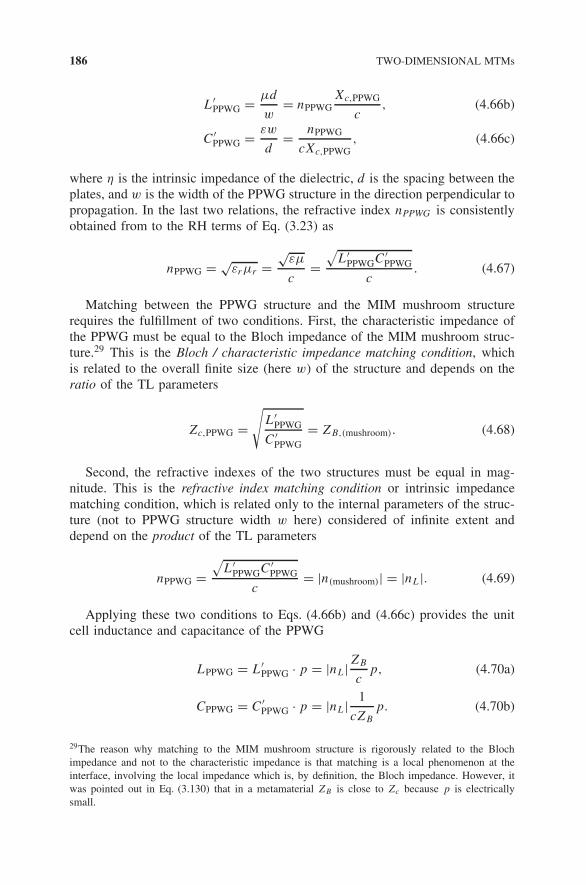
186 TWO-DIMENSIONAL MTMs
L′PPWG = µd
w= nPPWG
Xc,PPWG
c, (4.66b)
C′PPWG = εw
d= nPPWG
cXc,PPWG
, (4.66c)
where η is the intrinsic impedance of the dielectric, d is the spacing between the
plates, and w is the width of the PPWG structure in the direction perpendicular to
propagation. In the last two relations, the refractive index nPPWG is consistently
obtained from to the RH terms of Eq. (3.23) as
nPPWG = √εrµr =
√εµ
c=√
L′PPWGC′
PPWG
c. (4.67)
Matching between the PPWG structure and the MIM mushroom structure
requires the fulfillment of two conditions. First, the characteristic impedance of
the PPWG must be equal to the Bloch impedance of the MIM mushroom struc-
ture.29 This is the Bloch / characteristic impedance matching condition, which
is related to the overall finite size (here w) of the structure and depends on the
ratio of the TL parameters
Zc,PPWG =√
L′PPWG
C′PPWG
= ZB,(mushroom). (4.68)
Second, the refractive indexes of the two structures must be equal in mag-
nitude. This is the refractive index matching condition or intrinsic impedance
matching condition, which is related only to the internal parameters of the struc-
ture (not to PPWG structure width w here) considered of infinite extent and
depend on the product of the TL parameters
nPPWG =√
L′PPWGC′
PPWG
c= |n(mushroom)| = |nL|. (4.69)
Applying these two conditions to Eqs. (4.66b) and (4.66c) provides the unit
cell inductance and capacitance of the PPWG
LPPWG = L′PPWG · p = |nL|ZB
cp, (4.70a)
CPPWG = C′PPWG · p = |nL| 1
cZB
p. (4.70b)
29The reason why matching to the MIM mushroom structure is rigorously related to the Bloch
impedance and not to the characteristic impedance is that matching is a local phenomenon at the
interface, involving the local impedance which is, by definition, the Bloch impedance. However, it
was pointed out in Eq. (3.130) that in a metamaterial ZB is close to Zc because p is electrically
small.

DISTRIBUTED 2D STRUCTURES 187
focusfocus
refocusrefocus
sourcesource
1.0
0
0.5
(a)
focusfocus
refocusrefocus
sourcesource
2π
0
π
(b)
Fig. 4.44. Voltage distribution in the NRI slab network circuit of Fig 4.43 in the case
of perfect matching obtained by Eq. (4.70) with LPPWG = 0.928 nH and CPPWG = 3.459
pF. (a) Normalized magnitude. (b) Phase. From [23], IEEE; reprinted with permission.
Fig 4.44 shows the magnitude and phase distributions of the voltages, respec-
tively, at the nodes of the network circuit. High-voltage magnitude concentrations
are clearly observed at the expected locations of focus and refocus predicted by
Eqs. (2.56) and (2.58), and relatively concentric voltage phase distributions are
observed around the focus and refocus points, which verifies the NRI character-
istics of the LH TL slab. Some degree of aberration (Section 2.7 and Fig 2.7),
due to the slight anisotropy of the structure (Fig 4.37), is apparent. In addition to
focus and refocus concentration, field concentrations, corresponding to surface
plasmons (Section 4.4.4), are also visible along the interfaces.
For comparison, Fig 4.45 shows the voltage distribution along the network cir-
cuit with the slight mismatch that is present in the experimental structure due to
fabrication constraints [see Fig 4.47(a)]. For continuity with the upper substrate
of the mushroom structure and optimal matching, the experimental PPWG is con-
stituted by the combination of an upper substrate of thickness h1 = 0.127 mm
and permittivity εr1 = 2.2 and of a lower substrate of thickness h2 = 1.57 mm
and permittivity εr2 = 10.2, resulting in an effective permittivity of εeff ,PPWG =ε1ε1(h1 + h2)/(ε1h2 + ε2h1) = 8.02, which is not perfectly matched to the PPWG
in terms of refractive index (nPPWG = √εeff ,PPWG = 2.8 = |nL| = 3.4). The cor-
responding characteristic impedance of the PPWG is given by Eq. (4.66a) with
η = √µ0/(ε0εeff ,PPWG), d = h1 + h2, and w = N · p (with N = 19 cells along
the interface), as Zc,PPWG = 2.38 , which corresponds to an impedance per port of
Zport
c,PPWG = NZc,PPWG = 45.19 . This represents considerable Bloch/characteris-
tic impedance mismatch |Ŵ| = |(Zport
c,PPWG − ZB)/(Zport
c,PPWG + ZB)| =≈ −6 dB.
The PPWG unit cell inductance and capacitance are then obtained as LPPWG =nPPWGZ
port
c,PPWGp/c = 2.13 nH and CPPWG = nPPWGp/(cZport
c,PPWG) = 1.05 pF.
Despite the mismatch imposed by design constraints, focusing and refocusing
effects can also be observed in Fig 4.45.

188 TWO-DIMENSIONAL MTMs
focusfocus
refocusrefocus
sourcesource
1.0
0
0.5
(a)
focusfocus
refocusrefocus
sourcesource
2π
0
π
(b)
Fig. 4.45. Voltage distribution in the NRI slab network circuit of Fig 4.43 in the case of
the slight mismatch present in the experimental structure, corresponding to the PPWG
parameters LPPWG = 2.13 nH and CPPWG = 1.05 pF. (a) Normalized magnitude. (b)
Phase. From [23], IEEE; reprinted with permission.
source
focus
refocus
1.0
0
0.5
(a)
source
focus
refocus
2π
0
π
(b)
Fig. 4.46. Full-wave (FEM) simulated electric field distributions in the planar distributed
NRI slab of Fig 4.47 (f = 3.737 GHz) on the ground plane. (a) Normalized magnitude.
(b) Phase. From [23], IEEE; reprinted with permission.
Next, the field distributions along the real NRI slab of Fig 4.42 computed by
FEM full-wave analysis are shown in Fig 4.46. A perfect magnetic conductor
(PMC) boundary condition is introduced at the symmetry plane of the structure
to reduce computation time. Radiation boundary conditions are applied along the
x and y directions, and the open top of the structure is simulated by a perfectly
matched layer (PML) boundary condition. A vertical current line source is set
at 15 mm away from the interface to excite the PPWG mode. The observed
magnitude and phase field distributions qualitatively agree with the LC network
predictions of Fig 4.45.
Finally, the experimental prototype and results are shown in Figs. 4.47 and
4.48, respectively. The MIM caps are etched on the bottom side of the upper

DISTRIBUTED 2D STRUCTURES 189
PPWPPW
PPWPPW
source (coax.)source (coax.)
NRI lensNRI lens
(a)
h1
h2,PPW
h2,LH
PPW NRI lens
(b)
Fig. 4.47. Prototype of a 20 × 3-cell NRI slab (f = 3.737 GHz). (a) Top view. (b) Cross
section. From [23], IEEE; reprinted with permission.
sourcesource
2π0 π
1.00 0.5
aa
bb
Fig. 4.48. Measured electric field distribution on the LH structure (f = 3.737 GHz). A
vertical electric probe is used. (a) Magnitude. (b) Phase. From [23], IEEE; reprinted
with permission.
substrate. The lower substrates are laminated separately in the LH and PPWG
regions. The PPWG is excited by a coaxial cable through a hole in the ground
plane located at 15 mm of the interface. The size of the overall structure is
140 × 140 mm2. The refractive index and per-port characteristic impedances
of the PPWG are nPPWG = √εeff ,PPWG = 2.77 and Z
port
c,PPWG = (w/p)Zc,PPWG =

190 TWO-DIMENSIONAL MTMs
27.17 . The vertical electric field distribution is measured at 1 mm above the
NRI slab using a vertical coaxial probe fixed to an automated moving stage to
picking up the capacitors voltages. The observed distributions of the electric field
exhibits the expected NRI magnitude concentration and phase concentring fronts
in agreement with LC theory and full-wave simulation results.
REFERENCES
1. C. Kittel. Introduction to Solid State Physics, Seventh Edition, Wiley Text Books,
1964.
2. C. Christopoulos. The Transmission-Line Modeling Method TLM, IEEE Press, 1995.
3. A. Grbic and G. V. Eleftheriades. “Periodic analysis of a 2-D negative refrac-
tive index transmission lines,” IEEE Trans. Antennas Propagat., vol. 51, no. 10,
pp. 2604–2611, Oct. 2003.
4. C. Caloz and T. Itoh. “Positive / negative refractive index anisotropic 2D meta-
materials,” IEEE Microwave Wireless Compon. Lett., vol. 13, no. 12, pp. 547–549,
Dec. 2003.
5. M. D. Pozar. Microwave Engineering, Third Edition, John Wiley & Sons, 2004.
6. J. D. Joannopoulos, R. D. Meade, and J. .N. Win. Photonic Crystals, Molding the
Flow of Light, Princeton University Press, 1995.
7. J. -H. Kim and M. Swaminathan. “Modeling of irregular shaped power distribution
planes using transmission matrix method,” IEEE Trans. Advanced Packag., vol. 24,
no. 3, pp. 334–346, August 2001.
8. W. J. R. Hoefer. “The transmission line matrix (TLM) method,” in Numerical Tech-
niques for Microwave and Millimeter-Wave Passive Structures, edited by T. Itoh,
Wiley-Interscience, 1989.
9. P. B. Johns and R. L. Beurle. “Numerical solution of 2-dimensional scattering prob-
lems using a transmission line matrix,” Proc. IEE, vol. 118, no. 9, pp. 1203–1208,
Sept. 1971.
10. J. R. Whinnery and S. Ramo. “A new approach to the solution of high frequency
field problems,” Proc. I.R.E., vol. 32, pp. 284–288, May 1944.
11. P. P. M. So and W. J. R. Hoefer. “Time domain TLM modeling of metamate-
rials with negative refractive index,” IEEE-MTT Int’l Symp., Fort Worth, TX,
pp. 1779–1782, June 2004.
12. Multipurpose Electromagnetic Field Simulation Tool, Faustus Scientific Corporation,
http://www.faustcorp.com.
13. V. Veselago. “The electrodynamics of substances with simultaneously negative values
of ε and µ,” Soviet Physics Uspekhi, vol. 10, no. 4, pp. 509–514, Jan., Feb. 1968.
14. J. B. Pendry. “Negative refraction makes a perfect lens,” Phys. Rev. Lett., vol. 85,
no. 18, pp. 3966–3969, Oct. 2000.
15. P. P. M. So, H. Du, and W. J. R. Hoefer. “Modeling of metamaterials with nega-
tive refractive index using 2D-shunt and 3D-SCN TLM Networks,” IEEE Trans.
Microwave Theory Tech., vol. 53, no. 4, pp. 1496–1505, April 2005.
16. R. W. Ziolkowski. “Pulsed and CW Gaussian beam interactions with double negative
metamaterial slabs,” Optics Express., vol. 11, no. 7, April 2003.

REFERENCES 191
17. H. Raether. Surface Plasmons, Springer-Verlag, 1988.
18. R. Ruppin. “Surface polaritons of a left-handed material slab,” J. Phys. Condens.
Matter, vol. 13, pp. 1811–1818, 2001.
19. C. Caloz, C.-J. Lee, D. R. Smith, J. B. Pendry, and T. Itoh. “Existence and properties
of microwave surface plasmons at the interface between a right-handed and a left-
handed media,” IEEE AP-S USNC/URSI National Radio Science Meeting, Monterey,
CA, June 2004.
20. A. Grbic and G. V. Eleftheriades. “Subwavelength focusing using a negative-
refractive-index transmission line lens,” IEEE Antennas Wireless Propagat. Lett.,
vol. 2, pp. 186–189, 2003.
21. P. P. M. So and W. J. R. Hoefer. “Microwave CAD environment for metamaterials
with negative refractive index,” in Proc. European Microwave Conf., Amsterdam, The
Netherlands, Oct. 2004.
22. D. Sievenpiper, L. Zhang, R. F. J. Broas, N. G. Alexopolous, and E. Yablonovitch.
“High-impedance surface electromagnetic surfaces with a forbidden frequency band,”
IEEE Trans. Microwave Theory Tech., vol. 47, no. 11, pp. 2059–2074, Nov. 1999.
23. A. Sanada, C. Caloz, and T. Itoh. “Planar distributed structures with negative refrac-
tive index” IEEE Trans. Microwave Theory Tech., vol. 52, no. 4, pp. 1252–1263,
April 2004.
24. R. E. Collin. Field Theory of Guided Waves, Second Edition, Wiley-Interscience,
1991.

5GUIDED-WAVE APPLICATIONS
Many novel guided-wave applications can be devised on the foundation of the
CRLH MTM concept established in Chapters 3 and 4. The guided-wave applica-
tions presented in this chapter essentially refer to 1D CRLH (Chapter 3) compo-
nents, where electromagnetic energy remains confined in the metal and dielectric
media constituting the components. Although 1D CRLH structures can be con-
sidered as TLs embedded in a NRI medium when operated in their LH range
[Eq. (3.25)], they do not utilize negative refraction in the sense of Snell’s law,
since they do not involve angles. Rather, they exploit the unusual frequency
dependence of the guided wavelength and the low-frequency antiparallelism/
high-frequency parallelism existing between the phase and the group velocities
in CRLH structures.
Chapter 5 describes specific guided-wave properties of CRLH structures and
presents subsequent examples of practical applications. The properties include
dual-band operation, bandwidth enhancement, multilayer-architecture super-
compactness, arbitrary coupling level, and negative/zeroth-order resonance. The
corresponding applications are dual-band components (TLs, stubs, hybrid cou-
plers, Wilkinson power divider, subharmonically-pumped mixer) (Section 5.1),
enhanced-bandwidth components (with rat-race coupler example) (Section 5.2),
super-compact multilayer TLs (with diplexer application example) (Section 5.3),
phase and impedance couplers with arbitrary coupling level (asymmetric
CRLH/RH and symmetric CRLH/CRLH) (Section 5.4), and negative/zeroth order
Electromagnetic Metamaterials: Transmission Line Theory and Microwave Applications,By Christophe Caloz and Tatsuo ItohCopyright 2006 John Wiley & Sons, Inc.
192

DUAL-BAND COMPONENTS 193
resonator (Section 5.5). Other guided-wave applications based on the CRLH con-
cept are possible.
5.1 DUAL-BAND COMPONENTS
A dual-band (DB) component is a component accomplishing the same function
at two different arbitrary frequencies ω1 and ω2. Such a component is therefore
constituted of TL sections inducing equivalent1 phase shifts φ1 = −β1ℓ and φ2 =−β2ℓ, where ℓ is the length of the TL sections, at these two frequencies. In other
words, a DB component should exhibit a dispersion relation β(ω) satisfying the
double condition
β(ω1) = β1, (5.1a)
β(ω2) = β2, (5.1b)
where the two frequencies (ω1, ω2) and the two propagation constants (β1, β2)
are arbitrary. A CRLH TL possesses this DB property and can therefore be used
to transform virtually any microwave TL-based component into a DB compo-
nent. This DB property of CRLH TL is extremely beneficial to modern wireless
communication systems covering two bands because it reduces the number of
required circuit components for a given functionality.
5.1.1 Dual-Band Property of CRLH TLs
The DB property of CRLH TLs will be explained with the help of Fig 5.1, where
the phase curves of both a PRH TL and a CRLH TL are shown.
Let us first consider the case of the PRH TL, which is the building brick
of most conventional microwave components. A PRH TL is characterized by
the propagation constant and characteristic impedance given by Eqs. (3.36) and
(3.32), respectively,
βPRH = ω
√
L′RC′
R, (5.2a)
ZPRHc =
√
L′R
C′R
. (5.2b)
For this line to be matched to ports of impedance Zt and to provide the
appropriate phase shift at the first frequency ω1, it must satisfy the conditions
ZPRHc = Zt , (5.3a)
βPRH(ω = ω1) = β1, (5.3b)
1As will be seen in the forthcoming examples, “equivalent” does not mean exactly equal and does
not necessarily mean equal to the modulo 2π . For instance, in the case of a quadrature hybrid, the
equivalent phase shifts will be φ1 = −90
and φ2 = −270
(Section 5.1.3.1).

194 GUIDED-WAVE APPLICATIONS
PRH
CRLH
ω
φ = −βℓ
φ1 = −β1/d
φ2 = −β2/d
ω1 ω2 ωPRH2
Fig. 5.1. Dual-band property of a CRLH TL.
respectively. Inserting Eqs. (5.3) into Eq. (5.2) yields a linear system of two
equations with the two unknowns L′R and C′
R , which are easily found to be
L′R = Ztβ1
ω1
, (5.4a)
C′R = β1
ω1Zt
. (5.4b)
Consequently, the PRH TL is fully determined by the matching condition and
by the specification of a single operation frequency. The frequency at which
the required second band propagation constant of β2 is achieved is fixed to the
frequency
ωPRH2 = β2
β1
ω1, (5.5)
which is obtained by Eqs. (5.2a) with Eq. (5.4). In practical applications, it
is highly unlikely that ωPRH2 would coincide with the required second band

DUAL-BAND COMPONENTS 195
frequency ω2 (Fig 5.1). Therefore, a PRH TL is essentially monoband, and com-
ponents made of PRH TL are thus monoband.
Let us now consider the case of the balanced CRLH TL, for which the propa-
gation constant and characteristic impedance are given by (Eqs. 3.34) and (3.32),
respectively,
βCRLH = ω
√
L′RC′
R − 1
ω√
L′LC′
L
, (5.6a)
ZCRLHc =
√
L′R
C′R
=√
L′L
C′L
. (5.6b)
Matching to terminations of impedance Zt and phasing to β1 for a required
operation at frequency ω1 require
ZCRLHc = Zt , (5.7a)
βCRLH(ω = ω1) = β1, (5.7b)
respectively. These equations correspond in fact to three equations because the
matching condition splits into two equations from Eq. (5.6b). Thus, insertion
of Eq. (5.7) into Eq. (5.6) yields a linear system of three equations with the
four unknowns L′R, C′
R, L′L, C′
L, and there is therefore one available degree of
freedom that can be exploited to satisfy the second band condition [Eq. (5.1b)].
From the resulting system of four equations, we obtain, after some straightforward
calculations, the DB CRLH parameters
L′R = Zt
[
β2 − β1 (ω1/ω2)]
ω2
[
1 − (ω1/ω2)2] , (5.8a)
C′R = β2 − β1 (ω1/ω2)
ω2Zt
[
1 − (ω1/ω2)2] , (5.8b)
L′L = Zt
[
1 − (ω1/ω2)2]
ω1
[
(ω1/ω2) β2 − β1
] , (5.8c)
C′L = 1 − (ω1/ω2)
2
ω1Zt
[
(ω1/ω2) β2 − β1
] , (5.8d)
depending only on (ω1, ω2) − (β1, β2) and corresponding to the dispersion curve
shown in Fig 5.1.
The argument presented above is based on the ideal homogeneous CRLH TL,
described in Section 3.1. As pointed out in Chapter 3, such a TL does not exist
naturally and needs therefore to be synthesized in the form of an LC ladder

196 GUIDED-WAVE APPLICATIONS
network with identical responses in the frequency range of interest,2 as it was
shown in Section 3.23 and verified in Section 3.4 for a real distributed structure.
The exact phase shift produced by an LC network unit cell takes in general the
form [Eq. (3.81)]
φ = − arctan
1
ω
(ω/ωse)2 − 1
CLZc
(
1 − χ
4
)
+ Zc
ωLL
[
(ω/ωsh )2 − 1]
2 − χ
,
(5.9a)
with χ = ω2LRCR + 1
ω2LLCL
− LRCL + LLCR
LLCL
. (5.9b)
As shown in Section 3.2.3, in the frequency range where |φ| = βp ≪ 1,
this complicated LC network expression reduces to the much simpler expression
[Eq. (3.84)]
φ(ω → ω0) = −[
ω√
LRCR − 1
ω√
LLCL
]
, (5.10)
which can be shown to be identical to the ideal homogeneous TL expression
Eq. [(5.6a)] in the following manner. An artificial CRLH TL of physical length
ℓ is constituted by the repetition of N unit cells of length p, so that
ℓ = N · p. (5.11)
Because each cell induces a phase shift of φ, the total phase shift along the
line is then
φ = N · φ. (5.12)
With this relation, the relation β = −φ/ℓ and the fundamental substitutions
LR = L′R · p, CR = CR · p, LL = LL/p, CL = CL/p, (5.13)
the expression of Eq. (5.10) is reduced exactly to Eq. (5.6a).
It is of practical interest to relate the real inductance and capacitance values of
the LC components constituting the CRLH with the required phase shifts for dual
2In this range, the homogeneity condition |φ| = βp ≪ 1, where p is the physical length of the
unit cell, should be satisfied.3The equivalence is rigorously shown analytically in Eqs. 3.115 to 3.118 of Section 3.2.6.

DUAL-BAND COMPONENTS 197
band operation. This is accomplished by substituting βi = −φi/(Np) (i = 1, 2)
and Eq. (5.13) into Eq. (5.8) and yields the DB CRLH parameters
LR = Zt
[
φ1 (ω1/ω2) − φ2
]
Nω2
[
1 − (ω1/ω2)2] , (5.14a)
CR = φ1 (ω1/ω2) − φ2
Nω2Zt
[
1 − (ω1/ω2)2] , (5.14b)
LL = NZt
[
1 − (ω1/ω2)2]
ω1
[
φ1 − (ω1/ω2) φ2
] , (5.14c)
CL = N[
1 − (ω1/ω2)2]
ω1Zt
[
φ1 − (ω1/ω2) φ2
] , (5.14d)
depending only on (ω1, ω2) − (φ1, φ2) and also corresponding to the dispersion
curve shown in Fig 5.1.
5.1.2 Quarter-Wavelength TL and Stubs
The simplest DB application is the DB quarter-wavelength4 TL, and its corre-
sponding open- and short-circuited stubs [1].
A conventional quarter-wavelength TL is a PRH TL of length ℓ = λ/4. Such
a TL induces a phase shift of φ = −βℓ = −β(λ/4) = −(βπc)/(2ω) = −π/2
at the operating frequency ω. If this frequency is called ω1, in reference with
Fig 5.1, it is thus associated with the first band relation [Eq. (5.1a)]
β1 = β(ω1) = ω1
cor φ1 = φ(ω1) = −π
2. (5.15)
The next available frequency at which the PRH TL provides an equivalent
response is obtained after one additional full turn in the Smith chart, which corre-
sponds to the phase shift φ2 = −β2ℓ = −β2(3λ/4) = −(3β2πc)/(2ω) = −3π/2.
At this point, β2 = 3β1 and the frequency is ωPRH2 = 3ω1 according to Eq. (5.5).5
As explained in the previous section, ωPRH2 cannot be tuned without affecting the
first band, and it is unlikely to coincide with the second frequency ω2 of interest
in a specific application.
4In fact, the term “’quarter-wavelength’ here is abusive in the sense that it strictly applies only to
the first band. But it expresses the fact that the electrical lengths ℓ = λ/4 and ℓ = 3λ/4, which are
indistinguishable from the point of view of impedance, can be achieved at any arbitrary pair of
frequencies ω1 and ω2 (arbitrary ratio ω2/ω1).5A response equivalent to that of φ = −π/2 is obtained at all the odd harmonics of the design
frequency ω1, since the equivalent phase shifts φn+1 = −(π/2 + nπ) (n ∈ N) occur at the frequencies
ωn+1 = (2n + 1)ω1.

198 GUIDED-WAVE APPLICATIONS
In contrast, the CRLH TL can be designed to meet both bands conditions
Eq. (5.1). In the case of the quarter-wavelength transformer, the explicit expres-
sion for Eq. (5.1a) was already given in Eq. (5.15) and the explicit expression
for Eq. (5.1b) reads
β2 = β(ω2) = 3ω1
cor φ2 = φ(ω2) = −3π
2. (5.16)
The LC values of the CRLH TL for DB operation at the arbitrary pair of
frequencies (ω1, ω2) are then directly available from Eq. (5.14) with the phase
substitutions of Eqs. (5.15) and (5.16)
LR = Ztπ[
1 − 3 (ω1/ω2)]
2Nω2
[
1 − (ω1/ω2)2] , (5.17a)
CR = π[
1 − 3 (ω1/ω2)]
2Nω2Zt
[
1 − (ω1/ω2)2] , (5.17b)
LL = 2NZt
[
1 − (ω1/ω2)2]
πω1
[
3 (ω1/ω2) − 1] , (5.17c)
CL = 2N[
1 − (ω1/ω2)2]
πω1Zt
[
3 (ω1/ω2) − 1] . (5.17d)
We have considered here the pair of phases (φ1, φ2) = (−π/2, −3π/2), but
any pair of phases with π difference between ω1 and ω2 can be used in principle.
For instance, the pairs (φ1, φ2) = (+3π/2, +π/2) (f1 and f2 both in LH range)
and (φ1, φ2) = (+π/2, −π/2) (f1 in LH range and f2 in RH range) would yield
similar results. The choice of a pair of phases mostly depends on design con-
straints, such as location of the CRLH cutoff frequencies with respect to the two
bands of interest and characteristics of the available chip components. Bandwidth
considerations may also be important.6
In DB components, as in some other 1D applications of MTMs, the key prop-
erty of the transmission medium does not lie in its distributed characteristics of
the transmission medium, but in the net phase shift between its input and its out-
put. This cognizance allows the following practical simplification. We remember
from Section 3.2.5 that the real distributed CRLH TL of Fig 3.15 is indistinguish-
able from the series RH-LH TL combination of Fig 3.30 in terms of port-to-port
transmission characteristics if the structure is balanced, because under this con-
dition the equivalent circuit model of the CRLH TL decouples into separated
RH and LH subcircuits. This means that a TL configuration of the type shown
in Fig 3.30 produces exactly the same port-to-port response as a real CRLH TL.
Therefore, the RH section of the CRLH TL can be replaced by a naturally exist-
ing TL, such as a simple microstrip, for simplicity. In this case, the DB total
6As RH TLs, CRLH TLs induce smaller bandwidths when they are larger.

DUAL-BAND COMPONENTS 199
phase shift φ is split into the LH TL phase shift φLH and the RH TL phase shift
φRH: φ = φLH + φRH. The LH section is still directly designed by using the last
two expressions of Eq. (5.17), which provide the values of LL and CL leading
to the phase advance φLH. The natural homogeneous RH section is designed by
first computing LR and CR using the first two expressions of Eq. (5.17), which
determines the characteristic impedance, and then applying Eq. (5.12) with the
RH part only of Eq. (5.10) [or Eq. (3.72)] to determine the required RH phase
delay, which yields7
ZcR =√
LR
CR
, (5.18a)
φRH1 = −Nω1
√
LRCR. (5.18b)
From these two quantities, the design parameters of the homogeneous RH
TL (e.g., line width and length in the microstrip case) can be straightforwardly
obtained [2].
Fig 5.2 shows the photograph and equivalent circuit of a CRLH TL imple-
mented in the form of the series connection of an SMT-chips LH section and of
a conventional (RH) microstrip line. The design parameters of this DB quarter
wavelength transformer, based on the operation phases pair (φ1, φ2) = (−π/2,
−3π/2), are fully determined by Eqs. (5.17) and (5.18). The parameters obtained
in this manner as well as the actual parameters taking into account parasitic effects
and fabrication constraints are indicated in the caption of the figure. The slight
discrepancies between the ideal and actual design parameters are essentially due
to two factors: the availability of SMT components only in discrete values and
the natural RH parasitics of the SMT chip components. These parasitics induce
a small phase delay in the LH section (assumed in the analysis to exhibit pure
phase advance), which results in smaller phase advance, and requires reduction
of the length of the microstrip line for compensation. This is the reason why the
actual microstrip line in this design is 17% shorter than the predicted length.8
Figs. 5.4 and 5.3 show a DB quarter-wavelength short-circuited stub and a
DB quarter-wavelength open-circuited stub, respectively, based on the design
7It is important to realize that in the phase equation, we do not have φRH1 = φRH(ω = ω1) = −π/2
and φRH2 = φRH(ω = ω2) = −3π/2. φRH is designed to contribute to exactly the appropriate phase
shift inducing φ1 = φLH(ω1) + φRH(ω1) = −π/2 according to Eqs. (5.15) and φ2 = φLH(ω2) +φRH(ω2) = −3π/2 according to Eqs. (5.15) and (5.16).8In practice, the exact design procedure would typically be as follows: 1) Compute LL and CL by
the last two relations of Eq. (5.17), and use the closest possible combination of chip components; 2)
measure the isolated LH section including the real chips (using TRL calibration) and compare the
measured phase shift φLH with the theoretical phase shift given by Eq. (5.18b); the measured φLH is
smaller than the theoretical one by a value δ, which corresponds to the phase delay induced by the
RH parasitics; 3) calculate the actual microstrip line length to be used, corresponding to the phase
shift |φRH | − |δ|; 4) fabricate the complete line, including the LH and RH sections, and fine-tune
the RH length for optimal performances.

200 GUIDED-WAVE APPLICATIONS
Viahole
Viahole
RH-TL
LH-TL
LL
RH-TL
LL
2CL
ℓR 2CL
CL
ℓR
Viahole
Viahole
RH-TL
LH-TL
LL
RH-TL
LL
2CL
ℓR 2CL
CL
ℓR
Fig. 5.2. Prototype and equivalent circuit of a DB CRLH TL implementation utilizing
SMT chip components for the LH contribution and a conventional microstrip line (on
each side of the LH section) for the RH contribution. The substrate used is Duroid
6510 with permittivity 10.2 and thickness 1.27 mm. The two frequencies of operation
are f1 = 0.88 GHz and f2 = 1.67 GHz. The ideal parameters obtained from Eqs. (5.17)
and (5.18) are (Zc = 50 , N = 2) LL = 14.32 nH, CL = 5.73 pF, LR = 12.81 nH,
CR = 5.13 pF, ZcR = 50 , φRH1 = −162.38
, leading to wµstrip = 1.18 mm (width)
and ℓµstrip = 2ℓR = 58.9 mm (length). The actual design parameters are LL = 14.1 nH
(3 × 4.7 nH, in series), CL = 6 pF (2 × 3 pF, in parallel), wµstrip = 1.2 mm, and ℓµstrip =49.4 mm. From [1], IEEE; reprinted with permission.
3x4.7 nH
3x4.7 nH
3x4 pF
3x4 pF
2x3 pF
W : 1.20 mm
L : 23.6 mm
W:1.2 mm
L:24.78 mm
Viahole
IN OUT
(a)
0.6 0.8 1 1.2 1.4 1.6 1.8 2
frequency(GHz)
-40
-35
-30
-25
-20
-15
-10
-5
0
S11_measurement
S21_measurement
S11_simulation
S21_simulation
dB
(b)
Fig. 5.3. DB quarter-wavelength short-circuited stub corresponding to the design of
Fig 5.2. (a) Prototype and equivalent circuit. (b) Simulated and measured S-parameters.
From [1], IEEE; reprinted with permission.
parameters of Fig 5.2 for the frequencies f1 = 0.88 GHz and f2 = 1.67 GHz.
The input impedances of short and open TLs are given by [2]
Zshortin = jZc tan (βℓ)
d=λ/4,3λ/4= ∞, (5.19a)
Zopen
in = −jZc cot (βℓ)d=λ/4,3λ/4= 0, (5.19b)

DUAL-BAND COMPONENTS 201
3x4.7 nH
3x4.7 nH
3x4 pF
3x4 pF
2x3 pF
W : 1.20 mm
L : 24.6 mm
W:1.2 mm
L:24.78 mm
IN OUT
(a)
0.6 0.8 1 1.2 1.4 1.6 1.8 2
frequency(GHz)
-40
-35
-30
-25
-20
-15
-10
-5
0
S11_measurement
S21_measurement
S11_simulation
S21_simulation
dB
(b)
Fig. 5.4. DB quarter-wavelength open-circuited stub corresponding to the design of
Fig 5.2. (a) Prototype and equivalent circuit. (b) Simulated and measured S-parameters.
From [1], IEEE; reprinted with permission.
and are thus infinite and zero, respectively, at the impedance-inversion frequen-
cies, that is, at the frequencies f1 (where ℓ = λ/4) and f2 (where ℓ = 3λ/4).
Consequently, the shorted and opened stubs on a transmission line exhibit the
characteristics |S21| ≈ 0 dB and |S11| ≈ 0 dB, respectively, at both f1 and f2.
This is seen in Figs. 5.4 and 5.3, where excellent agreement between simulated
and measured results can be observed.
5.1.3 Passive Component Examples: Quadrature Hybrid and Wilkinson
Power Divider
The DB quarter-wavelength TL described in the previous section can be applied
to provide DB functionality in any TL-based microwave component. The design
procedure essentially consists in replacing conventional PRH TL branches by
CRLH TL branches designed to exhibit the required phase shifts at the desired
frequencies for a given operation (Fig 5.1). This section presents two examples
of passive DB components: the quadrature hybrid (QH) [1] and the Wilkinson
power divider (WPD).
5.1.3.1 Quadrature Hybrid The conventional QH, also known as a the branch-
line hybrid, is a 3-dB directional coupler with a 90
phase difference between the
outputs of the through and coupled arms [2]. A DB quadrature hybrid is obtained
by replacing the −90
RH branches by CRLH branches exhibiting −90
and
−270
phase shifts at f1 and f2, respectively, as shown in the schematics of
Fig 5.5.9 Therefore, the DB quarter-wavelength CRLH TL theory presented in
Section 5.1.2 is directly applicable here.
9The only difference between the two circuits of Fig 5.5(a) and 5.5(b) is the sign in the phase
difference between the output signals of ports 2 and 3.

202 GUIDED-WAVE APPLICATIONS
, 90°c
2
Z
, 90°c
2
Z
90°
cZ
90°
cZ
1
4
2
3∆ϕ = ϕ (S21) − ϕ (S31) = 90°
, 90°2
Z
, 90°2
Z
90°
Z
90°
Z
1
4
2
3
, 90°2
Z, 90°
2
Z
, 90°2
Z, 90°
2
Z
90°
Z
90°
Z
90°
Z
90°
Z
1
4
2
3∆ϕ = ϕ (S21) − ϕ (S31) = 90°
(a)
, 270°c
2
Z
, 270°c
2
Z
270°
cZ
270°
cZ
1
4
2
3∆ϕ = ϕ (S21) − ϕ (S31) = 270°
, 270°2
Z
, 270°2
Z
270°
Z
270°
Z
1
4
2
3
, 270°2
Z
, 270°2
Z
270°
Z
270°
Z
, 270°2
Z
, 270°2
Z
270°
Z
270°
Z
1
4
2
3∆ϕ = ϕ (S21) − ϕ (S31) = 270°
(b)
Fig. 5.5. Conceptual schematics of the DB QH. (a) At the first frequency, f1. (b) At
the second frequency, f2. The labels 1, 2, 3, and 4 correspond to the input, through
output, coupled output, and isolated ports, respectively, and Zc represents the characteristic
impedance of the input and output lines. From [1], IEEE; reprinted with permission.
Fig 5.6 shows a DB LH-SMT/RH-microstrip QH prototype10 operating at the
two frequencies (f1 = 0.93 GHz and f2 = 1.78 GHz) which are in the ratio of
f2/f1 = 1.59.11 The magnitude characteristics for this prototype are shown in
Figs. 5.7, and Fig 5.8 shows the phase differences between the two output ports.
In both simulation and measurement, the phase differences between S31 and
S21 are ±90, and quadrature phase differences are obtained with errors less than
1.5
at f1 and f2 (Fig 5.8). The amplitude imbalance between S31 and S21 is less
than 0.5 dB in both passbands, which means that the incident power is evenly
divided between port 2 and port 3. The 1-dB bandwidth, defined as the frequency
range in which the amplitude imbalance is less than 1 dB, S21 and S31 are larger
than −5 dB, isolation/return loss is larger than 10 dB, and quadrature phase error
is less than 11.1%, is larger than 3.4%.
A DB rat-race (RR) coupler, or ring hybrid, based on the same principle as
this CRLH DB QH is also demonstrated in [1]. The operating frequencies of
this RR are f1 = 1.5 GHz and f2 = 3.0 GHz (f2/f1 = 2). The three −90
RH
branches of the conventional RR are replaced by three CRLH branches of −90
at f1 and −270
at f2, whereas the −270
branch of the conventional RR is
replaced by the series connection of three similar CRLH TL sections.
5.1.3.2 Wilkinson Power Divider The conventional Wilkinson power divider
(WPD) is a three-port network used for power division (or power combination)
10The tuning stub was added (also included in the simulation) to compensate for the effects of
amplitude imbalance between the through and coupled ports caused by the frequency variations of
the reactance of the chip inductors and susceptance of the chip capacitors.11These two frequencies are chosen so as to correspond to the first and second bands of the global
system for mobile (GSM) communications (900 base station and 1800 mobile phone).

DUAL-BAND COMPONENTS 203
LH-TL
Port 1
Input
Isolation Output
Output
0Z0Z
Port 2
Port 3Port 4
3x4.7 nH
3x4.7 nH
3x4 pF
3x4 pF
2x3 pF
2x4 pF
(1.2+4.7+4.7) nH
(1.2+4.7+4.7) nH
4x4 pF
4x4 pF
W=
1.2
mm
L =
5.3
mm
21.03 mm
24
mm
2
0Z
2
0Z
LH-TL
0Z0Z0Z
3x4.7 nH
3x4.7 nH
3x4 pF
3x4 pF
2x3 pF
2x4 pF
(1.2+4.7+4.7) nH
(1.2+4.7+4.7) nH
4x4 pF
4x4 pF
W=
1.2
mm
L =
5.3
mm
2x4 pF
(1.2+4.7+4.7) nH
(1.2+4.7+4.7) nH
4x4 pF
4x4 pF
W=
1.2
mm
L =
5.3
mm
21.03 mm
24
mm
2
0Z0Z
2
0Z0Z
Tuning stub
Fig. 5.6. Prototype and equivalent circuit of a CRLH DB QH using SMT chip com-
ponents for the LH contribution and a conventional microstrip line contribution for the
RH contribution, as the TLs of Section 5.1.2. The characteristic impedance is Zc = 50
(Zc/√
2 ≈ 35.4 ). The overall dimension of the circuit is 81.8 mm × 71.3 mm. From
[1], IEEE; reprinted with permission.
[2]. The interest of this component lies in the fact that it can have all three
ports matched and isolation between the output ports thanks to the presence of a
resistance between the two output (or input) branches.12 Arbitrary power division
is achievable, but equal-split (3 dB) is the most common case. Fig 5.9 shows the
schematic of a DB WPD replacing the −90
branches of the conventional WPD
by CRLH branches inducing a phase of +90
(LH range, phase advance) at the
first frequency and the phase shift of −90
(RH range, phase delay) at the second
frequency,
φ1 = φ(ω1) = +π
2, (5.20a)
φ2 = φ(ω2) = −π
2, (5.20b)
12It is well-known that a loss-less (non-dissipative) three-port network cannot be matched simulta-
neously at all of its ports [3]. However, the introduction of a resistance makes matching at all ports
possible and is exploited in the Wilkinson divider/combiner.

204 GUIDED-WAVE APPLICATIONS
0.6 0.8 1 1.2 1.4 1.6 1.8 2
frequency(GHz)
-25
-20
-15
-10
-5
0
S11
S21
S31
S41
dB
(a)
0.6 0.8 1 1.2 1.4 1.6 1.8 2
frequency(GHz)
-25
-20
-15
-10
-5
0
S11
S21
S31
S41
dB
(b)
Fig. 5.7. S-parameters for the CRLH DB QH of Fig 5.6. (a) Simulation. (b) Measure-
ment. From [1], IEEE; reprinted with permission.
0.6 0.8 1 1.2 1.4 1.6 1.8 2
frequency (GHz)
-90
0
90
180Simulation
Measurement
2.1
ϕ(S
21)-
ϕ(S
31)
(deg
)
Fig. 5.8. Phases difference ϕ = ϕ(S21) − ϕ(S31) for the CRLH DB QH of Fig 5.6.
From [1], IEEE; reprinted with permission.
Zc
Z0
Z02Z0
√2Z0
√2Z0
/4
3λ/4
Z
Zc
Z02Z0
√2Z0
√2Z0+90
deg
1 2
3+90 deg
(a)
Z0
Z0
Z02Z0
√2Z0
√2Z0
λ/4
λ/4
Zc
Zc
Z02Z0
√2Z0
√2Z0
1 2
3
-90
deg
-90 deg
(b)
Fig. 5.9. Conceptual schematics of the CRLH DB WPD. (a) At the first frequency, f1.
(b) At the second frequency, f2. Zc represents the characteristic impedance of the input
and output lines.

DUAL-BAND COMPONENTS 205
leading, using Eq. (5.14), to the design parameters
LR = Ztπ[
(ω1/ω2) + 1]
2Nω2
[
1 − (ω1/ω2)2] , (5.21a)
CR = π[
(ω1/ω2) + 1]
2Nω2Zt
[
1 − (ω1/ω2)2] , (5.21b)
LL = 2NZt
[
1 − (ω1/ω2)2]
πω1
[
1 + (ω1/ω2)] , (5.21c)
CL = 2N[
1 − (ω1/ω2)2]
πω1Zt
[
1 + (ω1/ω2)] . (5.21d)
Fig 5.10 shows a DB LH-SMT / RH microstrip WPD prototype operating
at the two frequencies f1 = 1.0 GHz and f2 = 3.1 GHz, and the corresponding
results are presented in Fig 5.11.
5.1.4 Nonlinear Component Example: Quadrature Subharmonically
Pumped Mixer
After presenting examples of CRLH DB passive components applications in
Section 5.1.3, namely, a DB QH and a DB WPD, we propose now a more
Via7 mm
10
mm
100Ω
4.7
x 2
nH
4.7
x 2
nH
3 pF 4 pF4 pF
12
3
Fig. 5.10. Prototype and equivalent circuit of a CRLH DB WPD prototype using SMT
chip components for the LH contribution and a conventional microstrip line for the LH
contribution, as the TLs of Section 5.1.2. The frequencies of operation are f1 = 1.0 GHz
and f2 = 3.1 GHz. The characteristic impedance is Zc = 50 (√
2Zc ≈ 70.7 ). The
overall dimension of the circuit is 7 mm × 10 mm.

206 GUIDED-WAVE APPLICATIONS
0.5 1 1.5 2 2.5 3 3.5 4
frequency (GHz)
-40
-35
-30
-25
-20
-15
-10
-5
0
dB
Measured S11
Measured S32
Simulated S11
Simulated S32
(a)
0.5 1 1.5 2 2.5 3 3.5 4
frequency (GHz)
-40
-35
-30
-25
-20
-15
-10
-5
0
Simulated S22 and S33
Measured S22
Measured S33
dB
(b)
0.5 1 1.5 2 2.5 3 3.5 4
frequency (GHz)
-6
-5
-4
-3
-2
-1
0
1
2
dB
-7
-6
-5
-4
-3
-2
-1
0
1
2
3
4
de
gre
e
Simulated S21 and S31
Measured S21
Measured S31
Amplitude Imbalance
Phase Imbalance
(c)
Fig. 5.11. Characteristics of the CRLH DB WPD of Fig 5.10. (a) Input return loss and
isolation. (b) Output return loss. (c) Output amplitude and phase imbalance.
advanced CRLH DB nonlinear application, including several CRLH DB compo-
nents, thereby illustrating the generality of the CRLH DB concept: a dual-band
quadrature subharmonically pumped mixer (DB QSHPM).13 Subharmonic mix-
ers are particularly useful at high (millimeter-wave) frequencies where reliable
and stable LO sources are often unavailable, inefficient, or prohibitively expen-
sive [4]. Quadrature mixers are utilized in direct conversion systems, where the
in-phase/quadrature (I/Q) nature of IF ports is beneficial to broad-band digital
baseband modulation and demodulation schemes [5].
A circuit diagram of the DB QSHPM and a photograph of corresponding
prototype are shown in Figs. 5.12 and 5.13, respectively. The complete mixer
includes two CRLH DB WPDs, one CRLH ±45
DB phase advance/delay
TL, and two subharmonically pumped mixers (SHPMs) containing each two
CRLH dual-passband dual-stopband (DPDS) shunt terminations, representing a
total of seven CRLH DB components. The DB-WPDs, which were described
in Section 5.1.3.2, are used to split the RF and LO powers toward the I and
Q branches; two different DB-WPD designs are required since the RF and LO
13The mixer to be presented here is passive as exhibits conversion loss. However, extension to active
mixers, with conversion gain, is straightforward.

DUAL-BAND COMPONENTS 207
RF1RF2
Dual-Band
Power Splitter
Dual-Band
45º Delay Line
Dual-Band
Power Splitter
LO1
I1, Q2
Dual-Band
Sub-harmonic
Mixer
LO2
Q1, I2
Dual-Band Quadrature Mixer
RF1RF2
Dual-Band
Power Splitter
Dual-Band
45º Delay Line
Dual-Band
Power Splitter
LO1
I1, Q2
Dual-Band
Sub-harmonic
Mixer
LO2
Q1, I2
Dual-Band Quadrature Mixer
Fig. 5.12. Circuit diagram of a DB QSHPM.
LO WPD
RF WPDDual-Band
Sub-Harmonic Mixer
Dual-Band
±45° Delay Line
LO WPD
RF WPDDual-Band
Sub-Harmonic Mixer
Dual-Band
±45° Delay Line
LO
RF
IF1 IF2
Fig. 5.13. Prototype a DB QSHPM. The DB RF and LO frequencies are (fRF 1, fLO1
) =(1.0, 0.51) GHz for the first pair and (fRF 2
, fLO2) = (3.06, 1.56) GHz for the second pair.
The overall dimension of the circuit is 89.3 mm × 103.8 mm. A lowpass filter (simple
series-inductor shunt-capacitor filter, not shown in this picture) with cutoff frequency of
50 MHz is used in the IF lines to suppress fLO .
frequencies are different. The DB phase advance/delay TL is identical to the TL
described in Section 5.1.2 with (φ1, φ2) = (−45,+45
), ±45
corresponding
to ±90
at the utilized second harmonic of the LO, 2fLO . The two SHPMs are
identical to each other; we will describe them now.
Fig 5.14 shows a DB SHPM of the type used in the DB QSHPM of Figs. 5.12
and 5.13. The core of this mixer is an antiparallel diode pair. This diode arrange-
ment is known to automatically suppress fundamental mixing products as well

208 GUIDED-WAVE APPLICATIONS
RF
Term
ina
tion
LO Te
rmin
atio
n
RF LOanti-parallel
diode pair
DPDS
CRLH
DPDS
CRLH
LO1,2 short
RF1,2 open
LO1,2 open
RF1,2 shortfRF1 ≈ 2fLO1
fIF1 ≈ 2fLO1 − fRF1
fRF2 ≈ 2fLO2
fIF2 ≈ 2fLO2 − fRF2
(lower side-band)
(a)
CR
LH
op
en
stub
DPDS
CRLH
Y co
mp
en
satio
n
STEP 2
RF
Term
ina
tion
DPDS
CRLH
GOAL
CR
LH
op
en
stub
STEP 1
Ya Ya Yb
Y = Ya + Yb
RF1,2RF1,2 RF1,2
LO1,2LO1,2 LO1,2
YRF1,2= 0
YLO1,2= ∞
YLO1= ∞
YLO2= ∞
YRF1= Y1
YRF2= Y2
YbRF1= −Y1
YbRF2= −Y2
φa
(
fLO1
)
= −90
φa
(
fLO2
)
= +90
(b)
Fig. 5.14. DB SHPM based on CRLH dual-passband dual-stopband (DPDS) shunt stub
terminations. (a) Circuit diagram of the DB-SHPM (2nd LO harmonic) with DPDS stubs.
(b) Design procedure of the DPDS RF termination in (a). The design of the DPDS LO
termination in (a) is simply obtained by the substitution RF↔LO.
as odd harmonics of the LO [6]14 and is for this reason particularly suited for
second harmonic mixing.
A DB SHPM is obtained from the antiparallel diodes pair by terminating LO
at the RF port and RF at the LO port while presenting matched conditions to
RF at the RF port and to LO at the LO port for both band-pairs of RF/LO
frequencies(
fRF 1, fLO1
)
and(
fRF 2, fLO2
)
, as shown in Fig 5.14(a). This com-
plex function, involving four different frequencies, is accomplished by the CRLH
DPDS terminations following the procedure presented in Fig 5.14(b) for the case
of the RF termination, the principle being transposable to the LO termination
14As shown in [6], only frequencies mfLO + nfRF where m + n is an odd integer (in particular
the desired frequency 2fLO − fRF ) can flow outside the diode loop, with the other products and
harmonics (including DC and the undesired frequencies 2fLO , fLO ± fRF ) being “captured” (flowing)
inside the loop. The LO frequency fLO is suppressed by a simple lowpass filter.

DUAL-BAND COMPONENTS 209
by simple exchange of RF and LO. First, a CRLH DB inverter stub of admit-
tance Ya(f ), similar to those presented in Section 5.1.2 (open or short) using
for instance (φ1, φ2) = (+90,−90
), is introduced to terminate the two LO
frequencies, fLO1and fLO2
, by presenting infinite admittances YLO1= ∞ and
YLO2= ∞. This stub provides the appropriate termination at the LO frequencies
but does not induce the required zero admittance at the RF frequencies in general,
YRF 1= Y1 = 0 and YRF 2
= Y2 = 0, which produces unacceptable RF power loss.
To solve this problem, a second compensating stub of admittance Yb(f ) is added
to the first stub, so that the global admittance is now Y (f ) = Ya(f ) + Yb(f ),
as shown in Fig 5.14(b). If this admittance is adjusted so that YbRF 1= −Y1 and
YbRF 2= −Y2
15, the RF conditions YRF 1= 0 and YRF 2
are also satisfied, and
dual-band mixing is achieved. The admittances values of the CRLH DPDS RF
termination are listed in Table 5.1 for easier understanding.
The experimental results of the DB QSHPM of Fig 5.10 are shown in Fig 5.15.
LO to RF isolation [Fig 5.15(b)] has its maxima at fLO1= 0.51 and fLO2
=1.55 GHz. Conversion loss [Figs. 5.15(c) and 5.15(d)] is defined as the power
ratio between the RF power at the mixer input to a single channel output (I
or Q). Conversion loss is observed to exhibit minima at fRF 1= 1.0 GHz and
fRF 2= 3.06 GHz. These results conform the DB operation with frequencies
(fRF 1, fLO1
) = (1.0, 0.51) GHz and (fRF 2, fLO2
) = (3.06, 1.56) GHz.
In the scheme of the DB QSHPM of Figs. 5.12 and 5.13, the phase difference
between the IF output with the delay line and the other IF output in Fig 5.13
is +90
at (fRF 1, fLO1
) and is −90
at (fRF 2, fLO2
).16 Consequently, DB fre-
quency mixing at the same IF can be achieved by utilizing a 90
hybrid to
separate the two outputs. The design of Fig 5.12 corresponds to this case, since
fIF 1= fIF 2
= 200 MHz.
TABLE 5.1. Admittance of the CRLH DPDS RF
Termination of Fig 5.14(b) at the Different
Frequencies of Interest.
f Ya Yb Y = Ya + Yb
fLO1∞ Yx ∞
fLO2∞ Yy ∞
fRF 1Y1 −Y1 0
fRF 2Y2 −Y2 0
15In principle, a DB stub would be required to satisfy this requirement. However, if Y1 and Y2 are
very small, as is the case in the prototype of Fig 5.10, the design can be simplified by using a
single-band stub presenting a small susceptance of opposite sign, sufficient to reduce Y1 and Y2 to
negligible values.16The delay line, which is +45
at fLO1
, induces +90
phase shift at 2fLO1, while the same delay
line, which is −45
at fLO2, induces −90
phase shift at 2fLO2
. Therefore, after mixing, the difference
between the IF outputs with and without the delay line are +90
for fIF 1= 2fLO1
− fRF 1and −90
for fIF 2= 2fLO2
− fRF2.

210 GUIDED-WAVE APPLICATIONS
0.4 0.6 0.8 1 1.2 1.4 1.6
Frequency (GHz)
-50
-40
-30
-20
-10
0
dB
-60
-40
-20
0
20
40
60
80
deg
ree
44.809
-44.7542
S11
S21
phase(S21)510 MHz
1560 MHz
(a)
440 460 480 500 520 540 560 580 600
LO Frequency (MHz)
15
20
25
30
35
40
45
50
55
LO
to
RF
Iso
lati
on
(d
B)
1500 1520 1540 1560 1580 1600 1620 1640 1660
(b)
850 900 950 1000 1050 1100 1150 1200
RF Frequency (MHz)
15
16
17
18
19
20
21
22
23
Co
nvers
ion
Lo
ss (
dB
)
I Channel
Q Channel
(c)
2980 3000 3020 3040 3060 3080 3100 3120 3140 3160
RF Frequency (MHz)
14
16
18
20
22
24
26
28
Co
nv
ers
ion
Lo
ss
(d
B)
I Channel
Q Channel
(d)
Fig. 5.15. Measured results for the DB QSHPM of Fig 5.13. (a) Frequency response
of the isolated DB ±45
delay line used in one of the two LO branches for orthogonal
outputs generation at 2fLO . (b) LO to RF isolation versus LO frequency with PRF = −20
dBm, PLO = +4 dBm. (c) Conversion loss versus RF frequency around the first LO
band (fLO ,1 = 1.0 GHz) with fIF = 20 MHz (fixed) (LO is adjusted at each frequency
point following fLO = (fRF + fIF )/2. (d) Conversion loss versus RF frequency around
the second LO band (fLO,2 = 3.1 GHz) in the same conditions as in (c).
It should be noted that the operating frequencies of the prototypes, including
SMT chip components are limited by the self-resonance of the chips, which is
typically around 5 GHz to 10 GHz, depending on the values of the components.
In contrast, monolithic microwave integrated circuit (MMIC) implementations of
the described QH and RR, and other similar components, may be useful in many
DB applications of modern mobile communication, wireless local area network
(WLAN) multistandards, and uplink/downlink satellite systems, since MMIC pas-
sive components typically exhibit much higher self-resonant frequencies.
5.2 ENHANCED-BANDWIDTH COMPONENTS
The CRLH principles exposed in Chapter 3 can also lead to bandwidth enhance-
ment in various microwave components, such as for instance couplers, baluns,

ENHANCED-BANDWIDTH COMPONENTS 211
and phase shifters. An essential difference between enhanced-bandwidth (EB)
components, which will be presented in this section, and DB components, which
were presented in the previous section, is that in the case of EB components
only some of the conventional TL branches in a given component are replaced
by CRLH branches, whereas in the case of DB components this replacement per-
tains to all of the branches. The key idea in EB components lies in a judicious
combination of the hyperbolic-linear17 dispersion characteristic of the CRLH TL
with the linear dispersion characteristic of conventional (PRH) TL sections.
5.2.1 Principle of Bandwidth Enhancement
The problem of bandwidth enhancement can be generally formulated in the fol-
lowing manner. Consider an arbitrary component operating at a frequency ωs
and including two sets of PRH TL sections with phase shifts of φ1,s and φ2,s ,
respectively, at ωs .18 We will show that it is possible to maximize the bandwidth
of this component by replacing one of these two sets of PRH TL sections by
CRLH TL sections and keeping the other set unchanged.
The phase shift induced by a PRH TL of length ℓ can be written
φPRH = −βℓ = −nℓ
cω, with n = √
µeff εeff , (5.22)
where µeff and εeff are the effective permeability and permittivity of the line,
respectively. If this TL is required to exhibit a phase shift of φPRH ,s at ωs
φPRH (ω = ωs) = −nℓ
cωs = φPRH ,s, (5.23)
then Eq. (5.22) can be rewritten as
φPRH (ω) = φPRH ,s
ωs
ω. (5.24)
On the other hand, the phase shift induced by an N -cell (balanced) CRLH TL
can be written as [Eq. (3.85)]
φCRLH (ω) = −N
[
ω√
LRCR − 1
ω√
LLCL
]
(5.25)
17In the balanced-resonances case, the real CRLH dispersion curve is, according to Eqs. (3.34) or
(3.85), precisely the superposition (sum) of the LH hyperbolic dispersion function (dominant at lower
frequencies) and of the RH linear dispersion function (dominant at higher frequencies).18For instance, in the case of the rat-race coupler, which will be presented in Section 5.2.2, we will
have φ1,s = −90
and φ2,s = −270.

212 GUIDED-WAVE APPLICATIONS
in the frequency range around the transition frequency f0 or, rigorously and for
any frequency, by
φCRLH (ω) = N · φ(ω), (5.26)
where φ(ω) is the exact phase shift induced by a CRLH unit cell as given by
Eq. (5.9). Here, the CRLH TL will be required to exhibit a phase shift of φCRLH ,s
at ωs
φCRLH (ω = ωs) = −N
[
ωs
√
LRCR − 1
ωs
√LLCL
]
= φCPRH ,s, (5.27)
and, as the PRH TL, to be matched to termination ports of impedance Zc
√
LR
CR
= Zc, (5.28a)
√
LL
CL
= Zc. (5.28b)
Finally, we need to establish a relation providing bandwidth maximization
around ωs for the considered device including both PRH and CRLH TL sections.
Maximum bandwidth is achieved when the CRLH TL section phase curve exhibits
the same slope as that of the PRH TL sections. This implies that the phase
difference
φdiff (ω) = φPRH (ω) − φCRLH (ω)
= φPRH ,s
ωs
ω + N
[
ω√
LRCR − 1
ω√
LLCL
]
(5.29)
is minimum at ωs or dφdiff /dω]
ω=ωs= 0 with d2φdiff /dω2
]
ω=ωs< 0; that is,
with Eqs. (5.24) and (5.25),
φCRLH ,s
ωs
+ N√
LRCR + N
ω2s
√LLCL
= 0. (5.30)
The second derivative condition, ensuring that the extremum corresponding to
the zero of the first derivative is a minimum, is automatically satisfied, since we
have d2φdiff /dω2 < 0]
ω=ωs= −2N/
(
ω3s
√LLCL
)
< 0 for any set of parameters.
Eqs. (5.27), (5.28a), (5.28b), and (5.30) build a linear system of four equations

ENHANCED-BANDWIDTH COMPONENTS 213
with the four unknowns LR , CR , LL, and CL. The solutions to this system are
found to be
LR = −Zc
φPRH ,s + φCRLH ,s
2Nωs
, (5.31a)
CR = −φPRH ,s + φCRLH ,s
2NZcωs
, (5.31b)
LL = − 2NZc
ωs
(
φPRH ,s − φCRLH ,s
) , (5.31c)
CL = − 2N
Zcωs
(
φPRH ,s − φCRLH ,s
) . (5.31d)
Examination of these expression reveals limitations in the described band-
width maximization scheme. From the necessary condition that the LC values of
the CRLH must all be positive,19 with φPRH ,s < 0, we find that application of
Eqs. (5.31) is restricted to the range of phases20
|φCRLH ,s | ≤ |φPRH ,s |. (5.32)
Let us now consider two examples to illustrate this BE technique. In the
first example, presented in Fig 5.16, we consider that a phase difference of 90
is required between the two different sets of TLs in the component. Such a
difference is typically achieved in a conventional component by using PRH
TL sections with φ1,s = −90
and φ2,s = −180, corresponding to the phase
responses shown in Fig 5.16(a). The resulting component necessarily exhibits
narrow bandwidth because φdiff = φ1 − φ2 varies linearly with frequency around
the operation frequency ωs [Fig 5.16(a)] (and everywhere else). By replacing
the second PRH TL with a CRLH TL designed according to Eq. (5.31) with
φPRH = φ1 (φPRH ,s = −90) and φCRLH ,s = 0
, as shown in Fig 5.16(b), the
bandwidth of the component is dramatically increased because the new phase
difference φdiff = φPRH − φCRLH exhibits a zero slope at ωs , which means even
an important change in frequency only induces a negligible variation in the phase
difference. Defining bandwidth as the frequency range in which the phase dif-
ference variation is less than 10, we find for the case of Fig 5.16 that fractional
bandwidth has been increased from 2.8% in the conventional case [Fig 5.16(a)]
to 21.7% in the EB case [Fig 5.16(b)].
19Negative values of L of C represent inversion in the reactance sign, that is, transformation from
L to C if L < 0 or from C to L if C < 0, which leads to a TL different from the standard CRLH
prototype. The resulting modified prototype may be useful in the cases where the CRLH cannot
produce maximal bandwidth, but the difference in frequency dependence between inductive and
capacitive reactances must be taken into account to obtain a physically realizable structure.20LR, CR > 0 is always satisfied if φCRLH ,s < 0, but only satisfied when φCRLH ,s < |φPRH ,s | if
φCRLH ,s > 0; LL, CL > 0 is always satisfied if φCRLH ,s > 0, but only satisfied when |φCRLH ,s | <
|φPRH ,s | if φCRLH ,s < 0. The condition of Eq. (5.32) encompasses all of the cases.

214 GUIDED-WAVE APPLICATIONS
0 2.5 5 7.5 10 12.5 15−360
−270
−180
−90
0
90
180
270
360
frequency (GHz)
ph
ase
(deg
)
φ1
φ2
φdiff
(a)
0 2.5 5 7.5 10 12.5 15−360
−270
−180
−90
0
90
180
270
360
frequency (GHz)
phas
e(d
eg)
φPRH
φCRLH
φdiff
(b)
Fig. 5.16. Phase characteristics of the two sets of TL sections in a typical compo-
nent operating at fs = 5 GHz and requiring a phase difference of |φdiff | = 90
at fs .
(a) Conventional case, using two sets of PRH TLs with (φ1,s, φ2,s) = (−90,−180
).
(b) EB case, including a set of PRH TL sections and a set of CRLH TL sections, with
(φPRH ,s, φCRLH ,s) = (−90, 0
), and the CRLH parameters LR = 0.42 nH, CR = 0.17
pF, LL = 6.01 nH, CL = 2.43 pF computed by Eq. (5.31) with N = 3. The dots on the
CRLH curve are computed with the exact relation of Eq. (5.26). The transition frequency
of the CRLH TLs is f0 = fs = 5.0 GHz.
In the second example, illustrated in Fig 5.17, we consider that a phase differ-
ence of 180
is required between the two different sets of TLs in the component.
Such a difference is typically achieved in a conventional component by using
PRH TL sections with φ1,s = −90
and φ2,s = −270, which corresponds to the
phase responses shown in Fig 5.17(a). The results obtained by replacing the sec-
ond PRH TL with a CRLH TL designed according to Eq. (5.31) with φPRH = φ1
(φPRH ,s = −90) and φCRLH ,s = +90
are shown in Fig 5.17(b), offering a band-
width improvement from 1.4% in the conventional case [Fig 5.17(a)] to 16.7%
in the EB case [Fig 5.17(b)]. It should be noted that phase parameters in this
second example are at the limit of the validity range, given by Eq. (5.32), of the
formulas of Eq. (5.31), since φCRLH ,s = −φPRH ,s . In this limit, LR = CR = 0
[Eqs. (5.31a) and (5.31b)] and f0 = ∞ [Eq. (3.82)], which means that the CRLH
TL degenerates into a PLH TL. However, a perfectly PLH TL cannot be obtained
in practice. In a practical design, the values of LR and CR , although possibly
much smaller than those of LL and CL, will still be nonzero. Consequently, the
attainable bandwidth will be smaller than that predicted by Eq. (5.31). However,
it can still be very appreciable, as it will be shown in Section 5.2.2.
Before concluding this subsection on the principle of BE, let us discuss the
variation of bandwidth as a function of the difference between the absolute
values of the imposed phases at ωs , φdiff ,abs = ||φCRLH ,s | − |φPRH ,s ||. It is well-
known in the context of phase shifters that bandwidth decreases with the value
of the phase shift. The same applies here. In the limit case where φdiff ,abs = 0
(e.g., φCRLH ,s = φPRH ,s = −π/2), the optimal curve for the CRLH TL is the

ENHANCED-BANDWIDTH COMPONENTS 215
0 2.5 5 7.5 10 12.5 15−360
−270
−180
−90
0
90
180
270
360
frequency (GHz)
phas
e(d
eg)
φ1
φ2
φdiff
(a)
0 2.5 5 7.5 10 12.5 15−360
−270
−180
−90
0
90
180
270
360
frequency (GHz)
phas
e(d
eg)
φPRH
φCRLH
φdiff
(b)
Fig. 5.17. Phase characteristics of the two sets of TL sections in a typical component
operating at fs = 5 GHz and requiring a phase difference of |φdiff | = 180
at fs . (a)
Conventional case, using two sets of PRH TLs with (φ1,s, φ2,s) = (−90, −270
). (b)
EB case including a set of PRH TL sections and a set of CRLH TL sections, with
(φPRH ,s, φCRLH ,s) = (−90, +90
), and the CRLH parameters LR = CR = 0 (PLH limit),
LL = 3.05 nH, CL = 1.22 pF computed by Eq. (5.31) with N = 3. The dots on the CRLH
curve are computed with the exact relation of Eq. (5.26). The transition frequency of the
CRLH TLs is f0 = ∞ (PLH).
same as that of the PRH TL; thus, the CRLH TL degenerates into a PRH TL,
with LL = CL = 0, and bandwidth, trivially, becomes infinite. In contrast, when
φdiff ,abs increases (e.g., φCRLH ,s = 0 and φPRH ,s → −∞), Eqs. (5.31) reveal that
LL and CL become smaller. Consequently, the second derivative of the phase dif-
ference φdiff in Eq. (5.29), d2φdiff /dω2 < 0]
ω=ωs= −2N/
(
ω3s
√LLCL
)
, which
represents the rate of variation of φdiff , becomes more negative, which means
that the φdiff peak (bandwidth) becomes narrower. This trend is clearly appar-
ent in the transition from Fig 5.16(b) to Fig 5.17(b), where the (10-variation)
bandwidth is decreasing from 21.7% to 16.7%.
5.2.2 Rat-Race Coupler Example
We will now illustrate the BE principles exposed in Section 5.2.1 with the
example of an EB rat-race coupler (RRC) [7]. A RRC, or hybrid ring, is a
four-port network with a 0
phase shift or 180
phase shift between its two out-
put ports [2], as illustrated in Fig 5.18 for both the conventional RRC and the
EB RRC. This figure shows that if port 1, called the port, is used as the input,
the signal is evenly split into two in-phase components at ports 2 and 3 and port
4 is isolated, whereas if port 4, called the port, is used as the input, the signal
is evenly split into two anti-phase components at ports 2 and 3 and port 1 is
isolated. This component is widely used in microwave circuits, for instance in
balanced mixers and power amplifiers.
The conventional RRC is made of three −90
PRH TL sections and one
−270
PRH TL section. In the EB RRC, the −270
PRH TL section is replaced

216 GUIDED-WAVE APPLICATIONS
0Z
0Z 0Z
02Z
0Z
(a)
0Z
(b)
180
0Z
(c)
Fig. 5.18. Schematics of conventional and EB RRCs. (a) Equivalent circuit. (b) In-phase
operation. (c) Anti-phase operation. From [7], IEEE; reprinted with permission.
by a +90
CRLH TL section. This substitution does not change the output
phase difference, as shown in Fig 5.18, and the resulting component is there-
fore equivalent to the conventional RRC at the design frequency. The difference
between the conventional RRC and the new component will only appear in the
bandwidth, which is expected to be significantly enhanced in the EB RRC, if
based on the design guidelines of Eqs. (5.31), according the explanations given
in Section 5.2.1.
Fig 5.19 shows an EB RRC prototype, where the +90
CRLH TL section has
been implemented in SMT chip components. The TL sections appearing in the
CRLH TL account for the parasitic RH effects produced by the soldering pads.
Series-L/shunt-C configurations, allowing smaller LC values, are used to avoid
limitations caused by self-resonance of the SMT chip components, smaller LC
values having larger self-resonances. Replacement of the −270
PRH TL section
by the +90
CRLH TL section results in a 67% size reduction compared with the
conventional RRC. However, this benefit is only due to the SMT implementation,
which could also be used in the PRH case and not to the CRLH TL. The really
original and useful property of interest here is bandwidth enhancement.
The performances of the EB RRC of Fig 5.19 compared with those of a
conventional RRC on the same substrate are shown in Fig 5.20 and summarized

SUPER-COMPACT MULTILAYER “VERTICAL” TL 217
Fig. 5.19. Prototype of an SMT-CRLH/microstrip-PRH enhanced-bandwidth rat-race
coupler (EB RRC), utilizing a +90
CRLH TL section, with circuit shown on the right-
hand side, in replacement of the conventional PRH −270
section. The substrate used
is Duroid 6510 with permittivity 2.2 and thickness 1.57 mm. The value of all of the
inductances is 4.7 nH, and the value of all of the capacitors is 1.2 pF. The frequency of
operation is fs = 2.0 GHz. From [7], IEEE; reprinted with permission.
in Table 5.2. It can be seen that the EB RRC exhibits the important 58% and
49% bandwidth enhancement at 2 GHz in the anti-phase and in-phase modes,
respectively. The bandwidth enhancement with respect to the design frequency is
mostly toward the higher frequencies, as expected from the phase characteristics
of Figs. 5.16 and 5.17.
5.3 SUPER-COMPACT MULTILAYER “VERTICAL” TL
The DB and EB components presented in Sections 5.1 and 5.2, respectively,
are implemented with discrete SMT chip components, essentially providing the
series capacitance and shunt inductance required for left-handedness. As pointed
out in Section 5.1, chip component implementations are appropriate for low-
frequency applications, but they are limited in frequency by the self-resonance
of the chips. In addition, the fact that chip components are available only in
discrete values represents an important design limitation. Another limitation of
chips is that they cannot be easily integrated into complex structures, such as
multilayer or/and 3D structures. Finally, chip components tend to be inappropriate
for radiative applications (Chapter 6) because the geometry and constitution of
the chips cannot be modified to provide desired radiation characteristics.
In this section, we switch to a purely distributed implementation of a CRLH
TL, that is, a configuration that includes only dielectric slabs and patterned met-
allizations and no commercial chip components. It should be noted that the DB

218 GUIDED-WAVE APPLICATIONS
0.5 1 1.5 2 2.5 3 3.5
frequency (GHz)
-8
-7
-6
-5
-4
-3
-2
-1
insert
ion loss (
dB
)
S34 EB
S24 EB
S34 conv
S24 conv
(a)
0.5 1 1.5 2 2.5 3 3.5frequency (GHz)
150
160
170
180
190
200
210
phase b
ala
nce (
S21-S
34)
(deg)
EB
conv.
(b)
0.5 1 1.5 2 2.5 3 3.5frequency (GHz)
-40
-35
-30
-25
-20
-15
-10
-5
0
EB
conv.isola
tion (S
14) (d
B)
(c)
Fig. 5.20. Measured performances of the EB RRC of Fig 5.19 compared with those
of a conventional RRC on the same substrate. (a) Insertion loss. (b) Phase balance. (c)
Isolation. From [7], IEEE; reprinted with permission.
TABLE 5.2. Summary of the Measured Performances of the EB RRC of Fig 5.19
Compared with those of a Conventional RRC on the Same Substrate.
Conventional Proposed
Input Input Input Input
Output [dB] −3.14 ± 0.25 −3.15 ± 0.25 −3.19 ± 0.25 −3.28 ± 0.25
Frequency range [GHz] 1.73–2.32 1.73–2.32 1.67–2.59 1.65–2.62
Bandwidth [%] 29 29 43 46
Phase balance [deg] 0 ± 10 −180 ± 10 0 ± 10 180 ± 10
Frequency range [GHz] 1.68–2.40 1.67–2.33 1.36–(3.5) 1.68–(3.5)
Bandwidth [%] 35 33 >88 >70
Isolation [dB] < −20 < −20
Frequency range [GHz] 1.69–2.38 1.54–(3.5)
Bandwidth [%] 34 >78
Return loss [dB] < −15 < −15
Frequency range [GHz] 1.53–2.48 1.72–2.54
Bandwidth [%] 47 39

SUPER-COMPACT MULTILAYER “VERTICAL” TL 219
and EB principle developed in Sections 5.1 and 5.2, respectively, are universal in
the sense that they do not depend on the specific implementation. Therefore, DB
and EB components can be readily designed in purely distributed form as well.
The structure described in this section is a multilayered “vertical” (MLV)
CRLH TL. The first interest of this structure is that it provides an alternative
to the interdigital-capacitor/stub-inductor configuration introduced in Section 3.3
(which will be applied to couplers in Section 5.4). The MLV CRLH TL is very
different from planar CRLH TLs such as the interdigital-capacitor/stub-inductor
TL. Whereas in the latter propagation occurs in the plane of the substrate, the for-
mer has a direction of propagation that is “vertical” or perpendicular to the plane
of the substrate. The interest of the MLV CRLH TL, in addition to representing
an alternative architecture for a CRLH TL, is that it constitutes a super-compact
TL, as will be shown next.
5.3.1 “Vertical” TL Architecture
Achieving small size in a LH structure seems a priori a challenging task. A LH
structure requires a series capacitance CL and a shunt inductance LL, whereas
natural (RH) materials provide a series inductance LR and a shunt capacitance
CR , which globally results in the CRLH TL structure with the circuit model of
Fig 3.14. As a consequence, the reactances CL and LL must be produced artifi-
cially under the form of structured components, such as interdigital capacitors and
stub inductors (Section 3.3). Unfortunately, attempts to reduce the size of such
planar components typically result in reduction of the values of the reactances
associated with CL − LL and LR − CR , shifting the dispersion characteristics to
higher frequencies, and also in reduction of the ratio between the LH and the
RH reactances, eventually leading to complete disappearance of left-handedness
if the size of the unit cell becomes too small.
By replacing the planar capacitor CL by parallel-plate capacitors perpendicular
to the direction of propagation, large series capacitance values can be obtained
over a very small physical length with a moderate footprint, and miniaturized
LH structures can thereby be obtained. The LH shunt inductance can then still
be generated by a stub inductor. In addition, the RH series-L/shunt-C can be
reduced to extremely small values if necessary, which increases the bandwidth
of the LH range. An immediate benefit of such an architecture for MTMs is
that the reduced size of the unit cell provides improved homogeneity, due to
reduction of the electrical size of the unit cell (p/λg) in comparison with that
achieved in planar configurations, while requiring more unit cells for a given
electrical length.
The above considerations suggest a ML CRLH TL structure of the type shown
in Fig 5.21. Such a structure can be easily fabricated with today’s printed circuit
board (PCB) or low-temperature cofired ceramics (LTCC) processes.21 The ML
21In current LTCC technology, the distance between the plates can be accurately controlled with a
resolution of up to 1 µm.

220 GUIDED-WAVE APPLICATIONS
a
a’
b
b’
x
z
yInput stripline
Output
stripline
c
c’
Ground enclosure
(a)
20
20
20
20
20
10
20
20
10
210 210 180
Meander line Input strip line
Ground enclosure Output strip line
U-shapedmetallization
y
z
Unit cell40
(b)
180
210
210
400
Ports strip linesMeander line
y
x30
4512
Vertical conductor for U-shaped metallization
Metal patches
Ground enclosure
200 200
Ground enclosure
(c)
Fig. 5.21. Geometry of the MLV CRLH TL. Here the structure is periodic, with period
p = 1.57 mm and number of unit cells N = 3, so that the total length ℓ = Np = 4.72
mm. (a) 3D-view. (b) yz-plane cross section a − a′. (c) xy-plane cross section b − b′. All
the dimensions are in mil. From [8], IEEE; reprinted with permission.
CRLH TL is constituted of (periodically or not) stacked LH unit cells, each of
which is constituted by a pairs of U-shaped parallel plates connected to a ground
enclosure by meander lines. The ports of this TL are located on either side of
the structure, one at the top of it and the other one at the bottom of it. The
gaps between the U-shaped metallizations provide the LH series capacitances
CL, while the meander lines provide the LH shunt inductances LL. The vertical
conductors linking to two plates of the U-shaped structure introduce a small RH
series inductance LR and the spacing between these conductors and the metallic
enclosure introduce a RH shunt capacitance CR , which can be made extremely
small with a large spacing. An impedance transformation, which is here simply a
stepped impedance transformation, is necessary for the transition between the 50
termination strip lines and the patches to which they are connected and which
need to provide the capacitance value of 2CL for matching.

SUPER-COMPACT MULTILAYER “VERTICAL” TL 221
5.3.2 TL Performances
The performances of the MLV CRLH TL of Fig 5.21 are shown in Fig 5.22. The
agreement between full-wave FEM/FDTD results and LC network results based
on extracted parameters22 is seen to be very good.
It should be noted that the size of the unit cell p referred to the wavelength of
the embedding material λd is extremely small: p/λd ≈ 1/150 (p/λ0 ≈ 1/488)
at the center frequency (400 MHz)! This is exceptionally small in comparison
with the ratios typically obtained in most of the MTMs, which are usually of the
order 1/10 to 1/15. This small size ensures perfectly homogeneous behavior of
the structure.
It can be seen in Fig 5.22(a) that the TL exhibits a −10 dB bandwidth of
21.7%, extending from 260 to 660 MHz. The dispersion diagram of the structure,
shown in Fig 5.22(b), reveals that this frequency band is the LH band and that
the structure is unbalanced (gap above the LH band),23 the RH range extending
beyond the frequency range shown. The bandwidth predicted from the dispersion
diagram, extending from 260 to 815 MHz (50.0%), is more than twice larger
than the −10 dB bandwidth of the actual structure. This discrepancy is explained
as follows. The lower cutoff frequencies (fcL) of the scattering parameters and
dispersion diagram agree very well with each other because the lower cutoff
in the actual structure is very sharp and therefore well defined. In contrast, the
higher cutoff frequencies [fŴ1 = fse = 1/(2π√
LRCL)] are very different. This
is because this cutoff in the actual structure is very smooth and therefore not
clearly defined, whereas the dispersion diagram, in terms of β, provides a binary
information on the existence or not existence of a passband.24 If we consider the
−20 dB bandwidth instead of the −10 dB bandwidth, the scattering parameters
and dispersion diagram bandwidths compare very well.
22The extraction procedure presented in Section 3.3.3 can be used. A less elegant but sometimes
simpler procedure could be the following: 1) estimate CL by the static approximation C = εA/h;
2) full-wave compute the dispersion diagram with PBCs of the real TL structure to obtain the values
of the LH cutoff frequency fcL and of the β = 0 resonance frequencies fŴ1 and fŴ2. The quantity
fcL is given analytically in Eq. (3.94a) (general CRLH TL), [Eq. (3.96a)] (balanced CRLH TL) or
[Eq. (3.97a)] (PLH approximation), while the quantities fŴ1 and fŴ2 are given by the minimum
and the maximum, respectively, of Eqs. (3.54a) and (3.54b); 3) solve the resulting system of four
equations to determine the four unknowns LR , CR , LL, and CL. In case one of these parameters
is not available from full-wave simulations (e.g., fŴ2, which may be too high in frequency as in
Fig 5.22(b), curve fitting with the S11 and S21 curves using ABCD-to-LC relation of Eq. (3.66) can
be used.23As shown in Chapter 3, an unbalanced CRLH TL can only be matched over a restricted frequency
band because its characteristic impedance Zc is frequency dependant, as seen in Eq. (3.14). This
expression also shows that the frequency dependence of Zc decreases as the amount of unbalance is
decreased, i.e., fsh/fse → 1. In the case of Fig 5.22, the TL is strongly unbalanced since fsh/fse =√(LLCR)/(LRCL) = ZL/ZR ≈ 7. The line is matched here to the impedance ZL = 31 while
ZR = 217 . This indicates that the insertion loss could be reduced by decreasing the unbalance
ratio fsh/fse .24Quantitative information in the dispersion diagram, correlated with the scattering parameters of
the actual structure, can be obtained by taking into account the attenuation factor α (e.g., Fig 3.3(b)
and Section 3.1.4).

222 GUIDED-WAVE APPLICATIONS
0.0 0.2 0.4 0.6 0.8 1.0
-50
-40
-30
-20
-10
0
-40
-30
-20
-10
0
Frequency (GHz)
|S1
1 | (dB
)
|S2
1| (d
B)
FEM FDTD Equiv.Circ.
(a)
0.2
0.4
0.6
0.8
Fre
quency (
GH
z)
Phase Shift per Unit Cell
FEMEquiv.Circ.
0
(rad)p
fcL
fŴ1 = fsh
(b)
0.2 0.4 0.6 0.8
Phase
Velo
cit
yV
p*10
7 (
m/s
)
Frequency (GHz)
0
-1
-2
-3
-4
-5
Gro
up V
elo
city
Vg *
10
6 (m/s)
1
2
FEMEquiv.Circ.
0
3
4
(c)
0.2 0.4 0.6 0.8
10
20
30
Gro
up D
ela
y t g
(ns)
0
Frequency (GHz)
FEMEquiv.Circ.
(d)
Fig. 5.22. Simulated frequency characteristics for the MLV CRLH TL of Fig 5.21 with
embedding dielectric of permittivity εr = 10.2. (a) Insertion loss and return loss. (b)
Dispersion diagram, computed by Eq. (3.116b) for the circuit analysis. (c) Phase and group
velocities, computed by Eqs. (3.121) and (3.122), respectively, for the circuit analysis. (d)
Group delay, computed by tg = ℓ/vg for the circuit analysis. For the equivalent circuit
model, the extracted CRLH TL parameters are LR = 4.7 nH, CR = 0.1 pF, LL = 9.2
nH, CL = 9.6 pF, yielding the resonances fŴ1 = fse = 1/(2π√
LRCL) = 750 MHz and
fŴ2 = fsh = 1/(2π√
LLCR) = 5242 MHz. This corresponds to an unbalanced design,
with ZR = √LR/CR = 217 and ZR = √
LR/CR = 31 . From [8], IEEE; reprinted
with permission.
Considering the phase and group velocities [Fig 5.22(c)], we verify that the
phase velocity is negative, with a resonance pole corresponding to the cutoff
fŴ1 = fse at around 0.8 GHz, and that the group velocity is zero in the stop bands
(LH highpass stopband from 0 to 0.26 GHz and unbalanced CRLH stopband
above 0.8 GHz). The group delay [Fig 5.22(d)], although strongly varying at the
edge of the passband, becomes relatively flat around the center frequency of the

SUPER-COMPACT MULTILAYER “VERTICAL” TL 223
LH passband, which means that in this frequency range dispersion is moderate
and that a modulated signal can therefore be transmitted along this line with
small distortion.
The LH backward-wave propagation phenomenon, along the vertical direction
of propagation of the MLV CRLH TL structure, is verified by FDTD analysis in
Fig 5.23.
The experimental prototype corresponding to the dimensions in Fig 5.21 is
shown in Fig 5.24, and the corresponding measured performances are presented
t = 0 t = T /4 t = T /2 t = 3T /4 t = T
Fig. 5.23. Backward-wave effect observed by FDTD snapshots within one time period
at 0.4 GHz (time period T = 2.5 ns) for the MLV CRLH TL of Fig 5.21 in the xy-plane
cross section c − c′. The input and output lines are located at the bottom and top of the
structure, respectively. From [8], IEEE; reprinted with permission.
(a)
1 2 3-4 5 6-7
8 9-10 11 12
(b)
Fig. 5.24. Prototype of the MLV CRLH TL of Fig 5.21. The frequency of operation is
centered at 400 MHz, with the extremely small size of 0.08λd × 0.06λd × 0.016λd along
the directions x − y − z (λd = λ0/√
εr = 235 mm at the center of the passband, 400
MHz). The substrate is Duroid 6510 with permittivity εr = 10.2 and thicknesses h = 10
and h = 20 mil. (a) Assembled prototype. (b) Layer parts before assembling. Parts #1 and
#12: patch with stepped-impedance transition to a port (input/output); Parts #2 and #11:
separator for generation of 2CL (h = 10 mil); Parts #3 and #4, #6 and #7, #9 and #10:
assembled U-shaped metallization with meander line is sandwiched inside the U-shape;
Parts #5 and #8: separator for generation of CL (h = 20 mil). From [8], IEEE; reprinted
with permission.

224 GUIDED-WAVE APPLICATIONS
0.0 0.2 0.4 0.6 0.8 1.0
-40
-30
-20
-10
0
-40
-30
-20
-10
0
Frequency (GHz)
|S1
1 | (dB
)|S
21|
(dB
) Measured FEM (lossless) FEM (lossy)
airgaps
Airgaps
Fig. 5.25. Experimental insertion and return losses, compared with full-wave FEM
results, for the MLV CRLH TL of Fig 5.21. In simulation, “loss-less” means that all
metallizations are treated as perfect electric conductors, whereas “lossy” means that the
conductivity of copper (5.8 × 10⁷ S/m) is introduced for metal. The frequency shift
between the simulation and measurement results is clearly explained by the fact that
the effective permittivity of the dielectric is lowered by the unavoidable air films existing
between the layers in the hand-made prototype of Fig 5.24. From [8], IEEE; reprinted
with permission.
in Fig 5.25. Due to the unavailability of LTCC technology, the prototype is a
very rough hand-made structure built just for the proof of concept. Nevertheless,
the measured results are in reasonable agreement with full-wave predictions,
except for a systematic shift of the measured curves by around 100 MHz to
higher frequencies, easily explainable by the decreased effective permittivity of
the dielectric medium due to the presence of air films in the hand-made pro-
totype. The larger insertion loss observed in the experiment is probably due to
misalignment between the 12 different layers in the prototype.
This MLV CRLH TL exhibits the remarkably small size of 0.08λd × 0.06λd ×0.016λd (λd = λ0/
√εr ) along the directions x − y − z at the center of the pass-
band, 400 MHz, where a phase shift of +67
(phase advance) is achieved. The
MLV CRLH TL represents thus a very interesting miniaturized slow-wave struc-
ture. Comparison between the loss-less and lossy cases in full-wave simulation
shows that the size reduction has not been done at the expense of insertion loss, as
revealed by FEM lossy analysis, whereas losses typically increase dramatically if
size is reduced too much in a given structure, due to high current concentrations
at the discontinuities of the metallizations.
It should be emphasized that the prototype described here represents more an
illustration of the ML concept than a realistic implementation for real-life appli-
cations. The return loss is much too high, as seen in Fig 5.25. The reason for

SUPER-COMPACT MULTILAYER “VERTICAL” TL 225
such high loss is that the present design is unbalanced, as pointed out in the cap-
tion of Fig 5.22, which results in frequency-dependant characteristic impedance
preventing broadband matching [Eqs. (3.14)/(3.32), Eq. 3.86, and Section 3.2.3].
The observed passband in Fig 5.25 is the LH band only, extending from fc,LH =[Eq. (3.94a)] and fse . The resonance fse = 1/(2π
√LRCL) = 750 MHz is much
smaller than the resonance fsh = 1/(2π√
LLCR) = 5, 242 MHz, so that a huge
gap of 150% fractional bandwidth exists between these two resonances, which
corresponds to a very frequency dependent characteristic impedance, according
to Eq. (3.14), and hence poor matching (ZR/ZL = 7, whereas the balanced or
matched condition requires ZR/ZL = 1). This situation fse ≪ fsh is due to the
very high series capacitance CL provided by the MIM configuration utilized. The
matching condition ZR = ZL can be obtained in different manners, as for instance
by keeping fse constant (unchanged CL and LR) and bringing the metal enclosure
(ground plane) much closer to the parallel-plate structure [see Fig 5.21(b)] on the
side of the bottoms of the “Us” to increase CR by the appropriate amount (which
would represent for the present parameters an increase by a factor 72 = 49).
5.3.3 Diplexer Example
In this section, we present a more advanced application of the MLV CRLH
structure than the simple miniature slow-wave TL described above, a MLV CRLH
diplexer. Conventional diplexers [9, 10] often use lowpass and highpass filters
for design simplicity, low insertion loss, and low cost. However, in applications
where higher selectivity is required, the utilization of two narrow bandpass filters
is necessary. This typically implies increasing the size in a monopackaged device
to avoid spurious coupling effects between the integrated capacitors and inductors
of the two channels. There is thus a trade-off to find between the size of a diplexer
and its isolation in conventional RH implementations. The miniature ML CRLH
TL presents then a potential interest in highly selective compact diplexers. This
TL can be designed as a narrow-band filter by setting the frequencies fcL and
fŴ1 close to each other. Very high selectivity despite a very small footprint is
achievable in this structure by increasing the number of the vertically stacked
unit cells.
The geometry and dimensions of the MLV CRLH diplexer are shown in
Fig 5.26. The diplexer consists of two different MLV CRLH TLs operating each
as a band-pass filter centered at the desired frequency of the corresponding chan-
nel. The input line is branched out into two lines to feed the two channels; these
interconnecting lines are much shorter than the guided wavelength and exhibit
therefore negligible distributed effects. In addition, the output lines are set in
different opposite planes (top and bottom) so that propagations through the two
filters occur in opposite directions, resulting in excellent isolation between the
two channels due to cancelation of mutual coupling.
Fig 5.27 shows a picture of the hand-made MLV CRLH diplexer. The overall
size of this prototype is of 0.163λd × 0.096λd × 0.045λd along the directions
x − y − z (λd = λ0/√
εr ) at the center of the first channel.

226 GUIDED-WAVE APPLICATIONS
Port 1 (input)Port 2
A
a
a’
b
b’
Input strip line
(Port1)
Ground enclosure
x
z
y(Port3)(Port2)
Output striplines
B
(a)
40 100 80 100 40
Ground enclosure
20
20
20
20
20
10
20
20
10
Inductive lines Metals walls
y
z
(b)
Port connection& vertical line
40
100
40
40
200
12
12
20
45
Port 2(bottom)
Port 3(top)
200 Meander line
100
40
12
12
150
A
20
20
2-times bent line
Feed line for TL A
Input port1 (bottom)
x
y
200
Vertical metal strips
Ground enclosure
B
(c)
Fig. 5.26. Geometry of the MLV diplexer, composed of two multilayered vertical (MLV)
CRLH TLs. (a) 3D-view. (b) yz-plane cross section a − a′. (c) xy-plane cross section
b − b′. All the dimensions are in mil. From [8], IEEE; reprinted with permission.
Port 1 (input)
Port 3
Port 2
Fig. 5.27. Prototype of MLV diplexer of Fig 5.26 with channels at frequencies 1.0 GHz
(filter “A”, larger) and 2.0 (filter “B”, smaller) GHz. The overall size is of 0.163λd ×0.096λd × 0.045λd along the directions x − y − z (λd = λ0/
√εr = 94 mm at the center
of the first channel, 1 GHz). From [8], IEEE; reprinted with permission.

TIGHT EDGE-COUPLED COUPLED-LINE COUPLERS (CLCs) 227
0 1 2 3
-20
-15
-10
-5
0
Frequency (GHz)
|S1
1|(d
B)
FEMMeasured
(a)
0 1 2 3
-80
-60
-40
-20
0
Frequency (GHz)
|S2
1|(d
B)
FEMMeasured
(b)
0 1 2 3
-60
-40
-20
0
Frequency (GHz)
|S3
1| (d
B)
FEM Measured
(c)
0 1 2 3-100
-80
-60
-40
-20
0
Frequency (GHz)
|S3
2|(d
B)
FEMMeasured
(d)
Fig. 5.28. FEM-simulated and measured scattering characteristics (magnitude) of the
MLV diplexer of Fig 5.26. (a) Return loss, S11. (b) Transmission coefficient from port 1
to port 2, S21. (c) Transmission coefficient from port 1 to port 3, S31. (d) Isolation between
ports 2 and 3, S32. From [8], IEEE; reprinted with permission.
The FEM-simulated and measured scattering characteristics are shown in
Fig 5.28. Except for the frequency shift, again explained by the existence of
air films in the experimental prototype, good agreement is observed between
the simulated and measured curves. The channels at 1.0 and 2.0 GHz are clearly
apparent, and excellent isolation is obtained (38.8 GHz at 1.0 GHz and 48.9 GHz
at 2.0 GHz). The return loss is high due to the fact that the two MLV TLs
are unbalanced but could be reduced by balancing the TLs, as explained in
Section 5.3.2.
5.4 TIGHT EDGE-COUPLED COUPLED-LINE COUPLERS (CLCs)
MTM coupled-line couplers (CLCs) are obtained by replacing one or both
of the two lines constituting conventional CLCs by CRLH TLs. In the case of
edge-coupled CLCs, this substitution results in unique tight edge-coupled CLCs,

228 GUIDED-WAVE APPLICATIONS
providing arbitrarily high (up to almost 0 dB) coupling level, in addition to the
broad-bandwidth characteristics of typical conventional CLCs. These MTM CLCs
present thus a distinct advantage over conventional edge-coupled CLCs, which
suffer severe coupling-level limitations. Two types of CRLH edge-coupled CLCs
will be presented. The first one (Section 5.4.2) is an impedance coupler (IC),
so termed because its coupling mechanism is based on the difference between
the characteristic impedances of the even and odd modes; this coupler is sym-
metric because it is constituted of two identical CRLH TLs. The second one
(Section 5.4.3) is a phase coupler (PC), so termed because its coupling mecha-
nism is based on the difference between the phase velocities of the c and π modes;
this coupler is asymmetric as it is constituted of two different TLs, one conven-
tional PRH TL and one CRLH TL. Although based on fundamentally different
principles, these two CLCs will be shown to exhibit comparable performances.
We start in Section 5.4.1 with a synthetic overview of CLCs, which should ease
the understanding of the relatively involved mechanisms of the couplers presented
in Sections 5.4.2 and 5.4.3.
5.4.1 Generalities on Coupled-Line Couplers
A CLC is a four-port network constituted by the combination of two unshielded
TLs in close proximity to each other, as depicted in Fig 5.29.25 Due to this
proximity, the electromagnetic fields of each line interact with each other, which
results in power exchange between the two lines, or coupling. Essentially, two
different coupling mechanisms are possible, depending on the nature of the TLs
constituting the coupled-line structure and the interspacing s between these lines:
impedance coupling (IC) and phase coupling (PC).26 Conventional IC couplers
are called backward-wave couplers, and conventional PC couplers are called
forward-wave couplers, due to the location of their coupled port with the respect
to the input port, as indicated in Fig 5.29. The reader is referred to comprehensive
texts such as [11] for the detailed derivations leading to the formulas presented
in this subsection.
5.4.1.1 TEM and Quasi-TEM Symmetric Coupled-Line Structures with Small
Interspacing: Impedance Coupling (IC) A (perfectly) TEM TL (e.g., coaxial,
parallel-plate, and strip-line TLs) is a TL in which the component of the wave
vector transverse to the direction of propagation z is zero, k⊥ = 0, so that the
electric and magnetic fields are both in the plane perpendicular to z, in a plane
said transverse to z. Therefore, the propagation constant of a TEM TL is identi-
cal to that of the dielectric medium (εr , µr ) surrounding the metallizations of the
line, β = nk0 (n = √εrµr), associated with the phase velocity vp = c/n. When
two identical TEM TLs are combined so as to form a symmetric coupled-line
25Although we will consider mainly edge-coupled CLCs, the theory of the section fully applies to
broadside-coupled CLCs, and any types of other CLCs.26This terminology (IC and PC) is not conventional. It is introduced here to avoid later confusion,
as it will appear in Sections 5.4.2 and 5.4.3.

TIGHT EDGE-COUPLED COUPLED-LINE COUPLERS (CLCs) 229
➀ ➁
➂ ➃
θ = βℓ
zs
Input Through
IC: Coupled
PC: Coupled (Isolated for conv.)IC: Isolated
PC: Coupled (Coupled for conv.)
Fig. 5.29. Geometry and ports designation of a general (edge-coupled) CLC. In the case
of the IC, the port locations are identical for the conventional [2] and MTM couplers. In
the case of the PC, the coupled and isolated ports are exchanged between the cases of the
conventional [12] and MTM couplers.
structure, the TEM nature of propagation is preserved due to symmetry. Two fun-
damental modes of propagation can exist in the resulting coupled-line structure,
the even mode and the odd mode, represented in Fig 5.30, and the physical fields
existing in the structure can always be expressed as the superposition of these two
modes. Because the even and odd modes are associated with a magnetic wall or
open-circuit and with an electric wall or short circuit, respectively,27 the even/odd
four-port networks are reduced to even/odd two-port networks (ports 1 → 2 or
3 → 4 in Fig 5.29), which can be treated separately as simple fictitious even/odd
TLs. Because even and odd modes are necessarily TEM (by symmetry), the
even and odd TLs exhibit the same propagation constant, βe = βo = β = nk0.
On the other hand, they have different characteristic impedances Zce and Zco
due to their different per-unit-length effective capacitances C′e = C′
PP and C′o =
C′PP + 2C′
edge , as shown in Fig 5.30: Zce =√
L′/C′e = 1/(cC′
e) = 1/(cC′PP ) and
Zco =√
L′/C′o = 1/(cC′
o) = 1/[c(C′PP + 2C′
edge)] (Zce > Zco).
By writing the voltages and currents at each port k (k = 1, 2, 3, 4) Vk = Vke +Vko and Ik = Ike + Iko , we can calculate the input impedance of the coupled-
line structure as Zin = V1/I1 = (V1e + V1o)/(I1e + I1o), and we find thereby that
Zin = Zc (input matching condition to terminations of impedance Zc) is achieved
under the condition
Zc =√
ZceZco, (5.33)
27In the case of CLCs, the even mode is associated with an open circuit and the odd mode with a
short circuit. But other couplers, such as for instance the E-plane waveguide branch line coupler,
have even/odd modes characterized by the opposite association: even-short/odd-open.

230 GUIDED-WAVE APPLICATIONS
H-wall
open-circuit (virtual open)
+V+V
C′PP,1 C′
PP,2⇒
(a)
E-wall
short-circuit (virtual ground)
+V −V
C′PP,1 C′
PP,2
2C′edge2C′
edge
⇒
(b)
Fig. 5.30. Even and odd mode field distributions in a coupled-line structure and corre-
sponding equivalent circuits. (a) Even-mode. (b) Odd-mode. If the structure is symmetric,
the parallel-plate capacitances are equal, C ′PP ,1 = C′
PP,2 = C ′PP . Primes indicate per-unit-
length quantities.
from which all the scattering parameters of the coupled-line structure are found as
S11 = 0, (5.34a)
S21 =√
1 − k2
√1 − k2 cos θ + j sin θ
, (5.34b)
S31 = jk sin θ√1 − k2 cos θ + j sin θ
= CZ, (5.34c)
S41 = 0, (5.34d)
where θ = βℓ is the electrical length of the coupler and the quantity
k = Zce − Zco
Zce + Zco
, (5.35)

TIGHT EDGE-COUPLED COUPLED-LINE COUPLERS (CLCs) 231
is called the coupling factor, for a reason that will become obvious shortly. S11
is the return loss, which has been mentioned to be zero from Eq. (5.33), and S41
is related to the isolation, IdB = −20 log10(S41), which is infinite for a perfectly
TEM structure due to perfect anti-phase between the even and odd voltages at
port 4. It follows that directivity, DdB = IdB − CdB = 20 log(|S13|/|S14), is also
infinite.28 Thus, power is split between ports 2 and 3, with 2 being the through
port, and 3 the coupled port. Comparison of Eqs. (5.34b) and (5.34c) reveals
that the through and coupled ports are in quadrature with respect to each other,
irrespectively to the electrical length θ of the structure, a feature that is useful in
several applications. Because the coupled port is located on the same side of the
structure as the input port and power is subsequently coupled backward to the
direction of the source (−z), this coupler is conventionally called a backward-
wave coupler. It is clearly seen in Eq. (5.34) that coupling (S31) depends, via
k, on the difference between the even and odd characteristic impedances, which
justifies the more general terminology impedance coupler (IC) that is used here.
We note therefore S31 = CZ , where CZ stands for IC coupling coefficient, and IC
coupling in dB is CZ,dB = −20 log10(S31). It can be seen from Eq. (5.34c) that
maximum IC coupling (with the shortest electrical length) occurs when θ = π/2,
or ℓ = λ/4, and that the maximum coupling coefficient is then exactly equal to
the coupling coefficient
CZ,max = CZ(θ = π/2) = k, (5.36)
which justifies its name. This formula reveals the drawback of conventional edge-
coupled backward-wave couplers: high coupling levels require strong contrast
between Zce and Zco from Eq. (5.35),29 which is difficult and often impossible
to obtain in practical structures due to fabrication constraints. The main limitation
is the minimum attainable spacing s between the two coupled lines. For a given
substrate and technology, reduction of this parameter is the only available degree
of freedom to increase the ratio Zce/Zco = (C′PP + C′
edge)/C′PP for increase in
k via increase in C′edge . But the edge capacitance C′
edge tends to be so weak in
comparison with the parallel-plate capacitance C′PP that unpractically small spac-
ing s/λ would be required for high levels of coupling. In practice, the coupling
levels of these couplers are typically lower than 10 dB. This limitation prevents
their utilization in many applications such as balanced mixers and amplifiers
where 3 dB coupling is usually required, despite their attractive feature of broad
bandwidth (>25%), not shared by intrinsically tight-coupling couplers such as
the quadrature hybrid or the rate race coupler.
A dominantly but not perfectly TEM TL is called a quasi-TEM TL (e.g.,
microstrip TL). In such a line, there exists a nonzero but small transverse com-
ponent of the wavenumber (k⊥ = 0 and k⊥/β ≪ 1), and the even/odd mode
28The directivity is a measure of the coupler’s ability to isolate forward and backward waves and
represents thus an essential figure of merit in couplers.29The limit case of complete coupling, k = 1, would require Zce/Zco = ∞!

232 GUIDED-WAVE APPLICATIONS
velocities are therefore slightly different, βe = βo. However, for weak coupling,
the approximation βe ≈ βo can be made and the initial design can be determined
by still using Eqs. (5.33) through (5.36). As coupling becomes tighter, these
equations become less valid, and the modified conditions
Zc =(
Zce sin θe + Zco sin θo
Zce sin θo + Zco sin θe
)
√
ZceZco, (5.37a)
θ = 1
2(θe + θo) = 2π
λ0
√εee + √
εeo
2ℓ, (5.37b)
where θe = βeℓ and θo = βoℓ, must be used for input matching and electrical
length at the center frequency, respectively [9]. Thus, in a non perfectly TEM
structure, matching (S11 = 0) is still achievable, ensuring Eq. (5.37a), but iso-
lation cannot be perfect (S41 = 0) due to the unbalance in the even/odd modes
velocities, as will appear clearly below. As the difference between even/odd phase
velocities increases, |S41| increases and directivity becomes poorer.
5.4.1.2 Non-TEM Symmetric Coupled-Line Structures with Relatively Large
Spacing: Phase Coupling (PC) It has been pointed out that a very small spacing
between the two lines (Fig 5.29) is required for significant impedance coupling
CZ = S31. If a relatively large spacing s/λ exists between the two lines, the
edge capacitance C′edge is negligible in comparison with the parallel-plate capac-
itance C′PP (Fig 5.30); therefore, the even and odd characteristic impedances are
equal, Zce = Zco . This results in suppression of impedance coupling according to
Eq. (5.35), k = CZ,max = 0. If the structure is in addition TEM, all the power is
transferred to the through port according to Eq. (5.34b), which represents a triv-
ial non interesting case. If however some degree of non-TEM nature is allowed,
k⊥/β = 0, and thus different phase velocities for the even and odd modes, a
very different phenomenon occurs, despite the fact that the coupled-line structure
under consideration is still the same (Fig 5.29). Considering still, for simplicity,
a quasi-TEM structure, we obtain the following scattering parameters
S11 = 0, (5.38a)
S21 = e−j (βe+βo)ℓ
2 cos
[
(βe − βo)ℓ
2
]
, (5.38b)
S31 = 0, (5.38c)
S41 = −je−j (βe+βo)ℓ
2 sin
[
(βe − βo)ℓ
2
]
= Cφ, (5.38d)
where input matching is again ensured by Eq. (5.33). It appears from these
relations that port 3, which was the coupled port in the case of small-s/TEM-
propagation impedance coupler, has become the isolated port in the present case
of large-s/non-TEM-propagation and that port 4, which was the isolated port in

TIGHT EDGE-COUPLED COUPLED-LINE COUPLERS (CLCs) 233
the impedance coupler, has become the coupled port here. The present structure
is therefore conventionally called a forward-wave coupler. Because, as seen in
Eq. (5.38), coupling depends now on the difference between the even/odd phase
velocities, we will use here the more general terminology of phase coupler (PC),
and we call S41 = Cφ the PC coupling coefficient.
It appears in Eq. (5.38d) that complete power transfer from the input to the
coupled ports (|Cφ | = 1) can be achieved if the length of the coupler is chosen
as (shortest length)
ℓ = π
|βe − βo|= λ0
2∣
∣
√εee − √
εeo
∣
∣
, (5.39)
which is referred to as the coherence length. In addition, comparing Eqs. (5.38b)
and (5.38d) shows that the through and coupled ports are always in phase quadra-
ture, as in the case of the impedance coupler. Moreover, relation Eq. (5.38d)
immediately shows, as announced above, why and how directivity is reduced
in a non perfectly TEM impedance coupler when the difference between the
even/odd phase velocities increases.
In practical microwave structures, the difference between the even and odd
mode velocities are relatively small, which would require prohibitively long struc-
tures of several tens of wavelengths. For this reason, phase couplers (convention-
ally forward-wave) are rarely used in microwave engineering. In contrast, several
wavelengths still represent small dimensions in optics engineering, whereas the
quarter-wavelength dimension of impedance couplers (conventionally backward-
wave) tends to be unpractically small. Thus, phase couples are the CLCs almost
exclusively used in optics, whereas impedance couplers are the CLCs almost
exclusively used in microwaves.
5.4.1.3 Summary on Symmetric Coupled-Line Structures In summary, a
symmetric coupled-line structure, such as the one represented in Fig 5.29, exhibits
the following characteristics:
• If s/λ is very small (Zce/Zco large) and the structure is perfectly TEM
(βe = βo), a (backward-wave) impedance coupler (IC) is obtained, with
coupling CZ = S31 infinite isolation (S41 = 0).
• If s/λ is very small (Zce/Zco large) but the structure is only quasi-TEM
(βe ≈ βo), we still have a (backward-wave) impedance coupler, but isolation
and therefore directivity are not infinite; as the degree of non-TEM nature
increases, directivity decreases.
• If s/λ is relatively large (Zce/Zco ≈ 1) and the structure is not perfectly
TEM (βe = βo), but either quasi-TEM (βe ≈ βo) or strongly non-TEM
(βe = βo), a (forward-wave) phase coupler coupler is obtained, with Cφ =S41, and theoretically possible infinite isolation (S31 = 0) and directivity.
• A practical symmetric CLC is strictly speaking both an impedance and a
phase coupler since both types of couplers share a qualitatively identical

234 GUIDED-WAVE APPLICATIONS
configuration. What determines whether the structure is more of the former
or of the latter category is only quantitative, depending on the interspacing
s/λ and degree of TEM nature.
5.4.1.4 Asymmetric Coupled-Line Structures When the two lines constituting
a CLC are different, the structure is asymmetric.30 In this case, decomposition
in even and odd modes is not possible anymore. The analysis becomes more
difficult, and the even/odd modes have to be replaced by the more general c/π
modes, which are two fundamental independent modes, described in [11]. The
most general possible CLC, which corresponds to the case of a non-TEM asym-
metric structure, can be fully characterized by six quantities: the two complex
propagation constants of the c and π modes, γc and γπ , the two characteristic
impedances of one of the two lines in the presence of the other one for the c
and π modes, Zc,c1 (or Zc,c2) and Zc,π1 (or Zc,π2), and the two voltage ratios
between one line and the other one for the c and π modes, Rc and Rπ , related
to the impedances by
Zc,c1
Zc,c2
= Zc,π1
Zc,π2
= −RcRπ . (5.40)
As in the case of symmetric coupled-line structures, impedance-coupled and
phase-coupled asymmetric couplers are possible [11]. In this section, only the
latter category needs to be considered. The through and coupled scattering param-
eters of an asymmetric PC CLC are given by
S21 =
cos
[
(βc − βπ )ℓ
2
]
− j1 − p
1 + psin
[
(βc − βπ )ℓ
2
]
e−j (βc+βπ )ℓ
2 , (5.41a)
S41 = −2j
√p
1 + psin
[
(βc − βπ )ℓ
2
]
e−j (βc+βπ )ℓ
2 = Cφ, (5.41b)
with
p = − Rc
Rπ
. (5.41c)
It can be seen in Eq. (5.41b) that the coherence length (|S41| = |S41|max ) in
the asymmetric coupler takes a form similar to that of the symmetric coupler
[Eq. (5.39)] with the simple exchanges e ↔ c and o ↔ π ,
ℓ = π
|βc − βπ | . (5.42)
This formula provides maximum coupling but not necessarily complete cou-
pling. Complete coupling (|S41| = 1) requires in addition p = 1, which is equal
30One possible interest of asymmetric CLCs is that they provide broader bandwidth than their
symmetric counterparts.

TIGHT EDGE-COUPLED COUPLED-LINE COUPLERS (CLCs) 235
voltage ratios for the c and π modes. It can be shown that in the limit case where
the two lines become identical (symmetric structure), we have βc = βe, βπ =βo, Zc,c1 = Zc,c2 = Zce , Zc,π1 = Zc,π2 = Zco, Rc = 1 and Rπ = −1, so that
Eqs. (5.41a) and (5.41b) are reduced to Eqs. (5.38b) and (5.38d), respectively.
In this case, p = −1 is automatically satisfied, consistently with Eq. (5.39).
5.4.1.5 Advantages of MTM Couplers As already pointed out above, con-
ventional CLCs exhibit the advantage of broad bandwidth (typically more than
25%) but can achieve only loose coupling levels (typically less than 10 dB) in
the case of edge-coupled configurations.31 In contrast, branch line couplers, such
as the quadrature hybrid or the rat-race, naturally achieve tight (3 dB) coupling
but suffer of poor bandwidth (typically less than 10%). A widely used planar
coupler providing both broad bandwidth and tight coupling is the Lange coupler
[13]. But this coupler has the disadvantage of requiring cumbersome bonding
wires with subsequent parasitic effects at high frequencies. The CRLH couplers
presented in this section, both the IC coupler of Section 5.4.2 and the PC coupler
of Section 5.4.3, represent novel and unique alternatives to the Lange coupler,
because they are capable of arbitrarily tight coupling (up to virtually 0 dB!)
over a broad bandwidth (more than 30%), while still being planar and without
requiring bonding wires [14, 15], as will be shown.
5.4.2 Symmetric Impedance Coupler
An interdigital/stub prototype of CRLH IC edge-coupled CLC is shown in
Fig 5.31 [14]. A CRLH IC coupler is a symmetric coupled-line structure consti-
tuted of two identical CRLH TLs. Because the CRLH TLs are quasi-TEM, the
overall coupled-line structure is also quasi-TEM by symmetry, and the even/odd
propagation constants can therefore be considered approximately equal, βe ≈ βo.
Consequently, phase coupling will be negligible, as seen in Eq. (5.38d), Cφ ≈ 0,
and the only possible coupling mechanism will be an impedance coupling mech-
anism of the type expressed in Eq. (5.34c), with CZ large. We will see however
that the MTM IC mechanism is significantly different from the IC mechanism in
conventional couplers.
The equivalent circuit model for the IC CRLH coupler is shown in Fig 5.32,
with decomposition into the corresponding even and odd equivalent circuits.
Because the topologies of both of these circuits are identical to those of the
standard CRLH TL under the substitutions
LR → LR + 2Lm = LRe (even mode), (5.43a)
CR → CR + 2Cm = CRo (odd mode), (5.43b)
where Lm and Cm are the mutual inductance and coupling capacitance, respec-
tively, the even/odd (fictitious) TLs can be completely characterized by using the
theory developed in Chapter 3.
31Broadside configurations naturally provide much higher coupling levels, but such nonplanar con-
figurations tend to be more expensive and may be impractical in some applications.

236 GUIDED-WAVE APPLICATIONS
in
coupled
through
isolated
① ②
③ ④
Fig. 5.31. Prototype of a 0-dB (9-cell) impedance coupling (IC) edge-coupled directional
coupler constituted of two interdigital/stub CRLH TLs. The two microstrip lines of the
conventional coupler have been replaced by two CRLH TLs identical to that of Fig 3.42,
with the LC parameters given in Fig 3.43. The spacing between the two lines is of s = 0.3
mm. From [14], IEEE; reprinted with permission.
coupler
LR
LR
LR CR
CR
CR
LL
LL
LL
LL
CL
CL
CL
CL
LmCmwall
even mode
Magnetic wall
odd mode
Electric wall
LR + 2Lm
CR + 2Cm
①
①
①
②
②
②
③ ④
Fig. 5.32. Equivalent circuit model for the unit cell of an IC CRLH coupler, as the one
of Fig 5.31, and corresponding even/odd modes TL models. The topologies of the models
of both the even and the odd TLs are identical to those of a simple CRLH TL (Fig 3.14),
where LR has been replaced by LR + 2Lm and CL has been replaced by CL + 2Cm, Lm
and Cm being the mutual inductance and coupling capacitance, respectively. From [14],
IEEE; reprinted with permission.
Thus, the even/odd characteristic impedances Zci (i = e, o) are given from
Eq. (3.124) by
Zce =√
LL
CL
√
1 − ω2LReCL
1 − ω2LLCR
, (5.44a)
Zco =√
LL
CL
√
1 − ω2LRCL
1 − ω2LLCRo
, (5.44b)

TIGHT EDGE-COUPLED COUPLED-LINE COUPLERS (CLCs) 237
and the even/odd complex propagation constants γi = αi + jβi Zci (i = e, o)
(dispersion/attenuation diagram) are, rigorously given from Eq. (3.115) by
γe = 1
pcosh−1
1 − 1
2
[
ω2LReCR + 1
ω2LLCL
− LReCL + LLCR
LLCL
]
, (5.45a)
γo = 1
pcosh−1
1 − 1
2
[
ω2LRCro + 1
ω2LLCL
− LRCL + LLCRo
LLCL
]
, (5.45b)
which may be anticipated to be approximately equal (γe ≈ γo) under the quasi-
TEM propagation assumption. In addition, the even/odd series/shunt resonance
frequencies are given from Eq. (3.54) by
ωse,e = 1√LReCL
and ωsh,e = 1√LLCR
, (5.46a)
ωse,o = 1√LRCL
and ωsh,o = 1√LLCRo
, (5.46b)
whereas the even/odd maximum attenuation frequencies, relevant in the unbal-
anced case that will be seen to be prevailing here, is given from Eq. (3.13) by
ωoe = 14√
LReCRLLCL
, (5.47a)
ω0o = 14√
LRCRoLLCL
. (5.47b)
The even/odd scattering parameters for the IC coupler of Fig 5.31 are shown
in Fig 5.33. These are naturally qualitatively identical to the scattering parame-
ters of a simple CRLH TL (Fig 3.23(a)), as they correspond to similar equations.
Because each of the CRLH TL of the coupler, isolated from the other one,
is characterized by the balanced parameters (LR, CR, LL, CL) (same line as
in Fig 3.43(b)), the even/odd TLs with modified parameters (LRe, CR, LL, CL)/
(LR, CRo, LL, CL) are necessarily unbalanced, which gives rise to the observed
gaps, characterized by Eqs. (5.46) and (5.47).
The even/odd characteristic impedances for the IC coupler of Fig 5.31 are
shown in Fig 5.34, exhibiting as expected imaginary values in the stop bands.32
In general, input matching (S11 = 0) of a coupled-line structure, as pointed
out above, is achieved if the condition of Eq. (5.33) is satisfied. For this reason,
Fig 5.35 examines the magnitudes of the even/odd characteristic impedances as
well as their product for the structure of Fig 5.31. The results show that the quan-
tity√
ZceZco is fairly constant and equal to Z0 over a broad frequency range,
32The even/odd impedances can be computed either directly by Eq. (5.44) or from the
even/odd S-parameters by the formulas Zci = √(i − 1)/(i + 1) (i = e, o) with i =
(
S221i − S2
11i − 1)
/(2S11i ) [14].

238 GUIDED-WAVE APPLICATIONS
ωse,e ωsh,e
ω0e
(a)
ωsh,o ωse,o
ω0o
(b)
Fig. 5.33. Circuit simulated S-parameters for the even and odd modes of the coupler of
Fig 5.31 with the unit cell shown in Fig 5.32 using the extracted parameters Lm = 1.0
nH and Cm = 0.8 pF. (a) Even mode: fse,e = 3.14 GHz, f0e = 3.67 GHz, and fsh,e =4.30 GHz. (b) Odd mode: fse,o = 3.13 GHz, f0o = 3.68 GHz, and fsh,o = 4.33 GHz.
From [14], IEEE; reprinted with permission.
ωse,e ωsh,e
ω0e
(a)
ωse,o ωsh,o
ω0o
(b)
Fig. 5.34. Circuit simulated even/odd characteristic impedances (real/imaginary parts)
for the coupler of Fig 5.31 computed by Eq. (5.44) with the extracted parameters of
Fig 5.33. (a) Even mode. (b) Odd mode. From [14], IEEE; reprinted with permission.
which indicates that a broad matching frequency range will be obtained. The fre-
quency ωeq where the magnitudes of the even/odd characteristic impedances are
equal (not identical to ω0), |Zce| = |Zco |, can be easily derived from Eq. (5.44)
ωeq =√
LmCL + LLCm
LLCL(LRCm + LmCR + LmCm), (5.48)

TIGHT EDGE-COUPLED COUPLED-LINE COUPLERS (CLCs) 239
frequency (GHz)
|Zce|a
nd
|Zco|(
)
√|Z
ceZ
co|(
)
Z0e
Z0o
√Z0eZ0o
ωeq
Fig. 5.35. Circuit simulated even/odd characteristic impedances (magnitude) for the cou-
pler of Fig 5.31. Left-hand axis: magnitudes of the impedances. Right-hand axis: square
root of product of the impedances appearing in Eq. (5.33). The Zce/Zco crossing frequency
is 3.59 GHz and Zc = 50 . From [14], IEEE; reprinted with permission.
from which we have
ω
<
>
ωeq ⇒ Zce
<
>
Zco, (5.49)
as verified in Fig 5.35.
The most noteworthy point to be observed in Figs. 5.33 and 5.34 is that, very
unusually, the matching condition of the coupler Eq. (5.33) is satisfied in the gap
of the even/odd modes TLs, whereas in the conventional case such gaps cannot
even exist because the lines are of PRH nature. Since matching is obtained
within the even/odd TL gaps, we need to generalize the expression of the IC
coupling coefficient in Eq. (5.34c) by changing θ = βℓ into θ = γ ℓ = (α + jβ)ℓ,
where αe ≈ αo ≈ α and βe ≈ βo ≈ β under the quasi-TEM assumption. The IC
coefficient of Eq. (5.34c) becomes then
CZ = S31 = (Zce − Zco) tanh[
(α + jβ)ℓ]
2Zc + (Zce + Zco) tanh[
(α + jβ)ℓ] . (5.50)
Since the even/odd TLs are operated in their gap, we have |β| ≪ α, so that
α + jβ ≈ α. In addition, we can consider that αℓ > 1 in the middle of the gap,
as verified in Fig 5.36 for the coupler of Fig 5.31, so that tanh(αℓ) ≈ 1. Under
these two conditions, we obtain
CZ ≈
(
Zce
Zc
− Zco
Zc
)
2 +(
Zce
Zc
+ Zco
Zc
) . (5.51)

240 GUIDED-WAVE APPLICATIONS
Fig. 5.36. Full-wave (MoM) simulated even/odd modes attenuation lengths αed/αod .
From [14], IEEE; reprinted with permission.
By using Eq. (5.33) to eliminate either Zce or Zco and also taking into account
the fact that Zci = j Im(Zci ) (i = e, o) (Fig 5.35), this expression is further trans-
formed into
CZ ≈ ξ + ξ−1
2j + (ξ − ξ−1), with ξ = Zc
Im(Zco)or ξ = Im(Zce)
Zc
, (5.52)
with magnitude
|CZ| = |S31| ≈∣
∣
∣
∣
ξ + ξ−1
2 + j (ξ − ξ−1)
∣
∣
∣
∣
= ξ + ξ−1
√
4 + (ξ − ξ−1)2= 1.33 (5.53)
We have just shown that complete IC backward coupling can be achieved in a
symmetric CRLH CLC if the condition αℓ > 1, which requires CRLH unbalanced
even/odd modes (obtainable from individual balanced CRLH TLs). It is clear that
if complete coupling can be achieved, any level of coupling can be achieved by
reducing αℓ, that is by reducing the number of cells of the CRLH structure or
increasing the lines interspacing s. This result indicates that the IC CRLH is a
unique novel type of IC CLC, since coupling in conventional IC CLCs is severely
limited by the maximum attainable ratio Zce/Zco , as seen in Eq. (5.35). We will
also see shortly that this interesting property of arbitrary coupling level is not
obtained at the expense of bandwidth reduction in comparison with conventional
couplers.
32The last equality is easily verified by developing the denominator as√
4 + (ξ − ξ−1)2 =√
ξ2 + ξ−2 + 2 =√
(ξ + ξ−1)2 = ξ + ξ−1, which is equal to the numerator.

TIGHT EDGE-COUPLED COUPLED-LINE COUPLERS (CLCs) 241
Fig. 5.37. S-parameters for the coupler of Fig 5.31 reconstructed by Eq. (5.54) with the
full-wave even and odd parameters of Fig 5.33 (from circuit model of Fig 5.32). From
[14], IEEE; reprinted with permission.
Fig 5.37 shows the circuit model scattering parameters for the CRLH IC cou-
pler of Fig 5.31 reconstructed by the general coupler formulas [11]
S11 = S11e + S11o
2, (5.54a)
S21 = S21e + S21o
2, (5.54b)
S31 = S11e − S11o
2= CZ, (5.54c)
S41 = S21e − S21o
2, (5.54d)
with the even/odd scattering parameters of Fig 5.33. Fig 5.38 shows the same
scattering parameters obtained by the full-wave simulation. Finally, Fig 5.39
presents the experimental results compared with the circuit results of Fig 5.37.
Excellent agreement between LC circuit analysis, full-wave simulation, and mea-
surement can be observed. The simulation results show that, in addition to
complete backward coupling in the range from 3.2 to 4.5 GHz, there is a range
of through coupling from 1.5 to 3.1 GHz, suggesting possible dual-band/dual-
mode operation. In the experimental results, around 0.5 dB coupling (despite the
relatively large interspacing of s = 0.3 mm) is obtained in the range from 3.2
to 4.6 GHz, which corresponds to a bandwidth of 36%. The measured direc-
tivity (DdB = IdB − CdB = S41,dB − S31,dB) is approximately 25 dB. The length
of the coupler is approximately 1.05λe, where λe is the effective conventional
microstrip wavelength. This length is relatively large, but still one order of mag-
nitude smaller than the length required in a coupled-line forward-wave directional
coupler for complete power transfer.

242 GUIDED-WAVE APPLICATIONS
Fig. 5.38. Full-wave simulated (MoM) S-parameters for the coupler of Fig 5.31. The
coupling bandwidth corresponding to more than −2.5 dB coupling extends from 3.2 to
4.5 GHz. From [14], IEEE; reprinted with permission.
(a)
31
31
41
41
(b)
Fig. 5.39. Comparison between the circuit-model results of Fig 5.37 and the measured
results. (a) S11 and S21. (b) S31 and S41. From [14], IEEE; reprinted with permission.
Inspection of Eq. (5.54c) reveals that complete IC coupling requires fulfillment
of the double condition
|S11e| = |S11o| = 1 and φ(S11e) − φ(S11o) = 180. (5.55)
The first of these conditions is verified in Fig 5.33, whereas the second one
is verified in Fig 5.40.
The main characteristics of the IC CRLH coupler can be summarized as fol-
lows:
• The CRLH IC coupler can achieve any arbitrary level of coupling, up
to almost complete coupling (0 dB), even with a relatively large spacing
between the lines.

TIGHT EDGE-COUPLED COUPLED-LINE COUPLERS (CLCs) 243
Fig. 5.40. Phase difference between the even and odd reflection parameters plotted in
Fig 5.33. From [14], IEEE; reprinted with permission.
• The bandwidth of the CRLH IC corresponds to the LH bandwidth of the
isolated CRLH TLs. This can be seen in the following manner. The iso-
lated CRLH TLs are balanced, ωse = ωsh = ω0. By observing Eq. (5.46),
we notice that ωsh,e = ωsh and ωse,o = ωse , which means that the upper
edges of the even/odd gaps correspond to the transition frequency ω0 of
each of the individual CRLH TL forming the coupler. Thus, the frequency
range of the coupler lies entirely in the LH range of the individual CRLH
TLs.
• The electrical length of the CRLH coupler is not λg/4 as for the conven-
tional IC coupler [see Eq. (5.35)]. In fact, the electrical length of the coupler
at the transition frequency f0 of each CRLH TL (upper edge of the cou-
pling range) is known to be 0 and to increase progressively toward lower
frequencies (LH range). So, the electrical length of the CRLH IC coupler
ranges from 0 to larger values as frequency is decreased from the upper to
the lower edges of the coupling bandwidth.
• The even/odd modes characteristic impedances of the CRLH IC coupler are
purely imaginary in the coupling range. This means that the even/odd Tls
operate in a stopband. Consequently coupling is not related to the electrical
length of the even/odd lines θ = βℓ, but to the attenuation length αℓ of the
even/odd modes. This length is clearly directly proportional to the physical
length ℓ. It is also directly proportional to the even/odd attenuation factor α,
which depends on the width of the even/odd gaps. The larger the even/odd
gaps, the larger the value of α at a given frequency, all the parameters being
rigorously designable with Eqs. (5.43) to (5.53).
A 0-dB coupler is not very interesting per se, except possibly for DC blocks
[11]. The motivation for describing a 0-dB coupler was to demonstrate that any
coupling level is achievable. A practically more useful CRLH IC coupler, a 3-dB
coupler, is shown in Fig 5.41, and the corresponding scattering parameters are
shown in Fig 5.42.

244 GUIDED-WAVE APPLICATIONS
in
coupled
through
isolated
①
①①
②
① ④
Fig. 5.41. 3-dB (3-cell) backward “impedance” edge-coupled directional coupler.
The spacing between the lines is s = 0.3 mm. From [14], IEEE; reprinted with
permission.
Fig. 5.42. Measured S-parameters of the CRLH coupler of Fig 5.41. From [14], IEEE;
reprinted with permission.
The performances of this coupler are as follows. An amplitude balance of 2
dB is achieved over the huge fractional bandwidth of around 50%, from 3.5 to
5.8 GHz. The quadrature phase balance is 90 ± 5
from 3.0 to 4.0 GHz. The
average directivity is 20 dB. The length of the coupler is around λe/3. No attempt
has been made to try to reduce that length, but it is believed that this length can
be reduced by the spacing s, eliminating one-cell and increasing the LC loadings
to obtain exactly 3 dB coupling.
Finally, Fig 5.43 represents a comparative plot for the coupling level achieved
by the conventional and CRLH IC couplers versus the spacing between the lines.
It can be observed that the coupling enhancement obtained with the CRLH cou-
pler varies from around 10 dB to 25 dB as the line spacing is increased.

TIGHT EDGE-COUPLED COUPLED-LINE COUPLERS (CLCs) 245
-3 dB
-6 dB
-20 dB
-10 dB
Fig. 5.43. Comparisons of coupling levels for conventional and CRLH couplers on the
same substrate (RT/Duroid 5880, εr = 2.2 and h = 62 mils) as a function of the spacing
s between the two lines. From [14], IEEE; reprinted with permission.
5.4.3 Asymmetric Phase Coupler
In Section 5.4.2, we presented a symmetric IC CRLH coupler, constituted of
two identical CRLH TLs operated in their LH range. In this section, we will
explore an asymmetric PC coupler, constituted by the combination of a conven-
tional (PRH) TL and of a CRLH TL, operated in its LH range [14]. Fig 5.44
shows a microstrip-interdigital/stub CRLH PC coupler with its circuit
model.
This PC coupler can be intuitively understood in the following manner. As
a signal is injected at port 1, power (Poynting vector,−→S ) propagates toward
port 2, but phase (propagation constant, β) propagates backward toward port 1
because the CRLH TL is operated in its LH range. Therefore, because coupling
to the other line (3 − 4) occurs through transverse evanescent waves following
the phase direction, phase and power propagate in the same direction toward port
3 in the PRH microstrip line. Consequently, backward coupling is functionally
achieved, although the coupling mechanism is of PC nature, normally associated
with forward coupling in conventional PC couplers. Therefore, in the PC coupling
coefficient formula of Eq. (5.38d), the scattering parameter S31 has to be replaced
by S41 because of the reversal of phase direction in the CRLH TL (Cφ,FWD,conv →Cφ,BWD).
We have seen that in Section 5.4.1.4 that in an asymmetric CLC maximum
PC coupling corresponds to the coherence length of
ℓmax = π
|βc − βπ | . (5.56)

246 GUIDED-WAVE APPLICATIONS
in
coupled
through
isolated
k S
① ②
③ ④
(a)
LR
CR LL
CL
Lcµs
Ccµs
Lm Cm
Conventional microstrip TL
CRLH TL
① ②
③ ④
(b)
Fig. 5.44. Phase coupling (PC) edge-coupled directional coupler. (a) 0-dB coupling pro-
totype constituted of one conventional microstrip line (top line) and one interdigital/stub
CRLH TL (bottom line). (b) Equivalent circuit model for the unit cell. The design param-
eters of the (9-cell) CRLH TL (bottom line) are the same as in Fig 3.42, with the extracted
circuit parameters LR , CR , LL and CL given in Fig 3.43(a). The microstrip line (cµs) is
modeled by the parameters Lcµs and Ccµs representing the equivalent series inductance
and shunt capacitance, respectively, for one (lumped-implemented) unit cell. The param-
eters Cm and Lm represent the coupling capacitance and mutual inductance, respectively.
The spacing between the lines is s = 0.3 mm and the length of the coupler is ℓ = 62 mm.
From [15], IEEE; reprinted with permission.
involving the c and π modes. Because polarities in an individual RH TL and in
an individual LH TL are opposite (βLH − ‖βRH ), the isolated microstrip (RH)
and CRLH (LH) TLs may be considered approximation of the c/π equivalent
TLs: βµsp → βc → βe and βCRLH → βπ → βo. Although the small difference
|βe − βo| leads to poor coupling in the conventional case, we have here βo →−|βCRLH |, so that the difference in the denominator of Eq. (5.56) is turned into
a sum
ℓmax = π
|βCRLH | + βcµs
. (5.57)

TIGHT EDGE-COUPLED COUPLED-LINE COUPLERS (CLCs) 247
(a) (b)
Fig. 5.45. S-parameters for the coupler of Fig 5.44(a). (a) Full-Wave (MoM) simulation.
(b) Measurement. From [15], IEEE; reprinted with permission.
Thus, the negative sign in the denominator of Eq. (5.56) is replaced by a
positive sign, which suggests that a significantly smaller ℓmax can be attained in
the microstrip/CRLH coupler. This expression is based on an excessively crude
assumption in practice, as will be confirmed in Fig 5.46(b), but it provides a
useful insight into the possible capability of high coupling in an asymmetric
RH/LH coupler.
Fig 5.45 shows the full-wave simulated and measured scattering parameters
for the coupler of Fig 5.44(a). Excellent agreement can be observed between
simulated and experimental results. Quasi 0-dB (around −0.7 dB) backward
coupling is achieved over the range from 2.2 to 3.8 GHz (−10 dB bandwidth
in measurement), which represents the broad fractional bandwidth of 53%. An
excellent directivity of ℓ = 30 dB is achieved in the measured prototype. The
asymmetric coupler presented here was built on the same substrate, has the same
length and uses two CRLH lines identical to those of the symmetric CRLH-CRLH
coupler presented in Section 5.4.2. However, its operating frequency range is
lower (3.3 to 4.7 GHz for the symmetric coupler of Section 5.4.2), which means
that, after rescaling, the asymmetric PC PRH-CRLH coupler is more compact than
its symmetric counterpart. On the other hand, due to its asymmetry, the PRH-
CRLH does not exhibit 90 degrees phase balance in contrast to the symmetric
CRLH-CRLH coupler.
It should be noted that, as in the case of the IC coupler, if complete coupling
is possible, any arbitrary coupling level can be achieved, by reducing the length
of the structure or increasing the spacing between the two lines.
Fig 5.46(a) shows the scattering parameters of the coupler obtained from
the circuit model depicted in Fig 5.44(b). The agreement with full-wave sim-
ulations and measurements is remarkable, and the circuit model can therefore
be safely used to describe and design such a type of coupler. The parameters
of the microstrip line were computed from the formulas Lcµs = L′(ℓ/N) and
Ccµs = C′(ℓ/N), where C′ = √εeff /(c0Zc) and L′ = Z2
cC′ [2], and the coupling

248 GUIDED-WAVE APPLICATIONS
(a)
maxf
0 1 2 3 4 5 6 7 8 9 10 11 12 13 14 15-600
-500
-400
-300
-200
-100
0
100
200
300
400
500
600
β conv and β
CR
LH (ra
d/m
)
βconv
βCRLH
frequency (GHz)
0
10
20
30
40
50
60
70
80
90
100
π/|β
conv+
β CR
LH| (m
m)
π/|βconv
+βCRLH
|*1E3
CRLH
cLf 0
CRLHf CRLH
cRfc s
cfµ
0β =
62 mmd =
range
maxf
conv
βconv
βCRLH
β
π/|βconv
+βCRLH
|*1E3
CRLH
cLf 0
CRLHf CRLH
cRfc s
cfµ
=
=
βconv
βCRLH
π/|βconv
+βCRLH
|*1E3
CRLH
cLf 0
CRLHf CRLH
cRfc s
cfµ
=
=
(b)
Fig. 5.46. Results obtained from the circuit model of Fig 5.44(b) with the extracted
parameters Lcµs = 1.64 nH, Ccµs = 0.33 pF, LR = 2.21 nH, CR = 0.45 pF, LL = 3.04
nH, CL = 0.61 pF, Lm = 0.27 nH, Cm = 0.33 pF. (a) S-parameters. (b) Phase constants in
the isolated conventional and CRLH TLs (left-hand axis) and right-hand term of Eq. (5.57)
(right-hand axis). The values of the reference frequencies computed from Eqs. (5.58),
(5.59), and (5.60) are fcµs = 13.6 GHz, f CRLHcL = 1.8 GHz, f CRLH
0 = 4.3 GHz, f CRLHcR =
11.9 GHz. The frequency computed from the coherence condition Eq. (5.57) is fmax =2.8 GHz. From [15], IEEE; reprinted with permission.
capacitance Cm and mutual inductance Lm were estimated from curve fitting with
the full-wave and measurement results of Fig 5.45.
Fig 5.46(b) (left-hand axis) shows the propagation constants of the isolated
microstrip and CRLH TLs constituting the coupler [Fig 5.44(b)]. The lowpass
cutoff frequency of the microstrip lumped model of Fig 5.44(b)] is given by
f cµsc = 1
π√
LcµsCcµs
. (5.58)
For the CRLH TL, the LH highpass and RH lowpass cutoff frequencies are
rigorously given by Eq. (3.94) and approximately given by Eq. (3.98) (balanced
case), the latter reading
f CRLHcL ≈ 1
4π√
LLCL
, (5.59a)
f CRLHcR ≈ 1
π√
LLCL
+ fcL, (5.59b)
respectively, whereas the LH-to-RH transition frequency is given by Eq. (3.82)
f CRLH0 = 1
2π 4√
LRCRLLCL
. (5.60)

NEGATIVE AND ZEROTH-ORDER RESONATOR 249
Fig 5.46(b) (right-hand axis) also shows the right-hand term of Eq. (5.57).
Maximum coupling is expected when this quantity is equal to the length of
the coupler ℓ. The coherence frequency obtained from Eq. (5.57), fmax = 2.8
GHz, is consistent with the fact that 2.8 GHz lies in the center of the frequency
range of the coupler [Figs. 5.45 and 5.46(a)]. However, Eq. (5.57) also predicts a
maximum coupling at the frequency f = 3.8 GHz, which is not observed in the
experiment. This suggests that the “weak” coupling assumption in Eq. (5.57) (c
and π modes βs are equal to the isolated CRLH and microstrip βs) is too crude
in reality. Note that a pole of the right-handed term of Eq. (5.57) appears at the
frequency where the microstrip and CRLH line have same magnitude (3.2 GHz)
but opposite signs. This pole would suggest that an infinite length is required for
complete coupling at this frequency, which contradicts the results. Consequently,
the weak coupling assumption giving [Eq. (5.57)] is clearly inappropriate at this
particular frequency.
5.5 NEGATIVE AND ZEROTH-ORDER RESONATOR
In the applications of the previous sections (dual-band, enhanced-bandwidth, mul-
tilayer reduced-size and coupler components), the CRLH TL sections are always
designed to be matched to the elements that they are connected to and therefore
to support the propagation of traveling waves. They are thus treated as TLs ter-
minated by a matched load. If instead of being matched to the external elements,
a CRLH TL is open-ended or short-ended, it produces standing waves due the
open/short boundary conditions and becomes a resonator. Although this is also
true for a PRH TL, we will discover that a CRLH TL resonator exhibits some
unusual characteristics, such as allowing negative and zeroth-order resonances,
with interesting perspectives for dual-band and size-independent resonators.
5.5.1 Principle
In a conventional (PRH) distributed resonator, the resonance frequencies ωm
correspond to the frequencies where the physical length ℓ of the structure is a
multiple of half a wavelength or, equivalently, the electrical length θ = βℓ is a
multiple of π ,
ℓ = mλ
2or θm = βmℓ =
(
2π
λ
)
·(
mλ
2
)
= mπ, (5.61a)
with
m = +1, +2, . . . + ∞, (5.61b)
as illustrated in Fig 5.47.
The resonance frequencies are obtained by sampling the dispersion curve ω =ω(βPRH ), where βPRH = ω
√
L′RC′
R from Eq. (3.36), with a sampling rate of π/ℓ

250 GUIDED-WAVE APPLICATIONS
β
ω
ω(β)
0πℓ
2πℓ
3πℓ
ω1
ω2
ω3
(a)
z
voltage
ℓ = mλ2
m = 1m = 2
m = 3
(b)
Fig. 5.47. PRH (conventional) TL resonator. (a) Dispersion relation of the TL and res-
onance frequencies ωm of the corresponding resonator. (b) Typical field distributions
of the resonance modes; more precisely, voltage distribution for the case of an open-
circuited TL.
in the β variable, as it appears graphically in Fig 5.47(a). An infinite number of
resonances exist in an ideal continuous distributed TL, since such a line has an
infinite bandwidth, extending from ω = 0 to ω = ∞.
Because the electrical length of a PRH TL can only be strictly positive, only
nonzero and positive resonances [Eq. (5.61b)] are allowed in PRH TL resonators
and because the dispersion curve of a PRH TL is linear, the PRH resonances are
harmonics of the fundamental ω1, that is ωm = mω1.
Fig 5.48 shows the characteristics of a CRLH TL resonator, which is based
on an ideal homogeneous balanced CRLH TL (Section 3.1) for simplicity. The
case of the practical LC network implementation will be treated in Section 5.5.2.
In contrast to the PRH TL, the CRLH TL can have β = 0 (transition frequency)
and β < 0 (LH range). Therefore, the electrical length θ = βℓ can be zero and
negative, which means that the resonance index m becomes symmetrically defined
around m = 0. We have thus
ℓ = |m|λ2
or θm = βmℓ =(
2π
λ
)
·(
mλ
2
)
= mπ, (5.62a)
with
m = 0, ±1,±2, . . . ± ∞. (5.62b)
The resonance frequencies are obtained by sampling the dispersion curve ω =ω(βCRLH ), where βPRH = ω
√
L′RC′
R − 1/(
ω√
L′LC′
L
)
from Eq. (3.34), with a
sampling rate of π/ℓ in the β variable, as it appears graphically in Fig 5.48(a).
An infinite number of resonances is also obtained because the line considered is
also an ideal continuous distributed TL structure.

NEGATIVE AND ZEROTH-ORDER RESONATOR 251
β
ω
ω(β)
0 +πℓ
+2πℓ
+3πℓ
−πℓ
−2πℓ
−3πℓ
ω0
ω+1
ω+2
ω+3
ω−1ω−2ω−3
(a)
z
voltage
θm = mπ
m = 0
m = ±1
m = ±2
m = ±3
(b)
Fig. 5.48. CRLH TL resonator (ideal homogeneous TL case). (a) Dispersion relation of
the TL and resonance frequencies ωm of the corresponding resonator. (b) Typical field
distributions of the resonance modes; more precisely, voltage distribution for the case of
an open-circuited TL.
The CRLH TL resonator has several differences compared with the PRH TL
resonator:
• Negative resonances (m < 0) and (m = 0) exist in addition to the conven-
tional positive resonances (m > 0).
• Except for the mode m = 0, each mode (m) has a corresponding mode
with the opposite sign (−m) with identical field distribution. Therefore, each
pair (−m, +m) should have identical impedance.33 This property has been
exploited to realize a dual-band CRLH antenna (Section 6.7).
• Due to the nonlinear nature of the CRLH dispersion curve, especially in
the LH range, the resonant frequencies are not in harmonic ratios, that is,
ωm = ω−1/m for m < 0 and ωm = mω1 for m > 0. A strong compression
of the resonance spectrum is obtained at low frequencies.
• The m = 0 mode is particularly interesting: This mode corresponds to a
flat field distribution (no voltage gradient) and is therefore not related to
the physical length of the TL, which suggests that it can be used to realize,
theoretically, arbitrarily small resonators.
5.5.2 LC Network Implementation
Because no continuous distributed CRLH is readily available in nature, the CRLH
TL resonator has to be implemented in the form of an LC network structure
(Section 3.2). For the sake of the argument, we will first consider a periodic (and
33The impedances are expected to be identical at the resonance frequency, but the dissymmetry in
the CRLH dispersion curve indicates that the bandwidths will be different for +m and −m.

252 GUIDED-WAVE APPLICATIONS
still balanced) CRLH configuration, with period p, as in Section 3.2.6. We also
start with a loss-less structure, which is sufficient for our initial purpose of only
determining the position of the resonances. Losses will be introduced later on in
correlation with the quality factor.
An essential difference between an ideal homogeneous CRLH TL and an LC
network CRLH TL is that bandwidth is infinite in the former case Figs. 3.3/3.9(a)
whereas it is limited in the latter case (Fig 3.35). As a consequence, an LC
network CRLH TL resonator exhibits a finite number of resonance frequencies.
This is best understood by considering Fig 5.49. The LC network dispersion
relation is given by Eq. (3.118)
β(ω) = s(ω)
p
√
ω2LRCR + 1
ω2LLCL
− LRCL + LLCR
LLCL
, (5.63)
and is bandwidth-limited by the LH highpass and RH lowpass cutoff frequencies
given by Eq. (3.94) [Eq. (3.96) in the balanced case]. Therefore, only a finite
number of resonances can “fit” within the passband as the dispersion curve ω =ω(βCRLH ) is sampled with a sampling rate of π/ℓ in the β variable. The apparent
(infinite number of) space harmonic resonances appearing by periodicity outside
the Brillouin zone are degenerated with the fundamental resonances (same fields
distributions) and do not correspond to additional frequencies. For a resonator of
length ℓ constituted of N unit cells with period p (i.e., ℓ = Np), the Brillouin
zone is divided into N regions of width π/ℓ on each side of the axis β = 0.
There is thus N − 1 positive resonances and N − 1 negative resonances plus
the zeroth-order resonance, which represents a total of 2N − 1 resonances. It
β
ω
ω(β)
0−π
p+π
p+π
ℓ+2
π
ℓ+3
π
ℓ−π
ℓ−2
π
ℓ−3
π
ℓ
ω0
ω+1
ω+2
ω+3
ω−1ω−2
ω−3
LH (highpass) GAP
RH (lowpass) GAP
BRILLOUIN ZONE
ωcL
ωcR
Fig. 5.49. Resonances of a (balanced) periodic LC network CRLH TL resonator consti-
tuted of N unit cells (Here N = 4). The fields distributions are similar to those shown in
Fig 5.48(b). The length of the resonator ℓ and the period p are related by ℓ = Np, which
results in Brillouin zone edges of ±Nπ/ℓ = ±π/p.

NEGATIVE AND ZEROTH-ORDER RESONATOR 253
should be noted that the frequencies located at the edges of the Brillouin zone,
represented by an empty circle in Fig 5.49, do not provide resonance frequencies
for the resonator because they correspond to Bragg frequencies where the unit
cell is resonating (size p) instead of the full structure (size ℓ).
5.5.3 Zeroth-Order Resonator Characteristics
In Section 5.5.1, we considered the case of a balanced [ωse = ωsh in Eq. (3.9)
or Eq. (3.54)] CRLH structure, for which no gap exists between the LH and
the RH ranges (Fig 5.49). Whereas the balanced condition is necessary for good
matching in the propagating TL operation [Eq. (3.14)], it does not need to be
satisfied in resonator operation. If the CRLH TL is unbalanced, it exhibits two
resonance frequencies, ωse and ωsh , when it is terminated by matched load (i.e.,
used as a propagating transmission line) [Fig 3.35(b)]. If the line is open-ended
or short-ended to form a resonator, what will happen? Will ωse and ωsh be both
resonances of the resulting resonator or will only one of them or neither of them?
To address these questions, we will consider the open-ended and short-ended
cases separately.
In the open-ended case, represented in Fig 5.50(a), the input impedance Zin
seen from one end of the resonator toward the other end is given by
Zopen
in = −jZc cot(βℓ)β→0≈ −jZc
1
βℓ
= −j
√
Z′
Y ′
(
1
−j√
Z′Y ′
)
1
ℓ= 1
Y ′ℓ= 1
Y ′(Np)= 1
NY,
(5.64)
where Y is the admittance of the CRLH unit cell, given as Y = j [ωCR − 1/
(ωLL)] by Eq. (3.53b). This result shows that the input impedance of an open-
ended is 1/N times the impedance of the anti-resonant LL/CR shunt tank,
Zin = 1/(NY ). Because N is a simple integer, not affecting the susceptance, the
resonance of the whole resonator is the same as the resonance of the admittance
Y [2]. Therefore, there is a single resonance frequency,
ωopenres = ωsh = 1√
LLCR
. (5.65)
In contrast, no resonance occurs at ωse = 1/√
LRCL.
In the short-ended case, represented in Fig 5.50(b), the input impedance Zin
seen from one end of the resonator toward the other end is given by
Zshortin = jZc tan(βℓ)
β→0≈ −jZcβℓ
= −j
√
Z′
Y ′
(
j√
Z′Y ′)
ℓ = Z′ℓ = Z′(Np) = NZ,
(5.66)

254 GUIDED-WAVE APPLICATIONS
CRLH
TL1 2 N
ppp
ℓZinZin
Zc, β → 01
NY
(a)
CRLH
TL1 2 N
ppp
ℓZinZin
Zc, β → 0 NZ
(b)
Fig. 5.50. CRLH TL resonator and equivalent circuits in terms of unit cell immittances,
Z and Y . Each unit cell is identical to the LC cell shown in Fig 3.14(a). (a) Open-ended
case. (b) Short-ended case.
where Z is the admittance of the CRLH unit cell, given as Z = j [ωLR − 1/
(ωCL)] by Eq. (3.53a). This result shows that the input impedance of an open-
ended is N times the impedance of the resonant LR/CL shunt tank, Zin = NZ.
Since N is a simple integer, not affecting the reactance, the resonance of the
whole resonator is the same as the resonance of the series impedance Z [2].
Therefore, there is a single resonance frequency,
ωshortres = ωse = 1√
LRCL
. (5.67)
In contrast, no resonance occurs at ωsh = √LLCR .
In the particular case of balanced resonances, the zeroth-order resonance
described in Section 5.5.2 occurs for both the open-ended and the short-ended
resonators, since ωbal0 = ωse = ωsh .
The remarkable feature of the zeroth-order resonator is that, either for an open-
ended or a short-ended configuration, the resonance frequency depends only on
the circuit elements LR/CL or LL/CR of the unit cell and not on the physical
length ℓ of the resonator. This suggests that a zeroth-order resonator could be
made arbitrarily small34, the limitation in size reduction being the minimum
footprint required by the LC elements for the required LC values in a given
34It could naturally also be made arbitrarily large. Although this is not of interest in microwave
applications, it may be interesting at higher frequencies where the size of a conventional resonator
may be too small in some cases.

NEGATIVE AND ZEROTH-ORDER RESONATOR 255
technology. Consider a resonator constituted of N cells occupying each a length
p for a total length of ℓ = Np with unit cell values (LR, CR, LL, CL). For a
given configuration (open-/short-ended), this resonator exhibits one zeroth-order
resonance, which depends only on the LC values according to Eqs. (5.65) and
(5.67). If we can reduce the footprint p of the unit cell, for instance by switching
from an “in-plane” technology such as the microstrip one (Section 3.3.2) to a
“vertical” technology such as the multilayer one (Section 5.3), the overall length
ℓ of the resonator can be reduced without affecting the resonances. The limit
in size reduction is only determined by the limit in the capacity of engineering
small LC components with sufficiently high inductance/capacitance values.
The loss mechanism in the CRLH TL resonator at the zeroth-order reso-
nant state is also different from that of conventional resonators due to infi-
nite wavelength. Let us consider first the open-ended case. Since the input
impedance of the open-ended resonator is equal to 1/N times the impedance
of the shunt tank circuit of the unit cell [Eq. (5.64)], the equivalent LCG values
are [LL/N, NC R, 1/NG], as indicated in Fig 5.51(a). The unloaded Q-factor is
then obtained as
Qopen
0 = 1/NG
ωsh(LL/N)= 1/G
ωshLL
= ωsh(1/NG) · NCR = ωsh(1/G)CR
= 1
G
√
CL
LR
.
(5.68)
It can be seen that the unloaded-Q depends only on the loss G in the shunt
tank circuit and not on the loss R in the series tank circuit of the unit cell. This
can be understood by the following consideration: At the zeroth-order resonance,
ωsh , there is no voltage gradient (neither in magnitude nor in phase) between the
different nodes of the resonator due to the infinite-wavelength wave; therefore, no
current flows along the series resistor R. Consequently, no power is dissipated by
Zin
NCRLL
N
1
NG
(a)
Zin
CL
N
NLR NR
(b)
Fig. 5.51. Equivalent circuit and immittances for the CRLH TL resonator of Fig 5.50
for the n = 0 mode (and only for this mode). (a) Open-ended case. (b) Short-ended case.

256 GUIDED-WAVE APPLICATIONS
the series resistance R. In contrast, currents can flow from each nonzero voltage
nodes to the ground plane, which explains the dependence of Q0 on the shunt
admittance G. This appears clearly in Fig 5.51(a), where it is seen that the equiv-
alent total series branch is a simple short connection (R “invisible”), whereas the
equivalent total shunt branch includes the resistance 1/G (dissipating power).
The unloaded Q-factor of the short-ended case is obtained in a similar manner.
Since the input impedance of the short-ended resonator is equal to N times the
impedance of the series tank circuit of the unit cell [Eq. (5.66)], the equivalent
LCR values are [NLR, CL/N, NR], as indicated in Fig 5.51(b). The unloaded
Q-factor is then obtained as
Qshort0 = NR
ωseNLR
= R
ωseLR
= ωseNR · CL/N = ωseRCL
= R
√
CR
LL
.
(5.69)
In this case, the unloaded-Q depends only on the loss R in the series tank
circuit and not on the loss G in the shunt tank circuit of the unit cell. This appears
clearly in Fig 5.51(b), where it is seen that the equivalent total shunt branch is
a simple short connection (1/G “invisible”) whereas the equivalent total series
branch includes the resistance R (dissipating power).
A remarkable and essential feature of the zeroth-order resonator, pertaining to
both the open-ended and short-ended configurations, is that the unloaded Q-factor
is independent on the number of unit cells (and therefore length ℓ, of course) of
the resonator, according to Eqs. (5.68) and (5.69). A zeroth-order resonator seems
therefore to have the potential to exhibit a higher Q than that of conventional
resonators, since only one of the two possible (series and shunt) loss contributions
is present.
5.5.4 Circuit Theory Verification
The main characteristics of the CRLH TL resonator are verified by standard
circuit analysis in Fig 5.52. Fig 5.52(a) shows the resonances of the CRLH TL,
distributed along the dispersion curve of the TL, for a given set of parameters
(N;LR, CR, LL, CL), in the general case of an unbalanced design.
Fig 5.52(b) shows the corresponding transmission resonance frequencies of the
resonator excited via coupling capacitance/inductance: In the open-ended case,
the resonator is coupled to the external ports by a very small series capacitance
Ce (|ZCe | = 1/ωCe negligible in comparison with ZL, and ZR), whereas in the
short-ended case, the resonator is coupled to the external ports by a very small
shunt inductance Le (|YLe | = 1/ωLe negligible in comparison with 1/ZL and
1/ZR). As expected, 2N − 1 resonances (i.e., here, for N = 7, 13 resonances)

NEGATIVE AND ZEROTH-ORDER RESONATOR 257
–0.5 0 0.5 1.0
8.0
6.0
4.0
2.0
–4
–2–1
–3–5–6
1
3
2
4
56
–1.00
β/βc (βc = π/p)
freq
uen
cy(G
Hz)
n = 0fse
fsh
(a)
2.00 4.0 6.0 8.0
0
–40
–80
–120
–160
–4
–2–1
–3
–5
–6
1 324
56
open-ended resonator
short-ended resonator
n = 0
frequency (GHz)
|S2
1|d
B
fsefsh
(b)
2.00 4.0 6.0 8.0
0
–40
–80
–120
–160
–4
–2–1
–3
–5
–6
132 4
56
R = 10 Ω
R = 0.1 Ω
frequency (GHz)
|S2
1|d
B
0
fsh
(c)
Fig. 5.52. Circuit theory verification of the negative/zeroth-order (unbalanced) CRLH TL
resonator for the parameters N = 7, LR = 2.0 nH, CR = 1.5 pF, LL = 2.0 nH, CL = 1.0
pF, Ce = 0.01 pF (input/output series coupling capacitance for the open-ended config-
uration), and Le = 0.01 nF (input/output shunt coupling inductance for the short-ended
configuration); fsh = 2.91 GHz and fse = 3.56 GHz. (a) Resonance frequencies along
the dispersion curve (the dispersion curve is computed by PBCs assuming an infinitely
periodic structure, but the resonances are obtained by circuit theory for N = 7). (b) Cor-
responding resonances appearing in the transmission parameter S21. (c) Effect of series
resistance increase in the case of the open-ended configuration with G = 0.1 S.
are observed and there are N − 1 negative resonances, N − 1 positive reso-
nances, and one zeroth-order resonance. As predicted in Eqs. (5.65) and (5.67),
the zeroth-order resonance is at ωsh for the open-ended configuration and at ωse
for the short-ended configuration.
Finally, Fig 5.52(c) shows the effect of loss increase in the series resonant
tank of the unit cell for the open-ended resonator. Although increasing the series
resistance (from R = 0.1 to R = 10 ) decreases the Q-factor for all the
n = 0 modes, as in conventional resonators, the Q-factor of the n = 0 mode is
unaffected by the increase of R, as expected from Eq. (5.68).

258 GUIDED-WAVE APPLICATIONS
5.5.5 Microstrip Realization
To demonstrate the concept of zeroth-order resonance, an open-ended CRLH TL
resonator is implemented in microstrip technology [16], as shown in Fig 5.53.
Fig 5.54 shows full-wave (MoM) simulations of this resonator. The simulated
resonances (Fig 5.54(a)) are seen to agree well with the circuit theoretical val-
ues for the negative and zero resonances, whereas some discrepancies, which
might be due to higher order mode effects and frequency dependence of the LC
components, are observed for the positive resonances. The electric field distri-
butions [Fig 5.54(b)] demonstrate the expected uniform field distribution of the
zeroth-order mode.
slot
slot
Fig. 5.53. Prototype of a 7-cell microstrip CRLH TL (Section 3.3.2) open-ended res-
onator. Coupling is achieved via two weakly capacitive slots of width 200 µm on the
input/output microstrip traces at the edges of the structure. The substrate used is Duroid
6510 with permittivity 2.2 and thickness 1.57 mm.
2.00 4.0 6.0 8.0
0
–40
–80
–120
–4 –2
–1–3
–5
–6
MoM
Circuit
n0
frequency (GHz)
|S2
1|(
dB
)
(a)
2.56GHz
n = 0
1.66GHz1.98GHz 1.43GHz
–2–1 –3
x
(b)
Fig. 5.54. Full-wave (MoM) analysis of the microstrip CRLH TL resonator of Fig 5.53.
(a) Transmission parameter S21, compared with the curve obtained by circuit theory.
The n = 0 resonance is obtained at fsh = 2.56 GHz. A metal shield is surrounding the
structure. (b) Electric field distribution (x-component) at 1.5 mm (= 0.013λ0) above the
structure for the n = 0 mode and a few n < 0 modes. The lighter areas correspond to the
higher intensities.

REFERENCES 259
2.00 4.0 6.0 8.0
0
–40
–80
–120
–4 –2–1–3
–5
–6
Measurement
MoM
frequency (GHz)
|S2
1|(
dB
)n = 0
(a)
2.40 2.45 2.50 2.55
0
–10
–20
–30
|S21|
|S12|
|S11|
|S22|
frequency (GHz)
|S2
1|(
dB
)
(b)
Fig. 5.55. Measured frequency characteristics of the microstrip CRLH TL resonator of
Fig 5.53. The n = 0 resonance is obtained at fsh = 2.48 GHz. No shielding enclosure
is used, neither for the simulation nor for the measurement. (a) Transmission parameter
over a broad frequency range including all the resonances. (b) Transmission and reflection
parameters over a small frequency range zoomed around the n = 0 mode.
The experimental results are presented in Fig 5.55. Good agreement is observed
between the measured and predicted results. It should be noted that, since the
CRLH mode n = 0 lies in the fast-wave region of the dispersion diagram, it is
leaky in nature and can therefore radiate (Section 6.1). Although this property may
be exploited in potentially subwavelength antenna applications, it represents an
undesirable effect for guided-wave applications, such as filters, where a packaging
shield would be required for optimal performances.
The unloaded Q-factor, Q0 at the zeroth-order resonance can be computed
from the transmission and reflection scattering parameters [Fig 5.55(b)]. The Q-
factor obtained in this manner from measurement is Q0 = 290, whereas the
Q-factor of a conventional half-wavelength microstrip resonator with same fre-
quency is around Q0 = 430. However, no optimization has been carried out at
this point, and it is expected that the performances of the CRLH resonator can
be significantly improved, for instance, by increasing the ratio CL/LR in the
unit cell according to Eq. (5.68). A smaller CRLH with approximately identical
zeroth-order resonance has been experimented.
REFERENCES
1. I.-H. Lin, M. De Vincentis, C. Caloz, and T. Itoh. “Arbitrary dual-band components
using composite right/left-handed transmission lines,” IEEE Trans. Microwave Theory
Tech., vol. 52, no. 4, pp. 1142–1149, April 2004.
2. M. D. Pozar. Microwave Engineering, Third Edition, John Wiley & Sons, 2004.
3. F. E. Gardiol. Introduction to Microwaves, Artech House, 1983.
4. S. A. Maas. Microwave Mixers, Second Edition, Artech House, 1993.

260 GUIDED-WAVE APPLICATIONS
5. B. P. Lathi. Modern Digital and Analog Communication Systems, Third Edition,
Oxford University Press, 1998.
6. M. Cohn, J. E. Degenford, and B. A. Newman. “Harmonic mixing with an antipar-
allel diode pair,” IEEE Trans. Microwave Theory Tech., vol. 52, no. 3, pp. 667–673,
March 2004.
7. H. Okabe, C. Caloz, and T. Itoh. “A compact enhanced-bandwidth hybrid ring using
an artificial lumped-element left-handed transmission-line section,” IEEE Trans.
Microwave Theory Tech., vol. 52, no. 3, pp. 798–804, March 2004.
8. Y. Horii, C. Caloz, and T. Itoh. “Super-compact multi-layered left-handed transmis-
sion line and diplexer application,” IEEE Trans. Microwave Theory Tech., vol. 53,
no. 4, pp. 1527–1534, April 2005.
9. I. Bahl and P. Bhartia. Microwave Solid State Circuit Design, Wiley Interscience,
1988.
10. A. R. Brown and G. M. Rebeiz. “A high-performance integrated K-band diplexer,”
IEEE Trans. Microwave Theory Tech., vol. 47, no. 8, pp. 1477–1481, Aug. 1999.
11. R. Mongia, I. Bahl and P. Bhartia. RF and Microwave Coupled-Line Circuits, Artech
House, 1999.
12. B. E. A. Saleh and M. C. Teich. Fundamentals of Photonics, Wiley-Interscience,
1991.
13. J. Lange. “Interdigital stripline quadrature hybrid,” IEEE Trans. Microwave Theory
Tech., vol. 17, no. 12, pp. 1150–1151, Dec. 1969.
14. C. Caloz, A. Sanada, and T. Itoh. “A novel composite right/left-handed coupled-line
directional coupler with arbitrary coupling level and broad bandwidth,” IEEE Trans.
Microwave Theory Tech., vol. 52, no. 3, pp. 980–992, March 2004.
15. C. Caloz and T. Itoh. “A novel mixed conventional microstrip and composite
right/left-handed backward-wave directional coupler with broadband and tight cou-
pling characteristics,” IEEE Microwave Wireless Compon. Lett., vol. 14, no. 1,
pp. 31–33, Jan. 2004.
16. A. Sanada, C. Caloz, and T. Itoh, “Zeroth-order resonance in composite right/left-
handed transmission line resonators,” Asia-Pacific Microwave Conference, vol. 3,
pp. 1588–1592, Seoul, Korea, Nov. 2003.

6RADIATED-WAVE APPLICATIONS
In Chapter 5 we presented a number of novel CRLH MTM guided-wave concepts
and applications, where energy remains essentially confined within the MTM
structures. However, if a MTM structure is open to free space and supports a
fast-wave mode, called a leaky-wave (LW) mode, it radiates and can therefore
be used as an antenna or, by reciprocity, as a reflector1. Unique radiation effects
may be obtained with CRLH structures due to their rich and unusual propagation
properties. In addition, novel resonant-type MTM antennas, based on the MTM
resonators presented in Section 5.5, can also be designed. In Chapter 6, we present
several novel LW and resonant-type CRLH MTM radiated-wave concepts and
related antenna-reflector applications.
Section 6.1 presents the fundamental elements of LW structures needed in
the following sections. Section 6.2 describes the phenomenon of CRLH LW
backfire-to-endfire (including broadside) radiation with a frequency-scanned
antenna application. A fixed-frequency electronically scanned version of this
antenna is demonstrated in Section 6.3, and derivative “smart” reflectors are
presented in Section 6.4. Whereas the previous sections mainly regard 1D struc-
tures, 2D LW structures are described in Section 6.5, with the example of
a conical-beam bidimensional LW antenna. The next two sections deal with
resonant-type (as opposed to leaky) antennas; Section 6.6 presents a zeroth-order
1MTM LW radiation is fundamentally similar to Vavilov-Cerenkov radiation (Section 2.5), the mere
distinction between the two phenomena being that in the latter case the radiating particle or (beam
of particles) propagates in a bulk medium, whereas in the former case the radiating wave typically
propagates along a transmission line structure.
Electromagnetic Metamaterials: Transmission Line Theory and Microwave Applications,By Christophe Caloz and Tatsuo ItohCopyright 2006 John Wiley & Sons, Inc.
261

262 RADIATED-WAVE APPLICATIONS
(size-independent) resonant CRLH antenna, whereas Section 6.7 demonstrates a
dual-frequency CRLH resonating antenna. Finally, Section 6.8 demonstrates how
focusing can be achieved by a straight interface, or “meta-interface” by using the
principle of phase conjugation.
6.1 FUNDAMENTAL ASPECTS OF LEAKY-WAVE STRUCTURES
Sections 6.1.1 and 6.1.2 summarize the fundamental aspects of conventional
leaky-wave structures. A comprehensive text on this topic is found in [1]. Section
6.1.3 points out the similarities and differences between MTMs and conventional
LW structures.
6.1.1 Principle of Leakage Radiation
A leaky wave is a traveling wave progressively leaking out power as it propa-
gates along a waveguiding structure. Leaky-wave (LW) structures are structures
supporting one or several leaky waves. They are typically used as antennas,
where the leakage phenomenon is generally associated with high directivity. LW
antennas are fundamentally different from resonating antennas, in the sense that
they are based on a traveling-wave as opposed to a resonating-wave mechanism.
Therefore, their size is not related to the operation frequency, but to directivity.
A LW structure is schematically represented in Fig 6.1. The leaky wave in
free space above the structure exhibits the general wave form
ψ(x, z) = ψ0e−γ ze−jkyy =
(
e−jβze−αz)
e−jkyy, (6.1)
where γ = α + jβ is the complex propagation constant of the wave in the direc-
tion of the waveguide (z), and ky is the propagation constant perpendicular to
this direction, related to β by
ky =√
k20 − β2, (6.2)
z
y
(α, β)
θ
θ
β
ky
k0 const. amplitude
const. phase
Fig. 6.1. Schematic representation of a general LW structure. The solid and dashed lines
above the structure represent the constant amplitude and constant phase planes, respec-
tively, which are perpendicular to each other [3].

FUNDAMENTAL ASPECTS OF LEAKY-WAVE STRUCTURES 263
where k0 = ω/c is the free space wavenumber. This relation suggests the two
following possible situations. If the wave is slower than the velocity of light (vp <
c, slow wave) or β > k0, the perpendicular propagation constant is imaginary,
ky = j Im(ky), and there is exponential decay along y away from the interface,
e+Im(ky )y with Im(ky) < 0 ensuring decay (as opposed to unphysical growth). If
in contrast the wave is faster than the velocity of light (vp > c, fast wave) or
β < k0, the perpendicular propagation constant is real, ky = Re(ky) = q and there
is propagation along y, e−jRe(ky )y = e−jqy , which means that leakage radiation
occurs. Thus, a slow wave, characterized by β > k0, is a guided wave, whereas a
fast-wave, characterized by β < k0, is a leaky wave. The region of the dispersion
diagram where the condition β < k0 (or ω > βc) is called the radiation region
or radiation cone and is represented in Fig 6.2. Any waveguiding structure with
dispersion curves ω(β) penetrating into the radiation cone is a LW structure and
may be used as an antenna at frequencies within the radiation cone.
The complex propagation constant γ contains the two fundamental parameters
of a leaky-wave structure. The quantity β is the propagation constant of the
waveguide. As illustrated in the inset of Fig 6.1, β determines the angle θMB of
radiation of the main beam following the simple relation
θMB = sin−1(β/k0) (6.3)
and, via this relation, the width of the main beam by [1]
θ ≈ 1
(ℓ/λ0) cos(θMB )= 1
(ℓ/λ0) cos[
sin−1(β/k0))] , (6.4)
where ℓ is the length of the structure and λ0 the free space wavelength (λ0 =2π/k0). If the waveguide is dispersive (i.e., β is a nonlinear function of ω),
kx
ky
ω
ω = βc
β =√
k2x + k2
y
ω > βc
Fig. 6.2. Radiation cone for a 2D structure.

264 RADIATED-WAVE APPLICATIONS
the quantity β/k0 depends on frequency and therefore the main beam angle is
changed as a function of frequency, θMB = θMB (ω), according to Eq. (6.3).2 This
phenomenon is called frequency scanning. Eq. (6.3) also reveals that radiation in
any angle from backfire (θMB = −90) to endfire (θMB = +90
) can be potentially
achieved if the propagation constant of the wave varies across the range β ∈[−k0, +k0]. However, when frequency is changed, according to Eq. (6.4), the
width of the main beam is also changed and increases when the angle increases
from broadside (θMB = 0) toward backfire or endfire.
The other fundamental quantity of a LW structure is the leakage factor, α.
Whereas in a purely guiding structure the real part of the complex propagation
constant usually represents an undesirable loss coefficient (e.g., ohmic or dielec-
tric losses), the leakage factor in a LW antenna is clearly a necessary parameter,
as it represents radiation, and more precisely the amount of radiation per unit
length.3 If the α is small, which is usually desired in LW antennas, the struc-
ture can be made long before all the power has leaked out of it; therefore, the
radiation aperture [4] is large and high-directivity is obtained. If in contrast α is
large, all the power has leaked out after a short length and the beam is fat due to
the resulting small radiation aperture. Most LW structures tend to have relatively
small leakage factors (typically α/k0 < 0.05) and are thus highly directive. In
practice, a LW antenna is usually designed to radiate about 90% of the power,
corresponding the electrical length of
ℓ
λ0
≈ 0.18
α/k0
, (6.5)
while the remaining 10% is absorbed by a matched load [1]. This formula indi-
cates that, for instance, a typical ratio of α/k0 = 0.02 corresponds to an electrical
length of ℓ/λ0 ≈ 9; this corresponds to a much larger radiation aperture than that
of a resonant-type antenna (e.g., patch antenna) and explains the superior direc-
tivity of LW structures compared with that of resonant structures. It should be
noted however that the aperture size in the direction transverse to the direction
of propagation is usually very small. Consequently, a 1D leaky-wave structure
produces a fan beam, narrow in the scan plane and fat in the transverse plane.
Combining several 1D LW antennas in an array configuration naturally leads to
pencil beams and provides in addition 2D scanning capability, using frequency
2Otherwise, if β is a linear function of frequency, β = Aω (where A is a constant), β/k0 =(Aω)/(ω/c) = Ac, which is a constant. Therefore, according to Eq. (6.3), the angle of the main
beam θMB does not vary with frequency.3If the waveguide or TL is loss-less, the only contribution to α = Re(γ ) is the leakage factor.
Then this factor can be simply determined from the magnitude of the scattering parameter S21 by
Eq. (3.69b), α = − ln |S21| /ℓ. However, if ohmic losses (αc) or/and dielectric losses (αd ) are present
in the line, this formula corresponds to the total attenuation factor, − ln |S21| /ℓ = αtot , including
all the transmission losses, αtot = α + αc + αd , and the amount of leakage contribution α in the
resulting factor αtot cannot be discriminated from the amount of undesired/real losses αc and αd .
By using high-quality commercial substrates, we usually have αc, αd ≪ α, so that the formula
α ≈ − ln |S21| /ℓ provides a good (slightly overestimated) approximation of the leakage factor.

FUNDAMENTAL ASPECTS OF LEAKY-WAVE STRUCTURES 265
scanning in the plane of the LW structures and electronic scanning (typically
used in conventional arrays phase shifters) in the transverse plane.
Before concluding this subsection, let us consider a theoretical aspect regarding
the mathematical nature of a LW mode. A leaky wave is called a complex wave
because it has wavenumber components with distinct natures in the different
directions (e.g., kz = β for propagation and ky for radiation in Fig 6.1) [3]. In the
discussion of guidance/leakage associated with examination of the perpendicular
component of the wavenumber ky in Eq. (6.2), we have implicitly assumed that
kz was either purely imaginary (in the slow-wave region) or purely real (in the
fast-wave region), which is a sufficient assumption for the understanding of the
leakage mechanism and design of LW antennas. However, in general, ky has both
a real and an imaginary part, ky = Re(ky) + j Im(ky). Whereas, as mentioned
above, Im(ky) < 0 (exponential decay) in the slow-wave region, it can be shown
that a branch point occurs at β = k0 so that Im(ky) > 0 (improper wave) in
the fast-wave region, corresponding to exponential growth as one moves away
from the structure. Such a physical paradox can be understood by examining
Fig 6.1. At a given distance from the origin, z = z0, we observe that we indeed
meet planes of apparently increasing amplitudes as we move away from the
structure, which explains the reason why Im(ky) > 0. However, it is obvious
that no decrease of fields due to radiation has been taken into account when we
initially introduced ky in Eq. (6.1). In reality, there is, of course, radiation free-
space attenuation, so that the “constant amplitude planes” are not really constant
but have amplitudes decreasing along the direction of k0. Thus, physically, it
is true that the radiated wave increases over a short distance along y; however,
after the increase along y due to the improper nature of the leaky wave has
been exactly compensated by the decrease along k0 due to free space radiation,
the wave decreases monotonically, in conformity with the Sommerfeld radiation
condition.
It should be noted that the complex nature of the complex propagation con-
stant, γ = α + jβ, in a MTM LW structure induces a complex eigenfrequency,
ω = ωreal + jωimag, when this eigenfrequency is sought from the propagation
constant β. This fact may be understood as follows. From the point of view of
transmission along the waveguiding structure, leakage is perceived as loss. In
the TL approach, losses are represented by a per-unit-length resistance R′ and a
per-unit-length conductance G′, which results for a CRLH TL into the general
(lossy) dispersion relation [Eq. (3.45)]
γ = α + jβ =√
[R′G′ − X′(ω)B ′(ω)] − j [R′B ′(ω) + G′X′(ω)], (6.6)
where
X′(ω) = ωL′R − 1
ωC′L
, (6.7a)
B ′(ω) = ωC′R − 1
ωL′L
. (6.7b)

266 RADIATED-WAVE APPLICATIONS
The dispersion diagram corresponding to Eq. (6.6) can be computed either
by solving γ = γ (ω) (γ solution sought for each value of ω), which pro-
vides the propagation constant β(ω) and the leakage factor α(ω) (including also
ohmic/dielectric losses, method used in Sections 3.2.6 and 4.1) or by solving the
inverse problem ω = ω(γ ) (ω solution sought for each value of γ ). The latter
method is more difficult because the solutions have to be sought in the complex
γ plane. In practice, when no closed-form solution is available and one has to
resort to full-wave analysis with PBCs, the problem ω = ω(β) is solved instead.
As long as the mode lies in the guided (slow-wave) region, γ = jβ (α = 0)
and therefore real solutions, corresponding to a purely imaginary square root in
Eq. (6.6),4 are found for ω. When in contrast the mode penetrates in the leaky
(fast-wave) region, it becomes complex, γ = α + jβ. This means that the square
root in Eq. (6.6) has both an imaginary and a real part both depending on ω, and
the resulting complex function of ω is “incorrectly” set equal to jβ. As a con-
sequence, the eigenfrequencies also become complex, ω = ωreal + jωimag. The
imaginary part of the eigenfrequencies is related to the leakage losses (ωimag = 0
if R′ = G′ = 0 in a balanced CRLH TL, as shown in Section 3.1.3) and could
be related to R′ (G′ can be considered zero if only leakage loss is involved)
[5] by inverting Eq. (6.6). This phenomenon of complex eigenfrequency can be
associated with the relaxation time considered in resonant cavities [6].
6.1.2 Uniform and Periodic Leaky-Wave Structures
LW structures can be classified in two categories with distinct characteristics:
uniform and periodic LW structures.
6.1.2.1 Uniform LW Structures A uniform LW structure is a LW waveguide
with a cross section invariant along the direction of propagation or with only a
small, smooth, and continuous variation (taper) of the cross section along the
direction of propagation. In a uniform LW antenna, only the dominant mode of
the structure5 propagates and therefore this mode has to be fast for radiation
to occur, according to Eq. (6.2). If the structure is PRH, as it is the case in
conventional uniform LW antennas, it follows from Eq. (6.3) that only forward
angles can be obtained since β > 0 at all frequencies. In addition, broadside
radiation is not possible because it would require β = 0, which would occur at
DC! These angle-range limitations severely restrict the interest of conventional
uniform LW antennas despite their attractive high-directivity feature. Another
typical problem in uniform LW antennas is that they often require a complex
and inefficient feeding structure, to selectively excite the mode of interest and
suppress the lower-frequency modes, as will be illustrated in an example below.
4The principle is the same if no closed form solution is available.5Here “dominant” refers to the lowest-frequency fast-wave (leaky) mode. In some case, as for
instance the microstrip LW antenna (Fig 6.3), there may be a slow-wave (guided) mode in a lower
frequency range; this slow-wave mode is then eliminated by a mode suppressing mechanism, so
that the lowest-frequency fast-wave mode may be regarded as the dominant mode of the resulting
structure.

FUNDAMENTAL ASPECTS OF LEAKY-WAVE STRUCTURES 267
A perfectly uniform LW structure has a complex propagation constant that
does not vary along the direction of the structure, γ = γ (z). Whereas a perfectly
uniform propagation constant, β = β(z), is desirable for maximum directivity
with a given structure length, a constant leakage factor, α = α(z) does not pro-
duce optimal radiation performances, the exponential decay of power along the
line leading to high sidelobe level when the length of the structure is finite.6
Therefore, smooth-tapering techniques, strongly depending on the specific LW
structure, have been developed [7] to design a leakage factor profile α(z) min-
imizing the sidelobe level while keeping a relatively invariant phase constant
profile β = β(z).7 A closed-form formula, based on the fact that the radiation
pattern corresponds to the Fourier transform of the aperture distribution, A(z),
has been established to reduce the sidelobes and to obtain a desired radiation
pattern with a structure of length ℓ. This formula reads [1]
α(z) = |A(z)|22P(0)
P (0) − P(ℓ)
∫ ℓ
0
|A(ξ)|2 dξ −∫ z
0
|A(ξ)|2 dξ
, (6.8)
where P(z) is the power along the line.
To illustrate the characteristics of uniform LW structures, we consider the
microstrip LW antenna of Fig 6.3(a) [8, 9]. In this antenna, the dominant leaky
mode is an odd mode, excited by a balun and corresponding to the first higher-
order mode of the conventional microstrip line, the even/guided mode of which
is fully suppressed by the periodic slots etched in the center of the line.8 Due
to its odd-mode configuration, this antenna exhibits a polarization perpendicular
to the direction of the line. The complexity, and subsequent size inefficiency, of
the feeding mechanism, requiring both a balun and an even-mode suppressor, is
obvious in this configuration.
Fig 6.3(b) shows the β − α diagram of this antenna. It can be seen that
βmin/k0 ≈ 0.1, which corresponds from Eq. (6.3) to a minimum angle of radi-
ation of θMB ≈ 6. Clearly, broadside radiation cannot be achieved. Moreover,
α becomes very large and therefore directivity very poor for small angles in
this specific structure. An obvious problem is the fact that the narrow-bandwidth
nature of the excitation balun limits the usable bandwidth, which further restricts
the available scanning range.
6This fact can be easily understood by considering the LW structure as a continuous array fed at
each incremental length z by a virtual source with a magnitude corresponding to the exponential
decay of the leakage factor |I | = e−αz and phase corresponding to the accumulated phase of the
propagating wave ϕ(I) = e−jβz [5].7A difficulty in LW antennas is that α and β cannot always be controlled independently, which
means that it is sometimes not possible to obtain simultaneously the desired radiation patterns,
mostly determined by α(z), and the desired frequency scanning relation, mostly determined by
β(ω).8Another solution to suppress the microstrip line mode is to use short-circuiting vias to the ground
plane.

268 RADIATED-WAVE APPLICATIONS
−+ E
(a)
6 6.5 7 7.5 8 8.5 9 9.5 100
0.1
0.2
0.3
0.4
0.5
0.6
0.7
0.8
0.9
1
31 milh
2.33r
6 6.5 7 7.5 8 8.5 9 9.5 100
0.1
0.2
0.3
0.4
0.5
0.6
0.7
0.8
0.9
1
6 6.5 76 6.5 7 7.5 8 8.5 9 9.5 107.5 8 8.5 9 9.5 100
0.1
0.2
0.3
0.4
0.5
0.6
0.7
0.8
0.9
1
x/k0
x/k0
x/k0
x/k0
x/k0
x/k0
31 milh
460.6 mil460.6 milW
W
h 2.33r
frequency (GHz)
α/k
0,β/k
0
(b)
Fig. 6.3. Microstrip LW antenna. (a) Prototype. A balun is used to excite the odd/fast
(leaky) higher-order mode of the structure, and periodic slots at the center of the line
(input) are used to completely suppress the lower-frequency even/slow (guided) mode
of the conventional microstrip line. As a consequence of suppression of this mode, the
leaky mode becomes the dominant mode of the resulting structure. Due to the odd-mode
configuration, the polarization of the antenna is perpendicular to the direction of the line.
(b) β/α − ω diagram. From [2], IEEE; reprinted with permission.
6.1.2.2 Periodic LW Structures A periodic LW structure is a LW waveguide
with a cross section periodically modulated along the direction of propagation.
Due to periodicity, the wave can be represented in the form of a Floquet expansion
[Eq. (3.103)] and is thus constituted by the superposition of an infinite number
of space harmonics [Eq. (3.106)]
βn = β0 + 2nπ
p, (6.9)
which can be straightforwardly inserted into Eqs. (6.3) and (6.4) to determine the
radiation angle of the main beam and its width of any space harmonic n. In con-
trast to uniform LW antennas, periodic LW structures have a slow-wave/guided
dominant mode and their radiation can therefore be obtained only from the contri-
bution of one or several fast-wave space harmonics to the total field, as suggested
in the dispersion diagrams shown in Figs. 3.33(b) and 3.33(c), where the radiation

FUNDAMENTAL ASPECTS OF LEAKY-WAVE STRUCTURES 269
cone corresponds to the two lines n = 0− and n = 0+. Another difference with
uniform LW antennas is that backward radiation (θMB < 0) can be achieved by
using a negative space harmonic (typically the space harmonic n = −1) in addi-
tion to forward radiation using a positive space harmonic (Fig 3.33). However,
the systematic presence of a gap at β = 0 in conventional periodic structures pre-
vents broadside radiation because the gap edges correspond to a Bragg resonances
(vg = 0) associated with standing waves, whereas only traveling waves can be
leaky, according to Section 6.1.1. The presence of this gap also prevents a contin-
uous radiation from backward to forward angles because no radiation is possible
over the extent of the gap. Finally, even if the gap is relatively limited small,
switching from backward to forward angles requires switching from the excitation
of a negative space harmonic to a positive space harmonic, which may have very
different modal field distributions and input impedances, causing problems of
feeding. For these reasons, in practice, a periodic LW antenna can radiate only in
a restricted range of backward angles or in a restricted range of forward angles,
with the exclusion of broadside.9 Examples of periodic LW structures include
dielectric rectangular rods with grooves or metal strips, stepped-impedance res-
onating microstrip lines, and asymmetrical rough waveguides [1].
6.1.3 Metamaterial Leaky-Wave Structures
A MTM LW structure does not really represent a third category of LW structures in
addition to the uniform and periodic categories. A MTM LW structure is usually
structurally periodic because periodicity is a computational and fabrication con-
venience. However, it does not need to be periodic to operate, because it uses only
the fundamental mode when it has a periodic configuration (Fig 3.28), whereas
periodicity is essential to generate leaky space harmonics in a periodic LW struc-
ture. A MTM LW structure essentially behaves as a uniform LW structure due
to its effective-homogeneity nature. So, MTM LW structures may be considered
to electromagnetically belong to the category of uniform LW structures even if
they are structurally periodic.10
9Broadside radiation can be achieved in an indirect manner by using a relatively short structure and
omitting to terminate it by a matched load. In this case, the reflected wave radiates a beam on the
other side of the normal to the antenna than the incident-wave beam (the resulting pattern cannot
be completely symmetric due to the fact that the reflected wave has a smaller magnitude). If the
angle is small (i.e., β/k0 is small), the superposition of these two beams can generate a maximum
at broadside. But when the antenna is scanned, there is then always an undesired symmetric beam
due to the reflected wave. Another solution would be to excite the antenna in its center of symmetry,
so that two leaky waves of identical power may contribute to symmetric broadside radiation at
frequency where β is close to zero, by superposition; but this approach also produces an undesired
pair of beams at other frequencies.10The following terminology comment is appropriate here. The radiating mode of a conventional
uniform LW antenna is called the dominant leaky mode because it lies below the cutoff of higher
order modes. At the same time, a MTM, if periodic, is known to operate in the fundamental mode.
So, the radiating mode could be called either “fundamental” (material point of view) or dominant
(antenna point of view). Because periodicity is not an essential attribute of MTMs, we prefer to use
the term “dominant” to designate the radiating mode in the context of LW antennas.

270 RADIATED-WAVE APPLICATIONS
6.2 BACKFIRE-TO-ENDFIRE (BE) LEAKY-WAVE (LW) ANTENNA
In principle, any open CRLH TL structure can operate as a LW antenna since
the CRLH dispersion curve always penetrates in the radiation region, the tran-
sition frequency ω0 begin necessarily a fast-wave point since vp(ω0) = ∞ from
β(ω0) = 0. The most general dispersion diagram of a balanced CRLH TL struc-
ture [Eq. (3.119)],
β(ω) = 1
p
(
ω√
LRCR − 1
ω√
LLCL
)
, (6.10)
is represented in Fig 6.4 with the air lines ω = ±kc delimiting the radiation
region. This ω − β diagram exhibits the following four distinct regions: the LH-
guided region, the LH-leaky region, the RH-leaky region, and the RH-guided
region, which are characterized in Table 6.1. If the CRLH structure is unbalanced,
there is an additional gap region, from min(ωse , ωsh) to max(ωse, ωsh) between
the LH-leaky and RH-leaky regions, but this region is generally unfavorable
for antennas because it prevents broadside radiation and introduces a gap in the
scanning range.
Fig 6.5 illustrates the operation principle of the CRLH LW antenna. Accord-
ing to Eq. (6.3), backfire radiation (θ = −90) is achieved at the frequency ωBF
BRILLOUIN ZONE
RH (lowpass) GAP
LH (highpass) GAP
0
ω0
ωBF
ωEF
−π
p+π
p
ωcR
ωcL
ω
β
ω(β)
A
B
C
−β/c +β/c
I:Guided-LH
II:Leaky-LH III:Leaky-RH
IV:Guided-RH
Fig. 6.4. Dispersion diagram of a network balanced CRLH TL structure with its four
distinct regions, I: Guided (vp < c) LH (β < 0), II: Leaky (vp > c) LH (β < 0), III:
Leaky (vp > c) RH (β > 0), IV: Guided (vp < c) RH (β > 0).

BACKFIRE-TO-ENDFIRE (BE) LEAKY-WAVE (LW) ANTENNA 271
TABLE 6.1. Different Dispersion Regions of a Balanced CRLH TL Structure.
Region Frequency range β vp
LH-guided ωcL − ωBF < 0 (LH) < c (slow-wave)
LH-leaky ωBF − ω0 < 0 (LH) > c (fast-wave)
RH-leaky ω0 − ωEF > 0 (RH) > c (fast-wave)
RH-guided ωEF − ωcR > 0 (RH) < c (slow-wave)
x
y
z
θsource
BACKWARD
BROADSIDE
FORWARD
ωBF < ω < ω0
ω = ω0
ω0 < ω < ωEF
Fig. 6.5. Sketch of a CRLH TL LW antenna illustrating the three radiation regions:
backward (β < 0, LH range), broadside (β = 0, transition frequency, f0), and forward
(β > 0, RH range).
where β = −k0 (point A in Fig 6.4), broadside radiation (θ = 0) is achieved
at the frequency ω0 where β = 0 (point B) and endfire radiation (θ = +90) is
achieved at the frequency ωEF where β = +k0 (point C). Therefore, backfire-
to-endfire frequency-scanning capability is provided by an open balanced CRLH
structure. This backfire-to-endfire capability, first demonstrated experimentally in
[10] and explained by the CRLH concept in [11], is a very unique feature for a
LW antenna, which cannot be obtained in conventional (uniform or periodic) LW
structures, as explained in Section 6.1. In addition to this continuous backward-
to-forward angle scanning characteristic, we should emphasize the exceptional
broadside radiation capability of this antenna. Broadside radiation is a conse-
quence of the fact that the usual gap is suppressed (by mutual cancelation of
the series/shunt branches of the CLRH structure under the balanced condition).
Because there is no gap, group velocity is different from zero at the origin,

272 RADIATED-WAVE APPLICATIONS
frequency (GHz)
β/k
0
α/k
0
f0
A
B
C
fBF fEF
β/k0
α/k0
Fig. 6.6. Measured dispersion (β) and attenuation (α) diagrams for the microstrip
interdigital-C/stub-L CRLH LW antenna shown in the inset (same structure as that of
Fig 3.42). The β and α curves are computed from the measured scattering parameter
S21 with Eqs. (3.69a) and (3.69b), respectively. The points A, B, and C correspond to
the points shown in Fig 6.4: f = fBF : backfire radiation (θ = −90), f = f0: broadside
radiation (θ = 0), f = fEF : endfire radiation (θ = +90
).
vg(ω0) = 0 [Eqs. (3.41) and (3.123)]; consequently, a traveling wave (with infi-
nite vp) exists along the structure and broadside radiation can occur. Finally, a
further advantage of the present CRLH LW antenna is that, operating in a funda-
mental mode, it can be fed by a very simple and efficient (small and broadband)
mechanism, such as a simple line, in contrast to typical LW structures (e.g.,
Fig 6.3).
Experimental demonstration of the described characteristics of a CRLH LW
antenna is provided in Figs. 6.6 and 6.7 for the microstrip structure of Fig 3.42.11
Fig 6.6 shows dispersion/attenuation diagrams β(ω)/α(ω) of the structure. In this
design, the full-space scanning frequency range extends from around 3.2 GHz to
6.2 GHz, with the broadside transition at 3.9 GHz. Measured radiation patterns
for the same structure are shown in Fig 6.7 at three frequencies corresponding
to backward, broadside, and forward radiation angles. Finally the frequency-
scanning law θMB (f ) of the antenna is shown in Fig 6.8.
As explained in Section 6.1.1, the directivity of a LW antenna increases with
its physical length until the length where most of the power has leaked out. In
the case of the CRLH antenna presented here, this trend is apparent in Fig 6.9(a),
which shows that for the length corresponding to N = 24 cells (prototype demon-
strated above), the gain (≈ 7 dB) could be significantly increased (up to 12 dB) by
11If an open CRLH structure, such as this microstrip structure, is intended to operate as a transmission
line instead of as an antenna, a shielding cover may have to be added on the top of it to limit radiation
losses. It should be noted however that, because the radiation loss is extremely small for lengths
smaller than λeff , such a precaution may not be necessary in most applications. For instance, in
the backward couplers of Section 5.4, quasi complete coupling is achieved despite the fact that the
structures are open to air.

BACKFIRE-TO-ENDFIRE (BE) LEAKY-WAVE (LW) ANTENNA 273
0
+90-10-20-30-90
+30
+60
+120
+150
-30
-60
-120
-150
180
(dB)
0
ω0
ω ↑θ
Fig. 6.7. Measured radiation patterns for the CRLH LW antenna of Fig 6.6 at three
different frequencies: f = 3.3 GHz (β < 0, backward radiation), f = f0 = 3.9 GHz (β =0, broadside radiation), and f = 4.3 GHz (β > 0, forward radiation).
theory
experiment
frequency (GHz)
scan
ned
ang
leθ M
B(d
eg)
A
B
C
fBF fEFf0
Fig. 6.8. Scanned angle versus frequency, θMB (ω), for the CRLH LW antenna of Fig 6.6.
The theoretical curve is computed from the analytical expression of β Eq. (6.10) by
Eq. (6.3) with the extracted parameters (Section 3.3.3) LR = 1.38 nH, CR = 0.45 pF,
LL = 3.75 nH, CL = 1.23 pF. The experimental curve is obtained by measuring the
angles of the main beam.

274 RADIATED-WAVE APPLICATIONS
Number of unit cells N
Gai
n(d
B)
(a)
frequency (GHz)
Gai
n(d
B)
(b)
Fig. 6.9. Full-wave (MoM) simulated gain for the CRLH LW antenna of Fig 6.6. (a)
Gain versus number of cells at f = f0 = 3.9 GHz (broadside radiation). (b) Gain versus
frequency (and therefore angle [Eq. (6.3)]) for N = 24.
doubling the length of the antenna. The gain versus frequency curve of Fig 6.9(b)
confirms the trend predicted by Eq. (6.4): A maximum gain is obtained at broad-
side, and this gain decreases when the beam moves toward grazing angles.
A useful array factor approach has been developed [5] for fast and convenient
design of MTM LW antennas. In this approach, the LW structure is treated as
an array antenna in which the radiating elements are the unit cells of the MTM.
The radiation pattern R(θ) is then well approximated by the array factor AF(θ)
of the equivalent array,
R(θ) = AF(θ) =N
∑
n=1
Inej (n−1)k0p sin θ+jξn, (6.11a)
with
ξn = (n − 1)k0p sin θMB and In = I0e−α(n−1)p, (6.11b)
where N and p represent the number of unit cells and period of the structure,
respectively, In is an exponentially decaying function determined by the leakage
factor α = − ln |S21|/ℓ [Eq. (3.69b)], and θMB represents the angle of the main
beam, which is determined by θMB = arcsin(β/k0) [Eq. (6.3)] from the dispersion
relation β(ω) [Eq. (6.10)]. This formula may be applied to any LW structure once
α and β have been determined and provides excellent results in condition that the
electrical length of the structure is sufficiently large (ℓ/λ0 > 1), as it is generally
the case in LW structures.12 Typical results are shown in Fig 6.10.
12This fact can be understood in the following manner. The radiation pattern R(θ) in an array is the
product of the element pattern E(θ) and the array factor AF(θ), R(θ) = E(θ) · AF(θ). Consider
two limiting cases. If ℓ/λ0 → 0, then AF(θ) → 1 (omnidirectional); therefore, R(θ) → E(θ), which

ELECTRONICALLY SCANNED BE LW ANTENNA 275
0
3030
60 60
90 90
120 120
150150
180
-3-10-20-30
(a)
0
3030
60 60
90 90
120 120
150150
180
-3-10-20-30
(b)0
3030
60 60
90 90
120 120
150150
180
-3-10-20-30
(c)
Fig. 6.10. Radiation patterns predicted by the array factor approach [Eq. (6.11)] (solid
lines) compared with measurement (Fig 6.7) (dashed lines). (a) Backward radiation, f =3.4 GHz. (b) Forward radiation, f = 4.3 GHz. (c) Broadside radiation, f = 3.9 GHz.
The parameters used in the AF formulas are LR = 2.45 nH, CR = 0.5 pF, LL = 3.38 nH,
CL = 0.68 pF, R = 1 , G = 0 S, N = 24, p = 0.61 mm.
6.3 ELECTRONICALLY SCANNED BE LW ANTENNA
The frequency-scanned nature of conventional LW antennas is a disadvantage,
which, in addition to the absence of broadside radiation and continuous scan-
ning capability, has limited their applications in modern communication systems,
generally requiring fixed frequency operation for effective channelizing.
is very different from AF(θ) if E(θ) is very directive. In contrast, if ℓ/λ0 → ∞, then AF(θ) →δ(θ − θMB ) (infinite directivity); therefore, R(θ) → E(θMB ), which corresponds to a sample of the
element pattern at θMB , where θMB is the radiation angle predicted by the array factor. In practical
cases, where ℓ/λ is relatively large (but not infinite), AF(θ) provides thus a good estimate of R(θ).

276 RADIATED-WAVE APPLICATIONS
In the past, significant efforts have been directed toward developing frequency-
independent LW antennas with another scanning mechanism than frequency
tuning [12, 13, 14, 15]. Horn et al. [12] used PIN diodes as switches to electron-
ically vary the radiation angle by controlling the guided wavelength. However,
only two discrete radiation angles were available in this approach because diodes
have only two states (biased/ unbiased). Maheri et al. [13] reported a magneti-
cally scannable LW antenna built on a ferrite slab structure, in which the radiation
angle is scanned by tuning a DC magnetic field. However, a DC magnetic field
supply is not practical for most microwave applications. In [14], PIN diodes
were applied as switches to control the period of the structure, but this was again
limited to two discrete radiation angles.
To overcome these drawbacks while taking full advantage of the unique fea-
tures of the BE LW antenna presented in Section 6.2, a novel electronically
controlled BE LW antenna incorporating varactor diodes was proposed in [16].
This antenna is capable of continuous beam steering by tuning the reverse bias
voltages of the varactors at a fixed frequency. In addition, it provides the func-
tionality of beam-width control by using a nonuniform biasing distribution of the
diodes, whereas beamwidth is conventionally controlled by changing the geomet-
rical parameters of the structure or with a phased array of antennas [17, 18]. This
antenna represents an attractive alternative to conventional phased arrays with its
advantages of requiring only one radiating element, utilizing a very simple and
compact feeding mechanism and not necessitating any phase shifters.
6.3.1 Electronic Scanning Principle
The main beam angle θMB of a LW antenna is a function of the propagation
constant along the structure, θMB = θMB (β), according to Eq. (6.3), and the prop-
agation constant in a CRLH TL depends both on frequency and on the LC
parameters, β = β(ω; LR, CR, LL, CL), as seen for instance in Eq. (6.10). There-
fore, the angle of a leaky CRLH structure can be steered either by frequency
tuning, as in the frequency-scanned antenna of Section 6.2 [θMB = θMB (ω)],
or by LC parameters tuning at a fixed operation frequency. In the latter case,
varactor diodes can be integrated along the structure in each cell to provide
continuously variable capacitances via the control of their reverse bias voltage V
[θMB = θMB (V )].13 A prototype of electronically scanned CRLH BE LW antenna
is shown in Fig 6.11 [16].
As the value of the varactors capacitances (for CL, CR or both) are varied by
variation of the bias reverse voltage, the dispersion curve of Fig 6.4 is shifted in
the ω − β plane (and also slightly altered in shape). A “continuous family” of
curves β(V ) is obtained. Therefore, the radiation angle is varied by Eq. (6.3). This
principle is illustrated in Fig 6.12, where three bias conditions are represented.
13It would also be possible to utilize ferrite components to obtain a continuously tuned inductance,
but this option is less attractive in planar circuit technologies because ferrite components tend to
have high losses and to be too bulky; this problem may however be alleviated with the advent of
ferrite thin film technology. Ferroelectric capacitors may also be an option, especially when higher
power handling and higher frequency operation are required.

ELECTRONICALLY SCANNED BE LW ANTENNA 277
ctorShunt vara
varactorsSeries
-
+
Via
Feed)(DCInductor
)(VGND, b −
Via
- ++
)(VbiasDC b +
LZinP
38.34 (5.87 )strip
effcm µλ
3.02 (0.46 )strip
effcm µλ
1.2 (0.18 )strip
effd cm µλ=
1Port 2Port
ctorShunt vara
varactorsSeries
-
+
Via
Feed)(DCInductor
)(VGND, b −
Via
- ++
)(VbiasDC b +
LZinP
38.34 (5.87 )strip
effcm µλ
3.02 (0.46 )strip
effcm µλ
1.2 (0.18 )strip
effd cm µλ=
1Port 2Port
ctorShunt vara
varactorsSeries
-
+
-
+
Via
Feed)(DCInductor
)(VGND, b −
Via
- ++ - ++
)(VbiasDC b +
LZLZinP
38.34 (5.87 )strip
effcm µλ
3.02 (0.46 )strip
effcm µλ
1.2 (0.18 )strip
effd cm µλ=
1Port 2Port
Fig. 6.11. Prototype of a 3.3-GHz 30-cell electronically scanned CRLH BE LW
antenna implemented in microstrip technology (Section 3.3.2). The structure is built on
Duroid5880 with permittivity 2.2 and thickness 62 mil, and the varactors are Si abrupt
varactor diodes. The dimension of one cell is 1.2 × 1.2 cm, and the length of the overall
structure is 38.34 cm (5.87λµstrip
eff ). From [16], IEEE; reprinted with permission.
If the value of β can be varied from βBF = −ω/c to βEF = +ω/c in a voltage
range [VBF , VEF ], backfire-to-endfire electronic scanning is achieved. It should
be noted that only the dispersion curve crossing the frequency axis at ω0, β(V0),
needs to be balanced, since ω0 does not correspond to the transition frequency
for the other curves. This fact relaxes the design constraints in the design of the
antenna.
6.3.2 Electronic Beamwidth Control Principle
In the description of the electronically scanned antenna of Section 6.3.1, it was
implicitly assumed that the bias distribution was uniform, which means that bias
voltage is the same for all the cells of the structure, as illustrated in Fig 6.13(a).
This results in a truly periodic structure, since all the cells have the same capaci-
tance parameters. In addition, this structure can be considered uniform [β = β(z)]
since its unit cell is much smaller than wavelength, and therefore all the incre-
mental lengths (e.g., period p) of the structure radiate toward the same direction,
which leads to maximum directivity. In contrast, if a nonuniform bias voltage
distribution is applied, as shown in Fig 6.13(b), the structure becomes nonuni-
form [β = β(z)]. Therefore, the different cells radiate toward different angles,

278 RADIATED-WAVE APPLICATIONS
β
ω
−β/c +β/c
V−1
V0
V+1
V
β
0 βFWDβBWD βEFβBF
ω0
β(V−1)
β(V0)
β(V+1)
Fig. 6.12. Principle of the electronically scanned BE LW antenna. The operation fre-
quency is fixed at f0, where different values of β [Eq. (6.10)] and hence of θMB [Eq. (6.3)]
are obtained for bias different voltages.
1U 2U 3U 4U 5U 6U
0V 0V 0V 0V 0V 0V
Beamwidth
1U 2U 3U 4U 5U 6U
0V 0V 0V 0V 0V 0V
1U 2U 3U 4U 5U 6U
0V 0V 0V 0V 0V 0V
(a)
1U 2U 3U 4U 5U 6U
1V 2V 3V 4V 5V 6V
Beamwidth
1U 2U 3U 4U 5U 6U
1V 2V 3V 4V 5V 6V
(b)
Fig. 6.13. Principle of electronic beamwidth control in BE LW antenna. (a) Uniform
bias voltage distribution (maximum directivity). (b) Nonuniform bias voltage distribution
(increased beamwidth). From [16], IEEE; reprinted with permission.
and, as a result of superposition of all the radiation contributions, the beamwidth
is increased. Thus, nonuniform biasing provides a mechanism for electronic con-
trol of the beamwidth of the antenna. This beamwidth control feature could be
exploited to equalize the gain-frequency characteristic of the structure [Eq. (6.4)
and Fig 6.9(b)]. For this purpose, nonuniform biasing would have to be applied
at broadside (maximum gain under uniform biasing), and the biasing distribution

ELECTRONICALLY SCANNED BE LW ANTENNA 279
would have to be progressively uniformized as the angle |θMB | increases toward
backfire or endfire.
The array-factor approach described in Section 6.2 [Eq. 6.11)] can be con-
veniently used to analyze and optimize nonuniform LW antennas, since it can
deal with an array of an arbitrary number of elements N which can be all dif-
ferent from each other. In the electronically scanned case, the angle θMB of the
main beam is determined by Eq. (6.3) from the dispersion relation β(V ) to be
established in Eq. (6.12).
6.3.3 Analysis of the Structure and Results
Fig 6.14 shows the unit cell layout and equivalent circuit for the electronically
scanned CRLH BE LW antenna prototype of Fig 6.11. In this design, the unit
cell contains two series and one shunt varactors in order to maintain a fairly
constant characteristic impedance and to provide enough degrees of freedom
to achieve a wide scanning range. Due to the head-to-head orientation of the
three varactor diodes, with their anodes grounded through the shorted stubs,
a relatively simple biasing circuit is possible and the nonlinear performances
of the diodes are optimal. The resulting structure, due to the incorporation of
the varactors and their bias circuits, is significantly different from the standard
CRLH TL (Fig 3.18). However, it will be shown to provide similar performances
A
A
A
B
B
varactors
ground
ground inductor
Z/2Z/2
Y
LRvarCLvar
CRvar
LR1 CL1
LL1CR1
LL2
LDC
VDC
Fig. 6.14. Unit cell layout and equivalent circuit for the electronically scanned CRLH
BE LW antenna prototype of Fig 6.11. From [16], IEEE; reprinted with permission.

280 RADIATED-WAVE APPLICATIONS
with continuous angle scanning from backward to forward angles including
broadside.
The dispersion relation of the modified CRLH TL of Fig 6.14 can be computed
by Eq. (3.115),
β(V ) = 1
pcos−1
[
1 + Z(V )Y (V )
2
]
, (6.12)
with the modified immittances
Z(V ) =[
jωLRvar + 1
jωCLvar (V )
]
‖[
jωLR1 + 1
jωCL1
]
= j1 − ω2 [LRvarCLvar (V ) + LR1CL1] + ω4LRvarCLvar(V )LR1CL1
ω3CLvar (V )CL1 [LRvar + LR1] − ω [CL1 + CLvar(V )]
(6.13)
and
Y (V ) =[
1
jωLL1
‖jωCRvar (V )
]
+ jωCR1 + 1
jωLL2
= jωCRvar (V )
1 − ω2LL1CRvar (V )+ jωCR1 + 1
jωLL2
.
(6.14)
The capacitance value (CLvar and CRvar ) of the varactor diodes decreases
exponentially as the reverse bias voltage increases. A careful examination of
Eqs. (6.13) and (6.14) would reveal that, as a result, at relatively low voltages,
both Z(V ) and Y (V ) decrease with increasing voltage for typical design parame-
ters. Therefore, the magnitude of the product Z(V )Y (V ) in Eq. (6.12) decreases.
Because this product is negative (otherwise, β would be complex and no propaga-
tion would occur), cos(βp) = 1 + Z(V )Y (V ) increases toward 1 with increasing
V , which implies that |β| decreases toward 0. Consequently, from Eq. (6.3), the
main beam angle will be steered toward broadside as the voltage is increased
from low values. In addition, it can be verified that the slope of the relation
θMB (V ), dθMB (V )/dV = (∂β/∂V )/√
1 − (β/k0)2 is a negative quantity. It fol-
lows that the direction of scanning will be from forward to backward scanning
as the voltage is increased. This variation is verified theoretically and experimen-
tally at Fig 6.15, where an angle scanning range of [+50,−50
] is observed in
a bias voltage range of [0 V, 22 V]. Good agreement is obtained between theory
and measurement, the discrepancies being mostly due to the simplified varactor
model used.
The measured insertion and return losses as a function the reverse bias voltage
are shown in Fig 6.16. A reasonable and relatively flat matching curve (S11 =−12 dB to −8 dB) is obtained over the voltage range of 0 V to 22 V. The large

ELECTRONICALLY SCANNED BE LW ANTENNA 281
0 2 4 6 8 10 12 14 16 18 20 22-60
-40
-20
0
20
40
60
Theory
Measurement
reverse bias voltage (V)
scan
ned
ang
le(d
eg)
Fig. 6.15. Scanned angle versus reverse bias voltage for the electronically scanned
CRLH BE LW antenna of Fig 6.11 (f0 = 3.3 GHz). The theoretical curve is computed
by Eq. (6.12) with LC parameters extracted from full-wave (MoM) simulation following
the procedure of Section 3.3.3 at different voltages. From [16], IEEE; reprinted with
permission.
reverse bias voltage (V)
|S1
1|a
nd
S2
2(d
B)
|S2
1|(
dB
)
S21
S11
S22
Fig. 6.16. Measured insertion and return loss for the antenna of Fig 6.11 as a function of
the (uniform) bias voltage (f0 = 3.3 GHz). From [16], IEEE; reprinted with permission.
insertion loss is caused essentially by radiation leakage but also by resistive losses
in the varactors.
Fig 6.17 shows the radiation patterns measured for different bias voltages,
corresponding to the curve of Fig 6.15. As in any LW structure, the gain is
maximum at broadside and decreases as one moves toward backfire or endfire.
In this antenna, a gain of 18 dBi was obtained at broadside.

282 RADIATED-WAVE APPLICATIONS
0
30+
60+60−
30−
0
30+
60+60−
30−
0
30+
60+60−
30−
0
30+
60+60−
30−
0
30+
60+60−
30−
0
30+
60+60−
30−
0
30+
60+60−
30−
0
30+
60+60−
30−
0
30+
60+60−
30−
0
30+
60+60−
30−
0
30+
60+60−
30−
0
30+
60+60−
30−
000000
00000
0
0
−10−10−10−10−10−10
−10−10−10−10−10−10
−20−20−20
−20−20−20
18 V 10 V8 V
3.5 V
2 V1.5 V
Fig. 6.17. Measured normalized radiation patterns (dB scale) for the electronically
scanned CRLH BE LW antenna of Fig 6.11 for some (uniform) bias voltages (Fig 6.15)
(f0 = 3.3 GHz). From [16], IEEE; reprinted with permission.
Finally, Fig 6.18 shows how nonuniform biasing can be used to modulate the
beamwidth. In Fig 6.18(a), increased-beamwidth forward radiation is obtained
with a nonuniform distribution of voltages extending from 0 V to 10 V. Although,
as seen in Fig 6.18, the voltages above 3.5 V correspond to backward radiation in
the case of uniform biasing, the net radiation angle is in the forward range because
the influence of the first cells with lower voltages is higher than that of the last
cells with higher voltages due to the exponential decay of the leaky wave. The
last cells with higher voltages contribute to increase the beamwidth toward broad-
side. In Fig 6.18(b), increased-beamwidth backward radiation is obtained with a
nonuniform distribution of voltages extending from 5 V to 15 V. In this case, all
of the cells are biased at voltages corresponding to backward radiation in the uni-
form case (Fig 6.18), with the lower voltages increasing the beamwidth toward
broadside and the higher voltages increasing the beamwidth toward backfire.
Additional information on this antenna regarding the effects of the varactors,
such as parasitic resistive losses and intermodulation distortion, is provided in
[16]. In particular, the effects of the harmonics generated by the nonlinearity of
the varactor components used is shown to be sufficiently moderate to successfully
recover a 10-Mbps BPSK modulated signal.
It should be noted that the nonuniformly biased LW CRLH antenna represents
a nonuniform MTM structure, since this antenna is constituted of cells with
different parameter values.
6.4 REFLECTO-DIRECTIVE SYSTEMS
The concept of CRLH backfire-to-endfire frequency/electronically scanned LW
antennas can be extended to novel kinds of reflectors. This section presents
three examples of such LW reflectors: a purely passive retrodirective reflector
(Section 6.4.1), an arbitrary-angle frequency tuned reflector (Section 6.4.2), and
an arbitrary-angle electronically-tuned reflector (Section 6.4.3).

REFLECTO-DIRECTIVE SYSTEMS 283
2V2V2V1.5V1.5V1.5V1V1V1V0.5V0.5V0.5V0V0V0V 2V2V2V1.5V1.5V1.5V1V1V1V0.5V0.5V0.5V0V0V0V
10V10V10V9V9V9V8V8V8V7V7V7V6V6V6V 10V10V10V9V9V9V8V8V8V7V7V7V6V6V6V
-90 -60 -30 0 30 60 90-60
-50
-40
-30
-20
-10
0
Normalized, non-uniform, measurement
Normalized nonuniform distribution from theory
Uniform 0V
Uniform 1V
Uniform 2V
angle (deg)
rece
ived
po
wer
(dB
m)
(a)
10V9V9V9V8V8V8V7V7V6V6V6V5V5V5V 10V9V9V9V8V8V8V7V7V6V6V6V5V5V5V
15V14V14V14V13V13V13V12V12V12V11V11V11V10V10V 15V14V14V14V13V13V13V12V12V12V11V11V11V10V10V
-90 -60 -30 0 30 60 90-60
-50
-40
-30
-20
-10
0
Normalized, non-uniform, measurement
Normalized, non-uniform, theory
Uniform 5V
Uniform 8V
Uniform10V
-90 -60 -30 0 30 60 90-60
-50
-40
-30
-20
-10
0
Normalized, non-uniform, measurement
Normalized, non-uniform, theory
Uniform 5V
Uniform 8V
Uniform10V
angle (deg)
rece
ived
po
wer
(dB
m)
(b)
Fig. 6.18. Measured radiation patterns for the electronically scanned CRLH BE LW
antenna of Fig 6.11 for some for nonuniform bias voltage distributions compared with the
uniformly biased case patterns (f0 = 3.3 GHz). The theoretical curves are computed by
Eq. (6.11). (a) Voltage distribution range from 0 to 10 V (forward radiation). (b) Voltage
distribution range from 5 to 15 V (backward radiation). The numbers in the boxes above
the graphs indicate the applied reverse voltages in the 30 cells of the structure. This graph
should be compared with Fig 6.15. From [16], IEEE; reprinted with permission.
6.4.1 Passive Retro-Directive Reflector
Perhaps the simplest LW reflector that can be conceived is a purely passive retro-
directive reflector terminated at one end by a short circuit and at the other end
by a matched load, as depicted in Fig 6.19 [19]. When an incident wave hits
the LW antenna reflector, under an angle θ , it transforms into a traveling wave,
which propagates along the line toward the short-circuited end. The wave is then
reflected back by the short circuit and propagates along the line in the opposite
direction, producing a reflected beam at the same angle θ as the incident beam.
The matched load at the other end absorbs the remaining power of the reflected
wave, avoiding thereby a possible spurious beam at the opposite angle −θ . This
reflector is thus retrodirective, and may be considered as the LW counterpart of
the passive Van Atta retrodirective array [20]. However, the CRLH LW reflector
presents the advantage over the Van Atta reflector of providing retrodirectivity
with a single element without requiring an array with complex and narrow-band
interconnections.
In practice, a purely passive retrodirective reflector suffers the fundamental
limitation of the reflected wave being difficult to discriminate from the trans-
mitted wave because the two waves have the same frequency. In this case,
time gating14 is necessary at the receiver to isolate the reflected wave, which
14Time gating is a time domain filtering function available on some network analyzers. If the distance
between the interrogator and the reflector is ℓ, the returned signal is “gated” at t = 2ℓ/c (time

284 RADIATED-WAVE APPLICATIONS
z
x
y
0θ >
RH range 0ω θ∈ ⇒ >
0Z
1Γ = −
incPreflP
incβreflβ
incSreflS
0Z
θ θ
short circuit
matched load
(a)
z
x
y
0θ <
LH range 0ω θ∈ ⇒ <
0Z
incP reflP
1Γ = −
incβ reflβ
reflSincS
0Z
θ θ
matched load
short circuit
(b)
Fig. 6.19. Shorted/matched purely passive retro-directive CRLH LW reflector. The sym-
bols β and S correspond to the propagation constant and Poynting vector, respectively.
(a) RH range (forward operation). (b) LH range (backward operation).
is typically much weaker than the leakage signal between the transmitting and
receiving test antennas of the interrogator in the case of monostatic operation
(where the transmitting and receiving antennas are collocated) [4].
Fig 6.20 shows a prototype of the shorted/matched purely passive retro-
directive CRLH LW reflector described in Fig 6.19, where several CRLH TLs
have been etched in parallel on the substrate to obtain sufficient radar cross
section. The monostatic radar cross section (RCS) measurements of this reflector
are shown in Fig 6.21. Although RCS local peaks are observed at the expected
angles, these results highlight another problem of purely passive reflectors (also
shared by the Van Atta array): specular reflection (θ = 0) produced by the ground
plane of the overall structure dominates over retrodirective reflection. For this
reason, the active LW reflectors of the next two subsection are of much more
significant practical interest than the purely passive LW reflector described in this
section.
taken by the wave for the round trip to and back from the reflector), so that the leakage signal form
the transmitting and receiving antennas of the interrogator is filtered out and does not mask the
signal of interest.

REFLECTO-DIRECTIVE SYSTEMS 285
Fig. 6.20. Prototype of a shorted/matched purely passive retro-directive microstrip CRLH
TL (Section 3.4) LW reflector [19] operating according to the principle described in
Fig 6.19. Although only one line is functionally necessary, 16 parallel (independent) lines
similar to that of Fig 3.43(a) with the angle-frequency relation of Fig 6.8 have been used
to increase the radar cross section of the reflector. The lines are terminated by short
circuits to the ground plane on the left-hand side and terminated by chip 50 matched
loads on the right-hand side.
-40
-35
-30
-25
-20
-15
-10
-5
0
3.4 GHz
3.6 GHz
4.0 GHz
5.1 GHz
5.5 GHz
0 30 60 90-30-60-90angle (deg)
RC
S(d
B)
ω ↑ω ∈ LH ω ∈ RH
Fig. 6.21. Mono-static RCS measurements of the retrodirective reflector of Fig 6.20 (to
be compared with the angle-frequency relation of Fig 6.8).

286 RADIATED-WAVE APPLICATIONS
mixer 1 mixer 2
local oscillator 1 local oscillator 2
LPF BPFLNA
Tx: frequency-scanned
CRLH LW antenna
matched load
Rx: patch antenna
fin
fLO,1 fLO,2
fx = fLO,1 − fin
fout = fLO,2 + fx
Fig. 6.22. Schematic of the arbitrary-angle frequency tuned CRLH LW reflector.
6.4.2 Arbitrary-Angle Frequency Tuned Reflector
We have seen that the CRLH retrodirective reflector of Section 6.4.1, although
conceptually interesting, suffers two major drawbacks that limit its utilization in
practical applications. First, monostatic detection of the reflected signal neces-
sitates time gating to discriminate the signal reflected by the reflector from the
leakage signal between the Tx and Rx antennas of the interrogator because the Tx
and Rx frequencies are the equal, fTx = fRx ; this is a serious limitation because
the distance to the reflector must be known a priori to apply time gating. Second,
even with appropriate time gating, the parasitic specular reflection can be stronger
than the useful retrodirective reflection if the RCS of the antenna is too small,
and this phenomenon cannot be avoided in a simple manner. For these reasons,
a more elaborate reflector system was developed, which is the arbitrary-angle
frequency tuned CRLH LW reflector [21] presented in this subsection.
The general idea of this reflector is to receive the incoming signal at a fixed
frequency by a quasi-omnidirectional patch antenna (arbitrary input angle) and to
retransmit or “reflect” this signal under any desired output angle with a CRLH BE
LW antenna (Section 6.2). Because this antenna is a frequency-scanned device,
the incoming signal has to be converted to the appropriate frequency according
to the angle-frequency relation of the antenna (Fig 6.8). This new function is
accomplished by heterodyne mixing.
The LW reflecto-directive reflector may be seen as a LW counterpart of the
conventional heterodyne retrodirective array [22, 23]. However , the latter is only
capable of returning the incident signal toward the source θout = θin , whereas
the reflector presented here provides the additional functionality of returning the
signal to any arbitrary angle (θout arbitrary, θout = θin in general); for this reason,
this reflector is not called retrodirective but reflecto-directive, since it “reflects”
the incident signal to different desired directions. Moreover, this reflecto-directive
system requires only one antenna element, whereas conventional retrodirective
systems need an array of several radiating elements.

REFLECTO-DIRECTIVE SYSTEMS 287
A schematic of the arbitrary-angle frequency tuned CRLH LW reflector is
shown in Fig 6.22. The incoming signal of frequency fin is first downconverted
by a first mixer, with fixed frequency fLO,1, to the intermediate frequency fx =fLO,1 − fin . The resulting signal is lowpass filtered and enhanced by an LNA
and upconverted by a second mixer to the frequency range of the LW antenna,
fout = fLO,2 + fx = fLO,2 + fLO,1 − fin , (6.15)
where fLO,2 is tuned to yield the frequency providing the desired output angle,
according to angle-frequency law of the antenna (e.g., Fig 6.8). A bandpass filter
centered at the output RF frequency fout rejects unwanted frequencies before
the Tx antenna. In this scheme, two mixers are required if fin lies in the band
of the LW antenna (as it is typically the case) because, if only one mixer were
used, the input signal could not be filtered out and would therefore generate a
spurious angle corresponding to the frequency fin (except in the case where the
desired output angle corresponds to the frequency equal to the input frequency,
fout = fin ). This problem is solved by the proposed two-mixers circuit, where
fin is suppressed by the lowpass filter before the second mixer. According to
Eq. (6.15), the tuning frequency fLO,2 is controlled according to the formula
fLO,2 = fout + fin − fLO,1, (6.16)
where fin and fLO,1 are fixed, and fout is dictated by the angle-frequency law
of the CRLH LW antenna.
Fig 6.23 shows a prototype of the arbitrary-angle frequency tuned CRLH
LW reflector. The input frequency is fixed (fin = 5.0 GHz). The intermediate
frequency (fx = 1.0 GHz) is chosen low enough to allow efficient amplifica-
tion by way of LNA and far enough from the range of the output frequencies
(fout = 3.2 . . . 6.0 GHz) so that the signal at the input frequency is suppressed
by way of lowpass filtering for all angles θout .
The experimental results for this reflecto-directive system are shown in Fig 6.24.
The source test antenna sends a signal at the frequency 5.0 GHz at three different
fixed angles: θin = −30, 0
, and +30
. For each of these incidence angles, the
bistatic RCS [24] of the system is measured at three different output frequen-
cies: fout = 3.5 GHz, 4.5 GHz, and 5.5 GHz, corresponding to fLO,2 = 2.5 GHz,
3.5 GHz, and 4.5 GHz, respectively, according to Eq. (6.16). For all the inci-
dence angles tested, clear RCS peaks appear at the angles θout = −20, +20
, and
+50, for the frequencies fout = 3.5 GHz, 4.5 GHz, and 5.5 GHz, respectively,
in agreement with the LW antenna angle-frequency relation of Fig 6.8.
6.4.3 Arbitrary-Angle Electronically Tuned Reflector
As in the BE LW antenna, fixed frequency operation in the LW reflector may be
desired in practical applications for effective channelization, whereas frequency
tuning is required in the reflecto-directive system of Section 6.4.2 to steer the
reflection angle θout . The frequency-scanned LW antenna (Section 6.2) utilized

288 RADIATED-WAVE APPLICATIONS
mixer 1
mixer 2LO1
LO2
BPF
LPF
Rx: patch antenna
50 Ω chip resitor
LNA
3V bias
Tx: CRLH LW antenna
E
E
x
y
z
Fig. 6.23. Prototype of the arbitrary-angle frequency tuned CRLH LW reflector of
Fig 6.22 including the CRLH LW antenna of Fig 3.43(a) with the angle-frequency relation
of Fig 6.8. The patch antenna operates at fin = 5.0 GHz and the intermediate frequency
is chosen to be fx = 1.0 GHz. The polarization of the Rx and Tx antennas are along the
y and z directions, respectively.
in the reflector can then be replaced by its electronically scanned counterpart
(Section 6.3), so that the reflection angle is controlled electronically by the bias
voltage of integrated varactors at a fixed frequency. In fact, the resulting system
is even simpler than that of the frequency tuned reflector, because heterodyning
is not required any more since both the Rx and Tx antennas are independent
of frequency. The electronically tuned reflector is thus simpler and cheaper for
integration into wireless packages and does not consume any LO power.
The schematic of the proposed system is shown in Fig 6.25. It consists of four
components: a receiving (Rx) antenna, a low noise amplifier (LNA), a band-pass
filter (BPF), and a transmitting (Tx) antenna. A patch antenna is used for Rx
because its quasi-omnidirectionality allows detection of the incoming signal from
any arbitrary angle at a fixed frequency. An LNA is employed to compensate
for free space and passive device attenuation. The undesired harmonics from the
LNA are suppressed by the BPF. The electronically scanned LWA is used for
Tx. Therefore, the output frequency fout can be kept constant and chosen to be
identical to the input frequency fin . Since the scanned angle of this antenna is
a function of the bias voltage, according to Eqs. (6.3) and (6.12), the desired
reflected angle can be obtained by electronic tuning at a fixed frequency.

REFLECTO-DIRECTIVE SYSTEMS 289
-90 -70 -50 -30 -10 10 30 50 70 90-30
-25
-20
-15
-10
-5
0
3.5 GHz 4.5 GHz 5.5 GHz
angle θ (deg)
rece
ived
po
wer
(dB
)
(a)
-90 -70 -50 -30 -10 10 30 50 70 90-30
-25
-20
-15
-10
-5
0
3.5 GHz 4.5 GHz 5.5 GHz
angle θ (deg)
rece
ived
po
wer
(dB
)
(b)
-90 -70 -50 -30 -10 10 30 50 70 90-30
-25
-20
-15
-10
-5
0
3.5 GHz 4.5 GHz 5.5 GHz
angle θ (deg)
rece
ived
po
wer
(dB
)
(c)
Fig. 6.24. Measured bistatic (normalized) RCS of the arbitrary-angle frequency tuned
CRLH LW reflector of Fig 6.23 for the input frequency fin = 5 GHz for different posi-
tions of the source. (a) θin = −30. (b) θin = 0
. (c) θin = +30
. Each graph shows the
normalized RCS for three different output frequencies: fout = 3.5, 4.5, and5.5 GHz corre-
sponding to the output angles θout = 3.5, 4.5
, and5.5
according to Fig 6.8. From [21],
IEEE; reprinted with permission.
BPFLNA
Tx: electronically-scanned
CRLH LW antenna
matched load
Rx: patch antenna
fin
Fig. 6.25. Schematic of the arbitrary-angle electronically tuned CRLH LW reflector.

290 RADIATED-WAVE APPLICATIONS
-90 -70 -50 -30 -10 10 30 50 70 90-25
-20
-15
-10
-5
0
3 V
15 V
0angle θ (deg)
rece
ived
po
wer
(dB
)
(a)
-90 -70 -50 -30 -10 10 30 50 70 90-25
-20
-15
-10
-5
0
3 V
15 V
0angle θ (deg)
rece
ived
po
wer
(dB
)
(b)
Fig. 6.26. Measured bistatic (normalized) RCS of the arbitrary-angle electronically tuned
CRLH LW reflector corresponding to Fig 6.25 with the LW antenna of Fig 6.11 (with
angle-voltage law shown in Fig 6.15) at the fixed input/output frequency fin = fout =3.3 GHz for two arbitrary source positions. (a) θin = 0
. (b) θin = −20
. For both source
positions, the reflected angles of θout = 10
and −40
are detected at the reverse bias
voltages of 3 V and 15 V, respectively, in agreement with Fig 6.15.
Fig 6.26 presents experimental results for the arbitrary-angle electronically
tuned CRLH LW reflector, utilizing the electronically scanned LW antenna of
Fig 6.11 with the angle-voltage law shown in Fig 6.15. Because detection is diffi-
cult when the transmitting and receiving frequencies are the same, due to mutual
coupling between the Tx and Tx test antennas, a frequency converter slightly
changing the output frequency was used in this measurement. The expected
reflection angles corresponding to the angle-voltage law of the electronically
scanned LW antenna are detected.
The backfire-to-endfire capability of the MTM CRLH LW antenna thus enables
very novel and versatile reflector systems. The electronically tuned CRLH LW
reflector presented in this subsection is particularly remarkable because, with
the requirement of only one LNA, one BPF, and two antennas (Rx/Tx) easily
integrable on single substrate/package, it provides more functionality (arbitrary
angle) than complex and expensive conventional retrodirective arrays.
6.5 TWO-DIMENSIONAL STRUCTURES
As shown in Chapter 4, 1D MTM structures (Chapter 3) can be straightforwardly
extended to 2D MTM structures due to their effective-homogeneity. It is there-
fore natural to wonder what benefits 2D MTM may possibly offer in terms of
radiation properties for antenna and reflector applications. In particular, can 2D
MTMs or metasurfaces operate as 2D LW antennas, and, if this is the case, what
functionalities can they provide in addition to those of 1D structures? It is the
purpose of this section to address these questions.
6.5.1 Two-Dimensional LW Radiation
Possible 2D CRLH MTM structures have been described in Section 4.5.
These structures, and their derivatives, are essentially mushroom-type structures

TWO-DIMENSIONAL STRUCTURES 291
vg vp
(a)
vg vp
(b)
Fig. 6.27. Top view of a 19 × 19-cell (square lattice) open mushroom structure prototype
(see Figs. 4.30, 4.32, and 4.34) with illustration of an homogeneous/isotropic (circular)
wave launched by a source placed at the center. The substrate used is Rogers RT/duroid
5880 with dielectric constant εr = 2.2 and thickness h = 50 mil, and the unit cell size is
5 mm. The extracted CRLH parameters are LR = 0.66 nH, CR = 0.44 pF, LL = 1.66 nH,
and CL = 0.09 pF. (a) RH range (vp‖vg). (b) LH range (vp − ‖vg).
(Figs. 4.30 or 4.31), a prototype of which is shown in Fig 6.27, and are
either open [Figs. 4.32 and 4.34(b)] like microstrip structures in 1D or closed
[Fig 4.34(c)] like strip-line structures in 1D. Obviously, open structures are
required to produce free space radiation. However, closed structures including
radiating slots can also be envisioned. As pointed out in Section 4.5.3, the open
2D MTM structure generally couples to the TM air mode [Fig 4.35(a)], which
results in a dominant mixed RH-LH mode, whereas the closed structure supports
a purely LH dominant mode.
The CRLH parameters (LR, CR, LL, CL) of 2D MTM structures can be
extracted from full-wave analysis of the unit cell by using the 2D Bloch
impedance concept following the method developed in Section 4.5.3. Once these
parameters are determined, the TL network approaches of Section 4.1, 4.2, and
4.3 can be used to determine in a fast and insightful manner the characteris-
tics of the metastructure: the dispersion diagram is computed by the relation
(4.10), solution of the general 2D LC network eigenvalue problem (Section 4.1),
whereas the propagation characteristics and edges matching conditions of a prac-
tical finite-size structure excited by an arbitrary15 source can be analyzed by
driven-solution circuit techniques such as the TMM presented in Section 4.2 or
the TLM presented in Section 4.3.
Fig 6.28 shows the dispersion diagram and typical LW fields distributions for
the open mushroom structure of Fig 6.27. The dominant mixed RH-LH mode is
15The source may be connected to any cell of the structure and may be either single or multiple.

292 RADIATED-WAVE APPLICATIONS
0
5
10
15
20
25
30
X MΓ Γ
β
guided mixed RH-LH
leaky LH
leaky RH
A
B
fre
qu
en
cy (
GH
z)
(a)
LH (A) RH (B)
Poynting
E-field
H-field
(b)
Fig. 6.28. Modal characteristics for the open mushroom structure of Fig 6.27 obtained
by full-wave (FEM) analysis. (a) Dispersion diagram. The shaded areas correspond to the
radiation cone or leaky-wave region (Fig 6.2). (b) Field distribution of the leaky LH and
RH modes at the points A and B, respectively, of the dispersion diagram, corresponding
to the spectral value β = (0.1π/p) x.
purely guided (slow-wave) and can therefore not be used for radiation purposes.
Instead, the next two modes are utilized. In fact, the LW LH mode corresponds
(similar fields distribution) to the extension of the LH slow-wave part of the
dominant mode, which couples to the air mode k0 = β when the structure is
open.16 The field distributions verify the quasi-TEM nature of the LW modes,
also observed in the corresponding modes of the closed mushroom structure
(Fig 4.36). In addition, the antiparallelism (at the same phase instant) between the
Poynting vectors of the LH and RH modes confirms the opposite “handedness”
of these modes.
Fig 6.29 shows surface and isofrequency contours representations of the LW
LH and RH modes and verifies their quasi-isotropy in the complete LW region.
Since the radiation cone has its symmetry axis at the spectral origin (β = 0) a
high degree of isotropy is easy to obtain in CRLH LW antennas.
6.5.2 Conical-Beam Antenna
If a 2D MTM CRLH structure is excited in its center in a frequency range close to
the Ŵ point of the BZ, where fast-wave regime prevails and effective-homogeneity
is ensured, an homogeneous/isotropic circular [β = β(ϕ)] leaky wave is gener-
ated, as suggested in Fig 6.27. Fig 6.29(a) shows the phase fronts and power
directions when the structure is excited in its RH range, while Fig 6.29(b) shows
the phase fronts and power directions when the structure is excited in its LH
range. In the latter case, the propagation constant is radially directed inward
16In the closed structure (Fig 4.33), such coupling does not exist and the negative gradient LW curve
continuously extends to the slow-wave region along the dominant LH mode, as shown in Fig 4.35(b).

TWO-DIMENSIONAL STRUCTURES 293
LH RH
kxp/πkxp/π kyp/πkyp/π
(a)
RH
−1 −0.5 0 0.5 1−1
−0.5
0
0.5
1
13
14
15
16
1719
21 23
25
27
27
27
27
29
29
29
29
12
X
M
Γ
−0.2 −0.1 0 0.1 0.2−0.2
−0.1
0
0.1
0.2
9.4
9.4
9.4
9.4
LH
9.4
9.5
9.6
9.7
9.8
9.9
kx kx
ky
ky
(b)
Fig. 6.29. Leaky LH and RH modes of Fig 6.28 represented over the full BZ domain,
(kx , ky) = [−π/p,+π/p,−π/p,+π/p] with β =√
k2x + k2
y . (a) Mode surfaces fi(kx ,
ky) (i = LH,RH). (b) Isofrequency contour curves fi(kx , ky) = const (i = LH,RH). The
shaded circular regions correspond to the LW region.
toward the source with the opposite direction to that of the Poynting vector.17
As a consequence of the circular and fast wave propagation from the center of a
structure, a conical beam is radiated, where maximum power is obtained along a
circle when the antenna illuminates a plane surface, as illustrated in Fig 6.30.18
Because of the 2D nature of the LW, the same type of conical beam is obtained
in LH and in the RH range. This is illustrated in Fig 6.30(b), where it is seen
that for a given azimuthal angle of the main beam, ϕMB , the radiated power in
(ϕMB , θMB ) originates from the outgoing wave at ϕMB in the RH range and from
17In a time domain animation, the wavefronts are seen to propagate from large distances to the center
and collapse onto the source. This is the unusual effect that we would observe if we would throw a
pebble in a pond of LH water!18If the structure is excited at frequencies relatively far from the spectral origin (Ŵ point), its isofre-
quency curves degenerate into distorted circles and eventually into discontinuous curves, as seen in
Figs. 4.5 or 4.6. In the former case, the conical beam degenerates into an anisotropic cone with a
cross section similar to that of the isofrequency curve; in the latter case, radiation is restricted to a
limited range of angles around the diagonal direction of the structure.

294 RADIATED-WAVE APPLICATIONS
z
θ(ω)
(a)
vp vpvp vp
vg vgvg vg
βββ β
θMBθMBθMB θMBLH-LW RH-LW
(b)
Fig. 6.30. Principle of a conical-beam 2D LW antenna. (a) Perspective view illustration.
(b) Radiation phenomenon in the LH and RH ranges. A conical beam is obtained in both
the LH and in the RH ranges; as frequency is increased, the solid angle of the cone
decreases in the LH range and increases in the RH range.
the incoming wave at ϕMB + π in the LH range. But, because a conical beam is
observed in both the LH and RH ranges, these two ranges can be distinguished
only by the variation of the scanned angle in frequency. It can be inferred form
the dispersion diagram [Fig 6.28(a)] and the scanning angle law Eq. (6.3) that as
frequency is increased the cone closes up (θMB decreases) in the LH range while
it opens up (θMB increases) in the RH range.
The experimental radiation patterns and scanning angle versus frequency law
are shown in Figs. 6.31 and 6.32, respectively, and are seen to confirm the theoret-
ical predictions. For this antenna, the maximum and minimum gains are 17.3 dB
at 10.1 GHz and 12.4 dB at 11.0 GHz, respectively. These values are extremely
high considering that the radiated power is distributed circularly along the cone.
In the angle-frequency law shown in Fig 6.32, the theoretical curve is deter-
mined by the array factor approach [5] in 2D, corresponding to the formula
R(θ, ϕ) = AF(θ, ϕ) =[
M∑
m=1
Im1ej (m−1)(k0px sin θ cos ϕ+ξxm )
]
·[
N∑
n=1
I1nej (n−1)(k0py sin θ sin ϕ+ξym )
]
,
(6.17)

TWO-DIMENSIONAL STRUCTURES 295
-35-40-45-50
-55
11.0 GHz
13.0 GHz
15.0 GHz
-30-35-40
-50
-55
9.0 GHz
9.6 GHz
10.1 GHz
-45
180
135 135
9090
45
0
45
180
135 135
9090
45
0
45
LH range RH range
Fig. 6.31. Measured radiation patterns for the antenna of Fig 6.27 corresponding to the
dispersion diagram of Fig 6.28(a). As frequency is increased, the cone closes up and
opens up in the LH and RH ranges, respectively.
9 10 11 12 13 14 15 16 17 18
0
10
20
30
40
50
60
70
80
90
Measured
Theoretical
LH GAP RH
frequency (GHz)
θ MB
(deg
)
Fig. 6.32. Theoretical and measured scanning angle versus frequency law for the antenna
of Fig 6.27.
with
ξxm = −(m − 1)k0px sin θMB cos ϕMB and Im = I0e−αx (m−1)px , (6.18a)
ξyn = −(n − 1)k0py sin θMB sin ϕMB and In = I0e−αy (n−1)py , (6.18b)
where px and py are the periods, M and N are the number of cells, and αx
and αy are the leakage factors along the x and y directions, respectively. In the
prototype of Fig 6.27, we have px = py = 5 mm, M = N = 19, αx = αy = α.
The direction (θMB , ϕMB ) of the main beam is determined with this formula once

296 RADIATED-WAVE APPLICATIONS
ϕ
θ
x
y
z
Fig. 6.33. Illustration of a full-space scanning meta-surface.
β [yielding θMB by Eq. (6.3)] and α (yielding Im1, I1n) have been computed, the
angle ϕMB being set here to any arbitrary value due to azimuthal symmetry.
6.5.3 Full-Space Scanning Antenna
We have seen in the previous subsection that a LW metasurface excited in its
center operates as a conical-beam antenna. If in contrast the LW meta-surface is
excited at its edges, it can radiate a pencil-beam, as a 1D LW MTM structure
radiates a fan-beam (Sections 6.2 and 6.3). In this manner, full-space scanning,
as suggested in Fig 6.33, may be achieved. For instance, if the surface is square
and is excited along one of its four sides, with constant phase all the way along
this side, the structure will operate much like a 1D LW structure (with higher
RCS) and will exhibit backfire-to-endfire scanning capability in the plane con-
sidered. This means that elevation scanning θ = θ(ω)19 is obtained at a fixed
azimuthal angle ϕ = ϕ0. Because the structure is azimuthally isotropic and effec-
tively homogenenous, it may be shaped in an arbitrary manner, as for instance
cut out into the hexagonal shape shown in Fig 6.34, allowing switched azimuthal
scanning along with frequency or electronic elevation scanning.
Although some important issues, such as development of an efficient feeding
structure and out-of-angle leakage of the leaky-waves, are still to be resolved,
it seems that this antenna structure presents an interesting potential for full-
space scanning applications, where it might represent a simple and inexpensive
alternative to conventional phased arrays.
19Electronic scanning θ = θ(V ) utilizing varactors is also possible in a 2D surface [25]. Another
even more promising option would consist of the use of a distributed ferroelectric thin film below
the structure to steer the angle by capacitance modulation; a simpler fabrication process, a simplified
bias scheme, higher frequency capability, and larger power handling would result in this approach.

ZEROTH ORDER RESONATING ANTENNA 297
ϕ = 0, 180
ϕ = 60, 240
ϕ = 270, 120
Fig. 6.34. Example of full-space scanning CRLH LW meta-surface using frequency (or
electronic) scanning for elevation, θ(ω) [or θ(V )], and switched scanning for azimuth. In
this hexagonally shaped structure, an azimuthal resolution of ϕ = 60
is obtained.
Realizing a balanced design to close up gap between the LH to RH range,
thereby allowing broadside LW radiation, represents a more difficult task in a
2D than in a 1D structure. A special balancing technique, using two TLs of
different sections as the inductances LR between MIM-type capacitors CL, is
demonstrated in [26].
6.6 ZEROTH ORDER RESONATING ANTENNA
In the previous sections of this chapter, MTM radiation was based on a leaky-
wave mechanism, where the operating wave is a (fast) traveling wave progres-
sively leaking out energy along the structure to produce a beam in the direction of
phase coherence. However, since a MTM structure is effectively homogeneous,
or uniform,20 it can also be open-ended or short-ended, as any uniform struc-
ture, to produce radiation based on a resonance mechanism, where the operating
wave is a standing wave exhibiting constant-phase field distribution along the
structure, which leads to broadside radiation, and constructive field interference
above the structure to allow this radiation. This section and the next section
present examples of resonant-type MTM antennas, showing how MTM concepts
can be beneficial to resonant antennas and provide unique characteristics not
shared by conventional structures. It is important to realize that in these antennas
what resonates is the overall structure, due to open/short boundary conditions
and not its structural elements or unit cells.
20Electromagnetically, it is a uniform transmission line, surface or volume, in 1D, 2D, and 3D,
respectively.

298 RADIATED-WAVE APPLICATIONS
The MTM antenna considered in this section is a zeroth-order resonating
antenna, based on the zeroth-order resonator presented in Section 5.5 [27]. This
resonator was shown to be essentially a CRLH TL structure with short or open
coupling terminations operated at an arbitrarily-designed transition frequency
ω0, where constant-phase and constant-magnitude field distribution are achieved
along the structure (Fig 5.48), which corresponds to infinite propagation constant
and therefore zeroth-order mode (m = 0) according to the resonance condition
of Eq. (5.61b), ℓ = |m|λ/2. Due to the unique nature of this zeroth-order mode,
the size of the resonator does not depend on its physical length but only on the
amount of reactance provided by its unit cells. In terms of antenna, this represents
a potential interest for miniaturization. Reduction in size of an antenna, by what-
ever technique, necessarily results in the decrease of its directivity D and thereby
generally of its gain G, assuming a constant efficiency factor k = G/D [4]. A
potential advantage of the zeroth-order antenna lies in its constant-magnitude field
distribution. The corresponding perfectly even repartition of energy along the
structure leads to smaller ohmic losses than in other small antennas where high
current concentrations near discontinuities produce high losses. Consequently,
higher efficiency factor k can be obtained in the zeroth-order antenna, which
may mitigate, to some extent, the reduction in gain subsequent to size reduction.
Another zeroth-order effect helping to achieve an optimal gain for a given phys-
ical size of the antenna is the fact that the effective aperture [24, 4] is increased
and becomes larger than that of a typical antenna resonating in its first mode.
Comparative gain analysis with conventional small antennas is not provided here,
but the operation principle and experimental demonstration of the zeroth-order
resonating antenna are presented as a starting point for further developments.
Any CRLH architecture can be used to implement this antenna. As a microstrip
alternative to the structure of Figs. 3.39 and 3.42, the via-less configuration shown
in Fig 6.35 [28] is used here. Such a via-less configuration may be advantageous
in processes where implementation of vias is problematic.
The direct connection of the inductor LL to the ground is replaced in this struc-
ture by capacitive coupling through the virtual-ground capacitance Cg , which
is a high-value capacitance obtained by a large patch area. Consequently, the
LH-inductive branch of the standard CRLH model [Fig 3.14(a)] is transformed
into the impedance ZLC+Cg = jωLL − j/(ωCg). If Cg is sufficiently large, we
have ZLC+Cg ≈ jωLL and the structure becomes essentially equivalent to the
standard CRLH prototype of Fig 3.14(a). Rigorously, the dispersion relation of
Eq. (3.116b) is transformed into
β = 1
pcos−1
1 − 1
2
[
ω2L
ω2ζ + ω2
ω2R
−(
ω2sh
ω2R
ζ + ω2se
ω2R
)]
, (6.19a)
with
ζ = ω2
ω2 − ω2g
, (6.19b)

ZEROTH ORDER RESONATING ANTENNA 299
interdigital capacitors
meander-line
inductor
virtual-
ground
capacitor
(a)
LR
CRLL
CL
Cg
(b)
Fig. 6.35. Vialess microstrip implementation of the CRLH zeroth resonator, where the
shunt inductance LL is provided through the virtual-ground (very large) capacitance Cg:
ZLC+Cg = jωLL + 1/(
jωCg
)
≈ jωLL. (a) Layout of the TL resonator. (b) Equivalent
circuit of the unit cell.
where ωL = 1/√
LLCL, ωR = 1/√
LRCR , ωse = 1/√
LRCL, ωsh = 1/√
LLCR ,
and ωg = 1/√
LLCg . As a consequence of the introduction of the capacitance
Cg , the open-ended resonance of Eq. (5.65) is modified from ωsh to
ωopenres =
√
ω2sh + ω2
g, (6.20)
while the short-ended resonance of Eq. (5.67) remains unchanged. Fig 6.36 shows
dispersion diagrams of this structure. It can be seen in Fig 6.36(a) that the typi-
cal low-frequency LH and high-frequency RH characteristics of CRLH TLs are
achieved for Cg > Cg,lim = 1/(
ω2LL
)
, while Fig 6.36(b) illustrates how left-
handedness in the first band is lost when this condition is not satisfied. At the
limit Cg = Cg,lim , the TL is short circuited to the ground (ZLL+Cg = 0); no
propagation occurs and a flat curve is observed in the dispersion diagram.
The resonance characteristics of a N = 4-cell implementation of the zeroth-
order resonator structure of Fig 6.35 are shown in Fig 6.37. As explained in
Section 5.5.2, 2N − 1 = 7 resonances are obtained (i.e., here n = 0,±1, ±2,
±3). Since the structure is open-ended [see inset of Fig 6.37(b)], zeroth-order
resonance occurs at ωopenres , given by Eq. (6.20).
Fig 6.38 compares the size of the zeroth-order antenna with that of a con-
ventional patch antenna of identical resonance frequency. About 75% footprint
reduction is achieve in comparison with that of the λ/2 patch antenna. A much
more drastic size reduction can be obtained by using vias instead of virtual-ground
capacitors.
Radiation patterns of the antenna are shown in Fig 6.39. It clearly appears
in Fig 6.39(b) that directivity increases as the size of the structure is increased,
without any change in frequency. The angle offset in the 30-cell prototype is
believed to be due to an imperfect feeding structure.

300 RADIATED-WAVE APPLICATIONS
ΓX X
LH
RH
-1.0 -0.5 0 0.5 1.0
4.0
8.0
12.0
βp/π
frequency (GHz)
vg < 0
vp > 0
ωŴ1
ωŴ2
ωX1
(a)
ΓX X-1.0 -0.5 0 0.5 1.0
4.0
8.0
12.0
5 pF2 pF1 pF
0.5 pF
0.5
12
5
βp/π
frequency (GHz)
(Cg)
(b)
Fig. 6.36. Dispersion diagram for the MTM TL of Fig 6.35. (a) LR = 0.6 nH, CR =0.5 pF, LL = 1.0 nH, CL = 1.0 pF, and Cg = 5.0 pF. (b) LR = LL = 1.0 nH, CR =CL = 1 pF, and Cg = 0.5, 1.0, 2.0, 5.0 pF. The limit capacitance Cg,lim where ZLC+Cg =jωLL − j/(ωCg) = 0 is, for fse = fsh = f0 = 5.03 GHz, Cg,lim = 1.0 pF.
ΓX X
LH
RH
-1.0 -0.5 0 0.5 1.0
5
10
βp/π
frequency (GHz)
ω0
ω−1
ω−2
(a)
2 4 6 8 10 12-20
-10
0
–1–2
–3
1
2
-
–1–2
–3
1
2matching section
m = 0
50-to-75
frequency (GHz)
|S1
1|(
dB
)
(b)
Fig. 6.37. Resonance characteristics of a 4-cell zeroth-order resonator structure [see
Figs. 5.49 and 5.52(a)] with period p = 2.5 mm built on a substrate of permittivity 2.68
and thickness 0.787 mm. (a) FEM simulated dispersion diagram and resonances for N =4. (b) Measured resonances for the prototype are shown in the inset. The zeroth-order
resonance is fopenres = 4.88 GHz.
6.7 DUAL-BAND CRLH-TL RESONATING RING ANTENNA
The resonating antenna of the previous section is based on the mode m = 0. But
any mode ±m shown in Fig 5.49 can be exploited for resonant radiation, and
different modes exhibit different properties. An interesting choice of modes is
that of a LH/RH pair (−m, +m) (same |m| but negative sign for LH and pos-
itive sign for RH). As pointed out in Section 5.5.1, the modes of a pair ±m

DUAL-BAND CRLH-TL RESONATING RING ANTENNA 301
(a) (b)
Fig. 6.38. Size comparison between for antennas resonating at 4.9 GHz. (a) Con-
ventional patch antenna (f0 = 4.9 GHz). (b) Zeroth order CRLH resonator antenna
(f0 = 4.88 GHz).
exp. co
exp. cross
sim. co
sim. cross
angle θ (deg)
no
rmal
ized
gai
n(d
B)
(a)
4-cell meas.
4-cell sim.
30-cell sim.
frequency (GHz)
no
rmal
ized
gai
n(d
B)
(b)
Fig. 6.39. Radiation patterns for the zeroth-order CRLH resonator antenna. (a) MoM-
simulated and measured co/cross [co: direction of the line (E-plane), cross: direction of
the stubs (H-plane)] polarization for the 4-cell prototype shown in the inset of Fig 6.37(b)
(4-turn meander line LL, as in Fig 6.35(a), f0 = 4.88 GHz). (b) Comparison (co-pol.)
between MoM-simulation and measurement results for a 4-cell and a 30-cell prototype
with the layout shown in the inset (1-turn meander line LL, f sim4cells = 7.45 GHz, f meas
4cells =7.61 GHz, f sim
30cells = 7.75 GHz).
are associated with propagation constants of identical magnitude, |β+m| = |β−m|(same effective wavelength) and consequently exhibit similar fields distributions
and impedance characteristics. Therefore, they can provide dual-band resonant
operation with a single common feeding structure. In addition, the resulting res-
onator can be designed for any arbitrary pair of frequencies by using CRLH
design principles, as done for the dual-band components of Section 5.1. This ±m
dual-band resonance, is exemplified here by the ring antenna of Fig 6.40, which
exhibits some interesting properties specifically related to the loop configuration
of the ring.

302 RADIATED-WAVE APPLICATIONS
x
y
p = Rϕpϕp
I (ϕ = ϕ0)
V (ϕ = ϕ0)
ϕ
R
LR
CR
LL
CL
Fig. 6.40. CRLH TL ring resonator antenna configuration (composed here of N = 8 unit
cells).
Similar to the antenna structure of the previous section, the ring of Fig 6.40 is
a CRLH structure, but its closed loop configuration yields the modified boundary
condition
ξ(ϕ0) = ξ(ϕ0 + 2π), ∀ϕ0 (6.21a)
or
ξ(ζ ) = ξ(ζ + ℓ), ∀ζ = φR, (6.21b)
where ℓ = Np denotes the circumference of the ring and ζ represents any
field quantity along it. Consequently, in reference to the resonance formula of
Eq. (5.61b)
ℓ = |m|λ2, (6.22)
only m-even resonance modes can exist along this structure, that is modes for
which the circumference of the ring is an integer multiple of wavelength.21
An 8-cell dual-band CRLH TL ring resonator antenna, with inductive stubs
interconnected at the center, is shown in Fig 6.41. In this structure, we have for
m-even modes
V (ϕ0 + π) = ∓V (ϕ0), ∀ϕ0, (6.23)
21m-odd modes would correspond to the boundary condition ξ(ζ ) = −ξ(ζ + ℓ), which is possible
in the non-loop resonator of Section 6.6 (ℓ being the length of the structure) but excluded in a loop
configuration such as the ring under consideration here.

DUAL-BAND CRLH-TL RESONATING RING ANTENNA 303
x
y
(a) (b)
(c)
Fig. 6.41. Microstrip implementation of the dual-band m-even CRLH TL ring resonator
antenna of Fig 6.40. The center of the structure is a virtual ground and therefore does not
require any via (for m = 0). (a) Layout of the ring with open-ended (capacitive) coupling
structure. (b) Unit cell of the ring. (c) Fabricated prototype.
where the sign “−” holds for |m|/2 odd and “+” holds for |m|/2 even. This
condition implies, as shown in Fig 6.42, that the center point of the structure
is a virtual ground, eliminating the need for a via to obtain CRLH resonances.
The case m = 0 is an exception to this rule because it does not present a virtual
ground in the center point, which rather becomes a common floating potential in
the absence of via; the equivalent circuit in m = 0 is different from the CRLH
prototype, which requires grounded LL − CR (either by a real via connection or
by an equivalent virtual ground), and consequently does not exhibit any CRLH
resonance. The purpose of the present antenna is to provide dual-band operation
based on the resonances m = ±2 (m = 0). Because the resonance m = 0 does
not exist in the absence of the via, it cannot represent any danger of parasitic
resonance.
The dispersion diagram and resonance modes for the ring antenna of
Fig 6.41(c) are presented in Fig 6.43. As shown in this graph, among the 2N −

304 RADIATED-WAVE APPLICATIONS
m = 2 (ℓ = λ) m = 4 (ℓ = 2λ)
m = 6 (ℓ = 3λ) m = 8 (ℓ = 4λ)
Fig. 6.42. Symmetries in a circular loop configuration (such as the ring, without consid-
ering explicitly its “spokes”) for different modes. By symmetry, the voltage at the center
of the structure is a virtual ground for all the modes ±m, m = 0. These symmetries pro-
vide a good representation of the symmetries in the actual ring structure in the case where
a relatively large number of spokes (i.e., cells N) are present.
1 = 15 resonances existing in a N = 8 cell non loop configuration (Section 6.6),
only N − 2 = 6 resonance modes subsist in the ring. Here, the design has been
optimized for radiation in the modes m = ±2.
Fig 6.44 shows the simulated and measured return losses for the prototype
of Fig 6.41, and the corresponding radiation patterns are presented in Fig 6.45.
It can be seen that good matching is achieved in both the modes m = −2 and
m = +2 and that these modes produce relatively similar radiation patterns.
The MTM ring antenna presented in this section can be extended to a num-
ber of other applications. For instance, dual-band multipolarization (x−, y− or
xy−linear and RHC or LHC) operation can be obtained by feeding different
“spokes” of the ring. This represents interesting potential for this structure in
terms of frequency/polarization diversity for RF links in an indoor microwave
communication systems (such as for instance IEEE 802.11a,g).
6.8 FOCUSING RADIATIVE “META-INTERFACES”
Using two bulk media with opposite handednesses for negative refraction (Sec-
tions 2.7 and 4.5.4) is not the only way to achieve focusing from a planar

FOCUSING RADIATIVE “META-INTERFACES” 305
0 0.25 0.5 0.75 1 0.0
0.5
1.0
1.5
2.0
2.5
3.0
3.5
4.0
4.5
5.0
5.5
6.0
6.5
7.0
7.5
8.0
0 0.25 0.5 0.75 1
1.93
4.16
-2-4 -6
+2
+4
+6
βp/π
freq
uen
cy(G
Hz)
Fig. 6.43. Dispersion diagram and resonances of the CRLH TL ring of Fig 6.41, which
includes N = 8 unit cells. Only nonzero m-even resonance modes in Eq. (6.22) meet the
boundary conditions in the ring configuration. The labels on the curves correspond to the
parameter m in Eq. (6.22). The antenna corresponding to the data shown is built on a
substrate with permittivity of 2.2 and thickness of 1.57 mm, and exhibits the parameters
LR = 3.44 nH, CR = 0.99 pF, LL = 4.20 nH and CL = 0.70 pF (i.e., fse = 2.47 GHz
and fsh = 3.24 GHz). The m = ±2 resonances are f−2 = 1.93 GHz and f+2 = 4.16 GHz
and correspond to p = λ/8 or ℓ = 8p = λ.
interface. Another planar-interface focusing technique is based on the concept
of near-field phase conjugation [29, 30, 31]. This concept is inspired from the
so-called (far-field) retrodirective antenna arrays [20, 22, 23], where the phase
of the incoming signal is reversed at each element (phase conjugation), which
results in automatic re-radiation of the signal retro-directively toward the source.
Section 6.8.1 describes a planar the focusing interface based on heterodyne mix-
ing, while Section 6.8.2 presents a purely passive planar focusing interface based
on nonuniform LW radiation. In both cases, all the cause of focusing effect is spa-
tially concentred along a thin interface. This may represent a significant advantage
over real negative refraction systems since the source and focus may exist in a
same uniform and low-loss medium (typically air). Although the interface imple-
mentations of the following two sections are 1D, producing a mostly 2D focal
spot in the plane of the structure, 2D implementations leading to a volumetric
focal spot are also possible.
6.8.1 Heterodyne Phased Array
The principle of the implementation of the heterodyne phase array interface oper-
ating is illustrated in Fig 6.46(a) [29]. The system is designed to operate in the
near-field of the array but in the far-field of its elements. The antenna array
receives an incoming plane wave with incident angle θinc . This angle introduces

306 RADIATED-WAVE APPLICATIONS
-2
+2
1 1.5 2 2.5 3 3.5 4 4.5 5−40
−35
−30
−25
−20
−15
−10
−5
0
meas.
sim. (MoM)
frequency (GHz)
|S1
1|(
dB
)
(a)
1.7 1.75 1.8 1.85 1.9 1.7 1.75 1.8 1.85−40
−35
−30
−25
−20
−15
−10
−5
0
meas.
MoM sim.
FEM sim.
frequency (GHz)
|S1
1|(
dB
)
(b)
meas.
MoM sim.
FEM sim.
3.8 3.85 3.9 3.95 4 4.05 4.1 4.15 4.2−40
−35
−30
−25
−20
−15
−10
−5
0
frequency (GHz)
|S1
1|(
dB
)
(c)
Fig. 6.44. Return loss of the ring resonator antenna of Fig 6.41. (a) Broad-band view.
(b) Zoom around the resonance m = −2. (c) Zoom around the resonance m = +2.
-10
-20
-30
-40
0
Gain [dB]
-90°
-60°
-30°
0°
30°
60°
90°
co-pol. MoM sim.co-pol. meas.x-pol. meas.
y
z
(a)
co-pol. MoM sim.co-pol. meas.x-pol. meas.
0
-10
-20
-30
-40
10
Gain [dB]
-90°
-60°
-30°
0°
30°
60°
90°y
z
(b)
Fig. 6.45. Simulated and measured radiation patterns of the ring resonator antenna of
Fig 6.41 in the y − z plane (φ = 90). (a) At the resonance frequencies f−2. (b) At the
resonance frequencies f+2.

FOCUSING RADIATIVE “META-INTERFACES” 307
θinc
φ
φ - βdsinθinc
φ + βdsinθinc
-φ+ βdsinθinc
-φ - βdsinθinc
-φ
n
n+1
n-1
reflθ
0 180oo
φ - 2βdsinθinc
-φ+ 2βdsinθinc
-φ - 2βdsinθinc
n-2
n+2
φ + 2βdsinθinc
incidence
reflection refraction
(a)
RF
5.2 GHz
IF
5.22 GHz
LO
10.42 GHz
RF
5.2 GHz
IF
5.22 GHz
LO
10.42 GHz
RF
5.2 GHz
IF
5.22 GHz
LO
10.42 GHz
(b)
Fig. 6.46. Negative reflective/refractive “meta-interface” using a bi-directional phase-
conjugating array. (a) Principle. (b) Front side of a prototype. Slots on reverse side are
indicated by black rectangles. The inset shows the enlarged picture of a mixer. From [29],
IEEE; reprinted with permission.
a relative phase difference between the adjacent antenna elements causing the nth
element to lead the (n + 1)th element by βd sin θinc , where d is the inter-elements
spacing. After phase conjugation, the nth element lags the (n + 1)th element by
βd sin θinc , causing the “reflected” signal to have an angle θrefl equal to θinc and
the “refracted” signal to have an angle θrefr equal to 180 − θinc . Thus, this con-
figuration produces an effect equivalent to the reversal of Snell’s law or negative
refraction. This meta-interface may also be interesting in far-field applications.
Fig 6.46(b) shows an interface prototype, where the same bidirectional slot
array serves both the receiving and transmitting antennas. This interface is con-
structed of two main subcircuits, the antenna array and the mixer array. The
antenna array consists of eight slot antennas with operating frequency at 5.2 GHz.
The slot antenna is utilized for its omnidirectional radiation characteristic allow-
ing for the use of a single antenna array for both the reflecting and refracting ends
of the interface. The individual elements are placed a half-wavelength apart at
5.2 GHz in order to avoid grating lobes. The mixer array consists of eight Schot-
tky diode mixers utilized for phase-conjugating heterodyne mixing. The mixer
array is fed on the LO side by a corporate feed-line constructed with Wilkinson
power dividers. The IF-RF side of the eight mixers is connected to the eight
elements of the slot antenna array.
When operated in the far-field, the antenna array receives an incoming 5.2 GHz
signal from a source located at an angle θinc from the broadside of the interface.
The antenna array then feeds the RF end of the mixer. The LO end is fed by
a signal of approximately twice the RF. The phase-conjugated IF signal is then
radiated by the antenna array. Due to the phase-conjugation, the two main lobes
of the transmitted pattern will be located at θinc and 180 − θinc , constituting the

308 RADIATED-WAVE APPLICATIONS
negative reflection and refraction of the meta-interface. Note that in measurement,
while the LO is slightly greater than twice the RF in order to ease detection the
IF, it can also be operated with RF equal to IF. When operated in the near-field,
the received signal can no longer be considered a plane wave. Phase conjugation
in the process described above results in a maximum refracted power that will
mirror the location of the source.
Far-field bistatic RCS measurements are shown in Fig 6.47. A 5.2 GHz source
is placed initially at 0
relative to the broadside of the array. The mixer side of
the interface is fed with an LO of 10.42 GHz, resulting in a 5.22 GHz signal
measured at the receiver. The source was then moved to −30
and +30
relative
0
45
90
135
180
225
270
315
-10
-10
-20
-20
-30
-30-40
Measured RCS
Theoretical Array Factor
(a)
0
45
90
135
180
225
270
315
-10
-10
-20
-20
-30
-30-40
Measured RCS
Theoretical Array Factor
(b)
0
45
90
135
180
225
270
315
-10
-10
-20
-20
-30
-30-40
Measured RCS
Theoretical Array Factor
(c)
Fig. 6.47. Measured normalized RCS of meta-interface for source located at (a) 0,
(b) 30
and (c) 30. From [29], IEEE; reprinted with permission.

FOCUSING RADIATIVE “META-INTERFACES” 309
to the broadside. The array factor for an 8-element array is also included for
comparison.
For the broadside case we observe that the bi-directionality of the slot antenna
causes reflection at an angle of 0
and refraction at an angle of 180. When the
source is moved relative to the broadside, the negative reflection and refraction
become apparent. For the −30
case, the main lobes are located at −30
and
210, indicating negative reflection and refraction, respectively. Similarly, for
the +30
case there is reflection of angle +30
and negative refraction of angle
150. Note that the RCS measurement closely resembles the theoretical array
factor for an 8-element array. As this measurement was not performed in an
anechoic chamber, the scattering due to the environment causes slightly erratic
jumps in the pattern.
For the near-field measurement it was necessary for the source and the receiver
to be located in the near-field of the array (less than 185 cm), but in the far-field
of the slot antenna element (greater than 3 cm). The source and the receiver
were placed 11 cm from the array. The set-up for this measurement is shown
in Fig 6.48(a). The source was initially normal to the midpoint of the array and
we will refer to this position as the origin on the source side. The receiver was
moved relative to the origin on the receiver side, measuring the received power
along a path parallel to the interface. As in the far-field case, the source signal
was 5.2 GHz, the LO was 10.42 GHz, and the received signal was 5.22 GHz.
The measurement was made with the source at 0, ±3 cm, and ±6 cm relative to
the origin on the source side. Fig 6.48(b) shows the received power versus the
position of the receiver for the source at the locations described above.
The figure indicates that a displacement of the source relative to the origin on
the source side causes a displacement in the same direction of the peak received
power relative to the origin on the receiver side. This mirroring of source and
image demonstrates the converse of conventional lens behavior in which the
source and image displacement are in opposite directions.
TX RX
0 cm
+6 cm
-3 cm
-6 cm
Interface
+3 cm
(a)
-11-10-9 -8 -7 -6 -5 -4 -3 -2 -1 0 1 2 3 4 5 6 7 8 9 1011
Receiver Location [cm]
-35
-30
-25
-20
-15
-10
-5
0
Rela
tive P
ow
er [d
B]
Source Location Relative to Origin
-6 cm -3 cm 0 cm 3 cm 6 cm
(b)
Fig. 6.48. (a) Configurations for six near-field measurements with source located at 0,
3, and 6 cm with respect to origin and (b) measured received power pattern for varying
source displacements. From [29], IEEE; reprinted with permission.

310 RADIATED-WAVE APPLICATIONS
6.8.2 Nonuniform Leaky-Wave Radiator
The presence of mixers in a MTM may be undesired for several reasons, including
complexity of the resulting structure, bias requirements and difficulty of homog-
enization (Section 7.1). For this reason, a purely passive focusing interface was
proposed in [31].
This interface is a near-field planar nonuniform LW interface consisting of
a pair of Tx/Rx nonuniform backfire-to-endfire LW antennas (Section 6.2) con-
nected together at their center, as illustrated in Fig 6.49. The wave radiated from
a point source is received by the Rx antenna, then transmitted to the Tx antenna
by the interconnection, and finally radiated by the Tx antenna to form a focus
at a distance f from the interface on the other side. The nonuniform profile
β(z) of the antennas is designed to provide the appropriate position-dependent
radiation angle θ(z) for focus formation22, as suggested in Fig 6.49. Although
the ideal nonuniform profile is continuous, since the angles of radiation need to
vary continuously, the quasi-continuous uniform profile obtained by designing
MTM unit cells with appropriate different reactive parameters yields essentially
the same response, since p ≪ λg .
x
z
f
f
source
focus
Rx
Tx
δ ≈ 0
Fig. 6.49. Principle of focusing by a nonuniform LW antennas interface.
22Only the propagation constant needs to be nonuniform, β = β(z), for this focusing effect. A
constant characteristic impedance along the line, obtained by varying with z the inductive, and
capacitive elements in the same ratios, yields the best performances. A progressive nonuniform
(tapered) impedance profile Zc = Zc(z) [32] is acceptable.

FOCUSING RADIATIVE “META-INTERFACES” 311
x
yz
pℓ
f
r if = f x − zi z
ri
θi
r if
z′i
rf
focusTx antenna
Fig. 6.50. Dipole array model for the Tx antenna of Fig 6.49.
Only the Tx antenna is considered here. The array factor approach described
in Section 6.2 [5] may be straightforwardly applied to the case of a nonuniform
antenna. Assuming that the electric field is mainly directed along the direction
of the line (z), as in the case of the structure of Section 6.2, we model the
MTM structure as an array of z-directed infinitesimal dipoles representing the
contributions of the different cells. In reference with Fig 6.50, the field radiated
by each dipole i at the point r = (x, y, z) = (f, 0, 0) = rf reads [24, 4]
Ei(r if ) = E0jωµ
[
1 + 1
jk0|r if |− 1
(
k0|r if |)2
]
e−jk0|rf |
|r if |sin θi θi
+ 2E0η
[
1
|r if |− j
k0|r if |2]
e−jk0|rf |
|r if |cos θi ri
= xiExi (r if ) + yiEyi (r if ) + ziEzi (r if ),
(6.24)
where θi and ri are the unit vectors of the local coordinates shown in Fig 6.50.
In order to achieve focusing at the point rf , we need to determine the proper
phase distribution φi for the N elements of the MTM that will maximize the
magnitude of the electric field in the z direction at this point
∣
∣Ez(rf )∣
∣ =∣
∣
∣
∣
∣
N∑
i=1
Ii0ejφiEzi (r if )
∣
∣
∣
∣
∣
, (6.25)
where we have assumed that |Exi |, |Eyi | ≪ |Ezi |, as it is the case for the structure
of Section 6.2, and where Ii0ejφi and Ezi (r if ) are the excitation and radiated
fields of the ith element, respectively. This quantity is maximized when the
contributions from all the elements are arrive in phase at rf , a condition which

312 RADIATED-WAVE APPLICATIONS
is met when the sum of the line phase φi and the radiation phase ∠Ezi (r if ) is
the same for all the elements
φi + ∠Ezi (r if ) = ∠Ez(rf ), ∀i. (6.26)
By assuming that the point rf lies in the far-field of the elements of the array
(but naturally in the near-field of the array itself), we may neglect the near-field
0 2 4 6 8 10 12-18
-16
-14
-12
-10
-8
-6
-4
-2
0
x (λ0) (z=0)
No
rma
lize
d E
lectr
ic F
ield
(d
B)
L=12λ0
L=30λ0
0 2 4 6 8 10 12-18
-16
-14
-12
-10
-8
-6
-4
-2
0
x (λ0) (z=0)
No
rma
lize
d E
lectr
ic F
ield
(d
B)
L=12λ0
L=30λ0
(a)
-4 -2 0 2 4-30
-25
-20
-15
-10
-5
0
z (λ0) (x=F=6λ0)
No
rma
lize
d E
lectr
ic F
ield
(d
B)
12λ0
30λ0
-4 -2 0 2 4-30
-25
-20
-15
-10
-5
0
z (λ0) (x=F=6λ0)
No
rma
lize
d E
lectr
ic F
ield
(d
B)
12λ0
30λ0
(b)
(c)
Fig. 6.51. Field distributions |Ez| for different array lengths obtained from Eqs. (6.24)
or (6.25) (in dB) for the phase distribution given by Eq. (6.27) with f = 6λ0 (a) along
the axis z = 0; (b) along x = F = 6λ0 and z = 0; and over the x − z plane at (c) y = 0
and ℓ = 12λ0 (left-hand side) and y = 0 and ℓ = 30λ0 (right-hand side). From [31], IEEE; reprinted with permission.

REFERENCES 313
contributions in Eq. (6.24). This reduces Eq. (6.26) to
φi = −∠Ezi (r if ) + ∠Ez(rf ) ≈ k0
∣
∣r if
∣
∣ + constant, (6.27)
which corresponds to the expected phase conjugation profile required for the
generation of a focal point at rf .
Fig 6.51 demonstrates the concept of nonuniform LW interface focusing. An
array of p = λ0/2 is considered to avoid the problem of grating lobes [24]. The
phase distribution is calculated using Eq. (6.27) with f = 6λ0. A clear focus is
observed at the expected location. Comparison of the two graphs in Fig 6.51(c)
shows that the size of the focal spot along the x direction is reduced when the
length ℓ of the interface is larger, which is due to the fact that the directivity of
the array is increased when the effective aperture is increased.
In order to simplify the design of the MTM LW structure, it is possible to sub-
divide it into groups of different uniform LW antennas. The phase distribution of
Eq. (6.27) is then approximated by a piecewise linear curve. Reasonably confined
focal spots can be obtained even with a restricted number of groups [31].
REFERENCES
1. A. Oliner. “Leaky-wave antennas,” in Antenna Engineering Handbook, Third Edition,
edited by R. C. Johnson, McGraw Hill, 1993.
2. Y. Qian, B. C. C. Chang, T. Itoh, K. C. Chen, and C. K. C. Tzuang. “High efficiency
and broadband excitation of leaky mode in microstrip structure,” in IEEE-MTT Int’l
Symp., TH1B-1, Anaheim, CA, pp. 1419–1422, June 1999.
3. A. Ishimaru. Electromagnetic Wave Propagation, Radiation, and Scattering, Prentice
Hall, 1991.
4. J. D. Kraus and R. J. Marhefka. Antennas, Third Edition, McGraw Hill, 2001.
5. C. Caloz and T. Itoh. “Array factor approach of leaky-wave antennas and application
to 1D/2D composite right/left-handed (CRLH) structures,” IEEE Microwave Wireless
Compon. Lett., vol. 14, no. 6, pp. 274–276, June 2004.
6. F. E. Gardiol. Introduction to Microwaves, Artech House, 1984.
7. F. K. Schwering and S.-T. Peng. “Design of dielectric grating antennas for millime-
ter wave applications,” IEEE Trans. Microwave Theory Tech., MTT-S. 83, no. 2,
pp. 199–209, Feb. 1983.
8. W. Menzel. “A new travelling-wave antenna in microstrip,” Arch. Elektron. Ueber-
traegungstech., vol. 33, no. 4, pp. 137–140, April 1979.
9. A. A. Oliner. “Leakage from higher modes on microstrip lines with application to
antennas,” Radio Science, vol. 22, no. 6, pp. 907–912, Nov. 1987.
10. L. Liu, C. Caloz and T. Itoh. “Dominant mode (DM) leaky-wave antenna with
backfire-to-endfire scanning capability,” Electron. Lett., vol. 38, no. 23, pp. 1414–
1416, Nov. 2002.
11. C. Caloz and T. Itoh. “Novel microwave devices and structures based on the transmis-
sion line approach of meta-materials,” IEEE-MTT Int’l Symp., vol. 1, pp. 195–198,
June. 2003.

314 RADIATED-WAVE APPLICATIONS
12. R. E. Horn, H. Jacobs, E. Freibergs, and K. L. Klohn. “Electronic modulated beam
steerable silicon waveguide array antenna,” IEEE Trans. Microwave Theory Tech.,
MTT-S. 28, no. 6, pp. 647–653, June 1980.
13. H. Maheri, M. Tsutsumi, and N. Kumagi. “Experimental studies of magnetically
scannable leaky-wave antennas having a corrugated ferrite slab/dielectric layer struc-
ture,” IEEE Trans. Antennas Propagat., vol. 36, no. 7, pp. 911–917, Nov. 1988.
14. L. Huang, J.-C. Chiao, and M. P. De Lisio. “An electronically switchable leaky-
wave antenna,” IEEE Trans. Antennas Propagat., vol. 48, no. 11, pp. 1769–1772,
Nov. 2000.
15. J. U. I. Syed and A. D. Olver. “Variable beamwidth dual reflector antenna,” in Proc.
IEEE AP-S Intl. Symp. Dig., vol. 1, pp. 92–96, April 1995.
16. S. Lim, C. Caloz and T. Itoh. “Metamaterial-based electronically-controlled trans-
mission line structure as a novel leaky-wave antenna with tunable radiation angle
and beamwidth,” IEEE Trans. Microwave Theory Tech.,, vol. 53, no. 1, pp. 161–173,
Nov. 2005.
17. K. K. Bhan, S. Ghosh, and G. P. Srivastava. “Study of control of beamwidth of radi-
ation pattern of a waveguide using inclined slotted flanges,” IEEE Trans. Antennas
Propagat., vol. 2, no. 3, pp. 447–450, May 1978.
18. I. A. Korisch and B Rulf. “Antenna beamwidth control using parasitic subarrays,” in
Proc. IEEE AP-S Intl. Symp. Dig., pp. 117–120, Nov. 2000.
19. C. Caloz, S. Lim, and T. Itoh. “A novel leaky-wave retrodirective reflector using short/
matched terminations,” in Proc. of European Microwave Conference, pp. 1071–1074,
Oct. 2003.
20. L. C. Van Atta. “Electromagnetic reflector,” U.S. Patent 2908002, Oct. 1959.
21. S. Lim, C. Caloz, and T. Itoh. “A reflecto-directive system using a composite right/
left-handed (CRLH) leaky-wave antenna and heterodyne mixing,” IEEE Microwave
Wireless Compon. Lett., vol. 14, no. 4, pp. 183–185, April 2004.
22. C. .Y. Pon. “Retrodirective array using the heterodyne technique,” IEEE Trans. Anten-
nas Propagat., vol. 22, no. 2, pp. 176–180, March 1964.
23. R. Y. Miyamoto, Y. Qian, and T. Itoh. “An active integrated retrodirective transpon-
der for remote information retrieval-on-demand,” IEEE Trans. Microwave Theory
Tech., vol. 49, no. 9, pp. 1910–1919, Sept. 2001.
24. C. A. Balanis. Antenna Theory, Analysis and Design, Second Edition, John Wiley &
Sons, 1997.
25. D. F. Sievenpiper, J. H. Schaffner, H. J. Song, R. Y. Loo, and G. Tangonan. “Two-
dimensional beam steering using an electrically tunable impedance surface,” IEEE
Trans. Antennas Propagat., vol. 51, no. 10, pp. 2713–2722, Oct. 2003.
26. C. A. Allen, K. M. K. H. Leong, C. Caloz, and I. Itoh. “A two-dimensional edge ex-
cited metamaterial-based leaky-wave antenna,” IEEE-MTT Int’l Symp., pp. 301–304,
June 2004.
27. A. Sanada, K. Murakami, I. Awai, H. Kubo, C. Caloz, and T. Itoh. “A planar zeroth-
order resonator antenna using a left-handed transmission line,” 34th European Micro-
wave Conference, Amsterdam, The Netherlands, pp. 1341-1344, Oct. 2004.
28. A. Sanada, K. Murakami, S. Aso, H. Kubo, and I. Awai. “A via-free microstrip left-
handed transmission line,” IEEE-MTT Int’l Symp., Fort Worth, TX, pp. 301–304,
June 2004.

REFERENCES 315
29. C. A. Allen, K. M. K. H. Leong, and T. Itoh. “A negative reflective/refractive “meta-
interface” using a bi-directional phase-conjugating array” IEEE-MTT Int’l Symp.,
vol. 3, Philadelphia, PA, pp. 1875–1878, June 2003.
30. S. Maslovskia and S. Tretyakov. “Phase conjugation and perfect lensing,” IEEE Trans.
Antennas Propagat., vol. 94, no. 7, pp. 4241–4243, Oct. 2003.
31. I. -H. Lin, C. Caloz and T. Itoh. “Near-field focusing by a nonuniform leaky-wave
interface,” Micr. Opt. Technol. Lett., vol. 44, no. 5, pp. 416–418, March 2005.
32. M. D. Pozar. Microwave Engineering, Third Edition, John Wiley & Sons, 2004.

7THE FUTURE OF MTMs
Although composite structures (e.g., periodic, RH artificial, chiral, and bi-
anisotropic structures) have been investigated for many years, MTMs, defined
as effectively homogeneous media with properties not readily available in nature
(Section 1.1), really constitute a new field of science and engineering. If we
consider the first demonstration of a LH structure in 2000 and 2001 as the com-
mencement of MTMs [1, 2], this field is less than five years old in 2005! Due to
their embryonic nature, MTMs are evolving at an extremely fast pace at the time
of this writing. Although it is possible neither to account for all of their current
developments nor to predict all of their future directions and applications, we
will try in Chapter. 7 to identify a number of important challenges to be met and
to anticipate potential future applications for MTMs.
7.1 “REAL-ARTIFICIAL” MATERIALS: THE CHALLENGE
OF HOMOGENIZATION
The physics of most current MTMs, and in particular LH MTMs, has been
well established, theoretically, numerically, and experimentally. Many novel and
exciting refractive effects, such as for instance negative focusing, have been
abundantly demonstrated in the literature. However, the average lattice constant
p in current MTMs is still electromagnetically too large for high-quality refrac-
tion. Current MTMs are typically characterized by p/λg = 1/5 . . . 1/15, so that,
although refraction is dominating, diffraction/scattering effects tend to alter the
Electromagnetic Metamaterials: Transmission Line Theory and Microwave Applications,By Christophe Caloz and Tatsuo ItohCopyright 2006 John Wiley & Sons, Inc.
316

“REAL-ARTIFICIAL” MATERIALS: THE CHALLENGE OF HOMOGENIZATION 317
purity of refractive effects (e.g., diffuse focusing spot instead of highly confined
focus) and increase the transmission losses. This is illustrated for instance in the
distributed MTM structures of Section 4.5, where it is seen that, although nega-
tive refraction and focusing are clearly achieved (Figs. 4.45 to 4.48), refractive
effects are relatively diffuse, and consequently difficult to exploit in practical
applications. To obtain very pure refractive phenomena, such as those illustrated
in Figs. 4.22 to 4.29,1 it is necessary to homogenize the MTM, that is, to decrease
the structural feature p/λg by one order of magnitude or more. If this challenge
can be met, MTMs will behave as “real-artificial” materials, an oxymoronic term
that means that the unit cells of the MTM would be so small that they would
really behave as atoms in natural materials so as to produce a perfectly homoge-
neous macroscopic response. In natural media (such as air or teflon), the atomic
lattice constant is of the order of the angstrom (p ≈ 10−10 m); therefore, we have
in the microwave range an atomic lattice constant of the order of one thousand
of millions smaller than wavelength (p/λg = 10−9), which ensures a perfectly
homogeneous response to electromagnetic waves. Such a huge ratio between λg
and p is not necessary to obtain good refraction; a decrease of p/λg in MTMs
from ∼1/10 to 1/100 would be perfectly sufficient, since scattering would have
then become completely negligible. Is such a reduction in p/λg realistic or even
possible at all? To address this question and identify fundamental related issues,
we will consider here the paradigm of (nonresonant) CRLH MTMs.
The dispersion relation of a CRLH MTM has been extensively analyzed in
this book. It is given in the balanced case from Eqs. (3.34) with Eq. (3.55) by
β(ω) =1
p
(
ω√
LRCR −1
ω√
LLCL
)
, (7.1)
from which the refractive index is obtained as
n(ω) =β(ω)
k0
, (7.2)
where k0 = ω/c is the free space wave number, related to the guided wavelength
λg by
λg(ω) =2π
|β(ω)|. (7.3)
Consider now a MTM with a required refractive index nop at a given operat-
ing frequency ωop , nop = n(ωop) (typically negative). To homogenize the MTM,
we must reduce the average lattice constant p to a significantly smaller value
ph = p/ς (ς ≫ 1, at least ς > 10), without changing nop = n(ωop) and without
changing the overall size of the MTM.2 To achieve this homogenization to ph
1A very thin TLM mesh is used in these figures.2See for instance the LH slab case in Fig 4.46 for which a focusing quality of the type shown in
Fig 4.27 is targeted. The purpose of homogenization is to improve the quality of the focus, without
changing its location, the operating frequency, and the overall size of the structure.

318 THE FUTURE OF MTMs
without affecting nop = n(ωop), it is necessary to adjust the values of the induc-
tive and capacitive reactances in the dispersion relation [Eq. (7.1)] to new values
LRh , CRh , LLh , and CLh , so that β(ω) remains unchanged
β(ω) =1
ph
(
ω√
LRhCRh −1
ω√
LLhCLh
)
=ς
p
(
ω√
LRhCRh −1
ω√
LLhCLh
)
=1
p
(
ω√
ς2LRhCRh −1
ω√
LLhCLh/ς2
)
.
(7.4)
The most straightforward condition for Eq. (7.4) to be equal to Eq. (7.1) is3
ς2LRhCRh = LRCR andLLhCLh
ς2= LLCL, (7.5)
which typically suggests (ς > 0)4
LRh =LRh
ς, (7.6a)
CRh =CRh
ς, (7.6b)
LLh = LLh · ς, (7.6c)
CLh = LCh · ς. (7.6d)
Thus, the RH parameters have to be reduced by a factor ς . This fact does
not seem to represent a substantial problem since the inductance and capacitance
of a structure typically decrease when the size of the structure decreases (by
ς > 0), roughly by a same factor (ς > 0). However, the LH parameters have to
be increased by the factor ς . This seems to represent a real challenge as much
more electric and magnetic energy needs to be stored in a much smaller volume!
This challenge requires new architectures and new technologies. Novel
2D configurations, including high-permittivity ceramic or ferroelectric metal-
insulator-metal (MIM) capacitors as well as high-permeability ferrimagnetic
spiral inductors, will have to be developed. Due to the absence of magnetic
charges, the inductors are much harder to realize than the capacitors (only requir-
ing very small spacings or very high permittivity in MIM configurations). One
3It is clear that, at a single frequency ωop , a more general condition would be that the overall
expression of Eq. (7.4) be equal to the overall expression of Eq. (7.1) without necessarily having the
respective RH and LH contributions equal. However, the exact broadband characteristic of Eq. (7.1)
is reproduced only if condition of Eq. (7.5) is satisfied.4Of course, the following condition is not strictly necessary and can be relaxed by applying Eq. (7.5)
instead.

QUASI-OPTICAL NRI LENSES AND DEVICES 319
solution to synthesize high inductance in a very small volumes could be to embed
inductor wires within nano-structured (much smaller pitch than the unit cell of
the MTM) materials made of nano-ferrite particles5 in order to achieve both high
permeability and low loss thanks to suppression of Foucault currents. This would
give birth to a new class of MTMs, which may be termed multiscale MTMs, as
three (or more) structural levels separated by one order of magnitude (or more)
would be present: the overall MTM structure (e.g., 10 cm at 3 GHz), the unit cell
of the MTM (e.g., 500 µm), and the unit cell of the effective structure embedding
the inductors (e.g., 10 µm).
Another interest in being able to manipulate, as in the process of homogeniza-
tion, the unit cell of CRLH MTMs is the possibility of controlling the bandwidth
of the structure. This is particularly useful in 1D TLs. Assume a 1D CRLH TL
structure with a given unit cell size p. If, keeping p fixed, one increases the
product LLCL and decreases the product LRCR , then bandwidth is increased,
according to Eq. (3.80a) (lower LH highpass cutoff ωcL) and Eq. (3.80b) (higher
RH lowpass cutoff ωcR), respectively, without any change in the transition fre-
quency f0 [Fig 3.22(a)]. Increase of bandwidth in the LH range, toward lower
frequencies by reduction of ωcL, may be beneficial for the design of super slow-
wave LH structures, since very large values of |β| (β < 0), and therefore highly
compressed values of λg , can then be achieved by operating the structure just
above ωc. It should be noted however that this effect is narrow band in nature
due to the very flat ω(β) response of the structure in this region of the disper-
sion diagram.
In the case of resonant-type MTMs, other configurations, with other chal-
lenges, will exist (Section 7.3). Although a bandwidth increase without pro-
hibitive increase of losses is impossible in resonant-type MTMs (Section 1.7),
homogenization of these structures will bring up a problematic of the type
exposed in this section for CRLH MTMs.
7.2 QUASI-OPTICAL NRI LENSES AND DEVICES
Although the vast majority of investigations on MTMs recently reported in the
literature have dealt with negative refraction in LH MTMs, very few practical
applications of this phenomenon have been actually proposed. However, many
applications will most likely emerge from the development of novel and high-
quality MTMs. In addition, to more homogeneous dielectric-metal 2D MTMs
(Section 7.1), 3D isotropic LH MTMs (Section 7.3) will probably become avail-
able soon, and there might even be avenues to develop optical LH MTMs
(Section 7.4).
At microwave frequencies, a number of quasi-optical devices based on NRI
can be envisioned and readily implemented in planar configurations such as the
mushroom metastructures described in Section 4.5. In this section, as an example
5Nano-ferrites are composite ferrimagnetic or ferromagnetic materials made that include clusters of
magnetic dipoles isolated from each other.

320 THE FUTURE OF MTMs
of NRI application, we present planar conical RH/LH focusing interfaces or
lenses, which exhibit unique advantages over conventional RH lenses. Although
RH microwave lenses been described in many textbooks as radomes to increase
the gain of antennas [3, 4], LH microwave lenses represent a new concept, which
paves the way for novel types of configurations with interesting characteristics.
The required interface curve to realize lenses with NRI MTM is a conic section
that can be obtained by applying the optical path length (OPL) technique [5] to
the generalized section shown in Fig 7.1(a). The sum of the optical path lengths
for any ray of angle θ from the origin O (focus of the conical section) to the
corresponding point P on the conical curve and from this point P to the point
Q in the plane x = f must be equal to the optical path length for the ray with
θ = 0 from the origin O to the point L = r(0) in the same plane (x = f ). If
this condition is met, all outgoing waves from O arrive in phase in the plane
x = f , so as to form an outgoing plane wave (collimation); reciprocally, all ray
θ
r(θ)
f
xO
PQQ′
L
n1
n2
(a)
circular interface (n1 = 1, n2 = 0)
elliptical interface (n1 = 1, n2 = −0.5)
hyperbolical interface (n1 = 1, n2 = −2)
(b)
Fig. 7.1. Radiation focusing at the concave interface between a RH medium (medium 1
with refractive index n1) and a MTM (medium 2 with refractive index n2). (a) General
conical section interface for arbitrary ratio of refractive indexes n = n2/n1. (b) FEM
full-wave simulated focusing effect for a spherical, an elliptical and a hyperbolical inter-
faces, respectively (Table 7.1).

QUASI-OPTICAL NRI LENSES AND DEVICES 321
contributions from an incident plane wave in the plane x = f arrive in phase at
O (focusing). Thus, circular (or spherical in a 3D configuration) wave to plane
wave (or the reciprocal) is achieved.
The condition mentioned above reads
n1OP + n2PQ = n1OL, (7.7)
that is
n1r(θ) + n2
[
f − r(θ) cos θ]
= n1f, (7.8)
from which the following general conical function is obtained
r(θ) = fn1 − n2
n1 − n2 cos θ= f
1 − n
1 − n cos θ, (7.9a)
where
n =n2
n1
(7.9b)
is the contrast of permittivities between the two media. By considering that
medium 2 is a (CRLH) MTM, and allowing therefore negative and zero values
for n2, and that medium 1 is RH, we obtain the conical section solutions given
in Table 7.1. It is seen that, depending on n, the required section is a circle,
an ellipse, a parabola, or a hyperbola. It is worth noting (for instance by taking
the limiting case θ → 90) that, for a given contrast of electromagnetic densities
n and a given focal length f , the interface between two media of different
handednesses (RH and LH, n < 0) yields a larger value of r(θ) and therefore
a larger radius of curvature than an interface between two media of same hand-
edness (RH and RH, or LH and LH). This represents an advantage for RH/LH
interfaces over RH/RH interfaces, as interfaces with larger radius of curvature
induce less spherical aberration due to smaller variations in the incidence angles
[6] (Section 2.7). The full-wave simulation results shown in Fig . 7.1(a) confirm
these predictions.
TABLE 7.1. Conical Section RH/LH Interfaces for Focusing/Collimation of
Electromagnetic Waves.
n = n2/n1 Specific Equation r(θ) Type of Conical Section
n = 0 f circle
−1 ≤ n ≤ 0 f1 − n
1 − n cos θellipse
n = −12f
1 + cos θparabola
n ≤ −1 f1 − n
1 − n cos θhyperbola

322 THE FUTURE OF MTMs
Conventional lenses, which are generally nonmagnetic (µr2 = 1), need to have
a permittivity εr2 different from that of their environment, in general air with
εr1 = µr1 = 1, to produce their optical effect. As a consequence, the intrinsic
impedance of the lens η2 =√
µ2/ε2 is different from that of air η1 =√
µ1/ε1.
This represents an impedance discontinuity that results in undesired reflection of
part of the incident wave (see Fresnel coefficients, Section 2.8).
This drawback of conventional lenses suggested the idea of a reflectionless
parabolic (or perfectly matched) refractor, which was first proposed and demon-
strated numerically in [7] and then refined and demonstrated experimentally in
[8]. The idea is to achieve focusing from an interface with two media of the same
intrinsic impedance (η1 = η2), to suppress the reflections existing in conventional
optical and quasi-optical lenses. This is possible by interfacing a LH medium
and a RH medium with equal intrinsic impedances.6 In this case, examination
of the Fresnel coefficients [Eq. 2.59] reveals that, in the case of the parabolic
interface where η1 = −η2 (Tab. 7.1), zero reflection transmission is achieved,
for both polarizations under any angle of incidence, since θt = −θi∀θi due to the
absence of impedance discontinuity.7 Consequently, the RH/LH parabolic refrac-
tor exhibits a focusing efficiency very superior to that of the RH/LH counterpart.
The RH/LH parabolic refractor may be seen as the perfect refractive counterpart
of the well-known parabolic reflector: the focusing and collimation effects are
similar in both devices, except that in the case of the refractor the transformed
waves are mirrored on the other side of the parabola section. Full-wave demon-
stration of the parabolic refractor is provided in Fig 7.2(a). A LH slab structure
with same electromagnetic parameters is also shown in Fig 7.2(b) for comparison.
The parabolic refractor was implemented in the 2D CRLH mushroom structure
described in Section 4.5. It is shown in Fig 7.3 along with its simulated field
patterns confirming the generation of plane waves from a point source.
The parabolic refractor prototype and its measured electric field are shown
in Fig 7.4. Reasonable agreement can be observed between the FDTD and mea-
sured results. Although these results for the implemented refractor (Figs. 7.3 and
7.4) demonstrate the parabolic refractor concept, they are still far from those
obtained with an ideal perfectly homogeneous MTM (Fig 7.2). However, much
better results would be straightforwardly obtained after the structure has been
homogenized, as explained in Section 7.1.
We see from these few examples that MTMs provide a new paradigm to do
conventional optics and quasi-optics with nonconventional microwave structures
[9], the main challenge for their successful integration into real applications being
not of technological nature. An even greater diversity of novel devices will be
6It was shown in Chapters 1, 2, and 4 that the characteristic impedance Zc =√
L′L/C ′
L or the
intrinsic impedance η =√
µr/εr of LH medium were positive quantities, whereas its propagation
constant β = −1/(ω√
L′LC ′
L) or refractive index n = −√µrεr of such a medium were negative
quantities.7This is an effect comparable to the Brewster phenomenon. But this phenomenon exists exclusively
at the angle θB = tan−1(n2/n1) > 0 and for p-polarization at the interface between two RH media
[9]. The difference here is that reflectionless transmission is obtained at all incidence angles.

THREE-DIMENSIONAL ISOTROPIC LH MTMs 323
nII
nI
n1
n2
(a)
nII
nI
nIIn1
n1
n2
(b)
Fig. 7.2. FEM full-wave demonstration of refraction of at the interface between a RH
medium with εr1 = µr1 = +1 and a LH medium with εr2 = µr2 = −1. Here hypothetical
perfectly homogeneous LH slabs are considered. (a) Parabolic refractor. (b) LH slab. From
[8], IEEE; reprinted with permission.
xy
sourceRH
CRLH
(a) (b) (c)
Fig. 7.3. Parabolic refractor implemented in the 2D CRLH mushroom configuration. The
equation of the parabolic interface is given by x2 = 4fy, with f = 30 mm. The entire
refractor is implemented on a single piece of Rogers/RT 6010 (h = 1.27 mm, εr = 10.2).
The required phase-matching of the RH region to the CRLH region occurs at f =3.80 GHz, |βp| = 72
(Section 4.5.4). (a) Structure. (b) FDTD-simulated E-field mag-
nitude. (c) FDTD-simulated E-field phase. From [8], IEEE; reprinted with permission.
available with the advent of 3D isotropic LH MTMs, the subject of the next
section.8
7.3 THREE-DIMENSIONAL ISOTROPIC LH MTMs
Isotropic 3D effectively homogeneous structured materials, defined as structures
whose “atoms” are small metal or dielectric objects large compared with atomic
8For instance, an immediate application would be the 3D implementation of the parabolic refractor
described in this section.

324 THE FUTURE OF MTMs
SourceSource
(a) (b) (c)
Fig. 7.4. Parabolic refractor implemented in a CRLH mushroom configuration interfaced
with a PPWG structure. (a) Structure. (b) Measured E-field magnitude. (c) Measured E-
field phase. Measurements are performed at 3.77 GHz at 2 mm atop the CRLH region.
The CRLH region contains approximately 420 unit cells. The outlined region measures
80 × 100 mm2. From [8], IEEE; reprinted with permission.
dimensions but still small compared with the wavelength of the electromagnetic
waves acting in the “host” medium in which these inclusions are embedded
(e.g., [5, 10, 11, 12]),9 and often called artificial dielectrics, have been studied
for many years. However, it seems that no specific efforts have been dedicated
toward the conception of 3D isotropic artificial structures with negative consti-
tutive parameters, that is, 3D isotropic LH MTMs. Recently, some authors have
revisited the topic of artificial dielectrics in light of recent research on MTMs
and, based on the works of Lewin on the macroscopic properties of a 3D array of
particles embedded in a background matrix [13], have proposed theoretical solu-
tions for a 3D LH MTM [14, 15]. These solutions are very attractive because
they represent the first specific suggestions for the realization of 3D isotropic
LH MTMs.10
The relative effective permittivity εr,eff and effective permeability µr,eff for
a 3D array with average lattice constant p of spherical particles of radius r
and of relative permittivity and permeability εp and µp embedded in a host
9According to the definition of Section 1.1, these well-known structures could thus be regarded as
MTMs if they would exhibit properties not readily available in natural materials, but this is generally
not the case.10Note that the two-dimensionally LH MTM structure of Smith (Section 1.3 and Fig 1.4), in addition
to being very complex and difficult to fabricate, cannot be easily extended to 3D. It seems that,
separately, the TWs and the SRRs can be implemented in 3D architectures to yield 3D negative-ε
[16] and 3D negative-µ [17] structures, respectively, but that a 3D LH MTM cannot be generated
with the combination of the SRRs and TWs, due to the impossibility to generate in such a 3D
configuration the required symmetry necessary to avoid parasitic interactions between the SRRs and
the TWs, which to tend to eliminate left-handedness (Section 1.3, footnote 11).

THREE-DIMENSIONAL ISOTROPIC LH MTMs 325
εp, µp
εh, µh
p p
p
(a)
εp1, µp1εp2, µp2
εh, µh
p p
p
(b)
Fig. 7.5. Resonant-type 3D isotropic LH MTM (p ≪ λh). (a) Array of magneto-dielectric
spheres operating at their overlapping magnetic and electric Mie resonances [14]. (b)
Double-array of dielectric spheres of two different diameters operating at the overlapping
resonance frequency of TE011 (smaller spheres, magnetic moments) and TM011 (larger
spheres, electric moments) [15].
medium of relative permittivity and permeability εh and µh [Fig 7.5(a)] are
given by [13]11
εr,eff (ω) = εh
(
1 +3vf
F(θ)+2Ke
F(θ)−Ke− vf
)
, where Ke =εh
εp
, (7.10a)
µr,eff (ω) = µh
(
1 +3vf
F(θ)+2Km
F(θ)−Km− vf
)
, where Km =µh
µp
, (7.10b)
with
F(θ) =2(sin θ − θ cos θ)
(θ2 − 1) sin θ + θ cos θ, vf =
4
3π
(
r
p
)3
, θ = k0r√
εpµp.
(7.10c)
In these expression, Ke and Km are the contrasts between the permittivities
and permeabilities, respectively, of the host and particles media, and vf is the
volume filling ratio of the spherical particles with respect to the host medium.
The frequency ω is included in the variable θ via k0 = ω/c0 and is therefore
present in the function F(θ). The constitutive parameters given by Eq. (7.10)
11These formulas were later generalized by Khizhniak for tensors for artificial material formed by
an array of scatterers with arbitrary geometric shapes [11].

326 THE FUTURE OF MTMs
are clearly of resonant nature, just as the constitutive parameters of Pendry’s
plasmonic-type structures (Section 1.3): there exists a frequency ω0e where εr,eff
exhibits a pole and a frequency ω0m where µr,eff exhibits a pole. Because a
pole is associated with inversion of the sign of the real part of the constitutive
parameters, there are possibilities to design Lewin’s type structures where the
electric and magnetic resonances coincide, ω0e = ω0m. This is the idea exploited
by Holloway et al. in [14] and by Vendik et al. in [15].
The physical principle underpinning Lewin’s approach is the excitation of
the Mie resonances12 or resonance modes of the spheres [18]. The polarization
and magnetization densities of the effective medium constituted by an array
of spheres are related to the distribution of the scattering spheres and of their
polarizabilities according to the formulas of Eq. (7.10). Two important conditions
must be met to obtain a real effective medium based on Mie resonances. First, the
electromagnetic dimension of the spheres must be of the order of the wavelength
inside them
r ∼ λg,p = λ0/np, where np = √εpµp, (7.11)
so that they resonate. Second, the average lattice constant must be much smaller
than the effective wavelength
p ≪ λg,eff = λ0/neff , where neff = √εeff µeff , (7.12)
to ensure that the medium is indeed effective. By combining these two relations,
we obtain that
p ≪ r
√
εpµp
εeff µeff
= rnp
neff
< rnp
nh
, (7.13)
which shows that a Mie resonance-based MTMs requires a high contrast of
refractive indexes between the scattering particles and the host medium, since,
geometrically, we must necessarily have 2r < p.
Another crucial consideration in this type of structure, as in any resonating
structure, is the quality factor of the resonators, or their dielectric and/or magnetic
losses. If these losses are too high, they damp out the resonances, so that the
waves are rapidly attenuated inside the structure and no transmission occurs
through it.
12In the problem of scattering by a dielectric or metallic object, three scattering regions are generally
distinguished [19]. Consider for instance a spherical object of radius r . If the sphere is metallic, the
region r < 0.1λ0 is called the Raleigh region, where the RCS of the sphere is linearly increasing
with r/λ0; the region r > 2λ0 is called the optical region, where the RCS value approaches πr2, that
is, the physical area of the cross section of the sphere; the region 0.1λ0 < r < 2λ0 is called the Mie
or resonance region, where the RCS is an oscillatory function of p/λ0 around the value πr2. If the
sphere is dielectric, with internal wavelength λg,p = λ0/√
εp , where εp is the relative permittivity
of the sphere and εg,p ≫ εh (εh: permittivity of the host medium) so that the sphere’s surface may
be approximated by a magnetic wall, the Mie resonances occur in the region 0.1λg,p < r < 2λg,p .

THREE-DIMENSIONAL ISOTROPIC LH MTMs 327
Holloway et al. [14] proposed an array of magnetodielectric spherical particles,
as shown in Fig 7.5(a), to realize a 3D isotropic LH MTM. Unfortunately, the
magnetodielectric particles required for the realization of such a medium must
exhibit simultaneously strongly positive values of εp and µp (e.g., εp = 200,
µp = 200) in order to render εr,eff and µr,eff in Eq. (7.10) negative in the same
frequency range, which is a combination not physically attainable at microwave
frequencies. To circumvent this difficulty, the authors point out the possibility,
already previously suggested by Khizhniak et al.[11], to use particles that would
be composite themselves, such as particles coated with a layer of a different
material (either dielectric particles coated with a magnetic materials or the oppo-
site). They also numerically show that even relatively moderate losses totally
suppress the LH range of the structure.
Due to the impractical nature of the LH MTM proposed in [14],13 Vendik
et al. suggested an interesting alternative Lewin’s type LH MTM [15]. It is
the structure depicted in Fig 7.5(b), which consists of a double array of purely
dielectric spheres of two diameters 2r1 and 2r2 (εp1, εp2 ≫ εh, but µp1 = µp2 =1).14 The diameters of the spheres are adjusted so that the lowest Mie resonance
mode, the TE011 (smaller spheres), and the second Mie resonance mode, the
TM011 (larger spheres), are excited in the same frequency range. In this structure,
the TE011 and TM011 resonances emulate resonating magnetic and electric dipole
moments, respectively, from which left-handedness is obtained.15 As pointed out
previously, this structure should be realizable relatively easily with single crystal
ferroelectric or ceramic balls.
The 3D isotropic LH MTMs described above are of resonant nature and
are therefore characterized by a narrow bandwidth or by high losses. As in
mono-dimensionally and bi-dimensionally LH MTMs, a three-dimensionally LH
nonresonant TL-type MTM would thus be highly desirable. Such structures have
not been demonstrated yet. Fig 7.6 shows an artistic representation of a futuristic
CRLH 3D MTM structure. In this structure, the ground plane, not possible in
a 3D configuration, has been replaced by interconnections between neighboring
cells to provide the “shunt” inductances L′L, whereas the series capacitances C′
L
are simply provided by PPWG metal plates.
13Of course, a structure impractical today may become realistic later with the development of novel
micro/nano-materials and processes. With respect to the suggestion of using composite magnetodi-
electric particles, we note that a 1D composite ferrimagnetic-ferroelectric LH structure that could be
realized easily was already described theoretically [20].14For this structure, Lewin’s formulas would require an adjustment, since the field scattered by each
lattice site is due to a “bi-atomic” (two spheres) basis. However, in the case of spheres with very high
permittivity—which is the case of interest here (εr ≈ 1, 000), the interaction between the large and
the small spheres is negligibly small because the fields are strongly concentrated inside the spheres
as opposed to between them. This fact was confirmed by full-wave simulations, where results close
to those predicted by Lewin’s formulas were obtained [21].15In the case of an incident plane wave, the electric dipoles are excited in the TM011 mode of the
smaller spheres along the direction of the incident electric field, whereas the magnetic dipoles are
excited in the TE011 mode of the smaller spheres along the direction of the incident magnetic field,
so that the electric and magnetic dipoles are orthogonal to each other.

328 THE FUTURE OF MTMs
Fig. 7.6. Artistic representation of possible microwave 3D isotropic CRLH MTM. All
the gray areas represent metal.
7.4 OPTICAL MTMs
Although the phenomenon of refraction is more related to optics than to micro-
wave effects, no optical LH MTM (even 1D or 2D) seems currently available.
Structures including metal, such as the SRR-TW structure or TL structures,
are difficult to transpose to optical frequencies because nobel metals behave
as plasmas and not as conductors at optical wavelengths, where magnetism “dis-
appears” [22]. In addition, up-scaling of metallo-dielectric MTM structures to
optical dimension represents a difficult fabrication challenge.
Unfortunately, no nonmetallic LH MTM has been proposed to date. Back-
ward waves in dielectric Bragg gratings have been known for decades, but these
backward waves are always associated with space harmonics of the global field
as opposed to real fundamental-mode waves (Section 1.9), so that these waves
are based on diffraction/scattering phenomena, not appropriate for refraction.
Even the suggestions for 3D MTMs made of dielectric particles described in the
previous sections cannot be considered for optical operation because the high
permittivities required are not available in the optical range.
There have been a few suggestions to achieve LH materials in the infra-red (IR)
and visible regimes. These suggestions include the possibility of using plasmonic
parallel nanowires [23], modified SRRs in the near-IR region [24], closely-
packed inclusions with negative permittivity and their electrostatic resonances

“MAGNETLESS” MAGNETIC MTMs 329
[25], and defects in regular photonic band gap structures [26]. Another idea,
which bears some similarity with Lewin’s approach described in the previous
section, but with metallic instead of magnetodielectric spheres, has already been
suggested [27]. This idea consists in producing negative effective permeability
and permittivity by nano-inclusions made of metallic nanospheres excited in their
magnetic dipole resonance and electric dipole resonances, respectively, at opti-
cal frequencies. This approach is based on the collective resonance of the array
of plasmonic nanospheres arranged in a specific pattern (e.g., in a circular pat-
tern) to form a single subwavelength “loop macro-inclusion,” where it is not the
conventional conduction current (as in the SRR-TW structure at microwaves)
that produces the magnetic dipole moment but is the plasmonic resonant feature
of every nanosphere, that induces a circulating “displacement” current around
this loop.
7.5 “MAGNETLESS” MAGNETIC MTMs
As pointed out in Chapter 1, MTMs are not restricted to LH or CRLH structures.
Among the interesting other types of MTMs, we may mention “magnetless”
magnetic MTMs, which are effective structures exhibiting magnetism without
including magnetic components, such as the “Swiss roll” structure [17], which
is a variation of structures previously described in the literature [28, 29].
A Swiss roll is a cylinder constituted by closely packed concentric layers
of metal obtained by wounding a conducting sheet in spiral around a central
mandrel. The overall structure is made by a bundle of parallel rolls arranged in
a closely packed array. When it is excited by a magnetic field parallel to the
axis of the rolls, an electric current is induced in the spiral of the rolls, and the
distributed capacitances between the turns enable transverse current flow. Due
to the absence of metal connectivity in its transverse plane, the structure cuts
off direct current (DC) and allows only AC flow in RF operation from the self-
capacitance of the rolls, which induces a negative real part of the permeability
(in the direction of the axis of the rolls) just above the resonance frequency, in
a manner similar to the SRR structure [Section 1.3 and Eq. (1.4)].
The flux guiding property of the Swiss roll structure has been demonstrated
experimentally [30] by enhancement of magnetic energy transmission between
two coils from a roll placed between the coils and by a magnetic resonance
imaging (MRI) experiment, where comparable image quality is obtained with
the Swiss roll structure as with “body coils” built into the structure of the mag-
net. In this structure, the absence of DC magnetism is an important property to
avoid perturbing the static and low-frequency magnetic fields needed to obtain
image and spectral data. The authors [30] considered this concept of “magnetless”
magnetic structure as a new paradigm for the manipulation of RF flux in MRI
and spectroscopy systems. A related Swiss roll-based endoscope for near-field
imaging, utilizing a Swiss roll medium of much greater permeability and lower
loss with highly uniaxial anisotropy, has also been described [31].

330 THE FUTURE OF MTMs
7.6 TERAHERTZ MAGNETIC MTMs
Materials exhibiting a magnetic response, that is, materials with nonzero magnetic
polarization [M = µ0χmH = 0 or χm > 0 or µr = 1 + χm > 1 in Eq. (2.2a)],
are extremely rare at terahertz (THz) and optical frequencies. There is a funda-
mental physics reason for this fact [22], which may be formulated as follows
[32]: Magnetic polarization in materials follows indirectly either from the flow
of orbital currents or from unpaired electron spins. In magnetic systems, reso-
nant phenomena, analogous to the phonons or collective modes that lead to an
enhanced electric response at infrared or higher frequencies, tend to occur at
far lower frequencies, resulting in relatively little magnetic response at THz and
higher frequencies.
Yen et al. [32] proposed a MTM-based avenue to redeem the electromagnetic
imbalance of nature and provide magnetic materials in addition to the available
electric dielectric materials at THz frequencies. Their approach consisted in gen-
erating artificial magnetic moments by exploiting the resonance of SRR particles
in an SRR MTM [17]. When this structure is excited by a time-varying magnetic
field with a component perpendicular to the plane of the rings, solenoidal currents
are induced along the rings, giving rise to strong artificial magnetic moments at
the resonance of the rings and resulting in a structure exhibiting a resonant-type
macroscopic magnetic polarization. Although such a structure is resonant and is
therefore characterized by a modest fractional bandwidth, such a bandwidth may
be sufficient in absolute terms for THz applications. In addition, the operation
frequency of the SRR MTM is tunable by proper adjustment of the structural
design parameters.
An ellipsometry experiment was carried out [32] on a planar SRR MTM
structure to demonstrate the magnetic response of the medium. The SRR struc-
ture tested consisted of a monolayer 2D square lattice (lattice constants used:
36, 44, and 50 µm) of SRRs deposited on substrate. In this experiment, the ratio
between the reflectances of the two polarizations p (E‖ plane of incidence) and
s (E⊥ plane of incidence) (Section 2.8) was measured with a Fourier transform
interferometer. In the p-polarization case, the magnetic field has a component that
is perpendicular to the structure (case of oblique incidence), and was therefore
expected to excite the SRRs, whereas in the s-polarization case, the magnetic field
is purely parallel to the plane of structure, and was therefore expected not to excite
the SRRs. This ratio is therefore a measure of the magnetic response of the struc-
ture. Reflectance ratios significantly larger than 1 were measured with peaks at the
frequencies corresponding to the simulated resonances of the SRRs in the range
of 0.6 to 1.6 THz, which demonstrated the magnetic response of the MTM.16
16A broad resonance bandwidth of 30% is reported in the paper. However, the measured reflectance
ratio is a relative quantity that does not account for the absolute amount of energy transferred from
the source to the detector in each polarization. It is likely that this amount is very small and that
a lot of energy dissipated in the strips of the rings due to their very high ohmic losses of metal
at these frequencies. It is then not surprising that a broad bandwidth is observed: as pointed out
in Section 1.7, bandwidth is inversely proportional to losses in a resonating structure, so that very
broad bandwidth may be achieved at the expense of high losses.

SURFACE PLASMONIC MTMs 331
More recently, a THz LH SRR-TW MTM structure (exhibiting both mag-
netic and electric artificial response) was demonstrated by Moser et al. [33]. This
MTM, consisting of a 2D array of Ni and Au SRRs and rods embedded in an
AZ P4620 photoresist matrix, was shown by a transmittance measurement to
exhibit LH resonance between 1 and 2.7 THz. This represents an extension by
about three orders of magnitude the spectral range accessible than in previously
reported SRR-TW MTMs.
The realization of tailorable artificial electric and magnetic materials in the
THz range may represent an important step toward bridging the gap between
microwave/millimeter-wave and optical frequencies. It has been suggested that
they may lead to the development of novel devices for biological and security
imaging, biomolecular fingerprinting, remote sensing, and guidance in near-zero
visibility weather conditions [32]. Such THz MTMs and derivatives may also
play an important role in the development of engineering devices, such as THz
sources, harmonic generators, photo-mixers, and others [34].
7.7 SURFACE PLASMONIC MTMs
Surface plasmons (SPs), also called surface polaritons, are electromagnetic waves
propagating at the interface between two different media.17 SPs have been utilized
almost exclusively at optical frequencies because they require negative permittiv-
ity, as will be shown below, which is readily available only at these frequencies,
from metals18 [35]. In the microwave range, such interface waves, which are
generally referred to as Zenneck waves [36], cannot be used in practical devices
because their fields would be too loosely bound to the interface of available
materials [5]. However, the advent of MTMs, with tailorable constitutive param-
eters, opens the way for novel SP solutions and structures at any frequency. This
inspired to Caloz et al. the idea of producing microwave surface plasmons, based
on MTMs with appropriate ε − µ parameters for high field confinement; these
SPs could lead to the development of a novel class of microwave waveguiding
and resonating structures [37].
To derive the SP dispersion relation, let us consider the canonical problem of a
plane wave incident upon the interface between two arbitrary media (which may
be MTMs), first in the case of perpendicular polarization, which is illustrated
in Fig 2.6. The case of parallel polarization will follow by duality. From the
scalar wave equation (∇2 + k2i )Ey = 0 (Fig 2.6), where ki = (ω/c)
√εri µri and
i = 1, 2 labels the region of interest, the tangential wavenumber kx is related to
the normal wavenumber kiz by
k2x = εriµri
(ω
c
)2
− k2iz , (7.14)
17Let us recall that SPs participate in the subwavelength diffraction phenomenon in the LH slab, as
pointed out in Section 2.11 and illustrated by TLM simulations in Section 4.4.4.18Most metals behave as plasmas at optical frequencies, exhibiting a permittivity function of the
form εr (ω) = 1 − (ωp/ω)2 where ωp is the plasmon frequency.

332 THE FUTURE OF MTMs
and from the boundary condition at the interface, the reflection coefficient is
given by Eq. (2.59c)
R⊥ =µr2k1z − µr1k2z
µr2k1z + µr1k2z
. (7.15)
Because an SP corresponds to propagation of a guided wave along the inter-
face, the incident energy should completely couple to this wave and no reflection
should occur at frequencies where the SP exists. This leads, with Eq. (7.15), to
the Brewster condition
R⊥ = 0 ⇔ µr2k⊥1z = µr1k
⊥2z. (7.16)
The perpendicular-polarization RH-LH interface dispersion relation is then
obtained by inserting k1z of Eq. (7.16) into Eq. (7.14) with i = 1 and subse-
quently using Eq. (7.14) with i = 2 to eliminate k2z. The parallel-polarization
relation is obtained by exact duality. We obtain thus
k⊥x (ω) =
ω
c
√
µr1µr2(εr1µr2 − εr2µr1)
µ2r2 − µ2
r1
, (7.17a)
k‖x(ω) =
ω
c
√
εr1εr2(µr1εr2 − µr2εr1)
ε2r2 − ε2
r1
, (7.17b)
which are related to the z component of the wavenumber in each medium from
Eq. (7.14) by
kiz = pi − jαi =
√
k2i − k2
x if |kx | < |ki |
−j
√
k2x − k2
i if |kx | > |ki |. (7.18)
In the slow wave range |kx | > |ki |, kiz is purely imaginary and therefore the
wave decays exponentially away from the source as e−jkiz z = e−aiz [sgn(ai) =sgn(z)]; this is the condition for nonradiative SP formation, that is, propagation
of a SP wave completely guided at the interface. The larger the value of kx , the
larger the attenuation factor ai and therefore the more confined the energy at the
interface. At the limit kx → ∞, ai → ∞ and energy is perfectly confined: this
occurs at the SP resonance frequency ωSP given by the pole µr2(ω) = ±µr1 of
Eq. (7.17a) for k⊥x and by the pole εr2(ω) = ±εr1 of Eq. (7.17b) for k
‖x .
In comparison, the conventional (optical) SP only exists for parallel polariza-
tion and exhibits the dispersion relation obtained by setting µr1 = µr2 = 1 in
Eq. (7.17b)
kx(ω) = k‖x(ω) =
ω
c
√
εr1εr2
εr1 + εr2
, (7.19)

SURFACE PLASMONIC MTMs 333
kx
ω
ωp
ωSP
dielectric line:
ω = k0c/√
εr1
radiative SP
nonradiative SP
slow wavefast wave
Fig. 7.7. Conventional SP computed by Eq. (7.19) (parallel polarization). From [37],
IEEE; reprinted with permission.
with the plasmonic permittivity εr2(ω) = 1 − (ωp/ω)2 (|εr2| > εr1), plotted in
Fig 7.7 [35]. This SP has a fundamental nonradiative (purely bound) mode from
DC to ωSP , since this mode is restricted to the slow-wave region of the dispersion
diagram, and has a first higher-order radiative SP mode above ωp.19
It can be observed that the generalized metamaterial SP of Eqs. (7.17a) and
(7.17b) differs from the conventional SP in the following ways: 1) thanks to
additional degrees of freedom in the constitutive parameters, the fundamen-
tal SP mode can be radiative because the fast-wave condition |kx | < |ki | can
be achieved in Eq. (7.18), yielding the z variation e−jkiz z = e−jpiz (pi > 0); 2)
two SP resonances can exist due to the double pole µr2 = ±µr1 in Eq. (7.17a)
and εr2 = ±εr1 in Eq. (7.17b), respectively; 3) an additional general condition
for SP formation is that kx be real, or that the radicands in Eqs. (7.17a) and
(7.17b) be positive, so that generalized SPs may be limited to more restric-
tive frequency ranges than the conventional SP; and 4) a great diversity of
different types of dispersion relations may be obtained depending on the param-
eter values.
If medium 2 is a TL CRLH MTM, the constitutive parameters of 2 are given
by Eq. (3.3)
εr2(ω) =CR − 1/(ω2LL)
p ε0
, (7.20a)
µr2(ω) =LR − 1/(ω2CL)
p µ0
, (7.20b)
19The terminology “radiative” is commonly used in the SP literature [35]. Its meaning will be shortly
clarified.

334 THE FUTURE OF MTMs
0 2 4 6 8 103
2.5
2
1.5
1
0.5
0
0.5
1
0 50 100 1500
1
2
3
4
5
fsp
(a) (b)
kx
freq
uen
cy(G
Hz)
frequency (GHz)
εr2
εr2
µr2
µr2
εr2,µ
r2
dielectric
line
ABC
D
Fig. 7.8. (a) CRLH dispersive constitutive parameters computed by Eqs. (7.20a) and
(7.20b) for the parameters p = 50 mm, LR = 50 nH, CR = 0.2 pF, LL = 5 nH, CL =0.02 pF. For these specific design parameters, the permittivity and permeability become
positive at the same frequency (balanced CRLH), 5.03 GHz. (b) Corresponding perpen-
dicular polarization dispersion relation [Eq. (7.17a)] for the interface between air and the
CRLH materials. The SP frequency, given by Eq. (7.21a), is fSP = 3.35 GHz and the
intersection with the air line occurs at 3.08 GHz. From [37], IEEE; reprinted with
permission.
where p is the period of the structure, and the corresponding SP resonances are
therefore found to be
ω⊥SP =
1√
CL(LR ± µr1µ0), (7.21a)
ω‖SP =
1√
LL(CR ± εr1ε0). (7.21b)
We observe in these relations that two SP resonances (and therefore two SP
branches), corresponding to the plus and minus signs in these expressions, may
exist for each polarization at a RH/LH interface, whereas only one SP mode is
available at the interface between two media of same handedness.
The constitutive parameters of Eqs. (7.20) and their corresponding perpen-
dicular dispersion relation of Eq. (7.17a) are plotted in Fig. 7.8 for a particular
interface. The apparently larger-than-light (if dielectric = vacuum) group veloc-
ity (slope of the dispersion curve) above the dielectric line in Fig 7.8 does not

SURFACE PLASMONIC MTMs 335
surface plasmon
εri , µri
S
S xlaunching PPWG
εr1, µr1
air
εr2(ω), µr2(ω)
metamaterial
θi θc
Fig. 7.9. PPWG simulation setup for the observation of the SPs. The incidence angle
is θi = 45
and the constitutive parameters of media i and 1 are fixed to (εri , µri , ni) =(2.5, 1, 1.58) and (εr1, µr1, n1) = (1, 1, 1) (vacuum), respectively. The critical angle is
consequently θc = arcsin(n1/ni) = 39.2. The constitutive parameters of medium 2 are
adjusted for each frequency to follow the CRLH frequency-dispersion of Eqs. (7.20a) and
(7.20b) for medium 2, for the parameters of Fig 7.8, the data of which at the points A, B,
C and D, are reported in Table 7.2. The arrows labeled S represent the Poynting vector
at each side of the interface. From [37], IEEE; reprinted with permission.
violate any physics: k1z becomes real in this region and energy is simply refracted
through the interface with zero reflection [Brewster condition, Eq. (7.16)]. Thus,
because energy does not propagate along the interface, the slope of the curve in
the fast-wave region does not represent the group velocity (not a mode of the
interface), which solves this apparent paradox. The “radiative” part of the curve
simply corresponds to conventional refraction at the Brewster angle.20
The L-shaped PPWB structure shown in Fig 7.9 is used to numerically observe
the SPs. The material labeled i is the material from which the TEM plane wave
is launched, and the interface of interest is the interface between media 1 and
2. Since nonradiative SPs needs to be excited by evanescent waves,21 we use a
scheme similar to that of the attenuated total reflection (ATR) [35] used in optical
SPs: The wave is incident on the interface with an angle θi larger than the critical
angle, so that total internal reflection occurs in medium i and only evanescent
waves penetrates in medium 1, as required to excite the nonradiative SP.
20Note that this Brewster angle curve is a continuous function of frequency, as a consequence of the
fact that the constitutive parameters are dispersive.21This should be clear from Eq. (7.18). For a nonradiative SP, kx > |ki |. Therefore, kiz = −jαi
and the perpendicular dependence of the mode is the evanescent function e−αiz . Consequently, the
incident energy should have the same exponentially decaying form to couple to the SP if it is incident
perpendicularly on the interface (z direction). Another possibility, which may be more practical for
applications, would be to excite the SP by a coupling structure directed along the direction of the
interface.

336 THE FUTURE OF MTMs
It is worth noting that, as a consequence of the phase matching condition of
Eq. (2.51) at the interface, kx1 = kx2, and of the fact that the phase and group
velocities must be opposite in the LH medium, the Poynting vectors have opposite
directions on either side of the interface, as suggested in Fig 7.9. This fact may be
paralleled with the case of a coupled-line backward-wave coupler (Section 5.4.1),
where the two lines would correspond to the two media building the interface
here; phase propagates in the same direction on each line, but power is oppositely
directed on either line.
Fig 7.10 shows the numerical results obtained by full-wave FEM simulations.
In these simulations, the metamaterial (medium 2) is restricted to its LH range,
which is seen in Fig 7.8(a) to extend from DC to around 5 GHz. The expected
nonradiative SP can be clearly observed in Figs. 7.10(a), (b), and (c), correspond-
ing to the points A, B, and C in Fig 7.8(b), and phase animations clearly showed
propagation of this SP from left to right. We can observe that, as frequency is
decreased from ωSP , the guided SP wavelength is also decreased, as expected
from Fig 7.8(b) with the excellent agreement reported in Table 7.2, and that the
SP becomes less and less confined to the interface, as a consequence of the fact
that ai decreases in Eq. (7.18). Fig 7.10(c) corresponds to the limit case where
ω = k0c/√
εr1; therefore, according to Eq. (7.18), kz1 → ∞, which is a trend
(a) (b)
(c) (d)
Fig. 7.10. Full-wave FEM simulated RH/LH-interface SPs (E-field magnitude) at the
points A (a), B (b), C (c) and D (d) of Fig 7.8(b) using the scheme of Fig 7.9, except
for (d), where medium i has been replaced by air and medium 1 has been merged into
medium 2 (both metamaterial). From [37], IEEE; reprinted with permission.

SURFACE PLASMONIC MTMs 337
TABLE 7.2. SP Data at the Points A, B, C, and D of Fig 7.8.
εr2 (1) µr2 (1) f (GHz) λthx (mm) λsim
x (mm)
A −0.5907 −1.0545 3.3006 43.8 44.6
B −0.6652 −1.1719 3.2007 74.3 76.0
C −0.7538 −1.3277 3.0810 97.3 97.4
D −1.3783 −2.4280 2.5006 166.2 —
nicely observed in the field distribution. Finally, below point C in Fig 7.8(b), kz1
becomes real, and therefore only nonradiative SPs, coupling only to propagating
waves, can be observed. In fact, this simply corresponds to conventional refrac-
tion and here to the well-established phenomenon of negative refraction, which
can be observed in Fig 7.10(d).
It seems that the first investigations on MTM SPs were carried out by Ruppin
[38, 39, 40], based on the plamonic type expressions of Eqs. (1.2) and (1.4) for ε
and µ.22 Ruppin described [38] the SP at the surface of a LH sphere and showed
the following. When the real part of either the permittivity or the permeability,
but not both, are negative, the RCS (or “extinction cross-section”) of the sphere
is relatively high, as a consequence of the Mie resonances associated with SP
propagating at the surface of the sphere. In contrast, in the LH range of the
sphere, a dip appears in the RCS because the sphere becomes transparent to
electromagnetic radiation. Fields penetrate inside and through the structure, so
that RCS strongly decreases. Ruppin [39] also solved the problem of a semi-
infinite half-space (similar to that discussed above except for the fact that µ
is resonant here) and showed that a LH/RH interface supports SP modes with
possibly two SP resonances for each polarization. Ruppin [40] also treated the
problem of SP at the interfaces of a LH slab. He observed that, in the case of
the slab, the number of SP branches is twice the number of the corresponding
branches of a semi-infinite medium, due to the interaction between the modes
that are localized on either side of the slab, which cause a split up. This study
is particularly relevant for a deeper understanding of the subwavelength slab of
Pendry (Section 2.11).
Several further studies related to MTM SPs have been conducted and have
demonstrated the enriched possibilities provided by MTMs in SP phenomena. For
instance, Podolskiy et al. presented metal nanowire composites supporting SPs
[23] and acting as a LH MTM [41]. Ishimaru et al. addressed the problem of the
interface between a RH medium and an arbitrary MTM from the point of view
of complex poles, branch points, and zeros in the ε − µ diagram, analyzed the
location of the poles in the proper and improper Riemann sheets, and discussed
forward/backward surface waves, Zenneck waves, and the relations between the
Brewster angle and Sommerfeld poles [42]. Alu et al. investigated the problem
of this RH/LH interface excited by a monochromatic thin sheet of currents and
22Because µ is resonant in these expressions, the results of Ruppin are different from those discussed
above where both constitutive parameters are nonresonant, according to Eq. (7.20).

338 THE FUTURE OF MTMs
verified the antiparallelism existing between the Poynting vectors on either side
of the interface [43].
7.8 ANTENNA RADOMES AND FREQUENCY SELECTIVE
SURFACES
MTMs can also be used as antenna radomes or frequency selective surfaces
(FSSs) to control the directive emission of radiating sources. The availability of
MTMs with arbitrarily tailorable constitutive parameters creates opportunities for
engineering radomes and FSSs with unique performances. One of the main chal-
lenges in this field will be the development of 3D isotropic MTMs (Section 7.3)
since the radiation from small sources, the radiation patterns of which one may
typically wish to control, is omnidirectional.
For example, the parabolic refractor described in Section 7.2 may be used
as an interface or lens radome for a highly directive in-plane endfire antenna.
Along the same line, 2D plano-concave NRI SRR-TW lens was demonstrated by
Parazzoli et al. [44], where stronger focusing characteristics, lighter weight, and
reduced aberration (due to larger radius of curvature for the same focal length)
were pointed out as advantages of a curved NRI lens over a normal lens.
Ziolkowski et al. [45] demonstrated the possibility to increase the gain of an
antenna by surrounding it with a LH spherical shell. In this case, the LH shell
may be designed to act as a matching elements between the radiating part of the
antenna and free space. This idea was inspired by the observation that, whereas
a small dipole antenna within a RH medium exhibits a large capacitive reactance
(i.e., not matchable to free space), the same antenna within a LH medium exhibits
a large inductive reactance. The authors of the paper verified analytically and
numerically transposition to achieve excellent matching of a small dipole with
a shell surrounding the radiator. Increase in gain by orders of magnitude was
reported. Although such a LH shell is not readily available in practice, novel 3D
MTMs (Section 7.3) may provide a solution to engineer it in future.
Another idea to manipulate radiation of an antenna by a MTM was suggested
by Enoch et al. [46]. Consider a radiating source embedded in a MTM slab of
refractive index n1 in contact with air (n2 = 1), as depicted in Fig 7.11. If the
source is very small, it will radiate within the MTM in a relatively omnidirec-
tional manner and therefore rays will be incident on the MTM-air interface under
various angles θ1. By naive consideration of Snell’s law of refraction [Eq. (2.55)],
it may be anticipated that, if the MTM exhibits n1 ≈ 0, then the output angles
θ2 for all the rays, whatever the values of θ1, will be close to zero, since then
θ2 ≈ sin−1[
n1/n2 sin θ1
]
. This corresponds to the situation illustrated in Fig 7.11,
where all the incident rays are refracted in air in a quasi-parallel manner to form
a quasi-plane wave. Consequently, very directive radiation is achieved. Because
n = √εrµr , quasi-zero refractive index may be obtained either from εr = 0 or
from µr = 0. The authors of [46] considered the former case, and used a TW lat-
tice [16] to generate εr1 ≈ 0, by operating the medium slightly above the plasma

NONLINEAR MTMs 339
sourceMTMs
n1 ≈ 0 (> 0)
air
(n2 = 1)
Fig. 7.11. Directive emission obtained by a MTM with refractive index close to zero
[46].
frequency (in order to have εr > 0; otherwise, if εr < 0, the medium is opaque).
The structure has been demonstrated experimental [46].
It may be anticipated that various other kinds of radomes and FSSs will be
developed by using novel MTMs concepts and structures.
7.9 NONLINEAR MTMs
It seems that investigations on nonlinear MTMs were first reported by Zharov
et al. [47]. This paper theoretically considers two different types of nonlineari-
ties in the SRR/TW structure: a nonlinearity due to the presence of a nonlinear
dielectric (Kerr effect, εr ∝ |E|2 [48]) embedding the TWs and SRRs and a
nonlinearity due to dependence of µr on the local field intensity in the gap of
the rings. Moreover, the paper points out the hysteresis-type dependence of the
nonlinear magnetic permeability and shows that this hysteresis allows second-
order phase transitions from LH to RH properties and back. A similar analysis
for the SRR array alone and with parameters appropriate to optical frequencies
(Section 7.4) was performed by O’Brien et al. [24], where negative permittivity
at telecommunication wavelengths and enhanced nonlinear effects (Kerr type)
associated with bistable behavior are discussed. Another report in extension to
[47] was presented by Zharova et al. [49]. In this paper, the nonlinear capaci-
tance of the SRR (Fig 1.3), introduced in [47] to account for the fact that the
microscopic electric field can become much higher than the macroscopic electric
field carried by the propagating electromagnetic wave, is expressed in the form
C(V ) =r2ε
4dg
(
1 + α|V |2
V 2c
)
, (7.22)
where r is the average radius of the SRR, ε is the linear part of the permit-
tivity of the dielectric material inside the SRR gap, dg is the size of the gap,
V is the voltage across the gap, Vc is the characteristic nonlinear voltage, and

340 THE FUTURE OF MTMs
α = ±1 is a focusing factor. The value α = +1 corresponds to a focusing non-
linearity, where the eigenfrequency decreases with increasing intensity of the
electromagnetic field because of the growth of the SRR capacitance, whereas
the opposite effect obtained with the value α = −1 is referred to as defocusing
nonlinearity. Two nonlinear phenomena are described in [47] in conjunction with
the incidence of a wave on a nonlinear LH slab: nonlinearity-induced suppres-
sion of the wave transmission (by switching of µr,eff from positive to positive
values) and nonlinearity-induced transmission and generation of spatiotemporal
solitons.
In fact, many novel solitary waves or solitons and shock-wave phenomena
[50, 51] may occur in nonlinear MTMs to their potential for quasi-unlimited
diversity in terms of electromagnetic parameters and nonlinearity manipulations.
Solitary waves and solitons23 are pulse-like stationary waves, which may propa-
gate without ever altering in shape as they propagate in a dispersive and nonlinear
medium as a consequence of an exact balancing between the phenomena of
group velocity dispersion (GVD) and self-phase modulation (SPM) [51]. GVD,
also simply referred to as dispersion (as in this book), corresponds to frequency-
dependent nature of the group velocity vg and henceforth of the group delay
tg , which leads to signal distortion in general. If dtg(ω)/dω > 0, dispersion is
called normal and higher spectral components experience larger delays than lower
spectral components; the opposite case of dtg(ω)/dω < 0 is called anomalous
dispersion. SPM is associated with dependence of the refractive index on some
field intensity quantity ι (e.g., electric field for Kerr effect), n(t) = nlin + n[ι(t)],
which induces a chirp ω(t) in the instantaneous frequency, ω(t) = dφ(t)/dt =d[ω0t − n(t)k0]/dt = dω0[t − n(t)/c]/dt = ω0 + ω(t), where ω(t) =−(ω0/c)dn(t)/dt ; if dn(t)/dt > 0 a pulse propagating through the medium is
red-shifted (ω < 0), whereas it blue-shifted (ω > 0) if dn(t)/dt > 0. Shock
waves are waves that exhibit extremely sharp rising or tailing or both edges at
the output of a medium with SPM or/and GVD [51].
The interest of solitons and shock-waves is evident for applications requiring
pulse width conservation, compression, or expansion. An example of this the
new ultra wideband (UWB) technology, where information is directly coded by
electromagnetic pulses and data rates are directly proportional to the narrowness
of the transmission pulses [52]; thus, novel pulse compression and manipulation
(for modulation) techniques are strongly needed. It was suggested by Caloz et al.
[53] that LH TLs and MTM TLs could provide new avenues to meet these new
challenges. While optical solitons (bright solitons) are generally characterized
by anomalous GVD and negative SPM (dn(t)/dt < 0 for a signal of increasing
intensity), the LH-TL based on nonlinear series varactors exhibits also anomalous
GVD, but positive SPM, which may lead to efficient pulse compression and
manipulation by exploiting the tailorable properties of LH or CRLH TLs. RH
nonlinear TLs have been known for many years and shown by Lonngren et al.
23Solitons are a particular type of solitary waves, which have the specific property of being orthog-
onal, in the sense that when two of these waves cross one another in the medium their intensity
profile is not altered (only phase shifts are imparted as a result of the interaction).

OTHER TOPICS OF INTEREST 341
to support both solitons [54] and shock waves [55]; in this case, because a
RH TL is naturally nondispersive, dispersion has to be generated artificially,
typically by using a PRH series-L shunt-C network operated in the vicinity of
the lowpass cutoff. The fact that GVD is an intrinsic property of LH and CRLH
MTMs suggests that stronger and richer nonlinear effects will be obtainable in
LH nonlinear TLs than in RH nonlinear TLs.
Various types of natural materials can be used in conjunction with MTMs to
develop novel nonlinear engineering applications, such as for instance ferrimag-
netic [56, 57] or ferroelectric films [58].
7.10 ACTIVE MTMs
Active MTMs represent entirely unexplored fields to date. It may be predicted
that novel active applications will soon emerge from the new paradigm of MTMs
and MTM TL structures and extend the range of available active microwave and
optoelectronic devices [59].
An immediate direction for integration of active components into MTMs is
compensation of losses, which has been a critical issue in many MTMs and in
particular in SRR/TW structures. In the same manner as (passive) varactors were
distributed along MTM TL structures (Section 6.3.1), transistors may be imple-
mented, for instance to equalize and modulate the profile of the fields along
a LW structure to control its radiation characteristics, or to develop enhanced
gain-bandwidth distributed power amplifiers [60]. In the future, MTMs may
become part of complex radio-frequency integrated circuits (RFICs) and mono-
lithic microwave integrated circuits (MMICs) technology implementations [61].
7.11 OTHER TOPICS OF INTEREST
In this last section, we will list a number of topics of interest that did not fit in
the previous sections, either because they have not been really demonstrated yet
or because they are of purely prospective nature.
Although its has been the objective of most researchers to develop isotropic
MTMs, anisotropic MTMs may be useful in specific applications, such as quasi-
optical beam-forming (Section 7.2) or reflector systems. An orthogonally aniso-
tropic RH/LH TL MTMs has been presented by Caloz et al. [62]. Balmain et al.
[63] presented a resonance-cone “spatial spectrum analyzer” MTM constituted
by a planar wire-grid network with inductors along one direction and capacitors
along the other orthogonal direction. The idea of anisotropy can be pushed further
to nonuniform or graded-index MTMs, which have been used in the beam-tuning
CRLH antenna, demonstrated in Section 6.3.2 and in the focusing LW interface
presented in [64].
Another interesting topic is the subwavelength cavities proposed by Engheta
[65]. This cavity consists of the juxtaposition of RH and LH slabs within a PPWG

342 THE FUTURE OF MTMs
and exploits the phenomenon of phase compensation/conjugation between the RH
and the LH media to achieve a resonance not depending on the sum of the RH and
LH thicknesses, but only on their ratio.24 Although the practical implementation
of such a cavity is not readily possible, because reduction of actual size of the
cavity is limited by the size of the implants in current MTMs, cavities of sizes
far less than the conventional λg/2 are theoretically possible.
Another exciting idea, also proposed by Engheta, is the futuristic concept
of NRI nano-circuits and nano-TLs at optical frequencies [67] (Section 7.4).
Optical lumped nano-inductors and nano-capacitors would be conceivable from
plasmonic nano-layers exploiting displacement loop currents (Section 7.5) pro-
duced in an array of plasmonic nano-spheres arranged in a specific pattern to
form a single wavelength “loop macro-inclusion”.
Even more futuristic—or audacious!—is the exploration by Lakhtakia et al.
of MTMs in the context of special and general relativity, and their speculations
on the possible occurrence of the NRI phenomenon in “scenarios encompassing
space exploration, navigation, and communications; remotely guided extraterres-
trial manufacturing industries; and the unraveling of the evolution of our universe
after the last Big Bang” [68, 69].
Finally, it may be safely predicted that the combination of currently explod-
ing nanotechnologies [70] with novel MTMs will give birth to “intelli-
gent” novel innovative MTMs and structures with unique performances, such as
programmable or automatic reconfigurability for instance. MTMs may be imple-
mented in semi-conductor technologies and under various new forms, including
ferroelectric, ferrimagnetic/ferromagnetic, chemical, organic, or biological sub-
stances. The wealth of potential concepts and applications of MTMs is limited
only by our imagination.
REFERENCES
1. D. R. Smith, W. J. Padilla, D. C. Vier, S. C. Nemat-Nasser, and S. Schultz. “Com-
posite medium with simultaneously negative permeability and permittivity,” Phys.
Rev. Lett., vol. 84, no. 18, pp. 4184–4187, May 2000.
2. R. A. Shelby, D. R. Smith, and S. Schultz. “Experimental verification of a negative
index of refraction,” Science, vol. 292, pp. 77–79, April 2001.
3. C. A. Balanis. Antenna Theory, Analysis and Design, Second Edition, John Wiley &
Sons, 1997.
4. J. D. Kraus and R. J. Marhefka. Antennas, Third Edition, McGraw Hill, 2001.
24This concept bears some resemblance with the zeroth-order resonator presented in Section 6.6, in
the sense that both resonators can be independent on their overall physical length. Their are two
fundamental differences between these two concepts. First, whereas the zeroth-order resonator is
made one single MTM (CRLH), Engheta’s resonator includes two media (one RH and one LH).
Second, whereas the field distributions (magnitude and phase) along the zeroth-order are constant
(infinite wavelength), the fields distributions in the subwavelength resonator strongly vary across the
structure and exhibit surface plasmons at the RH/LH interface (Sections 2.11 and 4.4.4) [66].

REFERENCES 343
5. R. E. Collin. “Artificial Dielectrics,” (Chapter 12), in Field Theory of Guided Waves,
Second Edition, Wiley-Interscience, 1991.
6. D. Schurig and D. R. Smith. “Universal description of spherical aberrationfree lenses
composed of positive or negative index media,” ArXiv Physics e-Prints, 0307088,
July 2003.
7. C. Caloz, A. Lai, and T. Itoh. “Wave interactions in a LH mushroom structure,”
in Proc. IEEE-AP-S USNC/URSI National Radio Science Meeting, Monterey, CA,
June 2004.
8. A. Lai, W. -Y. Wu, K. M. K. H. Leong, T. Itoh, and C. Caloz. “Quasi-optical manip-
ulation of microwaves using metamaterial interfaces,” in Proc. IEEE-AP-S USNC/
URSI National Radio Science Meeting, Washington, DC, July 2005.
9. B. E. A. Saleh, and M. C. Teich. Fundamentals of Photonics, Wiley-Interscience,
1991.
10. L. Rayleigh. “On the influence of obstacles arranged in rectangular order,” Phil. Mag.,
ser. 5, vol. 34, pp. 481–502, 1892.
11. N. A. Khizhniak. “Artificial anisotropic dielectrics: I-II-III,” Zh. Tekh. Fiz., vol. 27,
pp. 2006–2037, 1957.
12. W. Rotman. “Plasma simulation by artificial dielectrics and parallelplate media,” IRE
Trans. Antennas Propagat., pp. 82–84, 1962.
13. L. Lewin. “The electrical constants of a material loaded with spherical particles,” in
Proc. Inst. Elec. Eng., vol. 94, pp. 65–68, 1947.
14. C. L. Holloway, E. F. Kuester, J. Baker-Jarvis, and P. Kabos. “A double negative
(DNG) composite medium composed of magnetodielectric spherical particles embed-
ded in a matrix,” IEEE Trans. Antennas Propagat., vol. 51, no. 10, pp. 2596–2603,
Oct. 2003.
15. O. G. Vendik and M. S. Gashinova. “Artificial double negative (DNG) media com-
posed by two different dielectric sphere lattices embedded in a dielectric matrix,”
in Proc. European Microwave Conf., Amsterdam, The Netherlands, pp. 1209–1212,
Oct. 2004.
16. J. B. Pendry, A. J. Holden, D. J. Robbins, and W. J. Stewart. “Low frequency plas-
mons in thin-wire structures,” J. Phys. Condens. Matter, vol. 10, pp. 4785–4809,
1998.
17. J. B. Pendry, A. J. Holden, D. J. Robbins, and W. J. Stewart. “Magnetism from con-
ductors and enhanced nonlinear phenomena,” IEEE Trans. Micr. Theory. Tech.,
vol. 47, no. 11, pp. 2075–1084, Nov. 1999.
18. M. Born and E. Wolf. Diffraction by a Conducting Sphere; Theory of Mie, Section
14.5 in Principle of Optics: Electromagnetic Theory of Propagation, Interference, and
Diffraction of Light, Seventh Edition, Cambridge University Press, 1999.
19. A. Ishimaru. Wave Propagation and Scattering in Random Media, Wiley-IEEE Press,
1999.
20. H. Liu, S. N. Zhu, Y. Y. Zhu, Y. F. Chen, and N. B. Ming, and X. Zhang.
“Piezoelectric-piezomagnetic multilayer with simultaneously negative permeability
and permittivity,” App. Phys. Lett., vol. 86, pp. 102904:1–3, 2005.
21. I. Vendik. Private communication.
22. E. M. Lifshitz, L. D. Landau, and L. P. Pitaevskii. Electrodynamics of Continuous
Media: Volume 8, Second Edition, Butterworth-Heinemann, 1984.

344 THE FUTURE OF MTMs
23. V. A. Podolskiy, A. K. Sarychev, and V. M. Shalaev. “Plasmon modes in metal nano-
wires and left-handed materials,” J. Nonlin. Opt. Phys. Mat., vol. 11, no. 1, pp. 65–74,
2002.
24. S. O’Brien, D. McPeake, S. A. Ramakrishna, and J. B. Pendry. “Near-infrared pho-
tonic band gaps and nonlinear effects in negative magnetic metamaterials,” Phys. Rev.
B, vol. 69, pp. 241101:1–4, 2004.
25. G. Shvets and Y. A. Urzhumov. “Engineering the electromagnetic properties of
periodic nanostructures using electrostatic resonances,” Phys. Rev. Lett., vol. 93,
pp. 2439021–4, 2004.
26. M. L. Povinelli, S. G. Johnson, J. D. Joannopoulos, and J. B. Pendry. “Toward
photonic-crystal metamaterials: creating magnetic emitters in photonic crystals,” Appl.
Phys. Lett., vol. 82, pp. 1069–1071, 2003.
27. N. Engheta. “Ideas for double-negative metamaterials, negative-index nano-layers,
nano-circuit elements and transmission lines at optical frequencies,” in Proc. Latsis
Symposium, Lausanne, Switzerland, pp. 54–56, March 2005.
28. H. J. Schneider and P. Dullenkopf. “Slotted tube resonator: a new NMR probe head
at high observing frequencies,” Rev. Sci. Instrum., vol. 48, no. 1, pp. 68–73, 1977.
29. W. H. Hardy and L. A. Whitehead. “Split-ring resonator for use in magnetic reso-
nance from 200–2000 MHz,” Rev. Sci. Instrum., vol. 52, no. 2, pp. 213–216, 1981.
30. M. C. K. Wiltshire, J. B. Pendry, I. R. Young, D. J. Larkman, D. J. Gilderdale, and
J. V. Hajnal. “Microstructured magnetic materials for RF flux guides in magnetic
resonance imaging,” Science, vol. 291, pp. 849–851, Feb. 2001.
31. M. C. K. Wiltshire, J. V. Hajnal, J. B. Pendry, D. J. Edwards, and C. J. Stevens.
“Metamaterial endoscope for magnetic field transfer: near field imaging with magnetic
wires,” Optics Express, vol. 11, no. 7, pp. 709–715, April 2003.
32. T. J. Yen, W. J. Padilla, N. Fang, D. C. Vier, D. R. Smith, J. B. Pendry, D. N.
Basov, and X. Zhang. “Terahertz magnetic response from artificial materials,” Sci-
ence, vol. 303, pp. 1494–1496, March 2004.
33. H. O. Moser, B. D. F. Casse, O. Wilhelmi, and B. T. Saw. “Terahertz response of
a microfabricated rod-split-ring-resonator electromagnetic metamaterial,” Phys. Rev.
Lett., vol. 94, pp. 063901:1–4, Feb. 2005.
34. D. L. Woolard, W. R. Loerop, and M. S. Shur (Editors). Terahertz Sensing Tech-
nology, (2 volumes) World Scientific, Selected Topics in Electronics and Systems,
vol. 32, 2003.
35. H. Raether. Surface Plasmons, Springer-Verlag, 1988.
36. J. A. Stratton. Electromagnetic Theory, McGraw-Hill, 1941.
37. C. Caloz, C.-J. Lee, D. R. Smith, J. B. Pendry, and T. Itoh. “Existence and properties
of microwave surface plasmons at the interface between a right-handed and a left-
handed media,” IEEE AP-S USNC/URSI National Radio Science Meeting, Monterey,
CA, June 2004.
38. R. Ruppin. “Surface polaritons of a left-handed material slab,” Solid State Commu-
nications, vol. 116, pp. 411–415, 2000.
39. R. Ruppin. “Surface polaritons of a left-handed medium,” Phys. Lett. A, vol. 277,
pp. 61–64, 2000.
40. R. Ruppin. “Surface polaritons of a left-handed material slab,” J. Phys. Condens.
Matter, vol. 13, pp. 1811–1818, 2001.

REFERENCES 345
41. V. A. Podolskiy, A. K. Sarychev, and V. M. Shalaev. “Plasmon modes and negative
refraction in metal nanowire composites,” Optics Express, vol. 11, no. 1, pp. 65–74,
2002.
42. A. Ishimaru, J. R. Thomas, and S. Jaruwatanadilok. “Electromagnetic waves over
half-space metamaterials of arbitrary permittivity and permeability,” IEEE Trans.
Antennas Propagat., vol. 53, pp. 915–921, March 2005.
43. A. Alu and N. Engheta. “Radiation from a traveling-wave current sheet at the inter-
face between a conventional material and a metamaterial with negative permittiv-
ity and permeability,” Microwave Opt. Technol. Lett., vol. 35, no. 6, pp. 460–463,
Dec. 2002.
44. C. G. Parazzoli, R. B. Greegor, J. A. Nielsen, M. A. Thompson, K. Li, A. M. Vetter,
and M. H. Tanielian. “Performance of a negative index of refraction lens,” App. Phys.
Lett., vol. 84, no. 17, pp. 3232–3234, April 2004.
45. R. W. Ziolkowski and D. Kipple. “Application of double negative materials to in-
crease the power radiated by electrically small antennas,” IEEE Trans. Antennas
Propagat., vol. 51, no. 10, pp. 2626–2640, Oct. 2003.
46. S. Enoch, G. Tayeb, P. Sabouroux, N. Guerin, and P. Vincent. “A metamaterial for
directive emission,” Phys. Rev. Lett., vol. 89, no. 21, pp. 213902:1–4, Nov. 2002.
47. A. A. Zharov, I. V. Shadrivov, and Y. S. Kivshar. “Nonlinear properties of left-
handed metamaterials,” Phys. Rev. Lett., vol. 91, no. 3, pp. 037401:1–4, July 2003.
48. R. W. Boyd. Nonlinear Optics, Second Edition, Academic Press, 2003.
49. N. A. Zharova, I. V. Shadrivov, A. A. Zharov, and Y. S. Kivshar. “Nonlinear trans-
mission and spatiotemporal solitons in metamaterials with negative refraction,” Optics
Express, vol. 13, no. 4, pp. 1291–1298, 2005.
50. A. C. Scott, F. Y. F. Chu, and D. W. McLaughlin. “The soliton: a new concept in
applied science,” Proc. IEEE, vol. 61, pp. 1443–1483, 1973.
51. G. P. Agrawal. Nonlinear Fiber Optics, Third Edition, Academic Press, 2001.
52. S. Roy, J. R. Foerster, V. S. Somayazulu, and D. G. Leeper. “Ultrawideband radio
design: the promise of high-speed, short-range wireless connectivity,” Proc. IEEE,
vol. 92, no. 2, pp. 295–311, Feb. 2004.
53. C. Caloz, I.-H. Lin and T. Itoh. “Characteristics and potential applications of non-
linear left-handed transmission lines,” Microwave Opt. Technol. Lett., vol. 40, no. 6,
pp. 471–473, March 2004.
54. J. A. Kolosick, D. L. Landt, H. C. Hsuan, and K. E. Lonngren. “Experimental study
of solitary waves in a nonlinear transmission line,” App. Phys., vol. 2, pp. 129–131,
Sept 1973.
55. K. E. Lonngren, D. L. Landt, C. M. Burde, and J. A. Kolosick. “Observation of
shocks on a nonlinear dispersive transmission line,” IEEE Trans Circ. Syst.,
pp. 376–378, April 1975.
56. M. Chen, M. A. Tsankov, J. M. Nash, and C. E. Patton. “Backward-volume-wave
microwave-envelope solitons in yttrium iron garnet films,” Phys. Rev. B, vol. 49,
no. 18, pp. 12773–12790, May 1994.
57. C. E. Zaspel, Y. G. Rapoport, K. Yashiro, and S. Ohkawa. “Shock formation in mag-
netic thin films,” IEEE Trans. Magnetics, vol. 37, no. 4, pp. 2460–2462, July 2001.
58. M. P. Brown, S. J. Newnham, and P. W. Smith. “The application of SbSi and other
ferroelectric materials to the generation of solitons and shock wave on nonlinear high

346 THE FUTURE OF MTMs
voltage transmission lines” in Proc. Seventh Int. Conf. Diel. Mat. Meas. App., no. 430,
pp. 76-81, Sept. 1996.
59. M. J. W. Rodwell, S. T. Allen, R. Y. Yu, M. G. Case, U. Bhattacharya, M. Reddy,
E. Carman, M. Kamegawa, Y. Konishi, J. Pusl, and R. Pullela. “Active and nonlinear
wave propagation devices in ultrafast electronics and optoelectronics,” Proc. IEEE,
vol. 82, no. 7, pp. 1037–1059, July 1994.
60. I. Bahl and P. Bhartia. Microwave Solid State Circuit Design, Wiley Interscience,
1988.
61. I. D. Robertson and S. Lucyszyn. RFIC and MMIC design and technology, IEEE
Circuits, Devices and Systems Series 13, 2001.
62. C. Caloz and T. Itoh. “Positive / negative refractive index anisotropic 2D meta-
materials,” IEEE Microwave Wireless Compon. Lett., vol. 13, no. 12, pp. 547–439,
Dec. 2003.
63. K. G. Balmain, A. A. E. Luttgen, and P. C . Kremer. “Power flow for resonance cone
phenomenon in planar anisotropic metamaterials,” IEEE Trans. Antennas Propagat.,
vol. 51, no. 10, pp. 2612–2618, Oct. 2003.
64. I.-H. Lin, C. Caloz, and T. Itoh. “Near-field focusing by a nonuniform leaky-wave
interface,” Microwave Opt. Technol. Lett., vol. 44, no. 5, pp. 416–418, March 2005.
65. N. Engheta. “An idea for thin subwavelength cavity resonators using metamaterials
with negative permittivity and permeability,” IEEE Antennas Wireless Propagat. Lett.,
vol. 1, pp. 10–13, 2002.
66. A. Alu and N. Engheta. “Pairing and epsilon-negative slab with a mu-negative slab:
resonance, tunneling and transparency,” IEEE Trans. Antennas Propagat., vol. 51,
no. 10, pp. 2558–2571, Oct. 2003.
67. N. Engheta. “Ideas for double-negative metamaterials, negative-index nano-layers,
nano-circuit elements and transmission lines at optical frequencies,” in Proc. Latsis
Symposium, Lausanne, Switzerland, pp. 54–56, March 2005.
68. A. Lakhtakia, T. G. Mackay, and S. Setiawan. “Global and local perspectives of grav-
itationally assisted negative-phase-velocity propagation of electromagnetic waves in
vacuum,” Phys. Lett. A, vol. 336, pp. 89–96, Jan. 2005.
69. T. G. Mackay, A. Lakhtakia, and S. Setiawan. “Gravitation and electromagnetic wave
propagation with negative phase velocity,” New J. Phys., vol. 7, no. 75, pp. 1–14,
March 2005.
70. R. Waser (Editor). Nanoelectronics and Information Technology, Wiley-VCH, 2003.

INDEX
ABCD or transmission matrix, 85
Active MTMs, 341
Admittance or Y parameters, 125
Analytical dispersion relation, 106–113
Anisotropic MTMs, 341
Anisotropy
network, 137
orthogonal, 137
Antenna
dual-band, 300–304
LW, 262–282
radomes, 338–339
resonant, 297–304
zeroth-order, 297–299
Antiparallel phase and group velocities, 99
Arbitrary-angle reflector
electronically tuned, 287–290
frequency tuned, 286–287
Artificial dielectrics, 324
Asymmetric coupled-line structures, 228, 234
Asymmetric unit cell, 85
Attenuated total reflection (ATR), 335
Backfire-to-endfire LW antenna, 270–274
Backward waves, 10–12
backward amplification, 11
space harmonics, 11
Electromagnetic Metamaterials: Transmission Line Theory and Microwave Applications,By Christophe Caloz and Tatsuo ItohCopyright 2006 John Wiley & Sons, Inc.
Backward-wave coupler, 231
Backward-wave oscillator (BWO), 11
Balanced and unbalanced resonances, 70–74
Balanced resonances, 86
Band-pass, 83
Bandwidth enhancement, 211–215
Beamwidth tuning, 277–279
Bi-isotropic materials, 22
Bloch impedance, 113–115
1D case, 113
2D case, 178
matching condition, 186
Boundary conditions (BCs), 38–39
Bragg-like diffraction, 18
Bragg-regime, 142
Brewster condition, 332
Brillouin zone (BZ), 110–111, 140
Characteristic impedance, 65, 96, 113
Chiral materials, 22
Circular (spherical) to plane wave
transformation (collimation), 321
Coherence length, 233
Collimation, 320
Complex wave, 265
Composite right/left-handed (CRLH)
2D microstrip configuration, 172
347

348 INDEX
Composite right/left-handed (CRLH)
(Continued)
2D strip-line configuration, 172
approximate cutoff frequencies (balanced),
105
asymmetric, 85
balanced case, 70
balanced condition, 17
balanced resonances, 63, 86
bandwidth enhancement, 211–215
Bloch impedance, 115
concept, 16–17
constitutive parameters, 68
couplers, 227–249
cutoff frequencies, 18
cutoff frequencies (balanced), 104
cutoff frequencies (unbalanced), 103
diplexer, 225–227
dispersion diagram, 64
dispersion relation, 63
distributed 2D structures, 170–190
dispersion and propagation characteristics,
173–178
NRI slab, 183–190
parameters extraction, 178–183
possible implementations, 171–173
dual-band property, 193–197
effective-homogeneity, 79
eigenvalue problem (2D), 134–143
general matrix system, 138
electric gap, 69
equivalent constitutive parameters, 67
experimental characteristics, 127–130
frequency of maximum attenuation, 64
group velocity, 65
guided wavelength, 65
ideal homogeneous TL
balanced/unbalanced resonances, 59, 70, 74
equivalent constitutive parameters, 67–69
fundamental characteristics, 60–67
losses, 74–79
impedance coupler (symmetric), 235–245
input impedance, 103
LC network, 79–119
analytical dispersion relation, 106–113
Bloch impedance, 113–115
cutoff frequencies, 103–105
difference with conventional filters, 83–84
finite size effect, 115–119
input impedance, 100–103
principle, 79–83
transmission matrix analysis, 85–100
magnetic gap, 69
microstrip TL, 122
mixer, 205–210
multilayer “vertical” implementation,
217–227
negative and zeroth-order resonator, 249–259
negative focusing, 165–167
negative refraction, 163–165
nonperiodic TL, 100
nonuniform TL, 100
NRI effects, 162–170
parameters conversion, 131
periodic TL, 100
phase coupler (asymmetric), 245–249
phase origin, 73, 96
phase velocity, 65, 162–163
quadrature hybrid and Wilkinson power
divider, 201–205
quarter-wavelength TL, 197–201
quasi-TEM mode, 175
rat-race coupler (enhanced-bandwidth),
215–217
real distributed, 119–127
real distributed 1D structures
design guidelines, 120–122
microstrip implementation, 122–124
parameter extraction, 124–127
refractive index, 69
resonances, 71
symmetric, 87
TLM (2D), 154–162
TMM (2D), 143–154
transition frequency, 17, 71
unbalanced case, 70
unbalanced resonances, 63
uniform TL, 100
unit cell phase shift, 80
Conical-beam antenna, 292–296
Constitutive parameters
relation with refractive index, 2
Coupled-line couplers (CLCs), 227–249
coherence length, 233
edge coupled, 227
generalities, 228–235
Couplers, 227–249
Curved MTM lenses, 320
Cutoff frequencies, 103–105
De-embedding, 125
Defocusing nonlinearity, 340
Diffraction, 2, 11
Diffraction limit, 54
Diplexer, 225–227
Direct lattice, 109
Direct or spatial lattice, 139
Dispersion, 33–38

INDEX 349
diagram, 18
dispersive medium, 33
frequency dispersion, 34
relation, 18
Dispersion diagram, 63, 109
Dispersion relation, 109
general 2D network, 137
Distributed technology, 121
Doppler effect (reversal), 39–41
Dual-band components, 193–210
dual-band property, 193–197, 201
Dual-passband dual-stop band terminations, 206
Effective homogeneity, 11, 18, 81
condition, 2, 81
definition, 2
Effective-homogeneity, 60
Effective phase, 116
Eigenfrequencies, 111
Eigensystem, 110
Eigenvalue problem (2D), 134–137
Electric dipole moments, 5
Electrical length, 80
Electromagnetic density, 47
Electronically Scanned LW antennas, 275–282
Endoscope, 329
Enhanced-bandwidth components, 210, 217
Entropy condition, 33–38
Even and odd modes, 229
Extraction frequency, 127
Fan beam, 264
Fast wave, 263
Fast-wave, 123
Filters (conventional), 83–84
Finite-size effect, 115–119
Flat LH lens, 46–48
Focusing
by a meta-interface–313
curved MTM lens, 321
LH slab, 47
observed by TLM, 165
observed by TMM, 153
planar distributed structure, 187
surface plasmons, 167
Focusing by a meta-interface, 304
heterodyne phased array, 305–309
nonuniform LW radiator, 310–313
Focusing factor, 340
Focusing nonlinearity, 340
Forward-wave coupler, 233
Fourier transform pair, 34
Fractional bandwidth, 121
Frequency chirp, 340
Frequency-scanned LW antenna, 270–274
Frequency scanning, 264
Frequency selective surfaces (FSSs), 338–339
Fresnel coefficients, 48–49
Full-space scanning, 296–297
Fundamental mode, 73, 84
Gain equalization, 278
Goos-Hanchen effect (reversal), 50–51
Group velocity, 33, 63, 65, 84, 99
Group velocity dispersion (GVD), 340
anomalous, 340
normal, 340
Guided wavelength, 65, 74
Heterodyne mixing, 286
Homogeneity condition, 81
Hyperbolic dispersion, 93
Hysteresis, 339
Ideal homogeneous TL, 59
Impedance coupler (symmetric), 235–245
Impedance matrix, 147
Impedance or Z parameters, 125
Imperfect matching, 115
Improper wave, 265
Input impedance, 100–103
Interdigital capacitors, 122
Interdigital structure
1D, 122
2D, 171
Irreducible BZ, 140
Isotropy, 137
Kerr effect, 339
Lattice
direct, 139
reciprocal, 139
square and rectangular lattice, 139
triangular or hexagonal, 139
Leakage factor, 264
Leaky-wave (LW) structures
backfire-to-endfire radiation, 270–274
conical-beam antenna, 292, 296
electronic beamwidth tuning, 277–279
electronic scanning principle, 276–277
electronic scanning, 275–282
electronically tuned reflector, 287–290
frequency scanning, 270–274
frequency tuned reflector, 286–287
full-space scanning, 296–297
fundamentals, 262–269

350 INDEX
Leaky-wave (LW) structures (Continued)
gain equalization, 278
improper wave, 265
leakage factor, 264
main beam, 263
MTM, 269
passive reflector, 283–285
periodic, 268–269
reflecto-directive systems, 282
uniform, 266–267
Left-handed (LH)
definition, 1–3, 28
first experimental demonstration, 4–9
Flat lens, 46–48
from Maxwell’s equations, 28–33
numerical and experimental confirmations,
9–10
propagation constant, 31
terminology, 12
triad, 30
Lenses
converging and diverging, 51–53
Linear dispersion, 90
Long-wavelength regime, 18, 141
Losses, 74–79
Low-temperature cofired ceramics (LTCC), 219
Magnetic dipole moments, 6
Magnetic MTMs, 329
Magnetic resonance imaging (MRI), 329
Magnetodielectric particles, 327
Magnetostatic backward volume waves
(MSBVWs), 2, 4, 11
Main beam, 263
Maximum attenuation, 65
Maxwell’s equations, 28–31
Meta-interfaces, 304–313
Metal-insulator-metal (MIM) capacitor, 121
Metamaterials (MTMs)
3D, 323–327
active, 341
anisotropic, 341
CRLH, 16
definition, 1–3
finite-size, 115
FSSs, 338–339
graded-index, 341
homogenization, 316–319
LW structure, 269
magnetic, 329
microstrip, 122
multiscale, 319
nonlinear, 339–341
nonresonant, 15
nonuniform, 282, 310, 341
optical, 328–329
planar, 15
quasi-optical, 319–323
radomes, 338–339
SPs, 331–338
terahertz, 330–331
tunable, 275–282
Metasurfaces, 133, 290
Microstrip
LW antenna, 267
vialess CRLH structure, 298
Microstrip CRLH TL, 122–124
Microwave surface plasmons (SPs), 331
Mie resonance, 326
Mixed RH-LH mode, 173–174, 183
Modes
even, 229
odd, 229
quasi TEM, 231
quasi-TEM, 228
TEM, 228
Multilayer “vertical” TL, 217–227
architecture, 219–220
diplexer, 225–227
performances, 221–225
Multiple reflections, 55
Multiscale MTMs, 319
Mushroom structure
closed, 172
interdigital, 171
microstrip, 172
MIM, 172
open, 172
original, 171
quasi-TEM, 175
stripline, 172
Nano-circuits, 342
Nanotechnologies, 342
Negative and zeroth-order resonator, 249–259
network implementation, 251–253
principle, 249–251
Negative focusing, 165–167
Negative refraction, 163–165
Negative refractive index (NRI) effects,
162–170
negative focusing, 165–167
negative refraction, 163–165
phase velocity, 162–163
surface plasmons (RH/LH interface),
167–169
unusual reflectors, 169–170
Negative resonances, 251

INDEX 351
Nondispersive reactances, 127
Nonlinear MTMs, 339–341
Nonperiodic TL, 100
Nonuniform biasing, 277
Nonuniform LW antenna, 310
Nonuniform TL, 100
NRI slab, 46–48, 183–190
Open-circuited stub, 199
Optical MTMs, 328–329
Orthogonal anisotropy, 341
Parabolic refractor, 322
Parallel phase and group velocities, 99
Parameter extraction, 124–127
Passive retro-directive reflector, 283–285
Pencil beam, 264
Perfectly absorbing reflector, 169
Perfectly retro-focusing reflector, 169
Periodic LW structure, 268
Periodic structures
lattice constant, 60
space harmonics, 11
Periodic TL, 100
Periodicity, 84
Phase advance, 91
Phase compensation, 104
Phase compensation (or conjugation), 342
Phase conjugation, 305
Phase coupler (asymmetric), 245–249
Phase lag, 90
Phase origin, 73, 88, 90–91, 96
Phase unwrapping, 88
Phase velocity, 63, 65, 99, 162–163
Phase-matching condition, 44
Photonic band-gap (PBG) structures
band-gap, 18
difference with MTMs, 17–20
Photonic Crystals, 17–20
Physical length, 80
Plane of incidence, 44
Plane wave to circular (spherical) wave
transformation (focusing), 321
Plasma frequency
electric, 5
magnetic, 6
Polaritons, 331
Polarization
parallel (or E, TMz, p), 48
perpendicular (or H, TEz, s), 48
Printed circuit board (PCB), 219
Purely left-handed (PLH), 72
constitutive parameters, 69
phase advance, 91
phase origin, 91
TL, 16, 61
Purely right-handed (PRH), 72
constitutive parameters, 69
phase lag, 90
phase origin, 90
TL, 14, 61
Quadrature hybrid, 201–202
Quality factor, 13
Quarter-wavelength stub, 197–201
Quarter-wavelength TL, 197–201
Quarter-wavelength transformer, 199
Quarter-wavelength transmission line, 197
Quasi-optical NRI devices, 319–323
Quasi-optical NRI lenses, 319–323
Quasi-TEM mode, 175
Quasi transverse electromagnetic (quasi-TEM),
228
Radar cross section (RCS), 284
bistatic, 287
monostatic, 284
Radiation cone, 263
Radiation-free directional interconnects, 169
Radomes, 338–339
Rat-race coupler (enhanced-bandwidth),
215–217
Ray optics, 52
Reciprocal lattice, 109
Reciprocal or spectral lattice, 139
Reflecto-directive systems, 282
Reflector
electronically tuned reflecto-directive,
287–290
frequency tuned reflecto-directive, 286–287
passive retrodirective, 283–285
reflecto directive, 290
reflecto-directive, 282
Refraction, 2
negative, 45
positive, 45
Refractive index matching condition, 186
Relativity, 342
Resonances, 63
Right-handed (RH)
triad, 30
Ring antenna, 301
Scattering, 2, 11
Scattering matrix, 147

352 INDEX
Scattering or S parameters, 87
Self-phase modulation (SPM), 340
Slow wave, 263
Slow-wave effect, 93
Slow-wave structures, 319
SMT chip components, 121
Snell’s law, 9
reflection, 44
refraction, 45
total internal reflection, 50
Snell’s law (reversal), 43–46
Solitary waves, 340
Solitons, 340
Space harmonics, 11
Spatial domain, 109
Spatial frequencies, 53
Spectral domain, 109
Spectral matching, 174–175
Spherical aberration, 48
Split-ring resonator (SRR) structure, 6
Stub inductor, 122
Sub-harmonically pumped mixer, 205–210
Subwavelength cavity resonator, 341
Subwavelength diffraction, 53, 57
Superluminal propagation, 143, 177
Surface mount technology, 121
Surface plasmonic (SP) MTMs, 331–338
Surface plasmons, 187
Surface plasmons (RH/LH interface), 167–169
Surface plasmons (SPs), 56, 331
Swiss roll structure, 329
Symmetric unit cell, 87
Telegraphist’s equations, 62
TEM waves, 67, 129
Terahertz magnetic MTMs, 330–331
Thin wire (TW) structure, 5
Three-dimensional (3D) isotropic LH MTMs,
323–327
TL MTMs
difference with conventional filters, 83–84
Total internal reflection, 50
Transition frequency, 71
Transmission line (TL)
approach, 12–15
effective phase, 116
homogeneous, 59
ideal, 59
PLH, 16–17, 61
PRH, 14, 17, 61
uniform, 59
Transmission line method (TLM), 154–162
material properties and TLM parameters,
159–161
modeling of the loaded host network,
158–159
modeling of the unloaded host network,
155–158
suitability for MTMs, 161–162
Transmission matrix method (TMM), 143–154
generalized transmission matrix, 144
interest and limitations, 154
principle, 144–145
scattering parameters, 145–147
voltages and currents distributions, 147–153
Transmission or [ABCD] matrix, 85
Transverse electromagnetic (TEM), 228
Traveling-wave tubes (TWT), 11
Truncated periodic network, 114
Two-dimensional CRLH structures
distributed implementations, 171–173
dispersion and propagation characteristics,
173–178
NRI slab, 183–190
parameters extraction, 178–183
Two-dimensional LW radiation, 290
Two-dimensional LW structures, 290–297
Two-dimensional MTM
Brillouin zone, 139, 143
dispersion diagram, 139, 143
driven problem by the TLM, 154–162
driven problem by the TMM, 143–154
eigenvalue problem, 134–143
lattice, 139, 143
symmetry points, 139, 143
Ultra wideband (UWB) technology, 340
Uniform biasing, 277
Uniform LW structure, 266
Uniform TL, 100
Vavilov-Cerenkov radiation (reversal), 41–43
Veselago’s speculation, 3–4
Via, 122
Virtual-ground capacitance, 298
Wilkinson power divider, 202–205
Zenneck waves, 331
Zeroth-order resonance, 251
Zeroth order resonating antenna, 297–299
Zeroth-order resonator
characteristics, 253–256
circuit theory verification, 256–257, 259
microstrip realization, 258