efficient use of radio spectrum in wireless networks with channel separation between close stations
TRANSCRIPT
Efficient Use of Radio Spectrum in Wireless Networks withChannel Separation between Close Stations �Alan A. Bertossi
Department of MathematicsUniversity of Trento
38050 Povo (Trento), Italy
Cristina M. PinottiIEI-CNR
56100 Pisa, Italy
Richard B. TanDept. of Computer Science
University of Sciences& Arts of Oklahoma, USA
ABSTRACTThis paper investigates the problem of assigning channels tothe stations of a wireless network so that interfering trans-mitters are assigned channels with a given separation andthe number of channels used is minimized. Two versionsof the channel assignment problem are considered whichare equivalent to two speci�c coloring problems { calledL(2; 1) and L(2; 1; 1) { of the graph representing the networktopology. In these problems, channels assigned to adjacentvertices must be at least 2 apart, while the same channelcan be reused only at vertices whose distance is at least 3or 4, respectively. E�cient channel assignment algorithmsusing the minimum number of channels are provided forspeci�c, but realistic, network topologies, including buses,rings, hexagonal grids, bidimensional grids, cellular grids,and complete binary trees.Categories and Subject DescriptorsC.2 [Computer-Communication Networks]; C.2.1 [Net-work Architecture and Design]: Wireless Communica-tion1. INTRODUCTIONThe tremendous growth of wireless networks requires an ef-�cient use of the scarce radio spectrum allocated to wire-less communications. However, the main di�culty againstan e�cient use of radio spectrum is given by interferences,caused by unconstrained simultaneous transmissions. Inter-ferences can be eliminated (or at least reduced) by means ofsuitable channel assignment techniques, which partition thegiven radio spectrum into a set of disjoint channels that canbe used simultaneously by the stations while maintainingacceptable radio signals. By taking advantage of physicalcharacteristic of the radio environment, the same channelcan be reused by two stations at the same time without in-terferences (co-channel stations), provided that the two sta-�This work has been supported by the \Provincia Autonomadi Trento (PAT)" and \MURST" under research grants.
tions are spaced su�ciently apart. The minimum distanceat which co-channels can be reused with no interferences iscalled co-channel reuse distance �. Unfortunately, the in-terference phenomena may be so strong that even di�erentchannels used at near stations may interfere if the channelsare too close. Therefore, channels assigned to near stationsmust be separated by at least a gap which is inversely pro-portional to the distance between the two stations. In otherwords, a minimum channel separation �i is required betweenchannels assigned to stations at distance i, with i < �, suchthat �i decreases when i increases [8]. The purpose of chan-nel assignment algorithms is to assign channels to transmit-ters in such a way that the co-channel reuse distance andthe channel separation constraints are veri�ed and the dif-ference between the highest and lowest channels assigned iskept as small as possible.Formally, the channel assignment problem with separation(CAPS) can be modeled as an appropriate coloring problemon an undirected graph G = (V;E) representing the networktopology, whose vertices in V correspond to stations, andedges in E correspond to pairs of stations that can heareach other transmission. Let the set of channels C be a setof nonnegative integers, and let the distance d(u; v) betweenstations u and v of the network be the number of edges on ashortest path between the corresponding vertices u and v ofG. Given the co-channel reuse distance � and the channelseparation vector (�1; �2; : : : ; ���1) of nonnegative integers,an L(�1; �2; : : : ; ���1)-coloring of the graph G is a function ffrom the vertex set V to the set C of channels, or colors, suchthat jf(u)�f(v)j � �i if d(u; v) = i, for i = 1; 2; : : : ; ��1.Note that the same color can be used for vertices whichare at least at distance �, while colors which are at least �iapart must be used for vertices at distance i, with i < �. Inparticular, the co-channel reuse constraint can be stated interms of the channel separation constraint by �xing all the�i to 1, for 1 � i � � � 1.A k-L(�1; �2; : : : ; ���1) -coloring is an L(�1; �2; : : : ; ���1)-coloring of the graph G such that C = f0; : : : ; kg. An opti-mal L(�1; �2; : : : ; ���1) -coloring is one k-L(�1; �2; : : : ; ���1)-coloring using the smallest number k. The largest colorused by an optimal L(�1; �2; : : : ; ���1)-coloring is denotedby �(G). Note that, since the set C contains 0, the over-all number of colors involved by an optimal coloring f is infact �(G) + 1 (although, due to the channel separation con-straint, some colors in f1; : : : ; �(G)� 1g might not be actu-
ally assigned to any vertex). Finally, given a network G, theco-channel reuse distance � and the channel separation vec-tor (�1; �2; : : : ; ���1), the CAPS problem does correspondto �nding an optimal L(�1; �2; : : : ; ���1)-coloring of G.The CAPS problem has been shown to be NP -hard for gen-eral graphs, and therefore it is computationally intractable.If the channel separation vector (�1; �2; : : : ; ���1) is equal to(1; 1; : : : ; 1), there is only the co-channel reuse constraint,but no channel separation constraint [9]. In such a case, thechannel assignment problem has been widely studied in thepast, e.g. see the paper by Chlamtac and Pinter [6]. In par-ticular, the intractability of optimal L(1; 1; : : : ; 1)-coloring,for any positive integer �, has been proved by McCormick[11]. For � = 3, Battiti, Bertossi and Bonuccelli [1] foundoptimal L(1; 1)-colorings for rings, hexagonal, cellular, andbidimensional grids, as well as e�cient heuristics for geomet-ric graphs. Optimal L(1; 1; : : : ; 1)-colorings, for any positiveinteger �, have been proposed by Bertossi and Pinotti [3] forrings, complete trees, and bidimensional grids. When thechannel separation constraint is present, the problem hasbeen studied only for � = 3 and (�1; �2) = (2; 1). The in-tractability of the L(2; 1)-coloring has been shown by Griggsand Yeh [7] along with bounds on the number of channelsfor buses, rings and hypercubes. Later, bounds for thisproblem on chordal graphs and arbitrary trees have beenfound, respectively, by Sakai [12], by Chang and Kuo [5].Approximated solutions for outerplanar, permutation andsplit graphs are presented by Bodlaender et al. [4]. As arelated case, when � = 3 and (�1; �2) = (0; 1), the L(0; 1)-coloring problem models that of avoiding only the so-calledhidden interferences, due to stations which are outside thehearing range of each other and transmit to the same re-ceiving station. Optimal L(0; 1)-colorings have been pro-vided by Makansi [10] for buses and bidimensional grids.Bertossi and Bonuccelli [2] proved the intractability of opti-mal L(0; 1)-coloring, giving also optimal solutions for ringsand complete binary trees. Finally, as another related case,observe that the classical minimum vertex coloring problemon undirected graphs arises when � = 2 and �1 = 1. Thus,the minimum vertex coloring problem consists in �nding anoptimal L(1)-coloring.This paper further investigates the L(2; 1)-coloring problem,and starts to investigate also the L(2; 1; 1)-coloring prob-lem. Since Griggs and Yeh intractability proof for L(2; 1)-coloring can be easily extended also to the L(2; 1; 1)-coloringproblem, optimal solutions for special networks are consid-ered. In particular, solutions to the L(2; 1)-coloring andL(2; 1; 1)-coloring problems are provided for hexagonal, bidi-mensional and cellular grids. Moreover, optimal solutions tothe L(2; 1; 1)-coloring problem are exhibited also for ringsand complete binary trees. For all networks, except for bi-nary trees, a channel can be assigned to any vertex in con-stant time, provided that the relative position of the vertexin the network is locally known. For binary trees, instead,a logarithmic time in the number of vertices is required.2. PRELIMINARIESThe channel assignment problem on a network N with nochannel separation constraint and co-channel reuse distance�, namely the L(1; 1; : : : ; 1)-coloring problem, can be re-duced to a classical coloring problem on an augmented graph
GN;� obtained as follows. The vertex set of GN;� is the sameas the vertex set of N , while an edge [r; s] belongs to the edgeset of GN;� if and only if the distance d(r; s) between thevertices r and s in N satis�es d(r; s) � � � 1. Now, col-ors must be assigned to the vertices of GN;� so that everypair of vertices connected by an edge is assigned a couple ofdi�erent colors and the minimum number of colors is used.Hence, the role of maximum clique in GN;� is apparent forderiving lower bounds on the minimum number of channelsfor the L(1; 1; : : : ; 1)-coloring problem on N . A clique Kfor GN;� is a subset of vertices of GN;� such that for eachpair of vertices in K there is an edge. By well-known graphtheoretical results, a clique of size n in the augmented graphGN;� implies that at least n di�erent colors are needed tocolor GN;�. In other words, the size of the largest clique inGN;� is a lower bound for the number of channels requiredto solve the channel assignment problem without channelseparation constraint. Clearly, in the presence of both thechannel separation and the co-channel reuse constraints, atleast as many channels are required as in the presence of theco-channel reuse constraint only. Formally, a lower boundfor the L(1; 1; : : : ; 1)-coloring problem is also a lower boundfor the L(�1; 1; : : : ; 1)-coloring problem, with �1 � 1. Inparticular, lower bounds for L(1; 1) and L(1; 1; 1) hold alsofor L(2; 1) and L(2; 1; 1).Let the complement graph G = (V;E) of a graph G = (V;E)be the graph having the same vertex set V as G and havingthe edge set E obtained by swapping edges with non-edgesin E. Recall that a Hamilton path is a path that traverseseach vertex of a graph exactly once.Lemma 1. Consider the L(�1; 1; : : : ; 1)-coloring problem,with �1 � 2, on a graph G = (V;E) such that d(u; v) < � forevery pair of vertices u and v in V . Then, �(G) = jV j � 1if and only if G has a Hamilton path.Proof To satisfy the channel separation constraint, two ver-tices of G may get two consecutive colors if and only ifthey are not adjacent, that is, if and only if they are ad-jacent in G. If �(G) = jV j � 1 then there is an order-ing v0; v1; : : : ; vjV j�1 of the vertices such that f(vi) = i,for i = 0; 1; : : : ; jV j � 1. Therefore, v0; v1; : : : ; vjV j�1 is aHamilton path for G. Conversely, if G has a Hamilton pathv0; v1; : : : ; vjV j�1, then the optimal L(�1; 1; : : : ; 1)-coloringis f(vi) = i, for i = 0; 1; : : : ; jV j � 1. 2Consider the star graph S� which consists of a center vertexc with degree �, and � ray vertices of degree 1.Lemma 2. Let the center c of S� be already colored. Then,the largest color required for a k-L(2; 1)-coloring of S� is atleast: k = � �+ 1 if f(c) = 0 or f(c) = �+ 1;�+ 2 if 0 < f(c) < �+ 1;Proof By Lemma 1, k � � + 1 since S� has no Hamiltonpath. If f(c) = 0 or f(c) = �+1, either color 1 or � violatesthe channel separation constraint and cannot be used at theray vertices. Similarly, if 0 < f(c) < � + 1, both colorsf(c) � 1 and f(c) + 1 cannot be used at the ray vertices.Therefore, one or two extra colors are required with respectto the star size, depending on the center color f(c). 2
5
3
5
3
1
1
5
3
5
3
1
1
2
0
2
0
4
2
0
2
0
4
2
0
2
0
4
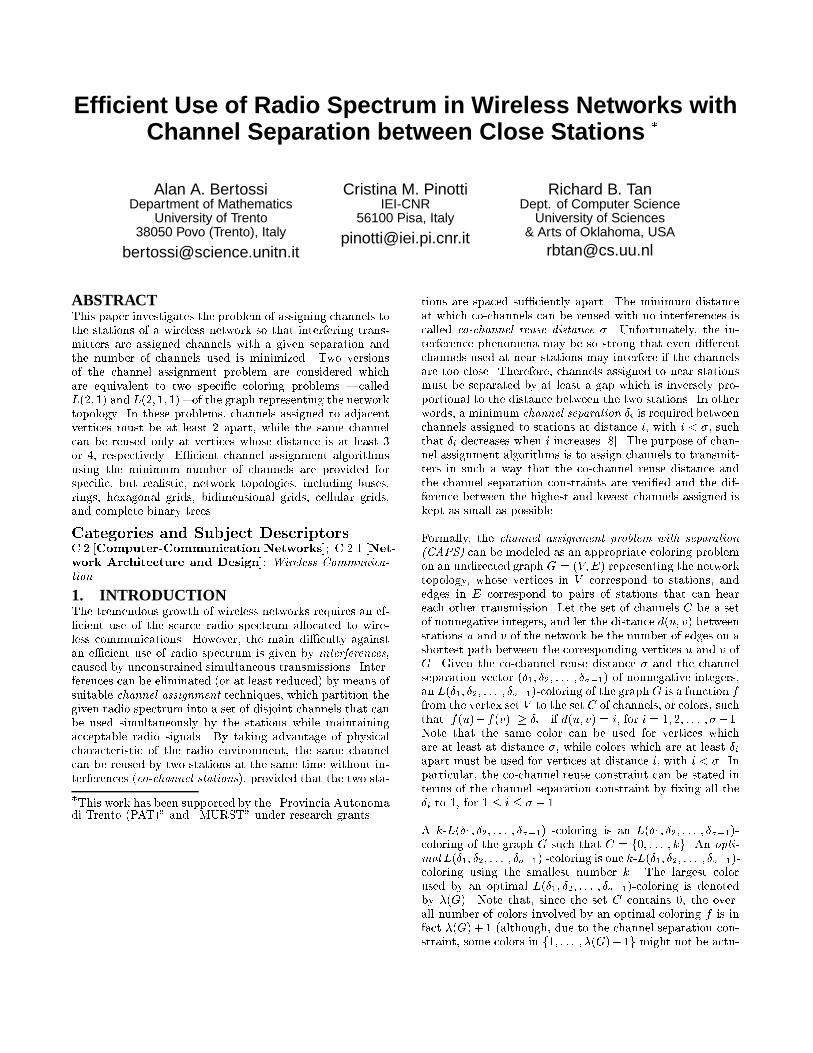
4 4 4Figure 1: Optimal coloring obtained by theHexagonal-5-L(2; 1)-coloring algorithm.In this paper, optimal channel assignment algorithms arepresented for the general case in which the network size issu�ciently large.3. HEXAGONAL GRIDSA hexagonal grid H of size r � c has r rows and c columns,indexed respectively from 0 to r � 1 (from top to bottom)and from 0 to c�1 (from left to right), with r � 3 and c � 2.A generic vertex u of H will be denoted by u = (i; j), wherei is its row index and j is its column index. Each vertexhas degree 3, except for some vertices on the borders. Inparticular, each vertex (i; j), which does not belong to thegrid borders, is adjacent to the following 3 vertices:1. 8>>><>>>: (i; j + 1) if (i is even and j is even) or(i is odd and j is odd)or(i; j � 1) if (i is even and j is odd) or(i is odd and j is even)2. (i� 1; j)3. (i+ 1; j)Lemma 3. For r � 3 and c � 3 there is a k-L(2; 1)-coloring of a hexagonal grid H of size r � c only if k � 5.Proof It follows immediately from Lemma 2 since there isat least one vertex of degree 3 that cannot be colored either0 or 4. Hence, �(H) � 5. 2An optimal coloring for a hexagonal grid of size 6 � 5 isillustrated in Figure 1. Below, an optimal 5-L(2; 1)-coloringis given to color all the vertices of any hexagonal grid H ofsize r � c, with r � 3 and c � 3.Algorithm Hexagonal-5-L(2; 1)-coloring (H; r; c);� If r � 3 and c � 3, then assign to each vertexu = (i; j) the color f(u) = (2i+ 3j) mod 6Theorem 1. The Hexagonal-5-L(2; 1)-coloring algorithmis optimal for any hexagonal grid H of size r� c, with r � 3and c � 3. 2
(1,0)
(2,0)
(0,0)
(1,1)
(2,1)
(0,1)
(1,0)
(2,0)
(0,0)
(1,1)
(2,1)
(0,1)
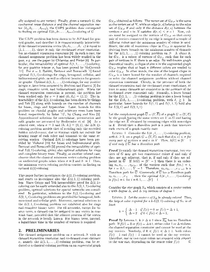
H HS SFigure 2: The subgraph HS with the dummy edges(dashed), and its complement HS.Lemma 4. For r � 3 and c � 3, or r � 5 and c = 2,there is a k-L(2; 1; 1)-coloring of a hexagonal grid H only ifk � 6.Proof Consider the augmented graph GH;4 = (V;E0) andthe subset S = f(0; 0); (0; 1); (1; 0); (1; 1); (2; 0); (2; 1)g. Sinceall the 6 vertices in S are mutually at distance at most 3 inH, they form a clique in GH;4. Therefore, �(H) � 5. Inthe case where r � 3 and c � 3, consider the subgraph HSinduced by S and also the vertex (3; 0). To satisfy the co-channel reuse constraint using exactly 6 colors, vertex (3; 0)must get the same color as vertex (0; 1). Moreover, dueto the channel separation constraint, the colors assigned tovertices (2; 0) and (3; 0) must have a gap of at least �1 = 2.Hence, also the colors of (2; 0) and (0; 1) must have a gap ofat least �1 = 2. This is equivalent to add in HS a dummyedge between vertices (2; 0) and (0; 1). The same reasoningcan be repeated for the pairs of vertices (1; 1) and (1; 0), and(2; 1) and (0; 0), as illustrated in Figure 2. Now, considerthe complement HS of HS, depicted also in Figure 2. Thereis no Hamilton path in HS since it consists of two connectedcomponents. It follows from Lemma 1 that �(H) � 6. Bya similar argument, the same lower bound can be provedwhen r � 5 and c = 2. 2Below, an optimal 6-L(2; 1; 1)-coloring is given to color allthe vertices of a hexagonal grid H of size r � c, with r � 3and c � 3.Algorithm Hexagonal-6-L(2; 1; 1)-coloring (H; r; c);� If r � 3 and c � 3 or r � 5 and c = 2, then assign toeach vertex u = (i; j) the color f(u) given as follows:
f(u) =8>>>>>>>>>>>>>>>>><>>>>>>>>>>>>>>>>>:
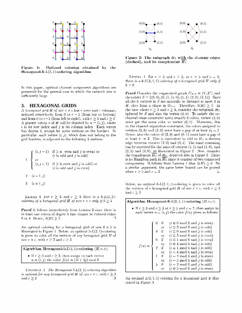
0 if (i � 0 mod 6 and j is even)or (i � 3 mod 6 and j is odd)4 if (i � 0 mod 6 and j is odd)or (i � 3 mod 6 and j is even)6 if (i � 1 mod 6 and j is even)or (i � 4 mod 6 and j is odd)2 if (i � 1 mod 6 and j is odd)or (i � 4 mod 6 and j is even)1 if (i � 2 mod 6 and j is even)or (i � 5 mod 6 and j is odd)5 if (i � 2 mod 6 and j is odd)or (i � 5 mod 6 and j is even)An optimal L(2; 1; 1)-coloring for a hexagonal grid is illus-trated in Figure 3.
2
0
1
5
6
4
2
0
6
4
5
1
2
0
1
5
6
4
2
0
6
4
5
1
2
0
1
5
6
4
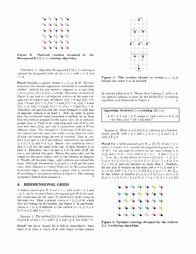
Figure 3: Optimal coloring obtained by theHexagonal-6-L(2; 1; 1)-coloring algorithm.Theorem 2. Algorithm Hexagonal-6-L(2; 1; 1)-coloring isoptimal for hexagonal grids of size r � c, with r � 3 andc � 3.Proof Consider a generic vertex u = (i; j) of H. By con-struction, the channel separation constraint is immediatelyveri�ed. Indeed, for any vertex v adjacent to u such thatv = (i; j � 1), f(v) = f(u)� 4 holds. Moreover, as shown inFigure 3, any pair u; v of adjacent vertices on the same col-umn can be colored only as follows f(u) = 0 and f(v) = 6,f(u) = 6 and f(v) = 1, f(u) = 1 and f(v) = 4, f(u) = 4 andf(v) = 2, f(u) = 2 and f(v) = 5, f(u) = 5 and f(v) = 0.Therefore, the gap between the colors assigned to each pairof adjacent vertices is at least 2. Now, in order to provethat the co-channel reuse constraint is veri�ed, let us showthat two vertices assigned to the same color are at distancegreater than 3. First of all, note that each row of H is col-ored with two colors, and any 3 consecutive rows of H usedi�erent colors. The i-th and (i+3)-th rows of H, for any i,are colored with the same two colors, except that the orderof such two colors along the row is swapped. That is, ver-tices (i; j) and (i; j+1) are colored, respectively, as vertices(i + 3; j + 1) and (i + 3; j). Hence, two vertices in rows iand (i + 3) get the same color only if their distance is atleast 4. Moreover, the i-th and (i + 6)-th rows of H, forany i, are colored the same. Hence, the same color can bereused on the same column only in two vertices at distance6. Finally, all the even (resp., odd) columns are colored thesame. Although the vertices (i; j) and (i; j+2) get the samecolor, their distance is 4 since there are no two consecutivehorizontal edges. Summarizing, a given color is reused onH according to the pattern shown in Figure 4. The coloringoptimality follows from Lemma 4. 24. BIDIMENSIONAL GRIDSA bidimensional grid B of size r � c, with both r � 2 andc � 2, can be obtained from a hexagonal grid H of the samesize connecting all the pairs of consecutive nodes lying onthe same row. Thus, a generic vertex u = (i; j) of B, whichdoes not belong on the borders, has degree 4. In particular,vertex u = (i; j) is adjacent to the vertices (i� 1; j); (i; j +1); (i+ 1; j) and (i; j � 1).Lemma 5. The optimal L(2; 1)-coloring of a bidimension-al grid B of size r� c, with r � 3 and c � 3, has �(B) = 6.Proof The lower bound for k follows immediately sincethere is at least a vertex of B with degree 4 that cannot
(i-6,j)
(i,j)
(i+6,j)
(i+3,j+1)
(i-3,j-1) (i-3,j+1)
(i,j+2)(i,j-2)
(i+3,j-1)
Figure 4: The vertices closest to vertex u = (i; j)where the color f(u) is reused.be colored either 0 or 5. Hence, from Lemma 2, �(B) = 6.An optimal solution is given by the Grid-6-L(2; 1)-coloringalgorithm and illustrated in Figure 5. 2Algorithm Grid-6-L(2; 1)-coloring (B; r; c);� If r � 3 and c � 3, assign to each vertex u = (i; j)the color f(u) = (2i+ 4j) mod 7.Lemma 6. There is a k-L(2; 1; 1)-coloring of a bidimen-sional grid B, with r � 5 and c � 4 or r � 4 and c � 5,only if k � 8.Proof For a bidimensional grid B = (V;E) of size r � c,with r � 5 and c � 4, consider the augmented graph GB;4 =(V;E0). For any pair of vertices on the same column u =(i; j) and v = (i + 3; j), with 0 � i � r � 4 and 1 � j �c� 2, let Su;v be the subset of vertices f(i; j); (i+1; j); (i+2; j); (i+ 3; j); (i+ 1; j � 1); (i+ 2; j � 1); (i+ 1; j + 1); (i+2; j + 1)g at pairwise distance no more than 3. Similarly,for any pair of vertices on the same row u = (i; j) and w =(i; j + 3), with 1 � i � r � 2 and 0 � j � c � 4, let S0u;wbe the subset of vertices f(i; j); (i; j + 1); (i; j + 2); (i; j +3); (i + 1; j + 1); (i + 1; j + 2); (i � 1; j + 1); (i � 1; j + 2)g0
0
2
2
2
2
2
0
0
0 4
4
4
4
4
6
6
6
6
1
1
1
1
3
3
5
5
5
3
3
53
6
1
5Figure 5: Optimal coloring obtained by the Grid-6-L(2; 1)-coloring algorithm.
s
ywz
t
v
u a
d
h
pg b
c
e
f
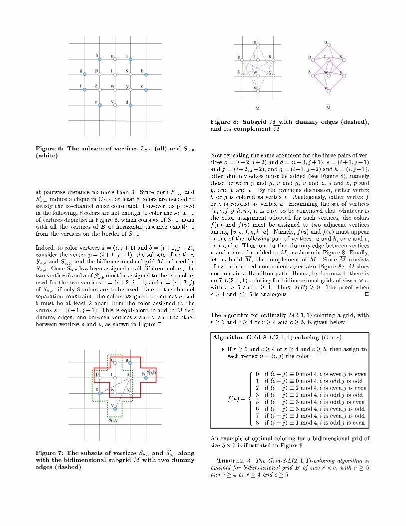
Figure 6: The subsets of vertices Lu;v (all) and Su;v(white).at pairwise distance no more than 3. Since both Su;v andS0u;w induce a clique in GB;4, at least 8 colors are needed tosatisfy the co-channel reuse constraint. However, as provedin the following, 8 colors are not enough to color the set Lu;vof vertices depicted in Figure 6, which consists of Su;v alongwith all the vertices of B at horizontal distance exactly 1from the vertices on the border of Su;v.Indeed, to color vertices a = (i; j + 1) and b = (i+1; j +2),consider the vertex p = (i+1; j � 1), the subsets of verticesSu;v and S0p;b, and the bidimensional subgrid M induced bySu;v. Once Su;v has been assigned to all di�erent colors, thetwo vertices b and a of S0p;b must be assigned to the two colorsused for the two vertices z = (i+2; j � 1) and v = (i+ 3; j)of Su;v, if only 8 colors are to be used. Due to the channelseparation constraint, the colors assigned to vertices a andb must be at least 2 apart from the color assigned to thevertex s = (i+1; j+1). This is equivalent to add to M twodummy edges: one between vertices s and z, and the otherbetween vertices s and v, as shown in Figure 7.Su,v
u
w
t b
v
a
’Sp,bp
z y
s
Figure 7: The subsets of vertices Su;v and S0p;b alongwith the bidimensional subgrid M with two dummyedges (dashed).
u
p s
ywz
t
v
u
p s
ywz
t
v
M MFigure 8: Subgrid M with dummy edges (dashed),and its complement M .Now repeating the same argument for the three pairs of ver-tices c = (i+2; j+2) and d = (i+3; j+1), e = (i+3; j�1)and f = (i+2; j�2), and g = (i+1; j�2) and h = (i; j�1),other dummy edges must be added (see Figure 8), namelythose between p and y, u and y, u and z, s and z, p andy, and p and v. By the previous discussion, either vertexh or g is colored as vertex v. Analogously, either vertex for e is colored as vertex u. Examining the set of verticesfv; e; f; g; h; ug, it is easy to be convinced that whatever isthe color assignment adopted for such vertices, the colorsf(u) and f(v) must be assigned to two adjacent verticesamong fv; e; f; g; h; ug. Namely, f(u) and f(v) must appearin one of the following pair of vertices: u and h, or v and e,or f and g. Thus, one further dummy edge between verticesu and v must be added to M , as shown in Figure 8. Finally,let us build M , the complement of M . Since M consistsof two connected components (see also Figure 8), M doesnot contain a Hamilton path. Hence, by Lemma 1, there isno 7-L(2; 1; 1)-coloring for bidimensional grids of size r� c,with r � 5 and c � 4. Thus, �(B) � 8. The proof whenr � 4 and c � 5 is analogous. 2The algorithm for optimally L(2; 1; 1)-coloring a grid, withr � 5 and c � 4 or r � 4 and c � 5, is given below.Algorithm Grid-8-L(2; 1; 1)-coloring (G; r; c);� If r � 5 and c � 4 or r � 4 and c � 5, then assign toeach vertex u = (i; j) the colorf(u) = 8>>>>>>>>><>>>>>>>>>:
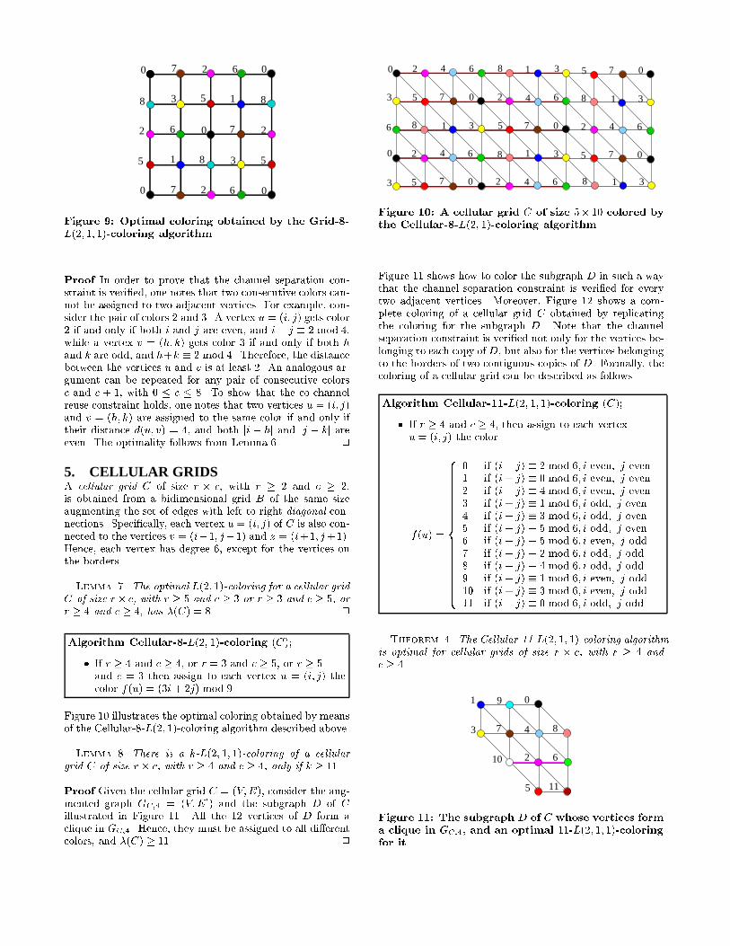
0 if (i+ j) � 0 mod 4; i is even,j is even1 if (i+ j) � 0 mod 4; i is odd,j is odd2 if (i+ j) � 2 mod 4; i is even,j is even3 if (i+ j) � 2 mod 4; i is odd,j is odd5 if (i+ j) � 3 mod 4; i is odd,j is even6 if (i+ j) � 3 mod 4; i is even,j is odd7 if (i+ j) � 1 mod 4; i is even,j is odd8 if (i+ j) � 1 mod 4; i is odd,j is evenAn example of optimal coloring for a bidimensional grid ofsize 5� 5 is illustrated in Figure 9.Theorem 3. The Grid-8-L(2; 1; 1)-coloring algorithm isoptimal for bidimensional grid B of size r � c, with r � 5and c � 4 or r � 4 and c � 5.
1
1
2
2 2
2
3
3
5
5 5
6
6
6
7
7
7
8
8
8
0 0
00
0
Figure 9: Optimal coloring obtained by the Grid-8-L(2; 1; 1)-coloring algorithm.Proof In order to prove that the channel separation con-straint is veri�ed, one notes that two consecutive colors can-not be assigned to two adjacent vertices. For example, con-sider the pair of colors 2 and 3. A vertex u = (i; j) gets color2 if and only if both i and j are even, and i+ j � 2 mod 4,while a vertex v = (h; k) gets color 3 if and only if both hand k are odd, and h+k � 2 mod 4. Therefore, the distancebetween the vertices u and v is at least 2. An analogous ar-gument can be repeated for any pair of consecutive colorsc and c + 1, with 0 � c � 8. To show that the co-channelreuse constraint holds, one notes that two vertices u = (i; j)and v = (h; k) are assigned to the same color if and only iftheir distance d(u; v) = 4, and both ji � hj and jj � kj areeven. The optimality follows from Lemma 6. 25. CELLULAR GRIDSA cellular grid C of size r � c, with r � 2 and c � 2,is obtained from a bidimensional grid B of the same sizeaugmenting the set of edges with left-to-right diagonal con-nections. Speci�cally, each vertex u = (i; j) of C is also con-nected to the vertices v = (i�1; j�1) and z = (i+1; j+1).Hence, each vertex has degree 6, except for the vertices onthe borders.Lemma 7. The optimal L(2; 1)-coloring for a cellular gridC of size r� c, with r � 5 and c � 3 or r � 3 and c � 5, orr � 4 and c � 4, has �(C) = 8. 2Algorithm Cellular-8-L(2; 1)-coloring (C);� If r � 4 and c � 4, or r = 3 and c � 5, or r � 5and c = 3 then assign to each vertex u = (i; j) thecolor f(u) = (3i+ 2j) mod 9.Figure 10 illustrates the optimal coloring obtained by meansof the Cellular-8-L(2; 1)-coloring algorithm described above.Lemma 8. There is a k-L(2; 1; 1)-coloring of a cellulargrid C of size r � c, with r � 4 and c � 4, only if k � 11.Proof Given the cellular grid C = (V;E), consider the aug-mented graph GC;4 = (V;E0) and the subgraph D of Cillustrated in Figure 11. All the 12 vertices of D form aclique in GC;4. Hence, they must be assigned to all di�erentcolors, and �(C) � 11. 2
8 1 0
8
8 1
10
0
0
0
0
0
8 1
18
3
4
42
6
6
3
5 7
4 6
2
3
3
3
6
2
62
5
5 7
4
7
6
3
2
5
5 7
4
7
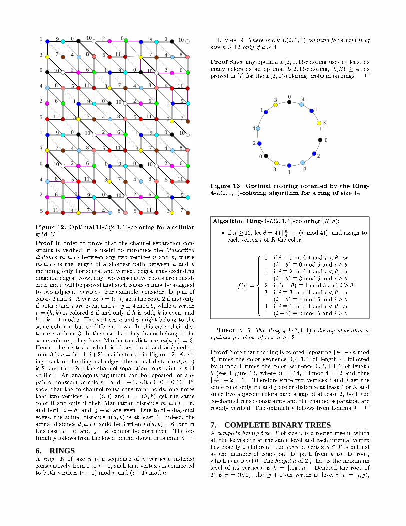
3Figure 10: A cellular grid C of size 5� 10 colored bythe Cellular-8-L(2; 1)-coloring algorithm.Figure 11 shows how to color the subgraph D in such a waythat the channel separation constraint is veri�ed for everytwo adjacent vertices. Moreover, Figure 12 shows a com-plete coloring of a cellular grid C obtained by replicatingthe coloring for the subgraph D. Note that the channelseparation constraint is veri�ed not only for the vertices be-longing to each copy of D, but also for the vertices belongingto the borders of two contiguous copies of D. Formally, thecoloring of a cellular grid can be described as follows.Algorithm Cellular-11-L(2; 1; 1)-coloring (C);� If r � 4 and c � 4, then assign to each vertexu = (i; j) the colorf(u) =
8>>>>>>>>>>>>>>>>><>>>>>>>>>>>>>>>>>:0 if (i+ j) � 2 mod 6; i even; j even1 if (i+ j) � 0 mod 6; i even; j even2 if (i+ j) � 4 mod 6; i even; j even3 if (i+ j) � 1 mod 6; i odd; j even4 if (i+ j) � 3 mod 6; i odd; j even5 if (i+ j) � 5 mod 6; i odd; j even6 if (i+ j) � 5 mod 6; i even; j odd7 if (i+ j) � 2 mod 6; i odd; j odd8 if (i+ j) � 4 mod 6; i odd; j odd9 if (i+ j) � 1 mod 6; i even; j odd10 if (i+ j) � 3 mod 6; i even; j odd11 if (i+ j) � 0 mod 6; i odd; j oddTheorem 4. The Cellular-11-L(2; 1; 1)-coloring algorithmis optimal for cellular grids of size r � c, with r � 4 andc � 4.
2
3
1
4
0
5
6
11
87
9
10Figure 11: The subgraph D of C whose vertices forma clique in GC;4, and an optimal 11-L(2; 1; 1)-coloringfor it.
2
5
6
11
7
9
4
0
3
1
7
9
3
1
7
9
3
1
7
9
3
1
7
9
2
5
6
11
10
8
0
5
3
1
3
1
2
4
2
4
0
5
6
11
87
9
10
10
7
1
2
4
0
5
6
11
87
9
10
10
11
10
4
0
8
2
3
1
4
0
5
6
11
87
9
10
2
4
0
5
6
11
8
10
2
4
0
5
6
11
8
9
4
0
3
1
7
2
5 118
10
8
6
8
2
4
0
5
6
11
8
10
3
9
610
Figure 12: Optimal 11-L(2; 1; 1)-coloring for a cellulargrid C.Proof In order to prove that the channel separation con-straint is veri�ed, it is useful to introduce the Manhattandistance m(u; v) between any two vertices u and v, wherem(u; v) is the length of a shortest path between u and vincluding only horizontal and vertical edges, thus excludingdiagonal edges. Now, any two consecutive colors are consid-ered and it will be proved that such colors cannot be assignedto two adjacent vertices. For example, consider the pair ofcolors 2 and 3. A vertex u = (i; j) gets the color 2 if and onlyif both i and j are even, and i+ j � 4 mod 6, while a vertexv = (h; k) is colored 3 if and only if h is odd, k is even, andh+ k � 1 mod 6. The vertices u and v might belong to thesame column, but to di�erent rows. In this case, their dis-tance is at least 3. In the case that they do not belong to thesame column, they have Manhattan distance m(u; v) = 3.Hence, the vertex v which is closest to u and assigned tocolor 3 is v = (i+1; j+2), as illustrated in Figure 12. Keep-ing track of the diagonal edges, the actual distance d(u; v)is 2, and therefore the channel separation constraint is stillveri�ed. An analogous argument can be repeated for anypair of consecutive colors c and c+ 1, with 0 � c � 10. Toshow that the co-channel reuse constraint holds, one notesthat two vertices u = (i; j) and v = (h; k) get the samecolor if and only if their Manhattan distance m(u; v) = 6,and both ji � hj and jj � kj are even. Due to the diagonaledges, the actual distance d(u; v) is at least 4. Indeed, theactual distance d(u; v) could be 3 when m(u; v) = 6, but inthis case ji � hj and jj � kj cannot be both even. The op-timality follows from the lower bound shown in Lemma 8. 26. RINGSA ring R of size n is a sequence of n vertices, indexedconsecutively from 0 to n�1, such that vertex i is connectedto both vertices (i� 1) mod n and (i+ 1) mod n.
Lemma 9. There is a k-L(2; 1; 1)-coloring for a ring R ofsize n � 12 only if k � 4.Proof Since any optimal L(2; 1; 1)-coloring uses at least asmany colors as an optimal L(2; 1)-coloring, �(R) � 4, asproved in [7] for the L(2; 1)-coloring problem on rings. 20 4
4
1
14
3
3
3
1
0
0
2
2Figure 13: Optimal coloring obtained by the Ring-4-L(2; 1; 1)-coloring algorithm for a ring of size 14.Algorithm Ring-4-L(2; 1; 1)-coloring (R;n);� if n � 12, let � = 4 �bn4 c � (n mod 4)�, and assign toeach vertex i of R the colorf(i) = 8>>>>>>>>>>><>>>>>>>>>>>:
0 if i � 0 mod 4 and i < �; or(i� �) � 0 mod 5 and i � �1 if i � 2 mod 4 and i < �; or(i� �) � 3 mod 5 and i � �2 if (i� �) � 1 mod 5 and i � �3 if i � 3 mod 4 and i < �; or(i� �) � 4 mod 5 and i � �4 if i � 1 mod 4 and i < �; or(i� �) � 2 mod 5 and i � �Theorem 5. The Ring-4-L(2; 1; 1)-coloring algorithm isoptimal for rings of size n � 12.Proof Note that the ring is colored repeating bn4 c� (n mod4) times the color sequence 0; 4; 1; 3 of length 4, followedby n mod 4 times the color sequence 0; 2; 4; 1; 3 of length5 (see Figure 13, where n = 14, 14 mod 4 = 2 and thusb 144 c � 2 = 1). Therefore since two vertices i and j get thesame color only if i and j are at distance at least 4 or 5, andsince two adjacent colors have a gap of at least 2, both theco-channel reuse constraints and the channel separation arereadily veri�ed. The optimality follows from Lemma 9. 27. COMPLETE BINARY TREESA complete binary tree T of size n is a rooted tree in whichall the leaves are at the same level and each internal vertexhas exactly 2 children. The level of vertex u 2 T is de�nedas the number of edges on the path from u to the root,which is at level 0. The height h of T , that is the maximumlevel of its vertices, is h = blog2 nc. Denoted the root ofT as r = (0; 0), the (j + 1)-th vertex at level i, u = (i; j),
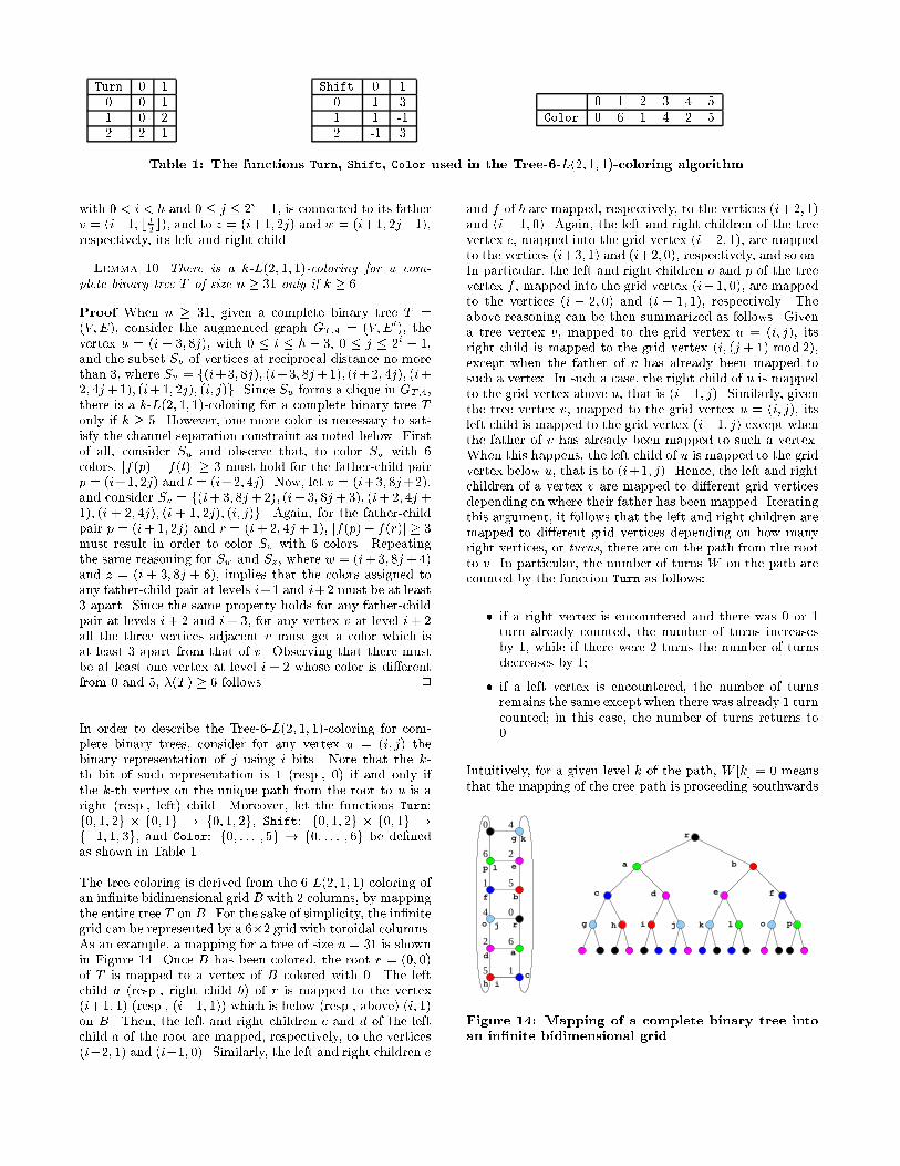
Turn 0 10 0 11 0 22 2 1 Shift 0 10 1 31 1 -12 -1 3 0 1 2 3 4 5Color 0 6 1 4 2 5Table 1: The functions Turn, Shift, Color used in the Tree-6-L(2; 1; 1)-coloring algorithm.with 0 < i < h and 0 � j � 2i� 1, is connected to its fatherv = (i�1; b j2 c), and to z = (i+1; 2j) and w = (i+1; 2j+1),respectively, its left and right child.Lemma 10. There is a k-L(2; 1; 1)-coloring for a com-plete binary tree T of size n � 31 only if k � 6.Proof When n � 31, given a complete binary tree T =(V;E), consider the augmented graph GT;4 = (V;E0), thevertex u = (i + 3; 8j), with 0 � i � h � 3, 0 � j � 2i � 1,and the subset Su of vertices at reciprocal distance no morethan 3, where Su = f(i+3; 8j); (i+3; 8j+1); (i+2; 4j); (i+2; 4j+1); (i+1; 2j); (i; j)g. Since Su forms a clique in GT;4,there is a k-L(2; 1; 1)-coloring for a complete binary tree Tonly if k � 5. However, one more color is necessary to sat-isfy the channel separation constraint as noted below. Firstof all, consider Su and observe that, to color Su with 6colors, jf(p) � f(l)j � 3 must hold for the father-child pairp = (i+1; 2j) and l = (i+2; 4j). Now, let v = (i+3; 8j+2),and consider Sv = f(i+3; 8j +2); (i+3; 8j +3); (i+2; 4j +1); (i + 2; 4j); (i + 1; 2j); (i; j)g. Again, for the father-childpair p = (i+ 1; 2j) and r = (i+ 2; 4j + 1), jf(p)� f(r)j � 3must result in order to color Sv with 6 colors. Repeatingthe same reasoning for Sw and Sz, where w = (i+3; 8j+4)and z = (i + 3; 8j + 6), implies that the colors assigned toany father-child pair at levels i+1 and i+2 must be at least3 apart. Since the same property holds for any father-childpair at levels i+ 2 and i+ 3, for any vertex v at level i+ 2all the three vertices adjacent v must get a color which isat least 3 apart from that of v. Observing that there mustbe at least one vertex at level i + 2 whose color is di�erentfrom 0 and 5, �(T ) � 6 follows. 2In order to describe the Tree-6-L(2; 1; 1)-coloring for com-plete binary trees, consider for any vertex u = (i; j) thebinary representation of j using i bits. Note that the k-th bit of such representation is 1 (resp., 0) if and only ifthe k-th vertex on the unique path from the root to u is aright (resp., left) child. Moreover, let the functions Turn:f0; 1; 2g � f0; 1g ! f0; 1; 2g, Shift: f0; 1; 2g � f0; 1g !f�1; 1; 3g, and Color: f0; : : : ; 5g ! f0; : : : ; 6g be de�nedas shown in Table 1.The tree coloring is derived from the 6-L(2; 1; 1)-coloring ofan in�nite bidimensional grid B with 2 columns, by mappingthe entire tree T on B. For the sake of simplicity, the in�nitegrid can be represented by a 6�2 grid with toroidal columns.As an example, a mapping for a tree of size n = 31 is shownin Figure 14. Once B has been colored, the root r = (0; 0)of T is mapped to a vertex of B colored with 0. The leftchild a (resp., right child b) of r is mapped to the vertex(i+1; 1) (resp., (i�1; 1)) which is below (resp., above) (i; 1)on B. Then, the left and right children c and d of the leftchild a of the root are mapped, respectively, to the vertices(i�2; 1) and (i�1; 0). Similarly, the left and right children e
and f of b are mapped, respectively, to the vertices (i+2; 1)and (i+ 1; 0). Again, the left and right children of the treevertex c, mapped into the grid vertex (i+2; 1), are mappedto the vertices (i+3; 1) and (i+2; 0), respectively, and so on.In particular, the left and right children o and p of the treevertex f , mapped into the grid vertex (i�1; 0), are mappedto the vertices (i � 2; 0) and (i � 1; 1), respectively. Theabove reasoning can be then summarized as follows. Givena tree vertex v, mapped to the grid vertex u = (i; j), itsright child is mapped to the grid vertex (i; (j + 1) mod 2),except when the father of v has already been mapped tosuch a vertex. In such a case, the right child of u is mappedto the grid vertex above u, that is (i�1; j). Similarly, giventhe tree vertex v, mapped to the grid vertex u = (i; j), itsleft child is mapped to the grid vertex (i�1; j) except whenthe father of v has already been mapped to such a vertex.When this happens, the left child of u is mapped to the gridvertex below u, that is to (i+1; j). Hence, the left and rightchildren of a vertex v are mapped to di�erent grid verticesdepending on where their father has been mapped. Iteratingthis argument, it follows that the left and right children aremapped to di�erent grid vertices depending on how manyright vertices, or turns, there are on the path from the rootto v. In particular, the number of turns W on the path arecounted by the function Turn as follows:� if a right vertex is encountered and there was 0 or 1turn already counted, the number of turns increasesby 1, while if there were 2 turns the number of turnsdecreases by 1;� if a left vertex is encountered, the number of turnsremains the same except when there was already 1 turncounted; in this case, the number of turns returns to0.Intuitively, for a given level k of the path, W [k] = 0 meansthat the mapping of the tree path is proceeding southwardsba
r
c e fd
c
a
e
b
r
d
h
g
f
p
o o pg h i
i
j j
k
k l
l
1
4
2
5
0
6
5
2
4
1
6
0
Figure 14: Mapping of a complete binary tree intoan in�nite bidimensional grid.
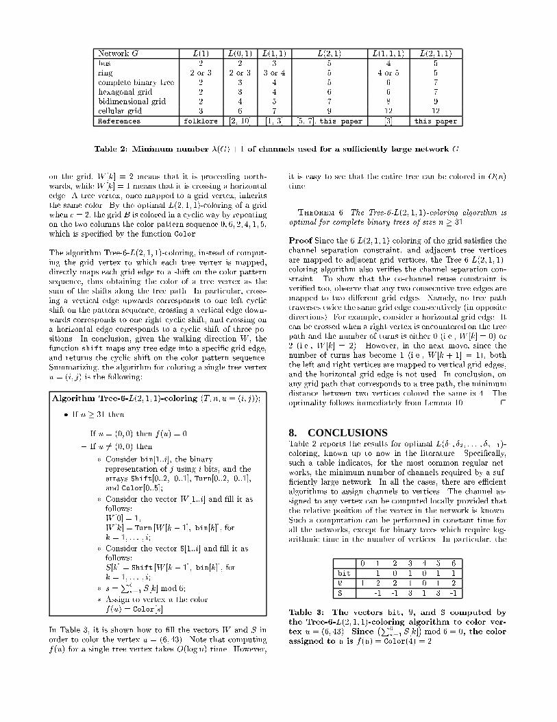
Network G L(1) L(0; 1) L(1; 1) L(2; 1) L(1; 1; 1) L(2; 1; 1)bus 2 2 3 5 4 5ring 2 or 3 2 or 3 3 or 4 5 4 or 5 5complete binary tree 2 3 4 5 6 7hexagonal grid 2 3 4 6 6 7bidimensional grid 2 4 5 7 8 9cellular grid 3 6 7 9 12 12References folklore [2, 10] [1, 3] [5, 7], this paper [3] this paperTable 2: Minimum number �(G) + 1 of channels used for a su�ciently large network G.on the grid, W [k] = 2 means that it is proceeding north-wards, while W [k] = 1 means that it is crossing a horizontaledge. A tree vertex, once mapped to a grid vertex, inheritsthe same color. By the optimal L(2; 1; 1)-coloring of a gridwhen c = 2, the grid B is colored in a cyclic way by repeatingon the two columns the color pattern sequence 0; 6; 2; 4; 1; 5,which is speci�ed by the function Color.The algorithm Tree-6-L(2; 1; 1)-coloring, instead of comput-ing the grid vertex to which each tree vertex is mapped,directly maps each grid edge to a shift on the color patternsequence, thus obtaining the color of a tree vertex as thesum of the shifts along the tree path. In particular, cross-ing a vertical edge upwards corresponds to one left cyclicshift on the pattern sequence, crossing a vertical edge down-wards corresponds to one right cyclic shift, and crossing ona horizontal edge corresponds to a cyclic shift of three po-sitions. In conclusion, given the walking direction W , thefunction shift maps any tree edge into a speci�c grid edge,and returns the cyclic shift on the color pattern sequence.Summarizing, the algorithm for coloring a single tree vertexu = (i; j) is the following:Algorithm Tree-6-L(2; 1; 1)-coloring (T; n; u = (i; j));� If n � 31 then{ If u = (0; 0) then f(u) = 0{ If u 6= (0; 0) then� Consider bin[1::i], the binaryrepresentation of j using i bits, and thearrays Shift[0::2; 0::1], Turn[0::2; 0::1],and Color[0::5];� Consider the vector W [1::i] and �ll it asfollows:W [0] = 1,W [k] = Turn [W [k � 1]; bin[k]], fork = 1; : : : ; i;� Consider the vector S[1::i] and �ll it asfollows:S[k] = Shift [W [k � 1]; bin[k]], fork = 1; : : : ; i;� s =Pik=1 S[k] mod 6;� Assign to vertex u the colorf(u) = Color[s].In Table 3, it is shown how to �ll the vectors W and S inorder to color the vertex u = (6; 43). Note that computingf(u) for a single tree vertex takes O(log n) time. However,
it is easy to see that the entire tree can be colored in O(n)time.Theorem 6. The Tree-6-L(2; 1; 1)-coloring algorithm isoptimal for complete binary trees of size n � 31.Proof Since the 6-L(2; 1; 1)-coloring of the grid satis�es thechannel separation constraint, and adjacent tree verticesare mapped to adjacent grid vertices, the Tree-6-L(2; 1; 1)-coloring algorithm also veri�es the channel separation con-straint. To show that the co-channel reuse constraint isveri�ed too, observe that any two consecutive tree edges aremapped to two di�erent grid edges. Namely, no tree pathtraverses twice the same grid edge consecutively (in oppositedirections). For example, consider a horizontal grid edge. Itcan be crossed when a right vertex is encountered on the treepath and the number of turns is either 0 (i.e., W [k] = 0) or2 (i.e., W [k] = 2). However, in the next move, since thenumber of turns has become 1 (i.e., W [k + 1] = 1), boththe left and right vertices are mapped to vertical grid edges,and the horizontal grid edge is not used. In conclusion, onany grid path that corresponds to a tree path, the minimumdistance between two vertices colored the same is 4. Theoptimality follows immediately from Lemma 10. 28. CONCLUSIONSTable 2 reports the results for optimal L(�1; �2; : : : ; ���1)-coloring, known up to now in the literature. Speci�cally,such a table indicates, for the most common regular net-works, the minimum number of channels required by a suf-�ciently large network. In all the cases, there are e�cientalgorithms to assign channels to vertices. The channel as-signed to any vertex can be computed locally provided thatthe relative position of the vertex in the network is known.Such a computation can be performed in constant time forall the networks, except for binary trees which require log-arithmic time in the number of vertices. In particular, the0 1 2 3 4 5 6bit 1 0 1 0 1 1W 1 2 2 1 0 1 2S -1 -1 3 1 3 -1Table 3: The vectors bit, W, and S computed bythe Tree-6-L(2; 1; 1)-coloring algorithm to color ver-tex u = (6; 43). Since �P6k=1 S[k]� mod 6 = 0, the colorassigned to u is f(u) = Color(4) = 2.
present paper dealt with the L(2; 1)- and L(2; 1; 1)-coloringproblems which consider a channel separation of at least 2between adjacent vertices, as required in many real wire-less environments. The proposed results extend those al-ready known in the literature for the L(0; 1)-, L(1; 1)- andL(1; 1; 1)-coloring problems. For the sake of completeness,Table 2 reports also the minimum number of colors requiredby the L(1)-coloring problem, which reduces to the clas-sical minimum vertex coloring of a graph. From a the-oretical point of view, it remains as an open question tosolve the general L(�1; �2; : : : ; ���1)-coloring problem, with�1 � �2 � : : : � ���1.9. REFERENCES[1] R. Battiti, A.A. Bertossi, and M.A. Bonuccelli,\Assigning Codes in Wireless Networks: Bounds andScaling Properties", Wireless Networks, Vol. 5, 1999,pp. 195-209.[2] A.A. Bertossi and M.A. Bonuccelli, \CodeAssignment for Hidden Terminal InterferenceAvoidance in Multihop Packet Radio Networks",IEEE/ACM Transactions on Networking, Vol. 3,1995, pp. 441-449.[3] A.A. Bertossi and M.C. Pinotti, \Mappings forCon ict-Free Access of Paths in BidimensionalArrays, Circular Lists, and Complete Trees", Tec.Rep. UTM-563, Depatment of Mathematics,University of Trento, 1999.[4] H.L. Bodlaender, T. Kloks, R.B. Tan and J. vanLeeuwen, \Approximation �-Coloring on Graphs", toappear in Proceedings STACS 2000.[5] G. J. Chang and D. Kuo, \The L(2; 1)-LabelingProblem on Graphs", SIAM Journal on DiscreteMathematics, Vol. 9, 1996, pp. 309-316.[6] I. Chlamtac and S.S. Pinter, \Distributed nodesOrganizations Algorithm for Channel Access in aMultihop Dynamic Radio Network", IEEETransactions on Computers, Vol. 36, 1987, pp.728-737.[7] J. R. Griggs and R.K. Yeh, \Labelling Graphs with aCondition at Distance 2", SIAM Journal on DiscreteMathematics, Vol. 5, 1992, pp. 586-595.[8] W.K. Hale, \Frequency Assignment: Theory andApplication", Proceedings of the IEEE, Vol. 68, 1980,pp. 1497-1514.[9] I. Katzela and M. Naghshineh, \Channel AssignmentSchemes for Cellular Mobile TelecommunicationSystems: A Comprehensive Survey", IEEE PersonalCommunications, June 1996, pp. 10-31.[10] T. Makansi, \Transmitted Oriented CodeAssignment for Multihop Packet Radio", IEEETransactions on Communications, Vol. 35, 1987, pp.1379-1382.
[11] S.T. McCormick, \Optimal Approximation of SparseHessians and its Equivalence to a Graph ColoringProblem", Mathematical Programming, Vol. 26,1983, pp. 153{171.[12] D. Sakai, \Labeling Cordal Graphs: Distance TwoCondition", SIAM Journal on Discrete Mathematics,Vol. 7, 1994, pp. 133-140.