effect of competition on gain in feedlot bulls from hereford selection lines

L. D. Van Vleck, L. V. Cundiff and R. M. KochEffect of competition on gain in feedlot bulls from Hereford selection lines

published online March 19, 2007J ANIM SCI

http://jas.fass.org/content/early/2007/03/19/jas.2007-0067.citationthe World Wide Web at:

The online version of this article, along with updated information and services, is located on

www.asas.org

by guest on September 13, 2011jas.fass.orgDownloaded from

http://jas.fass.org/

RUNNING HEAD: Competition effects on feedlot gain 1

2345

Effect of competition on gain in feedlot bulls from Hereford selection lines1678

L. D. Van Vleck†*2, L. V. Cundiff†, and R. M. Koch* 910

Roman L. Hruska U.S. Meat Animal Research Center, †Clay Center, NE 68933 and 11†*Department of Animal Science, University of Nebraska, Lincoln 68583-0908 12

13

1 The authors express appreciation to Darrell Light for data base support and to Donna White for secretarial support in preparation of this manuscript. 2 Correspondence: A218 Animal Sciences (phone: 402-472-6010; fax: 402-472-6362; e-mail: [email protected]).

Page 1 of 25 Journal of Animal Science

Published Online First on March 19, 2007 as doi:10.2527/jas.2007-0067 by guest on September 13, 2011jas.fass.orgDownloaded from


2

ABSTRACT: This study examined competition effects on average daily gain in the feedlot of 14

1,882 Hereford bulls representing eight birth years from a selection experiment. Each year, eight 15

feedlot pens were used to feed bulls in groups with two pens nested within each of the four 16

selection lines. Gains were recorded for up to eight periods of 28 d. Models for analyses included 17

pen effects (fixed or random), fixed effects such as year and line, and random direct genetic, 18

competition genetic (and in some analyses competition environmental effects) and environmental 19

effects. Each pen mate as a competitor affects records of all others in the pen. All lines traced to 20

common foundation animals so the numerator relationships among and within pens were the 21

basis for separating direct and competition genetic effects and pen effects. For this population 22

and pen conditions (average of 30 bulls per pen), major results were: 1) competition genetic 23

effects seemed present for the first 28 d period but not for the following seven periods, 2) models 24

with pens considered fixed effects could not separate variances and covariance due to direct and 25

competition genetic effects, 3) models without competition effects had large estimates of the 26

variance component due to pen effects for gain through eight periods, and 4) models with both 27

genetic and environmental competition effects accounted for nearly all of the variance 28

traditionally attributed to pen effects (even though estimates of the competition variance 29

component were small, the estimates of pen variance were near zero). 30

Key words: average daily gain, beef cattle, competition effects, genetic effects 31

32

INTRODUCTION 33

Muir and Schinkel (2002) introduced animal breeders to predicting both direct and 34

competition (associative) genetic effects for animals. Earlier, Federer (1955) had discussed 35

competition effects for plants and animals. Griffing (1967) developed theory for accounting for 36

Page 2 of 25Journal of Animal Science



3

direct and associative effects for plants. Van Vleck and Cassady (2005) reported results from 37

analyses of data simulated from models that included both direct and competition genetic effects. 38

With average daily gains (ADG) of Large White gilts housed in pens, Arango et al. (2005) 39

attempted to estimate variance components associated with pen mates. They reported for their 40

data structure and large pen sizes that accurate estimation of parameters for competition effects 41

was not possible. 42

The purpose of this study was to estimate variance and (co)variance components for 43

direct and competition effects for average daily gain for eight time periods for Hereford bulls 44

from three selection lines and one control line (Koch, et al., 1974a,b; 1994). An added goal was 45

to document problems with such analyses with different statistical models. 46

47

MATERIALS AND METHODS 48

Koch et al. (1974a, 1974b) have described the foundation Herefords and methods of 49

selection beginning in 1963 for the three selection lines and one control line. The selection lines 50

were selected for 1) weaning weight, 2) yearling weight, and 3) an index with equal weights for 51

yearling weight and muscle score. For line 3, a phenotypic index was used. For each year, 52

yearling weight divided by the year-sex phenotypic standard deviation for yearling weight was 53

added to muscle score divided by the year-sex phenotypic standard deviation for muscle score. 54

The control line was created using foundation sires and foundation dams of the selected lines. 55

The foundation lines were created from related animals so that numerator relationships across 56

lines and within lines were available to attempt to separate out components of variance due to 57

direct and competition genetic effects and that due to pen effects. 58




4

This analysis involves bull calves born in the three selection lines and the control line 59

from 1972-1979. Koch et al. (1994) described management of these bulls from birth to an 60

average age of 400 days. During the postweaning period, bulls from each line were split into two 61

randomly assigned replicate pens with progeny of sires cross classified with pens and were fed a 62

mixed diet of corn silage, rolled corn, and a protein mineral supplement containing about 2.69 63

Mcal of ME/kg of DM and 12.88% CP. Average daily gains (ADG) were calculated from initial 64

weights on test and weights at seven intervals of 28 days plus a shorter eighth interval. The 65

number of bulls per pen varied with number of bulls available per line each year but ranged from 66

about 25 to 30 head per pen. The eight pens, each measuring 15.4 meters in width (West to East) 67

and 61 meters in length (South to North) were situated adjacent to each other and ran 68

contiguously for 123.4 meters. The pens sloped gently (2.7%) from front (South) to back (North) 69

and even more gradually from East to West (0.6% slope at front and 0.9% at back). Mounds of 70

dirt measuring about 1 meter in depth at their center and running South to North for about 40 71

meters were situated in the center of each pen to provide relatively dry resting areas. At the north 72

end of each lot, gates accessed a working alley measuring 3.75 meters in width. Continuous 73

fence line feed bunks running the full width (15.4 meters which was considered adequate for 33 74

head) were situated at the front (South) of each pen. Automatic water troughs (heated in winter 75

months) were located in the fence line about 8.6 meters from the feed bunk in each pen. A 76

concrete slab extending 3 meters out from the feed bunk and around each water source was 77

provided in each pen. A wind break comprised of 3 rows of cedar trees was located about 12 78

meters from the North fence line. No shade was provided. 79

Numbers of bulls by year and unadjusted mean ADG (kg x 100) for periods 1 through 8 80

(ADG1,…, ADG8) are shown in Table 1 along with initial weights (kg). The total number of 81




5

bulls with initial weights was 1,882 with from 211 to 254 for each year. Those means and 82

numbers are in Table 1. Table 1 also shows that for four years, weights were not available for 83

Period 8 and that weights were not available for Period 7 for bulls born in 1975. Fixed effects in 84

models included linear covariates for day of year of birth, number of competitors, and initial 85

weight (some analyses) and fixed factors of year of birth (8 levels; 1972 to 1979) and selection 86

line (4 levels; 1, 2, 3 and control) for some analyses. Pens (up to 64) were considered to be 87

random factors for some analyses and to be fixed factors for other analyses and were ignored in 88

some analyses. 89

Table 2 (left side) describes the combinations of fixed and random factors used in 18 90

exploratory analyses. Random factors included direct and competition genetic effects (with and 91

without covariance), pen effects (when not ignored or considered a fixed factor) and residual 92

effects. Later analyses also included repeated environmental effects of competitors as not only 93

the competition genetic effect but also the competition environmental effect of a pen mate would 94

be expressed in the records of all other pen mates. Modification of the MTDFREML programs 95

(Boldman et al., 1995) has been described for including multiple competition genetic effects by 96

Van Vleck and Cassady (2004a). A similar modification was made to include competition 97

environmental effects in the model which would be comparable to permanent environmental 98

effects affecting all pen mates of a competitor. The unique feature of competition models is that 99

a factor (e.g., competition genetic) may have many levels of that factor (all competitors) 100

expressed in the record of a pen mate. Those many levels create blocks of non-zero values in the 101

coefficient matrix for the mixed model equations so that the coefficient matrix is much less 102

sparse than for most sets of mixed model equations. 103




6

A statistical description of an observation on animal, i, in pen, k, for the model with 104

competition genetic effects is as follows: 105

yik = µ + bwWi + bf Fi + ai +l Nk kc + + cK + pk + eik, 106

where yik is the observation, 107

µ represents a fixed effect common to all animals, 108

bwWi is the product of the regression coefficient and covariate for initial weight for animal i and 109

bf Fi is the product of the regression coefficient and covariate for number of competitors, 110

ai is the additive direct genetic value for animal i, 111

pk is the kth pen effect (fixed or random), 112

l Nk kc , ,cK are the genetic competition effects of other animals in the same pen (with a similar set 113

for models with permanent environment competition effects) and, 114

eik is the residual effect. 115

The dispersion parameters are similar to those for a maternal effects model. Let a be the 116

vector of additive direct genetic values augmented for animals in the relationship variance and c 117

be the vector of additive competition genetic values augmented for animals in the relationship 118

matrix. Then 119

oa

V G Ac

= ⊗

where A is the augmented relationship matrix, 120

⊗ is the right direct product operator and 121

2dcd

o 2dc c

Gσ σσ σ

=

with 122

2d ,σ the direct genetic variance; 123

2c ,σ the competition genetic variance, and 124




7

σdc, the direct-competition genetic covariance (for models without covariance this becomes 125

zero). 126

For the model with a vector of competition permanent environmental effects, the variance 127

structure is 2Ne pe Ne I where Iσ is an identity matrix of order the total number of animals with 128

observations and 2peσ is the variance of competition permanent environmental effects. When the 129

vector of pen effects is considered to be a vector of random effects, V(p) = 2Np p p I with Nσ the 130

number of pens and σ2p, the pen component of variance. As is usual, the residuals (vector e) are 131

assumed uncorrelated with V(e) = INσ2e with N the number of observations and σ

2e the variance 132

of residual effects. 133

See Van Vleck and Cassady (2005) for a matrix representation of a similar model and the 134

mixed model equations multiplied by σ2e . The vector of permanent environmental competition 135

effects would be added to their model and mixed model equations. 136

The competition genetic effect has also been analyzed with a classic random regression 137

model with the competition effects weighted by a 1 or a factor related to the number in the pen 138

(see, e.g., Arango et al., 2005 who used the BLUPF90 family of programs with such a model). 139

The full pedigree file for the selection experiment was available consisting of a total of 140

3,649 animals from which the inverse of the numerator relationship matrix was computed for use 141

in the augmented mixed model equations (Henderson, 1976). 142

The modified MTDFREML programs (Boldman et al., 1995) were used to estimate 143

(co)variance components and to calculate -2 times the logarithm of the likelihood given the data. 144

To compare models with different random factors care was taken to insure that the same 145

constraints were used for all models with the same fixed factors. In only a limited number of 146




8

cases was that actually necessary as discussed later. Convergence was declared for a set of 147

starting values when the variance of the -2logL in the simplex was less than .000001 and 148

estimates of parameters did not change in the first two decimal places. 149

For some models for ADG1, different starting values for variance components were used 150

with the derivative-free algorithm (Smith and Graser, 1986; Graser et al., 1987) to help insure 151

that a global minimum for -2logL was found or to show that for certain models estimates of 152

direct and competition (co)variances could not be separated. 153

Numerator relationships across lines imply that fixed line effects may not be necessary to 154

include in the model. Therefore for ADG1, analyses were done both with and without line as a 155

fixed factor in the model. 156

157

RESULTS AND DISCUSSION 158

Fit of Models (-2logL) 159

Exploratory analyses to determine the fit of 18 models to the data for ADG1,…,ADG8 160

and for initial weight with fit being measured as -2logL (smaller being better) are shown in Table 161

2. The first 9 models did not include initial weight as a covariate and the second 9 models did. 162

The patterns of -2logL were the same with or without initial weight as a covariate. The second 163

and fourth blocks of analyses considered pen as a fixed rather than a random factor: The patterns 164

of -2logL were also the same for these sets of three analyses with pen as a fixed factor. 165

A most important result (which may or may not be generalized to other designs and 166

relationship structures) was that with pen as a fixed factor, the -2logL were the same for analyses 167

with three models: direct genetic effects only, direct and competition genetic effects jointly, and 168

joint genetic effects with nonzero genetic correlation (genetic covariance). Different starting 169




9

values did not always return the same estimates at convergence but did always result in the same 170

-2logL. Such a result also may indicate a flat likelihood when pen is in the model as a fixed 171

factor. Generally, as will be seen in Table 3, the estimates of direct genetic variance and residual 172

variance changed less than estimates of competition genetic variance and direct-competition 173

genetic covariance but many combinations of direct and competition genetic variances and 174

direct-competition genetic covariance could result in the same -2logL at convergence. 175

This result is disappointing in that initial inspection of simulation results (Van Vleck and 176

Cassady, 2004b; 2005) suggested that analyses with pens as fixed effects would result in much 177

smaller standard errors for the estimates of genetic competition parameters (variance and 178

covariance). Closer inspection of the -2logL from their simulation results rather than just the 179

means and standard deviations from the 400 simulated replicates revealed the same result as 180

shown here. In all cases, the corresponding three models for analysis with pens as fixed effects 181

resulted in the same -2logL for each replicate and, of course, for the mean of 400 replicates. The 182

smaller standard errors and mean estimates near the initial parameters used for simulation appear 183

to have been an artifact of using parameter values as starting values to speed convergence. Even 184

though convergence was not to the starting values, the likelihood surface, although flat, seemed 185

to allow convergence near the starting values. Restarts of those models with starting values 186

different from the parameter values resulted in the same -2logL but also with different apparent 187

estimates of the parameters as also happened here with real data. 188

The -2logL values for models with pen as a random factor show a similar pattern with 189

different random effects in the model for the six analyses without the covariate of initial weight 190

and the six analyses with the initial weight covariate (not shown). . Interpretation of the -2logL is 191

difficult because of possible choices of nesting of models. What is clear is that all other models 192




10

had a better fit than the model with only a direct genetic effect for all traits. For ADG1, the 193

model with direct and competition effects was superior to the model with direct and pen effects 194

but the direct, competition and pen model had essentially the same -2logL as the model with 195

direct and competition genetic effects. In most cases, the model with covariance between direct 196

and competition genetic effects provided a better, but not significantly better, fit than the model 197

with direct and competition genetic effects without the covariance which could be due to a 198

negligible covariance or because the data were insufficient to obtain an estimate that is 199

statistically significant. 200

What the -2logL values with pen ignored as a random factor generally show is that an 201

analysis model with competition effects results in a better fit, although not usually a significantly 202

better fit, than models without the competition effect. The "better" fit implies that analyses with 203

enough data and actual effects could result in significant estimates of competition parameters 204

even if the magnitude of the parameters is small with this model but not necessarily for the 205

random regression model used by Arango et al. (2005) for ADG of swine. 206

For ADG3,…, 6, the analyses with direct genetic effects as the only random factor led to 207

automatic constraints for line and year effects which were sometimes different for more complex 208

models. When the same constraints were forced on the line and year effects, however, the -2logL 209

did not change. 210

The only analyses for which different constraints resulted in different -2logL were those 211

with pen fixed. With direct genetic effects as the only random factor, the covariate for number of 212

competitors was automatically constrained. When the constraints for the analysis model with 213

direct genetic effects only were changed to be the same levels for line and year, then the -2logL 214




11

were the same for the three analyses with initial weight as a covariate. Similarly, for the three 215

analyses with initial weight ignored the -2logL were the same. 216

Based on the exploratory analyses, only analyses with initial weight as a covariate and 217

with pen random or ignored will be reported for ADG. Blank lines in Table 2 separate the 218

models for analyses for six combinations of random factors. The corresponding -2logL also are 219

in Table 2. 220

The pattern for results in Table 3 suggest that competition genetic effects existed for 221

ADG1 although with relatively small estimates of the variance component. What is also apparent 222

is that for several models the variance due to competition effects declines steadily with additional 223

periods included in ADG. For example, ADG2 is basically the average of gains in Periods 1 and 224

2. Thus the estimates of the variance components due to competition effects for ADG2,…,ADG8 225

essentially suggest that competition effects were present only for Period 1 with estimates of 226

competition variance in cumulative periods due to carryover effects from Period 1. Such a result 227

suggests that genetic determination of competition effects changes over time, possibly due to 228

adaptation of animals in a pen to each other. 229

Similarly, for models with random pen effects, the estimates of variance due to pen 230

effects generally decreased with gain averaged over more periods with some exceptions. 231

For ADG1, the analysis model with direct and competition genetic effects fit better than 232

the model with direct genetic and pen effects. In fact, comparison of the model with D, C, and P 233

effects with the model with D and C effects showed that pen effects did not contribute to a better 234

fit for the model. Comparison of the model with D, C, and P with the model with D and P 235

showed a significant (P < 0.05) contribution of competition genetic effects to fit of the model for 236

ADG1. 237




12

The pattern for ADG through later periods was reversed from that for ADG1 with the D 238

and P model fitting better than the D and C model with a generally similar fit for the D and P 239

model and the D, C and P model but with differences not approaching significance (P > 0.05). 240

Except for ADG1, the fit of the full model was not significantly better than the fit of the D and P 241

model. 242

The patterns for estimates with increasing number of periods in ADG were similar for 243

most models including those with both C and P factors. For those models, estimates of 244

competition genetic variance, σ2c , were essentially zero after the first period. Estimates of both 245

pen and residual variances, σ2p and σ

2e , generally decreased substantially as number of periods 246

included in ADG increased as expected for variables that are little to moderately correlated from 247

period to period. Estimates of direct genetic variance, σ2d, were similar for ADG2 to ADG7 and 248

actually increased somewhat as number of periods increased. The similarity of estimates over 249

periods may be due to genetic correlations of near unity among gains in different periods. The 250

net effect was larger estimates of heritability for average daily gains accumulated over more 251

periods. 252

Analyses of initial weight 253

As a test of the ability of the models to separate variance due to direct and competition 254

genetic effects and pen effects, the same models as used for ADG were used for initial weight 255

which would not yet include pen or competition effects. Those analyses are summarized in Table 256

4. The last three rows again demonstrate the problem when pens are considered to be fixed 257

effects. The analyses shown by the top six rows of Table 4 resulted in near zero estimates of 258

variance due to competition and pen effects with identical likelihoods for all models except those 259

including a covariance between direct and competition genetic effects for which the large 260




13

negative estimates seem unrealistic. The reason why including pen as a fixed effect seems to 261

result in unrealistic estimates of variance and covariance of genetic competition effects is not 262

obvious. The reasons may include some mathematical artifact due to the model or data structure 263

but seems more likely to be due to a high level of confounding between pen effects and effects of 264

competitors within the pen (Van Vleck and Cassady, 2004c). 265

For ADG1, the estimates of direct-competition genetic covariances in Table 3 were also 266

large but positive and with larger estimates for competition genetic variance. None of the 267

differences in likelihoods were significant (P > 0.05) for the covariances between direct and 268

competition genetic effects for analyses summarized in Tables 3 and 4. 269

Comparison of results in Table 4 with those in Table 3 suggest for ADG that pen effects 270

are important and that competition effects may be present for ADG1. 271

Effects of selection line not in model 272

With animals in lines related through common foundation parents, those relationships 273

should account for differences in lines due to selection. Table 5 summarizes analyses of ADG1 274

for models with line effects ignored (first six rows) and with line effects in the model (last six 275

rows). The patterns for results are similar for the two sets of analyses with similar differences in 276

-2logL for the various models. For most models, estimates of σ2d were larger with line effects 277

ignored and accounted for through numerator relationships. Estimates of σ2c , however, were 278

somewhat smaller with line effects ignored. Estimates of direct-competition genetic correlations 279

were about 0.66 for all analyses including the direct-competition covariance. Estimates of σ2e280

were slightly smaller for the models with lines not included as fixed effects although estimates of 281

σ2p were slightly larger for models with random pen effects than for models with lines included 282

as fixed effects. These comparisons suggest for this data structure that ignoring line effects 283




14

makes little difference. The larger estimates of direct genetic variance and the smaller estimates 284

of residual variance may favor the models that ignore line effects. 285

Analyses with repeated competition effects 286

The model for a competition effect should include a genetic plus an environmental effect. 287

Such environmental effects also would be embedded in the record of each pen mate and would 288

create non-genetic covariances among records of pen mates. As with previous studies of 289

competition effects, the analyses shown in Tables 2 through 5 considered only the genetic 290

competition effect. One way to model the repeated environmental effects would be to include an 291

uncorrelated random effect associated with a competitor in the record of each of the competitor’s 292

pen mates. The model would be somewhat equivalent to a repeated records model but with the 293

repeated effect being associated with a competitor rather than with the animal or the dam of the 294

animal with a record. A competitor would contribute both genetic and environmental 295

competition effects to records of pen mates but the environmental competition effects would be 296

uncorrelated and not tied together through relationships. 297

The environmental competition effects would contribute to covariance between records 298

of pen mates as would the genetic competition effects but may have an even larger effect 299

depending on the magnitude of genetic and environmental variances. Covariances between pen 300

mates due to competition effects may contribute to variance due to pen effects even if true pen 301

effects are zero (Van Vleck and Cassady, 2004b; 2005) if competition effects exist and are 302

ignored. Such effects also would contribute other large blocks of nonzero elements in the 303

coefficient matrix of the mixed model equations. 304

The MTDFREML programs were modified to include competition environmental effects 305

as well as genetic competition effects. Table 6 summarizes estimates of variance components for 306




15

ADG1 for models ignoring line effects with some models including both competition genetic and 307

environmental effects (Models 1 and 3) and joint direct genetic and environmental competition 308

effects ignoring competition genetic effects (Models 2 and 4). Models 1 and 2 show that 309

accounting for genetic and environmental competition effects either separately or jointly even 310

when the estimates of variance components are small reduces the estimates of pen variance to 311

near zero. Models 5 through 7 without the competition environmental effects have larger 312

(poorer) -2logL. Models 6 and 7, with pen effects, have large estimates of variance due to pen 313

effects. These results suggest for ADG1 that the embedded competition effects (genetic and 314

environmental) account for most or nearly all of what would usually be termed variance due to 315

pen effects for traditional models having as random effects only direct genetic and pen effects. 316

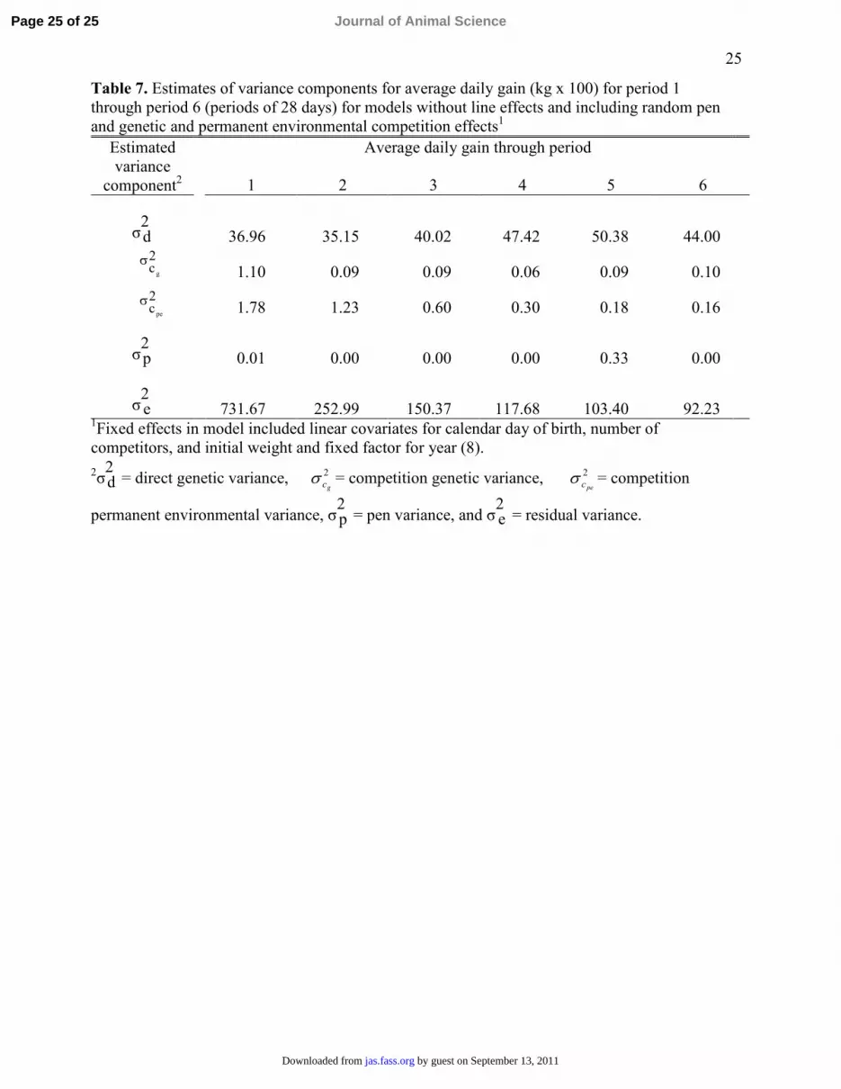
Summaries of estimates of variance components for ADG1 through ADG6 in Table 7 show that 317

the embedded genetic and environmental competition effects generally account for essentially all 318

of the variance of pen effects even though estimates of these variances are small after the first or 319

second period. 320

The estimates of variance components suggest that competition genetic and competition 321

environmental effects affected average daily gain for the first 28 days in the feedlot for these 322

Hereford bulls under the conditions of their feeding trials. Although an estimate of the fraction of 323

variance due to competition genetic effects is small, the index weights for an animal for direct 324

and competition genetic effects (estimated as d and c ) are 1 and n-1 where n is the number of 325

animals in a pen which make even a small fraction of variance important: 326

1 .ˆ ˆ( )I d n c= + −327

Thus, even with only a small variance associated with genetic competition effects, genetic 328

competition effects can be important economically. For example, from the estimates of variance 329




16

components for the full model in Table 6, then gd c36.96 6.08 and 1.10 1.05.σ σ= = = = If 330

gains for selection were one genetic standard deviation for both direct and competition genetic 331

values, then with 30 bulls per pen, the economic gain would be: ∆I = (6.08) + 29(1.05) = 6.08 + 332

30.45 with most of the gain from competition rather than direct genetic effects. Thus one 333

problem is how to decide how much emphasis to give to statistical significance of components of 334

variance (P < 0.05) and how much emphasis to give potential economic gain. With these data, 335

that question becomes less important because by the end of the fifth or sixth periods (or even the 336

second period; Models 5 and 6, Table 3) the standard deviation for genetic competition effects 337

for ADG becomes quite small. 338

In still another way, deciding which is the appropriate model with competition effects is 339

not entirely a statistical problem. If a model with competition effects and a model with pen 340

effects fit the data equally well as was the case for most time periods in this study, then 341

predictions of breeding value for the direct genetic effect may be equally accurate with both 342

models. But if competition effects exist and are to be selected for, then the question of which 343

model to use when statistical significance cannot be obtained is not easy to answer. A way to a 344

possible answer might be to obtain more data with a relationship structure that would allow 345

separation of competition and other pen effects (e.g., Van Vleck, 2005). Such data are not easy to 346

obtain and the pen structure and number of pen mates also need to be comparable for the 347

previous and future data. Arango et al. (2005) have discussed the problems with obtaining data 348

which might exhibit similar competition effects. 349

Although earlier simulation studies suggested models with pens as fixed effects would 350

reduce standard errors of estimates of competition variances, reexamination of those results and 351

results from these analyses show that when pens are treated as fixed effects, the direct and 352




17

competition variances and covariance cannot be separated. Whether this result is true for all 353

designs is not known. 354

355

LITERATURE CITED 356

Arango, J., I. Misztal, S. Tsuruta, M. Culbertson, and W. Herring. 2005. Estimation of variance 357

components including competitive effects of Large White growing gilts. J. Anim. Sci. 358

83:1241-1246. 359

Boldman, K. G., L. A. Kriese, L. D. Van Vleck, C. P. Van Tassell, and S. D. Kachman. 1995. A 360

manual for use of MTDFREML. A set of programs to obtain estimates of variance and 361

covariances [Draft]. USDA-ARS, Clay Center, NE. 120 pp. 362

Federer, W. T. 1955. Experimental design: Theory and application. The MacMillan Company, 363

New York. Chapter III. 364

Graser, H-U., S. P. Smith, and B. Tier. 1987. A derivative-free approach for estimating variance 365

components in animal models by restricted maximum likelihood. J. Anim. Sci. 64:1362-366

1370. 367

Griffing, B. 1967. Selection in reference to biological groups. I. Individual and group selection 368

applied to populations of unordered groups. Aust. J. Biol. Sci. 10:127-139. 369

Henderson, C. R. 1976. A simple method for computing the inverse of a numerator relationship 370

matrix used in prediction of breeding values. Biometrics 32:69-83. 371

Koch, R. M., L. V. Cundiff, and K. E. Gregory. 1974a. Selection in beef cattle. I. Selection 372

applied and generation interval. J. Anim. Sci. 39:449-458. 373

Koch, R. M., L. V. Cundiff, and K. E. Gregory. 1974b. Selection in beef cattle. II. Selection 374

response. J. Anim. Sci. 39:459-470. 375




18

Koch, R. M., L. V. Cundiff, and K. E. Gregory. 1994. Cumulative selection and genetic change 376

for weaning and yearling weight plus muscle score in Hereford cattle. J. Anim. Sci. 377

72:864-885. 378

Muir, W. M., and A. Schinckel. 2002. Incorporation of competitive effects in breeding programs 379

to improve productivity and animal well being. Proc. 7th World Congress Genetics 380

Applied Livestock Production. CD-ROM Communication n◦ 14-07. Montpellier, France. 381

Smith, S. P., and H-U. Graser. 1986. Estimating variance components in a class of mixed models 382

by restricted maximum likelihood. J. Dairy Sci. 69:1156-1165. 383

Van Vleck, L. D., and J. P. Cassady. 2004a. Modification of MTDFREML to estimate variance 384

due to genetic competition effects. J. Anim. Sci. 82(Suppl.2):38. (Abstr). 385

Van Vleck, L. D., and J. P. Cassady. 2004b. Unexpected estimates of variance components with 386

a true model containing genetic competition effects. J. Anim. Sci. 82(Suppl.1):84. 387

(Abstr). 388

Van Vleck, L. D., and J. P. Cassady. 2004c. Random models with direct and competition genetic 389

effects. Pages 17-30 in Proc. 16th Ann. Kansas State Univ. Conf. on Applied Statistics in 390

Agriculture. Manhattan, KS, April 25-27, 2004. 391

Van Vleck, L. D., and J. P. Cassady. 2005. Unexpected estimates of variance components with a 392

true model containing genetic competition effects. J. Anim. Sci. 83:68-74. 393

Van Vleck, L. D. 2005. Three designs for estimating variances due to competition genetic 394

effects. J. Anim. Sci. 83(Suppl.1):6. (Abstr).395




19

Table 1. Unadjusted means for initial weight (kg) and average daily gains (kg x 100) through Periods 1 through 8 by year of birth (1972-1979)

Average daily gain through period Year born No.1 Init. wt. 1 2 3 4 5 6 7 8

1972 245 221 32 92 86 85 91 82 87 87

1973 211 213 84 95 103 109 112 115 115 –

1974 235 172 94 90 79 87 85 91 90 94

1975 230 219 124 125 131 132 128 129 – –

1976 227 241 124 123 123 122 119 117 116 –

1977 254 230 111 95 103 105 109 109 109 –

1978 236 222 102 109 109 109 109 112 112 111

1979 244 220 130 113 118 116 116 112 113 110

Total no. 1882 1882 1876 1874 1867 1866 1864 1863 1634 946 1Number with an initial weight observation.




20

Table 2. Log likelihoods (-2 logL – 5,000) for 18 models for 9 traits (initial weight = 0; average daily gain through end of Periods 1, …, 8 after initial weight)MODEL1

Fixed Random Trait (inclusive period)I P D C R P 0 1 2 3 4 5 6 7 8

– – D – – – 9,362.78 9,552.75 7,724.90 6,831.32 6,442.63 6,253.61 6,040.23 4,713.93 512.61

– – D C – – 9,362.78 9,443.74 7,638.78 6,760.17 6,410.98 6,224.43 6,006.88 4,638.39 498.04

– – D C R – 9,360.04 9,442.68 7,635.70 6,758.46 6,410.20 6,222.83 6,005.55 4,636.17 496.19

– – D – – P 9,362.78 9,448.52 7,628.53 6,756.27 6,406.54 6,222.66 6,006.21 4,637.85 496.66

– – D C – P 9,362.78 9,443.68 7,628.53 6,756.27 6,406.49 6,222.04 6,005.21 4,636.47 496.56

– – D C R P 9,360.04 9,442.68 7,627.74 6,754.87 6,406.43 6,221.46 6,004.21 4,634.38 495.50

– P D – – – 9,107.52 9,097.48 7,333.63 6,491.06 6,167.91 5,990.64 5,779.27 4,415.05 377.41

– P D C – – 9,107.52 9,097.48 7,333.63 6,491.06 6,167.91 5,990.64 5,779.27 4,415.05 377.42

– P D C R – 9,107.52 9,097.48 7,333.63 6,491.06 6,167.91 5,990.64 5,779.27 4,415.05 377.41

I – D – – – – 9,519.92 7,654.93 6,768.12 6,392.97 6,215.93 5,997.36 4,675.80 487.96I – D C – – – 9,406.40 7,556.79 6,688.74 6,356.48 6,184.50 5,960.73 4,592.87 474.74I – D C R – – 9,404.88 7,552.97 6,686.66 6,355.82 6,182.83 5,959.41 4,590.27 472.80I – D – – P – 9,410.57 7,546.51 6,685.15 6,353.04 6,183.33 5,960.35 4,592.33 473.11I – D C – P – 9,406.25 7,546.51 6,684.48 6,352.75 6,182.42 5,959.09 4,590.82 473.03I – D C R P – 9,404.88 7,545.74 6,683.62 6,352.75 6,181.86 5,958.47 4,588.75 472.09

I P D – – – – 9,060.25 7,250.47 6,419.59 6,113.53 5,951.52 5,733.66 4,368.88 355.14I P D C – – – 9,060.25 7,250.47 6,419.60 6,113.53 5,951.52 5,733.65 4,368.88 355.02I P D C R – – 9,060.25 7,250.47 6,419.60 6,113.53 5,951.52 5,733.65 4,368.88 355.02

1Letter in column for model indicates effect was in the model, a "–" not in model; I = covariate for initial weight, fixed P = fixed pen effect, D = direct geneticeffect, C = competition genetic effect, R = covariance between D and C, random P = random pen effect.


by guest on September 13, 2011

jas.fass.orgD

ownloaded from


21

Table 3. Estimates of (co)variance components for six models1 for average daily gain (kg x 100) from initial weight through end of 1, 2, 3,…,7 periods of 28 days. The 8th period was usually less than 28 days Model Component2 1 2 3 4 5 6 7 8

1 σ2d 119.33 45.23 48.88 47.23 51.93 46.10 53.16 31.43

σ2e 749.24 276.36 160.06 126.03 108.72 97.25 93.89 93.31

2 σ2d 32.73 31.94 38.10 44.07 48.19 42.72 39.70 25.73

σ2c 2.67 1.29 0.62 0.32 0.24 0.22 0.48 0.21

σ2e 736.50 256.63 152.48 120.20 105.26 93.47 91.60 92.89

3 σ2d 48.28 43.57 41.23 44.79 47.81 42.35 42.49 28.17

σ2c 2.25 0.93 0.47 0.26 0.17 0.17 0.36 0.11

σdc 7.14 5.71 2.46 1.04 1.33 1.07 2.13 1.73

σ2e 735.00 256.51 153.72 121.27 107.21 95.21 92.63 93.86

4 σ2d 36.20 32.99 38.52 43.83 47.08 42.60 40.55 26.30

σ2p 103.56 36.48 19.84 10.04 8.38 7.90 15.71 6.87

σ2e 734.67 255.91 152.18 120.65 106.00 93.68 91.32 92.57

5 σ2d 33.67 33.36 38.76 43.78 47.40 42.41 40.21 26.16

σ2c 2.09 0.00 0.11 0.05 0.07 0.09 0.16 0.03

σ2p 18.05 36.43 15.51 8.53 5.58 4.60 10.10 5.87

σ2e 735.81 255.90 151.76 120.67 105.53 93.73 91.35 92.69

6 σ2d 47.85 35.39 39.98 43.74 47.66 42.02 41.98 27.13

σ2c 2.23 0.06 0.12 0.05 0.08 0.08 0.14 0.04

σdc 7.17 1.43 1.25 0.10 0.77 0.67 1.63 1.02

σ2p 0.02 31.77 13.26 8.39 4.13 3.69 7.85 3.80

σ2e 732.32 255.96 152.84 120.60 106.54 94.80 92.35 92.89

1Fixed effects of models also included linear covariates for calendar day of birth and number of competitors, selection line (4) and year of birth (8). 2σ

2d = direct genetic variance; σ

2c = competition genetic variance; σ

2p = pen variance; σ

2e = residual

variance; σdc = direct-competition genetic covariance.




22

Table 4. Estimates of (co)variance components from analyses of initial weight (kg) with nine models1

used for average daily gain

(Co)variance component2

Model2 σ2d σ

2c σdc σ

2p σ

2e -2logL

1 229.82 – – – 581.44 362.78

2 231.30 0.00 – – 580.78 362.78

3 279.65 0.06 -3.98 – 544.42 360.04

4 230.71 – – 0.00 580.50 362.78

5 230.14 0.00 – 0.00 580.98 362.78

6 269.38 0.04 -3.24 0.00 550.13 360.14

7 221.41 – – Fix 594.14 107.52

8 220.51 0.46 – Fix 594.58 107.52

9 203.95 3.53 -6.98 Fix 594.58 107.52 1Fixed effects part of model also included covariates for calendar day of birth and number of competitors, selection line (4) and year of birth (8). A numerical value indicates the effect was in the model and a dash indicates that the effect was not in model; Fixed = fixed pen effect . 2σ




2e = residual

variance; σdc = direct-competition genetic covariance and -2logL is minus twice the logarithm of the likelihood given the data – 14,000.




23

Table 5. Estimates of (co)variance components for models with and without line as a fixed factor for average daily gain (kg x 100) for Period 1 (Co)variance component2

Model1 σ2d σ

2c σdc σ

2p σ

2e -2logL

Without line in model

1 139.46 – – – 735.26 533.79

2 35.99 2.57 – – 734.64 421.71

3 48.55 2.14 6.74 – 733.97 420.10

4 53.36 – – 108.08 721.97 425.93

5 36.01 1.52 – 34.74 734.19 421.10

6 46.61 1.50 5.67 21.50 734.03 419.89

With line in model

7 119.33 – – – 749.24 519.92

8 32.73 2.67 – – 736.50 406.40

9 48.28 2.25 7.14 – 735.00 404.88

10 36.20 – – 103.56 734.67 410.57

11 33.67 2.09 – 18.05 735.81 406.25

12 47.85 2.23 7.17 0.02 735.32 404.881Fixed effects part of model also included covariates for date of birth, number of competitors, and initial weight and fixed factor for year of birth (8). A numerical value in a column indicates the effect was in the model and a dash indicates the effect was not in model. 2σ




2e =

residual variance; σdc = direct-competition genetic covariance and -2logL is minus twice the logarithm of the likelihood given the data – 14,000.




24

Table 6. Comparison of estimates of variance components for models1 without line effects for average daily gain in period 1(kg x 100) including models with and without competition permanent environmental effects

Estimate of variance component2

Model1 σ2d

σg

2c σ

pc

2c σ

2p σ

2e -2logL

1 36.96 1.10 1.78 0.01 731.67 420.23

2 54.24 – 3.77 0.04 716.68 423.92

3 37.10 1.11 1.77 – 731.75 420.23

4 53.94 – 3.78 – 716.31 423.92

5 35.99 2.57 – – 734.64 421.71

6 53.36 – – 108.08 721.97 425.93

7 36.01 1.52 – 34.74 734.19 421.101Fixed effects for all models included linear covariates for date of birth, number of competitors, and initial weight and a fixed factor for year of birth (8). A dash (–) in estimate of variance component column indicates that effect was not in the model. 2σ

2d = direct genetic variance, 2

cgσ = competition genetic variance, 2

cpeσ = competition permanent

environmental variance, σ2p = pen variance, and σ

2e = residual variance; -2logL is minus twice the

logarithm of the likelihood given the data – 14,000.




25

2cpe

σ

2cg

σ

Table 7. Estimates of variance components for average daily gain (kg x 100) for period 1 through period 6 (periods of 28 days) for models without line effects and including random pen and genetic and permanent environmental competition effects1

Average daily gain through period Estimated variance

component2 1 2 3 4 5 6

σ2d 36.96 35.15 40.02 47.42 50.38 44.00

1.10 0.09 0.09 0.06 0.09 0.10

1.78 1.23 0.60 0.30 0.18 0.16

σ2p 0.01 0.00 0.00 0.00 0.33 0.00

σ2e 731.67 252.99 150.37 117.68 103.40 92.23

1Fixed effects in model included linear covariates for calendar day of birth, number of competitors, and initial weight and fixed factor for year (8). 2σ

2d = direct genetic variance, 2

gcσ = competition genetic variance, 2pecσ = competition

permanent environmental variance, σ2p = pen variance, and σ

2e = residual variance.




Citations

ticleshttp://jas.fass.org/content/early/2007/03/19/jas.2007-0067.citation#otherarThis article has been cited by 4 HighWire-hosted articles:



effect of competition on gain in feedlot bulls from hereford selection lines

Documents