Ea

MDLSJIa

b

c

d

e

f

g

h

i

Fj

k

l

m

n

Co

p

q

r

Us

t

u

v

w

x

y

z

A

B

C

D

E

F

G

H

I

J

F

h1

Ecological Indicators 60 (2016) 947–962

Contents lists available at ScienceDirect

Ecological Indicators

j o ur na l ho me page: www.elsev ier .com/ locate /eco l ind

cological indicators to capture the effects of fishing on biodiversitynd conservation status of marine ecosystems

. Coll a,b,∗, L.J. Shannonc, K.M. Kleisnerd, M.J. Juan-Jordáe,f, A. Bundyg, A.G. Akogluh,. Banarui, J.L. Boldt j, M.F. Borgesk, A. Cookg, I. Diallo l, C. Fuj, C. Foxm, D. Gascueln,.J. Gurneyo, T. Hattabp, J.J. Heymansm, D. Jouffreq,r, B.R. Knights, S. Kucukavsarh,.I. Larged, C. Lynamt, A. Machiasu, K.N. Marshall v, H. Masskiw, H. Ojaveerx, C. Piroddib,y,. Tamz, D. ThiaoA, M. ThiawB, M.A. TorresC,D, M. Travers-TroletE, K. Tsagarakisu,. TuckF,G, G.I. van der MeerenH, D. Yemanec,I, S.G. Zador J, Y.-J. Shina,c

Institut de Recherche pour le Développement, CRH, Research Unit MARBEC (UMR 248), avenue Jean Monnet, CS 30171, 34203 Sète Cedex, FranceInstitute of Marine Science (ICM-CSIC), passeig Marítim de la Barceloneta, n◦ 37-49, 08003 Barcelona, SpainMarine Research Institute and Department of Biological Sciences, University of Cape Town, Private Bag X3, Rondebosch, Cape Town 7701, South AfricaNortheast Fisheries Science Center, National Marine Fisheries Service, NOAA, 166 Water Street, Woods Hole, MA 02543, USAAZTI, Marine Research Division, Herrera Kaia, Portualdea z/g, 20110 Pasaia, Gipuzkoa, SpainEarth to Ocean Research Group, Department of Biological Sciences, Simon Fraser University, 8888 University Drive, Burnaby, BC V5A 1S6, CanadaFisheries and Oceans Canada, Bedford Institute of Oceanography, 1 Challenger Drive, Dartmouth, NS B2Y 4A2, CanadaMiddle East Technical University, Institute of Marine Sciences, P.O. Box 28, 33731 Erdemli, Mersin, TurkeyAix-Marseille Université, Mediterranean Institute of Oceanography (M.I.O), UMR 7294, UR 235, Campus de Luminy, Case 901, 13288 Marseille Cedex 09,ranceFisheries and Oceans Canada, Pacific Biological Station, 3190 Hammond Bay Road, Nanaimo, BC V9T 6N7, CanadaInstituto Português do Mar e da Atmosfera, Av. de Brasília, 1449-006 Lisboa, PortugalCentre National des Sciences Halieutiques de Boussoura (CNSHB), 814 Rue MA500, Corniche sud Boussoura, BP 3738, Conakry, GuineaScottish Association for Marine Science, Scottish Marine Institute, Oban, Argyll PA37 1QA, UKUniversité Européenne de Bretagne, Agrocampus Ouest, UMR985 Ecologie et santé des écosystèmes, 65 route de Saint Brieuc, CS 84215, 35042 Rennesedex, FranceDepartment of Earth, Ocean and Atmospheric Sciences, 2207 Main Mall, University of British Columbia, V6T 1Z4 BC, CanadaJules Verne University of Picardie, Research Unit EDYSAN, FRE 3498 CNRS, 1 rue des Louvels, F-80037 Amiens Cedex 1, FranceInstitut de Recherche pour le Développement, Research Unit MARBEC, BP 1386, Dakar, SenegalLaboratoire de Biologie et d’Ecologie des Poissons en Afrique de l’Ouest (LABEP-AO, IRD/IFAN), Institut Fondamental d’Afrique Noire, Campus universitaireCAD, B.P. 206, Dakar, SenegalCawthron Institute, 98 Halifax Street East, Nelson 7010, New ZealandCentre for Environment, Fisheries and Aquaculture Science, Pakefield Road, Lowestoft, Suffolk NR33 0HT, UKHellenic Centre for Marine Research, Institute of Marine Biological Resources and Inland Waters, Agios Kosmas, 16610 Elliniko, Athens, GreeceSchool of Aquatic and Fishery Sciences, University of Washington, Box 355020, Seattle, WA 98195, USAInstitut National de Recherche halieutique, Bd Sidi Abderrahmane, Casablanca, MoroccoEstonian Marine Institute, University of Tartu, Lootsi 2a, 80012 Pärnu, EstoniaWater Resources Unit, Institute for Environment and Sustainability, Joint Research Centre, Via E. Fermi 2749, Ispra (VA) 21027, ItalyInstituto del Mar del Perú (IMARPE), Esquina Gamarra y Gral, Valle s/n, Apartado 22, Callao, Lima, PeruISRA/Centre de Recherches Océanographiques de Dakar-Thiaroye (CRODT), BP 2241, Dakar, SenegalLaboratoire d’Ecologie Halieutique-Afrique de l’Ouest (LEH-AO), ISRA/CRODT, Pôle de Recherche de Hann, BP 2241, Dakar, SenegalInstituto Espanol de Oceanografía (IEO), Centro Oceanográfico de Cádiz, Puerto Pesquero, Muelle de Levante, s/n, P.O. Box 2609, E-11006 Cádiz, SpainSwedish University of Agricultural Sciences, Department of Aquatic Resources, Institute of Coastal Research, Skolgatan 6, SE-742 42 Öregrund, Sweden

IFREMER, Fisheries Laboratory, 150 quai Gambetta, BP 699, 62321 Boulogne sur mer, FranceNational Institute of Water and Atmospheric Research Limited, Auckland, New ZealandDepartment of Statistics, University of Auckland, Private Bag 92019, Auckland 1149, New ZealandInstitute of Marine Research, The Hjort Centre for Marine Ecosystem Dynamics, PB 1870, Nordnes, NO-5817 Bergen, Norway

Fisheries Branch, Department of Agriculture, Forestry, and Fisheries, Private Bag X2, Rogge Bay, 8012 Cape Town, South Africa

Alaska Fisheries Science Center, National Marine Fisheries Service, NOAA, Seattle, WA 98115, USA

∗ Corresponding author at: Institut de Recherche pour le Développement, CRH, Research Unit MARBEC (UMR 248), avenue Jean Monnet, CS 30171, 34203 Sète Cedex,rance. Tel.: +33 0499573216.

E-mail address: marta.coll@ird.fr (M. Coll).

ttp://dx.doi.org/10.1016/j.ecolind.2015.08.048470-160X/© 2015 Elsevier Ltd. All rights reserved.

9

a

ARRA

KEMBRTSFC

1

umbt2fgts

dumIasehte2

ebpeotepiae

48 M. Coll et al. / Ecological Indicators 60 (2016) 947–962

r t i c l e i n f o

rticle history:eceived 15 April 2015eceived in revised form 17 August 2015ccepted 27 August 2015

eywords:cological indicatorsarine ecosystems

iodiversityedundancyrendstatesishing impactsonservation

a b s t r a c t

IndiSeas (“Indicators for the Seas”) is a collaborative international working group that was established in2005 to evaluate the status of exploited marine ecosystems using a suite of indicators in a comparativeframework. An initial shortlist of seven ecological indicators was selected to quantify the effects of fishingon the broader ecosystem using several criteria (i.e., ecological meaning, sensitivity to fishing, data avail-ability, management objectives and public awareness). The suite comprised: (i) the inverse coefficientof variation of total biomass of surveyed species, (ii) mean fish length in the surveyed community, (iii)mean maximum life span of surveyed fish species, (iv) proportion of predatory fish in the surveyed com-munity, (v) proportion of under and moderately exploited stocks, (vi) total biomass of surveyed species,and (vii) mean trophic level of the landed catch. In line with the Nagoya Strategic Plan of the Conven-tion on Biological Diversity (2011–2020), we extended this suite to emphasize the broader biodiversityand conservation risks in exploited marine ecosystems. We selected a subset of indicators from a list ofempirically based candidate biodiversity indicators initially established based on ecological significanceto complement the original IndiSeas indicators. The additional selected indicators were: (viii) mean intrin-sic vulnerability index of the fish landed catch, (ix) proportion of non-declining exploited species in thesurveyed community, (x) catch-based marine trophic index, and (xi) mean trophic level of the surveyedcommunity. Despite the lack of data in some ecosystems, we also selected (xii) mean trophic level ofthe modelled community, and (xiii) proportion of discards in the fishery as extra indicators. These addi-tional indicators were examined, along with the initial set of IndiSeas ecological indicators, to evaluatewhether adding new biodiversity indicators provided useful additional information to refine our under-standing of the status evaluation of 29 exploited marine ecosystems. We used state and trend analyses,and we performed correlation, redundancy and multivariate tests. Existing developments in ecosystem-based fisheries management have largely focused on exploited species. Our study, using mostly fisheriesindependent survey-based indicators, highlights that biodiversity and conservation-based indicatorsare complementary to ecological indicators of fishing pressure. Thus, they should be used to provideadditional information to evaluate the overall impact of fishing on exploited marine ecosystems.

© 2015 Elsevier Ltd. All rights reserved.

. Introduction

Changes in marine resources and ecosystems have been doc-mented worldwide (Butchart et al., 2010; Lotze et al., 2006) andultiple anthropogenic and climate-related drivers of change have

een identified (Halpern et al., 2008). These drivers can alter ecosys-em structure and functioning (Christensen et al., 2003; Frank et al.,005) and can affect the ecosystem services that humans obtainrom healthy oceans (Worm et al., 2006). Consequently there isrowing concern about the status of marine ecosystems and a needo define, test and prioritize robust indicators to track ecosystemtatus to inform management decisions.

In the marine science research field, there has been considerableiscussion about how to define, calculate, prioritize, test and eval-ate indicators to monitor the pressures on, and status of exploitedarine ecosystems (e.g., Rombouts et al., 2013; Shin et al., 2010a).

nitially, indicators were developed to include ecological consider-tions with the goal of capturing the impact of dominant pressures,uch as fishing or eutrophication (Cury et al., 2005; de Leiva Morenot al., 2000). However, recently the scope of ecosystem indicatorsas expanded to include socio-economic and governance issues andhe cumulative impacts of multiple human activities (e.g., Boldtt al., 2014; Halpern et al., 2012; Large et al., 2015; Levin et al.,009; Tittensor et al., 2014).

Fishing represents one of the greatest pressures on marinecosystems (Costello et al., 2010), and ecological indicators haveeen used to quantify its impacts on the status of ecosystems and torovide the rationale for scientific advice. Progress has included thestablishment of criteria and frameworks to: (i) guide the selectionf indicators (e.g., Rice and Rochet, 2005) that are used to assesshe effects of fishing via trend (e.g., Blanchard et al., 2010; Collt al., 2010b) and threshold (Large et al., 2013) analyses, (ii) define

In 2005, the IndiSeas (“Indicators for the Seas”) Working Groupwas initiated under the auspices of the European Network of Excel-lence, Eur-Oceans. IndiSeas followed from the Scientific Committeeon Oceanic Research of the Intergovernmental OceanographicCommission (SCOR/IOC) Working Group on “Quantitative Ecosys-tem Indicators” (Shin and Shannon, 2010; Shin et al., 2010b, www.indiseas.org). During the first phase of IndiSeas (2005–2010, here-after IndiSeas-phase I), the goals were to perform analyses ofecological indicators to quantify the impact of fishing on the sta-tus of exploited marine ecosystems in a comparative frameworkand to provide decision support criteria for an Ecosystem Approachto Fisheries (EAF) by means of a common suite of interpretationand visualization methods. The rationale was that, although thecurrent primary objective of fisheries management is to ensure sus-tainable levels of harvest for commercial stocks, the incorporationof broader ecosystem considerations into managing fisheries hasbecome an increasingly important obligation in many countries andregions throughout the world (e.g., Link, 2002; Murawski, 2000;Pikitch et al., 2004; Walters et al., 2005).

Thus, in IndiSeas-phase I, a suite of empirical ecological indi-cators was selected using several criteria (ecological meaning,sensitivity to fishing, data availability, management objectivesand public awareness), to create a shortlist of indicators thatwere easy to calculate from landings and surveys data and thatwere meaningful and comparable across many marine ecosystemsworldwide (Shin et al., 2012). These indicators were: (i) the inversecoefficient of variation of total biomass in the surveyed community(also referred to “Biomass Stability”, or BS), (ii) mean fish lengthin the surveyed community (“Fish Size”, LG), (iii) mean maximumlife span of surveyed fish species (“Life Span”, LS), (iv) proportionof predatory fish in the surveyed community (“Predators”, PF), (v)proportion of under and moderately exploited stocks (“Sustainable

reliminary reference levels and reference directions for selectedndicators (e.g., Link et al., 2002; Shin et al., 2010a), and (iii) developnd test evaluation frameworks (e.g., Bundy et al., 2010; Kleisnert al., 2013).

Stocks”, SS), (vi) total biomass of surveyed species (“Biomass”,

TB), and (vii) mean trophic level of the landed catch (“TrophicLevel”, TLc) (Table 1). All the indicators are survey-based with theexception of SS and TLc. In previous studies these indicators were

M. Coll et al. / Ecological Indicators 60 (2016) 947–962 949

Table 1IndiSeas-phase I ecological indicators used to track the impacts of fishing on exploited marine ecosystems and IndiSeas-phase II new ecological indicators used to track thebroader impacts of fishing on exploited marine ecosystems in relation to biodiversity and conservation-based issues (see Table S1 for details).

IndiSeas indicators Label Acronym Used for stateor trend

Survey (S), catch (C)or model based (M)

Phase I1 1/coefficient of variation of total biomass of surveyed species Biomass stability BS S S2 Mean fish length in the surveyed community Fish size LG S, T S3 Mean maximum life span of surveyed fish species Life span LS S, T S4 Proportion of predatory fish in the surveyed community Predators PF S, T S5 Proportion of under and moderately exploited stocks Sustainable stocks SS S C6 Total biomass of surveyed species Biomass TB T S7 Mean trophic level of the landed catch Trophic level TLc S, T C

Phase II1 Mean intrinsic vulnerability index of the fish landed catch Mean vulnerability IVI T C2 Proportion of non-declining exploited species Non-declining species NDES S S3 Catch-based marine trophic index Trophic index MTI S, T C4 Mean trophic level of the surveyed community Trophic level of the community TLsc S, T S

levelgs/Dis

ctCtpe

oitaoefhfP2absebie“

crstctwecoetcopit

o

5 Mean trophic level of the modelled community Trophic6 Proportion of discards in the fishery Landin

alculated for 19 exploited marine ecosystems, which includedemperate, tropical, upwelling, and high latitude ecosystems.omparative analyses of these indicators provided insights onhe relative states and trends of these ecosystems given fishingressures exerted upon them (e.g., Blanchard et al., 2010; Bundyt al., 2010; Coll et al., 2010b; Link et al., 2010; Shin et al., 2010a).

These comparative studies elucidated the need to expand the listf IndiSeas-phase I indicators to cover additional dimensions of thempacts of fishing, such as socioeconomic and governance interac-ions, to include the effects of a variable and changing environment,nd to emphasize the broader biodiversity and conservation risksf fishing when evaluating the status of marine ecosystems (Bundyt al., 2012; Shin et al., 2012). Socioeconomic and environmentalactors are addressed in the second phase of IndiSeas (2010–2014,ereafter IndiSeas-phase II), endorsed by IOC/UNESCO. Here we

ocus on the scientific challenges posed by the Nagoya Strategiclan of the Convention on Biological Diversity (2011–2020) (CBD,010) by emphasizing and testing the utility of key biodiversitynd conservation-based indicators while accounting for trade-offsetween different societal goals (e.g. conservation of biodiversity;ustainable exploitation) incurred in the management of marinecosystems (Brander, 2010; Palumbi et al., 2008). Some of theseiodiversity and conservation-based indicators can help illustrate

mportant conservation implications and can contribute to thevaluation of progress towards achieving the biodiversity-relatedAichi Targets” (Tittensor et al., 2014).

Here we first present the additional suite of biodiversity andonservation-based indicators studied in IndiSeas-phase II and theationale underlying their inclusion. Next, we examine the wholeuite of indicators across 29 exploited marine ecosystems dis-ributed worldwide and assess whether any of the indicators areorrelated and potentially redundant. We then use a compara-ive approach to evaluate the status of these ecosystems using thehole suite of indicators. Considering the complexity of marine

cosystems, the scale and scope of change manifested and the diffi-ulty of undertaking controlled experiments, comparative analysisf ecosystems is expected to provide insight on how drivers influ-nces dynamics of ecosystems (Murawski et al., 2009). In our case,his allows us to assess whether the additional biodiversity andonservation-based indicators provide new insights on the statusf exploited marine ecosystems. Finally, we test whether fishingressure is correlated with changes observed in our suite of ecolog-

cal indicators by investigating the relationship between indicatorrends and three measures of fishing pressure.

Our overall objective is to present a comprehensive suitef ecological indicators with the greatest potential to capture

of the model TLmc S, T Mcards D S, T C

broad biodiversity and conservation considerations of fishing onexploited marine ecosystems. Based on the examination of thesuite of ecological indicators for several ecosystems, we discussthe best subset of indicators that would complement the previ-ously selected ecological indicators of IndiSeas-phase I. In addition,we contribute to the evaluation of the status of exploited ecosys-tems, which is necessary for balancing conservation and fishingobjectives in marine ecosystems.

2. Material and methods

2.1. Case studies

Our analyses used 29 exploited marine ecosystems as casestudies (Fig. 1 and Table 2). They correspond to upwelling, highlatitude, temperate and tropical marine ecosystems, and cover arange of low to high productivity areas, located in the Atlantic andPacific Oceans, and the Mediterranean, Black and Baltic Seas. A keystrength of the IndiSeas approach lies in the participation of ecosys-tem experts who provide local data and specific, local interpretationof the indicators and who can inform comparisons and analyses ofany biases in data collection or generation of indicator results (Shinet al., 2010b, 2012). This study takes full advantage of these exper-tise and ecosystem experts provided insights to interpret indicatorscores.

2.2. Selection of biodiversity and conservation-based indicators

We used a step-by-step process to select indicators, as done inIndiSeas-phase I (Shin and Shannon, 2010; Shin et al., 2010b), toaugment the original indicators suite with additional biodiversityand conservation-based metrics that would capture the broadereffects of fishing on marine biodiversity and ecosystem function-ing (Table 1 and Table S1). The selection process included thefollowing steps: (i) potential indicators were identified by review-ing the scientific literature, (ii) indicators were evaluated with thescreening criteria, and (iii) a suite of potential biodiversity-andconservation-based ecological indicators was proposed for exami-nation in a subset of comparable ecosystem case studies. First, a listof potential indicators was identified from the scientific literaturefor consideration with no restriction on the number of indicators.

These indicators were subjected to screening criteria by experts sothat each candidate indicator was scored by local experts for 20 dif-ferent ecosystems, and scores were averaged per criteria for eachindicator (Table S2). Screening criteria comprised data availability,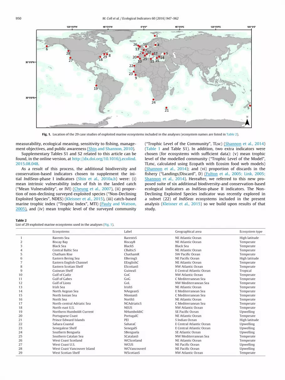

950 M. Coll et al. / Ecological Indicators 60 (2016) 947–962

tems

mm

f2

ctm(tEm2

TL

Fig. 1. Location of the 29 case studies of exploited marine ecosys

easurability, ecological meaning, sensitivity to fishing, manage-ent objectives, and public awareness (Shin and Shannon, 2010).Supplementary Tables S1 and S2 related to this article can be

ound, in the online version, at http://dx.doi.org/10.1016/j.ecolind.015.08.048.

As a result of this process, the additional biodiversity andonservation-based indicators chosen to supplement the ini-ial IndiSeas-phase I indicators (Shin et al., 2010a,b) were: (i)

ean intrinsic vulnerability index of fish in the landed catch“Mean Vulnerability”, or IVI) (Cheung et al., 2007), (ii) propor-

ion of non-declining surveyed exploited species (“Non-Decliningxploited Species”, NDES) (Kleisner et al., 2015), (iii) catch-basedarine trophic index (“Trophic Index”, MTI) (Pauly and Watson,

005), and (iv) mean trophic level of the surveyed community

able 2ist of 29 exploited marine ecosystems used in the analyses (Fig. 1).

Ecosystems Label

1 Barents Sea BarentsS

2 Biscay Bay BiscayB

3 Black Sea BlackS

4 Central Baltic Sea CBalticS

5 Chatham Rise ChathamR

6 Eastern Bering Sea EBeringS

7 Eastern English Channel EEnglishC

8 Eastern Scotian Shelf EScotianS

9 Guinean Shelf GuineaS

10 Gulf of Cadiz GoC

11 Gulf of Gabes GoG

12 Gulf of Lions GoL

13 Irish Sea IrishS

14 North Aegean Sea NAegeanS

15 North Ionian Sea NIonianS

16 North Sea NorthS

17 North-central Adriatic Sea NCAdriaticS

18 North-east U.S. NEUS

19 Northern Humboldt Current NHumboldtC

20 Portuguese Coast PortugalC

21 Prince Edward Islands PEI

22 Sahara Coastal SaharaC

23 Senegalese Shelf SenegalS

24 Southern Benguela SBenguela

25 Southern Catalan Sea SCatalanS

26 West Coast Scotland WCScotland

27 West Coast U.S. WCUS

28 West Coast Vancouver Island WCVancouver29 West Scotian Shelf WScotianS

included in the analyses (ecosystem names are listed in Table 2).

(“Trophic Level of the Community”, TLsc) (Shannon et al., 2014)(Table 1 and Table S1). In addition, two extra indicators werechosen (for ecosystems with sufficient data): (v) mean trophiclevel of the modelled community (“Trophic Level of the Model”,TLmc, calculated using Ecopath with Ecosim food web models)(Shannon et al., 2014); and (vi) proportion of discards in thefishery (“Landings/Discard”, D) (Fulton et al., 2005; Link, 2005;Shannon et al., 2014). Hereafter, we referred to this new pro-posed suite of six additional biodiversity-and conservation-basedecological indicators as IndiSeas-phase II indicators. The Non-

Declining Exploited Species indicator was recently explored ina subset (22) of IndiSeas ecosystems included in the presentanalysis (Kleisner et al., 2015) so we build upon results of thatstudy.

Geographical area Ecosystem type

NE Atlantic Ocean High latitudeNE Atlantic Ocean TemperateBlack Sea TemperateNE Atlantic Ocean TemperateSW Pacific Ocean TemperateNE Pacific Ocean High latitudeNE Atlantic Ocean TemperateNW Atlantic Ocean TemperateE Central Atlantic Ocean TropicalNW Atlantic Ocean TemperateC Mediterranean Sea TemperateNW Mediterranean Sea TemperateNE Atlantic Ocean TemperateE Mediterranean Sea TemperateC Mediterranean Sea TemperateNE Atlantic Ocean TemperateC Mediterranean Sea TemperateNW Atlantic Ocean TemperateSE Pacific Ocean UpwellingNE Atlantic Ocean TemperateS Indian Ocean High latitudeE Central Atlantic Ocean UpwellingE Central Atlantic Ocean UpwellingSE Atlantic Ocean UpwellingNW Mediterranean Sea TemperateNE Atlantic Ocean TemperateNE Pacific Ocean Upwelling

I NE Pacific Ocean UpwellingNW Atlantic Ocean Temperate

Indica

iotIa

2

taotctc

2

mtsubf

o(ooaatistlisst

(

es(ectss

tacacts

awa

M. Coll et al. / Ecological

All indicators were formulated so that a decrease in their values expected with greater fishing pressure. Thus, the lowest valuef the indicator, or a decrease of the indicator with time, wouldheoretically indicate a higher impact of fishing on the ecosystem.ndicators were used to represent the current state of the ecosystemnd/or trend over time (Table 1).

.3. Analyses of indicators

Indicators were calculated for the 29 exploited marine ecosys-ems included in this analysis (Table 2 and Fig. 1) using landingsnd survey data provided by local experts. Using the whole suitef indicators, we derived common metrics: (i) the current state ofhe indicators, and (ii) the overall trends of the indicators. Theseommon metrics were used to evaluate whether any of the indica-ors were correlated and potentially redundant, and to conduct aomparative study across marine ecosystems.

.3.1. Analyses of current states and overall trendsWe calculated the current state indicators as the mean of the

ost recent five years for which data were available (for most sys-ems this was 2005–2010) to provide a measure of the currenttate of the ecosystem. State indicator patterns were visualizedsing heat maps and petal plots, where values were standardizedetween 0 and 1, based on the minimum and maximum valuesound across all ecosystems.

We examined trends in indicators for years during 1980–2010,r for the years within this period for which data were availableFigure S7). We used two methods to quantify the overall directionf change for each indicator. The first method assumed linearityver time, using a generalized linear model and accounting forutocorrelation, where present, to fit a trend. The second methodllowed for the possibility of non-linearity over time and measuredhe overall trend based on the average rate of change across all yearsncluded (i.e., rate of increase or decrease between multiple con-ecutive years). Since indicator series differed in time coverage andime span due to data availability, only indicator series having ateast two consecutive years within a time series of data were usedn this analysis. Trend indicators were visualized using heat maps oflopes and average rates of change if the trends over time and theirignificance where values were scaled between 0 and 1, based onhe minimum and maximum values found across all ecosystems.

All state and trend analyses were conducted in R version 3.0.2R Core Team 2013).

(i) Analysis of trends assuming linearity over time: We fit a gen-ralized least-squares regression model to each indicator timeeries, first testing and correcting for autocorrelation where presentfollowing Blanchard et al., 2010; Coll et al., 2008). Trends werestimated using time series of normalized indicator values to allowomparison of trends (Blanchard et al., 2010), standardized by sub-racting the mean and dividing by the standard deviation. Thistandardization allows the indicators to be expressed on the samecale and with the same spread.

A two-stage estimation procedure was used to take into accountemporal autocorrelation in the residuals and to satisfy regressionssumptions (Coll et al., 2008). This procedure was generally suffi-ient for trend estimation as the time-series were relatively shortnd there was considerable flexibility in realizations of the auto-orrelated errors. We assessed the significance of the estimatedrend (p-value), the direction of the trend (positive or negativelope) and the magnitude of the slope.

(ii) Analysis of trends allowing for non-linearity over time: Tollow for the possibility of non-linearity over time in the indicators,e used a two-step estimation procedure to calculate the average

nnual rate of change for each indicator across all the years. First,

tors 60 (2016) 947–962 951

we converted the raw time series of each indicator to successiveannual rates of change (ri) (Juan-Jordá et al., 2011):

ri = ln ·(

Ii+1

Ii

)(1)

where Ii is the indicator value in time i and Ii+1 is the value of theindicator a year later (i + 1).

This method of estimating the ratios in log-scale enables theindicators to be expressed on the same scale, thus rendering themunitless. This is a common means of removing temporal autocorre-lation from a time series (Shumway and Stoffer, 2006). Therefore,unlike the first method, the indicators were not standardized forspread, but have equivalent units.

We then estimated the average of the annual rates of changeacross all the successive years for each indicator to obtain a metricof the overall rate of change of each indicator using the followingmodel form:

ri = ˇo + ei (2)

where ri, the dependent variable, is the successive annual (i) rateof change between two consecutive years in each indicator; ˇo,the model intercept, is the model average annual rate of change ineach indicator across all the years, and ei is the normally distributedresidual error. We assessed the significance of ˇo, the model aver-age annual rate of change across all the years (p-value), the directionof the rate of change (positive or negative) and the magnitude ofthe rate of change.

2.3.2. Complementarity and redundancy analysesWe performed separate analyses to test for correlation across

state and trend indicators among all ecosystems in order to iden-tify complementarity and redundancy in the indicators selected. Allcorrelations were evaluated using the Spearman’s non-parametricrank order correlation coefficient, which is a measure of statisti-cal dependence between two variables, ranging between −1 and1, i.e., perfect negative and positive correlation, respectively. Thistest assesses how well the relationship between two variablescan be described using a non-linear monotonic function. More-over, correlation coefficients among trends were summarized asa matrix of positive or negative correlations between indicators forall ecosystems to quantify the proportion of trends with a signifi-cant change and assess the overall redundancy. These correlationanalyses allowed us to evaluate the suitability of our suite of indica-tors to track the different ecosystem effects of fishing and whetherwe need to retain the full suite for further analyses. These analyseswere performed using R version 3.0.2 (R Core Team 2013).

2.3.3. Comparative approach to diagnose the exploitation statusof marine ecosystems

The current state and the magnitude, direction, and significanceof the trends of each indicator were used to compare the 29 casestudy ecosystems following a similar methodology to that in a pre-vious comparative analysis, which ranked ecosystems in terms oftheir exploitation level (Coll et al., 2010b; Shannon et al., 2009).

We first used the heat maps and petal plots to compare the cur-rent state of each indicator across all the ecosystems. We then usedheat maps to compare trends, including magnitude, direction andsignificance of trends of each indicator across all the ecosystems.Subsequently, we used non-parametric multivariate analyses (clus-ter analysis and non-metric MultiDimensional Scaling, nMDS) toperform a synthetic comparison of all ecosystems based on theirsimilarity. These analyses were performed using IndiSeas-phase

I indicators and then the whole suite of indicators so additionalinformation on ecosystem status from IndiSeas II indicators couldbe assessed. We evaluated the suitability of the suite of indicatorsand whether it was necessary to retain the full suite for further

9 Indica

avuo

2

cogiiIseamuaapipC

f2

3

3

aSieeottCCeeteiFpethTci

f2

tSieB

52 M. Coll et al. / Ecological

nalyses. All multivariate analyses were performed with PRIMER6 (Clarke and Gorley, 2006). Because the indicators have differentnits and scales, we normalized the data prior to the constructionf the Euclidean distance matrices (Clarke and Gorley, 2006).

.3.4. Correlation analyses with fishing pressureUsing Spearman’s non-parametric rank correlations, we cross-

orrelated time series of fishing pressure indicators and our suitef ecological indicators used for of trend analyses. First, we investi-ated the relationship between the trends in the suite of ecologicalndicators and a global fishing pressure indicator (the ratio of land-ngs to survey biomass, L/B). This indicator had been selected inndiSeas-phase I as it was simple and most readily available pres-ure indicator across the ecosystems examined at that time (Shint al., 2010b) (Figure S1). In IndiSeas-phase II, relative fishing effortnd relative fishing mortality were also available for a subset of ninearine ecosystems (Shannon et al., 2014, Figure S2). Therefore, we

sed a non-weighted mean of the relative fishing effort across fleetsnd species and a non-weighted mean of the fishing mortality ratecross species in order to test the correlations between our suite ofressure indicators of fishing pressure and our suite of ecological

ndicators. All correlations were evaluated using Spearman’s non-arametric rank order correlation coefficient in R version 3.0.2 (Rore Team 2013).

Supplementary Figures S1 and S2 related to this article can beound, in the online version, at http://dx.doi.org/10.1016/j.ecolind.015.08.048.

. Results

.1. State indicators

The current state (2005–2010) of IndiSeas-phase I indicatorscross all the ecosystems varied greatly (Fig. 2 and Figures S3 and4). The scores of most of the indicators were relatively low (morendicators showing values <0.5). For 19 ecosystems (66% of thecosystems): the Bay of Biscay, the central Baltic Sea, the east-rn English Channel, the Guinean Shelf, the Gulf of Cadiz, the Gulff Gabes, the Gulf of Lions, the Irish Sea, the north Aegean Sea,he north Ionian Sea, the North Sea, the north-central Adriatic Sea,he northern Humboldt Current, the Portuguese Coast, the Saharaoastal, the Senegalese Shelf, the southern Benguela, the southernatalan Sea, the western Scotian Shelf, suggesting a more impactedcosystem state on average compared to other ecosystems. In twocosystems (7%), the scores for most of the indicators were rela-ively high (more indicators showed values higher than 0.5): theastern Bering Sea and the west Coast Vancouver Island, suggest-ng these ecosystems have a less impacted ecosystem state overall.or 7 ecosystems (24%), the current state of the indicators varied,roducing a mixed signal: the Barents Sea, the Chatham Rise, theastern Scotian Shelf, the northeast U.S., the Prince Edward Islands,he west Coast Scotland and the western Coast U.S. The Black Seaad data available for only one indicator (TLc) in the recent years.he Prince Edward Islands lacked data for four of the six state indi-ators and nine ecosystems were missing data for the Fish Size (LG)ndicator (Fig. 2).

Supplementary Figures S3 and S4 related to this article can beound, in the online version, at http://dx.doi.org/10.1016/j.ecolind.015.08.048.

The current state (2005–2010) in the IndiSeas-phase II indica-ors across all the ecosystems also varied greatly (Fig. 2 and Figures

5 and S6). In eight ecosystems (28%) the scores of most of thendicators were relatively low (<0.5) suggesting a more impactedcosystem state on average compared to the other ecosystems: thelack Sea, the Gulf of Cadiz, the north Aegean Sea, the north Ionian

tors 60 (2016) 947–962

Sea, the north-central Adriatic Sea, the northern Humboldt Current,the Senegalese shelf and the southern Catalan Sea. In 13 ecosys-tems (45%) the scores for most of the indicators were relatively high(>0.5), suggesting these ecosystems have a less impacted ecosys-tem state: the Barents Sea, the Bay of Biscay, the Chatham Rise,the eastern Bering Sea, the eastern English Channel, the easternScotian Shelf, the Gulf of Lions, the North Sea, the northeast U.S.,the Portuguese Coast, the southern Benguela, the west Coast U.S.and the west Coast Vancouver Island. For six ecosystems (21%) theindicators showed contrasting patterns: the central Baltic Sea, theGuinean Shelf, the Gulf of Gabes, the Irish Sea, the west Coast Scot-land, and the western Scotian Shelf. There was not enough data toassess the state in the Sahara Coastal and the Prince Edward Islandsbecause they only had data for a single indicator. The two extraindicators, Landings/Discards and Trophic Level of the Model, wereonly available in nine and eleven ecosystems, respectively (Fig. 2),and showed a dominance of low values for those ecosystems withdata available (thus higher impacts).

Supplementary Figures S5 and S6 related to this article can befound, in the online version, at http://dx.doi.org/10.1016/j.ecolind.2015.08.048.

The combined assessment of IndiSeas-phase I and II indicatorsproduced similar results for 12 ecosystems (41%) (Fig. 2 and FiguresS3 and S5). Indicators were comparatively low (<0.5) for both suitesof indicators in nine ecosystems: the Black Sea, the Gulf of Cadiz, thenorth Aegean Sea, the north Ionian Sea, the north-central AdriaticSea, the northern Humboldt Current, the Sahara Coastal, the Sene-galese shelf and the southern Catalan Sea. Two ecosystems showedgenerally high indicators (>0.5) in suites of indicators: the easternBering Sea and the west Coast Vancouver Island, and one ecosystemshowed mixed signals: west Coast Scotland. In 59% of the ecosys-tems examined, high values for phase I indicators did not alwayscorrespond to high values for phase II indicators. For example, someupwelling systems such as the southern Benguela had higher scoresfor on IndiSeas-phase II indicators compared to the IndiSeas-phase Iindicators. Similar results were evident for Mediterranean systemssuch as the Gulf of Lions or the Gulf of Gabes.

3.2. Trend indicators

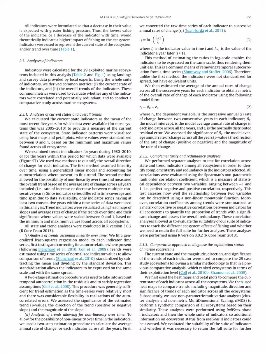
Between 1980 and 2010, the overall direction of change ofIndiSeas-phase I indicators varied greatly among ecosystems (Fig. 3and Figure S7). Six ecosystems (21%) showed an overall decrease inthe levels of indicators, suggesting an overall increasingly impactedecosystem over time: the Black Sea, the central Baltic Sea, theGuinean Shelf, the Sahara Coastal, the Gulf of Cadiz and the westCoast U.S. Three ecosystems (10%) showed an overall increase, sug-gesting these ecosystems have become less impacted over time:the Barents Sea, the Gulf of Lions and the west Coast Scotland.Ten ecosystems (35%) showed mixed signals, with some indicatorsincreasing and others decreasing significantly: the eastern ScotianShelf, the Irish Sea, the north Ionian Sea, the north-central AdriaticSea, the northeast U.S., the northern Humboldt Current, the Por-tuguese Coast, the Senegalese Shelf, the southern Benguela, and thewestern Scotian Shelf. Indicator scores for ten ecosystems (35%) didnot show any clear patterns because only one indicator showed asignificant trend (increasing or decreasing). Results using IndiSeas-phase II indicators were similar to those of IndiSeas phase-I indica-tors (Fig. 3 and Figure S7). Five ecosystems (17%) showed an overalldecrease: the central Baltic Sea, the eastern Scotian Shelf, the north-central Adriatic Sea, the Portuguese Coast and the Prince EdwardIslands. Two ecosystems (7%) showed an overall increase: the Bar-

ents Sea and the north Ionian Sea. Eight ecosystems (28%) showedmixed signals because indicators either increased or decreasedsignificantly: the Irish Sea, the north Aegean Sea, the northernHumboldt Current, the Senegalese Shelf, the southern Catalan Sea,

M. Coll et al. / Ecological Indicators 60 (2016) 947–962 953

F I (left

0 cosysta s figur

ttd

t0

ItetScsgniSGwdi

ig. 2. Heatmap of current state indicators (2005–2010) using both IndiSeas-phase

and 1, based on the minimum (red) and maximum (blue) values found across all end labels are listed in Table 2. (For interpretation of the references to colour in thi

he west Coast Scotland, the west Coast U.S. and the western Sco-ian Shelf, while 14 ecosystems (49%) did not show any clear patternue to the fact that only one indicator changed significantly.

Supplementary Figure S7 related to this article can be found, inhe online version, at http://dx.doi.org/10.1016/j.ecolind.2015.08.48.

The joint comparison of trends in IndiSeas-phase I and phaseI indicators illustrated that overall trends were similar betweenhe two suites of indicators for 16 ecosystems (55%) (Fig. 3). Onecosystem, the Barents Sea, showed an increasing trend in thewo suites of indicators, while one ecosystem, the central Balticea, showed a consistent decreasing trend in both suites of indi-ators. In addition, four ecosystems showed consistent mixedignals: the Irish Sea, the northern Humboldt Current, the Sene-alese Shelf and the western Scotian Shelf. Ten ecosystems showedo overall pattern of change in either one or the other suite of

ndicators: the eastern Bering Sea, the Bay of Biscay, the Blackea, the Chatham Rise, the eastern English Channel, the Gulf of

abes, the Gulf of Lions, the Sahara Coastal, the North Sea, theestern Coast Vancouver Island. The other 13 ecosystems showedifferent trends when comparing IndiSeas-phase I with phase II

ndicators.

panel) and II (right panel) indicators (Table 1). Indicator values are scaled betweenems. Full indicator names and acronyms are listed in Table 1 and ecosystem namese legend, the reader is referred to the web version of the article.)

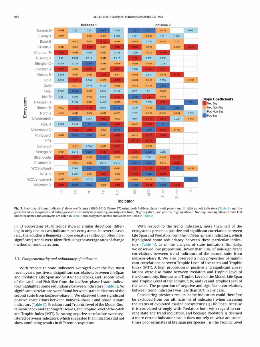
Most IndiSeas-phase I and phase II indicators across the majorityof ecosystems showed a non-significant overall direction of changewhen comparing the rates of change over time (Fig. 4). This methodis more sensitive to time series with low signal to noise ratio (indi-cators which are more variable over time) resulting in a lowerdetection of significant trends (Figure S7). However, because theindicators were not corrected for differences in spread with thismethod, the ecological significance of small changes in indicatorvalues is unknown. Only one or two indicators showed a significantdeclining average annual rate of change over time in four ecosys-tems. In the central Baltic Sea, the Trophic Level of the catch haddecreased on average −0.3% per year and the Mean Vulnerabilityhad decreased on average −0.2% per year over the time period con-sidered. In the southern Benguela, the Trophic Level of the Modelhad decreased on average −0.4% per year, and in the Guinean Shelfecosystem this indicator had declined on average −0.1% per year.In the west Coast U.S., Biomass had declined on average −6.4% peryear over the time period considered.

Although the sensitivity of the two methods used to estimateoverall trends in indicators varied greatly in terms of detecting sig-nificance (Figs. 3 and 4), we found that in eight ecosystems (28%)all trends showed the same positive or negative directions and

954 M. Coll et al. / Ecological Indicators 60 (2016) 947–962

F ing bg r timei s are l

ii(sm

3

raotsspitais

ig. 3. Heatmap of trend indicators’ slope coefficients (1980–2010, Figure S7) useneralized least-squares and autoregressive error analysis (assuming linearity ovendicator names and acronyms are listed in Table 1 and ecosystem names and label

n 13 ecosystems (45%) trends showed similar directions, differ-ng in only one or two indicators per ecosystems. In several casese.g., the Southern Benguela), more negative (although often non-ignificant) trends were identified using the average rates of changeethod of trend detection.

.3. Complementarity and redundancy of indicators

With respect to state indicators averaged over the five mostecent years, positive and significant correlations between Life Spannd Predators, Life Span and Sustainable Stocks, and Trophic Levelf the catch and Fish Size from the IndiSeas-phase I state indica-ors highlighted some redundancy between indicators (Table 3). Noignificant correlations were found between state indicators of theecond suite from IndiSeas-phase II. We observed three significantositive correlations between IndiSeas-phase I and phase II state

ndicators (Table 3): Predators and Trophic Level of the Model, Sus-

ainable Stock and Landings/Discards, and Trophic Level of the catchnd Trophic Index (MTI). No strong negative correlations were reg-stered between indicators, which suggested that indicators did nothow conflicting results in different ecosystems.

oth IndiSeas-phase I (left panel) and II (right panel) indicators (Table 1) and the). Neg: negative, Pos: positive, Sig: significant, Non-Sig: non-significant trend. Fullisted in Table 2.

With respect to the trend indicators, more than half of theecosystems present a positive and significant correlation betweenLife Span and Predators from the IndiSeas-phase I indicators, whichhighlighted some redundancy between these particular indica-tors (Table 4), as in the analysis of state indicators. Similarly,we observed low proportions (lower than 50%) of non-significantcorrelations between trend indicators of the second suite fromIndiSeas-phase II. We also observed a high proportion of signifi-cant correlations between Trophic Level of the catch and TrophicIndex (MTI). A high proportion of positive and significant corre-lations were also found between Predators and Trophic Level ofthe Community, Biomass and Trophic Level of the Model, Life Spanand Trophic Level of the community, and IVI and Trophic Level ofthe catch. The proportion of negative and significant correlationsbetween trend indicators was less than 50% in any case.

Considering previous results, some indicators could thereforebe excluded from our ultimate list of indicators when assessingthe status of exploited marine ecosystems: (i) Life Span, because

it is correlated strongly with Predators both with regard to cur-rent state and trend indicators, and because Predators is deemeda more certain indicator since it does not rely on what are some-times poor estimates of life span per species; (ii) the Trophic Level

M. Coll et al. / Ecological Indicators 60 (2016) 947–962 955

F ing be lowedN le 1 an

oabtt

TSec

ig. 4. Heatmap of trend indicators’ slope coefficients (1980–2010, Figure S7) usstimation of rates of change over time method (value shown in cell; analysis alon-Sig: non-significant trend. Full indicator names and acronyms are listed in Tab

f the Model, because there are strong correlations with Predators

nd Biomass in current state and trend indicators, respectively, andecause models are available only for a small number of ecosys-ems; and (iii) the Landings/Discards indicator, which was difficulto estimate for several ecosystems and showed redundancy with

able 3pearman’s non-parametric rank order correlation coefficients (values below the diagonaxploited marine ecosystems (n values included in the analysis are: BS = 27, LG = 20, LS = 26orrelations are highlighted in bold.

IndiSeas-phase I indicators

p-ValueR

BS LG LS PF SS

BS 0.77 0.84 0.13 0.59

LG 0.07 0.06 0.08 0.66

LS −0.04 0.44 0.04 0.00

PF −0.30 0.40 0.41 0.40

SS 0.11 −0.11 0.56 0.17

TLc −0.05 0.47 0.15 0.11 −0.28

NDES −0.09 0.10 0.18 −0.03 0.40

MTI 0.10 0.27 0.31 0.18 −0.03

TLsc 0.00 0.31 0.39 0.19 0.22

TLmc −0.41 −0.20 0.27 0.86 −0.25

D 0.23 0.77 0.49 0.21 0.82

oth IndiSeas-phase I (left panel) and II (right panel) indicators (Table 1) and the for non-linear changes over time). Neg: negative, Pos: positive, Sig: significant,d ecosystem names and labels are listed in Table 2.

Sustainable Stocks. Finally, (iv) the Fish Size indicator should be

considered carefully because of lower data availability and a highpercentage of positive correlations with relative fishing effort (con-trary to the expected decline in fish size with increasing fishingpressure; results presented in Section 3.5).

l) and associated p-values (values above the diagonal) of state indicators for the 29, PF = 27, SS = 27, TLc = 29, MTI = 28, NDES = 22, TLsc = 24, TLmc = 12, D = 9). Significant

IndiSeas-phase II indicators

TLc NDES MTI TLsc TLmc D

0.80 0.69 0.64 0.98 0.25 0.550.04 0.69 0.26 0.20 0.70 0.130.46 0.44 0.13 0.07 0.49 0.180.57 0.91 0.37 0.37 0.00 0.580.16 0.07 0.90 0.30 0.51 0.01

0.98 0.00 0.62 0.06 0.190.00 0.06 0.56 0.09 0.300.54 0.80 0.93 0.66 0.610.11 0.14 −0.02 0.85 0.440.58 −0.57 −0.16 0.08 0.440.49 0.39 −0.21 0.72 −0.35

956 M. Coll et al. / Ecological Indicators 60 (2016) 947–962

Table 4Proportion of negative and positive significant Spearman’s non-parametric rank order correlation coefficients of trend indicators for the 29 exploited marine ecosystems(values below the diagonal; negative and positive values separated by a semicolon). The proportions are calculated taking into account the number of time series availablein each ecosystem (values above the diagonal). Bold values highlight instances where the proportion of positive correlations between two indicators is more than 40%.

IndiSeas-phase I indicators IndiSeas-phase II indicators

Prop. −ve, +vecorrelations

LG LS PF TB TLc IVI MTI TLsc TLmc D

LG 19 20 20 20 20 20 19 7 5LS 0.05; 0.21 28 27 27 26 27 25 12 8PF 0.1; 0.35 0.04; 0.57 28 28 27 28 26 13 8TB 0.05; 0.15 0.26; 0.19 0.29; 0.11 29 28 29 26 12 8TLc 0; 0.25 0.19; 0.19 0.18; 0.18 0.07; 0.14 28 29 26 12 8IVI 0.05; 0.1 0; 0.19 0.07; 0.11 0.04; 0.11 0.14; 0.54 28 26 11 8MTI 0; 0.2 0.15; 0.11 0.11; 0.14 0.17; 0.14 0; 0.66 0.18; 0.36 26 12 8

3

usto

FIo

TLsc 0.05; 0.32 0.16; 0.48 0; 0.50 0.15; 0.12TLmc 0.14; 0.14 0.17; 0.25 0.15; 0.23 0.08; 0.58D 0; 0 0.13; 0 0.25; 0 0; 0.25

.4. Status of exploited marine ecosystems

When comparing the status of exploited marine ecosystems

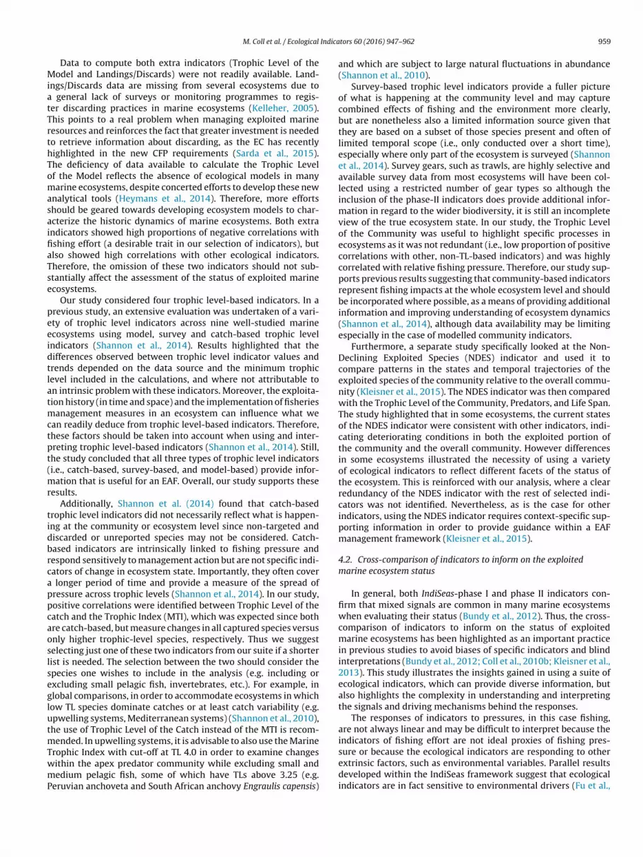
sing current state indicators from IndiSeas-phase I with the wholeuite of indicators, we observed that the classification of ecosys-ems using multivariate techniques (cluster analysis and nMDSrdinations) varied significantly (Fig. 5). Using IndiSeas-phase I

ig. 5. Cross-comparison of current states (2005–2010) of ecosystems using cluster andndiSeas-phase I, and (b–d) whole suite of indicators (excluding Life Span, Fish Size, Trophrder correlation contributions of each indicator are shown as vectors in the nMDS.

0.04; 0.19 0.04; 0.12 0.04; 0.19 11 70; 0.25 0.18; 0.09 0.25; 0.25 0.09; 0.27 40.13; 0.13 0.13; 0 0.13; 0 0; 0 0; 0

state indicators, three groups of ecosystems emerged: the northAegean Sea and the northeast U.S. emerged as different from theother ecosystems, which clustered together in a large group (Fig. 5a

and c). Using the whole suite of state indicators, all the ecosystemsclustered together and we did not discern any significant pattern(Fig. 5b and d). It should be noted that when the whole suite of indi-cators was used, the stress value in the nMDS ordination increased

non-metric MultiDimensional Scaling (nMDS) analysis with indicators from (a–c)ic Level of the Model and Landings/Discards). The Spearman’s non-parametric rank

M. Coll et al. / Ecological Indicators 60 (2016) 947–962 957

Fig. 6. Cross-comparison of trends (1980–2010, Figure S7) of ecosystems using cluster and non-metric MultiDimensional Scaling (nMDS) analysis with indicators from (a–c)IndiSeas-phase I, and (b–d) whole suite of indicators (excluding Life Span, Fish Size, Trophic Level of the Model and Landings/Discards). The Spearman’s non-parametric ranko .

(tgtia

ueonesii

owi

3

fi

rder correlation contributions of each indicator are shown as vectors in the nMDS

from 0.12 to 0.17). This moderately high stress value indicateshe difficulty in displaying the relationships, which generally sug-ests a loss of information when projecting from high dimensiono two dimensions, when more indicators are incorporated. Thesendicators brought additional dimensions of similarity7differencesmong ecosystems.

When comparing the status of exploited marine ecosystemssing IndiSeas-phase I trend indicators resulting from the gen-ralized least-squares analyses results, no different groups werebserved in the classification of ecosystems (cluster analysis andMDS ordinations) (Fig. 6c and d). However, the clustering ofcosystems was qualitatively different than when using the wholeuite of trend indicators (Fig. 6a and b). When the whole suite ofndicators was used, the stress value in the nMDS ordination alsoncreased (from 0.11 to 0.16).

Due to redundancy of some indicators and/or poor availabilityf data as described above, all the above analyses were performedithout Life Span, Fish Size, Trophic Level of the Model and Land-

ngs/Discards.

.5. Correlations with fishing pressure

Since the indicators were formulated to decrease with highershing pressure (using relative fishing effort and mortality as

proxies), we expected a high proportion of negative correlationsbetween the three measures of fishing pressure (Landings/Biomass,relative fishing effort and relative mortality) and the indicators.

The highest proportions of ecosystems with negative correla-tions were between Biomass and the fishing pressure indicator,Landings/Biomass (0.79; Table 5), which is logical due to theformulation of the pressure indicator. Among other indicators,proportions of significant positive or negative correlations withLandings/Biomass were less than or equal to 0.33. Among ecosys-tems with available relative fishing effort, the highest proportionof negative correlations were between Landings/Discards and rel-ative fishing effort (0.50; Table 6a) and between Trophic Level ofthe Model and relative fishing effort (0.43; Table 6a). In contrast,50% of the ecosystems showed a positive correlation between FishSize and relative fishing effort, although this information was onlyavailable for four ecosystems. The rest of the indicators showedvariable proportions (<0.29) of significant positive or negativecorrelations with relative effort. Among those ecosystems withavailable relative fishing mortality data, we observed that Biomassshowed the highest proportion of ecological indicators with sig-

nificant and negative correlations with relative fishing mortality(0.44; Table 6b). The rest of indicators showed variable proportions(<0.33) of significant positive or negative correlations with relativefishing mortality.

958 M. Coll et al. / Ecological Indicators 60 (2016) 947–962

Table 5Number and proportion of Spearman’s non-parametric rank order correlation coefficients between IndiSeas indicators and the Landings over Biomass ratio indicator. Thenumber per indicator provides the number of ecosystems with data available to test this relationship. Bold values highlight instances where the proportion of positivecorrelations between two indicators is more than 40%.

Landings/biomass IndiSeas-phase I indicators IndiSeas-phase II indicators

LG LS PF TB TLc IVI MTI TLsc TLmc D

−ve, +ve correlations 3, 2 5, 6 4, 8 23, 0 9, 6 8, 3 6, 8 0, 4 4, 2 1, 0−ve correlations (prop.)* 0.15 0.19 0.14 0.79 0.31 0.29 0.21 0.00 0.33 0.13

* 0

−ve:

4

4

cseomc

Istottlsrt

pmasitoscapm2

TNsp

+ve correlations (prop.) 0.10 0.22 0.29 0.0Number per indicator 20 27 28 29

* Proportion of significant correlations calculated with the number per indicator.

. Discussion

.1. IndiSeas ecological state and trend indicators

In this study we developed an analysis to evaluate a suite ofurrent state and trends of ecological indicators to determine thetatus of 29 exploited marine ecosystems. We considered severalcological indicators that were defined to measure fishing impactsn commercial stocks, and capture the broader effects of fishing onarine biodiversity and ecosystems, some of which have important

onservation implications.Overall, our results illustrate that the two suites of indicators,

ndiSeas-phase I and phase II, are often complementary and inome cases offer additional interpretations or information. Thus,he new suite of indicators selected to capture the broader effectsf fishing on marine biodiversity and ecosystems provided addi-ional information to complement that obtained by using onlyhe first suite of IndiSeas-phase I indicators. Our study also high-ights that the interpretation of indicators is complex because theyhow a diverse range of responses to fishing pressure and theyequire careful analyses and background knowledge of the ecosys-ems.

The first suite of ecological indicators chosen during IndiSeas-hase I (Shin and Shannon, 2010) were selected specifically toeasure ecosystem response to fishing pressure, and have greater

vailability in terms of temporal and spatial coverage in the 29 casetudies than the new indicators, chosen to capture aspects of thempacts of fishing on biodiversity. This is logical since the concep-ualization and development of indicators for measuring the effectsf fishing pressure on the exploited part of the community has beentudied for a longer period of time (Rochet and Trenkel, 2003). Inontrast, biodiversity issues have more recently been added to the

nalyses as the Ecosystem-based Approach to Fisheries and com-rehensive evaluations of marine ecosystems have been gainingomentum (Halpern et al., 2012; Pikitch et al., 2004; Tittensor et al.,

014).

able 6umber and proportion of Spearman’s non-parametric rank order correlation coefficien

eries. The number per indicator provides the number of ecosystems with data availableositive correlations between two indicators is more than 40%.

IndiSeas-phase I indicators

LG LS PF TB

(a) Fishing effort−ve, +ve correlations 0, 2 2, 1 2, 1 2, 1

−ve correlations (prop.)* 0.00 0.29 0.29 0.29

+ve correlations (prop.)* 0.50 0.14 0.14 0.14

Number per indicator 4 7 7 7

(b) Fishing mortality−ve, +ve correlations 0, 1 2, 2 3, 2 4, 0

−ve correlations (prop.)* 0.00 0.22 0.33 0.44

+ve correlations (prop.)* 0.20 0.22 0.22 0.00

Number per indicator 5 9 9 9

* Proportion of significant correlations calculated with the number per indicator. −ve:

0.21 0.11 0.28 0.15 0.17 0.0029 28 29 26 12 8

negative; +ve: positive.

The additional suite of IndiSeas-phase II indicators was alsoavailable in many of our study systems, with the exception ofthe two extra indicators (Trophic Level of the Model and Land-ings/Discards). This is a positive result in the drive to achievecurrent and future targets dictated by international and regionalframeworks, such as the Marine Strategy Framework Directive(MSFD) of the European Commission or the Aichi Targets of theConvention of Biological Diversity. The latest global evaluation ofthe Aichi Targets of the CDB only includes two indicators that canbe used to explicitly inform Aichi Target 6, which evaluates theaim to manage marine ecosystems, sustainably avoiding adverseimpacts on commercial and non-commercial species and habitats(Tittensor et al., 2014).

Our results also show that some redundancy between indica-tors exists and highlight the potential to remove a few indicatorsfrom our initial suite in order to reduce monitoring and data col-lection efforts. Regarding the IndiSeas-phase I suite (Shin et al.,2010b), the Life Span indicator could be removed in some ecosys-tems where it shows a redundancy with Predators. In addition, theFish Size indicator was not always available and showed positivecorrelations with higher fishing effort in some cases, which maybe counter-intuitive given the original rationale for the selectionof the indicator. This is an interesting result that needs furtherinvestigation; for example, the Fish Size indicator may be capturingenvironmental influences through the level of fish recruitment orthe success of size-based fishing limits in some regions, whereas inother highly degraded ecosystems its sensitivity to further heavierfishing may be limited. In addition, Fish Size and Trophic Levelare highly correlated in several systems, which may highlight thatsize-based and trophic-based phenomena in some exploited fishcommunities can follow similar directions of change at the commu-nity level, as previously suggested (Jennings et al., 2001). However,

Fish Size reflects important ecosystem functioning issues relevant,for instance, within the MSFD framework by involving at leastDescriptor 3 on Populations of Commercially Exploited Species andDescriptor 4 on Food Webs (EC, 2008, 2010).

ts between IndiSeas indicators and (a) fishing effort and (b) fishing mortality time to test this relationship. Bold values highlight instances where the proportion of

IndiSeas-phase II indicators

TLc IVI MTI TLsc TLmc D

0, 2 1, 1 0, 2 0, 2 3, 2 1, 00.00 0.14 0.00 0.00 0.43 0.500.29 0.14 0.29 0.29 0.29 0.007 7 7 7 7 2

0, 3 1, 2 1, 2 1, 2 3, 2 1, 00.00 0.13 0.11 0.11 0.33 0.330.33 0.25 0.22 0.22 0.22 0.009 8 9 9 9 3

negative; +ve: positive.

Indica

MiatTrthTomasaifiaTse

peeidtlatmctpt(mr

tidbrcappcaoslseglutmTwmP

M. Coll et al. / Ecological

Data to compute both extra indicators (Trophic Level of theodel and Landings/Discards) were not readily available. Land-

ngs/Discards data are missing from several ecosystems due to general lack of surveys or monitoring programmes to regis-er discarding practices in marine ecosystems (Kelleher, 2005).his points to a real problem when managing exploited marineesources and reinforces the fact that greater investment is neededo retrieve information about discarding, as the EC has recentlyighlighted in the new CFP requirements (Sarda et al., 2015).he deficiency of data available to calculate the Trophic Levelf the Model reflects the absence of ecological models in manyarine ecosystems, despite concerted efforts to develop these new

nalytical tools (Heymans et al., 2014). Therefore, more effortshould be geared towards developing ecosystem models to char-cterize the historic dynamics of marine ecosystems. Both extrandicators showed high proportions of negative correlations withshing effort (a desirable trait in our selection of indicators), butlso showed high correlations with other ecological indicators.herefore, the omission of these two indicators should not sub-tantially affect the assessment of the status of exploited marinecosystems.

Our study considered four trophic level-based indicators. In arevious study, an extensive evaluation was undertaken of a vari-ty of trophic level indicators across nine well-studied marinecosystems using model, survey and catch-based trophic levelndicators (Shannon et al., 2014). Results highlighted that theifferences observed between trophic level indicator values andrends depended on the data source and the minimum trophicevel included in the calculations, and where not attributable ton intrinsic problem with these indicators. Moreover, the exploita-ion history (in time and space) and the implementation of fisheries

anagement measures in an ecosystem can influence what wean readily deduce from trophic level-based indicators. Therefore,hese factors should be taken into account when using and inter-reting trophic level-based indicators (Shannon et al., 2014). Still,he study concluded that all three types of trophic level indicatorsi.e., catch-based, survey-based, and model-based) provide infor-

ation that is useful for an EAF. Overall, our study supports theseesults.

Additionally, Shannon et al. (2014) found that catch-basedrophic level indicators did not necessarily reflect what is happen-ng at the community or ecosystem level since non-targeted andiscarded or unreported species may not be considered. Catch-ased indicators are intrinsically linked to fishing pressure andespond sensitively to management action but are not specific indi-ators of change in ecosystem state. Importantly, they often cover

longer period of time and provide a measure of the spread ofressure across trophic levels (Shannon et al., 2014). In our study,ositive correlations were identified between Trophic Level of theatch and the Trophic Index (MTI), which was expected since bothre catch-based, but measure changes in all captured species versusnly higher trophic-level species, respectively. Thus we suggestelecting just one of these two indicators from our suite if a shorterist is needed. The selection between the two should consider thepecies one wishes to include in the analysis (e.g. including orxcluding small pelagic fish, invertebrates, etc.). For example, inlobal comparisons, in order to accommodate ecosystems in whichow TL species dominate catches or at least catch variability (e.g.pwelling systems, Mediterranean systems) (Shannon et al., 2010),he use of Trophic Level of the Catch instead of the MTI is recom-

ended. In upwelling systems, it is advisable to also use the Marinerophic Index with cut-off at TL 4.0 in order to examine changes

ithin the apex predator community while excluding small andedium pelagic fish, some of which have TLs above 3.25 (e.g.

eruvian anchoveta and South African anchovy Engraulis capensis)

tors 60 (2016) 947–962 959

and which are subject to large natural fluctuations in abundance(Shannon et al., 2010).

Survey-based trophic level indicators provide a fuller pictureof what is happening at the community level and may capturecombined effects of fishing and the environment more clearly,but are nonetheless also a limited information source given thatthey are based on a subset of those species present and often oflimited temporal scope (i.e., only conducted over a short time),especially where only part of the ecosystem is surveyed (Shannonet al., 2014). Survey gears, such as trawls, are highly selective andavailable survey data from most ecosystems will have been col-lected using a restricted number of gear types so although theinclusion of the phase-II indicators does provide additional infor-mation in regard to the wider biodiversity, it is still an incompleteview of the true ecosystem state. In our study, the Trophic Levelof the Community was useful to highlight specific processes inecosystems as it was not redundant (i.e., low proportion of positivecorrelations with other, non-TL-based indicators) and was highlycorrelated with relative fishing pressure. Therefore, our study sup-ports previous results suggesting that community-based indicatorsrepresent fishing impacts at the whole ecosystem level and shouldbe incorporated where possible, as a means of providing additionalinformation and improving understanding of ecosystem dynamics(Shannon et al., 2014), although data availability may be limitingespecially in the case of modelled community indicators.

Furthermore, a separate study specifically looked at the Non-Declining Exploited Species (NDES) indicator and used it tocompare patterns in the states and temporal trajectories of theexploited species of the community relative to the overall commu-nity (Kleisner et al., 2015). The NDES indicator was then comparedwith the Trophic Level of the Community, Predators, and Life Span.The study highlighted that in some ecosystems, the current statesof the NDES indicator were consistent with other indicators, indi-cating deteriorating conditions in both the exploited portion ofthe community and the overall community. However differencesin some ecosystems illustrated the necessity of using a varietyof ecological indicators to reflect different facets of the status ofthe ecosystem. This is reinforced with our analysis, where a clearredundancy of the NDES indicator with the rest of selected indi-cators was not identified. Nevertheless, as is the case for otherindicators, using the NDES indicator requires context-specific sup-porting information in order to provide guidance within a EAFmanagement framework (Kleisner et al., 2015).

4.2. Cross-comparison of indicators to inform on the exploitedmarine ecosystem status

In general, both IndiSeas-phase I and phase II indicators con-firm that mixed signals are common in many marine ecosystemswhen evaluating their status (Bundy et al., 2012). Thus, the cross-comparison of indicators to inform on the status of exploitedmarine ecosystems has been highlighted as an important practicein previous studies to avoid biases of specific indicators and blindinterpretations (Bundy et al., 2012; Coll et al., 2010b; Kleisner et al.,2013). This study illustrates the insights gained in using a suite ofecological indicators, which can provide diverse information, butalso highlights the complexity in understanding and interpretingthe signals and driving mechanisms behind the responses.

The responses of indicators to pressures, in this case fishing,are not always linear and may be difficult to interpret because theindicators of fishing effort are not ideal proxies of fishing pres-sure or because the ecological indicators are responding to other

extrinsic factors, such as environmental variables. Parallel resultsdeveloped within the IndiSeas framework suggest that ecologicalindicators are in fact sensitive to environmental drivers (Fu et al.,

9 Indica

2asirgsiim2ttpr

miHaesMepoit2tsfsreifilniehtwO(

Nmce2Biasoierios2et

60 M. Coll et al. / Ecological

015), which highlights that interactions between the indicatorsnd at least one other extrinsic factor is likely. In addition, analy-es of indicators assuming a linear relationship between responsendicators and pressure indicators may be too simplistic. In fact,ecent comprehensive studies of exploited marine ecosystems sug-est that detailed information about past and present exploitationtrategies, main productivity mechanisms, and dominant ecolog-cal and environmental traits are essential elements to correctlynterpret ecological indicators to determine the status of exploited

arine ecosystems (Fu et al., 2015; Kleisner et al., 2014; Link et al.,010; Shannon et al., 2014; Shannon et al., 2010). This emphasiseshe need to investigate the sensitivity and specificity of indicatorso different individual pressures, as well as multiple-interactingressures, and their responsiveness to management thresholds andeference points (Large et al., 2013, 2015; Shin et al., 2012).

In this study, we focused on the effects of fishing, which is aajor pressure in many ecosystems (Costello et al., 2010). Thus, the

ndicators were defined to decrease with greater fishing impact.owever, it is important to recognize that fishing impact is notlways the leading driver in an ecosystem, even in exploitedcosystems, and that other drivers, such as the environmentaltressors, can have significant effects on indicators (Link et al., 2010;ackinson et al., 2009). For example, in the Southern Benguela, the

ffects of fishing are confounded with ecosystem changes at leastartially due to environmentally induced shifts in the distributionf key resources (Shannon et al., 2010, 2014). This has importantmplications for birds or mammals, which are often of conserva-ion concern and also support tourism industries (e.g., Blamey et al.,015). Like the Southern Benguela, Senegal and Guinea are ecosys-ems in which fish communities and landings are dominated bymall pelagic stocks, thus the effects of fishing are probably con-ounded with ecosystem changes due to environmentally inducedhifts, influencing the abundance and distribution of these keyesources (Chavance et al., 2004; Roy et al., 2002). In the north-rn Humboldt Current anchovy is dominant when the ecosystems considered healthy, the impact of indicators is a decreased meansh length in the surveyed community, shortened mean maximum

ife span of surveyed fish species and reduced mean intrinsic vul-erability index of the fish landed catch, so that a decrease in these

ndicators is not always related to greater fishing impact (Chavezt al., 2008). In the west coast U.S. ecosystem, management actionsave recovered many harvested species, but survey-based indica-ors declined over the period observed (2003–2010), coincidentith 4–5 years of a warm, unproductive phase of the Pacific Decadalscillation and attenuation of a strong 1999 groundfish cohort

Keller et al., 2012; Tolimieri et al., 2013).The importance of environmental drivers is also seen in the

orth Ionian Sea, where extensive fishing pressure and environ-ental shifts have had negative implications for short-beaked

ommon dolphins (Piroddi et al., 2011). In the Portuguese Coast,nvironmentally induced shifts have also occurred (Borges et al.,010), while important alterations have taken place in the centralaltic Sea ecosystem due to climate and multiple human induced

mpacts (Möllmann et al., 2009; Österblom et al., 2007). In addition,nd compared to the other ecosystems, the relatively lower currenttate calculated for the Black Sea may be due to the dominancef small pelagic fish in this ecosystem and their strong fluctuationn landings due to nutrient enrichment, overexploitation andnvironmental change (Oguz et al., 2012). In the Barents Sea, theapid fluctuations in stock size and landings due to natural drivers,n addition to fisheries regulations, have led to under-exploitationf long-lived species and increased landings of short-lived pelagic

pecies in the presence good recruitment classes (Johannesen et al.,012). Therefore, as has been previously recognized (Shannont al., 2014; Shannon et al., 2010), detailed knowledge abouthe ecosystem is important to facilitate understanding of the

tors 60 (2016) 947–962

patterns revealed by the selected indicators. The influence of otherdrivers on ecosystems suggests that there is the need to consideradditional ecosystem-specific indicators, such as environmentallylinked response indicators (Boldt et al., 2014).

Despite these mixed signals, which in themselves should con-vey a need for cautious monitoring of future ecosystem conditionsand trajectories, some ecosystems analyzed in this study are likelymore impacted than others. Overall poor ecosystem status com-pared to other ecosystems considered can be described across thesuite of indicators for several case studies, e.g., the Black Sea, theGulf of Cadiz, the north Aegean Sea, the north Ionian Sea, thenorth-central Adriatic Sea, the northern Humboldt Current, theSahara Coastal, the Senegalese shelf and the southern Catalan Seaif considering current states, and central Baltic Sea if consideringtrends. This is in line with information from the literature (e.g., Collet al., 2008, 2010a; Gascuel et al., 2015; Piroddi et al., 2010; Torreset al., 2013). Therefore, this study illustrates that several exploitedmarine ecosystems have a relatively high impact by fishing, in linewith previous studies (Bundy et al., 2010; Coll et al., 2010b; Kleisneret al., 2013; Shannon et al., 2010) and highlights the need to developimproved management tools considering conservation issues ofnatural resources.

In addition, our results show important differences for howecosystems are classified using current state and trend indicatorswhen explicitly considering the impacts of fishing on biodiversity.Indicators that capture the dynamics of the fuller spectrum of fishwithin an ecosystem, such as Trophic level of the Community andthe Non-Declining Exploited Species indicator, convey additionalinformation that complement that already provided by the moretraditionally accepted suite of ecological indicators used for detec-ting fishing impacts, and can serve to strengthen the signals we maybe receiving as warning of impending ecosystem change. Thus, thenew suite of IndiSeas-phase II ecological indicators provide usefuladditional information in relation to wider biodiversity aspects ofthe effects of fishing and highlight the potential for other factorsthat should be considered when evaluating ecosystem status. Insystems where the patterns in the old and new suites of indica-tors are similar, they may still provide extra context and supportfor the patterns seen with the IndiSeas-phase I indicators. Theseindicators should be considered complementary to other ecologicalindicators that measure fishing impacts on commercial stocks andcommunities by capturing the broader effects of fishing on marinebiodiversity and ecosystems. While this study focusses specificallyon the effects of fisheries, wider ecosystem assessments of otherdrivers in the marine environment (e.g. marine tourism, miningand aquaculture) may also benefit from inclusion of a wider rangeof biodiversity and conservation-based indicators.

In a world largely focussed on exploited species, it seems thatindicators that capture the broader effects of fishing on marine bio-diversity help move towards the conciliation of exploitation andconservation issues (Brander, 2010; Palumbi et al., 2008; Wormet al., 2006). Thus, biodiversity and conservation-based indicatorsshould be used in concert to provide additional useful informa-tion to evaluate the overall impact of fishing on exploited marineecosystems.

Acknowledgements

We thank the Euroceans IndiSeas Working Group funded bythe European Network of Excellence EUR-OCEANS (FP6, Con-tract N◦ 511106), the European collaborative project MEECE –

Marine Ecosystem Evolution in a Changing Environment (FP7,Contract N◦ 212085) and IRD (Institute of Research for Develop-ment) and IOC/UNESCO. All participants of EUR-OCEANS IndiSeasproject (www.indiseas.org) are acknowledged. We would also like

Indica

tdClbtta(prNtMFPvwmEbEMbfm2(NepRItE

R

B

B

B

B

B

B

B

B

C

C

M. Coll et al. / Ecological

o acknowledge all those who conducted surveys to collect theata used in this study. MC was partially funded by the Europeanommission through the Marie Curie Career Integration Grant Fel-

owships – PCIG10-GA-2011-303534 – to the BIOWEB project andy the Spanish National Program Ramon y Cajal. LJS was supportedhrough the South African Research Chair Initiative, funded throughhe South African Department of Science and Technology (DST) anddministered by the South African National Research FoundationNRF). LJS and YS were also funded by the European collaborativeroject MEECE – Marine Ecosystem Evolution in a Changing Envi-onment – (FP7, Contract N◦ 212085). KMK was supported by theortheast Fisheries Science Center and the Nature Conservancy

hrough a grant from the Gordon and Betty Moore Foundation.JJJ was supported by an EU Marie Curie International Outgoing

ellowship – PIOF-GA-2013-628116. MFB was supported by theortuguese Oceanic and Atmospheric Institute and the trawl sur-ey data collected under Biological Sampling (PNAB) Program. LJGould like to thank the Joint Research Centre of the European Com-ission for support. HO was financed by the Estonian Ministry of

ducation and Research (Grant SF0180005s10). JJH was supportedy the Natural Environment Research Council and Department fornvironment, Food and Rural Affairs [Grant Number NE/L003279/1,arine Ecosystems Research Programme]. GIvdM was supported

y the Institute of Marine Research, Norway. KT was partiallyunded by the project PERSEUS (Policy-oriented marine Environ-

ental Research in the Southern EUropean Seas; FP7 Contract N◦

87600). MAT was funded by the Spanish Institute of OceanographyIEO) through a Predoctoral FPI fellowship. KNM was supported by aational Research Council fellowship at the Northwest Fishery Sci-nce Center. YJS and MTT were partially supported by the Frenchroject EMIBIOS (FRB, Contract No. APP-SCEN-2010-II). Chathamise trawl survey data were provided by the Ministry for Primary

ndustries. CL acknowledges DEVOTES – Development of innova-ive tools for understanding marine biodiversity and assessing goodnvironmental Status – EC project (FP7 Grant Agreement 308392).

eferences

lamey, L.K., Shannon, L.J., Bolton, J.J., Crawford, R.J.M., Dufois, F., Evers-King, H.,Griffiths, C.L., Hutchings, L., Jarre, A., Rouault, M., Watermeyer, K.E., Winker, H.,2015. Ecosystem change in the southern Benguela and the underlying processes.J. Mar. Syst. 144, 9–29.

lanchard, J., Coll, M., Cotter, J., Link, J., Trenkel, V., Vergnon, R., Yemane, D., Shin, Y.J.,2010. Trend analysis of indicators: a comparison of recent changes in the statusof marine ecosystems around the world. ICES J. Mar. Sci. 67, 732–744.

oldt, J.L., Martone, R., Samhouri, J., Perry, R.I., Itoh, S., Chung, I.K., Takahashi, M.,2014. Developing ecosystem indicators for responses to multiple stressors.Oceanography 27, 116–133.

orges, M.F., Velasco, F., Mendes, H., Pinho, M.R., Silva, C., Porteiro, C., Frid, C.L.J.,Paramor, O.A.L., Piet, G.J., Rogers, S.I., Le Quesne, W.J.F., 2010. Assessing theimpact of fishing on the Marine Strategy Framework Directive objectives forGood Environmental Status. Developing and testing the process across selectedRAC regions: The South Western Waters Region. Project Report Making Euro-pean Fisheries Ecosystem Plans Operational (MEFEPO).

rander, K., 2010. Reconciling biodiversity conservation and marine capture fish-eries production. Curr. Opin. Environ. Sustain. 2, 416–421.

undy, A., Coll, M., Shannon, L.J., Shin, Y.-J., 2012. Global assessments of marineexploited ecosystems and their management: what more is needed? Curr. Opin.Environ. Sustain. 4, 292–299.

undy, A., Shannon, L.J., Rochet, M.-J., Neira, S., Shin, Y.-J., Hill, L., Aydin, K., 2010. Thegood (ish), the bad, and the ugly: a tripartite classification of ecosystem trends.ICES J. Mar. Sci.: J. Conseil 67, 745–768.

utchart, S.H.M., Walpole, M., Collen, B., van Strien, A., Scharlemann, J.P.W., Almond,R.E.A., Baillie, J.E.M., Bomhard, B., Brown, C., Bruno, J., 2010. Global biodiversity:indicators of recent declines. Science 328, 1164.

BD, 2010. Decision Adopted by the Conference of the Parties to the Conventionon Biological Diversity at its Tenth Meeting, Decision X/2. The Strategic Plan forBiodiversity 2011–2020 and the Aichi Biodiversity Targets. Secretariat for theConvention on Biological Diversity, Nagoya, Japan.

havance, P., Bâ, M., Gascuel, D., Vakily, J.M., Pauly, D., 2004. Pêcheries maritimes,écosystèmes & sociétés en Afrique de l’Ouest: Un demi-siècle de changement[Marine Fisheries, Ecosystems and Societies in West Africa: Half a Century ofChange], actes du symposium international, Dakar (Sénégal), 24–28 juin 2002, Bruxelles, Office des publications officielles des Communautés européennes,

tors 60 (2016) 947–962 961

XXXVI – 532-XIV p., 6 pl. h.-t. coul., coll. Rapports de recherche halieutiqueA.C.P.-U.E., n◦ 15.

Chavez, F.P., Bertrand, A., Guevara, R., Soler, P., Csirke, J., 2008. The northern Hum-boldt Current System: brief history, present status and a view towards the future.Prog. Oceanogr. 79, 95–105.

Cheung, W.W.L., Watson, R., Morato, T., Pitcher, T.J., Pauly, D., 2007. Intrinsic vulner-ability in the global fish catch. Mar. Ecol. Prog. Ser. 333, 1–12.

Christensen, V., Guenette, S., Heymans, J.J., Walters, C., Watson, R., Zeller, D., Pauly,D., 2003. Hundred-year decline of North Atlantic predatory fishes. Fish Fish. 4,1–24.

Clarke, K.R., Gorley, R.N., 2006. PRIMER v6: User Manual/Tutorial (Plymouth Routi-nes in Multivariate Ecological Research). Primer-E Ltd., Plymouth.

Coll, M., Palomera, I., Tudela, S., Dowd, M., 2008. Food-web dynamics in the SouthCatalan Sea ecosystem (NW Mediterranean) for 1978–2003. Ecol. Model. 217,95–116.

Coll, M., Santojanni, A., Palomera, I., Arneri, E., 2010a. Ecosystem assessment of theNorth-Central Adriatic: towards a multivariate reference framework. Mar. Ecol.Prog. Ser. 417, 193–210.

Coll, M., Shannon, L.J., Yemane, D., Link, J.S., Ojaveer, H., Neira, S., Jouffre, D., Labrosse,P., Heymans, J.J., Fulton, E.A., Shin, Y.-J., 2010b. Ranking the ecological relativestatus of exploited marine ecosystems. ICES J. Mar. Sci. 67, 769–786.

Costello, M.J., Coll, M., Danovaro, R., Halpin, P., Ojaveer, H., Miloslavich, P., 2010. Acensus of marine biodiversity knowledge, resources and future challenges. PLoSONE 5, e12110.

Cury, P.M., Shannon, L.J., Roux, J.P., Daskalov, G.M., Jarre, A., Moloney, C.L., Pauly, D.,2005. Trophodynamic indicators for an ecosystem approach to fisheries. ICES J.Mar. Sci. 62, 430–442.

de Leiva Moreno, J.I., Agostini, V.N., Caddy, J.F., Carocci, F., 2000. Is the pelagic-demersal ratio from fishery landings a useful proxy for nutrient availability?A preliminary data exploration for the semi-enclosed seas around Europe. ICESJ. Mar. Sc. 57, 1091–1100.

EC, 2008. Directive of the European Parliament and the Council Establishing a Frame-work for Community Action in the Field of Marine Environmental Policy (MarineStrategy Framework Directive). European Commission, Directive 2008/56/EC,OJL 164.

EC, 2010. Decision on criteria and methodological standards on good environmentalstatus of marine waters. Decision 2010/477/EU. Off. J. Eur. Union L 232, 14–24.

Frank, K.T., Petrie, B., Choi, J.S., Leggett, W.C., 2005. Trophic cascades in a formerlycod-dominated ecosystem. Science 308, 1621–1623.

Fu, C., Large, S., Knight, B., Richardson, A., Bundy, A., Reygondeau, G., Boldt, J., vander Meeren, G.I., Torres, M.A., Sobrino, I., Auber, A., Travers-Trolet, M., Piroddi,C., Diallo, I., Jouffre, D., Mendes, H., Borges, M.F., Lynam, C., Coll, M., Shannon,L.J., Shin, Y.J., 2015. Relationships among fisheries exploitation, environmentalconditions, and ecological indicators across a series of marine ecosystems. J. Mar.Syst. 148, 101–111.

Fulton, E.A., Fuller, M., Smith, A.D.M., Punt, A.E., 2005. Ecological Indicators of theEcosystem Effects of Fishing. Final Report, Australian Fisheries ManagementAuthority Report. R99/1546. 239 pp.

Gascuel, D., Coll, M., Fox, C., Guénette, S., Guitton, J., Kenny, A., Knittweis, L., Nielsen,R., Piet, G., Raid, T., Travers-Trolet, M., Shephard, S., 2015. Fishing impact andenvironmental status in European seas: a diagnosis from stock assessments andecosystem indicators. Fish Fish., http://dx.doi.org/10.1111/faf.12090.

Halpern, B., Longo, C., Hardy, D., McLeod, K., Samhouri, J., Katona, S., Kleisner, K.,Lester, S., O’Leary, J., Ranelletti, M., Rosenberg, A., Scarborough, C., Selig, E., Best,B., Brumbaugh, D., Chapin, F., Crowder, L., Daly, K., Doney, S., Elfes, C., Fogarty, M.,Gaines, S., Jacobsen, K., Bunce-Karrer, L., Leslie, H., Neeley, E., Pauly, D., Polasky,S., Ris, B., St Martin, K., Stone, G., Sumaila, U., Zeller, D., 2012. An index to assessthe health and benefits of the global ocean. Nature 488, 615–620.

Halpern, B.S., Walbridge, S., Selkoe, K.A., Kappel, C.V., Micheli, F., D’Agrosa, C., Bruno,J.F., Casey, K.S., Ebert, C., Fox, H.E., Fujita, R., Heinemann, D., Lenihan, H.S., Madin,E.M.P., Perry, M.T., Selig, E.R., Spalding, M., Steneck, R., Watson, R., 2008. A globalmap of human impact on marine ecosystems. Science 319, 948–952.

Heymans, J.J., Coll, M., Libralato, S., Morissette, L., Christensen, V., 2014. Global pat-terns in ecological indicators of marine food webs: a modelling approach. PLOSONE 9, e95845.

Jennings, S., Pinnegar, J.K., Polunin, N.V., Boon, T.W., 2001. Weak cross-species rela-tionships between body size and trophic level belie powerful size-based trophicstructuring in fish communities. J. Anim. Ecol. 70, 934–944.

Johannesen, E., Ingvaldsen, R.B., Bogstad, B., Dalpadado, P., Eriksen, E., Gjøsæter, H.,Knutsen, T., Skern-Mauritzen, M., Stiansen, J.E., 2012. Changes in Barents Seaecosystem state, 1970–2009: climate fluctuations, human impact, and trophicinteractions. ICES J. Mar. Sci. 69, 880–889.

Juan-Jordá, M.J., Mosqueira, I., Cooper, A.B., Freire, J., Dulvy, N.K., 2011. Globalpopulation trajectories of tunas and their relatives. Proc. Natl. Acad. Sci. 108,20650–20655.

Kelleher, K., 2005. Discards in the world’s marine fisheries: an update. In: FAO Fish-eries Technical Paper 470, 134 p.

Keller, A.K., Wallace, J.R., Horness, B.H., Hamel, O.S., Stewart, I.J., 2012. Variationsin eastern North Pacific demersal fish biomass based on the US west coastgroundfish bottom trawl survey (2003–2010). Fish. Bull. 110, 205–222.

Kleisner, K., Coll, M., Lynam, C., Bundy, A., Shannon, J.L., Shin, Y.J., Boldt, J., Borges,

M.F., Diallo, I., Fox, C., Gascuel, D., Heymans, J.J., Juan Jordá, M.J., Jouffre, D., Large,S.I., Marshall, K.N., Ojaveer, H., Piroddi, C., Tam, J., Torres, M.A., Travers-Trolet,M., Tsagarakis, K., van der Meeren, G.I., Zador, S., 2015. Identifying communitychanges across marine ecosystems based on the biomass of exploited species.Ecosyst. Serv., http://dx.doi.org/10.1016/j.ecoser.2015.02.002.

9 Indica

K

K

L

L

L

L

L

L

L

L

M

M

M

M

O

Ö

P

P

P

P

P

R

R

62 M. Coll et al. / Ecological

leisner, K., Mansour, H., Pauly, D., 2014. Region-based MTI: resolving geographicexpansion in the Marine Trophic Index. Mar. Ecol. Prog. Ser. 512, 185–199.

leisner, K.M., Longo, C., Coll, M., Halpern, B.S., Hardy, D., Katona, S., Le Manach, F.,Pauly, D., Rosenberg, A., Samhouri, J., Scarborough, C., Sumaila, U.R., Watson, R.,Zeller, D., 2013. Exploring patterns of seafood provision revealed in the globalocean health index. AMBIO 42, 910–922.

arge, S.I., Fay, G., Friedland, K.D., Link, J.S., 2013. Defining trends and thresholds inresponses of ecological indicators to fishing and environmental pressures. ICESJ. Mar. Sci.: J. Conseil 70, 755–767.

arge, S.I., Fay, G., Friedland, K.D., Link, J.S., 2015. Quantifying patterns of change inmarine ecosystem response to multiple pressures. PLOS ONE 10, e0119922.

evin, P.S., Fogarty, M.J., Murawski, S.A., Fluharty, D., 2009. Integrated ecosystemassessments: developing the scientific basis for ecosystem-based managementof the ocean. PLoS Biol. 7, e1000014.

ink, J.S., 2002. What does ecosystem-based fisheries management mean? Fisheries27, 18–21.

ink, J.S., 2005. Translating ecosystem indicators into decision criteria. ICES J. Mar.Sci.: J. Conseil 62, 569–576.

ink, J.S., Brodziak, J.K.T., Edwards, S.F., Overholtz, W.J., Mountain, D., Jossi, J.W.,Smith, T.D., Fogarty, M.J., 2002. Marine ecosystem assessment in a fisheriesmanagement context. Can. J. Fish. Aquat. Sci. 59, 1429–1440.

ink, J.S., Yemane, D., Shannon, L.J., Coll, M., Shin, Y.J., Hill, L., Borges, M.F., Bundy,A., Aydin, K., 2010. Relating marine ecosystem indicators to fishing and envi-ronmental drivers: an elucidation of contrasting responses. ICES J. Mar. Sci. 67,787–795.

otze, H.K., Lenihan, H.S., Bourque, B.J., Bradbury, R.H., Cooke, R.G., Kay, M.C., Kidwell,S.M., Kirby, M.X., Peterson, C.H., Jackson, J.B.C., 2006. Depletion, degradation, andrecovery potential of estuaries and coastal seas. Science 312, 1806–1809.

ackinson, S., Daskalov, G., Heymans, J.J., Neira, S., Arancibia, H., Zetina-Rejón, M.,Jiang, H., Cheng, H.Q., Coll, M., Arreguin-Sanchez, F., 2009. Which forcing factorsfit? Using ecosystem models to investigate the relative influence of fishing andchanges in primary productivity on the dynamics of marine ecosystems. Ecol.Model. 220, 2972–2987.

öllmann, C., Diekmann, R., Müller-Karulis, B., Kornilovs, G., Plikshs, M., Axe, P.,2009. Reorganization of a large marine ecosystem due to atmospheric andanthropogenic pressure: a discontinuous regime shift in the Central Baltic Sea.Global Change Biol. 15, 1377–1393.

urawski, S.A., 2000. Definitions of overfishing from an ecosystem perspective. ICESJ. Mar. Sci. 57, 649–658.

urawski, S.A., Steele, J.H., Taylor, P., Fogarty, M.J., Sissenwine, M.P., Ford, M., Such-man, C., 2009. Why compare marine ecosystems? ICES J. Mar. Sci.: J. Conseil,fsp221.

guz, T., Akoglu, E., Salihoglu, B., 2012. Current state of overfishing and its regionaldifferences in the Black Sea. Ocean Coast. Manage. 58, 47–56.

sterblom, H., Hansson, S., Larsson, U., Hjerne, O., Wulff, F., Elmgren, R., Folke, C.,2007. Human-induced trophic cascades and ecological regime shifts in the BalticSea. Ecosystems, 877–889.

alumbi, S.R., Sandifer, P.A., Allan, J.D., Beck, M.W., Fautin, D.G., Fogarty, M.J., Halpern,B.S., Incze, L.S., Leong, J.-A., Norse, E., 2008. Managing for ocean biodiversity tosustain marine ecosystem services. Front. Ecol. Environ. 7, 204–211.

auly, D., Watson, R., 2005. Background and interpretation of the ‘Marine TrophicIndex’ as a measure of biodiversity. Philos. Trans. R. Soc. B: Biol. Sci. 360,415–423.

ikitch, E.K., Santora, C., Babcock, E.A., Bakun, A., Bonfil, R., Conover, D.O., Dayton,P., Doukakis, P., Fluharty, D., Heneman, B., Houde, E.D., Link, J., Livingston, P.A.,Mangel, M., McAllister, M.K., Pope, J., Sainsbury, K.J., 2004. Ecosystem-basedfishery management. Science 305, 346–347.

iroddi, C., Bearzi, G., Christensen, V., 2010. Effects of local fisheries and oceanproductivity on the northeastern Ionian Sea ecosystem. Ecol. Model. 221,1526–1544.

iroddi, C., Bearzi, G., Gonzalvo, J., Christensen, V., 2011. From common to rare: the

case of the Mediterranean common dolphin. Biol. Conserv. 144, 2400–2406.

ice, J.C., Rochet, M.-J., 2005. A framework for selecting a suite of indicators forfisheries management. ICES J. Mar. Sci. 62, 516–527.

ochet, M.-J., Trenkel, V.M., 2003. Which community indicators can measure theimpact of fishing? A review and proposals. Can. J. Fish. Aquat. Sci. 60, 86–99.

tors 60 (2016) 947–962

Rombouts, I., Beaugrand, G., Artigas, L.F., Dauvin, J.-C., Gevaert, F., Goberville, E.,Kopp, D., Lefebvre, S., Luczak, C., Spilmont, N., 2013. Evaluating marine ecosys-tem health: case studies of indicators using direct observations and modellingmethods. Ecol. Indic. 24, 353–365.

Roy, C., Cury, P., Fréon, P., Demarcq, H., 2002. Environmental and resource variabil-ity off Northwest Africa and in the Gulf of Guinea: review. In: McGlade, J.M.,Cury, P., Koranteng, K.A., Hardman-Mountford, N.J. (Eds.), The Gulf of GuineaLarge Marine Ecosystem: Environmental Forcing and Sustainable Developmentof Marine Resources. Elsevier, Amsterdam, pp. 121–139.

Sarda, F., Coll, M., Heymans, J.J., Stergiou, K.I., 2015. Overlooked impacts and chal-lenges of the new European discard ban. Fish Fish. 16, 175–180.

Shannon, J.L., Coll, M., Bundy, A., Shin, Y.J., Travers-Trolet, M., Gascuel, D., Kleisner,K., Tam, J., Piroddi, C., Heymans, J.J., Lynam, C.P., 2014. Trophic level-based indi-cators to track fishing impacts across marine ecosystems. Mar. Ecol. Prog. Ser.512, 115–140.

Shannon, L.J., Coll, M., Neira, S., 2009. Exploring the dynamics of ecological indicatorsusing food web models fitted to time series of abundance and catch data. Ecol.Indic. 9, 1078–1095.

Shannon, L.J., Coll, M., Yemane, D., Jouffre, D., Neira, S., Betrand, A., Diaz, E., Shin,Y.J., 2010. Comparing data-based indicators across upwelling and comparablesystems for communicating ecosystem states and trends. ICES J. Mar. Sci. 67,807–832.

Shin, Y.-J., Bundy, A., Shannon, L.J., Blanchard, J., Chuenpagdee, R., Coll, M., Knight,B., Lynam, C., Piet, G., Rice, J., Richardson, A.J., Group, I.W., 2012. Global in scopeand regionally rich: an IndiSeas workshop helps shape the future of marineecosystem indicators. Rev. Fish Biol. Fish. 22, 621–636.

Shin, Y.J., Bundy, A., Shannon, L.J., Simier, M., Coll, M., Fulton, E.A., Jouffre, D., Ojaveer,H., Heymans, J.J., Raid, T., 2010a. Can simple be useful and reliable? Using ecolog-ical indicators for representing and comparing the states of marine ecosystems.ICES J. Mar. Sci. 67, 717–731.

Shin, Y.J., Shannon, L.J., 2010. Using indicators for evaluating, comparing and com-municating the ecological status of exploited marine ecosystems. 1. The IndiSeasproject. ICES J. Mar. Sci. 67, 686–691.

Shin, Y.J., Shannon, L.J., Bundy, A., Coll, M., Aydin, K., Bez, N., Blanchard, J.L., Borges,M.F., Diallo, I., Diaz, E., Heymans, J.J., Hill, L., Johannesen, E., Jouffre, D., Kifani, S.,Labrosse, P., Link, J.S., Mackinson, S., Masski, H., Möllmann, C., Neira, S., Ojaveer,H., Ould Mohammed Abdallahi, K., Perry, I., Thiao, D., Yemane, D., Cury, P.M.,2010b. Using indicators for evaluating, comparing and communicating the eco-logical status of exploited marine ecosystems. Part 2: Setting the scene. ICES J.Mar. Sci. 67, 692–716.

Shumway, R.H., Stoffer, D.S., 2006. Time Series Analysis and Its Applications: WithR Examples. Springer Science & Business Media, New York.

Tittensor, D.P., Walpole, M., Hill, S.L.L., Boyce, D.G., Britten, G.L., Burgess, N.D.,Butchart, S.H.M., Leadley, P.W., Regan, E.C., Alkemade, R., Baumung, R., Bellard, C.,Bouwman, L., Bowles-Newark, N.J., Chenery, A.M., Cheung, W.W.L., Christensen,V., Cooper, H.D., Crowther, A.R., Dixon, M.J.R., Galli, A., Gaveau, V., Gregory, R.D.,Gutierrez, N.L., Hirsch, T.L., Höft, R.H., Januchowski-Hartley, S.R., Karmann, M.,Krug, C.B., Leverington, F.J., Loh, J., Lojenga, R.K., Malsch, K., Marques, A., Mor-gan, D.H.W., Mumby, P.J., Newbold, T., Noonan-Mooney, K., Pagad, S.N., Parks,B.C., Pereira, H.M., Robertson, T., Rondinini, C., Santini, L., Scharlemann, J.P.W.,Schindler, S., Sumaila, U.R., Teh, L.S.L., van Kolck, J., Visconti, P., Ye, Y., 2014. Amid-term analysis of progress toward international biodiversity targets. Science346, 241–244.

Tolimieri, N., Samhouri, J.F., Simon, V., Feist, B.E., Levin, P.S., 2013. Linking the trophicfingerprint of groundfishes to ecosystem structure and function in the Californiacurrent. Ecosystems 16, 1216–1229.

Torres, M.A., Coll, M., Heymans, J.J., Christensen, V., Sobrino, I., 2013. Food-webstructure of and fishing impacts on the Gulf of Cadiz ecosystem (South-westernSpain). Ecol. Model. 265, 26–44.

Walters, C.J., Christensen, V., Martell, S.J., Kitchell, J.F., 2005. Possible ecosystemimpacts of applying MSY policies from single-species assessment. ICES J. Mar.

Sci. 62, 558–568.

Worm, B., Barbier, E.B., Beaumont, N., Duffy, J.E., Folke, C., Halpern, B.S., Jackson, J.B.C.,Lotze, H.K., Micheli, F., Palumbi, S.R., Sala, E., Selkoe, K.A., Stachowicz, J.J., Watson,R., 2006. Impacts of biodiversity loss on ocean ecosystem services. Science 314,787–790.