arX

iv:g

r-qc

/000

5116

v1 2

5 M

ay 2

000 Dynamics of spatially homogeneous locally rotationally

symmetric solutions of the Einstein-Vlasov equations

A. D. Rendall

Max-Planck-Institut fur Gravitationsphysik, Am Muhlenberg 1

D-14476 Golm, Germany

and

C. Uggla

Department of Physics, University of Karlstad

S–65188 Karlstad, Sweden

February 7, 2008

Abstract

The dynamics of the Einstein-Vlasov equations for a class of cosmological modelswith four Killing vectors is discussed in the case of massive particles. It is shown thatin all models analysed the solutions with massive particles are asymptotic to solutionswith massless particles at early times. It is also shown that in Bianchi types I and IIthe solutions with massive particles are asymptotic to dust solutions at late times. ThatBianchi type III models are also asymptotic to dust solutions at late times is consistentwith our results but is not established by them.

1 Introduction

The most popular matter content by far in the study of spatially homogeneous cosmologicalmodels is a perfect fluid with linear equation of state (see e.g., the book [13]). It is importantto know if the results obtained for this class are structurally stable if we change the mattercontent. Thus it is of interest to investigate other types of sources. Here we will considercertain diagonalizable locally rotationally symmetric (LRS) spatially homogeneous modelswith collisionless matter. This class of models was previously studied in the case of masslessparticles in [10]. Here we will focus on the case with massive particles. We will recastEinstein’s field equations into a form so that one part of the boundary of the state space forthe massive case can be identified with the state space for the massless case while another

1

part can be identified with the state space for the corresponding dust equations. (In additionother parts of the boundary have the interpretation of state spaces associated with certainmodels with distributional matter.) It will be shown that these boundary submanifolds areintimately connected with the early and late time behaviour of the LRS massive collisionlessgas models respectively.

The results of our analysis can be summarized as follows. Consideration is restricted tomodels of Bianchi types I, II and III. This is enough to display a large variety of phenomena.At early times, i.e. close to the initial singularity, the dynamics of solutions with massiveparticles mimics closely the dynamics for the corresponding symmetry type with masslessparticles. In particular there are solutions whose behaviour near the singularity is quitedifferent from that of any fluid model of any of these Bianchi types. At late times, i.e. in aphase of unlimited expansion, the general picture is that the dynamics resembles that of a dustmodel. This is proved for Bianchi types I and II. For type III the results are consistent withdust-like asymptotics but we were not able to prove that this is what happens. If kinetictheory with massive particles always behaved like dust at late times this would provide ajustification of the use of a fluid model in that regime.

The outline of the paper is as follows. In section 2 we derive the dynamical system.Sections 3, 4 and 5 analyse the models of types I, II and III respectively, with the mainresults being stated in Theorems 2.1, 3.1 and 4.1. In section 6 we conclude with someremarks and speculations. An appendix contains some information about dynamical systemswhich is applied frequently in the paper.

2 A dynamical systems formulation

We will consider LRS models for which the metric can be written in the form

ds2 = −dt2 + g11(t)(θ1)2 + g22(t)((θ

2)2 + (θ3)2) , (1)

where θi are suitable one-forms describing the various symmetry types. The energy-momentumtensor Tij for the Einstein-Vlasov system with massive particles is assumed to be diagonaland is described by

ρ =

∫f0(vi)(m

2 + g11(v1)2 + g22((v2)

2 + (v3)2))1/2(det g)−1/2dv1dv2dv3 ,

pi =

∫f0(vi)g

ii(vi)2(m2 + g11(v1)

2 + g22((v2)2 + (v3)

2))−1/2(det g)−1/2dv1dv2dv3 , (2)

where ρ is the energy density and pi = T ii the pressure components of the energy-momentum

tensor. The function f0 is determined at some fixed time t0 by f0(vi) = f(t0, vi) where f is

2

the phase space density of particles. The covariant components vi are independent of time.The function f0 satisfies the condition f0(v1, v2, v3) = F (v1, (v2)

2 + (v3)2).

Some further technical conditions will be imposed on f0. It is assumed to be non-negativeand have compact support. It is also assumed that the support does not intersect the co-ordinate planes vi = 0. A function f0 with this property will be said to have split support.The reason for the assumption of split support will be seen later. In the following it willalways be assumed without further comment that the data considered have split support.It follows from the assumptions already made that f0(xi) = f0(−xi) for i = 2, 3. It willbe assumed that this also holds for i = 1 and functions f0 with this property will be calledreflection-symmetric. This ensures that the form of the phase space density of particles iscompatible with a diagonal metric and, in particular, that the energy-momentum tensor isdiagonal. For the symmetry types to be considered in the following it then follows thatthe entire system consisting of geometry and matter is invariant under three commutingreflections. For this reason, solutions where the metric is diagonal and f0 has the symme-try properties just mentioned will be called reflection-symmetric. A solution is said to beisotropic if f0(v1, v2, v3) = F ((v1)

2 + (v2)2 + (v3)

2) and if g11 ∝ g22 ∝ g33 for all time.The momentum constraints are automatically satisfied for these models. Only the Hamil-

tonian constraint and the evolution equations are left. Instead of considering a set of secondorder equations in terms of e.g., a and b, where

a2 = g11 , b2 = g22 , (3)

we will reformulate these equations as a first order system of ODEs by introducing a new setof variables. The mean curvature trk (where kij is the second fundamental form) is given by

trk = −(a−1da/dt + 2b−1db/dt) . (4)

A new dimensionless time coordinate τ is defined by −13

∫ tt0

trk(t)dt for some arbitrary fixedtime t0. (We will follow the conventions in [13]. The time variable thus differs by a factor3 from the one in [10]). In the following a dot over a quantity denotes its derivative withrespect to τ . The Hubble variable H is given by H = −trk/3. Now define the followingdimensionless variables:

z = m2/(a−2 + 2b−2 + m2) ,

s = b2/(b2 + 2a2) ,

M2 = σ2(a2/b4)(trk)−2 ,

M3 = 3σ3b−2(trk)−2 ,

Σ+ = −3(b−1db/dt)(trk)−1 − 1 , (5)

where σ2 is 1 for Bianchi types II, VIII, IX and 0 for Bianchi types I, III and the Kantowski-Sachs (KS) models. The coefficient σ3 is 1 for types III and VIII. It is −1 for KS and type

3

IX and 0 for types I, II 1. These variables lead to a decoupling of the equation for the onlyremaining dimensional variable H (or equivalently trk)

H = −(1 + q)H , (6)

where the deceleration parameter q is given by

q = 2Σ2+ + 1

2Ω(1 + R) . (7)

The quantity R is defined byR = (p1 + 2p2)/ρ , (8)

where

p1/ρ = (1 − z)sg1/h ,

p2/ρ = 12(1 − z)(1 − s)g2/h ,

g1,2 =

∫f0(vi)(v1,2)

2[z + (1 − z)(s(v1)2 + 1

2(1 − s)((v2)2 + (v3)

2))]−1/2dv1dv2dv3 ,

h =

∫f0(vi)[z + (1 − z)(s(v1)

2 + 12(1 − s)((v2)

2 + (v3)2))]1/2dv1dv2dv3 . (9)

The assumption of split support ensures that the function R(s, z) is a smooth (C∞)function of its arguments. The related quantity R+ defined by

R+ = (p2 − p1)/ρ . (10)

is a smooth function of s and z for the same reason.The normalized energy density Ω = ρ/(3H2) is determined by the Hamiltonian constraint

and, in units where G = 1/8π, is given by

Ω = 1 − Σ2+ − M2 − M3 . (11)

The assumption of a distribution of massive particles with non-negative mass leads toinequalities for R, R+ and Ω. Firstly, 0 ≤ R ≤ 1 with R = 0 only when z = 1 and R = 1only when z = 0. Secondly, −R ≤ R+ ≤ 1

2R with R+ = 12R for s = 0 and R+ = −R for

s = 1. Thirdly Ω ≥ 0. Using these inequalities in equation (7) in turn results in 0 ≤ q ≤ 2for Bianchi types I, II, III and VIII (i.e., the same inequality as for causal perfect fluids, see[13]).

1The motivation for the variable s comes from more general diagonal models where it is convenient tointroduce variables of the type si = gii/(g11 + g22 + g33). s is simply s1 in the case when g22 = g33.

4

The remaining dimensionless coupled system is:

Σ+ = −(2 − q)Σ+ − S+ + ΩR+ ,

s = 6s(1 − s)Σ+ ,

z = 2z(1 − z)(1 + Σ+ − 3Σ+s) ,

M2 = 2(q − 4Σ+)M2 ,

M3 = 2(q − Σ+)M3 , (12)

where S+ is given byS+ = −4M2 − M3. (13)

There are a variety of submanifolds corresponding to different symmetry types:

SI : M2 = M3 = 0 ,

SII : M2 > 0 ,M3 = 0 ,

SIII : M2 = 0 ,M3 > 0 ,

SKS : M2 = 0 ,M3 < 0 ,

SVIII : M2 > 0 ,M3 > 0 , (1 − s)M3 = 6M2s

SIX : M2 > 0 ,M3 < 0 , (1 − s)M3 = −6M2s . (14)

The relationship between the various models can be visualized in a symmetry reductiondiagram given in Fig. 1 (a collective treatment of the corresponding vacuum models from aHamiltonian perspective and with the aim of quantizing the models was given in [3]). Notethat while this diagram accurately reflects the relationship of the geometry in the differentcases, the relationship of the matter content is more subtle when types VIII or IX are involved.This complication does not occur for the Bianchi types studied in detail in this paper andwill therefore not be discussed further here.

Note that a non-negative energy density implies that Ω ≥ 0, which in turn implies that ourvariables are bounded for types I,II,III and VIII, since M2 and M3 are non-negative and sinceby definition z and s are bounded. These models expand indefinitely. The KS and type IXmodels are recollapsing models and since H becomes zero at the point of maximal expansion,the Hubble-normalized variables blow up at this point. However, one can find other variablesthat are bounded along the lines found in [11]. Neither are the above variables ‘optimal’for the other LRS models. One can adapt to the particular mathematical features thesemodels exhibit. However, we choose to use the above formulation since the present variablesare easier to interpret physically and are naturally generalizable to more general non-LRSmodels. For simplicity we will from now on study Bianchi types I,II, and III.

5

I

VIII IX

III II KS

Figure 1: Symmetry reduction diagram for the diagonal LRS models.

It is of interest to note that the metric functions a, b are expressible in terms of s, z in themassive case. The relations are

a2 = z(m2s(1 − z))−1, b2 = 2z(m2(1 − s)(1 − z))−1 . (15)

In addition to the symmetry submanifolds there are a number of other boundary sub-manifolds:

z = 0, 1 ,

s = 0, 1 ,

Ω = 0 . (16)

The submanifold z = 0 corresponds to the massless case. The submanifold z = 1 leads to adecoupling of the s-equation, leaving a system identical to the corresponding dust equations.The submanifolds s = 0, s = 1 correspond to problems with f0 being a distribution whileΩ = 0 constitutes the vacuum submanifold with test matter. Apart from these solutionsthere exists an isotropic solution in Bianchi type I characterized by Σ+ = R+ = 0 and aconstant value for s that depends on the function f0.

Including these boundaries yields compact state spaces for types I,II and III. In order toapply the standard theory of dynamical systems the coefficients must be C1 on the entirecompact state space G of a given model. This is necessary even for uniqueness. In thepresent case it suffices to show that R and R+ are C1 on G, i.e, that they are C1 for s, zwhen 0 ≤ s ≤ 1 , 0 ≤ z ≤ 1. As has already been pointed out, this follows from the assumptionof split support, which even implies the analogous statement with C1 replaced by C∞. Itwould be possible to get C1 regularity under the weaker assumption that f0 vanishes as fastas a sufficiently high power of the distance to the coordinate planes. We have not, however,

6

examined in detail how large the power would have to be since this is of little relevance toour main concerns in this paper.

Of key importance is the existence of a monotone function in the ‘massive’ interior partof the state space:

M = (s(1 − s)2)−1/3z(1 − z)−1 ,

M = 2M . (17)

Note that the volume ab2 is proportional to M3/2. This monotone function rules out anyinterior ω- and α-limit sets and forces these sets to lie on the s = 0, s = 1, z = 0 or z = 1parts of the boundary.

3 Type I models

It is natural to start investigating the type I system since it is a submanifold of the statespace of all other symmetry types. The physical state space, G, of these models is given bythe region in R

3 defined by the inequalities −1 ≤ Σ+ ≤ 1, 0 ≤ s ≤ 1 and 0 ≤ z ≤ 1.To understand the dynamics of the type I models, it is necessary to determine the station-

ary points and their stability. The coordinates, in terms of (Σ+, s, z), of the various stationarypoints are the following: (0, s0, 0),(

12 , 0, 0), (1, 0, 0),(1, 1, 0),(−1, 1, 0),(1, 0, 1),(1, 1, 1),(−1, 1, 1),

where s0 is a particular constant value of s depending on the function f0 (see [10]). Thesepoints are called P1, ...P8. (Note that they are numbered differently in the massless case com-pared to those in [10].) In addition there exist two lines of equilibrium points, (−1, 0,K), (0, F, 1),denoted by L1, L2, where K and F are constant values. The points P1, P2, P4, P6, P7, P8 arehyperbolic saddles while P5 is degenerate, with one zero eigenvalue. The point P3 is ahyperbolic source. The line L1 is a transversally hyperbolic saddle while the line L2 is atransversally hyperbolic sink. (For an explanation of this terminology we refer to the ap-pendix.)

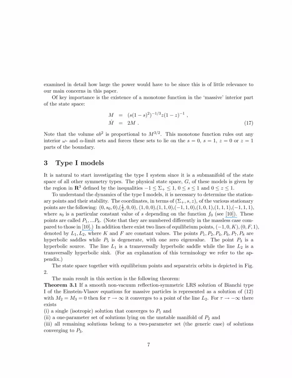
The state space together with equilibrium points and separatrix orbits is depicted in Fig.2.

The main result in this section is the following theorem:Theorem 3.1 If a smooth non-vacuum reflection-symmetric LRS solution of Bianchi typeI of the Einstein-Vlasov equations for massive particles is represented as a solution of (12)with M2 = M3 = 0 then for τ → ∞ it converges to a point of the line L2. For τ → −∞ thereexists(i) a single (isotropic) solution that converges to P1 and(ii) a one-parameter set of solutions lying on the unstable manifold of P2 and(iii) all remaining solutions belong to a two-parameter set (the generic case) of solutionsconverging to P3.

7

P

Σ

z

s

+

P

P

P

P

LL

8

5

12

1

7

P2 P3

6P

4

Figure 2: The LRS type I state space together with equilibrium points and separatrix orbits.

This will be proved in a series of lemmas. We refer to [13, 10] for terminology from thetheory of dynamical systems.Lemma 3.1 There exist open neighbourhoods U1 and U2 of the point P3 and the line L2

respectively such that:(i) if a solution belongs to U1 at any time it belongs to U1 at all earlier times and its α-limitset consists of the point P3 alone.(ii) if a solution belongs to U2 at any time it belongs to U2 at all later times and its ω-limitpoint consists of a single point of the line L2.Proof Part (i) follows from the fact that P3 is a hyperbolic source and the Hartman-Grobmantheorem. Part (ii) follows from the fact that L2 is a transversally hyperbolic sink and thereduction theorem ([10], Theorem A1).

As a step towards analysing the dynamics of the full system we determine the ω-limitpoints of solutions of the dynamical system on the parts of the boundary of G defined bys = 0 and s = 1. This information will later be combined with the monotone function Mwhen determining the ω-limit sets of solutions of the full system. In the case of the α-limitsets the monotone function alone accomplishes the same thing.Lemma 3.2 A solution of the restriction of the system to the part of the boundary of Gdefined by s = 1 for which neither z nor Σ+ take on one of their limiting values has the

8

endpoint of L2 with s = 1 as its ω-limit set.Proof If Σ+ ≥ 0 at any time, then Σ+ is decreasing. The rate of decrease remains uniformas long as Σ+ does not tend to zero. It follows that after a finite time Σ+ must be strictlyless than 1/2. On the other hand, z is monotone increasing in the region Σ+ < 1/2 and therate of increase remains uniform as long as z does not tend to one. It follows that z → 1 asτ → ∞. If Σ+ tends to zero in this limit then the conclusion of the lemma holds. OtherwiseΣ+ must become negative at some time. Thus it can be seen that any ω-limit points satisfyz = 1 and −1 ≤ Σ+ ≤ 0. From part (ii) of Lemma 3.1 it follows that any solution whichenters U2 has the desired ω-limit set. Since the ω-limit set is a union of orbits, it is possibleas a consequence to exclude the points with z = 1 and −1 < Σ+ < 0 from the ω-limit set. Tocomplete the proof of the lemma it remains only to exclude the point P8 from the ω-limit set.This point is a hyperbolic saddle of the restriction of the system to s = 1 and so it followsfrom the discussion in the appendix and what has been proved already that it cannot belongto the ω-limit set. For if P8 belonged to the ω-limit set points of its stable and unstablemanifolds would also have to do so, and this has already been ruled out.Lemma 3.3 A solution of the restriction of the system to the part of the boundary of Gdefined by s = 0 for which neither z nor Σ+ take on one of their limiting values has theendpoint of L2 with s = 0 as its ω-limit set.Proof Along any solution of this system z is monotone increasing on the part of the statespace of the restricted dynamical system with Σ+ 6= −1 and z(1 − z) 6= 0. Hence, by themonotonicity principle (see [13]), any ω-limit point must satisfy z = 1 or Σ+ = −1. HoweverΣ+ is increasing for Σ+ close to but not equal to −1. Hence there can be no ω-limit pointswith Σ+ = −1. It follows that z tends to one as τ → ∞ for any solution and any ω-limitpoint satisfies z = 1. From Lemma 3.1, any solution which enters U2 has the desired ω-limitset. Arguing as in the proof of Lemma 3.3 allows points with −1 < Σ+ < 0 and 0 < Σ+ < 1to be excluded. The point P6, which is a hyperbolic saddle of the restricted system, can beeliminated in the same way as was done in the case of P8 in the proof of Lemma 3.2 using theresults of the discussion in the appendix. Finally, the non-existence of ω-limit points withΣ+ = −1, already mentioned above, shows that the endpoint of the line L1 cannot lie in theω-limit set.Lemma 3.4 If a solution lies in the interior of G, then unless it lies on the unstable manifoldof P1 or P2 its α-limit set consists of the point P3.Proof Consider a solution in the interior of G which does not lie on the unstable manifoldof P1 or P2. If it intersects U1 then by Lemma 3.1 its α-limit set consists of the point P3.There can be no other α-limit points in U1. Because the function M tends to zero along thesolution as τ → −∞ the α-limit set must be contained in the surface z = 0. Recall that thesurface z = 0 corresponds to the case of massless particles which was analysed completely in[10]. (Note that the stationary points were numbered differently in that paper.) Considerthe boundary of the surface z = 0. Arguing as in the proof of Lemma 3.2, the lines joining

9

P3 to P2 and P4 can be excluded from the α-limit set. The discussion of the appendix andthe fact that P4 is a hyperbolic saddle with stable manifold Σ+ = 1 and unstable manifoldthe line connecting P4 to P5 can be used to exclude that line and the point P4 itself. Theline connecting P5 to the endpoint of the line L1 can be excluded in an analogous way, notingthat the non-hyperbolic point P5 is also covered by the discussion of the appendix. The pointP5 is also excluded by this argument. Applying the reduction theorem allows the line joiningthe endpoint of the line L1 to P2 to be excluded together with the endpoint of L1. At thisstage we can also exclude the point P2 itself, using the results of the appendix again and thefact that by assumption the solution does not lie on the unstable manifold of P2. Thus theonly point of the boundary of the set z = 0 which can belong to the α-limit set is P3. Nowsuppose that a point of the interior of the surface belongs to the α-limit set. If it is a pointof the unstable manifold of P2 then P2 also belongs to the α-limit set, in contradiction towhat has just been proved. If it is some other point other than P1 then, using the fact thatthe α-limit set is a union of orbits and Theorem 3.1 of [10], it follows that P3 belongs to theα-limit set and we obtain a contradiction again. Finally, if it were P1 then the results of theappendix would imply that other points of the interior would belong to the α-limit set, andthis has just been ruled out.Lemma 3.5 The ω-limit point of each solution in the interior of G is a point of the line L2.Proof Note first that the function M goes to infinity along any such solution as τ → ∞.It follows that any ω-limit point must satisfy z = 1, s = 0 or s = 1. If the solution entersthe set U2 then by part (ii) of Lemma 3.1 the ω-limit set is as claimed. There are no otherω-limit points of any solution in U2. Consider now the evolution of Σ+ on the surface z = 1.It either increases from −1 to 0 or decreases from 1 to 0. Since the ω-limit set is a union oforbits, we conclude that no point of the interior of the surface z = 1 or its boundary liness = 0 and s = 1 other than the points of the line L2 can belong to the ω-limit set. Using oncemore the fact that the ω-limit set is a union of orbits, it is possible to exclude the interiorof the surface s = 1 from the ω-limit set by Lemma 3.2 and the interior of s = 0 by Lemma3.3. Now all remaining possibilities other than points on L2 will be excluded successively.The nature of the line L1 as a transversely hyperbolic saddle suffices to eliminate it, as wellas the lines joining it to P8 and P2. The point P3, being a hyperbolic source, is clearly ruledout, and with it the lines joining it to P2 and P6. Further applications of the results of theappendix rule out the remaining lines, namely those joining P8 to P5, P5 to P4, P4 to P7 andP7 to P6. It follows that the ω-limit set is contained in the line L2. Applying the reductiontheorem then shows that the ω-limit set is a single point of L2.

The results of Lemma 3.4 and Lemma 3.5 together imply Theorem 3.1.Theorem 3.1 has been formulated entirely in terms of the dynamical systems picture. It

should, however, be pointed out that this allows asymptotic expansions for all quantities ofgeometrical or physical interest near the singularity or in an expanding phase to be obtained

10

if desired. For example, in an expanding phase in type I the following expansions can bederived:

Σ+ = αt−1 + o(t−1) (18)

s = s0 −49s0(1 − s0)t

−1 + o(t−1) (19)

z = 1 − βt−4/3 + o(t−4/3) (20)

H = 23 t−1 + O(t−7/3) (21)

Ω = 1 − αt−2 + o(t−2) (22)

ρ = 49 t−2 − 4

3α2t−4 + o(t−4) (23)

p1 = O(t−10/3) (24)

Here α and β are constants depending on the solution. It should be emphasized that these arenot just formal expansions, but rigorous results which emerge from the dynamical systemsanalysis.

A particular consequence of Theorem 3.1 is that all LRS type I models isotropize at latetimes. This was already proved by other means in [9], where it was also shown that non-LRSmodels of Bianchi type I isotropize and have dust-like behaviour for τ → ∞.

4 Type II models

The physical state space, G, of the LRS type II models is given by the region in R4 defined

by the inequalities M2 ≥ 0, 0 ≤ s ≤ 1, 0 ≤ z ≤ 1, and 1 − Σ2+ − M2 ≥ 0.

The coordinates, in terms of (Σ+, s, z,M2), of the various stationary points are the follow-ing: (0, s0, 0, 0),(

12 , 0, 0, 0), (1, 0, 0, 0),(1, 1, 0, 0),(−1, 1, 0, 0),(1, 0, 1, 0),(1, 1, 1, 0),(−1, 1, 1, 0),

(15 , 1, 0, 6

25),(18 , 0, 1, 3

64 ),(18 , 1, 1, 3

64 ), where s0 is the same particular constant value of s thatappeared in the previous type I section. These points are called P1, ...P11 (note that they arenumbered differently than in [10], in the massless case). In addition there exist two lines ofequilibrium points, (−1, 0,K, 0), (0, F, 1, 0), denoted by L1, L2, where K and F are constants.The first eight stationary points and the two lines correspond to points and lines of the samename in the Bianchi I system and their coordinates are obtained by appending a zero to thoseof the Bianchi I points. The points P1, P2, P3, P4, P6, P7, P8, P9, P10 are hyperbolic saddleswhile P5 is degenerate, with one zero eigenvalue. The point P11 is a hyperbolic sink with tworeal and two complex eigenvalues. The lines L1 and L2 are transversally hyperbolic saddles.

To prove results about the global properties of solutions it is helpful to use certain mono-tone functions. The first is defined for s < 1 by

Z1 = (2s/(1 − s))4/3M2 (25)

11

This is obtained by rewriting the function whose time derivative was calculated in equation(23) of [10] in terms of the variables of this paper and observing that it remains monotonein the massive case. It satisfies Z1 = 2qZ1. The second is obtained by combining Z1 withthe monotone function M available for all the Bianchi types considered in this paper. LetZ2 = Z1M

−2 = 24/3s2M2z−2(1− z)2 for z > 0. It satisfies Z2 = 2(q − 2)Z2. The function Z1

is defined on the part of the Bianchi II state space where s 6= 1 and monotonically increasingexcept where it vanishes. This is clear if q 6= 0. If q = 0 it follows that Σ+ = 0 and M2 = 1and at points satisfying these conditions Σ+ 6= 0. The function Z2 is defined on the partof the Bianchi II state space where z > 0 and is monotonically decreasing except on the setwhere it vanishes, since q = 2 implies Z2 = 0.Theorem 4.1 If a smooth non-vacuum reflection-symmetric LRS solution of Bianchi typeII of the Einstein-Vlasov equations for massive particles is represented as a solution of (12)with M3 = 0, then for τ → ∞ it converges to P11. For τ → −∞ there exists(i) a one-parameter set of solutions converging to the unstable manifold of P1 and(ii) a three-parameter set of all remaining solutions converging to the heteroclinic cycle onthe z = 0 submanifold, consisting of the orbits connecting the z = 0 endpoint of the line L1

to P5, P5 to P4, P4 to P3 on the type I boundary and P3 to the z = 0 endpoint of the line L1

via the vacuum boundary.Lemma 4.1 If a solution belongs to the interior of the type II state space then any α-limitpoint satisfies z = 0 and sM2 = 0. Any ω-limit point satisfies s = 1 and (z − 1)M2 = 0.Proof From the evolution equation for M it follows that z = 0 for any α-limit point and thatfor any ω-limit point z = 1, s = 0 or s = 1. Next the monotonicity principle will be appliedto the functions Z1 and Z2. Applying it to Z1 on the region where Z1 6= 0 shows that forany α-limit point s = 0 or M2 = 0. It also shows that there are no ω-limit points with s = 0.Combining this with the information obtained already shows that any ω-limit point satisfiesz = 1 or s = 1. If z 6= 1 then it follows from the monotonicity principle applied to Z2 thatM2 = 0 for any ω-limit point. The monotonicity of Z1 then implies that s → 1 as τ → ∞.Lemma 4.2 Consider the dynamical system obtained by restricting the type II system tothe plane defined by the conditions s = 1 and z = 1. If a solution belongs to the interior ofthe state space for this restricted system then it converges to P11 as τ → ∞.Proof The restricted dynamical system is identical with that for type II dust solutions. In[13] it was proved by using a monotone function derived by Hamiltonian methods that forτ → ∞ the dust solutions satisfy Σ+ → 1

8 and M2 → 364 . Hence it can be concluded that the

solution approaches P11 as τ → ∞.Lemma 4.3 If a solution lies in the interior of the type II state space then unless it lies onthe unstable manifold of P1 (and this does occur) the α-limit set consists of the heterocliniccycle described in the statement of Theorem 4.1.Proof By Lemma 4.1 we know that any α-limit point satisfies z = 0. Moreover it satisfiesM2 = 0 or s = 0. The situation is very similar to that in the massless case treated in [10]

12

and the proof may be taken over rather directly. It is only necessary to pay attention to thefact that it is the nature of the stationary points in the full massive Bianchi II state spacewhich must be taken into account and that the notation is different.

Suppose that the α-limit set contains a point with s = 0 and M2 6= 0. Then by Lemma4.3 of [10] it contains the endpoint of L1 and either P2 or P3. On the other hand, if itcontains a point with M2 = 0 then this belongs to the massless Bianchi I state space. Thenit must contain one of the points P1, P2, P3, P4, P5 or the endpoint of L1. To prove thelemma we may assume that the solution does not lie on the unstable manifold of P1. If P1

nevertheless belonged to the α-limit set then this set would have to include points belongingto the unstable manifold of P1 other than P1 itself. But these satisfy neither s = 0 norM2 = 0 and so this gives a contradiction. Thus under the given assumptions the α-limitset does not contain P1. If the α-limit set contained a point with M2 = 0, |Σ+| < 1 and0 < s < 1 it would contain P1 (in its role as ω-limit set for Bianchi type I solutions), leadingonce more to a contradiction. If the α-limit set contained P2 then by the results of theappendix it would contain P1, which is also not possible. Applying Lemma 4.3 of [10] againallows points with M2 6= 0 which are not on the vacuum boundary to be excluded from theα-limit set. The straight lines joining P2 to P3 and the endpoint of L1 are excluded as well.The conclusion is that the α-limit set is contained in the heteroclinic cycle mentioned in thestatement of Theorem 4.1. It remains to show that it is the whole heteroclinic cycle. This isstraightforward to do using the results of the appendix.Lemma 4.4 If a solution lies in the interior of the type II state space then it converges tothe point P11 as τ → ∞.Proof Consider any ω-limit point with z 6= 1. Then by Lemma 4.1 this point satisfies s = 1and M2 = 0. Any nearby ω-limit points must also satisfy these conditions. If any of theselimit points satisfied z = 0 then P4 and P5 would be ω-limit points of the given solution.Using the saddle point properties of these points then shows that P7 and P8 belong to theω-limit set. Repeating the same argument shows that the endpoint of L1 with s = 1 is anω-limit point. The fact that this point is a transversely hyperbolic saddle implies that itsunstable manifold in the hyperplane s = 1 is contained in the ω-limit set. By Lemma 4.2 theω-limit set also contains P11. Since P11 is a hyperbolic sink this contradicts the assumptionz 6= 1. Thus we conclude that the entire ω limit set is contained in the plane defined bythe equations s = 1 and z = 1. The argument just given rules out the possibility of ω-limitpoints with M2 = 0. Applying Lemma 4.2 once more shows that the only possible ω-limitpoint which does not lie on the vacuum boundary is P11. Finally the fact that P7 and P8 arehyperbolic saddles can be used to rule out points of the vacuum boundary, thus completingthe proof.

13

5 Type III models

The physical state space, G, of the LRS type III models is given by the region in R4 defined

by the inequalities M3 ≥ 0, 0 ≤ s ≤ 1, 0 ≤ z ≤ 1, and 1 − Σ2+ − M3 ≥ 0.

The coordinates, in terms of (Σ+, s, z,M3), of the various stationary points are the follow-ing: (0, s0, 0, 0),(

12 , 0, 0, 0), (1, 0, 0, 0),(1, 1, 0, 0),(−1, 1, 0, 0),(1, 0, 1, 0),(1, 1, 1, 0),(−1, 1, 1, 0),

(12 , 0, 0, 3

4),(12 , 0, 1, 3

4), where s0 the same particular constant value of s that appeared in theprevious type I section. These points are called P1, ...P10 (note that they are numbered dif-ferently than in [10], in the massless case). In addition there exist three lines of equilibriumpoints, (−1, 0,K, 0, 0), (0, F, 1, 0, 0), ( 1

2 , 1, z0,34 ), denoted by L1, L2, L3, where K,F and z0 are

constants. The first eight stationary points and the first two lines correspond to points andlines of the same name in the Bianchi I system and their coordinates are obtained by append-ing a zero to those of the Bianchi I points. The points P1, P2, P4, P6, P7, P8, P9 are hyperbolicsaddles while P5 and P10 are degenerate, with one zero eigenvalue each. The point P3 is ahyperbolic source. The lines L1 and L2 are transversally hyperbolic saddles while the line L3

is degenerate with two zero and two negative eigenvalues.To prove global results about the global properties of solutions it is useful to note the

existence of the following bounded monotone function

M3 = M3(2 − Σ+)−2 ,

˙M3 = 2M3[(1 − 2Σ+)2 + Ω(R + R+)](2 − Σ+)−1 . (26)

Theorem 5.1 If a smooth non-vacuum reflection-symmetric LRS solution of Bianchi typeIII of the Einstein-Vlasov equations for massive particles is represented as a solution of (12)with M2 = 0, then for τ → ∞ it converges to a point of the line L3 with z > 0. For τ → −∞there exists(i) a one-parameter set of solutions lying on the unstable manifold of P1 and(ii) a two-parameter set of solutions lying on the unstable manifold of P2 and(iii) all remaining solutions converge to P3.In all these solutions the scale factor a is monotone increasing at late times.Lemma 5.1 If a solution belongs to the interior of the type III state space any α-limit pointsatisfies M3 = 0. Any ω-limit point satisfies Σ+ = 1

2 , M3 = 34 and s = 1.

Proof The continuous function M3 on the state space must have a maximum and since itsgradient never vanishes this maximum can only be attained at points with M3 = 1 − Σ2

+.

Computing the derivative of M3 along the curve in the (M3,Σ+) plane defined by this relationshows that the maximum value is 1

3 and that it is attained when Σ+ = 12 and M3 = 3

4 . Now weapply the monotonicity principle. Let S be the part of the Bianchi III state space obtainedby removing the points with M3 = 0 and those with Σ+ − 1

2 = M3 − 34 = 0. This is an

invariant set for the dynamical system. It will now be shown that M3 is strictly increasing

14

along solutions on this set. If Σ+ 6= 12 or if Ω(R + R+) 6= 0 then this follows immediately

from (26). If Σ+ = 12 and Ω(R + R+) = 0 then

Σ+ = 34(M3 −

34) (27)

This completes the proof that M3 is strictly increasing on S. The monotonicity principlethen shows that any point in the α-limit set must be in the complement of S and such thatsuch that M3 does not take on its maximum value on S there. Hence M3 = 0 there. It alsoshows that any point in the ω-limit set must be in the complement of S and that M3 doesnot take on its minimum value there. Hence in the latter case Σ+ = 1

2 and M3 = 34 . It follows

from this that Σ+ → 12 as τ → ∞ and the equation for s then implies that s → 1.

Lemma 5.2 A solution which belongs to the interior of the type III state space converges toa point of the line L3 with z > 0 as τ → ∞.Proof Because of the result of Lemma 5.1 it only remains to prove that z tends to a positivelimit as τ → ∞. Note first that the evolution equation for s implies an equation of the form(d/dτ)(1 − s) = (1 − s)F where F = −6sΣ+. As τ tends to infinity F → −3 and a simplecomparison argument proves that 1 − s(τ) = O(e(−3+ǫ)τ ) as τ → ∞. In particular, 1 − sdecays exponentially to zero at late times. The evolution equations imply that Ω satisfies theequation:

Ω/Ω = (Σ+ − 12 )[(3 − R)Σ+ + 3

2(1 + R)] − 2Σ+(R+ + R) − (M3 −34)(1 + R) (28)

Note that R+ +R ≥ 0 so that the second term on the right hand side is negative. However itis exponentially small at late times since it contains a factor (1− s) when expressed in termsof the matter quantities. In particular Ω/Ω → 0 as τ → ∞ and Ω−1 = O(eǫτ ) for any ǫ > 0.This means that Ω converges to zero slower than any exponential. In other words, Ωeǫτ tendsto infinity for any ǫ > 0. Suppose that Σ+ ≥ 1

2 for some solution at some time. Then M3 ≤ 34

and the first and third terms in the expression for Ω/Ω are positive at late times while thesecond term is negative. It will now be shown that the third term decays slower than anyexponential and thus must eventually dominate the second term. For

Ω = (14 − Σ2

+) + (34 − M3) ≤ (3

4 − M3) (29)

It follows that Ω/Ω > 0 at late times as long as Σ+ > 12 . Since it follows from Lemma 5.3

that Ω → 0 as τ → ∞ it follows that for any time τ0 for which Σ+(τ0) > 12 there exists a

time τ > τ0 with Σ+ = 12 . When Σ+ = 1

2 then

Σ+ = (M3 −34)[34 (1 − R) − 1

4(R + R+)] (30)

Now it follows from the evolution equation for z that 1− z cannot approach zero faster than,for instance, e−τ and the same is then true of 1−R. It can be concluded that the first term in

15

the square bracket on the right hand side of (30) dominates the second at late times. Hence12 − Σ+ must be negative at late times, which in turns implies that z is increasing and thatit must tend to a positive limit.Lemma 5.3 If a solution lies in the interior of the type III state space then unless it lies onthe unstable manifold of P1 or P2 (and both of these cases occur) the α-limit set consists ofthe point P3.Proof Note first that it can be concluded as in the proof of Lemma 3.4 that any α-limit pointsatisfies z = 0. Thus, applying Lemma 5.1, it can be identified with a point of the state spacefor massless type I solutions. Now it is possible to proceed further following the method ofproof of Lemma 3.4. Consider the boundary of the state space for massless type I solutions.The point P3, being a hyperbolic source in the type III state space, can be excluded as anα-limit point of a solution of type III. It is then possible to successively exclude points ofthe boundary as in the proof of Lemma 3.4. The facts which need to be used are that allα-limit points satisfy M3 = 0 and z = 1 and that the points P4, P5 and the endpoint ofL1 are a hyperbolic saddle, a non-hyperbolic saddle topologically equivalent to a hyperbolicone and a transversely hyperbolic saddle, respectively. At this stage it can be concludedthat all α-limit points of solutions of type III are either P1, P2 or points of the unstablemanifold of P1. For all other points of the interior of the massless type I state space lie onsolutions which converge to the hyperbolic source P3 in the past time direction, and so areexcluded. It remains to examine what happens in a neighbourhood of the points P1 and P2,which are both hyperbolic saddles. The unstable manifold of P2 in the type III state spaceis three-dimensional and so there are solutions which converge to P2 as τ → −∞. Any othertype III solutions which had P2 as an α-limit point would have to have α-limit points on thestable manifold of P2, which has already been excluded. Hence solutions of type III which donot converge in the past to P2 cannot have P2 or a point of its unstable manifold as α-limitpoints. Thus the only remaining possibility is that solutions lie on the unstable manifold ofP1 and converge to that point in the past. Since the unstable manifold is two-dimensional,solutions of this kind exist.

The results of Lemma 5.2 and Lemma 5.3 together imply all the results of Theorem 5.1 exceptthe last directly. The statement about the scale factor a follows from the fact, derived in thecourse of the proof of Lemma 5.2, that Σ+ < 1

2 at late times.

6 Concluding remarks

In this paper we studied the dynamics of solutions of the Einstein-Vlasov equations which arelocally rotationally symmetric, reflection-symmetric and of Bianchi types I, II and III. Theinitial singularities are of four types. There are isotropic singularities which, in the dynamical

16

systems description used in this paper, are those which converge to the point P1 as τ → −∞.The general theory of isotropic singularities developed by Anguige and Tod [2, 1] implies as avery special case the occurrence of isotropic singularities in Bianchi models with collisionlessmatter and information about how many there are. They only developed the theory formassless particles and so in order to apply to the situations considered here it would haveto be generalized to the massive case. There are barrel singularities which occur in types Iand III but not in type II. In the dynamical systems picture these are the solutions whichconverge to P2 as τ → −∞. Fluid models with corresponding symmetries never have barrelsingularities and so this is a peculiarity of collisionless matter, both in the case of massiveparticles studied here and that of massless particles studied in [10]. There is the generic casein types I and III, which concerns solutions which develop from an open dense set of initialdata for each of these Bianchi types. These solutions have a cigar singularity and converge toP3 as τ → −∞. Finally, there are the generic solutions of type II, which have an oscillatoryinitial singularity.

As far as the late time behaviour is concerned, it is tempting to speculate that behavinglike a dust model at late times in an expanding phase may be a general feature of solutions ofthe Einstein-Vlasov equations with massive particles. We know of no counterexample to this.For the solutions of types I and II treated in this paper it has been proved to be true. For typeIII the situation appears to be delicate and the occurrence of degenerate stationary pointsof the dynamical system may require an application of centre manifold theory in order todetermine details of the asymptotics. A possible criterion for detecting cases where there maybe trouble is as follows. Consider a dust solution which is a candidate for the asymptotic stateof solutions of the Einstein-Vlasov equations. If each eigenvalue of the second fundamentalform of the homogeneous hypersurfaces, when divided by the mean curvature, is boundedbelow by a positive constant in the dust solution then it is a strong candidate. Otherwisedifficulties are to be expected. This criterion gives a positive recommendation for types I andII and a warning for type III. Thus at least for the models investigated in this paper it is agood guide. Using the information on dust models in chapter 6 of [13] it also gives a positiverecommendation for types I, II and VI0 without the need to restrict to the LRS case.

In this paper a dynamical system has been set up for all LRS Bianchi models of classA as well as for Kantowski-Sachs models and the type III models, which are of class B. Weexpect that techniques similar to those used here can be applied to analyse Kantowski-Sachsmodels and LRS models of type VIII and IX. An important feature of all these LRS modelsis that the Vlasov equation can be solved exactly. This is also true of general Bianchi typeI models. Some limited results on the dynamics of Bianchi type I solutions of the Einstein-Vlasov equations which are reflection-symmetric but not necessarily LRS were proved in[9]. A heuristic analysis of reflection-symmetric type I models was given using Hamiltoniantechniques in [7], where there are also interesting remarks on the general Bianchi I case. Itwould be very desirable to have a mathematically rigorous implementation of the ideas of [7].

17

What can be done in cases where the Vlasov equation cannot be solved exactly? If, asalready speculated above, the late time evolution resembles that of a dust solution and if thedust solutions are asymptotically LRS then it may be possible to give a good approximationto the solution of the Vlasov equation in that regime. There is one drawback of this ideaas a general tool for Bianchi class A models. Unfortunately there are no LRS spacetimes ofBianchi type VI0. In the case of fluids there exists a special class of Bianchi VI0 spacetimeswhich is often characterized by the rather opaque statement that nα

α = 0. These spacetimesdo have a simple geometric characterization which will now be explained. Every Bianchiclass A spacetime has a discrete group of isometries whose generators simultaneously reversetwo of the invariant one-forms on the group. The special class of Bianchi VI0 solutionscan be characterized by the existence of an additional isometry which reverses just one ofthe one-forms. It is possible to consider solutions of the Einstein-Vlasov equations with thecorresponding type of symmetry. We are, however, not aware that the Vlasov equation canbe solved exactly in these special spacetimes. If it could then this might fill the apparent gapin the strategy just suggested.

The oscillatory behaviour observed near the singularity in type II models appears at firstsight to indicate that collisionless matter does not fit into the analysis of general spacetimesingularities by Belinskii, Khalatnikov and Lifshitz [4]. On the other hand, the fact thatin the analysis of Misner [7] using a time-dependent potential we see the phenomenon ofwalls moving too fast to be caught suggests that the oscillations might go away in generalmodels. This issue requires further work. It could turn out that collisonless matter genericallybecomes negligible near the singularity, as originally stated for fluids in [4].

To conclude, we mention some further interesting open problems. What happens in thecase of a model with two species of particles, one massive and one massless? Of course thiscould be thought of as a simple cosmological model incorporating both baryonic matter andthe microwave background photons. It is related to the two-fluid models which have beenanalysed in [5]. Mixtures of fluids and kinetic theory could also be considered. We have seenthat the Einstein equations with collisionless matter as source may behave very differentlyfrom the Einstein equations with a fluid source at early times (and also at late times in themassless case). Under what circumstances are there intermediate stages of the evolution withcollisionless matter which can be well described by a fluid? Since the point P1 is a saddle thereare obviously solutions which approach this point and then go away again but is there morethat can be said about this issue? What can be said about inhomogeneous models? In [8]Rein analysed the behaviour at early times of solutions of the Einstein-Vlasov equations withspherical, plane and hyperbolic symmetry and massive particles. He identified open subsets ofinitial data for these symmetry types with a singularity resembling the generic LRS solutionsof types I and III. There is an overlap between the results of [8] and those of the presentpaper. It could be illuminating to attempt a common generalization of these. In any case, itis clear that one of the central challenges of the future in the study of cosmological solutions

18

of the Einstein-Vlasov equations, or indeed the Einstein equations coupled to any type ofmatter fields, is to develop techniques which apply to inhomogeneous problems. A thoroughunderstanding of the homogeneous case is likely to be an invaluable guide in addressing it.

A Appendix

In this appendix some general procedures which are useful in determining limit sets of solu-tions of dynamical systems will be outlined. Let γ be an orbit of a dynamical system andp a stationary point. We will discuss only ω-limit sets, but corresponding statements aboutα-limit sets follow immediately by reversing the direction of time. We consider the followingthree statements which may or may not be true for given choices of γ and p.

1. p is an ω-limit point of γ

2. γ lies on the stable manifold of p

3. there are ω-limit points of γ different from p which are arbitrarily close to p and lie onthe unstable manifold of p

4. there are ω-limit points of γ different from p which are arbitrarily close to p and lie onthe stable manifold of p

In the body of the paper we frequently use certain relations among the statements abovewhich hold under various assumptions on the nature of the stationary point p. Whatever thestationary point, it is always true that the statement 1. is implied by any of the statements2., 3. or 4. This is a consequence of the elementary fact that the ω-limit set is closed. Nowsuppose that p is a hyperbolic stationary point. In this case, if 1. is true and 2. is false thenboth 3. and 4. are true. This follows from Lemma A1 of [10]. Combining these statementswe see that for a hyperbolic stationary point there are two mutually exclusive cases underwhich 1. can hold. Either γ lies on the unstable manifold of p or the ω-limit set containspoints of both the stable and unstable manifolds of p arbitrarily close to p. In particular,if p is a hyperbolic source then it cannot be in the ω-limit set of γ and if p is a hyperbolicsink and p is in the ω-limit set of γ it is the whole ω-limit set. If we already have some apriori information about where ω-limit points can lie (due, for instance, to the existence ofa monotone function) then this gives more information about where the points on the stableand unstable manifolds whose existence is guaranteed by the general statements above canlie.

Next we consider the case of transversally hyperbolic stationary points. Suppose that pbelongs to a manifold of stationary points of dimension d. (Only the case d = 1 occurs inthis paper.) These points have a zero eigenvalue of multiplicity d. If all other eigenvalues

19

have non-vanishing real parts then the stationary point is called transversally hyperbolic.(Depending on the signs of the eigenvalues the manifold of stationary points is called atransversally hyperbolic source, sink or saddle.) By the reduction theorem (Theorem A1 of[10]) each of these points lies on an invariant manifold and the restriction of the flow to eachinvariant manifold is topologically equivalent to that near a hyperbolic stationary point. Thearguments for a hyperbolic stationary point adapt easily to give analogous statements fortransversally hyperbolic stationary points. In applying these results we can essentially ignorethe directions along the manifold of stationary points.

Finally we consider certain other non-hyperbolic stationary points. A result of the type weneed was proved in Lemma A2 of [10] but we would like to formulate the statement in a moretransparent way here. Consider an isolated stationary point p with a trivial stable manifoldand a one-dimensional centre manifold. Using the reduction theorem we see that the unstablemanifold divides a neighbourhood of p into two parts on each of which the restriction of thedynamical system is topologically equivalent to the restriction of a dynamical system with ahyperbolic stationary point. Whether the latter system has a saddle or a source depends on acertain sign condition. This condition may be different for the two halves. In the dynamicalsystems considered in this paper the only example of this is provided by the point P5. Onlyone of the halves belongs to the physical part of the state space and in that half the sign issuch that a saddle is obtained. The result of these considerations is that for the argumentsin this paper P5 may be treated just as if it had been a hyperbolic saddle, with the centremanifold taking over the role of the trivial stable manifold.

References

[1] Anguige K 1999 Isotropic cosmological singularities 3: The Cauchy problem for theinhomogeneous conformal Einstein-Vlasov equations. Preprint gr-qc/9903018.

[2] Anguige K and Tod K P 1999 Isotropic cosmological singularities 2: The Einstein-Vlasovsystem. Ann. Phys. (NY) 276 294-320

[3] Ashtekar A, Tate R S and Uggla C 1993 Minisuperspaces: observables and quantization.Int. J. Mod. Phys. D 2 15-50

[4] Belinskii V A, Khalatnikov I M and Lifshitz E M 1982 A general solution of the Einsteinequations with a time singularity. Adv. Phys. 31 639-67

[5] Coley A A and Wainwright J 1992 Qualitative analysis of two-fluid Bianchi cosmologies.Class. Quantum Grav. 9 651-665

20

[6] Jantzen R T 1987 Proc. Int. Sch. Phys. ‘E Fermi’ Course LXXXVI on ‘Gamov Cos-mology’ ed R Ruffini and F Melchiorri (Amsterdam: North Holland); 1984 Cosmologyof the Early Universe ed L Z Fang and R Ruffini (Singapore: World Scientific)

[7] Misner C W 1968 The isotropy of the universe. Astrophysical Journal 151 431-457

[8] Rein G 1996 Cosmological solutions of the Vlasov-Einstein system with spherical, planeor hyperbolic symmetry. Math. Proc. Camb. Phil. Soc. 119 739-762

[9] Rendall A D 1996 The initial singularity in solutions of the Einstein-Vlasov system ofBianchi type I. J. Math. Phys. 37 438-451

[10] Rendall A D and Tod K P 1999 Dynamics of spatially homogeneous solutions of theEinstein-Vlasov equations which are locally rotationally symmetric. Class. QuantumGrav. 16 1705-1726

[11] Uggla C and von Zur-Muhlen H 1990 Compactified and reduced dynamics for locallyrotationally symmetric Bianchi type IX perfect fluid models. Class. Quantum Grav. 7

1365-1385

[12] Uggla C, Jantzen R T and Rosquist K 1995 Exact hypersurface-homogeneous solutionsin cosmology and astrophysics. Phys. Rev. D 51 5522-5557.

[13] Wainwright J and Ellis G F R 1997 Dynamical Systems in Cosmology (Cambridge:Cambridge University Press)

21