arX

iv:0

706.

1488

v2 [

cond

-mat

.mes

-hal

l] 5

Mar

200

8

Dynamical matrix of bidimensional electron crystals

R. Cote,1 M.-A. Lemonde,1 C. B. Doiron,2 and A. M. Ettouhami3

1Departement de physique and RQMP, Universite de Sherbrooke, Sherbrooke, Quebec, Canada, J1K 2R12Department of Physics, University of Basel, Klingelbergstrasse 82, CH-4056 Basel, Switzerland

3Department of Physics, University of Toronto, 60 St. George St., Toronto, Ontario, Canada, M5S 1A7

(Dated: March 5, 2008)

In a quantizing magnetic field, the two-dimensional electron (2DEG) gas has a rich phase diagramwith broken translational symmetry phases such as Wigner, bubble, and stripe crystals. In thispaper, we derive a method to get the dynamical matrix of these crystals from a calculation of thedensity response function performed in the Generalized Random Phase Approximation (GRPA).We discuss the validity of our method by comparing the dynamical matrix calculated from theGRPA with that obtained from standard elasticity theory with the elastic coefficients obtained froma calculation of the deformation energy of the crystal.

PACS numbers: 73.20.Qt,73.21.-b,73.43.-f

I. INTRODUCTION

Theoretical calculations show that, in the presence ofa perpendicular magnetic field, a two-dimensional elec-tron gas (2DEG) should crystallize below a filling factorν ∼ 1/6.51. Several experimental groups have reportedtransport measurements indicative of this electron crys-tallization when the filling factor of the lowest Landaulevel is decreased below ν = 1/5. These measurementsinclude the observation of a strong increase in the diago-nal resistivity ρxx, non-linear I − V characteristics, andbroadband noise. All these observations have been in-terpreted as the pinning and sliding of a Wigner crystal(WC)2. Moreover, microwave absorption experiments3

have also detected a resonance in the real part of the lon-gitudinal conductivity, σxx (ω), that has been attributedto the pinning mode of a disordered Wigner crystal. Thevanishing of the pinning mode resonance at some criticaltemperature Tm (ν) has been used to derive the phasediagram of the crystal4 in the quantum regime wherethe kinetic energy is frozen by the quantizing magneticfield. Similar microwave absorption experiments alsoshowed a pinning resonance at higher filling factors closeto ν = 1, 2, 3 where the formation of a Wigner solid isexpected in very clean samples5,6,7. Finally, in Landaulevels of index N > 1, a study of the evolution of the pin-ning mode with filling factor reveals several transitions ofthe 2DEG ground state from a Wigner crystal at low ν tobubble crystals with increasing number of electrons perlattice site as ν is increased, and into a modulated stripestate (or anisotropic Wigner crystal) near half filling8.

In earlier works9,12, some of us have studied severalcrystalline states of the 2DEG using a combination ofHartree-Fock (HFA) and generalized random-phase ap-proximations (GRPA). In these works, the energy andorder parameters of the crystal were calculated in a self-consistent HFA while the collective excitations were de-rived from the poles of density response functions com-puted in the GRPA. This microscopic approach (HFA+ GRPA) works well at zero temperature but is diffi-cult to generalize to consider finite temperature effects

or to include quantum fluctuations beyond the GRPA.Finite-temperature or quantum fluctuations effects (notalready included in the GRPA), are most easily com-puted by writing down an elastic action for the system.For a crystaline solid, this requires the knowledge of thedynamical matrix (DM) or, equivalently, of the elasticcoefficients of the solid.

A direct way to obtain these elastic coefficients is tocompute the energy required for various static defor-mations of the crystal. Using elasticity theory, eachdeformation energy ∆Ei can be written in the form∆Ei = 1

2Ciu20 where u0 is a parameter characterizing

the amplitude of the deformation and Ci is generally acombination of elastic constants. In the limit u0 → 0, onecan obtain the elastic coefficients by computing the de-formation energy of one or more static deformations andusing the known symmetry relations between the elas-tic constants. Alternatively, one can obtain a DM fromthe GRPA density response function much more directlywithout the need to compute the elastic coefficients10.

In this paper, we compare the DM obtained from thesetwo methods (deformation energy and GRPA) in orderto find the range of validity as well as the limitations ofthe GPRA approach. We first consider the simple case ofan isotropic (triangular) Wigner crystal before tacklingthe more complex anisotropic Wigner crystal12 or stripephase that occurs near half-filling in the higher Landaulevels. We show that although the GRPA method givesa good description of the qualitative behavior of the DMas a function of filling factor, its quantitative predictionsmust be used with caution. As we show below, an averag-ing procedure must be applied to the method in order toobtain a DM in the GRPA that compares favorably withthe one obtained by computing the deformation energy.

Our paper is organized as follows. In Section II, we de-fine the elastic constants needed to build an elastic modelfor the Wigner and stripe crystals. We then explain, inSection III, how these elastic constants can be derived bycomputing the deformation energy of the crystals in theHFA. In section IV, we summarize the GRPA methodof obtaining the dynamical matrix. Our numerical re-

2

sults for the WC are discussed in Section V and those forthe stripe crystal in Section VI. Section VI contains ourconclusions.

II. ELASTIC CONSTANTS AND DYNAMICAL

MATRIX

We describe the elastic deformation of a crystal stateby a displacement field u (R) defined on each lattice siteR. The Fourier transform of this operator is given by:

u (k) =1√Ns

∑

R

e−ik·Ru (R) , (1)

where Ns is the number of lattice sites. In two dimen-sions, the general expression for the deformation energyof a crystal requires the use of 6 elastic coefficients cij

and is given, in the continuum limit, by the followingexpression11:

∆E =1

2

∫dr

[c11e

2x,x + 4c66e

2x,y + 4c62ex,yeyy

](2)

+1

2

∫dr

[2c12ex,xey,y + 4c16ex,xex,y + c22e

2y,y

],

where

eα,β (r) =1

2

(∂uα (r)

∂rβ+

∂uβ (r)

∂rα

)(3)

is the symmetric strain tensor.The Wigner and bubble crystals have a triangular lat-

tice structure for which the following equation holds:

c11 = c22 = 2c66 + c12. (4)

For such a triangular structure, the elastic energy in thelong-wavelength limit can be written in a form that con-tains only two elastic coefficients, namely:

∆E =1

2

∫dr

[c12

(e2

x,x + e2y,y + 2ex,xey,y

)

+ 2c66

(e2

x,x + e2y,y + 2e2

x,y

)]. (5)

The anisotropic stripe state can be seen either as acentered rectangular lattice with two electrons per unitcell or as a rhombic lattice with one electron per unitcell with reflection symmetry in both x and y axis. Thedeformation energy is given by

∆E =1

2

∫dr

[c11e

2x,x + 4c66e

2x,y

]

+1

2

∫dr

[2c12ex,xey,y + c22e

2y,y

]. (6)

In this paper, we assume that the stripes are alignedalong the y axis.

The above formulation of elasticity theory assumesshort-range forces only. For the electronic crystals that

we consider, these forces are of coulombic origin i.e. thehamiltonian of the crystal contains only the Coulomb in-teraction between electrons and the kinetic energy whichis frozen by the quantizing magnetic field. Both the di-rect (Hartree) and exchange (Fock) terms are consideredby the Hartree-Fock approximation as we explain in thenext section. To take into account in the elasticity theorythe long-range part of the Coulomb interaction presentin a crystal of electrons, it is necessary to add to ∆E thedeformation energy ∆EC given by

∆EC =e2

2

∫dr

∫dr′

δn (r) δn (r′)

κ |r − r′| (7)

=πe2

S

∑

q

δn (q) δn (−q)

κq,

where S is the area of the crystal, δn (q) =∫dre−iq·rδn (r) is the Fourier transform of the change

in the electronic density and κ is the dielectric constantof the host semiconductor. We consider the positivebackground of ionized donors as homogeneous and in-ert so that no linear term in δn (r) is introduced by theCoulomb interaction.

To define a dynamical matrix, we assume that the crys-tal can be viewed as a lattice of electrons with static formfactor h (r) on each crystal site (with the normalisation∫

drh (r) = 1). The time-dependent density can then bewritten as

n (r, t) =∑

R

h (r − R − u (R, t)) , (8)

and, to first order in the displacement field, we have fora density fluctuation

δn (k + G, t) = −ih (k + G)√

Ns (k + G) ·u (k, t) , (9)

where G is a reciprocal lattice vector and k a vector inthe first Brillouin zone of the crystal. It follows that wecan write the Coulomb energy as

∆EC = πn0e2∑

q

|h (q)q · u (q)|2κq

, (10)

where n0 = Ns/S is the average electronic density.We pause at this point to remark that the form factor

h (q) ∼ e−q2ℓ2/2 (with ℓ =√

ℏc/eB the magnetic length,B being the applied magnetic field) in Eq. (10) rendersthe summation over the wavectors rapidly convergent.Our Hartree-Fock calculation of the ground-state energyof the electronic crystals as well as our GRPA calculationof the dynamical matrix also involve summations overreciprocal lattice vectors G of some functions weightedby h (G). If the magnetic field is not too strong, we canperform these summations directly. There is no need touse Ewald’s summation technique as is the case if oneworks with a crystal of point electrons. Of course, as

3

the filling factor ν → 0, the magnetic length ℓ → 0 sothe electrons behave more and more like point particlesand the convergence is lost. In all cases that we consider,the summations involved are rapidly convergent becausewe restrict ourselves to filling factors ν = 2πn0ℓ

2 & 0.1

where ℓ/a0 is sufficiently large for e−G2ℓ2/2 to be small(a0 being the lattice constant). The cutoff in G is choosenso that the summations are evaluated with the requireddegree of accuracy.

The total deformation energy, which we now write as∆ET , now includes the long-range Coulomb interactionand can be written in the form:

∆ET =1

2

∑

k

uα (k)Dα,β (k)uβ (−k) , (11)

where we have introduced the dynamical matrix:

Dα,β (k) =∂2∆ET

∂uα (k) ∂uβ (−k). (12)

For the triangular lattice, a comparison of Eqs. (11) and(5) gives the dynamical matrix (to order k2) as:

Dx,x (k) = n−10

[(c12 (k) + 2c66) k2

x + c66k2y

], (13a)

Dx,y (k) = n−10 (c12 (k) + c66) kxky, (13b)

Dy,y (k) = n−10

[(c12 (k) + 2c66) k2

y + c66k2x

]. (13c)

The long-range Coulomb interaction renders the elasticcoefficient c12 (but not the shear modulus c66) nonlocal,so that c12 contains a diverging term ∼ 1/k. We shallwrite:

c12 (k) =2πn2

0e2

κk+ c12, (14)

where c12 is the weakly dispersive part of the elastic coef-ficient, and where the plasmonic (first) term on the rhs isdue to the long-range nature of the Coulomb interaction.

For the stripe state, Eq. (4) is no longer valid. Inaddition, all three elastic coefficients c11, c12, c22 becomenonlocal. We have in this case:

Dx,x (k) = n−10

[c11 (k) k2

x + c66k2y

]

+ n−10 Kk4

y, (15a)

Dx,y (k) = n−10 (c12 (k) + c66) kxky, (15b)

Dy,y (k) = n−10

[c22 (k) k2

y + c66k2x

], (15c)

where cij =2πn2

0e2

κk + cij , with i, j = 1, 2; and where

we added to Dx,x (k) a term Kk4y in order to take into

account the bending rigidity of the stripes which, due tothe small value of the shear modulus c66 in these systems,is quantitatively important over a sizeable region of theBrillouin zone12. Using the fact that n0 = ν/2πℓ2, wefinally obtain:

cij =

(e2

κℓ

)ν

kℓn0 + cij . (16)

We now want to discuss how one can evaluate the non-dispersive part cij of the elastic coefficients. This will bethe subject of the follwing section.

III. CALCULATION OF THE ELASTIC

COEFFICIENTS IN THE HARTREE-FOCK

APPROXIMATION

In the Hartree-Fock approximation, a crystalline phaseis described by the Fourier components 〈n (G)〉 of theaverage electronic density, where G is a reciprocal lat-tice vector. In the strong magnetic field limit wherethe Hilbert space is restricted to one Landau level, itis more convenient to work with the “guiding-center den-sity” 〈ρ (G)〉 which is related to 〈n (G)〉 by:

〈n (G)〉 = NϕFN (G) 〈ρ (G)〉 , (17)

where Nϕ is the Landau-level degeneracy and

FN (G) = e−G2ℓ2/4L0N

(G2ℓ2

2

)(18)

is the form factor of an electron in Landau level N(L0

N (x) being a generalized Laguerre polynomial). Themagnetic field B = Bz is perpendicular to the 2DEG.

The Hartree-Fock energy per electron in the partiallyfilled Landau level is given by9,12:

E

Ne=

1

2ν

∑

G

[H (G) (1 − δG,0) − X (G)] |〈ρ (G)〉|2 ,

(19)where the δG,0 term in this equation accounts for theneutralizing background of the ionized donors. The pa-rameter ν = Ne/Nϕ is the filling factor of the partiallyfilled level, and we take all filled levels below N to beinert. The Hartree and Fock interactions in Landau levelN are defined by:

H (q) =

(e2

κℓ

)1

qℓe

−q2ℓ2

2

[L0

N

(q2ℓ2

2

)]2

, (20a)

X (q) =

(e2

κℓ

)√2

∫ ∞

0

dx e−x2

(20b)

×[L0

N

(x2

)]2J0

(√2xqℓ

),

where J0 (x) is the Bessel function of the first kind.To compute the 〈ρ (G)〉′ s, we first write this quantity

in second quantization and in the Landau gauge A =(0, Bx, 0) as:

〈ρ(G)〉 =1

Nϕ

∑

X

e−iGxX+iGxGyℓ2/2⟨c†N,XcN,X−Gyℓ2

⟩.

(21)The average values 〈ρ(G)〉 are obtained by computingthe single-particle Green’s function (here and in whatfollows, Tτ denotes the time ordering operator):

G (X, X ′, τ) = −⟨TτcN,X (τ) c†N,X′ (0)

⟩, (22)

whose Fourier transform we define as:

G (G,τ) =1

Nφ

∑

X,X′

e−i2

Gx(X+X′)δX,X′−Gyℓ2G (X, X ′, τ) ,

(23)

4

so that:

〈ρ (G)〉 = G(G,τ = 0−

). (24)

We use an iterative scheme to solve numerically9 theHartree-Fock equation of motion for G (G,τ) . For theundeformed lattice, we use the basis vectors:

R1 = a0η sin (ϕ) x + a0η cos (ϕ) y, (25a)

R2 = a0y, (25b)

where η is the aspect ratio and ϕ is the angle betweenthe two basis vectors. For the triangular lattice, η = 1and ϕ = π/3. If we apply an elastic deformation u (r)to the lattice, the new lattice vectors are given by R′ =nR1 + mR2 + u (r) (where n, m are integers). We canwrite this expression as R′ = nR′

1 + mR′2 if we define

the new basis vectors as:

R′1 = a′

0η′ sin (ϕ′) x + a′

0η′ cos (ϕ′) y, (26a)

R′2 = a′

0y. (26b)

The parameters a′0, η

′ and ϕ′ are functions of the originallattice and of the type of deformation considered. Thereciprocal lattice vectors of the deformed lattice are eas-ily computed once these parameters are known. Then,the cohesive energy E(u0) of the deformed lattice can becalculated using the deformed reciprocal lattice vectorsand Eq. (9). Under these circumstances, we find thatthe deformation energy per electron is given by:

f =E (u0)

Ne− E (u0 = 0)

Ne. (27)

To find the elastic coefficients for the Wigner and stripecrystals, we need to consider the following deformations(note that the magnetic field and the number of electronsare kept fixed12,13):

(i) A shear deformation with ux (r) = u0y and uy (r) =0: the strain tensors in this case are given by ex,x (r) =ey,y (r) = 0, and ex,y (r) = u0/2. The area of the system,S, is not changed by this deformation and the elasticenergy is given by Fshear = 1

2Sc66u20. It then follows

that the shear modulus c66 is given by:

c66 = limu0→0

n0d2fshear

du20

, (28)

where f = F/Ne is the deformation energy per electron.The parameters of the distorted lattice for this shear de-formation are given by:

a′0 = a0, (29a)

η′ = η

√1 + u0 sin (ϕ) cos (ϕ) + u2

0 sin2 (ϕ), (29b)

sin (ϕ′) =sin (ϕ)√

1 + u0 sin (ϕ) cos (ϕ) + u20 sin2 (ϕ)

. (29c)

(ii) A one-dimensional dilatation along x, withux (r) = u0x and uy (r) = 0: here, the strain tensors

ex,x (r) = u0, ey,y (r) = 0, and ex,y (r) = 0, and the newarea of the system is S′ = (1 + u0)S and Fdx = 1

2Sc11u20.

It then follows that the compression constant c11 is givenby:

c11 = limu0→0

n0d2fdx

du20

, (30)

while the parameters of the deformed lattice are givenby:

a′0 = a0, (31a)

η′ = η

√1 + (2u0 + u2

0) sin2 (ϕ), (31b)

sin (ϕ′) =(1 + u0) sin (ϕ)√

1 + (2u0 + u20) sin2 (ϕ)

. (31c)

The surface of the deformed lattice is S′ = a′20 η′ sin (ϕ′) =

S (1 + u0), so that the filling factor is now given by ν′ =ν/ (1 + u0).

(iii) A one-dimensional dilatation along y withux (r) = 0 and uy (r) = u0y: now the strain tensorsex,x (r) = 0, ey,y (r) = u0 and ex,y (r) = 0. The new areaof the system is S′ = (1 + u0)S and Fdy = 1

2Sc22u20. The

compression constant c22 is therefore given by:

c22 = limu0→0

n0d2fdy

du20

. (32)

On the other hand, the parameters of the deformed lat-tice are given by:

a′0 = (1 + u0) a0, (33a)

η′ =η

(1 + u0)

√1 + (2u0 + u2

0) cos2 (ϕ), (33b)

cos (ϕ′) =(1 + u0) cos (ϕ)√

1 + (2u0 + u20) cos2 (ϕ)

. (33c)

The surface of the deformed lattice is S′ = a′20 η′ sin (ϕ′) =

S (1 + u0), so that the filling factor ν′ = ν/ (1 + u0) .

(iv) A two-dimensional dilatation with ux (r) = u0xand uy (r) = u0y: now, the strain tensors ex,x (r) =ey,y (r) = u0 and ex,y (r) = 0. The new area of the system

is S′ = (1 + u0)2S and Fdxy = 1

2S (c11 + 2c12 + c22)u20.

It follows that the combination c11 + 2c12 + c22 is givenby:

c11 + 2c12 + c22 = limu0→0

n0d2fdxy

du20

. (34)

For this case, there is no need to actually compute theenergy of the deformed lattice since we can extract c11 +2c12 + c22 from the Hartree-Fock energy E/Ne given inEq. (19) in the following manner. The area per electron,

s, in the deformed lattice is s = (1 + u0)2s0, so that (s0

here is the area per electron of the undeformed lattice):

c11 + 2c12 + c22 = 4s0

(d2fdxy

ds2

)

s=s0

. (35)

5

The change in s causes a change in the filling factor,which is now given by:

ν′ =ν

(1 + u0)2 =

2πℓ2

s′. (36)

Writing the HF energy as E/Ne =(

e2

κℓ

)A (ν), we have

the relation:

c11 + 2c12 + c22 =2

π

(e2

κℓ3

)ν2

[ν

d2A (ν)

dν2+ 2

dA (ν)

dν

].

(37)

Note that the long-wavelength Coulomb term2πn2

0e2

κkmust be added to c11, c12 and c22 that we compute inorder to get c11, c12 and c22.

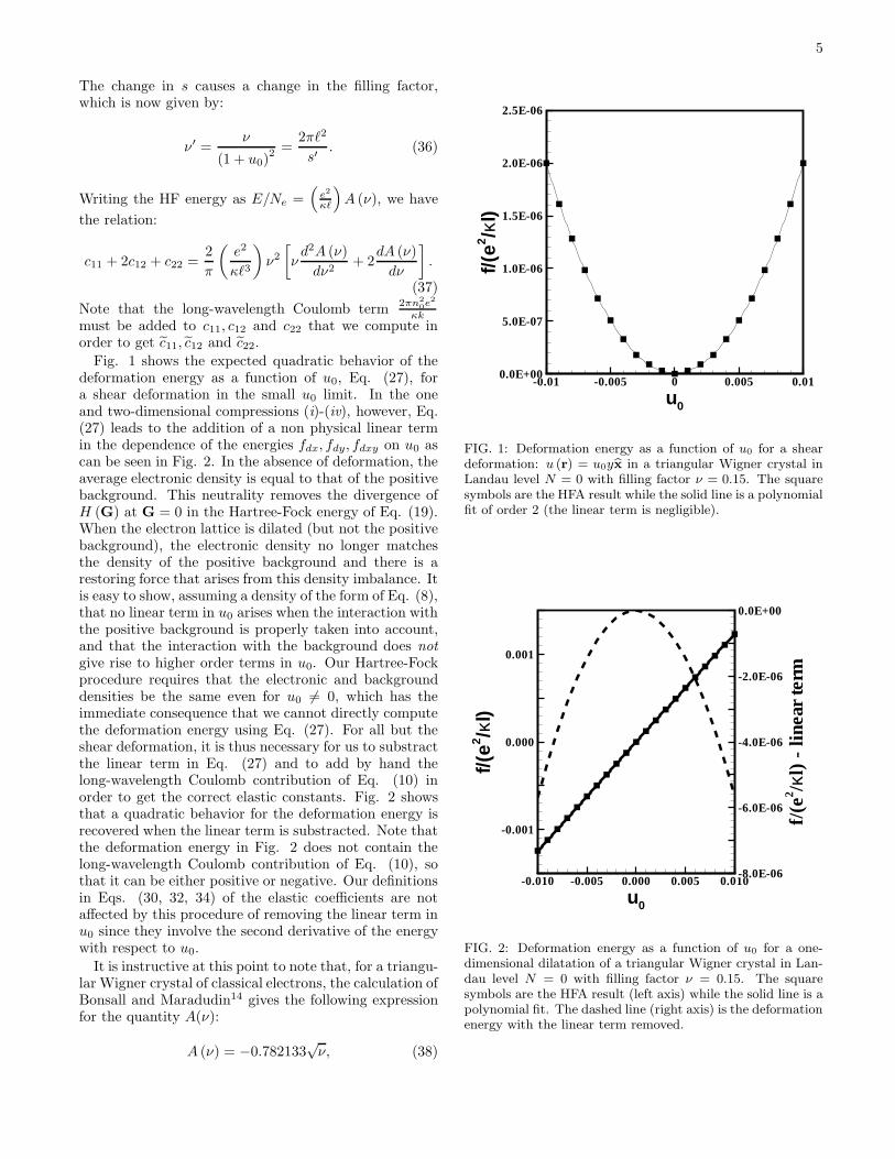
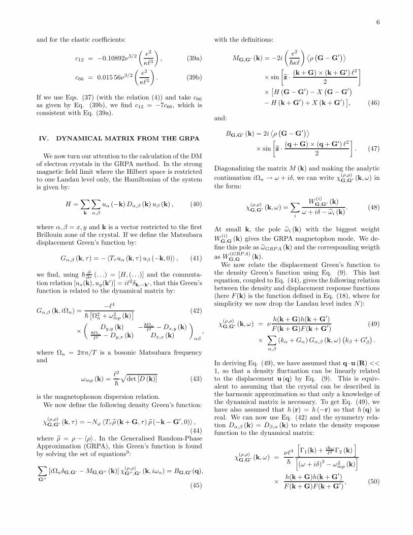
Fig. 1 shows the expected quadratic behavior of thedeformation energy as a function of u0, Eq. (27), fora shear deformation in the small u0 limit. In the oneand two-dimensional compressions (i)-(iv), however, Eq.(27) leads to the addition of a non physical linear termin the dependence of the energies fdx, fdy, fdxy on u0 ascan be seen in Fig. 2. In the absence of deformation, theaverage electronic density is equal to that of the positivebackground. This neutrality removes the divergence ofH (G) at G = 0 in the Hartree-Fock energy of Eq. (19).When the electron lattice is dilated (but not the positivebackground), the electronic density no longer matchesthe density of the positive background and there is arestoring force that arises from this density imbalance. Itis easy to show, assuming a density of the form of Eq. (8),that no linear term in u0 arises when the interaction withthe positive background is properly taken into account,and that the interaction with the background does notgive rise to higher order terms in u0. Our Hartree-Fockprocedure requires that the electronic and backgrounddensities be the same even for u0 6= 0, which has theimmediate consequence that we cannot directly computethe deformation energy using Eq. (27). For all but theshear deformation, it is thus necessary for us to substractthe linear term in Eq. (27) and to add by hand thelong-wavelength Coulomb contribution of Eq. (10) inorder to get the correct elastic constants. Fig. 2 showsthat a quadratic behavior for the deformation energy isrecovered when the linear term is substracted. Note thatthe deformation energy in Fig. 2 does not contain thelong-wavelength Coulomb contribution of Eq. (10), sothat it can be either positive or negative. Our definitionsin Eqs. (30, 32, 34) of the elastic coefficients are notaffected by this procedure of removing the linear term inu0 since they involve the second derivative of the energywith respect to u0.

It is instructive at this point to note that, for a triangu-lar Wigner crystal of classical electrons, the calculation ofBonsall and Maradudin14 gives the following expressionfor the quantity A(ν):

A (ν) = −0.782133√

ν, (38)

u0

f/(e

2 /κl)

-0.01 -0.005 0 0.005 0.010.0E+00

5.0E-07

1.0E-06

1.5E-06

2.0E-06

2.5E-06

FIG. 1: Deformation energy as a function of u0 for a sheardeformation: u (r) = u0ybx in a triangular Wigner crystal inLandau level N = 0 with filling factor ν = 0.15. The squaresymbols are the HFA result while the solid line is a polynomialfit of order 2 (the linear term is negligible).

u0

f/(e

2 /κl)

f/(e

2 /κl)

-lin

eart

erm

-0.010 -0.005 0.000 0.005 0.010

-0.001

0.000

0.001

-8.0E-06

-6.0E-06

-4.0E-06

-2.0E-06

0.0E+00

FIG. 2: Deformation energy as a function of u0 for a one-dimensional dilatation of a triangular Wigner crystal in Lan-dau level N = 0 with filling factor ν = 0.15. The squaresymbols are the HFA result (left axis) while the solid line is apolynomial fit. The dashed line (right axis) is the deformationenergy with the linear term removed.

6

and for the elastic coefficients:

c12 = −0.10892ν3/2

(e2

κℓ3

), (39a)

c66 = 0.015 56ν3/2

(e2

κℓ3

). (39b)

If we use Eqs. (37) (with the relation (4)) and take c66

as given by Eq. (39b), we find c12 = −7c66, which isconsistent with Eq. (39a).

IV. DYNAMICAL MATRIX FROM THE GRPA

We now turn our attention to the calculation of the DMof electron crystals in the GRPA method. In the strongmagnetic field limit where the Hilbert space is restrictedto one Landau level only, the Hamiltonian of the systemis given by:

H =∑

k

∑

α,β

uα (−k)Dα,β (k) uβ (k) , (40)

where α, β = x, y and k is a vector restricted to the firstBrillouin zone of the crystal. If we define the Matsubaradisplacement Green’s function by:

Gα,β (k, τ) = −〈Tτuα (k, τ) uβ (−k, 0)〉 , (41)

we find, using ℏ∂∂τ (. . .) = [H, (. . .)] and the commuta-

tion relation [ux(k), uy(k′)] = iℓ2δk,−k′ , that this Green’sfunction is related to the dynamical matrix by:

Gα,β (k, iΩn) =−ℓ4

ℏ[Ω2

n + ω2mp (k)

] (42)

×(

Dy,y (k) −ℏΩn

ℓ2 − Dx,y (k)ℏΩn

ℓ2 − Dy,x (k) Dx,x (k)

)

αβ

,

where Ωn = 2πn/T is a bosonic Matsubara frequencyand

ωmp (k) =ℓ2

ℏ

√det [D (k)] (43)

is the magnetophonon dispersion relation.We now define the following density Green’s function:

χ(ρ,ρ)G,G′ (k, τ) = −Nϕ 〈Tτ ρ (k + G, τ) ρ (−k − G′, 0)〉 ,

(44)where ρ = ρ − 〈ρ〉 . In the Generalised Random-PhaseApproximation (GRPA), this Green’s function is foundby solving the set of equations9:

∑

G′′

[iΩnδG,G′ − MG,G′′ (k)] χ(ρ,ρ)G′′,G′ (k, iωn) = BG,G′(q),

(45)

with the definitions:

MG,G′ (k) = −2i

(e2

ℏκℓ

) ⟨ρ

(G− G′

)⟩

× sin

[z · (k + G) × (k + G′) ℓ2

2

]

×[H (G − G′) − X

(G − G′

)

− H (k + G′) + X (k + G′)], (46)

and:

BG,G′ (k) = 2i⟨ρ

(G− G′

)⟩

× sin

[z · (q + G) × (q + G′) ℓ2

2

]. (47)

Diagonalizing the matrix M (k) and making the analytic

continuation iΩn → ω + iδ, we can write χ(ρ,ρ)G,G′ (k, ω) in

the form:

χ(ρ,ρ)G,G′ (k, ω) =

∑

i

W(i)G,G′ (k)

ω + iδ − ωi (k). (48)

At small k, the pole ωi (k) with the biggest weight

W(i)G,G (k) gives the GRPA magnetophon mode. We de-

fine this pole as ωGRPA (k) and the corresponding weigth

as W(GRPA)G,G (k).

We now relate the displacement Green’s function tothe density Green’s function using Eq. (9). This lastequation, coupled to Eq. (44), gives the following relationbetween the density and displacement response functions(here F (k) is the function defined in Eq. (18), where forsimplicity we now drop the Landau level index N):

χ(ρ,ρ)G,G′ (k, ω) = ν

h(k + G)h(k + G′)

F (k + G)F (k + G′)(49)

×∑

α,β

(kα + Gα)Gα,β (k, ω)(kβ + G′

β

).

In deriving Eq. (49), we have assumed that q ·u (R) <<1, so that a density fluctuation can be linearly relatedto the displacement u (q) by Eq. (9). This is equiv-alent to assuming that the crystal can be described inthe harmonic approximation so that only a knowledge ofthe dynamical matrix is necessary. To get Eq. (49), wehave also assumed that h (r) = h (−r) so that h (q) isreal. We can now use Eq. (42) and the symmetry rela-tion Dα,β (k) = Dβ,α (k) to relate the density responsefunction to the dynamical matrix:

χ(ρ,ρ)G,G′ (k, ω) =

νℓ4

~

[Γ1(k) + iℏω

ℓ2 Γ2 (k)]

[(ω + iδ)2 − ω2

mp (k)]

× h(k + G)h(k + G′)

F (k + G)F (k + G′), (50)

7

where we defined:

Γ1 (k) = −z · [(k + G) × D (k) × (k + G′)] · z, (51a)

Γ2 (k) = z · [(k + G) × (k + G′)] . (51b)

For ω close to the magnetophonon resonance, we canwrite:

χ(ρ,ρ)G,G′ (k, ω) ≈ νℓ4

ℏ

Z (k)

ω + iδ − ωmp (k)

h(k + G)h(k + G′)

F (k + G)F (k + G′)

,

(52)where we defined the quantity:

Z (k) =Γ1 (k)

2ωmp (k)+ i

ℏΓ2 (k)

2ℓ2. (53)

Then, equating Eq. (52) with Eq. (48) for ω close toωGRPA (k), we obtain:

νℓ4

ℏ

Z (k)

ω + iδ − ωmp (k)

h(k + G)h(k + G′)

F (k + G)F (k + G′)

=

W(GRPA)G,G′ (k)

ω + iδ − ωGRPA (k). (54)

Because ωmp (k) must be equal to ωGRPA (k), we canfinally write

νℓ4

ℏZ (k)

h(k + G)h(k + G′)

F (k + G)F (k + G′)= W

(GRPA)G,G′ (k) , (55)

or, taking the real and imaginary parts of this equation(we remind the reader that both functions h(k) and F (k)are real):

ℜ[W

(GRPA)G,G′ (k)

]=

ν

2

[h (k + G)h (k + G′)

F (k + G)F (k + G′)

]

× Γ1 (k) ℓ4

ℏωmp (k), (56a)

ℑ[W

(GRPA)G,G′ (k)

]=

ν

2

[h (k + G)h (k + G′)

F (k + G)F (k + G′)

]

×Γ2 (k) ℓ2. (56b)

We can get rid of the unknown form factors h (k + G) ifwe work with the ratio of the imaginary and real partsof the weights. We thus define:

ΓG,G′ (k) ≡ℜ

[W

(GRPA)G,G′ (k)

]

ℑ[W

(GRPA)G,G′ (k)

] , (57)

=−ℓ2

ℏωmp (k)

(k + G) × D (k) × (k + G′)

(k + G) × (k + G′).

A careful examination shows that, because ωmp (k) isgiven by the determinant of the dynamical matrix D (k),the quantity Γ1 (k) /ωmp (k) is unchanged if all the com-ponents of the dynamical matrix are multiplied by someconstant. Eq. (57) is thus indeterminate. To avoid this

problem, we replace ωmp (k) by ωGRPA (k) in Eq. (57).Our final result is thus:

ΓG,G′ (k) =−ℓ2

ℏωGRPA (k)

(k + G) × D (k) × (k + G′)

(k + G) × (k + G′).

(58)Because Dx,y (k) = Dy,x (k), we need to choose three

pairs of vectors(G,G′

)to get the components of the

dynamical matrix. To be valid, the dynamical matrixobtained in this way must satisfy the equation:

ωGRPA (k) =ℓ2

ℏ

√det [D (k)]. (59)

Eq. (59) provides a check on the validity of our calcula-tion.

V. NUMERICAL RESULTS FOR THE WIGNER

CRYSTAL

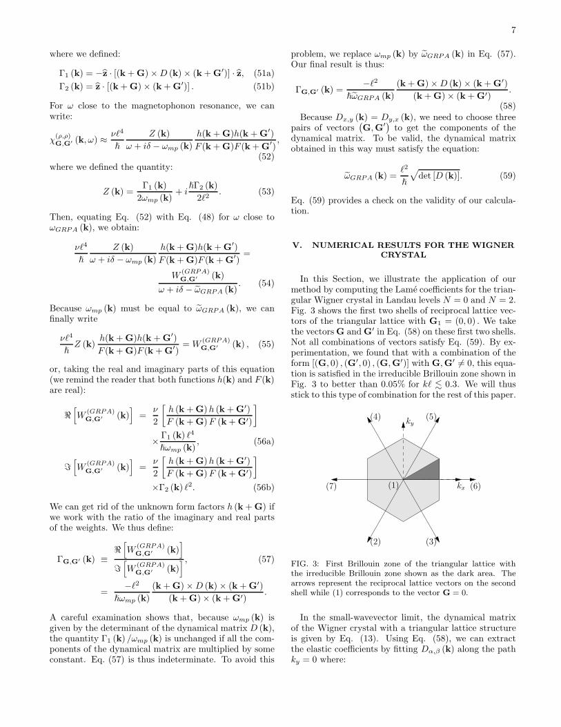
In this Section, we illustrate the application of ourmethod by computing the Lame coefficients for the trian-gular Wigner crystal in Landau levels N = 0 and N = 2.Fig. 3 shows the first two shells of reciprocal lattice vec-tors of the triangular lattice with G1 = (0, 0) . We takethe vectors G and G′ in Eq. (58) on these first two shells.Not all combinations of vectors satisfy Eq. (59). By ex-perimentation, we found that with a combination of theform [(G, 0) , (G′, 0) , (G,G′)] with G,G′ 6= 0, this equa-tion is satisfied in the irreducible Brillouin zone shown inFig. 3 to better than 0.05% for kℓ . 0.3. We will thusstick to this type of combination for the rest of this paper.

(6)

(5)(4)

(7)

(2) (3)

(1) kx

ky

FIG. 3: First Brillouin zone of the triangular lattice withthe irreducible Brillouin zone shown as the dark area. Thearrows represent the reciprocal lattice vectors on the secondshell while (1) corresponds to the vector G = 0.

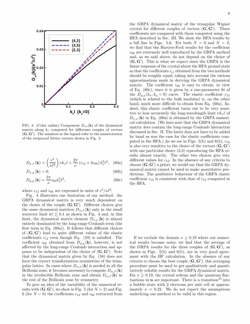
In the small-wavevector limit, the dynamical matrixof the Wigner crystal with a triangular lattice structureis given by Eq. (13). Using Eq. (58), we can extractthe elastic coefficients by fitting Dα,β (k) along the pathky = 0 where:

8

kxl (ky=0)

Dxx

(k)/

(e2/κ

l3 )

0 0.1 0.2 0.30

0.01

0.02

0.03

0.04

(4,2)(3,5)(2,3)

FIG. 4: (Color online) Component Dxx(k) of the dynamicalmatrix along kx computed for differents couples of vectors(G,G′). The numbers in the legend refer to the numerotationof the reciprocal lattice vectors shown in Fig. 3.

Dx,x (k) =

(e2

κℓ3

)νkxℓ +

2π

ν(c12 + 2c66) k2

xℓ2, (60a)

Dx,y (k) = 0, (60b)

Dy,y (k) =2π

νc66k

2xℓ2, (60c)

where c12 and c66 are expressed in units of e2/κℓ3.Fig. 4 illustrates one limitation of our method: the

GRPA dynamical matrix is very much dependent onthe choice of the couple (G,G′). Different choices givethe same dynamical matrices Dα,β (k) only in the smallwavector limit kℓ . 0.1 as shown in Fig. 4 and, in thislimit, the dynamical matrix element Dx,x (k) is almostentirely dominated by the long-range Coulomb term (thefirst term in Eq. (60a)). It follows that different choicesof (G,G′) lead to quite different values of the elasticcoefficients c12 even though Eq. (59) is satisfied. Thecoefficient c66 obtained from Dy,y (k), however, is notaffected by the long-range Coulomb interaction and ap-pears to be independent of the choice of (G,G′). Notethat the dynamical matrix given by Eq. (58) does nothave the correct transformation symmetries of the trian-gular lattice. In cases where Dα,β (k) is needed in all theBrillouin zone, it becomes necessary to compute Dα,β (k)in the irreducible Brillouin zone and obtain Dα,β (k) inthe rest of the Brillouin zone by symmetry.

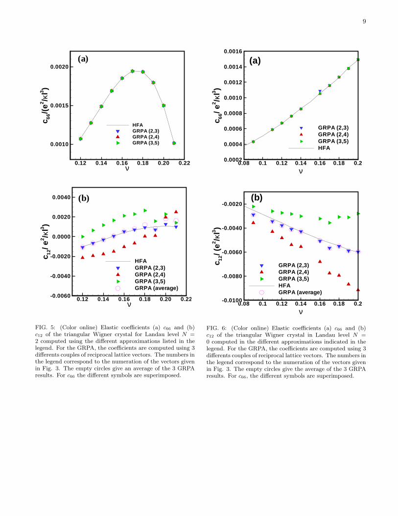
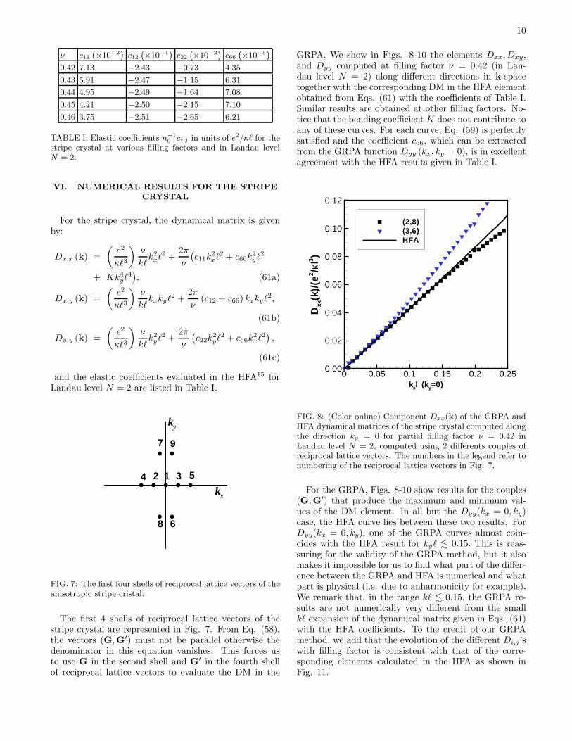
To give an idea of the variability of the numerical re-sults with (G,G′), we show in Fig. 5 (for N = 2) and Fig.6 (for N = 0) the coefficients c12 and c66 extracted from

the GRPA dynamical matric of the triangular Wignercrystal for different couples of vectors (G,G′). Thesecoefficients are compared with those computed using theHFA described in Sec. III. We show the HFA results bya full line in Figs. 5,6. For both N = 0 and N = 2,we find that the Hartree-Fock results for the coefficientc66 are extremely well reproduced by the GRPA methodand, as we said above, do not depend on the choice of(G,G′). This is what we expect since the GRPA is thelinear response of the crystal about the HFA ground stateso that the coefficients cij obtained from the two methodsshould be roughly equal, taking into account the variousapproximations made in deriving the GRPA dynamicalmatrix. The coefficient c66 is easy to obtain, in viewof Eq. (60c), since it is given by a one-parameter fit ofthe Dy,y (kx, ky = 0) curve. The elastic coefficient c12

(which is related to the bulk modulus) is, on the otherhand, much more difficult to obtain from Eq. (60a). In-deed, this elastic coefficient turns out to be very sensi-tive to how accurately the long-wavelength limit νkxℓ ofDx,x (k) in Eq. (60a) is obtained by the GRPA numeri-cal calculation. (We here note that the GRPA dynamicalmatrix does contain the long-range Coulomb interactiondiscussed in Sec. II. The latter does not have to be addedby hand as was the case for the elastic coefficients com-puted in the HFA.) As we see in Figs. 5(b) and 6(b), c12

is also very sensitive to the choice of the vectors (G,G′)with one particular choice (2,3) reproducing the HFA re-sults almost exactly. The other two choices give verydifferent values for c12. In the absence of any criteria tochoose (G,G′) a priori, we would say that the GRPA dy-namical matrix cannot be used to make quantitative pre-dictions. The qualitative behaviour of the GRPA elasticcoefficient c12 is consistent with that of c12 computed inthe HFA.

If we exclude the domain ν ≥ 0.19 where our numer-ical results become noisy, we find that the average ofthe GRPA results for the three couples of (G,G′), asshown in Figs. 5(b) and 6(b), are in very good agree-ment with the HF calculation. In the absence of anycriteria to choose the best couple (G,G′), this averagingprocedure must be used to get qualitatively and quanti-tatively reliable results for the GRPA dynamical matrix.For ν ≥ 0.19, the crystal softens and the quantum fluc-tuations in u are important. There is a transition10 intoa bubble state with 2 electrons per unit cell at approx-imately ν = 0.22. We do not expect the assumptionsunderlying our method to be valid in this region.

9

ν

c 66/

(e2 /κ

l3)

0.12 0.14 0.16 0.18 0.20 0.22

0.0010

0.0015

0.0020

HFAGRPA (2,3)GRPA (2,4)GRPA (3,5)

(a)

ν

c 12/

e2/κ

l3)

0.12 0.14 0.16 0.18 0.20 0.22-0.0060

-0.0040

-0.0020

0.0000

0.0020

0.0040

HFAGRPA (2,3)GRPA (2,4)GRPA (3,5)GRPA (average)

(b)

FIG. 5: (Color online) Elastic coefficients (a) c66 and (b)c12 of the triangular Wigner crystal for Landau level N =2 computed using the different approximations listed in thelegend. For the GRPA, the coefficients are computed using 3differents couples of reciprocal lattice vectors. The numbers inthe legend correspond to the numeration of the vectors givenin Fig. 3. The empty circles give an average of the 3 GRPAresults. For c66 the different symbols are superimposed.

ν

c 12/(

e2/κ

l3)

0.08 0.1 0.12 0.14 0.16 0.18 0.2-0.0100

-0.0080

-0.0060

-0.0040

-0.0020

GRPA (2,3)GRPA (2,4)GRPA (3,5)HFAGRPA (average)

(b)

ν

c 66/e

2/κ

l3)

0.08 0.1 0.12 0.14 0.16 0.18 0.20.0002

0.0004

0.0006

0.0008

0.0010

0.0012

0.0014

0.0016

GRPA (2,3)GRPA (2,4)GRPA (3,5)HFA

(a)

FIG. 6: (Color online) Elastic coefficients (a) c66 and (b)c12 of the triangular Wigner crystal in Landau level N =0 computed in the different approximations indicated in thelegend. For the GRPA, the coefficients are computed using 3differents couples of reciprocal lattice vectors. The numbers inthe legend correspond to the numeration of the vectors givenin Fig. 3. The empty circles give the average of the 3 GRPAresults. For c66, the different symbols are superimposed.

10

ν c11

`×10−2

´c12

`×10−1

´c22

`×10−2

´c66

`×10−5

´

0.42 7.13 −2.43 −0.73 4.35

0.43 5.91 −2.47 −1.15 6.31

0.44 4.95 −2.49 −1.64 7.08

0.45 4.21 −2.50 −2.15 7.10

0.46 3.75 −2.51 −2.65 6.21

TABLE I: Elastic coefficients n−1

0ci,j in units of e2/κℓ for the

stripe crystal at various filling factors and in Landau levelN = 2.

VI. NUMERICAL RESULTS FOR THE STRIPE

CRYSTAL

For the stripe crystal, the dynamical matrix is givenby:

Dx,x (k) =

(e2

κℓ3

)ν

kℓk2

xℓ2 +2π

ν

(c11k

2xℓ2 + c66k

2yℓ2

+ Kk4yℓ4

), (61a)

Dx,y (k) =

(e2

κℓ3

)ν

kℓkxkyℓ2 +

2π

ν(c12 + c66) kxkyℓ2,

(61b)

Dy,y (k) =

(e2

κℓ3

)ν

kℓk2

yℓ2 +2π

ν

(c22k

2yℓ2 + c66k

2xℓ2

),

(61c)

and the elastic coefficients evaluated in the HFA15 forLandau level N = 2 are listed in Table I.

12 34 5

7 9

8 6

ky

kx

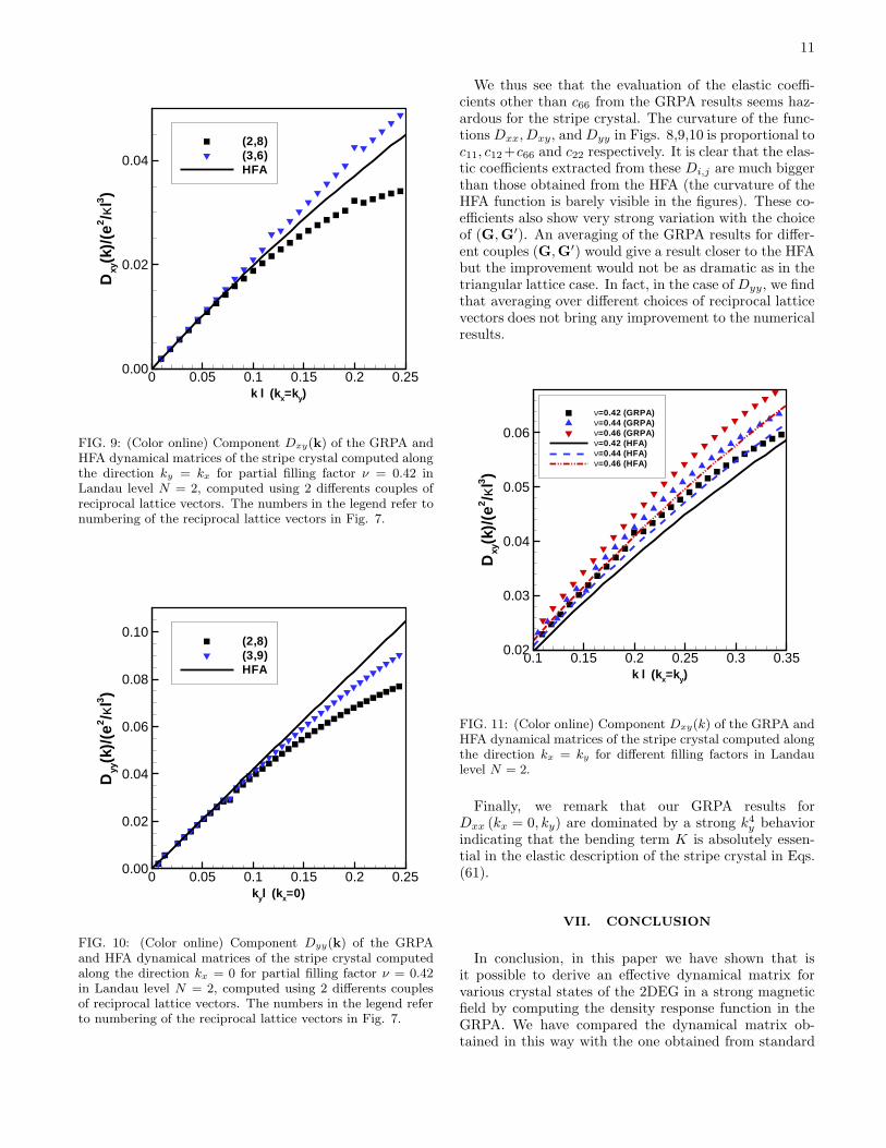
FIG. 7: The first four shells of reciprocal lattice vectors of theanisotropic stripe cristal.

The first 4 shells of reciprocal lattice vectors of thestripe crystal are represented in Fig. 7. From Eq. (58),the vectors (G,G′) must not be parallel otherwise thedenominator in this equation vanishes. This forces usto use G in the second shell and G′ in the fourth shellof reciprocal lattice vectors to evaluate the DM in the

GRPA. We show in Figs. 8-10 the elements Dxx, Dxy,and Dyy computed at filling factor ν = 0.42 (in Lan-dau level N = 2) along different directions in k-spacetogether with the corresponding DM in the HFA elementobtained from Eqs. (61) with the coefficients of Table I.Similar results are obtained at other filling factors. No-tice that the bending coefficient K does not contribute toany of these curves. For each curve, Eq. (59) is perfectlysatisfied and the coefficient c66, which can be extractedfrom the GRPA function Dyy (kx, ky = 0), is in excellentagreement with the HFA results given in Table I.

kxl (ky=0)

Dxx

(k)/

(e2 /κ

l3 )

0 0.05 0.1 0.15 0.2 0.250.00

0.02

0.04

0.06

0.08

0.10

0.12

(2,8)(3,6)HFA

FIG. 8: (Color online) Component Dxx(k) of the GRPA andHFA dynamical matrices of the stripe crystal computed alongthe direction ky = 0 for partial filling factor ν = 0.42 inLandau level N = 2, computed using 2 differents couples ofreciprocal lattice vectors. The numbers in the legend refer tonumbering of the reciprocal lattice vectors in Fig. 7.

For the GRPA, Figs. 8-10 show results for the couples(G,G′) that produce the maximum and minimum val-ues of the DM element. In all but the Dyy(kx = 0, ky)case, the HFA curve lies between these two results. ForDyy(kx = 0, ky), one of the GRPA curves almost coin-cides with the HFA result for kyℓ . 0.15. This is reas-suring for the validity of the GRPA method, but it alsomakes it impossible for us to find what part of the differ-ence between the GRPA and HFA is numerical and whatpart is physical (i.e. due to anharmonicity for example).We remark that, in the range kℓ . 0.15, the GRPA re-sults are not numerically very different from the smallkℓ expansion of the dynamical matrix given in Eqs. (61)with the HFA coefficients. To the credit of our GRPAmethod, we add that the evolution of the different Di,j ’swith filling factor is consistent with that of the corre-sponding elements calculated in the HFA as shown inFig. 11.

11

k l (k x=ky)

Dxy

(k)/

(e2 /κ

l3 )

0 0.05 0.1 0.15 0.2 0.250.00

0.02

0.04

(2,8)(3,6)HFA

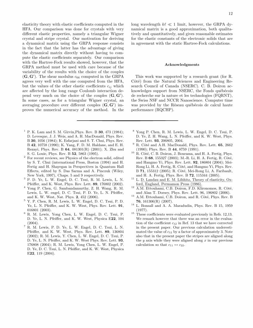
FIG. 9: (Color online) Component Dxy(k) of the GRPA andHFA dynamical matrices of the stripe crystal computed alongthe direction ky = kx for partial filling factor ν = 0.42 inLandau level N = 2, computed using 2 differents couples ofreciprocal lattice vectors. The numbers in the legend refer tonumbering of the reciprocal lattice vectors in Fig. 7.

kyl (kx=0)

Dyy

(k)/

(e2 /κ

l3 )

0 0.05 0.1 0.15 0.2 0.250.00

0.02

0.04

0.06

0.08

0.10(2,8)(3,9)HFA

FIG. 10: (Color online) Component Dyy(k) of the GRPAand HFA dynamical matrices of the stripe crystal computedalong the direction kx = 0 for partial filling factor ν = 0.42in Landau level N = 2, computed using 2 differents couplesof reciprocal lattice vectors. The numbers in the legend referto numbering of the reciprocal lattice vectors in Fig. 7.

We thus see that the evaluation of the elastic coeffi-cients other than c66 from the GRPA results seems haz-ardous for the stripe crystal. The curvature of the func-tions Dxx, Dxy, and Dyy in Figs. 8,9,10 is proportional toc11, c12+c66 and c22 respectively. It is clear that the elas-tic coefficients extracted from these Di,j are much biggerthan those obtained from the HFA (the curvature of theHFA function is barely visible in the figures). These co-efficients also show very strong variation with the choiceof (G,G′). An averaging of the GRPA results for differ-ent couples (G,G′) would give a result closer to the HFAbut the improvement would not be as dramatic as in thetriangular lattice case. In fact, in the case of Dyy, we findthat averaging over different choices of reciprocal latticevectors does not bring any improvement to the numericalresults.

k l (k x=ky)

Dxy

(k)/

(e2 /κ

l3 )

0.1 0.15 0.2 0.25 0.3 0.350.02

0.03

0.04

0.05

0.06

ν=0.42 (GRPA)ν=0.44 (GRPA)ν=0.46 (GRPA)ν=0.42 (HFA)ν=0.44 (HFA)ν=0.46 (HFA)

FIG. 11: (Color online) Component Dxy(k) of the GRPA andHFA dynamical matrices of the stripe crystal computed alongthe direction kx = ky for different filling factors in Landaulevel N = 2.

Finally, we remark that our GRPA results forDxx (kx = 0, ky) are dominated by a strong k4

y behaviorindicating that the bending term K is absolutely essen-tial in the elastic description of the stripe crystal in Eqs.(61).

VII. CONCLUSION

In conclusion, in this paper we have shown that isit possible to derive an effective dynamical matrix forvarious crystal states of the 2DEG in a strong magneticfield by computing the density response function in theGRPA. We have compared the dynamical matrix ob-tained in this way with the one obtained from standard

12

elasticity theory with elastic coefficients computed in theHFA. Our comparison was done for crystals with verydifferent elastic properties, namely a triangular Wignercrystal and stripe crystal. Our motivation for derivinga dynamical matrix using the GRPA response consistsin the fact that the latter has the advantage of givingthe dynamical matrix directly without having to com-pute the elastic coefficients separately. Our comparisonwith the Hartree-Fock results showed, however, that theGRPA method must be used with care because of thevariability of the results with the choice of the couples(G,G′). The shear modulus c66 computed in the GRPAagrees very well with the one computed from the HFA,but the values of the other elastic coefficients cij whichare affected by the long range Coulomb interaction de-pend very much on the choice of the couples (G,G′).In some cases, as for a triangular Wigner crystal, anaveraging procedure over different couples (G,G′) im-proves the numerical accuracy of the method. In the

long wavelength kℓ ≪ 1 limit, however, the GRPA dy-namical matrix is a good approximation, both qualita-tively and quantitatively, and gives reasonable estimatesfor the elastic constants of the electronic solids that arein agreement with the static Hartree-Fock calculations.

Acknowledgments

This work was supported by a research grant (for R.Cote) from the Natural Sciences and Engineering Re-search Council of Canada (NSERC). C. B. Doiron ac-knowledges support from NSERC, the Fonds quebecoisde recherche sur la nature et les technologies (FQRNT),the Swiss NSF and NCCR Nanoscience. Computer timewas provided by the Reseau quebecois de calcul hauteperformance (RQCHP).

1 P. K. Lam and S. M. Girvin,Phys. Rev. B 30, 473 (1984);D. Levesque, J. J. Weis, and A. H. MacDonald, Phys. Rev.B 30, 1056 (1984); K. Esfarjani and S. T. Chui, Phys. Rev.B 42, 10758 (1990); K. Yang, F. D. M. Haldane, and E. H.Rezayi, Phys. Rev. B 64, 081301(R) (2001); X. Zhu andS. G. Louie, Phys. Rev. B 52, 5863 (1995).

2 For recent reviews, see Physics of the electron solid, editedby S. T. Chui (international Press, Boston (1994) and H.Fertig and H. Shayegan in Perspectives in Quantum HallEffects, edited by S. Das Sarma and A. Pinczuk (Wiley,New York, 1997), Chaps. 5 and 9 respectively.

3 P. D. Ye, L. W. Engel, D. C. Tsui, R. M. Lewis, L. N.Pfeiffer, and K. West, Phys. Rev. Lett. 89, 176802 (2002).

4 Yong P. Chen, G. Sambandamurthy, Z. H. Wang, R. M.Lewis, L. W. engel, D. C. Tsui, P. D. Ye, L. N. Pfeiffer,and K. W. West, Nat. Phys. 2, 452 (2006).

5 Y. P. Chen, R. M. Lewis, L. W. Engel, D. C. Tsui, P. D.Ye, L. N. Pfeiffer, and K. W. West, Phys. Rev. Lett. 91,016801 (2003).

6 R. M. Lewis, Yong Chen, L. W. Engel, D. C. Tsui, P.D. Ye, L. N. Pfeiffer, and K. W. West, Physica E22, 104(2004).

7 R. M. Lewis, P. D. Ye, L. W. Engel, D. C. Tsui, L. N.Pfeiffer, and K. W. West, Phys. Rev. Lett. 89, 136804(2002); R. M. Lewis, Y. Chen, L. W. Engel, D. C. Tsui, P.D. Ye, L. N. Pfeiffer, and K. W. West Phys. Rev. Lett. 93,176808 (2004); R. M. Lewis, Yong Chen, L. W. Engel, P.D. Ye, D. C. Tsui, L. N. Pfeiffer, and K. W. West, PhysicaE22, 119 (2004).

8 Yong P. Chen, R. M. Lewis, L. W. Engel, D. C. Tsui, P.D. Ye, Z. H. Wang, L. N. Pfeiffer, and K. W. West, Phys.Rev. Lett. 93, 206805, 2004.

9 R. Cote and A.H. MacDonald, Phys. Rev. Lett. 65, 2662(1990); Phys. Rev. B 44, 8759 (1991).

10 R. Cote, C. B. Doiron, J. Bourassa, and H. A. Fertig, Phys.Rev. B 68, 155327 (2003); M.-R. Li, H. A. Fertig, R. Cote,and Hangmo Yi, Phys. Rev. Lett. 92, 186804 (2004); Mei-Rong Li, H. A. Fertig, R. Cote, and Hangmo Yi, Phys. Rev.B 71, 155312 (2005); R. Cote, Mei-Rong Li, A. Faribault,and H. A. Fertig, Phys. Rev. B 72, 115344 (2005).

11 L. D. Landau and E. M. Lifshitz, Theory of elasticity, Ox-ford, England, Permamon Press (1986).

12 A.M. Ettouhami, C.B. Doiron, F.D. Klironomos, R. Cote,and Alan T. Dorsey, Phys. Rev. Lett. 96, 196802 (2006).

13 A.M. Ettouhami, C.B. Doiron, and R. Cote, Phys. Rev. B76, 161306(R) (2007).

14 L. Bonsall and A. A. Maradudin, Phys. Rev. B 15, 1959(1977).

15 These coefficients were evaluated previously in Refs. 12,13.We remark however that there was an error in the evalua-tion of the coefficient c12 in Ref. 13 that we have correctedin the present paper. Our previous calculation underesti-mated the value of c12 by a factor of approximately 3. Notealso that in the present paper the stripes are aligned alongthe y axis while they were aligned along x in our previouscalculation so that c11 ↔ c22.