dynamic spectrum management (dsm) algorithms for multi-user xdsl

IEEE COMMUNICATIONS SURVEYS & TUTORIALS, ACCEPTED FOR PUBLICATION 1

Dynamic Spectrum Management (DSM)Algorithms for Multi-User xDSLSean Huberman, Christopher Leung, and Tho Le-Ngoc, Fellow, IEEE

Abstract—Dynamic Spectrum Management (DSM) is an ef-fective method for reducing the effect of crosstalk in DigitalSubscriber Line (DSL) systems. This paper discusses variousDSM algorithms, including Optimal Spectrum Balancing (OSB),Iterative Spectrum Balancing (ISB), Autonomous Spectrum Bal-ancing (ASB), Iterative Water-Filling (IWF), Selective IterativeWater-filling (SIW), Successive Convex Approximation for LowcomplExity (SCALE), the Difference of Convex functions Algo-rithm (DCA), and Distributed Spectrum Balancing (DSB). Theyare compared in terms of performance (achievable data rate)and computational complexity.

Index Terms—Digital Subscriber Line (DSL), Dynamic Spec-trum Management (DSM), resource allocation, power allocation,non-convex optimization.

I. INTRODUCTION

D IGITAL Subscriber Line (DSL) continues to be themost popular broadband access technology [1]. The most

significant factor in the performance of DSL systems is theinterference between cables, known as crosstalk. Crosstalk hasthe potential to severely limit the performance of the systemif it is not dealt with. The DSL channel is highly frequency-selective and, in general, at high frequency the crosstalk is verysignificant. In order to make use of the higher frequency bands,effective spectrum management techniques must be employed.The most basic form of spectrum management is StaticSpectrum Management (SSM) [2]. SSM implements identicalspectral masks based on a worst-case scenario assumption forall users. Clearly, this leads to inefficient spectrum manage-ment whenever the scenario is not the worst-case and leads tohighly sub-optimal performance.The poor performance of SSM systems led to the intro-

duction of Dynamic Spectrum Management (DSM) [3]. DSMis a wide field which looks to adaptively apply differentspectral masks for each user with the intent of maximizing thethroughput of the system. DSM allows for a far more efficientuse of the spectrum than SSM does. As a result, many differentDSM algorithms have been proposed. As well, it was shownin [4] that DSM allows for more efficient power usage thanSSM techniques.The main criteria in comparing different DSM algorithms

are their performance and their complexity. The performancerelates how well an approach succeeds at maximizing the

Manuscript received 30 September 2009; revised 26 April 2010, 27 July2010, and 3 September 2010.The authors are with the Department of Electrical and Computer

Engineering, McGill University, 3480 University Street, Montreal, Que-bec, Canada, H3A 2A7 (e-mails: [email protected]; [email protected]; [email protected]).Digital Object Identifier 10.1109/SURV.2011.092110.00090

achievable data rate as compared to the theoretical optimum.The complexity of the model is related to the amount of timerequired to derive the power allocation as the number of usersand frequency tones increase.There are two main types of DSM algorithms: centralized

and distributed. Centralized systems require a central hub withfull knowledge of the network. In general, this system allowsfor better performance at a cost of increasing the complex-ity and computational time. On the other hand, distributedsystems allow for every user to self-optimize. Distributedsystems that can operate fully autonomously without the needof explicit message passing are called autonomous systems.In general, distributed systems reduce the complexity andcomputational time but often sacrifice some optimality interms of performance.One of the first distributed DSM algorithms was Iterative

Water-Filling (IWF) [5]. In IWF, each user selfishly maximizestheir own data-rate. While IWF gives significant data-rateimprovements over SSM techniques, in many situations, itleads to sub-optimal performance.The sub-optimality of IWF is caused by inefficient use

of the frequency spectrum. In an attempt to increase theefficiency of the frequency spectrum, many other heuristicvariations were proposed. Interested readers are referred to[6], [7], and [8].Two similar algorithms which improve on the performance

of IWF are Band Preference Spectrum Management (BPSM)[9], and Iterative Power Pricing (IPP) [10]. Both apply the gen-eral IWF algorithm but BPSM gives preferences to differentusers in each frequency band, while IPP uses power pricingfor each frequency tone to allow weaker users to competemore fairly. The BPSM and IPP algorithms are intuitivelysimilar, except they solve different optimization problems.BPSM is used to maximize the achievable rate, while IPP isused to minimize the required power. Section II-C discussesthe different optimization problems in more detail.Another algorithm known as Selective Iterative Water-filling

(SIW) [11] was introduced. SIW selectively applies IWF tousers in the under-utilized sections of the frequency spectrumuntil all users use up their total power. While SIW showssignificant performance gains over IWF, the performance isstill sub-optimal.A centralized algorithm called Optimal Spectrum Balancing

(OSB) [12], which maximizes the weighted sum rate acrossthe users, was derived to solve for the globally optimal powerallocation. OSB uses dual decomposition to solve for theoptimal transmit powers for each user separately on eachfrequency tone by exhaustive search. While OSB is not

1553-877X/10/$25.00 c© 2010 IEEE

This article has been accepted for inclusion in a future issue of this journal. Content is final as presented, with the exception of pagination.

2 IEEE COMMUNICATIONS SURVEYS & TUTORIALS, ACCEPTED FOR PUBLICATION

computationally tractable for many users, it serves as an upperbound on the performance of other DSM algorithms for caseswith few users.A similar centralized algorithm called Grouping Spectrum

Management (GSM) [13] was introduced. GSM groups usersinto clusters based on similar line lengths and calculates areference line for each cluster. GSM then applies OSB onthe reference lines for each cluster in order to reduce thecomputational complexity.Another centralized algorithm, based on Monotomic Opti-

mization (MO), called MO-bAsed poweR controL (MARL)[14] was introduced. MARL finds globally optimal pointsby constructing a series of poly-blocks that approximate thefeasible region with increasing precision; however, MARL iscurrently not feasible in the case of many users or frequencytones.By representing the objective function of the non-convex

optimization problem in OSB explicitly as the Differenceof two Convex functions (DC) [15], (i.e., f = g − h), amodified prismatic branch-and-bound algorithm was proposedin [16]. The constraint set is convex since it consists of asystem of linear equations and one nonlinear constraint. ThePrismatic Branch and Bound (PBnB) algorithm [17] operatesby successively approximating the nonlinear constraint by apiecewise linear function, and finds a globally optimal solutionby solving a sequence of Linear Programming (LP) sub-problems. Although its computational complexity is still high,the algorithm proposed in [16] can substantially reduce thecomplexity of OSB in finding a globally optimal solution,especially for a large number of users. It can provide anupper-bound on the performance in many situations whereOSB is computationally intractable, and hence, can serve as acomparison measure for other more practical DSM algorithms.Since the previously mentioned global optimizing algo-

rithms are intractable for many users, a centralized algorithmcalled Iterative Spectrum Balancing (ISB) [18] [19] wasintroduced. ISB formulates the optimization problem similarto OSB, using the weighted sum rate and dual decomposition,but solves for the power allocations in an iterative fashionusing one-dimensional instead of N -dimensional exhaustivesearches (where N is the number of users). This allows forISB to be computationally tractable for many users.A similar algorithm called Generalized Iterative Spectrum

Balancing (GISB) [20] was proposed. GISB operates similarlyto ISB and OSB, where the difference lies in terms of thenumber of Power Spectral Densities (PSDs) over which theexhaustive search is performed. For GISB, the exhaustivesearch is performed over L users where 1 ≤ L ≤ N . Note thatISB and OSB are the special cases where L = 1 and L = N ,respectively. GISB allows for a tradeoff between performanceand computational complexity. The closer the value of L isto N , the better the performance will be at the expense ofcomputational complexity.Centralized systems are generally harder to implement in

practice. It is for this reason that many other algorithms wereintroduced. One such algorithm is Autonomous Spectrum Bal-ancing (ASB) [21]. ASB uses the same problem formulationas OSB and ISB but operates in a distributed fashion withoutthe need for any explicit message passing. ASB uses the

concept of a virtual line (referred to as a reference line),which represents the typical victim in the network. Each userself-optimizes to protect the reference line and hence attemptsto better the overall network. Generally ASB cannot find aglobally optimal solution; however, its performance has beenshown to be near-optimal in some situations while maintaininga relatively low complexity.One issue regarding the ASB algorithm is that the spectrum

update formula can be relatively time consuming. It is for thisreason that [22] proposed the ASB-2 algorithm. The ASB-2 algorithm works exactly like the ASB algorithm but usesa slightly different spectrum update formula. This spectrumupdate formula has a significantly lower complexity. ASB andASB-2 do not necessarily converge to the same solution; how-ever, the ASB-2 algorithm converges significantly faster thanASB, especially when the number of users and/or frequencytones are very large.The ASB and ASB-2 algorithms presented in [21] and [22]

only use one reference line; however, it was shown in [23]that using Multiple Reference Lines (MRL) can significantlyimprove performance while still maintaining a low complexity.Guidelines for choosing reference lines to ensure consistentlystrong performance were also presented in [23].An algorithm called Semi-Blind Spectrum Balancing (2SB)

[24] builds on the concepts introduced in ASB. 2SB operatesin the same fashion as ASB but also dynamically updatesa virtual reference line parameters for each user separately,to more accurately represent the network. The virtual linesare updated at a Spectrum Management Center (SMC) basedon message passing to and from the users. This removes theautonomous aspect of ASB, but generally leads to an improveddata-rate.Several Sequential Convex Programming (SCP) algorithms

(iterative algorithms which solve a sequence of convex sub-problems to find a locally optimal solution) will be discussedin this paper. One SCP algorithm, called Successive ConvexApproximation for Low-complExity (SCALE) [25] [26] canbe viewed as a hybrid centralized and distributed system sinceit can be implemented in a distributed fashion with explicitmessage passing. SCALE is an algorithm that applies a seriesof concave lower-bounds to the maximization problem. Thisenables SCALE to make use of the well researched area ofconvex optimization to maximize the concave lower-bound.Each successive iteration tightens the lower-bound towards alocally optimal solution.The PBnB algorithm (discussed above) makes use of the DC

property of the objective function to solve for globally optimalsolutions. Finding globally optimal solutions has a largecomplexity; hence, several SCP algorithms (discussed below)which make use of the DC property of the objective functionto solve for locally optimal solutions are more computationallyattractive.One such SCP algorithm discussed in this paper makes

use of the Difference of Convex functions Algorithm (DCA)presented in [27]. DCA is a centralized algorithm that beginsby re-writing the non-convex objective function in terms of thedifference of two convex functions (i.e., f = g−h); however,DCA iteratively creates an affine minorization (multivariatefirst-order approximation) of h, denoted by h, which is used


HUBERMAN et al.: DYNAMIC SPECTRUM MANAGEMENT (DSM) ALGORITHMS FOR MULTI-USER XDSL 3

to make the objective function, f = g − h, convex. Each suc-cessive iteration more closely approximates the locally optimalsolution. For any function f , many DC decompositions exist(e.g., g−h = (g+φ)−(h+φ)). The choice of decompositionhas a crucial impact on the convergence speed as well as theperformance. There are still a lot of heuristics regarding theDCA implementation which have yet to be explored in greatdetail.A similar algorithm called Convex Approximation Dis-

tributed Spectrum Balancing (CA-DSB) was proposed in [22].CA-DSB applies the DC property of the objective functionand follows a similar algorithm to DCA; however, CA-DSBuses a different DC decomposition than the DCA in [27] andtherefore can operate in a distributed manner. This makes useof parallel processing to reduce the complexity while stillmaintaining strong performance through the use of messagepassing.Another algorithm called Distributed Spectrum Balancing

(DSB) was proposed in [22]. DSB also writes the objectivefunction as a DC function but it applies the Karush–Kuhn–Tucker (KKT) conditions directly. With the use of a messagepassing system, the DSB algorithm solves for a locally optimalsolution in an iterative fashion. The DSB algorithm and CA-DSB algorithms are nearly identical in terms of performance;however, in general the runtime of DSB is slightly faster.The Multiple Starting Point DSB (MS-DSB) algorithm,

proposed in [22], is an extension of the DSB algorithm whichmakes use of multiple starting points. This allows for thealgorithm to find solutions that are at least as good as the DSBalgorithm without significantly increasing the complexity.The rest of this paper is organized as follows: Section

II presents a brief overview of DSM problems in multi-user xDSL. Section III discusses the eight algorithms: OSB,ISB, ASB, IWF, SIW, SCALE, DCA, and DSB. SectionIV presents illustrative examples and simulation results toevaluate and compare the performance of the eight algorithms,while Section V discusses the complexity behaviour of thealgorithms under consideration. Section VI provides someconcluding remarks.

II. DSM IN MULTI-USER DSL NETWORK

A. xDSL Environment

xDSL is a family of technologies which transmit digitaldata over twisted-pair copper telephone wires [3] [28]. xDSLoperates on the same twisted-pair copper wire as Plain OldTelephone Service (POTS) since it uses a higher frequencyband, while POTS uses a lower frequency band (less than4 kHz). The frequency band used for DSL depends onthe specific technology. For example, in Asymmetric DigitalSubscriber Line (ADSL) the maximum frequency used is1.1 MHz, in ADSL2+ the maximum frequency used is 12MHz, and in Very high bitrate DSL (VDSL) the maximumfrequency used is 30 MHz. There are dedicated frequencybands for upstream and downstream transmission. For mostDSL technologies, a larger frequency band is allocated fordownstream transmission than for upstream transmission.Twisted-pair copper wires are typically run underground in

binder groupings. Generally, the maximum number of twisted-

Fig. 1. DMT Block Diagram.

pair copper wires in a binder is 200. These are generallyorganized into sub-bundles of 25 twisted-pair copper wires.xDSL technology uses a scheme similar to Orthogonal

Frequency-Division Multiplexing (OFDM) known as DiscreteMulti-Tone (DMT). DMT is a multi-channel transmissiontechnique that divides the available spectrum into smaller sub-channels or frequency tones [29]. DMT differs from OFDMin that it is also capable of optimizing the bit and energydistribution over the sub-channels (e.g., channel partitioningor bit-loading) [3]. The basic idea of DMT transmission istransmit the data in parallel over each frequency tone (notethat some frequency tones might transmit no data, while otherscan transmit a lot of data).Figure 1 shows the DMT transmission block diagram. The

data is put through a serial to parallel converter. This formatsthe word size required for the parallel transmission. As well,this transforms the wide-band frequency selective channelinto many parallel narrow-band frequency flat tones. Eachfrequency tone is modulated independently using an M-arymodulation scheme (e.g., Quadrature Amplitude Modulation(QAM), Phase-Shift Keying (PSK)). The Inverse Fast FourierTransform (IFFT) is used to convert the waveform from thefrequency domain to the time domain. A Cyclic Prefix (CP) isthen added in order to avoid Inter-Symbol Interference (ISI)and Inter-Channel Interference (ICI). After the data passesthrough the DSL channel, the receiver performs the reverseoperations in order to recover the transmitted data.A low symbol rate is used to ensure an appropriate guard-

band between frequency tones. For example, typically xDSLsystems use a frequency tone spacing of 4.3125 kHz and asymbol rate of 4 kHz.The main advantage of DMT is that it is well suited to

handle large attenuation at high frequencies as is typical inxDSL systems. This is due to the fact that it converts the fre-quency selective channel into many frequency flat sub-carriers(or frequency tones) and solves each one independently. Thenumber of frequency tones depends on the frequency bandallocated to the xDSL technology used (e.g., ADSL uses 256frequency tones, whereas VDSL uses 4096 frequency tones).One advantage of xDSL is that since it uses the same

twisted-pair copper wire as POTS, no new wiring is required.xDSL technology makes more efficient use of the existingphone lines; however, twisted-pair copper wire has an atten-uation that increases with the line lengths, especially whenoperating at higher frequencies as in the case of xDSL.Due to the high attenuation at high frequencies, especially

for longer lines, xDSL is more suitable for “last mile”



networks or hybrid fiber/copper networks. More specifically,while using optical fiber instead of copper wire might yieldhigher data rates over longer distances, it is far more expensiveto implement optical fiber wire than to make use of the existingcopper wire. Thus, the ability to achieve similar data ratesusing copper wire is particularly interesting.High enough data rates would allow for more effective

hybrid fiber/copper network architectures (referred to as FTTxtechnology). One such example is Fibre To The Neighbour-hood or Node (FTTN). FTTN uses the more expensive fibre-optic cables [30] to transmit information to a neighbourhood(or a node closer to the customers’ premises) and then usesregular twisted-pair wiring from the neighbourhood to eachand every subscriber’s home. This is far cheaper than aFibre To The Home (FTTH) [30] network architecture, whereexpensive fibre-optic cable is used directly to each subscriber’shome.Other such network architectures exist, such as Fibre To The

Curb or Cabinet (FTTC), Fibre To The Building or Basement(FTTB), Fibre To The Premises (FTTP), and Fibre To TheOffice (FTTO) [31].Such network topologies can be found in practice in many

countries. For example, Japan deployed ADSL services andwas beginning to expand to VDSL services as of November2005 [32]. In the United States, AT&T deploys a VDSLservice called AT&T U-verse which provides internet, TVand phone through a FTTN network architecture to 2 millioncustomers across 22 states as of December 9, 2009 [33].Similarly, Bell Canada services over 1.8 million homes withVDSL2 through their FTTN networks in Montreal and Torontoas of February 4, 2010 [34]. This is expected to double by theend of 2010.Figure 2 shows an example of an xDSL network. In this

network, optical fibre is run to the Central Office (CO) andto two DSL Access Multiplexers (DSLAMs). From the COand the DSLAMs, twisted-pair copper wire is run to variousJunction Wire Interfaces (JWIs). The JWIs run twisted-paircopper wire to the customers premises and/or office building.As shown in Figure 2, there are sections of the network wherethe CO shares a binder with a DSLAM. Due to the long lengthof the CO relative to the DSLAM, the DSLAM lines can causesevere crosstalk to the CO users (this is known as the near-farproblem).

B. System Model

Consider a DSL network with a set of users (modems)N = {1, . . . , N} and a set of tones (frequency carriers)K = {1, . . . , K}. Using synchronous DMT modulation, thereis no ICI and transmissions can be modeled independently oneach tone k as follows:

yk = Hkxk + zk.

The vector xk � {xnk , n ∈ N} contains the transmitted

signals for all users on frequency tone k, where xnk is the

transmitted signal by user n on frequency tone k. Similarly,yk � {yn

k , n ∈ N} and zk � {znk , n ∈ N} where yn

k is thereceived signal for user n on frequency tone k. Likewise, zn

k

is the additive noise for user n on frequency tone k which

contains thermal noise, alien crosstalk and radio frequencyinterference.Hk is an N ×N matrix such that [Hk]n,m is thechannel gain from transmitter m to receiver n on frequencytone k, and is defined as hn,m

k . The transmit PSD of user non frequency tone k is defined as sn

k � E{|xnk |2}/Δf , where

E{·} denotes expected value, and Δf denotes the frequencytone spacing. The vector containing the PSD of user n on allfrequency tones is defined as sn � {sn

k , k ∈ K}.When the number of users is large enough, the interfer-

ence is well approximated by a Gaussian distributed randomvariable, and hence the bit loading (bits/s/Hz) of user n onfrequency tone k is defined as:

bnk � log2

(1 +

1Γ

|hn,nk |2sn

k∑m �=n |hn,m

k |2smk + σn

k

),

where Γ is the Signal to Noise Ratio (SNR) gap which is afunction of the desired Bit Error Rate (BER), coding gain, andnoise margin [28], and σn

k � E{|znk |2}/Δf is the noise power

density of user n on frequency tone k. The achievable datarate for user n is therefore

Rn = fs

∑k

bnk .

C. Spectrum Management Problem

The spectrum management problem, based on the systemmodel shown in Section II-B, involves selecting the transmitpowers for each of the N users on each of the K frequencytones.The Static Spectrum Management (SSM) approach assumes

a worst-case scenario where all the possible users in a cablebinder are active [2] [3]. Based on this assumption, theinterference plus noise term for each user does not change(i.e., it is static). Each user n must then adjust their transmitpower, sn

k , on each frequency tone k with the assumption thatthe interference plus noise seen is at its maximum.There are many different types of SSM technologies. One

example is called flat Power Back-Off (PBO). Flat PBOoperates by ensuring that each user transmits the minimumpossible flat PSD required to meet its Quality of Service (QoS)requirement. Another example is the reference noise methodwhere each user sets its transmit PSD such that the crosstalkfelt by the virtual modem is equal to the background noiseseen by the virtual modem.When all users are active and the situation is a worst-

case model, SSM provides reasonable spectrum management;however, whenever the total number of active users is less thanthe total number of users in the cable binder, SSM becomesoverly pessimistic and makes inefficient use of the spectrum.The worst-case model used by SSM is entirely determinedbased on the length and width of the cable used.In practice, many bridge-taps, splices, and other cable

imperfections exist, which make the SSM worst-case modeleven more inaccurate. As well, in practice, the number ofactive users changes constantly and therefore in order to makeefficient use of the spectrum, it is necessary to dynamicallyallocate transmit PSDs in order to maximize the achievablebit-rate.



Fig. 2. Example of a typical xDSL Network.

Dynamic Spectrum Management (DSM) dynamically allo-cates transmit powers for all users in response to changes inchannel conditions [3]. There are several physical constraintsimposed on the transmit powers for each user. One suchconstraint is the maximum power which each user is allowedto allocate over all of its frequency tones. The maximum powerconstraint for user n is denoted by Pn. Another constraint isthe maximum power which each user is allowed to allocate onany particular frequency tone referred to as a spectral mask.The spectral mask for user n on frequency tone k is denoted bysn,mask

k . Therefore the power constraints can be summarizedas:

∑k∈K

snk ≤ Pn and 0 ≤ sn

k ≤ sn,maskk ∀ n, k. (1)

There are many different possible spectrum managementproblems depending on the specific goal of the network. Forexample, maximizing the total achievable data rate (i.e., RateAdaptive (RA)) or minimizing the total power allocated (i.e.,Fixed Margin (FM))1 while still ensuring some QoS require-ments for each DSL customer. Regardless of the specific goalof the network, the physical constraints shown in (1) arealways present.One approach to DSM focuses on maximizing the achiev-

able data rate of one particular user (e.g., user 1), given thatthe rest of the users satisfy some QoS requirement. The QoSrequirement for user n is denoted by Rn,target. This approachto DSM can be summarized in the following RA optimizationproblem:

maxsn, n∈N

R1

subject to: Rn ≥ Rn,target, ∀ n > 1 (2)∑k∈K

snk ≤ Pn, ∀ n

0 ≤ snk ≤ sn,mask

k , ∀ n, k.

1Concepts of RA and FM are also discussed in a wireless communicationsetting (e.g., [35]).

It was shown in [12] that the optimal solution to the RAoptimization problem (2) is equivalent to the optimal solutionof the RA optimization problem (3) for some w � {wn, n ∈N}. wn is a weighting factor which represents the importanceof user n.

maxsn, n∈N

∑n∈N

wnRn

subject to:∑k∈K

snk ≤ Pn, ∀ n (3)


k , ∀ n, k.

In the most general form, one can incorporate both RA andFM into the spectrum management problem [26]. Let RAand FM denote the index sets of the RA and FM users,respectively. Assuming RA �= ∅ (i.e., there are some userswhich are trying to maximize their rate) the joint RA and FMspectrum management problem is shown below in (4). Notethat the rate for all of the users in RA are being maximizedwhile the rate for all of the users in FM are being fixed attheir respective QoS requirement in order to minimize theirpower consumption.

maxsn, n∈N

∑n∈RA

wnRn

subject to: Rn = Rn,target, ∀ n ∈ FM (4)∑k∈K

snk ≤ Pn, ∀ n ∈ N


k , ∀ k ∈ K, n ∈ N

If RA = ∅ (i.e., no users are trying to maximize their rate)the spectrum management problem reduces to the FM case.This is shown below in (5). Note that RA = ∅ ⇐⇒ N =FM and the maximization problem changes to a minimizationproblem. Here the total power consumed by all users on allfrequency tones is being minimized while ensuring each userstill meets their respective QoS requirements.



minsn, n∈N

∑n∈N

∑k∈K

snk

subject to: Rn ≥ Rn,target, ∀ n ∈ N (5)∑k∈K

snk ≤ Pn, ∀ n ∈ N


k , ∀ k ∈ K, n ∈ N

III. DSM ALGORITHMS UNDER CONSIDERATION

The eight DSM algorithms: OSB, ISB, ASB, IWF, SIW,SCALE, DCA, and DSB are discussed. OSB is a centralizedalgorithm which computes the globally optimal solution byusing N -dimensional exhaustive searches. ISB is a centralizedalgorithms which attempts to approximate OSB by iterativelyperforming 1-dimensional exhaustive searches.ASB is an autonomous algorithm which uses the concept

of a reference line to maximize the achievable data rate.IWF is an autonomous algorithm where every user selfishlymaximizes their own transmit power, until the point is reachedwhere no user can benefit from changing their transmit power.SIW iteratively performs IWF, which allows for weaker usersto make more efficient use of the frequency spectrum.SCALE is a hybrid centralized and distributed algorithm

since it is implemented in a distributed fashion by makinguse of explicit message passing to gain centralized knowl-edge. SCALE operates by successively applying convex lowerbounds to the objective function until a locally optimal pointis reached.DCA is a centralized algorithm which makes use of a

Difference of Convex functions (DC) property in order to solvefor a locally optimal points in an iterative fashion.DSB is a hybrid centralized distributed algorithm which

makes use of explicit message passing to gain centralizedknowledge. DSB is based on the necessary conditions for asolution to be locally optimal.

A. OSB

As will be discussed in Section V, solving for the optimalpower allocation of all N users on each of the K frequencytones using a brute force exhaustive search method has acomputational complexity of O(eKN ).OSB begins by re-writing the optimization problem shown

in (2) as the optimization problem shown in (3) [12], [18]. TheOSB algorithm then uses the concept of dual decomposition toeliminate the exponential complexity in terms of the number offrequency tones,K , and converts it into a linear complexity interms of the number of frequency tones, K . OSB converts theconstrained optimization problem in (3) into an unconstrainedoptimization problem using duality theory. Therefore, thePrimal Problem, (3), is replaced by the dual problem

maxs1,...,sN

L(s1, . . . , sN ) (6)

where L(s1, . . . , sN ) �∑

n

wnRn −∑

n

∑k

λnsnk .

The Lagrange multipliers (w1, . . . , wN , λ1, . . . , λN ) arechosen such that the Karush–Kuhn–Tucker (KKT) conditionsare satisfied:

λn(Pn −

∑k

snk

)= 0, ∀ n (7)

wn(Rn −

∑k

bnk

)= 0, ∀ n. (8)

Provided that Equations (7) and (8) hold, the dual problem(6) is equivalent to the primal optimization problem (3).Since synchronous transmission is assumed, in Section II-B,

there is no ICI and therefore the Lagrangian can be decom-posed over the frequency tones. This reduces the complexityof the algorithm from exponential to linear in the number offrequency tones, since the exhaustive search can be performedindependently on each frequency tone. Therefore, OSB re-duces a KN -dimensional exhaustive search to K differentN -dimensional exhaustive searches.Therefore, for each frequency tone k, the following opti-

mization problem must be solved:

maxs1

k,...,sNk

Lk(s1k, . . . , sN

k ) (9)

where Lk(s1k, . . . , sN

k ) �∑

n

wnRn −∑

n

λnsnk .

Since∑

k Lk(s1k, . . . , sN

k ) = L(s1, . . . , sN ), solving (9) in-dependently over each frequency tone is equivalent to solving(6). The process of writing out the Lagrangian dual problemand decomposing the Lagrangian across all the frequencytones is known as dual decomposition.The full OSB algorithm is outlined in Algorithm 1. One

important note is that the choice of ε can drastically effect theperformance of the algorithm. If ε is too small, the algorithmwill take an extremely long time to converge but if ε is toolarge, the algorithm may not converge at all. Ideally one musttweak the value of ε heuristically in order to ensure properconvergence of the algorithm. This is often a highly non-trivialtask. One method for specifying the choice of ε is shown in[36].

Algorithm 1: OSB Algorithm

repeatforeach k do

Solve by N -Dimensional exhaustive search:(s1

k, . . . , sNk )=arg max{s1

k,...,sNk }Lk(s1

k, . . . , sNk ) ;

endforeach n do

wn = max{wn + ε (Rn,target −∑k bnk ), 0} ;

λn = max{λn + ε (∑

k snk − Pn), 0} ;

enduntil sn

k converges ∀ k, n ;

Spectral masks can easily be incorporated into Algorithm 1by setting the value of Lk to a very large negative number ifsn

k > sn,maskk for each user n.

By reducing the complexity to linear in terms of the numberof frequency tones, OSB becomes computationally tractable



for large numbers of frequency tones; however, OSB is stillcomputationally intractable for large numbers of users. OSBcan therefore serve as an upper-bound with which to comparethe performance of other DSM algorithms for few users.

B. ISB

In Section III-A, it is shown that OSB is computationallyintractable for large N . This motivates the choice of aniterative algorithm which is tractable for largeN . ISB operatesin a similar fashion to OSB by re-writing the optimizationproblem shown in (2) as the optimization problem shown in(3) [18] [19]. ISB also uses the concept of dual decomposi-tion, discussed in Section III-A, to re-write the optimizationproblem as:

maxsn

k

Lk(s1k, . . . , sN

k ), (10)

where Lk(s1k, . . . , sN

k ) �∑

n

wnRn −∑

n

λnsnk .

Note that in ISB, the PSD of each user is searched forin an iterative fashion by updating one user’s PSD at a timewhile keeping all other users’ PSD values fixed. This can beseen in Equation (10) since the maximization is only over asingle user’s PSD, sn

k . It is important to note that for ISB,the KKT conditions shown in Equations (7) and (8) must stillbe satisfied in order to ensure that the solution to the dualproblem (10) for all k, is equivalent to the solution of theprimal problem (3).The full ISB algorithm is outlined in Algorithm 2. As

discussed in Section III-A, one method to select ε is describedin [36].

Algorithm 2: ISB AlgorithmLet εR > 0 and εP > 0 be given ;repeatforeach n dorepeatforeach k do

Fix smk ∀ m �= n ;

Solve by 1-Dimensional exhaustivesearch: sn

k = arg maxsnkLk(s1

k, . . . , sNk ) ;

endwn = max{wn + εR (Rn,target −∑k bn

k ), 0} ;λn = max{λn + εP (

∑k sn

k − Pn), 0} ;until wn, λn converge ;

enduntil sn


Spectral masks can be easily incorporated into Algorithm 2by setting the value of Lk to a very large negative number ifsn

k > sn,maskk for each user n.

While ISB cannot guarantee to find optimal power alloca-tions, it has been shown to lead to optimal power allocationsin many test cases, especially with few users. Unlike OSB,ISB has a complexity which is quadratic in the number ofusers and linear in the number of frequency tones; therefore,it is computationally tractable for many users. Even though it

cannot guarantee to find an optimal power allocation, it canbe used as a comparative measure since its performance isknown to be close to optimal.

C. IWF

The IWF algorithm [5] consists of performing water-fillingon each user iteratively until convergence is achieved. Sincethe concept of water-filling is crucial in the IWF algorithm, itwill be presented prior to discussing IWF itself.Water-filling is the process by which one user (denoted here

by n) attempts to maximize its rate capacity regardless of theeffect on other users. More specifically, water-filling attemptsto solve the following optimization problem:

maxsn

Rn

subject to:∑k∈K

snk ≤ Pn,


k , ∀ k.

Since the maximization problem is concave, it can be solvedby setting the derivative of its Lagrangian to 0. This results inthe spectrum update formula with a single unknown, λ, shownin Equation (11).

Define: (snk )∗ � 1

λ−∑

m �=n |hn,mk |2sm

k + σnk

|hn,nk |2/Γ

.

Then snk =

⎧⎪⎨⎪⎩

sn,maskk if (sn

k )∗ > sn,maskk ,

0 if (snk )∗ < 0,

(snk )∗ otherwise.

(11)

From a maximization point of view, the power constraintshould be active in order to achieve the highest rate. This canbe achieved by varying λ. The water-filling algorithm using abisection search to find λ is presented in Algorithm 3.

Algorithm 3: Water-filling Algorithm for user nLet ε > 0 be given ;Initialize PSD: sk = 0, ∀ k ;Initialize λmin = 0, λmax = 1 ;Update PSD using (11) with λmax as λ ;while

∑k sk > P do

λmax = 2λmax ;Update PSD using (11) with λmax as λ ;

endwhile 1 do

λ = (λmax + λmin)/2 ;Update PSD using (11) with λ ;if∑

k sk > P thenλmin = λ ;

else if P −∑k sk ≤ ε thenBreak ;

elseλmax = λ ;

endend



The IWF algorithm iteratively performs water-filling oneuser at a time. The users continuously perform water-fillingin turn until a Nash Equilibrium (NE) point (a point whereno user can benefit from changing its power allocation) isreached. When applying rate constraints, each user adjuststheir water-filling process to ensure that they achieve theirtarget rate. When applying water-filling, if a user achieves arate higher than its target rate, that user’s allowable total poweris reduced. Similarly, if a user achieves a rate lower than itstarget rate, that user’s allowable total power is increased. Notethat the allowable total power can never exceed the total powerconstraint. Therefore, the target rate set for the users must befeasible target rates for those users in order for the algorithmto converge. This process is summarized in Algorithm 4.

Algorithm 4: Iterative Water-filling AlgorithmLet ΔP > 0 be given ;Let Pn = Pn ∀ n ;Initialize PSD: sn

k = 0, ∀ n, k ;repeatforeach n do

Perform water-filling on user n (Algorithm 3)with Pn as total allowable power ;if Rn > Rn,target then

Pn = Pn − ΔP ;else if Rn < Rn,target then

Pn = Pn + ΔP ;if P n > Pn then

Pn = Pn ;end

enduntil sn


D. SIW

SIW [11] makes use of the fact that IWF forces userswith better channels to restrict their allowable total power.At the same time, it acknowledges that each user is limitedby a single water-filling level on each frequency tone. SIWattempts to remove these restrictions by allowing some usersto perform another IWF process. More specifically, at the endof every IWF process, SIW allows users who did not use up alltheir transmit power to perform another IWF process withoutaffecting the users who already used up their transmit powers.This allows some users to increase their water-filling level onsome frequency tones, and does so without affecting otherusers which gives performance benefits over IWF. Therefore,SIW lets all users use up their allowable total power. The SIWalgorithm is summarized in Algorithm 5.The modified IWF algorithm (Algorithm 4) used by SIW

must guarantee that at least one user is using all of itsallowable power. This is done to ensure that at each outeriteration of SIW, at least one user is removed from the newIWF process. One way of doing so is by maximizing oneuser’s rate while forcing all other users to meet their targetrates.At the end of every modified IWF process, the SIW

algorithm looks for the users that have used up all of their

Algorithm 5: Selective Iterative Water-filling Algorithm

Let N = N ;Let K = K ;Let Pn = Pn ∀ n ;while N �= ∅ and K �= ∅ do

Perform modified IWF with N , K, and powerconstraints Pn ∀ n ;foreach n ∈ N doif∑

k snk = Pn then

N = N \{n} ;foreach k ∈ K doif sn

k �= 0 then

K = K\{k} ;end

endend

endforeach n ∈ N do

Pn = Pn −∑k∈K\K snk ;

endend

allowable power and removes them from the next IWF round.As well, the frequency tones used by those users are alsoremoved. The removal of the frequency tones is crucial inpreserving the removed user’s data rates. This process ofperforming IWF, removing users and frequency tones and re-performing IWF, is repeated until either all the frequency tonesor all the users have been removed.One fall-back of SIW is that it requires a messaging system

to identify the removed users and tones.

E. ASB

Autonomous algorithms are distributed algorithms whichrequire no explicit message passing. The idea behind ASB isthat each user tries to maximize the throughput of the systemwhile ensuring that their performance is above some thresholdvalue. This is a more selfless system and hence, the overallperformance would be expected to improve since each user isno longer acting selfishly.The ASB algorithm [21] uses the concept of a virtual

reference line which attempts to mimic a typical victim line inthe interference channel. Each user then tries to minimize thedamage done to the reference line while ensuring that its owntarget data-rate is met. The reference line is determined usingstatistics of the network which are known a priori and hencethe ASB can be implemented autonomously. ASB makes useof the fact that DSL crosstalk channel gains are slowly time-varying and hence the reference line can represent a typicalvictim line.One choice for the reference line is the longest line within

the network, since the longest line tends to have the weakestdirect transfer function and therefore is most sensitive tocrosstalk. The only knowledge a modem needs is its own directchannel, background noise and the distance from the CO to



the Remote terminal (RT, assuming it is RT distributed). Allthese values can be measured locally or programmed at thetime the RT is installed. This allows for ASB to operate fullyautonomously during run-time.From user n’s point of view, the reference line’s rate is:

Rn,ref �∑

k

bnk ,

where

bnk � log2

(1 +

1Γ

|hn,nk |2sk

|hn,nk |2sn

k + σk

).

The crosstalk channel for the reference line, denoted |hn,nk |2

and |hn,nk |2, are modeled using empirical models (ANSI

models) that were developed in the standards [37], [38], and[39]. When using this model, the only parameters required todetermine the crosstalk channel values are the length of thecoupling line, offsets (network topology) and the cable widths,which can be programmed in by the network operator whenthe modem is installed. The reference line background noise,σk, is set to the static line noise seen by the reference line.Finally, sn

k is the transmit power of user n’s reference line onfrequency tone k and sn

k is the transmit power of user n ontone k.In general, the concept of a reference line could be extended

to multiple reference lines. For each M reference lines, theoptimization problem has up to M + 1 local maximums[21]. This increases the complexity but may also increase theperformance.The ASB optimization problem is now formulated as fol-

lows: each user n solves a different version of the followingoptimization problem:

maxsn

Rn,ref (12)

subject to: Rn ≥ Rn,target∑k

snk ≤ Pn


k , ∀ k.

For each user n, solving (12) requires optimizing its ownPSD sn

k which determines its own achievable rate (Rn) and the

reference line (Rn,ref). After each user solves the optimizationproblem, (12), the crosstalk values of the network change.Each user must then remeasure or estimate the new crosstalkchannel values and re-optimize using (12). This process isrepeated until the PSD values of all users converge.The approach to solving (12) is identical to those shown

in Section III-A and Section III-B where the total number ofusers is two (user n and user n’s reference line). The conceptof dual decomposition is then applied as in the OSB and theISB case giving:

Lnk = wnbn

k + wn,ref bnk − λnsn

k ,

where wn,ref is the weight of the reference line, which is setto 1 − wn when applying rate constraints. If rate constraintsare not used, the weight of the reference line is set to the

weight of the user that it is attempting to emulate (which isknown a priori).The optimal PSD, sn,∗

k , is then,

sn,∗k � arg max

snk∈[0, sn,mask

k ]

Lnk (wn, wn,ref , λn, s1

k, . . . , sNk ). (13)

Equation (13) can be solved for by evaluating ∂Lnk/∂sn

k =0. Equation (13) is equivalent to

0 = λn + wnfs|hn,nk |2

log(2)

(|hn,n

k |2 snk︸︷︷︸�

+P

i�=n Γ|hn,ik |2si

k+Γσnk

) (14)

− wn,reffs|hrefk |2sref

k Γ|href,nk |2

log(2)

(Γ|href,n

k |2snk +Γσref

k

)(|href

k |2srefk +Γ|href,n

k |2snk +Γσref

k

) .

Equation (14) can be simplified into a cubic equation interms of sn

k and hence has three roots that can be solvedfor in a closed form. It is necessary to compare the valueof Ln

k at each of the feasible roots as well as on the boundaryconditions, sn

k = 0 and snk = Pn (if no spectral mask is used,

or snk = sn,mask

k if one is used). The value of sn,∗k is chosen

to be a feasible PSD corresponding to the maximum value ofLn

k .In order to reduce the computational time associated with

the PSD update (solving a cubic equation many times can betime-consuming), [22] proposed an algorithm called ASB-2,which uses an alternate PSD update based on Equation (14).The ASB-2 algorithm re-arranges Equation (14) by isolating

for the snk term indicated by (�). The other sn

k terms take onthe value of the previous iteration, denoted by (sprev)

nk . This

gives the following spectrum update formula:

sn,∗k =

[wnfs/ log(2)

λn + PASB−2,nk

−∑


k + Γσnk

|hn,nk |2

]sn,maskk

0

,

where [x]ba � min{max{x, a}, b} andPASB−2,n

k �wn,reffs|href

k |2srefk Γ|href,n

k |2/ log(2)(Γ|href,n

k |2(sprev)nk +Γσref

k

)(|href

k |2srefk +Γ|href,n

k |2(sprev)nk +Γσref

k

) .After solving for the optimal PSD value, user n updates λn

to enforce the total power constraint and wn to enforce thetarget rate constraint. The algorithm presented uses a simplebisection search to find the Lagrange multiplier values. Usersiterate this process until all the users’ PSDs converge. Thecomplete algorithm is shown in Algorithm 6. The value ofthe upper bound on λn is denoted by Λn

max. It must be foundprior to beginning the λn bisection. One method for computingΛn

max is by initializing it to 1 and increasing it (e.g., doubling)until the power allocated is less than or equal to the total powerconstraint. This will ensure a feasible solution for λn exists.For more information about ASB, interested readers are

referred to [40].Thus far, the discussion regarding the ASB and ASB-2

algorithms only involved one reference line. As mentioned,extending ASB to Multiple Reference Lines (MRL) provideda significant increase in complexity (for every M reference



Algorithm 6: ASB AlgorithmLet εR > 0, εP > 0 be given ;Initialize PSDs: sn

k = Pn/K, ∀ n, k ;repeatforeach n do

Initialize wnmin = 0, wn

max = 1 ;while |∑k bn

k − Rn,target| > εR down = (wn

max + wnmin)/2 ;

Initialize λnmin = 0, λn

max = Λnmax ;

while|∑k sn

k − Pn| > εP and∑

k snk ≤ Pn do

λn = (λnmax + λn

min)/2 ;sn

k = arg maxsnk∈[0, sn,mask

k ] Lnk ∀ k ;

if∑

k snk > Pn then

λnmin = λn ;

endotherwise

λnmax = λn ;

endendif∑

k bnk > Rn,target then

wnmax = wn ;

endotherwise

wnmin = wn ;

endend

enduntil sn


lines, the PSD update requires solving a polynomial of order2M + 1 [22]); however, the ASB-2 algorithm can be easilyextended to MRL without a significant increase in complexity.As such, [23] extended the ASB algorithm using MRL

(ASB-MRL). It was shown that using MRL can providesignificant performance increases, and can drastically reducethe number of time-consuming interference measurements re-quired to be taken. This provides a very significant complexityreduction for practical systems.One issue regarding any ASB-based algorithm is the choice

of reference line(s). [23] presented three conditions in order toensure strong performance for ASB using MRL for a generalnetwork topology. The three conditions include:

1) Together, the reference lines must have non-zero PSDover every tone k ∈ K and must represent the generalcharacteristics of the DSL network.

2) Each reference line’s total transmit power must representwhat an actual line with similar characteristics mightrequire.

3) Reference lines require other reference lines in order tobetter reflect the interference they perceive.

These conditions ensure that the reference lines are repre-sentative of the actual network and therefore each user canself-optimize with local information, as well as the referencelines that act as approximations to global information in orderto gain performance improvements. The resulting algorithmis still fully distributed; however, the use of MRL as side

information provides meaningful information to each user.The reference lines are used to create a virtual network

representative of the original network, but consisting of Mreference lines and the local user. Therefore, when eachuser self-optimizes, they solve an M + 1-user, K-frequencytone optimization problem (i.e., solving for the optimal PSDof the virtual network). Since the reference line parametersand transfer functions are known locally, solving this virtualnetwork requires no additional time-consuming interferencemeasurements. As such, algorithms like DSB and SCALE,which have been shown to give strong performance but requiremany interference measurements (see Section IV-B) can beused to optimize the virtual network, and therefore updateeach user’s PSD. By selecting the reference line parametersaccording to the three conditions outlined above, the M + 1-user virtual network seems to approximate the true networkwell. As such, approximate global knowledge can be obtainedlocally.The ASB-MRL algorithm referred to for the remainder

of this paper will be referring to the ASB-DSB algorithmpresented in [23]. The ASB-DSB algorithm is named afterthe fact that every outer iteration is an ASB iteration, whileever inner iteration is a DSB iteration. More specifically,suppose each user, n, has M reference lines. Each user self-optimizes simultaneously (the ASB outer iteration); however,when each user self-optimizes with its reference lines, theDSB algorithm is run locally to solve the virtual network,using only the characteristics of the reference lines and locallyavailable information (the DSB inner iteration).

F. SCALE

Successive Convex Approximation for Low complExity(SCALE) was first introduced in [25] and [26]. It solvesproblem (3) by approximating it with a concave lower bound,maximizing the approximation, and repeating the processwith another approximation. SCALE introduces a method ofdistributing the required processing over multiple users.SCALE uses the approximation α log(z) + β ≤ log(1 + z)

with α � z0/(1 + z0) and β � log(1 + z0)− z0 log(z0)/(1 +z0). The inequality is tight when z = z0. By applying theinequality to the total rate capacity equation and replacing thevariables sn

k with snk where sn

k = exp(snk ), a concave equation

is obtained yielding a concave maximization problem:

maxs

∑k,n

(wnαn

k log2

( |hn,nk |2 exp (sn

k )/Γ∑m �=n |hn,m

k |2 exp (smk ) + σn

k

)+βn

k

),

which can be re-written as:

maxs

∑k,n

(wnαn

k

(log2

( |hn,nk |2Γ

)+ sn

k− (15)

log2

(∑m �=n |hn,m

k |2esmk + σn

k

))+ βn

k

).

Any convex optimization tool can be used to solve Problem(15), but SCALE proposes a gradient approach that can alsobe distributed among each users by using the function’sLagrangian:



L(s, λ) = −∑

n

λn

(∑k

esnk − Pn

)+

∑k

∑n

wnαnk

(log2

( |hn,nk |2Γ

)+ sn

k−

log2

( ∑m �=n

|hn,mk |2esm

k + σnk

))+ βn

k .

By taking the Lagrangian’s gradient and setting it equal tozero, the spectrum update formula shown in Equation (16) isobtained:

snk =

wnαnk

λn +∑

m �=n|hm,n

k |2wmαmkP

q �=m |hm,qk |2sq

k+σmk

. (16)

The denominator of the update equation, Equation (16),contains information about other users. This additional infor-mation allows the distributed algorithm to converge to a locallyoptimal point. In order to gather this information, a messagepassing system is required. Every user measures their totalinterference and noise on every tone and transmits it backto the Spectrum Management Center (SMC). Since the SMChas partial channel knowledge, the message passing systemand update formula can be simplified as follows:

Nnk =

wnαnk∑

m �=n |hn,mk |2sm

k + σnk

Mnk =

∑m �=n

|hm,nk |2Nm

k

snk =

wnαnk

λn + Mnk

. (17)

At every iteration, every user n calculates Nnk on every

tone and sends it to the SMC. The SMC produces the Mnk

values and distributes them to each user n. The full SCALEalgorithm is summarized in Algorithm 7.

Algorithm 7: SCALE AlgorithmAt each user n’s modem :

Initialize PSD: snk = 0, ∀ k ;

Initialize αnk = 0, ∀ k ;

repeatReceive Mn

k from SMC ;Update spectrum using (17) ;At every m iterations, update αn

k , ∀ k ;Generate Nn

k and send to SMC ;indefinitely

At the SMC :

repeatReceive Nn

k from every user ;Generate Mn

k and send to SMC ;indefinitely

G. DCA

DCA [27] and [41] solves problem (3) by iteratively writ-ing the objective function as the difference of two convexfunctions, f = g − h, applying an affine minorization onto h(multivariate first order approximation), and applying standardconvex optimization techniques.DCA is based on the local optimality conditions of

mins{f(s) : s ∈ C}, where C represents the constraints set.The general DCA approach makes use of the concept of sub-differentials, which generalizes the derivative at points wherethe objective function is non-differentiable; however, since forDSM purposes the objective function is differentiable, thispaper uses derivatives instead of sub-differentials.Starting from an initial point, s(0) ∈ C, two sequences

{s(k)} and {q(k)} are constructed such that, q(k) ∈ ∇h(s(k))and s(k+1) ∈ ∇g∗(q(k)), where g∗ is the conjugate of g.The first step of applying DCA to the DSM problem is to

re-write the RA optimization problem (3) in the form of aminimization problem,

minsn, n∈N

−∑n∈N

wnRn

subject to:∑k∈K

snk ≤ Pn, ∀ n (18)


k , ∀ n, k.

The next step is to write the objective function in terms ofthe difference of two convex functions,

−∑n∈N wnRn = −∑n∈N wn(fs

∑k∈K bn

k

)= −∑n,k wnfs log2

(1 + 1

Γ

|hn,nk |2sn

kPm �=n |hn,m

k |2smk +σn

k

)

= −∑n,k wnfs log2

(Pm �=n |hn,m

k|2sm

k +(|hn,n

k|2/Γ)sn

k +σnkP

m �=n |hn,mk

|2smk

+σnk

).

For simplicity, define:

Hn,mk �

{|hn,n

k |2/Γ if m = n

|hn,mk |2 if m �= n

, s � {snk : n ∈ N , k ∈ K}

Ank (s) �

∑m �=n

Hn,mk sm

k + σnk , Bn

k (s) � Ank + Hn,n

k snk .

The objective function of the DCA optimization problem(18) can then be re-written as:

f(s) = −∑n∈N

wn

(fs

∑k∈K

log2

(Bn

k (s)An

k (s)

))� g(s) − h(s),

where g(s) � −fs

∑n, k wn log2

(Bn

k (s))and h(s) �

−fs

∑n, k wn log2

(An

k (s)).

Using the fact that a summation of convex functions formsa convex function, and the fact that the negative log-sum isconvex, and that wn and fs are positive, it follows that g(s)and h(s) are also both convex functions. Therefore, f(s) =g(s)−h(s) is a DC function. There are many different possiblemethods of applying DCA to solve this problem, one methodis discussed in the following section.



Consider the derivatives of g(s) and h(s).

∂g(s)∂sn

k

= −fs

∑n

wn

ln(2)

Hn,n

k

Ank (s)

(19)

∂h(s)∂sn

k

= −fs

∑n�=n

wn

ln(2)

Hn,n

k

Bnk (s)

(20)

Note that the denominators of Equations (19) and (20) re-quire evaluating N -dimensional and (N -1)-dimensional sum-mations respectively.Since the sub-problem for the DC decomposition (f(s) =

g(s)−h(s)) is highly nonlinear, one method to solve it involvescreating a new DC decomposition to simplify the sub-problemcalculation. One DC decomposition (as shown in [27] and[42]) defines a new objective function as:

f(s) � 12ξ||s||2 − ( 1

2ξ||s||2 − f(s)),

where ξ > 0 to enforce convexity on g(s) � 12ξ||s||2. It

is shown in [43] that if ξ > ‖∇2g(s)‖∞, then h(s) �12ξ||s||2−f(s) is convex over the region of interest. ApplyingDCA on f(s) = g(s) − h(s) involves applying an affineminorization (multi-variant first order approximation) to h(s),which transforms the original general nonlinear optimizationproblem into a quadratic programming optimization problem.The benefit of this DC decomposition (shown in [27] and

[42]) is that it reduces the problem from a general nonlinearoptimization problem into a simple quadratic optimizationproblem, which is a very well-researched field containingmany algorithms to find solutions.The algorithm for applying this method of DCA to f(s) is

shown in Algorithm 8. On the r-th iteration, DCA approxi-mates the function h by its affine minorization (i.e., takingqr ∈ ∇h(sr)) which forces f to be convex. DCA thenminimizes the convex approximation using standard convexoptimization techniques (i.e., determining a point sr+1 ∈∇g∗(qr)). It is shown in [43] that it is sufficient to find apoint sr+1 ∈ argmins{g(s)− 〈s,qr〉 : s ∈ R

p}.

Algorithm 8: DCA Algorithm

Initialize s(0) to be a best guess ;Initialize step count to r = 0 ;repeat

Calculate qr = ∇h(s(r)) = ξs(r) −∇f(s(r)) ;Calculatesr+1 = arg mins{ 1

2ξ||s||2 − ⟨s,q(r)⟩

: s ∈ C} ;r = r + 1 ;

until sr converges ;

H. DSB

The Distributed Spectrum Balancing (DSB) algorithm [22]begins by writing out the objective function as a Difference ofConvex functions (DC) function and is based on applying theKKT conditions of the DC problem directly. The optimizationproblem for each user n is defined as:

maxsn1 ,...,sn

K

∑n,k

wnfs log2

(∑m

ΓHn,mk sm

k + Γσnk

)

−∑n,k

wnfs log2

( ∑m �=n

ΓHn,mk sm

k + Γσnk

)

subject to:∑

k

snk ≤ Pn, ∀ n (21)


k , ∀ n, k,

where Hn,mk is defined as in Section III-G, as follows:

Hn,mk = |hn,m

k |2 if m �= n and Hn,mk = |hn,m

k |2/Γ if m = n.By incorporating the constraints into the Lagrangian func-

tion, taking its derivative and setting it to zero, the followingequation can be derived in order to satisfy the KKT conditions(for all n and k):

0 = λn +wnfs|hn,n

k |2/ log(2)

|hn,nk |2 sn

k︸︷︷︸�

+∑


k + Γσnk

+∑m �=n

wmfsΓ|hm,nk |2/ log(2)∑

p�=m Γ|hm,pk |2sp

k + |hm,mk |2sm

k + Γσmk

−∑m �=n

wmfsΓ|hm,nk |2/ log(2)∑

p�=m |hm,pk |2sp

k + Γσmk

. (22)

The spectrum update formula for DSB can be found byisolating for the sn

k term indicated by (�) in Equation (22).This gives the following spectrum update formula:

snk =

[wnfs/ log(2)

λn + PDSB,nk

−∑

m �=n Γ|hn,mk |2sm

k + Γσnk

|hn,nk |2

]sn,maskk

0

,

(23)where

P DSB,nk �

∑m �=n

wmfsΓ|hm,nk |2

log(2)

( 1intnk

− 1recnk

),

intnk �∑m �=n

Γ|hn,mk |2sm

k + Γσnk ,

recnk � intnk + |hn,nk |2sn

k .

The DSB algorithm makes use of some message pass-ing in order to evaluate the spectrum update formula. Eachuser n measures the values for intnk and sends the message(

1intnk

− 1recnk

)to the SMC. The SMC then computes PDSB,n

k for

all n and sends each user their corresponding PDSB,nk . Each

user can then update their spectrum using Equation (23). Thisprocess is summarized in Algorithm 9. The DSB algorithmloops until the PSD of each user has converged.The DSB algorithm has been shown to be quite powerful

but since it is a local optimizing algorithm it can be quitesensitive to the choice of initial point. It is for this reasonthat the DSB algorithm was extended in [22] to the MultipleStarting point DSB (MS-DSB). For each frequency tone, theMS-DSB algorithm tries multiple initial points, runs a fewiterations with each starting point and selects the starting pointcorresponding to the best so far (based on the few iterations).



Algorithm 9: DSB AlgorithmAt each user n’s modem :

Initialize PSD: snk = sn,mask

k /2, ∀ k ;repeat

Receive message PDSB,nk from SMC ;

Update spectrum using (23) ;Generate message

(1intnk

− 1recnk

)and send to SMC ;

indefinitely

At the SMC :

repeatReceive message

(1intnk

− 1recnk

)from every user ;

Generate PDSB,nk for all users and send to SMC ;

until snk has converged ∀ N ;

Fig. 3. Network Topology.

This increases the probability (on a per-tone basis) that thelocally optimal solution found by the algorithm is in fact theglobally optimal one.The authors in [22] proposed testing N + 2 different initial

transmit spectrum for each frequency tone. Specifically, thevector whose components are all zero, sn

k = sn,maskk /2 and

en · sn,maskk , where en is the vector of all zeros and a one

in the n-th location. Intuitively, these correspond to no userstransmitting, every user transmitting evenly, and each usertransmitting while no other user does (for all N users). Afterselecting the initial PSD for each frequency tone, the standardDSB algorithm is applied (with the new initial PSD).

IV. ILLUSTRATIVE EXAMPLES

It has been shown that in symmetric or frequency-flatenvironments, many DSM algorithms perform near-optimally.Therefore the non-symmetric frequency selective near-far de-ployment, which is more common in practice, is of interest.This section will discuss the performance (achievable datarate) for various DSM algorithms in a typical near-far de-ployment.

A. 2-User Scenario

One way to visualize the performance of different DSMalgorithms is to construct (or plot) and compare the rateregions for each algorithm. The rate region is a plot whereeach axis represents the rate achieved for a different user inthe system. Therefore, the rate region of an algorithm showsall the possible achievable data rate combinations of the usersthat can be achieved. In general, for N users this would bean N -dimensional plot; therefore, the two-user case allowsfor easier visualization. In the two-user case, the rate regionis a 2-dimensional plot of the achievable rate of user 1 vs.

0 2 4 6 8 10 12 14 16 18−140

−120

−100

−80

−60

−40

−20

0

Frequency (MHz)

Tra

nsfe

r F

unct

ion

(dB

)

H11H21H12H22

Fig. 4. Two-User Test Case.

the achievable rate of user 2. This plot is represented by acurve. The further away the curve is from the origin, thehigher the achievable rate of the algorithm and therefore thebetter the performance. Points operating on the boundary ofthe rate region are considered to be optimal points. The goalof DSM algorithms is to generate points which are closest tothe optimal values, while operating at a low computationalcomplexity. The concepts extend naturally to the multi-usercase (as will be seen in Section IV-B).This section uses a non-symmetric frequency-selective net-

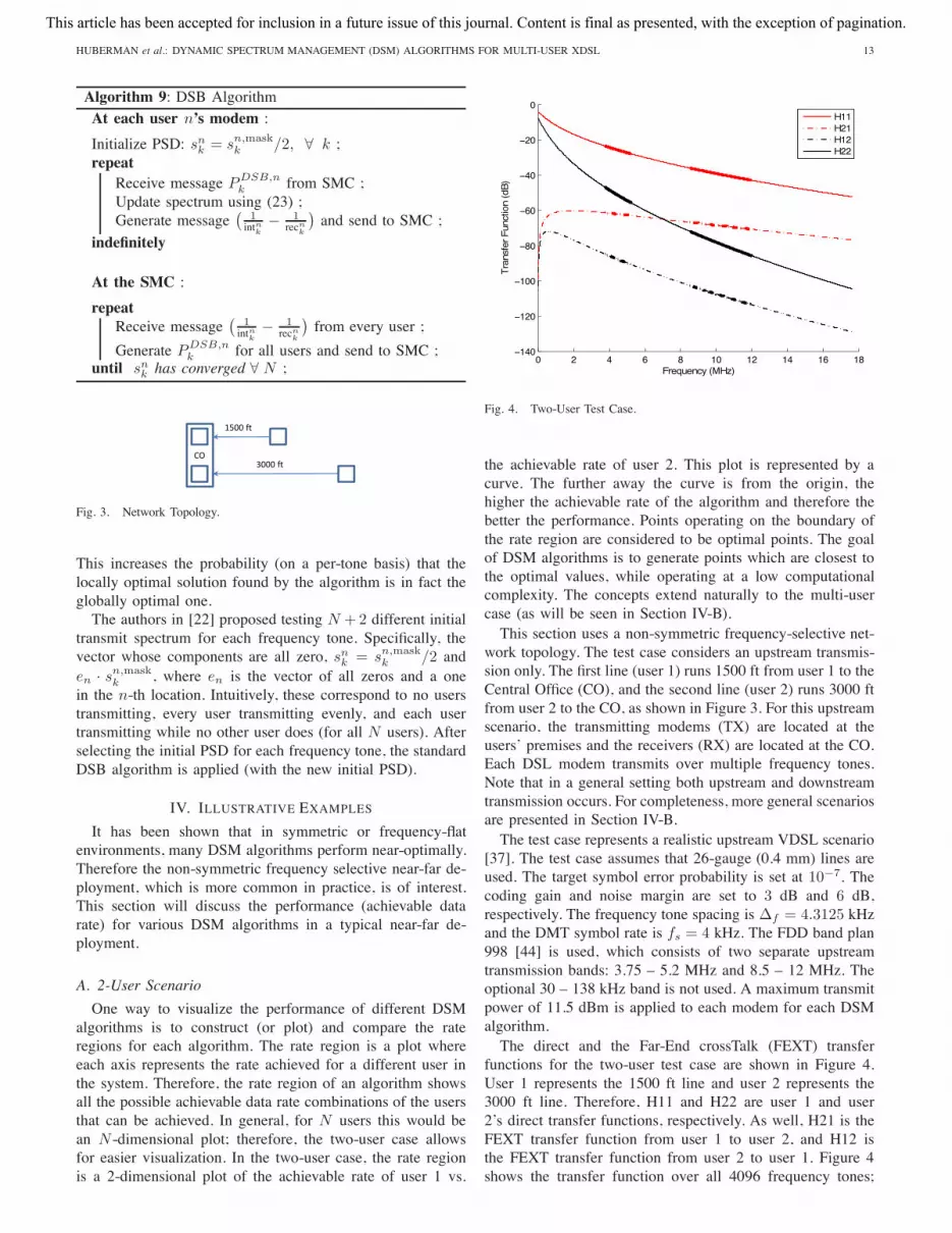
work topology. The test case considers an upstream transmis-sion only. The first line (user 1) runs 1500 ft from user 1 to theCentral Office (CO), and the second line (user 2) runs 3000 ftfrom user 2 to the CO, as shown in Figure 3. For this upstreamscenario, the transmitting modems (TX) are located at theusers’ premises and the receivers (RX) are located at the CO.Each DSL modem transmits over multiple frequency tones.Note that in a general setting both upstream and downstreamtransmission occurs. For completeness, more general scenariosare presented in Section IV-B.The test case represents a realistic upstream VDSL scenario

[37]. The test case assumes that 26-gauge (0.4 mm) lines areused. The target symbol error probability is set at 10−7. Thecoding gain and noise margin are set to 3 dB and 6 dB,respectively. The frequency tone spacing is Δf = 4.3125 kHzand the DMT symbol rate is fs = 4 kHz. The FDD band plan998 [44] is used, which consists of two separate upstreamtransmission bands: 3.75 – 5.2 MHz and 8.5 – 12 MHz. Theoptional 30 – 138 kHz band is not used. A maximum transmitpower of 11.5 dBm is applied to each modem for each DSMalgorithm.The direct and the Far-End crossTalk (FEXT) transfer

functions for the two-user test case are shown in Figure 4.User 1 represents the 1500 ft line and user 2 represents the3000 ft line. Therefore, H11 and H22 are user 1 and user2’s direct transfer functions, respectively. As well, H21 is theFEXT transfer function from user 1 to user 2, and H12 isthe FEXT transfer function from user 2 to user 1. Figure 4shows the transfer function over all 4096 frequency tones;



0 10 20 30 40 50 600

2

4

6

8

10

12

User 1 Rate (Mbps)

Use

r 2

Rat

e (M

bps)

Flat PBOIWFASBSIWOSB \ ISB \ DCA \ SCALE \ DSB

Fig. 5. Two-User Rate Regions.

specifically, the bolded parts of the curves are the upstreambands used for DSM.Simulations were run for: OSB, ISB, ASB, IWF, SIW,

SCALE, DCA, DSB and Flat PBO (a SSM technique (dis-cussed in Section II-C)). The results are summarized in Figure5. It is important to note that because of the simplicity of thetwo-user channel, without the presence of alien crosstalk, therate regions are more optimistic than usual. The test case usedhas few locally optimal points and therefore SCALE and DCAare able to converge to globally optimal points. In general,this is not the case, as with more interfering users the numberof locally optimal points grows significantly, which leads toreduced performance in locally optimizing algorithms (e.g.,DCA, DSB, and SCALE). As such, the algorithms must becompared in a multi-user setting to distinguish between thestronger algorithms, which is shown in Section IV-B.Based on the performance of the SSM algorithm (Flat

PBO) it is evident that the performance benefits of DSM aresignificant. In more complicated channels, where the numberof users increases, the performance of Flat PBO (and all SSMtechniques) is even worse as compared to the DSM techniques.

B. 25-User Scenarios

In order to better compare the performance of the DSMalgorithms, a multi-user setting is required. A 25-user scenariois very practical since while binders might contain up to 200lines, they generally contain sub-bundles of 25 users each.DSM can be applied to each sub-bundle of 25 users separatelywhile treating the interference of the other bundles (aliencrosstalk) as background noise.As well, due to the large complexity of some of the

centralized algorithms, they are not practical for a 25-userscenario. The focus then becomes on distributed (e.g., IWF,ASB, ASB-MRL, SIW) and semi-centralized algorithms (e.g.,SCALE, DSB).The network topology used for the 25-user scenarios is

shown in Figure 6. The lengths L1, . . . , LN are randomvariables uniformly distributed over the interval [0, 1000] feet.

Fig. 6. 25-User Test Case.

TABLE IUSER DISTRIBUTIONS FOR THE 25-USER SCENARIOS.

25 User Scenario - A 25 User Scenario - B# of CO users 12 9# of RT #1 users 13 8# of RT #2 users 0 8

PSD masks were applied using VDSL Profile 17a band plan[45], which consists of three downstream bands (0.276 – 3.75MHz, 5.2 – 8.5 MHz, and 12 – 17.664 MHz) and two upstreambands (3.75 – 5.2 MHz and 8.5 – 12 MHz).Two 25-user test cases were conducted. Each of these test

cases consisted of both upstream and downstream transmis-sion. The user distributions for the two test cases, 25 UserScenario - A and 25 User Scenario - B are summarized inTable I.One hundred network realizations were simulated and each

of IWF, ASB-2, ASB-MRL, SCALE, DSB and ISB solvedthe RA optimization problem (3) with wn = 1 ∀ n. Thisavoids the use of target rates, which speeds up simulationtime. Each algorithm was run until the sum of the L-2 norms(or Euclidean norms) of all the users PSDs converged towithin 1E-10 of the previous iteration (or a maximum of1000 iterations was reached). The ASB-2 algorithm was onlyrun to an accuracy of 1E-8 since it was observed that in alarge number of realizations, convergence was not achievedand instead the algorithm toggled between several points.Due to the fact that the SIW algorithm requires target rates

to operate, it was omitted from these comparisons. As well,the limitations of SIW was shown in the two-user test case(Section IV-A). DCA was omitted since the algorithm cannotbe applied with PSD masks, which is an important physicalconstraint in practical DSL systems.Since the choice of reference line for an arbitrary network

topology is still an open question, the ASB (respectively ASB-2) results vary depending on the choice of reference line. Fordownstream transmission, the reference line of each user wasselected as the longest possible CO line (i.e., a 2000-ft COline). For the upstream transmission, the reference line waschosen as the longest possible RT user which is most affectedby crosstalk (i.e., a 2000-ft RT #1 line for Scenario A and a1500-ft RT #2 line for Scenario B).The ASB-MRL algorithm was simulated using two pairs

of reference lines for each RT and CO subgroup. Morespecifically, for each RT and CO subgroup, four referencelines were selected (2 × 1000-ft line and 2 × 2000-ft line).The simulation results are based on the ASB-DSB approachoutlined in [23]; as well, the reference PSDs were generated



by performing single-user water-filling assuming no crosstalk.The PSDs of the stronger reference lines (most significantinterferers) were then scaled back to reflect a more accuraterepresentation of the PSD of each user.For the downstream 25 User Scenario - A, the RT reference

lines reduced their PSDs by 10 dB. For the upstream 25 UserScenario - A, the CO reference lines reduced their PSDs by20 dB and the RT reference lines reduced their PSDs by 10dB.For the downstream 25 User Scenario - B, the CO and

RT #1 reference lines reduced their PSDs by 10 dB and theRT #2 reference lines reduced their PSDs by 20 dB. For theupstream 25 User Scenario - B, the RT #1 and RT #2 referencelines reduced their PSDs by 10 dB and the CO reference linesreduced their PSDs by 20 dB.The PSDs were scaled by either 10 dB, 20 dB or not at

all, since these quantities heuristically seemed to work fairlywell. It is important to note that while some PSD scaling isnecessary, the relative scaling of the reference lines is verysignificant (e.g., strong reference lines should have higherPSD scaling than weak reference lines). The sensitivity to thechoice of scaling for an arbitrary network still needs to beinvestigated.The 25-user simulations are intended to distinguish between

the various high-performance (in terms of both achievablerate and runtime) distributed algorithms in a realistic scenario.The ISB algorithm was included as a performance measure ofhow well the distributed algorithms (with local knowledge ofthe network) performed compared to a near-optimal algorithm(with global knowledge of the network).1) Scenario - A: A summary of the results for 25 User

Scenario - A is shown in Table II. The sum rate (objectivefunction value) is the sum of the rates of all 25 users (sincewn = 1 ∀ n). The average number of iterations refers tothe outer iterations of the algorithm, and is also equal tothe number of interference measurements required to takewhen using simultaneous spectrum updates for each user. It isimportant to note that the time per iteration of IWF, ASB-2,ASB-MRL, DSB, and SCALE are all very small and thereforethe main constraint in terms of practical runtime is thenumber of iterations, since taking interference measurementscan be much more time-consuming than the runtime of eachiteration (e.g., one set of channel measurements over the 4096frequency tones is on the order of minutes using a typicalVDSL2 DSLAM) 2. The total power used refers to the totalpower consumed across the 25 users.Based on the results in Table II, it is clear that in both

the downstream and upstream scenarios, DSB, SCALE andASB-MRL achieve the best overall performance. For thedownstream scenario, SCALE provides a 0.4% performanceincrease over DSB, while still requiring fewer iterations (num-ber of time-consuming interference measurements required),on average. In the upstream scenario, both algorithms providethe same performance but DSB requires fewer time-consuminginterference measurements while SCALE requires less totalpower consumption, on average.

2Based on channel measurements taken in the Broadband CommunicationsResearch Lab at McGill University

TABLE IISUMMARY OF 25 User Scenario - A.

DownstreamAvg. Avg. Avg. Avg.

Sum Rate Runtime Number of Total Power Used(Mbps) (s) Iterations (dBm)

IWF 783.87 0.17 11.9 25.48ASB-2 810.76 0.58 22.0 24.50

ASB-MRL 858.15 0.85 13.4 22.96DSB 858.81 7.67 380.0 22.62SCALE 862.36 4.99 317.7 22.10ISB 847.62 hours 47.9 22.89

UpstreamAvg. Avg. Avg. Avg.


IWF 195.32 0.05 6.8 25.48ASB-2 247.54 0.04 2.9 12.09


Table II also shows that ASB-MRL achieved strong per-formance while maintaining a low number of iterations. Inparticular, the average performance of ASB-MRL was within1% of the average performance of DSB and SCALE inthe downstream scenario but it required an average of 13.4iterations, as opposed to more than 300 iterations requiredfor DSB and SCALE. Similarly, in the upstream scenario, theaverage performance of ASB-MRL was within 1.3% of theaverage performance of DSB and SCALE but it only requiredan average of 7.2 iterations, compared to more than 200iterations required for DSB and SCALE. The reduction of 200-300 time-consuming interference measurements demonstratesthat ASB-MRL can provide a significant practical complexityreduction over semi-centralized algorithms like SCALE andDSB, while operating fully autonomously and maintainingstrong overall performance.As well, the performance of the centralized ISB algorithm

for both the downstream and upstream scenarios was inferiorto that of SCALE and DSB, on average. For the downstreamscenario, in 67% of realizations the sum rate of ISB wassuperior to that of SCALE and DSB. The largest sum rateincrease in ISB over SCALE and DSB was 8.4 Mbps (1%performance increase); however, the largest sum rate decreaseby ISB over DSB and SCALE was 76.6 Mbps (8.6% per-formance decrease). Even though the sum rate achieved byISB was superior to that of DSB and SCALE in 67% ofthe realizations, the sum rate in the remaining 33% of therealizations was considerably lower than that of DSB andSCALE. This resulted in the average sum rate of ISB beingsmaller than that of DSB and SCALE. For the upstreamscenario, the performance of ISB was inferior to that ofSCALE and DSB for all network realizations, resulting in anaverage sum rate of approximately 24 Mbps (9.2%) lower.It is worthwhile to note that the performance of ISB was

often stronger than DSB and SCALE in the downstreamscenario; however, at times the ISB algorithm yielded asignificantly worse sum rate. This could be due to the fact thatwhen the ISB algorithm was implemented, the PSD of eachuser was updated in turn from user 1 to user 25, regardlessof the network realization. The order in which the userssequentially update their PSD can have a crucial impact on the



TABLE IIIINITIAL BEHAVIOR FOR 25 User Scenario - A.

Downstream Average Sum Rate (Mbps) for Iteration #1 2 3 Final

ASB-MRL 856.61 858.30 858.10 858.15DSB 765.81 795.93 811.62 858.81SCALE 557.20 670.92 712.54 862.36

Upstream Average Sum Rate (Mbps) for Iteration #1 2 3 Final

ASB-MRL 263.11 264.35 264.40 264.39DSB 205.65 221.86 232.18 267.75SCALE 148.64 187.72 204.24 267.75

final achievable rate. In order to apply ISB more appropriately,the algorithm would need to be re-run using various differentPSD update orders and selecting the maximum value.For the sake of time, the ISB algorithm was only run for

the one sequence of PSD updates for each network realization.These results suggest that for the realizations where thissequence of PSD updates was suitable, the sum rate achievedby ISB was superior to DSB and SCALE (on average by4 Mbps or 0.4%); however, for the realizations where thissequence of PSD updates was not suitable, the sum rateachieved by ISB was significantly inferior to DSB and SCALE(on average 40 Mbps or 5.1%).Table II shows that the average performance of IWF is infe-

rior to DSB and SCALE in terms of the total sum rate and thetotal power consumed; however, it requires significantly feweriterations which means it requires significantly fewer costlyinterference measurements, on average. The performance ofIWF in the downstream scenario is significantly better than inthe upstream scenario (relative to the other DSM algorithms).More specifically, IWF performs at 90.9% of the rate ofSCALE in the downstream scenario, while it can only performat 72.9% of the rate of DSB and SCALE in the upstreamscenario.Table II shows that when running ASB-2 to an accuracy

of 1E-8, significant performance improvements can be seen.In particular, ASB-2 achieves 94.0% of the SCALE rate inthe downstream scenario and 92.5% of the SCALE rate inthe upstream scenario. This performance is achieved at asignificant complexity reduction in terms of the number ofiterations. The main issue regarding the ASB-2 algorithm isits limiting behaviour.Beyond what is shown in Table II, when ASB-2 was run

to an accuracy of 1E-9, its downstream sum rate dropped by167 Mbps (20.6%) and its upstream sum rate dropped by 102Mbps (41.4%). Similar results were obtained when ASB-2 wasrun to an accuracy of 1E-10 (i.e., a 22.7% decrease in thedownstream scenario and a 49.9% decrease in the upstreamscenario, as compared to an accuracy of 1E-8). Regardlessof the accuracy on ASB-2, the maximum sum rate was oftenachieved on the first or first few iterations; afterwards, theperformance of ASB-2 rapidly decreased as the number ofiterations increased.Similarly, the average first iteration of ASB-2 for the down-

stream scenario yielded a sum rate of 844.01 Mbps (104.1%of the converged 1E-8 result). For the upstream scenario,the average number of iterations before convergence whenrunning an accuracy of 1E-8 was 2.9. As such, the average

TABLE IVSUMMARY OF 25 User Scenario - B.

DownstreamAvg. Avg. Avg. Avg.


IWF 811.90 0.11 6.1 25.48ASB-2 868.23 0.35 15.7 23.29


UpstreamAvg. Avg. Avg. Avg.


IWF 217.40 0.05 6.7 25.48ASB-2 221.91 0.28 26.9 18.03


third iteration of ASB-2 yielded a similar sum rate of 247.98Mbps (100.1% of the converged 1E-8 result) as the averageconverged sum rate.Due to the limiting behavior of ASB-2, care must be taken

to not “over-run” the algorithm, since running too manyiterations could drastically reduce the performance. As such,it is important to be aware of the potential benefits of ASB-2but even more so, the potential dangers of using it.The ideal algorithm would achieve strong performance in

very few iterations, while at the same time ensuring perfor-mance increases (or does not significantly decrease) as thenumber of iterations increases. DSB, SCALE and ASB-MRL(with appropriately chosen parameters) all exhibit this typeof behavior. A summary of the sum rate for the first threeiterations and the final sum rate for DSB, SCALE and ASB-MRL is shown in Table III.Table III shows that while SCALE achieves the largest

final sum rate, it approaches its final point slowly. ASB-MRLapproaches its final sum rate extremely quickly, on averageconverging to within 99% of the final sum rate in only acouple of iterations (both upstream and downstream). For thedownstream scenario, DSB and SCALE on average achieved94.5% and 82.7% of their final sum rate after three iterations,respectively. For the upstream scenario, DSB and SCALE onaverage achieved 86.7% and 76.3% of their final sum rate afterthree iterations, respectively.It is interesting to note that while Table II shows SCALE

requires fewer iterations on average than DSB in the down-stream scenario (317 compared to 380), Table III shows thatDSB’s initial steps are much closer to the final sum rate thanthat of SCALE.Overall, for the 25 User Scenario - A, ASB-MRL achieved

the best balance between maximizing the sum rate, whilerequiring fewer iterations to converge, for both the upstreamand downstream scenarios.2) Scenario - B: A summary of the results for 25 User

Scenario - B is shown in Table IV.Based on the results of Table IV, it is clear that DSB,

SCALE and ASB-MRL are the highest performing non-centralized algorithms. For both the upstream and downstreamscenarios, DSB and SCALE provide roughly the same perfor-



mance but SCALE required fewer iterations in the downstreamscenario, while DSB required fewer iterations in the upstreamscenario. For both scenarios, SCALE consumed less totalpower than DSB.Table IV also shows that the average performance of ASB-

MRL was within 1.0% of the average performance of DSBand SCALE achieved in the downstream scenario; as well,the average performance of ASB-MRL was within 1.9% ofthe average performance of DSB and SCALE achieved in theupstream scenario. For both scenarios, ASB-MRL requiredsubstantially fewer iterations to achieve convergence than DSBor SCALE (i.e., 38.6 compared to 392.5 and 287.6 in thedownstream scenario and 7.2 compared to 184.9 and 255.6 inthe upstream scenario).As shown in Table IV, the performance of the centralized

algorithm ISB for both the downstream and upstream scenarioswas inferior to that of SCALE and DSB, on average. Forthe downstream scenario, 49% of the network realizationssimulated resulted in a higher sum rate for ISB than for bothDSB and SCALE. The largest sum rate increase by ISB overDSB and SCALE was 7 Mbps (0.8% performance increase);however, the largest sum rate decrease by ISB over DSBand SCALE was 80 Mbps (8.7% performance decrease). Ingeneral, it was observed that in the 49% of realizations whereISB was superior, the performance gain was minor (on average0.2%); whereas, in the 51% of realizations where ISB wasinferior, the performance drops were more severe (on average2.1%). This resulted in an average sum rate for ISB belowthat of DSB and SCALE. In the upstream scenario, ISB wasinferior to DSB and SCALE for each network realization, butsince the achieved values were fairly close for each algorithm,the average sum rates achieved by all three are nearly identical.As discussed in Section IV-B1, the order in which each

user’s PSD was updated can greatly affect the results for agiven realization and could explain why for some realizationsISB achieved strong performance, but for other realizationsISB achieved poor performance. For the downstream scenario,in the 49% of realizations where ISB achieved better perfor-mance than DSB and SCALE, the average sum rate of ISB wasonly approximately 2 Mbps larger (less than 1% performanceimprovement).Table IV shows that the performance of IWF is much

stronger in the downstream scenario (86.3% of the DSBsum rate) than the upstream scenario (71.4% of the DSBsum rate). Similar to the Section IV-B1 results, IWF requiresfewer iterations to achieve convergence than the other DSMalgorithms for both the upstream and downstream scenarios.Beyond what is shown in Table IV, the limiting performance

of ASB-2 was very poor. More specifically, when ASB-2 wasrun to an accuracy of 1E-10, the sum rate achieved was 549.74Mbps (63.3% of the 1E-8 results) in the downstream scenarioand 101.68 Mbps (45.8% of the 1E-8 results) in the upstreamscenario.A summary of the sum rate for the first three iterations and

the final sum rate for DSB, SCALE and ASB-MRL is shownin Table V.Table V shows that ASB-MRL approached its final sum rate

extremely quickly, on average converging to within 99% of thefinal sum rate in only a couple of iterations (both upstream and

TABLE VINITIAL BEHAVIOR FOR 25 User Scenario - B.

Downstream Average Sum Rate (Mbps) for Iteration #1 2 3 Final

ASB-MRL 932.00 933.30 933.01 932.51DSB 795.85 833.97 854.25 940.72SCALE 617.39 742.63 790.92 942.09

Upstream Average Sum Rate (Mbps) for Iteration #1 2 3 Final

ASB-MRL 297.02 298.54 298.51 298.45DSB 232.50 253.77 266.73 304.52SCALE 147.78 194.56 211.76 304.42

downstream). For the downstream scenario, DSB and SCALEachieved 90.8% and 84.0% of their final sum rate after threeiterations, respectively. For the upstream scenario, DSB andSCALE achieved 87.5% and 69.6% of their final sum rateafter three iterations, respectively.Overall, for the 25 User Scenario - B, ASB-MRL achieved

the best balance between maximizing the sum rate, whileensuring fewer iterations to converge, for both the upstreamand downstream scenarios.

V. COMPLEXITY

Another significant factor in choosing a DSM algorithmis the run-time (or implementation time). The run-time ofdifferent algorithms depends on many factors including theprocessor(s) used, the coding used, the programming lan-guage used, etc. Therefore, the performance metric used inthis section to compare the DSM algorithms will be theircomputational complexity.Computational complexity represents the number of op-

erations required for the execution of an algorithm. Morespecifically, it shows the behavior of different algorithmsas the input sizes increase. In order to represent this, O(·)notation is used. It describes the limiting behavior of a functionwhen the arguments tend towards infinity. This is describedmathematically as follows:

f(x) = O(g(x)) ⇐⇒ |f(x)| ≤ c|g(x)| ∀ x as x → ∞,

where c ∈ R is some constant.Therefore, for an arbitrary algorithm dependent on some

variable X , a O(X) algorithm will converge faster than aO(X2) algorithm for sufficiently large X . The convergencetime of an algorithm is said to be exponential if it is O(eX),and is said to be polynomial if it is O(Xa) for a > 1. It isimportant to note that in algorithmic terms, exponential timeis extremely slow.For DSM purposes, there are two main inputs (variables)

of interest: the number of users, N , and the number offrequency tones, K . Hence, all algorithms will be of the formO(f(N, K)) for some function f(N, K). The total powerand target data rate constraints, shown in Equation (2), causecoupling over the frequency tones, which requires that eachuser’s PSD be searched for jointly over all frequency tones.Solving an X-dimensional exhaustive search has a compu-

tational complexity ofO(eX). Therefore, solving the DSM op-timal resource allocation through an exhaustive search in boththe number of users, N , and the number of frequency tones,



K , would lead to a computational complexity of O(eNK),which is computationally intractable.In Section I, the concept of centralized versus distributed

(and autonomous) systems was introduced. One key differenceis in how the total interference plus noise is found. Forautonomous algorithms, the total interference plus noise ismeasured locally by each user. For centralized algorithms,since the DSL channel is generally time-invariant, channelmeasurements can be taken a priori and stored at the CO (thesemeasurements would need to be updated periodically). Hence,full channel knowledge is assumed (i.e., |hn,m

k |2 is known∀ n, m ∈ N , k ∈ K). Depending on the implementation,distributed algorithms can either operate fully autonomouslyor in a semi-centralized manner by making use of explicitmessage passing.Operating in a centralized manner may require the time-

consuming computation of the interference plus noise for eachuser on each frequency tone in the system. More specifically,to compute the total interference plus noise for some user non a given frequency tone k, one must cycle through all theusers m �= n and multiply the channel transfer function byuser m’s transmit PSD for the specific frequency tone k andsum them. Hence, in order to compute the total interferenceplus noise for all N users on some frequency tone k, the totalcomplexity will be:

N × (N − 1) = N2 − N.

Therefore, the computational complexity of calculating thetotal interference plus noise for all N users on some frequencytones k will be:

CInterference = O(N2).

In addition, computing the bit-rates of all N users onsome frequency tone k is dominated by computing the totalinterference plus noise and therefore, is also O(N2). Notethat in order to compute the bit-rates of all N users on allK frequency tones, the computational complexity will beO(KN2).

A. IWF Complexity

Iterative Water-Filling (IWF) is a distributed algorithmbriefly described in Section III-C (Algorithm 4). IWF consistsof two loops where the outer loop cycles through the innerloop for all users. The inner loop performs water-filling forthe n-th user over all the K frequency tones. The water-fillingprocess involves a bisection search for that user’s Lagrangemultiplier, λ; Assuming that the number of bisection iterationsrequired for the PSD to converge is at most v1 and assumingthat the number of iterations required for the IWF algorithmto converge is v2, the total complexity of the IWF algorithmwill be v1 × v2 × N × K , which implies:

CIWF = O(KN).

It is important to note that for IWF, whenver a user isrequired to perform water-filling, that user must re-measureits total interference plus noise. Therefore, for N users and viterations, a total of vN measurements must be performed. Ifthe channel conditions are poor, the total number of iterations,

v, may be large. Therefore, if the values of N and v are large,taking vN measurements may be a bottleneck in terms of run-time.For such situations, IWF can be implemented in a central-

ized manner. As explained previously in Section V, since theDSL channel is very slow time-varying, channel measurementscan be taken a priori and stored at the CO. The CO can thencompute the total interference plus noise seen by user n in acentralized manner, which requires O(KN) operations. TheCO runs a virtual IWF game to generate the new PSD values.More specifically, on user n’s turn in the virtual game, the COcomputes the total interference plus noise seen by user n andthen updates user n’s virtual PSD. The CO plays this virtualgame until all of the users’ PSDs converge, at which point theCO informs each user of their new PSD value.Implementing IWF in a centralized manner, using the same

definitions as for the distributed manner, would require a totalcomplexity of N × (KN + v1 × v2 × K), which implies:

CIWF (centralized) = O(KN2).

Note that CIWF (centralized) has a higher complexity thanCIWF since it performs more computations during everyiteration. In practice, the run-time between the two methodscan vary greatly depending on the number of users in the sys-tem, as well as the channel conditions, which both affect thenumber of iterations and interference measurements required.

B. SIW Complexity

The Selective Iterative Water-filling (SIW) algorithm (de-scribed in Section III-D, Algorithm 5) performs two loopswhere the outer loop cycles through the inner loop for allusers where the inner loop performs IWF for all users. Atevery iteration of the outer loop, users (and their correspondingfrequency tones) that have already achieved their maximumpower are removed. It has been shown that each sequentialinner loop removes at least one user and frequency tone. Thisprocess is repeated until either all the users have been removedfrom the inner loop (maximum of N iterations), or until allfrequency tones have been removed (possibly in less thanN iterations). Therefore, the maximum number of additionalouter loop iterations is N , which leads to a total complexityof up to N times that of IWF, which implies:

CSIW = O(KN2).

C. OSB Complexity

The Optimal Spectrum Balancing (OSB) Algorithm is de-scribed in Section III-A (Algorithm 1). Assuming that thenumber of discrete bit-loadings is X , then the search spacefor all users’ PSDs will contain XN elements. Therefore, tosolve for the optimal PSD for each user, an exhaustive searchmust be performed over the XN combinations. For each bit-loading combination, the total rate must be calculated, whichadds a multiplicative factor of N2.The OSB algorithm performs the above exhaustive search

independently on each of the K frequency tones, and re-peats itself until each user’s Lagrange multipliers converge.Assuming that the number of iterations until all the Lagrange



multipliers converge is v1, the total complexity of the OSBalgorithm is v1 × K × N2 × XN , which implies:

COSB = O(KN2XN).

D. ISB Complexity

The Iterative Spectrum Balancing (ISB) algorithm is de-scribed in Section III-B (Algorithm 2). Assuming that thenumber of discrete bit-loadings is X , then the search spacefor each user’s PSD will contain X elements. For ISB, thereare two loops where the outer loop cycles through the innerloop for all users. The inner loop performs N different 1-dimensional exhaustive searches over each of the X elementsfor each user. For each bit-loading combination, the total ratemust be calculated, which adds a multiplicative factor of N2.Therefore, with respect to the number of users, N , each innerloop consists of N2 + N calculations. Assuming that thenumber of iterations required for the user’s PSDs to convergeis v1, and that the number of iterations for wn and λn toconverge is v2, the total complexity of the ISB algorithm isv1 × v2 × K × (N2 + N) × N × X , which implies:

CISB = O(KN3X).

E. ASB Complexity

The Autonomous Spectrum Balancing (ASB) algorithm isdescribed in Section III-E (Algorithm 6). ASB has threenested iterations; the outermost cycle iterates through theusers. Within each cycle, each user runs an outer loop whichupdates wn until the target data rate is achieved, and aninner loop which updates λn until the power constraint issatisfied. Bisection search is used in both loops and therefore,the number of iterations required for both the outer and innerloops to converge, while achieving an accuracy of εR and εP

respectively is log2(1/εR) × log2(1/εP ).For ASB, the complexity of each iteration is dominated

by finding the roots of the cubic polynomial (i.e., solvingequation (14)). Finding the roots of a cubic equation requires44 operations in total [46]. This equation must be solved foreach of the K frequency tones, hence the total complexityof finding the roots is 44K . Therefore, assuming that thealgorithm converges in a finite number of iterations, v, thetotal complexity of the ASB algorithm is v×N×log2(1/εR)×log2(1/εP ) × 44K which implies:

CASB = O(KN).

Note that the overall complexity of ASB-2 (described inSection III-E) is the same as ASB even though the complexityof each PSD update is reduced (i.e., solving a cubic equationis replaced by a simple water-filling like update). While theoverall computational complexities are the same, the ASB-2algorithm has a significantly lower runtime.The overall complexity of ASB-MRL is roughly the same as

that of ASB-2. The difference is that the P ASB−2,nk becomes a

summation over the number of reference lines. Therefore sincethe number of reference lines is a constant, the complexity ofASB-MRL is also O(KN). Note that even though ASB-MRLuses multiple reference lines, since it is based on the ASB-2algorithm, its PSD update formula still provides computationaladvantages over the original ASB’s.

F. SCALE Complexity

The Successive Convex Approximation for Low complExity(SCALE) algorithm is described in Section III-F (Algorithm7). SCALE is an iterative algorithm, each iteration beginsby user n updating its PSD on all K frequency tones. Untilthe Lagrange multipliers for each user converge, the processof measuring their total interference plus noise, sending themeasurements to the Spectrum Management Center (SMC),waiting for a reply and finally updating values accordingly,is repeated. Assuming v is the number of operations requiredto update a given user’s PSD, the total complexity from adistributed point of view is vK .The SMC receives a message constructed from the mea-

sured total interference plus noise from all users. The SMCthen sends each user the sum of the messages received fromall the other users. Therefore, generating the message for eachuser requires K ×N additions. This process must be repeatedfor all N users, leading to a complexity of KN2 at the SMC.Therefore, the total complexity of the SCALE algorithm is

KN2 + vK , which implies:

CSCALE = O(KN2).

G. DCA Complexity

The Difference of Convex functions Algorithm (DCA) isdescribed in Section III-G (Algorithm 8). The complexitywill be dominated by calculating the gradient of the objec-tive function and applying convex optimization techniques.Since there are K × N variables (e.g., sn

k for some k andsome n), calculating the gradient requires taking K × Nderivatives. For each of the K × N derivatives, as shown inEquations (19) and (20), a nested summation over all N andN −1 elements must be calculated, respectively. This requiresK × N × N2 computations the first time it is computed.While the denominators of Equations (19) and (20) are notthe same, by noticing that each is the same for all K × Nderivatives, additional computations can be avoided by re-using the previously computed summations (i.e., An

k (s) andBn

k (s), respectively). For each additional user the number ofcomputations required will be K × N × N . Therefore thecomplexity of taking the derivative will be:

CDCA(Derivative) = O(KN3 − KN2) = O(KN3)

at each iteration.Each iteration requires solving a convex quadratic program-

ming optimization problem (discussed in Section III-G). It isshown in [47] that a convex quadratic program can be solvedin O(n3L) arithmetic operations, where n is the number ofvariables (which is equal to N since the program can be solvedindependently on each frequency tone) and L is the encodinglength (which is a constant). Therefore, solving the convexquadratic program on each of the K frequency tones has acomplexity of O(KN3). Note that this algorithm solves forPSDs without using the spectral mask constraint. If spectralmasks are used, this complexity would increase.Therefore, assuming that the number of iterations required

until convergence is achieved is v, the total complexity is v×[(KN3 − KN2) + KN3], which implies:

CDCA = O(KN3).



TABLE VISUMMARY OF DSM ALGORITHM COMPLEXITIES.

DSM Complexity Message Passing

Algorithms Overall At SMC At User Per Update

IWF O(KN) – O(K) –

ASB O(KN) – O(K) –

SIW O(KN2) – O(K) ≤ KN

OSB O(KeN ) – –

ISB O(KN2) – –

DCA O(KN3) – –

SCALE O(KN2) O(K) 2KN

DSB O(KN2) O(K) 2KN

H. DSB Complexity

The Distributed Spectrum Balancing (DSB) algorithm isdescribed in Section III-H (Algorithm 9). DSB is an iterativealgorithm, each iteration begins by user n measuring itschannel and sending the message

(1intnk

− 1recnk

)to the SMC.

The SMC gathers the messages from all users, computesPDSB,n

k on all K frequency tones for all N users and sendsPDSB,n

k to each user, n. Each user then updates its PSDon all K frequency tones. Until the Lagrange multipliersfor each user converge, the process of measuring their totalinterference plus noise, sending the measurements to theSpectrum Management Center (SMC), waiting for a replyand finally updating values accordingly, is repeated. Since thenumber of operations required to update a given user’s PSDis a constant, the complexity from a distributed point of viewis O(K).Calculating the message that the SMC sends each user, n, is

a sum over N − 1 users of the product between the crosstalkchannel and the message received from user n. Therefore,generating the message for each user requires K × (N − 1)additions. This process must be repeated for all N users,leading to a complexity of KN2 − KN at the SMC.Therefore, assuming that v is the number of iterations

required for convergence, the total complexity of the DSBalgorithm is v × [KN2 − KN + O(K)], which implies:

CDSB = O(KN2).

I. Summary of Complexities

The complexities of the DSM algorithms are summarizedin Table VI.

VI. CONCLUDING REMARKS

This paper presented an overview of algorithms that adap-tively allocate resources in a multiuser DSL system. Theconcept of DSM and its advantages in comparison to SSM wasdiscussed. The following DSM algorithms were discussed indetail: OSB, ISB, ASB, IWF, SIW, SCALE, DCA and DSB.

Through the use of two illustrative examples (Section IV),it was shown that semi-centralized based algorithms with onlylocal knowledge of the network (i.e., SCALE and DSB) wereable to achieve comparable performance (achievable data rate)to a known full-centralized technique with global knowledgeof the network (e.g., ISB). For some network realizations,ISB outperformed DSB and SCALE by a maximum of lessthan 1%; however, the performance of both DSB and SCALEwas superior to ISB on average, by as much as 10% forsome realizations. It was also shown that a fully distributedalgorithm, ASB-MRL with the appropriate initialization pa-rameters, achieved comparable performance to SCALE andDSB.Through the use of computational complexity analysis

(Section V), it was shown that most of the DSM algorithmswould be computationally tractable for large numbers of usersand frequency tones. By comparing the computational com-plexities derived in Section V with the runtime and numberof iterations (interference measurements required) results ofSection IV-B, it is clear that IWF, ASB and ASB-MRL havesignificant computational advantages over DSB, SCALE andISB.As well, it was shown that SCALE often produced

marginally better results in terms of performance over DSB;nevertheless, DSB approached its solution at a much fasterrate. It was also shown that ASB-MRL approached its finalrate significantly faster than DSB or SCALE.Based on the above observations, it is clear that the com-

plexity benefits of IWF, ASB and ASB-MRL type algorithmsare very apparent over algorithms like DSB and SCALE, sincethey require significantly fewer interference measurements.Interference measurements can be time-consuming, and due tothe relatively fast time per iteration of all the non-centralizedalgorithms, they appear to be the limiting factor in terms ofthe practical implementation of the DSM algorithms.

ACKNOWLEDGMENTS

The authors would like to thank Dr. Raphael Cendrillon forhis discussions and advice on the implementation of ASB,Dr. Paschalis Tsiaflakis for his discussions on DSB, and Prof.Hoai-An Le-Thi, Mr. Anh Son Ta, Mr. Duc Quynh Tran andMr. Thuan Quang Nguyen of Universite Paul Verlaine - Metzfor various interesting discussions on DCA. The authors wouldalso like to thank the reviewers for their helpful comments.Finally, the authors would like to acknowledge the financialsupport of NSERC, Bell Canada, and FQRNT.

REFERENCES

[1] Broadband Forum, “3 million new north-american broadband sub-scribers added in first quarter 2009 despite economic downturn,” NewsRelease., Jun. 16, 2009.

[2] ANSI Standard T1.417-2001, “Spectrum management for loop trans-mission systems,” 2001.

[3] T. Starr, M. Sorbara, J. M. Cioffi, and P. J. Silverman, DSL Advances.Prentice-Hall, 2003.

[4] J. M. Cioffi, S. Jagannathan, W. Lee, H. Zou, A. Chowdhery, W. Rhee,G. Ginis, and P. Silverman, “Greener copper with dynamic spectrummanagement,” in Proc. IEEE Global Telecommun. Conf., pp. 1–5, Dec.2008.

[5] W. Yu, G. Ginis, and J. Cioffi, “Distributed multiuser power control fordigital subscriber lines,” IEEE J. Sel. Areas Commun., vol. 20, pp. 1105–1115, Jun. 2002.



[6] Y. Liu and Z. Su, “Distributed dynamic spectrum management for digitalsubscriber lines,” IEICE Trans. Commun., vol. E90B, no. 3, pp. 491–498, Mar. 2007.

[7] H. Bagheri, M. R. Pakravan, and B. H. Khalaj, “Iterative multi-userpower allocation: Performance evaluation & modification,” in Proc.IEEE Region 10 TENCON, vol. 3, pp. 216–219, Nov. 2004.

[8] D. Statovci, T. Nordstrom, and R. Nilsson, “The normalized-rate itera-tive algorithm: A practical dynamic spectrum management method forDSL,” EURASIP J. Appl. Signal Process., vol. 2006, Article ID 95175,17 pages, DOI: 10.1155/ASP/2006/95175, 2006.

[9] W. Lee, Y. Kim, M. H. Brady, and J. M. Cioffi, “Band-preferencedynamic spectrum management in a DSL environment,” in Proc. IEEEGlobal Telecommun. Conf., pp. 1–5, Nov. 2006.

[10] Y. Noam and A. Leshem, “Iterative power pricing for distributedspectrum coordination in DSL,” IEEE Trans. Commun., vol. 57, pp. 948–953, Apr. 2009.

[11] Y. Xu, S. Panigrahi, and T. Le-Ngoc, “Selective iterative water-fillingfor digital subscriber lines (DSL),” EURASIP J. Appl. Signal Process.,vol. 2007, Article ID 59068, 11 pages, DOI: 10.1155/2007/59068, 2007.

[12] R. Cendrillon, W. Yu, M. Moonen, J. Verlinden, and T. Bostoen,“Optimal multiuser spectrum management for digital subscriber lines,”IEEE Trans. Commun., vol. 54, pp. 922–933, May 2006.

[13] S. Wei, L. Youming, and Y. Miaoliang, “Low-complexity groupingspectrum management in multi-user DSL networks,” in Proc. IEEE Int.Conf. Commun., pp. 381–385, Jun. 2009.

[14] L. P. Qian and Y. Jun, “Monotonic optimization for non-concave powercontrol in multiuser multicarrier network systems,” in Proc. IEEEINFOCOM, pp. 172–180, Apr. 2009.

[15] T. Hoang, Convex Analysis and Global Optimization. Kluwer AcademicPublishers, 1998.

[16] Y. Xu, T. Le-Ngoc, and S. Panigrahi, “Global concave minimization foroptimal spectrum balancing in multi-user DSL networks,” IEEE Trans.Signal Process., vol. 56, pp. 2875–2885, Jul. 2008.

[17] R. Horst, T. Q. Phong, N. V. Thoai, and J. de Vries, “On solving a D.C.programming problem by a sequence of linear programs,” Journal ofGlobal Optimization, vol. 1, pp. 183–204, 1991.

[18] R. Cendrillon and M. Moonen, “Iterative spectrum balancing for digitalsubscriber lines,” in Proc. IEEE Int. Conf. Commun., May 2005.

[19] R. Lui and W. Yu, “Low-complexity near-optimal spectrum balancingfor digital subscriber lines,” in Proc. IEEE Int. Conf. Commun., May2005.

[20] A. Forouzan and L. Garth, “Generalized iterative spectrum balancingand grouped vectoring for maximal throughput of digital subscriberlines,” in Proc. IEEE Global Telecommun. Conf., vol. 4, pp. 2359–2363,Nov. 2005.

[21] R. Cendrillon, J. W. Huang, M. Chiang, and M. Moonen, “Autonomousspectrum balancing for digital subscriber lines,” IEEE Trans. SignalProcess., vol. 55, pp. 4241–4257, Aug. 2007.

[22] P. Tsiaflakis, M. Diehl, and M. Moonen, “Distributed spectrum man-agement algorithms for multiuser DSL networks,” IEEE Trans. SignalProcess., vol. 56, pp. 4825–4842, Oct. 2008.

[23] C. Leung, S. Huberman, and T. Le-Ngoc, “Autonomous spectrumbalancing using multiple reference lines for digital subscriber lines,”in Proc. IEEE Global Telecommun. Conf., Dec. 2010.

[24] R. Moraes, B. Dortschyy, A. Klautau, and J. R. i Riuy, “Semi-blindpower allocation for digital subscriber lines,” in Proc. IEEE Int. Conf.Commun., pp. 1420–1425, May 2008.

[25] J. Papandriopoulos and J. S. Evans, “Low-complexity distributed alo-girthms for spectrum balancing in multi-user DSL networks,” in Proc.IEEE Int. Conf. Commun., Jun. 2006.

[26] J. Papandriopoulos and J. S. Evans, “Scale: A low-complexity distributedprotocol for spectrum balancing in multiuser DSL networks,” IEEETrans. Inf.. Theory, vol. 55, pp. 3711–3724, Aug. 2009.

[27] D. T. Pham and H. A. Le Thi, “Convex analysis approach to d.c.programming: Theory, algorithms and applications,” Acta MathematicaVietnamica, vol. 22, pp. 289–355, 1997.

[28] T. Starr, J. M. Cioffi, and P. Silverman, Understanding Digital Sub-scriber Line Technology. Upper Saddle River, NJ: Prentice-Hall, 1999.

[29] J. M. Cioffi, S. Jagannathan, and W. Lee, “Digital subscriberline (DSL).” http://www.scholarpedia.org/article/Digital subscriberline (DSL), Aug. 2008.

[30] R. van der Berg, “Developments in fibre technologies and investment(working party on communication infrastructures and services policy),”Organisation for Economic Co-operation and Development, Apr. 3,2008.

[31] ZTE, “FTTx solution white paper,” http://www.telecomasia.net/pdf/ZTE/ZTE 091709.pdf , 2009.

[32] S. Yoshii, “Spectrum management of DSL systems in Japan,” in TEN-CON 2005 2005 IEEE Region 10, pp. 1–6, Nov. 2005.

[33] “AT&T u-verse TV marks 2 million customer milestone,” http://www.digitaltvnews.net/content/?p=11786, Dec. 9, 2009.

[34] “Bell high speed fibre rollouts enable new internet and TV services,”http://www.bce.ca/en/news/releases/bev/2010/02/04/75344.html, Feb.4, 2010.

[35] S. Sadr, A. Anpalagan, and K. Raahemifar, “Radio resource allocationalgorithms for the downlink of multiuser OFDM communication sys-tems,” IEEE Commun. Surveys Tuts., vol. 11, no. 3, pp. 92–106, 2009.

[36] P. Tsiaflakis, J. Vangorp, M. Moonen, J. Verlinden, and K. Van Acker,“An efficient search algorithm for the Lagrange multipliers of optimalspectrum balancing in multi-user xDSL systems,” in Acoustics, Speechand Signal Processing, 2006. ICASSP 2006 Proceedings. 2006 IEEEInternational Conference on, vol. 4, pp. IV–IV, May 2006.

[37] ETSI, “Transmission and multiplexing (TM); access transmission sys-tems on metallic access cables; very high speed digital subscriber line(VDSL); part 1: Functional requirements,” ETSI Std. TS 101 270-1,vol. Rev. V. 1.3.1, 2003.

[38] “Very high speed digital subscriber line (VDSL) metalic interface,” ANSIStd., vol. T1.424, 2004.

[39] “Very high speed digital subscriber line transceivers 2,” ITU Draft Std.,vol. G.993.2, 2006.

[40] M. Chiang, Advances in Applied Mathematics and Global Optimization,ch. Nonconvex Optimization for Communication Systems. Springer,2009.

[41] H. A. Le Thi and D. T. Pham, “The DC programming and DCA revistedwith DC models of real world non-convex optimization problems,”Annals of Operations Research, vol. 133, pp. 23–46, 2005.

[42] R. Blanquero and E. Carrizosa, “On covering methods for D.C. opti-mization,” Journal of Global Optimization, vol. 18, pp. 265–274, 2000.

[43] S. Huberman, C. Leung, and T. Le-Ngoc, “DSM algorithms in multi-user xDSL,” Tech. Rep., McGill University, Aug. 2009. http://www.ece.mcgill.ca/∼shuber6/.

[44] K. McCammon, “G. VDSL: VDSL band plan for North America,” ITUcontribution D, vol. 715, 2000.

[45] “Very high speed digital subscriber line transceivers 2,” ITU Draft Std.,vol. G.993.2 Amendment 1, 2007.

[46] R. Nickalls, “A new approach to solving the cubic: Cardan’s solutionrevealed,” Mathematical Gazette, vol. 77, pp. 354–359, 1993.

[47] D. Goldfarb and S. Liu, “An O(n3L) primal interior point algorithmfor convex quadratic programming,” Math. Program., vol. 49, no. 3,pp. 325–340, 1991.

Sean Huberman received his B.Sc. in engineering(with first-degree honours) from Queen’s University,Kingston, Canada, in applied mathematics and engi-neering control and communications, in May 2008.He began his M.Eng. in electrical engineering atMcGill University, Montreal, Canada, in September2008. In January 2010, he transferred into the PhDprogram in electrical engineering at McGill Univer-sity.His research interests include techniques of math-

ematical optimization, dynamic resource allocation,channel modeling and channel measurements.Mr. Huberman was the recipient of the Hydro Quebec Engineering Doctoral

Award in 2009. In 2010, he was the recipient of the Vadasz DoctoralFellowship in Engineering. He was also the recipient of a three-year doctoralNational Science and Engineering Research Council (NSERC) award and athree-year McGill Engineering Doctoral Award (MEDA).



Christopher Leung received his B.Eng. (withDistinction and Deans Honour List) in electri-cal engineering in 2009 from McGill University,Montreal, Quebec, Canada. He is currently finishinghis M.Eng., also in electrical engineering at McGillUniversity.Mr. Leung has received the Alexander Graham

Bell Canada Graduate Scholarship from the Na-tional Science and Engineering Research Council(NSERC) and the Bourses de maıtrise en recherchefrom the Fonds quebecois de la recherche sur la

nature et les technologies (FQRNT) for pursuing his M.Eng.

Tho Le-Ngoc Tho Le-Ngoc obtained his B.Eng.(with Distinction) in Electrical Engineering in 1976,his M.Eng. in 1978 from McGill University, Mon-treal, and his Ph.D. in Digital Communications in1983 from the University of Ottawa, Canada. During1977-1982, he was with Spar Aerospace Limited andinvolved in the development and design of satellitecommunications systems. During 1982-1985, he wasan Engineering Manager of the Radio Group in theDepartment of Development Engineering of SRT-elecom Inc., where he developed the new point-to-

multipoint DA-TDMA/TDM Subscriber Radio System SR500. During 1985-2000, he was a Professor at the Department of Electrical and ComputerEngineering of Concordia University. Since 2000, he has been with theDepartment of Electrical and Computer Engineering of McGill University.His research interest is in the area of broadband digital communications.He is the recipient of the 2004 Canadian Award in TelecommunicationsResearch, and recipient of the IEEE Canada Fessenden Award 2005. He holdsa Canada Research Chair (Tier I) on Broadband Access Communications, anda Bell Canada/NSERC Industrial Research Chair on Performance & ResourceManagement in Broadband xDSL Access Networks.


dynamic spectrum management (dsm) algorithms for multi-user xdsl

Documents