Don’t Let The Negatives Bring You Down:Sampling from Streams of Signed Updates

Edith CohenAT&T Labs–Research

180 Park AvenueFlorham Park, NJ 07932, USAedith@cohenwang.com

Graham Cormode, Nick DuffieldAT&T Labs–Research

180 Park AvenueFlorham Park, NJ 07932, USA

{graham,duffield}@research.att.com

ABSTRACTRandom sampling has been proven time and time again tobe a powerful tool for working with large data. Queries overthe full dataset are replaced by approximate queries over thesmaller (and hence easier to store and manipulate) sample.The sample constitutes a flexible summary that supports awide class of queries. But in many applications, datasetsare modified with time, and it is desirable to update sam-ples without requiring access to the full underlying datasets.In this paper, we introduce and analyze novel techniques forsampling over dynamic data, modeled as a stream of modi-fications to weights associated with each key.

While sampling schemes designed for stream applicationscan often readily accommodate positive updates to the dataset,much less is known for the case of negative updates, whereweights are reduced or items deleted altogether. We primar-ily consider the turnstile model of streams, and extend clas-sic schemes to incorporate negative updates. Perhaps sur-prisingly, the modifications to handle negative updates turnout to be natural and seamless extensions of the well-knownpositive update-only algorithms. We show that they pro-duce unbiased estimators, and we relate their performanceto the behavior of corresponding algorithms on insert-onlystreams with different parameters. A careful analysis is ne-cessitated, in order to account for the fact that samplingchoices for one key now depend on the choices made forother keys.

In practice, our solutions turn out to be efficient and accu-rate. Compared to recent algorithms for Lp sampling whichcan be applied to this problem, they are significantly morereliable, and dramatically faster.

Categories and Subject DescriptorsG.3 [Probability and Statistics]: Probabilistic Algorithms

General TermsAlgorithms, Measurement

Permission to make digital or hard copies of all or part of this work forpersonal or classroom use is granted without fee provided that copies arenot made or distributed for profit or commercial advantage and that copiesbear this notice and the full citation on the first page. To copy otherwise, torepublish, to post on servers or to redistribute to lists, requires prior specificpermission and/or a fee.SIGMETRICS’12, June 11–15, 2012, London, England, UK.Copyright 2012 ACM 978-1-4503-1097-0/12/06 ...$10.00.

Keywordssampling, deletions, data streams, updates

1. INTRODUCTIONRandom sampling has repeatedly been proven to be a

powerful and effective technique for dealing with massivedata. The case for working with samples is compelling: inmany cases, to estimate a function over the full data, it suf-fices to evaluate the same function over the much smallersample. Consequently, sampling techniques have found ap-plications in areas such as network monitoring, databasemanagement, and web data analysis. Complementing this,there is a rich theory of sampling, based on demonstratingthat different techniques produce unbiased estimators withlow or optimal variance.

Initial work on sampling from large datasets focused on arandom access model: the data is static, and disk resident,and we want to build an effective sample with a minimalnumber of probes to the data. However, in modern appli-cations we do not think of the data as static, but rather asconstantly changing. In this setting, we can conceive of thedata as being defined by a stream of transactions, and weget to see each transaction that modifies the current state.For concreteness we describe some motivating scenarios:

• First, we consider the case when the stream is a se-quence of financial transactions, each of which updatesan account balance. It is important to be able tomaintain a sample over current balances, which de-scribes the overall state of the system, and to providea snapshot of the system against which to quickly testfor anomalies without having to traverse the entire ac-count database.

• Internet Service Providers (ISPs) witness streams inthe form of network activities. These can set up ortear down (stateful) network connections. It is notpractical for the ISP to centrally keep a complete listof all current and active connections. It is neverthelesshelpful to draw a sample of these connections, so thatthe ISP can keep statistics on quality of service, round-trip delay, nature of traffic in its network and so on.Such statistics are needed to show that its agreementswith customers are being met, and for traffic shapingand planning purposes.

• Updates to a database generate a stream of trans-actions, to insert or delete records to tables. Thedatabase management system needs to keep statistics

on each attribute within a table, to determine whatindices to keep, and how to optimize query processing.Currently, deployed systems track only simple aggre-gates online (e.g. number of records in a table), andmust periodically rebuild more complex statistics witha complete scan, which makes this approach unsuitablefor (near) real-time systems.

In all these examples, and others like them, we can ex-tract a central problem. We are seeing a stream of weightedupdates to a set of keys, and we wish to maintain a samplethat reflects the current weights of the keyset. Specifically,we aim to support queries over the total weight associatedwith a subset of keys (subset-sum queries), which are the ba-sis of most complex queries [6]. If the set of keys ever seenis tiny, then we could just retain the weights of these keys,but in general there are many active keys at any one time,and so we want to maintain just a small sample. From thissample, we should be able to accurately address the prob-lems in the above examples, such as fraud detection, findinganomalies, and reporting behavior trends.

The core problem of sampling from a stream of distinct,unweighted keys is one of the earliest examples of what wenow think of as streaming algorithms [22]. In this paper,we tackle a much more general version of the problem: eachkey may appear multiple times in the stream. Each occur-rence is associated with a weight, and the total weight of akey is the sum of its associated weights. Moreover, the up-dates to the weights are allowed to be negative. This modelsvarious queuing and arrival/departure processes which canarise in the above applications. Despite the naturalness andgenerality of this problem, there has been minimal study ofsampling when the updates may be negative. Through ouranalysis, we are able to show that there are quite intuitivealgorithms to maintain a sample under such updates, thatoffer unbiased estimators, and whose performance can bebounded in terms of the performance of a comparable algo-rithm on an update stream with positive updates only. Wenext make precise the general model of streams we adoptin this paper, and go on to describe prior work in this areaand why it does not provide a satisfactory solution. At theend of this section, we summarize our contributions in thiswork, and outline our approach.

Streaming Model. We primarily consider the turnstilestream model, where each entry is a (positive or negative)update to the value of a key i. Here, the data is a streamof updates of the form (i, ∆), where i is a key and ∆ ∈ R.The value vi of key i is initially 0 and is modified with everyupdate, but we do not allow the aggregate value to becomenegative. Formally, the value of key i is initially vi = 0 andafter update (i, ∆),

vi ← max{0, vi + ∆} . (1)

1.1 Prior Work on Stream SamplingThe simplest form of sampling is Bernoulli sampling, where

each occurrence of an (unweighted) key is included in thesample with probability q. More generally, Poisson samplingincludes key i in the sample with probability qi (dependingon i but independent of other keys). The expected samplesize is

∑i qi. However, typically we wish to fix a desired

sample size k, and draw a sample of exactly this size.To draw a uniform sample of size k from a stream of

(distinct) keys, the so-called reservoir sampling algorithm

chooses to sample the ith key with probability 1/i, and over-write one of the existing k keys uniformly [18]. This algo-rithm, attributed to Waterman, was refined and extendedby Vitter [22].

Gibbons and Matias proposed two generalizations in theform of counting samples and concise samples for when thestream can contain multiple occurrences of the same (unitweight) key [14]. Concise samples are Bernoulli sampleswhere multiple occurrences of the same key are replaced inthe sample with one occurrence and a count, obtaining alarger effective sample. This approach is used in networkingas the basis of the “sampled netflow” format (http://www.cisco.com/en/US/docs/ios/12_0s/feature/guide/12s_sanf.

html). In the case of counting samples, however, the sam-pling scheme is altered to count all subsequent occurrencesof a sampled key. The same idea was referred to as Sampleand Hold (SH) by Estan and Varghese, who applied it tonetwork data with integral weights, and provided unbiasedestimators [10].

In detail, the SH algorithm maintains a cache S of keysand a counter ci for each cached key i ∈ S. The (true) valuevi of a key i is initially zero and each stream occurrenceincrements vi. When an increment of key i is processed,then if i ∈ S (the key is already cached), its counter isincremented ci ← ci + 1. Otherwise, i is inserted into thecache with (fixed) probability q and ci is initialized to 0.Clearly, the probability that a key is not cached is (1− q)vi

and when cached the distribution of vi − ci is geometricwith parameter q. SH is particularly effective when multipleoccurrences are likely. Because once a key is cached, allsubsequent occurrences are counted, the resulting sampleis more informative than “packet” sampling, where only a qfraction of the updates are sampled and the count of each keyis the number of sampled updates for this key. It thereforeoffers lower variance than a concise sample for the samecache size k.

A drawback of SH is the fixed sampling rate q, whichmeans that it is not possible to exactly control cache size.An adaptive version of sample and hold (aSH) was proposedin [14, 10] where subsampling is used to adaptively decreaseq so that the number of cached keys does not exceed somefixed limit k. Subsampling is applied to the current cachecontent and the result mimics an application of SH withrespect to the new lower q′ < q. A very similar idea withgeometric step sizes was proposed by Manku and Motwaniin the form of “sticky sampling” [19].

Estan and Varghese [10] showed that with SH, vi = 1/q +ci − 1 if i ∈ S and 0 otherwise is an unbiased estimate ofvi. Thus, an unbiased estimate on the total value of se-lected keys (based on a selection predicate P ) is the sum ofvi over cached (sampled) keys that satisfy P . With aSH,however, the analysis is complicated by dependence of therate adjustments in the randomization. Only in subsequentwork were unbiased estimators for aSH presented, as wellas estimators over SH and aSH counts for other queries in-cluding “flow size” distribution and secondary weights [6, 5].The technique used to get around the dependence was toconsider each key after “fixing” the randomization used forother keys. This could then be used to establish that thedependence actually works in the method’s favor, as corre-lations are zero or non-positive.

We review (increment-only) aSH as presented in [6, 5]:new keys are cached until the cache contains k + 1 keys.

The sampling rate is then “smoothly” decreased, such thatthe cache content simulates the lower rate, until one key isejected. Subsequent processing of the stream is subjectedto the new rate. When a new key is cached, the samplingrate is again decreased until one key is ejected. The sam-pling rate of this process is monotone non-increasing. Theset of keys cached by aSH is a PPSWR sample (samplingprobability proportional to size without replacement), alsoknown as bottom-k (order) sampling with exponentially dis-tributed ranks [21, 7, 8]. Here, keys are successively sampledwith probability proportional to their value and without re-placement until k keys are selected. Since (when there aremultiple updates per key) the exact values vi of sampledkeys are not readily available, we need to apply different(weaker) estimators than PPSWR estimators.

All the stream sampling techniques described so far, how-ever, rely on the fact that all weights are positive: theydo not allow the negative weights that arise in the moti-vating examples. In fact, there has been only very limitedprior work on sampling in the turnstile model, also knownas sampling with deletions. Gemulla et al. gave a gener-alization of reservoir sampling for the unweighted, distinctkey case [12]. They subsequently studied maintaining a SH-style sample under signed unit updates [13], and proposedan algorithm that resembles SH and adds support for unitdecrements by maintaining an additional “tracking counter”for each cached key. Our results are more general, and applyto arbitrary updates as well as to the much harder adaptiveSample and Hold case.

Other models. Under the regime of “distinct” sampling(also known as L0 sampling), the aim is to draw a sampleuniformly over the set of keys with non-zero counts [15].This can be achieved under a model allowing incrementsand decrements of weights by maintaining data structuresbased on hashing, but this requires a considerable overhead,with factors logarithmic in the size of the domain from whichkeys are drawn [9, 11].

More recently, the notions of “Lp sampling”and“precisionsampling” have been proposed, which allow each key to besampled with probability proportional to the pth power ofits weight (0 < p < 2) [20, 1, 17]. These techniques relyon sketch data structures to recover keys and can toleratearbitrary weight fluctuations. Our problem can be seen asrelated to the p = 1 case. In our setting, we do not allow theaggregate weight of a key to fall below 0. In contrast, thesketch-based techniques for Lp sampling can sample a keywhose aggregate weight is negative, with probability propor-tional to the pth power of the absolute value of the aggregateweight.

The sketch-based sampling techniques have limitationseven when the aggregate weights do not fall below zero:They incur space factors logarithmic in the size of the do-main of keys, which is not favorable for applications withstructured key domains (IP addresses, flow keys) that aremuch larger than the number of active keys. Extracting thesample from the sketches is a very costly process, since it re-quires enumerating the entire domain for each sketch. Ourmethods operate in a comparison model, and so can workon keys drawn from arbitrary domains, such as strings orreal values (although they do still need to store the sam-pled keys) and the space usage is proportional to the samplesize. The space factors in the sketch-based methods alsogrow polynomially with the inverse of the bias, whereas our

samples are unbiased, and thus allow the relative error todiminish with aggregation. Lastly, the weighted samplingperformed is “with replacement,” which suffers when theweights are highly skewed compared with our “without re-placement” sampling. Consequently, sketch-based methodsare very slow to work with, and require a lot of space to pro-vide an accurate sample, as we see in our later experimentalstudy.

A different model of deletions arises from the“sliding win-dow” model. In the time-based case, keys above a fixed ageare considered deleted, while in the sequence-based case,only the W most recent keys are considered active [2, 3].However, results in this model are not comparable to themodel we study, which has explicit modifications to keyweights.

1.2 Our ResultsWe present a turnstile stream sampling algorithm that

efficiently handles signed weighted updates, where the num-ber of cached keys is at most k. The presence of negativeupdates, the efficient handling of weighted (versus unit) up-dates, and an adaptive implementation which allows for fullutilization of bounded storage, pose several challenges andwe therefore develop our algorithm in two stages:

• SH with signed weighted updates. (Section 2)We first provide a generalization of Sample and Holdwhich allows arbitrary updates. When working withweighted updates, we find it convenient to work witha parameter we call the sampling threshold, which cor-responds to the inverse of the sampling rate when up-dates are one unit (τ ≡ 1/q). The sampling thresholdis an unbiased estimator on the portion of the totalvalue that is not accounted for in ci.

We quantify the impact of negative updates on perfor-mance, and specifically on the storage used. Althoughthe final sample only depends on vi, the occupancy ofthe sample at intermediate points may be much larger,due to keys which are subject to many decrements.We relate the probability that a key is cached at somepoint but not at the end to the aggregate sum of pos-itive updates.

When restricted to signed unit weight updates, our al-gorithm maintains a single counter ci for each cachedkey i ∈ S and the distribution of the counter ci is ex-actly the same as (increment-only) SH with value vi.This gives the benefit of using “off the shelf” SH esti-mators, and simplifies and improves over the previousefforts of Gemulla et al. [13].

• aSH with signed weighted updates. In Section 3we present aSH with signed weighted updates. Ouralgorithm generalizes reservoir sampling [22] (singleunit update for each key), PPSWR sampling (singleweighted positive update for each key) [21, 7, 8] andaSH [14, 10, 6, 5] (multiple unit positive updates foreach key).

We work with a bounded size cache which can store atmost k keys. At the same time, we want to ensure thatwe obtain maximum benefit of this cache by keepingit as full as possible. Hence, we allow the “effective”sampling threshold for entering the cache to vary: itincreases after processing positive updates but can also

decrease after processing negative updates. At the ex-treme, when negative updates cause ejections so thereare fewer than k cached keys, the “effective” samplingthreshold is zero.

As a precursor to presenting the adaptive algorithm,we study sampling changes that are randomization-independent. Specifically, we show how to efficientlysubsample weighted data, that is, how to modify countervalues of cached keys (possibly ejecting some keys) sothat we mimic an increase in the sampling thresholdfrom (fixed) τ to a (fixed) τ ′ > τ .

The analysis of our aSH with signed weighted updatesis delicate and complicated by the dependence of the“effective” sampling threshold on the randomization,on other keys, and on the implementation of “smooth”adaptation of sampling threshold to facilitate ejectingexactly one key when the cache is full. Nevertheless, weshow that it provides unbiased estimates with boundedvariance that is a function of the effective samplingrate. Along the way, we show how to handle a vary-ing sampling threshold that can decrease as well asincrease. When the sampling threshold decreases, wecannot “recover” information about keys which havegone by, but we can “remember” the effective samplingthreshold for the keys which are stored in the cache.Then for subsequent keys, a lower threshold makes itis easier for them to enter the cache.

To better understand the behavior of these algorithms, weperform an experimental study in Section 4. We comparethe more general solution, aSH with signed weighted up-dates, to the only comparable technique, L1 sampling, overdata drawn from a networking application. We show that,given the space budget, aSH is more accurate, and faster toprocess streams and extract samples.

Lastly, in Section 5, we conclude by briefly remarkingupon alternate models of stream updates, where instead ofincrementing values, a reappearance of a key “overwrites”the previous value. In contrast to many other problems inthis streaming model, we note some positive results for sam-pling.

2. SH WITH SIGNED WEIGHTED UPDATESWe present an extension of the SH procedure to the case

when the stream consists of signed, weighted updates. Thealgorithm maintains a cache S of keys and associated coun-ters ci, based on a sampling rate q ≡ 1/τ . Increments to keyi are handled in a similar way as arrivals in the original (un-weighted) SH setting: if i is already in S, then its counter ci

is incremented. Otherwise, i is included in S if ∆ exceeds adraw from an exponential distribution with parameter 1/τ .

Processing a decrement of key i can be seen as undoingprior increments. If i is not in the cache S, no action isneeded. But if i is in the cache, we decrement its associatedcounter ci. If this counter becomes negative, we remove ifrom S. The estimation procedure is unchanged from theincrement-only case. This procedure is formalized in Algo-rithm 1.

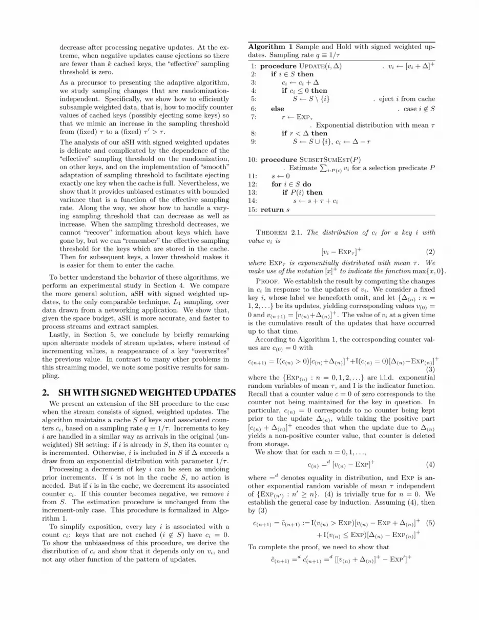
To simplify exposition, every key i is associated with acount ci: keys that are not cached (i 6∈ S) have ci = 0.To show the unbiasedness of this procedure, we derive thedistribution of ci and show that it depends only on vi, andnot any other function of the pattern of updates.

Algorithm 1 Sample and Hold with signed weighted up-dates. Sampling rate q ≡ 1/τ

1: procedure Update(i, ∆) . vi ← [vi + ∆]+

2: if i ∈ S then3: ci ← ci + ∆4: if ci ≤ 0 then5: S ← S \ {i} . eject i from cache

6: else . case i 6∈ S7: r ← Expτ

. Exponential distribution with mean τ8: if r < ∆ then9: S ← S ∪ {i}, ci ← ∆− r

10: procedure SubsetSumEst(P ). Estimate

∑i:P (i) vi for a selection predicate P

11: s ← 012: for i ∈ S do13: if P (i) then14: s ← s + τ + ci

15: return s

Theorem 2.1. The distribution of ci for a key i withvalue vi is

[vi − Expτ ]+ (2)

where Expτ is exponentially distributed with mean τ . Wemake use of the notation [x]+ to indicate the function max{x, 0}.

Proof. We establish the result by computing the changesin ci in response to the updates of vi. We consider a fixedkey i, whose label we henceforth omit, and let {∆(n) : n =1, 2, . . .} be its updates, yielding corresponding values v(0) =

0 and v(n+1) = [v(n)+∆(n)]+. The value of vi at a given time

is the cumulative result of the updates that have occurredup to that time.

According to Algorithm 1, the corresponding counter val-ues are c(0) = 0 with

c(n+1) = I(c(n) > 0)[c(n)+∆(n)]++I(c(n) = 0)[∆(n)−Exp(n)]

+

(3)where the {Exp(n) : n = 0, 1, 2, . . .} are i.i.d. exponentialrandom variables of mean τ , and I is the indicator function.Recall that a counter value c = 0 of zero corresponds to thecounter not being maintained for the key in question. Inparticular, c(n) = 0 corresponds to no counter being keptprior to the update ∆(n), while taking the positive part

[c(n) + ∆(n)]+ encodes that when the update due to ∆(n)

yields a non-positive counter value, that counter is deletedfrom storage.

We show that for each n = 0, 1, . . .,

c(n) =d [v(n) − Exp]+ (4)

where =d denotes equality in distribution, and Exp is an-other exponential random variable of mean τ independentof {Exp(n′) : n′ ≥ n}. (4) is trivially true for n = 0. Weestablish the general case by induction. Assuming (4), thenby (3)

c(n+1) = c(n+1) := I(v(n) > Exp)[v(n) − Exp + ∆(n)]+ (5)

+ I(v(n) ≤ Exp)[∆(n) − Exp(n)]+

To complete the proof, we need to show that

c(n+1) =d c′(n+1) =d [[v(n) + ∆(n)]+ − Exp′]+

where Exp′ is an independent copy of Exp. When v(n) +∆(n) ≤ 0 then c′(n+1) = c(n+1) = 0. When v(n) + ∆(n) > 0,the complementary cumulative distribution function (CCDF)of c′(n+1) is

Pr[c′(n+1) > z] = Pr[Exp < [v(n) + ∆(n) − z]+])

= 1− e−[v(n)+∆(n)−z]+/τ , for z ≥ 0.

The CCDF of c(n+1) can be derived from (5) as

Pr[c(n+1) > z] =Pr[Exp < min{v(n), [v(n) + ∆(n) − z]+}]+Pr[v(n) ≤ Exp] Pr[Exp(n) < [∆(n) − z]+]

(6)

When ∆(n) < z, the first term in (6) is

Pr[Exp < [v(n) + ∆(n) − z]+] = Pr[c′(n+1) > z]

and the second is zero. When ∆(n) ≥ z, then

Pr[c(n+1) > z]

= Pr[Exp < v(n)] + Pr[Exp ≥ v(n)) Pr[Exp(n) < ∆(n) − z]

= (1− e−v(n)/τ ) + e−v(n)/τ (1− e−(∆(n)−z)/τ )

= 1− e−(v(n)+∆(n)−z)/τ

= 1− e−[v(n)+∆(n)−z]+)/τ

= Pr[c′(n+1) > z]

Theorem 2.1 shows that the distribution of the counter ci

depends only on the actual sum vi, and is exactly capturedby a truncated exponential distribution. This is a powerfulresult, since it means that the sampling procedure is iden-tical in distribution to one where each key is unique, andoccurs only once with weight vi. From this, we can provideunbiased estimators for subset sums and bound the variance.In SubsetSumEst (Algorithm 1), each key is assigned anadjusted weight vi, which is τ + ci if i ∈ S, and 0 otherwise.Using the convention ci = 0 for deleted counters, this canbe expressed succinctly as

vi = I(ci > 0)(ci + τ)

Given a selection predicate P , we estimate the subset sum∑i:P (i) vi with

∑i:P (i) vi, the sum of adjusted weights of

keys in the cache which satisfy P . It suffices to show vi isan unbiased estimate of vi.

Lemma 2.2. vi is an unbiased estimate of vi.

Lemma 2.2 turns out to be a special case of the more generalTheorem 3.1 that we state and prove later in context.

2.1 Special case: unit updatesWe briefly consider the special case of unit updates, i.e.

where each ∆ ∈ {−1, +1}. In this case, we can adopt asimplified variant: note that the test of ∆ against an expo-nential distribution succeeds only when ∆ = +1, and doesso with probability q = 1/τ . When this occurs, we chooseto initialize ci = 0. Here, ci is integral and can be initial-ized with value ≥ 0 or uninitialized (when i is not cached).It is easy to see the correctness of this procedure: observethat if an i is sampled, then it will only remain in the cacheif there is no corresponding decrement later in the stream.

Thus we can“pair off” increments which are erased by decre-ments, and leave only vi “unpaired” increments. The key ionly remains in the cache if it is sampled during one of theseunpaired increments, and therefore has count ci with prob-ability q(1 − q)vi−ci , and is not sampled with probability(1− q)vi . That is, it exactly corresponds to a SH procedureon an increment-only input. Correctness, and unbiasednessof the SubsetSumEst procedure follows immediately as aresult. This improves over the result of [13], by removing theneed to keep additional tracking counters for cached keys.

2.2 Cache occupancyFrom our analysis, it is clear that the distribution of the

final count ci depends only on vi. In particular, the proba-bility that the key is cached at termination is 1−exp(−vi/τ).With the presence of negative updates in the update stream,however, a key may be cached at some point during the ex-ecution and then ejected. The key i is never cached if andonly if the independent exponential random variables r gen-erated at line 7 of Algorithm 1 all exceed their correspondingupdate ∆(n). This observation immediately establishes:

Lemma 2.3. The probability that key i is cached at somepoint during the execution is 1 − exp(−Σ∆+(i)/τ), whereΣ∆+(i) ≡ ∑

t max{0, ∆(n)} is the sum of positive updatesfor key i.

When Σ∆+(i) ¿ τ , the probability that a key ever getscached is small, and is approximately Σ∆+(i)/τ . The prob-ability that it is cached at termination is ≈ vi/τ . Summingover all keys, the worst-case cache utilization (which is ob-served after all negative updates occur at the end), is theratio of the sum of positive updates to the sum of values,∑

∆+(i) : vi.

3. ASH WITH SIGNED WEIGHTED UPDATESIn this section, we describe an adaptive form of Sample

and Hold (aSH), generalized to allow updates that are bothweighted and signed, while ensuring that the total numberof keys cached does not exceed a specified bound k.

3.1 Increasing the sampling thresholdIn order to bound the number of keys cached, we need a

mechanism to eject keys, by effectively increasing the sam-pling threshold τ . We show how to efficiently increase fromτ0 to τ1 > τ0 so that we achieve the same output distribu-tion as if the sampling threshold had been τ1 throughout.Algorithm 2 shows the procedure for a single key i ∈ S.With probability τ0/τ1, no changes are made; otherwise ci

is reduced by a value drawn from an exponential distribu-tion with mean τ1, and ejected if this is now below 0. Wecan formalize this as follows. Let c ≥ 0, 0 ≤ τ0, τ1, u be arandom variable uniformly distributed in (0, 1], and Expτ1

be an exponential random variable of mean τ1 independentof u. Then define the random variable

Θ(c, τ0, τ1) = I(uτ1 > τ0)[c− Expτ1 ]+ + I(uτ1 ≤ τ0)c

Note Θ(c, τ0, τ1) = c when τ1 ≤ τ0. We give an algorithmicformulation of Θ in Algorithm 2 as SampThreshInc, whichreplaces ci by the value Θ(ci, τ0, τ1) if this value is positive,and otherwise deletes the key i.

We now show that Θ preserves unbiasedness, and in par-ticular that the distribution of an updated count ci under Θis that of a fixed-rate SH procedure with threshold τ1:

Algorithm 2 Adjust sampling threshold from τ0 to τ1 forkey i

Require: τ1 > τ0, i ∈ S1: procedure SampThreshInc(i, ci, τ0, τ1)2: u ← rand()3: if τ1 > τ0

uthen

4: z ← rand()5: r ← (− ln(z))τ1 . r ← Expτ1

6: ci ← ci − r7: if ci ≤ 0 then S ← S \ {i}

Theorem 3.1. Let 0 ≤ τ0 < τ1 and c = Θ(c, τ0, τ1).

(i) E[I(c > 0)(c + τ1)|c] = c + τ0

(ii) If c =d [v − Expτ0 ]+, then c =d [v − Expτ1 ]

+.

Proof. (i)

E[I(c > 0)(c + τ1)|c]= (1− τ0/τ1)

∫ c

0

e−x/τ1(c− x + τ1) dx + (τ0/τ1)(c + τ1)

= (1− τ0/τ1)c + (τ0/τ1)(c + τ1) = c + τ0

(ii) Let c =d [v−Expτ0 ]+. Then Θ(c, τ0, τ1) can be rewrit-

ten as [v −W ]+ where

W = I(τ1u > τ0)(Expτ0 + Expτ1) + I(τ1u ≤ τ0)Expτ1

A direct computation of convolution of distributions showsthat Expτ0 + Expτ1 has distribution function

x 7→ (τ1Expτ1(x)− τ0Expτ0(x))/(τ1 − τ0).

Hence, using Pr[τ1u > τ0] = 1 − τ0/τ1, one computes thatW has distribution function

W (x) = Pr[τ1u > τ0](Expτ0 + Expτ1)(x) +

+Pr[τ1u ≤ τ0]Expτ1(x)

= Expτ1(x)

Proof of Lemma 2.2.From Theorem 2.1, ci =d [vi − Expτ ]+ = Θ(vi, 0, τ).Hence E[vi] = E[I(ci > 0)(ci + τ)] = vi as a special case ofTheorem 3.1(i).

3.2 Maintaining a fixed size cacheWe are now ready to present Algorithm 3, which main-

tains at most k cached keys at any given time. For eachcached key i, the algorithm stores a count ci and the key’seffective sampling threshold τi. This τi is set to the sam-pling threshold in force during the ejection following themost recent entry of that key into the cache. It may alsobe adjusted upward due to the ejection of another key, aprocess we explain below.

When the cache is not full, a new key i is admitted withsampling threshold τi = 0. When the cache is full, in thesense that it contains k keys, a new key is provisionallyadmitted, then one of the k + 1 keys is selected for ejec-tion. The procedure EjectOne adjusts the minimum sam-pling threshold τ∗ to the lowest value for which one key

Algorithm 3 aSH with signed weighted updates

1: procedure Update(i, ∆). Update weight of key i by ∆

2: if i ∈ S then3: ci ← ci + ∆4: if ci ≤ 0 then5: S ← S \ {i} . i ejected from cache.

6: else if ∆ > 0 then . i 6∈ S7: S ← S ∪ {i}, τi ← 0, ci ← ∆

. Insert i with sampling threshold 08: if |S| = k + 1 then9: EjectOne(S)

10: procedure SubsetSumEst(P ) . Estimate∑

i:P (i) vi

11: s ← 012: for i ∈ S do13: if P (i) then14: s ← s + τi + ci . estimate

return s

15: procedure EjectOne(S). Subroutine to increase sampling threshold so one keyis ejected

16: for i ∈ S do17: ui ← rand(), zi ← rand()18: Ti ← max{ τi

ui, ci− log(zi)

}. Ti is the sampling threshold that would eject i

19: τ∗ ← mini∈S Ti

. τ∗ is the new minimum sampling threshold20: for i ∈ S do21: if Ti = τ∗ then S ← S \ {i}22: else23: if τi ≤ τ∗ then24: if τ∗ui > τi then25: ci ← ci + τ∗ log zi

. Given Ti > τ∗ and τ∗ui > τi, then ci + τ∗ log zi > 0. Given Ti > τ∗ and τ∗ui ≤ τi, then ci is unchanged.

26: τi ← τ∗

will be ejected. This is implemented by considering the po-tential action of SampThreshInc on all counts ci simul-taneously, fixing a independent randomization of the vari-ates ui, zi for each i, and finding the smallest threshold τ∗

for which ci = Θ(ci, τi, τ∗) = 0 for some i. This key is

ejected, while the thresholds of surviving keys are adjustedas (ci, τi) ← (ci, τ

∗) if τi ≤ τ∗, and are otherwise left un-changed.

Lemma 3.2. vi retains its expectation under the action ofEjectOne.

Proof. We choose a particular key i, and fix all cj , andalso fix for j 6= i the random variates uj , zj from line 17 ofAlgorithm 3. This fixes the effect of random past selectionsand updates. Let Tj = max{τj/uj , cj/(− log zj)} and τ ′ =minj 6=i Tj , which are hence also treated as fixed. Then theupdate to ci is ci = Θ(ci, τi, τ

′); we will establish that vi =I(ci > 0)(ci + τ ′) is a (conditionally) unbiased estimator ofvi for any fixed τ ′, and hence unbiased.

We first check ci corresponds to the action on ci describedin Algorithm 3. For clarity we state

ci = I(τ ′ui > τi)[ci − Expτ ′ ]+ + I(τ ′ui ≤ τi)ci

and observe that −τ ′ log zi is the random variable Expτ ′

employed. When Ti < τ ′, i is selected for deletion. Thiscorresponds to the case {τ ′ > τi/ui} ∩ {τ ′ > ci/(− log zi)}.The condition τ ′ > τi/ui selects the first term in the expres-sion for ci, while the condition τ ′ > ci/(− log zi) makes thatterm zero, i.e. ci = 0 and the key is deleted. Otherwise, ifTi ≥ τ ′, the first or second term in ci may be selected, butboth cannot be zero.

Let vi denote the estimate of vi based on ci = Θ(ci, τi, τ′).

Then from Theorem 3.1(i)

E[vi|τ ′, ci > 0] = E[I(ci > 0)(ci + τ ′)|τ ′, ci > 0] = ci + τi

independent of τ ′. Hence

E[vi] = E[I(ci > 0)(ci + τi)] = vi.

Theorem 3.3. vi is an unbiased estimator of vi

Proof. Initially, the cache is empty and both vi = 0 andvi = 0. We need to show that the estimate remains unbiasedafter an update operation. The first part of a positive update∆ > 0 clearly preserves the expectation: τi is not modified(or initialized to 0 if i was not cached) and c is increased by∆. Hence vi increases by exactly ∆. Unbiasedness underthe second part, performing EjectOne if the cache is full,follows from Lemma 3.2.

To conclude the proof of the unbiasedness of the estima-tor, we invoke Lemma 3.6(i), which is stated and provedbelow. This Lemma uses a ‘pairing’ argument to pair offthe negative update with a prior positive update, and so re-duces to a stream with only positive updates, which yieldsthe same vi. Therefore, the result follows from the aboveargument on positive updates.

3.3 Estimation VarianceIt is important to be able to establish likely errors on

the unbiased estimators vi resulting from Algorithm 3. Astraightforward calculation shows that when ci =d [vi −Expτ ]+, the unbiased estimate vi = I(ci > 0)(ci + τi) hasvariance

Var[vi] = τ2i (1− e−vi/τi)

Moreover, Var[vi] itself has an unbiased estimator s2i that

does not depend explicitly on the value vi:

s2i = I(ci > 0)τ2

i .

The intuition behind s2i is clear: for a key in S, the uncer-

tainty concerning vi is determined by the estimated unsam-pled increments, which are exponentially distributed withmean τi and variance τ2

i . Observe that both Var[vi] and s2i

are increasing functions of τi.Note that the estimated variance associated with a given

key is non-decreasing while the key is stored in the cache,then drops to zero when the key is ejected, possibly growingagain after further updates for that key. Since s2

i is increas-ing in τi, a simple upper bound on the variance is obtainedusing the maximum threshold encountered over all instancesof EjectOne. This is because one of these instances musthave given rise to the largest threshold associated with eachparticular key.

Lemma 3.4. For any two keys i 6= j, E[vivj ] is invariantunder EjectOne.

Proof. Reusing notation from the proof of Lemma 3.2,let Tj = max{τj/uj , cj/(− log zj)} . We fix cj and τ ′ =minh 6=i,j Th. The update to ch (h ∈ {i, j}) is ch = Θ(ch, τh, τ ′),and (when ch > 0) the update to τh is τh = min{τ ′, Ti, Tj}.It suffices to show that

E[I(ci > 0, cj > 0)(ci + τi)(cj + τj)]

= I(ci > 0, cj > 0)(ci + τi)(cj + τj)] .

We observe that

E[I(ci > 0, cj > 0)(ci + τi)(cj + τj)]

= E[I(ci > 0, cj > 0)(ci + τ ′)(cj + τ ′)],

which holds because there can be a positive contribution tothe expectation only when Ti, Tj > τ ′. Under this condition-ing, however, τ ′ essentially functions as a fixed threshold.Thus, we can apply Theorem 3.1 (i) and obtain

E[I(ci > 0, cj > 0)(ci + τ ′)(cj + τ ′)]

= I(ci > 0, cj > 0)(ci + τi)(cj + τj).

Consequently, we are able to show that the covariancebetween the estimates of any pair of distinct keys is zero.

Theorem 3.5. For any two keys i 6= j, Cov[vi, vj ] = 0.

Proof. We show inductively on the actions of Updatein Algorithm 3 that E[vivj ] = vivj .

For a positive update (i, ∆), the claim is clear followingc ← c + ∆ (line 3 in Algorithm 3), when i is in the cache.Both vi and vi = I(ci > 0)τi + ci increase by ∆ and bothvj and vj are unchanged. Hence, if prior to the updatewe had E[vivj ] = vivj then this holds after the update. Apositive update may also result in EjectOne and we applyLemma 3.4 to show that E[vivj ] is unchanged.

To complete the proof, we also need to handle negative up-dates. We argue that the expectation E[vivj ] is the same asif we remove the negative update and a prior matching pos-itive update, leaving a stream of positive updates only. Thedetails of this argument are provided in Lemma 3.6(ii).

A consequence of this property is that the variance on sub-set sum estimate is the sum of single-key variances, just aswith independent sampling: Var[

∑i:P (i) vi] =

∑i:P (i) Var[vi].

In particular,∑

i:P (i) I(ci > 0)τ2i =

∑i∈S:P (i) τ2

i is an unbi-

ased estimate on∑

i:P (i) vi.

3.4 Analysis of negative updates under aSHOur analysis in Theorems 3.3 and 3.5 relies on replacing

a stream with a mixture of positive and negative weight up-dates with one which has positive weight updates only, andthen arguing that certain properties of this positive streammatch those of the original input. This generalizes the“pair-ing” argument outlined in Section 2.1 for the special case ofunit weighted updates. In this section, we provide moredetails of this pairing transformation, and prove that thispreserves the required properties of the estimates.

Pairing Process. In our pairing process, each negative up-date is placed in correspondence (“paired”) with preceding,previously unpaired, positive updates. We then go on to re-late the state to that on a stream with both paired updates

time

v

Unpaired increments

Figure 1: Value of key with time. Unpaired andpaired positive update and paired negative updatesare marked.

omitted. Figure 1 gives a schematic view of the pairing pro-cess for a key, which we describe in more detail below.

Specifically, a negative update of key i is paired with themost recent unpaired positive update of i. If there is no suchupdate, the negative update is unpaired. This occurs whenthe aggregate weight before the update is zero, in whichcase according to (1), vi remains zero, and we can ignorethis update.

Since updates are weighted, a negative update (i,−∆)may be paired with multiple positive updates, or with afraction of a positive update. Without loss of generality,each negative update will be paired with a “suffix” of a pos-itive update, followed by zero or more “complete” positiveupdates. If vi < ∆, the negative update only has its vi

“prefix” paired and vi −∆ “suffix” unpaired.To aid analysis, we observe that we can “split” updates

without altering the state distribution. More precisely, letσ be an update stream terminating with an update (i, ∆).Let σ′ be the same stream with the last update replacedby two consecutive updates (i, ∆1) and (i, ∆2) such that∆1 + ∆2 = ∆, and sign(∆1) = sign(∆2) = sign(∆). Thenthe distribution of the state of the algorithm after processingσ or σ′, conditioned on the initial state, is the same. Thismeans that by splitting updates, we can replace the originalsequence by another sequence (where each original updateis now a subsequence of updates), on which the algorithmhas the same final state but all updates are fully paired orfully unpaired.

We next prove the lemma we require to replace the originalstream with a positive-only stream.

Lemma 3.6. Consider an update stream where the `’thupdate is a negative update (i,−∆) and a modified streamwith the negative update, and all positive update(s) pairedwith it (if any) omitted. Then

(i) E[vi] and

(ii) for j 6= i, E[vivj ]

are the same for both streams.

Proof. We observe that a negative update can be un-paired if and only if vi = 0 just prior to the current negativeupdate. Since the counter ci ≤ vi, this means that i isnot cached and thus the processing of the unpaired negativeupdate has no effect on the state of the algorithm.

For paired negative updates, let σ0 be the prefix of thestream up to the corresponding paired positive update, σbe the suffix including and after the positive update, andσ′ ⊂ σ be an alternative suffix with the negative update andits paired positive update all omitted. Fix the execution ofthe algorithm on σ0. To complete the proof, we show that

(i) The distributions of (τi, ci) for key i after processingσ and σ′ are the same.

(ii) For a key j 6= i, if ci > 0, then the distribution of(τj , cj) conditioned on the final (τi, ci) when ci > 0 isthe same: (τj , cj)|σ, τi, ci =d (τj , cj)|σ′, τi, ci

Since the actual splitting point of updates does not affectthe state distribution, we can treat vi as defined by theupdate stream projected on i as a contiguous function of“time”. Initially, before any updates of i are processed, thetime is 0. If the time is t0 prior to processing an update(i, ∆), then for t ∈ [t0, t0 + |∆|], we interpolate the valuevi as a function of time as vi(t) = [vi(t0) + t − t0]

+. Afterprocessing the update, the time is t0+|∆|. Any point in timenow has a gradient, depending on whether vi is increasingor decreasing at that time. Pairing is between intervals ofequal size and opposite gradient. Figure 1 shows the valuevi as a function of time and distinguishes between updatesthat are paired and unpaired with respect to the final state.

Tracking the state of key i during execution, we mapan interval [0, ci] to positive update intervals in a length-preserving manner. The mapping corresponds to the pos-itive updates which contributed to the count ci, that is,the most recent unpaired positive update intervals of (to-tal) length ci. We refer to the point that 0 is mapped to asthe (most recent) entry point of key i into the cache. Upon apositive update, the counter is incremented by ∆ > 0. Themapping of [0, ci] is unchanged and the interval [ci, ci + ∆]maps to the interval [t0, t0 + ∆] of the current update onthe time axis. An EjectOne operation which reduces thecounter ci by r removes an r “prefix” of the counter interval:a positive update time previously paired with y ∈ [0, c] suchthat y > r is paired with the point y − r in the updatedinterval. A negative update of ∆ results in c ← [c − ∆]+.A ∆ “suffix” of [0, c] is removed (reflecting that the positiveupdate points this suffix was mapped to are now paired)and the mapping of the remaining [0, [c−∆]+] prefix is un-changed. Note that the positive update interval removed isthe one that is paired with the negative update just pro-cessed.

We now consider a negative update of ∆, and comparethe execution of the algorithm on suffixes σ and σ′.

• If i is not cached after σ0, then it would not be cachedafter any execution of either σ or σ′, since all positiveupdates of i are paired. If i was cached at the end of σ0

and ejected during σ, we fix the randomization in eachEjectOne performed when processing σ. We thenlook at executions of σ′ that follow that randomizationuntil (and if) the set of cached keys diverges. Under σ′,i has a lower c value (by ∆) than under σ. Thus, when

i is removed by an EjectOne at σ, it would also beremoved under σ′, unless it was removed already undera prior EjectOne. As all positive updates of i in σand σ′ are paired, once i is removed, then even if it re-enters the cache it will not be cached at terminationfor either σ′ or σ. Thus, the outcome for i under σand σ′ is the same.

• If i is cached after σ, its most recent entry point mustbe in σ0. We again fix the execution of the algorithmon σ, fixing all random draws when performing Ejec-tOne procedures. We will show that if the executionof σ′ follows these random draws, then i will not beejected and will have the same τi, ci values at termi-nation of σ′. Consider the execution of the algorithmon σ′ and let τ ′i , c

′i be the parameters for i. Initially,

c′i = ci − ∆. Clearly, any EjectOne where c is notchanged, retains i under both σ and σ′. If c is reducedunder σ, it still must be such that ci > ∆ for i to becached at the end, since all subsequent positive up-dates are paired, and the last update is of −∆. Thus,it would also remain cached under the correspondingEjectOne in σ′. Moreover, all other keys cached un-der σ would also be cached (and have the same (τj , cj)values) under σ′.

Lastly, we consider (τj , cj) for j 6= i conditioned on (τi, ci)when ci > 0. If i is not cached after σ, it is also not cachedunder σ′ and thus ci = 0. If i is cached after σ, it hasthe same state (τi, ci) as under σ′ (fixing randomization).Furthermore, the state (τj , cj) for any key and j 6= i is thesame.

From these observations, we can conclude that the expec-tation of the estimate for any key, and for any pair of dis-tinct keys (and likewise for higher moments), are the samefor both streams.

Note that once we have the above lemma, we can applyit repeatedly to remove all negative updates, and result ina “positive-only” stream. The distributions of the state ofalgorithm on these paired streams are identical.

4. EXPERIMENTSIn this section we exhibit the action of aSH on a stream

of signed updates, and compare its performance against acomparable state-of-the-art method, namely Lp sampling.

4.1 Implementation Issues.Our reference comparison was with Lp sampling. The Lp

sampling procedure builds on the idea of sketch data struc-tures, which summarize a d-entry vector x. A sketch builtwith parameter ε can provide an estimate of any xi witherror ε‖x‖2, using space O(ε−2 log d) [4]. In outline, for L1

sampling, we build a sketch of the vector xi = vi/ui, wherevi are the aggregate weights for key i, and each ui is a fixeduniform random variable in the range [0, 1] [17]. To draw asample, we find the entry of this vector which is estimatedas having largest xi value by the sketch. To obtain the cor-rect sampling distribution, we have to reject samples whosexi value does not exceed a fixed threshold as a function of‖v‖1, which in our case is just the sum of all update weights.As a result, the procedure requires a lot of space per sample:O(log2 d), even using a large constant value of ε. Further,the time to extract a sample can be high, since we have to

enumerate all keys in the domain. The search time could bereduced using standard tricks, but this would increase thespace by further factors of log d. We implemented both L1

sampling and our adaptive Sample and Hold algorithm ininterpreted languages (Perl, Python); we expect optimizedimplementations to have the same relative performance, butimproved scalability. To ensure comparability, we fix thespace used by aSH to draw a sample of size k (i.e. k tu-ples of (i, ci, τi, ui, zi)), and allocate this much space to Lp

sampling to be used for sketch data structures. Based onour parameter settings, the sketch used by Lp sampling toextract a single sample equates to the space for 10 samplesunder aSH.

4.2 Data DescriptionWe tested our methods on data corresponding to the ISP

network monitoring scenario described in the Introduction.The update stream was derived from arrival and departuresat a queue. The queue was driven by a synthetic arrivalprocess, comprising keyed items with sizes drawn indepen-dently from a Pareto(1.1) distribution. The arrival timesand key values were derived from an IP network trace of 106

packets. We simulated a FIFO queue in which each itemremains at the head of the queue for a time equal to its size,and converted the trace into a stream of 2 × 106 updates(i, s), where i is a key and s is positive for an arriving itemand negative of the same magnitude when that item hascompleted service for a departure, the stream items havingthe corresponding event order as for the queue. Thus thevalues vi correspond to the total size of items of key i in thequeue at a given time. We evaluate the methods based ontheir ability to accurately summarize the queue occupancydistribution of different subsets of keys.

4.3 ParametrizationWe parametrized different runs of the simulation as fol-

lows.

• Key Granularity: The trace contained about 110,000unique keys. These were mapped to smaller keys setsas i 7→ β = h(i) mod b with h a hash function and btaking values 1, 000, 10, 000 and 100, 000. This is thegranularity of keys in the sample set. Note that thetime for our aSH algorithm does not depend explicitlyon the key granularity, but Lp sampling incurs a costlinear in b; hence, we focus on moderate values of b tobound the experimental duration.

• Query Granularity: For determination of estimationaccuracy, we divide the keyspace into a different classes,and use the recovered sample to estimate the weightdistribution across these classes. Specifically, we as-signing each key β to a bin by β 7→ α = β mod a.(Note that the sampling methods are not aware of thisfixed mapping, and so are unable to take advantage ofit.) We used values 10, 100, and 1, 000 for a.

• Sample Size: we selected roughly geometric samplesizes k from 30, 100, 300 and 1, 000 for aSH, and allo-cated the equivalent space to Lp sampling, as describedabove.

Our subsequent experiments compare the performance intime and accuracy across the different combinations of thesesettings of a, b, and sample size k.

0

0.2

0.4

0.6

0.8

1

0 0.2 0.4 0.6 0.8 1

CD

F

Error

b=1000, a=10

aSH: k=1000aSH: k=300aSH: k=100aSH: k=30

Lp: k=1000Lp: k=300Lp: k=100Lp: k=30

0

0.2

0.4

0.6

0.8

1

0 0.2 0.4 0.6 0.8 1

CD

F

Error

b=100000, a=10

aSH: k=1000aSH: k=300aSH: k=100aSH: k=30

Lp: k=1000Lp: k=300Lp: k=100Lp: k=30

0

0.2

0.4

0.6

0.8

1

0 0.2 0.4 0.6 0.8 1

CD

F

Error

b=1000, a=100

aSH: k=1000aSH: k=300aSH: k=100aSH: k=30

Lp: k=1000Lp: k=300Lp: k=100Lp: k=30

0

0.2

0.4

0.6

0.8

1

0 0.2 0.4 0.6 0.8 1

CD

F

Error

b=100000, a=100

aSH: k=1000aSH: k=300aSH: k=100aSH: k=30

Lp: k=1000Lp: k=300Lp: k=100Lp: k=30

0

0.2

0.4

0.6

0.8

1

0 0.2 0.4 0.6 0.8 1

CD

F

Error

b=1000, a=1000

aSH: k=1000aSH: k=300aSH: k=100aSH: k=30

Lp: k=1000Lp: k=300Lp: k=100Lp: k=30

0

0.2

0.4

0.6

0.8

1

0 0.2 0.4 0.6 0.8 1

CD

F

Error

b=100000, a=1000

aSH: k=1000aSH: k=300aSH: k=100aSH: k=30

Lp: k=1000Lp: k=300Lp: k=100Lp: k=30

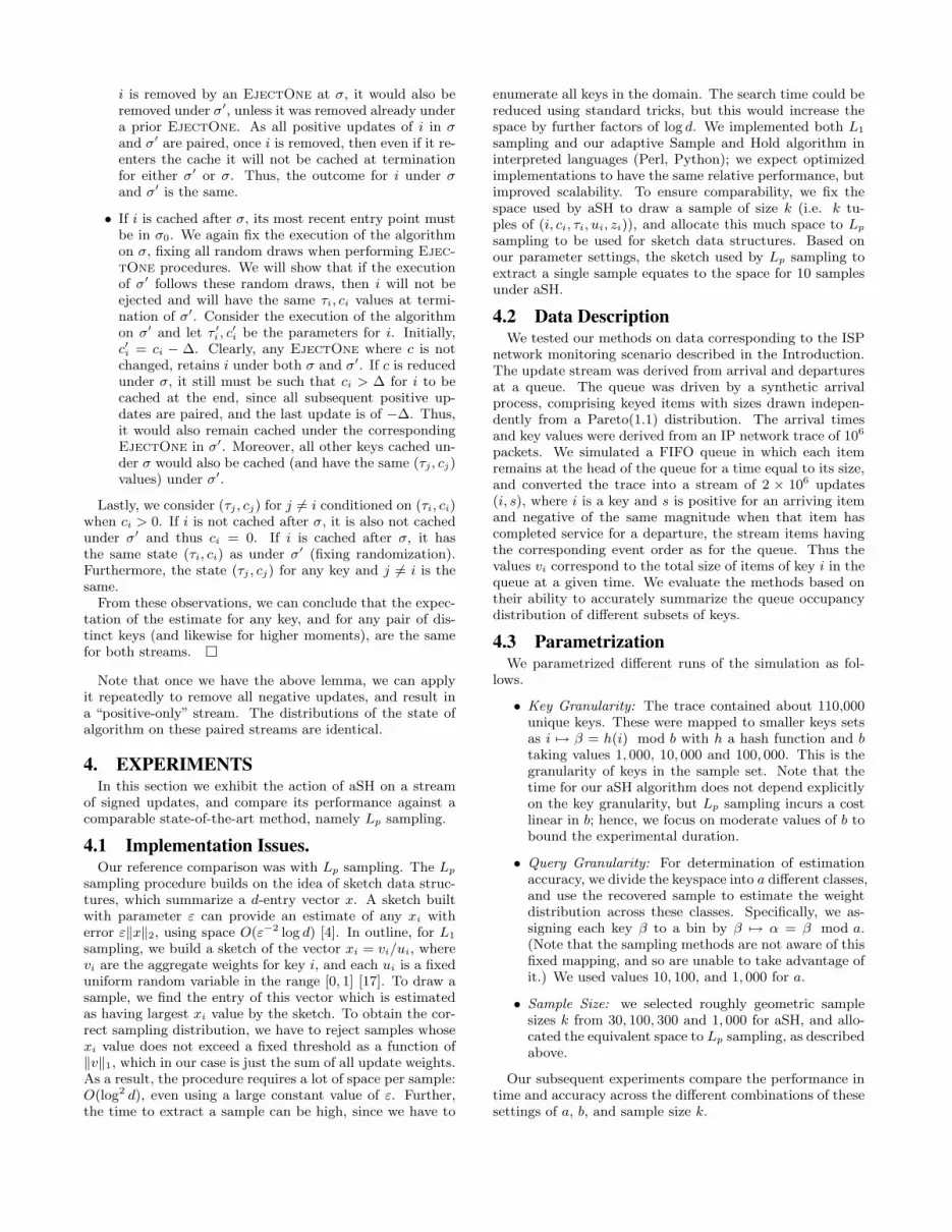
Figure 2: CDF of Estimation Error as a function of sample size k for aSH and Lp; key granularity b = 1, 000and 100, 000. Query granularity a = 10, 100 and 1, 000. aSH is consistently more accurate than Lp.

4.4 ResultsQuery Accuracy. Each time we probe the samples, weobtain the estimated weights of the a different bins. Wemeasure the accuracy by comparing the induced frequencydistribution to the true distribution computed offline. Thatis, let w(α) and w(α) the total and estimated weighted ineach query aggregate labeled by α = 1, 2 . . . a. Then accu-racy is measured by the distribution error

1

2

∑α

|w(α)

W− w(α)

W| ∈ [0, 1] (7)

where W =∑

α w(α) and W =∑

α w(α).This distribution error was computed for each positive

update for aSH and every 1000 updates in Lp sampling.

Figure 2 shows the empirical cumulative distributions of theerrors computed for each method, using key granularity b =1, 000 and 100, 000 and query granularity a = 10, 100 and1, 000.

On these plots, an ideal summary reaches the top left handcorner (i.e. if all queries have zero error). For aSH withk=1000, this is indeed achieved in the case b = 1000. Thatis, when there are only 1000 distinct keys, the sample of size1000 is able to represent this distribution exactly, and hencecan answer any query perfectly. In more realistic situations,k is less than b (often, much less than b). However, we seeeven for k = 100, corresponding to 10% of the active keys,we see that aSH does a good job of answering the query. Thisholds even for b = 100, 000, meaning the sample can capture

100

1000

10000

100 1000

proc

ess

time

/ sec

onds

size k

LpaSH

(a) Update Processing Time (in seconds) as a functionof sample size k for aSH and Lp.

0.1

1

10

100

1000

10000

1000 10000 100000 1e+06

prob

e tim

e / s

econ

ds

key granularity b

LP: k=1000LP: k=300LP: k=100LP: k=30

(b) Query Probe Time (in seconds) as a function of keygranularity b for Lp.

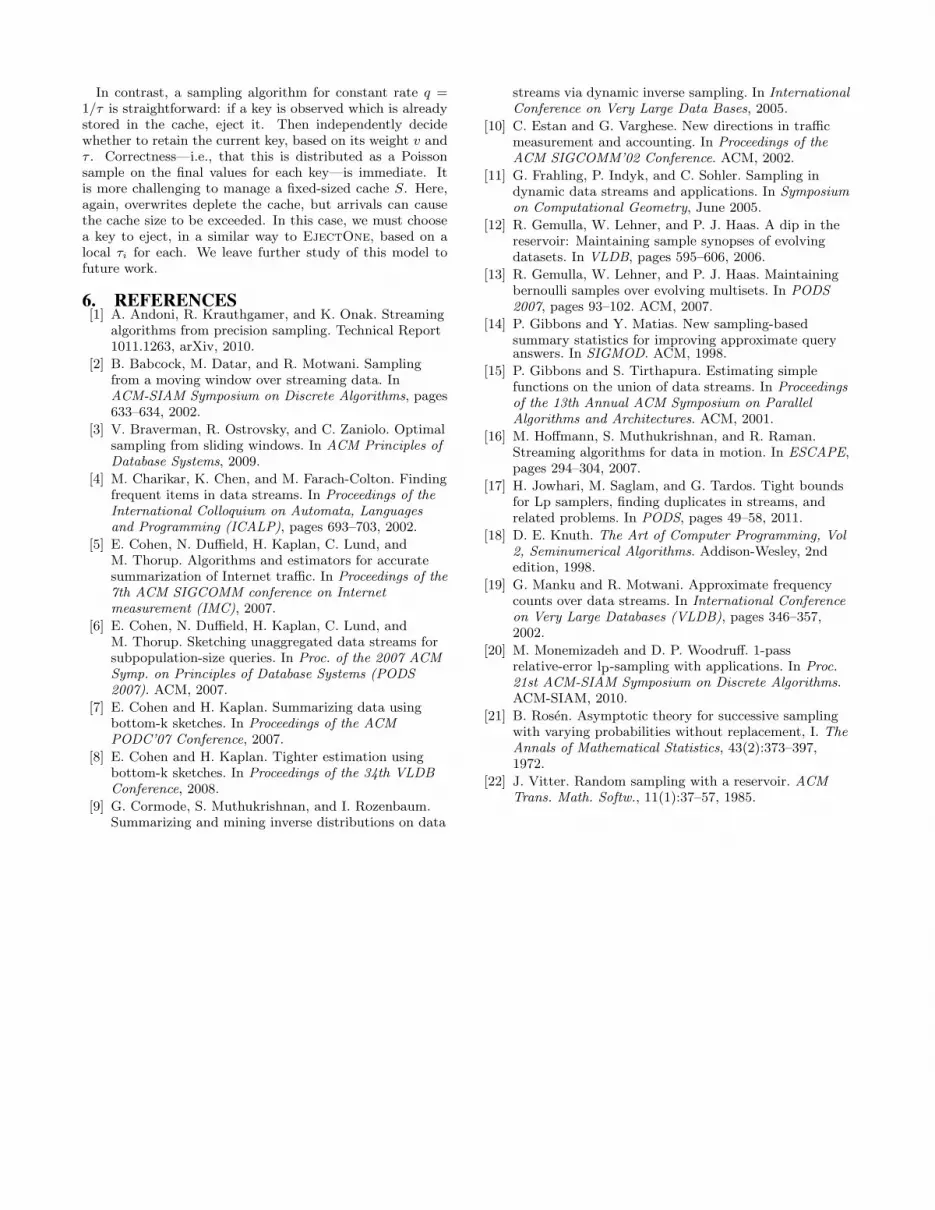
Figure 3: Timing results for stream processing and querying

only 0.1% of the keyspace. We note the accuracy tends toimprove as a decreases, meaning that there are fewer binsfor the query, and hence more keys in each bin. In this case,almost every query is answered with high accuracy.

In contrast, the accuracy from Lp sampling is quite low.The main reason is the much higher space overhead of thismethod. As noted above, even with space correspondingto k = 1000, Lp sampling only has room to recover up to100 samples. Moreover, each attempt to recover a samplefrom the sketch fails with constant probability (this is anintegral part of the method, which is needed to achieve thecorrect sample distribution). In practice, we were only ableto recover a small number of samples, often only in the singlefigures. As a result, we observe that Lp sampling with spacefor k = 1000 is often outperformed by aSH with k = 30, i.e.aSH is more accurate even with a much smaller summarysize.

Update Processing Time. Both aSH and Lp samplingwere run using interpreted languages on the same system.We measured the total processing time associated with pro-cessing the update stream. The update processing times islargely independent of key granularity, and was observed togrow roughly linearly as a function of the sample size k; seeFigure 3(a) which shows the cost on logarithmic axes. Underthis implementation, Lp sampling is roughly half an ordermagnitude (i.e. five times) slower than aSH.

Asymptotically, Lp sampling is truly linear in k: it up-dates O(k) different sketches, taking constant time for each.Hence, we do not expect to be able to improve substantiallyon this. The time cost for aSH includes the time to per-form EjectOne for every update. We note that the updatetime could be improved for aSH, at the expense of slightlyincreased space, by deferring this step. That is, suppose webuffer c arrivals, then perform c steps of EjectOne, oneafter another. This can be shown to be equivalent to de-termining a new threshold τ∗c which is sufficient to eject ckeys. Then we can perform a single pass over the c + k keysand track the c’th largest threshold in a heap. Thus, settingc = O(k) means that the update time could be reduced toO(log k), allowing larger samples to be drawn efficiently.

Query Answering Time. For the aSH summary, answer-ing queries is trivial: we just have to read the explicitly

maintained counts and thresholds, and use these within theSubsetSumEst routine. In our experiments, this time wasessentially nil. However, this is not the case for the Lp sam-pling case, due to the need to test the sketch-estimated counteach potential key value. Figure 3(b) displays the time toanswer perform this extraction as a function of key granular-ity b for different buffer sizes k. The results are in accordancewith the asymptotic cost, growing as O(bk). At the extremeend, the cost is of the order of 45 minutes to extract a sam-ple over a domain of b = 106, making real time analysisinfeasible. We would argue that this is not a particularlylarge domain (e.g. IP addresses span a domain 3 orders ofmagnitude larger). From this, we conclude that the timecost of working with Lp sampling is too high for anythingabove a moderate sized domain. In contrast, the time costfor working with aSH sampling is independent of b.

5. CONCLUDING REMARKSIn many situations, data is presented in the form of streams

of updates which can include negative weights. When thesestreams become large, it is important to be able to accu-rately maintain a sample over them. We have introduced anaSH sampling technique for such streams of weighted, signedupdates, which is unbiased and has zero co-variance betweenestimated keys. The procedure is easy to implement. Inour experimental study, we observed that its performs sub-stantially better than the Lp sampling technique based onsketches: given the same amount of space, aSH is more ac-curate, faster to process the stream, and dramatically fasterto answer queries.

Looking beyond this work, we note that other models ofstreaming arrivals are also of interest, but have similarlyreceived relatively little attention. One important case isthat of the overwrite streams model, where an update of theform (i, v) means that the weight associated with key i isupdated to v. The update (i, 0) corresponds to deletion ofthe key. This model captures a simple notion of “updating”information about a key. It is also of interest since manynatural streaming problems are hard in this setting, meaningthat they require space linear in the size of the input; seee.g. [16].

In contrast, a sampling algorithm for constant rate q =1/τ is straightforward: if a key is observed which is alreadystored in the cache, eject it. Then independently decidewhether to retain the current key, based on its weight v andτ . Correctness—i.e., that this is distributed as a Poissonsample on the final values for each key—is immediate. Itis more challenging to manage a fixed-sized cache S. Here,again, overwrites deplete the cache, but arrivals can causethe cache size to be exceeded. In this case, we must choosea key to eject, in a similar way to EjectOne, based on alocal τi for each. We leave further study of this model tofuture work.

6. REFERENCES[1] A. Andoni, R. Krauthgamer, and K. Onak. Streaming

algorithms from precision sampling. Technical Report1011.1263, arXiv, 2010.

[2] B. Babcock, M. Datar, and R. Motwani. Samplingfrom a moving window over streaming data. InACM-SIAM Symposium on Discrete Algorithms, pages633–634, 2002.

[3] V. Braverman, R. Ostrovsky, and C. Zaniolo. Optimalsampling from sliding windows. In ACM Principles ofDatabase Systems, 2009.

[4] M. Charikar, K. Chen, and M. Farach-Colton. Findingfrequent items in data streams. In Proceedings of theInternational Colloquium on Automata, Languagesand Programming (ICALP), pages 693–703, 2002.

[5] E. Cohen, N. Duffield, H. Kaplan, C. Lund, andM. Thorup. Algorithms and estimators for accuratesummarization of Internet traffic. In Proceedings of the7th ACM SIGCOMM conference on Internetmeasurement (IMC), 2007.

[6] E. Cohen, N. Duffield, H. Kaplan, C. Lund, andM. Thorup. Sketching unaggregated data streams forsubpopulation-size queries. In Proc. of the 2007 ACMSymp. on Principles of Database Systems (PODS2007). ACM, 2007.

[7] E. Cohen and H. Kaplan. Summarizing data usingbottom-k sketches. In Proceedings of the ACMPODC’07 Conference, 2007.

[8] E. Cohen and H. Kaplan. Tighter estimation usingbottom-k sketches. In Proceedings of the 34th VLDBConference, 2008.

[9] G. Cormode, S. Muthukrishnan, and I. Rozenbaum.Summarizing and mining inverse distributions on data

streams via dynamic inverse sampling. In InternationalConference on Very Large Data Bases, 2005.

[10] C. Estan and G. Varghese. New directions in trafficmeasurement and accounting. In Proceedings of theACM SIGCOMM’02 Conference. ACM, 2002.

[11] G. Frahling, P. Indyk, and C. Sohler. Sampling indynamic data streams and applications. In Symposiumon Computational Geometry, June 2005.

[12] R. Gemulla, W. Lehner, and P. J. Haas. A dip in thereservoir: Maintaining sample synopses of evolvingdatasets. In VLDB, pages 595–606, 2006.

[13] R. Gemulla, W. Lehner, and P. J. Haas. Maintainingbernoulli samples over evolving multisets. In PODS2007, pages 93–102. ACM, 2007.

[14] P. Gibbons and Y. Matias. New sampling-basedsummary statistics for improving approximate queryanswers. In SIGMOD. ACM, 1998.

[15] P. Gibbons and S. Tirthapura. Estimating simplefunctions on the union of data streams. In Proceedingsof the 13th Annual ACM Symposium on ParallelAlgorithms and Architectures. ACM, 2001.

[16] M. Hoffmann, S. Muthukrishnan, and R. Raman.Streaming algorithms for data in motion. In ESCAPE,pages 294–304, 2007.

[17] H. Jowhari, M. Saglam, and G. Tardos. Tight boundsfor Lp samplers, finding duplicates in streams, andrelated problems. In PODS, pages 49–58, 2011.

[18] D. E. Knuth. The Art of Computer Programming, Vol2, Seminumerical Algorithms. Addison-Wesley, 2ndedition, 1998.

[19] G. Manku and R. Motwani. Approximate frequencycounts over data streams. In International Conferenceon Very Large Databases (VLDB), pages 346–357,2002.

[20] M. Monemizadeh and D. P. Woodruff. 1-passrelative-error lp-sampling with applications. In Proc.21st ACM-SIAM Symposium on Discrete Algorithms.ACM-SIAM, 2010.

[21] B. Rosen. Asymptotic theory for successive samplingwith varying probabilities without replacement, I. TheAnnals of Mathematical Statistics, 43(2):373–397,1972.

[22] J. Vitter. Random sampling with a reservoir. ACMTrans. Math. Softw., 11(1):37–57, 1985.