does the internet reduce corruption? evidence from u.s. states and across countries

Does the Internet Reduce Corruption?

Evidence from U.S. States and Across Countries�

Thomas Barnebeck Andersen Jeanet Bentzen Carl-Johan Dalgaard

Pablo Selaya†

January 11, 2010

Abstract

The Internet is often claimed to be a powerful anti-corruption technology. In theory, the Internet raises

information levels and thus detection risks. Further, by enabling e-government, it obviates bureaucrats’

intermediary role in the provision of public services and increases transparency. To examine the Inter-

net/corruption nexus empirically, we develop a novel identification strategy for Internet diffusion. Power

disruptions damage digital equipment, which increases the user cost of IT capital and thus lowers the

speed of Internet diffusion. A natural phenomenon causing power disruptions is lightning activity, which

makes lightning a viable instrument for Internet diffusion. Using global satellite data and data from

ground-based lightning detection censors, we construct lightning density data for a large cross section

of countries and for the contiguous U.S. states. Empirically, lightning density is a strong instrument for In-

ternet diffusion. Our IV estimates show that Internet diffusion has reduced the extent of corruption across

countries and across U.S. states.

Keywords: Corruption; Internet; Instrumental variables estimation; Lightning

JEL Classification codes: K4; O1; H0

�We owe a special thanks to William A. Chisholm for generously sharing his expertise on the subject of lightning protection. Wealso thank Phil Abbot, Shekhar Aiyar, Mark Bills, Christian Bjørnskov, Matteo Cervellati, Areendam Chanda, Oded Galor, Chad Jones,Sam Jones, Phil Keefer, Pete Klenow, David Dreyer Lassen, Ross Levine, Norman Loayza, Ben Olken, Ola Olsson, Elena Paltseva,Nancy Qian, Martin Ravallion, Yona Rubinstein, Paolo Vanin, Dietz Vollrath, David Weil, Nadja Wirz, and seminar participantsat the University of Bergen, Brown University, University of Copenhagen, the Jerusalem Summer School in Economic Growth atHebrew University, ETH Zürich, the ZEW Conference on Economics of Information and Communication Technologies, the 2008Nordic Conference in Development Economics, the Growth Workshop at the 2008 NBER Summer Institute, the Southern EconomicAssociation annual meeting 2008, the Latin American Econometric Society Meetings 2009 in Buenos Aires, and the World Bank. Errorsare ours.

†All the authors are affiliated with the Department of Economics, University of Copenhagen, Studiestraede 6, DK-1455Copenhagen K, Denmark. Contact: Thomas Barnebeck Andersen ([email protected]), Jeanet Bentzen([email protected]), Carl-Johan Dalgaard ([email protected]), and Pablo Selaya ([email protected]).

1

1 Introduction

Corruption is commonly perceived to be a major stumbling block on the road to prosperity. Aside from

retarding growth (Mauro, 1995), corruption entails “fiscal leakage”, which reduces the ability of poor coun-

tries to supply essential public services such as schooling and health care (Reinikka and Svensson, 2004;

World Development Report 2004). Corruption is unquestionably a governance failure one would like to

dispose of. Yet, combating corruption has not proven to be easy.

In the present paper we hypothesize that the Internet is a potentially powerful tool in combating corrup-

tion around the world. We test this hypothesis using cross country data, and data for the 48 contiguous U.S.

states. Our estimates strongly support the proposition that the Internet has worked to reduce corruption

since its inception.

There are several reasons why the Internet could serve as an anti-corruption tool. First, the World

Wide Web (WWW) is a major source of information.1 Spreading information about official wrong-doing

inevitably increases the “risk of detection” for politicians and public servants thus making corrupt behavior

less attractive. A nice illustration of this mechanism at work is found in a 2001 scandal from India, which

nearly toppled the government. Reporters from the online news site <www.Tehelka.com> posed as arms

dealers and documented negotiations with top politicians and bureaucrats over the size of required side

payments to get the contract; in some instances the reporters even got the delivery of the bribe on camera.

Consequently, numerous politicians and top officials had to resign, chief among them the defence minister

George Fernandes.2

Second, the Internet is the chief vehicle for the provision of E-government worldwide.3 By allowing

citizens access to government services online, E-government obviates bureaucrats’ role as intermediaries

between the government and the public, thus limiting the interaction between potentially corrupt officials

and the public. Moreover, online systems require standardized rules and procedures. This reduces bureau-

cratic discretion and increases transparency as compared to the “arbitrariness” available to civil servants

when dealing with the public on a case-by-case basis. The celebrated “Bhoomi” program (located in the

state of Karnataka in India) constitutes a good example of the effectiveness of E-government in limiting the

interface between civil servants and the public. Starting in 1998 the program aimed to computerize land

records, and by now more than 20 million landholdings belonging to the state’s 6.7 million landowners

1Technically, there is a distinction between the Internet and the World Wide Web (WWW). The latter was launched in 1991 by CERN(the European Organisation for Nuclear Research), whereas the history of “the Internet” arguably is much older. See Hobbes’ InternetTimeline v8.2 <http://www.zakon.org/robert/internet/timeline/>. In this paper, we define the Internet/WWW as the network ofnetworks using the TCP/IP/HTTP protocols, which was spawned by the launch of WWW.

2See “The Sting That Has India Writhing” by Celia W. Dugger, The New York Times (March 16, 2001).3E-government is by now pervasive. More than 80% of all E-government is Internet based (West, 2005). Moreover,

in Britain, Directgov, an official Web page launched in 2004, aims to contain the entire British government in one place,<http://www.direct.gov.uk/en/index.htm>.

2

have been registered. Before online registration was available citizens had to seek out village accountants

to register, a process which involved considerable delays and the need for bribes to be paid. With the online

system there is no longer a need for the official “middlemen” (Bhatnager, 2003).4

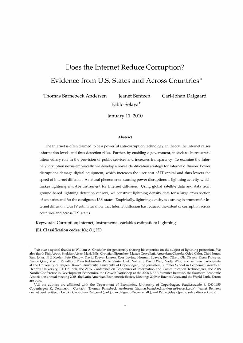
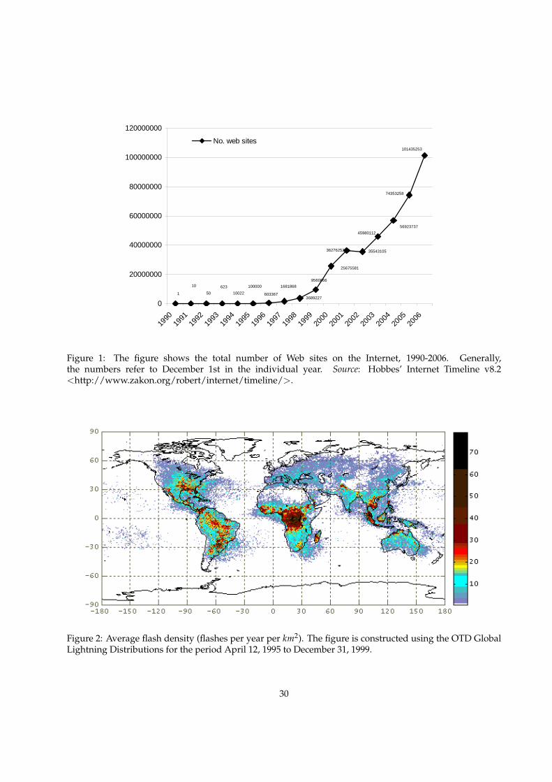
The Internet is a new technology, which in turn influences our estimation approach. Figure 1 illustrates

its remarkable growth since 1990. In roughly 15 years the number of Web sites has grown by 100 million.

- Figure 1 about here -

To examine the impact of the WWW we therefore estimate the impact of changes in Internet users on changes

in corruption levels from the early 1990s to 2006. Using cross-country data as well as data for the 48 con-

tiguous U.S. states we establish a strong partial correlation between the rate of changes in Internet uses and

the evolution of corruption, in accord with the hypothesis we are examining. However, since the speed of

Internet diffusion is likely endogenous, OLS estimates may well be misleading.

In an effort to establish causality, we develop an identification strategy designed to isolate exogenous

variation in the speed of Internet penetration. The theory underlying our instrument of choice is the fol-

lowing. Computer equipment is highly sensitive to power disruptions: power surges and sags lead to

equipment failure and damage. Consequently, a higher frequency of power disruptions implies higher

costs of IT equipment, either through elevating IT capital depreciation or due to incurrence of additional

costs in order to protect equipment from power disruptions. Frequent power disturbances are also likely

to reduce the productivity of IT capital (or its marginal benefit), as power disturbances produce downtime,

generate data glitches, etc. A natural phenomenon which produces power surges is lightning activity. In

fact, one third of all power disruptions in the U.S. are related to lightning activity. We therefore hypothesize

that higher lightning intensity is a viable candidate instrument for Internet diffusion. Using global satellite

data and state level measures of lightning density (ground strikes per square km per year) we establish

its influence on Internet diffusion: areas with a higher flash density have experienced a slower speed of

Internet adoption. Our 2SLS estimates confirm the OLS results: rising Internet use over the 1990s reduced

corruption in the U.S., and across countries.

A concern of first order importance is whether lightning density acts as a stand-in for other factors that

are correlated with changes in corruption. If so the critical exclusion restriction is violated, and our 2SLS

estimates are suspect. To address this concern one may observe that such omitted correlates with corruption

should tend to generate a time persistent impact of lightning on the evolution of corruption. That is, if

lightning acts as a stand-in for (say) human capital levels then lightning will be correlated with corruption

levels prior to the emergence of the WWW. However, as documented below, lightning density exhibits a

4A previous draft of the present paper (Andersen et al., 2008) contains additional examples and anecdotes.

3

time varying impact on corruption. Using U.S. data we show that the reduced form relationship between

lightning density and corruption does not exist prior to the inception of the WWW; it only exists from

1991 onwards. This falsification test makes probable that the lightning instrument meets the appropriate

exclusion restriction: lightning affects corruption only through its impact on Internet penetration, and does

not seem to act as a “stand-in” for other structural characteristics which influence corruption.5

The present research is related to the literature which studies the determinants of the level of corrup-

tion. Notable contributions include Ades and di Tella (1999), Treisman (2000), Brunetti and Weder (2003),

Persson, Tabellini, and Trebbi (2003), Glaeser and Saks (2006), and Licht, Goldscmidt, and Schwartz (2007).

Conceptually, Brunetti and Weder (2003) is perhaps the closest precursor to the present paper. The authors

find a corruption-reducing impact of a free press, and conclude that an independent press works to increase

transparency. In the present case we expect the Internet to affect corruption for partly the same reason.6

The paper is also related to the political economy literature that studies the impact of information on

governance more generally. This literature suggests that a better informed public serves to discipline the

political establishment, thus affecting governance (e.g. Besley and Burgess, 2002; Strömberg, 2004; Reinikka

and Svensson, 2004; Eisensee and Strömberg, 2007; Ferraz and Finan, 2008).

Finally, the paper is related to the literature which studies the determinants of the spread of the personal

computer (e.g. Caselli and Coleman, 2001) and the Internet (e.g. Chinn and Fairlie, 2007) across countries.

This literature has documented a positive impact of GDP per capita and the electricity infrastructure on

Internet penetration, and of human capital levels on the adoption of computers. Consequently, the level of

Internet penetration should a priori be viewed as endogenous, as noted above.

The paper is structured as follows. In Section 2 we present our empirical specifications of choice. Sec-

tion 3 outlines the identification strategy in detail; in particular, we explain how lightning activity impacts

digital equipment, and provide details on the data. Section 4 provides an analysis of how the Internet has

affected corruption across the U.S. states, whereas Section 5 provides cross-country evidence. Section 6

concludes.

2 Specification

Since governance indicators tend to be persistent over time, empirical work on the determinants of corrup-

tion usually seeks to explain differences in corruption levels. In the present context, however, we focus on

changes in corruption: the Internet is a recent phenomenon, and, as such, cannot have affected corruption

5Since historical series on country level corruption data is limited we are unfortunately unable to perform the same falsificationtest in the cross-country setting.

6Evidence to the importance of mass media more broadly, but still in the context of combating corruption, is provided in theinteresting study by McMillan and Zoido (2004).

4

levels prior to its inception, adoption, and widespread use. Consequently, we study whether changes in

Internet penetration can explain changes in corruption over the time-period during which the Internet has

been in operation.

We will mainly rely on the following parsimonious specification:

DCi = α0 + α1DINTERNETi + α2Cinitial,i + εi, (1)

where DCi is the change in corruption levels between an initial and a final year, C f inal,i � Cinitial,i and

DINTERNETi is the change in Internet penetration, INTERNETf inal,i � INTERNETinitial,i.

The inclusion of Cinitial,i makes explicit that changes in corruption almost inevitably is a function of the

initial level. For example, a country with no corruption cannot experience reductions in corruption levels.

Importantly, the usual first difference estimator will not capture this dependency.

Another virtue of including the initial level of corruption is that it automatically controls for (a poten-

tially large set of) variables which may influence the evolution of corruption. To see the latter point more

clearly, observe that (1) is equivalent to a levels regression with a lagged dependent variable:

C f inal,i = α0 + α1DINTERNETi + (α2 + 1)Cinitial,i + εi. (2)

Accordingly, all time invariant structural characteristics affecting the level of corruption will be picked up

by Cinitial,i. This reduces the scope for omitted variable bias in contaminating the estimate of α1 signifi-

cantly. Moreover, as explained in the Introduction, we will invoke lightning activity as an instrument for

DINTERNET and estimate (1) by 2SLS. Since it is difficult to rule out completely that lightning activity

might be correlated with various environmental variables, the inclusion of Cinitial,i in the regression serves

to increase our confidence in the the exclusion restriction; geographic factors should exert a time invariant

impact on corruption and, as such, be captured by Cinitial,i. We will further strengthen the case in favor

of the exclusion restriction by showing that lightning actually influences DINTERNET in a time varying

fashion.

Naturally, while specification (1) reduces the likelihood of omitted variable bias, it does not rule it out.

Time-varying characteristics may be omitted, which will induce OLS estimates of α1 to be biased. Hence, to

check the robustness of the link between changes in Internet penetration and changes in levels of corruption

we also invoke specifications of the form:

DCi = α0 + α1DINTERNETi + α2Cinitial,i + X0initial,iα3 + εi, (3)

where X contains additional controls. X includes the level of real income per capita in both the cross-state

5

and cross-country analysis. In addition, when studying the U.S. sample, where we rely on an outcome

based measure of corruption (total convictions), we also include a measure of state size (i.e, state popula-

tion) in X to ensure that all “scale effects” are pruned from the data. These controls are employed through-

out the analysis below. More generally, we have checked the robustness of the partial correlation between

DINTERNET and changes in corruption to a very large set of additional correlates, as explained below.

In spite of encouraging OLS results, to be reported below, one may worry about endogeniety. Indeed,

there is good reason to believe that the (initial) adoption of new technologies, such as the Internet, is endoge-

nous to governance. New technologies may create political as well as economic “losers”, for which reason

incumbent entrepreneurs and politicians may try to block adoption (Mokyr, 1990; Parente and Prescott,

1999; Acemoglu and Robinson, 2001). It seems plausible that places with widespread corruption, for ex-

ample, may have adopted the Internet later, due to the influence of politicians, civil servants, or both. This

mechanism rationalizes a positive impact of governance indicators, or income per capita, on the number of

Internet users. Consequently, OLS estimation is unlikely to identify the impact of Internet on corruption.

To address this concern we employ an IV approach. The next section describes our identification strategy

in detail.

3 Identification

3.1 Theory

Computers are highly sensitive to even ultra brief power disruptions. Such disruptions are likely to cause

down-time, though sudden power surges may also damage the equipment and randomly destroy or alter

data. As observed in The Economist:7 “For the average computer or network, the only thing worse than the

electricity going out completely is power going out for a second. Every year, millions of dollars are lost to

seemingly insignificant power faults that cause assembly lines to freeze, computers to crash and networks

to collapse.”

The reason why IT equipment is so sensitive to power disturbances is that computers are constructed

to work under a “clean” electrical current, featuring a particular frequency and amplitude of voltage. The

alternating power emanating from the commercial power plant is converted into direct current, after which

transistors turn this small voltage on and off at several gigahertz during digital processing (Kressel, 2007).

However, if the “input”, in the form of the alternating current, is disturbed or distorted the conversion

process is corrupted, which may in turn result in equipment failure and damage. Indeed, voltage distur-

bances measuring less than one cycle are sufficient to crash servers, computers, and other microprocessor-

7“The power industry’s quest for the high nines”, The Economist, March 22, 2001.

6

based devices; that is, at a 60 Hz frequency (the standard in the U.S.) this means that a power disturbance

of a duration less than 1/60th of a second is enough to crash a computer (Yeager and Stalhkopf, 2000;

Electricity Power Research Institute, 2003). Importantly, this issue is unlikely to diminish over time as the

sensitivity to small power distortions increases with the miniaturization of transistors, which is the key to

increasing speed in microprocessors (Kressel, 2007).

Accordingly, in areas with more power disturbances, the user cost of IT capital will be higher due to a

higher rate of IT capital depreciation (Hall and Jorgenson, 1967). By implication, the desired IT capital stock

will be lower, reducing IT investments and the speed of Internet diffusion. Of course, steps may be taken

to protect the equipment from power disturbances. A high-quality surge protector provides protection

against voltage spikes, for example. High-tech companies install generators to supplement their power

needs, thereby insuring themselves against power failure. They also add “uninterruptible power sources”

relying on batteries to power computers until generators kick in. However, these initiatives will in any case

increase the costs of acquiring digital equipment, and thereby the user cost of IT capital. The crux of the

matter is that if one lives in an environment with low power quality, this adds to the costs of a computer.8

To this one may add that in areas with frequent power disruptions and outages, the marginal benefit

of owning a computer is probably lowered as well. Obviously, in countries where firms and consumers

face regular power outages it will be difficult to employ IT efficiently. But even if power disruptions are

infrequent and of very short duration, power disruptions lead to glitches and downtime which serves

to lower the productivity of IT equipment. Both mechanisms, higher marginal costs and lower marginal

return/benefit, imply that poorer power quality should lead to a slower speed of Internet diffusion.

Naturally, power quality is not exogenous, and may well be determined by governance. As a result, we

employ a variable which generates exogenous variation in power quality, and thus IT costs and benefits,

as an instrument for Internet diffusion. A natural phenomenon which interferes with digital equipment,

by producing power failures, is lightning activity (e.g., Shim et al., 2000, Ch. 2; Chisholm, 2000). By all

accounts, the influence of lightning on power quality is substantial. According to some estimates, light-

ning is the direct cause of one third of all power quality disturbances in the United States (Chisholm and

Cummins, 2006). Moreover, the probability of lightning-caused power interruptions or equipment damage

scales linearly with lightning density (Chisholm, 2000; Chisholm and Cummins, 2006).9 As a result, in areas

with greater lightning density (strikes per square km per year) the (expected) rate of IT capital depreciation

8Besides, the above mentioned protective devises are not necessarily enough to ensure against damage. According to the NationalOceanic and Atmospheric Administration (NOAA), a typical surge protector will not protect equipment from a nearby lightningstrike. Generators, in turn, do not react fast enough and can deliver dirty power; batteries are expensive to maintain and may also notreact fast enough. See e.g., “The power industry’s quest for the high nines”, The Economist (March 22, 2001).

9This linear scaling can be expressed precisely. Let NS denote the number of strikes to a conducter per 100 km of power line length,h the average height (in meters) of the conducter above ground level, and GFD the ground flash density, then NS = 3.8 � GFD � h0.45

(see Chisholm, 2000).

7

will tend to be larger. This implies higher IT investment costs, and possibly lower IT productivity as well.

The problems associated with lightning activity in the context of IT equipment has not escaped the

attention of the popular press. A recent article in The Wall Street Journal highlights the practical relevance

of lightning activity, and stresses the difficulty in shielding IT equipment:10 “Even if electricity lines are

shielded, lightning can cause power surges through unprotected phone, cable and Internet lines - or even

through a building’s walls. Such surges often show up as glitches. "Little things start not working; we

see a lot of that down here," says Andrew Cohen, president of Vertical IT Solutions, a Tampa information-

technology consulting firm. During the summer, Vertical gets as many as 10 calls a week from clients with

what look to Mr. Cohen like lightning-related problems. Computer memory cards get corrupted, servers

shut down or firewalls cut out.”

Against this background we propose lightning density as an instrument for the speed at which Internet

use per capita changed over the period in question. Schematically we can express the theory underlying

our identification strategy in the following way

LIGHTNING DENSITY �! POWER DISTURBANCES �! INTERNET USE, (4)

where the second arrow implicitly subsumes the impact of power disturbances on the costs and benefits of

IT capital.

Lightning is certainly exogenous in a deep sense. However, this does not ensure validity of the exclusion

restriction. Climate-related circumstances may map into levels of corruption (indirectly capturing e.g. the

resource curse mechanism), and lightning may be more pronounced in some climate zones compared to

others. As mentioned in Section 2, however, the inclusion of Cinitial ensures that time invariant determinants

of corruption are controlled for; the resource curse mechanism is therefore unlikely to pose a problem vis-à-

vis the exclusion restriction. Rather, validity of the exclusion restriction requires that lightning has no direct

impact on changes in corruption over the period under study, conditional on the initial level of corruption,

Cinitial , and the initial level of income per capita. Naturally, with only one instrument a formal test of

the exclusion restriction is not feasible. However, an informal test is possible: In the analysis below we

construct a falsification test designed to shed light on the plausibility of the exclusion restriction.

3.2 Data on the Instrument: Lightning density

The raw data for flash densities (flashes per km2 per year) is provided by the National Aeronautics and

Space Administration (NASA). The Global Hydrology and Climate Center (GHCC) has designed, con-

structed, and deployed numerous types of groundbased, airborne, and spacebased sensors to detect light-

10“There Go the Servers: Lightning’s New Perils”. The Wall Street Journal, August 25, 2009.

8

ning activity and to characterize the electrical behavior of thunderstorms as part of their research on at-

mospheric science. The GHCC’s spacebased sensors detect all forms of lightning activity over land and

sea 24 hours a day. Such sensors allowed the development of the first global database of lightning ac-

tivity, which has been used so far for severe storm detection and analysis, and for lightning-atmosphere

interaction studies.

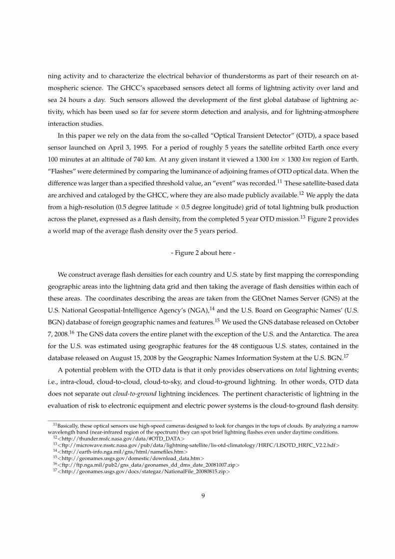
In this paper we rely on the data from the so-called “Optical Transient Detector” (OTD), a space based

sensor launched on April 3, 1995. For a period of roughly 5 years the satellite orbited Earth once every

100 minutes at an altitude of 740 km. At any given instant it viewed a 1300 km� 1300 km region of Earth.

“Flashes” were determined by comparing the luminance of adjoining frames of OTD optical data. When the

difference was larger than a specified threshold value, an “event” was recorded.11 These satellite-based data

are archived and cataloged by the GHCC, where they are also made publicly available.12 We apply the data

from a high-resolution (0.5 degree latitude � 0.5 degree longitude) grid of total lightning bulk production

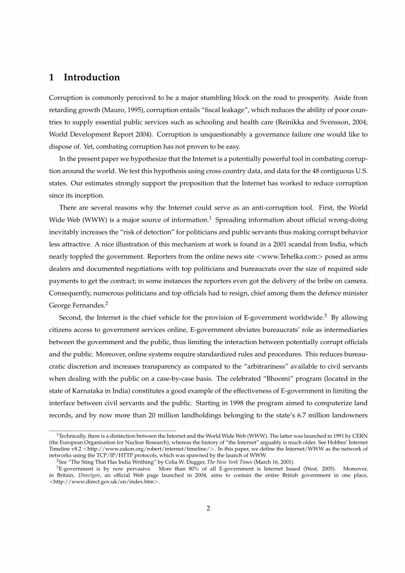
across the planet, expressed as a flash density, from the completed 5 year OTD mission.13 Figure 2 provides

a world map of the average flash density over the 5 years period.


We construct average flash densities for each country and U.S. state by first mapping the corresponding

geographic areas into the lightning data grid and then taking the average of flash densities within each of

these areas. The coordinates describing the areas are taken from the GEOnet Names Server (GNS) at the

U.S. National Geospatial-Intelligence Agency’s (NGA),14 and the U.S. Board on Geographic Names’ (U.S.

BGN) database of foreign geographic names and features.15 We used the GNS database released on October

7, 2008.16 The GNS data covers the entire planet with the exception of the U.S. and the Antarctica. The area

for the U.S. was estimated using geographic features for the 48 contiguous U.S. states, contained in the

database released on August 15, 2008 by the Geographic Names Information System at the U.S. BGN.17

A potential problem with the OTD data is that it only provides observations on total lightning events;

i.e., intra-cloud, cloud-to-cloud, cloud-to-sky, and cloud-to-ground lightning. In other words, OTD data

does not separate out cloud-to-ground lightning incidences. The pertinent characteristic of lightning in the

evaluation of risk to electronic equipment and electric power systems is the cloud-to-ground flash density.

11Basically, these optical sensors use high-speed cameras designed to look for changes in the tops of clouds. By analyzing a narrowwavelength band (near-infrared region of the spectrum) they can spot brief lightning flashes even under daytime conditions.

12<http://thunder.msfc.nasa.gov/data/#OTD_DATA>13<ftp://microwave.nsstc.nasa.gov/pub/data/lightning-satellite/lis-otd-climatology/HRFC/LISOTD_HRFC_V2.2.hdf>14<http://earth-info.nga.mil/gns/html/namefiles.htm>15<http://geonames.usgs.gov/domestic/download_data.htm>16<ftp://ftp.nga.mil/pub2/gns_data/geonames_dd_dms_date_20081007.zip>17<http://geonames.usgs.gov/docs/stategaz/NationalFile_20080815.zip>

9

Fortunately, since the mid-1980’s it has been possible to measure ground flash density more directly using

networks of electromagnetic sensors. Such Lightning Location Systems (LLS) are able to detect individual

ground strikes with high spatial and temporal accuracy. However, many parts of the world, particularly

the developing world, are not covered by the LLS data.18 But accurate cloud-to-ground data does exist

for the 48 contiguous U.S. states. These cloud-to-ground lightning flashes, which are measured by the U.S.

National Lightning Detection Network (NLDN), are provided by Vaisala for the period 1996-2005.19 NLDN

consists of numerous remote, ground-based lightning sensors, which instantly detect the electromagnetic

signals given off when lightning strikes Earth’s surface. Comparing the NLDN ground-based measures

with the NASA satelite-based measures for the U.S. provides an indication of the extent to which the total

amount of lightning is a reliable indicator of cloud-to-ground lightning.

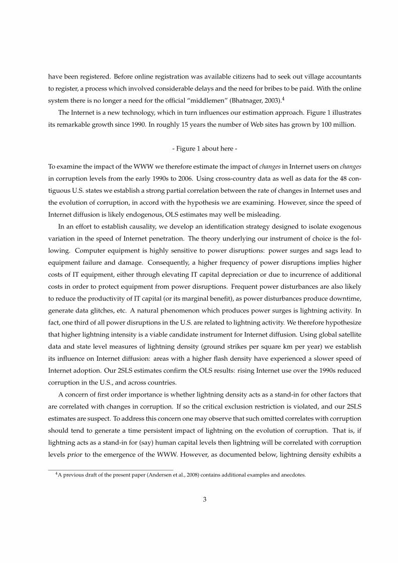
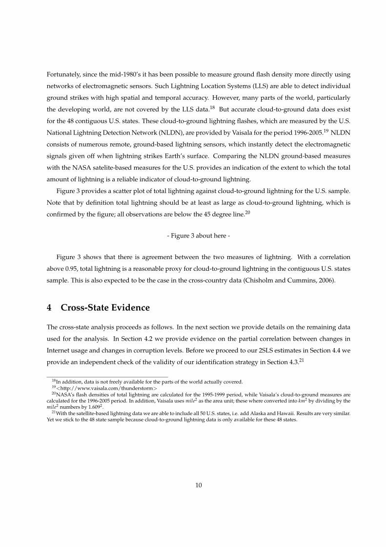
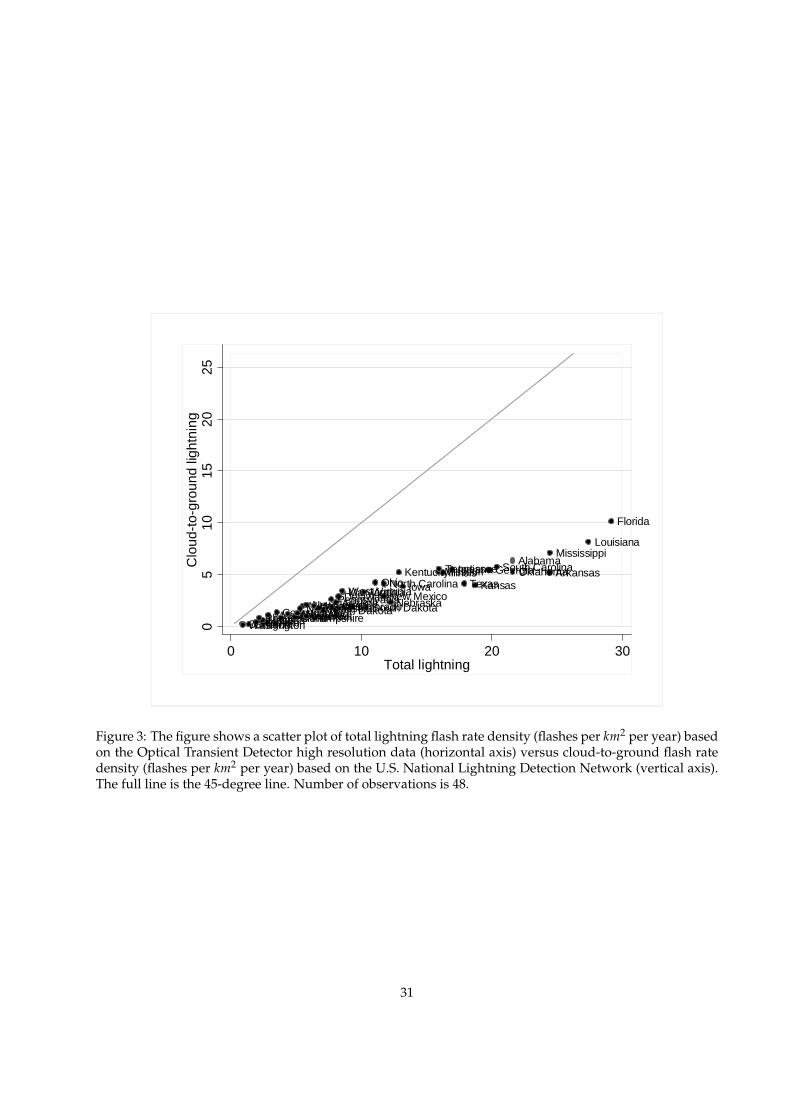
Figure 3 provides a scatter plot of total lightning against cloud-to-ground lightning for the U.S. sample.

Note that by definition total lightning should be at least as large as cloud-to-ground lightning, which is

confirmed by the figure; all observations are below the 45 degree line.20


Figure 3 shows that there is agreement between the two measures of lightning. With a correlation

above 0.95, total lightning is a reasonable proxy for cloud-to-ground lightning in the contiguous U.S. states

sample. This is also expected to be the case in the cross-country data (Chisholm and Cummins, 2006).

4 Cross-State Evidence

The cross-state analysis proceeds as follows. In the next section we provide details on the remaining data

used for the analysis. In Section 4.2 we provide evidence on the partial correlation between changes in

Internet usage and changes in corruption levels. Before we proceed to our 2SLS estimates in Section 4.4 we

provide an independent check of the validity of our identification strategy in Section 4.3.21

18In addition, data is not freely available for the parts of the world actually covered.19<http://www.vaisala.com/thunderstorm>20NASA’s flash densities of total lightning are calculated for the 1995-1999 period, while Vaisala’s cloud-to-ground measures are

calculated for the 1996-2005 period. In addition, Vaisala uses mile2 as the area unit; these where converted into km2 by dividing by themile2 numbers by 1.6092.

21With the satellite-based lightning data we are able to include all 50 U.S. states, i.e. add Alaska and Hawaii. Results are very similar.Yet we stick to the 48 state sample because cloud-to-ground lightning data is only available for these 48 states.

10

4.1 Data

The corruption data derives from the Justice Department’s “Report to Congress on the Activities and Op-

erations of the Public Integrity Section”. This publication provides statistics on the nationwide federal effort

against public corruption, including the number of federal, state, and local public officials convicted of a

corruption-related crime by state. As argued by Glaeser and Saks (2006), federal conviction levels capture

the extent to which federal prosecutors have charged and convicted public officials for misconduct. There

are potential problems with using conviction rates to measure corruption: in corrupt places, the judicial

system is itself likely to be corrupt, meaning that fewer people will be charged with corrupt practices. This

problem, however, is diminished when using federal convictions, the reason being that the federal judicial

system is somewhat isolated from local corruption. Consequently, it should treat people similarly across

states (Glaeser and Saks, 2006).

The change in corruption convictions, DCC, is calculated as the difference between corruption convic-

tions (CC) in 2006 and 1991:

DCCi = log(1+ CC2006,i)� log(1+ CC1991,i). (5)

The choice of initial year follows from the fact that the Internet (in the sense of the WWW) was invented (at

CERN) in 1990 (first Web page went online in 1991). Positive values for DCC are interpreted as reflecting

increasing corruption.22

The second key variable is Internet users, which we measure as the percentage of households with

Internet access. It is based on data collected in a supplement to the October 2003 Current Population Survey

(CPS), which includes questions about computer and Internet use.23 The CPS is a multi-stage probability

sample with coverage in all states. The sample was selected from the 1990 Decennial Census files and is

continually updated to account for new residential construction. To obtain the sample the United States is

divided into 2,007 geographic areas, and about 60,000 households are eligible for interviews.

Since U.S. corruption data goes back to 1991, the launch date of the WWW, we define the change in

Internet use by state population as

DINTERNETi = INTERNETi,2003 � INTERNETi,1991 = INTERNETi,2003,

since INTERNETi,1991 = 0 for all i (i.e., for all states).

22Note that an increased use of the Internet will both increase the risk of detection for a corrupt official (the detection technology isimproved) as well as lower the incentive to commit corrupt acts. Hence, in theory, increased Internet use could increase the numberof convictions if the former effect dominates. It might thus seem as if the Internet increases corruption. However, empirically the neteffect is negative, implying that the “incentive effect” dominates, as documented below.

23<http://www.census.gov/population/socdemo/computer/2003/tab01B.xls>.

11

Finally, in some specifications we control for the initial level of (real) income per capita in 1991 using

data on “personal income per capita”, taken from the State Personal Income Database from U.S. Bureau

of Economic Analysis (BEA). Nominal income per capita is deflated using the implicit price deflator for

personal consumption expenditures, index year 2000 (also from BEA). The natural log of income per capita

in 1991 is denoted as log(YCAP1991). Finally, we control for initial state population, which also derives from

BEA. The natural log of initial state population is denoted log (POP1991). Summary statistics are reported

in Appendix A.

4.2 Partial Correlations

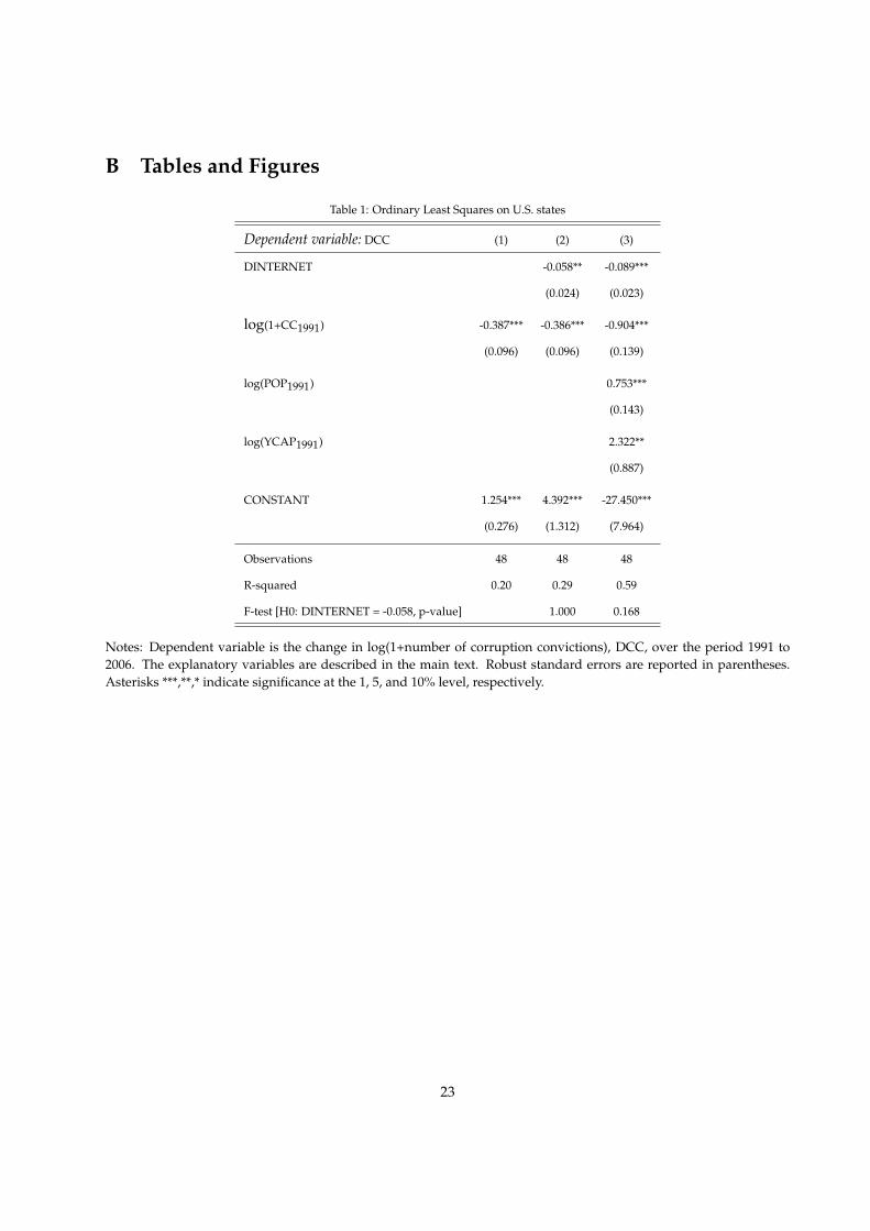
Table 1 documents the partial correlation between changes in Internet use and changes in corruption for

the 48 contiguous U.S. states. The dependent variable is defined by equation (5).

Column 2 estimates equation (1). DINTERNET is estimated with high precision. With a t-value of 2.37

in column 2 significance holds at roughly the 2% level. The specification in equation (1) (i.e. column 2) ac-

counts for almost 30% of the variation in DCC in the U.S. sample. Adding log(POP1991) and log(YCAP1991),

cf. column 3, does not impact on the partial correlation between DINTERNET and DCC. Indeed, while

significant at conventional levels, the inclusion of log(POP1991) and log(YCAP1991) does not (statistically)

change the DINTERNET point estimate. Hence the remaining variation in DINTERNET, once we have

partialled out the effect of initial corruption, is roughly orthogonal to the variation in income per capita

and the variation in population size. This finding provides some assurance that a parsimonious specifi-

cation such as (1) is appropriate for the U.S. sample. Overall, the results reported in Table 1 document a

noteworthy partial association between Internet diffusion and changes in corruption convictions from 1991

onwards.

- Table 1 about here -

In addition, we have gauged the robustness of the partial correlation between Internet diffusion and

changes in corruption levels using the list of corruption determinants discussed in Maxwell and Winters

(2005). They focus on four fundamental traits of U.S. states that should have predictable effects on corrup-

tion: (i) number of corruptible government bodies, (ii) the size of the state, (iii) socio-ethnic homogeneity,

and (iv) civic-minded and well-informed political cultures. In addition to proxies for these traits the au-

thors consider seven additional control variables, which, besides real income growth, consists of metropol-

itan population, general tax revenue, direct initiatives, direct initiatives threshold, campaign expenditure

restrictions, and open party primaries. The partial correlation between Internet and corruption is robust to

the sequential inclusion of all of these additional controls. These results are available upon request. In spite

of these encouraging results, to make further progress, we need to move beyond the OLS analysis.

12

4.3 Falsification Test

According to our identification strategy lightning only affects corruption through Internet penetration. By

implication, if lightning density affects changes in corruption levels solely due to its impact on Internet use,

lightning density should be uncorrelated with changes in corruption prior to the inception and spread of the

Internet. If lightning density is correlated with past changes in corruption levels, the variable is likely cap-

turing some other (omitted) determinant of corruption. If so, the validity of the lightning instrument should

be questioned. Hence, before we turn to our IV results we provide a falsification test of our instrument of

choice.

Specifically, we run the following regression:

DCCi = α0 + α1 log(LIGHTNING)i + α2CCinitial,i + X0initial,iα3 + εi, (6)

on two separate periods of time. First, we examine the sign and significance of α1 on the period 1991-2006.

We expect a positive and statistically significant estimate for α1, capturing a slower spread of the Internet

and thus smaller reductions in corruption, ceteris paribus. Second, we examine the sign and significance of

α1 on the period 1976-1990, where the initial year is a consequence of data availability on corruption con-

victions. Here we expect a numerically small and statistically insignificant estimate for α1. If α1 is estimated

to be significant this clearly falsifies our instrument.

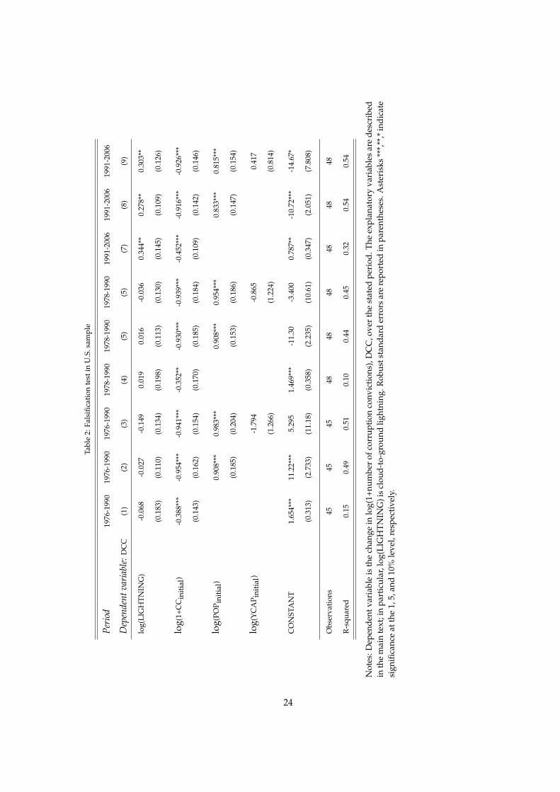
Table 2 reports results of the falsification test.


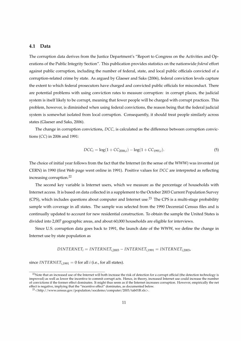
As shown in columns 1-6 lightning does not influence changes in corruption prior to the inception of

the WWW. This holds both for the period 1976-1990, where we have missing observations on corruption

convictions for three states, and for the 1978-1990 period, where there are no missing observations. It is

worth observing that the numerical size of the point estimate is close to zero; the rejection of α1 > 0 for

these periods is not simply a matter of a more imprecisely estimated parameter.

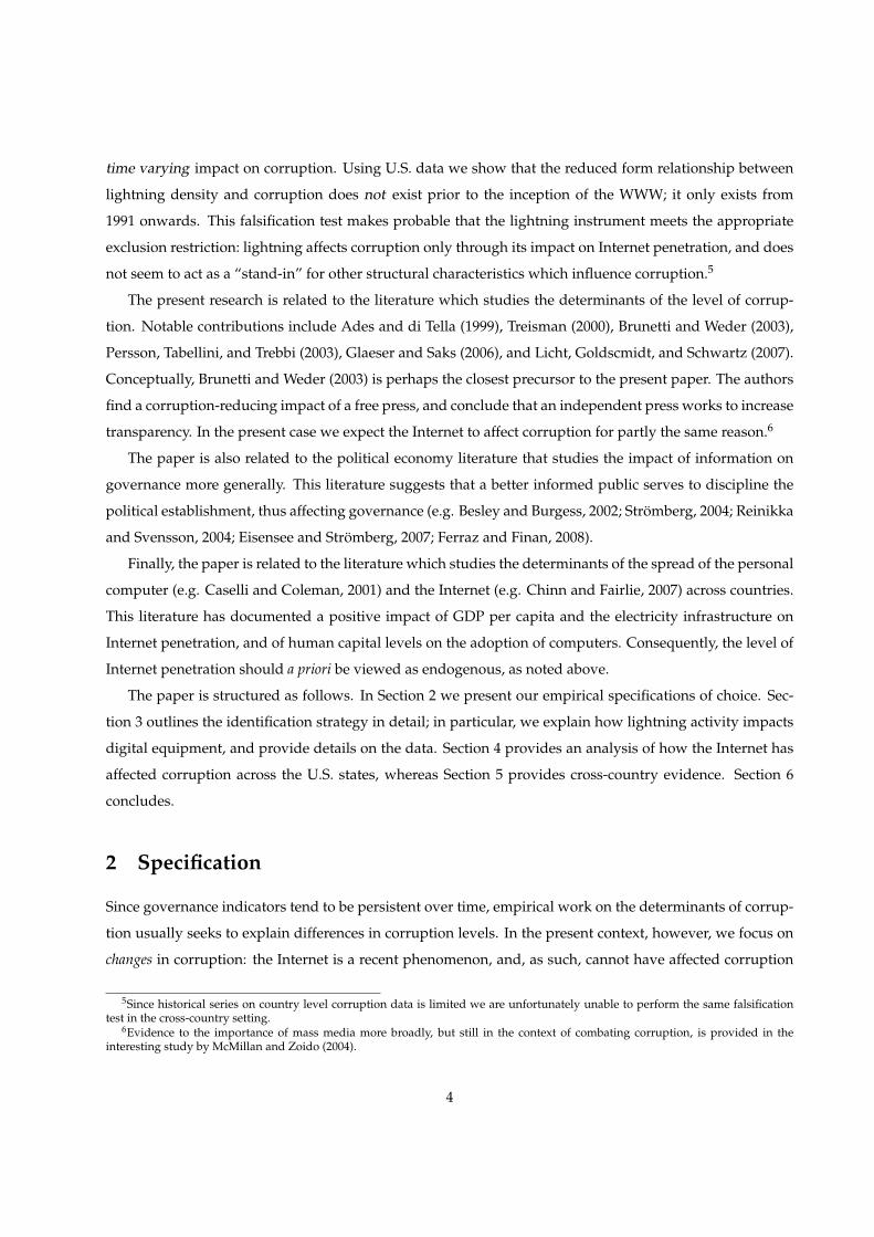
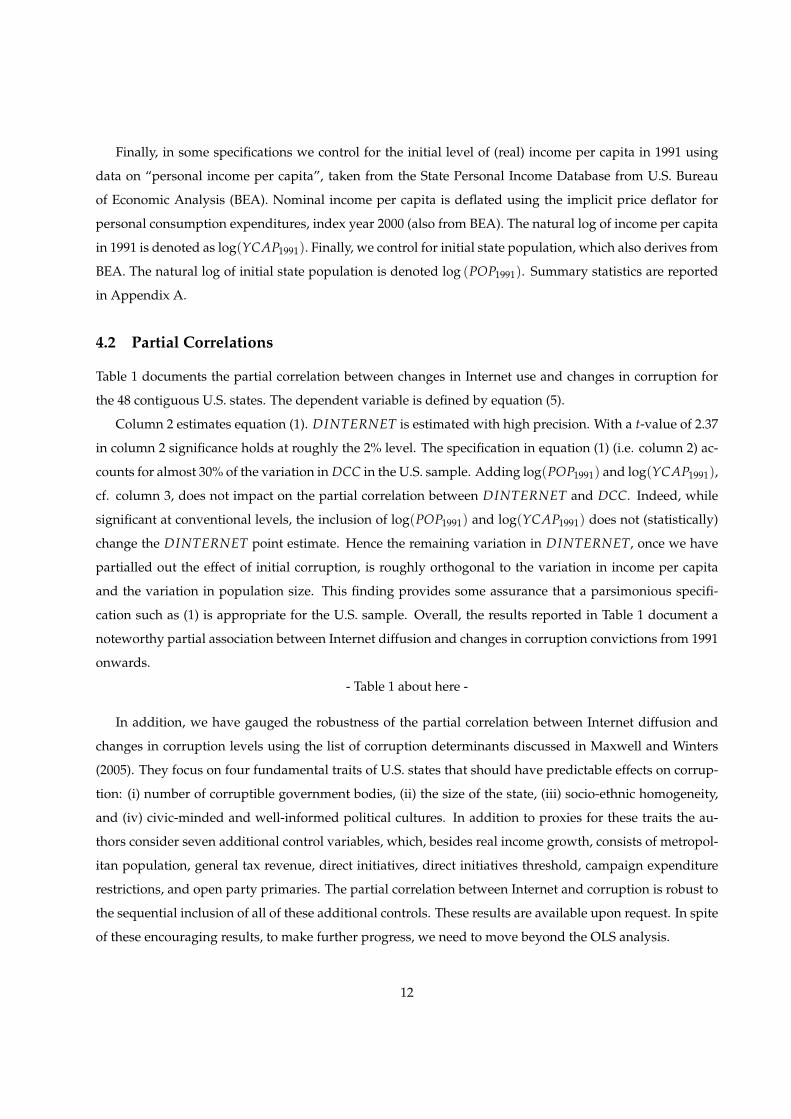
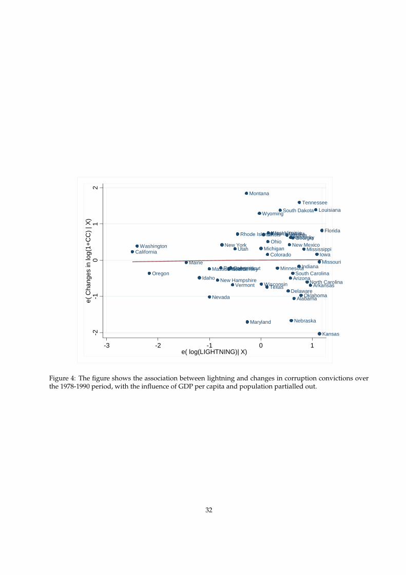
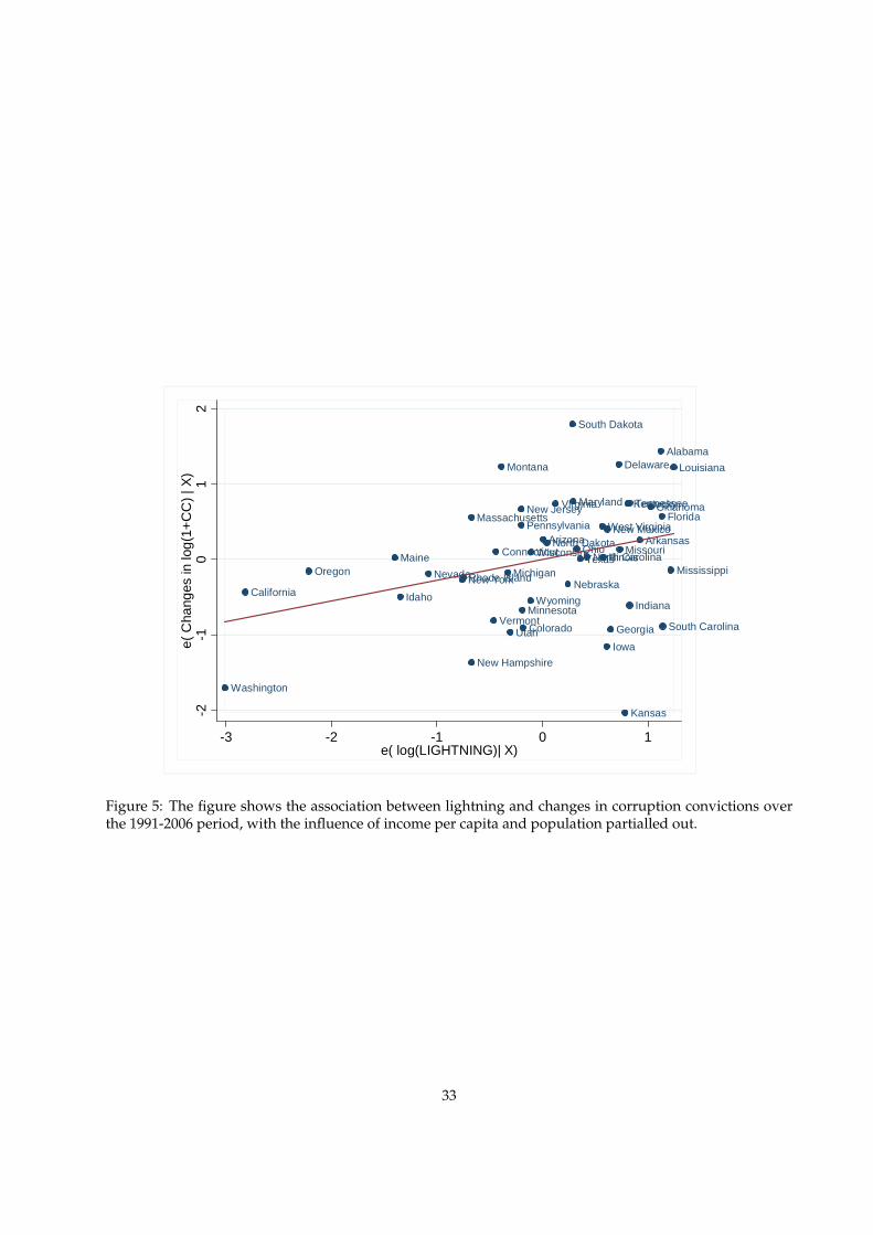
Columns 7-9 show that lightning exerts a statistically significant influence on corruption after the incep-

tion of the WWW. Figures 4 and 5 provide a visual impression of these findings.

- Figures 4 and 5 about here -

Overall, the results suggest that lightning is unlikely to be picking up omitted (time varying) deter-

minants of corruption. If lightning were picking up time varying determinants of corruption (like human

capital, say) it would be correlated with changes in corruption levels both before and after the inception of

13

the WWW.

As explained in Section 2, by including initial corruption in the regression it seems unlikely that the

exclusion restriction is jeopardized due to the exclusion of time invariant determinants of corruption, like

various geographic variables capturing (e.g.) a resource curse channel. Against this background we con-

clude that the exclusion restriction is plausible, and move on to our 2SLS estimates.

4.4 IV Estimates

The 2SLS results are reported in Table 3. Panel A reveals that lightning density is negatively related to

the diffusion of the Internet across U.S. states, in keeping with the theory underlying our identification

strategy. This holds whether we rely on the accurate cloud-to-ground lightning density or, alternatively,

the total lightning proxy. In column 3 we include log(POP1991) and log(YCAP1991). Importantly, lightning

remains a strong instrument despite the inclusion of these additional controls.24 Overall, 2SLS tends to

produce numerically larger point estimates compared with OLS.

Since we are unable to reject homoscedasticity the usual rule-of-thumb for strength of instruments is

informative. As the F-values are always above 30, the lightning instrument is very strong (Staiger and

Stock, 1997). These results strongly support the hypothesis that the Internet is an effective anti-corruption

tool.


What is the economic significance of Internet use in combating corruption? To answer this question we

begin with the levels specification associated with (2):

log(1+ CC2006) = α0 + α1DINTERNET+ (α2 + 1) log(1+ CC1991).

If we linearize, treating CC1991 as a constant, the following simple approximation emerges:

∆CC2006 ' α1 (1+ CC2006)∆INTERNET2003, (7)

where we have used that DINTERNET = INTERNET2003, cf. Section 4.1.

Next, to gauge economic significance, consider moving from the median to the third quartile in the

distribution of Internet users in 2003; this is equivalent to an increase of 3.1 Internet users per 100 people.

Using the 2SLS results reported in column 2 of Table 3 (the most conservative estimate) in equation (7) we

find that ∆CC2006 ' (�0.067) � (1+ 16) � (3.1) = �3. 53 yearly convictions.25 This would correspond to

24Using the total lightning proxy in column 3 provides similar results.25Using the most optimistic estimate (i.e. column 3) would roughly double the effect (i.e. �6.7 yearly convictions).

14

moving from the median to the 36th percentile in the U.S. state corruption convictions ranking in 2006.

Accordingly, the introduction of the Internet has reduced corruption levels below what would otherwise

have been observed absent this technology.

5 Cross-Country Evidence

In this Section we examine whether the results obtained above generalize to a cross-country sample. After

providing details on the data used in the cross-country setting (beyond lightning density), we discuss the

partial correlation between changes in corruption and changes in Internet users in Section 5.2. Section 5.3

contains the 2SLS estimate of the impact of the Internet on corruption.

5.1 Data

Global corruption is measured using the well-known Control of Corruption Index (CCI) compiled by Kauf-

mann et al. (2007). The CCI measure, which ranges from �2.5 (worst) to 2.5 (best), is available biannually

from 1996 to 2002 and annually from 2002 onwards.26 The CCI indicator attempts to measure “the extent

to which public power is exercised for private gain, including both petty and grand forms of corruption as

well as capture by elites and private interests” (Kaufmann et al., 2007, p. 4).27 The indicator is based on a

large number of individual data sources, which are then aggregated into one measure by an unobserved

components model. This means that the aggregate measure is a weighted average of the underlying in-

dividual data sources, with weights reflecting the precision of each of these underlying data sources; this

makes the CCI the most comprehensive measure of corruption around.28 Moreover, by virtue of being a

solution to a statistical signal extraction problem, the aggregate CCI indicator is presumably more informa-

tive than any individual data source.29

The change in corruption levels is calculated as the difference between CCI in 2006 and 1996, i.e.

DCCIi = CCI2006,i � CCI1996,i. (8)

26These boundaries correspond to the 0.005 and 0.995 percentiles of the standard normal distribution. For a few countries, countryratings can exceed these boundaries when scores from individual data sources are particularly high or low (Kaufmann et al., 2007).

27Some are sceptical concerning the use of perception-based corruption data (Svensson, 2005). Interestingly, however, Olken (2006)has provided novel evidence on the relation between corruption perceptions and a direct measure of corruption in the context ofvillages across Indonesia. The empirical results show that villagers’ perceptions of corruption do appear to be positively (albeitweakly) correlated with a direct “missing expenditure” measure.

28The widely reported Corruption Perception Index (CPI) compiled by Transparency International forms part of the CCI measure(see Kaufmann et al., 2007, Table A13). Reasuringly, the simple correlation between CCI and CPI is 0.97.

29Svensson (2005), however, notes that the aggregation procedures used by Kaufmann et al. presumes that subindicator measure-ment errors are independent across sources. In reality, errors may be correlated since producers of different indices read the samereports and most likely each other’s evaluations. If the assumption of independence is relaxed, the gain from aggregating a numberof different reports is less clear.

15

Observe that, by definition, positive values for DCCI means less corruption.

Ideally, we would like to go back to 1991, the launch date of the WWW. Unfortunately, with the preferred

CCI measure this is not feasible as 1996 is the earliest year for which the variable is available. However,

to check robustness we also run regressions using the ICRG corruption indicator (from the International

Country Risk Guide); the ICRG indicator allows us to go back to 1991. The change in the ICRG indicator,

DICRG, is defined analogously to (8).

Our key explanatory variable is the number of Internet users per 100 people. Increasingly, the number

of Internet users is based on regular surveys. In situations where surveys are not available, an estimate can

be derived based on the number of subscribers. Data is compiled by the International Telecommunication

Union (ITU) and made available in the World Development Indicators (WDI) 2007. Since global corruption

data goes back to 1996, we calculate the change in Internet users over this period:

DINTERNETi = INTERNETi,2005 � INTERNETi,1996,

where 2005 is the most recent year available for Internet users in the WDI (2007). When we examine the

period 1991-2006, using the ICRG indicator, we use the approximation that INTERNETi,1991 = 0, as in the

analysis of the U.S. states.

Real PPP-adjusted GDP per capita, YCAP, for the global sample is taken from WDI (2007). The natural

log of real GDP per capita in 1996 (1991) is denoted as log(YCAP1996) (log(YCAP1991)). Summary statistics

are provided in Appendix A.

5.2 Partial Correlations

Table 4 explores the partial correlation between changes in Internet use and changes in corruption for the

cross-country data; the dependent variable is DCCI, defined by equation (8).


Column 2 estimates the parsimonious specification (1). The sign of DINTERNET is positive, indicating

that increased Internet use is associated with more “control of corruption” (i.e. less corruption). Moreover,

DINTERNET is estimated with high precision. With a t-value above 4, significance is well below the

1% level. When we include the initial log of GDP per capita, DINTERNET remains significant albeit

numerically somewhat smaller. Hence, the positive (partial) association between changes in Internet use

and changes in corruption is not driven by omitted factors such as the level of economic development.30

30This is perhaps not surprising as the correlation between CCI1996 and YCAP1996 is as high as 0.8.

16

In addition, we have examined the robustness of the partial correlation between changes in corruption

and Internet per capita to the inclusion of the entire set of corruption determinants (included one-by-one)

used by Treisman (2007). Treisman includes variables that constitute “historical and cultural controls”;

“political controls”; and finally a set of “rents and competition controls”. The correlation between Internet

and corruption holds up, and the results are available upon request.

5.3 IV Estimates

Turning now to instrumental variables methods, Table 5 reports 2SLS-based results for the cross-country

sample. Panel A of the table provides results from first-stage regressions. In accordance with the logic of

the identification strategy, lightning density is negatively related to the diffusion of the Internet in column

1. In column 2, where we have also included the logarithm of real GDP per capita, the lightning instrument

turns insignificant; or, more appropriately, the instrument is weak.


The association between average lightning density and the change in Internet use in column 1, once the

influence of initial corruption is partialled out, is close to the “rule-of-thumb” value suggested by Staiger

and Stock (1997). Specifically, if the F-value associated with the null of zero explanatory power of the

instrument is above ten we need not concern ourselves with issues of weak identification: inference based

on 2SLS estimates will not be plagued with size distortions. This rule-of-thumb, however, requires that

the error variance is homoskedastic (see assumption M, part (c) in Staiger and Stock, 1997). While this

assumption is fulfilled in the second-stage regression, it fails in the first-stage regression. Consequently,

while inspection of panel A reveals that the F-value is “close” to ten in column 1, with non-constant error

variance it is not entirely clear what this means for the actual size of significance tests.

We address the problem of potential size distortions by invoking a method proposed by Chernozhukov

and Hansen (2008), which allows us to construct confidence intervals with the correct size regardless of the

strength of instruments.31 Moreover, Chernozhukov and Hansen show how these size-adjusted confidence

intervals can easily be made robust to non-spherical disturbances. Finally, the procedure has good power

properties.

Panel B reports such size-adjusted confidence intervals. As is evident from the table, 95% size-adjusted

confidence interval deems DINTERNET above zero in column 1. The midpoint of the confidence interval

is 0.05, which is above both OLS (0.016) and 2SLS (0.032) estimates. In column 2, where log(YCAP1996)

31These confidence intervals are weak-identification robust since information about the (partial) correlation between instrumentsand the endogenous variable is not used.

17

is included and where we face a severe identification problem, the 90% size-adjusted confidence interval

provides a sharp lower bound, which is strictly larger than zero; but the confidence interval is upwardly

unbounded, i.e. data are not informative about the upper bound. Weak identification notwithstanding, the

overall message is therefore that the causal impact of DINTERNET on DCCI is positive and statistically

significant.

Turning to economic significance: Using the results from 2SLS reported in column 1, Panel B of Table 5,

the effect of an increase in INTERNET2005, holding the initial levels of Internet use and corruption constant, is

∆CCI2006 ' α1∆INTERNET2005. (9)

We gauge economic significance as in Section 4.4. Increasing the number of Internet users in 2005 from

the median to the third quartile of the distribution (using the estimating sample associated with column

3 of Table 5) gives ∆INTERNET2005 = 19.48. Inserting in (9) gives ∆CCI2006 ' (0.032) � 19.48 = 0.62.

This means that moving from the median to the third quartile in terms of Internet users would move the

corruption score from the median to the 65th percentile.

Finally, as a matter of robustness, we replace the CCI index by the ICRG indicator. A virtue of the

ICRG index is that it allows us to examine the entire period 1991-2006. Table 6, columns 1 and 2 report OLS

results. Inspection reveals that DINTERNET is always significant, and that the inclusion of log(YCAP1991)

has little effect.

Columns 3 and 4 of the table report 2SLS results. The results are statistically considerably stronger than

those reported in Table 5, in the sense that identification is stronger. Qualitatively, however, the message

is the same. With the ICRG indicator we can bound the causal impact in column 4 to the 95% confidence

interval [0.009, 0.043] using the Chernozhukov and Hansen (2008) approach.


If we use the midpoint of this interval, i.e. 0.026, we can gauge economic significance as done above. Mov-

ing from the median to the third quartile in the Internet distribution would imply a move in the corruption

distribution of magninute ∆ICRG2006 ' (0.026) � 20 = 0.52. This corresponds to a move from the median

to the 68th percentile, which squares well with the results we obtained above using the CCI indicator.

6 Concluding remarks

The present analysis shows that the Internet is a powerful anti-corruption technology. The Internet facil-

itates the dissemination of information about corrupt behavior, making it more risky for bureaucrats and

18

politicians to take bribes. Via E-government, it also obviates the need for potentially corrupt officials to

serve as middlemen between the government and the public, and it allows for more transparency in the

context of public procurement.

In order to examine whether Internet penetration has had a causal impact on corruption, the paper de-

velops a new instrument for the user cost of digital equipment such as computers, and thereby for Internet

diffusion. Digital equipment is highly sensitive to power disruptions; and, to a considerable extent, light-

ning activity causes power disruption around the world. Indeed, according to some calculations, lightning

causes some 17,000 computers around the world to crash each second (Yeager and Stahlkopf, 2000).

Using data based on ground-based censors and global satellite data, we construct state and country

level measures of average lightning density. Across the U.S. we show that lightning is correlated with

changes in corruption after the emergence of the WWW, but uncorrelated with changes in corruption prior

to its invention. This finding strongly supports the use of lightning density as an instrument for Internet

diffusion. Empirically, lightning density turns out to be a strong instrument for Internet diffusion. Our 2SLS

estimates document that the spread of the Internet has lowered corruption, both in the U.S. and worldwide.

To the extent that corruption affects economic growth, these findings provide one mechanism by which

the Internet may work to spur growth. In this way, our findings also provide a new perspective on the

consequences of the well-documented global “digital divide”.

The identification strategy developed in this paper may prove useful in future research. By provid-

ing a strong instrument for Internet use, researchers may be able to make new progress on the impact of

computers and the Internet on other outcomes, like the return to education or productivity growth more

broadly.

19

A Summary Statistics

The summary statistics for the cross-country sample is found in panel A, whereas the similar data for the

U.S. is found in panel B.

- Table A.1. about here -

References

[1] Acemoglu, D. and J. Robinson, 2001. Political Losers As a Barrier to Economic Development. American

Economic Review, 90, 126-130

[2] Ades, A. and R. di Tella, 1999. Rents, Competition and Corruption. American Economic Review, 89, 982-

993

[3] Andersen, T., J. Bentzen, C.-J. Dalgaard, and P. Selaya, 2008. Does the Internet Reduce Corruption?

Evidence from U.S. States and Across Countries. Working Paper (University of Copenhagen)

[4] Besley, T. and R. Burgess, 2002. The Political Economy of Government Responsiveness: Theory and

Evidence from India. Quarterly Journal of Economics, CXVII, 1415–1451

[5] Bhatnagar, S., 2003. E-government and access to information. Global Corruption Report 2003, Trans-

parency International

[6] BSI, 2004. Bundesamt für Sicherheit in der Informationstechnik, IT-Grundschutz Manual. Available

online at <http://www.bsi.de/english/gshb/index.htm>

[7] Brunetti, A. and B. Weder, 2003. A free press is bad news for corruption. Journal of Public Economics, 87,

1801-1824.

[8] Caselli, F. and W.J. Coleman III, 2001. Cross-Country Technology Diffusion: The Case of Computers.

American Economic Review, 91, 328-335.

[9] Chernozhukov, V. and C. Hansen, 2008. The reduced form: A simple approach to inference with weak

instruments. Economics Letters, 100, 68-71

[10] Chinn, M.D. and R.W. Fairlie, 2007. The determinants of the global digital divide: a cross-country

analysis of computer and Internet penetration. Oxford Economic Papers, 59, 16-44

[11] Chisholm, W., 2000. Lightning Protection. Chapter 4.10 in: The Electrical Power Engineering Handbook.

Edited by Grigsby, L., IEEE Press.

[12] Chisholm, W., and Cummins, K., 2006. On the Use of LIS/OTD Flash Density in Electric Utility Relia-

bility Analysis. Paper presented at The Lightning Imaging Sensor International Workshop. Available online

at <http://lis11.nsstc.uah.edu/Papers/Proceedings.html>

20

[13] Eisensee, T. and D. Stömberg, 2007. New Droughts, New Floods and U.S. Disaster Relief. Quarterly

Journal of Economics, 122, 693-728

[14] Electricity Power Research Institute, 2003. Electricity Technology

Roadmap: 2003 Summary and Syntheses. Available online at

<http://www.iea.org/Textbase/work/2004/distribution/presentations/Gellings_bkgd_%20paper.pdf>

[15] Ferraz, C. and F. Finan, 2008. Exposing Corrupt Politicians: The Effect of Brazil’s Publicly Released

Audits on Electoral Outcomes. Quarterly Journal of Economics, 123, 703-745

[16] Glaeser, E. and R. Saks, 2006. Corruption in America. Journal of Public Economics, 90, 1053-1072

[17] Fredriksson, P. H. Vollebergh and E. Dijkgraaf, 2004. Corruption and energy efficiency in OECD coun-

tries: theory and evidence. Journal of Environmental Economics and Management, 47, 207-231

[18] Hall, R.E. and D. Jorgenson, 1967. Tax Policy and Investment Behavior. American Economic Review, 57,

391-414

[19] IEEE, 2005. How to Protect Your House and Its Contents From Lightning. IEEE Guide for Surge Protection

of Equipment Connected to AC Power and Communication Circuits. Standards Information Network,

IEEE Press

[20] Kaufmann, D., A. Kraay, and M. Mastruzzi, 2007. Governance Matters IV: Governance In-

dicators for 1996-2006. Available online at <http://www.worldbank.org/wbi/governance/wp-

governance.html>

[21] Kressel, H., 2007. Competing for the Future: How Digital Innovations are Changing the World. Cambridge

University Press

[22] Licht, A. N., C. Goldschmidt, and S. H. Schwartz, 2007. Culture Rules: The foundations of the rule of

law and other norms of governance. Journal of Comparative Economics, 35, 659-88

[23] Mauro, P. 1995. Corruption and Growth. Quarterly Journal of Economics 110, 681-712

[24] McMillan, J. and P. Zoido, 2004. How to Subvert Democracy: Montesinos in Peru. Journal of Economic

Perspectives, 18, 69-92

[25] Maxwell, A.E. and R.F. Winters, 2005. Political Corruption in America. Working Paper (Dartmouth

College)

[26] Mokyr, J., 1990. The Lever of Riches: Technological Creativity and Economic Progress. Oxford University

Press

[27] NASA, 2007. Lightning Detection From Space: A Lightning Primer. Available online at

<http://thunder.msfc.nasa.gov/primer>

21

[28] National Energy Technology Laboratory, 2003. The Value of Electricity When It’s Not Available. Avail-

able online at<http://www.netl.doe.gov/moderngrid/docs/The_Value_of_Electricity_When_It’s_Not

_Available.pdf>

[29] Olken, B., 2006. Corruption Perceptions vs. Corruption Reality. NBER Working Paper #12428

[30] Olken, B., 2007. Monitoring Corruption: Evidence from a Field Experiment in Indonesia. Journal of

Political Economy, 115, 200-249

[31] Parente, S. and E. Prescott, 1999. Monopoly Rights: A Barrier to Riches. American Economic Review,

1216-1233

[32] Persson, T., G. Tabellini and F. Trebbi, 2003. Electoral rules and corruption. Journal of the European

Economic Association, 1, 958-989.

[33] Reinikka, R. and J. Svensson, 2004. The power of information: Evidence from a newspaper campaign

to reduce capture. Policy Research Working Paper No. 3239, World Bank

[34] Shim, J.K., A Qureshi and J.G. Sieqel, 2000. The International Handbook of Computer Security. Glenlake

Publishing Company Ltd.

[35] Staiger, D., Stock, J., 1997. Instrumental variables with Weak Instruments. Econometrica, 65, 557-586

[36] Strömberg, D., 2001. Mass Media and Public Policy, European Economic Review, 45, 652-663

[37] Strömberg, D., 2004. Radio’s Impact on Public Spending, Quarterly Journal of Economics, 119, 189-221

[38] Svensson, J., 2005. Eight Questions about Corruption. Journal of Economic Perspectives, 19, 19-42

[39] Treisman, D., 2000. The causes of corruption: a cross-national study. Journal of Public Economics, 76,

399-457

[40] Treisman, D., 2007. What Have We Learned About the Causes of Corruption From Ten Years of Cross-

National Empirical Research? Annual Review of Political Science, 10, 211-244

[41] Yeager, K., Stahlkopf, K., 2000. Power for a Digital Society. Prepared

for the Department of Energy CF-170/1-1-DOE . Available online at

<http://www.rand.org/scitech/stpi/Evision/Supplement/yeager.pdf>

[42] WDI, 2007. World Development Indicators 2007. World Bank

[43] West, D., 2005. Digital Government. Princeton University Press

[44] West, D., 2008. Improving Technology Utilization in Electronic Government around the World. Brookings

Governance Studies

[45] World Development Report 2004. Making Services Work for the Poor. The World Bank

22

B Tables and Figures

Table 1: Ordinary Least Squares on U.S. states

Dependent variable: DCC (1) (2) (3)

DINTERNET -0.058** -0.089***

(0.024) (0.023)

log(1+CC1991) -0.387*** -0.386*** -0.904***

(0.096) (0.096) (0.139)

log(POP1991) 0.753***

(0.143)

log(YCAP1991) 2.322**

(0.887)

CONSTANT 1.254*** 4.392*** -27.450***

(0.276) (1.312) (7.964)

Observations 48 48 48

R-squared 0.20 0.29 0.59

F-test [H0: DINTERNET = -0.058, p-value] 1.000 0.168

Notes: Dependent variable is the change in log(1+number of corruption convictions), DCC, over the period 1991 to2006. The explanatory variables are described in the main text. Robust standard errors are reported in parentheses.Asterisks ***,**,* indicate significance at the 1, 5, and 10% level, respectively.

23

Tabl

e2:

Fals

ifica

tion

test

inU

.S.s

ampl

e

Peri

od19

76-1

990

1976

-199

019

76-1

990

1978

-199

019

78-1

990

1978

-199

019

91-2

006

1991

-200

619

91-2

006

Dep

ende

ntva

riab

le:D

CC

(1)

(2)

(3)

(4)

(5)

(5)

(7)

(8)

(9)

log(

LIG

HTN

ING

)-0

.068

-0.0

27-0

.149

0.01

90.

016

-0.0

360.

344*

*0.

278*

*0.

303*

*

(0.1

83)

(0.1

10)

(0.1

34)

(0.1

98)

(0.1

13)

(0.1

30)

(0.1

45)

(0.1

09)

(0.1

26)

log(

1+C

Cin

itia

l)-0

.388

***

-0.9

54**

*-0

.941

***

-0.3

52**

-0.9

30**

*-0

.939

***

-0.4

52**

*-0

.916

***

-0.9

26**

*

(0.1

43)

(0.1

62)

(0.1

54)

(0.1

70)

(0.1

85)

(0.1

84)

(0.1

09)

(0.1

42)

(0.1

46)

log(

POP i

niti

al)

0.90

8***

0.98

3***

0.90

8***

0.95

4***

0.83

3***

0.81

5***

(0.1

85)

(0.2

04)

(0.1

53)

(0.1

86)

(0.1

47)

(0.1

54)

log(

YC

AP i

niti

al)

-1.7

94-0

.865

0.41

7

(1.2

66)

(1.2

24)

(0.8

14)

CO

NST

AN

T1.

654*

**11

.22*

**5.

295

1.46

9***

-11.

30-3

.400

0.78

7**

-10.

72**

*-1

4.67

*

(0.3

13)

(2.7

33)

(11.

18)

(0.3

58)

(2.2

35)

(10.

61)

(0.3

47)

(2.0

51)

(7.8

08)

Obs

erva

tion

s45

4545

4848

4848

4848

R-s

quar

ed0.

150.

490.

510.

100.

440.

450.

320.

540.

54

Not

es:D

epen

dent

vari

able

isth

ech

ange

inlo

g(1+

num

ber

ofco

rrup

tion

conv

icti

ons)

,DC

C,o

ver

the

stat

edpe

riod

.The

expl

anat

ory

vari

able

sar

ede

scri

bed

inth

em

ain

text

;in

part

icul

ar,l

og(L

IGH

TNIN

G)i

scl

oud-

to-g

roun

dlig

htni

ng.R

obus

tsta

ndar

der

rors

are

repo

rted

inpa

rent

hese

s.A

ster

isks

***,

**,*

indi

cate

sign

ifica

nce

atth

e1,

5,an

d10

%le

vel,

resp

ecti

vely

.

24

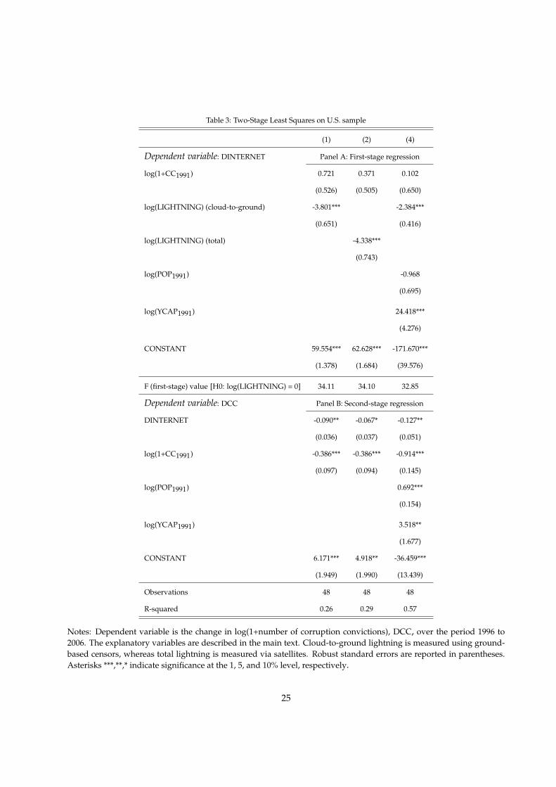
Table 3: Two-Stage Least Squares on U.S. sample

(1) (2) (4)

Dependent variable: DINTERNET Panel A: First-stage regression

log(1+CC1991) 0.721 0.371 0.102

(0.526) (0.505) (0.650)

log(LIGHTNING) (cloud-to-ground) -3.801*** -2.384***

(0.651) (0.416)

log(LIGHTNING) (total) -4.338***

(0.743)

log(POP1991) -0.968

(0.695)

log(YCAP1991) 24.418***

(4.276)

CONSTANT 59.554*** 62.628*** -171.670***

(1.378) (1.684) (39.576)

F (first-stage) value [H0: log(LIGHTNING) = 0] 34.11 34.10 32.85

Dependent variable: DCC Panel B: Second-stage regression

DINTERNET -0.090** -0.067* -0.127**

(0.036) (0.037) (0.051)

log(1+CC1991) -0.386*** -0.386*** -0.914***

(0.097) (0.094) (0.145)

log(POP1991) 0.692***

(0.154)

log(YCAP1991) 3.518**

(1.677)

CONSTANT 6.171*** 4.918** -36.459***

(1.949) (1.990) (13.439)


R-squared 0.26 0.29 0.57

Notes: Dependent variable is the change in log(1+number of corruption convictions), DCC, over the period 1996 to2006. The explanatory variables are described in the main text. Cloud-to-ground lightning is measured using ground-based censors, whereas total lightning is measured via satellites. Robust standard errors are reported in parentheses.Asterisks ***,**,* indicate significance at the 1, 5, and 10% level, respectively.

25

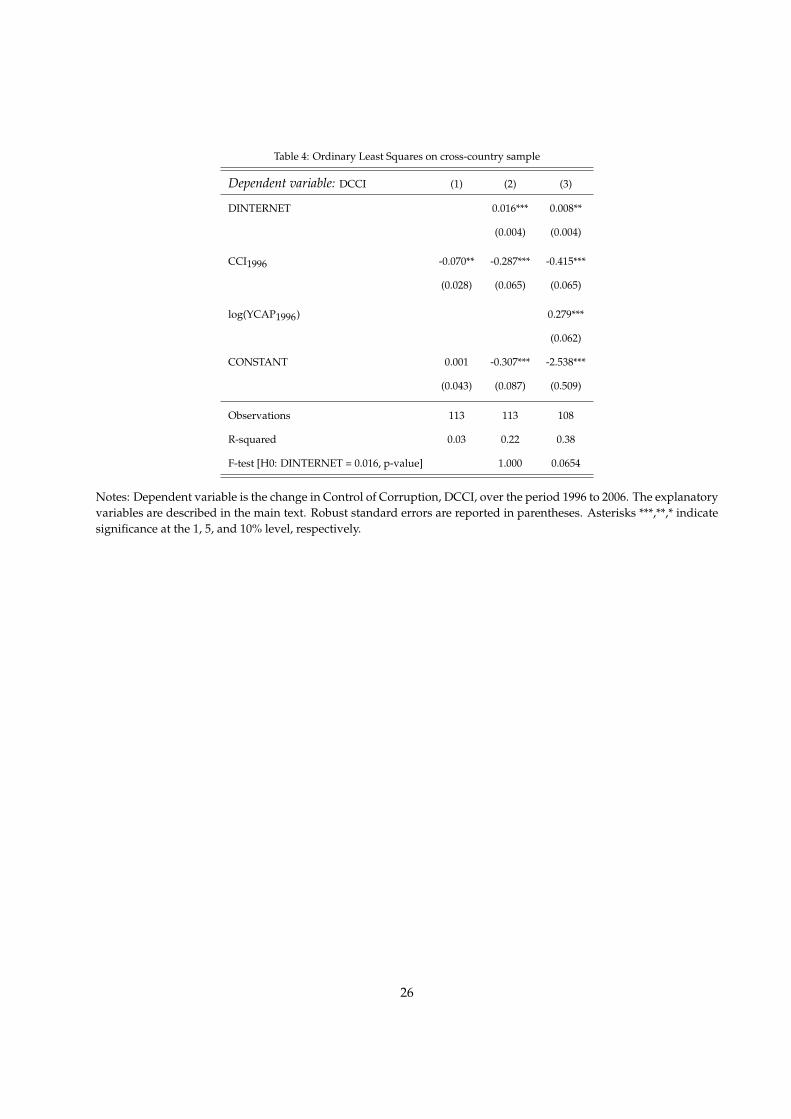
Table 4: Ordinary Least Squares on cross-country sample

Dependent variable: DCCI (1) (2) (3)

DINTERNET 0.016*** 0.008**

(0.004) (0.004)

CCI1996 -0.070** -0.287*** -0.415***

(0.028) (0.065) (0.065)

log(YCAP1996) 0.279***

(0.062)

CONSTANT 0.001 -0.307*** -2.538***

(0.043) (0.087) (0.509)


R-squared 0.03 0.22 0.38

F-test [H0: DINTERNET = 0.016, p-value] 1.000 0.0654

Notes: Dependent variable is the change in Control of Corruption, DCCI, over the period 1996 to 2006. The explanatoryvariables are described in the main text. Robust standard errors are reported in parentheses. Asterisks ***,**,* indicatesignificance at the 1, 5, and 10% level, respectively.

26

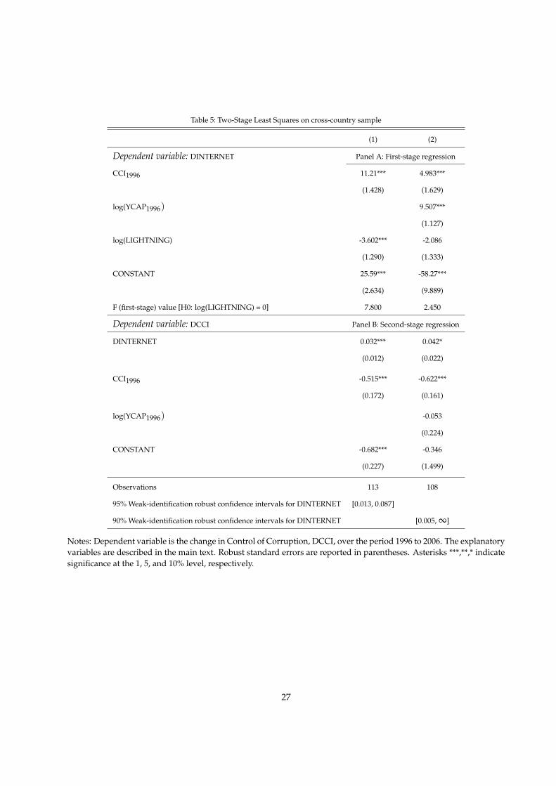
Table 5: Two-Stage Least Squares on cross-country sample

(1) (2)

Dependent variable: DINTERNET Panel A: First-stage regression

CCI1996 11.21*** 4.983***

(1.428) (1.629)

log(YCAP1996) 9.507***

(1.127)

log(LIGHTNING) -3.602*** -2.086

(1.290) (1.333)

CONSTANT 25.59*** -58.27***

(2.634) (9.889)

F (first-stage) value [H0: log(LIGHTNING) = 0] 7.800 2.450

Dependent variable: DCCI Panel B: Second-stage regression

DINTERNET 0.032*** 0.042*

(0.012) (0.022)

CCI1996 -0.515*** -0.622***

(0.172) (0.161)

log(YCAP1996) -0.053

(0.224)

CONSTANT -0.682*** -0.346

(0.227) (1.499)

Observations 113 108

95% Weak-identification robust confidence intervals for DINTERNET [0.013, 0.087]

90% Weak-identification robust confidence intervals for DINTERNET [0.005, ∞]

Notes: Dependent variable is the change in Control of Corruption, DCCI, over the period 1996 to 2006. The explanatoryvariables are described in the main text. Robust standard errors are reported in parentheses. Asterisks ***,**,* indicatesignificance at the 1, 5, and 10% level, respectively.

27

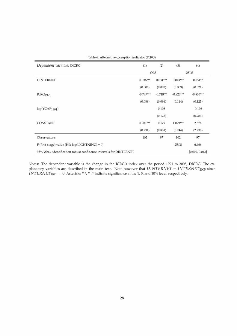
Table 6: Alternative corruption indicator (ICRG)

Dependent variable: DICRG (1) (2) (3) (4)

OLS 2SLS

DINTERNET 0.036*** 0.031*** 0.043*** 0.054**

(0.006) (0.007) (0.009) (0.021)

ICRG1991 -0.747*** -0.748*** -0.820*** -0.835***

(0.088) (0.096) (0.114) (0.125)

log(YCAP1991) 0.108 -0.196

(0.123) (0.284)

CONSTANT 0.981*** 0.179 1.079*** 2.576

(0.231) (0.881) (0.244) (2.238)

Observations 102 97 102 97

F (first-stage) value [H0: log(LIGHTNING) = 0] 25.08 6.466

95% Weak-identification robust confidence intervals for DINTERNET [0.009, 0.043]

Notes: The dependent variable is the change in the ICRG’s index over the period 1991 to 2005, DICRG. The ex-planatory variables are described in the main text. Note however that DINTERNET = INTERNET2005 sinceINTERNET1991 = 0. Asterisks ***, **, * indicate significance at the 1, 5, and 10% level, respectively.

28

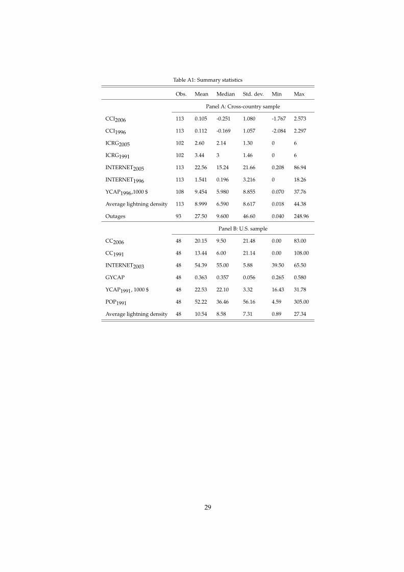
Table A1: Summary statistics

Obs. Mean Median Std. dev. Min Max

Panel A: Cross-country sample

CCI2006 113 0.105 -0.251 1.080 -1.767 2.573

CCI1996 113 0.112 -0.169 1.057 -2.084 2.297

ICRG2005 102 2.60 2.14 1.30 0 6

ICRG1991 102 3.44 3 1.46 0 6

INTERNET2005 113 22.56 15.24 21.66 0.208 86.94

INTERNET1996 113 1.541 0.196 3.216 0 18.26

YCAP1996,1000 $ 108 9.454 5.980 8.855 0.070 37.76

Average lightning density 113 8.999 6.590 8.617 0.018 44.38

Outages 93 27.50 9.600 46.60 0.040 248.96

Panel B: U.S. sample

CC2006 48 20.15 9.50 21.48 0.00 83.00

CC1991 48 13.44 6.00 21.14 0.00 108.00

INTERNET2003 48 54.39 55.00 5.88 39.50 65.50

GYCAP 48 0.363 0.357 0.056 0.265 0.580

YCAP1991, 1000 $ 48 22.53 22.10 3.32 16.43 31.78

POP1991 48 52.22 36.46 56.16 4.59 305.00

Average lightning density 48 10.54 8.58 7.31 0.89 27.34

29

3689227

35543105

101435253

74353258

5692373745980112

36276252

25675581

1

10

50623

10022100000

603367

16818689560866

0

20000000

40000000

60000000

80000000

100000000

120000000

1990

1991

1992

1993

1994

1995

1996

1997

1998

1999

2000

2001

2002

2003

2004

2005

2006

No. web sites

Figure 1: The figure shows the total number of Web sites on the Internet, 1990-2006. Generally,the numbers refer to December 1st in the individual year. Source: Hobbes’ Internet Timeline v8.2<http://www.zakon.org/robert/internet/timeline/>.

Figure 2: Average flash density (flashes per year per km2). The figure is constructed using the OTD GlobalLightning Distributions for the period April 12, 1995 to December 31, 1999.

30

AlabamaArkansas

Arizona

CaliforniaColoradoConnecticut

Delaware

Florida

GeorgiaIowa

Idaho

IllinoisIndianaKansas

Kentucky

Louisiana

Massachusetts

Maryland

MaineMichiganMinnesota

Missouri

Mississippi

Montana

North Carolina

North DakotaNebraska

New HampshireNew Jersey

New Mexico

NevadaNew York

OhioOklahoma

Oregon

Pennsylvania

Rhode Island

South Carolina

South Dakota

TennesseeTexas

Utah

Virginia

VermontWashington

WisconsinWest Virginia

Wyoming

05

1015

2025

Clo

udto

gro

und

light

ning

0 10 20 30Total lightning

Figure 3: The figure shows a scatter plot of total lightning flash rate density (flashes per km2 per year) basedon the Optical Transient Detector high resolution data (horizontal axis) versus cloud-to-ground flash ratedensity (flashes per km2 per year) based on the U.S. National Lightning Detection Network (vertical axis).The full line is the 45-degree line. Number of observations is 48.

31

Alabama

ArizonaArkansas

California Colorado

Connecticut

Delaware

FloridaGeorgia

Idaho

Illinois

Indiana

Iowa

Kansas

Kentucky

Louisiana

Maine

Maryland

Massachusetts

Michigan

Minnesota

Mississippi

Missouri

Montana

Nebraska

Nevada

New Hampshire

New Jersey

New MexicoNew York

North Carolina

North DakotaOhio

Oklahoma

OregonPennsylvania

Rhode Island

South Carolina

South DakotaTennessee

Texas

Utah

Vermont

Virginia

Washington

West Virginia

Wisconsin

Wyoming

21

01

2e(

Cha

nges

in lo

g(1+

CC

) | X

)

3 2 1 0 1e( log(LIGHTNING)| X)

Figure 4: The figure shows the association between lightning and changes in corruption convictions overthe 1978-1990 period, with the influence of GDP per capita and population partialled out.

32

Alabama

Arizona Arkansas

California

Colorado

Connecticut

Delaware

Florida

Georgia

Idaho

Illinois

Indiana

Iowa

Kansas

Kentucky

Louisiana

Maine

MarylandMassachusetts

Michigan

Minnesota

Mississippi

Missouri

Montana

NebraskaNevada

New Hampshire

New Jersey

New Mexico

New York

North CarolinaNorth DakotaOhio

Oklahoma

Oregon

Pennsylvania

Rhode Island

South Carolina

South Dakota

Tennessee

Texas

UtahVermont

Virginia

Washington

West Virginia

Wisconsin

Wyoming

21

01

2e(

Cha

nges

in lo

g(1+

CC

) | X

)

3 2 1 0 1e( log(LIGHTNING)| X)

Figure 5: The figure shows the association between lightning and changes in corruption convictions overthe 1991-2006 period, with the influence of income per capita and population partialled out.

33

does the internet reduce corruption? evidence from u.s. states and across countries

Documents